Large gaps imputation in remote sensed imagery of theenvironment

Valeria Rulloni, Oscar Bustos and Ana Georgina Flesia∗

CIEM-Conicet and FaMAF-UNCCordoba, Argentina

{vrulloni, bustos, flesia}@famaf.unc.edu.ar

June 23, 2010

Abstract

Imputation of missing data in large regions of satellite imagery is necessary when the acquiredimage has been damaged by shadows due to clouds, or information gaps produced by sensorfailure.

The general approach for imputation of missing data, that could not be considered missedat random, suggests the use of other available data. Previous work, like local linear histogrammatching, take advantage of a co-registered older image obtained by the same sensor, yieldinggood results in filling homogeneous regions, but poor results if the scenes being combined haveradical differences in target radiance due, for example, to the presence of sun glint or snow.

This study proposes three different alternatives for filling the data gaps. The first twoinvolves merging radiometric information from a lower resolution image acquired at the sametime, in the Fourier domain (Method A), and using linear regression (Method B). The thirdmethod consider segmentation as the main target of processing, and propose a method to fillthe gaps in the map of classes, avoiding direct imputation (Method C).

All the methods were compared by means of a large simulation study, evaluating performancewith a multivariate response vector with four measures: Q, RMSE, Kappa and Overall Accuracycoefficients. Difference in performance were tested with a MANOVA mixed model design withtwo main effects, imputation method and type of lower resolution extra data, and a blockingthird factor with a nested sub-factor, introduced by the real Landsat image and the sub-imagesthat were used. Method B proved to be the best for all criteria.

1 Introduction

Management of the environment and inventory of natural resources often requires appropriate remotesensing data acquired at specific times on earth locations. But quite often, good resolution opticalimages have large damaged areas with lost information due to clouds or shadows produced by clouds.

The general statistical approaches for imputation needs to consider the data loss in one of threecategories: missing at random data, completely missing at random data, (meaning that the missingdata is independent of its value), and Non-ignorable missingness, Allison(2000). The last case is themost problematic form, existing when missing values are not randomly distributed across observa-tions, but the probability of missingness cannot be predicted from the variables in the model. One

∗AGF is corresponding author

1

arX

iv:1

006.

4330

v1 [

stat

.AP]

22

Jun

2010

approach to non-ignorable missingness is to impute values based on data otherwise external to theresearch design, as older images, Little et al (2002).

Merging information acquired at the same time from two or more sensors (with possible differentresolution) is the core of data fusion techniques. Their historical goals are to increase image resolution,sharpening or enhancement of the output, Tsuda et al (2003); Ling (2007) and Pohl (1998), and theirmajor problem to overcome is the co-registration of the different sources to merge, Blum et al (2005).

In the last decade several adaptations of data fusion techniques for information recovery havebeen devised to mitigate the effect of clouds on optical images, a classical problem, since 50% of thesky is usually covered by light clouds. In Le Hegarat-Mascle et al. (1998) contextual modeling ofinformation was introduced in order to merge data from SAR (Synthetic Aperture Radar) images intooptical images, to correct dark pixels due to clouds. Arellano (2003) used Wavelet transforms first forclouds detection, and then to correct the information of the located clouds pixels by merging olderimage information with a wavelet multiresolution fusion technique. Rossi et al (2003), introduceda spatial technique, krigging interpolation, for correction of shadows due to clouds. Shadows andlight clouds do not destroy all information, only distort it, but dark clouds or rain clouds producenon-ignorable missingness, a harder problem for interpolation techniques.

Another interesting example of incomplete data is the damaged imagery provided by the Landsat7 ETM+ satellite after its failure on May 2003. A failure of the Scan Line Corrector, a mirror thatcompensates for the forward motion of the satellite during data acquisition, resulted on overlaps ofsome parts of the images acquired thereafter, leaving large gaps, as large as 14 pixels, in others.About 22% of the total image is missing data in each scene. In figure 1 we can see two parts of thesame Landsat 7 image, one with missing information and another almost without loss.

Figure 1: Left panel, a piece of a Landsat 7 image with lost information. Right panel, a center pieceof the same image almost without loss.

The Landsat 7 Science Team (2003), developed and tested composite products made with thedamaged Landsat 7 image and a database of older Landsat images, using local linear histogrammatching, a method that merges pieces of older images that best matches the surroundings of themissing information region, Scaramuzza et al 2004, USGS/NASA 2004, (United States GeologicalSurvey/ National Aeronautics and Space Administration). Commonwealth of Australia (2006) re-ported that the composite products appear similar in quality to non damaged Landsat 7 images, butmasked environment changes, an usual problem in data fusion when one of the sources is temporallyinaccurate.

Zhang and Travis (2006) developed a spatial interpolation method based on krigging, the krigginggeostatistical technique, for filling the data gaps in Landsat 7 ETM+ imagery, without need of extrainformation. They compare their method with the standard local linear histogram matching tech-nique chosen by USGS/NASA. They show in their case study that krigging is better than histogrammatching in targets with radical differences in radiance, since it produces an imputation value closerto the values of the actual neighbors. A drawback of spatial techniques is that they rely on a neigh-borhood that could be completely empty of real information. The algorithms start imputation in

2

the gap contour, where there are many good pixels, and use imputed and good values to create thenext pixel value. In center pixels of large gaps, algorithms based only on damaged images will usepreviously imputed values to generate the next imputation, degrading visual quality and increasinginterpolation error.

In this paper, we propose three methods based on data fusion techniques for imputation ofmissing values in images with non-ignorable missingness. We suppose there is available temporallyaccurate extra information for the gap scenes, produced by a lower resolution sensor. This is not avery restrictive hypothesis, since there are many satellite constellations that can provide temporallyaccurate data with different cameras at different resolutions.

This study proposes three different alternatives for filling the data gaps. The first method involvemerging information from a co-registered older image and a lower resolution image acquired at thesame time, in the Fourier domain (Method A). The second used a linear regression model with thelower resolution image as extra data (Method B). The third method consider segmentation as themain target of processing, and propose a method to fill the gaps in the map of classes, avoiding directimputation for the segmentation task (Method C). Radiometric imputation is later made assigninga random value from the convex hull made by the neighbor pixels within its class.

All the methods were compared by means of a large simulation study, evaluating performancewith a multivariate response vector with four measures: Q, RMSE, Kappa and Overall Accuracycoefficients. Two of these performance measures (Kappa and Overall Accuracy) are designed for theassessment of segmentation accuracy. The other two, Q and RMSE, measure radiometric interpo-lation accuracy. Difference in performance were tested with a MANOVA mixed model design withtwo main effects, imputation method and type of lower resolution extra data, and a blocking thirdfactor with a nested sub-factor, introduced by the real Landsat image and the sub-images that wereused. Method B proved to be the best for all criteria.

2 Methods

We are considering images acquired from the same geographic target, with fixed number of bands K,and 256 levels of gray per band. Damaged and older images have the same support, lower resolutionimages have different supports, and we suppose that there are nz pixels in the damaged image foreach pixel in the lower resolution image.

Let XD be the damaged image, Z a lower spatial resolution image , and Xold, an older imageacquired with the same sensor that XD. Let SD be the gap to be filled, i.e. the set of pixels of XD

with missing values. The goal is to input values on SD using available good data from XD in a smallneighborhood of each pixel, the values of Z and eventually, the values of Xold.

The first step in processing is the re-sampling of the lower resolution image in order to match thesupport of the three images. This is done replacing each pixel (c, r) of Z by a matrix of size nz × nz

with constant value Z(c, r).Imputation is done in each band separately with the same algorithm, thus the methods descrip-

tions consider the images as one band only.

2.1 Method A

The image Xold does not need to be co-registered with reference to the damaged image XD, sincethey have been acquired by the same sensor, but calibration is indeed necessary to increase mergingaccuracy.

We suppose a Gaussian calibration have been made on Xold per column, taking as pivots thevalues in the matched column of XD. Let XA

R be the composite image, output from the imputation

3

method A. We define XAR values in the gap as a mixture of high frequencies of the older image and

low frequencies taken from the actual but lower resolution image.

XAR (c, r) =

{|LC(Z)(c, r) +HC(Xold)(c, r)| (c, r) ∈ SD

XD(c, r) otherwise

with HC and LC the ideal High pass and Low Pass Fourier Filters.The filters are regulated by the C coefficient, the bigger C is the larger the influence of Z in the

imputation. High pass filters are related to detail, edges and random noise, and low pass filters tostructural information. Therefore, Method A takes structural information from the low resolutionimage and detail from the older one.

2.2 Method B

Imputation will be made with the only help of Z, a temporally accurate image with lower resolution.We have expanded the lower resolution image to match the support of XD, replacing each crossgrained pixel by a block of nz ×nz pixels with the same radiometric value. Each one of the constantblocks of the expanded Z image has a matched block in the damaged image XD, that could be valid(having all the information), or non valid, (with some loss).

We will follow a time series approach now. Let think we have data collected month to monthalong several years, and we have a missing January data. It is reasonably to impute that value usinga regression model that only involves other January data, and extra data collected on Summer thatyear.

In our case, we have missing information on a location (c, r) inside a block B, we may imputethat value using a regression model that only involves data in the same position inside the otherblocks of the image (January data), using as regressor variable the values of Z (Summer data).

XD(c, r) = α(c,r) ∗ Z(c, r, B) + β(c,r) + ε(c, r),

with ε(c, r) ∼ N(0, σ(c, r)2).The coefficients α(c,r) and β(c,r) are estimated by ordinary least squares using only valid blocks.

Then

α(c, r) =

∑B a valid block

(Z(c, r, B)− Z)(XD(c, r, B)−XD(c, r))

∑B a valid block

(Z(c, r, B)− Z)2,

β(c,r) = XD(c, r)− α(c,r)Z,

where

Z =∑

B a valid block

Z(c, r, B)

|number of valid blocks|

and

XD(c, r) =∑

B a valid block

XD(c, r, B)

|number of valid blocks|.

We define the imputed image XBR as XD in the pixels with no missing information and the value

predicted by the regression in each damaged pixel .

4

XBR ((d, g, B)) =

{α(d, g) ∗ Z(d, g, B) + β(d, g) (d, g) ∈ SD

XD((d, g, B)) otherwise.

2.3 Method C

Remote sense images are used in a wide range of applied sciences. For many of them, as Agriculturaland Experimental Biology, or Environmental Science, all useful information is contained on a classmap, where the classes are characterized by special features under study. Kind of crop, forested ordeforested areas, regions with high, medium and low soil humidity, are examples of such features.

In this section we will change our point of view by thinking on class maps instead on radiometricimages. Let suppose we have our damaged image XD, and a temporally accurate image Z with lowerresolution, and possible different number of radiometric bands. This is an advantage over radiometricimputation, which need the same spectral properties in both images.

We also suppose that a map of classes CD has been drawn from the damaged image XD, usinga non supervised method like K means, with K different classes. The class of missing informationpixels is another class, called class 0. The goal is to assign the pixels without radiometric informationto one of the K classes, and generate a radiometric value for them randomly from the selected class.

There are two main steps in this method

1. An enhancement of the initial classification CD, that could be made or not

2. Imputation of pixels in the zero class.

Initial enhancementAutomatic classification is a difficult task, and the imputation method under study heavily de-

pends of the accuracy of the initial map of classes. So it is important to pay special attention to thecoherence of the classes. We suggest a set of steps to improve class homogeneity as follows

1. Given XD construct a map of classes CD using K means, and assign the zero label to themissing information regions.

2. Given the class image CD, detect the pixels with non homogeneous neighborhood, i.e, pixelsthat have no neighbor pixels on the same class. Call this set NG.

3. For each pixel in NG, verify its label using a forward mode filter, and a backwards mode filter.The filters with give a label that is consistent with the mode of the labels in a (forward orbackward) neighborhood.

(a) If both filters give the same label, update the label of the pixel to match this one.

(b) If the labels are not the same, maintain the original label, and put the pixel in a new setcall NM .

4. For each pixel in NM that do not has label zero, we use again radiometric information forupdating the label.

(a) Take the one step neighbors of the pixels, and compute the arithmetic mean for each classpresent in the neighborhood.

(b) Update the label of the pixel by the label of the class whose arithmetic mean is closest (inEuclidean distance) to the radiometric value of the pixel.

5

It is important to note that after this process, some of the pixels of the zero class may have beenclassified into a real class, only using contextual information. The other classes should have moredefined borderlines.

Class zero imputationWe suppose now that we have a stable map of K classes CD, with missing information in class

zero, and auxiliary information provided by a temporally accurate lower resolution radiometric imageZ. If (c, r) is a pixel in class zero, it does not have radiometric information. We will impute a labelclass on it with the following algorithm

1. Let Nt be the smallest neighborhood of (c, r) that have a pixel with non zero label.

2. Let Zk be the arithmetic mean of the Z pixels that have positions in class k in Nt.

3. The label of (c, r) is the label of the class k that makes the smallest Euclidean distance fromZ(c, r) to each Zk.

k = arg mink

∥∥Z(c, r)− Zk(c, r)∥∥2.

After this process, all pixels have a class label, but pixels in the gaps have not been imputed withradiometric information yet. A pixel’s radiometric value is assigned randomly from the values of theconvex hull generated by the pixels of a small neighborhood within its class.

3 Precision assessment by simulation

Impartial imputation assessment is only possible when ground truth is available. Complete simula-tion of the three types of images involved in the methods (old, damaged and lower resolution) willintroduce errors beyond the ones produced by the imputation methods, degrading the quality ofthe assessment. For this reason, good quality Landsat 7 ETM+ imagery that have older matchedimagery available were selected, and strips similar to the gaps in the SLC-off ETM+ imagery werecut manually, guaranteeing ground truth to compare with and co-registration between the images.The four Landsat 7 ETM+ images selected were quit large, having many different textures in them,like crop fields, mountains and cities, that challenge the imputation methods differently.

Landsat 7 ETM+ had a lower resolution sensor in its constellation, the MMRS camera from theSAC C satellite, whose imagery could be used as extra data. But to control also co-registrationproblems, lower resolution imagery were simulated with three resolution reduction methods (RRM),by block averaging the ground truth, the CONGRID method from ENVI software and shifted blockaveraging. Block averaging is a crude way of reducing resolution, the CONGRID method reduces theblocking effect smoothing the output, giving better visual appearance, but block averaging allows toshift the blocks in a controlled fashion, simulating lack of co-registration.

In Figure 2 we see an example of four matched images, good, damaged, older and lower resolutionby block averaging. We can see a bright spot in the center of the image, which is still present inthe damaged one and the lower resolution one, but it is not present in the older one. Databaseconstruction details are giving in the subsection 3.1.

The performance measures (RMSE, Q, Kappa and Overall Accuracy) were modeled as a re-sponse vector in a MANOVA mixed model with main effects (imputation method, resolution re-duction method), and random nested effects (image and sub-image). Subsection 3.2 introduces theperformance measures and subsection 3.4 includes a detailed description of the MANOVA design.Following the Manova rejection, simultaneous multivariate comparisons were made by (Bonferronicorrected) two means Hotelling tests, and individual Anova results with simultaneous comparisons

6

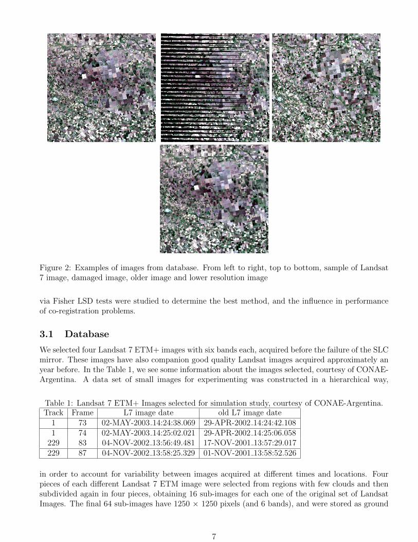
Figure 2: Examples of images from database. From left to right, top to bottom, sample of Landsat7 image, damaged image, older image and lower resolution image

via Fisher LSD tests were studied to determine the best method, and the influence in performanceof co-registration problems.

3.1 Database

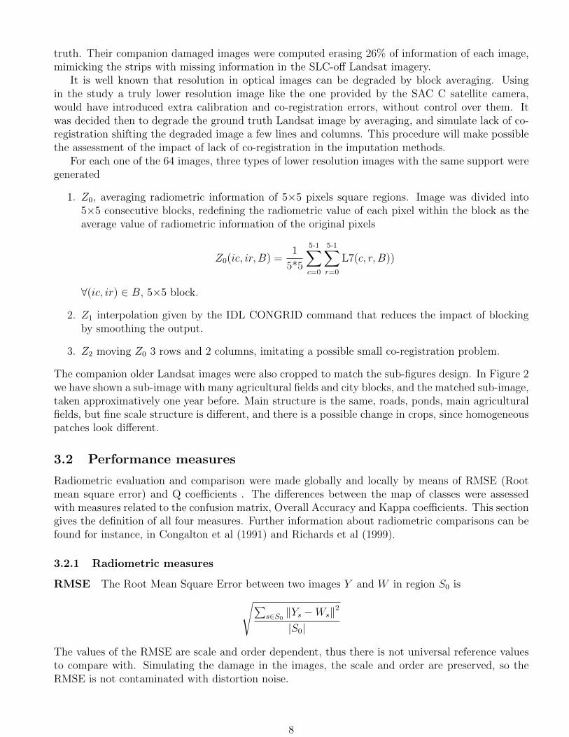
We selected four Landsat 7 ETM+ images with six bands each, acquired before the failure of the SLCmirror. These images have also companion good quality Landsat images acquired approximately anyear before. In the Table 1, we see some information about the images selected, courtesy of CONAE-Argentina. A data set of small images for experimenting was constructed in a hierarchical way,

Table 1: Landsat 7 ETM+ Images selected for simulation study, courtesy of CONAE-Argentina.Track Frame L7 image date old L7 image date

1 73 02-MAY-2003 14:24:38.069 29-APR-2002 14:24:42.1081 74 02-MAY-2003 14:25:02.021 29-APR-2002 14:25:06.058

229 83 04-NOV-2002 13:56:49.481 17-NOV-2001 13:57:29.017229 87 04-NOV-2002 13:58:25.329 01-NOV-2001 13:58:52.526

in order to account for variability between images acquired at different times and locations. Fourpieces of each different Landsat 7 ETM image were selected from regions with few clouds and thensubdivided again in four pieces, obtaining 16 sub-images for each one of the original set of LandsatImages. The final 64 sub-images have 1250 × 1250 pixels (and 6 bands), and were stored as ground

7

truth. Their companion damaged images were computed erasing 26% of information of each image,mimicking the strips with missing information in the SLC-off Landsat imagery.

It is well known that resolution in optical images can be degraded by block averaging. Usingin the study a truly lower resolution image like the one provided by the SAC C satellite camera,would have introduced extra calibration and co-registration errors, without control over them. Itwas decided then to degrade the ground truth Landsat image by averaging, and simulate lack of co-registration shifting the degraded image a few lines and columns. This procedure will make possiblethe assessment of the impact of lack of co-registration in the imputation methods.

For each one of the 64 images, three types of lower resolution images with the same support weregenerated

1. Z0, averaging radiometric information of 5×5 pixels square regions. Image was divided into5×5 consecutive blocks, redefining the radiometric value of each pixel within the block as theaverage value of radiometric information of the original pixels

Z0(ic, ir, B) =1

5*5

5-1∑c=0

5-1∑r=0

L7(c, r, B))

∀(ic, ir) ∈ B, 5×5 block.

2. Z1 interpolation given by the IDL CONGRID command that reduces the impact of blockingby smoothing the output.

3. Z2 moving Z0 3 rows and 2 columns, imitating a possible small co-registration problem.

The companion older Landsat images were also cropped to match the sub-figures design. In Figure 2we have shown a sub-image with many agricultural fields and city blocks, and the matched sub-image,taken approximatively one year before. Main structure is the same, roads, ponds, main agriculturalfields, but fine scale structure is different, and there is a possible change in crops, since homogeneouspatches look different.

3.2 Performance measures

Radiometric evaluation and comparison were made globally and locally by means of RMSE (Rootmean square error) and Q coefficients . The differences between the map of classes were assessedwith measures related to the confusion matrix, Overall Accuracy and Kappa coefficients. This sectiongives the definition of all four measures. Further information about radiometric comparisons can befound for instance, in Congalton et al (1991) and Richards et al (1999).

3.2.1 Radiometric measures

RMSE The Root Mean Square Error between two images Y and W in region S0 is√∑s∈S0‖Ys −Ws‖2

|S0|

The values of the RMSE are scale and order dependent, thus there is not universal reference valuesto compare with. Simulating the damage in the images, the scale and order are preserved, so theRMSE is not contaminated with distortion noise.

8

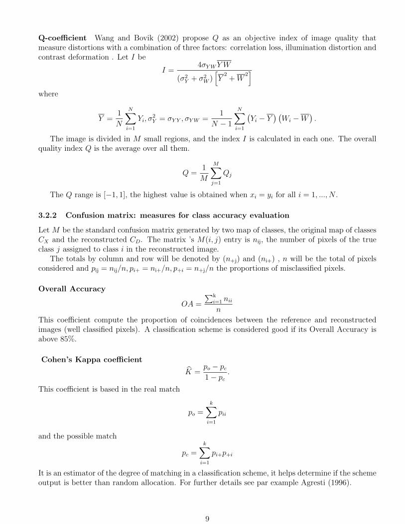
Q-coefficient Wang and Bovik (2002) propose Q as an objective index of image quality thatmeasure distortions with a combination of three factors: correlation loss, illumination distortion andcontrast deformation . Let I be

I =4σYWYW

(σ2Y + σ2

W )[Y

2+W

2]

where

Y =1

N

N∑i=1

Yi, σ2Y = σY Y , σYW =

1

N − 1

N∑i=1

(Yi − Y

) (Wi −W

).

The image is divided in M small regions, and the index I is calculated in each one. The overallquality index Q is the average over all them.

Q =1

M

M∑j=1

Qj

The Q range is [−1, 1], the highest value is obtained when xi = yi for all i = 1, ..., N .

3.2.2 Confusion matrix: measures for class accuracy evaluation

Let M be the standard confusion matrix generated by two map of classes, the original map of classesCX and the reconstructed CD. The matrix ’s M(i, j) entry is nij, the number of pixels of the trueclass j assigned to class i in the reconstructed image.

The totals by column and row will be denoted by (n+j) and (ni+) , n will be the total of pixelsconsidered and pij = nij/n, pi+ = ni+/n, p+i = n+j/n the proportions of misclassified pixels.

Overall Accuracy

OA =

∑ki=1 nii

n

This coefficient compute the proportion of coincidences between the reference and reconstructedimages (well classified pixels). A classification scheme is considered good if its Overall Accuracy isabove 85%.

Cohen’s Kappa coefficient

K =po − pc1− pc

.

This coefficient is based in the real match

po =k∑

i=1

pii

and the possible match

pc =k∑

i=1

pi+p+i

It is an estimator of the degree of matching in a classification scheme, it helps determine if the schemeoutput is better than random allocation. For further details see par example Agresti (1996).

9

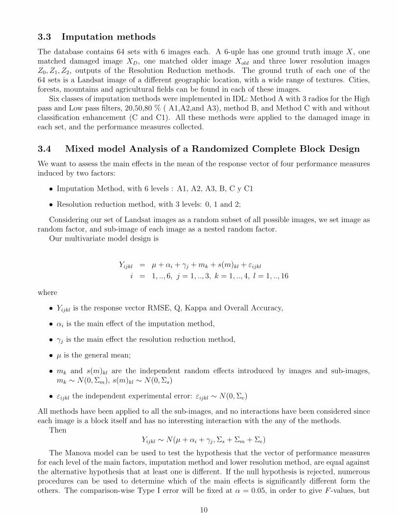
3.3 Imputation methods

The database contains 64 sets with 6 images each. A 6-uple has one ground truth image X, onematched damaged image XD, one matched older image Xold and three lower resolution imagesZ0, Z1, Z2, outputs of the Resolution Reduction methods. The ground truth of each one of the64 sets is a Landsat image of a different geographic location, with a wide range of textures. Cities,forests, mountains and agricultural fields can be found in each of these images.

Six classes of imputation methods were implemented in IDL: Method A with 3 radios for the Highpass and Low pass filters, 20,50,80 % ( A1,A2,and A3), method B, and Method C with and withoutclassification enhancement (C and C1). All these methods were applied to the damaged image ineach set, and the performance measures collected.

3.4 Mixed model Analysis of a Randomized Complete Block Design

We want to assess the main effects in the mean of the response vector of four performance measuresinduced by two factors:

• Imputation Method, with 6 levels : A1, A2, A3, B, C y C1

• Resolution reduction method, with 3 levels: 0, 1 and 2;

Considering our set of Landsat images as a random subset of all possible images, we set image asrandom factor, and sub-image of each image as a nested random factor.

Our multivariate model design is

Yijkl = µ+ αi + γj +mk + s(m)kl + εijkl

i = 1, .., 6, j = 1, .., 3, k = 1, .., 4, l = 1, .., 16

where

• Yijkl is the response vector RMSE, Q, Kappa and Overall Accuracy,

• αi is the main effect of the imputation method,

• γj is the main effect the resolution reduction method,

• µ is the general mean;

• mk and s(m)kl are the independent random effects introduced by images and sub-images,mk ∼ N(0,Σm), s(m)kl ∼ N(0,Σs)

• εijkl the independent experimental error: εijkl ∼ N(0,Σe)

All methods have been applied to all the sub-images, and no interactions have been considered sinceeach image is a block itself and has no interesting interaction with the any of the methods.

ThenYijkl ∼ N(µ+ αi + γj,Σs + Σm + Σe)

The Manova model can be used to test the hypothesis that the vector of performance measuresfor each level of the main factors, imputation method and lower resolution method, are equal againstthe alternative hypothesis that at least one is different. If the null hypothesis is rejected, numerousprocedures can be used to determine which of the main effects is significantly different form theothers. The comparison-wise Type I error will be fixed at α = 0.05, in order to give F -values, but

10

we will report the p-values also in all cases . Following a Manova rejection, it have been seen thatthe overall experiment-wise error rate stays within the limits of the α selected for individual Anovatests, helping answering the following research questions

1. Is there at least one method of imputation with a different performance from the others, withineach performance measure analysis?

2. Is there at least one method of resolution reduction with a performance different from theothers, within each performance measure analysis?

3. Does comparing performance (on any factor level), relative to the different measures of perfor-mance, produce the same results?

4 Results

4.1 Empirical findings

4.1.1 Visual Inspection

In Figure 3 it can be seen the original image and its reconstructions using methods B, A1 and A3, Cand C1. We should notice that radiometric imputation from the map of classes are the worse of themethods, texture and fine details are not reconstructed, giving a blurred appearance to the imputedstripes. But we stress that it is not that bad if the goal is classification.

We should also notice that globally, Method B produces an output with better visual quality thanthe others. Stripes are missing, but fine lines, small scale structure is less defined, like blurred. Thereconstructions made with Methods A1 and A3 show changes between the zones that are originaland the zones imputed, but the imputed stripes have better defined small scale structure. This isparticularly noticeable in reconstruction with Method A1, which introduces more information fromthe older image than Method A3.

4.1.2 Means Profiles

Visual inspection can only be made with few images, we have 64 sub-images with double size fromthe ones just shown. To inspect performance globally, we will study now the mean profiles of allperformance measures. We compute the sample means of each performance measure, for each methodand each image. This is, we average the values of a particular performance measure taken over all16 sub-images from a single image. A Mean Profile is a polygonal that links the four means (one perimage) from a particular performance measure, .

Methods mean profiles should be parallel, if there is no interaction between the performancemeasure and the images. Differences are then produced by the methods and not by the images. FlatProfiles indicates that each method produce similar values on any image, but that is not true. Imagesdepend not only of the geographic target observed, but the atmospheric conditions of the momentof acquisition. Variability is huge. If we consider our images as chosen at random, they will be onlya random effect that inflates the variance, but does not introduce a main effect that could mask theeffect of the Imputation Methods.

Also, it is important to note that in order to compare all methods using Kappa and OverallAccuracy, a map of classes must be made for each reconstructed image, as well as the original image.Methods A and B generates radiometric imputations, Method C and C1 generate maps of classesfirst, and then radiometric imputation, choosing at random a value within the class assigned. The

11

Figure 3: From left to right. First row: Original Sub-Image, reconstructions from Method B. SecondRow: Reconstructions from Method A1, and Method A3.Third Row: Reconstructions from MethodC and Method C1

automatic method K-means was used to obtain a map of classes for the original images and the onesreconstructed with methods A and B.

The coefficients Kappa, Q and Overall Accuracy are designed to give high scores to good recon-structions. On the contrary, RMSE is an error measure, then reconstruction is best when RMSE isat its lowest.

In Figure 4 we see two profile plots, Mean Overall Accuracy against Image, and Mean Kappaagainst Image, where the means are made over all the sub-images of the same image. The highestprofile will be then the best method and the lowest the worse, if all profiles are more or less parallel.

In both plots, Method C performed badly, and seems to interact with the images. Its profiledoes not follow the pattern of the others. Nevertheless, Method C1, a simplification of method C,has good performance with these measures that consider good classification. It follows a similarpattern than Method A1,2,3 and B, but with scores as good as Method B. Measures Kappa andOverall Accuracy depends heavily on good segmentation of the ground truth. Method C includesan enhancement that may give better defined classes, but separate it from the segmentation of the

12

Figure 4: Left panel :Overall Accuracy against Image,Right panel: Kappa against Image

ground truth, increasing the global error, outside the imputation error.In figure 5 we see other two profile plots, Mean Q against Image, and Mean RMSQ against Image.

Figure 5: Left Q agains Image and Right RMSE against image

The highest profile will be then the best method and the lowest the worse, when considering Q,and the reverse when considering RMSE, if all profiles are more or less parallel. Again, Method Chas bad performance, followed by Method C1. In this case, reasons for this behavior may be foundin the fact that imputation is made randomly within each class, which could have a very wide rangeof radiometric values. Method C1 may generate a map of classes very close to the real one, but notthe radiometric values of the missing pixels.

We will now explore possible interactions between Imputation Method and Resolution ReductionMethod (RRM), by making Mean Profile Plots of each Performance measure by Imputation Methodand plotting it against RRM. In Figure 6 we should notice that the plots of three versions of MethodA are not parallel, suggesting a possible interaction that should be further studied with an Anovatest.

4.1.3 Preliminary conclusions

In all cases, the mean profile of Method B seems to be best, followed by A3, fusion using a highvalue of threshold, that gives Z more influence than Xold. That corroborates the facts pointed out byvisual inspection on only one image. But we should test if the differences are statistically significantwith level α = 0.05. All A Methods are in pack, their differences may not be significant.

13

Figure 6: From Left to Right. First Row: Overall Accuracy against RRM by Method and Kappaagainst RRM by Method. Second Row: RMSE against RRM by Method and Q against RRM byMethod.

When studying interactions between the main factors, the A Methods suggested a change betweenMean performance using RRM 0 and RRM1. The most important change would be a significantdifference on Mean Performance between Methods when using RRM3, which is slightly out of sync.

In the next section, we will corroborate these empirical findings with Manova test of significance,and individual Anova tests. We will considering Image as a blocking factor, with a nested sub-factor,Sub-Image, discarding interaction as weak, Kuahl (1999). In both set of plots, we have reasons tobelieve that the profiles from Method C and C1 do not show interaction with the image factor, butother errors beside the ones measured by the particular performance index.

4.2 Manova Test Outputs

The vector of response variables contains the four measures considered, Overall Accuracy, Kappa,RMSE and Q. The Manova test search for significantly evidence to reject the following null hypothesis:

H10 : αi = 0, ∀i : i = 1, .., 6

H20 : γj = 0, ∀j = 1, .., 3.

14

with αi the vector of main effects introduced by the i- Imputation Method, and γj is the vector ofmain effects introduced by the j- Resolution Reduction Method. Rejection of each hypothesis means

H10 There is a Imputation method effect, there is at least one method that has a different vectorof performances than the others.

H20 There is a Resolution Reduction Method effect, there is at least one method of resolutionreduction with a vector of performance different than the others.

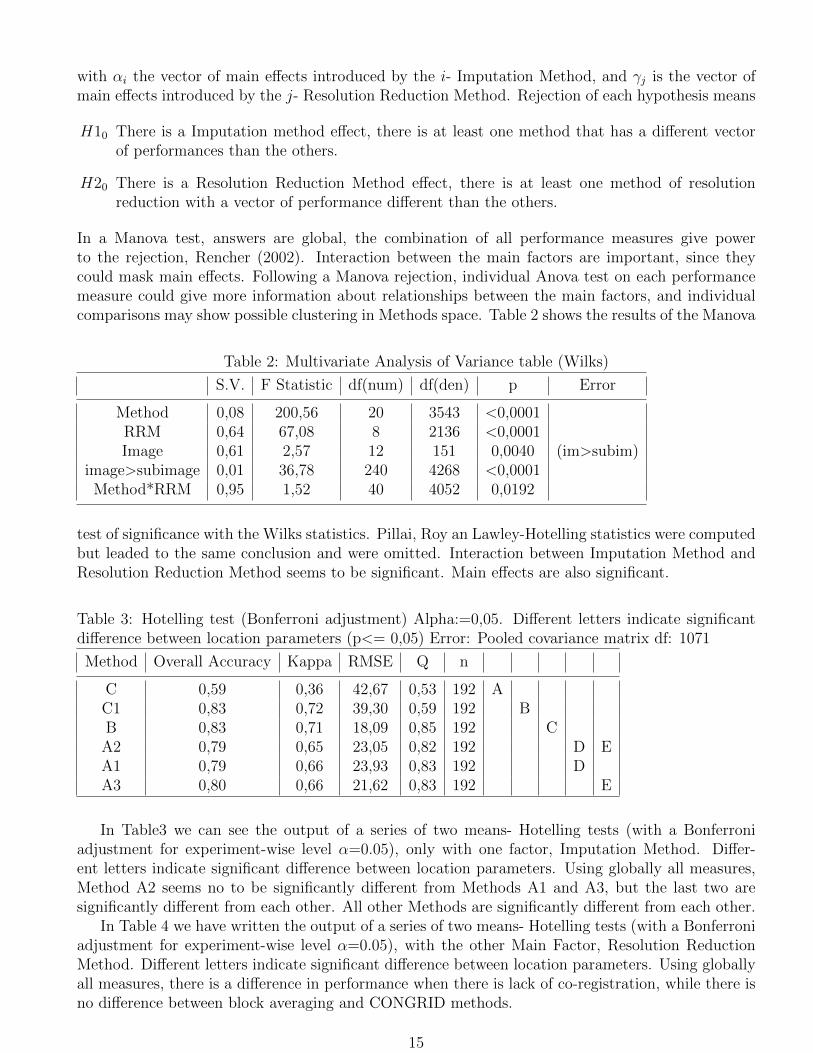
In a Manova test, answers are global, the combination of all performance measures give powerto the rejection, Rencher (2002). Interaction between the main factors are important, since theycould mask main effects. Following a Manova rejection, individual Anova test on each performancemeasure could give more information about relationships between the main factors, and individualcomparisons may show possible clustering in Methods space. Table 2 shows the results of the Manova

Table 2: Multivariate Analysis of Variance table (Wilks)

S.V. F Statistic df(num) df(den) p Error

Method 0,08 200,56 20 3543 <0,0001RRM 0,64 67,08 8 2136 <0,0001Image 0,61 2,57 12 151 0,0040 (im>subim)

image>subimage 0,01 36,78 240 4268 <0,0001Method*RRM 0,95 1,52 40 4052 0,0192

test of significance with the Wilks statistics. Pillai, Roy an Lawley-Hotelling statistics were computedbut leaded to the same conclusion and were omitted. Interaction between Imputation Method andResolution Reduction Method seems to be significant. Main effects are also significant.

Table 3: Hotelling test (Bonferroni adjustment) Alpha:=0,05. Different letters indicate significantdifference between location parameters (p<= 0,05) Error: Pooled covariance matrix df: 1071

Method Overall Accuracy Kappa RMSE Q n

C 0,59 0,36 42,67 0,53 192 AC1 0,83 0,72 39,30 0,59 192 BB 0,83 0,71 18,09 0,85 192 CA2 0,79 0,65 23,05 0,82 192 D EA1 0,79 0,66 23,93 0,83 192 DA3 0,80 0,66 21,62 0,83 192 E

In Table3 we can see the output of a series of two means- Hotelling tests (with a Bonferroniadjustment for experiment-wise level α=0.05), only with one factor, Imputation Method. Differ-ent letters indicate significant difference between location parameters. Using globally all measures,Method A2 seems no to be significantly different from Methods A1 and A3, but the last two aresignificantly different from each other. All other Methods are significantly different from each other.

In Table 4 we have written the output of a series of two means- Hotelling tests (with a Bonferroniadjustment for experiment-wise level α=0.05), with the other Main Factor, Resolution ReductionMethod. Different letters indicate significant difference between location parameters. Using globallyall measures, there is a difference in performance when there is lack of co-registration, while there isno difference between block averaging and CONGRID methods.

15

Table 4: Hotelling test (Bonferroni adjustment) Alpha:=0,05. Different letters indicate significantdifference between location parameters (p<= 0,05) Error: Pooled covariance matrix df: 1069

RRM Overall Accuracy Kappa RMSE Q n

2 0,74 0,57 30,71 0,69 384 A1 0,79 0,66 27,05 0,76 384 B0 0,79 0,66 26,58 0,77 384 B

We have studied globally the main effects from Imputation and Resolution Reduction Methods.But interaction between both factors is not advisable. We would like to see in detail which one ofthe measures (if not all of them) shows changes in performance when both factors are considered atthe same time.

4.3 Individual Anova tests

Knowing the results of the Manova test, we are confident that the level of the test of the individualAnova test are not far from its nominal value, α = 0.05.

In Table 5, we have the output of a Anova test for Q as response variable. Results are similarthan Manova, and it shows indeed significant interaction between Resolution Reduction Method andImputation Method. The other three Anova Tests, one of each response measure, Kappa, RMSE andOverall Accuracy also indicate significant main effects, but non of them shows significant interactionbetween the two main factors, being p-values 0.54, 0.37 and 0.70 respectively for the interaction test.We display only Overall Accuracy output for the sake of completeness in Table 5.

Table 5: Analysis of variance table (Partial SS) Variable: Q measure and Overall Accuracy

Q SS df MS F p-value (Error)

Model 26,33 80 0,33 57,76 <0,0001Method 19,85 5 3,97 696,52 <0,0001RRM 1,48 2 0,74 129,58 <0,0001Image 0,51 3 0,17 2,36 0,0803 (Image>subimage)

Image>subimage 4,36 60 0,07 12,75 <0,0001Method*RRM 0,14 10 0,01 2,40 0,0080

Error 6,10 1071 0,01Total 32,44 1151

Overall Accuracy SS df MS F p-value (Error)Model 10,79 80 0,13 43,07 <0,0001

Method 7,72 5 1,54 493,21 <0,0001RRM 0,70 2 0,35 112,28 <0,0001Image 0,29 3 0,10 2,77 0,0493 (Image>subimage)

Image>subimage 2,06 60 0,03 10,95 <0,0001Method*RRM 0,02 10 2,3E-03 0,72 0,7064

Error 3,35 1071 3,1E-03Total 14,15 1151

16

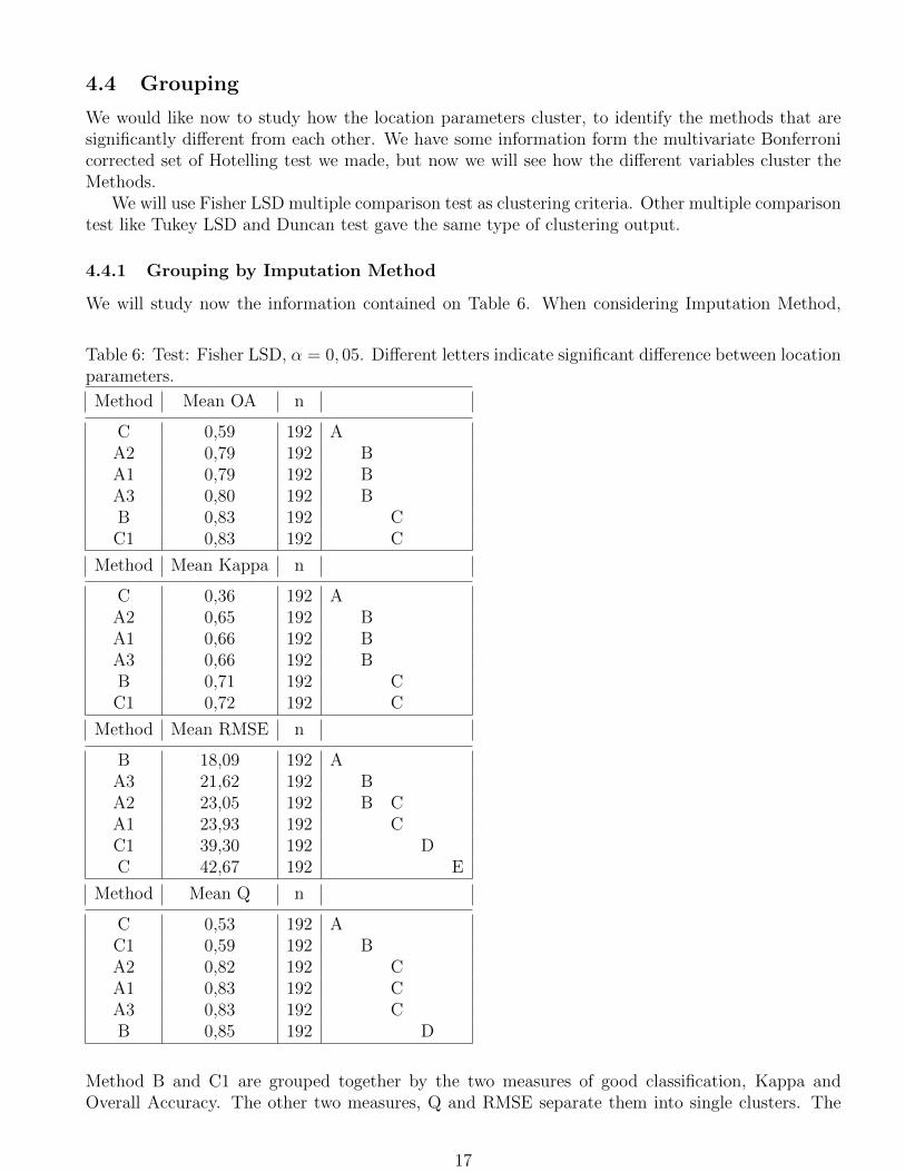
4.4 Grouping

We would like now to study how the location parameters cluster, to identify the methods that aresignificantly different from each other. We have some information form the multivariate Bonferronicorrected set of Hotelling test we made, but now we will see how the different variables cluster theMethods.

We will use Fisher LSD multiple comparison test as clustering criteria. Other multiple comparisontest like Tukey LSD and Duncan test gave the same type of clustering output.

4.4.1 Grouping by Imputation Method

We will study now the information contained on Table 6. When considering Imputation Method,

Table 6: Test: Fisher LSD, α = 0, 05. Different letters indicate significant difference between locationparameters.

Method Mean OA n

C 0,59 192 AA2 0,79 192 BA1 0,79 192 BA3 0,80 192 BB 0,83 192 CC1 0,83 192 C

Method Mean Kappa n

C 0,36 192 AA2 0,65 192 BA1 0,66 192 BA3 0,66 192 BB 0,71 192 CC1 0,72 192 C

Method Mean RMSE n

B 18,09 192 AA3 21,62 192 BA2 23,05 192 B CA1 23,93 192 CC1 39,30 192 DC 42,67 192 E

Method Mean Q n

C 0,53 192 AC1 0,59 192 BA2 0,82 192 CA1 0,83 192 CA3 0,83 192 CB 0,85 192 D

Method B and C1 are grouped together by the two measures of good classification, Kappa andOverall Accuracy. The other two measures, Q and RMSE separate them into single clusters. The

17

three versions of Method A have been grouped together by all the measures but RMSE, whichconsidered Method A1 and A3 significantly different. The two versions of Method C, C and C1, havebeen distinguished by all the measures.

The multivariate simultaneous comparison distinguished all methods but the versions of MethodA. And even though, Method A1 was considered significantly different from Method A3. It isinteresting to see that this is the way of grouping of the two radiometric measures. The classificationbased measures do not distinguish between Method B and C1, or A1, A2 and A3.

To the naked eye, Method B reconstruction of Figure 3 is very different from Method C1 recon-struction, and Method A1 is sharper than Method A3. The multivariate simultaneous comparisonagreed with this statement, with an experiment-wise Type I error α=0.05.

Now we can come back to the profile analysis of section 4.1.2. In that section, the performancemeasures means, computed over the sub-images of each image, were plotted as profiles, and thehighest value of Q, Kappa and Overall Accuracy indicated the best Imputation Method, and thelowest value of RMSE back up the same statement. Method B seemed to be the best of all them. Butthe analysis did not have any statistical confidence. The simultaneous comparisons made reportedMethod B as significantly different in mean performance from all the others, and Table 6 show themean value of measures Q, Overall Accuracy and Kappa the highest of all, and the lowest of theerror measure RMSE. These results give confidence to the previous profile analysis.

4.4.2 Grouping by Resolution Reduction Method

Now we are concerned with the fact that imputation may have reduced performance when the lowerresolution image used as extra information is not co-registered accurately. When simulating the lowerresolution image, it was chosen chose block averaging and CONGRID method as basic resolutionreduction methods, and as a third method, the block averaged image was moved slightly (MethodRRM2), simulating lack of co-registration. Simultaneous comparisons using Fisher LSD (see Table7) report that the two versions of block averaging are indistinguishably, but RRM2 produced asignificantly different mean in all measures, making them worse. In the case of Kappa, Q andOverall Accuracy, the means are smaller, and in the case of RMSE the mean is higher.

Table 7: Test:Fisher LSD. α:=0,05. Different letters indicate significant difference between locationparameters (p<= 0,05)

RRM Mean OA Mean Kappa Mean RMSE Mean Q n

2 0,74 0,57 30,71 0,69 384 A0 0,79 0,66 27,05 0,76 384 B1 0,79 0,66 26,58 0,77 384 B

5 Conclusions

Regression models are considered successful models for imputation in a wide range of situations in allApplied Sciences. In this paper, we introduced a Simple Regression Model for imputation of spacialdata in large regions of a Remote Sensed image,Method B, that had a statistically significant betterperformance than two other main methods also adapted from the literature, in the frame of a carefulsimulation study.

Multivariate simultaneous comparisons of all imputation methods agreed with the visual inspec-tion of the reconstructed images. Method B reconstruction shows less contrast between the imputed

18

stripes and the non imputed regions, but looses sharpness, and appear slightly blurred. MethodA1 and Method A3 reconstructions are different, A1 produced more fine detail, but also a lot morecontrast between imputed and non imputed regions, and A3 has a smoother appearance, closer toMethod B reconstruction, also with less detail.

Method C and C1 were designed to give good segmentations, despite the large regions withoutinformations, and Method C1 does. Pixels radiometric imputation is made choosing at random aa value form the convex hull of pixels of its class in a small neighborhood. Without the help ofradiometric extra data, radiometric imputation become quite poor. Method C has a preprocessingstep that makes the initial segmentation sharper, which increases the difference with the originalimage, not only on the imputed regions but in all regions.

One of the hypothesis of all methods was the existence of good, co-registered, temporally accurateimagery with possible lower resolution. To test the dependence of the methods of co-registration, theblock averaged image that act as lower resolution extra data was shifted slightly and the performanceof all methods diminished. This reduction was observed statistically significant with Fisher LSD testof simultaneous comparisons, for each performance measure, and globally with a series of Hotellingtests (Bonferroni adjusted).

Acknowledgements

The results introduced in this paper are part of the Masters Thesis in Applied Statistics of ValeriaRulloni, at Universidad Nacional de Cordoba. This work was partially supported by PID Secyt69/08. We would like to thank S. Ojeda, J. Izarraulde, M. Lamfri, and M. Scavuzzo for interestingconversations leading to the design of the methods. The imagery used in the simulation sectionwas kindly provided by CONAE, Argentina. Imputation methods and performance measures werecomputed with ENVI software. Statistical Analysis was made with INFOSTAT, UNC, provided byProf. Julio Di Rienzo.

References

[1] Agresti, A. (1996). Introduction to Categorical Data Analysis. pp 246. Wiley-Interscience.

[2] Arellano, P. (2003). Missing information in Remote Sensing: Wavelet approach to detect andremove clouds and their shadows. MSc Thesis. ITC Library.

[3] Congalton, R. G. y Green, K. (1999), Assessing the Accuracy of Remotely Sensed Data: Prin-ciples and Practices. Lewis Publishers.

[4] Commonwealth of Australia (2006) Landsat 7 ETM+ SLC-off composite products. Availableonline athttp://www.ga.gov.au/acres/referenc/slcoff_composite.jsp

[5] ENVI Software. ITT Visual Information Solutions.http://www.ittvis.com/portals/0/tutorials/envi/ENVI_Quick_Start.pdf

[6] INFOSTAT Software. http://www.infostat.com.ar/

[7] Kuehl, R. O. (1999),Design of Experiments: Statistical Principles of Research Design and Anal-ysis. Duxbury Press; 2 edition.

[8] Little, R. and Rubin,D. (2002). Statistical Analysis with Missing Data. John Wiley, New York.

19

[9] Allison,P. (2000). Multiple imputation for missing data: A cautionary tale. Sociol. Methods Res.28(3) (2000) 301309.

[10] Pohl, C. (1998). Multi-sensor image fusion in remote sensing: concepts, methods and applica-tions Int. J. Remote Sensing, vol. 19, no. 5, 823 854

[11] Blum, R. Zheng, L. (2005). Multi-Sensor Image Fusion and Its Applications (Signal Processingand Communications). CRC Press.

[12] Ling, Y., Ehlers, M., Usery,L. and Madden,M. (2007). FFT-enhanced IHS transform method forfusing high-resolution satellite images. ISPRS Journal of Photogrammetry and Remote Sensing,61, 6, 381392..

[13] Le Hegarat-Mascle, S., Bloch, I. y Vidal Madjar, D. (1998), Introduction of neighborhood in-formation in Evidence Theory and application to Data Fusion of radar and optical images withpartial cloud cover. Pattern Recognition, Vol 31: 11, pp1811–1823.

[14] Rencher, A. (2002). Methods of Multivariate Analysis.2d edition. Wiley Series in Probabilityand Statistics.

[15] Richards, J. A. y Jia, X. (1999), Remote Sensing Digital Image Analysis. An Introduction.Springer.

[16] Rossi, R. E.,Dungan,JL. and Beck,LR, (1994), Kriging in the shadows: Geostatistical interpo-lation for remote sensing.Remote Sensing of the Environment. ,49,pp. 32–40.

[17] Rubin, D (1987). Multiple imputation for nonresponse surveys. New York. Wiley.

[18] Scaramuzza, P., Micijevic, E. and Chander, G. (2004) SLC gap filled products: Phase onemethodology. Available online athttp://landsat.usgs.gov/data_products/slc_off_data_products/documents/

SLC_Gap_Fill_Methodology.pdf

[19] Tsuda, K. , Akaho, S., Asai,K. (2003). The EM algorithm for kernel matrix completeness withauxiliary data. Journal of Machine Learning Research, 4, 67–81.

[20] USGS, NASA and Landsat 7 Team(2003), Preliminary assessment of the value of Landsat 7ETM+ data following Scan Line Corrector malfunction. Available online athttp://landsat.usgs.gov/data_products/slc_off_data_products/documents/

SCL_off_Scientific_Usability.pdf

[21] Wang, Z. y Bovik, A. C. (2002), A Universal Image Quality Index. IEEE Signal processingletters, Vol. 9, N0. 3.

[22] Zhang, C., Li, W. and Travis, D. (2007) Gaps-fill of SLC-off Landsat ETM+ satellite imageusing a geostatistical approach. International Journal of Remote Sensing, 28:22,5103–5122.

20