Delft University of Technology

Scheduling Workloads of Workflows in Clusters and Clouds

Ilyushkin, Alexey

DOI10.4233/uuid:18b7ff8a-6e70-4c9b-8b8e-c5c595fd40eaPublication date2019Document VersionFinal published versionCitation (APA)Ilyushkin, A. (2019). Scheduling Workloads of Workflows in Clusters and Clouds.https://doi.org/10.4233/uuid:18b7ff8a-6e70-4c9b-8b8e-c5c595fd40ea

Important noteTo cite this publication, please use the final published version (if applicable).Please check the document version above.

CopyrightOther than for strictly personal use, it is not permitted to download, forward or distribute the text or part of it, without the consentof the author(s) and/or copyright holder(s), unless the work is under an open content license such as Creative Commons.

Takedown policyPlease contact us and provide details if you believe this document breaches copyrights.We will remove access to the work immediately and investigate your claim.

This work is downloaded from Delft University of Technology.For technical reasons the number of authors shown on this cover page is limited to a maximum of 10.

A.S. ILYUSHKIN

S CHEDUL INGWORKLOADS OF WORKFLOWSIN CLUSTERS AND CLOUDS

A.S.ILY

USH

KIN

SCHEDULIN

GW

ORKLOADSOFW

ORKFL

OW

SIN

CLUST

ERSANDCLOUDS

9 789463 662284

ISBN 978-94-6366-228-4

This dissertation addresses three key challenges that are characteristic to the onlinescheduling of workloads of workflows in modern distributed computing systems.

The first challenge is the realistic estimation of the resource demand of aworkflow, as it is important for making good task placement and resource alloca-tion decisions. Usually, workflows consist of segments with different parallelismand different interconnection types between tasks which affect the order how thetasks become eligible. Moreover, realistic task runtime estimates are not alwaysavailable.

The second challenge is the efficient placement of workflow tasks on com-puting resources for minimizing average workflow slowdown while achievingfairness. A wrongly chosen task placement policy can easily degrade the per-formance and negatively affect the fair access of workflows to computing resources.

The third challenge is the automatic allocation (autoscaling) of computing re-sources for workflows while meeting deadline and budget constraints. Computingclouds make it possible to easily lease and release resources. Such decisions shouldbe made wisely to minimize slowdowns and deadline violations, and to efficientlyuse the leased resources to reduce incurred costs.

To address these challenges, this dissertation proposes novel scheduling poli-cies for workloads of workflows and investigates the applicability of relevantstate-of-the-art policies to the online scenario. For new policies, implementationeffort and suitability for production systems are kept in mind. The consideredworkflow scheduling policies are experimentally evaluated by conducting a wideset of simulation-based and real-world experiments on a private multiclustercomputer. Additionally, a Mixed Integer Programming (MIP) approach is used tovalidate the obtained real-world experimental results versus the optimal solutionfrom a MIP solver.

A.S.ILY

USH

KIN

SCHEDULIN

GW

ORKLOADSOFW

ORKFL

OW

SIN

CLUST

ERSANDCLOUDS

Presentation: 14:30

Defense Ceremony: 15:00

Thursday, 19 December 2019

Senaatszaal

TU Delft Auditorium

Mekelweg 5, Delft

The Netherlands

Scheduling Workloads of Workflows

in Clusters and Clouds

Alexey Sergeyevich Ilyushkin

Scheduling Workloads of Workflows

in Clusters and Clouds

Dissertation

for the purpose of obtaining the degree of doctorat Delft University of Technology

by the authority of the Rector MagnificusProf. dr. ir. T.H.J.J. van der Hagen,Chair of the Board for Doctorates

to be defended publicly onThursday 19 December 2019 at 15:00 o’clock

by

Alexey Sergeyevich Ilyushkin

Master of Science inSoftware for Computing Machinery and Automated Systems,

Penza State University, Russia,born in Kuznetsk, Penza oblast, USSR.

This dissertation has been approved by the promotors:

Prof. dr. ir. D.H.J. EpemaProf. dr. ir. A. Iosup

Composition of the doctoral committee:

Rector Magnificus chairpersonProf. dr. ir. D.H.J. Epema Delft University of Technology, promotorProf. dr. ir. A. Iosup VU University Amsterdam and

Delft University of Technology, promotor

Independent members:

Prof. dr. K.G. Langendoen Delft University of TechnologyProf. dr. ir. B.R.H.M. Haverkort Tilburg UniversityProf. dr. E. Deelman University of Southern California, USAProf. dr. R. Prodan University of Klagenfurt, AustriaDr. P. Grosso University of AmsterdamProf. dr. E. Visser Delft University of Technology, reserve member

The work described in this dissertation has been carried out in the ASCI graduateschool. ASCI dissertation number 409. This work was supported by the Dutchnational program COMMIT within the IV-e (e-Infrastructure Virtualization fore-Science Applications) project. Part of this work has been done in collaborationwith the Standard Performance Evaluation Corporation (SPEC) within the CloudResearch Group.

Keywords: scheduling, workflow, directed acyclic graph, workload, queuing theory,slowdown, fairness, autoscaling, resource provisioning, allocation,cluster, datacenter, cloud computing, distributed computing

Email: alexey.ilyushkin@yandex.ru

Printed by: Gildeprint B.V., Enschede, The Netherlands

Cover by: A.A. Andreev. The cover shows an artistic interpretation of a regularmatchstick graph.

Copyright c© 2019 by A.S. Ilyushkin

ISBN 978-94-6366-228-4

Typeset by the author with the LATEX document preparation system.

An electronic version of this dissertation is available at http://repository.tudelft.nl.

В память о маме — Марине Юрьевне Илюшкиной.

In memory of my mother Marina Yuryevna Ilyushkina.

Contents

1. Introduction 11.1. Workflow Scheduling Approaches . . . . . . . . . . . . . . . . . . . 31.2. Workflow Scheduling Challenges . . . . . . . . . . . . . . . . . . . . 71.3. Workflow Applications . . . . . . . . . . . . . . . . . . . . . . . . . 81.4. Workflow Task Placement Policies . . . . . . . . . . . . . . . . . . . 101.5. Workflow Resource Allocation Policies . . . . . . . . . . . . . . . . 121.6. Workflow Management Systems . . . . . . . . . . . . . . . . . . . . 161.7. Problem Statement . . . . . . . . . . . . . . . . . . . . . . . . . . . 181.8. Research Methods . . . . . . . . . . . . . . . . . . . . . . . . . . . 191.9. Dissertation Outline and Contributions . . . . . . . . . . . . . . . . 20

2. Scheduling with Unknown Task Runtimes 232.1. Introduction. . . . . . . . . . . . . . . . . . . . . . . . . . . . . . . 232.2. Problem Statement . . . . . . . . . . . . . . . . . . . . . . . . . . . 25

2.2.1. The Model . . . . . . . . . . . . . . . . . . . . . . . . . . . 252.2.2. Performance Metrics . . . . . . . . . . . . . . . . . . . . . . 25

2.3. Scheduling Policies . . . . . . . . . . . . . . . . . . . . . . . . . . . 262.3.1. Calculating the Level of Parallelism . . . . . . . . . . . . . . 262.3.2. Queue Management and Task Selection . . . . . . . . . . . . 282.3.3. The Strict Reservation Policy . . . . . . . . . . . . . . . . . 282.3.4. The Scaled LoP Policy . . . . . . . . . . . . . . . . . . . . . 292.3.5. The Future Eligible Sets Policy . . . . . . . . . . . . . . . . 292.3.6. The Backfilling Policy . . . . . . . . . . . . . . . . . . . . . 30

2.4. Experiment Setup . . . . . . . . . . . . . . . . . . . . . . . . . . . 302.5. Experiment Results. . . . . . . . . . . . . . . . . . . . . . . . . . . 322.6. Related Work . . . . . . . . . . . . . . . . . . . . . . . . . . . . . . 372.7. Conclusion . . . . . . . . . . . . . . . . . . . . . . . . . . . . . . . 38

3. The Impact of Task Runtime Estimate Accuracy 393.1. Introduction. . . . . . . . . . . . . . . . . . . . . . . . . . . . . . . 393.2. Problem Statement . . . . . . . . . . . . . . . . . . . . . . . . . . . 41

3.2.1. The Model . . . . . . . . . . . . . . . . . . . . . . . . . . . 413.2.2. Performance Metrics . . . . . . . . . . . . . . . . . . . . . . 42

3.3. Scheduling Policies . . . . . . . . . . . . . . . . . . . . . . . . . . . 423.3.1. The Upward Rank Computation. . . . . . . . . . . . . . . . 433.3.2. Greedy Backfilling . . . . . . . . . . . . . . . . . . . . . . . 433.3.3. Critical Path Prioritization. . . . . . . . . . . . . . . . . . . 443.3.4. Online Workflow Management . . . . . . . . . . . . . . . . . 443.3.5. Fairness Dynamic Workflow Scheduling . . . . . . . . . . . . 443.3.6. Hybrid Rank . . . . . . . . . . . . . . . . . . . . . . . . . . 44

vii

viii Contents

3.3.7. Fair Workflow Prioritization . . . . . . . . . . . . . . . . . . 45

3.3.8. Workload HEFT . . . . . . . . . . . . . . . . . . . . . . . . 46

3.4. Experiment Setup . . . . . . . . . . . . . . . . . . . . . . . . . . . 47

3.4.1. Workloads . . . . . . . . . . . . . . . . . . . . . . . . . . . . 47

3.4.2. Simulation Environment . . . . . . . . . . . . . . . . . . . . 48

3.4.3. System Stability Validation . . . . . . . . . . . . . . . . . . 49

3.5. Experiment Results. . . . . . . . . . . . . . . . . . . . . . . . . . . 49

3.5.1. Performance of Dynamic Policies . . . . . . . . . . . . . . . 50

3.5.2. Effects of Heterogeneity . . . . . . . . . . . . . . . . . . . . 52

3.5.3. Performance of Plan-based WHEFT. . . . . . . . . . . . . . 55

3.5.4. Performance of a Batch Submission . . . . . . . . . . . . . . 56

3.5.5. Fairness . . . . . . . . . . . . . . . . . . . . . . . . . . . . . 57

3.6. Related Work . . . . . . . . . . . . . . . . . . . . . . . . . . . . . . 57

3.7. Conclusion . . . . . . . . . . . . . . . . . . . . . . . . . . . . . . . 59

4. An Experimental Performance Evaluation of Autoscalers 61

4.1. Introduction. . . . . . . . . . . . . . . . . . . . . . . . . . . . . . . 62

4.2. A Model for Elastic Cloud Platforms . . . . . . . . . . . . . . . . . 63

4.2.1. Requirements . . . . . . . . . . . . . . . . . . . . . . . . . . 63

4.2.2. Architecture Overview . . . . . . . . . . . . . . . . . . . . . 64

4.2.3. Workflow Applications and Deadlines . . . . . . . . . . . . . 65

4.3. Performance Metrics for Autoscalers . . . . . . . . . . . . . . . . . 66

4.3.1. Supply and Demand . . . . . . . . . . . . . . . . . . . . . . 66

4.3.2. Accuracy . . . . . . . . . . . . . . . . . . . . . . . . . . . . 66

4.3.3. Wrong-Provisioning Timeshare . . . . . . . . . . . . . . . . 68

4.3.4. Instability of Elasticity . . . . . . . . . . . . . . . . . . . . . 68

4.3.5. User-oriented Metrics. . . . . . . . . . . . . . . . . . . . . . 69

4.3.6. Cost-oriented Metrics. . . . . . . . . . . . . . . . . . . . . . 69

4.4. Autoscaling Policies . . . . . . . . . . . . . . . . . . . . . . . . . . 71

4.4.1. General Autoscaling Policies . . . . . . . . . . . . . . . . . . 71

4.4.2. Workflow-Specific Autoscaling Policies . . . . . . . . . . . . 73

4.5. Experimental Evaluation . . . . . . . . . . . . . . . . . . . . . . . . 75

4.5.1. Setup of Workflow-based Workloads . . . . . . . . . . . . . . 75

4.5.2. Setup of the Private Cloud Deployment . . . . . . . . . . . . 77

4.5.3. Experiment Configuration . . . . . . . . . . . . . . . . . . . 78

4.5.4. Experiment Results . . . . . . . . . . . . . . . . . . . . . . . 79

4.5.5. Performance of Enforced Deadline-based SLAs . . . . . . . . 86

4.6. Analysis of Performance Variability . . . . . . . . . . . . . . . . . . 89

4.6.1. Overall . . . . . . . . . . . . . . . . . . . . . . . . . . . . . 89

4.6.2. Performance Variability per Workflow Size . . . . . . . . . . 91

4.7. Autoscaler Configuration and Charging Model . . . . . . . . . . . . 92

4.8. Which Policy is the Best? . . . . . . . . . . . . . . . . . . . . . . . 93

4.8.1. Pairwise Comparison . . . . . . . . . . . . . . . . . . . . . . 93

4.8.2. Fractional Difference Comparison . . . . . . . . . . . . . . . 93

4.8.3. Elasticity and User Metrics Scores. . . . . . . . . . . . . . . 94

Contents ix

4.9. Threats to Validity . . . . . . . . . . . . . . . . . . . . . . . . . . . 954.10. Related Work . . . . . . . . . . . . . . . . . . . . . . . . . . . . . . 964.11. Conclusion . . . . . . . . . . . . . . . . . . . . . . . . . . . . . . . 97

5. Performance-Feedback Autoscaling 995.1. Introduction. . . . . . . . . . . . . . . . . . . . . . . . . . . . . . . 995.2. Problem Statement . . . . . . . . . . . . . . . . . . . . . . . . . . . 101

5.2.1. Autoscaling Model . . . . . . . . . . . . . . . . . . . . . . . 1015.2.2. Performance Metrics . . . . . . . . . . . . . . . . . . . . . . 103

5.3. Autoscalers . . . . . . . . . . . . . . . . . . . . . . . . . . . . . . . 1045.3.1. Planning-First Autoscaler . . . . . . . . . . . . . . . . . . . 1045.3.2. Scaling-First Autoscaler . . . . . . . . . . . . . . . . . . . . 1065.3.3. Performance-Feedback Autoscaler . . . . . . . . . . . . . . . 107

5.4. Experiment Setup . . . . . . . . . . . . . . . . . . . . . . . . . . . 1115.4.1. Apache Airflow Deployment and Configuration . . . . . . . . 1125.4.2. Billing Setup . . . . . . . . . . . . . . . . . . . . . . . . . . 1135.4.3. Workloads . . . . . . . . . . . . . . . . . . . . . . . . . . . . 114

5.5. Experiment Results. . . . . . . . . . . . . . . . . . . . . . . . . . . 1155.5.1. Algorithm Performance. . . . . . . . . . . . . . . . . . . . . 1165.5.2. Workload Performance . . . . . . . . . . . . . . . . . . . . . 1195.5.3. Elasticity Performance . . . . . . . . . . . . . . . . . . . . . 1195.5.4. System-Oriented Performance . . . . . . . . . . . . . . . . . 1205.5.5. Autoscaling Dynamics . . . . . . . . . . . . . . . . . . . . . 122

5.6. The Optimal Solution . . . . . . . . . . . . . . . . . . . . . . . . . 1235.6.1. Mixed Integer Programming Model . . . . . . . . . . . . . . 1235.6.2. Heuristics vs. the Optimal Solution . . . . . . . . . . . . . . 125

5.7. Related Work . . . . . . . . . . . . . . . . . . . . . . . . . . . . . . 1275.8. Conclusion . . . . . . . . . . . . . . . . . . . . . . . . . . . . . . . 127

6. Conclusion 1296.1. Conclusions . . . . . . . . . . . . . . . . . . . . . . . . . . . . . . . 1296.2. Suggestions for Future Work . . . . . . . . . . . . . . . . . . . . . . 131

Bibliography 133

Summary 147

Samenvatting 149

Acknowledgements 153

Curriculum Vitae 157

List of Publications 159

1

Introduction

Many activities can be split up into multiple smaller, interconnected tasks,which all together are often known by the general term workflow. Work-

flows are widely used in various spheres ranging from managing manufacturingactivities to orchestrating computing jobs. The history of workflows started inthe pre-electronic-computing era in the early 20th century. Even though the term“workflow” was not yet in use at that time, the principles that underlie the mod-ern workflow concept were already present. Originally, workflows were mostlyadopted to express the flow of materials, for example, machine parts, betweenmultiple workers to define supply chains and perform planning at the factory level.Taylor, Adamiecki, and Gantt were among the first who proposed to use scientificmethods to improve industrial efficiency [151, 121, 44]. While Taylor proposednew management approaches, Adamiecki and Gantt are mostly known for theircharts for visualizing a project schedule with dependencies between individualtasks. One of the most prominent early examples of industrial optimization is theintroduction of mass production technologies for car manufacturing by the FordMotor Company. Such manufacturing-related workflows nowadays are classified asproduction workflows [106]. These early developments helped to create planningtechniques for complex manufacturing processes with the goal to achieve betterwork balancing, increase overall worker performance, and make the manufacturingprocess continuous.

In the subsequent years, the demand for rationalization only increased, whichled to the emergence of new mathematical optimization techniques for improvingworkflow performance. For example, in 1939, Kantorovich established the principlesof linear programming [93, 94] when helping to optimize plywood production. Theproductivity of veneer peeling machines depended on the material being processed,which in turn affected the final product output for this group of machines. The newmethod exploited this circumstance to optimally distribute the materials among themachines to maximize the product output. In 1947, Danzig published the Simplexmethod [49] for solving linear programming problems of higher dimensionality,which gained success due to the appearance of electronic computers. In the late

1

1

2 1. Introduction

1950s, Walker and Kelley developed the Critical Path method [95] minimizingthe project cost and completion time. This method optimized project plans byconsidering the tasks lying on the longest path within a plan—the critical path.The tasks on the critical path, which determine the lower bound of the projectduration, were given priority.

Later on, the planning and rationalization principles started to find applicationin other non-purely industrial spheres, e.g., for formalizing and controlling theflow of documents and finances within organizations [37, 69]. Such administrative(organizational) workflow applications are currently classified as business work-flows [36]. The progress in computing machinery and in software enriched thetools for describing workflows in a completely digital form and further facilitatedautomated planning.

Finally, workflows started to get used for automating computations, especially indistributed systems. Such workflows are currently classified as computing workflows.A workflow (WF), or, alternatively, a Directed Acyclic Graph (DAG), is a convenientconcept for representing complex computing jobs, as a typical distributed computingapplication consists of tasks which communicate with each other. The tasks canperform different roles, which are dictated by the objectives of the application.While one task produces data, the dependent tasks consume them. With workflows,it is possible to define the relationships between the tasks and to control theexecution flow.

Computing workflows represent a wide scope of application structures: parallelapplications, e.g., Message Passing Interface (MPI) applications, data processingframeworks such as MapReduce [51], and conveniently parallel batch applicationssuch as bags-of-tasks [86]. The most prominent examples of modern computingworkflow applications are used in scientific research, especially in support of large-scale physics experiments. Examples are the Large Hadron Collider (LHC), whichproduced over 50 petabytes of physics data in 2016 [125] and already helped to dis-cover the Higgs boson [20], and the Laser Interferometer Gravitational Observatory(LIGO), which generates one petabyte of data per year [96] and helped to successfullydetect gravitational waves [21]. Of course, there are many workflow applicationsin other scientific fields, such as computational chemistry and biology [129, 143].Moreover, (often smaller) workflows are used for non-scientific applications, e.g., forsteering computations in clouds [57], processing sensor data [113], and orchestratingInternet-of-things devices [165].

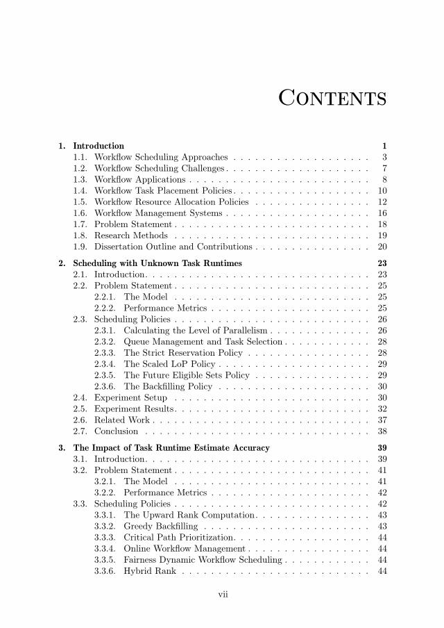
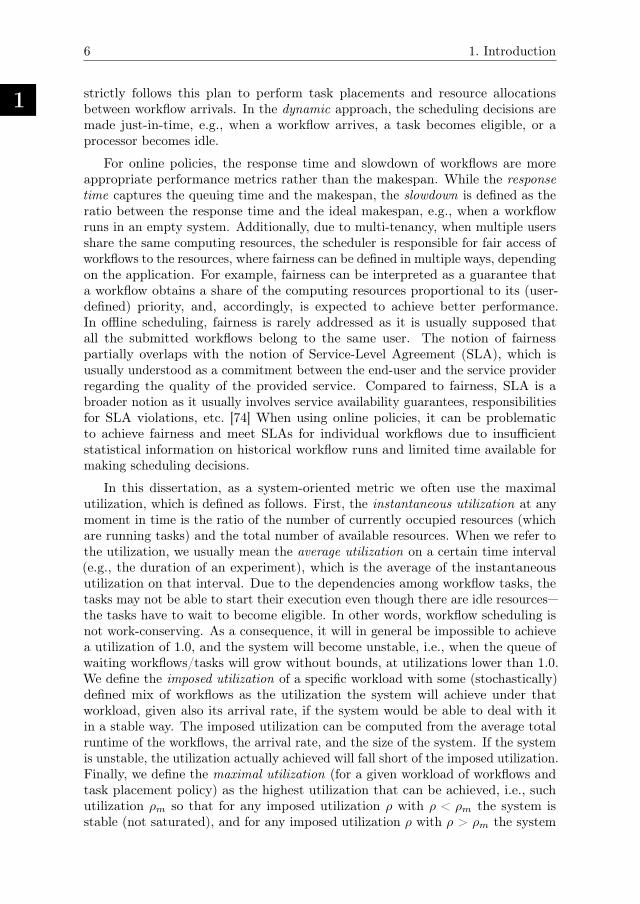
The most popular representation of workflows is by means of DAGs. In thisdissertation by job we understand the whole workflow DAG, by task we understanda node of a workflow DAG, and by a precedence constraint we understand an edgeof the DAG connecting two tasks. The size of a workflow is defined as the numberof its tasks. A workflow task is eligible for execution when all of its ancestors,according to the workflow structure, have completed and all the required data havearrived over the communication links.

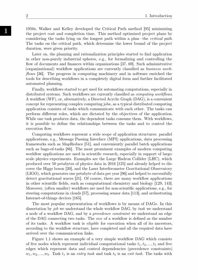
Figure 1.1 shows an example of a very simple workflow DAG which consistsof five nodes which represent individual computational tasks t1, t2, ..., t5 and fiveedges which represent data and control dependencies (precedence constraints)w1, w2, ..., w5. Task t1 is an entry task and task t5 is an exit task. The tasks with

1.1. Workflow Scheduling Approaches

1

3

t1

t2

t3

t4

t5

w1

w2

w3

w4

w5

Figure 1.1: An example of a workflow.

outgoing edges are called predecessors or parent tasks with regard to the tasks inwhich these edges enter. The tasks with incoming edges are called successors orchild tasks with regard to the tasks from where these edges originate. For example,t1 is a predecessor of t2 and t3, and t2 and t3 are successors of t1. In every workflowDAG it is possible to distinguish basic inter-task interaction patterns which areoften observed in practice:

1. The pipeline consists of a chain of tasks each of which (except for the firsttask in the chain) has only one precedence constraint in the DAG fromits predecessor in the chain. In Figure 1.1, the tasks t3 and t4 constitutea pipeline. The data produced by task t3 are transferred via link w4 andconsumed by task t4.

2. The data distribution or map operation models a situation when multipletasks have precedence constraints only to a single ancestor task. In Figure 1.1,a map operation consists of tasks t1, t2, t3 and the data transfer links betweenthem, namely, w1 and w2. The data produced by task t1 are distributed (ormapped) to tasks t2 and t3 via communication links w1 and w2.

3. The data aggregation or reduce operation models a situation when a singletask has precedence constraints to multiple ancestor tasks. In Figure 1.1,a reduce operation consists of tasks t2, t4, t5 and the data transfer linksbetween them, w3 and w5. The data produced independently by tasks t2 andt4 are transferred via links w3 and w5 to task t5 for aggregation.

4. The parallel processing model or bag-of-tasks represents the parallel indepen-dent execution of multiple tasks which do not have precedence constraintsamong them. In Figure 1.1 parallel processing is represented by tasks t2 andt3, and by t2 and t4. The tasks in either of these pairs can be executed inparallel.

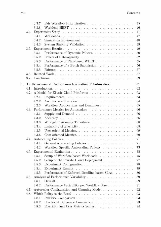
1.1. Workflow Scheduling ApproachesThe growing applicability of computing workflows has led to the development ofappropriate algorithms designed for scheduling them efficiently. Workflow schedul-ing can be seen from the task placement and resource allocation perspectives,where by task placement we understand the mapping of tasks to computing re-sources, and by resource allocation we understand the allocation and deallocationof computing resources. The allocation and deallocation of resources, e.g., virtual

1

4 1. Introduction

SingleWorklow

Batch ofWorklows

Stream ofWorklows

Repeatedsubmissions

Stochasticarrival process

SlowdownMakespan Fairness

Oline

WorklowArrival

Planning

Plan-basedPlacement and

Allocation

Task Execution

Fairness

1 2

2a

Worklow Schedulers

Online

Online: Plan-based

Planning

Plan-basedPlacement and

Allocation

Oline: Plan-based1a

Task Execution

DynamicPlacement and

Allocation

Oline: Dynamic1b

Task Execution

WorklowArrival

DynamicPlacement and

Allocation

Task Execution

2bOnline: Dynamic

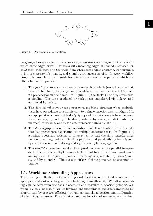
Figure 1.2: A hierarchy of classes of workflow scheduling approaches for task placement andresource allocation.

machines in a public cloud, is usually controlled automatically using autoscaling [72].Figure 1.2 presents the hierarchy of classes of workflow scheduling approaches fortask placement and resource allocation used in this dissertation.

Originally, computing workflows were mostly executed on standalone computersor on computing clusters and grids [100, 138, 23]. This execution model is still pop-ular, for example, in research institutions, and it usually implies a limited number ofknown users running a limited number of pre-defined workflows, possibly submittedand executed in batches. We classify scheduling policies designed specifically forstatic sets (i.e., initially present at the moment when the scheduling decisions aremade) of workflows with fully known inter-task dependencies as offline policies(Block 1 in Figure 1.2). As the same workflows or batches of workflows are oftenexecuted repeatedly, either the user or the scheduling system may be able to derivereasonable estimates of the task runtimes [124, 43]. In such a situation, using notonly the fully known inter-task dependencies but also the task runtime estimates,and, sometimes, the communication overheads between tasks, it is possible tocreate a task placement and resource allocation plan beforehand [155, 170, 23, 33].Such policies constitute the majority of the available state-of-the-art offline policies,

1.1. Workflow Scheduling Approaches

1

5

and we refer to them as offline plan-based policies (Block 1a). Another group ofoffline policies, while still scheduling an initially present set of workflows, does notconstruct any plan, but, instead, makes the scheduling decisions on-the-fly, e.g.,when a task becomes eligible or a resource becomes idle [116]. We refer to suchpolicies as offline dynamic policies (Block 1b).

For offline policies, the most common performance metric from the end-userperspective is the minimization of the makespan of a workflow or a batch ofworkflows. For a single workflow, the makespan is defined as the time between thestart of its first task until the completion of its last task. Accordingly, for a batch ofworkflows the makespan is defined as the time between the start of the first task ofany workflow in the batch until the completion of the last task of any workflow inthe batch. It is often supposed that a workflow or a batch is executed on resourcesreserved beforehand exclusively for the submitting user, so that the policy is fullyaware of the number and the type of the available resources [142, 24, 164]. Thismeans that during the execution of workflows belonging to a certain user, no directinterference on their performance can be observed from other users. Therefore, theaccess to computing resources among multiple users is usually outside the scopeof offline policies. When scheduling a batch of workflows, the user is normallyinterested in the minimization of the makespan of the whole batch rather than inthe minimization of the makespans of specific workflows within the batch.

Nowadays, computing workflows are used in a much wider scope comparedto their earlier applications in clusters and grids. They have become a popularautomation tool for controlling computations in various types of online systems, forexample, within website back-ends, in data analytics services, in computing clouds,etc. [162, 158]. In such environments, multiple users can constantly submit theirworkflow jobs, thus generating a stochastic arrival process, leading to workloads(streams) of workflows.

In such workloads of workflow, every arrival can contain a unique workflowstructure, so that deriving statistical information on task runtimes and inter-taskcommunication overhead is difficult [43]. Various workflows can also have differentpriorities. For example, while some workflows are responsible for running business-critical infrastructure and are very sensitive to delays, e.g., processing of radardata for a weather forecasting website, other workflows process auxiliary data,e.g., user preferences in social networks which are not time-critical. Additionally,workflows can be assigned deadlines that define the time by which each workflowshould be completed [164]. In cloud computing, the resources are paid for basedon usage, so that the user normally has a certain budget to spend on workflowexecution [119, 164]. Cloud computing services provide various types of resourceswith different performance characteristics and costs. The same workflow can beexecuted on different combinations of resource types, which leads to a variety ofperformance and cost options. All these factors make scheduling of workloads ofworkflows challenging and requires special policies [169, 77, 29]. The schedulingof workloads of workflows can be classified as an online problem (Block 2). Inonline scheduling, similarly to offline scheduling, we distinguish online plan-basedscheduling (Block 2a) and online dynamic scheduling (Block 2b). The plan-basedscheduling approach constructs a (partial) plan on every workflow arrival and

1

6 1. Introduction

strictly follows this plan to perform task placements and resource allocationsbetween workflow arrivals. In the dynamic approach, the scheduling decisions aremade just-in-time, e.g., when a workflow arrives, a task becomes eligible, or aprocessor becomes idle.

For online policies, the response time and slowdown of workflows are moreappropriate performance metrics rather than the makespan. While the responsetime captures the queuing time and the makespan, the slowdown is defined as theratio between the response time and the ideal makespan, e.g., when a workflowruns in an empty system. Additionally, due to multi-tenancy, when multiple usersshare the same computing resources, the scheduler is responsible for fair access ofworkflows to the resources, where fairness can be defined in multiple ways, dependingon the application. For example, fairness can be interpreted as a guarantee thata workflow obtains a share of the computing resources proportional to its (user-defined) priority, and, accordingly, is expected to achieve better performance.In offline scheduling, fairness is rarely addressed as it is usually supposed thatall the submitted workflows belong to the same user. The notion of fairnesspartially overlaps with the notion of Service-Level Agreement (SLA), which isusually understood as a commitment between the end-user and the service providerregarding the quality of the provided service. Compared to fairness, SLA is abroader notion as it usually involves service availability guarantees, responsibilitiesfor SLA violations, etc. [74] When using online policies, it can be problematicto achieve fairness and meet SLAs for individual workflows due to insufficientstatistical information on historical workflow runs and limited time available formaking scheduling decisions.

In this dissertation, as a system-oriented metric we often use the maximalutilization, which is defined as follows. First, the instantaneous utilization at anymoment in time is the ratio of the number of currently occupied resources (whichare running tasks) and the total number of available resources. When we refer tothe utilization, we usually mean the average utilization on a certain time interval(e.g., the duration of an experiment), which is the average of the instantaneousutilization on that interval. Due to the dependencies among workflow tasks, thetasks may not be able to start their execution even though there are idle resources—the tasks have to wait to become eligible. In other words, workflow scheduling isnot work-conserving. As a consequence, it will in general be impossible to achievea utilization of 1.0, and the system will become unstable, i.e., when the queue ofwaiting workflows/tasks will grow without bounds, at utilizations lower than 1.0.We define the imposed utilization of a specific workload with some (stochastically)defined mix of workflows as the utilization the system will achieve under thatworkload, given also its arrival rate, if the system would be able to deal with itin a stable way. The imposed utilization can be computed from the average totalruntime of the workflows, the arrival rate, and the size of the system. If the systemis unstable, the utilization actually achieved will fall short of the imposed utilization.Finally, we define the maximal utilization (for a given workload of workflows andtask placement policy) as the highest utilization that can be achieved, i.e., suchutilization ρm so that for any imposed utilization ρ with ρ < ρm the system isstable (not saturated), and for any imposed utilization ρ with ρ > ρm the system

1.2. Workflow Scheduling Challenges

1

7

Scheduler

Autoscaler

Stochastic arrival processof worklows

Users

Storage

Resources

Task

Task

Task

Data IO, status updates

Supply and demandinformation

Task placement

Allocation anddeallocation

Task andresource states

1

2

3

5

4

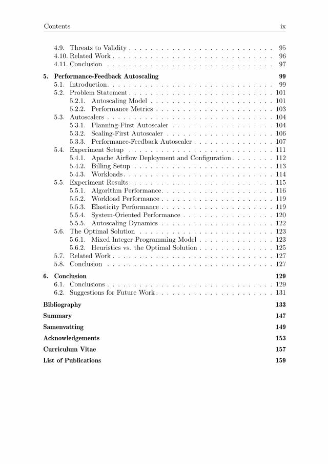
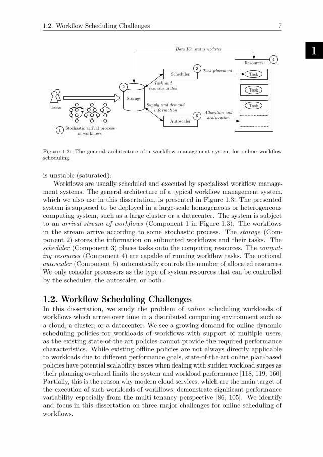
Figure 1.3: The general architecture of a workflow management system for online workflowscheduling.

is unstable (saturated).Workflows are usually scheduled and executed by specialized workflow manage-

ment systems. The general architecture of a typical workflow management system,which we also use in this dissertation, is presented in Figure 1.3. The presentedsystem is supposed to be deployed in a large-scale homogeneous or heterogeneouscomputing system, such as a large cluster or a datacenter. The system is subjectto an arrival stream of workflows (Component 1 in Figure 1.3). The workflowsin the stream arrive according to some stochastic process. The storage (Com-ponent 2) stores the information on submitted workflows and their tasks. Thescheduler (Component 3) places tasks onto the computing resources. The comput-ing resources (Component 4) are capable of running workflow tasks. The optionalautoscaler (Component 5) automatically controls the number of allocated resources.We only consider processors as the type of system resources that can be controlledby the scheduler, the autoscaler, or both.

1.2. Workflow Scheduling ChallengesIn this dissertation, we study the problem of online scheduling workloads ofworkflows which arrive over time in a distributed computing environment such asa cloud, a cluster, or a datacenter. We see a growing demand for online dynamicscheduling policies for workloads of workflows with support of multiple users,as the existing state-of-the-art policies cannot provide the required performancecharacteristics. While existing offline policies are not always directly applicableto workloads due to different performance goals, state-of-the-art online plan-basedpolicies have potential scalability issues when dealing with sudden workload surges astheir planning overhead limits the system and workload performance [118, 119, 160].Partially, this is the reason why modern cloud services, which are the main target ofthe execution of such workloads of workflows, demonstrate significant performancevariability especially from the multi-tenancy perspective [86, 105]. We identifyand focus in this dissertation on three major challenges for online scheduling ofworkflows.

1

8 1. Introduction

1. How to realistically estimate the resource demand of a workflow? Usually,workflows consist of segments with different parallelism and different inter-connection types between tasks which affect the order how the tasks becomeeligible. Moreover, realistic task runtime estimates are not always available inadvance and can only be obtained after a real workflow execution [43] or, insome cases, after a code analysis [99]. The user runtime estimates are oftensubjective [124] and thus less useful. The knowledge of resource demand isimportant for making good task placement and resource allocation decisions.

2. How to assign tasks of workflows to resources to minimize average slowdownwhile achieving fairness? A wrongly chosen task placement policy can easilydegrade the performance of certain workflows in workloads and negativelyaffect the fair access of workflows to computing resources [32]. Fairness is veryimportant in concurrent environments where multiple users simultaneouslyexecute their workflows, as different users could have different numbers andtypes of workflows submitted. However, the efficiency of certain schedulingpolicies could depend on the system utilization, and fairness can be interpreteddifferently depending on user and service provider interests. For example,jobs can be prioritized based on the total number of submitted jobs by a user,based on the disposable budget, or on the number of tasks in the jobs, etc.

3. How to allocate resources for workflows while meeting deadline and budgetconstraints? Modern computing infrastructures make it possible to easilylease and release computing resources. Autoscaling decisions should be madewisely to minimize slowdowns and, accordingly, minimize deadline violations.In order to minimize incurred costs, the over-provisioning of resources duringautoscaling should be minimized, and the use of leased resources by theplacement policy should be efficient. Online scheduling makes it possibleto react to changes in the number of allocated computing resources duringthe workload execution. Thus, preferably, the autoscaler and the schedulershould operate in tandem to achieve common optimization goals withoutcounteracting each other.

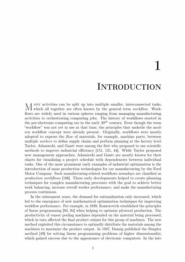
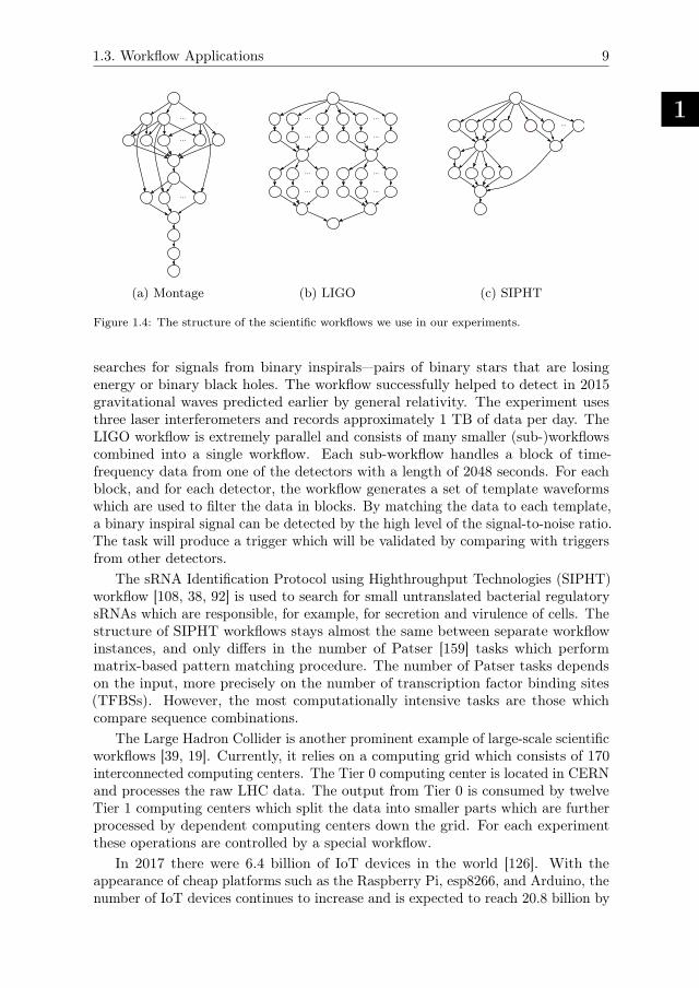
1.3. Workflow ApplicationsThe majority of extreme-scale workflows originate from the scientific domain. ThePegasus project [55] has done a great job on classifying and modelling manyimportant scientific workflows. Figure 1.4 shows the structure of three typicalscientific workflows from different fields. The Montage workflow [90, 152, 38,92], created by NASA/IPAC Infrared Science Archive, is used in astronomy forprocessing telescope images to produce large custom mosaic images of the sky.Various operations can be applied to the input images, for example, they can berotated, scaled, or their brightness can be adjusted. The geometry of the finalmosaic depends on the geometry of the input images. The workflow has a complexstructure, which is determined by the types of applied operations, and its size isdetermined by the number of processed images.

The LIGO Inspiral Analysis workflow processes the data from the detectorsof the Laser Interferometer Gravitational Wave Observatory (LIGO) [22], and

1.3. Workflow Applications

1

9

...

...

...

(a) Montage

...

...

...

...

...

...

...

...

(b) LIGO

...

(c) SIPHT

Figure 1.4: The structure of the scientific workflows we use in our experiments.

searches for signals from binary inspirals—pairs of binary stars that are losingenergy or binary black holes. The workflow successfully helped to detect in 2015gravitational waves predicted earlier by general relativity. The experiment usesthree laser interferometers and records approximately 1 TB of data per day. TheLIGO workflow is extremely parallel and consists of many smaller (sub-)workflowscombined into a single workflow. Each sub-workflow handles a block of time-frequency data from one of the detectors with a length of 2048 seconds. For eachblock, and for each detector, the workflow generates a set of template waveformswhich are used to filter the data in blocks. By matching the data to each template,a binary inspiral signal can be detected by the high level of the signal-to-noise ratio.The task will produce a trigger which will be validated by comparing with triggersfrom other detectors.

The sRNA Identification Protocol using Highthroughput Technologies (SIPHT)workflow [108, 38, 92] is used to search for small untranslated bacterial regulatorysRNAs which are responsible, for example, for secretion and virulence of cells. Thestructure of SIPHT workflows stays almost the same between separate workflowinstances, and only differs in the number of Patser [159] tasks which performmatrix-based pattern matching procedure. The number of Patser tasks dependson the input, more precisely on the number of transcription factor binding sites(TFBSs). However, the most computationally intensive tasks are those whichcompare sequence combinations.

The Large Hadron Collider is another prominent example of large-scale scientificworkflows [39, 19]. Currently, it relies on a computing grid which consists of 170interconnected computing centers. The Tier 0 computing center is located in CERNand processes the raw LHC data. The output from Tier 0 is consumed by twelveTier 1 computing centers which split the data into smaller parts which are furtherprocessed by dependent computing centers down the grid. For each experimentthese operations are controlled by a special workflow.

In 2017 there were 6.4 billion of IoT devices in the world [126]. With theappearance of cheap platforms such as the Raspberry Pi, esp8266, and Arduino, thenumber of IoT devices continues to increase and is expected to reach 20.8 billion by

1

10 1. Introduction

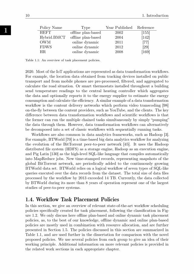
Policy Name Type Year Published ReferenceHEFT offline plan-based 2002 [155]Hybrid.BMCT offline plan-based 2004 [142]OWM online dynamic 2011 [77]FDWS online dynamic 2012 [29]HR online dynamic 2008 [169]

Table 1.1: An overview of task placement policies.

2020. Most of the IoT applications are represented as data transformation workflows.For example, the location data obtained from tracking devices installed on publictransport and from mobile phones are pre-processed, filtered, and aggregated tocalculate the road situation. Or smart thermostats installed throughout a buildingsend temperature readings to the central heating controller which aggregatesthe data and optionally reports it to the energy supplier to estimate the energyconsumption and calculate the efficiency. A similar example of a data transformationworkflow is the content delivery networks which perform video transcoding [98]on-the-fly between the content providers, such as YouTube, and the clients. The keydifference between data transformation workflows and scientific workflows is thatthe former can run the multiple chained tasks simultaneously by simply “pumping”the data through them. However, data transformation workflows can alternativelybe decomposed into a set of classic workflows with sequentially running tasks.

Workflows are also common in data analytics frameworks, such as Hadoop [3].For example, BTWorld [70] is a time-based big data analytics workflow for analyzingthe evolution of the BitTorrent peer-to-peer network [45]. It uses the Hadoopdistributed file system (HDFS) as a storage engine, Hadoop as an execution engine,and Pig Latin [130] as the high-level SQL-like language that compiles automaticallyinto MapReduce jobs. New time-stamped records, representing snapshots of theglobal BitTorrent network, are periodically added to the continuously growingBTWorld data set. BTWorld relies on a logical workflow of seven types of SQL-likequeries executed over the data records from the dataset. The total size of data filesprocessed by the workflow by 2013 exceeded 14 TB. Currently, the data collectedby BTWorld during its more than 8 years of operation represent one of the largeststudies of peer-to-peer systems.

1.4. Workflow Task Placement PoliciesIn this section, we give an overview of relevant state-of-the-art workflow schedulingpolicies specifically created for task placement, following the classification in Fig-ure 1.2. We only discuss here offline plan-based and online dynamic task placementpolicies, as, to the best of our knowledge, offline dynamic and online plan-basedpolicies are mostly used in combination with resource allocation, and are furtherpresented in Section 1.5. The policies discussed in this section are summarized inTable 1.1, and are used further in the dissertation for comparison with the novelproposed policies. We use several policies from each group to give an idea of theirworking principle. Additional information on more relevant policies is provided inthe related work sections in each appropriate chapter.

1.4. Workflow Task Placement Policies

1

11

Before describing the workflow task placement policies, we start with introducingsome notions. Scheduling of workflows often operates with the notions of eligibleset and level of parallelism. For a workflow, at any point in time before or duringits execution, its eligible set (of tasks) is the set of non-completed tasks of whichthe precedence constraints have been satisfied. In other words, the eligible set isthe set of all tasks that are currently running and those that are waiting but thatcould run if sufficient resources were available. More generally, we introduce thenotion of the generation-i eligible set (or the eligible set of generation i) at anypoint in the execution of a workflow, which is a potential future eligible set. Thegeneration-0 eligible set of a workflow is simply equal to its current eligible set. Thegeneration-(i+ 1) eligible set of a workflow contains all the tasks that will becomeeligible when (exactly and only) all the tasks from its generation-i eligible set havecompleted. It is important not to confuse eligible sets with levels in a workflow.The levels consist of the tasks that have the same distance from the entry task.However, the eligible sets of generation-i can differ from the levels, because pathsof different lengths can exist in a workflow from the entry task to any other singletask.

For a workflow that has not yet completed, we define its Level of Parallelism(LoP) as the maximum number of processors it may ever use at any future pointin its execution, which is equal to the maximum number of tasks in any of itspotential future eligible sets. Of course, the LoP of a workflow can only stay thesame or decrease during its execution. The LoP can be computed exactly [79] orapproximately [83].

The upward rank is often used to prioritize tasks in workflows based on theirduration and proximity to the exit task. The upward rank requires task runtimeestimates for all the resource types and communication overhead estimates forall the communication links to be known beforehand. Since the exit task has nosuccessors, its upward rank simply equals to its average estimated runtime on all theresource types. For each task in a workflow its upward rank is recursively calculated,starting from the exit task, as the sum of the average estimated runtime of the taskand the maximal sum (among all its immediate successors) of the upward rankof an immediate successor and the average communication overhead between thecurrent task and that successor. A more detailed definition of the upward rank isprovided in Section 3.3.1. The average estimated execution time is calculated foreach task using the average speed of the processors in the system. The averageestimated communication cost is calculated as the average communication start-uptime plus the size of the data to be transmitted, divided by the average transferrate between the processors. The length of the critical path of a workflow is equalto the maximum value of the upward rank among all its tasks. By workflow lengthwe mean the length of its critical path.

Similarly, the downward rank of a task is recursively calculated starting fromthe entry task as the maximal sum, among all the immediate predecessors, of thedownward rank of an immediate predecessor, the average estimated execution timeof the predecessor, and the average communication overhead between the currenttask and that predecessor. For the entry task the downward rank is zero.

We now turn to the discussion of the policies. The Heterogeneous Earliest Finish

1

12 1. Introduction

Time (HEFT) [155] is an offline plan-based policy proposed by Topcuoglu in 2002and it is one of the most well-known heuristics for scheduling individual workflows.Given a workflow DAG with known task runtime estimates and communicationdelays between the tasks, this policy produces a task placement plan which is usedto steer the workflow execution. HEFT uses upward rank to prioritize tasks. Itadds the tasks to the plan in descending order of their upward ranks and assignsthe tasks to processors that minimize their earliest finish times.

The Hybrid Balanced Minimum Completion Time (Hybrid.BMCT) [142] is anoffline plan-based policy proposed by Sakellariou and Zhao in 2004 and consistsof two parts: Hybrid and BMCT. The Hybrid part first sorts workflow tasks indescending order of their upward ranks, and then successively groups the tasks intoeligible sets so that each set contains tasks with no direct dependencies betweenthem. Each task can belong to a single eligible set only. For each workflow theeligible sets are numbered in the order of their creation, with the eligible setcontaining the entry node of the workflow having number one. The tasks from eacheligible set are assigned to processors using the BMCT list-scheduling policy withthe objective to complete the execution of all tasks as early as possible. In thebeginning, BMCT plans the tasks to the processors minimizing their execution time.After the initial assignment, BMCT tries to optimize the plan by moving tasksbetween processors to minimize the overall makespan until no further improvementis possible.

The Online Workflow Management (OWM) [77] is an online dynamic policyproposed by Hsu, Huang, and Wang in 2011. It maintains a single joint eligible setcontaining only a single eligible task (if any) with the highest upward rank fromevery workflow present in the system. As long as there are eligible tasks in thesystem, the scheduler selects the task with the highest upward rank from the jointset and tries to assign it to a processor. If the idle processors have different speeds,the task is placed on the fastest one. If the processors have the same speed, thepolicy checks for the busy processor which will be idle first, whether the task has alower estimated finish time on it rather than on any idle processors. If that thecase, the task is postponed, otherwise, it is placed on any of the idle processors.

The Fairness Dynamic Workflow Scheduling (FDWS) [29] is an online dynamicpolicy proposed by Arabnejad and Barbosa in 2012. It maintains a single jointeligible set in the same way as OWM. However, within the joint set each task isprioritized based on the fraction of remaining tasks of its workflow and the workflowlength.

The Rank Hybd (HR) [169] is an online dynamic policy proposed by Yu andShi in 2008. The policy maintains a single joint eligible set of all the eligible tasksfrom all the workflows in the system. If the tasks in the joint set belong to differentworkflows, the scheduler selects the task with the lowest upward rank. If the tasksin the joint set are from the same workflow, the algorithm selects the task with thehighest upward rank.

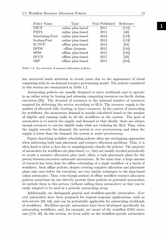
1.5. Workflow Resource Allocation PoliciesIn this section, we give an overview of different types of autoscalers for workflows—specialized policies targeting resource allocation. The resource allocation problem

1.5. Workflow Resource Allocation Policies

1

13

Policy Name Type Year Published ReferenceDSCS online plan-based 2011 [118]PBTS online plan-based 2011 [40]Scheduling-First online plan-based 2013 [119]Scaling-First online plan-based 2013 [119]IC-PCP offline plan-based 2013 [24]DPDS offline dynamic 2015 [116]SPSS offline plan-based 2015 [116]DCCP offline plan-based 2017 [33]MIP offline plan-based 2017 [164]

Table 1.2: An overview of resource allocation policies.

has attracted much attention in recent years due to the appearance of cloudcomputing with its on-demand resource provisioning model. The policies consideredin this section are summarized in Table 1.2.

Autoscaling policies are usually designed to serve workloads and to operatein an online setup by leasing and releasing computing resources on-the-fly duringexecution [25]. The demand of resources is the minimal number of resourcesrequired for delivering the service according to SLA. The resource supply is thenumber of allocated (idle, booting, or busy) resources. In the context of autoscalingfor workflows, the momentary demand is usually calculated based on the numberof eligible and running tasks in all the workflows in the system. The goal ofautoscalers is to match the supply and demand so that ideally, there are alwaysenough resources to execute eligible tasks while not violating the SLA. Thus, whenthe supply exceeds the demand, the system is over-provisioning, and when thesupply is lower than the demand, the system is under-provisioning.

Papers describing workflow scheduling policies often use overlapping approacheswhen addressing both task placement and resource allocation problems. Thus, it isoften hard to draw a clear line to unambiguously classify the policies. The majorityof autoscalers for workflows are plan-based, i.e., they are usually invoked periodicallyto create a resource allocation plan (and, often, a task placement plan) for theperiod between successive autoscaler invocations. At the same time, a large amountof research has been done for offline scheduling of a single workflow or a batch ofworkflows. Such offline policies, despite creating complete allocation and placementplans only once before the execution, use very similar techniques to the plan-basedonline autoscalers. Thus, even though authors of offline workflow resource allocationpolicies sometimes do not directly present these policies as potential autoscalers,we include them in this section (without calling them autoscalers) as they can beeasily adapted to be used in a periodic autoscaling setup.

Additionally, we distinguish general and workflow-specific autoscalers. Gen-eral autoscalers have been proposed for request-response applications, such asweb-servers [26, 64], and can be potentially applicable for autoscaling workloadsof workflows. Workflow-specific autoscalers have been developed specifically forautoscaling workflows, and, for example, are aware of the workflow DAG struc-ture [118, 40]. In this section, we focus solely on the workflow-specific autoscalers.

1

14 1. Introduction

The Dynamic Scaling-Consolidation-Scheduling (DSCS) policy [118] is an onlineplan-based autoscaler which combines scheduling and allocation approaches, pub-lished by Mao and Humphrey in 2011. DSCS is one of the first proposed autoscalersdedicated for workloads of workflows. The policy supports soft deadlines assignedon a per workflow basis by the user and supposes that the budget is unlimited. Themain optimization goal of DSCS is to meet as many workflow deadlines as possiblewhile minimizing the total operational cost. In the beginning, the policy groupsworkflow tasks that share the same predecessor and prefer the same resource type,and considers them as a single task. To improve the resource utilization, the policytries to plan sequential execution of certain parallel tasks, if it does not lead to thedeadline violation. Then DSCS distributes the per workflow deadline among itstasks proportionally to their runtimes on the most cost-efficient resources. If suchassignment does not allow the workflow to finish by its deadline, DSCS tries toreduce the workflow makespan by placing certain tasks on faster but more expensiveresources, which allow to shorten the maskespan at lowest increase in operationalcost. The resources are allocated based on so-called “load vectors”, where the loadvector represents the number of resources of a certain type required to finish thetask without violating its deadline. Finally, after resources are allocated, DSCSplans the tasks to the resources giving priority to the tasks with earliest deadlines.

The Partitioned Balanced Time Scheduling (PBTS) policy [40] is an onlineplan-based autoscaler proposed by Byun, Kee, Kim, and Maeng in 2011. The policycreates a resource allocation and task placement plan for each “time partition”which equals the billing period of the cloud provider, e.g., one hour. The goalof PBTS is to minimize the operational cost within a time partition and finishthe workflow within its deadline. To minimize the operational cost, PBTS placesthe tasks on resources by allowing workflow tasks to be delayed (by slack time) ifsuch a delay does not violate the workflow deadline. For that, PBTS, followingthe workflow structure, builds a task placement plan for each time partition todetermine how the required resource demand is going to change. Then the policydistributes the slack time over time partitions to minimize the operational cost.Finally, PBTS approximates the required resource capacity within the target timepartition and places the tasks on the resources.

The Scheduling-First policy [119] is another online plan-based autoscaler pro-posed by Mao and Humphrey in 2013. It is designed for autoscaling workloads ofworkflows in clouds with budget constraints. Each workflow has a user-assignednumeric priority, the budget is provided per autoscaling interval and is distributedamong all the submitted workflows based on their priority. The policy iteratesthrough the eligible tasks of all the workflows sorted in the descending order oftheir workflow priorities, and for each task it tries to allocate the fastest resourcewhile there is enough budget. After that, the policy consolidates the resources byplanning the execution of the remaining eligible and not-yet eligible tasks on theallocated resources.

The Scaling-First policy [119] is an online plan-based autoscaler proposed byMao and Humphrey together with Scheduling-First. It first creates an independentper-workflow plan so that the number of resources in each plan could be bigger thanthe actual maximal number of available resources in the system. Then it calculates

1.5. Workflow Resource Allocation Policies

1

15

the cost of each plan and scales it down to fit within the budget constraint. Finally,the policy allocates the resources based on the plan information and performs theresource consolidation.

The IaaS Cloud Partial Critical Paths (IC-PCP) policy [24] is an offline plan-based policy proposed by Abrishami, Naghibzadeh, and Epema in 2013. Thepolicy is designed for planning a workflow execution in an IaaS cloud, and supposesthat the workflow has a user-specified deadline and an unlimited budget. Theoptimization goal of the policy is to minimize the execution cost of the workflow,while completing the workflow before the deadline. IC-PCP finds the critical pathin the workflow and distributes the workflow deadline among the tasks on thecritical path in proportion to their minimum runtime. After that, each task on thecritical path has a deadline assigned which is used to compute task deadlines forall of its predecessors. Finally, the policy plans tasks on the cheapest resourcesthat allow to meet task deadlines.

The Dynamic Provisioning Dynamic Scheduling (DPDS) policy [116] is a offlinedynamic autoscaler proposed by Malawski in 2015. It is designed to provideautoscaling for already present ensembles of scientific workflows during the execution,where each workflow has a user-assigned numeric priority. In a sense, DPDS is atransitional phase between a purely offline plan-based policies and online dynamicpolicies. DPDS supports cost- and deadline-constrained provisioning of resourcesof a single type only, where the deadline and the budget are provided for the wholeensemble. DPDS calculates the number of resources to provision so that the entirebudget is consumed before the deadline. It allocates the calculated number ofresources at the beginning of the ensemble execution. Then it leases or releasesresources based on their utilization by the workflows according to given thresholds.To schedule workflow tasks, DPDS maintains a joint eligible set in the same wayas in the aforementioned HR policy (see Section 1.4). The tasks from the set areplaced on random idle resources according to the priority of the workflow to whichthey belong.

The Static Provisioning Static Scheduling (SPSS) policy [116] is an offlineplan-based policy also proposed by Malawski in the same paper as DPDS. SPSScreates a plan for each workflow in the ensemble in priority order, and rejects anyworkflow that exceeds the deadline or budget. The goal of the policy is to finisheach workflow by the deadline with the lowest possible cost to maximize the numberof workflows completed within the given budget. SPSS distributes the workflowdeadline to its individual tasks considering the slack time of the workflow, which isthe additional amount of time that a workflow can extend its critical path whilecompleting by the ensemble deadline. The slack time is distributed to each level ofthe workflow proportionally to the number of tasks in that level and the total taskruntime in that level. The tasks are then planned on resources that minimize theexecution cost and meet the task deadlines. A new resource is allocated if there areno slots available on the allocated resources that would allow the task to finish byits deadline. SPSS performs resource consolidation, similarly to Scheduling-Firstand Scaling-First policies, in order to increase the utilization of allocated resources.

The Deadline Constrained Critical Path (DCCP) policy [33] is an offline plan-based policy proposed by Arabnejad, Bubendorfer, and Ng in 2017. The policy has

1

16 1. Introduction

the same goal as the IC-PCP policy. For each workflow task, DCCP calculatesits distance to the exit task, which is the number of DAG edges on the shortestpath to the exit task, and then groups the tasks with the same distance. Thenthe user-defined deadline is distributed among the levels of the workflow so thatthe levels with bigger task runtimes get a larger share of the workflow deadline.DCCP relies on the notion of Constrained Critical Path (CCP) [97], which denotesthe subset of tasks laying on the critical path that are currently eligible. Forfinding the critical path, the policy utilizes modified upward and downward ranksthat aggregate the communication overhead between a task and its successorsand predecessors, instead of just selecting the maximum communication overhead.DCCP co-locates tasks from CCP that communicate within the same resource.The tasks are planned on resources that minimize their earliest completion timeand do not exceed the level deadline.

The Mixed Integer Programming (MIP) policy [164] is an offline plan-basedpolicy proposed by Wang, Xia, and Chen in 2017. The goal of MIP is to minimizethe operational cost of using different types of cloud resources while ensuring thecompletion of the scheduled workflows by their deadlines. In contrast to all theconsidered heuristic policies, the MIP approach guarantees that the producedsolution is optimal. The policy requires task runtime estimates and formulates theworkflow scheduling problem using five MIP constraints: (i) Precedence constraintsthat require the tasks to be executed in the order specified by the workflow,(ii) Resource constraints that describe the requirements of each task to certainresource types, and set the limits to the maximal number of resources of each typethat can be allocated, (iii) Non-overlapping constraints describe that each resourcecan run only a single task at a time, (iv) Ready time constraints that specify thetime when each workflow can start its execution, and (v) Deadline constraints thatrequire each workflow to finish by its deadline. The policy relies on the GurobiMIP solver [14] for finding the solution. The policy models the decision space as amatrix of time slots vs. resources where each element is a binary decision variablewhich represents a task assignment. The precision of the solution depends on thetime discretization used.

1.6. Workflow Management SystemsComputing workflows are usually executed by specialized workflow managementsystems. Even though such systems can provide different functionality, the funda-mental properties inherent to most workflow management systems are: controllingtask execution order in accordance with the workflow structure, and scheduling andplacing of tasks on resources. Optionally, workflow management systems implementdedicated interfaces for data exchange between tasks, and resource managementfunctionality.

To control the task execution order within a workflow, a workflow managementsystem needs to know which tasks are eligible to start their execution. To this end,a workflow management system either periodically or in an event-driven mannermonitors task statuses. Periodic monitoring means that the tasks are periodicallypolled by the workflow management system and their current status is checked.Event-driven approach means that a task sends a message to the workflow manage-

1.6. Workflow Management Systems

1

17

ment system when it changes its state, thus, potentially enabling faster triggeringof descendants. Alternatively, a task can send messages directly to its descendantsto trigger them. Various hybrid approaches are also possible, including the modifi-cation of inter-task dependencies during the workflow execution based on a certaincriteria. Periodic monitoring is employed by most workflow management systems,e.g., Pegasus [17, 54], ASKALON [61], and by the more recent Apache Airflow [2].Event-driven approach is common in serverless computing services, e.g., AmazonLambda [1], IBM Cloud Functions [15], and Azure Functions [5], where serverlesscomputing is a form of cloud computing enabling outsourcing of the operationallogic to the service provider.

The eligible tasks are placed on resources according to a scheduling policyimplemented by the workflow management system. Data can be exchanged betweentasks either in peer-to-peer manner or centrally, e.g., through a shared file system.In any case, the workflow management system is aware about the exchanged dataif that is important for determining task eligibility. Resource management is oftenperformed by a specialized independent software layer, which, in some cases, canperform automatic allocation and deallocation of resources to react and adapt tothe fluctuations in the number of eligible tasks to meet performance goals.

It is important to notice that the traditional approach, used by the majority ofstandalone workflow management systems, supposes that the user is responsiblefor deploying most of the software layers implementing the operational logic. Incontrast, serverless services do this job for user, guaranteeing that the workflowsare containerized, deployed, scheduled, provisioned, and available on demand, whileonly charging the user for the used resources. However, all the aforementionedworkflow management systems and even the serverless computing services, requirethe user to first define a workflow which will stay in the system and will further betriggered either periodically or by an event. Thus, most of the existing systems,even if they are capable of processing workloads of workflows, are still designedwith the offline approach in mind.

The Pegasus project [54, 55, 17] has developed a workflow management systemfor scientific workflows which first appeared in 2001. The development of Pegasuswas motivated by the necessity to match the growing computational needs ofthe scientific community and the available cyberinfrastructures. Pegasus supportsmultiple execution engines, thus, the same workflows can be run on different physicalinfrastructures such as clusters, grids, and clouds. Based on the user-providedXML description of a workflow, Pegasus generates an executable workflow, i.e.,the mapping of workflow tasks on the resources. The job scheduler controls theexecution flow of individual workflow jobs according to the mapping. Pegasus allowslocal and remote execution of workflow tasks, possibly structured as a sub-workflow.A separate monitoring component provides information on running workflows, tasksand performance.

The ASKALON grid environment [61, 34] is designed specifically for executionof workflows in dedicated datacenters and computing grids. In ASKALON, thescheduler is responsible for processing the user-provided XML-based workflowspecification and mapping workflow tasks onto resources. The scheduler usesHEFT as the primary scheduling policy, however, other policies are also supported.

1

18 1. Introduction

The execution process is controlled by an enactment engine which resolves thedata flow dependencies between tasks according to the mapping generated by thescheduler. The resources are controlled by the ASKALON resource manager whichis responsible for discovering and reserving the resources based on requests fromthe scheduler. ASKALON also provides functionality for predicting task runtimesand data transfer times using the history of previous executions.

E-Science Central [75, 10] is a cloud computing platform and a service forexecution of scientific workflows, data management, analysis and collaboration withsupport of private and public clouds. The platform provides a set of virtualizedservices that are available to the user as a Software-as-a-Service (SaaS) applicationthrough a Representational State Transfer (REST) interface. Workflows in e-ScienceCentral can be defined either graphically or using an XML-based language. Theplatform allows users to upload their own services, representing workflow tasks,which are deployed on demand by a workflow enactment engine when they arerequired for workflow execution. The services exchange messages through a messageexecution engine. The workflow execution engine is responsible for creating amessage plan which describes the order in which the services must be executed.

Apache Taverna [78, 4] is a workflow management system created for construct-ing and running workflows of services. It was originally designed for executingmolecular biology workflows. Taverna workflows can be executed either locally orremotely using the Taverna Server service, which allows sharing workflows to alarger community of scientists. Different types of web interfaces are supported byservices, constituting user workflows. The Freefluo enactment engine is responsiblefor executing the workflow based on the user-provided XML-definition, while thescheduling of workflow tasks and control of precedence constraints are driven bymessages exchanged between workflow services.

Apache Airflow [2] is a workflow management system designed initially by Airbnbfor automating data warehousing and analytics within the company. Airflow usesPython-based workflow descriptors which incorporate both inter-task dependenciesand the task implementation code. Airflow uses a central scheduler which runs as aseparate instance and makes decisions based on the status of workflows and tasksobtained from the database. Local and remote task execution are supported. Thesimplest way to distribute multiple workflow tasks over a set of Airflow workersis by using the Celery [7] asynchronous task queue. More elaborated executionmodels are supported with, for example, the Dask library [9] for parallel computingin Python to automatically parallelize individual workflow tasks.

1.7. Problem StatementThe research questions we address in this dissertation cover various aspects of taskplacement and resource allocation problems when dealing with the problem of onlinescheduling workloads of workflows in homogeneous or heterogeneous distributedcomputing environments. We identify the following research questions:

RQ1: What are appropriate policies for online scheduling of workflows withoutknowledge of task runtimes? Workflow scheduling policies often rely on the knowl-edge of task runtime estimates. However, in situations with unique arrivals, it isnot always possible to obtain such estimates. When the task runtime estimates are

1.8. Research Methods

1

19

unknown, the workflows and workflow tasks can be still prioritized in different waysusing alternative performance metrics, and various resource reservation schemescan be utilized.

RQ2: How do inaccurate task runtime estimates affect the performance ofworkflow scheduling algorithms? In situations when it is possible to obtain taskruntime estimates, for example, when tracking and analyzing repeated workflowsubmissions, the quality of such estimates can vary. The impact of inaccuracy intask runtime estimates is rarely addressed by the designers of workflow schedulingpolicies. Usually, fully correct task runtime estimates are assumed. Inaccuracies inruntime estimates can have a different performance impact depending on statisticalcharacteristics of workloads and the heterogeneity of the system.

RQ3: What is the performance of general versus workflow-specific autoscalers?Many general autoscalers which are agnostic to the controlled application typeshave been proposed. They are general because they mostly make their decisionsusing only external properties of the controlled system, e.g., workload arrival rates,or the output from the system, e.g., response time. At the same time, a variety ofworkflow-specific autoscalers have been proposed, which have access to the workflowstructure, task runtime estimates, etc., and, supposedly, are able to better predictfuture resource demand.

RQ4: What are the performance benefits of feedback mechanisms in onlinescheduling of workflows? Online scheduling of workloads of workflows may benefitfrom using a feedback loop on performance metrics for making scheduling decisions.Various performance metrics can be calculated on-the-fly during the workflowexecution. For example, if task runtimes are not available, the task throughput andpast CPU time consumption can be analyzed, and, if task runtimes are available,the slowdown of the already finished part of the workflow can be determined. Theseapproaches have not been previously applied to online workflow scheduling.

1.8. Research MethodsThe research presented in this dissertation was supported by the InfrastructureVirtualization for e-Science applications (IV-e) project of the national DutchCOMMIT program [8]. E-Science is a computationally intensive science that iscarried out in highly distributed computing environments where workflows arecommonly used. We choose scientific workflows described by the Pegasus project asthe main workload for our study. These workflows fit nicely within the considerede-Science paradigm, are publicly available and well defined, and are widely used bythe research community.

For studying workflow scheduling policies, we use both simulations and real-world experiments. With the task placement policies in Chapters 2 and 3, weuse simulations, as, in contrast to real-world experiments, simulations allow fortesting the considered policies with a much larger number of configurations, e.g.,under different system utilizations. For this purpose, we have developed a customsimulator based on the DGSim simulator [84], which was created in the DistributedSystems group of the Delft University of Technology.

For studying the autoscaling policies in Chapters 4 and 5, we execute real-worldexperiments with an actual workflow management system. Sacrificing the number

1

20 1. Introduction

of parameters that can be evaluated, real-world experiments usually produce morerepresentative results, as they, for instance, incorporate the possible overheadscaused by the involved software layers.

For the experiments in Chapter 4, we extend the Koala grid scheduler [62], alsodeveloped in the Distributed Systems group of the Delft University of Technology,by adding support to it for the execution of workflows defined in the XML format.In Chapter 5, we extend the code of the Apache Airflow workflow managementsystem [2] to incorporate resource allocation. To speed-up the experiments andtest more system configurations, in Chapter 5 we emulate resource allocation whileusing the actual Airflow [2] workflow management system. By such emulation wemean that the workflow management system continuously runs a set of resources,while marking the resources as allocated or deallocated instead of starting them upor shutting them down.

We run all our experiments on the DAS-4 multicluster system [35]. Usingthis private system minimizes the effects of background load, which is commonin public clouds [86]. For the cloud experiments in Chapter 4, we rely on theOpenNebula [123] cloud computing platform deployed on DAS-4. In Chapter 5,to validate the experimental results obtained from the Airflow system against theoptimal solution, we use a Mixed Integer Programming (MIP) optimization modeland implement it in the popular Gurobi solver [14].

1.9. Dissertation Outline and Contributions

In this section, we present the structure of the dissertation and our contributionsas the answers to the four research questions stated in Section 1.7.

Scheduling Workloads of Workflows with Unknown Task Runtimes. In Chap-ter 2 we answer RQ1 by proposing a family of four novel online workflow schedulingpolicies. The proposed policies include a greedy backfilling policy, which schedulesany eligible task of any workflow in the system, and three policies that employdifferent forms of processor reservation. The main distinguishing feature of the fourscheduling policies we propose is to what extent they are greedy in scheduling anytask of any workflow in the queue versus to what extent they reserve processorsfor workflows towards the head of the queue in order not to unduly delay theseworkflows. To be able to make processor reservations, we propose a method for therealistic estimation of workflow level of parallelism. We simulate a homogeneouscomputing system where we execute the proposed policies with synthetic workloadsof realistic workflows. As main metrics we use the average workflow slowdownand the maximal utilization that can be achieved. Our results show that evenat moderate imposed utilizations, the greedy backfilling policy achieves betterperformance compared to the policies which use processor reservation. This chapteris based on our publication:

Alexey Ilyuskin, Bogdan Ghit,, Dick Epema, “Scheduling Workloads of Workflows with Unknown

Task Runtimes”, IEEE/ACM International Symposium on Cluster, Cloud and Grid Computing(CCGrid), 2015.

1.9. Dissertation Outline and Contributions

1

21

The Impact of Task Runtime Estimate Accuracy on Scheduling Workloads ofWorkflows. In Chapter 3 we answer RQ2 by scheduling workloads of workflowswith varying accuracy of task runtime estimates that are available to the scheduler.We implement four state-of-the-art online dynamic workflow scheduling policies,and propose two novel online dynamic policies, one of which addresses fairness, andthe other one is our adaptation of the popular offline plan-based HEFT policy tothe online plan-based case. Additionally, we describe two methods for automaticvalidation of system stability. We simulate a heterogeneous computing system anduse two workloads, where the first workload consists of realistic workflows and thesecond one consists of random workflows. In our results, we can clearly see that theknowledge of task runtime estimates gives significant performance improvementin the average job slowdown for the considered dynamic online policies, but onlyat extremely high utilizations. Our fairness-oriented policy effectively decreasesthe variance of job slowdown and thus achieves fairness. The adapted HEFTpolicy demonstrates poor performance compared to dynamic online policies andbrings extra complexity to the scheduling process. We conclude that at moderateutilizations, simpler backfilling-based policies that do not use task runtime estimatesshow comparable performance to more advanced policies. This chapter is based onour publication:

Alexey Ilyuskin, Dick Epema, “The Impact of Task Runtime Estimate Accuracy on SchedulingWorkloads of Workflows”, IEEE/ACM International Symposium on Cluster, Cloud and GridComputing (CCGrid), 2018 (best paper award nomination).

An Experimental Performance Evaluation of Autoscalers. In Chapter 4 weanswer RQ3 by experimentally evaluating five state-of-the-art general autoscalersand two novel workflow-specific autoscalers. Moreover, we present and refineperformance metrics endorsed by the Standard Performance Evaluation Corporation(SPEC) [73] for assessing autoscalers, and define three approaches for comparingthe autoscalers using the considered metrics. The experimental results show thatgeneral autoscalers can demonstrate comparable performance to workflow-specificautoscalers, if the former have access to workload statistics. The workflow-specificautoscalers, in turn, require task or workflow runtime estimates. As many workflowshave deadline requirements on the tasks, we additionally investigate the effect ofautoscaling on meeting workflow deadlines. Besides that, we look into the effectof autoscaling on the accounted and hourly-based charged costs, and evaluateperformance variability caused by the autoscaler for various groups of workflowsizes. Our results highlight the trade-offs between the suggested policies, theirimpact on meeting the deadlines, and their performance in different operatingconditions. This chapter is based on our two publications:

Alexey Ilyushkin, Ahmed Ali-Eldin, Nikolas Herbst, Alessandro V. Papadopoulos, Bogdan Ghit,,

Dick Epema, and Alexandru Iosup, “An Experimental Performance Evaluation of Autoscaling Poli-cies for Complex Workflows”, ACM/SPEC International Conference on Performance Engineering(ICPE), 2017 (best paper award nomination).

Alexey Ilyushkin, Ahmed Ali-Eldin, Nikolas Herbst, Andre Bauer, Alessandro V. Papadopoulos,Dick Epema, and Alexandru Iosup, “An Experimental Performance Evaluation of Autoscalers forComplex Workflows”, ACM Transactions on Modeling and Performance Evaluation of ComputingSystems (TOMPECS), Vol. 3, No. 2, 2018.

1

22 1. Introduction

Performance-Feedback Autoscaling for Workloads Workflows. In Chapter 5 weanswer RQ4 when applied to the autoscaling problem. We compare two state-of-the-art online plan-based autoscalers with our novel online dynamic autoscaler. To makeautoscaling decisions, this novel autoscaler analyzes historical task throughputand uses the not yet finished part of the workflow, instead of relying on taskruntime estimates, as observing task throughput normally requires less effort thanobtaining task runtime estimates. We emulate a heterogeneous cloud systemwith two independent users and use two workloads with different task runtimedistributions. Overall, our approach shows lower time complexity and effectivelyminimizes workflow slowdowns compared to the state-of-the-art autoscalers. Theusage of historical throughput information provides fairly accurate estimationof resource speeds when dealing with workloads with a long-tailed task runtimedistribution. We additionally validate the experimental results by comparing theworkflow slowdowns obtained from an actual workflow management system with anoptimal solution obtained from solving the problem described as a mixed integerprogramming model. This chapter is based on our publication:

Alexey Ilyushkin, Andre Bauer, Alessandro V. Papadopoulos, Ewa Deelman, and AlexandruIosup, “Performance-Feedback Autoscaling with Budget Constraints for Cloud-based Workloadsof Workflows” (under review).

Conclusions. In the final Chapter 6 we summarize the main findings of thisdissertation and provide suggestions for future work.

2

Scheduling with

Unknown Task Runtimes

Workflows are important computational tools in many branches of science,and because of the dependencies among their tasks and their widely different

characteristics, scheduling them is a difficult problem. Most research on schedulingworkflows has focused on the offline problem of minimizing the makespan of singleworkflows with known task runtimes. The problem of scheduling multiple workflowshas been addressed either in an offline fashion, or still with the assumption ofknown task runtimes. In this chapter, we study the problem of scheduling workloadsconsisting of an arrival stream of workflows without task runtime estimates. Theresource requirements of a workflow can significantly fluctuate during its execution.Thus, we present four scheduling policies for workloads of workflows with as theirmain feature the extent to which they reserve processors to workflows to deal withthese fluctuations. We perform simulations with realistic synthetic workloads andwe show that any form of processor reservation only decreases the overall systemperformance and that a greedy backfilling-like policy performs best.

2.1. IntroductionWorkflows are widely used for all kinds of computational and data analysis problemsin many branches of science such as astronomy and bioinformatics. Because of thedependencies among their tasks and because of the diversity of their structures,sizes, and task runtimes, scheduling workflows efficiently on clusters and datacentersis a difficult problem. Most research on scheduling workflows focuses on the offlineproblem of minimizing the makespan of single workflows for which estimates of thetask runtimes are known. In contrast, in this chapter we propose four schedulingpolicies for online scheduling workloads consisting of arriving workflows withunknown task runtimes, and we perform simulations to evaluate their performance.

The problem of minimizing the makespan of single workflows has been studiedvery extensively, usually assuming that the task runtimes are known. Well-known

23

2

24 2. Scheduling with Unknown Task Runtimes

approaches for task selection when resources become available are the HEFTpolicy [155] that schedules each workflow task on the processor that minimizesits finish time, and policies that try to optimize the schedule of the critical pathof a workflow [100, 138, 23]. Scheduling multiple workflows has received someattention in the past. However, some of this work still considers the offline problemof minimizing the total makespan of a fixed set of workflows, without or with theadded requirement of fairness [170]. Other work does consider the online problemwith an arrival stream of workflows but translates the problem into scheduling andexecuting complete batches of workflows before considering later arrivals [76], orbuilds a single DAG from the DAGs representing a set of workflows [169]. In thischapter, we study the online problem of scheduling an arrival stream of workflows,which in addition to the problem of task selection involves the problem of workflowselection from which to pick tasks to run.

The workflows that are used in practice are still growing in size, complexity,as well as in the number of dependencies among their tasks [38, 92, 152]. Eventhough workflows are popular as an automation tool for e-Science experiments [132],obviously, the workloads of real clusters consist of jobs of different types in additionto workflows, such as parallel applications and bags-of-tasks. When workflows arerun very often, either the user or the system may be able to derive reasonableestimates of the runtimes of tasks of workflows.

However, in this chapter, we take a step back and we address the fundamentalresearch question: What are appropriate policies for online scheduling workflowswithout having knowledge of task runtimes, and what is their performance in termsof the job slowdown as a function of the system utilization, and of the maximalutilization?

When scheduling workflows from the queue of workflows that have been submit-ted but that have not yet completed, resources may be available while the workflowstowards the head of the queue may not have tasks that are eligible to run. Thus,the main distinguishing feature of the four scheduling policies we propose is towhat extent they are greedy in scheduling any task of any workflow in the queueversus to what extent they reserve processors for workflows towards the head ofthe queue in order not to unduly delay these workflows. Our policies range from avery strict reservation-based policy that guarantees no delay to the workflow at thehead of the queue due to later workflows, to a greedy backfilling policy. The jobsfor the simulations we generate based on real scientific workloads [38, 92, 132, 152].In our performance evaluation we report the average job slowdown of the workflowsand the maximal utilization—because workflow scheduling is not work-conservingdue to the precedence constraints among workflow tasks, the system may becomesaturated for utilizations well below 1.0. For the implementation of the systemmodel and the proposed scheduling policies we use an improved version of theDGSim discrete event simulator [85].

This chapter is organized as follows. In Section 2.2 we provide our problemstatement. Section 2.3 motivates and presents our scheduling policies. Section 2.4discusses our experimental setup and characterizes the synthetic workloads. In Sec-tion 2.5 we show and explain the obtained results. Section 2.6 contains a survey ofrelated work. Finally, in Section 2.7 we present our conclusions.

2.2. Problem Statement

2

25

2.2. Problem StatementThis section presents our model for the problem of scheduling workloads of workflowswith unknown task runtime estimates and the performance metrics.

2.2.1. The Model

We consider large-scale computing systems such as large clusters and datacentersthat are subject to an arrival stream of workflows. We only consider processorsas the type of system resources that can be controlled by the scheduler. Everycomputing node in the system contains only one processor. Furthermore, we assumethat the system is homogeneous, with identical processors and communication linksbetween them. Since we focus on the computational properties of workflows, weassume that the data transfer times between computing nodes in our simulatedsystem can be neglected. This is equivalent to the situation in a real systemwhen all the tasks of a workflow write their results to a shared storage so that allthe required data are immediately available for any workflow task when all of itsdependencies are satisfied.

In this chapter we assume that each workflow task requires only one processor.All the considered workflow structures have a single entry node and a single exitnode. We guarantee this by adding, if necessary, one or two artificial nodes withzero runtime.

Many workflow scheduling algorithms employ user estimates or predictions oftask runtimes. It is well known that the estimates provided by users are usuallyquite inaccurate [124]. At the same time, the runtime prediction approaches areoften relatively complex, do not work well for some situations, and can also beinaccurate. Finally, always new or unknown workflows can be submitted to systems.For all of these reasons, we suppose that the runtimes of the tasks of the workflowsare unknown to the scheduler.

2.2.2. Performance Metrics

In order to compare the implemented scheduling policies, we define a set of metricsand baselines. Scheduling workflows is in itself not work-conserving as there may beidle processors in the system while there is no waiting task with all its dependenciessatisfied. In addition, a property of several of our policies is that they reserveprocessors to workflows in order to deal with their fluctuating resource requirements.As a consequence, policies scheduling workloads of workflows may not be able todrive a system up to a utilization of 1.0. Therefore, we use the maximal utilization,which is defined in Section 1.1, as a system-oriented metric to assess the performanceof workflow scheduling policies.

As a user-oriented metric to assess workflow scheduling policies we use the(average) slowdown, which is defined in steps in the following way:

• The wait time tw of a workflow is the time between its arrival and the startof its first task.

• The makespan tm of a workflow is the time between the start of its first taskuntil the completion of its last task.

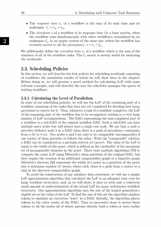
2

26 2. Scheduling with Unknown Task Runtimes

• The response time tr of a workflow is the sum of its wait time and itsmakespan: tr = tw + tm.

• The slowdown s of a workflow is its response time (in a busy system, whenthe workflow runs simultaneously with other workflows) normalized by itsmakespan t′m in an empty system of the same size (when the workflow hasexclusive access to all the processors): s = tr / t

′m.

We additionally define the execution time te of a workflow which is the sum of theruntimes of all of the workflow tasks. The te metric is mostly useful for analyzingthe workloads.

2.3. Scheduling PoliciesIn this section, we will describe the four policies for scheduling workloads consistingof workflows the simulation results of which we will show later in the chapter.Before doing so, we will present a novel method for calculating LoP with somerelevant concepts, and will describe the way the scheduler manages the queue ofwaiting workflows.

2.3.1. Calculating the Level of ParallelismIn some of our scheduling policies, we will use the LoP of the remaining part of aworkflow consisting of the tasks that have not yet completed for deciding how manyprocessors to reserve for it. Then, whenever a task of a workflow completes, the LoPof the remaining part of the workflow has to be recomputed, leading to a very largenumber of LoP recomputations. The DAG representing the non-completed part ofa workflow is a sub-DAG of the original workflow DAG. Such a sub-DAG can havemultiple entry nodes but will always have a single exit node. We say that a node aprecedes (follows) node b in a DAG when there is a path of precedence constraintsfrom a (b) to b (a). Two nodes a and b are said to be comparable (incomparable) ifone (none) of them precedes or follows the other. With the “comparable” relation,a DAG can be considered as a partially ordered set (poset). The value of the LoP isequal to the width of this poset, which is defined as the cardinality of the maximumset of incomparable elements in the poset. There exist multiple algorithms [79] tocompute the exact LoP using Dilworth’s chain partition of the original DAG, butthey require the creation of an additional comparability graph or a bipartite graph.Dilworth’s theorem [58] represents the width of a poset as a partition of the posetinto a minimum number of chains, where each chain is a path from a source to asink in the directed comparability graph.

To avoid the construction of any auxiliary data structures, we will use a simpleLoP approximation algorithm that calculates the LoP in an adequate time even forlarge workflow structures, and, as we will show, it does so with only a relativelysmall amount of underestimation of the actual LoP for many well-known workflowstructures. Our approximation algorithm uses the size of the largest generation-ieligible set as the value of the LoP. To find the size of this set the algorithm employstokens to simulate an execution “wave” in a DAG. Initially, the algorithm placestokens in the entry nodes of the DAG. Then in successive steps it moves thesetokens to all the nodes all of whose parents already hold a token or were earlier

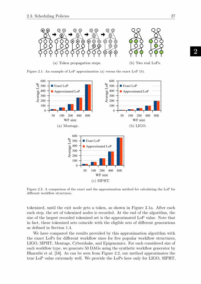
2.3. Scheduling Policies

2

27

(a) Token propagation steps. (b) Two real LoPs.

Figure 2.1: An example of LoP approximation (a) versus the exact LoP (b).

(a) Montage. (b) LIGO.

(c) SIPHT.

Figure 2.2: A comparison of the exact and the approximation method for calculating the LoP fordifferent workflow structures.

tokenized, until the exit node gets a token, as shown in Figure 2.1a. After eachsuch step, the set of tokenized nodes is recorded. At the end of the algorithm, thesize of the largest recorded tokenized set is the approximated LoP value. Note thatin fact, these tokenized sets coincide with the eligible sets of different generationsas defined in Section 1.4.

We have compared the results provided by this approximation algorithm withthe exact LoPs for different workflow sizes for five popular workflow structures,LIGO, SIPHT, Montage, Cybershake, and Epigenomics. For each considered size ofeach workflow type, we generate 50 DAGs using the synthetic workflow generator byBharathi et al. [16]. As can be seen from Figure 2.2, our method approximates thetrue LoP value extremely well. We provide the LoPs here only for LIGO, SIPHT,

2

28 2. Scheduling with Unknown Task Runtimes

and Montage, since Cybershake and Epigenomics show similar results. For bothmethods, the LoP values obtained for the 50 DAGs of each workflow type are allvery close to the mean. Of course, there can be situations where our approach doesunderestimate the LoP, see for instance the simple example in Figure 2.1. However,since the algorithm works well for the selected workflows, which are quite popularand representative, we will use the LoPs computed by it when simulating policiesthat use LoP in their scheduling decisions.

From the results in Figure 2.2, we can conclude that the tested workflows haverather regular, but still different, structures. First of all, for all three workflowstructures, the (average) LoP increases superlinearly (and especially for Montageand SIPHT, in a very strong way). Secondly, even for LIGO, but especially for theother two, the LoP is very large in relation to their total size. For LIGO, the LoPis slightly less than 200 for a workflow size of 800, but Montage and SIPHT alreadyreach that LoP for workflows of size less than 400.

2.3.2. Queue Management and Task SelectionWe assume that the scheduler maintains a single queue of waiting workflows. Everyarriving workflow is appended to the tail of the queue, and the scheduler decideswhich tasks of which workflows in the queue are scheduled when resources becomeavailable. For all the policies we will consider, the scheduler is invoked when a taskof a workflow completes, or when a new workflow arrives (possibly to a non-emptyqueue). The workflows are in principle processed in the order of their arrival, butmultiple workflows can be partially in execution while the remainder of their tasksare still waiting (either for a lack of resources or because of precedence constraintsbetween tasks), in which case we still regard them to be present in the queue. Aworkflow only leaves the queue when all of its tasks are finished.

When the scheduler is activated, it selects the workflows in the queue fromwhich tasks are scheduled in a way dictated by the actual scheduling policy. As weassume that all workflow tasks require only one processor and that we do not haveuser estimates or predictions of task runtimes, after the scheduler has selected aworkflow from which to start a task, it picks a task from the workflow’s eligibleset randomly. As the execution order of the tasks from the current eligible setmay influence subsequent eligible sets, and so, the makespan of the workflow, thisrandom task selection may not lead to the optimal schedule for the workflow, butwithout knowledge of task runtimes it is difficult to do better. Giving priorityto tasks in the eligible set that would enable large numbers of other tasks mightimprove the makespan of a workflow, but this is highly dependent on the taskruntimes.

2.3.3. The Strict Reservation PolicyThe most classic and simple general queuing policy is FCFS. When schedulingworkflows, the definition of FCFS is not completely straightforward. The ideabehind our version of the FCFS policy for workflows can be summarized by thecondition that the service to a workflow will only be influenced by the workflowsahead of it in the queue and never by workflows behind it in the queue. We enforcethis condition by strictly reserving for any workflow in the queue sufficient resources

2.3. Scheduling Policies

2

29

so that it will never be delayed by any later workflow—hence the alternative nameis Strict Reservation (SR) policy.

With the SR policy, when the scheduler is invoked and the workflow at thehead of the queue has fewer processors allocated to it than its LoP (which maybe in use or idle), it allocates additional available processors to the workflow atthe head of the queue until the workflow has LoP processors or until there are nomore available processors. When at a later time the scheduler is invoked againwhile the workflow at the head of the queue has not yet been completed, thescheduler recomputes workflow’s remaining LoP, keeps LoP processors allocated tothe workflow, and releases any excessive processors. If any idle processors remainafter LoP processors have been allocated to the workflow, the scheduler tries toschedule the next workflow in the queue—it does so in exactly the same way as ifthat workflow were at the head of the queue.

2.3.4. The Scaled LoP Policy

Of course, workflows may never attain their LoPs, and especially for large workflows,the SR policy may be very wasteful and lead to a low maximal utilization. Whereasthe SR policy executes a workflow in the shortest possible time once it startsallocating processors to it, the wait times of the workflows with SR may beexcessive. A straightforward solution to this problem is to reduce the reservation ofa workflow to a number of processors that is lower than its LoP. Thus, the ScaledLoP (SLoP) policy with scaling factor f, 0 ≤ f ≤ 1, tries at all times to keepf · LoP processors allocated to a workflow. This means that if at some point thesize of the eligible set of a workflow is smaller than f · LoP, the scheduler will tryto keep reserved a number of processors equal to the difference between these twovalues. If, however, at some point the size of the eligible set of a workflow exceedsf · LoP, the SLoP policy will allocate any available processors to eligible tasks ofthe workflow. The SLoP policy behaves similar to the SR policy albeit with a lowerreservation target, and in the boundary case when f = 1 it is equal to it. At theother extreme, as we will see below, our backfilling policy is in fact identical to theSLoP policy with scaling factor equal to 0.

2.3.5. The Future Eligible Sets Policy

The idea behind reserving processors for workflows is to reduce the delay in placingtasks in the eligible set. Rather than, when reserving processors, taking a worst-caseperspective on the number of processors a workflow may ever need as we did in theSR policy, we may also try to look into the future of the execution of the workflows.Thus, the Future Eligible Sets (FES) policy with depth n tries to allocate to aworkflow a number of processors that is equal to the size of largest eligible set ofany generation from 0 through n. With our approximation of computing the LoPas presented in Section 2.3.1, the FES policy with depth ∞ coincides with the SRpolicy. At the other extreme, as we will see below, our backfilling policy is in factidentical to the FES policy with depth equal to 0.

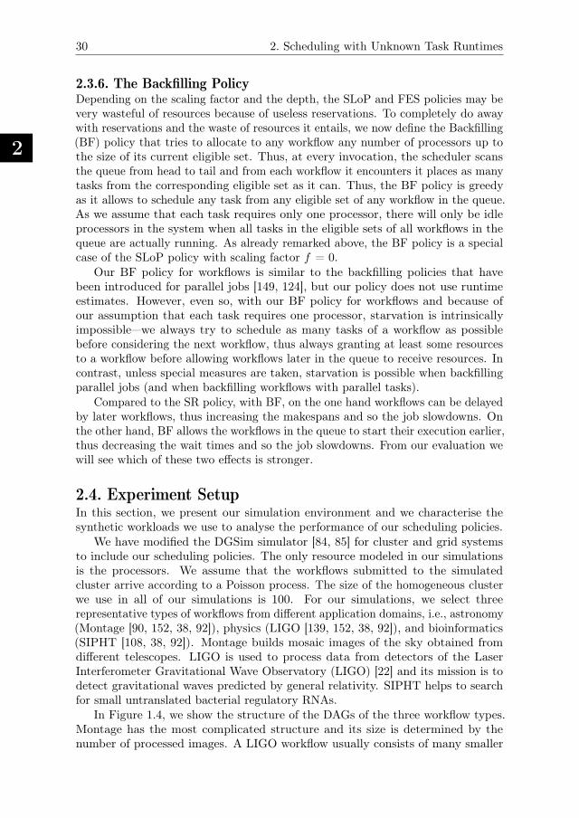
2

30 2. Scheduling with Unknown Task Runtimes

2.3.6. The Backfilling PolicyDepending on the scaling factor and the depth, the SLoP and FES policies may bevery wasteful of resources because of useless reservations. To completely do awaywith reservations and the waste of resources it entails, we now define the Backfilling(BF) policy that tries to allocate to any workflow any number of processors up tothe size of its current eligible set. Thus, at every invocation, the scheduler scansthe queue from head to tail and from each workflow it encounters it places as manytasks from the corresponding eligible set as it can. Thus, the BF policy is greedyas it allows to schedule any task from any eligible set of any workflow in the queue.As we assume that each task requires only one processor, there will only be idleprocessors in the system when all tasks in the eligible sets of all workflows in thequeue are actually running. As already remarked above, the BF policy is a specialcase of the SLoP policy with scaling factor f = 0.

Our BF policy for workflows is similar to the backfilling policies that havebeen introduced for parallel jobs [149, 124], but our policy does not use runtimeestimates. However, even so, with our BF policy for workflows and because ofour assumption that each task requires one processor, starvation is intrinsicallyimpossible—we always try to schedule as many tasks of a workflow as possiblebefore considering the next workflow, thus always granting at least some resourcesto a workflow before allowing workflows later in the queue to receive resources. Incontrast, unless special measures are taken, starvation is possible when backfillingparallel jobs (and when backfilling workflows with parallel tasks).

Compared to the SR policy, with BF, on the one hand workflows can be delayedby later workflows, thus increasing the makespans and so the job slowdowns. Onthe other hand, BF allows the workflows in the queue to start their execution earlier,thus decreasing the wait times and so the job slowdowns. From our evaluation wewill see which of these two effects is stronger.

2.4. Experiment SetupIn this section, we present our simulation environment and we characterise thesynthetic workloads we use to analyse the performance of our scheduling policies.

We have modified the DGSim simulator [84, 85] for cluster and grid systemsto include our scheduling policies. The only resource modeled in our simulationsis the processors. We assume that the workflows submitted to the simulatedcluster arrive according to a Poisson process. The size of the homogeneous clusterwe use in all of our simulations is 100. For our simulations, we select threerepresentative types of workflows from different application domains, i.e., astronomy(Montage [90, 152, 38, 92]), physics (LIGO [139, 152, 38, 92]), and bioinformatics(SIPHT [108, 38, 92]). Montage builds mosaic images of the sky obtained fromdifferent telescopes. LIGO is used to process data from detectors of the LaserInterferometer Gravitational Wave Observatory (LIGO) [22] and its mission is todetect gravitational waves predicted by general relativity. SIPHT helps to searchfor small untranslated bacterial regulatory RNAs.

In Figure 1.4, we show the structure of the DAGs of the three workflow types.Montage has the most complicated structure and its size is determined by thenumber of processed images. A LIGO workflow usually consists of many smaller

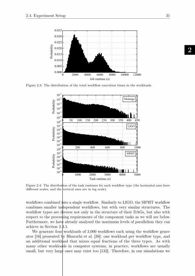
2.4. Experiment Setup

2

31

0 2000 4000 6000 8000 10000 12000Job runtime (s)

0.000

0.005

0.010

0.015

0.020

0.025

0.030

0.035

Prob

abili

ty

Figure 2.3: The distribution of the total workflow execution times in the workloads.

0 50 100 150 200 250 300 350 400 45010-610-510-410-310-210-1

Prob

abili

ty Montage

0 200 400 600 800 100010-610-510-410-310-210-1100

Prob

abili

ty LIGO

0 1000 2000 3000 4000 5000Task runtime (s)

10-610-510-410-310-210-1100

Prob

abili

ty SIPHT

Figure 2.4: The distribution of the task runtimes for each workflow type (the horizontal axes havedifferent scales, and the vertical axes are in log scale).

workflows combined into a single workflow. Similarly to LIGO, the SIPHT workflowcombines smaller independent workflows, but with very similar structures. Theworkflow types are diverse not only in the structure of their DAGs, but also withrespect to the processing requirements of the component tasks as we will see below.Furthermore, we have already analysed the maximum levels of parallelism they canachieve in Section 2.3.1.

We generate four workloads of 3,000 workflows each using the workflow gener-ator [16] presented by Bharathi et al. [38]: one workload per workflow type, andan additional workload that mixes equal fractions of the three types. As withmany other workloads in computer systems, in practice, workflows are usuallysmall, but very large ones may exist too [132]. Therefore, in our simulations we

2

32 2. Scheduling with Unknown Task Runtimes

distinguish small, medium, and large workflows, which constitute fractions of 75%,20%, and 5% of the workloads. We assume all workflows to have even sizes dueto the limitations of the generator. The size of the small, the medium, and thelarge workflows is uniformly distributed on the intervals [30, 38], [40, 198], and[200, 600], respectively.

In order to obtain simulation results for the different workflow types thatcan easily be compared (especially when simulating the mixed workload), we usethe same total execution time distribution for all three workflow types. Thisdistribution is a two-stage hyper-Gamma distribution derived from the modelpresented by Lublin and Feitelson [112]. The shape and scale parameters (α, β) oftwo component Gamma distributions are set to (5.0, 501.266) and (45.0, 136.709),respectively. Their proportions in the overall distribution are 0.7 and 0.3. Theaverage total execution time is one hour. Figure 2.3 visualizes this distribution. Forevery workflow, we normalize the task runtimes generated so that its total processingrequirement is equal to the corresponding sample of the execution time distribution.In Figure 2.4, we show the distributions of the normalized task runtimes for eachworkflow type. The maximum task runtimes in Montage and LIGO are an orderof magnitude smaller than the maximum task runtimes in SIPHT, but all threeworkflow types share the phenomenon that they are dominated by short tasks.

In our simulations, we vary the utilization starting at 0.05 with step size 0.05.If for some utilization the system did not become stable in the simulations, we willonly show performance results up to that utilization. We will consider the highestutilization for which the system did become stable as the maximal utilization,defined in Section 1.1. We set the scaling factor f in our SLoP policy to 0.2,0.8, and 0.9, and we evaluate the FES policy with depths 1, 2, and 10. For eachexperiment, we report the average job slowdown over three repetitions, and we onlyshow results when the system is in steady state. Thus, when reporting performanceresults, to be on the safe side, we omit the performance information for the first1,000 workflows in each simulation and for those workflows that have not completedtheir execution before the start of the last arriving workflow.

2.5. Experiment ResultsIn this section we report our simulation results and their analysis. In Figure 2.5,we show for all the policies and for all four workload types the mean workflowslowdown as it depends on the utilization in the system. The last point in all curvesis for the highest utilization for which the system is stable in the simulations. InTable 2.1, we summarize these maximal utilizations.

As a first general observation, we find that for all policies that do some formof reservation, the maximal utilization is low, or even very low. The worst isa maximal utilization of only 0.2 for the SR policy with the SIPHT workload.Apparently, reserved resources often remain idle, and the benefit of reservations fora short makespan do not balance their negative effect of having long wait times.

Our second general observation is that the performance both in terms of meanslowdown and maximal utilization varies considerably across the three workloadsconsisting of a single workflow type. However, the different workflow types almostalways have the same relative performance. In particular, for all the policies except

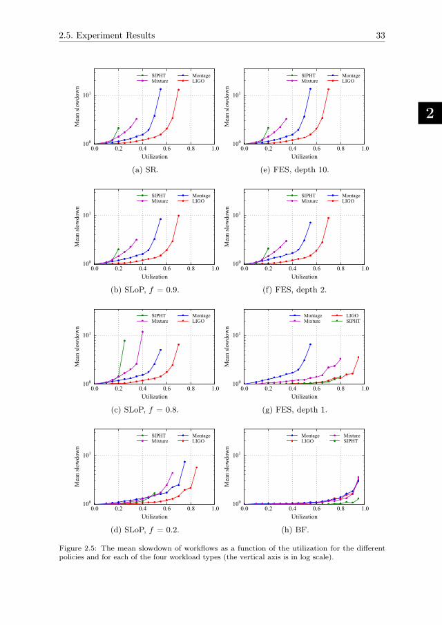
2.5. Experiment Results

2

33

0.0 0.2 0.4 0.6 0.8 1.0Utilization

100

101

Mea

n sl

owdo

wn

SIPHTMixture

MontageLIGO

(a) SR.

0.0 0.2 0.4 0.6 0.8 1.0Utilization

100

101

Mea

n sl

owdo

wn

SIPHTMixture

MontageLIGO

(b) SLoP, f = 0.9.

0.0 0.2 0.4 0.6 0.8 1.0Utilization

100

101

Mea

n sl

owdo

wn

SIPHTMixture

MontageLIGO

(c) SLoP, f = 0.8.

0.0 0.2 0.4 0.6 0.8 1.0Utilization

100

101

Mea

n sl

owdo

wn

SIPHTMixture

MontageLIGO

(d) SLoP, f = 0.2.

0.0 0.2 0.4 0.6 0.8 1.0Utilization

100

101

Mea

n sl

owdo

wn

SIPHTMixture

MontageLIGO

(e) FES, depth 10.

0.0 0.2 0.4 0.6 0.8 1.0Utilization

100

101

Mea

n sl

owdo

wn

SIPHTMixture

MontageLIGO

(f) FES, depth 2.

0.0 0.2 0.4 0.6 0.8 1.0Utilization

100

101

Mea

n sl

owdo

wn

MontageMixture

LIGOSIPHT

(g) FES, depth 1.

0.0 0.2 0.4 0.6 0.8 1.0Utilization

100

101

Mea

n sl

owdo

wn

MontageLIGO

MixtureSIPHT

(h) BF.

Figure 2.5: The mean slowdown of workflows as a function of the utilization for the differentpolicies and for each of the four workload types (the vertical axis is in log scale).

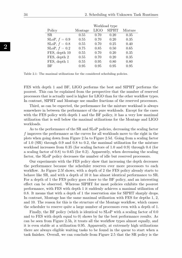
2

34 2. Scheduling with Unknown Task Runtimes

Workload typePolicy Montage LIGO SIPHT MixtureSR 0.55 0.70 0.20 0.35SLoP, f = 0.9 0.55 0.70 0.20 0.35SLoP, f = 0.8 0.55 0.70 0.25 0.40SLoP, f = 0.2 0.75 0.85 0.50 0.65FES, depth 10 0.55 0.70 0.20 0.35FES, depth 2 0.55 0.70 0.20 0.35FES, depth 1 0.55 0.95 0.80 0.80BF 0.95 0.95 0.95 0.95

Table 2.1: The maximal utilizations for the considered scheduling policies.

FES with depth 1 and BF, LIGO performs the best and SIPHT performs thepoorest. This can be explained from the perspective that the number of reservedprocessors that is actually used is higher for LIGO than for the other workflow types.In contrast, SIPHT and Montage use smaller fractions of the reserved processors.

Third, as can be expected, the performance for the mixture workload is alwayssomewhere in between the performance of the pure workloads. Except for the caseswith the FES policy with depth 1 and the BF policy, it has a very low maximalutilization that is well below the maximal utilizations for the Montage and LIGOworkloads.

As to the performance of the SR and SLoP policies, decreasing the scaling factorf improves the performance as the curves for all workloads move to the right in theplots when going down from Figure 2.5a to Figure 2.5d. Going from a scaling factorof 1.0 (SR) through 0.9 and 0.8 to 0.2, the maximal utilization for the mixtureworkload increases from 0.35 (for scaling factors of 1.0 and 0.9) through 0.4 (fora scaling factor of 0.8) to 0.65 (for 0.2). Apparently, when decreasing the scalingfactor, the SLoP policy decreases the number of idle but reserved processors.

Our experiments with the FES policy show that increasing the depth decreasesthe performance because the scheduler reserves ever more processors to eachworkflow. As Figure 2.5f shows, with a depth of 2 the FES policy already starts tobehave like SR, and with a depth of 10 it has almost identical performance to SR.For a depth of 1 the FES policy goes closer to the BF policy, and an interestingeffect can be observed. Whereas SIPHT for most policies exhibits the poorestperformance, with FES with depth 1 it suddenly achieves a maximal utilization of0.8. It means that with a depth of 1 the reservation size for SIPHT sharply drops.In contrast, Montage has the same maximal utilization with FES for depths 1, 2,and 10. The reason for this is the structure of the Montage workflow, which causesthe scheduler to reserve quite a large number of processors even with a depth of 1.

Finally, the BF policy (which is identical to SLoP with a scaling factor of 0.0and to FES with depth equal to 0) shows by far the best performance results. Ascan be seen from Figure 2.5h, it treats all the workflow types almost equally, andit is even stable at a utilization 0.95. Apparently, at extremely high utilizationsthere are always eligible waiting tasks to be found in the queue to start when atask finishes. Overall, we can conclude from Figure 2.5 that the SR policy is the

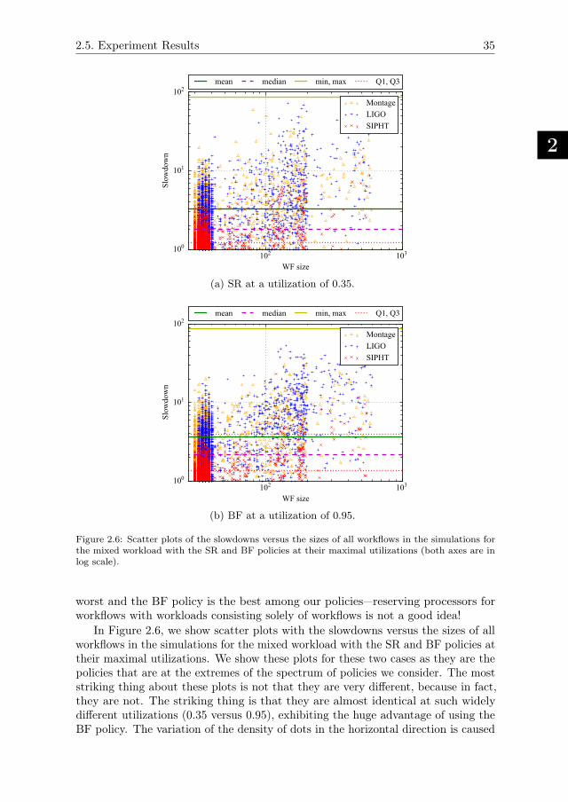
2.5. Experiment Results

2

35

102 103

WF size

100

101

102

Slow

dow

n

MontageLIGOSIPHT

mean median min, max Q1, Q3

(a) SR at a utilization of 0.35.

102 103

WF size

100

101

102

Slow

dow

n

MontageLIGOSIPHT

mean median min, max Q1, Q3

(b) BF at a utilization of 0.95.

Figure 2.6: Scatter plots of the slowdowns versus the sizes of all workflows in the simulations forthe mixed workload with the SR and BF policies at their maximal utilizations (both axes are inlog scale).

worst and the BF policy is the best among our policies—reserving processors forworkflows with workloads consisting solely of workflows is not a good idea!

In Figure 2.6, we show scatter plots with the slowdowns versus the sizes of allworkflows in the simulations for the mixed workload with the SR and BF policies attheir maximal utilizations. We show these plots for these two cases as they are thepolicies that are at the extremes of the spectrum of policies we consider. The moststriking thing about these plots is not that they are very different, because in fact,they are not. The striking thing is that they are almost identical at such widelydifferent utilizations (0.35 versus 0.95), exhibiting the huge advantage of using theBF policy. The variation of the density of dots in the horizontal direction is caused

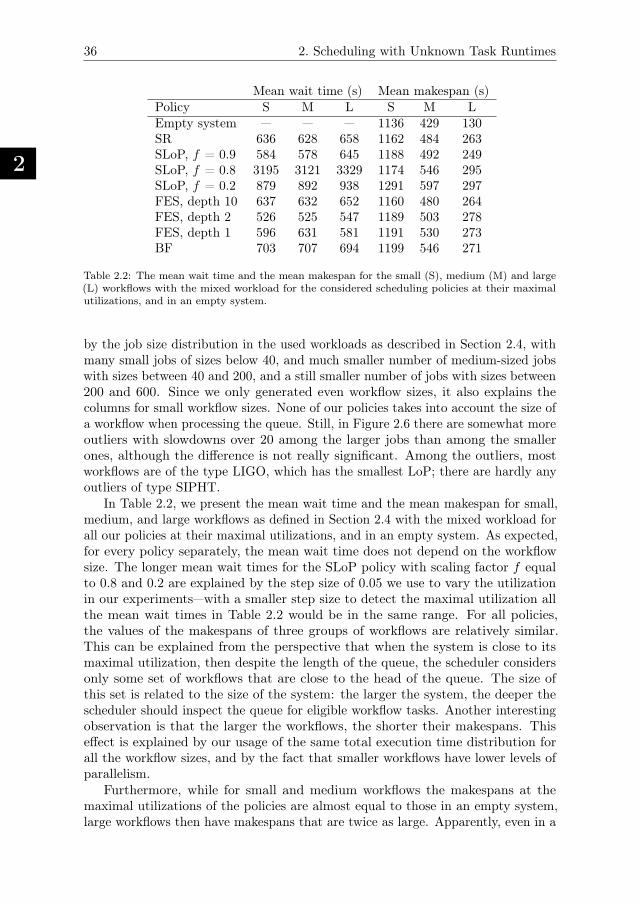
2

36 2. Scheduling with Unknown Task Runtimes

Mean wait time (s) Mean makespan (s)Policy S M L S M LEmpty system — — — 1136 429 130SR 636 628 658 1162 484 263SLoP, f = 0.9 584 578 645 1188 492 249SLoP, f = 0.8 3195 3121 3329 1174 546 295SLoP, f = 0.2 879 892 938 1291 597 297FES, depth 10 637 632 652 1160 480 264FES, depth 2 526 525 547 1189 503 278FES, depth 1 596 631 581 1191 530 273BF 703 707 694 1199 546 271

Table 2.2: The mean wait time and the mean makespan for the small (S), medium (M) and large(L) workflows with the mixed workload for the considered scheduling policies at their maximalutilizations, and in an empty system.

by the job size distribution in the used workloads as described in Section 2.4, withmany small jobs of sizes below 40, and much smaller number of medium-sized jobswith sizes between 40 and 200, and a still smaller number of jobs with sizes between200 and 600. Since we only generated even workflow sizes, it also explains thecolumns for small workflow sizes. None of our policies takes into account the size ofa workflow when processing the queue. Still, in Figure 2.6 there are somewhat moreoutliers with slowdowns over 20 among the larger jobs than among the smallerones, although the difference is not really significant. Among the outliers, mostworkflows are of the type LIGO, which has the smallest LoP; there are hardly anyoutliers of type SIPHT.

In Table 2.2, we present the mean wait time and the mean makespan for small,medium, and large workflows as defined in Section 2.4 with the mixed workload forall our policies at their maximal utilizations, and in an empty system. As expected,for every policy separately, the mean wait time does not depend on the workflowsize. The longer mean wait times for the SLoP policy with scaling factor f equalto 0.8 and 0.2 are explained by the step size of 0.05 we use to vary the utilizationin our experiments—with a smaller step size to detect the maximal utilization allthe mean wait times in Table 2.2 would be in the same range. For all policies,the values of the makespans of three groups of workflows are relatively similar.This can be explained from the perspective that when the system is close to itsmaximal utilization, then despite the length of the queue, the scheduler considersonly some set of workflows that are close to the head of the queue. The size ofthis set is related to the size of the system: the larger the system, the deeper thescheduler should inspect the queue for eligible workflow tasks. Another interestingobservation is that the larger the workflows, the shorter their makespans. Thiseffect is explained by our usage of the same total execution time distribution forall the workflow sizes, and by the fact that smaller workflows have lower levels ofparallelism.

Furthermore, while for small and medium workflows the makespans at themaximal utilizations of the policies are almost equal to those in an empty system,large workflows then have makespans that are twice as large. Apparently, even in a

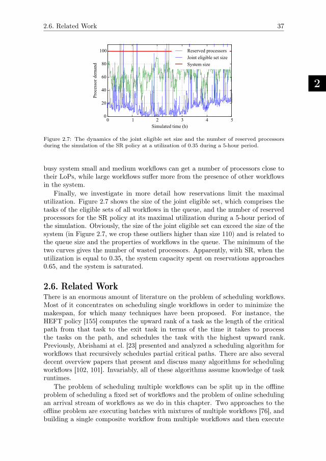
2.6. Related Work

2

37

0 1 2 3 4 5Simulated time (h)

0

20

40

60

80

100

Proc

esso

r dem

and

Reserved processorsJoint eligible set sizeSystem size

Figure 2.7: The dynamics of the joint eligible set size and the number of reserved processorsduring the simulation of the SR policy at a utilization of 0.35 during a 5-hour period.

busy system small and medium workflows can get a number of processors close totheir LoPs, while large workflows suffer more from the presence of other workflowsin the system.

Finally, we investigate in more detail how reservations limit the maximalutilization. Figure 2.7 shows the size of the joint eligible set, which comprises thetasks of the eligible sets of all workflows in the queue, and the number of reservedprocessors for the SR policy at its maximal utilization during a 5-hour period ofthe simulation. Obviously, the size of the joint eligible set can exceed the size of thesystem (in Figure 2.7, we crop these outliers higher than size 110) and is related tothe queue size and the properties of workflows in the queue. The minimum of thetwo curves gives the number of wasted processors. Apparently, with SR, when theutilization is equal to 0.35, the system capacity spent on reservations approaches0.65, and the system is saturated.

2.6. Related WorkThere is an enormous amount of literature on the problem of scheduling workflows.Most of it concentrates on scheduling single workflows in order to minimize themakespan, for which many techniques have been proposed. For instance, theHEFT policy [155] computes the upward rank of a task as the length of the criticalpath from that task to the exit task in terms of the time it takes to processthe tasks on the path, and schedules the task with the highest upward rank.Previously, Abrishami at el. [23] presented and analyzed a scheduling algorithm forworkflows that recursively schedules partial critical paths. There are also severaldecent overview papers that present and discuss many algorithms for schedulingworkflows [102, 101]. Invariably, all of these algorithms assume knowledge of taskruntimes.

The problem of scheduling multiple workflows can be split up in the offlineproblem of scheduling a fixed set of workflows and the problem of online schedulingan arrival stream of workflows as we do in this chapter. Two approaches to theoffline problem are executing batches with mixtures of multiple workflows [76], andbuilding a single composite workflow from multiple workflows and then execute

2

38 2. Scheduling with Unknown Task Runtimes

it [170]. In the paper by Yu et al. [169], an online stream of workflows is considered,but the authors use a DAG composition approach and task runtime information toprioritize the tasks using HEFT. Also in the paper by Hsu et al. [77], a stream ofarriving workflows is used and the ideas from the Yu’s paper [169] are extendedby considering the critical path for each workflow. In the work by Lee et al. [104],the Pegasus planner [54] and the DAGMan [67] batch workflow executor areused. In addition, a scheduling algorithm that allocates resources based on theirruntime performance is proposed and real-world experiments are conducted usinggrid middleware over clusters. Despite the fact that they treat each workflowseparately without composing a single DAG, their algorithm still uses task runtimeinformation. In the paper by Singh and Deelman [145], a trace of a Teragrid clusterwith applications representing (modified) Montage workflows is simulated. Differentprovisioning policies and priority schemes are considered, with a cap on the amountof resources that can be used by a single workflow.

A large body of work proposes backfilling as the main technique to improve thesystem utilization and reduce the job slowdowns in the area of parallel applica-tions [124, 107, 141, 144, 89]. Despite the simplicity of the backfilling technique,there exist many variations of the algorithm. For instance, the number of reser-vations granted by the backfilling algorithm distinguishes two main strategies,conservative and aggressive. The former assigns to each job a reservation when itenters the system and moves smaller jobs forward in the queue as long as no delaysare incurred on any of the previously queued jobs. The latter allows any job to bebackfilled as long as it does not delay the first job in the queue. The number ofqueued jobs considered by the backfilling algorithm may have a significant impacton the overall performance. To maximize the utilization, dynamic programmingmay be employed to find the optimal packing of the jobs [144]. These aspects havebeen analyzed and incorporated in the Maui project which currently provides areal-world implementation of the general backfill algorithm [89]. The main featuredistinguishing backfilling for parallel jobs and workflows is that with workflows, assoon as any number, however low, of resources are available, a workflow can makeprogress. So the concerns about not delaying workflows with backfilling are muchless pressing.

2.7. ConclusionIn this chapter, we have presented a family of four policies for scheduling workloadsconsisting of arrival streams of workflows with unknown task runtimes. The maindistinguishing feature of these policies is to what extent they reserve processors toworkflows towards the head of the queue to deal with fluctuations in their levelof parallelism. We have simulated these four policies in a cluster with syntheticworkloads derived from popular real workflows with as metrics the average workflowslowdown and the maximal utilization that can be achieved. Our main conclusionis that any form of processor reservation for workflows without runtime estimatesonly decreases the overall system performance, leading to low or even to very lowmaximal utilizations.

3

The Impact of Task Runtime

Estimate Accuracy

Workflow schedulers often rely on task runtime estimates when makingscheduling decisions, and they usually target the scheduling of single workflows

or batches of workflows. In contrast, in this chapter, we evaluate the impact of theabsence or limited accuracy of task runtime estimates on slowdown when schedulingcomplete workloads of workflows that arrive over time. We study a total of sevenpolicies: four of these are popular existing scheduling policies for (batches of)workloads from the literature, including a simple backfilling policy which is notaware of task runtime estimates, two are novel workload-oriented policies, includingone which targets fairness, and one is the well-known HEFT scheduling policy for asingle workflow adapted to the online workload scenario. We simulate homogeneousand heterogeneous distributed systems to evaluate the performance of these policiesunder varying accuracy of task runtime estimates. Our results show that forhigh utilizations, the order in which workflows are processed is more importantthan the knowledge of correct task runtime estimates. Under low utilizations,all policies considered show good results, even a policy which does not use taskruntime estimates. We also show that our Fair Workflow Prioritization (FWP)policy effectively decreases the variance of job slowdown and thus achieves fairness,and that the plan-based scheduling policy derived from HEFT does not showmuch performance improvement while bringing extra complexity to the schedulingprocess.

3.1. IntroductionIn workloads of modern computing systems, workflows are often used as a toolto drive complex computations, and their popularity continues to increase [52].Many of these workflows are usually submitted to the system repeatedly so that(statistical) runtime estimates of their tasks can be derived [92, 135]; alternatively,runtime estimates can be provided by users [76]. However, the accuracy of runtime

39

3

40 3. The Impact of Task Runtime Estimate Accuracy

estimates significantly depends on the employed estimation algorithm, or on theuser—user runtime estimates can be very unreliable [63, 103]. Most previous workon scheduling workflows [155, 169, 29, 32] has assumed some (and often evenperfect) knowledge of task runtimes. Moreover, often has been considered theoffline problem of scheduling a single workflow or a batch of workflows (which areall initially present), or periodic submissions with a fixed interval. In most cases,the makespan has been used as the main metric.

However, workflows may be submitted to a system over time according to somearrival pattern, in which case job slowdown is a much more appropriate performancemetric. Then, especially when workflows of widely different sizes are submitted,fairness becomes an issue, and an important goal is to reduce the variability ofjob slowdown. In this chapter, we investigate how the accuracy of task runtimeestimates affects the quality of scheduling, and we address the issue of fairnessin the online case of scheduling complete workloads of workflows. Moreover, weevaluate the system stability to know at which workflow arrival rates the systemstarts to uncontrollably accumulate waiting workflows. Besides that, we identifythe maximal achievable system utilization which guarantees the stability.

We distinguish dynamic and plan-based policies. Dynamic policies make taskplacement decisions just-in-time when a processor becomes idle or a new taskbecomes eligible. Plan-based policies construct a full-ahead plan on every workflowarrival and strictly follow this plan to perform task placements between the workflowarrivals.

Task runtime estimates have been heavily used for different forms of taskprioritization by various scheduling algorithms for single workflows and for batchesof workflows. The most popular approaches [155, 142, 76, 32] include upward anddownward ranking and different forms of list scheduling techniques. Workflow tasksare usually prioritized in ascending or descending order of their runtimes or by theirproximity to the entry or exit task. The individual workflows are often prioritizedbased on the length of their critical path (a longest path from an entry to the exittask). In this situation, inaccurate runtime estimates can significantly affect thetask and workflow ranking, as not only the length of the critical path can be affectedbut even a wrong critical path can be used. Knowing how the quality of estimatesaffects the performance helps to create better error-resilient scheduling policies andis useful when selecting policies which are less sensitive to incorrect estimates. InChapter 2, we used a different approach where we scheduled an arriving stream ofworkflows without using any runtime estimates at all, and completely relied on thestructure of the workflows when making scheduling decisions.

To study the influence of the accuracy of task runtime estimation on theperformance, in this chapter, we study a total of seven scheduling policies forworkloads of workflows, and we simulate their execution on two workloads ofrealistic workflows. Four of these are existing dynamic workflow scheduling policies,namely Greedy Backfilling (GBF), which came out best of all the policies weproposed in Chapter 2 when no runtime estimates are available, Online WorkflowManagement (OWM) [77, 32], Fairness Dynamic Workflow Scheduling (FDWS) [29,32], and Rank_Hybd (HR) [169]. We also propose the simple Critical PathPrioritization (CPP) policy and, in order to address the issue of fairness, the Fair

3.2. Problem Statement

3

41

Workflow Prioritization (FWP) policy. To check how existing plan-based schedulingalgorithms can be applied when scheduling workloads of workflows, we have adaptedthe Heterogeneous Earliest Finish Time (HEFT) [155] policy to the online case.All policies except GBF require task runtime estimates for their operation.

The main research questions we address in this chapter and our contributionstowards answering them, are:

1. What are the appropriate policies for dynamic scheduling of workloads ofworkflows with known task runtime estimates? We propose in Section 3.3 twonovel dynamic workflow scheduling policies (CPP and the fairness-orientedFWP), implement four state-of-the art online dynamic policies, and adaptthe popular HEFT policy to the online case.

2. How do inaccurate task runtime estimates affect the performance and fairness?We show in Section 3.5 the effect of incorrect task runtime estimates onthe performance and fairness when scheduling workloads of workflows in asimulated computing environment.

3. How does the knowledge of task runtime estimates help to improve the per-formance and achieve fairness, and how applicable are plan-based policiesfor online scheduling of workflows? We demonstrate in Section 3.5.1 thatthe knowledge of task runtime estimates improves the performance at highsystem utilizations, and in Section 3.5.3 we show that the plan-based approachstruggles to deal with workloads of workflows.

3.2. Problem StatementThis section presents our model for the problem of using runtime estimates forscheduling workloads of workflows and the performance metrics.

3.2.1. The ModelIn this chapter, we consider both homogeneous and heterogeneous computingsystems, in contrast to Chapter 2, where we only study homogeneous systems. Forthe rest, the system model, the arrival process, and the workflow definitions arethe same as in Chapter 2. When the system is heterogeneous, we suppose that theexecution time of a task on a processor is inversely proportional to the processorspeed.

The runtime estimates are often extracted from historical runs, simulations ofworkflow executions, or even are obtained from users [63, 43]. However, the qualityof such estimates can vary significantly depending on the estimation method. Tostudy the effect of the quality of task runtime estimates on the system performance,we modify the perfect task runtimes obtained from the synthetic workload using acertain pre-defined error factor fe. The error allows to either under-estimate orover-estimate the task runtimes. All of the evaluated schedulers are not aware ofunder- or over-estimation. They can only derive the error in task runtimes postfactum by comparing the given runtime estimates with the actual task runtimesobtained during the execution (as in our FWP policy, Section 3.3.7). We use threemethods to introduce the estimation errors:

3

42 3. The Impact of Task Runtime Estimate Accuracy

• Static error: Here we multiply the runtime of every task of every workflowby the error factor fe.

• Random error I: Here we multiply the runtime of every task within a singleworkflow by the same random error factor. This random error factor isindependently generated for every workflow in the workload by drawing itfrom the uniform distribution on the interval (0, fe × 2]. So on average, taskruntimes in the workload are under- or overestimated by a factor of fe.

• Random error II: Here we multiply the runtime of every task by an individuallygenerated random error. The runtime estimate of a task is computed bymultiplying its original correct task runtime dr by a random error factordrawn from the uniform distribution on the interval (0, fe/dr × 2]. This isan extreme case of introducing an error, as it changes the distribution oftask runtimes to a uniform distribution on the interval (0, fe × 2]. Thus, thescheduler operates with estimates which are very far from the original ones.

3.2.2. Performance Metrics

In this chapter, we use a set of metrics and baselines, similar to those definedearlier in Section 2.2.2. However, in contrast to Chapter 2, where task runtimesare unknown, in this chapter we suppose that task runtime estimates are available.Accordingly, we can calculate the critical path length c of a workflow using theperfect task runtimes obtained from the synthetic workload. We define the slowdowns of a workflow as its response time tr (in a busy system, when the workflow runssimultaneously with other workflows) normalized by the length c of its criticalpath: s = tr / c. The critical path length computation is originally presented inSection 1.4 and further explained in Section 3.3.1.

3.3. Scheduling Policies

In this section, we first provide a detailed definition of the upward rank computation,which is crucial for task prioritization in almost all of the scheduling policies weconsider. Then we present GBF the greedy backfilling dynamic policy which doesnot use task runtime estimates at all, and five dynamic policies: CPP, OWM,FDWS, HR, and FWP, that require task runtime estimates. Dynamic policiesmake scheduling decisions whenever a new task becomes eligible or a processorbecomes idle. Finally, we present the plan-based WHEFT policy which uses taskruntime estimates to construct a full ahead execution plan on every workflow arrival;between arrivals, the execution is completely guided by the precomputed plan. Weclassify the considered policies by their distinctive properties in Table 3.1. TheGBF policy is included in this chapter as it has shown good performance earlier inChapter 2. The dynamic policies that require task runtime estimates have beenselected based on the comparative study by Arabnejad et al. [32]. We choose HEFTas it is one of the most popular algorithms for workflow scheduling and it is oftenused as a reference [170].

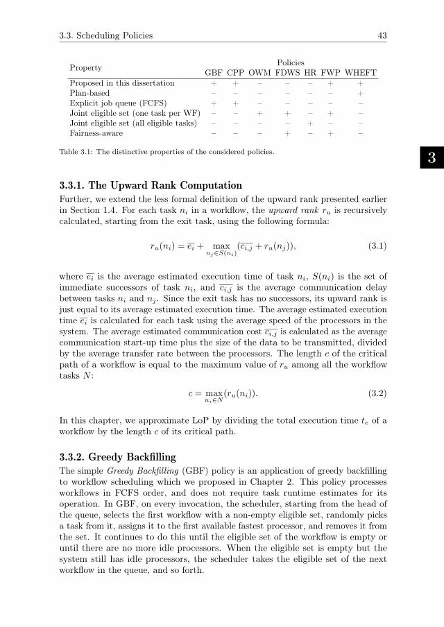
3.3. Scheduling Policies

3

43

PropertyPolicies

GBF CPP OWM FDWS HR FWP WHEFTProposed in this dissertation + + – – – + +Plan-based – – – – – – +Explicit job queue (FCFS) + + – – – – –Joint eligible set (one task per WF) – – + + – + –Joint eligible set (all eligible tasks) – – – – + – –Fairness-aware – – – + – + –

Table 3.1: The distinctive properties of the considered policies.

3.3.1. The Upward Rank Computation

Further, we extend the less formal definition of the upward rank presented earlierin Section 1.4. For each task ni in a workflow, the upward rank ru is recursivelycalculated, starting from the exit task, using the following formula:

ru(ni) = ei + maxnj∈S(ni)

(ci,j + ru(nj)), (3.1)

where ei is the average estimated execution time of task ni, S(ni) is the set ofimmediate successors of task ni, and ci,j is the average communication delaybetween tasks ni and nj . Since the exit task has no successors, its upward rank isjust equal to its average estimated execution time. The average estimated executiontime ei is calculated for each task using the average speed of the processors in thesystem. The average estimated communication cost ci,j is calculated as the averagecommunication start-up time plus the size of the data to be transmitted, dividedby the average transfer rate between the processors. The length c of the criticalpath of a workflow is equal to the maximum value of ru among all the workflowtasks N :

c = maxni∈N

(ru(ni)). (3.2)

In this chapter, we approximate LoP by dividing the total execution time te of aworkflow by the length c of its critical path.

3.3.2. Greedy Backfilling

The simple Greedy Backfilling (GBF) policy is an application of greedy backfillingto workflow scheduling which we proposed in Chapter 2. This policy processesworkflows in FCFS order, and does not require task runtime estimates for itsoperation. In GBF, on every invocation, the scheduler, starting from the head ofthe queue, selects the first workflow with a non-empty eligible set, randomly picksa task from it, assigns it to the first available fastest processor, and removes it fromthe set. It continues to do this until the eligible set of the workflow is empty oruntil there are no more idle processors. When the eligible set is empty but thesystem still has idle processors, the scheduler takes the eligible set of the nextworkflow in the queue, and so forth.

3

44 3. The Impact of Task Runtime Estimate Accuracy

3.3.3. Critical Path PrioritizationOur Critical Path Prioritization (CPP) policy extends our GBF policy. In CPP,on every invocation, the scheduler, starting from the head of the queue, selects thefirst workflow with a non-empty eligible set, picks the task from it with the highestru, assigns it to the first available fastest processor, and removes it from the set.For the rest, the CPP scheduler is similar to GBF.

3.3.4. Online Workflow ManagementThe Online Workflow Management (OWM) policy [77, 32] maintains a single jointeligible set which contains only a single eligible task (if any) with the highest rufrom every workflow in the system. At every scheduler invocation, as long as thesystem has workflows with eligible tasks, the scheduler selects the task with thehighest ru from the joint set. If the idle processors have the same speed, OWM findsthe busy processor which will become idle earlier than any other busy processor.If the estimated finish time of the selected task on that busy processor is smallerthan EFT on any of the idle processors, the task is postponed (stays in the jointset) until the next scheduler invocation. Otherwise, the task is assigned to any ofthe idle processors. If the idle processors have different speeds, the task is assignedto the fastest idle processor.

3.3.5. Fairness Dynamic Workflow SchedulingThe Fairness Dynamic Workflow Scheduling (FDWS) policy [29, 32] maintains asingle joint eligible set which is formed in the same way as in OWM. However,within the joint set each task of a workflow j is additionally prioritized with rankra (highest first) which considers the fraction of remaining tasks of the workflowand the length of its critical path. The additional rank ra is defined as follows:

ra,j =

(

mj

pj· cj

)−1

, (3.3)

where mj is the number of unfinished (not yet eligible or eligible) tasks in workflowj, pj is the total number of tasks in the workflow, cj is the initial length of theworkflow (at the moment of its arrival to the system). The first factor in theformula prioritizes workflows with lower fractions of remaining tasks, while thesecond factor in the formula gives priority to shorter workflows. There are twoversions of the FDWS policy in the literature. The first version considers both idleand busy processors for task allocation. If the selected processor is busy the taskis placed in its task queue. The second version considers only idle processors. Inboth cases the processor allowing the lowest estimated finish time for the task isselected. For better comparability with other considered policies, in this chapterwe use the version of the FDWS policy [32] without per processor queues.

3.3.6. Hybrid RankThe Hybrid Rank (HR, the original name is Rank_Hybd [169]) policy maintainsa single joint eligible set of all the eligible tasks from all the workflows in thequeue. On arrival of a workflow, the policy computes ru for all its tasks. At every

3.3. Scheduling Policies

3

45

scheduler invocation, if the tasks in the joint set belong to different workflows, thescheduler selects the task with the lowest ru. If the tasks in the joint set are fromthe same workflow, the algorithm selects the task with the highest ru. On the onehand, the HR policy tries to achieve fairness by allowing shorter workflows to starttheir execution earlier. On the other hand, during the execution of a workflow,the length of the remaining part of its critical path decreases as more tasks finish.Although HR could delay longer workflows just after their arrival, the policy givesthem more preference when they are about to finish.

3.3.7. Fair Workflow PrioritizationWe propose the Fair Workflow Prioritization (FWP) policy which is similar toOWM and FDWS in the way it forms the single joint eligible set, but which usesa different mechanism to compute task priorities to achieve even better fairnessthan FDWS. On every workflow completion, by averaging historical slowdowns ofpreviously finished workflows, FWP computes the target slowdown which all theworkflows in the system are supposed to experience. The workflows are prioritizedbased on their proximity to the target slowdown. The lower the current slowdownof a workflow than the target slowdown, the lower its priority, the higher the currentslowdown than the target slowdown, the higher its priority.

FWP allows to achieve better fairness when scheduling multiple workflowssimultaneously, as the acceleration of certain workflows is done at the cost ofdecelerating others. Thus, the number of possibilities to slow down a certainworkflow is limited by the number of workflows present in the system. To achievethe same target slowdown, workflows with longer critical paths should be delayedmore compared to workflows with shorter critical paths. If the system does nothave enough concurrent workflows, the workflows with longer critical paths willexperience lower slowdowns than the target. An alternative solution is to postponecertain workflows by periodically excluding their tasks from the joint eligible setand making them eligible for scheduling after a timeout. However, we keep thisimprovement for future work.

We calculate the target slowdown st based on the history of slowdowns si of Kpreviously finished workflows by averaging them:

st =1

K·

K∑

i=1

si. (3.4)

When the history is empty, the system is initialized with st = 1. For workflow j,its current slowdown sj is calculated as:

sj =tr,j + cj · ξ

cj · ξ, (3.5)

where tr,j is the current residence time of workflow j from its arrival till now, cj isthe length of the critical path of the remaining part of the workflow (which is notyet running), cj is the length of the workflow, and ξ is the correction coefficientwhich is required to cope with possibly incorrect estimates. Since FWP dependson critical path length to calculate s, incorrect task runtime estimates could affect

3

46 3. The Impact of Task Runtime Estimate Accuracy

the ranking. Thus, after the completion of each task, the policy stores its actualmeasured runtime dm and its estimated runtime de, and computes a correctioncoefficient ξ using information about the M tasks that finished last:

ξ =

M∑

i=1

dm,i

M

/

M∑

i=1

de,i

M. (3.6)

To prioritize the task from workflow j within the joint eligible set, FWP usesrank rb which is calculated as:

rb,j = sj − st, (3.7)

where sj is the current slowdown of workflow j and st is the target slowdown.

3.3.8. Workload HEFTThe Workload HEFT (WHEFT) policy is our adaptation of HEFT policy [155]for scheduling workloads of workflows. In addition to the scheduler, WHEFT usesa separate planner which maintains a global execution plan for all the workflowsin the system. For each non finished task in the workflow, the plan defines theprocessor where and when the task should run. On every new workflow arrival acompletely new global plan is created. Between the workflow arrivals the executionis completely guided by the scheduler using the plan.

Since the workload is an arriving stream of incoming workflows, to be able toapply HEFT it is required to combine the workflows in the system into one. Forthat, we use an Alternating DAGs approach proposed by Zhao and Sakellariou [170]as in the original paper it showed better performance compared to other approachesfrom the same group. To apply the Alternating DAGs approach, WHEFT plannerfirst combines the workflows in the system by adding a single joint exit node. Thenit computes upward ranks ru for all the tasks within the new combined workflow.Further, using the Hybrid policy [142], WHEFT splits the combined workflow intolevels where each level contains only independent tasks. The tasks within each levelare grouped according to the original workflow where they belong to. WHEFTswitches between the groups in a round robin manner to make a sorted list of tasksin (descending order of their ru). The plan is created by sequentially traversing thelevels and sequentially processing the sorted lists of tasks made from the groups byapplying HEFT to them.

The WHEFT scheduler is called after the plan construction and after eachtask completion. The scheduler sequentially checks the plan and tries to assignnon-running tasks from the plan to according processors. The tasks are checkedfor eligibility in the ascending order of their planned start times. If a task is notyet eligible, the scheduler proceeds to the next processor. When a task finishes,the scheduler removes it from the plan. The scheduler does not perform any taskpreemption. If, according to the plan, a certain task should be currently started,but the processor where it should run is still busy (as the plan could be incorrectdue to erroneous runtime estimates), the task which occupies the processor runsuntil its completion.

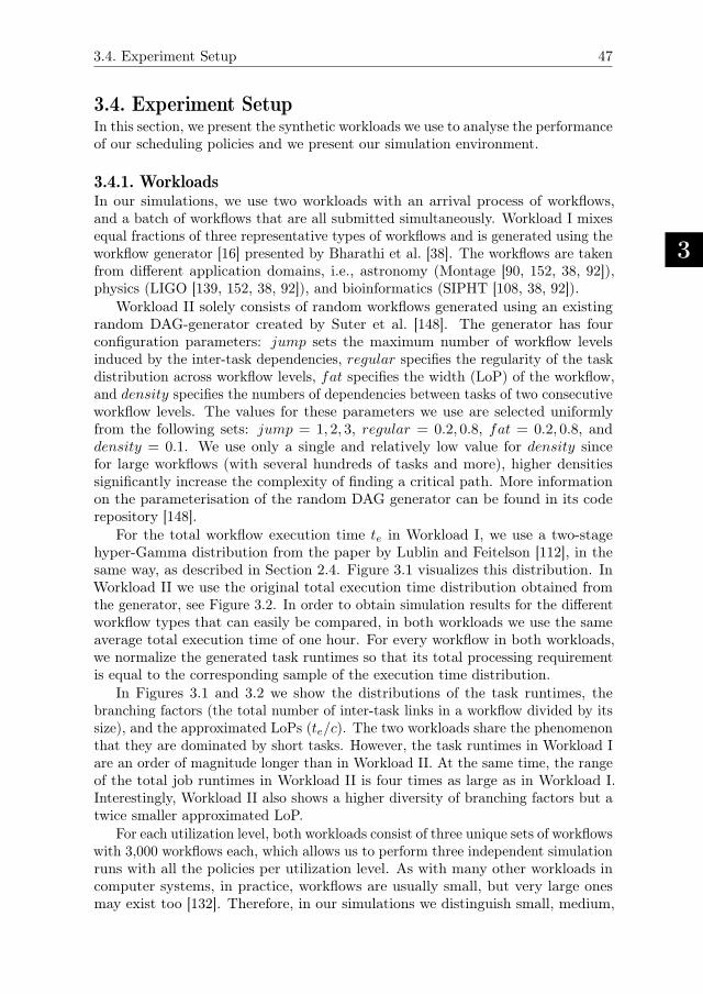
3.4. Experiment Setup

3

47

3.4. Experiment SetupIn this section, we present the synthetic workloads we use to analyse the performanceof our scheduling policies and we present our simulation environment.

3.4.1. WorkloadsIn our simulations, we use two workloads with an arrival process of workflows,and a batch of workflows that are all submitted simultaneously. Workload I mixesequal fractions of three representative types of workflows and is generated using theworkflow generator [16] presented by Bharathi et al. [38]. The workflows are takenfrom different application domains, i.e., astronomy (Montage [90, 152, 38, 92]),physics (LIGO [139, 152, 38, 92]), and bioinformatics (SIPHT [108, 38, 92]).

Workload II solely consists of random workflows generated using an existingrandom DAG-generator created by Suter et al. [148]. The generator has fourconfiguration parameters: jump sets the maximum number of workflow levelsinduced by the inter-task dependencies, regular specifies the regularity of the taskdistribution across workflow levels, fat specifies the width (LoP) of the workflow,and density specifies the numbers of dependencies between tasks of two consecutiveworkflow levels. The values for these parameters we use are selected uniformlyfrom the following sets: jump = 1, 2, 3, regular = 0.2, 0.8, fat = 0.2, 0.8, anddensity = 0.1. We use only a single and relatively low value for density sincefor large workflows (with several hundreds of tasks and more), higher densitiessignificantly increase the complexity of finding a critical path. More informationon the parameterisation of the random DAG generator can be found in its coderepository [148].

For the total workflow execution time te in Workload I, we use a two-stagehyper-Gamma distribution from the paper by Lublin and Feitelson [112], in thesame way, as described in Section 2.4. Figure 3.1 visualizes this distribution. InWorkload II we use the original total execution time distribution obtained fromthe generator, see Figure 3.2. In order to obtain simulation results for the differentworkflow types that can easily be compared, in both workloads we use the sameaverage total execution time of one hour. For every workflow in both workloads,we normalize the generated task runtimes so that its total processing requirementis equal to the corresponding sample of the execution time distribution.

In Figures 3.1 and 3.2 we show the distributions of the task runtimes, thebranching factors (the total number of inter-task links in a workflow divided by itssize), and the approximated LoPs (te/c). The two workloads share the phenomenonthat they are dominated by short tasks. However, the task runtimes in Workload Iare an order of magnitude longer than in Workload II. At the same time, the rangeof the total job runtimes in Workload II is four times as large as in Workload I.Interestingly, Workload II also shows a higher diversity of branching factors but atwice smaller approximated LoP.

For each utilization level, both workloads consist of three unique sets of workflowswith 3,000 workflows each, which allows us to perform three independent simulationruns with all the policies per utilization level. As with many other workloads incomputer systems, in practice, workflows are usually small, but very large onesmay exist too [132]. Therefore, in our simulations we distinguish small, medium,

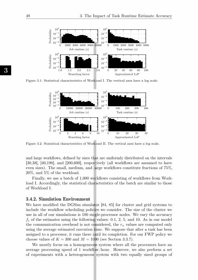
3

48 3. The Impact of Task Runtime Estimate Accuracy

0 2000 4000 6000 8000 10000

Job runtime (s)

10−3

10−2

10−1

100

Probability

0 1000 2000 3000 4000 5000

Task runtime (s)

100

10−2

10−4

10−6

1.0 1.5 2.0 2.5 3.0

Branching factor

100

10−2

10−4

10−6Probability

0 20 40 60 80 100

Approximated LoP

100

10−2

10−4

10−6

Figure 3.1: Statistical characteristics of Workload I. The vertical axes have a log scale.

0 10000 20000 30000 40000

Job runtime (s)

10−4

10−3

10−2

10−1

100

Probability

0 100 200 300 400

Task runtime (s)

100

10−2

10−4

10−6

0 2 4 6 8 10

Branching factor

100

10−2

10−4

10−6Probability

0 10 20 30 40

Approximated LoP

100

10−2

10−4

10−6

Figure 3.2: Statistical characteristics of Workload II. The vertical axes have a log scale.

and large workflows, defined by sizes that are uniformly distributed on the intervals[30,38], [40,198], and [200,600], respectively (all workflows are assumed to haveeven sizes). The small, medium, and large workflows constitute fractions of 75%,20%, and 5% of the workload.

Finally, we use a batch of 1,000 workflows consisting of workflows from Work-load I. Accordingly, the statistical characteristics of the batch are similar to thoseof Workload I.

3.4.2. Simulation EnvironmentWe have modified the DGSim simulator [84, 85] for cluster and grid systems toinclude the workflow scheduling policies we consider. The size of the cluster weuse in all of our simulations is 100 single-processor nodes. We vary the accuracyfe of the estimates using the following values: 0.1, 2, 5, and 10. As in our modelthe communication overhead is not considered, the ru values are computed onlyusing the average estimated execution time. We suppose that after a task has beenassigned to a processor, it runs there until its completion. For our FWP policy wechoose values of K = 300 and M = 1000 (see Section 3.3.7).

We mostly focus on a homogeneous system where all the processors have anaverage processing speed of 1 workflow/hour. However, we also perform a setof experiments with a heterogeneous system with two equally sized groups of

3.5. Experiment Results

3

49

processors: fast processors with an average processing speed of 1.5 workflow/hourand slow processors with an average processing speed of 0.5 workflow/hour.

For the majority of the simulations we use a system utilization of 98% since allthe considered dynamic policies can handle such high utilizations (we show thislater in Section 3.5). We only show results when the system is in steady state,i.e., when reporting performance results for workloads, we omit the performanceinformation for the first 1000 workflows and last 1000 workflows in each simulation.

3.4.3. System Stability ValidationTo be able to clearly distinguish situations when the system is or is not stable in along-term perspective, we use two methods: the statistical system stability checkproposed by Wieland et al. [166], as well as the Lyapunov drift theorem [128]. Forevery simulation run, we perform both stability tests. The system is consideredstable if each method shows at least two stable results out of three.

According to the Wieland approach, we take the observed number of workflowsin the system N(t) (both queued and partially running) at every moment t, where0 ≤ t ≤ τ with τ the total duration of the simulation, and split the observationsinto b batches, where b = 10. Then for each batch j = 2, . . . , b we compute thetime average number of workflows in the system within the batch as:

λN,j =

j·τ/b∫

(j−1)·τ/b

N(t)

τ/bdt. (3.8)

Then we compute the difference between the last and second batch observations:λN = λN,b − λN,2, and compute the variance σ2 of batch observations with b− 1degrees of freedom. We conclude whether the system is stable if

λN√2 · σ

> t1−α,b−2, (3.9)

where t1−α,b−2 is the 1− α Student-T quantile with b− 2 degrees of freedom. Forthe default values of b = 10 and α = 0.05, t1−α,b−2 = 1.86, thus, stability is rejected

if λN > 2.63 · σ.For the Lyapunov drift-based stability check we compute the mean Lyapunov

drift throughout the simulation as follows: δ(t) = l(t)−l(t−1), where l(t) = N(t)2/2.A low value of the mean Lyapunov drift after the initial transient indicates thatthe system converges and is stable. For our system we experimentally derive athreshold of 1 for the mean Lyapunov drift; if the mean drift exceeds 1, the systemis considered unstable.

3.5. Experiment ResultsIn this section, we present our experiment results. We first investigate how varyingthe error in task runtime estimates affects the slowdowns of workflows in homo-geneous and heterogeneous systems for the six dynamic scheduling policies weconsider. Then we show the performance of the plan-based WHEFT policy andthe performance when scheduling batches of workflows.

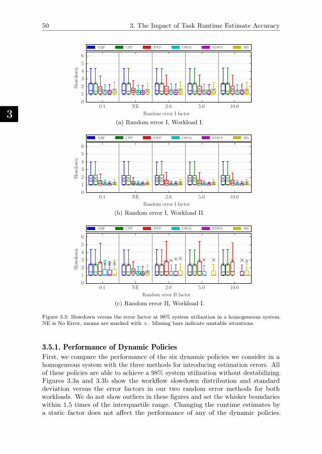
3

50 3. The Impact of Task Runtime Estimate Accuracy

(a) Random error I, Workload I.

(b) Random error I, Workload II.

(c) Random error II, Workload I.

Figure 3.3: Slowdown versus the error factor at 98% system utilization in a homogeneous system.NE is No Error, means are marked with ×. Missing bars indicate unstable situations.

3.5.1. Performance of Dynamic Policies

First, we compare the performance of the six dynamic policies we consider in ahomogeneous system with the three methods for introducing estimation errors. Allof these policies are able to achieve a 98% system utilization without destabilizing.Figures 3.3a and 3.3b show the workflow slowdown distribution and standarddeviation versus the error factors in our two random error methods for bothworkloads. We do not show outliers in these figures and set the whisker boundarieswithin 1.5 times of the interquartile range. Changing the runtime estimates bya static factor does not affect the performance of any of the dynamic policies.

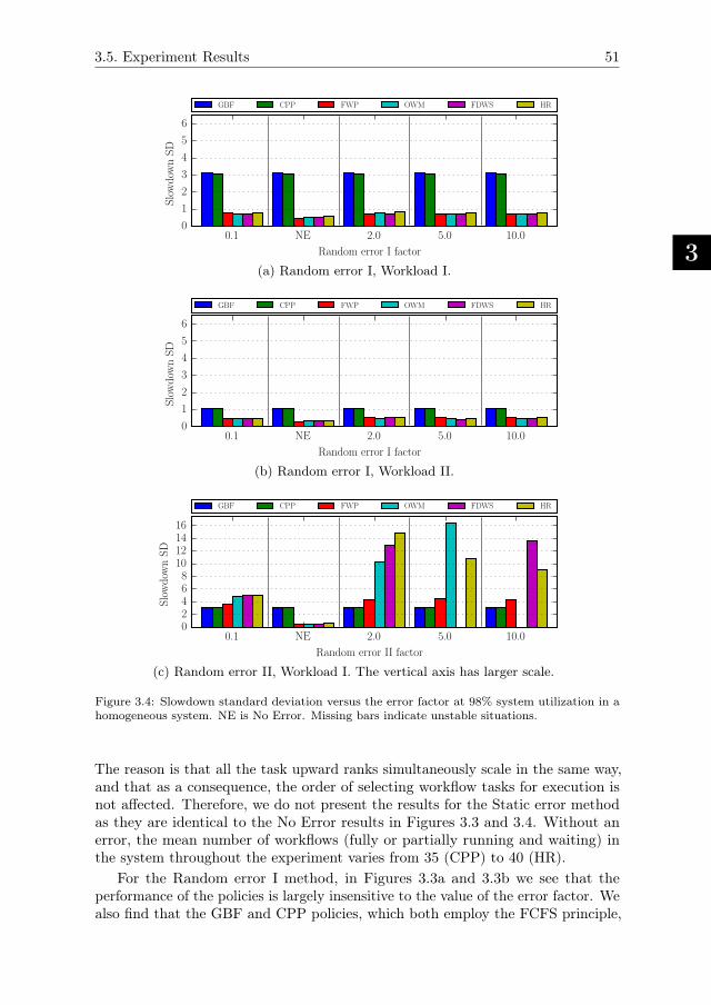
3.5. Experiment Results

3

51

(a) Random error I, Workload I.

(b) Random error I, Workload II.

(c) Random error II, Workload I. The vertical axis has larger scale.

Figure 3.4: Slowdown standard deviation versus the error factor at 98% system utilization in ahomogeneous system. NE is No Error. Missing bars indicate unstable situations.

The reason is that all the task upward ranks simultaneously scale in the same way,and that as a consequence, the order of selecting workflow tasks for execution isnot affected. Therefore, we do not present the results for the Static error methodas they are identical to the No Error results in Figures 3.3 and 3.4. Without anerror, the mean number of workflows (fully or partially running and waiting) inthe system throughout the experiment varies from 35 (CPP) to 40 (HR).

For the Random error I method, in Figures 3.3a and 3.3b we see that theperformance of the policies is largely insensitive to the value of the error factor. Wealso find that the GBF and CPP policies, which both employ the FCFS principle,

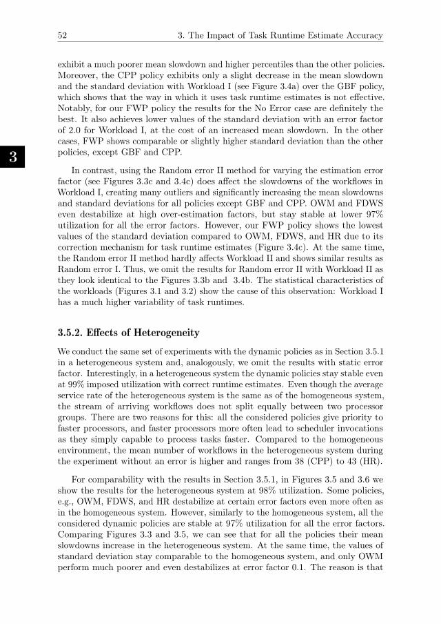
3

52 3. The Impact of Task Runtime Estimate Accuracy

exhibit a much poorer mean slowdown and higher percentiles than the other policies.Moreover, the CPP policy exhibits only a slight decrease in the mean slowdownand the standard deviation with Workload I (see Figure 3.4a) over the GBF policy,which shows that the way in which it uses task runtime estimates is not effective.Notably, for our FWP policy the results for the No Error case are definitely thebest. It also achieves lower values of the standard deviation with an error factorof 2.0 for Workload I, at the cost of an increased mean slowdown. In the othercases, FWP shows comparable or slightly higher standard deviation than the otherpolicies, except GBF and CPP.

In contrast, using the Random error II method for varying the estimation errorfactor (see Figures 3.3c and 3.4c) does affect the slowdowns of the workflows inWorkload I, creating many outliers and significantly increasing the mean slowdownsand standard deviations for all policies except GBF and CPP. OWM and FDWSeven destabilize at high over-estimation factors, but stay stable at lower 97%utilization for all the error factors. However, our FWP policy shows the lowestvalues of the standard deviation compared to OWM, FDWS, and HR due to itscorrection mechanism for task runtime estimates (Figure 3.4c). At the same time,the Random error II method hardly affects Workload II and shows similar results asRandom error I. Thus, we omit the results for Random error II with Workload II asthey look identical to the Figures 3.3b and 3.4b. The statistical characteristics ofthe workloads (Figures 3.1 and 3.2) show the cause of this observation: Workload Ihas a much higher variability of task runtimes.

3.5.2. Effects of Heterogeneity

We conduct the same set of experiments with the dynamic policies as in Section 3.5.1in a heterogeneous system and, analogously, we omit the results with static errorfactor. Interestingly, in a heterogeneous system the dynamic policies stay stable evenat 99% imposed utilization with correct runtime estimates. Even though the averageservice rate of the heterogeneous system is the same as of the homogeneous system,the stream of arriving workflows does not split equally between two processorgroups. There are two reasons for this: all the considered policies give priority tofaster processors, and faster processors more often lead to scheduler invocationsas they simply capable to process tasks faster. Compared to the homogeneousenvironment, the mean number of workflows in the heterogeneous system duringthe experiment without an error is higher and ranges from 38 (CPP) to 43 (HR).

For comparability with the results in Section 3.5.1, in Figures 3.5 and 3.6 weshow the results for the heterogeneous system at 98% utilization. Some policies,e.g., OWM, FDWS, and HR destabilize at certain error factors even more often asin the homogeneous system. However, similarly to the homogeneous system, all theconsidered dynamic policies are stable at 97% utilization for all the error factors.Comparing Figures 3.3 and 3.5, we can see that for all the policies their meanslowdowns increase in the heterogeneous system. At the same time, the values ofstandard deviation stay comparable to the homogeneous system, and only OWMperform much poorer and even destabilizes at error factor 0.1. The reason is that

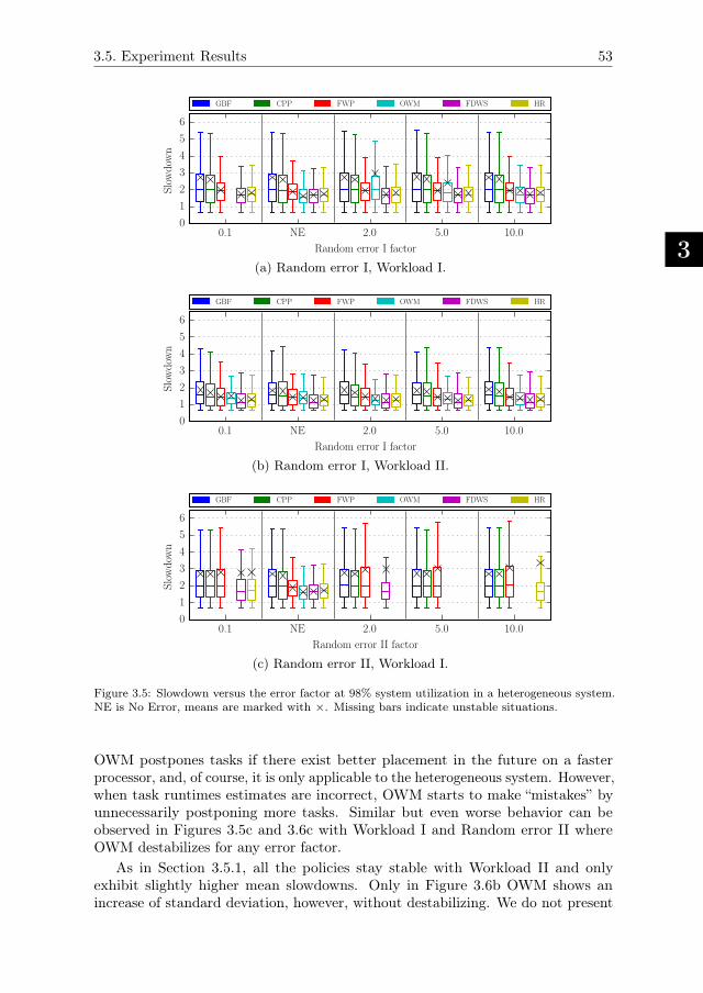
3.5. Experiment Results

3

53

(a) Random error I, Workload I.

(b) Random error I, Workload II.

(c) Random error II, Workload I.

Figure 3.5: Slowdown versus the error factor at 98% system utilization in a heterogeneous system.NE is No Error, means are marked with ×. Missing bars indicate unstable situations.

OWM postpones tasks if there exist better placement in the future on a fasterprocessor, and, of course, it is only applicable to the heterogeneous system. However,when task runtimes estimates are incorrect, OWM starts to make “mistakes” byunnecessarily postponing more tasks. Similar but even worse behavior can beobserved in Figures 3.5c and 3.6c with Workload I and Random error II whereOWM destabilizes for any error factor.

As in Section 3.5.1, all the policies stay stable with Workload II and onlyexhibit slightly higher mean slowdowns. Only in Figure 3.6b OWM shows anincrease of standard deviation, however, without destabilizing. We do not present

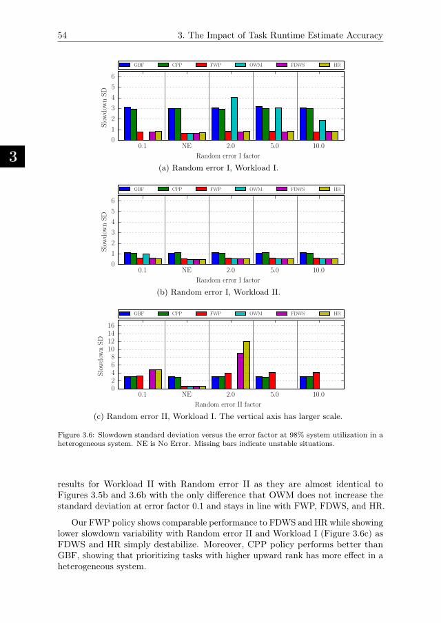
3

54 3. The Impact of Task Runtime Estimate Accuracy

(a) Random error I, Workload I.

(b) Random error I, Workload II.

(c) Random error II, Workload I. The vertical axis has larger scale.

Figure 3.6: Slowdown standard deviation versus the error factor at 98% system utilization in aheterogeneous system. NE is No Error. Missing bars indicate unstable situations.

results for Workload II with Random error II as they are almost identical toFigures 3.5b and 3.6b with the only difference that OWM does not increase thestandard deviation at error factor 0.1 and stays in line with FWP, FDWS, and HR.

Our FWP policy shows comparable performance to FDWS and HR while showinglower slowdown variability with Random error II and Workload I (Figure 3.6c) asFDWS and HR simply destabilize. Moreover, CPP policy performs better thanGBF, showing that prioritizing tasks with higher upward rank has more effect in aheterogeneous system.

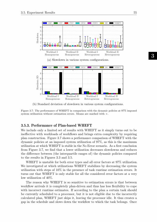
3.5. Experiment Results

3

55

(a) Slowdown in various system configurations.

(b) Standard deviation of slowdown in various system configurations.

Figure 3.7: The performance of WHEFT in comparison with the dynamic policies at 97% imposedsystem utilization without estimation errors. Means are marked with ×.

3.5.3. Performance of Plan-based WHEFT

We include only a limited set of results with WHEFT as it simply turns out to beineffective with workloads of workflows and brings extra complexity by requiringplan construction. Figure 3.7 shows a performance comparison of WHEFT with thedynamic policies at an imposed system utilization of 97%, as this is the maximumutilization at which WHEFT is stable in the No Error scenario. As a first conclusionfrom Figure 3.7, we find that a lower utilization decreases slowdowns and reducesthe difference between (the interquartile ranges of) the dynamic policies comparedto the results in Figures 3.3 and 3.5.

WHEFT is unstable for both error types and all error factors at 97% utilization.We investigated at which utilizations WHEFT stabilizes by decreasing the systemutilization with steps of 10% in the presence of task runtime estimation errors. Itturns out that WHEFT is only stable for all the considered error factors at a verylow utilization of 40%.

The reason why WHEFT is so sensitive to estimation errors is that betweenworkflow arrivals it is completely plan-driven and thus has less flexibility to copewith incorrect runtime estimates. If according to the plan a certain task shouldbe currently scheduled to a processor, but it is not eligible due to the incorrectlycalculated plan, WHEFT just skips it, leaving the processor idle. It thus creates agap in the schedule and slows down the workflow to which the task belongs. Once

3

56 3. The Impact of Task Runtime Estimate Accuracy

a task is wrongly placed in the plan due to incorrect estimates, it can only possiblybe relocated to a better position when a new workflow arrives. While WHEFTpostpones tasks “unintentionally”, OWM postpones tasks on purpose in the hopethat finally they will be scheduled on a faster processor. So the reason why WHEFTshows poor results is similar to why OWM becomes unstable in Section 3.5.2.

At a 97% utilization, our simulated system receives 97 workflows per hour (sincethe workflows have an average total execution time of 1 hour), which means that onaverage, the plan is recomputed 97 times per hour. So on average, every workflowtask has a chance to be relocated to a better position 97 times during the workflowexecution. Decreasing the utilization decreases the number of simultaneouslyscheduled workflows, but at the same time it decreases the number of possible taskrelocations.

Moreover, the original HEFT policy schedules tasks with higher upward ranksfirst. For this reason, WHEFT gives priority to longer workflows constituting thejoint workflow. Accordingly, WHEFT postpones shorter workflows, which representthe majority of both our workloads. That increases the average slowdown andaccumulates more workflows in the system, finally destabilizing it.

For plan-based policies in real-world non-simulated environments, the durationof the plan construction phase is crucial. Newly arrived workflows cannot starttheir execution until their tasks have been added to the plan. This can additionallyincrease job slowdown. In the considered simulated environment, from the perspec-tive of workflows plan construction takes zero time, but in real systems it shouldbe much smaller than the average workflow inter-arrival time. In our case, for 1000simultaneously running workflows (see Section 3.5.4) the plan construction takes40 minutes for a Python3 implementation running on a DAS-4 [35] node (2.4 GHzIntel E5620 CPU, 24 GB RAM). The planning time, however, can be reduced byusing a tree structure (e.g., a k-tree [134]) to store the information about the gapsin the plan. It will decrease the time required to find an appropriate gap for a taskat the cost of a higher memory consumption.

3.5.4. Performance of a Batch SubmissionIn this section, we investigate how the considered policies behave when handling abatch submission. Since this chapter mainly focuses on the analysis of workloadsof workflows, we only perform a limited set of experiments with a single batchsubmission of 1000 workflows based on Workload I in a homogeneous system.Figure 3.8 shows the total schedule length in hours of this batch with variableRandom error I. We do not show the results for Random error II as they arecomparable. There is a small difference for under- and over-estimating situations,with GBF and CPP producing schedules that are longer by half an hour (5.5%)than the other dynamic policies.

We do not report slowdowns, as we suppose that batch submissions usuallycome from a single user who is only interested in minimizing the total schedulelength rather than achieving fairness among the workflows in the batch. We canclearly see that WHEFT, indeed, constructs a shorter schedule than the dynamicpolicies. However, it is less resilient to errors as its scheduler postpones taskswhich are not eligible or if a target processor is occupied (as in Section 3.5.3). The

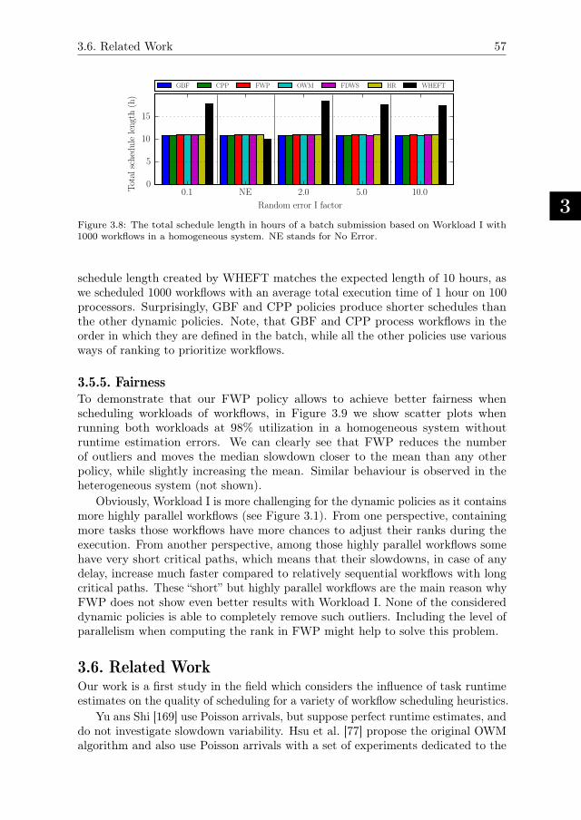
3.6. Related Work

3

57

Figure 3.8: The total schedule length in hours of a batch submission based on Workload I with1000 workflows in a homogeneous system. NE stands for No Error.

schedule length created by WHEFT matches the expected length of 10 hours, aswe scheduled 1000 workflows with an average total execution time of 1 hour on 100processors. Surprisingly, GBF and CPP policies produce shorter schedules thanthe other dynamic policies. Note, that GBF and CPP process workflows in theorder in which they are defined in the batch, while all the other policies use variousways of ranking to prioritize workflows.

3.5.5. FairnessTo demonstrate that our FWP policy allows to achieve better fairness whenscheduling workloads of workflows, in Figure 3.9 we show scatter plots whenrunning both workloads at 98% utilization in a homogeneous system withoutruntime estimation errors. We can clearly see that FWP reduces the numberof outliers and moves the median slowdown closer to the mean than any otherpolicy, while slightly increasing the mean. Similar behaviour is observed in theheterogeneous system (not shown).

Obviously, Workload I is more challenging for the dynamic policies as it containsmore highly parallel workflows (see Figure 3.1). From one perspective, containingmore tasks those workflows have more chances to adjust their ranks during theexecution. From another perspective, among those highly parallel workflows somehave very short critical paths, which means that their slowdowns, in case of anydelay, increase much faster compared to relatively sequential workflows with longcritical paths. These “short” but highly parallel workflows are the main reason whyFWP does not show even better results with Workload I. None of the considereddynamic policies is able to completely remove such outliers. Including the level ofparallelism when computing the rank in FWP might help to solve this problem.

3.6. Related WorkOur work is a first study in the field which considers the influence of task runtimeestimates on the quality of scheduling for a variety of workflow scheduling heuristics.

Yu ans Shi [169] use Poisson arrivals, but suppose perfect runtime estimates, anddo not investigate slowdown variability. Hsu et al. [77] propose the original OWMalgorithm and also use Poisson arrivals with a set of experiments dedicated to the

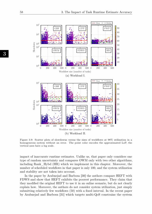
3

58 3. The Impact of Task Runtime Estimate Accuracy

(a) Workload I.

(b) Workload II.

Figure 3.9: Scatter plots of slowdowns versus the sizes of workflows at 98% utilization in ahomogeneous system without an error. The point color encodes the approximated LoP, thevertical axes have a log scale.

impact of inaccurate runtime estimates. Unlike us, that paper only considers onetype of random uncertainty and compares OWM only with two other algorithms,including Rank_Hybd (HR) which we implement in this chapter. Moreover, thenumber of scheduled workflows in that paper is only 100, and the system utilizationand stability are not taken into account.

In the paper by Arabnejad and Barbosa [30] the authors compare HEFT withFDWS and show that HEFT exhibits the poorest performance. They claim thatthey modified the original HEFT to use it in an online scenario, but do not clearlyexplain how. Moreover, the authors do not consider system utilization, just simplysubmitting relatively few workflows (50) with a fixed interval. In the recent paperby Arabnejad and Barbosa [31] which targets multi-QoS constrains the system

3.7. Conclusion

3

59

utilization is not considered either.The slowdown-based fairness problem has been addressed before. Zhao and

Sakellariou [170] proposed a plan-based policy which targets fairness using avariety of approaches. However, their algorithm has limited applicability forworkloads of workflows as it is plan-based. Recently, Wang et al. [163] proposedfairness-aware dynamic FSDP algorithm which, however, does not clearly link thecurrent slowdown and the target average slowdown which should be achieved, andrecomputes workflow priorities on every new workflow arrival only. In contrast,our FWP policy recomputes priorities when a task becomes eligible or a processorbecomes idle. An algorithm for fairness and granularity control for online schedulingof workflows is also addressed in a paper by Ferreira da Silva et al. [65]. Theirapproach, though, does not consider system utilization.

Among the algorithms which can operate without task runtime estimateswe distinguish PRIO [117] which was successfully implemented in the DAGMancomponent of the Condor distributed job scheduler [153]. However, we do notinclude it in the comparison, as it tries to maximize the number of eligible tasks inhope to increase the throughput of the system, while in this chapter we focus onupward rank-based policies.

3.7. ConclusionIn this chapter, we have investigated the effect of incorrect task runtime estimateson the performance of dynamic and plan-based scheduling policies in the onlinescenario of scheduling workloads of workflows.

We can clearly see the benefit of knowing task runtime estimates as we doobserve significant performance differences between the considered dynamic policiesand large improvements in average job slowdown, but only at extremely high systemutilizations. Similarly, the sensitivity to incorrect task runtime estimates increasesat higher system utilizations. The order in which the workflows are processed isvery important, as it allows to achieve a fairer distribution of slowdowns amongworkflows in the workload, as in our FWP policy.

Giving priority to workflows with longer critical paths, especially at extremelyhigh utilizations, easily destabilizes the system if the workload has a majority ofshort jobs, as these short jobs start to accumulate. At lower utilizations, which arevery common in real datacenters, simpler backfilling-based policies that do not usetask runtime estimates are quite applicable and show comparable performance tomore advanced fairness-oriented policies.

The plan-based WHEFT policy shows poor performance with workloads of work-flows, but it does construct the shortest schedule for batch submissions. Moreover,WHEFT is quite unstable with incorrect task runtime estimates, running stably onlyat the relatively low utilization of 40%. We believe that even more complex policieslike Hybrid.BMCT [142] would also suffer from this problem. Even though we donot exclude that plan-based approaches could achieve slowdowns comparable tothose of dynamic policies, their planning overhead and implementation complexitydo not seem to be worth it.

4

An Experimental

Performance Evaluation

of Autoscalers

Elasticity is one of the main features of cloud computing allowing customersto scale their resources based on the workload. Many autoscalers have been

proposed in the past decade to decide on behalf of cloud customers when andhow to provision resources to a cloud application based on the workload, utilizingcloud elasticity features. However, in prior work, when a new policy is proposed, itis seldom compared to the state-of-the-art, and is often compared only to staticprovisioning using a predefined Quality-of-Service target. This reduces the ability ofcloud customers and of cloud operators to choose and deploy an autoscaling policy asthere is often not enough analysis on the performance of the autoscalers in differentoperating conditions and with different applications. In this chapter, we conductan experimental performance evaluation of autoscaling policies, using workflows—a popular formalism for automating distributed computations for applications withwell-defined yet complex structures. We present a detailed comparative study ofgeneral state-of-the-art autoscaling policies, along with two new workflow-specificpolicies. To understand the performance differences between the seven policies, weconduct various experiments and compare their performance in both pairwise andgroup comparisons. We report both individual and aggregated metrics. As manyworkflows have deadline requirements on the tasks, we study the effect of autoscalingon workflow deadlines. Additionally, we look into the effect of autoscaling on theaccounted and hourly-based charged costs, and evaluate performance variabilitycaused by the autoscaler selection for each group of workflow sizes. Our resultshighlight the trade-offs between the suggested policies, how they can impact meetingthe deadlines, and how they perform in different operating conditions, thus enablinga better understanding of the current state-of-the-art.

61

4

62 4. An Experimental Performance Evaluation of Autoscalers

4.1. IntroductionCloud computing emerged as a computing model where computing services andresources are outsourced on an on-demand pay-per-use basis. To make this modeluseful for a variety of customers, cloud operators try to simplify the process ofobtaining and managing the provided services. To this end, cloud operators makeavailable to their customers various autoscaling policies (autoscalers, AS ), whichare essentially parametrized cloud scheduling algorithms that dynamically regulatethe amount of resources allocated to a cloud application based on the load demandand the Quality-of-Service (QoS) requirements typically set by the customer. Manyautoscalers have been proposed in the literature, both general autoscalers forrequest-response applications [26, 42, 157, 64, 127] and autoscalers for moretask- and structure-oriented applications such as workflows [25, 40, 60, 47, 136, 46].The selection of an appropriate autoscaling policy is crucial, as a good choice canlead to significant performance and financial benefits for cloud customers, andto improved flexibility and ability to meet QoS requirements for cloud operators.Selecting among the proposed autoscalers is not easy, which raises the problemof finding a systematic, method-based approach to comprehensively evaluate andcompare autoscalers. The lack of such an approach derives in our view from ongoingscientific and industry practice. For the past decade, much academic work hasfocused on building basic mechanisms and autoscalers for specific applications,with very limited work spent in comparisons with the state-of-the-art. In industrysettings, much attention has been put on building cloud infrastructures that enableautoscaling as a mechanism, and relatively less on providing good libraries ofautoscalers for customers to choose from [73, 133]. To alleviate this problem, in thischapter we propose and use the first systematic experimental method to evaluate andcompare the performance of autoscalers using workflow-based workloads runningin cloud settings as a use-case application.

Modern workflows have different structures, sizes, task types, run-time proper-ties, and performance requirements, and thus raise specific and important challengesin assessing the performance of autoscalers: How does the performance of generaland of workflow-specific autoscalers depend on workflow-based workload character-istics? Among the many application types, our focus on workflow-based workloadsis motivated by three aspects. First, there is an increasing popularity [150, 152]of workflows for science and engineering [22, 90, 108], big data [109], and businessapplications [154], and by the ability of workflows to express complex applicationswhose interconnected tasks can be managed automatically on behalf of cloud cus-tomers [88]. Second, although general autoscalers focus mainly on QoS aspects, suchas throughput, response-time and cost constraints, some autoscalers also take intoaccount application structure [115]. One of the main questions we want to answerin this chapter is: How does the performance of general and of workflow-specificautoscalers differ?

Another interesting aspect that arise with workflow scaling is the effect of theautoscalers on workflow deadlines. Many of the workloads have deadlines, basicallya bound on the tolerated time by the user between the workflow submission andwhen the computation results are available. Having enough capacity in the systemfor the workflows to finish their processing before the deadline can be severely

4.2. A Model for Elastic Cloud Platforms

4

63

affected by the presence of autoscalers. For that we enforce per-workflow andper-workload deadlines which allow us to see: How does each autoscaler affectdeadline violations?

One of the core properties of an autoscaler is the ability to minimize operationalcosts while keeping the required performance level. We calculate the incurred costsfor each considered autoscaler which allow us to answer the questions: How do theautoscalers affect charged and accounted costs?, and How do the autoscalers find abalance between performance and cost?

Towards addressing the aforementioned questions, our contribution is threefold:

1. We design a comprehensive method for evaluating and comparing autoscalers(Sections 4.2–4.4). Our method includes a model for elastic cloud platforms(Section 4.2), a set of relevant metrics for assessing autoscaler performance(Section 4.3), and a taxonomy and survey of exemplary general and workflow-specific autoscalers (Section 4.4).

2. Using the method, we comprehensively and experimentally quantify theperformance of 7 general and workflow-specific autoscalers, for more than15 performance metrics (Section 4.5). We show the differences betweenvarious policy types, analyze parametrization effects, evaluate the influenceof workload characteristics on individual performance metrics, and explainthe reasons for the performance variability we observe in practice.

3. We also compare the autoscalers systematically (Section 4.8), through 3 mainapproaches: a pair-wise comparison specific to round-robin tournaments, acomparison of fractional differences between each system and an ideal systemderived from the experimental results, and a head-to-head comparison ofseveral aggregated metrics.

4.2. A Model for Elastic Cloud PlatformsAutoscaling is an incarnation of the dynamic provisioning problem that has beenstudied in the literature for over a decade [41]: many autoscalers in essence tryto solve the problem of how much capacity to provision given a certain QoS,published state-of-the-art algorithms make different assumptions on the underlyingenvironment, mode of operation, or workload used. It is thus important to identifythe key requirements of all algorithms, and establish a fair cloud system forcomparison.

4.2.1. RequirementsIn order to improve the QoS and decrease costs of a running application, an idealautoscaler proactively predicts and provisions resources such that: a) there is alwaysenough capacity to handle the workload with no under-provisioning affecting theQoS requirements; b) the cost is kept minimal by reducing the number of resourcesnot used at any given time, thus reducing over-provisioning; and c) the autoscalerdoes not cause consistency and/or stability issues in the running applications.

Since there are no perfect predictors, no ideal autoscaler exists. Thus, thereis a need to have better understanding of the capabilities of the various available

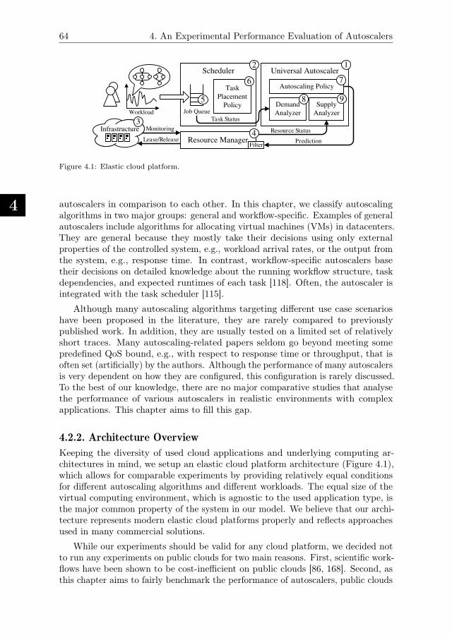
4

64 4. An Experimental Performance Evaluation of Autoscalers

Workload

Monitoring

Job Queue

Task

Placement

Policy

Lease/Release

Scheduler

Demand

Analyzer

Supply

Analyzer

Universal Autoscaler

Resource ManagerFilter

Prediction

Infrastructure

Autoscaling Policy

Resource Status

Task Status3

5

6

2

4

8 9

7

1

Figure 4.1: Elastic cloud platform.

autoscalers in comparison to each other. In this chapter, we classify autoscalingalgorithms in two major groups: general and workflow-specific. Examples of generalautoscalers include algorithms for allocating virtual machines (VMs) in datacenters.They are general because they mostly take their decisions using only externalproperties of the controlled system, e.g., workload arrival rates, or the output fromthe system, e.g., response time. In contrast, workflow-specific autoscalers basetheir decisions on detailed knowledge about the running workflow structure, taskdependencies, and expected runtimes of each task [118]. Often, the autoscaler isintegrated with the task scheduler [115].

Although many autoscaling algorithms targeting different use case scenarioshave been proposed in the literature, they are rarely compared to previouslypublished work. In addition, they are usually tested on a limited set of relativelyshort traces. Many autoscaling-related papers seldom go beyond meeting somepredefined QoS bound, e.g., with respect to response time or throughput, that isoften set (artificially) by the authors. Although the performance of many autoscalersis very dependent on how they are configured, this configuration is rarely discussed.To the best of our knowledge, there are no major comparative studies that analysethe performance of various autoscalers in realistic environments with complexapplications. This chapter aims to fill this gap.

4.2.2. Architecture Overview

Keeping the diversity of used cloud applications and underlying computing ar-chitectures in mind, we setup an elastic cloud platform architecture (Figure 4.1),which allows for comparable experiments by providing relatively equal conditionsfor different autoscaling algorithms and different workloads. The equal size of thevirtual computing environment, which is agnostic to the used application type, isthe major common property of the system in our model. We believe that our archi-tecture represents modern elastic cloud platforms properly and reflects approachesused in many commercial solutions.

While our experiments should be valid for any cloud platform, we decided notto run any experiments on public clouds for two main reasons. First, scientific work-flows have been shown to be cost-inefficient on public clouds [86, 168]. Second, asthis chapter aims to fairly benchmark the performance of autoscalers, public clouds

4.2. A Model for Elastic Cloud Platforms

4

65

will introduce variability due to the platforms as public cloud VM performance canvary considerably [86].

The core of our system is the autoscaling service (Component 1 in Figure 4.1)that runs independently as a REST service. The experimental testbed consistsof a scheduler (Component 2) and a virtual infrastructure service (Component 3)which maintains a set of computing resources. A resource manager (Component 4)monitors the infrastructure and controls the resource provisioning. Users submittheir workflows directly to the scheduler which maintains a single job queue(Component 5). The tasks from the queued workflows are mapped to the computingresources in accordance to the task placement policy (Component 6). The schedulerperiodically calls the autoscaling service providing it with monitoring data fromthe last time period. We refer to this period as the autoscaling interval.

The autoscaling service implements an autoscaling policy (Component 7) andhas a demand analyzer (Component 8) which uses information about running andqueued workflows to compute the momentary demand value. The supply analyzer(Component 9) computes the momentary supply value by analyzing the status ofcomputing resources. The autoscaling service responds to the scheduler with thepredicted number of resources which should be allocated or deallocated. Beforeapplying the prediction, the resource manager filters it trimming the obtained valueby the maximal number of available resources. To avoid error accumulation, theautoscaling interval is usually chosen so that the provisioning actions made duringthe autoscaling interval has already taken effect. Thus, it is guaranteed that theprovisioning time is always shorter than the autoscaling interval. In case whenthe provisioning time is longer than the autoscaling interval, the resource managershould apply the prediction only partially considering the number of “straggling”resources. In practice, it means that the resource manager should consider bootingVMs as fully provisioned resources.

4.2.3. Workflow Applications and Deadlines

For our experiments, in this chapter we use complex workflows as our systemworkload. We rely on the same workflow job definitions as presented in previouschapters (e.g., in Section 2.2.1). Scheduling of workflows is often time critical andinvolves meeting deadlines for the processing times. For example, workflows forprocessing satellite data should handle the received information while the satellitemakes a turn around the planet [137, 59]. Such workflows should finish beforea new batch of information is received. Another example is the case of moderncloud services where the user pays per time slot and the deadlines are boundedto the lengths of these time slots [114]. We assume that deadlines for workflowsare set on a per-workflow and per-workload basis. Per-workflow deadlines areunique for every workflow and are normally assigned based on user (statistical)estimates of the possible workflow runtimes. Per-workload deadlines are commonwhen processing batches of workflows. In this case, a per-workload deadline appliesto all the workflows in the workload. We consider soft deadlines which can beviolated without affecting the execution of a workflow. Soft deadlines is a measurethat can additionally reflect induced infrastructure costs for users.

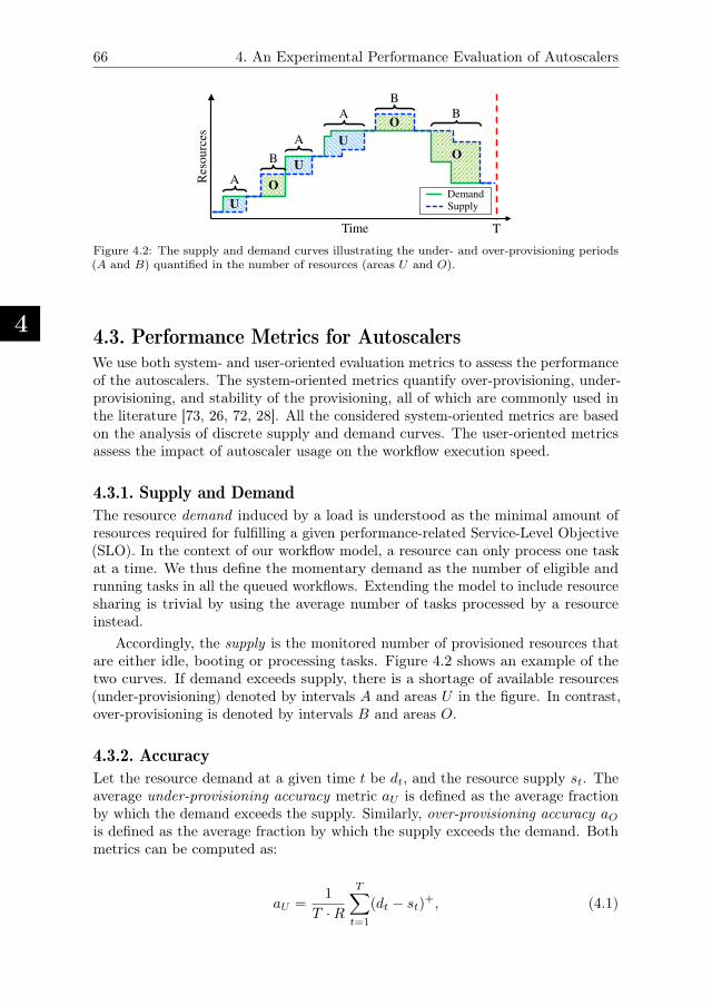
4

66 4. An Experimental Performance Evaluation of Autoscalers

Time

Demand Supply

Res

ourc

es

T

A

U

A

A

B

B

O

U

O B

U

O

Figure 4.2: The supply and demand curves illustrating the under- and over-provisioning periods(A and B) quantified in the number of resources (areas U and O).

4.3. Performance Metrics for AutoscalersWe use both system- and user-oriented evaluation metrics to assess the performanceof the autoscalers. The system-oriented metrics quantify over-provisioning, under-provisioning, and stability of the provisioning, all of which are commonly used inthe literature [73, 26, 72, 28]. All the considered system-oriented metrics are basedon the analysis of discrete supply and demand curves. The user-oriented metricsassess the impact of autoscaler usage on the workflow execution speed.

4.3.1. Supply and Demand

The resource demand induced by a load is understood as the minimal amount ofresources required for fulfilling a given performance-related Service-Level Objective(SLO). In the context of our workflow model, a resource can only process one taskat a time. We thus define the momentary demand as the number of eligible andrunning tasks in all the queued workflows. Extending the model to include resourcesharing is trivial by using the average number of tasks processed by a resourceinstead.

Accordingly, the supply is the monitored number of provisioned resources thatare either idle, booting or processing tasks. Figure 4.2 shows an example of thetwo curves. If demand exceeds supply, there is a shortage of available resources(under-provisioning) denoted by intervals A and areas U in the figure. In contrast,over-provisioning is denoted by intervals B and areas O.

4.3.2. Accuracy

Let the resource demand at a given time t be dt, and the resource supply st. Theaverage under-provisioning accuracy metric aU is defined as the average fractionby which the demand exceeds the supply. Similarly, over-provisioning accuracy aOis defined as the average fraction by which the supply exceeds the demand. Bothmetrics can be computed as:

aU =1

T ·R

T∑

t=1

(dt − st)+, (4.1)

4.3. Performance Metrics for Autoscalers

4

67

aO =1

T ·R

T∑

t=1

(st − dt)+, (4.2)

where T is the time horizon of the experiment expressed in time steps, R isthe total number of resources available in the current experimental setup, and(x)+ = max(x, 0), i.e., only the positive values of x. The intuition behind thetwo accuracy metrics is shown in Figure 4.2. Under-provisioning accuracy aUis equivalent to summing the areas U where the resource demand exceeds thesupply normalized by the duration of the measurement period T . Similarly, theover-provisioning accuracy metric aO is the sum of areas O where the resourcesupply exceeds the demand.

It is also possible to normalize the metrics by the actual resource demand,obtaining therefore a normalized, and more fair indicator. In particular, the twometrics can be modified as:

aU =1

T

T∑

t=1

(dt − st)+

max(dt, ε), (4.3)

aO =1

T

T∑

t=1

(st − dt)+

max(dt, ε), (4.4)

with ε > 0; in our setting we selected ε = 1. The normalized metrics are particularlyuseful when the resource demand has a large variance over time, and it can assumeboth large and small values. In fact, under-provisioning of 1 resource unit when2 resource units are requested is much more harmful than under-provisioning 1resource unit when 1000 resource units are requested. Therefore, this type ofnormalization allows a more fair evaluation of the obtainable performance.

Since under-provisioning results in violating SLOs, a customer might want touse a platform that minimizes under-provisioning ensuring that enough resourcesare provided at any point in time, but at the same time minimizing the amountof over-provisioned resources. The defined separate accuracy metrics for over-and under-provisioning allow providers to better communicate their autoscalingcapabilities and customers to select an autoscaler that best matches their needs.In the context of workflows, over-provisioning accuracy can also be represented inthe number of idle resources (i.e., the resources which were excessively provisionedand currently are not utilized).

In ideal situation when an autoscaler perfectly follows the demand curve, thereshould be no idle resources as the system will always have enough eligible tasks torun. Although, intuitively it seems that over-provisioned resources should alwaysbe idle, in situations when the actual demand exceeds the estimated demand (fromthe autoscaler’s perspective), the over-provisioned resources may not necessarily beidle. Since aO and aO metrics do not particularly distinguish the amount of idleresources in the system, we present an additional over-provisioning accuracy metricmU which measures the average number of idle resources during the experimenttime. If ut is the number of idle resources at time t, mU can be defined as:

mU =1

T ·R

T∑

t=1

ut, (4.5)

4

68 4. An Experimental Performance Evaluation of Autoscalers

4.3.3. Wrong-Provisioning TimeshareThe accuracy metrics do not distinguish cases when the average amount of under- orover-provisioned resources results from a few large deviations between demandand supply or rather by a constant small deviation. To address this, the followingtwo metrics provide insights about the fraction of time in which under- or over-provisioning occurs. As visualized in Figure 4.2, the following metrics tU andtO are computed by summing the total amount of time spent in an under- A orover-provisioned B state normalized by the duration of the measurement period.Letting sgn (x) be the sign function of x, the overall timeshare spent in under- orover-provisioned states can be computed as:

tU =1

T

T∑t=1

(sgn (dt − st))+, (4.6)

tO =1

T

T∑t=1

(sgn (st − dt))+. (4.7)

4.3.4. Instability of ElasticityAlthough the accuracy and timeshare metrics characterize important aspects ofelasticity, platforms can still behave differently while producing the same metricvalues for accuracy and wrong-provisioning timeshare. We define two instabilitymetrics k and k′ which capture this instability and inertia of the autoscalers.A low stability increases adaptation overheads and costs (e.g., in case of instance-hour-based pricing), whereas a high level of inertia results in a decreased SLOcompliance.

Letting Δdt = dt − dt−1, and Δst = st − st−1, the instability metric k whichshows the average fraction of time of over-provisioning trends in the system isdefined as:

k =1

T − 1

T∑t=2

�sgn(Δst)>sgn(Δdt), (4.8)

where � denotes the set indicator function, and where by over-provisioning trendswe mean situations when supply increases while demand is stable or when supplyincreases while demand decreases or when supply is stable while demand decreases.Similarly, we define k′ which shows the average fraction of time of under-provisioningtrends:

k′ =1

T − 1

T∑t=2

�sgn(Δst)<sgn(Δdt), (4.9)

where under-provisioning trends are situations when demand increases while supplyis stable or when demand increases while supply decreases or when demand isstable while supply decreases.

Both metrics k and k′ do not capture neutral situations when both supply anddemand move in the same direction (have the same sign) or both stay stable. Thus,if supply follows demand perfectly then both instability metrics are equal to zero.

4.3. Performance Metrics for Autoscalers

4

69

4.3.5. User-oriented Metrics

To assess the performance of autoscaling policies from the time perspective, weemploy the (average) elastic slowdown as a main user metric together with a set oftraditional metrics. In this chapter, we use capital letters for user- and cost-orientedmetrics to distinguish them from the elasticity metrics.

The definition of the elastic slowdown relies on the definition of response timefrom Sections 2.2.2 and 3.2.2, denoted here by Tr. The execution time of a workflowis denoted here by Te, and the workflow makespan is denoted by Tm. The elasticslowdown Se of a workflow is its response time in a system which uses an autoscaler(where the workflow runs simultaneously with other workflows) normalized by itsresponse time T ′

r in a system of the same size without an autoscaler (where theworkflow runs simultaneously with the same set of other workflows and where acertain amount of resources is constantly allocated): Se = Tr / T

′r. In the ideal

situation, where jobs do not experience slowdown due to the use of an autoscaler, theoptimal value for Se is 1. When Se is less than 1, then the workflow is accelerated bythe autoscaler. Additionally, we use the slowdown metric as defined in Section 3.2.2,but in this chapter we refer to this metric as Schedule Length Ratio (SLR) [29], tobetter distinguish it from the elastic slowdown Se.

We also calculate the average task throughput T which is defined as the numberof tasks processed per time unit. For each workflow, we define its deadline proximityratio Dp as Dp = Tr/D, where Tr is the completion time of a workflow and D isthe deadline. Dp is calculated for each workflow after the completion of its lasttask.

4.3.6. Cost-oriented Metrics

We define the average number of allocated resources V as:

V =1

T

T∑

t=1

st, (4.10)

which reflects the gain of using an autoscaler. Though V expresses the averageresource consumption, it does not show the incurred costs in relation to commoncloud pricing models.

Therefore, we introduce special metrics to measure consumed CPU hours.When calculating the CPU hours, we distinguish between accounted CPU hoursand charged CPU hours. Figure 4.3 illustrates this difference, where the lightorange blocks represent the charged CPU hours and the light green blocks representthe accounted CPU hours. The accounted CPU hours Hj for VM j we define as:

Hj =

T∑

t=1

st,j , (4.11)

where st,j is the number of supplied resources at time t for VM j. Hence, Hj

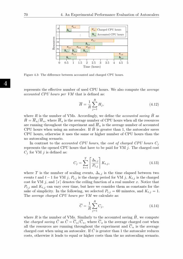
4

70 4. An Experimental Performance Evaluation of Autoscalers

Time (hours)

Res

ourc

es

Charged CPU hours

Accounted CPU hours

12

3n ci,j

hi,j

0 0.5 1 1.5 2 2.5 3 3.5 4 4.5 5

cn,1hn,1

c3,1h3,1

c2,1 c2,2 c2,3h2,1 h2,3h2,2

c1,1 c1,2h1,1 h1,2

...

...

Figure 4.3: The difference between accounted and charged CPU hours.

represents the effective number of used CPU hours. We also compute the averageaccounted CPU hours per VM that is defined as:

H =1

R

R∑

j=1

Hj , (4.12)

where R is the number of VMs. Accordingly, we define the accounted saving H asH = Ha/Hn, where Ha is the average number of CPU hours when all the resourcesare running throughout the experiment and Hn is the average number of accountedCPU hours when using an autoscaler. If H is greater than 1, the autoscaler savesCPU hours, otherwise it uses the same or higher number of CPU hours than theno autoscaling scenario.

In contrast to the accounted CPU hours, the cost of charged CPU hours Cj

represents the opened CPU hours that have to be paid for VM j. The charged costCj for VM j is defined as:

Cj =

T∑

t=1

⌈

∆t,j

Pt,j

⌉

Kt,j , (4.13)

where T is the number of scaling events, ∆t,j is the time elapsed between twoevents t and t− 1 for VM j, Pt,j is the charge period for VM j, Kt,j is the chargedcost for VM j, and ⌈x⌉ denotes the ceiling function of a real number x. Notice thatPt,j and Kt,j can vary over time, but here we consider them as constants for thesake of simplicity. In the following, we selected Pt,j = 60 minutes, and Kt,j = 1.The average charged CPU hours per VM we calculate as:

C =1

R

R∑

j=1

Cj , (4.14)

where R is the number of VMs. Similarly to the accounted saving H, we computethe charged saving C as C = Ca/Cn, where Ca is the average charged cost whenall the resources are running throughout the experiment and Cn is the averagecharged cost when using an autoscaler. If C is greater than 1 the autoscaler reducescosts, otherwise it leads to equal or higher costs than the no autoscaling scenario.

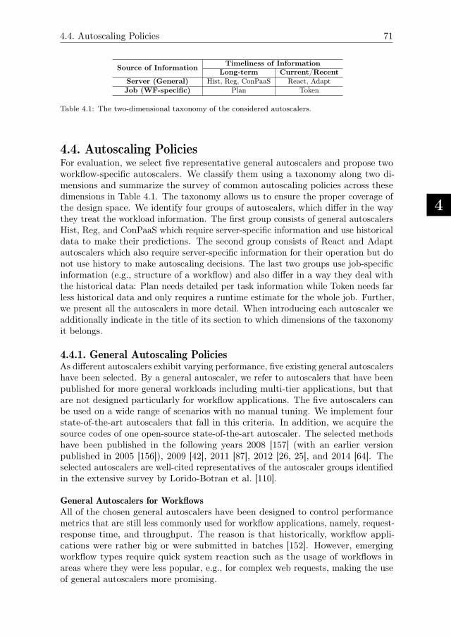
4.4. Autoscaling Policies

4

71

Source of InformationTimeliness of Information

Long-term Current/RecentServer (General) Hist, Reg, ConPaaS React, AdaptJob (WF-specific) Plan Token

Table 4.1: The two-dimensional taxonomy of the considered autoscalers.

4.4. Autoscaling PoliciesFor evaluation, we select five representative general autoscalers and propose twoworkflow-specific autoscalers. We classify them using a taxonomy along two di-mensions and summarize the survey of common autoscaling policies across thesedimensions in Table 4.1. The taxonomy allows us to ensure the proper coverage ofthe design space. We identify four groups of autoscalers, which differ in the waythey treat the workload information. The first group consists of general autoscalersHist, Reg, and ConPaaS which require server-specific information and use historicaldata to make their predictions. The second group consists of React and Adaptautoscalers which also require server-specific information for their operation but donot use history to make autoscaling decisions. The last two groups use job-specificinformation (e.g., structure of a workflow) and also differ in a way they deal withthe historical data: Plan needs detailed per task information while Token needs farless historical data and only requires a runtime estimate for the whole job. Further,we present all the autoscalers in more detail. When introducing each autoscaler weadditionally indicate in the title of its section to which dimensions of the taxonomyit belongs.

4.4.1. General Autoscaling PoliciesAs different autoscalers exhibit varying performance, five existing general autoscalershave been selected. By a general autoscaler, we refer to autoscalers that have beenpublished for more general workloads including multi-tier applications, but thatare not designed particularly for workflow applications. The five autoscalers canbe used on a wide range of scenarios with no manual tuning. We implement fourstate-of-the-art autoscalers that fall in this criteria. In addition, we acquire thesource codes of one open-source state-of-the-art autoscaler. The selected methodshave been published in the following years 2008 [157] (with an earlier versionpublished in 2005 [156]), 2009 [42], 2011 [87], 2012 [26, 25], and 2014 [64]. Theselected autoscalers are well-cited representatives of the autoscaler groups identifiedin the extensive survey by Lorido-Botran et al. [110].

General Autoscalers for WorkflowsAll of the chosen general autoscalers have been designed to control performancemetrics that are still less commonly used for workflow applications, namely, request-response time, and throughput. The reason is that historically, workflow appli-cations were rather big or were submitted in batches [152]. However, emergingworkflow types require quick system reaction such as the usage of workflows inareas where they were less popular, e.g., for complex web requests, making the useof general autoscalers more promising.

4

72 4. An Experimental Performance Evaluation of Autoscalers

The autoscalers aimed to control the response time are designed such that theytry to infer a relationship between the response time, request arrival rates, andthe average number of requests that can be served per VM per unit time. Then,based on the number of request arrivals, infer a suitable amount of resources. Thistechnique is widely used in the literature [68, 110] due to the non-linearity in therelationship between the response time and allocated resources.

A similarity does exist though between workflows and other cloud workloads. Atask in a workflow job can be considered as a long running request. The number oftasks becoming eligible can be considered as the request arrival rate for workflows.Therefore, we have adapted the general autoscalers to perform the scaling basedon the number of task arrivals per unit time.

The React Policy (Server, Current)Chieu et al. [42] present a dynamic scaling algorithm for automated provisioningof VM resources based on the number of concurrent users, the number of activeconnections, the number of requests per second, and the average response timeper request. The algorithm first determines the current web application instanceswith active sessions above or below a given utilization. If the number of overloadedinstances is greater than a predefined threshold, new web application instancesare provisioned, started, and then added to the front-end load balancer. If twoinstances are underutilized with at least one instance having no active session, theidle instance is removed from the load balancer and shutdown from the system. Ineach case the technique Reacts to the workload change. For the remainder of thischapter, we refer to this technique as React. The main reason we are includingthis algorithm in the analysis is that this algorithm is the baseline algorithm inour opinion since it is one of the simplest possible workload predictors. We haveimplemented this autoscaler for our experiments.

The Adapt Policy (Server, Recent)Ali-Eldin et al. [26, 25] propose an autonomous elasticity controller that changes thenumber of VMs allocated to a service based on both monitored load changes andpredictions of future load. We refer to this technique as Adapt. The predictions arebased on the rate of change of the request arrival rate, i.e., the slope of the workload,and aim at detecting the envelope of the workload. The designed autoscaler Adaptsto sudden load changes and prevents premature release of resources, reducingoscillations in the resource provisioning. Adapt tries to improve the performance interms of number of delayed requests, and the average number of queued requests,at the cost of some resource over-provisioning.

The Hist Policy (Server, Long-term)Urgaonkar et al. [157] propose a provisioning technique for multi-tier Internetapplications. The proposed methodology adopts a queuing model to determine howmany resources to allocate in each tier of the application. A predictive techniquebased on building Histograms of historical request arrival rates is used to determinethe amount of resources to provision at an hourly time scale. Reactive provisioningis used to correct errors in the long-term predictions or to react to unanticipatedflash crowds. The authors also propose a novel datacenter architecture that uses

4.4. Autoscaling Policies

4

73

VM monitors to reduce provisioning overheads. The technique is shown to be ableto improve responsiveness of the system, also in the case of a flash crowd. We referto this technique as Hist. We have implemented this autoscaler for our experiments.

The Reg Policy (Server, Long-term)Iqbal et al. [87] propose a regression-based autoscaler (hereafter called Reg). Theautoscaler has a reactive component for scale-up decisions and a predictive compo-nent for scale-down decisions. When the capacity is less than the load, a scale-updecision is taken and new VMs are added to the service in a way similar to React.For scale-down, the predictive component uses a second order regression to predictfuture load. The regression model is recomputed using the complete history of theworkload when a new measurement is available. If current load is less than theprovisioned capacity, a scale-down decision is taken using the regression model.This autoscaler was performing badly in our preliminary experiments due to twofactors; first, building a regression model for the full history of measurements forevery new monitoring data point is a time consuming task. Second, distant pasthistory becomes less relevant as time proceeds. After contacting the authors, wehave modified the algorithm such that the regression model is evaluated for onlythe past 60 monitoring data points.

The ConPaaS Policy (Server, Long-term)ConPaaS, proposed by Fernandez et al. [64]. The algorithm scales a web applicationin response to changes in throughput at fixed intervals of 10 minutes. The predictorforecasts the future service demand using standard time series analysis techniques,e.g., Linear Regression, Auto Regressive Moving Average (ARMA), etc. The codefor this autoscaler is open source. We downloaded the authors’ implementation.

4.4.2. Workflow-Specific Autoscaling PoliciesIn this section, we present two workflow-specific autoscalers designed by us. Theirdesigns are inspired by previous work in this field and adapted to our situation.The presented autoscalers differ in a way they use workflow structural informationand task runtime estimates.

The Plan Policy (Job, Long-term)This autoscaler makes predictions by constructing and analyzing a partial executionPlan of a workflow. Thus, it uses the workflow structure and workflow task runtimeestimates. The idea is partially based on static workflow schedulers [23]. On eachcall, the policy constructs a partial execution plan considering both workflowswith running tasks and workflows waiting in the queue. The maximal number ofprocessors which are used by this plan is returned as a prediction. The time durationof the plan is limited by the autoscaling interval. The plan is two-dimensional,where one dimension is time and another is processors (VMs).

The policy employs the same task placement strategy as the scheduler. In ourcase, the jobs from the main job queue are processed in the FCFS order and thetasks are prioritized in ascending order of their identifier. Each task of a workflowis supposed to be assigned with a unique numeric identifier using the classicalbreadth-first search algorithm, where the identifier of the entry task is 0. For

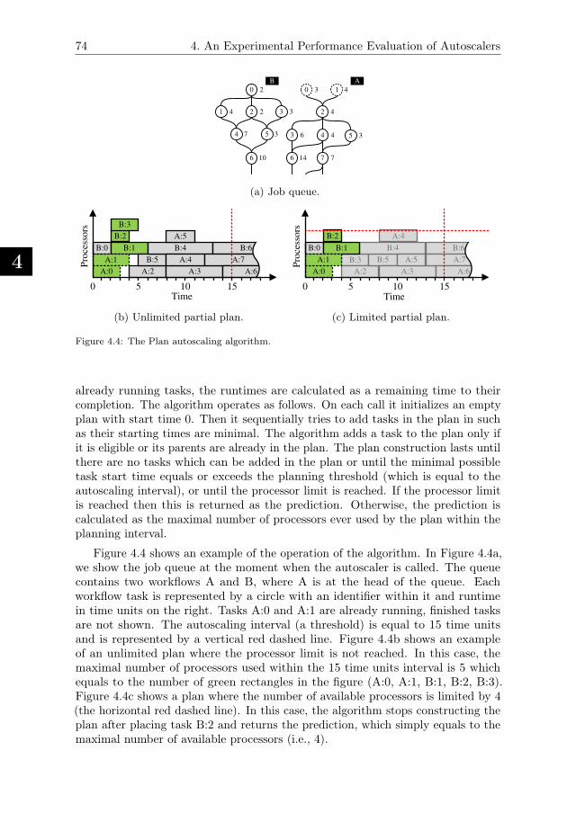
4

74 4. An Experimental Performance Evaluation of Autoscalers

0 3 1 4

2 4

3 6 4 4

6 14 7 7

0 2

2 2 3 31 4

4 7 5 3

6 10

5 3

AB

(a) Job queue.

0 5 10 15

B:0 B:1

B:2

B:3

A:2

B:5

B:4

A:3

A:4

B:6

A:7

A:6

A:5

Time

Pro

cess

ors

A:1

A:0

(b) Unlimited partial plan.

0 5 10 15

B:0

B:2

B:3

A:2

B:5

B:4

A:3

A:4

B:6

A:7

A:6

A:5

TimeP

roce

ssors

A:0

B:1

A:1

(c) Limited partial plan.

Figure 4.4: The Plan autoscaling algorithm.

already running tasks, the runtimes are calculated as a remaining time to theircompletion. The algorithm operates as follows. On each call it initializes an emptyplan with start time 0. Then it sequentially tries to add tasks in the plan in suchas their starting times are minimal. The algorithm adds a task to the plan only ifit is eligible or its parents are already in the plan. The plan construction lasts untilthere are no tasks which can be added in the plan or until the minimal possibletask start time equals or exceeds the planning threshold (which is equal to theautoscaling interval), or until the processor limit is reached. If the processor limitis reached then this is returned as the prediction. Otherwise, the prediction iscalculated as the maximal number of processors ever used by the plan within theplanning interval.

Figure 4.4 shows an example of the operation of the algorithm. In Figure 4.4a,we show the job queue at the moment when the autoscaler is called. The queuecontains two workflows A and B, where A is at the head of the queue. Eachworkflow task is represented by a circle with an identifier within it and runtimein time units on the right. Tasks A:0 and A:1 are already running, finished tasksare not shown. The autoscaling interval (a threshold) is equal to 15 time unitsand is represented by a vertical red dashed line. Figure 4.4b shows an exampleof an unlimited plan where the processor limit is not reached. In this case, themaximal number of processors used within the 15 time units interval is 5 whichequals to the number of green rectangles in the figure (A:0, A:1, B:1, B:2, B:3).Figure 4.4c shows a plan where the number of available processors is limited by 4(the horizontal red dashed line). In this case, the algorithm stops constructing theplan after placing task B:2 and returns the prediction, which simply equals to themaximal number of available processors (i.e., 4).

4.5. Experimental Evaluation

4

75

The Token Policy (Job, Recent)The Token policy uses structural information of a DAG and does not directlyconsider task runtimes to make predictions and instead requires an estimatedexecution time of the whole workflow. It uses tokens to estimate the Level ofParallelism (LoP) of a workflow by simulating an execution “wave” through a DAG,as described in Section 2.3.1. The algorithm processes the workflows in the queuein the FCFS order. For each workflow, the number of token propagation steps islimited by a certain depth δ, which is defined as δ = (∆t ·N)/L, where ∆t is theautoscaling interval, N is the number of tasks on the critical path of the workflow,and L is the total duration of the tasks on the critical path of the workflow. Thus,the intuition is to evaluate the number of “waves” of tasks (future eligible sets) thatwill finish during the autoscaling interval. When δ or the final task of a workflow isreached, the largest recorded number of tokenized nodes is the approximated LoPvalue. The algorithm stops when the prediction value exceeds the maximal totalnumber of available processors or when the end of the queue is reached. The finalprediction is the sum of all of the separate approximated LoPs of the consideredworkflows.

The token-based algorithm does not guarantee the correct estimation of theLoP. The quality of the estimation depends on the DAG structure. In Figure 2.1athe estimated LoP of 3 is lower than the maximal possible LoP of 4 in Figure 2.1b.However, in Section 2.3.1, we show that this method provides meaningful resultsfor popular workflow structures.

4.5. Experimental EvaluationIn this section, we present the workloads and the configuration of the cloud in-frastructure we use for the experimental evaluation of the unified cloud systemintroduced in Section 4.2. To design our workloads, we use a set of representativescientific workflows. We take an experimental approach to evaluate chosen autoscal-ing algorithms with an extensive set of experiments in a virtualized environmentdeployed on our multi-cluster system.

4.5.1. Setup of Workflow-based WorkloadsWe choose three popular scientific workflows from different fields, namely Montage,LIGO, and SIPHT. The main reason for our choice is the existence of validatedmodels for these workflow types. Montage [90] is used to build a mosaic image of thesky on the basis of smaller images obtained from different telescopes. LIGO [22] isused by the Laser Interferometer Gravitational-Wave Observatory (LIGO) to detectgravitational waves. SIPHT [108] is a bioinformatics workflow used to discoverbacterial regulatory RNAs.

We generate synthetic workflows using the workflow generator by Bharathiet al. [16, 38]. Each workflow is represented by a set of task executables and aset of input files. We use two workloads: a primary Workload 1 and a secondaryWorkload 2 each consisting of 200 workflows of different sizes in the range from30 to 600. Each workload contains an equal mixture of all of the three consideredworkflow types. As with many other workloads in computer systems, in practice,workflows are usually small, but very large ones may exist too [132]. Therefore,

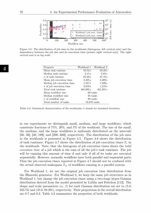
4

76 4. An Experimental Performance Evaluation of Autoscalers

0 100 200 300 400 500 600

Workflow size

0.0

0.2

0.4

0.6

0.8

Probab

ility

101

102

103

104

105

Job

exec.time(s)

Workload 1 job exec. times

Workload 2 job exec. times

Figure 4.5: The distribution of job sizes in the workloads (histogram, left vertical axis) and thedependency between the job size and its execution time (points, right vertical axis). The rightvertical axis is in log scale.

Property Workload 1 Workload 2Mean task runtime 33.52 s 33.29 sMedian task runtime 2.15 s 2.65 sσ of task runtime 65.40 s 87.19 sMean job execution time 2,325 s 2,309 sMedian job execution time 1,357 s 1,939 sσ of job execution time 3,859 s 1,219 sTotal task runtime 465,095 s 461,921 sMean workflow size 69 tasksMedian workflow size 35 tasksσ of workflow size 98 tasksTotal number of tasks 13,876 tasks

Table 4.2: Statistical characteristics of the workloads, σ stands for standard deviation.

in our experiments we distinguish small, medium, and large workflows, whichconstitute fractions of 75%, 20%, and 5% of the workload. The size of the small,the medium, and the large workflows is uniformly distributed on the intervals[30, 39], [40, 199], and [200, 600], respectively. The distribution of the job sizesin the workloads is presented in Figure 4.5. Figure 4.6 shows the distributionof task runtimes. Figure 4.7 shows the distribution of job execution times Te inthe workloads. Note, that the histogram of job execution times shows the totalexecution time of a job which is the sum of all the job’s task runtimes. The jobwill be running this amount of time if and only if all of its tasks are executedsequentially. However, normally workflows have both parallel and sequential parts.Thus the job execution times reported in Figure 4.7 should not be confused withthe actual observed makespans Tm of workflows running in a parallel system.

For Workload 1, we use the original job execution time distribution fromthe Bharathi generator. For Workload 2, we keep the same job structures as inWorkload 1, but change the job execution times using a two-stage hyper-Gammadistribution derived from the model presented by Lublin and Feitelson [112]. Theshape and scale parameters (α, β) for each Gamma distribution are set to (5.0,323.73) and (45.0, 88.291), respectively. Their proportions in the overall distributionare 0.7 and 0.3. Table 4.2 summarizes the properties of both workloads.

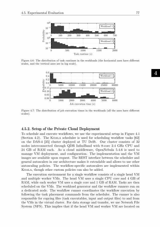
4.5. Experimental Evaluation

4

77

0 100 200 300 400 500 600 700

100

10−2

10−4

Workload 1

0 500 1000 1500 2000

100

10−2

10−4

Workload 2

0.0 0.2 0.4 0.6 0.8 1.0

Task runtime (s)

0.0

0.2

0.4

0.6

0.8

1.0

Probab

ility

Figure 4.6: The distribution of task runtimes in the workloads (the horizontal axes have differentscales, and the vertical axes are in log scale).

0 5000 10000 15000 20000 25000 300000.0

0.2

0.4

0.6Workload 1

0 1000 2000 3000 4000 5000 60000.00

0.05

0.10

0.15Workload 2

0.0 0.2 0.4 0.6 0.8 1.0

Job execution time (s)

0.0

0.2

0.4

0.6

0.8

1.0

Probab

ility

Figure 4.7: The distribution of job execution times in the workloads (all the axes have differentscales).

4.5.2. Setup of the Private Cloud Deployment

To schedule and execute workflows, we use the experimental setup in Figure 4.1(Section 4.2). The Koala scheduler is used for scheduling workflow tasks [62]on the DAS-4 [35] cluster deployed at TU Delft. Our cluster consists of 32nodes interconnected through QDR InfiniBand with 8-core 2.4 GHz CPU and24 GB of RAM each. As a cloud middleware, OpenNebula 5.4.6 is used tomanage VM deployment, and configuration. The implementation and the VMimages are available upon request. The REST interface between the scheduler andgeneral autoscalers in our architecture makes it extendable and allows to use otherautoscaling policies. The workflow-specific autoscalers are implemented withinKoala, though other custom policies can also be added.

The execution environment for a single workflow consists of a single head VMand multiple worker VMs. The head VM uses a single CPU core and 4 GB ofRAM, while each worker VM uses a single core and 1 GB of RAM. Tasks are thenscheduled on the VMs. The workload generator and the workflow runners run ona dedicated node. The workflow runner coordinates the workflow execution byfollowing the task placement commands from the scheduler. The runner is alsoresponsible for copying files (task executables, input and output files) to and fromthe VMs in the virtual cluster. For data storage and transfer, we use Network FileSystem (NFS). This implies that if the head VM and worker VM are located on

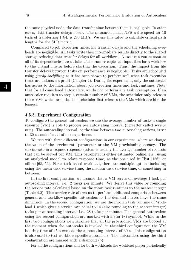
4

78 4. An Experimental Performance Evaluation of Autoscalers

the same physical node, the data transfer time between them is negligible. In othercases, data transfer delays occur. The measured mean NFS write speed for 10tests of transferring 1 GB is 280 MB/s. We use this value to calculate critical pathlengths for the SLR metric.

Compared to job execution times, file transfer delays and the scheduling over-heads are negligible. All tasks write their intermediate results directly to the sharedstorage reducing data transfer delays for all workflows. A task can run as soon asall of its dependencies are satisfied. The runner copies all input files for a workflowto the virtual cluster before starting the execution. Thus, the impact from filetransfer delays between tasks on performance is negligible. Tasks are scheduledusing greedy backfilling as it has been shown to perform well when task executiontimes are unknown a priori (Chapter 2). During the experiment, only the autoscalerhas access to the information about job execution times and task runtimes. Note,that for all considered autoscalers, we do not perform any task preemption. If anautoscaler requires to stop a certain number of VMs, the scheduler only releasesthose VMs which are idle. The scheduler first releases the VMs which are idle thelongest.

4.5.3. Experiment ConfigurationTo configure the general autoscalers we use the average number of tasks a singleresource (VM) is able to process per autoscaling interval (hereafter called servicerate). The autoscaling interval, or the time between two autoscaling actions, is setto 30 seconds for all of our experiments.

We test with three different configurations in our experiments, where we changethe value of the service rate parameter or the VM provisioning latency. Theservice rate in a request-response system is usually the average number of requeststhat can be served per VM. This parameter is either estimated online, e.g., usingan analytical model to relate response time, as the one used in Hist [156], oroffline [68, 56]. For a task-based workload, there are multiple options includingusing the mean task service time, the median task service time, or something inbetween.

In the first configuration, we assume that a VM serves on average 1 task perautoscaling interval, i.e., 2 tasks per minute. We derive this value by roundingthe service rate calculated based on the mean task runtimes to the nearest integer(Table 4.2). This service rate allows us to perform additional comparison betweengeneral and workflow-specific autoscalers as the demand curves have the samedimension. In the second configuration, we use the median task runtime of Work-load 1 which gives a service rate equal to 14 (also rounding to the nearest integer)tasks per autoscaling interval, i.e., 28 tasks per minute. The general autoscalersusing the second configuration are marked with a star (⋆) symbol. While in thefirst two configurations we guarantee that all the provisioned VMs are booted atthe moment when the autoscaler is invoked, in the third configuration the VMbooting time of 45 s exceeds the autoscaling interval of 30 s. This configurationis also used to test workflow-specific autoscalers. The autoscalers using the thirdconfiguration are marked with a diamond (⋄).

For all the configurations and for both workloads the workload player periodically

4.5. Experimental Evaluation

4

79

submits workflows to Koala to impose the average load on the system about 40%.The workflows submitted to the system arrive according to a Poisson process.The mean inter-arrival interval is 117.77 s which results into arrival rate of 30.57workflows per hour. Thus, the minimal duration of each experiment is approximately6.5 h. If the autoscaler tends to under-provision resources or the provisioning timein the system is rather large then the experiment can take longer. We choose thisrelatively low utilization level on purpose to decrease the number of situationswhen the demand exceeds the maximum possible supply ceiling. Additionally, asworkflow scheduling is non-work-conserving the system can saturate even at lowutilizations. Thus, low utilization allows us to see better the dynamic behavior ofthe autoscalers by minimizing the number of extreme cases.

We are aware that in computing clouds the job arrivals are often affected by thetime of the day and various external influences resulting in burstiness [63]. Evenfor a datacenter which serves requests from all around the globe the intensity ofjob arrivals could vary as the distribution of world population is not even acrossdifferent time zones, etc. We leave the experiments with other job arrival patternsto future work. However, the arrival of workflow tasks is non-Poissonian anddepends on the workflow structure and on the distribution of task runtimes withina workflow. Thus, the diversity of the workflow structures, workflow sizes, andtask runtime distributions which we use, allows us to suppose that our setup isrepresentative. Furthermore, for the considered duration of the experiment ofapproximately 6.5 h, we can simply claim that our emulated system serves requestsfrom multiple independent users.

4.5.4. Experiment Results

The main findings from our experiments are the following:

1. Workflow-specific autoscalers perform slightly better than general-autoscalersbut require more detailed job information.

2. General autoscalers show comparable performance but their parametrizationis crucial.

3. Autoscalers reduce the average number of used resources, but slow down thejobs.

4. Although autoscalers tend to reduce the accounted resource CPU hours, thecharged time can easily be higher compared to not using autoscaling.

5. Long VM booting times negatively affect the performance of the autoscalers,and mostly affect small and medium job sizes.

6. Over-provisioning could partially contribute for better fairness between dif-ferent job sizes.

7. Autoscalers with better autoscaling metrics show higher variability of deadlineviolations.

8. No autoscaler outperforms all other autoscalers with all configurations and/ormetrics.

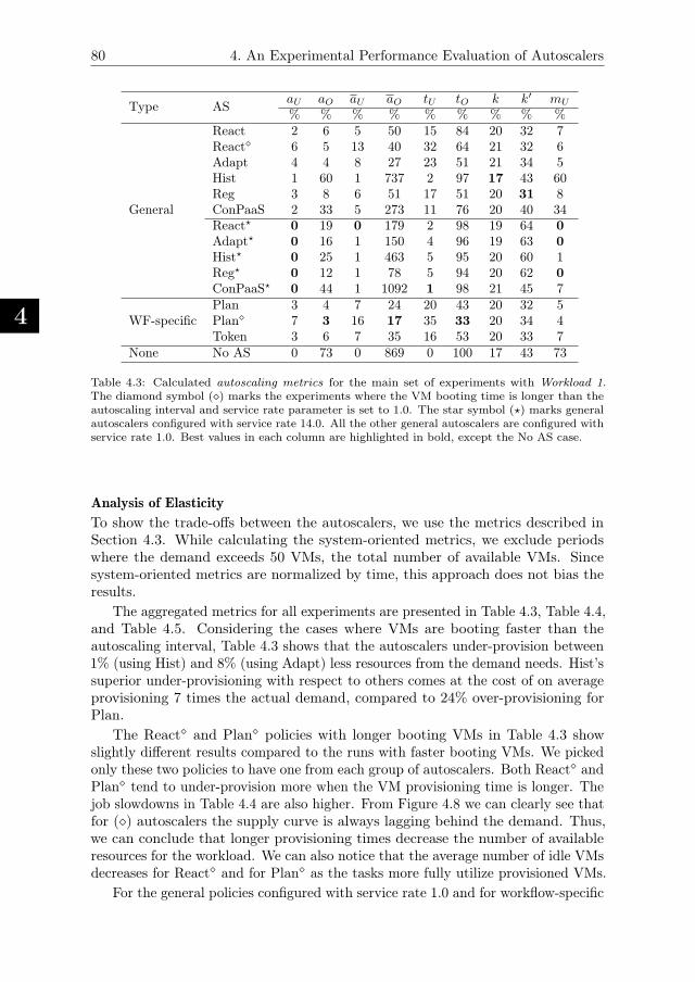
4

80 4. An Experimental Performance Evaluation of Autoscalers

Type ASaU aO aU aO tU tO k k′ mU

% % % % % % % % %

General

React 2 6 5 50 15 84 20 32 7React⋄ 6 5 13 40 32 64 21 32 6Adapt 4 4 8 27 23 51 21 34 5Hist 1 60 1 737 2 97 17 43 60Reg 3 8 6 51 17 51 20 31 8ConPaaS 2 33 5 273 11 76 20 40 34React⋆ 0 19 0 179 2 98 19 64 0Adapt⋆ 0 16 1 150 4 96 19 63 0Hist⋆ 0 25 1 463 5 95 20 60 1Reg⋆ 0 12 1 78 5 94 20 62 0ConPaaS⋆ 0 44 1 1092 1 98 21 45 7

WF-specificPlan 3 4 7 24 20 43 20 32 5Plan⋄ 7 3 16 17 35 33 20 34 4Token 3 6 7 35 16 53 20 33 7

None No AS 0 73 0 869 0 100 17 43 73

Table 4.3: Calculated autoscaling metrics for the main set of experiments with Workload 1.The diamond symbol (⋄) marks the experiments where the VM booting time is longer than theautoscaling interval and service rate parameter is set to 1.0. The star symbol (⋆) marks generalautoscalers configured with service rate 14.0. All the other general autoscalers are configured withservice rate 1.0. Best values in each column are highlighted in bold, except the No AS case.

Analysis of Elasticity

To show the trade-offs between the autoscalers, we use the metrics described inSection 4.3. While calculating the system-oriented metrics, we exclude periodswhere the demand exceeds 50 VMs, the total number of available VMs. Sincesystem-oriented metrics are normalized by time, this approach does not bias theresults.

The aggregated metrics for all experiments are presented in Table 4.3, Table 4.4,and Table 4.5. Considering the cases where VMs are booting faster than theautoscaling interval, Table 4.3 shows that the autoscalers under-provision between1% (using Hist) and 8% (using Adapt) less resources from the demand needs. Hist’ssuperior under-provisioning with respect to others comes at the cost of on averageprovisioning 7 times the actual demand, compared to 24% over-provisioning forPlan.

The React⋄ and Plan⋄ policies with longer booting VMs in Table 4.3 showslightly different results compared to the runs with faster booting VMs. We pickedonly these two policies to have one from each group of autoscalers. Both React⋄ andPlan⋄ tend to under-provision more when the VM provisioning time is longer. Thejob slowdowns in Table 4.4 are also higher. From Figure 4.8 we can clearly see thatfor (⋄) autoscalers the supply curve is always lagging behind the demand. Thus,we can conclude that longer provisioning times decrease the number of availableresources for the workload. We can also notice that the average number of idle VMsdecreases for React⋄ and for Plan⋄ as the tasks more fully utilize provisioned VMs.

For the general policies configured with service rate 1.0 and for workflow-specific

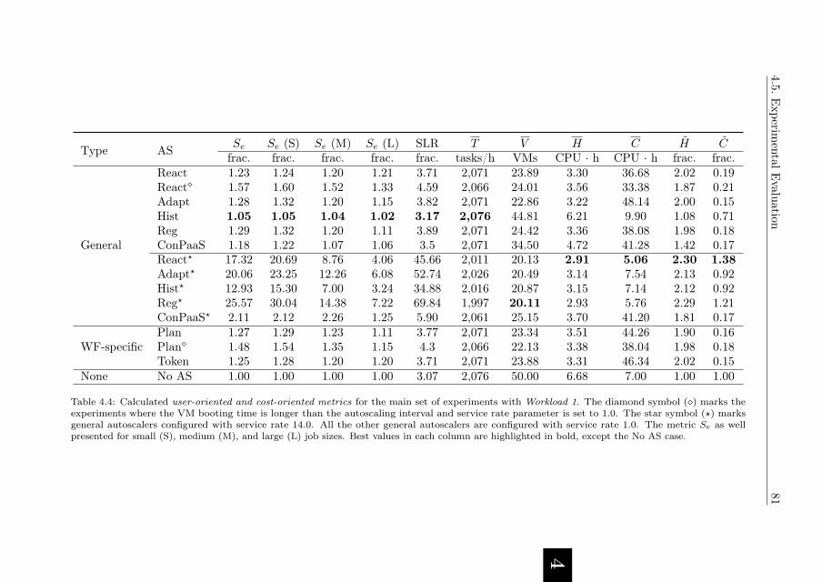
4.5

.E

xperim

ental

Evalu

ation

4

81

Type ASSe Se (S) Se (M) Se (L) SLR T V H C H C

frac. frac. frac. frac. frac. tasks/h VMs CPU · h CPU · h frac. frac.

General

React 1.23 1.24 1.20 1.21 3.71 2,071 23.89 3.30 36.68 2.02 0.19React⋄ 1.57 1.60 1.52 1.33 4.59 2,066 24.01 3.56 33.38 1.87 0.21Adapt 1.28 1.32 1.20 1.15 3.82 2,071 22.86 3.22 48.14 2.00 0.15Hist 1.05 1.05 1.04 1.02 3.17 2,076 44.81 6.21 9.90 1.08 0.71Reg 1.29 1.32 1.20 1.11 3.89 2,071 24.42 3.36 38.08 1.98 0.18ConPaaS 1.18 1.22 1.07 1.06 3.5 2,071 34.50 4.72 41.28 1.42 0.17React⋆ 17.32 20.69 8.76 4.06 45.66 2,011 20.13 2.91 5.06 2.30 1.38Adapt⋆ 20.06 23.25 12.26 6.08 52.74 2,026 20.49 3.14 7.54 2.13 0.92Hist⋆ 12.93 15.30 7.00 3.24 34.88 2,016 20.87 3.15 7.14 2.12 0.92Reg⋆ 25.57 30.04 14.38 7.22 69.84 1,997 20.11 2.93 5.76 2.29 1.21ConPaaS⋆ 2.11 2.12 2.26 1.25 5.90 2,061 25.15 3.70 41.20 1.81 0.17

WF-specificPlan 1.27 1.29 1.23 1.11 3.77 2,071 23.34 3.51 44.26 1.90 0.16Plan⋄ 1.48 1.54 1.35 1.15 4.3 2,066 22.13 3.38 38.04 1.98 0.18Token 1.25 1.28 1.20 1.20 3.71 2,071 23.88 3.31 46.34 2.02 0.15

None No AS 1.00 1.00 1.00 1.00 3.07 2,076 50.00 6.68 7.00 1.00 1.00

Table 4.4: Calculated user-oriented and cost-oriented metrics for the main set of experiments with Workload 1. The diamond symbol (⋄) marks theexperiments where the VM booting time is longer than the autoscaling interval and service rate parameter is set to 1.0. The star symbol (⋆) marksgeneral autoscalers configured with service rate 14.0. All the other general autoscalers are configured with service rate 1.0. The metric Se as wellpresented for small (S), medium (M), and large (L) job sizes. Best values in each column are highlighted in bold, except the No AS case.

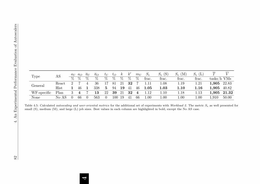
4

824.

An

Exper

imen

talPer

form

ance

Eva

luat

ion

ofA

uto

scale

rs

Type ASaU aO aU aO tU tO k k′ mU Se Se (S) Se (M) Se (L) T V% % % % % % % % % frac. frac. frac. frac. tasks/h VMs

GeneralReact 2 7 4 36 17 81 21 32 7 1.11 1.08 1.19 1.21 1,905 22.83Hist 1 46 1 338 5 94 19 41 46 1.05 1.03 1.10 1.16 1,905 40.82

WF-specific Plan 3 4 7 13 22 39 21 32 4 1.12 1.10 1.18 1.13 1,905 21.32None No AS 0 66 0 563 0 100 19 41 66 1.00 1.00 1.00 1.00 1,910 50.00

Table 4.5: Calculated autoscaling and user-oriented metrics for the additional set of experiments with Workload 2. The metric Se as well presented forsmall (S), medium (M), and large (L) job sizes. Best values in each column are highlighted in bold, except the No AS case.

4.5. Experimental Evaluation

4

83

policies in Table 4.4 and Table 4.5 job elastic slowdowns show low variability. Wecan conclude that the resources either significantly over-provisioned (Hist andConPaaS) or already provisioned resources are underutilized (React, Adapt, Reg,Plan, and Token). The non-zero values of mU metric in these cases confirm ourassumption.

The Influence of Different WorkloadsThe difference is also visible between the two used workloads. While Workload 1has the majority of short jobs, Workload 2 has a more equal distribution of jobexecution times and is thus less bursty. Elastic job slowdowns in both tables confirmthis tendency. For Workload 2 they slightly increase (the Plan policy in Table 4.5 isan exception) while going from small to large job sizes. We do not run Workload 2with service rate different from 1.0 as we expect that the trend will be the same asfor Workload 1.

The system-oriented metrics do not vary much between the workloads. Forexample, compare React in Table 4.3 and Table 4.4 with React in Table 4.5. OnlyHist over-provisions less while running with Workload 2 as can be explained bylower burstiness of the workload.

The Dynamics of AutoscalingFigure 4.8 shows the system dynamics for each autoscaling policy while executingWorkload 1. Some of the autoscalers have a tendency to over-provision resources(Hist and ConPaaS). The other policies appear to be following the demand curvemore or less closely. Note, that the demand curve has different shape for eachautoscaler as the autoscaling properties affect the order in which workflow tasksbecome eligible.

The workflow-specific Plan policy follows the demand curve quite well andshows results similar to general autoscalers React, Adapt, and Reg running withservice rate of 1.0. However, if a policy follows the demand too close that increasesjob slowdowns, as seen in Table 4.4. This trade-off is intuitive. The best policywhen it comes to reducing slowdown is to always have more capacity than neededas this will allow any task to run as soon as it becomes eligible.

The Influence of Service Rate Parameter on the Autoscaling DynamicsThe most noticeable differences in the results are between general autoscalersrunning with service rate 1.0 and with service rate 14.0, based on mean and medianworkload task runtimes, accordingly. Figure 4.9 shows general autoscalers runningwith the same Workload 1 as in Figure 4.8. The demand curves in these two figureslook very different, except for ConPaaS and ConPaaS⋆. In addition, the supplycurves do not follow the demand curves closely anymore. Although the servicerate chosen is the median-based, it does not reflect the temporal properties of theworkload when it comes to the length of running tasks. If longer jobs occur inparallel, a queue of tasks will build up resulting in enormous system slowdowns.This is clear from Table 4.4 where the slowdown between the two service rates is10 to 15 times larger when using a larger service rate. The k′ metric also increasesfor service rate 14.0 as the autoscalers need to estimate more while computing thenext predicted supply value and thus the curves are not so well synchronized. On

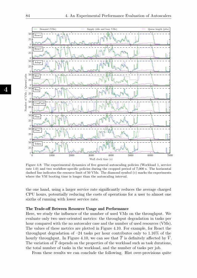
4

84 4. An Experimental Performance Evaluation of Autoscalers

0

25

50 React

Demand (VMs) Supply (idle and busy VMs) Queue length (jobs)

0

25

50 React⋄

0

25

50 Adapt

0

25

50 Hist

0

25

50

Number

ofVMs/Queued

jobs

Reg

0

25

50 ConPaaS

0

25

50 Plan

0

25

50 Plan⋄

0 1000 2000 3000 4000 5000 6000 7000

Wall clock time (s)

0

25

50 Token

Figure 4.8: The experimental dynamics of five general autoscaling policies (Workload 1, servicerate 1.0) and two workflow-specific policies during the cropped period of 7,000 s. The horizontaldashed line indicates the resource limit of 50 VMs. The diamond symbol (⋄) marks the experimentswhere the VM booting time is longer than the autoscaling interval.

the one hand, using a larger service rate significantly reduces the average chargedCPU hours, potentially reducing the costs of operations for a user to almost onesixths of running with lower service rate.

The Trade-off Between Resource Usage and PerformanceHere, we study the influence of the number of used VMs on the throughput. Weevaluate only two user-oriented metrics: the throughput degradation in tasks perhour compared with the no autoscaler case and the number of used resources (VMs).The values of these metrics are plotted in Figure 4.10. For example, for React thethroughput degradation of –24 tasks per hour contributes only to 1.16% of thehourly throughput. In Figure 4.10, we can see that T is definitely affected by V .The variation of T depends on the properties of the workload such as task durations,the total number of tasks in the workload, and the number of tasks per job.

From these results we can conclude the following. Hist over-provisions quite

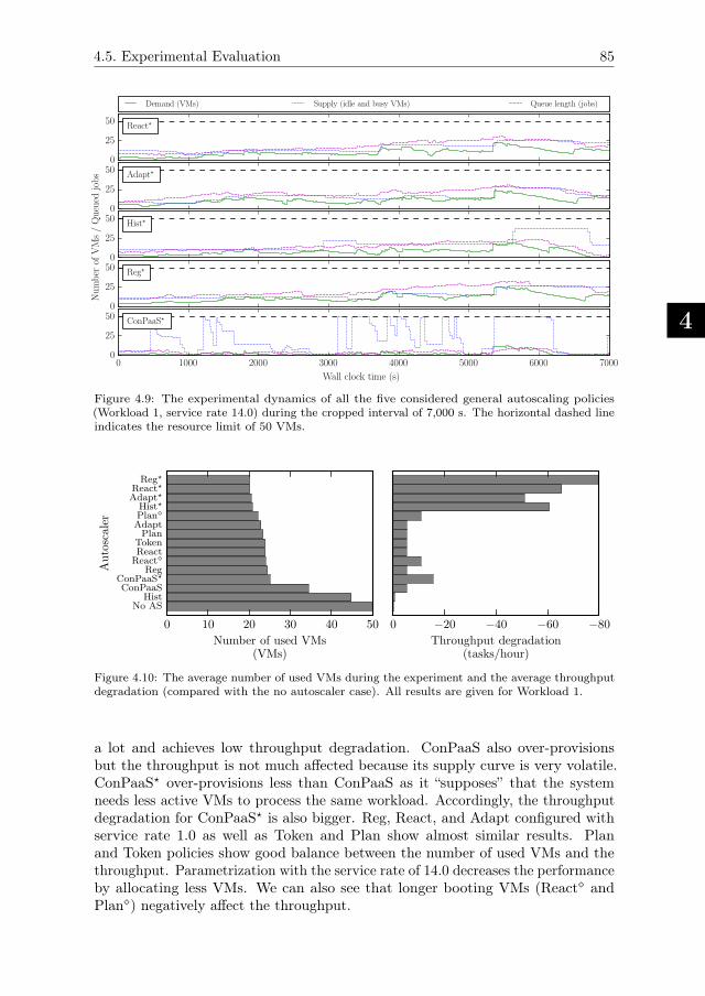
4.5. Experimental Evaluation

4

85

Figure 4.9: The experimental dynamics of all the five considered general autoscaling policies(Workload 1, service rate 14.0) during the cropped interval of 7,000 s. The horizontal dashed lineindicates the resource limit of 50 VMs.

0 10 20 30 40 50

Number of used VMs(VMs)

No ASHist

ConPaaSConPaaS⋆

RegReact⋄ReactTokenPlan

AdaptPlan⋄Hist⋆

Adapt⋆React⋆Reg⋆

Autoscaler

−80−60−40−200

Throughput degradation(tasks/hour)

Figure 4.10: The average number of used VMs during the experiment and the average throughputdegradation (compared with the no autoscaler case). All results are given for Workload 1.

a lot and achieves low throughput degradation. ConPaaS also over-provisionsbut the throughput is not much affected because its supply curve is very volatile.ConPaaS⋆ over-provisions less than ConPaaS as it “supposes” that the systemneeds less active VMs to process the same workload. Accordingly, the throughputdegradation for ConPaaS⋆ is also bigger. Reg, React, and Adapt configured withservice rate 1.0 as well as Token and Plan show almost similar results. Planand Token policies show good balance between the number of used VMs and thethroughput. Parametrization with the service rate of 14.0 decreases the performanceby allocating less VMs. We can also see that longer booting VMs (React⋄ andPlan⋄) negatively affect the throughput.

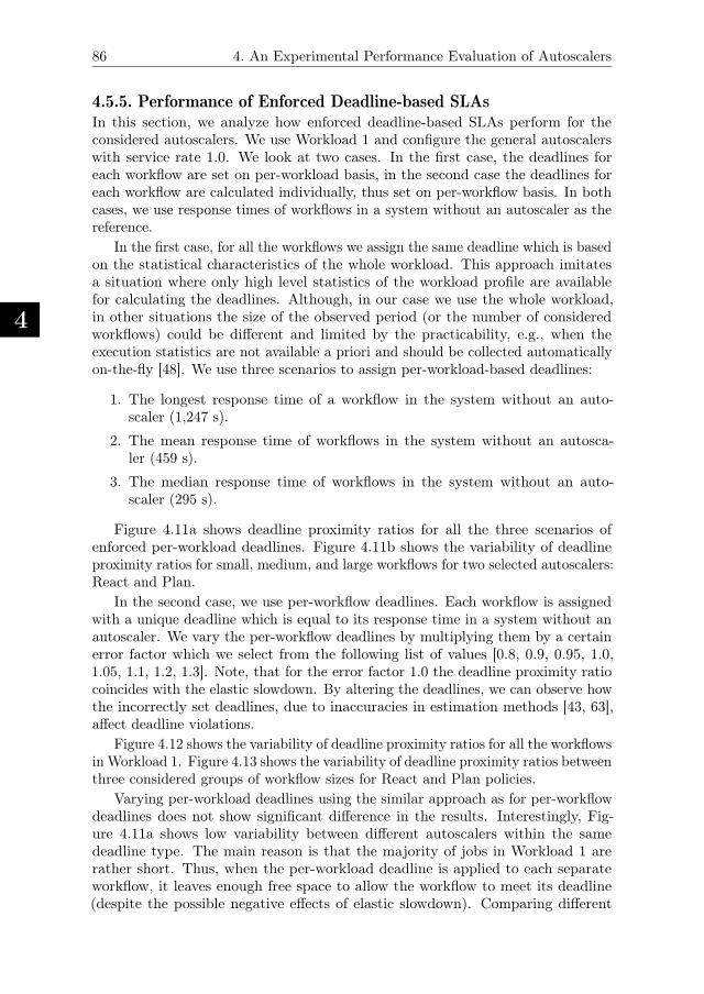
4

86 4. An Experimental Performance Evaluation of Autoscalers

4.5.5. Performance of Enforced Deadline-based SLAs

In this section, we analyze how enforced deadline-based SLAs perform for theconsidered autoscalers. We use Workload 1 and configure the general autoscalerswith service rate 1.0. We look at two cases. In the first case, the deadlines foreach workflow are set on per-workload basis, in the second case the deadlines foreach workflow are calculated individually, thus set on per-workflow basis. In bothcases, we use response times of workflows in a system without an autoscaler as thereference.

In the first case, for all the workflows we assign the same deadline which is basedon the statistical characteristics of the whole workload. This approach imitatesa situation where only high level statistics of the workload profile are availablefor calculating the deadlines. Although, in our case we use the whole workload,in other situations the size of the observed period (or the number of consideredworkflows) could be different and limited by the practicability, e.g., when theexecution statistics are not available a priori and should be collected automaticallyon-the-fly [48]. We use three scenarios to assign per-workload-based deadlines:

1. The longest response time of a workflow in the system without an auto-scaler (1,247 s).

2. The mean response time of workflows in the system without an autosca-ler (459 s).

3. The median response time of workflows in the system without an auto-scaler (295 s).

Figure 4.11a shows deadline proximity ratios for all the three scenarios ofenforced per-workload deadlines. Figure 4.11b shows the variability of deadlineproximity ratios for small, medium, and large workflows for two selected autoscalers:React and Plan.

In the second case, we use per-workflow deadlines. Each workflow is assignedwith a unique deadline which is equal to its response time in a system without anautoscaler. We vary the per-workflow deadlines by multiplying them by a certainerror factor which we select from the following list of values [0.8, 0.9, 0.95, 1.0,1.05, 1.1, 1.2, 1.3]. Note, that for the error factor 1.0 the deadline proximity ratiocoincides with the elastic slowdown. By altering the deadlines, we can observe howthe incorrectly set deadlines, due to inaccuracies in estimation methods [43, 63],affect deadline violations.

Figure 4.12 shows the variability of deadline proximity ratios for all the workflowsin Workload 1. Figure 4.13 shows the variability of deadline proximity ratios betweenthree considered groups of workflow sizes for React and Plan policies.

Varying per-workload deadlines using the similar approach as for per-workflowdeadlines does not show significant difference in the results. Interestingly, Fig-ure 4.11a shows low variability between different autoscalers within the samedeadline type. The main reason is that the majority of jobs in Workload 1 arerather short. Thus, when the per-workload deadline is applied to each separateworkflow, it leaves enough free space to allow the workflow to meet its deadline(despite the possible negative effects of elastic slowdown). Comparing different

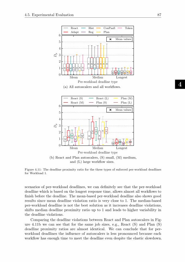
4.5. Experimental Evaluation

4

87

Mean Median Longest

Per-workload deadline type

0

1

2

3

4

5

6

Dp

React

Adapt

Hist

Reg

ConPaaS

Plan

Token

Mean values

(a) All autoscalers and all workflows.

Mean Median Longest

Per-workload deadline type

0

1

2

3

4

5

6

Dp

React (S)

React (M)

React (L)

Plan (S)

Plan (M)

Plan (L)

Mean values

(b) React and Plan autoscalers, (S) small, (M) medium,and (L) large workflow sizes.

Figure 4.11: The deadline proximity ratio for the three types of enforced per-workload deadlinesfor Workload 1.

scenarios of per-workload deadlines, we can definitely see that the per-workloaddeadline which is based on the longest response time, allows almost all workflows tofinish before the deadline. The mean-based per-workload deadline also shows goodresults since mean deadline violation ratio is very close to 1. The median-basedper-workload deadline is not the best solution as it increases deadline violations,shifts median deadline proximity ratio up to 1 and leads to higher variability inthe deadline violations.

Comparing the deadline violations between React and Plan autoscalers in Fig-ure 4.11b we can see that for the same job sizes, e.g., React (S) and Plan (S)deadline proximity ratios are almost identical. We can conclude that for per-workload deadlines the influence of autoscalers is less pronounced because eachworkflow has enough time to meet the deadline even despite the elastic slowdown.

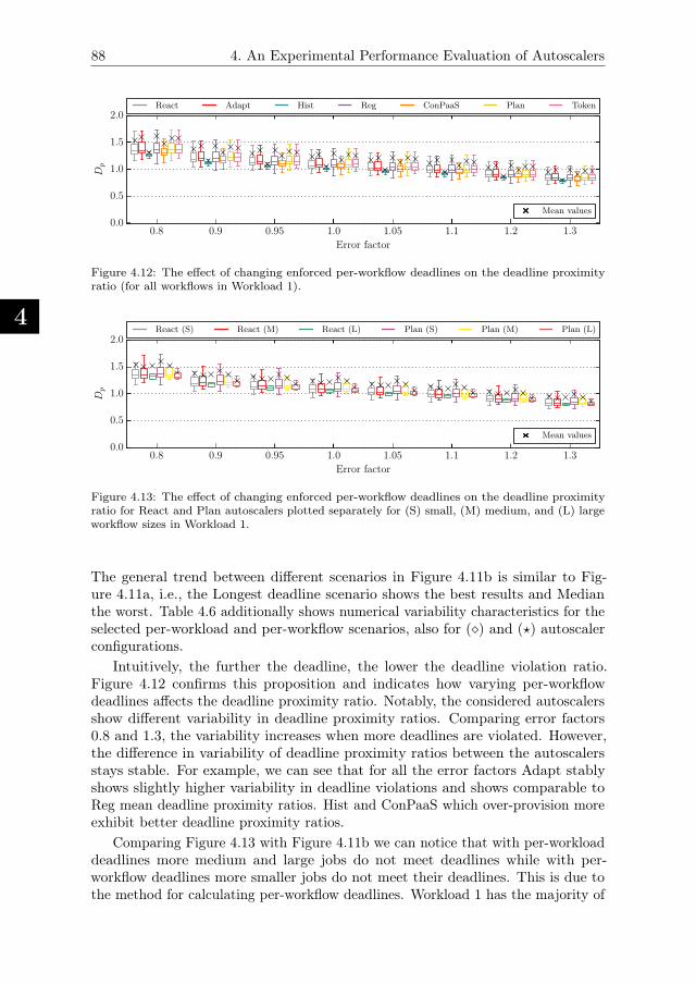
4

88 4. An Experimental Performance Evaluation of Autoscalers

0.8 0.9 0.95 1.0 1.05 1.1 1.2 1.3

Error factor

0.0

0.5

1.0

1.5

2.0

Dp

React Adapt Hist Reg ConPaaS Plan Token

Mean values

Figure 4.12: The effect of changing enforced per-workflow deadlines on the deadline proximityratio (for all workflows in Workload 1).

0.8 0.9 0.95 1.0 1.05 1.1 1.2 1.3

Error factor

0.0

0.5

1.0

1.5

2.0

Dp

React (S) React (M) React (L) Plan (S) Plan (M) Plan (L)

Mean values

Figure 4.13: The effect of changing enforced per-workflow deadlines on the deadline proximityratio for React and Plan autoscalers plotted separately for (S) small, (M) medium, and (L) largeworkflow sizes in Workload 1.

The general trend between different scenarios in Figure 4.11b is similar to Fig-ure 4.11a, i.e., the Longest deadline scenario shows the best results and Medianthe worst. Table 4.6 additionally shows numerical variability characteristics for theselected per-workload and per-workflow scenarios, also for (⋄) and (⋆) autoscalerconfigurations.

Intuitively, the further the deadline, the lower the deadline violation ratio.Figure 4.12 confirms this proposition and indicates how varying per-workflowdeadlines affects the deadline proximity ratio. Notably, the considered autoscalersshow different variability in deadline proximity ratios. Comparing error factors0.8 and 1.3, the variability increases when more deadlines are violated. However,the difference in variability of deadline proximity ratios between the autoscalersstays stable. For example, we can see that for all the error factors Adapt stablyshows slightly higher variability in deadline violations and shows comparable toReg mean deadline proximity ratios. Hist and ConPaaS which over-provision moreexhibit better deadline proximity ratios.

Comparing Figure 4.13 with Figure 4.11b we can notice that with per-workloaddeadlines more medium and large jobs do not meet deadlines while with per-workflow deadlines more smaller jobs do not meet their deadlines. This is due tothe method for calculating per-workflow deadlines. Workload 1 has the majority of

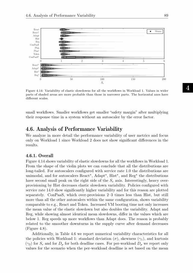
4.6. Analysis of Performance Variability

4

89

Figure 4.14: Variability of elastic slowdowns for all the workflows in Workload 1. Values in widerparts of shaded areas are more probable than those in narrower parts. The horizontal axes havedifferent scales.

small workflows. Smaller workflows get smaller “safety margin” after multiplyingtheir response time in a system without an autoscaler by the error factor.

4.6. Analysis of Performance VariabilityWe analyze in more detail the performance variability of user metrics and focusonly on Workload 1 since Workload 2 does not show significant differences in theresults.

4.6.1. OverallFigure 4.14 shows variability of elastic slowdowns for all the workflows in Workload 1.From the shape of the violin plots we can conclude that all the distributions arelong-tailed. For autoscalers configured with service rate 1.0 the distributions areunimodal, and for autoscalers React⋆, Adapt⋆, Hist⋆, and Reg⋆ the distributionshave second small peak on the right side of the Se axis. Interestingly, heavy over-provisioning by Hist decreases elastic slowdown variability. Policies configured withservice rate 14.0 show significantly higher variability and for this reason are plottedseparately. ConPaaS, which over-provisions 2–3 times less than Hist, but stillmore than all the other autoscalers within the same configuration, shows variabilitycomparable to e.g., React and Token. Increased VM booting time not only increasesthe mean value of the elastic slowdown but also doubles the variability. Adapt andReg, while showing almost identical mean slowdowns, differ in the values which arebelow 1. Reg speeds up more workflows than Adapt does. The reason is probablyrelated to the smoother downturns in the supply curve after demand decreases(Figure 4.8).

Additionally, in Table 4.6 we report numerical variability characteristics for allthe policies with Workload 1: standard deviation (σ), skewness (γ1), and kurtosis(γ2) for Se and for Dp for both deadline cases. For per-workload Dp we report onlyvalues for the scenario when the per-workload deadline is set based on the mean

4

904.

An

Exper

imen

talPer

form

ance

Eva

luat

ion

ofA

uto

scale

rs

Type ASSe

Dp Dp

per-workload, mean scenario per-workflow, err. factor 1.0σ γ1 γ2 mean σ γ1 γ2 mean σ γ1 γ2

General

React 0.42 2.93 9.13 1.06 0.77 0.63 –0.79 1.23 0.42 2.93 9.13React⋄ 1.12 3.65 14.85 1.17 0.77 0.56 –0.8 1.57 1.12 3.65 14.85Adapt 0.55 3.65 16.14 1.08 0.78 0.63 –0.77 1.28 0.55 3.65 16.14Hist 0.14 4.2 20.6 1.01 0.77 0.62 –0.82 1.05 0.14 4.2 20.6Reg 0.59 3.3 11.04 1.08 0.77 0.61 –0.81 1.29 0.59 3.3 11.04ConPaaS 0.49 5.19 31.85 1.06 0.8 0.66 –0.75 1.18 0.49 5.19 31.85React⋆ 34.75 2.81 6.76 4 1.56 0.08 –0.77 17.32 34.75 2.81 6.76Adapt⋆ 25.12 2.64 5.75 4.65 1.48 –0.6 0.18 20.06 38.67 2.51 4.92Hist⋆ 38.67 2.51 4.92 3.23 1.18 –0.45 –0.15 12.93 25.12 2.64 5.75Reg⋆ 45.91 2.13 2.99 5.46 1.32 0.17 –0.43 25.57 45.91 2.13 2.99ConPaaS⋆ 3.43 7.47 62.58 1.27 0.79 0.44 –0.89 2.11 3.43 7.47 62.58

WF-specificPlan 0.47 2.84 7.82 1.08 0.78 0.63 –0.79 1.27 0.47 2.84 7.82Plan⋄ 0.96 5.05 36.26 1.15 0.78 0.58 –0.77 1.48 0.96 5.05 36.26Token 0.44 3.04 11.28 1.08 0.79 0.67 –0.69 1.25 0.44 3.04 11.28

None No AS 0 0 –3 1 0.77 0.64 –0.81 1 0 0 –3

Table 4.6: Additional variability characteristics of Se and Dp metrics for per-workload and per-workflow cases for Workload 1. Best values in eachcolumn are highlighted in bold, except the No AS case. σ is standard deviation, γ1 is skewness and γ2 is kurtosis.

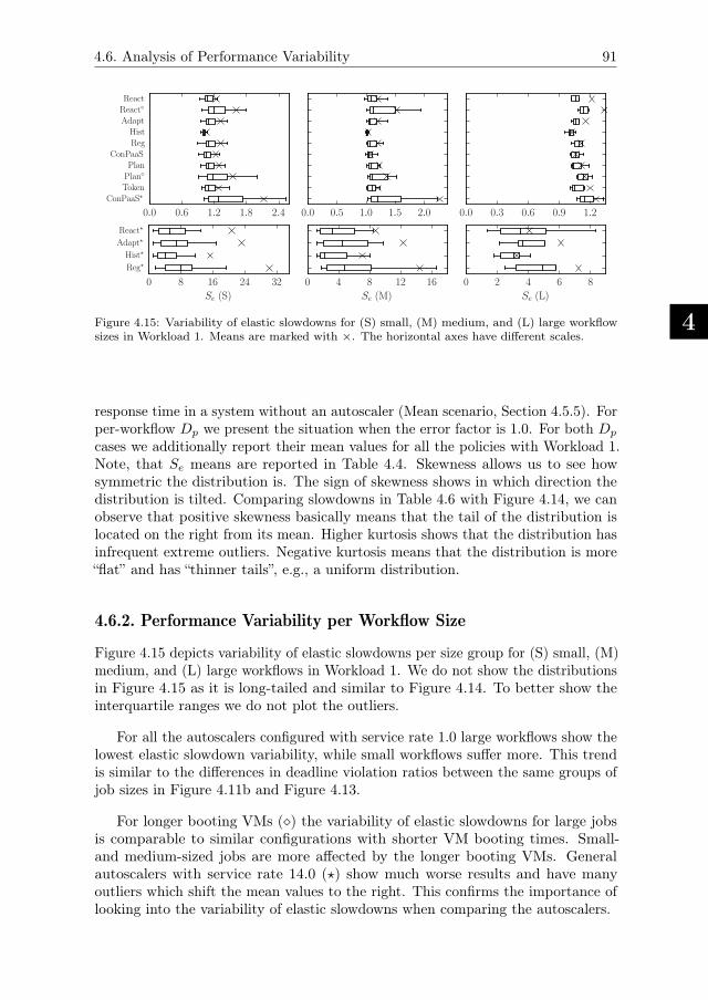
4.6. Analysis of Performance Variability

4

91

Figure 4.15: Variability of elastic slowdowns for (S) small, (M) medium, and (L) large workflowsizes in Workload 1. Means are marked with ×. The horizontal axes have different scales.

response time in a system without an autoscaler (Mean scenario, Section 4.5.5). Forper-workflow Dp we present the situation when the error factor is 1.0. For both Dp

cases we additionally report their mean values for all the policies with Workload 1.Note, that Se means are reported in Table 4.4. Skewness allows us to see howsymmetric the distribution is. The sign of skewness shows in which direction thedistribution is tilted. Comparing slowdowns in Table 4.6 with Figure 4.14, we canobserve that positive skewness basically means that the tail of the distribution islocated on the right from its mean. Higher kurtosis shows that the distribution hasinfrequent extreme outliers. Negative kurtosis means that the distribution is more“flat” and has “thinner tails”, e.g., a uniform distribution.

4.6.2. Performance Variability per Workflow Size

Figure 4.15 depicts variability of elastic slowdowns per size group for (S) small, (M)medium, and (L) large workflows in Workload 1. We do not show the distributionsin Figure 4.15 as it is long-tailed and similar to Figure 4.14. To better show theinterquartile ranges we do not plot the outliers.

For all the autoscalers configured with service rate 1.0 large workflows show thelowest elastic slowdown variability, while small workflows suffer more. This trendis similar to the differences in deadline violation ratios between the same groups ofjob sizes in Figure 4.11b and Figure 4.13.

For longer booting VMs (⋄) the variability of elastic slowdowns for large jobsis comparable to similar configurations with shorter VM booting times. Small-and medium-sized jobs are more affected by the longer booting VMs. Generalautoscalers with service rate 14.0 (⋆) show much worse results and have manyoutliers which shift the mean values to the right. This confirms the importance oflooking into the variability of elastic slowdowns when comparing the autoscalers.

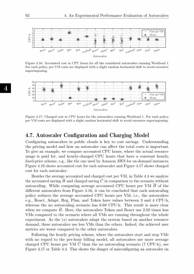
4

92 4. An Experimental Performance Evaluation of Autoscalers

React

React⋄

Adapt Hist Reg

ConPaa

SRea

ct⋆

Adapt

⋆

Hist⋆

Reg⋆

ConPaa

S⋆

Plan Plan⋄

Token

Autoscalers

012345678

CPU·h

Cost per VM

Means

Figure 4.16: Accounted cost in CPU hours for all the considered autoscalers running Workload 1.For each policy, per VM costs are displayed with a slight random horizontal shift to avoid excessivesuperimposing.

React

React⋄

Adapt Hist Reg

ConPaa

SRea

ct⋆

Adapt

⋆

Hist⋆

Reg⋆

ConPaa

S⋆

Plan Plan⋄

Token

Autoscalers

0

10

20

30

40

50

60

CPU·h

Cost per VM

Means

Figure 4.17: Charged cost in CPU hours for the autoscalers running Workload 1. For each policy,per VM costs are displayed with a slight random horizontal shift to avoid excessive superimposing.

4.7. Autoscaler Configuration and Charging ModelConfiguring autoscalers in public clouds is key to cost savings. Understandingthe pricing model and how an autoscaler can affect the total costs is important.To give an example, we compare accounted CPU hours, where the actual resourceusage is paid for, and hourly-charged CPU hours that have a constant hourly,fixed-price scheme, e.g., like the one used by Amazon AWS for on-demand instances.Figure 4.16 shows accounted cost for each autoscaler and Figure 4.17 shows chargedcost for each autoscaler.

Besides the average accounted and charged cost per VM, in Table 4.4 we analyzethe accounted saving H and charged saving C in comparison to the scenario withoutautoscaling. While comparing average accounted CPU hours per VM H of thedifferent autoscalers from Figure 4.16, it can be concluded that each autoscalingpolicy reduces the average accounted CPU hours per VM, i.e., the autoscalerse.g., React, Adapt, Reg, Plan, and Token have values between 3 and 4 CPU·h,whereas the no autoscaling scenario has 6.68 CPU·h. This result is more clearwhen we compute H. Here, the autoscalers Token and React use 2.02 times lessVMs compared to the scenario where all VMs are running throughout the wholeexperiment. As the (⋆) autoscalers adapt the system based on another resourcedemand, these autoscalers use less VMs than the others. Indeed, the achieved usermetrics are worse compared to the other autoscalers.

Following the hourly pricing scheme, where the autoscalers start and stop VMswith no regard to the per-hour billing model, all autoscalers use more averagecharged CPU hours per VM C than the no autoscaling scenario (7 CPU·h), seeFigure 4.17 or Table 4.4. This shows the danger of misconfiguring an autoscaler on

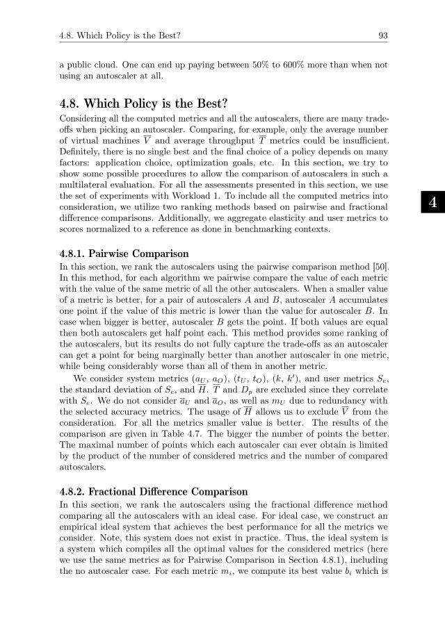
4.8. Which Policy is the Best?

4

93

a public cloud. One can end up paying between 50% to 600% more than when notusing an autoscaler at all.

4.8. Which Policy is the Best?Considering all the computed metrics and all the autoscalers, there are many trade-offs when picking an autoscaler. Comparing, for example, only the average numberof virtual machines V and average throughput T metrics could be insufficient.Definitely, there is no single best and the final choice of a policy depends on manyfactors: application choice, optimization goals, etc. In this section, we try toshow some possible procedures to allow the comparison of autoscalers in such amultilateral evaluation. For all the assessments presented in this section, we usethe set of experiments with Workload 1. To include all the computed metrics intoconsideration, we utilize two ranking methods based on pairwise and fractionaldifference comparisons. Additionally, we aggregate elasticity and user metrics toscores normalized to a reference as done in benchmarking contexts.

4.8.1. Pairwise Comparison

In this section, we rank the autoscalers using the pairwise comparison method [50].In this method, for each algorithm we pairwise compare the value of each metricwith the value of the same metric of all the other autoscalers. When a smaller valueof a metric is better, for a pair of autoscalers A and B, autoscaler A accumulatesone point if the value of this metric is lower than the value for autoscaler B. Incase when bigger is better, autoscaler B gets the point. If both values are equalthen both autoscalers get half point each. This method provides some ranking ofthe autoscalers, but its results do not fully capture the trade-offs as an autoscalercan get a point for being marginally better than another autoscaler in one metric,while being considerably worse than all of them in another metric.

We consider system metrics (aU , aO), (tU , tO), (k, k′), and user metrics Se,the standard deviation of Se, and H. T and Dp are excluded since they correlatewith Se. We do not consider aU and aO, as well as mU due to redundancy withthe selected accuracy metrics. The usage of H allows us to exclude V from theconsideration. For all the metrics smaller value is better. The results of thecomparison are given in Table 4.7. The bigger the number of points the better.The maximal number of points which each autoscaler can ever obtain is limitedby the product of the number of considered metrics and the number of comparedautoscalers.

4.8.2. Fractional Difference Comparison

In this section, we rank the autoscalers using the fractional difference methodcomparing all the autoscalers with an ideal case. For ideal case, we construct anempirical ideal system that achieves the best performance for all the metrics weconsider. Note, this system does not exist in practice. Thus, the ideal system isa system which compiles all the optimal values for the considered metrics (herewe use the same metrics as for Pairwise Comparison in Section 4.8.1), includingthe no autoscaler case. For each metric mi, we compute its best value bi which is

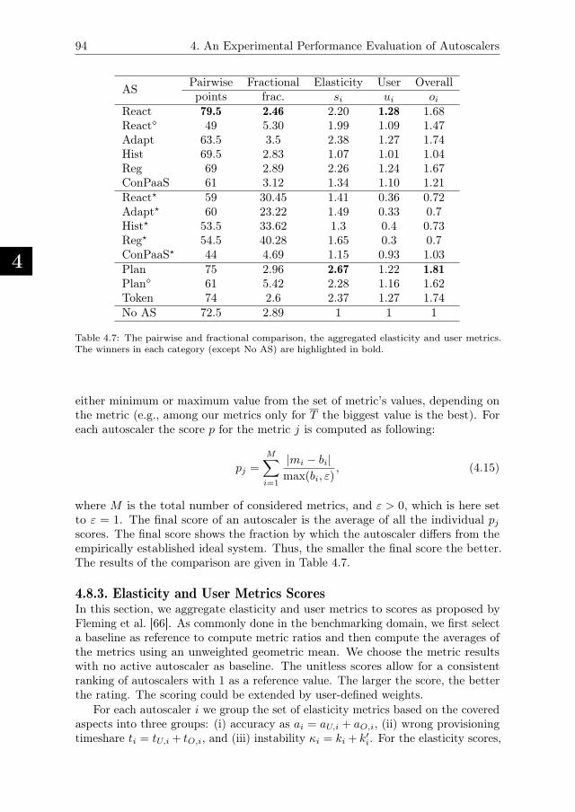
4

94 4. An Experimental Performance Evaluation of Autoscalers

ASPairwise Fractional Elasticity User Overallpoints frac. si ui oi

React 79.5 2.46 2.20 1.28 1.68React⋄ 49 5.30 1.99 1.09 1.47Adapt 63.5 3.5 2.38 1.27 1.74Hist 69.5 2.83 1.07 1.01 1.04Reg 69 2.89 2.26 1.24 1.67ConPaaS 61 3.12 1.34 1.10 1.21React⋆ 59 30.45 1.41 0.36 0.72Adapt⋆ 60 23.22 1.49 0.33 0.7Hist⋆ 53.5 33.62 1.3 0.4 0.73Reg⋆ 54.5 40.28 1.65 0.3 0.7ConPaaS⋆ 44 4.69 1.15 0.93 1.03Plan 75 2.96 2.67 1.22 1.81Plan⋄ 61 5.42 2.28 1.16 1.62Token 74 2.6 2.37 1.27 1.74No AS 72.5 2.89 1 1 1

Table 4.7: The pairwise and fractional comparison, the aggregated elasticity and user metrics.The winners in each category (except No AS) are highlighted in bold.

either minimum or maximum value from the set of metric’s values, depending onthe metric (e.g., among our metrics only for T the biggest value is the best). Foreach autoscaler the score p for the metric j is computed as following:

pj =M∑

i=1

|mi − bi|max(bi, ε)

, (4.15)

where M is the total number of considered metrics, and ε > 0, which is here setto ε = 1. The final score of an autoscaler is the average of all the individual pjscores. The final score shows the fraction by which the autoscaler differs from theempirically established ideal system. Thus, the smaller the final score the better.The results of the comparison are given in Table 4.7.

4.8.3. Elasticity and User Metrics ScoresIn this section, we aggregate elasticity and user metrics to scores as proposed byFleming et al. [66]. As commonly done in the benchmarking domain, we first selecta baseline as reference to compute metric ratios and then compute the averages ofthe metrics using an unweighted geometric mean. We choose the metric resultswith no active autoscaler as baseline. The unitless scores allow for a consistentranking of autoscalers with 1 as a reference value. The larger the score, the betterthe rating. The scoring could be extended by user-defined weights.

For each autoscaler i we group the set of elasticity metrics based on the coveredaspects into three groups: (i) accuracy as ai = aU,i + aO,i, (ii) wrong provisioningtimeshare ti = tU,i + tO,i, and (iii) instability κi = ki + k′i. For the elasticity scores,

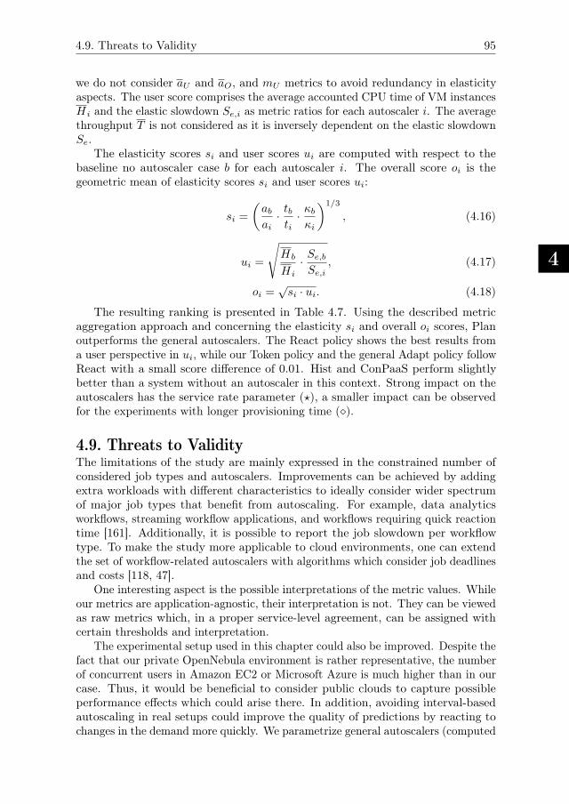
4.9. Threats to Validity

4

95

we do not consider aU and aO, and mU metrics to avoid redundancy in elasticityaspects. The user score comprises the average accounted CPU time of VM instancesHi and the elastic slowdown Se,i as metric ratios for each autoscaler i. The averagethroughput T is not considered as it is inversely dependent on the elastic slowdownSe.

The elasticity scores si and user scores ui are computed with respect to thebaseline no autoscaler case b for each autoscaler i. The overall score oi is thegeometric mean of elasticity scores si and user scores ui:

si =

(

abai

· tbti

· κb

κi

)1/3

, (4.16)

ui =

√

Hb

Hi

· Se,b

Se,i, (4.17)

oi =√si · ui. (4.18)

The resulting ranking is presented in Table 4.7. Using the described metricaggregation approach and concerning the elasticity si and overall oi scores, Planoutperforms the general autoscalers. The React policy shows the best results froma user perspective in ui, while our Token policy and the general Adapt policy followReact with a small score difference of 0.01. Hist and ConPaaS perform slightlybetter than a system without an autoscaler in this context. Strong impact on theautoscalers has the service rate parameter (⋆), a smaller impact can be observedfor the experiments with longer provisioning time (⋄).

4.9. Threats to ValidityThe limitations of the study are mainly expressed in the constrained number ofconsidered job types and autoscalers. Improvements can be achieved by addingextra workloads with different characteristics to ideally consider wider spectrumof major job types that benefit from autoscaling. For example, data analyticsworkflows, streaming workflow applications, and workflows requiring quick reactiontime [161]. Additionally, it is possible to report the job slowdown per workflowtype. To make the study more applicable to cloud environments, one can extendthe set of workflow-related autoscalers with algorithms which consider job deadlinesand costs [118, 47].

One interesting aspect is the possible interpretations of the metric values. Whileour metrics are application-agnostic, their interpretation is not. They can be viewedas raw metrics which, in a proper service-level agreement, can be assigned withcertain thresholds and interpretation.

The experimental setup used in this chapter could also be improved. Despite thefact that our private OpenNebula environment is rather representative, the numberof concurrent users in Amazon EC2 or Microsoft Azure is much higher than in ourcase. Thus, it would be beneficial to consider public clouds to capture possibleperformance effects which could arise there. In addition, avoiding interval-basedautoscaling in real setups could improve the quality of predictions by reacting tochanges in the demand more quickly. We parametrize general autoscalers (computed

4

96 4. An Experimental Performance Evaluation of Autoscalers

service rate parameter) using the statistical properties of the whole workload aswe have an access to this information. However, in the case when the workloadproperties are unknown different demand estimation methods can be used [147].We do not analyze CPU utilization and RAM usage as for the considered workloadsCPU and RAM information has low value as we primarily assign one task per VMand focus on performance characteristics from the perspective of job executiontimes.

The fractional difference comparison does not have upper bound for its scores.The comparison method can be improved by, for example, normalizing the set ofvalues for the single metric by the maximum value from that set, but this couldmake the results incomparable with results obtained in other environments inthe future. Another issue is related to the selection of metrics for tournamentsto have a proper balance between autoscaling-, user-, and cost-oriented metricswithin a single competition. The same stands for using the weights for prioritizingthe considered metrics. The choice of metrics and weights solely depends on thegoals which should be achieved. For this reason, since we are performing generalcomparison of diverse autoscalers and we are not inclined towards certain metrics,we use multiple types of tournaments. It depends on the reader’s preferences howthe metrics and tournament results will be interpreted.

4.10. Related WorkThis chapter provides the first comprehensive comparative experimental study ofautoscaling for workflows. We are unaware of any similar study in terms of themethodology taken, the number of policies compared, the number of performancemetrics, and the size of experiments run. The importance of comparing differentautoscaling algorithms has been recently discussed in the literature but mostly froma theoretical point of view [110, 133]. One exception is a tool that tries to utilize thedifferences between different autoscaling policies to achieve better QoS for customersby selecting a policy based on the workload [27]. That work, nevertheless, does notinclude any experimental comparison or deep analysis between the performance ofthe autoscalers as we do in this chapter.

The problem of scaling workflows has been studied in the literature with a focuson designing new autoscaling policies. Malawski et al. [115] discuss the schedulingproblem of ensembles of scientific workflows in clouds while considering cost- anddeadline-constraints. Mao et al. [119] optimize the performance of cloud workflowswithin budget constraints. They propose two algorithms, namely, Scheduling-Firstand Scaling-First. Cushing et al. [47] deal with prediction-based autoscaling ofscientific data-centric workflows. Buyn et al. [40] try to achieve cost-optimizedprovisioning of elastic resources for workflow applications. The authors use theBalanced Time Scheduling (BTS) algorithm to calculate the minimal requirednumber of resources which will allow to execute the workflow within a givendeadline. Dornemann et al. [60] consider scheduling of Business Process ExecutionLanguage (BPEL) workflows in the Amazon EC2 cloud. Their main findings includethe methods to automatically schedule workflow tasks to underutilized hosts andto provide additional hosts in peak situations. The proposed load balancer usesthe overall system load to take scaling decisions in contrast to other systems where

4.11. Conclusion

4

97

the throughput is more important. Heinis et al. [71] propose a design and evaluatethe performance of a workflow execution engine with self-tuning capabilities.

4.11. ConclusionIn this chapter, we propose a comprehensive method for comparing autoscalerswhen running workflow-based workloads in cloud environments. Our methodincludes a model for elastic cloud platforms, a set of over 15 relevant metrics forevaluating autoscalers, a taxonomy and survey of exemplary general and workflow-specific autoscalers, and experimental and analysis steps to conduct the comparison.Using our method, we evaluate 7 general and workflow-specific autoscalers, andseveral autoscaler variants, when used to control the capacity for a workload ofworkflows running in a realistic cloud environment. Our results across the diversemetrics highlight the trade-offs of using the different autoscalers. At the best ofour knowledge, the efficiency of general autoscalers was previously unknown forworkflows. We show that although workflow-specific autoscalers have the privilegeof knowing the workflow structure in advance, it is possible for properly configuredgeneral autoscalers to achieve similar performance. Our results demonstrate thata correct parametrization of general autoscalers is very important. In our case,the service rate parameter is not the only one to affect the performance of generalautoscalers. In particular, VM booting times and the choice of the autoscalinginterval are also crucial, as many general autoscalers are designed to stably operatewhen VM booting times do not exceed a certain threshold. Finding optimal valuesfor parameters could be even impossible (as they could be implementation-related)and will probably require more experiments. Remarkably, our workflow-specificPlan autoscaler shows comparable results to the general React autoscaler and wins2 out of 5 competitions while providing a good balance between operational costsand performance. The correct choice of an autoscaler is important but significantlydepends on the application type. Thus, no single universal solution exists. In sucha situation, the multilateral ranking methods which we use gain more importance.

5

Performance-Feedback

Autoscaling for

Workloads of Workflows

The growing popularity of workflows in the cloud domain promoted the develop-ment of sophisticated autoscaling policies that allow automatic allocation and

deallocation of resources. However, many state-of-the-art autoscaling policies forworkflows are mostly plan-based or designed for batches (ensembles) of workflows.This reduces their flexibility when dealing with workloads of workflows, as the work-loads are often subject to unpredictable resource demand fluctuations. Moreover,autoscaling in clouds almost always imposes budget constraints that should besatisfied. The budget-aware autoscalers for workflows usually require task runtimeestimates to be provided beforehand, which is not always possible when dealing withworkloads due to their dynamic nature. To address these issues, we propose a novelPerformance-Feedback Autoscaler (PFA) that is budget-aware and does not requiretask runtime estimates for its operation. Instead, it uses the performance-feedbackloop that monitors the average throughput on each resource type. We implementPFA in the popular Apache Airflow workflow management system, and comparethe performance of our autoscaler with other two state-of-the-art autoscalers, andwith the optimal solution obtained with the Mixed Integer Programming approach.Our results show that PFA outperforms other considered online autoscalers, as iteffectively minimizes the average job slowdown by up to 47% while still satisfyingthe budget constraints. Moreover, PFA shows by up to 76% lower average runtimethan the competitors.

5.1. IntroductionWorkflows have been introduced to cloud workloads over a decade ago [53]. To-day, the variety of workflow structures observed in modern cloud workloads andthe diversity of cloud resource types require much more sophisticated resource

99

5

100 5. Performance-Feedback Autoscaling

management and scheduling techniques [167, 52, 6]. Autoscalers [118] must notonly allocate resources but also deallocate them, delivering results in time withoutresource waste and without exceeding preallocated budgets. They must furtheroperate online, fulfilling dynamic requirements for multiple types of resourcesfrom a stream of multi-user requests. Meeting such demanding and dynamicService-Level Agreements (SLAs) is not trivial, and poses important challenges totraditional single-workflow [101, 155] and multi-workflow [170, 24] schedulers, offlineautoscalers for workflow ensembles [116, 33, 164], and online autoscalers [40, 119].Online autoscalers have better performance scalability, but currently they oftenproduce low quality demand estimations and thus could waste cloud resources [119],as we showed earlier in Chapter 4. Offline approaches use sophisticated planningtechniques to produce high quality schedules and demand estimations, but lackthe performance scalability needed to operate online in cloud settings [160, 82]. Inthis chapter, we aim to combine the qualities and avoid the drawbacks of previousapproaches. To this end, we design and evaluate experimentally the Performance-Feedback Autoscaler (PFA), which we aim to make highly scalable while producinghigh-quality estimations.

Previously, the problem of autoscaling for workflows has been seen often fromthe perspective of just a single user who submits to the cloud a batch (an ensemble)of workflows. Usually, the workflows in the batch have previously known taskruntimes, or good estimates obtained through code analysis, simulation, or fromrunning on a reference system. This approach has been successfully adopted forexecuting batches of scientific workflows [155, 170, 116], which are well-studied [92]and have rather fixed patterns of execution [16], but can be too rigid for workflows innon-scientific domains [165]. Moreover, task runtime estimates have not been shownto be robust for batches in cloud settings, e.g., under multi-tenancy effects [91] andperformance variability [120].

A more general approach assumes that the user submits a workload of workflowsof different types as, for example, if the user runs an application serving manyother, diverse customers. Many cloud-based services, such as Airbnb (rentals),Twitter (communication), and Netflix (video streaming), use this approach [131].

Autoscaling workloads of workflows is fundamentally different from autoscalingbatches of workflows. Normally, for both the cloud user has a budget, to be usedto run the workflows before their individual deadline. This is challenging becausecloud resources are heterogeneous, have different costs, and act as performanceblack boxes. But autoscaling workloads does not typically aim to minimize theaverage makespan, as autoscaling batches typically does. Because, in a workload,workflows arrive in the system dynamically as a stream, it is important to minimizethe workflow slowdown, as this leads to predictable service performance. Further,to keep their service sustainable under varying workload demand, cloud users arevery interested to reduce resource waste and thus reduce operational costs.

Many existing autoscalers for workflows operate offline [116, 33, 164]. Given abatch of workflows, they create full autoscaling and task placement plans, which arethen executed by the workflow management system. Online autoscalers, for whenworkflows stream over time forming a workload, are relatively rare [40, 119]; thefew online autoscalers mostly use a plan-based approach, as they create a partial

5.2. Problem Statement

5

101

plan to follow during an entire autoscaling interval. Although online plan-basedapproaches have showed promise in the past decade, we know now that they leadto unscalable time complexity when applied to workloads of workflows [160].

Autoscalers that do not scale well with the workload can negatively affect thestability of the system. Shorter autoscaling intervals, that are more in line withthe current trend of fine-grained billing [140], further complicate the problem,leaving even less time for making autoscaling decisions. Moreover, plan-driventask placement may slow down the execution of newly arrived workflows, as newtasks wait to be added to the plan. In this case, the plan-based, computationallyintensive autoscalers are not beneficial and should be substituted by simpler andfaster, dynamic approaches.

We envision further improving autoscaling for workloads of workflows by com-bining concepts inherent to general autoscalers [26] and to workflow-aware au-toscalers [119]. From general autoscalers, we aim to adopt the principle ofperformance-feedback, to derive and analyze runtime statistics during the exe-cution. For example, instead of deriving task runtime estimates [43], we can usetask throughput, which is easier to observe. From workflow-aware autoscalers,we can adopt token-based techniques for estimating the expected resource demand,which are less computationally intensive (Chapters 2 and 4). Overall, the main re-search questions addressed in this chapter, and our contributions toward answeringthem, are:

1. How to minimize workflow slowdowns within the budget constraint with un-known in advance task runtime estimates when autoscaling cloud resourcesfor workloads of workflows? We propose in Section 5.3.3 a novel, online,dynamic Performance-Feedback Autoscaler (PFA) that uses the resource taskthroughput information and a token-based estimator.

2. Does the autoscaling policy found when answering Question 1 has lower timecomplexity than the state-of-the-art plan-based online autoscalers? In Sec-tion 5.5, through real-world experiments, we show that PFA answers thisquestion favourably by outperforming two state-of-the-art, plan-based, onlineautoscalers.

3. How far is the performance and scalability of the policy found in Question 1from the optimal solution? We compare in Section 5.6 all the consideredautoscalers with the optimal solution obtained from a Mixed Integer Pro-gramming model.

5.2. Problem StatementThis section presents the model for the problem of autoscaling for workloadsof workflows. The section also presents a set of metrics we use to evaluate theperformance of the workloads and the performance of the studied autoscalers.

5.2.1. Autoscaling ModelWe consider a public cloud computing system which is a subject to an arrivingworkload of workflows. The workflow model is the same as in the previous chapters.

5

102 5. Performance-Feedback Autoscaling

The workload consists of multiple independent sub-workloads each belonging toan independent user.

The cloud computing system allows every user to dynamically allocate anddeallocate computing resources of various types, where each resource type has aspecific cost. Each resource can be in either of the following four states: down,idle, busy, or booting. The resource is down when it is deallocated and it is notreserved for any user. The resource is idle when it is allocated, reserved for acertain user, but has no currently assigned task. The resource is busy when it hasa task assigned. The resource is booting when it is in the transition state betweenthe down and idle states.

Once the resource is allocated, the user is charged and the resource is reservedfor the user until the end of the resource billing period, where the billing periodis the minimal time for which the cloud resource can be reserved for a particularuser. Each user has a certain operational budget per autoscaling interval, andthe total cost of all the resources reserved for the user on the autoscaling intervalcannot exceed the user budget. After the allocation, the resource spends sometime in the booting state, while already being reserved for the user, without beingable to execute any user tasks. At the end of the billing period, the resourcecan be deallocated or its reservation can be prolonged for the next billing period.In our model, the duration of the billing period equals to the duration of theautoscaling period. Before transitioning into the down state for deallocation, theresource should always pass the idle state first. The resource deallocation happensinstantaneously. The system size is the maximal resource capacity which is availablefor the system users.

Since the number of eligible tasks from each user varies over time, the systememploys an autoscaler to automatically control the number of allocated resourceson a per-user basis. The separate scheduler is responsible for placing tasks onto theallocated resources. In this chapter, as well as in Chapter 4, we focus on periodicautoscaling, so that the autoscaler is invoked at fixed intervals by the workflowmanagement system and monitors the controlled cloud environment. Accordingly,the autoscaling interval is the time between any two invocations of the autoscaler.

Despite that the system has resources of different types, we assume that there isno direct dependency between the cost of a resource type and the execution speedsof tasks running on it. Our motivation is based on the assumption that while sometasks can benefit from additional CPU cores, other tasks can be sequential in theirnature and, thus, can show better performance on resources with fewer cores butwith higher CPU frequency. Similar assumptions can be made for different RAMor storage requirements, etc.

The autoscaler and the scheduler operate in tandem with the goal to minimizeworkflow response time within the budget constraint. This can be achieved byallocating enough resources and finding an appropriate resource profile whichguarantees required performance. By resource profile we understand a specificcombination of resource types within the set of resources currently allocated for theuser. Additionally, the autoscaler can have a goal to achieve fairness among multiple

5.2. Problem Statement

5

103

users. Since the resources are reserved for each user until the end of their billingperiod, during that period each resource can execute only tasks from the reservinguser. This implies that the scheduler is not able to control the fairness among theusers as it is only allowed to place tasks belonging to a certain user to the resourcesthat are reserved for the same user. Thus, the only way to control fairness, by whichin this chapter we understand maintaining average task throughput proportionalto the user budget, is by controlling the number of allocated resources within theresource profile. Thus, if the autoscaler is fairness-aware, it should consider inaddition to the budget constraint also the fairness constraint.

We do not include deadlines in this study as, in contrast to the offline approach,in the dynamic workload scheduling deadlines can only be roughly estimated. Fur-thermore, for workloads the deadline compliance depends on the system utilization,thus, the deadlines that were derived previously at a certain utilization level canbe easily invalid for other utilizations. The dynamic nature of autoscaling forworkloads makes the response time minimization and the stability of the systemmore important goals rather than the deadline compliance. It is also reasonable toassume that the response time minimization usually increases the number of metdeadlines. Additionally, in our model we allow users to assign numeric prioritiesto workflows so that they can indicate which workflows are more important andshould be processed faster.

5.2.2. Performance Metrics

The system is constantly monitored by its users and operators, who assess itsperformance for a set of metrics commonly used in autoscaling settings. In thischapter, we mostly rely on metrics defined earlier in previous chapters.

User- and System-Oriented Metrics

As a main user-oriented metric we use slowdown which is defined in the same wayand using the same notations as in Section 3.2.2. We also consider the monetarycost per autoscaling interval as a user-oriented metric. By monetary cost weunderstand the total cost of allocated resources during any autoscaling interval.As a system-oriented metrics we use the percentage of busy resources throughoutthe experiment and the percentage of allocated resources per autoscaling interval.

Elasticity-Oriented Metrics

To evaluate the performance of the considered autoscalers, we take the elasticityinto account. We extend the system model from Chapter 4, where we allow eachresource to run only a single workflow task at a time. Thus, we rely on the samedemand and supply definitions as in Section 4.3, and use the same under- and over-provisioning accuracy metrics aU , aO, and under- and over-provisioning timesharemetrics tU , tO. However, since in this chapter we consider multiple users, the supplyand demand are additionally defined per user. From the resource heterogeneityperspective, we do not define the demand per resource type, as we suppose thattask resource preferences are unknown a priori to the scheduler.

5

104 5. Performance-Feedback Autoscaling

5.3. AutoscalersThis section explains in detail two state-of-the-art budget-aware autoscalers, thatrequire task runtime estimates for their operation, and presents our novel autoscaler,which, in contrast, operates without explicitly provided task runtime estimates. Theconsidered state-of-the-art autoscalers were proposed by Mao and Humphrey [119]and designed specifically for workloads of workflows. The relevance of theseautoscalers is supported by the recent survey [111].

5.3.1. Planning-First AutoscalerThe Planning First (PLF) [119] autoscaling policy uses currently eligible tasks toallocate resources within a budget constraint. Even though the name of the policyin the original paper is Scheduling First, further we refer to it as Planning First, asthis policy basically creates an execution plan for the tasks within the autoscalinginterval. The autoscaler consists of six steps which are executed on every policyinvocation, i.e., for every autoscaling interval:

1. Distribute the user budget among the workflows based on their priority.

2. Perform initial supply prediction by determining the number of each resourcetype to allocate within the budget constraint.

3. Consolidate the budget left after the initial supply prediction.

4. Allocate the resources according to the predicted supply.

5. Create an execution plan for the upcoming autoscaling interval.

6. Deallocate idle resources which do not have any tasks planned and areapproaching the end of their billing period.

In the first step, the policy computes the cost of already allocated resources,deducts their cost from the user budget, and distributes the remaining budgetto individual workflows proportionally to their priority, so that higher priorityworkflows get bigger budgets.

In the second step, the policy iterates through the eligible tasks of the workflow,sorted in the descending order of their workflow priorities, and for each task, whilethere is enough budget, it finds the resource type allowing to finish the task in theshortest time. The tasks are not assigned to the resources, only the number ofresources of each type is determined. If the budget is over, the autoscaler proceedsto the third step—the budget consolidation. In the original paper, the loop breakcondition depends on the cost of the cheapest resource in the system so that alreadyafter the second step the policy can overspend the budget (for each workflow) bythe cost difference between the fastest resource and the cheapest one. To avoidthis, we modify the policy and use the cost of the fastest resource for the currentlyprocessed workflow task instead.

In the third step, the policy performs budget consolidation, as some budgetcan be left by individual workflows after the initial demand estimation. Thereare two reasons why the initially distributed budget may not be fully spent: someworkflows could have not enough eligible tasks, or some workflows could haveremaining budget smaller than the cost of the fastest resource. So that these

5.3. Autoscalers

5

105

remaining per-workflow budgets can be redistributed among the workflows fromthe same user to include more fastest resources in the allocation plan. This allowsto determine fastest resource types for the remaining higher priority eligible tasksthat were not processed in the second step. After this step, the autoscaler producesthe final predicted number of instances of each type which should be allocated. Italso specifies for some or all eligible tasks on which resource types they should run.Some eligible tasks belonging to lower priority workflows still could be withoutassigned resource types, as the cost of their fastest resources did not fit within thebudget constraint.

In the fourth step, the policy allocates the resources according to the predictedsupply.

In the fifth step, the policy performs so-called resource consolidation whichbasically means the creation of an execution plan on the already allocated (atthe moment of the autoscaler invocation) and newly allocated resources (after thefourth step) for the upcoming autoscaling interval. For that, the policy determinesactual resources (not just the resource types) for each workflow task and tries tofill the resources in the plan with tasks until the end of the autoscaling interval.This is necessary, as after the third step only (a subset of) eligible tasks get theresource type assigned—those, that were used to predict the supply. Accordingly,the number of resources in the plan equals the number of running tasks and thenumber of tasks that have the resource type assigned after the third step.

Finally, in the sixth step, the resources that did not get any tasks assigned inthe previous steps and that are approaching the end of their billing period aredeallocated.

As the original paper [119] relies on simulations, many very important details,that are crucial when implementing the policy in a real system, are missing orimprecise. Further, we provide our interpretation of the resource consolidation step.When constructing the execution plan, PLF processes workflows in a random order.The newly allocated resources are considered as booting, thus, the planner takesinto account the allocation delay which is supposed to be known in advance. Theexecution plan is initialized with tasks that are already running at the momentof the autoscaler invocation. Then the policy adds in the plan the eligible tasksthat got the resource type assigned during the second or third autoscaling steps.The eligible tasks with known resource types are first assigned to idle resourcesof that type. If there are no idle resources, the planner checks the booting andbusy resources of the same type, which of those will become available earlier, andplaces the eligible tasks on the earliest one. After that, all the resources in the planshould have at least one task assigned. Finally, all the remaining eligible and notyet eligible tasks are processed while maintaining the precedence constraints, i.e., atask is added to the plan if all of its parents are already in the plan. Each taskis placed on the resource which is at the moment of task placement provides theminimal earliest possible start time. The planning process continues until there areno tasks that can start their execution before the end of the autoscaling interval.

5

106 5. Performance-Feedback Autoscaling

5.3.2. Scaling-First AutoscalerThe Scaling First (SCF) [119] autoscaling policy first creates for each workflow anindividual execution plan (without considering resource allocation constraints), andthen scales the plan so that it fits within the user budget constraint. The policyconsists of five major steps:

1. Perform initial supply prediction by creating a per-workflow execution planwithout limiting the number of resources.

2. Scale the initial prediction to fit within the budget constraint, and consolidatethe remaining budget.

3. Allocate the resources according to the predicted supply.

4. Create an execution plan for the upcoming autoscaling interval.

5. Deallocate idle resources in the same way as in the PLF policy.

In the first step, the policy creates an independent (from other workflows)per-workflow plan neither considering the system resource allocation limits norconsidering the budget constraint. Thus, the number of resources in each plan canbe bigger than the actual number of maximally available resources in the system.Since the original paper does not clearly explain this step, we present our detailedinterpretation of the procedure for creating the per-workflow plan which uses similarlogic as the resource consolidation step. First, the policy selects all the alreadyrunning tasks of the current workflow and places all of them in the plan. Theirresource types are already known, as well as the expected finish times. Second,the policy selects all the eligible tasks and places them on their fastest resourcetypes, calculating the appropriate expected finish time. Third, all the other notyet eligible tasks are placed in the plan on their fastest resources (if those requiredfastest resources are not yet in the plan then they are added) so that the earliestpossible start time for each task is minimized at the moment of its addition to theplan. Similarly to the resource consolidation step of PLF, a task is added to theplan only if all of its parents are already in the plan. The final number of resourcesfor each resource type that should be supplied is calculated as the rounded up sumof the runtimes of planned tasks on each resource type, divided by the length ofthe autoscaling interval.

In the second step, for each resource type the policy proportionally scales theinitially predicted supply by multiplying it by the factor calculated as the fractionof the user budget and the total cost of initially predicted resources. Since thenumber of resources is integer, some remaining budget can be left after scaling theinitial supply. This remaining budget is used to allocate more resources, if possible.For that the policy iterates in a round robin manner through the predicted in thefirst step resource types until even the resource of the cheapest type cannot beallocated.

In the third step, the policy allocates the resources according to the predictedsupply.

In the fourth step, the policy performs resource consolidation, which for SCFalso means the creation of an execution plan on the allocated resources for theupcoming autoscaling interval. We modify the resource consolidation approach

5.3. Autoscalers

5

107

described in the original paper for SCF, as it is does not mention the situation whenthe number of resources of a certain type after the scaling step is zero. Instead, weuse the approach similar to our interpretation of the resource consolidation for thePLF policy. There are two differences between SCF and PLF. First, in PLF, beforethe resource consolidation step, some (or all) eligible tasks have the resource typealready assigned, while in SCF the information on the preferred resource typesfrom the first step is completely discarded. Second, in SCF the tasks are added tothe plan in the order of their workflow priorities, so that higher priority tasks areadded to the plan earlier.

The fifth step of the SCF policy is identical to the resource deallocation stepof PLF.

5.3.3. Performance-Feedback Autoscaler

In this section, we present our novel Performance-Feedback Autoscaler (PFA), whichwe developed considering the limitations of the state-of-the-art workflow-specificautoscalers. We based the idea of PFA on observations on the performance ofgeneral and workflow-specific autoscalers from the literature [116, 160] and on ourown observations from the previous chapters.

We expect PFA to achieve better elasticity performance, as it constantly moni-tors the historical resource throughputs to derive faster resource types, and relies ona low complexity workload approximator to predict the future demand. Moreover,the dynamic task placement, used together with PFA, is expected to further reducetask waiting times and increase the resource utilization. The PFA autoscalerconsists of the following six steps:

1. Determine the resource type ratios from historical throughputs.

2. Determine the number of resources (the supply) that can be allocated withinthe user budget with the obtained ratios.

3. Estimate future resource demand using the token propagation approach andhistorical throughput information.

4. Scale down or inflate the profile-based supply to match the token-predicteddemand.

5. Allocate the predicted number of resources.

6. Deallocate idle resources that are staying idle the longest and approachingthe end of their billing period.

We detail steps 1–6 of PFA in the remainder of this section. Table 5.1 summarizesall the symbols used in the description of the autoscaler. To explain the algorithmsemployed by each PFA stage, we use a symbolic notation rather than pseudocode,because pseudocode descriptions are known to under-specify (obscure) explanationsto the point where schedulers cannot be reproduced in practice [122].

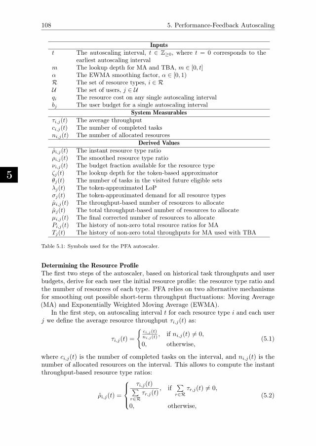
5

108 5. Performance-Feedback Autoscaling

Inputst The autoscaling interval, t ∈ Z≥0, where t = 0 corresponds to the

earliest autoscaling intervalm The lookup depth for MA and TBA, m ∈ [0, t]α The EWMA smoothing factor, α ∈ [0, 1)R The set of resource types, i ∈ RU The set of users, j ∈ Uqi The resource cost on any single autoscaling intervalbj The user budget for a single autoscaling interval

System Measurablesτi,j(t) The average throughputci,j(t) The number of completed tasksni,j(t) The number of allocated resources

Derived Valuesρi,j(t) The instant resource type ratioρi,j(t) The smoothed resource type ratioνi,j(t) The budget fraction available for the resource typeζj(t) The lookup depth for the token-based approximatorθj(t) The number of tasks in the visited future eligible setsλj(t) The token-approximated LoPσj(t) The token-approximated demand for all resource typesµi,j(t) The throughput-based number of resources to allocateµj(t) The total throughput-based number of resources to allocateµi,j(t) The final corrected number of resources to allocatePi,j(t) The history of non-zero total resource ratios for MATj(t) The history of non-zero total throughputs for MA used with TBA

Table 5.1: Symbols used for the PFA autoscaler.

Determining the Resource ProfileThe first two steps of the autoscaler, based on historical task throughputs and userbudgets, derive for each user the initial resource profile: the resource type ratio andthe number of resources of each type. PFA relies on two alternative mechanismsfor smoothing out possible short-term throughput fluctuations: Moving Average(MA) and Exponentially Weighted Moving Average (EWMA).

In the first step, on autoscaling interval t for each resource type i and each userj we define the average resource throughput τi,j(t) as:

τi,j(t) =

{

ci,j(t)ni,j(t)

, if ni,j(t) 6= 0,

0, otherwise,(5.1)

where ci,j(t) is the number of completed tasks on the interval, and ni,j(t) is thenumber of allocated resources on the interval. This allows to compute the instantthroughput-based resource type ratios:

ρi,j(t) =

τi,j(t)∑

r∈R

τr,j(t), if

∑

r∈R

τr,j(t) 6= 0,

0, otherwise,

(5.2)

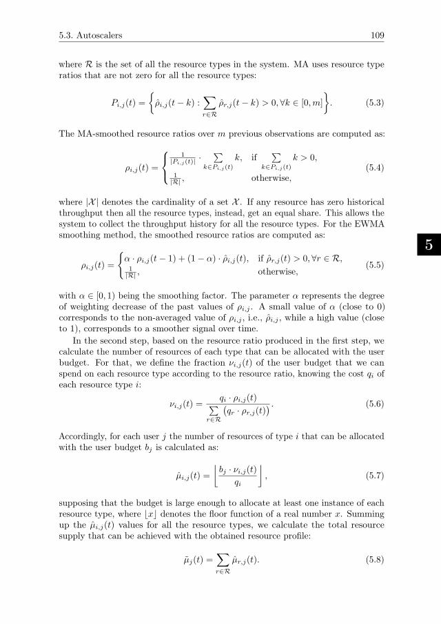
5.3. Autoscalers

5

109

where R is the set of all the resource types in the system. MA uses resource typeratios that are not zero for all the resource types:

Pi,j(t) =

{

ρi,j(t− k) :∑

r∈R

ρr,j(t− k) > 0, ∀k ∈ [0,m]

}

. (5.3)

The MA-smoothed resource ratios over m previous observations are computed as:

ρi,j(t) =

1|Pi,j(t)|

· ∑

k∈Pi,j(t)

k, if∑

k∈Pi,j(t)

k > 0,

1|R| , otherwise,

(5.4)

where |X | denotes the cardinality of a set X . If any resource has zero historicalthroughput then all the resource types, instead, get an equal share. This allows thesystem to collect the throughput history for all the resource types. For the EWMAsmoothing method, the smoothed resource ratios are computed as:

ρi,j(t) =

{

α · ρi,j(t− 1) + (1− α) · ρi,j(t), if ρr,j(t) > 0, ∀r ∈ R,1

|R| , otherwise,(5.5)

with α ∈ [0, 1) being the smoothing factor. The parameter α represents the degreeof weighting decrease of the past values of ρi,j . A small value of α (close to 0)corresponds to the non-averaged value of ρi,j , i.e., ρi,j , while a high value (closeto 1), corresponds to a smoother signal over time.

In the second step, based on the resource ratio produced in the first step, wecalculate the number of resources of each type that can be allocated with the userbudget. For that, we define the fraction νi,j(t) of the user budget that we canspend on each resource type according to the resource ratio, knowing the cost qi ofeach resource type i:

νi,j(t) =qi · ρi,j(t)

∑

r∈R

(

qr · ρr,j(t)) . (5.6)

Accordingly, for each user j the number of resources of type i that can be allocatedwith the user budget bj is calculated as:

µi,j(t) =

⌊

bj · νi,j(t)qi

⌋

, (5.7)

supposing that the budget is large enough to allocate at least one instance of eachresource type, where ⌊x⌋ denotes the floor function of a real number x. Summingup the µi,j(t) values for all the resource types, we calculate the total resourcesupply that can be achieved with the obtained resource profile:

µj(t) =∑

r∈R

µr,j(t). (5.8)

5

110 5. Performance-Feedback Autoscaling

Token-based Demand PredictionIn the third step, the resource demand σj(t) is predicted using the Token-basedApproximator (TBA), similar to the one described in Sections 2.3.1 and 4.4.2. Forthat, TBA considers all the submitted and not yet finished workflows of the user asa single workflow, excluding finished tasks, and places tokens in all the tasks thateither have no parents or whose parents have already finished. Then, in successivesteps, TBA moves these tokens to all the tasks all of whose parents already hold atoken or were earlier tokenized. TBA records the total number of token movementsand, after each step, the number of tokenized nodes.

The intuition is to evaluate the number of “waves” of tasks (future eligible sets)that will finish only during the autoscaling interval. When the lookup depth ζj(t)or the final task of the joint workflow is reached, the largest recorded number oftokenized nodes gives the approximated LoP λj(t), and the total number of tokenmovements θj(t) gives the total number of tasks in the visited future eligible sets.To limit the TBA lookup depth ζj(t), we use the average historical task throughputamong all the resource types smoothed either with MA over m previous autoscalingintervals, or with EWMA. For MA, the set of historical average throughputs for allthe resource types with skipped intervals with zero total throughput is defined as:

Tj(t) =

{

τi,j(t− k) :∑

r∈R

τr,j(t− k) > 0, ∀k ∈ [0,m], ∀i ∈ R}

, (5.9)

With MA, the TBA lookup depth is computed as:

ζj(t) =

⌈

1|Tj(t)|

· ∑

k∈Tj(t)

k⌉

, if∑

k∈Tj(t)

k > 0,

∞, otherwise,(5.10)

where ⌈x⌉ denotes the ceiling function of a real number x. Accordingly, the resourcedemand σj(t) with MA is computed as:

σj(t) =

⌈

θj(t) · |Tj(t)| ·(

∑

k∈Tj(t)k)−1

⌉

, if∑

k∈Tj(t)

k > 0,

λj(t), otherwise.

(5.11)

With EWMA, the TBA lookup depth is computed as:

ζj(t) =

⌈

α · ζj(t− 1) + (1− α) ·∑

r∈R

τr,j(t)

|R|

⌉

, if∑

r∈R

τr,j(t) > 0,

∞, otherwise.

(5.12)

And the resource demand σj(t) with EWMA is computed as:

σj(t) =

⌈

θj(t) · |R| ·(

∑

r∈R

τr,j(t))−1⌉

, if∑

r∈R

τr,j(t) > 0,

λj(t), otherwise.(5.13)

5.4. Experiment Setup

5

111

Scaling Down or Inflating the Profile

In the fourth step, we scale down or inflate, if necessary, the profile-based resourcesupply to match the predicted resource demand σj(t) and produce correctedvalues µi,j(t). Scaling down prevents allocation of potentially idle resources, andgives space to other users to utilize the resources. Inflating the profile, despitecreating possible imbalance in the throughput-based resource ratio, helps to copewith sudden demand surges by increasing the total throughput. If µj(t) exceedsthe predicted demand σj(t), we proportionally scale down µi,j(t) to produce thecorrected values µi,j(t):

µi,j(t) =

⌈

σj(t)

µj(t)· µi,j(t)

⌉

. (5.14)

However, if µj(t) is lower than the token-predicted demand σj(t), we insteadinflate the resource profile as follows: (i) Sort the resources in the ascending orderof their resource type cost. (ii) For each resource type i, except the most expensiveone, try to add to the original resource profile µi,j(t) as many resources of thattype as possible, until there is no budget available or until µj(t) reaches σj(t).This produces the inflated corrected µi,j(t) values. (iii) If σj(t) is not yet reached,starting from the second cheapest resource k, try to remove one instance of it fromµk,j(t) and, instead, add a number of instances to the previous cheapest resourcetype µk−1,j(t). This does not increase the total cost of the resource profile, butincreases µj(t). Continue, until the total number of resources in the profile reachesσj(t) or no more such exchanges are possible.

Allocating and Deallocating Resources

In the fifth step, the predicted number of resources is allocated according to theµi,j(t) values while taking into account the already allocated resources and thephysical system constraints. In the sixth step, PFA de-allocates at maximum thenumber of idle resources that exceeds the predicted supply. When de-allocating theidle resources, PFA gives priority to those that approach the end of their billinginterval.

Task Placement

The PFA autoscaler can operate with various independent task placement policies.Both state-of-the-art autoscalers considered in this work, PLF and SCF, employuser-defined workflow priorities, and both have embedded task placement policieswhich construct an execution plan. Thus, for comparability purposes, togetherwith PFA we use dynamic task placement policy which also considers user-definedworkflow priorities. Our task placement policy assigns eligible tasks according tothe priority of their workflows to the first available idle resource of any type.

5.4. Experiment SetupThis section describes the setup we used to conduct the experiments and thesynthetic workloads of workflows.

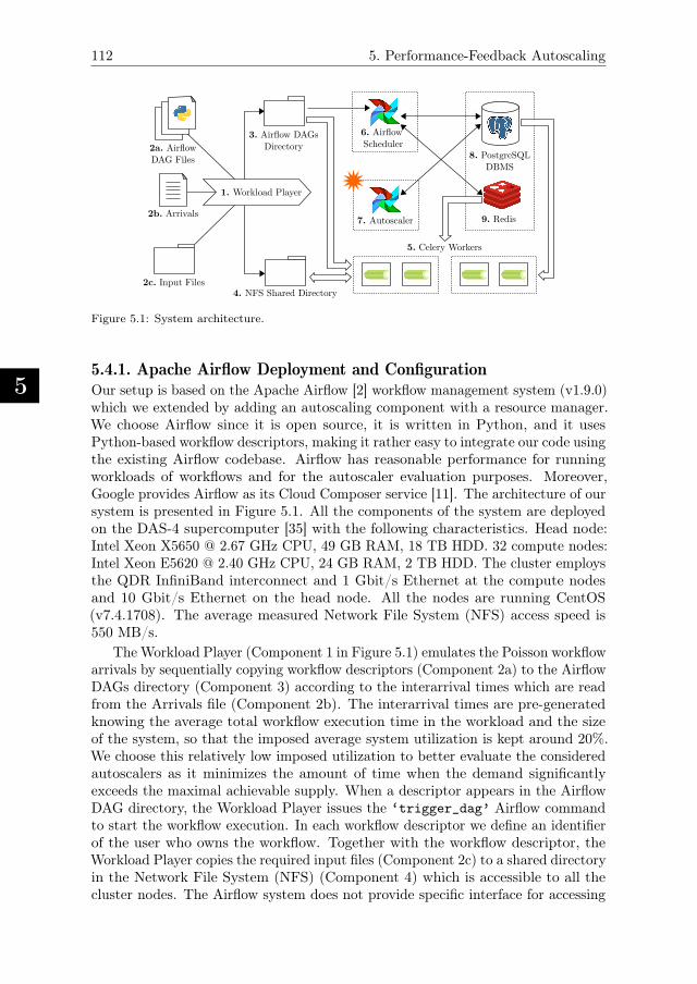
5

112 5. Performance-Feedback Autoscaling

6. Airlow

Scheduler

9. Redis

5. Celery Workers

4. NFS Shared Directory2c. Input Files

2a. Airlow

DAG Files

3. Airlow DAGs

Directory

2b. Arrivals

8. PostgreSQL

DBMS

7. Autoscaler

1. Workload Player

Figure 5.1: System architecture.

5.4.1. Apache Airflow Deployment and Configuration

Our setup is based on the Apache Airflow [2] workflow management system (v1.9.0)which we extended by adding an autoscaling component with a resource manager.We choose Airflow since it is open source, it is written in Python, and it usesPython-based workflow descriptors, making it rather easy to integrate our code usingthe existing Airflow codebase. Airflow has reasonable performance for runningworkloads of workflows and for the autoscaler evaluation purposes. Moreover,Google provides Airflow as its Cloud Composer service [11]. The architecture of oursystem is presented in Figure 5.1. All the components of the system are deployedon the DAS-4 supercomputer [35] with the following characteristics. Head node:Intel Xeon X5650 @ 2.67 GHz CPU, 49 GB RAM, 18 TB HDD. 32 compute nodes:Intel Xeon E5620 @ 2.40 GHz CPU, 24 GB RAM, 2 TB HDD. The cluster employsthe QDR InfiniBand interconnect and 1 Gbit/s Ethernet at the compute nodesand 10 Gbit/s Ethernet on the head node. All the nodes are running CentOS(v7.4.1708). The average measured Network File System (NFS) access speed is550 MB/s.

The Workload Player (Component 1 in Figure 5.1) emulates the Poisson workflowarrivals by sequentially copying workflow descriptors (Component 2a) to the AirflowDAGs directory (Component 3) according to the interarrival times which are readfrom the Arrivals file (Component 2b). The interarrival times are pre-generatedknowing the average total workflow execution time in the workload and the sizeof the system, so that the imposed average system utilization is kept around 20%.We choose this relatively low imposed utilization to better evaluate the consideredautoscalers as it minimizes the amount of time when the demand significantlyexceeds the maximal achievable supply. When a descriptor appears in the AirflowDAG directory, the Workload Player issues the ‘trigger_dag’ Airflow commandto start the workflow execution. In each workflow descriptor we define an identifierof the user who owns the workflow. Together with the workflow descriptor, theWorkload Player copies the required input files (Component 2c) to a shared directoryin the Network File System (NFS) (Component 4) which is accessible to all thecluster nodes. The Airflow system does not provide specific interface for accessing

5.4. Experiment Setup

5

113

workflow files, thus, the workflow code is responsible for file access operations. Eachtask can start its execution when all of its input files are read. Similarly, each taskis considered as finished when all of its output files are written. The minimal delaybetween any two dependent tasks is equal to the sum of these two values.

All the Airflow components communicate through the central Airflow databasewhich is in our setup deployed in the PostgreSQL database management system(Component 8). Our setup uses the Celery [7] distributed task queue (version4.1.1) with Redis [18] (Component 9) in-memory database (version 4.0.10) forsending tasks to the worker nodes. Each worker node runs 8 Celery workers(Component 5)—one per CPU core. In total we deploy 64 Celery workers on 8worker nodes.

The Airflow Scheduler (Component 6) is responsible for placing eligible tasksfor execution to the resources (Celery workers). The default Airflow scheduler is anonline dynamic scheduler as it simply sends the eligible tasks in the order of theirpriority to the single Celery queue which is monitored by the worker processes. Eventhough, Airflow supports pools of workers, it does not have functionality to monitorthe status of each individual worker, and does not support assigning workers tousers. To implement this functionality, we introduce individual Celery queues foreach worker (resource) and guarantee that no new task is placed in the resource’squeue if the queue is not empty, so that the queue can hold one task at maximum.We add a table in the central Airflow database which, for each queue (i.e., resource),stores the information on its current status and the identifier of the user whoreserved the resource. Such an approach is required since PLF and SCF autoscalersare not only responsible for the resource allocation, but also partially take the workfrom the scheduler by constructing a tasks placement plan for the whole autoscalinginterval. Thus, for PLF and SCF autoscalers our Airflow Scheduler simply placestasks to the idle resources just according to the plan. However, since our PFAautoscaler does not create any plan, the modified Airflow Scheduler, when workingin tandem with PFA, makes its own task placement decisions by sending eligibletasks according to their workflow priority and task priority to the first idle resource.In all the cases, the modified Airflow Scheduler only places tasks that belong to aspecific user to the resources that are reserved for the same user.

The Autoscaler (Component 7) is a novel independent component which isimplemented from scratch but heavily relies on the existing Airflow codebase. TheAutoscaler implements all the three considered autoscaling policies which can beconfigured through the main Airflow configuration file. The Autoscaler monitors thestatus of resources and changes their status through the central Airflow database.

The Workload Player, Airflow Scheduler, and Autoscaler are running on indi-vidual worker nodes. The PostgreSQL database management system is co-locatedwith the Redis in-memory database on the head node.

5.4.2. Billing SetupWe configure the system with two resource types: Small and Large, that havedifferent costs. Further, we use the generic currency sign ¤ when referring tomonetary costs. An instance of the Small resource type costs 1¤ per billing interval,while a Large instance costs 5¤ per billing interval. The system is configured to

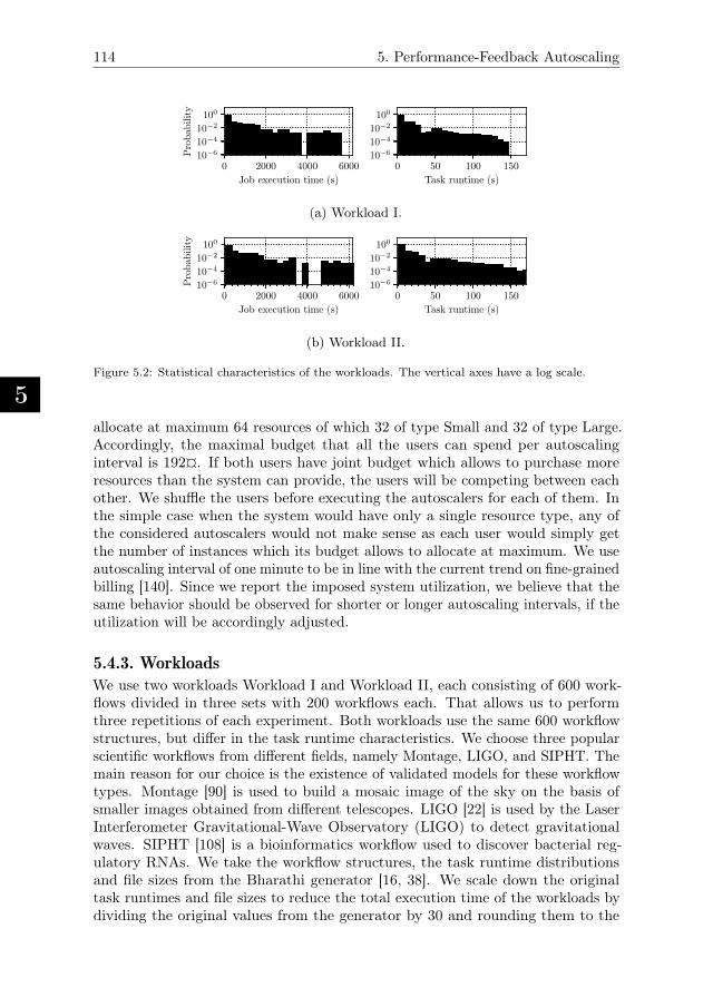
5

114 5. Performance-Feedback Autoscaling

0 2000 4000 6000

Job execution time (s)

100

10−2

10−4

10−6Probab

ility

0 50 100 150

Task runtime (s)

100

10−2

10−4

10−6

(a) Workload I.

0 2000 4000 6000

Job execution time (s)

100

10−2

10−4

10−6Probab

ility

0 50 100 150

Task runtime (s)

100

10−2

10−4

10−6

(b) Workload II.

Figure 5.2: Statistical characteristics of the workloads. The vertical axes have a log scale.

allocate at maximum 64 resources of which 32 of type Small and 32 of type Large.Accordingly, the maximal budget that all the users can spend per autoscalinginterval is 192¤. If both users have joint budget which allows to purchase moreresources than the system can provide, the users will be competing between eachother. We shuffle the users before executing the autoscalers for each of them. Inthe simple case when the system would have only a single resource type, any ofthe considered autoscalers would not make sense as each user would simply getthe number of instances which its budget allows to allocate at maximum. We useautoscaling interval of one minute to be in line with the current trend on fine-grainedbilling [140]. Since we report the imposed system utilization, we believe that thesame behavior should be observed for shorter or longer autoscaling intervals, if theutilization will be accordingly adjusted.

5.4.3. Workloads

We use two workloads Workload I and Workload II, each consisting of 600 work-flows divided in three sets with 200 workflows each. That allows us to performthree repetitions of each experiment. Both workloads use the same 600 workflowstructures, but differ in the task runtime characteristics. We choose three popularscientific workflows from different fields, namely Montage, LIGO, and SIPHT. Themain reason for our choice is the existence of validated models for these workflowtypes. Montage [90] is used to build a mosaic image of the sky on the basis ofsmaller images obtained from different telescopes. LIGO [22] is used by the LaserInterferometer Gravitational-Wave Observatory (LIGO) to detect gravitationalwaves. SIPHT [108] is a bioinformatics workflow used to discover bacterial reg-ulatory RNAs. We take the workflow structures, the task runtime distributionsand file sizes from the Bharathi generator [16, 38]. We scale down the originaltask runtimes and file sizes to reduce the total execution time of the workloads bydividing the original values from the generator by 30 and rounding them to the

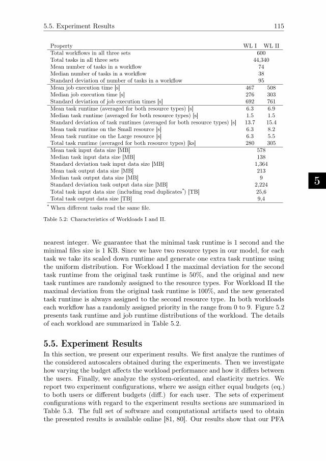
5.5. Experiment Results

5

115

Property WL I WL IITotal workflows in all three sets 600Total tasks in all three sets 44,340Mean number of tasks in a workflow 74Median number of tasks in a workflow 38Standard deviation of number of tasks in a workflow 95Mean job execution time [s] 467 508Median job execution time [s] 276 303Standard deviation of job execution times [s] 692 761Mean task runtime (averaged for both resource types) [s] 6.3 6.9Median task runtime (averaged for both resource types) [s] 1.5 1.5Standard deviation of task runtimes (averaged for both resource types) [s] 13.7 15.4Mean task runtime on the Small resource [s] 6.3 8.2Mean task runtime on the Large resource [s] 6.3 5.5Total task runtime (averaged for both resource types) [ks] 280 305Mean task input data size [MB] 578Median task input data size [MB] 138Standard deviation task input data size [MB] 1,364Mean task output data size [MB] 213Median task output data size [MB] 9Standard deviation task output data size [MB] 2,224Total task input data size (including read duplicates*) [TB] 25,6Total task output data size [TB] 9,4

* When different tasks read the same file.

Table 5.2: Characteristics of Workloads I and II.

nearest integer. We guarantee that the minimal task runtime is 1 second and theminimal files size is 1 KB. Since we have two resource types in our model, for eachtask we take its scaled down runtime and generate one extra task runtime usingthe uniform distribution. For Workload I the maximal deviation for the secondtask runtime from the original task runtime is 50%, and the original and newtask runtimes are randomly assigned to the resource types. For Workload II themaximal deviation from the original task runtime is 100%, and the new generatedtask runtime is always assigned to the second resource type. In both workloadseach workflow has a randomly assigned priority in the range from 0 to 9. Figure 5.2presents task runtime and job runtime distributions of the workload. The detailsof each workload are summarized in Table 5.2.

5.5. Experiment ResultsIn this section, we present our experiment results. We first analyze the runtimes ofthe considered autoscalers obtained during the experiments. Then we investigatehow varying the budget affects the workload performance and how it differs betweenthe users. Finally, we analyze the system-oriented, and elasticity metrics. Wereport two experiment configurations, where we assign either equal budgets (eq.)to both users or different budgets (diff.) for each user. The sets of experimentconfigurations with regard to the experiment results sections are summarized inTable 5.3. The full set of software and computational artifacts used to obtainthe presented results is available online [81, 80]. Our results show that our PFA

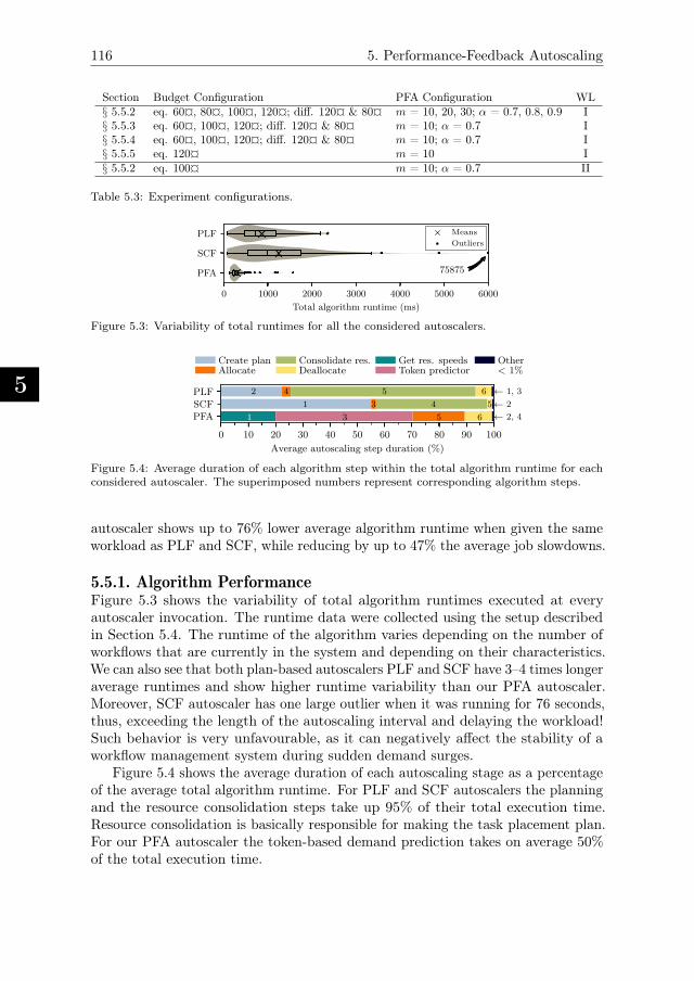
5

116 5. Performance-Feedback Autoscaling

Section Budget Configuration PFA Configuration WL§ 5.5.2 eq. 60¤, 80¤, 100¤, 120¤; diff. 120¤ & 80¤ m = 10, 20, 30; α = 0.7, 0.8, 0.9 I§ 5.5.3 eq. 60¤, 100¤, 120¤; diff. 120¤ & 80¤ m = 10; α = 0.7 I§ 5.5.4 eq. 60¤, 100¤, 120¤; diff. 120¤ & 80¤ m = 10; α = 0.7 I§ 5.5.5 eq. 120¤ m = 10 I§ 5.5.2 eq. 100¤ m = 10; α = 0.7 II

Table 5.3: Experiment configurations.

0 1000 2000 3000 4000 5000 6000

Total algorithm runtime (ms)

PLF

SCF

PFA 75875

Means

Outliers

Figure 5.3: Variability of total runtimes for all the considered autoscalers.

0 10 20 30 40 50 60 70 80 90 100

Average autoscaling step duration (%)

PLFSCFPFA

2 4 5 6 ← 1, 3

1 3 4 5← 2

1 3 5 6 ← 2, 4

Create planAllocate

Consolidate res.Deallocate

Get res. speedsToken predictor

Other< 1%

Figure 5.4: Average duration of each algorithm step within the total algorithm runtime for eachconsidered autoscaler. The superimposed numbers represent corresponding algorithm steps.

autoscaler shows up to 76% lower average algorithm runtime when given the sameworkload as PLF and SCF, while reducing by up to 47% the average job slowdowns.

5.5.1. Algorithm PerformanceFigure 5.3 shows the variability of total algorithm runtimes executed at everyautoscaler invocation. The runtime data were collected using the setup describedin Section 5.4. The runtime of the algorithm varies depending on the number ofworkflows that are currently in the system and depending on their characteristics.We can also see that both plan-based autoscalers PLF and SCF have 3–4 times longeraverage runtimes and show higher runtime variability than our PFA autoscaler.Moreover, SCF autoscaler has one large outlier when it was running for 76 seconds,thus, exceeding the length of the autoscaling interval and delaying the workload!Such behavior is very unfavourable, as it can negatively affect the stability of aworkflow management system during sudden demand surges.

Figure 5.4 shows the average duration of each autoscaling stage as a percentageof the average total algorithm runtime. For PLF and SCF autoscalers the planningand the resource consolidation steps take up 95% of their total execution time.Resource consolidation is basically responsible for making the task placement plan.For our PFA autoscaler the token-based demand prediction takes on average 50%of the total execution time.

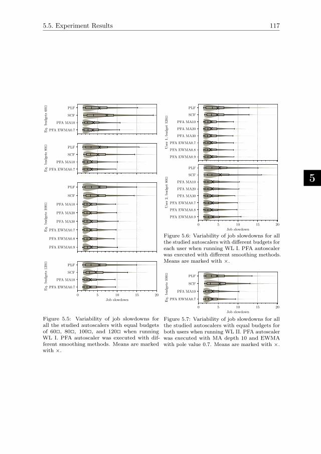
5.5. Experiment Results

5

117

PLF

SCF

PFA MA10

PFA EWMA0.7Eq.budgets60¤

PLF

SCF

PFA MA10

PFA EWMA0.7Eq.budgets80¤

PLF

SCF

PFA MA10

PFA MA20

PFA MA30

PFA EWMA0.7

PFA EWMA0.8

PFA EWMA0.9

Eq.budgets100¤

0 5 10 15 20

Job slowdown

PLF

SCF

PFA MA10

PFA EWMA0.7

Eq.budgets120¤

Figure 5.5: Variability of job slowdowns forall the studied autoscalers with equal budgetsof 60¤, 80¤, 100¤, and 120¤ when runningWL I. PFA autoscaler was executed with dif-ferent smoothing methods. Means are markedwith ×.

PLF

SCF

PFA MA10

PFA MA20

PFA MA30

PFA EWMA0.7

PFA EWMA0.8

PFA EWMA0.9

User1,budget

120¤

0 5 10 15 20

Job slowdown

PLF

SCF

PFA MA10

PFA MA20

PFA MA30

PFA EWMA0.7

PFA EWMA0.8

PFA EWMA0.9

User2,budget

80¤

Figure 5.6: Variability of job slowdowns for allthe studied autoscalers with different budgets foreach user when running WL I. PFA autoscalerwas executed with different smoothing methods.Means are marked with ×.

0 5 10 15 20

Job slowdown

PLF

SCF

PFA MA10

PFA EWMA0.7

Eq.budgets100¤

Figure 5.7: Variability of job slowdowns for allthe studied autoscalers with equal budgets forboth users when running WL II. PFA autoscalerwas executed with MA depth 10 and EWMAwith pole value 0.7. Means are marked with ×.

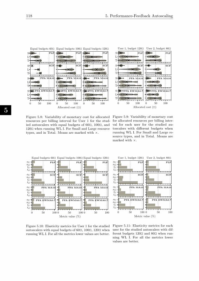
5

118 5. Performance-Feedback Autoscaling

T

L

S PLF

Equal budgets 60¤

T

L

S SCF

T

L

S PFA MA10

0 50 100

T

L

S PFA EWMA0.7

PLF

Equal budgets 100¤

SCF

PFA MA10

0 50 100

Allocated cost (¤)

PFA EWMA0.7

PLF

Equal budgets 120¤

SCF

PFA MA10

0 50 100

PFA EWMA0.7

Figure 5.8: Variability of monetary cost for allocatedresources per billing interval for User 1 for the stud-ied autoscalers with equal budgets of 60¤, 100¤, and120¤ when running WL I. For Small and Large resourcetypes, and in Total. Means are marked with ×.

T

L

S PLF

User 1, budget 120¤

PLF

User 2, budget 80¤

T

L

S SCF SCF

T

L

S PFA MA10 PFA MA10

0 50 100

T

L

S PFA EWMA0.7

0 50 100

PFA EWMA0.7

0.0 0.2 0.4 0.6 0.8 1.0

Allocated cost (¤)

0.0

0.2

0.4

0.6

0.8

1.0

Figure 5.9: Variability of monetary costfor allocated resources per billing inter-val for each user for the studied au-toscalers with different budgets whenrunning WL I. For Small and Large re-source types, and in Total. Means aremarked with ×.

aUaOtUtO

PLF

Equal budgets 60¤

aUaOtUtO

SCF

aUaOtUtO

PFA MA10

0 50 100

aUaOtUtO

PFA EWMA0.7

PLF

Equal budgets 100¤

SCF

PFA MA10

0 50 100

Metric value (%)

PFA EWMA0.7

PLF

Equal budgets 120¤

SCF

PFA MA10

0 50 100

PFA EWMA0.7

Figure 5.10: Elasticity metrics for User 1 for the studiedautoscalers with equal budgets of 60¤, 100¤, 120¤ whenrunning WL I. For all the metrics lower values are better.

aUaOtUtO

PLF

User 1, budget 120¤

aUaOtUtO

SCF

aUaOtUtO

PFA MA10

0 50 100

aUaOtUtO

PFA EWMA0.7

PLF

User 2, budget 80¤

SCF

PFA MA10

0 50 100

PFA EWMA0.7

Metric value (%)

Figure 5.11: Elasticity metrics for eachuser for the studied autoscalers with dif-ferent budgets 120¤ and 80¤ when run-ning WL I. For all the metrics lowervalues are better.

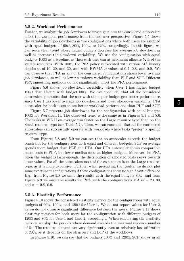
5.5. Experiment Results

5

119

5.5.2. Workload PerformanceFurther, we analyze the job slowdowns to investigate how the considered autoscalersaffect the workload performance from the end-user perspective. Figure 5.5 showsthe variability of job slowdowns in two configurations where both users are assignedwith equal budgets of 60¤, 80¤, 100¤, or 120¤, accordingly. In this figure, wecan see a clear trend where higher budgets decrease the average job slowdown aswell as decrease the slowdown variability. We use the configuration with equalbudgets 100¤ as a baseline, as then each user can at maximum allocate 52% of thesystem resources. With 100¤, the PFA policy is executed with various MA historydepths m of 10, 20, and 30, and with EWMA α values of 0.7, 0.8, and 0.9. Wecan observe that PFA in any of the considered configurations shows lower averagejob slowdowns, as well as lower slowdown variability than PLF and SCF. DifferentPFA smoothing methods do not significantly affect the PFA performance.

Figure 5.6 shows job slowdown variability when User 1 has higher budget120¤ than User 2 with budget 80¤. We can conclude, that all the consideredautoscalers guarantee that the user with the higher budget gets better performance,since User 1 has lower average job slowdowns and lower slowdown variability. PFAautoscaler for both users shows better workload performance than PLF and SCF.

Figure 5.7 presents job slowdowns for the configuration with equal budgets100¤ for Workload II. The observed trend is the same as in Figures 5.5 and 5.6.The tasks in WL II on average run faster on the Large resource type than on theSmall resource type (see Table 5.2). Thus, we can conclude, that all the consideredautoscalers can successfully operate with workloads where tasks “prefer” a specificresource type.

From Figures 5.8 and 5.9 we can see that no autoscaler exceeds the budgetconstraint for the configurations with equal and different budgets. SCF on averagespends more budget than PLF and PFA. Our PFA autoscaler shows comparablemean costs to PLF, but lower median costs at higher budgets. Moreover, for PFA,when the budget is large enough, the distribution of allocated costs skews towardslower values. For all the autoscalers most of the cost comes from the Large resourcetype, as it is more expensive. Further, when presenting the results, we do not plotsome experiment configurations if these configurations show no significant difference.E.g., from Figure 5.8 we omit the results with the equal budgets 80¤, and fromFigure 5.9 we omit the results for PFA with the configurations MA m = 20, 30,and α = 0.8, 0.9.

5.5.3. Elasticity PerformanceFigure 5.10 shows the considered elasticity metrics for the configurations with equalbudgets of 60¤, 100¤, and 120¤ for User 1. We do not report values for User 2,as we do not observe significant difference between the users. Figure 5.11 showselasticity metrics for both users for the configuration with different budgets of120¤ and 80¤ for User 1 and User 2, accordingly. When calculating the elasticitymetrics, we skip the periods where demand exceeds the maximal resource numberof 64. The resource demand can vary significantly even at relatively low utilizationof 20%, as it depends on the structure and LoP of the workflows.

In Figure 5.10, we can see that for budgets 100¤ and 120¤, SCF shows in all

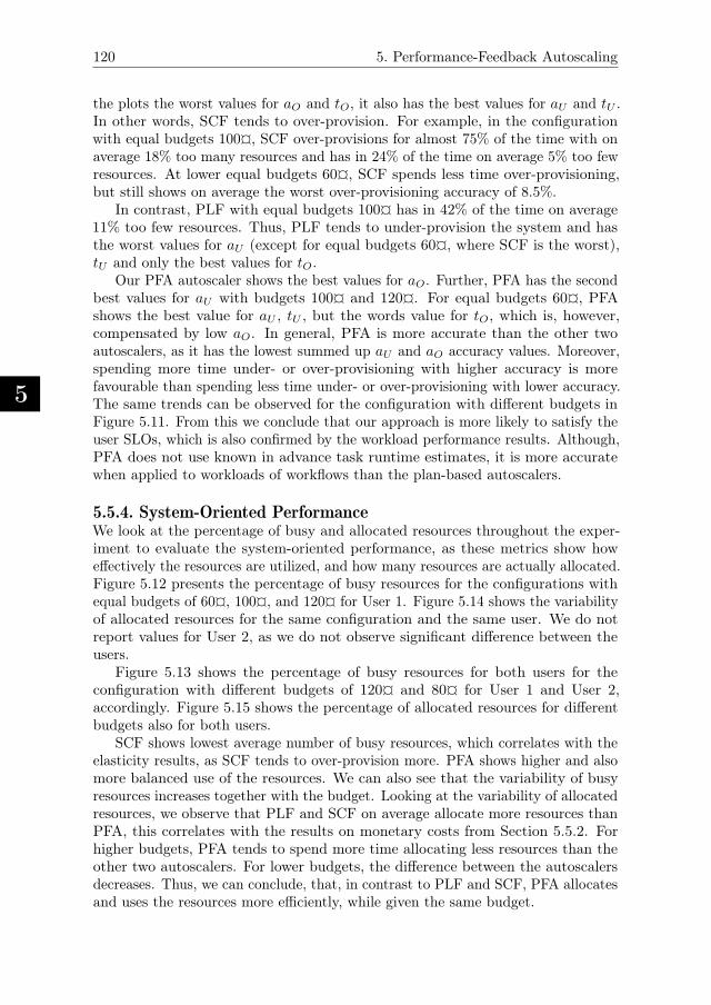
5

120 5. Performance-Feedback Autoscaling

the plots the worst values for aO and tO, it also has the best values for aU and tU .In other words, SCF tends to over-provision. For example, in the configurationwith equal budgets 100¤, SCF over-provisions for almost 75% of the time with onaverage 18% too many resources and has in 24% of the time on average 5% too fewresources. At lower equal budgets 60¤, SCF spends less time over-provisioning,but still shows on average the worst over-provisioning accuracy of 8.5%.

In contrast, PLF with equal budgets 100¤ has in 42% of the time on average11% too few resources. Thus, PLF tends to under-provision the system and hasthe worst values for aU (except for equal budgets 60¤, where SCF is the worst),tU and only the best values for tO.

Our PFA autoscaler shows the best values for aO. Further, PFA has the secondbest values for aU with budgets 100¤ and 120¤. For equal budgets 60¤, PFAshows the best value for aU , tU , but the words value for tO, which is, however,compensated by low aO. In general, PFA is more accurate than the other twoautoscalers, as it has the lowest summed up aU and aO accuracy values. Moreover,spending more time under- or over-provisioning with higher accuracy is morefavourable than spending less time under- or over-provisioning with lower accuracy.The same trends can be observed for the configuration with different budgets inFigure 5.11. From this we conclude that our approach is more likely to satisfy theuser SLOs, which is also confirmed by the workload performance results. Although,PFA does not use known in advance task runtime estimates, it is more accuratewhen applied to workloads of workflows than the plan-based autoscalers.

5.5.4. System-Oriented PerformanceWe look at the percentage of busy and allocated resources throughout the exper-iment to evaluate the system-oriented performance, as these metrics show howeffectively the resources are utilized, and how many resources are actually allocated.Figure 5.12 presents the percentage of busy resources for the configurations withequal budgets of 60¤, 100¤, and 120¤ for User 1. Figure 5.14 shows the variabilityof allocated resources for the same configuration and the same user. We do notreport values for User 2, as we do not observe significant difference between theusers.

Figure 5.13 shows the percentage of busy resources for both users for theconfiguration with different budgets of 120¤ and 80¤ for User 1 and User 2,accordingly. Figure 5.15 shows the percentage of allocated resources for differentbudgets also for both users.

SCF shows lowest average number of busy resources, which correlates with theelasticity results, as SCF tends to over-provision more. PFA shows higher and alsomore balanced use of the resources. We can also see that the variability of busyresources increases together with the budget. Looking at the variability of allocatedresources, we observe that PLF and SCF on average allocate more resources thanPFA, this correlates with the results on monetary costs from Section 5.5.2. Forhigher budgets, PFA tends to spend more time allocating less resources than theother two autoscalers. For lower budgets, the difference between the autoscalersdecreases. Thus, we can conclude, that, in contrast to PLF and SCF, PFA allocatesand uses the resources more efficiently, while given the same budget.

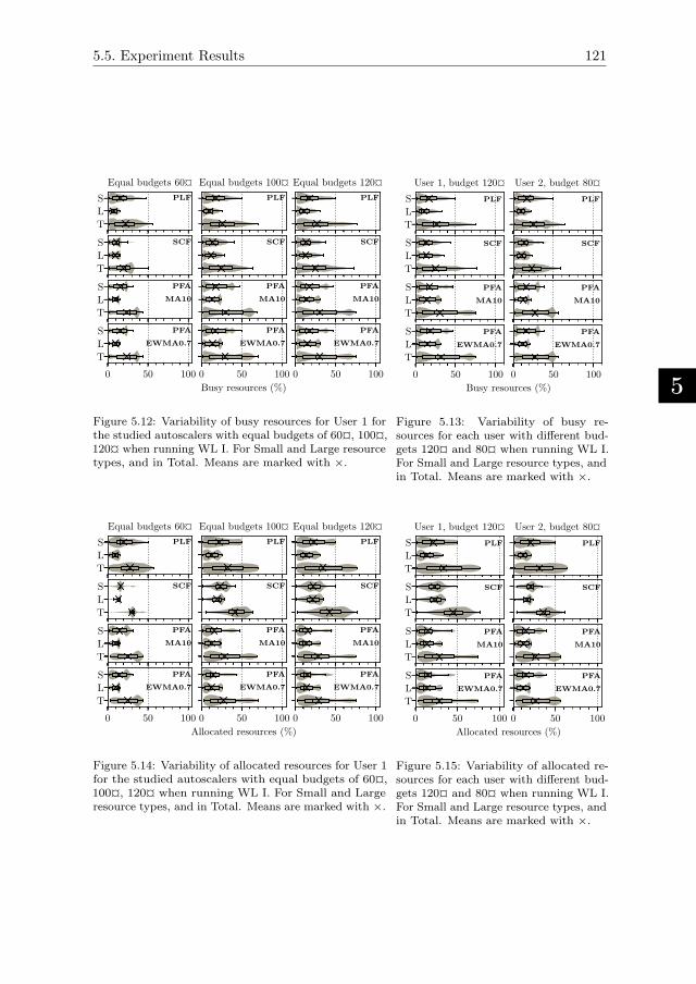
5.5. Experiment Results

5

121

T

L

S PLF

Equal budgets 60¤

T

L

S SCF

T

L

S PFA

MA10

0 50 100

T

L

S PFA

EWMA0.7

PLF

Equal budgets 100¤

SCF

PFA

MA10

0 50 100

Busy resources (%)

PFA

EWMA0.7

PLF

Equal budgets 120¤

SCF

PFA

MA10

0 50 100

PFA

EWMA0.7

Figure 5.12: Variability of busy resources for User 1 forthe studied autoscalers with equal budgets of 60¤, 100¤,120¤ when running WL I. For Small and Large resourcetypes, and in Total. Means are marked with ×.

T

L

S PLF

User 1, budget 120¤

PLF

User 2, budget 80¤

T

L

S SCF SCF

T

L

S PFA

MA10

PFA

MA10

0 50 100

T

L

S PFA

EWMA0.7

0 50 100

PFA

EWMA0.7

0.0 0.2 0.4 0.6 0.8 1.0

Busy resources (%)

0.0

0.2

0.4

0.6

0.8

1.0

Figure 5.13: Variability of busy re-sources for each user with different bud-gets 120¤ and 80¤ when running WL I.For Small and Large resource types, andin Total. Means are marked with ×.

T

L

S PLF

Equal budgets 60¤

T

L

S SCF

T

L

S PFA

MA10

0 50 100

T

L

S PFA

EWMA0.7

PLF

Equal budgets 100¤

SCF

PFA

MA10

0 50 100

Allocated resources (%)

PFA

EWMA0.7

PLF

Equal budgets 120¤

SCF

PFA

MA10

0 50 100

PFA

EWMA0.7

Figure 5.14: Variability of allocated resources for User 1for the studied autoscalers with equal budgets of 60¤,100¤, 120¤ when running WL I. For Small and Largeresource types, and in Total. Means are marked with ×.

T

L

S PLF

User 1, budget 120¤

PLF

User 2, budget 80¤

T

L

S SCF SCF

T

L

S PFA

MA10

PFA

MA10

0 50 100

T

L

S PFA

EWMA0.7

0 50 100

PFA

EWMA0.7

0.0 0.2 0.4 0.6 0.8 1.0

Allocated resources (%)

0.0

0.2

0.4

0.6

0.8

1.0

Figure 5.15: Variability of allocated re-sources for each user with different bud-gets 120¤ and 80¤ when running WL I.For Small and Large resource types, andin Total. Means are marked with ×.

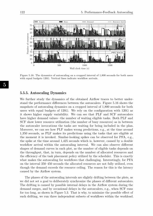
5

122 5. Performance-Feedback Autoscaling

0

25

50

75PLF

Supply Busy Demand Resource limit

0

25

50

75

Number

ofresources

SCF

0 500 1000 1500

Wall clock time (s)

0

25

50

75PFA MA10

Figure 5.16: The dynamics of autoscaling on a cropped interval of 1,800 seconds for both userswith equal budgets 120¤. Vertical lines indicate workflow arrivals.

5.5.5. Autoscaling Dynamics

We further study the dynamics of the obtained Airflow traces to better under-stand the performance differences between the autoscalers. Figure 5.16 shows thesnapshots of autoscaling dynamics on a cropped interval of 1,800 seconds for bothusers with equal budgets of 120¤. We rely on the configuration with 120¤ asit shows higher supply variability. We can see that PLF and SCF autoscalershave higher demand values—the number of waiting eligible tasks. Both PLF andSCF show lower resource utilization (the number of busy resources) as in betweenthe autoscaler invocations the tasks are waiting for being included in the plan.Moreover, we can see how PLF makes wrong predictions, e.g., at the time around1,350 seconds, as PLF makes its predictions using the tasks that are eligible atthe moment it is invoked. Similar-looking spikes can be observed for PFA, e.g.,the spike at the time around 1,425 seconds which is, however, caused by a doubleworkflow arrival within the autoscaling interval. We can also observe differentshapes of demand curves in each plot, as the number of eligible tasks depends onthe throughput, that, in turn, depends on the number of allocated resources andthe efficiency of the task placement policy utilized by the scheduler. This is exactlywhat makes the autoscaling for workflows that challenging. Interestingly, for PFAon the interval 350–450 seconds the allocated resources are not fully utilized, eventhough the demand exceeds the resource ceiling. The reason for this is the latencycaused by the Airflow system.

The phases of the autoscaling intervals are slightly drifting between the plots, aswe did not set a goal to deliberately synchronize the phases of different autoscalers.The drifting is caused by possible internal delays in the Airflow system during thedemand surges, and by occasional delays in the autoscalers, e.g., when SCF runsfor too long, as shown in Figure 5.3. That is why, to minimize the possible effect ofsuch drifting, we run three independent subsets of workflows within the workload.

5.6. The Optimal Solution

5

123

T The set of time slots T = {1, 2, . . . , T}W The set of workflows W = {1, 2, . . . ,W}S The set of workflows tasks S = {1, 2, . . . , S}M The set of billing intervals M = {1, 2, . . . ,M}V The set of resources V = {1, 2, . . . , V }L Number of time slots per billing intervalB Budget per billing intervalAw Arrival time of workflow wCw Critical path length of workflow wDw Earliest possible completion time for workflow wRj,k Runtime of task j on resource kPk Cost of running resource k on a billing intervalli,j Equals one if task i depends on task jhw(t) The value of workflow w finishing at time txtj,k Binary variable, equals one if task j starts at time t on resource k

ymk Binary variable, equals one if resource k is active on billing interval mzmk Integer variable, determines the number of active time slots for resource

k on billing interval mutw Binary variable, equals one if workflow w finishes at time t

Table 5.4: Symbols used for the MIP model.

5.6. The Optimal SolutionIn this section, to validate the performance of the considered policies, we comparethe results obtained from the Airflow system with the optimal solution obtainedfrom solving the optimization problem represented as a Mixed Integer Programming(MIP) model. For that, we modify the MIP model proposed by Wang et al. [164] toincorporate budget constraints, while following the similar notation, and implementthe model in the Gurobi [14] solver (v. 8.0.1). The symbols used for describingthe MIP model are presented in Table 5.4. The goal of the solver is to find theoptimal plan which, under the budget and resource constraints, finds the taskplacement plan and determines the number of resources of each type that should beallocated on each autoscaling interval, so that the response time of each workflowis minimized.

5.6.1. Mixed Integer Programming Model

The MIP model presents time as a set T = {1, 2, . . . , T} of discrete time slots ofequal duration, where T is the furthest time horizon. The time slots are groupedinto M billing intervals. Each billing interval consists of L time slots. The set ofbilling intervals is denoted by M = {1, 2, . . . ,M}, and T is divisible by L, so thatM = T/L. The budget B is given per billing interval and should not be exceeded.The input of the problem is a set of workflows W = {1, 2, . . . ,W}, where eachworkflow contains tasks. All the tasks in all the workflows are represented by theset S = {1, 2, . . . , S}, where each task can belong to a single workflow only. Thetask precedence constraints are represented by a binary matrix (li,j), ∀i, j ∈ S,where li,j = 1 if task i depends on task j, i.e., i can start only after j has finished,

5

124 5. Performance-Feedback Autoscaling

and li,j = 0 otherwise. By convention, each li,i = 0. Each workflow w has an arrivaltime Aw, known in advance length Cw of its critical path, and earliest possiblecompletion time Dw, so that Dw = Aw + Cw − 1. The model also defines a set ofcomputing resources V = {1, 2, . . . , V }.

If a task is scheduled on a resource, it runs on it exclusively until completion. Torepresent the task assignment, we use binary decision variables xt

j,k, where xtj,k = 1

if task i is scheduled to run on resource k starting at time slot t, and xtj,k = 0

otherwise. Each task should start only once, which we specify as follows:

∑

k∈V

∑

t∈T

xtj,k = 1, ∀j ∈ S. (5.15)

Let the integer variable 0 ≤ zmk ≤ L denote the number of active time slots on eachresource k on billing interval m. This requires the following constraints:

m·L∑

t=(m−1)·L+1

∑

j∈S

t∑

r=max(1,t−Rj,k+1)

xrj,k = zmk , ∀k ∈ V, ∀m ∈ M. (5.16)

Let the binary variable ymk denote the active/idle state of each resource k on billinginterval m, with ymk = 1 if some tasks are assigned on the resource, and ymk = 0otherwise. If the resource has no tasks scheduled, it is considered deallocated,however, if even a single task is assigned to the resource, it is considered active.Accordingly, we define the following constraints:

ymk = min(1, zmk ), ∀k ∈ V, ∀m ∈ M. (5.17)

The tasks are not allowed to overlap, i.e., for each time slot and each resourceat most one task is allowed to occupy the time slot on that resource. Let Rj,k

denote the running time of task j on resource k which is known in advance. Thenon-overlapping constraints are specified as follows:

∑

j∈S

t∑

r=max(1,t−Rj,k+1)

xrj,k ≤ 1, ∀k ∈ V, ∀t ∈ T . (5.18)

The precedence constraints are formulated as follows:(

∑

k∈V

∑

t∈T

t · xti,k −

∑

k∈V

∑

t∈T

(t+Rj,k) · xtj,k

)

· li,j ≥ 0,

∀i, j ∈ S.(5.19)

Further, we formulate the constraints that no task of any workflow can be scheduledto start before its arrival time:

∑

k∈V

∑

t∈T

t · xtj,k ≥ Aw, ∀w ∈ W, ∀j ∈ w. (5.20)

Since the optimization goal is to minimize the workflow response time within thegiven budget, we represent it as a profit maximization problem where higher profit

5.6. The Optimal Solution

5

125

corresponds to a shorter response time. For that, let hw : {1, 2, . . .} → R be anon-increasing value function, where hw(t) represents the value gained dependingon the time slot t where the workflow w is finished:

hw(t) =

{

1, if t ≤ Dw,

Dw − t, otherwise.(5.21)

For each workflow w and each time t we define a binary variable utw, where ut

w = 1if workflow w is completed at time t. Since each workflow can finish only once, weformulate the following constraints:

∑

t∈T

utw = 1, ∀w ∈ W. (5.22)

The completion time of the workflow can be written as∑

t∈T t · utw. Accordingly,

the constraints that all the tasks of a workflow w are completed by the workflowcompletion time can be formulated as follows:

∑

k∈V

∑

t∈T

(t+Rj,k − 1) · xtj,k ≤

∑

t∈T

t · utw, ∀w ∈ W, ∀j ∈ w. (5.23)

Let Pk be the cost of resource k, then the budget constraints are defined as follows:

∑

k∈V

Pk · ymk ≤ B, ∀m ∈ M. (5.24)

Finally, we can formulate the profit maximization objective:

max∑

w∈W

∑

t∈T

hw(t) · utw

s.t. (5.15)(5.16)(5.17)(5.18)(5.19)(5.20)(5.22)(5.23)(5.24).

(5.25)

5.6.2. Heuristics vs. the Optimal SolutionWe use three subsets of five workflows each from Workload I, submitted with afixed interval of 30 seconds in a system with 16 resources (vs. 64 resources in otherexperiments) of two types with 8 resources in each. For this reason, the maximalbudget required to allocate all the system resources is 48¤. The first group of fiveworkflows consists of one Montage, one SIPHT, and three LIGO workflows, with 183tasks in total. The second group contains one Montage, two SIPHT and two LIGOworkflows, with 241 tasks in total. The third group contains two Montage, oneSIPHT, and two LIGO workflows with 199 tasks in total. Further, we refer to these15 workflows as the MIP workload. We limit the number of considered workflowsand limit the number of resources due to much higher expected computational effortfor finding the optimal solution versus the considered heuristic approaches. To makethe workflows compatible with the MIP model, we round their task runtimes to 5seconds, which is the duration of the time slot in the MIP model, and set the sizesof all the exchanged files to zero to make the comparison more fair. We configurethe MIP model with 16, 18, or 19 billing intervals (depending on the workload

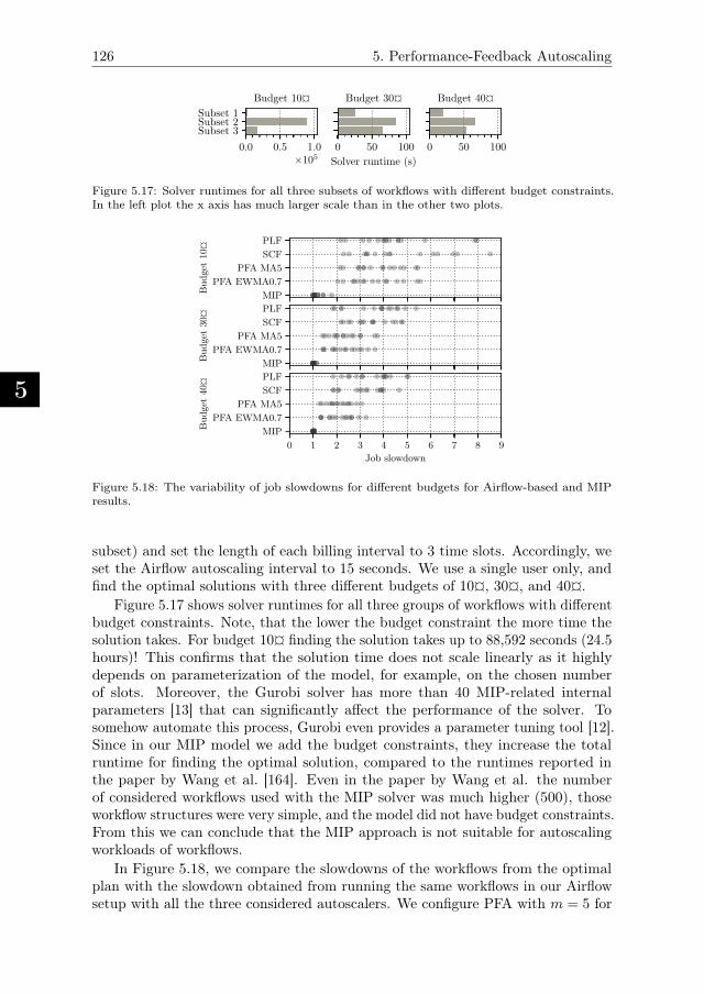
5

126 5. Performance-Feedback Autoscaling

0.0 0.5 1.0×105

Subset 1Subset 2Subset 3

Budget 10¤

0 50 100

Solver runtime (s)

Budget 30¤

0 50 100

Budget 40¤

Figure 5.17: Solver runtimes for all three subsets of workflows with different budget constraints.In the left plot the x axis has much larger scale than in the other two plots.

PLF

SCF

PFA MA5

PFA EWMA0.7

MIPBudget

10¤

PLF

SCF

PFA MA5

PFA EWMA0.7

MIPBudget

30¤

0 1 2 3 4 5 6 7 8 9

Job slowdown

PLF

SCF

PFA MA5

PFA EWMA0.7

MIPBudget

40¤

Figure 5.18: The variability of job slowdowns for different budgets for Airflow-based and MIPresults.

subset) and set the length of each billing interval to 3 time slots. Accordingly, weset the Airflow autoscaling interval to 15 seconds. We use a single user only, andfind the optimal solutions with three different budgets of 10¤, 30¤, and 40¤.

Figure 5.17 shows solver runtimes for all three groups of workflows with differentbudget constraints. Note, that the lower the budget constraint the more time thesolution takes. For budget 10¤ finding the solution takes up to 88,592 seconds (24.5hours)! This confirms that the solution time does not scale linearly as it highlydepends on parameterization of the model, for example, on the chosen numberof slots. Moreover, the Gurobi solver has more than 40 MIP-related internalparameters [13] that can significantly affect the performance of the solver. Tosomehow automate this process, Gurobi even provides a parameter tuning tool [12].Since in our MIP model we add the budget constraints, they increase the totalruntime for finding the optimal solution, compared to the runtimes reported inthe paper by Wang et al. [164]. Even in the paper by Wang et al. the numberof considered workflows used with the MIP solver was much higher (500), thoseworkflow structures were very simple, and the model did not have budget constraints.From this we can conclude that the MIP approach is not suitable for autoscalingworkloads of workflows.

In Figure 5.18, we compare the slowdowns of the workflows from the optimalplan with the slowdown obtained from running the same workflows in our Airflowsetup with all the three considered autoscalers. We configure PFA with m = 5 for

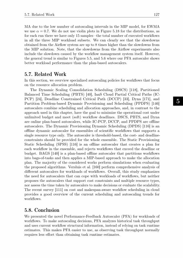
5.7. Related Work

5

127

MA due to the low number of autoscaling intervals in the MIP model, for EWMAwe use α = 0.7. We do not use violin plots in Figure 5.18 for the distributions, asfor each run there we have only 15 samples—the total number of executed workflowsin all the three MIP workload subsets. We can clearly see that the slowdownsobtained from the Airflow system are up to 8 times higher than the slowdowns fromthe MIP solution. Note, that the slowdowns from the Airflow experiments alsoinclude the slowdown caused by the workflow management system itself. However,the general trend is similar to Figures 5.5, and 5.6 where our PFA autoscaler showsbetter workload performance than the plan-based autoscalers.

5.7. Related WorkIn this section, we overview specialized autoscaling policies for workflows that focuson the resource allocation problem.

The Dynamic Scaling Consolidation Scheduling (DSCS) [118], PartitionedBalanced Time Scheduling (PBTS) [40], IaaS Cloud Partial Critical Paths (IC-PCP) [24], Deadline Constrained Critical Path (DCCP) [33], Dyna [171], andPartition Problem-based Dynamic Provisioning and Scheduling (PPDPS) [146]autoscalers combine scheduling and allocation approaches, and, in contrast to theapproach used in this chapter, have the goal to minimize the operational cost underunlimited budget and meet (soft) workflow deadlines. DSCS, PBTS, and Dynaare online plan-based autoscalers, while IC-PCP, DCCP, and PPDPS are offlineautoscalers. The Dynamic Provisioning Dynamic Scheduling (DPDS) [116] is anoffline dynamic autoscaler for ensembles of scientific workflows that supports asingle resource type only. The autoscaler is threshold-based, the cost- and deadline-constraints should be provided for the whole ensemble. The Static ProvisioningStatic Scheduling (SPSS) [116] is an offline autoscaler that creates a plan foreach workflow in the ensemble, and rejects workflows that exceed the deadline orbudget. BAGS [140] is a plan-based offline autoscaler that partitions workflowsinto bags-of-tasks and then applies a MIP-based approach to make the allocationplan. The majority of the considered works perform simulations when evaluatingthe proposed algorithms. Versluis et al. [160] perform comprehensive analysis ofdifferent autoscalers for workloads of workflows. Overall, this study emphasizesthe need for autoscalers that can cope with workloads of workflows, but neitherproposes the autoscalers that support cost constraints and multiple resource types,nor assess the time taken by autoscalers to make decisions or evaluate the scalability.The recent survey [111] on cost and makespan-aware workflow scheduling in cloudprovides a good overview of the current scheduling and autoscaling trends forworkflows.

5.8. ConclusionWe presented the novel Performance-Feedback Autoscaler (PFA) for workloads ofworkflows. To make autoscaling decisions, PFA analyzes historical task throughputand uses current workflow structural information, instead of relying on task runtimeestimates. This makes PFA easier to use, as observing task throughput normallyrequires less effort than obtaining task runtime estimates.

5

128 5. Performance-Feedback Autoscaling

Overall, PFA has lower time-complexity and effectively minimizes workflowslowdowns, compared to two state-of-the-art online plan-based autoscalers. Ourreal-world experiments with the Apache Airflow workflow management system showthat PFA, compared to other two autoscalers, has better applicability potentialdue to its good scalability when dealing with possible demand surges, and goodend-user and system-oriented characteristics.

6

Conclusion

In this dissertation, we have studied the problem of online scheduling of workloadsof stochastically arriving workflows, both from the task placement and the re-

source allocation perspectives. We have mostly focused on designing new schedulingpolicies, but we have also adapted existing state-of-the-art policies designed forscheduling a single workflow or batches of workflows to the case of online workflowscheduling. For new policies, we have kept their implementation effort and theirapplicability in production systems in mind. Our research methods include a wideset of simulation-based and real-world experiments on the DAS-4 multicluster tothoroughly evaluate the studied policies. Additionally, we have used a mixed integerprogramming approach to validate our real-world experimental results versus theoptimal solution. Below we present our conclusions, and our suggestions for futurework.

6.1. ConclusionsWe present the following conclusions based on the three workflow schedulingchallenges (Section 1.2) and the four research questions addressed in this dissertation(Section 1.7):

1. Greedy backfilling is the best policy for scheduling workloads of workflowswith unknown task runtimes compared to policies that employ processorreservation for workflows in the queue (Chapter 2). Any form of processorreservation for workflows without runtime estimates only decreases the overallsystem performance, leading to low maximal achievable utilizations.

2. Under realistic system utilizations backfilling-based policies allow achievinggood performance even without task runtime estimates (Chapters 2 and 3).More complex scheduling policies are beneficial only at extremely high systemutilizations and for scheduling batches of workflows.

3. Inaccurate runtime estimates negatively affect the slowdowns experienced bythe workflows in the workload, but their effect is more substantial with the

129

6

130 6. Conclusion

increase of the imposed system utilization (Chapter 3). In general, at highsystem utilizations the knowledge of task runtime estimates allows to achievesignificant improvements in the average workflow slowdowns.

4. The performance-feedback mechanism used by our novel Fair Workflow Pri-oritization (FWP) task placement policy to monitor workflow slowdownshelps to achieve a fairer distribution of slowdowns among workflows in theworkload (Chapter 3). FWP shows a lower standard deviation of the workflowslowdowns compared to the state-of-the-art policies without the feedbackmechanism. The order in which the workflows are processed by a task place-ment policy is very important, as an incorrectly chosen prioritization methodcan easily destabilize the system (Chapter 3).

5. When adapted to a plan-based online scenario, the relatively simple offlineHEFT scheduling policy underperforms (Chapter 3). We believe that evenmore complex policies [142] would also suffer from this problem. In general,online plan-based policies are more vulnerable to scalability issues duringworkload surges, and are harder to implement and parallelize compared todynamic online policies with similar performance.

6. It is possible to realistically estimate the resource demand of a workflowin terms of the number of required processors when the task runtimes areunknown by using our novel token-based algorithm for approximating thelevel of parallelism (Chapters 2, 4, and 5). We have thoroughly evaluated thealgorithm both in simulations and in real-world experiments, and it shows itseffectiveness when applied to popular scientific workflow structures.

7. Although workflow-specific autoscalers have the privilege of knowing theworkflow structure in advance, it is possible for properly configured generalautoscalers without such knowledge to achieve similar performance (Chap-ter 4). The correct choice of an autoscaler and its parameters significantlydepends on the application type. To assist the end-user in choosing an au-toscaler and its parameters, we have proposed comprehensive multilateralranking methods for comparing autoscalers which showed their applicabilityfor comparing general and workflow-specific autoscalers.

8. The novel feedback-based online dynamic Performance-Feedback Autoscaler(PFA) that uses task throughput and the workflow structure to make re-source allocation decisions outperforms online plan-based policies for onlinescheduling of workflows (Chapter 5). PFA has better applicability potentialdue to its good scalability when dealing with possible demand surges, andgood end-user and system-oriented characteristics compared to the plan-basedstate-of-the-art policies. The feedback mechanism in the novel autoscaleranalyzes historical task throughput. Observing task throughput normallyrequires less effort than obtaining task runtime estimates, while allowing forfairly accurate estimation of resource speeds when dealing with workloadswith a long-tailed task runtime distribution.

9. Obtaining an optimal solution for a workflow scheduling problem with amixed integer programming approach can be used to find how much the

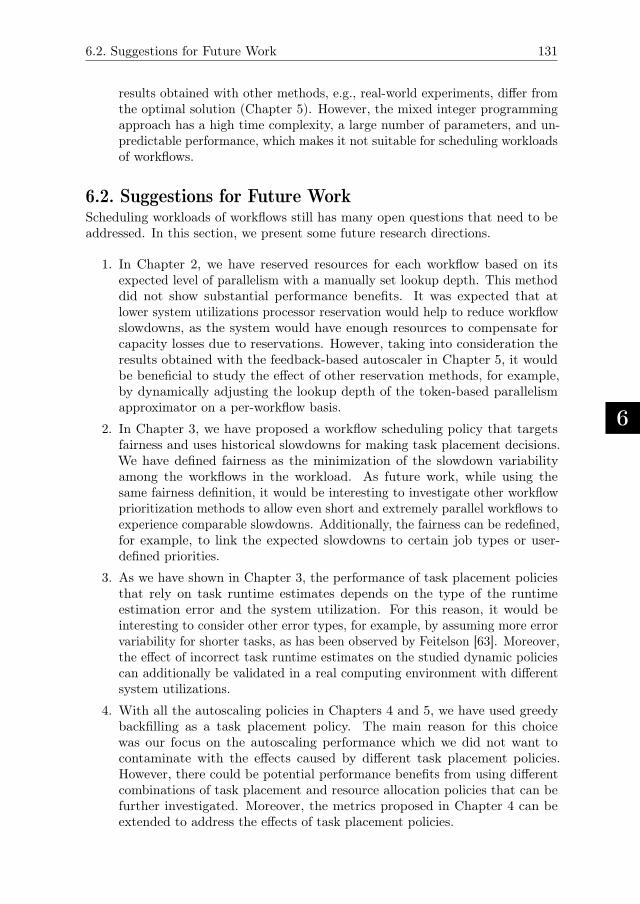
6.2. Suggestions for Future Work

6

131

results obtained with other methods, e.g., real-world experiments, differ fromthe optimal solution (Chapter 5). However, the mixed integer programmingapproach has a high time complexity, a large number of parameters, and un-predictable performance, which makes it not suitable for scheduling workloadsof workflows.

6.2. Suggestions for Future WorkScheduling workloads of workflows still has many open questions that need to beaddressed. In this section, we present some future research directions.

1. In Chapter 2, we have reserved resources for each workflow based on itsexpected level of parallelism with a manually set lookup depth. This methoddid not show substantial performance benefits. It was expected that atlower system utilizations processor reservation would help to reduce workflowslowdowns, as the system would have enough resources to compensate forcapacity losses due to reservations. However, taking into consideration theresults obtained with the feedback-based autoscaler in Chapter 5, it wouldbe beneficial to study the effect of other reservation methods, for example,by dynamically adjusting the lookup depth of the token-based parallelismapproximator on a per-workflow basis.

2. In Chapter 3, we have proposed a workflow scheduling policy that targetsfairness and uses historical slowdowns for making task placement decisions.We have defined fairness as the minimization of the slowdown variabilityamong the workflows in the workload. As future work, while using thesame fairness definition, it would be interesting to investigate other workflowprioritization methods to allow even short and extremely parallel workflows toexperience comparable slowdowns. Additionally, the fairness can be redefined,for example, to link the expected slowdowns to certain job types or user-defined priorities.

3. As we have shown in Chapter 3, the performance of task placement policiesthat rely on task runtime estimates depends on the type of the runtimeestimation error and the system utilization. For this reason, it would beinteresting to consider other error types, for example, by assuming more errorvariability for shorter tasks, as has been observed by Feitelson [63]. Moreover,the effect of incorrect task runtime estimates on the studied dynamic policiescan additionally be validated in a real computing environment with differentsystem utilizations.

4. With all the autoscaling policies in Chapters 4 and 5, we have used greedybackfilling as a task placement policy. The main reason for this choicewas our focus on the autoscaling performance which we did not want tocontaminate with the effects caused by different task placement policies.However, there could be potential performance benefits from using differentcombinations of task placement and resource allocation policies that can befurther investigated. Moreover, the metrics proposed in Chapter 4 can beextended to address the effects of task placement policies.

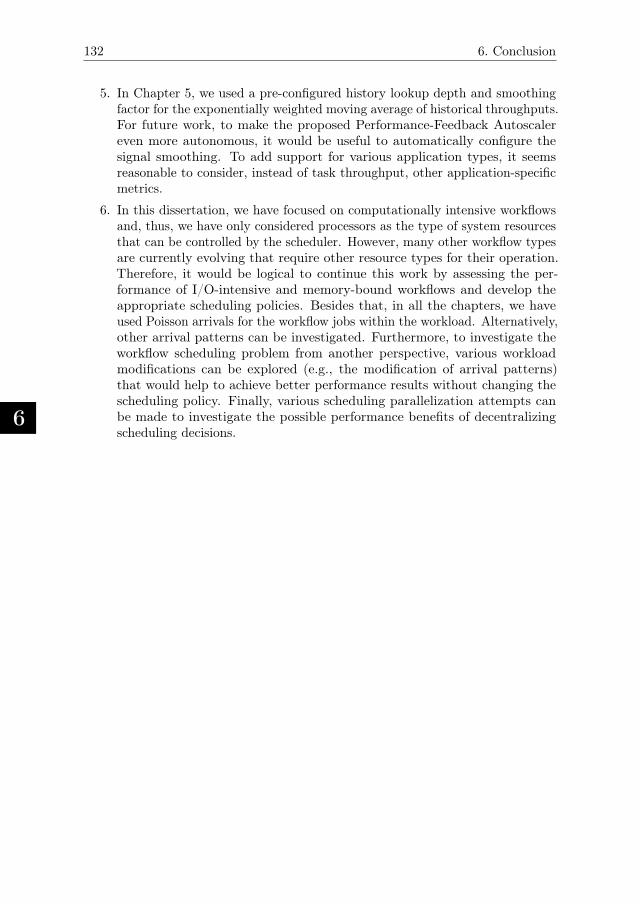
6

132 6. Conclusion

5. In Chapter 5, we used a pre-configured history lookup depth and smoothingfactor for the exponentially weighted moving average of historical throughputs.For future work, to make the proposed Performance-Feedback Autoscalereven more autonomous, it would be useful to automatically configure thesignal smoothing. To add support for various application types, it seemsreasonable to consider, instead of task throughput, other application-specificmetrics.

6. In this dissertation, we have focused on computationally intensive workflowsand, thus, we have only considered processors as the type of system resourcesthat can be controlled by the scheduler. However, many other workflow typesare currently evolving that require other resource types for their operation.Therefore, it would be logical to continue this work by assessing the per-formance of I/O-intensive and memory-bound workflows and develop theappropriate scheduling policies. Besides that, in all the chapters, we haveused Poisson arrivals for the workflow jobs within the workload. Alternatively,other arrival patterns can be investigated. Furthermore, to investigate theworkflow scheduling problem from another perspective, various workloadmodifications can be explored (e.g., the modification of arrival patterns)that would help to achieve better performance results without changing thescheduling policy. Finally, various scheduling parallelization attempts canbe made to investigate the possible performance benefits of decentralizingscheduling decisions.

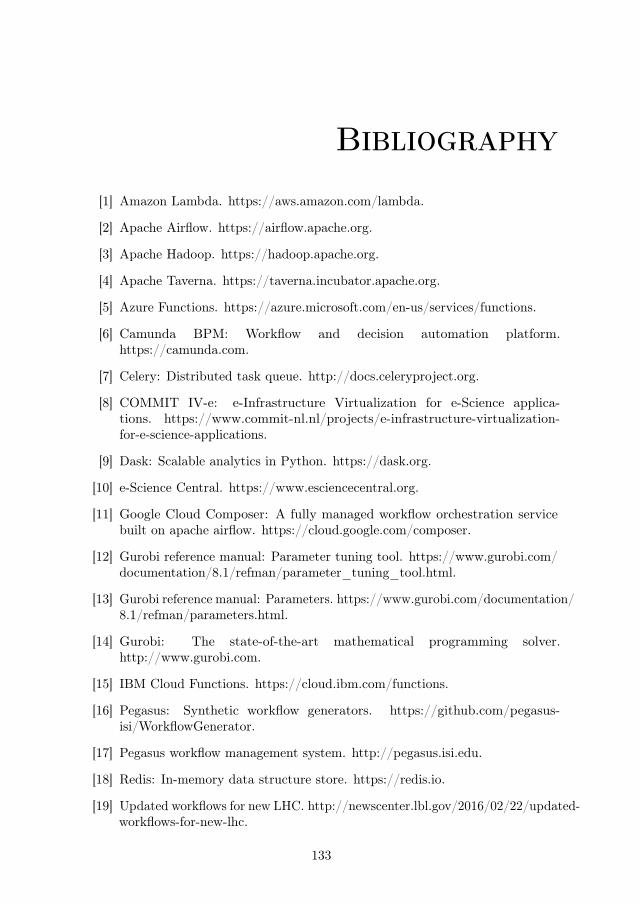
Bibliography

[1] Amazon Lambda. https://aws.amazon.com/lambda.

[2] Apache Airflow. https://airflow.apache.org.

[3] Apache Hadoop. https://hadoop.apache.org.

[4] Apache Taverna. https://taverna.incubator.apache.org.

[5] Azure Functions. https://azure.microsoft.com/en-us/services/functions.

[6] Camunda BPM: Workflow and decision automation platform.https://camunda.com.

[7] Celery: Distributed task queue. http://docs.celeryproject.org.

[8] COMMIT IV-e: e-Infrastructure Virtualization for e-Science applica-tions. https://www.commit-nl.nl/projects/e-infrastructure-virtualization-for-e-science-applications.

[9] Dask: Scalable analytics in Python. https://dask.org.

[10] e-Science Central. https://www.esciencecentral.org.

[11] Google Cloud Composer: A fully managed workflow orchestration servicebuilt on apache airflow. https://cloud.google.com/composer.

[12] Gurobi reference manual: Parameter tuning tool. https://www.gurobi.com/documentation/8.1/refman/parameter_tuning_tool.html.

[13] Gurobi reference manual: Parameters. https://www.gurobi.com/documentation/8.1/refman/parameters.html.

[14] Gurobi: The state-of-the-art mathematical programming solver.http://www.gurobi.com.

[15] IBM Cloud Functions. https://cloud.ibm.com/functions.

[16] Pegasus: Synthetic workflow generators. https://github.com/pegasus-isi/WorkflowGenerator.

[17] Pegasus workflow management system. http://pegasus.isi.edu.

[18] Redis: In-memory data structure store. https://redis.io.

[19] Updated workflows for new LHC. http://newscenter.lbl.gov/2016/02/22/updated-workflows-for-new-lhc.

133

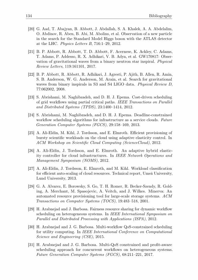
134 Bibliography

[20] G. Aad, T. Abajyan, B. Abbott, J. Abdallah, S. A. Khalek, A. A. Abdelalim,O. Abdinov, R. Aben, B. Abi, M. Abolins, et al. Observation of a new particlein the search for the Standard Model Higgs boson with the ATLAS detectorat the LHC. Physics Letters B, 716:1–29, 2012.

[21] B. P. Abbott, R. Abbott, T. D. Abbott, F. Acernese, K. Ackley, C. Adams,T. Adams, P. Addesso, R. X. Adhikari, V. B. Adya, et al. GW170817: Obser-vation of gravitational waves from a binary neutron star inspiral. PhysicalReview Letters, 119:161101, 2017.

[22] B. P. Abbott, R. Abbott, R. Adhikari, J. Agresti, P. Ajith, B. Allen, R. Amin,S. B. Anderson, W. G. Anderson, M. Arain, et al. Search for gravitationalwaves from binary inspirals in S3 and S4 LIGO data. Physical Review D,77:062002, 2008.

[23] S. Abrishami, M. Naghibzadeh, and D. H. J. Epema. Cost-driven schedulingof grid workflows using partial critical paths. IEEE Transactions on Paralleland Distributed Systems (TPDS), 23:1400–1414, 2012.

[24] S. Abrishami, M. Naghibzadeh, and D. H. J. Epema. Deadline-constrainedworkflow scheduling algorithms for infrastructure as a service clouds. FutureGeneration Computer Systems (FGCS), 29:158–169, 2013.

[25] A. Ali-Eldin, M. Kihl, J. Tordsson, and E. Elmroth. Efficient provisioning ofbursty scientific workloads on the cloud using adaptive elasticity control. InACM Workshop on Scientific Cloud Computing (ScienceCloud), 2012.

[26] A. Ali-Eldin, J. Tordsson, and E. Elmroth. An adaptive hybrid elastic-ity controller for cloud infrastructures. In IEEE Network Operations andManagement Symposium (NOMS), 2012.

[27] A. Ali-Eldin, J. Tordsson, E. Elmroth, and M. Kihl. Workload classificationfor efficient auto-scaling of cloud resources. Technical report, Umea University,Lund University, 2013.

[28] G. A. Alvarez, E. Borowsky, S. Go, T. H. Romer, R. Becker-Szendy, R. Gold-ing, A. Merchant, M. Spasojevic, A. Veitch, and J. Wilkes. Minerva: Anautomated resource provisioning tool for large-scale storage systems. ACMTransactions on Computer Systems (TOCS), 19:483–518, 2001.

[29] H. Arabnejad and J. Barbosa. Fairness resource sharing for dynamic workflowscheduling on heterogeneous systems. In IEEE International Symposium onParallel and Distributed Processing with Applications (ISPA), 2012.

[30] H. Arabnejad and J. G. Barbosa. Multi-workflow QoS-constrained schedulingfor utility computing. In IEEE International Conference on ComputationalScience and Engineering (CSE), 2015.

[31] H. Arabnejad and J. G. Barbosa. Multi-QoS constrained and profit-awarescheduling approach for concurrent workflows on heterogeneous systems.Future Generation Computer Systems (FGCS), 68:211–221, 2017.

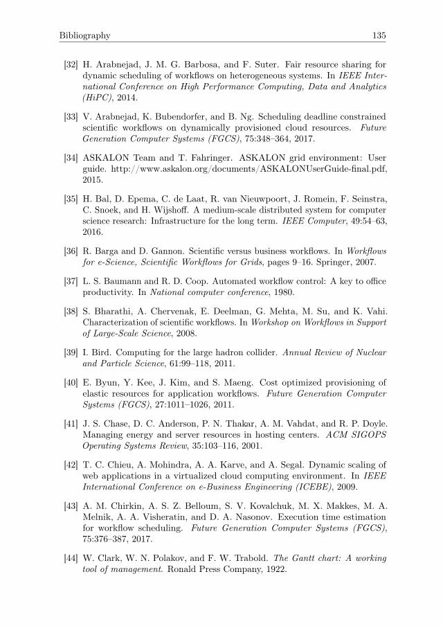
Bibliography 135

[32] H. Arabnejad, J. M. G. Barbosa, and F. Suter. Fair resource sharing fordynamic scheduling of workflows on heterogeneous systems. In IEEE Inter-national Conference on High Performance Computing, Data and Analytics(HiPC), 2014.

[33] V. Arabnejad, K. Bubendorfer, and B. Ng. Scheduling deadline constrainedscientific workflows on dynamically provisioned cloud resources. FutureGeneration Computer Systems (FGCS), 75:348–364, 2017.

[34] ASKALON Team and T. Fahringer. ASKALON grid environment: Userguide. http://www.askalon.org/documents/ASKALONUserGuide-final.pdf,2015.

[35] H. Bal, D. Epema, C. de Laat, R. van Nieuwpoort, J. Romein, F. Seinstra,C. Snoek, and H. Wijshoff. A medium-scale distributed system for computerscience research: Infrastructure for the long term. IEEE Computer, 49:54–63,2016.

[36] R. Barga and D. Gannon. Scientific versus business workflows. In Workflowsfor e-Science, Scientific Workflows for Grids, pages 9–16. Springer, 2007.

[37] L. S. Baumann and R. D. Coop. Automated workflow control: A key to officeproductivity. In National computer conference, 1980.

[38] S. Bharathi, A. Chervenak, E. Deelman, G. Mehta, M. Su, and K. Vahi.Characterization of scientific workflows. In Workshop on Workflows in Supportof Large-Scale Science, 2008.

[39] I. Bird. Computing for the large hadron collider. Annual Review of Nuclearand Particle Science, 61:99–118, 2011.

[40] E. Byun, Y. Kee, J. Kim, and S. Maeng. Cost optimized provisioning ofelastic resources for application workflows. Future Generation ComputerSystems (FGCS), 27:1011–1026, 2011.

[41] J. S. Chase, D. C. Anderson, P. N. Thakar, A. M. Vahdat, and R. P. Doyle.Managing energy and server resources in hosting centers. ACM SIGOPSOperating Systems Review, 35:103–116, 2001.

[42] T. C. Chieu, A. Mohindra, A. A. Karve, and A. Segal. Dynamic scaling ofweb applications in a virtualized cloud computing environment. In IEEEInternational Conference on e-Business Engineering (ICEBE), 2009.

[43] A. M. Chirkin, A. S. Z. Belloum, S. V. Kovalchuk, M. X. Makkes, M. A.Melnik, A. A. Visheratin, and D. A. Nasonov. Execution time estimationfor workflow scheduling. Future Generation Computer Systems (FGCS),75:376–387, 2017.

[44] W. Clark, W. N. Polakov, and F. W. Trabold. The Gantt chart: A workingtool of management. Ronald Press Company, 1922.

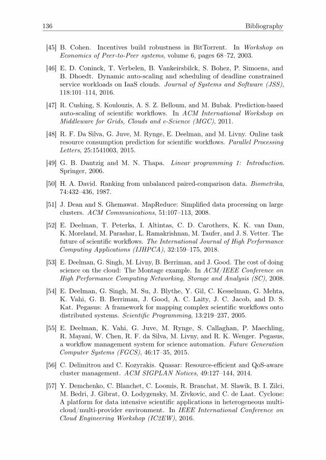
136 Bibliography

[45] B. Cohen. Incentives build robustness in BitTorrent. In Workshop onEconomics of Peer-to-Peer systems, volume 6, pages 68–72, 2003.

[46] E. D. Coninck, T. Verbelen, B. Vankeirsbilck, S. Bohez, P. Simoens, andB. Dhoedt. Dynamic auto-scaling and scheduling of deadline constrainedservice workloads on IaaS clouds. Journal of Systems and Software (JSS),118:101–114, 2016.

[47] R. Cushing, S. Koulouzis, A. S. Z. Belloum, and M. Bubak. Prediction-basedauto-scaling of scientific workflows. In ACM International Workshop onMiddleware for Grids, Clouds and e-Science (MGC), 2011.

[48] R. F. Da Silva, G. Juve, M. Rynge, E. Deelman, and M. Livny. Online taskresource consumption prediction for scientific workflows. Parallel ProcessingLetters, 25:1541003, 2015.

[49] G. B. Dantzig and M. N. Thapa. Linear programming 1: Introduction.Springer, 2006.

[50] H. A. David. Ranking from unbalanced paired-comparison data. Biometrika,74:432–436, 1987.

[51] J. Dean and S. Ghemawat. MapReduce: Simplified data processing on largeclusters. ACM Communications, 51:107–113, 2008.

[52] E. Deelman, T. Peterka, I. Altintas, C. D. Carothers, K. K. van Dam,K. Moreland, M. Parashar, L. Ramakrishnan, M. Taufer, and J. S. Vetter. Thefuture of scientific workflows. The International Journal of High PerformanceComputing Applications (IJHPCA), 32:159–175, 2018.

[53] E. Deelman, G. Singh, M. Livny, B. Berriman, and J. Good. The cost of doingscience on the cloud: The Montage example. In ACM/IEEE Conference onHigh Performance Computing Networking, Storage and Analysis (SC), 2008.

[54] E. Deelman, G. Singh, M. Su, J. Blythe, Y. Gil, C. Kesselman, G. Mehta,K. Vahi, G. B. Berriman, J. Good, A. C. Laity, J. C. Jacob, and D. S.Kat. Pegasus: A framework for mapping complex scientific workflows ontodistributed systems. Scientific Programming, 13:219–237, 2005.

[55] E. Deelman, K. Vahi, G. Juve, M. Rynge, S. Callaghan, P. Maechling,R. Mayani, W. Chen, R. F. da Silva, M. Livny, and R. K. Wenger. Pegasus,a workflow management system for science automation. Future GenerationComputer Systems (FGCS), 46:17–35, 2015.

[56] C. Delimitrou and C. Kozyrakis. Quasar: Resource-efficient and QoS-awarecluster management. ACM SIGPLAN Notices, 49:127–144, 2014.

[57] Y. Demchenko, C. Blanchet, C. Loomis, R. Branchat, M. Slawik, B. I. Zilci,M. Bedri, J. Gibrat, O. Lodygensky, M. Zivkovic, and C. de Laat. Cyclone:A platform for data intensive scientific applications in heterogeneous multi-cloud/multi-provider environment. In IEEE International Conference onCloud Engineering Workshop (IC2EW), 2016.

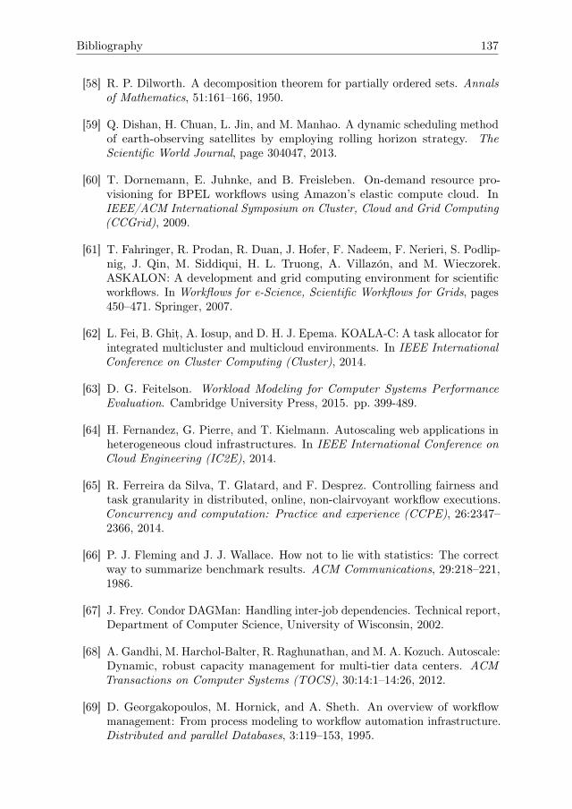
Bibliography 137

[58] R. P. Dilworth. A decomposition theorem for partially ordered sets. Annalsof Mathematics, 51:161–166, 1950.

[59] Q. Dishan, H. Chuan, L. Jin, and M. Manhao. A dynamic scheduling methodof earth-observing satellites by employing rolling horizon strategy. TheScientific World Journal, page 304047, 2013.

[60] T. Dornemann, E. Juhnke, and B. Freisleben. On-demand resource pro-visioning for BPEL workflows using Amazon’s elastic compute cloud. InIEEE/ACM International Symposium on Cluster, Cloud and Grid Computing(CCGrid), 2009.

[61] T. Fahringer, R. Prodan, R. Duan, J. Hofer, F. Nadeem, F. Nerieri, S. Podlip-nig, J. Qin, M. Siddiqui, H. L. Truong, A. Villazon, and M. Wieczorek.ASKALON: A development and grid computing environment for scientificworkflows. In Workflows for e-Science, Scientific Workflows for Grids, pages450–471. Springer, 2007.

[62] L. Fei, B. Ghit,, A. Iosup, and D. H. J. Epema. KOALA-C: A task allocator forintegrated multicluster and multicloud environments. In IEEE InternationalConference on Cluster Computing (Cluster), 2014.

[63] D. G. Feitelson. Workload Modeling for Computer Systems PerformanceEvaluation. Cambridge University Press, 2015. pp. 399-489.

[64] H. Fernandez, G. Pierre, and T. Kielmann. Autoscaling web applications inheterogeneous cloud infrastructures. In IEEE International Conference onCloud Engineering (IC2E), 2014.

[65] R. Ferreira da Silva, T. Glatard, and F. Desprez. Controlling fairness andtask granularity in distributed, online, non-clairvoyant workflow executions.Concurrency and computation: Practice and experience (CCPE), 26:2347–2366, 2014.

[66] P. J. Fleming and J. J. Wallace. How not to lie with statistics: The correctway to summarize benchmark results. ACM Communications, 29:218–221,1986.

[67] J. Frey. Condor DAGMan: Handling inter-job dependencies. Technical report,Department of Computer Science, University of Wisconsin, 2002.

[68] A. Gandhi, M. Harchol-Balter, R. Raghunathan, and M. A. Kozuch. Autoscale:Dynamic, robust capacity management for multi-tier data centers. ACMTransactions on Computer Systems (TOCS), 30:14:1–14:26, 2012.

[69] D. Georgakopoulos, M. Hornick, and A. Sheth. An overview of workflowmanagement: From process modeling to workflow automation infrastructure.Distributed and parallel Databases, 3:119–153, 1995.

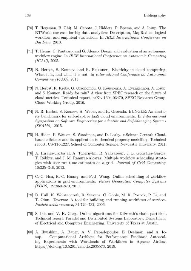
138 Bibliography

[70] T. Hegeman, B. Ghit,, M. Capota, J. Hidders, D. Epema, and A. Iosup. TheBTWorld use case for big data analytics: Description, MapReduce logicalworkflow, and empirical evaluation. In IEEE International Conference onBig Data, 2013.

[71] T. Heinis, C. Pautasso, and G. Alonso. Design and evaluation of an autonomicworkflow engine. In IEEE International Conference on Autonomic Computing(ICAC), 2005.

[72] N. Herbst, S. Kounev, and R. Reussner. Elasticity in cloud computing:What it is, and what it is not. In International Conference on AutonomicComputing (ICAC), 2013.

[73] N. Herbst, R. Krebs, G. Oikonomou, G. Kousiouris, A. Evangelinou, A. Iosup,and S. Kounev. Ready for rain? A view from SPEC research on the future ofcloud metrics. Technical report, arXiv:1604.03470, SPEC Research Group,Cloud Working Group, 2016.

[74] N. R. Herbst, S. Kounev, A. Weber, and H. Groenda. BUNGEE: An elastic-ity benchmark for self-adaptive IaaS cloud environments. In InternationalSymposium on Software Engineering for Adaptive and Self-Managing Systems(SEAMS), 2015.

[75] H. Hiden, P. Watson, S. Woodman, and D. Leahy. e-Science Central: Cloud-based e-Science and its application to chemical property modelling. Technicalreport, CS-TR-1227, School of Computer Science, Newcastle University, 2011.

[76] A. Hirales-Carbajal, A. Tchernykh, R. Yahyapour, J. L. Gonzalez-Garcıa,T. Roblitz, and J. M. Ramırez-Alcaraz. Multiple workflow scheduling strate-gies with user run time estimates on a grid. Journal of Grid Computing,10:325–346, 2012.

[77] C.-C. Hsu, K.-C. Huang, and F.-J. Wang. Online scheduling of workflowapplications in grid environments. Future Generation Computer Systems(FGCS), 27:860–870, 2011.

[78] D. Hull, K. Wolstencroft, R. Stevens, C. Goble, M. R. Pocock, P. Li, andT. Oinn. Taverna: A tool for building and running workflows of services.Nucleic acids research, 34:729–732, 2006.

[79] S. Ikiz and V. K. Garg. Online algorithms for Dilworth’s chain partition.Technical report, Parallel and Distributed Systems Laboratory, Departmentof Electrical and Computer Engineering, University of Texas at Austin.

[80] A. Ilyushkin, A. Bauer, A. V. Papadopoulos, E. Deelman, and A. Io-sup. Computational Artifacts for Performance Feedback Autoscal-ing Experiments with Workloads of Workflows in Apache Airflow.https://doi.org/10.5281/zenodo.2635573, 2019.

Bibliography 139

[81] A. Ilyushkin, A. Bauer, A. V. Papadopoulos, E. Deelman, andA. Iosup. Software Artifacts for Performance Feedback Autoscal-ing Experiments with Workloads of Workflows in Apache Airflow.https://doi.org/10.5281/zenodo.2635571, 2019.

[82] A. Ilyushkin and D. Epema. The impact of task runtime estimate accuracy onscheduling workloads of workflows. In IEEE/ACM International Symposiumon Cluster, Cloud and Grid Computing (CCGrid), 2018.

[83] A. Ilyushkin, B. Ghit,, and D. Epema. Scheduling workloads of workflowswith unknown task runtimes. In IEEE/ACM International Symposium onCluster, Cloud and Grid Computing (CCGrid), 2015.

[84] A. Iosup, O. Sonmez, and D. Epema. DGSim: Comparing grid resourcemanagement architectures through trace-based simulation. In EuropeanConference on Parallel Processing (Euro-Par), 2008.

[85] A. Iosup, T. Tannenbaum, M. Farrellee, D. Epema, and M. Livny. Inter-operating grids through delegated matchmaking. Scientific Programming,16:233–253, 2008.

[86] A. Iosup, N. Yigitbasi, and D. Epema. On the performance variabilityof production cloud services. In IEEE/ACM International Symposium onCluster, Cloud and Grid Computing (CCGrid), 2011.

[87] W. Iqbal, M. N. Dailey, D. Carrera, and P. Janecek. Adaptive resourceprovisioning for read intensive multi-tier applications in the cloud. FutureGeneration Computer Systems (FGCS), 27:871–879, 2011.

[88] M. Islam, A. K. Huang, M. Battisha, M. Chiang, S. Srinivasan, C. Peters,A. Neumann, and A. Abdelnur. Oozie: Towards a scalable workflow manage-ment system for Hadoop. In ACM SIGMOD Workshop on Scalable WorkflowExecution Engines and Technologies (SWEET), 2012.

[89] D. Jackson, Q. Snell, and M. Clement. Core algorithms of the Maui scheduler.In Workshop on Job Scheduling Strategies for Parallel Processing (JSSPP),2001.

[90] J. C. Jacob, D. S. Katz, G. B. Berriman, J. Good, A. C. Laity, E. Deelman,C. Kesselman, G. Singh, M. Su, T. A. Prince, and R. Williams. Montage:A grid portal and software toolkit for science-grade astronomical imagemosaicking. International Journal of Computer Sciences and Engineering(IJCSE), 4:73–87, 2009.

[91] V. Jeyakumar, M. Alizadeh, D. Mazieres, B. Prabhakar, and C. Kim. EyeQ:Practical network performance isolation for the multi-tenant cloud. InUSENIX Workshop on Hot Topics in Cloud Computing (HotCloud), 2012.

[92] G. Juve, A. Chervenak, E. Deelman, S. Bharathi, G. Mehta, and K. Vahi.Characterizing and profiling scientific workflows. Future Generation ComputerSystems (FGCS), 29:682–692, 2013.

140 Bibliography

[93] L. V. Kantorovich. Moi put’ v nauke (My way in science). Uspehi Matem-aticheskih Nauk, 42:183–213, 1987.

[94] L. V. Kantorovich. Mathematical-Economic Articles. Nauka: Novosibirsk,2011.

[95] J. E. Kelley Jr and M. R. Walker. Critical-path planning and scheduling. InIRE-AIEE-ACM computer conference, 1959.

[96] A. Kembhavi. Big data in astronomy and beyond. In Data Science Landscape,pages 59–66. Springer, 2018.

[97] M. A. Khan. Scheduling for heterogeneous systems using constrained criticalpaths. Parallel Computing, 38:175–193, 2012.

[98] D. K. Krishnappa, M. Zink, and R. K. Sitaraman. Optimizing the videotranscoding workflow in content delivery networks. In ACM InternationalConference on Multimedia Systems (MMsys), 2015.

[99] M. Kuhnemann, T. Rauber, and G. Runger. A source code analyzer forperformance prediction. In IEEE International Parallel and DistributedProcessing Symposium (IPDPS), 2004.

[100] Y.-K. Kwok and I. Ahmad. Dynamic critical-path scheduling: An effectivetechnique for allocating task graphs to multiprocessors. IEEE Transactionson Parallel and Distributed Systems (TPDS), 7:506–521, 1996.

[101] Y.-K. Kwok and I. Ahmad. Benchmarking and comparison of the taskgraph scheduling algorithms. Journal of Parallel and Distributed Computing(JPDC), 59:381–422, 1999.

[102] Y.-K. Kwok and I. Ahmad. Static scheduling algorithms for allocating directedtask graphs to multiprocessors. ACM Computing Surveys, 31:406–471, 1999.

[103] C. B. Lee, Y. Schwartzman, J. Hardy, and A. Snavely. Are user runtimeestimates inherently inaccurate? In Workshop on Job Scheduling Strategiesfor Parallel Processing (JSSPP), 2004.

[104] K. Lee, N. W. Paton, R. Sakellariou, E. Deelman, A. Fernandes, and G. Mehta.Adaptive workflow processing and execution in Pegasus. Concurrency andComputation: Practice and Experience, 21:1965–1981, 2009.

[105] P. Leitner and J. Cito. Patterns in the chaos—a study of performancevariation and predictability in public IaaS clouds. ACM Transactions onInternet Technology (TOIT), 16:15:1–15:23, 2016.

[106] F. Leymann and D. Roller. Production Workflow: Concepts and Techniques.Prentice Hall PTR, 2000.

[107] D. A. Lifka. The ANL/IBM SP scheduling system. In Workshop on JobScheduling Strategies for Parallel Processing (JSSPP), 1995.

Bibliography 141

[108] J. Livny. Bioinformatic discovery of bacterial regulatory RNAs using SIPHT.Bacterial Regulatory RNA: Methods and Protocols, 905:3–14, 2012.

[109] D. Logothetis, C. Olston, B. Reed, K. C. Webb, and K. Yocum. Stateful bulkprocessing for incremental analytics. In ACM symposium on Cloud computing(SoCC), 2010.

[110] T. Lorido-Botran, J. Miguel-Alonso, and J. A. Lozano. A review of auto-scaling techniques for elastic applications in cloud environments. Journal ofGrid Computing, 12:559–592, 2014.

[111] P. Lu, G. Zhang, Z. Zhu, X. Zhou, J. Sun, and J. Zhou. A review of cost andmakespan-aware workflow scheduling in clouds. Journal of Circuits, Systemsand Computers, 28:1930006, 2018.

[112] U. Lublin and D. G. Feitelson. The workload on parallel supercomputers:Modeling the characteristics of rigid jobs. Journal of Parallel and DistributedComputing (JPDC), 63:1105–1122, 2003.

[113] S. Ma, A. Ilyushkin, A. Stegehuis, and A. Iosup. ANANKE: A Q-learning-based portfolio scheduler for complex industrial workflows. In IEEE Interna-tional Conference on Autonomic Computing (ICAC), 2017.

[114] M. Malawski, K. Figiela, M. Bubak, E. Deelman, and J. Nabrzyski. Schedulingmultilevel deadline-constrained scientific workflows on clouds based on costoptimization. Scientific Programming, page 680271, 2015.

[115] M. Malawski, G. Juve, E. Deelman, and J. Nabrzyski. Cost-and deadline-constrained provisioning for scientific workflow ensembles in IaaS clouds.In ACM/IEEE Conference on High Performance Computing Networking,Storage and Analysis (SC), 2012.

[116] M. Malawski, G. Juve, E. Deelman, and J. Nabrzyski. Algorithms for cost-anddeadline-constrained provisioning for scientific workflow ensembles in IaaSclouds. Future Generation Computer Systems (FGCS), 48:1–18, 2015.

[117] G. Malewicz, I. Foster, A. L. Rosenberg, and M. Wilde. A tool for prioritizingDAGMa jobs and its evaluation. Journal of Grid Computing, 5:197–212,2007.

[118] M. Mao and M. Humphrey. Auto-scaling to minimize cost and meet appli-cation deadlines in cloud workflows. In ACM/IEEE Conference on HighPerformance Computing Networking, Storage and Analysis (SC), 2011.

[119] M. Mao and M. Humphrey. Scaling and scheduling to maximize applica-tion performance within budget constraints in cloud workflows. In IEEEInternational Symposium on Parallel and Distributed Processing (IPDPS),2013.

[120] A. Maricq, D. Duplyakin, I. Jimenez, C. Maltzahn, R. Stutsman, R. Ricci,and A. Klimovic. Taming performance variability. In USENIX Symposiumon Operating Systems Design and Implementation (OSDI), 2018.

142 Bibliography

[121] E. R. Marsh. The harmonogram of Karol Adamiecki. Academy of managementJournal, 18:358–364, 1975.

[122] J. T. Meehean. Towards Transparent CPU Scheduling. PhD thesis, Universityof Wisconsin-Madison, 2011.

[123] D. Milojicic, I. M. Llorente, and R. S. Montero. OpenNebula: A cloudmanagement tool. IEEE Internet Computing, 15:11–14, 2011.

[124] A. W. Mu’alem and D. G. Feitelson. Utilization, predictability, workloads,and user runtime estimates in scheduling the IBM SP2 with backfilling. IEEETransactions on Parallel and Distributed Systems (TPDS), 12:529–543, 2001.

[125] S. Murray, V. Bahyl, G. Cancio, E. Cano, V. Kotlyar, D. F. Kruse, andJ. Leduc. An efficient, modular and simple tape archiving solution for LHCRun-3. In Journal of Physics: Conference Series, volume 898, page 062013,2017.

[126] M. Nardelli, S. Nastic, S. Dustdar, M. Villari, and R. Ranjan. Osmotic flow:Osmotic computing + IoT workflow. IEEE Cloud Computing, 4:68–75, 2017.

[127] A. Naskos, E. Stachtiari, A. Gounaris, P. Katsaros, D. Tsoumakos, I. Kon-stantinou, and S. Sioutas. Dependable horizontal scaling based on probabilisticmodel checking. In IEEE/ACM International Symposium on Cluster, Cloudand Grid Computing (CCGrid), 2015.

[128] M. J. Neely, E. Modiano, and C. Li. Fairness and optimal stochastic controlfor heterogeneous networks. IEEE/ACM Transactions On Networking (TON),16:396–409, 2008.

[129] N. M. O’boyle, A. L. Tenderholt, and K. M. Langner. Cclib: A libraryfor package-independent computational chemistry algorithms. Journal ofcomputational chemistry, 29:839–845, 2008.

[130] C. Olston, B. Reed, U. Srivastava, R. Kumar, and A. Tomkins. Pig Latin: Anot-so-foreign language for data processing. In ACM SIGMOD InternationalConference on Management of Data, 2008.

[131] M. Oppitz and P. Tomsu. Cloud computing. In Inventing the Cloud Century,pages 267–318. Springer, 2018.

[132] S. Ostermann, R. Prodan, T. Fahringer, A. Iosup, and D. Epema. On thecharacteristics of grid workflows. In CoreGRID Symposium Euro-Par, 2008.

[133] A. V. Papadopoulos, A. Ali-Eldin, K. Arzen, J. Tordsson, and E. Elmroth.PEAS: A performance evaluation framework for auto-scaling strategies incloud applications. Tail response time modeling and control for interactivecloud services. ACM Transactions on Modeling and Performance Evaluationof Computing Systems (TOMPECS), 1:15:1–15:31, 2016.

[134] H. P. Patil. On the structure of k-trees. Journal of Combinatorics, Informationand System Sciences (JCISS), 11:57–64, 1986.

Bibliography 143

[135] I. Pietri, G. Juve, E. Deelman, and R. Sakellariou. A performance modelto estimate execution time of scientific workflows on the cloud. In IEEEWorkshop on Workflows in Support of Large-Scale Science (WORKS), 2014.

[136] M. Pundir, M. Kumar, L. M. Leslie, I. Gupta, and R. H. Campbell. Supportingon-demand elasticity in distributed graph processing. In IEEE InternationalConference on Cloud Engineering (IC2E), 2016.

[137] M. Rahman, X. Li, and H. Palit. Hybrid heuristic for scheduling data analyticsworkflow applications in hybrid cloud environment. In IEEE InternationalSymposium on Parallel and Distributed Processing Workshops (IPDPSW),2011.

[138] M. Rahman, S. Venugopal, and R. Buyya. A dynamic critical path algorithmfor scheduling scientific workflow applications on global grids. In IEEEInternational Conference on e-Science and Grid Computing (e-Science), 2007.

[139] A. Ramakrishnan, G. Singh, H. Zhao, E. Deelman, R. Sakellariou, K. Vahi,K. Blackburn, D. Meyers, and M. Samidi. Scheduling data-intensive work-flows onto storage-constrained distributed resources. In IEEE InternationalSymposium on Cluster Computing and the Grid (CCGrid), 2007.

[140] M. A. Rodriguez and R. Buyya. Budget-driven scheduling of scientificworkflows in IaaS clouds with fine-grained billing periods. ACM Transactionson Autonomous and Adaptive Systems (TAAS), 12:5:1–5:22, 2017.

[141] G. Sabin, R. Kettimuthu, A. Rajan, and P. Sadayappan. Scheduling ofparallel jobs in a heterogeneous multi-site environment. In Workshop on JobScheduling Strategies for Parallel Processing (JSSPP), 2003.

[142] R. Sakellariou and H. Zhao. A hybrid heuristic for DAG scheduling onheterogeneous systems. In IEEE International Parallel and DistributedProcessing Symposium (IPDPS), 2004.

[143] A. Shade and T. K. Teal. Computing workflows for biologists: A roadmap.PLoS biology, 13:e1002303, 2015.

[144] E. Shmueli and D. G. Feitelson. Backfilling with lookahead to optimizethe packing of parallel jobs. Journal of Parallel and Distributed Computing(JPDC), 65:1090–1107, 2005.

[145] G. Singh and E. Deelman. The interplay of resource provisioning and work-flow optimization in scientific applications. Concurrency and Computation:Practice and Experience, 23:1969–1989, 2011.

[146] V. Singh, I. Gupta, and P. K. Jana. A novel cost-efficient approach for deadline-constrained workflow scheduling by dynamic provisioning of resources. FutureGeneration Computer Systems (FGCS), 79:95–110, 2018.

[147] S. Spinner, G. Casale, F. Brosig, and S. Kounev. Evaluating approaches toresource demand estimation. Performance Evaluation, 92:51–71, 2015.

144 Bibliography

[148] F. Suter and S. Hunold. DAGGen: A synthetic task graph generator.https://github.com/frs69wq/daggen.

[149] D. Talby and D. G. Feitelson. Supporting priorities and improving utilizationof the IBM SP scheduler using slack-based backfilling. In IEEE InternationalParallel Processing Symposium and Symposium on Parallel and DistributedProcessing (IPPS/SPDP), 1999.

[150] D. Talia. Clouds for scalable big data analytics. IEEE Computer, 46:98–101,2013.

[151] F. W. Taylor. Scientific management. The Sociological Review, 7:266–269,1914.

[152] I. J. Taylor, E. Deelman, D. B. Gannon, and M. Shields. Workflows fore-Science, Scientific Workflows for Grids. Springer, 2007.

[153] D. Thain, T. Tannenbaum, and M. Livny. Distributed computing in prac-tice: The Condor experience. Concurrency and computation: Practice andexperience (CCPE), 17:323–356, 2005.

[154] S. Tilloo. Running arbitrary DAG-based workflows in the cloud.http://www.ebaytechblog.com/2016/04/05/running-arbitrary-dag-based-workflows-in-the-cloud, 2017.

[155] H. Topcuoglu, S. Hariri, and M. Wu. Performance-effective and low-complexitytask scheduling for heterogeneous computing. IEEE Transactions on Paralleland Distributed Systems (TPDS), 13:260–274, 2002.

[156] B. Urgaonkar, G. Pacifici, P. Shenoy, M. Spreitzer, and A. Tantawi. Ananalytical model for multi-tier internet services and its applications. In ACMSIGMETRICS Performance Evaluation Review, 2005.

[157] B. Urgaonkar, P. Shenoy, A. Chandra, P. Goyal, and T. Wood. Agiledynamic provisioning of multi-tier internet applications. ACM Transactionson Autonomous and Adaptive Systems (TAAS), 3:1:1–1:39, 2008.

[158] E. van Eyk, L. Toader, S. Talluri, L. Versluis, A. Ut,a, and A. Iosup. Serverlessis more: From PaaS to present cloud computing. IEEE Internet Computing,22:8–17, 2018.

[159] J. van Helden. Regulatory sequence analysis tools. Nucleic Acids Research,31:3593–3596, 2003.

[160] L. Versluis, M. Neacsu, and A. Iosup. A trace-based performance study of au-toscaling workloads of workflows in datacenters. In IEEE/ACM InternationalSymposium on Cluster, Cloud and Grid Computing (CCGrid), 2018.

[161] N. Vydyanathan, U. Catalyurek, T. Kurc, P. Sadayappan, and J. Saltz.A duplication based algorithm for optimizing latency under throughputconstraints for streaming workflows. In IEEE International Conference onParallel Processing (ICPP), 2008.

Bibliography 145

[162] P. Waibel, S. Videnov, M. Borkowski, C. Hochreiner, S. Schulte, andJ. Mendling. Process simulation for machine reservation in cloud manufactur-ing. In IEEE International Conference on Industrial Informatics (INDIN),2018.

[163] Y. Wang, S. Cao, G. Wang, Z. Feng, C. Zhang, and H. Guo. Fairnessscheduling with dynamic priority for multi workflow on heterogeneous systems.In IEEE International Conference on Cloud Computing and Big Data Analysis(ICCCBDA), 2017.

[164] Y. Wang, Y. Xia, and S. Chen. Using integer programming for workflowscheduling in the cloud. In IEEE International Conference on Cloud Com-puting (CLOUD), 2017.

[165] Z. Wen, R. Yang, P. Garraghan, T. Lin, J. Xu, and M. Rovatsos. Fogorchestration for Internet of Things services. IEEE Internet Computing,21:16–24, 2017.

[166] J. R. Wieland, R. Pasupathy, and B. W. Schmeiser. Queueing-networkstability: Simulation-based checking. In Winter Simulation Conference, 2003.

[167] F. Wu, Q. Wu, and Y. Tan. Workflow scheduling in cloud: A survey. TheJournal of Supercomputing, 71:3373–3418, 2015.

[168] K. Yelick, S. Coghlan, B. Draney, and R. S. Canon. The Magellan reporton cloud computing. Technical report, LBNL-5376E, U.S. Department ofEnergy, Washington D.C., USA, 2011.

[169] Z. Yu and W. Shi. A planner-guided scheduling strategy for multiple workflowapplications. In IEEE International Conference on Parallel Processing-Workshops (ICPP-W), 2008.

[170] H. Zhao and R. Sakellariou. Scheduling multiple DAGs onto heterogeneoussystems. In IEEE International Parallel and Distributed Processing Sympo-sium, 2006.

[171] A. C. Zhou, B. He, and C. Liu. Monetary cost optimizations for hostingworkflow-as-a-service in IaaS clouds. IEEE Transactions on Cloud Computing,4:34–48, 2016.

Summary

A workflow is a universal abstraction for representing complex activities consisting ofmultiple interconnected tasks. Workflows are often used to describe and orchestratecomputations at different scales. The growing applicability of such computingworkflows has led to the development of appropriate algorithms designed forscheduling and executing workflows efficiently. Workflow scheduling can be seenfrom the task placement and resource allocation perspectives, where task placementcontrols the mapping of tasks to computing resources, and resource allocationcontrols the number of dynamically available computing resources. Due to theusage patterns of earlier workflow applications in clusters and grids, most of theexisting workflow scheduling algorithms were designed to process statically presentsets of workflows. Such offline algorithms often fail to address the challengesintroduced by modern online applications of workflows, for example, in computingclouds where diverse workflows from different users arrive stochastically forminga workload. This provides a variety of opportunities for the development of newscheduling policies to meet the challenges of online scheduling.

In this dissertation, we identify and address three key challenges that are char-acteristic to the online scheduling of workloads of workflows in modern distributedcomputing systems, such as clusters and clouds. The first challenge is realisticestimation of the resource demand of a workflow, as it is important for both taskplacement and resource allocation. Second, is the efficient placement of workflowtasks to minimize average workflow slowdown while achieving fairness. A wronglychosen task placement policy can easily degrade the performance and negativelyaffect the fair access of workflows to computing resources. Third, is the automaticallocation (autoscaling) of computing resources for workflows while meeting dead-line and budget constraints. Computing clouds make it possible to easily lease andrelease resources. Such decisions should be made wisely to minimize slowdowns anddeadline violations, and to efficiently use the leased resources to reduce incurredcosts.

To address these challenges, we propose novel online scheduling policies andinvestigate applicability of relevant state-of-the-art workflow scheduling policiesto the online scenario. For new policies, we keep in mind their implementationeffort and their suitability for production systems. We experimentally evaluatethese workflow scheduling policies by conducting a wide set of simulation-basedand real-world experiments on a private multicluster computer. Additionally, weuse a Mixed Integer Programming (MIP) approach to validate our real-worldexperimental results versus the optimal solution obtained with a MIP solver.

In Chapter 1, we summarize workflow scheduling approaches and identify mainworkflow scheduling challenges from both task placement and resource allocationperspectives. We also provide an overview of state-of-the-art workflow schedulingpolicies and modern workflow managements systems. Furthermore, we present

147

148 Summary

research questions that aim to address the identified workflow scheduling challenges,the research methods used in this dissertation, the dissertation outline, and ourkey contributions.

In Chapter 2, we address the problem of online scheduling of workloads ofworkflows with unknown task runtime estimates. For this we propose a family offour novel online workflow scheduling policies which differ in to what extent theyreserve processors for the workflows towards the head of the queue. To be ableto make processor reservations, we propose a method for the realistic estimationof workflow level of parallelism. Our results show that even at moderate imposedutilizations, the greedy backfilling policy leads to lower average workflow slowdownscompared to the policies which use processor reservation.

In Chapter 3, we focus on scheduling workloads of workflows with varying accu-racy of task runtime estimates that are available to the scheduler. We implementfour state-of-the-art online dynamic workflow scheduling policies, and propose twonovel online dynamic policies, one of which addresses fairness, and the other oneadapts a popular offline plan-based policy for the online plan-based scenario. Inour results, we can clearly see that the knowledge of task runtime estimates givessignificant performance improvement in the average job slowdown, but only atextremely high utilizations. At moderate utilizations, simpler backfilling-based poli-cies outperform more advanced policies. The plan-based online policy demonstratespoor performance compared to dynamic online policies. Our fairness-oriented policyeffectively decreases the variance of job slowdown and thus achieves fairness.

In Chapter 4, we experimentally evaluate five state-of-the-art general autoscalersand propose two novel workflow-specific autoscalers. Moreover, we present and refineperformance metrics endorsed by the Standard Performance Evaluation Corporation(SPEC) for assessing autoscalers, and define three approaches for comparing theautoscalers using the considered metrics. The experimental results show thatgeneral autoscalers can demonstrate comparable performance to workflow-specificautoscalers, if the former have access to workload statistics. The workflow-specificautoscalers, in turn, require task or workflow runtime estimates. We additionallyinvestigate the effect of autoscaling on meeting workflow deadlines. Our resultshighlight the trade-offs between the suggested policies, their impact on meetingthe deadlines, and their performance in different operating conditions.

In Chapter 5, we propose a novel online dynamic autoscaler that employs afeedback mechanism for making autoscaling decisions. For that our autoscaleranalyzes historical task throughput and uses the not yet finished part of the workflow,instead of relying on task runtime estimates, as analyzing the task throughputrequires less effort than obtaining task runtime estimates. Our approach showslower time complexity and effectively minimizes workflow slowdowns compared totwo state-of-the-art autoscalers. The usage of historical throughput informationprovides fairly accurate estimation of resource speeds when dealing with workloadswith a representative long-tailed task runtime distribution. We additionally validatethe experimental results by comparing the workflow slowdowns obtained from anactual workflow management system with an optimal solution.

Finally, in Chapter 6, we present the main conclusions of this dissertation andwe provide suggestions for several future directions.

Samenvatting

Een workflow is een universele abstractie voor het weergeven van complexe activi-teiten die bestaan uit meerdere onderling verbonden taken. Workflows worden vaakgebruikt om berekeningen op verschillende schaal te beschrijven en te organiseren.De groeiende toepasbaarheid van zulke workflows heeft geleid tot de ontwikkelingvan geschikte algoritmen om ze efficient uit te voeren. Workflow scheduling kanvanuit twee perspectieven worden bestudeerd: Ten eerste vanuit task placement,waarbij taken zo geschikt mogelijk aan computer resources worden gekoppeld, enten tweede vanuit resource allocatie, waarbij men dynamisch computer resourcesbeschikbaar stelt. Aangezien in het verleden workflow applicaties voornamelijkwaren gericht op clusters en grids, zijn de scheduling algoritmes uit deze tijd gerichtop statische verzamelingen workflows. Zulke zogenaamde offline algoritmes zijnniet altijd even geschikt voor gebruik in de moderne online toepassing van work-flows, bijvoorbeeld in cloud netwerken. Daarin starten de diverse workflows vanverschillende gebruikers op verschillende tijdstippen, en vormen zo een stochastischeworkload van workflows. Dit biedt de mogelijkheid om nieuwe scheduling policieste ontwikkelen die in staat zijn om te gaan met de uitdaging van online scheduling.

In dit proefschrift worden drie sleuteluitdagingen geıdentificeerd en behandelddie karakteristiek zijn voor workloads van workflows in moderne gedistribueerdecomputersystemen, zoals clusters en clouds. De eerste uitdaging is het realistischinschatten van de resource-eisen van een workflow. Dit is belangrijk voor zoweltask placement als resource allocatie. De tweede uitdaging is het efficient plaatsenvan workflow-taken met als doel het minimaliseren van de gemiddelde slowdownvan workflows en het eerlijk verdelen van de resources. Een verkeerd gekozen taskplacement policy kan de prestaties sterk beınvloeden en kan een nadelig effecthebben op hoe eerlijk de computer resources verdeeld worden onder de verschillendeworkflows. De derde uitdaging is het automatisch toewijzen van computer resources(“autoscaling”) bij een beperkt budget en met de aanwezigheid van deadlines.Computer clouds maken het mogelijk om gemakkelijk computer resources te hurenen weer vrij te geven. Zulke beslissingen moeten op een verstandige manier wordengemaakt om de slowdown en het aantal schendingen van deadlines te minimaliseren,en om de computer resources efficient te huren zodat de kosten binnen de perkenblijven.

Om deze uitdagingen aan te gaan worden nieuwe online scheduling policies voor-gesteld, en wordt de geschiktheid van relevante moderne workflow scheduling policiesvoor het online scenario onderzocht. Voor de voorgestelde nieuwe policies wordtde moeite om ze te implementeren en hun geschiktheid voor productiesystemenin acht genomen. De workflow scheduling policies worden experimenteel getoetstmet een breed scala van simulaties, en met echte experimenten op een multiclustercomputersysteem. We gebruiken mixed integer programming om de experimenteleresultaten te vergelijken met een theoretisch gezien optimale oplossing.

149

150 Samenvatting

In hoofdstuk 1 vatten we workflow scheduling methoden samen en identificerenwe uitdagingen voor workflow scheduling vanuit het perspectief van task placementen resource allocation. Ook wordt er een overzicht gepresenteerd van state-of-the-artworkflow scheduling policies en moderne workflow management systemen. Boven-dien worden de onderzoeksvragen geformuleerd om de geıdentificeerde uitdagingenaan te gaan, en worden de in dit proefschrift gebruikte methoden, een overzichtvan het proefschrift, en de belangrijkste bijdragen gepresenteerd.

In hoofdstuk 2 wordt het probleem behandeld van de online scheduling vanworkloads van workflows zonder de beschikbaarheid van schattingen van de execu-tietijd van taken. Hiervoor worden vier nieuwe online workflow scheduling policiesgepresenteerd die verschillen in de mate waarin ze processoren reserveren voor deworkflows vooraan in de wachtrij. Om in staat te zijn processoren te reserverenwordt een methode voorgesteld die een realistische inschatting kan maken van hetniveau van parallellisme in workflows. De resultaten hiervan laten zien dat zelfsbij een matige bezettingsgraad de greedy backfilling policy leidt tot een lageregemiddelde workflow slowdown in vergelijking met de policies die gebruik makenvan processorreservering.

In hoofdstuk 3 ligt de focus op de scheduling van workloads van workflows metgebruik van schattingen van de executietijden van taken van varierende precisie.Hier worden vier state-of-the-art online dynamische workflow scheduling policiesgeımplementeerd, en worden twee nieuwe online dynamische policies voorgesteld.Een daarvan richt zich op eerlijke toewijzing, de tweede is geınspireerd op populaireoffline plan-based policies voor het online plan-based scenario. In de resultatenkan duidelijk worden gezien dat beschikbaarheid van informatie over de lengtevan taken een significante prestatieverbetering tot gevolg heeft in de gemiddeldejob slowdown, maar alleen bij extreem hoge bezettingsgraden. Bij matig gebruikpresteren simpele backfilling-based policies beter dan dynamische online policies.De eerlijkheid-georienteerde policy reduceert de variantie in job slowdown en is dusinderdaad eerlijker.

In hoofdstuk 4 worden er vijf state-of-the-art generieke autoscalers geanalyseerden worden er twee nieuwe workflow-specifieke autoscalers voorgesteld. Daarnaastworden de prestatiemetrieken aanbevolen door de Standard Performance EvaluationCorporation (SPEC) voor het beoordelen van autoscalers beschreven en verfijnd.Ook worden er drie manieren voorgesteld om autoscalers te vergelijken aan de handvan deze metrieken. De experimentele resultaten laten zien dat generieke autoscalersongeveer hetzelfde presteren als workflow-specifieke autoscalers indien deze laatstetoegang hebben tot workload-statistieken. De workflow-specifieke autoscalersvereisen schattingen van de executietijden van taken van workflows. Daarnaastwordt het effect van autoscaling op het behalen van workflow deadlines onderzocht.De resultaten laten goed de trade-offs tussen de verschillende policies, hun impactop het behalen van deadlines, en de prestaties in verschillende omstandighedenzien.

In hoofdstuk 5 wordt een nieuwe online dynamische autoscaler geıntroduceerddie gebruik maakt van een terugkoppelingsmechanisme. Deze autoscaler analyseerthistorische doorvoersnelheden van taken in plaats van gebruik te maken van schat-tingen van de executietijden van taken. Dit is voordelig, aangezien het minder

Samenvatting 151

moeite kost om doorvoersnelheden te analyseren dan vooraf voor elke taak eenschatting van zijn executietijd te maken. Deze benadering van het probleem heefteen lagere tijdscomplexiteit en minimaliseert de workflow slowdown in vergelijkingmet twee state-of-the-art autoscalers. Het gebruik van historische doorvoersnelhe-den biedt een redelijk accurate inschatting van resource snelheden bij workloadsmet een representatieve lange-staart verdeling van de executietijden van taken.Hiernaast worden de experimentele resultaten gevalideerd door de workflow slow-down verkregen met een hedendaags workflow management systeem te vergelijkenmet een optimale oplossing.

Tot slot worden in hoofdstuk 6 de algemene conclusies van dit proefschriftgepresenteerd en worden er suggesties gedaan voor vervolgonderzoek.

Acknowledgements

This dissertation would never happen without the help and support of numerouspeople who surrounded me through all these years.

First, I would like to thank my promotor Dick Epema for trusting me andgiving the opportunity to do science. Dick, I extremely appreciate your patience,discipline, and high standards for research. Among your many lessons, you taughtme how to be a clear communicator and an independent researcher. It was agreat pleasure working with you while sharing a broader view on solving appliedproblems.

I am grateful to my second promotor Alexandru Iosup. Alexandru, you inspiredme to work with autoscalers and greatly expanded my scientific network by in-troducing me to the SPEC research activities. Our meetings within the AtLargeteam helped me to learn from other peer researchers—that was extremely usefulfor making this dissertation done.

I am also thankful to Henk Sips, as he was involved in my admission to the PDSgroup. Henk, even though we did not work together, thank you for your supportduring the PhD process and your advice on research in general.

I would like to thank the defense committee members: Koen Langendoen, PaolaGrosso, Boudewijn Haverkort, Ewa Deelman, Radu Prodan, and Eelco Visser, forspending time on reading and evaluating my dissertation. Your useful commentsand suggestions helped to improve this work.

I was extremely lucky working together with Bogdan Ghit,. Bogdan, I reallyappreciate that you significantly helped me at the early stages of my PhD in bothtechnical and textual parts of my papers.

Special thanks go to Ahmed Ali-Eldin, Alessandro Vittorio Papadopoulos,Nikolas Herbst, Andre Bauer, and Samuel Kounev for our fruitful cooperationthrough the SPEC research group. Our joint activities enriched this dissertationsand gave me valuable experience working on large projects together.

I greatly enjoyed working with Alexandru Ut, a, Laurens Versluis, Sietse Au,and Shenjun Ma, our collaborations helped me to explore new topics in resourceautoscaling. I additionally thank Laurens for pointing me out to the MIP paperwhich gave me new ideas for one of the dissertation chapters.

Johan Pouwelse, your endless enthusiasm has always inspired me. I am verygrateful for your help in my career and all the conversations we had at our group.

I am thankful to Yuri Demchenko for giving me the opportunity to join theCyclone project at the SNE group of the University of Amsterdam.

To my office mates Riccardo Petrocco, Adele Lu Jia, Erwin van Eyk, AkbarMostafavi, Amin Rezaeian, and Vadim Bulavintsev, thank you for the great workingatmosphere and for all the nice chats.

To my colleagues, Otto Visser, Ana Varbanescu, Vincent van Beek, DimitraGkorou, Lucia d’Acunto, Jie Shen, Niels Zeilemaker, Mihai Capota, Elric Milon,

153

154 Acknowledgements

Lipu Fei, Ernst van der Hoeven, Paul Brussee, Martijn de Vos, Giorgos Oikonomou,Tim Hegeman, Jesse Donkervliet, Stefan Hugtenburg, and Maria Voinea, thankyou for contributing to the social side of my days at the (P)DS group. I will neverforget all the countless pizza evenings and game nights we had together.

I would like to thank Aleksandra Kuzmanovska for sharing her insights onresearch with me and the moral support. It was also a great time we spent in theUSA with the VU guys at CCGrid. I wish you all the best in your career.

Kees Verstoep, Paulo Anita, and Munire van der Kruyk, thank you for the ex-cellent technical support. Without your help, many experiments in this dissertationsimply would not happen. I am also grateful to all the secretaries Ilse Oonk, RinaAbbriata, Shemara van der Zwet, and Kim Roos for the administrative support.

I would probably never have come to the Netherlands to complete this disserta-tion if Ilia Vialshin would not have decided to start his own PhD in Nijmegen. Ilia,I am very happy knowing you for so many years and thank you for being such agreat friend and crazy chemist.

Vallın Garcıa Cruz, you are my first friend in the Netherlands, and you definitelymade my PhD time here unforgettable. Thank you for having such a good heartand for always being willing to help.

Gleb Polevoy, I really enjoyed all our profound philosophical conversations thatgave me insight into many topics from a completely new perspective. Your ideashelped me to shape this dissertation and enriched my stay in the Netherlands.

Dmitry and Yulia Kononchuk, it has been a great pleasure knowing you, andthank you a lot for making this PhD time in the Netherlands full of nice gatheringswith great thorough discussions.

I would like to thank all the Russian-speaking friends whom I met in Delft:Natalia Vtyurina, Maria Zamiralova, Emil Gallyamov, Irina Gallyamova, AlexanderNagui, Ivan Koryakovskiy, Mikhail Belonosov, Nick Gaiko, Sergey Bezrukavnikov,Inna Medvedeva, Mikhail Davydenko, Aleksandra Uuemaa, Tatiana Kozlova, OlegGuziy, Nikita Lenchenkov, Vladimir Kovalenko, and Ilya Popov, for making myPhD journey so bright and full of amazing memories.

Dear Natalia Vdovenko, Polina Platonova, Evgenia Platonova, Ekaterina Bala-banyuk, Nikita Dubov, and Tatiana Kosovets: The way I met all of you is simplyincredible, and I truly enjoyed spending time with you. Thank you a lot for yourpositive energy and your warm characters.

Many thanks go to Delfts Studenten Muziekgezelschap Krashna Musika for allthe great music performances we had together. Even though the word “krashna”does not exist in any Slavic language, somehow the official legend still says that itmeans beautiful. Let’s believe so. It was indeed a great pleasure to be a part ofsuch a beautiful society while making beautiful music.

Dena Kasraian, I promised that you will be the first in the Krashna list, and youhave definitely deserved that, being the first person to introduce me to the group.I genuinely appreciate it, and wish you all the best in your professorship! JaimeJunell, thank you for coping with me and for all the lovely musical collaborations wehad together. Ranko Toskovic, I appreciate your directness and your Montenegrinsense of humour. Daan van Dijk, I am so happy knowing you and being able todiscuss various scientific topics with you. Moreover, thank you for translating

Acknowledgements — Благодарности 155

the summary of this dissertation. Christina Widmer, you are simply the cherryon the top of the Krashna cake, I am glad meeting you there. Arturo AlvaradoBriasco, thank you for your support, patience and understanding for many years.Susana Pedraza de la Cuesta, thank you for sharing with me your excitement aboutfishkeeping and various forms of automation. Jay van der Berg, thank you forall the intricate dance moves. Encarna Mico Amigo, I adore your sunny natureand your positive attitude to everything. Tommaso Mannucci, Maarten Gramsma,Nathan Zuiderveld, Joris Jonk, Sophie Armanini and many more, I really appreciatethat I met all of you. I am grateful for all the music experiences we had together.

Tanya Tsui, thank you for being a great example of work-life balance and forbeing such an amazing housemate. I always enjoy philosophizing on science and lifewith you, which helped me to reflect on the last years of my PhD. Fabian Geizerand Kristen David, I am glad meeting you and spending time together. DavidMendez Sevillano and Jelle Duijndam, thank you for being so open-minded andfor all the exciting discussions we had. Matija Lovrak, Rohit Kacker, ChristopherRose, and Javier Fernandez de la Fuente, our PhD Start-up group has added lotsof bright moments to my PhD life. Guido Sluijsmans, I am thankful for the Dutchlife crash-course. Peter Novak, thank you for all your scientific ideas, views on lifeand politics, and for introducing me to Apache Airflow.

Maria Vostrikova, you are simply my best university friend ever, and I amreally happy having such a great soulmate. Alexandra Novikova, Andrey Andreev,Alexandra Vanchurina, Anna Fishbein, Maria Yarovaya, Ekaterina Melnikova, ElenaGorina, Dmitriy Paramoshkin, Olesia Paramoshkina, Dmitry Vdovkin, and IliaMoltyaninov, thank you for being such great friends through all these years. I reallyappreciate your support that helped me to complete this work. Special thanksgo to Andrey for creating the cover art for this dissertation. Many thanks toElena Vadimovna Syulaeva and Ekaterina Petrovna Karpova (Mescheryakova) forteaching me English.

Fortunately, not all the people in this world speak English, so the rest of theacknowledgements are in Russian.

Благодарности

В первую очередь я хотел бы выразить сердечную благодарность родителям,сестре Арине и всей семье за безусловную и полную поддержку на протяжениивсей моей жизни. Без вашей помощи я бы никогда не написал эту работу.

Кроме того, я очень благодарен своему школьному учителю информатикиТатьяне Степановне Игнатьевой за доброту и привитый интерес к алгорит-мам и программированию. Отдельное спасибо Галине Анатольевне Солодовой,научившей меня математике. Также я хотел бы отдать должное своим уни-верситетским преподавателям, в частности, Наталье Алексеевне Валиулловой,Ольге Анатольевне Шевченко, Светлане Дмитриевне Николайчук и ЮлииНиколаевне Копрянцевой за отличное образование, послужившее, по-сути,основой для этой диссертации.

Я особенно признателен Сергею Владимировичу Шибанову, который, бла-годаря своему бесконечному энтузиазму, стал моим проводником в науку.

Curriculum Vitae

Alexey Sergeyevich Ilyushkin (Алексей Сергеевич Илюшкин) was born in Kuznetsk,Penza oblast, USSR, on 21 January 1988. He graduated cum laude with an MScdegree in Software Engineering (Software for Computing Machinery and AutomatedSystems) from Penza State University, Russia, in 2009. In his thesis, supervised byDr. Sergey Shibanov, Alexey focused on designing and implementing a complexapplication server for a distributed statistics-processing automated informationsystem. During the whole period of his studies at Penza State University, Alexeywas the recipient of the federal scholarship of the Russian Federation. From 2007 hehas been participating in the research at the Department of Software Engineeringand Computer Applications of Penza State University, which led to a number ofpublications in Russian. Alexey also co-supervised several undergraduate students.

After his graduation, Alexey worked as a software engineer in the ScientificProduction Company Krug in Penza, where he obtained experience designingand implementing industrial Supervisory Control and Data Acquisition (SCADA)systems. After that, he worked in the Moscow-based SaaS company Moe Delo

where he was a part of the team that developed a custom search engine.In 2013, Alexey joined the Distributed Systems group of Delft University of

Technology as a PhD candidate. His research focused on workflow scheduling andautoscaling of resources in large computing systems like clusters, multiclusters, andclouds, and was guided by Prof. Dick Epema and Prof. Alexandru Iosup. During hisPhD studies, Alexey collaborated with researchers from Umea University, Sweden,University of Wurzburg, Germany, and Malardalen University, Sweden through theCloud Research Group of the Standard Performance Evaluation Corporation.

In 2015, Alexey received the best poster award at the ICT.OPEN conference.His papers were published in a number of international scientific conferences, andtwo of his papers were nominated for the best paper award in 2017 at ACM/SPECICPE and in 2018 at IEEE/ACM CCGrid conferences. Alexey was selected toparticipate at the 4th Heidelberg Laureate Forum in 2016. At Delft University ofTechnology, Alexey was also involved in teaching activities as an assistant in CloudComputing, Distributed Computing Systems, and Distributed Algorithms courses.

In 2017, for half a year Alexey worked as a postdoctoral researcher at theSystems and Networking group of University of Amsterdam in the Horizon 2020EU Cyclone project, which resulted in one co-authored publication. In 2018,Alexey joined as an evaluation committee member of the Artifact Evaluation trackof the ACM/SPEC ICPE conference.

Alexey is currently employed as a scientific software engineer for Science andTechnology B.V. in Delft, which he joined in 2018. One of the major projects whereAlexey is at this moment involved is the development of prototype data processorsfor the ESA Sentinel-5 Earth observation satellite.

157

List of Publications

1. A. Ilyushkin, A. Bauer, A. Papadopoulos, E. Deelman, A. Iosup, Performance-Feedback Autoscaling with Budget Constraints for Cloud-based Workloads ofWorkflows. Under review.

2. A. Bauer, V. Lesch, L. Versluis, A. Ilyushkin, N. Herbst, S. Kounev, Chamulteon:Coordinated Auto-Scaling of Micro-Services. In Workshop on Data Science of the39th IEEE International Conference on Distributed Computing Systems (ICDCS),Dallas, Texas, USA, 2019.

3. A. Ilyushkin, and D. Epema, The Impact of Task Runtime Estimate Accuracyon Scheduling Workloads of Workflows. In Proceedings of the 18th IEEE/ACMInternational Symposium on Cluster, Cloud, and Grid Computing (CCGrid), Wash-ington D.C., USA, 2018.

4. A. Ilyushkin, A. Ali-Eldin, N. Herbst, A. Bauer, A. Papadopoulos, D. Epema,A. Iosup, An Experimental Performance Evaluation of Autoscalers for ComplexWorkflows. In ACM Transactions on Modeling and Performance Evaluation ofComputing Systems (TOMPECS), Vol. 3, No. 2, 2018.

5. A. Ut,a, S. Au, A. Ilyushkin, A. Iosup, Elasticity in Graph Analytics? A Bench-

marking Framework for Elastic Graph Processing. In Proceedings of the 20th IEEEInternational Conference on Cluster Computing (CLUSTER), Belfast, UK, 2018.

6. A. Ilyushkin, A. Ali-Eldin, N. Herbst, A. Papadopoulos, B. Ghit,, D. Epema,

A. Iosup, An Experimental Performance Evaluation of Autoscaling Policies forComplex Workflows. In Proceedings of the 8th ACM/SPEC International Conferenceon Performance Engineering (ICPE), L’Aquila, Italy, 2017.

7. M. Slawik, C. Blanchet, Y. Demchenko, F. Turkmen, A. Ilyushkin, C. de Laat,C. Loomis, CYCLONE: The Multi-Cloud Middleware Stack for Application Deploy-ment and Management. In Proceedings of the 9th IEEE International Conferenceon Cloud Computing Technology and Science (CloudCom), Hong Kong, 2017.

8. S. Ma, A. Ilyushkin, A. Stegehuis, A. Iosup, Ananke: a Q-Learning-Based PortfolioScheduler for Complex Industrial Workflows. In Proceedings of the 14th IEEEInternational Conference on Autonomic Computing (ICAC), Columbus, Ohio, USA,2017.

9. A. Ali-Eldin, A. Ilyushkin, B. Ghit,, N. Herbst, A. Papadopoulos, and A. Iosup,

Which Cloud Auto-Scaler Should I Use for my Application?: Benchmarking Auto-Scaling Algorithms. In Proceedings of the 7th ACM/SPEC International Conferenceon Performance Engineering (ICPE), Delft, the Netherlands, 2016. Poster paper.

159

160 List of Publications

10. A. Ilyushkin, B. Ghit,, and D. Epema, Scheduling Workloads of Workflows with

Unknown Task Runtimes. In Proceedings of the 15th IEEE/ACM InternationalSymposium on Cluster, Cloud, and Grid Computing (CCGrid), Shenzhen, China,2015.

11. A. Ilyushkin, and D. Epema, Towards a Realistic Scheduler for Mixed Workloadswith Workflows. In Doctoral Symposium of the 15th IEEE/ACM InternationalSymposium on Cluster, Cloud, and Grid Computing (CCGrid), Shenzhen, China,2015.

12. Шибанов С.В., Мезенков А.А., Шевченко О.А., Илюшкин А.С., Принципыорганизации и функционирования активных пакетов для обмена информациейи конфигурирования распределенных приложений. Известия высших учебныхзаведений. Поволжский регион. Технические науки. 5–18, 2013.

13. Илюшкин А.С., Мезенков А.А., Шибанов С.В., Павлов А.С., Применение тех-нологии плагинов в активных информационных системах, Международныйсборник научных трудов «Математическое и программное обеспечение системв промышленной и социальной сферах» I, 65–71, 2011.

14. Шибанов С.В., Илюшкин А.С., Мезенков А.А., Скоробогатько А.А., Программ-ная платформа для построения адаптивных приложений информационныхсистем, Труды Международного симпозиума «Надежность и качество» I,267–272, 2011.

15. Шибанов С.В., Илюшкин А.С., Шевченко О.А., Макарычев П.П., Обмен ин-формацией в распределённых информационных системах с использованиемактивного пакета, Труды Международного симпозиума «Надежность и каче-ство» I, 288–292, 2010.

16. Илюшкин А.С., Шибанов С.В., Шевченко О.А., Концепция активного пакетадля распространения данных в распределенных системах, Материалы конфе-ренции «Технологии Майкрософт в теории и практике программирования»,158–160, 2010.

17. Илюшкин А.С., Шибанов С.В., Шевченко О.А., Система исполнения активногопакета в узлах распределенной системы, Материалы конференции «ТехнологииМайкрософт в теории и практике программирования», 165–167, 2010.

18. Шибанов С.В., Казакова Е.А., Апаров М.И., Илюшкин А.С., Архитектураметаданных в автоматизированной информационной системе «Прокуратура-статистика» как основа разработки и сопровождения, Труды Международногосимпозиума «Надежность и качество» II, 298–301, 2008.

A.S. ILYUSHKIN

S CHEDUL INGWORKLOADS OF WORKFLOWSIN CLUSTERS AND CLOUDS

A.S.ILY

USH

KIN

SCHEDULIN

GW

ORKLOADSOFW

ORKFL

OW

SIN

CLUST

ERSANDCLOUDS

9 789463 662284

ISBN 978-94-6366-228-4

This dissertation addresses three key challenges that are characteristic to the onlinescheduling of workloads of workflows in modern distributed computing systems.

The first challenge is the realistic estimation of the resource demand of aworkflow, as it is important for making good task placement and resource alloca-tion decisions. Usually, workflows consist of segments with different parallelismand different interconnection types between tasks which affect the order how thetasks become eligible. Moreover, realistic task runtime estimates are not alwaysavailable.

The second challenge is the efficient placement of workflow tasks on com-puting resources for minimizing average workflow slowdown while achievingfairness. A wrongly chosen task placement policy can easily degrade the per-formance and negatively affect the fair access of workflows to computing resources.

The third challenge is the automatic allocation (autoscaling) of computing re-sources for workflows while meeting deadline and budget constraints. Computingclouds make it possible to easily lease and release resources. Such decisions shouldbe made wisely to minimize slowdowns and deadline violations, and to efficientlyuse the leased resources to reduce incurred costs.

To address these challenges, this dissertation proposes novel scheduling poli-cies for workloads of workflows and investigates the applicability of relevantstate-of-the-art policies to the online scenario. For new policies, implementationeffort and suitability for production systems are kept in mind. The consideredworkflow scheduling policies are experimentally evaluated by conducting a wideset of simulation-based and real-world experiments on a private multiclustercomputer. Additionally, a Mixed Integer Programming (MIP) approach is used tovalidate the obtained real-world experimental results versus the optimal solutionfrom a MIP solver.

A.S.ILY

USH

KIN

SCHEDULIN

GW

ORKLOADSOFW

ORKFL

OW

SIN

CLUST

ERSANDCLOUDS

Presentation: 14:30

Defense Ceremony: 15:00

Thursday, 19 December 2019

Senaatszaal

TU Delft Auditorium

Mekelweg 5, Delft

The Netherlands

Propositions

accompanying the dissertation

Scheduling Workloads of Workflowsin Clusters and Clouds

by

Alexey Sergeyevich Ilyushkin

1. Dynamic online scheduling of workflows has lower complexity while deliveringbetter end-user and system performance compared to plan-based onlinescheduling (this thesis).

2. Feedback mechanisms in scheduling workloads of workflows yield performanceimprovements (this thesis).

3. When scheduling workloads of workflows, task runtime estimates are onlyuseful at extremely high system utilizations (this thesis).

4. The combination of general-purpose and workflow-specific autoscaling meth-ods gives better performance than using these approaches separately (thisthesis).

5. Algorithm designers should think more of the engineers who will implementtheir ideas.

6. Blindly following popular trends in the society for obtaining funds andattracting attention to research unnecessarily contributes to the growth ofundesirable trends.

7. A less formal approach to scientific publications would help to conductresearch faster and to reduce unnecessary costs.

8. The intangibility of software hides not only its beauty and complexity butalso the resource and energy consumption it induces.

9. The time required for doing a PhD project has remained surprisingly stableover many decades despite all modern tools and equipment.

10. Low-hanging fruit becomes overripe faster.

These propositions are regarded as opposable and defendable,and have been approved as such by the promotors

Prof. dr. ir. D.H.J. Epema and Prof. dr. ir. A. Iosup.