Deformation and creep modeling in polycrystalline Ti–6Al alloys

Acta Materialia 51 (2003) 4533–4549www.actamat-journals.com

Deformation and creep modeling in polycrystallineTi–6Al alloys

Vikas Hasijaa, S. Ghosha,∗, Michael J. Millsb, Deepu S. Josepha

a Department of Mechanical Engineering, The Ohio State University, Columbus, OH 43210, USAb Department of Materials Science and Engineering, The Ohio State University, Columbus, OH 43210, USA

Received 6 January 2003; received in revised form 15 May 2003; accepted 22 May 2003

Abstract

This paper develops an experimentally validated computational model for titanium alloys accounting for plasticanisotropy and time-dependent plasticity for analyzing creep and dwell phenomena. A time-dependent crystal plasticityformulation is developed for hcp crystalline structure, with the inclusion of microstructural crystallographic orientationdistribution. A multi-variable optimization method is developed to calibrate crystal plasticity parameters from experi-mental results of single crystals ofα-Ti–6Al. Statistically equivalent orientation distributions of orientation imagingmicroscopy data are used in constructing the polycrystalline aggregate model. The model is used to study global andlocal response of the polycrystalline model for constant strain rate, creep, dwell and cyclic tests. Effects of stresslocalization and load shedding with orientation mismatch are also studied for potential crack initiation. 2003 Published by Elsevier Ltd on behalf of Acta Materialia Inc.

Keywords: Crystal plasticity; FEM; Titanium alloys; Load shedding; Creep

1. Introduction

Titanium alloys based on theα (hexagonal closepacked, hcp) phase are attractive materials forstructural applications for several reasons. Theyhave high strength (in the range of 700–1000MPa), relatively low density, as well as good frac-ture toughness and corrosion resistance[1]. Alloyssuch as Ti-6242 and Ti–6Al–4V have found utiliz-ation in a number of high performance aerospace

∗ Corresponding author. Tel.:+1-614-292-2599; fax:+1-614-292-3163.

E-mail address: [email protected] (S. Ghosh).

1359-6454/03/$30.00 2003 Published by Elsevier Ltd on behalf of Acta Materialia Inc.doi:10.1016/S1359-6454(03)00289-1

applications, as well as in orthopedic, dental andsporting goods applications[2] due to their highspecific stiffness and strength. Despite theseattractive properties, the performance of Ti alloysis often hindered by time-dependent deformationcharacteristics at low temperatures, including roomtemperature[3–7]. This “cold” creep phenomenonoccurs at temperatures lower than that at which dif-fusion-mediated deformation is expected (roomtemperature is about 15% of the homologous tem-perature for titanium). Consequently, the creepprocess is not expected to be associated with dif-fusion-mediated mechanisms such as dislocationclimb. Indeed, TEM study has shown that defor-mation actually proceeds via dislocation glide,

4534 V. Hasija et al. / Acta Materialia 51 (2003) 4533–4549

where the dislocations are inhomogeneously dis-tributed into planar arrays. The planarity of slip hasbeen attributed to the effect of short range ordering(SRO) of Ti and Al atoms on the hcp lattice [8]. Inaddition, significant creep strains can accumulate atapplied stresses significantly smaller than the yieldstrength. Consequently, sufficient caution is exer-cised in the use of titanium alloys in high perform-ance structural applications where dimensional tol-erance is a critical factor. The creep process is oftransient kind or “exhaustion” type, i.e. the creeprate decreases continually with time [3–7]. Thereis some controversy in the literature regarding thestress level below which creep does not occurunder ambient conditions. However, creep hasbeen reported to occur at stresses as low as 60%of yield strength [6].

This characteristic has previously been attributedto rate sensitivity effects [9]. However, Ti alloystypically exhibit rate sensitivity values that are notvery different from those observed in other met-allic alloys that do not display a similar low tem-perature creep behavior [10]. More recently, it hasalso been recognized that crack initiation in Tialloys is associated with grains that have their[0 0 0 1] crystal orientations close to the defor-mation axis. While a number of sources have beenspeculated for this effect [11], it appears that localload-shedding between grains of differing orien-tations has a predominant effect on this behavior.

Plastic deformation in pure Ti and its alloys isknown to have considerable dependence on thecrystal orientation. These hcp materials exhibitcomplex modes of deformation on account of theirlow symmetries. The inelastic deformation by slipin hexagonal materials is highly anisotropic due todifference in deformation resistances in differentslip systems of the crystals [12]. For example, sin-gle crystals of single-phase α-Ti–6Al are signifi-cantly stronger when the deformation axis is ori-ented parallel to the [0 0 0 1] direction of thecrystal [11]. In this orientation, �c + a� dislocationslip on pyramidal planes is activated, which exhib-its a critical resolved shear strength (CRSS) that is3–4 times larger than the CRSS for �a�-type slipon prism or basal planes. Also, the strain hardeningexponents of Ti alloys are quite small as a conse-quence of planar slip [8]. This makes the effect

of grain boundaries and interfaces on deformationparticularly important. With little intrinsic abilityto strain harden, planar slip bands propagate acrossfavorably oriented grains upon initial loading.Large local stress concentrations consequentlydevelop in neighboring grains, which are less-fav-orably oriented for �a�-type slip. Local stresses areparticularly large when favorably oriented grainsare adjacent to grain that is oriented with its �c�-axis parallel to the macroscopic deformation direc-tion.

The major factors in modeling the deformationprocess in crystalline material are (i) the externalprocess variables such as stress, strain, strain rate,temperature and (ii) the internal microstructuralfeatures such as crystallographic texture, defor-mation localization and its evolution. In order tooptimize or improve the performance of a struc-tural component, a complete understanding ofthese factors is desired [12]. With a view thatdeformation in polycrystals is intrinsically inhomo-geneous, the present paper is aimed at gaining anunderstanding of the role of material microstruc-ture on the mechanical behavior of α-Ti–6Al alloysthrough a combination of modeling and experi-ments.

Rate-dependent and -independent crystal plas-ticity models have been extensively developed inliterature to predict anisotropy due to crystallo-graphic texture evolution, e.g. in [13–15]. Anandet al. have developed experiment based crystalplasticity computational models for OHFC copper(fcc) [16], aluminum (fcc) [12] and tantalum (bcc)[17], where material parameters are obtained bycurve fitting to polycrystalline experimental dataand then the predictive capability of the model isevaluated by comparing its predictions for stress–strain curve and texture evolution. Robust compu-tational and experimental effort for titanium (hcp)at high temperatures has also been reported by Bal-asubramanian and Anand [12,18]. Slip system datafor crystal plasticity parameters have been cali-brated from single crystal experiments with poly-synthetically twinned γ - TiAl + α2 - Ti3Al byGrujicic and Batchu [19]. Kad et al. [20] have usedthese single crystal based parameters to modelpolycrystalline material behavior.

The goal of the present research is to develop

4535V. Hasija et al. / Acta Materialia 51 (2003) 4533–4549

an experiment-based computational modelingcapability which can account for the large strains,material anisotropy and time-dependent nature ofplasticity, integral to creep and dwell phenomena.A time-dependent crystal plasticity formulation isemployed with the purpose of including micro-structural information such as crystallographic tex-ture, which has a major influence on deformation.A multi-variable optimization method is used tocalibrate crystal plasticity parameters for basal �a�,prismatic �a� and pyramidal �c + a� slip systems,from a limited set of constant strain rate tests ofsingle crystals of α-Ti–6Al (hcp). The polycrystal-line model is constructed by constructing equival-ent orientation distributions of those measured viaelectron-backscattered diffraction (EBSD) tech-niques. Results of the polycrystalline model arethen compared with experimentally measured con-stant strain rate and creep tests for different orien-tations.

2. Material description and model

The material studied in this work is single-phaseα-Ti–6Al which has a hcp crystal structure. Thematerial basis vectors corresponding to the hcp lat-tice structure are denoted by a set of nonorthogonalbase vectors, {a1, a2, a3, c}, with the constrainta1 + a2 + a3 = 0, as shown in Fig. 1. For compu-tational simplicity, an orthonormal basis{ec

1,ec2,ec

3} can be derived from these crystallo-graphic vectors [12,18]. The hcp crystals consist offive different families of slip systems, namely thebasal �a�, prismatic �a�, pyramidal �a�, first orderpyramidal �c + a� and second order pyramidal �c+ a� slip systems with a total of 30 possible slipsystems, as shown in Fig. 1. For elasticity, a trans-versely isotropic response with five independentelastic constants is used to model the anisotropy.

The deformation behavior of Ti–6Al is modeledusing a rate-dependent, isothermal, elastic–viscopl-astic, finite strain, crystal plasticity formulation fol-lowing the work of Anand et al. [12,16,18,21]. Inthis model, crystal deformation results from a com-bination of the elastic stretching and rotation of thecrystal lattice and plastic slip on the different slipsystems. The stress–strain relation in this model is

written in terms of the second Piola–Kirchoff stress(S = detFeFe�1sFe�T) and the work conjugate Lag-range Green strain tensor (Ee � (1 /2){FeTFe�I})as

S � C:Ee (1)

where C is a fourth order anisotropic elasticity ten-sor, s is the Cauchy stress tensor and Fe is an elas-tic deformation gradient defined by the relation

Fe � FFp�1, detFe � 0 (2)

F and Fp are the deformation gradient and its plas-tic component, respectively, with the incompress-ibility constraint detFp = 1. The flow rule govern-ing evolution of plastic deformation is expressedas in terms of the plastic velocity gradient

Lp � FpFp�1� �

a

gasa0 (3)

where the Schmidt tensor is expressed as sa0 �ma0�na0 in terms of the slip direction (ma0) and slipplane normal (na0) in the reference configuration,associated with the ath slip system. The plasticshearing rate ga on the ath slip system is given bythe power law relation:

ga � g |ta

ga|1/m

sign(ta), ta � (Ce:S)·sa0 (4)

Here g is the reference plastic shearing rate, ta

and ga are the ath slip system resolved shear stressand the slip system deformation resistance,respectively, m is the material rate sensitivity para-meter and Ce is the elastic stretch. The slip systemresistance is taken to evolve as:

ga � �nslip

b � 1

hab|gb| � �b

qabhb|gb| (5)

where hab corresponds to the strain hardening ratedue to self and latent hardening, hb is self-harden-ing rate and qab is a matrix describing the latenthardening. The evolution of the self-hardening rateis governed by the relation:

hb � hb0|1�gb

gbs |r

sign�1�gb

gbs�, gbs � g�gbg �n

(6)

where h0 is the initial hardening rate, gbs is the satu-


Fig. 1. Schematic showing the nonorthogonal basis {a1, a2, a3, c} and the slip systems in hcp materials.

ration slip deformation resistance, and r, g and nare the slip system hardening parameters. Formodeling cyclic deformation, it is important toinclude kinematic hardening. This has been doneby including a backstress in the power law equ-ation (4) as in [22,23]. Consequently, the rate ofcrystallographic slip on a particular slip system isexpressed as:

g(a) � g0|t(a)�c(a)

g(a) |1/m

sgn(t(a)�c(a)) (7)

where c(a) is the backstress on the ath slip system.As in [22,23], an Armstrong–Frederick type non-linear kinematic hardening rule is chosen for theevolution of backstress as

c(a) � cg(a)�dc(a)|g(a)| (8)

Here c and d are the direct hardening and thedynamic recovery coefficients, respectively.

2.1. Time integration and implementation inABAQUS Standard

An implicit time integration scheme isimplemented for integrating the rate-dependent

crystal plasticity equations (1)–(8). Various effec-tive implicit schemes have been proposed in litera-ture, e.g. by Kalidindi, Anand and others [16–18],Cuitino and Ortiz [24] using the backward Eulertime integration methods. Both of these algorithmsare based on the solution of a set of nonlinearalgebraic equations in the time interval t�t�t +�t using Newton Raphson or quasi-Newton sol-vers. However, the algorithm proposed in [16–18]requires the solution of six equations correspond-ing to the number of second Piola stress compo-nents, while that in [24] solves equations equal tothe number of slip systems. Since this is larger than6 for the hcp systems considered, the integrationalgorithm proposed in [16–18] is adopted in thispaper. The time integration and incremental updateroutine is incorporated in the user subroutineUMAT. Known deformation variables like defor-mation gradient F(t), plastic deformation gradientFp(t), backstress ca(t), and the slip system defor-mation resistance ga(t) at time t, and the defor-mation gradient F(t + �t) at t + �t are passed tothe material update routine in UMAT. The inte-gration algorithm in the UMAT subroutine updatesstresses, plastic strains and all slip system internal


variables to the end of the time step at t + �t. Thesecond Piola–Kirchoff stress is first evaluated inthis algorithm by solving the following set of non-linear equations iteratively:

S(t � �t)�C:�12

{A(t � �t)�I}� �

��a

�g(t � �t)(S(t � �t), ga(t (9)

� �t), ca(t � �t)) C:�12

{Asa0 � saT0 A}�

ga(t � �t) � ga(t) � �b

hab|�gb| (10)

and

ca(t � �t) �ca(t) � c�ga

1 � d|�ga|(11)

where A(t + �t) = Fp�T(t)FT(t + �t)F(t +

�t)Fp�1(t) and �gb is the increment of plastic shear

on the slip plane b. The solution is executed usinga two-step algorithm, in which the stress S(t +�t), the slip system resistance ga(t + �t) and thebackstress ca(t + �t) are each updated iteratively,holding the other unchanged during each iterativecycle. After convergence of the nonlinear equationis achieved, the plastic deformation gradient andthe Cauchy stress in each integration point of theelement are computed using equations

Fp(t � �t) � 1 � �a

�gasa0Fp(t) (12)

and

s(t � �t) �1

detF(t � �t)F(t � �t) Fp�1

(t (13)

� �t) S(t � �t) Fp�T(t � �t) FT(t � �t)

These are then passed on to the ABAQUS mainprogram [25] for equilibrium calculations. Inaddition, the Jacobian or tangent stiffness matrixgiven as Wijkl = ∂sij /∂ekl is computed in UMAT aswell and returned to ABAQUS. Details of this ten-sor are presented in [12]. In this paper, 3D eight-noded brick elements with reduced integration(C3D8R) are used for all the simulations.

3. Mechanical tests with single andpolycrystalline Ti–6Al

The computational models in this work are bothcalibrated and validated using results of mechan-ical tests, conducted with samples of single-phaseα-Ti–6Al. The nominal composition of the alloy,provided by Duriron Co., is given in Table 1. Thesingle crystals of Ti–6Al were grown utilizing avertical float zone technique in a Crystalox furnaceat Air Force Research Labs in Wright Patterson AirForce Base. In this process, crystal growth of 12mm rods was performed in an inert Ar atmosphere(3–4 psi) to reduce contamination. A molten zone(approximately 12 mm high) was created in therods using inductive R.F. heating and was held atapproximately 15–25 °C above the melting tem-perature utilizing an optical pyrometer for tempera-ture measurement. The molten zone was then trans-lated along the sample’s longitudinal axis bypulling the rod through the RF heating coils usingstepper motors for accurate control at a rate of 2.16mm/h. Successfully grown crystals ranged in sizefrom 5 to 25 mm. Compression samples of size4 mm × 4 mm × 12 mm were machined with allsurfaces ground to 600 grit. Prior to mechanicaltesting, the samples were all subjected to a conven-tional heat treatment schedule to produce a knownSRO state of Ti and Al atoms [8]. The sampleswere encapsulated in quartz glass tubes that hadbeen evacuated to 10�6 torr and backfilled with99.995% Ar gas. The samples were then heattreated at 900 °C for 24 h and air-cooled.

Two types of mechanical tests in a compressioncage, viz. uniaxial constant strain rate tests andcreep tests are performed for the single crystals andpolycrystalline alloys. For polycrystals, the strainsare measured using a strain gauge of resolution� 5×10�6 mm/mm, mounted directly on one sam-ple face. The strain and load data are acquired

Table 1Nominal chemical composition of as received Ti–6Al material

Alloy Al Fe O N (wt C H(wt%) (wt%) (wt%) ppm) (wt%) (wt%)

Ti–6Al 6.5 0.06 0.08 0.01 0.01 0.003


using a high speed LabView computer-based dataacquisition system. The constant strain rate testsare executed in an electro-mechanical, screw-driven Instron 1362 machine, in which the strainrate is controlled using a linear variable displace-ment transducer (LVDT) mounted on a rod andwith a tube extensometer across the compressioncage. The strain rate sensitivity is measured fromstrain rate jump tests. The tests are done for threedifferent rates, viz. 8.4 × 10�4, 1.5 × 10�4 and1.68 × 10�5 s�1. On the other hand, a dead-loadcreep frame is used for the creep tests.

Compression tests are conducted with singlecrystals, in which samples are each oriented tomaximize the resolved shear stress on one of thethree �a�-type slip directions on the prism and basalplanes. In addition, tests are conducted withsamples for which the [0 0 0 1] axis coincides withthe compression direction. The crystallographicorientation is determined in these tests using theLaue back-reflection X-ray techniques. A SiCabrasive saw is used to extract square cross-sec-tional compression samples of nominal dimen-sions 3 mm × 3 mm × 8 mm from the single colonyrod. The sample faces are ground flat by mountingthem in epoxy and hand grinding in a fixture toensure orthogonal faces, with a final grit size of1200 (6 µm). Each face is then polished on a vibra-tory polisher in 1 and 0.25 µm slurries to providea suitable final surface finish to facilitate slip lineanalysis after mechanical testing. The constantstrain rate compression testing is performed atroom temperature using an Instron model 1362mechanical test frame equipped with a com-pression cage. All tests are performed at a constantstrain rate of 1 × 10�4 s�1 to a total of 5% nominalplastic strain. An LVDT coupled to the com-pression platens via a rigid rod and tube assemblyprovides displacement data and strain rate controlfeedback to ensure an accurate and constant strainrate. All strain measurements from constant strainrate testing reported are made from the LVDT sys-tem.

4. Determination of material parameters fromexperiments

Systematically calibrated material parametersfrom experimental results are critical to the mean-

ingful simulation of deformation processes of crys-talline materials. Important material parametersinclude anisotropic elastic constants and crystalplasticity parameters for individual slip systems ineach crystal. For calibration purposes, constantstrain rate uniaxial compression tests at a rate of1.0 × 10�4 s�1 are conducted with single crystalα-Ti–6Al alloys. Three experiments are set up formaximum slip system activity (Schmid factor of0.5) along the basal �a�, prismatic �a� and pyrami-dal �c + a� slip systems, respectively. The compu-tational model for the single crystal Ti–6Al isdeveloped with ABAQUS Standard [25], in whicha rectangular block of dimensions 1×1×5 is meshedinto 2000 eight-noded brick elements with reducedintegration and hourglass control (element C3D8Rin ABAQUS Standard). The elastic–plastic consti-tutive relation for finite deformation is incorporatedin ABAQUS with the UMAT user interface. Avelocity field corresponding to the compressivestrain is applied on the top surface, and nodes onthe boundary are constrained to suppress all rigidbody modes of the block.

The elastic constants are calibrated by compar-ing the slope of the experimental stress–straincurve in the constant strain rate test for single crys-tals with that obtained from the finite elementsimulations. The material coordinate system isdefined by orthonormal basis {ec

1,ec2,ec

3}, where the1, 2, 3 directions are aligned with the [1 2 1 0],[1 0 1 0] and [0 0 0 1] directions of the hcp crystallattice, respectively. In this system, the componentsof the elastic stiffness tensor Cab (a = 1,…,6, b= 1,…,6) for a transversely isotropic material aredetermined from the experimental observations tobe: C11 = C22 = 136.0 GPa, C12 = 78 GPa, C13

= C23 = 68 GPa, C33 = 163 GPa, C44 = 29 GPa,C55 = C66 = 40.0 GPa and all other Cab’s = 0. Thestiffness components also compare well withvalues obtained by time resolved line focus acous-tic microscopy experiments [26].

Determination of the crystal plasticity para-meters involves a more complex process due to thenumber of parameters required to describe the slipsystem flow rule and shear resistance evolution,and the nonlinearity of these equations. Of the vari-ous parameters calibrated using the experimentalresults are (i) the material rate sensitivity m, (ii)


the reference plastic shearing rate g , (iii) the initialslip system deformation resistance ga0, (iv) theinitial hardening rate h0 and (v) various shearresistance evolution related parameters r, g and n.A continuous function optimization method isdeployed to minimize the difference betweenexperiments and model predictions for the set ofdesign variables, defined as �DV(m,g ,ga0,h0,r,g,n).

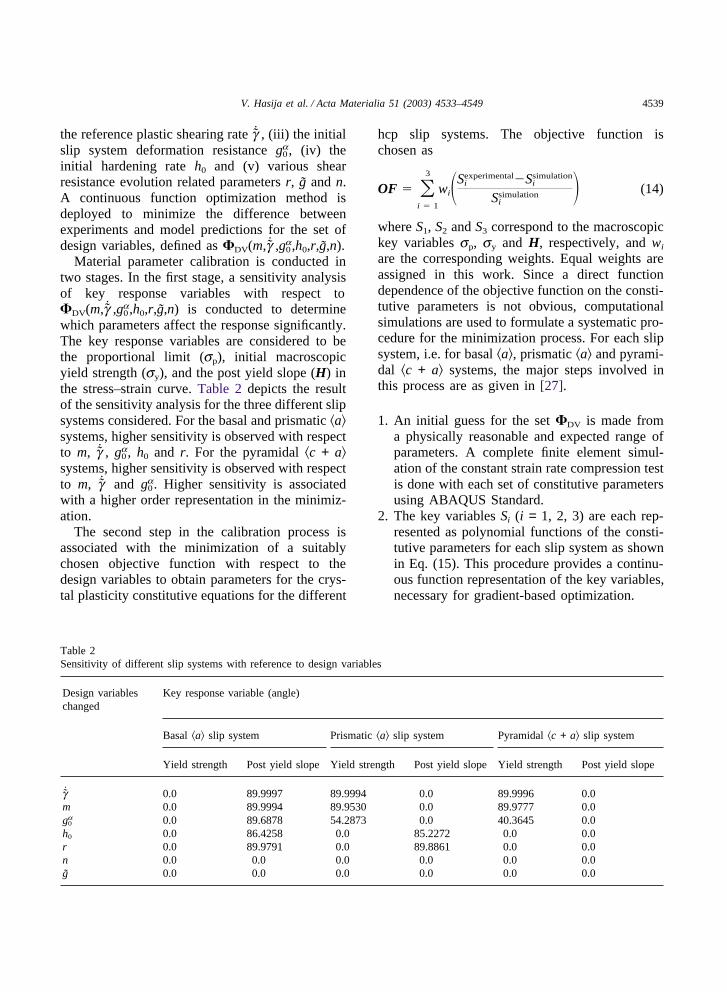
Material parameter calibration is conducted intwo stages. In the first stage, a sensitivity analysisof key response variables with respect to�DV(m,g ,ga0,h0,r,g,n) is conducted to determinewhich parameters affect the response significantly.The key response variables are considered to bethe proportional limit (sp), initial macroscopicyield strength (sy), and the post yield slope (H) inthe stress–strain curve. Table 2 depicts the resultof the sensitivity analysis for the three different slipsystems considered. For the basal and prismatic �a�systems, higher sensitivity is observed with respectto m, g , ga0 , h0 and r. For the pyramidal �c + a�systems, higher sensitivity is observed with respectto m, g and ga0. Higher sensitivity is associatedwith a higher order representation in the minimiz-ation.

The second step in the calibration process isassociated with the minimization of a suitablychosen objective function with respect to thedesign variables to obtain parameters for the crys-tal plasticity constitutive equations for the different

Table 2Sensitivity of different slip systems with reference to design variables

Design variables Key response variable (angle)changed

Basal �a� slip system Prismatic �a� slip system Pyramidal �c + a� slip system

Yield strength Post yield slope Yield strength Post yield slope Yield strength Post yield slope

g 0.0 89.9997 89.9994 0.0 89.9996 0.0m 0.0 89.9994 89.9530 0.0 89.9777 0.0ga0 0.0 89.6878 54.2873 0.0 40.3645 0.0h0 0.0 86.4258 0.0 85.2272 0.0 0.0r 0.0 89.9791 0.0 89.8861 0.0 0.0n 0.0 0.0 0.0 0.0 0.0 0.0g 0.0 0.0 0.0 0.0 0.0 0.0

hcp slip systems. The objective function ischosen as

OF � �3

i � 1

wi�Sexperimentali �Ssimulation

i

Ssimulationi

� (14)

where S1, S2 and S3 correspond to the macroscopickey variables sp, sy and H, respectively, and wi

are the corresponding weights. Equal weights areassigned in this work. Since a direct functiondependence of the objective function on the consti-tutive parameters is not obvious, computationalsimulations are used to formulate a systematic pro-cedure for the minimization process. For each slipsystem, i.e. for basal �a�, prismatic �a� and pyrami-dal �c + a� systems, the major steps involved inthis process are as given in [27].

1. An initial guess for the set �DV is made froma physically reasonable and expected range ofparameters. A complete finite element simul-ation of the constant strain rate compression testis done with each set of constitutive parametersusing ABAQUS Standard.

2. The key variables Si (i = 1, 2, 3) are each rep-resented as polynomial functions of the consti-tutive parameters for each slip system as shownin Eq. (15). This procedure provides a continu-ous function representation of the key variables,necessary for gradient-based optimization.


Si � (ai0 � ai1m � ai2m2) � (bi0

� bi1g � bi2g 2) � (ci0 � ci1ga0

� ci2ga20 ) � (di0 � di1h0 � di2h2

0) � (15)

(ei0 � ei1r � ei2r2) � (fi0 � fi1n) �

(gi0 � gi1g)

3. Approximately 150 ABAQUS simulations withdifferent parameters sets are conducted to evalu-ate the coefficients of the polynomial expansion.The computed values of Si (i = 1, 2, 3) arerecorded from the stress strain plots for eachsimulation. The coefficients are evaluated by aleast square method using MATLAB [28].Using these coefficients, the functions Si (i =1, 2, 3) can be constructed.

4. The crystal plasticity constitutive parameters arefinally obtained by minimizing the objectivefunction stated in Eq. (14), stated as

Minimize OF

wrt �DV

(16)

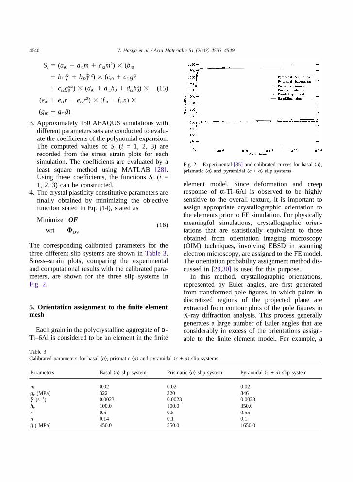
The corresponding calibrated parameters for thethree different slip systems are shown in Table 3.Stress–strain plots, comparing the experimentaland computational results with the calibrated para-meters, are shown for the three slip systems inFig. 2.

5. Orientation assignment to the finite elementmesh

Each grain in the polycrystalline aggregate of α-Ti–6Al is considered to be an element in the finite

Table 3Calibrated parameters for basal �a�, prismatic �a� and pyramidal �c + a� slip systems

Parameters Basal �a� slip system Prismatic �a� slip system Pyramidal �c + a� slip system

m 0.02 0.02 0.02g0 (MPa) 322 320 846g (s�1) 0.0023 0.0023 0.0023h0 100.0 100.0 350.0r 0.5 0.5 0.55n 0.14 0.1 0.1g ( MPa) 450.0 550.0 1650.0

Fig. 2. Experimental [35] and calibrated curves for basal �a�,prismatic �a� and pyramidal �c + a� slip systems.

element model. Since deformation and creepresponse of α-Ti–6Al is observed to be highlysensitive to the overall texture, it is important toassign appropriate crystallographic orientation tothe elements prior to FE simulation. For physicallymeaningful simulations, crystallographic orien-tations that are statistically equivalent to thoseobtained from orientation imaging microscopy(OIM) techniques, involving EBSD in scanningelectron microscopy, are assigned to the FE model.The orientation probability assignment method dis-cussed in [29,30] is used for this purpose.

In this method, crystallographic orientations,represented by Euler angles, are first generatedfrom transformed pole figures, in which points indiscretized regions of the projected plane areextracted from contour plots of the pole figures inX-ray diffraction analysis. This process generallygenerates a large number of Euler angles that areconsiderably in excess of the orientations assign-able to the finite element model. For example, a


total of 19 620 discrete orientations are obtainedfrom the experimental pole figure in Fig. 3. Thefinite element model in ABAQUS for a polycrys-talline model is assumed to contain 512 grains witha total of eight elements per grain. Since the num-ber of grains is far less than the number of orien-tations, statistically equivalent orientations withsimilar probability density distributions f(g) of thecrystallographic orientations are assigned to thefinite element mesh. The steps in this process are:

(i) An Euler angle space, in which the three coor-dinate axes are represented by three Euler

Fig. 3. (a) Contour plot of the experimental (0 0 0 1) pole figure. (b) Transformed experimental pole figure [35] from contour plotto points in the discretized regions of the projected plane. (c) Statistically equivalent orientations obtained from the orientationassignment method, put into the finite element model. (d) Orientation distribution for the FEM simulations of polycrystalline Ti–6Al.

angles (f1,f,f2), is discretized into n cubicorientation space elements and the discreteorientation data are recorded.

(ii) From the definition of probability densityfunction, f(g)dg = dVg /V is the probability ofobserving an orientation G in the intervalg�G�g + dg, where dVg is the volume ofcrystals with the orientation between g and dgand V is the total volume of all grains. There-fore, the volume fraction of crystal orientationsin the ith orientation space element ranging incoordinate space from (f1,f,f2) to ((f1 +df1,f + df,f2 + df2)) is determined as


V(i)f �

V(i)

V� �f2 � df2

f2

�f � df

f�f1 � df1

f1

(17)

f(g)8p2sinf df1 df df2

(iii) An orientation probability factor (Pi) for eachorientation space element is obtained as

Pi � K � V(i)f (18)

where K corresponds to a number that is equalto or larger than the number of orientations tobe assigned to the finite element mesh. Thecomplete set of statistically equivalent orien-tations is then given as

P � �n

i � 1

Pi (19)

where P is equal to or larger than the numberof grains in the finite element model.

(iv) Q (�P) sets of Euler angles are randomlyselected from the orientation population P andare assigned to the integration points of thedifferent grains. The computational modelwith this assigned orientation represents astatistically equivalent polycrystalline aggre-gate.

6. Simulation of deformation and creep inpolycrystalline Ti–6Al

The simulations are for two different types ofmechanical tests, (i) constant strain rate tests and(ii) creep tests which have been conducted withthe polycrystalline Ti–6Al in [10]. As mentionedin Section 3, constant strain rate tests are withstrain rates of 8.4×10�4, 1.5×10�4s�1 and1.68×10�5 s�1. From these tests, it has beenobserved in [10] that the strain rate sensitivity ofthis material is not very high in comparison withother metallic materials like steel and copper.Additionally, a comparison of the post yield hard-ening shows that the strain rate has little influenceon hardening. The overall hardening in thesepolycrystalline Ti–6Al alloys is also found to below. This is attributed to the planar slip due to the

presence of SRO of Ti and Al atoms, whichreduces the rate of hardening as well as the interac-tion between the different slip systems. The creeptests are conducted at two different stress levelsviz. 606 and 716 MPa. They enable the study ofstrain accumulation phenomenon, which can besignificant with time. Higher creep strains areobserved at higher stress levels. The creep strainaccumulation follows a power law behavior intime, with monotonically decreasing creep rates.

The finite element model for the polycrystallineaggregate consists of a cubic domain of unitdimensions that is discretized into 4096 eight-noded brick elements (C3D8R) in ABAQUS. Atotal of 512 grains, for which the crystallographicorientations are assigned using the orientationassignment method of Section 5, are assumed tobe contained in this model. The model texture isstatistically equivalent to the actual orientation dis-tribution obtained from the OIM results as shownin Fig. 3. Fig. 3d shows the distribution of orien-tations in the polycrystalline finite element model.To simulate the experimental conditions, no sym-metry constraints are imposed in the model. Onlythe constraints that are necessary to prevent therigid body modes are applied to the model. Thematerial parameters for both elasticity and crystalplasticity are the same as those for the single crys-tals that have been calibrated in Section 4.

For simulation of the constant strain rate tests,the strain rate boundary condition is applied usingthe DISP subroutine in ABAQUS. Consistent withthe constant strain rate ec, a displacement boundarycondition is applied on the top face of the cube as

u(t) � l0(exp(ect)�1) (20)

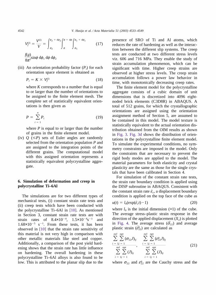
where l0 is the initial dimension (=1) of the cube.The average stress–plastic strain response in thedirection of the applied displacement (X2) is plottedin Fig. 4. The average stress (s22) and averageplastic strain (ep22) are calculated as

�nel

i � 1

�npt

j � 1

(s22J)ij

�nel

i � 1

�npt

j � 1

(J)ij

,

�nel

i � 1

�npt

j � 1

(ep22J)ij

�nel

i � 1

�npt

j � 1

(J)ij

(21)

where s22 and ep22 are the Cauchy stress and the


Fig. 4. Constant strain rate test for strain rate = 8.4 × 10�4,1.5 × 10�4 and 1.68 × 10�5 s�1.

true plastic strain at each element integration pointand J is the determinant of the jacobian matrix atthese integration points. The number of elementsin the model are designated as nel, and npt corre-sponds to the number of integration points perelement. These plots in Fig. 4 compare the experi-mental and the computational results for the differ-ent strain rates. The results show a remarkablyclose match between the experiments and compu-tations for all the three strain rates, even though thematerial parameters are calibrated with the singlecrystal tests. It is noted that the orientation playsa significant role in these overall stress–strain plotsand corresponding simulations appears to catch theoverall behavior rather well. The small discrep-ancies in Fig. 4 may be attributed to variousaspects, such as the orientations and material para-meters. The orientation assignment for the 3Dmodels from 2D OIM maps is a potential sourceof error. Additionally, the crystal plasticity para-meters are calibrated using a nonlinear functionminimization of the overall material response. Thelack of more detailed experiments for better cali-bration of individual parameters could lead to non-uniqueness in their values. For example, the latenthardening parameter, which is taken to be 1, couldbenefit from isolating experiments.

For the simulation of creep, the boundary con-dition is applied in two steps. In the first step, uni-form pressure load is applied on the top face usingthe DLOAD option in which the pressure is

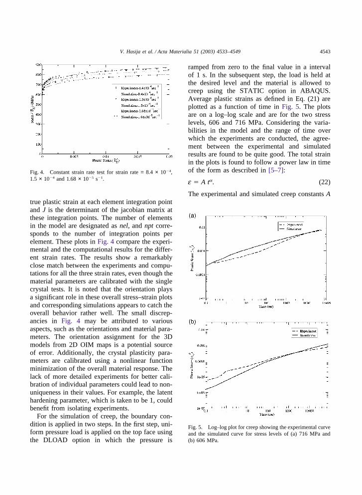
ramped from zero to the final value in a intervalof 1 s. In the subsequent step, the load is held atthe desired level and the material is allowed tocreep using the STATIC option in ABAQUS.Average plastic strains as defined in Eq. (21) areplotted as a function of time in Fig. 5. The plotsare on a log–log scale and are for the two stresslevels, 606 and 716 MPa. Considering the varia-bilities in the model and the range of time overwhich the experiments are conducted, the agree-ment between the experimental and simulatedresults are found to be quite good. The total strainin the plots is found to follow a power law in timeof the form as described in [5–7]:

e � A ta. (22)

The experimental and simulated creep constants A

Fig. 5. Log–log plot for creep showing the experimental curveand the simulated curve for stress levels of (a) 716 MPa and(b) 606 MPa.


and a for both stresses are calculated and shownin Table 4. It is observed that the value of the coef-ficient A depends on the applied stress, with lowercreep stresses leading to smaller A values. Thereis some discrepancy observed in the value of Abetween the experiments and the simulations forthe two stress levels. The time exponent a is seento compare well between the experiments and thesimulations. The fact that the value of the timeexponent a is less than unity demonstrates that ste-ady state creep is not observed in these experi-ments.

7. Creep and cyclic deformation with strengthmismatch

7.1. Load shedding with creep

This section discusses a finite element modelthat is created to reflect the effects of heterogeneityin the crystal structure on the local materialresponse to compressive creep loading. The modelconsists of two regions that have distinctly differ-ent orientations to reflect mismatch in strengthcharacteristics. The first region is constructed as acube of dimensions 0.2 m × 0.2 m × 0.2 m forwhich the c-axis in the crystallographic structureis aligned with the global loading axis. The secondis a cubic region of external dimensions 1 m × 1m × 1 m that surrounds the inner cube. The basalplane in the crystallographic structure of thisregion is parallel to the global loading axis. Thecrystallographic orientations are depicted by the

Table 4Creep constants for applied stress of 716 and 606 Mpa

Power law Simulation Experimentcreepconstants

716 MPa 606 MPa 716 MPa 606 MPa

A 0.000642 2.26e�05 0.00037 1.84e�05a 0.26 0.35 0.275 0.36

pole figure in Fig. 6b. It has been observed fromthe previous calibration exercise that the criticalresolved shear stress for the pyramidal �c + a� slipsystems is about 2.7 times that for the �a�-type slipsystems. Since only the �c + a� slip systems willbe active in the inner region for the given loading,it represents a region with a considerably higherstrength response in comparison with the outsideregion. The inner cube, as shown in Fig. 6a, is uni-formly discretized into a mesh of 512 eight-nodedbrick elements (C3D8R). The outside region con-sists of a graded mesh with 4608 eight-noded brickelements, to create more refined elements near theinterface. Such resolution is necessary toadequately represent the high gradients in stressand strains. The material properties for elasticityand all the crystallographic slip systems corre-spond to the calibrated values in Section 4. Themodel is subjected to a compressive creep loadingwith a constant applied pressure of 606 MPa heldover a period of 1000 s. This loading is applied onthe outer face of the model. All other boundaries

Fig. 6. (a) Contour plot showing the stress concentrationaround the hard phase for value of rate exponent m = 0.05; (b)(0 0 0 1) pole figure showing the orientation of the hard phaseand the soft phase.


are free to deform subject to the constraint of rigidbody motion. A total of 100 equal time steps areused to simulate the creeping process.

The results of the creep simulation are shown inFigs. 6–8. Fig. 6a shows the contour plot of thedominant stress (s22) in the loading direction at theend of the creep process. It can be seen from thisfigure that while the stress is generally uniform inthe outer region away from the interface, there aresignificant gradients near the interface in bothphases. The compressive stress just outside theinterface dips below the average but rises consider-ably near the interface in the inner phase. This isfurther illustrated in the graphs of the evolvingstress as a function of location in Fig. 7a. Thestress is plotted along the diagonal A–A. Both theminimum peak stress in the lower-strength phase(outer region) and the maximum peak stress in thehigher-strength phase (inner region) increase with

Fig. 7. (a) Evolution of dominant stress (s22) as a function oftime along the line A–A for rate exponent m = 0.05 and (b)total strain (e22) and plastic strain (ep22) at the end of the creepprocess, for rate exponent m = 0.05.

Fig. 8. Stress (s22) along the line A–A for different values ofthe strain rate sensitivity exponent, plotted at the end of thecreep process.

creep and time. With the onset of plastic defor-mation in the lower-strength phase, the outerregion sees an increase in the total strain due toplastic creep. The compatibility constraint at theinterface, however, requires the local strain nearthe interface to be lower than the rest of the outerregion. This causes a drop in the lower-strengthphase stress near the interface. Likewise, the com-patibility requirement in the high-strength phasecauses the strain near the interface to be higherthan that away from it. This gives rise to the highstress concentration near the interface. Withincreasing creep, the strain increases and hence thelocal stress also increases as a function of time.Fig. 7a, which corresponds to a strain rateexponent m = 0.05 clearly shows that the localpeak stress rises significantly as a function of time.However for m = 0.02, the rise in the peak stressfor the same interval is small. This result clearlypoints to the significant effect of strain rate sensi-tivity on local peak stress as a function of time.This phenomenon has been termed as load shed-ding in creeping heterogeneous materials. It isparticularly relevant in the context of fatigue crackinitiation because the regions of high stress con-centration are potential nucleation sites. It is inter-esting to note that the stress at the center of thestronger phase does not change with increasingcreep. This may be explained from the plasticstrain plot at the end of the creep process in Fig.7b. The total logarithmic strain (ln V, V is the leftstretch tensor) and the plastic strain (1 /2(FpT

Fp�


I)) are plotted along the diagonal A–A in this fig-ure. For the times considered, the material in a con-siderably large area around the center of thestronger phase does not yield and hence the strainis entirely elastic and unchanged with creep. Thestress behavior follows from its dependence on theelastic strain.

To understand the effect of the material rate sen-sitivity on the load shedding due to creep, theabove simulations are conducted with three differ-ent rate sensitive exponents i.e. m = 0.02, 0.035and 0.05 in Eq. (4). The corresponding stresses(s22) at the end of the creeping process are plottedalong the line A–A in Fig. 8. The effect of loadshedding reflected in the stress concentration at theinterface reduces considerably with reducing rateexponent. The lower bound of the stress disconti-nuity will occur for the rate-independent materialbehavior. It is evident through this example thatmismatch interfaces have a high potential of cracknucleation for creeping materials, especially withincreasing rate sensitivity.

7.2. Load shedding for various load histories

In this example, the effect of overall load histor-ies on the local evolution of stresses and strainsis examined for the polycrystalline material withdiscrete orientation mismatch. The computationaldomain consists of a large cubic grain of dimen-sion 0.25 m × 0.25 m × 0.25 m contained in anaggregate of 4032 grains occupying the externalcubic domain. The inner grain represents a higher-strength phase with c-axis parallel to the loadingaxis while the 4032 outside grains have randomorientations as shown in Fig. 9. In the finiteelement model, the inner grain is discretized intoa mesh of 64 eight-noded brick elements whileeach grain in the outer region is modeled using asingle eight noded brick element.

Four different overall loading conditions havebeen considered in this example. They are (a) creeploading with a peak load of 606 MPa, (b) cyclicloading with a peak load of 606 MPa and cycletime of 2 s, (c) dwell cyclic loading with a peakload of 606 MPa and a cycle time of 62 s with 60 sof dwell period and 2 s of unloading and reloadingperiod, (d) dwell cyclic loading with a peak load

Fig. 9. (0 0 0 1) Pole figure showing the random orientationdistribution.

of 606 MPa and a cycle time of 122 s with 120 sof dwell period and 2 s of unloading and reloadingperiod. All the cyclic loading cases are run with astress ratio of 0. The dwell load cycles have beenchosen from data on experiments performed ondwell fatigue of Ti alloys at the Ohio State Univer-sity. All the loadings are run for a total time of370 s. Since the loading considered in these casesare cyclic and include unloading, the kinematichardening terms discussed in Section 2 areincluded in the material model. The kinematichardening parameters are chosen to be c = 500 andd = 100 MPa for all the slip systems. The boundaryconditions and all the material parameters exceptm are the same as those discussed in Section 7.1.The value of m is chosen to be 0.02, correspondingto that calibrated from experiments.

The results of simulations for the four load his-tories are shown in Fig. 10. Fig. 10a shows theplastic strain in a representative grain as a functionof time. The plastic strain (ep22) in the loading direc-tion shows a continual increase with time indicat-ing plastic ratcheting. There is a significant differ-ence in the plastic strain accumulation for thecyclic loading case and the other cases, while theresponse is very similar for the creep and the dwellcyclic loading cases. Plastic strain accumulation isseen to increase slightly with increasing dwell timeas shown in the inset of Fig. 10a. This may beattributed to the fact that no plastic strain is added


Fig. 10. (a) Plastic strain plot in a representative grain in theloading direction for the four load cycles as a function of time.(b) Stress (s22) plot for the four load cycles along the line A–A at the end of 370 s.

during unloading–reloading phase of the cyclicloading. Fig. 10b shows the s22 stress plot alongthe diagonal A–A plotted at the end of the loadingfor the four different histories considered. Higherstresses are observed in the higher-strength phasenear the interface whereas for the outside regionnear the interface, the stresses are low. This is dueto load shedding as discussed in Section 7.1. Sincethe outside region consists of grains with randomorientations, local peaks (1, 2, 3, 4) are observedaway from the interface. However, these peaks areconsiderably smaller than those at the interface.The higher of these peaks at points 1 and 3 corre-spond to orientations which are close to c-axisorientation as seen from Fig. 9. Since the value ofm chosen is small (0.02), the time-dependent riseof the peak stress is not very significant. This is

consistent with the results obtained with the samerate exponent in Section 7.1.

8. Conclusion

Cold creep has been observed to be the dominantmode of deformation in Ti alloys at low tempera-tures, where significant strains can accumulate withtime. In an attempt to understand this behavior, thematerial response of α-Ti–6Al is analyzed using arate-dependent elastic crystal plasticity model inthis paper. The model accommodates the plasticanisotropy that is inherent to the Ti alloys andaccounts for time dependence that is observedunder deformation and creep behavior, with crystalplasticity parameters calibrated from experiments.For modeling polycrystalline aggregate of α-Ti–6Al, a statistically equivalent orientation distri-bution is assigned to the finite element modelthrough a special orientation assignment methodfrom OIM images of polycrystalline α-Ti–6Al.The model with the calibrated parameters is testedby comparison with the experimental results ofconstant strain rate and creep tests with excellentagreement. It is observed that the model canaccount for changes of many orders of magnitudein strain rate. It is also observed that the power lawin time (i.e. Andrade creep) is a direct consequenceof load shedding from soft- to hard-oriented grains.Previous explanations for the power-law creeptransient have been proposed in the literature [6].Several dislocation-based models attempting toexplain exhaustive creep at lower temperatureshave been forwarded—some rather recently byCottrell and Nabarro [31�33]. These models arguethat primary creep is due to the operation of dislo-cation sources with a distribution of energies, butmake the assumption that polycrystals deformhomogeneously. In fact, the extended power lawsin time naturally arise rather remarkably from thecrystal plasticity model simulations. Slip occursfirst in the most favorably oriented grains for prismand basal slip. As these grains deform, load is shedto neighboring grains, which are not as favorablyoriented, in order to ensure compatibility and equi-librium between the grains. It is therefore theevolving distribution of internal stresses which


leads to the creep transients observed. A concep-tually similar explanation for these transients hasbeen offered by Daehn [34] who has used a simplercellular automata (CA) modeling approach to pro-duce transients. The apparent “hardening” , orreduction in strain rate with time, is not due to anychange in material structure, but instead is theresult of load redistribution. With time, a largerfraction of the load is borne by higher-strengthgrains, whereas load is evenly distributed at shortertimes. The shape of the transient is intimatelyrelated to the distribution of strengths of individualgrains. Thus, this single-phase material is essen-tially deforming in a manner similar to a compositewith relatively “soft” and “hard” regions producedby the inherent plastic anisotropy of hcp grains.

An understanding of load shedding and localstress rising in polycrystalline aggregates of Tialloys is also developed from this study. This isimportant because creep and dwell cyclic loadingcan lead to local crack initiation at critical locationswithin the microstructure with large orientationmismatch. A model is created to understand thisphenomenon by assigning large orientation mis-match in the constituent grains of the aggregate. Itis observed that the stress concentration is signifi-cantly affected by the material rate sensitivity andthe peaks increase considerably with time,especially for higher values of m. An interestingobservation is that even though the applied macro-scopic stress (606 MPa) is only about 88% of theyield strength of the polycrystalline aggregate (693MPa in the constant strain rate test) and about 33%of the axial stress necessary to activate �c + a� slipin single crystals of the same composition (shownin Fig. 2), considerable local yielding leading toplastic strain is realized in the microstructure. Sig-nificant local stress concentrations evolve withtime in the material microstructure. For example,the stress amplification in the c-axis oriented grainwith respect to the applied stress is ~2, for m =0.05 at time 1000 s. The compatibility constraintat the interface causes the development of thesehigh local stress concentrations. Alternatively, thiscan be explained by considering the planar slipbands, which can propagate across the favorablyoriented grains. Higher local stresses will developdue to dislocation pile-ups when these slip bands

are impinging upon an adjacent grain that is ori-ented with c-axis parallel to the macroscopic defor-mation direction. This is clearly a potential locationof crack nucleation in creep or dwell fatigue load-ing for Ti alloys. The effect of cyclic loading withdifferent dwell periods is studied by incorporatingkinematic hardening in the material model. Thephenomenon of plastic ratcheting is observed inthese materials when subjected to cyclic loading.The time-dependent rise of the peak stress is smallfor the value of rate exponent considered. In con-clusion, the paper provides a good understandingof the plastic behavior of Ti alloys from a localstandpoint which is helpful to set up guidelines forthe study of their fatigue failure behavior.

Acknowledgements

This work has been supported by the FederalAviation Administration through grant No.DTFA03-01-C-0019 (Program Director: Dr. BruceFenton). This support is gratefully acknowledged.The authors are grateful to Drs. A. Woodfield, A.Chatterjee, J. Hall and J. Schirra for their insightfulsuggestions. The authors are also grateful to Dr.Vikas Sinha for providing the experimental data.Computer support by the Ohio SupercomputerCenter through grant # PAS813-2 is also acknowl-edged.

References

[1] Donachie Jr MJ. Titanium—a technical guide. Metals Park(OH): ASM International, 1998.

[2] Froes FH, editor. Non-aerospace applications of titanium.Warrendale (PA): TMS; 1998.

[3] Adenstedt HK. Metal. Progress 1949;65:658.[4] Inman MA, Gilmore CM. Metall. Trans. 1979;10:419.[5] Chu HP. J. Mater. 1970;5:633.[6] Odegard BC, Thompson AW. Metall. Trans. 1974;5:1207.[7] Miller WH, Chen RT, Starke EA. Metall. Trans.

1987;18A:1451.[8] Neeraj T, Mills MJ. Mat. Sci. Eng. A-Struct.

2001;319:415.[9] Thompson AW, Odegard BC. Metall. Trans. 1973;4:899.

[10] Neeraj T, Hou DH, Daehn GS, Mills MJ. Acta Mater.2000;48:1225.

[11] Paton NE, Baggerly RG, Williams JC. AFOSR ReportSC526.7FR. 1976.


[12] Balasubramanian S. Polycrystalline plasticity: applicationto deformation processing of lightweight metals. Ph.D.dissertation. Cambridge (MA): MIT; 1998.

[13] Peirce D, Asaro RJ, Needleman A. Acta Metall. Mater.1983;31:1951.

[14] Asaro RJ, Needleman A. Scripta Metall. Mater.1984;18:429.

[15] Harren SV, Asaro RJ. J. Mech. Phys. Solids 1989;37:191.[16] Kalidindi SR, Bronkhorst CA, Anand L. J. Mech. Phys.

Solids 1992;40:537.[17] Kothari M, Anand L. J. Mech. Phys. Solids 1998;46:51.[18] Balasubramanian S, Anand L. Acta Mater. 2002;50:133.[19] Grujicic M, Batchu S. J. Mater. Sci. 2001;36:2851.[20] Kad BK, Dao M, Asaro RJ. Mat. Sci. Eng. A-Struct.

1995;193:97.[21] Bronkhorst CA, Kalidindi SR, Anand L. Philos. Trans. R.

Soc. London A 1992;341:443.[22] Morrissey RJ, McDowell DL, Nicholas T. Int. J. Fatigue

2001;23:S55.[23] Goh CH, Wallace JM, Neu RW, McDowell DL. Int. J.

Fatigue 2001;23:S423.

[24] Cuitino AM, Ortiz M. Model. Simul. Mater. Sci.1993;1:225.

[25] ABAQUS reference manuals. Providence (RI): Hibbit,Karlsson and Sorenson, Inc, 2001.

[26] Kim JY, Yakovlev V, Rokhlin SI. CP615, vol. 21. Amer-ican Institute of Physics, 2002.

[27] Ghosh S, Ling Y, Majumdar BS, Kim R. Mech. Mater.2000;32:561.

[28] Matlab. Version 6.2, 2001.[29] Xie CL, Nakamachi E. J. Mater. Process Tech.

2002;122:104.[30] Xie CL, Nakamachi E. Mater. Design 2002;23:59.[31] Cottrell AH. Philos. Mag. Lett. 1996;74:375.[32] Cottrell AH. Philos. Mag. Lett. 1997;75:301.[33] Nabarro FRN. Philos. Mag. Lett. 1997;75:227.[34] Daehn GS. Acta Mater. 2001;49:2017.[35] Sinha V, Savage M, Tatalovich J. Unpublished research,

2001.

Deformation and creep modeling in polycrystalline Ti–6Al alloys

Documents

Transcript of Deformation and creep modeling in polycrystalline Ti–6Al alloys