Probabilistic description of fatigue crack growth in polycrystalline solids
189
PROBABILISTIC DESCRIPTION OF FATIGUE CRACK GROWTH UNDER CONSTANT-AND VARIABLE-AMPLITUDE LOADING b y 1. Ghonem and M. Zeng THE UNIVERSITY OF RHODE ISLAND Solid Mechanics Laboratory Department of Mechanical Engineering and Applied Mechanics DTIC E CTE MARCH 1989 JUN 0 7 1989 Prepared For l)I:P ARTMF NI'" O AIR FORCE \IR 1:()R('I 0I'II- OF SCIENTIFIC RI S ARCI I 1301I.ING AIP, FORCI" BASF. DC 20032 C.ntract \F SR 85-()302 > ".. .-. - ¢. j 023~
Transcript of Probabilistic description of fatigue crack growth in polycrystalline solids

PROBABILISTIC DESCRIPTIONOF FATIGUE CRACK GROWTH UNDER
CONSTANT-AND VARIABLE-AMPLITUDELOADING
b y
1. Ghonem and M. Zeng
THE UNIVERSITY OF RHODE ISLANDSolid Mechanics Laboratory
Department of Mechanical Engineering and Applied Mechanics
DTICE CTE MARCH 1989
JUN 0 7 1989
Prepared For
l)I:P ARTMF NI'" O AIR FORCE
\IR 1:()R('I 0I'II- OF SCIENTIFIC RI S ARCI I1301I.ING AIP, FORCI" BASF. DC 20032
C.ntract \F SR 85-()302
> ".. .-.- ¢. j 023~

6611111 CLASSIPOCAION Of T--S PAGE
REPORT DOCUMENTATION PAGEr$ MEPA P S~oNSv CLhSiICATiON 10 RESTRICTIVE MARKINGS
UNCLAISSIFIED
2&. SICUAIYY CLASSaPICAI0f6 AUTN1401V 3i O-STRIGUTIONAVAi.AILITY OF REPORT
Approved for Public Release;3WOCC.ASS''ICATION/0O0mGU4AOINGSC4IO.L Distribution is unlimited
4 PIMPOCMING ORGANIZATiON maPOor *4umEss 5 MONITOING,,~ ORGANiZArioNi REPORT NUMESNISI1114
"C" ' Igt ' 8 9 - 075NAIIIII OP PERFORMING OPIGANIZArioN 4 a OFFICE SykMIOI. 'a %AME OF %oiTORNNG OPIGANIZAriopii
UNIVERSITY OF RHODE ISLAND AFOSR/NA
a. A000111311 ICe'y. Ste#* and /JP Code ?b ADOMESS t,ev iidee sow /.IP CoaeDept of Mechanical Engineering T)uling 4+10Soli.d_ -cc: aburatory Balling AFB, Washington, DC 20332-6448
Kingston, RI 02881OL NAME OP PUP4OING/SPONSOMING ED OP''CE SvASOi. 9 PROCUREMENT iNSTRUMENT IO1ENTIPICATION 14UME1R
ORGANIZATION 11f .uPI~ce~~ "FSR8-06
AFOSR/NAAFS-506
ft. L16ONESS IC'tY. S. 4 w4 ZIP Cad40 '0 SOWPICE OF F UNOING NOS. _____________
PROGRAM PROJECT TASK WORK umiTBuilding 410 E L.E ME N rNo NO NOO. No.
Bolling AFB, Washington DC 20332-6448 61102F 2302 B2FaITIguE Crasckd Growthy ulml~~ne Pr a -A ltde odn
i~ TITLE I~clfl jees.,,R 09aneIicploiudeb Loaring
12. PERSONAL AUTPMORISI2H. Ghonern and M. Zeng
113. Tv'P6 OP REPORT i13.T ?M1 COE vI 6 I0A11 JArS OF REPORT It,. Wo , D0yj is, PAO E COUNT
FINAL mo Ii 89-4-15 180If. SUPP9L&MINTARV NOTATION
17 COSATI cools Is SUBJECT TERMS 'C7,,q,,,.e GA *frICr itlcsf ACCIUP'i ddentify by 11WdIII RufftbeI
-01ELO GROUP F SUE Go CRACK OVERLOAD, STOCHASTIC PROCESS, RETARDATION
I, AESTRACT 'CaaIuI1ime* MON S tY#I fCfIIA& JAd dIe II.' oy Nuc" A-br
rc:port is concece %kith the di script ion of the development and application of a stochasticlzroIth model. It is hulilt as a discontinuous Markov process anid is inhonioigeflous wi th
to the numbner of c,\ des required for the crack to reach a sp%,ifled crack lentgth. The model'ihen used to describe the ev.oluition of' the crack length in terms of growth cuirves, eachi of
Aho~e points possess cqtlua prohabilitv of adlvancing from one position to another forward2swi~on. The v-alidlty of the mnodel is estaiblished by applying it to constant-as well as to variable
.'pi.eloading. In those appl caltions the theoretical constant probabili ty crack gro wth cuir\es.:cae y the mnodel c 01 pared to t hiie cexperimenttallIy obtained using Al 7075 -T6 arid
-T I041 material for constatit-atoplitude loadingt while Ti-6AI-4V was used in singleP-r oaid applicatioti. Results of these comparisons indlicate the ability of the proposed niodel 'Alhen
Aith parametecrs %khosec vaIlues canT be obtaitted from a limlited Inmbers ot cxperimntl1to predict the tr.ack icro%%i fthHiti ticutder different loading condition,,.
20 STIS CAVLE6 00 ~ AS1U*I 2I AISTRACT SECUAI?'I CLASSIFICATioNd
UPICLA111I111111/1UMLIMITIO 2 SAME AS OPT Zr6-c ,sas I UNCLASSIFIED
33.L N"AME OP RE4SPOP4111Se1.11 NO'0VIOWAL 22b ?ELEP-ONf NUM11ER1 22c OPPIC6 SYMUOO.
* Imefud 4me Code,G. llarito, 202-767-04t)3 NA
00 FORM 1473, &3 APR 10rTION OF I Aft 73 13 OS1SOLEI1
SECURITY CLASSIPICATION OP TN-5 PAGG

1. REPORT NO. 2. GOVERNMENT AGENCY 3. RECIPIENTS CATALOG NO.
4. TITLE AND SUBTITLE 5. REPORT DATAProbabilistic Description of Fatigue Crack March 1989Growth Under Constant- and Variable Mac 18
Amplitude Loading 6. PERFORMING ORG. CODE
7. AUTHORS 8. PERFORMING ORG. REPT NO.
H. Ghonem and M. Zeng URI-MSL-891
9. PERFORMING ORG NAME AND ADDRESS 10. WORK UNIT NO.
University of Rhode IslandDepartment of Mechanical Engineering II. CONTRACT OR GRANT NO.Solid Mechanics LaboratoryKingston, RI 02881 AFOSR-85-0362
12. SPONSORING AGENCY NAME AND ADDRESS 13. TYPE REPT. /PERIODCOVERED
U.S. Air Force Office of Scientific Research Final ReportBoiling Air Force BaseWashington, DC 20032 14. SPONSORING AGENCY CODE
15. SUPPLEMENTARY NOTES
This report is concerned with the discription of the development and application of a stochasticcrack growth model. It is built as a discontinuous Markov process and is inhomogeneous withrespect to the number of cycles required for the crack to reach a specified crack length. The modelis then used to describe the evolution of the crack length in terms of growth curves, each ofwhose points possess equal probability of advancing from one pos~tion to another forwardposition. The validity of the model is established by applying it o constant-as well as to variableamplitude loading. In those applications the theoretical constant probability crack growth curvesgenerated by the model compared to those experimentally obtained using Al 7075-T6 andAl 2024-T3 material for constant-amplitude loading while Ti-6AI-4V was used in singleoverload application. Results of these comparisons indicate the ability of the proposed model whenfitted with pararreters whose values can be obtained from a limited numbers of experimentaltests, to predict the crack growth statistics under different loading conditions.
17. KEYWORDS (SUGGESTED BY AUTHORS) 18. DISTRIBUTION STATEMENT
Crack, Overload, Stochastic Process, Retardation
19. SECURITY CLASS THIS(REPT) 20. SECURITY CLASS THIS(PAGE) 21. NO PGS. 22. PRICE
U n class ifie d Unclassi fied !180

ABSTRACT
This report is concerned with the discription of the development
and application of a stochastic crack growth model. It is built as a
discontinuous Markov process and is inhomogeneous with respect to
the number of cycles required for the crack to reach a specified crack
length. The model is then used to describe the evolution of the crack
length in terms of growth curves, each of whose points possess equal
probability of advancing from one position to another forward
position. The validity of the model is established by applying it to
constant as well as to variable amplitude loading. In those
applications the theoretical constant probability crack growth curves
generated by the model were compared to those experimentally
obtained using Al 7075-T6 and Al 2024-T3 materials for constant-
amplitude loading while Ti-6AI-4V was used in single overload
application. Results of these comparisons indicate the ability of the
proposed model, when fitted with parameters whose values can be
obtained from a limited numbers of experimental tests, to predict the
crack growth statistics under different loading conditions.
A cesic;,N] IS c'r:,,
/ I

ACKNOWLEDGEMENT
This work was supported by the U.S. Air Force Office of Scientific
Research under contract AFOSR 85-0362 monitored by Dr. G. Haritos.
This support is gratefully acknowledged.
ii

TABLE OF CONTENTS
Page
ABSTRACT i
ACKNOWLEDGEMENT ii
TABLE OF CONTENTS iii
LIST OF TABLES v
LIST OF FIGURES vi
CHAPTER I INTRODUCTION
CHAPTER II CONSTANT PROBABILITY CRACK
GROWTH MODEL 4
2.1 Mathematical Elements 4
2.2 Experiment Verification 6
CHAPTER III VARIABLE-AMPLITUDE LOAD
APPLICATION 8
3.1 Introduction 8
3.2 Proposed Model 11
3.2.1 Mathematical Elements 11
3.2.2 Effective f(Keff) During Retardation 12
iii

Page
3.3 Single Overload Application 25
3.3.1 Experimental Creek Growth Curve 25
3.3.2 Theoretical Crack Growth Curves 29
CHAPTER IV CONCLUSIONS 68
REFERENCES 78
APPENDIX A Probabilistic description of fatigue crack growth
in polycrystalline solids 83
APPENDIX B Experimental study of the constant-probability
crack growth curves under constant amplitude
loading 102
APPENDIX C Constant-probability crack growth curves 128
APPENDIX D Potential drop measurement 145
iv

LIST OF TABLES
Table Page
1 Chemical composition of Ti-6AI-4V material in wt% 13
2 Effect of varying R, overload ratio and AK on crack
growth delay (Nd) in Ti-6AI-4V 22
3 Percentage error between the theoretical and
experimental constant-probability crack growth 41
V

LIST OF FIGURES
Figure Page
1 Different cases of transient crack growth behaviorfollowing a tensile peak overload 9
2 A series of pairs of hardness indentations made
along two lines parallel to and equal distance fromthe expected nominal crack path 14
3 Schematic sketch of closure measurement 16
4 Photograph of the schematic sketch shown in figure
3 16
5(a) Load-displacement measurements for crack openingdisplacement 17
5(b) Load-displacement measurements for crack opening
displacement 18
6-(a) KR model test 23
6-(b) KR model test 24
6-(c) KR model test 24
6-(d) KR model test 25
7 Typical results of crack length vs number of cycles 27
8 Crack growth sample curves (from 65 Ti-6AI-4V) 28
9(a) Constant probability crack growth curves 29
vi

Figure Page
9(b) Nine of the experimental constant probability crackgrowth curves shown in Fig. 9(a) 30
10(a) Comparision of theoretical and experimentalcrack growth curves (P=0.1) 33
10(b) Comparision of theoretical and experimental
crack growth curves (P=0.2) 34
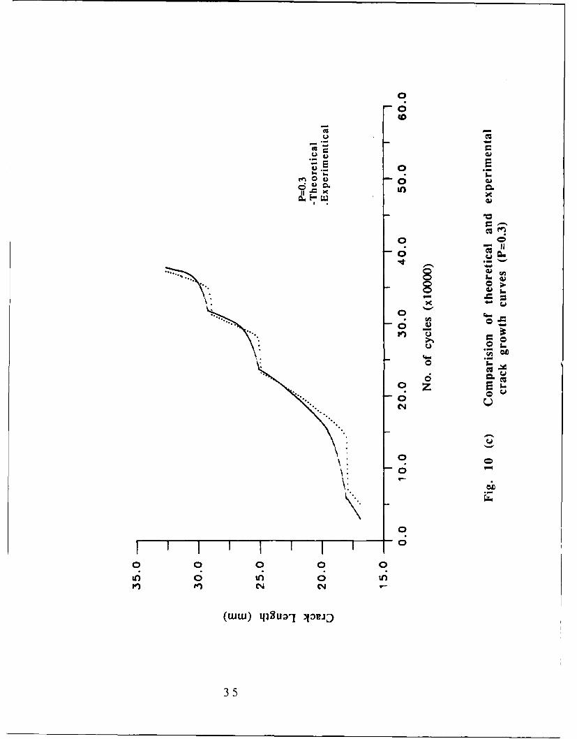
10(c) Comparision of theoretical and experimental
crack growth curves (P=0.3) 35
10(d) Comparision of theoretical and experimentalcrack growth curves (P=0.4) 36
10(e) Comparision of theoretical and experimental
crack growth curves (P=0.5) 37
10(f) Comparision of theoretical and experimentalcrack growth curves (P=0.6) 38
10(g) Comparision of theoretical and experimental
crack growth curves (P=0.7) 39
10(h) Comparision of theoretical and experimentalcrack growth curves (P=0.8) 40
11 (a) Overview of an overload zone showing the
ductile reputure area and delayed zone 72
11 (b) Details of the repture area shown above 72
12 Ductile rupture zones following overload applicationat different crack length 73
vii

Figure Page
13(a) Striation of the facture surface before overload
application 74
13(b) Striation in the delayed zone following an ocerload
application in the same specimen of the above figure 74
14(a) Change in the crack orientation due to overload 75
14(b) Close up of the de'lected zone 75
15 Scanning and optical microscope patterns of the
transition of the kinked crack 76
16 The deflected part of the surface crack after the
overload application and the depth of this transitionin the interior of the specimen 77
D-l Schematic sketch of system for d.c. potential drop
measurement and servodraulic test machine control 147
D-2 Two potential measurements 148
D-3 Optical microscope observation of crack length
in tile calibra:ion 149
D-4 Calibration curve and calibration equation for use
of the potential drop system 150
VIii

CHAPTER I
INTRODUCTION
Prediction of the fatigue crack growth process is generally made by
using one of the determiristic crack growth laws which views the
process as continuous in time and state. Under these laws the growth
rate is calculated from the experimental knowledge of the applied
stress, current crack length and other influencing parameters. As
pointed out by Lauschmann[1], three applications of the mean-value
operator on the crack growth are implicitly irivalued in standard
concepts of the growth law: averaging along the crack front,
averaging ii) the direction of crack propagation close to the given
crack length and averaging over individual realization of the process.
This averaging technique provides the advantage of simplicity and
the ability to respond to changes in the process's physical conditions.
It suffers, however, from the inability to express the process's
inherent random properties, a factor critical to engineering design
and reliability management. The use of statistical distributions or
probabilistic models thus becomes a necessary tool 'or a more
reliable prediction of crack growth. In this approach one can
distinguish three different groups of probabilitic models. The first
group, see for example references[2-7], depends on the introduction
of random variables to replace the constants in the appropriate
deterministic law. The second group, examples of which are shown in
references[8-10], introduces a joint probability distribution whose

variables are crack length and number of loading cycles. The last
group of probabilistic models assigns a non-decreasing evolutionary
feature to the growth process by using the concepts of the stochastic
theory, in particular, the Markov process. Detailed analysis of these
different types of models is given in reference[l 1]. The work in this
research program falls within the definition of the last group, i.e. the
stochastic Markov model. The first generation of these models,
represented in the work of Bogdanoff et al[12-15], Ghonem et
al[16,17] and Sedlacek[18], while having the ability to describe the
random crack growth process in defined cases, has difficulty in
estimating its predictive ability to cases where no experimental data
is available. In recent years a different generation of stochastic
models has evolved. In these models, variability in the process is
taken into account by means of generalizing the growth law, using
the stochastic theory, into a probability form. The work of Ghonem
and Dore[19] and others[20-23] are examples of this approach. The
purpose of this report is to describe the theoretical and experimental
work that has been carried out in developing the model of Ghonem
and Dore[191 termed the constant probability crack growth model.
This description will be covered in the following three chapters. The
mathematical elements of the model are introduced in chapter II,
which will also deal with the correlation between the elements and
the micro-physical condition of the growth process. The experimental
set-up and procedure used for verifying the model in the case of
constant-amplitude loading will be discussed in this chapter. Chapter
Il! deals with an extension of the model base to include the case of
random loading by utilizing a simple single overload spectrum. In
2

this chapter retardation experiments and their relation to the
estimation of the crack growth law in the delayed zone will be
described. The last chapter summarizes the findings of this research
program and suggests avenues for further model refinement and
application. Mathematical derivations and experimental procedures
which have been published in literature during the course of this
research program will not be repeated in the main text of the report.
Reference will be made to these publications, some of which will be
included as appendices.
3

CHAPTER II
COSTANTANT PROBABILITY CRACK GROWTH MODEL
2.1 Mathematical Elements
Formulations of this model and its theoretical development have
been detailed in references [11, 19], see appendix A and C. In brief
summary, the model is based on the view that the crack front is
identified as having a large number of arbitrarily chosen points.
While each of these points can propagate under repeated cyclic
loading in three dimensional geometry. The model considers only the
mode I crack propagation along a plane perpendicular to that of the
externally applied load. The fracture surface is divided into equally
spaced states each of which has a width equal to the expected
experimental error Ax. Adhering to the mechanistic properties of a
propagation crack and considering the growth process to be
evolutionary discrete state and time-inhomogeneous, the model
yields a crack survival probability which is written as:
In P,(i) = - f , di + L (1)
where P,(i) is the probability of the crack tip being in the state r
when Ai cycles elapsed, X, is the transition intensity parameter at
state r and L is an integration constant.
4

The solution of equation (1) depends on the mathematical
definition of X,. Earlier work of Ghonem and Provanj16, 171
considered Xr linearly dependent on r in the form
Xr = rX (2)
where X is a material constant. This yields a growth process well
described as a Markovian linear birth process. Difficulties in this
approach have been analyzed in the reference[l 1].
In the present program, Xr was established as a crack length, cycle
and stress dependent parameter in the form
Xr = L(r) ek. (3)
where L and k are state position dependents (see Appendix A). This
equation in conjuction with equation (1) yields a probabilistic crack
growth equation in the form
In P,(i)= B( eK 0.- eK, ) i > I
(4)
In Pr(i) = 0 1< I
the parameter B, K and I depend on state r through the
experimental functional forms
5

niB = cl r
K =C2 r n2(5 )0 = c3 ((r-lI
where c. and n. are constants depending on load conditions,J J
enviroment, etc. Equations (4) and (5) are the basic results. They are
used to construct constant probability crack growth curves. The
constants in equation (5) can be calculated by considering the crack
growth curve obtained by using a continuous equation as the
P,(i)=0.5 curve. This can be done numerically and the constant
probability crack growth curves can be established under any
loading conditions without the need to perform a large number of
fatigue tests. The results of this approach, when applied to data
proceeded by Virckler et al[24] on Al 2024-T3, were in agreement
with the experimental curves with an average error in the
theoretical curves estimated at 5% (see reference[19] and Appendix
A for detailes of this application).
2.2 Experimental Verification
In order for the model to have a wider scope of application, a
verification of the model was carried out for different loading
conditions on the same material. An in-house experimental program
was followed, during 1985 and 1986. on Al 7075-T6. In this
program, tests were conducted at three different stress levels
(R=4,5,6), and at each stress level sixty replications were employed,
crack length versus number of cycles was measured using a
6

photographic technique. The crack length measurements obtained
were from 9mm to 23mm on center crack retangular specimens with
dimensions of 320mm x 101mm and the thickness of 3.175mm.
Diagrams of sample functions were obtained and converged into
constant probability crack growth curves for each test condition.
Equations (4) and (5) were then employed to obtain the theoretical
constant probability crack growth curves for each corresponding test
loading condition. Comparision with experimental data yielded very
good correlation. The experimental program, procedure,
measurement technique and analysis are described in detail in
reference[l 1, 251 and Appendix B.
7

CHAPTER III
VARIABLE-AMPLITUDE LOAD APPLICATION
3.1 Introduction
A practical load spectrum contains overloads or underloads which
bring about crack retardation or acceleration respectively. Single
tensile overload represents the most basic and simplest situation
involving retardation, see Fig. 1. Various researchers have attempted
to develop predictive crack growth models involving random loading
by correlating the transient effects of retardation with a wide range
of variables associated with loading, metallurgical properties,
environment, etc. The models are generally built around one of
serveral suggested retardation mechanisms. While no one mechanism
can offer interpretations of all retardation characteristics. It is
possible to identifiy the principal mechanisms as:
1. Compressive residual stress created in the overload plastic zone
due to the clamping action of the elastic material surrounding this
zone[25-29].
2. Crack tip blunting, especially in materials with work hardening
properties, which leads to a decrease of the actual AK at the crack tip
[30].
3. Crack closure due to crack surface contact above minimum load
as a result of the residual tensile strain in the material element in
the wake of the crack tip. This mechanism is predominant under a
plane strain condition[31, 321.
8

Kol -
Kmax --- -
Kmin .... .
Cycle number N
no effect retardation
yCCi
delayed retardation lost retardation
Fig. 1 Different cases of transient crack growth behavior
following a tensile peak ovdrload
9

4. Crack plane orientation; the plane of a mode I fatigue crack has
a specific orientation in relation to the applied stress. Under overload
condition there can be a change of crack plane orientation producing
transient effects[33].
5. Metallurgical factors, such as yield strength[34], type of
precipitates[35] and strain hardening / softening characteristics[(36J.
As pointed out by Arone[37], almost all these mechnism can be
expressed in term of the effective stress intensity factor concept
which permits the calculation of the crack growth rate after overload
in the same form as for the constant-amplitude loading except that
the stress intensity factor is replaced by its effective value. The
value is generally expressed in terms of load parameters,
environmental conditions, material properties and specimen (or
component) geometry. The defficiency in this approach is that, again,
it does not take into account the inherent randomness of the
retardation phenomenon[39] which is manifested in the high degree
of scatter observed in retardation experiments[38]. The work
presented in this chapter is an attempt to extend the concept of the
constant-probability crack growth model to include the transient
retardation effects. This is achieved by introducing an effective
stress intensity parameter, AKef, into the definition of the transition
intensity of the stochastic crack growth process. By considering the
load interaction effects in an appropriate expression of AK~ff, the
model generates a unified probability growth law that can be used to
10
predict scatter in complex random load history.
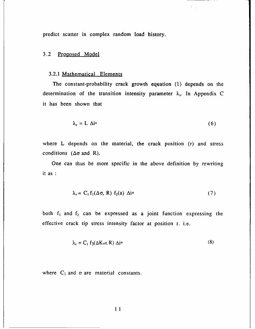
3.2 Proposed Model
3.2.1 Mathematical Elements
The constant-probability crack growth equation (1) depends on the
determination of the transition intensity parameter Xr. In Appendix C
it has been shown that
X. = L Ai- (6)
where L depends on the material, the crack position (r) and stress
conditions (Aa and R).
One can thus be more specific in the above definition by rewriting
it as :
Xr= C, f l (Aoy, R) f2(a) Ai, (7)
both f, and f2 can be expressed as a joint function expressing the
effective crack tip stress intensity factor at position r. i.e.
X- = C1 f3(AKeff, R) Ai- (8)
where C1 and c are material constants.
11

This transition intensity is, in fact, similar to that proposed by
Ditlersen and Sobczyk[39]. By substituting (8) in (1) and setting a
boundary condition that Pr(i)=l when Ai = 0, one obtains
Ai = f(AKeff R) (- In P,(i))O (9)
l+a Iwhere f(AKeff,R)=( -c1 )f3(AKeff,R)] "O and P=
The equation above defines the number of cycles required for the
crack tip, under the driving force of f(AKeff, R) to advance from state
r to state r+l (i.e. from crack length a to a+Aa) with a survival
probability Pr(i). When Pr(i) is kept constant, while incremental
values of Ax, i.e. crack length increments, are substituted in an
appropriate form of f(AKeff, R) a crack growth curve whose points
posses the same propagation probability, can be generated.
The critical element in equation (9) is the determination of an
approriate f(AKeff, R) which includes the effects of overload. This is
the subject of the following section.
3.2 f(AKeff, R) During Retardation
From the introduction of this chapter and the extensive review on
the subject of overload[41], the principal would-be mechanism
responsible for crack retardation is the closure stress resulting from
the induced plasticity in the wake of the crack and the constraining
compressive residual stress in the overload plastic zone in front of
the crack tip. If one recognizes that these two effects act
simultaneously, effects to define the corresponding effective stress-
12

intensity factor would be more difficult than operating in a region
where only one effect plays the major role. Closure stress is defined
as the stress required to fully open the crack. If an externally
applied load is set above the closure stress level, one can assume that
f(AKeff, R) can be calculated by accounting only for the crack tip
compressive residual stress. This condition was achieved by carrying
out closure experiments on compact tension specimen made of rolled
and annealed Ti-6AI-4V material sheets. Specimen geometry is
shown in Appendix D while material composition is listed in table 1.
C Fe N Al V H 0
0.026 0.09 0.011 5.8 5.8 0.008 0.14
Table 1 Chemical Composition of Ti-6AI-4V Material in WT%
The notch-mounted COD gauge technique was used to measure the
crack opening displacement. The experiments were carried out under
constant AP defined by maximum and minimum load, Pmax and Prnin
respectively, with the frequency of 15 Hz. A single overload P01 was
applied at crack length of 18mm, 25mm and 29mm with frequency
of about 0.5 Hz. The interval crack length is large enough to avoid the
overload interaction. This was carried out for different Pmin, Pmax and
13

I"':. In all these test, while a permanent increase in COD measurnents
,was registered following the overload application, no closure could be
detected. This was attributed to the possible insensitivity of COD
gauge resulting from the long distance between the crack tip and the
position of the gauge at the mouth of the crack, which in all tests was
more than 20 mn. A new set of experiments was then executed. In
these a series of pairs of hardness indentations were made along two
lines parallel to and equal distance from the expected nominal crack
path(Fig. 2). Each pair measures 3mm apart. A strain extensometer.
with an accuracv of 5x]0 -5 was used with the tips of its head resting
in the pair of indentations whose connecting line was perpendicular
FiU. 2 .\ series of pairs of hardness indentations
made along two lines partallel to alnd equal
distance from the expected nominal cirack
p a t h
I i

to the crack plane. The position of the extensometer followed behind
the advancing crack tip. Closure measurements were made in the
same pattern discribed above, but only at the distance of 3mm
behind the crack tip. A schematic of this surface measurement
procedure and an illustrative photograph are shown in Figure 3 and
Figure 4 respectively. Output from this experiment, in the form of
load versus displacement curves for different crack lengths a and
different Pra/Pmax' is shown in Figures 5(a) and (b); the indication
being that, for this material, the onset of the closure depends on Pmin.
No closure was observed for Pmin > I KN. Thus it was assumed that for
these Ti-6AI-4V specimens and load conditions with Prnin > I KN, the
governing retardation mechanism is the crack tip constraining
compressive residual stress.
A number of models accounting for the effect of residual stress due
to overloading have been suggested. The modified Willenberg et
a1136] appeared to be the one most frequently referenced. According
to this model, the stress intensity for crack growth is modified by a
residual stress intensity factoi KR that decays linearly with crack
extension. This KR is written as:
r 1 Kth/Kmax] A
K = s Ii Kn " Kol
K h is the maximum stress intensity factor associated with t' igue
crack growth threshold at R=0- Aa,, is crack growth fol lowing the
o'erload and S i's defined as a shut off ratio corresponding to thai
15

indentations
A strain extensometerresolution 5x1 0A(-5)
Y- specimen
Fig. 3 Schematic sketch of closure measurement
(the position of the gauge leads A are maintained at 3m
behind the crack tip B at the moment of applying overload)
Fig. 4 Photograph of the schematic sketch shown in Fig. 3
I=~~ 0, -

1~~
04.
_ _ 1 - -
_ _ -- - - - - - _ _ _ __ _ _
_____ __ 1 1 17

012
10 rc
____ _ _ ___ ___ _ __ __ __ _ ___ ___ _ C
____ .ccI I CL
I In
_ _ _ _ _ _ _ _

olvalue of the ratio Kmax/Kmax, where crack arrest is expected to result;
Z., is the overload affected zone and equal to
Z01 = 2ln a( / ay )2 (I11)
where y is an experinental constant; For Ti-6AI-4V material y and S
are expected to be 4 and 2.8, respectively [43,441 while cy is 924
N/Mm 2 . Additional work by Wei et al[42] suggests that further
modifications be made to the above equations. These modifications
preserve the basic concept that a residual stress intensity factor KR is
produced by the overload. The rate of decay is, however, assumed to*
be proportional to (I - Aao1/Zo1 )2 over the range of Aaoi from Zo0 to Zoi.
This is expressed as:
0 AaO)KR ( - 0o)2 < ao < Zo1 (12)
Zl indicates the delayed zone and is assumed to be equal to the
appropriate cyclic plastic zone size. Z01 is the overload effected zone.
KR° is the residual stress indensity factor immediately following the
overload, i.e. at Aaoi = 0; it is given as:
1_ 1-Kth/Kmax oi- 1 (Kax - Kmax) (13)
19

In a deterministic sense, equation (12) could be used in conjuction
'vith a Paris type crack growth law to calculate the crack growth rate
in the overload affective zone. One of these laws, which exibits a
strong dependency on R, is what developed by Walker[461 in the
form:
dadN C Kax AK"
which could be further expressed as
da C K maxm (I-R)" (14)
dN
where C and m are material constants.
The above equation is, in fact, identical to the equation derived by
Fitzgerald[47] on the basis of empirical data fitting. In his form
however, the value of AK is reduced by AK0 which is defined as a
parameter indicating an apparent threshold value.
Now, by assuming that the compressive residual stress at the crack
tip due to the overloading is the main mechanism, equation (14)
could then be modified as
da= C K " (1-a) ( 15)
20

where K. R Kmin-KRwK=K -KR,,, =and substituting these into eq.(15)
we will get
dadN= C (K,,-KR)m AK" (16)
There is no available information in the literature indicating the
validity of the above equation for overload conditions which do not
promote closure by crack tip plasticity. Therefore experimental tests
were carried out on specimens of Ti-6AI-4V, having the compact
tension geometry previously described, to test equations (12) and
(16) in the overload affected region. These tests included varying
parameters of stress ratio, overload and AK as shown in table 2. In
each test crack length and the associated growth rate were measured
during base loading as well as during the delayed zone after the
overload application. ND was also measured and listed in table 2.
Some experimental results of this work, in the form of da/dN versus
crack length during retardation, are shown in Figures 6(a)-6(d).
Results using [12] and [16] for the same loading conditions are also
presented in these figures. It was observed, however that by
modifying Wei and Shih's form, i.e., equation [121, to
KolKmax
KR - 1-Kth/KmxS_l - Kmax) Kmax (17)
21

(PoI-Pmax)/Pmax 50% 70% 109%
(%)
Overload(KN) 16.5 18.7 23.0
AK NK Nd AK Nd
(N-mm)N (N-mm)
Pmin=2.2KN 685.2 532 581.5 1763 678.7 12,267
Pmax=11KN 875.0 376 873.6 1502 871.1 10,940
R=0.20 1037.0 135 1007.0 8,549
Pmin=5KN 465.1 1,218 464,3 2,810 463.5 88,208
Pmax=11KN 596.1 898 594.8 2,481 593.5 48,615
R=0.46 748.5 563 686.0 2,264 686.5 38,267
Pmin=6.6KN 339.4 4,080 340.2 45,120 343.1
Pmax=11KN 440.6 1,094 439.7 17,788 435.2 18,388
R=0.6 559.1 936 501.8 16,217 500.4 13,332
Table 2 Effect of Varying R, overload ratio and AK onCracK Growth Delay (Nd) in Ti-6AI-4V
22

A closer fitting, as shown also in the above mentioned figures can be
achieved. This empirical modification emphasizes the influence of the
overload ratio. Several other observations obtained from this
experimental program will be discussed in the following chapter. The
major conclusion drawn from this work, however, is that the
effective stress intensity factor for the overload affected zone could
be determined. Once this has been achieved, the next step is to
generate experimentally the scatter crack growth curves. From these,
constant probability crack growth curves could be established and
compared with those theoretically obtained using the proposed
model. This will be detailed in the following section.
0.00010
0.00008 . " ".. . ..
2 0.00006 : *
"-. U . Experiment
0.00004 a By Authorsp * BV Wei and ShihS'Load Condition:
0.00002 -. Pmin=4KNPmax=9KNPoI=18KN
0 .0 0 00 0 , , ,17 18 19 20
Crack Length (mm)
Fig. 6-(a) KR model test
23

0.0003
0.0002
. Experment
0 "a By Authers0.0001• By Wei and Shi
Load Condition:.4 Pmin=SKN
' ;, '-=Pmax=-11KNU PoI=23KN
0.0000 1 1 4 , , * ,
17 18 19 20 21 22
Crack Length (mm)
Fig. 6-(b) KR model test
0.0004
0.0003 U.....
2 .** *.- U ' Experiment0.0002 **" 3 U By Authors
*. + By Wei and Shih* Load Condition:
0.0001 Pmn=22KN, Prnax=lIlIKN
PoI=23KN
0.0000 r -I- m m
17 18 19 20 21 22Crack Length (mm)
Fig. 6-(c) KR model test
24

2.00e-4
". 1.80e-4 -m
S 1.60e-4 -
E1.40e-4 Experiment
• . By Authors= ".e"4 "= * By Wei and ShihV Load Condition:
1.O 4; Pmin=6.6KN" 1.00e-4 • .Prnax=1 1KN
PoI=16.5KN8.00e-5 1 •
24 25 26 27 28 29Crack Length (mm)
Fig. 6-(d) KR model test
3.3 Single Overload Application
3.3.1 Experimental Crack Growth Curves
Crack growth scatter curves, including durations of delayed zones,
were generated by using sixty-five identical compact-tension
specimens of Ti-6AI-4V material which are used throughout this
program. Each specimen supplied one sample crack growth curve
containing three overload regions at crack lengthes of 18, 25 and 29
mm. These intervals were seleted so that no one overload region
could interact with any other overload region on the same curve.
Basic load conditions were Pmin = 4 KN and Pmax= 9 KN; overload P.,
was 18 KN. Load frequency was 15 Hz and the base loading as well as
25

the overloads was applied by using an automatic function generator
system linked to the servohydraulic material testing machine which
was run by the same operator in a temperature-controlled room
during the entire test program. Data was collected in the form of
number of cycles and corresponding crack length at intervals of
1,500 cycles with each data point representing an average of three
measurements taken with a frequency of 500,000 points per second.
Crack length was measured using a current reversing potential drop
system developed by the authors and decribed in Appendix D.
Typical results of crack length a vs number of cycles N are shown in
Figure 7. Each of these sixty-five sample curves, which are shown in
Figure 8, corresponding to initial and final crack lengths of 16 and
32mm, respectively, was divided into 160 segments; each
representing a crack state position with a width of 0.1 mm. Number
of cycles in each state was calculated as irj where lr<160 and
1<j565. This data was then utilized in a manner identical to that
described in references[l1, 27] to generate experimental constant
probability crack growth curves which include retardation zones.
The curves are shown in Figures 9(a) and 9(b).
26

0
000
0
zz
0_
C.)
o00~ 0
on o
(ww)~ ~ ~ 6ju- oi
27Z

00
E
0 rA
z
r Z4 00
2
00
oo 0)
0 C!
6N E
(ww)q)9u-l 410z
280

0
0
-6-
0 0 0
Ln 0 n 0 oIn~ C* C
(ww) l~uol1:)UI
29u

0
0
00
- 0
o o
0 0
00 0
30

3.3.2 Theoretical Crack Growth Curves
The next step was to produce the corresponding theoretical curves
using the proposed model. This was achieved in the following
combined form by employing equations (7), (9) and (16) and
considering the threshold level
Ai = C (Kmax-KR) m (AK-AK 0)- n (-lnP)O (18)
By maintaining the value of P constant and calculating Kmax, KR and
AK for a crack length a; a=1 Ax, one obtains the number of cycles AN
corresponding to increament Aa at a crack length a. This yields an
individual constant probability crack growth curve. The length Zo, of
the overload affected zone was determined by using equation (11).
The full solution of equation (18) requires the knowledge of the
parameters c, m, n and 3. As the objective of this part of the study
was to predict the overload delayed zone, use was made of the
portions of the experimental constant-probability curves
corresponding to the constant amplitude load cycles to estimate the
constants using minimum least square curve fitting method. If the
unit of stress intensity factor is N. mm- 1.5 and Ax=O.1mm the results
are
C = 9.881x10'°
m = 0.93
n = 2.03
and 13 = 0.46
31

Those constants were used in equation (18) to generate the
theoreticai constailL probability crack growth curves for the delayed
regions. Eight of those are shown in Figure 10(a)-Figure 10(h) and
compared with constant probability curves from the experiment
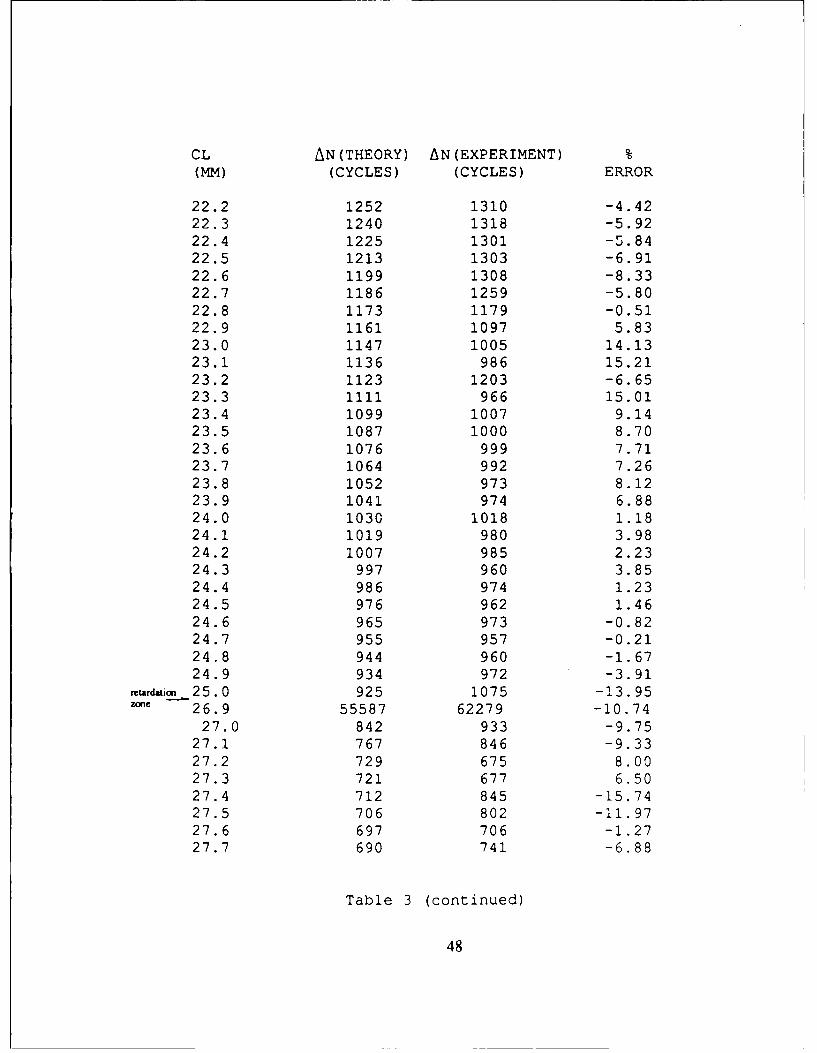
(Figure 9(b)). Furthermore, delayed cycles obtained both
experimentally and theoretically are presented in table 3, in which
the degree of error between the two sets of results was listed. The
average error in data predicted by the proposed model is 8%.
Discussion of the results and observations concerning the
retardation process are the subject of the following chapter.
32

C0(a
CuU -Cu
U 0 C Es-I~
0 1..In
Cu~0* 0o ~II.4-
0
oC
0cu,~6
CuI.-o
V Cu0
* 00I-
0-o
0 0 0 0 0In 0 In 0 In
(4 (4
(ww) q~u~rj ~p~ij
33

0
0
.E~ 0
4-
0
ciJ
oo
0 0.0
In in In
34
0
-0
In
C.C)
0
0 0 0
CN N
(ww) )2uo- JOLo
355

'j.(0
0n 0040
Iw)q U-1 ) OVII
360

00
(0
02
0 4.)
0*
0 0 0
04)tu 4.)olvii
37)0

0
(0
rAu
0
o;
I, C14
(ww)qlgu-l JTS.o
380

00
(0W
C;u
0
c2
4..0.01
h.
04.
0*4 04
(ww) ql'suo- jnD
39

00
tn
0 ~0
00 0 0.9:6
00
0
040
o40

P=0. 1
CL AN(THEORY) AN (EXPERIMENT) %(MM) (CYCLES) (CYCLES) ERROR
16.9 3093 2625 17.8317.0 3055 3425 -10.8017.1 3019 3645 -17.6917.2 2983 3322 -10.2017.3 2947 2896 1.7617.4 2913 3070 -5.1117.5 2878 2897 -0.6617.6 2844 3211 -11.4317.7 2810 3314 -15.2117.8 2778 2897 -4.1117.9 2745 2647 3.70
atio 18.0 2713 3096 -12.37zn 19.6 103154 105209 -1.95
19.7 2524 2256 11.8819.8 2470 2172 12.0619.9 2445 2170 12.6720.0 2241 1922 16.5920.1 2131 1862 14.4520.2 2108 1870 12.7320.3 2084 1866 11.6820.4 2061 1871 10.1520.5 2038 1869 9.0420.6 2015 1874 7.5220.7 1993 1828 9.0320.8 1971 1826 7.9420.9 1949 1865 4.5021.0 1927 1823 5.7021.1 1906 1730 10.1721.2 1885 1731 8.9021.3 1865 1728 7.9321.4 1843 1850 -0.3821.5 1824 1847 -1.2521.6 1803 1727 4.4021.7 1784 1721 3.6621.8 1764 1722 2.4421.9 1745 1719 1.51
Table 3 Percentage error between the theoreticaland experimental constant-probabilitycrack growth curves
41
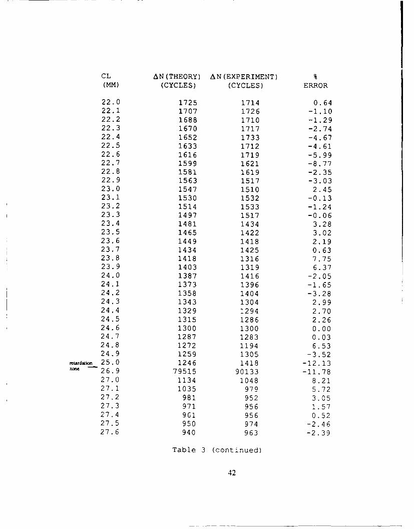
CL AN(THEORY) AN(EXPERIMENT) %(MM) (CYCLES) (CYCLES) ERROR
22.0 1725 1714 0.6422.1 1707 1726 -1.1022.2 1688 1710 -1.2922.3 1670 1717 -2.7422.4 1652 1733 -4.6722.5 1633 1712 -4.6122.6 1616 1719 -5.9922.7 1599 1621 -8.7722.8 1581 1619 -2.3522.9 1563 1517 -3.0323.0 1547 1510 2.4523.1 1530 1532 -0.1323.2 1514 1533 -1.2423.3 1497 1517 -0.0623.4 1481 1434 3.2823.5 1465 1422 3.0223.6 1449 1418 2.1923.7 1434 1425 0.6323.8 1418 1316 7.7523.9 1403 1319 6.3724.0 1387 1416 -2.0524.1 1373 1396 -1.6524.2 1358 1404 -3.2824.3 1343 1304 2.9924.4 1329 1294 2.7024.5 1315 1286 2.2624.6 1300 1300 0.0024.7 1287 1283 0.0324.8 1272 1194 6.5324.9 1259 1305 -3.52
rtdio 25.0 1246 1418 -12.13zoe 26. 9 79515 90133 -11.78
27.0 1134 1048 8.2127.1 1035 979 5.7227.2 981 952 3.0527.3 971 956 1.5727.4 961 956 0.5227.5 950 974 -2.4627.6 940 963 -2.39
Table 3 (continued)
42

CL AN(THEORY) AN(EXPERIMENT) %(MM) (CYCLES) (CYCLES) ERROR
27.7 930 960 -3.1327.8 920 950 -3.1627.9 910 975 -6.6728.0 900 970 -7.2228.1 890 971 -8.3428.2 881 967 -8.8928.3 871 967 -9.9328.4 861 889 -3.1428.5 852 944 -9.7428.6 843 976 -13.6328.7 834 921 -9.4528.8 824 938 -12.1528.9 816 935 -12.72
rio_ 29.0 807 896 -9.93Wfe 31.1 70242 77076 -8.87
31.2 658 731 -9.1331.3 624 732 -14.7531.4 618 724 -14.6431.5 610 725 -15.8631.6 604 722 -16.3431.7 597 702 -14.9631.8 590 70C -15.7131.9 583 697 -16.3532.0 576 696 -17.2432.1 571 698 -18.1932.2 563 680 -17.2032.3 557 662 -15.8632.4 551 660 -16.5032.5 545 657 -11.7032.6 538 657 -18.1132.7 532 623 -14.6132.8 526 610 -13.7732.9 520 601 -13.4833.0 513 598 -14.21
Table 3 (continued)
43

P=0.2
CL AN (THEORY) AN(EXPERIMENT) %(MM) (CYCLES) (CYCLES) ERROR
16.9 2623 2203 19.0617.0 2591 2324 11.4917.1 2561 2682 -4.5117.2 2529 2432 3.9917.3 2500 2331 7.2517.4 2470 2623 -5.8317.5 2441 2542 -3.9717.6 2412 2428 -0.0617.7 2384 2364 0.8517.8 2356 2322 1.4617.9 2328 2320 0.03
reiardatio 18. 0 2301 2329 -1 .20zone 19.6 90204 100892 -10.59
19.7 2480 2229 11.2619.8 2265 2231 1.5219.9 2073 2026 2.3220.0 1901 2014 -5.6120.1 1808 1927 -6.1720.2 1787 1917 -6.7820.3 1768 1822 -2.9620.4 1748 1823 -4.1120.5 1728 1827 -5.4220.6 1709 1856 -7.9220.7 1690 1813 -6.7820.8 1672 1817 -7.9820.9 1653 1768 -6.5021.0 1634 1610 1.4921.1 1617 1603 0.8721.2 1598 1612 -0.8721.3 1582 1611 -1.8021.4 1563 1613 -3.1021.5 1547 1598 -3.1921.6 1529 1416 7.9821.7 1513 1411 7.2321.8 1496 1308 14.3721.9 1480 1404 5.4122.0 1463 1311 10.3922.1 1448 1387 4.4022.2 1432 1314 8.98
Table 3 (Continued)
44

CL AN(THEORY) AN(EXPERIMENT) %(MM) (CYCLES) (CYCLES) ERROR
22.3 1416 1402 1.0022.4 1401 1326 5.6622.5 1385 1394 -0.6522.6 1371 1406 -2.4922.7 1355 1400 -3.2122.8 1341 1403 -4.4222.9 1326 1404 -5.5523.0 1312 1380 -4.9323.1 1298 1315 -1.2923.2 1283 1410 -9.0123.3 1270 1356 -6.6323.4 1256 1316 -4.5623.5 1243 1298 -4.2423.6 1229 1309 -6.1123.7 1216 1305 -6.8223.8 1202 1296 -7.2523.9 1190 1290 -8.1824.0 1177 1305 -9.8124.1 1164 1284 -9.3524.2 1152 1003 14.8624.3 1139 988 15.2824.4 1127 986 14.3024.5 1115 983 13.4324.6 1103 987 11.7524.7 1091 963 13.2924.8 1079 977 10.4424.9 1068 985 8.43
retrdaion 25 .0 1056 1102 -4 .17zoe 26.9 66908 76760 -12.83
27.0 961 971 -1.0327.1 877 952 -7.8827.2 833 943 -11.6627. 3 824 930 -11.4027.4 814 901 -9.6527.5 806 889 -9.3427.6 798 841 -5.1127.7 788 849 -7.1827.8 780 839 -7.0327.9 772 849 -9.06
Table 3 (continued)
45

CL AN(THEORY) AN(EXPERIMENT) %(MM) (CYCLES) (CYCLES) ERROR
28.0 763 862 -11.4828.1 755 850 -11.1728.2 747 825 -9.4528.3 739 858 -13.8728.4 730 847 -13.8128.5 723 804 -10.0728.6 715 760 -5.9228.7 707 770 -8.1828.8 699 754 -7.2928.9 692 767 -9.78
rtardmio 29.0 684 824 -16.99zone 31.1 55293 60602 -8.76
31.2 558 622 -10.2831.3 530 607 -12.6831.4 523 604 -13.4131.5 518 615 -15.7731.6 512 559 -8.4131.7 506 598 -15.3831.8 500 517 -3.2831.9 495 556 -10.9732.0 489 558 -12.3632.1 484 499 -3.0032.2 478 545 -12.2932.3 472 418 -12.9232.4 467 468 -0.0232.5 462 519 -10.9832.6 457 511 -10.5632.7 451 459 1.7732.8 446 405 10.1232.9 441 402 9.7033.0 435 416 4.57
Table 3 (continued)
46

P=0. 3
CL AN(THEORY) AN(EXPERIMENT) %(MN) (CYCLES) (CYCLES) ERROR
16.9 2295 1879 22.1417.0 2267 1879 20.6517.1 2240 1894 18.2717.2 2214 2321 -4.6117.3 2187 1880 16.3317.4 2161 1884 14.7017.5 2136 2011 6.2217.6 2111 1976 6.8317.7 2086 1937 7.6917.8 2061 1890 9.0517.9 2037 1884 8.12
r.wio_ 18.0 2014 1947 3.44ze 19.6 88950 96093 -7.43
19.7 2001 1844 8.5119.8 1982 1833 8.1219.9 1814 1814 0.0020.0 1663 1759 -5.4620.1 1582 1725 -8.2920.2 1564 1719 -9.0220.3 1547 1749 -11.5520.4 1529 1415 8.0620.5 1513 1416 6.8520.6 1495 1424 4.9920.7 1479 1304 13.4220.8 1463 1409 3.8320.9 1446 1311 10.3021.0 1430 1426 0.2821.1 1415 1307 8.2621.2 1398 1310 6.7221.3 1384 1312 5.4921.4 1368 1310 4.4321.5 1353 1300 4.3121.6 1339 1394 -3.9521.7 1323 1387 -4.6121.8 1309 1396 -6.2321.9 1295 1309 -1.0722.0 1281 1303 -1.6922.1 1267 1328 -4.59
Table 3 (Continued)
47
CL AN(THEORY) AN(EXPERIMENT) %(MM) (CYCLES) (CYCLES) ERROR
22.2 1252 1310 -4.4222.3 1240 1318 -5.9222.4 1225 1301 -5.8422.5 1213 1303 -6.9122.6 1199 1308 -8.3322.7 1186 1259 -5.8022.8 1173 1179 -0.5122.9 1161 1097 5.8323.0 1147 1005 14.1323.1 1136 986 15.2123.2 1123 1203 -6.6523.3 1111 966 15.0123.4 1099 1007 9.1423.5 1087 1000 8.7023.6 1076 999 7.7123.7 1064 992 7.2623.8 1052 973 8.1223.9 1041 974 6.8824.0 1030 1018 1.1824.1 1019 980 3.9824.2 1007 985 2.2324.3 997 960 3.8524.4 986 974 1.2324.5 976 962 1.4624.6 965 973 -0.8224.7 955 957 -0.2124.8 944 960 -1.6724.9 934 972 -3.91
reurduii_ 25.0 925 1075 -13.95Zme 26.9 55587 62279 -10.74
27.0 842 933 -9.7527.1 767 846 -9.3327.2 729 675 8.0027.3 721 677 6.5027.4 712 845 -15.7427.5 706 802 -11.9727.6 697 706 -1.2727.7 690 741 -6.88
Table 3 (continued)
48

CL AN(THEORY) AN(EXPERIMENT) %(MM) (CYCLES) (CYCLES) ERROR
27.8 683 672 1.6427.9 675 773 -12.6828.0 668 749 -10.8128.1 660 681 -3.0828.2 654 684 -4.3928.3 646 671 -3.7228.4 640 674 -5.0428.5 632 634 -0.3128.6 625 637 -1.8828.7 619 685 -9.6428.8 612 681 -10.1328.9 605 632 -4.27
mardian 29.0 599 668 -10.32zaeC 31.1 44706 46274 -3.39
31.2 488 497 -1.8131.3 464 481 -3.5331.4 458 500 -8.4031.5 453 501 -9.5831.6 448 421 6.4131.7 443 451 -1.7731.8 438 485 -9.6931.9 432 419 3.1032.0 428 417 2.6432.1 423 463 -8.6332.2 419 418 0.2432.3 413 410 0.7332.4 409 456 -10.3032.5 404 407 -0.7432.6 399 404 -1.2432.7 395 409 -3.4232.8 390 399 -2.2532.9 386 396 -2.5233.0 382 397 -3.78
Table 3 (continued)
49

P= .4
CL AN(THEORY) AN(EXPERIMENT) %(MM) (CYCLE) (CYCLE) ERROR
16.90 2023 1832 10.4317.00 2000 1835 8.9917.10 1976 1835 7.6817.20 1952 1888 3.3917.30 1930 1848 4.4417.40 1906 1828 4.2717.50 1884 1880 0.2117.60 1861 1836 1.3617.70 1840 1880 -2.1317.80 1818 1849 -1.6817.90 1796 1878 -4.37
meardsio 18.00 1776 1880 -5.53zon 19.60 69614 76566 -9.08
19.70 1753 1615 8.5419.80 1748 1619 7.9719.90 1600 1517 5.4720.00 1467 1309 12.0720.10 1395 1350 3.3320.20 1379 1311 5.1920.30 1365 1307 4.4420.40 1348 1344 0.3020.50 1334 1311 1.7520.60 1319 1413 -6.6520.70 1305 1394 -6.3820.80 1290 1313 -1.7520.90 1275 1303 -2.1521.00 1262 1414 -10.7521.10 1247 1284 -2.8821.20 1234 1137 8.5321.30 1220 1104 10.5121.40 1207 1195 1.0021.50 1193 1092 9.2521.60 1181 1119 5.5421.70 1167 1058 10.3021.80 1155 1043 10.7421.90 1142 1095 4.2922.00 1129 1072 5.3222.10 1117 1075 3.9122.20 1105 1068 3.46
Table 3 (continued)
50

CL AN(THEORY) AN(EXPERIMENT) %(MM) (CYCLE) (CYCLE) ERROR
22.30 1093 1108 -1.3522.40 1081 989 9.3022.50 1069 990 7.9822.60 1058 1000 5.8022.70 1046 973 7.5022.80 1035 986 4.9722.90 1023 972 5.2523.00 1013 990 2.3223.10 1001 979 2.2523.20 991 999 -0.8023.30 980 940 4.2623.40 969 1002 -3.2923.50 959 980 -2.1423.60 948 972 -2.4723.70 939 981 -4.2823.80 928 867 7.0423.90 918 982 -6.5224.00 908 990 -8.2824.10 899 876 2.6324.20 888 907 -2.0924.30 880 816 7.8424.40 869 965 -9.9524.50 861 796 8.1724.60 851 958 -11.1724.70 842 866 -2.7724.80 833 872 -4.4724.90 824 858 -3.96
,,urdsio 25.00 815 887 -8.12zc 26. 90 49499 52846 -6.33
27.00 743 708 4.9427.10 676 605 11.7427.20 643 647 -0.6227.30 635 670 -5.2227.40 629 608 3.4527.50 622 669 -7.0327.60 615 630 -2.3827.70 609 671 -9.2427.80 602 631 -4.6027.90 596 631 -5.55
Table 3 (continued)
51

CL AN(THEORY) LN(EXPERIMENT) %(MM) (CYCLE) (CYCLE) ERROR
28.00 589 671 -12.2228.10 582 547 6.4028.20 577 604 -4.4728.30 570 580 -1.7228.40 563 532 5.8328.50 558 581 -3.9628.60 552 581 -4.9928.70 545 554 -1.6228.80 540 573 -5.7628.90 534 576 -7.29
riardaio 29.00 528 513 2.92zoe 31.10 42429 40755 4.11
31.20 431 469 -8.1031.30 409 418 -2.1531.40 404 418 -3.3531.50 399 402 -0.7531.60 395 415 -4.8231.70 391 416 -6.0131.80 386 362 6.6331.90 382 413 -7.5132.00 377 412 -8.5032.10 373 402 -7.2132.20 369 410 -10.0032.30 365 406 -10.1032.40 360 390 -7.6932.50 357 391 -8.7032.60 352 350 0.5732.70 348 334 4.1932.80 344 316 8.8632.90 340 313 8.6333.00 337 311 8.36
Table 3 (continued)
52

P= .5
CL AN(THEORY) AN(EXPERIMENT) %(MM) (CYCLE) (CYCLE) ERROR16.90 1780 1616 10.1517.00 1759 1622 8.4517.10 1737 1679 3.4517.20 1718 1644 4.5017.30 1696 1620 4.6917.40 1677 1633 2.6917.50 1657 1618 2.4117.60 1637 1537 6.5117.70 1618 1648 -1.8217.80 1599 1537 4.0317.90 1580 1604 -1.50zurdia_ 18.00 1562 1431 9.1519.60 63381 71592 -11.4719.70 1683 1503 11.9819.80 1537 1454 5.7119.90 1408 1310 7.4820.00 1290 1187 8.6820.10 1227 1122 9.3620.20 1213 1107 9.5820.30 1200 1101 8.9920.40 1186 1105 7.3320.50 1173 1101 6.5420.60 1160 1219 -4.8420.70 1148 1188 -3.3720.80 1134 1102 2.9020.90 1122 1108 1.2621.00 1109 1104 0.4521.10 1098 1082 1.4821.20 1085 1079 0.5621.30 1073 1079 -0.5621.40 1061 1063 -0.1921.50 1050 1095 -4.1121.60 1038 975 6.4621.70 1027 998 2.9121.80 1015 972 4.4221.90 1005 993 1.2122.00 993 879 12.9722.10 983 874 12.47
Table 3 (continued)
53

CL AN(THEORY) AN(EXPERIMENT) %(MM) (CYCLE) (CYCLE) ERROR
22.20 971 888 9.3522.30 962 983 -2.1422.40 950 966 -1.6622.50 941 877 7.3022.60 930 975 -4.6222.70 920 917 0.3322.80 910 963 -5.5022.90 900 880 2.2723.00 891 958 -6.9923.10 881 919 -4.1323.20 871 966 -9.8323.30 862 911 -5.3823.40 852 885 -3.7323.50 844 881 -4.2023.60 834 821 1.5823.70 825 872 -5.3923.80 816 824 -0.9723.90 808 795 1.6424.00 799 775 3.1024.10 790 714 10.6424.20 782 687 13.8324.30 773 739 4.6024.40 765 776 -1.4224.50 757 696 8.7624.60 748 688 8.7224.70 741 677 9.4524.80 732 689 6.2424.90 725 669 8.37
rmLrdazi 25.00 717 658 8. 97zone 26.90 43217 46671 -7.40
27.00 653 632 3.3227.10 595 631 -5.7127.20 565 631 -10.4627.30 559 630 -11.2727.40 553 629 -12.0827.50 548 631 -13.1527.60 541 628 -13.8527.70 535 583 -8.23
Table 3 (continued)
54

CL AN (THEORY) AN (EXPERIMENT) %(MM) (CYCLE) (CYCLE) ERROR
27.80 529 528 0.1927.90 524 527 -0.5728.00 518 531 -2.4528.10 513 528 -2.8428.20 506 531 -4.7128.30 502 569 -11.7828.40 496 428 15.8928.50 490 435 12.6428.60 486 468 3.8528.70 479 441 8.6228.80 475 466 1.9328.90 470 456 3.07
'f__ 29.00 464 468 -0.8531.10 34678 32033 8.2631.20 379 412 -8.0131.30 359 415 -13.4931.40 356 414 -14.0131.50 351 407 -13.7631.60 347 413 -15.9831.70 344 414 -16.9131.80 340 353 -3.6831.90 335 409 -18.0932.00 332 408 -18.6332.10 328 402 -18.4132.20 325 394 -17.5132.30 321 298 7.7232.40 317 305 3.9332.50 313 297 5.3932.60 310 293 5.80
Table 3 (continued)
55

P= .6
CL AN(THEORY) AN(EXPERIMENT) %(MM) (CYCLE) (CYCLE) ERROR
16.90 1547 1394 10.9817.00 1528 1393 9.6917.10 1510 1290 17.0517.20 1492 1205 23.8217.30 1475 1202 22.7117.40 1457 1248 16.7517.50 1440 1415 1.7717.60 1422 1317 7.9717.70 1406 1321 6.4317.80 1390 1340 3.7317.90 1373 1410 -2.62
ardaai __18.00 1357 1325 2.42zoe 19.60 57403 64368 -10.82
19.70 1462 1280 14.2219.80 1336 1310 1.9819.90 1223 1292 -5.3420.00 1121 1196 -6.2720.10 1067 996 7.1320.20 1054 970 8.6620.30 1043 979 6.5420.40 1030 1003 2.6920.50 1020 976 4.5120.60 1008 1002 0.6020.70 997 987 1.0120.80 986 975 1.1320.90 975 873 11.6821.00 964 981 -1.7321.10 953 893 6.7221.20 943 879 7.2821.30 933 867 7.6121.40 922 894 3.1321.50 913 883 3.4021.60 902 879 2.6221.70 892 967 -7.7621.80 882 867 1.7321.90 873 881 -0.9122.00 864 819 5.4922.10 853 822 3.7722.20 845 791 6.42
Table 3 (continued)
56

CL AN(THEORY) AN(EXPERIMENT) %(MM) (CYCLE) (CYCLE) ERROR
22.30 835 875 -4.5722.40 826 826 0.0022.50 818 784 4.3422.60 808 859 -5.9422.70 800 740 8.1122.80 790 783 0.8922.90 783 784 -0.1323.00 774 766 1.0423.10 765 703 8.8223.20 757 691 9.5523.30 749 739 1.3523.40 741 695 6.6223.50 733 644 13.8223.60 725 641 13.1023.70 717 618 16.0223.80 709 641 10.6123.90 702 639 9.8624.00 694 676 2.6624.10 687 639 7.5124.20 679 642 5.7624.30 672 636 5.6624.40 665 639 4.0724.50 658 637 3.3024.60 650 640 1.5624.70 644 638 0.9424.80 636 633 0.4724.90 630 673 -6.39
ta rdafio- 25.00 623 583 6.86zone
26.90 37575 40279 -6.7127.00 568 528 7.5827.10 517 527 -1.9027.20 491 529 -7.1827.30 486 506 -3.9527.40 481 485 -0.8227.50 475 440 7.0527.60 470 445 5.6227.70 465 428 8.6427.80 460 426 7.98
Table 3 continued)
57

CL AN(THEORY) AN(EXPERIMENT) %(MM) (CYCLE) (CYCLE) ERROR
27.90 456 425 7.2928.00 450 429 4.9028.10 445 426 4.4628.20 441 427 3.2828.30 435 430 1.1628.40 431 425 1.4128.50 427 428 -0.2328.60 421 412 2.1828.70 417 426 -2.1128.80 413 433 -4.6228.90 408 411 -0.73
ardation 29.00 403 402 0.25Zone 31.10 32136 30647 4.86
31.20 329 320 2.8131.30 312 312 0.0031.40 309 313 -1.2831.50 306 318 -3.7731.60 302 309 -2.2731.70 298 309 -3.5631.80 295 316 -6.6531.90 292 305 -4.2632.00 288 271 6.2732.10 286 303 -5.6132.20 282 298 -5.3732.30 278 295 -5.7632.40 276 296 -6.7632.50 272 294 -7.48
Table 3 (continued)
58

P= .7
CL AN(THEORY) AN(EXPERIMENT) %(MM) (CYCLE) (CYCLE) ERROR
16.90 1312 1154 13.6917.00 1295 1084 19.4617.10 1280 1120 14.2917.20 1265 1190 6.3017.30 1250 1085 15.2117.40 1235 1198 3.0917.50 1221 1103 10.7017.60 1206 1118 7.8717.70 1192 1211 -1.5717.80 1178 1113 5.8417.90 1164 1120 3.93
.,dio_ 18.00 1150 1207 -4.72zon 19. 60 48744 50186 -2.87
19.70 1240 1184 4.7319.80 1132 1103 2.6319.90 1037 1080 -3.9820.00 950 973 -2.3620.10 904 977 -7.4720.20 894 881 1.4820.30 884 883 0.1120.40 874 884 -1.1320.50 864 825 4.7320.60 855 877 -2.5120.70 845 846 -0.1220.80 835 790 5.7020.90 827 819 0.9821.00 817 870 -6.0921.10 808 821 -1.5821.20 800 820 -2.4421.30 790 820 -3.6621.40 782 804 -2.7421.50 773 748 3.3421.60 765 762 0.3921.70 756 769 -1.6921.80 749 739 1.3521.90 739 769 -3.9022.00 732 741 -1.2122.10 724 741 -2.2922.20 716 698 2.58
Table 3 (continue)
59

CL AN(THEORY) AN(EXPERIMENT) %(MM) (CYCLE) (CYCLE) ERROR
22.30 708 618 14.5622.40 700 640 9.3822.50 693 644 7.6122.60 685 685 0.0022.70 678 636 6.6022.80 671 613 9.4622.90 663 639 3.7623.00 656 614 6.8423.10 649 636 2.0423.20 641 642 -0.1623.30 635 637 -0.3123.40 628 614 2.2823.50 622 639 -2.6623.60 614 635 -3.3123.70 608 639 -4.8523.80 601 637 -5.6523.90 595 635 -6.3024.00 589 637 -7.5424.10 582 635 -8.3524.20 576 636 -9.4324.30 569 582 -2.2324.40 564 584 -3.4224.50 557 584 -4.6224.60 552 585 -5.6424.70 545 575 -5.2224.80 540 570 -5.2624.90 534 573 -6.81
retardatio 25. 00 528 578 -8.65zone 26.90 32479 37184 -12.65
27.00 481 425 13.1827.10 438 423 3.5527.20 417 427 -2.3427.30 412 425 -3.0627.40 407 420 -3.1027.50 403 426 -5.4027.60 398 423 -5.9127.70 395 424 -6.8427.80 330 423 -7.80
Table 3 (continue)
60

CL AN(THEORY) AN(EXPERIMENT) %(MM) (CYCLE) (CYCLE) ERROR
27.90 386 424 -8.9628.00 381 421 -9.5028.10 378 424 -10.8528.20 373 426 -12.4428.30 370 424 -12.7428.40 365 420 -13.1028.50 361 423 -14.6628.60 358 401 -10.7228.70 353 389 -9.2528.80 350 367 -4.6328.90 346 396 -12.63
retardation 29.00 342 387 -11.63zone 31.10 24646 20704 19.04
30.60 515 518 -0.5830.70 461 479 -3.7630.80 414 413 0.2430.90 373 397 -6.0531.00 338 348 -2.8731.10 306 312 -1.9231.20 279 315 -11.4331.30 265 304 -12.8331.40 262 304 -13.8231.50 259 315 -17.7831.60 256 274 -6.5731.70 253 276 -8.3331.80 250 311 -19.6131.90 247 280 -11.7932.00 245 266 -7.8932.10 241 266 -9.4032.20 239 266 -10.1532.30 237 261 -9.20
Table 3 (continued)
61

P= .8
CL AN(THEORY) AN(EXPERIMENT) %(MM) (CYCLE) (CYCLE) ERROR
16.90 1057 941 12.3317.00 1044 943 10.7117.10 1031 942 9.4517.20 1020 1004 1.5917.30 1007 986 2.1317.40 996 966 3.1117.50 983 926 6.1617.60 972 928 4.7417.70 961 893 7.6117.80 949 883 7.4717.90 938 925 1.41
ardazion 18.00 928 987 -5.98ze 19.60 39254 48723 -19.43
19.70 999 893 11.8719.80 913 807 13.1419.90 835 818 2.0820.00 766 802 -4.4920.10 729 822 -11.3120.20 720 792 -9.0920.30 712 743 -4.1720.40 705 787 -10.4220.50 696 741 -6.0720.60 689 676 1.9220.70 681 640 6.4120.80 674 642 4.9820.90 666 640 4.0621.00 658 674 -2.3721.10 652 642 1.5621.20 644 643 0.1621.30 637 641 -0.6221.40 630 641 -1.7221.50 623 640 -2.6621.60 617 639 -3.4421.70 609 617 -1.3021.80 603 633 -4.7421.90 597 622 -4.0222.00 589 637 -7.5422.10 584 636 -8.18
Table 3 (continued)
62

CL AN(THEORY) AN(EXPERIMENT) %(MM) (CYCLE) (CYCLE) ERROR
22.20 577 639 -9.7022.30 570 668 -14.6722.40 565 636 -11.1622.50 558 636 -12.2622.60 552 597 -7.5422.70 547 535 2.2422.80 540 537 0.5622.90 534 537 -0.5623.00 529 537 -1.4923.10 523 531 -1.5123.20 517 536 -3.5423.30 512 532 -3.7623.40 506 535 -5.4223.50 501 534 -6.1823.60 495 533 -7.1323.70 490 537 -8.7523.80 485 533 -9.0123.90 479 533 -10.1324.00 474 533 -11.0724.10 470 531 -11.4924.20 464 532 -12.7824.30 459 529 -13.2324.40 454 532 -14.6624.50 449 530 -15.2824.60 445 482 -7.6824.70 439 481 -8.7324.80 435 467 -6.8524.90 430 412 4.37
reirdation 25. 00 426 430 -0. 93zon 26.90 27758 31478 -11.82
27.00 388 349 11.1727.10 353 375 -5.8727.20 336 374 -10.1627.30 332 309 7.4427.40 328 306 7.1927.50 325 321 1.2527.60 321 306 4.9027.70 318 319 -0.31
Table 3 (continued)
63

CL AN(THEORY) &N(EXPERIMENT) %(MM) (CYCLE) (CYCLE) ERROR
27.80 314 308 1.9527.90 311 306 1.6328.00 308 337 -8.6128.10 304 306 -0.6528.20 301 305 -1.3128.30 298 320 -6.8828.40 294 306 -3.9228.50 291 304 -4.2828.60 288 288 0.0028.70 285 302 -5.6328.80 282 307 -8.1428.90 279 331 -15.71
ardasion 29.00 275 332 -17.17ze 31.10 21589 17284 24.91
31.20 225 272 -17.2831.30 213 271 -21.4031.40 211 250 -15.6031.50 209 225 -7.1131.60 206 228 -9.6531.70 204 208 -1.9231.80 202 206 -1.9431.90 199 205 -2.9332.00 197 203 -2.96
Table 3 (continued)
64

P= .9
CL LN(THEORY) AN(EXPERIMENT) %(MM) (CYCLE) (CYCLE) ERROR
17.50 696 592 17.5717.60 688 607 13.3417.70 681 643 5.9117.80 672 682 -1.4717.90 664 643 3.27
mmr io 18.00 657 617 6.4819.60 25363 24362 4.1119.70 707 644 9.7819.80 646 606 6.6019.90 592 638 -7.2120.00 542 640 -15.3120.10 516 564 -8.5120.20 510 541 -5.7320.30 505 537 -5.9620.40 498 541 -7.9520.50 493 539 -8.5320.60 488 518 -5.7920.70 482 538 -10.4120.80 477 535 -10.8420.90 472 533 -11.4421.00 466 518 -10.0421.10 462 534 -13.4821.20 456 504 -9.5221.30 451 487 -7.3921.40 446 454 -1.7621.50 441 435 1.3821.60 437 434 0.6921.70 431 435 -0.9221.80 427 411 3.8921.90 423 439 -3.6422.00 417 431 -3.2522.10 413 411 0.4922.20 409 433 -5.5422.30 404 432 -6.4822.40 400 433 -7.6222.50 395 433 -8.7822.60 391 432 -9.4922.70 387 431 -10.2122.80 382 394 -3.05
Table 3 (continued)
65

CL AN (THEORY) 6N (EXPERIMENT) %(MM) (CYCLE) (CYCLE) ERROR
22.90 379 360 5.2823.00 374 375 -0.2723.10 370 355 4.2323.20 367 535 -31.4023.30 362 410 -11.7123.40 358 329 8.8123.50 355 408 -12.9923.60 351 351 0.0023.70 347 332 4.5223.80 343 337 1.7823.90 339 310 9.3524.00 336 329 2.1324.10 332 310 7.1024.20 329 329 0.0024.30 325 308 5.5224.40 321 309 3.8824.50 319 303 5.2824.60 314 327 -3.9824.70 312 308 1.3024.80 308 308 0.0024.90 304 330 -7.88
rardaion 25.00 302 332 -9.04zon 26.90 19422 22168 -12.39
26.60 410 405 1.2326.70 368 404 -8.9126.80 333 306 8.8226.90 302 304 -0.6627.00 274 304 -9.8727.10 251 284 -11.6227.20 237 284 -16.5527.30 235 273 -13.9227.40 233 273 -14.6527.50 230 274 -16.0627.60 227 273 -16.8527.70 225 274 -17.8827.80 223 273 -18.3227.90 220 272 -19.1228.00 218 273 -20.15
Table3 (continued)
66

CL AN(THEORY) AN(EXPERIMENT) %(MM) (CYCLE) (CYCLE) ERROR
28.10 215 272 -20.9628.20 213 272 -21.6928.30 211 273 -22.7128.40 208 272 -23.5328.50 207 271 -23.6228.60 204 273 -25.2728.70 201 271 -25.8328.80 200 273 -26.7428.90 197 273 -27.84
mdi 29.00 196 272 -27.94zone 31.10 14578 11642 25.22
30.60 294 298 -1.3430.70 263 299 -12.0430.80 236 278 -15.1130.90 213 278 -23.3831.00 193 237 -18.5731.10 175 227 -22.9131.20 159 217 -26.7331.30 151 196 -22.9631.40 149 196 -23.9831.50 148 196 -24.4931.60 146 196 -25.5131.70 145 195 -25.6431.80 142 193 -26.4231.90 142 194 -26.80
Table 3 (continued)
67

CHAPTER IV
CONCLUSIONS
1. The goal of this research program was to develop a crack growth
model which takes into account the random nature of the crack
evolution in real solids. This was achieved by viewing the growth
process as a Markovian stochastic process, discrete in state and
inhomogenous with respect to time. This led to the derivation of a
law that predicts the crack jump from ond state to the following state
with a specified probability, i.e. yielding constant probability crack
growth curves. In the model, the transition intensity of the process is
identified as a function of the effective stress intensity factor. This
permits the consideration of the load interaction history and makes
the model a valuable design and reliablity tool for constant, as well
as, random load applications. A fundamental concept of the model is
the assumption that the crack growth curve produced by an
appropriate continuum law is identical to the median probability
curve which corresponds to the value of Pr(i)=0. 5 6 ; this was
sufficient to identify the remaining constant probabilitty crack
growth curves.
2. An in-house experimental program was executed to generate
constant probability crack growth curves for three different loading
conditions by using 180 Al 7075-T6 center-notched flat specimen. A
comparison was then made between these curves and those
theoretically obtained for each corresponding test condition; full
analysis of this application is provided in Appendices A-C.
68

3. An in-house experimental program was carried out to generate
constant probability crack growth curves for conditions of overload
application. In these tests sixty-five Ti-6A1-4V compact tension
specimens were used under the same base loading and for the same
overload ratio applied to three different crack lengths. The
corresponding theoretical constant probability crack growth curves
were calculated using the proposed model. A critical step in these
calculations was the determination of the effective stress intensity
factor during retardation. This was accomplished by separating the
retardation mechanisms and setting up experimental load conditions
so that the only governing mechanism was the crack tip compressive
residual stress. Comparision between experimental and theoretical
crack growth curves indicated prediction error of average 8%.
Several remarks concerning the experimental observations are
called for here:
A- Following an overload, two separate zones can be distinguished in
front of the crack tip as shown in Fig. 11. The first is a ductile
rupture zone and coincides with the sudden peak in the crack growth
rate. The width of this zone increases as the crack length, at which
the overload is applied, increases; see figure 12. The second region is
the retardation zone; it was observed that for the same stress ratio.
R, and the same overload ratio, the number of cycles, Nd, spent in
this region decrease- as the crack length increases. This is contrary to
observations made by AroneI371. Also results of the current
experiments seem to validate the conclusions drawn by Lankford
and Davidson[451 that Nd decreases as R increases.
69

B- In several tests an apparent temporary crack tip arrest was
observed in the retardation zone. In each case the crack succeeded in
crossing this zone and regaining an accelerated growth equal to that
existing prior to the overload. Further investigation of these arrrest
regions showed, in all test specimens, traces of crack growth
striations indicating that growth existed in duration of apparent
ariest. The failure to detect this behavior could be due to the
inability to measure the associated very small crack growth using the
potential drop measurement system. Examples of these types of
striations, before overload application as well as in the region of
apparent arrest, are shown in figure 13.
C- The test specimens, all of which were made of Ti-6AI-4V, a highly
textured material, responded to the application of the overload by
instantaneous crack tip extension via ductile rupture on a plane
inclined to the normal-to-load plane, see figure 14. The length of the
defected crack component and its angle, b and q, respectively, in
Figure 15 were found to depend on the crack length at which the
defection occurs; as the crack length increases, b increases while q
decreases. Due to the orientation of the deflected component, the
governing stress intensity factor at its tip is viewed as a combination
of KI and K11. As the loading cycle returns to its base form, the value
of KiI decays gradually as the deflected crack tip orients itself back
towards the original fracture plane, see Figure 15. The length of tile
deflected crack and its transition coincides with tile combined length
of the overload rupture and delayed zones. It must however, be
noted that this crack deflection phenomenon is limited to tile surface
7 0

layer, i.e. the plain stress condition with a depth of less than 500 .m
as illustrated in Figure 16.
Finally, while the work in this program encourages the validity of
the proposed model's ability to predict scatter in the crack growth
behavior, it also emphasizes a specific shortcoming:
On the basis of the extensive experimental work carried out during
this program, it has been observed that crack growth scatter could be
divided into two stages; the first corresponding to short crack lengths
and the second corresponding to long cracks. Short lengths promote
the highest scatter reflecting the faci that at this length the
microstructural parameters, such as grain size and slip system
dominate. As the crack length increases scatter tends to decrease, an
indication that the growth process becomes a stress controlled
phenomenon. The use of stochastic models should therefore, be
directed primarily towards short crack applications. In this respect
the proposed model should be further developed to include, in an
explicit form, parameters that indentify the role of microstructure.
71

Crack growth directiofl
IL Ir ] (a) ON erNicN o f, a 1 o~e.Tload Z~one sho\% ifith (li d titiI e re p tu I] I' a l (Id :I." cd(
&W ~J
AeI 121 1 57 14K M70 IOP WD39~ ftitrplrta~i h

Crack growth direction
Figure 12 D~uctile rupture zones followingov'erload application at different crackIe n gt h

Figure 13(a) Striation of' the fracture surface Ibcfore
I- i,- i r c 130I)) Striat ion in tlit (ItclaN d z oI e0( 'o I I()~ Nmu i
afi mert'f1d :ipplicti oll ill tl(li il
sjuttiiiiti f thu ;ihimu buiji>

Crack growth direction
Figure 14(a) Change in the crack orientation due to overload
Fo
V "
!1
Figure 14(b) Close up of the deflected zone

0004 0KO .415 . 0

C-
3)
C-
l"i"urC 16 The deflected part of the surface crack afterthe o~erload application and the depth ofthis transition in the interior (F thespe c i III ell

I1REFERENCES
[1] H. Lauschmann, A stochastic model of fatigue crack growth inheterogeneous material, Engng Fracture Mech. 26, (1978)
[2] D.W. Hoeppner and W. E. Krupp, Prediction of component life by
application of fatigue crack growth knowledge, Engng Fracture
Mech. 6, (1974)
[3] Karl-Heinz Schwalbe, Comparison of several crack propagation
laws with experimental results, Engng Fracture Mech. 6, (1974)
(4] S. Chand and S. B. L. Garg, Propagation under constantAmplitude loading, Engng Fracture Mech. 21, (1985)
[5] S. C. Saunder, On the probability determination of scatterfactors using Miner's rule in fatigue life studies, ASTM STP 511
[6] J. N. Yang and R. C. Donath, Statistics of a superalloy under
sustained load, J. Engng Mater. Tech. 106, (1984)
[7] S. Tauaka, M. Ichickawa and S. Akita, Variability of m and C infatigue crack propagation law da/dn=C(AK) m, Int. J. Fract. 17,
(1981)
[81 K. P. Oh, A weakest-link model for the prediction of fatiguecrack growth rate, J. Engng Mater. Tech. 100. (April 1978)
19] W. Weibull, A statistical representation of fatigue failure in
solids, Trans. Roysl Inst. Tech. (Stockholm), No. 27, (1949)
[101 A. Tsurui and A. Igarashi, A probabilistic approach to fatiguecrack growth rate. J. Engng Mater. Tech. 102, (July 1980)
78

[11] H. Ghonem and S. Dore, Probabilistic description of fatigue crackgrowth in aluminum alloys. AFOSR-83-0323, (April 1986)
[12] J. L. Bogdanoff, A new cumulation damage model-Part I, J.
Appl. Mech. 45, (1987)
[13] J. L. Bogdanoff and W. Krieger, A new cumulative damagemodel-Part II, J. Appl. Mech. 45, (1978)
[14] J. L. Bogdanoff, A new cumulative fatigue model-Part III, J.Appl. Mech. 45, (1978)
[15] J. L. Bogdanoff and F. Kozin, A new cumulative damage model-Part IV, J. Appl. Mech. 47, (1980)
[16] H. Ghonem and J. M. Provan, Micromechanics theory of fatigue
crack initiation and propagation. Engng Fracture Mech.13,(1980)
[17] J. Provan and H. Ghonem, Probabilistic description ofmicrostructual fatigue failure, continuum model of discrete
systems. University of Waterloo Press, (1977)
[18] J. Sedlacek, The stochastic interpretation of service strength
and reliability of mechanical systems. Monographs andMemoranda 6, National Institute of Machine Design, Prague,(1968)
[191 H. Ghonem and S. Dore, Probabilistic description of crackgrowth in polycrystalline solids. Engng Fracture Mech. 21,(1985)
[201 H. Lauschmann, To the probabilistic description of fatigue crackgrowth. C. Sc. Dissertation, Technical University of Prague,
(1985)
79

[21] F. Ellyin and C. 0. Fakinlede, Probabilistic simulation of fatiguecrack growth by damage accumulation, Engng Fracture Mech.22, (1985)
[22] 0. Ditlevsen, Random fatigue crack growth-a first passage
problem. Engng Fracture Mech. 23, (1986)
[23] H. Alawi, A probabilistic model for fatigue crack growth underrandom loading. Engng Fracture Mech. 23, (1986)
[24] D. A. Virckler, B. M. Hillberry and P. K. Goel, The statisticalnature of fatigue crack propagation. ASME, J. Engng Mater.Tech. 101, (April 1979)
[25] H. Ghonem and S. Dore, Experimental study of the constantprobability crack growth curves under constant amplitudeloading. Engng Fracture Mech. 27, (1987)
[26] J. Willenborg, R. M. Engle and H. A. Wood, A crack growthretardation model using an effectivestress concept. AFFDL-TM-FBR-81-1, Air Force Dynamics lab, (1971)
[27] 0. Wheeler, Spectrum loading and crack growth. J. Basic Engng,
94 D, 181, (1972)
[28] S. Matsuoka and K. Tauaka, Delayed retardation phenomenon offatigue crack growth resulting from a single application ofoverload. Engng Fracture Mech.10, (1978)
[29] T. D. Gray and J. P. Gallagher, Predicting fatigue crackretardation following a single overload using a modifiedwheeler model. Mechanics of Crack Growth, ASTM, STP590,(1976)
[301 R. H. Christensew, Metal Fatigue, McGraw Hill, New York, (1959)
80

[31] W. Elber, The significance of crack clousure. ASTM STP 486,(1971)
[32] C. Bathias and M. Vancon, Mechanics of overload effect on
fatigue crack propagation in Al alloys. Engng Fracture Mech.10, (1978)
[33] J. Schijue, Fatigue damage accumulation and incompatible crackfront orientation. Engng Fracture Mech. 6, (1974)
[34] R. J. Bucci A. B. THakker, T. H. Sanders, R. R. Sawtell and J. T.Rankinging, 7075 Al alloys fatigue crack growth resistance
under constant amplitude and spectrum loading. ASTM STP714, (1980)
[35] J. Petit and S. Suresh, Constant amplitude and post overload
fatigue crack growth in Aluminum-Lithium alloys. Division ofEngineering, Brown University, Providence, Rhode Island,(1985)
[36] R. Hertzberg, Micromechanisms of fatigue crack advance inPVC. J. Mater. Sci. 8, Nov. 1973
[37] R. Arone, Fatigue crack gorwth under random overloads
superimposed on constant-amplitude cyclic loading. EngngFracL'jre Mech 24, (1986)
[38] W. J. Mills and R. W. Hertzberg, Load interaction effect onCatigue crack propagation in 2024-T3 Aluminum alloy. Engng
Fracture Mech. 8, (1976)
[391 0. Ditlevsen and K. Sobczyk, Random fatigue crack growth withretardation. Engng Fracture Mech. 24, (1986)
[401 H. Ghonem, Constant probability crack growth curves. EngngFracture Mech. 30, (1988)
81
[41] Crack growth analysis for arbitrary specimen loading, VolumeI-results and discussion, Final Report, Air Force Danamics
Laboratory
[42] R. P. Wei, N. E. Fenelli, K. D. Unangst and T. T. Shih, Fatigue crackgrowth responce following a high-load excursion in 2219-T851
Aluminum alloy. Transaction of the ASTM, Vol. 102, (July1980)
[43] 0. Jonas and R. P. Wei, An exploratory study of delay in fatigue-crack growth, Int. J. Fract. Mech. 7, (1971)
[44] R. P. Wei and T. T. Shih, Delay in fatigue crack growth, Int. J.
Fract. Mech. 10, (1974)
[45] J. Lankford and D. L. Davidson, Fatigue crack tip plasticity
associated with overloads and subsequent cycling. J. EngngMat. Tech. (Jan. 1976)
[46] K. Walker, The effect of stress ratio during crack propagationand fatigue for 2024-T3 and 7075-T6 Aluminum. ASTM STP462, (1970)
[47] J. H. Fitzgerald, Empirical formulations for the analysis and
prediction of trends for steady-state fatigue crack growth
rates. J. of Testing and Evalution, JTEVA, Vol. 5, No. 5, Sept.
1977
82

APPENDIX A
PROBABILISTIC DESCRIPTION OF FATIGUE CRACKGROWTH IN POLYCRYSTALLINE SOLIDS
83

fn 'ierrnk, f ratre .i'( h-tis So 21. No 6. pp 1151- 1168. 195 0013-794 N5 03() - 00Printed in the L S A C 1985 Perganmon Pres, Lid
PROBABILISTIC DESCRIPTION OF FATIGUE CRACKGROWTH IN POLYCRYSTALLINE SOLIDS
H. GHONEM and S. DOREMechanics of Solids Laboratory, Department of Mechanical Engineering and Applied
Mechanics. University of Rhode Island. Kingston. RI 02881. U.S.A.
Abstract-A stochastic model describing the crack evolution and scatter associated %kith thecrack propagation process has been built on the basis of the discontinuous Markovian process.The evolution and scatter are identified in terms of constant probability curves whose equationis derived as In P(i) = B(eA 'I - e"). i a i., where i is the number of cycles. B and K arecrack-length-dependent variables. P,(i) is the probabiliity of the crack being at position r alongthe fracture surface after i cycles elapse and I is the minimum number of cycles required forthe crack to advance from one position on the fracture surface to the next. The validity of themodel is established by comparing the crack growth curves generated for Al 2024-T3 at a specificloading condition with those experimentally obtained.
INTRODUCTION
LABORATORY TESTS conducted on different polycrystalline materials exhibited considerable var-iation in the crack growth characteristics data. This variation, or scatter, is considered a majorfactor in the gap that exists between theoretical predictions of existing continuum crack prop-agation models and experimental observations.
Several studies. employing theory of probability concepts. have been developed to predictand characterize the variation in crack propagation data. These studies generally follow twoapproaches. The first approach is based on the introduction of random variables encompassingthe scatter sources to replace the deterministic parameters in continuum crack propagationrules such as the Paris-Erdogan Equation [II which is widely studied and used. The result ofthis operation is viewed as a sample crack growth equation by which mean crack position andassociated variance can be calculated. Examples of models belonging to this approach are thoseof Hoeppner and Krupp [2]. Gurney [3]. Ostergaard and Hillberry [4] and others 15-71.
The second approach is based on the assumption that the crack propagation process couldbe formulated in terms of a particular discontinuous Markovian process. This leads to thedescription of the crack length in the form of its probability distribution whose evolution intime characterizes the nondeterministic nature of the crack propagation process. Examples ofthese models are found in the work of Ghonem and Provan 181 and Bogdanoff and Kozin [91.
This paper is an attempt to extend the concepts presented in Ref. 181 to produce a theoreticalmethod which will estimate the crack growth scatter at any stress level. This is achieved bydeveloping the sample functions of the crack growth process in terms of a constant-probabilit%crack growth criterion. Mathematical elements of this criterion are detailed in the first part ofthis paper while the second part deals with the use of the model in a numerical example toestimate crack growth scatter in Aluminum 2024-T3. Emphasis is placed on the adherence ofthe model to the physical aspects of the crack growth plocess and the degree of agreementbetween the theoretical results of the model and corresponding experimental data.
MATHEMATICAL ELEMENTS OF THE MODEL
The stochastic model of the fatigue crack propagation as briefly described iin 181 is de\ elopedin terms of a general pure birth, discontinuous Markosian stochastic process. The model ishaed on the assumption that the crack front can be approximated, as ,ho\sn in Fig. I. hx alarge number of elements . I...... ,I. each of' .,hich. in term,, ofthe theor\ of probabilit .identifies a statistical trial or cxperiment. The fracturc ,titlc of the (t h trial at c c i is gI elh% the crack length or the random , ariable a, ss hose e ,olt oiol ilth tillic shall then be estab-lished. 'a, s,,ill hereafter be referred to as a,
t1<I

II~2H. GHONENI an0 S. DORE
1 2
Fig. 1. Schematic of Mode I crack propagation fracture -;urlace-
Due to the built-in limitations of all experimental techniques the observed value of a, canonly be specified within the range of
x< 11, < x -Ax, 1
,Ahere Ax Is the experimental error and x is the crack position calculated .-s (see Fig. 2)
0l

Fatigue crack growth in pol.\crystalline solids 1153
x = rlkx: rto < r < rt 2
Here r identifies the observable zone or state along the fracture surface: r, is the initial prop-agation state, r,. is the state just prior to catastrophic failure of the specimen and r ,I .....r, - I are the intermediate zones.
Given that the crack is in state r. then after i cycles have elapsed from the instant of reachingr. one of two events would occur: ai would remain in state r (event 'E,) or a, would not be instate r (event 'E,). The following observations can now be made:
1. Due to the fact that the propagation process is an irreversible one. the crack, if it doesnot stay in r. must exist in a state greater than r.
2. Since it is not possible for the crack to propagate from one state to any other state withoutpenetrating the immediate neighboring state, each crack could then be identified by the numberof cycles required to advance from a given state to the following one.
Based on these observations the two events 'E, and 'E, can be seen as the element of ameasurable sample space Q. see Ref. [9]. and the following definition of the probability measureof a, becomes possible. At any fatigue cycle i the probability that ,a, is in state r, i.e. theprobability of 'E,. is defined as
P{aE'E,} = P{x < a, < x + Ax}.
i.e.
P(E,) = Pi) (3)
Therefore the probability of a, not falling within r is
P('E,) = Pi) = I - Pi). (4)
Here Pi) continuously increases as the number of cycles increase.Furthermore. it is known that the existence of the crack front at a particular position inside
the material depends on its present mechanical and microstructure details and is not directlyinfluenced by the details of any of its other previous positions. More specifically. the probabilityof a, propagating from state r to r + I in the cycle interval (i. i + A i) depends on the event'E, and is independent of any event "E, ..... 'E occurring prior to i: 0 < j < i. This can beexpressed as
P{'E.1, E ... .. . .E .. .... .E, = P{'E,,rE, = P,(i) (5)
where t = r - I and *," denotes a conditional probability measure. These characteristics togetherwith the evolution of a, within the tMo-event space 11. describe a discontinuous Markovianprocess. The function Prdi) could then be considered the transition probability linking theprobability measures of two consecutive states r and t: t = r - I. along the fracture surface.
It is now possible to describe the propagation process of the crack front in terms of thefollo" ing criteria:
1. The probabilit of a, propagating to a state different than r in Ai cycles is given b\
PjAi = PJEtL, 'E, - O(.Ai)
,Ahere &, is a positive parameter describing the crack transition rate from state r to t in AcclcN and is thus considered a material- and time-dcpcndent ',ariablc see Bharucha-Reid Jill.
2. he corresponding prohabilit, that a, Aill be in state r during the c. cl intcr\al A1i t
I' \i i'I:_2 , 'l 0 - %i)
- (I A,2AiI 0) A.-).

1154 H. GHONEM and S. DORE
3. The probability that a, is in a state different from r + I is
P,,(Mi) = PIE.,rE,}
= 0(Ai): t > r + !. (8)
Since
P{rEi- .} = P{rE/j1E,} . PjrE, (9)
therefore substituting eqns (6). (7) and (8) in eqn (9), the probability of the event 'E.1, can beobtained as
P,(i + Ai) = (I - \,Ai)P,(i) + 0(1i). (10)
By transposing and taking the limit Ai--* 0, eqn (10) becomes
dPr(i) (11)= -XPri).( I)di
The solution of this equation is
InPr(i) - f x, di + L,, (12)
where L, is a constant.An important element in solving this equation is the parameter \r which is seen here as a
measure of the crack growth rate. This measure is assumed to have the following properties:1. In the presence of continuous cyclic loading the longer the cycle duration during which
the crack is in a specific state, the higher the probability that the propagation threshold of thecrack tip is satisfied and the higher the probability that the crack will advance. This indicatesthat in a general case. Xr increases monotonically with an increase in the number of cycles i.
2. Ar being a material-dependent variable should then possess a nonzero positive value atcycle i = 0.
Based on these observations A, is chosen to have the form
Xr = L 2eK. (13)
where L2 and K are crack-position independent and time dependent parameters. Substituting(13) in (12) one obtains
In P,i) = -Be" + Li, (14)
where
L.B =
K
Upper and lower limits of P,i) in the above equation are
I - P, (i) - 0.
The form of eqn (141 suggests that i has a lower houndar A hich satisfies the upper limit ofP,(i). This means that eqn (14) will be valid only for i - o. % herc IN i the lower houndar ofi or simply the minimum number of c~cles required for the crack to advancc from state r. Inthis approach. concepts such as those of the weakest-link theory b\ Wcihu!l 1121 and others

Fatigue crack growth in polycrystalline solids 1155
[13. 141 have not been taken into consideration. Hence. the upper limit condition for Pi) canbe expressed as
P4) = 1. i <it.
By invoking this upper limit condition on eqn (14) the constant LI is obtained as
L, = BeAho (15)
Equation (14) could then be written in the form
P'(i) = e e" i > Io. (16)
Pi) = I: i < Io.
This result, illustrated in Fig. 3. describes a set of curves which can be obtained by varyingP,i). Each of these curves is a constant probability curve identifying the discrete crack positionand the corresponding number of cycles. Since the variables B. K and 1 are functions of thecrack length, they are related to the :'rack length through certain constants. These constantscan be determined by using one known constant probability crack growth curve and eqn (16)consequently becomes fully defined. The significance of this concept is that if the crack growthcurve obtained by using a continuum model is considered as being the mean growth curve, i.e.the P(i) z 0.5 curve, a view that is consistent with the application of the majority of thecontinuum models, the parameters B. K and 10 can then be calculated and eqn (16) becomessufficient te identify the crack length and associated scatter in number of cycles at any stresslevel without the need to perform scatter experiments, in the next part of the paper this model,will be employed in a numerical example to estimate the crack growth curves of Aluminum2024-T3 and results will be compared to available experimental data.
8 Pz.95 P .50 Pr.01
77
4 -7-
,/ - - - - - -
0.01
Sl hcni,. . ' o i mimit -prohhili% s.tack ijo.iv th ckur ' , asi cenmeied h% eqn I

1156 H. GHONEM andS DORE
APPLICATION
The first step to be dealt with here is the determination of the unknown variables B. K and1o in eqn (16). To achieve this the authors utilized experimental crack growth scatter dataobtained by Virkler, Hillberry and Goel [15] and Yang, Donath and Salivar [16.
The first set of data [151 is obtained from 68 identically prepared Aluminum 2024-T3 tensionspecimens with a central slot perpendicular to the loading axis. The data consists of the numberof cycles necessary to reach the same specified crack length for each specimen: 164 cracklengths are recorded ranging from 9 mm to 49.8 mm for a half crack length. The 68 samplecrack growth curves are shown in Fig. 4. These curves were utilized to obtain constant prob-ability crack growth curves as follows: The total crack length was divided into 204 states: eachwith a width of 0.2 mm. The number of cycles spent in each state was calculated and arrangedin ascending order: the largest number was assigned a probability of
Pri) I (x/68): X = 68.
and so on. up to a probability of
PAi) = I -(x/68): r = 1.
for the shortest number of cycles. Points with equal probability were connected and a set often constant probability curves was generated as shown in Fig. 5. Data points representing thenumber of cycles corresponding to similar discrete crack positions along three different constantprobability growth curves. P,() 0.05. 0.50 and 0.95. were used as input for eqn (16) to de-termine the variables B. K and Io. The values obtained are listed in Table 1. These values areplotted versus the crack length position. i.e. state r in Figs. 6(a. b. c): and by using regressionanalysis the following relationships were constructed:
B = 0.018r" 2'.
K 2.498 x 10- 7r'- . (17)
1o 0.94 x 10'1(r - 0V-"1 - r- .
To confirm these relationships, another set of crack growth scatter data of IN 100. a superalloy
60 - 164 ATA POINTS PER TEST68 REPLICRTE TESTSCIELTR P = 4.20 KIPP Vx = 5.2S KIPA0 9.00 PMM.
so-R .20Z
40 /
- 30
20
:0
S 65 '30 i95 250 325
NUMBEP OF CYCLES X 10
Fit! 4 Rcph ate a % r . u, i dota set front \ irklcr, ,.tiijj [III

Fatigue crack growth in polycrystalline solids 1157
0.9 0.75 0.5 025 0.1245[
14 5t95~
451
0 60 120 180 240 300 360NUMBER OF" CYCLES X 10
3
Fig. 5. Experimental constant-probability crack growth curves generated from data in Ref. [151.
used in certain gas turbine engines, was used [161. The data consisted of the distribution ofcrack size as function of load cycles for two different load conditions as shown in Figs. 7(a.b).Analysis similar to that done on the work of Virkler and co-workers was carried out, yieldingtwo sets of values for B. K and Io. They are shown in Table 2. These values are again plottedvs the crack length position asshown in Figs. 8(a.b.c) and 9(a,b.c) and the following relation-ships were obtained.
Test condition I
B = 0.055r" 6 ,
K = 1.362 x 10-hr 2 34 . (18)
I = 2.743 x 10⁵[(r - 0.- O 7 1 - r-( 71].
Test condition IIB = 0.059r0, 3.
K = 6.68 x 10-r7 r2 ' 5 (19)
10 = 1.943 x 10¹⁰'(r -1' 5 - r- 1 4]
Table I. Values of B. K and L, for different crack length positionr (Ax 0.2 mm)
Crack length II B Kposition r lccles) X 10 2 x I0 X 1
55 3166 5.5 0.61765 2269 5.8 0.85675 1706 h.() 1.13385 1331) 6.2 1.44695 1066 0.4 I 79f
105 873 6.6 2.183I 15 729 6.8 2.604125 618 6.9 3.063135 531) 7.1 3.555145 460 7.2 4.086155 403 7.3 4.647I6;' 356 7.5 5.2491'5 3f 7.6 e.885185 283 6.54919,5 255 '.8 7.2492.115 231 8.0 '.984215 211 S.A 8"51225 192 8.2 9.547235 176 8.3 I It.1 O
24S 162 8 4 11. Q"

1158 H. GHONEM and S. DORE
0.09
140
o0 EXPERIMENTAL120N IN
0.6-- REGRESSION LINE
CRC 100T/b
640
120
60
55 95 135 175 215 255
CRACK LENGTH/AX
4000
0 EXPERIMENTAL
3000 - REGRESSION LINE
to100
(CYCLES)
2000
1000 (c
0155 95 1 3 5 !7 215 255
'r ACK( LEtIGTH/AX
F ig 6Relationship hct ccn B. A and 1,, and c:rck leingt h hamscd oin c \pcnmcnj;,I kjmt.j t1,11,Ret llI

Fatigue crack growth in polycrystalline solids 1159
5 10 25 50 75 g0 951.9
= 1.7- 1.5
I- 1.3
-J1.1
< 0.9
0.7
0.50 2 4 6 8 10 1z 14 16
NUMBER OF CYCLES X 104
510 25 50 75 90 95
- 1.5
13
S1.1
U 0.9U, (b)
0.7
0.5
0 10 20 30 40 50
NUMBER OF CYCLES X 10 4
Fig. 7. Experimental constant-probability crack growth curves for al Test Condition I and 1b)Test Condition 11 (Ref. [161).
Table 2. Values of B. K and 1, for different crack length positions(.x = 0.1 in)
Crack length I, B Kposition (cycles) Ix 10') 1I0
Test Condition 1
6 10280 1.915 0.9468136 2.715 1.117
; 7203 2.836 1.7199 5460 3.014 2.144
IO 4169 3.143 3.206II 3387 3.263 3.77712 2806 3.518 4.40713 2326 3.981 5.15(0
T(,i Condition II6 39940 2,189 0.2687 2887) 2.423 (.33138 24050 2.688 427
9 14410 2.998 0 4671) 9275 .228 0.609II 7618 108 1 1)14(2 64o2 3.63 1AW
I74 1 814 1 136

tIN) H. GRONENI and S. DORE
0.6 0 EXPERIMENTAL
0.5 -- REGRESSION LINE
0.4
0.2 (a))0.1
0.06 8 10 12
CRACK LENGTH/&X
S 0
4K
(X 10-4) 3
2 (b)
06 8 10 12
CRACK _aNGTH/aX
12
10
C)10
(X 10 3) 604
2
06 8 10 12
CRACK LENGTH-/aX
Fig. 8. Relattionship bet~een H. A and A, and crack length position for Test Condition Ifor Ret.
By observing eqns 1 17). (18), 119) general forms of B. K and /,)in terms of crack length a. couldbe wxritten as
B Ci"'
K C'ua". (20)
In=C1Ila - A.)"' - (I'' I.
An attempt can noA he made using eqn 116) in conjunction wAith eqn (2011 to generate constantprohahilt curesc, for the test conditions, of Virkiler vf alI. 1151. These curves, Could then becompared to those cxperimentallk obtained in Fig. 5. The first step is to obtain the mean crackgroAth curve utiliz'ing. its mentioned before, at continuum crack grow th equation. In this ap-plication the Paris-FLrdogan equation in the fMiowxing form is used to generate such a curve
A ( -1 (Ti~ '' 1t?''1 t

Fatigue crack growth in polycrystalline solids 1161
0.450.40 (a)
0.350
B00.30 EXPERIMENTAL
0.25- REGRESSION LINE
0.20 = i
6 7 8 9 10 It 12 13 14
CRACK LENGTH/AX
12.5
10.5 (b)
K
(X 10-5 )
6.5 o o EXPERIMENTAL
4.5- REGRESSION LINE
2.5d
0 7 8 9 10 ?1 12 13 14
CRACK LENGTH/AX
40430 o EXPERIMENTAL
35
- REGRESSION LINE
30
10 s o (c)
(X IO3 ) 20
10 0
5
6 7 8 9 10 i 12 13 14
CRACK LENGTH/AX
f-ig Relaton~hip her ~cen B. & ,and I, mnd crac:k length posriron fo.r Icst (ondmon II in Ref
- I II I I I hiI

ti~2 H. GHONE%1 and S. DORE
245 C37 01
195 PE1/0.
145
0 60 120 180 240 300 360NUMBER OF CYCLES X 1
Fig 10. The esperimental mean crack growth curve (P,ti) 0-51 and the corresponding the-oretical curves~ using the P-F equation %%ith different C %ais
for Al 2024-T3 the index n is equal to 4 while the p.Aiameter C attains values ranging from 3.5x 10- ' to 3.79 x 10-"'. Equation (21) was then used to obtain the crack growth curve asshown in Fig. 10 (C =3.79 x 10 - '. a,, = 9 mm and Au = 7Ksi). This curve is viewed hereas equivalent to the experimental mean curve. i.e. the PG) =0.5 curve.
The number of cycles corresponding to six discrete crack positions along the Paris-Erdogancurve was then used as, input for eqns ( 16) and (20). where Pjli) = 0.5. These six equations"~ere solved b an iterative technique employing Newton-Raphson's method. Converging val-ues for the six constants were found as followed:
C, = 0,0563: C, = 2.04 x 10⁷ C, 1.022 x 10
nj=0.298:= 1.917: n; --1.0.
0.9 0.75 0.5 0.25 0.1245 'I
195/
S145
95
450 60 120 180 240 300 360
NUMBER OF~ CYCLES X 10O3
Ii; II Iihc,,rfc al, constant-prohahiIlt1 crack groth ij c venerated Im the ict condid,ni cportcd in Rct I I

Fatigue crack growth in polycrystalline solids 1163
-~r ar ~. xeCjCi
3C -r3C '
r-re~~C r i
Z----------------------c rie eeriea ' ra
~i - ee e = i ~ 7.7. --. 7 Cr '7
ICI Ct 7 7 7 ., , . . , . . -C -. -t -. - ee- -
C--
7 '
~I 1
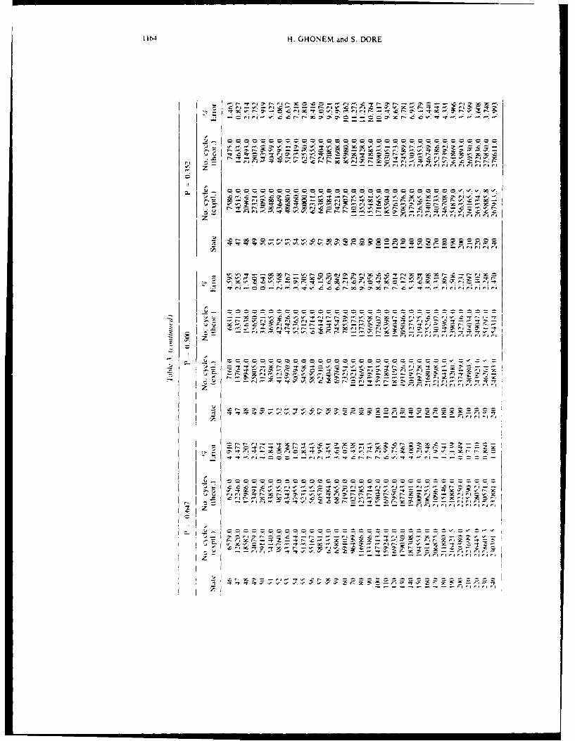
lit" H. GHONEM and S. DORE
i ., r.t 3:
-i raeZ .7.7 4 .7 e 1. r- r- x -'I wae.r = -! ret .4.~ C- C, c r- - .3-14 --rre re r rarerI rar 'I IsaIs rare
-z
-T Cr -C - ' 3 0 - - r- e,.- a - 7eCc .X 3 eea,..-
r,. 'c x .7 r (ee. efC 3 .r- r- x -T 'o. r 3'
~~~U~ I- Crr-- - r- 3 -ri r- 7er,. CDz ----2r r re raer raer rare- - 4-
:z cr- x -rr- .,.C- 140
wn flC. Ia .a ,d.eteti- a Cr~ ,,re.re- r..e v.
----------------------------,rr ra C
3.C.. ~ ~ ~ ~ ~ ~ ~ -0X at C 0 C Cr ~-'Cre .rere3'C..'X 07r, c -r -r~
E. c cx -
-. ~ ~ ~ ~ ~ 3 x'_ - - - - - - - - - - -

Fatigue crack growth in polycrystalline solids 1165
zz
,S ---=. -, r- r-R 'r
WN Nw.'~ -x rl eqC Cc *1C4 W. .
, a-. . ,7 - . . C ," .... _ _U~ ~ ~~O 0N,' 0 '~r'*~
-- - -hr 4 hir.7- hra- Si O ", .- .r- .,o -- ,-
. . . . hr . . . . . . hr. h . h,
. ., . . . . . .. - . . . r . .-I ci C : Ca a4
. . . . . . . . . . . . . . . . . . N . . . . .. . . . - . . N .: 3 ' M 4 1- ri j to' r - j r. N *I FtZ t r- -C V r- S .al : -:i m a
Cit 14 rll hrct .CCr-Clhh~
. . .. . . ... ... .
-- O C 3c hr. n. hr N Nci hr. h. .7. 11
x 7..7rhrhrh x h-rhThh.Z t ih.h. CFtV V' x z _-. _ Car xaCUC
-7.7~- hr Cr N: t' 0 - cSaa-ctN ~ r r
Ix,
T ;c
_r t .T _h r h

1166 H. GHONEM and S. DORE
10
PZ90
. ........... ............. .
-10 ,. . a .10
-20
45 95 145 195 245
CRACK LENGTH/AX
Fig. 12. Error in percent of the proposed model for C (in the Paris-Erdogan equation) = 3.79x j0-l0.
Making use of these constants. eqns (16) and (20) were again utilized to generate a set oftheoretical constant-probability crack growth curves as shown in Fig. II. These curves werecompared to those experimentally obtained in Fig. 5 and results of this comparison in the formof percentage of error of number of cycles corresponding to similar crack lengths are listed inTable 3 and summarized in Fig. 12. On the basis of these results the following observationscan be made:
I The present model succeeds in describing the evolution of the crack growth by estimatingthe number of cycles required for the crack to advance from one discrete position along thefracture surface to the following one. The evolution process was carried out for constant-probability crack growth curves. From these curves the scatter in the crack length at a specificfatigue as well as the scatter in the number of cycles required to advance the crack to a specificlength, can be estimated. The results of the model, when applied to Al 2024-T3 that have beensubjected to fatigue cycles with a constant stress amplitude, are in agreement with those ex-perimentally obtained. Average error in the theoretical curves is estimated to be 5%, whic. iswithin the scatter limit of any experimental curve. The accuracy of the model. however, see sto depend on the degree of agreement between the crack growth curve obtained using a cc Itinuum theory and the experimental mean curve. To examine this effect in the present appication, the value of the parameter C in the Paris-Erdogan Equation was changed from 3.79 ),10- ,to 3.51 x 10- " so that the deviation of the theoretical mean curve from the experimentalone is increased as shown in Fig. 10. As a result the average error in the prediction of themodel, as illustrated in Fig. 13. is increased from 5% to 13%.
0 P:.90
-10 . ..
" -20
-30'45 95 145 195 245
CRACK LENGTH/&X
Fi I Error tin per:enl) It the propo,,eu model for C(in the Parir-trdogan equllin = '
ItI

Fatigue crack growth in polycrystalline solids 1167
150
125
100
6 S
25
45 70 95 120 145 170 195 220 245
CRACK LENGTH/AX
Fig. 14. Variation of scatter range as function of crack length position.
2. The degree of scatter in the number of cycles Qorresponding to a specified state is observedto decrease as the crack length increases. At higher crack lengths all the cracks require aboutthe same number of cycles to advance from one discrete position to the following one. Thismay then lead to the conclusion that the degree of scatter in the number of cycles to failuredepends on the large scatter observed in the early stages of crack propagation. This is illustratedin Fig. 14. The effect of scatter associated with "short" cracks on the variation in the numberof cycles required for the crack to reach a critical length is currently under investigation bythe authors.
3. The notion that there is a minimum number of cycles required for the crack to advancefrom one position on the fracture surface to the next immediate one has been theoreticallyderived in this model through the parameter I,4 in eqn (16). This concept of "incubation time"
could be interpreted in relation to the time required for the crack tip propagation threshold(such as a specified mobile dislocation density, a thermodynamic activation level or any othercriterion) to be satisfied. This concept warrants further study.
CONCLUDING REMARK
A model is presented here describing the crack propagation process as a discontinuousMarkovian process. Based on this. the concept of constant-probability crack growth curveshas been quantitatively derived. With the assumpotion that the crack growth curve given byany continuum crack growth model coincides with the experimental mean growth curve, theproposed model has demonstrated that it could sufficiently describe the evolution of the cracklength and associated scatter at any stress level.
.4Amnn ledtp'rnpnni-The authors wish to acknow ledge support of this research program by the Air Force Office ofScientific Research through Contract No. AFOSR.84-0235-TEF.
REFERENCES
III P. Paris and F. Erdogan. A critical analksis of crack propagation lay.. J B tsi l:,ttav Trim% 4NrW. . cr 1) 85it)ecember 193)
I21 1). W. Hoeppner and W E krupp. Prediction of component life bh application ot fatigue crack gromth knom, ledge.n.,ni r tri ,tf' I 6 (1974)
131 F R (jurne .. Fl 'lolo ,' Sl rlifd /ir, t %rs Cambridge t'ni'ersi,, Pres 119"74)141 I) F- (),tergaard and 13 %1 Hillherr\ . (haracteri/ation of the sariahil t in faltigue crack propagation d.ta Pr, I,-
eihiltt Fro tlrt' 'e( 1i1pm and 'otIckili' .c l'ctid' Apph 0ll ,, ,1 .r Xtr ural Id r cti i aid toiintcooi " (Fditedh% J %I llioom and J C Fkh.ill .. 4.11 .li 798. pp 9"7-11 AS \NI l('s3l(11 (I () Johnston. Statisticil scatter in fracture toughncss and fatigue gro\%.h raltC dL.i,i. in }Ir, I thilistic l-'i twr%f,', hilotti % Ind I olivilt'' Alt'thcls ,ppih, atwin /,r .Sipm mo l OI l .rsivii it Id iitloin c i Edited t,% J %I Hloommd I ( Fk -kalli. .41 Iif S11, 798. pp .2-N
, ..\S IM 149;),
1168 H. CHONEM and S. DORE
161 L. N. IvcCartnev and P. W. Cooper. A new method of analyzing fatigue crack propagation data. Engng FructurelMech 912) (1977).
1! R. G. Forman. V. E. Kearney and R. W. Engle. Numerical analysis of crack propagation in cyclic-loaded structures.J. Basic Engnq Ser. D 89 (1967).[81 H. Ohonemn and J. M. Prov an. Micromechanics theory of fatigue crack initiation and propagation. Engag Fracture
Mlech. 13(4) (1980).191 F. Kozin and J. L. Bogdanff. A critical analysis of some probabilistic models of fatigue crack growth. Engnig
Fracture Mech. 14 (198 1),[101 H Ghonem. Stochastic fatigue crack initiation and propagation in polycrystalline solids. Ph.D. Thesis. McGill
University (1978)[1l1 A. T. Bharucha-Reid. Elepnents of thze TheorY of liark-ov Proc-esses and Its Applications. McGraw-Hill. New
York (1960).[121 W Weibull. A statistical theory of the strength of materials. lng. Vetenskaps Hkad. Handl. (151) (1939).[13] K P. Oh. A wseakest-link model for the prediction of fatigue crack growth rate. ASME J. Engng Miater. Technol.
100 (April 1978).1141 A. Tsurui and A. Igarashi. A probabilistic approach to fatigue crack growth rate. ASMVEJ. En~gg aler. Technol.
102 (July 1980).I 151 D. A. Virkler. B. M. Hillberrv and P. K. Goed. The statistical nature of fatigue crack propagation. ASMEJ. Enkn.k'
Mlaier Technol. 101 (April 1979).1161 Ji. N. Yang. R. C. Donath and G. C. Salivar. Statistical fatigue crack propagation of IN 100 at elevated temperatures.
ASME Int. Conf. on Advances in Life Prediction Methods. Albany. NY (18-20 April 1983).

APPENDIX B
EXPERIMENTAL STUDY OF THE CONSTANT-PROBABILITY CRACK GROWTH CURVES UNDER
CONSTANT AMPLITUDE LOADING
102

Eagweermg Fwctuwe .Mechwtcs Vol. 2". No. 1. pp. 1-25. 1987 0013-794487 $3.00 + 0.00Pnnted in Great Brain Pe'psmon Journas LId-
EXPERIMENTAL STUDY OF THE CONSTANT-PROBABILITY CRACK GROWTH CURVES UNDER
CONSTANT AMPLITUDE LOADING
H. GHONEM AND S. DOREMechanics of Solids Laboratory, Department of Mechanical Engineering and Applied Mechanics,
University of Rhode Island, Kingston, RI 02881, U.S.A.
Abstract - This paper is concerned with the application of a mathematical model that describesthe fatigue crack growth evolution and associated scatter in polycrystalline solids. The model has
been built on the basis that an analogy exists between a particular discontinuous Markovianstochastic process. namely the general pure birth process, and the crack propagation process. The,crack evolution and scatter were then defined in terms of material, stress and crack-length dependentproperties and crack tip incubation time.
The application of the model is carried out by comparing the constant-probability crackgrowth curves generated for three different load levels with those obtained from testing sixty Al7075-T6 specimens for each load level. A photographic method was utilized to measure the crack-length in this test program, by recording the residual deformation that accompanies the flanks ofthe crack during propagation.
INTRODUCTION
PREDICTION OF fatigue crack growth, even under constant amplitude loading, has not been an easytask. This is mainly because the manner in which the various parameters, such as loads, materialproperties and crack geometries, affect the crack propagation is not clearly understood[l]. This,consequently, had led to a proliferation of hypotheses and laws for describing fatigue crackpropagation (see review articles in refs [1, 2 and 3]). Most of these models are based on conceptsof the continuum theory with the assumption that cracks propagate in an ideal continuum media.Actual metallic materials, however, are composed of random microstructure described by variousmicroparameters which can seriously affect the growth of a crack in these materials. As a result,the deterministic theories can only be accepted as an approximation of the actual random fatiguecrack propagation process.
The ue of statistical distributions or probabilistic models thus becomes necessary to makepredictions of crack growth more reliable. The search for the "true" statistical distribution hasbeen a difficult task since in any application, the amount of crack-growth data which has beencollected for any particular case would not be sufficient to discriminate between the different typesof distributions[4]. In addition, when a series of tests on identical specimens is performed toestablish the scatter due to material properties, the uncertainties in load values and crack-lengthmeasurements are also included in the scatter data. Due to this limitation, it is difficult to isolatethe scatter associated with material properties in any experiment. One is also hampered by thelack of an exact physical description of the fatigue process[5]. When taking these two fators intoconsideration, any probabilistic or statistical model can identify the variability of crack-lengthonly in a comparative sense. This means that the absolute values of the variability at a specificload level predicted by a model may not be equal to those obtained experimentally. However, itis possible for a ratio of variabilities predicted for two different load conditions to be equal tothat of the experimental results obtained at the same loading conditions. In this, the experimentalerrors being independent of the magnitude of the applied loads, are eliminated.
There are basically two kinds of mathematical models in existence to predict the variabilityin fatigue crack growth. The first employs a statistical approach in which random variables areintroduced instead of the constants in the appropriate deterministic crack growth equation. Whilethese models (see, for example refs [6-11 ]) are simple to use and versatile in application, theypossess some disadvantages. First, all of them are based on Paris law[ 12] where it has been shownthat other laws like the Forman's law[13] are more applicable. Secondly, the scatter parametersin these models have no physical description and no attempts have been made to link theseparameters to the micro-structural properties. Lastly, though these models generate crack-growth
. . , i i iI I II

2 H. GHONEM and S. DORE
data that match the experimental data reasonably well in some cases, they do not provide anyinsight into the nature of the fatigue crack propagation process.
The second approach employs evolutionary methods in which the propagation of the crackis treated in a probabilistic or stochastic sense instead of a statistical one. Making use of a specificprobability process, namely the Markovian process, the models with this approach strive tocorrelate the properties of this process with those of fatigue crack propagation.
Examples of this approach are the models by Ghonem et al.[14, 15], Kozin and Bogdanoffhj16]and Aoki and Sakata[17]. The major disadvantage in using these models is the lack of crack-growth scatter data for different conditions which would have been helpful to check the validityof the probabilistic assumptions on which these models were built.
The objective of this paper is to examine the results of the stochastic model developed byGhonem and Dore( 15] when utilized for the prediction of the crack growth evolution, in the samematerial, at different loading conditions. Before proceeding on this application, a brief review ofthe fundamentals of the model is presented in the next section. This will be followed by thedescription of the experimental study and detailed analysis of the results.
REVIEW OF THE PROPOSED MODEL
In this model, the fracture surface is divided into a finite number of crack "states" of equalwidth; a probability space of two events was defined with the condition that the crack is in state" r" after i cycles have elapsed from the instant bf'reaching "r ". They are, the event that the crackwill remain in the state "r- and the event that the crack will not be in "r". Assuming that thecrack propagation process is irreversible and utilizing the fact that under conditions of constantamplitude loading the existence of a crack at a particular state depends only on its presentmechanical and microstructural details, a definition for the transition probability was arrived at.Using the criteria attached to the discontinuous Markovian process[18], a transition intensity (A,)could be defined. In this approach, A is assumed to be a material parameter which in addition tobeing a function of the crack position 'r', should explicitly depend on both the initial elapsedcycles i and the incremental duration Ai. The propagation process thus becomes time-inhomogeneous. This characteristic is a departure from the works of Ghonem and Provan[14]and Kozin and Bogdanoff[16].
The probability equation was then derived and can be written as:
In P,(i) = B(eKI - eA'i) ; i> 1 1 (I)
=0 , i <1
where i is the number of cycles. B and K are crack-length and stress dependent variables, Pi) isthe probability of the crack being at a state 'r" on the fracture surface after i cycles elapse andto is the minimum number of cycles required for the crack to advance from one position on thefracture surface to the next and is also crack-length and stress dependent.
This derivation was made by defining the transition intensity A, and the Incubation time 10in the following form.
BB eK' (2)
K
/ C,[(r - I)" - r " ] (3)
where 14)
B = C, r"' (5)
K = C, r"
and C. C.. C. ni. n. and n, arc material, applied stress and enironment dependent parameters,.These functions (eqs 2 and 3) were veritied with the aailable crack growth scatter data based onthe works of Virkler et al.[19] and Yang ct al.[6]

Constant-probability crack growth curves 3
As can be seen, identification of the six constants is sufficient to define eq. (1) at any crackposition so as to calculate the associated number of cycles elapsed for any probability (P,(i)) value.Carrying out this operation for a given probability value at all the crack states in a cumulativemanner, will generate a crack-position versus number-of-cycles curve representing the probabilitywith which a crack spends a certain number of cycles at any state.
Here, one should observe that the constants in these mathematical functions can be calculatedby considering the crack growth curve obtained by using a continuum equation as being the,.P,(i) = 0,5 curve. This can be done numerically, and the crack growth scatter at any crack lengthand at any fatigae load can be defined without the need to perform large number of fatigue tests.As mentioned before, the results of the model, when applied to Al 2024-T3 that wassubjected to load cycles of constant amplitude, were in agreement with those experimentallyobtained with the average error in the theoretical curves estimated to be 5%.
In order for the model to have a wider scope of application, it has to be substantiated fordifferent loading conditions and for different materials. The first step in that direction is theverification of the model for different loading conditions on the same polycrystalline material. Theexperimental set-up and procedure used for this purpose are described in the next section.
DESCRIPTION OF THE EXPERIMENTAL SET-UP
Tests were conducted on Aluminium 7075-T'6 alloy and crack-length versus number of cyclesdata were collected at three different stress levels. Each level was tested by using 60 identicalspecimens to establish the degree of crack-length scatter during propagation.
A rectangular specimen (320 mm x 101 mm) with a thickness of 3.175 mm and a center-cracked tension geometry was used throughout the test program. The direction of the center-crackchosen was perpendicular to the rolling direction of the sheet from which the specimens were cutas shown in Fig. I. The dimensions of the specimen and the crack initiating notch are based onthe ASTM E647 recommendations and are shown in Figs 2 and 3 respectively. The specimen endswere fixed to the test system by flat end grips whose dimensions are also based on the ASTME647 recommendations.
A study was carried out to compare the available crack-length measuring techniques namely,
(a) The Photographic Technique,(b) The Drop Potential Method.(c) The Mechanical Method,(d) The Electrical Technique,(e) The Acoustic Method.(f) The Ultrasonic Method and(g) The Visual Method.
The results of this study. based on refs [20, 21 and 22] are detailed in ref. [23]. The conclusionwas that the method of photographing the crack during propagation was the one most suited forthe present program. since it is capable of tracing the growth of one point along the crack-frontas opposed to a technique that measures the average position of the crack front.
The photographic technique used in this study depends on the reproduction of a sharp imageof the deformed material along the flanks of the crack to make it possible to locate the crack-tipimage and, consequently, to determine the crack-length with an acceptable degree of resolution.Since it is certain that in ductile materials, a sizable plastically deformed zone accompanies thecrack during its propagation. especially in plane stress applications isee Fig. 4). this zone can beutilized as an accurate crack-length indicator. An example of this deformed zone is shown in Fig.5 It can be seen that the interface between the two fracture surfaces (the crack) is not presentalong with this image. As the crack :ncreases in length. leading to a higher crack openingdisplacement. the separation of the fracture surfaces becomes visible as a dark line within thedeformed zone. This is shown in Fig. 6.
The testing configuration included a camera and a continuous lieht source positioned on oneside of the specimen. The camera was triggered by an electrical pulse sent by a microcomputerthat kept track of the elapsed number of cycles. Also, a number of shutter speeds, aperture settings.devcloping solutions, processing times and film types were experimented with to achieve the best

4 H. GHONEM and S. DORE
0 0 0 126.4 (1)
320.67 (12 5/6)
THICKNESS 3.175 (1/8)
160.33 (6 5/16)
002S.4 (1)
0.326 (3/8) DIA
6 H LES 25.4 (1) 25.4 (1)
ALL DIMENSIONS IN MM (INCHES)
Fig. 2. Test specimen in the present study.
reproduction of this shear zone, these parameters are fully described in ref. [23].A transmitted-light microscope equipped with a horizontal travelling table was used to
determine the length of the image of the plastically deformed zone. The measurements were madeby a digital micrometer having a resolution of I um and transferred, after suitable interfacing, toa microcomputer for acquisition and subsequent analysis (see Fig. 7).
The error in these measurements was determined by comparing an actual crack-length,measured directly on the specimen's surface, and the length of its corresponding shear zone. Thiscomparison, which was made in the cases of I x and 2 x magnifications (see in Table 1 (indicatedthat the errors associated with the 2 x magnification, which was adopted throughout the testprogram. were lower. The region of interest used for recording the shear zone was limited to thecentral 28 mm on the 36 mm frame. Lsing a 2 x magnification. this meant that a maximum of14 mm of crack growth was photographed in any test.
All the 180 tests carried out in this study were performed on a closed loop. servo-hydraulicMaterial Test System ITS 880) capable of controlling loads within 0.2"%.
Based on ASTM E647 recommendations, the initial crack-length, a, wa,; chosen t- he100*) mm. however, the crack-lengths were recorded from a length of 9.00 mm onwards. The finalcrack-length (a,) for the purposes ot this test program was limited to 23 mm measured from thecenter line of the test specimen. The loading parameters were then selected so that the cracktransition from the normal mode to the shear mode could not occur before the crack reached this

Constant-probability crack growth curves 5
specified length, i.e. 23 mm. This condition was imposed on the loading parameters in order toavoid the problem of defining the crack-length in the shear mode.
Tests were executed at three different stress ratios R; R = Pmin/Pmax, where Pri is the minimumload level and Pmax is the maximum load level. The loading sequence for fatigue pre-cracking andthe three test load conditions are detailed in Tables 2 and 3, respectively. A frequency of 10 Hzand a ramp waveform were selected for the loading cycle.
Figure 8 is an example of the results obtained in this test program showing the progress ofthe crack length at different loading cycles for one of the loading conditions.
EXPERIMENTAL RESULTS
As mentioned in the previous section sixty specimens were tested for three stress levels andcrack-length (a) versus number-of-cycles (N); data was recorded from a length of 9 mm to a lengthof 23 mm. It may be recalled that the initial crack-length chosen for this test program was 10 mmand not 9 mm. Data between 9 mm and 10 mm will be used for future work on short crack.behaviour and the comparison between the theoretical probability crack-length versus number ofcycles data. The experimental data will be made from the initial crack-length of 10 mm onwards.Crack-growth data (a vs N) for the three stress conditions is shown in Figs 9-11.
The next step in the analysis is the selection of the width-of-crack state for producingexperimental data suitable for comparison with that generated by the mathematical model [15].As can be seen from Table 1, the maximum error between the shear zone recorded on film andthe crack-length measured from the specimen was estimated to be 0.163 mm. Using a conservativeapproach, the maximum error was assumed to be 0.2 mm and this was considered to bc thc statewidth.
2a
a
4.762 (3/161 dia.
DRILLED
- 9.625 (3
7.144 (9/32) 2.31(3/32) il
14.288 (9/16)
Scale 5:1
All Dimensions in MM (inches)
F-ig I ( rack nihling notch

6 H. GHONEM and S. DORE
Table 1. Comparison of the actual crack-length with the length measured from the film (all dimensions in mini
Measured value Magnification Corrected Actual Error(M) (M) (C) (A) (A-C)
(C = Ma/m)
4.882 1.058 4.612 4.831 0.2188.047 1.045 7.700 7.755 0.055
11.624 1.045 11.123 11.206 0.08318.855 1.045 18.043 18.082 0.039
8.208 2.000 4.104 4.202 0.09817.028 2.000 8.514 8.677 0.16315.950 2.000 7.975 8.042 0.06717.692 2.000 8.846 8.924 0.07819.841 2.000 9.920 9.956 0.03523.023 2.000 11.501 11.592 0.09026.161 2.000 13.080 13.153 0.07229.803 2.000 14.901 15.018 0.11631.623 2.000 15.811 15.892 0.081
Table 2. Loading sequence for fatigue pre-cracking (all loads in kN)
Load level till Load level tillcrack was generated crack reached 7.5mm
(20 Hz) (20 Hz)Test P P AP P,=* PmP
Condition
1 25.95 8.30 17.65 ?6.55 13.55 13.00II 29.30 7.70 2160 24.80 10.65 14.15
1II 26.30 7.70 18.60 21.50 7.30 14.20
Table 3. Test load conditions (all loads in kN)
Test load level(10 Hz)
Test ACondition
1 22.79 13.68 9,11 0.61[ 22.25 11.13 11.12 05I1 15 19 6.08 911 0.4
Shear Zone
~Plastic Zone
(A)
Plastic Zoneconverted toShear Zone
(B)
(C)
I ih! 4 Ionc of pi iitc dcformation in the ', initl Or the I,1itlc .LrckJ '11

(onstanz-probabi)iz, crack groth cures7
4- *
40 IL
• , : - ;, ,..
( rack Dircctuon
I ) I Direction o( cr ck lh rc,pct to the grain ,rtlclurc
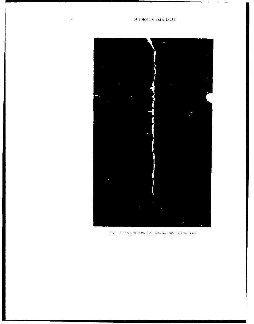
S H1. (iHONUNM and S~ DORF
IL t t2' lhbCJ Tt /onTc ti-omlflflflL the ritk

(onslarl-pr bbht crac igrovath curses9

0 H. GHONEM and S. DORE
I. (rack length = 9.495 mm 2. Crack length = 10.498 mmNumber of cycles 6380 Number of cycles = 15510
3. Crack length 1(.912 mm 4. Crack Ingth - 12.0)31 mmNumber of cle, 1S960 Number of c~cles 25364)
S".lck I.le gth I -' 6310 in in 6 (rack length I 10)0 111i1Niirllhcr t cL*cIe, 2X2I)) Numinber of c ,cIc, -")S(X
I ic ' I iil k Ct itiohlll n ic t rdc irmnl I .Ii inw n inbtr I .,ihlccicd to I eq ( inktlio,.-I ( Nj l 2nllk- 1,111
. ....... .... I II• I ~n~l • I IIx).
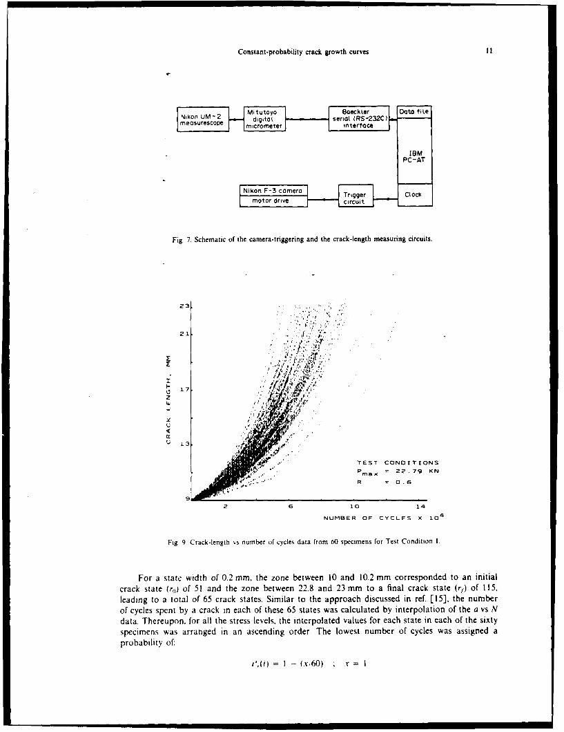
Constant-probability crack growth curves II
23seriat RS-232C)measurescope I ~rmtrinterface
IBMPC-AT
[Nikon F-3 camera I JTrigger L ~cmot or drive circuitt V -'-
Fig. 7. Schematic of the camera-triggering and the crack-length measuring circuits.
17
z
-JJ
U : .. , .,
TEST CONDITIONS
=22.79 KN
R =0.6
2 6 10 14
NUMBER OF CYCLES X10
Fig, 9 Crack-length vs number of cycles data from 60 specimens for Test Condition I.
For a statc width of 0.2 mm, the zone between 10 and 10.2 mm corresponded to an initialcrack state (r,) of 51 and the zone between 22.8 and 23 mm to a final crack state (r,) of 11 5.leading to a total of 65 crack states. Similar to the approach discussed in ref. [15], the numberof cycles spent by a crack in each of these 65 states was calculated by interpolation of the a vs Ndata. Thereupon, for all the stress levels, the interpolated values for each state in each of the sixtyspecimens was arranged in an ascending order. The lowest number of cycles was assigned aprobability of:
= I - (x60) x =

1 H. GHONEM and S. DORE
23
217
13
TEST CONDITIONS
Pmax 22.25 KN
R =0.5
9
2 6 10 14
NUMBER OF CYCLES X 10O4
Fig. 10. Crack-length vs number of cycles data from 60 specimens for Test Condition 11.
23
21
17
I I TEST CONDITIONS
Pma 15.19 KN
~1 jijR =0.49
4 1220 28 36
NUMBER OF CYCLES X 10O4
1 fg I (rck-k'rigth ksnumber of c Ice data from 60 spvcimens for Test Condition III

Constant-probability crack growth curves 13
and so on up until the highest number of cycles whose corresponding probability value was:
P,(i) = I - (x'60) x = 60.
A probability range of 0.9-0.1 was selected for comparison of the experimental and thetheoretical data. The curves obtained experimentally are plotted in Figs 12-14 with the probabilityvalues having decrements of 0.1.
In these figures it is observed that the widest scatter band is associated with the test conditionthat produced the smallest mean crack-growth rate, Test Condition Il, while the narrowest scatterband is associated with the Test Condition 1I in which the mean crack growth rate is the highest.This is due to the fact that when loads are high, the influence of the microstructure on crackpropagation is diminished so that the degree of scatter of the a vs N sample curves, in relation tothe mean growth curve, tends to be limited. Similar observations were made by Yang et aL.[7]and this is perceptible in Fig. 15.
THEORETICAL RESULTS
Firstly, the continuum growth law to be utilized in the mathematical model was arrived atby investigating a number of crack growth equations with known material constants whichrecognize the effect of the stress ratio. Forman's equations[13,24] and the equation derived byHardath et a/.[25] fall into this category.
Forman's equation is generally written as:
da C(AK )11(6
dN - (I - R)K - AK (6)
where a is the crack-length, N is the number of cycles, K is the stress intensity factor range, K, isthe critical stress intensity factor, R is the stress ratio and C and n are material constants.
P=O. 524 P=O. I
P=O. 9
22
2 18(
14
• 'C 1 ) 14 ,1,
N NiMB ( it ( Y(LF% X I)4
Fig 12 Experimental conNtant-pro1hahihli, crat:k gro.'th cur'c, generated for Test Conditon I

14 H. GHONEM and S. DORE
24
22
2 18
U
U14
10 _2 6 10 14 18
NUMBER OP CYCLES X10
Fig. 13. Experimental constant-probability crack growth curves generated for Test Condition 11.
24 =09P=0.5 P=0.1
22
E
Z is
14
10
26 10 14 18
NLJMBF P OV CYC:LES X 10 4
Fig. 14 FxperimentaI constain-prohabiliii% crack gro-. h ctune' generated for Test C'onditionIl

Constant-probability crack growth curves 15
The values of K~, C and n for Aluminium 7075-T6 are listed in ref.[13] as:
Kc= 68 Ksi-in' (74 M Pa-rnt
C = 5 x 10-13 U.S. Customary Units
= 1.63 x 10- 1 SI Units
n =3
and in ref.[24] as:
Kc =40 Ksi-in'(44 MPa-m')
C =2.13 x 10- 1 U.S. Customary Units
=1.60 x 10⁻¹⁸ SI Units
n =3.2 1.
The equation derived by Hardarth et aI.[25] is:
d a (7 )
where Ke(8)
and Kff (s...i - so) ji-r F (9)
s,,,., is the maximum stress, so is the crack opening stress, \/;ra F is the stress intensity parameterfor specimen configuration, K,,. is the maximum stress intensity factor, K, is the fracture parameter[81 Ksi-in' (89 M Pa-mt)], C and n are material parameters.
*C 3.83 x 10⁻⁸ SI Units
n =3.17.
L.0
X 14
- 0
Z
0
z
10 14 18 22
U CRACK LENGTH. MM
Fig 15 Variation of the scatter range with crack length for the three Test Conditions

16 H. GHONEM and S. DORE
Of the above two laws, the one provided by Forman et al.[13] was selected because it isbased on data obtained from different laboratories as opposed to the equation of Hudson et al.[24]that was derived after correlation with one set of experimental data. The growth law of Hardarthet aI.[25] was also not utilized because the present mean experimental growth rate was differentfrom that predicted by the law, by an order of magnitude for all the three stress levels.
Having defined the continuum growth law and the corresponding material constants, the sixconstants C1, C', C3, n1, n, n3 were next calculated by obtaining their converged values usingNewton-Raphson's method.
The six constants for each load condition are:
1 TI III
C, 0.015127 0.010064 0.010105C, 1.9371 X 10⁻⁶ 3.4055 x 10- 6 1.9758 x 10- 6
C3 1.5940 x 10⁶ 1.0888 x 10⁶ 2.3151 x 10⁶n, 0.8000 0.7957 0.8514n, 1.4946 1.4991 1.3501n3 -0.7000 -0.6820 -0.8537
Following the analysis presented in ref. [15] the theoretical probability curves were plotted makinguse of these constants, in Figs 16-18.
The percentage error of the number of cycles is plotted in Figs 19-21. The average value offthe absolute errors was found to be 7%, 5% and 8% for the ', II and the III load conditions,respectively.
A remark is warranted on the six constants that cl-aracterize the crack growth scatter.Though these constants depend on the load parameters, no attempt has been made to derive anexplicit relationship. In fact, there is no need for an explicit relationship since they are computeddirectly from the continuum growth law.
CONCLUSIONS
(1) The mathematical model developed here provides a physical description for fatigue crackpropagation as well as capability of predicting crack growth scatter at different stress levels.While the model uses the crack growth data from a continuum law as its input, it does notdepend on a specific law. The only requirement is that such a law must be a correctrepresentation of the mean growth curve. The model has been validated for two aluminiumalloys Al 2024-T3 and Al 7075-T6 subjected to four different stress levels and is in the processof being applied to steel and titanium alloys.
(21 The scatter data recorded for the second load condition (AP = 11.12 kN, Pra, = 22.25 kN)of the experimental program has been observed to be the least widespread when comparedwith that obtained from other load conditions with lower values of AP. This can be attributedto the following phenomenon. The crack transition from a specific state is governed by acritical threshold energy at the crack tip. When such a threshold is satisfied in one cycle oran accumulation of several cycles, depending on the load condition and crack-geometry, thecrack tip can then advance from its present state to the following one. Hence for larger loadsand longer crack-lengths, the probability that this propagation threshold is satisfied increasesrapidly with the number of elapsed load cycles while, for smaller loads and shorter crack-lengths. the probability of discrete crack growth advancement increases gradually. In thishypothesis the degree of scatter in achieving the required threshold energy reflects on thedegree of scatter of crack growth. Fractographic analysis of fracture surfaces shows that. atthe same crack-length. more striations per unit distance are present along the fracture surfaceof specimens subjected to a large load level (Test Condition II. see Fig. 22b) than in thespecimens subjected to a lower load level (the Test Conditions I and Il. see Figs 22a and22cl. It is known that ductile fracture striations are formed due to a change in the orientation
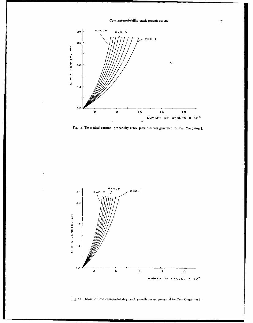
Constant-probability crack growth curves 17
P=O .924 P=O1
22
2 18
Uj
UI
14
2 6 10 14 18
NUMBER OF CYCLES X 104
Fig. 16. Theoretical constant-probability crack growth curves generated for Test Condition 1.
P=O. 524 P=0.9 / 0'o 1
22\
*18
z
<14
1~02 6 10 14 1 H
NUMBER OF CYCLE,; X 104
Fig. 1 7 Thcortical constant-probahility crack groth curve-, generated for Test Condition 11

18 H. GHONEM and S. DORE
24 P=o. 5
P-O. 9-/ P0. .
22I1
Z 18wIJ
U
U14
102 6 10 14 18
NUMBER OF CYCLES X 104
Fig. 18. Theoretical constant-probability crack growth curves generated for Test Condition III.
40
20 I-- P=O. 1
U(x .P=0 .9a. - .91l ..l q I , I I , ,,; I l
0 P=0 . 7
0
-20
-40 ,
10 14 18 22
CRACK LENGTH. MM
Fig. 19. Error in percent of the proposed model in the constant prohhility crack growth curcS for Test
Condition I

Constant-probability crack growth curves 19
I iL

lo~H. CHONEM and S. DORE
Ei.
le. (a '

('Onstant-probabilit,, crack growth curves 2
L D>

Constant.probability crack growth cutves 23
4 0
20
z
z P=O. 9
P=O. 30 P=O. 6
-20
i -~~~~ ~~-40 , , ,I
10 .14 18 22
CRACK LENGTH. MM
Fig 20. Error in percent of the proposed model in the constant probability crack growth curves for Tes:Condition II.
40
20
p=o
Szo P=O.z
- 20P=0.9
-40 _ _,_,_,__
10 14 18 2
CRACP LENGTH. MM
1-ig 21 Frror in percent of the propo%ed model in the conqtant pro habilt crack growth cures for Te%(
(Condition Ill

24 H. GHONEM and S. DORE
of the fracture surface along a specific slip plane[26, 27]. Therefore, a denser striation patternis observed at loading conditions associated with higher growth rates because numerousorientation changes take place in a unit distance of the fracture surface. It follows that theenergy required for these changes is achieved more frequently under these conditions. Usingthis analogy at a macroscopic level, it can be said that the crack tip propagation thresholdis also achieved more often. These observations may act as another factor that substantiatethe fact that larger loading conditions result in a smaller degree of crack-growth scatter.
The changes in the orientation of the fracture surface along a specific slip-plane arereflected as the waviness of the crack path on the specimen surface. This is shown in Figs23(a) and (b). In view of the explanation given previously, increased waviness of the crackpath (measured in terms of the horizontal distance required for the crack propagation directionto change) is related to increase in the externally applied load levels and thus the degree ofcrack growth scatter at a particular load level could be related to the wavines of the crackpath. Quantification of this dependence has not been attempted here.
The phenomenon of crack-tip branching was also observed. Typical examples are shownin Fig. 24(a) and (b). While the existence of branching certainly contributes to the degree ofcrack growth scatter due to random loss of propagation energy at the crack tip, the extentof this contribution is not known. Both the effect of the waviness and that of the crack-tipbranching on the degree of crack growth scatter are under study by the authors.
(3) The use of the present model is directed towards two applications. The first is the constantamplitude loading which, while representing a simple load spectrum, does occur in practice:e.g. pressurization cycles in transport aircraft cabins, rotating bending stresses in generators,thermal stress cycles in pressure vessels. This application has been examined in this paper.The second application is the variable amplitude loading which could be a two-step loadsequence now-high, high-low) or a spectrum of random loads. Variable amplitude loading is.however, a complex problem due to the fact that the crack tip damage per cycle under suchloading is not only controlled by the stress amplitude of the current cycle, but also by thepreceding load history. It is generally agreed[28-30] that this dependence is only transientin nature and should not exist after a certain duration of cycling.
Reflecting this concept on the fundamentals of the constant-probability crack growthmodel, one observes two areas where modifications can be made to account for the historydependence of the crack growth process due to load changes. The first, is the assignment ofappropriate mathematical functions for the variables B, K and 1r to take this phenomenoninto consideration. The Markovian approach in the model is not violated because even thoughthe crack tip conditions depend on the loading history, the propagation process is affectedonly by the present crack tip conditions. On the basis of the existing works on variableamplitude loading, it can be said that the mathematical functions cannot be arrived at bysimple superimposition. However, quantification of the crack growth rates for variableamplitudes, even in the deterministic sense has not been accomplished so far. Only if that isachieved, will modifications for B, K and l0 be possible.
The other area where modification must be made is the consideration of initial crack-length (a,). In the present model, a0 was a constant as a result of an imposed experimentalcondition. Thus, the model provides a distribution of the number of cycles required fora crack to reach a specified discrete state from a,. No attempt has been made to consideran initial crack-length distribution and the manner in, which it will affect the constantprobability curves. Attempts to interpret the constant-probability growth curves in terms ofa distribution of crack states after a specified number of cycles have elapsed from the instantthe crack reached a, were also not made. Only this type of a distribution is useful for xariable-amplitude loading application because the history of the fracture process is described in termsof the number of cycles The recognition of this distribution is an important step since itiepiesents the initial crack-length configuration which is a necessary boundary condition forthe new load spectrum.
4,0y. ,, -hdi+m<on This %ork w supported hy the I" S Air Force (fice of Scientific Research under ( ontra. .Nt. )SR85 'ori2 i,, niiorcd h., Dr (j, larito. and Dr N Pagano

Constant-probability crack growth curves 25
REFERENCES
[I] D W Hoeppner and W. E. Krupp, Prediction of component life by application of fatigue crack growth knowledge.Engng Fracture Mech. 6. 47-70 (1974).
[2] Karl-He: :z Schwalbe, Comparison of several fatigue crack propagation laws with experimental results. Engng FractureAteth 6, 325- 341 11974).
[3] S. Chand and S. B. L. Garg. Propagation under constant amplitude loading, Engng Fracture Mech. 21, 1-30 (1985).[4) S. C. Saunders. On the probabilistic determination of scatter factors using Miner's rule in fatigue life studies. ASTM
STP 511.[5] W. J. Plumbndge. Review: fatigue crack propagation in metallic and polymeric materials. J. Mater. Sci. 7 (1972).[6] J. N Yang, R. C. Donath and G. C. Salivar. Statistical fatigue crack propagation of IN 100 at elevated temperatures,
AS AE Int. Conf. on Advances in Life Prediction Methods. Albany, New York (1983).[7] J. N. Yang and R. C. Donath, Statistics of crack growth of a super-alloy under sustained load. J. Engng Mater.
Technol 106, 79-83 (1984).(8] S. Tanaka, M. Ichikawa and S. Akita, Variability of m and C in fatigue crack propagation law da/dN - C(AK)r.
Int. J. Fracture 17, R 121-124 (1981).[9] T. R. Gurney, Fatigue of Welded Structures. Cambridge University Press (1979).
[10] D. F. Ostergaard and B. M. Hillberry, Characteristic of the variability in fatigue crack propagation data, ProbabilisticFracture Mechanics and Methods: Applications for structural design and maintenance, ASTM STP 798, 97-115 (1983).
[iI] B. R. Ellingwood, Probabilistic Assessment of low cycle fatigue behaviour of structural welds, . Press. Vess. Technol.26-29 (February 1976).
L12] P. Paris and F. Erdogan, A critical analysis of crack propagation law, J. bas. Engng 528-534 (December 1963).[13] R. G. Forman, V. E. Kearney and R. M. Engle, Numerical analysis of crack propagation in cyclic loaded structures,
J. Bas. Engng 459-464 (Septerr.,er 1967).[14] H. Ghonem and J. W. Provan, Micromechanics theory of fatigue crack initiation and propagation, Engng Fracture
Mech, 13, 963-977 (1980).[15] H. Ghonem and S. Dore. Probabilistic description of fatigue crack propagation in polycrystalline solids. Engng
Fracture Mech. 21, 1151-1168 (1985).[16] J. L. Bogdanoff and F. Kozin. Probabilistic Models of Cumulative Damage. John Wiley & Sons (1985).[17] S. Aoki and M. Sakata, Statistical approach to delayed fracture of brittle materials, Int. i. Fracture 16, 454-468
(1980).[18] A. T. Bharucha-Reid, Elements of the theory of Markov processes and its applications. McGraw-Hill (1960).[19] D. A. Virkler. B. M. Hillberry and P. K. Goel, The statistical nature of fatigue crack propagation, J. Engng Mater.
Technol. 101, 148-153 (1979).[20] N. E. Frost, K. J. Marsh and L. P. Pook. Metal fatigue, Vol. 225. Clarendon Press, Oxford (1974).[21] C. J. Beevers (Ed ). Advances in Crack Length Measurement Techniques. Chameleon Press, London, 1982.[22] R. B. Thompson and D. 0. Thompson, Ultrasonics in Nondestructive Evaluation. Proc. IEEE, 1716-1755 (December
19851.[23] H, Ghonem and S. Dore. Probabilistic description of fatigue crack growth in aluminium alloys, AFOSR-83-0322.
lApril 19:[24] C M Hudson and J. T. Scardina, Effect of stress ratio on fatigue crack growth in 7075--T6 aluminium alloy sheet.
Ening Fracture Alech. 1, 429-446 (1969).[25] H F. Hardarth. J. C. Newman. Jr, W. Elber and C. C. Poe, Jr., Recent developments in analysis of crack propagation
and fracture of practical materials. NASA TM-78766 (June 19781.[26] R. W Hertzberg and P. C. Paris, Application of electron fractography and fracture mechanics to fatigue crack
propagation. Proc. First mIt Conf Fracture, Sendai. Japan (1965).[27] R. M N. Pelloux and J. C. McMillan, Analysis of fracture surfaces by electron microscopy. Proc. First Int. Conf.
Fracture. Sendai. Japan (19651.[28] J. Schij.e. Fatigue crack growth under spectrum loads, ASTM STP 595, 3-23 (1976).[29] W Elber. Damage tolerance in aircraft structures. ASTM STP 486, 230--242 (1971).[30] R Sunder. A mathematical model of fatigue crack propagation under variable amplitude loading. Engng Fracture
fech 12. 155 165 11979)[31] H L. Ealds and R J H Wanhill. Fracture Mechanics, Vol. 176. Edward Arnold, London (1984).
(Received 29 Mai 1986)

APPENDIX C
CONSTANT-PROBABILITY CRACK GROWTH CURVES
128

Enguswmg Frrmac. Mocies Vol. 30. No. 5. pp. 685-699. 1988 0013-7944/U S3.00+.00Prnted in Great Brntan. P-etma Pr m C
CONSTANT-PROBABILITY CRACKGROWTH CURVES
H. GHONEMDepartment of Mechanical Engineering and Applied Mechanics, University of Rhode Island,
Kingston, RI 02881, U.S.A.
Abstract-This paper details a stochastic, time-inhomogeneous model that serves as a theoreti-cal basis for the prediction of crack growth and its variability under constant-amplitude loading.Crack evolution is described as a set of constant probability curves, each of whose points possessequal probability of advancing from one position to another forward position. This probability isgoverned by a transition intensity parameter for which two mathematical interpretations areexamined. A simplified crack growth rate equation, employing one of the definitions, is derivedand applied to AI 7075-T6 material for different loading conditions. Results of this applicationare compared with those experimentally obtained.
INTRODUCTION
THE WORK of Ghonem et al[f, 2] describes a [Orobabilistic crack growth model based on theassumption that fracture history can be established by employing a particular discontinuousMarkovian process which takes into account the fundamental aspects of the crack growthmechanism. This approach leads to the description of the sample curve of the crack growthprocess in terms of a constant-probability criterion. When considering that the crack growthcurve given by any continuum crack growth model coincides with the median growth curve, theprobabilistic model would then be sufficient to describe the evolution of the crack length andassociated scatter at any stress level[3,4]. The present paper is an attempt to extend theconcepts of the model by including a different definition for the transition intensity probability ofthe growth process. This will lead to the derivation of a simple and explicit probabilistic crackgrowth rate equation similar in structure to the Paris-Erdogan equation.
The first part of the paper focuses on the constant probability crack growth curve conceptand its model derivation, while the second part will deal with the application of the proposed law.
MODEL
The basic model is based on the assumpion the crack front in the crack propagation stage, asshown in Fig. 1, can be approximated by a large number M of arbitrarily chosen points a,a = 1 ..... ,. Each of these points in terms of the theory of probability, identifies a statistical"trial" or "experiment" conducted under identical conditions. The fracture state of the ath trialat cycle "i" is given by the crack length or random variable 'a(xi, x 2, x 3) whose evolution withtime shall then be established.
I DIRCTION OFCRACK PROPAGATION
Fig I Schematic of crack front positions along the fracture surface.
685

686 H. GHONEM
The following observations can be made regarding *ad:1. The evolution of *a, in the x1, x2 and x3 directions are statistically independent of each
other.2. The statistical evolution of 'ai(xi) is different from those of *ai(X) and ai(x 3) in that the
former consistently increases while the latter may be described as a type of random-walkphenomenon.
3. For an external load applied in the xt direction, the crack evolution in the x2 and x3
directions are orders of a lesser magnitude than that in the x, direction.On the basis of these observations this model is limited to the evolution of 'ai(xi) by assuming
that the crack growth distributions of 'a,(X2) and 'a(x 3) can be described by Dirac-Deltafunctions. So, *a will hereafter be referred to as ai.
Due to the built-in limitations of all experimental techniques in crack measurement, theobserved value of a, can only be specified within a range of:
x < a1 < x +Ax,
where Ax is the experimental error and x is the crack position calculated as (see Fig. 2):
x=rAx; ro<r<rf. (1)
Here "r" identifies the observable zone or state along the fracture surface; ro is the initialpropagation state, ry is the state just prior to catastrophic failure of the specimen andri, r2,. .. , r1_1 are the intermediate zones, all zones having the same width.
Given that the crack is in state r, then after i cycles from the instant of reaching r, one of
r 6
_-FAX
22
x 1 REFERENCE
.aic p a. t LINE
Fig. 2, Schematic of the proposed fatigue crack propagation along the fracture surface states.

Constant-probability crack growth curves 687
two events will occur. Either ad will remain in state r (event 'E) or a will not be in state r (eventE). The following points should now be noted.
(a) The crack propagation process is irreversible (i.e. there is no rewelding of cracksurfaces). Hence the crack, if it is not in state r after i cycles, must exist in a state greater than r
(b) Since it is not possible for the crack to propagate from one state to another state withouipenetrating the adjacent one, the crack can be identified by the number of cycles (i) required tcadvance from a given state to the immediately following state.
Based on these observations, events 'E and 'Ej can be seen as elements of a measurablespace (fl) (see ref. [3]) and the following definition of the probability measure of a becomespossible. At any fatigue cycle i, the probability that a, is in state r, i.e. the probability of 'E, isdefined as:
P{a, E rE, = P{x < ai < x +x4, (2)
i.e.
P('E,) = P,(i). (3)
Therefore, the probability of ad not falling within r, i.e. the probability of 'E, is,
P('E) = 1 - P,(i). (4)
It can be seen that, P,(i) should continuously decrease as the number of cycles increases. Beforeproceeding further to identify the parameters that define P,(i), it is necessary to make thesecomments.
Under conditions of constant amplitude loading, where no overloading effects are con-sidered, the growth of a crack from a particular state depends only on its present mechanical andmicrostructural details. More specifically, the probability of ai propagating from state r to r + Iin the cycle interval (i, i + 6i) depends on the event ('E,) and is independent of the events prior toi, ('Ej, j < i). To elaborate, let (','E) be the event of a, jumping to (r+ 1) from r in the interval(i, i+A i). This represents a future event if (rE,) is an event in the present. Clearly, the futureevent is conditional on the occurrence of the present event. Given that the present has occurred,the probability of the future is not affected by the probability of the occurrence of the past ('E,j < i). Also, the occurrence of ('E,) precludes the occurrence of the (SEj, j < i, s > r) due to theirreversible nature of the crack growth process.
The above feature is similar to that of a pure birth Markovian process in which the future isdetermined only by thc present and not by the past, and in which the discrete space variablenever decreases in magnitude with increase of time. This analogy helps to define a transitionprobability that is also a Markovian property and introduce the condition probability functionthat governs the crack growth process as:
P+' E /'E, ..... FE, ..... 'Eo, P{+i EAi/i'E
= P,,(i; ii, (5)
where P,,(i) is the transition probability linking the probability measures of two consecutivestates "r' and "'" 0 = r+ 1) along the fracture surface and "/" denotes the conditionalprobability. This property, together with the evolution of aj within the two event sample space(fl). describes a discrete space continuous time Markov process.
Since the analogy to the Markovian process has been shown, the criteria attached to thisprocess can be assumed to be valid for the crack growth as well.
1. The probability that a, propagating to a state different from r in Ai cycles, where Ai is verysmall, after i cycles elapse in state r is:
P,(Ai) = P{'EAi/'E.} + O(Ai),
=A,Ai+0(Ai); t=r+1. (6)
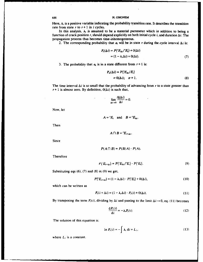
688 H. GHONEM
Here, A, is a positive variable indicating the probability transition rate. It describes the transitionrate from state r to r + 1 in i cycles.
In this analysis, A, is assumed to be a material parameter which in addition to being afunction of crack position r, should depend explicitly on both initial cycle i, and duration Ai. Thepropagation process thus becomes time-inhomogeneous.
2. The corresponding probability that a will be in state r during the.cycle interval Ai is:
P,(W) = P{'E,/'E} + O(Ai)
= (I - AAi) + O(Ai). (7)
3. The probability that a, is in a state different from r + I is:
P,,(Ai) = P{'E&,IE }
= O(Ai); tr+ 1. (8)
The time interval Ai is so small that the probability of advancing from r to a state greater thanr + 1 is almost zero. By definition, 0(Ai) is such that,
lim (A i) = 0.,,i-o A
Now, let
A = 'Ei and B = Ew.
Then
Af nB = rEi,,,.
Since
P(Af B) = P(BIA) P(A).
Therefore
pl',& , = P{'EA, 1I'E}" P{E,}. (9)
Substituting eqs (6), (7) and (8) in (9) we get,
P{'E,.,A} = (1 - A,Ai)• P{'E,} + 0(Ai), (10)
which can be written as
P,(i + Ai) = (I - Ai).- P,(i) + 0(Ai). 0(1l)
By transposing the term P,(i), dividing by Ai and passing to the limit Ai- 0, eq. (11) becomes
dP,(i) =A,P,(i). (12)di
The solution of this equation is:
In P,(i) =-f A, di + Li, (13)
where L, is a constant.

Constant-probability crack growth curves 689
This equation describes the crack growth probability from state r, after i cycles elapse, interms of the constant L, and the transition rate A, which is discussed below.
The parameter A, was introduced in this model as the transition intensity by which a,propagates from one state to the next. Adopting the notion that the crack growth process is adiscrete one, the crack transition from a specific state can be viewed as being governed by acritical threshold energy at the crack tip. When such a threshold (which is environmental,material, stress and crack-length dependent) is satisfied by cyclic energy accumulation, a cracktip transition can be said to occur. Therefore the larger the cycle duration associated with thecrack in a specifc state, the grea!er the probability that the propagation threshold :, sat: fied andthe greater the probability that the crack advances to the following state.
The transition intensity, A,, can be assumed to have several physical interpretations,however, the primary concern at this point is whether A, is a material property present only whenthere is application of cyclic loads or whether it exists even when there is no cycling.
If A, is a property that owes its existence to cyclic loading, then it could represent adislocation accumulation rate, a microvoid growth rate, a ductility exhaustion rate or a rate atwhich any physical phenomenon occurs in the grain structure of a polycrystalline material to aidthe propagation of a crack. In that case, the magnitude of A, should be zero at any instant there isno cycling. Specifically, its magnitude should be equal to zero at i = 0, the instant at which theload cycling is about to begin, after the crack has reached a particular state, r. Keeping in mindthe fact that A, should monotonically increase with i, the following expression for A, can then bechosen.
A,(i) = L(r)ia( '), (14)
where L(r) and a(r) are functions of the crack state.If, on ,he other hand, A, is a property present even when there is no cyclic loading, the
physical analogy for A, would be completely different. A, would then represent a dislocationdensity in the microstructure or a microvoid density in the microstructure of a material. Thuswhile the property A, does increase in magnitude during cycling, it does not cease to exist whenthe cycling is absent. Hence, from this point of view, A, should have a value corresponding toi = 0, the instant at which the cycling is about to begin after the crack has reached a specifiedstate, r. The following expression could then be considered.
A, = L(r) e''. (15)
From a purely mathematical point of view expression (15) was first selected to be utilized in thepresent model. By substituting eq. (15) in (13), it yields:
In P,(i) = -B e c + LI, (16)
where B = LIC.The upper and lower limits of P,(i) in the above equation are:
I - P,(i) - 0. (17)
The form of eq. (15) suggests that J has a lower boundary that satisfies the upper limit conditionof P,(). Equation (16) thus becomes:
nP,(i) = B(e c lI -e c ') i> J0(18)
= 0 i -_o
where the parameters B. C and Io, the incubation time, are found to be:
B = Ca",; (19
C= C 2a",2 (20)erg iO:5-1

690 H. GHONEM
and
10 = C3[a,- 1 - a,"] (21)
C1, C2, C,, ni, n2 and n3 are material-, stress- and environment-dependent parameters.The lication of the above eq. (18) to different steel and aluminum alloys is detailed in
ref. [3].In this paper the interpretation concerning A,, as given in eq. (14), will be examined. By
substituting this equation in (13) and setting the upper and lower limits of P,(i) to:
I -_ P(0) > 0,
one can arrive at the following solution
Ai = A(-ln P,(i))1, (22)
where
A--I+ a and 19-.
A and B are considered here to be material-, stress- and crack-position dependent.The above equation identifies the duration of fatigue cycles required for a crack at position r
to propagate with a specific constant probability P,(i), to a position r+ 1 along the fracturesurface. By calculating such durations for states r, to rf- 1 , the history of the entire constant-probability crack growth curve can be obtained. If an assumption is made that the crack growthcurve generated by a continuum model coincides with the median growth curve, i.e., theP,(i) = 0.5 curve, parameters A and P can be determined and eq. (22) becomes fully defined fora particular material and a particular constant amplitude stress condition. The work describedbelow explains the procedure for determining the expressions of both A and P.
Following the approach detailed in ref. [3], work of Virckler et al.[5], which combines crackgrowth data of 68 replicate tests of A12024-T3, shown in Fig. 3(a) was arranged in 9 constantprobability crack growth curves as shown in Fig. 3(b). Data points representing cycle intervalscorresponding to similar discrete crack propositions along three different constant-probabilitycurves; P,(i) = 0.05, 0.5 and 0.95, were used as input to eq. (22) to determined the parameters Aand )9. Using curve regression analysis parameter 0 was found to be constant for all statepositions with a value of 0.166. The parameter A varied as function of r in a pattern shown inFig. 3 which is fitted into the form:
A = 1.5 X 10((r- 1r- r-). (23)
Similarly. data of Yang et al.[6], Fig.4, which consist of the distribution of crack size as functionof load cycles for IN-100 tested for two different load conditions, were used to obtain theexpressions for A and P. These expressions were obtained as:
Test condition I
A = 4.3 X 10((r- 1)- 07 0 - r' 7).(24)
= 0.155, (average)
Test condition 11
A = 4.06 x 10⁶((r- 1)- ' a - r- 14).(25)
/3 = 0.266. (average)

Constant-probability crack growth curves 691
164 data poin~ts/test68 replicate tests
44. 0 6P = 4.2 KipE Pmax, 5.25 Kip
4 0 9. 0 nvn
Z 32.0 i
W
.J
20.0 ,
U
8.00 15 30NUMBER OF CYCLES x 104
Fig. 3(a). Sample curves of data set from Virckler's study.
0.19 0.75 0.,5 0.25 0.1
245-
<c 195-
zzW 145J
U
S 95U
45
0 12 24 36
NUMBER OF CYCLES x 104
Fig. 3(b). Experimental constant-probability crack growth curves generated from the data in Fig. 3(a);,Ix = 0.2 mm.
By observing the forms of A and P, as expressed in eq. 23-25, obtained from two different typesof alloys, one can conclude that, while )3 seems to depend mainly on the material and stresscondition, a general form of A depends on the crack position and can be written as:
A = C,((r- 1)"1- r),
where C1 and y are material- and stress-dependent parameters. Therefore, one can write eq. (2 1)as:
Ai = Cl((r- 1)r- - r)-) n P(0))2
= C-' [Axlr - 0ly - Ax 'r']l-In P)-8 (26)
-- IIAI,

692 H. GHONEM
5105 50 75 90 951.9
. 7- 1.5
.3
z -J1.1
'~0.9
0.7 (a)
0 2 4 6 6 10 12 14 16
NUMBER OF CYCLES X 104
,10 2S so 7S 90 9S
1.7
1.5
z
*,j 1.3 . .
9-u 119
NJ (b)0.7
o.s
0 10 ZO 30 40 50
NUMBER OF CYCLES X 10
4
Fig. 4. Experimental constant-probability growth curves for (a) Test condition I and (b) Testcondition 11(6].
since the crack length a, can be written as a, = Ax • ., thus, eq. (26) becomes
Ai = C2(a.-1 - a,)(-ln P)O, (27)
where C2 -= C,/Ax 7 . One should remember here that Ai is the number of cycles counted fromthe instant the crack tip reaches state r and P is the probability that the crack will not propagatefrom state r to the following state within Ai cycles. For the same value of P,(i), i.e. operating on asingle crack growth curve, eq. (27) can be manipulated as follows:
Ail = it -0 = C2(ao*- a ')(-In p)O,
where ao is a constant that represents the initial crack length.
Ai 2 i2 - il = C 2(aT- a,)(-In P)?
Ai,= 4-i - i, = C2(a,-, - a ')(- In P)O.
By summing Ail + Ai2 +• + Ai, one obtains
i,=C2(a 0'- a,) (-In P)O.

Constant-probability crack growth curves 693
Differentiating both ends w.r.t. i; thus:
I = C2-7a.7-1 La) )(-In P)O.
2 a. di
This equation can be rearranged as:
d C 3a 8 (-ln P)-O, (28)di
where
-1C3 =-:L and 8 =1 -Y.
C2 Y
By multiplying and dividing eq. (28) with Aou2 a; where Aao is the stress range, one can obtain:
da
= CAo,28 r~a(-ln P)-, (29)
where C = C 3/Ao- 28rr.
Equation (29) could then be written as:
daCi(AK)(-In P)-P (30)
which represents a crack growth rate equation for a crack progressing from one state to thefollowing state along the fracture surface with a constant probability P.
As mentioned before a basic assumption in the work of ref. [2] is that the median of theconstant probability crack growth equation, i.e., the curve with P,(i) = 0.5, can be describedusing a continuum crack growth law. By invoking this assumption the validity of eq. (30) could
be examined using results of tests carried out on A17075-T6 specimens (3). In this work thecrack length versus number-of-cycles was obtained for three different stress conditions. Eachcondition was tested by using sixty identical center-notched flat specimens (320.67 x 50.8 ,3.175 mm) resulting in sixty crack-growth curves, each consisting of 2_ , points generatedthrough the use of an automated photographic technique detailed in ref. [3]. The results of thisstudy and the correspondirg experimental constant probability crack growth curves are shown inFigs 5-8. Following an argument discussed in the above mentioned study, Forman's eq. (6) wasselected as a suitable continuum crack-growth law since it recognizes the effect of the stress ratioR and is well documented for A17075-T6; it is written as
da CAK(3di (1 - R)(K, - Kn,,)' (31)
where
K, = 74 MPa in1t 2 ,
C = 1.63 x 10-
m = 3.065.
The results of the comparison of this equation with those experimentally obtained for P,(i) = 0.5are shown in Fig. 9; they indicated close agreement.
The above equation could now be equated to eq. (30) in which P(i) = 0.5. In this equalitythe parameter 6 is set equal to m of Formann equation, i.e., 8 = 3.065. Using an iterative

694 H. GHONEM
24.-0
E 20.0
S16.0z
-J
U 250 data points/test< 60 replitate testsU 12.0 Pma 22.79 Kid
a0 --9 My
8.0
0.0 4.0 8.0 12.0
NUMBER OF CYCLES x 104
Fig. 5(a). Sample curves of test condition I (A1X =0.2 mm).
0.9 0.5 0.1
22/
0 18-z
U
< 4 ac = 10 mmU (see Ref. 4)
100 4 8 12
NUMBER OF CYCLES x 104
Fig INh. Constant-probability curves generated from Fig, 5(a).

Constant-probablity crack growth curves 695
24 .0
E20.0-
z 16.0
w
250 data points/testU 60 replicate tests
aP=11.12 KNp z22.25 KNU 12.0- a
a0 z9 mn
0.0 2.0 4.0 6.0 8.0 10.0
NUMBER OF CYCLES x10
Fig. 6(a). Sample curves of test condition II (AX =0.2 mm).
0.9 0.5 0.1
22.-
* 18 .0Oz
U/14.0--
Ua 0 10 MM
10.01
0.0 4.0 8.0NUMBER OF CYCLES x 104
Fig 1hN Constant-proaility curves generated from data in Fig 6(al

696 H. OHONEM
24 .0-
E 20.0-E
z
U(U 12.2: data pofnts/test
pma . .19 K14
a =9wxi0
B I0.0 8.0 16.0 24.0 32.0
NUMBER OF CYCLES x 104
Fig. 7(a). Sample curves of test condition IIl (AX =0.2 mm).
0.9 0.5 0.1
22 .0-
z
y
ac 10 MM
(see Reg 4)
0.0 4.0 8.0 12.0 16.0 20.0
NUMBER ..,F CYCLES x 18
Fig 71h). Constant-piobability curve% generated from data in Fig 7(a).

Constant-probability crack growth curves 697
0.4
TEST TEST 0.3 TEST- CONOIToN I CONDITION -' CONDITION III
0.70.5 0.6
; 0.4 0.5
0. P9 Pt= 0P9:09
03 04
0.3
0 2
P t0. 02 *0.1 0.0
0.1
0.1 _ _ _ _I I z
I __ _ _ _ __ _ i__ _ _ _
5 6 7 8 5 6 7 5 6 7AK &K AK
Fig. 8. Experimental crack growth rate vs AK for the three test conditions shown in Figs 5-7(AK in MPa Mr/2).
0.9
- Experimental--8 Forman 's Ecln.
0. 7 -
0.6
0.5 TEST TEST0.4 CONOIT:ON I CONDITION II
0.3 -- //0.2 -/ TEST
CONDITION III
6 a 9 10
zsK(,Pa m/
Fig 9 Comparison between median curves obtained experimentally and those calculated using
Forman's equations.
• -, . am I I I I l l i

698 H. GHONEM
numerical technique that employs the Newton-Raphston method, values of C, and 0 for thethree different load conditions were obtained:
Test condition I Test condition I Test condition III
C, 2.64 x 10- 4 1.65 x 10- 4 1.42 x 10- 4
i 0.195 0.203 0.299
The parameters C and 3 were then substituted in eq. (30) to generate, for each load condition,the entire spectrum of the constant probability crack growth rate curves. These curves werecompared to those experimentally obtained in Fig. 8. Results of this comparison, in the form ofpercentage-of-error of number-of-cycles corresponding to a similar crack length, are sum-marized in Fig. 10. These results show that the error of the model under test conditions 1, I1 andIII are ±2.5%, ±5% and ±8% respectively. This degree of error is similar to that obtained whenA, is expressed by eq. (15), see ref. [3]. Furthermore, a comparison between both the theoreticaland experimental cumulative distribution function for selected crack lengths, at the threedifferent loading conditions, are shown in Fig. 11; they indicate a very close agreement.
20
P 0.5
2P00
ERROR 0/ o.
P 0.1
ERROR 0
% - TEST- CONDITION I
-20 -
10 16 22
20
"1/P =0.5
H/P 0.9ERRCROR
L pNT 0.1
%
TEST, CONDITION 11
-20 7 1
F E 16 22
a dP 0.5ERROR 0 /P 0.9
- P =0.91
-20 ti l I
10 16 22
CRACK LENGTH, m
Fi, 10. Error in per cent between constant-probability crack growth curves generated using the
mathematical model and those obtained experimentally in Figs 5-7

Constant-probability crack growth curves 699
* Exporirrmental
Theoretical
TES TEST TEST
0 a 6 16 0 4 a 12 16 0 4 8 12 16
NUMBER OF CYCLE x 10 4
Fig. 11. Cumulative distribution functions for three crack length positions; A = A2 m, B B 5 mm, and
C = 21t mm obtained for the three test conditions in Figs 5-7/.
CONCLUSIONS
This paper has outlined the principle of a stochastic model aimed at describing crack growthand its variability due to random characteristics of the microstructure of polycrystalline solids.The model was built by developing an analogy to a discontinuous Markovian process. Thistreatment leads to the calculation of the cycle duration required for a point along the crack tip to
advance with a particular probability to a forward state along the fracture surface. Thisprobability is governed by a transition intensity parameter, A,, which is viewed here as material-and cycle-dependent. In the absence of a definite physical interpretation of this parameter, it hasbeen given two mathematical expressions which differ in that one expression, A., possesses avalue when Ai approaches zero, while in the other expression A, becomes zero as Ai--0. Thepaper examined the latter c tion which then led to the derivation of a crack growth rateequation in which a probability term is explicit. Comparison of the results of this equation, whenapplied to A17075-T6 for th eresiont loading conditions, indicates agreement with experi-
mental results obtained by the author for the same loading conditions.
Acknowledgement-This work was supported by the U.S. Air Force Office of Scientific Research under ContractAFOSR-85-0362 monitored by Dr G. Haritos.
REFERENCES
[1) H. Ghonem and J. W. Provan, Micromechanic. theory of fatigue crack initiation and propagation, Engng FracnreMech. 13, 963-977 (1980).
[2) H. Ghonem and S. Dore. Probabilistic description of fatigue crack propagation in polycrystalline solids, EngngFracture Mech. 11, 1151-1168 (1985).
[3] H. Ghonem and S. Dore. Probabilistic description of fatigue crack growth in aluminum alloys, AFOSR-83-0322(April 1986).
[41 H. Ghonem and S. Dore, Experimental study of the constant-probability crack growth curves under constantamplitude loading, Engng Fracture Mech. 27, 1-25 (1987).
[5] D. A. Virckler, B. M. H1illberry and P. K. Goel. The statistical nature of fatigue crack propagation, J. Engng MaterTechnol. 101, 148-153 (1979).
[6] J. N. Yang and R. C. Donath, Statistics of crack growth of a super-alloy under sustained load, J. Engng MaterTechnol. 106, 79-83 (1984).
(7] R. G. Forman, V. E. Kearney and R. M. Engle, Numerical analysis of crack propagation in cyclic loaded structures,I. Basic Engng. 459-464 (September 1967).
(Received 17 August 1987)

APPENDIX D
POTENTIAL DROP MEASUREMENT
145

APPENDIX D
Potential Drop Measurement
1. Potential Drop
The crack measurement technique used in this report is the d.c.
electrical potential drop method which is a widcly accepted method
of monitoring crack initiation and growth in controlled lab tests. In
its simplest form it involves passing a constant current through the
specimen and then measuring the electrical potential across the crack
plane- As the crack propagates the resisiance of the specimen, and
hence the potential drop (P.D.) increases due to the reduction in
uncracked cross sectional area of the specimen.
The P.D. technique has many advantages over optical
measurements of crack length. It provides a total measurement
inclusive of crack front curvature, and because it does not require
visual accessibility, tests may conducted in any sealed environment.
The output is continuous which permits automatic data collection and
processing together with a 24 hours usage of testing machine
capacity. The block diagram of our d.c. potential system is illustrated
in Fig. D-1.
In order to obtain a relation of potential and crack length, which is
independent of current and temperature variations, the potential
measurements are modified and compared using the ratio of two
measurement VR, which is expressed as:
146

0Vi-V °
VR =V 2 -V 1
where V1 and V2 are two potential measurements as shown in Fig D-0 0
andV 1 and V 2 are the null voltage of Vi and V 2 respectively
measured when current is shut off, both of which account for the
thermocouple effects. VR instead of V1 is used here to allow
compensation for temperature, current and material variations with
time.
The crack length in calibration was observed by optical microscope
as shown in Fig. D-3. The relationship between d.c. potential and
crack length for the specimen shown in Fig. D-4 was obtained
through calibration test in which data pairs of crack length and
potential were recorded during crack propagation. The dimension of
the specimen used in this study is shown in Fig. D-5.
2. Computer hardware and software
The control system has constructed around a IBM-PC. Machine
control, data acquisition and storage, and output of results are
affected via a computer interface which includes DASH-16, a
multifunction high speed analog/digital I/O expansion board for the
IBM Personal Computer.
The test machine cyclic load and frequency are controlled through
a 410 Digital Function Generator.
The application software has been written in BASIC and its
operation is summarized in the flow diagram shown in Fig. D-6. The
programs are also attached to this appendix in Fig. D-7.
147

000
00.
0 0
w co~
148

0
0
- V1 V20
ja0
Fig. D-2 Two potential measurements
880T , ; t(' © hTe ,t S t . ,, G 0
Fig. D)-3 Optical microscope bscration of crack length
in the calibraltion

NON
00
0
co
150

0 US
0.6v h2 h3
b
w=76.lmmao(Iength of notch)=5mmnb=7.2mmbl=6.lmmb2=34.4mmb 3=43.3 mm
Fig. D-5 Test specimen used in the present study
151

D-7 Flow chart of the main program used in the experiment
Start
Clear
DefineSegmentAddress
Load DASH-16
DimensionandInitializeDASH-16
Set Function
lnpu1 required data
data
152

From Last Page
Load
Chart
Set SampleRate andScan Limits
Set Time to00:00:00
OutputBreakpointVoltage toFun. Generator
OutputSetpointVoltage
TakeFunctionGeneratorGate High
Start Test
LNext page
153

Q! ~From last ag
lastr DMAe
70 0 conerion
Set minmax
values oneach channel
154
Start DMA
8 Do A/D-0 conversions- Trasnsfer Data
Read converterSet value forchange
Print out
time andcount
ra-m+65535
154

lFrom last pageI
Count=m+change+csPchange=change
Transfer datafrom memoryto arrays
Reset timel1
155u

omlast
Determinev~oltaae ratio
Add total currentand previousvoltage ratio
Add previouscount andcurrent count
cascade arraysof count andvoltage ratios
I Average previous1and currentvoltaae ratio I
Ueen craklength from previous1and current voltageratios and calibrationequation
Pn t ou t coun rand volt
Determin changein crack length andcount
Netpage
156

From last page
Print out cracklength, voltage ratiocurrent overstress
Transfer rapid
reading data
aon ages arnd
take average of groupof ten. /
PittPrint to Print to
f ii 2data file31 data fil data file3
Increament K
157

IPrintcurrent is offdon't overstress
IWrite digitalotput to turncrrent off
Time3=Timer
Reset channel
delay
80
Surn voltages an
Set channels notused to zero
Print out nulvoltacie
nex page
158

From last page
Write digital outputto turn current on
90
Pslope=slop~e
Read counter
Read counterTime3=Timer
Bcount=changeset scan rate forrapid reading
Do A/D conversiosand transfer datato memory
Read counter
159
• . .=counter

[From last page_
Output overstressvoltage to FunctionGenerator
lccount=change
readings
mI=mll
scan rate toOnormal reading rate
+
St Fnllton usenetor
correct rapid readingsI
160.. . ..,n I I I

/Promote userto change normal
or overload voltage
P rmte or
ne
y
sus reue nc,,
Promote userfo /tnge normal lae
overload voltage
Promote user
to resume
161
. . . .• . i l I I I

40
ead counterwlunt-change
Kadconer+0
TRe 1outer
1~o 0 10 0
16 2

Output gate lowto Function Generator
[ Print tile names
163

PROGRAM
164

Program for test control
10 'THIS IS THE FINAL VERSION OF THE TEST PROGRAM20 ' AS OF 6-02-88 AND50 ' IS STORED AS NEWNUL1l.BAS100 ' THIS NEWNUL11.BAS IS FOR COLLECTING AND RECORDING THE DATAFROM120 ' MTS MACHINE,EXTENSOMETER AND POTENTIONAL DROP150 '200'250 '300 CLEAR350 DEF SEG=0400 SG=256*PEEK(&H511)+PEEK(&H510)450 SG=SG+49152!/16500 DEF SEG=SG550 BLOAD "DASH 16.BIN",0600'650 'INITIALIZE PROGRAM700'750 DIM DIO%(4),DT%(2000!),CH%(2000!),DAVG(I0),DSUM(10),VOLT(10),BSUM(100)800 DIM PVR(100),PCOUNT(100)850 DIO%(0)-832900 DIO%(1)=2950 DIO%(2)=11000 MD%=01050 FLAG%=01100 DASH16=01150 CALL DASH16 (MD%,DIO%(0),FLAG%)1200 IF FLAG% <>0 THEN PRINT "INITIALIZATION ERROR #";FLAG% :STOP1250 ML--O1300 N=11310 ON ERROR GOTO 220001350 KEY (5) ON1400 KEY (6) ON1450 KEY (2) ON1470 KEY (9) ON1500 KEY (10) ON1550 ON KEY (5) GOSUB 190501600 ON KEY (6) GOSUB 171001650 ON KEY (2) GOSUB 149001670 ON KEY (9) GOSUB 210001700 ON KEY (10) GOSUB 181001750 CLS:INPUT"NAME FOR NORMAL RATE DATA FILE";F$1800 INPUT"NAME FOR FIRST RAPID RATE DATA FILE";G$
165

1850 INPUTNAME FOR SECOND RAPID RATE DATA FILE";H$1900 INPUT"NAME FOR THIRD RAPID RATE DATA FILE";E$1950 INPUT"STARTING NUMBER OF CYCLES";CS2000 OPEN F$ FOR APPEND AS #12050 OPEN G$ FOR OUTPUT AS #22100 OPEN H$ FOR OUTPUT AS #32150 OPEN E$ FOR OUTPUT AS #42160 METAL$=LEFT$(F$,1)2170 IF METAL$="T" OR METAL$="t" THENC1=-17.12129:C2=-15.72081:C3--9.748079:C4=175.5466:C5=29.258412180 IF METAL$="S" OR METAL$ ="s" THENC1=-12.41537:C2=-6.551828:C3=13.0006:C4=61.65978:C5-169.01922190 PRINT TAB(10)"The coefficients:"2200 PRINT TAB(10) USING" # .# ";C1,C2,C32210 PRINT TAB(10) USING" #.#";C4,C52250 INPUT"SETPOINT LOAD AS % OF FULL RANGE";SETPOINT2300 SET--4095 *(SETPOINT/50)2350 SET2=SET2400 INPUT"NORMAL LOAD AS % OF FULL RANGE";NORM2450 NORM 1--4095*(NORW50)2500 NORM2=NORM 12550 INPUT"OVERLOAD AS % OF FULL RANGE";OVER2600 OVER 1 -4095*(OVER/50)2640 NUM= 1:X=20:LL%= I:UL%=5:RATE=5000:CONVER= 1000:RATE2=32000: SEC= 12650 PRINT"NUMBER OF OVERLOAD CYCLES";NUM2700 PRINT"TIME BETWEEN AUTOREADINGS";X2750 PRINT"LOWER CHANNEL LIMIT";LL%2800 PRINT"UPPER CHANNEL LIMIT";UL%2850 PRINT"NORMAL READING RATE";RATE2900 PRINT"NUMBER OF NORMAL RATE READINGS PER SAMPLE";CONVER2950 PRINT"RAPID READING RATE";RATE23000 PRINT "SECONDS OF RAPID READINGS";SEC3050 CONVERI=SEC*RATE23100 XX=03150 K=CONVERI+1003200 INC=((UL%-LL%)+I)*103205 INPUT"HYDRAULICS ON";DUMB3210 INPUT"FAN ON";DUMB3215 INPUT"DC POWER SUPPLY DCR40-35A AT 10 AMPS";DUMB3220 INPUT"CURRENT SWITCH, DC POWER SUPPLY AND OSCILLOSCOPEON";DUMB3225 INPUT"EVENT COUNTER SET TO ZERO FOR A NEW TEST";DUMB3230 INPUT"TEST MACHINE RANGE SET TO DESIRED NUMBER (10,20,50 OR100)";DUMB3250 INPUT "PUSH RETURN TO BEGIN TEST";DUMB$3260 LPRINT"NORMAL RATE DATA FILE: ";F$3265 LPRINT"STARTING NUMBER OF CYCLES: ";CS
166
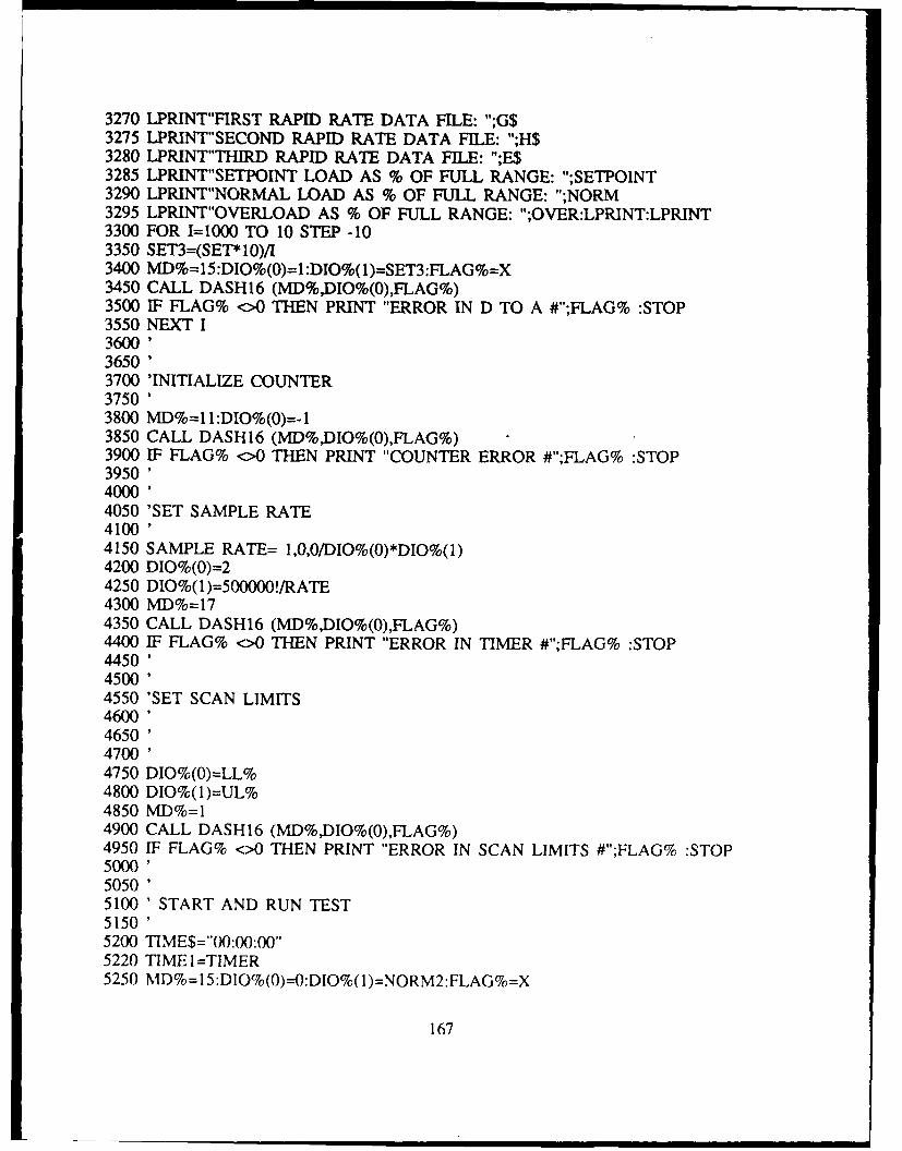
3270 LPRINT"FIRST RAPID RATE DATA FILE: ";G$3275 LPRINT"SECOND RAPID RATE DATA FILE: ";H$3280 LPRINT"THIRD RAPID RATE DATA FILE: ";E$3285 LPRINT"SETPOINT LOAD AS % OF FULL RANGE: ";SETPOINT3290 LPRINT"NORMAL LOAD AS % OF FULL RANGE: ";NORM3295 LPRINT"OVERLOAD AS % OF FULL RANGE: ";OVER:LPRINT:LPRINT3300 FOR I=1000 TO 10 STEP -103350 SET3=(SET* 10)/I3400 MD%=15:DIO%(0)=1:DIO%(1)=SET3:FLAG%=X3450 CALL DASH16 (MD%,DIO%(0),FLAG%)3500 IF FLAG% <>0 THEN PRINT "ERROR IN D TO A #";FLAG% :STOP3550 NEXT I360036503700 'INITIALIZE COUNTER3750 '3800 MD%=I I:DIO%(0)=-I3850 CALL DASH16 (MD%,DIO%(0),FLAG%)3900 IF FLAG% <>0 THEN PRINT "COUNTER ERROR #";FLAG% :STOP395040004050 'SET SAMPLE RATE4100 '4150 SAMPLE RATE= 1,0,0/DIO%(0)*DIO%(1)4200 DIO%(0)=24250 DIO%(1)=500000!/RATE4300 MD%=174350 CALL DASH16 (MD%,DIO%(0),FLAG%)4400 IF FLAG% <>o0 THEN PRINT "ERROR IN TIMER #";FLAG% :STOP4450 '45004550 'SET SCAN LIMITS4600465047004750 DIO%(0)=LL%4800 DIO%(1)=UL%4850 MD%=I4900 CALL DASH16 (MD%,DIO%(0),FLAG%)4950 IF FLAG% <>0 THEN PRINT "ERROR IN SCAN LIMITS #";FLAG% :STOP500050505100 ' START AND RUN TEST5150 '5200 TIME$="00:00:00"5220 TIME I =TIMER5250 MD%=1 5:DIO%(O)--0:DIO%( I)=NORM2:FLAG%=X
167

5300 CALL DASH16 (MD%,DIO%(O),FLAG%)5350 IF FLAG% <>0 THEN PRINT "ERROR IN D TO A #";FLAG% :STOP5400 MD%=15:DIO%(0)=1 :DIO%(1)=SET2:FLAG%=X5450 CALL DASH16 (MD%,DIO%(0),FLAG%)5500 IF FLAG% <>0 THEN PRINT "ERROR IN D TO A #";FLAG% :STOP5550 MD%=1 3:DIO%(0)=1 :FLAG%=X5600 CALL DASH16 (MD%,DIO%(0),FLAG%)5650 IF FLAG% <>0 THEN PRINT "ERROR IN DIGITAL OUT #";FLAG% :STOP5750 IF N>(60/X) THEN GOSUB 131005780 IF N>(60/X) THEN LPRINT USING"# ######## ##.#### ##.##########... ;COUNT,TIME5,CL,PSLOPE,SLOPE5800 IF N>(60/X) THEN N=I5830 IF N>(60/X) THEN LPRINT USING"##,,,-# ######## ##.#### .#########
.;COUNT,TIME5,CL,PSLOPE,SLOPE
5850 FOR I= LL% TO UL%5900 DSUM(I)--05950 MIN(I)=100006000 MAX(I)=-100006050 BMIN(I)=I00006100 BMAX(I)=- 100006150 NEXT I6200 IF (TIMER-TIME1)<(X-.25) THEN GOTO 62006250 GOSUB 63506300 GOTO 82006350 'START DMA6400 DIO%(0)=CONVER6450 DIO%(1)=&H20006500 DIO%(2)=16550 DIO%(3)=06600 MD%=66650 CALL DASH16 (MD%,DIO%(0),FLAG%)6700 IF FLAG% <>0 THEN PRINT "ERROR IN DMAN #";FLAG% :STOP6750 GOSUB 68506800 GOTO 70506850 MD%=12:DIO%(0)=l :DIO%(1)--06900 CALL DASH16 (MD%,DIO%(0),FLAG%)6950 IF DIO%(1)<0 THEN CHANGE=-I-DIO%(1) ELSE CHANGE=65535!-DIO%(1)7000 RETURN7050 PRINT ....7100 PRINT ....7150 PRINT USING" ELAPSED TIME = ######.## SEC";TIMER7200 TIME5=TIMER7250 IF PCHANGE>CHANGE THEN M=M+65535!7300 COUNT=M+CHANGE+CS7350 'PRINT USING "#######.";PCOUNT(1)7400 PCHANGE=CHANGE7450 PRINT USING" NUMBER OF CYCLES =#######";COUNT
168

7500 PRINT ..7550 TIMlE2=TIMER7600 DEL=(CONVER/RATE)+.057650 IF (TIMER-TIME2)<DEL THEN GOTO 76507700 'RETRIVE DATA7750 DIO%(0)=CONVER7800 DIO%(1)=&H20007850 DIO%(2)=07900 DIO%(3)=VARPTR(DT%(0))7950 DIO%(4)=VARPTR(CH%(0))8000 NM%=98050 CALL DASH 16 (MD%,DIO%(0),FLAG%)8100 TIME 1=TIIMER8150 RETURN8200 'DISPLAY DATA8250 FOR 1=0 TO (CONVER-1)8300 DSUM(CH%(I))=DSUM(CH-%(I))+DT%(I)8350 IF MAX(CH%(I))<DT%(I) THEN -MAX(CH%(I))=DT%(I)8400 IF MIN(CH%(I))>DT%(I) THEN MIN(CH%(I))=DT%(I)8450 NEXT I8500 FOR I=LL% TO (LL%-I1)8550 DAVG(I)=DSUM(I)/(CONVER/((UL%-LL%)i- ))8600 VOLT(D)=(DAVG(I)/2048)* 108650 CVOLT(I)=VOLT(I)-NVOLTql)8700 PRINT USING" VOLTAGE CHANNEL## = ###.#### VOLTS ";I,CVOLT(I)8750 NEXT I8800 FOR I = (LLT%+2) TO UL%8850 VMAX(I)=(MAX(I)/2048)* 108900 VMIN(I)=(MIN(I)/2048)* 108950 NEXT 19000 NORM2=NORM2-((((MAX(5)-MIN(5))*4)-NORM1)/2)9050 SET2=SET2-(((MIN(5)*4)-SET)/2)9100 PRINT USING" MAX-MIN VOLTAGE FG #### ####VOLTS ";VMAX(3),VMIN(3)9150 MAXLOAD =VMAX(5)*5
9200 MINLOAD =VMIN(5)*5
9250 PRINT USING" MAX-MIN LOAD #### ####KN";MAXLOAD,MINLOAD9300 MAXSTRAIN =VMAX(4)9350 MINSTRAIN =VMIN(4)9400 PRINT USING" MAX-MIN COD ####MM";MAXSTRAIN,,MINSTRAIN9450 VR=CVOLT(LL%+ I)/CVOLT(LL%)9500 TPVR=0O9550 TPCOUNT=0O9600 TCVR=0O9650 TCCOUNT=0O
169

9700 PVR(5)=VR9750 PCOUNT (5)=COUNT9800 FOR NN=1 TO 59850 TPVR =TPVR+PVR(NN-1)9900 TCVR=TCVR+PVR(NN)9950 TPCOUNT=TPCOUNT+PCOUNT(NN- 1)10000 TCCOUNT=TCCOUNT+PCOUNT(NN)10050 NEXT NN10100 FOR NN=0O TO 410150 PVR (NN)=PVR(NN+1)10200 PCOUNT (NN)= PCOUNT(NN+1)10250 NEXT NN10300 APVR=TPVR/510350 ACVR=TCVR/510400 APCOUNT=TPCOUNT/510450 ACCOUNT=TCCOUNT/510500 CL=C1 +(C2*(VR))+(C3*(VRA2))+(C4*(VRA3))+(C5*(VRA4))10550 PCL-=Cl1+(C2*(APVR))+(C3*(AP VRA2))+(C4*(AP VRA3))+(C5 *(APVRA4))10600 CCL=ClI+(C2*'(AC VR))+(C3 *(AC VRA2))+(C4* (AC VRA3))+(C5 *(ACVRA4))1 0650'LPRINT USING"###.#####";VOLT(1 ),C VOLT(l1),NVOLT(l1),VOLT(2),CVOLT(2),NVOLT(2),VR,CL10700 'LPRINT USING "####.";COUNT,TIME510750 PRINT #1,USING "####.#";COUNT,TIME510800 PRINT# 1 ,USING"###.#####;CVOLT(l1),N VOLT(lI),CVOLT(2),N VOLT(2),VR,CL10810 PRINT # 1,U SING"###.####";VMAX(3),VMIN(3),VMAX(4),VMIN(4),VMAX(5),VMIN(5)10850 DELCL=CCL-PCL10900 DELCOUNT=ACCOUNT-APCOUNT10950 SLOPE=DELCL/DELCOUNT11000 PRINT USING" CRACK LENGTH = ####"C11050 PRINT USING" VOLTAGE RATIO = ####"V11I100 'LPRINT DELCL,DELCOUNT11150 PRINT" CURRENT dA/dN =";SLOPE
11200 PRINT' OVER STRESS dA/dN =";PSLOPE
11210 [F FLAG(1)=-0 AND CL>17 THEN FLAG(1)=1:FLBEEP=111220 [F FLAG(2)=0O AND CL>23 TIEN FLAG(2)=l:FLBEEP=l11230 IF FLAG(3)=0O AND CL>28 THIEN FLAG(3)=1:FLBEEP= 111233 IF FLAG(4)=0O AND CL>40 THEN FLAG(4)=1:FL4O=111237 IF CL>45! THEN 13OSUB 1905011240 IF FLBEEP=1 THEN BEEP: BEEP: PRINT"* ***CHECK dA/dN BE[-OREOVERSTRESS (Hlit F9 to stop message) * * * *":BEEP:BEEP11245 IF FL-40=1 THEN B3EEP: BEEP:PRINT"** THIS TEST WILL AUTOMATICALLYEND AT 4 5mrn * * *11250 'LPRINT SLOPE1 1260 PRINT #I,SLOPE,PSLOPE11300)
170

11350 'THIS PORTION TRANSFERS RAPID READINGS11400 'AND AVERAGES IN GROUPS OF 1011450 '11500 IF K>CONVER1 THEN GOTO 1275011550 DIO%(0)=(INC*30)11600 DIO%(1)=&H300011650 DIO%(2)=K11700 DIO%(3)=VARPTR(DT%(0))11750 DIO%(4)=VARPTR(CH%(0))11800 MD%=911850 CALL DASH16 (MD%,DIO%(0),FLAG%)11900 IF FLAG% <>0 THEN PRINT "ERROR DATA RETRIVAL #";FLAG% :STOP11950 FOR Y = 0 TO (INC*29) STEP INC12000 FOR B =Y TO (Y+(INC-1))12050 BSUM(CH%(B))=BSUM(CH%(B))+DT%(B)12100 NEXT B12150 FOR L = LL% TO UL%12200 BAVG(L)=BSUM(L)/1012250 RVOLT(L)=(BAVG(L)/2048)* 1012300 BVOLT(L)=RVOLT(L)-NNVOLT(L)12350 BSUM(L)=012400 IF ML=I THEN PRINT #2, L, BVOLT(L),SCOUNT,XX12450 IF ML=2 THEN PRINT #3, L, BVOLT(L),SCOUNT,XX12500 IF ML=3 THEN PRINT #4, L, BVOLT(L),SCOUNT,XX12550 NEXT L12600 XX=XX+112650 NEXT Y12700 K=K+(INC*30)12750 N=N+112800 GOTO 525012850 '1290012950 'THIS PORTION TURNS OFF THE CURRENT13000 'AND TAKES NULL READINGS13050 '13100 PRINT ....13150 PRINT ..13200 PRINT "******* CURRENT IS OFF WAIT DO NOT OVERSTRESS ****13250 MD%= 13:DIO%(0)=3:FLAG%=X13300 CALL DASH16 (MD%,DIO%(0),FLAG%)13350 IF FLAG% <>0 THEN PRINT "ERROR IN DIG OUT #";FLAG% :STOP13400 TIME3=TIMER13450 FOR I = LL% TO UL%13500 NSUM(I)=013550 NEXT I13600 IF (TIMER-TIME3)<10 GOTO 136()13650 GOSUB 6350
171

13700 FOR I--0 TO (CONVER-1)13750 NSUM(CH%(I))=NSUM(CH%(I))+DT%(I)13800 NEXT I13850 PRINT "..13900 FOR I=LL% TO UL%13950 NAVG(I)=NSUM(I)/(CONVER/((UL%-LL%)+ 1))14000 NVOLT(I)=(NAVG(I)/2048)* 1014050 NEXT I14100 NVOLT(UL%)=0!14150 NVOLT(UL%-1)--0!14200 NVOLT(UL%-2)--0!14250 FOR I= LL% TO (LL%+I)14300 PRINT USING" NULL VOLTAGE CHANNEL## = ##.##### VOLTS";I,NVOLT(I)
14350 NEXT I14400 PRINT ""14450 PRINT "*** CURRENT BACK ON WAIT TILL AFTER NEXT READING ***"
14500 MD% =13:DIO%(0)=1 :FLAG%=X14550 CALL DASH16 (MD%,DIO%(0),FLAG%)14600 IF FLAG% <>0 THEN PRINT "ERROR IN DIG OUT #";FLAG% :STOP14650 RETURN14700 '1475014800 'TAKE RAPID READINGS WITH OVERSTRESS14850 '14900 PSLOPE=SLOPE14950 GOSUB 685015000 COUNT=M+CHANGE+CS15050 SCOUNT=COUNT15100 GOSUB 685015150 TIME3=TIMER15200 BCOUNT=CHANGE15250 DIO%(0)=215300 DIO%(1)=500000!/RATE215350 MD%=1715400 CALL DASH16 (MD%,DIO%(0),FLAG%)15450 DIO%(0)=CONVERI15500 DIO%(1)=&H300015550 DIO%(2)=I15600 DIO%(3)--015650 MD%=615700 CALL DASH16 (MD%,DIO%(0),FLAG%)15750 GOSUB 685015800 IF (CHANGE-BCOUNT)<6 GOTO 1575015850 MD%= 15:DIO%(0)--0:DIO%( I)--OVER 1 :FLAG%=X15900 CALL DASH16 (MD%,DIO%(0),FLAG%)15950 CCOUNT=CHANGE
172

16000 GOSUB 685016050 IF (CHANGE-CCOUNT)<NUM THEN GOTO 1600016100 MD%=15:DIO%(0)=0:DIO%(1)=NORM1:FLAG%=X16150 CALL DASH16 (MD%,DIO%(0),FLAG%)16200 IF FLAG% <>0 THEN PRINT "ERROR IN A TO D #";FLAG% :STOP16250 IF (TIMER-TIME3)<(SEC+.05) THEN GOTO 1625016300 ML=ML+116350 K--016400 DIO%(0)=216450 DIO%(1)=500000!/RATE16500 MD%=1716550 CALL DASH16 (MD%,DIO%(0),FLAG%)16600 IF FLAG% <>0 THEN PRINT "ERROR IN TIMER #";FLAG% :STOP16650 TIME1=TIMER16700 FOR I=LL% TO UL%16750 NNVOLT(I)=NVOLT(I)16800 NEXT I16850 RETURN 525016900 '1695017000 'THIS PORTION SUSPENDS OPERATION17050 '17100 INPUT "DO YOU WANT TO STOP THE FUNCTION GEN.(Y,N)";GEN$17110 LPRINT:LPRINT:LPRINT"FUNCTION KEY 6 HAS BEEN ACTIVATED.":BEEP17120 LPRINT" HAS THE FUNCTION GENERATOR BEEN STOPPED? ",GEN$17150 IF GEN$="N" THEN GOTO 1735017200 MD%=13:DIO%(0)=0:FLAG%=X17250 CALL DASH16 (MD%,DIO%(0),FLAG%)17300 IF FLAG% <>0 THEN PRINT "ERROR IN DIGITAL OUT#";FLAG% :STOP17350 INPUT "DO YOU WANT TO CHANGE THE SETPOINT,NORMAL LOAD OROVERLOAD (Y,N)?";V$17400 IF V$="N" THEN GOTO 1780017410 INPUT "NEW SET POINT LOAD AS % OF FULL RANGE:";SETPOINT17415 LPRINT"NEW SET POINT LOAD AS % OF FULL RANGE: ";SETPOINT17420 SET2=4095*(SETPOINT/50)17430 SET=SET217450 INPUT"NEW NORMAL LOAD AS % OF FULL RANGE:";NORM17455 LPRINT"NEW NORMAL LOAD AS % OF FULL RANGE: ";NORM17500 NORM 1=4095*(NORM/50)17550 NORM2=NORM I17600 INPUT"NEW OVERLOAD AS % OF FULL RANGE:";OVER17605 LPRINT"NEW OVERLOAD AS % OF FULL RANGE: ";OVER17650 OVER 1=4095*(OVER/50)17800 INPUT "PRESS ENTER TO RESUME";DUMB17810 BEEP:LPRINT:LPRINT17850 RETURN 525017900
173

1795018000 'THIS PORTION OVERSTRESSES WITHOUT RAPID READINGS18050 '18060 PSLOPE=SLOPE18100 GOSUB 685018150 BCOUNT=CHANGE18200 GOSUB 685018250 IF (CHANGE-BCOUNT)<2 GOTO 1820018300 MD%=1 5 :DIO% (0)=0:DIO%( 1)--OVER I :FLAG%=X18350 CALL DASH16 (MD%,DIO%(0),FLAG%)18400 GOSUB 685018450 CCOUNT=CHANGE18500 GOSUB 685018550 IF (CHANGE-CCOUNT)<NUM THEN GOTO 1850018600 MD%=15:DIO%(O)=0:DIO%(1)=NORM1:FLAG%=X18650 CALL DASH16 (MD%,DIO%(0),FLAG%)18700 K=CONVER1+10018750 TIME 1=TIMER18800 RETURN 575018850 '1890018950 ' THIS PORTION ENDS THE TEST19000'19050 MD%=13:DIO%(0)=0:FLAG%=X19100 CALL DASH16 (MD%,DIO%(0),FLAG%)19150 IF FLAG% <>0 THEN PRINT "ERROR IN DIGITAL OUT #";FLAG% :STOP19200 FOR 1=1 TO 10019250 SET3=SET/I19300 MD%= 15:DIO%(0)= 1 :DIO%(1)=SET3:FLAG%=X19350 CALL DASH16 (MD%,DIO%(0),FLAG%)19400 IF FLAG% <>0 THEN PRINT "ERROR IN D TO A #";FLAG% :STOP19450 NEXT I19500 MD%= 15:DIO%(0)= I :L)iO%(I)=0:FLAG%=X19550 CALL DASH16 (MD%,DIO%(0),FLAG%)19600 PRINT ....19650 PRINT ....19700 PRINT ***********************************************19750 PRINT " YOUR NORMAL RATE DATA FILE IS NAMED ";F$19800 PRINT " YOUR FIRST RAPID RATE DATA FILE IS NAMED ";G$19850 PRINT " YOUR SECOND RAPID RATE DATA FILE IS NAMED ";H$19900 PRINT " YOUR THIRD RAPID RATE DATA FILE IS NAMED ";E$19950 PRINT " WRITE THEIR NAMES DOWN !!!!!!20000 PRINT"*************************************************"20050 CLOSE20060 LPRINT USING"####### ######## ##.#### ##.######## ##.########## TESTENDED";COUNT,TIME5,CLPSLOPE,SLOPE20070 LPRINT:LPRINT:LPRINT:LPRINT
174

20100 END21000 FLBEEP=0:RETURN21010 END22000 PRINT"ERROR: ";ERR;"' OCCURED't:LPRINT"ERROR: ";ERR;"' OCCURED":GOTO19050
175

Program for calibration
50 'THIS PROGRAM IS STORED AS NEWCAL.BAS100 'used for calibration150 '200250300 CLEAR350 DEF SEG=0400 SG=256*PEEK(&H511)+PEEK(&H510)450 SG=SG+49152!/16500 DEF SEG=SG550 BLOAD "DASH16.BIN",0600'650 'INITIALIZE PROGRAM700750 DIM DIO%(4),DT%(2500!),CH%(2500!),DAVG(10),DSUM(10),VOLT(10),
BSUM(100)800 DIO%(0)=832850 DIO%(1)=2900 DIO%(2)=1950 MD%--01000 FLAG%=01050 DASH16--01100 CALL DASH16 (MD%,DIO%(0),FLAG%)1150 IF FLAG% <>) THEN PRINT "INITIALIZATION ERROR #";FLAG%:STOP1200 ML--01250 N=71300 KEY (6) ON1350 KEY (5) ON1400 KEY (10) ON1450 ON KEY (6) GOSUB 92001500 ON KEY (5) GOSUB 99001550 ON KEY (10) GOSUB 47001600 INPUT"NAME FOR DATA FILE";F$1650 OPEN F$ FOR OUTPUT AS #11700 INPUT"NORMAL LOAD AS % OF FULL RANGE";NORM1750 NORM 1 =(4095*(NORM/100))*21800 INPUT"LOWER CHANNEL LIMIT";LL%1850 !NPUT"UPPER CHANNEL LIMIT";UL%1900 INPUT"READING RATE";RATE1950 INPUT"NUMBER OF READINGS PER SAMPLE";CONVER2000 XX--0205Q X=102100
176

2150 'INITIALIZE COUNTER2200 '2250 MD%=1 1:DIO%(0)=-12300 CALL DASH16 (MD%,DIO%(0),FLAG%)2350 IF FLAG% <>0 THEN PRINT "COUNTER ERROR #";FLAG% :STOP240024502500 'SET SAMPLE RATE2550 '2600 'SAMPLE RATE= 1,000,000/DIO%(0)*DIO%(1)2650 DIO%(0)=22700 DIO%(1)=500000!/RATE2750 MD%=172800 CALL DASH16 (MD%,DIO%(0),FLAG%)2850 IF FLAG% <>0 THEN PRINT "ERROR IN TIMER #";FLAG% :STOP2900'29503000 'SET SCAN LIMITS3050 '310031503200 DIO%(0)=LL%3250 DIO%(1)=UL%3300 MD%=I3350 CALL DASH16 (MD%,DIO%(0),FLAG%)3400 IF FLAG% <>0 THEN PRINT "ERROR IN SCAN LIMITS #";FLAG%:STOP345035003550 ' START AND RUN TEST3600'3650 MD%=15:DIO%(O)=0:DIO%(1)=NORMI :FLAG%=X3700 CALL DASH16 (MD%,DIO%(0),FLAG%)3750 IF FLAG% <>0 THEN PRINT "ERROR IN D TO A #";FLAG% :STOP3800 MD%=13:DIO%(0)=1 :FLAG%=X3850 CALL DASH16 (MD%,DIO%(0),FLAG%)3900 IF FLAG% <>0 THEN PRINT "ERROR IN DIG OUT #";FLAG% :STOP3950 TIME$="00:00:00"4000 FOR I= LL% TO UL%4050 DSUM(I)--04100 NEXT I4150 TIME 1=TIMER4200 IF N>(60/X) THEN GOSUB 76004250 IF N>(60/X) THEN N=24300 IF N=3 THEN PRINT " OK F10 TO TAKE READING ****"4350 IF N=3 THEN PRINT" F6 TO SUSPEND F5 TO END"4550 IF (TIMER-TIME1)<(X-.25) THEN GOTO 45504600 N=N+I
177

4650 GOTO 41504700 GOSUB 48004750 GOTO 66004800 'START DMA4850 DIO%(0)=CONVER4900 DIO%(1)=&H20004950 DIO%(2)=15000 DIO%(3)=05050 MD%=65100 CALL DASH16 (MD%,DIO%(0),FLAG%)5150 IF FLAG% <>0 THEN PRINT "ERROR IN DMAN #";FLAG% :STOP5200 GOSUB 53005250 GOTO 55505300 MD%=12:DIO%(0)=1 :DIO%(1)=05350 CALL DASH16 (MD%,DIO%(0),FLAG%)5400 IF FLAG% <>0 THEN PRINT "ERROR IN READING COUNTER #";FLAG%
:.s IOP5450 IF DIO%(1)<0 THEN CHANGE=;I-DIO%(1) ELSE
CHANGE=65535!-DIO%(1)5500 RETURN5550 PRINT ....5600 PRINT ....5650 PRINT USING" ELAPSED TIME = ########.## SEC";TIMER5700 IF Y>CHANGE THEN M=M+65535!5750 COUNT=M+CHANGE+CS5800 Y=CHANGE5850 PRINT USING" NUMBER OF CYCLES =######";COUNT5900 PRINT ....5950 TIME2=TIMER6000 DEL=(CONVERI(1000000!/RATE))+.056050 IF (TIMER-TIME2)<DEL THEN GOTO 60506100 'RETRIVE DATA6150 DIO%(0)=CONVER6200 DIO%(1)=&H20006250 DIO%(2)--06300 DIO%(3)=VARPTR(DT%(0))6350 DIO%(4)=VARPTR(CH%(0))6400 MD%=96450 CALL DASH16 (MD%,DIO%(0),FLAG%)6500 TIME I=TIMER6550 RETURN6600 'DISPLAY DATA6650 FOR I=0 TO (CONVER-1)6700 DSUM(CH%(I))=DSUM(CH%(I))+DT%(I)6750 NEXT I6800 INPUT"CRACK LENGTH";CL6850 CL=CL+15.2
178

6855 LPRINT6860 LPRINT USING" CL ###.####";CL6900 FOR I=LL% TO UL%6950 DAVG(D=DSUM(I)/(CONVER/((UL%-LL%)+1))7000 VOLT(D=(DAVG(I)/2048)* 107050 CVOLT(I)=VOLT(I)-NVOLT(I)7100 PRINT USING" VOLTAGE CHANNEL## = ###.##### VOLTS";I,
CVOLT(I)7150 PRINT #1, CVOLT(I),7200 NEXT I7225 VR=CVOLT(2)/CVOLT(1)7230 PRINT USING" VR ###.####";VR7235 INVR=1/VR7240 PRINT USING" INVR ###.####";INVR7245 LPRINT USING" VR ###.####";VR7246 LPRINT USING" INVR ###.####";INVR7250 PRINT #1,COUNT,CL,VR7300 RETURN 40007350 '74007450 'THIS PORTION TURNS OFF THE CURRENT7500 'AND TAKES NULL READINGS7550 '7600 PRINT ....7650 PRINT ....7700 PRINT "******* CURRENT IS OFF WAIT ******"7750 MD%=1 3:DIO%(0)=3:FLAG%=X7800 CALL DASH16 (MD%,DIO%(0),FLAG%)7850 IF FLAG% <>0 THEN PRINT "ERROR IN DIG OUT #";FLAG% :STOP7900 TIME3=TIMER7950 FOR I = LL% TO UL%8000 NSUM(I)=08050 NEXT I8100 IF (TIMER-TIME3)<10 GOTO 81008150 GOSUB 48008200 FOR 1=0 TO (CONVER-1)8250 NSUM(CH%(I))=NSUM(CH%(I))+DT%(I)8300 NEXT I8350 PRINT8400 FOR I=LL% TO UL%8450 NAVG(I)=NSUM(I)/(CONVER/((UL%-LL%)+ 1))8500 NVOLT(I)=(NAVG(I)/+2048)* 108550 NVOLT(UL%)=0!8600 NVOLT(UL%- 1)=0!8650 PRINT USING" NULL VOLTAGE CHANNEL## = ##.##### VOLTS";I,
NVOLT(I)8700 NEXT I
179
|7. 1

8750 PRINT ..8760 MD%=13:DIO%(0)=l :FLAG%=X8770 CALL DASH16 (MD%,DIO%(0),FLAG%)8780 IF FLAG% <>0 THEN PRINT "ERROR IN DIG OUT #";FLAG% :STOP8800 PRINT "*** CURRENT BACK ON WAIT 10 SEC FOR NEXT READING ***"8850 PRINT8900 PRINT8950 RETURN 42509000'9050'9100 'THIS PORTION SUSPENDS OPERATION9150'9200 MD%=13:DIO%(0)--0:FLAG%=X9250 CALL DASH16 (MD%,DIO%(0),FLAG%)9300 IF FLAG% <>0 THEN PRINT "ERROR IN DIG OUT #";FLAG% :STOP9301 INPUT"DO YOU WANT TO CHANGE THE DELTA LOAD (Y,N)";V$9302 IF V$="N" THEN GOTO 93509303 INPUT "NEW DELTA LOAD";NORM9304 NORM 1--4095*(NORM/50)9305 MD%= 15 :DIO%(0)--0:DIO%(1)=NORM1:FLAG%=X9306 CALL DASH16 (MD%,DIO%(0),FLAG%)9307 IF FLAG% <>0 THEN PRINT "ERROR IN D TO A #";FLAG% :STOP9350 INPUT "PRESS ENTER TO RESUME";DUMB9400 MD%=13:DIO%(0)=1:FLAG%=X9450 CALL DASH16 (MD%,DIO%(0),FLAG%)9500 IF FLAG% <>0 THEN PRINT "ERROR IN DIG OUT #";FLAG% :STOP9550 RETURN 400096009650970097509800 'THIS PORTION ENDS THE TEST98509900 MD%=1 3:DIO%(0)=0:FLAG%=X9950 CALL DASH16 (MD%,DIO%(0),FLAG%)10000 IF FLAG% <>0 THEN PRINT "ERROR IN DIG OUT #";FLAG% :STOP10050 PRINT ....10100 PRINT10150 PRINT ********************************************10200 PRINT " YOUR DATA FILE IS NAMED ";F$10250 PRINT " WRITE THE NAME DOWN!!!!!"10300 PRINT *********************************************10350 CLOSE10400 END
180