MANUSCRIPT APPEAR IN IEEE TRANSACTIONS ON MEDICAL IMAGING, VOL. 15, NO. 3, JUNE 1996 1Deformable Models with Parameter Functionsfor Cardiac Motion Analysisfrom Tagged MRI DataJinah Park, Dimitri Metaxas, Alistair A. Young, Leon AxelAbstract|We present a new method for analyzing the mo-tion of the heart's left ventricle (LV) from tagged magneticresonance imaging (MRI) data. Our technique is based onthe development of a new class of physics-based deformablemodels whose parameters are functions. They allow the def-inition of new parameterized primitives and parameterizeddeformations which can capture the local shape variation ofa complex object. Furthermore, these parameters are intu-itive and require no complex post-processing in order to beused by a physician. Using a physics-based approach, weconvert the geometric models into dynamic models that de-form due to forces exerted from the datapoints and conformto the given dataset. We present experiments involving theextraction of the shape and motion of the LV's mid-wallduring systole from tagged MRI data based on a few pa-rameter functions. Furthermore, by plotting the variationsover time of the extracted LV model parameters from nor-mal and abnormal heart data along the long axis, we areable to quantitatively characterize their di�erences.Keywords| Physics-based modeling, Deformable models,Left ventricle (LV) shape and motion analysis and visualiza-tion. I. IntroductionAlteration of heart wall motion is a sensitive indicatorof heart disease such as ischemia [32], which is typicallycaused by occlusion of a coronary vessel: The local anemiacaused by the obstruction of the blood supply results in ab-normal ventricular wall motion even before any signi�cantclinical symptoms develop [35]. Moreover, abnormalities inheart wall motion are taken very seriously by physicians,because they can be life threatening injuries. However,since the heart undergoes complex motion, proper charac-terization of its motion still remains an open and challeng-ing research problem.The main di�culties in assessing heart wall motion comefrom two sources: 1) limitation of conventional cardiacimaging methods in terms of providing good datasets formotion studies, and 2) the absence of computational tech-niques for automatic extraction of the three dimensional(3D) heart wall motion parameters in a way that is use-ful to physicians. Recently, the introduction of magnetictagging [2], [39] in Magnetic Resonance Imaging (MRI) hasprovided a powerful tool to study the heart wall motion.J. Park and D. Metaxas are with the Department of Computer& Information Science at the University of Pennsylvania, Philadel-phia, PA 19104-6389 USA; E-mail: jinah@graphics.cis.upenn.edu ordnm@central.cis.upenn.edu.A. Young is with the Department of Physiology at the Universityof Auckland, Auckland, New Zealand.L. Axel is with the Department of Radiology at the University ofPennsylvania, Philadelphia, PA 19104-6086 USA.

The MR taggingmethods provide temporal correspondenceof material points on featureless structures like the heartwall in a non-invasive manner. Unfortunately, the taggedMR images are not easily analyzed with simple qualitativeviewing, while current quantitative analysis techniques arenot only time consuming, but also yield data that may notbe easily interpreted for diagnosis.A precise model that can re ect the mechanics of ven-tricular myocardium would provide a better understandingof the complex regional changes under pathological condi-tions. In addition, it is also important that the model beconstructed and analyzed in close to real-time to be use-ful in a clinical environment. The goal of our work is todevelop computational techniques for automatic extractionof the 3D heart wall motion parameters that are not onlycompact, but also can give accurate descriptions of ventric-ular function based on tagged MR images.A. Previous WorkIn order to quantify the complicated motion of the leftventricle (LV) and to interpret its measured deformation,it is necessary to represent the LV by a model. Simpleanalytical shapes like spheres, ellipsoids, or cylinders areoften used to approximate the shape and motion of theLV [1], [6], [13]. However, since they are formulated interms of very few parameters, they can o�er only a grossapproximation to the LV motion.Recently, 3D surface models and associated computervision or graphics techniques have been developed to cap-ture the shape and motion of the inner or the outer wallof the LV from medical image data. These models are ei-ther �nite element meshes derived from a polyhedron-basedsurface reconstruction of a stack of cross sections [8], [11],physics-based elastic models [9], [12], [15], [20], [33], bend-ing and stretching models [3], [31], or axisymmetrical geo-metric models with augmented local details [4], [18]. Someof above techniques are brie y described as follows:� Amini and Duncan [3] developed bending and stretch-ing thin-plate models for motion tracking of the LVwall, which allow point matching based on the amountof the bending energy. Shi et al. [31] further developedthe models and presented results of the shape-basedtechnique applied to MRI data showing motion tra-jectories of selected endocardial points.� Pentland et al. [33], [28] developed a deformable modelbased on modal analysis, which can decompose themotion into modes, and applied the technique to re-

2 MANUSCRIPT APPEAR IN IEEE TRANSACTIONS ON MEDICAL IMAGING, VOL. 15, NO. 3, JUNE 1996cover the nonrigid motion of a heart from 2D X-rayimages. Extending their work, Nastar and Ayache [20]performed \spectrum" analysis in modal space for var-ious LVs from radio-nuclide images in order to classifynonrigid motion.� Friboulet et al. [11] constructed a polyhedral modelfrom a set of cross-section slices obtained from volu-metric MRI data. The motion of the model was ap-proximated by an a�ne transformation with transla-tion, rotation, and dilation motion parameters.� Huang and Goldgof [12] developed a spring-mass,adaptive-size mesh model and applied it to CT dataof a canine heart during a cardiac cycle to track theLV motion based on the displacement of correspondingmodel nodes at di�erent time points.� By adapting the deformable balloon model of Cohenand Cohen [9], McInerney and Terzopoulos [15] devel-oped a 3D deformable model composed of triangularC1 �nite elements based on the physics-based frame-work developed by Metaxas and Terzopoulos [17].They applied it to CT data of a canine heart in orderto reconstruct the LV shape at di�erent time framesduring one cardiac cycle.� Bardinet et al. [4] estimated in detail the LVshape by using the technique of free-form deforma-tions [29] to model local deformations in deformablesuperquadrics [5].The main limitation of these techniques is that they donot provide intuitive motion parameters to describe therigid and nonrigid motion of the LV. Most of the tech-niques [3], [8], [9], [12], [15], [18], [31] provide only local dis-placement vectors which require non-trivial post-processingto be useful to a physician, and they are good only forqualitative visualization. In contrast to these approaches,models like [4], [11] are formulated in terms of very few pa-rameters that can o�er only a gross approximation to theLV motion. There have been some attempts to character-ize the LV motion with a small number of parameters [20],[33], but these parameterizations do not correspond to thegeometry of the LV closely enough to provide better un-derstanding of the LV motion.Moreover, most techniques [3], [4], [11], [12], [15], [18],[20], [33] ignore the twisting or wringing motion of the LVknown to occur during systole, since the input datasetgenerally does not provide temporal correspondence be-tween frames. In order to accurately capture the heartwall motion, material points on the myocardium must belocated and tracked. Therefore, techniques based on suchmarker-based methods, such as tagged MRI, can providethe most accurate motion of the left ventricle of a heart.They include the �nite element models of Young et al. [36]and Moore et al. [19], and the multidimensional stochasticmodel of Denney and Prince [10]. However, these repre-sentations do not directly lend themselves to an under-standing of the underlying kinematics in an intuitive way.The parameters of the models are local displacements, re-sulting in a large number of parameters, and therefore thephysical interpretation of the parameters can be di�cult.

z

x

y (a) (b)Fig. 1. (a) Superquadric ellipsoid (b) Primitive with parameter func-tions.The three-dimensional strain tensor in [36], for example,has three normal components and three shear components,each of which may vary throughout the LV wall. In or-der to understand the complex relationship between thesecomponents and other motion parameters, it is desirableto characterize the motion in terms of a small number ofphysical parameters without sacri�cing su�cient accuracy.To overcome the problems of the above techniques,namely the accurate estimation of the LV surface shapeand motion and the extraction of parameters that can beeasily interpreted by physicians, we have developed a classof deformable primitives whose global parameters are func-tions (see also [21], [22]). Our technique describes the time-varying shape, deformation, and motion of the LV in termsof a few global parameter functions, such as twisting,whose values vary locally. In this way, the complex mo-tion of the heart is described by the same small number ofparameters, whose values may vary from region to region.Furthermore, these parameters can be used by a physiciandirectly without further complex processing.B. Proposed Model: Deformable Models with ParameterFunctionsWe present a new family of parameterized deformableprimitives suitable for applications where a complex shapeneeds to be described in terms of a small number of intu-itive parameters. These deformable primitives are parame-terized through a few number of parameters which are func-tions, and therefore each parameter's value varies acrossthe shape of the primitives, as opposed to being constant.Through the use of appropriate parameterization, the axesof our deformable primitives can be curved. This is a majorgeneralization compared to other parameterized primitivessuch as superquadrics and cylinders, commonly used in thevision literature. Even though generalized cylinders [14] al-low shapes with curved axes, they do not o�er a represen-tation of shape in terms of a few parameters. Furthermore,our models can represent open parameterized shapes1 suit-able for modeling the shape and motion of the LV. Fig. 1(b)shows an example of the deformable primitives with param-eter functions whose shape is de�ned by generalizing theparametric equations of an ellipsoid shown in Fig. 1(a).The complex nonsymmetric shape in Fig. 1(b) was createdby varying only six parameter functions.While these new shape primitives can be used in manyapplications, this paper describes shape and motion esti-mation results for the LV. By incorporating the geometric1not a closed surface, but more like a cup

PARK ET AL.: DEFORMABLE MODELS WITH PARAMETER FUNCTIONS FOR CARDIAC MOTION ANALYSIS 3x

s

cyx

z

φ

vu

yx

z

φ

φ

Φ

material coordinates (u,v)Φmodel frame and inertial frameFig. 2. Model frame �de�nition of the models into the physics-based frameworkdeveloped by Metaxas and Terzopoulos [16], [17], we cre-ate dynamic models that deform due to forces exerted from3D tagged datapoints, thereby causing the models to con-form to the given dataset. The LV extracted parameters,plotted in parameter graphs, can then be directly used foranalysis by a physician. We applied our technique to var-ious subjects and analyzed the results of our parameterextraction. These results quantitatively veri�ed qualita-tive knowledge about the LV known to physicians. Fur-thermore, we present a method for visualizing the model�tting results.In the following sections, we �rst de�ne the geometry ofthe deformable models with parameter functions (DMPF),and then describe the physics-based framework throughwhich the geometric models are converted into dynamicmodels. Finally, we present experiments where we appliedour technique to LV datasets from healthy volunteers andpatients with hypertrophic cardiomyopathy.II. Model DefinitionThe class of DMPF allows the use of global parametersthat can characterize an object's shape in terms of a few pa-rameter functions. The model is a 3D surface2 whose mate-rial coordinates u = (u; v) are de�ned in a domain . Thepositions of points on the model relative to an inertial frameof reference � in 3D space are given by a vector-valued,time-varying function x(u; t) = (x(u; t); y(u; t); z(u; t))>,where > denotes transposition. We set up a non-inertial,model-centered reference frame � and express the positionof a point on a model asx = c+Rs;where the center of the model c(t) is the origin of � andthe rotation matrixR(t) gives the orientation of � relativeto � with a reference shape s (see Fig. 2). Thus, s(u; t)gives the positions of points on the model relative to themodel frame. Local deformations [17] are not used, sincethe global deformations s will be de�ned based on parame-ter functions capable of capturing the local variation of theLV shape.We de�ne the reference shape ass = T(e; �0(u); �1(u); : : :);2The model can be generalized into a volumetric model, but it isbeyond the scope of this paper (See [23], [24]).

where e can represent either a set of 3D points in space3 ora geometric primitive e(u; �0(u); �1(u); : : :) de�ned para-metrically in u and parameterized by the variables �i(u).The shape represented by e is subjected to the deformationT which depends on the deformation parameter functions�i(u). Although generally nonlinear, e and T are assumedto be di�erentiable4 so that we may compute the Jacobianof s. T may be a composite sequence of primitive deforma-tion functions T(e) = T1(T2(: : :Tn(e))). We concatenatethe deformation parameters into the vector qs:qs = (�0(u); �1(u); : : : ; �0(u); �1(u); : : :)>:The parameters �i and �i are functions of u, insteadof constants as in our previous work [17]. This de�nitionallows us to generalize de�nitions of primitives (e.g., su-perquadrics, cubes) and parameterized deformations (e.g.,twisting), as will be shown in the following section and wasdemonstrated in Fig. 1(b).A. De�ning the Reference ShapeOur technique for creating primitives with parameterfunctions can be applied to any parametric primitive, byreplacing its constant parameters with di�erentiable pa-rameter functions. For example, we de�ne a generalizedprimitive e = (e1; e2; e3)> to be used for modeling the LVwall as follows:e = e(u; a0(u); a1(u); a2(u); a3(u))= a0(u)0@ a1(u) cosu cos va2(u) cosu sin va3(u) sinu 1A ; (1)where ��=2 � u � �=4, �� � v < �, a0(u) > 0, and0 � a1(u); a2(u); a3(u) � 1. This primitive is created froman ellipsoid primitive eeee = a00@ a1 cosu cos va2 cosu sin va3 sinu 1A ; (2)where ��=2 � u � �=2, �� � v < �, a0 > 0, and0 � a1; a2; a3 � 1, by replacing its constant parameterswith parameter functions. a0 is a scale parameter and a1,a2 and a3 are the aspect ratio parameters along the x-, y-and z-axes, respectively. Note that the ranges of the u andv parameters for our generalized primitive (1) are restrictedto a subset of those for an ellipsoid primitive de�ned by (2),in order to construct an open parameterized primitive. Theorientation of a model used for our application is schemat-ically drawn in Fig. 3. The model-centered reference frame� is chosen at the center of the LV with the y-axis pointingtowards the right ventricle (RV). The material coordinatesu = (u; v) are depicted in Fig. 3(b), where u runs from theapex to the base of the LV, and v starts and ends at the3In that case, the material coordinates u coincide with the Carte-sian space in which the 3D points are expressed.4In the case where e is a set of points, the above assumption doesnot apply.

4 MANUSCRIPT APPEAR IN IEEE TRANSACTIONS ON MEDICAL IMAGING, VOL. 15, NO. 3, JUNE 1996LV

RV

(a )

(a )

1

2y

x

LVRV

(a )3

y

z

Short-axis view Long-axis view

φxy

z

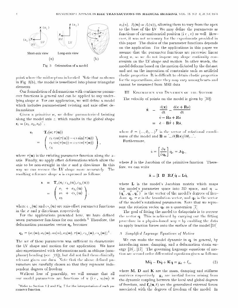
v

u(a) (b)Fig. 3. Orientation of a modelpoint where the mid-septum is located. Note that as shownin Fig. 3(b), the model is tessellated into planar triangularelements.Our formulation of deformations with continuous param-eter functions is general and can be applied to any under-lying shape e. For our application, we will de�ne a modelwhich includes parameterized twisting and axis o�set de-formations.Given a primitive e, we de�ne parameterized twistingalong the model axis z, which results in the global shapest = (s1; s2; s3)>:st = Tt(e; � (u))= 0@ e1 cos(� (u)) � e2 sin(� (u))e1 sin(� (u)) + e2 cos(� (u))e3 1A ;where � (u) is the twisting parameter function along the z-axis. Finally, we apply o�set deformations which allow theaxis to be non-straight in the x and y directions. In thisway we can recover the LV shape more accurately. Theresulting reference shape s is expressed as follows:s = To(st; e1o(u); e2o(u))= 0@ s1 + e1o(u)s2 + e2o(u)s3 1A ;where e1o(u) and e2o(u) are axis-o�set parameter functionsin the x and y directions, respectively.For the applications presented here, we have de�nedseven parameter functions for our models.5 Therefore, thedeformation parameter vector qs becomesqs = (a0(u); a1(u); a2(u); a3(u); � (u); e1o(u); e2o(u))>:The set of these parameters was su�cient to characterizethe LV shape and motion for our application. We havealso experimented with deformations such as oblique (non-planar) bending (see [21]), but did not �nd them clinicallyrelevant given our data. Note that the above de�ned pa-rameters are carefully chosen so that they represent inde-pendent degrees of freedom.Without loss of generality, we will assume that allour model parameters are functions of u (i.e., �i(u) =5Refer to Section 4.2 and Fig. 7 for the interpretation of each pa-rameter function.

�i(u); �i(u) = �i(u)), allowing them to vary from the apexto the base of the LV. We may de�ne the parameters asfunctions of circumferential position (i.e., v) as well. How-ever, it was not necessary for the experiments provided inthis paper. The choice of the parameter functions dependson the application. For the applications in this paper weassume that the parameter functions are piecewise linearalong u, so we do not impose any shape continuity con-straints on the LV shape and motion. In other words, themodel deforms based on the motion dictated by the datasetand not on the imposition of constraints such as arti�cialelastic properties. It is di�cult to obtain elastic propertiesfor the myocardium, since they may vary among hearts andcannot be measured from MRI data.III. Kinematics and Dynamics of the SystemThe velocity of points on the model is given by [30]:_x = d(x)dt = d(c +Rs)dt= _c+ _Rs+R _s= _c+B _� +R _s;where � = (:::; �i; :::)> is the vector of rotational coordi-nates of the model and B = [:::@(Rs)=@�i:::]:Furthermore, _s = � @s@qs � _qs = J _qs;where J is the Jacobian of the primitive function. There-fore, we can write_x = [I B RJ] _q = L _q;where L is the model's Jacobian matrix which mapsthe model's parameter space into 3D space, and q =(q>c ;q>� ;q>s )> is the vector of the model's degrees of free-dom. qc = c is the translation vector, and q� is the vectorof the model's rotational parameters. Note that we repre-sent the rotation vector q� as a quaternion [7].The goal of �tting the model to datapoints is to recoverthe vector q. This is achieved by carrying out the �ttingprocedure in a physics-based way { by enabling the datato apply traction forces onto the surface of the model [34].A. Simpli�ed Lagrange Equations of MotionWe can make the model dynamic in q, in general, byintroducing mass, damping, and a deformation strain en-ergy [16], [17]. The governing Lagrange equations of mo-tion are second order di�erential equations given as follows:M�q +D _q+Kq = gq + fq; (3)where M, D and K are the mass, damping and sti�nessmatrices respectively. gq are inertial forces arising fromthe dynamic coupling between the local and global degreesof freedom, and fq(u; t) are the generalized external forcesassociated with the degrees of freedom of the model. In

PARK ET AL.: DEFORMABLE MODELS WITH PARAMETER FUNCTIONS FOR CARDIAC MOTION ANALYSIS 5z

p

1x

x2

x3

f

m2f

1m fm3f

z

z

z

zFig. 4. Force distributionshape estimation problems [16], it makes sense to simplifythe motion equations while preserving useful dynamics bysetting the mass density to zero to obtainD _q+Kq = fq: (4)The above equation yields a model that has no inertia andcomes to rest as soon as all the applied forces equilibrate orvanish. We useD as a stabilizing factor only, and we do notimpose any physical damping which cannot be measuredfrom our data. Therefore, we assume that D is diagonaland constant over time.Given that the datapoints from medical images are rela-tively accurate, and we want to avoid undesired smoothingcaused by the model, we further simplify (4) by introducingnull sti�ness to the global parameters of our model (this islike a plastic deformation where there is no resistance todeformation). Finally, the resulting equation of motion is:D _q = fq: (5)For fast interactive response, a �rst-order Euler method[26] is employed to integrate (5).B. Model Force ComputationThe generalized forces fq are computed using the for-mula [16] fq = Z L>f du:These forces modify the components of q, where f (u; t) isthe 3D force distribution applied to the model. Approxi-mating each triangular element of the model with a plane,we determine the closest point p on the model for eachgiven datapoint z. The force that z exerts on the model iscomputed from fz = (z � p); (6)where is the strength of the force. We then linearly dis-tribute fz to the nodes x1, x2, and x3 of the associatedtriangular element based on the formulafxi = mi fz; i = 1; 2; 3; (7)where the mi are computed from the solution of the fol-lowing linear system Xi mixi = p (8)

and their sum is such thatXi mi = 1:0: (9)Therefore the following equation is also trueXi mifz = fz: (10)Intuitively, each of the mi's is a weight given to each ele-ment node and the vector p is the location of the center ofmass of the element.Since the tagged dataset provides correspondence overtime of individual 3D points, we apply the force distribu-tion algorithm only once for the initial frame. In subse-quent frames, the corresponding points will exert a forceto the same point on the model as computed in the �rstframe. In this way we can recover the LV twisting motion.IV. Model Fitting to Tagged DataA. Data AcquisitionWe apply our technique to SPAMM data sequences fromtwo normal hearts and two abnormal hearts with hyper-trophic cardiomyopathy. The data were obtained from theDepartment of Radiology at the University of Pennsylva-nia and were collected during the LV systole over �ve in-tervals. When a saturation pulse sequence is applied priorto imaging, the amplitude of the magnetization varies spa-tially, in a sinusoidal-like fashion. At the minima of thissinusoidal-like variation of the magnetization, dark linesappear. If we continue to image the tissue after the satura-tion pulse sequence is applied, we can see those dark linesmove, allowing us to track the motion of the underlyingtissue. Figs. 5(b) and (c) show short axis views of an LVat early systole and towards end-systole, respectively. Onedrawback of the current MR tagging technique is that thetracking is possible only during systole or diastole at onetime (i.e. not for a complete heart cycle), due to the decayof the magnetization signal over time as can be observedin Fig. 5.The SPAMM technique provides data throughout theheart wall. However, since our modeling technique is sur-face based, we chose to �t the LVmid-wallmotion since thisis most accurately de�ned by the SPAMM imaging tech-nique. The datasets used in the current study comprised400 material points each, whose position described the ge-ometry and motion of the mid-wall surface of the LV duringsystole. The mid-wall data was obtained from 3D recon-structions of the geometry and motion of the LV performedpreviously [36], [37], [38]. Brie y, the locations of the innerand outer boundaries of the LV were de�ned manually oneach frame, and the tags were tracked using a semiauto-matic procedure based on snakes [38]. A high-order �nite-element model was �tted to the locations of the inner andouter LV contours at end-diastole. This model comprisedsixteen 3D �nite elements (40 nodes) with bicubic inter-polation in the circumferential and longitudinal directionsand linear interpolation in the transmural direction [36].

6 MANUSCRIPT APPEAR IN IEEE TRANSACTIONS ON MEDICAL IMAGING, VOL. 15, NO. 3, JUNE 1996LV Midwall

RV

LV(a) short-axis view (b) early systole (c) end systoleFig. 5. SPAMM imagesThe model then deformed to match the displacements ofthe tracked tag data, based on a least-squares based ap-proach. The mid-wall surface of the model was sampled toprovide a set of material points equally spaced around thesurface. This data was then used as input for the experi-ments presented in the following section.B. Model Fitting to Tagged Datapoints over TimeGiven a set of tagged 3D datapoints from the LV mid-wall during systole, we �rst �t a model to the initial timeframe (i.e., end-diastole). This is done by �rst overlay-ing a simple model, which resembles an ellipsoid, onto thedata. Initially, the model frame is placed at the center ofmass of the datapoints (square dots in Fig. 6). The forcesacting on the model will cause it to translate and to ro-tate, to �nd a suitable position and orientation as shown inFig. 6(a). Then the nodes on the model are pulled towardsthe datapoints by the generalized forces, described in Sec-tion 3, concurrently updating all the deformation parame-ter values. When all applied forces equilibrate or vanish, orthe error of �t (the distance between a datapoint and themodel surface) diminishes below an acceptable threshold,the model comes to rest. Fig. 6(c) shows our model �ttedto the data. Fig. 6(b) shows for demonstration purposesonly, a model with constant parameters (an ellipsoid) �ttedto the data. The inadequacy of such a model to obtain anaccurate �t is obvious, and we can easily observe the im-provement of �tting in Fig. 6(c) compared with Fig. 6(b).The length of the LV is approximately 100 mm. The av-erage distance error of �t for Fig. 6(b) is 1:3 mm and theRMS error for Fig. 6(b) is 0:83 mm, while the average dis-tance error for Fig. 6(c) is 0:86 mm and the RMS error forFig. 6(c) is 0:48 mm.The model �tted to the data from the �rst time frameis then used as the initial shape to �t the data from thesecond time frame. Then, the model �tted to the secondtime frame is used as the initial shape to �t the data fromthe third time frame, likewise for the subsequent frames.Since the datapoints in subsequent time frames are tagged,the model deforms to the corresponding points in the nexttime frame. Fig. 9(a) shows the model shown in Fig. 6(c)from a di�erent viewpoint, and Figs. 9(b-e) show the model

Parameters Representationa1(u); a2(u) radial contractionsa3(u) longitudinal contraction� (u) twisting about the long axise1o(u); e2o(u) long axis deformationTABLE IParameters�tted to subsequent time frames during systole.As described in Section 2, our model is de�ned by six de-formation parameter functions in addition to global trans-lation and rotation. In the process of �tting the model todatapoints from subsequent time frames, the global trans-lation is kept constant, because the amount of translationof the model frame depends on where the center of massof the datapoints is located at each frame. It may be arbi-trary and may result in false estimation of the deformationparameters especially the longitudinal contraction of theLV. But if there is a signi�cant translation in xyz, we canrecover it, since it will be re ected in the e1o(u), e2o(u) anda3(u) parameters. We compute the global rotation of themodel frame before estimating the model deformations. Inthis way, we can estimate separately the global rotationand the twisting deformations.The scaling parameter function a0(u) is also kept un-changed during the �tting of subsequent time frames sothat the scaling variation is captured by the aspect ratioparameters (a1(u), a2(u) and a3(u)) over time. Therefore,our model requires only six deformation parameter func-tions in order to characterize the LV motion, as summa-rized in Table 1, and a quaternion vector to represent therotation of the model.B.1 Deformation ParametersThe parameter functions we use in our experiments canbe interpreted intuitively without any further complex pro-cessing. Since our model is in a normalized scale, we uti-lize the scaling parameter function a0(u), which is constantover u. Once the value of a0(u) is set for the �rst timeframe (i.e., end-diastole), it does not change during subse-

PARK ET AL.: DEFORMABLE MODELS WITH PARAMETER FUNCTIONS FOR CARDIAC MOTION ANALYSIS 7(a) (b) (c)Fig. 6. Fitting a model to data of the LV mid-wall from a normal heart.c

parametervalue

time 1 (ED)

time 2

time 3

time 5 (ES)

time 4

apex baseu

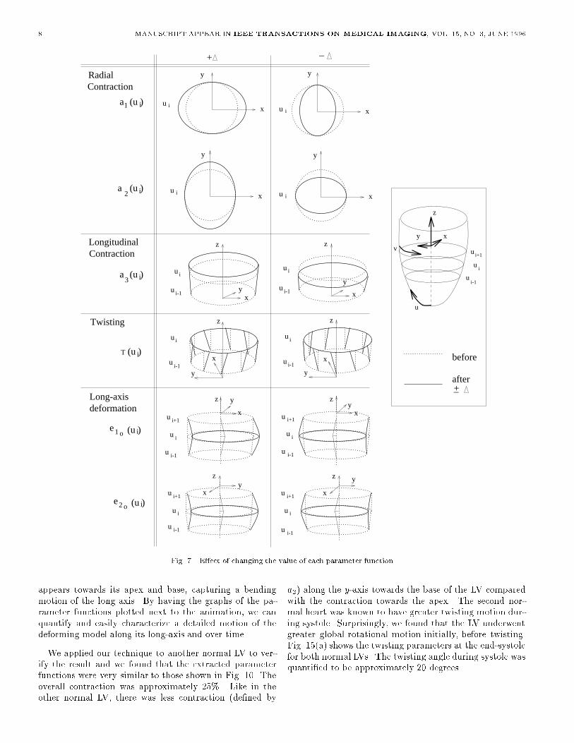
uFig. 8. Interpretation of parameter graphsquent time frames. a1(u), a2(u) and a3(u) are the aspectratios along the x-, y- and z-axes, respectively. Since theshort-axis views of the LV lie in the xy plane, the changesin a1(u) and a2(u) over time will capture the radial con-traction of the LV. Likewise, the changes in the aspect ratioalong the z-axis (i.e., a3(u)) will capture the longitudinalcontraction of the LV. The twisting parameter � (u) is de-�ned about the z-axis which coincides with the long axis ofthe LV. The axis o�set parameters e1o(u) and e2o(u) allowthe long axis to be non-straight in the x and y directions, inorder to capture more accurately the shape variation overtime of the LV.Fig. 7 demonstrates the e�ect of changing the value ofeach parameter function at a particular point ui along u.+� and �� denote an increase or decrease, respectively, inthe value of the relevant parameter function at ui. The dot-ted lines denote the initial shape of the deformable modelat ui, while the solid line denotes its shape after changingthe value of the relevant parameter function.C. LV Fitting ResultsFig. 8 depicts how we plot the parameter functions in thegraphs shown in Fig. 10 and Fig. 12. The parameter valuesare plotted as a function of u, which varies from the apexto the base of an LV, for each time frame t (t = 1 � � �5).In this way, we can observe their variation along the longaxis of the LV (u) for each time frame. As an example, inFig. 8 we show how to observe the parameter value changesduring systole at the long axis location u = c.

C.1 Normal LVs in SystoleFig. 9 shows two di�erent views of the model �tting re-sults to data from a normal heart taken over 5 time se-quences during systole (from end-diastole (t = 1) to end-systole (t = 5)). We can easily observe the contraction aswell as twisting of the model. Using the parameter func-tions, we can quantify the observed variations along thelong axis of the LV over time.In Fig. 10 we plot some of the extracted model parame-ter functions over the �ve time frames for the normal heart.Figs. 10(a) and (b) show the plots of the model's param-eter functions a1(u) and a2(u), which are associated withits length in the x and y directions, respectively. For eachframe we plot the percentage of change in each parameterfunction during frame t = 2:::5, with respect to its valueat the initial frame (t = 1). Fig. 10(c) shows plots of thedisplacement of the length along the z direction computedfrom the parameter function a3(u). Fig. 10(d) shows plotsof the model's twisting parameter function � (u). Finally,Figs. 10(e) and (f) show plots of the model's long axis de-formation parameters e1o(u) and e2o(u), respectively.From these graphs, we can quantify the shape and mo-tion of the LV during its systole. For example, by studyingthe graphs of a1(u) and a2(u) (Figs. 10(a,b)), we can con-clude that the magnitude of contraction in the radial direc-tion (i.e., along the x- and y-axes) during systole is approx-imately 20 � 25%. While the graph of a1 shows uniformcontraction along the long axis of the LV, the graph of a2shows less contraction towards the base of the LV makingthe base look more elliptical. This result supports clini-cal study �ndings where more stress is exerted at the apexduring the LV motion, and also there is an increased simi-larity of the LV base shape to an ellipse, during systole. Wemeasure from the graph shown in Fig. 10(c), that the totaldisplacement along the z-axis, which corresponds to con-traction along the z-axis, is approximately 18 mm, wherethe length of the LV is approximately 75 mm. Therefore,the contraction along the z-axis known as longitudinal con-traction is approximately 24% for this LV. From the graphin Fig. 10(d), we can quantify the twisting motion of theLV during systole to approximately 18 degrees. The graphshows that there is a small amount of twisting in early sys-tole with gradual increases towards end-systole. Finally,from the long axis deformation parameters (or axis o�setparameters) shown in Figs. 10(e-f), we observe that thereare only slight deformations and most of the deformation

8 MANUSCRIPT APPEAR IN IEEE TRANSACTIONS ON MEDICAL IMAGING, VOL. 15, NO. 3, JUNE 1996

i+1

u i

u i-1

yz

x

(u )ia1

(u )ia3

(u )iT

(u )ieo1

e2 o (u )i

u i+1

u i

u i-1

y

x

z

(u )i2a

RadialContraction

Contraction

Twisting

Long-axisdeformation

Longitudinal

u i x

y

u i x

y

u i

i-1u

z

xy

ui-1

u i

z

y

x

+ _

u i

u

x

y

u i x

y

u i+1

u i

u i-1

xy

z

u i+1

u i

u i-1

yz

x

u i-1

u i

z

x

y

u i

u i-1

z

x

y

+ _

y

z

x

ui

ui-1

u i+1

u

v

before

after

Fig. 7. E�ect of changing the value of each parameter functionappears towards its apex and base, capturing a bendingmotion of the long axis. By having the graphs of the pa-rameter functions plotted next to the animation, we canquantify and easily characterize a detailed motion of thedeforming model along its long-axis and over time.We applied our technique to another normal LV to ver-ify the result and we found that the extracted parameterfunctions were very similar to those shown in Fig. 10. Theoverall contraction was approximately 25%. Like in theother normal LV, there was less contraction (de�ned by a2) along the y-axis towards the base of the LV comparedwith the contraction towards the apex. The second nor-mal heart was known to have greater twisting motion dur-ing systole. Surprisingly, we found that the LV underwentgreater global rotational motion initially, before twisting.Fig. 15(a) shows the twisting parameters at the end-systolefor both normal LVs. The twisting angle during systole wasquanti�ed to be approximately 20 degrees.

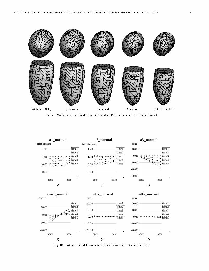
PARK ET AL.: DEFORMABLE MODELS WITH PARAMETER FUNCTIONS FOR CARDIAC MOTION ANALYSIS 9(a) time 1 (ED) (b) time 2 (c) time 3 (d) time 4 (e) time 5 (ES)Fig. 9. Model �tted to SPAMM data (LV mid-wall) from a normal heart during systole.

a1_normal

1.00

time1time2time3time4time5

a1(t)/a1(ED)

u

0.60

0.80

1.20

apex base

a2_normal

1.00

time1time2time3time4time5

a2(t)/a2(ED)

u

0.60

0.80

1.20

apex base

a3_normal

0.00

time1time2time3time4time5

mm

u-30.00

-20.00

-10.00

10.00

apex base(a) (b) (c)twist_normal

0.00

time1time2time3time4time5

degree

u-20.00

-10.00

10.00

apex base

offx_normal

0.00

time1time2time3time4time5

mm

u-20.00

-10.00

10.00

20.00

apex base

offy_normal

0.00

time1time2time3time4time5

mm

u-20.00

-10.00

10.00

20.00

apex base(d) (e) (f)Fig. 10. Extracted model parameters as functions of u for the normal heart.

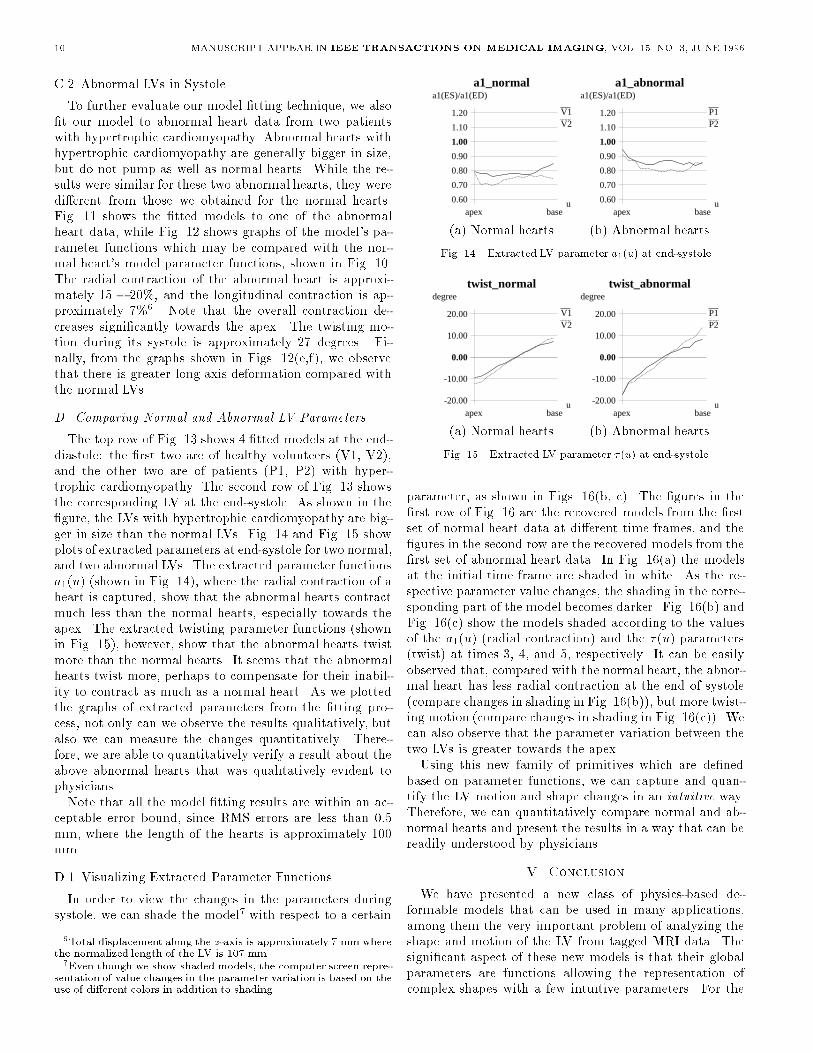
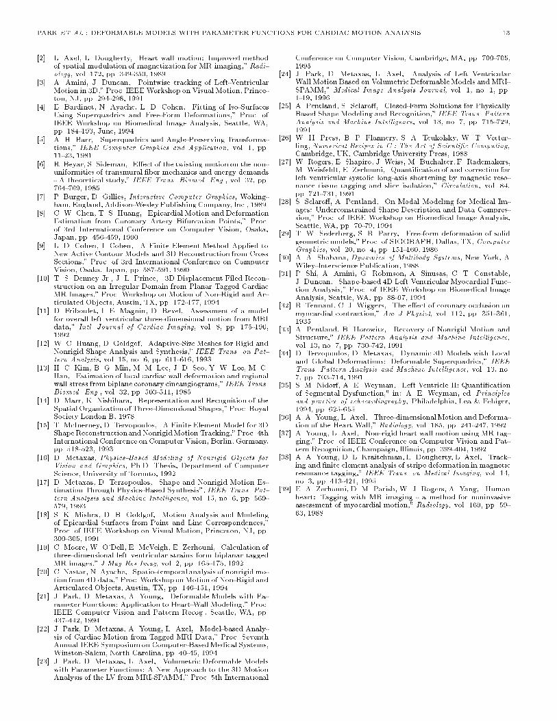
10 MANUSCRIPT APPEAR IN IEEE TRANSACTIONS ON MEDICAL IMAGING, VOL. 15, NO. 3, JUNE 1996C.2 Abnormal LVs in SystoleTo further evaluate our model �tting technique, we also�t our model to abnormal heart data from two patientswith hypertrophic cardiomyopathy. Abnormal hearts withhypertrophic cardiomyopathy are generally bigger in size,but do not pump as well as normal hearts. While the re-sults were similar for these two abnormal hearts, they weredi�erent from those we obtained for the normal hearts.Fig. 11 shows the �tted models to one of the abnormalheart data, while Fig. 12 shows graphs of the model's pa-rameter functions which may be compared with the nor-mal heart's model parameter functions, shown in Fig. 10.The radial contraction of the abnormal heart is approxi-mately 15 � 20%, and the longitudinal contraction is ap-proximately 7%6. Note that the overall contraction de-creases signi�cantly towards the apex. The twisting mo-tion during its systole is approximately 27 degrees. Fi-nally, from the graphs shown in Figs. 12(e,f), we observethat there is greater long axis deformation compared withthe normal LVs.D. Comparing Normal and Abnormal LV ParametersThe top row of Fig. 13 shows 4 �tted models at the end-diastole: the �rst two are of healthy volunteers (V1, V2),and the other two are of patients (P1, P2) with hyper-trophic cardiomyopathy. The second row of Fig. 13 showsthe corresponding LV at the end-systole. As shown in the�gure, the LVs with hypertrophic cardiomyopathy are big-ger in size than the normal LVs. Fig. 14 and Fig. 15 showplots of extracted parameters at end-systole for two normal,and two abnormal LVs. The extracted parameter functionsa1(u) (shown in Fig. 14), where the radial contraction of aheart is captured, show that the abnormal hearts contractmuch less than the normal hearts, especially towards theapex. The extracted twisting parameter functions (shownin Fig. 15), however, show that the abnormal hearts twistmore than the normal hearts. It seems that the abnormalhearts twist more, perhaps to compensate for their inabil-ity to contract as much as a normal heart. As we plottedthe graphs of extracted parameters from the �tting pro-cess, not only can we observe the results qualitatively, butalso we can measure the changes quantitatively. There-fore, we are able to quantitatively verify a result about theabove abnormal hearts that was qualitatively evident tophysicians.Note that all the model �tting results are within an ac-ceptable error bound, since RMS errors are less than 0:5mm, where the length of the hearts is approximately 100mm.D.1 Visualizing Extracted Parameter FunctionsIn order to view the changes in the parameters duringsystole, we can shade the model7 with respect to a certain6Total displacement along the z-axis is approximately 7 mm wherethe normalized length of the LV is 107 mm.7Even though we show shaded models, the computer screen repre-sentation of value changes in the parameter variation is based on theuse of di�erent colors in addition to shading.

a1_normal

1.00

V1V2

a1(ES)/a1(ED)

u0.60

0.70

0.80

0.90

1.10

1.20

apex base

a1_abnormal

1.00

P1P2

a1(ES)/a1(ED)

u0.60

0.70

0.80

0.90

1.10

1.20

apex base(a) Normal hearts (b) Abnormal heartsFig. 14. Extracted LV parameter a1(u) at end-systoletwist_normal

0.00

V1V2

degree

u-20.00

-10.00

10.00

20.00

apex base

twist_abnormal

0.00

P1P2

degree

u-20.00

-10.00

10.00

20.00

apex base(a) Normal hearts (b) Abnormal heartsFig. 15. Extracted LV parameter �(u) at end-systoleparameter, as shown in Figs. 16(b, c). The �gures in the�rst row of Fig. 16 are the recovered models from the �rstset of normal heart data at di�erent time frames, and the�gures in the second row are the recovered models from the�rst set of abnormal heart data. In Fig. 16(a) the modelsat the initial time frame are shaded in white. As the re-spective parameter value changes, the shading in the corre-sponding part of the model becomes darker. Fig. 16(b) andFig. 16(c) show the models shaded according to the valuesof the a1(u) (radial contraction) and the � (u) parameters(twist) at times 3, 4, and 5, respectively. It can be easilyobserved that, compared with the normal heart, the abnor-mal heart has less radial contraction at the end of systole(compare changes in shading in Fig. 16(b)), but more twist-ing motion (compare changes in shading in Fig. 16(c)). Wecan also observe that the parameter variation between thetwo LVs is greater towards the apex.Using this new family of primitives which are de�nedbased on parameter functions, we can capture and quan-tify the LV motion and shape changes in an intuitive way.Therefore, we can quantitatively compare normal and ab-normal hearts and present the results in a way that can bereadily understood by physicians.V. ConclusionWe have presented a new class of physics-based de-formable models that can be used in many applications,among them the very important problem of analyzing theshape and motion of the LV from tagged MRI data. Thesigni�cant aspect of these new models is that their globalparameters are functions allowing the representation ofcomplex shapes with a few intuitive parameters. For the

PARK ET AL.: DEFORMABLE MODELS WITH PARAMETER FUNCTIONS FOR CARDIAC MOTION ANALYSIS 11(a) time 1 (ED) (b) time 2 (c) time 3 (d) time 4 (e) time 5 (ES)Fig. 11. Model �tted to SPAMM data from an abnormal heart during systole.

a1_abnormal

1.00

time1time2time3time4time5

a1(t)/a1(ED)

u

0.60

0.80

1.20

apex base

a2_abnormal

1.00

time1time2time3time4time5

a2(t)/a2(ED)

u

0.60

0.80

1.20

apex base

a3_abnormal

0.00

time1time2time3time4time5

mm

u-30.00

-20.00

-10.00

10.00

apex base(a) (b) (c)twist_abnormal

0.00

time1time2time3time4time5

degree

u-20.00

-10.00

10.00

apex base

offx_abnormal

0.00

time1time2time3time4time5

mm

u-20.00

-10.00

10.00

20.00

apex base

offy_abnormal

0.00

time1time2time3time4time5

mm

u-20.00

-10.00

10.00

20.00

apex base(d) (e) (f)Fig. 12. Extracted model parameters as functions of u for the abnormal heart.

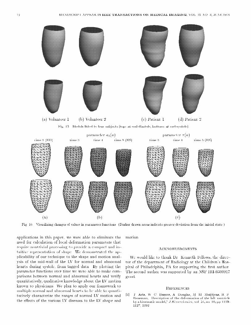
12 MANUSCRIPT APPEAR IN IEEE TRANSACTIONS ON MEDICAL IMAGING, VOL. 15, NO. 3, JUNE 1996(a) Volunteer 1 (b) Volunteer 2 (c) Patient 1 (d) Patient 2Fig. 13. Models �tted to four subjects (top: at end-diastole, bottom: at end-systole)parameter a1(u) parameter � (u)time 1 (ED) time 3 time 4 time 5 (ES) time 3 time 4 time 5 (ES)(a) (b) (c)Fig. 16. Visualizing changes of values in parameter functions. (Darker drawn areas indicate greater deviation from the initial state.)applications in this paper, we were able to eliminate theneed for calculation of local deformation parameters thatrequire nontrivial processing to provide a compact and in-tuitive representation of shape. We demonstrated the ap-plicability of our technique to the shape and motion anal-ysis of the mid-wall of the LV for normal and abnormalhearts during systole, from tagged data. By plotting theparameter functions over time we were able to make com-parisons between normal and abnormal hearts and verifyquantitatively, qualitative knowledge about the LV motionknown to physicians. We plan to apply our framework tomultiple normal and abnormal hearts to be able to quanti-tatively characterize the ranges of normal LV motion andthe e�ects of the various LV diseases to the LV shape and

motion. AcknowledgmentsWe would like to thank Dr. Kenneth Fellows, the direc-tor of the department of Radiology at the Children's Hos-pital of Philadelphia, PA for supporting the �rst author.The second author was supported by an NSF IRI-9309917grant. References[1] T. Arts, W. C. Hunter, A. Douglas, M. M. Muijtjens, R. S.Reneman, \Description of the deformation of the left ventricleby a kinematicmodel," J Biomechanics, vol. 25, no. 10, pp.1119-1127, 1992.

PARK ET AL.: DEFORMABLE MODELS WITH PARAMETER FUNCTIONS FOR CARDIAC MOTION ANALYSIS 13[2] L. Axel, L. Dougherty, \Heart wall motion: Improved methodof spatial modulation of magnetization for MR imaging," Radi-ology, vol. 172, pp. 349-350, 1989.[3] A. Amini, J. Duncan, \Pointwise tracking of Left-VentricularMotion in 3D," Proc. IEEE Workshop on Visual Motion, Prince-ton, NJ, pp. 294-298, 1991.[4] E. Bardinet, N. Ayache, L. D. Cohen, \Fitting of Iso-SurfacesUsing Superquadrics and Free-Form Deformations," Proc. ofIEEE Workshop on Biomedical Image Analysis, Seattle, WA,pp. 184-193, June, 1994.[5] A. H. Barr, \Superquadrics and Angle-Preserving Transforma-tions," IEEE Computer Graphics and Application, vol. 1, pp.11-23, 1981.[6] R. Beyar, S. Sideman, \E�ect of the twisting motion on the non-uniformities of transmural �ber mechanics and energy demands- A theoretical study," IEEE Trans. Biomed. Eng., vol. 32, pp.764-769, 1985.[7] P. Burger, D. Gillies, Interactive Computer Graphics, Woking-ham, England, Addison-WesleyPublishing Company, Inc., 1989.[8] C. W. Chen, T. S. Huang, \Epicardial Motion and DeformationEstimation from Coronary Artery Bifurcation Points," Proc.of 3rd International Conference on Computer Vision, Osaka,Japan, pp. 456-459, 1990.[9] L. D. Cohen, I. Cohen, \A Finite Element Method Applied toNew Active Contour Models and 3D Reconstruction from CrossSections," Proc. of 3rd International Conference on ComputerVision, Osaka, Japan, pp. 587-591, 1990.[10] T. S. Denney Jr., J. L. Prince, \3D Displacement Filed Recon-struction on an Irregular Domain from Planar Tagged CardiacMR Images," Proc. Workshop on Motion of Non-Rigid and Ar-ticulated Objects, Austin, TX, pp. 172-177, 1994.[11] D. Friboulet, I. E. Magnin, D. Revel, \Assessment of a modelfor overall left ventricular three-dimensional motion from MRIdata," Intl. Journal of Cardiac Imaging, vol. 8, pp. 175-190,1992.[12] W. C. Huang, D. Goldgof, \Adaptive-Size Meshes for Rigid andNonrigid Shape Analysis and Synthesis," IEEE Trans. on Pat-tern Analysis, vol. 15, no. 6, pp. 611-616, 1993.[13] H. C. Kim, B. G. Min, M. M. Lee, J. D. Seo, Y. W. Lee, M. C.Han, \Estimation of local cardiac wall deformation and regionalwall stress from biplane coronary cineangiograms," IEEE Trans.Biomed. Eng., vol. 32, pp. 503-511, 1985.[14] D. Marr, K. Nishihara, \Representation and Recognition of theSpatial Organizationof Three-DimensionalShapes," Proc. RoyalSociety London B, 1978.[15] T. McInerney, D. Terzopoulos, \A Finite Element Model for 3DShapeReconstructionand NonrigidMotion Tracking," Proc. 4thInternational Conference on Computer Vision, Berlin, Germany,pp. 518-523, 1993.[16] D. Metaxas, Physics-Based Modeling of Nonrigid Objects forVision and Graphics, Ph.D. Thesis, Department of ComputerScience, University of Toronto, 1992.[17] D. Metaxas, D. Terzopoulos, \Shape and Nonrigid Motion Es-timation Through Physics-Based Synthesis", IEEE Trans. Pat-tern Analysis and Machine Intelligence, vol. 15, no. 6, pp. 569-579, 1993.[18] S. K. Mishra, D. B. Goldgof, \Motion Analysis and Modelingof Epicardial Surfaces from Point and Line Correspondences,"Proc. of IEEE Workshop on Visual Motion, Princeton, NJ, pp.300-305, 1991.[19] C. Moore, W. O'Dell, E. McVeigh, E. Zerhouni, \Calculation ofthree-dimensional left ventricular strains form biplanar taggedMR images," J Mag Res Imag, vol. 2, pp. 165-175, 1992.[20] C. Nastar, N. Ayache, \Spatio-temporal analysis of nonrigid mo-tion from 4D data," Proc.Workshop onMotion of Non-Rigid andArticulated Objects, Austin, TX, pp. 146-151, 1994.[21] J. Park, D. Metaxas, A. Young, \Deformable Models with Pa-rameter Functions: Application to Heart-Wall Modeling," Proc.IEEE Computer Vision and Pattern Recog., Seattle, WA, pp.437-442, 1994.[22] J. Park, D. Metaxas, A. Young, L. Axel, \Model-based Analy-sis of Cardiac Motion from Tagged MRI Data," Proc. SeventhAnnual IEEE Symposiumon Computer-BasedMedical Systems,Winston-Salem, North Carolina, pp. 40-45, 1994.[23] J. Park, D. Metaxas, L. Axel, \Volumetric Deformable Modelswith Parameter Functions: A New Approach to the 3D MotionAnalysis of the LV from MRI-SPAMM," Proc. 5th International

Conference on Computer Vision, Cambridge, MA, pp. 700-705,1995.[24] J. Park, D. Metaxas, L. Axel, \Analysis of Left VentricularWall Motion Based on Volumetric DeformableModels and MRI-SPAMM," Medical Image Analysis Journal, vol. 1, no. 1, pp.1-19, 1996.[25] A. Pentland, S. Sclaro�, \Closed-Form Solutions for PhysicallyBased Shape Modeling and Recognition," IEEE Trans. PatternAnalysis and Machine Intelligence, vol. 13, no. 7, pp. 715-729,1991.[26] W. H. Press, B. P. Flannery, S. A. Teukolsky, W. T. Vetter-ling, Numerical Recipes in C : The Art of Scienti�c Computing,Cambridge, UK, Cambridge University Press, 1988.[27] W. Rogers, E. Shapiro, J. Weiss, M. Buchalter, F. Rademakers,M. Weisfeldt, E. Zerhouni, \Quanti�cation of and correction forleft ventricular systolic long-axis shortening by magnetic reso-nance tissue tagging and slice isolation," Circulation, vol. 84,pp. 721-731, 1991.[28] S. Sclaro�, A. Pentland, \On Modal Modeling for Medical Im-ages: Underconstrained Shape Description and Data Compres-sion," Proc. of IEEE Workshop on Biomedical Image Analysis,Seattle, WA, pp. 70-79, 1994.[29] T. W. Sederberg, S. R. Parry, \Free-form deformation of solidgeometricmodels," Proc. of SIGGRAPH, Dallas, TX, ComputerGraphics, vol. 20, no. 4, pp. 151-160, 1986.[30] A. A. Shabana, Dynamics of Multibody Systems, New York, AWiley-Interscience Publication, 1988.[31] P. Shi, A. Amini, G. Robinson, A. Sinusas, C. T. Constable,J. Duncan, \Shape-based 4D Left Ventricular Myocardial Func-tion Analysis," Proc. of IEEE Workshop on Biomedical ImageAnalysis, Seattle, WA, pp. 88-97, 1994.[32] R. Tennant, C. J. Wiggers, \The e�ect of coronary occlusion onmyocardial contraction," Am J Physiol, vol. 112, pp. 351-361,1935.[33] A. Pentland, B. Horowitz, \Recovery of Nonrigid Motion andStructure," IEEE Pattern Analysis and Machine Intelligence,vol. 13, no. 7, pp. 730-742, 1991.[34] D. Terzopoulos, D. Metaxas, \Dynamic 3D Models with Localand Global Deformations: Deformable Superquadrics," IEEETrans. Pattern Analysis and Machine Intelligence, vol. 13, no.7, pp. 703-714, 1991.[35] S. M. Nidorf, A. E. Weyman, \Left Ventricle II: Quanti�cationof Segmental Dysfunction," in: A. E. Weyman, ed. Principlesand practice of echocardiography, Philadelphia, Lea & Febiger,1994, pp. 625-655.[36] A. A. Young, L. Axel, \Three-dimensionalMotion and Deforma-tion of the Heart Wall," Radiology, vol. 185, pp. 241-247, 1992.[37] A. Young, L. Axel, \Non-rigid heart wall motion using MR tag-ging," Proc. of IEEE Conference on Computer Vision and Pat-tern Recognition, Champaign, Illinois, pp. 399-404, 1992.[38] A. A. Young, D. L. Kraitchman, L. Dougherty, L. Axel, \Track-ing and �nite element analysis of stripe deformation in magneticresonance tagging," IEEE Trans. on Medical Imaging, vol. 14,no. 3, pp. 413-421, 1995.[39] E. A. Zerhouni, D. M. Parish, W. J. Rogers, A. Yang, \Humanheart: Tagging with MR imaging - a method for noninvasiveassessment of myocardial motion," Radiology, vol. 169, pp. 59-63, 1988.