DEALING WITH VISUAL FEATURES LOSS DURING A

VISION-BASED TASK FOR A MOBILE ROBOT

SHORTENED TITLE: TREATING IMAGE LOSS DURING A VISION-BASED TASK

David Folio12 and Viviane Cadenat12

1 LAAS-CNRS; Universite de Toulouse; 7, avenue du Colonel Roche, F-31077 Toulouse, France.2 Universite de Toulouse ; UPS.

In this paper, we address the problem of computing the image features when they become

temporarily unavailable during a vision-based navigation task. The method consists in

analytically integrating the relation between the visual features motion in the image and the

camera motion. Then, we use this approach to design sensor-based control laws able to tolerate

the complete loss of the visual data during a vision-based navigation task in an unknown

environment. Simulation and experimentation results demonstrate the validity and the interest

of our method.

Keywords: Mobile robots, visual servoing, image features loss, obstacle avoidance, visibility

management.

1. INTRODUCTION

Visual servoing techniques aim at controlling the robot motion using vision data

provided by a camera to reach a desired goal defined in the image (Hutchinson et al.

1996; Chaumette and Hutchinson 2006). Thus, these approaches require that the image

features remain always visible. Therefore, these techniques cannot be used anymore

if these features are lost during the robotic task. A first common solution is to use

methods allowing to preserve the visual features visibility. Most of them are dedicated

to manipulator arms, and propose to treat this kind of problem by using redundancy

(Marchand and Hager 1998; Mansard and Chaumette 2005), path-planning (Mezouar

and Chaumette 2002), specific degrees of freedom (DOF) (Corke and Hutchinson

2001; Kyrki et al. 2004), zoom (Benhimane and Malis 2003) or even by making a

tradeoff with the nominal vision-based task (Remazeilles et al. 2006). In a mobile

robotic context we have to preserve not only the image data visibility, but also the robot

safety. In that case, techniques allowing to avoid simultaneously collisions and visual

data losses such as (Folio and Cadenat 2005a; Folio and Cadenat 2005b) appear to

be limited. Indeed, this kind of methods is restricted to missions where an avoidance

motion exists without leading to local minima (Folio 2007). Therefore, they do not

allow to perform robotic tasks which cannot be realized if the visual features loss

is not tolerated. A first solution is to let some of the features appear and disappear

temporarily from the image as done in (Garcia-Aracil et al. 2005). However, this

approach is limited to partial losses, and does not entirely solve the problem.

Address correspondence to David Folio and Viviane Cadenat, LAAS-CNRS; 7, avenue du Colonel Roche,F-31077 Toulouse, France. E-mails: dfolio@laas.fr, cadenat@laas.fr. Phone: +33 561 336 451.

1

2 DAVID FOLIO AND VIVIANE CADENAT

NOMENCLATURE

dcoll distance between the robot and obstacles

docc distance between the visual data and oc-cluding object (in pixel)

D−, D0 and D+ distances allowing to evaluatethe occlusion risk µocc (in pixel)

d−, d0 and d+ distances allowing to evaluate thecollision risk µcoll

f camera focal length

Jr robot jacobian matrix

L the interaction matrix

q robot control input

s visual features

Te sampling time

vcr the camera kinematic screw

v mobile-base linear velocity

V linear velocity

(X,Y ) coordinates of a point in image frame

z the point depth in camera frame

Greek Symbols

ϑ pan-platform orientation

µcoll risk of collision

µocc risk of occlusion

Ω angular velocity

ω mobile-base angular velocity

pan-platform angular velocity

Subscripts

−→x c,−→y c,

−→z c the camera frame axis

cg center of gravity

coll collision

occ occlusion

vs visual servoing

k evaluate at time tk

In this paper, our first goal is to propose a method allowing to compute the

visual features when they are lost or unavailable for a short amount of time during

a vision-based task (eg. temporary camera or image processing failure, landmark

occlusion,. . . ). In this work, the whole image is considered to be momentarily entirely

unavailable in order to treat total visual data losses. Our second motivation is to use

this approach to design sensor-based control laws able to tolerate the total loss of the

image data during a vision-based task to reach the desired goal defined in the image.

The article is organized as follows. In section 2., we present the robotic system

and state the problem. In section 3., we describe our estimation method. In section 4.,

we address some control issues and show how to use the proposed estimation technique

to design control laws able to treat the visual features loss. Finally, we present some

experimental results to validate our work.

2. THE ROBOTIC SYSTEM AND PROBLEM STATEMENT

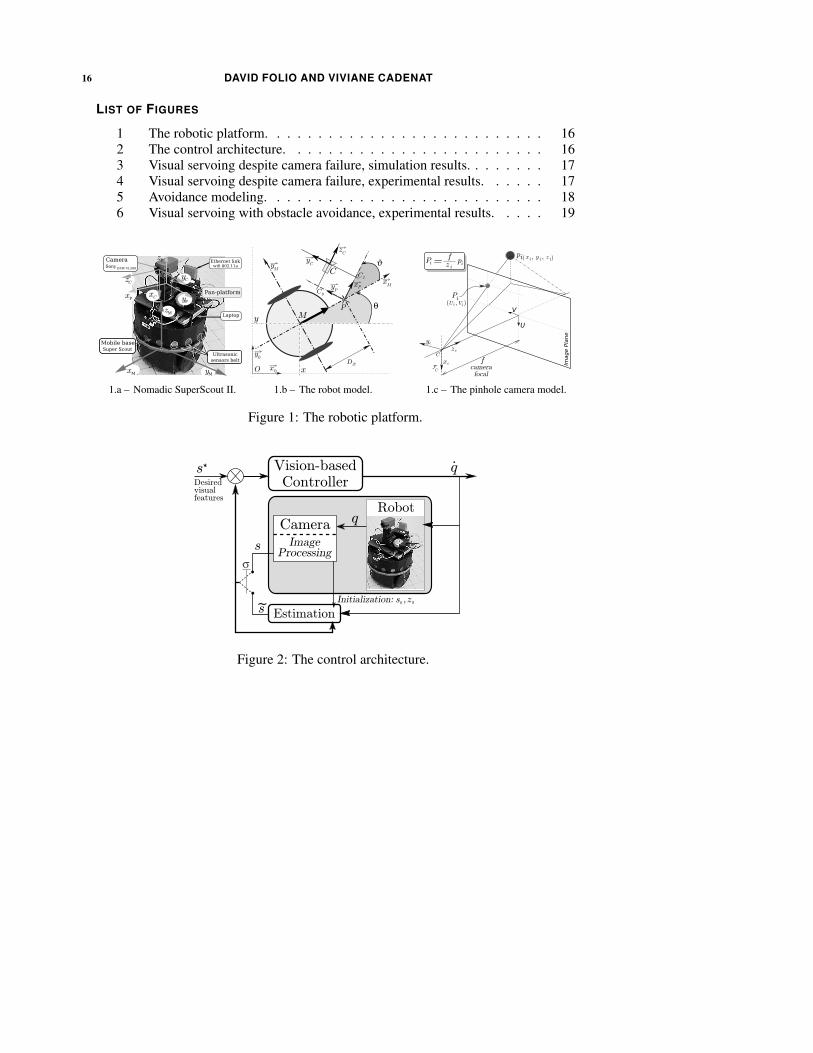
First, let us describe the robotic platform, before modelling our system. We

consider the mobile robot SuperScout II1 equipped with an ultrasonic sensor belt and

a camera mounted on a pan-platform (see figure 1.a). This is a cylindric cart-like

vehicle, dedicated to indoor navigation. Incremental encoders provide the pose and

the velocity of the robotic system. A DFW-VL500 Sony color digital IEEE 1394 camera

captures pictures in YUV 4:2:2 format with 640 × 480 resolution. An image processing

module extracts interest points from the image. The robot is controlled by an on-

board laptop computer running under Linux on which is installed a specific control

architecture called Gen

oM (Generator of Module) (Fleury and Herrb 2001).

1The mobile robot SuperScout II is provided by the AIP-PRIMECA (http://www.aip-primeca.net).

TREATING IMAGE LOSS DURING A VISION-BASED TASK 3

Let us modelling our system to express the camera kinematic screw. To

this aim, by considering figure 1.b, we define the following successive frames:

FM (M,−→xM ,−→yM ,

−→zM ) linked to the robot, FP (P,−→xP ,−→yP ,

−→z P ) attached to the

pan-platform, and Fc (C,−→x c,−→y c,

−→z c) linked to the camera. Let ϑ be the direction

of the pan-platform wrt. −→xM , P the pan-platform center of rotation and Dx the

distance between the robot reference point M and P . The control input is defined by:

q = [v, ω,]T , where v and ω are the cart linear and angular velocities, and is

the pan-platform angular velocity wrt. FM . For this specific mechanical system, the

camera kinematic screw vc= [V TC/F0

, ΩTFC/F0

]T is related to the control input by the

robot jacobian J: vc = Jq. As the camera is constrained to move horizontally, it is

sufficient to consider a reduced kinematic screw vcr , and a reduced jacobian matrix Jr

as follows:

vcr =

V−→yc

V−→zc

Ω−→xc

=

− sin(ϑ) Dx cos(ϑ) + Cx Cx

cos(ϑ) Dx sin(ϑ) − Cy −Cy

0 −1 −1

v

ω

= Jr(ϑ) q (1)

where Cx and Cy are the coordinates of C along axes −→xP and −→yP (see figure 1.b).

We consider the problem of executing a vision-based navigation task in an un-

known environment. During such a task, unexpected events may occur: camera or

image processing failure, landmark losses, collisions with obstacles, and so on. In this

paper, we focus on the problem of the visual features temporary loss during the mission

and we propose a method allowing to compute them when they become unavailable.

We then show how to embed it in our vision-based navigation task to reach the desired

goal defined in the image frame.

3. VISUAL DATA ESTIMATION

In this section, we address the image data estimation problem. We first present

some preliminaries and state the estimation problem before presenting our approach.

3.1. Preliminaries

We consider a static landmark with respect to which is defined the vision-based

navigation task to be realized. We assume that it can be characterized by n inter-

est points which can be extracted by our image processing. Then, in this case, the

considered visual data are represented by a 2n-dimensional vector s made of the coor-

dinates (Xi, Yi) of each projected point Pi in the image plane (see figure 1.c), that is:

s= [X1, Y1, . . . , Xi, Yi, . . . , Xn, Yn]T . For a fixed landmark, the variation of the visual

signals s is related to the reduced camera kinematic screw vcr by means of the interac-

tion matrix L(s) as shown below (Espiau et al. 1992):

s = L(s) vcr = L(s) Jr q (2)

In our specific case, the interaction matrix L(s) is deduced from the optic flow equa-

tions. Indeed, for one point Pi it is given by (Espiau et al. 1992):

L(Pi) =

(L(Xi,zi)

L(Yi,zi)

)=

(0 Xi

zi

XiYi

f

− fzi

Yi

zif + Yi

2

f

)(3)

4 DAVID FOLIO AND VIVIANE CADENAT

where zi is the depth of each projected point Pi and f is the camera focal length (see

figure 1.c). Therefore, the whole interaction matrix L(s)= [. . . ,L(Xi,zi)T ,L(Yi,zi)

T , . . .]T

depends on the depth z = [z1, . . . , zn]T of the considered visual data.

3.2. Estimation Problem Statement

Now, we focus on the problem of estimating (all or some) visual data s whenever

they become unavailable during a vision-based task. Thus, the key-assumption which

underlies our works is that the whole image is considered to be temporarily com-

pletely unavailable. Hence, the methods which only allow to treat partial losses of the

visual features such as (Malis et al. 1999; Garcia-Aracil et al. 2005; Comport et al.

2004) are not suitable here. Following this reasoning, we have focused on techniques

dedicated to image data reconstruction. Different approaches, such as signal processing

techniques or tracking methods (Favaro and Soatto 2003; Jackson et al. 2004; Lepetit

and Fua 2006), may be used to deal with this kind of problem. Here, we have chosen

to use a simpler approach for several reasons. First of all, most of the above techniques

rely on measures from the image which are considered to be totally unavailable in

our case. Second, we suppose that we have few errors on the model and on the

measures2. Third, as it is intended to be used to perform complex navigation tasks,

the estimated visual signals must be provided sufficiently rapidly with respect to the

control law sampling period. Another idea is to use a 3D model of the object together

with projective geometry in order to deduce the lacking data. However, this choice

would lead to depend on the considered landmark type and would require to localize

the robot. This was unsuitable for us, as we do not want to make any assumption on the

landmark 3D model. We have finally chosen to solve (2) using the previous available

image measurements and the control inputs q. Thus, we assume in the sequel that the

visual data can be measured at the beginning of the robotic task.

Therefore, our idea is to solve the dynamic system (2) to reconstruct the image

data s. However, as, in our case, (2) requires the depth z, we have to compute it to

be able to solve this system. Several approaches may be used to determine z. First

of all, it can be measured using specific sensors such as a telemeter or a stereoscopic

system. Nevertheless, as none of them is mounted on our robot, we have to focus

on approaches allowing to reconstruct it. For instance, a first possible solution is to

use structure from motion (SFM) techniques (Jerian and Jain 1991; Chaumette et al.

1996; Soatto and Perona 1998; Oliensis 2002), signal processing methods (Matthies

et al. 1989), or even pose relative estimation (Thrun et al. 2001). Unfortunately,

these approaches require to use measures from the image, and, thus, they cannot be

applied here when it becomes unavailable. That is why we propose another solution

consisting in estimating depth z together with the visual data s (see remark 1). Our

idea is to express the analytical relation between the variation of z and the camera

motion. As we consider a target made of n points, we only have to determine the depth

variation of each of these points. It can be easily shown that, for one 3D point pi of

coordinates (xi, yi, zi)T expressed in Fc projected into a point Pi(Xi, Yi) in the image

plane as shown in figure 1.c, the depth variation zi is related to the camera motion

according to: zi = L(zi)vcr = L(zi)Jrq. In our case, L(zi) = (0, −1, zi

fYi). Then,

2In the case where this assumption is not fulfilled, different techniques such as Kalman filtering for instancemay be used to take into account explicitely the different noises present on the system.

TREATING IMAGE LOSS DURING A VISION-BASED TASK 5

the dynamic system to be solved for one point Pi(Xi, Yi) is given by:

Xi = Xi

ziV−→zc

+ XiYi

fΩ−→xc

(4)

Yi = − fziV−→yc

+ Yi

ziV−→zc

+(f +

Y 2i

f

)Ω−→xc

(5)

zi = −V−→zc− zi

fYiΩ−→xc

(6)

where V−→yc, V−→zc

and Ω−→xcare given in (1). Thus, our goal is to integrate the above

differential equations during the control law sampling period Te, that is for any

t ∈ [tk, tk+1]. Then, introducing ψ= [sT , zT ]T and L(ψ)=

[L(s)

T , L(z)T]T

, the

differential system to be solved can be expressed as follows:ψ = L(ψk) vcr = L(ψk) Jr(ϑ(t)) q(tk)

ψk = ψ(tk) =(sTk , z

Tk

)T= (X1k, Y1k, . . . , Xnk, Ynk, z1k, . . . , znk)

T(7)

where ψk and q(tk)= (vk, ωk, k)T are the values of ψ and q evaluated at tk (see

remark 1). As, on our robot, the control input is hold during Te, the velocities vector q

can be considered as constant during this time interval.

Remark 1: While the image remains available, sk is directly obtained from the image features

extraction processing, and the initial depth zk can be computed using one of the methods listed

above: SFM, signal processing techniques, pose relative estimation approaches. . . When the image is

lost, ψk =(s

Tk ,z

Tk

)Tis determined from our estimator (see figure 2).

Remark 2: Another idea to reconstruct the visual features would be to consider the exponential mapapproach and the direct measure of the camera velocity. This approach allows to determine the 3Dcoordinates of the point pi(xi, yi, zi) using the following relation (Soatto and Perona 1998):

pi = −VC/F0(t) − ΩFC/F0

(t) ∧ pi(t) ↔ pi(tk+1) = R(tk)pi(tk) + T (tk)

where R ∈ SO(3) (special orthogonal group of transformations of R3) and T ∈ R

3 define respectivelythe rotation and translation of the moving camera. Indeed, R and T are related to the camera rotationΩFC/F0

and translation VC/F0motion thanks to an exponential map (Murray et al. 1994), that is:(R T

0 1

)= exp

([Ω]× VC/F0

0 0

)

where [Ω]× belongs to the set of 3 × 3 skew-matrices and is commonly used to describe the cross

product of ΩFC/F0with a vector in R

3. However, this approach can be used only if the camera

kinematic screw vc= [V TC/F0

, ΩTFC/F0

]T can be assumed constant during the sampling period Te,

which is not our case.

3.3. Resolution

A first idea is to solve differential system (7) using numerical schemes as done

in (Folio and Cadenat 2007a; Folio and Cadenat 2007b). In these previous works,

different numerical techniques such as Euler, Runge-Kutta, Adams-Bashforth-Moulton

or Backward Differentiation Formulas have been used and compared. The main advan-

tage of this kind of approaches is that it can be applied to any set of image features and

to any kind of robots, provided that the estimation problem can be expressed using

system (7). However, it is well known that numerical schemes always approximate

the “true” solution and that the accuracy of the obtained result is closely related to the

chosen method and to the integration step size. Here, as the considered visual data and

robotic system are sufficiently simple, system (7) can be solved analytically. Although

the obtained solution is restricted to our specific case, it appears to be much more

accurate than the previous ones, as it is the exact solution of system (7) on the time

control interval Te. This is its main advantage.

6 DAVID FOLIO AND VIVIANE CADENAT

Now, let us determine the analytical solution of the differential equation (7).

In order to simplify the expressions, we will only treat the case of one point P of

coordinates X(t), Y (t), z(t), which leads to solve the set of equations (4), (5) and (6).

Subscript i will not then be considered in the following calculus.

First, we compute the depth z(t). To this aim, we derivate equation (6) with

respect to time:

z = −V−→zc− (Y z(t) + Y (t)z)

Ω−→xc

f−Y (t)z(t)

fΩ−→xc

(8)

Then, multiplying (5) by z(t) and (6) by Y (t), we get:

Y z(t) + Y (t)z = −fV−→yc(t) + fz(t)Ω−→xc

(t)

Moreover, using (1), it can be shown that: V−→zc= (−vk sin(ϑ(t)) +Dxωk cos(ϑ(t))) k and

Ω−→xc= 0. Replacing these different terms in (8), we finally obtain the following second

order differential equation to be solved for z(t):

z + z(t)(ωk +k)2 = Cxk(ωk +k) − (ωk + 2k)V−→yc

(t) (9)

After some computations, we get the following results for z(t) depending on the

control inputs ωk and k (a detailed proof is available in (Folio 2007)):

• if ωk 6= − k and ωk 6= 0 :

z(t)=c1 sin (A1 (t− tk)) + c2 cos (A1 (t− tk))

−Dx cos (ϑ(t)) + vkωk

sin (ϑ(t)) − Cx

• if ωk = − k 6= 0 :

z(t)= ωk

kDx (cos (ϑ(t)) − cos (ϑk))

− vkk

(sin (ϑ(t)) − sin (ϑk)) + zk

• if ωk = 0 and k 6= 0 :

z(t)=c3 sin ( k (t− tk)) + c4 cos ( k (t− tk))

−vk (t− tk) cos (ϑ(t)) + vk2 k

sin (ϑ(t)) − Cx

• if ωk = k = 0 :

z(t)=−vk cos (ϑk) (t− tk) + zk

,with:

A1 =(ωk + k)

c1 = vkωk

cos (ϑk) +Dx sin (ϑk)

−Ykzk

f− Cy

c2 =Dx cos (ϑk) + zk

− vkωk

sin (ϑk) + Cx

c3 = vk2 k

cos (ϑk)

−Ykzk

f− Cy

c4 =− vk2 k

sin (ϑk) + zk + Cx

(10)

Now, we consider the determination of X(t). Equation (4) can be rewritten as:XX(t) = − z

z(t) . X(t) can then be computed by integrating this last relation for

t ∈ [tk, tk+1], and we get:

X(t) =zkXk

z(t)(11)

Finally, Y (t) is easily deduced from (6) as follows: Y (t) = −fz+V−→zc

(t)

z(t)Ω−→xc(t) , where

V−→zc(t) and Ω−→xc

(t) can be computed from the control inputs by using (1). Using the

TREATING IMAGE LOSS DURING A VISION-BASED TASK 7

solution z(t) given by (10), Y (t) expresses as:

• if ωk 6= − k and ωk 6= 0 :

Y (t)=−fCy−c1 cos(A1(t−tk))−c2 sin(A1(t−tk))−Dx sin(ϑ(t))−

vkωk

cos(ϑ(t))

z(t)

• if ωk = − k 6= 0 :

Y (t)=f v(cos(ϑ(t))−cos(ϑk))+ kzkYk

z(t) k

• if ωk = 0 and k 6= 0 :

Y (t)=−fc1 cos(A1(t−tk))−c2 sin(A1(t−tk))+vk(t−tk) sin(ϑ(t))−

vk2 k

cos(ϑ(t))+Cy

z(t)

• if ωk = k = 0 :

Y (t)=−f vk sin(ϑk)(t−tk)+Ykzkz(t)

(12)

As Y (t) depends on depth, we observe the same different cases as in z(t), depending

on the values of ωk and k. Moreover, the computation of X(t), Y (t), z(t) requires

the determination of the pan-platform direction: ϑ(t). This angle can be calculated

by integrating ϑ = k between tk and t, that is: ϑ(t) = k (t− tk) + ϑk, where ϑkrepresents the pan-platform angular value at t = tk, which is provided by the embedded

encoder. Hence, as the robot jacobian depends on ϑ(t), the camera kinematic screw vcris not constant during the control law sampling time Te (see remark 2).

Finally, the solution for the set of the n points of the landmark is obtained by

applying the above solution on each component of the previously defined vector ψ.

4. APPLICATIONS

We propose in this section a panel of applications showing the interest and the

relevance of our approach. Indeed, our estimation technique can be used in different

related fields such as vision or image processing. Here, we have chosen to apply it

in a vision-based context to compute the visual data whenever they are unavailable

during the navigation task. Therefore, we will address some control issues and we

will show how to use the proposed estimation method to design control laws able to

treat the image data loss. We have considered two kinds of tasks: the first one is a

positioning vision-based task during which a camera failure occurs; the second one is

a more complex task consisting in realizing a visually guided navigation task amidst

obstacles despite possible occlusions and collisions.

4.1. Execution of a Vision-Based Task Despite Camera Failure

Here, our objective is to perform a vision-based task despite a camera failure.

We first describe the considered robotic task before presenting the control strategy and

the obtained results.

4.1.1. Vision-based task Our goal is to position the embedded camera with respect

to a landmark composed of n points. To this aim, we have applied the visual servoing

technique given in (Espiau et al. 1992) to mobile robots as in (Pissard-Gibollet and

Rives 1995). The proposed approach relies on the task function formalism (Samson

et al. 1991) and consists in expressing the visual servoing task by the following task

function to be regulated to zero:

evs = C(s − s⋆)

8 DAVID FOLIO AND VIVIANE CADENAT

where s⋆ represents the desired value of the visual signal, while C is a full-rank

combination matrix allowing to take into account more visual features than available

DOFs (Espiau et al. 1992). A classical controller q(s) making evs vanish can be

designed by imposing an exponential decrease, that is: evs = −λvsevs = CL(s)Jrq(s),

where λvs is a positive scalar or a positive definite matrix. Fixing C = L(s⋆)+ as in

(Espiau et al. 1992), the visual servoing controller q(s) can be written as follows:

q(s) = (CL(s)Jr)−1(−λvs)L(s⋆)

+(s − s⋆) (13)

4.1.2. Control strategy As previously mentioned, the goal is to perform a positioning

vision-based task with respect to a landmark, despite visual data loss due to a camera

failure. The robot will be controlled in different ways, depending on the visual data

availability. Two cases may occur: either the camera is able to provide the visual data or

not (see figure 2). In the first case, controller (13) can be directly applied to the robot

and the task is executed as usually done. In the second case, we use equations (11)

and (12) to compute an estimation (Xi, Yi) of (Xi, Yi) of each point of the considered

landmark. It is then possible to deduce the estimated visual data s, and to use it to

evaluate controller (13). Hence, during a camera failure, the vehicle is driven by a new

controller: q(s) = (CL(s)Jr)−1(−λvs)L(s⋆)

+ (s − s⋆). Therefore, we propose to use

the following global visual servoing controller:

qvs = (1 − σ)q(s) + σq(s) (14)

where σ = 0, 1 is a flag set to 1 when the image is unavailable.

Remark 3: There is no need to smooth controller (14) when the image features are lost and recovered.

Indeed, when the occlusion occurs, the last provided information are used to feed our reconstruction

algorithm and the values of s and s are close. In a similar way, when the visual data are available

anew, the same result holds, provided that the estimation errors remain small. If not, it will be

necessary to smooth the controller by defining σ as a continuous function of time t for instance.

4.1.3. Simulation results To validate our work, we have first realized numerous sim-

ulations using Matlab software. Moreover, to compare the different approaches effi-

ciency, we will show the results obtained with the proposed analytical solutions and

with the numerical schemes used in our previous works (Folio and Cadenat 2007a;

Folio and Cadenat 2007b). Four classical algorithms have been considered: the well-

known first order Euler scheme and three fourth order methods, namely the Runge-

Kutta (RK4), Adams-Bashforth-Moulton (ABM) and Backward Differentiation Formu-

las (BDF) techniques. Therefore, we have simulated a mission whose objective is to

position the camera relatively to a landmark made of n = 9 points. For each test, the

initial conditions are identical, and the robot realizes the same navigation task (see

figure 3.a). At the beginning of the task, the image data are available and the robot

is then controlled using q(s). After 20 steps, we simulate a camera failure, then our

estimation procedure is enabled and the robot is driven using controller q(s) until the

end of the mission.

Figures 3.b and 3.c show the values of the estimation errors norms ‖s − s‖

and ‖z − z‖ for each considered numerical schemes and the analytical solution. As

previously mentioned, the latter is the most accurate approach as the obtained errors

are close to zero. This result appears to be consistent, as the proposed method provides

the exact solution of the considered dynamical system for any t ∈ [tk, tk+1], whereas

TREATING IMAGE LOSS DURING A VISION-BASED TASK 9

numerical schemes can only give an approximate result with cumulative errors. More-

over, the conditions of simulation are “ideal”, that is there is no noise and every

necessary data is perfectly known. This is the reason why the errors obtained when

using the analytical solution are nearly zero.

4.1.4. Experimental results We have also experimented our approach on our Super-

Scout II. We have considered a vision-based navigation task which consists in position-

ing the embedded camera in front of a given landmark made of n = 4 points. Figure 4.a

shows the trajectory performed by the robot. As previously, at the beginning of the

task, the visual data are available and the robot is then controlled using q(s). After

a few steps, the landmark is manually occluded. At this time, the visual signals are

computed by our estimation procedure and the robot is driven using controller q(s). It

is then possible to keep on executing a task which would have aborted otherwise.

Figures 4.b and 4.c show the value of the estimation errors norms ‖s − s‖ and

‖z − z‖. Two specific experimental aspects must be pointed out to analyze these

results. First, our estimation algorithm requires an initialization phase (which lasts

about 25 steps) to produce the necessary data (z-depth, etc.) and to respect some

experimental synchronization constraints. Then, the errors are fixed to zero during this

step (see figures 4.b and 4.c). Second, when the reconstruction process is launched, the

estimation errors are deduced by comparing the computed image features to the ones

provided by the camera. When the occlusion occurs, no more measure is available

to evaluate the error. In that case, we determine it on the base of the last measure

available and on the predicted value. Therefore, during this phase which is represented

by the grey zone on figures 4.b and 4.c, the estimation errors are meaningless. When

the image data are available anew, the errors can be computed again and we can then

appreciate the accuracy of our estimation algorithm. As we can see, when the occlusion

is over, the errors are small, showing the efficiency of the proposed approach.

As one could have expected, simulation provides better results than experimenta-

tion. In particular, when testing our algorithm, we have to deal with several constraints

related to our robotic platform. First, our SuperScout II does not run under a real time

operating system; thus, the sampling period Te is not known accurately. Moreover, our

modelling does not take into account the noises which appear on the image features

extraction processing (about 1 pixel) and on the measurement of the robot velocities

q. Note that they are processed from the embedded encoders, as our platform is not

equipped with dedicated sensors. Nevertheless, despite these typical experimental

constraints, and although the z-depth estimation is not very accurate, it is important

to note that the image data remain properly estimated (as ‖s− s‖ < 1 pixel). The robot

can then reach the desired goal defined in the image.

4.2. Dealing with occlusions and collisions

Now, we aim at demonstrating the interest and the efficiency of our estimation

technique to treat the specific problem of occlusions during a vision-based navigation

task in a cluttered environment. When executing this kind of task, two problems must

be addressed: the visual data loss and the risk of collision. A first solution is to design

control strategies allowing to avoid simultaneously these two problems as proposed in

(Folio and Cadenat 2005a; Folio and Cadenat 2005b). However, these methods are

restricted to missions where such an avoidance motion is possible without leading to

local minima (Folio 2007). Moreover, some robotic tasks cannot be performed if the

10 DAVID FOLIO AND VIVIANE CADENAT

visual features loss is not tolerated. Thus, trying to avoid systematically collisions and

occlusions does not always appear as the most relevant strategy. In this context, the

estimation technique developed above can be an interesting tool to enhance the range

of realizable navigation tasks, provided that it can be embedded in the control strategy.

Therefore, in this part, we show how to integrate the proposed estimation technique in

the control law to treat the occlusions or camera failure. We first briefly describe how to

detect the risks of occlusion and collision. In a second step, we detail our sensor-based

control strategy before presenting some experimental results to validate our approach.

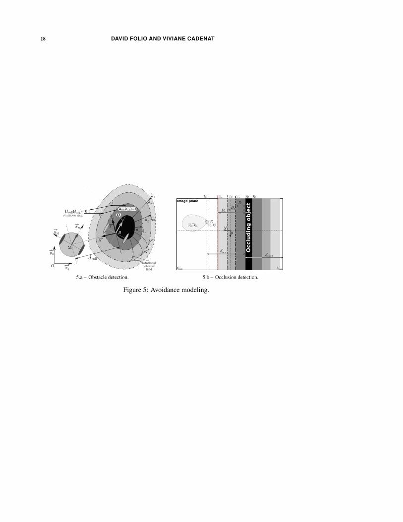
4.2.1. Collision and occlusion detection To perform the desired task, it is necessary

to detect the risks of collision and occlusion. The danger of collision is evaluated

using the data provided by the embedded ultrasonic sensors. From these data, it is

possible to compute the distance dcoll and the relative orientation α between the robot

and the obstacle (see figure 5.a). Let ξ+, ξ0, ξ− be three envelopes which surround

each obstacle at distances d+ > d0 > d−. It is then possible to model the risk of

collision by a parameter µcoll(dcoll) which smoothly increases from 0 when the robot

is far from the obstacle (dcoll > d0) to 1 when it is close to it (dcoll < d−). The occlusion

risk is evaluated in the image by detecting the occluding object left and right borders.

From these data, we can deduce the shortest distance docc between the image features

and the occluding object O as shown on figure 5.b. Defining three envelopes Ξ+, Ξ0,

Ξ− around the occluding object located at D+ > D0 > D− from it, we propose to

model the risk of occlusion by a parameter µocc(docc) which smoothly increases from

0 when O is far from the visual features (docc > D0) to 1 when it is close to them

(docc < D−). Any expression satisfying the previous constraints can be used to define

µcoll(dcoll) and µocc(docc). A possible choice for these parameters can be found in

(Folio and Cadenat 2005a).

4.2.2. Global control law design Our global control strategy relies on the risks of

collision and occlusion, that is on parameters µcoll(dcoll) and µocc(docc). It consists

in two steps. First, we design two controllers allowing respectively to realize the

sole vision-based task and to guarantee non-collision, while dealing with occlusions

if needed. Second, we switch between these two controllers depending on the risk of

collision. There exist several approaches for sequencing robotic tasks (Pissard-Gibollet

and Rives 1995; Soueres and Cadenat 2003; Mansard and Chaumette 2007). . . Here,

we have chosen a method which relies on convex combinations between the successive

controllers (Cadenat et al. 1999). In that case, applications can be more easily carried

out, but it is usually harder to guarantee the task feasibility (see remark 4). Thus, we

propose the following global controller:

q = (1 − µcoll(dcoll)) qvs + µcoll(dcoll)qcoll (15)

where qvs is the previously defined visual servoing controller (14), while

qcoll= (vcoll, ωcoll, coll)T handles obstacle avoidance and visual signal estimation if

necessary. This controller will be designed in the sequel.

Remark 4: Let us notice that µcoll(dcoll) and µocc(docc) are defined to be maintained to 1 once they

have reached this value (Folio and Cadenat 2005a). Moreover, the different envelops are chosen close

enough to reduce the transition phase duration. Thus the control strategy is built to insure that the

robot will be rapidly controlled by the most relevant controller. In this way, the risks of instability,

target loss or collision during the switch are significantly reduced and the task feasibility can be

considered to be guaranteed.

TREATING IMAGE LOSS DURING A VISION-BASED TASK 11

4.2.3. Obstacle avoidance We propose to use a similar obstacle avoidance strategy

to the one used in (Cadenat et al. 1999). The idea is to define around each obstacle

a rotative potential field so that the repulsive force is orthogonal to the obstacle when

the robot is close to it (dcoll < d−), parallel to the obstacle when the vehicle is on ξ0envelop, and slightly directed towards the obstacle between d0 and d+ (see figure 5.a).

The interest of such a potential is that it can make the robot move around the obstacle

without requiring any attractive force, reducing local minima problems. This leads to

the following potential function X(dcoll) (Cadenat et al. 1999):X(dcoll)=

12k1

(1

dcoll− 1

d+

)2

+ 12k2 (dcoll − d+)

2if dcoll ≤ d+,

X(dcoll)=0 otherwise

where k1 and k2 are positive gains to be chosen. The virtual repulsive force is de-

fined to generate the desired rotative potential field around the obstacle by the cou-

ple (F, β), where F = −∂X(dcoll)

∂dcollis the modulus of the virtual repulsive force and

β = α− π2d0

dcoll +π2 its direction wrt. FM . The mobile base velocities vcoll and ωcoll

are then given by (Cadenat et al. 1999):

qbase =(vcoll ωcoll

)T=(kvF cosβ kω

FDx

sinβ)T

(16)

where kv and kω are positive gains to be chosen. Equation (16) drives only the mobile

base in the obstacle neighborhood. However, if the pan-platform remains uncontrolled,

it will be impossible to switch back to the execution of the vision-based task at the end

of the avoidance phase. Therefore, the coll design problem must also be addressed.

Two cases may occur in the obstacle vicinity: either the visual data are available or

not. In the first case, the proposed approach is similar to (Cadenat et al. 1999) and

the pan-platform is controlled to compensate the avoidance motion while centering the

target in the image. As the camera is constrained to move within an horizontal plane,

it is sufficient to regulate to zero the error ecg = Ycg − Y ⋆cg where Ycg and Y ⋆cg are

the current and desired ordinates of the target gravity center. Rewriting equation (1)

as vcr = Jbaseqbase + Jcoll and imposing an exponential decrease to regulate ecgto zero (ecg = L(Ycg)v

cr = −λcgecg, λcg > 0), we finally obtain (see (Cadenat et al.

1999) for more details):

coll =−1

L(Ycg)J(λcgecg + L(Ycg)Jbaseqbase) (17)

where L(Ycg) is the 2nd row of L(Pi) evaluated for Ycg (see equation (3)). However,

if the obstacle occludes the camera field of view, s is no more available and the pan-

platform cannot be controlled anymore using (17). At this time, we compute the visual

features using the analytical solutions (11) and (12), and we deduce an estimation Ycg

of Ycg. The pan-platform controller during an occlusion phase will then be determined

by replacing the real target gravity center ordinate Ycg by the computed one Ycg in

(17), that is: ˜ coll = −1L(Ycg)J

(λcgecg + L(Ycg)Jbaseqbase), where ecg = Ycg − Y ⋆cg,

and L(Ycg) is deduced from (3). Now, it remains to apply the suitable controller to the

pan-platform depending on the context. Recalling that parameter µocc ∈ [0; 1] allows

to detect occlusions, we propose the following avoidance controller:

qcoll =(vcoll, ωcoll, (1 − µocc)coll + µocc ˜ coll

)T(18)

12 DAVID FOLIO AND VIVIANE CADENAT

Thanks to this controller, it is possible to avoid the obstacle while treating — if

needed — the temporary visual features occlusion.

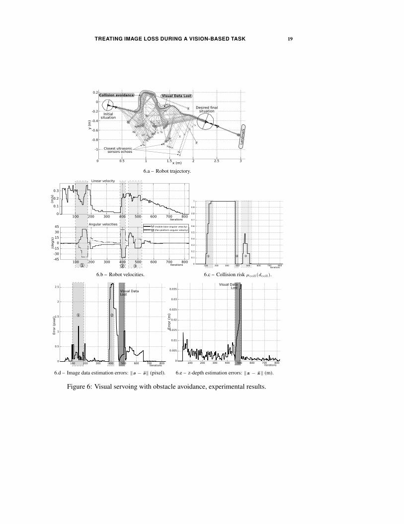
4.2.4. Experimental results We present hereafter some experimental results to vali-

date the proposed approach. In this example, the landmark is made of n = 4 points.

We still consider a positioning navigation task, but, now the environment is cluttered

with one obstacle. Envelopes ξ−, ξ0 and ξ+ are respectively located at d− = 40cm,

d0 = 56cm and d+ = 70cm from the obstacle. Figure 6 present the obtained results.

As one can see, the mission is correctly performed despite the obstacles. Now, let

us describe the sequence of the different events which occurred during the task. At

the beginning of the task, there is no risk of collision, and the visual features are

available. The robot is then controlled using q(s) and starts converging towards the

landmark. Then, it enters the vicinity of the obstacle, inducing a danger of collision.

µcoll(dcoll) increases to reach 1 (see figure 6.c) and the control law applied to the

vehicle smoothly switches to controller qcoll (18). The linear velocity decreases while

the angular velocities ωcoll and coll grow (see figure 6.b) to make the mobile base

avoid the obstacle, while the pan-platform centers the target in the image. When the

obstacle is overcome, µcoll vanishes, the control progressively switches back to q(s)

and the robot is then driven to converge towards the target. However, at this time,

the landmark is manually occluded and we apply controller q(s) instead of q(s). The

vehicle can then keep on executing the mission despite the image data loss. The vision-

based task is then successfully realized (see figure 6.a).

Now, let us analyze the efficiency of the reconstruction. To this aim, we consider

figures 6.d and 6.e which present the values of the norm of the errors ‖s − s‖ and

‖z − z‖. These figures show that these errors increase suddenly when we switch from

one controller to the other. This phenomenon is closely related to the small delay

and drift with which the embedded encoders provide the velocities to our estimation

algorithm. Nonetheless, despite these problems, the errors remain small, showing the

relevance of our approach.

5. CONCLUSIONS AND FUTURE WORKS

In this paper, we have considered the problem of the visual features loss during

a vision-based navigation task. First of all, we have developed a method allowing

to reconstruct these data when they become temporarily unavailable because of an

occlusion or any other unexpected event. Then, we have shown how to embed this

method in our sensor-based control laws to successfully perform the desired missions,

despite the total loss of the image features. Our approach has been properly validated

by experimental tests. Although the proposed reconstruction technique is subject to

drift and limited to short duration visual signal losses, it offers a nice solution to recover

from a problem which generally leads to a task failure. The obtained results clearly

demonstrates the relevance and the interest of the designed approach to improve the

mission execution. Thanks to our method, a wider range of visually guided navigation

tasks is now realizable.

However, the developed analytical solutions are restricted to landmarks which

can be characterized by points and dedicated to a particular robotic system. Therefore,

a natural extension of these works would be to solve this problem for other kinds

of visual features and more complex robots. Furthermore, it would be interesting to

TREATING IMAGE LOSS DURING A VISION-BASED TASK 13

consider a moving landmark instead of a static one and to improve our global control

strategy by sequencing dynamically the different controllers. Finally, we also aim

at testing signal processing techniques such as Kalman filtering to take into account

explicitely the different noises present on our real system.

REFERENCES

Benhimane, S. and E. Malis. 2003. Vision-based control with respect to planar

and non-planar objects using a zooming camera. Proceedings of Int. Conf. on

Advanced Robotics 2: 991–996, Coimbra, Portugal.

Cadenat, V., P. Soueres, R. Swain, and M. Devy. 1999. A controller to perform

a visually guided tracking task in a cluttered environment. Proceedings of

IEEE/RSJ Int. Conf. on Intelligent Robots and Systems 2: 775–780, Korea.

Chaumette, F., S. Boukir, P. Bouthemy, and D. Juvin. 1996. Structure from

controlled motion. IEEE Trans. Pattern Anal. Mach. Intell. 18(5): 492–504.

Chaumette, F. and S. Hutchinson. 2006. Visual servo control, part I: Basic ap-

proaches. IEEE Robot. Autom. Mag. 13(4): 82–90.

Comport, A. I., E. Marchand, and F. Chaumette. 2004. Robust model-based tracking

for robot vision. Proceedings of IEEE/RSJ Int. Conf. on Intelligent Robots and

Systems 1: 692–697, Sendai, Japan.

Corke, P. and S. Hutchinson. 2001. A new partitioned approach to image-based

visual servo control. IEEE Trans. Robot. Autom. 17(4): 507–515.

Espiau, B., F. Chaumette, and P. Rives. 1992. A new approach to visual servoing in

robotics. IEEE Trans. Robot. Autom. 8(3): 313–326.

Favaro, P. and S. Soatto. 2003. Seeing beyond occlusions (and other marvels of a

finite lens aperture). Proceedings of IEEE Comp. Soc. Conf. on Computer Vision

and Pattern Recognition 2: II-579 – II-586, Saint Louis, USA.

Fleury, S. and M. Herrb. 2001. Gen

oM: User Manual. LAAS-CNRS.

Folio, D. 2007. Strategies de commande referencees multi-capteurs et gestion de

la perte du signal visuel pour la navigation d’un robot mobile. Ph. D. thesis,

Universite Paul Sabatier, Toulouse, France.

Folio, D. and V. Cadenat. 2005a. A controller to avoid both occlusions and obstacles

during a vision-based navigation task in a cluttered environment. Proceedings of

European Control Conference: 3898–3903 , Seville, Spain.

Folio, D. and V. Cadenat. 2005b. Using redundancy to avoid simultaneously

occlusions and collisions while performing a vision-based task amidst obstacles.

Proceedings of European Conf. on Mobile Robots, Ancona, Italy.

Folio, D. and V. Cadenat. 2007a. A new controller to perform safe vision-based

navigation tasks amidst possibly occluding obstacles. Proceedings of European

Control Conference, Kos, Greece.

Folio, D. and V. Cadenat. 2007b. Using simple numerical schemes to compute

visual features whenever unavailable. Proceedings of Int. Conf. on Informatics

in Control Automation and Robotics, Angers, France.

14 DAVID FOLIO AND VIVIANE CADENAT

Garcia-Aracil, N., E. Malis, R. Aracil-Santonja, and C. Perez-Vidal. 2005. Contin-

uous visual servoing despite the changes of visibility in image features. IEEE

Trans. Robot. Autom. 21(6): 1214–1220.

Hutchinson, S., G. Hager, and P. Corke. 1996. A tutorial on visual servo control.

IEEE Trans. Robot. Autom. 12(5): 651–670.

Jackson, J., A. Yezzi, and S. Soatto. 2004. Tracking deformable objects under severe

occlusions. Proceedings of IEEE Int. Conf. on Decision and Control 3: 2990–

2995, Atlanta, USA.

Jerian, C. and R. Jain. 1991. Structure from motion: A critical analysis of methods.

IEEE Trans. Syst., Man, Cybern. 21(3): 572–588.

Kyrki, V., D. Kragic, and H. Christensen. 2004. New shortest-path approaches to

visual servoing. Proceedings of IEEE/RSJ Int. Conf. on Intelligent Robots and

Systems 1: 349–355.

Lepetit, V. and P. Fua. 2006. Monocular model-based 3d tracking of rigid objects.

Found. Trends. Comput. Graph. Vis 1(1): 1–89.

Malis, E., F. Chaumette, and S. Boudet. 1999. 2 1/2d visual servoing. IEEE Trans.

Robot. Autom. 15(2): 238–250.

Mansard, N. and F. Chaumette. 2005. A new redundancy formalism for avoidance

in visual servoing. Proceedings of IEEE/RSJ Int. Conf. on Intelligent Robots and

Systems 2: 1694–1700, Edmonton, Canada.

Mansard, N. and F. Chaumette. 2007. Task sequencing for sensor-based control.

IEEE Trans. Robot. Autom. 23(1): 60–72.

Marchand, E. and G. Hager. 1998. Dynamic sensor planning in visual servoing.

Proceedings of IEEE Int. Conf. on Robotics and Automation 3: 1988–1993,

Leuven, Belgium.

Matthies, L., T. Kanade, and R. Szeliski. 1989. Kalman filter-based algorithms for

estimating depth in image sequences. Int. J. of Computer Vision 3(3): 209–238.

Mezouar, Y. and F. Chaumette. 2002. Avoiding self-occlusions and preserving vis-

ibility by path planning in the image. Robotics and Autonomous Systems 41(2):

77–87.

Murray, R., Z. Li, and S. Sastry. 1994. A mathematical introduction to robotic

manipulation. Boca Raton, FL: CRC Press.

Oliensis, J.. 2002. Exact two-image structure from motion. IEEE Trans. Pattern

Anal. Mach. Intell. 24(12): 1618–1633.

Pissard-Gibollet, R. and P. Rives. 1995. Applying visual servoing techniques to

control a mobile hand-eye system. Proceedings of IEEE Int. Conf. on Robotics

and Automation 1: 166–171, Nagoya, Japan.

Remazeilles, A., N. Mansard, and F. Chaumette. 2006. Qualitative visual servoing:

application to the visibility constraint. Proceedings of IEEE/RSJ Int. Conf. on

Intelligent Robots and Systems: 4297–4303, Beijing, China.

Samson, C., M. L. Borgne, and B. Espiau. 1991. Robot Control : The task function

approach (Clarendon Press ed.). Oxford science publications.

TREATING IMAGE LOSS DURING A VISION-BASED TASK 15

Soatto, S. and P. Perona. 1998. Reducing ”structure from motion”: A general frame-

work for dynamic vision part 2: Implementation and experimental assessment.

IEEE Trans. Pattern Anal. Mach. Intell. 20(9): 943–960.

Soueres, P. and V. Cadenat. 2003. Dynamical sequence of multi-sensor based tasks

for mobile robots navigation. Proceedings of Int. IFAC Symp. on Robot Control:

423-428, Wroclaw, Poland.

Thrun, S., D. Fox, W. Burgard, and F. Dallaert. 2001. Robust mote-carlo localization

for mobile robots. Artifial Intelligence 128(1–2): 99–141.

16 DAVID FOLIO AND VIVIANE CADENAT

LIST OF FIGURES

1 The robotic platform. . . . . . . . . . . . . . . . . . . . . . . . . . . 16

2 The control architecture. . . . . . . . . . . . . . . . . . . . . . . . . 16

3 Visual servoing despite camera failure, simulation results. . . . . . . . 17

4 Visual servoing despite camera failure, experimental results. . . . . . 17

5 Avoidance modeling. . . . . . . . . . . . . . . . . . . . . . . . . . . 18

6 Visual servoing with obstacle avoidance, experimental results. . . . . 19

1.a – Nomadic SuperScout II. 1.b – The robot model. 1.c – The pinhole camera model.

Figure 1: The robotic platform.

Figure 2: The control architecture.

TREATING IMAGE LOSS DURING A VISION-BASED TASK 17

3.a – Robot trajectory.

3.b – Image data estimation errors: ‖s−s‖ (pixel). 3.c – z-depth estimation errors: ‖z − z‖ (m).

Figure 3: Visual servoing despite camera failure, simulation results.

4.a – Robot trajectory.

4.b – Image data estimation errors: ‖s − s‖ (pixel). 4.c – z-depth estimation errors: ‖z − z‖ (m).

Figure 4: Visual servoing despite camera failure, experimental results.

18 DAVID FOLIO AND VIVIANE CADENAT

5.a – Obstacle detection. 5.b – Occlusion detection.

Figure 5: Avoidance modeling.

TREATING IMAGE LOSS DURING A VISION-BASED TASK 19

6.a – Robot trajectory.

6.b – Robot velocities. 6.c – Collision risk µcoll(dcoll).

6.d – Image data estimation errors: ‖s − s‖ (pixel). 6.e – z-depth estimation errors: ‖z − z‖ (m).

Figure 6: Visual servoing with obstacle avoidance, experimental results.