
Data-Driven Prediction for Reliable Mission-Critical ...
164
Aalborg Universitet Data-Driven Prediction for Reliable Mission-Critical Communications Lechuga, Melisa Maria Lopez Publication date: 2022 Document Version Publisher's PDF, also known as Version of record Link to publication from Aalborg University Citation for published version (APA): Lechuga, M. M. L. (2022). Data-Driven Prediction for Reliable Mission-Critical Communications. Aalborg Universitetsforlag. Ph.d.-serien for Det Tekniske Fakultet for IT og Design, Aalborg Universitet General rights Copyright and moral rights for the publications made accessible in the public portal are retained by the authors and/or other copyright owners and it is a condition of accessing publications that users recognise and abide by the legal requirements associated with these rights. - Users may download and print one copy of any publication from the public portal for the purpose of private study or research. - You may not further distribute the material or use it for any profit-making activity or commercial gain - You may freely distribute the URL identifying the publication in the public portal - Take down policy If you believe that this document breaches copyright please contact us at [email protected] providing details, and we will remove access to the work immediately and investigate your claim. Downloaded from vbn.aau.dk on: July 09, 2022
-
Upload
khangminh22 -
Category
Documents
-
view
8 -
download
0
Transcript of Data-Driven Prediction for Reliable Mission-Critical ...

Aalborg Universitet
Data-Driven Prediction for Reliable Mission-Critical Communications
Lechuga, Melisa Maria Lopez
Publication date:2022
Document VersionPublisher's PDF, also known as Version of record
Link to publication from Aalborg University
Citation for published version (APA):Lechuga, M. M. L. (2022). Data-Driven Prediction for Reliable Mission-Critical Communications. AalborgUniversitetsforlag. Ph.d.-serien for Det Tekniske Fakultet for IT og Design, Aalborg Universitet
General rightsCopyright and moral rights for the publications made accessible in the public portal are retained by the authors and/or other copyright ownersand it is a condition of accessing publications that users recognise and abide by the legal requirements associated with these rights.
- Users may download and print one copy of any publication from the public portal for the purpose of private study or research. - You may not further distribute the material or use it for any profit-making activity or commercial gain - You may freely distribute the URL identifying the publication in the public portal -
Take down policyIf you believe that this document breaches copyright please contact us at [email protected] providing details, and we will remove access tothe work immediately and investigate your claim.
Downloaded from vbn.aau.dk on: July 09, 2022


Melisa ló
pez lech
ug
aD
ata-D
riven
preD
ictio
n fo
r r
eliab
le Missio
n-c
ritic
al c
oM
Mu
nic
ation
s
Data-Driven preDiction forreliable Mission-critical
coMMunications
byMelisa lópez lechuga
Dissertation submitteD 2022


Data-Driven Prediction forReliable Mission-Critical
Communications
Ph.D. DissertationMelisa López Lechuga
Aalborg UniversityDepartment of Electronic Systems
Fredrik Bajers Vej 7BDK-9220 Aalborg
Dissertation submitted: February 2022
PhD supervisor: Assoc. Prof. Troels Bundgaard Sørensen Aalborg University
Assistant PhD supervisors: Prof. Preben Mogensen Aalborg University
Dr. István Z. Kovács Nokia
Dr. Jeroen Wigard Nokia
PhD committee: Associate Professor Jimmy Jessen Nielsen (chairman) Aalborg University, Denmark
ProfessorSofiePollin The Katholieke Universiteit Leuven (KU Leuven)
Senior Mobile RAN architect Henrik Lehrmann Christiansen TDC NET
PhD Series: Technical Faculty of IT and Design, Aalborg University
Department: Department of Electronic Systems
ISSN (online): 2446-1628ISBN (online): 978-87-7573-941-7
Published by:Aalborg University PressKroghstræde 3DK – 9220 Aalborg ØPhone: +45 [email protected]
© Copyright: Melisa López Lechuga, except where otherwise stated.
Printed in Denmark by Rosendahls, 2022

Curriculum Vitae
Melisa López Lechuga
Melisa López Lechuga received her B.Sc. and M.Sc. degrees in telecommuni-cation engineering from Universitat Politecnica de Catalunya (ETSETB-UPC,Barcelona, Spain) in 2016 and 2018, respectively. Since 2018, she pursues herPhD degree at the Electronic Systems Department from Aalborg University(Denmark) in collaboration with Nokia Bell Labs. Her research interests in-clude radio propagation, field measurements, and cellular-based connectivityfor mission-critical communications.
iii

Curriculum Vitae
iv

Abstract
5G New Radio (NR) technology is expected to provide connectivity to a widevariety of services with different Quality of Service (QoS) requirements. Forsome applications, Key Performance Indicators (KPIs) such as reliability, la-tency, or data rate may have stringent targets, which will be challenging tomeet with the existing Radio Resource Management (RRM), QoS, and mo-bility management procedures. These procedures are mostly reactive, i.e.,a service degradation is only mitigated once it has already occurred. Hav-ing some prior knowledge of the network conditions that the User Equip-ment (UE) will experience can help avoid a situation that may be criticalfor the service. Specifically, the service could benefit from a more proac-tive QoS management in the so-called mission-critical communications, suchas Vehicle-To-Everything (V2X) or Unmanned Aerial Vehicles (UAV) usingcellular networks. The need for this approach is stated by associations andgroups such as the 5G Automotive Association (5GAA) or the Aerial Connec-tivity Joint Activity (ACJA). Both consider a context where the network canpredict changes in the QoS.
A relevant parameter involved in the RRM decisions, as well as for QoSprediction, is the signal level experienced by a UE, typically expressed usingthe Reference Signal Received Power (RSRP). RSRP is a key metric, as it isused for several procedures such as cell selection and re-selection, or powercontrol. Therefore, estimating the signal level is essential when designinga reliable system. Accurate estimations of the RSRP levels that the UE willexperience along the path could provide in-advance information on the ex-pected service availability and reliability conditions. This thesis studies theuse of RSRP estimations to predict potential critical areas along the knownmoving path of a UE using a mission-critical service. The use of ray-tracingor empirical models versus a measurement-based approach for RSRP estima-tion is analyzed. The Ph.D. project answers research questions such as: Howaccurate can signal strength be estimated using measurement data? Canmeasurement data reported by UEs that have previously passed through thesame location be used to estimate the signal level that a UE will experiencein that same location? Can that estimation be corrected using UE context in-
v

Abstract
formation? Can the RSRP estimations be used to predict the expected criticalareas along the route? These questions are investigated for the V2X and UAVuse cases.
Firstly, a new approach for estimating the serving signal level that a UEwill observe along the route is studied. We analyze the achievable accuracyof a data-driven estimation method, consisting of the aggregation of the mea-surements recorded by multiple UEs in a certain location. The estimation islocation-based, i.e., the measurements are aggregated regardless of the cellthat is serving the user, such that the estimation is valid for any UE passingthrough that location. Secondly, we evaluate the accuracy provided by a ray-tracing tool and two empirical models when estimating the signal variationsthat the user will experience along the route. For that purpose, the estima-tions are compared to experimental data. The study is done for ground-leveland UAV measurement data. Therefore, multiple drive tests and UAV fieldmeasurements have been performed during this Ph.D. in urban and ruralenvironments in Denmark. Results show that the data-driven approach im-proves the estimation error over the traditional techniques studied. This workalso investigates how the estimation error can be further reduced by predict-ing the mean individual offset that each specific UE will observe with respectto the initially estimated value once the UE starts moving along the path.The different results observed for ground compared to airborne predictionsare also discussed. Lastly, the work includes an evaluation of how to use theRSRP estimations to calculate the probability that there is a service outage interms of service availability and reliability. Results show that the data-drivenestimation approach allows detecting at least 70 % of the existing critical ar-eas.
vi

Resumé
5G New Radio (NR) teknologien forventes at kunne skabe forbindelse tilen lang række services med forskellige krav til Quality of Service (QoS).For visse applikationer er der udfordrende krav til performance indikatorer(KPI’er) såsom pålidelighed, forsinkelse eller datarate, og som derfor bliveren udfordring at imødekomme med de eksisterende procedurer til håndter-ing af radioresourcer (RRM), QoS, og mobilitet. Disse procedurer er for detmeste reaktive, dvs. en serviceforringelse kan først afbødes efter, at den harfundet sted. Et forudgående kendskab til hvilke netværksforhold en terminal(UE) vil komme ud for, kan hjælpe med at undgå en ellers kritisk situationfor den benyttede service. Specielt services kategoriseret som missionskritiskkommunikation, eksempelvis Vehicle-To-Everything (V2X) eller UnmannedAerial Vehicles (UAV) via cellulære netværk, kunne drage fordel af en mereproaktiv QoS håndtering. Behovet for denne tilgang er dokumenteret af sam-menslutninger og arbejdsgrupper såsom 5G Automotive Association (5GAA)og Aerial Connectivity Joint Activity (ACJA) der begge tager udgangspunkti en kontekst, hvor netværket kan forudsige ændringer i QoS.
En relevant parameter, som har betydning for radioresourcehåndtering,såvel som for prædiktion af QoS, er signalniveauet ved terminalen - typiskudtrykt ved Reference Signal Received Power (RSRP). RSRP er en væsentligperformance indikator, da den bliver brugt i mange radiorelaterede proce-durer såsom valg og skift af radiocelle, eller justering af sendeeffekten. Deter derfor vigtigt at estimere signalniveauet, når man vil designe et pålideligtsystem. Præcise estimeringer af RSRP-niveauer, som terminalen oplever langsen given rute, kan give forhåndsinformation om service-tilgængelighed ogpålidelighed. Denne afhandling har fokus på brugen af RSRP-estimeringer,til at forudsige eventuelle kritiske områder i brugen af en missionskritiskservice, når terminalen bevæger sig langs en given kendt rute. Brugen afray-tracing (RT) eller empiriske modeller, versus en målebaseret tilgang tilestimering af RSRP, analyseres i afhandlingen. Ph.D. projektet besvarer vi-denskabelige spørgsmål som: Hvor nøjagtigt kan man estimere signalstyrkeved brug af måledata? Kan måledata rapporteret af terminaler, som tidligerehar passeret igennem samme lokation, bruges til at estimere det signalniveau,
vii

Resumé
som en terminal vil opleve i denne samme lokation? Kan denne estimer-ing korrigeres ved at bruge kontekstinformation? Kan RSRP estimeringernebruges til at forudsige de forventede kritiske områder langs ruten? Dissespørgsmål undersøges for både V2X og UAV brugsscenarier.
Først undersøges en ny tilgang for estimering af det signalniveau, som enterminal observerer langs ruten. Vi analyserer den opnåelige nøjagtighed afen data-drevet estimeringsmetode, som består af en aggregering af målingerfra flere terminaler på en bestemt lokation. Estimeringen er lokationsspecifik,dvs. målingerne aggregeres uden hensyn til den radiocelle, som servicererbrugeren, således at estimeringen er gyldig for en hvilken som helst termi-nal, der passerer den bestemte lokation. Dernæst evaluerer vi nøjagtighedenaf RT og to udvalgte empiriske modeller til estimering af de signalvaria-tioner som terminalen oplever langs ruten, i en sammenligning med eksperi-mentelle data. Undersøgelsen er udført med eksperimentelle data for V2X ogUAV scenarier som er indsamlet gennem adskillige felteksperimenter underkørsel langs vej og flyvning i lav højde i by- og landområder. Resultaterneviser, at den data-drevne tilgang forbedrer estimeringsfejlen i sammenligningmed de undersøgte traditionelle teknikker. Afhandlingen undersøger også,hvordan estimeringsfejlene kan reduceres yderligere når terminalen er startetpå ruten, ved at prædiktere det terminalspecifikke offset som hver terminalvil opleve i forhold til det overordnede og initialt estimerede signalniveau.Afvigelsen mellem resultater for V2X og UAV scenariet diskuteres i afhan-dlingen. Endelig indeholder afhandlingen også en evaluering af, hvordanman benytter RSRP estimeringer til at beregne sandsynligheden for, at der etserviceudfald mht. service-tilgængelighed og pålidelighed. Resultater viser,at man ved den data-drevne estimering kan detektere mindst 70 % af deeksisterende kritiske områder.
viii

Contents
Curriculum Vitae iii
Abstract v
Resumé vii
Glossary xiii
Thesis Details xvii
Acknowledgements xix
I Thesis Summary 1
1 Introduction 31 Mission-Critical Communications . . . . . . . . . . . . . . . . . 4
1.1 Vehicle-To-Everything . . . . . . . . . . . . . . . . . . . . 61.2 Unmanned Aerial Vehicles . . . . . . . . . . . . . . . . . 91.3 The need for RSRP Estimation . . . . . . . . . . . . . . . 12
2 Objectives of the Thesis . . . . . . . . . . . . . . . . . . . . . . . 133 Research Methodology . . . . . . . . . . . . . . . . . . . . . . . . 154 Contributions . . . . . . . . . . . . . . . . . . . . . . . . . . . . . 165 Thesis Outline . . . . . . . . . . . . . . . . . . . . . . . . . . . . . 19References . . . . . . . . . . . . . . . . . . . . . . . . . . . . . . . . . . 20
2 Signal Level Estimation 251 Impacting Factors . . . . . . . . . . . . . . . . . . . . . . . . . . . 252 Traditional Estimation Approaches . . . . . . . . . . . . . . . . . 26
2.1 Empirical Models . . . . . . . . . . . . . . . . . . . . . . . 272.2 Ray-Tracing . . . . . . . . . . . . . . . . . . . . . . . . . . 292.3 Using Drive Tests to Improve the Estimations . . . . . . 30
3 New Estimation Approaches . . . . . . . . . . . . . . . . . . . . 31
ix

Contents
References . . . . . . . . . . . . . . . . . . . . . . . . . . . . . . . . . . 32
3 Data-Driven Estimation Approach 351 Measurement Campaigns . . . . . . . . . . . . . . . . . . . . . . 35
1.1 V2X Data Collection . . . . . . . . . . . . . . . . . . . . . 361.2 UAV Data Collection . . . . . . . . . . . . . . . . . . . . . 37
2 Data-Driven Estimation . . . . . . . . . . . . . . . . . . . . . . . 372.1 Pre-Service Stage . . . . . . . . . . . . . . . . . . . . . . . 372.2 On-service Stage . . . . . . . . . . . . . . . . . . . . . . . 40
3 Outage Probability Estimation . . . . . . . . . . . . . . . . . . . 413.1 Service Availability . . . . . . . . . . . . . . . . . . . . . . 423.2 Service Reliability . . . . . . . . . . . . . . . . . . . . . . 43
4 Summary of Main Findings . . . . . . . . . . . . . . . . . . . . . 44
4 Conclusions 49
II Papers 53
A Experimental Evaluation of Data-driven Signal Level Estimation inCellular Networks 551 Introduction . . . . . . . . . . . . . . . . . . . . . . . . . . . . . . 572 Measurement Campaign . . . . . . . . . . . . . . . . . . . . . . . 593 Data Processing . . . . . . . . . . . . . . . . . . . . . . . . . . . . 614 Results . . . . . . . . . . . . . . . . . . . . . . . . . . . . . . . . . 64
4.1 Rural Environment . . . . . . . . . . . . . . . . . . . . . . 644.2 Urban Environment . . . . . . . . . . . . . . . . . . . . . 66
5 Discussion and Conclusion . . . . . . . . . . . . . . . . . . . . . 68References . . . . . . . . . . . . . . . . . . . . . . . . . . . . . . . . . . 70
B Measurement-Based Outage Probability Estimation for Mission-CriticalServices 731 Introduction . . . . . . . . . . . . . . . . . . . . . . . . . . . . . . 75
1.1 Contributions . . . . . . . . . . . . . . . . . . . . . . . . . 761.2 Related Work . . . . . . . . . . . . . . . . . . . . . . . . . 77
2 Service Reliability Provisioning . . . . . . . . . . . . . . . . . . . 783 Measurement Campaign . . . . . . . . . . . . . . . . . . . . . . . 80
3.1 Measurement Setup . . . . . . . . . . . . . . . . . . . . . 803.2 RSRP Recording . . . . . . . . . . . . . . . . . . . . . . . 82
4 Data-Driven Estimation Technique . . . . . . . . . . . . . . . . . 834.1 Estimation Accuracy and Performance Comparison . . . 86
5 Mean Individual Offset Correction . . . . . . . . . . . . . . . . . 905.1 Pre-service . . . . . . . . . . . . . . . . . . . . . . . . . . . 905.2 On-Service . . . . . . . . . . . . . . . . . . . . . . . . . . . 92
x

Contents
6 Outage Probability Estimation . . . . . . . . . . . . . . . . . . . 946.1 Service Availability . . . . . . . . . . . . . . . . . . . . . . 946.2 Service Reliability . . . . . . . . . . . . . . . . . . . . . . 100
7 Conclusion . . . . . . . . . . . . . . . . . . . . . . . . . . . . . . . 102References . . . . . . . . . . . . . . . . . . . . . . . . . . . . . . . . . . 103
C Shadow Fading Spatial Correlation Analysis for Aerial Vehicles:Ray tracing vs. Measurements 1071 Introduction . . . . . . . . . . . . . . . . . . . . . . . . . . . . . . 1092 Methodology . . . . . . . . . . . . . . . . . . . . . . . . . . . . . 110
2.1 Field Measurements . . . . . . . . . . . . . . . . . . . . . 1102.2 Ray Tracing Model . . . . . . . . . . . . . . . . . . . . . . 1112.3 Shadow Fading Estimation . . . . . . . . . . . . . . . . . 114
3 Results . . . . . . . . . . . . . . . . . . . . . . . . . . . . . . . . . 1153.1 Correlation Coefficients between measurements and pre-
dictions . . . . . . . . . . . . . . . . . . . . . . . . . . . . 1153.2 Shadowing distribution . . . . . . . . . . . . . . . . . . . 115
4 Discussion . . . . . . . . . . . . . . . . . . . . . . . . . . . . . . . 1165 Conclusion . . . . . . . . . . . . . . . . . . . . . . . . . . . . . . . 117References . . . . . . . . . . . . . . . . . . . . . . . . . . . . . . . . . . 119
D Service Outage Estimation for Unmanned Aerial Vehicles: A Measurement-Based Approach 1231 Introduction . . . . . . . . . . . . . . . . . . . . . . . . . . . . . . 1252 UAV Radio Measurements . . . . . . . . . . . . . . . . . . . . . . 1263 Signal Level and Outage Estimations . . . . . . . . . . . . . . . . 127
3.1 Individual Offset Correction . . . . . . . . . . . . . . . . 1283.2 Service Outage Probability . . . . . . . . . . . . . . . . . 130
4 Results . . . . . . . . . . . . . . . . . . . . . . . . . . . . . . . . . 1314.1 Service Outage Estimation . . . . . . . . . . . . . . . . . 132
5 Discussion and Conclusions . . . . . . . . . . . . . . . . . . . . . 136References . . . . . . . . . . . . . . . . . . . . . . . . . . . . . . . . . . 137
xi

Contents
xii

Glossary
1G 1st Generation
2G 2nd Generation
3G 3rd Generation
3GPP 3rd Generation Partnership Project
4G 4th Generation
5G 5th Generation
5GAA 5G Automotive Association
ACJA Aerial Connectivity Joint Activity
BLER Block Error Rate
BS Base Station
BVLOS Beyond Visual Line-of-Sight
C2 Command and Control
DL Downlink
DPM Dominant Path Model
eMBB Enhanced Mobile Broadband
FN False Negative
FNR False Negative Rate
FP False Positive
FPR False Positive Rate
GNSS Global Navigation Satellite System
xiii

Glossary
GPS Global Positioning System
GRU Gated Recurrent Unit
HO Handover
IMT-2020 International Mobile Telecommunications for 2020 and beyond
IRT Intelligent Ray Tracing
ITU International Telecommunications Union
KPI Key Performance Indicators
LOS Line-Of-Sight
LSTM Long Short Memory Term
LTE Long Term Evolution
MAE Mean Absolute Error
mcMTC Mission-critical Machine Type Communications
MCS Modulation and Coding Scheme
MDT Minimization of Drive Tests
MIO Mean Individual Offset
ML Machine Learning
mMTC Massive Machine Type Communications
mmW Millimiter Wave
MNOs Mobile Network Operators
MTC Machine Type Communications
NLOS Non-Line-Of-Sight
NN Neural Networks
NR New Radio
NWDAF Network Data Analytics Function
PCI Physical Cell ID
QoS Quality of Service
RAN Radio Access Network
xiv
Glossary
REM Radio Environment Maps
RLF Radio Link Failure
RMSE Root Mean Square Error
RRM Radio Resource Management
RSRP Reference Signal Received Power
RSRQ Reference Signal Received Quality
RSSI Received Signal Strength Indicator
SF Shadow Fading
SIR Signal-To-Interference-Plus-Noise Ratio
SIR Signal-To-Interference Ratio
SNR Signal-To-Noise Ratio
SON Self-Organizing Networks
SS Signal Strength
TN True Negative
TNR True Negative Rate
TP True Positive
TPR True Positive Rate
UAV Unmanned Aerial Vehicles
UE User Equipment
UL Uplink
URLLC Ultra-Reliable Low-Latency Communications
V2I Vehicle-To-Infrastructure
V2N Vehicle-To-Network
V2P Vehicle-To-Pedestrian
V2V Vehicle-To-Vehicle
V2X Vehicle-To-Everything
xv

Glossary
xvi

Thesis Details
Thesis Title: Quality of Service Enhancements for Reliable Communi-cations for Aerial and Terrestrial Vehicles using CellularNetworks
Ph.D. Student: Melisa LópezSupervisors: Prof. Troels Bundgaard Sørensen, Aalborg UniversityCo-supervisors: Prof. Preben Mogensen, Aalborg University
István Z. Kovács, NokiaJeroen Wigard, Nokia
This PhD thesis is the outcome of three years of research at the WirelessCommunication Networks (WCN) section (Department of Electronic Sys-tems, Aalborg University, Denmark) in collaboration with Nokia (Aalborg).The work was carried out in parallel with mandatory courses required to ob-tain the PhD degree. The papers supporting the work presented in the thesiswere published in peer-reviewed journals and conferences.
The main body of the thesis consists of the following articles:
Paper A: M. López, T. B. Sørensen, I. Z. Kovács, J. Wigard and P. Mogensen,“Experimental Evaluation of Data-driven Signal Level Estimationin Cellular Networks”, IEEE 94th Vehicular Technology Conference(VTC2021-Fall), September 2021.
Paper B: M. López, T. B. Sørensen, I. Z. Kovács, J. Wigard and P. Mogensen,"Measurement-Based Outage Probability Estimation for Mission-Critical Services," IEEE Access, vol. 9, pp. 169395-169408, 2021.
Paper C: M. López, T. B. Sørensen, P. Mogensen, J. Wigard and I. Z. Kovács,“Shadow fading spatial correlation analysis for aerial vehicles:Ray tracing vs. measurements”, IEEE 90th Vehicular TechnologyConference (VTC2019-Fall), September 2019.
Paper D: M. López, T. B. Sørensen, J. Wigard, I. Z. Kovács and P. Mo-gensen, "Service Outage Estimation for Unmanned Aerial Vehi-cles: A Measurement-Based Approach", IEEE Wireless Commu-
xvii

Thesis Details
nications and Networking Conference (WCNC) 2022, Accepted forpublication.
This thesis has been submitted for assessment in partial fulfilment of thePhD Degree. The thesis is based on the submitted or published papers thatare listed above. Parts of the papers are used directly or indirectly in theextended summary of the thesis. As part of the assessment, co-author state-ments have been made available to the Doctoral School of Engineering andScience at AAU and also to the assessment committee.
xviii

Acknowledgements
This thesis is the outcome of more than three years of work that I could nothave done alone, so I take this opportunity to thank all the people that havehelped me through it.
First, I would like to thank my supervisors for their support and guid-ance during these years. Having four supervisors was not always easy, buteach contributed in his way. I thank Troels B. Sørensen for thoroughly re-viewing all my papers and this thesis, which helped produce high-qualitymaterial. Jeroen Wigard for always having the right words and helping mebuild a business point of view for my project; István Z. Kovács for his endlesssupport, knowledge, and good advice; and Preben Mogensen for his criticalpoint of view that always helped me find my way during the project.
I would like to give a special mention to my non-official advisor, Igna-cio Rodríguez. Your technical and personal coaching, and the beers in myterrace, have always come at the right time and lifted me up in the lowmoments. I also thank all my colleagues in AAU and Nokia for provid-ing a friendly working environment and good technical discussions. Specialthanks to the international alliance, the funny not-so-technical discussions,the Friday breakfasts, and the multiple lunch breaks talking about everythingand nothing at the same time. Also, thanks to Dorthe Sparre for efficientlysolving all my questions with a nice smile.
On the personal side, I should thank many people—Majken and Dani, forthe sushi and wine nights and for always having my back. Roberto, for en-couraging me to pursue this Ph.D. and supporting me in the bad moments.Elisa, for the walks, the ice-creams, the honest conversations, and your con-tagious joy. Mundo, for all the efforts made to understand what this meantto me and helping me believe in myself, this achievement is partly yours.
I cannot forget my international friends. Living abroad is never easy, butI always managed to find the right people to make Aalborg feel like home(despite the weather). Many of them are still in Denmark, and many othersleft, but they all contributed to making my time here lovely and enjoyable.Special thanks to María, Mada, Lisha, Emilio, Marta, David, Pilar, Filipa, andJoao for all the fun, the trips, the nights out, the board games, the volleyball,
xix

Acknowledgements
and the endless amount of activities and plans that made all these years muchbetter. Thank you to my friends in Mallorca and Barcelona for supporting mein the distance and constantly reminding me that the sun is always shiningeven if you cannot see it! A special shout out to Thomas, who never quitsending bad jokes to make my days slightly better.
I would not have made it through this Ph.D. without Enric. Thank you forthe insane amount of steps (figurative and literally) that led us where we aretoday. For acting as my left hemisphere whenever I needed it and letting myright one take over yours every once in a while. For always being my homeand my balance. You have been a friend and a partner during the past 12years and have not disappointed me even once. I love you and your terriblesense of humor.
Last, I would like to thank my family for the unconditional support theyhave given me in every step I have taken in my life and for making mefeel them close even in the distance. Special thanks to my siblings for theirannoying way of telling me that I am "the smart one". And to my parents.You two have always given me everything I needed to get where I wanted tobe. You all are the best family I could ask for, and I will always be thankfulfor that.
Melisa LópezAalborg University, February, 2022.
xx

Part I
Thesis Summary
1

Chapter 1
Introduction
Wireless communications has become essential in our personal and profes-sional lives and currently plays a crucial role in the global economy anddevelopment. It was initially designed for human-centric communicationpurposes: from voice services in the 1st Generation (1G) to data services withincreasing data rates in the 2nd Generation (2G), 3rd Generation (3G) and 4thGeneration (4G). The rapid advance of technology has motivated the need tosupport new applications, and cellular communications is the main candi-date. The 5th Generation (5G) NR is expected to serve the new emerging usecases which, according to the International Telecommunications Union (ITU)International Mobile Telecommunications for 2020 and beyond (IMT-2020),are grouped in three different categories [1]:
• Enhanced Mobile Broadband (eMBB): Includes all the services focus-ing on human-centric communication. The demand for multi-mediacontent, data, and voice services has only increased over the years. This5G use case focuses on providing higher data rates, improved perfor-mance, and seamless user experience.
• Ultra-Reliable Low-Latency Communications (URLLC): Also knownas Mission-critical Machine Type Communications (mcMTC) [2], this5G use case is characterized by the high reliability, low latency, andhigh availability requirements of the services involved.
• Massive Machine Type Communications (mMTC): This use case refersto services with a large number of devices such as sensors or actuatorsthat typically transmit small amounts of non-sensitive data, are lowcost, and have low power consumption.
Examples of the three 5G categories can be seen in Fig. 1.1: from voiceand data services with increased data rates to smart cities, remote surgery,augmented reality, connected vehicles, drones, and many other applications.
3

Chapter 1. Introduction
Fig. 1.1: Usage scenarios of IMT-2020 [1].
Manufacturing companies and standard organizations have invested theirresources in developing the different cellular telecommunications technolo-gies and have jointly formed the 3rd Generation Partnership Project (3GPP),which provides system description and specifications for each technologyand their multiple scenarios and use cases. The following section includesthe description, main challenges, and requirements for the specific use casesstudied in this thesis.
1 Mission-Critical Communications
The definition of mission-critical communications can be broad, but it allcomes down to the same main requirement: high reliability. Seamless andreliable connectivity is essential since a failure may pose a risk to humanlife [3]. This type of communication was initially meant to provide commu-nication between emergency services such as police, ambulances, or firefight-ers. Nowadays, the term can apply to many other industries and applicationsamong the increasing number of use cases in the 5G NR. Examples suchas remote surgery, real-time automation, connected vehicles, or autonomousrobotics, where a communication failure can have severe consequences, showthe need for robust and reliable communication at any time.
Within the 5G categories, mission-critical communications is enclosed inthe mcMTC, which entails new and completely different needs that were
4

1. Mission-Critical Communications
not a concern in conventional (handheld) communications. Mainly, mission-critical applications are characterized by three requirements:
• High-reliability: different definitions can be found in the 3GPP spec-ifications depending on the context. For network layer packer trans-missions, it is defined as the percentage of successfully delivered pack-ets within the time constraint required by the target service [4]. ForPHY/MAC layer transmissions, it is often evaluated using the BlockError Rate (BLER) i.e., the ratio of failed packets to the total number oftransmitted packets [5].
• High-availability: as described in [6], availability is the probability thatthe network can provide service. In [7], the authors claim that it couldalso be included within the definition of reliability since it indicates theprobability of establishing a safe communication link.
• Low- and Ultra-low latency: latency typically refers to the time elapsedfrom the generation of a data packet in the transmitter until it is cor-rectly decoded at the receiver. 3GPP distinguishes between user planelatency, control plane latency [4] and end-to-end latency [8].
• Scalability: as explained in [9], the network should be able to dynam-ically adjust its resources to the number of devices per coverage areaand their different service requirements.
The requirements may vary depending on the use case and the service thenetwork aims to provide. There are very stringent use cases such as remotesurgery with latency below 1 ms and a BLER of 10−9 [10], and use cases withmore relaxed requirements such as automation with latency requirement ofmaximum 100 ms and a 10−1 BLER [11]. The constant growth in demand formcMTC has motivated Mobile Network Operators (MNOs), standardizationbodies, and academic researchers to investigate potential solutions to meetthese requirements.
This thesis contributes towards the fulfillment of the mission-critical com-munication requirements, focusing on two use cases: V2X and UAVs. Thesolutions proposed in Chapter 3 contribute to ensure service availability andservice reliability in the studied scenarios. The following sub-sections pro-vide definitions, requirements, and challenges, of the V2X and UAV1 usecases. A review of potential solutions available in the state-of-the-art is alsoincluded.
1Also termed Uncrewed Aerial Vehicles or drones.
5

Chapter 1. Introduction
1.1 Vehicle-To-Everything
Vehicular communications has been considered a key use case within the 5Gemerging services [12]. The general V2X term includes Vehicle-To-Infrastructure(V2I), Vehicle-To-Network (V2N), Vehicle-To-Pedestrian (V2P), and Vehicle-To-Vehicle (V2V) communications. Examples of these are self-driving cars,collision avoidance, vehicle traffic optimization, speed regulation, pedestriansafety notifications, or communication with V2X application services [13].These are safety-critical applications and, therefore, will all have very strin-gent QoS requirements [14]. In this sub-section, we present the main require-ments and challenges and review the recent literature addressing them. Thekey QoS requirements for the V2X use case and related service applicationsare [15]:
1. Support of high radio dynamics. Not only the UE will be moving atrelatively high speeds, but also the surrounding environment will bevariant, and the objects around may be in motion. Considering also thespatio-temporal changes in the wireless network, the different Key Per-formance Indicators (KPI) experienced by the UE will fluctuate rapidly.These fluctuations may implicitly lead to worse QoS performance [16].
2. Extremely low-latency. This requirement is meant for cases such as col-lision avoidance, pedestrian safety notifications, and other situationalawareness examples, which are time-critical. End-to-end latency re-quirements as low as 3 ms are observed for some applications.
3. High capacity. The massive number of connected vehicles and the re-quired signaling will lead to a high volume of messages. Among others,efficient resource allocation is required.
4. High reliability and availability. These are required especially forsafety-critical applications, where reliability and availability of the com-munication link need to be ensured before and during the service.
5. Extremely high security and privacy. There is a need for data andprivacy protection since there will be broadcast messages from vehicleto vehicle or from vehicle to network containing the vehicle’s speed,location, or other relevant information that can be used to harm thevehicle or the service.
A common assumption for V2X service studies is that the UE’s route isknown or can be predicted before the service starts, since vehicles can usuallyprovide information on their starting location and final destination. Somestudies aim at optimizing the route based on the expected radio conditions.An example is [17], the authors present a real-time route planning modelconsidering the information collected by the network.
6

1. Mission-Critical Communications
Furthermore, as stated by the 5GAA in [18], the service would stronglybenefit from predicting the expected changes in QoS. In-advance awarenessof potential QoS degradation allows the network to counteract before thedegradation occurs, adapting to future conditions and reducing or avoidingcompletely its consequences.
QoS prediction can be performed at different entities of the communica-tion link:
• Network-based QoS prediction: provide predicted QoS notificationsbased on real-time KPIs available on the network side. The networkKPIs are typically averaged over a certain period and therefore cannotobserve the rapid fluctuations mentioned above. An example is pre-sented in [19], where the authors discuss the use of machine learningtechniques to predict the performance of the network where UE data isnot available.
• UE-based QoS prediction: The prediction is performed at the UE sideand uses real-time KPIs. An example can be seen in [20], where the au-thors use RSRP and Reference Signal Received Quality (RSRQ) samplesavailable at the UE to perform data rate prediction.
• Combined approach: using real-time UE information combined withnetwork data to perform QoS predictions [21].
Relevant prediction-related contributions can be found in the availableliterature for cellular V2X communications. The authors of [22] proposea statistical learning framework for predicting QoS in V2X. The presentedframework combines the prediction of channel model characteristics usingcontextual information with a statistical learning model to predict QoS. Aqualitative performance assessment is included using an example with simu-lation data. A similar scheme is proposed in [16], where the authors analyzethe necessary functions to predict QoS for a certain time horizon using real-time measurements.
Since mobility is one of the main reasons for service degradation due tothe Handover (HO) procedure, there are several publications in the litera-ture aiming at predicting HO and mobility-related parameters. An exampleis [23], where the authors combine a vector auto-regression model and aGated Recurrent Unit (GRU) to predict user trajectory and use the results tooptimize the HO procedure and reduce signaling. Their proposed algorithmreduces HO processing costs by 57 % and transmission costs by 28 %. Theauthors of [24] propose two prediction schemes for HO prediction based onchannel features. They evaluate the performance using simulation data indifferent scenarios, showing that the proposed schemes reduce the numberof unnecessary HOs. Both schemes outperform the existing ones. The first
7

Chapter 1. Introduction
achieves a prediction success of 99 % using Received Signal Strength Indica-tor (RSSI) values of all surrounding Base Station (BS)s, and the second showsthe same success rate by using Signal-To-Noise Ratio (SNR), RSSI, availablebandwidth and UE data rate.
Due to the latency-critical applications, latency is considered a relevantKPI for prediction. In [25], they propose a prediction framework combiningMachine Learning (ML) and statistical approaches that uses RSRP, RSRQ, andpast latency samples to predict latency. They use measurement data from dif-ferent locations in an urban environment to show that the proposed approachcan reduce the estimation error and the corresponding standard deviation by45 % and 25 %, respectively, compared to other approaches. The authorsof [21] also predict latency inputting measurement data from an urban sce-nario to a Neural Networks (NN). They propose a classification predictionbased on a threshold, and use expected end-to-end delay, speed, Signal-To-Interference-Plus-Noise Ratio (SIR), RSRP, and RSSI to predict whether la-tency will be below or above the threshold. They show that their approachachieves f1-scores (the harmonic mean of precision and recall [26]) of up to88%, which they considered insufficient accuracy for safety-related applica-tions.
Those applications in which a minimum throughput is required will ben-efit from throughput prediction, as it will allow to detect potential servicedegradation. In [27], the authors show throughput prediction using a ran-dom forest algorithm. As inputs, they use UE category and cell frequencyband, physical layer radio measurements collected at the UE (RSRP, RSRQ,and RSSI), context information (indoor/outdoor conditions, distance UE-BS,UE speed), and Radio Access Network (RAN) measurements (average cellthroughput, BLER, and others). For performance evaluation, they use themedian absolute error ratio, which is defined as the absolute value of thedifference between the predicted and the actual throughput, divided by theactual throughput. Their algorithm reaches a median absolute error ratio of0.1. The work presented in [28] uses simulation data to evaluate the use ofLong Short Memory Term (LSTM) networks to predict uplink throughputfor a time window of 7 s. They input network-related parameters and QoSmetrics (location, speed, distance to serving cell, cell load percentage, andobserved uplink throughput at time t) to the LSTM network, and obtain anoverall Root Mean Square Error (RMSE) of 2.5 Mbps, and 3.5 Mbps at the 7thsecond.
Other KPIs have been investigated for prediction, depending on the ser-vice requirements that the authors are targeting to meet. The authors in [29]conduct a study to predict cellular bandwidth using past throughput samplesand lower layer information from real-time experimental data, and proposean ML framework that provides accurate predictions. With a time granular-ity of 1 s, they show an average prediction error in the range of 3.9% to 19%
8

1. Mission-Critical Communications
in all the studied scenarios (stationary and highway drive test). The workin [30] studies the performance of deep NNs to predict packet loss usingV2X throughput as input. Their work is based on simulation data and theproposed model provides accurate results, with RMSE values between 0.02and 0.5.
The above-presented studies show the wide variety of KPIs that can bepredicted to improve the QoS experienced by a user. There are differentprediction methods, many of them based on ML, and the accuracy variesdepending on the predicted parameter and the approach used. The vastavailable state of the art shows the need for predictive algorithms for V2Xservices using cellular networks, where simulated data is commonly usedfor performance evaluation. In addition, many of them use signal strengthas an input to the prediction algorithm, which evidences the relevance ofthat parameter for QoS prediction. This will be further developed in sub-section 1.3, where the importance of RSRP and the benefits of its predictionfor mission-critical use cases are motivated.
1.2 Unmanned Aerial Vehicles
The UAV market has experienced a rapid expansion in recent years. New ap-plications such as infrastructure monitoring and inspection, entertainment in-dustry, delivery of goods, or search and rescue motivated the need to providesafe and reliable communication between the UAV and its controller [31]. Es-tablishing a reliable Command and Control (C2) link is essential for the op-eration of UAVs through cellular networks Beyond Visual Line-of-Sight (BV-LOS) since it carries flight-related information that needs to be exchanged be-tween the drone and its controller [32]. We consider as relevant safety-criticalapplications those where the drone is remotely controlled over cellular net-works using the C2 link.
Different requirements are introduced by 3GPP in [33], depending on theservice. For the C2 link, data rates up to 100 kb/s and packet error lowerthan 0.1 % within 50 ms latency are required. For the data link, requirementswill depend on the use case, with data rate requirements of up to 50 Mb/s.
The propagation conditions experienced by a UAV will show key differ-ences with respect to the ones observed by a ground user. The main chal-lenges to be considered when addressing the problem of cellular networksfor UAV communication can be summarized as follows:
• Radio visibility conditions: while ground users typically suffer fromobstructions in the propagation path (especially in urban environments)due to the presence of buildings and nearby objects, UAVs experiencedominant Line-Of-Sight (LOS) conditions. For flight altitudes near theclutter height, UAVs observe obstructed LOS conditions, with higher
9
Chapter 1. Introduction
LOS probabilities than in the ground since the signal may interact with,e.g., the roofs of the buildings (LOS probability is not 100 %). For flightaltitudes above clutter height, drones experience LOS conditions, whereminimal fading is expected since there are no objects in the transmissionpath [34].
• Interference: due to the good propagation conditions observed in theair, the number of visible cells is higher than in the ground. In addition,cellular networks are optimized for ground coverage, with down-tiltedBS antennas, which will sometimes cause UAVs to observe strong signalstrength from the side lobe of far BSs. This will turn into increasedinterference, especially in uplink [35], [36].
• Mobility: this challenge was also observed in the V2X scenario. How-ever, UAVs show generally higher mobility and degrees of freedomthan vehicles. While vehicle mobility can be assumed two-dimensionaland following predictable paths (road segments), drone mobility mod-els need to account for the height dimension (3D) [37].
Based on the presented challenges and requirements, there are severalstudies in the literature focusing on providing a reliable C2 link. Accordingto the ACJA, knowledge of the expected radio conditions and link qualityis required before, and during the flight [38]. They propose a two-phaseframework: a planning phase and a flight phase. The planning phase as-sumes the existence of flight corridors and flight path planning for UAV ser-vices. The planned flight path’s expected coverage should be evaluated inthe planning phase, which could be done using coverage maps, propagationmodels, or other approaches that provide signal level estimations. Duringthe flight phase, the required KPIs for safe operation should be monitored,and real-time data used to predict and react against possible service qualitydegradation.
The usefulness of predictive mechanisms discussed in the previous sub-section also applies for UAVs. There are already some studies addressingprediction-based solutions to provide a reliable UAV communication overcellular networks. Considering the challenges described above and that mostof the services have requirements in terms of latency, availability, and relia-bility, much of the literature focuses on interference mitigation, mobility andRRM management, and channel prediction. Many of them use ML to predictrelevant parameters, as pointed out by the authors of [39].
In [40], the authors propose a deep reinforcement learning algorithm thatminimizes the interference that UAVs connected to cellular networks causeon ground UEs. The approach allows each UAV connected to the networkto decide on the traveled path, transmission power level, and cell association
10

1. Mission-Critical Communications
vector. Using simulation data, they show that the presented method reducesthe latency experienced by the UAVs and increases the rate per ground UE.
The authors of [41] address the mobility challenges. They propose a newhandover method to support reliable connectivity. Using deep learning, theydesign a dynamic algorithm that optimizes handover decisions for UAVs.The algorithm is tested using simulation data and shows to reduce the num-ber of handovers at the cost of a slight decrease in signal strength. The UEsreport measurement information accordingly to the configuration providedby the RAN. The reporting can be done periodically or event-triggered, aslater explained in Chapter 2.
In [42], the authors propose a two-stage online (on-the-fly) framework topredict the achievable Downlink (DL) throughput. They design a recurrentNN architecture where they input past throughput samples along with theircorresponding geographic location. Numerical results using simulation datashow that their proposed framework outperforms the existing approaches.
The authors of [43] present a ML approach to predict the radio signalstrength in urban environments. They propose the combination of measure-ment data and a 3D map of the area to predict RSRP and use convolutionalNNs to learn the relationship between them. The algorithm is tested usingdata generated by a ray-tracing tool in a simulated urban environment. Re-sults show an average absolute error of 11 dB for a randomly generated tra-jectory. In [44], they evaluate the performance of random forest and k-nearestneighbors algorithm for path loss prediction of air-to-ground Millimiter Wave(mmW) channels. They use UAV coordinates and altitude, propagation dis-tance, number of buildings within the transmission path, the average heightof buildings in the transmission path, percentage of buildings in the squarearea, and elevation angle as inputs to the algorithm. They evaluate the accu-racy of the proposed method by comparing the predictions to data generatedusing a ray-tracing tool. The proposed method shows an RMSE as low as1.6 dB. The authors of [45] use artificial NNs to predict the received SignalStrength (SS) experienced by a UAV connected to a cellular network. Theyinput location and elevation from UAV and serving cell, building height, andantenna height to the NN. Their proposed algorithm provides an RMSE of 3dB for pure LOS conditions.
The available literature shows, also for UAVs, the need for predictingradio metrics and the benefits that it would bring to service reliability. Gath-ering measurement data is challenging for the UAV case due to flight regu-lations. Therefore, many of the available studies in the literature use simu-lation data or ray-tracing generated data. Different radio metrics are chosenfor estimation since, depending on the service requirements, it may be moreconvenient to predict, e.g., throughput than latency. The most commonlyestimated radio metric in the available literature is signal strength or pathloss since it is essential to evaluate the feasibility of the usage of cellular net-
11

Chapter 1. Introduction
works to serve drones. The following subsection motivates the importance ofRSRP estimation, including some state-of-the-art that supports the presentedarguments.
1.3 The need for RSRP Estimation
There are several relevant radio metrics in a cellular network, but the mostfundamental is RSRP due to its use for basic procedures. 3GPP defines RSRP,referred to as signal strength or signal level, as the linear average over thepower contributions (in W) of the resource elements that carry cell-specificreference signals within the measurement frequency bandwidth measuredat and by the UE [46]. It indicates the signal strength perceived by a UEfrom a certain cell, and it is used for procedures such as cell selection andre-selection, handover, and power control.
The estimation of signal level has been widely investigated as it is keyfor coverage estimation and network planning. There are traditional meth-ods for signal strength estimation, such as empirical models or ray-tracing,that operators often use to plan and optimize their networks. However, therecould be other uses of RSRP estimations that can contribute to improving theQoS experienced by the UEs. An efficient and seamless HO procedure and aproper transmission power management are necessary for optimal operationof the RAN. Experiencing low signal levels due to a lack of coverage or ineffi-cient mobility management can lead to low experienced QoS [21]. Therefore,accurate prediction of RSRP help prevent potential drops in the experiencedQoS of a UE.
Since RSRP represents the average cell power, it mainly depends on theusers’ location, its environment, and corresponding distance to the servingcell [47]. It is not affected by network load or interference. Therefore, onewould expect that the RSRP value observed in a particular location is stablein that sense, and it can provide estimations with low time variability.
The authors in [48] use measurement data to study the temporal be-haviour of RSRP, RSRQ and throughput in static conditions. While RSRQand throughput show different values depending on the time of the day dueto cell load, noise, and interference variation, RSRP shows long periods ofstability. Using static measurements over fifty-six days, they show that RSRPstandard deviation gets as low as 0.1 dB with occasional jumps of approxi-mately 1 dB. They explain that these and other RSRP variations are relatedto rainy days (with wet surfaces reflections) and claim that they can also bedue to changes in the environment.
In [49], the authors evaluate signal strength fluctuations at a particularlocation for vehicular scenarios. They characterize variations for a singleuser in static periods and a dual-system (two vehicles) in motion in differentenvironments (roads, towns, and cities). For the static periods, they show
12

2. Objectives of the Thesis
fluctuations of up to 2.5 dB in the same location, which they attribute to nearenvironment changes (vehicles or pedestrians moving around the measure-ment location). The dual-system shows higher variability, with a standarddeviation higher than 6 dB for all scenarios.
The RSRP value observed at a certain location is stable compared to otherradio metrics, which are impacted by factors such as cell load or interference.On a smaller scale, the received signal strength shows fluctuations due toother effects such as interactions with the environment and the error intro-duced by the receiver processing (analogue RF and digital baseband). Thiswill be explained in detail in Chapter 2.
2 Objectives of the Thesis
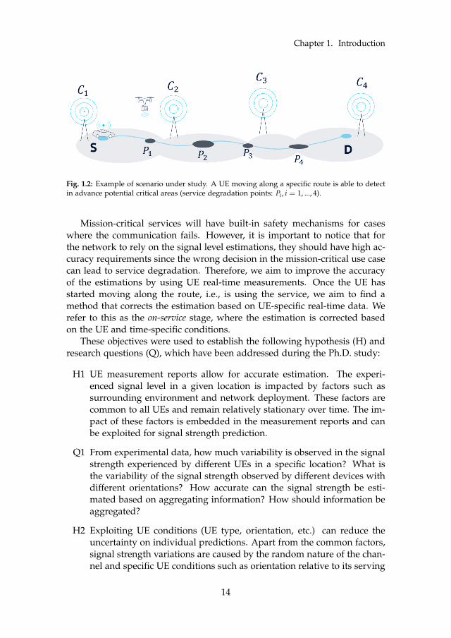
The state-of-the-art presented in the previous section suggests the potentialof cellular networks to provide safe communications for mission-critical ser-vices. Predictive mechanisms are promising to contribute in meeting theservice-specific requirements. This thesis studies the use of RSRP estimationto improve service availability and reliability for autonomous cars and dronesconnected to cellular networks. The aim is to propose and evaluate a proac-tive solution that prevents service degradation for these use cases, targetingin-advance detection of what we refer to as critical areas. We consider criticalareas those locations where the probability of not meeting the requirementsfor the service under evaluation is high. Using the example scenario shownin Fig. 1.2, the main objective is that the network is aware of which are thecritical areas in the route (P1 to P4) that a UE moving from source (S) to desti-nation (D) will experience. In-advance detection of these areas would allow,e.g., for more proactive mobility, QoS, and RRM.
Considering the RSRP relevance presented in the previous section, thisthesis targets to investigate how to exploit the RSRP measurements that theUEs report to the network for service availability and reliability prediction.The study is performed in scenarios with different propagation conditionssuch as urban/rural or ground/air.
The presented estimation approach is adapted to the two-stage frameworkproposed by 5GAA and ACJA. The work is done under the assumption that,in the studied scenarios, it is common to know the possible routes of the UEbefore the critical service starts, which allows for evaluation of the expectedservice availability and reliability. This evaluation can only be done in whatwe refer to as the pre-service stage, where we aim to assess the expected avail-ability and reliability in the route before the UE starts the mission-criticalservice. In this stage, we aim to provide an estimation that is valid for anyUE at any time in that location, choosing the appropriate radio metric forthat purpose.
13
Chapter 1. Introduction
Fig. 1.2: Example of scenario under study. A UE moving along a specific route is able to detectin advance potential critical areas (service degradation points: Pi , i = 1, ..., 4).
Mission-critical services will have built-in safety mechanisms for caseswhere the communication fails. However, it is important to notice that forthe network to rely on the signal level estimations, they should have high ac-curacy requirements since the wrong decision in the mission-critical use casecan lead to service degradation. Therefore, we aim to improve the accuracyof the estimations by using UE real-time measurements. Once the UE hasstarted moving along the route, i.e., is using the service, we aim to find amethod that corrects the estimation based on UE-specific real-time data. Werefer to this as the on-service stage, where the estimation is corrected basedon the UE and time-specific conditions.
These objectives were used to establish the following hypothesis (H) andresearch questions (Q), which have been addressed during the Ph.D. study:
H1 UE measurement reports allow for accurate estimation. The experi-enced signal level in a given location is impacted by factors such assurrounding environment and network deployment. These factors arecommon to all UEs and remain relatively stationary over time. The im-pact of these factors is embedded in the measurement reports and canbe exploited for signal strength prediction.
Q1 From experimental data, how much variability is observed in the signalstrength experienced by different UEs in a specific location? What isthe variability of the signal strength observed by different devices withdifferent orientations? How accurate can the signal strength be esti-mated based on aggregating information? How should information beaggregated?
H2 Exploiting UE conditions (UE type, orientation, etc.) can reduce theuncertainty on individual predictions. Apart from the common factors,signal strength variations are caused by the random nature of the chan-nel and specific UE conditions such as orientation relative to its serving
14

3. Research Methodology
cell.
Q3 What UE-specific conditions causes significant variations? Can it beused to reduce the estimation error of individual UE predictions?
H4 Differences in the propagation environment between the air (UAV sce-nario) and the ground (V2X scenario) will require re-adjustments inthe estimation approach between the two. The directivity of the UE an-tenna is more pronounced in the signal strength observed in the air dueto dominant LOS conditions. Consequently, the variability of the signalstrength at a specific location can be higher due to UEs with differentorientations being connected to different serving cells.
Q4 What are the quantifiable differences between UAVs and V2X? How arethey useful to improve the prediction?
H5 The measurement-based estimation can provide accurate signal levelestimations, which can be used to predict with 95 % accuracy the proba-bility of RSRP dropping below the required availability threshold of theservice, i.e., a critical area. Additionally, using the same approach forthe estimation of the interfering radio cells (also known as neighbors)RSRP, the expected Signal-To-Interference Ratio (SIR) can be calculatedand used to predict the service reliability along the route with the sameaccuracy.
Q5 How accurate should the signal strength estimation be to detect at least95 % of the upcoming service availability and reliability critical areas?Can that accuracy be achieved?
3 Research Methodology
The study is developed following a classical research methodology to fulfillthe study objectives and answer the research questions presented in Section2. After the classical problem description, literature review and hypothesisformulation, the following essential steps were identified:
1. Field Measurements: Multiple field measurement campaigns are per-formed over LTE networks, both on the ground (for the V2X scenario)and in the air (for the UAV scenario). The measurement equipmentconsists of a radio network scanner and four commercial smartphoneswith a test firmware. In contrast to many of the studies available in theliterature, this work is measurement-based. The use of measurementsgives realism to the presented results, as real data represents what UEsusing mission-critical services such as autonomous vehicles or drones
15
Chapter 1. Introduction
will experience when moving along a specific route. Urban and ruralscenarios are evaluated assuming that these are the most likely for theconsidered use cases.
2. Measurement Data Analysis and Modelization: The data collectedduring the measurement campaign is processed, structured, and ana-lyzed, which allows identifying data trends, repeatability, and outliers.
3. Estimation Methods Design: The trends and values observed in themeasurement data analysis step are used to design the estimation meth-ods presented in this thesis. Examples of these methods are the data-driven estimation approach for accurate signal level estimation beforethe service starts, the UE-specific correction of the estimation using real-time data recorded by the UE, and the service outage probability calcu-lation for critical areas estimation.
4. Performance Evaluation: The proposed solutions are evaluated usingthe data gathered during the measurement campaigns. The data-drivenestimation approach is compared to other techniques often used by op-erators and calibrated using measurement data.
4 Contributions
The main contributions of the Ph.D. study can be summarized as follows:
1. Proposal of an implementation of the two-stage framework presentedby ACJA.
This thesis proposes a two-stage framework implementation for mission-critical communications. The framework is initially introduced by [38]for the UAV use case. The implementation presented in this thesis con-sists of a pre-service and an on-service stage and is valid for all studiedscenarios. In the first, the network estimates the potential critical areasfor a UE using a specific service and planning to move along a specificroute using data-driven RSRP estimations. It occurs before the servicestarts and can lead to path re-planning in the case of critical areas de-tection. In the second, the RSRP estimations are corrected for the usermoving along the path, and the critical areas predicted during the pre-service stage are fine-tuned based on the corrected estimations. Thisstage can only occur once the UE is using the service. It can help avoidupcoming critical areas and lead to more proactive management of themobility and the network resources.
2. Proposal of a technique that provides accurate cell-agnostic RSRP es-timations in the pre-service stage.
16

4. Contributions
This thesis proposes and evaluates a data-driven approach to estimatethe expected RSRP for a mission-critical user planning to move along aspecific path. The signal level is estimated using data recorded by UEsthat have previously passed through the same path. The proposed data-driven technique provides a cell-agnostic estimation, valid for any userin that same path. The data-driven approach is compared to traditionaltechniques such as empirical models or ray-tracing, using the recordedmeasurements to calibrate the predictions. The data-driven techniqueprovides higher estimation accuracy for all studied scenarios.
3. Proposal of a method for UE-specific corrections of the RSRP estima-tion in the on-service stage.
This thesis proposes and evaluates a method to reduce the estimationerror further. By using real-time data recorded by the UE, we propose astatistical method to correct the UE-specific offset, referred to as MeanIndividual Offset (MIO). The error samples from the specific UE areused to determine whether they statistically belong to error distribu-tions from UEs that have previously moved along the same path. Themethod is adjusted to the different propagation conditions of the usecases under study (V2X/UAV), increasing estimation accuracy for bothof them.
4. Evaluation of the use of data-driven approach for critical areas detec-tion in all studied scenarios.
This thesis evaluates the use of accurate RSRP estimations for in-advancedetection of critical areas. The critical areas are defined in this study interms of service availability and service reliability. For service avail-ability, an estimation of the probability of RSRP dropping below thenecessary threshold to meet the service requirements is proposed con-sidering the RSRP estimation and its corresponding error. In the caseof service reliability, the same data-driven estimation is applied firstfor the neighbors’ RSRP. The SIR is then used to identify the criticalareas in the path. This contribution verifies the two-stage frameworkproposed in contribution no. 1.
5. Performance evaluation using experimental data gathered throughdifferent measurement campaigns.
The proposed framework and estimation approach are evaluated usingexperimental data. As shown in previous sections, many of the con-tributions available in the literature use simulation data, especially forthe UAV case. Using experimental data leads to more realistic results,accounting for certain factors that cannot be modeled through simula-tions.
17

Chapter 1. Introduction
These contributions are presented in a collection of papers. The scientificfindings obtained during this study are presented to the research communitythrough scientific publications, targeting high-impact conferences and jour-nals. Part of this investigation was also a contribution to the European UnionHorizon 2020 framework DroC2om project [50]. Additionally, the work waspresented and discussed in several Nokia forums. The main contributionsand findings are included in the following list of scientific publications:
Paper A: M. López, T. B. Sørensen, I. Z. Kovács, J. Wigard and P. Mogensen,“Experimental Evaluation of Data-driven Signal Level Estimationin Cellular Networks”, IEEE 94th Vehicular Technology Conference(VTC2021-Fall), September 2021.
Paper B: M. López, T. B. Sørensen, I. Z. Kovács, J. Wigard and P. Mogensen,"Measurement-Based Outage Probability Estimation for Mission-Critical Services", IEEE ACCESS, vol. 9, pp. 169395-169408, 2021.
Paper C: M. López, T. B. Sørensen, P. Mogensen, J. Wigard and I. Z. Kovács,“Shadow fading spatial correlation analysis for aerial vehicles:Ray tracing vs. measurements”, IEEE 90th Vehicular TechnologyConference (VTC2019-Fall), September 2019.
Paper D: M. López, T. B. Sørensen, J. Wigard, I. Z. Kovács and P. Mo-gensen, "Service Outage Estimation for Unmanned Aerial Vehi-cles: A Measurement-Based Approach", IEEE Wireless Commu-nications and Networking Conference (WCNC) 2022. Accepted forpublication.
Additionally, three successful patents were disclosed in relation to thework done on the thesis:
Patent Application 1: I. Z. Kovács, J. Moilanen, W. Zirwas, T. Henttonen,T. Veijalainen, L. U. Garcia, M. M. Butt, M. Cente-naro, M. López, "Providing producer node machinelearning based assistance", WO2021063500A1, Pub-lished: April 2021, Nokia Technologies.
Patent Application 2: I. Z. Kovács, A. Feki, A. Pantelidou, M. M. Butt,O. E. Barbu, M. López, "Channel state informationvalues-based estimation of reference signal receivedpower values for wireless networks",WO2021209145A1, Published: October 2021, NokiaTechnologies.
Patent Application 3: I. Z. Kovács, O. E. Barbu, M. López, "Method of andapparatus for machine learning in a radio network",
18

5. Thesis Outline
WO2021213685A1, Published: October 2021, NokiaTechnologies.
The data gathered during the different measurement campaigns and thediscussions with other researchers has resulted in the following scientificpublications related to the studied topic:
• M. Bucur, T. Sørensen, R. Amorim, M. López, I. Z. Kovács, and P. Mo-gensen. (2019, September). Validation of large-scale propagation char-acteristics for UAVs within urban environment. IEEE 90th VehicularTechnology Conference (VTC2019-Fall), September 2019.
• B. Sliwa, M. J. Geis, C. Bektas, M. López, P. Mogensen and C. Wietfeld"DRaGon: Mining Latent Radio Channel Information from Geographi-cal Data Leveraging Deep Learning", IEEE Wireless Communications andNetworking Conference (WCNC) 2022. Accepted for publication.
5 Thesis Outline
The thesis is divided into 2 parts. Part I summarizes the main contributionsand results obtained during the Ph.D. work, while Part II presents the articlessupporting it.
• Chapter 2: This chapter provides a brief background on radio propa-gation and further motivates the choice of signal level as the estimatedparameter for critical areas prediction. It presents state of the art on tra-ditional and non-traditional techniques used for signal level estimation,as it is a widely studied topic.
• Chapter 3: This chapter includes a description of the proposed sig-nal level estimation method for both the pre-service and the on-servicestages in all studied scenarios. It also presents the results of using thedata-driven estimations obtained with the proposed method for esti-mating the expected service availability and reliability. The probabilityof the UE passing through a critical area is calculated using estimatedsignal strength. The work presented in this chapter is supported byPapers A, B, C, and D.
• Chapter 4: Presents the conclusion of the studies conducted during thePh.D., summarizing the main findings, and discussing the recommen-dations and suggestions that should be addressed in future work.
19

References
References
[1] Series, M, “IMT Vision–Framework and overall objectives of the future develop-ment of IMT for 2020 and beyond,” Recommendation ITU, vol. 2083, p. 0, 2015.
[2] Yilmaz, Osman and Johansson, N, “5G radio access for ultra-reliable and low-latency communications,” Ericsson Research Blog, vol. 1, 2015.
[3] Zarri, M, “Network 2020: Mission critical communications,” tech. rep., GSMA,2017.
[4] 3GPP, “Service requirements for the 5G system, Stage 1 (Release 15),” Tech. Rep.22.261 V15.9.0, Sept. 2021.
[5] 3GPP, “User Equipment (UE) conformance specification; Radio transmission andreception (FDD),” Tech. Rep. 34.121-1 V12.5.0, Sept. 2016.
[6] D. Öhmann, M. Simsek, and G. P. Fettweis, “Achieving high availability in wire-less networks by an optimal number of Rayleigh-fading links,” in 2014 IEEEGlobecom Workshops (GC Wkshps), pp. 1402–1407, IEEE, 2014.
[7] M. Bennis, M. Debbah, and H. V. Poor, “Ultrareliable and low-latency wirelesscommunication: Tail, risk, and scale,” Proceedings of the IEEE, vol. 106, no. 10,pp. 1834–1853, 2018.
[8] 3GPP, “Study on latency reduction techniques for LTE (Release 14),” Tech. Rep.36.881 V14.0.0, June 2016.
[9] H. Alves, G. D. Jo, J. Shin, C. Yeh, N. H. Mahmood, C. Lima, C. Yoon, N. Ra-hatheva, O.-S. Park, S. Kim, et al., “Beyond 5G URLLC Evolution: New ServiceModes and Practical Considerations,” arXiv preprint arXiv:2106.11825, 2021.
[10] 5GPPP Association, “5G and e-health,” Tech. Rep. White Paper, Oct. 2015.
[11] N. A. Mohammed, A. M. Mansoor, and R. B. Ahmad, “Mission-critical machine-type communication: An overview and perspectives towards 5G,” IEEE Access,vol. 7, pp. 127198–127216, 2019.
[12] Alliance, NGMN, “5G White Paper,” Next generation mobile networks, white paper,vol. 1, 2015.
[13] M. Boban, A. Kousaridas, K. Manolakis, J. Eichinger, and W. Xu, “Usecases, requirements, and design considerations for 5G V2X,” arXiv preprintarXiv:1712.01754, 2017.
[14] 3GPP, “Service requirements for enhanced V2X scenarios,” Tech. Rep. 22.186V16.2.0, June 2019.
[15] C. S. I. Cordero, Carlos Director, “Optimizing 5G for V2X - Requirements, Im-plications and Challenges,” in IEEE VTC Mission-Critical 5G for Vehicle IoT, IEEE,2016.
[16] A. Kousaridas, R. P. Manjunath, J. Perdomo, C. Zhou, E. Zielinski, S. Schmitz,and A. Pfadler, “QoS Prediction for 5G Connected and Automated Driving,”IEEE Communications Magazine, vol. 59, no. 9, pp. 58–64, 2021.
20

References
[17] P. Wang, J. Zhang, H. Deng, and M. Zhang, “Real-time urban regional routeplanning model for connected vehicles based on V2X communication,” Journal ofTransport and Land Use, vol. 13, no. 1, pp. 517–538, 2020.
[18] 5G Automotive Association, “ Making 5G proactive and predictive for the auto-motive industry,” Tech. Rep. White Paper, Jan. 2020.
[19] J. Riihijarvi and P. Mahonen, “Machine learning for performance prediction inmobile cellular networks,” IEEE Computational Intelligence Magazine, vol. 13, no. 1,pp. 51–60, 2018.
[20] R. Falkenberg, K. Heimann, and C. Wietfeld, “Discover your competition in LTE:Client-based passive data rate prediction by machine learning,” in GLOBECOM2017-2017 IEEE Global Communications Conference, pp. 1–7, IEEE, 2017.
[21] L. Torres-Figueroa, H. F. Schepker, and J. Jiru, “QoS Evaluation and Predictionfor C-V2X Communication in Commercially-Deployed LTE and Mobile EdgeNetworks,” in 2020 IEEE 91st Vehicular Technology Conference (VTC2020-Spring),pp. 1–7, IEEE, 2020.
[22] M. A. Gutierrez-Estevez, Z. Utkovski, A. Kousaridas, and C. Zhou, “A StatisticalLearning Framework for QoS Prediction in V2X,” in 2021 IEEE 4th 5G WorldForum (5GWF), pp. 441–446, IEEE, 2021.
[23] N. Bahra and S. Pierre, “A Hybrid User Mobility Prediction Approach for Han-dover Management in Mobile Networks,” in Telecom, vol. 2, pp. 199–212, Multi-disciplinary Digital Publishing Institute, 2021.
[24] K. M. Hosny, M. M. Khashaba, W. I. Khedr, and F. A. Amer, “New vertical han-dover prediction schemes for LTE-WLAN heterogeneous networks,” PloS one,vol. 14, no. 4, p. e0215334, 2019.
[25] W. Zhang, M. Feng, M. Krunz, and H. Volos, “Latency Prediction for Delay-sensitive V2X Applications in Mobile Cloud/Edge Computing Systems,” inGLOBECOM 2020-2020 IEEE Global Communications Conference, pp. 1–6, IEEE,2020.
[26] T. Fawcett, “An introduction to roc analysis,” Pattern recognition letters, vol. 27,no. 8, pp. 861–874, 2006.
[27] A. Samba, Y. Busnel, A. Blanc, P. Dooze, and G. Simon, “Instantaneous through-put prediction in cellular networks: Which information is needed?,” in 2017IFIP/IEEE Symposium on Integrated Network and Service Management (IM), pp. 624–627, IEEE, 2017.
[28] S. Barmpounakis, L. Magoula, N. Koursioumpas, R. Khalili, J. M. Perdomo, andR. P. Manjunath, “LSTM-based QoS prediction for 5G-enabled Connected andAutomated Mobility applications,” in 2021 IEEE 4th 5G World Forum (5GWF),pp. 436–440, IEEE, 2021.
[29] C. Yue, R. Jin, K. Suh, Y. Qin, B. Wang, and W. Wei, “LinkForecast: cellular linkbandwidth prediction in LTE networks,” IEEE Transactions on Mobile Computing,vol. 17, no. 7, pp. 1582–1594, 2017.
[30] A. R. Abdellah, A. Alshahrani, A. Muthanna, and A. Koucheryavy, “Perfor-mance Estimation in V2X Networks Using Deep Learning-Based M-Estimator
21

References
Loss Functions in the Presence of Outliers,” Symmetry, vol. 13, no. 11, p. 2207,2021.
[31] SESAR Joint Undetaking, “"U-Space Blueprint brochure,” Publications Office ofthe European Union, Luxermbourg,” 2017.
[32] M. Neale and D. Colin, “Mobility challenges for unmanned aerial vehicles con-nected to cellular LTE networks,” in Technology Workshop - Remotely Piloted AircraftSystems Symposium, Mar. 2015.
[33] 3GPP, “Study on Enhanced LTE Support for Aerial Vehicles (Release 15),” Tech.Rep. 36.777 V0.3.1, Oct. 2017.
[34] E. Vinogradov, H. Sallouha, S. De Bast, M. M. Azari, and S. Pollin, “Tutorial onUAV: A blue sky view on wireless communication,”
[35] X. Lin, V. Yajnanarayana, S. D. Muruganathan, S. Gao, H. Asplund, H.-L. Maat-tanen, M. Bergstrom, S. Euler, and Y.-P. E. Wang, “The sky is not the limit: LTEfor unmanned aerial vehicles,” IEEE Communications Magazine, vol. 56, no. 4,pp. 204–210, 2018.
[36] I. Kovacs, R. Amorim, H. C. Nguyen, J. Wigard, and P. Mogensen, “Interferenceanalysis for UAV connectivity over LTE using aerial radio measurements,” in2017 IEEE 86th Vehicular Technology Conference (VTC-Fall), pp. 1–6, IEEE, 2017.
[37] J. Stanczak, I. Z. Kovacs, D. Koziol, J. Wigard, R. Amorim, and H. Nguyen,“Mobility challenges for unmanned aerial vehicles connected to cellular lte net-works,” in 2018 IEEE 87th Vehicular Technology Conference (VTC Spring), pp. 1–5,IEEE, 2018.
[38] ACJA, GSMA and GUTMA, “Interface for Data Exchange between MNOs andthe UTM Ecosystem: Network Coverage Service Definition, v1.00.,” Feb. 2021.
[39] P. S. Bithas, E. T. Michailidis, N. Nomikos, D. Vouyioukas, and A. G. Kanatas, “Asurvey on machine-learning techniques for UAV-based communications,” Sen-sors, vol. 19, no. 23, p. 5170, 2019.
[40] U. Challita, W. Saad, and C. Bettstetter, “Interference management for cellular-connected UAVs: A deep reinforcement learning approach,” IEEE Transactions onWireless Communications, vol. 18, no. 4, pp. 2125–2140, 2019.
[41] Y. Chen, X. Lin, T. A. Khan, and M. Mozaffari, “A deep reinforcement learningapproach to efficient drone mobility support,” arXiv preprint arXiv:2005.05229,2020.
[42] Y. Jiang, K. Nihei, J. Li, H. Yoshida, and D. Kanetomo, “Learning on the fly:An RNN-based online throughput prediction framework for UAV communica-tions,” in 2020 IEEE International Conference on Communications Workshops (ICCWorkshops), pp. 1–7, IEEE, 2020.
[43] E. Krijestorac, S. Hanna, and D. Cabric, “Spatial signal strength prediction us-ing 3d maps and deep learning,” in ICC 2021-IEEE International Conference onCommunications, pp. 1–6, IEEE, 2021.
[44] G. Yang, Y. Zhang, Z. He, J. Wen, Z. Ji, and Y. Li, “Machine-learning-basedprediction methods for path loss and delay spread in air-to-ground millimetre-wave channels,” IET Microwaves, Antennas & Propagation, vol. 13, no. 8, pp. 1113–1121, 2019.
22

References
[45] S. K. Goudos, G. V. Tsoulos, G. Athanasiadou, M. C. Batistatos, D. Zarbouti, andK. E. Psannis, “Artificial neural network optimal modeling and optimization ofUAV measurements for mobile communications using the L-SHADE algorithm,”IEEE Transactions on Antennas and Propagation, vol. 67, no. 6, pp. 4022–4031, 2019.
[46] 3GPP, “Physical layer; Measurements (Release 16),” Tech. Rep. 36.214 V16.2.0,Mar. 2021.
[47] C. Ide, R. Falkenberg, D. Kaulbars, and C. Wietfeld, “Empirical analysis of theimpact of lte downlink channel indicators on the uplink connectivity,” in 2016IEEE 83rd Vehicular Technology Conference (VTC Spring), pp. 1–5, IEEE, 2016.
[48] V. Raida, P. Svoboda, M. Koglbauer, and M. Rupp, “On the Stability of RSRP andVariability of Other KPIs in LTE Downlink-An Open Dataset,” in GLOBECOM2020-2020 IEEE Global Communications Conference, pp. 1–6, IEEE, 2020.
[49] M. Toril, V. Wille, S. Luna-Ramírez, M. Fernández-Navarro, and F. Ruiz-Vega,“Characterization of Radio Signal Strength Fluctuations in Road Scenarios forCellular Vehicular Network Planning in LTE,” IEEE Access, vol. 9, pp. 33120–33131, 2021.
[50] SESAR Joint Undetaking - Project no. 763601, “Deliverable 5.2. Report of firstdrone flight campaign.,” Dec. 2018.
23

References
24

Chapter 2
Signal Level Estimation
This chapter continues the discussion on the importance of RSRP estima-tion started in Section 1.3 of Chapter 1. It presents details on the factorsthat impact RSRP variations and therefore affect the signal strength mea-sured by a UE in a certain location. It also includes a review of the tradi-tional approaches used for channel modeling that are later compared withthe proposed data-driven estimation approach. A discussion on well-knownfine-tuning methods for estimated signal level is presented, aiming to pointout the differences with the work presented in this thesis. A state-of-the-artreview of recent techniques for signal strength estimation is also included.
1 Impacting Factors
After briefly discussing the importance of RSRP in Section 1.3, we summarizehere the main factors impacting the signal propagating from the transmitterto the receiver. Understanding the physical principles of electromagneticwaves propagation over the air is essential for estimating the received signalstrength. The free-space path loss model allows for the calculation of thereceived power in free-space propagation conditions, which depends mainlyon the transmitted power and the distance between the transmitter and thereceiver [1]. However, free-space propagation conditions is rarely the casein most wireless propagation scenarios. In practice, any obstacle or changein the radio wave path or environment can cause signal strength variationsand will be added to the default distance attenuation. This effect is known asfading, and it is distinguished between [2]:
• Large-scale Fading: the attenuation of the signal over large areas, causedby obstacles in the surrounding environment of the propagation path.It is mostly impacted by the terrain shape (hills, mountains) and large
25

Chapter 2. Signal Level Estimation
building or objects in the environment present between the transmit-ter and the receiver. It includes pathloss and shadowing effects, whereshadowing is considered the deviation of the received power from itsoverall mean value, and is statistically modelled using a log-normaldistribution [3].
• Small-scale Fading: represents the rapid changes in the radio signalover a short period of time (on the order of seconds) [4]. It occurs whenthe obstacles in the environment cause the signal to be reflected, andmultiple versions of the same signal with different delays arrive at thereceiver. Factors such as multipath environment, UE speed (Dopplershift at each multipath component), environment dynamics, and trans-mission bandwidth of the channel affect small-scale fading [5].
Since the work presented in this thesis is based on experimental data, itis important to consider error sources in the UE measurement reports. Inpractice, the measured RSRP may fluctuate not only due to channel effectsbut also due to receiver processing.
There are ways of mitigating the impact of these effects for accurate RSRPestimation. A Layer 1 filter is typically applied to overcome measurement in-accuracy due to fast-fading effects. Further averaging to remove fading, mea-surement noise and measurement/estimation errors is performed at Layer3 [6]. This is further explained in Section 3 of Paper B. However, the ran-dom nature of the signal will always limit the accuracy of the signal strengthestimation.
Modeling the impact of the different factors or finding a method thatestimates the received signal strength as accurately as possible has been thesubject of much investigation. The following sections present a review of thetraditional and new estimation methods and a summary of the data-drivenapproach studied in this thesis.
2 Traditional Estimation Approaches
Estimating the signal strength that the user will experience is crucial for thedesign of a reliable network. Over-estimating the signal power can lead topoor coverage, and under-estimating it can be costly for the MNOs due to un-necessarily dense network deployment. Channel models can be divided intoempirical and theoretical. The following sub-sections introduce both types,focusing on the examples that are later used in Chapter 3 for comparisonwith the proposed data-driven approach.
26

2. Traditional Estimation Approaches
2.1 Empirical Models
Empirical channel models, often referred to as statistical models, are the re-sult of using measurement data to model the behavior of the radio channelthrough statistics. The parameters of an empirical model strongly dependon the scenario, as the propagation characteristics of, e.g., urban, suburban,or rural environments are very different. The main problem of this estima-tion approach is generalization, as it aims at estimating the average behaviorof the signal. Despite finding common attributes in a particular propaga-tion scenario, specific signal variations due to, e.g., a building in the pathbetween the transmitter and the receiver in a city can not be captured by ageneral model for urban scenarios. Therefore, MNOs use correction factors tofine-tune the model and adapt it to the specific area where they are planningto deploy a network.
There are several known empirical models [7], the earliest one being thefree-space propagation model [1], which is often used as part of the Friistransmission equation [8]. The two-ray ground reflection model considersthe effect of multipath due to ground reflections and assumes that the sig-nal reaches the receiver from two different paths [2]. However, free-spacepropagation models are not a good representation for scenarios where ob-jects (buildings, vegetation, vehicles, etc.) are in the propagation path. Thereare specific models for the different scenarios. The most commonly usedare meant for urban and rural environments. Examples are the Okumura-Hata model [9], the models proposed by 3GPP [10], the 231 Walfisch-Ikegamimodel [11] or the guidelines included in ITU-R M.2412 [12] for propagationmodeling. The first two are used in this thesis for comparison with the pro-posed data-driven approach. Therefore, an extended explanation of thesemodels is included:
• Okumura-HataThis model was built using a large set of signal strength measurementsin different scenarios (varying terrain, vegetation, and urban clutter) atmultiple frequencies. It is commonly used for network planning, and ithas experienced several corrections over the years, adapting the modelto the specific propagation conditions of the scenario under study. TheOkumura-Hata model used for comparison in this dissertation is de-fined in Eq. (2.1). The estimated path loss for an urban area is givenby:
PL = 69.55 + 26.16log10( fc)− 13.82log10(hb)
− α(hm) + (44.9− 6.55log10(hb))log10(d)[dB] (2.1)
Where the d is the distance between the transmitter and the receiver inkm, the carrier frequency fc is in MHz, the effective transmitter (hb) and
27

Chapter 2. Signal Level Estimation
receiver (hm) antenna heights are in m and α(hm) is a correction factorthat for small/medium cities such as the one under study in our drivetests is:
α(hm) = (1.1log10( fc)− 0.7)hm − (1.56log10( fc)− 0.8) (2.2)
The above equations are a simplified version of the Okumura-Hatamodel, which does not include the multiple correction factors that maybe used when applying the model for planning mobile radio systems.However, they are considered a good representation of the estimationaccuracy level that the Okumura-Hata model can provide.
• 3GPP TR 38.9013GPP proposed in [10] a study on channel model for frequencies rang-ing from 0.5 to 100 GHz. The model is constructed by combining theresults from the measurements campaigns performed by many of thedifferent 3GPP partners. It is a common approach for path loss esti-mation for three scenarios: Rural Macro (RMa), Urban Macro (UMa),and Urban Micro (UMi). Since the comparison with the data-driven ap-proach is only shown for the urban environment case, we include herethe equations for the UMa scenario. The equation is different depend-ing on the visibility conditions (LOS/Non-Line-Of-Sight (NLOS)).
For LOS conditions, the path loss estimation depends on the breakpointdistance d
′BP, which is defined as the distance between the transmitter
and the receiver where the propagation mode changes. In [10]:
d′BP = 4hBShUT
fc
c[m] (2.3)
In 2.3, hBS and hUT are the effective antenna heights in m of the BS andthe UE, respectively, fc is the carrier frequency in Hz, and c = 3.0x10⁸
m/s is the propagation velocity in free space. Two distances are dis-tinguished: two-dimensional d2D distance, and three-dimensional (ac-counting for height) d3D distance, both between transmitter and re-ceiver. For d2D between a minimum distance of 10 m and d
′BP, path
loss for LOS conditions is given by:
PLUMa−LOS(1) = 28.0 + 22log10(d3D)
+ 20log10( fc)[dB] (2.4)
For a d2D distance above d′BP and below 5 km, the LOS path loss esti-
mation becomes:
28

2. Traditional Estimation Approaches
PLUMa−LOS(2) = 28.0 + 40log10(d3D) + 20log10( fc)
− 9log10((d′BP)
2 + (hBS − hUT)2)
[dB] (2.5)
As expressed in Eq. (2.6), for NLOS visibility conditions, the path lossestimation will be the maximum between the estimated path loss forLOS conditions and the value obtained using Eq. (2.7).
PLUMa−NLOS = max(PLUMa−LOS, PL′UMa−NLOS) [dB] (2.6)
PL′UMa−NLOS = 13.54 + 39.08log10(d3D)+
20log10( fc)− 0.6(hUT − 1.5)[dB] (2.7)
As it will be further explained in Chapter 3, for the comparison performedin this thesis, the 3GPP TR 38.901 model has been fine-tuned with the ap-propriate visibility conditions (LOS/NLOS) based on ray-tracing predictions,corresponding BS heights and an assumed UE height of 1.5 m.
2.2 Ray-Tracing
Ray-tracing is a propagation modeling tool that allows estimating path loss,angle of arrival, and delay spread by modeling electromagnetic waves asrays [13]. It uses physics to calculate the path that a radio signal will follow,considering its interaction with the objects in the propagation environment.It will account for effects such as reflection, diffraction, scattering, as well asthe dielectric properties of the surfaces with which the signal is interactingand its carrier frequency. To that end, ray-tracing requires 3D modeling ofthe propagation scenario:
• Terrain elevation and material properties
• Buildings position, shape, height, and material properties
• Vegetation position, size, and type
Deployment information is also necessary to compute the paths of therays from the transmitter to the receiver: BS height, BS transmit power, UEheight, and carrier frequency. Therefore, very accurate modeling of the prop-agation scenario is needed for the estimations to provide satisfactory accu-racy. This will be further proved in Chapter 3.
One of the main advantages of ray-tracing compared to the empiricalmodels explained in the previous sub-section is that the estimations are spe-cific for the scenario under study. Therefore, the accuracy of the path loss
29

Chapter 2. Signal Level Estimation
estimation provided by ray-tracing is expected to be higher, but this comes atthe cost of increased complexity and computational load.
In this thesis, the evaluation of ray-tracing is done using the WinProp toolfrom Altair© [14]. The tool offers different simplifications of full ray-tracingprediction models, and it allows model calibration using experimental data.Two of the prediction models are investigated in this thesis [15]:
• Intelligent Ray Tracing (IRT): The received power is calculated by su-perposing up to hundreds of rays resulting from computing the multi-ple paths that the signal can travel through. Due to the high number ofrays, the computation time of this method is very high.
• Dominant Path Model (DPM): In most cases, when using IRT, only 2or 3 of the computed rays are contributing significantly to the total re-ceived power. For that reason, the DPM model focuses on determiningthe most dominant paths using geometry and calculates path loss usingthe equation in [15].
Although the accuracy of ray-tracing is acceptable for network planning,it will be shown in Chapter 3 that it is not sufficient for service availabilityand reliability critical areas estimation.
2.3 Using Drive Tests to Improve the Estimations
The methods introduced above are typically integrated into professional ra-dio planning tools that allow MNOs to perform network planning and opti-mization. An example is the Atoll tool by Forsk© [16], which is commonlyused by operators as it includes a wide variety of empirical propagation mod-els as well as ray-tracing. To improve the estimations after network deploy-ment, operators perform the so-called drive tests. They drive along a specificroute using dedicated measurement equipment that provides statistics of thenetwork coverage and performance. Some radio planning tools allow us-ing measurement data to correct and calibrate the estimations and performnetwork optimization [17].
3GPP introduced in Release 10 a more economic and automatized alter-native to drive tests: Minimization of Drive Tests (MDT) [18]. The main ideabehind MDT is to exploit the UEs’ measurement capabilities to collect realdata from a specific area. It enables the UEs to collect periodically (or not,depending on the MDT mode) radio measurements along with their location,even if the UE is in idle state, and report them when in active state [19].
This information serves for radio measurements analysis and statisticaldata processing. Therefore, MNOs use it for anomaly detection and networkcapacity and performance optimization, among others. The MDT feature en-ables the generation of Radio Environment Maps (REM), which is a function-ality that provides awareness on the radio environment using geo-located
30

3. New Estimation Approaches
measurements. A REM is a centralized database that contains informationon the surrounding radio environment (device locations, available services,geographical features, etc.), and more intelligent entities may use them toperform network optimization.
There are two major concerns regarding MDT. First, the fact that not allUEs support this feature as it is not mandatory. In practice, MDT can only beused with test devices owned by the operator or an MDT service provider.The second concern is the positioning method that provides the location in-cluded in the measurement reports. A poor Global Navigation Satellite Sys-tem (GNSS) signal or the absence of it, rounding of latitude/longitude valueswhen reported, and generally the inaccuracies of the positioning method canreduce the benefits of MDT reports. For GNSS, which is typically used inMDT, inaccuracies are below 10 m in outdoor environments and recent liter-ature shows methods to improve it [20], leading to positioning errors as lowas 5 m [21] in urban scenarios.
MDT is however considered to be a useful approach for sample collectionfor the data-driven method evaluated in this thesis. The data-driven approachis similar to the REM functionality, as they are both based on the collection ofmeasurement data to estimate the UEs’ expected signal strength. One of themain differences is that the estimations provided by REM are cell-specific,whereas the ones provided by the proposed data-driven approach are cell-agnostic. This, and other differences, will be further explained in Chapter3.
3 New Estimation Approaches
This section summarizes some of the state-of-the-art non-traditional tech-niques for signal strength prediction. Most of the publications are motivatedby improving wireless coverage prediction to reduce network deploymentcosts. As in this thesis, others aim at high accuracy predictions for reliabilityassurance purposes.
There are plenty of studies about the use of ML for signal strength pre-diction. Especially during the past ten years, they have increased since it isgenerally considered a good solution for predicting QoS-related KPIs. Theauthors of [22] propose a ML framework to predict the signal strength us-ing crowd-sourced data from urban, suburban, and rural scenarios. Theyfeed features such as context information (e.g., phone model, UE speed, timeof the day), RAN configuration parameters (e.g., frequency, transmit power,antenna details, or location of the serving cell), and UE-BS distance to a gra-dient boosted tree (LightGMB). They predict RSRP and obtain an RMSE of7.4 dB. The work presented in [23] studies the prediction of RSRP with amethod based on path sequence regression. They simulate the transmission
31

References
path of the signal, extract the path’s features (clutter and antenna heights,distances between UE and BS), and combine them with other antenna infor-mation such as transmit power to predict RSRP using NN. Their proposedalgorithm reaches an RMSE of 10.3 dB. In [24], the authors also propose amodel for feature extraction to estimate signal strength, but they account formore physical and environmental features. They consider in total 18 differentfeatures: environmental clutter type (water, vegetation, building, road, andothers), frequency, UE-BS angles, BS information, heights and distances, etc.They test their model over measurement data, and achieve an RMSE of 5.1dB in an urban environment. The studies in [25] design the features for theirmodel based on the Cost 231-Hata empirical model and the geometrical lo-cation. They later use feature selection to reduce the number of inputs to theNN used for signal strength prediction, achieving an RMSE of 7.5 dB. In [26],the authors present a deep-learning approach to predict signal strength. Theyextract the radio environment characteristics from top-view satellite imagesof the receiver’s location and combine that information with expert knowl-edge. The model is tested over different environments, showing an RMSE ofapproximately 6 dB.
As observed in the previous section, there are a lot of similarities betweenthe studies aiming to tackle the RSRP prediction problem. It is challenging tofind estimation approaches that do not involve ML in recent literature. Manyof them use a certain number of features that characterize and impact thesignal strength reaching the UE. Some select the features based on empiricalmodels, some use feature selection techniques, and some include images or3D models containing information about the surrounding environment. Themain differences between them are how they obtain the information (mea-surement or simulation data) and their prediction methods. The data-drivenapproach presented in the following section relies on the fact that all thesefeatures are inherent in the RSRP value measured at the UE.
References
[1] A. Goldsmith, Wireless communications. Cambridge university press, 2005.
[2] T. S. Rappaport et al., Wireless communications: principles and practice, vol. 2. pren-tice hall PTR New Jersey, 1996.
[3] M. Gudmundson, “Correlation model for shadow fading in mobile radio sys-tems,” Electronics letters, vol. 27, no. 23, pp. 2145–2146, 1991.
[4] T. Jiang, D. Chen, C. Ni, and D. Qu, OQAM/FBMC for future wireless communica-tions: Principles, technologies and applications. Academic Press, 2017.
[5] B. Sklar, “Rayleigh fading channels in mobile digital communication systems. i.characterization,” IEEE Communications magazine, vol. 35, no. 7, pp. 90–100, 1997.
32

References
[6] M. Anas, F. D. Calabrese, P.-E. Ostling, K. I. Pedersen, and P. E. Mogensen, “Per-formance analysis of handover measurements and layer 3 filtering for utran lte,”in 2007 IEEE 18th International Symposium on Personal, Indoor and Mobile RadioCommunications, pp. 1–5, IEEE, 2007.
[7] O. O. Erunkulu, A. M. Zungeru, C. K. Lebekwe, and J. M. Chuma, “Cellularcommunications coverage prediction techniques: A survey and comparison,”IEEE Access, vol. 8, pp. 113052–113077, 2020.
[8] H. T. Friis, “A note on a simple transmission formula,” Proceedings of the IRE,vol. 34, no. 5, pp. 254–256, 1946.
[9] M. Hata, “Empirical formula for propagation loss in land mobile radio services,”IEEE transactions on Vehicular Technology, vol. 29, no. 3, pp. 317–325, 1980.
[10] 3GPP, “Study on channel model for frequencies from 0.5 to 100 GHz. (Release16),” Tech. Rep. 38.901 V16.1.0, Dec. 2019.
[11] J. D. Parsons, The mobile radio propagation channel. Wiley, 2000.
[12] M. Series, “Guidelines for evaluation of radio interface technologies for imt-2020,” Report ITU-R M. 2412-0, Tech. Rep., 2017.
[13] Z. Yun and M. F. Iskander, “Ray tracing for radio propagation modeling: Princi-ples and applications,” IEEE Access, vol. 3, pp. 1089–1100, 2015.
[14] R. Hoppe, G. Wölfle, and U. Jakobus, “Wave propagation and radio networkplanning software winprop added to the electromagnetic solver package feko,”in 2017 International Applied Computational Electromagnetics Society Symposium-Italy (ACES), pp. 1–2, IEEE, 2017.
[15] R. Wahl and G. Wolfle, “Combined urban and indoor network planning using thedominant path propagation model,” in 2006 First European Conference on Antennasand Propagation, pp. 1–6, IEEE, 2006.
[16] Forsk - Atoll Overview, “Atoll Radio Planning and Optimisation Software,” 2021.https://www.forsk.com/atoll-overview, Last accessed on 2021-11-30.
[17] Forsk - Atoll Overview, “Measurement-Based Optimization,” 2021. https://www.forsk.com/measurement-based-optimisation, Last accessed on 2021-11-30.
[18] 3GPP, “Radio measurement collection for Minimization of Drive Tests (MDT);Overall description; Stage 2,” Tech. Rep. 37.320 V10.1.0, Mar. 2011.
[19] W. A. Hapsari, A. Umesh, M. Iwamura, M. Tomala, B. Gyula, and B. Sebire,“Minimization of drive tests solution in 3gpp,” IEEE Communications Magazine,vol. 50, no. 6, pp. 28–36, 2012.
[20] K. Strandjord, P. Axelrad, D. M. Akos, and S. Mohiuddin, “Improved urbannavigation with direct positioning and specular matching,” in Proceedings of the2020 International Technical Meeting of The Institute of Navigation, pp. 787–800, 2020.
[21] L. Icking, T. Kersten, and S. Schön, “Evaluating the Urban Trench Model ForImproved GNSS Positioning in Urban Areas,” in 2020 IEEE/ION Position, Locationand Navigation Symposium (PLANS), pp. 631–638, IEEE, 2020.
33

References
[22] A. Ghasemi, “Data-driven prediction of cellular networks coverage: An inter-pretable machine-learning model,” in 2018 IEEE Global Conference on Signal andInformation Processing (GlobalSIP), pp. 604–608, IEEE, 2018.
[23] C. L. Z. Huang, Y. Wang, M. Liang, J. Hu, and T. Song, “Radio Wave PropagationPrediction Based on Path Sequence Regression,” in 2020 IEEE 6th InternationalConference on Computer and Communications (ICCC), pp. 238–242, IEEE, 2020.
[24] Y. Zheng, Z. Liu, R. Huang, J. Wang, W. Xie, and S. Liu, “Feature Extractionin Reference Signal Received Power Prediction Based on Convolution NeuralNetworks,” IEEE Communications Letters, 2021.
[25] L. Tao, J. Lu, X. Wang, and L. Qian, “Feature engineering based intelligent wire-less propagation model for RSRP prediction,” in IOP Conference Series: MaterialsScience and Engineering, vol. 768, p. 042038, IOP Publishing, 2020.
[26] J. Thrane, B. Sliwa, C. Wietfeld, and H. L. Christiansen, “Deep learning-basedsignal strength prediction using geographical images and expert knowledge,”in GLOBECOM 2020-2020 IEEE Global Communications Conference, pp. 1–6, IEEE,2020.
34

Chapter 3
Data-Driven EstimationApproach
The RSRP estimation approach presented in this dissertation addresses theprediction of the signal level that a UE using mission-critical services willexperience along a particular path. Intending to predict service availabilityand reliability along the route to avoid potential drops, we require highlyaccurate RSRP estimations at specific locations. For the pre-service stage,we aim at providing estimations that are valid for any UE planning to movealong the same path.
The first part of this study included the evaluation of the proposed data-driven approach for signal level estimation and its performance comparisonwith traditional approaches. The study was done for both use cases un-der evaluation (V2X and UAVs) and in different environments. This sectionpresents the data-driven approach and summarizes the results presented inPapers A, B, C, and D. Additionally to the following explanations, Section 4of this chapter presents the main findings and a summary each paper.
1 Measurement Campaigns
Collecting measurement data was the first step in this study. We gatheredground and airborne data in urban and rural environments in Denmark. Themeasurement equipment consisted of a TSME scanner from R&S and fourcommercial smartphones with QualiPoc© test firmware. These allowed torecord L1 and L3 filtered RSRP values and their corresponding Physical CellID (PCI) of the serving cell in the case of the phones and the surrounding vis-ible cells in the case of the scanner. For all cases, the measurement equipmentwas locked to measure in the 1800 MHz band. In the following, a summary
35

Chapter 3. Data-Driven Estimation Approach
Fig. 3.1: Example of phone configuration in setup A during the drive test campaigns.
of the different measurement campaigns is presented.
1.1 V2X Data Collection
As explained in the following sub-section, the data-driven approach consistsof averaging measurements performed by different UEs at the same location.Therefore, the campaign was designed to include as much UE heterogeneityas possible in the collected data. This was achieved through:
• Use of four commercial smartphones from two different models (twoSamsung Galaxy S5 and two Samsung Galaxy S9). The two models haddifferent chipsets and antenna implementations, leading to differentantenna patterns (as seen in Fig. B.3 from Paper B) and measuredsignal levels.
• Position of the devices in three different configurations (setups A, B,and C in Papers A and B), including different orientations and positionsinside and outside the car. An example (setup A) is shown if Fig. 3.1.For a better understanding, the reader is referred to Table A.1 and Fig.A.1 in Paper A.
The TSME scanner was connected to a paddle antenna in a fixed positionand remained in the car top carrier during the measurements. The datarecorded by the scanner was used for reference, as explained in Paper A. Thedata was recorded in urban and rural environments in and nearby the city of
36

2. Data-Driven Estimation
Aalborg (Denmark) to evaluate the performance of the data-driven approachin scenarios with completely different shadowing and visibility conditions.For the rural environment, two round-trips of a 14.8 km stretch were drivenwith each of the three setups. The urban route was a 3.3 km closed loop,and three loops were driven with each setup. Detailed information on thismeasurement campaign can be found in Paper A.
1.2 UAV Data Collection
In this case, two different measurement campaigns were carried out:
• Campaign A: With the aim of evaluating ray-tracing performance forthe estimation of Shadow Fading (SF) in the air. Measurements fromseventeen different streets were collected in the city of Aarhus (Den-mark), at 10 m, 15 m, and 30 m heights. In this case, data was recordedusing the TSME radio network scanner only, connected to an omnidi-rectional antenna that was mounted extending about 50 cm above thedrone fuselage. Details can be found in Section 2.1 of Paper C.
• Campaign B: Performed to evaluate the data-driven estimation approachfor the UAV use case. The drone flew in a 5 km stretch (two round-trips) in a rural environment nearby Aalborg (Denmark) on two dif-ferent days. The four smartphone devices were hung from the dronefuselage. Each phone was pointing to one of the four main compass di-rections to increase UE heterogeneity and include directional antennaeffects. Pictures of the measurement setup and other details regardingthis measurement campaign can be found in Section 2 of Paper D.
2 Data-Driven Estimation
2.1 Pre-Service Stage
This subsection briefly describes the pre-service RSRP estimation approach,which is introduced mainly in Paper A. For the pre-service stage, the RSRPvalues recorded by all the different UEs in a certain location are averaged, asshown in Eq. A.1 in Paper A. Data processing and further explanations onhow is the data-driven estimation obtained can be found in Paper A.
The values recorded by the different UEs in a segment are averaged re-gardless of the serving cell of the UE recording the value. Therefore, unlikethe available literature on signal strength estimation presented in the previ-ous sections, the data-driven approach provides cell-agnostic estimations.
Paper A presents the results obtained when using the data-driven signalstrength estimation approach in the pre-service stage for the ground case. Re-
37
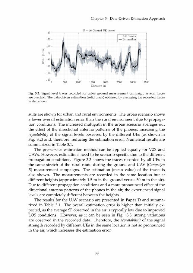
Chapter 3. Data-Driven Estimation Approach
Fig. 3.2: Signal level traces recorded for urban ground measurement campaign; several tracesare overlaid. The data-driven estimation (solid black) obtained by averaging the recorded tracesis also shown.
sults are shown for urban and rural environments. The urban scenario showsa lower overall estimation error than the rural environment due to propaga-tion conditions. The increased multipath in the urban scenario averages outthe effect of the directional antenna patterns of the phones, increasing therepeatability of the signal levels observed by the different UEs (as shown inFig. 3.2) and, therefore, reducing the estimation error. Numerical results aresummarized in Table 3.1.
The pre-service estimation method can be applied equally for V2X andUAVs. However, estimations need to be scenario-specific due to the differentpropagation conditions. Figure 3.3 shows the traces recorded by all UEs inthe same stretch of the rural route during the ground and UAV (CampaignB) measurement campaigns. The estimation (mean value) of the traces isalso shown. The measurements are recorded in the same location but atdifferent heights (approximately 1.5 m in the ground versus 50 m in the air).Due to different propagation conditions and a more pronounced effect of thedirectional antenna patterns of the phones in the air, the experienced signallevels are completely different between the heights.
The results for the UAV scenario are presented in Paper D and summa-rized in Table 3.1. The overall estimation error is higher than initially ex-pected, as the average SF observed in the air is typically low due to improvedLOS conditions. However, as it can be seen in Fig. 3.3, strong variationsare observed in the recorded data. Therefore, the repeatability of the signalstrength recorded by different UEs in the same location is not so pronouncedin the air, which increases the estimation error.
38

2. Data-Driven Estimation
Fig. 3.3: Overlaid signal level traces recorded in the same stretch for ground (a) and drone (b) inthe rural scenario. The data-driven estimation (solid black) is also shown for both cases.
Performance Comparison
As explained in Chapter 2, to show the performance improvements providedby the data-driven estimation approach, the results are compared to tradi-tional methods.
For the ground level case, the proposed approach is compared to em-pirical models (Okumura-Hata and 3GPP TR 38.901) and ray-tracing. Re-sults are introduced in Paper A, and the details on how the comparison isperformed are explained in Paper B. Table B.4 in Paper B summarizes theperformance of the different estimation approaches, showing that traditional
Table 3.1: Overall estimation error ∆ of the pre-service and on-service stage data-driven estima-tions in all studied scenarios.
V2X - Papers A and B UAV - Paper DPre-service
[dB]On-service
[dB]Pre-service
[dB]On-service
[dB]Rural 6.3 5.1 4.8 2.7Urban 4.9 3.7 - -
39

Chapter 3. Data-Driven Estimation Approach
Table 3.2: Paper C - σSF of the UAV measurement data recorded in Campaign A and the IRT/DPMpredictions from the ray-tracing tool.
Height Measurements σSF [dB] IRT σSF [dB] DPM σSF [dB]Ground Level 6.3 4.3 4.6
10 m 8.4 5.3 515 m 6.2 4 3.730 m 4.1 2.8 2.8
methods present very high estimation error compared to what is observedwith the proposed data-driven approach.
A slightly different approach is followed for the UAV case. The perfor-mance of the data-driven, presented in Paper D, is shown only for the ruralenvironment and without comparison to traditional approaches. However,Paper C studies the feasibility of ray-tracing for predicting the SF experi-enced by UAVs in an urban scenario. The study is done using measurementdata from Campaign A, and it compares the observed SF standard deviationσSF with that predicted by the ray-tracing tool. The results presented in Pa-per C are summarized in Table 3.2. As observed, the ray-tracing tool tendsto underestimate σSF and occasionally shows high inaccuracies when pre-dicting the signal trends along the path. Details can be found in Paper C,where it is claimed that this is mostly due to map inaccuracies in the 3Dbuilding database. However, ray-tracing inaccuracies remained after the 3Dmaps were updated, suggesting that this estimation approach is not suitablefor QoS prediction purposes.
The data-driven approach also shows high estimation error for the UAVuse case. However, the estimation error can be further reduced using real-time data from the UE moving along the route. As it can be observed inFig. D.5 of Paper D, each of the users will observe an offset in the measuredRSRP with respect to the estimation provided by the data-driven approachin the pre-service stage. This offset is referred to as Mean Individual Offset(MI0), and it is where the propagation differences between the V2X and theUAV use cases are mostly noticed, as it will be explained in the followingsubsection.
2.2 On-service Stage
As it is shown in Eq. A.3 in Paper A, if known, the Mean Individual Offset(MIO) can be corrected, leading to a decrease in the estimation error. FiguresA.5 and A.7 in Paper A show the MIO of each UE in the ground level use casefor rural and urban environments, respectively. The MIO is consistent for UEtraces from phones oriented towards the same direction, suggesting that UEorientation is the main factor impacting the MIO. Considering also that the
40

3. Outage Probability Estimation
signal reaching the receiver will be subject to the effects of the directional an-tenna patterns of the devices, Paper B presents an attempt of compensatingfor it. Results conclude that the practical challenges of accounting for all pos-sible signal interactions do not provide enough reduction of the estimationerror.
Therefore, Paper B proposes an alternative method to exploit the con-sistency of the MIO between UEs in the same orientation, The method isdescribed using the scheme of Fig. B.9, and it consists of comparing currentestimation error samples with estimation error distributions observed by pre-vious UEs. Paper B presents the tests and corresponding results performedfor the ground level case. Fig. B.10 shows a good match between the actualMIO values for each UE trace in the urban environment and the predictedones using the MIO correction approach. Results are summarized in TableB.6 in Paper B, where the achievable estimation error observed in Paper A isreached after MIO correction.
While the error is mainly constant in the ground-level use case and can becorrected once for the whole route, it varies in the air. This can be observedin Fig. 3.3, where the different UE traces show very similar trends on theground but not in the air. The difference is due to a higher impact of thedirectional antenna patterns in the UAV scenario, characterized by pure LOSconditions. Therefore, the MIO correction needs to be updated every certaindistance. Fig. D.3 in Paper D shows the scheme of what we refer to assliding window MIO correction method, and results in Table D.1 show thatit can significantly reduce the overall estimation error.
The on-service estimations improve the overall estimation errors for allstudied cases. As explained in Chapter 2, these estimations have differentuses. The following section presents a potential use studied in this thesis,consisting of estimating the expected service availability and reliability alongthe route.
3 Outage Probability Estimation
In this thesis, the RSRP estimations are used to estimate the expected serviceavailability and reliability that UEs using mission-critical services will expe-rience. Papers B and D present the results for the ground and UAV cases,respectively.
The main objective is to detect those areas in the route where the proba-bility that the service availability and reliability requirements will not be metis high. As previously mentioned, requirements will vary depending on theservice. A segment of the grid will be declared critical if the service require-ments are not met. For performance evaluation, we compare the recordedcritical areas to the estimated ones and use classification metrics. Since we
41

Chapter 3. Data-Driven Estimation Approach
Table 3.3: Service availability estimation results. Summary for all studied scenarios and estima-tion approaches.
ScenarioEstimationApproach
TPR[%]
FPR[%]
RuralGround
γRSRP = -115 dBm
Data-drivenPre-service
85 4
Data-drivenOn-service
74 3
UrbanGround
γRSRP = -100 dBm
Okumura-Hata 100 963GPP 38.901 70 38Ray-tracing 63 31Data-drivenPre-service
94 16
Data-drivenOn-service
99 10
RuralUAV
γRSRP = -100 dBm
Data-drivenPre-service
81 50
Data-drivenOn-service
88 23
are after the correct estimation of as many critical areas as possible, we aim tomaximize the True Positive Rate (TPR). However, we would also like to min-imize the False Positive Rate (FPR) to avoid a waste of resources by takingaction against non-existent upcoming critical areas.
3.1 Service Availability
Service availability is obtained calculating the probability that the estimatedRSRP is below a certain threshold γRSRP, as show in Eq. B.3 in Paper B. Itconsiders the estimated RSRP value RSRP at a segment and the correspond-ing estimation error distribution N (0, σ).
Results for all studied scenarios are summarized in Table 3.3. We firstfocus on the performance comparison of the data-driven approach with tra-ditional methods. Based on the RSRP estimation accuracy of the traditionalapproaches, it is expected that the estimation of the critical areas shows lessaccurate results. As it is shown if Fig. B.12 in Paper B, the empirical meth-ods seem to underestimate the signal. This, and the high RSRP estimationerror, causes the availability estimations to declare all segments in the routeas critical due to the low estimated RSRP values, confirming that these meth-ods are not suitable for service availability estimations. Even though betterresults are observed when using ray-tracing estimation, the performance is
42

3. Outage Probability Estimation
still poor. The best results for the pre-service stage in the urban scenario areobserved with the data-driven approach.
Secondly, we compare the pre-service stage estimation with the on-servicestage estimations. One would expect that, since the overall RSRP estima-tion error is better in the on-service stage, the service availability estimationswould show improved performance compared to the pre-service stage. Thisis true for the ground urban and the rural UAV scenarios. However, the ruralground scenario, presents a lower percentage of detected critical areas. In theurban ground case, the MIO is constant along the whole route, while in therural ground case, despite being more stable than in the air, it may vary alongthe 15 km route. This can cause some inaccuracies in the corrected RSRP esti-mation, leading to worse performance in the service availability estimations.For the rural UAV, since sliding window MIO is used, the improved RSRPestimations lead to more accurate critical areas detection. Examples of ser-vice reliability estimations for ground and UAV cases can be seen in PapersB and D, respectively.
3.2 Service Reliability
For service reliability estimations, we first calculate the SIR using RSRP recor-ded data from the serving and the neighboring cells and an estimation of theload. We calculate SIR for low, medium, and high estimated load values. TheSIR traces are compared to recorded Modulation and Coding Scheme (MCS)traces and, as shown in Fig. D.7 in Paper D, there is a good match, suggestingthat the SIR approximation is correct. For SIR estimation, the same calculationapproach is followed, but now using the RSRP estimations of the serving celland the neighboring cells instead, as shown in Eq. B.8 in Paper B.
For service reliability critical areas, we calculate, for each segment, theprobability that the SIR is below a certain threshold γsir using Eq. B.3 inPaper B. Results for all studied scenarios are summarized in Table 3.4. Forall cases, MIO correction results in a decrease of both the TPR and the FPR.As aforementioned, the main objective is detecting the critical areas to avoidpotential drops in service reliability. However, high FPR can lead to a misuseof resources, so it is also important to minimize it. On that basis, MIO correc-tion should depend on the service priorities. Service reliability estimationscould be further improved by using real load values for each of the neighbor-ing cells involved in the calculation of the SIR. Further details can be foundin Papers B and D.
43

Chapter 3. Data-Driven Estimation Approach
Table 3.4: Service reliability estimation results for an average load of 30 %. Summary for allstudied scenarios and estimation approaches.
ScenarioEstimationApproach
TPR[%]
FPR[%]
RuralGround
γSIR = -3 dB
Data-drivenPre-service
72 38
Data-drivenOn-service
65 28
UrbanGround
γSIR = -3 dB
Data-drivenPre-service
88 41
Data-drivenOn-service
77 31
RuralUAV
γSIR = -3 dB
Data-drivenPre-service
69 28
Data-drivenOn-service
67 23
4 Summary of Main Findings
This section outlines the main findings of the Ph.D. study and includes Tables3.5 to 3.7, which summarize the content of the papers. The main findings ofthis thesis can be summarized as:
• Use of the data-driven approach provides more accurate RSRP estima-tions than other approaches available in the literature, as shown in Fig.3.4.
• UE orientation is the main factor affecting the individual offset ob-served by a UE.
• Correction of the offset can only be done using real-time data, exploit-ing the estimation error observed by previous UEs in the route.
• Due to a more pronounced effect of the directional antenna patterns ofthe UEs, UAV estimations require specific on-service stage corrections.
• The data-driven approach allows detecting at least 70 % of the criticalareas of the route, thus not fulfilling the typical 95 % target.
44

4. Summary of Main Findings
Fig. 3.4: Performance comparison of the data-driven approach (pre-service and on-service) withray-tracing and empirical methods.
45

Chapter 3. Data-Driven Estimation Approach
Tabl
e3.
5:Pa
per
sum
mar
yI:
use
case
,mea
sure
men
tca
mpa
ign,
and
obje
ctiv
es.
Pape
rID
Use
Cas
e
Mea
sure
men
tC
ampa
ign
Obj
ecti
ves
TSM
ESc
anne
rPh
ones
A
V2X
Loca
ted
inth
eca
rto
pca
rrie
r,co
nnec
ted
toan
omni
dire
ctio
nal
ante
nna
mou
nted
hori
zont
ally
.
Diff
eren
tse
tups
(A,B
&C
).Se
epa
pers
.
-D
escr
ipti
onof
the
data
-dri
ven
esti
mat
ion
appr
oach
.-
Perf
orm
ance
eval
uati
onof
the
pre-
serv
ice
stag
eda
ta-d
rive
nap
proa
ch.
B
-Pr
esen
tati
onof
the
two-
stag
efr
amew
ork
conc
ept.
-Pe
rfor
man
ceco
mpa
riso
nof
the
data
-dri
ven
appr
oach
wit
htr
adit
iona
lmet
hods
.-
Des
crip
tion
and
perf
orm
ance
eval
uati
onof
the
MIO
corr
ecti
onm
etho
d.-
Eval
uati
onof
crit
ical
area
ses
tim
atio
nin
term
sof
serv
ice
avai
labi
lity
and
relia
bilit
y.
C
UA
V
Han
ging
from
the
dron
efu
sela
ge.C
onne
cted
toan
omni
dire
ctio
nala
nten
na,
mou
nted
50cm
abov
eth
edr
one
fuse
lage
.
Not
used
-Fe
asib
ility
stud
yon
the
use
ofra
y-tr
acin
gfo
rsh
adow
fadi
ngpr
edic
tion
usin
gIR
Tan
dD
PM.
-C
ompa
riso
nof
mea
sure
dR
SRP
tren
dsw
ith
trac
espr
edic
ted
byth
era
y-tr
acin
gto
ol.
DN
otus
edPh
ones
Dro
ne
-Pe
rfor
man
ceev
alua
tion
ofth
eda
ta-d
rive
nap
proa
ch(p
re-s
ervi
cean
don
-ser
vice
stag
es).
-D
escr
ipti
onan
dpe
rfor
man
ceev
alua
tion
sof
the
slid
ing
win
dow
MIO
corr
ecti
onm
etho
d.-
Eval
uati
onof
crit
ical
area
ses
tim
atio
nin
term
sof
serv
ice
avai
labi
lity
and
relia
bilit
y.
46

4. Summary of Main Findings
Table 3.6: Paper summary II: scenario and numerical results. ∆ is the estimation error.
PaperID
Scenario Numerical Results Summary
A
Rural15 km stretch
- Pre-service ∆: 6.3 dB- Achievable ∆ after MIOcorrection: 4.9 dB
Urban3.3 km loop
- Pre-service ∆ = 4.9 dB- Achievable ∆ after MIO correction: 3.6 dB- Data-driven shows ∆ 3 dB better thanray-tracing and up to 6 dB better thanempirical.
B
Rural15 km stretch
- Achieved ∆ after MIO correction usingz-test with real-time data: 5.1 dB- Average on-service stage critical areadetection: 70 %- Average on-service stage critical areamisdetection: 20 %
Urban3.3 km loop
- Achieved MIO correction using z-testwith real-time data: 3.7 dB.- Average on-service stage critical areadetection: 88 %- Average on-service stage critical areamisdetection: 21 %
CUrban
17 streets@10 m, 15 m, 30 m
- Predicted σSF is generally 2 dB belowmeasured σSF.- Correlation coefficient between predictedtrends and measured trends range isfrom -0.6 to almost 1.
DRural5 km stretch@ 50 m
- Pre-service ∆: 4.8 dB- On-service ∆ using sliding window MIOcorrection: 2.7 dB.- Average on-service stage critical areadetection: 78 %- Average on-service stage critical areamisdetection: 23.3 %
47

Chapter 3. Data-Driven Estimation Approach
Table 3.7: Paper summary III: conclusions.
PaperID
Conclusions Summary
A
- Pre-service data-driven estimations provide accurate RSRPestimations.- Improved performance was observed with respect to otherestimation approaches.- Data-driven estimation can be improved if MIO is corrected.
B
- MIO correction cannot be performed in the pre-service stage.- The estimation error can be reduced to the achievable by usingerror distributions from previous UEs and comparing them withreal-time data of the moving UE.- A high percentage of critical areas can be detected, but there is atrade-off with misdetection.- The algorithm does not predict the 95 % target, but it shows thebest performance observed in the state if the art.
C
- Ray-tracing can be used to estimate the UAV radio channelif accurate maps of the environment are used.****While this is true for overall shadowing predictions, the accuracy is lowwhen predicting specific trends and variations along the UAV path.
D
- Data-driven approach can be used for RSRP estimation inthe UAV case.- Slight modifications are required in the MIO correction methoddue to a more pronounced effect of the device antenna pattern inthe air.- Performance in critical area detection shows similar trends to theones observed on the ground.
48

Chapter 4
Conclusions
Cellular networks are used to provide reliable communications for mission-critical services. This use case could benefit from predictive mechanisms(radio conditions, radio resources, traffic, etc.) since predicting a poten-tial service degradation would allow to mitigate it proactively, reducing oravoiding the damage caused by it. This thesis provides an in-depth exper-imental analysis and develops a framework for predicting service degrada-tion for mission-critical communications in practical V2X and UAV scenarios.The work proposes a two-stage framework: pre-service and on-service. Thepre-service stage occurs before the UE uses the service and allows for routeplanning and optimization. The on-service stage occurs once the service hasstarted and allows for mobility, RRM and QoS management optimization.
Among the different metrics that can be predicted to avoid service degra-dation, this thesis aims at providing accurate RSRP predictions, primarilydue to two reasons. First, RSRP is a metric used for fundamental radio pro-cedures, and in-advance awareness of the UE experienced RSRP values canallow for proactiveness in all of them. Second, the RSRP observed in a spe-cific location is more resilient to load and interference variations than othermetrics, allowing to provide an estimation for all UEs at any time of the dayin that location.
The first part of this study focuses on signal strength estimation. Theproposed estimation approach uses experimental data and aggregates theRSRP values reported from different UEs in a specific location, regardless oftheir serving cell. The evaluation of the algorithm is done for two scenarios(rural and urban) and use cases (V2X and UAVs) with different propagationconditions. The ground-level urban environment, characterized mainly byNLOS conditions, presents the lowest estimation error with the data-drivenapproach. The observed repeatability of the signal levels in the urban scenariois high due to the increased multipath propagation in this environment. The
49

Chapter 4. Conclusions
signal levels observed by the different phones follow the same trends, whichresults in lower estimation errors. The rural environment, on the other hand,is mainly characterized by LOS conditions, and the signal levels experiencedby UEs in different orientations present slightly different trends in some partsof the route. This is due to a more pronounced effect of the directive antennapatterns of the devices in the rural environment, and causes an increase in theoverall estimation error. The effect of the directive antenna patterns is evenhigher in the air, where there are improved LOS conditions, and differentcells are serving the phones in a specific location.
The study compares the performance of the data-driven approach withempirical approaches and ray-tracing estimations. For the ground-level case,the comparison is made for the urban scenario. Results show that the data-driven approach outperforms empirical and ray-tracing methods. In the UAVcase, ray-tracing is evaluated for shadow fading prediction only. Resultsshow that ray-tracing typically underestimates the signal variations, resultingin a lower estimated standard deviation of the shadow fading σSF. The esti-mation error observed when using traditional approaches suggests that theseare not suitable for the purpose of this study, as highly accurate estimationsare required.
Each UE presents a mean individual offset (MIO) with respect to the esti-mated value. The data-driven estimations can be improved in the on-servicestage by using real-time data from the UE moving along the route. Afterevaluation of MIO correction in the pre-service stage, it is concluded thatreal-time data is needed. On-service correction is performed by comparingthe estimation error samples observed by the current UE with error distri-butions from previous UEs in the same route. A statistical test determineswhether the observed samples belong to a certain error distribution. If thetest is positive, the mean value of the distribution is used as a correction off-set. While at ground level, the MIO can be corrected once for the whole routedue to the consistency of the offset, it needs to be updated in the UAV case.The on-service MIO correction reduces the overall estimation error for allstudied scenarios, reaching a very low overall estimation error, particularlyin the UAV case.
Last, this work studies the estimation of the probability of RSRP or SIRbeing below a certain threshold, using the signal strength estimations ob-tained through the data-driven approach. These probabilities are used forin-advance detection of the critical areas in the route. Compared to the prob-abilities calculated based on the experimental data, results show that thedata-driven approach allows for at least 70 % of the critical areas to be de-tected. Misdetection can reach 40 % for some scenarios. For most of thestudied cases, the target of 95 % critical areas detection is not met.
The main key takeaways of the work presented in this thesis can be sum-marized as follows:
50

• A measurement-based estimation can improve the estimation error ofray-tracing by 3 dB and more than 4 dB for empirical methods. Usingreal-time data can improve user-specific data-driven estimations oncethe UE is using the service.
• Good visibility conditions and lack of obstacles increase the effectof directive antenna patterns in the UE, causing lower repeatabilityand higher estimation error for the presented data-driven approach.This effect is more pronounced in the UAV scenario, with improvedvisibility conditions.
• Despite not meeting the 95 % target, the data-driven provides betterperformance for RSRP estimations than much of the work availablein the literature, and the network may use it for predicting servicedegradation.
As part of future work, it would be interesting to investigate the system-level gain provided by estimating a critical area and mitigating it before itoccurs. If, e.g., a service reliability drop is estimated due to an SIR drop,the network can activate an interference mitigation mechanism. In the sameway, the damage caused by false critical area prediction can be explored.Future work could also be extended with the exploration of different usesof the accurate RSRP data-driven estimations: mobility management (e.g.,prepare and execute HO based on the estimations), power control, or otherprocedures.
51

Chapter 4. Conclusions
52

Part II
Papers
53

Paper A
Experimental Evaluation of Data-driven Signal LevelEstimation in Cellular Networks
Melisa López, Troels B. Sørensen, István Z. Kovács, JeroenWigard and Preben Mogensen
The paper has been published in theIEEE 94th Vehicular Technology Conference (VTC-Fall 2021)

© 2021 IEEEThe layout has been revised.

1. Introduction
Abstract
Estimating accurately the signal levels that a user equipment experiences along amovement route is a key step in the process of providing and guaranteeing the re-quired service quality. Obtaining accurate location-specific estimations of the signallevel is challenging due to its random variations. In this paper we investigate theuse of aggregated measurements from multiple User Equipment (UE) to estimatethe serving Reference Signal Received Power (RSRP) that the user will experiencealong a route. We use Long Term Evolution (LTE) measurements obtained in ruraland urban areas from drive tests and analyze the dependence of data variability. Re-sults show that the accuracy of data-driven estimation is impacted significantly by thevariability in the underlying data due to UE orientation, UE characteristics and theirimmediate environment. With compensation for a subset of these effects the standarddeviation of the estimation error can be lowered from an overall approximately 8 dBdown to 4 dB.
1 Introduction
The need of accurate estimations and/or predictions of the Key PerformanceIndicators (KPI) involved in a wireless communications system is becomingmore obvious with the wide variety of services and real-time applications thatthe upcoming 5G New Radio (NR) is aiming to provide. Some applications,such as the critical type of communications as e.g., Vehicle-To-Everything(V2X) [1] or Unmanned Aerial Vehicles (UAV) [2], will have strict latencyand/or reliability demands in order to meet the required Quality of Service(QoS).
Estimating accurately the signal levels that would be experienced by aUserEquipment (UE) along a route allows to evaluate the service availability andreliability with certain accuracy, e.g. Signal-To-Interference-Plus-Noise Ra-tio (SIR) along the route before the UE starts using the service. This can bespecifically useful for the mentioned critical services, where reliability plan-ning ahead is involved.
There are different approaches to estimate signal strength. Traditionalempirical and statistical models are inferred from measurements and aim forthe generalization of the estimation in a specific environment, which com-promises their location-specific accuracy [3]. An alternative method for sig-nal strength estimation are deterministic models such as ray tracing or otherphysical-based models. These methods provide more accurate estimationsbut are computationally complex and require detailed modelling of the envi-ronment [4].
Another option for estimating signal strength is using a data-driven ap-proach. It is specified in [5] that the network may require the UE to provide
57

Paper A.
radio measurements such as its Reference Signal Received Power (RSRP) as-sociated with the corresponding location information. This feature, knownas Minimization of Drive Tests (MDT), was standardized as part of 3rd Gen-eration Partnership Project (3GPP) Release-10 specifications for Long TermEvolution (LTE), and it is typically used by network operators for optimiza-tion purposes. Data-driven RSRP estimation could be performed using radiomeasurements that could be easily acquired exploiting the MDT feature. TheRSRP estimations obtained would be location-specific. A drawback of thisapproach, as we will explore in this paper, is the impact from device hetero-geneity due to antenna patterns and coupling effects, device orientation andplacement, and how they interact and compare with the variability causedby the random nature of the wireless propagation channel. Other potentialinaccuracies introduced by MDT such as positioning and quantization errorsor scarcity of user reports are discussed in [6].
In our experimental evaluation we have limited the number of differentdevices to two specific UE models, but included these in many different con-figurations within our measurement setup. The two models have been ver-ified to have significantly different radiation patterns, but are calibrated toremove average measurement offsets. Any offset in our analysis will there-fore result from the mentioned heterogeneity effects, which cause the realvariability in the data. Implementation (chipset) specific measurement off-sets will occur in reality but are degenerate to those effects. In addition, wehave performed measurements in two different environments – urban andrural – to see the impact of any interaction between propagation environ-ment and devices. This methodology attempts to include a similar range ofdiversity as if we had included several different UE models in our analy-sis. RSRP measurements have been collected over several measurement drivetests in an LTE network in Denmark. For data aggregation we use the geo-metric average of the collected RSRP data. The specific contribution in ourwork is the identification of factors that significantly impact the accuracy ofthe data driven approach and therefore should be accounted for when pro-cessing measurements obtained from MDT. Not only do such corrections sig-nificantly improve the accuracy of the data driven approach, but it also givesa clear performance improvement over the alternative use of ray-tracing.
Several approaches have been proposed in the recent years to improveaccuracy in the signal level estimation, most of them using machine learningtechniques. In [7] the authors use a neural network to estimate path loss,and achieve an estimation error of 6-7 dB standard deviation depending onthe frequency. The authors of [8] propose the use of a convolutional neuralnetwork and satellite images to estimate path loss, achieving a Root MeanSquare Error (RMSE) between 6 dB and 9 dB with standard deviations ofup to 6 dB depending on the scenario used for testing the model. In [9]they propose a feed-forward neural network to predict path loss. Using field
58
2. Measurement Campaign
measurements from different environments, they achieve an RMSE of 6.3 dB.These studies provide better accuracy than traditional approaches. They
rely mainly on regression or learning techniques and require training andtesting over different environments. Differently from the existing literature,the work in this paper is a simple approach that provides a realistic estima-tion of the actual signal levels experienced by the user at a specific locationwithout additional features in the network.
The rest of the paper is organized as follows: Section 2 shows the mea-surement campaign details. Data processing and estimation procedures areshown in Section 3 and Section 4 presents the obtained results. Conclusionsare presented in Section 5.
2 Measurement Campaign
A drive test was carried out using four commercial smartphone devices withRohde&Schwarz QualiPoc firmware and a TSME professional radio scan-ner1. The use of mobile devices with specific measurement capability limitsthe number of available device models. However it considerably eases thedata collection and ensures a consistent, calibrated and regular measurementupdate rate as a basis for our analysis. The scanner was connected to a refer-ence paddle antenna in a fixed position. The reference antenna was mountedhorizontally outside and on top of the car with its main lobe extending toboth sides of the car. It served to check the repeatability between measure-ments e.g. impact of changing network and environment conditions (fastfading, load/interference, etc.).
With respect to the smartphone devices, we used two different modelsfrom the same vendor: two Samsung Galaxy S5 (S51, S52) and two SamsungGalaxy S9 (S91, S92) and positioned them in a total of 8 different orientations.We drove several times along two different scenarios in different directionsto ensure as much variance (in terms of received signal levels in the differentphones) as possible in our data.
All phones and scanner were locked to measure a 20 MHz LTE carrier inthe 1800 MHz band. The phones had a sampling rate of 500 ms and wereforced to be in active mode during the whole test. Each recorded measure-ment from the phones consisted in the RSRP of the serving cell and its corre-sponding Physical Cell ID (PCI). Differently, the scanner provided the RSRPand corresponding PCI of all the visible cells in the 1800 MHz frequencyband. Location of the devices was tracked during the test using GPS. Theinstantaneous RSRP measurements recorded by the phones and the scannerare subject to L1 and L3 filtering. As explained later in Section 3, they are
1QualiPoc and TSME ©Rohde & Schwarz more information can be found athttps://www.rohde-schwarz.com
59

Paper A.
Fig. A.1: Phones-Scanner positions in the car top carrier. Phone ID in Table A.1.
Table A.1: Measurement Setups Description
ID Phone Setup Position Orientation1 S51 A
Standing N2 S52 Standing E3 S91 Laying Up4 S92 Standing S5 S51 B
Laying Down6 S52 Laying Up7 S91 Laying Up8 S92 Laying Down9 S51 C
Front Seat E10 S52 Glove Compartment Up11 S91 Back Seat Up12 S92 Trunk Up
also spatially averaged, which reduces the fast fading effects and measure-ment errors [10]. According to our calibration test, this reduces the RSRPmeasurement error of the estimation to below ±1 dB in all cases.
The measurements were performed using three setups (A, B and C) wherethe phones had different orientations. The orientation and position for eachphone in every setup is included in Table A.1, where the north reference isthe front of the car. The reader can locate in Fig. A.1 the ID numbers fromTable A.1 for better understanding. For setups A and B, the phones andthe scanner were mounted (laying or standing) in a car top carrier, while forsetup C the phones were moved inside the car, keeping the scanner in the topcarrier.
The measurement campaign was conducted in rural and urban scenariosnearby and in the city of Aalborg (Denmark, Sept. 2020). The measurementroute for the rural environment consisted of two round-trips in a 14.8 kmstretch from point X to point Y, whereas in the urban scenario the car drove
60

3. Data Processing
X
Y
Fig. A.2: Measurement Areas.
three times along a 3.3 km loop (see Fig. A.2). An average driving speedof 65 km/h was kept in the rural case, while it was 22 km/h in the urbanscenario. The averageBase Station (BS) height in the LTE networks is 29 mand 24.7 m for the rural and urban scenarios, respectively. BS heights rangingfrom 20 m to 39 m and down-tilts between 3 and 6 degrees are observed inthe rural case while the urban scenario presents heights between 10 m and 58m, and down-tilts within 0 and 10 degrees. The rural radio environment ismostly characterized by LOS conditions. The urban scenario is a city center,where the average height of the buildings is approximately 15 m and con-ditions are dominantly Non-Line-Of-Sight (NLOS). In both cases, the terrainprofile is flat and on average 5 m above sea level.
3 Data Processing
The reference estimation is obtained by averaging signals recorded by mul-tiple UEs that have previously passed through a certain route. We use theRSRP measurements recorded by all the different phones to obtain a statis-tical estimation of the average signal level that any user will experience in aspecific location. The metric chosen for data aggregation is the geometricalmean.
Each measurement route was split in a distance grid of J segments of 10m as shown in Fig. A.3. For each UE and run/loop, the measurement traceof the serving cell recorded by that UE was located in the distance grid, av-
61

Paper A.
eraging (also using geometrical mean) all the data points located within thesame 10 m segment. This further reduced the fast fading effects and mea-surement errors aforementioned. The number of samples recorded by eachphone in one segment depends on the driving speed: for the rural scenariowe observed 1-2 samples per segment, while for urban case, 4-5 samples persegment were recorded. For cases where a handover occurred in the middleof the grid segment, we used only the samples related to the serving cell withthe highest number of recorded samples within that 10 m segment.
For each segment in the distance grid we have available a set of valuescorresponding to measurements recorded by multiple UEs in the differentruns or loops. Regardless which cells are serving those UEs the measure-ments are aggregated to one average signal level estimate. The main reasonfor this approach is data sparsity as we will discuss in the results section.Aggregating all values provides a continuous and more reliable estimate ofnetwork availability along that route. Furthermore, aggregating serving cellmeasurements irrespective from the serving PCI is a reasonable approach ifwe aim to estimate the expected average signal level in a segment, since thecell selection/re-selection procedures tend to equalize the measured signals,minimizing the effect of distance between the UE and the corresponding serv-ing BS. The aggregation process is illustrated in Fig. A.3, where each segmentin the distance grid, from seg1 to segJ , has an estimated value which is ob-tained using the geometric average from all the values in the correspondingsegment from UE1 to UEN , regardless which cell these users are connectedto. The RSRP estimation for that location (10 m segment) is the mean, inlogarithmic scale (dBm units), of that set of values.
RSRPsegj =1N
N
∑i=1
RSRPi,segj (A.1)
where RSRPsegj is the RSRP estimated value in the grid segment j, andi = 1, ..., N indexes the collected values in that location (10 m grid segment).N is different for each environment:
• Rural: 4 phones, 3 setups, 4 runs (two round-trips) gives N = 48 recordedvalues for the mean. With a stretch length of 14.8 km, Number of seg-ments is 1480.
• Urban: 4 phones, 3 setups, 3 loops gives N = 36 recorded values forthe mean. With a stretch length of 3.3 km, Number of segments is 330.Only one driving direction was measured due to traffic restrictions.
The radio network scanner data was used as a reference, so that measure-ments on the same serving cell PCIs as the phones were extracted in eachcase. The same averaging process over the 10 m distance grid was applied to
62

3. Data Processing
Fig. A.3: Measurement averaging and distance grid scheme. Estimations (blue lowest row) arebuilt using measurements from multiple UEs (white upper rows).
this data, and an estimation for each UE based on scanner data was obtainedfor each grid segment. An average of 5 and 8 samples per segment was usedfor the rural and urban environments, respectively.
To evaluate the accuracy of the RSRP estimation, we calculate for everysegment of the grid the difference between the estimated value and each ofthe measured values used to obtain the estimation at that grid segment. Theestimation error ∆ (in dB) for a UE i in a grid segment j is defined as:
∆UEi ,segj = RSRPUEi ,segj − RSRPsegj (A.2)
where RSRPUEi ,segj is the actual measured value by a certain UE i in grid
segment j and RSRPsegj is the estimated value for grid segment j. The erroris calculated for each of the N available UEs (i = 1, ..., N) used to estimate theaverage signal level at segment j.
To evaluate the estimation accuracy over all samples we use the meanand standard deviation of the estimation error in Eq. A.2. We aim to obtainan error distribution with a σ as low as possible as this would indicate thatthe difference between the estimation and the actual values of the individ-ual phones is low in expectation regardless the UE and its driving directionor orientation. The distribution of the estimation error, as shown furtherin Section 4, is generally well behaved for all the analyzed cases, having asymmetric uni-modal characteristic with good approximation to a Gaussian
63

Paper A.
distribution. It therefore motivates our choice of the mean aggregation func-tion based on the logarithmic signal values since mode, median and meandegenerates to the same case.
Furthermore, instead of evaluating the distribution of the estimation errorfor all phones, the mean µ and standard deviation σ of the estimation erroris shown for each individual UE and run separately (as later shown in Fig.A.5). This allows to observe the mean individual offset of each phone withrespect to the overall mean value (estimation). We also evaluate the effect thatremoving the phone individual offset has in the overall standard deviation bysubtracting, for each of the phones, their corresponding mean value µ. Theestimation error (in dB) is in this case calculated as:
∆′UEi ,segj= RSRPUEi ,segj − µ∆UEi
− RSRPsegj (A.3)
where µ∆UEiis the mean value of the estimation error for UEi over the full
measurement run.
4 Results
The results presented in this section show how the estimation error in thedata-driven estimations is impacted by:
• Environment effects: Shown by presenting separately the rural and urbanscenarios.
• UE directional antenna pattern effects: We present results for devices withdifferent orientations and compare them to the scanner reference mea-surements.
• UE driving direction: Results for rural environment compare estimationerror when using a single estimation based on the combined directionswith the case where different estimations are used for the two direc-tions.
• UE Conditions: Such as e.g. whether the UE is inside or outside the car.
4.1 Rural Environment
Two approaches are followed for the analysis of this environment. First, weevaluate the results obtained when using the N = 48 available values to calcu-late the estimation at each grid segment. Later, we evaluate the two differentdriving directions separately, i.e. N = 24 recorded values are used to calcu-late the estimation. Therefore, for the latter case, there are two estimationsfor each grid segment, one for each direction.
64
4. Results
A summary of the overall standard deviation for all the studied cases be-fore and after correction of the individual phone offsets can be found in TableA.2. The mean of the distributions of the estimation error is zero regardlessthe data used for the estimation (combined/separate directions) or the sourceof it (phones /scanner) due to normalization.
We use the scanner results as a reference considering that its position isfixed for all runs in all setups. The scanner shows a standard deviation of5.1 dB for combined directions and 4.1 dB and 3.6 dB for the separate di-rections analysis. This illustrates that the moving direction of the UE willaffect its experienced signal level. Cells serving the UEs are mostly differ-ent when driving in opposite directions, which is assumed to be one of thecauses for the standard deviation of the estimation error to increase whencombining directions. For the scanner measurements, variability due to ori-entation and position is mostly eliminated, but measurements from differentcells are combined. Furthermore, in reality there is a small difference in thereference antenna pattern between the two sides of the car, due to the an-tenna itself and the impact of the car structure. The inherent measurementprocess will also lead to slightly different results for the two directions due tothe temporal evolution of the signals, the impact of interference in the mea-surement, etc. In general, much of this variability cannot be removed fromany measurement.
The phones present a standard deviation of 6.3 dB for combined direc-tions, as observed in Fig. A.4-a, whereas if the two directions are treatedseparately, the standard deviation is barely reduced to 6 dB (X to Y direction,as shown in Fig. A.4-b) and 5.5 dB (Y to X direction). These values are higherthan the ones observed for the scanner, and we assume that this is mainlydue to the different UE antenna orientations and placement.
In Fig. A.5 we evaluate the estimation error over the full route for eachindividual UE in the separate directions analysis. The estimation error iscalculated with respect to the corresponding estimated average for each di-rection (X-Y or Y-X). It can be seen that µ is generally stable between differ-ent runs for the same phone and direction. However, different means areobserved for each phone, which suggests that the effective antenna patternsand placement have an effect on the received signal. This difference is espe-cially noticeable for setup C, which shows a negative mean for all phones dueto the car body blockage. This suggests that the overall standard deviationof the error could be reduced by identifying if the phone is inside or outsidethe car. The standard deviation shows values varying from 3 dB to 6 dB.These are, for some cases, not consistent between opposite directions. Theoverall scanner standard deviation is 3.8 dB (average from the two separatedirections).
We correct the phone individual offsets as per Fig. A.5 using Eq. A.3. Theresults show that standard deviation is further reduced to 4.3 dB (as shown
65

Paper A.
Fig. A.4: Rural ∆ distributions for the different compensations applied.
Table A.2: Rural Environment - Std. Dev. Results
CombinedDirections
Separate Directions@Phones
Separate Directions@Scanner
Phones Scanner X-Y Y-X X-Y Y-Xσ [dB] Before
Offset Correction6.3
5.16 5.5
4.1 3.6σ [dB] After
Offset Correction4.9 4.3 4
in Fig. A.4-c) in the X to Y direction and 4 dB in the Y to X direction afterindividual offset correction. These values, as observed in Table A.2, are muchcloser to the ones obtained with the scanner data. Similar improvements canbe obtained by identifying the phones located in the car top carrier i.e., onlysetups A and B included in the mean value calculation. It is shown in Fig.A.4-d that the estimation error in that case is reduced to 3.9 dB in the X to Ydirection and 4.2 dB in the Y to X direction i.e., the error decreases on average1.7 dB with respect to Fig. A.4-b.
4.2 Urban Environment
The same analysis as previously shown for the rural environment was per-formed for the urban scenario. Results for this case are summarized in TableA.3. For scanner data an overall standard deviation of 3.3 dB is observed.The phones, on the other hand, show an overall standard deviation of 4.9 dB,cf. Fig. A.6-a. In this scenario, we further compare the results with two ref-
66

4. Results
Fig. A.5: Rural environment phone-individual estimation error statistics before mean offset cor-rection.
erence methods. First, we show the results for ray-tracing estimations, whichprovide a σ of 7.6 dB after calibrating the Dominant Path Model (DPM) [11]with our measurement data. Secondly, the UMa TR38.901 model [12] is usedfor comparison. The estimations for this model are tuned to Line-Of-Sight(LOS)/NLOS conditions based on ray tracing predictions, and it shows a σof 9.3 dB when calibrating parameters to this specific scenario. These resultsillustrate that the data-driven estimation approach can provide much higheraccuracy than the traditional methods, as the estimation is obtained usingreal data from previous UEs passing by that exact same location.
In Fig. A.7 we show the individual analysis for each phone. As it wasobserved in the rural case, the mean offset for each of the phones is dif-ferent but stable between different loops for the same phone, and standarddeviation varies between 2 dB and 5 dB. Different results are also observedbetween setups A-B and setup C. We remove the offset for each of the phonesindividually, and show in Fig. A.6-b the overall standard deviation, which isreduced to 3.6 dB, closer to the scanner reference. Approximately the sameeffect is observed when excluding setup C from the estimation, which as
67

Paper A.
Fig. A.6: Urban ∆ distributions for the different compensations applied.
Table A.3: Urban Environment - Std. Dev. Results
Phones ScannerRay-tracingReference
3GPP 38.901 UMaReference
σ [dB] BeforeOffset Correction
4.9
σ [dB] AfterOffset Correction
3.63.3 7.6 9.3
shown in Fig. A.6-c, shows a standard deviation of 3.9 dB.In the urban scenario propagation mechanisms differ, primarily by the in-
creased multi path propagation compared to the rural environment. There-fore, the impact of UE directional characteristic as we saw for the rural, willbe less pronounced and lead to reduced standard deviation.
5 Discussion and Conclusion
Initially we made a choice to aggregate measurements over a segment re-gardless the serving cell PCI. The choice was mainly in consideration of datasparsity since with cell specific data aggregation it would be difficult to col-
68

5. Discussion and Conclusion
Fig. A.7: Urban environment phone-individual estimation error statistics before mean offsetcorrection
Table A.4: PCI Overlap % in Rural and Urban Scenarios
UrbanRural Same
Driving DirectionsRural Opposite
Driving DirectionsAvg. PCI
Overlap [%]80.3 69.6 53.7
lect a sufficient number of samples to obtain a reliable estimate for each andevery grid segment along a route. The main reason for this is that the UEsare not likely to have the same serving cells in a particular segment. TableA.4 shows the summary analysis of the average percentage of grid segmentsalong the route in which the serving cell is the same for different UEs, whichwe refer to as PCI overlap percentage. The urban scenario is clearly showingthe highest average PCI overlap percentage. For the rural environment, thepercentage is clearly higher when driving in the same direction than whenthe opposite directions are analyzed. As one can imagine, the price to paywhen mixing measurements irrespective of the serving cell is that more vari-ation is included which in turn leads to higher estimation error. This relatesvery well to our results, e.g. highest PCI overlap is observed in the urban en-vironment where lowest estimation error is observed, and for the rural casehigher PCI overlap is observed between UEs driving in the same directionwhich also shows lower estimation error than when different directions arecombined. There are many factors one could speculate impacting these re-sults, e.g. the distance to the serving cell or the absence or presence of LOScondition. We have investigated most of these factors in an attempt to reducethe estimation error, but have found no clear relation yet.
69

References
The main benefit of our chosen data aggregation for the data driven esti-mation approach is its simplicity and that estimation errors of approximately3.5 to 4 dB are possible by identifying a few main impacting factors. Theycan be accounted for by similarly simple means, i.e. having knowledge of thedriving direction, as well as approximate location, and being able to removethe UE individual offset resulting from UE placement, orientation and imme-diate environment conditions. Information on the driving direction reducesthe overall standard estimation error by almost 3 dB on average, and anotheradditional 1.5 dB reduction results when accounting for the individual off-sets. The estimation of individual offsets is for future work, but a range ofmethods are available such as based on adaptive filtering or statistical infer-ence.
As we have illustrated by comparison with the use of ray tracing andstatistical estimation methods, the data driven approach has the potential toconsiderably improve the estimation accuracy.
References
[1] 5G Automotive Association, “ Making 5G proactive and predictive forthe automotive industry,” Tech. Rep. White Paper, Jan. 2020.
[2] Vodafone and Ericsson, “Vodafone and Ericsson trial automated flightpaths for connected drones,” Press Release, Mobile Europe.
[3] O. O. Erunkulu, A. M. Zungeru, C. K. Lebekwe, and J. M. Chuma, “Cel-lular communications coverage prediction techniques: A survey andcomparison,” IEEE Access, vol. 8, pp. 113 052–113 077, 2020.
[4] Z. Yun and M. F. Iskander, “Ray tracing for radio propagation modeling:Principles and applications,” IEEE Access, vol. 3, pp. 1089–1100, 2015.
[5] 3GPP, “Radio measurement collection for Minimization of Drive Tests(MDT); Overall description; Stage 2,” Tech. Rep. 37.320 V10.1.0, Mar.2011.
[6] H. N. Qureshi, A. Imran, and A. Abu-Dayya, “Enhanced MDT-basedperformance estimation for AI driven optimization in future cellular net-works,” IEEE Access, vol. 8, pp. 161 406–161 426, 2020.
[7] M. Ayadi, A. B. Zineb, and S. Tabbane, “A UHF path loss model us-ing learning machine for heterogeneous networks,” IEEE Transactions onAntennas and Propagation, vol. 65, no. 7, pp. 3675–3683, 2017.
[8] J. Thrane, B. Sliwa, C. Wietfeld, and H. L. Christiansen, “Deep learning-based signal strength prediction using geographical images and expert
70
References
knowledge,” in GLOBECOM 2020-2020 IEEE Global Communications Con-ference. IEEE, 2020, pp. 1–6.
[9] S. I. Popoola, E. Adetiba, A. A. Atayero, N. Faruk, and C. T. Calafate,“Optimal model for path loss predictions using feed-forward neural net-works,” Cogent Engineering, vol. 5, no. 1, p. 1444345, 2018.
[10] 3GPP, “Requirements for support of radio resource management (Re-lease 17),” Tech. Rep. 36.133 V17.3.0, Sep. 2021.
[11] R. Wahl, G. Wölfle, P. Wertz, P. Wildbolz, and F. Landstorfer, “Dominantpath prediction model for urban scenarios,” 14th IST Mobile and WirelessCommunications Summit, Dresden (Germany), 2005.
[12] 3GPP, “Study on channel model for frequencies from 0.5 to 100 GHz.(Release 16),” Tech. Rep. 38.901 V16.1.0, Dec. 2019.
71

References
72

Paper B
Measurement-Based Outage Probability Estimationfor Mission-Critical Services
Melisa López, Troels B. Sørensen, István Z. Kovács, JeroenWigard and Preben Mogensen
The paper has published in theIEE Access, 2021.

© 2021 IEEEThe layout has been revised.

1. Introduction
Abstract
An accurate estimation of the service quality that the user will experience along aroute can be extremely useful for mission-critical services. Based on availability andreliability estimations, it can provide the network with in-advance information onthe potential critical areas along the route. If such estimation is based on empir-ical/statistical or site-specific estimations, both of which are typically used for cel-lular network planning, it will lead to significant uncertainty in the estimation, aswe demonstrate in this paper. Instead, if estimations are based on previously col-lected measurements, the uncertainty can be significantly reduced. In this paper, weanalyze the achievable accuracy of such a data-driven estimation which aggregatesmeasurements from multiple User Equipment (UE) moving along the same route byaveraging the measured signal levels over a route segment. We evaluate the esti-mation error for both empirical/statistical, site-specific and data-driven estimationsfor measurements collected in urban areas. Based on the demonstrated advantage ofdata-driven estimation, and the relevance of including context information that weproved in a previous paper, we discuss and analyze how the estimation error can bereduced even further by predicting the Mean Individual Offset (MIO) that each spe-cific UE will observe with respect to the average. To this end, we propose and evaluatea technique for MIO correction that relies on observing a time series of signal levelsamples when the UE starts a mission-critical service. By observing 100-300 m ofreal-time samples along the route results show that the overall estimation error canbe reduced from 5-6 dB to 4 dB using MIO correction. Finally, using the obtainedresults, we illustrate how the signal level estimations can be used to estimate theoutage probability along the planned route.
1 Introduction
5G New Radio (NR) technology is expected to provide connectivity to a widevariety of services with different Quality of Service (QoS) requirements. Forsome applications, Key Performance Indicators (KPI) such as reliability, la-tency, or data rate may have stringent targets which will be challenging tomeet with the existing Radio Resource Management (RRM), QoS, and mo-bility management procedures in Long Term Evolution (LTE) [1]. These pro-cedures are mostly reactive, i.e. actions against a drop in the signal level orthe QoS are taken after the drop has already occurred. Having prior knowl-edge of the network conditions that the User Equipment (UE) will experi-ence can help to avoid a situation that can be critical for the service require-ments to be met. Therefore, recently proposed solutions have adopted pre-dictive algorithms and aim for more proactive management of the networkresources [2, 3].
The service could strongly benefit from proactive QoS management in the
75

Paper B.
so-called mission-critical communications, such as Unmanned Aerial Vehi-cles (UAV) or Vehicle-To-Everything (V2X) over cellular networks. The needfor this approach is stated by the 5G Automotive Association (5GAA) in [4]where they present the concept of predictive QoS, which consists of in-advancenotifications from the network to the UE about predicted changes in the QoS.Furthermore, the Aerial Connectivity Joint Activity (ACJA) presents a two-phase operational context for UAVs in [5]. They propose a planning phasewhere there is the need to determine RF conditions for the planned path anda flight phase where constant monitoring of the requirements is performedand used for predictive mechanisms based on real-time radio KPIs. A similarframework could be expected for autonomous driving in the V2X context.
A relevant parameter for RRM decisions, as well as for QoS prediction, isthe signal level experienced by a UE, typically expressed using the ReferenceSignal Received Power (RSRP) [6]. RSRP is a key measure used for severalprocedures such as cell selection and re-selection, handover, and power con-trol. Therefore, the estimation of the signal level perceived by a UE in acertain area is essential in the process of designing a reliable system. Accu-rate estimations of RSRP levels that the UE will experience along the pathcould provide in-advance information on the expected service availabilityand reliability conditions.
There are well-known techniques for planning and estimating the signallevel using empirical or deterministic propagation models. However, as itwill be shown in this article, despite the ability of these traditional techniquesto characterize the signal level in a particular environment, their accuracyalong specific paths is too low for predictive QoS purposes.
1.1 Contributions
In [7] a data-driven approach for serving cell signal level estimation waspresented. The approach aggregates measurements from UEs in the samelocation and uses their average as an estimation for that location. The tech-nique is shown to achieve an overall estimation error of 5-6 dB, which can befurther reduced to 4 dB if the Mean Individual Offset (MIO) of a specific userwith respect to the estimation is corrected. The novel contributions includedin this article are the following:
• Quantify the advantage of data-driven estimations over statistical anddeterministic techniques. We use two empirical models as well as theestimations provided by a ray-tracing tool to show the improved per-formance of our approach.
• Propose and evaluate an MIO estimation and correction technique thatshows an advantage over the use of context information, using real-timemeasurements of the UE moving along the path.
76
1. Introduction
• Present a framework that estimates areas with a high probability of sig-nal and service degradation that the UE will experience along a route.
1.2 Related Work
Different KPIs can be used to estimate the QoS and outage probability de-pending on the service requirements. However, RSRP is one of the mostcritical parameters when designing a cellular network. Furthermore, the au-thors in [8] show that, unlike other KPIs such as Reference Signal ReceivedQuality (RSRQ) or throughput, RSRP remains stable for long periods and canbe modeled as time-invariant. This stability motivates the choice of RSRP, asit ensures that the estimation is valid for any time of the day.
Estimating the propagation conditions is a widely studied topic in theliterature. Empirical models are a practical approach where measurementsare used to develop statistical models of the channel and estimate path lossfor a particular type of environment. Although there are different modelsfor the different propagation scenarios, their accuracy in a specific locationis compromised by the generalization of the model. For the urban environ-ment, there are well-known empirical path loss models such as COST-231Walfisch-Ikegami [9], and Okumura-Hata [10]. On the other hand, geomet-ric models rely on physics to compute the dominant and secondary pathsof the radio waves propagating through a specific propagation environment.This approach is generally more accurate than the empirical techniques butmore computationally complex. A common implementation of this estima-tion technique is ray-tracing [11].
The computational cost of ray-tracing, and the lack of accuracy of stochas-tic models, led to the study of new approaches. In recent literature, there hasbeen extensive work on signal level estimation. The authors in [12] charac-terize the fluctuations of signal strength using a large measurement datasetin roads and cities. They conclude that, for static periods, the RSRP showsfluctuations between 1.8 and 2.2 dB, increasing up to 6 dB when consideringmobility. In [13], the authors propose a two-step algorithm (clustering andk-nearest neighbor) to predict an RSRP map using UE measurement reportsand show a Mean Absolute Error (MAE) of 3.5 dB.
More complex approaches based on Machine Learning (ML) techniquescan also be found in the literature. The work in [14] fuses crow-sourcedmeasurements from LTE users with other context information to build a pre-dictive model that provides a Root Mean Square Error (RMSE) of 7.4 dB.In [15] the authors present a deep learning approach where they use satel-lite images to extract the features of the receiver’s surrounding environment,obtaining a prediction RMSE of approximately 6 dB. The authors in [16] usea feed-forward Neural Networks (NN) for path loss estimation showing anRMSE of 6.3 dB when testing the algorithm over measurements from differ-
77

Paper B.
ent scenarios. The work in [17] uses a NN for path loss estimation at differentfrequencies, resulting in a minimum observed RMSE value of 6 dB. The au-thors of [18] present path loss prediction using artificial NNs, achieving anRMSE of 7 dB.
The proposed technique in [7] is simple. It exploits UE measurementreports for signal level estimation, providing reasonably improved accuracycompared to the existing traditional and non-traditional techniques, espe-cially after using the techniques presented in this article to correct the MIOof the UE. Unlike the literature mentioned above, the technique in [7] islocation-specific, i.e., it provides an estimation of the signal level that the UEwill experience in a particular location, regardless of which Base Station (BS)the UE will connect to along the route. The RSRP estimations are used in thisarticle to estimate the outage probability that a particular mission-critical UEwill experience along a specific route. This type of estimation is not availablein the current literature to the best of the authors’ knowledge.
The rest of the article is organized as follows. Section 2 presents ourvision on service availability and reliability provisioning for mission-criticalcommunications. In Section 3 we explain how we have obtained the mea-surements for the analysis in this article, while Section 4 shows a summaryof the data-driven estimation approach and results presented in [7] as well asa comparison with the traditional signal level estimation techniques. Section5 shows results for MIO correction in the pre-service and on-service stages.In Section 6 we exemplify how these estimations can be used to provide infor-mation on the outage probability along the route and compare the estimationresults with recorded values. Section 7 concludes the paper with a summaryof the findings.
2 Service Reliability Provisioning
The mission-critical communication services will most likely require reliabil-ity assurance mechanisms within the cellular network. In this context, webuild upon the same architecture as specified for QoS sustainability analyt-ics [19], where the Network Data Analytics Function (NWDAF) can notify anexternal (third-party) application server when QoS degrades over a path ofinterest.
The Radio Access Network (RAN) is composed of radio cells in the net-work and handles all radio interface protocols ensuring a minimum QoS canbe delivered to the UEs. The core network configures the RAN cells, theanalytics function (e.g., NWDAF), and establishes signaling links to the ap-plication server for the specific mission-critical service. The application serveris assumed to be able to communicate directly with the application layer inthe UE.
78

2. Service Reliability Provisioning
Fig. B.1: Service availability/reliability provisioning scheme.
In our case, following the structure presented in [5], we further consider atwo-stage framework for the addressed mission-critical communication ser-vices: a "pre-service" and an "on-service" stage, as it is shown in Fig. B.1. Thefollowing explanations can be linked to Fig. B.1 through notation (#).
In the pre-service stage, the application server determines that a UE in-tends to move along a certain route (e.g., UAV flight or V2X drive)(1) andprovides information about the planned movement path to the analyticsfunction(2), which then performs route quality estimations(3). For the routequality estimations, the analytics function can use the measurement-basedRSRP estimations, e.g., from all other UEs moving along the same path com-bined potentially with historical measurement data. The service availabilityestimation is obtained by considering serving cell RSRP estimations and acertain connectivity threshold. For service reliability, Signal-To-InterferenceRatio (SIR) estimations (assuming interference-limited scenarios) can be ob-tained based on the RSRP reports for the serving and the strongest neigh-boring cells and compared with the minimum service requirements. RSRPand SIR are used to estimate QoS metrics such as service availability andservice reliability, which help to identify the potential critical communicationareas along the planned route of the UE. Next, the analytics function repliesto the application server with the corresponding route quality estimations(4),and the application server communicates the decision to the UE applicatione.g., permission to start the mission along the route. Assuming the answeris positive, the application server informs the analytics function(5) and theUE application(6). The analytics function can optionally trigger the proce-
79

Paper B.
dure to perform more proactive management of the radio resources along theplanned movement path of the UE (e.g., prepare potential serving cells)(7).
The "on-service" stage is triggered when the UE starts moving along theplanned path(8). Once the UE service is started, the UE reports the mea-sured RSRP values to the RAN(9), which forwards them to the analyticsfunction(10). The analytics function uses these measurement reports to pre-dict the RSRP MIOs for a certain time horizon(11). This allows a more accu-rate estimation of the service availability and reliability along the route. Thisinformation would allow the RAN to take action with regard to critical areas,e.g., activate multi-connectivity or apply interference mitigation techniquesbefore SIR becomes too low, etc. Furthermore, the information could be for-warded to the application server, which could potentially revisit its decision.
3 Measurement Campaign
3.1 Measurement Setup
An extensive LTE measurement campaign was carried out in order to eval-uate the data-driven approach. This campaign aimed to collect RSRP mea-surements recorded by multiple UEs in a specific route.
Four commercial phones with a test firmware (QualiPoc©) and a profes-sional radio network scanner (R&S TSME) [20] were used during this mea-surement campaign. Using a specific firmware to measure the radio KPIsensured that the recorded data was consistent, calibrated, and reliable. How-ever, it also limited the number of mobile devices and the available vendorsthat could be used for the campaign. Two Samsung Galaxy S5 (S51, S52) andtwo Samsung Galaxy S9 (S91, S92) measured several times the same route inmultiple positions and orientations. In this article, we used three differentsetups (referred to as A, B, and C) to obtain as much UE heterogeneity aspossible in terms of experienced signal levels along the route, i.e., to increasevariation in the aggregated measurements. Further information on the po-sition and orientation of each of the phones in the different setups can befound in Table B.1. The scanner antenna remained in a car-top carrier dur-ing the whole measurement campaign, and so did the phones for setups Aand B, as shown in Fig. B.2. During the recording with setup C, the phoneswere located inside the car. As it will be further explained in Section 4, therecorded data by each of the UEs is averaged to obtain an estimation.
The antenna patterns of the phones were measured using a multi-probeantenna measurement system [21]. Fig. B.3 shows the measured antennapatterns for each of the four phones. As it can be observed, the patterns aresimilar between the same phone model but significantly different when com-paring the S5 and S9 models. As expected, none of them is omnidirectional.
80

3. Measurement Campaign
Table B.1: Measurement setups information. The IDs can be used as a reference to identify thephones placement in Fig. B.2.
ID Phone Setup Position Orientation1 S51 A
Standing F2 S52 Standing L3 S91 Laying Up4 S92 Standing B5 S51 B
Laying Down6 S52 Laying Up7 S91 Laying Up8 S92 Laying Down9 S51 C
Front Seat L10 S52 Glove Compartment Up11 S91 Back Seat Up12 S92 Trunk Up
The different shapes and orientations of the multiple phones will introducevariation within the traces used to build the serving cell RSRP estimation.
A reference paddle antenna was connected to the radio network scannerand mounted in a fixed position with its main lobe extending towards bothsides of the car. This reference was used to exclude the effects of the direc-tional patterns of the phones, allowing us to observe the influence of factorsthat are inherent to the measurement process, such as changes in the networkand/or environment conditions.
In our experimental investigations the UE heterogeneity is achieved through:
• Use of two device models with different chipsets and device antennaimplementation (type, placement on the frame, coupling to the frame,etc.), which impact the signal levels observed when the devices aremoving.
• Position of the mobile devices with their corresponding directional an-tenna patterns in different orientations outside the car.
• Location of the mobile devices inside the car in one of the setups, suchthat the effect of the car body blocking the received signal is also in-cluded in the aggregated measurements.
As it is shown in [7], to evaluate the accuracy of the estimation in dif-ferent environments, data was collected in two scenarios distinguished bycompletely different characteristics: rural and urban. For the rural case, thecar drove 2 round-trips along a 14.8 km stretch with each of the 3 setups,recording RSRP measurements for the two different driving directions. Inthe urban environment, the route was a 3.3 km loop through which the car
81

Paper B.
Fig. B.2: Phones placement and orientation in setups A&B in the car top carrier. The numbers inthis figure can be mapped to descriptions in Table B.1. The radio network scanner is also shownin the center of the car top carrier. For setup C, the phones were located inside the car.
Table B.2: Relevant measurement campaign information.
Rural UrbanCarrier Frequency 1800 MHzCarrier Bandwidth 20 MHz
RSRP Sampling Rate 500 msRoute Length 14.8 km 3 3km
Avg. Driving Speed 65 km/h 22 km/hAvg. Recorded Samples/10 m 5 8
Coverage Sparse DenseVisibility Mainly LOS Mainly NLOS
drove 3 times with each of the setups in one direction only due to traffic re-strictions. Other relevant information regarding the measurement campaignfor the corresponding scenarios can be found in Table B.2. For further details,the reader is referred to [7].
3.2 RSRP Recording
The LTE RAN typically configures the UE to report these measurements peri-odic or event-triggered. The Minimization of Drive Tests (MDT) feature firstintroduced in Rel-10 [22], allows operators to configure their UEs to reportmeasurements with a specific periodicity to evaluate or improve network per-formance. This feature could be particularly useful for data gathering in thedata-driven estimation approach.
This experiment uses the measurements recorded by the different devices,which go through the L1 and L3 filtering mentioned above. The measure-
82

4. Data-Driven Estimation Technique
Fig. B.3: Total Radiated Power (TRP) in dBr (relative) of the measured antenna patterns fromthe different test phones. The position of the phones in the multi-probe antenna measurementsystem was along the z-axis with their front (screen) facing against y-axis.
ments are obtained with a sampling rate of 500 ms, as shown in Table B.2. Toevaluate the variability of the measured RSRP, we performed a static over-the-air test of 6 minutes duration, where all phones were connected to thesame serving cell and pointed towards the same orientation. The observedsignal levels for the four phones are shown in Fig. B.4. The mean µ andstandard deviation σ of the measurements collected during the static test arealso included in the figure. Different mean values are observed between thedifferent phones, which further confirms the UE heterogeneity mentionedin Section 3.1. It can also be seen that all mobile devices show a standarddeviation of approximately 1 dB, generally lower than the results observedin [12] due to a stable environment during the test (no cars or moving objectssurrounding). The static test affirms that RSRP recordings are stable and notsignificantly impacted by noise in the measurement acquisition. In practice,devices will show an offset between them due to implementation differences.In our analysis, this is degenerate to the offsets caused by the position andorientation of the phones/devices, i.e., a static mean offset.
4 Data-Driven Estimation Technique
Considering the previous work in [7], this section summarizes how the recordeddata is used to obtain the estimations. Using Fig. B.5 as a reference, we ex-plain how the estimation is built based on the values recorded by differentUEs moving along the same route.
83

Paper B.
Fig. B.4: Static test of measurement acquisition evaluation. The phones were in the same positionand orientation, all connected to the same serving cell.
The routes of the two environments are split in a distance grid of J seg-ments of 10 m length. This means that e.g., for the urban environment, the3.3 km are split in J = 330 segments of 10 m. The serving cell traces recordedby each of the UEs in every run or loop are located in the correspondingdistance grid. If UE1 is taken as an example, it may correspond to e.g., thetrace recorded in the urban environment by mobile device S51 in SetupA andLoop1. Then UE2 would correspond to the trace recorded by the same de-vice, same setup, but Loop2. The process would continue until the N tracesare located in the distance grid, where N results from the following:
• Urban: 4 available phone devices in 3 different setups, where 3 loopsof the route were driven. This results in a total of N = 36 recordedserving cell traces used to estimate the average signal level experiencedby a UE driving along that urban route.
• Rural: 4 available phone devices in 3 different configurations or setups,where 4 runs (2 in each direction) of the route were driven. This resultsin a total of N = 48 recorded serving cell traces used to estimate theaverage signal level experienced by a UE driving along that same ruralroute.
When a serving cell trace is located in the distance grid, multiple recordedsamples are observed within a 10 m segment. The average number of sam-ples recorded per segment depends on the driving speed and can be foundin Table B.2. As it is shown in Fig. B.5, all the samples within the same grid
84

4. Data-Driven Estimation Technique
Fig. B.5: Data processing scheme. The different UE traces are located in a distance grid andaveraged to obtain the estimation.
segment are spatially averaged. This further averages fast fading effects pre-viously mentioned in Section 3.2 the selected 10 m segments fulfill the Leecriteria (40λ = 6.6 m) [23].
Once the N traces are organized in the distance grid, they are averaged toobtain an estimation. This is done on a segment basis, i.e. for each segmentj = 1, ..., J the values from all UEs i = 1, ..., N are averaged, providing asa result an estimated value for each corresponding segment. The estimatedRSRP value at a segment j is defined as the geometric average:
RSRPsegj =1N
N
∑i=1
RSRPi,segj [dBm] (B.1)
where N takes the values defined above and RSRPi,segj is the RSRP valuerecorded by UEi in segment j.
The RSRP measurements recorded by the UEs in a certain segment willbe aggregated regardless of the cell that they are connected to. The mainmotivation behind this is that we aim to estimate the average signal level thatany UE in that location would experience.
When aggregating measurements from different serving cells, it could beexpected that UE-BS distance impacts the estimation error. The estimationerror, shown in Fig. B.6 and defined in Eq. (B.2), does not seem to be im-pacted by the UE-BS distance. This can be partially due to the cell selection
85

Paper B.
Fig. B.6: Estimation error versus UE-BS distance for the different scenarios: (a) rural and (b)urban.
and re-selection processes, which tend to minimize this effect. There is a highspread of the estimation error values regardless of the distance in both ruraland urban scenarios.
In practice, the proposed data-driven approach requires measurementgathering from different users, which could be achieved through MDT. Theaccuracy of the estimations would be subject to factors such as Global Posi-tioning System (GPS) inaccuracy, environment changes, or measurement sys-tem differences. While GPS inaccuracies are reduced by averaging every 10m, but not otherwise considered in our analysis, measurement system differ-ences are considered by including UE heterogeneity. Similarly, we include theunpredictable environment changes in the estimations by performing severaldifferent measurement rounds during the campaign. Additionally, keepingupdated estimations and error distributions will require large database stor-age.
4.1 Estimation Accuracy and Performance Comparison
To evaluate the performance of the RSRP estimation algorithm, we comparethe estimations to those obtained using empirical models and ray-tracing.
86

4. Data-Driven Estimation Technique
Table B.3: Data-driven estimation errors based on UEs (before and after MIO correction) andscanner data.
Rural ∆ [dB] Urban ∆ [dB]Before MIO Correction 6.3 4.9After MIO Correction 4.9 3.6
Scanner 3.6 3.2
Only urban environment data is used for the comparison due to the unavail-ability of 3D models and terrain elevation maps in the ray-tracing tool for therural area.
As the performance metric, we use the estimation error calculated foreach of the UEs and segments independently. For each UEi (i = 1, ..., N) theestimation error ∆UEi,segj
is calculated segment by segment as the difference
between the recorded RSRPUEi,segjvalue and the estimated RSRPsegj value:
∆UEi,segj= RSRPUEi,segj
− RSRPsegj [dB] (B.2)
As was shown in [7], the distribution of the estimation error is uni-modaland can be well approximated with a Gaussian N (0, σ). This suggests thatthe results obtained would remain unchanged regardless of the metric usedfor aggregation (mean, mode or median). Each UE presents an MIO with re-spect to the overall estimation, which, if corrected, can reduce the estimationerror. Table B.3 shows the overall estimation error with and without MIOcorrection for both urban and rural environments. Later in Section 5.2 wewill introduce a technique for MIO correction to actually achieve the approx-imately 4 dB estimation error shown for MIO correction in Table B.3.
For the comparison with empirical models and ray-tracing, Fig. B.7 showsthe recorded RSRP values versus distance to the serving BS together with theestimations based on these traditional approaches. The model parametershave been calibrated using measurement data or environment-specific pa-rameters in each case. The data-driven estimations are not shown since theyare cell agnostic and cannot be referenced to a specific site.
Table B.4 shows the estimation error, as per Eq. (B.2), for all the stud-ied techniques. In the case of the empirical and ray-tracing estimations,the estimated value is obtained for the corresponding Physical Cell ID (PCI)recorded by the UE during the measurement campaign, sample by sample.These estimations are then averaged on a segment basis to obtain a serv-ing RSRP estimation at each segment. Further details on the respective ap-proaches are:
87

Paper B.
Empirical Models
Two empirical models have been used for comparison: Okumura-Hata and3rd Generation Partnership Project (3GPP) TR 38.901 for Urban Macro (UMa)environments. The operator provided network information (BS location, BSheight, and BS radiated power), which was used to calculate the correspond-ing UE-BS distance for the specific serving cell and other relevant parametersfor these empirical models. The UE assumed height is 1.5 m, and the centerfrequency is 1.8 GHz.
The Okumura-Hata Model [24] was developed using the results of veryextensive measurements performed in different environments (urban andsuburban). It is typically used by operators, which apply the necessary cor-rections to fine-tune the model to the specific physical environment underevaluation.
The 3GPP TR 38.901 standardized path loss model for the 3D UrbanMacro (UMa) Line-Of-Sight (LOS) and Non-Line-Of-Sight (NLOS) scenar-ios [25] is also used for comparison. The visibility conditions (LOS/NLOS)between the UE and the BS have been determined using the ray-tracing tool,and the corresponding equation from [25] is applied for each case.
By observing Fig. B.7 it can be seen that for a particular UE-BS distancethe spread of the recorded measurements is high. The value estimated bythe empirical models, which depends on the distance to the BS and visibilityconditions, may not represent the signal level expected in a particular loca-tion. This is consistent with what is observed in Table B.4, where the highestestimation errors are observed for the two empirical models. Both show es-timation errors 4-6 dB higher than the observed when using the data-drivenapproach.
Ray-Tracing
A ray-tracing tool is used to obtain predictions for comparison with the data-driven approach [26]. The Dominant Path Model (DPM) is selected to com-pute the estimations, which calculates the dominant path between the trans-mitter and the receiver [27]. The 3D maps used in the tool have a 2.5 m spatialresolution. The predictions are further averaged on a 10 m radius in order tocompare them with the other two approaches properly. The same is appliedfor the LOS/NLOS predictions, which are estimated every 2.5 m, and settledusing a majority vote of LOS/NLOS conditions within a 10 m radius.
As observed in Fig. B.7, ray-tracing shows more accurate estimations thanthe empirical models since it accounts for the specific physical environmentsurrounding the UE and not only the average area characteristics. This is alsoreflected in Table B.4, where an 7.6 dB estimation error is observed. While thisvalue is 2-4 dB lower than the one observed with the empirical techniques, it
88
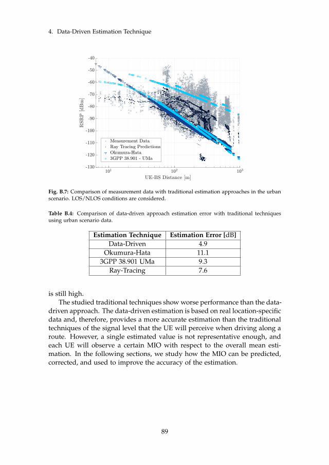
4. Data-Driven Estimation Technique
Fig. B.7: Comparison of measurement data with traditional estimation approaches in the urbanscenario. LOS/NLOS conditions are considered.
Table B.4: Comparison of data-driven approach estimation error with traditional techniquesusing urban scenario data.
Estimation Technique Estimation Error [dB]Data-Driven 4.9
Okumura-Hata 11.13GPP 38.901 UMa 9.3
Ray-Tracing 7.6
is still high.The studied traditional techniques show worse performance than the data-
driven approach. The data-driven estimation is based on real location-specificdata and, therefore, provides a more accurate estimation than the traditionaltechniques of the signal level that the UE will perceive when driving along aroute. However, a single estimated value is not representative enough, andeach UE will observe a certain MIO with respect to the overall mean esti-mation. In the following sections, we study how the MIO can be predicted,corrected, and used to improve the accuracy of the estimation.
89

Paper B.
5 Mean Individual Offset Correction
5.1 Pre-service
Correcting the MIO in the pre-service stage would allow the network to per-form more accurate estimations on the potential critical areas before the UEstarts moving along the route. For that, the network should be able to predictthe UE’s MIO using relevant context information such as UE’s placement (in-side/outside the car), UE’s orientation, or UE’s pattern type, assuming thesecan be available.
UE Antenna Orientation
The MIO for each UE in the rural (a) and urban environments (b) is shown inFig. B.8. As it can be observed, the offset remains constant between differentruns or loops for the same phone-setup combination where the device isoriented towards the same direction. However, different offsets are observedbetween devices that are pointing in different directions. This illustrates therelevance of UE orientation to determine the MIO. A clear distinction can alsobe made between setups A-B and setup C. The phones were located inside thecar in the latter, and the penetration loss due to the vehicle’s structure causedthe signal level to be much lower (7 dB on average) than the one experiencedby the phones located in the car top carrier. This resulted in negative MIOswith respect to the overall estimation for all phones located inside the car.Therefore, it is reasonable to assume that another relevant factor impactingthe MIO of a UE is its placement (inside/outside) in the car. However, thatinformation would only allow identifying the sign of the MIO, but not thevalue of it, which seems to depend mainly on the UE orientation and drivingdirection (as previously shown in [7]).
UE Antenna Pattern Effects Compensation
The consistency of the offset values observed among loops of each UE Fig.B.8, as well as the different offsets for the multiple UEs, suggest that theorientation of the UE is potentially the main factor impacting the MIO. Thesignal level reaching the receiver will also be subjected to the device’s effec-tive antenna pattern, which is directional for all test phones (see Fig. B.3).
Therefore, compensation for the antenna pattern effect could reduce theestimation error. The approach has been tested for the rural scenario data: thereduced interactions of the received signal with surrounding objects and thedominance of LOS conditions simplifies the antenna pattern compensationin that environment. The angle of incidence α of the transmitted signal (fromthe BS) in the UE antenna pattern is calculated using the bearing angle of
90

5. Mean Individual Offset Correction
Fig. B.8: MIO with respect to the route estimation. (a) Results for each of the 48 UE traces in therural environment and (b) for the 36 UE traces in the urban environment.
the serving BS (as recorded by the UE) with respect to the car direction. Toaccount for possible inaccuracies in the calculation of α, the compensation isbased on the average relative power shown in Fig. B.3 within a ±15° rangein both azimuth and elevation directions.
Results in Table B.5 show the overall estimation error ∆ for the rural sce-nario when using setups A and B, before and after pattern compensation.As it can be observed, the antenna pattern compensation has a low impact,resulting in a reduction of 0.4 dB. Setup C is omitted due to the challenge ofaccounting for the vehicle blockage.
The antenna patterns were measured in an anechoic chamber, where theeffects of the car structure or the car top carrier are not considered. Fur-thermore, the UE-BS distance is considerably high for the rural case, andpossible signal interactions with the buildings in the path or ground reflec-tions cannot be accounted for. Although deterministic compensation seems
91

Paper B.
Table B.5: Effective antenna pattern compensation effects on overall estimation error in the ruralscenario.
∆ [dB]Before Antenna Pattern Compensation 5.1After Antenna Pattern Compensation 4.7
intractable, the stability of the estimation error between UEs oriented towardsthe same direction suggests that the antenna pattern effect is statistically in-cluded in the estimation error distribution. In the following section, we studyan approach that exploits the stability of the estimation error of the UE tracesrecorded by devices oriented towards the same direction.
5.2 On-Service
The results in the previous section show that fully correcting the MIO inthe pre-service stage is complex. In the following, we present how we usethe estimation error characteristics and the observed error based on recordedRSRP during the on-service stage to correct the MIO. The main idea of thisapproach is to use the most recent information recorded by the UE that ismoving along a particular route to predict the MIO that it will observe forthe rest of the route.
We use the so-called z-test [28], which is a parametric hypothesis testthat can be used to determine whether a set of samples belongs to a certaindistribution. The test calculates the probability of observing as extreme atest result as the one observed (p-value), assuming that the null hypothesis iscorrect.
As shown in Fig. B.9 (using notation (#)) this approach requires to main-tain a database where estimation error distributions from previous UEs arestored (1). The distributions from each UE could be approximated by a nor-mal distribution with the corresponding mean and standard deviation. Oncethe UE starts to move along the route, after a certain number of observederror samples (2), these are checked against the available distributions in thedatabase. The z-test will provide the mean of the best-fit distribution (4) byaccepting the distribution with the highest p-value.
To investigate this approach, we store N − 0.25 ∗ N distributions in theestimation error database and use the 25 % of the UE traces (i.e., 9 UE tracesin the urban environment) for testing the algorithm. A set of 9 random tracesis left out in every iteration until all the UEs have been tested. Fig. B.10shows the results obtained for urban scenario. The MIOs of the N = 36 UEsrecorded in the urban environment are shown, as well as the predicted valuesusing the z-test when observing 30 samples (equivalent to an observation dis-tance of dobs = 300 m). The MIO values can generally be accurately predicted.
92

5. Mean Individual Offset Correction
Fig. B.9: MIO correction procedure in the on-service stage. The moving UE estimation errorsamples are compared to the error distributions stored in the database and provide an estimationof the MIO.
Table B.6 shows a summary of the results obtained for both rural and ur-ban scenarios. The table shows the overall results obtained when the MIO isknown and corrected (Target ∆ [dB]) and the results obtained when predict-ing and correcting the MIO using the z-test. The overall results when usingthe z-test for MIO estimation are reasonably close (maximum 0.2 dB differ-ence) to the values using known offsets. Therefore, the MIO can be correctedusing this technique as long as UEs with similar conditions/orientation havepreviously passed through the same route.
Table B.6 also includes the required observation distance dobs. In the urbanenvironment a dobs of 300 m is required, whereas for the rural scenario a dobsof 100 m is sufficient. In the urban environment, an observation distance of100 m reduces the overall estimation error from 4.9 dB to 4.1 dB, but a longerobservation distance further decreases that value down to 3.7 dB. In the ruralcase, the error does not decrease regardless of the observation distance. Thisis most likely due to the stronger signal variations and higher dynamics thatwere observed in the rural scenario compared to the urban case.
93

Paper B.
Fig. B.10: Necessary MIO corrections to improve estimation accuracy (light blue) and estimatedon-service MIO corrections for all test UE traces in urban scenario (dark blue).
Table B.6: Z-test results comparison with best performance observed in [7].
Target ∆ [dB](known MIO)
Z-Test∆ [dB] dobs [m]
Rural 4.9 5.1 100Urban 3.6 3.7 300
6 Outage Probability Estimation
As mentioned in Section 2, signal level estimations can be used by the net-work to obtain information on the potential critical areas along the route,which are defined in terms of expected service availability and reliability. Inthe following, we further define these QoS metrics and exemplify their use.For a real reference, we focus on the specifications of the V2X services. Al-though the open literature claims that a requirement of 95 % reliability isenough for a safe communication [29], most of the use cases considered inthe V2X 3GPP specifications [30] require a 99.99 % reliability, and that is therequirement we use for evaluation.
6.1 Service Availability
Service availability estimations are obtained by calculating the probabilityPout,SA that RSRP will drop below a certain threshold γRSRP along the route.
94

6. Outage Probability Estimation
Table B.7: Average performance metrics for RSRP-based service availability estimations.
.TPR
(Hit Rate) [ %]
TNR
(Specificity) [ %]
FNR
(Miss Rate) [ %]
FPR
(Fall-out) [ %]
Rural
γRSRP = -115 dBm
Data-Driven
Pre-Service85.2 95.7 14.8 4.3
Data-Driven
On-Service74.3 97.1 25.7 2.9
Urban
γRSRP = -100 dBm
Okumura-Hata 100 4.3 0 95.7
3GPP 38.901 70 62.4 30 37.6
Ray-Tracing 63.1 69.4 36.9 30.6
Data-Driven
Pre-Service93.8 83.8 6.2 16.2
Data-Driven
On-Service99.5 89.5 0.5 10.5
For each segment, we provide an estimate of the average RSRP, RSRP. Weknow from Eq. (B.2) that the difference to the actual RSRP value, RSRP −RSRP, is Gaussian distributed with standard deviation sigma. Hence as-suming, or conditioned on, RSRP being the average RSRP, we calculate theoutage probability as the one-sided p-value of the Gaussian distribution atthe threshold value, i.e.:
Pout,SA = P(RSRP < γRSRP|RSRP = RSRP)
= Φ(γRSRP − RSRP
σ)
(B.3)
where Φ is the cumulative distribution function of the standard normaldistribution.
In Fig. B.11 we show the availability estimation results along the ru-ral route for a γRSRP = −115 dBm. This threshold is selected based onthe observed intra-frequency mobility thresholds configured by the operator(which range between -115 dBm and -100 dBm in the 1800 MHz band). Fig.B.11a shows the 48 recorded serving RSRP traces, while Fig. B.11b presentsthe estimated availability for that route, where P(RSRP > −115 dBm), i.e.1− P(RSRP < −115 dBm) is shown such that a 99.99 % threshold is used as areference to declare a critical area for the selected use case. As it can be seen,the estimated potential critical areas visually match with the ones actually ex-perienced by the UEs. Table B.7 shows a summary of the service availabilityestimations performance. Service availability is evaluated for each segmentin the distance grid. For the RSRP traces recorded by the different UEs, out-age is declared in a grid segment if the recorded RSRP value in that segmentis below γRSRP. For the estimated service availability, outage is declared in agrid segment if P(RSRP > γRSRP) < 99.99 % in that segment. Performance
95

Paper B.
Fig. B.11: Service availability estimation example with rural environment data. (a) Actual RSRPvalues recorded by all 48 UEs used to build the estimation and (b) P(RSRP > −115 dBm) alongthe route, calculated based on the serving cell RSRP estimation.
of service availability estimations is evaluated using the average over all UEtraces of the following metrics [31]:
• True Positive Rate (TPR) or Hit Rate: Percentage of correctly estimatedservice availability outage segments in the grid. It is calculated as thenumber of correctly estimated outage segments - True Positives (TP) -over the number of actual outage segments (P).
TPR =TPP
[%] (B.4)
• True Negative Rate (TNR) or Specificity: Percentage of correctly esti-mated service availability "safe" (non-outage) segments in the grid. It iscalculated as the number of correctly estimated non-outage segments -True Negatives (TN) - over the number of actual non-outage segments
96

6. Outage Probability Estimation
(N).
TNR =TNN
[%] (B.5)
• False Negative Rate (FNR) or Miss Rate: Complementary metric forTPR. Represents the number of missed outage areas.
FNR = 1− TPR [%] (B.6)
• False Positive Rate (FPR) or Fall-out: The complementary metric forTNR. Represents the number of "false alarms," i.e., the percentage ofcases where a grid segment was incorrectly estimated as outage area.False positives would lead to a situation where countermeasures areinitiated to solve a critical situation that does not exist.
FPR = 1− TNR [%] (B.7)
Other metrics that are typically used to evaluate classification techniqueswere not included as they were considered to be misleading in the purposeof this context. Accuracy is typically used to summarize the performanceof the estimations, as it represents the rate of correct estimations (positiveand negative). However, for the case under evaluation, where the numberof actual positives is much lower than the number of actual negatives (un-balanced dataset), accuracy presented very high values (above 90 % for thedata-driven approach) and was considered to be non-representative of theestimation performance. F1-Score, on the other hand, is typically used forunbalanced datasets and is calculated such that the cost of false positives andfalse negatives is equally significant for performance evaluation [32]. Thismetric presented low values (below 65 %) due to the low number of criticalareas for some of the UEs.
Results in Table B.7 show the mean value of the metrics in Eqs. (B.4-B.7) over all UEs. For rural environments, the pre-service stage estimationspresent high TPR and TNR, indicating that most outage and non-outage areasare correctly estimated. A trade-off is observed in the on-service stage, wherethe MIO corrections cause a decrease in the TPR and an increase in the TNR.
Another example of service availability estimation is shown in Fig. B.12,where urban data is used to compare the estimation of critical areas whenusing the data-driven approach in comparison to the traditional estimationtechniques. To show the accuracy of the estimations, the availability thresh-old is raised in this scenario to -100 dBm as higher reliability should be con-sidered in higher population density areas. As shown in Fig. B.12b and inTable B.7, the higher the signal level estimation error, the lower is the accu-racy of the estimated critical areas. Using the Okumura-Hata model RSRP
97

Paper B.
Fig. B.12: Service availability estimation example with urban environment data. (a) Actual RSRPvalues recorded by all 36 UE traces used to build the estimation and (b) P(RSRP > −100 dBm)obtained when using the estimations provided by the different studied RSRP estimation ap-proaches.
estimations results in a very inaccurate estimation of the potential critical ar-eas. Since the full route is declared critical the TPR is 100 %. However, italso presents a very high FPR of 96 %. The 3GPP model estimations showlower FPR than the Okumura-Hata, but still considerably high (38 %). Sim-ilar results are observed for the ray-tracing estimations that show a TPR of63 % and an FPR of 31 %. The data-driven approach provides an averageTPR of 94 % in the pre-service stage while maintaining a relatively low FPR(16 %). This shows how the data-driven signal level estimation techniqueprovides better results than traditional techniques when the network aims toobtain in-advance information about the expected service availability alongthe path.
To further show the benefits of using the data-driven estimations againstother traditional techniques, we show in Table B.8 the reliability margin (RM)that needs to be considered to guarantee a certain reliability requirementwhen using the different estimation techniques. The values in the table show
98

6. Outage Probability Estimation
Table B.8: Reliability margin (RM) for different reliability requirements (with γRSRP =−100 dBm).
90 % 95 % 99.99 %Okumura-Hata 15.2 19.5 27.63GPP TR 38.901 12.3 15.7 22.3
Ray-Tracing 10 12.8 18.1Data-DrivenPre-service
6.2 8 11.3
Data-DrivenOn-service
4.6 5.9 8.3
that the reliability margin highly decreases when using the data-driven ap-proach. For a 99.99 % reliability requirement, the Okumura-Hata estimationsshow an RM of almost 28 dB, whereas the data-driven approach reduces themargin to 8 dB in the on-service stage. Higher reliability requirements arenot considered in the table as the RM values would be on the limit of whatcould be practically useful for the purpose of the estimations considered inthis article.
In Fig. B.13 we show the effect that MIO correction has on the estimationof critical areas in the on-service stage. Three UEs were used as an exam-ple, one from each of the setups. For each UE, the z-test was used to obtainthe corresponding MIO estimation. After an observation distance of dobs =300 m, the serving RSRP estimation was corrected according to the estimatedMIO, and the probability of RSRP being below -100 dBm was recalculated. InFig. B.13a the actual serving RSRP traces recorded by each of the three UEsare shown. Fig. B.13b shows P(RSRP > −100 dBm) in the pre-service stage(valid for any UE planning to move through the same path) and the correctedon-service probability for each of the 3 example UEs (UE-specific estimation).The setup A UE, with positive MIO with respect to the overall estimation, haslower probabilities of dropping below the threshold than initially estimated.There are no critical areas estimated after MIO correction, which matcheswith the recorded values for that UE (never below -100 dBm). For Setup CUE, with generally lower signal levels due to vehicle blockage, the estimatedprobabilities of the serving signal level dropping below the threshold arehigher than estimated in the pre-service stage, representing well the actualsignal levels experienced by that user. The results for on-service stage per-formance in the urban environment in Table B.7 show that on average, TPRincreases to 99 % with respect to 94 % obtained in the pre-service stage, andTNR increases up to 89 % compared to the previous 84 %.
99

Paper B.
Fig. B.13: Service availability estimation example with urban environment data. (a) Actual RSRPvalues recorded by 3 example UEs (from setups A, B, C) and (b) P(RSRP > −100 dBm) alongthe route, for the pre-service estimation of all UEs in that path and the on-service estimationsfor the individual example UEs.
6.2 Service Reliability
To estimate service reliability we first estimate SIR:
SIR =SI=
RSRPSC
∑NCj=1 RSRPj · δ
[dB] (B.8)
RSRPSC is the RSRP estimation of the serving cell, RSRPj is the estimationof the j = 1, ..., NC neighboring cells and δ is a model for the impact of thetraffic load. A maximum of NC = 3 strongest neighbors, when available, areused to calculate SIR.
As in Eq. (B.2), since RSRP− RSRP is Gaussian with zero mean we canview the linear value of the estimator RSRP as a log-normal random variablewhose logarithmic mean and standard deviation is respectively the predic-tion RSRP and σ. This is true for both serving and interfering signals. Theinterference sum will be approximately log-normal, statistics of which can becalculated numerically by the Schwarz & Yeh algorithm [33]. The same algo-
100

6. Outage Probability Estimation
Table B.9: Average performance metrics for SIR-based service reliability estimations (δ = 30 %).
TPR(Hit Rate) [ %]
TNR(Specificity) [ %]
FNR(Miss Rate) [ %]
FPR(Fall-out) [ %]
RuralγSIR = -3 dB
Data-DrivenPre-Service
72.4 62.4 27.6 37.6
Data-DrivenOn-Service
65 72.3 35 27.7
UrbanγSIR = -3 dB
Data-DrivenPre-Service
88.2 58.8 11.8 41.2
Data-DrivenOn-Service
77 68.7 23 31.3
rithm, with some extensions for correlated signals, can be used to calculatethe logarithmic mean and standard of the SIR [34] which is also approxi-mately log-normal. Assuming a correlation coefficient of 0.5 [35] betweensignals of the serving and the interfering cells we use this framework to eval-uate the probability P(SIR < γSIR).
Fig. B.14b shows the reliability estimation results when considering low,medium and high load (10 %, 30 % and 60 %, respectively) for γSIR = -3 dB.In Fig. B.14c a color map is used to plot the results for medium load withthat same threshold in the urban scenario. The corresponding performancemetrics in Table B.9 show a TPR of 88 % and a FPR of 41 %, with a mean F1-score of 16 %. With the on-service stage corrections using MIO correction forthe serving cell, results show the same trade-off TPR/TNR above-mentioned.For the rural environment, the values follow the same trend.
The presented results are sensitive to different network traffic load, crit-ical thresholds, and correlation coefficients between the serving cell and theinterfering neighbors. For most cases, MIO correction reduces True PositiveRate (TPR) and increases True Negative Rate (TNR), indicating a trade-off be-tween missing outage areas and initiating actions against non-existent ones.Failing to estimate an outage area poses a risk to the service reliability, whichis crucial for mission-critical services. On the other hand, estimating non-existent critical areas may lead to a misuse of network resources. On thatbasis, MIO correction in the on-service stage is beneficial for outage areasestimation. However, initiating MIO correction in the on-service stage maydepend on the service priorities, i.e. prioritization of outage area detection ormore efficient resource utilization. Furthermore, service reliability could alsobenefit from the on-service MIO corrections due to the availability of actualload values, which could be adjusted individually for each correspondingneighbor.
101

Paper B.
Fig. B.14: Service reliability estimation example with urban environment data. (a) SIR valuescalculated using recorded RSRP values from serving and neighboring cells for all of the 24 UEsused and assuming average medium load, (b) estimated probability P(SIR > −3 dB) for low,medium and high load and (c) same results at medium load in a color map.
7 Conclusion
In this article, we use experimental data recorded during an extensive LTEmeasurement campaign in rural and urban environments to show that thesignal level that a UE will experience along a route can be estimated by aggre-gating measurements recorded by UEs that have previously passed throughthat same route.
First, we show how this approach provides an estimation error of 5-6 dB,improving the estimation error obtained using traditional estimation tech-niques such as empirical models or ray-tracing by 3-6 dB. We show howidentifying the MIO of each UE with respect to the overall estimation, usinga technique that exploits the estimation error experienced by previous UEs,further reduces the overall RSRP estimation error to approximately 4 dB.
Lastly, we use the signal level estimations to calculate service outage prob-ability in terms of availability (RSRP-based) and reliability (SIR-based). Thedata-driven approach shows improved accuracy in outage areas estimation
102

References
with respect to traditional techniques, detecting a minimum of 70 % of theoutage areas with less than 30 % of false alarms. This approach allows pro-viding the network with in-advance information on the expected service con-ditions in a specific route where the UE is planning to move and can be usedby the network to make a decision of whether it is safe for the UE to start theservice or it should re-plan the route when possible. Furthermore, we showhow using context information during the service can improve the overallaccuracy of the service availability and reliability estimations, which the net-work may use to take in-advance countermeasures for upcoming signal andQoS drops, respectively.
References
[1] 3GPP, “Management and orchestration; 5G end to end Key PerformanceIndicators (KPI) (Release 17),” Tech. Rep. 28.554 V17.4.0, Sep. 2021.
[2] J. Riihijarvi and P. Mahonen, “Machine learning for performance predic-tion in mobile cellular networks,” IEEE Computational Intelligence Maga-zine, vol. 13, no. 1, pp. 51–60, 2018.
[3] L. Alho, A. Burian, J. Helenius, and J. Pajarinen, “Machine LearningBased Mobile Network Throughput Classification,” in 2021 IEEE WirelessCommunications and Networking Conference (WCNC). IEEE, 2021, pp. 1–6.
[4] 5G Automotive Association, “ Making 5G proactive and predictive forthe automotive industry,” Tech. Rep. White Paper, Jan. 2020.
[5] ACJA, GSMA and GUTMA, “Interface for Data Exchange betweenMNOs and the UTM Ecosystem: Network Coverage Service Definition,v1.00.” Feb. 2021.
[6] 3GPP, “Physical layer; Measurements (Release 16),” Tech. Rep. 36.214V16.2.0, Mar. 2021.
[7] M. Lopéz, T. B. Sørensen, I. Z. Kovács, J. Wigard, and P. Mogensen, “Ex-perimental evaluation of data-driven signal level estimation in cellularnetworks,” in 2021 IEEE 94th Vehicular Technology Conference (VTC2021-Fall). IEEE, 2021, pp. 1–6.
[8] V. Raida, P. Svoboda, M. Koglbauer, and M. Rupp, “On the Stability ofRSRP and Variability of Other KPIs in LTE Downlink-An Open Dataset,”in GLOBECOM 2020-2020 IEEE Global Communications Conference. IEEE,2020, pp. 1–6.
103

References
[9] J. Walfisch and H. L. Bertoni, “A theoretical model of uhf propagationin urban environments,” IEEE Transactions on antennas and propagation,vol. 36, no. 12, pp. 1788–1796, 1988.
[10] I. Data, “Prediction methods for the terrestrial land-mobile service usingthe frequency range 30 mhz to 3 ghz’,” CCIR Report, pp. 567–4.
[11] Z. Yun and M. F. Iskander, “Ray tracing for radio propagation modeling:Principles and applications,” IEEE Access, vol. 3, pp. 1089–1100, 2015.
[12] M. Toril, V. Wille, S. Luna-Ramírez, M. Fernández-Navarro, and F. Ruiz-Vega, “Characterization of Radio Signal Strength Fluctuations in RoadScenarios for Cellular Vehicular Network Planning in LTE,” IEEE Access,vol. 9, pp. 33 120–33 131, 2021.
[13] F. Sohrabi and E. Kuehn, “Construction of the rsrp map using sparsemdt measurements by regression clustering,” in 2017 IEEE internationalconference on communications (ICC). IEEE, 2017, pp. 1–6.
[14] A. Ghasemi, “Data-driven prediction of cellular networks coverage: Aninterpretable machine-learning model,” in 2018 IEEE Global Conference onSignal and Information Processing (GlobalSIP). IEEE, 2018, pp. 604–608.
[15] J. Thrane, B. Sliwa, C. Wietfeld, and H. L. Christiansen, “Deep learning-based signal strength prediction using geographical images and expertknowledge,” in GLOBECOM 2020-2020 IEEE Global Communications Con-ference. IEEE, 2020, pp. 1–6.
[16] S. I. Popoola, E. Adetiba, A. A. Atayero, N. Faruk, and C. T. Calafate,“Optimal model for path loss predictions using feed-forward neural net-works,” Cogent Engineering, vol. 5, no. 1, p. 1444345, 2018.
[17] M. Ayadi, A. B. Zineb, and S. Tabbane, “A UHF path loss model us-ing learning machine for heterogeneous networks,” IEEE Transactions onAntennas and Propagation, vol. 65, no. 7, pp. 3675–3683, 2017.
[18] E. Ostlin, H.-J. Zepernick, and H. Suzuki, “Macrocell path-loss predic-tion using artificial neural networks,” IEEE Transactions on Vehicular Tech-nology, vol. 59, no. 6, pp. 2735–2747, 2010.
[19] 3GPP, “Architecture enhancements for 5G System (5GS) to support net-work data analytics services,” Tech. Rep. 23.288 V17.0.0, Mar. 2021.
[20] Rohde & Schwarz, “R&S Test Equipment Information,” 2020, https://www.rohde-schwarz.com/dk/products/, Last accessed on 2021-12-21.
104

References
[21] Satimo - Microwave Vision Group, “StarGate 24 anechoicchamber,” 2020, https://www.mvg-world.com/en/products/antenna-measurement/multi-probe-systems/sg-24, Last accessedon 2021-12-21.
[22] 3GPP, “Radio measurement collection for Minimization of Drive Tests(MDT); Overall description; Stage 2,” Tech. Rep. 37.320 V10.1.0, Mar.2011.
[23] W. Lee and Y. Yeh, “On the estimation of the second-order statistics oflog normal fading in mobile radio environment,” IEEE Transactions onCommunications, vol. 22, no. 6, pp. 869–873, 1974.
[24] O. Hata, “Propagation prediction model for uhf range in the predictionmethods for the terrestrial land mobile service in the vhf and uhf bands,”ITU-R Recommendation P. 529-2, Geneva: ITU, pp. 5–7, 1995.
[25] 3GPP, “Study on channel model for frequencies from 0.5 to 100 GHz.(Release 16),” Tech. Rep. 38.901 V16.1.0, Dec. 2019.
[26] Altair Hyperworks, “Winprop Manual,” version 2018.1.2.
[27] R. Wahl, G. Wölfle, P. Wertz, P. Wildbolz, and F. Landstorfer, “Dominantpath prediction model for urban scenarios,” 14th IST Mobile and WirelessCommunications Summit, Dresden (Germany), 2005.
[28] L. J. Kitchens, Basic Statistics and Data Analysis. Thomson/Brooks/Cole,2002.
[29] G. Pocovi, M. Lauridsen, B. Soret, K. I. Pedersen, and P. Mogensen, “Au-tomation for on-road vehicles: Use cases and requirements for radio de-sign,” in 2015 IEEE 82nd Vehicular Technology Conference (VTC2015-Fall).IEEE, 2015, pp. 1–5.
[30] 3GPP, “Study on enhancement of 3GPP Support for 5G V2X Services(Release 16),” Tech. Rep. 22.886 V16.2.0, Dec. 2018.
[31] C. Ferri, J. Hernández-Orallo, and R. Modroiu, “An experimental com-parison of performance measures for classification,” Pattern RecognitionLetters, vol. 30, no. 1, pp. 27–38, 2009.
[32] J. Brownlee, Imbalanced classification with Python: better metrics, balanceskewed classes, cost-sensitive learning. Machine Learning Mastery, 2020.
[33] S. C. Schwartz and Y.-S. Yeh, “On the distribution function and momentsof power sums with log-normal components,” Bell System Technical Jour-nal, vol. 61, no. 7, pp. 1441–1462, 1982.
105

References
[34] T. B. Sørensen, “Intelligent distributed antenna systems (idas): Assess-ment by measurement and simulation,” 2002.
[35] T. Sorensen, “Slow fading cross-correlation against azimuth separationof base stations,” Electronics Letters, vol. 35, no. 2, pp. 127–129, 1999.
106

Paper C
Shadow Fading Spatial Correlation Analysis forAerial Vehicles: Ray tracing vs. Measurements
Melisa López, Troels B. Sørensen, Preben Mogensen, JeroenWigard and István Z. Kovács
The paper has been published in theIEEE 90th Vehicular Technology Conference (VTC-Fall 2019).

© 2019 IEEEThe layout has been revised.

1. Introduction
Abstract
Although the use of cellular networks to serve drones has been investigated in severalrecent works, the path loss or shadowing variation is still relatively unexplored. Thevariation and its dynamic behaviour is of importance in characterizing the reliabilityof the drone communication link, but difficult to assess by experimental means on alarge scale. The main goal of this paper is to study the feasibility of ray tracing modelsto accurately predict shadow fading variations at different heights, so that the shadowfading correlation distances for the Unmanned Aerial Vehicles (UAV) channel canbe found in both vertical and horizontal directions, without the need of performingextensive field measurement campaigns. For that, predictions obtained through a raytracing tool are compared to field measurements in an urban scenario. Our resultsshow that with accurate 3D maps, the tool is useful for predicting the dynamics ofthe UAV propagation channel, and therefore can be used partly as a substitute forfield measurements.
1 Introduction
The 5th Generation (5G) New Radio (NR) cellular system is expected to servea wide range of services. Mission-critical communications, where reliabilityand a short-time response of the system is needed typically for safety rea-sons [1], is expected to be one of those services. Some examples wouldinclude Vehicle-To-Everything (V2X) communications, railway communica-tions or the Command and Control (C2) link for Unmanned Aerial Vehicles(UAV). All the three examples are characterized by high mobility. Long TermEvolution (LTE) and 5G networks investigations for meeting the requirementsof such type of communication [2–4] have been carried out.
The application of interest in this paper is the use of LTE/5G for servingthe control link of UAVs. There are multiple UAV uses such as transportof medical goods, rescue services, inspection of telecommunications infras-tructure, to name a few [5]. All the mentioned use cases are more attractiveif a UAV can fly Beyond Visual Line-of-Sight (BVLOS) of the controller, i.e.,allowing the UAV to be controlled from a remote pilot location. For pub-lic safety reasons, it is expected that reliability will be a major requirementfor BVLOS operation. One of the consequences of this requirement is thatthe drones, as they are also commonly known, need to be connected to aflight control unit, through the C2 link, which carries mainly flight-relatedinformation. The existing cellular networks are a potential option to providesuch communication, since their coverage is ubiquitous, and they are alreadyserving many cellular network users, and therefore provide a cost-efficientoption. Connection reliability in cellular networks is impacted not only bythe coverage provided, but also by the dynamic behaviour of the coverage,
109

Paper C.
for what concerns both desired and interfering signals. The dynamics impactfor example the radio mobility which determines cell selection, reporting andhandovers.
There are already several publications such as [6–8] where the radio per-formance of drones when using cellular networks for the C2 link and somepotential interference mitigation schemes are studied. A path loss modelfor the radio channel between the UAV and cellular networks is proposedin [6], [8], [9]. This height dependent model, based on measurements, sug-gests a path loss exponent and shadowing which decrease as the UAV heightincreases. Whereas path loss characterises the (static) large-scale effect, it isalso important to consider and model the temporal and/or spatial dynamiceffects in propagation, to realistically evaluate connection reliability when thedrone moves through airspace. These dynamic effects are typically charac-terised by the standard deviation, and the correlation properties of shadowfading. There is a need to have more empirical evidence for the study of cor-relation properties of the radio channel in aerial scenarios. However, achiev-ing this purely by experimental procedure is difficult, given the practicalitiesin conducting drone flights, particularly in urban environments.
In this paper, we present a large-scale study at different heights, with amultiple transmitters scenario, on the accuracy of the ray tracing tool whenpredicting shadowing variations by comparing it to field measurements.
The paper is organized as follows: Section 2 introduces the ray tracingmodels analysed in this study, the measurement setup and the scenario. Re-sults, discussion and conclusions are followed, respectively, in Sections 3, 4and 5.
2 Methodology
2.1 Field Measurements
To be able to compare ray-tracing predictions with real channel measurementsamples, field measurements were required. Two measurement campaignswere performed in a live LTE network in the 1800 MHz frequency band: adrive test campaign at ground level and an airborne campaign with a droneat different heights. Both campaigns were performed in a small area of ap-proximately 0.25 km2 in the city center of Aarhus, in Denmark, where 17different locations where measured. The studied area is hilly, and the terrainelevation in the topographic maps varies between 0 m and 27 m. As it isshow in Fig. C.1, the network in this area consists of 23 tri-sectorial siteswith heights between 15 m and 60 m and average Inter-Site Distance (ISD) of470 m. Full information of the cells including antenna tilt, orientation, etc.,provided by the network operator was used for the study.
110

2. Methodology
Fig. C.1: Measurement route (in green) in Aarhus (Denmark), including LTE network sites loca-tion provided by a local operator.
In both measurement campaigns, the car and the drone were equippedwith the Rohde & Schwarz FreeRider system [10]. The scanner was equippedwith an external omnidirectional antenna, mounted on the rooftop of the car,and respectively, extending about 50 cm above the drone fuselage and rotorplane, as it is shown in Fig. C.2. The GPS position was logged for eachmeasured Reference Signal Received Power (RSRP) sample.
2.2 Ray Tracing Model
Two different propagation models available in the AWE WinProp tool arestudied: the Dominant Path Model (DPM) and the Intelligent Ray Tracing(IRT). The authors in [11] describe the algorithm of DPM for an urban sce-nario, which consists of the determination of the dominant path contributingto the power reaching the receiver. They present the general performance ofDPM at ground level and compare it with IRT, which considers all significantpossible contributions of the different rays reaching the receiver [12]. It is aone-transmitter study, where results show that DPM considerably reducescomputation time respect to IRT, and that mean value and standard devi-ation of the difference between measurements and predictions is not onlyequal but sometimes better with DPM.
For this analysis we used average signal power predictions from Win-Prop, which mainly depend on the propagation exponents settings: before
111

Paper C.
Fig. C.2: Measurement set up for the drone campaign.
and after breakpoint Line-Of-Sight (LOS) and Obstructed-LOS (OLOS). SinceWinProp offers the possibility to tune these parameters by using field mea-surements, those obtained from the campaigns mentioned in Section 2.1 wereused to calibrate the models. The 3D maps (including building shapes andterrain topography of the area) used in the ray tracing tool to perform thisstudy cover an area of 8.5 km2 with 5m resolution around the campaign area.The building database includes 10019 buildings, where the minimum heightis 43 m and the maximum height is 146 m. First, calibration of the propaga-tion exponents was performed for ground level and all the different heights,separately. Calibration in WinProp is a standard procedure and it is per-formed automatically [13]. It calculates the Minimum Mean Squared Error(MMSE) of the difference between measurements and predictions. The scan-ner samples were converted from RSRP to signal power and further averagedover 5 m, to match with the 3D maps resolution.
We show in Table C.1 the 50%-ile value of the signal power distributionsof measurements and predictions before and after calibration for the groundlevel case. For both cases, the models provide a better estimation of the signal
Table C.1: 50 %-ile of signal power distributions for measurements and predictions - DPM andIRT models before/after calibration
Before Calibration After CalibrationMeasurements -72.1
DPM -84.9 -72.1IRT -66.3 -72.2
112

2. Methodology
Table C.2: Propagation exponents for DPM/IRT predictions
Ground Level 10 m, 15 m, 30 mDPM IRT DPM/IRT
LOS exp. 2.6 2.8 2.2OLOS exp. 2.7 2.9 2.4
LOS exp. after breakpoint 3.5 3 3.3OLOS exp. after breakpoint 4 3 3.3
power after calibration.Calibration was performed for both DPM and IRT models, and the results
for both models were analysed before and after calibration. For IRT, we firstran predictions using the default WinProp values for ground level. As thedifference between calibrated DPM and default WinProp IRT propagationexponents for the ground level case was minimum, we decided to use thecalibrated DPM propagation exponents to run IRT predictions at differentheights. Results after calibration improved slightly only for the ground levelcase, whereas for the different heights the results worsened. For this reason,IRT propagation exponents shown in Table C.2 are the calibrated values forground level case only. For the different heights, the parameters used for IRTwere the same as for DPM corresponding to the same height.
The factor for breakpoint distance determination was set to 2π as it isrecommended in [13] for the urban case. The initial value for the breakpointdistance is calculated using the heights of the transmitter and receiver, andthe wavelength [13]. The exponents after breakpoint distance were not de-termined during calibration for above ground, and therefore they were set tothe default value set in the tool.
A summary of the overall standard deviation of the difference betweenmeasurements and predictions for the different heights after DPM calibra-tion is presented in Table C.3. As it can be observed, the overall (includingall transmitters) standard deviation of the difference between measurementsand predictions is high compared to results in [11] even after calibration. Toexplain that, we present in Table C.4 a per transmitter analysis, where onlysome of the transmitters used for calibration of DPM at ground level areshown. The results in Table C.4 are obtained by subtracting, pixel by pixel,measurements to predictions for each transmitter independently. It can be no-ticed that, per transmitter, there is a considerable spread of the mean values,between -6.1 dB to +14.5 dB, which contributes to the overall high standarddeviation of the difference. This will be further discussed in Section 4.
113

Paper C.
Table C.3: Std. dev. of the overall difference between measurements and predictions aftercalibration for the different heights
Height # of transmitters used for calibration Std. Dev. [dB]Ground Level 14 10.62
10 16 12.9615 17 11.6630 28 8.03
Table C.4: Per-transmitter statistics of the difference between measurements and predictions @Ground Level
Tramsmitter ID Mean Value [dB] Std. Dev. [dB]A 3.5 6.5B 10.7 7.8C -0.1 5.0D 14.5 4.7E -11.5 5.7F 5.5 5.1G -6.1 5.0
2.3 Shadow Fading Estimation
Once calibration was performed, we ran new predictions with the optimalpropagation exponents. The results obtained from those predictions wereused for the analysis presented in Section 3.
To analyse shadow fading, distance-dependency was removed from bothmeasurements and predictions. The values were subsequently de-trendedper transmitter prediction, so that only the variation in the local mean powerlevel remained. Processed like this, the resulting values are therefore propor-tional to the shadowing in large-scale propagation.
To measure the accuracy of the predictions, we performed cross-correlationof time sequence samples between measurements and predictions. The cross-correlation coefficient, ry1y2, used for this analysis is presented in Eq. (C.1),where cy1y2 represents the cross-covariance, defined in Eq. (C.2), of the timeseries y1 and y2, and s1 and s2 are the sample standard deviation of the timeseries y1 and y2, respectively, as it is shown in Eq. (C.3).
ry1y2 =cy1y2(k)sy1sy2
; k = 0,±1 (C.1)
114
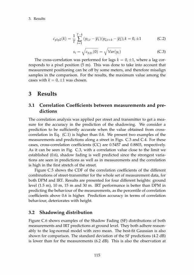
3. Results
cy1y2(k) =1T
T−k
∑t=1
(y1,t − y1)(y2,t+k − y2); k = 0,±1 (C.2)
si =√
cyiyi (0) =√
Var(yi) (C.3)
The cross-correlation was performed for lags k = 0,±1, where a lag cor-responds to a pixel position (5 m). This was done to take into account thatmeasurement positioning can be off by some meters, and therefore misalignsamples in the comparison. For the results, the maximum value among thecases with k = 0,±1 was chosen.
3 Results
3.1 Correlation Coefficients between measurements and pre-dictions
The correlation analysis was applied per street and transmitter to get a mea-sure for the accuracy in the prediction of the shadowing. We consider aprediction to be sufficiently accurate when the value obtained from cross-correlation in Eq. (C.1) is higher than 0.6. We present two examples of themeasurements and predictions along a street in Figs. C.3 and C.4. For thesecases, cross-correlation coefficients (CC) are 0.5457 and 0.8803, respectively.As it can be seen in Fig. C.3, with a correlation value close to the limit weestablished (0.6), shadow fading is well predicted since the strongest varia-tions are seen in predictions as well as in measurements and the correlationis high in the first stretch of the street.
Figure C.5 shows the CDF of the correlation coefficients of the differentcombinations of street-transmitter for the whole set of measurement data, forboth DPM and IRT. Results are presented for four different heights: groundlevel (1.5 m), 10 m, 15 m and 30 m. IRT performance is better than DPM inpredicting the behaviour of the measurements, as the percentile of correlationcoefficients above 0.6 is higher. Prediction accuracy in terms of correlationbehaviour, deteriorates with height.
3.2 Shadowing distribution
Figure C.6 shows examples of the Shadow Fading (SF) distributions of bothmeasurements and IRT predictions at ground level. They both adhere reason-ably to the log-normal model with zero mean. The best-fit Gaussian is alsoshown for comparison. The standard deviation of the SF predictions (4.2 dB)is lower than for the measurements (6.2 dB). This is also the observation at
115
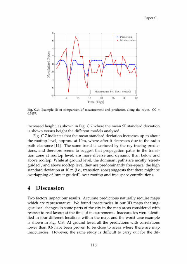
Paper C.
Fig. C.3: Example (I) of comparison of measurement and prediction along the route. CC =0.5457.
increased height, as shown in Fig. C.7 where the mean SF standard deviationis shown versus height the different models analysed.
Fig. C.7 indicates that the mean standard deviation increases up to aboutthe rooftop level, approx. at 10m, where after it decreases due to the radiopath clearance [14]. The same trend is captured by the ray tracing predic-tions, and therefore seems to suggest that propagation paths in the transi-tion zone at rooftop level, are more diverse and dynamic than below andabove rooftop. While at ground level, the dominant paths are mostly "street-guided", and above rooftop level they are predominantly free-space, the highstandard deviation at 10 m (i.e., transition zone) suggests that there might beoverlapping of "street-guided", over-rooftop and free-space contributions.
4 Discussion
Two factors impact our results. Accurate predictions naturally require mapswhich are representative. We found inaccuracies in our 3D maps that sug-gest local changes in some parts of the city in the map areas considered withrespect to real layout at the time of measurements. Inaccuracies were identi-fied in four different locations within the map, and the worst case exampleis shown in Fig. C.8. At ground level, all the predictions with correlationslower than 0.6 have been proven to be close to areas where there are mapinaccuracies. However, the same study is difficult to carry out for the dif-
116

5. Conclusion
Fig. C.4: Example (II) of comparison of measurement and prediction along the route. CC =0.8803.
ferent heights, as the transmitters observed by the drone are sometimes faraway [6].
On the other hand, there is a limited accuracy on the building data bases[11]. The buildings are modelled as a polygonal cylinder of uniform height,where the rooftop shape is not being considered. This is surely affecting theabove-rooftop predictions and explains why some of the transmitters presenthigh mean value and standard deviation on the difference between measure-ments and predictions, as it is shown in Table C.4. For the same reason,shadowing variation is slightly lower for the predictions than for the mea-surements, but it can be seen in Figs. C.6 and C.7 that they follow the sametrend.
Despite the maps inaccuracies, results show that predictions using IRTand DPM show about the same standard deviation versus height, but IRTis better in capturing the temporal dynamics of the SF process. The cost ofusing the IRT model is computation time, which is considerably higher thanfor DPM [11].
5 Conclusion
This paper studies, by comparing with field measurements, the feasibility ofray tracing predictions and models to accurately predict shadowing varia-tions at different heights.
117
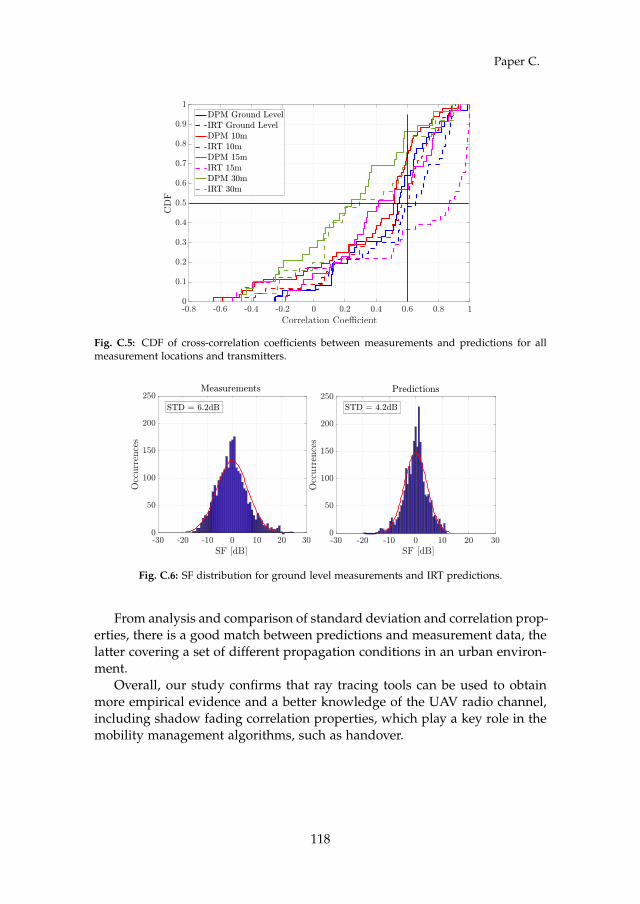
Paper C.
Fig. C.5: CDF of cross-correlation coefficients between measurements and predictions for allmeasurement locations and transmitters.
Fig. C.6: SF distribution for ground level measurements and IRT predictions.
From analysis and comparison of standard deviation and correlation prop-erties, there is a good match between predictions and measurement data, thelatter covering a set of different propagation conditions in an urban environ-ment.
Overall, our study confirms that ray tracing tools can be used to obtainmore empirical evidence and a better knowledge of the UAV radio channel,including shadow fading correlation properties, which play a key role in themobility management algorithms, such as handover.
118

References
Fig. C.7: Average SF standard deviation values over all transmitter-street combinations.
Acknowledgment
This research has received funding from the SESAR Joint Undertaking un-der the European Union’s Horizon 2020 research and innovation programme,grant agreement No 763601. The research is conducted as part of the DroC2omproject.
References
[1] G. P. Fettweis, “The tactile internet: Applications and challenges,” IEEEVehicular Technology Magazine, vol. 9, no. 1, pp. 64–70, 2014.
[2] T. Doumi, M. F. Dolan, S. Tatesh, A. Casati, G. Tsirtsis, K. Anchan, andD. Flore, “LTE for public safety networks,” IEEE Communications Maga-zine, vol. 51, no. 2, pp. 106–112, 2013.
[3] S. Mukherjee and C. Beard, “A framework for ultra-reliable low la-tency mission-critical communication,” in 2017 Wireless Telecommunica-tions Symposium (WTS). IEEE, 2017, pp. 1–5.
[4] R. Ferrus and O. Sallent, “Extending the LTE/LTE-A Business Case:Mission-and Business-Critical Mobile Broadband Communications,”IEEE Vehicular Technology Magazine, vol. 9, no. 3, pp. 47–55, 2014.
[5] M. Mazur, A. Wisniewski, J. McMillan et al., “Clarity from above: Pwcglobal report on the commercial applications of drone technology,” War-saw: Drone Powered Solutions, PriceWater house Coopers, 2016.
[6] R. Amorim, H. Nguyen, P. Mogensen, I. Z. Kovács, J. Wigard, and T. B.Sørensen, “Radio channel modeling for uav communication over cellular
119

References
Fig. C.8: Portion of the studied area: actual maps (top) and 3D database (bottom).
networks,” IEEE Wireless Communications Letters, vol. 6, no. 4, pp. 514–517, 2017.
[7] I. Kovacs, R. Amorim, H. C. Nguyen, J. Wigard, and P. Mogensen, “Inter-ference analysis for UAV connectivity over LTE using aerial radio mea-surements,” in 2017 IEEE 86th Vehicular Technology Conference (VTC-Fall).IEEE, 2017, pp. 1–6.
[8] W. Khawaja, O. Ozdemir, and I. Guvenc, “Uav air-to-ground channelcharacterization for mmwave systems,” in 2017 IEEE 86th Vehicular Tech-nology Conference (VTC-Fall). IEEE, 2017, pp. 1–5.
[9] 3GPP, “Study on Enhanced LTE Support for Aerial Vehicles (Release15),” Tech. Rep. 36.777 V0.3.1, Oct. 2017.
[10] Rohde & Schwarz, “R&S Test Equipment Information,” 2020, https://www.rohde-schwarz.com/dk/products/, Last accessed on 2021-12-21.
[11] R. Wahl, G. Wölfle, P. Wertz, P. Wildbolz, and F. Landstorfer, “Dominantpath prediction model for urban scenarios,” 14th IST Mobile and WirelessCommunications Summit, Dresden (Germany), 2005.
120

References
[12] R. Hoppe, G. Wolfle, and F. Landstorfer, “Accelerated ray optical prop-agation modeling for the planning of wireless communication net-works,” in RAWCON 99. 1999 IEEE Radio and Wireless Conference (Cat.No. 99EX292). IEEE, 1999, pp. 159–162.
[13] Altair Hyperworks, “Winprop Manual,” version 2018.1.2.
[14] B. Van der Bergh, A. Chiumento, and S. Pollin, “LTE in the sky: Tradingoff propagation benefits with interference costs for aerial nodes,” IEEECommunications Magazine, vol. 54, no. 5, pp. 44–50, 2016.
121

References
122
Paper D
Service Outage Estimation for Unmanned AerialVehicles: A Measurement-Based Approach
Melisa López, Troels B. Sørensen, Jeroen Wigard, István Z.Kovács and Preben Mogensen
The paper has been accepted for publication in theWireless Communications and Networking Conference 2022.

© 2022 IEEEThe layout has been revised.

1. Introduction
Abstract
One of the key enablers for the use of cellular networks to provide connectivity toUAV is reliability assurance. Estimating accurately the expected service availabilityand reliability that a UAV will experience along a planned route, helps to avoidcritical situations. In this paper, we evaluate the use of a data-driven approach toestimate the expected serving signal level of a UAV planning to fly along a specificpath. The estimation approach, presented in a previous study for the ground-levelcase, is based on the aggregation of measurements of UAV that have previously beenflying along the same route. Using this approach we achieve an estimation error aslow as 2.7 dB. Based on the estimations we calculate the expected outage probabilityin terms of service availability and reliability and provide estimations of the expectedcritical areas along the route. Results show that 90 % of the availability and 65 % ofthe reliability critical areas in the route can be accurately estimated.
1 Introduction
The market potential for commercial applications which make use of Un-manned Aerial Vehicles (UAV), or drones, is rapidly increasing [1]. Mostof these applications require the operation of drones Beyond Visual Line-of-Sight (BVLOS). Ubiquitous cellular networks are considered to be one of themain candidates to provide this service. Strict regulatory requirements en-forced in standardization [2] have led to extensive research efforts to ensurethat the network can provide reliable communication between the drone andits controller.
The existing literature focuses on pointing out the challenges of UAVcommunications over cellular networks and proposing techniques to over-come them [3]. Studies such as [4] and [5] point out the key role of interfer-ence in the performance of UAV communications. Potential solutions suchas beamforming, are shown to be a good candidate to improve service re-liability in [6]. In [7] and [8], the authors present the benefits of using adual-operator hybrid access scheme to avoid outages caused by latency. Al-though there are solutions to improve UAV communications, the use of themis mostly based on reactive schemes. It would be beneficial for the serviceif the network could foresee the critical situation and proactively act againstit. The Aerial Connectivity Joint Activity (ACJA) initiative proposes in [9] atwo-phase operational context for UAVs. In the planning phase, RF condi-tions for the planned path are estimated, and in the flight phase, real-timeradio Key Performance Indicators (KPI) are monitored and used to estimateupcoming critical situations. Having beforehand information of a potentialdrop in the serving signal level or the Signal-To-Interference Ratio (SIR) couldcontribute to more efficient management of the network resources as well as
125

Paper D.
more reliable User Equipment (UE) mobility and experienced Quality of Ser-vice (QoS) [10]. The most basic approach to obtain this information is to esti-mate, as accurately as possible, the Reference Signal Received Power (RSRP)that a UE will experience along a route that it is planning to fly through.There are well-known methods to estimate the radio coverage based on em-pirical and deterministic models such as ray-tracing. However, the estimationaccuracy provided by these methods is poor [11].
In this paper, we present an outage estimation method that provides thenetwork with in-advance information on the expected service availability andreliability along a route that a UAV is planning to fly. First, we evaluate theperformance of a data-driven approach for serving signal level estimation,which was previously presented in [12] for ground-level scenarios. The es-timation is evaluated using real Long Term Evolution (LTE) measurementsand consists of the aggregation of RSRP samples recorded by UEs that havepreviously passed through the same location, regardless of the cell that theyare connected to (i.e. pre-service estimation). We show how the estimationscan be further corrected using RSRP recorded by the UE during the flightphase (i.e. on-service estimation). Furthermore, we use the serving RSRP es-timations to obtain the expected service availability and reliability. With thisinformation, the network can proactively act against upcoming areas wherethe signal level or the SIR are likely to drop (critical areas).
The paper is organized as follows: in Section 2 we include the descriptionof the UAV radio measurements. In Section 3 we briefly describe the esti-mation approach. Results and conclusions are included in Sections 4 and 5,respectively.
2 UAV Radio Measurements
To evaluate the performance of the data-driven estimation approach we per-formed field UAV measurements at 50 m height in a rural scenario nearby thecity of Aalborg in Denmark. The measurement route, as depicted in Fig.D.1,covered the last 5 km of a 15 km path (from X to Y) that was previously mea-sured at ground-level [12]. In total, we performed eight round-trips in the5 km route. The radio environment is characterized by scattered buildingswith average heights below 10 m and a terrain profile with variation below7 m. The measurements, which were conducted in a sparsely coveraged LTEnetwork, are in the 1800 MHz band. The average inter-site distance of 8.3 km,base station heights range from 20 m to 39 m and down-tilts between 3 and6 degrees.
The measurements were recorded using four commercial smartphones(2 Samsung Galaxy S5 and 2 Samsung Galaxy S9) with the QualiPoc© testfirmware [13]. All of them were mounted underneath a drone, with each of
126

3. Signal Level and Outage Estimations
Fig. D.1: Measurement routes and LTE base station sites in Aalborg, Denmark. X and Y markthe beginning and end of the UAV route, respectively.
the UEs oriented towards one of the four main compass directions, as shownin Fig. D.2. The UEs recorded mainly the RSRP of the serving cell, and, in thecase of the S5 model, also of the neighbors. An average number of 4 sampleswere recorded every 10 m.
3 Signal Level and Outage Estimations
The estimation approach used in this paper was previously presented in [12]for ground-level measurements. The serving RSRP values recorded by differ-ent UEs in a certain location are averaged (in dB scale) such that an estimationof the mean serving signal level that a UE is going to experience in that samelocation can be obtained. The estimation is location-based and should bevalid for any UE regardless of the cell that it is connected to.
To evaluate this approach, the traces recorded by the UEs were organizedalong a 10-meter distance grid in j = 1, ..., J segments. With a 5 km flightroute, this led to a total of J = 500 segments. The mean value of all themeasurements recorded by a UE in a certain grid segment j (4 samples onaverage, as mentioned in Section 2) is used as the RSRP value recorded bythat UE in segment j (RSRPi,segj in dB).
For every segment, the mean (in dBm) of all the serving RSRP valuesrecorded by all the different UEs is used as the estimated value in that seg-ment, i.e. the estimation in segment j is defined as:
127

Paper D.
Fig. D.2: Measurement setup (left) - DJI Matrice 600 drone front picture with one of the QualiPocsmartphones visible and (right) orientation scheme of UE positions where the red arrow indi-cates the drone flight direction.
RSRPsegj =1N
N
∑i=1
RSRPi,segj [dBm] (D.1)
The traces recorded by the UEs in opposite flying directions (X to Y andvice-versa) were considered as traces recorded by different UEs. With 4 mea-suring UEs and a total of 8 round-trips, the number of samples used to obtainthe estimation in Eq. (D.1) equals N=32.
The precision of the signal level estimation is obtained by calculating,in each segment, the difference (in dB scale) between the estimation in thatsegment and each of the N = 32 actual recorded values. The distribution ofthis difference can be well approximated by a Gaussian distribution N (0, σ),where σ is the standard deviation of the estimation error (referred to as ∆).
3.1 Individual Offset Correction
To improve the performance of the estimation, we propose a method to cor-rect the individual offset that a certain UE is observing with respect to thepre-service estimation in Eq. (D.1). To do this, we use real-time samplesthat the UAV is experiencing during the service (on-service estimation), aswell as error distributions based on individual UEs that have previouslypassed through that same route. As for the aggregate distribution discussedabove, the individual error distributions also have good approximation to aGaussian with same standard deviation but different Mean Individual Offset(MIO) relative to the aggregate distribution mean. We use the z-test [14] as a
128

3. Signal Level and Outage Estimations
Fig. D.3: Mean individual offset correction procedure.
parametric hypothesis test to determine whether a set of samples is likely tocome from one of the individual error distributions.
Compared to the ground-level study case, where the MIO was stablealong the route [12] and only a few samples at the beginning of the routeallowed for full-route MIO correction, we observed that in the UAV case thereis a need for updating the correction as the UAV moves along the route. Thisdifference is most likely due to the higher impact of the directional antennapatterns of the UEs in the air compared to the ground. At a 50 m height andwith good Line-Of-Sight (LOS) conditions, the number of cells that the UEscan observe is higher than at 1.5 m. Therefore, UEs in the same location butwith different orientations in the air have higher probability to be connectedto different cells and observe different signal levels.
To compensate for the variation of the MIO along the route, we updatethe offset estimation every dupd = 500 m (sliding window MIO correction).We show in Fig. D.3 the procedure for MIO correction, where the steps 1-4indicate the order of the steps. When a UAV starts flying along the route(step 1), the samples observed within the first dupd meters are tested againstthe stored distributions of each of the p UEs that have previously passedthrough that area (step 2).
The UE distribution with the highest p-value is selected (step 3) based onthe z-test, and its MIO is used as a correction factor for the estimation in Eq.
129

Paper D.
(D.1) (step 4). The hypothesis is tested every dupd meters and the offset iscorrected based on the latest observed samples.
3.2 Service Outage Probability
Since an accurate estimation error is observed after correcting the MIO of aMIO, the serving RSRP estimations are further used to estimate the serviceavailability and reliability that can be experienced along the route.
For service availability, we calculate the outage probability Pout,SA thatRSRP will drop below the availability threshold γRSRP. The probability iscalculated as:
Pout,SA = P(RSRP < γRSRP|RSRP = RSRP)
= Φ(γRSRP − RSRP
σ)
(D.2)
Φ is the cumulative distribution function of the standard normal distribu-tion and σ is the known standard deviation of that distribution. This equationfollows from the observation that the estimation error distribution can be wellapproximated with a Gaussian.
For the service reliability estimations, we first estimate the SIR:
SIR =SI=
RSRPSC
∑NCk=1 RSRPk · δ
[dB] (D.3)
RSRPSC is the serving cell signal level estimation, RSRPk the estimationof the k = 1, ..., NC neighboring cells (NC = 5 strongest neighbors if available)and δ a fixed constant accounting for the impact of the traffic load.
The outage probability Pout,SR that the SIR drops below a certain thresh-old γSIR is calculated following the same procedure from Eq. (D.2). Giventhe Gaussian shape of the estimation error, the linear value of the estimatorRSRP can be seen as a log-normal random variable with mean RSRP andstandard deviation σ. This is valid for both serving and interfering signals.The interference sum in the denominator of Eq. (D.3) will be approximatelylog-normal, as will the SIR ratio. Their statistics in the form of logarith-mic mean and standard deviation can be calculated numerically by an ex-tended version of the Schwarz & Yeh algorithm with account for correlatedsignals [15]. We calculate P(SIR < γSIR) assuming a correlation coefficientof 0.3 between the serving and interfering signals.
130

4. Results
Fig. D.4: Data-driven approach estimation error ∆ [dB] before (a) and after (b) MIO correction.
4 Results
We first show the results obtained for the serving RSRP estimations usingthe data-driven approach. We aggregate the samples of N = 32 UE tracesrecorded to obtain an estimation that, as shown in Fig. D.4a, presents anoverall estimation error of 4.9 dB for the pre-service stage. We compare theseresults with the ones observed in the ground-level case in Table D.1. Forreference, we also include the shadow fading values at area level. Since theestimations obtained with the data-driven approach are location-based, theestimation accuracy is below the shadow fading in the area. Due to theimproved visibility conditions of the drone, and the lack of obstacles betweenthe transmitter and the receiver, shadow fading for the UE (4.3 dB) is almost3 dB lower than at ground-level (7.2 dB).
Results in [12] show an overall estimation error of 6.3 dB at ground-level.The fit in the UAV case is not so obvious as the error distribution seemsto present multiple modes, which are most likely caused by the differentsignal levels experienced by UEs oriented towards different directions. This
131

Paper D.
Table D.1: Results Summary: Ground Level vs. UAV
Ground Level UAVData-Driven ∆ [dB]Before MIO Correction
6.3 4.8
Data-Driven ∆ [dB]Full-route MIO Correction
5.1 -
Data-Driven ∆ [dB]Sliding Window MIO Correction
4.8 2.7
Shadow Fading [dB](Areal Level)
7.2 4.3
leads to differences when correcting the MIO in the air. At ground-level, thestability of the offset for a specific UE oriented towards a certain directionallowed for the correction to be performed at the beginning of the route andbe valid for the rest of it (full-route MIO correction). This method is notvalid in the UAV case as the MIO of the whole route varies along the routeand the samples observed for the z-test are not able to find a matching errordistribution to the ones stored in the database (from UEs that have previouslypassed through the same route). Therefore, as explained in Section 3.1, MIOcorrection needs to be updated along the route. For the results presentedhere, p = N ∗ 0.75, i.e. 25 % (eight) of the available traces were used fortesting the correction approach, with eight random traces in every testinground until all of them were tested. Results in Fig. D.4b show that notonly the standard deviation of the estimation error is reduced to 2.7 dB, butalso the distribution is uni-modal and symmetric now that the offsets dueto directivity have been removed. Although the distribution is clearly morepeaked than a Gaussian, we keep that assumption for simplicity in the sequel.We also include in Table D.1 the results for sliding window MIO correction atground-level. The difference when using the full-route correction is 0.3 dB(5.1 dB vs 4.8 dB). This indicates that the sliding window approach has a lowimpact as the error is stable along the whole route.
4.1 Service Outage Estimation
Achieving a high accuracy of 2.7 dB allows us to further use the servingRSRP estimations to estimate the expected service availability and reliabilityas per (D.2) and (D.3). Fig. D.6 shows the results for service availabilitywhen using γRSRP = -100 dBm. For reference, we include in Fig. D.5 the 32serving RSRP traces recorded in the 5 km route along with the estimationand the threshold. In Fig. D.6a, we choose three example UEs pointingtowards different directions (and with different MIOs) to show the effects of
132

4. Results
Fig. D.5: N = 32 recorded traces and data-driven serving RSRP estimation.
Table D.2: Accuracy of service availability and reliability outage areas estimation.
TPR [%](Hit Rate)
TNR [%](Specificity)
FNR [%](Miss Rate)
FPR [%](Fall-Out)
AvailabilityPre-service
81.1 49.9 18.9 50.1
AvailabilityOn-service
88.4 76.6 11.6 23.4
ReliabilityPre-service
68.8 71.5 31.2 28.5
ReliabilityOn-service
66.9 76.8 33.1 23.2
MIO correction. As it can be seen, the corrected estimation traces in the on-service stage follow the trend of the actual ones better than the pre-serviceestimation. This is also observed in Fig. D.6b, where the outage probabilityfor service availability is shown. If we choose UE A as a reference, we observethat the actual recorded RSRP level is below -100 dBm up to approximatelytwo kilometers, in agreement with the estimated outage probability. For UEC, on the other hand, the actual trace is shown to be above the thresholdalong the whole route. Contrary to what was initially estimated in the pre-service stage, where almost half of the route would be declared critical, theon-service stage estimates a very low service availability outage probabilityfor UE C.
To evaluate the performance of the outage probability estimations, weclassify the segments into critical (true positive or critical area) and non-critical (true negative or non-critical area). We use True Positive Rate (TPR),
133

Paper D.
Fig. D.6: Service Availability: (a) real and estimated traces of three example UEs and (b) outageprobability estimations based on pre-service and on-service estimations for the three exampleUEs.
True Negative Rate (TNR), False Negative Rate (FNR), and False PositiveRate (FPR) for evaluation, as these metrics are typically used for classifica-tion methods [16]. Other metrics such as accuracy and F1-score have notbeen included as they were considered to be misleading for the purpose ofour evaluation due to the low number of critical areas (unbalanced dataset).Our main objective is to obtain the highest TPR possible, which indicates thenumber of positives that are correctly classified, i.e. the number of criticalareas that are correctly estimated since both service availability and reliabil-ity outages would be very critical for UAV communication. However, wewould also like to reduce as much as possible the FPR, i.e. the number ofincorrectly classified critical areas (false alarms), since that may lead to inef-
134

4. Results
Fig. D.7: Comparison of estimated SIR with δ = 30% with the recorded Avg. Modulation andCoding Scheme (MCS) trends(example UE).
ficient resource management (e.g. unnecessary resource reservation). Resultsare shown in Table D.2. Service availability estimations show an 81 % TPRand a high FPR of 50 % in the pre-service stage. However, in the on-servicestage, almost 90 % of the service availability critical areas can be estimatedwhile observing only 20 % of false alarms. As observed in Fig. D.5, the num-ber of samples dropping below the threshold is small (approximately 10 %)compared to the total number of samples
For the service reliability estimations we first calculate, following Eq.(D.3), the SIR for each of the 16 UE traces at which the strongest neigh-bors RSRP were also recorded (S5 smartphones). The SIR is calculated usingan estimation of low, medium, and high load values (10 %, 30 %, and 60 %,respectively). Fig. D.8a shows the resulting SIR traces for δ = 30 % and thecorresponding threshold γSIR = -3 dB. The SIR is obtained by estimating thesame load for all neighboring cells. To show that this is a fair representa-tion of the actual quality experienced by the UAV, we include Fig. D.7. Wecompare an example UE trace of the calculated SIR (with δ = 30 %) and thecorresponding recorded average MCS which the is selected by the UE propor-tionally to the data channel SIR. As it can be observed, the trends observed inthe average MCS trace are also followed by the calculated SIR. On that basis,we calculate the service reliability outage probability using the approach ex-plained in Section 3.2. Results in Fig. D.8b show that the outage probabilityincreases with the load in the network. It can also be observed how the δ =30 % outage probability estimation matches best the SIR calculated traces inFig. D.8a. As previously done for service availability, the performance of theestimations is shown using the classification metrics. Table D.2 shows that 69
135

Paper D.
Fig. D.8: Service Reliability: (a) N = 16 SIR traces estimated based on actual values and (b)outage probability estimation based on pre-service estimation.
% of the critical areas are correctly estimated in the pre-service stage with anFPR of 28 %. The TPR slightly decreases to 67 % in the on-service stage, butso does the FPR to 23 %. The benefits of MIO correction are not so obviousfor the service reliability estimations as the MIO correction is only performedfor the serving cell. MIO correction was not possible for the neighbors dueto the very different error distributions observed from previous UEs (highnumber of cells observed).
5 Discussion and Conclusions
The estimation results shown in Section 4 contribute to ensuring reliable com-munication between the UAV and its controller. Seen in the ACJA operationalcontext to ensure reliable communication, the network can consider the pre-service estimations to decide whether the UAV can start the service or it
136

References
should re-plan the route. Furthermore, the on-service estimations can con-tribute to more proactive and seamless UE mobility and QoS management.Decisions such as activating dual connectivity or an interference mitigationtechnique can be made in advance, i.e., before the signal level or the qualityof service is degraded.
In this paper, we discuss the use of a data-driven approach to estimate theexpected serving signal level of a UAV along a planned path. The data-drivenestimation consists of aggregating measurements from UEs that have previ-ously passed through the same location. The method provides an overallaccuracy of 4.9 dB.
The error can be further reduced to 2.7 dB by proactively correcting theMIO of the flying UAV with respect to the overall estimation. The correc-tion is done using error distributions from previous UEs and updated basedon observations of the most recent samples. The data-driven estimation ap-proach and the MIO correction procedure require data from previous UEs tobe available, limiting the use of these approaches.
With an accurate estimation of the serving RSRP, the network is able tocalculate the expected service outage probability in terms of availability andreliability. The estimations show that almost 90 % of the expected criticalareas along the route in terms of availability can be detected in advance,showing only 20 % of false alarms. For service reliability, the network wouldbe able to detect almost 70 % of the critical areas, maintaining the fall-outrate below 25 %.
Acknowledgement
The authors would like to thank Telenor (Denmark) for supporting this workby sharing the network information. We would also like to express gratitudeto Steffen Hansen, our drone pilot, and other colleagues at Aalborg Univer-sity for the help provided during the measurement campaign.
References
[1] L. Godage, “Global unmanned aerial vehicle market (uav) industry anal-ysis and forecast (2018–2026),” Montana Ledger: Boston, MA, USA, 2019.
[2] 3GPP, “Study on Enhanced LTE Support for Aerial Vehicles (Release15),” Tech. Rep. 36.777 V0.3.1, Oct. 2017.
[3] A. Fotouhi, H. Qiang, M. Ding, M. Hassan, L. G. Giordano, A. Garcia-Rodriguez, and J. Yuan, “Survey on uav cellular communications: Prac-tical aspects, standardization advancements, regulation, and security
137
References
challenges,” IEEE Communications Surveys & Tutorials, vol. 21, no. 4, pp.3417–3442, 2019.
[4] H. C. Nguyen, R. Amorim, J. Wigard, I. Z. Kovács, T. B. Sørensen, andP. E. Mogensen, “How to ensure reliable connectivity for aerial vehiclesover cellular networks,” Ieee Access, vol. 6, pp. 12 304–12 317, 2018.
[5] H. Marques, P. Marques, J. Ribeiro, T. Alves, and L. Pereira, “Experi-mental evaluation of cellular networks for uav operation and services,”in 2019 IEEE 24th International Workshop on Computer Aided Modeling andDesign of Communication Links and Networks (CAMAD). IEEE, 2019, pp.1–6.
[6] T. Izydorczyk, M. Bucur, F. M. Tavares, G. Berardinelli, and P. Mogensen,“Experimental evaluation of multi-antenna receivers for uav communi-cation in live lte networks,” in 2018 IEEE Globecom Workshops (GC Wk-shps). IEEE, 2018, pp. 1–6.
[7] R. Amorim, I. Z. Kovacs, J. Wigard, G. Pocovi, T. B. Sorensen, andP. Mogensen, “Improving drone’s command and control link reliabilitythrough dual-network connectivity,” in 2019 IEEE 89th Vehicular Technol-ogy Conference (VTC2019-Spring). IEEE, 2019, pp. 1–6.
[8] J. Güldenring, P. Gorczak, F. Eckermann, M. Patchou, J. Tiemann,F. Kurtz, and C. Wietfeld, “Reliable long-range multi-link communica-tion for unmanned search and rescue aircraft systems in beyond visualline of sight operation,” Drones, vol. 4, no. 2, p. 16, 2020.
[9] ACJA, GSMA and GUTMA, “Interface for Data Exchange betweenMNOs and the UTM Ecosystem: Network Coverage Service Definition,v1.00.” Feb. 2021.
[10] N. Bui, “Prediction-based techniques for the optimization of mobile net-works,” 2017.
[11] J. Thrane, D. Zibar, and H. L. Christiansen, “Comparison of empiricaland ray-tracing models for mobile communication systems at 2.6 ghz,”in 2019 IEEE 90th Vehicular Technology Conference (VTC2019-Fall). IEEE,2019, pp. 1–5.
[12] M. Lopéz, T. B. Sørensen, I. Z. Kovács, J. Wigard, and P. Mogensen, “Ex-perimental evaluation of data-driven signal level estimation in cellularnetworks,” in 2021 IEEE 94th Vehicular Technology Conference (VTC2021-Fall). IEEE, 2021, pp. 1–6.
[13] Rohde & Schwarz, “R&S Test Equipment Information,” 2020, https://www.rohde-schwarz.com/dk/products/, Last accessed on 2021-12-21.
138

References
[14] L. J. Kitchens, Basic Statistics and Data Analysis. Thomson/Brooks/Cole,2002.
[15] T. B. Sørensen, “Intelligent distributed antenna systems (idas): Assess-ment by measurement and simulation,” 2002.
[16] M. Hossin and M. N. Sulaiman, “A review on evaluation metrics for dataclassification evaluations,” International journal of data mining & knowledgemanagement process, vol. 5, no. 2, p. 1, 2015.
139

Melisa ló
pez lech
ug
aD
ata-D
riven
preD
ictio
n fo
r r
eliab
le Missio
n-c
ritic
al c
oM
Mu
nic
ation
s
ISSN (online): 2446-1628ISBN (online): 978-87-7573-941-7