Damage and Fracture Mechanics
616
-
Upload
khangminh22 -
Category
Documents
-
view
0 -
download
0
Transcript of Damage and Fracture Mechanics


Damage and Fracture Mechanics

Taoufik Boukharouba • Mimoun Elboujdaini
Damage and Fracture Mechanics
Failure Analysis of Engineering Materials
Guy Pluvinage
Editors
and Structures

Printed on acid-free paper
9 8 7 6 5 4 3 2 1
springer.com
© Springer Science + Business Media B.V. 2009No part of this work may be reproduced, stored in a retrieval system, or transmitted in any form or by anymeans, electronic, mechanical, photocopying, microfilming, recording or otherwise, without written per-mission from the Publisher, with the exception of any material supplied specifically for the purpose ofbeing entered and executed on a computer system, for exclusive use by the purchaser of the work.
Editors
Université des Sciences et de la
Technologie Houari Boumediene (USTHB)
16111 Algiers
Taoufik Boukharouba
El Alia, Bab Ezzouar, Algeria
Guy Pluvinage
57012 Metz
France
e-ISBN: 978-90-481-2669-9ISBN: 978-90-481-2668-2
Mimoun Elboujdaini
Université Paul Verlaine - Metz
Natural Resources Canada CANMET
Materials Technology Lab.
568 Booth Street
Canada
Library of Congress Control Number: 2009926284
Ottawa, ON K1A 0G1
Dépt. Génie M canique & Productiqueé

v
Table of Contents
Acknowledgments ...................................................................................xiii
Editors’ Biographies ................................................................................xv
Foreword ................................................................................................xvii
Preamble..................................................................................................xix
Determination of the Hardness of the Oxide Layers of 2017A
Alloys...........................................................................................................1
Chahinez Fares, Taoufik Boukharouba, Mohamed El Amine Belouchrani, Abdelmalek Britah and Moussa Naït Abdelaziz
Effect of Non-Metallic Inclusions on Hydrogen Induced Cracking ....11
Mimoun Elboujdaini and Winston Revie
Defect Assessment on Pipe Transporting a Mixture of Natural
Gas and Hydrogen ...................................................................................19
Guy Pluvinage
Reliability Analysis of Low Alloy Ferritic Piping Materials................33
A. Guedri, B. Merzoug, Moe Khaleel and A. Zeghloul
Experimental Characterization and Effect of the Triaxiality
on the Behavior of the HDPE..................................................................43
K. Hachour, R. Ferhoum, M. Aberkane, F. Zairi and M. Nait Abdelaziz
Effects of Aggressive Chemical Environments on Mechanical
Behavior of Polyethylene Piping Material.............................................49
Souheila Rehab-Bekkouche, Nadjette Kiass and Kamel Chaoui

Table of Contents
vi
Hydrogen Embrittlement Enhanced by Plastic Deformation
of Super Duplex Stainless Steel...............................................................59
A. Elhoud, N. Renton and W. Deans
Hydrogen Effect on Local Fracture Emanating from Notches
in Pipeline Steels ......................................................................................69
Julien Capelle, Igor Dmytrakh, Joseph Gilgert and Guy Pluvinage
Reliability Assessment of Underground Pipelines Under Active
Corrosion Defects.....................................................................................83
A. Amirat, A. Benmoussat and K. Chaoui
An Overview of the Applications of NDI/NDT in Engineering
Design for Structural Integrity and Damage Tolerance in Aircraft
Structures .................................................................................................93
A.M. Abdel-Latif
Improvement in the Design of Automobile Upper Suspension
Control Arms Using Aluminum Alloys................................................ 101
M. Bouazara
Nadhira Kheznadji Messaoud-Nacer
Damaging Influence of Cutting Tools on the Manufactured
Idriss Amara, Embarek Ferkous and Fayçal Bentaleb
Lotfi Hamitouche, Mostapha Tarfaoui and Alain Vautrin
Vibroacoustic Sources Identification of Gear Mechanism
Abbassia Derouiche, Nacer Hamzaoui and Taoufik Boukharouba
Performances of Vehicles’ Active Suspensions ...................................113
Surfaces Quality.....................................................................................121
Design and Test of a Sandwich T-Joint for Naval Ships ....................131
Transmission .......................................................................................... 143

Table of Contents
vii
Prediction of Structural and Dynamic Behaviors of Impacted
Application of Structural INTegrity Assessment Procedure
Nenad Gubeljak and Jozef Predan
Yu. G. Matvienko
Degradation and Failure of Some Polymers (Polyethylene
Boubaker Bounamous and Kamel Chaoui
On the Structural Integrity of the Nano-PVD Coatings Applied
Miroslav Piska, Ales Polzer, Petra Cihlarova and Dagmar Stankova
Investigation of Energy Balance in Nanocrystalline Titanium
O. Plekhov, O. Naimark, R.Valiev and I. Semenova
M. Benachour, A. Hadjoui and F.Z. Seriari
Spall Fracture in ARMCO Iron: Structure Evolution and Spall
Oleg Naimark, Sergey Uvarov and Vladimir Oborin
Damage Modelling of Impacted Tubular Structures by Using
Mostapha Tarfaoui, Papa Birame Gning and Francis Collombet
Abdelhamid Miloudi and Mahmoud Neder
Plates ....................................................................................................... 153
to Nuclear Power Plant Component.....................................................163
Failure Assessment Diagrams in Structural Integrity Analysis ........ 173
and Polyamide) for Industrial Applications ........................................183
on Cutting Tools..................................................................................... 195
Under Cyclic Loading............................................................................ 205
Behavior of Stainless Steel 316L Under Impact Test .........................213
Strength .................................................................................................. 219
Material Property Degradation Approach..........................................227

Table of Contents
viii
W.R. Tyson
L. Marsavina and T. Sadowski
Crack Propagation in the Vicinity of the Interface Between Two
Luboš Náhlík, Lucie Šestáková and Pavel Huta
Ivo Dlouhý, Zden k Chlup, Hynek Hadraba and Vladislav Kozák
Numerical and Experimental Investigations of Mixed Mode
M.R.M. Aliha, M.R. Ayatollahi and B. Kharazi
Experimental and Numerical Determination of Stress Intensity
S. Belamri, T. Tamine and A. Nemdili
Dynamic Response of Cracked Plate Subjected to Impact
R. Tiberkak, M. Bachene, B.K. Hachi, S. Rechak and M. Haboussi
L. ehá ková, J. Kalousek and J. Dobrovská
Correlation of Microstructure and Toughness of the Welded
Rrahim Maksuti, Hamit Mehmeti, Hartmut Baum, Mursel Rama and Nexhat Çerkini
Effect of the Residual Fatigue Damage on the Static and Toughness
P. Cadenas, A. Amrouche, G. Mesmacque and K. Jozwiak
Fracture Control for Northern Pipelines............................................. 237
The Influence of the Interface on Fracture Parameters.....................245
Elastic Materials .................................................................................... 255
Fracture Behaviour of TiAl Intermetalics...........................................265
Fracture in Granite Using Four-Point-Bend Specimen .....................275
Factors of Crack in Plate with a Multiple Holes.................................285
Loading Using the Extended Finite Element Method (X-FEM)........297
On Heterogeneity of Welded Joint by Modelling of Diffusion........... 307
Joint of Pipeline Steel X65..................................................................... 315
Properties................................................................................................ 323

Table of Contents
ix
Influence of Fatigue Damage in Dynamic Tensile Properties
U. Sánchez-Santana, C. Rubio-González, G. Mesmacque and A. Amrouche
M. Bournane, M. Bouazara and L. St-Georges
Damage of Glulam Beams Under Cyclic Torsion: Experiments
Myriam Chaplain, Zahreddine Nafa and Mohamed Guenfoud
Statistical Study of Temperature Effect on Fatigue Life of Thin
Abdelmadjid Merabtine, Kamel Chaoui and Zitouni Azari
Residual Stress Effect on Fatigue Crack Growth of SENT
M. Benachour, M. Benguediab and A. Hadjoui
Analysis of Elliptical Cracks in Static and in Fatigue
B.K. Hachi, S. Rechak, M. Haboussi, M. Taghite, Y. Belkacemi and G. Maurice
Influence of Coating on Friction and Wear of Combustion Engine
Abdelkader Guermat, Guy Monteil and Mostefa Bouchetara
Optimization Constrained of the Lifetime of the CBN 7020
Slimane Benchiheb and Lakhdar Boulanouar
Comparison of Simulation Methods of Pulsed Ultrasonic
W. Djerir, T. Boutkedjirt and A. Badidi Bouda
of AISI 4140T Steel ................................................................................331
Low-Cycle Fatigue of Al–Mg Alloys .................................................... 341
and Modelling......................................................................................... 349
Welded Plates ......................................................................................... 357
Specimen................................................................................................. 367
by Hybridization of Green’s Functions ...............................................375
Piston Rings............................................................................................ 387
During the Machining of Steel 100 Cr6 ............................................... 395
Fields Radiated in Isotropic Solids.......................................................405

Table of Contents
x
Investigation of Ag Doping Effects on Na1.5Co2O4 Elastic
Ibrahim Al-Suraihy, Abdellaziz Doghmane and Zahia Hadjoub
The Dynamics of Compressible Herschel–Bulkley Fluids
F. Belblidia, T. Haroon and M.F. Webster
Numerical Simulation of the Behaviour of Cracks in Axisymmetric
N. Amoura, H. Kebir, S. Rechak and J.M. Roelandt
Numerical Evaluation of Energy Release Rate for Several Crack
N. Kazi Tani, T. Tamine and G. Pluvinage
Numerical Simulation of the Ductile Fracture Growth Using
Gaëtan Hello, Hocine Kebir and Laurent Chambon
Enriched Finite Element for Modal Analysis of Cracked
M. Bachene, R. Tiberkak, S. Rechak, G. Maurice and B.K. Hachi
A New Generation of 3D Composite Materials: Advantage
Z. Aboura, K. Khellil, M.L. Benzeggagh, A. Bouden and R. Ayad
Benefit from Embedded Sensors to Study Polymeric Composite
Francis Collombet, Matthieu Mulle, Hilario-Hernandez Moreno, Redouane Zitoune, Bernard Douchin and Yves-Henri Grunevald
Effect of Temperature and Initiator on Glass Fibre/Unsaturated
Nabila Belloul, Ali Ahmed-Benyahia, Aicha Serier and Nourdine Ouali
Parameters.............................................................................................. 415
in Die–Swell Flows .................................................................................425
Structures by the Dual Boundary Element Method ...........................435
Orientation and Position to the Bi-Material Interface Plates ............ 445
the Boundary Element Method ............................................................455
Plates ....................................................................................................... 463
and Disadvantage................................................................................... 473
Structures ............................................................................................... 485
Polyester Composite: Cross-linking, Mechanical Properties.............497

Table of Contents
xi
Theoretical and Experimental Investigations of the Plane
Strain Compression of Amorphous Polymers in the form
Nourdine Ouali, Krimo Azouaoui, Ali Ahmed Benyahia and Taoufik Boukharouba
Djedjiga Ait Aouit and Abdeldjalil Ouahabi
Characterization of Mixed Mode Delamination Growth
M. Kenane and M.L. Benzeggagh
Modification of Cellulose for an Application in the Waste Water
Lamia Timhadjelt, Aicha Serier, Karima Boumerdassi, Mohamed Serier and Zoubir Aîssani
A Full 3D Simulation of Plastic Forming Using a Heuristic
Tewfik Ghomari, Rezak Ayad and Nabil Talbi
A Novel Approach for Bone Remodeling After Prosthetic
Habiba Bougherara, Václav Klika, František Maršík, Ivo A. Ma ík and L’Hocine Yahia
Hybrid Composite-Metal Hip Resurfacing Implant for Active
Habiba Bougherara, Marcello Papini, Michael Olsenb, Radovan Zdero, Paul Zalzal and Emil H. Schemitsch
O. Bélaidi Chabane Chaouche, N.E. Hannachi and Y. Labadi
The Behaviour of Self-Compacting Concrete Subjected
Riçal Khelifa, Xavier Brunetaud, Hocine Chabil and Muzahim Al-Mukhtar
of a Flat Plate ......................................................................................... 505
Wavelet-Based Multifractal Identification of Fracture Stages..........513
and Thresholds....................................................................................... 523
Treatment ............................................................................................... 531
Generalised Contact Algorithm............................................................539
Implantation........................................................................................... 553
Patient ..................................................................................................... 567
Anisotropic and Unilateral Damage Application to Concrete ........... 573
to an External Sulphate Attack ............................................................583

Table of Contents
xii
S. Bouziane, H. Bouzerd and M. Guenfoud
Three-Dimensional T-Stress to Predict the Directional Stability
of Crack Propagation in a Pipeline with External Surface
M. Hadj Meliani, H.Moustabchir, A. Ghoul, S. Harriri and Z. Azari
Mixed Finite Element for Cracked Interface ......................................591
Crack....................................................................................................... 601

xiii
Acknowledgments
We would like to thank all of our partners and sponsors of the First African InterQuadrennial ICF Conference “AIQ-ICF2008”, which was held in Algiers from 01 till 05 June 2008, for their help to the organization of this scientific event.

xv
Editors’ Biographies
Prof. Taoufik Boukharouba
Received his Mechanical Engineering Degree (1987) in Mechanical Engineering from the University of Annaba, his Magister (1991) in Mechanical Engineering from Polytechnic School of Algiers and then his Doctorate (1995) from the University of Metz in France. He joined the staff of Houari Boumédiène Sciences and Technology University, (USTHB) in 1996. He was Director of the Mechanical Institute (IGM of USTHB) from 1998 to 2000. Presently, he is member of the “Haut Conseil Universitaire et de Recherche Algéro-Français (HCUR)”. He is president of the Algerian Association of Mechanics and Materials and member of the “Commission Universitaire Nationale (CUN)”.
He is supervising many projects on fatigue of materials as well as cooperation projects with CNRS and CMEP with French laboratories.
His research interest is in damage of composite materials and materials in biomechanics. He has published several technical papers. He is a reviewer for many international conferences and he organized the “Congrès de Génie des Procédés” (2000) in Ouargla, the “Congrès Algérien de Mécanique de Construction” (2007) in Algiers and the First African InterQuadrennial ICF Conference “AIQ-ICF2008”.
Dr. Mimoun Elboujdaïni
Received his Mechanical Engineering degree and Diplôme d’Etude Approfondie (DEA) at the University of Technology of Compiègne (UTC) in France. He obtained an M.Sc. at physical metallurgy at Ecole Polytechnique of Montreal and his Ph.D. at the Laval University in Canada. In 1989 he joined the CANMET the Materials Technology Laboratory of Natural Resources Canada in Ottawa as research scientist working on many industrial projects and very active in the professional field of pipelines – oil/gas/petrochemical industries and has been participating in many professional organizations such as NACE, CIM, ICF, ECS, ASM, etc.
He leads several Canadian as well as international projects in different fields (hydrogen-induced cracking (H2S), hydrogen embritlement, stress-corrosion cracking (SCC), galvanizing, liquid metal embritlement, etc.). He has published in excess of 100 technical papers, contributions to chapters in handbook; edited books and over 14 conference proceedings and organized several conference sessions and symposia.

Editors’ Biographies
xvi
He holds adjunct professorship in the Department of Chemical and Materials Engineering at the University of Alberta and trained and supervised national and foreign Ph.D. students and invited by several universities to serve as external examiner of Ph.D. theses. Selected as Distinguished Lecturer for 2006–2007 by the Canadian Institute of Mining, Metallurgy, and Petroleum (CIM). He also served as a member of organizing committees of several national and international conferences. Invited as Distinguished Speaker in addition received many national and international invitations (e.g.; China, USA, Egypt, Canada, etc) and universities. Organized and chairs several short courses. Presently, is the general Chair (2005–2009) for The Twelfth International Conference on Fracture (ICF12) to be held in Ottawa, Canada in 2009 (www.icf12.com).
Prof. Guy Pluvinage
Received his Doctorat de 3éme cycle in 1967 and his Doctorat d’état in 1973 at the University of Lille in France. He was successively Assistant Professor at Université de Valenciennes (1968–1974) and Professor at Université de Metz since 1974.
He was invited professor at University of Newcastle (Australia), (1982), University of Tokyo (Japon), (1984), University of’Auburn (USA) (1986). He was Director of “Laboratoire de Fiabilité Mécanique” from 1974 to 2002. Vice-President of the University of Metz (Research Council) (1988–1992) and Director of Maison du Pôle Universitaire Européen Nancy-Metz (1996–2003).
His expertise is mainly focused on strength of materials and particularly on fatigue and fracture Mechanics. He has published 167 papers in refereed journals: and 322 published communications to scientific meetings: He is author of several books in French, English and Russian. He is member of the editorial board and reviewer of several journals. He has received several honours and awards: Grand Prix du Centenaire de l’AAUL.
Officier des Palmes Académiques; Professor Honoris Causa University of Miskolc (Hungary); Doctor Honoris Causa Univerity Polytechnic of Tirana (Albania).

xvii
Foreword
The First African InterQuadrennial ICF Conference “AIQ-ICF2008” on Damage and Fracture Mechanics – Failure Analysis of Engineering Materials and Structures”, Algiers, Algeria, June 1–5, 2008 is the first in the series of InterQuadrennial Conferences on Fracture to be held in the continent of Africa. During the conference, African researchers have shown that they merit a strong reputation in international circles and continue to make substantial contributions to the field of fracture mechanics. As in most countries, the research effort in Africa is under-taken at the industrial, academic, private sector and governmental levels, and covers the whole spectrum of fracture and fatigue.
The AIQ-ICF2008 has brought together researchers and engineers to review and discuss advances in the development of methods and approaches on Damage and Fracture Mechanics. By bringing together the leading international experts in the field, AIQ-ICF promotes technology transfer and provides a forum for industry and researchers of the host nation to present their accomplishments and to develop new ideas at the highest level. International Conferences have an important role to play in the technology transfer process, especially in terms of the relationships to be established between the participants and the informal exchange of ideas that this ICF offers.
Topics covered in AIQ-ICF2008 include: concepts of damage and fracture mechanics of structures, cumulative damage crack initiation, crack growth, residual strength, probability aspects and case histories; macro and micro aspects of fatigue; analytical methods for fatigue life assessment in structures; and applications of linear fracture mechanics to failure analysis and fracture control, fracture toughness and fatigue testing techniques, and environmental effects. These are areas where corrosion scientists, chemists, mechanical, civil, metallurgical and chemical engineers, corrosion prevention and coating specialists, operating and maintenance personnel can unite their efforts to better understand the complexities of these phenomena and develop effective preventive methods. Mechanistic understanding of cracking failures of metals and alloys can be used in conjunction with phenomenological data to identify and quantify the influence of environmental and material para-meters. The conference has been devoted to the exchange of ideas and information on the evaluation of materials performance, and the development of advanced materials for resistance to damage and fracture in severe conditions.
Twelve plenary keynote presentations and ten introductory conferences covered a wide range of topics: Computational Materials Engineering/Modelling; Nano-
materials; Biomaterials/Biomechanics; Pipeline Materials; Stress Corrosion
Cracking & Hydrogen Embrittlement; Materials & Joining/Welds; High Strength
Steel; Fracture Mechanics; Failure Analysis; Fatigue; Fracture Dynamics, etc…

Foreword
xviii
As chairs of this conference, we would like to express our thanks to all authors and reviewers who, collectively, have participated in making this conference a success and for their written contributions that make this proceedings volume a valuable record of the recent advances in Damage and Fracture Mechanics.
Prof. Taoufik Boukharouba Dr. Mimoun Elboujdaini Prof. Guy Pluvinage

xix
Preamble
Ahmed Djebbar, is mathematician with diploma from Université Paris Sud (1972),
from Université de Nantes (1990) and from Ecole des Hautes Etudes en Sciences
Sociales de Paris (1998). He is Emeritus Professor at Université des Sciences et
des Technologies de Lille. (France).
Advisor for Education, Culture and Communication at the Presidency of the
Algerian Republic (January, 1992–June, 1992) and minister of Education, of Higher
Education and Scientific Research (July, 1992–April, 1994).
He is one of the specialists of the history of sciences and in his assets a dozen
works, from which some were translated in several languages. He is one of the
specialists of the Arab World whom they consult on questions related to the
provision of Arabic and Muslims in science.
We wanted by this preamble just to give a historical overview and not to write
the history of sciences and point out the provision of Muslim civilization in sciences
and particularly in mechanics object of the First African InterQuadrennial ICF
Conference “AIQ-ICF2008”.
We apologize to the author for possible errors in the translation of his original
text which was sent to us in French language.
The original version of the text is available to anyone who wants to have the
original copy.
The Arabic Phase of the Mechanics
For the first time in the history of the International Congress on Fracture, the works of the InterQuadriennal Conference presented in this Book, take place in the land of Africa, in Algeria precisely, one of the regions of the Maghreb which made its contribution to science and technology within the framework of the Arabian-Moslem civilization. How then omit evoking, even quickly, an important chapter of the history of the mechanics, the least known maybe, which was written within the framework of this civilization. The organizers of this meeting thought of it. A conference on this subject was presented. Here is a modest summary which is essentially homage to these discoverers of the past and to my colleagues specialists of mechanics who, through different roads, immortalize the same scientific adventure.
From the end of the VIIIth century to the middle of the XVIth, a new mechanical tradition, expressing itself essentially in Arabic, developed in the immense space governed in the name of Islam and which extended, in certain times, from

Preamble
xx
Samarkand to Saragossa and from Palermo to Tombouctou. As quite other scientific activity was practised during this period, the mechanics elaborated at the same time on the theoretical aspect and on the applied one as well, and on both aspects it produces significant results.
The theoretical part of this discipline was integrated into the physics. It concerns the study of statics, of the hydrostatics and the dynamics. Its applied part, which was called “Science of the ingenious processes”, is subdivided into three big domains. The first domain is the one of the playful mechanics. It concerns machines and all the realizations which aim at distracting or at amazing the caliphs, the princes and fortunate people. The second corresponds to the utilitarian mechanics which aims at resolving the problems of the everyday life. The third concerns the military technology and, more particularly, the conception of weapons and machines of seat.
In the VIIIth century, we already mastered a set of techniques which served in the various domains which have just been evoked. Some of them were of unknown origin but the others had been used by the Romans, the Byzantine or the Persians. With the advent of the phenomenon of translation, writings dedicated to the mechanics were dug up and translated into Arabic. In our knowledge, they were all written in Greek. Having assimilated the ideas found in these texts, the first Moslem specialists of this domain tried, from the IXth century, to bring improvements and complements among which some were real innovations. But these last ones did not concern the only technical aspect. They also allowed bringing to light new concepts, never applied before. Some of them will be completely put into practice to realize complex systems. Others will stay in the state of ingenious findings and will be exploited only much later when they will be rediscovered in Europe.
It is finally necessary to indicate that the researches in this domain continued until the XVIth century and that they became a reality in numerous publications. The contents of those who reached us reveal a rich tradition which was born in Bagdad but which bloomed in the other metropolises of the Muslim empire, as Damascus, Cordoba and Istanbul [1].
1. The playful mechanics
In this domain, the ancient written heritage which reached the first technicians of the countries of Islam is exclusively Greek. The most important references are the Book of the pneumatic devices and the hydraulic machines of Philon of Byzantium (IIIrd century BC) [2] and the Mechanics of Heron of Alexandria (Ist century BC). After assimilation of the contents of these papers, the first specialists began to conceive new machines. In their research for original ingenious systems, they had the idea to use former principles and to realize combinations of technical constituents, as siphons, valves, airholes, cogwheels, ballcocks and cranks. They

Preamble
xxi
also introduced new principles as that of the conical valve and that of the double concentric siphon.
The oldest Arabic work dealing with this subject is the Book of the ingenious processes of the brothers Banû Mûsâ (IXth century). One hundred of mechanical systems which are described there, 95 are machines [3]. We have no information about the repercussions of this first contribution during the period going from the Xth century to the XIIth century. But it seems that the practices and the knowledge acquired during the first phase remained alive until the publication of the known big second Arabic treaty of mechanics, that of al-Jazarî (XIIth century). This last one indeed makes reference to some of the contributions of his predecessors (others than Banû Mûsâ) by recognizing them the priority in certain innovations. In his work, entitled the Useful collection of the theory and the practice in the
ingenious processes, he describes about twenty mechanical systems which are grouped together in two big categories: Water jets and musical machines or jugs of liquids [4]. Most of these mechanisms are his own invention. These subjects perpetuate during the centuries and we find them, in the XVIth century, in the work of Taqiy ad-Dîn Ibn Ma’ rûf (1585) [5].
Considering the manufacturing costs of these machines, only a comfortable clientele could finance their realization. It was quite found among the caliphs, the local kings, the governors, the princes, the fortunate traders, the notables and, generally speaking, the members of the elite who appreciated this type of entertainment.
2. The civil engineering
It especially concerned the hydraulic problems (harnessing and routing of water) and mills. As we notice it by looking at a map of the Muslim empire, this region of the world had, always, to manage the rarity of the water and the weak flows of most of the rivers. This worrisome situation could only deteriorate with the demographic development of cities, the acclimatization of new subsistence crops and the rise of the standard of living of certain layers of the population. It is necessary to add the water requirements of certain vital sectors of the economy, as the paper industry and the textile industry. All these needs encouraged the research for technical means to pump the water, to store it and to forward it to the places of consumption.
The first known work which looked at some of these problems is the one of al-Jazarî (XIIth century) which was already evoked. We find, in particular, the description of sophisticated systems to raise the water of a river or a well by using the animal or hydraulic force. One of them is a device with pendulum, which uses the principle of the gearing segmentaire. Another system conceived for the same usage would have been the first one to use a crank integrated joined into a machine. The third is a water pump whose conception was quite new for that period because it worked by converting the circular movement in an alternative linear

Preamble
xxii
movement and by use of suction pipes [6]. It is necessary to precise that these models did not stay of simple technological curiosities. Some were realized and their smooth running is attested by their longevity. It is the case of the machine that was built by the middle of the XIIIth century, on the river Yazîd in Syria, the native country of the author, and which worked until the middle of the XXth century [7]. This tradition of engineering continued after al-Jazarî but we have, at the moment, only a single confirming document it and it is issued very late. It is about the Book of the noble processes on the magnificent instruments of Taqiy ad-Dîn Ibn Ma’ rûf, a mathematician and astronomer native of Damascus. Its contents prolong that of his predecessor, in particular in the field of water pumps [8]. With regard to this and considering the nature of this sector, its vitality is especially attested by hundreds of hydraulic systems which were built almost everywhere in the Muslim empire of which remain vestiges which are still often very lifelike.
As regards the mills which were used in the Muslim empire, we can classify them in several categories according to their size, to their use and to their energy consumption. With regard to the size, it goes from the small mill of farm pulled by a mule to the real complex which worked in Bagdad, and which activated hundred pairs of grindstones at once. Sometimes, mills were distributed in the city as it was the case in Nichapour where 70 devices worked at the same time, and in Fes where there would have been up to 400 devices for the local industry of paper and for the grinding of wheat.
The working of these mills depended on local conditions and on the available energy. So, there were systems activated by hand or by animals, as it was practised well before the advent of Islam. There were also those who used the drainage of river waters and who were fixed to the banks of rivers, to the piles of bridge or who floated on barges, in the middle of the river, as those of Bagdad which used the water of Tigre. From the IXth century, we indicate the increasing use of the wind energy in the windiest regions of the empire, as those of Central Asia. We would have even realized, in the XIth century, around Bassora, mills activated by the tide.
Besides two big domains which have been evoked, the works of mechanics present other ingenious processes for other usages: machines of lifting, systems of ventilation, locks with combinations, automatic lamps and even a roasting spit working with vapor.
3. Instruments to measure the time
The measure of time was a constant concern in the profane and religious everyday life of the societies of the Muslim empire. One of the oldest processes was the gnomon, a simple stalk fixed vertically or horizontally and whose shade indicates the time approximately. As this system could not work at night, we looked for other solutions. The most practised, well before the advent of Islam, is based on the principle of the continuous flow of a liquid (what gave water clocks), or of a

Preamble
xxiii
solid enough fluid, as mercury. From the IXth century, the first technicians of the countries of Islam had at their disposal, through the translations, Greek texts giving ingenious solutions of this problem. It is the case of the Book of the
manufacturing of clocks attributed to Archimède (212 BC) [9]. From there, a powerful tradition developed and certain number of works which reached us testifies of the high degree of ingenuity and of technicality reached by the specialists of this domain.
The oldest known text was published by Andalusian Ibn Khalaf al-Murâdî (XIth century). It is entitled “The book of the secrets on the results of thoughts”. 19 models of clocks are described there. The one of them announces the hours with lamps which ignite automatically, the other one possesses mirrors which are illuminated, successively, at the end of every hour [10]. At the same time, in Egypt, the big physicist Ibn al-Haytham (1041) described a mechanism giving the hour but its text was not found. From the XIIth century, the treaty of al-Khâzinî reached us, “The balance of the wisdom”, a chapter of which is dedicated to an original water clock called “balance of hours”. Some decades later, Ridwân as – Sâ’âtî publishes his Book on the construction of clocks and their use, dedicated to this subject [11]. He describes a monumental clock which his father had built, in 1154, in Damascus and which we had tried to restore repeatedly. It is finally the author who succeeds in restarting it completely in 1203. The information reported by as-Sâ’âtî confirm the continuous character of the tradition of clocks in East and reveal the existence, in the XIIth century, of a real profession specialized in the realization and maintenance of these devices [12]. It is moreover at the same time that al-Jazarî described, in its famous work which we have already evoked, six water clocks and four clocks with candles [13].
After him, and until XVIth century, we do not know works having immortalized this tradition. But there could have been existed specialists whose papers did not reach us or which realized clocks without feeling the need to speak about it. It is probably the case of certain craftsmen of al-Andalus and the Maghreb as authorize us to think of it the testimonies which we have. We know, for example, due to the information contained in the Libros del Saber, drafted by the middle of the XIIIth century at the request of Castillan king Alphonse X (1252–1284) that water clocks and clocks with mercury or with wax candle were used in Andalus before the reconquest of Toledo in 1085 [14]. We also know that in the XIVth century, the engineer Ibn al-Fahhâm, native of Tlemcen, conceived and realized, in Madrasa Bou Inânia of Fes, a clock which would have amazed his contemporaries [15]. The vestiges of this clock are still visible today. We can also see, in the mosque Qarawiyîn of the same city, what stays of a clock, built by 1357 by the mathe-matician al-Lajâ’î (1370).
It is finally necessary to indicate, the contributions of one of the last represent-atives of this tradition, Taqiy ad-Dîn Ibn Ma’ rûf, who published two works containing descriptions of clocks. In the first one, entitled: The book of the sublime
processes on the magnificent instruments, he presents hourglasses and water

Preamble
xxiv
clocks. The second entitled: The precious planets for the construction of clocks, is completely dedicated to the mechanical clocks [16].
4. The military engineering
Since the conquests of the VIIth century, the war instruments of the Moslem armies did not stop perfecting and diversifying. If we are only held in those which were described in the specialized works and in the history books, we count tens more or less sophisticated: handguns (sabres, daggers, javelins), bows, (wooden or steel), crossbows, machines of seat, rams, incendiary bombs, without forgetting artillery and rifles, for the last period of the empire history. The Arabic works dealing with these subjects were not all dug up. Those who were studied take place after the XIIth century but what they describe concerns partially the previous period. It is necessary to clarify that we have, today, two types of works. In the first category, the authors expose, in three big different subjects, all the subjects linked to the art of the war. Both first ones deal with the cavalry and with the technology of bows. It is in the third, reserved for the tactics, for the military organization and for the weapons, that the technological aspects are developed. Beside this category of general works, there were treaties more specialized in particular on the subject which interests us here. The oldest of them is probably the Book on the war instruments of the brothers Banû Mûsâ (IXth century) which was not found yet. The most known is the Elegant book on the mangonneaux of az-Zaradkâshî (ca. 1462) which is dedicated to catapults and to inflammatory missiles [17].
From a heritage probably of Persian origin, the technicians of the Moslem armies introduced very early the instruments of seat. We indicate their presence in all the important wars until the middle of the XVIth century, date which corresponds to the introduction of artillery in the Ottoman armies and thus giving up the classic shell throwers. The longevity of catapults also explains by their multiple features because various variants were adapted to the nature of missiles: stone coal nuts, arrows, balls of naphte, flares, asphyxiating bombs and even bowls filled with snakes or with scorpions to terrorize the besieged.
At the end of this fast flying over the Arabic mechanical tradition, we can consider that this discipline, by its technological and theoretical contributions at once, not only participated in the extension of the field of the scientific practices, but it also strengthened the links between the learned knowledges and the know-how, allowing these last ones to reach the status of “sciences”. It also has, by its ingenious realizations, illustrated this capacity of the specialists of this domain, when the conditions allowed it, to innovate by by-passing various types of obstacles. For these reasons, and independently of its realizations, the Arabic phase of the mechanics is an important link in the long history of the technologies.

Preamble
xxv
References
[1] A. Djebbar: Une histoire de la science arabe, Paris, Seuil, 2001, pp. 241–262 (en français). [2] J. Shawqî: Les fondements de la mécanique dans les traductions arabes, Koweït, Fondation
pour l’Avancement des Sciences, 1995 (en arabe). [3] Banû Mûsâ: Livre des procédés ingénieux, A.Y. Al-Hassan (édit.), Alep, Institute for the
History of Arabic Science, 1981 (en arabe). [4] Al-Jazarî: Le recueil utile de la théorie et de la pratique dans l’art des procédés ingénieux,
A.Y. Al-Hassan (édit.), Alep, Institute for the History of Arabic Science, 1979, pp. 223–438 (en arabe).
[5] A.Y. Al-Hassan: Taqiy ad-Dîn et l’ingénierie mécanique arabe, Alep, Institute for the History of Arabic Science, 1976 (en arabe).
[6] Al-Jazarî: Le recueil utile de la théorie et de la pratique …, op. cit., pp. 441–465. [7] A.Y. Al-Hassan and D. Hill: Sciences et techniques en Islam, Paris, Edifra-UNESCO, 1991,
pp. 44–45. [8] A.Y. Al-Hassan: Taqiy ad-Dîn et l’ingénierie mécanique arabe, op. cit. [9] D.R. Hill: Arabic Water-Clocks, Alep, Institute for the History of Arabic Science, 1981,
pp. 15–35. [10] Op. cit., pp. 36–46. [11] Ms. Gotha, Ar. 1348. [12] D.R. Hill: Arabic Water-Clocks, op. cit., pp. 69–88. [13] Al-Jazarî: Le recueil utile de la théorie et de la pratique, op. cit., pp. 7–221. [14] D.R. Hill: Arabic Water-Clocks, op. cit., pp. 125–129. [15] Y. Ibn Khaldûn: Le souhait des précurseurs sur l’histoire des Abd al-Wadids, Alger,
Bibliothèque Nationale, p. 119. [16] A.Y. Al-Hassan: Taqiy ad-Dîn et l’ingénierie mécanique arabe, op. cit., p. 26. [17] Az-Zaradkâshî: Le livre élégant sur les mangonneaux, Alep, Institute for the History of
Arabic Science, 1985.

1
T. Boukharouba et al. (eds.), Damage and Fracture Mechanics: Failure Analysis of Engineering
Materials and Structures, 1–10. © Springer Science + Business Media B.V. 2009
Determination of the Hardness of the Oxide
Layers of 2017A Alloys
Chahinez Fares1, Taoufik Boukharouba
1, Mohamed El Amine
Belouchrani2, Abdelmalek Britah
3 and Moussa Naït Abdelaziz
4
1Laboratoire de Mécanique Avancée (LMA), faculté GM&GP, l’USTHB, BP 32, 16111
Bab-Ezzouar, Alger Algeria
2Laboratoire Génie des Matériaux E.M.P, BP17C, Bordj El Bahri, Alger Algeria
3Laboratoire Génie des Matériaux, E.M.P, BP17C, Bordj El Bahri, Alger Algeria
4Laboratoire de Mécanique de Lille, Ecole Polytechnique Universitaire de Lille, Cité
Scientifique Avenue Paul Langevin 59600 Villeneuve d’Asq, France
Abstract In order to improve the resistance of materials to surface damage by mechanical and
environmental action, considerable research has been conducted to increase the hardness of the
surface of mechanical parts. This is achieved, for example, by anodisation of aluminium alloys.
The objective of designing films possessing optimum mechanical properties cannot avoid the
determination of their hardness as precisely as possible. Unfortunately, direct measurement of
film hardness by conventional micro-hardness testing is not possible for a large range of
indentation loads because the substrate also participates in the plastic deformation occurring
during the indentation process. It is often assumed that this phenomenon, which involves the two
materials, begins to be noticeable for loads such that the depth of the indent exceeds one tenth of
the film thickness. In this situation, the hardness number is thus the result of the combined
substrate and film contributions. In order to determine the true hardness of the film, it is
necessary to separate these contributions. Numerous mathematical models were proposed for that
purpose on the basis of different assumptions. The objective of the present work is to study
hardness response of oxide film developed by sulphuric anodisation on annealing aluminium
alloys substrates (2017A) over a range of applied loads. The hardness values were determined
experimentally using conventional Vickers microhardness measurements. The results were
analysed using the work-of-indentation model for the hardness of coated systems. Both
experimental measurements and modelling work in this area will be aimed at obtaining the
estimates mechanical properties of oxide layer.
Keywords: Aluminum Alloy, Anodisation, Annealing, Microhardness, Indentation Model.
1. Introduction
According to their excellent mechanical, optical and electrical properties, aluminium
films are currently deposited using methods such anodisation with excellent results.
oxide thin films are used in a very large range of applications [1–3]. Alumina thin

2 C. Fares et al.
Therefore, research to determine the material properties and the reliability of
the Aluminium Anodic Oxide (AAO) structure is currently taking place. Among
the various techniques to investigate the material characteristics, the simplest
method is the nano-indentation technique, which is based on the application of
very low load and continuous measurement of the indenter penetration depth from
the surface [4, 5].
When nano-indentation equipment is not available, determination of the intrinsic
film hardness requires the analysis of a set apparent hardness values obtained
experimentally for different indentation loads using standard micro-indentation
equipment. Consequently, numerous models of analysis have been developed in
This research investigated the mechanical properties of AAO film developed
by sulphuric anodisation on aluminium alloys substrates (2017A) over a range of
applied loads. The various influences of the substrate for amorphous alumina thin
film were studied by measuring the hardness before and after heat treatment.
2. Model for determining hardness
It is known that, depending on the thickness of the film and on the applied load,
indentation measurements give apparent hardness values (HC), which are the
results of contributions, by both the substrate (HS) and the film (HF). There is a
need therefore to separate these two contributions in order to determine the true
hardness of the film.
Whatever many hypotheses, have in common the supposition of a linear
additive law for the expression of the composite hardness (HC), as a function of
the film (HF) and substrate (HS) hardness, and a contribution coefficient of the
film, . Coefficient , can take different expressions depending on the hypotheses,
physical or empirical, which are stated. Generally these models are written under
the following form (see Eq. 1):
SFSC HHHH (1)
Hogmark model is the following (Eq. 2):
SS
ff
C HA
AH
A
AH (2)
where Af and AS, are the load-supporting area of the film and the substrate
respectively, A is the total projected contact area (A = AS + AF).
order to extract the true film hardness from standard indentation tests [6–13].
Among predictive models that of Jönsson and Hogmark are still widely used
because it is very simple to employ [12]. The original form of the Jönsson and

Determination of the Hardness of the Oxide Layers of 2017A Alloys 3
expression for the composite hardness given by (Eq. 3)
SfSC HHd
tC
d
tCHH
222 (3)
where t is the coating thickness, d is the indentation diagonal and C is a constant
dependent on indenter geometry.
The model involves a parameter C which can take two different values depending
to the toughness of the film: C=0.5 for brittle material, C=1 for ductile material.
Korsunsky [10, 11] proposed another model for the composite hardness behaviour
based on the total energy dissipated in deforming the composite.
The total energy dissipated during composite deformation contains contributions
from both the substrate and the coating; however, the division of the energy
between coating and substrate varies with the relative indentation depth. The total
work is composed of two parts: the plastic work of deformation in the substrate
(WS), and the deformation and fracture energy in the coating (WF) (see Eq. 4):
FST WWW (4)
Considering the dependence of individual contributions on the relative indentation
depth, coating and substrate properties, and the following expression for HC can be
derived (Eq. 5):
21 k
HHHH SF
SC (5)
where = /t denotes the indentation depth normalized with respect to the coating
thickness and has been termed the relative indentation depth. is the maximum
penetration depth, for Vickers indenters, = d/7 where d is the indentation diagonal,
t presents coating thickness.
The composite hardness HC can be thought to depend only on the dimensionless
parameters k and , and the hardness difference between the coating and the
substrate. The parameter k is proportional to the dimensionless ratio GC/HS t, and
scales inversely with the coating thickness for fracture-dominated cases.
Where GC denotes the thickness fracture toughness of coatings. The parameter
k varies from (t/0.2) for thin coatings to (t/0.4) for thick coatings. The film
hardness is obtained for very low relative indentation depth as: HC = HF as 0
From geometric considerations of the size, Jönsson and Hogmark derived an

4 C. Fares et al.
3. Experimental methods
3.1. Anodisation process
Specimens of dimensions, 6 0.5 0.5 cm were machined from 2017A aluminum
alloys. The chemical composition of the alloy is given in Table 1. The specimens
were annealed at 300°C and cool down at room temperature. This treatment of
homogenization is used to eliminate deformations that may have been produced
during machining. After this treatment, Anodisations were carried out in thermo-
statically controlled electrochemical cell ( 2°C), using a lead cathode and a heat-
treated aluminum alloy anode. Individual specimens were anodized in sulfuric
bath (200 g/l H2SO4) at constant cell voltage of 12 V for 60 min, at 20°C. After
anodising, specimens were washed in distilled water and sealed in boiling water
for 60 min at 97°C.
Table 1. Chemical composition of the material used
Al Cu Fe Si Mn Mg Zn Cr Ti
Balance 3.5–4.5 Max 0.7 0.2–0.8 0.4–1 0.4–1 0.25 0.1 Traces
3.2. Hardness measurements
Vickers indentations were then performed on the as deposited samples using a
High Wood HWDM-1 hardness tester with loads ranging from 25 g to 2 kg. The
applied loads ranged from 5 to 15 g were performed with Leitz MM6 micro-
hardness tester. Three tests were performed at each load chosen in order to have
reasonable confidence in the calculated average hardness value. Film thickness
was about 16 µm measured directly by scanning electron microscopy. After
indentations were performed with a Vickers diamond pyramid both in uncoated
substrates and various coating-substrate composites, and the average values of
impression diagonals were recorded, the composite hardness was computed using
the formula (Eq. 6):
222 /4.1854/ mdgfPmgfHV (6)
value for C equal to 0.5. The film hardness is then obtained for very low relative
indentation depth. In order for the HF values estimated by the both models to be
compared together, we chose to calculate HF at a ratio of t/d = 1. A justification of
this procedure is given in the paper published by Lesage et al. [7].
Figure 1 represents the experimental hardness data calculated by formula (Eq. 6).
The fitting models developed by Korsunsky [10, 11], Jönsson and Hogmark [12]
are directly applied to the data. For the model of Jönsson et al. We choose a

Determination of the Hardness of the Oxide Layers of 2017A Alloys 5
3.3. Structure examination
After anodisation, morphologies of anodic layers were investigated using an
Electron Probe MicroAnalyser (EPMA) SX100 from CAMECA, France. All
samples were cross-sectioned, embedded in epoxy resin, polished and carbon
coated with a Bal-Tec SCD005 sputter coater. Secondary (SE) and back scattered
electrons (BSE) images were carried out at 20 kV, 10 nA. Oxygen (O), copper
(Cu) and aluminium (Al) X-ray profiles were carried out at 20 k 40 nA,
magnesium (Mg), manganese (Mn), and Cu quantifications at 15 kV, 15 nA, and,
Al, Cu, Mn and Mg X-ray mappings at 15 kV, 40 nA. Intensity profiles are
representative of the concentration of the element present in the oxide film. The
quantitative measurements were obtained using standards samples (Al2O3, pure
Cu, MgO and pure Mn). For profiles, quantifications or mappings, a PC2 crystal
was used to detect the O K X-ray, a TAP crystal for Al and Mg K X-rays and a
LiF crystal for Cu and Mn K X-rays.
4. Results and discussion
Figure 1 represents the experimental hardness data as a function of normalized
depth ( /t = d/7t) for the both heat-treated and untreated anodized specimens.
The composite hardness of the annealed samples was more important, that is
justified because the aluminum alloys of series 2000 were hardened by heat
treatment. It’s immediately apparent from this figure that there is a transition of
behavior; the film indentation response is for < 0.1 for the both samples.
The results corresponding to the film hardness determined by different models
applied, for each sample, are reported in Fig. 2. These figures illustrate the change
of film hardness as a function of the normalized depth. The Kornusky et al. model
predicts values for the film hardness fairly greater than those obtained with
The hardness of film was obtained from d/t = 1. The clean hardness of alumina
is very large, one notices for the two samples the same shape of the curves, and
the surface part of the layer is, in general, much more to tend that in the vicinity of
the barrier layer.
The change of film hardness between untreated and annealed samples showed
that hardness was reduced as the porosity increased. The annealed samples present
more heterogeneity in the oxide film than untreated ones. Back-scattered electrons
(BSE) images (Fig. 3) of the two anodized alloys (annealed or untreated) revealed
the presence of cracks on the anodic layers. However, cracks are more important
after the annealing heat treatment.
Jönsson and Hogmark model (Table 2).

6 C. Fares et al.
Fig. 1. Composite hardness of aluminium alloys 2017A anodised before and after annealing
treatment
S F F
Annealing 88.000 118 160
Untreated 75.000 80 100
Korsunsky et al. for: (a) annealing samples, (b) untreated samples
H H (Jönsson-Hogmark) H (Korsunsky)
Table 2. Hardness of oxide film by Jönsson-Hogmark and Korsunsky models
Fig. 2. Comparison of film hardness behavior according to the models of Jönsson-Hogmark and
Normalised indentation depth
0
Co
mp
osit
e h
ard
ness (
gf/
mm
2)
170
150
130
110
90
70
500,2 0,4 0,6 0,8 1
Annealing-Anodisation Anodisation
21,2 1,4 1,6 1,8

Determination of the Hardness of the Oxide Layers of 2017A Alloys 7
Figure 4 showed that high copper content in the case of the annealing treatment
accompanies the presence of defects in the anodic layers. The observed pores are
attributed to the preferential dissolution of copper (grain boundary precipitates)
during anodizing in sulfuric bath.
Figure 4 illustrates the weight percentage of Mg, Mn and Cu in the sample as a
function of depth in the oxide layer for both samples along a same line (as showed
in Fig. 3) from the inside of the sample (1) to the edge (2) (oxide layers for both
heat treatments). They revealed the presence of very few copper through the
whole depth of the film. The copper concentration decreases from the interface to
the surface of the oxide layer for the two different heat treatments.
Fig. 3. Micrographs of 2017 alloys anodized for: (a) annealed samples, (b) untreated samples
Fig. 4. Weight percentage of element in the oxide layer as function of depth: (a) annealed samples,
(b) untreated samples
2
2 3 4 5 6 7
Depth (mm)
Depth (mm)
8 9 10 11 12 13 14 151
0
4(a)
(b)
Weig
ht
perc
en
tag
e (
%)
Weig
ht
perc
en
tag
e (
%)
3,5
2,5
1,5
0,5
–0,5
3
2
1
0
2,5
1,5
0,5
–0,5
2
1
0
6 8 10 12 14 16 184
Mg Mn Cu
Mg Mn Cu

8 C. Fares et al.
Fig. 5. X-ray cartography of Al, Cu, Mn, and Mg in the oxide layer after: (a) annealed samples,
(b) untreated samples
X-ray cartographies (Fig. 5) of annealed samples showed the presence of a
coarse-grained material. The largest coarse-grained materials are made of Al2Cu.

Determination of the Hardness of the Oxide Layers of 2017A Alloys 9
This phase can affect the morphology of oxide layers (cracks) as showed in Fig. 4.
When Al2Cu particles rich in copper are present as coarse grained, they support
micro galvanic coupling between intermetallic particles and the adjacent matrix.
Thus, these particles constitute local cathodes, which stimulate the dissolution of
the impoverished zone [14].
Then, the intermetallic dissolution during anodisation treatment involves the
formation of a heterogeneous surface layer rich in copper. The copper diffusion in
this case is more significant because the copper is in the shape of precipitated
Al2Cu in the boundary grains. The precipitation of copper in the form of stable -
Al2Cu can impoverish out of copper the close solid solution. In a corrosive medium,
the stripped zone will form an anodic way and will dissolve preferentially. Since
we apply an anodisation treatment the selective dissolution will incorporate copper
to the alumina.
5. Conclusions
In this research, hardness of AAO structures were investigated applying to numerous
ment obtained by conventional micro-hardness testing. The various intermetallic
compounds, which are present in the substrate, have various shapes, sizes and
compositions according to the heat treatment used. Direct oxidation of alloying
elements and incorporation oxides into the film during anodisation treatment
involves the formation of a heterogeneous surface layer rich in copper and causes
modifications in porous film growth, film and microstructure composition which
affect the film hardness.
The film hardness obtained by micro-hardness measurements and calculated
surface part of the layer is much more to tend that in the vicinity of the barrier
layer. Further, when aluminium alloy was annealed, a new intermetallic phase was
formed (Al2Cu) whose the low resistance favours the oxidation and dissolution of
these particles, increasing the porosity of the oxide. By consequent the film
hardness obtained by the both models are very different in annealed state.
References
[1] Hwang SK, Jeong SH, Hwang HY, Lee OJ, Lee KH (2002) Fabrication of highly ordered
pore array in anodic aluminum oxide. Korean J. Chem. Eng. 19/3: 467.
[2] Doener MF, Nix WD (1986) A method for interpreting data from depth-sensing indentation
instruments. J. Mater. Res. 1: 601.
[3] Oliver WC, Pharr GM (1992) An improved technique for determining hardness and elastic
modulus using load and displacement sensing indentation experiments. J. Mater. Res. 7:
1564.
mathematical models of Jönsson-Hogmark and Korsnusky to the measure-
using Jönsson and Hogmark and Korsunsky models have confirmed that the

10 C. Fares et al.
[4] Zeng K, Chiu CH (2001) An analysis of load–penetration curves from instrumented
indentation. Acta Mater. 49: 141.
[5] Musil J, Kunc F, Zeman H, polakova H (2002) Relationships between hardness Young’s
modulus and elastic recovery in hard nanocomposite coatings. Surf. Coat Technol. 154:
304.
[6] Wen SP, Zong RL, Zeng F, Gao Y, Pan F (2007) Evaluating modulus and hardness
enhancement in evaporated Cu/W multilayers. Acta Mater. 55: 345.
[7] Lesage J, Pertuz A, Puchi Carbrera ES, Chicot D (2006) A model to determine the surface
hardness of thin films from standard micro-indentation tests. Thin Solid Films 497: 232.
[8] Chicot D, Bénarioua Y, Lesage J (2000) Hardness measurements of Ti and TiC multilayers:
a model. Thin Solid Films 359: 228.
[9] Korsunsky AM, McGurk MR, Bull SJ, Page TF (1998) On the hardness of coated systems.
Surf. Coat. Technol. 99: 171.
[10] Tuck JR, Korsunsky AM, Davidson RI, Bull SJ, Elliott DM (2000) Modelling of the
hardness of electroplated nickel coating on copper substrates. Surf. Coat. Technol. 127: 1.
[11] Ichimura H, Rodriguez FM, Rodrigo A (2000) The composite and film hardness of TiN
coatings prepared by cathodic arc evaporation. Surf. Coat. Technol. 127: 138.
from various indentation techniques for thin films intrinsic hardness modelling. Thin Solid
[14] Fratila-Apachitei LE, Terryn H, Skeldon P, Thompson GE, Duszczyk J, Katgerman L
(2004) Influence of substrate microstructure on the growth of anodic oxide layers.
Electrochim. Acta 49: 1127.
[12] Jönsson B, Hogmark S (1984) Hardness measurements of thin films. Thin Solid Films 114: 257.
[13] Chicot D, Bemporad E, Galtieri G, Roudet F, Alvisi M, Lesage J (2008) Analysis of data
Films 516: 1964–1971.

11
T. Boukharouba et al. (eds.), Damage and Fracture Mechanics: Failure Analysis of Engineering
Materials and Structures, 11–18. © Springer Science + Business Media B.V. 2009
Effect of Non-Metallic Inclusions on Hydrogen
Induced Cracking
Mimoun Elboujdaini and Winston Revie
CANMET Materials Technology Laboratory, Natural Resources Canada, 568 Booth S,
Ottawa, Ontario, K1A 0G1, Canada
Abstract Two types of cracking, namely sulphide stress cracking (SSC) and hydrogen-induced
cracking (HIC), were evaluated in linepipe steels using NACE standard solution to establish the
metallurgical parameters that control HIC and SSC. Quantitative experiments indicate a
threshold hydrogen concentration for HIC below which no cracking will initiate. Propagation of
cracks occurs by hydrogen assisted fracture of the matrix surrounding the site where initiation
occurs. The HIC susceptibility of steels containing Cr, Ni, and Mo under stress and hydrogen
diffusion was been investigated by electrochemical methods. As the content of alloying elements
increased, the apparent hydrogen diffusion coefficient (D) and threshold hydrogen permeation
rate (Jth) for hydrogen embrittlement decreased. Hydrogen content (Co) in the steel in NACE
TM-0177 solutions increased due to decreasing D with increased Cr content, although hydrogen
permeability (J × L) decreased, and the susceptibility to sulfide stress cracking (SSC) increased
as a result. Moreover, Mo exhibited clear effect of decreasing J × L, and consequently the
resistance to SSC improved with increasing Cr content.
Keywords: Oil and Gas, Non-Metallic Inclusions, Pipeline Steels, NACE Solution, C–Mo–Ni,
SCC, HIC, Hydrogen Embrittlement.
1. Introduction
Numerous research results have been published on the hydrogen embrittlement of
carbon steel and low-alloy steel. Some common features of HIC are now known:
HIC occurs when hydrogen concentration, Co, in the steel matrix exceeds the
threshold hydrogen concentration, Cth. The Cth might be considered as a parameter
unique to a given material [1]. With increased materials strength, threshold
hydrogen content (Cth) tends to decrease, and threshold stress-intensity factor KIH
becomes dependent on hydrogen concentration (Co) irrespective of material (KIH
tends to decrease with increasing hydrogen concentration (Co)). Co is known to be
dependent on alloy composition, H2S partial pressure, and pH, whereas Cth
depends on inclusions and segregation in the matrix [2, 3].
The atomic hydrogen formed at the reacting surface can diffuse into the steel
where it may cause embrittlement and/or accumulate at the inclusion/matrix
interface, building up pressure that leads to cracking. Two typical types of HIC
cracks are shown in Fig. 1, namely, centre line cracks and blister cracks.

12 M. Elboujdaini and W. Revie
Blister cracks are those hydrogen induced cracks that are formed near the
surface so that the hydrogen pressure is able to raise the material, developing
blisters that are observable on the surface Fig. 1b. The formation of blister cracks
seems to be directly related to the type and distribution of non-metallic inclusions
in the steel [4].
Fig. 1. Two types of HIC: (a) center line cracks; and (b) blister crack
Hydrogen sulfide (H2S) is known to poison the hydrogen recombination reaction,
H H2, thereby increasing hydrogen absorption in steel. As a consequence,
hydrogen sulphide accelerates HIC and SSC in carbon steel and low-alloy steel in
sour environments.
In contrast to the research on hydrogen effect in carbon steel and low-alloy
steel, research on HIC in chromium steel is sparse. As reported in the literature,
chromium steel is highly resistant to CO2; however, this steel is known to be
susceptible to SSC in sour environments, and the influence of H2S on HIC
behaviour of chromium steel has not been systematically explored [5, 6].
The aim of this work is to understand the influence of inclusions, segregation,
chemical composition and alloying elements on both HIC and SSC.

Effect of Non-Metallic Inclusions on Hydrogen Induced Cracking 13
2. Experimental procedure
The chemical compositions of the steels used in this study are presented in Table 1.
Table 1. Chemical analysis (wt%)
Steel code C Mn P S Si Cu Ni Cr
WC-1
G-2
AM-1
PC-1
CTR-2
0.105
0.130
0.120
0.090
0.100
1.03
1.09
0.69
0.73
0.84
0.010
0.012
0.006
0.013
0.018
0.0270
0.0084
0.0031
0.0036
0.0013
0.075
0.165
0.008
0.200
0.175
0.20
0.22
0.33
0.23
0.005
0.08
0.07
0.095
0.08
0.25
0.05
0.06
0.17
0.06
0.03
2.1. Hydrogen-induced cracking tests
HIC tests were carried out according to NACE standard TM-0284 [7]. The quantity
of diffusible hydrogen in the specimens exposed for the 96 h was determined.
Coupons were examined for cracks by ultrasonic C-scan before and after hydrogen
charging using an Automated Ultrasonic Flaw Imaging System (AUFIS) or
“TOMOSCAN”.
2.2. Quantitative metallography of inclusions
Metallographic specimens were prepared from sections for many of the linepipe
steels, and were examined in the as-polished condition by optical microscopy.
Quantitative measurements of inclusion length and volume fractions were obtained
using a Leco 2001 Image Analysis System. The inclusion populations in 200 micro-
scopic fields were measured on each metallographic sample to obtain statistically
significant data on volume fraction and size of the nonmetallic inclusions present.
3. Results and discussion
3.1. Diffusible hydrogen and threshold hydrogen concentration
The use of Cth of a steel as a measure of its resistance to HIC would be a rational
alternative to that used in the present NACE standard test. There would be less
difficulty in ranking steels in their susceptibility to HIC; also, the Cth value of steel
can be related directly to the performance of that linepipe steel containing a
corrosive sour environment. In such pipe, permeation methods can be used in the

14 M. Elboujdaini and W. Revie
field to determine the maximum concentration of dissolved hydrogen in the wall
C0; HIC should only occur when C0 > Cth.
The basic limitation of the metallographic evaluation of HIC could be
overcome by using the ultrasonic C-scan test which is rapid and sensitive to
determining cracks in samples. However, quantitative data on cracking, such as
crack length ratio, are not obtained by this method. Figure 2 shows a typical
output from a C-scan test carried out after the steels is exposed to H2S-saturated
solution in the HIC test.
Fig. 2. Ultrasonic C-scan image of six coupons tested in TM-0284 solution: three coupons with
significant cracks tested at pH 4, and three coupons no cracking tested at pH 5.5
3.2. Threshold hydrogen concentration, Cth, and pHth
Data on threshold hydrogen concentration, Cth, and pHth values for linepipe steels
of Group #1 in Table 1: WC-1, G-2, AM-1, PC-1, CTR-2 and AM-2 are
summarized in Table 2. Also reported in the table is the occurrence of cracking as
indicated by ultrasonic C-scans. For each steel the threshold hydrogen concent-
ration, Cth, and pHth are arrived at from the data presented in the corresponding
table for that steel. It may be noted here that cracking was observed below pH 5 in
all but two of the steels. Two steels, CTR-2 and AM-2, did not crack even at pH 1,
whereas the other steels showed cracking below pH 5. The most probable
mechanism of the accelerating effect of hydrogen sulphide involves the formation
of a molecular surface complex (Fe H-S-H)ads which on cathodic polarization
leads to formation of hydrogen atoms. Some of the hydrogen atoms may recombine
while others diffuse into the metal.
Fe + HS Fe (HS-)ads (1)
20 mm 20 mm 20 mm 20 mm 20 mm 20 mm
10
0 m
m
1 2 3 4 5 6
pH 4 pH 5.5

Effect of Non-Metallic Inclusions on Hydrogen Induced Cracking 15
Fe(HS-)ads + H3O Fe (H-S-H)ads +H2O (2)
Fe (H-S-H)ads + e- Fe(HS-)ads + Hads (3)
Among the steels studied CTR-2 and AM-2 would be the best choice for use in
sour media.
Table 2. Data on threshold pH and hydrogen concentration
Steels Thresh
pH
Threshold hydrogen concentration
mL (STP)/100 g steel
Ca/S ratio Cracking
(Yes/No)
WC-1 5.3 0.3 0.1 0.15 Yes
G-2 5.3 0.6 0.3 0.50 Yes
PC-1 5.3 0.4 0.3 0.96 Yes
Three samples
were tested in
each pH
AM-1 5.3 1.2 0.4 1.31 Yes
CTR-2 <1.1 > 1.5 0.2 2.62 No Six samples
were tested in
each pH AM-2 <1.1 > 2.0 0.2 2.50 No
3.3. Significance of inclusions
Scanning electron microscopic examination indicated the presence of cracks as
shown in Fig. 3. The EDX microanalysis revealed that the inclusions in cracks are
manganese sulphide.
The present investigation shows that MnS inclusions are the dominant initiation
sites for cracking. These MnS inclusions provided sites for hydrogen to accumulate,
leading to higher HIC susceptibility.
3.4. Mapping by image analysis of linepipe steels
In order to assess the relationship between HIC and non-metallic inclusions and in
particular planar arrays of aligned inclusions, it was desired to obtain quantitative
metallographic information for the inclusion population in a number of linepipe
steels that were assessed for HIC.
This was achieved by image analysis where two types of inclusion geometry
were identified and measured separately, namely, long strings of fragmented
inclusions and other dispersed inclusions.
16 M. Elboujdaini and W. Revie
Crack +MnS
Fig. 3. SEM of coupons tested in sour environment showing massive and elongated non-metallic
inclusion (MnS) and cracking surface
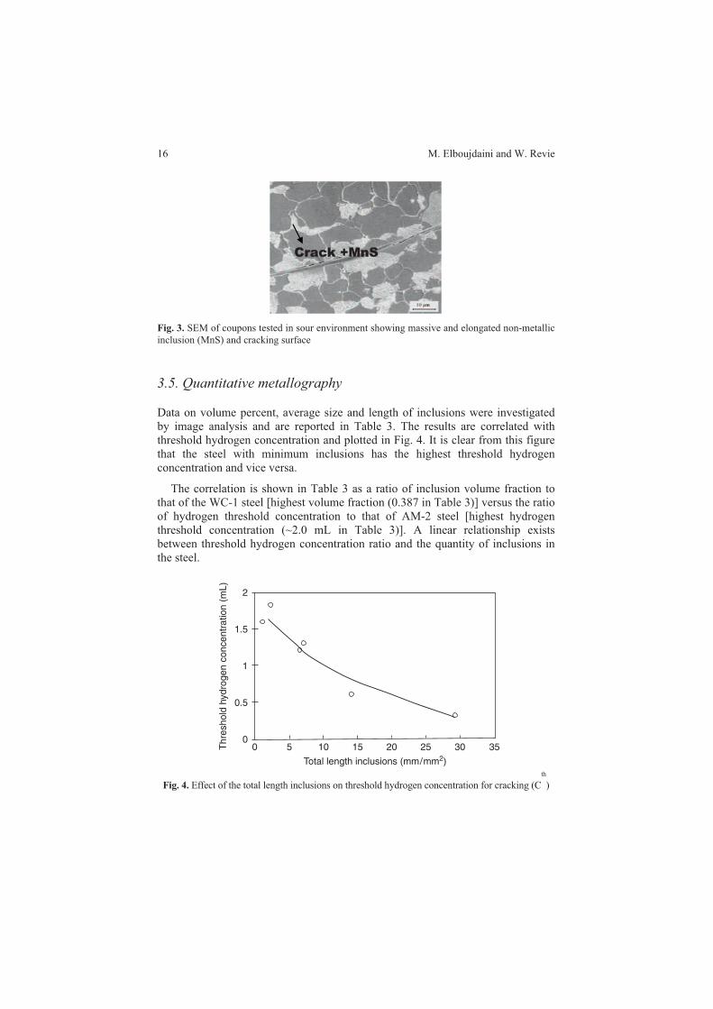
3.5. Quantitative metallography
Data on volume percent, average size and length of inclusions were investigated
by image analysis and are reported in Table 3. The results are correlated with
threshold hydrogen concentration and plotted in Fig. 4. It is clear from this figure
that the steel with minimum inclusions has the highest threshold hydrogen
concentration and vice versa.
The correlation is shown in Table 3 as a ratio of inclusion volume fraction to
that of the WC-1 steel [highest volume fraction (0.387 in Table 3)] versus the ratio
of hydrogen threshold concentration to that of AM-2 steel [highest hydrogen
threshold concentration (~2.0 mL in Table 3)]. A linear relationship exists
between threshold hydrogen concentration ratio and the quantity of inclusions in
the steel.
Fig. 4. Effect of the total length inclusions on threshold hydrogen concentration for cracking (C
th
)
0
Th
resh
old
hyd
rog
en
co
nce
ntr
ation
(m
L)
0.5
1
2
1.5
5
Total length inclusions (mm/mm2)
10 15 20 25 30 350

Effect of Non-Metallic Inclusions on Hydrogen Induced Cracking 17
Table 3. Linepipe steels data on inclusions
Sample Vol. % Average size
(Fm)
#/mm2 Length/mm
2 Threshold hydrogen
concentration mL (STP)/100 g
WC-1 0.387 1.73 16963 29.3 0.3
G-2 0.338 2.45 5729 14.1 0.6
AM-1 0.209 3.71 1774 6.5 1.2
PC-1 0.205 4.96 1382 6.9 1.3
CTR-2 0.042 3.25 278 0.9 >1.5
AM-2 0.034 1.41 1614 2.2 >2.0
The size and shape of the inclusions were considered to depend on the Ca/S
ratio in steel. The Ca/S ratio in Table 2, showed that a greater ratio of Ca/S
decreases the hydrogen damage susceptibility; i.e. steels CTR-2 and AM-2.
According to the results, steel susceptibility to SSC and HIC depends on the stress
localization around large and hard inclusion particles. This localized stress could
exceed the yield strength.
4. Conclusions
There is good correlation between inclusion measurements and HIC. The elongated
MnS and planar array of other inclusions are primarily responsible for cracking.
Lower volume fractions of inclusions corresponded to higher resistance to HIC.
However, the microstructure may also play a role in HIC, in particular, heavily
banded microstructures could enhance HIC by providing low fracture resistance
paths for cracks to propagate more easily.
Acknowledgments The authors acknowledge helpful discussions with colleagues at the
CANMET Materials Technology Laboratory. This project was funded in part, by the Federal
Interdepartmental Program of Energy R&D (PERD).
References
[1] Ikeda et al. (1977), Proc. of the 2nd International Conference on Hydrogen in Metals,
Paris, 4A-7.
[2] Tau L, Chan SLI, Shin CS (1996), Effects of anisotropy on the hydrogen diffusivity and
fatigue crack propagation of a banded ferrite/pearlite steel, Proc. of the 5th International
Conference on Hydrogen Effect in Materials, edited by AW Thompson and NR Moody,
The Minerals, Metals and Materials Society, pp. 475.
[3] Ikeda A, Kaneke T, Hashimoto I, Takeyama M, Sumitomo Y, Yamura T (1983), Proc. of
the Symposium on Effect of Hydrogen Sulphide on Steels, 22nd Annual Conference of
Metallurgists, August 22–24, Edmonton, Canada, Canadian Institute of Mining and
Metallurgy (CIM), Montreal, pp. 1–71.

18 M. Elboujdaini and W. Revie
[4] Elboujdaini M, Revie RW, Shehata MT, Sastri VS. Ramsingh RR (1998), Hydrogen-
induced cracking and effect of non-metallic inclusions in linepipe steels, NACE Inter-
national, Houston, Texas, Paper No. 748.
[5] Turnbull A, Saenz de Santa Maria M, Thomas ND (1989), Corrosion Science, vol. 29,
No. 89
[6] Tamaki K, Shimuzu T, Yamane Y (1991), Corrosion/91, Paper 14.
[7] Standard Test Method TM-0284, Test method evaluation of pipeline steels for resistance
to stepwise cracking, NACE International, Houston, Texas.

19
T. Boukharouba et al. (eds.), Damage and Fracture Mechanics: Failure Analysis of Engineering
Materials and Structures, 19–32. © Springer Science + Business Media B.V. 2009
Defect Assessment on Pipe Transporting
a Mixture of Natural Gas and Hydrogen
Guy Pluvinage
Laboratoire de Fiabilité Mécanique, ENIM, Ile du Saulcy Metz 57045, France
Abstract Procedure of defect assessment for steel pipes used for hydrogen or mixture of
natural gas and hydrogen is proposed. The hydrogen concentration is controlled by a cathodic
polarisation method. Fracture toughness for blunt pipe defect such as dent is measured on
“roman tile specimen”. It can be determined either critical J parameter or critical notch stress
intensity factor. Then the defect assessment is made using a notch modified failure assessment
diagramme (NMFAD).
Keywords: Hydrogen, Defect Assessment, Fracture Toughness, Failure Assessment Diagramme.
1. Introduction
Nowadays, pipelines for gas and oil transportation are very significant component
of national economic infrastructures as well as global. There are the huge plans for
installation of new transcontinental pipelines that require of increased attention to
their reliable and safe exploitation. In this frame, the hydrogen degradation of
pipeline steels is the important problem among other structural integrity problems
from the following reasons.
Specific long term exploitation of pipelines promotes of steel hydrogenating
process. First of all, pipeline steels encounter hydrogen during transport of sour
crude oil and other petroleum products [1]. Moreover, external environmental
conditions cause free corroding processes, where hydrogen can evaluate on metal
surface as result of cathodic counterpart of the anodic dissolution reaction. This
fact has been proved by several studies [2–4]. Also under in-service condition
when a cathodic protection system is in place, hydrogen charging of pipeline
steels is possible too [4, 5]. As result there is the problem of structural integrity of
aging buried pipelines having cathodic protection [5].
Second reason, which increases of attention to the problem hydrogen degradation
of pipeline steels, is fact that hydrogen will play a decisive role in a future energy
system, when fossil fuels have become scarce and thus expensive and/or unsuitable
from ecological reasons. The number of aspects related to the technical feasibility
and economics of developing a hydrogen energy infrastructure are presented and
discussed in literature during last decades [6, 7]. The possible use of existing
pipeline networks for mixtures of natural gas and hydrogen offers a unique and

20 G. Pluvinage
cost-effective opportunity to initiate the progressive introduction of hydrogen as
part of the development of a full hydrogen energy system [6, 8].
2. Determination of hydrogen concentration pipelines steels
Hydrogen concentration in metal has been determined on the base of hydrogen
discharging process under anodic polarisation with using of hydrogen electro-
chemical oxidation method proposed in work [9]. Hear, the standard three-
electrode electrochemical cell has been used (Fig. 1). The hydrogen discharging of
specimen were curried out in 0.2 M NaOH (pH = 12.4) solution under anodic
polarisation )(168 SCEmVEanodic during some defined time dis . The total
quantity of absorbed hydrogen by metal can be defined as (Fig. 2):
0
under const.
dis
abs
H H ref anodicQ I I d E (1)
where HI is anodic polarisation current for hydrogen charged specimen and
refI is anodic polarisation current for specimen without hydrogen (reference
curve). Calculation of hydrogen concentration was done according to formula:
zFv
QC
absH
H (2)
where z is the number of electrons take in reaction; F is the Faraday constant;
v is the effective volume of specimen: 3
mol cmHC ; sAQabsH . ; 1z ;
F=9,65 104 C/mol; v=0.256cm3. Process of hydrogen charging of pipeline steels
at the given conditions of cathodic polarisation was characterised by following
parameters: hydrogen concentration in metal HC ; total quantity of evaluated evQ
and absorbed absQ hydrogen; averaged meaning of cathodic current density ci and
coefficient of efficiency of hydrogen permeation in metal evabs QQk .
Comparative assessment of X52, X70 and X100 steels showed that last possesses
of highest resistance to hydrogen absorption. The steel X70 is the most sensitive to
hydrogen-charging in assigned testing conditions (Fig. 3a). The hydrogen
evaluation process is slightly intensive for X100 steel than the for X52 and X70
steels. For all steels, the efficiency of hydrogen permeation in metal is quite low
and depends on time of exposition. It can be stated that under 20 hours there
is the tendency of monotonic decreasing of parameter evabs QQk = up to level
0.0012 0.0024k (Fig. 3b).

Defect Assessment on Pipe Transporting a Mixture of Natural Gas and Hydrogen 21
4 mm
8 mm
8 mm
Open metal
surface
Isolation
coating
4 mm
8 mm
8 mm
Open metal
surface
Isolation
coating
(b)
(a)
Fig. 1. Schematic view of the electrochemical cell (a) and specimen (b) for determining of
hydrogen discharging current
Time of Exposition
Pola
risa
tion
Curr
ent .constEanodic
HI
refI dis
Time of Exposition
Pola
risa
tion
Curr
ent .constEanodic
HI
refI dis
Fig. 2. Schematic view of hydrogen discharging process under anodic polarisation
0,01
0,1
1
10
0 50 100 150 200
Time of exposition , hours
Hy
dro
ge
n c
on
ce
ntr
ati
on
C
H,
10
6m
ol/
cm
3
X52
X70
X100
0,0001
0,001
0,01
0,1
1
0 50 100 150 200
Time of exposition , hours
k=
Qa
bs/Q
ev
X52
X70
X100
Fig. 3. (a) Hydrogen concentration in metal versus time of exposition of unloaded specimens
under cathodic polarisation of pipeline steels API X52, X70 and X100. (b) Efficiency of
hydrogen permeation in metal versus time of exposition of specimens under given cathodic
polarisation
Applied stress (gross stress gross which corresponds of the internal pressure in
pipe under exploitation exp bar70p ) can intensify the hydrogen charging
COMPUTER
CE
GAS
RE
SALT-BRIDGE
EXHAUST GAS
EPOXY
HOLDER
SPECIMEN
WE
POTENTIOSTAT
NoCH
KCI

22 G. Pluvinage
process in several times at least. At that, under hours100 the difference
between hydrogen concentration in unloaded and stressed metal can exceed more
than five times. Based on experimental results; the increasing of hydrogen
concentration in metal versus time of exposition of specimens in the
hydrogenating conditions can be described by power relation:
6 310 mol/cm
m
HC A (3)
where A and m are constants (Table1).
Table 1. Meanings of constants in formula (3)
Steel Unloaded metal Stressed metal
API X52 C =0.253 106
0.24 C =0.300 10
6
0.57
API X70 C =0.049 106
0.67 C =0.400 10
6
0.42
API X100 C =0.200 106
0.19 –
3. Hydrogen embrittlement and brittle to ductile transition
with hydrogen concentration
For fracture toughness test the special “Roman tile” [10] specimens were used.
The specimens were notched for modeling of the longitudinal external defects
under operating internal pressure. Here, should be noted that prevail number of
reported studies [11–14] were conducted with using of cathodic charging of
hydrogen under high density of polarisation current. Such charging is not truly
representative of the hydrogen entry conditions in real operating pipelines, where
there is the situation of freely corroding system [15].
This fact was pointed out in work [4]. Accounting the fact that a steady state
condition of hydrogen charging cannot be imposed nor obtained in a freely
corroding situation, in presented study the following procedure has been made.
The specimens were hydrogen charged at some constant potential of polaris-
ation ,constE p which is slightly negative than free corrosion potential for given
steel: m1000 V( )cathE SCE and m800 V( )corrE SCE .
For this experimental procedure the potentiostat VMP [16] has been used. The
specimens were immersed into the cell with special NS4 solution and exposed
under constant potential of polarisation constcathE .
The surface of auxiliary electrode was parallel to notch plane with some
constant distance h . The mutual location of working (specimen) and auxiliary
electrodes is given in Fig. 4.

Defect Assessment on Pipe Transporting a Mixture of Natural Gas and Hydrogen 23
AE System
Potentiostat
Computer
2CO
Nitrogen
1
3
2
45
7
6 2
AE System
Potentiostat
Computer
2CO
Nitrogen
1
3
2
45
7
6 2
Fig. 4. Mutual location of working electrode (specimen) and auxiliary electrode
Displacement,
Load, P
*
Fracture start according to AE response
)(totalfW
)( plasticfW
Displacement,
Load, P
*
Fracture start according to AE response
)(totalfW
)( plasticfW
Fig. 5. Scheme of local fracture work determining
During the hydrogen-charging process, the specimens are loaded. The level of
load was defined as gross hoop stress gross which corresponds of the internal
pressure in pipe under exploitation exp 70 bar.p The hydrogen-charging process
was controlled by registration of the cathodic polarisation current cathI . The
total quantity of evaluated hydrogen on metal surface can be assessed as: After
assigned exposition under hydrogenating conditions, all specimens were tested to
failure under increasing static loading, according to three-point bending scheme.
Testing machine INSTRON was used under the constant rate of displacement of
grips 0.02mm sd d . The “load displacement” diagram and acoustic emission
(AE) signals were simultaneously registered by PC during the tests. The start of
fracture process has been defined by acoustic emission method.
.exp
0
constEunderdIQ cathcathevH (4)
Fracture toughness of notched specimens is given, which reflect of local
strength of pipeline steels in presence of hydrogen.

24 G. Pluvinage
The data were presented as dependencies of total work of local fracture
)(totalfW emanating from notch or its plastic component )( plasticfW versus time of
exposition of specimens under hydrogenating conditions. The scheme of
determination of parameters )(totalfW and )( plasticfW is given in Fig. 5. For steel X52
the value of critical hydrogen concentration is 6 3
4.3.10 mol cmHC (Fig. 6). The
steel X70 is very sensitive to notch effect even in air and the presence of
hydrogen strengthens this tendency. The hydrogen concentration about 6 3
2.1.10 mol cmHC can be considered as critical, because at this conditions
the given steel losses in 2.5 times its local strength with comparison of test in air.
Therefore, for assigned testing conditions, steel X52 is preferable than steel X70
from the point of view of local strength at notches. It should be stated that
definition “critical concentration” is often used in studies of problems of hydrogen
in metals and alloys. Although in different works this term has different physical
sense. Hydrogen treatment below the “critical” content was found to cause the
substantial rearrangement of dislocations and de-cohesion of grain boundaries and
in overcritical condition, the formation of micro crevices at the grain and phase
boundaries has been occurred. Two characteristic value of hydrogen concentration
in metal of pipe may be classified. First one is concentration 0HC , beginning
from which hydrogen affects on local strength of material. Second one is critical
concentration criticalHC , which causes the significant loss of local fracture
resistance of material. This critical hydrogen concentration defines a real brittle to
ductile transition.
0
5
10
15
20
25
30
35
0 1 2 3 4 5 6
CH, 106mol/cm
3
Wf, N
m
API X52
API X70
Fig. 6. Comparison of local fracture work emanating from notch in steel API X52 and X70
versus hydrogen concentration in metal
4. Determination of gaz pipe steel fracture toughness
in presence of dentes
Stress concentration is considered as the origin in more than 90% of the failures in
service.

Defect Assessment on Pipe Transporting a Mixture of Natural Gas and Hydrogen 25
In Canada it can be seen that the failure caused by corrosion is very important,
expressed in 42% cases [15]. In Europe, due to more densely populated area’s, the
statistics are different; more damage is caused by external interference [16]. A
very important fraction of failures is also connected with mechanical damage due
to soil digging or excavating by machines. Frequently, notch-like defects are
formed in pipelines by machines used in ground removal during construction.
Together with cracks caused by stress corrosion, these notches are stress raisers,
reducing the material resistance to fatigue and fracture. Therefore, structural
integrity of pipelines under various service conditions including the presence of
notch-like defects should be evaluated. Therefore it is necessary to measure the
pipe steel fracture toughness in a proper way. The concept of the notch stress
intensity factor based on the volumetric method has been employed and the
corresponding notch fracture toughness cK , was measured. Furthermore, the notch
fracture toughness cJ , in terms of the J-integral has been determined by means
of the load separation method.
The experimental procedure for measurement of the notch fracture toughness of
the API 5L X52 steel using a non-standard curved specimen with a notch
simulating the expected scratch damage of gas pipelines. The concept of the notch
stress intensity factor based on the volumetric method has been employed and the
corresponding notch fracture toughness cK , was measured. Furthermore, the notch
fracture toughness cJ , in terms of the J-integral has been determined by means
of the load separation method. The concept of the critical notch stress intensity
factor and corresponding local fracture criterion assume that the fracture process
requires a certain fracture process volume [8]. This volume is assumed as a
cylinder with a diameter called the effective distance. Determination of the effective
distance is based on the bi-logarithmic elastic–plastic stress distribution on the
continuation of the notch because the fracture process zone is the highest stressed
zone. This zone is characterized by an inflexion point in the stress distribution at
the limit of zones II and zone III in Fig. 7. This stress distribution is corrected by a
weight function in order to take into account the distance from notch tip of the
acting point and the stress gradient at this point. The effective distance corresponds
is to the inflexion point with the minimum of the relative stress gradient which
can be written as:
r
r
rr
yy
yy
1 (5)
The effective stress is considered as the average value of the stress distribution
within the fracture process zone.
drrrX
effX
yyeff
eff0
1 (6)

26 G. Pluvinage
Here, eff , effX , ryy and r are effective stress, effective distance,
maximum principal stress and weight function, respectively. The notch stress
intensity factor is defined as a function of the effective distance and the effective
stress [17].
effeff XK 2 (7)
where K is the notch intensity factor, is a constant. Failure occurs when the
notch stress intensity factor K reaches the critical value, i.e. the notch fracture
toughness c,K which reflects the resistance to fracture initiation from the notch tip.
ef
efX
Log(r)
(r))Log( yy
Stress distribution along defect root
Geometrical defect
I II III
Fracture Process Zone (FPZ)
Notch stress intensity virtual crack
efef X2K
ef
efX
Log(r)
(r))Log( yy
Stress distribution along defect root
Geometrical defect
I II III
Fracture Process Zone (FPZ)
Notch stress intensity virtual crack
efef X2K
Fig. 7. Schematic distribution of elastic–plastic stress ahead of the notch tip on the line of notch
extension and the notch stress intensity concept
The load separation method was adopted to measure the notch fracture
toughness in terms of the J-integral. The J-integral can be calculated as the sum of
elastic eJ and plastic pJ components [18].
aWB
A
aWB
AJJJ
plpl
elelpe (8)
where '
21
EE , E is Young’s modulus; is Poisson ratio; el and pl are
elastic and plastic correction factors, respectively; plel AA , are elastic and plastic
area under the load versus load-line displacement curve, respectively; W and B are
thickness (direction of the notch continuation) and width of the “Roman tile”
specimen, respectively; a is notch depth in thickness direction. More recognized
equation is given by:

Defect Assessment on Pipe Transporting a Mixture of Natural Gas and Hydrogen 27
2
'
pl
e p pl
AKJ J J
E B W a (9)
where K is the notch stress intensity factor. Such dividing the J-integral could be
useful to analyse a contribution of elastic and plastic J-components in deformation
and fracture process. The J-integral can be also written using its energy rate
interpretation.
da
dA
BJ
plpl
1 (10)
The classical and numerical methods to determine pl -factors are based on the
energy rate interpretation of the J-integral for a body with a crack. In this case,
from Eqs. (9) and (10) the pl -factor is found to be:
da
dA
A
b
da
dA
A
aW pl
pl
pl
plpl (11)
where baW is remaining ligament length, pl
PdApl0
. In the Eq. (11) the
value of P represents the load applied during the test and the value of vpl is the
plastic load-line displacement. The procedure of calculating the pl -factor can be
also based on the load separation method. The method assumes that the load can
be represented as a product of two functions, namely, a crack geometry function G
and a material deformation function H, it is assumed the load to be in the form:
WH
W
bGP
pl (12)
Using this load separation form, it is possible from Eqs. (11) and (12) to
represent the pl -factor as follows:
W
bG
W
bG
bdb
dvW
vH
W
bGd
dvW
vH
W
bG
bpl
pl
plpl
pl
'
(13)

28 G. Pluvinage
The load separation concept introduces a separation parameter Sij as the ratio of
loads P(a, vpl) of same specimens but with two different crack lengths ia and ja
over the whole domain of the plastic displacement, namely.
constvplj
pliij
pl
vaP
vaPS
,
, (14)
Substituting Eq. (13) into Eq. (14), we obtain another presentation of the
separation parameter Sij:
const
W
bG
W
bG
W
vH
W
bG
W
vH
W
bG
W
bS
plpl
pl
v
j
i
v
plj
pli
v
iij (15)
It was suggested that for a given material in the separation region, the
W
bS i
ij parameter as a function of remaining ligament ib determined at constant
plastic load-line displacement can be fitted with a power law pl
W
bC
W
bG , i.e.
pl
pl
pl
pl
pl
W
bA
W
bC
W
bC
W
bS i
m
v
j
i
v
iij (16)
where C is a constant. Thus, the slope of the WbSij / curve is the pl -factor in
Eq. (16). The results of the notch fracture toughness cJ , as a function of the notch
cJ , increases
with the decrease of the notch aspect ratio.
Thus, the present results on the notch fracture toughness of the API 5L X52
steel can be used in the modified failure assessment diagram for structural
integrity assessment of gas pipelines damaged by scratches.
aspect ratio are presented in Fig. 9. It can be seen that the value of

Defect Assessment on Pipe Transporting a Mixture of Natural Gas and Hydrogen 29
y = 3471,6x-1,2548
R2 = 0,9043
0
10000
20000
30000
40000
50000
60000
70000
80000
0,1 0,15 0,2 0,25 0,3 0,35 0,4 0,45 0,5 0,55 0,6 0,65 0,7
a/W
JIc
(J/m
²)
Fig. 8. Dependence of the notch fracture toughness Jp,c of the “Roman tile” specimens of the API
5L X52 steel pipe versus the notch aspect ratio. The value of Jp,c for a/W = 0.2 was represented
as a result of the tests of 11 specimens
5. The use of a modified failure assessment diagram for notches
and dentes
The critical non dimensional stress intensity crk and critical non dimensional
loading parameter c
rL delineate the critical design curve according to the available
codes, e.g., EPRI, RCC-MR, R6 and SINTAP This curve depicts the integrity area
as the area under the interpolation curve between critical points (0,1) and (1,0).
The non dimensional crack driving force rk and non dimensional applied stress
rL are primarily defined as the ratio of applied stress intensity factor, Kapp, to the
fracture toughness of material, *
cK .
*c
appr
K
Kk (17)
The British Standard (BS) is firstly improved the FAD diagram by introducing
the J integral or crack opening displacement as
mat
appr
mat
appr kor
J
Jk (18)
where, appJ , app are the applied J integral and crack opening displacement and
matJ and c are fracture toughness in terms of critical value of J integral or
critical crack opening displacement of the material. For notch and dents problems,
the kr parameter is defined from the notch stress intensity factor.

30 G. Pluvinage
c
appr
K
Kk
,
, (19)
where K , c is the critical notch stress intensity factor. Non dimensional stress rL
is described as the ratio of the gross stress g over flow stress (chosen as yield
stress Y , ultimate stress; U or classical flow stress 2/)( UYcR ).
c
g
RrL (20)
The critical assessment points leading to fracture yield an assessment inter-
polation curve between two specific or reference limit states: brittle fracture
[ 1k r ; 0Lr ]; plastic collapse [ 0k r ; 1Lr ]. The assessment point of a
component can be highlighted by a point of coordinates *
rk and*
rL . If this point is
inside the boundary lines of the diagram which is limited by the interpolation curve;
the structure is safe. If not, failure occurs, and the assessment point is situated
outside of the interpolation curve (Fig. 9).
As illustrated in Fig. 9, the safety factor is denoted using ratio OC over OA for
chosen assessment point. According to the codes safety factor consideration, the
assessment point is positioned within the acceptable zone of the FAD and the
structure fulfils the required conditions for practical engineering applications. The
interpolation curve in terms of non dimensional load is given by the level 1
SINTAP formula:
LrLr
Lrf 6.6.0exp7.03.0.
2
21
1 LrLr max,0 (21)
yLr
1505.2
1max, (22)
The safety factor can be defined from the Fracture Analysis Diagram (FAD),
starting with the assumption that the defect will not extend under applied loading.
It is presented in Fig. 10 that the safety factor can be defined on the radial straight
line in the form of the ratio FS = OB/OA. Figure 10 gives an example of safety
factor resulting from the presence of a notch in a gin a gas pipe under a service
pressure of 70 bars.

Defect Assessment on Pipe Transporting a Mixture of Natural Gas and Hydrogen 31
rk
rL1.00
1.00
O 0.750.500.25
0.25
0.50
0.75Interpolating curve
SAFE
FAILURE
Assessment point,
SF=OC/OA>2
*
rk
*
rL
A
B
C
Interpolating curve
including SF=OC/OB=2
Plastic co
llapse
Brittle fracture
Fig. 9. Typical failure assessment diagram (FAD) indicating safe, failure zone and desirable
assessment point
6. Conclusions
Special attention needs to be paid for defect assessment for pipes transporting pure
hydrogen or a mixture of natural gas and hydrogen. This is necessary due to hydrogen
embrittlement above a critical hydrogen concentration which is relatively low and
decreases with the steel yield stress. A special procedure is also necessary for
determining fracture toughness in pipe in radial direction due to surface curvature.
Then the Modified Notch failure assessment diagramme can be used to
determine the safety factor associated with dent geometry and service pressure.
Fig. 10. Modified failure assessment diagram and safety factor associated with defect geometry
and internal pressure. Central long notch (t = 6.1 mm, d = t/2, d/L=0.1, = 0.15 mm)
The use of roman tile specimen is recommended.
d
L
0,0 0,1 0,2 0,3 0,4 0,5 0,6 0,7 0,8 0,9 1,0 1,1 1,2 1,30,0
0,1
0,2
0,3
0,4
0,5
0,6
0,7
0,8
0,9
1,0
1,1
1,2
FS=0B/OA=1.704
Fs=0C/OA=3.408
SINTAP failure margin
SINTAP security margin
Assessment point for semi-elliptical defect
B
SINTAP Level 0 failure margin
C
O
kr
Lr
A
Assessment point
SINTAP Level 0 security margin
cut-off cut-off

32 G. Pluvinage
References
[1] Azevedo C. Failure analysis of a crude oil pipeline. Engineering Failure Analysis 14 (2007)
978–994.
[2] Cheng Y.F., Niu L. Mechanism for hydrogen evolution reaction on pipeline steel in near-
neutral pH solution. Electrochemistry Communications 9 (2007) 558–562.
[3] Cheng Y.F. Fundamentals of hydrogen evolution reaction and its implications on near-
neutral pH stress corrosion cracking of pipelines. Electrochimica Acta 52 (2007) 2661–
2667.
[4] Dey S., Mandhyan A.K., Sondhi S.K., Chattoraj I. Hydrogen entry into pipeline steel under
freely corroding conditions in two corroding media. Corrosion Science 48 (2006) 2676–
2688.
[5] Shipilov S.A., May I.L. Structural integrity of aging buried pipelines having cathodic
protection. Engineering Failure Analysis 13 (2006) 1159–1176.
aspects. Kluwer Academic Publisher, the Netherlands (1995), 352p.
[7] Hanneken J.W. Hydrogen in metals and other materials: a comprehensive reference to
books, bibliographies, workshops and conferences. International Journal of Hydrogen Energy
24, No. 10 (1999) 1005–1026.
[8] Ibeh B., Gardner C., Ternan M. Separation of hydrogen from a hydrogen/methane mixture
using a PEM fuel cell. International Journal of Hydrogen Energy 32 (2007) 908–914.
[9] Yan M., Weng Y. Study on hydrogen absorption of pipeline steel under cathodic charging.
Corrosion Science 48 (2006) 432–444.
[10] Adib-Ramezani H., Jeong J., Pluvinage G. Structural integrity evaluation of X52 gas pipes
subjected to external corrosion defects using the SINTAP procedure. International Journal
of Pressure Vessels and Piping 83 (2006) 420–432.
[11] Hardie D., Charles E.A., Lopez A.H. Hydrogen embrittlement of high strength pipeline
steels. Corrosion Science 48 (2006) 4378–4385.
[12] Torres-Islas A., Salinas-Bravo V.M., Albarran J.L., Gonzalez-Rodriguezd J.G. Effect of
hydrogen on the mechanical properties of X-70 pipeline steel in dilutedNaHCO3 solutions
at different heat treatments. International Journal of Hydrogen Energy 30 (2005) 1317–
1322.
[13] Zhang T., Chu W.Y., Gao K.W., Qiao L.J. Study of correlation between hydrogen-induced
stress and hydrogen embrittlement. Materials Science and Engineering A347 (2003) 291–
299.
[14] Cheng Y.F. Analysis of electrochemical hydrogen permeation through X-65 pipeline steel
and its implications on pipeline stress corrosion cracking. International Journal of Hydrogen
Energy 32 (2007) 1269–1276.
[15] Li M.C., Cheng Y.F. Mechanistic investigation of hydrogen-enhanced anodic dissolution of
X-70 pipe steel and its implication on near-neutral pH SCC of pipelines. Electrochimica
Acta 52 (2007) 8111–8117.
[16] Rapport de l’enquête MH-2-95, Fissuration par corrosion sous tension des oléoducs et
gazoducs canadiens, Office National d’Energie (1996), Canada. 16th EGIG report 1970–
2004, December 2005, “Gas Pipeline Incidents”, Doc. Number EGIG 05.R.0002
[17] Akourri O., Louah M., Kifani A., Gilgert G., Pluvinage G. The effect of notch radius on
fracture toughness JIC. Eng Fract Mech 65 (2000) 491–505.
[18] SINTAP: Structural integrity assessment procedure. Final report E-U project BE95-1462.
Brite Euram Programme, Brussels, 1999.
[6] Yurum C.R. (ed.) Hydrogen energy systems: production and utilisation of hydrogen and future

33
T. Boukharouba et al. (eds.), Damage and Fracture Mechanics: Failure Analysis of Engineering
Materials and Structures, 33–42. © Springer Science + Business Media B.V. 2009
Reliability Analysis of Low Alloy Ferritic Piping
Materials
A. Guedri1, 4
, B. Merzoug2, Moe Khaleel
3 and A. Zeghloul
4
1Department of Maintenance, University Center of Souk Ahras, Algeria
2University of Badji Mokhtar, Algeria
3PNNL Laboratory, PO Box 999, 902 Battelle Boulevard, Richland, WA 99352, USA
4LPMM Laboratory, UMR CNRS 7554, Paul Verlaine University, Metz, France
Abstract The aim of this study is to improving microstructure and mechanical properties of the
weldable gas pipeline steel using laboratory mill. To achieve the required microstructure and
mechanical properties of thermo mechanically processed HSLA steels, it is necessary to have an
idea about the role of composition and process parameters. The large numbers of parameters
obtained during the production process in the plant were systematically changed to optimize the
strength and toughness properties. The optimized parameters were used for the production of the
API X60/X70 steel. However, the controlled cooling after rolling should result in transformed
products that provide excellent combination of strength and toughness. The coiling at an
appropriate temperature have the advantage of the precipitation strengthening, giving further rise
to the high yield strength and also improvement in toughness of the steel. The coiling
temperature is a decisive parameter because it determines the beginning of the formation of fine
precipitations. Therefore, four different laboratory cooling systems were used, in this study to
simulate the rolling conditions of a real industrial Thermomechanically controlled process, as
close as possible and to check the possibilities of improving the mechanical properties of the
welded pipeline steel.
Keywords: Micro Alloying, TMCP, Controlled Rolling, Controlled Cooling, Processing Para-
meters, Mechanical Properties.
1. Introduction
Piping systems experience fatigue damage as a result of anticipated plant transients
(e.g. rapid cooling of the piping during auxiliary feed water initiation following a
scram) and because of unanticipated transients (e.g. check valve leakage) [1]. This
paper describes the probabilistic fracture mechanics computer code and structural
mechanics modelling approach used to simulate the effects of these cyclic fatigue
stresses on the reliability of reactor piping.
Probabilistic fracture mechanics (PFM) calculations often assume that the stress
state in the pipe wall is uniform through the wall thickness. This approach is
appropriate for stresses as a result of internal pressure and for bending stresses as a
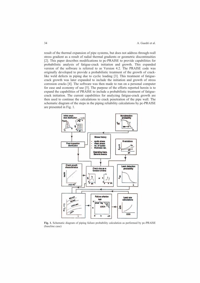
34 A. Guedri et al.
result of the thermal expansion of pipe systems, but does not address through-wall
stress gradient as a result of radial thermal gradients or geometric discontinuities
[2]. This paper describes modifications to pc-PRAISE to provide capabilities for
probabilistic analysis of fatigue-crack initiation and growth. This expanded
version of the software is referred to as Version 4.2. The PRAISE code was
originally developed to provide a probabilistic treatment of the growth of crack-
like weld defects in piping due to cyclic loading [3]. This treatment of fatigue-
crack growth was later expanded to include the initiation and growth of stress
corrosion cracks [4]. The software was then made to run on a personal computer
for ease and economy of use [5]. The purpose of the efforts reported herein is to
expand the capabilities of PRAISE to include a probabilistic treatment of fatigue-
crack initiation. The current capabilities for analyzing fatigue-crack growth are
then used to continue the calculations to crack penetration of the pipe wall. The
schematic diagram of the steps in the piping reliability calculations by pc-PRAISE
are presented in Fig. 1.
Fig. 1. Schematic diagram of piping failure probability calculation as performed by pc-PRAISE
(baseline case)

Reliability Analysis of Low Alloy Ferritic Piping Materials 35
2. Description of general model
The components of a probabilistic fracture mechanics model of structural
reliability that considers the realistic case of two-dimensional cracks are presented
in Fig. 1, which also shows the interrelationship of the various components. The
approach is applicable to a wide variety of two-dimensional cracks, but the case of
semi-elliptical surface cracks of arbitrary aspect ratio in a body of finite thickness
will be considered here. Such a crack is shown schematically in the upper left
corner of Fig. 1, and is characterized by two dimensions (a) and (b). The model
depicted in Fig. 1 is described in detail in [5], so only a brief review will be
presented here.
The procedures shown in Fig. 1 are applicable to a given location in a structure,
such as a weld of volume V. The as-fabricated crack size distribution is combined
with the nondetection probability to provide the post-inspection distribution. The
manner in which the cracks that escape detection grow is then calculated by
fracture mechanics techniques. The cumulative probability of failure at any time is
simply the probability of having a crack at that time equal to or larger than the
critical crack size [6].
The crack size distribution at the time of the first in-service inspection (ISI) can
be calculated. This pre-inspection distribution is combined with the non-detection
probability to provide the post-inspection distribution. Fracture mechanics
calculations then proceed up to the next ISI, at which time the procedures are
again applied. Calculations of the failure probability for the general model are
performed numerically because of the complexity of the fracture mechanics
calculations of the growth of two-dimensional cracks as well as the complicated
bivariate nature of the crack size distribution [2, 6]. A specific example of results
from the general model will be presented later along with a discussion of inputs to
the model.
3. Praise modifications to consider fatigue – crack initiation
The Argonne National Laboratory (ANL) crack initiation correlations were for
cycles for the tensile load to drop by 25%. This corresponds to a crack of
approximately 3 mm depth (0.12 in.) [7, 8]. The specimen size was assumed to be
about 2 in. (51.76 mm) gouge length. The fatigue tests were performed under fully
reversed loading (i.e., a mean load of zero).
The subroutine provided by the Pacific Northwest National Laboratory (PNNL)
already had size-effect and surface-finish adjustments, but a single factor was
considered to account for size regardless of size. The subroutine provides cycles to
initiation for a given probability of initiation and set of conditions (material, cyclic
stress, strain rate, oxygen level, and sulfur content). The relations, “should not be
extrapolated beyond a probability of 0.02%” [7, 8]; hence, they are not suitable for
initiation probabilities below about 2.10 4.

36 A. Guedri et al.
Modifications were made to pc-PRAISE to consider the initiation of cracks and
their subsequent growth to become through-wall. For initiation, the PNNL
subroutine for initiation was used in conjunction with Monte Carlo simulation to
estimate the probability of initiation as a function of time. The subroutine provides
results for a constant stress amplitude, whereas the stress histories to be
considered have cyclic stresses of different amplitudes. The Miner’s rule was used
to account for these more complex stress histories. The cycles per year are equal to
the cycles per 40-year life divided by 40; that is, the cycling rate is considered to
be constant. A description of each transient is usually provided. Since multiple
initiation sites are employed, some adjustment should be made to the size/surface
finish compensations made by ANL. A portion of the size/surface finish effect
introduced by ANL is removed by multiplying each sampled initiation time by a
constant between 1 (using the ANL size/surface finish factor) and 4 (using the
ANL laboratory specimen correlations). Tire distribution of initiation time is
determined for each of the specimens in a component. The initiation times in each
specimen can either be independent or dependent. If dependent and no stress
gradient, then each specimen will initiates a crack at the same time. This results in
initiated cracks being as long as the component, such as completely around the
circumference for a girth weld in a pipe. This leads to all leaks being double-
ended pipe breaks. Hence, independent initiation is believed to be the most
realistic.
4. Praise modifications for crack growth and linking
of multiple cracks
Once a crack initiates, pc-PRAISE calculates its subsequent growth. An initiated
crack is considered to be 3 mm (0.12 in.) deep. It is still necessary to specify the
surface length 2b0 of the initiated crack. Although cracks that grow from a small
defect will tend to be nearly semi-circular (b0/a0 = 1), the median length of an
initiated crack is taken to be 7.6 mm (0.3 in.). This is believed to be conservative.
The initial length is taken to be a random variable. The value of b0 itself could be
the random variable, and this is one alternative that was considered.
Taking b0 to be lognormal with a median value of 7.6 mm (0.30 in.), it is then
only necessary to define the shape parameter, in order to define the complete
distribution. A couple of items of interest in the distribution of b0 [2] are
1. The probability that (b/a) at initiation is less than 1, which is physically
unrealistic because the crack would then be tunnelling into the specimen.
2. The probability that 2b0 would be greater than the “specimen” size of
50.76 mm (2 in.).
Multiple cracks can initiate in a component and then grow to perhaps
eventually coalesce. The criteria for linking of multiple cracks are already in pc-
PRAISE to account for multiple initiations of stress corrosion cracks [4, 5]. The

Reliability Analysis of Low Alloy Ferritic Piping Materials 37
criteria are based on procedures in the American Society of Mechanical Engineers
(ASME) Boiler and Pressure Vessel Code.
5. Correlations between initiation and growth properties
It is conceivable that there is a correlation between the initiation and growth
properties of the material. That is, if the crack-initiation characteristics are poor,
then the growth characteristics are also poor. Pc-PRAISE provides for treating
these properties as either independent or correlated.
If they are correlated, then the one minus the sampled random number used for
the initiation simulations is used for the growth relation.
6. Modification of fatigue crack growth relations for ferritic
material
The fatigue-crack-growth characteristics for ferritic steels that are built into pc-
PRAISE are for LWR environments. At very high values of K, the crack growth
relation falls below the air line for this material, which is physically unrealistic.
For ferritic steel in air, the crack growth rate is given by:
726.3)( KCdN
da (1)
The exponent 3.726 comes from the ASME Boiler and Pressure Vessel Code.
No effect of R is considered for growth in air. C for the ASME air line is
2.67 × 10 11, which is an upper-bound value. Consider C to be log normally
distributed with the ASME value being at the 95th percentile.
The scatter in air will be less than in water. Therefore, the shape parameter, µ,
used in pc-PRAISE will be less than for values for water. Taking µ to be the
smallest value used in the treatment in pc-PRAISE for water provides a value of
0.542. Once is fixed, the median value of C can be evaluated, which leads to
C50 = 1.10 × 10 11.
To analyze fatigue crack growth in ferritic materials in water, a sample is
drawn for the fatigue crack growth rate in water. The same random number is used
to sample the fatigue crack growth rate in air. The crack growth rate is then taken
to be the largest of the two.

38 A. Guedri et al.
7. Example
The example problem of the previous section was analyzed using 18 initiation
sites with a multiplier on t, of 3 and using (b0–a0) as the random variable
describing the size of the initiated cracks.
8. Probability result
In addition to probability of crack initiation, the probability of a leak (through-wall
crack), is evaluated. Analyses were performed for no circumferential variation of
the stresses. The results provide information on the relative leak-to-break probability
for situations with and without variations of stress on the surface. Such inform-
ation is useful in leak-before-break assessments.
For no circumferential stress variation, the stresses were taken to be axisym-
metric, and the results are for times extending to 60 years. Figure 2 provides a plot
of these results. No results are plotted for the Double-Ended Pipe Break (DEPB)
probability because no such failures occurred in the 100 trials performed.
Provisions were added to the pc-PRAISE output to summarize the linking of
cracks, which is described here. The results for this example problem with no
stress gradient are considered.
Figure 3 provides an example of the information in pc-PRAISE on crack
initiations, and a summary of crack initiation and linking. Such results are printed
out for each evaluation time that is a multiple of 10. Hence, the crack-linking
information is printed out for 20, 40, 50 and 60 years. Table1 includes the crack-
linking information at 60 years. The results are summarized on a crack-by-crack
basis, so information is lost regarding cracks on a weld-by-weld (trial-by-trial) basis.
Fig. 2. Cumulative failure probability as functions of time

Reliability Analysis of Low Alloy Ferritic Piping Materials 39
The effects of the number of initiated cracks sites are shown in Fig. 4, and the
benefit effect of (ISI) are shown in Fig. 5. Cracks in the depth range of
0.95 < a/h < 99% are mostly through-wall cracks, which are of particular interest.
Table entries for this range of depths provide information on the length
distribution of through-wall cracks and how many cracks linked to form them.
Any cracks that grew to become leaks before 60 years also appear in the Table 1.
Fig. 3. Crack initiation information from pc-Praise
Table 1. Example of crack-linking information printed out in pc-Praise at Time60 Years

40 A. Guedri et al.
Fig. 4. Effect of initiation site number on the cumulative failure probability
Fig. 5. Effect of pre-service and in-service inspection on the cumulative failure probability

Reliability Analysis of Low Alloy Ferritic Piping Materials 41
Table 2 summarizes results on a weld-by-weld (trial-by-trial) basis. The
number of individual cracks involved is not given, but only the sum of the surface
lengths.
Table 2. Crack size data sorted on a weld by weld basis 60 years
9. Conclusions
A probabilistic fracture mechanics model of structural reliability is summarized
that considers cracks to be two-dimensional such as semi-elliptical surface cracks.
The model uses a fatigue initial crack and crack growth model to grow pre-
existing, semi-elliptical, fabrication defects. Critical flaw sizes for pipe breaks are
based on a net section collapse criteria of fracture.
Numerical results obtained for a weld in a large reactor pipe are then presented
for randomly distributed material properties. As a conclusion, using the initiation
only show a weakly cumulative probability of leak in the ferritic components, one
may say it will be better to combine the effect of the initiation with a pre-existing
crack.
Acknowledgments The authors would like to thank Khaleel M.A. for his support and his
invaluable guidance during the course of this work.
References
[1] Khaleel, M.A. and F.A. Simonen, 1994. A Parametric Approach to Predicting the Effects of
Fatigue on Piping Reliability. ASME PVP Vol. 288 Service Experience and Reliability
Improvement: Nuclear, Fossil and Petrochemical Plants, Vol. 1, pp. 117–125.
[2] Khaleel, M.A. and F.A. Simonen, 2000. Effects of Alternative Inspection Strategies on
Piping Reliability. Nuclear Engineering and Design 197, pp. 115–140.
[3] Harris, D.O., E.Y. Lim, and D.D. Dedhia, 1981. Probability of Pipe Fracture in the primary
Coolant Loop of a PWR Plant, Vol. 5: Probabilistic Fracture Mechanics NUREG/CR-2189.
US Nuclear Regulatory Commission, Washington, DC.
[4] Harris, D.O., D.D. Dedhia, E.D. Eason, and S.P. Patterson, 1986. Probability of Failure in
BWR Reactor Coolant Piping, NUREG/CR-4792, Vol. 3. US Nuclear Regulatory
Commission, Washington, DC.
[5] Harris, D.O., D.D. Dedhia, and S.C. Lu, 1992. Theoretical and User’s Manual for pc-
PRAISE, A Probabilistic Fracture Mechanics Computer Code for Pipe Reliability Analysis.
NUREG: CR-5864, UCRL-ID-109798. US Nuclear Regulatory Commission, Washington,
DC.

42 A. Guedri et al.
[6] Harris, D.O. and E.Y. Lim, 1983. Applications of a Probabilistic Fracture Mechanics Model
to the Influence of In-Service Inspection on Structural Reliability, Probabilistic Fracture
Mechanics and Fatigue Methods: Applications for Structural Design and Maintenance.
ASTM STP 798, J.M. Bloom and J.C. Ekvall, Eds., American Society for Testing and
Materials, pp. 19–41.
[7] Keisler, J.M. and O.K. Chopra, 1995. Statistical Analysis of Fatigue Strain-Life Data for
Carbon and Low-Alloy Steels, Risk and Safety Assessment: Where Is the balance? ASME
PVP-vol296/SERA-Vol. 3, pp. 355–366.
[8] Keisler, J.M. and O.K. Chopra, and W.J. Shack, 1996. Statistical for Estimating Fatigue
Strain-Life Behavior of pressure Boundary Materials in Light water Reactor Environments.
Nuclear Engineering and Design, Vol. 167, pp. 129–154.

43
T. Boukharouba et al. (eds.), Damage and Fracture Mechanics: Failure Analysis of Engineering
Materials and Structures, 43–48. © Springer Science + Business Media B.V. 2009
Experimental Characterization and Effect of the
Triaxiality on the Behavior of the HDPE
K. Hachour1, R. Ferhoum
1, M. Aberkane
1, F. Zairi
2 and M. Nait
Abdelaziz2
1Laboratoire d’Energétique Mécanique et Matériaux. Faculté du Génie de la Construction.
Université Mouloud Mammeri, BP 17 RP Tizi-Ouzou 15000, Algéria
2 Laboratoire de Mécanique de Lille UMR CNRS 8707 Polytech’lille, Cité Scientifique-
Avenue Paul Langevin 59655 Villeneuve d’Ascq Cedex, France
Abstract In this work, a particular interest is granted to the effect of triaxial stress states on the
behaviour of the HDPE in uniaxial tensile test. To investigate this effect, tensile tests were
performed using notched round bars with four different notch radii (2, 4, 10 and 80 mm). These
tests were achieved on an Instron testing machine at constant strain-rate 10-3 s-1 and at ambient
temperature. The measure of the local strain is done from the minimal cross-section diameter.
We get then the transverse strain. The curves of behaviour deducted of these tests show that
the yield stress (defined at the maximal strength point on the conventional stress–strain curve) of
the material increases with the reduction of the notch radii. This tendency is due to the fact that the
triaxial stress increases with the reduction of the notch radii.
Keywords: HDPE, Damage, Triaxiality, Vidéo-Traction.
1. Introduction
The first studies of the plastic behavior of the semi-crystallines polymers, achieved
in the 60 years, were based on nominal laws that don’t take into account the plastic
instabilities (necking) occurring during the distortion. The following studies tried to
establish the true plastic behavior of the material and to characterize the micro-
mechanisms of distortion that controls it.
During tensile tests, the necking leads a considerable modification of the
triaxial stress that affects on their turn the experimental measures of the stress and
the necessary strain for the characterization of these materials.
For the isochores strain (to constant volume), this triaxiality is corrected by a
factor given by Bridgman [1]. On the other hand the polymers are subject to
phenomena of plastic damage that increase their specific volume [2].
In this work we examine the effect of the stress triaxiality on the behavior of
the HDPE diabolo specimens during uniaxial tensil tests.

44 K. Hachour et al.
2. Experimental procedure
2.1. Material
The HDPE studied in this paper is furnished in a first time as granules, imported
by the CHIALLI Company (Algeria) and extruded in order to manufacture tubes
of different diameters. The specimens are cuts as parallelepipeds from these tubes
in the axial sense (see Fig. 1), and machined as notched round bars specimens with
four different curvature radius (see Fig. 2). This geometry permits to localize the
necking in the zone of minimal cross-section diameter [3].
Fig. 1. Cutting sense of the specimens in HDPE tube
Fig. 2. Notched round bars specimens dimensions
2.2. Tensile tests
Uniaxial tensile tests are conducted at a room temperature on an Instron computer-
controlled tension machine on the four kinds (Type 1, 2, 3 and 4) of specimens
considered in our tests. The strain rate is imposed constant and equal to 3 1
10 s& . Three (03) tests are made for every type of specimen (notch radii),
giving a total of 12 tests.
D : specimen diameter
r : notch radius
of curvature
l : notch length
d : notch hole diameter
L : specimen length
Type 1 : r = 2; l = 3,87 Type 2 : r = 4; l = 7,42 Type 3 : r = 10; l = 13,23 Type 4 : r = 80; l = 39,69
D=10; L=66; d=5 For all
specimens
D
r
d
L l

Experimental Characterization and Effect of the Triaxiality 45
The local deformations in a representative volume element (RVE) are measured
with an intelligent optical extensometer by the video-traction technique developed
by the team of Professor G’SELL [4, 5] and marketed by the Appolor® society. A
digital video camera analyzes the relative displacements of markers printed on the
tensile specimens. Mechanical data analysis, stress and strain, are measured in real
time, while the axial strain is dynamically regulating at a constant rate.
3. Experimental results
The videoTraction tests provide the true stress versus true strain curves from local
measures. The analysis system marks the minimal diameter of the notch and
therefore, the variation of the diameter. We obtain then the transverse strain.
Through this test, the software analyzes and records permanently the following
data:
The applied axial strength
The time
The minimal diameter
The transverse deformation at the minimal diameter
The axial true stress that takes into account the section reduction of the
specimen
During the tests, the deformation of specimen exhibit “diffuse” necking which
is greatly localized (see Figs. 3 and 4).
Fig. 3. Videotraction system
Fig. 4. Necking formation in specimens during tensile test
load interface
video interface
control
interface
video
traction
keyboard
VCR
printer
Windows 95/NT
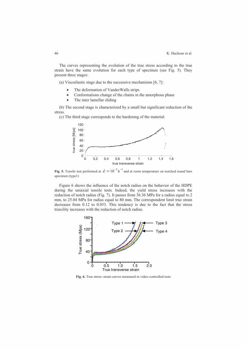
46 K. Hachour et al.
The curves representing the evolution of the true stress according to the true
strain have the same evolution for each type of specimen (see Fig. 5). They
present three stages:
(a) Viscoélastic stage due to the successive mechanisms [6, 7]:
The deformation of VanderWalls strips
Conformations change of the chains in the amorphous phase
The inter lamellar sliding
(b) The second stage is characterized by a small but significant reduction of the
stress.
(c) The third stage corresponds to the hardening of the material.
Fig. 5. Tensile test performed at 3 1
10 s& and at room temperature on notched round bars
specimen (type1)
Figure 6 shows the influence of the notch radius on the behavior of the HDPE
during the uniaxial tensile tests. Indeed, the yield stress increases with the
reduction of notch radius (Fig. 7). It passes from 36.36 MPa for a radius equal to 2
mm, to 25.04 MPa for radius equal to 80 mm. The correspondent limit true strain
decreases from 0.12 to 0.053. This tendency is due to the fact that the stress
triaxility increases with the reduction of notch radius.
Fig. 6. True stress–strain curves measured in video-controlled tests
120
100
80
60
40
20true s
tress [
Mpa]
00 0,2 0,4
true transverse strain
0,6 0,8 1 1,2 1,4 1,6
01.0
True transverse strain0 0.5 1.5 2.0
Tru
estr
ess (
Mpa
) Type 1
40
80
120
160
Type 2
Type 3
Type 4
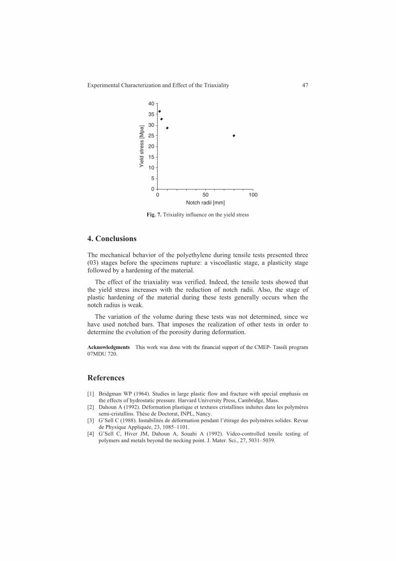
Experimental Characterization and Effect of the Triaxiality 47
Fig. 7. Trixiality influence on the yield stress
4. Conclusions
The mechanical behavior of the polyethylene during tensile tests presented three
(03) stages before the specimens rupture: a viscoélastic stage, a plasticity stage
followed by a hardening of the material.
The effect of the triaxiality was verified. Indeed, the tensile tests showed that
the yield stress increases with the reduction of notch radii. Also, the stage of
plastic hardening of the material during these tests generally occurs when the
notch radius is weak.
The variation of the volume during these tests was not determined, since we
have used notched bars. That imposes the realization of other tests in order to
determine the evolution of the porosity during deformation.
Acknowledgments This work was done with the financial support of the CMEP- Tassili program
07MDU 720.
References
[1] Bridgman WP (1964). Studies in large plastic flow and fracture with special emphasis on
the effects of hydrostatic pressure. Harvard University Press, Cambridge, Mass.
[2] Dahoun A (1992). Déformation plastique et textures cristallines induites dans les polymères
semi-cristallins. Thèse de Doctorat, INPL, Nancy.
[3] G’Sell C (1988). Instabilités de déformation pendant l’étirage des polymères solides. Revue
de Physique Appliquée, 23, 1085–1101.
[4] G’Sell C, Hiver JM, Dahoun A, Souahi A (1992). Video-controlled tensile testing of
polymers and metals beyond the necking point. J. Mater. Sci., 27, 5031–5039.
40
35
30
25
20
15
10Yie
ld s
tress [M
pa]
5
00 50
Notch radii [mm]
100

48 K. Hachour et al.
[5] G’Sell C, Hiver JM, Dahoun A (2002). Experimental characterization of deformation
damage in solid polymers under tension and its interrelation with necking. Int. J. Solids
Struct., 39, 3857–3872.
[6] G’Sell C, Dahoun A (1994). Evolution of microstructure in semi-crystalline polymers under
large plastic deformation. Mater. Sci. Eng., A175, 183–199.
[7] Glenz W, Peterlin A (1971) Plastic deformation of polymers. Peterlin A (ed.) Marcel
Dekker, New York, pp 13–29.

49
T. Boukharouba et al. (eds.), Damage and Fracture Mechanics: Failure Analysis of Engineering
Materials and Structures, 49–57. © Springer Science + Business Media B.V. 2009
Effects of Aggressive Chemical Environments
on Mechanical Behavior of Polyethylene Piping
Material
Souheila Rehab-Bekkouche, Nadjette Kiass and Kamel Chaoui
LR3MI, Mechanical Engineering Department, Badji Mokhtar University, BP 12, Annaba,
23000, Algeria
Abstract During the construction process of fluid handling structures, material selection for
pipe applications is an important step. Both natural gas and drinkable water are mainly
transported in underground polyethylene (PE) pipe networks. It is known that the interaction
between materials like HDPE (high density PE) and its service environment represents critical
factors of influence on the structure behaviour for short and long terms. The goal of this study is
to establish the effect of some chemical agents on the mechanical properties of PE tubes for
underground use. The results are discussed basing on the stress–strain curves and according to
the mechanical resistance to aggressive environments. It was found that the environments
consisting of solvents show degradation of the mechanical properties of tubes and a structural
weakening of the rigidity of the system is observed. Organic solvents have significant oxidizing
capacity which weakens polyethylene chains, whereas acids such as H2SO4 have less influences
on the mechanical properties compared to organic solvents. In the case of crude oil, results show
moderate effect although it is known to attack many polymers. In the case of solvents, the
elasticity modulus is reduced up to 64% for crude oil which represents a serious problem for the
underground polyethylene networks. Design equations of such structure should take into account
serious adjustments of long term loads when polyethylene is exposed to aggressive environment.
Keywords: Polyethylene, Pipe, Filaments, Stress, Strain, Chemical Agents, Degradation.
1. Introduction
High density polyethylene resins (HDPE) are largely used in distribution and
transmission of fluids such as natural gas and water. The choice of polyethylene
(PE) for the manufacturing of gas and water distribution networks rises from the
many technical and economic advantages presented by such polymeric materials.
PE is a resistant and lightweight material, which facilitates the handling operations
and implementation for above and underground applications.
PE systems have good corrosion resistance and support efficiently ground
movements’ effects due to soil instabilities and high temperature gradients
overnight. Because of their good resistance to cracking, the PE pipes have a high
reliability level for normal conditions of use.

50 S. Rehab-Bekkouche et al.
In such cases, their lifespan is estimated at more than 50 years on the basis of
bursting tests used to build a regression curve correlating stress level and failure
times [1]. Because the creep phenomenon of polymers can be important even at
ambient temperature, the effect of deformation on polymers widely differs from
that of structural metals as it is not only function of the magnitude of the stress but
also of exposure time. Thus, lifetime management of underground pipelines is
mandatory for safety and the use of HDPE tubes subjected to internal pressure,
external loading and environmental stress cracking agents requires a reliability
study in order to define the service limits and the optimal operating conditions.
In a recent work, a reliability-based study of pipe lifetime model was carried
out to propose a probabilistic methodology for lifetime model selection and to
determine the pipe safety levels as well as the most important parameters for
pipeline reliability [2, 3]. Mechanical properties of HDPE tubular structures are
the subject of several research works concerning various aspects, such as the
variation of the physical and mechanical properties in relation to the molecular
structure [4], the applied load patterns [5–7] and the effects of environments
during service conditions [8]. These properties can also be influenced by the
manufacturing processes, post production treatments and service life of the
finished product [9].
The resistance of polymeric materials to chemical agents depends on the nature
of polymer as well as additives processed during extrusion [10]. The strongly
oxidizing acids may chemically attack plastics, provoke fading and substantially
degrade the mechanical properties. The organic liquids such as fuel oils, mineral
oils and various organic solvents cause swellings, softening or finally the dissolution
of polymer [11]. Another study treated the degradation of the surface active
environment with Arkopal in de-ionized water and it was found that failure times
of PE pipes increased continuously with the age of the solutions. This is a good
indication of how dangerous, could be the exposure to various chemicals. In
addition, ranking of several PE pipe materials can be established based on
behavior in aggressive environments.
This study presents a new approach to investigate the mechanical heterogeneity
through the wall thickness of a high resistance PE pipe and analyses the interaction
between the polymer and some chemical environments representing service environ-
ment aggressiveness.
2. Experimental approach
2.1. Material
The material used in this study was extruded by STPM CHIALI Co. of Sidi Bel-
Abbès (Algeria). The HDPE resin was obtained by addition polymerization,
whereas the tubes were manufactured by co-extrusion.

Effects of Aggressive Chemical Environments 51
Typical properties of this polymer are provided in Table 1 [12]. External
diameter and pipe wall thickness are respectively 113 and 12 mm.
Table 1. Physical properties of HDPE-100
Property Value
Density 3
MFI 0.75 g/10 min
Back carbon content
Toughness 1/2
Vitreous transition temperature 300 (K)
Softening temperature 390 (K)
Thermal expansion coefficient 1)
Oxidation stability 20 min
Resistance to cracking in surface-active environment 15 mm/day
2.2. Specimen preparation
In order to measure the mechanical properties in every layer within the pipe, it is
needed to prepare specimens with the following criteria: (1) the specimens should
be directly extracted from the pipe so that to preserves the build-in thermo-
mechanical history, (2) they must obey a reproducible preparation methodology
and (3) structural morphology disturbances should be kept to minimum through
the reduction of contact stresses during the automatic machining operation.
Several cutting conditions were tried with a machining program to obtain the most
regular filament section.
Filament cutting was performed continuously in the radial direction with 2 mm
steel right tool at a low spinning speed of 45 rpm and a constant depth of cut of
0.96 mm/tr. A batch of five continuous filaments and set of three test specimens of
dimensions 120 × 4 × 0.5 mm3 is depicted in Fig. 1a, b.
(a)
(b)
Fig. 1. (a) Machined PE filaments and (b) Prepared set of specimens
0.95 - 0.98 g/cm
2.0 - 2.5%
2 - 5 MPa m
150 - 300 (m K

52 S. Rehab-Bekkouche et al.
2.3. Experimental procedure
Test specimens (Fig. 1b) were subjected to tensile loads using a Zwick 1120
universal testing machine on the basis of the general recommendations of ASTM
D-638. The TestXpert® software controlled and recorded the output data in real
time using a computer interface. The testing speed was 1.66 mm/s and the
specimens were immerged solutions for 15 months. In H2SO4, crude oil and a
mixture of toluene–methanol.
3. Results and discussion
Typical tensile tests are presented in the form of stress-strain curves at constant
speed as illustrated in Figs. 2 and 3. Globally, the curves show three distinct
zones: (I) elastic, (II) cold drawing and (III) plastic hardening. These curves show
that HDPE has elastic–plastic behavior like the majority of polymers and is
drastically influenced by chemical environments.
Fig. 2. Stress–strain curves of HDPE-100 in free air
Fig. 3. Stress–strain curves of HDPE-100 in a 50–50% toluene–methanol solution
A
B
0 200 400 600 800 1000
0
5
10
15
20
Strain (%)
Str
ess
(N
/mm
2)
Zone I
Zone II Zone III
0 200 400 600 800 1000
0
5
10
15
Strain (%)
Str
ess
(N
/mm
2)

Effects of Aggressive Chemical Environments 53
3.1. Stress strain behavior in air
During and after machining, each HDPE filament is left to deform freely in order
to avoid any further effects due to handling. This step is observed in the same way
for all specimens and as a result, the inherent manufacturing residual stresses
conferred a curly shape which is kept as it is until testing time (Fig. 1b). Stress and
deformation values were checked and they are similar to those obtained using
standard test specimens.
The spreading of the curves represented by zone II in Fig. 2 is a good indication
on how much heterogeneity is contained in a polyethylene pipe wall since all the
curves describe the whole pipe wall thickness (from outer to inner layer). The
mechanical behavior of HDPE-100 under monotonous traction and which was
exposed only to ambient air is depicted in Fig. 2. Three characteristic zones are
observed: (I) an elastic zone over less than 25% strain, (II) a zone of drawing
propagation which extends roughly over 550% strain and (III) a zone of plastic
over-drawing over approximately 250% strain. Zone III is characterized by
maximum material orientation and is terminated by tearing.
3.2. Interaction PE with toluene-methanol
Figure 3 presents the interaction of HDPE with a mixture of toluene-methanol
which is known to be a good solvent of many materials. It is found that the yield
stress is definitely smaller and the thresholds of matter flow (onset of drawing)
occurred at slightly more important deformations compared to air results. The
drawing phenomenon being located at around 11 MPa is appreciably shortened
than that of air. With regard to the onset of plastic hardening, the slope is reduced;
i.e. it becomes weaker indicating a direct effect of the mixture of both solvents on
the polyethylene structural chains which are now completely oriented around
500% strain up to 900%. The strain at failure reached the 950% limit with less
dispersion before rupture.
3.3. Interaction PE with Algerian crude oil
Interaction of HDPE pipe material with crude oil was also studied and substantial
decreases in all mechanical properties relating to the state of stress are observed.
Indeed, yield stress, drawing stress threshold and average drawing stress are all
smaller than those of the air case. The dispersion of the curves obtained for the
whole thickness of the tube is rather important especially for zones (II). As an
example, the average stress during drawing is spread out between 9.5 and 12.5
MPa, while the nominal breaking stress approaches 19 MPa. A consequent
contraction is also noted in the drawing zone which lies over only (~400% strain)
to compared to a total of 1000%.

54 S. Rehab-Bekkouche et al.
The interaction with crude oil is probably owing to the fact that certain oil
fractions might be transported by the gas flow. Moreover, the hardening plastic
slope is almost rolled out (distance A–B in Fig. 2) while for both air and toluene-
methanol environments the transition is quite drastic.
3.4. Interaction PE with sulfuric acid
In contact with the H+ ions coming from sulfuric acid, the HDPE presents
behaviors contrasting those of crude oil and toluene–methanol environments. The
yield stress is comparable with that of the air case. The mean drawing stress is also
similar to that of the air (~12.5 MPa) whereas its extent largely exceeds that of the
reference case (Fig. 2).
The zone of plastic hardening remains comparable but the strains at failure
approaches approximately 1000%, which represents more than 200% compared to
the air. It remains much less than that of crude oil environment. Zone III is also
characterized by a strong dispersion and the nominal stress at failure is relatively
smaller compared to all other cases.
3.5. Mechanical properties evolution across pipe thickness
The change in elastic modulus (E) is depicted in Fig. 4. It is observed that all
environments influence negatively the HDPE pipe as compared to air. The most
important reduction is associated with crude oil as the change reached more than
one third especially at pipe outer and middle regions. Sulfuric acid, crude oil and
toluene–methanol solutions affected also the structure reducing E by 36%, 64%
and 55%, respectively.
Through the pipe thickness, some fluctuations of E are pointed out but it seems
that the lower values are basically at the outer pipe layers. For the yield stress
values (Fig. 5), the effect order is inverted as toluene–methanol solution is more
aggressive and reduced the elastic limit by 14%. Crude oil remains the most
degrading environment for stress values especially at inner pipe layer which
presents most critical condition for natural gas distribution networks.
In the case of the nominal drawing stress, definitely toluene–methanol solution
is the most aggressive as it lowered the stress level by 16%. The inner layer shows
heterogeneous effects dominated by crude oil whereas sulfuric acid is shown to
have very minute effect since its curve is overlapping with that of air.
In terms of strain, Fig. 6 illustrates the effects of the environments on the
failure strain. It is observed that crude oil has the most preponderant activity as it
emerges from the lot with strain at failure 200% higher.

Effects of Aggressive Chemical Environments 55
Fig. 4. Young’s modulus evolution as a function of pipe thickness
Fig. 5. Changes in yield stress as a function of pipe thickness
Fig. 6. Evolution of nominal failure strain through pipe thickness
Pipe outer layer
Dimensionless pipe thickness
900
800
700
600
500
400
300
200
100
0
0 0.2 0.4 0.6 0.8 1
Yo
un
g’s
mo
du
lus, (N
/mm
2)
Ambient air
Crude oil
Toluene Methanol
Pipe inter layer
H2SO4 (20%)
Dimensionless thickness
10
11
12
13
14
15
16
17
18
19
20
0 0.2 0.4 0.6 0.8 1
Yie
ld s
tress, (N
/mm
2)
Outer layer Inner layer
Ambient air
Crude oil
Toluene Methanol
H2SO4 (20%)
Dimensionless thickness
0
200
400
600
800
1000
1200
1400
1600
1800
2000
0 0.2 0.4 0.6 0.8 1
Failu
re s
train
, (%
)
Outer layer Inner layer
Ambient air
Crude oil
Toluene Methanol
H2SO4 (20%)

56 S. Rehab-Bekkouche et al.
On the other hand, for the drawing extent, it is found that the outer layer present
an average value of 600% for most of the environments (Fig. 7). Then, dispersion
starts evolving at mid pipe thickness towards the outer layers and the case of crude
oil is the striking as CD fell from 625% to 150%.
Fig. 7. Evolution of drawing extent through pipe thickness
Table 2 gives a comparison of the values of E, Rp0.2 (elastic limit at 0.2%), y
(maximum yield stress), y (yield strain), rupt (strain at failure), CD (mean
drawing stress) and CD (extent of drawing in terms of % strain) for the HDPE
exposed to considered environments. It can be seen that in term of yield strain,
crude oil is allowing the highest value while sulfuric acid exhibits the highest
change in cold drawing strains.
It is also noted that the mechanical properties of plastic pipes are strongly
influenced by the contact with the chemical agents and swelling plays another
role. The resistance of polymeric materials to chemical agents depends on the
nature of polymer as well as additives especially anti-oxidants [11].
Table 2. Comparison of mains results
Environment E N/mm² Rp0.2 N/mm² y (N/mm²) y (%) rupt (%) CD (N/mm²) CD (%)
Air 669.42 6.39 15.33 14.56 737.50 12.22 520.62
Toluene–methanol 461.16 4.29 13.45 19.15 791.74 10.74 452.18
Crude oil 239.82 8.64 13.00 27.95 1245.44 11.02 452.90
H2SO4 (20%) 277.36 10.72 15.01 19.32 731.90 12.40 553.50
The results indicate that there is an evolution of properties from the external
layer towards the inner layer and this is probably due to crystallinity changes
which increase in the same direction [13].
Dimensionless thickness
800
700
600
500
400
300
200
100
0 0.2 0.4 0.6 0.8 1
Dra
win
g e
xte
nt,
%
Outer layer Inner layer
Ambient air
Crude oil
Toluene Methanol
H2SO4 (20%)

Effects of Aggressive Chemical Environments 57
Crude oil and its derivatives should be kept away from HDPE pipes as long
term mechanical properties are drastically degraded with exposure time.
4. Conclusions
This study showed that the developed technique of filament machining through HDPE
pipe thickness is convenient to highlight extruded material mechanical heterogeneity.
Thus, studying aggressive environments effects is possible using stress strain
curves. It is found that toluene–methanol solution is very effective in degrading
stress components while sulfuric acid basically affects strain ones.
Crude oil effect is important especially on Young’s modulus and on the drawing
extend. These changes in mechanical properties are consequences of crystallinity
changes imposed by the manufacturing process.
References
[1] C. Munier, E. Gaillard-Devaux, A. Tcharkhchi, J. Verdu, Durability of cross-linked
polyethylene pipes under pressure. J. Mater. Sci., 37, 4159–4163 (2002).
[2] R. Khelif, A. Chateauneuf, K. Chaoui, Reliability-based assessment of polyethylene pipe
creep lifetime. Int. J. Pres. Ves. Pip., 84 (12), 697–707 (2007).
[3] J.M. Lagaron, N.M. Dixon, W. Reed, J.M. Pastor, B.J. Kip, Morphological characterisation
of the crystalline structure of cold-drawn HDPE used as a model material for the
environmental stress cracking (ESC) phenomenon. Polymer, 40, 2569–2586 (1999).
[4] L. Hubert, L. David, R. Séguéla, G. Vigier, C. Degoulet, Y. Germain, Physical and
mechanical properties of polyethylene for pipes in relation to molecular architecture: I.
Microstructure and crystallization kinetics. Polymer, 42 (20), 8425–8434 (2001).
[5] H.B.H. Hamouda, M. Simoes-betbeder, F. Grillon, P. Blouet, N. Billon, R. Piques, Creep
damage mechanisms in polyethylene gas pipes. Polymer, 42 (12), 5425–5437 (2001).
[6] J. Christopher, G. Plummer, A. Goldberg, A. Ghanem, Micromechanisms of slow crack
growth in polyethylene under constant tensile loading. Polymer, 42 (23), 9551–9564 (2001).
[7] B.-H. Choi, Z. Zhou, A. Chudnovsky, S.S. Stivala, K. Sehanobish, C.P. Bosnyak, Fracture
initiation associated with chemical degradation: observation and modelling, Int. J. Solid
Struct., 42 (2), 681–695 (2005).
[8] Marilda Munaro, Leni Akcelrud, Polyethylene blends: A correlation study between
morphology and environmental resistance. Polym. Degrad. Stabil., 93 (1), 43–49 (2008).
[9] J. Cazenave, B. Sixou, R. Seguela, Structural approaches of polyethylene environmental
stress-crack resistance. Oil Gas Sci. Technol. – Rev. IFP, 61, No. 6, 735–742 (2006).
[10] Y. Zhou, X. Lu, Z. Zhou, N. Brown, The relative influence of molecular structure on brittle
fracture by fatigue and under constant loads in polyethylene. Polym. Eng. Sci., 36, 2101–
2107 (1996).
[11] G. Pinter, M. Haager, R.W. Lang, Influence of nonylphenol–polyglycol–ether environments
on the results of the full notch creep test. Polym. Test., 26 (6), 700–710 (2007).
[12] STPM Chiali, Tubes polyéthylène et accessoires. Technical Catalog, Sidi Bel-Abbes,
(www.stpm-chiali.com), 2000.
[13] N. Kiass, R. Khelif, L. Boulanouar, K. Chaoui, Experimental approach to mechanical
property variability through a high-density polyethylene gas pipe wall. J. Appl. Polym. Sci.,
97, 272–281 (2005).

59
T. Boukharouba et al. (eds.), Damage and Fracture Mechanics: Failure Analysis of Engineering
Materials and Structures, 59–67. © Springer Science + Business Media B.V. 2009
Hydrogen Embrittlement Enhanced by Plastic
Deformation of Super Duplex Stainless Steel
A. Elhoud1, N. Renton
2 and W. Deans
2
1Abalt Solutions Limited, Davidson House, Aberdeen Science and Technology Park, Campus
1, Aberdeen, AB22 8GT, Scotland, UK
2University of Aberdeen, School of Engineering, Kings College, Aberdeen, AB24 3UE,
Scotland, UK
Abstract The effect of variations in plastic deformation percentage on hydrogen embrittlement
of super duplex stainless steel alloy was investigated. Samples were strained to 4%, 8%, 12%,
and 16% of plastic strain prior to hydrogen charging. Sufficient hydrogen for embrittlement
was achieved by cathodic charging in 0.1 M H2SO4 for 48 h at a current density of 30 mA/cm2.
Hydrogen embrittlement susceptibility was highly dependent on the amount of plastic deformation.
Experimental results showed that prestraining of super duplex stainless steel and hydrogen
charging affected the elongation and the values of the strain required to failure. The total
elongation for the samples with no prestraining deformation and tested in air was 29%. This
elongation reduced to 25% when the same sample condition (no prestraining) charged with
hydrogen. Further reduction in elongation and strain to failure was observed when the prestraining
samples were charged with hydrogen prior to tensile testing. Load–displacement results showed
that as the percentage of the plastic deformation increased, the elongation and strain to failure
decreased. Comparison between the prestrained samples, charged and uncharged with hydrogen,
showed a noticeable difference in strain at failure in the hydrogen charged specimens.
Keywords: Super Duplex Stainless Steel, Plastic Deformation, Hydrogen Embrittlement.
1. Introduction
The oil and gas industry has been designing equipment and facilities made of
carbon steels for decades. In recent years however, with the discovery of deep,
sour-gas wells, the use of corrosion resistant alloys (CRAs) has increased [1].
These CRAs contain alloying elements, such as chromium, nickel, and molybdenum,
to improve the materials resistance to corrosion and cracking. Some CRAs
combine this high corrosion resistance with high strength. The increased mechanical
properties are sometimes achieved through the application of cold work during the
mill manufacturing process. The effect of cold-wok on the corrosion performance
of specific alloys is often not well understood. Duplex and super duplex stainless
steels are one of the groups of corrosion resistance alloys of interest. They are
attractive materials for both surface and downhole applications due to their
combination of high strength and high resistance to pitting corrosion and chloride
stress corrosion cracking [2].

60 A. Elhoud et al.
Despite their good resistance to stress corrosion cracking in chloride solution,
under some circumstances environmentally assisted cracking in the duplex stainless
steels by absorbed hydrogen atoms in the environments containing hydrogen
should be considered [3].
One of the ways in which hydrogen can be absorbed in metals is either by
atomic hydrogen generated on the metal surface during natural corrosion or during
cathodic polarization when metals are connected galvanically with a more active
metal and by cathodic charging in aqueous solutions. Protection in corrosive
environments, via the use of sacrificial anodes, can result in in-service potentials
in the order of 1000 to 1100 mV (SCE).
At more negative potentials, generation of atomic hydrogen at the steel surfaces
may lead to significant hydrogen pick-up. The body centered cubic ferrite phase is
generally susceptible to hydrogen embrittlement, whilst face centered cubic austenite
is much less susceptible but not immune. Consequently, duplex and super duplex
steels with mixed ferrite–austenite structure show susceptibility to hydrogen
embrittlement [2–4].
One grade of particular interest for downhole applications is UNS 39274,
25Cr–07Ni–0.28N which is cold-worked as a seamless tube. While the effect of
straining on the hydrogen embrittlement susceptibility of single phase stainless
steels has been studied by a number of authors, see [5] for a list of references,
there are a limited number of studies examining the behaviour of super-duplex
grades [6]. Understanding of the material’s behaviour following hydrogen
absorption under conditions of cathodic charging is therefore of significance from
a practical standpoint. The aim of this study was to quantify the effect of hydrogen
absorption in super duplex stainless steel and the effect of cold-work on hydrogen
embrittlement behaviour.
2. Experimental procedure
The material used in this study was UNS 39274 super duplex stainless steel with
chemical composition shown in Table 1. This material was solution annealed at
1050 C for 1hour followed by water quench. Cylindrical samples 5 mm in
diameter and 100 mm in length were machined into tensile specimens described in
schematic view in Fig. 1a.
The region of the specimens to be exposed in the test were ground with emery
paper up to 1200 grit, polished with alumina powder to 0.3 micron, then washed
with distilled water and dried by hot air. The specimens were then strained in the
axial direction beyond the elastic limit and into the plastic deformation range. Five
different specimen types were created by applying different amounts of strain
namely 0%, 4%, 8%, 12% and 16% elongation at a slow strain rate of 0.1 mm/mm.
Following cold-work, one group of specimens was exposed to a hydrogen charging
solution while a second reference group was not.

Plastic Deformation of Super Duplex Stainless Steel 61
Hydrogen charging was carried out using a cathodic charging cell which consisted
of a power supply controlling the applied current, platinum electrode connected to
the positive lead in the power supply and the tested sample connected to the negative
lead at the power supply was applied, Fig. 1b is a schematic for the cathodic
charging cell.
The working electrode of super duplex stainless steel was cathodically charged
at a constant current of 30 mA/cm2 for 48hrs in solution containing 0.1 M H2SO4
with 10 mg/L of Arsenic oxide as a promoter element for the rate of hydrogen
uptake in the duplex stainless steel during the cathodic charging process. Both
charged and non-charged specimens were then strained to failure in air in a
uniaxial tensile test at a strain rate of 1 mm/min. The elongation and strain to
failure were measured after each tensile test and the results were recorded. After
the tensile tests, all specimens were examined using optical and scanning electron
microscopic techniques.
Table 1. SDSS chemical composition (wt%)
C% Si% Mn% Cr% Ni% Mo% W% N% Cu% Fe%
0.02 0.34 0.45 24.84 6.54 3.10 2.07 0.280 0.46 Rest
(a)
(b)
Fig. 1. Experimental apparatus, (a) straining test sample and (b) cathodic charging cell
3. Experimental results
3.1. Load–displacement results
The load versus displacement behavior of super duplex stainless steel alloy
obtained in air for the hydrogen free specimens and specimens charged in 0.1 M
H2SO4 solution are shown in Fig. 2.
Dealing with the hydrogen free specimens first, Fig. 2a shows that the yield
load was increased with increasing cold work, 12.7 kN for 0% pre-strain and
100mm
90mm
5mm
5mm

62 A. Elhoud et al.
17.15 kN for 16% pre-strain. A small increase in the ultimate load was also
recorded for increasing cold-work. There was a decrease in strain to failure with
increasing cold work, 0.29 at 0% pre-strain down to 0.086 at 16% pre-strain. The
significant reduction in the displacement and an increase in the yield load were
caused by the plastic strain hardening of the specimens during the pre-straining.
All three results together demonstrate the effect of the cold-work on the material’s
constitutive relation. Turning to the specimens charged with hydrogen for 48 h in
0.1 M H2SO4. Figure 2b shows the load–displacement behaviour was affected by
the hydrogen at all pre-straining levels. There was a small increase in the yield
load of 0.55% across all specimens compared with the non-charged specimens.
However, there was a sizable reduction in the extension to failure with exposure to
hydrogen. The extension to failure for 0% pre-strain was reduced from 29.2 mm in
the hydrogen free specimen to 24.28 mm in the hydrogen exposed specimen, a
reduction of approximately 20%. Similar reductions were experienced at 4%, 8%,
12% and 16% specimens.
0
2
4
6
8
10
12
14
16
18
20
0 2 4 6 8 10 12 14 16 18 20 22 24 26 28 30
Displacement (mm)
Lo
ad
(k
N)
0% 4% 8% 12% 16%
(a) No Hydrogen charging
(b) Hydrogen charged specimens
0
2
4
6
8
10
12
14
16
18
20
0 2 4 6 8 10 12 14 16 18 20 22 24 26 28 30
Displacement (mm)
Lo
ad
(k
N)
0% 4% 8% 12% 16%
Fig. 2. Displacement curves for SDSS specimens strained in air

Plastic Deformation of Super Duplex Stainless Steel 63
A comparison of the elongation to failure of the hydrogen free and the hydrogen
charged specimens is contained in Fig. 3. The results show that the largest
difference between hydrogen free/hydrogen charged specimens occurred at the
12% pre-strain level. The figure confirms that the properties of SDSS are adversely
affected by exposure to hydrogen environment, and that the materials resistance to
hydrogen embrittlement reduces with increasing cold work from 0–12%. The 16%
pre-strained specimens showed only a small reduction in strain to failure, consistent
with the fact that the pre-straining level was well beyond yield and close to the
ultimate strain of the material.
0
0.05
0.1
0.15
0.2
0.25
0.3
0.35
0% 2% 4% 6% 8% 10% 12% 14% 16% 18%
% Pre-strain (Cold-work)
Str
ain
to F
ail
ure
No Charging
H2 Charging
Fig. 3. The effect of hydrogen charging and cold-work on strain to failure of SDSS
3.2. Fracture morphology results
3.2.1. Low power magnification microscope
A fracture morphology investigation was carried out using low power optical micro-
scope. The difference in behaviour between specimens which were not exposed to
hydrogen and the hydrogen charged specimens is shown in Fig. 4a–d.
Figure 4a shows that the hydrogen free specimen exhibited typical ductile
fracture behaviour with severe necking around the fracture. The charged specimen,
shown in Fig. 4b, behaved in a different manner, with high numbers of secondary
cracks running perpendicular to the direction of loading. Unlike the hydrogen free
specimen, the charged specimens showed only minimal necking at the fracture
indicating a loss of ductility. The effect of pre-straining deformation on the materials
behaviour was investigated by comparing the external fracture surfaces of the
specimens charged with hydrogen after 0%, 4%, 8%, 12%, and 16% pre-strain.

64 A. Elhoud et al.
(a)
(b)
(c)
(d)
Fig. 4. Low magnification images of the strained to failure specimens
(a) X1.25 0% pre-strain, No-charging, (b) X1.25 0% pre-strain, H2 charging, (c) X1.25 8% pre-
strain, H2 charging and (d) X1.25 12% pre-strain, H2 charging
Results revealed that the area affected by secondary cracks decreased with
increasing plastic deformation. However, the mass and the severity of these
secondary cracks increased with increasing the amount of deformation. Examples
of this behaviour are shown in Fig. 4c, d which show 8% and 12% pre-strained
specimens charged with hydrogen.
3.2.2. High power magnification microscope SEM
A second fracture morphology investigation was carried out using a scanning
electron microscope (SEM). Figure 5a shows the fracture surface for 0% pre-strain
specimen with no hydrogen. Ductile fracture with extensive necking was observed
as shown in the figure, and the fracture surface has a typical dimpled ductile
fracture aspect. Contrary results were found for the same metallurgical condition
specimen charged in 0.1 M H2SO4 solution and strained to failure in air.
Figure 5b image shows extensive brittle fracture around the edges of fracture
surface where the material was exposed to hydrogen. The center of fracture surface of
this specimen evidenced ductile fracture aspect. The effect of deformation associated
with cold work on the material’s resistance to hydrogen embrittlement is demonstrated
in Fig. 5c, d which shows SEM fractographs of 8% pre-strain and 16% pre-strain.
The images show that the material was embrittled to a greater depth in the pre-
strained specimen. Observing the fracture surface of the 4%, 8%, 12%, and 16%
pre-strained specimens demonstrated that the greater the pre-strain percentage, the
greater the depth of the embrittlement zone. Observing the embrittled zone at
higher magnification revealed that a combination of the deformation caused by
pre-straining and the hydrogen charging resulted in trans-granular hydrogen
cracks and the appearance of severe cleavage fracture.

Plastic Deformation of Super Duplex Stainless Steel 65
The SEM results provided evidence of the physical mechanisms involved in
the reduction of elongation to failure recorded in the specimens charged with
hydrogen, and that the greater the plastic deformation present in the specimen, the
greater the embrittlement of the material.
(a)
(b)
(c)
(d)
Fig. 5. SEM fracture morphology: (a) 0% pre-strain, No-charging, (b) 0% pre-strain, H2 charging,
(c) 8% pre-strain, H2 charging and (d) 16% pre-strain, H2 charging
4. Discussion
The experimental results confirmed that cold-work increases the strength of super-
duplex in specimens not exposed to hydrogen.
This increase in strength is often the reason behind the selection of cold-worked
materials for engineering applications. Cold work can result in an increase in both
vacancy and dislocation densities, and one would therefore expect the hydrogen
content of a steel to increase with cold work.

66 A. Elhoud et al.
Hudson and Stragand [7] measured the hydrogen concentration in steels cold
worked to different amounts, after different exposure times to an aqueous sulfuric
acid solution. The results indicated that the concentration of hydrogen and the
absorption rate are increased significantly with increasing cold work. This is
caused by the creation of more hydrogen trapping sites, such as slip bands and
dislocations during the plastic deformation process. These potential sites promote
hydrogen adsorption on the metal surface and more absorption inside the metal
thickness. This increases the hydrogen saturation phenomena for the material.
In this study, the effect of plastic deformation and cold work on hydrogen
embrittlement of super duplex stainless steel was investigated by straining the
alloy to a wide range of plastic deformation then pulled to failure after charging
with hydrogen. The hydrogen charged specimens confirmed the mechanisms
described above and the detrimental effect of cold-work on the hydrogen embrittle-
ment susceptibility of the super duplex stainless steel alloy.
This was evidenced by the reduction of elongation and strain to failure as a
function of increasing pre-strain 4%, 8%, 12%, and 16%, these finds are shown
in detail in Fig. 2 and summerised in Fig. 3. This effect was noted at even
comparatively small deformations such as those caused by low cold work up to
4% deformation in the super duplex stainless steel material studied. Failure and
fracture morphology at all pre-straining levels confirmed that the SDSS was
highly affected by cold work and hydrogen related embrittlement. Huang et al. [8]
confirmed that cold work results in both an increase in permeability and decrease
in diffusivity of hydrogen in steel.
This implies an increase in the solubility of hydrogen in the steel and the
authors have suggested that cold work increases hydrogen uptake. This increase
often has a detrimental affect on the material’s mechanical properties, such as
crack resistance and notch tensile strength [9, 10]. The high magnification images
gained from the SEM investigation, shown in Fig. 5, revealed that hydrogen
trapping had occurred around the external surface of the specimen.
The depth of material affected by hydrogen saturation phenomenon was clearly
controlled by the amount of cold-work. Increasing the cold work also led to deeper
secondary and transgrannular cracks. It can be concluded that plastic deformation
associated with cold-work increases the solubility of hydrogen in super duplex
stainless steel alloys causing hydrogen embrittlement by the interaction of dissolved
hydrogen atoms with stress defects and dislocations.
This has a detrimental effect on SDSS’s mechanical properties, with a reduction
in strain to failure and likely reduction in crack resistance. New developments in
the oil and gas industry are seeing greater reservoir depths, higher pressures and
downhole temperatures, and an increase in corrosive species.
To keep up with these demands, further research is required to identify the role
that cold-work has on the in-service performance of corrosion resistant alloys such
as super-duplex stainless steel.

Plastic Deformation of Super Duplex Stainless Steel 67
5. Conclusions
The conclusions of the study are as follows:
Cathodic charging in 0.1 M H2SO4 at room temperature for 48 h, results in
hydrogen embrittlement susceptibility of SDSS.
Experimental results confirmed that pre-straining cold work of super-
duplex stainless steel is detrimental to the material’s resistance to hydrogen
embrittlement. This susceptibility to hydrogen embrittlement increases as
plastic deformation increase. The strain to failure of the super duplex
stainless steel alloy reduced by a combination of hydrogen and cold-work.
Fracture morphology revealed deformation controlled embrittled zones.
The depth of these zones increased as the amount of deformation increased.
End users should consider the detrimental effect of cold work on SDSS’s
susceptibility to hydrogen embrittlement during material selection. Practical
engineering examples include cold-drawn and expandable production
tubulars.
Future research will focus on the effect of charging temperature on embrittlement
behaviour.
References
[1] S. E. Mahmoud and C. W. Petersen, Temperature and texture effect on properties of CRAS,
P828, Corrosion 92. The NACE Annual Conference and Corrosion Show (1992).
[2] P. Woollin and W. Murphy, Hydrogen embrittlement stress corrosion cracking of super
duplex stainless steel. Corrosion, paper 01018 (2001).
[3] T. Sourmail, A review of the effect of cold-work on resistance to sulphide stress cracking.
Corrosion, paper 07104 (2006).
[4] Shyan-Liang Chou, Wen-Ta Tasi, Hydrogen embrittlement of duplex stainless steel in
concentrated sodium chloride solution. Materials Chemistry and Physics 60, 137–142 (1999).
[5] A. M. Brass and J. Chene, Hydrogen uptake in 316L stainless steel, Consequences on the
tensile properties. Corrosion Science 48, 3222–3242 (2006).
[6] T. Zakroczymski, A. Glowacka, W. Swiantnicki, Effect of hydrogen concentration on the
embrittlement of a duplex stainless steel. Corrosion Science 47, 1404 (2005).
[7] R. M. Hudson and G. L. Stragand, Effect of cold drawing on hydrogen behavior in steel.
Corrosion 16, 253–257 (1960).
[8] Y. Huang, A. Nakajim, A. Nishikata, and T. Tsuru, Effect of mechanical deformation on
permeation of hydrogen in iron. ISIJ 43, 548–554 (2003).
[9] H. Asahi and M. Ueno, Effect of cold-working on sulfide stress cracking resistance of low
alloy martensitic steels. ISIJ 33, 1275–1280 (1993).
[10] H. Fuchigami, H. Minami, and M. Nagumo, Effect of grain size on the susceptibility of
martensitic steel to hydrogen related failure. Philosophical Magazine Letters 86, 21–29
(2006).

69 T. Boukharouba et al. (eds.), Damage and Fracture Mechanics: Failure Analysis of Engineering
Materials and Structures, 69–82. © Springer Science + Business Media B.V. 2009
Hydrogen Effect on Local Fracture Emanating
from Notches in Pipeline Steels
Julien Capelle1, Igor Dmytrakh
2, Joseph Gilgert
1
and Guy Pluvinage1
1Laboratoire de Fiabilité Mécanique, École Nationale d’Ingénieurs de Metz et Université Paul Verlaine Metz, France
2Karpenko Physico-Mechanical Institute of National Academy of Sciences of Ukraine,
Abstract The comparative assessment strength and fracture of three API grade pipeline steels: X52; X70 and X100 has been done for conditions of hydrogenating. The factors of cathodic hydrogen charging, time of exposition, hydrogen concentration in metal and applied load were taken into account. The relationship between hydrogen concentration and critical (failure) loading has been found. Also, the existence of some critical hydrogen concentration, which causes the significant loss of local fracture resistance of material, was shown.
Keywords: Hydrogen Charging of Metal, Cathodic Polarisation, Acoustic Emission, Total and Plastic, Work of Local Fracture.
1. Introduction
Nowadays, pipelines for gas and oil transportation are very significant component of national economic infrastructures as well as global. There are the huge plans for installation of new transcontinental pipelines that require of increased attention to their reliable and safe exploitation. In this frame, the hydrogen degradation of pipeline steels is the important problem among other structural integrity problems from the following reasons. Specific long term exploitation of pipelines promotes of steel hydrogenating process. First of all, pipeline steels encounter hydrogen during transport of sour crude oil and other petroleum products [1]. Moreover, external environmental conditions cause free corroding processes, where hydrogen can evaluate on metal surface as result of cathodic counterpart of the anodic dissolution reaction. This fact has been proved by several studies [2–4]. Also under in-service condition when a cathodic protection system is in place, hydrogen charging of pipeline steels is possible too [4, 5]. As result there is the problem of structural integrity of aging buried pipelines having cathodic protection [5]. Second reason, which increases of attention to the problem hydrogen degradation of pipeline steels, is fact that hydrogen will play a decisive role in a future energy system, when fossil fuels have become scarce and thus expensive and/or unsuitable
(KPhMI), Ukraine

70 J. Capelle et al.
from ecological reasons. The number of aspects related to the technical feasibility and economics of developing a hydrogen energy infrastructure are presented and discussed in literature during last decades [6, 7]. The possible use of existing pipeline networks for mixtures of natural gas and hydrogen offers a unique and cost-effective opportunity to initiate the progressive introduction of hydrogen as part of the development of a full hydrogen energy system [6, 8]. In the present study the comparative assessment strength and fracture of three API grade pipeline steels: X52; X70 and X100 has been done for conditions of hydrogen charging. Here, the factors of cathodic hydrogen charging, time of exposition, hydrogen concentration in metal and applied load were taken into account. The relationship between hydrogen concentration and critical (failure) loading has been considered.
2. Object of study
The objects of study were three API grade pipeline steels, namely: X52; X70 and X100. The specimens for tests were machined from real pipes (Table 1).
Table 1. Pipes size and mechanical properties of steels in air
Steel grade Outerdiameter (mm) Thickness (t, mm) (MPa)U (MPa)Y
Elongation (%)
X52 610 11.0 528 410 30.2
X70* 710 12.7 702 578 45
X100* 950 15.0 833 858 17 *According to works [1, 11].
3. Experimental procedure
3.1. Specimens
For fracture toughness test the special “Roman tile” [9] specimens were used. As an example, this type specimen with X52 steel is presented in Fig. 1. The specimens were notched for modelling of the longitudinal external defects under operating internal pressure. The notch geometry is given in Fig. 2.
D=610mm
11 mm40 mm
o70D=610mm
11 mm40 mm
o70
Fig. 1. “Roman tile” specimen with X52 steel

Hydrogen Effect on Local Fracture Emanating from Notches in Pipeline Steels 71
45°
r=0.15mm0.2 t
t
45°
r=0.15mm0.2 t
t
45°
r=0.15mm0.2 t
t
Fig. 2. Geometry of notch
3.2. Hydrogen evolution reaction on pipeline steel in near-neutral
pH solution
The study was conducted in special soil solution NS4 with pH = 6.7 [10]. Chemical composition of this environment is given in Table 2.
Table 2. Chemical composition of NS4 solution (g/L) [10]
NaHCO3 KCl CaCl2 MgCL2.H2O
0.483 0.120 0.137 0.131
In these conditions i.e., in deoxygenated, near-neutral pH solution, hydrogen atoms are generated on the steel surface by the electrochemical reduction of water molecules [2, 3]:
OHHeOH ads2 (1)
The adsorbed hydrogen atoms can subsequently combined to H2 molecules by the chemical reaction:
22 HH ads (2)
Or the electrochemical reaction:
OHHeOHHads 22 (3)
Or can be absorbed by the steel:
absads HH (4)
The absorbed hydrogen atom concentration under the cathodic polarisation depends on the hydrogen atom recombination mechanisms. When the chemical reaction (2) dominates the hydrogen atom recombination, the applied cathodic polarization enhances the generation of hydrogen atoms and thus the amount of

72 J. Capelle et al.
hydrogen atoms penetrating into the steel. The absorbed hydrogen atom concent-ration will increase continuously with the cathodic polarization potential. In the case of electrochemical reaction (3) dominating the hydrogen atom recombination, the cathodic polarization promotes the generation of hydrogen atoms through reaction (1), and simultaneously, enhances the hydrogen atom recombination through reaction (3). Thus, the role of cathodic polarisation is to generate hydrogen atoms and also to recombine hydrogen atoms.
3.3. Procedure of hydrogen charging of specimens
Here, should be noted that prevail number of reported studies [11–14] were conducted with using of cathodic charging of hydrogen under high density of polarisation current. Such charging is not truly representative of the hydrogen entry conditions in real operating pipelines, where there is the situation of freely corroding system [15]. This fact was pointed out in work [4]. Accounting the fact that a steady state condition of hydrogen charging cannot be imposed nor obtained in a freely corroding situation, in presented study the following procedure has been made. The specimens were hydrogen charged at some constant potential of polarisation Ep = const, which is slightly negative than free corrosion potential for given steel: Ecath = 1000 mV (SCE) and Ecorr = 800 mV (SCE). For this experimental procedure the Potentiostat VMP [16] has been used. The specimens were immersed into the cell with special NS4 solution and exposed under constant potential of polarisation Ecath = const. The surface of auxiliary electrode was parallel to notch plane with some constant distance h. The mutual location of working (specimen) and auxiliary electrodes is given in Fig. 3.
h=20 mm
Working Electrode
Auxiliary Electrode
h=20 mm
Working Electrode
Auxiliary Electrode
Fig. 3. Mutual location of working electrode (specimen) and auxiliary electrode
During the hydrogen-charging process, the specimens are loaded. The level of load was defined as gross hoop stress gross which corresponds of the internal pressure in pipe under exploitation pexp = 70 bar. The hydrogen-charging process was controlled by registration of the cathodic polarisation current Icath( ). The total quantity of evaluated hydrogen on metal surface can be assessed as:
d IQ cathevH
exp
0 .constE under cath (5)

Hydrogen Effect on Local Fracture Emanating from Notches in Pipeline Steels 73
3.4. Determination of hydrogen concentration in pipelines steels
Hydrogen concentration in metal has been determined on the base of hydrogen discharging process under anodic polarisation with using of hydrogen electro-chemical oxidation method proposed in work [17]. Hear, the standard three-electrode electrochemical cell has been used (Fig. 4). The hydrogen discharging of specimen were curried out in 0.2 M NaOH (pH = 12.4) solution under anodic polarisation Eanodic = +168 mV (SCE) during some defined time dis (see Fig. 5). The total quantity of absorbed hydrogen by metal can be defined as
d IIQdis
refcathabsH
0 .constE under anodic (6)
where IH( ) is anodic polarisation current for hydrogen charged specimen and Iref( ) is anodic polarisation current for specimen without hydrogen (reference curve).
(a)
4 mm
8 mm
8 mm
Open metalsurface
Isolationcoating
4 mm
8 mm
8 mm
Open metalsurface
Isolationcoating
(b)
Fig. 4. View of the electrochemical cell (a) and specimen (b) for determining of hydrogen concentration
Time of Exposition
Pol
aris
atio
nC
urre
nt .constEanodic
HI
refI dis
Time of Exposition
Pol
aris
atio
nC
urre
nt .constEanodic
HI
refI dis
Fig. 5. Schematic view of hydrogen discharging process under anodic polarisation
Calculation of hydrogen concentration was done according to formula:
vabsHH zFQC / (7)

74 J. Capelle et al.
where z is the number of electrons take in reaction; F is the Faraday constant; v is the effective volume of specimen: 3mol cmHC ; sAQabs
H; 1z ;
49,65 10 C molF .
3.5. Sequence of fracture toughness tests
After assigned exposition under hydrogenating conditions, all specimens were tested to failure under increasing static loading, according to three-point bending scheme. Testing machine INSTRON [18] was used under the constant rate of displacement of grips d /d = 0.02 mm/s. The “load – displacement” diagram and acoustic emission (AE) signals (Fig. 6) were simultaneously registered by PC during the tests. The start of fracture process has been defined by acoustic emission method [19]. The general scheme of test is given in Fig. 6.
a aa a AE System
Potentiostat
Computer
2CO
Nitrogen
1
3
45
7
6 2
AE System
Potentiostat
Computer
2CO
Nitrogen
1
3
45
7
6 2
(a)
(b)
Fig. 6. (a) Location of AE sensors on specimen. (b) View of testing equipment for fracture toughness determining of hydrogen charged specimens: 1 – “Roman tile” specimen; 2 – loading device of machine; 3 – corrosion cell; 4 – pH electrode; 5 – reference calomel electrode; 6 – auxiliary electrode; 7 – acoustic sensors
4. Assessment of hydrogen concentration in pipeline steels
under “SOFT” cathodic charging
Process of electrolytic hydrogen charging of pipeline steels was characterised by following parameters: hydrogen concentration in metal CH; total quantity of evaluated Qev and absorbed Qabs hydrogen; averaged meaning of cathodic current density iC and coefficient of efficiency of hydrogen permeation in metal k=Qabs/Qev. The values of these parameters are given in Tables 3 and 4. Comparative assess-ment of three steels showed that last possesses of highest resistance to hydrogen absorption.
The steel X70 is the most sensitive to hydrogen-charging in assigned testing conditions (Fig. 7). The hydrogen evaluation process is slightly intensive for X100 steel the for X52 and X70 steels (Fig. 8).

Hydrogen Effect on Local Fracture Emanating from Notches in Pipeline Steels 75
For all, the efficiency of hydrogen permeation in metal is quite low and depends on time of exposition. It can be stated that under 20 h there is the tendency of monotonic decreasing of parameter k = Qabs/Qev up to level k = 0.0012 – 0.0024 (Fig. 9). Applied stress (gross stress gross which corresponds of the internal pressure in pipe under exploitation pexp = 70 bar) can intensify the hydrogen charging process in several times at least (Figs. 10, 11 and 12). Under 100 h the difference between concentration in unloaded and stressed metal can exceed more than five times.
Table 3. Data for determining of hydrogen concentration in unloaded pipeline steels
1 hourdis , hours
, mA sev
HQ2, mA cmci
, mA sabs
HQ 6 3, 10 mol cmHC
evH
absH
Q
Qk
1 297.59 0.129 4.18 0.169 0.0140
3 636.23 0.092 9.85 0.399 0.0155
15 989.55 0.029 18.43 0.746 0.0186
66 5148.3 0.038 22,11 0.895 0.0043
148 5371.3 0.0157 15.51 0.628 0.0029 AP
I X
52
168 12443.3 0.0364 16.75 0.678 0.0013
1 157.991 0.0281 2.830 0.115 0.0179
3 458.481 0.0663 18.455 0.747 0.0403
18 2251.34 0.0651 12.139 0.491 0.0054
72 6890.18 0.0453 9.689 0.392 0.0014 AP
I X
100
141 11726.7 0.0344 14.196 0.575 0.0012
1 322.725 0.0574 0.536 0.022 0.0017
3 541.672 0.0784 5.652 0.229 0.0104
17 2126.96 0.0543 16.193 0.655 0.0076 AP
I X
70
64 3584.19 0.0243 14.499 0.397 0.0024
Table 4. Data for determining of hydrogen concentration in stressed pipeline steels
1 hourdis , hours , mA sev
HQ
2, mA cmci
mA sabs
HQ 6 3, 10 mol cmHC
evH
absH
Q
Qk
46 57360 0.226 362.4 2.224 0.0063
101 168798 0.240 1216.5 5.924 0.0072
118 147522 0.524 458.6 2.814 0.0031
X52
167,3 178564 0.463 – – –
24 55189 0.276 346.1 1.408 0.0063
64 144032 0.246 576.4 2.133 0.0040 X70
115 300806 0.315 490.662 1.997 0.0016

76 J. Capelle et al.
0,01
0,1
1
10
0 50 100 150 200
Time of exposition , hours
Hy
dro
gen
co
ncen
trati
on
C
H,
10
6m
ol/
cm
3
X52
X70
X100
Fig. 7. Hydrogen concentration in metal versus time of exposition of unloaded specimens under cathodic polarisation of pipeline steels API X52, X70 and X100
1,00E+00
1,00E+01
1,00E+02
1,00E+03
1,00E+04
1,00E+05
0 50 100 150 200
Time of exposition , hours
Q,
mA
s
X52-Qev X70-Qev X100-Qev X52-Qabs X70-Qabs X100-Qabs
Fig. 8. Total quantity of evaluated and absorbed hydrogen versus time of exposition of unloaded specimens under cathodic polarisation of pipeline steels API X52, X70 and X100
0,0001
0,001
0,01
0,1
1
0 50 100 150 200
Time of exposition , hours
k=
Qab
s/Q
ev
X52
X70
X100
Fig. 9. Efficiency of hydrogen permeation in metal versus time of exposition of specimens under given cathodic polarisation of pipeline steels API X52, X70 and X100

Hydrogen Effect on Local Fracture Emanating from Notches in Pipeline Steels 77
0,01
0,1
1
10
0 50 100 150 200
, hours
CH, 10
6m
ol/cm
3
Stressed
UnloadedSteel API X52
0,01
0,1
1
10
0 50 100 150 200
, hours
CH, 10
6m
ol/cm
3
Stressed
UnloadedSteel API X52
(a) (b)
Fig. 10. Influence of applied stress on hydrogen concentration in steels X52 (a) and X70 (b)
1,00E+00
1,00E+01
1,00E+02
1,00E+03
1,00E+04
1,00E+05
1,00E+06
1,00E+07
0 50 100 150 200
, hours
Q, m
As
Qev-stressed
Qev-unloaded
Qabs-stressed
Steel API X521,00E+00
1,00E+01
1,00E+02
1,00E+03
1,00E+04
1,00E+05
1,00E+06
0 50 100 150 200
, hours
Q, m
As
Qev-stressed
Qev-unloaded
Qabs-stressed
Steel API X70
(a) (b)
Fig. 11. Influence of applied stress on total quantity of evaluated and absorbed hydrogen in steels X52 (a) and X70 (b)
0
0,005
0,01
0,015
0,02
0 50 100 150 200
, hours
k=Q
abs/Q
ev
Stressed
Unloaded
Steel API X52
0
0,005
0,01
0,015
0 50 100 150 200
, hours
k=Q
abs/Q
ev
Stressed
Unloaded
Steel API X70
(a) (b)
Fig. 12. Influence of applied stress on efficiency of hydrogen permeation in steels – X52 (a) and X70 (b)
Based on experimental results, the increasing of hydrogen concentration in metal versus time of exposition of specimens in the hydrogenating conditions can be described by power relation (8) and Table 5.
3mH mol/cm AC 610 , A and m are constants (8)
Table 5. Meanings of constants in formula (8)
Steel Unloaded metal Stressed metal
API X52 CH=0.253 10 6 0.24 CH=0.300 10 6 0.57 API X70 CH=0.049 10 6 0.67 CH=0.400 10 6 0.42 API X100 CH=0.200 10 6 0.19 –

78 J. Capelle et al.
5. Local strength of pipelines steels at notches in presence
of hydrogen
There are known studies [11–13, 20] of pipeline steels in with the aim of determining of their standard mechanical characteristics under the presence of hydrogen. These data reflect of hydrogen influence on the bulk of material properties. Below, the results of fracture toughness study of notched specimens are given, which reflect of local strength of pipeline steels in presence of hydrogen. The data were presented as dependencies of total work of local fracture Wf(total) emanating from notch or its plastic component Wf(plastic) versus time of exposition of specimens under hydrogenating conditions (Fig. 13).
Displacement,
Lo
ad,
P
*
Fracture start according to AE response
)(totalfW
)( plasticfW
Displacement,
Lo
ad,
P
*
Fracture start according to AE response
)(totalfW
)( plasticfW
Fig. 13. Scheme of local fracture work determining
The dependencies of parameters )(totalfW and )( plasticfW on the hydrogen
concentration HC in metal were also presented. It has been done with using of
analytical relation (8). The received data are presented in diagrams (Figs. 14 and 16) and in Table 6. The main observation to be made from these results is existence of some critical time of exposition and as consequence – some critical hydrogen concentration criticalHC , when the essential decreasing of fracture
toughness value is observed. Therefore, a concentration of hydrogen in metal defines its fracture resistance.
Table 6. Data of fracture toughness tests of notched Roman tile specimens
, hours ( )N mf totalW
( )N mf plasticW ( )N mf elasticW 6 3, 10 mol cmHC 6 3, 10 mol cmHC
46 32.12 19.22 12.91 2.224 2.660
101 26.57 15.44 11.12 5.924 4.165
118 15.53 4.68 10.85 2.814 4.551 X52
167.3 10.47 3.90 6.57 – 5.553
Air 9.50 0 9.50 0 0
24 5.28 0 5.28 1.408 1.520 X70
0
64 3.81 0 3.81 2.133 2.294

Hydrogen Effect on Local Fracture Emanating from Notches in Pipeline Steels 79
0
5
10
15
20
25
30
35
40 60 80 100 120 140 160 180
, hours
Wf, N
m
Wf(total)
Wf(plastic)
Steel API X52
CH(critical)
0
5
10
15
20
25
30
35
2 3 4 5 6
CH, 106mol/cm
3
Wf, N
m
Wf(total)
Wf(plastic)
Steel API X52
CH(critical)
(a) (b)
Fig. 14. Work of local fracture emanating from notch in steel API X52: as function of time of exposition of specimens in hydrogenating conditions (a), as function of hydrogen concentration in metal (b)
0
2
4
6
8
10
0 10 20 30 40 50 60 70
, hours
Wf, N
m
Wf(total)
Steel API X70
0
2
4
6
8
10
0 0,5 1 1,5 2 2,5
CH, 106mol/cm
3
Wf, N
m
Wf(total)
Steel API X70
(a) (b)
Fig. 15. Work of local fracture emanating from notch in steel API X70 as function of time of exposition of specimens in hydrogenating conditions (a) and hydrogen concentration in metal (b)
For steel X52 the value of critical hydrogen concentration is 6 34.3 10 mol cmHC (Fig. 14). The steel X70 is very sensitive to notch effect
even in air and the presence of hydrogen strengthens this tendency. The hydrogen
concentration about 6 32.1 10 mol cmHC can be considered as critical,
because at this conditions the given steel losses in 2.5 times its local strength with comparison of test in air (Fig. 15). Therefore, for assigned testing conditions, steel X52 is preferable than steel X70 from the point of view of local strength at notches (Fig. 16).It should be stated that definition “critical concentration” is often used in studies of problems of hydrogen in metals and alloys [7, 21–23]. Although in different works this term has different physical sense. For example, according to work [21], hydrogen treatment below the “critical” content was found to cause the substantial rearrangement of dislocations and de-cohesion of grain boundaries and in overcritical condition, the formation of micro crevices at the grain and phase boundaries has been occurred. Others authors use this definition under developing of local fracture criteria [7, 22]. Here, in given study two characteristic value of hydrogen concentration in metal of pipe may be classified. First one is concentration 0HC , beginning from which hydrogen affects on local strength of
material. Second one is critical concentration criticalHC , which causes the
significant loss of local fracture resistance of material.

80 J. Capelle et al.
0
5
10
15
20
25
30
35
0 1 2 3 4 5 6
CH, 106mol/cm
3
Wf, N
m
API X52
API X70
Fig. 16. Comparison of local fracture work emanating from notch in steel API X52 and X70 versus hydrogen concentration in metal
The general tendency of hydrogen effect on local strength of pipeline steels at notches is given in Fig. 17.
Hydrogen Concentration
Local fr
actu
re p
ara
mete
r
)0(HC )(criticalHC
Hydrogen Concentration
Local fr
actu
re p
ara
mete
r
)0(HC )(criticalHC
Fig. 17. General tendency of hydrogen effect on local strength of pipeline steels at notches
Presented study is limited by a case of fracture toughness of notched specimens that is modelling of the mechanical defects like to scratches or dents. It is evident that for deeper understanding of hydrogen contribution in durability of pipelines under real operating conditions, the corrosion and corrosion fatigue studies are required. The hydrogen may affect on early stages of fatigue damage accumulation on the surface [24], especially when there is a gradient of hydrogen concentration at near-surface layer and bulk of material [25]. The problem of fatigue crack propagation accelerated by hydrogen is also important, because sometimes the
6. Conclusions
The studies of hydrogen-charging process of three API grade pipeline steels: X52; X70 and X100 were conducted and their local strength at notches in presence of hydrogen was determined. The received results have led to the following conclusions. All steel demonstrate the sensitivity to hydrogenating in deoxyge-nated, near-neutral pH NS4 solution under “soft” cathodic polarisation at
)(1000 SCEmVEcath .
pipeline leak occurs as result of sub-critical crack growth [26].

Hydrogen Effect on Local Fracture Emanating from Notches in Pipeline Steels 81
Comparative assessment of X52, X70 and X100 steels showed that last possesses of highest resistance to hydrogen absorption. The steel X70 is the most sensitive to hydrogen-charging in assigned testing conditions. For all steels, the efficiency of hydrogen permeation in metal is quite low and depends on time of exposition. It can be stated that under 20 h there is the tendency of monotonic
decreasing of parameter evabs QQk up to level k=0.0012–0.0024. Applied
stress, which equivalent to gross hoop stress in pipe wall under operating internal pressure 70 bars, significantly accelerates hydrogen-charging of steels. For example, for steel X52 the difference between hydrogen concentration in unloaded and stressed metal can exceed more than five times. Concentration of hydrogen in metal defines its local fracture resistance. For assessment of local strength at notches in presence of hydrogen the diagram “work of local fracture – hydrogen concentration” is effective and it can be considered as an invariant curve for a given system “material – environment”. For steel X52 some critical hydrogen
concentration exists ( 6 34.3 10 mol cmHC ), which causes the significant loss
of local fracture resistance of material.
This value can be recommended as one of important engineering parameter for reliability assessment of exploited pipelines. Steel X70 is very sensitive to notch effect even in air and the presence of hydrogen strengthens this tendency. The
hydrogen concentration about 6 32.1 10 mol cmHC can be considered as
critical, because at this conditions the given steel losses in 2.5 times its local strength with comparison of test in air.
References
[1] Azevedo C. Failure analysis of a crude oil pipeline. Engineering Failure Analysis 14 (2007) 978–994.
[2] Cheng Y.F., Niu L. Mechanism for hydrogen evolution reaction on pipeline steel in near-neutral pH solution. Electrochemistry Communications 9 (2007) 558–562.
[3] Cheng Y.F. Fundamentals of hydrogen evolution reaction and its implications on near-neutral pH stress corrosion cracking of pipelines. Electrochimica Acta 52 (2007) 2661–2667.
[4] Dey S., Mandhyan A.K., Sondhi S.K., Chattoraj I. Hydrogen entry into pipeline steel under freely corroding conditions in two corroding media. Corrosion Science 48 (2006) 2676–2688.
[5] Shipilov S.A., May I.L. Structural integrity of aging buried pipelines having cathodic protection. Engineering Failure Analysis 13 (2006) 1159–1176.
aspects. Kluwer Academic Publisher, the Netherlands, (1995), 352p. [7] Hanneken J.W. Hydrogen in metals and other materials: a comprehensive reference to
books, bibliographies, workshops and conferences. International Journal of Hydrogen Energy 24, No. 10 (1999) 1005–1026.
[8] Ibeh B., Gardner C., Ternan M. Separation of hydrogen from a hydrogen/methane mixture using a PEM fuel cell. International Journal of Hydrogen Energy 32 (2007) 908–914.
[6] Yurum C.R. (ed.) Hydrogen energy systems: production and utilisation of hydrogen and future

82 J. Capelle et al.
[9] Adib-Ramezani H., Jeong J., Pluvinage G. Structural integrity evaluation of X52 gas pipes subjected to external corrosion defects using the SINTAP procedure. International Journal of Pressure Vessels and Piping 83 (2006) 420–432.
[10] Mao S.X., Li M. Mechanics and thermodynamics on the stress and hydrogen interaction in crack tip stress corrosion: experiment and theory. Journal of the Mechanics and Physics of Solids 46 (1998) No. 6, 1125–1137.
[11] Hardie D., Charles E.A., Lopez A.H. Hydrogen embrittlement of high strength pipeline steels. Corrosion Science 48 (2006) 4378–4385.
[12] Torres-Islas A., Salinas-Bravo V.M., Albarran J.L., Gonzalez-Rodriguezd J.G. Effect of hydrogen on the mechanical properties of X-70 pipeline steel in diluted NaHCO3 solutions at different heat treatments. International Journal of Hydrogen Energy 30 (2005) 1317–1322.
[13] Zhang T., Chu W.Y., Gao K.W., Qiao L.J. Study of correlation between hydrogen-induced stress and hydrogen embrittlement. Materials Science and Engineering A347 (2003) 291–299.
[14] Cheng Y.F. Analysis of electrochemical hydrogen permeation through X-65 pipeline steel and its implications on pipeline stress corrosion cracking. International Journal of Hydrogen Energy 32 (2007) 1269–1276.
[15] Li M.C., Cheng Y.F. Mechanistic investigation of hydrogen-enhanced anodic dissolution of X-70 pipe steel and its implication on near-neutral pH SCC of pipelines. Electrochimica Acta 52 (2007) 8111–8117.
[17] Yan M., Weng Y. Study on hydrogen absorption of pipeline steel under cathodic charging. Corrosion Science 48 (2006) 432–444.
[18] INSTRON-8500 testing machine. Manual, USA, 1997. [19] Vallen-Systeme acoustic emission. Manual, Vallen-Systeme GmbH, Germany, 2006. [20] Contreras A., Albiter A., Salazar M., Perez R. Slow strain rate corrosion and fracture
characteristics of X-52 and X-70 pipeline steels. Materials Science and Engineering A407 (2005) 45–52.
[21] Lunarska E., Ososkov Y., Jagodzinsky Y. Correlation between critical hydrogen concentration and hydrogen damage of pipeline steel. International Journal of Hydrogen Energy, 22 (1997) No. 2/3, 279–284.
[22] Lufrano J. and Sofronis P. Enhanced hydrogen concentrations ahead of rounded notches and cracks – competition between plastic strain and hydrostatic stress. Acta Metalurgica 46 (1998) No. 5, 1519–1526.
[23] Venegas V., Caleyo F., Gonza lez J.L., Baudin T., Hallen J.M., Penelle R. EBSD study of hydrogen-induced cracking in API-5L-X46 pipeline steel. Scripta Materialia 52 (2005) 147–152.
[24] Akid R., Dmytrakh I.M. and Gonzalez-Sanchez J. Fatigue damage accumulation: the role of corrosion on the early stages of crack growth. Corrosion Engineering, Science and Technology 41 (2006) No. 4, 328–335.
[25] Olden V., Thaulow C., Johnsen R., Ostby E. Cohesive zone modelling of hydrogen-induced stress cracking in 25% Cr duplex stainless steel. Scripta Materialia 57 (2007) 615–618.
[26] Dmytrakh I. Corrosion fatigue cracking and failure risk assessment of pipelines. In: Safety,
G. Pluvinage and M.H. Elwany), Springer Netherlands (2008). Reliability and Risks Assessments with Water, Oil and Gas Pipelines (edited by
[16] Potentiostat V.M.P., Manual, Priceton Applied Research, Oak Ridge, TN, USA, 2004.

83
T. Boukharouba et al. (eds.), Damage and Fracture Mechanics: Failure Analysis of Engineering
Materials and Structures, 83–92. © Springer Science + Business Media B.V. 2009
Reliability Assessment of Underground
Pipelines Under Active Corrosion Defects
A. Amirat1, A. Benmoussat
2 and K. Chaoui
1
1Research Laboratory LR3MI: mechanics of materials and plant maintenance University
Badji Mokhtar, BP 12, Annaba 23000, Algeria
2Mechanical department, University Aboubaker Belkaid, Tlemcen, Algeria
Abstract Reliability assessment of underground pipeline steel structures for hydrocarbon
transmission and distribution systems under active corrosion defects has been investigated. The
aim of this work is to obtain a decision-making tool for risk-based inspection and maintenance
program. The basic idea consists in statistical analysis of corrosion defect measurements in a
buried pipeline as to sort out the corresponding depths and lengths after several years of service.
As a result steady corrosion rate model is proposed to estimate the growth in the dimensions of
corrosion defects. Then, a degradation model based on ASME modified B31G standard is used
as a mechanical model in order to assess the failure probability or the reliability index through
defect dimensions and associated uncertainties. Meanwhile, the main assumption of the
probabilistic analyses for corroded pipelines is the randomness of load and resistance parameters
determining the limit state functions. The statistical distribution of the uncertainties in the
parameters involved in the limit state functions is modeled using normal and lognormal
distributions. The reliability software PHIMECA is used to compute the reliability index and
the probability of failure Pf, when increasing dimensions of the defect within the respective
measured values of depth and length during inspection and maintenance operations. The
reliability calculation allows carrying out the sensitivity of the variables according to their
importance, their mean value and their coefficient of variation. The probability of failure and
reliability index are obtained assuming in one hand constant depth of defect with increasing
length and in the other hand a relationship between the depth to length corrosion defect ratio is
given as a function of reliability index . The latter can be used as a parameter for risk-based
inspection and maintenance operations.
Keywords: Reliability Analysis, Corrosion, Underground Pipelines.
1. Introduction
Corrosion is a major problem for steel hydrocarbon pipelines despite considerable
effort and material expenditures spent in the last four decades on their failure
prevention or on research [1, 2]. Coatings, cathodic protection, paints are usually
used to protect the pipes. Unfortunately, corrosion protection failures do occur
consequence there have been several techniques such as those specified in B316
because of a variety of causes leading to localized corrosion [3, 4, 5]. As a

84 A. Amirat et al.
[6] or Z184 [7] as well as hydrostatic test to estimate the remaining strength of a
localized corrosion defect in a pipeline.
Meanwhile, the most commonly used method for evaluating corroded pipe is
the ANSI/AMSE Modified B31G Criterion [6]. The latter is usually based on
deterministic approach wherein the nominal values are used for both load and
resistance parameters neglecting the uncertainty of random variables rising from
geometrical measurements, pipe manufacturing and operating conditions. Therefore
probabilistic approach [8, 9] is the only way to give realistic answers for design and
maintenance by handling the system uncertainties and fluctuations. There is much
effort nowadays in reliability assessment in preventing pipeline failures [10, 11].
The aim of the present paper is to provide a reliability based inspection tool for
corroded pipeline for better estimates of the remaining life of underground pipelines.
The major results of this work are to sort out a relationship between lengths to
depth ratio of a defect as a function of reliability index to make it a parameter risk
based decision. In addition the sensitivity analyses have been carried out on random
variables to identify the importance of the parameters involved in the reliability
mechanical model.
2. Mechanical model
For pressurized pipelines, much attention is usually given to longitudinal surface
corrosion defects existing in the wall. It is rarely that circumferential corrosion
defects are concerned. This defect may be geometrically modeled as shown in Fig. 1.
Fig. 1. Section through pipe wall showing an idealised defect
Where t is the pipe wall thickness, d is the defect depth and L is the defect length.
The commonly used equation, and widely accepted in practice in based on the
criterion safety for pipeline specified in B31G on which details are largely diffused
in literature [6]. The summary of the B31G model is given in Eqs. (1) to (6).
1
0
0
1
1
MA
A
A
A
SS (1)
d
Lt

Reliability Assessment of Underground Pipelines 85
3
2 dLA (2)
3
2 dLA tLA0 (3)
22
42
003375.06275.01tD
L
Dt
LM for
tD
L2
(4a)
Otherwise 3.3032.02
Dt
LM for 50
2
tD
L (4b)
MPaS e 95.68_
(5)
D
t
dtM
dt
D
StPu e
1
3
21
3
21
)95.68(22 (6)
where, A – Area of the missing metal; A0 Original cross sectional; D External tube
diameter; d – defect depth; L Distance between defect supports; M Follias factor;
Pu ultimate fluid pressure capacity of a corroded pipe; S Hoop stress at
failure;_
S Material flow stress area; t pipe wall thickness; e – Specific minimum
yield strength of the material.
In site, the evaluator must determine the overall axial and circumferential extent
of each separate area of metal loss. There are two main decisions [6] to take
according to the depth of defect.
In one hand, if the deepest pit (d) is determined to be less than or equal to 20%
of the specified nominal wall thickness and that the least remaining wall thickness
(t d) is at least 80% of the original wall thickness, the segment containing the
area is acceptable for continued service.
In the other hand, if the deepest pit (d) is determined greater than 80% of the
original wall thickness, than the segment containing the area of metal loss should
be replaced or repaired.

86 A. Amirat et al.
3. Corrosion pipe inspection
Measurements of defect dimensions together with their orientation, and the
measuring position have been achieved using ultra sound inspection probe through
a 75 km pipeline portion on one of the main Algerian high pressure gas
transportation that has been in service for three decades. The depth and length of
corrosion pits have been reported in charts as illustrated in Figs. 2 and 3.
The evolution of depth of the pits along the pipeline portion allows determining
the exact position of the defects. Basically, most of the defect depths were below
30% of the wall thickness. The longest pit was 3152 mm for d/t of 57% and the
smallest pith length was 5 mm for d/t of 11%. The most important observation is
that there has been is no correlation between the length of the pit and its depth. In
fact for a given pit depth there has been a great number of corresponding pit
lengths and vice versa.
4. Reliability model
In this section, the probabilistic model to be used in remaining life pipeline
reliability analyses is presented. Each parameter has to be represented by random
variable, described distribution type and parameters generally, mean and standard
deviation. Specific algorithms are applied for searching the most probable failure
configuration. In the present work, the software PHIMECA [12] has been used to
perform the reliability analyses. This software offers several methods for reliability
calculation such as Monte Carlo simulations and First/Second Order Reliability
Methods (FORM/SORM) [13]. Investigating the effect of pit length will be of
great interest in making a decision of repairing or replacing the damaged portion.
Fig. 2. Depths of corrosion defects along a 30-year-old pipeline
80
70
60
50
40
30
20
10
0
51
3524
5751
6020
7523
9210
10542
12355
15744
20959
25520
30034
34012
36870
46328
50928
56105
66590
71172
Pit D
epth
%
Measurement distance (m)
61170
40787

Reliability Assessment of Underground Pipelines 87
Fig. 3. Lengths of corrosion defects along a 30-year-old pipeline
The limit state function G(x) corresponds to a boundary between desired and
undesired performance of a structure. In this case, a mode of pipeline failure could
be when the pipeline operating service or loads exceeds the pipeline failure
pressure or capacity. The limit state function or performance function can be then
defined as the difference between the pipeline failure pressure Pfp and the pipeline
operating pressure Pop.
opf PPxG0
(7)
This margin is defined such as G(x) > 0 indicates safety and G(x) 0
corresponds to conventional failure: xj are the random variables in the system. In
this expression, the operating pressure is dependent on the pit dimensions. For the
failure scenario, the reliability index is defined as the minimum distance
between the origin and the failure domain in the equivalent Gaussian space ui. In
first order reliability methods (FORM), the failure probability Pf is simply
calculated by:
)(0Pr GP f (8)
where Pr is the probability operator and is the cumulative Gaussian probability
function. The uncertainties have been associated with the corrosion parameters, and
many others result from geometry, loading, manufacturing and service conditions.
For instance, as our work is focussed on defect dimensions and the corrosion
phenomena, the related probabilistic models are established using geometrical
measurements and material testing.
Table 1 indicates the principal random variables involved and their statistical
parameters.
3500
Measuring distance (m)
3000
2500
2000
1500
1000
500
5138
3157
8880
4081
9292
2111
232
1322
817
719
2310
827
453
3213
935
183
3838
344
174
4928
853
889
6052
866
219
7078
2
0
Pit L
en
gth
(m
)

88 A. Amirat et al.
5. Pipeline remaining life assessment
Corrosion measurements revealed that there is no correlation between the depth
and the length of the corrosion defect. In fact for a given depth of the corrosion pit
there is a range of associated lengths. For example, for a depth of 20% of the wall
thickness, the length varied from 8 to 608 mm.
Therefore the reliability assessment is focussed on the effect of defect length on
the remaining life of a corroded pipeline. How this range affects the lifespan of the
pipeline is of great interest. For instance, the defect depth is taken as a random
variable with a probabilistic distribution and the length as a deterministic
parameter ranging from 8 to 608 mm. This allows running parametric reliability
analyses. Figure 4 illustrates the effect of defect length on the reliability index ,
for different defect depths.
Table 1. Random variables and corresponding parameters
Type of variables Symbols Description Dimension Distribution Coefficient of
variation
Material e Yield strength MPa Lognormal 0.1
Geometry D External diameter Mm Normal 0.003
D Defect depth Mm Normal 0.1
L Defect length Mm Normal 0.05
T Wall thickness Mm Normal 0.1
Load Pop Operating pressure MPa Normal 0.1
Fig. 4. Effect of defect length on the reliability index
6
5
4
3
2
1
0
10 15 20 25 30 35 40 45 5550
ZF
d/t=50% d/t=60% d/t=70%
d/t=30%
3,7272
d/t=25%d/t=20%
ZIZS
Defect length, L (mm)

Reliability Assessment of Underground Pipelines 89
Considering an acceptable value of equals to 3.7272, which is used in industrial
structures, one can make some discussion around this value. The discussion can be
divided into two parts as a function of depth to thickness d/t ratios; when d/t is
above 50%, the failure domain is reached, and when d/t is below 50%, the
behaviour is dependent of the defect length. The present investigation stopped
after only 55 mm pit length as decreased drastically.
Therefore all the following discussions are made for a depth to thickness d/t
ratio up to 50% within a range of lengths of 8 to 55 mm. The remaining life of the
pipeline can be divided into three zones: safety zone ZS, Transition zone ZT and
Failure zone ZF. In the safety zone, up to a defect length of 25 mm, all the values
of were above the acceptable value, which means that the pipeline is within a
safety domain, therefore there is no need to drop the pressure service. In the
transition zone, 25 to 38 mm defect length, much care should be taken because the
reliability index falls below the acceptable value when d/t exceeds 25%.
The third zone is the failure zone when the length of the corrosion pit increases
beyond 38 mm. In this case, in all cases of d/t ratios, the pressure service must
reduced leading to a fall in gas production in to order to maintain the pipeline
safer. A correlation can be obtained between the three main geometrical parameters
d, L and t by considering the evolution of the reliability index as a function of
the depth to length d/L ratio. This is illustrated in Fig. 5 which shows that is an
important index to estimate the remaining life of the pipeline as a function of the
two ratios: d/t and d/L.
Fig. 5. Reliability index as a function of d/t and d/L defect ratios
6
5
43,7272
3
2
1
01,0 0,9 0,8 0,7 0,6 0,5 0,4 0,3 0,2 0,1 0,0
Depth to length defect ratio, d/L
d/t= 50%
d/t = 60% d/t= 70%
d/t = 30%
d/t= 25%d/t = 20%

90 A. Amirat et al.
A risk based decision can be taken as summarised in Table 2 which gives the
performance of the pipeline as the difference between the pipeline failure pressure
Pfp and the pipeline operating pressure Pop with regard to d/t and d/L. The proposed
reliability assessment based on acceptable reliability index is very objective in
preventing lost in production and failure that can lead to disaster if the good
decision has not been taken at the right time. Three parameters are of great
importance when a corrosion pit starts: the depth of defect d, the pipe wall
thickness t and the yield strength of the material e.
The reliability analysis permits also to find out what is the importance of the
variables involved in the mechanical model. A good illustration is given in Fig. 6
which gives the part of each variable. The most dominant parameter for d/t ratio
equals to 0.2 is the defect depth which is 70% importance against 22% for the
thickness and 7% for the yield strength.
As the pit gets deeper, the depth d becomes more and more dominant until,
neither the wall thickness nor the yield strength can withstand the stressing depth
of the defect. It is evident that at the end the only rescue for the pipeline is to
avoid the rupture of the last ligament of the remaining material.
Table 2. Pipeline performance as a function of d/t and d/L
N° d/t d/L Performance Dicision
1 <25% <0.1 Safety Ok
2 <50% <0.2 Safety Ok
3 >50% = 1 Failure Decrease Pop
Fig. 6. Variable importance for the remaining pipeline safety
7.12% 22.31%
70.57%
16.08%3.71%
80.20% 86.71%
11.87%1.41%
89.99%
8.83%1.18%
95.05%
1.18%3.77%
97.26%
0.36%2.38%
d/t=20% d/t=25% d/t=30%
d/t=50% d/t=60% d/t=70%
d t

Reliability Assessment of Underground Pipelines 91
6. Conclusions
The remaining life of a three-decade service underground pipeline affected with
corrosion pits has been investigated using reliability method. The mechanical
model is based on the modified ANSE/ASME B31G criterion.
The main objective of this work consists in determining the effect of defect
dimensions on the probability failure of the pipeline. The idea comes from
statistical analyses of corrosion pits dimensions measured on a 74 km portion of a
gas pipeline.
They revealed that for a given depth there has been a great range of defect
lengths and vice versa and that there is no correlation between the depth of the pit
and its length. Introducing the reliability index is of great importance since it
allows defining a correlation between the geometrical ratios of the defect d/t and
d/L and hence helps to take a risk based decision in assessing the remaining life of
a gas pipeline.
Acknowledgments The authors are very grateful to the Algerian gas transport TRC for their
great help to make a part of this work to be done. They also appreciate financial support from the
Algerian ministry of higher education and scientific research under the project code J2301/03 52 06.
References
[1] Maes M.A, Dann M and Salama, M.M. Influence of grade on the reliability of corroding
pipelines, Reliability Engineering and System Safety 93(3) (March 2008) 447–455.
[2] Teixeira, A.P, Guedes Soares C, Netto T.A and Estefen S.F. Reliability of pipelines with
[3] 2000 pipeline investigation report. Report No. P00H0037. Transportation Safety Board of
Canada, Hull, 2001.
[4] 1999 pipeline investigation report. Report No. P99H0021. Transportation Safety Board of
Canada, Hull, 2002.
transportation, December 2003. http://primis.rspa.dot.gov/gasimp/mtg_120203.htm.
[6] ASME-B31G. Manual for determining the remaining strength of corroded pipelines – a
supplement to ASME B31G code for pressure piping. New York: American Society for
Mechanical Engineer, 1991.
[7] CANICSA-ZKWM86. Gas Pipeline Systems. Canadian Standards Association, 1986.
[8] Ahammed M. Probabilistic estimation of remaining life of a pipeline in the presence of
active corrosion defects. International Journal of Pressure Vessels and Piping 75 (1998)
321–329.
[9] Caleyo F, Gonzalez J.L. and Hallen J.M. A study on the reliability assessment methodology
for pipelines with active corrosion defects. International Journal of Pressure Vessels and
Piping 79 (2000) 77–86.
[10] Shipilov S.A, Iain Le May. Structural integrity of aging buried pipelines having cathodic
protection. Engineering Failure Analysis 13 (2006) 1159–1176.
corrosion defects. International Journal of Pressure Vessels and Piping, 85(4) (April 2008)
228–237.
[5] Stress Corrosion Cracking (SCC) Workshop. Office of Pipeline Safety. US Department of

92 A. Amirat et al.
[11] Amirat A, Mohamed-Chateauneuf A, Chaoui K. A Reliability assessment of underground
pipelines under the combined effect of active corrosion and residual stress. International
Journal of Pressure Vessels and Piping 83 (2006) 107–117.
[12] PHIMECA Engineering. PHIMECA – reliability-based design and analysis. Users manual,
version 1.6, Aubiere, France; 2002.
[13] Lemaire M. Evaluation des indices de fiabilité associés à des modèles de mécanique de
structure. Revue Française de Mécanique 1992.

93
T. Boukharouba et al. (eds.), Damage and Fracture Mechanics: Failure Analysis of Engineering
Materials and Structures, 93–100. © Springer Science + Business Media B.V. 2009
An Overview of the Applications of NDI/NDT in
Engineering Design for Structural Integrity and
Damage Tolerance in Aircraft Structures
A.M. Abdel-Latif
Adjunct Professor, Faculty of Engineering and Design, Carleton University, Ottawa, Ontario,
Canada
Abstract Most of the civilian commercial aircraft were designed in the past for at least 20–25
years and up to 90,000 flights. The aircraft design philosophy was based on safe life or fail-safe
approaches. Many operators of commercial transport aircraft exceed these design service goals.
Consequently, Non-destructive inspections (NDI) are mandatory for determining maintenance
cycles, and as means for assessing damage and extent of the needed repair work. Presently,
aircraft types are designed for the same service life, structural design according to fatigue and
damage tolerance requirements. The ultimate purpose of the damage tolerance evaluation is the
development of a recommended structural inspection program considering probable damage
locations, crack initiation mechanisms, crack growth time histories and crack detectability, in the
airframe structure and engine components to minimize the maintenance costs and to comply with
the requirements of airworthiness regulations. The applications of damage tolerance requirements
and the advances in light weight materials and composites lead to the need for defining structural
integrity through NDI inspection program to ensure a high degree of reliability supported by
evaluation tests for structural integrity. The damage tolerance principles, fatigue life assessment
and new advances of NDI methodologies will be reviewed.
Keywords: NDI/NTD, Structural Integrity, Damage, Aircraft Structures.
1. Introduction
The current generation of civil transport aircraft were designed for at least 20–25
years and up to 90,000 flights. Many operators of jets and turboprops have
exceeded these design service goals. Future aircraft types are designed for at least
the same goals, but structure with higher fatigue life (endurance); higher damage
tolerance capability and higher corrosion resistance are required to minimize the
maintenance costs and enhanced airworthiness regulations. Ageing aircraft fleets
are required to remain in service well beyond their original life expectancy. Life
management tools range from those that may be employed during the initial
design phase of new aircraft to those required to make technology insertion, repair
and retain or-retire decisions.
Traditionally, fatigue has been the limiting factor in the determination of the
economic life of aircraft fleets.

94 A.M. Abdel-Latif
Recent research has also identified interactions between corrosion and fatigue
such that the presence of corrosion accelerates damage due to fatigue; thereby
further reducing the total service life of an aircraft [1, 2].
The total economic service life of any aircraft fleet is determined by damage
incurred as a result of fatigue and corrosion. The challenges to aircraft manu-
facturers, military and commercial users and technical community are: (a) identify
and correct structural deterioration that could threaten aircraft safety; and (b) prevent
or minimize structural deterioration that could become an excessive economic
burden or affect the safety of the aircraft.
Non-destructive inspections (NDI) are significant means to monitor defects and
assessment of repairs. The aim of this article is to review the aging of aircraft;
current fatigue design approaches, and presents an overview of the role of non-
destructive testing and evaluation within the application of damage tolerance and
structural integrity approaches.
2. Fatigue damage in aging aircraft
One of the signs of aging in aircraft structures is the occurrence of multiple
damages at adjacent locations, which influence each other. There are two types of
damage that are likely to result from the interaction of dynamic loading conditions
and environment.. The first type is the multiple site fatigue damage (MSD in the
same structural element. The second type is the multiple element damage (MED)
in the form of fatigue cracking in similar adjacent structural elements. Widespread
Fatigue Damage (WFD) is reached when the MSD or MED cracks are of sufficient
size and density that the structure will no longer meets structural integrity and safety
criteria. Recent research has also identified interactions between corrosion and
fatigue at the fastener holes further reducing the total service life of an aging
aircraft [3–5].
The USA Air Force has initiated the Aircraft Structural Integrity Program (ASIP)
and durability studies and damage tolerance assessments of aging aircraft [6].
There is a requirement to develop new techniques and instrumentation to detect
fatigue, corrosion-fatigue interactions, stress corrosion cracking, and nondestructive
inspection of corrosion initiation at fastener holes, without prior removal of the
fasteners [7, 8]. Proper application of NDE technology can offer significant
improvements in diagnostic capabilities by monitoring fatigue cracking, and stress
corrosion conditions that are, or could become, a flight-safety concern.
3. Fatigue design philosophies
Purely static loading is rarely observed in modern engineering components or
structures. Fatigue, or metal fatigue, is the failure of a component as a result of
cyclic stress.

An Overview of the Applications of NDI/NDT in Engineering Design 95
Failure occurs in three phases: crack initiation, crack propagation, and catastrophic
overload failure. The duration of each of these three phases depends on many
factors including fundamental raw material characteristics, magnitude and orientation
of applied stresses, processing history. Therefore, the design analysts must address
the implications of repeated loads, fluctuating loads, and rapidly applied loads. As
a result, fatigue analysis has become an early driver in the product development
processes in the aerospace industry.
Fatigue failures are typically characterized as low-cycle or high cycle. Low cycle
fatigue failures involve large cycles with significant localized plastic deformation
and relatively short life. Most metals with a body centered cubic crystal structure
have an endurance limit, a threshold stress limit below which fatigue cracks will
not initiate within the first 2 × 10⁶ cycles as shown in Fig. 1. Total lives are then
reported as the sum of the initiation and propagation segments. Metals with a face
center cubic crystal structure (e.g., aluminum, austenitic stainless steels, copper,
etc.) do not typically have endurance limits. High-cycle fatigue failures occur
where stresses and strains are largely confined to the elastic region. The Stress-
Life (S-N) or Total Life (TL) method is widely used for high-cycle fatigue
applications [9, 10].
Fig. 1. An S-N diagram plotted from the results of completely reversed axial fatigue tests.
Material: UNS G41300 steel normalized SMT = 1.16 kpsi, maximum SMT = 125 kpsi (data
from NACA Technical Note 3866, December 1966)
4. Design principles
Two approaches are mainly used to design for establish the retirement life of parts
considering the possibility of the presence of initial flaws or cracks of realistic
size, and supplementing retirement lives by inspection plans based on testing and
analysis.
100 101 102 103 104 105 106 107 108
140
120
14090
80
70
60
50
40
30
Fatigue S
tren
gth
, kpsi
Number of stress cycles, N
Infinite life
Finite life
Low cycle High cycle

96 A.M. Abdel-Latif
4.1. Safe-Life
In aerospace, fatigue life evaluation has been specifically based on using a
probabilistic approach for establishing the safety of their aircraft in the past on
what is defined as safe-life design, whereby, the component/aircraft is virtually
able to withstand its whole design-life without inspection. The “safe life”
approach was introduced as the result of the Aircraft Structural Integrity Program
(ASIP) to take into consideration the effects of cyclic loading on the airframe. The
Safe- Life Design is based on Miner’s rule of linear cumulative damage. Miner’s
Rule simply states that failure will occur when the summation of the damage
caused by individual cycles exceeds unity [11]. Once a crack has occurred, or
whenever the design life has expired, the component has to be removed. This
highly conservative approach gives rise to very short inspection intervals that
cannot be practically implemented by operators in an inspection program [10–12].
4.2. Damage tolerance
With the emergence of fracture mechanics, damage tolerance design principle was
introduced to allow each individual component in an engineering structure to be
used to the limit of its ability. Depending on the materials used in manufacture,
many engineering components can tolerate the propagation of preexisting cracks,
provided they do not exceed some critical size [13]. The critical size is the point at
which the defect becomes unstable and very rapid crack growth to final failure
may be expected [15, 16]. The point of instability is reached when the stress
intensity at the crack tip (K) reaches the fracture toughness of the material (Kc),
then the crack will run to failure at a catastrophic speed (Figs. 2 and 3). For values
of (K) much lower than (Kc) slow and stable crack growth may be expected and
the part may operate relatively safely [13–16]. Damage tolerance allows each
individual part to be operated until a crack is detected by the best available NDT
inspection method. If a crack is not detected then the part is returned to service. If
no crack is found, then the same procedure is applied again, for the same
inspection period.
Fig. 2. Principle of damage tolerance investigation [3]
Detectable crack length
In service loads
TimeTime
Flights
Str
ess
Str
ess
Static load(limit load) C
rack
leng
th
Failure under
Fatigue loading
Critical crack length
Crack growth period

An Overview of the Applications of NDI/NDT in Engineering Design 97
Fig. 3. A sample display of fatigue crack propagation rate [5]
Once a crack is determined, it has to be clearly quantified with respect to its
dimensions. This approach requires knowledge of crack growth rate, and critical
crack sizes to allow for a limited continuation of the aircraft’s operation as long as
the crack cannot reach the maximum allowable crack length. Thus, more flexible
maintenance schedules (Fig. 4) could be implemented based on the development
of NDT structural inspection program [11–14].
Fig. 4. Development of structure inspection program [3]
4.3. Holistic structural integrity program (HOLSIP)
The total economic service life of any aircraft fleet is determined by damage
incurred as a result of fatigue and corrosion. Traditionally, fatigue has been the
limiting factor in the determination of the economic life of aircraft fleets.
Corrosion was not included in the current life prediction paradigms namely, safe-
life and/or damage tolerance. Therefore, any corrosion damage that is discovered
had to be repaired immediately, resulting in significant aircraft maintenance costs
and reduced aircraft availability [15, 16].
Material data Geometry Loads
fatigue load spectrumstatic limit load
Determination of fatigue life,
crack growth, and residual strength
Damage detectabilityDamage tolerance
analysisInspection areas
and elements
assumptionstest results
Structural inspection programthresholdintervalareamethod
MRB
Procedure for definition of
maintenance tasks (MSG3)
100
10 1
10 2
10 3
10 4
10 5
10 6
10 7
10 8
1 10 100 400
Stress Intensity Factor Range, K, ksi-in1/2
Fatigue C
rack P
ropagation R
ate
, da/d
N, in
./cycle
Stress
Ratio, R
1.00 65
18
1111
550.5-30
0.5-330.5-33
0.5-33
13.7-30 44135
8593
0.7
0.0
0.30.7
Frequency,
f, Hz
No. of
Specimens
No. of
Data Points

98 A.M. Abdel-Latif
The Holistic Structural integrity program (HOLSIP) was proposed to address
the synergistic effects of cyclic loading and environmental exposure to ensure
structural integrity of aging aircraft and accurate determination of proactive
planned maintenance cycles (Fig. 5). The success of this new program depends on
the development of novel NDI/NDT methods and techniques for detecting wide
spread fatigue (WFD) and Wide Spread Corrosion Damage wide spread damage
(WSCD) in fasteners, as well as detecting delamination in composites.
5. Role of NDT in structural integrity and fatigue management
Non-destructive testing (NDT) are noninvasive techniques to determine the integrity
of a material, component or structure or quantitatively measure some characteristic
of an object. The reliability and sensitivity of an NDT method is an essential issue.
By use of artificial flaws, the threshold of the sensitivity of a testing system has to
be determined. If the sensitivity is to low defective test objects are not always
recognized. If the sensitivity is too high parts with smaller flaws are rejected
which would have been of no consequence to the serviceability of the compo-
nent [16–18]. The Aircraft inspection involves multiple inspection solutions and
diversification of inspection equipment to optimize the cost-effectiveness of the
system. The most common NDT Methods are: Ultrasonic Testing (UT), Radio-
graphic Testing (RT), and Eddy Current (EC). Other methods include guided wave
inspection techniques (GW), Edge-Of-Light EOL, conventional ultrasonic pulse-
echo (UT) and eddy current techniques (ET) for corrosion detection in aircraft
structures [19, 20].
6. Evolving DNT methods
Computed Tomography is a radiographic NDT-method to locate and size planar
volumetric details in three dimensions.
Fig. 5. Conceptual diagram of the HOLSIP program
ASSOCIATED
CONCEPTUAL
STEP
ASSUME ANY DSC BELOW A
GIVEN DETECTION LIMIT IS
PRESENT AT THE CRITICAL
LOCATION
DSC PROPAGATES AS CRACK
UNDER CYCLIC AND STATIC
LOADING, RATE IS INFLUENCED
BY ENVIRONMENT
CRACK PROPAGATES UNTIL
CRITICAL LOAD/CRACK SIZE IS
REACHED: FRACTURE OCCURS
INFORMATION
REQUIRED
NDI INSPECTION LIMITS
AND/OR PROOF CYCLE
SCREENED LIMITS
ANTICIPATED SERVICE
STRESSES AND
ENVIRONMENTS
INFLUENCE OF LOAD
HISTORY & ENVIRONMENT
ON FINAL FRACTURE
REQUIRED
DATA
PROBABILITY OF DSC
DETECTION VS. DSC SIZE
AND SHAPE
da/dN vs. K, DETERMINE Kth,
da/dt vs. Kmax IN SERVICE
ENVIRONMENT
KIc, Kc, KIsec, KIb, KIIc, JIc,
Stu OR STATIC FRACTURE
CRITERIA
FRACTURE
CONTROL
STEPS
SET INITIAL INSPECTION
REQUIREMENT
SELECT MATERIALS &
PROCESS CONTROL
DETERMINE EXPECTED
SERVICE LIFE
SET INSPECTION INTERVALS
TO AVOID FRACTURE OR
DETECT CRACK WELL
BEFORE INSTABILITY

An Overview of the Applications of NDI/NDT in Engineering Design 99
A CT-scanner generates X-ray attenuation measurements that are used to
produce computed reconstructed images of defects in composite structure with
their effects to the fatigue and the damage behavior of the test specimen [19–22].
Ultrasonic inspection using C-Scan (Fig. 6) is widely used in aircraft inspection
for the detection of delimitations in composite structures, detection of crushed
core, de-bonds in honeycomb structures, impact damage, and exfoliation
corrosion. Ultrasonic inspection is usually performed with two techniques: (a)
Reflection (Pulse echo) technique and (b) through transmission technique. Pulse
echo’ technique is most widely used in estimating location and size of the defect
in testing metallic, nonmetallic, magnetic or nonmagnetic materials. Ultrasonic
energy data (transmitted or reflected) are displayed or recorded and presented in
two dimensional graphical presentations that could be digitized, stored for post
processing [20–23].
Fig. 6. A schematic sketch of a CT-scan
6. Conclusions
1. The “safe-life” approach was introduced as the result of the Aircraft Structural
Integrity Program (ASIP). It involves rigorous fatigue testing of a representative
of crack free airframe and certain components for 40,000 h “ensuring” a safe
life of 10,000 h.
2. The damage tolerance design principle accommodates the presence of preexisting
cracks in aerospace structures. Fracture mechanics provides the concepts to
predict the propagation of these cracks based on a rigorous NDT inspection
program.
3. The holistic approach was developed to incorporate corrosion and fretting into
ASIP program.
4. New inspection techniques such as computer tomography and Acoustic emission,
thermography are being developed to monitor structural integrity of engineering
structures containing composites and newly developed lightweight materials.
5. There is a requirement to develop new techniques and instrumentation to
detect corrosion initiation at fastener holes, without prior removal of the
fastener, and to quantify the detectability of corrosion damage.
Test ComponentImage Intensifier
Computer
Controlled Turntable
Turntable
Interface
Unit Analog Video
Signal
X-ray Tube
X-ray Beam

100 A.M. Abdel-Latif
References
[1] Swift T (Sept. 1997), Aging aircraft from the viewpoint of FAA. Presentation at Daimler-
Benz Aerospace Airbus GmbH, Hamburg, Germany.
[2] Research agenda for test methods and models to simulate the accelerated aging of
infrastructure materials: Report of a Workshop. http://www.nap.edu/catalog/9622.html.
[3] Schmidt HJ, Tober G (June 1999), Design of modern aircraft structure and the role of NDT.
NDT.net, vol 4, no 6.
[4] Hobbs C, Smith R, Beneath the surface. British Airways Technical Journal.
[5] Haviland GP (1973), The USAF aircraft structural integrity program (ASIP). USAF,
Aeronautical Systems Div., Wright-Patterson AFB.
[6] Manual on low cycle fatigue testing (1969), American Society for Testing and Materials.
ASTM STP 465, ASTM (Philadelphia).
[7] Bannantine J, Comer J, Handrock J (1990), Fundamentals of metal fatigue analysis. Prentice
Hall, New Jersey.
[8] Miner MA (1945), Cumulative damage in fatigue. Journal of Applied Mechanics, vol 12,
Trans. ASME, vol 67, pp. A159–A164.
[9] Dowling NE (1982), A discussion of methods for estimating fatigue life. Proceedings SAE
Fatigue Conference. Society of Automotive Engineers, Warrendale, PA, p. 109.
[10] Broek D, Fail safe design procedures. Fracture Mechanics of Aircraft Structures, Chapter V,
Liebowitz, Ed Agard, Document No 176.
[11] Nicholls LF, Jefferson A, Martin CIP, Application of fracture mechanics in the fail-safe
[12] Smith SH, Simpson FA, Damage tolerance analysis of an aircraft structural joint. AGARD-
AG-257.
[13] Damage Tolerance Design Handbook (1973). Parts 1 and 2, MCIC-HB-01.
[14] Design of integrally stiffened structures, %–1. AGARD-AG-257.
[15] Bellinger NC, Liao M, Forsyth DS, Komorowski JP, Advances in risk assessment
technologies – HOLSIP. NRC Presentation in Canada.
[16] Shinde S, Hoeppner DW (2007), Fretting fatigue case studies and failure analysis in holistic
structural integrity closed loop design. Siemens Power Generation, Inc., Presented at ISFF5,
Montreal, Quebec, Canada, April 21.
[17] Birt EA, Jones LD, Nelson LJ, Smith RA (March 2006), NDE corrosion metrics for life
prediction of aircraft structures, insight vol 48, no 3.
[18] ASNT-Nondestructive Testing Handbook (1996), vol 9 and vol 10.
[19] Khan AU (1999), Non destructive application in commercial aircraft maintenance. NDT-net
June 1999, vol 4, no 6.
[20] Forsyth DS, Komorowski JP, Marincak (February 2005), Correlation of enhanced visual
inspection image features with corrosion loss measurements. III International Workshop on
Advances in Signal Processing in NDE, Quebec City.
[21] Mustafa V, Chahbaz A, Hay DR, Brassard M, Dubois S (December 1996), Imaging of
disbonds in adhesive joints with lamb waves. Nondestructive Evaluation of Materials and
Composites, SPIE vol 2944.
[22] Chahbaz J, Gauthier M, Brassard and Hay R (September 20–23, 1999), Ultrasonic
techniques for hidden corrosion detection in aircraft wing skin. Third Joint DoD/FAA/
NASA conference on Aging Aircraft, Albuquerque, New Mexico.
[23] Oster R, Eurocopter, Munich D (March 15–17, 1999), Computed tomography as a non-
destructive test method for fiber main rotor blades in development, series and maintenance.
International Symposium on Computerized Tomography for Industrial Applications and
Image Processing in Radiology, Berlin, Germany.

T. Boukharouba et al. (eds.), Damage and Fracture Mechanics: Failure Analysis of Engineering
© Springer Science + Business Media B.V. 2009
Improvement in the Design of Automobile
Upper Suspension Control Arms Using
Aluminum Alloys
M. Bouazara
Applied Sciences Department, University of Quebec at Chicoutimi, Saguenay, Quebec, G7H-
2B1, Canada
Abstract Suspension control arms are important parts in a vehicle. Conventionally, these parts
were made of steel, a heavy metal. Their geometry was designed by means of traditional
engineering methods. Today we try to use the much lighter metal aluminum, to manufacture
these parts instead of steel. Fuel consumption and emission of polluting gases are strongly
dependent on car weight. So the automotive industry is looking at innovative technological
processes making use of light alloys and new design methodologies. Cutting weight by using
aluminum parts can help cars and trucks brake quicker, handle better and accelerate faster.
Hence, aluminum is the fastest growing material in the automobile industry today. In this work,
we present a static, dynamic behavior and road profile study of automobile vs. aluminum
mechanical parts (control arms) and stress analysis using advanced methods.
Keywords: Design of Automobile, Upper Suspension, Aluminum Alloys, Arms.
1. Introduction
The application of light alloys designed to reduce weight is becoming an urgent
need in the transport industry due to environmental and social pressure. Fuel
consumption and emission of polluting gases are strongly dependent on car weight
and for this reason the automotive industry is looking at innovative process
technologies which make use of light alloys and new design methodologies [1–4].
Aluminum helps build a better car because it delivers environmental, safety and
driving performance advantages.
Environmental performance, Aluminum saves weight, which leads to fewer emissions and greater fuel economy. Safety performance, Aluminum can absorb more crash energy. Driving performance, Cutting weight by using aluminum parts
shows examples of current aluminum applications in vehicles produced in North America [3, 4]. The aluminum content of an average passenger car or light truck is 267 and 279 pounds per vehicle, respectively [3, 4]. Aluminum can offer a weight saving of up to 55 percent compared to an equivalent steel structure, while match-ing or exceeding crashworthiness standards of same-sized steel structures.
Materials and Structures, 101–112.
101
can help cars and trucks brake quicker, handle better and accelerate faster. Figure 1

102 M. Bouazara
The lifetime fuel savings of these vehicles can amount to 500-700 gallons of gasoline. This equals about $600 in the U.S. today, and more than three times that amount in Europe and Japan. Many companies in the world now have aluminum-intensive test vehicles on the road, providing a weight reduction of 46 percent in the structure, with no loss in crash protection. We know that the design of alumi-num parts is not easy in particular suspension arms.
in millions of pounds
Fig. 1. Aluminum content in North American vehicles [2]
The problem is that the aluminum part must satisfy the same performance stan-dards as the steel part. Fig. 2 shows an example of steel and aluminum control arms. Note that in the aluminum alloy, we need an evolved design as shown by Fig. 3. Suspension control arms are important parts in a vehicle as shown by Fig-ure 4 [5, 6]. Conventionally, these parts were made of steel, which is a heavy metal. Their design geometry was created by means of traditional engineering methods. In this study, we use a modern engineering method to design and opti-mize the geometry of suspension arms, to reduce their weight and to improve their reliability and resistance. Static and dynamic analytical methods are used to cut weight, optimize shape, measure strength and natural frequency of dynamic be-haviour.
The Evolutionary Structural Optimization (ESO) method is used in this study. ESO is based on the idea that by gradually removing inefficient material, the re-sidual shape of structure evolves toward an optimum. This method has been suc-cessfully used for this work [7]. It is necessary to evaluate the dynamic behaviour of the suspension system and the roadway profile model.
Rahnejat studied the dynamics of the Macpherson suspension system in a quar-ter vehicle model [8]. The spring and the shock absorber are modeled as a single element with a constant stiffness. In the present study, a complete vehicle model is developed.
In this model, the partial stability of the vehicle is ensured by a suspension control system. The validity of this research is demonstrated through the use of aluminum alloys replacing steel in the suspension control arm. The upper control suspension arm is made of A357 materials.

Improvement in the Design of Automobile 103
Fig. 2. Examples of two control arms in different materials
Fig. 3. Examples of two different designs of control arms
2. Vehicle model
In general, a vehicle is composed of the body (sprung mass), the suspension and the wheels (unsprung mass). On any vehicle, the primary job of the suspension is to isolate the body from shock loading and vibration. The suspension does all this by allowing the wheels to move vertically with respect to the chassis. Secondly, it prevents the car from shaking itself to pieces. The suspension must help and not impair the stability and handling of the entire car. This is accomplished with a damping system that also helps in the load distribution onto the wheels. The main materials for suspension arms were steel. Most suspensions in use today are of the independent type as shown by Fig. 4. As indicated by the name, an independent suspension works on its own and does not affect the suspension of the other wheels [8, 9].
When designing suspension parts, the vibration must be studied. Mechanical vibration is always associated with the fluctuation of mechanical loads; therefore, with fluctuation of mechanical stresses, there is fatigue failure of mechanical components such as the loosening of threaded connections, friction and wear, and damage of other delicate components.

104 M. Bouazara
Force at lower pivot point
Force at Upper Ball
7100=1.1in
1100lb
CL of Car
Fig. 4. Suspension system
Finally, vibration can affect comfort, performance and the health of people sub-jected to it, as in motion sickness due to ship, car or high-rise building oscillation. These facts make it imperative that engineers understand the vibration behaviour of every mechanical component, machine, structure, and system. To model a vi-bratory automotive system, there are many approaches described in literature. The following section presents the kinematics equations of a vehicle. The kinematics equations of a vehicle are based on three approaches: the three bar mechanism, four bar mechanism and a quarter vehicle models [6, 10]. The three-bar mecha-nism as shown by Fig. 5, represents the sum of the components at Y=0, where:
0sincos 987 LLL DF (1)
And the sum of the components at Z=0:
0cossin 1087 LLL DF (2)
By solving these two equations with the Newtonian method for a non-linear
systems, we can find the values of 7, LF as a function of D . By finding the rate
of change of 7L as a function of time, we can find the force exerted by the mass
system, spring and shock absorber.
FH 2 (3)
HDI 2 (4)
iDLL cos87 (5)

Improvement in the Design of Automobile 105
We find that the force exerted by the mass system, spring and shock absorber is represented by the following equation:
77107 )( LCLLSKF (6)
Where S represents the initial compression of the spring and C, the dynamic viscosity coefficient of the shock absorber.
L6
L1
L7
L9
L8
L10
C
D
G
F
b
d
d
F
8
1 V8
Fig. 5. Three bar mechanism
The four bar mechanism is shown in Fig. 6. The vehicle is composed of three main parts: the chassis, the suspension and the wheel. The four bars mechanism is defined by the points ABCD. Suppose the chassis rotates around the point P. The equations of the position constraint and the velocity of point E are obtained by [10]. Using the sum of the components at Y=0:
0)cos(sin)cos(sin 0312 AbD LLLL (7)
The sum of the components at Z=0:
0)sin(cos)sin(cos 0312 AbD LLLL (8)
The sum of the components of the upper chord members at Z is equal to 0:
0sincos2
)sin(sincos2 5
314
2 LL
LLL
bD (9)
By solving equations 7, 8 and 9 using the Newtonian method for non-linear systems, we can find the values of D , b and A as a function of .

106 M. Bouazara
For the equations of speed constraint we use the speed at Z of point E expressed by the superior and inferior chord members is equal to 0:
0cossin2
))(cos(cossin2
53
142
LL
LLL
bb
DD
(10)
0cossin2
))(cos(cossin2
53
042
LL
LLL
bb
AA
(11)
And finally, the sum of the speeds at Y of the two chord members is equal to:
0cos))(sin(
))(sin(cos
30
12
bbAA
DD
LL
LL (12)
By solving these three equations with the Newtonian method for non-linear sys-
tems, we can thus find the angular velocity values of D , b and A as a function
of .
An automotive suspension can also be represented by two-degrees of freedom system, where the suspension system is described by a quarter vehicle model as shown by Fig. 7 [6]. In this case, four springs and four dampers support a car weighing about 1600 kg; the chassis weight is about 1200 kg. (300 kg on each wheel) and the wheel unsprung weight is 40 kg /wheel. To avoid the kinematics complexities of the suspension system, many researchers use this simplified quar-ter vehicle model.
A
D
C
E
L1
B
P
L0
L3
L2
L2
L4
L4
L5
d
b
a
Z
Y
Fig. 6. Four bar mechanism

Improvement in the Design of Automobile 107
)()()(
)()(
twwwccwcsww
wccwcscc
zzKzzCzzKzm
zzCzzKzm
:cm Mass of chassis;
:wm Mass of wheel with suspension;
:sK Coefficients of linear stiffness for spring;
:cC Coefficients of damping for damper;
:tK Coefficients of linear stiffness for tire;
:wc zz Suspension deflection;
:cz Absolute velocity of the mass of chassis;
:tw zz Tire deflection;
:wz Absolute velocity of the wheel mass;
:cz Absolute acceleration of the chassis mass;
:wz Absolute acceleration of the wheel mass Fig. 7. quarter vehicle model
3. Optimization methods
Today, new and faster computer technology is increasing the use of software itera-tively to apply finite element analysis to design, while varying dimensional char-acteristics of the design. This is called size and shape optimization. Most com-monly, shape optimization is the process of changing the physical dimensions of a structural part to reduce weight while staying within design constraints, usually maximum stress or deflection. There are many optimization methods in the litera-ture, such as the Simplex optimization method, Fuzzy sets for multicriteria opti-mization and Evolutionary Structural Optimization (ESO) [7, 11].
The ESO is a new technology that draws inspiration from nature to produce computer code that will always seek the optimum structure under any set of single or multiple conditions. This new development from Australia can treat size, shape and topology optimization.
The process of structural optimization has traditionally followed a parametric or design variable path where the shape or topology of an object is defined by a set of parameters. An optimization objective is set, such as minimum volume or maximum stiffness and the parameters are adjusted, allowing for constraints, using a mathematical search engine such as sequential quadratic programming (SQP). After more than forty years of intensive research this still proves to be difficult and of limited success. The ESO method developed in 1993 by Steven and Xie overcomes all of the difficulties associated with traditional methods and is able to

108 M. Bouazara
treat size, shape and topology optimization. It has also proved to be very general with its capabilities and can support: completely general and multiple load envi-ronments including thermal loads and inertial loads: completely general and mul-tiple kinematics environments; completely general structural shapes in 2D and 3D; completely general and multiple material environments¸ static, dynamic and sta-bility optimizations, and combinations of these and material and geometric non-linearity. The process of ESO starts with a high density finite element mesh. Fol-lowing multiple finite element analysis with all the load and kinematics environ-ments treated, each element is assessed for its effect on the optimization objec-tives, be it stress, stiffness, natural frequency or whatever, and if the element is not important to these objectives then it is removed. Elements are removed in a steady, orderly way. After much analytical iteration, with tighter tolerances on the range of stress or strain, the final optimized structure evolves. Many practical situations have been examined and some have been modeled to demonstrate the efficacy of the ESO method. The ESO method has been chosen for this work, be-cause it has been found to be the most suitable.
4. Design of suspension control system
We used the numerical method to formulate our design. The conventional upper arm is shown in Fig. 8. The weight is 1.19 kg and the size is 320mm x 260mm x 68mm [3]. We choose the thixoforming alloy A357 for upper arm. The advantages of thixoforming A357 are: dimensional precision; light weight; complex net shape; low porosity; high volume; thin wall capability; and competitive pricing. The properties of A357 are: Density = 2670.3 kg/m³; Heat treat T6; Tensile strength =330-358MPa; Yield strength = 275MPa; Elongation=9%; Elastic modulus= 70-80 GPa and Poisson’s ratio= 0.33. These typical automobile suspen-sion arms have been chosen for the static, dynamic and vibration analysis that will allow us to cut down weight and develop an optimal shape.
Fig. 8. Aluminum alloy suspension upper control arm
This takes advantage of the geometric modeling and automatic analyzing capa-bilities of the parametric associative CAD system. In our situation, we are doing shape development by Abaqus. This software cannot do shape optimization auto-

matically, but it can measure the strength for each element and give us necessarily information. Hence, we can develop parts by the ESO method. ESO, described below, is an evolutionary structural optimization [7].
First, we have a safety factor defined by y/ max=k (k=1.05-1.15), y is yield
strength and max is maximum strength of the part under the force. So max
should be less than y . Then we verify the rate e/ max <75% ( e < y ), where
e is the stress on the element. So the objective function can be written as f( ) =
e/ max < value (the value<75%). In this area, we can cut the materials for reduc-ing the weight. Depending on this function, we can reduce the weight and opti-mize the shape of the part.
section, we set the boundary conditions at the two holds as shown by Fig. 9. We consider two kinds of conditions. First, all directions and rotations are fixed (axes: X=Y=Z=0; Rotation: URx=URy=URz=0). We define BC fixed. Second, axes
this study, we use a random amplitude curve that represents the real case of main road excitation. This amplitude is derived from the vehicle model described in the previous section. The Maximum Stress Misses contour of the upper arm is 203.6 MPa in BC fixed boundary condition and 109 MPa in BC UR2 boundary condition.
Fig. 9. Boundary conditions
Improvement in the Design of Automobile 109
X=Z=Free, Y=0; Rotation URz, URx=0, URy=0.52, we define BC UR2 [3]. In
Load Setting: Using the vehicle suspension system developed in the previous

Using the ESO method, we can continue to render the aluminum parts lighter. The final upper arm shape obtained depends on our objective function. The results
boundary condition and 103.9 MPa in BC UR2 boundary condition. It is less thanthe yield strength of 275 MPa of aluminum A357.
This demonstration proves that the design of aluminum upper suspension arm is successful in replacing the steel one. In the simulation above, we have loaded ran-dom forces under the fixed and rotation boundary conditions. Through the simula-tion of vibrations (not shown in this paper), we verified vibrations and improved the suspension arms.
Fig. 10. Stress Misses contour of development upper arm with random force, BC fixed
Fig. 11. Stress Misses contour of development upper arm with random force, BC-UR2
The final shape of the upper arm is obtained after analysing their natural fre-quency. To highlight this result, Fig. 12 illustrates the deformation mode associ-ated with the natural frequency (mode 1 and mode 3).
The results of the vibration analysis are satisfactory. Finally, Table 1 highlights the comparison of weight and mechanical properties of an aluminum vs. steel sus-pension arm. The weight of the aluminum arm is 51.2% less than the steel one.
110 M. Bouazara
in Figs. 10 and 11 shows that the maximum stresses are 156 MPa in BC fixed

Mode 1
Mode 3
Fig. 12. Deformation mode
Table 1. Comparison of aluminum vs. steel suspension control arm.
Suspension upper control arm
Material Yield strength (Pa)
Density
(kg/m^3)
Mass
(kg)
Weight save (%)
Steel 2.9e+008 7800 2.04 N/A
A357 2.75e+08 2670.3 0.996 51.2
5. Conclusions
Through this research, we have developed a flexible method for designing alumi-num parts for automobile application. This method enables us to closely imitate real life conditions and make accurate predictions based on set boundaries. We have studied the kinematics of the mechanical systems, aluminum properties and application of aluminum parts in an automobile. We did complex part design using the CAD system and the knowledge of mechanical design. We have also studied the vibration movement of a dynamic system and the amount of stress it induces in a mechanical part.
It is important to analyze this in order to prevent part failures, which is crucial in ensuring the safety of the passengers. Through this research, the use of modelling
Improvement in the Design of Automobile 111

and simulation software in conjunction with the ESO method allowed us to com-pare the properties and advantages of aluminum alloy versus steel in the manufac-turing of an automobile control arm.
The results demonstrate that the aluminum alloy under specific design conditions is able to efficiently sustain the stresses acting on the control arm with the advantage of a weight loss compared to steel parts.
This advantage is significant since it will not only allow considerable savings in the manufacturing process, but a lighter car also improves energy consumption and driving performance, leading to not only a reduction in cost for both the manufacturer and the consumer but also to a safer and better driving experience.
References
[1] SAE world congress papers confirm, «Aluminum technologies offer SUVS safety and fuel economy», March 5, 2003.
[2] The Aluminum Association Inc., «Automotive aluminum the performance advantage», Webpage http://www.autoaluminum.org, 2004.
[3] Fanglin Cai, «Conception et analyse mécaniques des pièces en aluminium pour application automobile», Master thesis, University of Quebec at Chicoutimi, Quebec, Canada, 2006.
[4] Sheng Mhau Industray Co., Ltd., «Specialist in steering & suspension system», 1998. [5] GILLESPIE, Thomas D., «Fundamentals of Vehicle Dynamics», Warrendale: Society of
Automotive Engineers, 495p, 1992. [6] M. Bouazara, «Étude et analyse de la suspension active et semi-active des véhicules rou-
tiers» Ph.D. thesis, Laval University, Quebec, Canada, 197p, 1997. [7] O. M. Querin, «Evolutionary structural optimisation: stress based formulation and imple-
mentation». Ph.D thesis, Department of Aeronautical Engineering, University of Sydney, Australia, 1997.
[8] H. Rahnejat, «Multi-Body-Dynamics: vehicles, machines and mechanisms», Society of Au-tomotive Engineers, 355p, 1998.
[9] M. Bouazara and M. J. Richard, «An optimisation method designed to improve 3-D vehicle comfort and road holding capabilities through he use of active and semi-active suspension» Eur. J. Mech., A/Solids 20, pp. 509-520. 2001.
[10] J. P. Trejo, «Simulation d’une suspension automobile», Master thesis, Laval University, Quebec, Canada, Page 41-46, 2005.
[11] T. Lindby and J. L. T. Santos, «Shape optimization of three-dimensional shell structures with the shape parameterisation of a CAD system», Page 6, 2, 1999.
112 M. Bouazara

T. Boukharouba et al. (eds.), Damage and Fracture Mechanics: Failure Analysis of Engineering
© Springer Science + Business Media B.V. 2009
Performances of Vehicles’Active Suspensions
Nadhira Kheznadji Messaoud-Nacer
Laboratoire de Mécanique Avancée, Département CMP, Faculté GM&GP,USTHB, BP32
BEZ, El Alia, 16111 Alger, Algeria
Abstract Most complex industrial systems are difficult to control automatically. Such
difficulties are due to the non linearity and to the variation of these systems’ parameters, as well
as to the quality of measurable variables. In view of the efficiency and of the performances
obtained by the introduction of active suspension systems in vehicles, researchers undertook
more work on this field. Until now, in the modelling used for such systems, the least possible
degrees of freedom are introduced in order to mitigate the difficulties of the study. Hence, many
studies on models of a quarter of vehicles, with two degrees of freedom only, are available. This
article deals in the first section with the performances that are obtained on this type of model by
the method of fuzzy sliding mode which uses, in the present case, the fuzzy logic techniques to
adjust the control gains that occur under the sliding mode. To put into evidence the efficiency
and the performances of such a control system, we have compared the results obtained through
the sliding mode technique solely, then through the combination of the fuzzy logic theory and the
set up by the sliding mode, and the fuzzy sliding mode. The second section of the study aims at
extending this kind of work to a half vehicle model with four degrees of freedom. The
computation of the command force to apply to the system in order to control the suspension was
based on the fuzzy logic theory for which three essential steps were developed: fuzzification,
inferences, and defuzzification. The simulations made were validated, on the one hand, through a
comparison to the same passive system and, on the other hand, to results available in literature.
Keywords: Vehicle Suspension, Active Control, Fuzzy Logic, Sliding Mode.
1. Introduction
Nowadays, for the purpose of providing more comfort conditions, more safety for
passengers, and a better road holding by vehicles, it is essential to conceive
optimized suspension systems. As passive suspensions are not always able to meet
such requirements, researchers were rather interested in the conception of semi-
active or active suspensions which could change their control parameters in
function of the road conditions.
2. Active suspension system of a quarter vehicle model
Let us consider an active suspension system of a quarter vehicle model with two
degrees of freedom (see Fig. 1). The matrix equation of the motion for the vehicle
body is given by
113
Materials and Structures, 113–120.

EWBUAXX& , where T
xxxxX 4321 ,,, (1)
X is the state vector with us1 zzx , s2 zx & , ru3 zzx , u4 zx &
Ms
zs
bs ks U fa Controller
zuMu
kt zr
zr
x1,
Uf
Uéq
Fuzzy
controller
U Actuator
Fig. 1. Quarter vehicle model Fig. 2. Control strategy by fuzzy sliding mode
us
ss
utus
ss
us
ss
Mb
1
Mb
1
Mk
00
0
Mb
0
Mb
1
Mk
0
Mk
0
A ,
a
r
T
Tus
fU
zW
0,1,0,0E
M1,0,M1,0B
& (2)
2.1. Optimal control theory applied on a quarter vehicle model
The criteria of comfort, road-holding, and suspension travel were selected to
optimize the system studied. The performance index can hence be written as
dtUzqzqzzqzzqEJ usruus0
224
23
22
21
2
1&& (3)
As the general form of the performance index is
dtRUUNUX2QXXEJ TTT (4)
Problem solving will therefore consist in determining control force U, while
minimizing linear performance index J: X.GU . Where G is the control gain
matrix: PBNBG TT1 . P is a symmetric matrix defined as positive, given by the
solution of Riccatti’s equation:
0.1 TTT NPBRNPBQPAPA (5)
follows [4]:
114 N.K. Messaoud-Nacer

Performances of Vehicles’Active Suspensions
We consider that it is system disturbance, due to road surface velocity &z r , and
that this is a white noise: 0tzE r& and HVtztzE rr && . H is a
parameter related to the roughness of the road; V is the speed of the vehicle and
is Dirac’s function. The spectrum density of the road profile reads then: 2HV
rz .
2.2. Sliding mode control
It is a non linear control which consists in bringing the state trajectory of a system
towards the sliding surface [1]. In the case of the suspension system studied, the
sliding surface takes the following analytical form:
1221, xxxxS , 0 (6)
Control law U, meeting the sliding condition, is constituted of two components:
géq UUU ; where éqU is the equivalent control force, as defined by Utkin [7],
and gU is the singular one. In ideal sliding mode, the expression of surface and
its derivative form are nulls, thus:
EWAXBUéq1 or 2211
1ˆ xaxabUéq (7)
where 1a and 2a are respectively ss Mk , and ss Mb . b̂ is a gain of the control
related to sM as: maxminˆ bbb . minb , maxb : empty or loaded vehicle
respectively. b̂ can be also chosen among the values of a limited interval defined
by: b
b̂1 where maxmin bb .
The singular control gU is introduced to ensure convergence towards the
sliding surface. It is defined by:
)sgn(ˆ 1 SKbU g , (8)
K satisfying the sliding condition [5, 6]
2.3. Fuzzy sliding mode control
The fuzzy sliding mode control appeared in order to ease the chattering pheno-
menon which constitutes the main inconvenience of the sliding mode, as it can
damage actuators and be prejudicial to the performances of the system.
115

The fuzzy sliding mode control requires the application of the principle of self-
adaptation of the gains which occur at the force control. Figure 2 summarizes
the control principle of the fuzzy sliding mode using a self-regulator [3]:
féq UUU where:
éqU is calculated in the same way as for the sliding mode solely.
pff uGUU
pf is calculated with the first controller (see Fig. 3).
upf
S
S
SS
Ss
FLC1
Test
S
GU
Sa
SFLC2
Fig. 3. Calculation steps of upf Fig. 4. Calculation of GU
The variation S is such as TtStStS and the average tSa :
iTtSN
tSN
ia
1
0
1 (9)
where T is a sampling period, and N is the number of samples: TtN . The first
fuzzy controller has two inputs [3]:
CGSSS
GSSS
s
s (10)
GS and CGS are gains that are conditioned by the evolution of the sliding
surface. The center of gravity method is used to defuzzify the inferred output upf.
The gain GU is obtained from the output of a 2nd fuzzy controller (see Fig. 4).
Defuzzification process allows the obtention of the value of gain GU.
2.4. Simulations and results
For comparison and validation purposes of our results with what is available in
literature, we have deliberately taken an excitation of the road profile, under a
sinusoidal form:
5.2
rV2
tsinCKtz (11)
u
(force control calculated by the fuzzy logic theory [2]).
116 N.K. Messaoud-Nacer

Performances of Vehicles’Active Suspensions
where: 7.7 rad/s; CK is function of the quality of the road; V = 30 m/s Mu = 30
kg ; Ms = 230 kg ; ks = 15 000 N/m. kt = 150,000 N/m; bs = 1000 N/m s 1 ; 10 ;
70K ; 1b̂ =250. The results obtained with these values, by optimal control,
sliding mode, and fuzzy sliding mode are presented on Figs. 5 and 6. The
suspension travel (see Fig. 5) is better respected by the sliding mode. Responses of
the fuzzy sliding mode and of the optimal control are nearly similar, and equally
satisfactory. As a whole, we can affirm that optimal control and fuzzy sliding
mode yield very close results.
0 0.5 1 1.5 2 2.5 3-0.1
-0.05
0
0.05
0.1
t [s]
GF
G
O
0 0.5 1 1.5 2 2.5 3
-6
-4
-2
0
2
4
6
8
t [s]
Accélé
ration m
asse M
s [
m/s
2]
GF
G
O
Fig. 5. Suspension travel (GF = Fuzzy Sliding, Fig. 6. Sprung mass acceleration G = Sliding,
O = Optimal control)
For a slightly higher cost, the setting up by fuzzy sliding mode produces better
performances in terms of comfort, whereas the sliding mode is more appropriate
to the functioning space of suspension. Furthermore, let us notice, that by
deteriorating some 30% of the intrinsic characteristics of the suspension studied,
(by increasing the mass of the frame and decreasing by 30% the damping
stiffness) we could also check the strong validity of these control methods.
3. Half vehicle model of the active suspension system
Figure 7 gives a representation of the half vehicle model of the active suspension
system with four degrees of freedom. Calculations are based on the setting of the
control forces by means of fuzzy controllers directly acting on the system (Figs. 8,
9 and 10). The matrix equation of the motion for the vehicle body reads therefore
as follows:
EWDutdXtKXDFtCXM )()())(( &&& (12)
Tbbaa WWWWW ),,,( && is the excitation that is due to the road profile at the
front and rear wheels; Tbbaa xxxxX ),,,( 2121 the state-vector.
117

xc
c ca
m2a
mx1b
l
b
la
k1b
x1a
k1a fb fa
x2
b
x2am2b
k2b k2a
wb wa
c
Fig. 7. Half vehicle model
To calculate the damping and stiffness forces of suspension, we took:
ciiiici dxxcf )( 21&& and kiiiiki dxxkf )( 211 , i = a, b. fci and fKi: are
respectively the damping and spring forces of suspension. Tba fff ),( is the
force vector whose components fa et fb are given by the actuators of front and rear
secondary suspensions. These are generated by pistons in the hydraulic cylinders
of each one of the two actuators, (see Ref. [8]). We can therefore write that:
iiiyii uxxAf )( 21&& , b ai , (13)
With Ayi representing the surfaces of the pistons, and ui corresponding to
control forces that we will calculate later. Under the matrix form, we will then
have: uxFf & where F is the matrix of surfaces:
Tba
ybyb
yayau uu and
AA
AAF ,
00
00 (14)
Two regulators intervene at the control by the fuzzy logic for the front wheel
and the rear wheels with two inputs i1 , i2 and one output i . On this scheme:
isfciii Cx 1111 / and isfciii Cx 2212 /&& (15)
1i, 2i are due to rotation effect. C1isf and C2isf are scale factors. uLi is a linear
control function of the vertical acceleration of the frame. uLi = gLi. and uNi = gNi i
where uNi is a non-linear control obtained by the fuzzy regulators. gLi et gNi are
control gains, and i is calculated at the output of the fuzzy controller. Membership
functions are totally similar for the input and output variables of the two fuzzy
regulators. They are of triangular and trapezoidal symmetrical shapes with an
equidistant distribution, and a number of fuzzy subsets equal to seven in order to
have a fine tuning. The basis for the rules is set under the form of a diagonal and
118 N.K. Messaoud-Nacer

Performances of Vehicles’Active Suspensions
symmetrical inferences table. It aims at covering all possible situations of the
system, assess the various values attributed to i1 , i2 and all corresponding
values of i . In our computations, we used the “Sum – Prod” inference method
and proceeded with defuzzification through the gravity center method.
The various parameters that intervene in the model are: mc = 430Kg; Ic = 600
Kgm2; m2a = 30 Kg; m2b = 25 Kg; la = 0.871 m; lb = 1.469 m; k2a = k2b = 152
KN/m; v = 20 m/s; a = 0.05 m 1 ; A = 10 6 m; Aya = Ayb = 15 Ns/m; C1asf = C1bsf
= 0.02; C2asf = C2bsf = 0.03; 1a = 3.2; 2a = 0.5; 1b = 5.2; 2b = 0.8.
We tested three typical excitations: sinusoidal, white noise and bump. For each
case, it was necessary to adapt command gains to come up with a satisfactory
control. In what follows, we nevertheless limited ourselves to some results only.
In general, we note on all the responses that the amplitudes of the active system
are very small as compared to those of the passive system (Figs. 11, 12 and 13).
-0,2-0,15
-0,1-0,05
0
0,050,1
0,150,2
0 0,5 1 1,5 2 2,5 3
Active
Passive
-5-4-3-2-1012345
0 0,5 1 1,5 2 2,5 3
Active
Passive
Fig. 8. Displacement of the vehicle body Fig. 9. Pitching Acceleration
-0,25-0,2
-0,15-0,1
-0,050
0,050,1
0,150,2
0,25
0 0,5 1 1,5 2 2,5 3
Temps(t)
Active
Passive
-0,02
-0,015
-0,01
-0,005
0
0,005
0,01
0,015
0,02
0 0,5 1 1,5 2 2,5 3
Temps(s)
Active
Passive
Fig. 10. Suspension deflexion of the front Fig. 11. Tire deflexion of the front
-800
-600
-400
-200
0
200
400
600
800
0 1 2 3-1000
-800-600-400-200
0200400600800
1000
0 0,5 1 1,5 2 2,5 3
Fig. 12. Control force fa Fig. 13. Control force fb
119

4. Conclusions
The application of the sliding mode solely to the suspension system of a quarter
vehicles allows the obtention of good performances, but the introduction of the
fuzzy logic in this same control mode does improve the results. Optimal control
ends up with results that are very close to the fuzzy sliding mode. Among the
inconveniences met in the application of these methods, we have noticed that:
The selection of the sliding surface for the fuzzy mode and the fuzzy sliding
mode is very complex when the order of the system to control is high.
The determination of computation coefficients by sliding mode is subject to
the rules of automatism, which are often very tedious.
Chattering phenomenon leads to high frequency commutations of the actuator
that can damage the controller.
The fuzzy logic theory applied to the sliding mode enables to fix the chattering
phenomenon.
The sliding and fuzzy sliding methods are very stout as compared to the
optimal control which yields good performances only for the system nominal
values.
The fuzzy logic control done on an active suspension system of a half-vehicle
model with four degrees of freedom led to the conclusion that fuzzy controllers
provide a great improvement in terms of comfort and road-holding as compared to
the passive suspension system, on the one hand, and to ensure that the results that
are obtained by the fuzzy logic are globally of the same scale of sizes than those
calculated by other control methods. But, in order to obtain the best results with
the fuzzy logic, the control gains must be carefully adjusted. This research is still
preceded by trial and error, which keeps it particularly tedious and time-
consuming.
References
[1] Bühler (1986). Réglage par mode de glissement. Presses Polytechniques Romandes.
[2] Bühler (1994). Réglage par logique floue. Presses Polytechniques Romandes.
[3] Chen-Sheng Ting, Tzuu-Hseng S Li and Fan Chu Kung (1995). Design of fuzzy controller
for active suspension control system. Mechatronics, Vol. 5(2), pp. 365–383.
[4] Hac A (1985). Suspension optimization of a 2 DOF vehicle model using a stochastic
optimal control technique. J. Syst. Vehicle, Vol. 100(3), pp. 343–357.
[5] Slotine J.J. (1984). Sliding controller design for non linear systems. Int. J. Control, Vol. 40,
pp. 421–434.
[6] Slotine J.J. (1986). Adaptative sliding controller synthesis for non linear systems. Int. J.
Control, Vol. 43, pp. 1631–1651.
[7] Utkin V. (April 1986). Variable structure systems with sliding modes. IEEE Transactions
on automatic control, Vol. AC-22, (2).
[8] Yoshimura T, Nakaminami K, Kurimoto M and Hino J (1999) Active suspension of
passenger cars using linear and fuzzy-logic controls. Control Eng. Pract., Vol. 7, pp. 41–47.
120 N.K. Messaoud-Nacer

T. Boukharouba et al. (eds.), Damage and Fracture Mechanics: Failure Analysis of Engineering
© Springer Science + Business Media B.V. 2009
Damaging Influence of Cutting Tools on the
Manufactured Surfaces Quality
Idriss Amara, Embarek Ferkous and Fayçal Bentaleb
Mechanical Laboratory, Mentouri University of Constantine, Chaab Ersas, Campus, Ain El
Bey Road, 25000 Constantine, Algeria.
Abstract Since their apparition, machining techniques underwent multiple improvements. The
put on shape material processes by abduction of material are constantly revised on order to
satisfy the economic or ecological industrial requirements. Nowadays, the manufacture engineer
must be able to answer multitude questions in order to achieve pieces quickly wile satisfying the
required quality with least cost. The cutting tools have generally a complex geometry which
results often from compulsory and purely empirical focusing within the workshop, sometimes
from more analytical studies observing diverse criteria (damage resistance or generated surface
quality), but rarely from a real optimization which would require a modelling of the drainage of
one or several shavings. In the field of the metals cutting, the wear of the cutting tools leads to a
degradation of the cutting zone and work. It is thus important to study the evolution of the
cutting criteria allowing to follow the tool degradation during a manufacturing operations and
thus to decide whether to replace he tool or not. An experimental device, particularly, a high
resolution sensor, had been used and gave the real wear shape of the cutting face. In order to
deduce this shape by using the B-Spline method, a mathematical model has been proposed.
Keywords: Cutting Tools, Machining, Surfacing Geometry, Roughness, Damage.
1. Introduction
The part design by machining requires an implementation of machining operations.
These operations can provide a multiplicity of processes which must fulfil the
part’s specification requirements, whose dimensions and their surface qualities must
be within an interval of tolerance, obtained by machining, and the constitutive
material properties. The metal machining represents a significant part of the
modern industrial activity. In this field, as in much of other, the increase demand
in one hand, and, the competition laws in the other, incites the industrialists to
implement and produce as the lowest possible cost [1]. The metals cut phenomenon
showed when a tool penetrates in a metal part to form a chip, the material located
close to surface is strongly sheared. The deformation is carried out at very high
speeds. The temperatures and stresses at the interface level are considerably high
and lead to complex physicochemical phenomena. Those taking place in a very
small area around the tool point, the cut tribology related phenomena related are
very difficult to study and model [2].
121
Materials and Structures, 121–130.

I. Amara et al.
From that we can say that the cut of metals is a strongly coupled thermo-
mechanical process in which plastic deformations, the heat and the friction
phenomena play a critical role in term of wear [3].
2. Experimental study
The work undertaken within the framework of this study shows that the various
cutting tools change the cutting conditions of materials, as well as, on the chip
forming and on the level of the energy necessary to the cut (forces and power).
The objective of this work is to apprehend, as much as possible, the dynamics of
wear of the coatings. It is integrated in order a large industry concern, to set up a
protocol of tests allowing the characterization of the coating wear. Actually, there
are many coating characterization methods:
Chemical compositions, structural and texture
Mechanical properties: hardness, module, etc.
Friction coefficient, etc.
But, these modes of characterization are static based tests. However the coating
dynamic behaviour is very different from the static one. Consequently, we
endeavoured to use techniques allowing recording the dynamic variations of the
coatings behaviour and if possible to characterize its mode deterioration.
2.1. Determination of the entry parameters
The entry parameters to be defined are referred to
The cutting tools and selected coatings
The machined materials whose mechanical properties of workability will
aim to differentiate the behaviour of the tungsten carbide coatings
The cutting conditions adopted on a machine tool better adapted better to
an experimental design
2.1.1. Tools and coatings
To define a tool, a great number of geometrical data enter in account
The choice of the substrate (mechanical cutting tool behaviour)
The cut edge shape
The cut angle: pressure angle on the part
The shape breeze chip intended to attenuate the wear of the tool by limiting
the chip friction surface on the tool
It is thus essential to set operating conditions as reproducible and simple as
possible. This is why, it was selected:
122

Damaging Influence of Cutting Tools on the Manufactured Surfaces Quality
The tool carrying plate shape fixed and adapted to the turning conditions
(reference CTGPL 16 16 K16)
A not comprising chip breakers plate shape, since it introduces an
additional variability into the chip flow on the tool and must be adapted to
the coating
2.1.2. Plates description
The selected plate (Fig. 1) selected is reversible, Sandvik type (reference TPMN
16 03 08) comprising three cut edges by plate.
Fig. 1. Sandvik plate TPMN 16 03 08
2.2. Cutting geometry
The cutting geometry is influenced by several parameters
The type of machining: here slide-lathing
Orientation space plate compared to the machined matter
2.3. Machined matter
The behaviour of the coatings and their wear depend on the machined matter and
its crystalline state, because the mechanical cut conditions depend on the matter
characteristics. It is thus significant to take account of this effect. The used matter
during the experimentation is steel a slightly allied soaked with fine grains,
Fk20MnCr5, used in industry, initially, with a 50 mm on diameter of and 500 mm
in length.
2.4. Cutting parameters
The general framework selected to test our coatings is slide-lathing. It results from
it that we can schematize the configuration of the cut by the following drawing
(Fig. 2). It is necessary to define the machining parameters, in order to avoid to be
placed under cutting edge degradation conditions too fast. To define these parameters,
123

I. Amara et al.
it is necessary to delimit first of all the entry field. This last was defined in order to
limit wear phenomena [4, 5]. Once the field is fixed, it is appropriate to fix the
cutting conditions.
Depth of cut
ap
Cutting speed
Vc
Advance f
Depth of cut
ap
Cutting speed
Vc
Advance f
Fig. 2. Machining configuration
2.4.1. Cutting speed
For the determination of the cutting speeds we used the coatings under industrial
tests conditions, i.e. under optimal but very likely, different machining conditions
[6]. The objective is to study the deterioration of the coatings. That poses a certain
number of additional questions because, like we noted in the preliminary tests, the
deterioration determination is generally not accessible by direct controls means.
Consequently, we can test the coatings under the same conditions and to compare
the obtained results in
Lifespans
Minimum cutting forces
Surface qualities of the machined part, etc.
But, this simple procedure presents a double disadvantage:
It deliberately challenges the couple tool-matter concept, on which
machining in the industrial world is founded.
It does not satisfy a scientific step, if it leads to tests out of the using
intrinsic optimal zones of the coatings in machining. Moreover, the
conclusions of such tests would have only a little interest for industry.
According to [7] for an operation of light outline, to machine steel slightly
allied with a coating carburizes metal (the case of material and the plate used)
under industrial conditions, the cutting speeds are limited to 85 m/min. For the
experimental case, the cutting speeds vary from 45 to 77 m/min.
2.4.2. Advance cutting tool
This study is situated within the framework of a light outline, which forces to limit
advance tool speeds. We know that roughness Ra can be determined according to
the geometry of the tool, the advance and the cutting depth, in accordance with
124

Damaging Influence of Cutting Tools on the Manufactured Surfaces Quality
Fig. 3. In order to have an acceptable surface quality and to do not degrade the
parameter Ra, it is necessary to have a minimal advance. However, it is also
significant to take account of a minimum speed required in advance by the
formation of a chip having a sufficient and no thickness. Indeed, below a lower
limit, the machined matter is crushed by plasticization and slips under the tool,
generating a significant wear by abrasion. In order to locate, as much as possible,
these tests under industrial conditions, according to [7] the advance value is 0.1
mm/tr. For our case the advance value is 0.11 mm/tr.
Cutting
Depth ap
Advance tool
f
Radius of
the plate r
Cutting
Depth ap
Advance tool
f
Radius of
the plate r
Fig. 3. Bond between surface quality, advance tool and depth of the cut
2.4.3. Cutting depth
In order to present the surface quality criterion industrially primordial, under the
light outline machining conditions, we must also limit the cutting depth in an
interval well determined; for that, and according to [7] cutting depths vary from
1.5 to 4 mm. For our case the cutting depth is 1.5 mm.
2.5. Machining and measurement procedures
Slide-lathing was selected like machining operation in this experiment (Fig. 4).
The cutting conditions applied during this experiment are given in the Table 1.
Fig. 4. Test-tube in machining
125

I. Amara et al.
Table 1. Values of the cut parameters and the tool geometry
Vc = 47 – 71 (m/min) = 6
F = 0.11 mm/tr = 6°
ap = 1.5 mm r = 0.8 mm
Tool P 40
Microscopy analyses with a microscope L2000-A indicate that for certain
cutting conditions, wear by diffusion strongly prevails, the image acquisition was
done by a numerical camera Canon Power Shot G5 type (Fig. 5). These analyses
were undertaken at the Laboratoire Mécanique des Matériaux et Maintenance
Industrielle Structure (LR3MI) Annaba University – Algéria.
The measurements were carried out on a three-dimensional measuring site
without contact equipped with a High Resolution Sensor (HRS) (Fig. 6) at the
Laboratoire de l’Equipe d’Analyse et de Modélisation des Systèmes Mécaniques
et de leurs Signatures (EA(MS)2) de l’Institut Universitaire de Technologie d’Aix
en Provence – France.
Numerical CameraCanon Shot G5
Microscope
L 2000 A
Light KL
1500 LCD
Fig. 5. Microscope L 2000-A
Fig. 6. Measuring site
126

Damaging Influence of Cutting Tools on the Manufactured Surfaces Quality
3. Observations
During this experiment, a variation of the plate radius topology was noticed, as
showed in Fig. 7. A brought back edge was formed on the ray of the plate. The
brought back edge mechanism is of great practical importance, it is due to a wear
by adhesion, since the rupture occurs within the chip mass and from the fragments
of chips come to adhere on the tool by diffusion (Fig. 8), which modifies the
machined part dimensions and its surface quality.
B e f o r e A f t e r
Fig. 7. Variation of the plate radius topology
From the undertaken test investigation, it will be necessary then to develop a
methodology making characterization possible, and to define the influence of the
cutting parameters (modes of wear) but especially to understand the influence of
the evolution of the coatings wear on the surface quality and the integrity of the
finished part [8, 9].
Fig. 8. Diffusion of the matter in plate (enlargement 400 times)
4. Results and interpretations
The use of the HRS equipped 3-D measuring without contact station has permitted
to trace the various wear shapes, the number of points obtained through various
measurements, as well as the real tracing of the nozzle ray variation of the used
plate, and the cutting face (Fig. 9).
The number of points recorded by the sensor at each of its displacements is of
1,000 points, and the number of passes is 65, which gives a number of 65,000
points for each measurement [10]. But for the following calculations, 64 points
will be taken into account, which represents the real pace of the nozzle ray
variation.
127

I. Amara et al.
For that, the edge topography was divided into regular steps having variation
x = 50 µm and y = 100 µm. The goal is to define the wear equation for a
uniform curve passing by the 64 points of control which represents the real pace of
the nozzle radius variation (Fig. 10).
0 0 .5 1 1 .5 2 m m
m m
0
0 .5
1
1 .5
2
2 .5
3
3 .5
4
4 .5
5
µm
0
5
1 0
1 5
2 0
2 5
3 0
3 5
4 0
4 5
5 0
5 5
µm
0
5
10
15
20
25
30
35
40
45
50
55
Fig. 9. Surface of cut in 2D and 3D
X [mm]
0
0,5
1
1,5
2
2,5
3
0 0,5 1 1,5 2 2,5
Y [m
m]
X [mm]
0
0,5
1
1,5
2
2,5
3
0 0,5 1 1,5 2 2,5
Y [m
m]
Fig. 10. Real pace of the nozzle ray variation
0,00
0,20
0,40
0,60
0,80
1,00
1,20
1,40
1,60
0 0,5 1 1,5 2 2,5
X [mm]
Y [
mm
]
0,00
0,20
0,40
0,60
0,80
1,00
1,20
1,40
1,60
0 0,5 1 1,5 2 2,5
X [mm]
Y [
mm
]
Fig. 11. Pace obtained by B Spline méthod
To define the equation of this wear, we used the B Spline method expressed by
the following relation:
tiiiiSplineBi MMMMMttttP 211
23 ..1 (1)
128

Damaging Influence of Cutting Tools on the Manufactured Surfaces Quality
With:
Mi: co-ordinates of the control points
MB-Spline : The B Spline matrix given by
0001
0033
0363
1331
6
1SplineBM (2)
We found 16 equations, each one of them is the interpolation of 4 points with
the B Spline method. The obtained results are
4402.004.001.00133.0 231 xxxxP (3)
3835.001.003.004.0 232 xxxxP (4)
Hence the last equation:
1839.12501.05003.01868.0 2316 xxxxP (5)
Figure 11 gives a representative form of the real pace of the nozzle ray
variation after interpolation with the B-Spline method.
5. Conclusions
The cutting operation consists in transforming a material into a part by the action
of tools animated by a machine tool. It is carried out by efforts, couples and
heating, which generally moves and fluctuates during the operation and which are
likely to compromise the respect of the dimensional tolerances.
In the zones of strong pressure on the edge of cut, deterioration is manifest
since the first passes. The coatings which have a very low thickness of deposit,
about a few microns, are thus eliminated from the initial edge of the tool from
the first seconds of machining. We deduce that this presence is enough to modify
the cutting conditions. On the other hand, we identified deterioration modes of the
tungsten carbide coatings: abrasion, diffusion, surface heating, plastic deformation,
cracking, etc, as well as the formation of a brought back edge.
The experimental device used made it possible to better see the real wear pace
of the cutting face. The mathematical model suggested facilitated the deduction of
this pace by the interpolation of this result by using the method of B-Splines
method.
129

I. Amara et al.
Finally, the surface elaboration process of or the cutting process can be
considered as creation of a surface with a prescribed precision and roughness on
the machined part, by the mean of the relative movement tool-part, carried out by
the machine tool.
References
[1] A. Benamar, G. Inglebert, M. Boumahrat. Durée de vie d’un carbure P20 pour le chariotage
d’un acier C38 à rugosité contrôlée. Mécanique et Industries, 2006 (6), p 635–640.
[2] L. Gautier (2004). Etude des mécanismes d’endommagement des outils carbure WC-CO par
la caractérisation de l’interface outil copeau application à l’usinage à sec de l’alliage
d’aluminium aéronautique AA2024 T351. Thèse de doctorat soutenu en décembre 2004 à
[4] B. Roumesy. C. Bedrin. Mise en œuvre de plans d’expériences pour la détermination de la loi
d’usure des outils de coupe. Technologies et Formations, 1994, N°52, p23–34.
[5] B. Roumesy. Détermination des lois d’usure des outils de coupe. Machines outils, Mai 1975,
N°301, pp. 34–36.
[6] Radu Pavel et al, (2005). Effect of tool wear on surface finish for a case of continuous and
interrupted hard turning. Journal of Materials Processing Technology 170, 341–349.
[7] Outils de tournage. Sandvik Cormant, (2000), p A 248–249.
[8] J. Wang, C.Z. Huang, W.G. Song. The effect of tool flank wear on the orthogonal cutting
process and its practical implications. Journal of Materials Processing Technology Vol. 142
(2003), 338–346.
[9] C. Pagés. Comportement de revêtements céramiques sur outil en tournage à sec de finition,
thèse de doctorat, soutenue en novembre 2003 à l’Ecole Centrale de Lyon – France.
[10] Bentaleb Fayçal (2007) Impact du phénomène de coupe sur la géométrie des outils de
coupe. Thèse de magister soutenu en juillet 2007 au Département de Génie Mécanique,
Faculté des Sciences de l’Ingénieur, Université Mentouri Constantine Algérie.
l’Ecole Nationale Supérieure d’Arts et Métiers Centre de Bordeaux – France.
[3] H. Gökkaya, M. Nalbant (2005). The effects of cutting tool geometry and processing para-
meters on the surface roughness of AISI 1030 steel. Materials and Design Vol. 28, p 717–721.
130
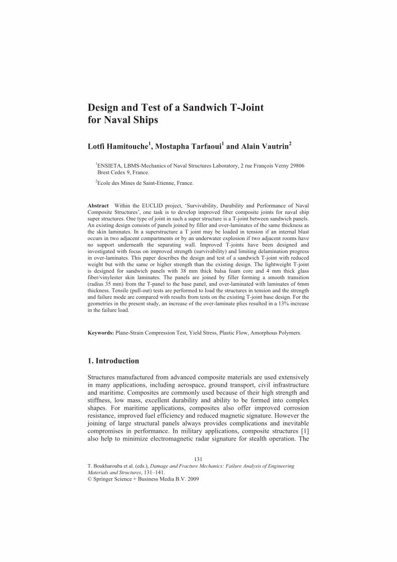
T. Boukharouba et al. (eds.), Damage and Fracture Mechanics: Failure Analysis of Engineering
© Springer Science + Business Media B.V. 2009
Design and Test of a Sandwich T-Joint
for Naval Ships
Lotfi Hamitouche1, Mostapha Tarfaoui
1 and Alain Vautrin
2
1ENSIETA, LBMS-Mechanics of Naval Structures Laboratory, 2 rue François Verny 29806
Brest Cedex 9, France.
2Ecole des Mines de Saint-Etienne, France.
Abstract Within the EUCLID project, ‘Survivability, Durability and Performance of Naval
Composite Structures’, one task is to develop improved fiber composite joints for naval ship
super structures. One type of joint in such a super structure is a T-joint between sandwich panels.
An existing design consists of panels joined by filler and over-laminates of the same thickness as
the skin laminates. In a superstructure a T joint may be loaded in tension if an internal blast
occurs in two adjacent compartments or by an underwater explosion if two adjacent rooms have
no support underneath the separating wall. Improved T-joints have been designed and
investigated with focus on improved strength (survivability) and limiting delamination progress
in over-laminates. This paper describes the design and test of a sandwich T-joint with reduced
weight but with the same or higher strength than the existing design. The lightweight T-joint
is designed for sandwich panels with 38 mm thick balsa foam core and 4 mm thick glass
fiber/vinylester skin laminates. The panels are joined by filler forming a smooth transition
(radius 35 mm) from the T-panel to the base panel, and over-laminated with laminates of 6mm
thickness. Tensile (pull-out) tests are performed to load the structures in tension and the strength
and failure mode are compared with results from tests on the existing T-joint base design. For the
geometries in the present study, an increase of the over-laminate plies resulted in a 13% increase
in the failure load.
Keywords: Plane-Strain Compression Test, Yield Stress, Plastic Flow, Amorphous Polymers.
1. Introduction
Structures manufactured from advanced composite materials are used extensively
in many applications, including aerospace, ground transport, civil infrastructure
and maritime. Composites are commonly used because of their high strength and
stiffness, low mass, excellent durability and ability to be formed into complex
shapes. For maritime applications, composites also offer improved corrosion
resistance, improved fuel efficiency and reduced magnetic signature. However the
joining of large structural panels always provides complications and inevitable
compromises in performance. In military applications, composite structures [1]
also help to minimize electromagnetic radar signature for stealth operation. The
131
Materials and Structures, 131–141.
L. Hamitouche et al.
mode of failure [2] of GFRP under static or dynamic loadings could be mainly due
to matrix cracking or delaminations.
Delamination, being the more severe of the two, causes stiffness reduction and
often leads to the catastrophic failure of the structure. Even invisible delaminations
can severely degrade the mechanical properties and the load carrying capability of
the structure.
Recently, a European collaborative project (EUCLID), “Survivability, Durability
and Performance of Naval Composite Structures”, has been carried out to experi-
mentally investigate static and dynamic response of composite T-joints [3]. The
objective of the project is to strengthen the technological basis for the large-scale
application of fiber reinforced composite materials for naval vessels and structures,
so that such vessels (or major parts thereof, e.g. superstructures) can be designed
with confidence on the basis of modeling and failure predictions [4, 5]. One task is
to develop improved joints for naval ship super structures manufactured from fiber
composites. Among the joints in such a super structure we consider a T-joint
between sandwich panels.
In the first phase of the project an existing design, called Base Design (BD), of
a T-joint has been tested and characterized [6]. The Base Design T-joint consists
of balsa core sandwich panels joined by filler forming a smooth transition (radius
35 mm) from the T-panel to the base panel, and over-laminated with laminates
of the same thickness as the skin laminates. In the next phase of the project
Candidate New Designs (CND) of T-joints were proposed, and some of them were
selected for further investigation by testing. One of these CND T-joints, proposed
by the Danish consortium, is inspired by Karlskronavarvet in Sweden [7], and it is
based on sandwich panels with PVC foam core, which are joined by filler by the
aid of two triangular PVC foam fillets. Investigations performed on a T-joint with
triangular fillets and over-laminates loaded in compression state that the efficiency
of the joint is not so good as for T-joints with over-laminates and filler fillet or a
foam pad fillet [8]. In the other hand, a number of papers have paid attention to the
analysis and improvement of single composite skin T-joints [9–15].
Hawkins and Shenoi [16] investigated geometry effects, including fillet radius
and over-laminate thickness, for T-joints under 45° pull-off loading, which simulates
the worst case scenario of flooding inside one compartment of the ship [9].
Phillips and Shenoi [9] found that the curved parts of the T-joint over-laminate,
where the delamination first occurred, were the critical component under 45° pull-
off loading as well as three point-bending. Similar results have also been reported
by Rispler et al. [12] and Kumari and Sinha [13]. Read and Shenoi [17] also
investigated the behavior and failure mechanisms of T-joints under fatigue
loading. Dharmawan et al. [14] investigated the effect of geometry and disbond
between the fillet and the over-laminate on the T-joint with a triangular fillet. It
was found that the presence of an initial disbond altered the distribution of axial
strain through the thickness of the over-laminate; this caused outward bending of
the over-laminate when the T-joint is subjected to tension load. This effect
132

Design and Test of a Sandwich T-Joint for Naval Ships
indicated that the fillet functioned as an important medium of load transfer in the
T-joint.
In contrast to the use of a single composite skin, composite sandwich panel T-
joints has been investigated [18–21].
Two kinetic models of fracture were identified: (1) the delamination between
the leg and base panel, and (2) core shear failure in the base panel. Turaga and Sun
[21] developed a few designs to improve the strength of T-joints. It was shown
that using bolts in a circular fillet joint could cause early failure in the core and
would not increase the ultimate join strength. Theotokoglou and Moan [18] stated
that there were no significant differences in the ultimate strength of the two failure
modes; the ultimate failure mode for a specific T-joint depends on the fabrication
defects, e.g. voids in the fillet area. It is also found that the strength of T-joints is
slightly influenced by the geometry of the over-laminate.
Toftegaard and Lystrup [22] proposed a new design of sandwich T-joint with
reduced weight by use of two triangular PVC foam fillets, rather than the
traditional circular fillet. It was found that the new T-joint configuration has 20%
higher strength than that of the existing design and the weight reduced by 60%. To
ensure the T-joint reliability, the behavior and performance under various loading
conditions must be known. This paper outlines a study on the fracture behavior of
a glass fiber reinforced polymer T-joint commonly used in composite marine
vessels.
Experimental analysis was conducted to investigate the fracture behavior of the
structure for the present design. In this paper we present a new T-joint, witch is
over-laminated as a Base Design T-joint, but with a few ply laminates of base
panel. This paper focuses on the design and test of the static tensile strength of the
new T-joint, as one of the tests performed to characterize the Base Design T-joint.
Also, the observed modes of damage during the tests will be reported here and
discussed. This paper focuses on the design and test of the static tensile strength of
the DCNS New Design T-joint, as one of the tests performed to characterize the
T-joint.
2. Design of lightweight T-joint named DCNS_1, DCNS_2
and DCNS_3
The selected design based on the outcome of the EUCLID RTP3.21 study of the
BD is called DCNS_X (X = 1, 2, 3). The specification for the design, materials
and the over-all dimensions of the test specimens for the DCNS_T are
summarized in Table 1, and the T-joint is illustrated in Fig. 1.
133

L. Hamitouche et al.
Table 1. Materials and basic dimensions of the composite T-joint, DCNS_T
Item description Materials Item symbol Value (mm)
Overall Width 250
Overall Length, L 800
Height of T-section, H 300
T-joint
Rounding radius, R 35
Length, L1 & L2 150
Thickness, T01 6
Over-laminate E glass fiber: taffetas 500 g/m2
Matrix: vinylester dion
Thickness, T02 4
Thickness, Ts1 4 Skin laminate E glass fiber: taffetas 500 g/m2
Matrix: vinylester dion Thickness, Ts2 2
Thickness, C1 & C2 38 Core Baltek SB100
R 28.5
Fillet Crestomer 1152 PA Thickness, Tg 5
Fig. 1. Sketch of a new T-joint
3. Inspection of T-joint
The T-joints are manufactured by DCNS. The T-joint specimens are used for the
tensile tests. An incoming quality inspection of the dimension, geometry and
weight of the T-joint is performed, and shown in the quality inspection sheets,
Table 2. Holes in the filler material are observed at both sides on both specimens.
The thickness of the filler and the dimensions of the over-laminates deviate from
the specifications.
The following is measured:
134
Ts1
Ts2
Ts1
Ts2TO1
TO1
TO2
Tg
L2
C1
L1
C2
R
L
H

Design and Test of a Sandwich T-Joint for Naval Ships
Table 2. Inspection of T-joint
Thickness of filler Tg = 5–6 mm
Length of over-laminates L1 & L2 = 150–155 mm
Thickness of over-laminate T01 = 6.1 mm, T02 = 4.1 mm
Rounding radius R = 28–29 mm
4. Manufacturing of test specimens
The sandwich panels for the T-joints are manufactured by a resin infusion
technique. All the glass fiber fabrics and the balsa core are laid up on a flat table,
vacuum bagged, evacuated and vacuum resin infused in one shot. The base panel
is infused in a size of 1,000 1,750 mm, and the T-panel in a size of 420 1,750
mm. The vacuum infusion is done at room temperature under a vacuum pressure
of about 100 mbar. At the end of the infusion the pressure is raised to about 900
mbar, and the panel is allowed to cure at room temperature before it is demoulded
and post cured at 60°C for 24 h. The edges of the infused and cured panels are
trimmed to the desired geometry. Small grooves are used as spacers to ensure
correct gaps for the filler. The T-joints are manufactured and completed in widths
of approximately 1.75 m and subsequently sectioned into the 250 mm wide test
specimens, Fig. 2.
Fig. 2. Manufacturing of T-joint
5. Test specification
5.1. Test set-up and test rig
In the static tensile test of the T-joint, the sample is mounted to the load cell at the
top of the T-panel, and the load is applied at both ends of the base panel, with a
135

L. Hamitouche et al.
distance of 640 mm. The test rig with a sample mounted in the testing machine is
shown in Fig. 3.
The test sample is loaded through pairs of square steel tubes 400 80 25 mm,
which are connected by two 20 mm diameter threaded steel rods. The steel rods
are mounted in spherical bearings to allow for free rotation of the test sample at
the ends.
The top of the T-panel is connected to the testing machine through two 10-mm
thick steel plates of 400 140 mm (H W). The steel plates are bolted to the test
sample by five M20 bolts positioned at the end of the T-panel, symmetrically
around the mid-plane and with a distance of 76 mm between each bolt. The top-
end of the steel plates is connected to the load c ell though a spherical bearing,
Fig. 3.
Fig. 3. Sketch of the principal test set-up for quasi-static testing
5.2. Instrumentation and test procedure
Strain gauge data was performed with a SPIDER device. The gauges were mounted
on specimens at the middle of the width of the sample and at the nine locations as
shown in Fig. 3. Gauge n° 2 to 8 are 2 mm long with a resistance of 120
(KYOWA KFG-2-120-C1-11).
Gauges 1 and 9 are a 0°/90° couple (KYOWA KFG-2-120-D16-11), where
each single gauge is 2 mm long with a resistance of 120 . Gauge 2, 3, 4, 5, 8 and
the 0° gauge of couple 1 and 9 are oriented parallel to x-axis (G1X, G2X, G3X,
G4X, G5X, G8X and G9X), gauge 6 and 7 parallel to the y-axis (G6Y and G7Y)
and the 90° gauge of couple 1 and 9 parallel to the z-axis (G1Z, G9Z). Load,
displacement and strain gauges are computer sampled at a rate of one per second,
Fig. 4a. The load is recorded by a certified 250 kN load cell. The displacement is
both recorded as the movement of piston (cross-head) on the tensile machine, and
by three calibrated LVDT (Linear Variable Differential Transformer, DINEL P
925 L1 AN S) devices, which detect the displacement of the bottom plate of the
base panel. One LVDT, with a working range of 40–60 mm, is positioned at the
centre, and the other two are positioned symmetrically 188 and 198mm away from
136
Element fixed to load cell
T-joint
Lower support 80
140
120
800 400
Stiffened base

Design and Test of a Sandwich T-Joint for Naval Ships
the centre, respectively. The tests are also recorded on video and still-photos with
the cameras in a fixed position during the test, showing a side view of the T-joint.
The tensile test is performed on a 250 kN servo hydraulic testing machine (Instron
1342), at a constant cross-head speed of 1 mm/min. Load, displacement, strain
gauges and LVDT gauges are computer sampled at a rate of one data set per
second, Fig. 4b.
Fig. 4. Position numbering of strain gauges and the three LVDT devices
6. Results
6.1. Load, displacement and strain
Plots of load versus cross-head displacement and load versus LVDT displacement
are shown for one of the three specimens in Fig. 5. The initial value of the load is
around 0.2 kN due to pre-stressing and the weight of the four square steel tubes
and the four threaded steel rods. The measured cross-head position and measured
position from each of the three LVDT devices are used to determine the cross-
head displacement and the LVDT displacements. The LVDT’s away from the
centre show a symmetric deformation, indicating a symmetric load of the sample.
The load–displacement curve at the centre (for x = 0) is almost linear up to a load
Fig. 5. Load versus displacement of specimen
137
(a) (b)
6 7
85
3 2
115 115
1 9
28
150
4
GaugeRef. 1
X-Z X-ZX X X X XY Y
2 3 4 5 6 7 8 9
Straindirection 188 198

L. Hamitouche et al.
of 25 kN (displacement 10mm). Thereafter, the curve becomes slightly non-linear
until a load of 32 kN (displacement 13 mm). From there on, the test sample
undergoes heavy deformation for only a slight increase in load until final failure at
a load and displacement of 42 kN and 20 mm, respectively.
In Fig. 6 the strain values were arbitrarily set to zero at the start of the test.
Negative strains were multiplied by “–1” and a minus sign was added in front of
the strain gauge name (–G1X, –G2X, –G3X and –G9X). A plus sign was added in
front of the positive strain (+G4X, +G5X, +G6Y, +G7Y, +G8X and +G9Z).
Fig. 6. Load versus strain
6.2. Failure load and damage kinetic
The ultimate tensile failure load, corrected for weight of fixtures, for the three
specimens is 42.8, 42.0, and 41.8 kN, respectively. With a specimen width of approxi-
mately 250 mm it corresponds to a failure load per width (in the z-direction - see
Fig. 4) of 171.2, 168, and 167.2 kN/m, respectively. This is an increase in failure
Table 3. Failure load of static tensile tested T-joints
Sample # Elastic strength (kN/mm) Failure load (kN) Failure load per unit length (kN/m)
DCNS_1 2.8 42.8 171.2
DCNS_2 2.6 42.0 168.0
DCNS_3 2.7 41.8 167.2
New
Average 2.6 42.2 168.8
EUCLID – 2.5 36.0 141.4
138

Design and Test of a Sandwich T-Joint for Naval Ships
load of about 20% compared to the reference Base Design T-joint, which has a
failure load per width of 141kN/m, Table 3. Audible cracking started early during
the tests, and continued to failure.
Fig. 7. T-joint, specimen DCNS_1 and DCNS_2 Fig. 8. T-joint, specimen DCNS_3
The relation between cross-head displacement and load (Fig. 5) is seen to be
linear. The actual fracture appearance was quite different for the three specimens.
Specimen DCNS_1 and DCNS_2 showed both a shear failure at the base panel, a
de-bonding between the over-laminates and the skin laminate of the base panel,
and fracture in the filler material.
Whereas specimen DCNS_3 showed a shear failure in the base panel, the
interface failure between the skin and the core of T-panel, and a minor de-bonding
between the over-laminate and the skin laminate at middle of the over-laminate on
one side only. Figs. 7 and 8 show a damage history of the T-joint specimens.
7. Conclusions
In this paper we present a new T-joint, witch is over-laminated as a Base Design
T-joint, but with a little geometrical modification of the skins and the over-
laminates. This simple technique provides a higher strength in tension, 169 kN/m.
This is an increase in failure load of about 20% compared to the reference Base
Design T-joint, which has a failure load per width of 141 kN/m.
In a super structure a T-joint may be loaded in tension if an internal blast occurs
in two adjacent compartments, or by an underwater explosion, where the whole
ship is moving upward (out of the water), and acceleration forces act on heavy
equipment placed in two adjacent rooms with no support underneath the separating
wall. In this study one can introduce these conclusions:
Three sandwich T-joints have been tested in static tensile in a special
designed fixture
The average tensile failure load per unit length is 169 kN/m
139

L. Hamitouche et al.
Two type of damage kinetic for the three specimens
A majority of the load/strain signals in the joint region are linear until
failure
References
[1] http://research.dnv.com/euclid_rtp3.21.
[2] B. Haymana, A.T. Echtermeyer, D. McGeorge. Use of composites in naval ships. Warship
2001 – future surface warships. 20–21. London: Royal Inst. of Naval Architects, 2001.
[3] A. Groves, A. Lystrup, D. McGeorge, and H.V. Aanhold. Dynamic and static performance
of composite T-joints. Presented at Symposium on Combat Survivability of Air, Space, Sea
and Land Vehicles, NATO/RTO, Aalborg, Denmark, 2002.
[4] B.D. Agarwal, L.J. Broutman. Analysis and performance of fiber composites. New York:
Wiley-Interscience, 1990.
[5] G.H. Sih, A.M. Skudra. Failure mechanics of composites. New York: Elsevier Science,
1985.
[6] J.E. Van Aanhold, A. Groves, A. Lystrup, D. McGeorge. Dynamic and static performance
of composite T-joint. Symposium on combat survivability of air, space, sea and land
vehicles. Denmark: NATO/RTO Aalborg, 2002.
[7] S.E. Hellbratt. Use of lightweight sandwich joints in a 72m high speed vessel entirely built
of carbon fibres. In: Bäcklund J et al., editors. Composites and sandwich structures. Second
north European conference (NESCO II), Stockholm, 22–23 October 1997. EMAS
Publishing, pp. 151–155, 1997.
[8] R.A. Shenoi, F.L.M. Violette. A study of structural composite Tee joints in small boats.
Journal of Composite Mater, vol. 24, pp. 644–666, 1990.
[9] H.J. Phillips, R.A. Shenoi. Damage tolerance of laminated tee joints in FRP structures.
Composites Part A: Applied Science and Manufacturing, vol. 29, pp. 465–478, 1998.
[10] R.A. Shenoi, G.L. Hawkins. Influence of material and geometry variations on the behaviour
of bonded tee connections in FRP ships. Composites, vol. 23, pp. 335–345, 1992.
[11] A.R. Dodkins, R.A. Shenoi, G.L. Hawkins. Design of joints and attachments in FRP ships’
structures. Marine Structures, vol. 7, pp. 365–398, 1994.
[12] A.R. Rispler, G.P. Steven, L. Tong. Failure analysis of composite T-joints including inserts.
Journal of Reinforced Plastics and Composites, vol. 16, pp. 1642–1658, 1997.
[13] S. Kumari, P.K. Sinha. Finite element analysis of composite wing T-joints. Journal of
Reinforced Plastics and Composites, vol. 21, pp. 1561–1585, 2002.
[14] F. Dharmawan, R.S. Thomson, H. Li, I. Herszberg, E. Gellert. Geometry and damage
effects in a composite marine T-joint. Composite Structures, vol. 66, pp. 181–187, 2004.
[15] H.C.H. Li, F. Dharmawan, I. Herszberg, S. John. Fracture behaviour of composite maritime
T-joints. Composite Structures, vol. 75, pp. 339–350, 2006.
[16] G.L. Hawkins, R.A. Shenoi. A parametric study to determine the influence of geometric
variations on the performance of a bulkhead to shell plating joint. In: Proceedings of the 9th
International Conference on Composite Materials, ICCM/9, 12–16 July 1993, Madrid:
Woodhead Publishing Ltd., vol. 4, pp. 97–104.
[17] P.J.C.L. Read, R.A. Shenoi. Fatigue behaviour of single skin FRP tee joints. International
Journal of Fatigue, vol. 21, pp. 281–296, 1999.
[18] E.E. Theotokoglou. Study of the numerical fracture mechanics analysis of composite
T-joints. Journal of Reinforced Plastics and Composites, vol. 18, pp. 215–223, 1999.
[19] E.E. Theotokoglou, T. Moan. Experimental and numerical study of composite T-joints.
Journal of Composite Materials, vol. 30, pp. 190–209, 1996.
140

Design and Test of a Sandwich T-Joint for Naval Ships
[20] E.E. Theotokoglou. Strength of composite T-joints under pull-out loads. Journal of
Reinforced Plastics and Composites, vol. 16, pp. 503–518, 1997.
[21] U.V.R.S. Turaga, C.T. Sun. Failure modes and load transfer in sandwich Tjoints. Journal of
Sandwich Structures and Materials, vol. 2, pp. 225–245, 2000.
[22] H. Toftegaard, A. Lystrup. Design and test of lightweight sandwich T-joint for naval ships.
Composites Part A: Applied Sci. and Manufacturing, vol. 36, pp. 1055–1065, 2005.
141

T. Boukharouba et al. (eds.), Damage and Fracture Mechanics: Failure Analysis of Engineering
© Springer Science + Business Media B.V. 2009
Vibroacoustic Sources Identification
of Gear Mechanism Transmission
Abbassia Derouiche1, Nacer Hamzaoui
2 and Taoufik
Boukharouba1
1Laboratoire de Mécanique Avancée (LMA), Faculté de Génie Mécanique et Génie des
Procédés, BP 32 El Alia 16111 Bab Ezzouar, Alger, Algérie
2Laboratoire Vibrations Acoustique, Institut National des Sciences Appliquées de Lyon
Domaine Scientifique de la Doua, Bt Antoine de Saint Exupéry, 25 bis, avenue Jean Capelle
69621 Villeurbanne Cedex, France
Abstract The prediction and the identification of the vibroacoustic sources of the toothed
gearings remain rather complex in spite of various carried out work. Often, they are experimental
statements on a significant number of transmissions which finish by councils given to the
designers in order to limit or to reduce the radiated noise. Our work consists in contributing to
treat on a hierarchical basis the vibroacoustic sources on a transmission system defined well, and
this, while being based on the method of principal components analysis (PCA). PCA method is
based on the statistical analysis, thus partial virtual coherence and multiple virtual coherence are
used to quantify the coherent shares with the acquired signals autospectres.
Keywords: Gears, Vibration, Noise, Signal Processing, PCA, Coherence.
1. Introduction
The vibratory and acoustic behaviour of gear transmission result from several
sources and numerous works have been done [1, 2]. It is allowed generally that the
radiated noise is due mainly to the vibrations of the casing, itself excited by
internal and external sources which are transmitted to it. We seek to implement a
methodology who would allow us to make a hierarchisation of the vibroacoustic
sources. Tests were carried out on a transmission system by gears transmission
mechanism at the acoustics and vibration laboratory of the INSA of Lyon. We
used sensors which are accelerometers and microphones in order to raise measure-
ments of acceleration and acoustic pressure for various operation configurations.
We calculate the interspectral matrix for the 32 ways simultaneously acquired that
we will be able to define for any engine speed and various positions of the
accelerometers as well as a sweeping of the antenna comprising the microphones
around the vibrating mechanism. The principal components analysis method is one
of the techniques which can contribute to the hierarchisation of the vibroacoustic
sources of our gears transmission mechanism, by estimating the partial virtual
143
Materials and Structures, 143–152.

A. Derouiche et al.
coherences and multiples shares between the virtual sources and the acquired
2. Principal Components Analysis (PCA)
The spectral analysis in principal components has the autospectres and the inter-
spectres as data. The principle consists in numerically separating the various signals
considered in “virtual” incoherent sources. The decomposition in principal
components formulation results from the autospectres and interspectres matrice
2.1. Interspectral matrix formulation
The interspectral matrix of all the signals acquired simultaneously is built as
follows:
mmmm
m
m
XX
SSS
SSS
SSS
S
21
22221
11211
............
...
...
(1)
With Sii autospectre of i way and Sij interspectre of i and j ways.
2.2. Interspectral matrix decomposition
The matrix square shapeXXS enables us to write the following relation based on
its decomposition in eigenvalues and eigen vectors:
)(*
mpS mpppmpmmXX (2)
With pp
diagonal matrix of the p nonzero eigenvalues and p corresponding
eigen vectors matrix mp
arranged in columns.
While posingpppp
2 , we can rewrite:
*
mpmpmmXXS with ppmpmp (3)
signals [3].
expression of all the signals acquired simultaneously [5, 6].
144

Vibroacoustic Sources Identification of Gear Mechanism Transmission
The interspectral matrix XXS can be expressed by the superposition of the
interspectral matrices:
mpesvisvisvisvi
XX
svpXX
sviXX
svXXXX
ofcolumniSw
SSSS
,ith
, ... ...
*
1
(4)
Such a summation of interspectral matrices is characteristic of the superposition
of uncorrelated vibratory phenomena. Each virtual source contribution in fact is
characterized by the answer vector svi , being able to be interpreted like the
structure deformation induced by the single virtual source n°i.
2.3. Virtual coherence and multiple virtual coherences
Coherence is a tool which quantifies the share of the coherent signal autospectre
with another signal. Virtual coherence will quantify the share of the signal
coherent autospectre with a virtual source. The autospectre decomposition in
<contributions> of the virtual sources is simple and robust, being given the virtual
sources incoherence. Partial virtual coherence of a signal )t(X jcompared to the
virtual source i is:
jj
svijj
svijS
S2, (5)
Virtual coherence is a tool possibly making it possible to locate the physical
sources related to the principal components, by admitting that the strongly
coherent signals with a particular virtual source are physically close to the real
source. But it is an expertise tool to be used with precautions. The principal
interest of virtual coherence is that it easily makes it possible to determine the
number of uncorrelated phenomena observed on a particular signal. For that, we
introduce the multiple virtual coherence of a signal )(tX j :
jj
svijj
svjj
svjj
svisvsvjS
SSS ....212
,...,2,1: (6)
When the virtual sources number i make it possible to obtain a multiple virtual
coherence near to 1, which means that the maximum number of uncorrelated
phenomena observed on signal )(tX j is i. The PCA is a tool for pre-processing of
multi-source results of measurement in environment.
145

A. Derouiche et al.
The spectral analysis technique in principal components (PCA) was used since
the article of Price and Bernhard [4].
3. Experimental set up
The experiments were made in acoustics and vibration laboratory (LVA) of the
INSA of Lyon. The measurements were made in a semi-anechoic room, the ground
being out of concrete and the covered glass wool walls (Fig. 1). At the beginning
of each accelerations and acoustic pressures acquisition, the background noise of
the room is measured.
Fig. 1. Test rig in semi-anechoic room (LVA INSA Lyon)
3.1. Description of the gear transmission mechanism
The mechanism to study consists of a cylindrical gear including a couple 45/65
teeth. The principal characteristics of this gear are given in Table 1. The wheels of
steel are full and assembled on diameter shaft equal to 0.020 m. The entry shaft is
connected to the engine by a flexible coupling.
Table 1. Test gear main parameters (LVA, INSA Lyon)
Pinion Driven wheel
Number of teeth 45 65
Normal module (m) 0.002 0.002
Face width (m) 0.020 0.020
Base radius (m) 45 65
Normal pression angle (deg) 20 20
146

Vibroacoustic Sources Identification of Gear Mechanism Transmission
Fig. 2. Gear mechanism transmission
The shafts are guided in rotation by bearings. The simple casing form is a
parallelepiped of dimensions (0.40 × 0.35 × 0.16 m) and the thickness is 0.025 m
except for face 5 of the top casing, it is of 0.005 m. The casing consists of two
materials, steel and Perspex. They have as a density of 7,800 kg/m3 and 1,300
kg/m3, a Young modulus E = 2.1011 N/m2 and 3.3. 109 N/m2 and for Poisson’s
ratio 0.3 and 0.37, respectively. Faces 3 and 5 (cover) are of Perspex, all others are
of steel. The mechanism was coupled with an engine at variable speed.
3.2. Data acquisition
The measurement accelerometers number is 14 distributed as follows with their
respective direction:
Three accelerometers on the engine (19(y), 20(x), 26(z))
Two accelerometers on face 1 (25(y), 29(z))
Two accelerometers on face 2 (21(y), 30(z))
Three accelerometers on face 3 (22(z), 23(z), 32(x))
Four accelerometers on face 4 (24(x), 27(z), 28(z), 31(z))
An antenna microphones placed at the top of the mechanism can move on a
parallel level (Z constant). It makes it possible to measure in a number of desired
points the acoustic pressures; the antenna comprises 30 microphones. Several
configurations were considered for measurements.
We will treat two cases for our mechanism sources radiation; the first corresponds
to the case where the mechanism is open (without cover) and the second to the
case of the closed mechanism (with cover). The position of the 18 microphones
carried by the antenna and the face number of the carter are shown on the gear
mechanism transmission (Fig. 2). Measurements were recorded on OROS 32 ways.
147

A. Derouiche et al.
The recorder is connected to a portable computer, and we used the software
NVGate for the recordings, the time being 10 s for each acquisition. Once the
various ways gauged with the autorange, we carry out measurements.
The data recorded by OROS are downloaded on NVGate from frontal OROS
towards the PC, and then exported in mat format of MATLAB in order to be to
exploit.
For any operation configuration, the 32 ways are recorded over a time of 10 s,
sampled at the frequency of 32,768 Hz. We chose a frequential resolution of 1 Hz.
To find the virtual sources, it is necessary to make a spectral decomposition in
principal components of the interspectral matrix on the 32 ways. We visualize the
energy contributions of the 32 virtual sources representing these ways.
The virtual sources can be classified by order of preponderance, i.e. in the order
descending of the associated eigenvalues.
We realize that the first virtual source is rather dominating and that the first two
virtual sources are enough alone to represent the vibroacoustic mechanism. Their
sum in energy contribution exceeds the 85%.
The curves (Figs. 3 and 4) represent the contribution of the 32 virtual sources
obtained by respectively considering the mechanism closed and open and
operating at the speed of the engine equal to 2,500 rpm. We notice a similarity
between them to the surroundings of 10,000 Hz, beyond there is a change in the
percentage of the first virtual source and it is more significant for the closed
mechanism. On the other hand, for the second and the third virtual sources, they
are more significant in high frequencies for the open mechanism.
Fig. 3. Energy contribution of the 32 virtual sources (closed mechanism)
148

Vibroacoustic Sources Identification of Gear Mechanism Transmission
Fig. 4. Energy contribution of the 32 virtual sources (open mechanism)
The averages of multiple virtual coherences are traced on the curves (Figs. 5
and 6), by taking as reference one, two, three and four dominating sources. The
average virtual coherences carried out (Figs. 5 and 6) on the first virtual source
expressed as a percentage shows an energy contribution of about 53% on all
the ways put besides those of the engine i.e. numbers 19, 20 and 26. For the second
virtual source, the virtual coherence average is about 20%. The third and fourth
virtual sources are more marked on the engine ways; their sum reaches the 30% of
energy contribution.
The average of virtual coherences on the virtual source 1 (SV1) for the closed
mechanism (Fig. 5), shows the effect in staircase on the 18 ways measuring the
acoustic pressures, this is explained by the position of the microphones (Fig. 2).
The virtual coherences contribute for 55% to ways 1, 7 and 13, decrease slightly
on ways 2, 8 and 14 and so on for ways 3, 9 and 15 etc. For the other ways (21,
22, 23, 24, 25, 27, 28, 29, 30, 31 and 32), their virtual coherences resemble each
other and are about 52%. The SV1 can be assigned to the way of the bearing
located on face 3 (with Perspex). Concerning the SV2, its average shows a
contribution of about 20% and it seems homogeneous for the ways. For the SV3
and SV4, their contributions in virtual coherence are more significant on the levels
in the engine ways (19, 20 and 26).
When the mechanism is open (Fig. 6), the virtual coherence of the SV1 is of the
same order of magnitude 50% on the 18 ways of the antenna, on the other hand it
decreases to reach the 40% on the ways of the casing, and it is about 20% on the
level of the engine ways. Concerning the SV2, its virtual coherence is about 20%
on the microphones, 26% on the casing ways and 13% on the engine ways. The
average of virtual coherences for SV3 and SV4 are almost parallel with a percentage
149
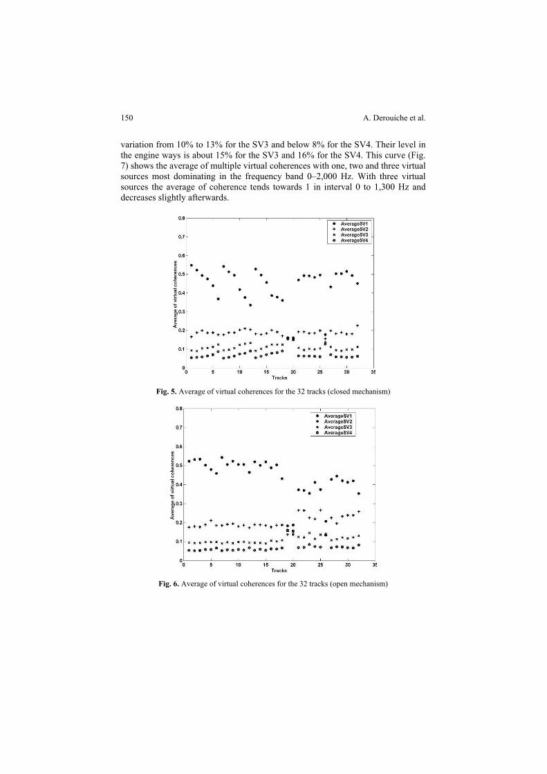
A. Derouiche et al.
variation from 10% to 13% for the SV3 and below 8% for the SV4. Their level in
the engine ways is about 15% for the SV3 and 16% for the SV4. This curve (Fig.
7) shows the average of multiple virtual coherences with one, two and three virtual
sources most dominating in the frequency band 0–2,000 Hz. With three virtual
sources the average of coherence tends towards 1 in interval 0 to 1,300 Hz and
decreases slightly afterwards.
Fig. 5. Average of virtual coherences for the 32 tracks (closed mechanism)
Fig. 6. Average of virtual coherences for the 32 tracks (open mechanism)
150

Vibroacoustic Sources Identification of Gear Mechanism Transmission
Fig. 7. Average of virtual coherences (multiples) with 1(2, 3) dominating virtual source(s)
4. Conclusions
The PCA method was applied in order to treat on a hierarchical basis the vibro-
acoustic sources of a transmission system by gears. The decomposition of the
interspectral matrix enables us to estimate the contribution expressed as percentage
energy of each virtual source.
The multiple virtual coherences which represent the share of an autospectre of
answer caused by all the virtual sources, was also used. This method effectively
quantifies the number of uncorrelated vibratory phenomena of the vibrating
mechanism. The total uncorrelation of the phenomena makes it possible to provide
robust virtual indicators (virtual coherence, virtual transfer function). The relation
between real physical sources and virtual sources is not obvious, because a
principal component can characterize several different sources physical according
to the frequency observed.
The PCA method was used as a tool for pre-processing of multi-source results of
measurement in environment. We tried to bind these virtual sources to the reference
signals where the sensors are situated and to look for a way given to the strongest
virtual source.
References
[1] H. Opitz. Noise of gears. Phil. Trans. of Royal Society, vol. 263, pp. 369–380, 1969.
[2] D. Welbourn. Fundamental knowledge of gear noise-a survey. Conference on Noise and
Vibrations of Engines and Transmissions, Cranfield Institute of Technology. C177/79,
9–29, 1979.
151

A. Derouiche et al.
[3] J.S. Bendat et A.G. Piersol Engineering applications of correlation and spectral analysis.
New York: Wiley-Interscience, 1980, 302 p.
[4] S.M. Price. et R.J. Bernhard, Virtual coherence: A digital signal processing technique for
incoherent source identification. In: Proceedings of IMAC 4, Schenectady, NY, USA, 1986.
[5] Q. Leclère, Support technique de la toolbox matlab d’analyse spectrale ACP, 2003, p. 1–10.
[6] Q. Leclère, Etude et Développement de la mesure indirecte d’efforts, Application à
l’identification des sources internes d’un moteur Diesel, thèse: Insa, Lyon, 2003.
152

T. Boukharouba et al. (eds.), Damage and Fracture Mechanics: Failure Analysis of Engineering
© Springer Science + Business Media B.V. 2009
Prediction of Structural and Dynamic Behaviors
of Impacted Plates
Advanced Mechanical Laboratory, University of Science and Technology Houari
Boumediene USTHB, BP 32, Al Alia 16112, Algiers, Algeria
Abstract A numerical model for the flexural vibrations of rectangular isotropic and orthotropic
plates is developed, in order to investigate transient response of impacted plate. The established
model, referred to a modified Hertzian contact law, has been validated and used to study the
influence of different impact parameters. The obtained results are in good agreement with those
given with the finite element simulations. The validated model has been used to study the
distribution of the stress field and its evolution under the effect of the different impact
parameters.
Keywords: Impact Simulation, Impact Simulation, Duration.
1. Introduction
There are many practical situations where plate structures are subjected to transient
impact loading of high intensity. Despite their importance, however, impact effects
are usually ignored or oversimplified in the dynamic analysis of plate structures.
One reason is the complexity involved as contact-impact problems. Understanding
of the impact phenomenon and damage mechanisms is essential for developing
improved materials and design methods accounting for impact. Many experimental
works carried out on materials subjected to dynamic loads allowed a satisfactory
characterisation of these materials and the identification of the damages induced.
However, such works remain expensive and require very sophisticated equipment.
This is why, any analytical or numerical study which permit a suitably approach of
the behaviour of structures subjected dynamic loads would be a great help to the
scientific and industrial community.
Mathematical models used for the prediction of the contact force and the
structural response must adequately represent the global motion of the structure,
the dynamics of the impactor, and the local deformation in the contact region. In
order to predict the structures vibration, analytical models are used for simple
cases, usually using the modal analysis approach. In this case, using the modal
analysis method, a large number of modes need to be included to determine the
response, and the wave propagation approach may be more practical. For more
complex situations, the finite element method is also used.
Abdelhamid Miloudi and Mahmoud Neder
153
Materials and Structures, 153–162.

2. Elastic modelling of impact
Several modelling of the impact have been adopted, we can note those consist in
representing the impact by an energy balance. The main advantage of this present-
ation type, reside in the fact that parameters of entry are directly the characteristic
parameters of the impact: incidental speed, geometric and mechanical properties
of the plate and the impactor. In his works, Greszuk [1] has modelled the impact
while adding the contact energy to the one of bending. Shivakumar et al. [2]
improved the previous model while coupling to bending a rigidity of Ks shearing
and while introducing a rigidity of membrane Km in the case of the thin plates. The
balance of energy is constituted of the contact energy and the one of bending.
While using this model, Benmedakhène [3], made predictions of displacements
values of and the maximal loads according to energies of impact. In this survey it
showed that values of the model remain near of the experience in the low energies
where the weak damages don’t change the global behaviour of the plate.
2.1. Mass-springs model
The model based on the balance of energy presented permits to calculate the
ultimate values of displacements and strengths previously, but it doesn’t permit to
predict the history of the loading, the speed or the displacement. On the other
hand, the use of the model mass-spring will permit to retrace all the history of the
different parameters of the impact. Different types of models mass-springs have
been developed for modelling the impact at low speed. The main characteristic of
this model type consists in the fact that they don’t take in account any localization
of the distortion. So the projectile incidental energy is absorbed on all the volume
of the plate. Among the most important models presented in the literature, the
one of Caprino et al. [4] are mentioned. These authors present the impact by only
one degree of freedom. The rigidity of the spring corresponds to the static rigidity
of the plate.
A good agreement, between calculated and measured strength, is noted until 2.5
m/s speed. In this model bending effects, the plate inertia is not taken in
consideration, from where limits of use for the more important speeds. Sjoblom et
al. [5] suggested a model of two dof that permits to integrate the non linearity at
the contact level. With this model it’s possible to uncouple contact and the plate
rigidity. Nevertheless, the shearing effect is localized around the impact point,
important for the thick plates or is not taken in account for the very elevated
speeds. It is why Lal [6] developed a model to three springs Kcs, Kbs and Ks
representing rigidities of stamping, bending and shearing respectively. This model
is valid for small displacements, diverges for the big ones. Shivakumar et al. [2]
took them in consideration membranes effects while using mass-spring models of
one and two degrees of freedom (Fig. 1) with four springs of rigidity Km, Kbs, Ks
and Kcs. The indications m, s, b and c represent the membrane, shearing, bending
and the plate contact respectively with impactor.
A. Miloudi and M. Neder154

Prediction of Structural and Dynamic Behaviors of Impacted Plates
(a)
K
M V0
(b)
kc
Km
Kb
Ks
MI
MP
x1(t)
x2(t)
Fig. 1. Mass-springs models: (a) one degree of freedom, Caprino et al. [4], (b) two degrees of
freedom model, Shivakumar et al. [2]
In this model the two masses MI and MP are connected by a spring Hertzian
representing the law of load-deformation of contact. Properties of transverse
strength-deformation are represented by the combination of bending, shearing and
membrane springs. Displacements tx1 and tx2 represent the displacement
response of the two masses at every instant t.
The corresponding speeds are represented by tx1& and tx2
& . The transverse
displacement of the plate is represented by tx2 , and the contact deformation is
represented by: txtx 21 . The balance of the projectile and the plate can be
written:
0)()(
0)(
232
23
1
(t)x-(t)x n txk(t)x ktxM
(t)x-(t)x n txM
213
2m2bsP
21I
&&
&& (1)
where:
2
2
1
1
xx pour
xx pour
1
1 (2)
The initial conditions are:
0)0(0)0()0(0)0( 2211 x ,x ,Vx ,x I&& (3)
These two coupled equations are non linear differential equations which can be
solved by a numeric integration method [7] until 02 tx .
2.2. The numerical model
The numerical model that we propose is simple, efficient and gives very satisfactory
results. This model takes into account the higher modes in the impact force and
the dynamic plate response calculations. It refers also to the Hertz contact law and
the plate classical theory.
155

At the beginning of the contact, the spherical impactor is animate by an
incidental speed Vi, knock a thin plate and apply on this one, the force P which
represents the impact force (Fig. 2). By the action and reaction principle, the plate
applies on the sphere an equal force to P but in opposite sense. The dynamic
balance of the spherical striker and the plate is given respectively by
IIII
II
Vzetzz
PzM
)0(0)0()0(
0
.
&&
&&
(4)
And:
00,,0,,
)()(4
yxwyxw
yyxxPwDwh oo
&
&& (5)
The expression for the contact force P developed during elastic impact of a
spherical impactor or radius R with a rigid plane surface of a semi-infinite solid
was given by Hunter [8] as a function of the relative advance between impactor
and the impacted plane surface:
2/3nP (6)
where : is the relative advance between impactor and the impacted plane surface:
),,()( tyxwtz ooI (7)
And kc is the contact stiffness, which depends on the geometrical and rheological
characteristics, of the two bodies in contact, given by
2
2
2
1
21
)1()1(
EE R
3
4kc (8)
1, 2 and E1, E2 are Poisson’s ratios and elasticity modulus of the sphere and the
impacted object, respectively. xo and yo are the impact point coordinates.
The contact force given in Eq. (3) is an extension of the well-known Hertz
contact theory developed for the static contact of curved bodies.
Thereafter, we solve the motion equations simultaneously by an iterative
numerical method using the modal decomposition for the transverse deflexion of
the plate and a Newmark integration scheme for the contact force [9].
A. Miloudi and M. Neder156
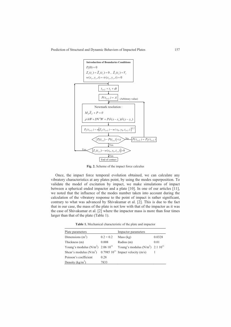
Prediction of Structural and Dynamic Behaviors of Impacted Plates
dttt i1i
A)t(P 1i (Arbitrary value)
Newmark resolution :
0PZM II&&
)()(4..
oo yyxxPWDWh
231i001iI1i1 )t,y,x(w)t(Zn)t(P
)()( 111 ii tPtP
End of contact
Yes
No )t(P)t(P 1i11i
Yes 0),,()( 1001 iiI tyxwtZ
Yes
Introduction of Boundaries Conditions
0),,(),,(
)(,0)()(
0)0(1
tyxwtyxw
VtZtZtZ
P
oooo
IoIoIoI
&
&&&
Fig. 2. Scheme of the impact force calculus
Once, the impact force temporal evolution obtained, we can calculate any
vibratory characteristics at any plates point, by using the modes superposition. To
validate the model of excitation by impact, we make simulations of impact
between a spherical ended impactor and a plate [10]. In one of our articles [11],
we noted that the influence of the modes number taken into account during the
calculation of the vibratory response to the point of impact is rather significant,
contrary to what was advanced by Shivakumar et al. [2]. This is due to the fact
that in our case, the mass of the plate is not low with that of the impactor as it was
the case of Shivakumar et al. [2] where the impactor mass is more than four times
larger than that of the plate (Table 1).
Table 1. Mechanical characteristic of the plate and impactor
Plate parameters Impactor parameters
Dimensions (m2) 0.2 × 0.2 Mass (kg) 0.0328
Thickness (m) 0.008 Radius (m) 0.01
Young’s modulus (N/m2) 2.06 10
11 Young’s modulus (N/m
2) 2.1 10
11
Shear’s modulus (N/m2) 0.7985 10
11Impact velocity (m/s) 1
Poisson’s coefficient 0.28
Density (kg/m3) 7833
157

To this end, we compare our results with those obtained in the bibliography (Lu
Chun [12]) where we took the first 49 modes contributions of a simply supported
plate. We propose to compare the forces of interaction calculated by the numerical
approach suggested and those obtained by Lu Chun [12], in the case of an impact
applied to the centre of the plate. The results of simulations are represented in Fig. 3,
with the contribution of 49 modes. The analysis of the results obtained by our
approach shows that they are almost identical to those obtained by the references
results obtained by Wu et al. [13] resulted from finite element method calculations.
(a) Reference (Lu Chun [12]) (b) Our approach
Fig. 3. Impact force comparison
3. Numerical example and discussion
In what follows, we study the effect of different parameters affecting the impacted
plate’s behaviour. The studied parameters will be: the impact point position,
impact velocity and the impact energy. For this, two plates of the same surfaces
and boundary conditions will be an application subject. To treat the most factors
which influence the impact force, we made some simulations to show their effects
on the magnitude and the impact duration.
3.1. Effect of the boundaries conditions on the impact force
We are now studying the influence of the plate’s boundaries conditions on the
impact force. To this end, we conduct numerical simulations on the same plate
that previously with the impact characteristics as follows (Table 2):
A. Miloudi and M. Neder
(Wu et al. [13] and Karas [14]) mentioned on the Fig. 3a. Let us note that the
158

Prediction of Structural and Dynamic Behaviors of Impacted Plates
Table 2. Characteristic of the impact
Impact parameters
Impactor mass (kg) 1 Impactor Radius (m) 0.0125
Density (kg/m3) 7800 Incident velocity 2
Young’s modulus (N/m2) 2.1 10
11
As shown in Table 3, the obtained results prove that the plate’s boundaries
conditions have a significant influence on the impact force.
Table 3. Effect of the boundaries conditions on the magnitude and the impact duration
Impact point (0.5a, 0.5a) Impact point (0.12a, 0.38a) Boundaries
conditions Maximum
magnitude (N)
Impact
duration (ms)
Maximum
magnitude (N)
Impact
duration (ms)
SFSF 7096 8.20 × 10² 6901 8.05 × 10
2
SSSF 6503 7.75 × 10² 6309 6.60 × 10
2
SCSF 6404 7.70 × 10² 6185 7.50 × 10
2
SSSS 6610 7.85 × 10² 6096 7.45 × 10
2
SSSC 6482 7.75 × 10² 6003 7.35 × 10
2
SCSC 6396 7.70 × 10² 5913 7.30 × 10
2
3.2. Influence of some parameters on the stress temporal evolution
For this part, two plates of same surfaces and boundaries conditions will be
studied. The geometrical and mechanical characteristics of the two plates are
summarised in Table 4.
Table 4. Geometrical and mechanical characteristics of the plates
Characteristics Isotropic plate Orthotropic plate
Length (m) a = 0.5 a = 0.5
Width (m) b = 0.5 b = 0.5
Thickness (m) h = 0.002 h = 0.00609
Mass density (kg/m3) = 7800 = 2094
Young modulus (N/m2) E = 2.1 10
11 Ex = 23.514 10
9; Ey = 23.514 10
9; Ez = 7.46 10
9
Shear modulus (GPa) G = 8.4 1010
Gxy = 8.4 1010
; Gxz = 8.4 1010
; Gyz = 8.4 1010
Poisson’s coefficient = 0.3 xy = 0.1; xz = 0.29; yz = 0.29
In order to validate the used method, it will be preceded to a comparison
between the evolution of the stress deduced from the proposed analytic method
and that determined by finite element software (Cosmos [15]).
159

This comparison is illustrated on Fig. 4. The results obtained show a perfect
agreement between the two methods.
0 10 20 30 40-200
-150
-100
-50
0
50
Time (ms)
Str
ess (M
Pa)
Stress at the point ( 0.50a , 0.50b )
AnalyticF.E.M.
0 10 20 30 40-30
-25
-20
-15
-10
-5
0
5
10
Time (ms)
Str
ess (M
Pa)
Stress at the point ( 0.50a , 0.50b )
AnalyticF.E.M.
Fig. 4. Comparatives studies of x at the impact position (a) isotropic plate and (b) orthotropic plate
3.2.1. Influence of the impact point position
The temporal evolution of the stress x according to the impact point is illustrated
on the Fig. 5. It is necessary to note the good similarity of the different impact
positions behaviors. However the central position (0.5a, 0.5b) remains most
unfavourable.
0 10 20 30 40 50-200
-150
-100
-50
0
50
Time (ms)
Str
ess (M
Pa)
1 ( 0.50a , 0.50b )2 ( 0.25a , 0.25b )
2
1
0 10 20 30 40-30
-25
-20
-15
-10
-5
0
5
10
Time (ms)
Str
ess (M
Pa)
1 ( 0.50a , 0.50b )2 ( 0.25a , 0.25b )
1
2
Fig. 5. Influence of the impact point position on the stress y evolution at the impact point position,
(a) isotropic plate and (b) Orthotropic plate
The distribution of the stress field on the plate surface solicited by impact, is
illustrated by the equal-contours (Fig. 6). These last was traced for the instant t
corresponding to the maximum stress affecting the plate. They have already been
drawn for the three impact positions of already selected. It should be noticed that
the equal-contours of circular shape around the impact point position tend to be
deformed far from the impact point position.
A. Miloudi and M. Neder160

Prediction of Structural and Dynamic Behaviors of Impacted Plates
a) Stress x, plate impacted at (0.5a, 0.5b)
b) Stress y, plate impacted at (0.5a, 0.5b)
c) Stress x, plate impacted at (0.25a, 0.25b) d) Stress y, plate impacted at (0.25a, 0.25b)
e) Stress x, plate impacted at (0.50a, 0.25b) f) Stress y, plate impacted at (0.50a, 0.25b)
Fig. 6. Stress field for an orthotropic plate
4. Conclusions
In this study, we developed a numerical approach to determine the impact force
and dynamic response of a rectangular plate impacted by a spherical projectile.
The plate’s response is determined by modal decomposition using a Newmark
integration scheme. The obtained results were validated by those given by the
literature. Finally, a study of the influence of some parameters on the impact force,
the plate dynamic response and the stress distribution was made. From this study
we can highlight the following:
161

When calculating the impact force, the modes of higher order are not
negligible, when the mass of the plate is important in front of the impactor.
The plate boundaries conditions have a significant influence on the impact
force.
The shock is not perfectly elastic, but we can see that the shock is less
elastic when the impactor mass becomes important.
The equal-contours of circular shape around the impact point position
tend to be deformed far from the impact point position.
References
[1] L.P. Greszuk. Damage in Composite Materials due to Low Velocity Impact. Impact
Dynamics, Z.A Zukas et al., Wiley editions, New York, pp 55–94, 1982.
[2] K.N. Shivakumar, W. Elber and W. Illg. Prediction of Impact Force and Duration due to
Low Velocity Impact on Circular Composite Laminates. J. Appl. Mech., 52, pp 674–680,
1985.
[3] S. Benmedakhène, Etude phénoménologique du comportement à l’impact des matériaux
composites, Thèse de Doctorat de l’Université de Technologie de Compiègne, France, 1996.
[4] G. Caprino, I. Crivelli-Visconti and A. Di Ilio. Elastic Behaviour of Composite Structures
under Low Velocity Impact. Composites, 15, 3, pp 213–234, 1984.
[5] P. Sjoblom. Simple Design Approach Against Low Velocity Impact Damage. Proc. 32nd
SAMPE Symp., Anaheim, CA, pp 30–52, 1987.
[6] K.M. Lal. Residual Strength Assessment of Low Velocity Impact Damage of Graphite-
Epoxy Laminates, Jour. Reinf. Plast. Comp, 2, pp 226–238.
[7] K.J. Bathe and E.L. Wilson. Numerical Methods in Finite Element Analysis, Prentice-Hill,
inc. Englewwood Cliffs, New Jersey, 1976.
[8] S.C. Hunter. Energy Absorbed by Elastic Waves During Impact. J. Mech. Phys. Solids 5, pp
162–171, 1957.
[9] M. Neder et A. Miloudi, Approche Numérique pour la Prédiction du Comportement
Dynamique de Plaques Impactées, Actes de la 4ème Conférence Internationale sur les
Mathématiques Appliquées et des Sciences de l’Ingénieur, Casablanca, Maroc, 2002.
[10] B. Hachemane , M. Neder, A. Ahmed Benyahia A. Miloudi and T. Boukharouba. Study of
the Dynamic Behaviour of Plates Subjected to Impact – A Numerical Approach. The 7th
International Conference on Production Engineering, Design and Control, Vol. II, pp 661–
669, Alexandria, Egypt, 2001.
[11] M. Neder et A. Miloudi, Etude paramétrique du Comportement Dynamique de Plaques
Impactées ”, Actes du 16ème Congrès Français de Mécanique, Nice, France, 2003.
[12] Lu Chun, K.Y. Lam. Dynamic Response of Fully-Clamped Laminated Composite Plates
Subjected to Low-Velocity Impact of a Mass. Int. J. Solids Struct., Vol. 35, No. 11,
Elsevier, pp 963–979, 1998.
[13] T. Wu, His-Yung and Fu-Kuo Chang. Transient Dynamic Analysis of Laminated Composite
Plates Subjected to Transverse Impact. Comput. Struct., 31(3), pp 453–466, 1989.
[14] K. Karas. Platten Unter Seitlichem Stoss, Ing. Archiv 10, pp 237–250, 1939.
[15] Cosmos/M2.0 for Windows A Complete Finite Element Analysis System, Structural Research
and Analysis Corporation (SRAC), May 1998.
A. Miloudi and M. Neder162

T. Boukharouba et al. (eds.), Damage and Fracture Mechanics: Failure Analysis of Engineering
© Springer Science + Business Media B.V. 2009
Application of Structural INTegrity Assessment
Procedure to Nuclear Power Plant Component
Nenad Gubeljak and Jozef Predan
University of Maribor, Faculty of Mechanical Engineering, Maribor, Slovenia with
Smetanova 17, SI-2000 Maribor, Slovenia.
Abstract Quite few analytical flow assessments methods as specific standard and guidelines
there have been developed in recent years. Today, as one of a most comprehensive assessment
procedure is SINTAP- Structural INTegrity Assessment Procedure. The SINTAP introduced the
basic principles of R6 (rev. 3) and ETM. SINTAP procedure is possible to performed assessment
for inhomogeneous configurations such as strength mis-matched weldments and an effect of
residual stresses. Nevertheless, the SINTAP procedure take into account temperature transition
region from ductile-to-brittle behavior of material. In the contribution the SINTAP procedure
was applied to the failure analysis of cracked component. Structure integrity assessment is issued
to failure prediction of cracked structural component regarding to increasing applied load or
crack size. In order to ensure safe use of cracked structural component the many standards and
procedures are available (e.g. SINTAP). The results obtained by using of these procedures
consist always certain portion of conservatism, what leads to underestimation of the real carrying
capacity of engineering component. In this paper a T-joint of 8 in. RHR nozzle on 29 in. RC hot
leg as the part of a high pressured pipeline of the nuclear power plant has been considered as
engineering component subjected to thermal shock.
Keywords: Integrity Assessment, Steam Pipeline, T-Joint, Finite Element Analysis.
1. Introduction
Structure integrity assessment is issued to failure prediction of cracked structural
component regarding to increasing applied load or crack size. In order to ensure
safe use of cracked structural component the many standards and procedures are
available (e.g. BS7910, API 579, SINTAP, R6), cited as Refs. [1–4]. The results
obtained by using of these procedures consist always certain portion of conservatism,
what leads to underestimation of the real carrying capacity of engineering
component. The calculation based on analytical solutions given in such procedures
defines in the rule a lower value of critical crack size, which causes the failure of
structure. In the other hand the solutions for component carrying capacity or
critical crack size determined by numerical model corresponds specific geometry
of component and crack’s parameters. The main disadvantage of this approach is
that numerical model demands long term and exhausting modelling, especially in
the case when the engineering component geometry or crack geometry is complex,
e.g. semi-elliptical and spherical crack located out of the model symmetry.
163
Materials and Structures, 163–172.

N. Gubeljak and J. Predan
In this paper a T-joint of 8 in. RHR nozzle on 29 in. RC hot leg as the part of a
high pressured pipeline of the nuclear power plant has been considered as
engineering component. The critical part of a T-joint is the transition between two
pipes of different diameters, because the difference in the pipes’ shell thicknesses
causes higher stress intensity. Some experiences of operators show that a semi-
elliptical surface crack can occur at this place during exploitation of steam pipelines.
T-joint of pipes as the part of primary pipeline of the power plant (Fig. 1) is
subjected to the operating pressure of 17.13 MPa and temperature of +290°C up to
+350°C according to the technical specification. Weld joint has been made from
the material with higher strength than base material, what could be the reason for
crack appearing in the base metal at the vicinity of the joint. Material properties
are obtained by testing at service temperature +350°C (yield strength Rp0,2 = 270
MPa, ultimate tensile strength Rm = 575 MPa, elastic modulus E = 185 GPa,
Poisson’s number = 0,3 and fracture toughness CTODmat = 0,75 mm) [5]. This
crack due to dynamic loading during the service could extend from the outer side
toward inner surface. The possible location of the surface crack is presented in
Fig. 1 (in the heat affected zone parallel to the axis of symmetry of the pipe with
greater diameter). Based on the project documentation a solid model of the T-joint
of pipes with no crack has been modelled by using of SolidWorks [6] and it is
presented on Fig. 2. From the theoretical point of view, the highest stresses could
be expected on the outer side of the pipe with larger diameter. The first step by
finite element analysis (ANSYS 10.0 [7]) was to prove this assumption defining
the critical place of the surface crack (position and orientation). In that sense, 3D
finite element model (Fig. 3) has been performed increasing the internal pressure
incrementally to the value, which causes the stresses over the yield strength of
corresponding base material in the region of highest stress concentration. This
region could be recognised from Fig. 4, where the principal stresses are presented
as the stress vector. The aim of the structural integrity calculation is to estimate
the loading conditions of cracked component, where the existed crack or flaw
could propagate either stable (leak before break – LBB or plastic collapse effect)
or unstable, what has brittle fracture for the consequence. From the safety side,
toughness of component material should be high enough, in order to ensure leak-
before-break or plastic collapse. It makes possible stopping of the system
operation without any extraordinary measures.
R1=370,2mm
t1=59,18mm
R2=88,875mm
t2=79,45mm
a=19mm
2c=100mm
Fig. 1. Geometry of the T-joint
164

Application of Structural INTegrity Assessment Procedure
Fig. 2. Solid model of the T-joint Fig. 3. Finite element model of T-joint
Fig. 4. Vector of principal stresses
2. SINTAP procedure
The SINTAP (Structural Integrity Assessment Procedure) is structured in a
hierarchic manner consisting of various analysis levels constituted by the quality
and completeness of the required input information.
0
1
Lr= F/ Fy
Kr=
KI(a,F
)/K
mat f(Lr)
Lrmax
Loading path
safe
predict ion of
init iat ion
fracture Deterministic analysis
Fig. 5. Schematic illustration of fracture initiation at Failure Assessment Diagram (FAD)
165

N. Gubeljak and J. Predan
Higher levels are more advanced than lower levels: they need more complex
input information but the user is “rewarded” by less conservative results. An
important feature of the procedure is that the analyses can alternatively be based
on a Failure Assessment Diagram (FAD) philosophy (Fig. 5). Applying the FAD
philosophy a failure line is constructed by normalising the crack tip loading by the
material’s fracture resistance. The assessment of the component is then based on
the relative location of a geometry dependent assessment point with respect to this
failure line. In the simplest application the component is regarded as safe as long
as the assessment point lies within the area enclosed by the failure line. It is
potentially unsafe if it is located on or above the failure line. The normalising
crack tip loading parameter Lr is defined as ratio of the applied load (i.e. service
pressure p = 17,133 MPa) and the limit load (i.e. pressure pY), or respectively as
the ratio of an applied net section stress ref and the yield strength of the material,
Y:
Y
ref
YYr
p
p
F
FL (1)
The latter being given as Y eL for materials with and Y P0.2 for materials
without the Lüders plateau. The reference stress of the plate geometry considered
within this paper can easily be determined as hoop stress hoop or by profile of
stress distribution through thickness of cylinder. At the basic level only the
toughness and both the yield strength and the ultimate tensile strength of the
material have to be known. Different sets of equations are offered for materials
with and without Lüders plateau. At basic level failure acceptance curve f(Lr)
without the Lüders plateau is defined as
10for exp7,03,0x2
11)( r
6r
2/12rr LLLLf (2)
With:
6,0
/ 001,0min
2,0pRE (3)
And
maxrr
2/)1(rrr 1for x )1()( LLLLfLf NN (4)
166

Application of Structural INTegrity Assessment Procedure
m
2,0p1 3,0
R
RN (5)
2,0p
m2,0pmaxr
2
1
R
RRL (6)
With maxrL being the limit against plastic collapse.
3. Determination of the carrying capacity of the T-joint of pipes
It is necessary to perform structural integrity assessment of T-joint of pipes
regarding the loading level. The crack geometry is usually determined by non-
destructive inspection of component (e.g. ultrasonic testing). In our paper the
semi-elliptical surface crack has been considered. The assumed size of crack
(a = 19 mm, 2c = 100 mm) can be reliably determined by ordinary testing
equipments. Integrity assessment generally is based on analytical expressions for
fracture mechanics parameters (stress intensity factor, limit load).
The solutions are given in literature (e.g. [8]) or in software packages, but
solutions are constrained to a very small range of pipe thicknesses and diameter
ratios. Such expressions for stress intensity factors given in literature are used for
the structural integrity assessment of structures with present cracks. They can later
significantly differ from real solutions for observed components. Thus the
confidence level of the obtained result stays unknown.
Opposite to this, numerical modelling of the joint geometry and moreover of
the crack geometry requires the time and experience. Numerical solutions for
stresses obtained by FEM are closest to the real stresses in the joint. This is
because it takes into account all the geometric details of the joint and shows a
realistic model of the material behaviour. However, the FEM results are usually
limited to only one-crack geometry, as for every crack length a new model has to
be created or algorithms for crack propagation have to be used.
Alternatively, analytical expressions for the stress intensity factor calculation
could be based on the stresses distribution obtained by FEA with no crack.
Therefore, the aim of this paper was to compare these three different approaches
defining the carrying capacity of one cracked T-joint in steam pipes:
(a) Engineering approach based on the stress intensity factor (SIF) calculation
by using equations given in literature and an expression for the hoop stress
(b) Combined approach based on the analytical SIF calculation by using
arbitrary stress distribution through the thickness obtained from the
finite element analysis for the structure with no crack and
167

N. Gubeljak and J. Predan
(c) Numerical calculation of SIF from the finite element model of the joint
with real crack geometry.
3.1. Engineering approach
Expression for the SIF for the semi-elliptical axial surface crack in tube [8]:
stress hoop is where,c
aY
t
caK (7)
pt
RRo
2
1 (8)
Ro is outer radius, R1 is inner radius of pipe, t is the wall-thickness and p is
internal pressure, a is crack depth and Y is the geometry shape function and for the
interval 3 < 2c/a < 12 is valid as
14
05,02
20191,0
202,01
20055,0
2053,012,1
1, 2
2
2
io RRt
t
c
t
c
t
c
t
c
Qt
c
c
aY (9)
65,1
464,11c
aQ (10)
: For earlier defined piping tees geometry and crack parameters (a = 19mm,
2c/a = 5.263) the value of SIF at the surface of pipe by using Eqs. (7–10) for
p = 17.133 MPa was calculated as: K = 1779.43 Nmm 3/2. Yield pressure could be
Yi
YR
t
M
p1
1
(11)
tR
cM and
t
at
i
2
61,11 (12)
168
calculated either by using formulae for semi-elliptical axial surface crack in tube [11]:

Application of Structural INTegrity Assessment Procedure
4,1
8,0
2,11
0,4-1x1,11
x
t
a
M
t
a
t
a
pp oY (13)
where:
tR
cM
R
tp
o
oo
25,064-42
Y
and x103549,5026905,02987,11
and x
(14)
Yield pressure calculated by using of Eqs. (13) and (14) is much closer to real
solutions and is equal to pY = 30 MPa. In that case the normalised crack tip
loading parameter amounts to Lr = 0.57.
3.2. Combined approach
In this approach the stress distribution through the thickness of T joints is
calculated by using of FEM. This distribution is used for calculation both Stress
Intensity Factor-SIF and limit load for surface crack, as is described in the Ref.
[9]. It is known that the tension and bending stresses are usually required as input
data to calculate the limit load of the component with a crack.
20
30
40
50
60
70
80
90
100
110
120
130
140
0 5 10 15 20 25 30 35 40 45 50 55 60
Wall-thickness, mm
Str
ess z
-direction
, M
Pa
1
2
a=19mm
Fig. 6. Opening stress distributions over the wall-thickness of the larger pipe at p = 17.133 MPa
169
Or by using of equation defined by Zahoor [12] for surface crack at crotch in
piping tees:

N. Gubeljak and J. Predan
The SIF-solutions based on the method of weight functions can be used for an
arbitrary stress distribution over the wall-thickness. Figure 6 shows the stress
distribution and principles for determination 1 and 2 as edges stress values over
the wall-thickness of the no-cracked pipe with larger diameter.
By linearization of stress distribution at crack tip position (crack opening stress
z in our case at p = 17.133 MPa), the membrane and bending stress can be
calculated as:
MPa 5.372
30105
2
:and
MPa 5.672
30105
2
21b
21m
(15)
Now it is possible to calculate the parameter Lr for FAD diagram from the
values of the membrane stress m and bending stress b by using simplified
expressions for the semi-elliptical surface crack in the plate under variable stress:
e2
2m
22
b
e2
b
)1(
)1(3
)(
)1(
3)(
R
g
R
g
Lr (16)
where:
)( and
2201)(
75,03
ctt
ca
c
ag (17)
Considering the yield strength for the corresponding material as Re = 270 MPa,
and using Eqs. (16) and (17), the parameter Lr is calculated as Lr = 0.36.
3.3. Numerical determination of the SIF
The value of SIF determined by finite element analysis presents most accurate
solution, but it consumes the time and requires good experience of operator. Its
main disadvantage is that obtained SIF solution is valid for only specific crack-
geometry.
Semi-elliptical surface crack has been modelled by ABAQUS [10] combining
tetrahedral and hexagonal elements in the vicinity of the crack front. Equivalent
stress distribution in the T-joint at p = 17.133 MPa is presented in the Fig. 7a and
more detailed in Fig. 7b.
170

Application of Structural INTegrity Assessment Procedure
SIF solution for the considered surface crack with 2c/a = 5.263 and a = 19 mm
was determined numerically. Figure 8 shows comparison between numerically
determined loading paths against failure assessment curve. The crack size is
constant, only internal pressure was increased up to p = 60 MPa.
Figure 8 shows that increase of loading causes crack propagation at inside point
of semi-elliptical crack. Solution based on the hoop stress provides linear loading
path and higher loading ration. Since, linear hoop-solution cross the failure curve
at lower internal pressure value than FEM solution, it is possible to recognize that
hoop solution is most conservative compare to arbitrary stress solution and finite
element solutions, e.g. critical pressure by hoop stress is p*crit = 45 MPa,
arbitrary stress solution p**crit = 48 MPa while by FEM analysis, the critical
stress is pcrit = 53.6 MPa for surface point.
(a)
(b)
Fig. 7. Mises stress distributions in the T-joint of pipes at p = 17.133 MPa
0
0,5
1
1,5
0 0,2 0,4 0,6 0,8 1 1,2 1,4 1,6 1,8 2
L r=p/p y
Kr=f(Lr)
Lrmax
Loading curve f(Lr)
for Basic Level
FEM failure
points
p=5MPa
30MPa
40MPa
a=19mm =const.
2c=100mm =const.
Hoop solution failure
for surface point
p*=60MPa
30MPa
40MPa
50MPa
Arbitrary stress
solution-surface
p=17,1MPap=60MPa50MPa
deepest
surface p=60MPa
Fig. 8. Comparison between hoop stress solution, arbitrary stress solution and FEM solution
during increasing internal pressure
171

N. Gubeljak and J. Predan
4. Conclusions
The structural integrity assessment is performed on one cracked T-joint in steam
pipes, using two different approaches based on fracture mechanics. The obtained
results show significant differences depending on the expressions used in the
calculations. The largest deviation from the results obtained by FEM is noted in
those solutions, where the stress intensity factor was calculated by using the
expression for hoop stress. It is possible to assume that the solution obtained by
FEM is closest to the real stress in the joint. This is because it takes into account
all the geometric details of the joint and shows a realistic model of the material
behaviour, indicating that for such a solution greater effort is needed, as well as
time and knowledge. The FEM results are also limited to only one-crack geometry, as
for every crack length a new model has to be created or algorithms for crack
propagation have to be used. In a single case an alternative approach can be used,
where analytical expressions for stress intensity factor calculation are combined
with the crack geometry and stress state. Thus, geometry of the joint is partially or
completely simplified, because the crack geometry is almost neglected when
calculating the stress intensity factor. The analytically or numerically obtained
distributions of the stress crack opening through the thickness serves as the basis
for determination of membrane stress and bending stress independent of the crack
length. The results obtained in such a way can be of acceptable accuracy, they are
obtained over a shorter time, and enable partially change of crack length and depth
as opposed to the FEM solutions.
Acknowledgments Authors would like to thank to Ministry of High Education, Science and
Technology of Slovenia for the support realised through financing of Eureka MOSTIS project.
References
[1] BS 7910. Specification Formulation. Journal of Engineering, Vol. 2, No. 2, 1999, pp 223–228.
[2] API 579. API Recommended Practice 579. Fitness for Service, First Edition, March 2000.
[3] SINTAP: Structural INTegrity Assessment Procedures for European Industry. Final Revision,
EU Project BE 95-1462, Brite Euram Programme, 1999.
[4] R6: Assessment of the integrity of structures containing defects. Nuclear Electric Procedure
R/H/R6, Revision 3, 1998.
[5] Gubeljak, N., Kozak, D., Vojvodi -Tuma, J., Predan, J., Aplikacija mehanike loma pri
revitalizaciji energijskih komponent, Kon no poro ilo, Elaborat za nuklearno elektrarno Krško
[6] SolidWorks, 2005.
[7] ANSYS Release 10.0, 2005.
[8] Schwalbe, K.-H., Zerbst, U., Kim, Y.-J., Brocks, W., Cornec, A., Heerens, J., Amstutz, H.,
“EFAM ETM 97- the ETM method for assessing the significance of crack-like defects in
engineering structures, comprising the versions ETM 97/1 and ETM 97/2”, GKSS-
Forschungszentrum Geesthacht GmbH, Geesthacht, 1998.
[9] Berger, Ch., et al. Fracture mechanics proof of strength for engineering components. FKM
Guideline, Forschungskuratorium Maschinenbau (FKM), 2004.
[10] ABAQUS Release 6.5, 2006.
in Pressurised Cylinders, ASTM STP 536: 461–481.
[12] Zahoor, A., Closed Form Expressions for Fracture Mechanics Analysis of Cracked Pipes.
ASME J. Pressure Vessel Technology, 107: 203–205.
172
[11] Kiefner, J.F., Maxey, W.A., Eiber, R.J., Duffy, A.R., (1973) Failure Stress Loads of Flaws

T. Boukharouba et al. (eds.), Damage and Fracture Mechanics: Failure Analysis of Engineering
© Springer Science + Business Media B.V. 2009
Failure Assessment Diagrams in Structural
Integrity Analysis
Yu. G. Matvienko
Mechanical Engineering Research Institute of the Russian Academy of Sciences, 4 M.
Kharitonievsky Per., 101990 Moscow, Russia
Abstract The methodology of the criterion of average stress in the cohesive zone ahead of the
crack/notch was employed to develop failure assessment diagrams for a solid with a finite
crack/U-notch under mode I loading. The cohesive stress is treated according to Von Mises yield
criterion as a property of both the yield stress and the T-stress which was introduced into the
criterion to quantify constraint in different geometries and type of loading. A brief survey of the
basic principles of a failure assessment diagram for a body with a crack- or notch-like defect and
its application in the structural integrity analysis has been presented. To determine an acceptable (safe)
region of the damaged component, safety factors against fracture and plastic collapse were
introduced in the fracture criterion and the failure assessment diagram. Basic equations have
been presented to calculate the safety factor against fracture and to estimate an acceptable (safe)
region for an engineering component with a crack- or notch-like defect of the acceptable size. It
was shown that the safety factor against fracture for a notch-like defect is a function of the yield
stress as well as the elastic stress concentration factor and the safety factor against plastic
collapse. The methodology of the failure assessment diagram has been employed for the
structural integrity analysis and assessment of acceptable sizes of surface longitudinal notch-like
defects in a pressure vessel. The load separation method is recommended to measure the notch
fracture toughness in terms of the J-integral for non-standard specimens with a notch.
Keywords: Failure, Integrity, Crack/Notch, Von Mises Yield Criterion, Diagram FAD.
1. Introduction
The basic failure curve of the failure assessment diagram (FAD) is written
as rr LfK , where Cr KKK 1/ is the ratio of the applied stress intensity
factor K to the material’s fracture toughness CK1 and rL is equal to the ratio of
applied load P to plastic collapse load YP . If the assessment point rr LK , is
situated within the non-critical region enclosed by the line of the FAD, failure of
the cracked structure does not occur. Details of the FAD approach are given in the
SINTAP procedure. In engineering, most assessment of component reliability are
made deterministically so that failure is avoided by including safety factors on
each of the different equation inputs. In this case, safety factors against fracture
and plastic collapse have been considered [1, 5]. The safety factors are set to unity
for the evaluation of critical conditions.
173
Materials and Structures, 173–182.

The aim of this paper is to give a brief survey of the basic principles of a failure
assessment diagram for a component with a crack- or notch-like defect and its
application in the structural integrity analysis. The FAD has been based on the
criterion of the average stress ahead of the crack/notch tip and considered in terms
of Cnotch KK 11 / and YC / . Acceptable state of the damaged component with a
crack- or notch-like defect will be determined by introducing safety factors against
fracture and plastic collapse in the fracture criterion describing the failure
assessment diagram.
2. Failure assessment diagram for a solid with a crack
2.1. Failure criterion
The local failure criterion in the form of the average stress limitation in the
fracture process zone ahead of the sharp crack tip can be given in the following
form [3].
o
d
y drrd 0
1 (1)
To describe a critical state of a solid with a crack. Here, d is the fracture
process zone length, ry is the normal elastic stress distribution ahead of the
crack/notch tip. The critical stress 0 is the material strength which depends on
the material model and can be assumed to be the yield strength, ultimate strength
or some effective strength taking into account the constraint effect. An infinite
plate with a crack length a2 is assumed to be subject to remote uniaxial stress .
The stresses ry on the crack extension line are the principal normal stresses
described by the exact elastic solution according to Westergaard’s theory.
22 ax
xxy (2)
Averaging the local stress (see Eq. 2) over the fracture process (cohesive) zone,
the failure criterion (Eq. 1) leads to the following equation [3].
2
11 1coh
CCKK (3)
174 Yu. G. Matvienko

Failure Assessment Diagrams in Structural Integrity Analysis
Which describes the failure assessment diagram. Here, KI is the stress intensity
factor at the crack tip, C is the applied (critical) stress at failure.
2.2. The cohesive strength
To estimate the cohesive strength, the following approach has been suggested. The
general form of the linear elastic stress fields ahead of the crack tip can be given
by Williams’s solution.
jiijij Tfr
K11
2 (4)
where ij is Kronecker’s delta, functions ijf define the angular variations of
in-plane stress components. The T-stress can be used as a constraint parameter
which has an influence on the cohesive strength ahead of the crack tip.
The T-stress scales linearly with applied load in infinite geometries, most
computational studies report T-stress values for various crack configurations as
follows.
WaT / (5)
where Wa / is a dimensionless parameter (so-called biaxiality ratio) which
depends on geometry and loading mode, is an applied stress, a and W are the
crack length and width of a body, respectively. Values of Wa / can be
considered as a normalized measure of the crack tip constraint and have been
tabulated for various geometries in the literature.
In the present work, the cohesive strength coh ahead of the crack tip is
determined by von Mises yielding criterion within the fracture process zone
according to flow law.
02,,, 2231
232
221321 YY (6)
where Y is the yield strength.
Moreover, the cohesive strength is treated as the stress which is independent on
the separation distance because the effect of the shape of the traction-separation
curves in the fracture process zone can be relatively weak. The stresses 1 , 2
and 3 are the principal normal stresses and assumed to be constant in the
fracture process zone ahead of the crack tip for certain crack geometries and
loading conditions.
175

Analogously to Williams’s solution, the stress 2 parallel to the crack plane is
suggested to be given by equation T12 . The stress 3 is equal to
21 and 0 for plane strain and plane stress, respectively. The cohesive
strength coh is supposed to be 1 and can be expressed from von Mises yield
condition (Eq. 6) taking into account Eq. (5) as follows.
2
222
21
1/ 1
4
1
2
YC
Y
C
Y
C
Y
coh , plane strain (7)
2
4
31
2 Y
C
Y
C
Y
coh , plane stress (8)
Thus, the cohesive strength for finite geometries can be rewritten as a function
of the applied failure stress C and the crack tip constraint.
3. Notch failure assessment diagram
The criterion of the average stress (Eq. 1) has been adopted for a solid with a
notch as well as a crack. The stress distribution is simplified considerably on the
continuation of the U-notch [2].
rr
Kr notch
y2
12
1 (9)
where is the notch tip radius. The stress intensity factor at the notch tip is
denoted as notchK1 . It should be pointed out that such stress distribution was
suggested for blunt cracks when the distance ahead of the crack tip is much
smaller than the crack length and greater than the crack tip radius. Averaging the
local stress (Eq. 9) over the fracture process zone ahead of the notch tip, the
failure criterion (Eq. 1) leads to the notch failure assessment diagram [3, 4].
2/1
2
22
11
111
tC
coh
coh
CCnotch
KKK (10)
Here, tK is the elastic stress concentration factor. The cohesive strength coh
ahead of the notch tip in Eq. (10) is given by Eqs. (7) and (8).
176 Yu. G. Matvienko

Failure Assessment Diagrams in Structural Integrity Analysis
The failure criterion (Eq. 10), describing the notch failure assessment diagram,
suggests that the loss of constraint due to a notch is independent on the loss of
constraint due to the T-stress which was introduced into the cohesive strength to
quantify constraint in different geometries and type of loading. It should be also
noted that, in contrast to the SINTAP procedure and the FITNET assessment, this
simple methodology does not require finite element analysis to obtain the effective
distance for calculating the notch failure assessment diagram.
4. Structural integrity assessment of a notch-like defect
The notch failure assessment diagram (Eq. 10) can be adopted for a component
with a notch-like defect (or blunt crack with a finite tip radius). To determine an
acceptable (safe) region, it should be reasonable to introduce safety factors (e.g.
[1, 5]) in the failure criterion. The following condition should be fulfilled if
detected or assumed notch-like defect of a certain size should be assessed as
acceptable.
2/1
2
22
11
111
tC
coh
coh
C
K
Cnotch
KSF
KK (11)
where KSF is safety factor against fracture. The acceptable applied stressC
is
suggested to be not more than: YY SF/ , i.e.
Y
YC
SF (12)
where YSF is safety factor against plastic collapse.
For the evaluation of critical conditions for the acceptable stress, the safety
factor KSF in Eq. (11) is set to unity. Any reliable method to calculate the stress
intensity factor notchK1 can be employed if these methods are validated. The
safety factor KSF can be calculated by making an assumption that the applied
acceptable stress should be not less than the yield stress (Eq. 12) of material for an
engineering component with a notch-like defect of the acceptable size [5]. In this
case, the failure criterion for a notch-like defect of the acceptable size on the
boundary of fracture and plastic collapse can be given by
2/1
2
22
1
111
2
1
tY
coh
coh
YCtT
KKK (13)
177

Here, the stress intensity factor at the notch-like defect tip is assumed to be as
given by the relationship.
tnotch KK2
11 (14)
The safety factor YSF against plastic collapse corresponding to Eq. (12) is
introduced in the failure criterion (Eq. 11) to determine the acceptable defect as:
2/1
2
22
1 1
/1
/1
2
1
tYY
coh
coh
YY
K
Ct
Y
Y
KSF
SF
SF
KK
SF (15)
Combining Eqs. (13) and (15), the safety factor KSF against fracture can be
presented as:
2
22
2
22
1
/11
11
/1
tYY
coh
coh
Y
tY
coh
coh
YY
YK
KSF
K
SF
SFSF (16)
Here, the cohesive strength (Eqs. 7 and 8) can be defined taking into account
Eq. (12).
2
222
21
1/ 1
4
1
2
Y
YYY
coh SF
SFSF, plane strain (17)
2
4
31
2 YYY
coh
SFSF, plane stress (18)
Thus, the right-hand side of Eq. (11) defines the acceptable region in the notch
failure assessment diagram. If the assessment point falls within this region, the
component with a notch-like defect is acceptable, i.e. it fulfils the required safety
demands. For the special case of a crack ( tK ) the failure assessment
diagrams (Eqs. 10 and 11) are transferred to the failure assessment diagram for
component with a sharp crack, and the safety factor (Eq. 16) becomes the safety
factor against fracture of cracked component.
178 Yu. G. Matvienko

Failure Assessment Diagrams in Structural Integrity Analysis
It can be seen from Eq. (16) that the safety factor against fracture is a function
of the yield stress as well as the elastic stress concentration factor and the safety
factor against plastic collapse. Calculation of the safety factor against fracture as a
function of the elastic stress concentration factor leads to the following
dependence for plane strain and plane stress (Fig. 1). The value Ycoh / was
accepted in the form given by Eqs. (17) and (18). A crack-like defect is transferred
in a sharp crack at tK . In this case, the safety factor against fracture tends to
its minimum value, i.e. typical value for a sharp crack.
2 4 6 8 10 12 14 16 18
1,2
1,6
2,0
2,4
2,8
3,2
3,6
4,0 Plane Stress (Defect)
Plane Strain (Defect)
Plane Stress (Crack)
Plane Strain (Crack)
Sa
fety
Fa
cto
r A
ga
inst
Fra
ctu
re,
SF
K
Elastic Stress Concentration Factor, Kt
Fig. 1. The effect of the elastic stress concentration factor on the safety factor against fracture
( = 1, = 0.3, SFY = 1.5)
To demonstrate the structural integrity assessment procedure, an infinite plate
with a notch-like defect under uniform remote tensile stress has been considered.
Equation (15) gives the approximate relation for a notch-like defect of the
acceptable size a as follows:
22
2
2
2
21
41
1
Y
Ycoh
Ycoh
Y
Y
Y
K
C SF
SF
SF
SF
Ka (19)
The elastic stress concentration factor is assumed to be equal to the acceptable
factor tK , i.e. /][2 aKK tt . The following mechanical properties of the
material and the safety factor against plastic collapse for plane strain were
used: mMPa 1021CK , MPa 340Y , ,1 3.0 , 5.1YSF . Calculation
of the safety factor against fracture from Eq. (16) at tK gives 59.1KSF . It
is seen that the acceptable size of a notch-like defect decreases with the increase of
the elastic stress concentration factor tending to its limiting value, i.e. the
acceptable size of a sharp crack (Fig. 2).
179

An acceptable (safe) region for an engineering component with a notch-like
defect of the acceptable size can be represented from Eq. (11).
6 8 10 12 14 16 18 20
24
26
28
30
32
34
Defect
CrackA
ccepta
ble
Defe
ct Length
, m
m
Elastic Stress Concentration Factor
Fig. 2. Acceptable defect length in an infinite plate as a function of the elastic stress concentration
factor
5. Acceptable surface longitudinal notch-like defects
in a pressure vessel
An assessment of the acceptable surface longitudinal notch-like defects in a
pressure vessel is based on the notch failure assessment diagram described by Eq.
(15). Substituting Eq. (16) into Eq. (15), the acceptable elastic stress concentration
factor tK can be written as follows:
22
2
21 1
4
T
coh
coh
T
T
Ct
KK (20)
Thus, acceptable state of the damaged pressure vessel has been presented by the
following criterion ][ tt KK , where tK is the elastic stress concentration factor
for the surface notch-like defect under consideration.
The pressure vessel/defect geometry is described by the wall thickness t, vessel
outer diameter D, defect depth l and defect tip radius . In the analysis presented
below a wall thickness of 30 mm and a diameter of 1,200 mm are applied. The
notch-like defect length is assumed to be an infinite value.
t
lY
lKt 2 (21)
180 Yu. G. Matvienko

Failure Assessment Diagrams in Structural Integrity Analysis
where tlY / is a geometrical correction factor for the stress intensity factor in the
case of the SENT specimen.
0 3 6 9 12 15 180
10
20
30
40
50
60
70
80
90
Kt
(l/ )1/2
FEM: l=3.5 mm, 0.025< <0.4 (mm)
FEM: l=7.5 mm, 0.05< <1.0 (mm)
FEM: l=10.5 mm, 0.05< <1.0 (mm)
l=3.5 mm
l=7.5 mm
l=10.5 mm
Fig. 3. The results of calculation of the elastic stress concentration factor for surface longitudinal
notch-like defects by the FEM and Eq. (21)
To determine the elastic stress concentration factor for the surface external
defect, the 2D finite element simulations of steel pressure vessels were carried out
using the ANSYS code. It was shown that the elastic stress concentration factor
can be given by the following equation (Fig. 3).
The following mechanical properties of the steel and the safety factor against
plastic collapse for plane strain were used: mMPa 1001CK , MPa 285Y ,
3.0 , 5.1YSF . In this case, the acceptable depth of a surface notch-like
defect in the pressure vessel amounts to 10.23 mm.
6. Conclusions
Structural integrity assessment of the engineering components damaged by crack-
or notch-like defects is discussed from point view of the failure assessment
diagram. The methodology of the criterion of average stress in the fracture process
zone ahead of the crack/notch was employed to develop failure assessment
diagrams for a solid with a finite crack/U-notch under mode I loading.
The cohesive strength is treated according to von Mises yield criterion as a
property of both the yield stress and the T-stress which was introduced into the
criterion to quantify constraint in different geometries and type of loading.
181

Acceptable state of the damaged component with a crack- or notch-like defect
was determined by introducing safety factors against fracture and plastic collapse
in the fracture criterion describing the failure assessment diagram. It was shown
that the safety factor against fracture is a function of the yield stress as well as the
elastic stress concentration factor and the safety factor against plastic collapse.
The methodology of the notch failure assessment diagram has been employed for
the structural integrity analysis and assessment of acceptable sizes of surface
longitudinal notch-like defects in a pressure vessel.
Acknowledgments Professor Yu. G. Matvienko acknowledges the support of the NATO (Grant
CBP.NR.NRCLG 982800).
References
[1] Brickstad B, Bergman M, Andersson P, Dahlberg L, Sattari-Far I, Nilsson F (2000)
Procedures used in Sweden for safety assessment of components with cracks. Int J Pres Ves
Piping 77: 877–881.
[2] Creager M, Paris PC (1967) Elastic field equations for blunt cracks with reference to stress
corrosion cracking. Int J Fract 3: 247–252.
[3] Matvienko YuG (2003) Local fracture criterion to describe failure assessment diagrams for
a body with a crack/notch. Int J Fract 124: 107–112.
[4] Matvienko YuG (2005) Erratum: Local fracture criterion to describe failure assessment
diagrams for a body with a crack/notch. Int J Fract 131: 309.
[5] Matvienko YuG, Makhutov NA (1999) Strength and survivability analysis in engineering
safety for structures damaged by cracks. Int J Pres Ves Piping 76: 441–444.
182 Yu. G. Matvienko
T. Boukharouba et al. (eds.), Damage and Fracture Mechanics: Failure Analysis of Engineering
© Springer Science + Business Media B.V. 2009
Degradation and Failure of Some Polymers
(Polyethylene and Polyamide) for Industrial
Applications
Boubaker Bounamous and Kamel Chaoui
LR3MI, Mechanical Engineering Deptartment, Badji Mokhtar University, BP 12, Annaba,
23000, Algeria
Abstract The use of polymeric material such as polyethylene (PE) and polyamides (PA) made
it possible to achieve significant profits in design construction times and installation costs. The
objective of this study is to highlight the various mechanisms of rupture of polyethylene pipes in
service and in laboratory conditions under fatigue and creep loadings. It is known is some cases
that at least two mechanisms control PE pipe failures based on results cumulated in operating
conditions. They are nominally ductile and brittle mechanisms respectively characterizing short
and long-term failures. Several laboratory tests are used to extract design data for long-term
failure-type prediction based on stress and time-to-failure relationship. It remains difficult to
assess the relation between creep and fatigue loadings on one side. On the other side, the
manufacturing process of the test specimens influences considerably the obtained performance
for viscoelastic materials subjected to working conditions and environmental effects. Brittle-to-
ductile transition is studied under fatigue crack propagation mode using an energy criterion. The
brittle fracture damage zone is characterized by a single craze made up by locally drawn fibers
and dispersed voids whereas ductile rupture is rather dominated by highly yielded material and
significantly transformed matter as observed under polarized-light microscopy. The assessment
of polyethylene pipe and polyamide parts failure mechanisms is to contribute to a better
understanding of effects of other external chemical agents such as solvents in degrading the pipe
overall resistance. Recent results from environmental stress cracking of PE pipe and exposed
polyamide PA66 to detergent will be presented and correlated to mechanical properties
degradation.
Keywords: Polyethylene, Polyamide, Failure, Fatigue, Creep; Damage, Wear.
1. Introduction
Despite the large acceptance of polymers as an economic alternative, safety and
reliability remain basic issues, especially for long-term brittle-like failure and
accelerated stress corrosion cracking for many industrial applications. Many studies
have been carried out to highlight various behavioral aspects of usual polymers in
terms of service lifetime, mechanical characterization, failure mechanisms and
environmental effects [1, 2]. To a certain extent, it is possible to control the
mechanical properties of semicrystalline polymers by morphology management
during processing operations. Substantially improved Young’s moduli and tensile
183
Materials and Structures, 183–194.

B. Bounamous and K. Chaoui
strengths have been obtained in shear-controlled orientation in injection-molded
and high-pressure injection-molded HDPE because of the appearance of highly
oriented structures. The search for homogeneous geometrical dimensions imposes
rapid cooling and as a result, residual stresses in the extrusion or injection molding
processes are generated on external layers, whereas internal layers develop positive
stresses. The resistance to crack propagation is influenced by the state and magnitude
of these residual stresses.
This work is aimed to investigate mechanisms of failure in polyethylene pipes
and those of wear in polyamide gears under service and laboratory conditions. The
understanding of those mechanisms needs to study some associated phenomena
such as damage evolution and the various changes in mechanical properties
caused the extrusion or injection processes. Also, it is necessary to understand the
effects of environment on the long-term behavior.
2. Polyethylene pipe interactions
In real conditions, plastic pipe is in constant interaction with the other underground
networks (sewers, drinking water, cables, etc.), which are not necessary made out
of polymers. So its vulnerability increases as the risks of being deteriorated might
become significant. The protection measures are re-examined by including different
means of protections and suitable pipe backfills. It should be emphasized that most
significant applications of PE pipes remain related to fluid conveyance. HDPE is the
reference material used for gas transport under pressure. Stress is related to the
allowable pipe pressure through the following equation shown in French Standard
NF EN 921 for pressurized plastic pipe:
2h
h-ODP hoop (1)
where, is hoop stress, P is gas pressure, OD is average outside diameter and h
is minimum wall thickness. ASTM D-2837 defines the pressure rating of the pipe
as the estimated maximum pressure that the medium in the pipe can exert
continuously with a high degree of certainty that failure of the pipe will not occur.
Safety factors impose a working pressure in the pipe lower than this upper limit.
When exposed to hot water, long-term HDPE pipe failure occurs by precipitation
and diffusion-controlled migration of antioxidants combined to thermal oxidation
of the polymer.
For drainage pipes, most gravity water flow systems are constructed using
corrugated HDPE pipes. They basically comprise mostly sewers, drains, under-
drains and sanitary sewers. In drainage systems, underground pipe diameters may
be as large as 1,524 mm and they are calculated to support both soil and live loads.
HDPE pipe flexibility is used to transfer a portion of the overload onto the
surrounding soil. The risk of pipe buckling exists as a result of excessive deformation.
184

Degradation and Failure of Some Polymers (Polyethylene and Polyamide)
Corrugation is incorporated into the pipe profile to increase the structural
stiffness of the structure and according to AASHTO M294 standard; three types of
HDPE pipe profiles are used. They are: (1) Type C: Full circular cross-section with
an annular corrugated surface both inside and outside, (2) Type S: Full circular dual-
wall cross-section with an outer corrugated pipe and (3) Type D: Circular cross
section consisting with smooth inner wall joined to an outer wall.
Observed field problems [3] included: (i) deflection resulting from the lack of
control of construction procedures and the use of poor backfill materials, (ii)
erosion at outlet ends which often resulted in significant loss of material and
longitudinal bending and cracking of the corrugated HDPE pipe and (iii) erosion
as a result of joint leakage. In this case protection ducts, HDPE pipes are used as
external shields to isolate cables or pipes from external aggressive environments.
Usually, the protection is aimed to reduce significantly the presence of both
moisture and oxygen.
In the gas industry, HDPE ducts are commonly used to protect steel pipelines
crossing swampy and marine environments.
3. Polyethylene pipe testing
The Plastic Pipe Institute selected stress rupture testing as the most suitable test
method for rating plastic piping materials. The design of is achieved through
the “Rate Process Method for Projecting Performance of Polyethylene Piping
Components” which is standardized in ASTM D-2837, ISO 9080 and D-2513. It
well established that PE creep rupture curve may be divided into three regions as
illustrated in Fig. 1 and the same testing procedure allows differentiating between
various PE resins and manufacturing processes.
Log (Time to failure)
Log (
hoop s
tres
s )
Region I
Region III
Region II
Fig. 1. Schematic of a creep rupture curve for PE pipes at high temperature and long-term
185

B. Bounamous and K. Chaoui
The calculation is based on three coefficients equations [4], which relates
lifetime, t or the time-to-failure (in hours), hoop stress, (in Pa) and testing
temperature, T (in K) in the following form:
T
LogB
T
BA Logt (2)
where A, B, C are constants. Either ASTM D-2837 based on hydrostatic design
basis (HDB) or ISO 9080 based on minimum required strength (MRS) use data
from sustained hydrostatic pressure tests of pipe specimens, but the extrapolation
protocols are different.
It is understood that the actual long-term performance under internal pressure
and temperature will be the same regardless of the method. Normally, HDB and
MRS are used to obtain allowable pressure ratings considering pipe diameter,
thickness and a safety factor. Under conditions of constant low stress and room
temperature, it is established that PE resins fracture by slow crack growth. This
mode of failure limits pipe lifetime but constant tensile load (CTL) test was
devised to extract long-term information from accelerated testing [5]. Available
data from such a test is able to differentiate between similar products coming from
different manufacturers or using different copolymers in the extrusion process.
CTL is a good quality assurance test to evaluate new pipe lots and to set a
minimum required resistance.
1,00E-01
1,00E+00
1,00E+01
1,00E+02
1,00E+03
1,00E+00 1,00E+01 1,00E+02 1,00E+03 1,00E+04 1,00E+05
Time to failure under creep, hr
Tim
e t
o f
ail
ure
un
de
r fa
tig
ue
, h
r
PE 1: MDPE, compression molded
PE 2: HDPE, compression molded
PE 3: MDPE, extruded pipe
PE 4: MDPE compression molded
M6006
M5502
M4903
M5202
TR140
TR418
Fig. 2. Relationship between failure times under creeps and fatigue modes for different resins
Generally, fatigue can be defined as a phenomenon that takes place in components
and structures subjected to time-varying external loading and that manifests itself
in the deterioration of the material ability to carry an applied load that is well
186

Degradation and Failure of Some Polymers (Polyethylene and Polyamide)
below the elastic limit. Testing under fatigue has been used in different studies
as an accelerating agent to deduce PE lifetime under specific conditions. The
correlation between creep and fatigue strengths, undertaken by Parsons et al. [6],
showed that MDPE was much more creep resistant than HDPE, but MDPE pipes
was much more sensitive to strain rate in fatigue In the same approach, Zhou and
Brown [7] concluded that a higher resistance to fatigue does not necessarily
correlate with a higher resistance to failure under creep. Since ASTM tests are
based on creep data, it is interesting to compare it with fatigue data. Figure 2
illustrates such relation between failure times from both creep and fatigue modes.
Mechanisms of
Polymer Cracking
Ductile Failure Brittle Failure
Yielding
Creep-related
Creep rupture Impact Stress Cracking
Fatigue-related
Fig. 3. Failure mechanisms occurring during polymer cracking under different loadings
The data were gathered from literature and a proportional relation is found to
characterize both modes. This is an important result which states that fatigue tests
can also be used to draw conclusion on pipe life under acting pressure. Figure 3
shows the various mechanisms of cracking in polymers. Usually, ductile and
brittle cracking are in competition and which are aggravated with environmental
factors such as temperature and stress cracking chemical agents.
4. Wear measurements in polyamide gears
In the following example, the wear resistance of gear teeth is measured on
commercial PA66 polyamide wheel produced by mould injection process. In order
to assess the effect of water on wears in each flank of wheel teeth, an industrial
polyethylene-washing machine is used. The testing machine consists in PA66 spur
gears composed of a 19-teeth pinion and a 132-teeth driven wheel. The pinion
under investigation is enclosed in an upper box and rotates at a speed of 140 rpm.
The driven wheel is a crown wheel supporting a 3 kg capacity cylindrical clothes
drum that is placed in a lower box shaped basin (520 mm high, 460 mm wide and
570 mm deep).
The upper box is linked to the lower box through pins that allows closing and
opening when loading or unloading the lower box. The machine for wear test is
shown in Fig. 4.
187

B. Bounamous and K. Chaoui
Fig. 4. (a) Kinematics diagram of the testing rig, (b) back view of the gears
Wear measurement of the pinion is carried out every 250,000 wheel revolutions
in the clockwise direction. Before each measure, the test piece is cleaned in order
to remove small sticking particles that have been generating from the wear process
and dried to squeeze out humidity. Three testing conditions have been applied: in
water, in detergent water solution and under dry driving. The water detergent
solution has the following composition:
Less than 5% of nonionic tension credits soap
From 5% to less than 15%: tension anion credits, bleaching agents
From 15% to less than 30%: phosphates
It also contains: enzymes, perfume, activator, carbonate, silicate, optical bluing.
It is interesting to note that throughout the testing period, all the teeth have been
subjected to wear resistance only in the addendum zone, between the pitch
diameter and the outside diameter. This is due to two main reasons. First, when
gearing, the normal force due to the applied pressure on the contact point at the
pitch diameter with a pressure angle of 20° generates axial force that is fairly high
enough to push out the gears as to create a small displacement. Secondly, the
material is water absorber, since polyamides have a water absorption rate of 1.5%
at 23°C after 24 h. Regarding the flanks, there is a slight difference between the
right and left flanks wear. In fact, when operating the testing rig follows a washing
machine cycle. The distribution of wear around the wheel can be obtained when
observing its morphology throughout the 19 teeth. In this case, wear measurements
on the surface (XY-plane) at a distance of 0.5 mm from the external diameter have
been reported in histogram plots for the three testing conditions.
5. Failure mechanisms of polyethylene pipes
Ductile failures are characterized by large-scale material yielding adjacent to the
failure location. For instance, a flow phenomenon takes place represented by cold
drawing during in typical tensile tests of semicristalline polymer samples. Ductility
is more expressed as applied stresses are higher and usually rupture occurs in a
relatively short time.
188

Degradation and Failure of Some Polymers (Polyethylene and Polyamide)
This mechanism is related to the viscoelastic behaviour of PE materials and
specifically refers to the creep rupture. Typical brittle and ductile failures in
HDPE pipes are exhibited in Fig. 5. Less deformation characterizes the fracture
process, which is a long-term mechanism.
Temperature [8] is known to accelerate brittleness from sustained pressure
tests. Brittle failure in semicrystalline polymers has been claimed to originate from
chain disentanglement in fibrils, and recently other studies have also concluded
that chain breaking due to applied stress during crack propagation involves fibrillation
within the damage zone [9].
A level of complexity lies in the intramolecular heterogeneity of co-unit distri-
bution that should be as efficient as intermolecular heterogeneity for producing tie
molecules and random chain folding at the expense of regular chain folding.
Crystalline domains within semicrystalline polymers strongly influence such low-
strain-rate properties as the elastic modulus, yield stress, SCG, and environmental
stress cracking, whereas high-strain-rate properties such as impact, tear, and rapid
crack propagation are basically controlled by amorphous regions. In many cases,
complementary techniques have been adopted to assess from physical property
measurements molecular information.
a b
Fig. 5. SEM observation of the inner part of the craze zone at higher magnification; (a) brittle
crack and (b) ductile crack
For instance, brittle fracture toughness, crazing, and SCG measurements have
been used to determine the tie-molecule concentration and to infer valuable
structural information. In simpler cases, tie-molecule concentrations have been
evaluated from the modulus of a mechanically oriented material. Post yield
experiments assume that tie molecules and entangled chains behave like rubbery
networks in the drawing and strain-hardening regions; these molecules are steadily
pulled out from fragmented lamellae to become part of an oriented amorphous
domain.
6. Brittle to ductile transition
In the brittle regime, the plastic zone is very small and is associated with a main
craze. The latter is made of yielded material and structural voids. Under polarized
light, the extent of damaged material is confined to a narrow zone next to the
189

B. Bounamous and K. Chaoui
crack plane. For the ductile regime, the damaged zone is much important and the
craze are longer compared the brittle stage. The SEM examination illustrates the
multiple crazes and the highly deformed material at the crack-tip. Around the damage
zone, another part of the transformed material is highly affected plastically as its
limits extend many folds until the specimen edge. At higher magnifications, the
hierarchical events inside the craze zone appear to be constituted of highly yield
local matter and important voids. In order to study the FBDT, it is interesting to
use an energetic approach proposed by Klingbeil [10] for ductile solids failed
under fatigue. This study is concerned with a new theory of fatigue crack growth
(FCG) in ductile solids based on the total plastic energy dissipation per cycle
ahead of the crack tip. The FCG is explicitly given in terms of the total plastic
dissipation par cycle and the plane strain fracture toughness of the material from
the equation:
dN
dW
dN
da
t C0 G
1
1 (3)
where Gc is the critical energy release rate. In this instance, typical plots of the
rate of irreversible plastic work as a function the crack propagation rate are
constructed. These plots for 20%, 25%, 30% and 35% of yield stress are shown in
Fig. 6. It is observed that both damage mechanisms are well separated and each
slope would represent an independent resistance to fatigue crack propagation. It is
found that the brittle regime critical energy release rate so calculated lays between
97.7 J/m2 and 264 J/m2 and these values are quite small compared to the measured
energy rates from potential energy evolution.
0
0,005
0,01
0,015
0,02
0,025
0,03
0,00E+00 5,00E-05 1,00E-04 1,50E-04 2,00E-04 2,50E-04 3,00E-04
t0(da/dN), m²/cycle
dW
i/d
N,
J/c
yc
le
20%
0
0,01
0,02
0,03
0,04
0,05
0,06
0,00E+00 5,00E-05 1,00E-04 1,50E-04 2,00E-04 2,50E-04 3,00E-04
t0(da/dN), m²/cycle
dW
i/d
N, J
/cy
cle
25%
0
0,02
0,04
0,06
0,08
0,1
0,12
0,14
0,16
0,00E+00 6,00E-05 1,20E-04 1,80E-04 2,40E-04 3,00E-04
t0(da/dN), m²/cycles
dW
i/d
N,
J/c
yc
le
35%
0
0,02
0,04
0,06
0,08
0,1
0,00E+00 5,00E-05 1,00E-04 1,50E-04 2,00E-04 2,50E-04 3,00E-04
t0(da/dN), m²/cycles
dW
i/d
N, J
/cy
cle
30%
(c) (d)
(a) (b)
Fig. 6. Rate of irreversible work spend on deformations as a function of fatigue crack growth rate
at (a) 20%, (b) 25%, (c) 30% and (d) 35% of applied stress
190

Degradation and Failure of Some Polymers (Polyethylene and Polyamide)
The ductile regime energy is important as it considers a lot of energy spent on
damage and high deformation. There is a consistent evolution of calculated Gc as
this value is much higher when ductility becomes important. This approach is
interesting as it allows separating brittle from ductile contributions in a given FCP
test. The use of microscopy enables to confirm the extents of each mechanism
from fracture surface analysis and damage dissemination within PE. Compared to
long-term hydrostatic strength (LTHS), FCP may be considered as a more efficient
approach since it helps produce BDT in much shorter times.
7. Wear evolution on polyamide 66
Figure 7 is a view of new and used polyamide gears. It is observed that wear
changes teeth shapes and such result allows measuring wear evolution. In Figs. 8
and 9, the evolution of wear as a function of number of cycles for the 19 teeth, in
dry condition, detergent water solution and water is illustrated. It can be clearly
seen that wear behavior on the right flanks is not the same for all wheel teeth. In
all conditions, it appears that the most sensitive tooth to wear is the flaw molding
injection tooth and the less sensitive is the opposite tooth. As far as the teeth are
away from the injection tooth, as they are more resistant to wear. A conventional
trend is obtained throughout the three testing conditions for both flanks. The first
feature to sort out is that wear is faster in wet condition then in dry conditions.
This is obviously as explained above, due to water absorption that gives more
volume to the tooth. When adding detergent in water solution, wear drops down.
In fact, the presence of soap helps the gears to slide easily rather than in water,
therefore wear phenomenon is reduced. In dry conditions, wear occurs because of
dry friction but the temperature generated is soon dissipated as the next meshing
tooth occurs. Three phases characterized by a running in, a youth and a final phase
are observed. Regarding trends on the right flank, the running in phase for the
three conditions is reached within the 250,000 cycles where 17.22 mm3 in water,
13.08 mm3 in detergent and 11.27 mm3 in dry conditions. The youth phase longs
up to 1,250,000 cycles in water, 1,500,000 cycles in detergent and 1,750,000
cycles in dry conditions; the corresponding values in volume reduction are 25.23,
20.22 and 16.86 mm3.
a) b)
Fig. 7. Polyamide pinion (PA66): (a) initial shape, new gear; (b) final shape, worn gear
When the youth phase ends the final phase starts with rapid increase in volume
lost until the gears stops after 3 106 cycles when significant wear occurs to run out
the gears; the corresponding values are 46.88, 36.3 and 29.7 mm3. As wear is
191

B. Bounamous and K. Chaoui
concerned in polyamide gears, and in order to increase lifetime and reduce energy
consumption, it is evident to consider the right flank trend for wear assessment.
The wear trend shows a regular evolution from the beginning of the youth phase to
the end of the final phase leading to a fitting curve that can be expressed by an
equation for each testing condition.
0
5
10
15
20
25
30
35
40
45
50
0 0,5 1 1,5 2 2,5 3
Number of cycles x 10E+06
Wea
r V
olu
me
mm
3
Water
Detergent
Dry
Série7
Série8
Série9
Right Flank
Left Flank
Fig. 8. Evolution of wear volume in flanks of a polyamide pinion tooth
0
5
10
15
20
25
30
35
40
45
50
0 0,5 1 1,5 2 2,5 3
Nombre of cycles x 10E+06
We
ar
vo
lum
e (
mm
3)
WaterDetergentDryWaterDetergentDry
Simulation
Results
Weigth
Results
Fig. 9. Comparative wears volume removal between acquisition system simulation (dimensional
measurements) and weight results
In water solution: N10 wat
7
eW 7.397.15 (4)
In detergent solution: N10 7
eW 7.3det 43.12 (5)
Dry conditions: N10 dry
6
eW 4.326.10 (6)
192

Degradation and Failure of Some Polymers (Polyethylene and Polyamide)
8. Environmental stress cracking
Perhaps this topic is the most complicated when considering mechanisms of
failure in PE pipes. It is a mixture of aspects in connection with material integrity,
environment parameters and the stress-strain relationship (Fig. 10). Environmental
stress cracking (ESC) occurs when PE or PA is subjected to a combination of a
stress field and an environmental agent (chemical). Although, fundamental
molecular mechanism of ESC in both PE and PA is still discussed; nevertheless,
both ESC and SCG share many similarities, such as load and temperature
dependence of failure time, and brittle-like failure surface. Therefore, it is thought
that they probably have a common microscopic deformation mechanism that
governs failure. If so, it would be valuable to use ESC as a tool to evaluate the
long-term behavior of polyethylene and polyamide materials, since the ESC
testing times are much shorter compared to other tests [11]. The acceleration
process is supposed to be due to the pressure of aggressive agents and to diffusion
and/or absorption within crystallites.
o Temperature
o Chemicals
o UV
o Atmospheric
o Coatings
Chemical Attack
Weathering
Environment
Stress Cracking
ESC
MATERIAL
o Polymer Additives
o Processing history
o Surface condition
o Crystallinity
o Morphology
Environmentally
assisted fatigue
o Service stress (P°)
o Time-to-failure
o Residual stress/strain
o Strain rate
o Test type
STRESS/STR
ENVIRONMEN
Fatigue
Fig. 10. Interaction between material, environmental parameters and the stress–strain relationship
in ESC in polymers
It is concluded that both solvents (mixture of toluene-benzene and dichloro-
methane solution) are very aggressive to PE pipe materials. On the other hand,
detergents are also aggressive to polyamide materials [12, 13]. The problem is that
those solvents could be present in natural gas streams and might degrade irreversibly
the polymer parts. The evolution of cristallinity should also be studied and how it
is redistributed after, injection moulding, welding; cutting and machining at high
speeds [14]. Our studies conclude towards a specific evaluation of ESC of polymers
that should be governed by reliability approaches. In a recent work, we have
shown that such an approach is desirable as it answers many questions to the
uncertainty and probabilistic variable controlling lifetime in polymeric and metallic
materials [15]. Therefore, many aspects have to be considered such as the
knowledge of thermal history, the degree of molecular interpenetration from both
melts and the role of pigments and some additives.
193

B. Bounamous and K. Chaoui
9. Conclusions
Polymers are finding various technical applications in industry due to important
advantages. Technical developments of PE and PA are found in long-term perform-
ance evaluation and how research is trying to bridge between different approaches
such as fatigue and creep. Mechanisms of failure of PE pipes are basically driven
towards the understanding of brittleness, as it is the most dangerous for the integrity
of a PE underground structure. The study of brittle-to-ductile transition is a potential
way to establish PE toughness from short-term fatigue tests. Wear analysis of PA
is possible to approach experimentally and integrating the effect of stress cracking
environments.
References
[1] W. G. Perkins. Polymer toughness and impact resistance. Polym. Eng. Sci. 39 (12) (1999)
2445–2460.
[2] R. Seguela. Critical review of the molecular topology of semicrystalline polymers: The
origin and assessment of intercristalline tie molecules and chain entanglements. J. Polym.
Sci. Part B: Polym. Phys. 43 (2004) 1729–1748.
[3] Y. G. Hsuan and T. J. McGrath. HDPE pipe: Recommended material specifications and
design requirements, Report 429, NCHRP (1999).
[4] T. Trankner, M. Hedenqvist and U. W. Gedde. Structure and crack growth in gas pipes of
medium and high density PE. Polym. Eng. Sci. 36(16) (1996) 2069–2076.
[5] H. B. H. Hamouda, M. Somoes-betbeder, F. Grillon, P. Blouet, N. Billon and R. Piques.
[6] M. Parsons, E. V. Stepanov, A. Hiltner, E. Baer. Correlation of fatigue and creep SCG in
MDPE pipe material. J. Mater. Sci. 35 (2000) 2659–2674.
[7] Y. Zhou and N. Brown. Anomalous fracture behaviour in polyethylenes under fatigue and
constant load. J. Mater. Sci. 30 (1995) 6065–6069.
[8] A. L. Ward, X. Lu, N. Brown. Accelerated test for evaluating slow crack growth of
polyethylene copolymers in Igepal and air. Polym. Eng. Sci. 30(18) (1996) 1175–1179.
[9] R. Khelif, A. Chateauneuf and K. Chaoui. Statistical Analysis of HDPE Fatigue Lifetime.
Meccanica, published on line 3 April 2008, DOI: 10.1007/s11012-008-9133-7.
[10] N. W. Klingbeil. A total dissipated energy theory of fatigue crack growth in ductile solids.
Int. J. Fatigue 25 (2003) 117–128.
[11] N. Kiass, R. Khelif, B. Bounamous, A. Amirat and K. Chaoui. Etude expérimentale des
propriétés mécaniques et morphologiques dans un tube de gaz en HDPE-80. Mécanique &
Industries, N° 7 (2006) 423–432.
[12] K. Mao. Gear tooth contact analysis and its application in the reduction of fatigue wear.
Wear 262 (2007) 1281–1288.
[13] C.H. Kim. Durability improvement method for plastic spur gears. Tribology International
39 (2006) 1454–1461.
[14] Brauer, S. Andersson. Simulation of wear in gears with flank interference – a mixed FE and
analytical approach. Wear 254 (2003) 1216–1232.
[15] A. Amirat, B. Bounamous, R. Khelif, A. Chateauneuf, K. Chaoui. Reliability Assessment
of Pipelines Using Phimeca Software. Proceedings of the NATO Advanced Research
Workshop on Safety, Reliability and Risks Associated with Water, Oil and Gas Pipelines.
Alexandria, Egypt, 4–8 February 2007, pp. 233–259.
Creep damage mechanisms in polyethylene gas pipes. Polymer 42 (2001) 5425–5437.
194

T. Boukharouba et al. (eds.), Damage and Fracture Mechanics: Failure Analysis of Engineering
© Springer Science + Business Media B.V. 2009
On the Structural Integrity of the Nano-PVD
Coatings Applied on Cutting Tools
Miroslav Piska, Ales Polzer, Petra Cihlarova and
Dagmar Stankova
Institute of Manufacturing Engineering, BUT FME Brno, Technicka 2, 616 69 Brno, Czech
Republic
Abstract Many modern trends in metal cutting, high speed/feed machining, dry cutting, hard
cutting and ecological impacts set more demanding characteristics for cutting tool materials. The
exposed parts of the cutting edges must be protected against the severe mechanical and chemical
loading conditions resulting in wear of tools and quality of products. The paper deals with three
modifications of the hard (Ti1-xAlx)N/a nano-crystallites embedded in an x-ray nearly
amorphous Si3N4 matrix, analyses of the WC carbide-coating interface, its integrity and cohesion
to the substrate. Advanced cutting tests and wear morphology in the operation of longitudinal
turning of carbon steel C45 were done. Some technological and economical impacts for an
application of the coatings are also highlighted that confirms their a very good cutting
performance, characterized by the very good of chip formation, mean standard deviation of the
machined surface from Ra = 1.00–1.50 m to Ra = 6.30–12.50 m (start and end of testing),
convenient cutting force composition, tool life 52–56 min (compared to the expected 15–20 min)
for cutting speed 130 m/min, depth of cut 1.5 mm and feed per revolution 0.18 mm. Two
mechanism of wear have been watched – sub-layers delaminating and abrasion.
Keywords: Nano-Composite, Coating, Integrity, Interface, Cutting, Wear.
1. Introduction
Hard coatings for cutting tools can be divided by production methods and physical
properties. The coating protects the tool against abrasion, adhesion, diffusion,
formation of comb cracks and other wear due to the high strength of their covalent
inter-atomic bond, small bond distance, high coordination number and its Vickers
are TiN (the long-term standard from the late 1970s), Ti(C,N), (Ti,Al)N, (Al,Ti)N,
(Ti,Al,Si)N, (Al,Cr)N and CrN are applicable not only to the carbides, but also on
HSS tools. In many cases the deposition of the cutting tool with a hard coating
increases cutting performance and tool life in the range of 100–1,200%.
The reasons for the outstanding features of the (Ti, Al)-based coatings [9]
can be seen in a very high hardness (25–38 GPa), with relatively low residual
compression stresses 3–5 GPa), high hot hardness, resulting in low hardness lost
hardness HV of 40–60 and >70 GPa [1, 2, 5–9]. The widely used PVD hard coatings
195
Materials and Structures, 195–204.

M. Piska et al.
(30–40%) up to temperatures of 800°C, high oxidation resistance (the same rate
for Ti(C,N) at 800°C as for TiN at 400°C) and low heat conductivity (up to 30%
lower relative heat indention coefficient than for TiN).
The research of the substrates or the highly protective coating in specific
machining operations can have serious impact on machining productivity and
economy. The coating industry is enormously innovative today. There is a lot of
research and solutions even to improve these outstanding features of coatings,
especially the (Ti, Al)N for a suitable combination of ARC and sputtering, an
effective filtering of ARC-droplets, an optimization of process parameters like
ARC-current, BIAS-voltage, N2-pressure, etc.
Some research works have been focused on a optimization of the crystalline
structure to avoid the columnar structure and corrosion, a deposition of the
multilayers to increase coating toughness and thickness, convenient addition of
other alloying components, such as chromium and yttrium (to increase oxidation
resistance), zirconium, vanadium, boron and hafnium (to improve wear resistance)
or silicon to increase hardness and resistance against chemical reactions coatings [9].
Nevertheless, the three most important nano-structures are deposited today:
Nanogradients (with continuous changing of the composition from the
substrate to the top of a cutting tool)
Nanolayers (with typical sublayer’s thicknesses of 3–10 nm) and non-
linear relation of hardness depending on precisely specified periods of
coating)
Nanocomposites – nanocrystalline grains nc-AlTiN are embedded into an
amorphous matrix a-Si3N4 due to the spinodal segregation (silicon is not
in the metallic phase); the strong interface hinders grain boundary sliding
at crystallite size less than 10 nm
Generally, the coatings can be divided into two main categories:
1. Superhard nanocomposites – ceramic based coatings, e.g. nc-MenN/a-
Si3N4 (Me = Ti, V), nc-TiN/a-BN/a-TiB2, nc-(Ti1-xAlx)N/a-Si3N4. The
coatings offer superhardness (H 50 GPa), high resistance to brittle
fracture, high thermal stability and oxidation resistance.
2. multi-functional nanostructured coatings – these coatings offer high hardness
(20–35 GPa) and excellent wear resistance combined with other important
properties, such as high toughness, impact resistance, dry lubrication or
biocidal, antibacterial and antifungal properties.
Nevertheless, some typical problems can arise from the application of the hard
coatings and structural integrity between coatings and substrate – Figs. 1 and 2,
stemming from the technological processes or due to the physical and chemical
bonds and imperfections.
196

On the Structural Integrity of the Nano-PVD Coatings Applied on Cutting Tools
Fig. 1. A decohesion on the tool-coating interface (REM)
Fig. 2. Flank wear of the multilayered tool (BSE)
2. Theory of the cutting tests
There are many techniques how measure the performance of hard coatings –
laboratory techniques, case studies in companies, etc. Machining technologies
seem be very effective methods of the coating resistance testing due to complexity
of stresses and other impacts on the active surfaces [3, 10]. A precise measurement
of cutting forces can directly reflect changes in the geometry of chip–tool contact
without any interruption of testing and a manipulation with cutting tool – see Figs.
3, 4 and 5 and Eqs. (1, 2 and 3), based on modern method of metrology [4]. The
time development of feed force Ff is linked to flank and the flank wear land,
measured normally by the VB parameters [3].
Figure 5 shows differences at the wear land for coated tools and distinguishes
the area of pure wear of coating {ABC} and the period of composed wear
following (behind the point D) with a substrate share (according to ISO the land
between points B–D is known as VB parameter) A similar situation is on the
general face between points {EFG}, where the upper surface is compressed and
sheared by the chip flow and the point G limits the coating-substrate interface.
197

M. Piska et al.
Fig. 3. A principle of tool force composition when orthogonal cutting [11], force and stress
composition (in the shear plane)
Fig. 4. The system of force measurement with dynamometer Kistler 9257B
Similar calculations can be derived for the rake wear and other force components
(cutting force Fc, passive force Fp, coefficient of friction cutting force Fc and the
other variables (1–3). However, a lot of variables can affect the final cutting result
such as technological preparation of the substrate [6, 7], its chemical composition,
grain size, phase distribution, thermal stability, hardness/toughness, etc. A special
care should be put in the technology of grinding, lapping, polishing, cutting edge
chamfering, rounding and pre-preparation of the interface for a coating procedure
to avoid such typical problems of decohesion and extensive delamination of
the coatings on the rake of cutting tools.
2
1
2
12
1
2
1
2
12
1
dtt
Fdt
t
Fdt
t
F
dtt
Fdt
t
Fdt
t
FdF
fc
MzMyMx
(1)
100
fnn
clclclcl dFdr
r
Fd
Fdt
t
FdF (2)
198
3 2 1
yx
xz
zx xy
x
x
Ff
FN
F
y
x
Fp
Fc
Psh
F shN
Fsh
F
Z

On the Structural Integrity of the Nano-PVD Coatings Applied on Cutting Tools
nn
ffff dr
r
FdVB
VB
Fdt
t
FdF
1111 (3)
3. Experimental work, results
Three chemically the same hard nanocomposite coatings (Ti,Al)N in amorphous
(with purity covering the range from >1000 ppa up to <100 ppa) were used on six
96001527, producer Pramet Tools Ltd. (Seco). A standard series (A) and two
R&D PVD technologies (B, C) – from TUM, Germany were tested. To guarantee
The constructional carbon steel CSN 41 2050.1 (DIN C45), in a blank 200/
1100 mm, chemical composition according to the Table 1, with pearlitic–ferritic
structure was used as workpiece material. The blank was turned to the starting
diameter 189/1070 mm. Standardized centres were drilled in each face and a new
life centre was used. A universal lathe SU 50A 1500/11kW equipped with a
continuous regulation of cutting speed and number of rotations was used. No
releasing, chattering or a failure of the apparatus has been watched during all
machining tests.
Table 1. Chemical composition of the machined material
Weight content of elements Steel DIN
C45 C (%) Mn (%) Si (%) P (%) S (%) Cr (%) Ni (%) Fe (%)
SN 41
2050.1
0.42–0.5 0.5–0.8 0.17–0.37 0.004 0.004 0.25 0.30 rest
Hardness 270–272 HB (minimal tensile strength Rm = 530 MPa)
Table 2. Cutting data
Cutting condition unit Set values
Cutting speed (vc) (m/min) 130
Rotations (n) (1/min) According to the real workpiece diameter
Feed per revolution (f) (mm) 0,18
Axial depth of cut (ap) (mm) 1.5
Cooling – Dry longitudinal turning
Wear criterion (phenomena) – Steep rise of cutting forces (~25 N/min), VB 0.5–
0.7 mm, deterioration of machined surface, burrs
All data were worked out with Statgpraphics v.5 software (ANOVA of the time
series). Analytical electron microscopy (AEM) was done with REM PHILIPS
199
safe clamping conditions a new turning holder SCLCR2525H09 KT241 was used.
multi-carbide indexable turning inserts – ISO P20, code CNMA 120408/ 029
Si1-xNx matrix (thickness 2.5–3.0 m) were tested. Different coating technologies

M. Piska et al.
XL30. Cutting conditions were set according to the machine, workpiece,
machined material and safety regulations – Table 2.
4. Results
All coated tools confirmed a very good cutting performance; a safe chip formation
was watched. Analysis of the cutting forces confirmed a gradual rise of all
components, so good stability of cutting edge (geometry, substrate, coating)
measured and checked by means of specific cutting variables was confirmed.
Some differences in cutting forces were watched at the beginning of cutting, but a
continuous rise in all force components was watched for all tested tools – Figs. 5
and 6 (selected results).
Fig. 5. Cutting performance of the A-tools
Fig. 6. Cutting performance of the C-tools
200
1500
1200
900
600
300
0
0 12.5 25
Time [min]
Time Sequence Plot
Fc
A1 – A4 Ff
Fp
Fc,
Ff, F
p [N
]
37.5 50 62.5
1500
1200
900
600
300
0
0 12.5 25
Time [min]
Time Sequence Plot
Fc
C1 – C4 Ff
Fp
Fc,
Ff, F
p [N
]
37.5 50 62.5

On the Structural Integrity of the Nano-PVD Coatings Applied on Cutting Tools
Multiple regression analyses of mean cutting forces for all tested series ( ±
2. , reliability 95%) confirmed the following relations (4–6) for the cutting forces
(time series with t in minutes):
Coatings A: 2314.0080.3012.895 ttFc (4)
Coatings B: 2026.0095.0232.841 ttFc (5)
Coatings C: 2037.0700.0081.844 ttFc (6)
The mode of loading on the rake consisted mainly from thrust normal stresses
(more then 90%). The samples with standard coatings in the end of testing exhibited
sharp rise in the feed force reflecting bigger wear land.
Fig. 7a. Wear of a tool from the series A (BSE)
Fig. 7b. Wear of the tool A – (BSE)
The wear morphology of the cutting tool (Fig. 7a, b) showed prevailing abrasive
mechanism. No cobalt bleaching on the WC-coating interface has been found. A
different integrity of the substrate-coating interface can be recognized from Fig. 8a, b.
201

M. Piska et al.
On the photos a thin sub-layer between the coating and substrate was observed
(containing some impurities and mainly oxides). It was not possibly to quantify
the properties of the interphase reliably (by the AEM). However, the tool life
increased dramatically (more then 100%) when a production of the interphase
layer has been suppressed compared to the standard coating conditions (this
phenomena is a subject of a new project).
Fig. 8a. Wear of the tool C – SEM
Fig. 8b. Wear of the tool C – BSE
The values for achieved tool lives can be seen in the Table 3, box and whiskers
plots (Sheffé 95%) for tested series in the Fig. 9. This analyses denoted a
statistically significant differences of the group A against B and C, not B against
C. Surface roughness measured with hand device Talysurf Intra showed a rise of
mean standard deviation from Ra = 1.00–1.50 m at the beginning of tests
compared to Ra = 6.30–12.50 m in the end of testing (some local deteriorations
of the machined surface by burrs and unsuitable chip was also observed).
Table 3. Tool lives for all tested samples
Samples A1–A4 Average B1–B4 Average C1–C4
16.25 22.34 41.30 48.69 46.80
21.25 44.10 50.40
25.60 53.10 51.60
Tool lives (min)
26.25 56.25 56.25
202

On the Structural Integrity of the Nano-PVD Coatings Applied on Cutting Tools
Fig. 9. Tool life box and whiskers plots (95%) for the tested series
5. Discussion
According to Veprek [2], quasi-binary superhard nanocomposites – such as
nc-TiN/a-Si3N4 – show oxidation resistance significantly better than (Ti-xAlx)N
coatings. Moreover, a Si3N4 barrier in the superhard nc-(Ti1-xAlx)N/a-Si3N4
coatings stabilizes them up to a temperature of 1,200°C and preserve this
decomposition to a level typical for cemented carbide substrates. Very similar
results and research conclusions for superhard nanocomposites based on spinodal
phase segregations suitable for machining purposes were published [11] and wide
range of research results were published recently.
6. Conclusions
All tested coated tools protected with hard (Ti1-xAlx)N in Si3N4 matrix confirmed
a very good cutting performance in the turning test, overcoming standard nano-
coating and tool life by more than 100%. A very smooth, acceptable machined
surface was observed. A very slow mean of cutting force rise and good chip
formation was achieved in the dry cutting conditions for the series C.
Nevertheless, it has been analysed that the coating-substrate interface (Ti1-xAlx)
N/Si3N4 matrix to the carbides/Co-binder influences the mechanical properties and
cutting performance of the extremely loaded cutting edges. The purity of coating
and interfacial bonding of the nano-crystallites (coherent, semi-coherent bond to
crystalline/amorphous matrix and other phases) belong to the most important
factors for coatings protecting cutting tools. Ultra-pure target, pre-cleaning of the
deposition chamber and fast pumping of residuals can influence the interfacial
strength and interphase integrity. Interphase de-cohesion and different size of
phases can result in a weakening of the structural integrity, rapid wear of coating
and low tool life.
203
A
STANDARD
Box and Whisker Plots
for Factor Level Data
B C
50
60
40
30
TO
OL
LIF
E [m
in]
20
10
0

M. Piska et al.
Anyway, nano-structured multifunctional coatings prevail in a strong protective
capability of the cutting edges in general, combined with a very good wear
resistance. These important functional properties of cutting tools make remarkable
technological and economical benefits in such specific applications like high
speed cutting, high feed cutting, hard machining, dry machining, etc.
Acknowledgments This work was kindly supported by the Research Plan MSM 262100003 –
BUT, Faculty of Mechanical Engineering, Brno, and The Research Foundation of BUT FME for
the Doctoral Study 2007.
References
[1] Veprek S. et al. (2003). Limits to the strength of super and ultrahard nanocomposite
coatings. J. Vac. Sci. Technol. A, Vol. 21, No. 3, pp. 532–545.
[3] Shaw M.C. (2005) Metal Cutting Principles. Oxford University Press, 2nd ed., Oxford
(2005), pp. 651, ISBN 0-19-514206-3.
[4] Mrkvica, I. a Moravec, V. Funktionsvergleich von VHM-Bohrergeometrie. In. Science
Report Project PL-007 Modern Metrology in Quality Management Systems. Kielce: Kielce
University of Technology (2006), p. 181–188. ISBN 978-83-8906-66-4. Bunshah, R.F.
(2001) Handbook of hard coatings. Noyes Publications/William Andrew Publishing,
New York, p. 550. ISBN 0-8155-1437-7.
[5] Prochazka J., Karvankova, P. Veprek-Heijman M.G.J., Veprek S. (2004). Conditions
required for achieving superhardness of 45 GPa in nc-TiN/a-Si3N4 nanocomposites.
Mater. Sci. Eng., A 384, pp. 102–116.
[6] Rosén J., Larsson K., Schneider J.M. (2005). J. Phys.-Condens. Mat. 17, L137.
[7] Rosén J., Widenkvist E., Larsson K., Kreissig U., Mráz S., Martinez C., Music D.,
Schneider J.M. (2006). Appl. Phys. Lett. 88, 191905-1.
[8] Baranek, I. (2004) Cutting materials for HSC, hard and dry machining. TnUAD, Tren ín
(2004), pp. 112, 1sted., ISBN 80-8075-013-0.
[9] Cselle T., Holubar P. (2003) Driving forces of today´s manufacturing technology. p. Milling
III. pp. 33–60, Brno (2003), ISBN 80-214-2436-2.
[10] Marinescu, I.D. et al. (2004) Tribology of abrasive machining processes. 1st ed. William
Andrew, Norwich, pp. 724, ISBN 0-8155-1490-5.
[11] Humar, A., Piska, M. (2004) Modern cutting tools and cutting materials. MM Prumyslove
spektrum, Vol. 2004, No. Special IX, pp. 112. ISSN 1212-2572.
[2]
decomposition and softening of (Al1 xTix)N coatings by the formation of stable superhard
204
Veprek S., Männling H.-D., Jilek M., Holubar P. (2004) Avoiding the high-temperature
nc-(Al1 xTix)N/a-Si3N4 nanocomposite. Materials Science and Engineering A, Vol. 366,
Issue 1, pp. 202–205.

T. Boukharouba et al. (eds.), Damage and Fracture Mechanics: Failure Analysis of Engineering
© Springer Science + Business Media B.V. 2009
Investigation of Energy Balance in
Nanocrystalline Titanium Under Cyclic Loading
O. Plekhov1, O. Naimark
1, R. Valiev
2 and I. Semenova
2
1Institute of continuous media mechanics of Russian Academy of Sciences, 614013 Perm,
Koroleva 1
2Institute of physics of perspective materials , 450000, Ufa, Charles Marksa 12
Abstract The paper investigates thermodynamics of the cyclic deformation of the bulk
nanostructural titanium Grade 2 prepared by the method of intensive plastic deformation. The
peculiarities of energy balance in nanocrystalline titanium were investigated using IR techniques
for fast determination of the fatigue limit. The polycrystalline titanium exhibits an ordinary
behavior. After passing the fatigue limit the temperature rises abruptly due to a sharp change of
the damage accumulation kinetics. The dependence of temperature kinetics on the stress
amplitude in the nanocrystalline titanium is linear up to a failure of the specimen. This fact
allows us to conclude that nanocrystalline titanium, characterized by a specific state of the
ensemble of grain-boundary defects, has a unique structural mechanism for energy absorption
and dissipation and can use this mechanism both at small and high stress amplitudes. Based on
these experimental results and our previous theoretical investigation on collective properties of
mesodefect ensemble we propose to investigate a poly-nanostructural transition in metals by
analogy with phase transitions.
Keywords: Nanocrystalline Titanium, Cyclic Loading, Energy Absorption Mechanisms.
1. Introduction
Recent discoveries of the unique properties of bulk submicrocrystalline materials
(BNM) (unusual mechanisms of deformation, anomalies of conductivity, magnetic
and optical properties) have given an impetus to a new scientific direction –
nanotechnology. Physical and mechanical properties of solid nano- and mesostruc-
tural media offer unique possibilities for electronics, medicine, various technical
applications, for instance in the field of aero-space technologies.
At present time, two general approaches to the development of BNM are
considered. The first approach, the so-called “bottom-up approach”, involves
compaction of the nano-size powders (ultra disperse powders can be obtained by
gas condensation in the inertial atmosphere or by plasma-chemical method, aerosol
and chemical synthesis, and also by grinding of powders in a spherical mill, etc.).
Some of these methods have been successfully used for creation of BNM and
serve as a basis for studying the structure and properties in the nanocrystalline state.
205
Materials and Structures, 205–211.

O. Plekhov et al.
At the same time, development of these methods represent considerable problems
related to residual porosity formed at compacting of bulk material, pollution of
samples during powder preparation or their consolidation.
The second approach, originally proposed by V.M. Segal and developed by R.Z.
Valiev [1], is widely known as the “top-down approach”. According to this technique,
the formation of BNM is by grinding of the initial microstructure up to a nano-size
scale under intensive plastic deformation (IPD). The IPD methods provide refine-
ment of the grain structure in various metallic materials, however, the character of
grain structure (size and shape of grains, types of grain size, phase structure, etc.)
depends on the processing conditions, phase structure and initial microstructure of
materials. IPD processing leads to the formation of ultra fine grains separated by
nonequilibrium grain boundaries. This state is characterized by generation of high
density lattice defects and grain boundary defects with long-range correlation
properties.
The BNM prepared by the methods of intensive plastic deformation are
characterized by specific state of the ensemble of grain-boundary defects with
long-range spatial correlation that provides a unique mechanical behavior of the
material. Physical properties of BNM are defined by the length and intensity of the
grain boundaries, which for the grain sizes of about 10–100 nm contain 10–50%
of atoms of the material. Hence, the transition to bulk nanocrystalline state is
characterized by pronounced scaling effects and a change of the material properties
caused by a decrease of the grain size and increasingly growing role of the grain
boundary defects. One of the most important questions in studying the BNM
physics is the existence of a sharp boundary between the bulk polycrystalline and
nanocrystalline state, i.e. the existence of an area below some characteristic grain
size, where the properties are characteristic of a nanocrystalline solid. There is
also a thermodynamic statement of the problem, which considers the analogy of
the transition from polycrystalline to nanocrystalline state with the first kind phase
transition. An effective method for studying material properties under transition to
nanocrystalline state is the analysis of energy absorption mechanisms, which by
analogy with phase transitions can lead to qualitative changes in materials with
fine-grain structure related to the specific interaction between the grain boundary
defects. This paper is concerned with investigation of the energy absorption
process in coarse grain and fine grain titanium under cyclic loading. It has been
found that BNM exhibit energy dissipation anomaly, which can be treated as a
result of specific structural evolution in this material.
2. Material and experimental conditions
The samples of titanium Grade 2 in submicrocrystalline state were manufactured
by the method of intensive plastic deformation [2] and had the grain size of about
150 nm. The mechanical properties of titanium Grade 2 in polycrystalline and
submicrocrystalline state are presented in Table 1.
206

Investigation of Energy Balance in Nanocrystalline Titanium
The geometry of samples is represented in Fig. 1. The cyclic loading was
carried out using a resonant electrodynamic testing machine Vibrophore Amsler
providing uniaxial loading with the prescribed boundary conditions for stress. The
resonance frequency of the sample was 76 Hz. The temperature field was recorded
with the infra-red camera CEDIP Jade III. Sensitivity of the camera is higher than
25 mK at 300°K, a spectral range is 3–5 m, and the maximal size of the frame is
320 × 240 points. The experimental procedure corresponded to the express IR
techniques for determination of the fatigue limit [3]. This technique was based on
the hypothesis about correlation of the value of the fatigue limit with the stress
threshold of structural evolution. After passing the fatigue limit (loading with
stress amplitude higher than the fatigue limit) an intensive structural evolution
and, as a result, an intensive temperature rise was observed in the specimens. The
fatigue history of each sample including “cyclic” blocks contained 30,000 cycles,
with the asymmetry factor of a cycle equaling 0.1.
Table 1. Mechanical properties of titanium Grade 2 at coarse and fine grain states
Type of treatment Tensile strength,
(MPA)
Yield stress, 0.2
(MP )
Ultimate elongation
( %)
Initial coarse grain state (grain
size 25 m)
440 370 38
IPD + hot rolling (grain size 0.3
m) 1090 20 980 20 13 1
Fig. 1. Geometry of samples used for cyclic tests. The sizes of a gage part of a sample
15 × 5 × 3.5 mm
For each subsequent block the average stress was increased by 10 P . At each
step of loading a temperature rise in the sample was measured. Between cycles the
samples were unloaded and relaxed until they reached thermal equilibrium with
the environment.
3. Experimental results
Figure 2 presents the results of experiments. The polycrystalline titanium shows
nonlinear two-step growth of heat dissipation.
207
A
3.5 5 8A
AA
15
100

O. Plekhov et al.
According to the used technique the point of crossing of straight lines in Fig. 2
determines the value of the fatigue limit for the coarse-grained titanium (the
average stress is 80 MPa, the maximal stress is 145 MPa).
Fig. 2. Mean temperature increment of titanium samples in coarse-grained (curve 1) and nano-
crystalline states (curves 2, 3) versus mean stress; dashed lines determine approximately the
value of fatigue limit (the stress corresponding to the knee point)
Experiment with the coarse-grained titanium was stopped before failure in the
case when the sample temperature overran a working range of the camera with
exposition 1100 µs (75° ).
The results of infra-red scanning show that cyclic loading of nanocrystaline
titanium is accompanied by a qualitative change in the mechanisms of dissipation.
At small stress amplitudes the average temperature of the sample with a fine grain
structure insignificantly exceeds the temperature of the coarse-grained titanium
sample. At the stress of about the fatigue limit the picture qualitatively changes.
For the stress higher than the fatigue limit of the coarse-grained titanium the
increment of temperature in the nanocrystalline sample is much less than in the
samples in a polycrystalline state. A linear dependence of the temperature growth
rate on the average stress was observed for all fatigue histories of nanocrystalline
samples.
The temperature of samples is stabilized approximately after 20,000 cycles
which reflects the ability of the samples with submicrocrystalline structure to form
an equilibrium defect system (probably grain boundary defects) and qualitatively
confirms the theoretical result about the formation of defect “lattice”, whose
characteristic size (density of dislocation) homogeneously increases with increase
in the average stress.
208
45 –1
–2
–340
35
30
25
20
15
10
5
30 40 50 60 70
Stress (MPa)
tem
pera
ture
incre
ment (K
)
80 90 100 110 120 130

Investigation of Energy Balance in Nanocrystalline Titanium
Submicrocrystalline samples during cyclic loading experienced brittle failure,
which occurred at the stress amplitude 35–40% higher than in titanium samples in
an ordinary polycrystalline state.
Fig. 3. The plot of mean temperature growth rate versus mean stress for coarse-grained (curve 1)
and nanocrystalline titanium (curves 2, 3); dashed line denotes linear approximation of curves 2, 3
4. Discussion
Intensive plastic deformation of titanium leads to the formation of ultrafine-grained
nonequilibrium structures containing high density lattice and grain boundary defects
with long range elastic stress fields. This circumstance allows us to consider
nanostructural state of materials as metastable. As a result the plastic and/or cyclic
deformation of these materials is accompanied by anomalies of energy dissipation
and absorption. The earlier developed statistical-thermodynamic theory of solids
with mesodefects allowed us to define a new class of the critical phenomena
caused by collective behavior of the ensembles of dislocation defects - structural-
scaling transitions, and to suggest an explanation of the laws governing the
transitions from polycrystalline to bulk nanostructural conditions [4].
The main feature of this new class of the critical phenomena, which is characteristic
of nonequilibrium systems with defects, is the existence of additional order para-
meter – the parameter of structural scaling depending on the scale characteristics
of materials and the interaction between the defects. The thermodynamics and
phenomenology developed on the basis of the statistical description is the generaliz-
ation of the Ginsburg-Landau approach. It allowed us to establish qualitatively
different dynamics of structural-scaling transitions in the corresponding areas of
structural scaling parameters. These dynamics were defined by the types of
collective modes of the defect ensembles typical for quasi-brittle, plastic and bulk
209
3
2.5
2
1.5
1
0.5
020 40 60 80 100 120 140
Stress (Mpa)
dT
/ds (
K/M
Pa)
–1
–2
–3

O. Plekhov et al.
nanocrystalline conditions. Kinetics of the specified order parameters defines a
relaxation ability of a material during formation of plastic shifts; the characteristic
features of transitions from disperse to macroscopical destruction, the law of
absorption and dissipation of the energy during deformation.
Qualitative distinctions in the behavior of materials in poly- and nanocrystalline
states are caused by various types of collective modes in the dislocation substructures
(ensembles of grain boundary defects) formed under conditions of structural-
scaling transitions. These features are demonstrated most clearly at cyclic loading,
in particular, at high cyclic loading – the wide-spread type of deformation
characterized by repeated (more than 106 cycles) periodic changes in the stress
amplitude.
The change in the kinetics of the structural-scaling transitions is determined by
the type of collective modes related to a change of deformation mechanisms and,
as a consequence, to a change of the system symmetry. It is shown in [4] that a
transition from polycrystalline to bulk nanocrystalline state is accompanied by a
replacement of the collective modes described by the solution-like solution by
spatially located motionless structures formed at some characteristic spatial scales.
A qualitative change of the collective modes reflects the change of the deformation
mechanisms defined by the threshold stress (it is characteristic of solution-like
modes describing localization of plastic deformation) in the case of polycrystalline
materials and the formation of “lattices” of the grain boundary defects (“dislocation
crystals”) in the submicrocrystalline state.
It is well known, that the energy balance at plastic deformation is characterized
by dissipation and configuration contributions. The former leads to a temperature
rise in the sample, the latter, configuration, is determined by the quantity of energy
stored in the elastic stress fields of the structural defect at various scale levels. For
polycrystalline materials plastic deformation is realized as a consecutive scale
transition to dislocation substructures of greater and greater scales until it reaches
the last scale characterized by exhausting shift mobility and formation of the
failure centers. For materials with nanocrystalline structure the scale transitions
are implicit and deformation is accompanied by formation of the “lattice” of the
grain boundary defects and their rather homogeneous growth. A transition to
failure in this case is accompanied by formation of a cluster of grain boundary
defects and leads to the development of quasi-brittle fracture scenario. This
difference in evolution of dislocation substructures for poly- and nanocrystalline
materials has qualitative analogy to phase transitions.
The analysis of the data presented in Figs. 2 and 3 confirms the conclusion about
the qualitative difference in the energy dissipation and failure mechanisms of
polycrystalline and nanocrystalline titanium. In Fig. 3 the dependence of “intensity”
of the energy dissipation on the average stress is well approximated by the line for
different samples of nanocrystalline titanium. This qualitatively differs from a
behavior of the material in coarse-grained polycrystalline state. In the material
with a fine grain the fatigue limit cannot be treated as stress value the achievement
210

Investigation of Energy Balance in Nanocrystalline Titanium
of which leads to a qualitative change in the mechanisms of structural relaxation
characterized by multi-scale character of the final stage of deformation.
The growth of the average temperature of the nanocrystalline sample, and, hence,
the integrated capacity of heat sources caused by material structure evolution is
directly proportional to the quantity of energy (a square of the stress amplitude),
spent on deformation of a sample for all investigated values of the applied stress.
This fact characterizes the ability of a submicrocrystalline material to use effectively
the structural (configuration) channel of energy absorption, involving in this process
all nanocrystalline volume. Our observation revealed much less difference in the
mechanical properties of coarse-grain and fine grain material under cyclic loading
than under quasi-static tensile loading.
This difference can be explained by the difference in the defect kinetics under
cyclic loading. Actually, the structural relaxation of materials with fine-grained
structure is less pronounced than in the coarse-grained (plastic) materials owing to
the effects of localization of deformation. This explains a quasi-brittle character of
failure of nanostructural materials, which is mainly due to formation of coherent
clusters of grain boundary defects. It should be noted that in nanostructural materials
(in contrast to coarse-grained) this transition is typically not accompanied by
localization of deformation and corresponding structural relaxation.
Acknowledgments The authors thank the laboratory LAMEFIP ENSAM (personally Dr. T.
Palin-Luc and Dr. N. Saintier) for help in experimental research and fruitful discussion. Work is
partially supported by grants of the Russian Fund for Basic Research 07-08-96001, 07-01-91100.
References
[1] R.Z. Valiev, T.G. Langdon. Principles of equal-channel angular pressing as a processing
tool for grain refinement. Progress in Materials Science, Vol. 51 (2006), pp. 881–981.
[3] M.P. Luong. Infrared thermographics scanning of fatigue in metals. Nuclear Engineering
and Design, 158 (1995), pp. 363–376.
[4] O.B.Naimark. On topological transitions in ensembles of grain boundary defects and
physics of nanocrystalline state. The Physics of Metals and Metallography, Vol. 84, No. 4
(1997), pp. 327–337.
[2] V. Latysh, I. Semenova, G. Salimgareeva, I. Kandarov, Y. Zhu, T. Lowe, R. Valiev.
Microstructure and Properties of Ti Rods Produced by Multi-Step SPD. Materials Science
Forum, Vol. 503–504 (2006), pp. 763–768.
211

T. Boukharouba et al. (eds.), Damage and Fracture Mechanics: Failure Analysis of Engineering
© Springer Science + Business Media B.V. 2009
Behavior of Stainless Steel 316L Under
Impact Test
M. Benachour, A. Hadjoui and F.Z. Seriari
Automatic Laboratory of Tlemcen, Department of Mechanical Engineering, University of
Tlemcen, BP 230, 13000, 13000, Algeria
Abstract The stainless steels remain not easily replaceable taking into consideration their high
mechanical characteristic (capacity resistance, hardness and impact resistance) what their offer to
be used in significant fields such as the nuclear power, the storage of the chemical products. This
work presents an experimental study of the behavior of austenitic stainless steel 316L under the
impact. The various tests with the impact were led to various temperatures. The increase in the
temperatures shows their effects on energy of fracture and tenacity. The Charpy test specimen
are used where the influence of the angle and the depth of the notch were studied. The results
thus presented show the effect of the temperature on the ductile behavior of material.
Keywords: Impact, Charpy Test, Stainless Steel 316L, Temperature, Tenacity.
1. Introduction
Stainless steels are primarily of steel, i.e. metal alloys Fe–C. The addition of
chromium, the essential element to the corrosion of steel, led to the development
of various grades of steel, and then stainless qualified. For the phenomenon of
passivity of a steel can establish and sustain, it is necessary that the alloy has a
minimum chromium content in the range of 10–11%, chromium is in solution [1].
Beyond this concentration, steel form spontaneously in the surface layer and
protective continues chromite Cr2O3. Austenitic stainless steels at ordinary
temperature retain CFC austenitic.
These steels are the group most stainless steels used in practice. Outside of
chromium which ensures the inoxydabilité, nickel is the largest of the alloying
materials mainly because of its genre. Austenitic stainless steels are commonly
called 18–8 or 18–10 of after their respective levels chromium and nickel [2].
Different parameters affect the formation of precipitates of stainless steel such as:
temperature, chemical composition, time of precipitation [3, 4]. This precipitation
affects the fracture behavior.
Much empirical evidence had been accumulated by the 1920/1930s which
showed that high strain rates applied at temperatures close to or somewhat below
room temperature in the presence of notches were more likely to result in brittle or
sudden failure [5].
213
Materials and Structures, 213–218.

M. Benachour et al.
This issue was highlighted in a number of catastrophic failures in steel structures
and whilst the science of fracture mechanics increasingly allows a rigorous approach
to designing against brittle fracture in steel structures, the Charpy test remains as a
well recognized method of specifying steel quality. After the mid 1950s, Charpy
testing became an essential part of steel specification.
Empirical correlations have been shown between Charpy value and service
performance. Temperature is the one parameters effect used and presented in the.
The temperature effect between 20°C and 600°C was made for an austenitic
shown the effect of temperature, dimension of notch of the stainless steel 316L
under impact test (Charpy test).
2. Material and impact tests
The Charpy test provides a measure of the energy required to break a material
under impact loading. It was first standardized some 60 years ago to allow
comparison between different types of steel made from a variety of manufacturing
processes. The test consists essentially of a hammer with a given amount of
energy striking a notched test piece of fixed dimensions and recording the energy
required to fracture test piece at a specific temperature and recording whether the
fracture mode was ductile or brittle.
Test specimens of stainless steel 316L were obtained from 12 mm thickness
plate, which were produced by rolling. Chemical composition of the studied
material is shown in Table 1 and mechanical properties are shown is Table 2
Table 1. Chemical compositions of 316L in wt%
Fe Cr Ni Mo Mn N S C Si P
62 72 16 18 10 14 10 14 2 3 0 1 0 0.3 0 0.3 0.75 0 0.45
Table 2. Mechanical properties
e (MPa) 0.2 (MPa) r (MPa) E (GPa) A% Z%
3 7 8 3 9 0 . 5 4 7 1 0 1 8 6 . 7 5 5 1 . 5 5 0
Impact test (Charpy test) was performed on pendulum motion “Charpy 300J”
shown in Fig. 1. Charpy specimens with U and V notch are obtained in two orient-
ations L-T and T-L. The variation of temperature test is obtained by using an electric
furnace (Fig. 2). The Charpy specimens are heated to 500°C and maintained at one
hour before the test. Temperatures are measured before each test once the
specimen deposited at the sheep pendulum through an electronic thermometer.
stainless steel 316L under a specified environment [6]. The aim of this work is to
obtained by tensile tests [7].
214

Behavior of Stainless Steel 316L Under Impact Test
Dial reading
Fig. 1. Charpy pendulum
Fig. 2. Electrical furnace
3. Experimental results and discussions
Once the testing, the absorbed energy is determined on the dial reading (see
Fig. 1). The absorbed energy is used to determine the toughness of the material by
the relationship:
S
WK (1)
W is absorbed energy and S the section of the specimen.
3.1. L-T specimen orientation
Figure 3 shows the variation of the tenacity as a function of temperature in U-notch
specimen. The increase in temperature from 25°C to 200°C permits to increase the
tenacity of the material. Between 25°C and 80°C is the constant tenacity, this
present the ductile stage.
215

M. Benachour et al.
The tests on the V-notch specimen (V60°) (Fig. 4) also show the ability to
resistance shock by increasing the temperature up to 200°C. Between 100°C and
150°C, tenacity is almost constant which is reflected the same micro structural
resistance.
50
52
54
56
58
60
62
64
0 50 100 150 200 250
T°C
K (
J/c
m²)
e = 5 mm
a = 2 mm
Notch in U
L-T orientation
Fig. 3. Tenacity vs. Temperature
50
51
52
53
54
55
0 50 100 150 200 250
T°C
K(J
/cm
²)
e = 5 mm
a = 3 mm
Notch in V60°
L-T orientation
Fig. 4. Tenacity vs. Temperature
3.2. T-L specimen orientation
The impact test performed on specimens machined in T-L orientation (Figs. 5, 6
and 7) shows the same variation of change of tenacity. A slight augmentation of
the tenacity is noticed between tests at room temperature and tests at temperatures
above nearby. This increase is due to micro structural changes. The resilience has
been increased and the material is more ductile.
216

Behavior of Stainless Steel 316L Under Impact Test
0
10
20
30
40
50
0 100 200 300 400
T°C
K(J
/cm
²)
e = 8 mm
a = 3 mm
Notch in U
T-L Orientation
0
10
20
30
40
0 50 100 150 200 250 300
T°C
K(J
/cm
²)
e = 8 mm
a = 3 mm
Notch in V
T-L Orientation
Fig. 5. Tenacity vs. Temperature Fig. 6. Tenacity vs. Temperature (V45°)
0
5
10
15
20
25
30
35
40
0 100 200 300 400
T°C
K(J
/cm
²)
e = 8 mm
a = 3 mm
Notch in V
T-L Orientation
Fig. 7. Tenacity vs. Temperature (V60°)
3.3. Notch effect
Experimental results show the variation in the shape of the notch impact on the
capacity of resistance to shock. Figure 8 shows a higher variation of the tenacity
for U-notch and V-notch specimen (V60°) with 5 mm of thickness. At high temper-
atures, a difference on the tenacity is important. The increase in the thickness
affects the variation of tenacity (Fig. 9).
50
55
60
65
0 100 200 300
T°C
K(J
/cm
²)
Ep en U
Ep en V
0
10
20
30
40
50
0 100 200 300 400
T°C
K(J
/cm
²)
Ep en V
Ep en U
Fig. 8. Notch effect (thickness 5 mm) Fig. 9. Notch effect (thickness 8 mm)
217
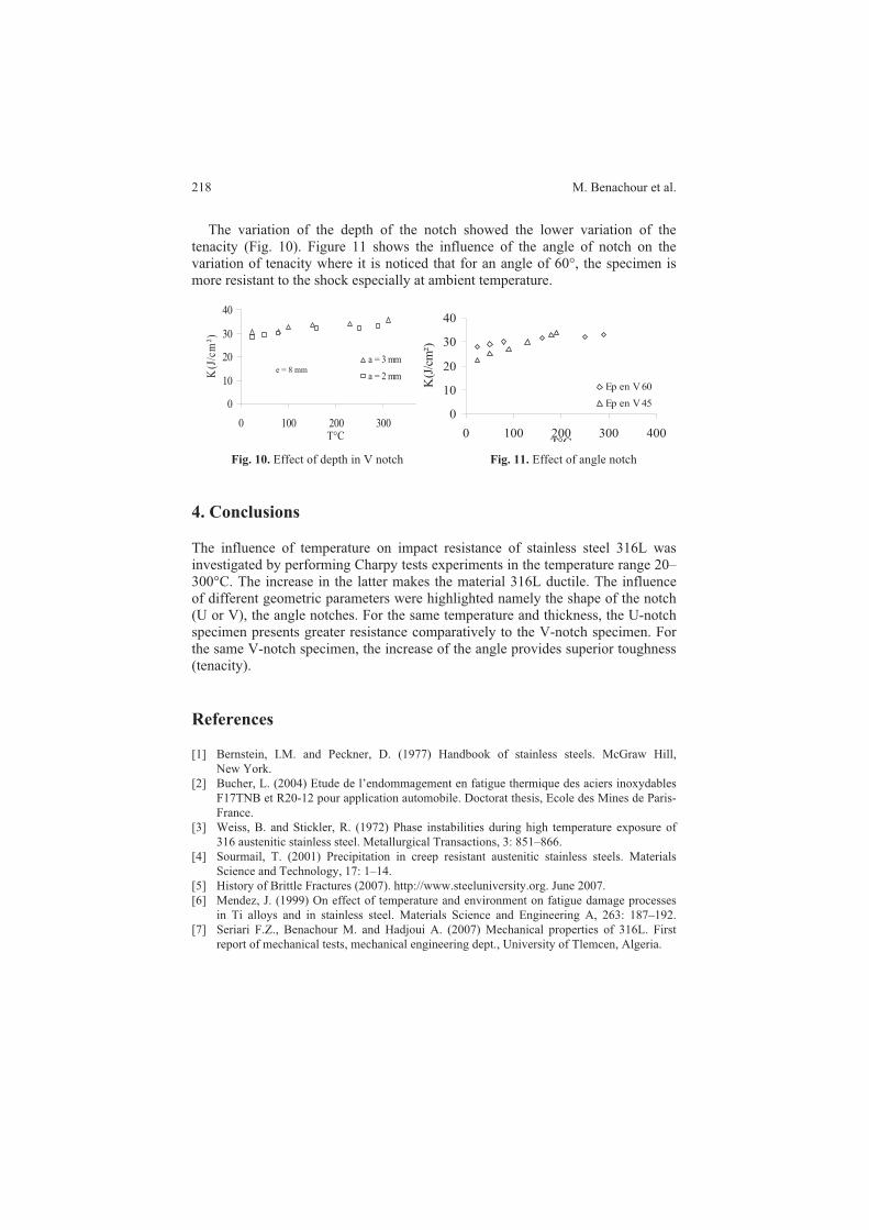
M. Benachour et al.
The variation of the depth of the notch showed the lower variation of the
tenacity (Fig. 10). Figure 11 shows the influence of the angle of notch on the
variation of tenacity where it is noticed that for an angle of 60°, the specimen is
more resistant to the shock especially at ambient temperature.
0
10
20
30
40
0 100 200 300T°C
K(J
/cm
²)
a = 3 mm
a = 2 mme = 8 mm
0
10
20
30
40
0 100 200 300 400T°C
K(J
/cm
²)
Ep en V 60
Ep en V 45
Fig. 10. Effect of depth in V notch Fig. 11. Effect of angle notch
4. Conclusions
The influence of temperature on impact resistance of stainless steel 316L was
investigated by performing Charpy tests experiments in the temperature range 20–
300°C. The increase in the latter makes the material 316L ductile. The influence
of different geometric parameters were highlighted namely the shape of the notch
(U or V), the angle notches. For the same temperature and thickness, the U-notch
specimen presents greater resistance comparatively to the V-notch specimen. For
the same V-notch specimen, the increase of the angle provides superior toughness
(tenacity).
References
[1] Bernstein, I.M. and Peckner, D. (1977) Handbook of stainless steels. McGraw Hill,
New York.
[2] Bucher, L. (2004) Etude de l’endommagement en fatigue thermique des aciers inoxydables
F17TNB et R20-12 pour application automobile. Doctorat thesis, Ecole des Mines de Paris-
France.
[3] Weiss, B. and Stickler, R. (1972) Phase instabilities during high temperature exposure of
316 austenitic stainless steel. Metallurgical Transactions, 3: 851–866.
[4] Sourmail, T. (2001) Precipitation in creep resistant austenitic stainless steels. Materials
Science and Technology, 17: 1–14.
[5] History of Brittle Fractures (2007). http://www.steeluniversity.org. June 2007.
[6] Mendez, J. (1999) On effect of temperature and environment on fatigue damage processes
in Ti alloys and in stainless steel. Materials Science and Engineering A, 263: 187–192.
[7] Seriari F.Z., Benachour M. and Hadjoui A. (2007) Mechanical properties of 316L. First
report of mechanical tests, mechanical engineering dept., University of Tlemcen, Algeria.
218

T. Boukharouba et al. (eds.), Damage and Fracture Mechanics: Failure Analysis of Engineering
© Springer Science + Business Media B.V. 2009
Spall Fracture in ARMCO Iron: Structure
Evolution and Spall Strength
Oleg Naimark, Sergey Uvarov and Vladimir Oborin
Institute of Continuous Media Mechanics of Russian Academy of Sciences, 1 Koroleva str.,
614013 Perm, Russia.
Abstract The experimental study of material responses in a wide range of loading rate reveals
some insight into dynamic failure and shows the linkage of solid behavior with the evolution of
mesoscopic defects such as microcracks and microshears. This situation is strongly connected to
dynamic and shock wave loading, when the time for mesodefect evolution, across different
length-scales approaches the characteristic loading times. Taking into account the nature of
plastic deformation and failure the key problems are related to the statistics and thermodynamics
of the mesoscopic defects. This is revealed in the features of non-equilibrium systems with “slow
dynamics”. “Slow dynamics” is the consequence of collective interactions between mesodefect
modes with slow spatial-temporal response in comparison to the acoustic properties of the
material (elastic wave propagation). The existence of these slow modes dominates the failure in
dynamically loaded and shocked materials. The original study was conducted to support
theoretical results and constitutive relations, which describe a different scenario of damage-
failure transition with a self-organized criticality in mesodefect behavior – the structural-scaling
transition.
Keywords: Dynamic Fracture, Plate Impact, Spalling, Mesodefect, Self-Similarity.
1. Collective modes in mesodefect ensembles
Statistical theory of the collective behavior of mesodefect ensemble [1] allowed us
to describe the phenomenology of solids with mesodefects and the interpretation
of failure kinetics as non-equilibrium structural-scaling transition in mesodefect
ensembles. The non-equilibrium free energy F represents generalization of the
Ginzburg-Landau expansion in terms of order parameters - defect density tensor
(defect induced deformation zzp p in uni-axial case) and structural scaling
parameter , that depends on characteristic length-scales of mesodefects and
plays a role similar to the “effective temperature” in non-equilibrium mesoscopic
systems.
2642 ,6
1
4
1,
2
1ppDp CBpp AF lc* (1)
219
Materials and Structures, 219–225.

O. Naimark et al.
where zz is the stress, is the non-locality parameter, , , ,A B C D are the
material parameters, * and c are characteristic values of structural-scaling
parameter (bifurcation points) that link the range of nonlinear material response to
the defect growth. These ranges correspond to the characteristics of the collective
modes generated in different ranges of , (Fig. 1).
pc
cc
c
c
c
p
p
*
*< <
< >
x
x
z
zt
o
Fig. 1. Characteristic responses on the defect growth
These are responsible for plastic relaxation and the damage-failure transition.
These collective modes are the self-similar solutions ( , )Sp x t of the growth
equations [1]:
( ( )),p l lp F p x p x
F
&
& (2)
where ,ç are the kinetic coefficients, is the non-locality parameter. These
solutions have the form of the quasi-periodic solution for the fine-grain state 1S ,
the auto-solitary waves for plastic strain localization area 2S and blow-up
dissipative structures 3S for damage localization “hotspots”, Fig. 2. The blow-up
solution reads.
( ) (1 ) mc
p g t f
g t G t, Cx L (3)
where c is the so-called “peak time” ( p at ct ), CL is the scale of
damage localisation, 0, 0G m are the parameters describing the non-linearity,
which characterise the free energy release rate for c .
The function ( )f determines the distribution of defect density in the damage
zone. The characteristic stages of damage-failure transition are similar to the
220

Spall Fracture in ARMCO Iron: Structure Evolution and Spall Strength
kinetics of heat localisation in the theory of combustion [2, 3] and include an
induction, or nucleation, time and the “peak-time” or growth-rate parameter.
1S
2 S 3S
Fig. 2. Dissipative structures
Solution (3) describes the nucleation of simple structure–failure hotspot (localized
on the scale CL ) and the generation of complex dissipative structures on the scales
~ , 1,2...D ÑL kL k , due to the interaction on the spatial scales related to the
current blow-up localization scales. Depending on the load history (stress amplitude,
pulse duration) different scenario of damage-failure transitions can be realized:
generation of simple dissipative structure that is characteristic for high amplitude
impact load and complex dissipative structures that can be excited by low
amplitude but temporally long pulse. The failure wave phenomenon in glasses was
linked in [3, 4] with subsequent excitation of simple blow-up dissipative structures
with a minimum delay time C of failure front after the back stress front. Similar
phenomena were observed in [5] for spall failure as the asymptotic limit of spall
failure time, the so-called “dynamic branch under the spall”.
2. Experiment
Spalling is a specific kind of fracture which is loading history dependent. The
multiscale nature of failure hotspot nucleation was studied in the recovery plate
impact test for Armco-iron specimens subject to low amplitude shock. A setup for
plate impact experiment has been developed at ICMM UB RAS to study dynamic
fracture at strain rates up to 106 s 1. Setup consists of 125 mm gas gun and
measurement equipment (VISAR).
Soft recovery of a specimen allowed us to investigate structure changes caused
by plate impact. Specimen (target) was 10 mm thick and polished with 1 m
diamond powder in order to make sharp wave front. Impactor was made from the
same material and was 5 mm thick. So spall should be at 5 mm from the rear (free)
surface of the specimen.
221

O. Naimark et al.
Experiments were carried out at a different impactor velocity in order to
investigate dependency on loading conditions. Pure (so-called “ARMCO”) iron
specimens were tested (Table 1).
Table 1. Chemical composition of material under investigation (rest of material – Fe)
% Mn% Si% S% P% Cu% Cr% Ni% Mo% W% Al% N%
0.004 0.04 0.05 0.005 0.005 0.051 0.038 0.057 0.01 0.015 0.07 0.006
All specimens was annealed at 800°C for 4 h. Optical microscopy and 3D
profilometer observations was used for investigation of the mechanisms of spall
fracture at different scales. Cross-section of the specimen was analyzed. Etching
reveals the residual stresses because different rate of etching caused by residual
stress leads to formation of corresponding 3D profile (Fig. 3 left image). On Fig. 3
one can find slip bands inside grains. These slip bands (pointed by arrows)
corresponds to damage accumulation on the “thermodynamic” brunch (stresses
from zero to c on Fig. 1). In the material closer to the spall surface (Fig. 4) one
300 m
Fig. 3. 2 mm from the free surface. Impact velocity is 375 m/s. Left image – optical, right – 3D
profile
Fig. 4. 3.5 mm from the free surface Impact velocity is 375 m/s. Left image – optical, right – 3D
profile (scale is the same as in previous figure)
222

Spall Fracture in ARMCO Iron: Structure Evolution and Spall Strength
can find small cracks. The concentration of these cracks increases with approaching
to the spall surface (Fig. 5). This shows that stress level and defect density is
approaching to the critical value. On Fig. 6 one can point high level of fragmentation
of the grains in the layer close to the spall surface (left side of the image) and
comparative lower residual stress level.
Fig. 5. 4 mm from free surface Impact velocity is 375 m/s. Left image – optical, right – 3D profile
(scale is the same as in previous figure)
Spall surface
Fig. 6. 4.9 mm from the free surface. Spall surface is on the left impact velocity is 375 m/s. Left image – optical, right – 3D profile (scale is the same as in previous figure)
Fig. 7. Microcracks in the bulk of the specimen 3.5 (left) and 1.5 (right image) mm from free
surface (1.5 and 3.5 mm from the spall surface respectively), impact velocity is 250 m/s
223

O. Naimark et al.
300 m
Fig. 8. Microcracks close to the spall surface (on the right), impact velocity is 250 m/s
At lower impact velocities type of the failure is different. One can see sets of
cracks parallel to the main spall situated quite far (comparing to previous case).
This can be explained as follows: as stress level is low there is not enough initial
defects generated by the compression pulse. And rate of defect growth prior to
reach of critical value is low. So spall failure takes longer time (because induction
time is bigger) and area where stress level is enough to create damage is wider
(Figs. 7 and 8).
3. Conclusions
Damage-failure transition is described as a specific form of self-organized criticality
in the ensemble of mesoscopic defects – structural-scaling transition. Characteristic
features of this transition are the generation of collective modes in mesodefect
ensemble that are responsible for damage localization and transition to failure.
Collective modes have the nature of self-similar solution and describe the blow-up
damage localization kinetics with characteristic time (peak-up time) on the set of
spatial scales. Mechanism of spall failure can be linked with resonance excitation
of blow-up collective modes and has the nature of delayed failure with the delay
time corresponding to the peak-time of the self-similar solution.
References
[1] O.B. Naimark. Defect induced transitions as mechanisms of plasticity and failure in
multifield continua (review paper). In Advances in Multifield Theories of Continua with
Substructure, Birkhauser Boston, Inc., Eds: G. Capriz, P. Mariano, 2003, pp. 75–114.
[2] O.B. Naimark. Collective properties of mesodefect ensembles and some nonlinear problems
of plasticity and failure. Physical Mesomechanics, 2003, v. 6, pp. 45–72.
[3] O.B. Naimark, S.V. Uvarov. Nonlinear crack dynamics and scaling aspects of fracture
(experimental and theoretical study). International Journal of Fracture, 2004, v. 128, n. 1,
pp. 285–292.
224

Spall Fracture in ARMCO Iron: Structure Evolution and Spall Strength
[4] O.B. Naimark, S.V. Uvarov, D.D. Radford et al. The failure front in silica glasses, In Fifth
International Symposium on Behaviour of Dense Media Under High Dynamic Pressures,
Proceedings of the International Conference, Saint Malo, France, 2003, v. 2, pp. 65–74.
[5] O.A. Plekhov, D.N. Eremeev and O.B. Naimark. Failure wave as resonance excitation of
collective burst modes of defects in shocked brittle materials. Journal of Physique IV Colloq
C., 2000, v. 10, pp. 811–816.
225

T. Boukharouba et al. (eds.), Damage and Fracture Mechanics: Failure Analysis of Engineering
© Springer Science + Business Media B.V. 2009
Damage Modelling of Impacted Tubular
Structures by Using Material Property
Degradation Approach
Mostapha Tarfaoui1, Papa Birame Gning
1 and
Francis Collombet2
1ENSIETA, LBMS-Mechanics of Naval Structures Laboratory, 2 rue François Verny 29806
Brest Cedex 9, France
2Ecole des Mines de Saint-Etienne, France
Abstract This paper presents a finite element analysis of dynamic tests on thick filament
wound glass/epoxy tubes. The overall objective of the current research is to develop progressive
failure analysis methodology for laminated composite structures under impact loading
conditions. The first part deals with the identification of damage initiation and its development in
dynamic tests. Under impact the dynamic responses without damage are well simulated just like
the loading in biaxial stress of the tubes. The FEA results of the dynamic tests resulting in no
damage appeared satisfactory. The second part of the paper is concerned with an impact model
used for damage prediction. Most of the well established failure criteria are included in the
damage model. A simple post-failure property degradation scheme is proposed for carrying out
the progressive failure analysis. Simulated damage is compared with that obtained experi-
mentally. The sizes of projected and cumulated surfaces are of the same order of magnitude as
experimental measurements.
Keywords: Tubular Structures, Damage, Material Property Degradation.
1. Introduction
During their use, it is noted that certain impacted composite cylinders do not
sustain operating pressures which correspond to the dimensioning values. However,
the damage introduced by accidental impact can jeopardize the capacity to fulfill
the designated function. Indeed, taking into account the low speed of the immersed
objects, it is a question of studying the impact behavior at the time of a low-energy
impact. The lack of understanding of the tolerance to impact for the tubular
structures is one of the aspects which prevent greater use.
In order to improve the safety of the composite structures in marine environment,
it is important to evaluate and predict the damage resulting from an impact with a
low incidental speed and to assess the incidence of the damage compared with a
stress in external hydrostatic pressure.
227
Materials and Structures, 227–235.

M. Tarfaoui et al.
Krishnamurthy et al. [1] made a vast finite element analysis (FEA) study,
similar to that of Kim et al. [2], on the dynamic response of thin carbon/epoxy
composite cylinders in, subjected to impact by a falling weight. Tubes, 200 mm in
diameter, 2.54 mm thick and 420 mm long with 0°, 45° and 90° lay-up are
studied. The results are compared with those obtained on models of cylindrical
panels of the same thicknesses, with variable curvature. The projectile is 12 mm in
diameter with an incident speed of a few meters per second. The Fourier series
analysis used to determine the shell deflection during impact as proposed by
Christoforou and Swanson [3] and the Choi and Chang criterion [4] is adopted.
They produced results of a parametric FEA study whose variables are the mass
of the projectile, incidental speed, panel curve, layers orientations and boundary
conditions. They showed that speed had more influence on the contact force than
the mass of the projectile, both for elastic and plastic impact. From this point of
view the cylindrical shells behavior is similar to that of the plates at the time of
impact. As Kim et al. [2] noted, the contact force increases with the curve while
the deflection of the target and the contact time decrease.
The damage form and size tend to stabilize towards a peanut shape when the
curves are low. However, for large curves, the effects on the damage cannot be
correctly studied due to the fact that this curve significantly changes the size of the
studied panel and influences its response to the impact.
After carrying out the static, dynamic and implosion tests on the composite
cylinders [5–7], the aim of this study is their modeling by using finite element
method. Initially, certain models are used for validating material characteristics
and predicting their elastic behavior for static and dynamic loadings. Then, the
prediction of the damage after impact is studied. For that, analytical models and
finite element analysis are presented.
2. Materials, geometry and reference mark
The materials examined in the study were all manufactured using the filament
winding process. E-glass fibres were impregnated with a low viscosity epoxy
resin. These cylinders were cured at 125°C for 7 h and measured fiber volume
fraction Vf was 62%. Porosity was about 10%. The cylinders used have an
internal diameter of 55 mm and a wall thickness of 6.5 mm. Samples for impact
and pressure testing are 110 mm long. Micrographic observations show a [ 55]10
stacking sequence lay-up. Material properties are shown in Table 1. Figure 1
shows the principal notations and coordinates adopted in this study.
Table 1. Material properties used for modeling
Material E11 (GPa) E22 (GPa) G12 (GPa) 12
Glass/epoxy ply 0° 49.5 15.9 5.6 0.255
228

Damage Modelling of Impacted Tubular Structures
(a) Sample
Fig. 1. Materials, geometry and reference mark
3. Finite element analysis (FEA)
The studied cylinders are thick (di/t > 10) because of dimensioning to the buckling
which confers a strong thickness. Furthermore, they are modeled by two types of
finite elements, solid and shell elements. The models presented were studied using
ABAQUS version 6.2 [8]. Shell elements with reduced integration S4R with
Mindlin formulation and hexahedral solid elements, C3D8R, in impact cases
available in the library were used with geometric nonlinearity. Based on micro-
scopic observations, the tube’s thickness was modeled as shell and solid laminated
cylindrical elements with transversely isotropic plies. The impactor, of great
stiffness (quenched steel) compared to the composite cylinder, was modeled as
rigid body. Modeling as deformable body requires 3D elements which demands
considerable computing time. Plate and cradle, were considered also as rigid
bodies and were taken as the “master surface”. The contact algorithm used is based
on the penalty method. Also, a specific contact law is implemented to reproduce
local Hertzian contact effects during the quasi-static indentation phase. Meshes
consist of isometric elements. For these two types of elements, five integration
points are considered in the thickness of each layer. The integration method uses
the Simpson rule. The selected elements have linear interpolation. They give better
results for modeling contact and impact with the possibility of severe distortions
of the elements.
4. Impact without damage
A series of impact tests was performed on 40 cylinders. A new cylinder was
impacted for each test, using a 1.6 kg, 50 mm diameter hemispherical quenched
steel impactor. Increasing drop height varied the impact energy. In this part, an
examination of the prediction of the dynamic responses of the cylinders under
impact by finite element analysis is proposed. In order to model the dynamic
phenomena under ABAQUS, it is possible to solve the problems with an Explicit
or Implicit algorithm.
229
(b) Tube coordinates and notations
h
1
3
0
2
–q+j
–j
z
r
t
ri r = r
i+t
2

M. Tarfaoui et al.
Our choice being carried on a modeling with shell elements, the simulation of
the elastic impact uses the same geometries as those of Fig. 2a. The impact speed
is imposed as an initial condition on the projectile at reference point 1.6 kg weight.
An example of the recorded force and displacement versus time plot for one
of non-damaging tests is shown in Fig. 2, together with a model prediction.
Comparatively, the results give a satisfactory prediction to the filtered experimental
signals. Moreover, the models in implicit dynamics predict the experimental
results well and are invaluable in order to have short computing times compared
with those of explicit modeling. Also, regarding the continuation of the numerical
study, modeling with Abaqus/Standard would seem more judicious. The other
reason for this choice is of a technical nature. Indeed, the subroutine used in
Section 5, in order to take into account the damage of the tubes after impact, is
available only in the implicit dynamics algorithm in this version of ABAQUS.
Fig. 3. FEA of a quarter and a whole tube, 2J impact (1.55 m/s)
In order to reduce computing times by the reduction in the element number of
the models without harming the quality of simulation results, one strategy consists
in exploiting the geometrical symmetries. Knowing that there are terms of
membrane/twist coupling related to the [±55]n lay-up, it should be checked that
their effects do not deteriorate the modeling of a quarter cylinder. The results are
compared in Fig. 3.The two models give the same responses for the contact load
and the displacement of the projectile versus time. This satisfactory result led us to
work on a quarter of cylinder with shell elements.
Fig. 2. Model (a) and elastic responses with explicit and implicit algorithms (b), 2J impact (1.55 m/s)
230
7000
Projectile
Sample
Cradle
6000
5000
4000
3000
2000
1000
0 0.5 1
Time (ms)
ImplicitTest
Explicit
Load (
N)
1.50
7000
6000
5000
4000
3000
2000
1000
0 0.5 1 1.5
Time (ms)
Lo
ad
(N
)
Whole model1/4 model
0
0 1Time (ms)
Whole model
1/4 model0.1
0.2
0.3
0.4
0.5
0.5 1.5
0.6
0.7
0.8
0
(a) (b)

Damage Modelling of Impacted Tubular Structures
5. Numerical study of the damage
All preceding simulations related to tube behavior are compared and validated by
experimental measurements. The tests showed that beyond 4J incidental energy,
damage occurs in the wall of the tubes tested. This damage corresponds to through-
the-thickness delamination, which propagates as the incident energy increases.
The damage mechanism in static punching and impact tests is the same [7, 8].
Firstly, a small local indentation at the contact point is noted for low incident
speeds or energies. At that level only the superficial resin coat layer of about
0.3mm thickness is damaged and after the threshold energy level is reached,
delamination occurs through the thickness as noted by Alderson and Evans [9].
For energies up to 7 J, transverse intra-layer cracks appear, weakening the already
delaminated plies. Delamination propagates through the tube thickness in conical
shape of damaged volume for lower energies.
5.1. Damage modeling: material property degrdation
To simulate the evolution of the damage, modeling must take into account the
various forms of damage occurring at the impact tests. It is not necessary that the
numerical model take account all the physical phenomena observed if their
presence does not affect in a relevant way the tubes behavior. It was decided to
restore only the damage of the matrix and fiber/matrix shear. For that, the Hashin
criteria [10] were used.
The expressions (1) and (2) predict the matrix cracking, respectively in traction
and compression, when me reaches unity. Equation (3) predicts fiber/matrix shear
for a value of fe equal to 1. These criteria are calculated in all the integration
points of all the layers of the cylinder.
22
12
2
2m
c
eSY
(1)
22
12
2
2m
t
eSY
(2)
22
12
2
1f
c
eSX
(3)
231

M. Tarfaoui et al.
Table 2. Dependence of the elastic properties on the field’s variables FV1 and FV2
State of material Elastic properties FV1 FV2
Undamaged E1 E2 12 G12 0 0
Matrix cracks E1 0 0 G12 1 0
Fiber-matrix de-bonding E1 E2 0 0 0 1
In progressive failure analysis, once failures are detected in a ply, the
corresponding material properties are degraded (the corresponding mechanical
characteristic becomes nil). Since damage initiation was observed along all the
edges of specimen, a uniform mesh size was used. A standard user subroutine
USDFLD in ABAQUS was written, which allows the user to define material
properties as a function of the field variables (FV1, FV2) at a material point. The
material properties of the laminated tube were defined in order to be dependent
upon two field variables. The states of material taken into account are the healthy
case, the damage of the matrix and the decohesion fiber/matrix presented in Table 2.
5.2. Damage evolution
The progressive failure analysis methodology uses the C0 four-node shell element
S4R of the ABAQUS element library based on the first order shear deformation
theory, due to its better performance in large deformation analysis. Loads and
displacement versus time are coherent with experimental measurements. The
damage is initiated and progresses as much as the tube becomes deformed until
maximum deformation has been reached. When the impactor rebounds, the
damage does not evolve any more. To validate this modeling method, we measure
the evolution of the projected and cumulated delamination area as a function of
incident energy. Figure 4 compares the evolutions of the surfaces predicted by the
model with experimental measurements [5–6].
Fig. 4. Comparison of the measured and calculated surfaces damaged
232
800
FEA-AbaqusFEA-Abaqus
TestTest
TendencyTendency
Cum
ula
ted s
urf
ace (
mm
2)
700
600
500
400
300
200
100
00
Pro
jete
d s
urf
ace (
mm
2)
2 4 6 8
Impact energy (J)
1000 2 4 6 8 10
Impact energy (J)
3000
2500
2000
1500
1000
500
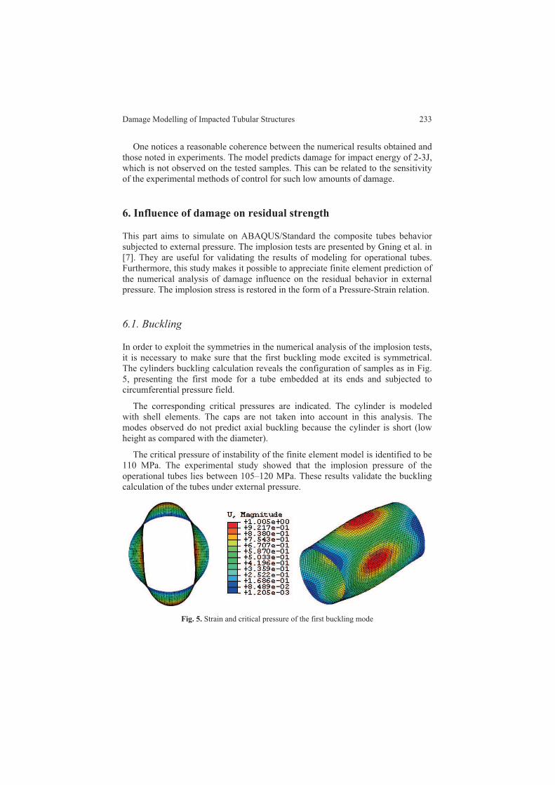
Damage Modelling of Impacted Tubular Structures
One notices a reasonable coherence between the numerical results obtained and
those noted in experiments. The model predicts damage for impact energy of 2-3J,
which is not observed on the tested samples. This can be related to the sensitivity
of the experimental methods of control for such low amounts of damage.
6. Influence of damage on residual strength
This part aims to simulate on ABAQUS/Standard the composite tubes behavior
subjected to external pressure. The implosion tests are presented by Gning et al. in
[7]. They are useful for validating the results of modeling for operational tubes.
Furthermore, this study makes it possible to appreciate finite element prediction of
the numerical analysis of damage influence on the residual behavior in external
pressure. The implosion stress is restored in the form of a Pressure-Strain relation.
6.1. Buckling
In order to exploit the symmetries in the numerical analysis of the implosion tests,
it is necessary to make sure that the first buckling mode excited is symmetrical.
The cylinders buckling calculation reveals the configuration of samples as in Fig.
5, presenting the first mode for a tube embedded at its ends and subjected to
circumferential pressure field.
The corresponding critical pressures are indicated. The cylinder is modeled
with shell elements. The caps are not taken into account in this analysis. The
modes observed do not predict axial buckling because the cylinder is short (low
height as compared with the diameter).
The critical pressure of instability of the finite element model is identified to be
110 MPa. The experimental study showed that the implosion pressure of the
operational tubes lies between 105–120 MPa. These results validate the buckling
calculation of the tubes under external pressure.
Fig. 5. Strain and critical pressure of the first buckling mode
233

M. Tarfaoui et al.
6.2. Influence of damage on residual strength
The tube behavior under external hydrostatic pressure loading is well predicted
numerically. The damage is introduced into the modeling of the impact tests. The
purpose of this section is to check the damage influence in the simulation of
implosion tests. The steps consist in modeling the impact on a tube then recovering
the geometry of the damaged tube for a calculation of loading under external
pressure. There are two different simulations. In the first case, the modeled tube
interacts with a rigid cradle and projectile, while in the second it is necessary to
have the deformable closing caps at the ends of the tube.
To pass from one to the other, it is necessary to safeguard the state of damage
(FV1 and FV2) of all the integration points of the tube at the end of the impact
calculation, then to reallocate this state at the same points of integration of the
tube at the beginning of the implosion simulation. In this second calculation, the
initial damage resulting from the impact can evolve with the pressure.
The material characteristics degradation is included when the criteria (3), (4)
and (5) are reached. Table 3 shows the external collapse pressure as a function of
the impact energy. Up to 5 J the impact residual pressure is retained at the same
level as that of undamaged tubes. Beyond this value the loss of pressure resistance
is very significant, up to 40% between 5 J and 9 J impacts. Further increase in
impact energy leads to a small additional loss and for a 9 J impacted tube the loss
of pressure is about 50%. This indicates a significant loss of pressure resistance
for quite low impact energies. Simulations of external pressurization are made for
tubes impacted between 2 and 9J.
Table 3. Numerical and experimental critical pressures for various energies of impact
Impact energy (J) FE pressure (MPa) Tests pressure (MPa)
0 110 113
2 39 110
4 39 –
5 39 111
9 36 72
7. Conclusions
The FEA results of the quasi-static and dynamic tests without damage appear
satisfactory. The simulation of implosion of the tubes gives results in coherence
with the experimental values. The impact model, including material property degrade-
ation, predicts a truncated form of the damaged volume. The sizes of projected
and cumulated surfaces are of the same order of magnitude as experimental
measurements.
234

Damage Modelling of Impacted Tubular Structures
The simulation of implosion of previously impacted FE models is complex.
The study showed an effect of the damage on the residual pressures of implosion
with a fall more severe than what is observed in experiments. The validity of the
model depends on the choice of the failure criteria and precision on the materials
parameters. In our case, Hashin criterion was selected. The identification of the
data materials to failure is facilitated by the assumption of brittle elastic behavior.
The study showed that there is a strong coupling between the structure and
material and it is then important to control the influence of the conditions of
development on the limiting values of material. Once validated, the modeling
allows for parametric studies.
References
[1] Krishnamurthy K.S., Mahajan P., and Mittal R.K. Impact response and damage in laminated
composite cylindrical shells. Composites Structures, 59: 15–36, 2003.
[2] Kim S.J., Goo N.S., and Kim T.W. The effects of curvature on the dynamic response and
impact-induced damage in composite laminates. Composites Science and Technology, 57:
763–773, 1997.
[3] Christoforou A.P. and Swanson S.R. Analysis of simply supported orthotropic cylindrical
shells subjected to lateral impact loads. Journal of Applied Mechanics, 27: 376–382, 1990.
[4] Choi H.Y. and Chang F.K. A model for predicting damage in graphite/epoxy laminated
composites resulting from low velocity point impact. Journal of Composite Materials,
26(14): 2134–2169, 1992.
[5] Gning P.B., Tarfaoui M., Davies P. and Collombet F. Damage development in thick
composite tubes under impact loading and influence on implosion pressure: Experimental
observations. Composites Part B: Engineering, 36(4): 306–318, June 2005.
[6] Gning P.B., Tarfaoui M., Davies P. and Collombet F. Prediction of damage in composite
cylinders after impact. Journal of Composite Materials, 39(10): 917–928, 2005.
[7] Tarfaoui M., Gning P.B. and Collombet F. Residual strength of damaged glass/epoxy
tubular structures. Journal of Composite Materials, 41(18): 2165–2182, 2007.
[8] Hibitt, Karlsson, and Sorensen, Inc. ABAQUS 6.3 Example problems Manual. 2003.
[9] Alderson K.L. and Evans K.E. Failure mechanisms during the transverse loading of
filament-wound pipes under static and low velocity impact conditions. Composites, 23(3):
167–173, 1992.
[10] Hashin Z. Failure criteria for unidirectional fiber composites. Journal of Applied Mechanics,
47: 329–334, 1980.
235

T. Boukharouba et al. (eds.), Damage and Fracture Mechanics: Failure Analysis of Engineering
© Springer Science + Business Media B.V. 2009
Fracture Control for Northern Pipelines
W.R. Tyson
CANMET Materials Technology Laboratory
Natural Resources Canada 568 Booth St. Ottawa, Ontario, K1A 0G1, Canada
Abstract Natural gas has been discovered in Canada’s north, and a pipeline is being designed
to bring it to markets in the south. The line will cross regions of unstable terrain, and may be
required to withstand substantial deformation from ground movement. Prevention of fracture
under these conditions is an engineering challenge. The main features of the fracture control plan
being developed will be discussed, in particular the prevention of girth weld rupture and the
arrest of running fractures.
Keywords: Pipeline, Steel, Fracture, Toughness, CTOA.
1. Introduction
Canada’s conventional reserves of gas and oil have passed peak production, and
increasing reliance is being placed on “frontier” resources in the tar sands of Alberta,
the east coast offshore, and the north. Major reserves of gas have been identified
in the Mackenzie Delta, and a gas pipeline down the Mackenzie Valley is in an
advanced stage of planning (line through the Northwest Territories, Fig. 1).
Fig. 1. Planned gas pipelines in Canada’s north
237
Materials and Structures, 237–244.

These pipelines will pass through environmentally sensitive terrain, and the
consequences of a leak or rupture would be severe. Also, the unstable terrain can
cause deformation of the pipe through ground movement in the form of landslides
or frost heave. These conditions place heavy responsibility on an adequate fracture
control plan.
2. Fracture Control
There are two main approaches to fracture control at the design stage: prevention
of initiation, and assurance of arrest. In the longer term, environmental degradation
can lead to corrosion and stress-corrosion cracking, which is outside the scope of
this paper and will be dealt with elsewhere.
Fig. 2. Incomplete fracture of Charpy sample of high-strength steel
Regarding crack arrest, the problem is to choose a material that is tough enough
to stop a crack within a short distance. This has traditionally been done using a
model developed by Battelle in the 1970s, relying on Charpy absorbed energy to
characterize toughness and calibrated using steels then available. However, with
the introduction of clean steelmaking and advanced rolling practices, steel is now
much tougher and may not be completely fractured in a traditional test (Fig. 2).
This has led to a need for alternative approaches to characterize the toughness. A
leading candidate is the crack-tip opening angle (CTOA) (Fig. 3), which can be
measured [1] by analysis of the load-time trace in a drop-weight tear test (DWTT).
Methods to measure CTOA are now well advanced, and there is a draft ASTM
standard for measurement of CTOA in sheet materials. However, consensus on the
best approach for assuring crack arrest in pipelines using CTOA has not yet been
established, and it is likely that full-scale burst-test validation of arrest capabilities
of candidate steels will be required for some time to come.
Regarding crack initiation, this generally occurs from pre-existing defects. In
the case of northern pipelines, the concern is about small imperfections in the girth
welds that may escape detection. If the pipe is subjected to bending deformation or
tensile loading, and if the toughness is inadequate, these imperfections may grow
into through-wall cracks and cause leaks or ruptures. There is a well-developed
technology to estimate the material toughness required to prevent crack growth
beyond an acceptable amount that began with the introduction of the “COD design
curve” in the 1960s.
238 W.R. Tyson

Fracture Control for Northern Pipelines
Fig. 3. Crack opening profile of a propagating crack; CTOA = 23.5
This methodology has evolved into the “Failure Acceptance Diagram” approach
exemplified by the British standard BS 7910 [2]. The toughness measure used in
the FAD is the crack-tip opening displacement (CTOD) or, equivalently, the J-
integral. The amount of crack growth corresponding to a given CTOD is measured
to generate the “resistance curve”, or R-curve. This is then related to the crack
driving force in service which can be calculated using finite element methods, and
the toughness at an acceptable amount of crack growth or at instability can then be
deduced. Traditionally, the R-curve has been measured using a pre-cracked bar
subjected to a bending load (Fig. 4). This gives a conservative measure of the
resistance and, if the specimen is above a certain minimum size, the R-curve will
be a material property, i.e., independent of specimen size.
Fig. 4. Test set-up for CTOD measurement
The FAD approach to defect assessment has served engineering practice well.
Applied to pipelines, the method enables the selection of materials and welding
procedures to guard against brittle fracture and excessive ductile crack growth.
The vast majority of applications have been in a “stress-based design” context, in
which the applied loads are designed to be below the yield stress of the material.
In some circumstances the design stress can be as high as 80% of the yield stress,
but even so the total strains are small, i.e. less than 0.5%. However, for pipelines
passing through unstable terrain such as Canada’s north, it is necessary to design
against large-scale ground movement in which the pipe can be subjected to
deformations large enough to cause plastic strain in the pipe.
239

In particular, the girth welds can be subjected to tensile strains significantly
larger than 0.5%, and it is necessary to ensure that even in this case any weld
imperfections do not cause fracture. To achieve this, the approach of “strain-based
design” has been introduced.
2.1. Strain-based design (SBD)
The basic approach to fracture control using SBD is the same as in stress-based
design, that is, the crack driving force (J or CTOD) is calculated using finite
element methods for a given material (i.e. stress–strain properties) as a function of
load and geometry. The results (i.e., critical strain as a function of critical CTOD,
yield-to-tensile ratio Y/T, and crack geometry 2c/t and a/t) are usually approxi-
mated with an analytical expression for convenience in use. It is then straight-
forward to deduce the required toughness properties for a given applied strain. The
difficulty, however, is that the toughness requirements can be quite severe – so
severe, in fact, that the R-curve measured using the conventional bend test may
give unacceptably low values. Fortunately, however, it is well known that the R-
curve for steels of thickness typical of line pipe is geometry dependent, i.e. that
the results depend on specimen size and, more importantly, on mode of loading.
The toughness in tension is significantly higher than in bending, typically by a
factor of two or so.
A typical result, calculated using the Gurson model for ductile fracture, is
shown in Fig. 5. It is important to take this effect into account in order to design
against fracture in SBD using high-strength steels. For steels of X80 or X100
grade, the yield-to-tensile ratio Y/T can be high (0.9 or so) and the uniform strain
small (10% or so), and it can be a challenge to guarantee adequate toughness,
particularly in the heat-affected zone (HAZ) of circumferential girth welds. To
take advantage of the full tensile toughness of the material, it is necessary to have
an established method for performing the test – in other words, a standardized test.
Unfortunately however, such a test has not been standardized in North America,
although there is a DNV recommended practice for installation methods involving
cyclic strain that includes a fracture test in tension.
Fig. 5. J-resistance curves evaluated by FEA (Gurson model) for 3D SE(B) and SE(T) samples
240 W.R. Tyson
0
400
800
1200
1600
0 1 2 3 4 5
a (mm)
SE(B), Plane strain
SE(B), Plain-sided
SE(T), Plane strain
JR (
kJ/m
2)

Fracture Control for Northern Pipelines
Fig. 6. FEA mesh for SE(T) pin-loaded sample
A pin-loaded sample is shown in Fig. 6. In addition to the crack depth and
cross-section width and thickness, the significant variables are the distance
between the points of load application H and the mode of loading (pin-loaded as in
the figure, or fixed-grip, i.e. clamped). The reason for the relevance of the loading
mode is that pin loading allows the specimen to rotate which introduces bending
into the specimen, while a fixed-grip condition minimizes the amount of rotation.
As the specimen becomes longer (i.e., as H increases), the difference between pin-
loaded and fixed-grip conditions diminishes.
2.2. Constraint
The basic reason for the difference in R-curves in tension and in bending is the
difference in constraint between the two loading modes. Figure 7 shows a side
view of a notched sample loaded in tension in the y direction. The contraction in
the through-thickness direction is evident. This contraction gives rise to a strain
gradient in the through-thickness direction that generates stresses and causes the
central region of the crack front to be in a state of near plane strain. This is the so-
called “out-of-plane” constraint, in contrast to the “in-plane” constraint that
corresponds to stress and strain gradients in the x–y plane. It has been shown
clearly by Wallin [4] that the fracture toughness is controlled by the in-plane
dimensions, and especially by the size of the ligament (the distance in the x
direction between the crack front and the specimen back plane). The reason for
this is that the majority of the crack front is in a state of nearly plane strain even
for specimens much thinner than is normally assumed, and it is the constraint
resulting from the degree of confinement of the plastic deformation in the x–y
plane that dominates the R-curve. In particular, the much more highly contained
plasticity in the bend specimen compared to the tensile specimen leads to much
higher stresses at the crack tip in bending than in tension. This drives the cracking
processes – in ductile fracture, these are microvoid initiation, growth and
241

coalescence – to completion in the so-called “process zone” at the crack tip more
rapidly in bending than in tension and lead to more crack growth in bending.
y
x
Fig. 7. Cracked sample loaded in tension
Figure 8 shows the stress distribution at the crack tip of a part-circumferential
crack in a pipe calculated using 3-D finite element analysis; the HRR curve gives
the asymptotic Hutchinson–Rice–Rosengren stress. The crack-tip opening stress
has been normalized by the yield stress 0, and the distance r from the crack tip
has been normalized by J/ 0. It is helpful to recall that the CTOD = (1/m) (J/ 0)
where m (= 1 to 4) is a parameter dependent on material and mode of loading.
Hence, at a distance of one CTOD from the crack tip we have r/(J/ 0) = 1/m. That
is, the peak stress in the finite element solution occurs at a distance from the crack
tip of the order of one CTOD. The finite element calculations shown in Fig. 8
have been carried out for increasing J. Normalization of J by b 0 (where b is the
ligament length) enables comparison of the ligament length with the CTOD. Since
J/(b 0) = m(CTOD/b), this parameter is of the order of the inverse of the ligament
divided by the CTOD. In other words, for the range of J/(b 0) = 0.0047 to 0.0645,
the CTOD increases from approximately 0.005 to 0.06 of the ligament (for m = 1),
i.e. from 1/200th to 1/15th of the ligament. The crack-tip stresses are significantly
below the HRR limit even for small J values, i.e. there is significant loss of
constraint for this geometry. Note in Fig. 8 that the finite element stresses at a
given J value lie at approximately a constant amount below the HRR stress within
the region of r/(J/ 0) = 1 to 5, i.e. within approximately one to five CTODs of the
crack tip. This region is the fracture “process zone” referred to above, within
which the micromechanical fracture processes of void growth and coalescence
take place. It has also been shown that the loss of constraint in the process zone
can be represented by the superposition of a hydrostatic stress on the HRR field.
The magnitude of this stress (normalized by the yield stress) has been represented
by the Q parameter defined as Q = ( HRR)/ 0, usually evaluated at r/(J/ 0) = 2.
The value of Q gives a good measure of the extent of constraint loss; constraint
loss increases as Q becomes more negative. Since void growth and coalescence
are very sensitive to hydrostatic stress, it is expected that at a given value of
the crack driving force (i.e., J) the amount of crack growth would depend on the
value of Q. That is, Q = 0 represents a highly constrained condition, equivalent to
small-scale yielding which is modelled by the HRR field and approximated by the
high-constraint bend test. For the toughness test to give a good simulation of
service conditions, it is required that the constraint in the test be matched to that in
service, i.e. that the J–Q relations be similar.
242 W.R. Tyson

Fracture Control for Northern Pipelines
0
1
2
3
4
5
6
0 1 2 3 4 5 6 7
r/(J/ 0)
0
HRR
0.0047
0.00251
0.0498
0.0645
Pipe with ext. circ. crack, a/t=0.2,
2c/t=3.64, H/D=1J/(b 0)=
Fig. 8. Crack-tip opening stress for an external part-circumferential crack (3D) in a pipe
Figure 9 compares the J–Q relations for cracks in single-edge-notched tension
SE(T) specimens with those for circumferential cracks in pipe (i.e., girth weld
defects). In these calculations, the loading arrangements for the SE(T) tests are
either fixed-grip (clamped) or pin-loaded, and the spacing H between the load
points is given by H/W = 10 where W is the specimen width. This value of H/W
has been chosen by DNV [3] for tension testpiece geometry to match surface
circumferential cracks in a pipe. Results for crack depths of a/W = 0.2 and 0.5 are
shown in the figure. As expected, the J-Q curve for the shallow crack lies below
that of the deep crack, i.e., Q is more negative for the shallow crack, corresponding to
more constraint loss, at a given value of J. Note also that the mode of loading, i.e.
clamped or pin-loaded, has negligible effect on the J–Q relation for this condition
of a rather large “daylight” between the loading points.
0
0.03
0.06
0.09
0.12
0.15
0 0.5 1 1.5 2-Q
J/(b
0)
SE(T), a/W=0.2, fixed-grip
SE(T), a/W=0.5, fixed-grip
SE(T), a/W=0.2 pin-load
SE(T), a/W=0.5 pin-load
pipe 3D, a/t=0.2, a/c=0.1, H/D=1
pipe, a/t=0.2, H/D=10
pipe, a/t=0.5, H/D=10
H/W=10 for all SE(T)
samples
Fig. 9. J–Q relations for pipe and SE(T) samples [5]
243

It may be concluded from Fig. 9 that a tensile specimen with H/W = 10 loaded
in either fixed-grip or pin-loaded mode provides reasonable constraint matching to
long surface circumferential cracks in pipes subjected to large-scale bending or
tension.
3. Summary
Fracture control is critical for pipelines that traverse environmentally sensitive and
unstable terrain such as that found in Canada’s north. Adequate fracture control
relies on two components: resistance to initiation, and arrest of running fracture.
Crack arrest is assured by specifying the impact toughness, traditionally the
Charpy absorbed energy CVN. However, it has been found for modern high-
strength steels that the CVN may be questioned as a reliable measure of arrest
capability, and increasing attention is being paid to characterization of toughness
using full-thickness specimens and drop-weight tear testing, with the toughness
parameter being the crack-tip opening angle CTOA. Initiation resistance is
achieved by assuring that girth weld defects are below a critical size that is
calculated using the toughness of the weld. It is argued here that the toughness
should be characterized by the CTOD in a tensile test of a pre-cracked sample
with the geometry chosen to provide constraint matching to girth weld defects in
pipe subjected to bending or tension load.
Acknowledgments The work reported in this review has been done by the author’s colleagues
at MTL/CANMET, in particular Réal Bouchard, Su Xu, and Guowu Shen. We are grateful for
support provided by CANMET experts in welding and by personnel in Engineering and
Technical Services, and for the supply of materials by colleagues in industry, notably
TransCanada PipeLines Ltd. Financial support has been provided primarily by the Canadian
Federal Government Program on Energy Research and Development (PERD).
References
[1] Xu SR, Bouchard R, Tyson WR (2007). Simplified single-specimen method for evaluating
CTOA. Eng. Fract. Mech 74: 2459–2464.
[2] Guide on methods for assessing the acceptability of flaws in metallic structures, BS 7910,
British Standards Institution, UK.
[3] Fracture control for pipeline installation methods introducing cyclic plastic strain (2006).
Recommended Practice DNV-RP-F108, Det Norske Veritas, Norway.
[4] Wallin, KRW (2005). ASTM STP 1461. American Society for Testing and Materials, West
Conshohocken, PA, pp 433–453.
[5] Shen G, Bouchard R, Gianetto JA, Tyson WR (2008). Fracture toughness evaluation of high
strength steel pipe, submitted to PVP2008. ASME Pressure Vessel and Piping Division
Conference, July 27–31, 2008, Chicago, Illinois, USA.
244 W.R. Tyson

T. Boukharouba et al. (eds.), Damage and Fracture Mechanics: Failure Analysis of Engineering
© Springer Science + Business Media B.V. 2009
The Influence of the Interface on Fracture
Parameters
L. Marsavina1, 2
and T. Sadowski1
1Lublin University of Technology, Faculty of Civil and Sanitary Engineering, 20-618 Lublin,
Nadbystrzycka 40 street, Poland
2POLITEHNICA University of Timisoara, Department Strength of Materials, Blvd. M.
Viteazu, Nr.1, Timisoara 300222, Romania
Abstract The presence of cracks has a major impact on the reliability of advanced materials,
like fiber or particle reinforced ceramic composites, and laminated ceramics. The understanding
of the failure mechanisms is very important, as much as the estimation of fracture parameters at
the tip of the crack approaching an interface. This paper presents the numerical results for
singularity order, asymptotic stress field and fracture parameters for a crack ending on a bi-
material ceramic interface. The effect of bi-axial loading on asymptotic stress field and stress
intensity factors was investigated.
Keywords: Crack, Bi-Material Interface, Singularity Order, Stress Intensity Factor.
1. Introduction
The presence of cracks has a major impact on the reliability of advanced materials,
like fiber or particle reinforced ceramic composites, and laminated ceramics. The
understanding of the failure mechanisms is very important, as much as the estimation
of fracture parameters at a tip of the crack approaching an interface and crack
propagation path.
Four major classes of interface crack problems could be identified:
Crack approaching a bi-material interface, Fig. 1a
Crack reaching the interface, Fig. 1b
Crack deflection on interface, Fig. 1c
Crack penetration the interface, Fig. 1d
Different researchers have investigated the interaction between an interface and
a perpendicular or inclined crack. Zak and Williams [1] showed that the stress
field singularity at the tip of a crack perpendicular to an interface or terminating at
the interface is of order r , where is the real part of the eigenvalue and depends
on the elastic properties of the bi-material. Cook and Erdogan [2] used the Mellin
transform method to derive the governing equation of a finite crack perpendicular
to the interface and obtained the stress intensity factors. Erdogan and Biricikoglu
245
Materials and Structures, 245–254.

L. Marsavina and T. Sadowski
[3] solved the problem of two bounded half planes with a crack going through the
interface.
Bogy [4] investigated the stress singularity of an infinite crack terminated at the
interface with an arbitrary angle. Wang and Chen [5] used photoelasticity to determine
the stress distribution and the stress intensity factors of a crack perpendicular to
the interface. Lin and Mar [6], Ahmad [7] and Tan and Meguid [8] used finite
element to analyze cracks perpendicular to bi-material in finite elastic body. Chen
[9] used the body force method to determine the stress intensity factors for a
normal crack terminated at a bi-material interface. Chen et al. [10] used the
dislocation simulation approach in order to investigate the crack tip parameters for
a crack perpendicular to an interface of a finite solid. He and Hutchinson [11] also
considered cracks approaching the interface at oblique angles. Chang and Xu [12]
presented the singular stress field and the stress intensity factors solution for an
inclined crack terminating at a bi-material interface. A theoretically description of
the stress singularity of an inclined crack terminating at an anisotropic bi-material
interface was proposed by Lin and Sung [13]. Wang and Stahle [14] using a
dislocation approach presented the complete solution of the stress field ahead of a
crack approaching a bimaterial interface. They also calculate the stress intensity
factor solutions and the T-stress. Liu et al. [15] determined the mixed mode stress
intensity factors for a bi-material interface crack in the infinite strip configuration
and in the case where both phases are fully anisotropic. Kaddouri et al. [16] and
Madani et al. [17] used the finite element analysis to investigate the interaction
between a crack and an interface in a ceramic/metal bi-material.
They investigated the effects of the elastic properties of the two bonded materials
and the crack deflection – penetration at the interface using the energy release rate.
Marsavina and Sadowski [18] highlighted the effect of shielding and anti-shielding
at a tip of a crack approaching a bi-material interface. A biaxial specimen subjected to
mixed mode load was studied using finite element analysis. The competition
between deflection and penetration of a crack ended on a bi-material interface was
investigated by He et al. [19], Zhang and Suo [20], Marsavina and Sadowski [21]
among others. This paper presents the asymptotic stress field and the fracture
parameters at the tip of cracks ended inclined to a bi-material interface. The
numerical results were obtained by considering the two materials as combinations
of Al2O3 and ZrO2, often used in ceramic composite materials.
Fig. 1. Classes of cracks and interfaces
246
Material 1
a b c d
Material 2
Crack
Interface
Material 1
Material 2
Crack
Interface
Material 1
Material 2
Crack
Interface
Material 1
Material 2
Crack
Interface

The Influence of the Interface on Fracture Parameters
2. Singular stress field for an inclined crack terminating
at a bi-material interface
Considering the general case of an inclined crack terminating at the interface with
angle 0 (Fig. 2) the stress and displacement fields could be described by [12]:
11121
11121,,
ij
ij
ij
ij
ij
ijjrj
eDeAeBr
eCeBeAri
(1)
111
111,,2
ij
ij
ijj
ij
ij
ijjjjrj
eCeAeBr
eDeBeAruiu (2)
where (r, ) represents the polar coordinates, is the stress singularity (the
eigenvalue), the complex conjugate of , Aj, Bj, Cj and Dj and their conjugates
are undetermined complex coefficients, j = 1, 2, 3 corresponding with region “j”,
and 1i . The boundary conditions near the crack tip are:
02,01, ,, ruru rr (3a)
02,01, ,, ruru (3b)
03,01, ,, ruru rr (3c)
03,01, ,, ruru (3d)
02,01, ,, rr (3e)
02,01, ,, rr rr (3f)
03,01, ,, rr (3g)
247

L. Marsavina and T. Sadowski
03,01, ,, rr rr (3h)
0,2, r (3i)
0,2, rr (3j)
0,3, r (3k)
0,3, rr (3m)
Substituting Eqs. (1) and (2) into Eq. (3) leads to a linear equation system with
twelve undetermined coefficients: Aj, Bj, Cj, Dj and their conjugates. From its
nontrivial condition it can be obtained the following eigenequation which allows
the determination of the singularity order:
0cos)1()2(sin)1(
)2cos(cos)1(2cos1))(1(
22220
22
2
02
022
(4)
With and the Dundur’s bi-material parameters [22]:
11
11
1221
1221 and 11
11
1221
1221 (5)
where i and i are the shear modulus and Poisson’s ratio of material i (i = 1, 2),
ii 43 for plane strain and iii 1/3 for plane stress. Equation (4)
has basically two solutions in the interval 0 to 1 named 1 and 2. It can be
observed that the stress singularity depends on the material parameters and crack
inclination angle. For 00 or ± the considered model from Fig. 1 becomes an
interface crack model, and Eq. (4) simplifies to:
i2
10cossin 2,1
222 (6)
Known the oscillatory singularity solution for the interface crack, where the
oscillatory index :
248

The Influence of the Interface on Fracture Parameters
1
1ln
2
1 (7)
Here if = = =0 we obtain the well known singularity for a crack in homo-
genous material 1 = 2 = 0.5.
For 2/0the case of normal crack to interface Eq. (4) reduces to:
0cos)1()1)((2 222 (8)
According with [3] and shows two equal real eigenvalues 1 = 2.
An extrapolation method could be applied for the determination of the stress
intensity factors. For example if the singularity orders 1 2) are real values the
stress field could be expresses as:
1
21
11121 rKirKi r for = 0 (9)
And the stress intensity factors could be found:
)(lim),(lim01
1
0201
1
01
21
rrr
rKrK (10)
In order to investigate the stress singularity, combinations between two ceramic
materials were considered: Al2O3 and ZrO2 and angles between crack and
interface from 00 to 900 with 50 increments. The results of Eq. (4) are presented in
Fig. 3 for plane strain. Only the stress singularities 1 and 2 values between 0 and
1 were considered.
Table 1. Material properties and Dundur’s parameters
Properties/material Al2O3 ZrO2
Modulus of elasticity (MPa)
Poisson’s ratio
Fracture toughness (MPa m0.5
)
400000
0.22
4.5
200000
0.25
12
Combinations:
Material 1/Material 2
Dundur’s parameters
ZrO2/Al2O3 Al2O3/ZrO2
E1/E2 ( )
0.5
0.333
0.120
2.0
0.333
0.120
249

L. Marsavina and T. Sadowski
For both material combinations at small angles 0 we obtained complex
oscillatory solutions for 1 and 2, than multiple singularities 1 2 and double
root singularity 1 = 2 for 0 = 900. It can be observed in Fig. 3 that higher
singularities than 0.5 were obtained when the crack is in the ZrO2 (E1/E2 = 0.5),
and lower values when the crack was in the stiffer material for E1/E2 = 2.
Fig. 2. Crack terminating at a bi-material interface
Fig. 3. Singularity orders 1 and 2 as function of crack angle
3. The influence of bi-axial loading on the asymptotic stress field
In order to study the effect of the biaxial load on the asymptotic stress field a quarter
of a biaxial specimen with an interface was numerically investigated with
FRANC2DL code [23]. Plane strain conditions were considered and the model
dimension was w = 50 mm. The materials for the analysis were combinations
between Al2O3 and ZrO2, Table 1. Quadrilateral isoparametric elements were used
for the model with a refined mesh near to crack tip. The mesh consists on 11754
elements connected in 34353 nodes, Fig. 4a. Eight singular elements were placed
around the crack tip as a common technique to model the stress singularity, Fig. 4b.
250
y
Material 2
Region 2
Region 3
Region 1
Material 1
x
r 0
0.7
Real part
Imaginary part
E1/E2=0.5
E1/E2=2.0
0.6
0.5
0.4
0.3
0.2
0.1
00 15 30 45 60
2
l1,l2
2
q0
1
1
75 90

The Influence of the Interface on Fracture Parameters
a. Mesh and boundary conditions b. Crack detail
Fig. 4. Mesh, boundary conditions and crack detail for the FEM model
The model was loaded with different combinations of the applied stresses x
and y (k = x/ y) in order to produce mixed modes from pure Mode I (k = 1) to
pure Mode II (k = 1). The symmetric boundary conditions were imposed. The polar
coordinate system (r, ) was considered with the origin at the crack tip, Fig. 4b.
The singularity orders 1 and 2 were determined numerically from the
asymptotic stress field on a direction = 150 as the slope (1 1,2) of the log
( y) versus log (r/a), respectively log ( r y). The results of singularity orders
are presented in Table 2.
Table 2. Singularity orders for different combinations of mixed mode loading
Material combination k 1.0 0.50 0.0 0.5 1.0
E1/E2 = 0.5 1 0.5475 0.5566 0.5730 0.5995 0.6501
2 0.8342 0.8321 0.6342 0.6457 0.5942
E1/E2 = 2.0 1 0.4587 0.4475 0.4296 0.4086 0.3756
2 0.1955 0.2250 0.371 0.4039 0.4186
The results from Table 2 show that the singularity orders vary significantly
with applied load combination and material properties. Figure 5 presents the radial
variation of the stresses and r for the case when material 1 is ZrO2 on a
radial direction with = 150 and for 0 < r/a < 0.028.
For both material combinations it can be observed that the singularity order is
changing with the load parameter k. In Table 2 and Fig. 5.a it can be observed that
the singularity order 1 increase with the increasing of mode II load (decreasing
k). The singularity order 2 which characterize the singularity of r decreases
with decreasing k. In contrary for the material combination with E1/E2 = 2.0 the
singularity order 1 decrease and 2 increase with decreasing k.
251

L. Marsavina and T. Sadowski
The circumferential stress distributions are plotted at a distance r/a = 0.01 from
the crack tip, in order to be in the singularity zone. For the materials combination
with E1/E2 = 0.5 in Fig. 6 are plotted the circumferential variations of the
normalized stresses to the applied stress in y direction.
Fig. 5. Logarithmic distribution of stresses on a radial direction ( = 150, E1/E2 = 0.5)
It can be observed that the distribution of is changing from symmetric for
k = 1 to skew-symmetric for k = 1, and vice versa for r distribution. The
maximum values for the normal stress on the crack direction ( = 00) were
obtained for k = 1 (mode I) and the minimum for k = 1 (mode II) Fig. 6.a as we
expect. Figure 6b shows that the maximum circumferential stress r on the crack
line ( = 00) was obtained for k = -1 (load in pure mode II) and is 0 for k = 1 (load
in pure Mode I). The maximum values of the circumferential stress r moves
from = 00 for k = 1 to = 74.50 for k = 1. The stress results from Fig. 6 confirm
the stress free boundary conditions on the crack faces ( = ±1800).
Fig. 6. Circumferential distribution of normal stresses at distance r/a = 0.01 from the crack tip
for, E1/E2 = 0.5
The determination of the stress intensity factors was performed using Eq. (10),
by extrapolating at the crack tip the asymptotic results of and r for = 00.
Taking into account the dimensions for the SIF’s (MPa m1 ) it is hard to make
comparisons between other published results. The results were normalized:
252
log( / y)
2
1.5
0.5
0–3.5 –2.5
log(r/a)
–1.5–3 –2
1 k=1
k=0.5
k=0
k=–0.5
k=–1
E1/E2=0.5(a) (b)
log( r / y)
log(r/a)
2
1.5
0.5
0
–0.5
–2.5 –2.3 –2.1 –1.9 –1.7 –1.5
1
E1/E2=0.5 k=1
k=0.5
k=0
k=–0.5
k=–1
q[deg]q[deg]
E2/E1=0.5 E1/E2=0.5(a) (b)
–180 –150 –120 –90 –60 –30 0 30 60 90 120 160 180
–180 –150 –120 –90 –60 –30 0 30 60 90 120 150 180–5
15
10
5
–10
–15
0
–5
15
10
5
–10
0
k=1.0
k=0.5
k=0.0
k=–1.0
k=–0.5
k=1.0
k=0.5
k=0.0
k=–0.5
k=–1.0
sqq/sytrq/sy

The Influence of the Interface on Fracture Parameters
)/( 2,11
2,12,1 aKf (11)
And are shown in Fig. 7. The computed values of the non-dimensional SIF’s
cover entire domain from pure mode I (k = 1) to pure mode II (k = 1). Higher
values for non-dimensional SIF’s were obtained for the case when the crack is in
the compliant material for all load combinations.
Fig. 7. Non-dimensional stress intensity factors f1, f2
4. Conclusions
For the two material combinations by solving the eigenequation different types of
singularities were obtained: complex, multiple or double depending on crack angle
0 and on material combinations. The singularity orders 0 < < 0.5 when the
crack is in the stiffer material and meets the compliant ones, and 0.5 < < 1
when vice versa. Two material combinations for an inclined crack terminating on
a bi-material interface were numerically investigated.
The eigenequation has multiple solutions and the numerical results confirmed
this. The stress intensity factors are estimated by extrapolation technique, based on
the numerical results for the asymptotic stress field. The effect of the bi-axial load
on the asymptotic stress field and on the stress intensity factors for an inclined
crack terminated on the interface was highlighted for five applied mixed modes
and for two material combinations.
Acknowledgments The authors gratefully acknowledge the support of Marie Curie Transfer of
Knowledge project MTKD-CT-2004-014058.
253
2f1, f2
k
1.5
1
0.5
–0.5 0 0.5 1–1
0
f2 (E1/E2 =2)
f2 (E1/E2 =0.5)
f1 (E1/E2 =2)
f1 (E1/E2 =0.5)

L. Marsavina and T. Sadowski
References
[1] Zak AR, Williams ML (1963) Crack point stress singularities at a bi-material interface. J.
Appl. Mech 30:142–143.
[2] Cook TS, Erdogan F (1972) Stress in bonded materials with a crack perpendicular to the
interface. Int. J. Eng. Sci. 10:677–697.
[3] Erdogan F, Biricikoglu V (1973) Two bonded half planes with a crack going through the
interface. Int. J. Eng. Sci. 11:745–766.
[4] Bogy DB (1971) On the plane elastic problem of a loaded crack terminating a material
interface. J. Int. Fract. 38:911–918.
[5] Wang WC, Chen JT (1993) Theoretical and experimental re-examination of a crack at a
bimaterial interface. J. Strain Anal. 28:53–61.
[6] Lin KY, Mar JW (1976) Finite element analysis of stress intensity factors for crack at a
bimaterial interface. Int. J. Fract. 12:451–531.
[7] Ahmad J (1991) A micromechanics analysis of cracks in unidirectional fibre composite. J.
Appl. Mech. 58:964–972.
[8] Tan M, Meguid SA (1996) Dynamic analysis of cracks perpendicular to bimaterial
interfaces using new singular finite element. Finite Elements in Analysis and Design,
22:69–83.
[9] Chen DH (1994) A crack normal to and terminating at a bimaterial interface. Eng. Fract.
Mech. 19:517–532.
[10] Chen SH, Wang TC, Kao–Walter S (2003) A crack perpendicular to the bi-material
interface in finite solid. Int. J. Solids Struct. 40:2731–2755.
[11] He MY, Hutchinson JW (1993) Crack deflection at an interface between dissimilar elastic
materials. Int. J. Solids Struct. 25:1053–1067.
[12] Chang J, Xu J-Q (2007) The singular stress field and stress intensity factors of a crack
terminating at a bimaterial interface. Int. J. Mechanical Sciences, 49: 88–897.
[13] Lin YY, Sung JC (1997) Singularities of an inclined crack terminating at an anisotropic
biomaterial interface. Int. J. Solids Struct. 38:3727–3754.
[14] Wang TC, Stahle P (1998) Stress state in front of a crack perpendicular to bi-material
interface. Eng.. Fract. Mech. 4:471–485.
[15] Liu L, Kardomateas GA, Holmes JW (2004) Mixed – mode stress intensity factors for a
crack in an anisotropic bi-material strip. Int. J. Solids Struct. 41:3095–3017.
[16] Kaddouri K, et al. (2006) Finite element analysis of crack perpendicular to bi-material
interface: Case of couple ceramic–metal. Comput. Mater. Sci. 35:53–60.
[17] Madani K, et al. (2007) Crack deflection at an interface of alumina/metal joint: a numerical
analysis. Comput. Mater. Sci. 35:625–630.
[18] Marsavina L, Sadowski T (2008) Fracture parameters at bi-material ceramic interfaces
under bi-axial state of stress. Comput. Mater. Sci. doi:10.1016/j.commatsci.2008.06.005.
[19] He MY, Hsueh CH, Becher PF (2000) Deflection versus penetration of a wedge-load crack:
effects of branch-crack length and penetrated-layer width. Composites: Part B 31:299–308.
[20] Zhang Z, Suo Z (2007) Split singularities and the competition between crack penetration
and debond at a biomaterial interface. Int. J. Solids Struct. 44:4559–4573.
[21] Marsavina L, Sadowski T (2007) Effect of biaxial load on crack deflection/penetration at
bi-material ceramic interface. Int. J. Fracture 148:79–84.
[22] Dundurs J (1969) Effect of elastic constants on stress in a composite under plane
deformation. J. Compos. Mater. 1:310–322.
[23] Iesulauro E (2002) FRANC2D/L a Crack Propagation simulator for plane layered materials.
Cornell University, Ithaca.
254

T. Boukharouba et al. (eds.), Damage and Fracture Mechanics: Failure Analysis of Engineering
© Springer Science + Business Media B.V. 2009
Crack Propagation in the Vicinity of the Interface Between Two Elastic Materials
Luboš Náhlík, Lucie Šestáková and Pavel Huta
Institute of Physics of Materials ASCR, Žižkova 22, 616 62 Brno, Czech Republic and Institute of Solid Mechanics, Mechatronics and Biomechanics, Faculty of Mechanical Engineering BUT, Technická 2, 616 69 Brno, Czech Republic
Abstract The objective of the paper is to investigate the direction of a further crack propagation from the interface between two elastic materials. The angle of crack propagation changes when the crack passes the interface. The suggested procedure based on a generalized form of Sih’s strain energy density factor makes it possible to estimate an angle of propagation under which the crack will propagate into the second material. The assumptions of linear elastic fracture mechanics and the elastic behavior of the body with interfaces are considered. The finite element method was used for numerical 2D and 3D calculations. The results obtained might contribute to a better understanding of the failure of materials with interfaces (e.g. layered composites, materials with protective coatings, etc.).
Keywords: Bimaterial Interface, Crack Propagation Direction, Layered Composites.
1. Introduction
Real structures often contain regions with different material characteristics, which are mutually divided by an interface. The presence of the interface, where the material characteristics are changed in step, has an important influence on stress distribution in the structure as well as on fracture failure resistance. The influence of the interface between two materials on crack propagation has been studied in many works from various points of view. The existence of a material interface changes the local stress distribution in the vicinity of a crack tip. In contrast to a crack in a homogeneous body where the stress singularity around the crack tip is
of type 5.0r , the stress singularity of a crack touching the interface is of type pr , where r is a radial distance from the crack tip and p is a stress singularity exponent that can be complex and its real part resides within the interval 1)Re(0 p (e.g.
[4, 7 ]). This fact complicates the use of classical linear elastic fracture mechanics (LEFM) approaches and the establishing of criteria for estimating the behaviour of cracks of this type. Due to the different properties of each material(s), the crack changes its propagation direction at the interface. Crack behaviour of this kind has been described e.g. in experimental work [5].
255
Materials and Structures, 255–263.

L. Náhlík et al.
In the paper presented we report the results of a theoretical study concerning the behaviour of a crack with its tip at the interface, see Fig. 1. The aim of the paper is to answer the following question: In which direction in the second material will the crack propagate after its passing through the interface? The problem is studied under the assumptions of linear elastic fracture mechanics, small scale yielding conditions and the interface is considered as being of a welded type (perfect adhesion).
Fig. 1. Crack terminating at the interface between two materials
2. Stress field around the crack tip
The stress distribution around a crack touching the interface (Fig. 1) can be found e.g. in [4]. Stress-free crack faces require the following boundary conditions:
0,,,, 3131 rrrr rr (1a)
where the subscript 1, 3 indicates region 1 and 3, in Fig. 1. Continuity conditions at the interface lead to the following eight equations for displacements and stress components:
,,
,,
,,
,,
21
21
21
21
rr
rr
ruru
ruru
rr
rr
rrrr
rr
ruru
rruru
rr
rr
,,
,,
,,
,,
23
23
23
23
(1b)
Twelve conditions Eqs. (1a,b) lead to the system of 12 linear equations 01212 xB x , where B is the matrix of the system and x is the vector
of 12 unknown coefficients. The system contains 13 unknowns in total. The thirteenth unknown is the eigenvalue which can be obtained from the condition of the existence of a nontrivial solution of the system, i.e. 0 det B . The
solution of the system (1) has generally two complex roots 1 and 2 .
256

Crack Propagation in the Vicinity of the Interface
For most of the crack orientations considered the eigenvalues 1 and 2 have
only real part that furthermore resides within the interval 1;0 , see [2, 4] for
details. The corresponding stress singularity exponents can be determined from eigenvalues as:
11 1p and 21 1p (2)
The general expression describing the stress field around the crack tip touching the interface between two materials (see Fig. 1) is given by the following equations (generally, two stress singularity exponents p1 and p2 exist):
,,,,2
,,,,2
222
111 21 pfr
Hpfr
Hij
pij
pij (3)
where H1 ][ 1PmMPa and H2 ][ 2P
mMPa are generalized stress intensity factors,
,,,,11 pf ij and ,,,,22 pf ij are known functions, (r, ) are polar
coordinates with their beginning at the crack tip and p1 and p2 are stress singularity exponents. , are Dundurs parameters [3] and represent elastic constants of a bimaterial body:
11
11
1221
1221 11
11
1221
1221 (4)
where the shear modulus mmE 12/ (Em is Young’s modulus) and
parameters m
mm 1
3 for the case of plane stress or mm 43 for plane
strain (m = 1, 2 corresponds to the number of the material).
Note that values H1 and H2 do not mark the appurtenance to the normal or the shear mode of loading, but the values include both modes of loading. For a crack touching the interface the general form of the stress components is given by Eqs. (5).
1cos31sin3
1cos11sin1
2 )()(
)()(12
1
)(
iij
iiij
i
iij
iiij
ii
i
ijrr
dc
bar
Hi (5a)
1cos1sin
1cos1sin1
2 )()(
)()(12
1
)(
ij
iij
i
ij
iij
iii
i
ij
dc
bar
Hi (5b)
257

L. Náhlík et al.
1sin11cos1
1sin11cos1
2 )()(
)()(12
1
)(
iij
iiij
i
iij
iiij
ii
i
ijr
dc
bar
Hi (5c)
The subscript i = 1, 2 means the number of singularity within the interval (0;1). The superscript j = 1, 2, 3 marks the number of region in Fig. 1. The constants
ai(j),bi
(j),ci(j),di
(j) represent the known eigenvector x , see e.g. [2, 4] for details.
3. Estimation of crack propagation direction
In this section the procedure for an estimation of crack propagation direction is formulated for a crack terminating at the interface at an angle , see Fig. 2. Note that the crack generally propagates under mixed mode loading conditions. The strain energy density factor S was originally introduced by Sih (e.g. [12, 13]) for cracks in homogeneous materials. In the following the generalized strain energy density factor for a crack terminating at the interface is presented. Note that the generalized strain energy density factor in the case of the stress singularity exponent is different from the ½ used by Sih and Ho [14] or Seweryn [11] for cracks growing from sharp V-notches. In the case of a crack touching the interface between two materials was used in the author’s works [8, 9].
Fig. 2. A crack terminating at the interface at the angle . The direction of the crack growth in the material 2 is given by the angle
3.1. Strain energy density factor
The strain energy density for plane problems can be written as follows:
222 48
1rrrrrk
dV
dW (6)
where is a shear modulus, rr, and r are polar stress components and the constant k = (1 )/(1 + ) for plane stress and k = (1 2 ) for plane strain conditions. In the vicinity of the crack tip Eq. (6) can be written as:
258

Crack Propagation in the Vicinity of the Interface
22212
211 2
1IIIIII KaKKaKa
rdV
dW (7)
where r is a radial distance from the crack tip, KI and KII are stress intensity factors for mode I and II of loading respectively, a11, a12 and a22 are known functions of polar angle (e.g. [12]). Sih introduced the strain energy density factor S which is independent on the radial distance r ahead of the crack tip:
22212
211 2 IIIIII KaKKaKarwS (8)
It is assumed that the crack starts to grow in the direction where S possesses the minimum, i.e.:
0S
02
2S (9)
By substituting the stress components Eq. (5) into the Eq. (6) and after some arrangement, we can obtain a generalized form of the strain energy density factor
r, for bimaterial body, which contrary to S depends on the radial distance
from the crack tip, r, :
2222
212112
12111
21 2211 2, HArHHArHArrpppp (10)
where H1, H2 are generalized stress intensity factors. Constants A11, A12 a A22 are described in details in [10].
The function r, generalizes the strain energy density factor for cracks
terminating at the interface, i.e. for the case of stress singularity different from ½.
3.2. Choice of radial distance ahead of crack tip
Due to the dependence of ,r on radial distance from the crack tip, the
distance r must be appropriately chosen. The distance r is related to the crack propagation mechanism. For a brittle type of fracture, the distance r can be related to the ‘fracture ligament’, i.e. the distance ahead of the crack tip, where the opening stress reaches the value of the failure stress of the material, see e.g.
[14] for details. A suitable value of distance r is different for a different ratio of Young’s modulus (E1/E2), but its dependence on the ratio E1/E2 is not strong and does not have a significant effect on the estimated crack propagation direction. It is necessary to determine only the order of the distance r.
259

L. Náhlík et al.
4. Numerical example
As a numerical example of the procedure suggested, the influence of the interface between two dissimilar elastic materials was studied on a bimaterial body loaded by a tensile load. The dimensions of the bimaterial body were chosen as 100 × 20 × 30mm (length × width × thickness), see Fig. 3. The thickness of both materials considered (1 and 2) was the same, i.e. t1 = t2 = 15 mm.
The elastic properties of the bimaterial were: Poisson’s ratio 3.021 and
ratio of Young´s moduli of materials 0.5, 1 and 2. For necessary finite element calculations the commercial system Ansys was used. The calculations were made under different conditions: for a 2D body under plane stress and plane strain conditions and for a 3D body.
The change of crack propagation direction at the interface was studied under both the conditions referred to in the plane models. In the case of the 3D model further crack propagation direction was estimated in the center of the body (i.e. for w/2) and on the surface. The crack front was touching the interface along all its length. The bimaterial body was subjected to the remote tensile load 100appl MPa.
Fig. 3. Scheme of considered bimaterial specimen
Fig. 4. Comparison of estimated crack propagation direction for surface and center of 3D specimen for different ratio of Young’s modulus of materials and angle of initiation
260

Crack Propagation in the Vicinity of the Interface
The radial distance r ahead of the crack tip, where the criterion for the estimation of crack propagation direction was applied, had been chosen as 0.01 mm. Results obtained from 2D and 3D numerical calculations are shown in Figs. 4 and 5.
(a) (b)
(c)
Fig. 5. Estimation of crack propagation direction for different Young’s moduli ratio: a) E1/E2 = 0.5; b) E1/E2 = 1 (homogeneous case); E1/E2 = 2
5. Discussion
The influence of the interface between two different materials on further crack propagation direction in material 2 can be seen in Fig. 5. For ratio E1/E2 < 1 (crack propagates from softer material to the stiffer one) the deviation angle is smaller than in the homogeneous case (i.e. for E1/E2 = 1). In the opposite case (for E1/E2 > 1) the deviation is bigger than in the homogeneous case. This means that the crack will incline in its further propagation to the direction perpendicular to the remote load more rapidly.
This conclusion is valid for all the cases and conditions studied. The results are similar for 2D simulations (plane strain and plane stress conditions) as well as for
261

L. Náhlík et al.
deviation angles obtained from 3D simulations in the center of a bimaterial body (conditions in the center of the body are comparable with a 2D solution under plane strain condition). The results obtained for an estimation of crack propagation direction on the surface of a bimaterial body are different from 2D solution under plane stress condition. This difference can be explained by corner (vertex) singularity which influences the stress distribution close to the free surface (see e.g. [1, 6] for details). Due to the existence of corner stress singularity it is not possible to use accurately the procedure suggested for an estimation of crack propagation direction in thin bimaterial bodies (the influence of the free surface is significant in this case). Figure 4 provides a comparison of results obtained for the center and for the surface of a bimaterial body for all the Young’s moduli ratios considered. The difference is evident. For a more precise estimation of crack propagation direction in the case of thin bodies, corner singularity should be taken into account.
6. Conclusions
A tentative procedure for an estimation of crack propagation direction was introduced for a crack touching the interface between two dissimilar elastic materials. Sih’s strain energy density factor S was generalized for a crack with its tip at the bimaterial interface and used for the estimation of the crack propagation direction for different angles between crack and interface and different material properties of a bimaterial body.
The procedure is based on the extension of linear elastic fracture mechanics to general singular stress concentrators. The numerical simulations were performed on 2D and 3D models and the results mutually compared. The results show that for the ratio of Young’s moduli E1/E2 > 1 the angle of further crack propagation in material 2 is bigger than for a homogeneous material (i.e. E1 = E2). In the opposite case (for E1/E2 < 1) the deviation angle is smaller than in the homogeneous case. The different crack propagation direction estimated for the center and surface of 3D specimen was discussed. To prove the validity of the procedure, comparison with suitable experimental data is being prepared.
The results obtained contribute to a better understanding of the failure of materials with interfaces (e.g. composites, materials with protective coatings) and to a more reliable estimation of the service life of such structures.
Acknowledgments This research was supported by Faculty of Mechanical Engineering, Brno University of Technology and by the grant no. KJB200410803 of the Grant Agency of AS CR and grant no. 106/06/P239 of the Czech Science Foundation.
262

Crack Propagation in the Vicinity of the Interface
References
[1] Bažant Z P, Estenssoro L F (1979) Surface singularity and crack propagation. International Journal of Solids and Structures 15:405–426.
[2] Bogy D B (1971) On the plane elastostatic problem of a loaded crack terminating at a material interface. Journal of Applied Mechanics 38(4):911–918.
[3] Dundurs J (1967) Effect of elastic constants on stress. In: A Composite Under Plane Deformation. Journal of Composite Materials 1:310–322.
[4] Fenner D N (1976) Stress singularities in composite materials with an arbitrarily oriented crack meeting an interface. International Journal of Fracture 12(5):705–721.
[5] Hadraba H, Klimes J, Maca K (2007) Crack propagation in layered Al2O3/ZrO2 composites prepared by electrophoretic deposition. Journal of Materials Science 42:6404–6411.
[6] Heyder M, Kuhn G (2006) 3D fatigue crack propagation: experimental studies. International Journal of Fatigue 28:627–634.
[7] Meguid S A, Tan M, Zhu Z H (1995) Analysis of cracks perpendicular to bimaterial interfaces using a novel finite element. International Journal of Fracture 73:1–23.
[8] Náhlík L, Knésl Z (2001) Estimation of the critical stress for failure of protective coating. In: Proceedings of International conference on Materials structure & micromechanics of fracture 3, Brno University of Technology, Brno.
[9] Náhlík L, Šestáková L, Huta P (2008a) Estimation of the crack propagation direction of a crack touching the interface between two elastic materials. Materials Science Forum 567–568:225–228.
[10] Náhlík L, Knésl Z, Klusák J (2008b) Crack initiation criteria for singular stress concentrators. Part III: an application to a crack touching a bimaterial interface. Engineering Mechanics 15(2):99–114.
[11] Seweryn A, Lukaszewicz A (2002) Verification of brittle fracture criteria for elements with V-shaped notches. Engineering Fracture Mechanics 69:1487–1510.
[12] Sih G C (1974) Strain energy density factor applied to mixed mode crack problems. International Journal of Fracture 10(3):305–321.
[13] Sih G C (1977) A special theory of crack propagation. In: Sih G C (ed) Mechanics of Fracture, Noordhoff International Publishing, Leyden.
[14] Sih G C, Ho J W (1991) Sharp notch fracture strength characterized by critical energy density. Theoretical and Applied Fracture Mechanics 16(3):179–214.
263

T. Boukharouba et al. (eds.), Damage and Fracture Mechanics: Failure Analysis of Engineering
© Springer Science + Business Media B.V. 2009
Fracture Behaviour of TiAl Intermetalics
Ivo Dlouhý, Zden k Chlup, Hynek Hadraba and
Vladislav Kozák
Institute of Physics of Materials, Academy of Sciences of the Czech Republic, Zizkova 22,
61662 Brno, Czech Republic
Abstract The role of microstructural parameters in fracture behaviour of TiAl intermetalics at
room and increased temperatures will be in focus of interest. Based on experimental findings
sampled in this field and arising from literature knowledge an overview of typical fracture
micromechanisms acting in different microstructures of TiAl intermetalics will be presented.
Where possible semi-quantitative evaluation of toughening effects will be presented. Tensile
properties, flexural strength and fracture toughness have been evaluated mainly for Ti-40Al-2Cr-
2Nb-1B and Ti-46Al-0.7Cr-0.1Si-7Nb-0.2Ni alloys. For fracture toughness determination
chevron-notch specimen technique have been applied except for standard pre-cracked samples.
Positive effect of Nb on fracture resistance has been found; fracture toughness of the high Nb
alloy increased at contemporary increase of flexural strength. Fracture surfaces have been
evaluated using scanning electron microscopy showing the key role of mechanical twinning in
deformation of both alloys followed. As a governing mechanism of crack nucleation microcrack
formation at boundaries between mechanical twins and grains has been confirmed.
Keywords: TiAl Intermetalics, Crack Nucleation, Behaviour.
1. Introduction
TiAl based intermetalics represent structural material with high application potential.
They are being considered as structural materials in a number of aerospace and
automotive applications as turbocharger wheels, turbine blades etc. [1, 8, 13].
They experienced intensive development during last decade, in particular in
field of refinements of grain and lamellar microstructure [2, 13], alloying
modification and microalloying [10, 12], fabrication technologies development [2,
16], including synergy of these factors and their relationship to high temperature
properties. Much less effort has been paid to the TiAl intermetalics performance
and fracture resistance at room and slightly increased temperatures. Just this
behaviour represents an obstacle for more extensive applications [15, 16].
The exceptional properties of TiAl intermetalics are predetermined by strong
partly covalent bonding between atoms. The alloys containing -TiAl and less
volume fraction of 2-Ti3Al are mostly interesting [18]. The first phase is formed
by face centered slightly tetragonal lattice, not too much different from the cubic
265
Materials and Structures, 265–274.

I. Dlouhý et al.
one, the later by hexagonal closed packed structure. From the point of view of
microcrack nucleation three typical microstructures can be distinguished:
Microstructures formed by equiaxed -TiAl grains, typical for alloys
containing higher Al content (about 52 at%) [11].
Duplex microstructures (46 to 50 at% Al) that are formed by heat
treatment into two-phase + region or by passing through this region
during cooling [2].
Lamellar microstructures (less than 48 at%) that are formed by -TiAl
and 2-Ti3Al created by -phase decomposition below 1125°C [4].
Low ductility and fracture toughness at room temperature is caused by strong
interatomic bonds causing crystal ordering and therefore by limited number of slip
systems.
Intrinsic and extrinsic mechanisms can be used for the toughness enhancement
[3]. In the first case, the suitable alloying and heat treatment represent the only
way. General trend consists of Al content decrease and, at the same time, increase
of elements affecting the creep resistance (Cr, W, Si) and/or oxidation resistance
amounts of Cr, Si and B were found as the most effective [10]. In case of extrinsic
mechanisms, crack tip shielding effects can lead to toughness increase, e.g. crack
bridging and/or crack trajectory change, the last reflected by increase of crack path
tortuosity. Fully lamellar structures are more resistant to fracture than those having
Specification of conditions for microcrack nucleation and fracture initiation
explaining the role of microstructure in failure micromechanism at the same time
is important for further optimisation of TiAl intermetalics. Aim of the paper was
to analyse the acting fracture micromechanisms in investigated TiAl alloys based
on mechanical characteristics evaluation and fracture surfaces investigation.
2. Material and experimental methods
Two experimental alloys, labelled as I and F, were used for investigation. (Table
1). The alloys were produced by Flowserve Corporation Dayton and were supplied
in form of round rods (ingots) with diameter of 60 mm.
The average grain sizes determined using optical micrographs by line intercept
method were 105 and 182 m for alloy I and F, respectively [9]. Samples for
mechanical tests were fabricated in longitudinal direction by electric discharge
machining and finished by electrochemical polishing.
Table 1. Alloys used for investigations (in at %)
Alloy I Ti-40Al-2Cr-2Nb-1B
Alloy F Ti-46Al-0.7Cr-0.1Si-7Nb-0.2Ni
near and/or duplex microstructures [4, 5].
(Nb) [14, 16, 17]. For room temperature plastic properties the Nb content and small
266

Fracture Behaviour of TiAl Intermetalics
Flat samples with rectangular cross-section of 3 × 4 mm in gauge length with
wedge heads were applied for tensile properties determination. Tests were carried
out at constant cross-head speed of 100 µm/min, specimen elongation was
measured by means of extensometer with 12 mm initial gauge length. Tensile
strength (rupture stress) has been determined as the maximum force divided by
cross-sectional area measured after the test. For fracture toughness determination
rectangular bars of cross-section 3 × 4 mm were applied. Chevron notch in
direction of higher dimension was produced by two cuts of thin diamond wheel.
The tests were carried out in three-point bending using 20 mm distance of rollers
and loading rate of 100 µm/min. Fracture toughness KIC was determined from
maximum force and chevron notch depth [6]. For the alloy F also flexural specimens
with cross-section of 6x9 mm were used for fracture toughness determination.
Specimens were pre-cracked and tested at room temperature according to corres-
ponding standards [7].
3. Results
3.1. Basic mechanical properties of alloys
Tensile stress-strain curves are shown in Fig. 1. They reflect main differences in
deformation behaviour. Very limited plastic deformation in tension leads to earlier
fracture initiation and premature fracture for alloy I. The fracture load is thus
affected by the limited deformation ability.
Fig. 1. Tensile stress–strain curves obtained at room temperature and 800°C
Fracture surface macromorphology in Fig. 2 confirms this higher susceptibility
of the alloy I to premature fracture. The fracture was triggered from the specimen
surface (left side of the Fig. 2a). Contrary to this behaviour the alloy F initiated
from location lying on some distance from the specimen surface (Fig. 2b). Its
higher plasticity inhibits the susceptibility of the alloy to surface defects and
premature fracture.
267

I. Dlouhý et al.
(a)
500 m
(b)
Fig. 2. Fracture surfaces of the tensile samples broken at room temperature for alloy I (a) and
alloy F (b); specimen surface left
For both alloys Fig. 3 shows a comparison of tensile strength values obtained at
room temperature and at 600°C. The stresses are represented here in normalised
values as a ratio of measured values of rupture stress to supposed lowest limit
value predetermined by potential applications. Not only the strength but also
plastic properties are comparably higher for the high Nb alloy. A part of the
strength enhancement observed in alloy F comparing to alloy I is due to higher
plasticity lowering the alloy susceptibility to surface flaws effect and to premature
fracture.
Fig. 3. Normalised tensile rupture stress (ratio of measured rupture stress to optimum design
stress) for both alloys investigated
3.2. Fracture behaviour
Temperature dependence of fracture toughness of alloy I is shown in Fig. 4. This
alloy possesses very brittle behaviour. Even at 800°C the alloy displayed fracture
without extensive plastic deformation work. The temperature increase was probably
not sufficient to activate additional slip systems and dislocation mobility both
necessary for the alloy plasticity increase.
268

Fracture Behaviour of TiAl Intermetalics
Fig. 4. Temperature dependence of fracture toughness for alloy I
Fig. 5. Temperature dependence of fracture toughness for alloy F
This is not the case of the alloy F. At room temperature the alloy shows
evidently higher fracture toughness values comparing to alloy I, as follows from
Fig. 5. In addition, higher scatter of data is possible to observe.
By measurement on larger samples with fatigue pre-cracking, tested according
to standard procedures, validity of the chevron notch values obtained at room
temperature has been proved. The data are lying in the scatter band of data
obtained with chevron notch specimens (Fig. 5).
Nearly twofold increase of fracture toughness level is possible to observe with
increasing test temperature for alloy F. Change in dislocation mobility can be only
responsible for such marked toughness increase. Although still valid, the tests at
400°C and higher temperatures were on the limit of chevron notch functionality.
These fracture toughness values are shown as informative values only in Fig. 5
and must be verified. Experiments at higher temperatures are in progress. The
fracture surfaces investigation revealed dependence of fracture behaviour on
orientation of lamellar structure in relation to main fracture plane, the last being
controlled by chevron notch plane. Fracture surface morphology observed for the
minimum and maximum toughness value of the scatter band is in Fig. 6.
269
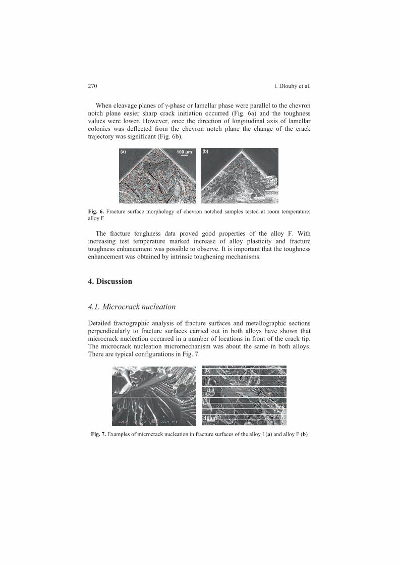
I. Dlouhý et al.
When cleavage planes of -phase or lamellar phase were parallel to the chevron
notch plane easier sharp crack initiation occurred (Fig. 6a) and the toughness
values were lower. However, once the direction of longitudinal axis of lamellar
colonies was deflected from the chevron notch plane the change of the crack
trajectory was significant (Fig. 6b).
100 m (a) (b)
Fig. 6. Fracture surface morphology of chevron notched samples tested at room temperature;
alloy F
The fracture toughness data proved good properties of the alloy F. With
increasing test temperature marked increase of alloy plasticity and fracture
toughness enhancement was possible to observe. It is important that the toughness
enhancement was obtained by intrinsic toughening mechanisms.
4. Discussion
4.1. Microcrack nucleation
Detailed fractographic analysis of fracture surfaces and metallographic sections
perpendicularly to fracture surfaces carried out in both alloys have shown that
microcrack nucleation occurred in a number of locations in front of the crack tip.
The microcrack nucleation micromechanism was about the same in both alloys.
There are typical configurations in Fig. 7.
(a) (b)
10 m
Fig. 7. Examples of microcrack nucleation in fracture surfaces of the alloy I (a) and alloy F (b)
270

Fracture Behaviour of TiAl Intermetalics
Usually, it is possible to observe several damage sites on certain distances from
the crack tip showing the fracture initiation occurred by joining the main crack tip
with the nearest microcrack/damage site. The separate microcracks are often
nucleated at boundaries of two lamellas or on boundary of lamellar colony with
equiaxed -TiAl grain. Local influence of deformation twin and/or intensive slip
band onto this boundary and microcrack nucleation in neighbouring grain in local
tensile stress field appears to be the most probable mechanism of the microcrack
formation. For the alloy I, there is a facet formed by fracture of equiaxed grain, a
step morphology formed by fine lamellar microstructure and river like traces
typical for fracture of nonlamellar microstructure component (see Fig. 7a). The
occurrence of facets created by equiaxed grains cleavage is comparably lower in
alloy F, one of such locations is shown in Fig. 7b. In almost all facets of alloy F
some curvature due to plastic deformation typical for quasicleavage was possible
to observe, Fig. 7b. The fracture mechanism of both alloys is nearly the same
differing only by the extent of plastic deformation proceeding to cleavage facets
nucleation. Configuration of fracture facets shown in Fig. 7a is the most frequently
observed phenomena in fracture surfaces once the equiaxed -TiAl grains are
present in microstructure. The presence of the equiaxed -TiAl grains is detrimental
for crack resistance; it affects strongly both the crack initiation toughness and
crack resistance curve. The equiaxed -phase is supposed to degrade the crack
growth resistance by inhibiting action of shear ligament toughening.
4.2. Fracture initiation
For pre-cracked test specimens of both alloys tested at room temperature crack tip
stress-strain distributions preceding and corresponding to fracture initiation have
been calculated by finite element modelling. Development of maximum principal
stress at forces below and at the fracture force has shown that there is no plastic
deformation nearly up to fracture load. Certain amount of effective plastic
deformation was developed just before the reaching the critical load (700–770 N).
This is because of singularity on the stress distribution still at loads corresponding
to yield stress and zero value of effective plastic deformation at 600 N loads. Only
after this point a peak on maximum stress distribution is formed and shifted to
higher distances from the crack tip. Presumably, critical stress for crack nucleation
and plastic deformations for the joining the microcrack nuclei with the crack tip
are the necessary condition for the crack initiation. The plastic deformation itself
is more or less apparent value, because the joining of microcrack nuclei with the
main crack tip is carried out mainly by microdamage processes rather than
deformation, in particular in alloy I. In the last the effective plastic deformation
was comparably lower and no evidences of plastic deformation could be found in
fracture surfaces. For the alloy F the stress-strain conditions at the moment of
crack initiation are obvious from Fig. 8. From the micromechanical point of view
additional analyses will be needed (e.g. determination of critical values of stress
and of strain), nevertheless coincidence of the peak position on maximum
principal stress distribution and triaxiality distribution could reflect unfavourable
271

I. Dlouhý et al.
conditions for the crack tip blunting. Inhibiting this blunting process and local
stress relaxation at the crack tip a stage ready for crack initiation followed by
immediate crack propagation is reached.
Fig. 8. Distributions of maximum principal stress, stress triaxiality and effective plastic strain
below the crack tip, alloy F
50 m
Fig. 9. Section perpendicularly to main crack plane in vicinity of the crack tip in unbroken test
specimen (SEM-BSE)
The possible source for intrinsic toughening thus can be seen in such changes in
alloy chemistry and microstructural state that produce different positions of the
peak on maximum tensile stress distribution and the peak on stress triaxiality
distribution below the crack tip.
This can be obtained by increase of plasticity of the alloy, excluding the
detrimental effect of the -TiAl grains in lamellar microstructure and/or by
forming microstructure with more plastic constituent, e.g. - alloys are the best
hope for this. When comparing the room temperature fracture properties and
fracture micromechanism the niobium appears to be one of elements increasing
effectively the plasticity and toughness of the alloy. It has been already mentioned
that this is the most effective way of toughness enhancement if titanium aluminides
when the intrinsic mechanisms are exploited.
272

Fracture Behaviour of TiAl Intermetalics
5. Conclusions
Mechanical properties and fracture performance of two TiAl alloys with different
Nb content have been followed in the work. Positive effect of Nb on tensile
strength and, at the same time, on deformation properties has been shown.
Enhancement of fracture toughness was observed at the same time. Significant
dependence of the scatter in fracture characteristics on orientation of lamellas in
location of fracture initiation origin has been proven. In both alloys, effective
toughening mechanism, shear ligament toughening, i.e. combination of multiple
microcrack nucleations in lamellar microstructure and shear bridges between these
microcracks has been observed.
Defectiveness of the microstructure paradoxically contributes to significant
toughening; the higher the interlamellar distance is the higher defectiveness and
thus toughness increase is possible to detect. Thanks to intrinsic toughening
exploited in alloy F this alloy possesses very high toughness level and increasing
crack resistance curve.
Acknowledgments Financial support to this investigation through grants of Czech Science
Foundation Nr 106/07/0762 and Research plan Nr. AV0Z20410507.
References
[1] Bieler TR, Pourboghrat, Mason DE, et al. (2005). Fracture initiation/propagation parameters
for duplex TiAl grain boundaries based on twinning. Intermetalics 13:979–984.
[2] Campbel JP, Venkateswara Rao KT, Ritchie RO (1999). The effect of microstructure on
fracture toughness and. Metall and Mat Trans 30A(3):563–577.
[3] Cao R, Yao HJ, Chen JH, Zhang J (2006). On the mechanism of crack propagation
resistance of fully lamellar TiAl alloy. Mat Sci Eng A420:122–134.
[4] Chan KS, Kim YW (1995). Effects of lamellae spacing and colony size on the fracture
resistance of a fully lamellar TiAl. Acta Metall Mater 43(2):439–451.
[5] Chan KS, Wang P, Bhate N, Kumar KS (2004). Intrinsic and extrinsic fracture resistance in
lamellar TiAl alloys. Acta Mater 52:4601–4614.
[6] SN P CENT/TS 14425-3 (2003). III: Method of flexural test with chevron notch
specimen.
[7] ISO 12135 (2002). Metallic materials – Unified method of test for determination of
quasistatic fracture toughness.
[8] Kim YW (1992). Microstructural evolution and mechanical properties of a forged gamma
titanium aluminide alloy. Acta Met et Mat 40(6):1121–1134.
[9] Krahula K, Dlouhý I (2005). Microstructure and mechanical properties of TiAl based
intermetalics (in Czech). In Multilevel Design of Advanced Materials, 95–102.
[10] Mercer C, Soboyejo WO (1997). Effects of alloying on crack tip definition and shielding in
gamma-based titanium aluminides. Acta Mater 45(3):961–971.
[11] Ng BC, Simkin BA, Crimp MA, Bieler TR (2004). The role of mechanical twinning on
microcrack nucleation and crack propagation. Intermetallics 12:1317–1323.
[12] Quast JP, Boehlert CJ (2007). Comp. of the microstructure tensile and creep behaviour for
Ti24Al17NbxMo alloys. Met and Mat Trans 38A(3):529–536.
273

I. Dlouhý et al.
[13] Schaden T, Clemens H, Fischer FD, Ebner R (2005). Intermetallics in Technology: Needs
and Application, KMM-NoE Integr. Summer School, Udine.
[14] Simkin BA, Crimp MA, Bieler TR (2003). A factor to predict microcrack nucleation at -
grain boundaries in TiAl. Scripta Mater 49(2):149–154.
[15] Werwer M, Kabir R, Cornec A, Schwalbe KH (2007). Fracture in lamellar TiAl simulated
with the cohesive model. Eng Fract Mech 74:2615–2638.
[16] Xu XJ, Xu LH, Lin JP, Wang YP, Lin Z, Chen GL (2005). Pilot processing and
microstructure control of Nb containing TiAl alloy. Intermetallics 13:337–341.
[17] Yang CT, Li YC, Koo CH (2002), The high temperature tensile properties and
microstructural analysis of Ti–40Al–15Nb alloys. Intermetalics 10:161–169.
[18] Zheng RT, Cheng GA, Li XK, Cao GX, Fu LF, Zhang YG, Chen CQ (2007). The
relationship between fracture toughness and. J Mater Sci 42:1251–1260.
274

T. Boukharouba et al. (eds.), Damage and Fracture Mechanics: Failure Analysis of Engineering
© Springer Science + Business Media B.V. 2009
Numerical and Experimental Investigations
of Mixed Mode Fracture in Granite Using
Four-Point-Bend Specimen
M.R.M. Aliha, M.R. Ayatollahi and B. Kharazi
Fatigue and Fracture Lab., Department of Mechanical Engineering, Iran University
of Science and Technology, Narmak, Tehran, 16846, Iran
Abstract Asymmetric four-point-bend (FPB) specimen is an appropriate test configuration for
investigating mixed mode fracture behaviour in engineering materials like ceramics, rocks,
polymers and metals. In this paper, a combined numerical, experimental and theoretical study of
mixed mode I/II fracture behaviour using this specimen is presented. For calculating the stress
intensity factors, KI and KII, the specimen is analyzed using finite element software, ANSYS.
Then mixed mode fracture is investigated experimentally for a type of granite by means of the
FPB specimen for different combinations of mode I and mode II. The obtained test data are then
compared with some well known two fracture theories. It is shown that the test data are in
agreement with the theoretical predictions of well known fracture criteria the maximum
tangential stress theory and the maximum energy release rate theory.
Keywords: Mixed Mode Fracture, Asymmetric Four-Point-Bend Specimen, Finite Element,
Granite, Experiment.
1. Introduction
It is well established that the crack growth is one of the main reasons for the
overall failure and brittle fracture in various engineering materials. Cracks and
inherent discontinuities are frequently found in rock materials and concrete structures.
In many practical applications, such as concrete dams, tunnelling, mining,
excavation process and analyses of rock slope stability, the evaluation of crack
growth is an important task for rock and concrete structures designers. Most of
previous rock and concrete fracture studies have concentrated only on crack
opening mode (or mode I loading) which is induced from the tensile stresses.
However, in practice, the cracked rock structures are usually subjected to complex
loading and hence the fracture of rock masses may occur under a combination of
tension-shear (mixed mode I/II) loading. Therefore, it is important to investigate
the mode I, the mode II and mixed mode fracture in rock structures and geo-
materials. There are some theoretical and experimental methods for evaluating the
fracture behaviour under mixed mode I/II loading conditions. Fracture toughness
of cracked materials is generally investigated by means of suitable test samples.
The cracked rectangular bar subjected to asymmetric four-point-bend loading is
275
Materials and Structures, 275–283.

M.R.M. Aliha et al.
one of the favourite test configurations frequently used by researchers investigating
mixed mode fracture in rocks and concretes (e.g. [1–4]) and also in other brittle
materials [5–9]. The simple geometry and loading set up, the convenient pre-
cracking of specimen and the ability of introducing full mode mixities (from pure
mode I to pure mode II) are among the advantages of FPB specimen. Additionally
the specimen is loaded by a compressive type of load which is more suitable for
testing brittle materials like rocks. For studying mixed mode fracture in each test
specimen, the mode I and mode II stress intensity factors (KI and KII) should be
known. In this paper, a combined numerical and experimental study using the FPB
specimen is presented for mixed mode loading. In the forthcoming sections, first
the stress intensity factors of the four-point-bend specimen are determined by
means of the finite element analysis. Then mixed mode fracture is investigated
experimentally for a granite sample using the FPB specimen.
2. Four-point-bend specimen
Fig. 1 shows a schematic drawing of asymmetric four point bend (FPB) specimen.
The ratio of mode I and mode II stress intensity factors can be easily changed in
this specimen by moving the locations of top and bottom supports. This is because
the shearing force and the bending moment along the crack plane and hence the
crack opening and the crack sliding are dependent on the locations of loading
points. Therefore, the FPB specimen can be used for providing pure mode I (crack
opening), pure mode II (in-plane sliding) and various mode mixities for fracture
experiments. When the loading points are symmetric with respect to the crack
plane (L1 = L2 and L3 = L4 < L2), the specimen is subjected to pure mode I loading.
Pure mode II is also provided by anti-symmetric loading of specimen (i.e. L1 = L4
and L2 = L3). In this situation unlike the symmetric condition, the crack line in the
FPB specimen is subjected to a pure shear force. For any other options for the
locations of top and bottom supports (L1, L2, L3 and L4) the specimen experiences
mixed mode loading conditions.
Fig. 1. Cracked rectangular plate subjected to asymmetric four point bending
276
B
L1 L2
L4L3
F
L / 2 L / 2
W

Numerical and Experimental Investigations of Mixed Mode Fracture in Granite
Some analytical [7, 8] and numerical [10] methods are available for obtaining
the stress intensity factors in the FPB specimen. The finite element method is a
suitable and powerful technique for calculating KI and KII in cracked specimens.
In the next section, the finite element method is employed for analyzing the FPB
specimen under various loading conditions.
3. Finite element modeling
Fig. 2 shows a typical mesh pattern generated for simulating the FPB specimen in
the finite element code ANSYS. In the created model, the following dimensions
have been considered: crack length a = 20 mm, specimen thickness B = 19 mm,
width W = 40 mm and length L = 220 mm. Thus the crack length ratio, a/W, was
equal to 0.5. A total number of 568 plane stress and eight-nodded elements were
used for simulating the model. The crack tip stress singularity was generated by
using the singular elements in the first ring of elements surrounding the crack tip.
The stress intensity factors, KI and KII, for the FPB specimen can be written as:
III,,
1
31
5.0
iL
L
BW
aFiYiK (1)
where YI and YII are the mode I and mode II geometry factors, respectively. In the
analyzed models, pure mode I (symmetric loading), pure mode II (anti-symmetric
loading) and different mixed mode conditions were considered. All models were
solved by considering a constant value of F = 5,000 N and fixed values for L1, L2
and L4 as L1 = 70 mm, L2 = 30 mm, L4 = 70 mm. In order to change mode mixity,
different values were taken for L3. The Material properties of a typical granite
(E = 45 GPa and = 0.28) were used for the finite element analysis of FPB
specimen. The mode I and mode II stress intensity factors were directly extracted
from the ANSYS code. Variations of YI and YII versus L3/L1 for the analyzed FPB
specimens are presented in Fig. 3. It is seen from this figure that by moving from
the symmetric loading conditions (pure mode I) toward anti-symmetric loading
conditions (pure mode II), YI decreases and YII increases.
Fig. 2. Finite element model created for asymmetric four-point-bend specimen
277

M.R.M. Aliha et al.
4. Fracture experiments
A series of mixed mode fracture experiments were conducted on a type of granite
using the four-point-bend specimen. Several test specimens with dimensions of
220 × 40 × 19 mm were cut from a sheet of Takkab (a region in the north western
of Iran) granite.
Then an edge crack having a length of 20 mm was created in the centre line of
each test specimen using a thin rotary diamond blade. For each desired mode
mixity, the specimen was placed in a suitable location inside the loading fixture
and then was loaded until the final fracture. Figure 4 shows the loading set up for
one of the tests. The servo hydraulic Amsler/Zwick test machine was used for
fracture tests.
The loading rate for all tests was 0.25 mm/min. the load–displacement history
for each test was recorded during the test using a computerized data logger. The
critical stress intensity factors for each loading condition were calculated using
Eq. (1) and the fracture load obtained from the tests.
a
0.0 0.1 0.2 0.3 0.4 0.5
0.00
0.02
0.04
0.06
0.08
0.10
0.12
0.14
0.16
a/w=0.5
13/LL
IY
b
0.0 0.1 0.2 0.3 0.4 0.5
0.010
0.015
0.020
0.025
0.030
0.035
a/w=0.5
IIY
13 / LL
Fig. 3.Variations of (a) mode I geometry factor YI and (b) mode II geometry factor YII with L3 /L1
in the FPB specimen
Fig. 4. Loading set up for FPB specimen made of Takkab granite
278

Numerical and Experimental Investigations of Mixed Mode Fracture in Granite
5. Results and discussion
The maximum tangential stress (MTS) criterion [17], the minimum strain energy
density criterion [18] and the maximum energy release rate criterion [19] are three
well-known theories for mixed mode fracture. Based on these criteria, fracture in a
cracked body under mixed mode I/II loading will occur in a specific direction
when the stress or energy quantities in this direction reaches its critical value. For
example, the onset of fracture for a cracked body subjected to mixed mode loading
takes place according to the maximum tangential stress criterion [17] when:
0020 sin
2
3
2cos
2cos IIIIc KKK (2)
And based on the maximum energy release rate or G criterion [19] when:
2
12
02
002
02
2
0
0
02
cos59cossin8cos31
1
1
cos3
2
0
IIIIII
Ic
KKKK
K (3)
where 0 is the angle of fracture initiation with respect to the original crack line.
The angle 0, is predicted by the MTS criterion from:
825.0tan2
22
10
II
I
II
I
K
K
K
K (4)
Similar relation can be found in [19] for 0 when using the G criterion. By
increasing the load, the stress intensity factors, KI and KII in the right hand side of
Eqs. (2) and (3) also increase. Mixed mode fracture occurs when the right hand
side of Eqs. (2) or (3) reaches or exceeds the mode I fracture toughness KIc. The
theoretical predictions of fracture by these criteria can be presented in a KII/KIC
versus KI/KIC diagram as shown in Fig. 5. Also shown in this figure is the test data
obtained from mixed mode fracture experiments conducted on Takkab granite.
Despite a natural scatter that exists in the experimental results, Fig. 5 shows that
the obtained test data are generally in agreement with the theoretical predictions of
the maximum tangential stress and the maximum energy release rate criteria. In
fact, the mixed mode data lie between the curves related to these two fracture
criteria. The scatter observed in the test data can be attributed to parameters like
natural inhomogeneity and anisotropy of tested granite and possible inaccuracies
279

M.R.M. Aliha et al.
in manufacturing, pre-cracking and loading set up of FPB test samples. The mixed
mode fracture toughness of engineering materials can be displayed by effective
stress intensity factor, Keff:
Ic
IIIeff
K
KKK
22
(5)
where KI and KII in Eq. (5) are the stress intensity factors corresponding to the
fracture load. Figure 6 shows the variations of mixed mode fracture toughness
versus the mode mixity parameter (Me) for Takkab granite. The parameter Me is
defined by:
II
Ie
KK
M arctan2
(6)
Fig. 5. Mixed mode fracture toughness data obtained for tested granite using FPB specimens
A curve fitted to the test results is also shown in Fig. 6. A comparison between
the results of pure mode I and pure mode II indicates that the mode II fracture
toughness (KIIc) for the tested granite is less than its mode I fracture toughness
(KIc). However, previous investigations [20–23] suggest that unlike KIc the value
of measured KIIc is not merely a material constant and depends also on the
geometry of test specimen and its loading configuration. For example, the ratio of
KII/KIC for cracked materials tested with various test samples varies in a wide
range from 0.45 to 2.3 [7, 20–23]. The experimental results show that Takkab
granite is weaker against shear loads compared to the tensile loads since KII/KIC is
about 0.51.
280
KI/K
Ic
0.0 0.2 0.4 0.6 0.8 1.0
KII/K
Ic
0.0
0.2
0.4
0.6
0.8
1.0
1.2
1.4
1.6
G Criterion [19]
Test data
MTS Criterion [17]
Takkab Granite

Numerical and Experimental Investigations of Mixed Mode Fracture in Granite
The curve presented in Fig. 6 can be used as a design curve for estimating the
optimum condition for practical applications like rock cutting process to determine
the minimum required cutting energy and in hydraulic fracturing to calculate the
fluid pumping power.
The compressive loading set up used for the cracked beams subjected to
bending makes the FPB specimens more suitable for fracture testing on brittle
materials like rocks and concretes which are weak against tensile loads. In
comparison with the asymmetric three-point-bend loading configuration (which is
another well known test specimen being used for mixed mode loading [11–13]),
the FPB configuration requires a more complicated fixture and also more care in
the experimental set up. However, the three-point-bend test configuration can be
used only for limited combinations of mode I and mode II.
In particular, pure mode II cannot be introduced by this specimen. But as
mentioned earlier, the full combinations of modes I and II can be easily introduced
in the four-point-bend specimen by changing the locations of loading rollers. The
mode I fracture toughness obtained for the tested granite is about 1.4 MPa m0.5
which is in good agreement with the reported values for other types of granite
materials [14–16]. As shown in Fig. 7, for mode I condition where the applied
loads are symmetric relative to the crack line, fracture occurs in a self-similar
manner and along the initial crack line.
However, for mixed mode conditions where both shear force and bending
moment are present along the crack line, the path of crack growth deviates from
the initial crack line. Such deviations can be seen in Fig. 7 that shows the crack
growth trajectory in some of the granite specimens tested under different mode
mixities. In all of the experiments it was observed that the crack growth started
from the crack tip, extended along a curvilinear path, and finally terminated at the
nearest loading roller.
Me
0.0 0.2 0.4 0.6 0.8 1.0
Ke
ff
0.4
0.5
0.6
0.7
0.8
0.9
1.0
1.1
Test data
Line fitted to test data
Me
Ke
ff
Me
0.0 0.2 0.4 0.6 0.8 1.0
Ke
ff
0.4
0.5
0.6
0.7
0.8
0.9
1.0
1.1
Test data
Line fitted to test data
Me
Ke
ff
Fig. 6. Variations of mixed mode fracture toughness (Keff) with Me in the tested granite samples
281

M.R.M. Aliha et al.
6. Conclusions
Mixed mode I/II fracture toughness of Takkab granite was investigated numerically
and experimentally by means of the asymmetric four-point-bend (FPB) specimen
in the full range of mixed mode loading from pure mode I to pure mode II.
The experimental results obtained for the tested granite falls between the
theoretical curves predicted by the maximum tangential stress criterion and the
maximum energy release rate criterion.
According to the FPB test results, Takkab granite is weaker in mode II fracture
than in mode I fracture.
Mode I Mode II
KI/KII= 1.988
KI/KII = 0.545
KI/KII= 1.035
KI/KII = 0.204
Fig. 7. Crack growth trajectory in some of the FPB specimens broken different mode mixities
282

Numerical and Experimental Investigations of Mixed Mode Fracture in Granite
References
[1] Ingraffea R (1981) Mixed mode fracture initiation in Indiana limestone and Westerly
granite. Proc. 22nd US Symp. On Rock Mechanics, Cambridge MA, pp 186–191.
[2] Huang J., Wang S (1985) An experimental investigation concerning the comprehensive
fracture toughness of some brittle rocks. Int J Rock Mech. Min. Sci Geomech Abstr,
22(2):99–104.
[3] Li S, Huang SM, Yang SC (2004) Experimental investigation on criterion of three-
dimensional mixed-mode fracture for concrete. Cem Conc Res 34:913–916.
[4] Mario MA, Francis TL (2005) Numerical simulation of quasibrittle fracture in concrete.
Eng Fract Mech 72(3):387–411.
[5] He MY, Cao HC, Evans AG (1990) Mixed mode fracture: the four-point shear specimen.
J Metallurg Mat 38:839–846.
[6] Suresh S, Shih CF, Morrone A, O_Dowd NP (1990) Mixed-mode fracture toughness of
ceramic materials. J Am Ceram Soc 73(5):1257–1267.
[7] Li M, Sakai M (1996) Mixed-mode fracture of ceramics in asymmetric four-point bending.
J Am Ceram Soc 79(10):2718–2726.
[8] Tikare V, Choi SR (1997) Combined mode I–mode II fracture of 12-mol%-ceria-doped
tetragonal zirconia polycrystalline ceramics. J Am Cer Soc 80:1624–1626.
[9] HE MY, Hutchinson JW (2000) Asymmetric four-point crack specimen. J Appl Mech
67:207–209.
[10] Shahani AR, Tabatabaei SA (2008) Computation of mixed mode stress intensity factors in a
four-point bend specimen. Appl Math Model 32(7):1281–1288.
[11] Fett T, Gerteisen G, Hahnenberger S, Martin G, Munz D (1995) Fracture tests for ceramics
under mode-I, mode-II and mixed-mode loading. J Eur Cer Soc 15:307–312.
[12] Xeidakis GS, Samaras IS, Zacharpoulos DA, Papakaliatakis GE (1996) Crack growth in a
mixed-mode loading on marble beams under three point bending. Int J Fract 79:197–208.
[13] Jenq TS, Shah SP (1987) Mixed mode fracture parameters of concrete. SEM/RILEM Int
Conf on fracture of concrete and rock, Texas, Shah SP, Swartz SE, (EDS), pp 359–369.
[14] Olofsson T (1978) Evaluation of fracture parameters and elastic properties of rock
materials. Report 195E, university of Lulea, Sweden.
[15] Singh RN, Sun GX (1989) Relationships between fracture toughness, hardness indices and
mechanical properties of rocks. Department of Mining engineering university of Nottingham,
England, Magazine XLI, pp 49–62.
[16] Chang SH, Lee CI, Jeon S (2002) Measurement of rock fracture toughness under modes I
and II and mixed-mode conditions by using disc-type specimen. J Eng Geol 66:79–97.
[17] Erdogan F, Sih GC (1963) On the crack extension in plates under plane loading and
transverse shear. J Basic Eng Trans ASME 85: 519–525.
[18] Sih GC (1974) Strain-energy-density factor applied to mixed mode crack problems. Int J of
Fract 10:305–321.
[19] Hussain MA, Pu SL, Underwood J (1974) Strain energy release rate for a crack under
combined mode I and Mode II Fracture Analysis. ASTM STP 560. American Society for
Testing and Materials, Philadelphia, pp 2–28.
[20] Awaji H, Kato T (1999) Criterion for combined mode I–II brittle fracture. Mat Trans JIM
(Japan Institute of Metals), 40(9):972–979.
[21] Ayatollahi MR, Aliha MRM (2007) Fracture toughness study for a brittle rock subjected to
mixed mode I/II loading. Int J Rock Mech Min Sci 44(4):617–624.
[22] Aliha MRM, Ashtari R, Ayatollahi MR (2006) Mode I and mode II fracture toughness
testing for marble. J Appl Mech Mater 5-6:181–188.
[23] Singh D, Shetty DK (1989) Fracture toughness of polycrystalline ceramics in combined
mode I and mode II loading. J Am Cer Soc 72 (1):78–84.
283

T. Boukharouba et al. (eds.), Damage and Fracture Mechanics: Failure Analysis of Engineering
© Springer Science + Business Media B.V. 2009
Experimental and Numerical Determination
of Stress Intensity Factors of Crack in Plate
with a Multiple Holes
S. Belamri1, T. Tamine
2 and A. Nemdili
3
1ARCELOR MITTAL, Direction Régionale Ouest, 02 rue Mekki Khalifa 31000 Oran,
Algeria
2Laboratoire LCGE, Faculté de Génie Mécanique, Université des Sciences et de la
Technologie d’Oran Algérie, BP 1505 EL M’NAUER 31000 Oran, Algérie
3Laboratoire LRTTFC Faculté de Génie Civil & d’Architecture
Abstract The optical method of photoelasticity was used to measure stress field and stress
intensity factors of crack with the presence of holes in a polycarbonate PSM-1 birefringeant
plates under tension. Tests were used for variable numbers and dimensions of holes. The present
study takes into account the several positions of holes and crack in plates. Stress intensity factor
has been determined from the crack tip fringe pattern by multiple points’ technic. Experimental
results have been confirmed with a good agreement numerical estimation of stress intensity
factors obtained with the finite element method (FRANC 2D).
Keywords: Photoelasticity, Fringe, Crack, Stress Field, Stress Intensity Factor, FRANC 2D.
1. Introduction
The lifetime of engineering materials may be associated with the size, the shape
and the location of flaws or cracks in components. In mechanic applications it is
often used a perfored or drilled holes. They can be a large number with a regular
or random distribution. Then, it is important to estimate the stress concentration
around theses holes and their influence on the mechanic behaviour. The problem
of calculating the displacement and stress field in an elastic body containing holes
interested many authors. For infinite plane with multiple circular holes under
uniaxial tension [4, 6, 7, 9] resolved stress problems on multiply connected
domains with the boundary integral equation. The application of this theory showed
an extreme stability of this approach for a higher number of holes and cracks in
loaded infinite plate. The circumferential stress is determined for different
configuration and location of circular holes. Knowing the role of stress field near
orthotropic material an optimization analysis in order to decrease the stress
intensity factor. It is shown that the stress field at the crack boundary can be
significantly improved by noncircular shapes.
the crack tip in fracture mechanics analysis, authors in [12] used for isotropic and
285
Materials and Structures, 285–295.

S. Belamri et al.
Furthermore to adhesive patching, it is well known that drilled stop holes can
reduce stress intensity factor. In this context, Junping Pu [8] used sub region BEM
(Boundary Element Method) to study the effect of defective holes on crack.
Results show that if the location of these drilled holes are chosen unsuitably, they
can not only decrease the stress intensity factor, but also increase the crack
expanding even more. It showed that for elliptic defective holes, the effect for the
studied
the effectiveness of the arrangement of a stop-drilled hole and additional holes on
retarding crack growth and developed an analysis on the stress concentration. In
the present study, a finite element method and the experimental technique of
photoelasticity is used to determine the stress field around circular holes in finite
plate under uniaxial tension. Effect of the number of holes and distance on the
magnitude of the stress concentration is also analysed. The presence of crack
emanating from central hole and the location of lateral holes complete our study
through their interaction and their influence on the stress intensity factors.
2. Experimental method
Tension load testing is applied to a drilled holes and crack hole specimens. A
photoelasticity method (Fig. 1) is applied to measure stress around holes. By
rotating the circular polariscope, it can be obtained a monochromatic or a white
light from which an isochromatic or isocline fringe patterns can be recorded. The
photos are taken with a numerical camera and are treated by image digitalisation
software.
Fig. 1. Photo of photoelasticimetry installation
2.1. Material
Photoelastic specimens are machined from a polycarbonate sheet with a dimension
of 254 × 254 mm and a thickness of t = 5 mm.
stress intensity factor on Mode-I loading is less than those of circular holes of which
the radii are equal to the elliptic length axis. Also, Murdani et al. [2, 3]
286

Experimental and Numerical Determination of Stress Intensity Factors of Crack
According to the manufacturer, the Young’s modulus and Poisson’s ratio of the
sheet material are E = 2390 MPa and 0.38, and the material fringe value f is 7.1
KPa (fringe/m).
2.2. Test specimens
Specimens are cut from a polycarbonate sheet, material having height sensitivity
to the stress. Specimen E-1 (Fig. 2) is a plate with two holes aligned with the x-
axis and separated by a distance a (a is the small hole radius). The geometric
plate ratio is W/H = 0.25 and the radius ratio is equal to b/a = 5. Figure 3 shows a
plate with the ratio W/H = 0.2, containing a colineair holes with the same radius a
and a distance = 4a.
Fig. 2 and 3. Specimen E-1 and E-1
machined from the central hole. The radius ratio is equal to b/a = 2 and the
distance between holes is = 4a in the load direction (X axis) and = 2a in the Y
Fig. 4, 5 and 6. Specimen F-1, F-2 and F-3
(Figs. 4, 5 and 6). In addition to the holes, a symmetrical crack with a depth l is
For the stress intensity factor study, the specimens F-1, F-2 and F-3 are used
axis (for the specimen F-2 and F-3).
287
2b
2H
2a
2W
2H
2W2a
2H
2W0 0
00
0
2b
l
2a
2H
2W
2b
l
2a
2H
2W
y0
2b
l
2a
x0
2d

S. Belamri et al.
3. Method of resolution
During tests, photoelasticity method is applied and the isochromatic fringes have
been recorded with a numerical camera. The data measures are obtained from the
fringe by using the image digitalisation software. From the separation of principal
model, the maximum shear can be written as:
h
fN
2
.
2
21max (1)
1 and 2 are respectively the principal stress in the first and the second
direction, N is the fringe pattern order, f is the sensitivity of the material, h is the
specimen thickness.
The shear stress xy can be found from Mohr circle and its formulation is:
2sin.2
.2sin.
2
21
h
fNxy (2)
is the angle between x (or y) and 1(or 2).
In plane stress, [8] used the following equilibrium equations:
0yx
xyx and 0yx
yxy (3)
Integrating on the X direction, stress can be written as:
2/1001
1
0
xxx dxy
xx xy
x
xx
xyxx (4)
0x and 1x are the corresponding points boundary of meshing line where the
stress should be determined.
Applying Matlab 6.5 software, it can be possible to resolve the system of
equations and to calculate the local stress. For F-1 and F-2 specimens, experimental
results are obtained from digitalisation of fringe patterns in the vinicity of crack
and by applying the multipoints method
related to fringe parameters by the relationship:
fNh
rK I
2 (5)
stresses technique [1, 5, 10, 11], local stress can be determined. For any point of the
[5, 11]. Therefore, stress intensity factor is
288

Experimental and Numerical Determination of Stress Intensity Factors of Crack
4. Results
The application of separation of principal stress technique and the mutipoints
method with a MATLAB program allowed the determination of local stress and
the stress intensity factors. In the other hand, finite element method with Franc 2D
software is used for all specimens. As most of specimens are symmetrical, just a
quarter of them are meshed with T6 and Q8 elements. A plane stress resolution is
applied.
As example, Fig. 7 shows a superposition of an experimental fringes and
numerical shear stress for collinear holes. The same concentration of shear stress
is observed on the experimental and the numerical resolution.
Fig. 7. Example of experimental and Numerical Shear stress distribution in Specimen E2;
(a) Experimental results and (b) Numerical results
4.1. Specimen with two holes (E-1)
Experimental and numerical results have allowed plotting the normalized stress
acting on the boundary of the first (central) and the second hole respectively versus
the angle 1 and 2 (Fig. 8). For the central hole, the numerical resolution gives the
maximum stress concentration at a location 1 = 89.2°. The same value is found
by the photoelasticimetry method for the radius ratio b/a = 5.
The stress concentration decrease when the ratio (b/a) is equal to 3. This
observation is noted by Jianlin Wang et al. [6] for the same radius ratio and
distance for infinite plate with two holes. We have studied the effect of the ratio
( /a) the stress in the first hole and the second (Fig. 9). We notice that /a, has a
very little influence on the variation of local stress for the central hole whereas it
is important for the second hole.
289
0.5222E+07
(a)(b)
0.5630E+07
0.5038E+07
0.4446E+07
0.3853E+07
0.3261E+07
0.2660E+07
0.2077E+07
0.1485E+07
0.8930E+06
0.3000E+06
Fracture Analysis Code
KSU-Cornell
Version :L1.5 12/98 -Beta
Make a selection
Component: TAU MAX
Active Layer :1
10mm
FRANC20/

S. Belamri et al.
0 30 60 90 120 150 180
0
1
2
3
4
/a=4
Norm
aliz
ed
Str
ess
xx/
0
Angle 1 (°)
xx Méthode Numérique b/a=5
xx Méthode Expérimentale b/a=5
xx Méthode Numérique b/a=3
0 30 60 90 120 150 180
0
1
2
3
4
/a=4
Norm
aliz
ed S
tress
xx/
0
xx Méthode Numérique b/a=5
xx Méthode Expérimentale b/a=5
xx Méthode Numérique b/a=3
Angle 2 (°)
Fig. 8. Stress distribution in the first (central hole) and second holes of specimen E-1
0 30 60 90 120 150 180
-1
0
1
2
3
4
5
No
rma
lize
d S
tre
ss
xx/
0
Angle 1 (°)
xxNumerical Method /a=0.1
xxNumerical Method /a=0.4
xxNumerical Method /a=1.0
xxNumerical Method /a=4.0
xxExperimental Method /a=4.0
0 30 60 90 120 150 180
0
1
2
3
4
5
xx Numerical Method /a=0.1
xx Numerical Method /a=0.4
xx Numerical Method /a=1.0
xx Numerical Method /a=4.0
xx Experimental Method /a=4.0
No
rma
lize
d S
tre
ss
xx/
0
Angle 2 (°)
Fig. 9. Stress distribution in the first hole (central hole) and second hole for various ratio /a
4.2. Specimen with collinear holes
Loaded Plate with equally spacing collinear circular holes along x axis (specimen
E-2) is considered. A variable number of holes has been studied (1, 3,…15 holes)
with /a = 1, /a = 2 and /a = 4. Normalized stress for /a = 4 and /a = 1 are
plotted in Fig. 10.
For /a = 1 and /a = 4 the maximum stress in central hole is located at the
angle 1 = 89.2 some either the number of holes in specimen. For a number of
holes N 3 and /a = 4, the maximum stress values are higher than those obtained
for /a = 4.Taking into account the maximum values from the above graphs, we
have plotted the stress concentration factor ( max/ 0) for a number N of colineair
holes in the specimen E-2 (Fig. 11). Stress concentration curve for /a = 4 is more
important than for /a = 2 and /a = 1. For /a = 4, results approach the asymptotic
value of 2.80 for N = 3 holes. When this ratio is equal to 2, the asymptotic begins
from N = 5 holes with a value of 2.55.This value decreases to 2.35 from N = 7
holes when /a = 1.
290

Experimental and Numerical Determination of Stress Intensity Factors of Crack
Upon comparing the results obtained for /a = 2 by the present method with
those of [4] we found the same distribution of the stress concentration with an
asymptotic tendency. Our values are slightly overhead compared to results of
these authors. It would seem that the finite geometrical size of plate has an effect
on the concentration values.
0 30 60 90 120 150 180
-1
0
1
2
3
No
rma
lize
d S
tre
ss
xx/
0
/a=1
Angle 1 (°)
01 Hole
03 Holes
05 Holes
07 Holes
09 Holes
11 Holes
13 Holes
15 Holes
0 30 60 90 120 150 180
0
1
2
3
No
rmaliz
ed
Str
ess
xx/
0
/a=4
Angle 1 (°)
01 Hole
03 Holes
05 Holes
07 Holes
09 Holes
11 Holes
Fig. 10. Evolution of normalized stress in central hole for /a = 1 and /a = 4
0 2 4 6 8 10 12 14 16
0
1
2
3
max/
0
Num ber of Holes
/a=1.0
/a=4.0
/a=2.0
Fig. 11. Stress concentration factor for N holes
4.3. Specimen with collinear holes and a symmetrical crack
From the previous case it has been found that the maximum stress is located in the
central hole for the angle 1 = 90°. Then, a symmetrical crack emanating from
central hole has been machined at this position. After loading the F-1 specimen,
we obtained the fringes from experimental method and shear stress distribution by
291

S. Belamri et al.
finite element method. It is noticed in Fig. 12 that the fringes concentration is
around the crack tip. This is confirmed by the numerical results.
Fig. 12. Shear stress distribution in collinear holes with symmetrical crack specimen (a) Experimental
shear stress and (b) Numerical shear stress distribution
0 ,4 0 0 ,4 2 0 ,4 4 0 ,4 6 0 ,4 8 0 ,5 0 0 ,5 2
0 ,6
0 ,8
1 ,0
1 ,2
1 ,4
KI/(
xx.(
.(l+
b))
1/2
( l+ b ) /w
N u m é r ic a l M e th o d
E x p e r im e n ta l M e th o d
Fig. 13. Evolution of normalized stress intensity factor
0 ,4 0 0 ,4 2 0 ,4 4 0 ,4 6 0 ,4 8 0 ,5 0 0 ,5 2
0 ,0
0 ,3
0 ,6
0 ,9
1 ,2
1 ,5
K
I/(
xx.(
.(l+
b))
1/2
( l+ b ) /w
b /a = 2 W ith 5 H o le s
b /a = 1 W ith 5 H o le s
b /a = 1 W ith 3 H o le s
b /a = 2 W ith 3 H o le s
Fig. 14. Evolution of normalized stress intensity factor with number of holes
The stress intensity factor is evaluated by Eq. (5) and numerically with the
FEM using the fracture post-processor available on Franc 2D software. Results are
292
(a) (b)
5 mm
0.2198E+02
0.1979E+02
0.1760E+02
0.1540E+02
0.1321E+02
0.1102E+02
0.8828E+01
0.6635E+01
0.4443E+01
0.2251E+01
0.5926E - 01

Experimental and Numerical Determination of Stress Intensity Factors of Crack
plotted in Fig. 13. Analyse of experimental and numerical values showed that the
divergence between them is low, estimated to 3%. The influence of the presence
of a high number of holes in X direction (collinear) and the radius ratio b/a on
the stress intensity factors are represented in Fig. 14. For the same distance between
holes /a = 4, either the number of holes, the normalized stress intensity factor
values decreases appreciably (30%) when b/a = 1.
4.4. Central hole with symmetrical crack and lateral holes
Specimen F2 is loaded in tension. Experimental and numerical methods are applied.
Figure 15 represents the experimental fringes and the numerical shear stress
distribution around the crack tip. The normalized stress intensity factor is plotted
for different value of normalized crack depth (Fig. 16). A good agreement is
observed between the numerical and the experimental results if we take into
account the effect of fringe interference between lateral holes and crack tip.
Fig. 15. Shear stress distribution for specimen F-2: (a) experimental shear stress and (b) numerical
shear stress distribution
0,40 0,42 0,44 0,46 0,48 0,50 0,52
0,5
1,0
1,5
2,0
(l+b)/w
KI/(
xx.(
.(l+
b))
1/2
Numerical Method
Experimental Method
Fig. 16. Evolution of normalized stress intensity factor for specimen F-2
293
(a)
0.2446E+02
0.2202E+02
0.1957E+02
0.1713E+02
0.1469E+02
0.1225E+02
0.9809E+01
0.7367E+01
0.4926E+01
0.2485E+01
0.4318E-1
(b)

S. Belamri et al.
4.5. Collinear holes with symmetrical crack and lateral holes
It is interesting to study if the effect of drilling holes near the crack can decrease
the stress intensity factor. We consider a plate with the same geometrical ratio as the
specimen F-1 but having in more four holes (two on all sides of crack tip) with
the radius ratio d/b = 0.2 for the first analysis and d/b = 0.4 for the second. The
lateral hole is located from the crack tip by the coordinate (X0, Y0).
For the resolution, we used the normalized crack depth (l + b)/W = 0.514 as the
above case (Fig. 17) and a constant position X0/l = 1. By varying the lateral holes
position Y0, we found the stress intensity factor for symmetrical crack. Figure 17
present the twin case resolution corresponding to d/b = 2.5 and d/b = 5.0.
- 0 , 6 - 0 , 4 - 0 , 2 0 , 0 0 , 2 0 , 4
0 , 8
1 , 0
1 , 2
1 , 4
X0/ l = 1
KI/[
0.(
(l+
b))
1/2
]
L a t e r a l H o le P o s i t i o n Y0/ l
b / d = 2 . 5
b / d = 5 . 0
Fig. 17. Evolution of normalized stress intensity factor for various lateral hole location
The presence of lateral holes decreases the stress intensity factor. It is confirmed
if we compare the results with the above case for the specimen without lateral
holes. The fall in the value of this parameter is as much more important when the
lateral holes radius increases.
The minimum value of the stress intensity factor is noted for the position of lateral
holes Y0/l included between 0.3 and 0.2. For this position the stress intensity
factor decreases of about 29% in comparison with the results of the specimen F-1.
The same constitution have been found by [6] who study the effect of circular or
elliptic hole position on the stress intensity factor for a plate with a central crack.
5. Conclusions
For all specimens tested, stress concentration and stress intensity factors determined
by the finite element method are in good agreement with results obtained by
experimental photoelasticimetry technique. For a plate with two holes, the maximum
stress is observed in the central hole at the angle position = 89.2°.
294

Experimental and Numerical Determination of Stress Intensity Factors of Crack
The effect of the ratio (b/a) is important since the maximum stress decrease
when this ratio change from the value 5 to 3. On the other hand the maximum
stress in the second hole increase when b/a decrease.
The ratio ( /a) has a very little influence on the stress for central hole whereas it
is important for the second hole. These results are noted for the infinite plate study
by [6]. Results on specimens E-2 with collinear holes showed that for the same
number of holes, the stress concentration factor increase with the ratio /a.
The evolution of the stress concentration factor ( max/ 0) has an asymptotic
tendency. For the crack specimens, a small divergence of results in term of stress
intensity factors (3%) between numerical and experimental method are obtained in
spite of the fringe interference in the crack tip. The hole number don’t affect the
value of stress intensity factors. On the other hand, this parameter is influenced by
the radius ratio of holes b/a.
In our study, we have incorporated lateral holes near the crack tip by using the speci-
men F-3. It showed that for the same crack depth, the stress intensity factor decreases
of about 29% with the lateral holes location in comparison with the result of
specimen F-1 (without lateral holes). The size of lateral hole and the position by
report to crack tip has high influence on the stress intensity factor (Fig. 17). This is
noticed by [8] in their works on the effect of defective holes on a central crack in plate.
References
[1] A Ajovalasit, G Pitarresi, B Zuccarello (2006). Limitation of carrier fringe methods in
[2] A Murdani, C Makabe, A Saimoto, R Kondou (2008). A crack growth arresting technique
in aluminium alloy. Engineering Failure Analysis 15: 302–310.
[3] A Murdani, C Makabe, A Saimoto, Y Irei, T Miyazaki (2007). Stress concentration at stop
[4] B Wang, K T Chau (2001). New boundary element method for mixed boundary value
problems involving cracks and holes: Interactions between rigid inclusions and cracks.
International Journal of Fracture 110: 387–406.
[6] Jianlin Wang, Steven L Crouch, Sofia G Mogilevskaya (2003). A complex boundary
integral method for multiple circular holes in an infinite plane. Engineering Analysis with
Boundary Elements 27: 789–802.
[7] Johan Helsing, Anders Jonsson (2002). Stress calculations on multiply connected domains.
Journal of Computational Physics 176: 456–482.
[8] Junping Pu (2006). Effect of defective holes on crack using the boundary element method.
Engineering Analysis with Boundary Elements 30: 577–581.
[9] K T Chen, K Ting, W S Yang (2000). Stress analysis of two dimensional perforated plates
using boundary element alternating method. Computers and Structures 75: 515–527.
[10] M R Ayatollahi, H Safari (2003). Evaluation of crack tip constraint using photoelasticity.
International Journal of Pressure Vessels and Piping 80: 665–670.
digital photoelasticity. Optics and Lasers in Engineering 45(5): 631–636.
drilled holes and additional holes. Engineering Failure Analysis 15(7): 810–819.
releasing. Structural and Multidisciplinary optimization, 28(4): 243–251.
295
over arbitrary boundaries. Experimental Mechanics 30(4): 319–327.
Kogakushi.
[12] P Pederson (2004) Design study of hole positions and hole shapes for crack tip stress
[5] H Mahfuz, T L Wong, R O Case (1990). Separation of principal stresses by SOR technique
[11] W Dally, W F Riley (1978). Experimental Stress Analysis, second edition, Mc Graw Hill,

T. Boukharouba et al. (eds.), Damage and Fracture Mechanics: Failure Analysis of Engineering
© Springer Science + Business Media B.V. 2009
Dynamic Response of Cracked Plate Subjected
to Impact Loading Using the Extended Finite
Element Method (X-FEM)
R. Tiberkak1, M. Bachene
2, B.K. Hachi
3, S. Rechak
4
and M. Haboussi5
1Département de Mécanique, Université Saad Dahleb, BP 270 Soumaa, Blida 09000, Algérie
2Département de Mécanique, Université de Médéa 26000, Algérie
3Département Electromécanique, Centre Universitaire de Djelfa, BP 3117 Ain-Cheih 17000,
Djelfa, Algérie
4Laboratoire de Génie Mécanique et développement, Ecole Nationale Polytechnique, BP 182
El-Harrach 16200, Alger, Algérie
5Laboratoire d’Energétique et de Mécanique Théorique et Appliquée (LEMTA), ENSEM-
INPL, BP 160 F-54504 Vandœuvre-Lès-Nancy, France
Abstract Yet and according to our knowledge, the extended finite element method X-FEM has
not been used in the dynamic response of cracked plates subjected to impact loading, subject of
this study. From prior knowledge of the impact properties (contact force and central deflection)
of a virgin plate, one can quantitatively through the present study predicts the eventual presence
of discontinuities in plates by comparison of impact properties of cracked plate to the virgin
ones. In the numerical implementation, conventional finite element without any discontinuity is
first carried out, then enriched functions are added to nodal displacement field for element nodes
containing cracks. Therefore no remeshing of the domain is required, leading to a great gain in
time computing. The mathematical model includes both transverse shear deformation and rotatory
inertia effects. Based on the above, a self contained computer code named “REDYPLAF”,
written in FORTRAN is hence developed. The effects of Crack length and crack position on
contact force and on plate deflection are analyzed. The obtained results show that the contact
force is divided into three zones. The same fact is also observed for the maximum plate deflection.
Another observed fact is related to crack dissymmetry which has a direct effect on the maximum
plate deflection.
Keywords: Dynamic Response, Cracked Plate, Extended FEM, Impact Loading.
1. Introduction
The presence of cracks, at least at a microscopically level, always exists in mechanical
components. After certain hours of services, these micro cracks initiate and propagate
to become effectively dangerous by decreasing the dynamic-mechanical properties
of components.
297
Materials and Structures, 297–306.

R. Tiberkak et al.
The existence of discontinuities in structures generally induces difficulties
during their numerical implementation. The extended finite element method (X-
FEM) applied to divers fracture mechanic problem has proved its efficiency where
all numerical difficulties and all shortcomings associated with meshing of the crack
surfaces encountered with the classical finite element are alleviated. However, the
finite element method is used as the building block in the extended finite element
method, and hence much of the theoretical and numerical developments in finite
elements can be readily extended and applied. For crack modeling, a discontinuous
function and the two-dimensional asymptotic crack-tip displacement yields are
added to the displacement-based finite element approximation. Partition of unity
enrichment methods for discontinuities and near-tip crack yields were introduced
by Belytschko and Black [1]. Moes et al. [2] proposed the generalized Heaviside
function as a means to model the crack away from the crack tip, and developed
simple rules for the introduction of the enrichment function at the crack-tip.
In the present study, enriched finite element method (X-FEM) is developed for
the dynamic analysis of cracked plates subjected to impact loading. Plates containing
through edge crack and central crack are considered. In addition, different configur-
ations in which we vary crack parameters, i.e.; crack length and crack position are
included. The hypothesis made in the study is to consider the crack parallel to one
edge of the plate and to stop at the end of each element. Contact force and maxi-
mum deflection of the plate are therefore computed. The paper is structured as
follow. In the next section, the extended finite element method is presented. We
first present the mathematical model used followed by the X-FEM formulation
and ending up with the establishment of mass and stiffness matrices. In Section 3,
we describe the development in the computation of the contact force and central
deflection. Numerical applications are presented and discussed in Section 4. We
finalize the paper by drawing some conclusions.
2. Mathematical model and X-FEM formulation
2.1. Displacement field
The mathematical model is based on Mindlin plates. Let us consider a Cartesian
co-ordinate system in such a way that the xy plane coincides with the midplane of
the plate of sides a, b and thickness h (Fig. 1). The displacement field can be
expressed as [3, 4]:
y)(x,zw=z)y,w(x,
y)(x,z= z)y,v(x,
y)(x,z= z)y,u(x,
0
y
x
(1)
298

Dynamic Response of Cracked Plate Subjected to Impact Loading
where u, v, w are the displacements in the x, y, z directions, respectively, 0w
denotes the transverse displacements of the mid surface, x and y are the normal
rotations of the mid surface normal in the xz and yz planes, respectively.
y
x
z
a
b
h
2.2. X-FEM formulation
The X-FEM analysis consists first in the discretization of the plate by conventional
finite element method without crack consideration [5, 6]. The effects of the
discontinuity of the nodal displacement of cracked elements are enriched by the
enrichment functions. Details of the enrichment can be found in [1, 2]. Since in
the dynamic analysis, we consider that the crack path is parallel to one side of the
plate and supposed to stop at the end of each element, the X-FEM approximation
can be written as follows:
Ii JjjjiI uxHNuNu ')( (2)
As represented by Eq. (2), the X-FEM can be regarded as the superposition of
the classical FEM represented by the first right hand side term and a discontinuous
enrichment represented by the second right hand side term. In Eq. (2), iN and iu
are the classical shape function, and the classical nodal displacement at node i,
respectively. I is the set of all nodal points of the plate, while J represents the set
of nodes of the elements located on the discontinuity. jju j' are the nodal
degrees of freedom to be enriched, and H ( x ) is a discontinuous function defined
as the Heavyside function:
H(x) =crack theof surface top 1
crack theof surface top 1
theon
theon (3)
Fig. 1. Geometry of cracked rectangular plate
299

R. Tiberkak et al.
In the following, elements of stiffness matrix and mass matrix will be derived
from the expression of the potential energy and the kinetic energy. The FEM
formulation based on the Mindlin–Reissner plate theory tacking into account the
effects of shear deformation and rotatory inertia is used. Each node possesses
three degrees of freedom iw , xi and yi . In conjunction with Eq. (2), the
displacement field in the X-FEM formulation can be written as:
0
x i i j j
I J
y
w
N N H (4)
The strain fields in curvature and transverse shear derived from Eq. (4) are as:
ji
jix 0
y 0 0 i
j ji i
xy 0 x 0 i
I
xz y 0 i
i j
iyz j
i ji
j
NN0 H 00 0
xxNN
0 0 H0 0yy
wN NN N
0 0 H Hy x y x
N NN 0 H N H 0
x xN N
0 N H 0 N Hy y
0 j
x 0 j
J
y 0 j
w (5)
The above equations can be written in a compact form:
'' uBuB ji jj HBB ' (6)
The stress field in term of moments and transverse shear force is:
''jjii CBCB (7)
where C is the matrix of elastic rigidities, and are the generalized stresses. When
the plate is discretized with the usual finite element method, the potential energy
of an element e of the plate can be written as follows:
u
uKuuU eTTe
2
1 (8)
where eK is the element stiffness matrix, expressed as follows:
300

Dynamic Response of Cracked Plate Subjected to Impact Loading
ee
ee
Aj
Tj
Ai
Tj
Aj
Ti
Ai
Ti
ejj
eji
eij
eiie
dABCBdACBB
dABCBdACBB
KK
KKK (9)
The kinetic energy of an element e of the plate is:
u
uMuuT eTTe
&
&&&
2
1 (10)
where the dot point indicates the first derivative of the displacement field with
respect to time and is the material density of the plate. Where eM is the
element mass matrix:
hdAN NhdAN N
hdAN NhdAN N
MM
MMM
jA
jiA
j
jA
iiA
i
ejj
eji
eij
eiie
ee
ee (11)
3. Contact force
In the following section, we present the mathematical development for the
computation of contact force and central deflection. The dynamic equation of plate
is given by the following [7, 8]:
FuKuM && (12)
where M and K are the plate mass matrix and stiffness matrix, respectively.
u and u&& are respectively the displacement and acceleration vector. F is the
equivalent of external load, which include the impact force. The dynamic equation
of a rigid ball is given by the use of the Newton’s second law:
cii Fwm && (13)
where mi is the mass of the ball (impactor) and Fc is the contact force. Consider
the contact between a spherical ball made of an isotropic material and a target
laminated composite plate containing N transversely thin layers. The contact is
located at the center of the plate. Figure 2 describes the impact procedure of the
two structures (rigid body and the composite plate).
301

R. Tiberkak et al.
t=0
Vi
t=t
F
F
t
t)y,(x,ws(t)wi
Fig. 2. Description of impact procedure
The contact force between the impactor and the plate is calculated using a
modified non-linear Hertzian indentation law proposed by Yang and Sun [9].
ingFor unloadF
gFor loadink
Fq
mm
0
0
2/3
(14)
where q, are experimental constants, k is a contact stiffness coefficient, the
various analytical and experimental techniques for determination of k have been
proposed in the literature. Coefficient Fm and m means, respectively, maximum
impact force reached before unloading, and corresponding maximum indentation
depth, corresponding to Fm, before the unloading phase. 0 is the permanent
indentation depth in the target (plate). The contact deformation , defined as the
difference between the displacement of the impactor and that of the composite
laminates (Fig. 2), is given by the following:
)()( twtwt si (15)
)t(wi and )t(ws are the displacement of the impactor and the impacted point
on the mid surface of the plate. The displacement of impactor at the time step
(n + 1) is determined by applying Newmark’s integration scheme for the
differential equation:
1
22
1 44 nci
niinini Fm
tw
twtww &&& (16)
Substituting the above expression for wi in the contact laws defined in Eqs. (14)
and (15) we obtained the following equations for the loading and unloading phase:
302

Dynamic Response of Cracked Plate Subjected to Impact Loading
5.1
1
2
11 44 nci
nsninininc Fm
tww
twtwKF &&& (17)
q
nci
nsninininc Fm
tww
twtwKF
1
2
0111 44&&& (18)
4. Numerical applications
In this section, the one through crack model (Fig. 3) parallel to x axis is present
before the contact force is applied. The crack is of length a and extends along the
x axis. Non-dimensionalized parameters used in the text are given:
,/,/ Lbblaa and lcc / .
l
L
.
x
y
z
b c
a
Impact
Fig. 3. Geometry and sign convention
A parametric study by varying various parameters such as: crack length,
position of the crack in x and y directions, is performed. Contact force and central
deflection are thus computed using REDYPLAF computer code.
laa / (Ratio of crack length along x-axis to the plate length)
lbb / (Ratio of crack position along y-axis to the plate length)
lcc / (Ratio of crack position along x-axis to the plate length)
The properties of the target plate and of the impactor used in the numerical
applications are: plate proprieties: 3
1267 GPa, 0.33, 2, 800 KgmE .
Impactor proprieties: 3
12200 GPa, 0.3, 7, 800 Kgm , 12.5 mmE r .
303

R. Tiberkak et al.
4.1. Effect of the crack length
An isotropic square plate 20 cm long, 20 cm wide, 8 mm thick, and clamped on its
four edges is considered. The plate is impacted at its center by a steel ball of 12.7
mm diameter with an impact velocity equal to 5 m/s. Figures 4 and 5 show the
maximum contact force and maximum central deflection for various parameters of
the crack, from which general observations are made.
One can effectively observe that the maximum contact force decreases with the
increase of crack length, while the maximum central deflection increases with the
increase of the crack length.
From Fig. 4 it can be observed that the variation of the maximum contact force
versus the ratio a , and for different values of ratio b passes generally by three
different zones: Zone 1, Zone 2, and zone 3. Zone 1 is characterized by a constant
variation of the maximum contact force cF , meaning that the presence of crack
does not influence the maximum contact force.
Fig. 4. Maximum contact force for two Fig. 5. Maximum central deflection for two
different position of crack different position of crack
The maximum contact force remains constant in the interval of the crack
ratio 1.00 a . Zone 2, is characterized by a brusque variation of the maximum
contact force cF . The maximum contact force decreases rapidly when the crack
ratio a varies between 0.1 and 0.15.
The plate in this region looses rapidly its strength. Zone 3, is characterized by a
slow variation of the maximum contact force cF for values of crack ratios a
greater than 0.15. Almost, similar physical fact is observed for the case of the
maximal central deflection.
304 M
axim
um
conta
ct
forc
e
a
0.00 0.10 0.20 0.30
10.72
10.77
10.82
10.87
10.92
0.05b
0.1b
Maxim
um
centr
al deflection
0.00 0.05 0.10 0.15 0.20 0.25 0.30 0.35
0.044
0.045
0.046
0.047
0.048
0.049
1.0b
0.05 b
a

Dynamic Response of Cracked Plate Subjected to Impact Loading
4.2. Effect of the crack position
The variation of contact force and central deflection versus time is illustrated for
different values of position of the crack ratio along y-axis b . According to Fig. 6,
the presence of symmetric crack affects slowly the contact force for crack ratios
b less than 0.1. When b is greater than 0.1 there is no significant effect on the
contact force. However, for crack ratios less than 0.3 a significant effect on the
central deflection is observed (Fig. 7).
Fig. 6. Contact force history: a = 0.2, c = 0.4 Fig. 7. Central deflection history for:
a = 0.2, c = 0.4
Figure 8 show central deflection with respect to the crack position ratio in the
x-axis c . It can be seen from this figure that central deflection increases with
the increase of the crack position ratio c . This can be explained by the fact that the
central deflection increases when the crack position is close to the impact surface.
Fig. 8. Central deflection history for a = 0.2, c = 0.1
305
3.0b
Time (ms)
0 20 40 60 80 100 120
0.02
0.03
0.04
0.05
0.01
0.05b
0.1 b
0.06
0.00
Conta
ct d
efle
xio
n
Time (ms)
0 20 40 60 80 100 120
0.05b
0.1b
3.0b
Cen
tral def
lect
ion
0.00
0.01
0.02
0.03
0.04
0.05
Cen
tral def
lect
ion (m
m)
Time (ms)
0 20 40 60 80 100 1200.00
0.01
0.02
0.03
0.04
0.05
0.0c
4.0c

R. Tiberkak et al.
5. Conclusions
The effects of crack on the dynamic response of impacted crack are studied. A
model including both transverse shear deformation and rotatory inertia has been
numerically implemented using the extended finite element method (X-FEM). A
FORTRAN computer code REDYPLAF has been developed. A parametric study
in which the effects of crack length and position has been studied. The tendency of
results show that the contact force decreases with the increase of the crack length,
while but the central deflection increases with the increase of crack length. It is
observed that the path of the maximum contact force and central deflection pass
by three different zones. This study can be extended to the cases of composite
plates.
References
[1] Belytschko T and Black T (1999). Elastic crack growth in finite elements with minimal
remeshing. Journal for Numerical Methods in Engineering 45(5): 601–620.
[2] Moes N, Dolbow J and Belytschko T (1999). A finite element method for crack growth
without remeshing. J Numerical Methods in Engineering 46(1): 131–150.
[3] Tiberkak R, Bachene M, and Rechak S (2007). The effect of cracks on impact of isotropic
plates using the extended finite element method (X-FEM). First National Conference on
Mechanics and Engineering Systems NCMES’07. Boumerdes, May 26–27.
[4] Bachene M, Tiberkak R, and Rechak S (2007). Analyse modale des plaques fissurées par la
méthode des éléments finis étendus X-FEM.18e Congrès Français de Mécanique CFM’07,
du 27 au 31 Août. Domaine Universitaire De Grenoble. France.
[7] Tam T M and Sun C T (1982) Wave propagation in graphite/epoxy laminates due to impact.
NASA CR 168057.
[8] Tiberkak R et al. (2008) Damage prediction in composite plates subjected to low velocity
impact. Journal of Composite Structures 83: 73–82.
[9] Yang S H and Sun C T (1981) Indentation law for composite laminates. Amercian Society
for Testing And Materials, ASTM STP 787: 425–449.
basis. Vols 1 & 2. Butterworth-Heinemann.
[6] Bathe K J and Wilson E L (1976) Numerical methods in finite element analysis. Prentice
Hall Engle-wood Cliffs, N.J.
306
[5] Zienkiewicz O C and Taylor R L (2000) The Finite Element Method. Fifth edition: The

T. Boukharouba et al. (eds.), Damage and Fracture Mechanics: Failure Analysis of Engineering
© Springer Science + Business Media B.V. 2009
On Heterogeneity of Welded Joint by Modelling
of Diffusion
L. ehá ková, J. Kalousek and J. Dobrovská
Faculty of Metallurgy and Materials Engineering, VŠB-Technical University Ostrava, 17. listopadu 15, 708 33 Ostrava, Czech Republic
Abstract The paper deals with estimation of chemical heterogeneity by modelling of diffusion of selected substitutive elements across the weld interface of two steels. The work presents proprietary approach in obtaining and evaluation of data set. Heat-resistant low-alloyed CrNiMoV and silicon steel, both of ferrite structure, form welded joint. The welded pairs were isothermally annealed in electric furnace from 500°C to 1,000°C. Concentration profiles in the plane perpendicular to the weld were investigated by energy dispersion X-rays microanalysis (EDX), along three abscissas. Theoretical fundament for evaluation of data was the solution of 2nd Fick’s law. Parameters of the diffusion equation were calculated by non-linear regression. The new adaptation of Levenberg-Marquart’s algorithm was developed, accompanied by statistic quantities. Differences in position of concentration profiles in three segments can be considered as a measure of heterogeneity. They prove that the parameters of diffusion equation depend on local conditions. The detailed description follows below in the paper.
Keywords: Diffusion, Mathematical Modelling, Welded Joint of Steels, Distribution of Substitution Elements.
1. Introduction
Welded joints of steel with increased contents of alloying elements are almost always accompanied by higher chemical and structural heterogeneity that is characteristic particularly for transition zone of the welded joint. The accompanying redistribution of interstitial carbon strengthens the tendency of heterogeneity. Chemical and structural heterogeneity in transition zone caused by redistribution of elements can also considerably determine strength and other mechanical properties of contacting metals. In technical practice adverse effects of chemical and structural hetero-geneity manifest themselves in welded joints of heat-resistant steels that are subjected to long-time loads by increased temperatures statically during operation and dynamically during interruption of operation. The margin of safety – or vice versa danger – depends certainly on time and temperature of annealing. Cases of catastrophic failures of steam piping due to instability of transition zones of welded joints exposed to high temperatures were registered in steam piping of both conventional and nuclear power plants.
307
Materials and Structures, 307–314.

References [1, 2] introduced various models of diffusion with application on interstitial elements, particularly carbon. This work follows the above mentioned publications as far as the substitution elements are concerned. The aim is to show primarily a possibility of assessment of chemical heterogeneity of the weld on the basis of difference of positions of calculated concentration profiles of three lines. Modelling comprises also determination of diffusivities of investigated elements. The paper deals with diffusion of silicon as an example of many other investigated elements.
2. Experimental part
2.1. Welded joint of steels, its chemical composition
and temperatures of diffusion annealing
Measurement of redistribution of silicon was made in the welded joint formed by heat-resistant low-alloy CrNiMoV steel (steel marked as P2) and low-alloy silicon steel (steel marked as V) in the temperature range 500–1,000°C. Table 1 gives chemical composition of the steels.
Table 1. Chemical composition of steels of welded joint (wt%)
Steel C Mn Si P S Cr Ni Cu Mo V Al Fe
P2 0.16 0.48 0.28 0.009 0.010 2.20 1.29 0.06 0.59 0.100 0.01 rest
V 0.80 0.66 2.34 0.026 0.033 0.09 0.05 0.09 0.004 0.007 0.15 rest
2.2. Preparation of samples
Samples in the form of small flat cylinders with diameter of 12 mm and height 4mm were prepared from the steels of the specified chemical composition. Polished metallographic section was prepared on frontal surface of each cylinder. Samples were welded on ground and polished surfaces in diffusion pairs by electric shock under protective argon stream. Welded diffusion pairs were afterwards sealed into quartz tubes with titanium splinters and they were isothermally annealed in electric resistance furnace in the temperature range from 500°C to 1,000 C with grading of 50 C. The samples were after annealing removed from quartz tubes, cut in half perpendicularly to the welded interface. Then as the further processing by microanalysis requires planparalel, not incurvate, surface opposite to the metallo-graphic section – the halfcylinder has been cut by electric spark to the height of approximately 4 mm. Finally, the surface of metallographic section has been cleaned and polished again.
308 L. ehá ková et al.

On Heterogeneity of Welded Joint by Modelling of Diffusion
2.3. Analysis of selected elements diffusing through the weld
interface
Distribution of selected elements perpendicularly on both sides of the weld interface were investigated by energy dispersion X-ray micro-analysis with use of the instrument JEOL – JXA 8600/KEVEX. This analysis was made in selected points, along three straight lines, perpendicularly to the weld interface, long approx. 180
m, with step of 3 m. Concentration set containing 61 values of concentrations of silicon and other measured elements – aluminium, nickel, titanium, chromium, manganese, iron and molybdenum were obtained from one measured segment. Three such sets were obtained from each sample (see Fig. 1). The aim of Fig. 1 is to present the mutual position of the three lines, which is the same for all samples.
P2
V
25 m
1 2 3
Fig. 1. Structure of welded joint P2/V with marked lines for microanalysis, sample (650°C/80 h)
2.3.1. Theoretical basis
Calculation of concentration profiles is based on solution of one-dimensional diffusion according to the 2nd Fick’s law. Basic equations are given in the work [3], possibly with respect to analogy between diffusion and conduction of heat also in the work [4], then for x > 0:
309

tD
xBAtxN
1111
2erf, (1)
For x < 0:
tD
xBAtxN
2222
2erf, (2)
The values N, D correspond to concentrations and diffusivities in relevant areas, the constants A, B are determined from initial and boundary conditions. Initial conditions assume concentrations N1, N2 identical with chemical composition in both areas. Boundary conditions are based on the presumption of equality of concentrations and densities of diffusion flux at the co-ordinate x = 0 in time t > 0. Concentration profile is continuous at x = 0, if diffusivities of the given component in both areas are identical. Solution results in this relation:
tD
xxNNNtxN
i
i2
erfc5.0, 0121 (3)
Here Ni (x,t) corresponds to the measured concentrations at the distance x from the welded joint in the time t, indexed values N1, N2 correspond to initial concentrations in both areas of the welded joint, x0 is correction of the coordinate eliminating inaccuracy of measurement of the interface between metals of the welded joint. More detailed information about this deduction can be found in the works [5, 6].
2.3.2. Evaluation of experimental data
The objective of data evaluation consists in calculation of concentration profiles and diffusivities. The tool for achieving this objective is the calculation optimisation program, which determines free optimisation parameters for solution of the diffusion equation (3) that is D, x0, N1, N2. The values N1 (corresponding to the initial concentration in the steel P2), N2 (corresponding to the steel V) were included into this group because local chemical microanalysis can differ from the average chemical analysis of the whole due to chemical and structural heterogeneity of the given area of the sample. Substance of solution lies in non-linear regression. A proprietary original method was developed, which uses adaptation of the basic Levenberg-Marquardt’s algorithm [7].
Calculation with data encumbered with scatter showed that merit function – in fact residual sum of squares – is not uni-modal and can contain many minima in dependence on starting values. For this reason heuristic adaptation of the mentioned
310 L. ehá ková et al.

On Heterogeneity of Welded Joint by Modelling of Diffusion
algorithm was chosen, which is based on the following steps: exclusion of physically inadmissible negative values of parameters D, N1, N2 and limitation of deviation of parameters N1, N2 from the average chemical analysis of the sample. Afterwards the most advantageous relative minimum was searched by successive variations. Three sets of measured concentrations from all lines enable variant access of optimisation processing:
(A) Complex of all measured concentrations uses all available data from three lines as input into computation program
(B) Optimisation of the mean experimental concentrations from three data sets.
(C) Optimisation of each set separately. (D) Determination of an arithmetic mean of parameters N1, N2, D and of their
errors from method C. (E) Optimisation of a median of all experimental concentrations. This procedure
is a certain form of robust regression; that is it does not exclude boundary points, but gives lesser weight to them.
The following Tables 2, 3 and 4 present the results of evaluation of diffusion coefficients according to above mentioned methods.
Table 2. Comparison of diffusion coefficients values for sample (550°C, 529 h) according to different methods
Method 1015DSi (cm2s 1) Coefficient of determination Adj. coefficient of determination
A 4.4 ± 1.6 0.987 0.987
B 4.4 ± 1.9 0.995 0.995
C – line 1 3.8 ± 2.7 0.989 0.989
C – line 2 2.4 ± 1.8 0.988 0.988
C – line 3 7.9 ± 3.1 0.992 0.992
D 4.7 ± 2.6 0.990 0.990
E 4.2 ± 2.1 0.995 0.995
Table 3. Comparison of diffusion coefficients values for sample (600°C, 383 h) according to different methods
Method 1015DSi (cm2s 1) Coefficient of determination Adj. coefficient of determination
A 10.1 ± 5.8 0.948 0.947
B 10.1 ± 2.6 0.996 0.996
C – line 1 8.5 ± 4.3 0.990 0.990
C – line 2 14.7 ± 5.1 0.991 0.990
C – line 3 9.3 ± 2.8 0.994 0.994
D 10.8 ± 4.1 0.992 0.991
E 10.4 ± 2.8 0.996 0.996
311

Table 4. Comparison of diffusion coefficients values for sample (750°C, 7 h) according to different methods
Method 1013DSi (cm2s 1) Coefficient of determination Adj. coefficient of determination
A 5.8 ± 0.8 0.990 0.990
B 5.8 ± 0.7 0.997 0.997
C – line 1 8.7 ± 1.6 0.993 0.993
C – line 2 4.9 ± 1.2 0.990 0.990
C – line 3 3.2 ± 0.8 0.992 0.992
D 5.6 ± 1.2 0.992 0.992
E 6.1 ± 0.8 0.997 0.997
Figure 2 shows distinctly distinguishable three lines at higher concentration of silicon, which can manifest heterogeneity of chemical composition. The curves correspond to initial and boundary conditions according to Eq. (3). The term “calculated concentrations – all dates” is not the mean value of dates, related to lines 1, 2, 3, but the result of computation taking into account all measured points. Similar situation is given in Fig. 3 in this case the individual curves representing the silicon redistribution in 1st, 2nd, 3rd line practically coincide. Figures 2 and 3 represent two extreme examples of degree of heterogeneity, considered from the differences in mutual positions of calculated concentration profiles.
0
0.5
1
1.5
2
2.5
3
3.5
-100 -80 -60 -40 -20 0 20 40 60 80 100x [ m]
NS
i [w
t.%
]
all measured concentrationcalculated concentration - all datescalculated concentration - line 1measured concentration- line 2calculated concentration - line 2measured concentration- line 3calculated concentration - line 3measured concentration - line 1
Fig. 2. Redistribution of silicon, sample (600°C, 383 h)
312 L. ehá ková et al.

On Heterogeneity of Welded Joint by Modelling of Diffusion
0
0.5
1
1.5
2
2.5
3
-100 -80 -60 -40 -20 0 20 40 60 80 100x [ m]
NS
i [w
t.%
]
measured concentration - line 1
calculated concentration - line 1
measured concentration - line 2
calculated concentration - line 2
measured concentration - line 3
calculated concentration - line 3
calculated concentration - all dates
Fig. 3. Redistribution of silicon sample (750 C, 7 h)
3. Discussion
Dozens of calculations of parameters of concentration profiles for the elements Cr [5], Si, Mo and Ni were made by methodological approaches described above and they were successful even in case of large scatter of experimental data. Less favourable side of large scatters are magnitudes of parameters’ errors.
The model used assumes diffusion in homogenous environment. This condition need not be always sufficiently fulfilled. There can occur various rates of diffusion in the mass of crystal and along grain boundaries [8] forming of inter-metallic compounds [9, 10], segregation in poly-component system, influencing of diffusion by phase transformations, by changing activities of diffusing components and by other situation of thermo-dynamic disequilibrium.
These phenomena need not be of random character and may not have Gaussian distribution. Until they are sufficiently quantified and implemented by the system of physical–chemical laws into calculation program, the statistic assessment of scatters remains as indirect quantitative indicator of heterogeneity of the area of welded joint.
The submitted model is based on use of the 2nd Fick’s law individually for each element, it neglects influence of inter-diffusion coefficients, considered particularly in ternary systems, see e.g. [11]. Systematic error of simplified method reflects also in errors of parameters.
313

4. Conclusions
The paper presents original results of methodology for evaluation of experimental concentration data and heterogeneity of structure at redistribution of elements in the welded joint. This used methodology is illustrated by examples from re-distribution of silicon in two types of steels, which are poly-component system of elements.
Adaptation of the Levenberg-Marquardt’s algorithm for solution of optimisation of parameters of diffusion equation is also original, as well as its use for evaluation of heterogeneity of transition area of the welded joint.
The obtained results can be potentially used for obtaining of practical information about redistribution and heterogeneity of silicon in the given or similar type of the welded joint as it is implied in discussion. They serve also as an incentive for next theoretical and experimental investigation of this topic.
Acknowledgments This work was created within the frame of the project of the Ministry of Education, Youth and Sports of the Czech Republic, reg. No. MSM6198910013. The authors express their acknowledgements to Ing. Antonín Rek, CSc. (Military Institution for Protection Brno, Czech Republic) for performed concentration measurements of elements with use of method of energy dispersion X-ray spectral micro-analysis.
References
[1] Stránský K (1977). Thermodynamics of quasistationary diffusion of carbon in steels and its application (in Czech). Academia Praha.
[2] Pilous V, Stránský K (1989). Structure stability of weld deposits and welded joints in energetic engineering (in Czech). Academia Praha.
[3] Crank J (1975) The Mathematic of Diffusion, second ed. Oxford University Press, London, 38–39.
[4] Carlslaw HS, Jaeger JC (1959). Conduction of Heat in Solids, second ed. Oxford Clarendon , London.
[5] ehá ková L, et al. (2006). On methodology of concentration data processing at mathematical modelling of substitution element diffusion in the zone of welded point of steels. Acta Metallurgica Slovaca 12: 388–398.
[6] Ku era J, et al. (1996). Redistribuce substitu ních a intersticiálních prvk ve svarových spojích ocelí ( SN 412013+0,0755N)/( SN 417241). Kovove Mater. 34:336–348.
[7] Press WH, Teukolsky SA, Vetterling WT, Flandery RB (1992). Numerical Recipes in C, second ed. Cambridge University Press, 609–689.
[8] Zhu J, Chen LQ, Shen J, Tikare V (2001). Microstructure dependence of diffusional transport. Comp. Mater. Sci. 20:37–47.
[9] Dimmler G, et al. (2003). Quantification of the Laves phase in advanced 9–12% Cr steels using a standard SEM. Mater. Charact. 512:341–352.
[10] Schaffernak C, Cerjak H (2001). Design of improved heat resistant materials by use of computational thermodynamics. Calphad 25:241–251.
[11] Zhang D, Morral JE, Brody HD (2006). Measurements for Cu and Si diffusivities in Al-Cu-Si alloys by diffusion couples. Mater. Sci. Eng. A 447:217.
314 L. ehá ková et al.

T. Boukharouba et al. (eds.), Damage and Fracture Mechanics: Failure Analysis of Engineering
© Springer Science + Business Media B.V. 2009
Correlation of Microstructure and Toughness
of the Welded Joint of Pipeline Steel X65
Rrahim Maksuti1, Hamit Mehmeti
1, Hartmut Baum
2,
Mursel Rama1 and Nexhat Çerkini
3
1Faculty of Mining and Metallurgy, Mitrovica-University of Prishtina, Kosova
2TU, Bergakademie, Freiberg, Germany
3IMK, Factory for welded steel pipes, Ferizaj, Kosova
Abstract The integrity and the performance of the welded joint of pipelines depend on the
microstructure and associated properties. The welded joint of steel pipes produced by two-pass
double sided submerged arc welding (SAW) consisted of the weld metal (WM), heat affected
zone (HAZ) and base metal (BM) and as a result the welded joint is characterized by a wide
range of different microstructures. This microstructural heterogeneity of the welded joint cause
substantial differences on the toughness behaviour of the welded joint. The object of this
research work was to investigate these differences in toughness using Charpy V-notch impact
testing in conjunction with microscopic observations of fractured surfaces of selected Charpy V-
notch specimens. The obtained results using LOM (Light Optical Microscopy), SEM (Scanning
Electron Microscopy) and Charpy V-notch (CVN) impact testing are presented in this study and
this is an attempt to clarify a correlation between microstructure and impact toughness of two-
pass double sided submerged-arc welded joint of pipeline steel API 5L grade X65.
Keywords: As-Deposited Microstructure, As-Reheated Microstructure, Pipeline, Impact Toughness,
Weld Metal.
1. Introduction
The relationship between microstructure and mechanical properties of high strength
low alloy steels (HSLA) has been the subject of considerable research. Line pipe
steels fall into the category of HSLA steels and are widely used for oil and natural
gas transport in the petroleum industry. These steels require combinations of various
properties such as strength, toughness and weldability. API 5L (American Petroleum
Institute) grade steels offer the appropriate ranges of desirable properties only by
careful control of microstructure. It is well known that a steel can have a wide
range of microstructures depending upon the chemical composition and manufac-
turing conditions (i.e. cast or wrought, any heat treatments, etc.) and that these
microstructures can have very different mechanical properties. Research on the
weld metal microstructures has evolved somewhat separately from the mainstream
of steel research, and there are considerable problem in identifying microstructural
constituents which differ in transformation mechanism [1, 2]. The interrelation of
315
Materials and Structures, 315–322.

R. Maksuti et al.
microstructure and properties is an important factor in any investigation of the
behavior of metals. Weld metal properties are mainly controlled by the
microstructure in the low alloy steel welds [4–6]. The relationship between
microstructures and toughness of weld metals is very complex since a number of
factors are involved and thus several researchers have attempted to investigate this
correlation.
Knowledge about weld pool solidification is very limited. It is mainly comprised
of an extrapolation of the knowledge of the solidification of castings and related
processes. However, in such cases the thermal gradient is much higher than in
casting, and weld pool normally cooled very quickly so that it does not strictly
obey the Fe-Fe3C equilibrium diagram [1, 3].
The microstructure obtained as the weld cools from the liquid phase to ambient
temperature is called the as-deposited or primary microstructure [7–9]. During
two-pass or multi-pass welding some of the regions of the primary microstructure
are reheated to temperatures high enough to cause reverse transformation into
austenite, which during the cooling part of the thermal cycle retransforms into a
variety of different microstructures. The microstructure of the reheated regions is
called the reheated or secondary microstructure [7–9].
During two-pass welding of line pipes, underlying weld metal or previous (first-
W1) pass is often reheated to high enough temperatures to cause either partial or
complete transformation to austenite. The weld metal of first pass adjacent to the
fusion zone of the second pass (W2) experiences complex thermal and stress
alterations, giving heat affected zone (HAZ-WM) similar to those found in the
base metal (HAZ-BM), Fig. 1. Toughness is a very important factor for welded joint
of pipelines, in particular when they operate under low temperature conditions and
taking account the microstructural heterogeneity of the welded joint (BM, HAZ,
W), the object of this study was to investigate toughness properties of these
distinct regions.
Fig. 1. Sketch of the welded joint of double sided SAW
316
b23
b23
e2
e1
h1
h2
n3n2n1
n H
b2
b22
b22
b21
b21
b13b
13b1
b12
b12
b11
b11
2
4 3 2 11
I
II
III
IV
17
13
14
18
19
20
16
15
11
10
9
12 7
6
5
8

Correlation of Microstructure and Toughness of the Welded Joint
2. Experimental procedure
Spiral line pipes Ø 813 × 12 mm were fabricated using high strength steel coils X65
according to API 5L (American Petroleum Institute) standard, which chemical
composition and mechanical properties are given in Tables 1 and 2, according to
the Certificate of Quality.
Table 1. Chemical composition of microalloyed steel X65
Steel coils Chemical composition wt%
C Mn Si P S V
API grade X65 0.09 1.31 0.43 0.020 0.005 0.048
Table 2. Mechanical properties of microalloyed steel X65
Steel coils Mechanical properties
Re, MPa Rm, MPa A, % Kv1, J Kv2, J Kv3, J Kv, J
ISO-V-0°C
API grade X65 549 649 23,6 132 102 143 126
Spiral line pipes Ø 813 × 12 mm were welded in two-stage process by double
sided SAW through an “X” groove configuration, according to the BLOHM+
VOSS, with welding parameters given in Table 3.
Table 3. Welding parameters
Welding parameters
Welding flux: LWF780
Welding Wire: S2Mo
First pass (inside weld): W1 Second pass (outside weld): W2
I U v E I U V E
Line pipe
A V m/min kJ/cm A V m/min kJ/cm
The Charpy V-notch (CVN) testing is used to measure the impact energy. The
Charpy V-notch specimens were cut out from the double sided welded joint,
perpendicular to the welding direction and from base metal, perpendicular to the
axis of line pipe Ø 813 × 12 mm, as shown in Fig. 2.
Impact test of standard Charpy V-notch specimens (10 × 10 × 55 mm), with
2 mm notch depth and 0.25 mm root radius, Fig. 3, were carried out with the
instrumented impact machine MOHR-FEDERHAFF-LOSENHAUSEN, at 25°C,
0°C and 20°C.
317

R. Maksuti et al.
Fig. 2. Sketch illustrating the orientations of the Charpy V-notch test specimens used
Fig. 3. Shape and dimensions of the standard Charpy V-notch specimen
V-notch were located in the base metal (BM), in the center line, i.e. in the
centre of the solidification front in the weld metal (WM) and in the coarse grained
heat affected zone (CG HAZ), immediately adjacent to the fusion line, Fig. 4. The
location of the V-notch positions were determined by light wet metallographic
grinding and etching in 3% nital solution.
Fig. 4. Details of extraction of Charpy V-notch specimens from welded joint
For the observation of macro and microstructure of welded joint, metallographic
specimen was extracted from the same region (specimen M + M). Metallographic
specimen was wet ground and polished using standard metallographic techniques
and etched in 2% nital solution, to develop the macro and microstructure for
analysis with LOM (Light Optical Microscopy). In order to directly correlate the
toughness to microstructural features, including the as deposited weld metal and
reheated weld metal, Charpy V-notch testing were made on the base metal (BM),
coarse grained heat affected zone (CG HAZ) and weld metal (WM).
3. Results and discussion
Macrostructure in Fig. 5 shows a typical cross section of double sided welded joint
of line pipes at low magnification.
318
BM
M+M
WM
CGHAZ
55mm
10mm 8mm
10mm

Correlation of Microstructure and Toughness of the Welded Joint
Fig. 5. Macrostructure of double sided welded joint of line pipes
The macrostructure of a double sided line pipe weld is generally non-uniform,
being composed of areas of as-deposited metal with columnar grains and areas
that have been reheated by subsequent pass. Light Optical Microscopy (LOM) is
one of the most commonly used techniques for micro-structural characterization in
the development of weld metals.
Figure 6 shows the microstructures of the welded joint. The following characteri-
stic are indicated: BM-the as received microstructure of base metal (API grade X65)
consisted of banded ferrite and pearlite elongated grains as a result of rolling.
CGHAZ- coarse grained heat affected zone shows the presence of sideplate or lath
ferrite with significant grain growth occurred as a result of the high peak temper-
ature experienced during welding. In the inside weld (W1), the microstructure was
composed predominantly of acicular ferrite with small proportion of grain boundary
ferrite and polygonal ferrite, whereas in the outside weld (W2), the microstructure
also consisted of acicular ferrite delineated by grain boundary ferrite and a small
amount of polygonal ferrite.
BM CG HAZ
W1 W2
Fig. 6. Microstructures of the two pass welds
319

R. Maksuti et al.
Visual inspection of the Charpy V-notch fracture surfaces shows that exist
fracture morphology differences between BM, CGHAZ and WM. The fracture
surfaces of the Charpy V-notch specimens of BM, CGHAZ and WM, with lowest
impact energy tested at 20°C are illustrated in Fig. 7. The fracture surface of BM
is fibrous and its color is dull, whereas the fracture surfaces of WM and CGHAZ
are also fibrous with e little presence of shiny color. There are notable sliplines
and other evidence of plastic deformation in the fractured surface. The width of
the end opposite the notch shows large plastic deformation in all Charpy V-notch
tested specimens. Fracture surface of BM shows some cracks like separations
perpendicular to the axis of the V-notch.
(a) (b) (c)
Fig. 7. Typical fracture surfaces of Charpy V-notch specimens
The SEM (Scanning Electron Microscopy) examinations of the fractured surfaces
of Charpy V-notch specimens were carried out on SEM Leo 1530, and obtained
results are shown in Figure 8. The scanning electron microfractographs show the
fracture morphologies from the centre region of the fracture surfaces for BM and
CGHAZ with lowest Charpy V-notch values at 20°C.
The fracture appearance of BM specimen (a) reveals numerous coarse and fine
deep dimples, characteristic of a ductile fracture with high V-notch toughness. For
the specimen of CGHAZ (b), the fracture occurs with mixed mode of ductile and
brittle appearance.
(a) (b)
Fig. 8. SEM microfractographs of Charpy V-notch specimens
320

Correlation of Microstructure and Toughness of the Welded Joint
The toughness data obtained using the Charpy V-notch specimens are illustrated
in Fig. 9. It can see from the figure that the BM has the highest absorbed energy,
followed by the WM and CG HAZ. Each data point represents the average values
of three samples and the test results revealed general decreasing tendency with
decreasing of the temperature. The lowest toughness of the welded joint was
measured in the CG HAZ (45.0 J), at 20°C whereas the highest toughness was
measured in the BM (139 J), at 20°C CG HAZ. The lowest toughness of the CG
HAZ (45.0 J), at 20°C fulfil the minimum average requirement of 27.0 J
according to API 5L (American Petroleume Institute) standard.
0
10
20
30
40
50
60
70
80
90
100
110
120
130
140
150
-20 0 20
Temperature (oC)
Ch
arp
y V
-no
tch
en
erg
y (
J)
BM
HAZ
W
Fig. 9. Charpy V-notch toughness of the welded joint
4. Conclusions
From the results presented in this work, it is possible to draw the following
conclusions:
The macrostructure of a two pass double sided submerged arc weld of line
pipes is generally non-uniform, comprised of as-deposited region with columnar
grains and reheated region with some characteristic sub-regions depending on the
gradient temperature. Each regions of a two pass weld is characterized by unique
microstructure and this necessarily lead to variations in mechanical properties, a
feature which is most obviously reflected in the toughness properties of such welds.
Toughness properties of the double sided submerged arc welded joint depends
to the location of the V-notch in the constitutive parts of the welded joint, due to
the microstructural constituents existing within these parts. Weld metal (WM)
with acicular ferrite microstructure has high notch toughness.
The presence of vanadium (V) from base plate dilution effects has contributed
significantly to the formation of acicular ferrite in the as deposited weld metal,
which is the most desirable microstructural constituents with high strength and
good impact toughness. Coarse grained heat affected zone (CGHAZ) has lowest
321

R. Maksuti et al.
toughness, due to the microstructural changes during submerged arc welding cycles.
In this zone, presence of vanadium (V) also has contributed to produce some
modification on the microstructural transformation behaviour.
The toughness of welded joint of line pipes is mainly determined by that of the
weakest zone, i.e., coarse grained heat affected zone (CGHAZ).
Correlation between microstructure and toughness of the welded joint is very
complex since a number of factors are involved; there is a need for further
research to obtain more quantitative results between microstructure and toughness
properties of the welded joint.
References
[1] L. G. Taylor and R. A. Farrar. Metallurgical Aspects of the Mechanical Properties of
Submerged-Arc Weld Metal. Welding and Metal Fabrication, May 1975, pp. 305–310.
[2] R. E. Dolby. Advances in Welding Metallurgy of Steels. Metals Technology, September,
1983, Vol. 10, pp. 349–361.
[3] L. E. Svensson. Control of Microstructures and Properties in Steel Arc Welds, CRC Press,
Boca Raton-Ann Arbor-London-Tokyo, 1994.
[4] Sh. Ohkita and Y. Hori. Recent Development in Controlling the Microstructure and
Properties of Low Alloy Steel Weld Metals. ISIJ Int., Vol. 35, 1995, No. 10, pp. 1170–1185.
[5] H. K. D. H. Bhadeshia, L. E. Svensson and B. Gretoft. A Model for the Development
of Microstructure in Low-Alloy Steel Weld Deposits. Acta Met. Vol. 33, No. 7, 1985,
pp. 1271–1283.
[6] A. A. B. Sugden and H. K. D. H. Bhadeshia. A Model for the Strength of the As-Deposited
Regions of Steel Weld Metals. Metallurgical Transactions A, 19A, 1988, pp. 1597–1602.
[7] J. F. Lancaster. Metallurgy of Welding. Abington Publishing, Cambridge, 1999.
[8] K. Easterling. Introduction to the Physical Metallurgy of Welding. Butterworth Heinemann
Ltd, Oxford, 1992.
[9] R. Honeycombe and H. K. D. H. Bhadeshia. Steels – Microstructure and Properties, Second
Edition. Edward Arnold, London, New York, Sydney, Auckland, 1995.
322

T. Boukharouba et al. (eds.), Damage and Fracture Mechanics: Failure Analysis of Engineering
© Springer Science + Business Media B.V. 2009
Effect of the Residual Fatigue Damage on the
Static and Toughness Properties
P. Cadenas1, A. Amrouche
1, G. Mesmacque
1 and K. Jozwiak
2
1Laboratoire de Mécanique de Lille, UMR CNRS 8107, IUT A GMP Le recueil. Rue de la
recherche BP 179, 59653 Villeneuve d’Ascq, France
2Poznan University of Technology, Institute of Materials Science, Poznan, Sklodowskiej-
Curie 5, Poland
Abstract This investigation has been carried out in order to study the influence of the residual
fatigue damage on the tensile and fracture toughness properties of a 6082-T6 aluminum alloy
during high cycle fatigue. The results obtained show that the tensile mechanical properties do not
change with the amount of residual fatigue damage. The mechanical properties remained unchanged
because in high cycle fatigue, the magnitude of plastic strain was smaller than for low cycle
fatigue. However, the fracture toughness results have shown that the critical crack opening
displacement CODc decreases in the range of 10–40% and the critical energetic parameter J1C
decreases in the range of 20–25% with fractional lifetime n/Nf for the maximum stresses applied
of 200 and 275 MPa respectively. This decrease of the toughness parameters could be attributed
to microcracks evolution during high cycle fatigue.
Keywords: 6082-T6 Aluminum Alloy, Fatigue Damage, Toughness Parameters, Lifetime.
1. Introduction
Fatigue damage increases with the application of load cycles in a cumulative manner.
Cumulative fatigue damage takes a large place in life prediction of components
and structures. Since the introduction of fatigue damage accumulation concept [1],
many damage models have enlarged the Miner’s approach by integrating non
linear rules [2] and by taking into account the loading histories. In another work
[3], some propositions of these approaches were summarized. Lemaitre, for low
cycle fatigue (LCF), has proposed a cumulative damage based on the variation of
the Young’s modulus [4]. Fatigue damage is a process of continuous deterioration
of material properties under cyclic loading [2]. The damage variable is dependent
on the number of cycles and the magnitude of the stress and strain applied. It is
well known, that the static mechanical properties of a material, such as yield strength
(Sy), ultimate strength (Su), as well as toughness properties, are the most important
parameters in structural design, particularly in stress calculation and analysis of
structural components and machine elements in service. For most engineering
structures and components operating under cyclic loading conditions, a common
noticeable feature is that their service properties, especially mechanical properties
323
Materials and Structures, 323–330.
P. Cadenas et al.
deteriorate progressively with increasing lifetime [5]. This degradation in material
mechanical properties due to cyclic loading, also called residual fatigue damage,
seriously affects the in service safety of structures and/or machines elements and
thus is an important consideration in safe design against fatigue failure. On the
other hand, remaining lifetime studies of engineering structures and/or machines
elements in service generally requires the evaluation of the damage degree of
fatigued materials [6]. Therefore, the investigation of the change in the static
mechanical properties of engineering materials subjected to cyclic loading and the
correlation of such a change with fatigue damage evolution is of practical interest.
The fatigue behavior of engineering alloys, including cyclic hardening/softening
properties, cyclic stress–strain, S-N and -N curves, etc., have been widely
investigated. However, only relatively few studies have been focused on the
behavior and changes in the static mechanical properties of such materials during
cyclic loading and the vast majority of such studies [7, 9] have been conducted
under LCF conditions. Lehéricy and Mendez [9], on AISI 304L austenitic stainless
steel, have observed on the specimen surface, after 15% of the fatigue lifetime
(damage), very few slip traces and some more intense marks, which can be located
at slip bands or at grain boundaries. In contrast, surface cracks were clearly identified
in SEM examinations performed after 30% of the lifetime. Cracks were mainly
initiated in some intense slip bands but they have also been observed at grain or
twin boundaries. In the case of 50% damage, SEM examinations indicated that the
number of slip traces remained very limited and but fatigue cracks were more
numerous and longer. Thus, this present investigation has been carried out in order
to study the change in static mechanical properties and fracture toughness parameters
(critical value of the energetic parameter J (J1c), critical value of critical crack
opening displacement (CODc) and tearing modulus (T(J)) of 6082-T6 aluminum
alloy subjected to high cycle fatigue (HCF) and to obtain a better understanding of
its mechanical behavior, such that it could be used in remnant life analysis. This
aluminum alloy constitutes a very important engineering material widely employed
in land transportation applications, for the manufacture of different parts and
components, due to its high strength-to-density ratio. The variation in both the
static mechanical properties and in the fracture toughness parameters of this alloy,
as well as the correlation between such changes and the evolution of fatigue
damage during HCF, are then discussed on the basis of the experimental results.
2. Experimental procedures
2.1. Fatigue test
The present investigation was carried out with samples of a 6082-T6 aluminum
alloy of the following chemical composition (wt%): 0.6 Zn, 0.6 Mg, 0.06 Cu, 0.24
Fe, 0.70 Si, 0.90 Mn, 0.02 Cr and Al, bal. The material was supplied as sheets of
1 × 1000 × 1500 mm, from which a number of tensile and fatigue specimens were
324

Effect of the Residual Fatigue Damage on the Static and Toughness Properties
machined in longitudinal orientation relative to the rolling direction following the
ASTM standard E466-96. A number of specimens were subjected to HCF for
constant stress ratio R = 0.1 up to failure, at different level of maximum alternating
stresses, which allowed the determination of the S-N curve applying a number of
cycles to failure, Nf. The frequency used was 25 Hz while all tests were conducted
at room temperature. The Eq. (1) represents the S-N curve of 6082-T6 aluminum
alloy that was obtained for such experimental conditions. This relationship is
based on a Basquin’s fitting of the experimental results of the S-N curve.
0854.0710 fN (1)
In order to induce fatigue damage the specimens were subjected to cyclic loading
applying a specified percentage of number of cycles, n, equivalent to a given
lifetime at each maximum stresses applied. The selected maximal stresses were of
200, 225, 250 and 275 MPa. The corresponding total number of cycles to failure was
of 2.9 × 10⁶, 5.9 × 10⁵, 2 × 10⁵ and 70 × 103, respectively. The pre-fatigue tests
were performed until the specimen has reached a predetermined fatigue damage
degree n/Nf, namely between 20% and 70%. The tensile, fatigue and tearing tests
were all conducted on a 100 kN conventional INSTRON servo-hydraulic machine.
In every case, for the evaluation of the static and toughness properties three samples
were tested. Optical Microscopy (OM) and Scanning Electron Microscopy (SEM)
examinations were performed using a Nikon Epiphot and a JEOL JSM6480 LV,
respectively.
2.2. Tensile test
Tensile tests using virgin specimens following the ASTM standard E8-04 were
carried out in order to determine the initial mechanical properties (elastic modulus
Eo, yield strength Syo, ultimate strength Suo, Ko, and hardening exponent, no).
Specimens were previously subjected to cyclic loading at specified fractional
lifetime at each different maximum stresses applied.
The specimens were tested by tension in order to evaluate their residual mechanical
properties (E, Sy , Su, K, and n).
2.3. Fracture toughness test
In order to determine the fracture toughness properties, not standardized specimen
geometry were used (Fig. 1a). The machining of the fracture toughness samples
involved a notch of 9 mm in length and 0.3 mm thick.
325

P. Cadenas et al.
The notch was realized using a diamond disc (300 m in thick) at low speed
saw to avoid residual stresses. This notch was normal to the tensile axis, located in
the middle section of specimens. The specimens were loaded by the two holes (10
mm in diameter) where the axis of load was located at the beginning of the notch.
The samples were not precracked. During fracture toughness test, a video camera
with scale of 0.05 mm was used to determine the crack opening displacement and
the crack propagation. Figure 1b, gives an example of the registration to measure
the COD and the crack propagation. The energetic parameter J was calculated by
)( aWB
UJ (2)
where: elastic–plastic coefficient = 2; B: thickness (B = 1 mm), W: width of minimal
section (W = 20 mm), a = (ao + da), (ao) is the the notch size (ao = 9 mm), (da) is the
crack propagation size and the relation ao/W is equal to 0.45, U: potential energy
that is equal to the area under load vs load displacement curve.
daCOD
a) b)
Fig. 1. (a) Specimen geometry for fracture toughness test, (b) COD and crack propagation
measurement, da
3. Experimental results
3.1. Static mechanical properties after fatigue damage
The static mechanical properties for each fractional lifetime n/Nf, and maximum
stress applied are given in Table 1.
It can be observed that after fatigue damage the static mechanical properties
remain almost unchanged. Such results can be interpreted in terms of the small
plastic strain amplitude achieved in HCF, in comparison with those achieved in
LCF. Previous investigations [5, 7, 9] have shown that under the latter conditions,
the static mechanical properties of the material vary with the number of cycles
applied.
[10] equation:
326

Effect of the Residual Fatigue Damage on the Static and Toughness Properties
Table 1. Elastic modulus, E; Yield Strength, Sy; Ultimate Strength, Su; K and hardening exponent,
n; after fatigue damage for each maximal stresses applied
max (MPa) n/Nf (%) E (GPa) Sy (MPa) Su (MPa) K (MPa) n
0 74 305 340 460 0.090
200 25 73.5 305 337 458 0.089
50 72.1 303 339 459 0.089
75 71.2 302 338 456 0.088
225 25 73.1 304 337 461 0.092
50 72.6 303 339 458 0.085
75 72 303 340 456 0.089
250 25 73 304 341 454 0.088
50 72 302 342 456 0.088
75 71 303 338 455 0.087
275 25 71 298 339 453 0.090
50 70.3 300 336 460 0.089
75 69.9 302 338 458 0.889
3.2. Toughness properties after fatigue damage
Figure 2 shows the evolution of the load versus load displacement obtained for
each fractional lifetime at the corresponding maximum stress applied of 200 MPa.
It can be observed in Fig. 2 that the position of load displacement at the maximal
load (A, B, C, D) decreases with fractional lifetime. It seems that ductility of
material decreases with fatigue damage, it means that the energy absorbed for the
material with fatigue damage is less than the energy absorbed for the virgin
material. Therefore, the ductility of alloy decreases with fatigue damage and this is
in agreement with the literature concerning LCF [7, 8].
0
0.25
0.5
0.75
1
0 0.5 1 1.5 2 2.5 3
D i s p l a c e m e n t ( m m )
Lo
ad (
kN
)
n/ Nf =0%
n/ Nf =20%
n/ Nf =50%
n/ Nf =70%
a A
BCD
Fig. 2. Load versus load displacement at each fractional lifetime for maximum stresses applied of
200 MPa
327

P. Cadenas et al.
Figure 3a shows the evolution of the crack opening displacement (COD) with
the crack propagation (da) at each fractional lifetime for 200 MPa. The critical crack
opening displacement (CODc) and the critical energetic parameter (J1c) which
describes the static toughness at initiation parameters were determined from Fig. 3a, b,
respectively. The tearing modulus T(J) which describes the static tearing toughness
parameter was determined from Fig. 3b. These results are given in Table 2. Figure 4a
shows that CODc decreases in 10% and 40% with fractional lifetime for two
maximum applied stresses (275 and 200 MPa). Figure 4b on the other hand, shows
that the critical energetic parameter J1c also decreases in 20% and 25% with
fatigue damage for the same loading conditions. These results show that fatigue
damage has an influence on the toughness properties.
0
0,4
0,8
1,2
1,6
2
0 1 2 3 4 5
da (mm)
CO
D (
mm
)
n/Nf=70%
n/Nf=50%
n/Nf=20%
n/Nf=0%
aa) Blunting line COD= 2da
0
50
100
150
200
250
300
0 1 2 3 4 5 6
da (mm)
J (
kJ/m
^2)
n/Nf=0%
n/Nf=20%
n/Nf=50%
n/Nf=70%
a
b) Blunting Line J = 2Sy a
Fig. 3. (a) Crack opening displacement and (b) energetic parameter versus crack propagation at
each fractional lifetime for maximum stresses applied of 200 MPa
Table 2. Critical crack opening displacement, CODc; Critical energetic parameter, J1c and tearing
modulus, T(J) after fatigue damage
max (MPa) n/Nf % CODC (mm) J1c (kJ/m2) T(J)
- 0 0.82 104 33
200 20 0.75 88 36
50 0.63 81 36
70 0.48 78 38
275 30 0.69 104 32
45 0.80 90 31
70 0.75 93 29
0,5
0,6
0,7
0,8
0,9
1
0 0,2 0,4 0,6 0,8 1
n/Nf
CO
Dc/C
OD
co
Smax 200MPa
S max 275 MPa
0,5
0,6
0,7
0,8
0,9
1
0 0,2 0,4 0,6 0,8 1
n/Nf
J1c/J
1co
S max 200 MPa
S max 275 MPa
(a) (b)
Fig. 4. (a) Critical crack opening displacement, (b) critical energetic parameter J1c
328

Effect of the Residual Fatigue Damage on the Static and Toughness Properties
3.3. Micrographic observations
Figure 5a shows the smooth surface of the virgin material, where only precipitations
and/or inclusions (not analyzed) are present. Figure 5b, c show the surface of the
pre-fatigued specimens at 70% of fractional lifetime for 275 and 200 MPa,
respectively. Intergranular microcracks with an average size of 18 µm due to fatigue
damage at higher stress applied were observed (Fig. 5b). The microcracks observed
for lower stress were shorter with an average size of 10 µm (Fig. 5c). It is worth to
notice that they have initiated on precipitates and propagated rather transgranulary
and perpendicular to load direction. Figure 6 shows the fracture surface after tearing
test at the initiation of the tearing crack propagation zone. Effect of coalescence of
microcavities during tearing of virgin alloy typical for ductile fracture is shown in
Fig. 6a, b and c show the fracture surface after tearing test for the specimens. With
70% fractional lifetime and for maximum stresses applied of 275 and 200 MPa,
respectively. Mixed brittle – ductile fractures were observed for both cases with
microcracks perpendicular to load direction which are generally longer (100 µm)
than fatigue microcracks observed in OM (Fig. 5b, c).
(a) (b) (c)
Fig. 5. Surface observation of specimens pre-fatigued: (a) virgin; n/Nf = 0; (b) n/Nf = 70%;
Smax = 275 MPa; (c) n/Nf = 70%; Smax = 200 MPa (scale = 20 µm)
(a) (b) (c)
Fig. 6. Fracture surfaces of specimens at the initiation of crack propagation zone: (a) virgin;
n/Nf = 0; (b) and (c) n/Nf = 70%; Smax = 275 MPa and Smax = 200 MPa
4. Discussions
The results obtained show that, under the present experimental conditions, the
tensile mechanical properties almost do not change with the amount of residual
fatigue damage.
329

P. Cadenas et al.
It seems that mechanical properties remain unchanged because in high cycle
fatigue the magnitude of plastic strain is lower than during low cycle fatigue.
Some works [7, 8] have proved that static mechanical properties decreased with
increasing number of cycles during LCF. It seems that the microcracks observed
in our study were long not enough to influence the tensile properties.
CODc which is the local parameter and J1c which is a global parameter for
crack initiation in static loading decreased with the fatigue damage and appeared
sensitive to maximum applied stress in fatigue loading. We attribute the decrease
of the two parameters to the damage induced by microcracks during fatigue (Figs.
5 and 6). On the other hand, the tearing modulus T(J), which describe the crack
propagation by static loading is not sensitive to the damage accumulated and to the
maximum applied stresses in fatigue loading (Table 2). This decrease of toughness
properties is in agreement with data reported in the literature, and it is attributed to
the decrease of the material abilities to absorb energy with the number of applied
cycles [7]. Moreover, it is possible that the critical energetic parameter J1C has
decreased due to a loss of ductility because the predominant fracture mechanism
in tearing test was the brittle (cleavage) one (Fig. 6b, c).
5. Conclusions
The static mechanical properties evaluated by means of tensile tests conducted
after fatigue damage (E, Sy, Su, K and n) were weakly affected by the fractional
lifetime n/Nf, whereas the global (J1c) and local (CODc) parameters were quite
sensitive to the residual damage induced by HCF. On the other hand the tearing
modulus T(J) was not affected by fatigue damage in the HCF.
References
[1] Miner M (1945). Cumulative damage in fatigue. J. Appl. Mech., 67: A159–A164.
[2] Marco SM, Starky WL (1954). Transactions of the ASME, 76: 627–632.
[3] Fatemi A, Yang L (1998). Cumulative fatigue damage and life’s prediction theories:
A survey of the state of the art for homogenous materials. Int. J. Fatigue, 20 (1): 9–34.
[4]
[5] Lemaitre J, Dufailly J (1987). Damage measurement. Eng. Fract. Mech. 28: 643–661.
[6] Chaboche JL (1981). Continuous damage mechanics: A tool to describe phenomena before
crack initiation. Nucl. Eng. Des. 64: 233–238.
[7] Duyi Y, Zhenlin W (2001). Change characteristic of static mechanical property parameters
and dislocations structure of 45 medium carbon structural steel during fatigue failure
process, Elsevier. Mat. Science Eng. A 297: 54–61.
[8] Murakami Y, Miller KJ (2005). What is fatigue damage. A view point from the observation
of low cycle fatigue process. Int. J. Fatigue 27: 991–1005.
[9] Lehéricy Y, Mendez J (2006). Effect of low cycle fatigue damage on the residual fatigue
strength of a 304l austenitic stainless steel. Int. fatigue Congress. Atlanta USA, F 335.
Lemaitre J (1992). A course on damage mechanics, 1st edn. Springer-Verlag, Berlin, Heidelberg
New York.
330
[10] Rice J, Paris P, Merkle JG (1973). Progress in flaw growth and fracture toughness testing
ASTM STP 536: 231–245.

T. Boukharouba et al. (eds.), Damage and Fracture Mechanics: Failure Analysis of Engineering
© Springer Science + Business Media B.V. 2009
Influence of Fatigue Damage in Dynamic
Tensile Properties of AISI 4140T Steel
U. Sánchez-Santana1, C. Rubio-González
1, G. Mesmacque
2
and A. Amrouche2
1Centro de Ingeniería y Desarrollo Industrial. CEDESI, Pie de la Cuesta 702, Desarrollo
San Pablo, 76130 Querétaro, Qro., México
2Laboratoire de Mécanique de Lille, Université de Lille 1, UMR CNRS 8107 Villeneuve
d’Ascq 59650, France
Abstract Usually material properties are determined from damage free materials, but is unknown
if these properties can vary with respect to previous fatigue damage. In different engineering
applications such as automobile and train crashes, the high speed impact of debris as well as the
high speed manufacturing processes, makes it necessary to have deep understanding of the
dynamic behavior of materials and components. In this work experimental results are presented
in the static and dynamic behavior of steel with fatigue damage and subject to impact loading.
Samples subjected to previous high and low cycle fatigue are considered. The material used is
AISI 4140T steel, this material is used in several engineering applications and they present
different mechanical behavior. Fatigue damage was introduced on the specimens at levels of
25%, 50% and 75% of the fatigue life. Once the fatigue damage was generated, the specimens
were tested on a Hopkinson bar test apparatus modified to tension loading condition. The results
show how the previous fatigue damage can modify the mechanical properties of the material
tested, as the yield stress, ultimate stress, elongation percentage and reduction of area percentage.
Keywords: Fatigue, Damage, Dynamic, AISI 4140T Steel.
1. Introduction
The demand for increased vehicle safety has become a matter of considerable
concern of users. Fatigue is the principal cause of premature failure of engineering
components. Sometimes these failures can be quite catastrophic. It is well known
that the mechanical behavior, such as yield stress, ductility and strength of materials,
change under different strain-rate loadings and temperatures [1]. The consideration
of rate dependence on material behavior is very important in the design of structures.
An understanding of the deformation of metals over a wide range of temperatures
and strain rates is important in metal forming, high speed machining, high velocity
impact, penetration mechanics, explosive-metal interaction, and other similar dynamic
conditions. Impact problems have been studied for long time. A complete material
description involves not only stress–strain response as a function of large strains,
high strain-rates, high temperatures, stress state and loading history variations, but
also the damage accumulation and failure mode [2].
331
Materials and Structures, 331–340.

U. Sánchez-Santana et al.
2. Experimental procedure
2.1. Test material and specimen preparation
The structural material tested was AISI 4140T steel, this chromium molybdenum
alloy steel is oil hardening steel of relatively high hardening ability and is among
the most widely used versatile machinery steels, the T condition consists a hardening
and tempering heat treatment. The specimen geometries are shown in Fig. 1, one
for the stress control tests (a) and the other by strain control tests (b).
Fig. 1. Specimens used in the quasi-static and dynamic tests (dimensions in mm)
Table 1 gives the chemical composition, it was determined using a spark emission
spectrometer. Quasi-static mechanical properties material was obtained on a MTS810
machine applying monotonic load at constant speed of 1 mm/min. The yield
strength reported in Table 2 was obtained employing the 0.2% offset method, for
both configurations. Additionally, a 25.4 mm MTS-634.11F-25 extensometer was
used to measure the strain in the specimens.
In addition, SEM micrographs shown in Fig. 2 demonstrate the micrographic of
steel, bands of martensite are observed in the samples, the steel sample was oxidized
heating it at 850°C during 1 h. On that figure it is observed no grain deformation.
Grain size is approximately ASTM 9.
Table 1. Chemical composition of AISI 4140 steel (wt.%)
Material C Mn Si Cr Mo P S
AISI 4140T steel 0.38 0.75 0.20 0.80 0.15 0.40 0.04
Table 2. Quasi-static mechanical properties at different damage levels
Stress control Strain control
D 0.25 0.50 0.75 D 0.25 0.50 0.75
E (GPa) 185.7 185.5 185.5 185.5 185.7 178.6 169.9 163.8
Re 1026 778 789 748 1014.4 944.6 911.6 890.6
Rm 1265 1037 1014 1005 1265.2 1085.2 1023.8 984.7
D = Damage Free, Re = Yield Stress (MPa) and Rm = Ultimate Stress (MPa).
332

Influence of Fatigue Damage in Dynamic Tensile Properties
(a) (b)
Fig. 2. Micrographs of the specimen cross-section
2.2. Stress control fatigue tests
Fatigue tests with stress and strain control were conducted in an MTS810 testing
system using senoidal waveform at room temperature. Stress-life curves applying
uniaxial cyclic loading with stress ratio R = min/ max = 0.2, and 35 Hz were obtained.
Strain-life curves were obtained as well with strain ratio R = min/ max = 0.75 and
1 Hz. Knowing the fatigue life, it was possible to induce fatigue damage on the
tensile specimens at damage levels of D = 0.25, 0.50 and 0.75, according with
Palmgren-Miner model [3].
2.3. Impact test apparatus and dynamic tests
Hopkinson bar test has been widely accepted to produce strain rates in the order of
102 to 104 s 1. The apparatus consists mainly of an air gun, a projectile, two
Hopkinson pressure bars (one incident and one transmitter), a velocity measuring
device and recording equipment [4]. Three fatigue damage levels were considered:
D = 0.25, 0.50 and 0.75; and three projectile speeds were used on the Hopkinson
bar tests v = 18, 25 and 30 m/s.
3. Results and Discussion
3.1. Quasi-static tension tests
To determine the influence of previous fatigue damage, quasi-static tension tests
were performed on specimens with fatigue damage D = 0.25, 0.50, and 0.75.
Quasi-static stress–strain curves material were determined and are shown in Fig. 3
with stress–strain curves of damage-free materials included for comparison. Table 2
gives the mechanical properties at room temperature of damage free material.
333

U. Sánchez-Santana et al.
Quasi-static mechanical properties were obtained on a MTS810 machine applying
monotonic load.
0
300
600
900
1200
1500
0 0.03 0.06 0.09 0.12
Str
ess
(M
Pa
)
Straina)
0
300
600
900
1200
1500
0 0.03 0.06 0.09 0.12
Str
ess
(M
Pa
)
Strainb) Damage free D=0.25 D=0.50 D=0.75
Fig. 3. Quasi-static stress–strain curves on (a) stress control and (b) strain control for different
damage levels
Figure 4 shows micro-hardness profiles over the specimen cross-section, distance
is measured from the edge.
The mechanical behavior material was investigated using Vickers microhardness.
The values of Vickers microhardness on the specimens cross-section are measured
with D = 0 (damage free) and D = 0.75 during the process of stress and strain
controlled fatigue. In stress and strain controlled fatigue was observed an increase
of 8.5% in the microhardness with a parallel trend line also with microhardness
value in damage free material.
300
320
340
360
380
400
420
0.0 0.2 0.4 0.6 0.8 1.0 1.2 1.4 1.6
Mic
ro-h
ard
ne
ss (H
V)
Distance (mm) Damage free Stress control (D=0.75) Strain control (D=0.75)
Fig. 4. Micro-hardness profiles on the specimen cross-section
334

Influence of Fatigue Damage in Dynamic Tensile Properties
3.2. Dynamic tension tests
Dynamic stress–strain curves obtained by using the Hopkinson bar apparatus for
AISI 4140T steel are shown in Fig. 5. Quasi-static stress-strain curves for damage-
free materials are included for comparison. Different damage levels and projectile
velocities (strain rates) were considered. Note that in all cases the yield stress
decreases as the damage level increases. Different damage levels and projectile
velocities (strain rates) were considered. Note that in all cases the yield stress
decreases as the damage level increases. This effect is better appreciated on Fig. 6
where the influence of strain rate is presented as well [5, 6]. Observe in Fig. 6a,
stress control case, that y decreases about 27% and u about 20% increasing the
damage level, that decrease is more important at low damage levels, there is a big
change on the mechanical properties from D = 0 to D = 0.25. After D = 0.25 y
and u remain almost stable.
0
400
800
1200
1600
0 0.02 0.04 0.06 0.08 0.1 0.12
Stress(MPa)
Strain
Projectile velocity =18 m/s
0
400
800
1200
1600
0 0.02 0.04 0.06 0.08 0.1 0.12
Stress(MPa)
Strain
Projectile velocity =25 m/s
0
400
800
1200
1600
0 0.02 0.04 0.06 0.08 0.1 0.12
Stress(MPa)
Strain
Projectile velocity =30 m/s
(a)
0
400
800
1200
1600
0 0.01 0.02 0.03 0.04 0.05
Stress(MPa)
Strain
Projectile velocity =18m/s
0
400
800
1200
1600
0 0.01 0.02 0.03 0.04 0.05
Stress(MPa)
Strain
Projectile velocity =25m/s
0
400
800
1200
1600
0 0.01 0.02 0.03 0.04 0.05
Stress(MPa)
Strain
Projectile velocity =30m/s
(b)
Damage free D=0.25 D=0.50 D=0.75 Quasi-static
Fig. 5. Dynamic stress–strain curves for (a) stress control and (b) strain control for different
damage levels
200
400
600
800
1000
1200
1400
1600
0 0.25 0.5 0.75
Yieldstress(M
Pa)
Damage
600
800
1000
1200
1400
1600
1800
0 0.25 0.5 0.7
Yieldstress(M
Pa)
Damage
(b)
(a)
30m/s 25m/s 18m/s Quasi-statique y Quasi-statique u
Fig. 6. Effect of fatigue damage on quasi-static and dynamic mechanical properties of AISI
4140T steel, (a) stress control and (b) strain control
335

U. Sánchez-Santana et al.
Looking at Fig. 6a, it is observed that the yield stress is not affected by the damage
level at high strain rates (projectile velocity v = 30 m/s), y is almost constant at
different values of D. However, at low strain rates (v = 18 m/s) the influence of D on
y is important; there is a reduction of about 29% on y when increasing the
damage level. Observe in Fig. 6b, strain control case, that y decreases about 12%
and u about 22% increasing the damage level. There is a reduction on y of about
23% increasing D. That reduction occurs at an approximately constant rate when
increasing D.
3.3. Effect on ductility
To assess the effect of previous fatigue damage and strain rate on ductility of steel
samples, two ductility related parameters were evaluated: the percent elongation,
% f, and the percent reduction in area, %RA, given by:
i
fiA
i
iff
A
AAR
L
LL100%100% (1)
These parameters compare the gage section final length, Lf, with the initial Li;
and the cross-sectional area after fracture, Af, with the original area Ai. The percent
elongation and the percent reduction in area of steel specimens for stress control
are shown in Fig. 7a and strain control test in Fig. 7b. Note in Fig. 7a that % f
decreases considerably on the dynamic tests as D increases. This loss of ductility
is more important after D = 0.5. There is a decrease of about 32% when increasing
damage from D = 0 to 0.75. Also, there is a small effect of the projectile speed on
this parameter. From the results of the quasi-static tests, % f does not change
when increasing D. A similar behavior is observed for %RA shown in Fig. 7b. On
the dynamic response there is a loss of about 18% when increasing damage from
D=0.75 to 0 and the projectile speed shows only slight effects. For the quasi static
tests %RA changes from 8% to 3% increasing D. Hence, previous fatigue damage
has a detrimental effect on ductility of 4140T steel, mainly on the dynamic tests.
Note in Fig. 8a, a decrease of about 15% to 9% when increasing damage from
D = 0 to 0.75. Also, there is a small effect of the projectile speed on this parameter.
From the results of the quasi-static tests, % f with damage is included as well and
it changes from 7% to 4% when D goes from 0 to 0.75. A similar behavior is
observed for %RA shown in Fig. 8b. On the dynamic response there is a loss of
about 20% to 10% when increasing damage from D = 0.75 to 0 and the projectile
speed shows only slight effects. For the quasi static tests %RA changes from 16%
to 8% increasing D. Hence, previous fatigue damage has a detrimental effect on
ductility of AISI 4140T steel, mainly on the dynamic tests. This result in steel is a
consequence mainly of strain hardening due to cyclic plasticity. In addition, SEM
micrographs shown in Fig. 2 demonstrate bands of martensite in steel samples.
336

Influence of Fatigue Damage in Dynamic Tensile Properties
0
5
10
15
20
25
30
35
40
0 0.25 0.5 0.75
Elongation(%)
Damage
0
5
10
15
20
25
30
0 0.25 0.5 0.75
Reductioninarea(%)
Damage
(a) (b)
30m/s 25m/s 18m/s Quasi-static
Fig. 7. Effect of fatigue damage on ductility parameters of AISI 4140T steel in stress control tests
2
4
6
8
10
12
14
16
18
0 0.25 0.5 0.75
Elongation(%)
Damage
5
10
15
20
25
0 0.25 0.5 0.75
Reductioninarea(%)
Damage
(b) (a)
30m/s 25m/s 18m/s Quasi-static
Fig. 8. Effect of fatigue damage on ductility parameters of AISI 4140T steel in strain control tests
3.4. Failure modes
Figure 9 shows the effect of fatigue damage and strain rate on the failure modes of
steel samples on the dynamic experiments. The fracture surface plane is oriented
about 45o with respect to the specimen axis when v = 18 m/s and approximately
60o when v = 25 m/s for damage free materials, while that angle is near 90o when
D = 0.75 for both projectile speeds. In other words, yielding occurs on specimens
with small values of D presenting fracture surfaces at inclined planes, while
fracture surfaces become normal at high values of D. This suggests a transition on
the steel behavior increasing D; a ductile response is observed at small values of D
while a brittle behavior is exhibited by the material at high damage levels. Figure
10 presents the specimen surface after the quasi-static tension test. Note that
specimens without damage exhibit a clean surface after the tension test, while
specimens with previous fatigue damage present slip steps and surface cracks
(mainly Fig. 10b).
337

U. Sánchez-Santana et al.
(a)
(b)
Fig. 9. Fracture modes of (a) stress control tests and (b) strain control tests at different strain
rates and fatigue damages
Fig. 10. Micro-photographs of the specimen surface without and with previous fatigue damage
after the quasi-static (a) damage free, (b) D = 0.75 stress control damage, (c) D = 0.75 strain
control damage, and dynamic tension test, in dynamics cases the projectile speed was v = 25 m/s,
(d) damage free, (e) D = 0.75 stress control damage, (f) D = 0.75 strain control damage
338

Influence of Fatigue Damage in Dynamic Tensile Properties
Similarly, shows the specimen surface close to the fracture zone after the
dynamic tension tests. Note that the steel specimen without damage (Fig. 11a)
exhibits a typical ductile fracture mechanism, while the specimen with damage,
D = 0.75 (Fig. 11b) presents a brittle fracture surface with evident cleavage and
little plastic deformation [7]. This transition from ductile to brittle fracture
increasing the damage level on steel specimens is in agreement with the loss of
ductility observed previously.
(b)(a)
Fig. 11. SEM micrographs of specimens fracture surface, (a) no damage, v = 30 m/s, (b) D = 0.75,
v = 30 m/s
4. Conclusions
The influence of previous fatigue damage on the quasi-static and dynamic tensile
behavior of AISI 4140T steel has been evaluated. Dynamic tension tests were
performed on a Hopkinson bar apparatus.
The yield and ultimate stresses are significantly higher for the damage-free material
and do not change significantly with the damage level, they remain almost constant
after D = 0.25. The yield stress is not affected by the damage level at high strain
rates; however, at low strain rates the influence of damage on the yield stress is
important, it decreases about 40% when increasing the damage level.
The behavior fracture surface plane was oriented about 45° with respect to the
specimen axis for damage free specimens, while that angle was near 90° when
D = 0.75 for all projectile speeds. In other words, yielding occurs on specimens
with small values of D presenting fracture surfaces at inclined planes, while
fracture surfaces become normal at high values of D.
This suggests a transition on the steel behavior increasing D; a ductile response
is observed at small values of D while a brittle behavior is exhibited by the
material at high damage levels. This is in agreement with the decrease in % f and
%RA when the damage level is increased.
339

U. Sánchez-Santana et al.
References
[1]
[2] Zucas JA (1990). Impact Dynamics, Wiley International Publication, New York, NY.
[3] Dowling NE (2007). Mechanical behavior of materials. Prentice Hall, ISBN-10: 0131863126.
[4] Kolsky H (1963). Stress waves in solid media. Dover Publications, New York, NY.
[5] Sánchez-Santana U, Rubio-Gonzalez C, Mesmacque G, Amrouche A and Decoopman X,
(2008). Dynamic tensile behavior of materials with previous fatigue damage. Materials
Science and Engineering: A, 497, 51–60.
[6] Sánchez-Santana U, Rubio-Gonzalez C, Mesmacque G, Amrouche A and Decoopman X,
(2008). Effect of fatigue damage induced by cyclic plasticity on the dynamic tensile
behavior of materials. International Journal of Fatigue, 30, 1708–1719.
340
New York, NY.
Meyers MA (1994). Dynamic Behavior of Materials. Wiley International Publication,
mic fracture toughness of pre-fatigued materials. International Journal of Fatigue, 30(6),
[7] Rubio-González C, Gallardo-González JA, Mesmacque G, Sánchez-Santana U (2008). Dyna-
1056–1064.

T. Boukharouba et al. (eds.), Damage and Fracture Mechanics: Failure Analysis of Engineering
© Springer Science + Business Media B.V. 2009
Low-Cycle Fatigue of Al–Mg Alloys
M. Bournane, M. Bouazara and L. St-Georges
Applied Sciences Department, University of Quebec at Chicoutimi, Saguenay, Quebec,
G7H-2B1, Canada
Abstract The effect of low-cyclic fatigue on the elastic and microplastic behaviours of
concentrated solid solutions of Al–Mg alloys was studied using the internal friction method. For
the porous alloy, it was established that the low-cyclic fatigue doesn’t influence the elasticity
(Young modulus) but changes the microplasticity (internal friction level). The microplastic
behaviour doesn’t vary but a variation of the modulus of elasticity for the nonporous solid
solutions was observed. These behaviours can be associated to the different interactions of
dislocations with the Mg solute elements in the oversaturated solid solutions of Al–Mg alloys.
Keywords: Fatigue, Al–Mg, Internal Friction, Microplastic, Elastic, Ageing.
1. Introduction
The study of the elastic and microplastic behaviours of materials under cyclic loading
(fatigue) is of fundamental and practical importance.
A new revolution in the deformation mechanisms is to understand the basic
nature of the fatigue at the microstrain level. This revolution is supported by the
development of new materials and the need to understand the behaviour of
conventional materials under various environments.
The internal friction (IF) method is widely used to study the elasticity and the
microplasticity of solid materials, since the damping capacity (value of IF) caused
by the microstrain is intimately related to the density and the mobility of
dislocations [1–4]. The elasticity and the microplasticity of the diluted and
concentrated solid solutions (SS) of Al–Mg alloys [5–8] were the subject of many
studies.
It is very important to notice that when we measure each value of IF, the
specimen is always maintained under constant cyclic strain amplitude (forced
oscillations) before its free decay. These unwanted forced oscillations can cause
the low-cyclic fatigue. This last phenomenon can affect the elastic and the
microplastic properties of various solid materials. But unfortunately, it is often
neglected if not completely ignored. The aim of this work is to study, by means of
IF method, the elastic and microplastic behaviours characterised respectively by
the resonance frequency of oscillations and the IF level of the concentrated SS of
Al–Mg alloys taking into account the fatigue phenomenon.
341
Materials and Structures, 341–347

M. Bournane et al.
2. Experimental procedure
For our study, the following Al–Mg alloys were used: Al-8 wt% Mg porous solid
solution (Fig. 1a); Al-(3.8) wt% Mg non porous solid solution (Fig. 1b). The porous
and non porous alloys were obtained by sand casting and die-casting respectively.
The average size of the crystalline grains is 150 m [9]. The metallographic observ-
ation shows that the pores are localised along the grains boundaries (Fig. 1a). The
dimension of pores varies from 30 to 70 m and the porosity level is 2%.
100 m
(a)
Pores
(b)
100 m
Fig. 1. Microstructure of Al-8 wt% Mg quenched supersaturated solid solutions: (a) – porous,
(b) – non porous [9]
The samples for IF measurements have a cylindrical form with a diameter of
3.5 mm and useful length of 25 mm. They were cut out from the same ingot. The
obtained specimens were homogenised at 430°C ± 5°C during 17, then quenched
in heated water at 80°C. The oversaturated solid solutions (OSS) were obtained
after this operation.
2.1. Internal friction method
In this study, the IF measurements were carried out at ambient atmosphere and
strain amplitude varied within the range from 33 × 10 6 to 3311 × 10 6 while using
a direct torsion pendulum. The measured data were obtained at ambient temperature
and resonance frequency around 64 Hz.
During the measurement, a portion of the applied mechanical energy is transferred
into heat (dissipation energy) when a sample is submitted to mechanical vibrations
with small strain amplitude. The IF is not only an intrinsic property of the material;
it can also be used to study the evolution of physical, elastic and microplastic
properties of materials. Each domain of resonance frequency corresponds to a
specific technique of IF measurement. For low frequencies, the direct torsion
pendulum is the most proper technique. In this method, an individual IF value is
obtained for each maximal strain deformation max when sample is subjected to
free damped vibrations. The strain amplitude t, as a function of time, is given by:
342

Low-Cycle Fatigue of Al–Mg Alloys
te tt sinmax (1)
where and are the vibration pulsation and damping coefficient respectively.
Herein, the logarithmic decrement of free damped vibrations was used to
measure the IF value Q 1 by means of the technique of the direct torsion pendulum
(Fig. 2). For small strain amplitudes, the following relations are obtained:
1Q (2a)
E
E
2
1 (2b)
Tt
tIn (2c)
where E = Et Et+T is the energy damped during one oscillation, T-oscillation
period.
Considering n cycles of free damped vibration, we obtain:
n
i
t
tIn
n
1 (3)
where
n
i
t
t – ratio of the initial strain amplitude
it divided by the stain amplitude
after n cycles of vibration nt
.
In our experiment, 1
n
i
t
twas used. Consequently:
nn
In 693.02 (4)
To measure n , the extremity of the specimen (1) is rigidly mounted on a
clamped rod (2) made of a non-conducting material. The other end of the sample
is fixed to a light T-shaped pendulum. A magnet (4) connected to a generator (5)
is installed at the end of the horizontal rod of the pendulum (3).
343

M. Bournane et al.
The maximal strain amplitude is selected by means of an amplitude discriminator
(7). When the start button of the generator is rapidly released, the specimen begins
its free damped oscillations. The number of these oscillations n is given by the
meter (6). The experimental setup can be operated in large ranges of temperatures
(20–1,000°C) and maximum strain amplitudes (33–3311 × 10 6). Measurements
can be carried out at ambient atmosphere or in vacuum (up to 10 4 torr).
Fig. 2. Experimental setup used to measure internal friction
3. Results and discussion
In our former works [10, 11], the microplastic behaviour of the Al–Mg alloys in
the field of the microstrain was studied. We showed that:
The ascending and descending curves of strain amplitude-dependent internal
friction (SADIF) of the Al–Mg nonporous OSS coincide almost perfectly.
For the Al–Mg porous OSS, this superposition phenomenon was only
observed in the high strain amplitudes field, whereas the ascending curve
is always located below that of the descending one at low and average
strain amplitudes.
The presence of the pores in the material leads to an important damping
capacity (value of IF).
The rise of Mg concentration in the nonporous OSS involves an increase of
the IF level.
The mechanisms of deformation were associated to the reversible and the
irreversible movements of dislocations in the nonporous and porous Al–Mg
OSS respectively.
In [12], the ageing effect at 250°C of the Al–Mg porous OSS on the resonance
frequency (elastic characteristic) and on the SADIF parameters was investigated.
It was showed that the ageing leads to the no monotonous variation of the IF level:
during the ageing, it raises first then decreases. It was established that the mechanism
of deformation occurs by multiplication of dislocations. In our previous works, we
never considered the fatigue effect which could occur during IF measurements
before the beginning of the free decay. It is known that when the IF value is
measured, the specimen involuntarily undergoes the forced oscillations under each
344
11
15
7
161. Sample
1917 9
1818 1
2
8 3 4
20
12
5
13
6
10
14
11. Power supply12. Chronometer13. Printer14. Commutation switch15. Micro-voltmeter16. Copper piece17. Solenoid18. AC source19. DC source
2. Support rod
4. Electromagnet5. Oscillation meter6. Amplitude discriminator7. Recording sensor8. Furnace9. Data recording system10. Electronic key
3. Titanium horizontal rod

Low-Cycle Fatigue of Al–Mg Alloys
fixed strain amplitude during a short time before its free decay. Thus, it’s probable
that this holding at fixed amplitude could affect the elastic and/or the microplastic
behaviours of the tested material. To our knowledge this effect was never studied.
Figure 3 shows that the IF level of the Al–Mg nonporous OSS remains constant
for different holding times at fixed strain amplitude under forced oscillations of
the specimen. This constancy indicates that the mechanism of deformation can be
linked to the reversible movement of dislocations for these OSS [3, 13]. In another
hand, the IF level of the porous OSS increases at the beginning then remains
constant. This variation can be associated to the multiplication of dislocations [3].
It is known that the Young modulus and the modulus of rigidity of solid materials
are proportional to the square frequency f 2: f is the resonance frequency of
material subjected the cyclic oscillations [2, 15]. Considering the proportionality
between the elastic modulus and the f 2, it is enough to follow the evolution of f
2
to study the elastic behaviour of a material. The value of f is easily determined by
IF measurements. Figure 4 shows that, with the increase of the holding time at
fixed stain amplitude under forced oscillations, the square of resonance frequency
doesn’t practically vary for the porous OSS and it deceases for nonporous OSS. In
[14], Liu et al. studied the damping phenomenon of the pure aluminum with
various densities of porosity. It was highlighted that the value of IF increases
considerably with the increase of the density of porosity.
0 40 80 1200
30
60
90
5
4
3
21
820.10-6 1432.10
-6
2246.10-6 2040.10
-6
2040.10-6
. 1
0 -
4
Holding time (s)
Fig. 3. Variation of logarithmic decrement (internal friction) of the Al–Mg oversaturated solid
solutions as function as the holding time under forced oscillations (low-cyclic fatigue) for
various strain amplitudes. Curves (1, 2, 3) – 3 wt% Mg nonporous alloy, 4–8 wt% Mg nonporous
alloy, 5–8 wt% Mg porous alloy
345

M. Bournane et al.
0 40 80 1204900
5250
5600
5950
6300
5
4
3
21
820.10-6 (1) 1432.10
-6 (2)
2246.10-6 (3) 2040.10
-6 (4)
2040.10-6 (5)
f 2 (
Hz2
)
Holding time (s)
Fig. 4. Variation of the square frequency of Al–Mg oversaturated solid solutions as function of
the holding time during at forced oscillations for various strain amplitudes: (1,2,3) – 3 wt% Mg
nonporous, 4–8 wt% Mg nonporous, 5–8 wt% porous
This rise was associated to the irreversible movement of dislocations located on
the surfaces of the pores. Theses surfaces constitute regions with high stresses
concentrations. For the studied Al–Mg porous OSS, the variation and the non-
variation of the IF level can respectively be attributed to the displacements of the
mobile dislocations located on the surfaces of the pores and to the pinning of these
dislocations by the diffused Mg solute elements. In the considered Al–Mg nonporous
OSS, the mobile dislocations are strongly anchored by the Mg solute elements
which are numerous in the mother matrix. This can lead to the non-variation of the
IF level. The small variation of f 2 can be related to the movements of the Mg
elements in the cores of dislocations.
4. Conclusions
The study of the effect of the low cyclic fatigue on the elastic and microplastic
behaviours of the Al–Mg oversaturated solid solutions showed that the mechanism
of deformation occurs differently for porous and nonporous alloys.
In the case of the nonporous OSS of Al–Mg alloys, this mechanism doesn’t
occur because the mobile dislocations are anchored solidly by the Mg solute
elements; but the displacements of the mobiles dislocations present on the pores
surfaces lead to the microplasticity of the oversaturated solid solution of Al–Mg
porous alloy.
For this alloy, the pinning of the mobile dislocations by the diffusion of the Mg
solute elements causes the non-variation of the IF level from a certain value of
holding time under forced oscillations.
346

Low-Cycle Fatigue of Al–Mg Alloys
References
[1] Blanter MS, Golovin IS, Neuhäuser H, Sinning HR (2007). Internal Friction in Metallic
Materials: A Handbook. Springer, Berlin Heidelberg.
[2] Kustov S, Gremaud G, Benoît W (1999). Strain amplitude-dependent anelasticity in Cu-Ni
solid solution due to thermally activated and athermal dislocation-point obstacle interactions.
J. Appl. Phys. 85: 1444–1459.
[3] PuskarA (2001). Internal Friction of Materials. CISP, Cambridge.
[4] Asano S, Amaki Y (2002). Change in damping capacity of aluminum as a result of work
hardening, solid-solution hardening and precipitation hardening. J. Japan Inst. Metals 66:
109–116.
[5] Tan Q, Kê TS (1991). Development of the double amplitude internal friction peaks in cold-
worded aluminum-magnesium solid solutions. Phys. Stat. Sol. (a) 126: 345–354.
[6] Kê TS, Fang QF (1990). Evolution of the anomalously amplitude dependent internal friction
peaks in Al-Mg solid solutions and the discovery of a new peak. Phys. Stat. Sol. (a) 121:
139–148.
[7] Bournane M, Lahlouh M, Nedjar M (2003). Etude du mécanisme de microdéformation dans
la solution solide Al-Mg. In: Proceeding of 6ème
Congrès de Mécanique “Mécanique des
Solides” Tome I. Tanger-Maroc, pp 215–216.
[8] Bournane M, Nedjar M, Sadaoui Y, Sirenko AF (1999). Elasticité et Microplasticité de
l’Alliage Poreux Al-Mg. In: Proceeding of 4ème
Congrès Marocain de Mécanique “Mécanique
des Solides” Tome I. Mohammadia-Maroc, pp 99–100.
[9] Bournane M, Nedjar M, Sirenko A F (1999). Precipitation in solid solutions of Al-Mg.
Scripta Materialia 40: 375–382.
[10] Bournane F, Bournane M, Sadaoui Y, Nedjar M (2001). Détermination des caractéristiques
microplastiques de l’alliage poreux Al-Mg au cours de son vieillissement après déformation. In:
Proceeding of 5ème
Congrès Marocain de Mécanique “Mécanique des Solides” Tome I.
Meknès-Maroc, pp 96–97.
[11] Bournane M, Nedjar M, Roebben G (2002). Amplitude-dependent internal friction in
concentrated Al–Mg solid solutions. In: Abstracts Book of 13th International Conference on
Internal Friction and Ultrasonic Attenuation in Solids. Bilbao.
[12] Bournane M, Nedjar M, Hakem A, Sirenko AF (2002). Amplitude-dependent internal friction
in aged Al–Mg porous Alloy. In: Abstracts Book of XXX Summer School in Advanced
Problems in Mechanics APM’2002. St-Petersburg.
[13] Asano S (1970). Theory of nonlinear damping due to dislocation hysteresis. J. Phys. Soc.
Jap. 29: 952–963.
[14] Liu CS, Zhu ZG, Han FS (1998). Internal friction of foamed aluminium in the range of
acoustic frequencies. J. Materials Science 33: 1769–1775.
[15] Krichtal MA, Piguzov YV, Golovin S A (1964). Internal Friction in Metals and Alloys (in
russian). Metallurguya, Moscow.
347

T. Boukharouba et al. (eds.), Damage and Fracture Mechanics: Failure Analysis of Engineering
© Springer Science + Business Media B.V. 2009
Damage of Glulam Beams Under Cyclic
Torsion: Experiments and Modelling
Myriam Chaplain1, Zahreddine Nafa
2 and Mohamed Guenfoud
2
1US2B, Université Bordeaux 1, 69 route d’Arcachon, 33612 Cestas Cedex, France
2 LGCH, Université 08 mai 45, BP. 401, 24000 Guelma, Algérie
Abstract The aim of this paper is to study the behaviour and the lifetime of glued-laminated
small scale beams (GL) submitted to cyclic torsion. Experimental programmes have been carried
out: periodic triangular alternate torques with varying amplitude is applied to GL samples with
rectangular cross section. Experimental lifetime is presented by semi logarithmic SL-N curves
(SL is the maximum torque stress level and N is the number of cycles to failure). From angular
distortion records, we propose a method to obtain the damage evolution versus time. The
prediction of load duration of GL specimens under cyclic torque is approached by a damage
theory. The usual wood damage model proposed by Barrett and Foschi has been chosen. This
model does not take into account the influence neither of the frequency nor of the middle
moment. Also, to perform the model, we introduce a rheological model in the damage formula
and the threshold moment is supposed to depend on the middle moment.
Keywords: Torsion, Damage, Modelling, Glued-Laminated.
1. Introduction
In timber constructions, structural elements are subjected to complex state stress
due to combination of simple loads and also due to structure geometry. Thus,
torsion stress can appear under the effect of simple torque or under the effect of a
geometrical instability like lateral-torsion buckling. In addition, loading can be
constant or varying (for example, loads due to wind or earthquakes). The aim of
this paper is to study and to model the behaviour and the lifetime of glulam beams
(GL) under cyclic torsion. Despite the importance of wood production, studies on
the behaviour under cyclic loading of wood are limited. We can cite the work of
Okuyama [9, 12]: the authors studied the behaviour of solid wood (spruce) under
tension or compression cyclic loading. The influence of various parameters has
been studied: for the same stress level, the number of cycles to failure is greater in
compression than in tension; lifetime also increases with the frequency of the
loading (Fig. 1). Regarding the effect of the signal shape, the authors found that
the square loading is more severe and provides shorter time to failure than
triangular loading. For a given number of cycles to failure, triangular loading
produces smaller loss of energy.
349
Materials and Structures, 349–356.

M. Chaplain et al.
Fatigue of wood has mainly been studied under bending loadings; thus, Bonfield
[5, 8, 13] exposed results of tests putting in evidence simultaneous effects of slow
cyclic fatigue and creep on chipboards. Four points bending test was carried out
on several types of chipboards. Under the same peak stress, authors concluded that
deformation rate of samples is greater than under cyclic load.
The recent application of glued-laminated in the manufacture of wind turbine
blades has led researchers in the investigation of the fatigue properties of glulam.
Bond and Ansell [3, 4] have carried out series of fatigue tests on glulam made of
three different wood species. Tests have been essentially realised under alternating
loading tension–compression (R = 1) but other R ratios were also explored; R is
the ratio of minimum load to maximum load. Results suggests that for a given
peak stress, the number of cycles to failure increases with the absolute value of R.
There are few papers concerning the behaviour of wood or wood-based products
in torsion: Ayina [1] presents results of short-term and long-term (creep) tests on
glulam of Movingui and Bilinga species under torsion. The proposed models are
linear and parabolic for short-term tests, while they proposed a power law and
exponential models for creep tests. In another paper, Chen, Gabbitas and Hunt [7]
study the effect of grain orientation on the torsional fatigue properties of hardwoods
and softwoods. In both static and cyclic loading tests, failure mode of hardwoods
is slow and incomplete, whereas, softwoods fail suddenly and completely. The
crack growth is along the tangential direction in the hardwood cross-section and
along the radial direction in the cross-section.
Fig. 1. Influence of the stress level and of frequency on number of cycles to failure (triangular
loading) [9]
Through our study, we want to provide answers on the cyclic torsion behaviour
of GL structural beams. In particular, we seek to understand the effects of the
amplitude and maximum moment on the lifetime of these elements. Starting from
cyclical results of tests on specimens, we develop a damage model applicable to
structural elements subject to various repeated loadings. Although the effects of
moisture are non-negligible on viscous behaviour of wood, they are not studied
hereafter.
350
130
120
110
100
90
80
70Tension 0.1Hz
Compression 0.1Hz
Tension 10 Hz
60
0 1 2
Log(cycles to failure)
Compression 10Hz
3 4 5 6 7
Str
ess leveL
SL
(%
)

Damage of Glulam Beams Under Cyclic Torsion: Experiments and Modelling
2. Experimental procedures and results
2.1. Experimental programme
The specimens were small models of beams used for construction. They were 900
mm long and were obtained by gluing six spruce lamellas of 40 mm wide and 10
mm thick (Fig. 2) [10, 11]. The used adhesive was Enocol RLF 185; it is a mixture
of resorcine, phenol, and formalin. All tests were performed in a room where
temperature and humidity were constant or varying weekly. The moisture content
of specimens is about 11%.
2
spec
imen
2
spec
imen
Fig. 2. Dimensions of specimen and experimental device
Short term (monotonous) tests were carried out to measure the “static” torsion
strength moment. Tests were led under controlled displacement with a constant
gradient of 2°/s. Long term tests were led under controlled moment with a
constant speed of 110 N.m/s and different frequencies for each amplitude. The
signal was triangular [10]. To emphasize the effects of the amplitude and of the
maximum moment (Mmax), three fatigue programs were carried out. For the first
set, the middle moment was equal to zero with various maximum moment
(R = Mmax/Mmin = 1). For the second set, the amplitude was constant and the
maximum moment changed. For the third set, the maximum moment was fixed
while the amplitude changed. Because of the large number of specimens and in
order to limit the total time of test execution, a conventional limit of 2,000 cycles
was fixed. In this study, stress level (SL) is defined as the ratio of maximum
moment applied to estimated static strength moment Ms of the specimen. Ms is
the average monotonous failure torque (torsion strength) of the considered beam
series.
2.2. Results and discussion
For different values of amplitude, the evolution of the torsion angle versus torque
shows stabilization (accommodation) for SL lowers than 0.5 (Fig. 3a). Above this
value, damage appears; it results in a progressive increase of torsion angle that
leads to failure (Fig. 3b).
351

M. Chaplain et al.
Fig. 3. Torsion angle-moment curves: (a) for low stress level SL-accommodation (b) for high
stress level SL-failure
The alternating tests (R = 1) showed the existence of a limit value of the stress
level around 50% above which failures appear. Above this limit, the number of
cycles to failure decreases exponentially with the increase of amplitude. Under a
constant maximum moment, the general observation is that maxi-mal distortion
increases with middle moment. For a given maximum moment, the ruptures do not
occur first for the highest but for the lowest middle moments. This can be
explained by the fact that in torsion, there is neither positive nor negative stress as
in tension-compression. One alternating loading cycle (R = 1) is equivalent to
two wavy loading cycles (R = 0); alternating loading causes more damages than
wavy loading (Fig. 8) (more dissipated energy). These results are in agreement
with other experimental observations [3].
2.3. Damage measurement
The damage or the no-damage can be observed looking at the curve number of
cycles – angular deformation. For tests at low amplitude (Fig. 4a), specimens are
not damaged: after a first flow, the angular evolution versus number of cycles
becomes quite linear (second flow). For higher amplitudes, as soon as a crack
appears in the beam, the angle-cycles curves become exponential (third flow) and
failure occurs after a little number of cycles (Fig. 4b). The determination of the
damage evolution is obtained by considering the flow angular deformation (Fig.
5). The difference between the tertiary flow and the secondary flow is selected as
damage index (Fig. 5a). The obtained flow p is normalized to 1 to obtain a damage
parameter noted D (Fig. 5b).
9
9,2
9,4
9,6
9,8
10
0 500 1000 1500 2000
Angle (°)
Number of cycles
SL=0,40
-40
-30
-20
-10
0
10
20
30
40
0 500 1000 1500
Angle (°)
Number of cycles
SL=0,50
(a) (b)
Fig. 4. Evolution of the torsion angle according to number of cycles
352
-200
-100
0
100
200
mo
me
nt
(Nm
)
-8 -6 -4 -2 0 2 4 6 8
angle (8) angle (8)
(a)
R = -1
SL = 0,45
-300
-200
-100
0
100
200
300
mom
ent (N
m)
-40 -30 -20 -10 0 10 20 30
R=1
SL = 0,60
failure
(b)
40

Damage of Glulam Beams Under Cyclic Torsion: Experiments and Modelling
17
18
19
20
21
0 10 20Number of cycles
Angle (°)
p
SL=0,80 pf
0
0,2
0,4
0,6
0,8
1
0 0,2 0,4 0,6 0,8 1
D
SL=0,80
Normed number of cycles
(a) (b)
Fig. 5. Determination of the damage parameter D: (a) maximum angular deformation against
number of cycles: determination of a damage index p (p = pf at the failure) – (b) damage evolution
D = p/pf
3. Modelling
The prediction of number of cycles to failure is studied using a damage theory.
The damage is characterized by a parameter D which varies between 0 when the
material is not damaged and Dc when failure appears. Because of a lack of results,
we take Dc = 1.
3.1. Damage model expression
The experimental results show the influences of stress level, frequency and loading
amplitude on the time duration. Only non-linear damage evolution and non-linear
cumulative damage have been held. The usual dam-age models do not take into
account the influence of frequency, i.e. they do not integrate the viscoelastic
behaviour of the material. To bridge this gap, Chaplain [6] has proposed to couple
a rheological model (Fig. 6) with the damage model of Barrett and Foschi [2].
MD(t)
M(t),
k
= /k
: viscosity
k : torsion stiffness - k=ko.(1-D)
ko : torsion stiffness of the no-damage material
D : damage parameter
MD : elastic torque in the spring
k = o/(1-D) avec o= /k
Fig. 6. Kelvin–Voigt model M: applied torsion torque, : angular deformation
The viscous behaviour of wood is represented by the basic rheological model of
Kelvin–Voigt. We believe that only the elastic part of the material is damaged;
thus, stiffness k depends on damage; k follows the law presented in Fig. 6.
In the damage model formula, we integrate the elastic torque (MD) and not the
applied torque Eq. (1). This moment MD depends on the parameter and on the
353

M. Chaplain et al.
state of damage D (hence its name). The expression of the new model obtained is
as follows in Eq. (1):
oD
oDs
oD
M(t)M if0dt
dD
M(t)MfiD(t)
b
M
M(t)Ma
dt
dD
(1)
where MD is the part of the moment in the spring. Ms is the static torsion strength
and Mo is the threshold moment. a, b and are parameters. |.| means absolute
value. As the applied moment can be negative, stresses must be expressed as
absolute values. The model has not given good predictions for results of tests with
varying middle moment yet. The model does not take into account the effect of
middle moment or the effect of R on the failure. A new model is developed from
the old one; it has the same expression except that the threshold moment is not
constant anymore but it depends on the middle moment as shown in Eq. (2).
)1(s
looM
MMMM (2)
With: Mo threshold moment, M middle moment, Mlo threshold moment at R=-1,
Ms static torsion strength, fitting parameter. For a given stress level SL, when
the amplitude decreases, i.e. when R in-creases, the threshold moment increases,
which produces an increase of the lifetime predicted by the model.
3.2. Model predictions
The model parameters are determined from the results in alternating cyclic loading.
In this case, the middle torque is equal to zero and the threshold moment Mo is equal
to Mlo. Looking at the experimental results, the threshold (moment) level (Mlo/Ms)
is taken equal to 0.47. It corresponds to values of damage threshold level found in
literature. At the tested frequency (around 0.1 Hz), the viscosity of material is
quite not solicited; the hysteresis loop observed is not very large (Fig. 3a).
Viscosity could not be measured. The value = 0.03 s, found by Chaplain [6],
has been chosen. The numerical values of a, b and are determined to obtain the
best accuracy between predictions of time to failure and predictions of damage
evolution for alternating loading (R = 1). Their values are obtained by successive
simulations: simulations are performed for various set of parameters. The predict-
tions are visually compared with experimental results.
The “best” values of a, b, and obtained are: a = 1, E14 s 1, b = 30, = 0.05
s 1. The value of = 1.26 is also obtained after several simulations to obtained the
best times to failure for different R values.
354

Damage of Glulam Beams Under Cyclic Torsion: Experiments and Modelling
0
0,2
0,4
0,6
0,8
1
0 0,2 0,4 0,6 0,8 1
Normed number of cycles
D
SL=0,8
SL=0,7
SL=0,6
Fig. 7. Damage evolution under alternating torque (R = 1). Full line: experimental results –
dotted line: theoretical evolutions
0,4
0,5
0,6
0,7
0,8
0,9
1
1,1
1,2
1,3
1 10 100 1000 10000number of cycles to failure
R=0,5R=0R=-0,5R=-1R=0,5R=0R=-0,5R=-1
Experimantal results
Simulations
SL
Fig. 8. Comparisons of model predictions and experimental results
Figure 7 shows the theoretical and experimental damage evolution under alter-
nating cyclic loading (R = 1). Figure 8 presents experimental and theoretical
evolutions of the number of cycles to failure against the stress level for four values
of R. Considering the uncertainties on the values of the stress level (estimation of
Ms of the beam tested under cyclic loading) and despite the dispersion of results
and the lack of experimental points, the model predictions are acceptable.
4. Conclusions
Cyclic alternating torsion tests show the influence of the stress level SL on beha-
viour and lifetime of glue-laminated beams. Obviously, a higher stress level leads
to smaller time to failure. Failures appear before 2,000 cycles (test limit) only for
SL above 50%.
Wavy cyclic tests with varying amplitude emphasize the effect of the shape of
loading on duration of load. For a given stress level SL, alternating loading
(amplitude level moment = 2SL) leads to smaller lifetime compared to wavy
cycles load with amplitude level lower than 2SL. The developed damage model is
355

M. Chaplain et al.
based on the second model of Barrett and Foschi. This model is coupled with the
rheological model of Kelvin–Voigt to integrate viscoelastic behaviour of wood.
The influence of the average moment on lifetime is taken into account through a
threshold damage moment: this moment is not constant but it is function of the
middle moment. The model has been applied to predict damage evolution and
lifetime of beams under cyclic triangular torque at different R values. Despite the
incertitude on determination of stress level, the predictions are in good agreement
with experimental results. To improve the model, other tests must be realized in
order to increase the number of fitted points and mitigate the effect of dispersion.
References
[1] Ayina O, Morlier P. Comportement en torsion du matériau bois. Materials and Structures,
Vol 33, 1998, pp. 405–410.
[2] Barrett J D, Foschi R O. Duration of load and probability of failure in wood. Part I.
Modelling creep rupture. Canadian Journal of Civil Engineering, Vol 5, 1978, pp. 505–514.
[3] Bond I P, Ansell M P. Fatigue properties of jointed wood composites. Part I. Statistical
analysis, fatigue master curves and constant life diagrams. Journal of Materials Science, Vol
33, 1998, pp. 2751–2762.
[4] Bond I P, Ansell M P. Fatigue properties of jointed wood composites. Part II. Life
prediction analysis for variable amplitude loading. Journal of Material Science, Vol 33,
1998, pp. 4121–4129.
[5] Bonfield P W, Dinwoodie J M, Ansell M P, Hacker C L. Fatigue and creep of chipboard.
Part 1. Fatigue at R = 0.01. Wood Science and Technology, Vol 28, 1994, pp. 423–436.
[6] Chaplain M. Comportement sous sollicitations sévères des assemblages de structures en
bois: modélisation de l’endommagement. Thèse de Doctorat, Université Blaise Pascal,
Clermont Ferrand II, 1996.
[7] Chen Z, Gabbitas B, Hunt D. The fracture of wood under torsional loading. Journal of
Material Science, Vol 41, 2006, pp. 7247–7259.
[8] Dinwoodie J M, Paxton B H, Bonfield P W, Mundy J S. Fatigue and creep of chipboard.
Part II. The influence of slow cyclic fatigue on the creep behaviour of chipboard at a range
of stress levels and moisture contents. Wood Science and Technology, Vol 29, 1995, pp.
64–76.
[9] Marsoem SN, Bourdonné P-A, Okuyama T. Mechanical responses of wood to repeated
loading. II. Effect of wave form on tensile fatigue. Mokuzai Gakkaishi, Vol 33(5), 1987, pp.
354–360.
[10] Nafa Z. Etude du comportement de poutres en bois lamellé-collé sous torsion cyclique,
doctorat d’état en Génie Civil, Universite Badji Mokhtar, Annaba, Algérie, 2007.
[11] Nafa Z, Araar M. Applied data for modeling the behavior in cyclic torsion of beams in
glued-laminated wood: influence of amplitude. Journal of Wood Science, Vol 49, 2003, pp.
36–41.
[12] Kohara M, Okuyama T. Mechanical responses of wood to repeated loading. V. Effect of
duration time and number of repetitions on the time of failure in bending. Mokuzai
Gakkaishi, Vol 38(8), 1992, pp. 753–758.
[13] Thompson R J H, Bonfield P W, Dinwoodie J M, Ansell M P. Fatigue and creep of
chipboard. Part 3. The effect of frequency. Wood Science and Technology, Vol 30, 1996,
pp. 293–305.
356

T. Boukharouba et al. (eds.), Damage and Fracture Mechanics: Failure Analysis of Engineering
© Springer Science + Business Media B.V. 2009
Statistical Study of Temperature Effect
on Fatigue Life of Thin Welded Plates
Abdelmadjid Merabtine1, Kamel Chaoui
1 and Zitouni Azari
2
1 LR3MI, Badji Mokhtar University, BP12, Annaba, 23000 Algeria.
2 LFM, Ecole Nationale des Ingénieurs de Metz (ENIM) – Ile du Saulcy, 57045 France.
Abstract Martensitic stainless steel sheets with 12% Cr are used as protective envelopes for
hot and vibrating structures such as aircraft engines and gas turbines. Since the envelope shape
may be complex, butt welding is chosen to assemble the parts which can undergo fatigue failure
especially in the heat-affected zone (HAZ). The aim of this study is to present experimental
fatigue life results showing the effect of temperature and to present a reliable statistical approach
in order to correctly describe a given loading level, in relation to its fatigue life, which has not
yet been tested using the only available experimental data. This situation is dictated by
optimizing the costly and lengthy fatigue experiments for modeling. Normal and Weibull
statistical models are used to predict fatigue lifetime based on S-N curves in welded and
seamless plates. Both models provide comparable results with experimental data at 293 K and
690 K for failure probability limits of 5% and 95%. Based on Weibull model, untested levels are
assessed using a cumulative fatigue life function. Two new dimensionless parameters (X: square
stress ratio and H: thermal life ratio) are used to calculate, for a given stress level, the
corresponding fatigue life in accordance to the sought lower and upper confidence limits. The
proposed modified Weibull approach delivers results within less than 5% error.
Keywords: AISI 410, Welding, Fatigue, Temperature Effect, Weibul.
1. Introduction
Material damage and subsequent fatigue failure are usually led by progressive
strength deterioration as a result of fluctuating applied stresses and eventually
hostile service conditions. Several well-known steel structures, such as ferrite/
pearlite, bainite, martensite and austenite are considered to manufacture industrial
components. Each of these structures exhibits considerably different mechanical
properties that may be up-rated using appropriate tempering and quenching
treatments according to a given application [1].
Martensitic stainless steels obtained for 12% chromium and above are used as
heat and corrosion resisting parts in the chemical industry, as heat-protecting
metallic envelopes for aircraft engines, turbo-machinery equipment, propulsion
motors and as gas turbines casing in the petroleum industry. These steels present
many advantages; i.e., easily welded by most current procedures, stress corrosion
resistant and usually harden by precipitation.
357
Materials and Structures, 357–366.

A. Merabtine et al.
Commonly, heat treatments improve most of the mechanical characteristics,
ameliorate corrosion résistance on polished surfaces, and lead to an improved
fatigue life behaviour for welded joints [2].
Practically structural elements, assembled by welding techniques and which
undergo cyclic loadings for long periods of time are subject of important reduction
in intrinsic resistance. Some precautions are observed in order to improve both
quality and resistance of welded joints in terms of surface preparation, welding
parameters and operation skills which minimize the probability of defects occurrence.
Common defects range from lack of fusion, incomplete melt penetration, irregularities
of molten beat radius to geometrical misalignment [3]. The latter defects usually
generate maximum local stresses at the joint and intensely influence the welded
zone behaviour under alternating loading. Because of adverse effects of stress
concentration produced by the geometrical discontinuities and temperature gradients
in the welded zone, it is necessary to assess design procedures in a more conserv-
ative approach to ensure safety and to allow obtaining statistical strength and
fatigue life time [4].
Many industrial structures such as gas turbine exhaust components used in jet
planes, low pressure piping elements and rotating parts made out of stainless steels
are butt welded and are operated at temperatures reaching 700 K [5]. Applied
working stresses, added to welding residual stresses, act within the material and
perpendicularly to the butt-welded joints. At this step, to raise hardness level in
the heat affected zone (HAZ) and to lower residual stress intensity, it is mandatory
to specify the heat treatment type which guarantees the highest fatigue life and the
most improved weld reliability [6].
Fatigue analysis of welded structures is studied using the S-N curve approach
(Wöhler curve) which presents the applied mean stress level as a function of
elapsed number of cycles. Such reference curve once established informs about
the endurance limit which is a design criterion for structures subjected to alternating
loads. The statistical investigation concerning cyclic stress amplitude indicated
that many distributions are fitting correctly the experimental data, meanwhile normal
and minimum value models were most appropriate for correlations [7]. Because of
the greatly randomized aspect of the fatigue behaviour in stainless steels, statistical
characterization of component lifetime becomes an important matter when searching
for correlations with damage extents, failure rates, reliability indexes and environ-
mental parameters such as aggressiveness and temperature.
The objective of this work is to present experimental fatigue life results dealing
with the effect of temperature in thin stainless steel sheets. Subsequently, make
use of the generated results to propose a statistical approach in order to correctly
describe a given loading level, in relation to its fatigue life for interpolation
purposes. That means the studied condition has not yet been tested while reliable
extracted data are needed to construct the complete evolution using the only
available experimental ones. This situation is imposed from cost optimization of
fatigue experiments used for design goals and reliability analyses.
358

Statistical Study of Temperature Effect on Fatigue Life of Thin Welded Plates
2. Experimental approach
2.1. Material
The material used in this study is martensitic steel known as AISI 410 (also
referred to as X15Cr13 for DIN, and CA15 for ASTM) and which was received in
the form of rolled sheets 1 mm ± 0.1 thick. Basically, it is corrosion resistant
stainless steel as its chromium content is above 12%. Table 1 summarizes the
material chemical composition.
Table 1. Chemical composition of AISI 410 Stainless Steel (wt%)
C Cr Ni Mo Mn P Cu S Si
0.15 12.25 0.5 0.5 1.0 0.04 0.5 0.008 1.0
The tested steel is employed to wrap plane engines which have low horsepower
as shown in Fig. 1. Usually an important heat flux is delivered from combustion
chambers making overall temperature to reach approximately 690 K. For this
reason, the latter temperature is chosen to be the maximum value at which tensile
and fatigue testing will be carried out. Its fusion temperature Tf is 1758 K.
Fig. 1. Sectional view of a typical plane engine illustrating external envelope, compressor,
combustion chambers and propulsion turbine [9]
2.2. Testing conditions
The tensile static tests are carried out using a servo-hydraulic MTS machine having
a maximum loading capacity of 250 kN. A set of specially conceived grips is
employed to maintain the test specimen aligned within the furnace. The specimen
geometry for a welded case is shown in Fig. 2 with the various dimensions as
expected from standard testing conditions.
359

A. Merabtine et al.
The welded zone width did not exceed 3.5 mm and was obtained using TIG
procedure to control uniformity in all the welds. Load displacement curves are
obtained at 293 and 690 K. A constant speed of 2.5 mm/min is adopted for tensile
tests. For high temperature tests, a furnace with an electrical resistance allows to
obtain the controlled environment of 690 K. Three electrodes are placed along the
central line of the sample in order to have a homogenous radiating heat flux within
the confined volume of the furnace and bi-metallic thermocouples are used to
monitor the temperature while testing.
Fig. 2. Geometry of the test-specimen
For fatigue testing, a sinusoidal function with constant amplitude is chosen
under controlled load mode. A frequency of 10 Hz and a ratio of load R = 0 are
used to represent the practical working conditions of the envelope. Because of the
low rigidity of the specimen and it’s relatively low thickness. A reference preload
is used to avoid the relaxation phenomenon which may occur especially at high
temperature. Such preload did not exceed 5% of the mean applied load in all tested
cases. Longitudinal strain is followed through a blade extensometer mounted on the
central gauge length of the specimen. Each fatigue conditions is tested using six
specimens for statistical purposes.
3. Results and discussion
3.1. Tensile strength
Tensile tests results for seamless and welded specimens at 293 and 690 K are
summarized in Fig. 3. Globally, both type of specimens (seamless and welded)
show the same behaviour for stainless steel testing for true stress strain curves. For
seamless sheets, it is noted that temperature effect leads to an important reduction
of the elastic limit and the elasticity modulus by 21.7% and 15.6% respectively.
The effect is more pronounced for the stress at failure as it drops by 45.6%.
Meanwhile, the total deformation is relatively high at room temperature but it is
cut by half as the high limit temperature is reached.
360

Statistical Study of Temperature Effect on Fatigue Life of Thin Welded Plates
This indicates the material hardening takes place with temperature. For the
welded specimens, the same trend is also observed as there is a decrease in all
mechanical properties. Elastic limit, Young’s modulus and stress at failure show
reduction by 19.4, 15.8 and 28.7% respectively; thus, indicating that material
microstructure changes are occurring at elevated temperature [4].
Fig. 3. Stress–strain curve for the samples with and without welding with 293 and 690 K
3.2. Fatigue
Fatigue experimental results are obtained at both temperatures for various mean
loads. Three load levels are considered for each temperature. From S-N curves, it
is shown that at 293 K. welding effect is negligible on strength at high load levels;
however as the testing load level is decreased. The welded plates exhibit much
lower fatigue lifetime. This change may be as low as 50% at 600 MPa. At high
temperature, welded specimens show lower lifetimes ranging between 30% and
95% as compared to seamless ones. Consequently, the endurance limit of welded
specimens falls to much lower values as stress concentration effects usually
accompany welded areas tied to a redistribution of residual stresses within the
weld which has not been heat treated.
4. Statistical analysis
In order to predict the fatigue lifetime of a material, a statistical analysis is carried
out according to common distribution models which are the normal and the Weibull
distributions. The application of these models is limited to estimating lifetime with
a probability of failure for a given stress level where the experimental data are
available [8]. As stated earlier, the gaol is to develop correlations between the
parameters implied in such models and those specified by the testing conditions
which are presented in S-N diagram.
The diagrams, thus suggested through such analysis, make it possible to evaluate
the various parameters associated on an arbitrary stress level and then, to predict
361
1400
1200
1000
800
600
400
200
0
0 10 20 30 40
Strain (%)
Str
ess (
MP
a)
690 K, welded
690 K, Seamless293 K, welded
293 K, Seamless

A. Merabtine et al.
the lifetime for this arbitrary condition. The majority of the existing methods for
fatigue lifetime analysis in the literature are based on deterministic criteria which,
by nature, cannot provide real failure estimates, for a given loading since total life
is basically statistical. More, the searched goal is to determine basically a safety
coefficient and as the number of external factors increases, it becomes delicate to
use experimental data from tested specimens for design purposes. These factors
could be temperature gradient effects, size or scale effects, weld joint nature,
surface quality, heat treatments and environment factors.
4.1. Weibull distribution function
The density function of N lifetime in cycles is given by the following equation [9]:
b
a
b
aa NN
NN
NN
NN
NN
bNF
0
0
1
0
0
0
exp (1)
where b Shape parameter and often identified as the slope of Weibull plot; N0
Scale parameter corresponding to a minimum life (N0 0); Na Characteristic of the
fatigue lifetime associated with a failure probability of 63.2%. On the other hand,
the cumulative Weibull function noted F(N) is obtained by the integration of the
density function:
N
N
dNNfNF0
)()( (2)
Such calculation leads to the following result:
b
a NN
NNNF
0
0exp1 (3)
Consequently, the cumulative function might be put in a linear form, by making
use of a double logarithm of the previous equation:
3662.0)(ln)ln()(1
1lnln 00 NNbNNb
NFa (4)
According to the cumulative equation, linear regression between
01
1ln
NNFand 0NN coordinates is made. As a result, the N0
362

Statistical Study of Temperature Effect on Fatigue Life of Thin Welded Plates
parameter representing the minimum life is found from the linearity of the right-
hand side using the method of least squares. Subsequently, the slope of the right-
hand side b and Na are calculated.
The experimental fatigue results at both temperatures for seamless and welded
specimens were analysed with Weibull and normal statistical models. In both cases,
failure probabilities of 5% and 95% were used as requested in fatigue analysis.
The results are shown in Fig. 4, for seamless specimens and in Fig. 5 for the
welded ones. It is noted that for a 50% probability of failure, both models give the
same difference, In addition, the normal distribution analysis gives up to 8% more
conservative lifetime forecasts compared to the Weibull distribution for the lower
probability limit as indicated in Figs. 4 and 5, whereas for seamless material, the
prediction is less conservative at 690 K (Fig. 4).
Fig. 4. S-N curve seamless specimen at 293 and 690 K with lifetime prediction at 5% and 95%
levels
Fig. 5. S-N curve for welded specimen at 293 and 690 K with lifetime prediction at 5% and 95%
levels
4.2. Correlation of the Weibull parameters
It is accepted that parameters b and N0 for Weibull distribution can only be given
at stress levels for which experimental data were obtained. In fact, experiments are
needed for each of these two parameters as they condition the applicability of the
Weibull model. For statistical reasons, it is needed to create intermediary positions
for calculations as experimental data are costly and time consuming to obtain. The
363
400
600
800
1000
1,E+03 1,E+05 1,E+07
Nomber of cycles (N)
applied
str
ess
(MPa).
293 K
400
600
800
1000
1,E+03 1,E+05 1,E+07
Nomber of cycles (N)
Applie
d s
tres
s (M
Pa)
690 K
400
600
800
1000
1,E+03 1,E+05 1,E+07
Nomber of cycles (N)
Applied
str
ess
(MPa).
293 K
400
600
800
1000
1,E+03 1,E+05 1,E+07
Nomber of cycles (N)
Applied
str
ess
(MPa)
690 K

A. Merabtine et al.
idea is to develop correlations between these parameters and the static properties
of material, including temperature changes. When examining the parameter b as a
process variable. It is revealed that, for a given temperature, this parameter
depends mainly on the level of the imposed stress.
Consequently, a new variable is introduced and defined according to the
applied stress and the corresponding state of the static properties u and y. The
proposed form of the squared stress ratio, X. is as follows:
22
. yu
X (5)
When plotting the parameter b as a function of the X. Which is a dimensionless
quantity, it is seen that all data follow a regular curve as indicated in Fig. 6. The
obtained correlation has a high determination coefficient (0.98) and represents at
the same time welded and seamless specimens at low and high temperatures. The
correlation of b is:
7172.0ln3925.0 Xb (6)
Alternatively, the scale parameter, N0, is normalized by Nm (which is the
experimental median) and associating a temperature ratio limited by fusion
temperature Tf. The so-called thermal life ratio is defined as follows:
1.0
0
T
T
N
NH
fm
(7)
The evolution of standardized H parameter according to the dimensionless stress
ratio is shown in Fig. 6. A logarithmic relation is found describe very well the
correlation between H and X as illustrated from determination coefficient (0.98).
Again, all cases studied are (welded and seamless for low and high temperatures).
The obtained relationship is:
5557.0ln1765.0 XH (8)
In contrast to what is observed in Fig. 6 for the parameter b. the standardized
parameter H is increasing with X for the fatigue data considered. Finally it can be
concluded that by introducing the squared stress ratio X. it is possible to represent
the Weibull shape parameter (or the slope. b) and the thermal ratio H using a
linear logarithmic relationship in the forms:
21 ln Xb (9)
364

Statistical Study of Temperature Effect on Fatigue Life of Thin Welded Plates
21 ln XH (10)
where 1, 2, 1 and 2 are constants depending on the material nature and the
testing conditions.
Fig. 6. Correlation of the parameter b and N0 of Weibull with X
5. Conclusions
It is shown that welded specimens exhibit much lower resistance at high temper-
ature while the global trend of the stress strain behaviour is very similar to seamless
ones.
In terms of fatigue lifetime. At 690 K. the reduction is 20% and 70% for
welded and seamless cases respectively. Such differences may be caused
by the heating effect within the welded zone (HAZ) and the subsequent
microstructure changes accompanying applied alternating loads at high
temperatures.
Both Weibull and normal statistical models show the same difference at
50% of failure probability when comparing behaviours of both types of
specimens at both temperatures. It should be noted that the normal model
is more conservative than the Weibull model for the lower probability
limit.
Making use of fatigue life data. a modified Weibull model is presented to
correlate stress level, temperature and fatigue lifetime for interpolation
purposes. It makes use of the squared stress parameter parameters X and
thermal fife ratio H.
Both the Weibull shape factor b and H are found to be correctly described
as a function of X with logarithmic equations of the form 21 ln Xb and
21 ln XH where 121 ,, and 2 are constants which depend on
the material nature and the corresponding testing conditions.
365
1.8
1.6
1.4
1.2
1
0.8
0.6
0.4
0.2
00
b ret
em
ara
P
Para
mete
r sta
ndard
ized H
.0
00.2
A dimensionelle variable of the stresses X
0.2
0.20.4
0.4
T=293 K, Seamless
T=293 K, Seamless
T=690 K, SeamlessT=690 K, Seamless
T=690 K, Welded
T=690 K, Welded
T=293 K, Welded
T=293 K, Welded
0.6
0.6
0.60.40.8
0.8
0.81
1
1
A dimensional variable of the stresses X
1.21.2

A. Merabtine et al.
References
[1] W.-S. Lee, T.-T. Su. Mechanical properties and microstructure features of AISI 4340 high-
strength alloy steel under quenched and tempered conditions. Journal of Materials
Processing Technology, Vol. 87, pp. 198–206, 1999.
[2] K. Dang Van, A. Bignonnet. J.L, Fayard. Assessment of Welded Structures by a Structural
Multiaxial Fatigue Approach. Biaxial Multiaxial Fatigue and Fracture. Editors: Andrea
Carpinteri. Manuel de Freitas. Andrea Spagnoli. pp. 3–19. Elsevier Publication, 2003.
[3] L. Allais, Q. Auzoux, M. Reytier, A. Pineau. Fissuration en relaxation des jonctions soudées
en aciers inoxydables austénitiques. Mécanique & Industries, Vol. 6, pp. 45–54, 2005.
[4] V. Le Corre, “Etude de la Compétition Déchirure Ductile/ Rupture Fragile: Application à la
Tenue Mécanique des Tubes en Acier C-Mn et de leurs Joints soudés”. PhD Thesis. Ecole
Centrale de Lille. USTL France, 2006.
[5] T. K. Ha, H. T. Jeong, H. J. Sung. High temperature fatigue behaviour of stainless steels for
automotive exhaust. Journal of Materials Processing Technology, Vol. 187, pp. 555–558,
2007.
[6] H. M. Shalaby, W.T. Riad. Failure investigation of gas inlet chamber. Failure Engineering
Analysis, Vol. 15, pp. 38–42, 2008.
[7] F. Labesse-Jied, B. Lebr, E. Petitpay, J.L. Robert. Multiaxial Fatigue Assessment of Welded
Structures by Local Approach. Editors: Andrea Carpinteri. Manuel de Freitas. Andrea
Spagnoli. pp. 43–60. Elsevier Publication, 2003.
[8] G. Crupi, V. Crupi, E. Guglielmino, D. Taylor. Fatigue assessment of welded joints using
critical distance and other methods. Engineering Failure Analysis, Vol. 12, pp. 129–142,
2005.
[9] L.F Zhang. M. Xie. L. C. Tang. A study of two estimation approaches for parameters of
Weibull distribution based on WPP. Reliability Engineering and System Safety, Vol. 92, pp.
360–368, 2007.
366

T. Boukharouba et al. (eds.), Damage and Fracture Mechanics: Failure Analysis of Engineering
© Springer Science + Business Media B.V. 2009
Residual Stress Effect on Fatigue Crack Growth
of SENT Specimen
M. Benachour1, 2
, M. Benguediab2 and A. Hadjoui
1
1Automatic Laboratory of Tlemcen, University of Tlemcen, BP 230, 13000 – Algeria
2Department of Mechanical Engineering, Sidi Bel Abbes University, 22000 – Algeria
Abstract The safety of the structures in various fields with knowing aeronautics, the car and
pipes rests on the study of the fatigue behaviour and the prevention of various scenarios. This
study relates to the fatigue behaviour of aluminum alloy 2024 T351 SENT specimen with semi-
circular notch where various scenarios are studied. The effect of the load ratio is highlighted,
where one notices a shift of the curves of crack growth. The presence of the compressive residual
stresses in structure is the significant scenario of crack growth retardation. The fatigue behavior
with the presence of residual stresses is studied using the AFGROW code when NASGRO model
is used. The comparative study between the fatigue behavior without and with residual stress
shows the variation on the fatigue life.
Keywords: Fatigue, Crack, Aluminum Alloy, Compressive Residual Stress, Load Ratio.
1. Introduction
The behavior of crack propagation is a significant issue in the establishment of
inspection and maintenance procedures in variety industries such as aerospace,
automotive, oil industries, rail wheel...etc. In any analysis of crack propagation,
crack must be based on the calculation and the use of the parameters of the breaking
process. Such parameters describe the local effect of cracking on a structure. The
primary parameters of fracture mechanics which can have interest for the crack
propagation are the stress intensity factors K with and without residual stress. The
determination of the crack growth rate curves of the materials subjected to the
cyclic loading presents a major interest.
The major problem is to take into account the various parameters that affect the
propagation of fatigue cracks in both the intrinsic and extrinsic parameters as well
as the estimation of the fatigue life. In this context, we are studying the effect of
compressive residual stress and the effect of load ratio on fatigue crack growth of
aluminum alloy 2024 T351 for SENT specimen with semi circular notch. The
important material used in aerospace applications is aluminum alloy 2024 T351.
Many author’s are studied the fatigue behavior of this material [1–6] when different
effects are examined such as effect of load ratio, overload, corrosion, environment,
residual stress, heat treatment, etc.
367
Materials and Structures, 367–373.

M. Benachour et al.
2. Generation of residual stress field and origin
The residual stresses are divided into three levels, residual first-order called residual
macroscopic residual stresses of the second order, called microscopic residual stresses
homogeneous and residual third-order called microscopic residual heterogeneous.
The field of residual stress appears to be the superposition of residual stress of the
three orders. The residual stresses present diver’s origin and several shapes [7–16]
namely shot-penning, expansion of hole, overloads, under-load, static load without
cyclic load, welding. The stress field is beneficial if the stress is in compressive state
[17, 18]. Contrary to this, the fatigue crack is accelerated. On one hand, the stress
may be introduced in structures before putting into service [19]. On the other
hand, they can be induced during the service with overload or under-load [20, 21].
For residual stresses induced by cold expansion [22], the fatigue life and the
fatigue crack growth rate for aluminum alloy 2024 T351 are affected by a decline
in the progress of expansion ratio. O’Dowd et al. [23] have introduced residual
stress in CT specimen by mechanical compression. The level of compression load
was determined by the finite element method. Mahmoudi and al. presented various
methods of generation of residual stress on laboratory specimens [24] namely, the
mechanical, thermal methods and welding process. To study the effect of residual
stress on fatigue crack growth, a residual stress fields are adopted at the semi-
circular notch. This field has been generated in a similar manner by cold
expansion [22] before finishing specimen by machining. Three different levels of
residual stress field are considered; low, medium and high level (Fig. 1).
-200,0
-150,0
-100,0
-50,0
0,0
50,0
100,0
0 5 10 15 20 25 30
Width W (mm)
Resid
ual s
tress (
MP
a)
Residual stress level 1
Residual stress level 2
Residual stress level 3
Fig. 1. Residual stress distribution a long the fatigue crack length
3. Fatigue crack growth of SENT specimen
The material used in this study is the aluminium alloy 2024-T351 heated and
treated. L-T orientation is subjected to numerical fatigue tests. The basic mechanical
properties for Aluminum alloys 2024-T351 are given in Table 1.
Numerical fatigue crack growth in mode I used SENT specimen with through
crack located at the center of semicircular edge notch (Fig. 2).
368

Residual Stress Effect on Fatigue Crack Growth of SENT Specimen
Fig. 2. SENT specimen with semicircular edge notch
Table 1. Mechanical properties of 2024 T351 (database of AFGROW code)
0.2 (MPa) KIC (MPa. m0.5
) KC (MPa. m0.5
) E (GPa)
358.53 36.26 72.53 73.10 0.33
The stress intensity factor for the studied specimen “SENT specimen with semi
circular edge notch” is developed by Newman [25] and implemented in AFGROW
code. The equation of this factor depends on several parameters and is written
bellow:
ijQaK ./ (1)
When is the boundary correction factor and Q is the shape factor.
AFGROW code developed by NASA [26] is used for simulation of fatigue crack
growth with and without residual stress. Many models for fatigue crack growth are
implemented. The interest model is NASGRO model when totality of fatigue
crack growth curves is considered. Skorupa et al. [27] applied the strip-yield model
from the NASGRO commercial computer software to predict fatigue crack growth
in two different aircraft aluminium alloys under constant amplitude loading and
programmed and random variable amplitude load histories.
The interaction between models such as Elber, NASGRO and Wheeler model is
presented by Meggiolaro [28] when the modifications to the Wheeler model
showed an excellent agreement with the experimental data and NASGRO model.
NASGRO model are expressed bellow:
q
crit
p
thn
K
K
K
K
KR
fC
dN
da
max1
1
1
1 (2)
f present the contribution of crack closure and the parameters C, n, p, q were
determined experimentally and Kth is the crack propagation threshold value of
the stress–intensity factor range. For constant amplitude loading, the function f
determined by Newman [29] can be written as:
369
W = 30 mm
R = W*0.0625
a0
= 0.5 mm
t = 6
mm

M. Benachour et al.
22
02
0,max
10
10
33
2210
maxRAA
RRAA
RRARARAAR
K
Kf
op (3)
where the polynomial coefficients are given by:
12,1,/071.0415.0
,/2
cos05.034.0825.0
10331020max1
1
0max2
0
AAA AAAA A
A (4)
is plane stress/strain constraint factor ( = 1 for plane stress and = 3 for
plane strain).
4. Results and discussions
4.1. Effect of load ratio
SENT specimens in L-T orientation are subjected to a constant loading with
various load ratios. The Kmax fracture criteria are adopted for the limit of crack
growth. Figure 3 showed the effect of load ratio on fatigue crack growth rate and
illustrates a general increase in da/dN with R for a given K. An important effect
of R has been observed clearly for this material at high K. Theses results are in
agreement with the results of Srivastava and Garg [30].
4.2. Effect of compressive residual stress at notch
The residual stress fields presented in Fig. 2 are applied for fatigue crack growth
simulation. Figure 4 show the variation and comparison of fatigue life with and
without different residual stress fields for load ratio R = 0.24. The fatigue life
increase when the level of compressive residual stress at notch increases.
Retardation in fatigue crack is caused by the variation of compressive residual
stress levels near the notch.
The effect of residual stress on fatigue crack growth rates da/dN is shown in
Fig. 5. An influence of this residual stress has been observed at lower stress intensity
factor for the variation of level compressive residual stress. In stable fatigue crack
growth (Paris domain), we notice clearly the increase in crack growth rate in
absence of the compressive residual stress. At high stress intensity factor, an
370

Residual Stress Effect on Fatigue Crack Growth of SENT Specimen
increasing of crack growth rates is shown for the curves with residual stress. This
increasing is due for the presence of tensile residual stress at the end of specimen.
1,0E-08
1,0E-07
1,0E-06
1,0E-05
1,0E-04
1,0E-03
1,0E-02
1 10 100
DK (MPa.Sqrt(m))
da
/dN
(m
/cy
cle
) R = 0.01
R = 0.10
R = 0.24
R = 0.40
Fig. 3. Effect of load ratio R on fatigue crack growth rate for 2024 T351
0,0E+00
5,0E-03
1,0E-02
1,5E-02
1,0E+02 1,0E+03 1,0E+04 1,0E+05 1,0E+06 1,0E+07
N (number of cycles)
Cra
ck
le
ng
th (
m)
Without residual stress
Residual stress level 1
Residual stress level 2
Residual stress level 3
Fig. 4. Effect of residual stress on fatigue life for R = 0.24
1,0E-10
1,0E-09
1,0E-08
1,0E-07
1,0E-06
1,0E-05
1,0E-04
1,0E-03
1,0E-02
1 10 100
DK (MPa.Sqrt(m))
da
/dN
(m
/cy
cle
)
Without residual stress
Residual stress level 1
Residual stress level 2
Residual stress level 3
Fig. 5. Crack growth rates versus K for R = 0.24
5. Conclusions
Paper presents the results of simulation of fatigue crack growth using AFGROW
code. The effect of loading ratio and residual stress field are investigated. The
371

M. Benachour et al.
results showed that the presence of compressive residual stress affected the fatigue
crack behavior by delaing crack propagation.
References
[1] Mayon, G (2005). A unified a ( K+.Kmax)1/2
crack growth models for aluminum 2024 T351.
International Journal of Fatigue, 27: 629–638.
[2] Rodopoulos, C.A., Choi, J. H., De Los Rios, E.R., Yates, J.R (2004). Stress ratio and the
fatigue damage map – Part II: The 2024 T351 aluminum alloy. International Journal of
Fatigue, 26: 747–752.
[3] Srivastava, Y.A. and Garg, S.B.L (2004). Influence of R on effective stress range ratio and
crack growth. Engineering Fracture Mechanics, 22(6): 915–926.
[4] Mahmoud, S., Lease, K (2004). Influence of R on effective stress range ratio and crack
growth. Engineering Fracture Mechanics, 22(6) 915–926.
[5] Imad, A., Wilsius, J., Naït Abdelaziz M. and Mesmacque, G (2003). Experiments and
numerical approaches to ductile tearing in an 2024-T351 aluminum alloy. International
Journal of Mechanical Sciences, 45: 1849–1861.
[6] Benguediab, M. (1980). A fatigue crack propagation study under flight simulation loading
based on a reduced spectrum. J. Petit and Col. Eds, Elsevier Applied Science, London, p.
309.
[7] Pavier, M.J., et al. (1999). Effect of residual stress around cold worked holes on fracture
under superimposed mechanical load. Engineering Fracture Mechanics, 63: 751–773.
[8] Makabe, C., et al. (2004). Effect of surface deformation and crack closure on fatigue crack
propagation after overloading and under-loading. International Journal of fatigue, 26: 1341–
1348.
[9] John, R., Jata K.V. and Sadananda, K (2003). Residual stress effects on near-threshold
fatigue crack growth in friction stir welds in aerospace alloy. International Journal of
fatigue, 25: 939–948.
[10] Wang, H., et al. (1999). Numerical and experimental analysis of residual stress for fatigue
crack growth. Computational Materials Science, 16: 104–112.
[11] Barralis, J., Castex, L. and Maeder, G (2004). Précontraintes et traitements superficiels.
Technique de l’Ingénieur, traité matériaux métalliques M1 180.
[12] Withers P.J., and Bhadeshia, H.K.D.H (2001). Residual stress – Part 2: Nature and Origins.
Materials Sciences and Technology, 17.
[13] Lim Won-Kyum, Jeong-hoon Song, Sankar, B.V (1981). Effect of ring indentation on fatigue
crack growth in an aluminum alloy plate. International Journal of Fatigue, 51: 61–69.
[14] Benedetti, M., Bortolamedi, T., Fontanriand, V. and Frendo, F (2004). Bending fatigue
behavior of differently shot penned Al 6082 T5 alloy. International Journal of Fatigue, 26:
889–897.
[15] Fett, T. (1997). Residual crack profiles under weak phase transformation conditions.
Engineering Fracture Mechanics, 56: 275–284.
[16] Silberschmidt, V.V. and Werner, E (1999). Analysis of thermal residual stresses in duplex-
type materials. Computational Material Science, 16: 39–52.
[17] Lam, Y.C., and Lian, K.S (1989). The effect of residual stress and its redistribution on
fatigue crack growth. Theoretical and Applied Fracture Mechanics, 12: 59–66.
[18] Beghini, M. and Bertini, L (1990). Fatigue crack propagation through residual stress fields
with closure phenomena. Engineering Fracture Mechanics, 36: 379–387.
[19] Wagner, L., Lütjering, G. and Sedlàcek, V (1988). Fatigue crack growth retardation in an Al
alloy 2024 in a residual compressive stress field. International Conference on Residual
Stresses: ICRS2, 23–25 November, 803–808.
372

Residual Stress Effect on Fatigue Crack Growth of SENT Specimen
[21] Suresh, S., and Ritchie, R.O (1981). On the influence of fatigue underload on cyclic crack
growth at low stress intensities. Materials Sciences and Engineering, 51: 61–69.
[22] De Matos, P.F.P., et al. (2007). Analysis of the effect of cold-working of rivet holes on the
fatigue life of an aluminum alloy. International Journal of Fatigue, 29 (3), 575–586.
[23] O’Dowd, N.P., Nikbin, K.M., Wimpory, R.C., Biglari, F.R. and O’Donnell, M.P (2006).
Computational and experimental studies of high temperature crack growth in the presence
of residual stress. PVP2006-ICPVT-11. ASME Pressure Vessels and Piping Division
Conference, July 23–27, Vancouver, BC, Canada.
[24] Mahmoudi, A.H., Aird, C., Truman, C.E., Mirzaee-Sisan, A., and Smith, D.J (2006).
Generating well defined residual stress in laboratory specimens. PVP2006-ICPVT-11, 2006
ASME Pressure Vessels and Piping Division Conference, July 23–27. Vancouver, Canada.
[25] Newman JC Jr (1992). Fracture parameters for small fatigue cracks. ASTM STP 1149,
J. Larson and J.E. Allison, Eds. American Society for Testing and Materials, Philadelphia,
6–33.
[26] Harter, J.A (2006). AFGROW users guide and technical manual: AFGROW for Windows
2K/XP. Version 4.0011.14, Air Force Research Laboratory.
[27] Skorupa, M., Machniewicz, T., Schijve, J., and Skorupa, A (2007). Application of the strip-
yield model from the NASGRO software to predict fatigue crack growth in aluminium
alloys under constant and variable amplitude loading. Engineering Fracture Mechanics, 74:
291–313.
[28] Meggiolaro, M.A., and Pinho de Castro, J.T (2001). Comparison of load interaction models
in fatigue crack propagation. 16th Brazilian Congress of Mec. Engineering Fracture
Mechanics, 12: 247–256.
[29] Newman, J.C (1984). A crack opening stress equation for fatigue crack growth.
International Journal of Fracture, 24(3): R131–135.
[30] Srivastava, Y.P. and Garg, B.L (1985). Influence of R on effective stress range ratio and
crack growth. Engineering Fracture Mechanics, 22(6): 915–926.
stress field on fatigue crack growth in aluminum alloy. Journal of Materials Processing Tech-
[20] Wahab, M.A., et al. (2004). Experimental study on the influence of overload induced residual
nology, 153–154: 945–951.
373

T. Boukharouba et al. (eds.), Damage and Fracture Mechanics: Failure Analysis of Engineering
© Springer Science + Business Media B.V. 2009
Analysis of Elliptical Cracks in Static and in
Fatigue by Hybridization of Green’s Functions
B.K. Hachi1, S. Rechak
2, M. Haboussi
3, M. Taghite
3,
Y. Belkacemi2 and G. Maurice
3
1Department of Mechanical Engineering, Djelfa University, BP 3117 Ain-Cheih, 17000
Djelfa, Algeria
2LGMD, Department of Mechanical Engineering, E.N.P., BP 182 Harrach 16200, Algiers,
Algeria
3LEMTA, Nancy University, CNRS, 2 avenue de la Forêt de Haye BP 160 F-54504,
Vandoeuvre Cedex, France
Abstract A hybrid weight function technique is presented. It consists of dividing an elliptical
crack into two zones, then using the appropriate weight function in the area where it is more
efficient. The proportion between zones is determined by optimizing two crack parameters (axis
ratio and curvature radius). Stress intensity factors are hence computed by a self developed
computer code. Static and fatigue loadings are considered. The results found by the present
approach are in good correlation with the analytical and experimental solutions (when available)
as well as with those obtained numerically by other researchers.
Keywords: Hybridization, Weight Function, SIF, Elliptical Crack, Fatigue-Crack-Growth.
1. Introduction
The principle of the weight function (called the Green’s function) technique consists
of employing one or more known solutions (known as reference solutions) of a
particular case in order to find the solution for the general case. The reference
solution generally comes from the analytical results (exact). But in some cases, the
absence of such results obliges researchers to use approximate solutions which
could be already existing weight functions. In this paper, a method improving the
calculation of SIF in mode I for elliptical and semi-elliptical cracks is developed
by means of hybridization of two weight functions and coupling to the Point
Weight Function Method (PWFM). In the fatigue problems, two crack propagation
laws have been incorporated. Crack propagation life and crack profile are investig-
ated for various applications. The development of weight functions in fracture
mechanics started with the work of Bueckner [2], based on the formulation by the
Green’s function, for a semi-infinite crack in an infinite medium. The investigation
of the weight functions on the one hand and the evaluation of the energy balance
formula of Rice [14] on the other hand, allowed the extension of the use of the
weight functions by several authors such as Oore and Burns [10] and Bortmann
375
Materials and Structures, 375–385.

B.K. Hachi et al.
and Banks-Sills [1]. In 1986, Gao and Rice [4] introduced the study of the stability
of the rectilinear form of a semi-infinite crack front during its coplanar propag-
ation from which result the values of stress intensity factor (SIF) along the crack
front. Recently, Sun and Wang [16] gave in-depth interpretations of the energy
release rate of the crack front. Other investigations followed related especially to
the crack shape (ellipse, half of ellipse, quarter of ellipse, rectangle, …) as well as
to the fracture mode (I, II, III or mixed) and to the application domain (elastoplastic,
elastodynamic, …). This paper is structured as follow. Detailed presentation of the
hybridization approach is presented in Section 2. Fatigue crack propagation models
are then implemented into the hybridization technique, subject of Section 3. In the
next section, two industrial applications are discussed, one of them is in static and
the other one is in fatigue loading. We end this paper by drawing some conclusions.
This work is an extension of already published studies of crack modeling by the
hybridization technique [5, 6, 8].
2. Presentation of the hybridization technique
The solution of the SIF in mode I using the weight function technique is given by
the general form [10]:
SQQQI dSQqWK ).( (1)
where QIK is the stress intensity factor in mode I at the Q' point of the crack front.
QQW is the weight function related to the problem and q(Q) symmetrical loading
applied to the arbitrary Q point of the crack area S.
This study is based on the hybridization of two weight functions deduced from
a Green’s function formulation.
The first one is developed by Oore and Burns [10] to model any closed shape of
a crack in an infinite body, including elliptical cracks. Its expression is as follows:
2
22
Q
QQQQ
dlW (2)
The second one is developed by Krasowsky et al. [9] to model elliptical cracks
in an infinite body. Its expression is as follows:
2
2
2
24/1
)(
)(1)(2
Q
QQQQ
dl
R
raW (3)
376

Analysis of Elliptical Cracks in Static and in Fatigue by Hybridization
In expressions (2) and (3), r and are the polar coordinates of an arbitrary
point Q. QQl is the distance between the Q' point and the arbitrary Q point. is
the curve of the ellipse (the crack front), and Q is the distance between the
Q point and the elementary segment d , is a function such
as )cos(sin)cos(sin)( 222242 and =a/b.
Fig. 1. Subdivision of the elliptical crack in two zones and its geometrical parameters
The principle of hybridization is to divide, as shown in Fig. 1, the elliptical
crack into two zones, an internal zone I (ellipse in grey) and an external zone II (in
white), then to use each of the two weight functions in the area where it is more
efficient. The two zones are defined by the following relations:
1:
1:
22
22
aybxIIzone
aybxIzone (4)
where a and b are such as bbaa and 1,0 , being the proportion
between the two zones and a, b are the axes of ellipse (e.g. Fig. 1).
The weight function of Eq. (3) is intended exclusively for cracks of elliptical
form. Nevertheless, it presents an additional singularity (1 r/R) 1/2 compared to
Eq. (2). This makes Eq. (3) less efficient in the vicinity of the crack front )( Rr .
This argument leads us to make the following choice:
IIZoneQifEqofWW
IZoneQifEqofWW
QQQQ
QQQQ
)2(.
)3(. (5)
It remains to determine the appropriate proportion between two zones I and
II. By construction of each weight function (see details in [6, 8]), the function (2)
is preferable to the function (3) in the two following cases:
377

B.K. Hachi et al.
o When the crack front is close to a circle ( 1 )
o When the crack front is close to a straight line (low values of with
value of far from zero)
In fact, these two cases correspond to situations where the variation of the
curvature radius Rc of the crack front is weak, excluding a very narrow zone
corresponding of the smallest values of Rc ( close to zero with low values of ).
In this case and for a relatively high variation of the curvature radius of ellipse, the
weight function (3) of Krasowsky et al. is more adapted. This is confirmed by the
presence via the function ( ) of curvature radius )()/( 2/3aRc in the
expression of the function (3).
Consequently, more the radius of curvature is relatively weak or its derivative
(spatial gradient of the radius of curvature) is high, more the zone I should
increase with respect to the zone II and vice versa.
Taking into account all these considerations, we propose the relative parameter
expressed by:
bbRb c ,min1 (6)
For the representation of the influence of the curvature radius compared to the
large axis of the ellipse b, and the following one:
minmaxmin
2cccc RRRR
(7)
To represent the influence of the gradient of the curvature radius for a given .
In this relation /c
R is the partial derivative with respect to the angular
position of the point Q , its maximum and minimum values are calculated by
“sweeping” completely the contour of the ellipse for a given . The computation
of the partial derivative is achieved numerically.
The proportion parameter takes the value:
21,max (8)
Details of the method regarding its numerical implementation, treatment of
singularities, meshing can be found in references [5, 6, 8].
To extend the use of this hybrid approach for the semi-elliptical crack modelling,
it’s coupling with the point weight function method [11] (PWFM) is considered in
order to take into account the free edge effect. More details of the coupling
between the present hybrid technique and the PWFM method can be found in [7].
378

Analysis of Elliptical Cracks in Static and in Fatigue by Hybridization
3. The hybrid method in fatigue
The fatigue crack growth prediction is classically based on the SIF approach,
known as the Paris law [12]. This last one is given as follows:
mIc KCdNda )(/ (9)
C and m are material parameters related to Paris law usage.
Fig. 2. Algorithmic schemes of the computing procedure
As previously mentioned, the fatigue crack growth prediction can also be based
on the SEDF approach. Its expression has first been given in 1979 by Sih [15], in
which the strain energy density factor range replaces the stress intensity factor
range in classical laws (Paris law for example). The Sih’s law (based on SEDF
approach) has the following form:
nc SDdNda )(/ min (10)
D and n are material parameters related to Sih’s law usage.
In the above equation Smin is the necessary strain energy density factor for a crack
to propagate, and satisfying the condition dS = 0. This factor may be obtained in
mode I according to the SIF value [15].
379

B.K. Hachi et al.
Written for two points A ( = 90°) and B ( = 0°) of the ellipse contour (e.g.
Fig. 1), one can obtain from Eqs. (9) and (10), respectively:
mBI
AIBA KKCCdbda /)/(/ (11)
And:
nBABA SSDDdbda /)/(/ (12)
From Eqs. (11) and (12), one can say that for two different values of SIF range
KA and KB or SEDF range SA and SB, two different values of the crack
growth segments da and db can be obtained. Consequently, a change in the crack
profile is expected. On the algorithmic scheme presented in Fig. 2, are illustrated
the different steps for the computation of the fatigue life and the evolution of the
crack shape.
4. Numerical tests, results and discussions
In this section, practical applications are numerically treated using the computer
operational software with graphic interface using the C++ object-oriented language
named HWFun which we develop for this purpose.
4.1. Internal semi-elliptical surface crack in a pressurized tube
The theory of thick tubes (Lamé’s theory) shows that longitudinal cracks located
on an internal face of the tube are the most dangerous ones. For this kind of
application, the efficiency of hybridization approach coupled with the PWFM [11]
is evaluated. For values of = 1.0 and = 0.4, numerical tests are carried out on
tubes of t/Rint = 0.1, where t is the thickness of tube and Rint is its internal radius.
The loading inside the crack has the form p = (y/a)i with .3,2,1i
In accordance with the PWFM method ad for the sake of comparison, we
choose a reference solution in the form p = 0. The present results are for two
characteristics angles = 0° and = 90°, and for linear (i = 1), quadratic (i = 2)
and cubic (i = 3) loadings. From Fig. 3, the present results are in good agreement
with those found by Raju and Newman [13] using finite element method and those
of Krasowsky et al. [9], Vainshtok [17] et Orynyak et al. [11] using weight
function methods such as ))(()( 4/1
0akEKK
II, where E(k) is the elliptic
integral of second kind and 21k . According to those graphs, loading mode
has a significant effect on the stress intensity factor (SIF). In fact:
380

Analysis of Elliptical Cracks in Static and in Fatigue by Hybridization
The SIF values increase with the decrease of
The maximum value of SIF is for a uniform loading
Only uniform loading induces a more important value of SIF at a surface
point ( = 0°) than at a depth point of ( = 90°)
Fig. 3. Adimensional SIF of a semi elliptical crack at the internal surface of a tube
4.2. Out-of-plane gusset welded joint
To this mechanical component (see Fig. 4) a tensile cyclic load is applied. Due to
stress concentration, a surface crack can initiate either at the junction between
portions 2 and 1, or between portions 2 and 3. Two cases have been considered:
= 0 mm and = 30 mm ( is the radius of curvature of the welded joint) as
shown on Fig. 4. The numerical computations in [3] used a finite element code
known as “LUSAS”. The mechanical properties of the treated component are those
of the steel called POSTEN 80. They are given in [3] as = 77GPa, and = 0.3.
In the numerical computations, and in order to take into account of the stress
concentration, the coefficient Fg was given in a format of curves [3]. It is introduced
by modifying the value of the tensile stress by the term Fg t at both points A and B
and at each crack growth da or db. To facilitate the numerical implementation, this
coefficient Fg has been substituted by a fifth order polynomial obtained by fitting
the above mentioned curves.
The values of the crack growth material parameters D, n, C, m are those used by
[3]. It should be pointed out that the parameter D has been modified by multiplying
it by a factor ( )n. This difference comes from the fact that in the case of plane
stress, the SEDF equals to 4/)21(2
IK .
381
1.4
This paper (HWFun)
This paper (HWFun)
Raju & Newman (FEM)
Raju & Newman (FEM)
1.2
1.0 Krasowsky et al. (WFM)
Krasowsky et al. (WFM)
Orynyak et al. (PWFM)Vainshtok et al. (WFM)0.8
0.6
0.4
0.2
0.0
0
(a) (b)
Loading exponent, i Loading exponent, i1 2 3
This paper (HWFun)
This paper (HWFun)
Raju & Newman (FEM)
Raju & Newman (FEM)Krasowsky et al. (WFM)
Krasowsky et al. (WFM)
Orynyak et al. (PWFM)Vainshtok et al. (WFM)K
1K
1
1.6
1.4
1.2
1.0
0.8
0.6
0.4
0.2
0.0
0 1 2 3

B.K. Hachi et al.
Fig. 4. Configurations and dimensions of the mechanical component
The first numerical tests deal with those treated in [3], and concern the following
configurations:
(a) = 0 mm, and R = 0.1
00.4 mma , 4.0
0,
0max2.0 aa , 93 MPa
t
00.4 mma , 4.0
0,
0max2.0 aa , 124 MPa
t
00.4 mma , 4.0
0,
0max2.0 aa , 155 MPa
t
(b) = 30 mm, and R = 0.1
00.3 mma , 1.0
0,
0max2.0 aa , 124 MPa
t
00.3 mma , 1.0
0,
0max2.0 aa , 155 MPa
t
00.3 mma , 1.0
0,
0max2.0 aa , 207 MPa
t
Figure 5a, b shows the fatigue crack growth life numerically estimated via
different approaches, and experimentally measured as well. At the first stage, one
can make the following physical observations:
1. The fatigue life is much affected by the radius of curvature . Indeed, as the
radius of curvature decreases ( = 0), the fatigue life decreases.
2. The fatigue life is also affected by the stress range , i.e. as increases,
the fatigue life decreases.
The second observations deal with the numerical comparisons from which one
can state the following:
1. The hybrid approach (HWFM) is in correlation with the experimental data,
for both radius of curvature and for the various values of .
2. For the lower value of the radius curvature ( = 0), the SEDF approach gives
better predictions than the SIF one.
In the following numerical computations, the influence of the physical stress
ratio parameter R on the fatigue crack growth is discussed. Figure 6 shows in a
382

Analysis of Elliptical Cracks in Static and in Fatigue by Hybridization
log-log scale, the number of cycles to failure Nc, versus the stress range for the
curvature radius = 0 and = 30, and for various values of the stress ratio R.
On the same figure, the experimental data given by [3], which are only
available for R = 0.1 are inserted. One can observe that a good correlation exists
between the previously mentioned data and the numerical results obtained by the
HWFM when using the SEDF approach. However, the usage of the SIF approach
gives less accuracy in the fatigue life prediction. From Fig. 6a, b, it is also
observed that the fatigue life decreases as the stress ratio increases. Overall, it is
noticed that the curve relative to the number of cycles versus stress range obtained
by the usage of the SIF approach lies in between the curves R = 0.1 and R = 0.3,
obtained when using the SEDF approach. This interval can be considered as the
interval of validity of the SIF approach for such treated problem.
(b)(a)
Fig. 5. Fatigue life prediction with different approaches: (a) = 0, (b) = 30 mm
(b)(a)
Fig. 6. Influence of the parameter R on the fatigue crack growth: (a) = 0 mm, (b) = 30 mm
383

B.K. Hachi et al.
5. Conclusions
In this work, a hybridization weight function approach based on Green’s function
formulation is developed. The method has been applied to static and fatigue loads.
The idea of hybridization leads us to an optimization problem of two geometrical
parameters (the ratio axes and curvature radius of ellipse). A computer code named
HWFun has been developed and tested on various practical applications under
static and fatigue loadings. In this modeling, a computation dealing with the stress
intensity factors in mode I is first performed. The results obtained show a clear
reduction in the error. The present approach was also tested on fatigue-crack-growth
problems. The predicted crack shape evolution and the fatigue crack growth life are
in perfect concordance with the results obtained by other researchers. The idea of
hybridization undoubtedly opens horizons for the treatment of other complex
problems in fracture mechanics such as mixed mode and interaction among cracks.
References
[1] Bortmann Y, Banks-Sills L (1983). An extended weight function method for 2D and
3D-problems. J. Appl. Mech. 50:907–909.
[2] Bueckner HF (1970). A novel principle for the computation of stress intensity factors.
Z. Angew. Meth. 50:529–546.
[3] Choi DH, Choi HY (2005). Fatigue life prediction of out-of-plane gusset welded joints
using strain energy density factor approach. Theor. Appl. Fract. Mech. 44:17–27.
[4] Gao H, Rice JR (1986). Shear stress intensity factors for planar crack with slightly curved
front. J. Appl. Mech. 53:774–778.
[5] Hachi BK, et al. (2005). A Hybrid weight function approach for the computation of stress
intensity factor in elliptical and semi-elliptical cracks. In: 11th International Conference of
Fracture, Turin.
[6] Hachi BK, Rechak S, Belkacemi Y, Maurice G (2005). Modelling of elliptical cracks in
infinite body and in pressurized cylinder by a hybrid weight function approach. Int. J. Press.
Vess. Piping 82:917–924.
[7] Hachi BK, Rechak S, Ouadjaout M, Haboussi M (2005). Semi-elliptical cracks modelling
by coupling of the hybrid weight function method with the point weight function method.
In: CFM’2005, N° 887, U.T. Troyes.
[8] Hachi BK, Rechak S, Haboussi M, Taghite M (2006). Embedded elliptical cracks modeling
with hybridization of weight functions (in French). C.R. Mecanique 334:83–90.
[9] Krasowsky AJ, Orynyak IV, Gienko AYu (1999). Approximate closed from weight
function for an elliptical crack in an infinite body. Int. J. Fracture 99:117–130.
[10] Oore M, Burns DJ (1980). Estimation of stress intensity factors for embedded irregular
cracks subjected to arbitrary normal stress fields. T-ASME J. Press. Vessel Technol. 102:
202–211.
[11] Orynyak IV, Borodii MV (1995). Point weight function method application for semi-
elliptical mode I crack. Int. J. Fracture 70:117–124.
[12] Paris P, Erdogan F (1963) A critical analysis of crack propagation laws. T-ASME J. Basic
Eng. 528–534.
[13] Raju IS, Newman JC Jr (1982). Stress-intensity factors for internal and external surface
cracks in cylindrical vessels. T-ASME J. Press. Vess. Technol. 104:293–298.
384

Analysis of Elliptical Cracks in Static and in Fatigue by Hybridization
[14] Rice JR (1972). Some remarks on elastic crack-tip stress fields. Int J Sol Struct 8:751–758.
[15] Sih GC (1979). An Introduction to Fracture Mechanics, Reference Material for the course
on Adv. Fracture Mechanics. Lehigh Univ., Bethlehem-Pa, USA.
[16] Sun CT, Wang CY (2002). A new look at energy release rate in fracture mechanics. Int. J.
Fracture 113:295–307.
[17] Vainshtok VA (1991). Application of the weight function method to solving multi-
parametric three-dimensional fracture mechanics problems. Int. J. Fracture 47:201–212.
385

T. Boukharouba et al. (eds.), Damage and Fracture Mechanics: Failure Analysis of Engineering
© Springer Science + Business Media B.V. 2009
Influence of Coating on Friction and Wear
of Combustion Engine Piston Rings
Abdelkader Guermat1, Guy Monteil
2 and Mostefa Bouchetara
3
1Institut des Sciences et de Technologie, Université de Mascara, BP 763, 29000, Algérie
2Laboratoire de Microanalyse des Surfaces LMS, ENSMM, 26 Chemin de l’épitaphe, 25030 Besançon cedex, France
3Laboratoire de Mécanique Appliquée, Faculté de Génie Mécanique, Université des Sciences et de la Technologie d’Oran USTO, BP 1505 El-Menouar, 31000, Algérie
Abstract The top piston rings of the internal combustion engines are generally covered with a hard chromium coating ensuring a good longevity. However this type of coating is obtained by an electrolytic deposition process which uses CrVI, product classified as toxic. Consequently, it is necessary to identify other deposit processes or alternate materials of coating. In this work one tested a certain number of alternative solutions of coating likely to replace the current coating used on the piston rings of engine. One used a tribometer of the type PLINT TE 77 designed for the study of friction in lubricated mode and functioning with reciprocating motion. At the end of the tests and after the analysis of the results, a hierarchical list of these alternate materials will be drawn up, whose performances in friction and wear resistance will be higher or equal to the current solution.
Keywords: Friction, Combustion, Longevity, Performances.
1. Introduction
The protection of the environment and the safeguarding of the fossil resources constitute a major stake for the decades to come. Many efforts were already carried out in this field but it remains still much of possibilities to explore. Automobile transport constitutes a considerable source of gas emissions for greenhouse effect (CO2). Indeed, the greenhouse effect of the gas emissions is due mainly to the incomplete fuel combustion. The most effective ways to reduce these emissions resides in the improvement of the effective output of the engine which can be obtained for example by the reduction of the friction losses in the piston ring–piston liner system which accounts for 40% of the friction losses and in the reduction of the consumption which involves a reduction of the emissions at the source [8].
One chose the reduction of frictions at the top piston ring /liner contact. The interest of this choice is double since one can implicitly contribute to improve the ecological and toxicological impact of the manufacture of these parts of engine.
387
Materials and Structures, 387–394.

A. Guermat et al.
The top piston rings of engine are very often covered with a hard chromium coating. However these coatings are obtained by an electrolytic process which requires the use of the hexavalent chromium at the time of its realization, product classified like toxic [10]. The identification of a solution of replacement to the electrolytic hard chromium which would make it possible reduce friction to the piston ring liner contact and improve the ecological and toxicological impact of manufacture constitutes the essential spot of this study.
2. Lubrication model
The control of the piston rings lubrication is based on the calculation of the oil film thickness, the oil flow and the friction of the piston rings. In several studies, one considers many identical assumptions.
The piston ring cylinder liner assembly used for the study of tribological performances is generally assimilated, for the mathematical modelling, to a sample of cylinder liner in contact with a piston ring (Fig. 1) which has a parabolic profile and separated by an oil film [3].
Fig. 1. Schematic model of the contact piston ring/liner
3. Importance of the selected parameters
The losses of power due to the segmentation are function of the oil viscosity and the piston ring liner coefficient of friction. The control of lubrication of piston rings is very important for the reduction of power losses and oil consumption. The principal parameters of operation affecting the friction force are speed of engine and its load [4]. Many studies showed that unit piston ring/piston/liner has various modes of lubrication [7]. Increase in the engine speed involves an increase in hydrodynamic friction and reduction in mixed friction [4]. The impact of friction reductions, following the changes of the operating conditions, is important in fuel consumption at weak load, and is less important at full load [4].
388
Influence of Coating on Friction and Wear of Combustion Engine Piston Rings
4. Influence of coating
The surface treatments, in particular the unconventional processes developed recently, are the largest allies of metals since they contribute to mitigate their defects by deposit of a protective material. For many years it has been possible to deposit a wide range of hard wear-resistant coatings on to steel substrates using different PVD techniques and others [5]. Varieties of coatings were developed and employed such as coatings based on MoS2 or the carbon (graphite) [9] or nitriding which is extensively used in the automotive industry. However, only some special alloys steel showed the best characteristics after being nitrided. To mitigate that, the hardness of surface of some slightly allied steels was improved by surface alloying with Aluminium following by nitriding [2].
Coatings Diamond Like Carbon (DLC) are also used. They are hard and they produce a lower friction compared to the nitrided hard coatings. Me-C: H is a type of DLC coating which was tested on a great number of automobile parts during the 10 last years [6]. The coatings have proved to be very successful and are widely used in providing protection against wear for general components, such as gears and engine parts [5].
5. Experimental conditions
The tribological interactions met in a contact piston-ring-liner are difficult to reproduce in a system of laboratory (chemistries of the lubricants, temperature, pressure, combustion gas, etc.). For these reasons, one must use simpler means of laboratory which one easily controls the parameters most representative of the studied real contact. The tribometer Cameron Plint TE77 which kinematics is close to the operating conditions of a piston ring in an engine allows the use of samples taken in real parts. Using this machine one can vary the normal load (W) between 10 and 500 N, and the rotational frequency (f) of the engine between zero and 20 Hz (either the equivalent of 0 and 1 m/s). Also one can measure the displacement of the piston ring, the effort of friction (Ft) and the normal effort. Their values are posted and/or measured by the system of data acquisition. Thus, one can represent the efforts of friction according to the kinematics conditions of the contact.
5.1. Parts of test
The tests are carried out on samples of cast iron liners taken directly in parts of engine. The test-tubes of piston rings are also taken in compression piston rings of engine. Table 1 gives the list of the five coatings of piston rings to be tested in diesel engine architecture DW10 of PSA.
389

A. Guermat et al.
Table 1. Coatings of test for piston rings
Coatings Specifications
A cast iron + electrolytic chromium coating reinforced by alumina
B cast iron + electrolytic chromium coating reinforced by diamond
C cast iron + HVOF coating (WC-CrC)
D lamellar cast iron without coating
E spheroïdal cast iron + chromium nitride PVD coating
F ion nitrided alloyed steel
The selected conditions of test are given with an aim of building the curve of Stribeck for each pair of piston ring and liner tested. Under these conditions, it is necessary to test a certain number of combinations of loads and speeds, in order to simulate the conditions met from the boundary regime to the hydrodynamic regime. The normal loads W used were fixed at 20, 40 and 80 N. For each one of these loads, the frequencies of oscillation f were 0.2; 1; 7 and 9 Hz. The race of sliding of the piston ring is 15 mm ( 7.5 mm). The lubricant used is a pure mineral oil without additives of the type N175 (kinematics viscosity is 5 cST at 100°C). This lubricant is regarded as Newtonian. Measurements are taken for each condition of test on 10 cycles, with 400 points of measurement per cycle. All the couples tested undergo the same number of cycles. As regards the tests of wear, the applied load is about 90 N under a boundary functioning mode or regime with a frequency of oscillation equal to 0.4 Hz. Each couple is left in friction during 8 h where recordings were made at the beginning (just 2 min after the beginning of the tests, the process of wear not being started yet) and at the end of the tests (after 8 hof continuous friction).
6. Results
6.1. Lubrication modes of various coatings of piston rings
First one vary the load W (from 20 to 80 N) and/or speed f (from 0.2 to 9 Hz) according to displacement as that is illustrated by the figures (Figs. 2 and 3) for the case of the coating C. It clearly appears on these curves that one passes gradually from a mixed or boundary mode (Fig. 2) to a hydrodynamic mode (Fig. 3).
Tests with higher load and lower frequency would give a rectangular pace to the curve Ft = f (displacement) and give the same values of the maximum effort.
One can obtain for each type of coating a series of measurements of friction for various configurations (combinations of load W and frequency f) which make it possible to plot the corresponding curves of Stribeck (Fig. 4).
390

Influence of Coating on Friction and Wear of Combustion Engine Piston Rings
Fig. 2. Effort of friction according to displacement for boundary regime
Fig. 3. Effort of friction according to displacement for the hydrodynamic regime
Fig. 4. Construction of the Stribeck curve
391

A. Guermat et al.
The maximum pressure of contact between the piston ring and the liner is calculated using the equation of Hertz (Eq. 1) [1]:
2
22
1
21
21
21
max11
L
W
798.0
EE
DD
DD
P (1)
where W normal load, L length of the contact, 1 liner Poisson’s ratio, 2 piston ring Poisson’s ratio, E1 liner Young modulus, E2 piston ring Young modulus, D1
diameter of the liner and D2 diameter of the piston ring.
6.2. Comparative study of the coatings performances
6.2.1. Friction case
One can simplify the study of the various coatings by observing the levels of the efforts of friction translated into coefficients of friction in boundary regime. Under these conditions, one retains only the curves translating the tangential effort/ displacement relation where the friction efforts are maximum (the curves with frequencies of oscillations f equalize to 0.2 and 1 Hz) and then one trace a graph in the form of histogram to make the comparison (after the calculation of the friction coefficients). Such a graph is represented on figure (Fig. 5) where one notices a significant difference between the coefficients of boundary friction, and this in spite of uncertainties on the values of the friction coefficient of the various coatings tested. One notes that the piston rings with the coating C produces the lowest effort of friction in boundary mode. It is slightly lower than the piston ring of reference, covered with chromium-ceramics (coating A).
Fig. 5. Values of the friction coefficients in boundary regime for various coatings
392

Influence of Coating on Friction and Wear of Combustion Engine Piston Rings
One finds in fact two families of results, one whose level of the coefficient of friction is around 0.15 and the other whose value of the coefficient of friction is around 0.2. In the first family one find the coating C, the chromium of reference (A) and nitriding steel (F).
In the second family, one has the naked cast iron, chromium doped diamond (B) and the PVD deposit of CrN (E). After this comparison, the classification of the various coatings with respect to the coefficient of friction is as follows: C, A, F, E, B and naked cast iron D.
6.2.2. Wear case
In the study of wear one follows the same steps of analysis applied for the case of friction. In the tests of wear, the factor time plays a very significant part (8 h of continuous friction). Measurements of Ft were taken at the beginning (after 2 min from the beginning of the test for each couple) and at the end of the test. After 8h of continuous friction, under 90 N of load W and 0.4 Hz of frequency f for each couple, the changes of the friction curves shape were observed.
The comparison is carried, on this case, on the values of Ft in the middle of the race, which enabled to us to trace a histogram of each couple (Fig. 6). Figure 6 shows a difference in behaviour of the various coatings. As for the case of the friction tests, the coating C presents during the 8 h of tests the most stable behaviour compared to the other coatings, in spite of uncertainties.
For the naked Cast iron the situation is practically unchanged. For the other coatings, one has CrN PVD (E) which relatively changed. For the case of coatings A and F, they have about the same behaviour during 8 h of permanent contact. The couple which the form is much changed is the coating B.
Fig. 6. Histogram of the friction efforts in the middle of the race
393

A. Guermat et al.
7. Conclusions
This study shows that it is possible using simple means of laboratory to simulate the contact piston ring liner and to evaluate the performances in friction of a certain number of alternate coatings with hard chromium used currently. Interesting alter-natives could be found by introducing new techniques of development such as thermal projection. Indeed, the coating HVOF chromium tungsten present the levels of friction much lower than the current reference coating, as well in a boundary mode, corresponding to the high and low dead points of a driving operation, as in quasi-hydrodynamic mode corresponding to the displacement of the piston in the middle of the race of an engine.
After a test of wear, it preserves its initial characteristics without generating wear on the liner. Nitriding steel proves to be also with an interesting level of friction but probably not rather low than the reference consisted by hard chromium reinforced ceramic (coating A).
The chromium nitride obtained by PVD deposit is close to the reference and presents the advantage of resorting to an alternative manufacturing process at the use of chromium VI. The reinforcement of hard chromium by diamond additions proves too abrasive a priori, especially during the launching phase of the engine.
References
[1] Aublin M, et al (1998). Systèmes mécaniques, théorie et dimensionnement. Dunod Ed., Paris.
[2] Bindumadhavan PN, et al (2000). Aluminizing and subsequent nitriding of plain carbon low alloy steels for piston ring applications. J Surface Coatings Technol 127:252–259.
[3] Dowson D, et al (1978). Piston ring lubrication. Part II. Theoretical analysis of a single ring and a complete ring pack. In: Energy conservation through fluid film lubrication technology, Frontiers in Research and Design. ASME Winter Annual Meeting, New York, pp 23–52.
[4] Feuga L, Bury C (1984). Piston and ring mechanical losses. J SAE 841296:173–179. [5] Fox V, Jones A, Renevier NM, Teer DG (2000). Hard lubricating coatings for cutting and
forming tools and mechanical components. J Surface Coatings Technol 125:347–353. [6] [7] Monteil G, Lebeaud C (1998). Réduction des frottements dans le contact segment-piston-
chemise d’un moteur thermique, Contribution à l’amélioration du rendement. J Ingénieurs de l’Automobile numéro de mars:45–49.
[8] Priest M, Taylor CM (2000). Automobile engine tribology, approaching the surface. J Wear
[9] Teer DG, Hampshire J, Fox V, Bellido V (1997). J Surface Coatings Technol 572:94–95. [10] Théry D (2004). Le marché du chromage dur en Europe, présent et futur. In: Conférence
Internationale sur le chromage, 4th edn. Saint-Étienne.
241, 2:193–203.
394
Gåhlin R, et al (2001). ME-C: H coatings in motor vehicles. J Wear 249, 3-4:302–309.

T. Boukharouba et al. (eds.), Damage and Fracture Mechanics: Failure Analysis of Engineering
© Springer Science + Business Media B.V. 2009
Optimization Constrained of the Lifetime
of the CBN 7020 During the Machining of Steel
100 Cr6
Slimane Benchiheb and Lakhdar Boulanouar
Mechanical Research Laboratory of Materials and Industrial Maintenance (LR3MI), University Badji Mokhtar, BP12 Annaba 23000, Algeria
Abstract The purpose of the study is to evaluate the performances of material of cut CBN 7020 produced during turning bearing steel 100 Cr6 soaked. The method adopted for the realization of these tests is that of the experimental designs. A mathematicals models validated by the criterion of Fisher, allowed to predict the lifetime T of the tested tool material, also the waited roughness Ra (surface integrity). They are necessary for optimization and the industrial exploitation. The experimental results has a better output in terms of lifetime (T = 68.64 min), and surfaces roughness (Ra = 0.38 to 1.04 µm) to Vc = 120 m/min (cutting speed) taken at the same moment as the comparable wear has for those the grinding (Ra = 0.2 to 1.1 µm). Non linear optimization of the life time material (CBN 7020) constrained inequality (surface roughness Ra) by the means of Matlab allowed to release an optimum (T = 68.33 min) to Vcop = 120 m/min near to the experimental value with 99%.
Keywords: Constrained optimization, Lifetime, Roughness, CBN 7020.
1. Introduction
The technological progress of machining steel is related to the behavior improve-ment of the cutting materials and the increases in their performances influence directly on the production. Manufacturers are in need of optimizing their production methods in order to increase the productivity, to reduce the wear of the cutting tools, to shape ecologically with a limited quantity of oil machinery, and to take the produced surface into consideration. In all of the time, the hard turning produces surfaces qualities, reduces the number of operations and the scrap components. The turning of steels hardened by soaks (the superior hardness to 50 HRC) needs the usage of constituent’s materials which have better proprieties of hardness at high temperature, wear resistance (strength), and chemical stability. The advent of new tools such as micrograins coated carbides, ceramics, CBN and diamonds allows the industrial exploitation of this technology [1]. The latters show relatively a good performance when substituting turning for grinding finish operations [2]. In this case the choice of cutting material and the components of the mode of the cut is a delicate step. In fact it is difficult to cope with the choice of the complete factorial design method in order to investigate the effects of the tested variables on
395
Materials and Structures, 395–403.

S. Benchiheb and L. Boulanouar
the studied phenomenon. Different studies [3, 4] were done on the influence of the components that affect the tool’s lifetime and the produced surface state. The results show that the components of the mode of cut have a considerable impact. Actually many studies are developed to optimize certain cutting parameters (cutting speed, feed rate and pass dept) with taking in consideration one or many criterions. Koenig et al. [5] presented the advantages of using hard turning over grinding and its potential to control surface integrity by optimizing tool geometry and machining parameters. Matsumoto et al. [6] addressed the issue of obtaining favorable surface integrity in hard turning processes. It is also evident from a large number of other experimental works that the tool geometry and selected machining parameters have complex relations with cutting forces, tool life, surface roughness and integrity of the finished surfaces. Chou et al. [7] showed the influence of using various cubic boron nitrite (CBN) contents in the cutting tools on tool wear and surface integrity. Thiele et al. [8] have shown that cutting edge geometry has a great influence on the residual stresses induced by hard turning. Özel et al. [9] have identified the factors influencing cutting forces and surface roughness. This complex nature of parameter relations makes it difficult to generate explicit analytical models for hard turning processes. On the other hand, according to a review by Dimla et al. [10], the relations between the machining parameters including tool geometry and the performance measure of interest can be obtained with non-linear models by training neural networks using experimental data as reported by many researchers. Özel and Nadgir [11] applied neural networks modeling to predict tool wear in different edge geometry tools in hard turning. It is also highly complicated to predict surface roughness generated by machining processes as claimed by Benardos and Vosniakos [12]. Özel and Karpat [13] have also shown that neural network modeling is a viable approach for predicting both surface roughness and tool wear for honed and chamfered cutting tools. In obtaining optimal solutions for these multi-objective problems, a number of heuristic algorithms including genetic algorithms (GA), evolutionary algorithms (EA) and simulated annealing (SA), as well as a recently developed optimization algorithm called particle swarm optimiz-ation (PSO) are used. These methods are summarized by Zitzler et al. [14]. The PSO is a population based research algorithm, which was inspired by the social behavior of bird flocks as originally developed by Eberhart and Kennedy [15]. The PSO operates on a population of potential solutions. Conventional optimization techniques, such as gradient-based methods, do not function effectively solving multiple objective functions without reducing the objectives into a single function and handling it accordingly. On the other hand, the PSO algorithms have some drawbacks such as exploration and exploitation while searching the solution space [16]. Many researchers such as Coello and Lechuga [17] find the PSO as an efficient alternative over other research algorithms especially when dealing with multi-objective optimization problems.
The chosen method used at the first time concerns the optimization of the function T of wear is based on the maximisation technic developed in Matlab software which uses a pre-programmed function (fmincon) [18].
396

Optimization Constrained of the Lifetime of the CBN 7020
In this case we seek to find a relative optimum of the cutting mode leading to better behavior of the tool’s lifetime under a constrained surface state.
2. Experimental procedure
Tests have been conducted on a parallel lathe SN40 with a spindle power of 6.6 kW, a speed range of 45 to 2,000 RPM and feed rates from 0.08 to 6.4 mm/ revolution. The workpieces have been quenched at 1,100°C in a 4.5 kW furnace. A 3°C precision digital thermometer probe has been used to check the homogeneity of the internal furnace temperature while heat treating is carried out. A 5 µm precision optical microscope having two cross travelling carriages has been employed to follow the wear propagation. The material used in this study is a quenched bearing 100 Cr6 (AISI 52100) with the following specifications [(1.41Cr, 0.96C, 0.22Si, 0.35Mn, 0.013S, 0.013P)%]. The material present a martensitic structure with large proportion of carbides M7C3 type of 1 µm size, and small proportion secondary carbides M3C type. The heat treatment has followed quenching for 60 min at 850°C after 45 min temperature stabilization then tempering at 200°C for 60 min after 30 min stabilization time. This causes the hardness to increase from 28 to 60 HRC. The former steel is chosen on the basis that in machining applications, it presents 47% of the heat treated manufactured parts [19]. Turning tests have been conducted on cylindrical heat treated 100 Cr6 specimens of 57 mm diameter and 350 mm length. Because of its high wear resistance, it is largely employed for making bearing balls, rollers, rings and cages. It is also used in cold forming as in forming matrix, cylinders of rolling mill and wear coating. The tool insert material nuance CBN 7020 (57% CBN + 35% TiCN + 8% authors) are a mixture of CBN and TiCN with ceramic bind leading to combination of wear resistance, and chemical stability under high temperatures ideal for the turning of the hardness components. This kind of amovible tools inserts material of square shape is advised for continued cutting or weakly interrupted. The ISO standard for the tool insert material is given according to the following nuance: SNGA 12 04 08 S01020, and the tool bar insert holder is PSBNR2525M12 having a geometry as follows: Xr = 75°; = 6°; = 6°; = 6°. The nozzle radius is R = 0.8 mm.
3. Results and discussion
3.1. Flank wear (Vb)
The realised tests had allowed getting an experimental result shown in (Figs. 1 and 2). This forms expresses the effect time result on the cutting speed and the different combinations of complete factorial design of flank wear Vb of tested tool material (N = 23). Each combination has been reproduced twice. The acceptable wear recommended by ISO is Vb = 0.3 mm.
397

S. Benchiheb and L. Boulanouar
As a conclusion the effect of the cutting speed on the lifetime is more marqued for the spaces of high speeds. That means by the fact when we work with high cutting speeds, the shaping system becomes instable duo to high vibrations listed during machining, and the temperature in cutting zone increases (specially in interfaces “chip-rake face” and “component-principal flank surface”), which encourages the manifestations of different wear mechanisms of tool following the decrease of its hardness. The micrographies taken by mean of MEB (scanning electron microscopy) to the cutting speed Vc = 350 m/min (Fig. 3) with a different enlargements shows a flank wear Vb under the shape ladle caused by the friction of the principal flank surface with the cutting surface of the component.
0 10 20 30 40 50 60 70 800
0.1
0.2
0.3
0.4
0.5
Life time T(min)
Fla
nk w
ear
Vb
(m
m)
CBN 7020 - Steel 100 Cr6
f = 0.08 mm/rev - ap = 0.2 mm
Vc = 120 m/min
Vc = 180 m/min
Vc = 220 m/min
Vc = 240 m/min
Vc = 350 m/min
Fig. 1. Flank wear evolution (Vb) of CBN 7020 as a function of time with a different cutting speeds
0 10 20 30 40 50 60 70 800
0.05
0.1
0.15
0.2
0.25
0.3
0.35
0.4
Life time T(min)
Fla
nk w
ear
Vb
(m
m)
CBN 7020
(1)
(2)
(3) (4)
(5)
(6) (7)
(8)
(1) : Vc = 120m/min - f = 0,08 mm/rev - ap = 0,2 mm
(2) : Vc = 120m/min - f = 0,08 mm/rev - ap = 0,3 mm
(3) : Vc = 120m/min - f = 0,14 mm/rev - ap = 0,2 mm
(4) : Vc = 120m/min - f = 0,14 mm/rev - ap = 0,3 mm
(5) : Vc = 350m/min - f = 0,08 mm/rev - ap = 0,2 mm
(6) : Vc = 350m/min - f = 0,08 mm/rev - ap = 0,3 mm
(7) : Vc = 350m/min - f = 0,14 mm/rev - ap = 0,2 mm
(8) : Vc = 350m/min - f = 0,14 mm/rev - ap = 0,3 mm
Fig. 2. Effect time on flank wear (Vb) of CBN 7020 for different combinations of complete factorial design
398

Optimization Constrained of the Lifetime of the CBN 7020
Fig. 3. Flank wear Vb of CBN 7020 to Vc = 350 m/min, f = 0.08 mm/rev, ap = 0.2 mm
3.2. Roughness (Ra)
The results show that the roughness decrease then it stabilize when the cutting speed increase (Fig. 4). This improvement of the surface state explains by the fact that the machining material is less ductile and the chosen cutting speeds are high, which is not in favour of the shaping built-up edge, (then the absence of surface degradation by sticking particles or chip fragments on the wear surface). This confirms that the tool works in agreeable conditions to very high cutting speeds. The CBN 7020 assure a good state of the surfaces (Ra = 0.38 to 1.04 µm) by grinding comparison (Ra = 0.2 to 1.1 µm) (Fig. 5) [20].
50 100 150 200 250 300 350 4000.2
0.25
0.3
0.35
0.4
0.45
0.5
0.55
0.6
Cutting speed Vc (m/min)
Ro
ug
hn
ess R
a (
µm
)
CBN 7020 - f = 0,08 mm/rev - ap = 0,2 mm
Fig. 4. The roughness (Ra) evolution of soaked steel 100 Cr6 through the cutting speed function obtained on a length of 10 mm
Fig. 5. Comparison of the getting surface quality with different cutting speed between hard turning and grinding for the CBN 7020 (f = 0.08 mm/rev, ap = 0.2mm)
399
Ra Max / Min Grinding
120
1,2
1
0,8
0,6
0,4
0,2
0180 220 240 350
Cutting speed Vc (m / min)
Ro
ug
hn
ess R
a (
mm
)

S. Benchiheb and L. Boulanouar
3.3. Optimization
The optimization problem (P) of type Minimization or Maximization of n dimension can be written following the Eq (1):
MaxXX MinX
Q 1,2,J XH
P 2, 1,I XG P
r x
f Max
J
I
n
obj
0
0)( (1)
objf : It is a criterion to minimize or to maximize called also objective function;
maxX X , and minX : They are respectively unknown vectors and the borders of
the accessible field ; hj(x) et gi(x): present equalities and inequalities constraints. The problem’s solution is given by a group of parameters X, for these the objective function presents a minimal value with respect to the equalities, inequalities and field constraints.
3.3.1. Mathematical models
In our case, these functions are polynomials calculated through the experiences design techniques (complete factorial design) [21]. The statistic handling of the behaviour T and the state surface Ra product through the coefficients trust interval. This handling permitted a deduction of mathematical models (Eqs. 2 and 3) that expresses a functional relation between cutting mode parameters and the studied one:
25.011.02358405.225.011.0333.323
25.02352699.011.02354927.0
25.004.3511.016.74235239.0942.32
32132
3121
321
xxxxx
xxxx
xxxT
(2)
11.025.12350005434.0433.0 21 xxRa (3)
where x1, x2 and x3 respectively represent the cutting speed Vc (m/min), the feed rate (mm/rev) and the pass depth (mm).
Statistical analyses have been carried out in order to determine the reliability of the results (Table 1) [22] according to Fisher criterion (Eq. 4).
400

Optimization Constrained of the Lifetime of the CBN 7020
rep
resexp
S²
S²F < F Theoretical = 4.46 (4)
For an adequate model, where S²res and S²rep representing respectively the residual variances and reproducibility.
Table 1. Models statistical exploitation
Studied parameters Coefficients trust interval Experimental FISHER criterion
Lifetime T 0.418 4.987.10-6
Roughness Ra 0.116 0.56
3.3.2. Optimum research
The problem is to maximize of the objective function T of the tool behavior under constraint inequality Ra (roughness) and it is written as follows (Eq. 5):
14.0 x08.0
320120
1.12.0
2
1x
to Subject
Ra
T
(5)
The proposed system resolution leads us to call to the pre-programmed function fmincon. For this effect the following program (flow chart) was established.
FUNCTION F = OBJECTIF(X). % PRINCIPAL PROGRAM: % INITIAL SOLUTION BETWEEN LB AND UB: X0 = [250 .1 .22]; % LOWER BOUNDS: LB = [120 .08 .2]; % UPPER BOUNDS: UB = [350 .14 .3]; % INEQUALITIES CONSTRAINTS (A*X < B): A1 = [-.0003582 .956 0]; A2 = [.0003582 -.956 0]; A3 = [0 0 0]; A = [A1; A2; A3]; B = [0.06043; 0.2956; 0]; OPTIONS = OPTIMSET('LARGESCALE','OFF'); X = FMINCON(@MYFUN,X0,A,B,[],[],LB,UB,[], OPTIONS) DISP(X) THE OBTAINED SOLUTION IS:
401

S. Benchiheb and L. Boulanouar
X = 120.0000 0.0800 0.2000
The optimal cutting parameter obtained is: Vcop = 120 m/min, fop = 0.08 mm/rev, apop = 0.2 mm.
4. Conclusions
The leading study on the behaviour of the cutting material (CBN 7020) and on the surface state produced during the steel 100 Cr6 machining allowed to get the following conclusions:
The CBN 7020 allow to obtain surfaces states (Ra = 0.38 to 1.04 µm) include in the roughness boarders obtained by grinding (Ra = 0.2 to 1.1 µm).
The non linear optimization of the lifetime material (CBN 7020) under the surface state taken as inequality constraint to Matlab mean allowed to release an optimum (T = 68.33 min) to Vcopt = 120 m/min near to the experimental value with 99%.
This technical optimization by maximization through Matlab mean had allows to obtain a satisfactory results (better lifetime in service of CBN 7020), which will lead us in the future works to broaden the issue to multi objective optimization by introducing other constraint functions, such as, the cutting force and the machining cost that are necessary for an industrial exploitation.
References
[1] Koenig W, Berktold A (1993) Comparison of surface integrity aspects and attainable accuracies. Annals of the CIRP 42/: 39–43.
[2] Schultz H (1997) State of the art of high speed machining. First French and German Conference of High Speed Machining, pp 1–7.
[3] Thiele JD, Melkote SN (2000) Effect of cutting-edge geometry and workpiece hardness on surface residual stresses in finish hard turning of AISI 52100 steel. ASME, Journal of Manufacturing Science and Engineering 122: 642–649.
[4] Barry J, Byrne G (2001) Cutting tool wear in the machining of hardened steels, Part II: CBN cutting tool wear. Wear 247: 152–160.
[5] König W, Komanduri R (1984) Machining of hard materials. Ann CIRP 33/2: 417–427. [6] Matsumoto Y, Hashimoto F (1999) Surface integrity generated by precision hard turning.
Annals of the CIRP 48/1: 59–62. [7] Chou YK, Evans CJ (2002) Experimental investigation on CBN turning of hardened AISI
52100 steel. J. Mater Process Technol 124: 274–283. [8] Thiele JD, Melkote SN (2000) Effect of cutting-edge geometry and workpiece hardness on
surface residual stresses in finish hard turning of AISI 52100 steel. ASME J. Manuf Sci Eng 122: 642–649.
402

Optimization Constrained of the Lifetime of the CBN 7020
[9] Özel T, Hsu TK (2005) Effects of cutting edge geometry, workpiece hardness, feed rate and cutting speed on surface roughness and forces in finish turning of hardened AISI H13 steel. Int J. Adv Manuf Technol 25: 262–269.
[10] Dimla DE, Lister PM (1997) Neural network solutions to the tool condition monitoring problem in metal cutting – a review critical review of methods. Int J. Mach Tools Manuf 39: 1219–1241.
[11] Özel T, Nadgir A (2002) A Prediction of flank wear by using back propagation neural network modeling when cutting hardened H-13 steel with chamfered and honed CBN tools. Int J. Mach Tools Manuf 42: 287–297.
[12] Benardos PG, Vosniakos GC (2003) Predicting surface roughness in machining: a review. Int J. Mach Tools Manuf 43: 833–844.
[13] Özel T, Karpat Y (2005) Predictive modeling of surface roughness and tool wear in hard turning using regression and neural networks. Int J. Mach Tools Manuf 45: 467–479.
[14] Zitzler E, Laumanns M A (2002) tutorial on evolutionary multiobjective optimization, Workshop on Multiple Objective Metaheuristics, MOMH, Springer, Berlin Heidelberg New York.
[15] Eberhart CR, Kennedy J (1995) Particle swarm optimization. Proc IEEE International Conference on Neural Networks, Piscataway, NJ, pp 1942–1948.
[16] Shi Y, Eberhart RC (1998) Parameter selection in particle swarm optimization. Proc 7th Annual Conference on Evolutionary Programming, San Diego.
[17] Coello CA, Lechuga MS (2002) Mopso: A proposal for multiple objective particle swarm optimization. Proc IEEE, World Congress on Computational Intelligence, pp 1051–1056.
[18] Coleman TF, Li Y. (1994) On the Convergence of Reflective Newton Methods for Large-Scale Nonlinear Minimization Subject to Bounds. Mathematical Programming 67/2: 189–224.
[19] Poulachon G (1999) Aspects phénoménologiques, mécaniques et métallurgiques en tournage des aciers durcis. Thèse de doctorat, Ecole Nationale Supérieure d’Arts et Métiers Centre de Cluny France, pp 38.
[20] Remadna M (2001) Le comportement du système usinant en tournage dur, Application au cas d’un acier trempé usiné avec des plaquettes CBN. Doctorat INSA-Lyon, pp 138–141.
[21] Clement B (2000) Design and analysis of experiments. Genistat Conseils Inc. [22] Benchiheub S, Boulanouar L (2007) In Optimizing CBN 7050 lifetime during hard turning.
International Review of Mechanical Engineering IREME 1/3: 250–256.
403

T. Boukharouba et al. (eds.), Damage and Fracture Mechanics: Failure Analysis of Engineering
© Springer Science + Business Media B.V. 2009
Comparison of Simulation Methods of Pulsed
Ultrasonic Fields Radiated in Isotropic Solids
W. Djerir1, 2
, T. Boutkedjirt2 and A. Badidi Bouda
1
1Laboratory of Characterization and Instrumentation, Technical and Scientific Research Centre for Welding and control, BP64, Route de Dely Brahim, Chéraga, Alger, Algeria
2Faculty of Physics, USTHB, BP. 32, El-Alia, DZ-16111 Algiers, Algeria
Abstract The modelling of pulsed ultrasonic fields radiated by transducers in materials of various types is of particular interest in industrial applications of non destructive testing. Knowledge of the ultrasonic field allows defining and optimizing the control conditions. For the calculation of harmonic and pulsed ultrasonic fields, various methods have been used such as exact, semi-analytical, asymptotic and purely numerical methods. In this work, these methods are reviewed for the case of a planar and circular ultrasonic source coupled to a semi-infinite isotropic solid. In the second part, the solution of a semi-analytical method, which uses particular approximations, is compared to that of an exact one. The numerical calculations achieved by using the exact method are very tedious but allow the interpretation of physical phenomena involved. In contrast to that, the semi-analytic one permits the calculations to be undertaken in a more reasonable time. However, Rayleigh waves and head waves are not revealed by this method.
Keywords: Ultrasound, NDT, Pulsed field, Isotropic Solid, Transducer.
1. Introduction
The theoretical problem of the calculation of the displacement field generated by a point source and normal harmonic force is known in the literature as the problem
2. Review of field calculation methods
The exact method of resolution suggested by Eason [1] allows the calculation of the field radiated by a contact transducer, considered as a source of normal, uniform and transient force. Numerical calculations are tedious but highlight four types of waves. Gakenheimer and Miklowitz [2] have solved the transient problem for a point source of normal constraint to the surface of the solid. The Green function is given in an integral form. The resolution of the problem uses a
of Lamb, who was the first to propose its solution. The specific solution suggestedis given in integral form. In the following some methods describing the field radia-ted by a transducer in a solid are reviewed.
405
Materials and Structures, 405–413.

W. Djerir et al.
transformation technique suggested by Cagniard and De Hoop [3, 4]. Djelouah and Baboux [5] used integral transformations to express the components of the displacement in the form of multiple integrals. Miller and Pursey [6] proposed an asymptotic solution of the Lamb problem in the case of a monochromatic source of normal constraint. A good far field approximation [7, 8] does not account for head waves or Rayleigh waves. Monochromatic approaches allow treating the equations of elasticity provide a simple analytical description. The transient problem can also be treated by Fourier analysis [9]. Gridin [10] calculated the field of a circular or a rectangular transducer a so-called high frequency asymptotic solution. By using the Cagniard–De Hoop method, Bresse and Hutchins [11] expressed the displacement as a convolution integral. Weight [12] proposed an empirical model for solids. Semi-analytical solutions permit, by using some approximations, the calculation of the field in a reasonable time. Gendreu [13] developed two formulations of the impulse response which have been obtained by integrating the Green functions suggested by Gakenheimer et al. [2]. According to the first one, the model is valid within the wave-fronts approximation for coupled L- and S-waves. In the second formulation the two kinds of waves are decoupled and the head waves are neglected. Such calculation, which is valid in the far field, has been carried out for the normal or tangential forces by Lhémery [14]. These two functions are integrated on the transmitting surface by using the Stepanishen method [15]. Purely numerical methods such as finite element method [16] and finite differences [17].
3. Description and assumptions of the selected models
We considered the ultrasonic field radiated at point M of an isotropic solid medium by a source at point R of the active surface of the transducer. The elastic tensor can be expressed versus Lamé coefficients and .
ur
Being the displacement field, the equation of propagation can be given by:
udivut
u2
2
0 (1)
where 0 is the density of the propagation medium. The displacement can be
decomposed as the sum of a longitudinal and transversal wave displacement:
TLuuurrr
(2)
With
406

Comparison of Simulation Methods
rrr
rr
T
L
u
u (3)
and r
are the scalar and vector acoustic potential respectively. This leads to
the uncoupled equations of propagation:
2
2
22 1
tcL
(4)
2
2
22 1
tcT
rr
(5)
With 0
2 2cL and .
0
2cT Lc and Tc are the velocities of the
longitudinal and shear waves respectively.
3.1. Boundary and initial conditions
In order to approach real conditions, the following assumptions are made:
o The surface of the sample in contact with the transducer is planar. o The piece is assumed to be sufficiently large to avoid reflection of the
boundaries. o The stress and the displacements are initially null in the solid medium
and on the boundaries.
3.2. Description of Lhémery model
With considering the free field Green function, the integral formulation of the displacement created by point force at field point r
r can be given by:
Rt
t
jiji
jl
l
jij
R
cr
cr
jiji
jji
dsr
crt
cT
r
crt
cT
dtr
TTtruT
L
)4
)(
4
)(
)(1
4
)3(()),(,,(
20
20
'/
/
'3
0
rr
(6)
407
W. Djerir et al.
where iu is the displacement at point rr
, which is due to the stress Tj applied at r
. i is the cosine director defined by rr
rr iii /)( and i and j indicate
the components in the referential (Oxyz).
The last two terms of (Eq. 6) describe the (1/r) decrease of the amplitude of the two longitudinal and shear spherical volume waves. The behaviour of the first term of (Eq. 6) in (1/r2) is more complex since it is neither irrotational nor solenoidal. It expresses a coupling between the L-waves and the S-waves in the near field. This term is neglected by Lhémery (Eq. 6) becomes:
RR
tRRjijji
R
lRRj
R
jii ds
rr
crrtrT
rr
crrtrTtru
2
/
2
/
2, (7)
This formula allows the numerical evaluation of the displacement in much
The separation of time and space variables allows rewriting (Eq. 7) it in the form of a temporal convolution for the two components of the displacement vector. That is:
Rtzl
R
ztz
Rtzrl
R
zrtr
dsr
crt
r
crttTPtru
dsr
crt
r
crttTPtru
2
/1
2
/
2,
2
/
2
/
2,
22
0
0
(8)
where Rrrr and t represents the temporal convolution operator. The two
integrals on R are the impulse responses respectively of the radial and axial components of the displacement. Each component of the displacement vector contains compressional waves and shear waves. By defining ),( trh
rl and ),( trhr
t the
impulse responses for the radial displacement of the compressional wave and a shear wave respectively and, ),( trh
zl
and ),( trh zt those for the z component.
trhtrhtTPtru
trhtrhtTPtru
zt
zltz
rt
rltr
,,,
,,,
0
0 (9)
3.3. Description of Djelouah model
The most methods used to solve the partial derivative in (Eq. 1) are those which call for transformation techniques such as Laplace–Hankel or Fourier–Hankel
simpler way than the integration of the exact solution [1, 5, 9, 11 and 17].
408

Comparison of Simulation Methods
transforms [5]. The application of these integral transformations on and
respectively (Eqs. 4 and 5), leads to simple equations on their transforms T and
T . The solutions and are then deduced by inverse integral transforms.
Fourier transforms of displacement components can be written:
),,()(),,( zrFz Uriu r (10)
),,()(),,( zrFz U ziu z (11)
where ),,( zrU ri and ),,( zrU zi represent the transfer functions for the radial
and axial components of the displacement respectively. These are given by:
drJaJ
e
eK
G
KazrU
drJaJ
eK
KeK
G
azrU
T
L
T
L
Kz
KzTL
zi
KzT
LKz
Tri
01
2
22
0
2
122
01
2
122
2
12222
0
2
122
2
122
2
122
2
122
2
2,,
22,,
(12)
With:
2/1222/1222222 )()(4)2()( TLT KKKG (13)
4. Results
To simulate the displacement provided by the two models, the situation of a circular transducer of radius a, transmitting ultrasonic waves in a semi infinite block of steel is examined. (Figs. 1 and 2) compare the results predicted by Lhémery with the exact solution obtained of Djelouah for the axial and radial components of the particle velocity, z and respectively. The field is calculated
at the axial distance “ mm15z ” at various radial distances. In order to interpret
these results, the following notations in (Figs. 1 and 2) are used. Op indicates the
compressional direct plane wave which arrives at instant lt0 . OBl (respectively
OBt) indicates the compressional edge (respectively shear) wave on the axis
409

W. Djerir et al.
( 0r ). OBl1 indicate the contribution of the compressional waves (respectively
shear waves) resulting from the nearest edge of the source, which arrives at the
observation point at instant lt1 .
OBl2 indicates the contribution of the compressional waves (respectively shear waves) resulting from the farthest edge of the source arriving at the observation
point at instant lt2 . In the field region ar0 , so-called “region of direct
radiation”, and on axis ( 0r ), the axial component of the particle velocity zv
obtained by the application of the two models is the sum of three components (Fig. 1a): the first one, which has the same waveform as the “excitation” arrives at instant lt0 and is called “compressional plane wave”.
II I
Fig. 1. Temporal variation of the axial components of the particle velocity radiated by a circular transducer ( a = 10 mm), at 0z = 15 mm and (a): 0 mmr , (b): 5 mmr and (c):
mm 51r
410

Comparison of Simulation Methods
The second component, of low amplitude compared to the plane wave and of opposite polarities is called “compressional edge wave”. The third component which has the lowest amplitude and the same polarity as the plane wave is called “shear edge wave”. Out of axis ( 5r mm), the velocity field is constituted of three
edge waves of small amplitudes in addition to the plane wave which interfere with the first longitudinal edge wave (Fig. 1b).
In the region ( ar ), so-called the “shadow region”, the ultrasonic field is
constituted of four edge waves (longitudinal and transversal) of small amplitudes (Fig. 1c). Note the existence of a wave of small amplitude (encircled) at instant
ttt 0min (Fig. 1a, b) and which corresponds to a “transversal plane wave”, which
has no physical significance. In Fig. 2 and for the two models, in the region ar0 and on axis, the radial particle velocity is the sum of two components.
I II
Fig. 2. The temporal variation of the radial components of the particle velocity by a circular transducer ( a =10 mm), at z0 = 15 mm and (a) mm 0r , (b) mm 5r and (c) mm 51r
The first one is called “compressional edge wave” and the second one “transversal edge wave” (Fig. 2a). Note that the radial component of the particle
411

W. Djerir et al.
velocity is null on axis. At 5r mm, a radial component of the particle velocity
consists of four visible pulses corresponding to two edge waves (longitudinal and transversal) respectively. For the region ( ar ) and at 15r mm, one can notice
an interference between the second edge longitudinal wave and the first edge transversal wave resulting from the nearest and farthest edge of the transducer respectively.
5. Discussion and conclusions
The objective of our work is to model the impulse ultrasonic field radiated in the isotropic solids in all points of the solid. In this order, the first step was to recall the theoretical bases of the propagation in an elastic medium and to choose the model which approaches reality and permits field calculation in a reasonable time. The great advantage of the Lhémery method remains the computation time (much less than one second on a personal computer for the two axial and radial components). Efficient calculation of the ultrasonic field can be included in a more general program of calculation to predict radiation, propagation and reception of the short pulses resulting from defects in solids.
Numerical calculations based on exact solutions are very tedious but allow the interpretation of physical phenomena and show all four types of waves propagating in the solid. The temporal variations of the velocity field predicted by Lhémery and those calculated by using the exact theory are overall in good agreement. According to the approximations made by Lhémery the ultrasonic field radiated close to the solid surface such Rayleigh and head waves are not revealed. This is not the case for the “exact” model. Lhémery model predicts the behaviour of the longitudinal and transversal volume waves. A small pulse arriving at instant tt0
corresponding to a time of flight of a “shear plane wave” to the field point is observed. This shear wave has no physical explanation.
References
[1] Eason G (1966) The displacements produced in an elastic half space by a suddenly applied surface force. J Inst Maths Applics 2:299–326.
[2] Gakenheimer DC, Miklowitz J (1969) Transient excitation of an elastic half space by a point load travelling on the surface. J Appl Mech 36:505–515.
[3] Cagniard L (1939) Réflexion et réfraction des ondes séismiques progressives: Gauthiers-Villars, Paris.
[4] De Hoop (1956) AT A modification of Cagniard’s method for solving seismic pulse problems. Appl Sci Res B8:349–356.
[5] Djelouah H, Baboux (1990) Transient ultrasonic field radiated by a circular transducer in a solid medium. J Acoust Soc Am 92:2932–2941.
[6] Miller GF, Pursey H (1954) The field and radiation impedance of mechanical radiators on the free surface of a semi-infinite isotropic. I: solid Proc R Soc, London, A223, pp 521–541.
412

Comparison of Simulation Methods
[7] Lord Jr AE (1966) Geometric diffraction loss in longitudinal and shear-wave attenuation measurements in an isotropic half space. J Acoust Soc Am 39(4):650–662.
[8] Hutchins DA, Dewhurst RJ and Palmer SB (1981) Directivity patterns of Laser generated ultrasound in aluminium. J Acoust Soc Am 70(5):1362–1369.
[9] Kawashima K (1984) Quantitative calculation and measurement of longitudinal and transverse ultrasonic wave pulses in solid IEEE Trans Son & Ultras: SU-41(2).
[10] Gridin D, Fradkin LJ (1998) High-frequency asymptotic description of pulses radiated by a circular normal transducer into an elastic half-space. J Acoust Soc Am 104(6):3190–3198.
[11] Bresse LF, Hutchins DA (1989) Transient generation of elastic waves in solids by a disk-shaped normal force source. J Acoust Soc Am 86:810–817.
[12] Weight JP (1987) A model for the propagation of short pulse of ultrasound in a solid. J Acoust Soc Am 81:815–826.
[13] Gendreu P (1995) Étude des champs ultrasonores impulsionnels générés dans les liquides et les solides par des transducteurs piézo-composites: Application à la focalisation dans les solides : Barrettes de phase en contact. Thèse de Doctorat, Université Paris VII.
[14] Lhémery A (1994) A model for the transient ultrasonic field radiated by an arbitrary loading in a solid. J Acoust Soc Am 96(6):3776–3786.
[15] Stepanishen PR (1971) Transient radiation from pistons in an infinite planar baffle. J Acoust Soc Am 49(5):1629–1638.
[16] Ilan A, Weight JP (1990). The propagation of short pulses of ultrasound from a circular source coupled to an isotropic solid. J Acoust Soc Am 88:1142–1151.
[17] Laturelle (1989) Finite element analysis of wave propagation in an elastic half-space under step loading. Comput Struct 32:721–735.
413

T. Boukharouba et al. (eds.), Damage and Fracture Mechanics: Failure Analysis of Engineering
© Springer Science + Business Media B.V. 2009
Investigation of Ag Doping Effects
on Na1.5Co2O4 Elastic Parameters
Ibrahim Al-Suraihy, Abdellaziz Doghmane and Zahia Hadjoub
Laboratoire des Semi-Conducteurs, Université Badji-Mokhtar, BP12, Annaba 23000, Algérie
Abstract In this work, we investigate elastic properties of intrinsic Na1.5Co2O4 and Ag-doped
Na1.5Co2-xAgxO4 with 0 < x 0.5. Such properties, seldomly investigated, are very importance in
many device applications and in fundamental understanding of inter-atomic forces and varying
bonding structures. Hence, we first deduce the values of propagating surface acoustic wave
velocities as well as bulk and Poisson ratio for intrinsic and doped structures. It was found that
as Ag doping increases, longitudinal velocities vary form 4057 to 5620 m/s whereas shear
velocities from 2338 to 3268 m/s. The calculated reflectance functions put into evidence that
critical angles correspond to the excitation of longitudinal and Rayleigh modes depend on Ag
doping. Moreover, the deduced acoustic materials signatures exhibited periodic behaviors; they
were also shown to be very sensitive to the Ag addition that lead to an increase in Rayleigh
velocities accompanied with an enhancement of the curves amplitude.
Keywords: Mechanical Properties, Na1.5Co2O4, Acoustic Signatures, SAW Velocities, Doping
Effects.
1. Introduction
Cobalt oxide systems are new materials which have recently attracted increased
attention due to their superconductivity. The most promising synthesized sodium
cobalt oxide NaxCo2O4, formed out of oxide sheets (O2 and Co atoms) having Na
atoms in between, can be doped by the introduction of Ag atoms. The investigation
of layered cobalt oxides concerns both solid-state physicists and chemists because
of various unusual physical properties and their technologically important properties,
such as fast-ion conduction for battery materials and large thermopower in thermo-
electric coolers [1, 2]. In particular, unconventional superconductivity found in
Na0.35CoO2 1.3H2O much stimulates our intellectual curiosity, because the origin of
the superconductivity seems to be associated with rather unusual spin-triplet-type
electron pairing with ferromagnetic spin-fluctuation [3, 4]. Another interesting
property of NaCo2O4 is the relatively high carrier concentration in spite of being
an oxide; oxides in general have been regarded as unsuitable for thermoelectric
application because of their poor mobility. A large thermoelectric power is an
important factor from the point of view of application of compounds to high-
performance thermoelectric device. The physical properties of such materials have
been widely studied but their elastic properties are poorly investigated despite
415
Materials and Structures, 415–424.

I. Al-Suraihy et al.
their great importance in many device applications and in fundamental under-
standing of inter-atomic forces and varying bonding structures. In this context, we
investigate intrinsic Na1.5Co2O4 and Ag-doped Na1.5Co2-xAgxO4 with 0 < x 0.5.
We first deduce their mechanical properties such as bulk modulus, B, Poisson
ratio, , as well as longitudinal and shear surface acoustic wave, SAW, velocities.
Then calculate reflection coefficients as well as acoustic materials signatures for
all intrinsic and doped materials. Finally, Rayleigh velocity on Ag doping is also
reported.
2. Materials and methodology
2.1. Materials
Thermoelectric materials of Na1.5Co2 xAgxO4 (x = 0, 0.1, 0.2, 0.3, 0.4, 0.5) were
prepared from the powder precursors obtained from the polymerized complex
(PC) method [5]. Figure 1 shows the schematic view of the oxygen network of the
CoO2 block in NaCo2O4. Edge-shared distorted octahedra (and Co in the center of
them) form a triangular lattice. Na cations and CoO2 blocks alternately stack along
the c axis to make a layered structure. To study, nondestructively, the mechanical
properties of these structures, the best method would be scanning acoustic micro-
scopy, SAM, which distinguishes between modulation of the signal by the viscous
properties of a material and its elastic properties. The first is represented by acoustic
attenuation, the latter by the acoustic impedance. Deformation by the ultrasound
waves is extremely small (in the subnanometer range). Hence, elastic properties of
a variety of materials may be determined, qualitatively and/or quantitatively, via the
scanning acoustic microscopy technique based on the emission and reflection of
surface acoustic waves.
Fig. 1. Schematic representation of oxygen networks of CoO2 block in NaCo2O4
416

Investigation of Ag Doping Effects on Na1.5Co2O4 Elastic Parameters
2.2. Formulation of elastic parameters
Elastic properties of isotropic materials of density, , can be expressed in term of
independent parameters, shear modulus, G, Young’s modulus, E, bulk modulus, B,
and Poisson ratio, . These parameters can be determined by ultrasonic longitudinal
sound velocity VL and shear sound velocity VS as follows:
2SVG (1)
22
22 43
SL
SL
VV
VVGE (2)
22
4
3SL VVB (3)
12 2
SV
E (4)
2.3. Acoustic signatures
The most important property of quantitative scanning acoustic microscopy is the so-
called V(z) signatures. These acoustic signatures show the variation of the voltage,
V, generated by an acoustic microscope as the distance, z, between the microscope
lens and the specimen when the latter is displaced in the z direction towards the
lens. V(z) curves are used for measuring different properties of materials: evaluation
of velocity and attenuation of surface waves [6, 7], measurement of coating thickness
[8], anisotropy investigations [9, 10] crack detections [11] surface hardening
measurement [12], determination of residual stress patterns in materials [13]. To
better clarify the SAM instrumentation and principle, we illustrate its schematic
diagram in Fig. 2 together with the ray trajectories in the system. The acoustic lens
is located above the specimen while the coupling fluid ensures good SAW
transmission in between. It is now well established [14, 15] that, after being reflected
by the object, principally two types of rays can reach the transducer, which is
mounted at the top of the lens rod. One type of rays is critically reflected rays,
generally at Rayleigh angles, ray 1 in Fig. 2. This ray undergoes some horizontal
shift. The second types are centrally reflected rays which strike the object vertically.
Ray 2 comes back to lens after being reflected by the top surface of the specimen.
417

I. Al-Suraihy et al.
Then by keeping the lens and the sample at a fixed (x, y) position whereas
translating the lens towards the object in the z direction; one observes a series of
oscillations in the transducer output as a function of z. This is because the axial
and Rayleigh rays that contribute to signal at the transducer will alternate between
being in phase and out of phase.
Fig. 2. Schematic diagram of the acoustic microscope experimental setup
The dependence of the variation of the signal output, V, on the defocus z can be
modeled and expressed as [16]:
2
0
cos22 cossin)()()( dePRzV kzi (5)
where is the angle between a wave vector (k) and the lens axis (z), P( ) is the
pupil function of the lens, and R( ) is the reflection function of the specimen.
From the spatial period, z, of the resulting oscillations in V(z), Rayleigh
velocity, VR, can be deduced [17]:
2).2
1(1
zf
V
VV
Liq
LiqR (6)
where, VLiq is the velocity in the coupling fluid and f the operating frequency.
2.4. Reflectance function
The reflectance function, R , which is a complex function admitting a modulus
R and a phase , is calculated by solving the acoustic Fresnel law and can be
written in terms of the angles SL ,, that the incident ray make with the normal
to the surface [14, 15, 18, 19]; subscripts L and S stand for layer and substrate. It
depends on the coupling liquids-isotropic solid boundary conditions (impedance
Z, density, incidence angle and velocity of different wave modes).
418

Investigation of Ag Doping Effects on Na1.5Co2O4 Elastic Parameters
ZZZ
ZZZR
SSSL
SSSL
2sin2cos
2sin2cos)(
22
22
(7)
Moreover, the choice of the coupling liquid is an important point that has to be
mentioned. Several characteristics are involved in the choice of the liquids studied
as coupling fluids. The main factors are the velocity of the acoustic waves and
their attenuation in the liquid, as well as the chemical reactivity of the liquid with
the materials constituting the lens and the sample. The velocity of the longitudinal
mode of acoustic waves in liquids increases with the interactions between
molecules [20]. The choice of fast coupling fluids should be directed towards
polar liquids. Water is one of the more polar solvents. In the present work, we
used water as coupling liquid whose VL = 1,500 m/s and = 1,000 kg/m3.
3. Results and discussions
3.1. Acoustic parameters
It should be stressed that only few results were reported on Na1.5Co2O4 elastic
properties; very recently Seetawan et al. [21] published some measured results of
E and G of Ag doped material. In this work, making use of such results and
relations 1 to 4, we first determine the whole set of acoustic parameters ( , B, VL
and Vs) of doped Na1.5Co2 xAgxO4 (with x = 0; 0.1; 0.2; 0.3; 0.4; 0.5). Summarised
in Table 1 are the calculated values of Poisson ratio, bulk modulus, longitudinal
and shear velocities. The effect of varying the Ag concentration is clearly
observable due to density changes in the material structures as well as to atomic
bounding. In fact, the microstructure of the non-doped sample is composed of
significantly coarse grains about 10–20 m in size and it leads to low density. On
the other hand, the microstructure of the Ag-doped sample is composed of
significantly fine grains and Ag particles around 10 m in size that precipitate on
the grain boundary and it leads to high density.
Table 1. Measured and calculated parameters of Na1.5Co2 xAgxO4 with 0 < x 0.5
Experimental [21] Calculated Sample composition
(kg/m3) E (GPa) G (GPa) B (GPa) VL (m/s) VS(m/s)
Na1.5Co2O4 3640 49.8 19.9 0.251 33.68 4057 2338
Na1.5Co1.9Ag0.1O4 3870 67.4 27.0 0.248 44.61 4564 2641
Na1.5Co1.8Ag0.2O4 4030 91.5 36.6 0.250 61.00 5220 3014
Na1.5Co1.7Ag0.3O4 4040 81.7 32.7 0.249 54.30 4923 2845
Na1.5Co1.5Ag0.5O4 4250 113 45.4 0.245 73.71 5620 3268
419

I. Al-Suraihy et al.
3.2. Ag-doping effects on |R( )|
As mentioned above the reflection coefficient is complex-valued function; therefore
we separately calculate its amplitude (modulus) R( ) and phase from Eq. 7 for
waves incident on the structure: water half-space/Na1.5Co2 xAgxO4. The results
obtained for the amplitude are illustrated in Fig. 3 for undoped (x = 0) and other
different Ag doping (0.1; 0.3; 0.4 and 0.5). It can clearly be noticed that, when the
incident angle increases, all the curves exhibit similar behaviour: (i) a saturation,
(ii) a sharp peak, (iii) another saturation, (iv) a smooth increase and (v) a final
saturation with R = 1 corresponding to the case where no energy can be
propagated. However, we also notice that as Ag doping increases several features
can be observed:
Fig. 3. Amplitude of reflection coefficient as function of incident angle, with water coupling, of
Ag-doped Na1.5Co2 xAgxO4; ( x = 0, 0.1, 0.3, 0.4 and 0.5)
I. The displacement of all these critical angles is towards lower values (with
water coupling) when the amount Ag doping increases.
II. The value for zero angle of incidence = 0 varied by small amount from
undoped compound. This small variation corresponds to the slight change
in the crystal structure due to adding Ag.
III. The cusps near ( L = 21°; 19°; 17.9°; 17.5° and 15.2°) where R for all
curves first rises to one, which corresponds to the longitudinal-wave
critical angle of Na1.5Co2 xAgxO4 ( x = 0; 0.1; 0.3; 0.4 and 0.5) respectively.
IV. The kink near ( S = 38.5°; 34°; 31.2°; 30° and 27.2°) where the value of
R next rises to one, which corresponds to the shear-wave critical angle
for Na1.5Co2 xAgxO4; (x = 0; 0.1; 0.3; 0.4 and 0.5) respectively.
V. The constancy near ( R = 40.5°; 35°; 32.3°; 31° and 28°) just past the kink,
which corresponds to the Rayleigh-wave critical angle for water-
Na1.5Co2 xAgxO4; (x = 0; 0.1; 0.3; 0.4 and 0.5) respectively.
3.3. Ag-doping effects on R( ) phase
The phase of reflection coefficient is illustrated in Fig. 4 as a function of incident
angles for water/Na1.5Co2-xAgxO4; at different Ag doping levels (x = 0; 0.1; 0.3;
0.4 and 0.5).
420

Investigation of Ag Doping Effects on Na1.5Co2O4 Elastic Parameters
The phase of R( ), experiences several small fluctuations around the longitudinal
critical angle ( L = 21° to 15.2°), but its most dramatic behavior (a 2 transition)
occurs around the Rayleigh-wave critical angle ( R = 40.5 to 28°). The deduced
variations of critical angles ( L and R) with Ag doping are regrouped in Table 2
whose analysis confirms all the above behaviors obtained with amplitude R .
Fig. 4. Phase of reflection coefficient as function of incident angle, with water coupling, of
Ag-doped Na1.5Co2 xAgxO4; (x = 0; 0.1; 0.3; 0.4 and 0.5)
Table 2. Deduced critical angels and velocities of longitudinal and Rayleigh modes for different
Ag-doping in Na1.5Co2 xAgxO4
x 0 0.1 0.3 0.4 0.5
L [deg.] 21 19 17.9 17.5 15.2
R [deg.] 40.5 35 32.3 31 28
VL [m/s] 4045 4558 5193 4911 5036
VR [m/s] 2217 2402 2633 2698 3009
3.4. Doping effects on V(z) curves
Acoustic signatures, or V(z), can be either measured experimentally or determined
theoretically. In the present investigation, we considered the latter case via the
application of Eq. 5 deduced by the angular spectrum model [16].
In Fig. 5, we illustrate the calculated acoustic signatures for a 50° lens opening
angle, a frequency of 140 MHz and water coupling. It can be seen that there are
strong oscillations, where a series of periodic maxima and minima occurs,
characterized by a period (z).
This region is characteristic of the sample’s acoustic properties. The patterns
vary with the material doping, as do the depths of the minima and the relative
magnitude of the maxima which on Ag doping as well.
421
20 30
Incident angle [deg.]
40
Ag 0
Ag 0
.1A
g 0
.3
Ag 0
.4
Ag 0
.5
50
0
–
+
10
Phase o
f re
flection c
oeffic
ient
[rad.]

I. Al-Suraihy et al.
Fig. 5. V(z) of Ag-doped Na1.5Co2 xAgxO4 (x = 0; 0.1; 0.3; 0.4 and 0.5)
3.5. Analysis of V(z) curves
To analyze and quantify acoustic signature of Fig. 5, we first subtract the effect of
the acoustic lens signal from these curves to obtain the real material signatures as
shown in Fig 6a. Then, these periodic signals can be quantified through fast
Fourier transform (FFT), a spectral method used in numerical signal processing.
Figure 6b displays the obtained spectra; it clearly puts into evidence the evolution
of the shape of the FFF curves, deduced from the acoustic signature of the Na1.5Co2-x
AgxO4 with 0 < x 0.5 and its related attenuation of the propagation mode.
Fig. 6. Analysis of acoustic signatures plotted in Fig. 5
422
0 100 200 300 400 500
Ag 0
Ag 0.1
Outp
ut vo
ltage [a.u
.]
Ag 0.3
Ag 0.4
Ag 0.5
z
z [ m]

Investigation of Ag Doping Effects on Na1.5Co2O4 Elastic Parameters
The peak corresponding to the longitudinal mode appears for all Ag doping
concentration. The magnitude of VL peaks is weakened with increase of the
doping amount. The Rayleigh mode, VR, merges in a single widened peak. As a
consequence; the velocity VR of the Rayleigh mode is obtained and moved to the
lower value of ray number which means that VR increase with increase Ag.
3.6. Doping effects on velocities
Since, under the present simulation conditions, Rayleigh mode dominates all other
types of propagating surface acoustic waves. From Eq. (6) we were able to deduce
the dependence of Rayleigh velocities, VR, of Na1.5Co2-xAgxO4. After FFT analysis,
it was found that (see Table 2, last two lines) as the doping amount increases from
0 to 0.5 the Rayleigh velocities vary form 2,217 m/s to 3,009 m/s; similarly
longitudinal velocities vary form 4,045 m/s to 5,591 m/s. Hence, all investigated
acoustic parameters (Young’s and shear moduli as well as longitudinal, shear and
Rayleigh velocities) exhibit an identical increase with additional Ag doping.
4. Conclusions
Elastic properties of intrinsic and Ag doped Na1.5Co2-xAgxO4 with 0 < x 0.5 were
deduced. The parameters of the former case were found to be B = 19.9 GPa,
= 0.251, VL = 4057 m/s, VS = 2338 m/s and VR = 2217 m/s. Whereas, it was
shown that the introduction of Ag doping atoms lead to some variations in the
above parameters. These variations are the result of the microstructure of the Ag-
doped sample that is composed of significantly fine grains and Ag particles that
precipitate on the grain boundary. Moreover, these changes were also put into
evidence via the calculation of reflectance function and acoustic signatures.
References
[1] Braconnier J J, Delmas C, Fouassier C, Haggenmuller P (1980) Comportement électro-
chimique des phases NaxCoO2. Mat Res Bull 15: 1797–1804.
[2] Terasaki I, Sasago Y, Uchinokura K (1997). Large thermoelectric power of NaCo2O4 single
crystals. Phys Rev B 56: 12685–12687.
[3] Chen D P, Chen H C, Maljuk A, Kulakov A, Zhang H, Lemmens P, Lin C T (2004) Single
crystal growth and investigation of NaxCoO2 and NaxCoO2 vH2O. Phys Rev B 70: 024506.
[4] Singh D J, (2003) Quantum critical behavior and possible triplet superconductivity in
electron-doped CoO2 sheets. Phys Rev B 68: 020503.
[5] Seetawan T, Amornkitbamrung V, Burinprakhon T, Maensiri S, Kurosaki K, Mutab H,
Unob M, Yamanaka S (2006) Thermoelectric power and electrical resistivity of Ag-doped
Na1.5Co2O4. J Alloys Compd 407: 314–317.
[6] Kushibiki J, Ohkubo A., Chubachi N (1982) Effect of leaky SAW parameters on V(z)
curves obtained by acoustic microscopy. Electron Lett 18: 668–670.
423

I. Al-Suraihy et al.
[7] Bouhedja S, Hadjoub I, Doghmane A, Hadjoub Z (2005) Investigation of Rayleigh wave
attenuation via annular lenses in acoustic microscopy. Physical Status Solidi a, 202: 1025–
1032.
[8] Weglein R D, Mal A K (1991) Elastic characterization of diamond films by acoustic
microscopy. Surf Coating Tech 47: 677–686.
[9] Kushibiki J, Ohkubo A, Chubachi N (1982) Material characterization by acoustic line-focus
beam. Acoust Imaging Plenum Press, New York. 12: 101–111.
[10] Gomez-Moralez J, Rodrigues R, Durand J, Ferdj-Allah H, Hadjoub, Attal J , Doghmane A
(1991), Characterisation and identification of berlinite crystals by acoustic microscopy.
J Mater Sci 6: 2448–2489.
[11] Daft C M W, Weaver J M, Briggs G A (1985) Phase contrast imaging of tissue in the
scanning acoustic microscope. J Microscopy 139: RP3–RP4.
[12] Yamanaka K, Enomoto Y, Tsuya Y (1982), Application of accoustic microscope to the
study of fracture and wear. Acoust Imaging Plenum Press, New York.12: 79–87. [13] Liang K, Khuri-yakub B T, Bennett S D, Kino G S (1983) Phase measurements in acoustic
microscopy. Proc Ultrasonics Symp 2: 591–604.
[14] Briggs A (1992) Acoustic Microscopy. Clarendon : Oxford.
[15] Yu Z, (1995) Scanning acoustic microscopy and its applications to material characterization.
Rev Mod Phys 67: 863–891.
[16] Sheppard C J R, Wilson T (1981) Effects of high angles of convergence on V(z) in the
scanning acoustic microscopy. Appl Phys Lett 38: 858–859.
[17] Kushibiki J, Chubachi N (1985) Material characterization by line focus-beam acoustic
microscope. IEEE Trans Sonics Ultrason 32:189–212.
[18] Doghmane A, Hadjoub Z (1997) Theoretical and experimental investigation of acoustic
signatures of materials using scanning microscopes with variable lens illumination. J Phys
D Appl Phys 30: 2777–2782.
[19] Beldi I, Hadioub Z, Doghmane A (2008) Etude de la Réflexion des ondes acoustiques de
surface aux Interfaces dans le Système Liquide/Couche Mince/Substrat. Phys Chem News
41: 30–35.
[20] Cros B, Gigot V Despaux G (1997) study of the coupling fluids for acoustic microscopy.
Appl Surf Sci 119: 242–252.
[21] Seetawan T, Amornkitbamrung V, Burinprakhon T, Maensiri S, Kurosaki K, Mutab H,
Unob M, Yamanaka S (2005) Mechanical properties of Ag-doped Na1.5Co2O4. J Alloys
Compd 403: 308–311.
424

T. Boukharouba et al. (eds.), Damage and Fracture Mechanics: Failure Analysis of Engineering
© Springer Science + Business Media B.V. 2009
F. Belblidia1, T. Haroon
2 and M.F. Webster
1
1Institute of non-Newtonian Fluid Mechanics, School of Engineering, Swansea University,
Singleton Park, Swansea, SA2 8PP, UK
2Visiting researcher, COMSATS Institute of Information Technology, Abbottabad, Pakistan
Abstract In a variety of industrial applications, modelling compressible inelastic free-surface
flows remains a numerical challenge. This is largely due to the physical phenomena involved and
the computational cost associated with the simulations of such flows. In particular, the die-swell
benchmark problem is characterised by specific features. These are related to the presence of a
sharp separation point at the die-exit, the location and the shape of the free-surface, and
additionally the consideration of fluid compressibility under various forms of material modelling.
In this article, a time-marching pressure-correction scheme is considered to solve both
incompressible and compressible inelastic flows. This is achieved via a pressure-based approach
within a finite element framework employing efficient high-order time-stepping schemes. A
Tait-type model is utilised to express the equation of state that links density to pressure, so that
pressure is retained as a primary variable. Various material models are considered in this
numerical study for the die-swell problem, where the material rheological characteristics have a
direct impact upon the location and form of the free-surface. Initially, unyielded material is
considered through Newtonian and power-law assumptions. Further complication is then
introduced through the Bingham model, where fluid yield stress is taken into account. More
general rheological modelling is constructed via the Herschel–Bulkley model, combining
inelastic behaviour with yield stress presence. This is complimented by relaxing incompressible
assumptions, allowing the effects of compressibility to enter the problem. Results are presented
for steady and transient flow scenarios and numerical solutions are validated against published
data. There is Focus upon on the effect of variation in compressibility parameter setting, inertia
level, power-law index and yield stress level, with regard to the evolving shape/location of the
free-surface and the response in extrudate swell. Extrudate swell is observed to decline with
decrease in power-law index. With increase in Reynolds number, extrudate swell decreases
before finally reaching a plateau at high Reynolds number, in agreement with experimental
results. Swelling also decreases with rise in yield stress levels. The combination of these
parameters within the compressible Herschel–Bulkley model renders it difficult to predict, a
priori, the outcome in terms of die-swell behaviour.
Keywords: Die-Swell, Inelastic, Power-Law, Bingham, Herschel–Bulkley Model, Yield Stress.
1. Introduction
Nowadays, extruded materials include metals, ceramics, polymers, paints, coatings
and food products. Much research has focused attention on low-pressure, high-flow
425
Materials and Structures, 425–434.
Fluids in Die-Swell Flows
The Dynamics of Compressible Herschel–Bulkley

F. Belblidia et al.
extrusion processes in an effort to better understand and prevent interfacial
instabilities. The die-swell problem naturally introduces free surface modelling,
provocative transient evolution states, material rheology and influence of com-
pressibility. In spite of a variety of industrial applications, modelling compressible
free surface flows itself remains a numerical challenge, largely due to the physical
phenomena involved. For example, the free surface of the jet introduces mixed-
type boundary conditions on the flow. Various slip (velocity) conditions may be
pertinent on the tube wall, while the jet itself supports traction (or stress) boundary
conditions. This local and sudden change in the type of boundary conditions will
generate a singular stress field, accompanied with steep velocity gradients. There
are many approaches to treat free surface computations, such as the volume of
fluid technique (VOF), marker and cell method (MAC) and the arbitrary Lagrangian
Eulerian (ALE) scheme. Most studies have assumed incompressible flow and
unyielded material through Newtonian or power-law model. A yield stress response
may be adapted through the Bingham model, or with inelastic effects, through the
Herschel–Bulkley model. To date, the extrusion problem has attracted much interest
within the literature. Beverly and Tanner [1] analysed the effects of yield stress on
extrudate swell in a tube, and found that yield stress inclusion reduced the degree
of swell. Mitsoulis and co-workers [2] studied entry and exit flows of Bingham
fluids, observing the presence of unyielded regions within the flow. Compressible
viscoelastic domain remains relatively uncharted in the literature, Georgiou [3]
has addressed non-Newtonian inelastic fluid modelling for compressible flows,
expressing interest in slip effects. In addition, compressible flow computations
were covered by Webster and co-workers [4, 5].
2. Governing equations
For compressible Newtonian fluid flow under isothermal setting, the governing
equations may be expressed in non-dimensional form as:
0u t
(1)
p-uu tt
uReRe (2)
where field variables are , u, , p, for density, velocity, stress and pressure,
respectively. 00 /Re lU represents the conventional dimensionless Reynolds
number.
Stress is related to field kinematics through a constitutive law, which is defined
for compressible Newtonian fluids as:
426

The Dynamics of Compressible Herschel–Bulkley Fluids in Die-Swell Flows
ijijij ud 32 (3)
where is the viscosity (constant or function of shear-rate, see on), ij is the
Kronecker tensor, Tuud2 is the rate of deformation tensor, and the 2/3
term vanishes under incompressible assumptions. Further equations are necessary
(see below), relating to free surface computation, material modelling and
compressibility considerations.
2.1. Compressibility considerations
Under compressible flow settings, the modified two-parameter (B,m) Tait equation
[6], is considered to relate density to pressure. Thus,
mBBp (4)
By differentiating the equation of state, one gathers [4]:
2,txc
Bpmp (5)
where txc , is the derived speed of sound. Such dependencies have influence upon
transient evolution.
2.2. Free surface considerations
Under the extrusion flow problem, no-slip boundary conditions are assumed along
the wall, and free kinematic conditions on the free surface. This generates a singular
stress field at the die-exit. On the free surface, zero normal velocity, zero shear
stress and normal stress are set. We appeal to the evolving free surface equation:
z
hu
t
hzr (6)
where tz/ trv uu zr ,/, is the velocity vector and h=h(x,t) is the radial
height. The die-swell ratio is defined as = hf /h0, where hf and h0 are the final
extrudate radius and die radius, respectively (see Fig. 1).
An ALE-technique is performed to radially adjust mesh.
427

F. Belblidia et al.
2.3. Material modelling considerations
The so-called ‘yield stress 0’ (first introduced by [7]), governs the transition from
solid-like to liquid-like response. It is the presence of yielded and unyielded
regions across the domain, which provides the intrinsic discontinuity within the
model. To overcome this deficiency, several modifications have been proposed
(see on). The power-law model allows for a degree of deviation from Newtonian
behaviour (n = 1). Thus, shear-thinning is observed for n < 1, and n > 1 corresponds
to shear-thickening. The generalised Herschel–Bulkley (HB) model provides further
rheological richness, incorporating both power-law type and Bingham type.
2.4. Flow equations
For non-Newtonian fluids, the viscosity is considered as a nonlinear function of
the second invariant ( d) of the rate-of-strain tensor (dij), which modifies (3)
accordingly. A Bingham material remains rigid when the shear-stress is below the
yield stress 0, but flows like a Newtonian fluid when the shear-stress exceeds 0:
&
2
10
2 d
for 20 ; and 0& for 2
0 (7)
Papanastasiou [8] proposed a modified Bingham model, by introducing a
regularisation stress growth exponent (m) to control the rate-of-rise in stress, in the
form:
&
2
10
2
1
d
m de (8)
Other rheological derivations to accommodate for shear characteristics, may be
considered through power-law model:
&&1n
k (9)
where k is the consistency parameter.
It is the Herschel–Bulkley (HB) model that incorporates both a yield stress
and shear behaviour. To address the shortcoming of infinite apparent viscosity at
vanishing shear-rates, Mitsoulis [9], Alexandrou et al. [10] introduced the modified
HB-model, viz:
428

The Dynamics of Compressible Herschel–Bulkley Fluids in Die-Swell Flows
2
102
11
d
mn
d
de k for 2
0 ; and 0& for 2
0 (10)
3. Numerical discretisation
A time fractional-staged Taylor-Galerkin incremental pressure-correction (TGPC)
framework is considered (see [4, 5] for derivation). The first phase involves a
predictor-corrector doublet (Lax-Wendroff ) for velocity and stress. The second
phase is a pressure-correction scheme that ensures second-order accuracy in time.
A third phase recaptures the velocity field at the end-of-time step loop. Triangular
tessellation is employed based on a quadratic velocity and linear pressure
interpolations. For density, a piecewise-constant interpolation is employed, with
recovered density gradients, over an element. The discrete compressible TGPC
may be expressed via Eqs. (11–14). Note, the equations for compressible and
incompressible flows differences appear mainly under the continuity equation (13).
nnnnu
n
u PPPPLUUNUSUSt
M
:1a Stage
11
2
1
2
1
2/
(11)
2
11
1*
2
1 nnnnnuu UUNPPPPLUSUS
t
M
:1b Stage
(12)
*1
2
1UL
tPK
t
M
:2 Stage
PnC
(13)
nnn PPL UUt
M
:3 Stage
1*1 (14)
429

F. Belblidia et al.
4. Numerical results and discussion
Our approach is to start by analysing an incompressible Newtonian fluid and then
systematically introduce further complexity through inertia, compressibility, genera-
lised Newtonian and HB representation. The capillary radius is held constant
(unity) and only half of the die-swell domain is analysed (symmetry). Applied
boundary conditions and die-swell dimensions are supplied in Fig. 1.
P =0
Ur=0, Vz (p)
P =0R Ur=Vz =0
Ur= Vz =0
Z
hf lfs lw h0
Three meshes: M2-4 lw=2, lw=4 M4-6 lw=4, lw=6 M2-10 lw=2, lw=10
Fig. 1. Die-swell schema
4.1. Newtonian case
4.1.1. Effect of die-swell design and mesh consistency analysis
Effects of mesh refinement, extrudate length and capillary length on the swelling
ratio are analysed. During the transient development, one observes a common
maximum swelling at the same location followed by different swelling ratio steps
in the jet, being larger with longer jet-lengths.
Once a steady development is achieved, swelling height reaches the ratio of
1.13, independent of the level of refinement used. The transient pressure response
is achieved instantaneously, following a linear development trend in pressure-drop.
4.1.2. Effect of inertia
A generally accepted finding is that under incompressible assumptions, the jet
swelling reduces as inertia (Re) increases, see Georgiou and co-workers [11]. This
is clearly illustrated in Fig. 2, when based on mesh M2-4, we detect two distinct
regions: below Re = 7.5, there is expansion through jet swelling, whilst, above this
Re-level, we observe compression of the jet, reaching a plateau of = 0.91 at
larger levels of Re > 40. There is a clear evidence of pressure-drop reduction as
Re-increases.
430

The Dynamics of Compressible Herschel–Bulkley Fluids in Die-Swell Flows
4.1.3. Influence of compressibility
For Newtonian fluids and various compressible settings (Ma = 0.0 to Mamax = 0.55),
the free surface shape and extrudate swell-ratio are insignificantly affected by the
three proposed die-swell designs and mesh refinements. This fact was also high-
lighted by Georgiou [12]. This is mainly due to the imposition of no-slip boundary
conditions on the wall. Detailed analysis of various slip conditions is the subject of
a future study.
Re
0 20 40 60 80
0.9
1
1.1
1.2
Jet expansion
Jet compression
Re=7.5
Fig. 2. Inertial effect on jet swelling; incompressible, Newtonian
4.2. Inelastic power-law representation
4.2.1. Effect of power-index (n)
The variation of swelling ratio with power-index is depicted in Fig. 3. , under
k = 1.0. Here, a longer channel length (M4-6) is selected to allow for the full
development of the velocity profile from its parabolic inlet state. In agreement
with Mitsoulis [13] findings, the general trend is that die-swell increases with the
increase of power-law index n, except in the range 0 < n < 0.2, where a slight
contraction or negative swell is observed.
n0 0.5 1 1.5
-5
0
5
10
15
20
25
Data
Mitsoulis (2007)
Fig. 3. Die-swell as a function of power-law index n for the power-law model
431

F. Belblidia et al.
4.3. Viscoplasticity-Bingham yield stress
We analyse the effect of yield stress on the flow based on the modified Bingham
model. The ( )-response against Bn is shown in Fig. 4.
Bn10
-610
-510
-410
-310
-210
-110
0
2
4
6
8
10
12
14
Mitsoulis (2007)
Data
Fig. 4. Swelling ratio as function of yield stress with modified Bingham model
We observe a substantial decrease of swelling for levels of yield stress above
0.1, whilst there is a sustained plateau in swelling for Bn below 0.01, as in [13].
Similarly, the pressure-drop increase with increased yield stress, as the increase is
more pronounce for Bn > 0.1, whilst, pressure remains relatively constant over the
low Bn-range.
4.4. Herschel–Bulkley modelling
Swelling under the HB-model is governed by the variation of both power-law
index n and yield stress 0. At steady-state, the swelling under n = 0.9 and 0 = 0.1
reaches a level of = 1.1, as already observed under power-law modelling (Fig.
3). This position is not affected by the yield stress level over this plateau range of
Bn-value (see Fig. 4). Steady-state shear-rate and viscosity contour plots for n=0.9
and two levels of Bn=10 3 and 10 1 are depicted in Fig. 5. The shear-rate contours
are similar for both levels of yield stress, whilst there is a clear increase in the
maximum viscosity attained at larger 0 applied.
a) Bn=10-3
b) Bn=10-1
1 1.02 1.04 1.06 1.08
max= 1.1
0.0 0.1 4.0 8.0 10.0
max= 19.2
0.0 0.1 4.0 8.0 10.0
max= 19.9
1.00 1.02 1.04 1.06 1.08
max= 5.7
Fig. 5. Shear-rate and viscosity contours for a) Bn = 0.001 and b) Bn = 0.1
432

The Dynamics of Compressible Herschel–Bulkley Fluids in Die-Swell Flows
5. Conclusions
The die-swell benchmark problem naturally introduces free surface modelling,
sharp separation point at the die-exit, provocative transient evolution states and
material modelling. Focus is placed on the jet shape dynamic evolution and the
free surface location. Steady and transient flow situations are presented under
incompressible and compressible assumptions, with findings validated against
recent published data. Initially, unyielded material is considered through Newtonian
and power-law assumptions. Further complication is then introduced through the
Bingham model, where fluid yield stress is taken into account. Subsequently, a
more rheological generalisation is built via the Herschel–Bulkley model.
The study demonstrated that extrudate swell is unaltered by compressibility
considerations under no-slip wall conditions. However, it is expected that this position
will be altered under slip-wall settings. The swelling is observed to decline with
decrease in power-law index. Swelling also decreases with rise in yield stress
levels. Therefore, predictions remain difficult, a priori, under the parameters
combination within the Herschel–Bulkley model. Further challenges posed will be
elevated from its generalised Herschel–Bulkley model, to a novel visco-elasto-
plastic material modelling, permitting a direct comparison across regimes for
compressible representation, ranging from viscoplastic, to viscoelastic, to visco-
elasto-plastic alternatives.
Acknowledgments We gratefully acknowledge financial support under the EPSRC grant
funding from HEC of Pakistan.
References
[1] C.R. Beverly and R.I. Tanner. Numerical Analysis of Extrudate Swell in Viscoelastic
Materials with Yield Stress. J. Rheol. 33 (1989) 989–1009.
[2] S.S. Abdali, E. Mitsoulis and N.C. Markatos. Entry and exit flows of Bingham fluids. J.
Rheol. 36 (1992) 389–407.
[3] G.C. Georgiou. The time-dependent, compressible Poiseuille and extrudate-swell flows of a
Carreau fluid with slip at the wall. J. Non-Newt. Fluid Mech. 109 (2003) 93–114.
[4] M.F. Webster, I.J. Keshtiban and F. Belblidia. Computation of weakly-compressible highly-
viscous liquid flows. Eng. Comput. 21 (2004) 777–804.
[5] I.J. Keshtiban, F. Belblidia and M.F. Webster. Numerical simulation of compressible
viscoelastic liquids. J. Non-Newt. Fluid Mech. 122 (2004) 131–146.
[7] E.C. Bingham. Fluidity and Plasticity. McGraw-Hill, New York, 1922.
[8] T.C. Papanastasiou. Flows of materials with yield. J. Rheol. 31 (1987) 385–404.
[9] E. Mitsoulis. Numerical simulation of planar entry flow for a polysobutylene solution using
an integral constitutive equation. J. Rheol. 37 (1993) 1029–1040.
[10] A.N. Alexandrou, T.M. McGilvreay and G. Burgos. Steady Herschel–Bulkley fluid flow in
three-dimensional expansions. J. Non-Newt. Fluid Mech. 100 (2001) 77–96.
‘Complex Fluids and Complex Flows – Portfolio Partnership’, TH acknowledge research visit
[6] P.G. Tait, Physics and Chemistry of the Voyage of H.M.S. Challenger, 2, Part IV (1888),
HMSO, London, England.
433

F. Belblidia et al.
[11] E. Taliadorou, G.C. Georgiou and E. Mitsoulis. Numerical simulation of the extrusion of
strongly compressible Newtonian liquids. Rheol. Acta 47 (2008).
[12] G.C. Georgiou. The compressible Newtonian extrudate swell problem. Int. J. Num. Meth.
Fluids 20 (1995) 255–261.
[13] E. Mitsoulis. Annular extrudate swell of pseudoplastic and viscoplastic fluids. J. Non-Newt.
Fluid Mech. 141 (2007) 138–147.
434

T. Boukharouba et al. (eds.), Damage and Fracture Mechanics: Failure Analysis of Engineering
© Springer Science + Business Media B.V. 2009
Numerical Simulation of the Behaviour of
Cracks in Axisymmetric Structures by the Dual
Boundary Element Method
N. Amoura1, H. Kebir
2, S. Rechak
3 and J.M. Roelandt
2
1Mechanical Department, Centre Universitaire de Médéa, 26001, Algeria
2Roberval laboratory, UMR UTC/CNRS 6253, BP 20529, 60205 Compiègne, France
3LGMD laboratory, ENP, 10 H. Badi 16200 EL-Harrach, Algeria
Abstract The study of defected axisymmetric structures is among important industrial applications.
Detection of such defects, and or the evaluation of intrinsic parameter leads to a better design of
those mechanical parts. The first part of the conducting research concerns the evaluation of the
stress intensity factors (SIF) in axisymmetric elastic structures with internal or circumferential
edge crack using the dual boundary element method (DBEM). Its application to axisymmetric
problems requires a stress (hypersingular) boundary integral equation together with the displace-
ment (standard) boundary integral equation, one applied to each side of the crack. This process
requires a great algebraic handling due to the complexity of the axisymmetric kernels. Crack
surfaces are discretized with discontinuous quadratic boundary elements to satisfy the existence
of the finite-part integrals and the continuity of the unit outward normal at corners. SIF evaluation
is done using displacements extrapolation at the crack tip. Examples of axisymmetric geometries
are analyzed and obtained results are compared to others researchers.
Keywords: Boundary Element Method, Cauchy Principal Value, Hadamard Finite-Part, Fracture
Mechanics, Hypersingular Integrals, Linear Elasticity.
1. Introduction
The boundary element method has been successfully applied to axisymmetric
elasticity during several years, starting with the works of Kermanidis [1], Mayr [2]
and Cruse et al. [3]. Dual integral equations were introduced by Watson [4], in a
formulation based on the normal derivative of the displacement equation in plain
strain. Hong and Chen [5] presented a general formulation, which incorporates the
displacement and the traction boundary integral equations. An effective numerical
implementation of the two dimensional DBEM for solving general linear elastic
fracture mechanics problems with finite-parts defined was presented by Portela
et al. [6]. An axisymmetric hypersingular boundary integral formulation for elasticity
problems was developed in De Lacerda and Wrobel [7, 8]. Hypersingular boundary
integral equations (HBIE) are derived from a differentiated version of the standard
BIE, considering the asymptotic behaviour of their singular and hypersingular
435
Materials and Structures, 435–443.

N. Amoura et al.
kernels with evaluation of stress intensity factors in, and propagation of cracks inside
cylinder. The strongly singular and hypersingular equations in this formulation are
regularized by De Lacerda and Wrobel by employing the singularity subtraction
technique. Mukherjee [9] has revisited the same problem and interpreted the HBIE
in a finite part sense [10]. The DBEM is a well-established method for the analysis
of crack problems [11–14]. Its application to axisymmetric geometries requires the
use of the stress boundary integral equation together with the displacement boundary
integral equation.
2. Standard and hypersingular boundary integral equations
for axisymmetric elastic solid
Axisymmetric geometry is obtained by a 2 rotation of a two-dimensional body
about z-axis. Under an axisymmetric loading, displacements and stresses are
independent of the hoop direction. As consequence of this axisymmetry, a 3-D
domain is reduced to a 2-D one, and directions r and z are sufficient to define the
problem. In the absence of body forces, the axisymmetric elasticity equation for an
internal point of a linear elastic solid with boundary has the following form:
d Qu QPT Qd Qt QPU QPu jijjiji ,, (1)
With i, j= r, z, (Q)=2 r(Q).
P is the internal source point where the ring unit load is applied; Q is the
integrating field point. r(Q): is the radial distance from the field point to the axis of
symmetry and ur, uz and tr, tz are the radial and axial displacements and tractions
respectively. Uij and Tij are the axisymmetric displacement and traction kernels,
which are functions of the complete elliptic integrals of the first and second kind
K and E [15]. Details on the singular behaviour of U and T are presented in
reference [7]. When the source point is on and out of the axis of symmetry, U is
a combination of regular and weak-singular (O ln r ) terms, whereas T includes
regular, weak, and strong singular terms (O 1r ). The case where P is on the axis
of symmetry is still discussed in [7], but not reported here, since we consider an
axial hollow geometry. For a source point P on the boundary , the displacement
boundary integral equation (Eq. 1), in a limiting process, can be written for a
smooth boundary:
d Qu QPT Qd Qt QPU QPu jijjiji ,,2
1 (2)
436

Numerical Simulation of the Behaviour of Cracks in Axisymmetric Structures
The first integral on the right-hand side of Eq. (2) is of Riemman type since the
integrand has at most a logarithmic singularity, while the second one is evaluated
as a Cauchy Principal Value integral, (the sign on the second integral indicates
CPV). An alternative approach to the solution of axisymmetric elasticity problems
comes from the Somigliana identity for stresses. Differentiating the displacement
equation (Eq. 2) with respect to directions r and z, substituting into the linear strain-
displacement equations and applying Hook’s law, an integral equation for stresses
at boundary points can be obtained:
d Qu QP SQd Qt QPD QP kijkkijkij ,,2
1 (3)
With i, j, k = r, z. Kernels Dijk and Sijk, are linear combinations of derivatives of
Uij and Tij, and consequently, complete elliptic functions K and E. The first
integral on the right-hand side of Eq. (3) is evaluated in the CPV sense, while the
second one is also improper and must be evaluated in the Hadamard Finite-Part
sense, (the sign on the second integral indicates HFP). Multiplying both sides of
Eq. (3) by the normal components at the source point nj(P) leads to the traction
equation:
d Qu QP SQnd Qt QPD QnPt kijkjkijkji ,,2
1 (4)
3. The dual boundary element method
The advantage of the DBEM in solving fracture mechanics problems comes from
the fact that only boundaries are discretized, which considerably reduces the size
of systems to be solved. Crack propagation analysis is integrated without difficulties
since only crack increments are added to the mesh. Discontinuous quadratic elements
are employed for the discretization of both geometries (non-crack boundaries, and
the crack itself). Discontinuous elements have their edge nodes shifted towards the
centre of the element in order to satisfy, smoothness at the boundary nodes,
continuity of the displacement derivatives, and boundary curvature at these points.
Every crack element has two sides on witch equations (2) and (4) are applied to
the elements of each side. A discretized system of equations is obtained where
integrals over each element are evaluated.
437

N. Amoura et al.
4. Numerical treatments
The evaluation of different integrals that arise in Eqs. (2) and (4) depends on their
singularity. For regular integrals, Gaussian quadrature is straightforward, whereas
for singular ones, special treatments are required depending on the singularity
type. For weak singular integrals, a local transformation with Gaussian quadrature
is employed to improve the accuracy of their evaluation [16]. The singularity
subtraction method [6] is used for improper integrals (strong singular and hyper-
singular). In the neighborhood of a collocation node, the regular part of the
integrand is expressed as a Taylor’s expansion of sufficient terms to isolate the
singularity. The original improper integral is thus transformed into a sum of regular
integral and an integral of a singular function. Standard Gaussian quadrature is
then used for numerical evaluation of the regular integral, while the singular
function is evaluated analytically. Elliptic functions K and E are approximated by
polynomial expressions [15].
4.1. The stress intensity factors evaluation
Near the crack tip, the elastic field is defined by an infinite series expansion that
can be decoupled into mode I and II components [17]. Considering only the first
term of the expansion, the displacement field on the crack surfaces is identical to
the plane strain one. In a polar coordinate system centred at the crack tip, one can
write:
2 1
4(1 )( ) ( )
2I
ru u K
G (5)
1 1
4(1 )( ) ( )
2II
ru u K
G (6)
where G is the shear modulus, and the Poisson’s ratio, KI and KII are the stress
intensity factors for the deformation modes I and II respectively, they can be
computed from Eqs. (5) and (6), when the displacements on the crack surfaces are
known.
4.2. Crack propagation
The crack growth direction is determined by the maximum principal stress criterion,
which stipulates that the crack will grow perpendicularly to the principal stress
direction at the crack tip. If KI and KII are known, this direction is calculated by the
following expression:
438

Numerical Simulation of the Behaviour of Cracks in Axisymmetric Structures
1 212 8 /
4I IItg k k k K K (7)
where is measured from the crack axis in front of the crack tip.
Once the growth direction is known, an increment of length a is added to the
crack at each tip. This procedure constitutes an extremely easy re-meshing approach,
since the new increments contributes with a few extra rows and columns to the
global system of equations, quickly assembled.
5. Numerical applications
5.1. Evaluation of the convergence of the method
Different cases of axisymmetric cracks in a thick-walled cylinder are considered,
using KSP code [19], with implementation of a new module for axisymmetric
DBEM. The convergence of results using the crack displacement extrapolation is
apparent from Fig. 1 as the number n of boundary elements increase. Less than 1%
error was achieved with n = 32 for the two cases (internal and external circumferential
crack) confirming the possibility to carry out good results using smutty meshes.
Fig. 1. Evaluation of the error according to the full number of elements used to discretize the
geometry
5.2. Axially loaded thick-walled cylinder with circumferential crack
Consider a thick-walled cylinder with internal radius Ri, external radius Re, height
H and material properties E = 70,000 MPa and = 0.3, subjected to a tensile axial
439

N. Amoura et al.
stress = 1.0. The cylinder contains a circumferential crack (internal or external),
with radius a perpendicular to the axis of symmetry at mid-height position.
Normalized KI is computed for three values of the ratio Ri/Re and results are
compared to those of the reference [18].
Fig. 2. Comparison of normalized stress intensity factor of an internal circumferential crack in a
thick-walled cylinder
Fig. 3. Comparison of normalized stress intensity factor of an external circumferential crack in a
thick-walled cylinder
A very close agreement can be seen for the two smaller values of the ratio, but
the difference tends to increase as the thickness of the cylinder decreases for
internal crack case (Figs. 2 and 3).
440

Numerical Simulation of the Behaviour of Cracks in Axisymmetric Structures
5.3. Cone crack propagation
In this example, simulation of the propagation of a centred internal cone crack, in
a thick-walled cylinder is illustrated under different static loading conditions. Data
for this example are: Ri/Re = 0.4, H = 4a, initial crack length a/t = 1/12 and the
cone crack is at 45°, E = 70,000 and = 0.3.
The boundary mesh includes 20 discontinuous quadratic elements at each
segment. At the crack, 10 equal discontinuous quadratic elements were initially
located on each side. At each increment, the crack grows by two elements (one at
each tip) of the same type and size of those used for the initial crack. For each load
case, a crack trajectory is obtained, for a total of 20 crack increments (Fig. 4a–c).
Similar previous results could not be found in literature for comparison but the
present results are regular with each applied load.
Initial Crack
(b) Tensile radial load
(a) Tensile axial load
(c) Combined tensile axial and compressive radial load
Initial Crack
Initial Crack
Final crack trajectory Amplified deformed shape
z
r
Fig. 4. Crack propagation of a cone crack inside a thick-walled cylinder under three different
loading conditions
441

N. Amoura et al.
6. Conclusions
Cracked axisymmetric elastic solids have been analyzed using the dual boundary
element method. The DBEM incorporates two independent boundary integral
equations with their corresponding fundamental solutions.
Monomial transformation was applied to weak singular integrals, to improve
precision with a reduced number of Gauss points. Singularity subtraction technique
was applied to strong singular and hypersingular kernels, to allow evaluation of
the Hadamard and Cauchy principal Value integrals.The use of discontinuous
quadratic boundary element ensure continuity of the strains at the collocation
nodes and then, the existence of the finite-part integrals. Stress intensity factors for
circumferential or internal cracks were evaluated using the displacement extrapolation
technique, and results were compared to analytical solutions. Accurate results
were obtained for all treated applications.
References
[1] Kermanidis T (1975) A numerical solution for axially symmetrical elasticity problems. Int J
Solids Struct 11:493–500.
[2] Mayr M (1976) The numerical solution of axisymmetric problems using an integral
equation approach. Mech Res Commun 3:393–398.
[3] Cruse T, Snow DW, Wilson RB (1977) Numerical solutions in axisymmetric elasticity.
Comput Struct 7:445–451.
[4] Watson JO (1986) Hermitian cubic and singular elements for plain strain. In Banerjee and
[5] Hong H, Chen J (1988) Derivations of integral equations of elasticity. J Eng Mech, ASCE;
114:1028–1044.
[6] Portela A, Aliabadi MH, Rooke DP (1991) The DBEM: effective implementation for crack
problems. Int J Num Meth Eng 33:1269–1287.
[7] De Lacerda LA, Wrobel LC (2001) Hypersingular boundary integral equation for
axisymmetric elasticity. Int J Num Meth Eng 52:1337–1354.
[8] De Lacerda LA, Wrobel LC (2002) DBEM for axisymmetric crack analysis. Int J Frac
113:267–284.
[9] Mukherjee S (2002) Regularization of hypersingular boundary integral equations: a new
approach for axisymmetric elasticity. Eng Anal Bound Elem 26: 839–844.
[10] Mukherjee S (2000) CPV and HFP integrals and their applications in the boundary element
method. Int J Solids Struct 37:6623–6634.
[11] Portela A, Aliabadi MH, Rooke DP (1993) DBEM: Incremental analysis of crack
propagation. Comput Struct 46:237–247.
[12] Kebir H, Roelandt JM, Foulquier J (1996) Dual boundary element incremental analysis of
crack growth in bolted joints. Improvement of materials, Mat-Tec. 223–230.
[13] De Lacerda LA, Wrobel LC (2002) An efficient numerical model for contact-induced crack
propagation analysis. Int J Solids Struct 39:5719–5736.
[14] Gaiech Z, Kebir H, Chambon L, Roelandt JM (2007) Computation of fracture mechanics
parameters for structures with residual stresses. Eng Anal Bound Elem 31:318–325.
[15] Becker AA (1986) The Boundary Integral Equation Method in Axisymmetric Stress
Analysis Problems. Springer eds, Berlin.
Watson (eds.), Develop in boundary elt meth 4, Elsevier ASP, 1–28.
442

Numerical Simulation of the Behaviour of Cracks in Axisymmetric Structures
[16] Johnston PR, Elliott D (2002) Transformations for evaluating singular boundary element
integrals. J. Comp App Math 146: 231–251.
[17] Williams ML. Stress singularities resulting from various boundary conditions in angular
corners of plates in extension. J Appl Mech ASME, 1952; 19:526–528.
[18] Tada H, Paris PC, Irwin GR (2000) The Stress Anal of Cra Handbook, 3rd ed. ASME, NY.
[19] Kebir H (2008) Kernel Simulation Program. DBEM C++ code, V 2.0, Roberval Laboratory,
Université de Technologie de Compiègne, France.
443

T. Boukharouba et al. (eds.), Damage and Fracture Mechanics: Failure Analysis of Engineering
Numerical Evaluation of Energy Release Rate
for Several Crack Orientation and Position
to the Bi-Material Interface Plates
N. Kazi Tani1, T. Tamine
1 and G. Pluvinage
2
1Laboratory LCGE, Faculty of Mechanical engineering, University of Sciences
and Technology of Oran, USTO MB, BP 1505 El-M’nauer, 31000 Oran, Algeria
2Laboratoire de Fiabilité Mécanique ENIM, 57040 Metz, France
Abstract The finite element method and fracture mechanics concept were used to study the
interfacial fracture of bimaterial structure. The effects of mechanical materials properties,
position and orientation between crack and the bimaterial interface are developed. The numerical
results show that the energy release rate of the interface crack is influenced considerably by these
parameters. For the several examples studied, a good agreement is obtained with different
authors in term of normalised stress intensity factor and the energy release rate.
Keywords: Bi-material, Interface Crack, Mixed Mode, Stress Intensity Factor, Energy Release
Rate, Finite Element.
1. Introduction
Many authors have studied the cracks in complex media as non-homogeneous
materials. Recently, some researchers have been interested by the problems of the
interfacial cracks in bimaterial plates. Marur and Tippur [9] have solved the interfacial
crack problems in bimaterial plates analytically by the development of the stress
field formulations into analytical series. Using the boundary element method
(BEM), Liu and Nan Xu [13] have determined the stress intensity factors for a
curved interfacial cracks. The same parameters have been expressed analytically
by J.P. Shi [6] using the variational approach. In their paper, Bjerken and Persson
[3] have used the crack closure integral method to determine the complex formul-
ation of the stress intensity factors for the cracks at the interface in bimaterial
plates. For the cracks perpendicular to the interface, Wang and Stahle [12] have
determined the stress field near the crack tip by using the Muskhelishivili’s
potentials. Yilan and Hua [7] have calculated the stress intensity factors from the
displacement equations near the crack tip for an edge crack perpendicular to the
interface where the position of crack tip is at the interface. Using the photoelasticity
experimental techniques, Cirello and Zuccarello [1] have studied the effect of
crack propagation perpendicular to the interface in non homogenous media which
445
© Springer Science + Business Media B.V. 2009
Materials and Structures, 445–454.

N. Kazi Tani et al.
contains two dissimilar materials. The aim of this present study is to describe the
effects of the position and the crack orientation with the presence of interfaces in
bimaterial plates on the fracture parameters, especially the stress intensity factor
(K) and the restitution energy rate (G). The influence of the crack length (a) and
fracture mixed modes have been developed in this paper for the both cases when
the crack is parallel and perpendicular to the interface. The results obtained
2. Basic formula
2.1. Stress field for the crack parallel to the bimaterial interface
Fig. 1. Geometry of the crack and coordinate system in bimaterial plate
The complex form of the stress field near the crack tip for a crack at the
),(2
),(2
IIi
Ii
r
Krm
r
Kre (1)
),(r are the polar coordinates system and , are the material indices 1 and
2. is the parameter that characterized the bimaterial specimen defined by the
equation:
D
D
1
1ln
2
1 (2)
With: D is the Dundur’s parameter [5].
The complex stress intensity factor K is defined as:
ieKKiKK 21 (3)
numerically have been compared to recent research works.
interface (Fig. 1) can be expressed as follows [8]:
446
material 2
material 1
E2 V2
E1 V1
X2
r
X1

Numerical Evaluation of Energy Release Rate for Several Crack Orientation
where: , is the phase angle, which depends of the bimaterial constant .
The functions ),(I and ),(II are equal to unity along the interface
ahead of the crack tip )0( . For ,)0( the angular functions can be found in
[10]. For ,0 Eq. (1) reduces to the expression for the stress field close to a
crack tip in a homogeneous material. For ,0 the stresses 22 and 12 at the
interface directly ahead of the tip are given by:
irr
iKKi
2
211222 (4)
The associated crack surface displacements, 1 and ,2 at a distance r behind
the tip, are given by [3] as:
*21
122cosh21
8
E
rr
i
iKK i
i
(5)
21*
11
2
11
EEE (6)
21 j
jj
EE in plane strain, jj EE in plane stress, j = 1, 2.
When the possibility of crack advance is considered, the energy release rate is
often used as a measure of the driving force. For an interfacial crack, Malyshev
and Salganik [2] showed that the energy release rate G, in terms of the complex
stress intensity factor K is:
*2
2
cosh E
KG (7)
2.2. Stress field for the perpendicular crack to the bimaterial
interface
Consider the plane elastic problem as shown in Fig. 2. A finite crack is perpendi-
cular to a bimaterial interface. A Cartesian coordinate system oxy is attached on
the interface.
447

N. Kazi Tani et al.
The x axis is along the interface and the y axis is normal to the interface and
coincident with the crack elongation direction [12]. Both materials are isotropic
and homogeneous. The material I is occupied by the upper half plane 1S and the
materials II is occupied by the lower half plane 2S .
Fig. 2. A finite crack perpendicular to a bimaterial interface
Stress and displacement in an elastic solid can be represented by two
Muskhelishivili potentials:
potentials complex z z
zzzzziuu
zzzzzi
z
yx
xyy
eyx
,
2
4
'
'
(8)
The complex potentials for an edge dislocation at ,SZ in an infinite elastic
solid can be expressed as follows:
yx ibb1i
B
s-z
s-s B
sz
Bz
sz
Bz
20
0
(9)
448
y
Material IMatériau I
Matériau II
Interface
a
2a
0
b
Material II
A
Crack
xI
xI
xII
y
y
O
:
x

Numerical Evaluation of Energy Release Rate for Several Crack Orientation
where xb and yb are the x- and y-components of the dislocation, 43 for
plane strain, Poisson’s ratio and is the shear modulus.
If the edge dislocation is embedded in material II and according to [11], the
complex potentials are:
2020
101
)()()()1(
)(SzzzSzz
z (10)
D
DD
11 and
D
DD
12 (11)
where D and D are two Dundur’s [5] parameters.
The crack can be considered as a continuous distribution of dislocations. Hence
for this problem, we have:
dtitz
ibybx
iz
b
a2
20
1 (12a)
b
a
b
a
dtitz
ibybxtdt
itz
ibybx
iz
2
2
2
2
20
)(
)1(
)(
)1()( (12b)
,)(Tm is the first Chebyshev polynomial [12].
a and b are the distances from the crack tips A and B to the interface,
respectively.
3. Numerical simulations of cracks in bimaterial plates
3.1. Cracks normal to the interface in bimaterial plates
In this following application, we consider a bimaterial cracked specimens aluminium/
PSM-1 (W = L = 15 mm, t = 5.5 mm) as the ones used in [1] Fig. 3 by Cirello and
Zuccarello. Different crack lengths have been chosen according to the geometric
ratio (a/w = 0.1, 0.2, 0.3, 0.4, 0.5, 0.6, 0.7, 0.8, 0.9, 0.99).
The specimens are subjected to a global tensile force F = 6,600 N that it yields
a stress field at the upper and lower edge of the plate as shown in Fig. 4.
449

N. Kazi Tani et al.
Due to the symmetry according to the both axis of ),( yx reference, we have
considered only the quart of the plate in the modelisation of the specimen as
shown in Fig. 4.
Fig. 3. Geometry of the cracked specimen subjected to the tensile loading [1]
Fig. 4. Modelisation of bimaterial plates [1]
Figure 5 shows the results of the stress intensity factors obtained numerically
by FEM and those obtained by Cirello and Zuccarello in [1] using experimental
RGB photoelasticity and a semi analytic relationship defined as:
450
2a
30
F
F
Crack
Aluminium
Polycarbonate
(PSM-1)
15 15
y
y1 y2
ww
P
a
x
H=5w
Material 1 Material 2

Numerical Evaluation of Energy Release Rate for Several Crack Orientation
1
1111
221
DD
w
aTanK DD
D
DDI (13)
where DD , are the Dundur parameters and 1 is the order of singularity.
Fig. 5. Numerical FEM evaluation of normalised stress intensity factor vs. crack length
a
KK
y
I (14)
The values of the normalised stress intensity factor obtained numerically by the
FEM [4] are in a good agreement with the ones evaluated in [1] by RGB experi-
mental photoelasticity and Eq. (13). In the Fig. 5, the presence of the crack in the
less stiffened material and the effect of interface materials mismatch, yield a
“closing” bridging stress intensity factor that decreases the stress intensity factor
resulting from the external loading with the crack length i.e. when the crack tip is
close to the interface.
Fig. 6. Evaluation of the normalised SIF with the crack propagation and material properties
451
00 0.99
0.2
0.4K1 n
orm
alis
é
0.6
0.8
1
Kl
Expérimental
method [1]
FEM evaluation
Numerical
0.0
0.8
1.0
1.2
1.4
Material 1: Aluminium
Material 2: PSM-1
Material 1:PSM-1
Material 2: Aluminium
1.8
0.2 0.4 0.8a / W
No
rma
lize
d S
tre
ss I
nte
nsity F
acto
r K
1

N. Kazi Tani et al.
The numerical simulation in Fig. 6 shows the decreased tendency of the
normalised stress intensity factors when the crack propagation is in the domain of
material 1 (PSM-1, E = 3050 MPa, = 0.39). The same evaluation has been
considered when the crack propagation is in the more stiffened domain of the
bimaterial plate (Aluminuim, E = 64,300 MPa, = 0.33).
In this case, the normalized stress intensity factor increases with the geometric
ratio a/w. It is important to note that the ratio of the evolution of the IK
parameter in Fig. 6 will be more significant when the geometric crack ratio is
greater than a/w = 0.4; it means that when the crack tip is close to the interface.
3.2. Cracks parallel to the interface
In the following simulation, we try to show the effect of lateral position of the
crack on the restitution energy rate G when the crack is located at a distance h
from the interface. The evolution of parameter G is plotted in Fig. 7. The obtained
results in Fig. 7 show that the G parameter increases when the crack is too far
from the interface. The evolution ratio of this tendency depends on the material
elastic constants of the domain containing the crack and the geometric factor a/w.
Fig. 7. Evolution of G with the lateral position h of the crack
The greater values of G are noted when the crack evolution is in the less
stiffened domain (E = 206 GPa, = 0.30).
3.3. Interface cracks in mixed mode
This section concerns the effect of mixed mode and the mechanical properties of
the bimaterial on the fracture parameters, especially on the restitution energy rate
G. The specimen used in this application is a bimaterial plate containing an
inclined edge crack with various geometric ratio (a/w = 0.1, 0.2, 0.3, 0.4, 0.5, 0.6)
and inclination angles. The cracked plate is subjected to a tensile loading ( g = 1
MPa), Fig. 8. A finite element method is used for the modelisation of the
specimen Fig. 9. The problem has been solved in plane stress.
452
0.00E+000.1 0.2 0.3 0.4
a / W a / W
2.00E–08
4.00E–08
6.00E–08
8.00E–08
1.00E–07
1.20E–07
1.40E–07
h = 0,5w
h = 1,5w
h = w
G (
Mp
a.m
m)
2w
hE=304 GPa E=206 GPa
v=0.27
2w
2w g
v=0.3[2a]
h = 0,5w
h = 1,5w
0.00E+000.1 0.2 0.3 0.4
2.00E–08
4.00E–08
6.00E–08
8.00E–08
1.00E–07
1.20E–07
1.40E–07
h – wG (
Mp
a.m
m)
2w
hE=206 GPa E=304 GPa
v=0.3
2w
2w g
v=0.27[2a]

Numerical Evaluation of Energy Release Rate for Several Crack Orientation
Fig. 8. Inclined edge crack in bimaterial plate Fig. 9. Finite element modelling of the crack
tip near the interface
After numerical resolution, the restitution energy rate values are plotted for
several crack orientations and material positions in Fig. 10 in term of Geq given by
Eq. (15).
22IIIeq GGG (15)
The graphs of Geq in Fig. 10 show that this parameter increases with the crack
length. It is important to note that when the crack propagation is located in the
more stiffened domain of the specimen (E = 304 GPa, = 0.27), the values of the
restitution energy rate Geq decreased Fig. 10 for all studied inclination crack
angles.
Fig. 10. Restitution energy rate Geq vs. crack inclination angle and the ratio a/w
4. Conclusions
In this paper, the stress field near the crack tip has been studied for several
orientations and positions of crack by means of numerical analysis. The oscillatory
singularity of the stress and its complication for cracks along the interface has
been considered in the evaluation of energy restitution rate G. When the crack is
perpendicular to the interface, the decreased evolution of the normalised stress
intensity factor IK obtained by Cirello and Zuccarello [1] is confirmed for all the
453
Material I
2w
w
agg
2w
Material II
0.2–1.19E-03
G e
q. (M
pa
.mm
)
8.10E-04
2.81E-03
4.81E-03
6.81E-03
8.81E-03
1.08E-02
1.28E-02
1.48E-02
0.4
30
45
60
0.5 0.6 0.7
E=304 GPa
v=0.27
E=206 GPa
v=0.3
2w
w
a
g g
2w
0.2–1.19E-03
G e
q. (M
pa
.mm
)
8.10E-04
2.81E-03
4.81E-03
6.81E-03
8.81E-03
1.08E-02
1.28E-02
1.48E-02
0.4
30
45
60
0.5 0.6 0.7 0.8
E=304 GPa
v=0.27
E=206 GPa
v=0.3
2w
w
a
2w

N. Kazi Tani et al.
geometric ratio a/w (Fig. 5). This decreased tendency is explained in [1] by the
significant presence of “bridging effect”. The graphs plotted in Fig. 6 show that
the influence of the “bridging effect” is negligible when the crack propagation is
in the aluminium domain, i.e., the normalized stress intensity factor increases with
the crack length. In this present study, the crack eccentricity from the interface and
its position are considered for both cases i.e when the crack is in the material I
(E = 304 GPa, = 0.27) and in the material II (E = 206 GPa, = 0.30). The
obtained graphs in Fig. 7 show that G increases with the distance h from the
interface. It is important to note that the values of restitution energy rate are
significantly higher when the crack is located in the less stiffened domain (E = 206
GPa, = 0.30). It seems that the crack needs more extension force in this weak
domain. For the inclined edge crack emanating form the interface, the results in
Fig. 10 shows that G parameter increases with the crack inclination angle, this
increased tendency is more significant when a/w 0.4 and ( = 60°). The elastic
mismatch effect on the restitution energy rate is more important when the crack tip
orientation is closed to the interface. As mentioned above, the elastic constants of
the domain containing the crack has the same effect on the restitution energy rate G.
References
[1] A Cirello, B. Zuccarello (2006) On the effects of a crack propagating toward the interface of
a bimaterial system. Journal of Engineering Fracture Mechanics 73: 1264–1277.
[2] B M Malyshev, R L Salganik (1965) The strength of adhesive joints using the theory of
cracks. International Journal of Fracture Mechanics 5: 114–128.
[3] Christina Bjerken, Christer Persson (2001) A numerical method for calculating stress intensity
factors for interface cracks in bimaterials. Engineering Fracture Mechanics 68: 235–246.
[4] Code CASTEM 2000. Commissariat à l’Energie Atomique CEA-DEN/DMSS/SEMT.
[6] J P Shi (1998) Stress intensity factors for interface crack in finite size specimen using a
generalised variational approach. Theoretical and Applied Fracture Mechanics 28: 223–230.
[7] Kang Yilan, Lu Hua (2002) Investigation of near-tip displacement fields of a crack normal
to and terminating at a bimaterial interface under mixed-mode loading. Engineering Fracture
Mechanics 69: 2199–2208.
[8] Nao Aki Noda, Takao Kouyane, Yositomo Kinoshita (2006) Stress intensity factors of an
inclined elliptical crack near a bimaterial interface. Engineering Fracture Mechanics 73:
1292–1320.
[9] P R Marur, H V Tippur (1999) A strain gage method for determination of fracture
parameters in bimaterial systems. Engineering Fracture Mechanics 64:87–104.
[10] J R Rice, Z Suo, J-S Wang (1990) Mechanics and thermodynamics of brittle interfacial
failure in bimaterial systems. Pergamon, New York, 269–294.
[11] Z Suo (1989) Singularities interacting with interface and cracks. International Journal of
Solids and Structures 25: 1133–1142.
[12] T C Wang, P Stahle (1998) Stress state in front of a crack perpendicular to bimaterial
interface. Engineering Fracture Mechanics 59: 471–485.
[13] J Yijun, Liu & Nan Xu (2000) Modeling of interface cracks in fiber-reinforced composites
with the presence of interphases using the boundary element method. International Journal
Mechanics of Materials 32: 769–783.
shear loading. Journal Applied Mechanics 36: 650–652.
454
[5] J Dundur (1969) Edge-bonded dissimilar orthogonal elastic wedges under normal and

T. Boukharouba et al. (eds.), Damage and Fracture Mechanics: Failure Analysis of Engineering
© Springer Science + Business Media B.V. 2009
Numerical Simulation of the Ductile Fracture
Growth Using the Boundary Element Method
Gaëtan Hello1, Hocine Kebir
1 and Laurent Chambon
2
1Laboratoire Roberval, UTC, BP 20529–60205 Compiègne Cedex
2EADS IW,18 rue Marius Terce BP 13050–31025 Toulouse Cedex 3
Abstract This work aims at simulating the ductile fracture phenomenon occurring in thin
cracked structures thanks to the boundary element method. A process based on the dual integral
formulation of the problem has been developed so as to solve elastoplastic cracked problems.
Since this method provides accurate mechanical fields at the crack tip, the Rice and Tracey
criterion for ductile fracture can be evaluated during the post-processing step. The validity of the
method is at last addressed with the comparison between numerical and experimental results for
a test on a CCT specimen.
Keywords: Boundary Element Method (BEM), Non-Linear Fracture Mechanics, Local Approach
of Ductile Fracture, R-Curve.
1. Introduction
Taking into account the resistance to fracture is a mandatory aspect of the design
process for aeronautical structures. Indeed the mass gain imperatives must conciliate
efficiently both economical aspects and security requirements. Thus the behaviour
of a cracked structure under loading has to be predicted with a good accuracy.
Dealing with thin metallic structures, this issue is handled thanks to the classical
R-curve notion. This curve links the energy release rate with the progressive crack
advance. In fact, contrary to thick cracked structure which break down as soon as
the K-factor reaches a critical value, the thin ones on the opposite may exhibit a
stable propagation of the defect before the occurrence of the final collapse. This
stability is due to the competition opposing the irreversible mechanisms of dissip-
ation taking place simultaneously at the crack tip, namely the crack propagation
and the plastic dissipation. On a micro-mechanical point of view, the ductile
fracture phenomenon is based on the creation of micro-voids around inclusions or
flaws in the metallic matrix, their progressive growth and finally their coalescence
leading to macro-cracks [1]. Two main classes of models have been developed.
The first one includes models where the damage does not modify the constitutive
equations [2–4]. This uncoupled strategy has the advantage to be easily imple-
mented into an existing numerical tool since it only requires the update of fracture
parameters at a post-processing step.
455
Materials and Structures, 455–461.

G. Hello et al.
On the other hand, coupled models [5–7], incorporate damage parameters into
the constitutive equations so as to describe the altered behaviour of the damaged
zones. These more sophisticated models lead to specific numerical developments
since the elasticity and plasticity are now explicitly dependant on fracture parameters.
For a given structure, the R-curve has the interesting property to be solely dependant
on the material and thickness parameters. In this it is possible to extrapolate the
behaviour of a complete structure from the curve obtained with a simple specimen
of the same thickness and material.
2. Context and objectives
For the moment, the determination of the curve relies on experimental tests made
on normalized specimens. Previous works carried out by the UTC and EADS IW
(formerly EADS CCR) has shown that it was nevertheless possible to use the
finite elements method to predict the answers of specimens and even of full
structures [8]. The strategy presented in this paper intend to take advantage of
the qualities of the boundary element method (good representation of the fields at
the crack tip, liberty toward (re)meshing issues, simplified programming of the
propagation) so as to determine numerical R-curves with precision.
The direct industrial application aims at reducing the number of experimental
tests that may be pretty expensive especially in the case of large structures. The
first step of the works has consisted into developing an efficient method for the
solving of plasticity problems in cracked structures. The boundary element
formulation of the problem is based on dual integral formulation presented in [9].
The material non linearity is taken care of by the mean of a classical radial-return
algorithm enabling the integration of the elastoplastic behaviour [10]. The mechanical
fields at the crack tip being especially accurate, it is therefore possible to use them
in order to evaluate the ductile fracture criterion of Rice and Tracey [3] during a
post-processing step. The final determination of the R-curve then requires only a
correlation of the fracture parameter critical value with experimental tests.
3. Solving elastoplastic problems in cracked structures
3.1. Dual boundary element formulation
If an elastoplastic problem has to be solved in a cracked structure, the classical
integral formulation has to be extended. This classical solution is based on two
equations, the first one in displacement for the points of the boundary (1), the other
one in stress for points strictly inside the domain (2). In both equation can
be found the unknown mechanical fields: displacement u and tension t on the
456

Numerical Simulation of the Ductile Fracture Growth Using the Boundary Element
boundary, plastic deformations p in the domain. These fields are multiplied by the
known kernels U, T, D, S, et of the Kelvin fundamental solution [11].
; ;1
2 ;
ij j ij j
ip
ijk jk
U X Y t Y d Y T X Y u Y d Y
u XX Y Y d Y
(1)
; ;
;
ijk k ijk k
ijp p
ijkl kl ij kl
D X Y t Y d Y S X Y u Y d Y
XX Y Y d Y f X
(2)
This formulation has proven its efficiency when the structure does not contain
any defect [12]. Nonetheless, the introduction of the crack, whose lips are geo-
metrically confounded, leads to a singular matrix that cannot be used numerically.
Among the different methods permitting to get rid of the singularity, it has been
chosen to use the dual formulation described in [9]. This method has both the
advantages to be quite close to the classical formulation and to require just a few
extra numerical developments. It is based on the two previous equations that are
completed by two new ones for the crack points: another displacement equation
for the upper lip (3) and a tension equation for the lower lip (4).
; ;
1
2 ;
ij j ij j
i ip
ijk jk
U X Y t Y d Y T X Y u Y d Y
u X u XX Y Y d Y
(3)
; ;1
12 ;2
ijk k ijk k
i i jp p p
ijkl kl ij kl ij kl
D X Y t Y d Y S X Y u Y d Y
t X t X n X
X Y Y d Y f X f X
(4)
3.2. Boundary elements and linear systems
Starting from the integral equations (1) to (4), the obtainment of the discrete form
of the problem consists into a first step of decomposition of integrals on
subdomains and a second step of local approximation for the unknown mechanical
fields [13]. The displacement and tension fields on the boundary are locally
represented with 1D quadratic non conformal polynomials.
457

G. Hello et al.
The plastic deformations in the domain are approximated with 2D linear non
conformal polynomials. This choice of non-conformal representation of the fields
has the advantage to permit the collocation of integral equations on points with a
suitable level of continuity.
These steps of discretisation of the geometry and the fields lead to two different
linear systems (5) and (6) of discrete unknowns {u}, {t}, { p}, respectively the
displacement vector, the tension vector and the plastic deformations vector.
pDtBuA (5)
pEtBuA '' (6)
3.3. Algorithm for the integration of the elastoplastic behavior
The effective solving of the problem relies on an implicit elastoplastic algorithm
which involves the systems (5) and (6). The local integration of the behaviour is
made by the mean of the classical Simo and Taylor radial return technique [10] for
each plastified domain point. In this the algorithm shows at the same time an
incremental aspect linked with the gradual increase of the load (either displacement
or stress driven) and an iterative aspect due to a convergence process on each load
step.
3.4. Numerical results
The validation of the method will be achieved with the comparison, for a given
problem, of the numerical results obtained by the BEM code with those given by
the commercial FEM code ABAQUS. Here the problem considered is the thin
cracked plate depicted on Fig. 1.
The meaningful parameters retained for the comparison are the displacement
components on the crack lips. The quantities have the double interest to be a pertinent
proof of the precise representation of the plastic field and to be immediately
accessible in both BEM and FEM results. Concretely the FEM model is composed
of 4350 CPS6 elements (quadratic plane stress) (Fig. 2). The BEM model on its
side has 60 boundary elements and 492 2D cells.
The comparison between the BEM solver and ABAQUS is done for different
level of stress: 100, 120, 140 and 160 MPa. It has to be noticed that for this last
load the plastic zone is definitely not confined to the crack tip, it has almost
propagated to the whole BEM discretisation of the surface (Fig. 3). On Fig. 4 are
summarized the deformed cracks obtained by both codes for the different levels of
loading. The predictions given by the two codes are in very good agreement.
458

Numerical Simulation of the Ductile Fracture Growth Using the Boundary Element
Fig. 1. Problem Fig. 2. FEM mesh Fig. 3. BEM discretisations
Fig. 4. Comparison of deformed cracks between BEM and FEM
4. Numerical simulation of the ductile fracture
Since the BEM solver for elastoplastic cracked problem has proven its efficiency
to predict the fields at the crack tips, it is now possible to add a post-processing
step dealing with the evaluation of the Rice and Tracey fracture parameter. This
fracture criterion (7) depends on the stress and plastic deformations fields and
describes the growth of micro-cavities leading to the propagation of the crack.
p2
3exp
R
R
VM
h &
&
283.0 (7)
This fracture parameter is incremented at the end of each load step and compared
to its critical value so as to determine a potential crack advance. The evaluation of
this numerical critical value is based on a comparison with experimental curves
(resulting load versus crack length and crack opening measures obtained by
optical captors).
459

G. Hello et al.
In this it is now possible to simulate simultaneously the irreversible processes
of plasticity and crack propagation. Considering a CCT160 specimen under a
progressive displacement load, a stable propagation phase can be observed before
the breakdown occurs (Fig. 4). Finally the desired R-curve can be obtained (Fig. 5).
Fig. 5. Total load versus crack opening curves – comparison between experimental and
numerical results for different values of the fracture parameter
Fig. 6. Effective K-factor versus effective crack-length curves – comparison between experimental
and numerical results for different values of the fracture parameter
5. Conclusions
The boundary element method has proven its efficiency in simulating elastoplastic
crack problems. The stress and plastic strains fields are described with a very good
accuracy.
460
70000
60000
50000
40000
30000
20000
10000
0
Opening - mm
Lo
ad
- N EXPERIMENTAL_1
EXPERIMENTAL_2
BEM_0,2mm_1,09
BEM_0,2mm_1,10
BEM_0,2mm_1,11
BEM_0,2mm_1,12
0 0,2 0,4 0,6 0,8 1 1,2 1,4
0
20
40
60
80
100
120
da eff - mm
K_
eff
- M
Pa
* s
qrt
(m
)
EXPERIMENTAL_1
EXPERIMENTAL_2
BEM_0,2mm_1,09
BEM_0,2mm_1,10
BEM_0,2mm_1,11
BEM_0,2mm_1,12
0 2 4 6 8 10 12 14 16 18 20

Numerical Simulation of the Ductile Fracture Growth Using the Boundary Element
The local fracture criterion of Rice and Tracey, function of these two fields, can
therefore be evaluated precisely near the crack-tip. The ductile fracture pheno-
menon is hence modelled numerically with a BEM solver for elastoplatic cracked
structures combined with a post-processor based on the uncoupled damage model.
An appropriate fitting of the fracture parameter with experimental results leads to
numerical R-curves overlapping the experimental ones (Fig. 6). The efficiency of
the strategy is thus proven. The next step will deal with the determination of the
numerical parameters conditioning the extrapolation of specimens’ results to real
aeronautical structures.
References
[1]
[2] F.A. McClintock. A criterion for ductile fracture by growth of holes. J. Appl. Mech. 35,
1968, pp. 363–371.
[3] J.R. Rice and D.M. Tracey. On the ductile enlargement of voids in triaxial stress fields.
J. Mech. Phys. Solids 17, 201.
[4] W.H. Tai and B.X. Yang. A new damage mechanics criterion for ductile fracture. Eng.
Fract. Mech. 27 (4), 1987, pp. 371–378.
[5] A.L. Gurson. Continuum theory of ductile rupture by void nucleation and growth: part 1-
yield criteria and flow rules for porous ductile media. J. Eng. Mat. Tech. 99, 1977, pp. 2–13.
[6] Tvergaard and A. Needleman. Analysis of the cup-cone fracture in around tensile bar. Acta
Metall. 32, 1984, pp. 157–169.
[7] G. Rousselier. Ductile fracture models and their potential in local approach of fracture.
Nucl. Eng. Des. 105, 1987, pp. 97–111.
[8] J. Delmotte. Modélisation numérique de la déchirure ductile en milieu bidimensionnel à
l’aide d’une approche locale. Simulation des courbes de résistance à la fissuration. Thèse de
doctorat, Université de Technologie de Compiègne.
[9] Y. Mi and M.H. Aliabadi. Dual boundary element method for three-dimensional fracture
mechanics analysis. Eng. Anal. Bound. Elem. 10 (2), 1992, pp. 161–171.
[10] M. Bonnet. Boundary Integral Equations Methods for Solids and Fluids. Wiley, New York,
1999.
[12] G. Hello. Application de la méthode des éléments de frontière à la résolution de problèmes
élastoplastiques. Actes Giens 2005, Hermès, pp. 445–450.
[13] H. Kebir, J.M. Roelandt and J. Foulquier. A new singular boundary element for crack
problems: application to bolted joints. Eng. Fract. Mech. 62 (6), April 1999, pp. 497–510.
T.L. Anderson. Fracture Mechanics: Fundamentals and Applications. Second edition, 1995,
CRC Press.
461
[11] M.H. Aliabadi. The boundary element method, volume 2: applications in solid and structures.
Wiley, 2002, ISBN: 978-0-470-84298-0.

T. Boukharouba et al. (eds.), Damage and Fracture Mechanics: Failure Analysis of Engineering
© Springer Science + Business Media B.V. 2009
Enriched Finite Element for Modal Analysis
of Cracked Plates
M. Bachene1, R. Tiberkak
2, S. Rechak
3, G. Maurice
4
and B.K. Hachi5
1Mechanical physics and mathematical modeling Laboratory, University of Medea, Algeria
2Department of Mechanical engineering, University of Blida, Algeria
3Mechanical Engineering and Development Laboratory, National Polytechnic School
of Algiers, Algeria
4LEMTA/ENSEM-INPL, 2 avenue de la Forêt de Haye BP 160 F-54504 Vandœuvre-lès-
Nancy, France
5Department of Electromechanical Engineering, CUD, BP 3117 Ain-Cheih, 17000 Djelfa,
Algeria
Abstract In this Paper, the extended finite element method (X-FEM) is adopted then numerically
implemented for the analysis of the vibratory behaviour of isotropic homogeneous plates having
a through crack located at various positions. The mathematical model includes the effects of
rotary inertia and transverse shear deformation. Various applications including plates with
central crack and edge crack are considered. The results obtained in terms of Eigen frequencies
with respect to the crack length show a net decrease in the frequency with an increase in the
crack length. This physical effect is more pronounced for particular vibratory modes as it also
depends on the nature of the crack. Overall, the present results compare well with the
experimental, analytical, and numerical results consulted in the literature.
Keywords: Vibratory Behavior, Natural Frequencies, X-FEM, Cracked Plates.
1. Introduction
The development of numerical techniques for the analysis of cracked structures
still attracts many researchers. The presence of discontinuities in these structures
poses the problem in their numerical representation. The vibratory phenomenon of
cracked rectangular plates was first reported by Lynn and Kumbasar [1]. In their
work, a Fredholm integral equation is obtained using a Green’s function approach.
Stahl and Keer [2] reported the vibration and stability of cracked rectangular
plates. Their development is based on a dual series equation to reach the solution
in terms of a Fredholm integral equation of the second kind. Liew et al. [3] used
domain decomposition in determining frequencies of cracked plates. Khadem
et al. [13] introduced a modified comparisons functions (MCFs) to analyze vibration
463
Materials and Structures, 463–471.

M. Bachene et al.
of a rectangular cracked plate. Those MCFs are derived using the Rayleigh–Ritz
method.
The finite element method has been employed to analyze vibration problems of
cracked plates [5–7]. Krawczuk and Ostachowicz [5] calculated the flexibility
matrix of a plate with the crack as a sum of the noncracked plate and an additional
flexibility matrix caused by the crack. The extended finite element method (X-
FEM) applied to various fracture mechanics problems shows to be a promising
alternative, and thus all discrepancies on the standard finite element method are
alleviated. In the X-FEM, the crack is independently represented of the mesh by
adding functions on discontinuity nodes to the standard finite element. Those
added functions take into account of the singularities due to the crack. The main
objective of the present work is to analyze the vibratory behavior of cracked plates
and demonstrate as well the efficiency of the X-FEM in the analysis of such
physical problem. This paper continues previous work conducted by the authors
[11]. Up to our knowledge, the usage of the X-FEM in the modal analysis of
cracked plates has not yet been reported in the literature. The methodology
presented by Moës et al. [9] is followed in the development of the numerical
model. Cases of plates with through central cracks and side cracks, and under
various boundary conditions, are considered.
2. X-FEM formulation
The extended finite element method analysis consists at a first stage to mesh the
domain (2D or 3D) regardless of the crack. The effect of the crack is then introduced
into the expression of the displacement field for nodes in the neighborhood of the
crack. Those nodes are thus enriched by functions taking into account of dis-
continuities and peculiarities due to the crack. Let us consider a through cracked
rectangular plate of sides a, b and thickness h. A Cartesian coordinate system (x, y,
z) is taken in such way that the (x, y) plane coincide with plate’s midsurface. In the
X-FEM approximation, the displacement field of an arbitrary point x within the
plate can be expressed as:
Jj
jj
Ii
iixfxNxNx )()()()( (1)
where i
N and i are the classical shape function, and the classical nodal
displacement at node i, respectively. I is the set of all nodal points of the plate,
while J represents the set of nodes of the elements located on the discontinuity.
j Jj are the nodal degrees of freedom to be enriched, and f is the enrichment
function. However, with regard to Fig. 1, two kinds of discontinuities can be
presented: (i) the element is completely cut by the crack, in this case the Heaviside
function H(x) is used to enrich the nodes of element; (ii) the second case of
464

Enriched Finite Element for Modal Analysis of Cracked Plates
discontinuity is when the element contains the crack tip, in this case the asymptotic
function is used. More details of the enrichment can be found in [9, 10].
Fig. 1. Plate with an arbitrary crack nodes in square are enriched with an asymptotic function
In the present study, we impose in the finite element discretization that the
crack stops at the edge of elements, i.e. there are no elements containing crack tip,
and therefore only the Heaviside function is used for enrichment. Equation (1) can
thus be rewritten as:
Jj
jj
Ii
iixHxNxNx )()()()( (2)
The Heaviside function H(x) takes the value +1 above the crack and 1
otherwise.
3. Elements of stiffness and mass matrices
In this section, elements of stiffness matrix and mass matrix will be derived from
the expression of potential energy and kinetic energy. The FEM formulation is
based on the Mindlin–Reissner plate theory in which the effects of shear deformation
and rotatory inertia are taken into account. Each node possesses three degrees of
freedom w , xand
y. In conjunction with Eq. (2), the displacement field in the
X-FEM formulation can be written as:
I J
jjii
y
xxHxNxN
w
)()()(
0
(3)
where T
yixiiiw
0 and
T
yjxjjjw
0
The strain fields in term of curvature and transverse shear is derived from
Eq. (3) and can be expressed as:
jj
I
iiBB (4)
465

M. Bachene et al.
Where
iyi
ixi
xiyi
yi
xi
i
NN
NN
NN
N
N
B
0
0
0
00
00
,
,
,,
,
,
and jj
HBB
The x and y subscript denotes the first derivative about the x and y directions
respectively. Equation (4) can be rewritten in a compact form as:
BB (5)
The stress field in term of moments and transverse shear force is:
BCCB (6)
where C is the matrix of elastic rigidities, and is the generalized stresses. When
the plate is discretized with the usual finite element method, the potential energy
for an element e of the plate can be written as follows:
eTT
A
Te KdAU
e
2
1
2
1 (7)
eA is the element area and eK is the element stiffness matrix, expressed as
follows: dABCBCBB
BCBCBBK
eA
TT
TT
e
The kinetic energy for an element e of the plate is:
j
ieT
j
T
i
A
e
T
e
e MhdAT
e
&
&&&&&
2
1
2
1 (8)
The dot point indicates the first derivative of the displacement field with
respect to time and is the material density of the plate, eM is the element mass
matrix:
eA jjij
jiiie hdAHNHNHNN
HNNNNM
))(()(
)( (9)
The free vibration problem can then be formulated as follows:
466

Enriched Finite Element for Modal Analysis of Cracked Plates
0M)(K (10)
where K is the global stiffness matrix, M is the global mass matrix, are
eigenvalues and are eigenvectors.
4. Numerical studies and results
The numerical computations are carried out via a self FORTRAN computer code
developed for this purpose. In order to check the validity of results, a comparative
study is made on the first fundamental frequencies, where the actual results are
compared to those obtained by analytical solutions. The subspace iteration method
[12] is used when calculating eigenvalues and eigenvectors.
In all cases, we present the non-dimensioned natural frequencies as 2/12 )/( Dha , where D is the bending rigidity of the plate.
4.1. Simply supported rectangular plate with an edge crack
The first application deals with an isotropic simply supported rectangular plate
possessing an edge crack. The dimensions of the plate are such that, the ratio of
the lengths a/b = 2.0, the aspect ratio h/a = 0.001, and its Poisson’s ratio = 0.3.
The crack is at the middle of side b, and parallel to the x-axis (Fig. 2). A nine node
isoparametric element is used in the discretization and the plate is subdivided into
400 elements i.e.; 20 × 20 elements. We impose that the crack path is aligned with
the boundary of the element (Fig. 3).
x
y
c
a
b
Fig. 2. Square plate with a side crack Fig. 3. Crack position with respect to the
meshing (only nodes in square are enriched)
This hypothesis permits the usage of the classical numerical scheme without
any numerical locking problem. Nevertheless, in the present paper reduced
integration technic is used for its efficiency for the case of thin Mindlin’s plate’s
theory including transverse shear deformation and rotatory inertia effects. Table 1
shows adimensional fundamental frequency as a function of the crack length.
467

M. Bachene et al.
On the same table are also presented the results given by Stahl and Keer [2],
and Liew et al. [3]. The values in parenthesis are the percent errors with respect to
Stahl’s and Keer’s solution. One can observe a severe drop in the fundamental
frequency of about 44%, demonstrating the effect of an edge crack. We will see in
the next section that a central crack has less effect than the edge crack does. The
accuracy of the present method is very high as compared to the analytical solution
given in reference [2]. The maximum percentage error is about 0.11%. One can
conclude that the X-FEM is efficient in the dynamic analysis of cracked plates.
Table 1. Dimensionless fundamental frequencies of a simply supported isotropic rectangular
plate with a side crack (a/b = 2.0, = 0.3 and h/a = 0.001)
c/a Present Analytical solution in Ref.
[2]
Stahl and Keer
[2]
Liew et al. [3]
0.0 49.348 (0.00) 49.348 49.35
0.2 48.971 (0.03) 48.953 49.05
0.4 44.486 (0.06) 44.512 45.40
0.6 36.158 (0.04) 36.172 37.44
0.8 29.874 (0.11) 29.905 30.50
1.0 27.508 (0.10) 27.536 27.52
4.2. Simply supported square plate with a central crack
for the first three adimensional natural frequencies for a simply supported square
plate centrally cracked for various values of the crack ratio c/a (crack length/plate
length). For sake of comparison, we present on the same table, the analytical
results given by Stahl and Keer [2], and the numerical results given by Liew,
Hung and Lim [3]. As far as the accuracy is concerned, one can say that the
present numerical results compare very well with those of [2, 3].
One can observe that the frequency of all modes decreases as the crack length
increases. This physical fact is more pronounced for the antisymetrical mode in
y-axis. In fact, the drop in the adimensional frequency of this mode is about 60%.
However, the drop in the adimensional fundamental frequency is 44% meaning
that the central crack has less effect on the fundamental frequency than the edge
crack does. For example, with reference to Stahl’s and Keer’s results, the
maximum errors when omitting the case of c/a = 1.0, are 0.06%, 0.07%, and
The second application is the one of an isotropic simply supported square plate and
ratio (thickness to the plate length) is equal to 0.001. Table 2 shows numerical results
possessing a through central crack (Fig. 4). It’s Poisson’s = 0.3, and its aspect
0.13% for mode1, mode2, and mode3, respectively.
468

Enriched Finite Element for Modal Analysis of Cracked Plates
x
y
c
a
b
Fig. 4. Square plate with a centrally located crack
Table 2. Dimensionless fundamental frequencies of a simply supported isotropic square plate
with an internal crack
c/a 0.0 0.2 0.4 0.6 0.8 1.0
Mode 1 Present 19.74 19.31 18.28 17.18 16.41 16.13
Ref. [2] 19.74 19.30 18.28 17.19 16.40 16.13
Ref. [3] 19.74 19.38 18.44 17.33 16.47 16.13
Present 49.35 49.18 46.64 37.99 27.75 17.83
Mode 2 Ref. [2] 49.35 49.17 46.62 37.98 27.77 16.13
Ref. [3] 49.35 49.16 46.44 37.75 27.43 16.13
Present 49.35 49.32 49.03 48.21 47.20 46.73
Mode 3 Ref. [2] 49.35 49.33 49.03 48.22 47.26 46.74
Ref. [3] 49.35 49.31 49.04 48.26 47.27 46.74
4.3. Clamped-free-clamped-free rectangular plate centrally cracked
The third application is a rectangular plate (a, b) containing a central crack parallel
to the x-axis. The sides parallel to x-axis are fixed while the two others are free
(Fig. 5). The plate configurations as given in [3] are:
Plate sides ratio a/b = 0.5
Aspect ratio (plate thickness to plate length) h/a = 0.001
Ratio (crack length to plate length) c/a = 0.4
And a Poisson’s ratio = 0.31
Table 3 shows adimensional frequencies of the five modes of vibration. Along
with the present results and for sake of comparison, results given by Liew, Hung
and Lim [3], and Fujimoto and Sumi [8] are also presented on the same table.
Compared to the experimental results [8], the present once are satisfactory with a
maximum percentage error of 2%.
Figure 6 shows the first five eigenfunctions obtained for the cases c/a = 0.4 and
c/a = 1.0, where the crack is visible for mode 1 and mode 5 (symmetric about x,
symmetric about y).
469

M. Bachene et al.
For the ratio c/a = 0.4, the frequency drops up to 21% and 14% for mode 1 and
mode 5, respectively. On the other hand the crack has no big effect on the other
three eigenfunctions.
Table 3. Comparison of Non-dimensional fundamental frequencies for a FCFC rectangular
plate with a centrally located crack a/b = 0.5, c/a = 0.4 and = 0.31
N° Mode Present Experiment [8] Liew [3]
1 5.31 5.3 5.26
2 8.98 9.0 8.98
3 15.15 15.6 15.11
4 20.58 20.6 20.50
5 26.75 26.3 26.56
x
y
c
a
b
Fig. 5. FCFC square plate with a centrally located crack
Mode Number c/a
1 2 3 4 5
0.4
=5.31 =8.98 =15.15 =20.58 =26.75
1.0
=4.22 =8.72 =15.05 =20.37 =23.11
Fig. 6. Eigenfunctions for the first five modes of a FCFC rectangular plate with a centrally
located crack a/b = 0.5, c/a = 0.4 and = 0.31
5. Conclusions
The effects of crack on the dynamic response of plates have been considered using
the extended finite element method (X-FEM). The mathematical model includes
transverse shear deformation and rotatory inertia. Based on this model a self
470

Enriched Finite Element for Modal Analysis of Cracked Plates
contained computer code written in FORTRAN has been developed and validated
through applications reported by previous researchers. It is shown that the crack
has significant effects on frequencies of vibration. In fact, results show a net
decrease in all the frequency modes while the crack increases. These physical
facts more pronounced for typical modes of vibration, as it depends on the crack
peculiarities. Overall, the X-FEM is suitable in the dynamic analysis of cracked
plates.
References
[1] Lynn PP, Kumbasar N (1967) Free vibration of thin rectangular plates having narrow cracks
with simply supported edges. Proceedings of the 10th Midwestern Mechanics Conference
Colorado State University, Fort Collins CO, pp 911–928.
[2] Stahl B, Keer LM (1972) Vibration and stability of cracked rectangular plates. Int J Solids
Struct, 8: 69–92.
[3] Liew KM, Hung KC, Lim MK (1994) A solution method for analysis of cracked plates
under vibration. Eng Fract Mech, 48(3): 393–404.
[4] Qian GL, Gu SN, Jiang JS (1991) A finite element model of cracked plates and application
to vibration problems. Comput Structs, 39(5): 483–487.
[5] Krawczuk M, Ostachowicz WM (1993) A finite plate element for dynamic analysis of a
cracked plate. Comput Meth Appl Mech Eng, 115: 67–78.
[6] Krawczuk M (1993) Natural vibration of rectangular plates with a through crack. Arch Appl
Mech, 63: 491–504.
[7] Lee HP, Lim SP (1993) Vibration of cracked rectangular plates including transverse shear
deformation and rotary inertia. Comput Struct, 49(4): 715–718.
[8] Fujimoto T, Sumi S (1987) Vibration characteristics of center cracked plates under tension.
Bull Jpn Sot Mech Engrs, 53: 1124–1131.
[9] Moës N, Dolbow J and Belytschko T (1999) A finite element method for crack growth
without remeshing. Int J Numer Meth Eng, 46: 131–150.
[10] Belytschko T, Moës N, Usui S et al. (2001) Arbitrary discontinuities in finite elements. Int J
Numer Meth Eng, 50: 993–1013.
[11] Bachene M, Tiberkak R, Rechak S, Hachi BEK (2007) Analyse du comportement vibratoire
des plaques fissurées par la X-FEM. 18th French Congress on Mechanics, Grenoble,
France, August.
New Jersey, 07458.
[13] Khadem SE, Rezaee M (2000) Introduction of modified comparison functions for vibration
analysis of a rectangular cracked plate. Journal of Sound and Vibration, 236(2): 245–258.
471
[12] Bathe KJ, Wilson EL (1996) Finite element procedures. Prentice Hall, Upper Saddle River,

T. Boukharouba et al. (eds.), Damage and Fracture Mechanics: Failure Analysis of Engineering
© Springer Science + Business Media B.V. 2009
A New Generation of 3D Composite Materials:
Advantage and Disadvantage
Z. Aboura1, K. Khellil
1, M.L. Benzeggagh
1, A. Bouden
2
and R. Ayad3
1
Centre de Recherches de Royallieu, BP 20529 - 60205 Compiègne cedex, France
2L3M IUT de Tremblay en France, Rue de la Rapperie 93290 Tremblay-en-France
3Group of Mechanic for Materials and Structures (GMMS, EA 2617), ESIEC/Université de
Reims Champagne-Ardenne, Esp. Roland Garros, BP1029, 51686 Reims, France
Abstract The advent of a new generation of materials composite, known as three-dimensional
composite, raises as many hopes as new scientific challenges. Indeed, the reinforcement in the
third direction allows the reduction of the interlaminar stresses, the improvement of the impacts
behavior and the increase of the performances in the third direction. However, the complexity of
architectures imposes a modification of the experimental and theoretical approaches used until
now for traditional composite materials. This article proposes a summary of the work carried out
within the Roberval laboratory of the University of Technologie of Compiègne on this type of
material. It aims to highlight the advantages and the disadvantages of this new generation of
composite materials as well as the weaknesses of the experimental and theoretical used
approaches.
Keywords: 3D Composite Materials, Impact, Behaviour, Mode I.
1. Introduction
The development of the techniques of weaving allowed, these ten last years, the
development of new architectures of three-dimensional reinforcements. Thus was
born a new generation of composite materials whose elastic and rupture performances
in the third direction are not any more to show (Dransfield et al., 1994). Moreover
the reinforcement in the third direction allows a clear improvement of the inter-
laminar resistance which remains one of main concerns with respect to laminated
composite materials [1, 2]. However this reinforcement presents certain disadvant-
ages. Indeed, in the case of the stitched reinforcements for example, the passageway
of the seam in the basic 2D fabric involves a bursting of the yarn and generates
areas rich in resin [3]. Moreover the ringlet of weaving at the foot of the seam is a
zone of weakness (yarn strongly twisted). Thus the tensile properties can be faded
during the introduction of a stitch [4]. With regard to bending behaviour, the
works listed in the literature is rather contradictory.
Laboratoire ROBERVAL UMR - CNRS 6263, Université de Technologie de Compiègne,
473
Materials and Structures, 473–483.

Z. Aboura et al.
Indeed certain authors [5] find that the stitch introduction allows the enhancement
of the elastic modulus and the stress failure in the case of 4 points bending tests.
On the contrary, other authors, such as Mouritz [6], indicate that the bending
properties can be degraded with the introduction of a seam. In fact the properties
are strongly related to the density and the nature of the seam. The experimental
analysis of these new materials requires a sophistication of the means due to the
complexity of their architectures. Thus, recent work [7] showed that it was
essential to crosschecking several investigation techniques (acoustic emission,
strain fields analysis, in-situ and post mortem microscopic observations) in order
to understand the ruin process of interlock composite material. Concerning the
behaviour modelling approaches of these materials, some attempts are proposed
but remain limited to the elastic behaviour and in the case of simple solicitation [8,
9]. It is obvious that this aspect of the problem remains very complex more
especially as it is far from being solved in the case of composite materials with 2D
reinforcement. It comes out from this short introduction that these new materials
raise as many hopes as new scientific challenges. Through this article, we will
present two cases of figures. The first relates to the behaviour of these materials
under Mode I solicitation where we will reveal the great advantage of these
materials. The second case relates to the impact and post-impact behaviour where
the contribution of reinforcement in the third direction is mitigated and remains
dependant on the architecture of the reinforcement.
2. Materials presentation
The study concerns seven families of materials made up of the same RTM 6 epoxy
resin. Two groups will be distinguished. First is consisted of the 3 mm thickness
materials whose basic reinforcement is a carbon T300 5-satin weave. This reinforce-
ment is then stitched either with T900 and 5 mm step (A2) or with the same stitch
and 7 mm step (B2) or with a 5 mm step and a T300 stitch (C2). The not stitched
material (2D) will be used as reference. Second consists of materials which differ
by nature of the reinforcements. It concern a stitched (A3) an orthogonal 3D fabric
(G3) and an interlock (H3), Table 1.
Table 1. Presentation of materials
Reference Type of reinforcement
2D 5-weave satin
A2 Stitch T900, 5 mm step, 3 mm thickness
B2 Stitch T900, 7 mm step, 3 mm thickness
C2 Stitch T300, 5 mm step, 3 mm thickness
A3 Stitch T900, 5 mm step, 6 mm thickness
G3 Orthogonal 3D fabric T300, 8 mm thickness
H3 Interlock fabric T300, 8 mm thickness
474

A New Generation of 3D Composite Materials: Advantage and Disadvantage
3. Mode I interlaminar fracture of stitched textile composite
materials
Few works have been done on interlaminar fracture of stitched composites and no
specific methodology is proposed. We will thus base on the compliance method.
The data reduction will be refined by observations carried out during the tests
followed by microscopic analyzes. Let start by studying the load/displacement
curves of materials A2, A3, B2 and B3 (Figs. 1 and 2).
Fig. 1. Curves load/displacement respectively of materials A2 and A3
Fig. 2. Curves load/displacement respectively of materials B2 and B3
Table 2 summarizes the main behaviour observed during the tests.
Table 2. Behaviours observed during tests
Ref. Behaviours observed during the tests.
A2 Few samples present seams debonding. For the majority of samples there is rupture of
the sample upper arm by bending around the first row of seam.
B2 Delamination and washing away of the seams.
A3 Delamination and washing away of the seams.
B3 Delamination and washing away of the seams.
Another important fact is noted. It relates to the position of the pre defect
compared to the first seam. Thus for the materials A2, A3, and B3 the crack front
is to 15 mm of the first stitch row whereas it is only to 5 mm for material B2.
Thus, the firsts parts of the load/displacement curves of the materials A2, A3 and
475
60
40
20
0
0
-1000
-2000
-3000
-4000
Displacement (mm)0 5 10 15 20 25
Material A2S
train
10
Loa
d(N
)
200150
100
500
250
Displacement (mm)0 10 20 30
Material A3
120
100
80
604020
0
AE
Activ
ity10L
oa
d(N
)
Displacement (mm)
0 10 20 30 40
10080
0
Loa
d(N
)
60
4020 Material B2
16
12
8
4
0
AE
Activ
ity1
03
Displacement (mm)0 10 20 30
1000
800
600400200
0
AE
Activ
ity10
3
150
100
50
0
Lo
ad
(N)
Material B3

Z. Aboura et al.
B3 correspond to the delamination of 5-weave satin produced on the first 15 mm
(between the first row of the stitches and the crack front of the pre defect) who is
characterized by a load fall. This phase is followed by a load increases which
corresponds to a stitches solicitation. As regards the load / displacement curve of
the B2 material, it does not present a first load fall because the stitches are directly
requested. The following diagram summarizes these remarks (Fig. 3). As regards
the determination of the strain energy release rate for the basic 2D material, the
problem is simple. It is enough to use the compliance method introduced by
Benzeggagh [10] on the first part of the load/displacement curve. Concerning the
of the strain energy release in the presence of the seams two possibilities exist
(Fig. 3):
o To measure the compliance on area 2–3, thus we will consider that the
crack is directly in the presence of the stitches and we will disregard all
initial damage.
o To measure the compliance from the first point (point 0) up to point 3. This
compliance must be including the whole of the phenomena produced at the
beginning of the loading.
The second method should be more representative of the behaviour of materials,
nevertheless the two methods will be used and a comparison of the results will be
carried out.
Displacement
Load
12
3Compliance considering simply the stitch effect
Compliance including the whole
of the phenomena from the beginning of loading
Displacement
Load
Initiation in 2D area
Stitches failure
Stitches failure
Propagation phase in 2D area
Beginning of the stitch solicitation
1 2
3
Fig. 3. Fracture scenery for specimens A2, A3 and B3 and compliance selection
The histogram of Fig. 4 presents the main results. They indicate a considerable
difference between the energy values issue from the two methods for the materials
B3 and C3. In fact the first method which does not take account of the damages
establish by the cracking of the 2D, over-estimates the energy of delamination of
stitched composite. The second method which includes the whole of damages
phenomena must be more reliable, more especially as between the material B2 and
C3 the value of energy is practically the same one. With regard to the performances
of various materials, it appears that A3 material with a T900 seam and a 5 mm
stitch step, offers the best performances. Thus the stitch step has an influence on
the Mode I energy value. A difference of 20% is observed between average GImax
A3 material (5 mm stitch step) and B3 material (7 mm stitch step). The influence
of the nature of the stitch is even stronger. Indeed for the same step, the seam in
T900 offers performances definitely higher (56%) than those of the T300.
476

A New Generation of 3D Composite Materials: Advantage and Disadvantage
This first part shows the unquestionable interest of the reinforcement in the third
direction for mode I solicitation. On the other hand the data reduction techniques
seem to be insufficient. Thus the determination the crack energy propagation
remains impossible in the current state of knowledge. Much remains to be made in
order to control the behaviour of these materials. In the second part, we will show
that the 3D composite materials do not have only advantages. In the case of the
impact behaviour, for example, the introduction of reinforcement into the third
direction can prove, in certain cases, harmful.
0
1000
2000
3000
4000
5000
6000
Str
ain
en
erg
y r
ele
ase
ra
te (
J/m
2)
2D A2 B2 A3 B3 C3
GIc micro GIc max 1
GIc max 2
Fig. 4. Strain energy release rate obtained by the two methods
4. Analysis of post-impact bending behavior
The experimental protocol adopted for this study is declined in four stages:
Carry out impact Charpy tests until failure in order to analyze the influence
of the geometrical and mechanical parameters of the reinforcement.
Introduce, by the means of various levels of impacts, the damages within
materials.
Identify the nature of the damages by microscopic observations.
Post impact three points bending test and follow-up of the damage by the
technique of acoustic emission. The results of the first stage are shown on Fig. 5.
Two main parameters are measured: the failure energy Er (at maximum load) and
the maximum energy Emax (area under load / displacement curve). The introduction
of reinforcement into the third direction is not inevitably synonymous with
performance enhancement. Indeed, with regard to the maximum energy absorptive,
the material not strengthened 2D offers the best performances. It preserves this
capacity to dissipate energy by delamination which is abolished in other materials
by the effect of the introduction of the seam. It also presents the failure energy
higher of 10% than stitched material A2. On the other hand the B2 material,
whose stitch step is 7 mm, makes it possible to improve of 16% the energy of
failure compared to 2D material not stitched.
477

Z. Aboura et al.
The C3 material presents the weakest performances due to a stitch step of 5 mm
and a less powerful stitch (T300 compared with T900). As regards the second
group, we will compare the performances due to different architectures of weaving.
The comparison of material A3 to the materials G3 and H3 cannot be made
because of the difference the thicknesses. Concerning the materials G3 and H3, we
note that generally, the G3 material with 3D orthogonal reinforcement presents the
higher energy absorption. The gap between energies of failure is about 40%.
However this difference is reduced to 8% if maximum energies are compared.
Thus, it appears that the difference between the energy of failure and the energy
maximum of the G3 material is very reduced whereas this gap is very important
for the material with interlock reinforcement (H3). The G3 material probably
dissipates practically the whole energy during the first fall of load, whereas the H3
material continues to dissipate energy, probably by delamination, beyond the first
damages.
1,90
1,73 2,221,57
2,513,132,56
3,531453 1494
1289
1614
0
0,5
1
1,5
2
2,5
3
3,5
4
2D A2 B2 C3
Materials
En
erg
y (
J )
0
200
400
600
800
1000
1200
1400
1600
1800
Ch
arg
e (
N )
Er (J) Emax (J) Fmax (N)
10.09
17.14
6.45
17.9219.62
10.52
3843
5732 5979
0
5
10
15
20
25
A3 G3 H3
Materials
En
en
gy
( J
)
0
1000
2000
3000
4000
5000
6000
7000
Ch
arg
e (
N )
Er (J) Emax (J) Fmax (N)
Fig. 5. Results of impact until failure
4.1. Bending and post-impact bending tests
The three points bending tests were carried out in accordance with the ISO standard
179NF-035. The distance between supports is 40 mm (conditions identical to
those of Charpy). In the case of the materials of the first group, the state of stress
generated by these conditions would be combined: bending + shearing. On the
other hand the materials of the second group will be subject to a pure shearing
because of their thickness.A comparison criterion, independent of the geometry of
the specimens, was retained: the parameter R which is the ratio between the slope
P of the curve charge–displacement (rigidity) and the specimen section (R = P/A).
Table 3 presents the value of this parameter for the study materials. It appears that
the not stitched material (5-weave satin) is the most rigid material among materials
of the first group. This material has a higher rigidity R of 10%. Rigidities of the
materials A2 B2 and C3 are almost identical.
It is clear that, neither the density nor nature of the stitches affect the value of
R. As regards materials of the second group, architecture H3 and G3 offer similar
performances.
478

A New Generation of 3D Composite Materials: Advantage and Disadvantage
Three points bending tests were conducted following the introduction of damage
into materials by the means of impacts to energy levels ranging between 25% and
75% of failure energy. Figure 6 shows an example of the load / time curve superposed
to energy/time curves. The load diagrams are presented in the form of typical bell
of a resilient contact.
Table 3. R values for the different materials
Materials C2
3mmNR
2D
32.46
A2
28.41
B2
29.07 29.08
Materials
3mmNR
A3
77.25
G3
86.58
H3
85.59
Fig. 6. Impact at different energies levels
If we analyze the results of Table 4, relating to materials of the first group, it is
noted that for the same energy level of impact, the materials stitched with a T900
seam (A2 and B2) present the less important stiffness loosing. They are followed
by the materials 2D and C3. This maximal loss of 10% of rigidity remains
acceptable. The thickening of the specimens and the change of the nature of the
stress (shearing) increase this stiffness loosing as it showing by material A3
(compared to A2). This loss reaches 14% for a level of impact of 62% of failure
energy. This phenomenon is accentuated by changing the nature of the architecture
of the reinforcement. Indeed, in the case of the orthogonal material G3, a loss
being able to reach the 70% for a level of impact of 75% of failure energy. The
loss of rigidity in the case of the H3 material is a little less but reaches neverthe-
less 41% for a level of impact of 75%. The explanation of such phenomena will be
provides by the microscopic analysis correlated to acoustic emission technique.
During the bending tests all specimens were instrumented by an acoustic emission
(AE) sensor. Previous works [2] allotted the ranges of amplitudes recorded to
physical phenomena occurring during the damage process. In this paper, the case
of the G3 materials will be discussed (Table 5). The Fig. 7a, b illustrate the
distributions of amplitudes recorded to the beginning and at the end of the loading,
on the H3 material not impacted. A superposition with the load diagram makes
possible to have an outline on the level of loading.
479
1200
1000
800
600
400
200
0
Load (
N)
86420
Time ( s)
3.0
2.5
2.0
1.5
1.0
0.5
0.0
Energ
ie (J
)
Matériau B2
25% 0.5 J 50% 1 J
70% 1.5 J 100%
2.215 J
10x103

Z. Aboura et al.
The beginning of damage is related to the cracking of the matrix corresponding
to the range of amplitude between 40 and 55 dB. This phenomenon is classical
because of the architecture of orthogonal materials present important areas rich in
resin. This phenomenon continues with the emergence of damage at the interfaces
for a loading level close to the 2100 N. The fibres failure occurs at the end of the
loading when the whole of the interfaces is damaged. This phenomenon is
showing on the Fig. 4b where signals of AE amplitudes higher than 80 dB appear.
The stiffness of material is 8726 N/mm. The impact of material with 25% of the
failure energy introduces damages mainly localized into the areas rich in resin.
Thus, as the Photo 1a shows it, these damages appear in the form of 45° inclined
crack synonymous of a shear stress state. Moreover interfaces around the vertical
reinforcement are also strongly degraded. An impact with a stronger energy. The
layers in the stratification plane are crossed by a tilted crack beginning on a
vertical reinforcement and reaching the following (Photo 1b).
Table 4. Stiffness loosing in the case of materials of the first group
Materials Thickness (mm) Impact energy in % of failure energy Percentage of stifness
loosing
2D 3.04 26 4.4
52 8
79 9
A2 3.07 29 <1
58 2
B2 3.10 23 <1
47 2
70 8
C3 2.98 32 8
64 10
Table 5. Stiffness loosing in the case of materials of the second group
Materials Thickness (mm) Impact energy in % of failure energyPercentage of stifness
loosing
16 7
31 13 A3 6.08
62 14
25 36
50 50 G3 (3D) 8.14
75 70
30 6
50 13 H3 (Interlock) 8.17
75 41
480

A New Generation of 3D Composite Materials: Advantage and Disadvantage
The introduction of these damages completely amends the failure process after
takeover the sample on three points bending. The Fig. 8a, b present the distri-
butions of AE amplitudes. They were recorded at the beginning and the end of
loading for a material impacted at 75% of rupture energy. The appearance of the
first acoustic events is much earlier and rich in phenomena compared to the
material which does not have undergoes impact.
The main phenomena relate to the resin but also to the fibers. The resin and the
interfaces having been damaged by the impact the fibers support directly the
efforts. The shape of the load curve presents an important nonlinearity (Fig. 8b).
Compared to Fig. 7b, the falls of brutal load are replaced by a more stable
propagation of the damages. Rigidity passes to 2645 N/mm and the maximum
load to 4465 N against 6346 N in the case of the material not impacted.
The impact involved a dissociation of the vertical reinforcements of those
existing in the plan. The residual behavior is strongly affected. We can summarize
the performances of the two groups of materials, according to the nature of
reinforcement, by Table 6. It appears that the reinforcement in the third direction
is not necessary synonym of increasing properties. Here again the composite is
synonym to compromise.
Fig. 7(a) and (b). Amplitudes distributions at the beginning and the end of the test
Photos 1(a) and (b). Material G3 impacted at 25% and 75% of failure energy
481
COUNTS vs AMPLITUDE(dB)
All Channels
COUNTS vs AMPLITUDE(dB)
All Channels100
80
60
40
20
0
500
400
103
300
200
100
0
0
(a) (b)20 40 60 80 100 0 20 40 60 80 100
F = 433 N
P = 8726 N/mm
F = 6346 N
0 00:00:04 0 00:02:37

Z. Aboura et al.
Fig. 8(a) and (b). Amplitudes distributions in the case of impacted specimen
Table 6. Summary of performances
Ref. Er Emax Rigidity (R) Percentage of rigidity loosing
after impact
2D ++ +++ ++ ++
A2 ++ + + +++
B2 +++ ++ + +++
C2 + + + +
A3 + ++ ++ ++
G3 +++ +++ +++ +
H3 ++ +++ +++ +
5. Conclusions
This work made it possible to give an outline on the mechanical behaviour of 3D
composites material. This reveals that the reinforcement in the third direction is
not synonymous with enhancement of mechanical properties. Thus in the case of
the Mode I behaviour, the reinforcement in the third direction takes all its interest.
Energy is multiplied by factor 10 compared to the 2 D conventional composite
materials. Whereas in the case of bending and impact behaviour, the composite
material not strengthened in the third direction presents the best performances. In
this case of figure we note well that the presence of reinforcement in the third
direction is regarded as a disadvantage. On the other hand as regards to post
impact behavior, the contribution of the reinforcement in the thickness makes it
possible to improve rigidity and to delay the ruin of the specimen. These two cases
illustrate well the broad field of investigation which this new generation of
materials requires. Moreover, as we saw, the data reduction methods of these
materials remain, in certain cases, insufficient. Many works remain to make in this
field. More than ever, composite materials with three-dimensional reinforcements
remain synonymous with a compromise between the performances in the third
direction and the performances in the plan.
482
COUNTS vs AMPLITUDE(dB)
All Channels
COUNTS vs AMPLITUDE(dB)
All Channels
500
400
103
300
200
100
0
500
400
300
200
100
0
0 20 40 60 80 100 0 20 40 60 80 100
F = 392 N
P = 2654 N/mmF = 4465 N
0 00:00:05 0 00:02:31
(a) (b)

A New Generation of 3D Composite Materials: Advantage and Disadvantage
References
[1] Aboura Z, et al. (1995) Mode I Interlaminar Failure of Stitched Textile Ccomposites
Materials: Proposition of predictive Reinforcement Model. 10ème Conférence Internationale
des Matériaux Composites. ICCM 10 Vancouvert.
[2] Aboura Z, et al. (2002) Sur la pertinence de l’utilisation de l’émission acoustique comme
moyen de suivi des endommagements dans les matériaux composites. Sigma 2002 1er
Congrès international de mécanique, Oran, Algérie.
[3] Benzeggagh ML [1980] Application de la mécanique de la rupture aux matériaux
composites. Exemple de la rupture par délaminage d’un stratifié. Thèse de l’UTC 1980.
[4] Ch. EL Hage, et al. (2008) Analytical and numerical modeling of mechanical characteristics
[5]
[6] Dransfield K, Baillie C et Mai, YW (1994) Improving the delamination resistance of CRFP
by Stitching-a review. Comp. Sci. Tech. V 50, pp 305–317.
[7] Herszberg I et al. (1996) The residual tensile strength of stitched and unstitched carbon/
[8] Lascoup B, Aboura Z, Khellil K and Benzeggagh ML (2006) On the mechanical effect of
stitch addition in sandwich panel. Compos. Sci. Technol. 66, pp 1385–1398.
[9] Mouritz AP (1996) Flexural properties of stitched GRPlaminates. Composites 27A,
pp 525–530.
[10] Mouritz AP, et al. (1997) Flexural and interlaminar shear properties of stitched GRP
laminate following reapeated impacts. Compos. Sci. Technol. V 57, pp 509–522.
of orthogonal 3D CFRP. Compos. Sci. Technol., V 69, pp 111–116.
stitched multidirectional composites. Mat. Sci. Eng. A112, pp 157–173.
Chung WC, Jang BZ, Chang TC, Hwang LR and Wilcox RC (1989) Fracture behavior of
epoxy laminates impacted under tensile load. Congress on Applied Mech. pp 309–314,
Melbourne, Australia.
483

T. Boukharouba et al. (eds.), Damage and Fracture Mechanics: Failure Analysis of Engineering
© Springer Science + Business Media B.V. 2009
Benefit from Embedded Sensors to Study
Polymeric Composite Structures
Francis Collombet1, Matthieu Mulle
1, Hilario-Hernandez
Moreno1, 2
, Redouane Zitoune1, Bernard Douchin
1 and
Yves-Henri Grunevald3
1Université de Toulouse; INSA, UPS; LGMT (Laboratoire de Génie Mécanique
de Toulouse); 133C, avenue de Rangueil, 31077 Toulouse, France
2Instituto Politécnico Nacional, ESIME Unidad Ticomán, Av. Ticomán No. 600,
Col. San José Ticomán, 07340, México D.F., México
3Composites Expertises Solutions (CES), 31320, Castanet Tolosan, France
Abstract The present paper deals with the use of optical fibers with Bragg gratings for the
identification of process-properties relations for composite structures. This study relates a 7 year-
experience in the field of process and mechanical characterization of composite parts. It highlights
some major topics in terms of technological issues such as sensor integration, information dis-
crimination and measurement accessibility. Results of process monitoring concerning autoclave
cure and filament winding are shown through which initial states are identified. Finally, structural
tests of instrumented parts are presented, showing the efficiency of the embedded sensors to
allow test-calculation dialogues and thus properties identification.
Keywords: Composites, Optical Fibers, Process and Mechanical Characterization, Properties
Identification.
1. Introduction
This paper concerns themes associated to the processing of composite materials
using the main industrial manufacturing means such as an autoclave, a resin
transfer molding unit (RTM) and a filament winding machine. Diverse and
numerous research programs are undertaken around topics concerned with the
influence of process parameters over material properties variability. Physico-
chemical and mechanical studies of cured parts and structures may bring an
important knowledge on the influence of the manufacturing conditions but they
won’t be able to precisely trace the material elaboration history. Indeed, the
specific operating modes of these manufacturing means (high pressures, high
temperature, rotation…) present technological difficulties to undertake in situ
measurement acquisitions during the fabrication phase. This research activity has
been involved for many years in the use of optical fibre technologies to take on
this challenge [1–3]. Advantage is taken of the composite material integration
485
Materials and Structures, 485–496.

F. Collombet et al.
potential so that composite parts are instrumented with embedded optical fiber
Bragg gratings (OFBG).
The present paper starts by relating our finding and positioning over some of
the major issues concerning OFBG embedment and measurement understanding.
It is then shown how technological issues related to each manufacturing means are
solved in order that OFBGs deliver exploitable information. Some curves of strain
assessment during manufacturing process are presented. Finally, themes concerned
with material properties identification taking into account the influence of process
parameters [4–6] are approached. They are based on experiments which are carried
out over elementary coupons and also on representative industrial composite speci-
mens. Instrumenting this kind of specimen is obviously more difficult because
they present geometrical singularities and complex staking sequences but the
knowledge of the material properties within these structures is the final target.
2. Preliminary issues
A first preliminary aspect concerns the sensor integration in the host material.
The interface OFBG/matrix quality and the effective load transfer were estimated
experimentally through a series of SEM observations (Fig. 1), and standard
elementary tests including Interlaminar Shear Stress (ILSS) tests (Fig. 2, left)
which are most revealing to detect any defect or weakness.
Numerical simulations (Fig. 2, right) are also undertaken in order to estimate the
thermo mechanical influence of the OFBG on its environment. Results show that
the invasive character of the sensor is negligible and that the structural integrity of
the instrumented part is not altered if the optical fibers are deployed parallel to the
reinforcement fibers [7].
Fig. 1. SEM observations of an optical embedded with OF parallel to the reinforcements (left)
and OF transverse to reinforcements (right)
The second major point of interrogation concerns the understanding of
information delivered by the fiber Bragg grating (FBG) sensor. Indeed, during
486
125 µm 05 X053 X 250 µm125 µm 05 X053 X 250 µm

Benefit from Embedded Sensors to Study Polymeric Composite Structures
manufacturing processes or mechanical tests, several quantities (mainly strain and
temperature) may be acting on the embedded sensor at the same time.
Fig. 2. Standard ILSS tests for carbon-epoxy coupons with and without optical fiber (left) and
thermo mechanical numerical 3D simulations about effect of OF embedded parallel to rein-
forcements of UD carbon epoxy laminate with transverse stress cartography (right)
The Bragg wavelength-shift , in response to a strain change , and a temper-
ature change T, is given in a simplified way by equation 1:
KTKTB (1)
where, KT and K are the temperature and strain sensitivities of the FBG respectively
[6].
Various discrimination methods have thus been used and analyzed. Our work
has focused on two different techniques. The first one is an association of a bare
FBG with an encapsulated FBG (Fig. 3, left). The second technique is an
association of an FBG with a thermocouple. In both cases the second sensor
delivers the thermal component of the total information. The first technique gives
very accurate results in condition of varying temperature but the tube is to
invasive to envisage mechanical studies. In case both thermal and mechanical
studies are envisaged then, the second technique is more appropriated.
Fig. 3. Bare FBG associated to “encapsulated” FBG in order to discriminate strain and temperature
(left) and scheme of the experimental set-up for the FBG calibration (right)
487
FBG 1
Silicone seal
FBG 2Tube Optical fiber

F. Collombet et al.
However, it requires a very precise calibration procedure of the temperature
and strain sensitivities characterizing the FBG employed. This is undertaken in an
oven equipped with an upper and bottom hole through which may go the OF, as
described in Fig. 3 (right).
There is a third point of interrogation. Indeed, prior to any exploitation of FBG
results, it was found necessary to validate the embedded optical sensor information.
This phase was carried out through a series of comparisons with other techniques
of analysis. Thermal expansion measurements are considered with Thermo
Mechanical Analysis (TMA) or high temperature resistive strain gages. Mechanical
measurements are also considered with traditional strain gages and with digital
image correlation techniques (DIC). Finally, both thermal and mechanical situations
are simulated with numerical models. Results show overall good match, however
some slight discrepancies are observed between surface measurements (strain
gages and DIC) and in-core measurements [6] whereas the latter present an
excellent correlation with numerical results. This emphasizes the importance to
capture the experimental information inside the material [7, 8]. The structural
specimen in Fig. 4 is respectively made of 36 plies in the current part (9 mm thick)
with a stacking sequence of [0/45/0/ 45/0/90/ 0/45/0/ 45/0/90/0/45/0/ 45/0/0]s
and 72 plies in the reinforced zone (18 mm thick); the complementary stacking
sequence is the same as above. This leads to the following reinforcement
distribution: 55.6% at 0°, 33.3% at +/ 45° and 11.1% at 90° [8].
Fig. 4. Multi-instrumented structural specimen submitted to a three-point bending test with
surface instrumentation (3D-DIC, strain gages and FBGs) and embedded FBGs
3. Process monitoring
3.1. Autoclave cure
Many stages of this manufacturing process present situations that are a risk for the
integrity of FO. Compacting, vacuuming, pressurizing is likely to subject OFs to
more or less important folding. Some may attenuate the reflected signal in some
critical extend, but they may even be responsible of fiber ruptures. The OF
curvatures must be reduced as much as possible. Figure 5 (left) shows a solution
to minimize them by using beveled silicone foam. For similar reasons a specific
488

Benefit from Embedded Sensors to Study Polymeric Composite Structures
device was especially conceived to allow the passage of optical fibers through the
wall of the autoclave (Fig. 5, right).
The major difficulty is to ensure a perfect sealing without breaking the optical
fibers.
Fig. 5. Optical fibre ingress protection in prepreg before the autoclave curing process (left) and
OF gate device of the autoclave (right)
The adopted solution is a silicone stopper placed in a tube crossing the wall of
the autoclave. The stopper may be finely squeezed by means of a hollow screw.
The autoclave manufacturing process is particularly effective for high performance
structures. This elaboration mode is largely used in the aeronautical and aerospace
fields. The quality of the parts is obtained thanks to the association of three process
parameters: pressure, vacuum and temperature. Each one of them has an important
influence on the initial properties of the structure, such as the fiber content ratio,
presence of porosity, degree of advance or level of cure residual stresses (CRS)
which may have a considerable influence on the damage sensitivity of composite
structure under loading and Rupture. CRSs are closely related to the strain evolution
within the material throughout the process. Thus, the capacities of FBGs are
exploited to undertake the cure monitoring of various specimens and to analyze
the various phases of the autoclave curing process. The assessment of process
induced strains in two structural specimens is shown in Fig. 6 (bottom). The FBG
is positioned in the middle of the third ply of the thin zone of the structural
specimen which counts a total of 20 plies stacked in a typical aeronautical way
(50/40/10) (Fig. 6, top). Looking at Fig. 6 (bottom), it may be observed that, at the
beginning of the cycle, the setting under pressure and vacuum phase is clearly
marked by a strong positive deformation. At this stage prepregs are relatively rigid
and the stress fields which are exerted on the FBGs are not easily identifiable if
one sticks to the optical answer. During the rise in temperature, the tensions on
OFs seem to be released. Then strains stabilize until the beginning of the 180°C
isothermal shelf. There, an increase in the strain appears and corresponds to the
beginning of gelation. During the isothermal shelf, the strains are stabilized again
even if one distinguishes a light reduction (contraction) which could be associated
to chemical contraction. The evolution of strain during the cooling phase is not
made in a linear way. The material seems to contract with variable progressions.
The mould expansion, on which the specimens are placed, is certainly not foreign
to this irregular change. A brutal change of orientation of the strain curves appears
towards the end of cooling, at the moment when the pressure and the vacuum are
489

F. Collombet et al.
released. This is explained by the relaxation of the interfacial constraints between
mould and specimen.
At the end of the curing process, residual strain is estimated for both specimens
(respectively 80 and 50 µm/m). This example highlights how FBGs are able to
translate specific manufacturing phases such as temperature change, pressurization,
vacuum setting up, gelation, mould-part interaction and build up of residual strains
[3, 4, 6].
Fig. 6. Geometry of the structural specimen and FBG positioning (top) and strain changes vs.
cure cycle for two structural specimens (bottom)
3.2. Filament winding and cure
It deals with the technological challenge and the development of specimens
instrumented with embedded FBGs and thermocouples. The aim is to monitor the
temperature and strain changes during the cylinder manufacturing process. Specimens
are filament wound glass reinforced epoxy composites. Two technological problems
have to be solved: the first question is to collect data during fabrication and the
second is to withdrawn the specimen from the mandrel without damaging sensors.
This first issue is solved through the development of a rotating interface between
the filament winding machine and the composite cylinder in fabrication (Fig. 7,
left). The second issue is solved thanks to a specially designed split mandrel (Fig.
7, right). The filament winding machine rotary-static cable interface design leads
signal transmission from rotary sensors (embedded sensors in the rotary specimen)
to the static reading instruments (Fig. 7, centre). Cylinders are thin walled having
a 4.42 mm thick, the reinforcement fiber is continuous glass roving (1200 tex),
490
OF
OF
Ply 3 Bare FBG Encapsulated FBG
300 mm
30 mm

Benefit from Embedded Sensors to Study Polymeric Composite Structures
with a 3.5 mm width. The matrix system is a mixture of araldite LY 5052 and
hardener HY 5052.
Combined rotational and axial movements produce double helical trajectories
and a rhomboid shape pattern. The winding has a pattern of 5 rhomboids in the
circumferential direction. The 350 mm long is obtained with a machining
operation. The number of layers is 7. At both ends of the cylinder, there are zones
of reinforcing fibers with an angle of 90°. Fiber orientation has an angle of ±55°,
which is a classical winding angle used for pressure vessels. Layer patterns are
placed to be stacked coincident in order to have the same material pattern through
the thickness direction. Winding angles are strictly maintained for all layers, this
produces a slight increase in cell size with thickness. Mean measured thicknesses
are 4.4 ± 0.16 mm. The specimens are wound and cured, at 50 °C for 15 h to save
rotating connectors. Fiber content ratios were obtained by burn off method giving
a mean of 51% ± 2.1%. Detailed information can be found in [4].
Fig. 7. Connector system on winding machine (left), mandrel-connector system (centre) and
cable passage of the split mandrel (right)
In such cylinders, FBGs are aligned in axial and circumferential directions,
with a thermocouple placed next to each Bragg grating. Once the conditioned
mandrel with the rotary interface and sensors is installed in the filament winding
machine, the placement of the first layer is carried out. Next, sensors are placed
over the first layer, one Bragg grating and one thermocouple in the circumferential
direction and in the axial direction respectively. The second layer is carefully
wound over the first layer covering sensors, and then the rest of the layers are
wound like any other non instrumented specimen. As indicated on Fig. 8 (left), the
circumferential strain evolution during winding is a historical file of the winding
process, where the most important events occurring during winding are recorded.
The number of the waves and the period of them correspond to the number of
layers and the time spent for winding layers. Tests are performed to measure in
situ strain and temperature during cure (here for six nominally identical filament
wound cylinders). Several points and events of the curing process are identified;
these points can be grouped in two classes, one group is formed by points limiting
the different phases, the second group is formed by points where material transfor-
mations occur. The characteristic points and event explanations are shown in Tables
1 and 2. Axial and circumferential mean strains of all specimens from optical
sensors are plotted on Fig. 8 (right). Strain values at the end of winding segment
are almost zero, this situation is expected because during winding resin is still
491

F. Collombet et al.
liquid and no bound is present between resin and the optical fiber, so Bragg
grating is only exposed to thermal excitation. At the beginning of the curing cycle
(in oven), both strains climb as the temperature rise during curing cycle warm up.
It corroborates the fact that during the test, incipient polymerization is observed
at the end of the winding phase. A characteristic point is noticed before the end of
the warm up segment (point a), where axial strain changes from a positive slope to
negative, even if the warm up segment is not finished yet.
Fig. 8. Event detections during winding phase (left) and mean strains delivered by FBGs and
characteristic points during curing phase (right)
Table 1. Process characteristic phase identification
Process phase identification Phase description
1–2 Winding
3–4 Waiting between winding and curing cycle
4–5 Heating
5–6 Curing constant temperature phase
6–7 Cooling
Table 2. Phenomena and transformation identification
Characteristic point
identification
Point description and occurring transformation
A Point from which elastic response and thermo-elastic behavior begin to
appear during heating
B
Point where axial strain shows a fast decrease, and may indicate a
transformation. From this point there is no elastic response nor thermo-
elastic behavior
C Point at which a transformation occurs from semi liquid or liquid state in to
a solid state. Material shows again an elastic and thermo-elastic behaviors
This means that in axial strain the beginning of a material transformation is
detected. This point is coincident with the gelation temperature of the resin system
(58°C). On the contrary, in circumferential strain this characteristic point is not
detected, and circumferential strain follows temperature tendency to climb. It can
492

Benefit from Embedded Sensors to Study Polymeric Composite Structures
be noted here, that the composite cylinder over the cylindrical mandrel is free of
constrain in axial direction, but in circumferential direction the composite cylinder
has to follow mandrel expansion during warm up, this may be the reason why the
characteristic point a is not detected by circumferential strain response. During
constant temperature segment, in the curing cycle (5–6), axial strain decreases
until zero, while circumferential strain remains almost constant, this response
indicates a transformation within the material (axial strain releasing), which is
supposed to be related with the polymerization process. During cooling down
segment (6–7) both strains follow temperature evolution and one can suppose that
polymerization has finished and strain evolution is due to thermo elastic behavior.
After the curing cycle, strain values are different from zero, which reveals the
presence of residual strains within the material. In axial direction specimens
follow a contraction (negative strain mean value: 995 ) and in circumferential
direction positive values indicate an expansion (mean value: 134 ), which is
related to mandrel expansion because composite elongation in circumference is
imposed by mandrel expansion (Fig. 8, right).
4. Property identifications
As it has been shown the initial state of a structure may be approached thanks to
FBG. Once the composite part is cured, the embedded sensors may be used to
identify experimental values. It may be a basis to elaborate test-calculation dialogues
in order to identify material properties.
4.1. Thermo-mechanical testing of autoclave cured structures
In an economical way [5], a test-calculation dialogue can be undertaken successfully
using as few FBGs as possible. However, for a deeper and more precise investing-
ation on the material properties it is possible to increase the number of sensors.
Such study was undertaken using a similar structural specimen than that described
in Section 5.2. Four OFBGs were embedded and superimposed in the reinforced
zone of the specimen in order to estimate the through-thickness strain distribution
during thermo mechanical tests. FBGs are disposed as shown in Fig. 9. This zone
is composed of 28 plies, stacked in a typical aeronautical way (50/40/10) and
FBGs are one on top of each other in plies 3, 10, 19 and 26.
Fig. 9. Distributed instrumentation in the reinforced zone of the structural specimen in plies 3, 10,
19 and 26
493

F. Collombet et al.
Once embedded in composite parts, FBGs may be used to study the thermal
behavior of the material. This has been done for the above mentioned structural
specimen, thanks to the 4 FBGs embedded in the reinforced zone (Fig. 10, left).
Through reheating procedures in oven, expansion coefficients have been identified
though the thickness of the reinforced zone. Surprisingly, a variability of thermal
elastic properties values is determined [6]. The specimen was submitted to a four-
point bending and a numerical FEM simulation was carried out. A test-calculation
dialogue enabled to identify a set of properties that correlates much better than the
given manufacturer’s data (Fig. 10, right).
Thermal strains
for T = -155°C
Fig. 10. Thermally induced strain distribution vs. heating cycle in the structural specimen (left)
and strain distribution in the reinforced zone of a structural specimen during a four-point bending
test (comparison between FBG measurements and numerical FEM results, right)
4.2. Filament wound cylinders under external pressure until rupture
Specimen was tested under external pressure to validate embedded instrumentation
during service and to continue the monitoring of a composite filament wound
structure until failure. The test was performed in the IFREMER facilities at
Plouzané (France), using the hyperbaric testing chamber. For this test, one closure
is provided with a sealed passage tube to connect the optical fibers in the specimen
interior to the chamber cover (Fig. 11).
Specimen Sealed passage
conduit
Metallic closure
Fig. 11. Bragg grating and strain gage multi instrumented specimen conditioned for external
pressure testing
494

Benefit from Embedded Sensors to Study Polymeric Composite Structures
This device was designed by IFREMER. Additionally specimen was instrumented
with strain gages to compare with the Bragg grating results. These are bonded on
the inner surface, three of them in the circumferential direction and one in the
axial direction. Test is carried out by applying loading and unloading pressure
cycles, having increments in pressure of 10 bar, starting at 10 bar. Results from
this test show that specimen implosion pressure is 6.7 MPa, a 3 lobe buckling
circumferential failure mode is observed, which is coincident with values obtained
in previous tests of non-instrumented specimens [4] from which a mean value of a
6.5 MPa was determined with a standard deviation of 0.4 MPa.
This result indicates that the embedded instrumentation has no significant
influence on mechanical strength at implosion. Bragg grating strain responses and
strain gage responses show similar evolution. Bragg grating strain during the last
three cycles presents a deviation compared with strain gages. As far as pressure-
strain diagrams are concerned (Fig. 12), critical pressure can be observed around
5.5 MPa (the pressure at which the pressure versus strain plot becomes non-
linear). Beyond this point a Bragg grating hysteresis response is noted which is not
detected by strain gages.
A particular aspect of this phenomenon is that both gratings recorded it, and
reacted in the same way, even though both are embedded in different places, both
in the central section (half length of the cylinder), but at different circumferential
positions. If this phenomenon is a local event (for instance optical fiber and resin
interface debonding), each grating would react independently.
Fig. 12. Pressure - axial strain (left) and pressure – circumferential strain (right) diagrams during
external pressure testing
5. Conclusions
Although the recognized capacities of FBGs are expected to be employed for
Structural Health Monitoring (SHM), we show in this paper that the optical
sensors represent a precious advanced tool for the identification of composite
material properties. Furthermore, FBGs give the possibility to identify the material
properties within the structure itself.
495

F. Collombet et al.
Our studies are undertaken on structural specimens that present singular zones
(reinforced zone, ply drop off) or filament wound cylinders. FBGs are extremely
useful and reliable sensors for process monitoring and further cured part analysis
as long as optical fibers are deployed and tested in the appropriate direction and in
non significant transverse and/or non uniform stress fields. FBGs give the
possibility to estimate initial state, in terms of residual stresses and strains. They
may be exploited to investigate thermal elastic behaviours and determine expansion
coefficients. Moreover, when mechanical tests are carried out, the gathered experi-
mental information turn out to be very precious in a test-simulation dialogue.
References
[1] Guemes J.A., Menéndez J.M., Response of Bragg grating fiber-optic sensors when
embedded in composite laminates. Composites Science and Technology, Vol. 62, Issue 7–8,
pp. 959–966, 2002.
[2] Botsis J., Humbert L., Colpo F., Giaccari P., Embedded fiber Bragg grating sensors for
internal strain measurements in polymeric materials. Optics and lasers in Engineering, Vol.
43, pp. 491–510, 2005.
[3] Okabe Y., Yashiro S., Tsuji R., Mizutani T., Takeda N., Effect of thermal residual stress on
the reflection spectrum from fiber Bragg grating sensor embedded in CFRP laminates.
Composite Part A, Vol. 33, pp. 991–999, 2002.
[4] Hernández-Moreno H., Monitoring de la fabrication de tubes composites réalisés par
enroulement filamentaire et comportement mécanique sous pression externe. PhD thesis of
Paul Sabatier University (in French), Toulouse, France, 2006.
[5] Collombet F., Mulle M., Grunevald Y.-H., Zitoune R., Contribution of embedded optical
fiber with Bragg gratings in composite structures for tests-simulations dialogue. Mechanics
of Adv. Materials and Structures, Vol. 13, Issue 5, pp. 429–439, 2006.
[6] Mulle M., Zitoune R., Collombet F., Olivier P., Grunevald Y.-H., Thermal expansion of
carbon–epoxy laminates measured with embedded FBGS – comparison with other experimental
techniques and numerical simulation. Composites Part A: Applied Science and Manufacturing,
Vol. 38, Issue 5, pp. 1414–1424, 2007.
[7] Mulle M., Eprouvettes technologiques instrumentées à cœur par réseau de Bragg pour
l’analyse du matériau composite dans la structure. PhD thesis of Paul Sabatier University
(in French), Toulouse, France, 2007.
[8] Mulle M., Collombet F., Périé J.N., Grunevald Y.-H., Instrumented Technological
Specimen: Curing Process and Mechanical Characterization Using Embedded Fiber Bragg
Gratings. ECCM11, Rhodes (Greece), CD Rom of the Proc.: C137.pdf, 10 pages May 31–
June 3, 2004.
496

T. Boukharouba et al. (eds.), Damage and Fracture Mechanics: Failure Analysis of Engineering
© Springer Science + Business Media B.V. 2009
Effect of Temperature and Initiator on Glass
Fibre/Unsaturated Polyester Composite:
Cross-linking, Mechanical Properties
Nabila Belloul1, Ali Ahmed-Benyahia
2, Aicha Serier
1
and Nourdine Ouali2
1Laboratoire Revêtement, Matériaux et Environnement, Université M’Hamed Bougara de
Boumerdes, Avenue 1er
Novembre 35000 Boumerdes – Algérie
2Laboratoire de Mécanique Avancée (LMA), Université Houari Boumediène, BP 32 El-Alia
16100 Bab Ezzouar, Algérie
Abstract The influence of temperature (20–60°C) and initiator ratio (1–3%) on the cross-
linking and mechanical properties of the matrix resin and of glass fibre/unsaturated polyester
composite; prepared by hand lay-up process and used in marine structures, is studied. Reactivity
tests have shown that the effect of temperature increase is similar to that of initiator ratio. They
increase reaction rate and reduce the gelation time and exothermic peak. Conversely, the Fourier
transform infrared spectroscopy analyses have shown that the final conversions of styrene and
polyester vinyl groups are almost complete, and that whatever the chosen operating conditions.
Tensile and bending tests have shown that the mechanical properties (Elastic modulus, tensile
strength…) are optimal for the samples operated at 40°C with 1% of initiator and those operated
at 20°C with 2% of initiator.
Keywords: Glass Fibre/Unsaturated Polyester Composite, Temperature, Initiator, Cross-Linking,
Mechanical Properties.
1. Introduction
The composites based on polyester reinforced with glass fibers are widely used in
naval construction due to their light weight, their resilience and their ease of
implementation. Generally, the manufacturing process more used is the hand lay-
up process which consists in posing glass fiber coupons (mat and woven) on a
mould then to soak them with resin until obtaining desired thickness of the
laminated part. However, the non mastery of operating conditions of this kind of
materials such as the temperature and the concentration of initiator will cause
certainly falls of the general properties of the finished product.
In the literature treating of the behaviour of the resin polyester, it is largely
established that when the concentration of initiator increases, the reaction rate
increases and the time of gelation decreases [1]. It is established, also, that when
the operating temperature increases, the reaction rate and the final conversion
497
Materials and Structures, 497–504.

N. Belloul et al.
increase and time to reach this final conversion decrease [2, 3]. Adami [4] noted
the same thing, but from a certain critical temperature estimated at 32°C, the final
conversion decreases. As regards the mechanical properties, it is established that
they depend primarily on the chemical structure of the resin [5, 6], of the type of
the three-dimensional network which is formed after hardening as well as nature
of the reinforcements used and their distribution in the material [7].
This article is part of a work by which we want to help our manufacturers to
better understand their products, establish technical data sheets and define the
development process to follow. We will study the influence of the operating
temperature and the concentration of initiator on the cross-linking and on the
mechanical properties of the polyester resin and the composite glass/polyester
used in the construction of fishing vessels.
2. Experimental
2.1. Materials
The composites materials glass/polyester are moulded in the form of laminated
plates (300 × 300 × 3.4 mm3) of sequence [mat300/mat450/mat600/woven500].
The plates are prepared by hand lay-up process with considering the operating
conditions summarised in Table 1. The average porosity is of 2.3% with diameters
varying mainly between 1 µm and 50.88 µm.
Table 1. Operating conditions of resins and laminates
Samples n° 1 2 3 4 5 6 7
Initiator ratio (%) 1 2 3 1 1 1 1
Temperature (°C) 20 20 20 30 40 50 60
The resin used in this work is pre-accelerated unsaturated polyester (RESIMER
55 E-1323) supplied by EUROMERE with a content styrene of 32wt%. A methyl
ethyl ketone peroxide solution (PMEC 50) is used to initiate the hardening
reaction. The analysis by x-ray fluorescence of the resin reveals the presence of
several additives based of Si, Mg, Na…, and who are added by the producer with
an aim of making improvements specific to its product. The Cobalt (Co) which is,
in theory, the accelerator of the reaction of cross-linking, is detected with a rate of
0.06%. The viscosity of the resin is of 764 cps at 20°C and it decreases with the
increase in the temperature. The fibres are E-glass with a textile/plastic finish
compatible with polyester resins supplied by AHLSTROM. The reinforcement is
mat of 300, 450 and 600 g/m2 surface weight and taffeta woven of 500 g/m2 surface
weight.
498

Effect of Temperature and Initiator on Glass Fibre/Unsaturated Polyester Composite
The composite specimens are cut from the plates described above, according to
the size recommended by the standards ISO 527 for the tensile test and standards
NF T 51-001 for the bending test (Fig. 1).
Fig. 1. Specimen dimensions for: (a) tensile tests, (b) bending tests
Some virgin resin specimens are also prepared by casting in glass moulds,
under the same conditions given in Table 1. The shape and dimensions of
specimens are recommended by ASTM D 638-77a for tensile tests and standard
NF T 51-001 for the bending tests (Fig. 2).
Fig. 2. Specimen dimensions for: (a) tensile tests (h = 3 mm), (b) bending tests (h = 4 mm)
2.2. Techniques
2.2.1. Reactivity measurement
The tests of the reactivity are carried out according to the standard ISO 2535 under
the same conditions of temperatures and concentration of initiator previously
chosen.
The procedure consists in immersing a thermometer in a beaker containing 50 g
of resin, catalyzed and carried at the chosen temperature with using a Marie bath.
The stopwatch is launched immediately after addition of the initiator, and that, to
follow the change of the temperature of the reaction according to time.
499
L=20h
L=15h
15 m
m
(b)
25 m
m
50 mm
250 mm
(a)19 m
m
3 m
m
165 mm
50 mm
(a)
60mm
80mm
15 m
m
(b)

N. Belloul et al.
2.2.2. Fourier transform infrared spectroscopy (FT-IR)
Identification of various chemical transformations occurred during the curing of
the resin is realized by an FT-IR analysis with a resolution of 8 cm 1 in absorbance
at room temperature. This analysis is done on a drop of resin with no additional
initiator and tough in the form of films elaborated in the conditions of temperature
and concentration of initiator such as defined in Table 1.
2.2.3. Mechanical tests
Tensile and bending tests are performed on a series of five samples (Zwick/Roell
Z050 machine) at controlled displacement mode with a speed of 2 mm/min. For
tensile tests, the displacement is measured by using an extensometer placed on the
calibrated portion of the specimen. For the bending test, the distance between
support ensures a twinge l/h = 15 (length between support/thickness values). The
examination of the results enabled us to determine the elastic modulus, strength
and elongation at fracture.
3. Results and discussion
3.1. Reactivity measurement
The addition of the PMEC to the pre accelerated resin leads to an exothermic
reaction. Since the gel initiation, the resin temperature starts to increase gradually
to a maximum afterwards; it decreases slowly until the room temperature.
The determination of the gelation time and the exothermic peak is very important
for the construction of a composite because they correspond respectively to the
maximum processing time of the resin and that one necessary to remove from the
mould of the part. We established thermograms showing the behaviour of the resin
mixtures for various temperatures and various initiator concentrations (Fig. 3).
The gel of mixtures prepared in ambient temperature starts at 36°C according to
Adami [4]. For resins prepared at temperatures above 30°C we have considered
that the gel starts at the beginning of the temperature increase. We note that the
point of gelation and the exothermic peak are reached more quickly during hot
hardening and for important concentrations of initiator. This phenomenon leads to
an increase of the reaction rate of cross-linking. These results agree well with
those of the literature [1–3].
500

Effect of Temperature and Initiator on Glass Fibre/Unsaturated Polyester Composite
20 30 40 50 600
50
100
150
200
250
(a)
2
1
Tim
e (
min
)
Temperature (°C)
1 2 30
50
100
150
200
2502
1
(b)
Tim
e (
min
)
Initiator ratio (%)
1: gelation time; 2: exothermic peak
3.2. Fourier transform infrared spectroscopy
The polyester and styrene vinyl groups, responsible for the resin hardening, are
detected respectively at 982 and 915 cm–1 (Fig. 4). The spectra of the polyester
films obtained by FT-IR analysis are presented in Figs. 5 and 6. All the spectra
reveal the almost total disappearance of the characteristic peaks corresponding to
the reactive polyester and styrene vinyl groups detected before the hardening of
the resin (Fig. 4). It is therefore deduced that the cross-linking is obtained with
high conversions into polyester and styrene. The increase of the curing temperature
and initiator concentrations has little effect on the final conversion rate. However,
this analysis did not inform us about the mode of combination between polyester
and styrene knowing that one can have copolymerization UPS and homo-
polymerisation UPUP and SS.
Fig. 4. IR spectra of the RESIMER 55 E-1323 resins without initiator
Fig. 3. Effect of temperature (a) and initiator ratio (b) on the gelation time and exothermic peak:
501
4000
0
2
4
6
8
3500 3000 2500 2000
Wave numbers (cm 1)
Absorb
ance
1500 1000

N. Belloul et al.
Fig. 5. Spectra comparisons of resin films elaborated in various temperatures
Fig. 6. Spectra comparisons of resin films elaborated in various initiator concentrations
3.3. Mechanical tests
Tensile and bending tests showed that the resin and the laminate of the study have
a linear elastic behaviour with an almost fragile fracture. The results for the optimal
mechanical properties are represented in Table 2 (the results of tests conducted on
bending resin without reinforcements were not considered due to their dispersal).
In order to better illustrate the effect of the increase in temperature and initiator
concentrations on the mechanical behaviour of the resin and the laminate, the results
obtained (for the elastic modulus) are represented in the form of diagrams (Fig. 7).
502
4
0
2
0
4
0
4
6
1500 1000 500
4
0
4
0
0
4
2
Ab
so
rban
ce
Wave numbers (cm-1)
1% 20°C
4000
2
30003500 2500 2000
1% 30°C
1% 40°C
1% 50°C
1% 60°C
2% 20°C
3% 20°C
1% 20°C
0
2
4
6
1
4
5
6
0
2
4
2
3
2% 20°C
3% 20°C
1% 20°C
0
2
4
6
1
5
6
0
2
4
3
2% 20°C
3% 20°C
1% 20°C
0
2
4
6
1
4
5
6
0
2
4
2
3
Ab
so
rb
an
ce
2% 20°C
3% 20°C
1% 20°C
4000 3500 3000 2500 2000 1500 1000 500
0
2
4
6
1
5
6
0
2
4
3
Wave numbers cm-1

Effect of Temperature and Initiator on Glass Fibre/Unsaturated Polyester Composite
Table 2. The results for the optimal mechanical properties vs. resins and laminates
Samples Elastic modulus (GPa) Fracture strength (MPa) Fracture elongation (%)
(a)Resin
1 4.12 ± 0.15 39.41 ± 9.87 1.52 ± 0.18
(a)Resin
2 4.08 ± 0.19 41.10 ± 2.73 1.42 ± 0.08
(a)Laminate
1 17.20 ± 0.82 172.18 ± 15.52 5.40 ± 0.00
(a)Laminate
3 17.65 ± 0.76 171.13 ± 0.70 4.69 ± 0.05
(b)Laminate
2 12.59 ± 0.30 345.38 ± 27.38 3.82 ± 0.12
(b)Laminate
3 11.95 ± 0.23 344.61 ± 25.15 4.17 ± 0.06
(a)Tensile test,
(b)Bending test.
(1) (2%–20°C),
(2) (1%–30°C),
(3) (1%–40°C)
20 30 40 50 602
4
6
8
10
12
14
16
18 (a)
3
2
1
Ela
stic m
od
ulu
s (
GP
a)
Temperature (°C)
1 2 32
4
6
8
10
12
14
16
18 (b)
3
2
1
Ela
stic m
od
ulu
s (
GP
a)
Initiator ratio (%)
Fig. 7. Evolution of elastic modulus vs. temperature and initiator, 1 Resins (traction), 2 Laminates
(Flexion), 3 Laminates (Flexion)
Figure 7 shows that the increase in the curing temperature and the initiator
concentrations generate an optimal value of the tensile elastic modulus corres-
ponding respectively to a temperature of 30°C for the resin and 40°C for the
laminate and a rate 2% of initiator for the resin and the laminate (see Table 2).
These results are confirmed by the bending test in the case of the laminate. The
same evolution is recorded for the diagrams of strength at fracture according to the
temperature and for this of the initiator concentration.
While referring to the results of FT-IR analysis, we can deduce that we have a
three-dimensional network which offers better mechanical properties corresponding
to the optima obtained by the mechanical tests. We can say that the increasing of
curing temperature and the initiator concentrations influence directly the combin-
ation mode between polyester and styrene. It should be also noticed that there is a
difference between the optimal temperature of the resin and the laminate. This
difference is due probably to the presence of the reinforcement in the composite
because, it was established that the glass fibers slightly influences the progression
of the cross-linking reaction by delaying it [8].
503

N. Belloul et al.
The whole results analysis leads us to conclude in the existence of equivalence
between the effect of the curing temperature increase and that of the initiator
concentration. Moreover, it should be noticed that the laminate elaborated at 20°C
with 2% of initiator has the same behaviour as that elaborated at 40°C with 1% of
initiator.
4. Conclusions
The aim of this work was the study of the influence of the curing temperature and
the concentration of peroxide initiator on the cross-linking and the mechanical
properties of the resin and the composite materials glass/polyester elaborated by
hand lay-up process.
The reactivity measurement of the polyester resin showed that the increase in
the curing temperature and the initiator concentrations have a similar effect on the
chemical and rheological characteristics (faster reaction, shorter gelation time of
and exothermic peak). The FT-IR analysis showed that the cross-linking occurred
with high enough conversions for all the samples. This is deduced from an almost
total disappearance of the peaks characteristic of polyester and styrene.
The results of the mechanical characterization revealed that the mechanical
properties are optimal for samples prepared at 40°C with 1% of catalyst and for
those prepared at 20°C with 2% catalyst.
References
[1] J.L. Vilas, J.M.Laza, M.T. Garay, M. Rodriguez, L.M. Leon (2001) J. Appl. Polym. Sci.,
Vol 79, pp. 447–457.
[2] K. De La Caba, P. Guerero, A. Eceiza, I. Mondragon (1997) Eur. Polym. J., Vol 33, No 1,
pp. 19–23.
[3] H. Yang, L.J. Lee (2001) J. Appl. Polym. Sci., Vol 79, pp. 1230–1242.
[4] Julien Adami (2004) Thèse, Lyon, 189 p.
[5] E.Bureau, k. Chebli, C. Cabot, J.M. Saiter, F. Dreux, S. Marais, M. Metayer (2001) Eur.
Polym. J., Vol 37, pp. 2169–2176.
[6] Jean-Claude Jannel (1992) Technique de l’ingénieur, traité Plastique et Composites, AM
3445, pp. 1–19.
[7] M. Hildebrand (1992) Ifremer, Actes de colloques n° 15, communication n° 21, pp. 214–223.
[8] H. Ng, I. Manas- Zloczower (1989) Polym. Eng. Sci, Vol 29, pp. 302–307.
504
T. Boukharouba et al. (eds.), Damage and Fracture Mechanics: Failure Analysis of Engineering
© Springer Science + Business Media B.V. 2009
Theoretical and Experimental Investigations
of the Plane Strain Compression of Amorphous
Polymers in the form of a Flat Plate
Nourdine Ouali, Krimo Azouaoui, Ali Ahmed Benyahia
and Taoufik Boukharouba
Laboratoire de Mécanique Avancée (LMA), Département de Construction Mécanique &
Productique. USTHB, B.P. 32 El-Alia, 16111 Bab-Ezzouar, Alger/Algérie.
Abstract This paper studies a test method which overcomes some of the disadvantages of the
tensile test. It is based on the plane-strain compression test, initially developed by Green, and is
suitable for large strains. The experimental investigation of plane-strain compression test is
carried out on Polymethylmethacrylate (PMMA) in the form of a flat plate, over a wide range of
experimental conditions which cannot be reached in tensile tests owing to the brittle nature of the
material. Over the whole range investigated, load-compression curves exhibit a well-defined
maximum followed by a part where the load is minimum. The maximum is taken as the yield
point and the minimum corresponds to the stationary plastic flow mode. The Stress analysis is
made on the basis of plasticity theory, taking into account the influences of geometry and friction
at the interfaces dies-sample. The equivalent yield stress is shown equal to the one obtained with
other stress systems (uniaxial compression, uniaxial extension, simple shear). The plot of the
stationary value of equivalent plastic flow stress normalized to the shear modulus versus the
temperature normalized to Tg, formally illustrates the existence of two deformation regimes.
After plane-Strain compression test, the grid dug by scanning electron microscope into the
sample on the surface normal to the longitudinal axis of the dies allows visualization of the
deformation state under optical microscope.
Keywords: Plane-Strain Compression Test, Yield Stress, Plastic Flow, Amorphous Polymers,
PMMA.
1. Introduction
The majority of former work on the plastic deformation of vitreous polymers used
modes of stress in uniaxial stresses (traction, compression) or in any case rather
simple (shearing). If the materials studied are presented in the form of flat plate
the uniaxial compression test is not applicable to the latter (the analysis of the state
of deformation is very complex: triaxial deformation). The tensile test does not
offer a solution of replacement since the amorphous polymers, at a temperature
lower than Tg-20, under this stress presents a rupture at weak deformation (before
reaching the plastic range). The plane-strain compression test is compatible with
the condition related to the sample geometry in the shape of flat plate.
505
Materials and Structures, 505–512.

N. Ouali et al.
2. Plane strain compression test and material
The schematic representation of the plane-strain compression test is shown in
Figs. 1 and 2. The specimen in the form of a flat plate is placed between two
parallel dies (Fig. 2), which are forced the plate from either side. The two parallel
faces are highly polished in order to minimize interfacial friction between the
sample and the dies. The specimen suffers no constraint to elongation in the
direction normal to the dies. The deformed material under the tools is restrained
from moving in a parallel direction to the dies by the friction at the interfaces dies-
sample and by the constraint of the undeformed material on either side of the
deformed section and resulting in zero strain in this direction. This test has the
advantage that the area under load remains constant and no instability due to
reduction in area can occur. In order to apply a plane-strain compression, flat
plates of PMMA 1.90 mm thick, 14 mm width, 25 mm length were selected.
Fig. 1. Principle of the plane-strain Fig. 2. Experimental setup for plane-strain compression
compression test test
3. Theoretical considerations
Two principal noted to help theoretical analysis:
o If the length of the specimen L is larger than the dies width 2a, the deformation
along axis 0Z is negligible compared to those which occur in plan X0Y
(friction prevent deformation of the material along Z axis): conditions of a
plane-strain, which notably simplifies the mechanical analysis of problem;
o This deformation has two symmetry planes: planes X0Z and Y0Z. In
experimental study, the application of the load on the mobile dies results
reducing in the thickness of plate. At any time, during plane-strain compression
test, there exists a relationship between the specific conditions of the test
(load and speed of plane-strain compression, the geometry contact of the dies
506
2a 2h
X
ZY
L
F

Theoretical and Experimental Investigations of the Plane Strain Compression
(width 2a) and specimen (length L and thickness 2h) and two unknown
parameters related to material under plane strain compression: its equivalent
stress and the friction force at the interface dies-specimen.
That is relationship which the various methods for mechanics of continuous
mediums and, in our case, the plasticity mechanics make it possible to establish. In
order to adapt the theory of plasticity to the stress analysis of polymers a number
of assumptions will be considered. These assumptions are:
o The deformation occur at the constant volume.
o The deformation occur at the constant strain rate.
o The material is assumed to be isotropic. Anisotropy only becomes apparent
after considerable deformation has occurred.
With these assumptions, the problem to be solved is that of large strains
deformation with a non-linear relationship between stress and strain for constant
conditions of loading, strain rate and temperature. Yielding is assumed to occur
according to the Maxwell–Von Misses criterion [1]:
22222kzyzxxy (1)
where k, is a parameter depending on the amount of prior strain. The variation of k
with strain can be described by means of a curve relating * an equivalent stress
and * an equivalent strain defined in terms of principal stress as:
222*
2
1zyzxxy (2)
And:
222*
3
2zyzxxy (3)
The Prandtl–Reuss relationship between these functions and the stress–strain
components is expressed in the follows form:
zxyx2
1*
*
(4)
Let y be the stress applied to the dies being forced into the material. The stress
along the dies axis may be assumed to be zero [1, 2] and x = 0. The material
undergoing deformation is restricted from moving along the dies axis and there is,
therefore, zero strain in this direction and z = 0.
507

N. Ouali et al.
Substitution in Eq. (3) gives: x = y. From Eq. (6): x = 0.5 y. Substituting
in Eqs. (2) and (3) gives: xy2
3* . The analysis of strain is carried out
in terms of contraction ratios defined in logarithmic terms, and: h
h0* ln3
2. h0
is the half thickness of simple before testing, and h is the half thickness of the
simple during the test. The geometry of the specimens verifies a ratio h/a <1,
consequently, the analysis will be carried by the method of the vertical sections
[3]: for this purpose, we cut fictitiously our material into vertical slices infinitely
thin along the X axis (Fig. 3).
y
2h
XdX
L
2a
y
y
)X(x
)dXX(x
Fig. 3. Analysis by the method of the vertical sections
The friction dies – specimen results only in one friction force at the interface
dies – sample. Computation can be carried out by using the follows Tresca friction
law:
3
*
fC (5)
With Cf is the Tresca friction coefficient, which in the case of a perfectly plastic
material leads to a constant friction force on the entire interface. Let us consider
half of the plate where x >0 (Fig. 3). The force balance for one vertical slice along
the X axis is written with > 0.
At the second order: dXdX
dXdXX x
xx
The force balance is: dX LXhLdXdX
dXhL x
xx 222
From where, hdX
d x . Since does not depend on X, the integration of
equation gives: Xah
axx . At aX , normal surface to the X axis is
508

Theoretical and Experimental Investigations of the Plane Strain Compression
free (no longer in contact with the dies) and therefore: 0ax and
Xah
x . We deduce the values of The maximum stress,
h
a*max
3
2.
The plane-strain compression force:
a
yh
aLadXXLF
0
*
23
222 .
The average plane-strain compression stress:
323
2
2
**
fapp Ch
a
La
F.
From above equation the equivalent stress * can be written:
h
aC f
appl
41
2
3
*
4. Results and discussion
The plane-strain compression force developed Figure 4a shows the equivalent
stress-equivalent strain curves during plane-strain compression tests at a constant
deformation rate, & , of 7.10 4 s 1, measured at several temperatures, T, between
292 and 363 K. Figure 4b also present the equivalent stress-equivalent strain curve
during plane-strain compression test measured at T = 233 K, but by using a
constant deformation rate lower than that before used and & = 9.10 5 s 1; because
at low temperatures under deformation rate & = 7.10 4 s 1, the specimen fractured
before arriving the yield zone. These curves results resemble to those usually
found in the literature for glassy polymers [4] and can be divided into four parts:
An initially linear part corresponding to the elasti response
A part where the curve reaches a maximum in stress, indicating a softening
of material with an accompanying drop in stress
A minimum stress part, corresponding to the stationary plastic flow mode;
A final part where the stress increases, corresponding to homogeneous
deformation with increasing work hardening
The value corresponding to stationary conditions is referred as stat . It is
instructive to compare results of the plane-strain compression test with those
obtained at the same conditions of temperature and deformation rate in uniaxial
compression and simple shear tests.
509

N. Ouali et al.
The yield equivalent plane-strain compression stress (Fig. 5a), in the same
conditions of temperature and deformation rate, is shown equal to the yield
compression stress (Fig. 5b) [5]. Furthermore, and as shows it the Figs. 6a and b,
the yield compression stress is equal to the double of the yield shear stress.
Fig. 4. Effect of the temperature on the plastic behavior of the PMMA
Figure 7 where the stationary value of plane-strain compression plastic flow
stress stat normalized to the shear modulus G (G = 2,500 MPa) is plotted as a
function of temperature T normalized to the glass transition Tg (Tg = 380 K). The
data points are obtained from Fig. 4a, b and the hatched area represents the area
that contains experimental points from the literature [2, 6–11]. The stress
corresponding to published experimental points that were obtained using a
different deformation rate was extrapolated in order to allow its comparison with
our own data corresponding to a deformation rate of 7 10 4 s 1.
Fig. 5a. Plane strain compression stress–strain curve Fig. 5b. Compression stress–strain curve
510
20 40 60 80
EQUIVALENT STRAIN [%]
20 40 60 80
EQUIVALENT STRAIN [%]
a
T=292 K
T=323 K
T=363 K
2
4
6
8
10
EQ
UIV
ALE
NT
ST
RE
SS
/ 1
0 [M
Pa]
T=233 K
b
4
8
12
16
EQ
UIV
ALE
NT
ST
RE
SS
/ 1
0 [M
Pa]
= 7.104 S
1 = 9.105 S
1
a
EQ
UIV
ALE
NT
ST
RE
SS
/ 1
0
[MP
a]
TRUE EQUIVALENT STRAIN [%]
2
4
6
8
10
2
4
6
8
10
25 50 75
T=292 K
b
TR
UE
ST
RE
SS
/ 1
0
[MP
a]
25 50 75
TRUE STRAIN [%]
T=292 K
7.10 4 s 1 7.10 4 s 1

Theoretical and Experimental Investigations of the Plane Strain Compression
Figure 7 shows that Log Gstat / initially linearly decreases with increasing
temperature and then decreases increasingly more rapidly as temperature
approaches Tg and the temperature separation formally separates the low from the
high temperature behavior.
Fig. 6a. Compression stress–strain curve Fig. 6b. Shear stress–shearing strain curve [6]
Fig. 7. Experimental ratio of the plastic flow plane-strain compression stress over the unrelaxed
modulus plotted against normalized temperature [2, 6–11]
It is instructive to see the state of deformation of a sample after plane-strain
compression test at room temperature: Photography of Fig. 8 taken under optical
microscope shows the grid dug by scanning electron microscope into the sample
on the surface normal to the longitudinal axis of the dies (surface perpendicular to
the axis OZ, see Fig. 1) before the test. The irradiated path is depolymerised, then
dissolved using an appropriate solvent: Propanol 70–30% Methyl ethyl ketone.
511
0
–1
–2
–30.2 0.4 0.6
T/Tg
0.8
Log (
sst
at/G
)
2
4
6
TR
UE
ST
RE
SS
/ 1
0
[MP
a]
20 40 60 80
STRAIN [%]
a
T=303 K
14s10
2
4
6
SH
EA
R S
TR
ES
S /
10 [M
Pa]
14 s10
20 40 60 80
SHEARING STRAIN [%]
CISAILLEMENT [%]
30°C
50°C
70°C
90°C
50 100CIS
SIO
N [M
Pa]
20
10
30
40
T=303 K
14s10
b

N. Ouali et al.
The line pitch of the grid is 50 m. After deformation (to * true = 0.2), the
photography of Fig. 9 makes it possible to evaluate the deformation locally and to
thus distinguish the zones presenting strong deformation ratio of those remaining
neutral or slightly distorted. Thus, we can clearly distinguish five deformation
zones: (i) zones A and E: where the grid does not distort (neutral zones), in
agreement with the analysis of this type of test [1]; (ii) zone B, where the
deformation is mainly of shear; (iii) zone C, where the deformation is of tensile;
(iv) finally, the zone D, revealing at the same time tensile and shearing strains.
Fig. 8. Grid dug on the PMMA Fig. 9. Grid after plane-strain compression test; the in with
a serted figure corresponds to the plasticine (Green [1])
5. Conclusions
In this work we adapted the plane–strain compression test to the study of the
mechanical behavior of sub-Tg PMMA under varying conditions of temperature
and deformation rate. The equivalent yield stress is shown equal to those obtained
in uniaxial compression and uniaxial tensile stresses systems. The temperature
which separates the two deformations regimes, the low from the high temperature
behavior, is formally identified. The grid dug into the sample allows, after plane-
Strain compression test, visualisation of the deformation state under optical
microscope.
References
[1] Green, A.P., 1951, Phil. Mag., Vol. 42, series 7, p. 900.
[2] Bowden, P.B., 1976, Edited by Haward, R.N., London, p. 279.
[3] Daignieres, P., 1976, Métaux et alliages. Paris, Edition CNRS. p. 245.
[4] Ward, I.M., 1971, London: Wiley Interscience, 375 p.
[5] Williams, J.G. and Ford, H.J., 1964, Mec. Eng. Sci., Vol. 6, N°4, p. 405.
[6] Bouton-Rochelle, C. and G’sell, C., 1991, The Plastics and Rubber Institute, 8th Inter-
national Conference on deformation yield and fracture of polymers, p. 67/1.
[7] Lefebvre, J.M., 1982, Ph. D. Thesis, Université des Sciences et Techniques, Lille, France.
[8] Bauwens-Crowet, C., 1973, J. Mater. Sci., Vol. 8, p. 968.
[9]
[10] Perez, J., 1992, Physique et Mécanique des Polymères Amorphes., Edt. Lavoisier, 384 p.
with scanning electron microscope
[11] Ouali, N., Mangion, M.B.M., and Perez, J., 1993, Phil. Mag. A, Vol. 67, p. 827.
Ouali, N., 1992, Ph. D. Thesis, INSA-Lyon, France.
512
D
E
0.2mm
Plasticine Experiments
A B C

T. Boukharouba et al. (eds.), Damage and Fracture Mechanics: Failure Analysis of Engineering
© Springer Science + Business Media B.V. 2009
Wavelet-Based Multifractal Identification
of Fracture Stages
Djedjiga Ait Aouit and Abdeldjalil Ouahabi
Ecole Polytechnique de l’Université de Tours, 7 avenue Marcel Dassault, 37200 Tours,
France
Abstract Because fracture phenomena are highly nonlinear and non-stationary, the classical
analyzis of fracture lines development is not adapted for their characterization. Multifractal
analysis is now increasingly used to characterize these irregular patterns. In this investigation,
multifractal analyzis based on the continuous Wavelet Transform Modulus Maxima method
(WTMM) is proposed to give a multifractal discrimination of the profile lines development at
different fracture stages: fracture initiation, fracture propagation and final rupture. This multifractal
analyzis makes it possible to take into account the local regularity of fracture profiles. The degree
of these fluctuations is quantified by Hölder exponent , computed from WTMM coefficients of
the signal. The proposed wavelet-based multifractal approach is mainly compared to standard
multifractal one based on the box-counting method (BCM). We noted that WTMM describes
reasonably well the scaling properties of fracture patterns distributions at three distinct fracture
stages. The results suggest that parameters of the multifractal spectrum such as the capacity
dimension D0, the average singularity strength 0, the aperture of the left side 0 q and the
total width ( max min) of the f( ) spectra may be useful as parameters characterizing the
different fracture stages and mechanisms of elastomeric material.
Keywords: Fracture, Profile, Roughness, Wavelet, Singularity, Multifractal Spectrum.
1. Introduction
The concept of fractal XE “fractal” geometry has been proved to be very useful in
describing fracture XE “fractal” morphology of materials [1]. Much greater abilities
of a multifractal XE “fractal” description of simulated and real fracture lines
development are shown by Stach’s works [2–4], essentially based on the box-
counting method (BCM). That consists to vary the square box sizes to give multi-
scale analysis. Except that, an oscillate box gives the best multi-scale analysis and
the best singularity detection of fluctuate signals. This oscillate box called wavelet
was introduced by Morlet and Grossmann for seismic signals study [5]. The
wavelet transform (WT) is a mathematical used for the decomposition of a signal
(or surface) into a set of functions characterized by position and scale parameters
[6]. Arneodo and his team [7] present the continuous WT as a mathematical
microscope which is well suited for characterizing the local regularity of rough
surfaces. However, a new approach of multifractal XE “miltifractal” analysis of
513
Materials and Structures, 513–522.

D. Ait Aouit and A. Ouahabi
irregular XE “irregular”signals was born [8]. It is based on the Wavelet XE
“Wavelet”. Transform Modulus Maxima (WTMM). Indeed, the WTMM represent-
ation is emphasized as a very efficient and accurate numerical tool for scanning
the singularities of mathematics or physical signals. The principle of this novel
approach is to determine the singularity spectrum XE “singularity spectrum” (or
multifractal XE “miltifractal” spectrum) of the studied signal. That consists of
associating to each Hölder exponent XE “Hölder exponent” (local regularity
exponent) the dimension of the sets of points which exhibit the same value of .
The Hölder exponent estimation is given by the local maxima modulus of
continuous wavelet transform WTMM of the signal [9]. We refer the reader to
references [10, 11] for rigorous mathematical description. Created by The purpose
of the present work is to generalize the canonical WTMM method from 1D
fracture XE “fracture” profiles XE “fracture profiles” of an elastomeric XE
“elastomeric” material in order to give best characterization of three different
fracture stages: fracture initiation, fracture propagation and final rupture.
2. Materials and methods
In this study, crack propagation tests using a Dynamic Mechanical Analyzer
system (a TA instrument DMA 2980) have been carried out under following
fatigue mechanical conditions: frequency f = 5 Hz and strain = ±20%.
Fig. 1. Examples of digitized fracture surface; (a) 3D roughness profile, (b) three different fracture
profiles extracted at (1) crack initiation zone, (2) crack propagation one and (3) final rupture
514

Wavelet-Based Multifractal Identification of Fracture Stages
For the crack propagation study, we used an edge cracked simple tension
specimen. The elastomeric XE “elastomeric” sample dimensions are: 13 mm of
length × 9 mm of width × 2 mm of thickness. In order to make a global study of
the fracture XE “fracture” surface roughness, we have digitized the obtained
fracture surfaces with a white light optical profiling using vertical scanning
interferometer (Wyko NT 1100 profilometer). The time of the entire surface scan
(with the given above dimensions) is about 5 to 6 h. The obtained image covers
more than 2,000 different profiles. An example of 3D and 1D fracture profiles XE
“fracture profiles” is given by Fig. 1. The extraction process of the 1D profile is
carried out in the direction of the crack propagation.
2.1. Fourier spectra analysis of the fracture XE “fracture” profiles
Spectral analysis provides an essential tool for understanding the frequency
components of a surface roughness. It has been used to study different topics such
as the upper and lower limits of fractal XE “fractal” dimensions of a fracture XE
“fracture” surface and the selection of a proper sampling bandwidth for 3D surface
topography measurement. The power spectral method can simply be realized by
means of the fast Fourier transformation and it leads to useful results. As demon-
strated in Fig. 2, an example of fracture XE “fracture” surface displays a 3/8f
power-law shape over a range of frequencies (f = spatial frequency (mm 1)). This
decrease of power-law corresponds to a scale-invariance by anisotropic transfor-
mation. This phenomenon is observed for all the fracture surfaces obtained from
the same fracture condition (20%–5Hz). The average Hurst exponent XE “Hurst
exponent” (roughness exponent) obtained from the fracture surfaces of ten samples
equals to H = 0.7955 ± 0.0103. This result is close to the universal exponent of the
self-affine fracture surface, H = 0.8. This parameter confirms the self-affine nature
of the fracture XE “fracture” surfaces of the studied material.
-3 -2 -1 0 1 2 3 4 5 6 76
8
10
12
14
16
18
20
22
24
log(spatial frequency(mm-1))
log
(sp
ec
tra
l d
en
sit
y)
HffP 21)(
Fig. 2. Log–log plot of the power spectral density of the fracture profiles resulting from: (a)
20%–5Hz fracture conditions
x
515

D. Ait Aouit and A. Ouahabi
Unfortunately, it presents global quantity that do not account for the possible
local fluctuations of the fracture surface morphology. So, we propose a multifractal
XE “multifractal” description of the acquired profiles, to give a locale description.
2.2. Multifractal spectrum calculation
Fractals are rough or fragmented geometric shape that can be subdivided in parts,
each of which is a reduced copy of the whole. These fragmented patterns can be
characterized using the increase of a measure (Bx(r)) at different scales, where
)(rBx is the volume element of size r and centered at x, this element is square box
in the case of box-counting method. If 0r , the measure (Bx(r)) is defined as:
)(~))(( xx rrB (1)
)(x is the local singularity strength of the measure at a given x.
The singular spectrum (or multifractal XE “multifractal” spectrum ‘MS’)
)(f describes the statistical distribution of the singularity , it is defined with
the Legendre transform as:
))((inf)( qqfRq
(2)
Multifractal measures given by the formula (2) describe the behavior of the
objects not only at different scales r, but also for different statistical moments q.
Thus, the idea of covering the support is also applied in different moments,
which leads to the definition of partition function:
)(
1
))((),(rN
i
qi rBrqz (3)
And the partition function behaves:
)(~),( qrrqz (4)
One of the powerful properties of the continuous wavelet transform CWT is
that we can detect and measure the strength of the singularities points in the signal
at multiple scales through the local maxima coefficients (WTMM) [12]. The other
fundamental advantage of using CWT is that the skeleton defined by the WTMM,
provides an adaptative space-scale partitioning from which we can extract the
)(f singular spectrum. This specification of the WTMM is related to the partition
function given by the formula (3), replaced by:
516

Wavelet-Based Multifractal Identification of Fracture Stages
)( ',)',(
)',)((sup),(sLl
q
sslsu
suXWsqz (5)
where )(XW is the wavelet transform of the signal X, using mother wavelet of
type at a location u and a scale s:
R
dxs
uxX
ssuXWsRu
1),)((,0, (6)
The major implementation steps of the MS computation based WTMM can be
formulated as follows:
i. Calculate the continuous wavelet transform (CWT) of the signal at
multiple scales.
ii. Find the local maxima of the absolute values of wavelet transforms in
each scales.
iii. Chain the wavelet maxima points from the coarse scales to fine scales.
iv. Compute the partition functions.
v. Compute )(),(, qandf .
This procedure is illustrated by Fig. 3. That relates to the fracture XE “fracture”
profile analysis given by Fig. 3a. We notice that the WTMM chains which are
prolonged almost on all scales (see Fig. 3c) are pointed towards the strong
singularities (or the strong fluctuations) of the profile. The applied wavelet can be
any wavelet with the number of vanishing moments defined by the formula (7)
that are one degree higher than highest vanishing moment of the signal. The best
wavelet examples are the derivatives of the Gaussian, such as the first derivative
of Gaussian.
1,,1,0 Nk L R
k dxxx 0)( (7)
2.3. Multifractal Analysis of fracture XE “fracture” profiles
In this section, we present an illustration of multifractal XE “multifractal” analysis
applied on fractographic study of elastomeric XE “elastomeric” material. It is
reasonable to assume that different fracture XE “fracture” stages on the material
should affect both the morphology and the scaling of the fracture surface [13].
Therefore, a special interest is to achieve multifractal XE “multifractal” discrimination
of different fracture stages on the material: fracture initiation, fracture propagation
and final rupture. To ensure a good reproducibility on the average multifractal XE
“multifractal” spectrum parameters, it was necessary to extract at least ten profiles
per zone (crack initiation zone, crack propagation zone and final rupture zone, see
517

D. Ait Aouit and A. Ouahabi
Fig. 1), from ten digitized fracture XE “fracture” surfaces obtained from the same
fracture conditions. The range of q in our work was selected by taking into
account coefficients of determination, R2, of the fitted straight line equal to or
greater than 0.90. Thus, )(f spectra were computed in the range 10 < q < 10
for successive 0.2 steps. The selected parameters values obtained for the two
methods are the average of 100 spectra per zone (one spectrum by fracture XE
“fracture” profile).
2.4. Based box-counting method
The average multifractal XE “multifractal” spectra estimated on the three crack
zones with the BCM are shown in Fig. 4. All plots are characterized by a typical
concave parabolic shape, but exhibit very different symmetry features.
518
Fig. 3. The different steps of the MS computation based WTMM of the fracture profile given by
graph (a). (b) continuous wavelet transform (CWT) of the profile, (c) local maxima of CWT,
(d) (q) graph and (e) multifractal spectrum
200
-a-
-c- -d-
-e-
-b-
0–0.05–0.04–0.03–0.02–0.01
00.010.020.030.040.05
log2(s
cale
)
log2(s
cale
)
10
9
8
7
6
5
4
3
2
400 600 800
Local Maxima of CWT
CWT
1000 1200 1400 1600 1800
1
2
3
4
5
6
7
8
(q)
10
5
0
–5
–10
–15
q
–10 –8 –6 –4 –2 0 2 4 6 8 10
0 200 400 600 800 1000 1200 1400 1600
200 400 600 800 1000 1200 1400 1600
f()
0.2
0.3
0.4
0.5
0.6
0.7
0.8
0.9
1
0.9 0.95 1 1.05 1.1 1.15 1.2 1.25 1.3 1.35 1.4

Wavelet-Based Multifractal Identification of Fracture Stages
order zero, 0 , and order q, q , are parameters that can be used to distinguish
between fracture XE “fracture” patterns distribution at the three crack zones.
Average values of the minmax , and 0 computed respectively with the most
positive, negative and the zero order moments are listed in Table 1. The value of
0 quantifies the average scale or mass density (or probability); in other terms; it
is the average of the singularity strength of the fracture XE “fracture” patterns
distribution. The crack zone with the maximum 0 exhibited on average the
lowest degree of mass concentration, and the opposite, such that the crack zone
with minimum 0 presented on average the highest degree of local density.
Starting from this description, the values of this parameter obtained with BCM are
not appropriate for an efficient characterization of the three crack zones seen that
they are very close (see Table 1).
The total width minmax and the left side one q0 of the )(f
spectra are also evaluated and may be useful as predictive parameters that capture
some of the inner details of the whole singularity of the fracture XE “fracture”
lines development. These parameters showed significant differences between
crack zones (Table 1). The range of the left side q0 of the )(f spectra
was highest for crack propagation profiles zone, 4989.00 q , and lowest
for final rupture profiles zone, 3325.00 q . The same characterization is
given by the total width estimated on the crack path direction,
4764.0,6364.0,5877.0 at crack initiation, crack propagation and final
rupture zone, respectively. Values of the capacity dimension D0 were not
significantly different for the three spectra.
Table 1. Main parameters from multifractal XE “multifractal” analysis based BCM of fracture
XE “fracture” profile line development
Multifractal features Crack initiation Crack propagation Final rupture
max 1.2027 ± 0.015 1.1703 ± 0.011 1.1791 ± 0.017
min 0.6150 ± 0.013 0.5339 ± 0.019 0.7027 ± 0.008
0 1.0335 ± 0.008 1.0328 ± 0.012 1.0352 ± 0.005
0- min 0.4185 ± 0.010 0.4989 ± 0.015 0.3325 ± 0.009
= max- min 0.5877 ± 0.011 0.6364 ± 0.016 0.4764 ± 0.010
D0 0.9998 ± 0.002 0.9999 ± 0.001 0.9998 ± 0.001
519
At first sight, we note that the discrimination of the three crack zones through
the spectra position is difficult. Especially, the spectra estimated at the crack
propagation and final rupture zones tend to be superimposed. Hölder exponents of

D. Ait Aouit and A. Ouahabi
2.5. Based wavelet modulus maxima method
We notice on the Fig. 4 that the positions of the spectra corresponding to the three
crack zones are definitely separable, both the max and the min exhibit a trend to
increase on the crack path direction. This finding of the multifractal XE “multifractal”
spectra based WTMM allows a better characterization and differentiation of these
zones (Fig. 5).
Crack propagation
Crack initiation
Finale rupture
Fig. 4. Average multifractal spectra (MS) estimated with BCM of different profiles extracted at
three zones: crack initiation, crack propagation and final rupture zones
Crack propagation
Crack initiation
Finale rupture
Fig. 5. Average multifractal spectra (MS) estimated with WTMM of different profiles extracted
at three zones: crack initiation, crack propagation and final rupture zones
520

Wavelet-Based Multifractal Identification of Fracture Stages
Now, if we analyze the features extracted from these spectra listed in Table 2,
we observe that the determination coefficients in estimating 0 allow
discrimination between crack initiation zone with 0967.1 , crack propagation
with 0608.10 and final rupture profiles with 1309.10 . We can also say
that the profiles extracted upon crack propagation zone develop a strong
singularity than other profiles. Concerning the left side q0 and total width
of the spectra, crack propagation zone profiles exhibit a higher width or
aperture than those of the crack initiation and final rupture one. Heterogeneity can
also be assessed by the magnitude of changes around D0, seen that this parameter
presents an important difference between the three zones (Table 2). The whole of
the features estimated with multifractal XE “multifractal” analysis based WTMM
shows significant difference between fracture XE “fracture” profiles complexity
on the three crack zones.
Table 2. Main parameters from multifractal XE “multifractal” analysis based WTMM of fracture
XE “fracture” profile line development
Multifractal features Crack initiation Crack propagation Final rupture
max 1.3540 ± 0.023 1.3173 ± 0.019 1.3987 ± 0.028
min 0.6811 ± 0.017 0.5805 ± 0.045 0.7305 ± 0.025
0 1.0967 ± 0.021 1.0608 ± 0.033 1.1309 ± 0.012
0– min 0.4156 ± 0.019 0.4803 ± 0.027 0.4004 ± 0.020
= max– min 0.6729 ± 0.015 0.7368 ± 0.030 0.6682 ± 0.019
D0 0.9642 ± 0.006 0.9771 ± 0.005 0.9376 ± 0.002
3. Conclusions
The degree of the profile line development depends on the mechanical resistance
of the material and on its physico-chemical properties. However, the study of the
fracture XE “fracture” morphology complexity allows a better understanding of
the material behaviour at the fatigue state. The self-affinity of the fracture XE
“fracture” surfaces of the elastomeric XE “elastomeric” studied material is
revealed. The global roughness exponents H are found to be similar values close
to the Hurst universal exponent of the self-affine fracture surfaces, H = 0.8.
Several multifractal XE “multifractal” attributes such as capacity dimension,
D0, the width of the left side q0 of the )(f spectra, and the width of the
)(f spectra itself minmax showed significant differences between fracture
XE “fracture” surface morphology at different fracture stages. Notably, with the
multifractal analysis based WTMM, the whole of the estimated features
0minmax0min0max ,,,,, D q can be very useful to characterize and
to describe the irregularity evolution on the crack path direction.
521

D. Ait Aouit and A. Ouahabi
Through theses results we can easily isolate and identify the crack initiation on
the studied material. With the multifractal XE “multifractal” analysis based BCM,
we noted that the results of the estimated parameters evolve according to the same
tendency as those obtained with WTMM method, except that some parameters
such as 0 and D0 are not exploitable for an apparent discrimination. These two
parameters are very close in the case of the three crack zones. We conclude that
the choice of multi-scale tool is very important for the multifractal XE “multifractal”
features estimation.
References
[1] Mandelbrot BB, Passoja DE and Paulay AJ (1984) Fractal character of fracture XE
“fracture” surfaces of metals. Nature, vol. 308, pp. 721–722.
[2] Stach S et al (2004) Multifractal or fractographic fracture XE “fracture” line description.
Materials Characterization’04, vol. 140(3), pp. 440–443.
[3] Stach S, Cybo J and Chmiela J (2001) Fracture surface _ fractal XE “fractal” or multifractal
XE “multifractal”. Materials Characterization’01, vol. 26, pp. 163–167.
[4] Stach, S. and Cybo J (2003) Multifractal description of fracture XE “fracture” morphology:
theorical basis. Materilas Characterization’03, vol. 51(1), pp. 79–86.
[5] Grossmann A and Morlet J (1984) Decomposition of Hardy functions into square integrable
wavelets of constant shape. SIAM Journal on Mathematical Analysis, vol. 15, pp. 723–736.
[6] Mallat S (1998) A wavelet tour of signal processing. New York: Academic Press.
[7] Arneodo A, Decoster N and Roux SG (1999) A wavelet-based method for multifractal XE
“multifractal” image analysis I. Methodology and test applications on isotropic and
anisotropic random rough surfaces. The European Physical Journal B, vol. 15, pp. 567–600.
[8] Abry P, Goncalves P and Levy Vehel J (2002) Lois d’échelle, fractales et ondelettes. Paris,
Hermes Science Publications, vol. 1, ISBN : 2-7462-0409-6, p. 270.
[9] Jaffard S (2004) Wavelet XE “Wavelet” techniques for pointwise regularity. Proceedings of
Symposia in Pure Mathematics, pp. 91–151.
[10] Mallat SG and Hwang WL (1992) Singularity detection and processing with wavelets. IEEE
Transactions on Information Theory, vol. 38, pp. 617–643.
[11] Jaffard S (1997) Multifractal formalism for functions part I: Results valid for all functions.
SIAM Journal on Mathematical Analysis, vol. 28, pp. 945–970.
[12] Jaffard S (2004) Wavelet XE “Wavelet” techniques in multifractal XE “multifractal” analysis.
Fractal Geometry and Applications: A Jubilee of Benoit Mandelbrot. Eds. M. Lapidus et M.
van Frankenhuysen. Proc. of Symp. in Pure Mathematics.
[13] Ouahabi A and Ait Aouit D (2008) Wavelets and fractals for signal and image analysis. In:
Siarry P., editor, Optimization in Signal and Image Processing, France: ISTE, HERMES
Science & Lavoisier Company, ISBN: 9781848210448, p.352.
522

T. Boukharouba et al. (eds.), Damage and Fracture Mechanics: Failure Analysis of Engineering
© Springer Science + Business Media B.V. 2009
Characterization of Mixed Mode Delamination
Growth and Thresholds
M. Kenane1 and M.L. Benzeggagh
2
1USTHB, Faculté GM-GP, LSGM, BP32, El Alia, 16111, Bab Ezzouar, Alger, Algerie
2Université de Technologie de Compiègne, laboratoire Roberval 1505, BP649 Compiègne
Cedex, France
Abstract Interlaminar fracture is the dominant failure mechanism in most advanced composite
materials. The delamination behaviour of materials is quantified in terms of the strain energy
release rate G. In this paper, the measured growth rates, da/dN, were correlated with the corres-
ponding strain energy release rates, GI, GII and GT. The strain energy release rate thresholds
GTth, below which no delamination would occur, were also measured. Three specimen types
were tested: Double cantilever beam (DCB), end-loaded split (ELS), and mixed-mode bending
(MMB), for mode I, mode II, and mixed-mode (I+II) loading, respectively. A large number of
mode ratios have been used in order to cover the maximum number of cases in the range from 0
to 100%.
Keywords: Composite, Fatigue, Mixed mode Fracture, Crack Growth Rate Threshold.
1. Introduction
A considerable amount of current research activity is devoted to the study of
failure mechanisms in laminated composite materials. The most common failure
mechanism in laminated composites is the interlaminar damage. It results generally
from mode I, mode II, or mixed-mode (I+II). Double cantilever beam (DCB), end-
loaded split (ELS), and mixed-mode bending (MMB) specimens are used in this
experiments. In this study of cyclic tests, experimental results are used to predict
delamination growth rate through the Paris’ power law: dT )GB(
dN
da. Thus
for each value of the mode ratio T
II
G
G there are corresponding values of d and B.
However, it was assumed that if the delamination had not begun to grow after 1
million cycles, the applied load and, hence, the corresponding TG could be
considered below a threshold value. Then, no delamination growth behaviour was
investigated for mode I, mode II, and mixed-mode (I+II) loadings in terms of the
total strain energy release rate threshold TthG .
523
Materials and Structures, 523–530.
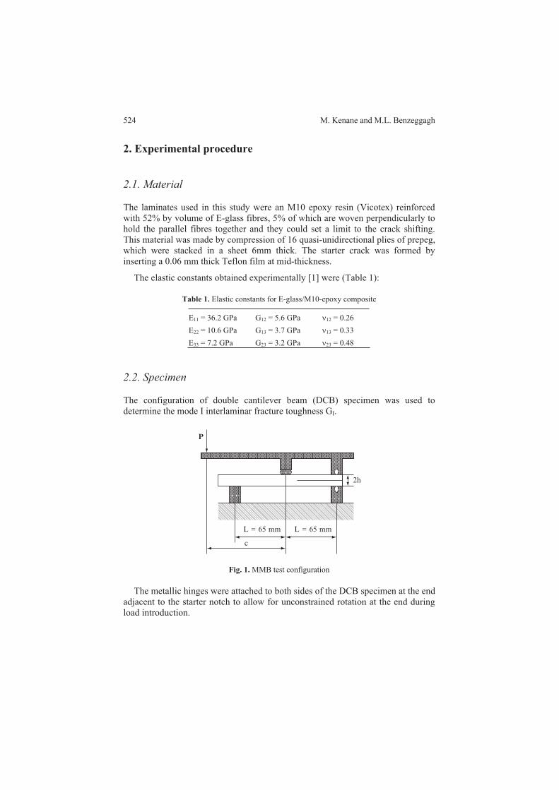
M. Kenane and M.L. Benzeggagh
2. Experimental procedure
2.1. Material
The laminates used in this study were an M10 epoxy resin (Vicotex) reinforced
with 52% by volume of E-glass fibres, 5% of which are woven perpendicularly to
hold the parallel fibres together and they could set a limit to the crack shifting.
This material was made by compression of 16 quasi-unidirectional plies of prepeg,
which were stacked in a sheet 6mm thick. The starter crack was formed by
inserting a 0.06 mm thick Teflon film at mid-thickness.
The elastic constants obtained experimentally [1] were (Table 1):
Table 1. Elastic constants for E-glass/M10-epoxy composite
E11 = 36.2 GPa G12 = 5.6 GPa 12 = 0.26
E22 = 10.6 GPa G13 = 3.7 GPa 13 = 0.33
E33 = 7.2 GPa G23 = 3.2 GPa 23 = 0.48
2.2. Specimen
The configuration of double cantilever beam (DCB) specimen was used to
determine the mode I interlaminar fracture toughness GI.
Fig. 1. MMB test configuration
The metallic hinges were attached to both sides of the DCB specimen at the end
adjacent to the starter notch to allow for unconstrained rotation at the end during
load introduction.
524
c
L = 65 mm L = 65 mm
2h
P

Characterization of Mixed Mode Delamination Growth and Thresholds
The end-loaded split (ELS) specimen was used for characterizing mode II
fracture toughness GII. The toughness for mixed-mode was evaluated using the
mixed-mode bending (MMB) configuration developed by Reeder and Crews [2, 3].
This test is a simple combination of the DCB (mode I) specimen and the ENF (mode
II) specimen (Fig. 1). Actually, the MMB is included in the ASTM standards [4].
2.3. Test conditions
The experiments were carried out in a 1 kN, computer-controlled, servo-hydraulic
testing machine (Instron 1341). They were conducted under constant-amplitude
fatigue tests at a minimum to maximum cyclic load ratio (R) of 0.1 and a
frequency of 4 Hz. During tests, the maximum and the minimum strain-energy
release rates, Gmax, Gmin and delamination growth ratedN
da, were monitored.
The threshold was found by reducing the applied load with level of 10–15%
until the crack growth arrests, and when the delamination had not begun to grow
after 106 cycles. Then, the applied load and, hence, the corresponding Gth could
be considered below a threshold value.
2.4. Energy release rates
The delamination strain energy release rate can be expressed as:
da
dC
b
PG
2
2
(1)
where b is the width of the specimen (mm), P is the applied load (N) and C is the
compliance (N mm 1). The compliance of the DCB can be shown to be equal to a
power law function of the delamination length of the form:
h
a
PC
n
(2)
where n and h are determined experimentally (n = 1.89, h = 24.78 × 10⁵).
An analysis similar to that for mode I was adopted for mode II and mixed-mode
(I+II), for which the compliance can be expressed as 3C .
The constants and can be found by plotting experimental values of C versus
a3 the T
II
G
Gmodal ratio considered (Table 2).
525

M. Kenane and M.L. Benzeggagh
Table 2. Constants for compliance fits
GII/GI (%) 28 53 82 ModeII
(103 mm.N
1) 33.86 15.38 11.48 1.85
(107 N
1.mm2)3.52 1.11 1.05 1.06
The critical strain–energy release rates, ICG and IICG , from mode I and mode
II tests, respectively, and the total critical strain-energy rate, TCG , from mixed mode
considered in this work can be calculated [5] and results are given in Table 3.
Table 3. Total strain energy release rate values
GII/GI (%) 0 28 53 82 100
GTC(J/m2) 118.02 (2.72) 340 (37.26) 579.62 (58.66) 1822 (84.47) 2906 (224.55)
3. Results
3.1. Delamination growth rate determination
As a delamination grows at a constant cyclic load, the cyclic TG changes; hence,
the delamination growth rate changes. A plot of dN
da versus TG may be obtained
for each over T
II
G
G mode ratio, pure mode I and pure mode II, as shown in Figs. 2,
3, and 4 and the results may be fitted by Eq. (3). The coefficients B and d,
obtained by least-squares fitting of the fatigue-crack growth rate curve, are
presented in the Table 4.
Table 4. Experimental values of d and B parameters
GII/GI (%) 0 28 53 82 100
d 1.9 2.13 2.62 3.33 4.2
B 21.6 1012
1.02 1012
0.29 1012
1.04 1016
1.73 1023
The results published in the literature show that the d exponent for graphite/
epoxy composites is generally much higher than that for glass/epoxy composites
[6–8]. For glass/epoxy composite, the d value found by Prel et al. [8] is closer to
what we have obtained. However Bathias and Laksimi [9] have studied glass-
cloth-reinforced epoxy under similar loading conditions, and obtained a high d
526

Characterization of Mixed Mode Delamination Growth and Thresholds
values for mode I (d = 3.71) and mode II (d = 7). In this case a crack can be
confronted locally with several rigidities, unlike in unidirectional composites
where the crack propagates in the plane in which the rigidity is relatively homo-
geneous. However, contrarily to graphite/epoxy composite, results obtained for
glass /epoxy in this study show that the d exponent increases with T
II
G
G.
Fig. 2. da/dN versus the strain-energy release rate, GT, for GII/GI = 28%
Fig. 3. da/dN versus the strain-energy release rate, GT, for GII/GI = 53%
527
0.0110 2
10 3
10 4
10 5
10 6
10 7
101
GT (J/M2)
102 103
GII / GT = 28%
da /
dN
(m
m / c
ycle
)
0.0110 2
10 3
10 4
10 5
10 6
10 7
10
GT (J/M2)
102 103
GII / GT = 53%
da /
dN
(m
m / c
ycle
)

M. Kenane and M.L. Benzeggagh
Fig. 4. da/dN versus the strain-energy release rate, GT, for GII/GI = 82%
3.2. Threshold total strain energy release rate
The total strain energy release rate threshold TthG is characterized by a very
weak delamination growth rates dN
da (<10 6 mm/cycle). Therefore, a crack can’t
propagate during a test which can last during many thousands of cycles. The
TthG values are obtained by the decreasing load method. Three to five
specimens were tested for each TII GG / mode ratio considered. In this study, the
TthG values correspond to (10 6 <dN
da<10 7).
As shown in Figs. 2, 3, and 4, the threshold value is progressively reached after
having described a curve representing the transition between the curve linear part
(Paris’ law) and the threshold value. This is a characteristic of the glass–fibre
composites. However, for the carbon–fibre composites, the threshold value is
suddenly reached just after the curve linear part.
Table 5 summarises the results of the TthG values as function of TII GG /
mode ratio. The obtained results show a logical development. The higher the
TII GG / mode ratio, the greater the value of TthG .
Table 5. Threshold total strain energy release rate results
GII/GI (%) 0 28 53 82 100
GTth (J/m2) 56.17 (5.65) 78.90 (4.81) 115.52 (12.11) 243.88 (10.37) 281.11 (18.05)
528
10 1
10 2
10 3
10 4
10 5
10 6
10 7
GT (J/M2)
103102 104
GII / GT = 82%
da /
dN
(m
m / c
ycle
)

Characterization of Mixed Mode Delamination Growth and Thresholds
Studies presenting the measured delamination growth dN
da as function of the
strain release rate TG (Paris law), have proposed by numerous investigators.
But, few studies including the threshold for no delamination growth are presented
in the literature.
However, for unidirectional carbon-fibre reinforced epoxy composites, many
authors Mall et al. [6], Russell and Street [10], Gustafson and Hojo [11] have
shown that the total strain energy release rate TthG decreases when T
II
G
G mode
ratio increases. In the case of unidirectional glass-fibre reinforced epoxy composites,
the opposite phenomenon is noted.
Numerous fatigue studies Mall et al. [6], Russell and Street [10] have shown
that the total strain energy release rate threshold increases when the matrix
toughness decreases in mode I, mode II, and mixed mode (I+II).
4. Conclusions
The present investigation has examined the delamination mode I, mode II and
mixed-modes (I+II) delamination growth and threshold in unidirectional laminates
of E-glass/epoxy composite under fatigue conditions. This entailed the use of
DCB, ELS, and MMB fracture mechanics coupons. The conclusions of this study
may be summarised as follows:
For each TII GG / mode ratio considered in this study, results are presented in
the form of TG versus dN
da plots which fit the Paris law. Threshold values of the
total strain energy release rate below which no initiation of delamination growth
occurs were determined for both mode I, mode II, and mixed mode (I+II). In order
to propose a semi-empirical threshold fatigue criterion, the study of a large
number of TII GG / mode ratios is necessary.
References
[1] Gong X.J. (1992) Rupture interlaminaire en mode mixte (I+II) du composite stratifié
verre/epoxy unidirectionnel et multidirectionnel. Thèse de docteur de l’UTC, France.
[2] Crews J.H. & Reeder J.R. (1988) A Mixed Mode Bending apparatus for delamination
testing. NASA TM 100662 Report.
[3] Reeder J.R. & Crews J.H. (1991) Non linear analysis and redesign of the Mixed Mode
Bending delamination test. NASA TM 102777 Report.
[4] ASTM D 6671-01 (2004) Standard test method for mixed mode I-mode II interlaminar
fracture toughness of unidirectional fiber-reinforced polymer matrix composites.
529

M. Kenane and M.L. Benzeggagh
[5] Benzeggagh M.L. & Kenane M. (1996) Measurement of mixed-mode delamination fracture
toughness of unidirectional glass/epoxy composites with mixed-mode apparatus. Composite
Science and Technology, 56, pp 439–449.
[6] Mall S., Yun K.T. & Kochhar N.K. (1989) Characterization of Matrix Toughness Effect on
Cyclic Delamination Growth in Graphite Fiber Composite. ASTM STP 1012, pp 296–310.
[7] Martin R.H. & Muri G.B. (1990) Characterization of Mode I and Mode II, Delamination
Growth and Threshold in AS4/PEEK Composite. ASTM STP 1059, pp 251–270.
[8] Prel Y., Davies P., Benzeggagh M.L. & De charentenay F.X. (1989) Mode I and Mode II
Delamination of Thermosetting and Thermoplastic Composites. ASTM STP 1012, pp 251–269.
[9] Bathias C. & Laksimi A. (1985) Delamination Thershold and Loading Effect in Fiber Glass
Epoxy Composite. ASTM STP 876, pp 217–237.
[10] Russell A.J. & Street K.N. (1987) The Effect of Matrix Toughness on Delamination: Static
and Fatigue Fracture Under Mode II Shear Loading of Graphite Fiber Composites.
Toughened Composites, ASTM STP 937, pp 275–294.
[11] Gustafson C.G. & Hojo M. (1987) Delamination Fatigue Crack Growth in Unidirectional
Graphite/Epoxy Laminates. Journal of Reinforced Plastics and Composite, pp 36–52.
530

T. Boukharouba et al. (eds.), Damage and Fracture Mechanics: Failure Analysis of Engineering
© Springer Science + Business Media B.V. 2009
Modification of Cellulose for an Application
in the Waste Water Treatment
Lamia Timhadjelt, Aicha Serier, Karima Boumerdassi,
Mohamed Serier and Zoubir Aîssani
Laboratory of Coating, Materials and Environment (LRME); University M’Hamed Bougara
of Boumerdes; Avenue of the Independence, 35000 Boumerdes, Algeria
Abstract Today’s dramatic shortage of water resources and alarming pollution has recently
triggered a lot of research for alternative water resources. This study consists in modifying
cellulose by grafting of the amidoxime groups for its use in the adsorption of the Cu2+
, Cr3+
and
sulphide ions present in industrial waste waters. Cellulose is an abundant biodegradable polymer.
The amidoxime groups are strong complexants of metal ions. The grafting is achieved in two
steps: cyanoethylation and amidoximation, confirmed by FT-IR. The optimum conditions and
the parameters influencing the two reactions are determined by the kjeldahl’s method and by FT-
IR. The amidoxime quantity is determined by measuring the quantity of the amine functions by
HCl proportioning. The implementation of the modified cellulose is intended for the adsorption
of the metal ions Cu2+
and Cr3+
and sulphide ions S2
in a double adsorption. The FT-IR analysis
reveals that the fixing of metal cations is based on the complexation of the latter with the ligands
of the adsorbent. The optimum adsorption was recorded at pH = 6 for a contact time of 5 h and
an initial concentration of 101M in metals. The desorption of fixed metals is possible by the
EDTA, and the re-use of the adsorbent confirms the effectiveness of recycling.
Keywords: Cellulose, Modification, Sorption, Heavy Metals, Waste Water Treatment.
1. Introduction
The fast changes of polymeric materials due to technological and industrial practices
have made their use more effective and less expensive. Thus, new implementations
are regularly carried out with chemically modified polymers such as in the waste
water treatments. However, the biopolymers and particularly cellulosics was the
subject of these modifications. Indeed, during these last years, works of research
were about the possibility of finishing controlled changes in the properties of the
cellulosic materials [4] as cotton and cellulose [1, 5, 6] and bagasse [2, 3].
These last are very often chemically modified by amino groups. This alternative
has the advantage of increasing the value of some natural products and sub-products
[7]. In addition, the re-use of used waters represents a solution to the problem of
water shortage, and takes part in the reduction of the pollution generated by the
industrial effluents. The economic limits of the traditional techniques of metal
processing liquid waste resulted in developing new processes implementing
531
Materials and Structures, 531–538.

L. Timhadjelt et al.
properties of adsorption and complexation of biomaterials, particularly those
based on the cellulose [4]. Indeed, in this field, the lignocellulosic materials seem
promising by the adsorption of toxic heavy metals [8].
The objective of our work thus consists of the introduction of the amidoxime
groups, complexants, into cellulose for an application in the field of the waste
water treatments by the adsorption of heavy metals and with sulphide ions. The
latter are eliminated by fixing in the second adsorption on the metals already
trapped on amidoximated cellulose.
2. Material and methods
Pure cellulose powders some (60–65% crystalline) (Sigma-Aldrich Chemistry
limited liability company, France), Acrylonitrile (Aldrich), hydroxylamine (Fluka
Chimie, France). The heavy metal ions (Cu2+ and Cr3+) were obtained starting
from the metal salts (CuCl2, 2H2O) and (CrCl3, 6H2O) adjusted with pH between 3
and 6 using the solutions of Clarck-Lubs [6], by using the potassium hydro-
genophthalate (Table 1).
Table 1. Clarck-Labs buffer solutions [6]
pH Metals Solution
(ml)
Potassium
Hydrogeno-
Phthalate 0.2 M
(ml)
HCl 0.2 M (ml) NaOH 0.2 M, (ml) Deionized water
3 250 250 101.6 2 Dilute for 1,000 ml
4 250 250 / 119.25 Dilute for 1,000 ml
5 250 250 / 227.25 Dilute for 1,000 ml
6 250 250 / / Dilute for 1,000 ml
The products are characterized by a spectrometer FT-IR of Thermo-Nicolet
Nexus series at ambient temperature. After drying under 40°C during 48 h, 3 mg
of the sample is crushed with 150 mg of KBr then pressed. The pastille of Ø = 6
mm is analyzed.
The influence of the various parameters on the reactions was expressed by the
degree of substitution (DS) determined by the Kjeldahl’s method (Eq. 1) and by
FT-IR. The proportioning of the metal ions in solution is carried out by an atomic
adsorption spectrometer, SOLAAR M6, after acidification, dilution and filtration
of the solutions.
The spectrometer UV, JASCO 3200, is used to highlight the effectiveness of
the regeneration of Amidoxime Cellulose (Am-Cel). The solutions are introduced
into a basin of optical way of 1cm. The quantity of the sulphide ions fixed is
determined by iodic proportioning.
532

Modification of Cellulose for an Application in the Waste Water Treatment
2.1. Modification of cellulose
Obtaining the amidoxime cellulose (Am-Cel) passes by the preparation of the
cyanoethyl cellulose (CE-Cel) like first stage. The latter is obtained by the action
of the acrylonitrile (AN) on the cellulose (Cel) in alkaline medium, NaOH with
36% in weight, in the presence of tetramethylammonium chloride (TMAC) [3, 6].
The Degree of substitution (DS) of the CE-Cel is obtained from the ultimate
analysis of nitrogen rate N (%) using the following relation [6]:
(%)100
(%)
NMM
NMDS
ANN
Cel (1)
The CE-Cel prepared is then treated by an aqueous hydroxylamine hydrochloride
solution [6] at constant temperature (60–80°C) for variant time (90–180 min). The
modified cellulose obtained is washed with deionized H2O and filtered under
vacuum. The results are expressed by the quantity of amidoxime QA, obtained by
the absorption of HCl by the amidoxime groups [6].
2.2. Adsorption and desorption of the heavy metal ions
The experiments of adsorption were carried out in a batch for a ratio of mass of
adsorbent/volume of solution of 1/100 (g/ml), with the variation successively of
the pH of the solution between 3 and 6, the contact time from 0 to 48 h and the
initial heavy metal (Cu2+ and Cr3+) concentrations from 0 to 101 M. For the same
ratio of mass of adsorbent/volume of solution, a well defined mass of Am-Cel was
immersed in an adequate volume of solution containing Cu2+ and Cr3+ ions for
24 h at ambient temperature under continuous agitation. The suspension is then
filtered. The quantities of the Cu2+ and Cr3+ ions were determined by atomic
absorption spectroscopy. The Am-Cel was regenerated by desorption of the metal
ions adsorbed by a solution of EDTA at 0.1 N. A quantity of 0.1 g of Am-Cel is
immersed in this last solution at ambient temperature during 24 h. The suspension
is then washed by deionized H2O, filtered and finally analyzed by UV
spectroscopy. After the adsorption of the metal ions on the Am-Cel, the sulphide
ions are eliminated in the second adsorption by immersing 0.005 g of the powder
not regenerated in a sulphide solution with various concentrations: 2·10 2, 4·10 2
and 8·102 M in closed bottles with continuous agitation.
3. Results and discussions
The CE-Cel and the Am-Cel are characterized by FT-IR. The comparison of the
respective spectra (Fig. 1) shows the appearance of a peak characteristic of the C N
533

L. Timhadjelt et al.
groups to 2254 cm 1 on the spectrum of the CE-Cel, while on that of the Am-Cel,
we observe a considerable reduction in the peak characteristic of the C N groups
and the appearance of a peak characteristic of double bond C = N to 1,666 cm 1,
thus indicating the formation of the CE-Cel and the Am-Cel respectively. Tables 2
and 3 indicate the influence of the conditions of cyanoethylation and amidoxi-
mation reactions respectively on DS and quantity of amidoxime (QA).
Fig. 1. Cellulose (1), CE-Cel (2) and Am-Cel (3) infrared spectrum
Table 2. Parameters influencing the cyanoethylation reaction
TMAC Time (min) (NaOH) (%) DS
Without 90 36 1,510
With 90 36 2,297
With 45 36 0,847
With 150 36 2,385
With 90 10 0,391
With 90 20 0,739
Table 3. Parameters influencing the amidoximation reaction
Temp (°C) Time (min) (NH2OH) (%) DS of CE-Cel QA (mmol/g)
80 90 5 2.297 3.80
80 90 10 2.297 4.27
80 60 10 3.385 3.73
80 90 10 3.385 4.10
80 150 10 3.385 4.40
80 180 10 3.385 5.00
60 90 10 3.385 3.37
534
2946,502254,94
1666,79 917,062
4
12
10
8
6
(3)
(2)
(1)
% T
ransm
itance
Wave numbers (cm 1)
3500 3000 2500 2000 1500 1000

Modification of Cellulose for an Application in the Waste Water Treatment
Fig. 2. Am-Cel (1) and Cu2+
-Am-Cel (2) infrared spectrum
We note an increase in the DS of the CE-Cel with the presence of tetramethylam-
monium chloride (TMAC), time and the NaOH concentration up to an optimal
value of 20% of the later. QA contained in the Am-Cel, increases with the temper-
privileged by a concentration in NH2OH of 10%. These results agree with
literature works [2, 3, 5, 6]. Contrary to the Cel and the CE-Cel, the Am-Cel
showed a great affinity for heavy metals (Cu2+ and Cr3+). An octahedral complex
which is characterized by the FT-IR analysis (Fig. 3) tends to be formed between
the latter and the Am-Cel in the presence of the phthalates anions [8] at ambient
temperature. The results (Fig. 3) show that the quantity of (Cu2+ and Cr3+) ions
adsorbed increases with their initial concentration.
Fig. 3. Variation of the quantity of Cu2+
(1) and Cr3+
(2) ions adsorbed with their initial concentration
stage beyond 180min indicates a maximum of conversion. The amidoximation is
ature and time until 180 min (Fig. 2). According to authors [2, 5, 6], obtaining a
535
00
1
2
3
4
5
6
7
8
9
0,02 0,04 0,06
Initial metal ions concentration (mol/I)
Qu
an
tity
of
heavy m
eta
l io
ns
ad
so
rbed
(m
mo
l/g
)
0,08
(1)
(2)
0,1 0,12
(2)
(1)
2247,71
1610,12
2247,71 919,86
1666,59
911,81
22
26
42
38
34
30
% T
ransm
itance
2000 1500 10003000 25003500
Wave numbers (cm-1)

L. Timhadjelt et al.
Figure 4 shows that the quantity of (Cu2+ and Cr3+) ions increases with the time
of contact, the equilibrium time is 5 h; the curves tend then towards a stage in
accordance with the theory, indicating the saturation of the adsorption sites. The
reduction recorded after 24 h can be explained by a light desorption due to the
molecular collisions.
Fig. 4. Variation of the quantity of Cu2+
and Cr3+
ions adsorbed with the contact time
The results represented on Fig. 5 show in the case of chromium, that the
quantity of the Cr3+ ions adsorbed increases with the solution pH. A small quantity
was recorded towards pH = 3, this is due to the inhibiting effect. On another side,
with pH = 6, we observe the precipitation of the metal ions with the OH ions.
Fig. 5. Variation of the quantity of Cr3+
ions adsorbed with solution’s pH
Figure 6 shows an increase in the quantity of Cu2+ ions adsorbed with QA
contained in the adsorbent. This is foreseeable because the amidoxime groups
represent the sites of adsorption.
536
0 10 20 30 40 50 60
0
1
2
3
4
5
6
Time (hour)
Qu
an
tity
of
heavy m
eta
l io
ns
ad
so
rbed
(m
mo
l/g
)
2
Solution’s pH
0
0,1
0,2
0,3
0,4
0,5
0,6
0,7
0,8
3 4 5 6 7
Qu
an
tity
of
Cr3
+ io
ns a
dso
rbed
(mm
ol/g
)

Modification of Cellulose for an Application in the Waste Water Treatment
Fig. 6. Variation of the quantity of Cu2+
ions adsorbed with the quantity of the amidoxime
The results deferred on Table 4, show that the Cu2+ ions is selectively adsorbed
on the amidoxime cellulose. This result agrees with works of Gauthier and al. [6]
and EL-Wakil et al. [2].
Table 4. Determination of the quantity of Cu2+
and Cr3+
ions adsorbed for evaluation of their
selectivity
Sample Initial Concentration
(mol/l)
Metal ion non
adsorbed content
(mol/l)
Metal ion adsorbed
content
(mol/l) = metal ion
adsorbed quantity
(mmol/0.01 g)
Metal ion adsorbed
quantity (mmol/g)
Cu2+
7 102 0.885 10
2 6.114 10
2 6.11(4)
Cr3+
7 102 3.782 10
2 3.218 10
2 3.21(8)
It is carried out by desorption of the Cu2+ and Cr3+ ions by a solution of EDTA
0.1 N. In the presence of the latter, the Am-Cel doesn’t show any affinity towards
the metal ions. The effectiveness of regeneration is proven by the re-use of the
treated powder. It is highlighted by the change of color yellowgreen obtained
by immersion of the powder in a sulphide solution during t = 30–60 min. Figure 7
shows that the quantity of the sulphide ions fixed increases with their initial
concentration.
Fig. 7. Variation of the quantity of S2-
ions fixed with their initial concentrations
537
3,53,75
3,77
3,79
3,81
3,83
3,85
3,87
3,7 3,9 4,1
QA of the adsorbent (mmol/g)
4,3 4,5 4,7 4,9 5,1
Qu
an
tity
of
Cu
2+
io
ns
ad
so
rbed
(m
mo
l/g
)
0 0,01 0,02 0,03 0,04 0,050
0,1
0,2
0,3
0,4
0,5
0,6
Initial concentration of S2– ions (mol/l)
Qu
an
tity
of
S2– io
ns
fixed
(m
mo
l/g
)

L. Timhadjelt et al.
4. Conclusions
The cellulose was modified into Am-Cel while passing by the CE-Cel. The
amidoxime groups can be chelated with heavy metals by formation of an octahedral
complex metal-Am-Cel, which make them useful in the waste waters treatment.
The operating conditions of preparation are simple. The adsorption of heavy
metals is influenced by several parameters. It increases with their initial concent-
ration, the time of contact and the pH of the solution. The sulphide ions are fixed
on the heavy metals adsorbed beforehand on the Am-Cel. The regeneration of the
Am-Cel is possible using a solution of EDTA at 0,1N.
References
[1] Gustaro Rocha de Castro, Ilton Luiz de Alcântara, Paulo dos Santos Roldan (2004)
Synthesis, characterization and determination of the metal ions adsorption capacity of
cellulose modified with p-aminobenzoic groups. Mat. Res., 7(2): 12.
[2] Hassan M. L., EL-Wakil N. A. (2003) Heavy metal ion removal by amidoximated bagasse.
Wiley Periodicals. J. Appl. Polym. Sci., 87: 666–670.
[3] Hassan M. L., EL-Wakil N. A., Sefain M. Z. (2001) Thermoplasticization of Bagasse by
cyanoethylation. Inc. J. Appl. polym. Sci., 79: 1965–1978.
[4] Hebeish A., Guthrie J. T. (1981) The chemistry and Technology of cellulosic copolymers.
Springer, Berlin Heidelberg, New York, 342p.
[5] Kuboka H., Shigehisa Y. (1995) Introduction of amidoxime groups into cellulose and its
ability to adsorb metal ions. Inc. J. Appl. Polym. Sci., 56(2): 147–151.
[6] Saliba R., Gauthier H., Gauthier R., Petit-Ramel M. (2000) Adsorption of copper (II) and
chromium (III) ions onto Amidoximated cellulose. Inc. J. Appel. Poly. Sci., 75: 1624–1631.
[7] Satge Céline (2002) Etude de nouvelles stratégies de valorisation de mono et polysaccharides.
Ph.D. thesis, Limoges University, 137p.
[8] Seko N., Tamada M., Yoshii F. (2004) Current status of adsorbent for metal ions with radiation
grafting and crosslinking techniques. 6th International Symposium on Ionising Radiation
and Polymers, IRAP.
538

T. Boukharouba et al. (eds.), Damage and Fracture Mechanics: Failure Analysis of Engineering
© Springer Science + Business Media B.V. 2009
A Full 3D Simulation of Plastic Forming Using
a Heuristic Generalised Contact Algorithm
Tewfik Ghomari1, Rezak Ayad
2 and Nabil Talbi
3
1University of Sciences and Technology of Oran (USTO), Mechanical Department, BP 1505
El-Mnaouar, Oran, Algeria
2University of Reims Champagne-Ardenne, Group of Research in Sciences for Engineers
Mechanics (GRESPI), Reims, France ESIEC, Esp. Roland Garros, BP 1029, Reims, France
Abstract A full 3D contact approach is proposed for simulating forming processes of plastic
bodies. It uses a new local searching procedure which is based on the product of the geometrical
positions of the “Slave” node before and after having crossed a plan “master”. Coupling with the
finite element method is achieved by using a classical 8-node hexahedral element. The use of a
Mooney-Rivlin constitutive model allows getting a final simulation tool in order to optimise the
mechanical behaviour of plastic bodies during their forming processes. Applications are
essentially focused on 3D problems involving contact between solids, with a particular attention
to the thermoforming process.
Keywords: Finite Element, 3D Contact, Hyperelastic, Plastic Forming Process.
1. Introduction
The contact problems are very frequently encountered in industry. The codes of
market such as ABAQUS, LS-DYNA, MARC, PAM-CRACH etc., take into
account the problem of contact with or without friction. That made it possible to
solve a rather vast number of industrial problems considered difficult. The main
difficulties of a contact problem come owing to the fact that the boundary
conditions related to the contact are not known in advance and they depend on the
solution (boundary conditions evolutionary). Thus, the real contact surface and the
contact reactions belong to the unknown factors of the problem. In case of great
transformations, nonlinearities coming from the contact are added to the geometrical
and material nonlinearities, making the forming problem quite difficult to solve.
The general problem of the balance of a linear elastic solid in contact without
friction with a rigid foundation, it was necessary to wait the Sixties so that Duvaut
the Seventies many numerical methods to be born. The first algorithm allowing
making leave the nodes “Master” and “slave”, in the case of the problems 2D and
(sorting of limp).
the existence and the unicity of the solution. This obviously made it possible during
and Lions [1] proposed the variational inequations making it possible to establish
3D, was established by Hallquist [2]. It is based on the concept of Bucket-sorting
539
Materials and Structures, 539–552.

T. Ghomari et al.
bringing back the search for three dimensions to only one dimension, thanks to
an approach called “position codes” making it possible to codify all the nodes
according to the positions of the nodes and of the numbers of limp circumscribed.
This technique allows to simplify the search of the areas of contact by examining
the “position codes” (codified position of the nodes) of each node, after a binary
sort as a preliminary. By using this algorithm, the cost of total search is thus
reduced to (NLog2N) operations of permutations. It does not remain about it less
proposed the algorithm unified by combining the technique of “position codes”
with a labellized approach “HITA” (Hierarchy Territories and Contact Territories).
Although these methods and/or algorithms, proposed and developed for total
search, remain in their globality rather effective, it does not remain about it less
than effective algorithms for the local research of contact remain rather little
not a node slave is in contact. The algorithms of local contact available in the
literature are based on the algorithm known as “of node to segment” or “node on
distances from penetration of the “Slave” node through the segment “master”. In
the majority of the problems with contact, the iteration count can strongly increase
for small values of tolerance (lower than 10 3 test of stop), or if the geometry of
the segment “master” presents sharp angles. Moreover it is unstable in certain case
when the nodes candidates are opposite several segments. To improve the
algorithm. The aforementioned is based on the orientation of the normal vectors
carried by the element “master” and the trajectory of the “Slave” node between
iteration I and i + 1. This method is considered to be fast because no iteration is
added. However, from the problems can emerge at the edge between two segments
or two or several bilinear surfaces called “areas of dead angle”, because there is no
more continuity of the normal between two segments. The areas of dead angles are
the weak points of the local algorithms of search. To overcome these difficulties
develop an algorithm of search for total contact able to treat the contact impact
(Crash landing of car). It was implemented on Software PRONTO 3D. The afore-
mentioned belonged to the algorithms of search for contact based on the technique
“bucket sorting”. A formula thus makes it possible to calculate the code of limp
unbounded, which distinguishes the algorithm from that Zhong (position codes).
The algorithm of search for contact developed in our work rests on this technique
with a new algorithm of search local which is based on the product of the
geometrical positions of the “Slave” node before and after having crossed a plan
“master”.
In 1994, Oldenbourg and Nilsson [3] simplified the preceding algorithm while
than the process of total search is not very effective. To improve it, Zhong [4]
developed [5]. The local research is employed to determine with precision so yes or
algorithm of “node slave/segment master”, Wang [5] proposed the “Inside–outside”
by making a smoothing from the points of the cubic segments using splines.
Ju [7], an algorithm of local research proposed which eliminates the sharp angles
540
surface [6]. The method of Raphson Newton is often employed to determine the
But the possibility of multiple solutions of the contact of a node by several seg-
ments affects the effectiveness of the search for contact. Heinstein and al. [8] could

Simulation of Plastic Forming Using a Heuristic Generalised Contact Algorithm
2. Basis 8 node hexahedral element in total lagrangian
formulation (FLT)
We present the main equations used for the implementation of a behavior law in a
classical three-dimensional solid element (8-node hexahedral element H8). A
Total Lagrangian displacement Formulation is used.
2.1. Geometrical approximation and displacement formulation
The position vector of a point in the meridian plan, expressed in the Cartesian co-
ordinate system, is given by:
Nodes
i
Nodes
i
ii
Nodes
i
iiiip zNzyNyxNxwithkzjyixx
1 11
;;rrrr
(1)
The 3D displacement field of point p is defined by the following classical tri-
linear approximation:
8
1
8
1
8
1
;;
i i
ii
i
iiii WNWVNVUNU (2)
The shape functions and their derivatives are those of a conventional 8-node
hexahedral element (H8) (Fig. 1). 2 × 2 × 2 gauss points are sufficient to get an
exact integration of the stiffness tangent matrix.
Fig. 1. 3D 8-node hexahedral element
8
8
8
1
1
1
81
81
81
81
81
81
81
81
81
,,
,,
,,
,,
,,
,,
,,
,,
,,
,
,
,
,
,
,
,
,
,
W
V
U
W
V
U
NN
NN
NN
NN
NN
NN
NN
NN
NN
W
W
W
V
V
V
U
U
U
zz
yy
xx
zz
yy
xx
zz
yy
xx
z
y
x
z
y
x
z
y
x
M
K
K
K
K
K
K
K
K
K
(3)
541
y x
U
V
W
z

T. Ghomari et al.
2.2. Green–Lagrange deformation tensor
The displacement gradient tensor [F] and the Cauchy Green Right stress tensor [C]
are written in the Cartesian co-ordinate system as:
3332311
232221
131211
,,,
,,,
,,,
C
1
1
1
CCC
CCC
CCC
FF
WWW
VVV
UUU
F T
zyx
zyx
zyx
(4)
2
,
2
,
2
,,,,,,,,,,,,,
,,,,,,
2
,
2
,
2
,,,,,,,
,,,,,,,,,,,,
2
,
2
,
2
,
11111
11111
11111
zzzzyzyzyxzzxzx
zyzyzyyyyyxxyyx
xzzxzxyxxyyxxxx
WVUWWVVUUWWVVUU
WWVVUUWVUWWVVUU
WWVVUUWWVVUUWVU
C (5)
I1, I2 and I3 are the invariants of tensor [C]:
2
1233
2
1322
2
23111323123322113
2
13
2
23
2
121133332222112
3322111
2 CCCCCCCCCCCCI
CCCCCCCCCI
CCCI (6)
The Green-Lagrange tensor is written as:
ICE2
1 (7)
2.3. Minimum total potential energy principle
The total potential energy is defined by:
k
kext
kint (8)
kint is the elementary internal potential energy which can be written as:
0212int 0 ,, dvJIIW
vk (9)
W represents the deformation energy per unit of no-deformed volume,
accumulated in the structure during the deformation:
542

Simulation of Plastic Forming Using a Heuristic Generalised Contact Algorithm
JWIIWJIIW sd ),(),,( 2121 (10)
22121 1
2
13231,, JICICJIIW (11)
1I and 2I are modified invariants. The first variation of the external potential
energy k
ext is given by:
0S
kext dS pu0 (12)
u is the displacement vector in the local base nttrrr
,, 21 and p the
compressive distributed forces. Residual vector:
0S
k dS pu0int (13)
where kint represents the first variation of the internal elementary energy.
00
21int ,,V
k VdJIIW (14)
We obtain the vector of the internal forces:
8881int 11det WVUWVUUwithdddJrU nn
kK (15)
kk fU intint (16)
Introducing a Mooney-Rivlin law leads to:
00
332211int Vk dVIAIAIA (17)
With:
33
5
3223
4
31133
2
3223
1
311
1
2
1
3
2
3
1,, Ij;
J
JIICIICA ICA ICA (18)
For a Mooney-Rivlin law [9], W is given by Crisfield [10]:
543

T. Ghomari et al.
321 , IandII The variations of the invariants of the right tensor represent.
2323111312131322231233122313
33
2
12221122
2
13331111
2
2333223
2323131312123322112233111133222
3322111
222
222
)(
CCCCCCCCCCCCCC
CCCCCCCCCCCCI
CCCCCCCCCCCCCCCI
CCCCtrI (19)
These theoretical developments allows getting the following expression of kint :
0
1321int V
Nodes
i
0k dV WfVfUf (20)
6,,,,5,,,,
4,,,,3,,2,1,,1
1
12212
BNUNUBNUNU
BNUNUBNUBUBNUf
ziyyizzixxiz
yxxyzizyxx
(21a)
6,,,,5,,,,
4,,,,3,,2,,1,,2
1
12122
BNVNVBNVNV
BNVNVBNVBNVBNVf
yizziyxizzx
xiyyixzizyyxix (21b)
6,,,,5,,,,
4,,,,3,,2,,1,,3
11
1222
BNWNWBNWNW
BNWNWBNWBNWBNWf
yizzyxizzix
xiyyixzzyiyxx (21c)
And:
3131223112236
3231222132135
3231333122124
3
2
1222112221113
3
2
1333112331112
3
2
2333222332211
2
2
2
ACCCCACB
ACCCCACB
ACCCCACB
ACCCACCAB
ACCCACCAB
ACCCACCAB
(22)
The final internal force vector kfint is written as:
dddJffffffWVUWVUTk det321321888111int LL (23)
544

Simulation of Plastic Forming Using a Heuristic Generalised Contact Algorithm
kk fU intint (24)
3. Tangent matrix
The calculation of the elementary tangent matrix can be explicitly defined by
expressing the second variation of the elementary virtual work or by a perturbation
technique. We have adopted the last technique which usually used. It is based on a
finite difference scheme:
j
jj
TU
UURUURK
j 2 (25)
We present a searching algorithm for the analysis of 3D contact. It’s based, on
searching algorithm with a penalty method that we’ve developed in this work.
There are other searching techniques of contact areas, which make it possible to
containing nodes in each zone are updated at each new introduction of object. The
simplest structure is the regular mesh covering the field. Each box of mesh is
In order to cure the need for locating the nodes candidates in contact with an
arbitrary manner, a total strategy is adopted which consists in the following:
Initialize the vector (nbox) which contains the numbers of the nodes in
Find the code Bi for each node.
Store the codes of all nodes i in a vector (lbox): lbox (I) = Bi.
Increment the storyteller for the codes of such kind: nbox (Bi) = nbox
(Bi) +1.
avoid a systematic sweeping of the whole of the nodes to each step of time. The prin-
indexed by an entirety. This structure is described on the Figs. 2 and 3.
Fig. 2. Virtual mesh Fig. 3. The position code buckets
each bucket of a virtual mesh (Figs. 2 and 3).
545
the one hand, on the work of Heinstein et al. [8], and, on the other hand, on a local
ciple rests on a space division using a virtual mesh (Figs. 2 and 3). The lists of objects
D
X
Y
positioncode Bi
i
ZS
y
S
i
xS
xz
(xmin, ymin, zmax)
(xmin, ymax, zmin)
(xmin, ymin, zmin)i
y

T. Ghomari et al.
Calculate the pointer of each code j in a list of nodes.
Npoint (1) = 1, npoint (j) = npoint (j-1) + nbox (j-1).
Initialize nbox with zero.
Find the nodes slaves in agreement with the numbers of code in a list
(ndsort).
Ndsort (nbox (lbox (I))+npoint (lbox (I)))=Inbox (lbox (I))=nbox(lbox
(I))+1.
The code of each bucket is determined by the expression below:
iXX
iYYX
iZi SSSSSSB 11 (26)
bucketofwidthb
bzzS
byyS
bxxS
bzzS
byyS
bxxS
s
SiiZ
SiiY
SiiX
SZ
SY
SX
:
1/)(int
1/)(int
1/)(int
;
1/)(int
1/)(int
1/)(int
min
min
min
minmax
minmax
minmax (27)
The cutting which contains any node is calculated as follows:
1/int,min
1/int,min
1/int,min
1/int,min
1/int,min
1/int,min
minmaxmax
minmaxmax
minmaxmax
minminmin
minminmin
minminmin
SZ
SY
SX
SZ
SY
SX
bzzcSkbox
byycSjbox
bxxcSibox
bzzcSkbox
byycSjbox
bxxcSibox
(28)
min,CX , max,CX , min,CY , max,CY and min,CZ , max,CZ are the ends of buckets
widened in the direction of X, Y and Z.
Identification of the code of each bucket widened while determining arranged
in three directions X Y and Z:
LoopEnd
LoopEnd
LoopEnd
iboxSjboxSSkboxB
kboxtokboxkboxfromLoop
jboxtojboxjboxfromLoop
iboxtoiboxiboxfromLoop
xyxi . 11
maxmin
maxmin
maxmin
(29)
All the codes of the nodes calculated are able potentially to interact with the
main segment. On the level of the search for local contact, an algorithm is worked
out to detect the Slave nodes which can crossed the segment master by checking
546

Simulation of Plastic Forming Using a Heuristic Generalised Contact Algorithm
the product the positions before and after if it is negative indeed node A crosses if
the product is positive two cases can the this presented either node does not have
crosses the segment or the node has cross-piece the segment before and after this last
Segment
Master
0),( yxf
0),( yxf
0),( yxf
CyBxAyxfWith ),(
Nœud
Slave
Segment
Master
),( 11 tt yxP
),( tt yxP0),( yxf
Segment
Master
0),( yxf
0),( yxf
0),( yxf
CyBxAyxfWith ),(
Segment
Master
0),( yxf
0),( yxf
0),( yxf
CyBxAyxfWith ),(
Nœud
Slave
Segment
Master
),( 11 tt yxP
),( tt yxP0),( yxf
0),,( zyxf
0),,( zyxf
0),,( zyxf
zCyBxAzyxfAvec ),,(
Surface
Master
Nœud
Slave
),,( 111 ttt zyxP
),,( ttt zyxP
0),,( zyxf
0),,( zyxf
0),,( zyxf
zCyBxAzyxfAvec ),,(
Surface
Master
Nœud
Slave
),,( 111 ttt zyxP
),,( ttt zyxP
(a) case 2D (b) case 3D
4. Discretization
ntrr
, with tr
nv
sin:
cos:;
11212 s
cXXLwith
cs
nsc
XXL
t (30)
(s)
4
2
(s)
1
3
1iP
iP
2nr
1nr
*P1
tX
2
tX
tX
nX
(s)
4
2
(s)
1
3
1iP
iP
2nr
1nr
*P1
tX
2
tX
tX
nX
That is to say the standardized curvilinear coordinate of p (the projection of S
on the segment (1-2)) for the case two dimensional:
tXXL S 1/1 with 10 (31)
Fig. 4. Detection of the passage of the node compared to the line
Fig. 5. Local State 3D
case can generates some concern (Fig. 4), before curing it one needs an additional
checking of the product the position of the node in its initial position and its final position.
The local reference mark is defined on the element (1-2) by the base
tangent vector and t he normal vector whose components in the total reference
mark with two dimensions such as:
547

T. Ghomari et al.
The normal gap is the distance from penetration of the node S through the
tangential gap is defined by:
tXXxandnXXx stSn
*1
(32)
The reactions are calculate by Coulomb law and are given by the following
expressions:
Tangential reaction
0nx If no contact ;0nr 0nx If contact nnn xkr (33)
Tangential reaction
reactiontangentialxkrandreactioncriticalrr tttntcri (34)
where µ represents the friction coefficient:
t
tttttttttt
x
xrrcontact slippingrrifxkrcontact adheringrrif
cricricri; (35)
The contribution of the reactions of a node of contact in the residue of total
balance is written:
t
nTncnt r
rQF (36)
The tangent matrices of contact are evaluated in the following:
Q
k
k
k
QK
n
t
tTn
cnt
00
00
00
adhering contact (37a)
Q
k
QK
n
Tncnt
00
000
000
contact (37b)
With [Q] is the matrix of passage of the local at total reference.
The algorithm search for contact must be able to manage ambiguous situations
element (1-2) or a surface is expressed in the local reference (Fig. 5) mark like; the
which can occur at the time of the procedure of search for contact (see Fig. 6):
548

Simulation of Plastic Forming Using a Heuristic Generalised Contact Algorithm
The free node, or in contact, is opposite a dead angle, and does not have
any projection on the close main elements; in that case two situations
The node active slave free, in contact or penetrating, is opposite a valley
and thus has several projected on main elements in this case, we associate
one of the main elements to him nearest from which the distance from the
point candidate and its projection on this element is smallest.
Zone of
dead angle
Master
Node
Rigid (mould)
Zone of
dead angle
Master
Node
Rigid (mould) Surface
Slave D
Zones d’angles morts 3D
2
An
1
Bn
2
Bn
2
Cn
1
Cn
2
Dn
1
Dn
1
An
Nœud Master
Position X(t-1)
Nœud Master
Position X(t)
Surface
Slave D
Zones d’angles morts 3D
2
An
1
Bn
2
Bn
2
Cn
1
Cn
2
Dn
1
Dn
1
An
Nœud Master
Position X(t-1)
Nœud Master
Position X(t)
Zones d’angles morts 3D
2
An
1
Bn
2
Bn
2
Cn
1
Cn
2
Dn
1
Dn
1
An
Nœud Master
Position X(t-1)
Nœud Master
Position X(t)
4.1. Numerical experiments
All our geometry and results have been drawn and visualized using the educational
version of GID software (www.gidhome.com).
4.2. Circular plate under uniform pressure
present themselves (see Fig. 6) case 2D.
Fig. 6. Ambiguous cases 2D and 3D trajectories met
We consider a circular plate treated by Hughes et al. [11], Radius L and thickness h
are respectively 190.5 and 12.7 mm. The plate is fixed on its circumference and
549
subjected to a pressure on one of its faces (Fig. 7).
z
rL
P
h
z
rL
P
h
z
rL
Pz
rL
P
hm
We use a quasi-incompressible hyperelastic material represented by the Mooney-
1 2
factor used to penalize the internal energy is taken equal to K = 68.9 MPa. The
curve of loading of the pressure is obtained by controlling the extreme node of the
Rivlin’s model [9] with the constants C = 0.55 MPa and C = 0.14 MPa. The penalty
plate (Figs. 8 and 9).
Fig. 7. Geometry of plate under pressure

T. Ghomari et al.
0 2 4 6 8
0
5
10
15
20
25
30
35
Pre
ssio
n (
Psi)
Déplacement vertical(in)
H8
Hughes
4.3. Thermoforming of a cup
A second example treats the thermoforming of a cup. In this problem we consider
a plastic paraison thickness 2.54 mm simply pressed on a cup cylindrical and
(type Mooney Rivlin): with the constants MPa 0.142 C1 , MPa 4-e 2.2 C2 and
MPa 68.94k (Bulk Modulus). The resolution is carried out using an implicit
scheme of type Newton Raphson. The contact of paraision is supposed sticking
and the coefficient of penalty taken equal to 107. The objective of this test, famous
to be severe, is to study the thicknesses distribution of the cup at during time
attenuating the strong numerical oscillations observed. A comparison with the
element SFR-Axi is made for a better examination of the performances and
of thicknesses distribution along the generator of the cup.
The results provided by the two models are in agreement with the experimental
tests. A pressure of 0.0716 MPa proved to be necessary to completely plate the
preform against the mould. It should be noted that calculation in round back-
ground areas (bottom of the cup) requires a considerable CPU time. To cure it, it
is completely possible that a mending of meshes localized of the areas with round
Fig. 8. Courbe de charge Pression déplacement
subjected to a uniform pressure. The geometry is illustrated on Fig. 10. This example
was treated by DeLorenzi [12]. Calculation is made on a material hyper-elastic
forming (Fig. 11). The pitches of loading will have to be very small for better
precision on the distribution thicknesses. Figure 12 shows the shape of the curve
550
0.30971
0.29100
0.27243
0.25279
0.23915
0.21650
0.19706
0.17922
0.16058
0.14194
0.30971
0.29100
0.27243
0.25279
0.23915
0.21650
0.19706
0.17922
0.16058
0.14194
Fig. 9. Circular plate under pressure

Simulation of Plastic Forming Using a Heuristic Generalised Contact Algorithm
cavities is carried out. Another solution consists in applying load factors of strong
value for implicit calculation.
0 2 4 6 8 10 12 14
0,0
0,1
0,2
0,3
0,4
0,5
0,6
0,7
0,8
0,9
1,0
h/h
°
Absisses curviligne (in)
Experience (DeLorenzi)
SFRQ-Ax
H8
Fig. 10. Thermoforming of a cup
Fig. 11. Distribution thickness according to the curvilinear coordinate
Fig. 12. Plastic forming process
551
R =0.5
D =5.2
D =0.1
D =
8
D =4.5

T. Ghomari et al.
References
[1] Duvaut G. and Lions J.L. (1976) Inequalites in mechanics and physics. Springer, Berlin.
[2] Hallquist J.O. (1993) LS-DYNA3D Theoretical Manual. Livermore Software Technology
Corporation, Livermore, Rev. 2.
[3] Oldenburg M. and Nilsson L. (1994) The position code algorithm for contact searching. Int.
J. Numer. Meth. Eng., 37:359–386.
[4] Zhong Z.H. and Nilsson L.A. (1996) Unified contact algorithm based on the territory
concept. Comput. Method. Appl. Mech. Eng., 130:1–16.
[5] Wang S.P. and Nakamachi E. (1997) The inside–outside contact search algorithm for finite
element analysis. Int. J. Numer. Meth. Eng., 40(19):3665–3685.
[6] Hallquist J.O., Goudreau G.L. and Bension D.J. (1985) Sliding interfaces with contact–
impact in large-scale lagrangian computations. Comput. Method. Appl. Mech. Eng.,
51:107–137.
[7] Ju S.H. (1998) Cubic-spline contact element for frictional contact problems. J. Chin. Inst.
Eng., 21(2):119–128.
[8] Heinstein M.W., Mello F.J., Attaway S.W. and Laursen T.A. (2000) Contact-impact
modeling in explicit transient dynamics. Comput. Method. Appl. Mech. Eng., 187:621–640.
[9] Rivlin R.S. (1948) Large elastic deformation of isotropic materials. i. Fundamental
concepts. Philos. T. Roy. Soc., 240:459–490.
[10] Crisfield M.A. (1991) Non-linear finite element analysis of solids an structures, vol. 2.
Wiley, England.
[11] Hughes T.J.R. and Carnoy E. (1983) Non linear finite element shell formulation accouting
for large membrane strains. Comp. Meth. Appl. Mech. Eng., 39:69–82.
[12] DeLorenzi H.G., Nied H.F. and Taylor C.A. (1988) Blow molding and thermoforming of
plastics: finite element modeling. Comput. Struct., SPE, Tech. (34):797–799.
552

T. Boukharouba et al. (eds.), Damage and Fracture Mechanics: Failure Analysis of Engineering
© Springer Science + Business Media B.V. 2009
A Novel Approach for Bone Remodeling After
Prosthetic Implantation
Habiba Bougherara1, Václav Klika
2, František Maršík
3,
Ivo A. Ma ík4 and L’Hocine Yahia
5
1Department of Mechanical and Industrial Engineering, Ryerson University, 380 Victoria street, Toronto, Ontario, Canada, M5B 3K2
2Faculty of Nuclear Sciences & Phys. Eng. CTU, Zikova 4, 166 36 Prague 6, Czech Republic 3Institute of Thermomechanics CAS, Dolejškova 5, 182 00 Prague 8, Czech Republic 4Ambulant Centre for Defects of Locomotor Aparatus, Olsanska 7, Prague 3, Czech Republic 5Laboratory for Innovation and Analysis of Bioperformance (LIAB), École Polytechnique, Montréal, Québec, Canada, H3T 1J4
Abstract The aim of the present study is to predict the functional adaptation of bone in response to changes in mechanical loading using a new biothermodynamic model for bone remodeling. In our approach, which fits into the framework of open systems, changes in the density are governed by balance of mass and balance of entropy supplemented by additional mass and entropy sources. The governing equations of bone remodeling process are based on irreversible thermodynamics and kinetics of chemical reactions. The key feature of this model is its ability to simulate the coupling between the mechanical and biochemical parameters that control bone remodeling, in particular the effect of dynamical loading, frequency of load and nutrition. Besides, the model can be used to predict some skeletal diseases such as bone fractures and osteoporosis. In the present paper, a biothermodynamic model was applied to the design of prosthetic implants. Numerical computations of bone density distributions after Total Hip Replacement (THR) using 3D finite element analysis showed that the biomimetic composite stem exhibit a better density patterns compared to the conventional titanium stem, indicating that the biomimetic prosthesis promotes higher remodeling rate and consequently less stress shielding. Furthermore, the model showed that the concentration of a new bone strongly depends on the history and intensity of loading and also on nutrition.
Keywords: Bone Remodeling, Dynamical Loading, FEM, Stem Cells, Composite Hip Stem.
1. Introduction
The process of bone remodeling has attracted the attention of researchers for many
that bone structure could adapt in response to ever changing mechanical environ-ment. This change is related to the mechanical stimulus history and the underlying physiologic mechanisms. Early 1970s, several mathematical theories of bone adaptation were developed to predict changes in bone shape and density based on
decades. Theories of bone adaptation begin in the XIXth century. Wolff [1] stated
553
Materials and Structures, 553–565.

H. Bougherara et al.
strain, stress and damage [2–9]. Generally, these models derive the rate of change of bone structure in response to stress, strain or damage. Despite the success achieved with these biomechanical models to predict normal bone architecture, they involve three major limitations, as Huiskes [5] pointed out. First, they have their empirical nature in common, by relating stress or strain in bone to adaptive remodeling behavior, without considering the relationship between the mechanical and biological mechanisms. Second, they considered bone as a continuum material, for which the theories of linear elasticity are valid. Third, these models are (quasi) static ones, effects of loading rates, visco-elastic effects and inertial effects are not considered. Therefore, the biomechanical models don’t correspond to reality. Over the past decade the interest has shifted from biomechanics to mechanobiology. There have been several attempts to investigate bone remodeling process using mechanostat theory introduced by Frost [10]. This theory relates cellular activity in bone modeling and remodeling to external forces and explains adaptive behavior of bone at a microscopic level. Osteocytes were assumed to be mechanosensitive and capable of translating signals to the bone surface to attract the called basic multicellular units BMU’s, which control the net apposition or removal of bone tissue [11–14]. While, mechanobiological models are suitable to investigate the morphological consequences of alternative loading conditions, metabolic disorders, as well as their pharmaceutical interventions, they involve two main limitations. Obviously, the metabolic effects of mechanical loading on bone are expressed through biochemical signals. However, bone physiology is not included in such theories. Second, theses models can provide valuable information on the morphological phenomena of bone at a microscopic level, unluckily, all of them consider a unique governing equation for the whole process of bone remodeling. Furthermore, they are characterized by single phase continuum model of bone. Currently, new theories based on the activities of osteoclasts and osteoblasts were developed to obtain some insight in bone remodeling processes. There are a few papers published that define, from a mathematical point of view, the dynamics of bone remodeling at the cellular level. Two of them propose a mathematical model accounting for the differential activity of PTH administration on bone accumulation [15, 16]. The third one suggests a mathematical model of autocrine and paracrine interactions among osteoblasts and osteoclasts [17]. The last model incorporates the RANK-RANKL-OPG pathway [18]. According to the latter model, it is possible to simulate skeletal diseases by inserting dysfunctional connections in the coupling network to explore different disease hypotheses. Although these new models give some insights into bone remodeling at the molecular level, none of them considered the bone as an open system. Limitations with these models are related to the formulation of the remodeling theory itself. Many simplifications and assumptions were made including the reduction of cell interaction equations, model’s variables and parameters. For instance, in Lemaire model, cell interaction for the whole bone remodeling process were only described by the set of three differential equations [19], while it should be, at least, described by five equations as mentioned in the work of Petrtýl and Danešová [20]. In addition the dynamical loading, which is crucial for bone remodeling was not included. Thus, further work is clearly needed in this area.
554

A Novel Approach for Bone Remodeling After Prosthetic Implantation
The objectives of the study are twofold. The first is to predict the functional adaptation of bone around total hip stems made of Ti and HA-coated composite, using a new thermodynamic algorithm combined with the finite element analysis method. The second is to investigate the influence of the model parameters on bone remodeling.
2. Materials and methods
2.1. Biochemical description of bone remodeling processes
Bone resorption and formation involves the activity of two types of cells: osteoclasts and osteoblasts. Osteoclasts are coupled to multinuclear cells according to the following correlation:
1
11 4
k
kD MCELL MNOC D ( = 1) (1)
where D1 is mixture of substances that are initiating the reaction with mononuclear cells (MCELL). MNOC referrers to multinucleated osteoclasts and D4 is a remaining product from the th reaction. The osteoclasts cells break down bone by acting on trabecular bone surface to erode minerals and matrix. This action is described by the following chemical reaction:
2
26 7_
k
kMNOC Old B D D ( = 2) (2)
where Old_B is the abbreviation for old bone, and D6 and D7 are products made during bone decomposition. The product D7 participates in the activation of osteoblasts.
Before osteoblasts (OB) repair and fill the eroded cavities, they need to be activated by the activator (Activ OB), which is produced after bone resorption. The action of osteoblasts can be described as follows:
3
37 9_ _
k
kD Old B Activ OB D ( = 3) (3)
4
412_
k
kActiv OB OB Osteoid D ( = 4) (4)
where 12D is a remaining substratum.
555

H. Bougherara et al.
The final stage of remodeling is bone calcification. The bone surface is restored and covered by a layer of lining cells according to:
5
513 15_
k
kD Osteoid New B D ( = 5) (5)
where D13 is is the substratum, that initializes mineralization of osteoid, New_B is the abbreviation of new bone formed by remodeling process and D15 is the residue of bone formation reaction. The above chemicals equations ( = 1) ( = 5) have a common form (i.e., Menten–Michaelis reaction) and describe the two most important stages in bone remodeling formation and resorption.
2.2. Thermodynamical description of bone remodeling process
(BRT)
Bone remodeling, a coupled process, can be viewed as an irreversible thermodynamic system that operates far away from equilibrium. In this way, non-equilibrium thermodynamics [21] can be applied to describe interactions between the mechanical loading and chemical reactions (see Fig. 1). According to the second law of thermodynamics, the entropy production of bone remodeling process is always positive.
(1)( ) A . , , 0,T S pd w n pj (6)
where 1 2 3
1 2 3(1)
v v vd
x x x
& is the trace of deformation rate tensor, p is a
mechanical energy concentration or pressure, w and A are the chemical reaction
rate and affinity of -the reaction respectively. The sum . , ,n pj is the
rate of entropy production and , ,D c ej j j j represents the fluxes of chemical
component which include the diffusion fluxes, Dj
, mass flux cj and
bioelectrical current ej . Cowin et al. (1995), showed that all fluxes are driven by
the gradients of concentrations n , pressure p and bioelectrical potential
according to the following relation:
, , , , ,T
D c e n pj j j L (7)
where L is the matrix of phenomenological coefficients.
556

A Novel Approach for Bone Remodeling After Prosthetic Implantation
These coefficients have to be determined experimentally or estimated on the base of corresponding biophysical models using Onsager symmetrical rules.
The cross coupling effects between the pressure (p) and chemical reactions rates (wp) are expressed by Onsager’s relations:
(1)vv vp l d l A (8)
(1) ,vw l d l A (9)
Here vvl represent the viscosity and l is the constant of chemical reaction
rate. Onsager has shown that for fluxes and affinities, the cross effects in Eqs. (8) and (9) must satisfy the Osanger’s reciprocal relation
v vl l .
These cross effects must also satisfy the second law of thermodynamics. By substituting Eqs. (8) and (9) into Eq. (6), the following conditions must be considered:
0 & 0vvl l (10)
and:
1,1v
vv
lq
l l
(11)
where q denote the coupling parameter.
2.3. The role of coupling between mechanical loading and chemical
reaction
To illustrate the importance of the mechanical loading, let us define the efficiency of interaction H, which represent the ratio of the mechanical loading to the chemical reaction:
(1)
w AH
pd w A (12)
The relationship between the efficiency H and the coupling parameter q is thus:
557

H. Bougherara et al.
2
21 2
qH
q (13)
With:
(1)
vv
dl
l A (14)
In nature, all systems including living tissues are optimized [22]. Accordingly, we can assume that the efficiency described by Eq. (12) should have the absolute
highest value. This value is reached when: 21 11 q
q q. The most effective
interaction corresponds to:
2
max2 2
11
2 1 1 1
qH
q q
(15)
The physical meaning of the above Eqs. (6–15) can be interpreted as follows:
o In the case of coupling (q 0), the chemical reactions are driven by mechanical loading if the chemical reaction rate is positive and the affinity is negative.
o If both parameters the chemical reaction rate the affinity are positive the chemical reactions are running spontaneously.
o Without coupling (q = 0), the efficiency Hmax = 1, the mechanical loading has a stimulatory effect on bone remodeling even when the affinity is negative.
2.4. Mathematical formulation of the host tissue biochemistry
The host tissue (i.e. bone) is a considered as a self organizing system (open system) that exchanges matter energy and entropy with its surroundings. Time evolution of the concentrations of all biochemical components of the bone is described by the set of differential equations, which are formulated, on the bases of chemical kinetics theory and non-equilibrium thermodynamics. The change of the concentration of chemical substances in the point 1 2 3( , , )x x x x and time t
can be expressed by the following differential equations:
5
1
,i i in w& (16)
558

A Novel Approach for Bone Remodeling After Prosthetic Implantation
where i = 1,2,…,15 and refers to the chemical substances. MCELL,MNOC…, D7…, D15, i
is the stoichiometrical coefficient of thi chemical component for
substrates and i is the stoichiometrical coefficient of thi chemical component of
products. The differential equation (16) can be expressed in dimensionless by scaling variables according to:
2 0 0 2 0
2 2(1) 2 0 2 0
, , , ,
, j
B i i B i i B
v B j B
tk n N n n k k B n
l d k n J k nD
(17)
where is time, Ni is the rate of concentration of the thi substance, is the ratio of rate of th reaction to second reaction, D is the parameter that describes the influence of dynamical loading on rate of th chemical reaction, i is the concentration of the thi substance and
0Bn is the sum of initial molar concent-
ration of relevant substances, one gets the set of equations. All parameters involved in equations ( = 1,...5) can be calculated by solving the kinetic chemical equations and the time evolution of concentrations of substances (Eq. 18).
1 1 3 _ 1
_3 _ _ _ _
3 7 _ _ 14 _ _ 2 3
_3 7 _
,
2 2 ,
MCELLMCELL MCELL New B
Old B
MCELL Old B Activ B Osteoid New B Old B
Old B Activ OB Osteoid Old B New B
Activ B
Old B
NN N J J
NN N N N N N
N N N N N J
NN
D
D D
_ _ _
4 10 _ _ 3 4
4 10 _ _ 5 13 _ 4 5
_5 13 _ _ 5
2( )
,
,
,
Activ B Osteoid New B Old B
Osteoid New B Activ OB
OsteoidOsteoid New B Activ OB New B Osteoid
New B
New B Osteoid New B
N N N N
N N N
NN N N N N
NN N J
D D
D D
D
(18)
2.5. Simulation of thermodynamic bone remodeling (BRT)
after total hip replacement (THR)
To conduct the finite element analysis the commercially available software (ANSYS 10; Ansys, Inc., Montreal, CA) is used with the implantation of Runge-Kutta 4 program to solve the system of differential equations (Eq. 18). The bone remodeling algorithm is tested first in a standard proximal femur. The idea is to qualitatively observe the results from the remodeling model due to a rather realistic environment.
559

H. Bougherara et al.
3D geometry of a proximal femur was reconstructed from CT scan slices of a composite femur [23]. For structural analysis, cortical and cancellous bones were both simplified as homogeneous linear-elastic materials with transversely isotropic behavior. The second model of application is the proximal femur implanted with conventional stem made of Ti-base alloy (E = 110 GPa, = 0.3), whereas, in the third model, a biomimetic composite stem is used. The latter (composite stem) is extensively described in previous work [24, 25]. It is composed of a 3 mm-thick sub-structure made of several layers of a carbon fiber/polyamide 12 (CF/PA12) polymer composite laminate with pre-determined fiber orientation, an internal polymeric core and a 100 microns thick bioactive HA coating in the proximal section to enhance bone ingrowth and increase the fixation strength.
The first and the second FE models are meshed with eight-nodded brick type element (SOLID45) with three degrees of freedom attributed to each node. For the third model, the sub-structure is meshed with eight nodded shell type element (SHELL 99). The bone-implant interface (HA coating) was modeled using surface-to-surface contact elements (CONTA174 and TARGE170). The three FE models are loaded with the most critical load case of gait of a body weight of 88 kg (a single limb stance phase). It consisted of a 1.9 kN force applied to the femoral head and a 1.24 kN abductor muscle force [26, 27]. This load is distributed over several nodes to avoid stress concentration and the displacement of all nodes at the distal end of the femoral bone is rigidly constrained.
3. Results and discussion
3.1. Validation of the FE model
The system of differential equations (Eq. 18) is solved using both MATLAB and ANSYS software. The iterative process for the thermodynamic model of (BR) outlined on figure is obtained when no changes in the time evolution of bone density occur.
Figure 1 represents the variation of the time evolution of the elastic modulus in the z direction (EZZ) in two different zones of the bone versus the number of iterations (N). As can be seen, with the increase of (N), values of (EZZ) decrease and the steady state is reached after approximately 35 iterations. To validate the FE model, the bone configuration obtained using the BRT model is compared to the frontal longitudinal midsection of upper femur (Fig. 2a), as well as the diagram of the lines of stress from Henry Gray Anatomy [28]. Prediction of bone remodeling in normal healthy bone (Fig. 2b) shows similar bone density patterns to those the inner structure of proximal femur (Fig. 3b). This result is also supported by numerous clinical investigations (Fig. 3a).
560

A Novel Approach for Bone Remodeling After Prosthetic Implantation
Fig. 1. Elastic modulus in z direction (EZZ) in two different zones of the bone vs
The thermodynamic model is also compared to the classical adaptive bone remodeling model developed previously by Huiskes et al. [29] and Weinans et al. [6]. This model uses the strain energy density (SED) as the mechanical stimuli that lunches and controls bone remodeling process. By comparing bone density distri-butions in the two models (Fig. 4), it can be said that the structure of the femur are comparable. We can notice the clear formation of cortical and cancellous bone in both models. However, difference in the range values of bone density can be observed. This is due, on one hand, to the boundary conditions used in the model. In the classical model, values of starting and end points for the predicted apparent density are constant (i.e., the apparent density varies between 00.1 and 1.74 g/cm3) while, in the thermodynamic model, these limits are calculated and depend strongly on the model parameters (see Fig. 3a).
On the other hand, it can also be attributed to the fact that the classical model considers only the mechanical loading as the driving force for remodeling process and neglects the effect the chemical reactions which, however, is included in the thermodynamic model.
Fig. 2. Cuts of a proximal femur (a) isovalues of Von Mises stress (b) bone density evolution
561
. 660084
.752213
MN
MX
Z
Y X
.844341
14000
12000
10000
8000
6000
4000
2000
0
cancellous b.
cortical b.
Iteration
EZZ
0 5 10 15 20 25 30 35
.93647
1.029
1.121
1.213
1.305
1.397
1.489
A = 1.5
B = 2.5
C = 3
D = 1.5
E = 5
G = 30
H = 45
F = 14
0.660084
0.825916
0.991747
1.158
1.323
1.489
(b)(a)
X
Z
X
Z

H. Bougherara et al.
(b) (a)
Fig. 4. Predicted bone density in the femur using
3.2. Time evolution of bone density after total hip replacement
As initial state an isotropic homogenous density was used for the whole femoral bone. The impact of bone remodeling in each part of the bone was then calculated at each step. Figures 5 and 6 illustrated the time evolution of bone density under a physiological load using both Ti and biomimetic composite stems.
Fig. 5. Bone density distribution using Fig. 6. Bone density distribution using Ti CF/PA12 stem after 46 iterations stem after 46 iterations
Fig. 3. Frontal longitudinal midsection of the upper adapted from (a) grey anatomy atlas [28] and
562
(b) X-rays [30]
(a) (b)

A Novel Approach for Bone Remodeling After Prosthetic Implantation
The time evolution of bone density distributions using Ti stem (Fig. 5) were lower and ranged between 0.32 and 1.29 g/cm3, with a peak density of 1.29 g/cm3 than those obtained when the biomimetic composite was used (Fig. 6) (bone density ranged between 0.32 and 1.34 g/cm3 and a peak density of 1.34 g/cm3), demonstrating that the biomimetic prosthesis promotes higher remodeling rate and consequently less stress shielding.
3.3. Influence of the locomotion (dynamical loading)
Locomotion or dynamical loading is crucial for proper bone development and remodeling. To illustrate the effect of dynamic loading we varied the parameters D of the model. If no stimulus is present, the bone resorbs (i.e., concentration of both old bone and new bone is decreasing) and after some period of time reaches equilibrium where almost no new bone is being produced (Fig. 7a, blue line).
On the other hand if proper exercise is applied (yet not possible to determine what type of exercise it represents) we may observe a moderate decrease in density at first. This decrease is soon shifted into significant rise where formation predominates resorption. When the activity is increased furthermore (by higher frequency or higher load) the stationary solution may become unreal (negative value of the concentration of the old bone black line in Fig. 7a). According to model, there is a threshold for dynamic loading. Exceeding this threshold leads to breaking of bone.
Fig. 7. Influence of locomotion on bone density
563
0.10
0
0.2
0.4
0.6
New
bone
0.8
1
1.2
1.4
1.6
1.8without mech. loadwith mech. loadlower mech. loadingload treshold exceeded
without mech. loadwith mech. load
–0.1 0.2 0.3
Old bone
(a) (b)
0.4 0.5
arting point
End points; stationary points
Thermodynamical model of bone remodelling Thermodynamical model of bone remodelling
0.6 0.7 0.8 00.2
0.4
0.6
0.8
1
1.2
1.4
1.6
1.8
0.5 1 1.5 2 2.5
time
den
sity
3 3.5 4 4.5 5

H. Bougherara et al.
4. Conclusions
The thermodynamic bone remodeling model (BRT) proposed combine both – the mechanical stimulus and also the biological background. Using FEM software we were able to calculate the density distribution throughout the whole bone which is great agreement with knowledge of bone anatomy. Using this approach we may simulate different loading cases (exercise, patients) as well as nutrition or other biological features (e.g., the influence of several hormones involved in bone remodeling). These simulations and possible predictions for skeletal diseases are currently being studied.
References
[1] Wolff J. Das Gesetz der Transformation der Knochen, translated as: The law of bone remodeling: Hirschwald, Berlin; 1892.
[2] Cowin SC, Hegedus DH. Bone remodeling I: Theory of adaptive elasticity. J. Elasticity 1976; 6(3):313–326.
[3]
[4] Cowin SC, Hart RT, Balser JR, Kohn DH. Functional adaptation in long bones: establishing in vivo values for surface remodeling rate coefficients. J. Biom. 1985; 18:665–864.
[5] Huiskes R, et al. Adaptive bone-remodeling theory applied to prosthetic-design analysis. J. Biomech. 1987; 20:1135–1150.
[6] Weinans H, Huiskes R, Grootenboer HJ. The behavior of adaptive bone-remodeling simulation models. J. Biomech. 1992; 25:1425–1441.
[7] Prendergast PJ, Taylor D. Prediction of bone adaptation using damage accumulation. J. Biomech. 1994; 27:1067–1076.
[8] Wang X, Dumas GA. Simulation of bone adaptive remodeling using a stochastic process as loading history. J. Biomech. 2002; 35(3):375–380.
[9] Levenston ME, Carter DR. An energy dissipation-based model for damage stimulated bone adaptation. J. Biomech. 1998; 31(7):579–586.
[10] Frost HM. The mechanostat: a proposed pathogenetic mechanism of osteoporoses and the bone mass effects of mechanical and nonmechanical agents. Bone and Min 1987; 2:73–85.
[11] Mullender M, Huiskes R. Proposal for the regulatory mechanism of Wolff’s law. J. Orthop. Res. 1995; 13(4):503–512.
[12] Huiskes R, Ruimerman R, van Lenthe GH, Janssen JD. Effects of mechanical forces on maintenance and adaptation of form in trabecular bone. Nature 2000; 405:704–706.
[13] Ruimerman R, Huiskes R, van Lenthe GH, Janssen JD. A Computer-simulation model relating bone-cell metabolism to mechanical adaptation of trabecular architecture. Comp. Meth. Biomech. Biomed. Eng. 2001; 4:433–448.
[14] Taylor D, O’Brien F, Lee TC. A theoretical model for the simulation of microdamage accumulation and repair in compact bone. Meccanica 2002; 37:397–406.
[15] Kroll MH. Parathyroid hormone temporal effects on bone formation and resorption. B. Math. Biol. 2000; 62(1):163–188.
[16] Rattanakul C, Lenbury Y, Krishnamara N, Wollkind DJ. Modeling of bone formation and resorption mediated by parathyroid hormone: response to estrogen/PTH therapy. Biosystems 2003; 70(1):55–72.
Carter D, Hayes WC. The behavior of bone as a two-phase porous structure. J. Bone Joint
564
Surg. 1977; 59A:954–962.

A Novel Approach for Bone Remodeling After Prosthetic Implantation
[17] Komarova SV, Smith RJ, Dixon SJ, Sims SM, Wahl LM. Mathematical model predicts a critical role for osteoclast autocrine regulation in the control of bone remodeling. Bone 2003; 33(2):206–215.
[18] Lemaire V, Tobin FL, Greller LD, Cho CR, Suva LJ. Modeling the interactions between osteoblast and osteoclast activities in bone remodeling. J. Theor. Biol. 2004; 229(3):293–309.
[19] Lauffenburger DA, Linderman JJ. Receptors: Models for Binding, Trafficking, and Signaling. New York: Oxford University Press; 1996.
[20] Petrtýl M, Danešová J. Principles of bone remodelling – the limit cycles of bone remodelling. Acta Bioeng. Biomech. 2001; 3(1):75–91.
[21] Nicolis G, Prigogine I. Selforganization in Nonequilibrium Systems. Wiley, NewYork; 1977. [22] Bejan A. Shape and Structure from Engineering to Nature. Cambridge University Press; 2000.
[26] Bergmann G, Graichen F, Rohlmann A. Hip joint loading during walking and running, measured in two patients. J. Biomech. 1993; 27(8):969–990.
[27] Terrier A, Rakotomanana RL, Ramaniraka AN, Leyvraz FP. Adaptation model for anisotropic bone. Comput. Method. Biomech. Biomed. Eng. 1997; 1(1):47–59.
[28] Gray H. Anatomy of the Human Body. Available from: http://www.bartleby.com. 1918. [29] Huiskes R, Weinans H, Grootenboer HJ, Dalsra M, Fudala B, Sloof TJ. Adaptive bone-
remodeling theory applied to prosthetic-design analysis. J. Biol. 1987; 20(11 12):135–1150.
[23] Papini M, Zalzal P. Thirdgen.zip, from the International Society of Biomechanics (ISB)
Finite Element Mesh Repository, Istituti Ortopedici Rizzoli. Italy, Available from: http://www.
cineca.it/hosted/LTM-IOR/back2net/ISB_mesh/isb_mesh.html.
[24] Bougherara H, Bureau MN, Campbell M, Vadean A, Yahia L’H. Design of a biomimetic
polymer-composite hip prosthesis. J. Biomed. Mater. res. 2007; 81A(1):27–40.
[30] Truong L-H, Kuliwaba J, Tsangari H, Fazzalari N. Differential gene expression of bone
anabolic factors and trabecular bone architectural changes in the proximal femoral shaft of
primary hip osteoarthritis patients. Arthritis Research & Therapy 2006; 8(6):R188.
565

T. Boukharouba et al. (eds.), Damage and Fracture Mechanics: Failure Analysis of Engineering
© Springer Science + Business Media B.V. 2009
Hybrid Composite-Metal Hip Resurfacing
Implant for Active Patient
Habiba Bougherara1, Marcello Papini
1, Michael Olsenb
2,
Radovan Zdero2, Paul Zalzal
3 and Emil H. Schemitsch
2, 4
1Department of Mechanical and Industrial Engineering, Ryerson University, Toronto, ON,
Canada
2Martin Orthopaedic Biomechanics Lab, St. Michael’s Hospital, Toronto, ON, Canada
3Department of Surgery, McMaster University, Toronto, ON, Canada
4Department of Surgery, Faculty of Medicine, University of Toronto, Toronto, ON, Canada
Abstract
present investigation, a hybrid composite-metal resurfacing implant is proposed. The cup is made
of carbon fibre/polyamide 12 (CF/PA12) covered with a thin layer of (Co-Cr). Finite element
(FE) method was applied to analyze and compare the biomechanical performances of both
composite and Co-Cr implants. Results of the finite element analysis showed that the composite
implant leads to stresses in the cancellous bone16% higher than Co-Cr, indicating a lower
potential for stress shielding and higher potential for bone apposition with the hybrid resurfacing
implant.
Keywords: Hip Resurfacing, Modelling, Stress shielding, Finite Element Method, Biomimetic
composite, Neck fracture.
1. Introduction
The successful reintroduction of the improved Metal-On-Metal (MOM) bearings
has led to a resurgence of interest for hip resurfacing procedure as a viable
alternative to conventional arthroplasty for younger, active patients [1, 2]. The
reported benefits of hip resurfacing (HR) include reduced dislocation rate and
increased function compared to total hip arthroplasty (THA) [3–5]. Other
advantages of HR compared with THA include minimal bone resection, easier
revision, and reduction in the stress shielding in the proximal femur [2]. Femoral
neck fracture and stress shielding remain a concern with resurfacing hip
prostheses [6, 7]. Most implants for hip joint replacements including resurfacing
implants are manufactured from stiff materials (i.e., stainless steel, Co-Cr etc.).
These materials undergo stress shielding that may lead to implant failure, including
implant loosening and femoral neck fracture [8]. A new hybrid composite-Co-Cr
resurfacing implant is proposed to prevent stress shielding and bone fracture.
in which the femoral head is reshaped to accept metal cap with small guide stem. In the
Hip resurfacing technique is a conservative arthroplasty used in the young patient
567
Materials and Structures, 567–572.

H. Bougherara et al.
The aim of this article is thus to present the concept design for the hybrid
resurfacing implant and secondly, to compare its performance with conventional
hip resurfacing (Fig. 1).
Fig. 1. Birmingham Metal-on-Metal hip resurfacing implant
2. Material and methods
2.1. 3D geometries and concept design
Computerized tomography (CT) scan sections were performed every 0.5 mm
along the length of the composite femur (Sawbones 3rd generation composite
bone models) and used to generate the 3-D solid model of the proximal femur [9]
(Fig. 2a). The original density and the elastic modulus of the simulated cortical
(short fibre filled epoxy) and cancellous (rigid polyurethane foam) based on CT
scan and ASTM D-638, D-695, D-1621 tests were equal to 1.64 g/cm3, 16.7 (GPa)
and 0.32 g/cm3, 137 (MPa).
(b)(a)
Fig. 2. 3D geometry of the femur: (a) reamed bone and (b) bone with hybrid HR implant
The concept and geometry of the hybrid resurfacing component are shown in
Fig. 3. The femoral cup with a diameter of 46 mm (Birmingham) is composed of
568

Hybrid Composite-Metal Hip Resurfacing Implant for Active Patient
2 mm-thick shell structure made of several layers of a continuous Carbon Fibre/
Polyamide 12 (CF/PA12) composite fabric, onto which a 1 mm layer of Co-Cr is
overlaid in order to avoid wear debris formation. The guide stem is composed of
the same material as the cup (i.e. CF/PA12-Co-Cr).
CF/PA12
CF/PA12-Co-Cr
Co-Cr surface
Fig. 3. Concept design of the hybrid composite-metal HR implant
2.2. Details of the FE models and loading conditions
3D FE-Models of a composite femur were meshed and analyzed using ANSYS
11.0 software. The femoral head was reamed and embedded with two types of hip
resurfacing implants. The first was a model of the femoral bone in which the
implanted stem was made of a Cr-Co-base alloy (E = 200 GPa, = 0.3) (Fig. 4),
while the second was the hybrid composite (CF/PA12) – metal (Co-Cr) stem. The
properties of the composite are shown in Table 1.
Table 1. Mechanical properties of the composite prosthesis
Material Modulus of elasticity (MPa) Shear modulus (MPa) Poisson’s ratio
Ex = 15,400 Gxy = 3,000 xy = 0.3
Ey = 15,400 Gxz = 3,500 xz = 0.25
CF/PA12 composit (±45°)
Ez = 3,500 Gyz = 3,200 yz = 0.2
Bonded conditions were assumed at bone-femoral head component interface,
while bone-femoral stem interface was left unbonded (frictionless contact was
used) (Fig. 4). For each FE model, the load corresponded to 8 running and
consisted of a 3704 kN load applied to the femoral head and a 1085 kN great
trochanter muscles load [10].
The loads were distributed over several nodes to avoid stress concentration, and
for all FE analyses, the displacement of all nodes at the distal end of the femoral
bone was rigidly constrained (Fig. 5).
569

H. Bougherara et al.
(a) (b)
Fig. 4. (a) Finite element model and types of contact used, (b) Load conditions
3. Results
3.1. Stresses in the trabecular bone
The Von Mises stresses in the trabecular bone with the Cr-Co and CF/ PA12
resurfacing implants are shown in Fig. 6. The stress inside the trabecular bone was
higher for the conventional Co-Cr resurfacing implant (Von Mises stress of
between 0 and 4.7 MPa, than the one using the hybrid CF/PA12-Co-Cr, Von
Mises stress level ranged between 0 and 4.1 MPa). The highest stress patterns
were noted in the posteroinferior region near the rim of the implant. Peak stresses
were 6.13 MPa for the Co-Cr prosthesis and 5.26 MPa for the hybrid HR.
Fig. 5. Von Mises stress in the cancellous bone using the metallic HR implant
Fig. 6. Von Mises stress in the trabecular bone using the hybrid composite HR implant
570

Hybrid Composite-Metal Hip Resurfacing Implant for Active Patient
3.2. Stresses in the implant
The values of stresses in the conventional Co-Cr implant were ranged between 0
and 77 compared to 0 and 68 MPa when the hybrid implant is used. The peak
stress in the conventional implant was higher (173.2 MPa) than that found in the
hybrid implant (152.9) (Figs. 7a and 7b).
Fig. 7a. Von Mises stress in the metallic Co-Cr implant
Fig. 7b. Von Mises stress in the trabecular bone using the hybrid composite-Co-Cr HR implant
4. Discussion
The new concept design for hip resurfacing using a hybrid composite-metal was
described. Finite element analysis has been performed to evaluate and analyse the
potential of the proposed design concept.
In the case of the hybrid implant, numerical results have shown that the von
Mises stresses were more uniform and higher by more than 15% in the cancellous
bone. This indicates the potential of the hybrid composite implant to reduce stress
shielding, especially in the great trochanter region. Also higher peak stress in the
cancellous bone was found when the Co-Cr is used, which may lead to one
fracture. Again the use of the hybrid implant reduced considerably the peak bone
stress in the cancellous bone and thus prevent from bone fracture.
Results of simulation indicate also that the hybrid implant reduced the stress in
the femoral cup by approximately 10–20%. Therefore more loads are transferred
to the bone with the hybrid composite-Co-Cr resurfacing implant than the
conventional ones.
571
173.18 Max
0.00011017 Min
153.94
134.7
115.46
96.213
76.97
57.728
38.485
19.243
152.9 Max
0.0001927 Min
135.91
118.92
101.93
84.944
67.955
50.966
33.978
16.989

H. Bougherara et al.
5. Conclusions
The outcome of this study shows that the hybrid composite-metal hip resurfacing
has the potential to reduce stress shielding, preserve bone stock and prevent from
bone fracture compared to conventional metallic hip resurfacing implants.
References
[1] Back DR, Young D, Shimmin A. Early results of primary Birmingham hip resurfacings. An
independent prospective study of the first 230 hips. J. Bone Joint Surg. 2005;87(B):324–
329.
[2] Daniel J, Pynsent, PB, McMinn, D. Metal-on-metal resurfacing of the hip in patients under
the age of 55 years with osteoarthritis. J. Bone Joint Surg. 2004;86(B):177–188.
[3] Adams D, Quigley S. Hip resurfacing: Past, present and future. J. Orthop. Nur. 2005;9(2):87–94.
[4] Beaule PE, Le Duff M, Campbell P, Dorey FJ, Park SH, Amstutz HC. Metal-on-metal
surface arthroplasty with a cemented femoral component: A 7-10 year follow-up study. J.
Arthroplasty 2004;19(8, Supplement 1):17–22.
[5] Ebied A, Journeaux S. (iv) Metal-on-metal hip resurfacing. Curr. Orthopaed. 2002;16(6):
420–425.
[6] Ramakrishnan R, Jaffe WL, R. Kennedy W. Metal-on-metal hip resurfacing: radiographic
[7] Hayaishi Y, Miki H, Nishii T, Hananouchi T, Yoshikawa H, Sugano N. Proximal femoral
bone mineral density after resurfacing total hip arthroplasty and after standard stem-type
cementless total hip arthroplasty, both having similar neck preservation and the same
articulation type. J. Arthroplasty 2007;22(8):1208–1213.
[8] Pearson AM, Foguet P, Little C, Murray D, McLardy-Smith P, Krikler S. Can we prevent
fractures in hip resrfacing? J. Bone Joint. Surg. Br. 2005;87-B(SUPP_I):41.
[9] Papini M, Zalzal P, Thirdgen.zip, from the International Society of Biomechanics (ISB)
Finite Element Mesh Repository, Istituti Ortopedici Rizzoli. Available from: http://www.
cineca.it/hosted/LTM-IOR/back2net/ISB_mesh/isb_mesh.html.
[10] Bergmann G, Graichen F, Rohlmann A. Hip joint loading during walking and running,
measured in two patients. J. Biomech. 1993;27(8):969–990.
evaluation techniques. J. Arthroplasty 2008;23(8):1099–1104.
572

T. Boukharouba et al. (eds.), Damage and Fracture Mechanics: Failure Analysis of Engineering
© Springer Science + Business Media B.V. 2009
Anisotropic and Unilateral Damage Application
to Concrete
O. Bélaidi Chabane Chaouche1, N.E. Hannachi
1 and Y. Labadi
2
1Laboratoire lamons, Faculté du Génie de la Construction, Université Mouloud Mammeri, BP
17 RP, Route de Hasnaoua, Tizi Ouzou, Algérie
2CFAI de l’Aube, 12 rue Québec, 10430 Rosières-Près-Troyes, France
Abstract The effect of the nucleation and growth of microvoids and/or microcracks (damage)
on the overall response behavior of a wide class of materials is now clearly understood. The
damage of materials occurs when atomic bonds break at the microstructural level. These
microscopic alterations react upon the macroscopic thermomechanical materials properties,
elastic softening, decreased conductictivity, plastic yield surface alteration, etc. For concrete, the
experimental behavior analysis (concrete is assumed initially isotropic) let us say the principal
following phenomena:
A loss of stiffness beyond a certain stress point due to damage which is strongly
anisotropic due the directionality of the defects (induced anisotropy)
A permanent or irreversible strains with the loss of material stiffness (which are due to
growth of damage)
A stiffness recovery with the change from the damaging loading in traction to a
compression loading called “unilateral bahavior” (the damage can be active or
inactive, when the microcracks are respectively open or closed)
A dissymetric behavior between traction and compression and a softening behavior
during traction and compression.
In many engineering situations, concrete can be considered as an elastic material susceptible
of damage. Continuum Damage Mechanics (CDM) is intended to interpret and describe the
phenomena connected with the deterioration of materials before the macroscopic rupture.
However, the behaviour of this material is of most complexes and its modelling can generate
numerous variables. In this survey we present a local simple model of anisotropic damage, to
traduce phenomena of deterioration of the concrete. We endeavored to describe the damage by
one alone variable, making call that restricts intrinsic parameters of the material easily accessible
Keywords: Elasticity, Damage, Non Linear Behaviour, Concrete, Numerical Aspects.
1. Introduction
It is well known that the deformation of most engineering materials is often
accompanied by irreversible changes in their internal structures. The nucleation
and the growth of distributed microscopic cavities and cracks do not only induce
by the experimentation. The final objective being to drive calculations of structures, the implan-
tation being returned of this comfortable fact.
573
Materials and Structures, 573–582.

O. Bélaidi Chabane Chaouche et al.
the occurrence of macro-cracks, but also lead to the deterioration of material
properties due to internal microstructural changes. Therefore, understanding and
knowledge of the damaging process and its effects on the macroscopic behaviour
of materials are very important prerequisites for accurate analysis of structural
integrity of practical problems. An approach to these problems can be provided by
the recently developed theory of continuum damage mechanics (CDM), which
involves irreversible micro structural changes implicitly. Several CDM models
have been proposed for brittle materials. For example, the Chow and Yang model
1991 [1], is based on the hypothesis of damage surface that is similar to the yield
function in plasticity theory and uses one scalar valued internal variable to represent
the damage state. The Chaboche model [2] assumes anisotropic damage basically
have been proposed. But these theories show either a discontinuous stress–strain
response when the unilateral condition takes place or an unacceptable non-symmetric
Strength and stiffness degradation can be effectively modelled in the framework
of CDM: isotropic damage models with a single damage variable [8] or a tension
damage variable and a compression damage variable [3, 9], anisotropic damage
models [6, 10, 11], to cite a few. The aim of the paper is to propose a thermo-
dynamically consistent model, which accounts for some anisotropy induced by
damage, and which includes unilateral effects related to crack closure. Attention is
paid to limiting the complexity of the model, and especially the number of parameters,
in order to make the model a viable candidate for practical engineering computations.
2. The damage model
2.1. Generality
Introduced in 1958 by Kachanov [12] for creep failure of materials under uniaxial
loads, and proposed a creep damage evolution model. Later Rabotnov (1969) [13]
improved Kachanov’s creep model by introducing an extra coefficient to show
that the damage rate is influenced more strongly by the degree of damage than by
the global mechanical behavior. Continuum damage mechanics has been applied
in the 1980 for simulating the non linear behaviour of concrete [8, 14, 15].
and introduces tensorial damage variables. Therefore, it can be considered that there
exists a relationship between small cracks (damage) and strain direction. However,
a detailed method to apply this model to anisotropic damage in any direction
is still under development. Moreover CDM theories, which incorporate vectors
[3], scalars [4], second-order tensors [5, 6, 19, 20], and fourth-order tensors [7]
elastic behaviour for some loading conditions [21]. In this paper, we attempt to
describe the non-linear elastic constitutive equation using CDM and evaluate the
structural integrity of brittle material components by the damage parameter intro-
duced in this type of theory.
574

Anisotropic and Unilateral Damage Application to Concrete
Thermodynamics of irreversible processes gave the framework to formulate the
adapted constitutive laws (e.g., [16]). Considering the material as a system described
by a set of variables and a thermodynamic potential, constitutive laws are
systematically derived along with conditions on the kinematics of damage.
However, an adequate choice of the potential and of the damage variable (scalar,
tensor, etc.) remains to be made. Several anisotropic damage models have already
been proposed by Dragon and Mroz [17] and Mazars and Pijaudier-Cabot [18].
Possible applications cover also dynamic problems [11, 12], porous materials
2.2. Elasticity modelling
The model is formulated within a strain space framework. In order to make the
subsequent implementation in finite element code easier, Helmotz’s strain based
free energy has been chosen. The Cauchy strain tensor, , will be split into a
volumetric part, v , and a deviator part e , so that:
ev 1. (1)
The stress-strain relation:
1...2 TrKeG (2)
where K and G, are the bulk and shear modulus of the undamaged material.
2.3. Elasticity coupled with anisotropic damage
To traduce the damage, two independent variables are chosen:
A scalar variable representing the volumetric damage of material, i.e.,
the reduction, in effective volume of a damaged unit element volume
compared with a virgin one. The material behaviour is due to the effect of
a strong hydrostatic pressure applied to the micro porous structure of the
concrete.
A second order symmetric damage tensor D . This tensor is meant to be
representative of ‘surface damage’, i.e., the reduction in effective area of
surface elements with different orientations from the undamaged to the
damaged state.
[22] and chemical damage [23]. A recent literature review on damage mechanics
575
can be found in ref. [24].

O. Bélaidi Chabane Chaouche et al.
The damage and the inelastic strains evolve simultaneously. These micro voids
are the cause of the inelastic strains. The thermodynamic forces associated to e ,
D and have as expressions:
122
11)1.(1..1.2 22/12/1
KDDGTrKDeDTrG (3)
DeeDGeeGY D 2. (4)
TrKKTrY 2
2
1 (5)
From Relation [3] one deduces the inelastic stress which is written:
122
1 2KDDGan
(6)
We can observe that the total stress is divided into two parts:
An isotropic contribution, relating to the volumetric damage variable :
12K
An anisotropic contribution, relating to the surface damage variable D :
DDG2
2.4. Unilateral damage modelling
This unilateral damage effect usually leads to complex models when damage
anisotropy is considered, One writes.
cteee (7)
In the same way one postulates the existence of two independent internal
variables, t
D and c
D for traction and compression respectively. Allowing for
unilaterality, the following expression is proposed for the Helmotz’s the stress-
strain relationship of the material:
576

Anisotropic and Unilateral Damage Application to Concrete
11)1()1(.
)1()1(.2
2/12/1
2/12/1
TrKDeDTrG
DeDTrG
ccc
ttt
(8)
Derivation of equation with respect to the damage variables yields the damage
driving forces conjugate to and:
tt
t
t
D eeGD
Y .. (9a)
cc
c
c
D eeGD
Y .. (9b)
2.2
1)(TrKY (9c)
3. Damage evolution laws
3.1. Evolution law of tensile damage
In each principal direction i, the level of damage is governed by positive strains
the formulation of the behaviour law one writes the law of damage in explicit
form:
)(exp1 00
Dtit
i
Dti eeb
e
eD (10)
b is a material parameter driving the slope of the softening branch.
3.2. Evolution law of compressive damage
Compressive damage in a particular direction is considered only as a consequence
of the tensile behaviour of the material and, is taken equal to a function of the state
of tensile along the orthogonal directions [25], i.e., the increase in cracking in
577

O. Bélaidi Chabane Chaouche et al.
2
tk
tjc
i
DDD (11)
is a material parameter.
3.3. Evolution law of volumic damage
This variable of damage can be interpreted like a macroscopic effect of volumetric
damage. To define the evolution of the damage variable, one poses a relation
between the absolute value of the trace of the strain and .
)(exp1 00
DD Trb
Tr (12)
4. Numerical results
To examine the utility of the constitutive and damage evolution equations
formulated in the preceding section, the process of elastic and brittle fracture of
concrete will be analysed. The capabilities of the proposed model in reproducing
the mechanical response of material elements subjected to different stress histories
in the nonlinear field are illustrated in next sections.
4.1. Uniaxial tension test
The analysis is performed at the material level. We present here, the response of
concrete representative volume element (RVE) submitted to a uniaxial tension
under controlled displacement.
The calculation is carried out under the hypothesis of two dimensional plane
strains. The material parameters used for the analysis are: (The data of the tested
specimen are the following): E = 20,000 MPa, ft = 2.5 MPa, fc = 25 MPa,
Gf = 0.05 Nmm/mm2, Do = 0.0001, Hypothetical values of: = 8.10 4, = 3 .10 4.
The numerical results obtained from the simulation of the uniaxial tensile test
are reported below. The response in tension is represented on the Fig. 1. The
model returns the principal characteristics of the material:
compression is induced by the transverse and positive extensions [26]. One uses a
law power of the form:
578

Anisotropic and Unilateral Damage Application to Concrete
A loss of stiffness beyond a certain stress point due to damage which
is strongly anisotropic due the directionality of the defects (induced
anisotropy)
A permanent or irreversible strains with the loss of material stiffness
(which are due to growth of damage)
Fig. 1. Tension test
4.2. Response of the model under compressive loadings
A unit volume of material is loaded in uniaxial compression under controlled
displacement. The analysis is performed at the material level. The material
parameters used for the analysis are: E = 20,000 MPa, ft = 2.5 MPa, fc = 25
MPa, Gf = 0.05 Nmm/mm2, Do = 0.0001.
Fig. 2. Compression test Fig. 3. Surface and volumetric damage evolution
579
Strain %
Str
ess
(Mpa)
0.00E+0
0.00
0.50
1.00
1.50
2.00
2.50
4.00E–4 8.00E–4 1.20E–3
-10
-20
-30
-40
-50
-3E-3 -2E-3 -1E-3 0 1E-3 2E-3
Stre
ss (M
pa)
Strain (%)
Longitudinal strain
transverse strain
Volume strain
20 30 40
Number of the increment
0 10 50
0.20
0.30
0.40
0.00
0.50 Volumetric damageSurface damage
Dam
age

O. Bélaidi Chabane Chaouche et al.
In Fig. 1 the stress–strain plot in uniaxial compression is shown. The asymmetric
behaviour in compression typical of brittle materials is correctly described. The
response of the model in terms of stress versus the longitudinal and transverse
strain is represented on the Figs. 2 and 3. One can observe that the model is able to
describe the volumetric response of the material satisfactorily.
4.3. Response of an RVE under cyclic loading
For instance, Fig. 4 shows the numerical simulation of a uniaxial tension followed
by compression on one element.
The dissymmetric behavior between traction and compression and a softening
behavior during traction and compression is captured by the model. A Fig. 4 show
that the unilateral condition applied to the anisotropic damage model preserve the
continuity of the response and gives a stiffness recovery with the change from the
damaging loading in traction to a compression loading.
Fig. 4. Unilateral effect
5. Conclusions
A new anisotropic damage model is proposed for brittle materials such as concrete.
The model is formulated in the framework of the continuum damage mechanics. A
second-rank symmetric tensor is used to characterize material surface damage due
to oriented microcracks; the volumic damage is characterized by a scalar damage
variable. This anisotropic model is combined with a unilateral condition in order
to take into account the crack closure phenomenon and elastic moduli recovery.
The validity of the model is tested through numerical predictions in various
loading conditions.
580
–6E–3 –4E–3 –2E–3
0.00
Strain en %
10.00
–10.00
Str
ess
(Mpa)
–30.00
0E–0 2E–3
–20.00

Anisotropic and Unilateral Damage Application to Concrete
The overall performance of the model is evaluated. The proposed damage model
is capable of capturing several aspects of the nonlinear behaviour of brittle solids,
namely, the damage-induced anisotropy, the unsymmetric behaviour in tension
and compression, the ‘unilateral’ behaviour of the material (i.e., stiffness recovery
upon crack closure) and the development of irreversible strain. Extensions are still
required to incorporate in the model important phenomena, such as the hysteresis
loops at fixed level of damage during cyclic loadings, which were neglected in the
present version.
Acknowledgments This work must much with the framing of my reader, Mister Prof. NE
Hannachi. I particularly make a point of thanking it for his moral support and his constant
availability in my connection. I am particularly very grateful to Mr. Y. Labadi to have assisted
me and have directed along this work. Its councils were to me of a great utility.
References
[1] Chow CL, Yang F (1991). On one-parameter description of damage state for brittle
material. Eng. Fract. Mech., Vol 40, no. 2, pp. 335–343.
[2] Chaboche JL, Lesne PM, Maire JF (1995). Continuum damage mechanics, anisotropy and
damage deactivation for brittle materials like concrete and ceramic composites. Int. J.
Damage Mech., Vol 4, no. 1, pp. 5–22.
[3] Krajcinovic D, Fonseka GU (1981). The continuous damage theory of brittle materials,
parts II and I. J. Appl. Mech. ASME, Vol 48, pp. 809–882.
[4] Ladeveze P, Lemaitre J (1984). Damage effective stress in quasi-unilateral material
conditions, IUTAM Congress, Lyngby, Denmark.
[5] Cordebois C, Sidoroff F (1979). Endommagement anisotrope en élasticité et plasticité,
Journal de Mécanique appliquée, Vol 25, pp. 45–60.
[6] Ramtani S (1990). Contribution à la modélisation du comportement multiaxial du béton
endommagé avec description de l’effet unilatéral”, thèse de doctorat de l’université Paris
VI, France.
[7] Ju LW (1989). On energy-based coupled elastoplastic damage theories: constitutive
modelling and computational aspects, Int. J. Solids Struct., Vol 25, no. 7, pp. 803–833.
[8] Lemaitre J, Mazars J (1982). Application de la théorie de l’endommagement au comportement
non linéaire et à la rupture du béton de structures, Annales de l’ITBTP, Vol 401.
[9] Comi C (2001). A non local model with tension and compression damage mechanisms. Eur.
J. Mech. A-Solid., Vol 20, pp. 1–22.
[10] Ghrib F, Tinawi R (1995). Non linear behaviour of concrete dams using damage mechanics.
J. Eng. Mech., Vol 121, no. 4, pp. 513–527.
[12] La Borderie Ch (1991). Phénomènes unilatéraux dans un matériau endommageable:
modélisation et application à l’analyse des structures en béton”, thèse de doctorat, Université
Paris 6.
[13] Rabotnov YN (1968). Creep rupture. Proc. XII Int. Appl; Mech. Conference, ed by
M Htenyi and H Vicinti, Stanford University, pp. 342–349.
[14] Krajcinovic D (1983). Constitutive equations for damaging material. J. Appl. Mech. ASME,
Vol 50, pp. 355–360.
581
[11] Ragueneau F, La Borderie Ch, Mazars J (2000). Damage model for concrete like materials
coupling cracking and friction, contribution towards structural damping: first uniaxial
application. Mechanics cohesive frictional materials, Vol 5, pp. 607–625.

O. Bélaidi Chabane Chaouche et al.
[15] Ladevèze P (1983). Sur une théorie de l’endommagement anisotrope. Int. Report No. 34,
Laboratoire de Mécanique et Technologie, Cachan, France.
[16] Lemaitre J, Chaboche JL (1985). Mécanique des matériaux solides, ed Dunod-Bordas, Paris,
France.
[17] Dragon A, Mroz Z (1979). A continuum model for plastic-brittle behaviour of rock and
concrete. Int. J. Eng. Sci., Vol 17, pp. 121–137.
[18] Mazars J, Pijaudier-Cabot G (1989). Continuum damage theory: application to concrete. J.
Engrg. Mech., ASCE, Vol 115, no. 2, pp. 114–122.
[20] Mazars J, Berthaud Y, S Ramtani S (1990). The unilateral behaviour of damaged concrete.
Eng. Fract. Mech., Vol 35, Issues 1–3, pp. 607.
[21] Chaboche JL (1992). A new unilateral condition for the description of the behavior of
materials with anisotropic damage. Académie des Sciences (Paris), Comptes Rendus, Série
II - Mécanique, Physique, Chimie, Sciences de la Terre et de l'Univers (ISSN 0764-4450),
[22] Pijaudier-Cabot G, Burlion N (1996). Damage and localisation in elastic materials with
[23] Gérard B, Pijaudier-Cabot G, La Borderie C (1998). Coupled diffusion-damage modelling
pp. 4107–4120.
damage in concrete: constitutive modelling and application to dynamics. LMT-Cachan,
ENS Cachan/CNRS/Université P. et M. Curie Comput. Methods Appl. Mech. Engrg. 183,
291–308
[25] Fichant S, Pijaudier-Cabot G, Laborderie C (1997). Continuum damage modelling: Approxi-
mation of crack induced anisotropy. Mechanics Research Communications, 24(2): 109–114.
linéaire et à la rupture du béton de structure, Thèse de Doctorat ès Sciences, Université Paris
6, France.
582
Engineering Fracture Mechanics, Vol 35, Issues 4-5, pp. 629–635.
[19] Mazars J, Berthaud Y, Ramtani S (1990).The unilateral behaviour of damaged concrete.
Vol 314, no. 13, June 18, 1992, pp. 1395–1401.
and the implications on failure due to strain localisation, Int. J. Solids & Structures, Vol 35,
[24] Burlion N, Gatuingt F, Pijaudier-Cabot G, Daudeville L (2000). Compaction and tensile
voids, Int. J. Mech. of Cohes.-Frict. Mat., Vol 1, pp. 129–144.
[26] Mazars J (1984) Application de la mécanique de l’endommagement au comportement non

T. Boukharouba et al. (eds.), Damage and Fracture Mechanics: Failure Analysis of Engineering
© Springer Science + Business Media B.V. 2009
The Behaviour of Self-Compacting Concrete
Subjected to an External Sulphate Attack
Riçal Khelifa1, 2
, Xavier Brunetaud1, Hocine Chabil
2
and Muzahim Al-Mukhtar1
1Centre of Research on Divided Matter, University of Orléans, CNRS-CRMD, 1 b, rue de la
Férollerie, 45071 Orléans Cedex 2, France
2Civil Engineering Department, University Mentouri of Constantine, Route de Ain El-Bey
25000 Constantine, Algeria
Abstract The research presented in this communication relates to the effect of external sulphate
attack on self-compacting concretes. In this aim, four types of self-compacting concretes were
made out of Algerian cements, aggregates and adjuvants. Each concrete has been subjected to
three external sulphate attack protocols: total immersion, immersion-drying at 105°C and
immersion-drying at 60°C. Although all behaviours are not fully stabilized, it is already possible
to identify the main conclusions. Two different behaviours of our concretes were distinguished:
some concrete samples were damaged by the external sulphate attack whereas other concretes
samples were damaged by the salts precipitation.
Keywords: Self-Compacting Concrete, External Sulphate Attack, Expansion, Damage, Dynamic
Modulus.
1. Introduction
Many current structures are characterized by the complexity of their architecture
(variable shapes and multiple bends) and a high concentration of reinforcements,
which often makes it difficult to use concrete with conventional plasticity. Recent
researches have been conducted in order to adapt concrete to these structures [1,
2]. The resulting concrete formulations are characterized by better workability,
while remaining stable with good mechanical properties and durability. These new
types of concrete can fit in place under the influence of gravity (without any
vibration), hence the term Self-Compacting Concrete “SCC”. Some regions of the
world have very few rivers, thus considerably reducing the availability of alluvial
aggregates (rolled), which are commonly used to produce a good self-compacting
concrete “SCC”. However, in these regions there are plenty of quarries that can
produce crushed limestone aggregates. The aim of our study is to demonstrate the
feasibility of using crushed aggregates in the manufacture of a stable and durable
self-compacting concrete. Research carried out here aims at proposing formulas
for durable SCC with respect to an external sulphate attack, by simulating a soil or
air pollution.
583
Materials and Structures, 583–590.

R. Khelifa et al.
In fact, the external sulphate attack occurs only if sufficient amounts of sulphate
are supplied in liquid or gas form. Sulphates can react with some concrete hydrated
phases (including portlandite and calcium monosulfoaluminate) to produce gypsum
or secondary ettringite. The precipitation of large amounts of these new hydrated
phases can lead to the swelling of concrete and its cracking. The obtained results
led to select the most durable concrete with respect to an external sulphate attack
and to propose reliable acceleration protocols.
Finally, the selected type of concrete formulation, may represents a strong
interest for the development of the building industry.
2. Experimental programs
Four types of self compacting concrete satisfying all tests on fresh state have been
prepared with Algerian aggregates and admixtures (adjuvants). They are based on
two types of cement and two different Water/Cement (W/C) ratios (see Table 1).
The different types of concrete are almost similar in terms of slump, yield stress
and spread. Concrete samples (11 × 22 cm cylinders) and mortar samples (4 × 4 × 16
cm prisms) were made. After being immersed in water for a maturation period of
28 days, the 11 × 22 cm cylinders underwent a core sampling to produce smaller
cylinders (4 × 8 cm). Three protocols of sulphate attack were applied:
Total immersion in a solution of Na2SO4, 10H2O
Cycles of drying at 105°C-immersion in a solution of Na2SO4, 10H2O
Cycles of drying at 60°C-immersion in a solution of Na2SO4, 10H2O
Table 1. Composition of different types of self-compacting concrete (SCC)
SCC CEMII/59 CEMI/59 CEMII/49 CEMI/49
Cement (42,5) CEM II/A CEM I CEM II/A CEM I
Water/Cement 0.590 0.590 0.490 0.490
super plasticizer 1.4% C 1.1% C 2.0% C 1.6% C
Colloidal agent 0.05% C 0.05% C – –
2.1. Total immersion
The immersion of the concrete and mortar specimens in water with 5% of Na2SO4,
10H2O as specified in literature [3], is renewed every 30 days. Each week, all
samples are weighed and the speed of sound through the samples is measured. In
addition, the expansion of mortar specimens is measured, since only those
specimens are equipped with expansion plots. This protocol is the most common
in the bibliography; it simulates the typical case of a sulphate attack on the
concrete through soil pollution such as gypsum soil [4, 5].
584

The Behaviour of Self-Compacting Concrete
2.2. Cycles of immersion-drying at 105°C
This protocol was chosen to accelerate the ageing of concrete caused by the total
immersion; it is based on 24-h cycles of immersion/drying. The specimens are
immersed in water with 5% of Na2SO4, 10H2O during 4 h until saturation and then
dried in an oven at 105°C for 20 h. This protocol is based on standardized ageing
test of stones under the effect of salts precipitation [6].
2.3. Cycles of immersion-drying at 60°C
This protocol is identical to the previous one except that samples are dried at 60°C
instead of 105°C. The idea is to accelerate the effect of total immersion, without
making the test as severe as drying at 105°C. The choice of a 5% concentration of
Na2SO4, 10H2O is based on the bibliography [5, 7]. Concerning the chosen
temperatures:
The first one, 105°C, was selected to maximize the effect of immersion-
drying cycles and thus obtaining the fastest ageing process. The only
drawback is the risk of an internal sulphate attack, hence the choice of a
second lower temperature.
The second one, 60°C, was selected because the combination of both
internal and external sulphate attacks is impossible. The delayed formation
of the ettringite has never been diagnosed below 65°C [8].
3. Experimental results
Only mortar specimens were equipped with plots to measure any expansion and
no mortar samples were affected by an external sulphate attack. Cases of damage
diagnosed on mortar samples were due to salts precipitation and not to a chemical
interaction between sulphates and cement hydrates. This kind of damage does not
generate any significant swelling.
The small cylinders of concrete that were affected by a significant external
sulphate attack were not equipped with expansion plots. However, it was possible
to measure a local variation of the sample diameter of about 10% for concrete
CEMII/59 that was subjected to a complete immersion and cycles of immersion-
drying at 60°C.
The dynamic modulus G (in N/m²) is related to the speed of sound V (in m/s)
by the following relation: G = ·V², where is the density (in kg/m s2). This
dynamic modulus characterizes the rigidity of the cement material and thus
estimates the damage induced in it.
585

R. Khelifa et al.
3.1. Total immersion
The 11 × 22 cm concrete cylinders and mortar samples behaved rather well in
general, and the changes in the dynamic modulus were insignificant. Regarding
small cylinders, the self-compacting concrete CEMII/59 was considerably affected
compared to the other three types. The mass increase associated with a localized
swelling (Fig. 3) along with a very important decrease in the dynamic modulus
due to cracking of the sample (Figs. 1 and 2) proved that these specimens were
affected by an external sulphate attack [9].
3.2. Cycles of immersion-drying at 60°C
Small cylinders of concrete CEMII/59 exposed to cycles of immersion-drying at
60°C were affected by an external sulphate attack. In fact, in this case too, we
noticed a simultaneous increase in mass with a swelling of the sample and a
decrease in the dynamic modulus (Figs. 4, 5 and 6). So far, no macroscopic signs
of damage have been observed on the mortar specimens.
3.3. Cycles of immersion-drying at 105°C
All samples of CEMII/59 – small cylinders and mortar – were partially damaged
at the surface, generating a loss of matter around the edges (Figs. 7 and 8). The
dynamic modulus, which reflects the state of damage of the sample’s core, showed
no variation. Moreover, there was no mass increase associated with the opening of
deep cracks.
In fact, it was a phenomenon that affected only a few millimetres at the surface
of the samples. This corresponds to the symptoms of degradation of stones by the
crystallization of salts. The damage is not due to an external sulphate attack but to
salts precipitation.
0
0,2
0,4
0,6
0,8
1
1,2
1,4
1,6
1,8
30 40 50 60 70 80 90 100
Duration (days)
Ma
ss c
ha
ng
e (
%)
CEMII/59 CEMI/59
CEMI/49 CEMII/49
Fig. 1. Mass variation of small cylinders subjected to total immersion
586

The Behaviour of Self-Compacting Concrete
-5,E-01
1,E+10
2,E+10
3,E+10
4,E+10
5,E+10
6,E+10
7,E+10
30 40 50 60 70 80 90 100
Duration (days)
Dy
na
mic
mo
du
lus
ch
an
ge
(P
a)
CEMII/59 CEMI/59
CEMII/49 CEMI/49
Fig. 2. Evolution of dynamic modulus of small cylinders subjected to total immersion
Fig. 3. Photographs of a small cylinder of concrete CEMII/59 subjected to total immersion at the
end of test
Fig. 4. Photograph of a small cylinder of concrete CEMII/59 subjected to cycles of immersion-
drying at 60°C
-0,5
0
0,5
1
1,5
2
2,5
3
3,5
0 20 40 60 80 100
Duration (days)
Ma
ss
ch
an
ge
(%
)
CEMII/59 CEMI/59
CEMII/49 CEMI/49
Fig. 5. Mass change of small cylinders subjected to cycles of immersion-drying at 60°C
587

R. Khelifa et al.
-5,E-01
1,E+10
2,E+10
3,E+10
4,E+10
5,E+10
6,E+10
0 20 40 60 80 100
Duration (days)
Dy
na
mic
mo
du
lus
ch
an
ge
(P
a)
CEMII/59 CEMII/49
CEMI/49 CEMI/59
Fig. 6. Evolution of dynamic modulus of small cylinders subjected to cycles of immersion-
drying at 60°C
Fig. 7. Photographs of a small cylinder subjected to cycles of immersion-drying at 105°C at the
end of test
Fig. 8. Photographs of a mortar sample subjected to cycles of immersion-drying at 105°C at the
end of test
4. Discussions and conclusions
The concrete CEMII/59 prepared with cement CEM II/A 42.5 is the most damaged
under the various exposure conditions. Both types of concrete CEMI/59 and CEMI/
49, prepared with cement CEMI 42.5 “sulphate resistant” do not show any sign of
damage subsequent to the three protocols. A lower sulphate resistance of CEMII/59
compared to CEMII/49, prepared with the same cement, can be explained by the
effect of the W/C ratio: 0.59 for CEMII/59 and 0.49 for CEMII/49. A lower W/C
ratio with sulphate resistant cement ensures a better durability. The cycles of
immersion-drying at 105°C induces the precipitation of salts, not an external
sulphate attack on our types of concrete. There is no swelling or cracking of
samples exposed to this protocol; it does not fit the objectives of our study. The
two protocols, total immersion and the cycles of immersion-drying at 60°C
protocols show that samples are damaged by an external sulphate attack; there is
swelling and cracking of samples.
588

The Behaviour of Self-Compacting Concrete
Damage takes much time to occur in the case of total immersion compared to
immersion/drying at 60°C whereas final damage to samples subjected to total
immersion is greater. As a consequence, cycles of immersion-drying at 60°C are
the protocol which gave in this study the fastest response, while remaining fully
consistent with the total immersion test.
This protocol may therefore be an alternative acceleration test with regard to a
simple immersion. The behaviour of mortar samples and cylinders is different from
that of small cylinders; so far the latter have been the only samples undergoing an
external sulphate attack.
The initial dynamic modulus of small cylinders is lower than that of mortar
specimens; this could be due to coring. The fact that these samples are mechanically
weaker may be the cause of their higher sensitivity to sulphates. Another difference
is that the cored samples do not have any skin layer, unlike the cylinders of concrete
or mortar. Initially, the paste/aggregate interfaces, which are the preferential
precipitation zone for ettringite, are peeled off for small cylinders. This could
explain their higher sensitivity to sulphates.
Finally, results obtained demonstrate clearly the feasibility to use crushed aggre-
gates in the manufacture of stable and durable self-compacting concrete. Different
types of self-compacting concrete were formulated. Variable test conditions that
simulated a sulphate attack were applied. Three of the prepared types of concrete
showed a good resistance to aggressive environments containing high levels of
sulphates. Further studies, in progress, deal with the durability of different types of
prepared concrete:
Macroscopic tests concerning the porosity, permeability, and mechanical
resistance at different testing periods.
Microscopic tests concerning mineralogical changes (via X-ray diffraction
and thermo-gravimetric tests), microstructure and texture changes (scanning
electron microscope and mercury porosimetry tests).
References
[1]
[2] Khayat K (1997) Les bétons autonivelants-Les bétons bases et données pour leur
formulation. Eyrolles France.
[3] Sahmaran M, Erdem TK, Yaman IO (2006) Sulphate resistance of plain and blended
cements esposed to wetting–drying and heating–cooling environments. Construction and
Building Materials 10.1016/j.
[4] Merida A, Talah A, Kharchi F, Chaid R (2005) Contribution à l’étude de la corrosion des
BHP de pouzzolane en milieu sulafaté (in French). Colloque CMEDIMAT 2005, Algeria.
[5] Ghrici M, Kenai S, Meziane E (2006) Mechanical and durability properties of cement
mortar with Algerian natural pouzzolana. Journal of Material Science, Springer 101007/s.
[6] EN 12370 (1999) Natural stone test methods – determination of resistance to salt
crystallization. Comié Européen de Normalisation (CEN).
589
Olivier JP et al. (2008) La durabilité des bétons. Ecole nationale des ponts et chaussées, Paris.

R. Khelifa et al.
[7] Sideris KK, Savva AE, Papayianni J (2005) Sulphate resistance and carbonation of plain
and blended cements. Cement and Concrete Composites 28: 47–56.
[8] Brunetaud X (2005) Etude de l’influence de différents paramètres et de leurs interactions
sur la cinétique et l’amplitude de la réaction sulfatique interne au béton. PhD. Thesis (in
French), Ecole Centrale des Arts et Manufactures – Ecole Centrale de Paris.
[9] Bonnet S and Khelidj A (2004) La durée de vie des ouvrages en béton armé situés sur la
façade atlantique. MEDACHS, Iterreg IIIB Atlantic Space – Project N°197, Report N°2-1.
590

T. Boukharouba et al. (eds.), Damage and Fracture Mechanics: Failure Analysis of Engineering
© Springer Science + Business Media B.V. 2009
Mixed Finite Element for Cracked Interface
S. Bouziane1, H. Bouzerd
1 and M. Guenfoud
2
1Civil Engineering department, University of Skikda, Skikda, Algeria
2Laboratory of Civil Engineering and Hydraulics, University of Guelma, Guelma, Algeria
Abstract Several disorders observed in an existing work on civil engineering may have their
origin in local phenomena which reveal the weak points of this work. These critical zones are
located, on the one hand in the links between materials or interfaces, on the other hand in
singularly formed areas such as cavities, angles and cracks, seats of strong stress concentrations.
In this paper, the finite element method (mixed formulation) is used for the study of the
interfacial cracks in bimaterials. A special finite element based on the mixed formulation, able to
take into account the continuity of the interface on the coherent part (mechanical and geometrical
continuity), and the discontinuity of this one on the cracked part (edge effect), is used to model at
best this type of interface. This element was developed by H. Bouzerd using a direct formulation:
the shape functions of the displacement and stress fields are built directly starting from the real
configuration of the element in a reference (x, y). In this purpose, this element was reformulated
starting from a reference element in a natural plan ( , ). This formulation presents, in addition to
the simplification of calculations, the enormous advantage of modelling the types of cracks and
their orientations. This interface element was associated with the virtual extension–crack to
evaluate the energy release rates using only one meshing by finite elements. Several numerical
examples concerning the interfacial cracks are analysed to assess the validity of this element by
comparing with an available analytical solution or numerical ones obtained from others finite
elements.
Keywords: Mixed Finite Element of Interface, Cracked Interface, Energy Release Rate, Virtual
Crack Extension, Bimaterial, Brittle Fracture.
1. Introduction
Disorders observed in an existing civil engineering structure, have generally their
origin in local phenomena which reveal the weak points of this structure. These
critical zones are located, on the one hand in the links between materials or
interfaces, on the other hand in singularly formed areas such as cavities, angles
and cracks, locations for strong stress concentrations.
In this paper, the mixed finite element method is used for the study of the
interfacial cracks in bimaterials. The mixed variational formulation has several
advantages [2] over the conventional finite element formulations, including direct
evaluation of nodal stresses along with nodal displacements and improved
accuracy of both displacements and stresses.
591
Materials and Structures, 591–600.

S. Bouziane et al.
The mixed finite element method developed by Herrmann [10] for plate bending
analysis has been extended to plane elasticity problems by Mirza and Olson [12].
Aivazzadeh [1] developed a family of rectangular mixed interface element using
Reissner’s mixed variational principle. Habib [9] presented various axisymmetric
mixed element for studying bonded assemblies and laminate structure. Bichara [3]
and Sarhan-Bajbouj [17] developed mixed finite elements for one or multi
interfaces. Wu and Lin [19] presented a two dimensional mixed finite element
scheme based on a local high-order displacement model for the analysis of sandwich
structure. Carrera [5, 6] also presented various mixed models based on Reissner’s
mixed variational principle. Ramtekkar et al. [15] developed a three dimensional
mixed finite element model using the minimum potential energy principle. Desai
and Ramtekkar [7] presented a mixed finite element based on displacement theory
satisfying fundamental elasticity relations. In this work a mixed finite element
model has been presented using Reissner’s mixed variational principle. The model
takes into account the continuity of the interface on the coherent part (mechanical
and geometrical continuity) and the discontinuity of this one on the cracked part
(edge effect). This mixed finite element was developed by Bouzerd [4] using a
direct formulation: the shape functions of the displacement and stress fields are
built directly starting from the real configuration of the element in a physical (x, y)
plane. In the present paper, this element was reformulated starting from a parent
element in a natural ( , ) plane. This interface element was associated with the
virtual crack extension method to evaluate the energy release rates using only one
meshing by finite elements.
2. Formulation of the interface element
The stages of construction of the proposed interface element are schematized on
Fig. 1. The RMQ-7 (Reissner Modified Quadrilateral) element is a quadrilateral
mixed element with 7 nodes and 14 degrees of freedom [4]. Three of its sides are
compatible with linear traditional elements and present a displacement node at
each corner. The fourth side, in addition to its two displacement nodes of corner
(node 1 and node 2), offers three additional nodes: a median node (node 5) and
two intermediate nodes in the medium on each half-side (nodes 6 and 7),
introducing the components of the stress vector along the interface. The Continuity
of the displacement and stress vectors can be taken into account on the level on
this particular side, which must be placed along the interface.
2.1. Construction of the parent element RMQ-5
The RMQ-5 element is obtained by adding a displacement node to the Reissner
mixed element. It has a side (associate with the interface) presenting three nodes,
the medium node (displacement node) characterizes the crack tip in the final version
of the element.
592

Mixed Finite Element for Cracked Interface
The RMQ-5 and the Reissner elements present the same static behaviour. The
stress field is expressed by the same shape functions. The element displacement
component is approximated by:
qNu (1)
where {q} is the vector of nodal displacements and [N] is the matrix of interpolation
functions for displacements.
The shape functions are:
114
1,11
4
1,11
4
1321 NNN
112
1,11
4
1 254 NN (2)
The stress field in any point is written:
M (3)
where [M] is the matrix of interpolation functions for stresses and { } vector of
nodal stresses.
Fig. 1. Stages of construction of RMQ-7 element
593

S. Bouziane et al.
The element matrix [Ke] is given by:
0t
u
u
e
K
KK
K (4)
Here:
e
A
tdAMSMeK
e
(5)
And:
e
A
tu dABMeK
e
(6)
where: e is the thickness, [S] is the compliance matrix, Ae is the element area and
[B] is the strain-displacement transformation matrix.
2.2. Construction of the RMQ-11 element
The RMQ-11 element is obtained starting from the parent element RMQ-5 by
relocalisation [18] of certain variables inside the element and by displacement of
static nodal unknown of the corners towards the side itself.
The displacements nodes are still unchanged either by number sum, or in
position. Do the elements RMQ-5 and RMQ-11 present the same shape functions.
In the configuration of Fig. 1, the shape functions used to approximate 22 , 12
are given as follows:
1213
1
,1213
1,2121
6
1,2121
6
1
72
82
72
62
i
iii
M
MMM
(7)
The element stiffness matrix is written in the form given by the Eqts. 4, 5 and 6.
This matrix can be evaluated by Gauss numerical integration scheme, with four
points (2x2) on the element.
594

Mixed Finite Element for Cracked Interface
2.3. Construction of the RMQ-7 element
The four intern’s nodes of RMQ-11 element complicate the operation of setting in
data, and increase the size half-width of band during the assembly, which causes
an increase of the computing time. The method used for condensation of the
internal degrees of freedom to contour is related to the general concept of reduction
of the size of an equations system per elimination of a certain number of variables.
Gallagher [8] used this type of procedure in structural analysis.
3. Virtual crack extension method
The virtual crack extension method proposed by Parks [14] can calculate the
energy release rate as:
ne
1i
iit
i ua
Ku
2
1
da
dUG (8)
where U is the potential energy of the system, a is the length of a crack, a is the
length of the virtual crack extension, and Ki and {u}i are the difference of the
stiffness matrixes and the nodal displacements vectors of the elements i, surrounding
a crack tip at the virtual crack extension, respectively.
4. Numerical examples
4.1. Example 1
In order to evaluate the validity and the credibility of the present element, a study
of the convergence on a cantilever beam in bending is carried out. A cantilever
beam, with dimensions and loading as shown in Fig. 2, is subjected to two types of
loading. This problem has been solved by the present mixed element (for various
meshes) to compare our result with the literature result.
Table 1 presents a comparison of deflections at the point A. Table 1 shows the
good results obtained with the present mixed element compared with those of the
analytical solution. Indeed, with a number of degrees of freedom definitely lower
than those retained in the other comparative elements, excellent results are obtained.
To see the convergence rapidity of the deflection at point A, several meshes are used.
Figure 3 represents the convergence of the deflection. It is noted that the interface
mixed element converges very quickly for a number relatively low of degrees of
freedom.
595

S. Bouziane et al.
Fig. 2. Test of cantilever beam – Mesh
Table 1. Deflection in a cantilever problem solved by various elements
Deflection at point A (mm) Element type Number of degrees of freedom
Loading 1 Loading 2
Displacement (4 nodes) 728 0.961 0.922
Reissner (4 nodes) 1431 1.023 0.998
Quad-1 Bichara [3] 498 1.029 1.000
Present mixed element 150 1.000 0.976
Classical theory – 1.000 1.000
Timoshenko theory – 1.030 1.000
Fig. 3. Convergence of deflection in a cantilever beam
4.2. Example 2
Simply supported sandwich beam has been considered. This beam presents three
isotropic layers and presenting coherent interfaces. A sandwich beam, with
dimensions and loading as shown in Fig. 4, is subjected to uniform load and the
interest is primarily centered on the study of transverse shear stresses and the
deflection.
596
160140
Number of degrees of freedom
1201008060402000
0,2
0,4
0,6
0,8
1
1,2u2/u2 theory
180 200
Loading 1
Loading 2
Theory

Mixed Finite Element for Cracked Interface
Fig. 4. Sandwich beam analyzed
To see the convergence rapidity of the transverse shear and deflection several
meshes are used. Figures 5 and 6 show the variation of the deflection at x = L/2
and the transverse shear respectively with the number of degrees of freedom. It
appears that the mixed interface element converges very quickly for a number
relatively low of degrees of freedom. It can be seen that the results from the present
mixed element are in very good agreement with the elasticity solution [13].
Fig. 5. Convergence of deflection at x = L/2
Fig. 6. Convergence of transverse shear at x = L/4 (y = hc/2)
597
Number of degrees of freedom
Present mixed element
Pagano
0 50 100 150 200 250 300 350 400 4500
0,2
0,4
0,6
0,8
1
1,2u2/u2 theory
Number of degrees of freedom
00,5
0,7
0,9
1,1
1,3
1,5
50 100 150 200 250 300
Pagano
Present mixed element
350 400 450
12/ 12 theory

S. Bouziane et al.
4.3 Example 3
In this example, we analyzed a dissimilar square plate with a center crack in the
interface plan between two isotropic materials [11] as shown in Fig. 7. In this
problem, the present element is associated to the virtual crack extension method to
evaluate the energy release rate G. During numerical calculation, the choice of the
crack length variation a is very important. To see the influence of this variation
on the precision of calculation, we considered only one mesh with 50 elements
and 286 degrees of freedom and we varied the extension in the interval
500
1
10
1
a
a.
Results obtained with present interface element are compared with the values of
the analytical solution [16] and the values of the numerical modelling of Lin and
Mar [11]. These authors gave like results of their studies the stress intensity
factors KI and KII from which we evaluated the energy release rate. Table 2 gives
the values obtained according to E1/ E2.
The results obtained confirm the importance of the choice of the extension and
the validation of the present element for the cracked structure.
Fig. 7. A center crack in a dissimilar square plate
Table 2. Energy release rate of center interface crack between dissimilar materials
E1/E2 Energy release rate G (N/mm)
Rice and Sih [16] Lin and Mar [11] Present mixed element
1 3.14 3.20 2.43
3 6.17 6.28 6.28
10 16.43 16.67 17.36
100 144.20 144.60 149.23
598

Mixed Finite Element for Cracked Interface
5. Conclusions
The mixed finite element method is used to derive a special interface element. The
present mixed element was built in order to answer as well as possible the
conditions of continuity of displacement and stress vectors in the coherent part,
and of discontinuity of displacements and effect edge on the cracked part. In the
formulation of this element, we used Reissner’s mixed variational principle to
build the parent element. The mixed interface finite element is obtained by
successively exploiting the technique of relocalisation and the static condensation
procedure in a natural plane.
This interface element was associated with the virtual crack extension method
to evaluate the energy release rates using only one meshing by finite elements.
Economy of analysis is achieved when the present elements are included with a
relatively smaller mesh and present sufficiently accurate results.
The accuracy of the element has been evaluated by comparing the numerical
solution with an available analytical solution or numerical ones obtained from
others finite elements. Results obtained from the present mixed interface element
have been shown to be in good agreement with the analytical solutions.
References
[1] Aivazzadeh S (1984) Eléments finis d’interface: Application aux assemblages collés et
structures stratifiées. Thèse de docteur-ingénieur, Université de Technologie de Compiègne.
[2] Alturi SN, Gallagher S, Zienkiewicz OC (1983) Hybrid and mixed finite element method.
Wiley, New York.
[3] Bichara M (1990) Formulation d’éléments d’interface. Application aux assemblages collés.
Thèse de doctorat, Université Paris VI.
[4] Bouzerd H (1992) Elément fini mixte pour interface cohérente ou fissurée. Thèse de
doctorat, Université de Claude Bernard (Lyon I).
[5] Carrera E (1996) C0 Reissner-Mindlin multilayered plate elements including zig-zag and
interlaminar stress continuity. Int. J. Num. Meth. Eng. 39:1797–1820.
[6] Carrera E (1998) Mixed layer-wise models for multilayered plates analysis. Compos. Struct.
43:57–70.
[7] Desai YM, Ramtekkar GS (2002) Mixed finite element model for laminated composite
beams. Struct. Eng. Mech. 13:261–276.
[8] Gallagher RH (1976) Introduction aux éléments finis. Pluralis (traduction française).
[9] Habib M (1989) Eléments finis axisymétriques d’interface pour l’analyse des structures
stratifiées et des assemblages collés. Thèse de doctorat, Université Claude Bernard (LyonI).
[10] Herrmann LR (1966) A bending analysis for plates. Proc. Conf. Matrix Methods in
Structural Mechanics, AFFDL-TR-66-80, pp. 577–604.
[11] Lin KY, Mar JW (1976) Finite element analysis of stress intensity for cracks at a
biomaterial. Int. J. Fracture 12:521–531.
[12] Mirza FA, Olson MD (1980) The mixed finite element method in plane elasticity. Int.
J. Num. Meth. Eng. 15:273–289.
[13] Pagano NJ (1970) Exact solutions for rectangular bidimensionnal composite and sandwich
plates. J. Compos. Mater. 4:20–35.
599

S. Bouziane et al.
[14] Parks DM (1974) A stiffness derivative finite element technique for determination of elastic
crack tip stress intensity factors. Int. J. Fracture 10:487–502.
[15] Ramtekkar GS, Desai YM, Shah AH (2002) Mixed finite element model for thick
composite laminated plates. Mech. Adv. Mater. Struct. 9:133–156.
[16] Rice JR, Sih GC (1965) Plane problems of cracks in dissimilar media. J. Appl. Mech. 32
series E n°2:418–423.
[17] Sarhan-Bajbouj A (1990) Eléments finis d’interface pour le calcul des structures
hétérogènes. Thèse de doctorat, Université de Claude Bernard (Lyon I).
[18] Verchery G (1987) Méthodes numériques de calcul des champs de contraintes dans les
matériaux hétérogènes. Calcul des Structures et Intelligence Artificielle’, Fouet J. M.,
Ladeveze P., Ohayon R., vol. 1, Paris, Pluralis, pp. 7–21.
[19] Wu CP, Lin CC (1993) Analysis of sandwich plates using mixed finite element. Compos.
Struct. 25:397–405.
600

T. Boukharouba et al. (eds.), Damage and Fracture Mechanics: Failure Analysis of Engineering
© Springer Science + Business Media B.V. 2009
Three-Dimensional T-Stress to Predict the
Directional Stability of Crack Propagation
in a Pipeline with External Surface Crack
M. Hadj Meliani1, 4
, H. Moustabchir4, A. Ghoul
2, S. Harriri
3
and Z. Azari4
1Department of Mechanics, FSS, University Hassiba Benbouali of Chlef. P.O.Box 151, Hay
Salem, Chlef 02000, Algeria
2On leave from absence from the Hassiba BENBOUALI University of Chlef
3Department of Mechanics and comportment of Materials. Ecole des Mines de Douai, 941
rue Charles Bourseul B.P. 838 – 59508 Douai Cedex
4Laboratory of Mechanical Reliability, LFM-ENIM, Ilea of saulcy, 57045, University of
Metz, France
Abstract In industrial structures, the presence of cracks under critical loads leads to complete
ruin. Fracture rupture mechanics allowed studying macroscopic defect harmfulness. This
requires the knowledge of the stresses fields and the deformations near of the crack. Our work is
an application of fracture mechanics into the domain of the pressurised structures with defects in
the presence of the T-stress parameter. Design of this type of structures is subjected to standards,
codes and regulations driven by the potential risk which they represent. The knowledge of the
limit pressures in these structures allows appreciating the safety domain of. We present
numerical solutions by the commercial code CASTEM2000 in three dimensional 3D and
experimental results for the stress intensity factor SIF and the transverse stress noted T-stress,
distribution at defect-tip in a Pipeline. The elastic structure modelling will be treated by the
finites elements simulation. We study the influence of the geometrical parameters for surface
notches and the measures of strains near defects in the studied model have been made by strain
gauges. On the basis of the detailed 3D elastic FE analysis results, solutions presented are
believed to be the most accurate, and thus provide valuable information for structural integrity
assessment considering a notch-tip constraint. The experimental results validate allow numerical
simulation.
Keywords: Crack, Pressure, T-stress, SIF, Finite element simulation, Strain Gauges.
1. Introduction
Despite of the T-stress solution’s publication for a range of specimen geometries,
of T-stress to the assessment of structural integrity. Despite the numerous discussions
the concept of the two-parameter approach to fracture problems did not seem to have
received much attention until recently [1]. This increased interest in the application
601
Materials and Structures, 601–611.

M. Hadj Meliani et al.
presented in literature on stress intensity factor solutions and T-stress for notches
in Pipelines, the available results are based on crude estimates, and their accuracies
in predicting crack growth are even less known. On the other hand, numerical
solutions for surface cracks have diverged so widely from authors to authors that
they present problems in themselves. Several methods or techniques resolve this
problem. The basic disciplines are fracture mechanics, and generally reliability of
components of the structures. These scientific basic techniques, don’t often give
regrettably an easy analytical solution for the complex structures, so we have to
resort to the numerical methods. The finites elements method gives a good solution
to industrial problems. This paper is focused on the K-T approach which was
derived from a rigorous asymptotic solution and has been developed for a two-
parameter fracture. With K being the driving force and T a constraint parameter,
this approach has been successfully used to quantify the constraints of notch-tip
fields for various proposed geometry and loading configurations. Note that the
parameter T is almost independent of its position near the notch-tip. Experimental
tests which were realized on gas Pipelines, confirm the values given by the
numerical modelling.
2. Bibliography reviews
2.1. Stress intensity factors (SIF) in pipeline
The local fracture criterion presumed that the fracture process requires a certain
fracture volume [2] or a distance from a crack-tip. Therefore, the notch stress
intensity factor (NSIF) is defined as a function of effective distance and effective
stress. In the case of a crack, the stress intensity factor is given by Irwin [3]
formula. For finite element (FE) results, we obtained a distance xeff corresponding
to the value of the yielding stress e . Creager and Paris [4] propose that the stress
distribution at the notch is identical to that of a crack, but is moved in the direction
of the crack-tip by a distance of 2/ .
Table 1. Recapitulation of the stress intensity factor for different methods
Author’s Effective stress, effective
distance
Stress intensity factor equation
Crack [30] 0,0max rx aakK ntIrwinI max,
FE 0,max rxx eff effeffFEI xK 2,
Creager [4] 0,2/ rxeff 2/22/, effCreagerIK
Panasyuk [5] **, dxeffeff 8/2886.0 *, effyPanasyukI dK
602

Crack Propagation in a Pipeline with External Surface Crack
Panasyuk et al. [5] proposed a parametric equation y, which determines the
stress intensity factor KI [5]. The stress intensity factors (SIFs) and the notch stress
intensity factors (NSIFs) for different used methods are presented in Table 1.
2.2. Effect of transverse stress
A second fracture parameter, the T-stress, is used in order to understand the effect
of structural and loading configuration at the crack tip, even though the physical
significance of the parameter is unknown. In order to correlate the higher term
effects to an appropriate physical parameter, some authors [6–9] simplified the
higher terms to define the T term. T-stress is defined as constant stress acting
parallel to the crack and its magnitude is proportional to the nominal stress in the
vicinity of the crack. In an isotopic linear elastic body containing a three-
dimensional crack subject to symmetric loading, the stresses for each of the fields
can be written as a series expansion [10]. Near the tip of the crack, where the
higher order terms of the series expansion are negligible, stresses for mode I write:
Tr
K Ixx
2
3sin
2sin1
2cos
2 (1a)
2
3sin
2sin1
2cos
2 r
K Iyy
(1b)
TEr
Kzz
Izz
2cos2
2 (1c)
2
3cos
2cos
2sin
2 r
K Ixy (1d)
The subscripts x, y and z suggest a local Cartesian co-ordinate system formed
by the plane normal to the crack front and the plane tangential to the crack front
point; r and are the local polar co-ordinates, KI is the mode I local stress
intensity factor, E is the Young’s modulus and is the Poisson’s ratio. T is the T-
stress, representing a tensile/compressive stress. In the mode (I) loading, equation
(1) shows that xx comprises the singular term and T. This implies that T can be
determined along any direction where the singular term of xx vanishes or can be
set to zero by superposing with a fraction of yy . This corresponds to mode I
positions around the crack tip.
603

M. Hadj Meliani et al.
0,0ryyxxxxT (2)
Various studies have shown that T-stress has significant influence on crack
growth direction, crack growth stability, crack tip constraint and fracture toughness
[11–16]. In addition, crack path direction has received attention beginning by
Larsson and Carlsson [17] and Rice [18] showed that the sign and magnitude of
the T-stress substantially change the size and shape of the plane strain crack tip
plastic zone at finite load levels. Kirk et al. [19] and Sorem et al. [20], in their
experimental studies, have also shown that the fracture toughness of a given
material can be considerably dependent on the size and geometry of the crack
body. Analytical and experimental studies have shown that T can be used as a
measure of constraint for contained yielding; see for example Hancock at al. [21]
and Sumpter [22]. Recently, Ganti and Parks [23], Zhang et al. [24] and Jayadevan
et al. [25] investigated the effect of the T-stress on the constraint of elastic
interface crack. Very recently, Li and Xu [26] extensively discussed the T-stresses
across static crack kinking.
3. Experimental tests
The aim of theses experimental tests is to measure the strain near defect tip in a
Pipeline. In the following the experimental devices and the equipments used in the
different tests are presented subsequently: (i) Test Parameters: tube geometry,
loading…etc, (ii) Material characterizations: chemical composition and mechanical
properties, (iii) The different devices used to control crack evolution. The experi-
mental study is done on a specimen made with cylinder closed at the end by two
tore spherical shell with large radius.
Figure 1 gives the geometrical parameters of the studied structure. Figure 2
presents the experimental conventional stress strain curve evolution and indicates
clearly the ductile behaviour of the material. The mechanical properties are:
Young’s modulus of 2,07,000 MPa, Poisson’s ratio of 0.3, Yield stress of 360
MPa, Ultimate strength is 440 MPa and Elongation of 35%. The chemical
composition of the material is given in Table 2.
Fig. 1. Specimen geometry
604

Crack Propagation in a Pipeline with External Surface Crack
0
250
500
0,00 0,20 0,40
s t r a i n
s t r e s s
Fig. 2. Stress–strain curve of the material
Table 2. Chemical compositions (mass%)
% C Min S Yew P Al
Material 0.135 0.665 0.002 0.195 0.013 0.027
Standard (max) 0.18 1 0.015 0.4 0.025 0.02
The pipe is submitted to an internal water pressure which induces nominal
stress n = 48.3 MPa. The studied specimen is Pipeline with including semi
elliptical surface cracks. The defect is characterized by a ratio a/t = 0.2, with crack
depth measured in radial direction, 2c is the crack length, a thickness t = 10 mm
and Ri = 193.2 mm the internal radius. Figure 3 represents the geometries of
longitudinal notches and by the same technique of measure are represented the
circumferential notches.
2 c = 8
t=10 =0,25
a=2
Fig. 3. Cylindrical geometries and specimen dimensions
For the second step, we aim to determine the experimental strain distribution
near of the crack tip (elastic domain), in order to validate our numerical models.
The specimens are instrumented by some gauges in the defect zone. For an optimal
comparison with numerical computation, a total of 90 gauges were necessary (see
Fig. 4).
605

M. Hadj Meliani et al.
Fig. 4. Sight of the gauges in the vicinity of default and the position and orientation of the gauges
in the vicinity
4. Finite element analysis
The finite element method was used to determine the crack-tip parameters stress
intensity factor (KI) and the transverse stress in the xx direction, noted Txx, for the
pipe specimens. The structures were modeled by CASTEM 2000 code [27] in
three dimensions under plane strain conditions using free-meshed isoperimetric 8-
nodes elements. Only one half of the test apparatus was modelled due to symmetry
in the geometry and loading conditions. The concept of the cylindrical structure
with external surface notch is divided into several steps. The principle is to build a
block of notch which rests on the extrusion of a grid 2D of a plane notch along the
face of notch (curve of semi elliptic form). This operation makes it possible to
generate an essential volume, Fig. 5a. The specimen is loaded by a uniform
distribution of a pressure in elastic conditions. The support and symmetric
boundary conditions are used in this model (see Fig. 5b). The material used was
steel P264GH, the stress/strain curve is represented by the Ramberg–Osgood
curve hardening expression:
n
yy
0
(3)
In Eq. (3), 0 ,y, and n are constants, with E 0 = y .
The deformation plasticity option with a small geometry change continuum
model was invoked. We take = 1 and y = 340 MPa. Two values of the strain
hardening exponent n were selected, n = 1 and n = 0.0446. A series of finite
element analyses was performed for different crack length ratios (a/t).
606
Longitudinal defect
R
Ji = gauges
J1 J2 J3 J4 J5

Crack Propagation in a Pipeline with External Surface Crack
Fig. 5. (a) Various steps of design notched sample for simulation, (b) typical 3D finite-element
mesh used to model the cracked a Pipeline for elastic analysis
5. Results and discussions
In the vicinity of the default, we stuck a chain of 5 gauges (J1, J2, J3, J4 and J5) in
the longitudinal direction. Figure 6a gives the circumferential deformation
according to the pressure (in bars). It is noticed that the zone of measurement
nearest to the defect passes in the plastic range to a pressure of about 42 bars.
Figure 6b gives the circumferential deformations measured by the chain compared
with the numerical results for crack and notch default, for an internal pressure of
25 bars. In the zone of disturbances of the default, the three results of deformations
obtained numerically and in experiments are very close and the maximum variation is
5.2%. This deformation becomes constant when one moves away from the default
and his zone of influence. The notch is characterized by a concentration stress
factor Kt defined by Peterson [28]. The value of Kt equal to 7.2 with a pressure
applied = 48.3 MPa and the maximum stress obtained by finite element is
max = 360.33 MPa. It is noted that the results obtained by our calculations are the
closest to those obtained in literature. The finite element method treats various
geometries of the structure studied and determines the distribution of the elastic
stress at the notch-tip. We confronted the results of the calculation of the stress
intensity factor, obtained by using the computer code CASTEM2000 [27], for the
semi-elliptic notch and those obtained by simulation of N’Diaye [29].
The Pipeline, considered internal diameter of 193.2 mm and a thickness t of 10
mm, carries a two types of surface notches, noted D1 in the longitudinal sense and
D2 in the circumferential sense, of depth a, an acuity = 0.25 mm are subjected to
an internal pressure of 25 bars (see Table 3). The values of SIFs, obtained by
various authors, are shown in Table 4. The simulation by [30] shows a maximum
variation of 10%. The SIF comprising a crack is larger than the stress intensity
factor of pipe with notch.
607
(1)
(4)
(2)
(5)
(3)
(6)
(a)
(b)

M. Hadj Meliani et al.
0 500 1000 1500 2000 2500 3000 3500 40000
10
20
30
40
50
60
70
80
pre
ssure
[bar]
|[ def]
Pressure de défaut longitidinal (J1)
Fit de Pressure de défaut longitidinal (J1)
2 4 6 8 10
100
200
300
400
500
600
700
Chainette C1d
éf
Distance [mm]
Expérience(entaille)
Numérique(fissure)
Numérique(entaille)
Fig. 6. (a) Deformation ( ) according to the pressure in the first gauge (J1) near the notch-tip,
(b) circumferential deformations in the chain C1 according to the distance (P = 25 bar)
The maximum relative variation of the stress intensity factor between the
approach method of finite elements and the method of Panasyuk remain lower
used to determine T-stress for a distance x behind the notch for different used
methods. These results show the variation of the transverse stress (T-stress) with
longitudinal surface notch at the deep point for a ratio a/t = 0.2. The results are
influenced by numerical errors normally expected from FE results in highly
stressed zones. The effects of the higher order terms in William’s series expansion
are significant along of the ligament.
Table 3. Dimensions of defaults
Default a (mm) 2c (mm) R (mm) t (mm) Pressure (bars)
D1 2 8 193.2 10 25 Longitudinal circumferential
D2 2 8 193.2 10 25
Table 4. Determination of SIF and normalised T-stress by various authors
Methods of calcul MEF (Notch) Panasyuk [5] MEF (crack) [30] Creager and
Paris [4]
Notch D1 SIF MPa·m1/2
) 3.370 2.380 3.810 3.350
(Teff/ e) 0.246 0.288 0.289 0.231
Notch D2 SIF(MPa.m1/2
) 0.729 0.724 2.023 0.717
(Teff/ e) 0.053 0.067 1.889 0.046
The test data adopted in this paper are from two specimen geometries. We have
a project to extend for various specimen geometries and different loading with
different dimensions and orientations of notches. It should be mentioned that, the
two notches with the same configurations and the sense different in orientation,
have different constraint levels. The constraint augmentation in percent between
the longitudinal notch and the circumferential is about 80%.
than 29%. The stress difference method (SDM) proposed by Wang et al. [31, 32] is
608

Crack Propagation in a Pipeline with External Surface Crack
These results prove that the longitudinally oriented notches are known to be
more vulnerable than along the circumferential direction mainly because the hoop
stress for closed-end vessels is twice of the longitudinal stress. Noted that, the
constraint in a crack is always greater than in a notch in each direction. The
maximum errors values of normalized T-stress between the three methods ‘MEF,
Creager and Panasyuk, is about 25%. The purpose of using multiple specimen
geometries is to obtain different constraint levels such that a broad range of T-
stress at fracture load can be achieved. For instance, we study the K-T approach
for short notches (a<t = 0.2) and it’s important to investigated for long notch. As
noted, several study remarks that the next term may not be negligible for long
notches (the order of the grain size).
6. Conclusions
In this elastic part, we studied the distribution of the stress at the notch-tip as
reported by several authors. It is noted that the maximum stress decrease gradually
to reach a minimum along the ligament. The stabilization of this distribution
represents the nominal stress. We determined the stress intensity factors (SIFs)
and the notch stress intensity factors (NSIFs) in a Pipeline with external surface
default subjected to an internal pressure for various approaches. Analyses carried
out on these approaches give that the maximum relative variation of the stress
intensity factor is lower than 10% between the method of [30] and the approach
used here. This shows that the stress intensity factor in pipeline with a crack is
greater than the stress intensity factor in a pipe with a notch. On the other hand the
maximum relative variation of the stress intensity factor obtained by the method of
Creager [4] and the approach method of Panasyuk [5] remain lower than 30%. By
the finite element method (FEM), we show that the adopted digital model gives
results coherent with the model of Creager (E < 1%) and in conformity with those
which exist in the literature. The ratio obtained from the numerical results by
several researchers showed some difference from the predicted stress intensity
factor in mode I with and without presence of T-stress. To study size effect, FEA
was performed for the two defects presented above and made all the in plane
dimensions ten times larger. It is shown that for a given specimen geometry and
loading configuration, the relation between: KIeff and Teff, represent the apparent or
the effective FIC and T-stress, in the other hand, KIC, Tcrit, represent the stress
intensity factor with the ASTM-E399 conditions and the critique T-stress.
1
22
crit
eff
IC
Ieff
T
T
K
K (4)
where is an empirical constant, Tcrit is the critical T-stress.
609

M. Hadj Meliani et al.
Acknowledgments This investigation reported in this paper was supported by Cooperation
Project “Tassili”: CMEP 07 MDU 720 between the Paul Verlaine University of Metz, France,
and the Mouloud Maamri University of Tizi-ouzou, Algeria. The first author wishes to thank Dr.
Meziane Aberkane from Mouloud Maamri University of Tizi-ouzou for project support and Pr
Said Harriri who provides some experiments.
References
[1] Bhuyan GS, Webster CTL (1997). Fracture performance of NGV cylinder designs. Project
report, Powertech Laboratory Inc., 12388-88th Avenue, Surrey, BC Vancouver, V3W 7R7
Canada.
[2] Pluvinage G. Fracture and fatigue emanating from stress concentrators. Dordrecht: Kluwer;
2003.
[3] Irwin JR (1974). Limitations to the-scale yielding approximation for crack-tip plasticity. J.
Mech. Phys. Sol. 22, 17–26.
[4] Creager M, Paris PC (1967). Elastic field equations for blunt cracks with reference to stress
corrosion cracking. Int J. Fracture 3:247–252.
[5] Panasyuk VV, Ivanytska GS, Ostash OP (1993). A new approach to the determination of
the macrocrack nucleation period near a stress concentrator. Fatigue Fract. Eng. Mater.
Struct. 16(4):453–464.
[6] Nakamura T, Parks DM (1991). Determination of elastic T-stress along three-dimensional
crack fronts using an interaction integral. Int. J. Solids Struct. 29:1597–1611.
[7] Bilby BA, Cardew GE, Goldthorpe MR, Howard ICA (1986). Finite element investigation
of the effect of specimen geometry on the fields of stress and strain at the tips of stationary
cracks. In: Size effects in fracture. London: Mechanical Eng. Publications Limited. p:37–46.
[8] Betegon C, Hancock JW (1991). Two-parameter characterization of elastic. plastic crack tip
fields. ASME J. Appl. Mech. 58:104–110.
[9] Du ZZ, Hancock JW (1991). The effect of non-singular stresses on crack tip constraint. J.
Mech. Phys. Solids 39:555–567.
[10] Fett, T (1998). T-stresses for components with one-dimensional cracks. Report FZKA 6170,
Forschungs-zentrum Karlsruhe.
[11] Williams JG, Ewing PD (1972). Fracture under complex stress – the angled crack problem.
Int. J. Fract. 8(4):416–441.
[12] Ueda Y, Ikeda K, Yao T, Aoki M (1983). Characteristics of brittle failure under general
combined modes including those under bi-axial tensile loads. Eng. F. Mech. 18(6):1131–
1158.
[13] Smith DJ, Ayatollahi MR, Pavier MJ (2001). The role of T-stress in brittle fracture for
linear elastic materials under mixed-mode loading. Fatigue Fract. Eng. Mater. Struct.
24(2):137–150.
[14] Cotterell B, Rice JR (1980). Slightly curved or kinked cracks. Int. J. Fracture 16:155–169.
[15] Du ZZ, Betegon C, Hancock JW (1991). J-dominance in mixed mode loading. Int. J.
Fracture 52:191–206.
[16] O’Dowd NP, Shih CF (1991). Family of crack tip fields characterized by a triaxiality
parameter-I. Structure of fields. J. Mech. Phys. Solids 39:989–1015.
[17] Larsson SG, Carlsson AJ (1973). Influence of non-singular stress terms and specimen
geometry on small-scale yielding at crack tips in elastic–plastic materials. J. Mech. Phys.
Solids 21:263–278.
[18] Rice JR (1974). Limitations to the-scale yielding approximation for crack-tip plasticity. J.
Mech. Phys. Sol. 22:17–26.
[19] Kirk MT, Koppenhoefer KC, Shih CF (1993). Effect of constraint on specimen dimensions
needed to obtain structurally relevant toughness measures. Constraint in Fracture, ASTM
610

Crack Propagation in a Pipeline with External Surface Crack
STP 1171 (edited by E.M. Hachett, K.-H. Schwalbe and R.H. Dodds), American Society for
testing and Materials, Philadelphia, 79–103.
[20] Sorem WA, Dodds RH, Rolfe ST (1991). Effects of crack depth on elastic plastic fracture
toughness. Int. J. Fracture 47:105–126.
[21] Hancock JW, Reuter WG, Parks DM (1993). Constraint and toughness parameterized by T.
constraint effects in Fracture, ASTM STP 1171 (edited by E.M. Hackett, K.-H. Schwalbe
and R.H. Dodds), American Society for Testing and Mat., Philadelphia, 21–40.
[22] Sumpter JDS (1993). An experimental investigation of the T stresses approach. Constraint
effects in Fracture, ASTM STP 1171 (edited by E.M. Hackett, K.-H. Schwalbe and R.H.
Dodds), American Society for Testing and Materials, Philadelphia, 492–502.
[23] Ganti and Parks DM (1997). Elastic–plastic fracture mechanics of strength-mismatch
interface cracks. In: Mahudhara RK et al., editors. Recent advances in fract.. London, 13–25.
[24] Zhang ZL, Hauge M, Taulow C (1997). The effect of T -stress on the near tip stress field of
an elastic–plastic interface crack. In: Karihaloo BL et al., editors. Proceedings of the Ninth
International Conference on Fracture, vol.4.Amsterdam:Pergamon.vp.2643.50.
[25] Jayadevan KR, Thaulow C, Østby E, Berg B, Skallerud B, Holthe K, Nyhus B (2005).
Structural integrity of pipelines: T-stress by line-spring. Fatigue Fract. Eng. Mater. Struct.
28:467–488.
[27] Cast3MTM
(2006). Commissariat à l’énergie atomique CEA.
[28] Peterson RS (1989). Stress Concentration Factors. Wiley, New-York.
[29] N’Diaye A, Hariri S, Pluvinage G, Azari Z (2006). Stress concentration factor analysis for
notched welded tubular T-joints. Int. J. Fatigue 29(8):1554–1570.
[30] Elhakimi A (2006). Etude numérique et expérimentale de la nocivité des défauts dans des
coques cylindriques et sphériques sous pression. Thèse de doctorat, Ecole des Mines de
Douai, France.
[31] Wang X (2003). Elastic T-stress solutions for semi-elliptical surface cracks in infinite
thickness plates. Eng. Fract. Mech. 70:731–756.
[32] Wang X, Bell R (2004). Elastic T-stress solutions for semi-elliptical surface cracks infinite
thickness plates subject to non-uniform stress distributions. Eng. Fract. Mech. 71:1477–
1496.
611
[26] Li XF, Xu LR. T-stresses across static crack kinking. J. Appl. Mech, 74(2):181–190.