ADDIS ABABA UNIVERSITY

ADDIS ABABA INSTITUTE OF TECHNOLOGY

SCHOOL OF CIVIL AND ENVIRONMENTAL ENGINEERING

Fracture Mechanics in Concrete and its Application on Crack

Propagation and Section Capacity calculation

A Thesis in Structural Engineering

By Andargachew Mekonen

18/02/2018

Addis Ababa

Submitted in Partial Fulfillment of the Requirements for the Degree

of Master of Science

i

ADDIS ABABA UNIVERSITY-ADDIS ABABA INSTITUTE OF THECHNOLOGY

SCHOOL OF CIVIL AND ENVIRONMENTAL ENGINEERING

“Fracture Mechanics in Concrete and its Application on Crack

Propagation and Section Capacity calculation”

By

Andargachew Mekonen

Approved by the Board of Examiners:

Asnake Adamu (PhD) _______________ ____________

Advisor Signature Date

Adil Zekaria (PhD) _______________ ____________

Internal Examiner Signature Date

Esayas G/Youhannes(PhD) _____________ ____________

External Examiner Signature Date

…………….... ______________ ____________

Chairman Signature Date

ii

Acknowledgement

First of all, I would like to thank to my MSc advisor, Dr. Asnake Adamu, for supporting me

during my thesis work and sharing his great knowledge and experience with me. Without his

supervision and constant help, this Thesis would not have been possible. Under his guidance I

successfully overcame many difficulties and learned a lot. It has been an honor to be his student.

I will forever be thankful to Mr. Bayelign, Solomon, Garomisa and Tina for their helping and

Advise to complete the final goal of my thesis, Especial thanks for Liyuye, you were my

strength when I was doing my thesis.

I would like to pay high regards to my Family who I love for their sincere encouragement and

inspiration thorough my research work and lifting me uphill this phase of life. I owe everything

to them.

Last but certainly not least, I would like to thank my family members and friends for

their invaluable support.

iii

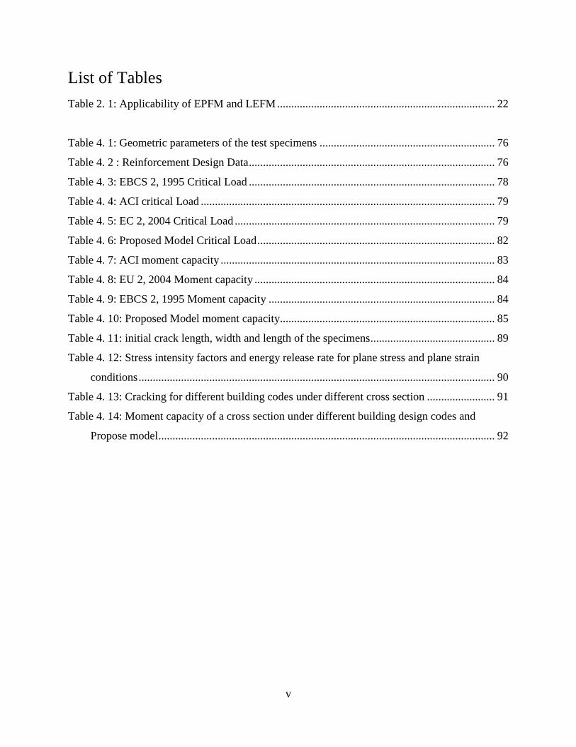
Contents

List of Tables .................................................................................................................................. v

List of Figures ................................................................................................................................ vi

List of symbols ............................................................................................................................. viii

Abstract ........................................................................................................................................... x

1 Introduction .................................................................................................................................. 1

1.1 Background ........................................................................................................................... 1

1.2 Objective and Scope of the study.......................................................................................... 1

1.3 Thesis organization ............................................................................................................... 2

2 Literature Review on Fracture Mechanics. .................................................................................. 3

2.1 Introduction ........................................................................................................................... 3

2.2 Types of Fracture and Basics of Fracture Mechanics ........................................................... 5

2.2.1 Types of Fracture ............................................................................................................... 5

2.2.2 Fracture Energy .................................................................................................................. 6

2.2.3 Stress Intensity Factor (SIF) (KI) ...................................................................................... 9

2.2.4 An Atomistic View of Fracture ........................................................................................ 10

2.2.5 Types of Fracture Mechanics ........................................................................................... 13

i. Linear Elastic Fracture Mechanics ...................................................................................... 13

ii. Nonlinear Fracture Mechanics (Elastic-Plastic FM) ........................................................... 19

2.3 Cracks in Reinforced Concrete Structures .......................................................................... 22

2.3.1 Variation of Tensile Strength of Concrete ....................................................................... 23

2.3.2 Code Provision of Cracks ................................................................................................ 23

2.4 Section Capacity of Reinforced Concrete Elements ........................................................... 40

2.4.1 Stress and strain diagram ................................................................................................. 40

2.4.2 Code provisions on stress strain diagram......................................................................... 43

iv

3 Fracture Mechanics of Concrete ................................................................................................ 48

3.1 Pre/Post-Peak Material Response of Steel and Concrete .................................................... 48

3.2 Stress versus crack opening displacement Diagram ........................................................... 49

3.3 Concrete Models for Fracture Analysis .............................................................................. 50

3.3.1 Fictitious crack model (Cohesive Crack Model) ............................................................. 50

3.3.2 Crack Band Model (CBM)............................................................................................... 51

4 Application of Fracture Mechanics ............................................................................................ 54

4.1 Numerical Approach of Fracture Mechanics ...................................................................... 54

4.2 SIF and propagation criteria................................................................................................ 55

4.3 Proposed crack propagation model ..................................................................................... 58

4.4 Proposed section capacity model ........................................................................................ 71

4.5 Fracture Mechanics using Finite element software ............................................................ 74

4.6 Numerical Examples .......................................................................................................... 76

4.7 Comparisons and Discussions............................................................................................. 91

5 Conclusion and Recommendations ............................................................................................ 95

5.1 Conclusions ......................................................................................................................... 95

5.2 Recommendations ............................................................................................................... 96

References ..................................................................................................................................... 97

Appendix ..................................................................................................................................... 100

v

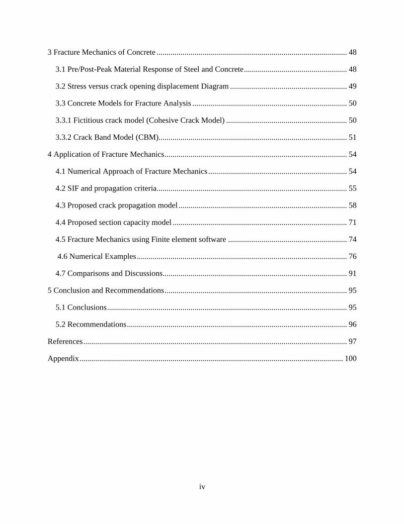
List of Tables

Table 2. 1: Applicability of EPFM and LEFM ............................................................................. 22

Table 4. 1: Geometric parameters of the test specimens .............................................................. 76

Table 4. 2 : Reinforcement Design Data ....................................................................................... 76

Table 4. 3: EBCS 2, 1995 Critical Load ....................................................................................... 78

Table 4. 4: ACI critical Load ........................................................................................................ 79

Table 4. 5: EC 2, 2004 Critical Load ............................................................................................ 79

Table 4. 6: Proposed Model Critical Load .................................................................................... 82

Table 4. 7: ACI moment capacity ................................................................................................. 83

Table 4. 8: EU 2, 2004 Moment capacity ..................................................................................... 84

Table 4. 9: EBCS 2, 1995 Moment capacity ................................................................................ 84

Table 4. 10: Proposed Model moment capacity............................................................................ 85

Table 4. 11: initial crack length, width and length of the specimens ............................................ 89

Table 4. 12: Stress intensity factors and energy release rate for plane stress and plane strain

conditions .............................................................................................................................. 90

Table 4. 13: Cracking for different building codes under different cross section ........................ 91

Table 4. 14: Moment capacity of a cross section under different building design codes and

Propose model ....................................................................................................................... 92

vi

List of Figures

Figure 2. 1: Three basic modes for cracked body :( a) Mode I (b) Mode II (c) Mode III, [18]. ..... 5

Figure 2.2 : Plate with crack length a, [2]. ...................................................................................... 6

Figure 2.3 : Plate with elliptic hole subjected to tension, [5]. ........................................................ 7

Figure 2.4: Amount of Energy and corresponding crack length, .................................................... 8

Figure 2. 5: Elastic stress distribution near crack tip, [5] ............................................................. 10

Figure 2.6: The energy curve (top) and force versus dislocation radius, [4] ................................ 11

Figure 2. 7: crack tip variables for Sharp crack, [6] ..................................................................... 14

Figure 2. 8: Response of three point bend specimens with initial crack length ao ....................... 15

Figure 2. 9 : Crack tip stress conditions, [7] ................................................................................. 16

Figure 2. 10 : Crack tip radius for elastic and plastic zone, [4] .................................................... 17

Figure 2. 11: Stress conditions causing opening and closing of crack tip, [2] ............................. 17

Figure 2. 12 : The fracture Process Zone developed beyond the crack is large enough to be

considered, [6]....................................................................................................................... 19

Figure 2.13: Blunted crack beyond the sharp crack, [5] ............................................................... 20

Figure 2. 14: Shows crack tip opening displacement [5] .............................................................. 20

Figure 2. 15: Quarter points and collapsed elements, [5] ............................................................. 32

Figure 2. 16: a) Plate corner with included angle; b) Special case of sharp Crack, [5] ................ 33

Figure 2. 17: Orientation of the crack plane, [5] ........................................................................... 33

Figure 2. 18: Biaxial loading for Westergaard solution, [14] ....................................................... 36

Figure 2. 19: Plate subjected to far field stress, [2] ...................................................................... 38

Figure 2. 20: Section body, [14] .................................................................................................. 40

Figure 2. 21: Tractions decomposition, [14] ................................................................................. 41

Figure 2. 22: EBCS 2, 1995 provision for stress-strain diagram for concrete under compression,

[18] ........................................................................................................................................ 43

Figure 2. 23: EU 2, 1994, provision for Parabolic-rectangular stress-strain diagram for concrete

under compression, [17]........................................................................................................ 44

Figure 2. 24: EU 2, 1994, provision for bilinear stress-strain diagram for concrete under

compression, [17] .................................................................................................................. 44

Figure 2. 25: Typical Concrete stress-strain curve according to ACI provision, [10] .................. 45

vii

Figure 2. 26: Typical concrete stress-strain diagram under compression with different

compressive strength, [10] .................................................................................................... 45

Figure 2. 27: Stress-strain and stress-displacement diagram for concrete section, [10] ............... 46

Figure 2. 28: Dependency of the stress-strain diagram in the depth of compression zone, c, [10]

............................................................................................................................................... 47

Figure 3. 1: Stress-Strain Curves of reinforcement bars and Concrete, [28] ................................ 48

Figure 3. 2: Hillerborg Fictitious Crack Model, [28].................................................................... 51

Figure 4. 1: Plate subjected to far field tensile stress with central hole, ....................................... 60

Figure 4. 2: The plane stress and plane strain plastic zone, [5] .................................................... 61

Figure 4. 3: Area of special curve called Lemnsicate, .................................................................. 61

Figure 4. 4: Approximate process zone beyond crack tip ............................................................. 61

Figure 4. 5: Transverse and longitudinal section of three point bend beam ................................. 63

Figure 4. 6: Beam subjected to central loading............................................................................. 68

Figure 4. 7 : Beam part near the crack .......................................................................................... 68

Figure 4. 8: Magnified view in the vicinity of the crack .............................................................. 68

Figure 4. 9: Stress carried by rebars and concrete, [29] ................................................................ 69

Figure 4. 10: Simple linear softening Model, [28]........................................................................ 70

Figure 4. 11: Linear strain distribution for flexure type loading .................................................. 72

Figure 4. 12: Beam subjected to two point Loading ..................................................................... 76

Figure 4. 13: Stress-strain diagram for reinforcement .................................................................. 76

Figure 4. 14: Cracking loads versus size using different building codes and Proposed model .... 91

Figure 4. 15: Section capacity varies with beam size using different building codes and Proposed

Model .................................................................................................................................... 92

Figure 4. 16: a) Variations of stress intensity for mode I with proportion crack growth ............. 94

viii

List of symbols

a = initial crack length

acr = critical crack length

A = area of concrete

As = area of tensile longitudinal steel reinforcement

[B] = element strain-displacement matrix

CMOD = crack mouth opening displacement

c = Plastic zone length

C = Depth of compression zone

da = maximum aggregate size

d = Distance from the extreme compression fiber to the centroid of the

Longitudinal tension reinforcement

[D] = material stiffness matrix

E = Young Modulus

Eb = Bond energy between atoms

fc = concrete cylinder uniaxial compressive strength

f'ct = specified mean tensile strength

fr = modulus of rupture strength

G = Energy release rate

J = nonlinear energy release rate

k = Bond stiffness

KI = Mode I stress intensity Factor

KII = Mode II stress intensity Factor

KIII = Mode III stress intensity Factor

ix

Mu = ultimate moment

R = crack résistance force

ry = plastic zone using elastic analysis

rp = plastic zone using plastic analysis

Ua = Surface energy

Ud = dissipated Energy

Ue = total input energy to the system

Ui = internal strain energy

U = kinetic energy

w = average crack width

W = Energy density function

Z = empirical value to control cracks

𝛽 = Brittleness number

ch = characteristic strain for concrete in tension

ε cr = concrete cracking strain

εcx = average net concrete axial strain, in the x-direction

εcy = average net concrete axial strain, in the y-direction

휀sm = mean strain of the reinforcement

θ = angle of crack inclination

ρx = longitudinal tensile steel reinforcement ratio

ρy = transverse steel reinforcement ratio

σx = applied axial stress in the x-direction

σy = applied axial stress in the y-direction

τxy = applied shear stress

x

Abstract

Reinforced Concrete structures have been designed for long time using the Elastic and Plastic limit

state theories. However, real life experiences shows that these theories are not sufficient for having

the expected Failure Mode which is called Ductile Failure. In the Limit States theory, one of the

major drawback is, it assumes strength as a material property independent of size. But in reality,

the size effect is significant phenomena in controlling the failure mode. Limit States theory missed

the concept of Size Effect. The basic concept behind the Size Effect is, as the size of the material

increase, the volume of micro cracks and flaws also increase. This internal micro cracks and flaws

are points where stress concentrations occurs. Through time, these micro crack and flaws will

develop in to macro cracks. Therefore, the strength (Tensile and compressive) are dependent on

Material member length and cross section.

In this Thesis, crack propagation and section capacity for Reinforced Concrete structures are

analyzed using the size effect concept which is addressed using Fracture Mechanics

1

1 Introduction

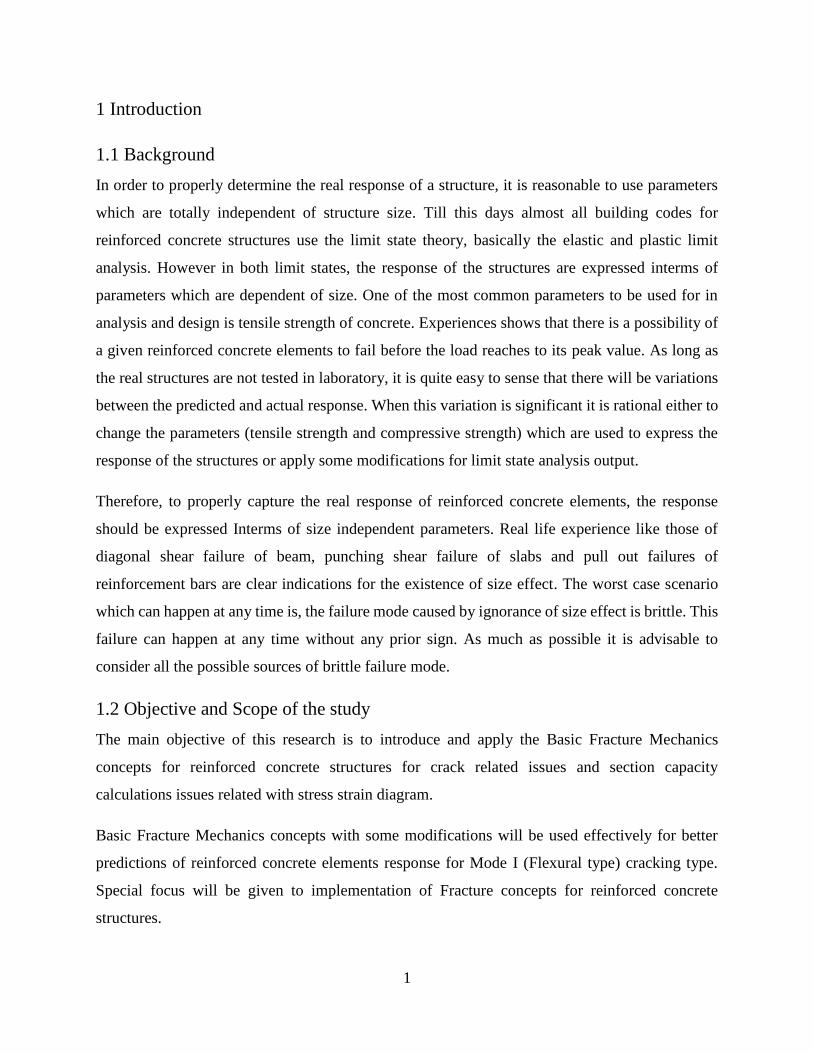
1.1 Background

In order to properly determine the real response of a structure, it is reasonable to use parameters

which are totally independent of structure size. Till this days almost all building codes for

reinforced concrete structures use the limit state theory, basically the elastic and plastic limit

analysis. However in both limit states, the response of the structures are expressed interms of

parameters which are dependent of size. One of the most common parameters to be used for in

analysis and design is tensile strength of concrete. Experiences shows that there is a possibility of

a given reinforced concrete elements to fail before the load reaches to its peak value. As long as

the real structures are not tested in laboratory, it is quite easy to sense that there will be variations

between the predicted and actual response. When this variation is significant it is rational either to

change the parameters (tensile strength and compressive strength) which are used to express the

response of the structures or apply some modifications for limit state analysis output.

Therefore, to properly capture the real response of reinforced concrete elements, the response

should be expressed Interms of size independent parameters. Real life experience like those of

diagonal shear failure of beam, punching shear failure of slabs and pull out failures of

reinforcement bars are clear indications for the existence of size effect. The worst case scenario

which can happen at any time is, the failure mode caused by ignorance of size effect is brittle. This

failure can happen at any time without any prior sign. As much as possible it is advisable to

consider all the possible sources of brittle failure mode.

1.2 Objective and Scope of the study

The main objective of this research is to introduce and apply the Basic Fracture Mechanics

concepts for reinforced concrete structures for crack related issues and section capacity

calculations issues related with stress strain diagram.

Basic Fracture Mechanics concepts with some modifications will be used effectively for better

predictions of reinforced concrete elements response for Mode I (Flexural type) cracking type.

Special focus will be given to implementation of Fracture concepts for reinforced concrete

structures.

2

1.3 Thesis organization

The Thesis is organized it to Five Chapters. Chapter 1 deals with the General introduction and the

need for further study in the field of crack propagation and section capacity for Reinforced concrete

structures.

Chapter 2 covers literature Reviews on Fracture Mechanics. As this science was used mainly for

metals, General introductions are discussed using simple concepts. In additions, codes prescription

for crack propagations and section capacity is also elaborated. A critical concepts of stress and

strain in the vicinity of the crack tip have been also discussed with special finite elements

Chapter 3 provides information on the pre and post peak nature of Reinforced concrete structures.

The need for having stress-crack tip opening displacement diagram is also discussed. Ideas on

recent advances on concrete modeling for Fracture analysis are also provided.

Chapter 4 states about application of Fracture Mechanics for Reinforced concrete structures.

Basics Fracture Parameters like Stress intensity Factors is also discussed. Assumption for the two

proposed models with numerical examples is also included in this chapters. Comparisons of code

based formulas and proposed model results are also given in this chapter. Conclusion and

Recommendations are discussed in chapter 5.

3

2 Literature Review on Fracture Mechanics.

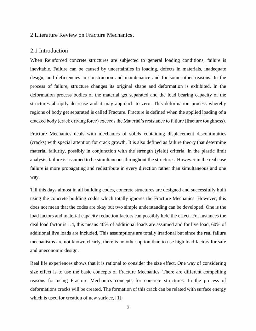
2.1 Introduction

When Reinforced concrete structures are subjected to general loading conditions, failure is

inevitable. Failure can be caused by uncertainties in loading, defects in materials, inadequate

design, and deficiencies in construction and maintenance and for some other reasons. In the

process of failure, structure changes its original shape and deformation is exhibited. In the

deformation process bodies of the material get separated and the load bearing capacity of the

structures abruptly decrease and it may approach to zero. This deformation process whereby

regions of body get separated is called Fracture. Fracture is defined when the applied loading of a

cracked body (crack driving force) exceeds the Material’s resistance to failure (fracture toughness).

Fracture Mechanics deals with mechanics of solids containing displacement discontinuities

(cracks) with special attention for crack growth. It is also defined as failure theory that determine

material failurity, possibly in conjunction with the strength (yield) criteria. In the plastic limit

analysis, failure is assumed to be simultaneous throughout the structures. However in the real case

failure is more propagating and redistribute in every direction rather than simultaneous and one

way.

Till this days almost in all building codes, concrete structures are designed and successfully built

using the concrete building codes which totally ignores the Fracture Mechanics. However, this

does not mean that the codes are okay but two simple understanding can be developed. One is the

load factors and material capacity reduction factors can possibly hide the effect. For instances the

deal load factor is 1.4, this means 40% of additional loads are assumed and for live load, 60% of

additional live loads are included. This assumptions are totally irrational but since the real failure

mechanisms are not known clearly, there is no other option than to use high load factors for safe

and uneconomic design.

Real life experiences shows that it is rational to consider the size effect. One way of considering

size effect is to use the basic concepts of Fracture Mechanics. There are different compelling

reasons for using Fracture Mechanics concepts for concrete structures. In the process of

deformations cracks will be created. The formation of this crack can be related with surface energy

which is used for creation of new surface, [1].

4

When crack occurs, new surface is created at the same time. This shows that crack formation is

related with energy one way or the other way. In Fracture Mechanics, Energy related with crack

formation has got great attentions. Besides the current strength based analysis and design results

show that some important material parameters are independent of size. In the limit analysis,

strength is expressed as material property which is independent of size. However experiments

shows that materials like reinforced concrete structures shows load deflection which is neither

similar to ductile materials nor like those of brittle material. From the load deflection diagram, it

is concluded that reinforced concrete structures are quasi brittle material. Therefore, better

prediction of response can be obtained if Fraction Mechanics with some modification is used.

In addition, it is rational at least to minimize the rate of occurrence of brittle mode of failure. One

way of making sure that the failure mode is ductile is to consider the amount of energy absorbed

and ductility nature of the material. The simplest principle is to make sure that the strain energy of

the given cross section is less than the amount of energy required for creation new surface. In the

Fracture Mechanics one of the most known size independent parameter is Fracture Energy.

Fracture Energy is defined as the specific energy required for crack growth in an infinite large

specimens. The main importance of this definition is to eliminate the effect of sizes, shapes and

type of loading on the fracture energy. This basic parameter needed for rational predictions of

brittle failure of concrete structures. Another very important parameter is the Fracture Process

Zone (FPZ). This is a zone where softening occurs. It is a place where Fracture initiates, [2].

Finally, it is observed that plastic limit analyses provide no information on the post peak load

deflection diagram and the amount of energy dissipated in the fracture process. However, using

Fracture Mechanics, information lost in plastic limit analysis can be captured, [2].

5

2.2 Types of Fracture and Basics of Fracture Mechanics

2.2.1 Types of Fracture

Once the crack is nucleated on the surface of the structure, its growth occurs in presence of a very

high gradient associated stress field. Three basic modes for crack growth are defined in many

literatures. These are Mode I, which is the “opening” or “tensile mode”, where the crack faces

separate symmetrically with respect to the x1 -x 2 and x 1 -x 3 planes. In Mode II, the

“sliding” or in “plane shearing” mode, the crack faces slide each other symmetrically about

the x 1 -x 2 plane but anti-symmetrically with respect to the x1 -x3 plane. In the “tearing” or

“anti-plane” mode, Mode III, the crack faces also slide each other but anti symmetrically with

respect to the x 1 -x 2 and x 1 -x 3 planes. In several practical cases, loads excite simultaneously

two modes and make the crack propagation depending on a so-called “mixed-mode fracture

mechanism” [4]. In this paper only Mode I type of crack is given attention, [18].

Figure 2. 1: Three basic modes for cracked body :( a) Mode I (b) Mode II (c) Mode III, [18].

6

2.2.2 Fracture Energy

For a system of constant temperatures, first law of thermodynamics states that the total amount of

energy that is supplied to a material volume per unit of time (e

u ) must be transferred to the internal

energy(iu ) surface energy(

au ) dissipated energy(du ) and kinetic energy(

ku ).

The internal energy is the elastically stored energy, the surface energy comes in to effect when

crack propagates, the kinetic energy is function of material speed and finally the dissipated energy

is due to friction and plastic deformation.

In Fracture process, the surface of the crack varies so it can be taken as state variable. If the

thickness, b, is assumed to be constant, the only state variable will be the crack length, a. Since

Area=b*a.

When crack happens in material, the internally stored energy acts as source of energy. For the

figure below assume the width, b, to be constant,

Figure 2.2 : Plate with crack length a, [2].

Using first law of thermodynamics

. . . . .

1e i a d kU U U U U [JS ] (2.1)

From simple calculus using Change of Variables

. .e e e edu du du dudA

ba adt dt dA bda da

If the dissipated energy and kinetic energy are neglected, the available external energy and

internal energy is transferred to surface energy.

e aidu dudu

da da da

7

This equation is called Griffith energy balance.

Divide both side by b yields the Energy Release Rate (G)

e edu du1

Gb da da

And the Crack Resistance Force (R)

adu1

Rb da

Griffith crack criteria G = R

For the case of fixed grips (u = 0)

e aidu dudu

0da da da

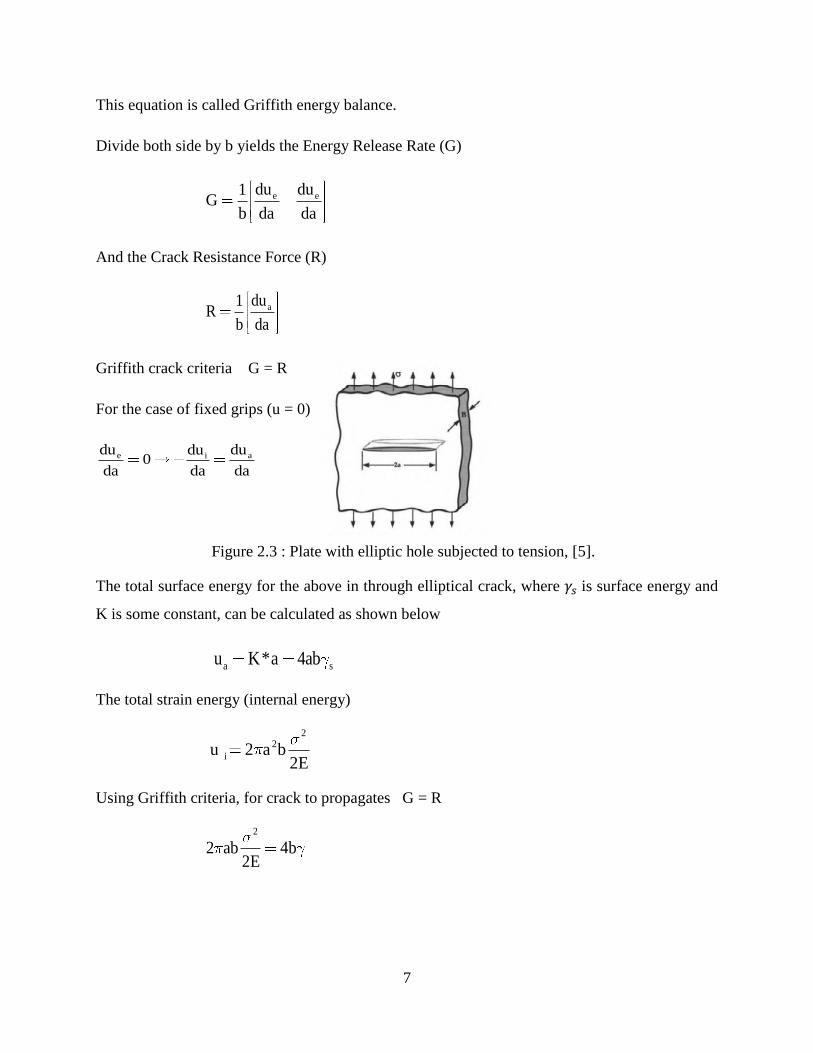
Figure 2.3 : Plate with elliptic hole subjected to tension, [5].

The total surface energy for the above in through elliptical crack, where 𝛾𝑠 is surface energy and

K is some constant, can be calculated as shown below

a su K*a 4ab

The total strain energy (internal energy)

22

iu 2 a b2E

Using Griffith criteria, for crack to propagates G = R

2

2 ab 4b2E

8

From the above the critical crack length will be

.

scr 2

2 Ea (2.2)

Where .

E

.E for planestress

E Efor planestrain

1

Energy available (source of energy)

22

iU 2 a b2E

Energy needed for new surface generation a sU 4a b

Figure 2.4: Amount of Energy and corresponding crack length,

In Griffith energy balance, energy dissipated in the system is neglected .This cause discrepancy

between the experiment and analytic values. The discrepancy between the experiment and

analytically calculated values can be shown by both the stress and energy approach.

For materials which are very brittle, the amount of energy dissipated is very small, enough to be

ignored when crack growth. But for ductile materials, showing significant energy dissipation the

energy release rate can be 105 times the crack growth resistance force (R), [15].

9

For brittle material

.

sc

2 E

a

And For Ductile material

.

s p

c

2( ) E

a

Where 𝛾𝑠 plastic work per unit area of surface created. For ductile material s p

,this shows

ignoring or neglecting the amount of energy dissipated can be a source of erroneous result. Energy

release rate (G) can be calculated using different techniques like those of fixed and constant loads.

In both techniques for energy release rate (G) determination, compliance, which is the ratio of

opening to force, approach will be used. G can also be calculated from the force displacement

curve, [4].

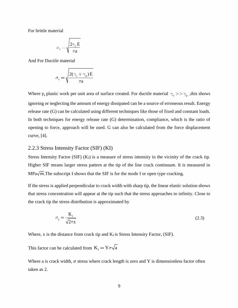
2.2.3 Stress Intensity Factor (SIF) (KI)

Stress Intensity Factor (SIF) (KI) is a measure of stress intensity in the vicinity of the crack tip.

Higher SIF means larger stress pattern at the tip of the line crack continuum. It is measured in

MPa√𝑚.The subscript I shows that the SIF is for the mode I or open type cracking.

If the stress is applied perpendicular to crack width with sharp tip, the linear elastic solution shows

that stress concentration will appear at the tip such that the stress approaches to infinity. Close to

the crack tip the stress distribution is approximated by

I

y

K

2 x (2.3)

Where, x is the distance from crack tip and KI is Stress Intensity Factor, (SIF).

This factor can be calculated from IK Y a

Where a is crack width, 𝜎 stress where crack length is zero and Y is dimensionless factor often

taken as 2.

10

.

Figure 2. 5: Elastic stress distribution near crack tip, [5]

As the stress approaches infinity, the analysis of crack stability and crack propagation cannot be

based on the comparison with the strength of material. At this point it is rational to introduce new

criterion which dictates that crack will start propagating when the SIF reaches a critical values,

Kc, which is assumed to be material property, [5].

SIF is used in analysis and design by arguing that material can with stand crack tip stress up to a

critical value of stress intensity termed as KIC beyond which the crack propagate faster. This KIC

measures material toughness.

Failure stress then calculated to the crack length a and fracture toughness KIC by

IC

f

K

a (2.4)

Where 1 for edge crack and different 𝛼 can be found for different crack positions. Generally

SIF can be expressed as IK a where depends on the location of pre-existing notch,

[24].

2.2.4 An Atomistic View of Fracture

The bond strength that exist between atoms plays a great role when the issues of Fracture arises.

This is mainly because failure occurs when only the stress developed between atoms is greater

than the bond stress that already exist. The stress developed is supplied by the external load while

the force of attraction between atoms is the main source of the bond stress.

11

Figure 2.6: The energy curve (top) and force versus dislocation radius, [4]

From the figure at x = 0, the force between atoms is null. This distance is called equilibrium

spacing.

The area under the force versus dislocation radius of atoms gives the amount of energy needed to

displace the atoms and cause failures, and it is called Bond energy ( bE )

o

x

b

x

E Pdx

Where, P is the applied force. By assuming of one half the period of sine wave for the

interatomic force displacement relationships

o

c

x xP P sin

With the origin defined at X0.

For very small displacement sin x x , using the same analogy

o

c

x xP P

12

The above equations can be simplified as

F K x

Where o cx x x ,K P and F P

Therefore, the bond stiffness is

c

c

K P

K * P *

Since P

Kx

c c

PP * for P P

x

x* , Dividing both side by ox

o

*x

Since E

and rearranging Where E is elastic Modulus and c is

cohesive strength.

Finally the cohesive strength can be expressed in simple form as:

c

0

E*

*x

For 𝑥0 = 𝜆 , the theoretical cohesive strength can be simplified to the form

c

0

E*

*x ( 2.5)

It is clear that there will be some energy requirements for the new surface to be created. Let the

energy required to create single surface is surface energy denoted by s

13

o

o

x

s

x

s c c

0

2* x dx

1 xsin dx

2

This shows that the Fracture energy is about two times of the surface energy.

Finally after some simplifications

sc

0

E*

x (2.6)

The theoretical cohesive strength is approximated to be E

. however, due to the presence of

flaws there will be discrepancy between the theoretically calculated and experimentally obtained

values. But the basic point here is Fracture can never occur unless the defects play role in

magnifying the stress around so that the magnified stress will be greater than the normal cohesive

strength, [6].

2.2.5 Types of Fracture Mechanics

Based on the size of the Fracture Process Zone (FPZ), there are two types of Fracture Mechanics.

These are Linear Elastic Fracture Mechanics (LEFM) and Nonlinear Fracture Mechanics also

called Elastic Plastic Fracture Mechanics (NLFM or EPFM).

i. Linear Elastic Fracture Mechanics

A large field of Fracture mechanics uses concepts and theories in which Linear Elastic material

behavior is an essential assumption. This is the case for Linear Elastic Fracture Mechanics

(LEFM).

The basic assumption of the Linear Elastic Fracture Mechanics (LEFM) is that the size of Fracture

Process Zone that is found beyond the crack tip is relatively small compared to the structure

dimensions. Sometimes it is also called Small Scale Yielding (SSY).

It is also identified in its sharp cracks. This type of failure mechanics works well for those material

where the crack initiation load and the failure load is almost similar like those of most metals. The

14

global stress strain response of the material is linear and elastic. The basic formulation is based on

energy balance.

Figure 2. 7: crack tip variables for Sharp crack, [6]

In the above figures, the Fracture Process Zone is very small compared to the structure dimensions.

F means area of Fracture Process Zone, N means area of nonlinear zone and L means part of the

structure in the linear state. It is clear that most of the material cross-section is in the linear state

so it is best to implement the LEFM.

All LEFM applies to sharp cracks in Elastic bodies. It is rational to apply this Fracture Mechanics

for any material as long as the material is in the linear state and for the regions far away from the

sharp crack tips, Implementation of LEFM near sharp crack leads to the predictions of infinite

stress at crack tip. However, materials have finite stress capacity. The LEFM fails at molecular

level or around the crack tip.

Literatures proposed some analytical tools to predict the Fracture Mechanics, which are based on

the assumption of the linear elastic behavior of material. In the so called Linear Elastic Fracture

Mechanics (LEFM), prediction of crack growth is based on the energy balance. Griffith

states “crack growth will occur, when there is enough energy available to generate new crack

surface.” The “energy release rate” is an essential quantity in energy balance criteria. The

resulting crack growth criterion is referred to as being “global”, because a rather volume of

material is considered. The crack growth criterion can also be based on the stress state at the crack

tip. This stress field can be determined in several cases through an analytical approach.

15

It is characterized by the definition of the “stress intensity factor” (SIF). Stress intensity factor K:

characterizes the stresses, strains and displacement fields near the crack tip, it is local parameter.

The crack growth criterion can also be based on the stress state at the crack tip. This stress field

can be determined analytically. The resulting crack growth criterion is referred to as local, because

attention is focused at a small material volume at the crack tip.

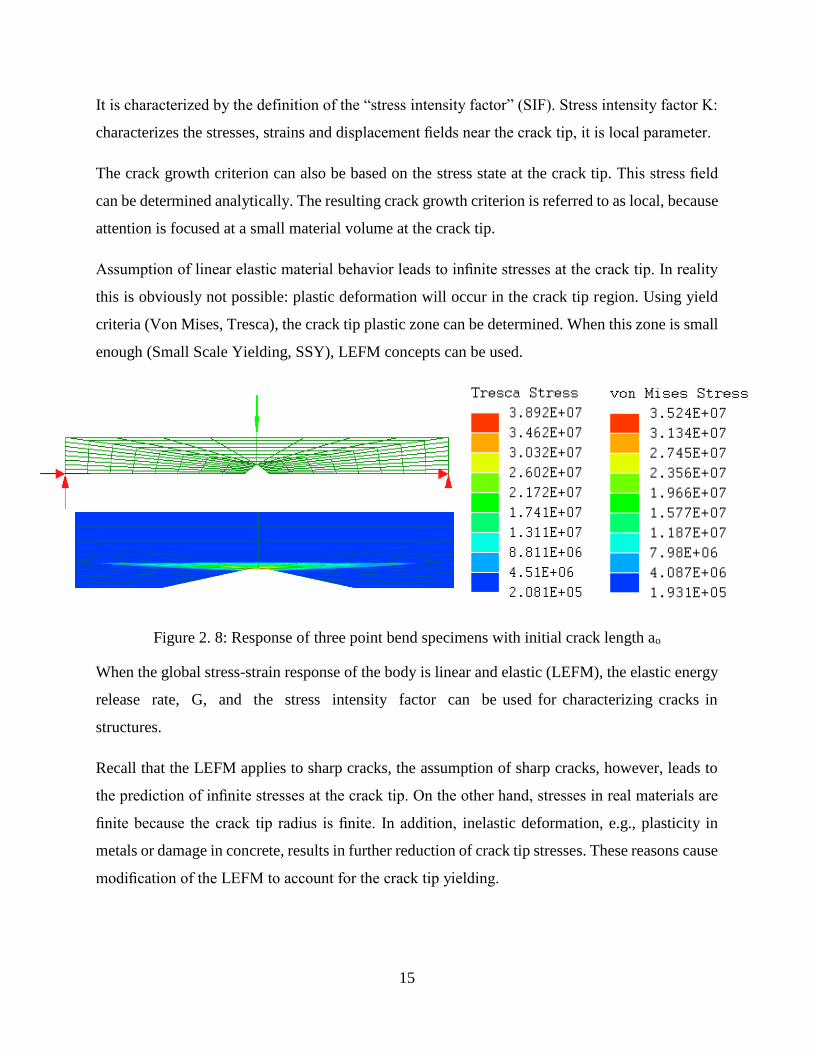
Assumption of linear elastic material behavior leads to infinite stresses at the crack tip. In reality

this is obviously not possible: plastic deformation will occur in the crack tip region. Using yield

criteria (Von Mises, Tresca), the crack tip plastic zone can be determined. When this zone is small

enough (Small Scale Yielding, SSY), LEFM concepts can be used.

Figure 2. 8: Response of three point bend specimens with initial crack length ao

When the global stress-strain response of the body is linear and elastic (LEFM), the elastic energy

release rate, G, and the stress intensity factor can be used for characterizing cracks in

structures.

Recall that the LEFM applies to sharp cracks, the assumption of sharp cracks, however, leads to

the prediction of infinite stresses at the crack tip. On the other hand, stresses in real materials are

finite because the crack tip radius is finite. In addition, inelastic deformation, e.g., plasticity in

metals or damage in concrete, results in further reduction of crack tip stresses. These reasons cause

modification of the LEFM to account for the crack tip yielding.

16

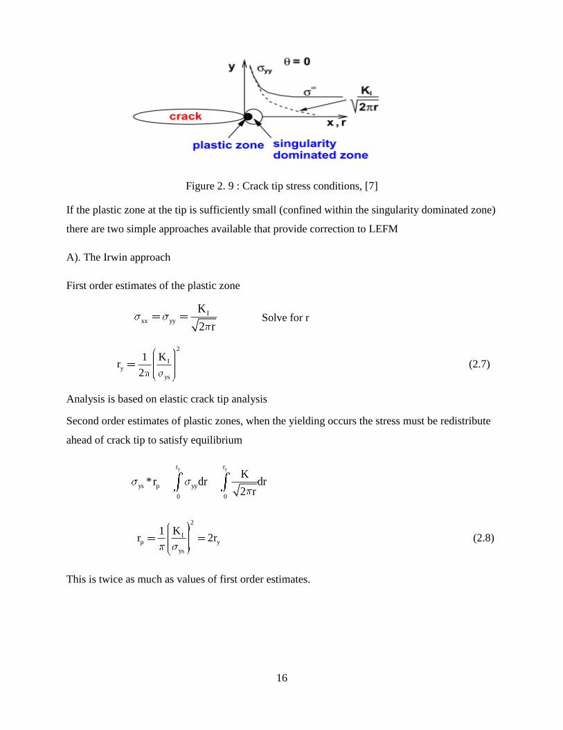
Figure 2. 9 : Crack tip stress conditions, [7]

If the plastic zone at the tip is sufficiently small (confined within the singularity dominated zone)

there are two simple approaches available that provide correction to LEFM

A). The Irwin approach

First order estimates of the plastic zone

I

xx yy

K

2 r Solve for r

2

Iy

ys

K1r

2 (2.7)

Analysis is based on elastic crack tip analysis

Second order estimates of plastic zones, when the yielding occurs the stress must be redistribute

ahead of crack tip to satisfy equilibrium

y yr r

ys p yy

0 0

K*r dr dr

2 r

2

Ip y

ys

K1r 2r (2.8)

This is twice as much as values of first order estimates.

17

Figure 2. 10 : Crack tip radius for elastic and plastic zone, [4]

B). The strip yield model (suitable for polymers)

The strip yield model was first proposed by Dugdale and Barenblatt. They assumed a long slender

plastic zone at the crack tip in non-hardening material in plane stress. This model is a classical

application of the principle of superposition as it approximates the elastic-plastic behavior by

superimposing two elastic solutions: a through crack under remote tension and a through crack

with closure stresses at the tip.

Figure 2. 11: Stress conditions causing opening and closing of crack tip, [2]

Since the stresses at the strip yield zone are finite, there cannot be a singularity at the crack tip (the

stress intensity factor at the tip of plastic zone must be equal to zero). Thus the plastic zone length

ρ is found from the condition that the stress intensity factors from the remote tension and closure

stress cancel one another.

To proceed, consider first a through crack in an infinite plate loaded by a normal force P applied

at a distance x from the center line of the crack. The stress intensities for the two crack tips are

then give by

P a x P a xK a K a

a x a xa a

If the closure stress is 𝜎𝑦𝑠 acts through a distances dx, the force developed due the closure stress

18

ys

a

ys

closure

a

P dx

a x a - xK dx

a - x a xa

Solving the integral

-1

closure ys

a aK -2* cos

a

The SIF for the remote stress is given by

K a

For the crack tip stress to be finite closureK K

After simplifications

ys

acos

a 2

Using the Taylor series for cosine functions where

2 4 6 8x x x xcos x 1 ......

2! 4! 6! 8!

Using the same analogy

2 4 6 8

ys ys ys ys

ys

2 2 2 2cos 1

2 2! 4! 6! 8!

If only two terms are taken and the rest are neglected and solve for plastic zone size gives

22 2

ys ys

a 1

2 (2.9)

Irwin plastic zone correction focused mainly on using effective crack length. However Dugdale

focused on the ideas that stress at the elastic plastic boundary is not singular.

19

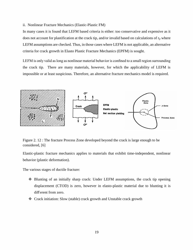
ii. Nonlinear Fracture Mechanics (Elastic-Plastic FM)

In many cases it is found that LEFM based criteria is either: too conservative and expensive as it

does not account for plastification at the crack tip, and/or invalid based on calculations of rp where

LEFM assumptions are checked. Thus, in those cases where LEFM is not applicable, an alternative

criteria for crack growth in Elasto Plastic Fracture Mechanics (EPFM) is sought.

LEFM is only valid as long as nonlinear material behavior is confined to a small region surrounding

the crack tip. There are many materials, however, for which the applicability of LEFM is

impossible or at least suspicious. Therefore, an alternative fracture mechanics model is required.

Figure 2. 12 : The fracture Process Zone developed beyond the crack is large enough to be

considered, [6]

Elastic-plastic fracture mechanics applies to materials that exhibit time-independent, nonlinear

behavior (plastic deformation).

The various stages of ductile fracture:

Blunting of an initially sharp crack: Under LEFM assumptions, the crack tip opening

displacement (CTOD) is zero, however in elasto-plastic material due to blunting it is

diff erent from zero.

Crack initiation: Slow (stable) crack growth and Unstable crack growth

20

Figure 2.13: Blunted crack beyond the sharp crack, [5]

There are two parameters characterizing the nonlinear behavior at the crack tip:

a. CTOD - crack tip opening displacement

b. J counter integral

Critical values of CTOD and J give nearly size-independent measures of fracture toughness, even

for relatively large amount of crack tip plasticity. But there are still limits to the applicability of J

and CTOD, but these limit are much less restrictive than the validity requirements of LEFM, [5].

a. Crack-tip opening displacement (CTOD)

In LEFM the displacement of material points in the region around the crack tip can be calculated.

With the crack along the x-axis, the displacement uy in y-direction is known as a function of r

(distance) and θ (angle), both for plane stress and for plane strain.

Figure 2. 14: Shows crack tip opening displacement [5]

The displacement of points at the upper crack surface results for θ = π and can be expressed in the

coordinate x, by taking r = a − x, where, a is the half crack length. The origin of this xy-coordinate

system is at the crack center. The crack opening displacement (COD) δ is two times this

displacement.

21

It is obvious that the opening at the crack tip (CTOD), t , is zero.

2Iy 2 2

K rv sin k 1 2cos

2 2

For crack plane and r a x

y 2

1 1 kv 2a a x

E

COD = Crack Opening Displacement = t

t y

1 1 k2v * * 2a(a x)

E (2.10)

Irwin and Dugdale both proposed different theories in the determinations of CTOD.

b. J-CONTOUR INTEGRAL

Rice presented a path-independent contour integral of analysis of cracks and showed that the value

of this integral, called J, is equal to the energy release rate in a nonlinear elastic body that contains

crack. Hutchinson and also Rice and Rosengren further showed that J uniquely characterizes crack

tip stresses and strains in nonlinear material. Thus, the J integral can be viewed as both an energy

parameter and a stress intensity parameter.

`Comparisons of Linear and Nonlinear Fracture Mechanics

Linear Elastic Fracture Mechanics assumes that the material behaves in brittle manner and local

parameter, stress intensity factor, can be used as valid fracture index. In this Fracture Mechanics,

the plastic zone in the vicinity of the crack is about one-tenth of the initial crack length. However,

if there is large scale yielding in the vicinity of the crack tip, another form of Fracture Mechanics

called Non Linear Fracture Mechanics which is also called Elastic Plastic Fracture Mechanics

should be used. In the Elastic Plastic Fracture Mechanics, There are two important Fracture

parameters: The J-integral and Crack Tip Opening Displacement for handling the problem of large

scale yielding.

22

Table 2. 1: Applicability of EPFM and LEFM

Elastic Plastic Fracture Mechanics Linear Elastic Fracture Mechanics

Beyond small-scale yielding Small-scale yielding applies

Lower strength materials High strength materials

Tough, ductile materials Brittle materials

Small thickness

Large thickness

Plane stress Plane strain

High temperatures Low temperatures

Slow loading rates High loading rates

2.3 Cracks in Reinforced Concrete Structures

Members such as beams and slabs which are subjected to bending moment will develop flexural

cracks when the stress in the tension zones exceeds the bending strength of plain concrete. From

experience, crack extends commonly from tension face to the location of neutral axis of the cross

section.

Cracking occurs in concrete member when the stress in concrete reaches the tensile strength, fct.

The value of fct depends on several parameters. Choice of the appropriate values of fct is the first

difficulty in the analysis of cracks. It was believed that the most important factor for controlling

flexural crack is the magnitude of the strain in the reinforcing steel.

Control of strain in the reinforcing steel is believed to be the most effective means to limit the

crack width. Other factors which have influence on the crack width are concrete cover, size of the

reinforcing steel and distribution of reinforcing steel in tension zone. However it is difficult to

predict the number and width of flexural cracks because of the complex process those are involved.

As a result there is no uniform approach for estimating these quantities and various design codes

use different techniques.

Cracks in Reinforced Concrete elements can be caused by force induced and displacement induced

cracking. Provision of bonded reinforcement of sufficient magnitude and appropriate detailing can

effectively limit the crack width. However size effect should come in to consideration before any

conclusion is made. Some of the parameters which are used in crack width calculation are mean

crack spacing (Srm ) and coefficient used to account for the additional stiffness which concrete in

tension provide.

23

2.3.1 Variation of Tensile Strength of Concrete

The tensile strength of concrete may be subjected to large variation due to many reasons. One of

the most common reason for the variation in strength is environmental effect. However, the

variation caused by size effect is not captured well.

In most Reinforced Concrete structures analysis and design Hand Books, Upper (𝑓𝑐𝑡𝑘,𝑚𝑎𝑥) and

lower values (𝑓𝑐𝑡𝑘,𝑚𝑖𝑛) of characteristic axial tensile strength with 𝑓𝑐𝑡𝑘,0=10Mpa.

2

3ck

ctk,min

ctk,0

ff 0.95

f And

2

3ck

ctk,max

ctk,0

ff 1.85

f (2.11)

Note that the tensile strength is independent of size. This means size effect is not yet considered.

2.3.2 Code Provision of Cracks

EBCS2, 1995.

Our building code discuss the issue of cracks under the serviceability states by different

mechanisms. The code states that there are different source for cracks and there are some

limitations regarding the limit state of crack formation and the limit states of crack width. But there

is nothing which states about crack propagation.

The code states that creep and ambient conditions can cause cracks in concrete structures and the

cracks are related with the characteristic compressive strength. The code states that when the issues

of cracks needs to be considered, there are some issues which should be discussed along with

crack. One of the most common is the amount of reinforcement bars in concrete. Another issue is

the nature of stress distribution in the section.

Limit states of crack formation

According to our code, crack will be formed as long as the tensile stress caused by load exceeds

the prescribed values in code. For flexure type of loading, the cracking tensile strength is about

1.7fctk and for direct tension it will be about fctk.

24

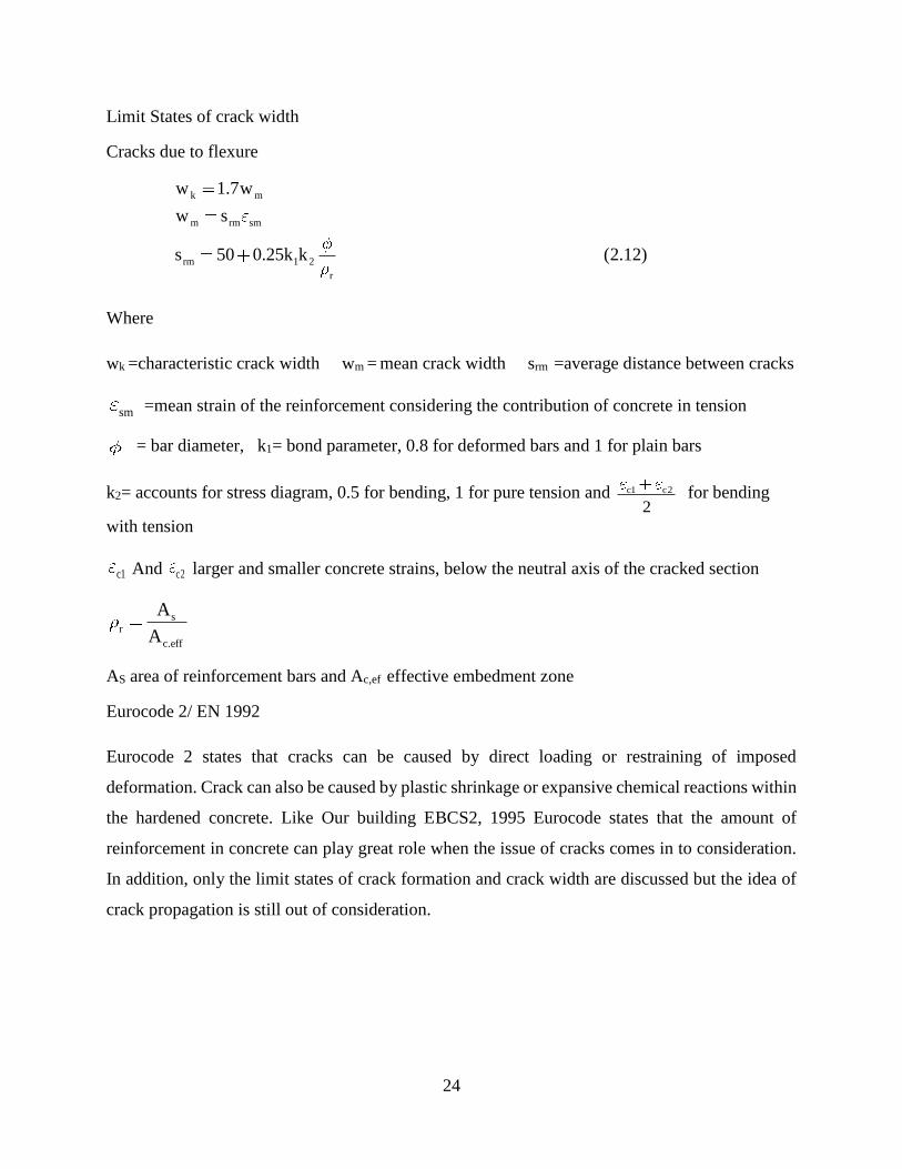
Limit States of crack width

Cracks due to flexure

k m

m rm sm

rm 1 2

r

w 1.7w

w s

s 50 0.25k k (2.12)

Where

wk =characteristic crack width wm = mean crack width srm =average distance between cracks

sm =mean strain of the reinforcement considering the contribution of concrete in tension

= bar diameter, k1= bond parameter, 0.8 for deformed bars and 1 for plain bars

k2= accounts for stress diagram, 0.5 for bending, 1 for pure tension and c1 c2

2 for bending

with tension

c1 And c2 larger and smaller concrete strains, below the neutral axis of the cracked section

sr

c.eff

A

A

AS area of reinforcement bars and Ac,ef effective embedment zone

Eurocode 2/ EN 1992

Eurocode 2 states that cracks can be caused by direct loading or restraining of imposed

deformation. Crack can also be caused by plastic shrinkage or expansive chemical reactions within

the hardened concrete. Like Our building EBCS2, 1995 Eurocode states that the amount of

reinforcement in concrete can play great role when the issue of cracks comes in to consideration.

In addition, only the limit states of crack formation and crack width are discussed but the idea of

crack propagation is still out of consideration.

25

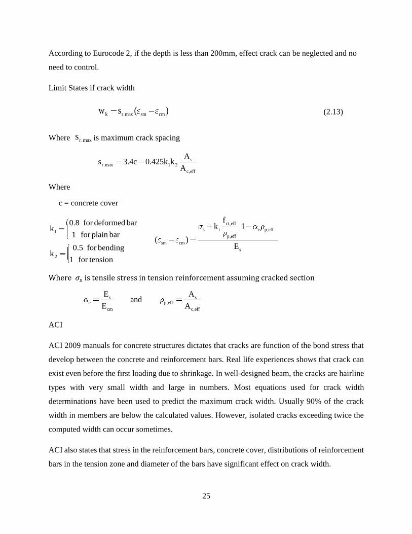
According to Eurocode 2, if the depth is less than 200mm, effect crack can be neglected and no

need to control.

Limit States if crack width

k r.max sm cmw s ( ) (2.13)

Where r.maxs is maximum crack spacing

sr.max 1 2

c,eff

As 3.4c 0.425k k

A

Where

c = concrete cover

1

2

0.8 for deformed bark

1 for plain bar

0.5 for bendingk

1 for tension

ct,eff

s t e p,eff

p,eff

sm cm

s

fk 1

( )E

Where 𝜎𝑠 is tensile stress in tension reinforcement assuming cracked section

s se p,eff

cm c,eff

E Aand

E A

ACI

ACI 2009 manuals for concrete structures dictates that cracks are function of the bond stress that

develop between the concrete and reinforcement bars. Real life experiences shows that crack can

exist even before the first loading due to shrinkage. In well-designed beam, the cracks are hairline

types with very small width and large in numbers. Most equations used for crack width

determinations have been used to predict the maximum crack width. Usually 90% of the crack

width in members are below the calculated values. However, isolated cracks exceeding twice the

computed width can occur sometimes.

ACI also states that stress in the reinforcement bars, concrete cover, distributions of reinforcement

bars in the tension zone and diameter of the bars have significant effect on crack width.

26

By considering the major factors which can possibly affect the crack width, ACI committee 224

recommends the following flexural crack-width formula, which is based on the Gergely-Lutz

equation:

3s cw 55.88 d A (2.14)

Where

w = most probable crack width [mm]

= ratio of distance between neutral axis and tension face to distance between neutral

axis and centroid of reinforcing steel

s = strain in the reinforcement due to applied load

dc = concrete cover from tension face to center of reinforcing bars.[mm]

Ac = area of concrete symmetric with reinforcing bars divided by the number of bars

[mm2]

The ACI Code (ACI 318-89) does not include a formula to compute explicitly crack width under

the service load. However, it uses Z-value to control cracks indirectly:

3s cZ f d A (2.15)

The ACI code places limits on the Z-value as a means to control crack width. This emphasis that

the strain in the reinforcing bars plays critical role in crack width and it is rational to use this rather

than the direct prediction of crack width which is very susceptible to uncertainty.However,usng

the Z-value in crack width control, spacing of the cracks cannot be captured.

CEB/FIP Approach

The CEB/FIP Model Code 1990 (CEB 1990) for concrete structures uses an approach for

crack control that differs from the ACI approach. The CEB/FIP technique considers the

mechanism of stress transfer between the concrete and reinforcement to estimate crack

width and spacing.

27

Prior to cracking, tensile load applied to the beam causes equal strains in the concrete and steel.

The strains increase with increasing load until the strain capacity of the concrete is reached, at

which cracks develop in the concrete. At the crack locations, the applied tensile load is resisted

entirely by the steel. Adjacent to the cracks, there is slip between the concrete and steel, and

this slip is the fundamental factor controlling the crack width.

The slip causes transfer of some of the force in the steel to the concrete by means of interracial

stress (called bond stress) acting on the perimeter of the bar. Therefore, the concrete between the

cracks participates in carrying the tensile force. The bond-slip mechanism causes the strains in

the concrete and steel to have a periodic variation along the length of the member, At a crack,

the steel strain is maximum and the concrete strain is zero. In between cracks, the steel

strain is minimum and the concrete strain is maximum. If, under increasing load, the concrete

strain reaches the limiting tensile strain, an intermediate crack forms between two previously

formed cracks.

Crack width is rated to the distance over which slip occurs and to the difference between the

rebar and concrete strains in the slip zones on either sides of the crack.

k s,max sm cm csw l ( ) (2.16)

Where, wk characteristic crack width

ls,max = maximum distance over which slip between concrete and rebar occurs

sm = Average rebar strain within ls, max

cm = Average concrete strain within lsmax

cs = Concrete shrinkage strain

Approximately

s,max

s,eff

l3.6

28

Where = bar diameter s,eff = area of rebars divided by effective area of concrete in

tension

In the CEB/FIP approach, the bond stress is assumed to be uniform over the slip distance

and equal to 1.8 times the concrete tensile strength. According to this bond-slip model,

intermediate cracks can occur only when the spacing between cracks exceeds ls,max . Thus

crack spacing will range from ls,max to 0.5 ls,max .

To evaluate crack width, it is necessary to evaluate the difference between the average steel

and average concrete strains within the slip zone. This difference is approximated by the

following (CEB 1990):

sm cm s2 sr2

Where

s2 = steel strain at location of crack under service load

sr2 = steel strain at location of crack under load that causes cracking of the

effective concrete area

=empirical factor to assess average strain within ls,max ( = 0.6 for short-

term loading and =0.38 for long-term loading).

2.3.3 Finite Element Analysis of Cracks

Finite Element Analysis is one of the numerical methods to obtain approximate solutions to many

of the Fracture Mechanics problems. To briefly explain the methodology consider 2D stress

analysis. The displacement variable ∅𝑐(𝑥, 𝑦) in each elemnt domain can be defined as

c 2 2

1 2 3 4 5 6x, y a a x a y a xy a x a y

Interms of nodal values

c

1 1 2 2 3 3 4 4x, y N x, y N x, y N x, y N x, y

29

For triangular elements with nodes (i, j, k) at the three vertices, the displacements (U, V) within

the elements

1 1 2 2 3 3

1 1 2 2 3 3

U x, y N (x, y)u N (x, y)u N (x, y)u

V x, y N (x, y)v N (x, y)v N (x, y)v

Strain components

x y xy

u v v u

x y x y

The above relation can be expressed in matrix form as shown below

1ji i

1

x

j 2i ky

2

xy

3ji i i k k

3

uNN N0 0 0

vx x x

N uN N0 0 0

vy y y

uNN N N N N

vy x x x x x

In compact form eUB

The stress strain relation, also known as constitutive relation, for linear isotropic plane stress

x x

y y2

xy xy

1 0E

1 01

10 0

2

Or in compact Form D

By using minimization of the total potential energy, the element stiffness matrix will be

Tek B D B hdA

30

Where,

h is thickness of the material.

The element stiffness matrix can be assembled to form the global stiffness matrix [K].Thus

finally FE equation can be written as

K U P

Where,

[ P ] = applied nodal loads

[ U ] = Nodal displacement and [ K ] = element Stiffness matrix

There are some direct methods to determine Fracture Mechanics parameters for crack analysis.

The stress-strain fields in 2D crack problems can be determined in general by using 3-node, 6-

node triangular elements, 4-noded quadrilateral or 8- node isoperimetric elements.

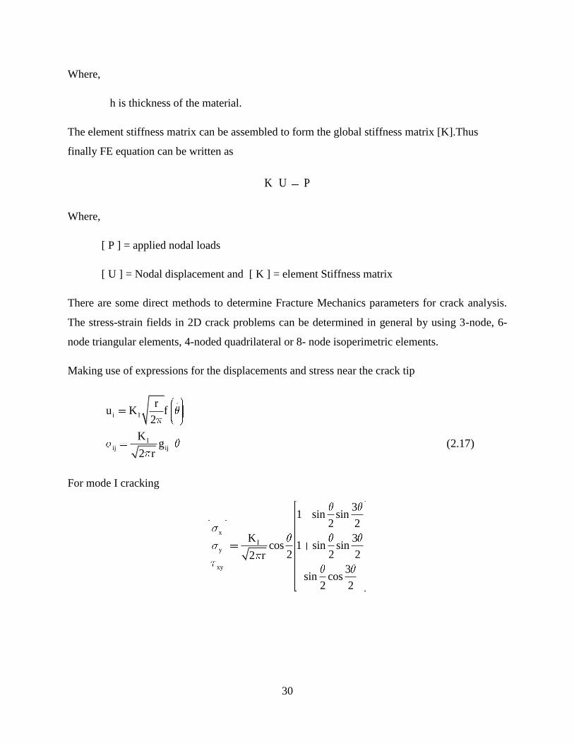
Making use of expressions for the displacements and stress near the crack tip

.

i I

Iij ij

ru K f

2

Kg (2.17)

2 r

For mode I cracking

x

Iy

xy

31 sin sin

2 2

K 3cos 1 sin sin

2 2 22 r

3sin cos

2 2

31

And the displacement field for plane strain condition

2

I

2

cos 1 2 sinU 2 2K r

2 1V E 2

sin 2 2 cos2 2

KI can be calculated from the stress field

I ij

ij

2 rK

g

Or from the known displacements

I ij

ij

2K

f r

In crack growth criteria of LEFM and NLFM, a crack growth parameter has to be calculated and

compared to the critical value. Crack parameters G, K, CTOD and J integral can be calculated

analytically but this is only possible with great deal of mathematical effort.

Special elements

Refinements at the crack tip mesh to get better result may result the solution to be divergent. One

possible solution for such type of problem is to change the interpolation function of the element.

This element is called enriched elements which is used for crack tip analysis. Another method is

to use hybrid elements where stress are unknown nodal variables.

In 1976, Barsoum used quarter point elements to determine the stress singularity at the crack tip.

They are 8-noded quadrilateral and 6-noded triangular elements where two mid side points are

positioned towards one corner node such that they divide the sides in then ratio 1:3.

32

Some examples of quarter point elements

Figure 2. 15: Quarter points and collapsed elements, [5]

2.3.4 Crack tip stress and strain

Even though the actual stress-strain state near the crack tip is in triaxiall state, many researchers in

the area including Irwin and Dugdale assumed that the stress-strain state near the crack tip is

uniaxial in the determination of the plastic zone.

By adopting 2D basic concepts, cracked structures subjected to external loads can be properly

analyzed and closed form solution can be obtained. Researchers such as Westergaard, Irwin,

Sneddon and Williams are among the first to publish the closed form solutions.

These researchers shows that once the polar coordinates at the crack tip is defined, the stress-strain

state at any radius and angle can be expressed as shown below

nm

m2ij ij m ij

m 0

Kf A r g

r

Where,

𝜎𝑖𝑗 𝑖𝑠 𝑎 𝑠𝑡𝑟𝑒𝑠𝑠 𝑡𝑒𝑛𝑠𝑜𝑟 , K is a constant (SIF), and

𝑓𝑖𝑗 𝑖𝑠 𝑑𝑖𝑚𝑒𝑛𝑠𝑖𝑜𝑛𝑙𝑒𝑠𝑠 𝑓𝑢𝑛𝑐𝑡𝑖𝑜𝑛 𝑜𝑓 𝜃

33

a) b)

Figure 2. 16: a) Plate corner with included angle; b) Special case of sharp Crack, [5]

Stress-strain state at the crack tip can be analyzed by variety of methods. Two of the most common

are Williams and Westergaard Approaches. The basic idea of Williams approach is considering

the local stress fields under generalized in plane loading while Westergaard consider the

connection of local fields to global boundary condition in certain configuration.

Williams Approaches:

Williams actually began by considering the stress-strain state at the corner of the plate with various

boundary condition and included angles. From Williams works, crack is defined as special case of

plate with corner angle of 2𝜋 and where the surface are traction free.

Williams postulated the following stress function

1 *

1 * * * *

1 2 3 4

r * ,

r C sin 1 C cos 1 C sin 1 C cos 1

Where

𝐶1 , 𝐶2 , 𝐶3 𝑎𝑛𝑑 𝐶4 are non zero constants, and 𝜃∗ are defined as shown in the figure below.

Figure 2. 17: Orientation of the crack plane, [5]

34

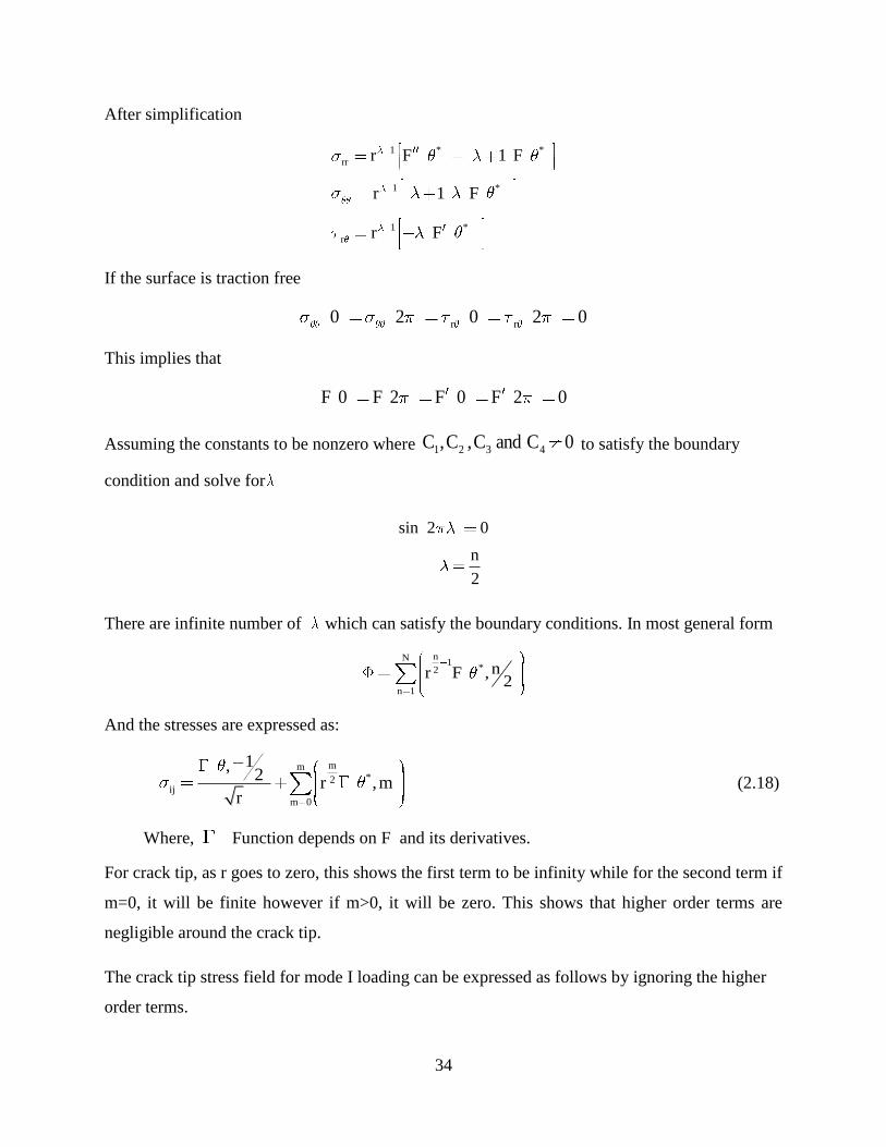
After simplification

1 * *

rr

1 *

1 *

r

r F 1 F

r 1 F

r F

If the surface is traction free

r r0 2 0 2 0

This implies that

F 0 F 2 F 0 F 2 0

Assuming the constants to be nonzero where 1 2 3 4C ,C ,C and C 0 to satisfy the boundary

condition and solve for

sin 2 0

n

2

There are infinite number of which can satisfy the boundary conditions. In most general form

nN1

*2

n 1

nr F ,2

And the stresses are expressed as:

mm

*2ij

m 0

1,2

r ,mr

(2.18)

Where, Function depends on F and its derivatives.

For crack tip, as r goes to zero, this shows the first term to be infinity while for the second term if

m=0, it will be finite however if m>0, it will be zero. This shows that higher order terms are

negligible around the crack tip.

The crack tip stress field for mode I loading can be expressed as follows by ignoring the higher

order terms.

35

rr

I

r

5 1 3cos cos

4 2 4 2

K 3 1 3cos cos

4 2 4 22 r

1 1 3sin sin

4 2 4 2

For mode II loading, the stress field around the crack

rr

II

r

5 3 3sin sin

4 2 4 2

K 3 3 3sin sin

4 2 4 22 r

1 3 3cos cos

4 2 4 2

Where KI and KII are stress intensity factors for Mode I and Mode II loading conditions. This

parameters defines the amplitude of the stress singularity around the crack tip. As long as the crack

is stationary, the stress and strain state increase in proportion to the stress intensity factor (K) (SIF).

Previous work by researcher’s shows that SIF (K) can be expressed Interms of the √𝐺𝐸

expressions, where G is the fracture energy (Energy release rate) and E is modulus of elasticity.

Westergaard Approaches:

Westergaard shows that complex stress function Z (z) can be used to solve certain limited problems

where Z z x iy where I = √−1.

Westergaard stress function

Re Z y Im Z

dZ dZZ and Z

dz dz

36

This shows that

'

xx

'

yy

'

xy

Re Z y Im Z (2.19)

Re Z y Im Z (2.20)

y Im Z (2.21)

Figure 2. 18: Biaxial loading for Westergaard solution, [14]

From the above it is clear that the shear stress vanishes when y = 0, implying that the crack plane

is principal plane. The original form of the Westergaard approaches is limited to certain types of

Mode I crack problems. In the Westergaard approaches the local stress is related to the global

stress and crack size.

2.3.5 Plastic crack- tip zone

Near the crack tip, the elastic stress intensity factors reaches to infinity which is impossible due to

finite capacity of the material. In reality, the material yield before the stress reaches to infinity

value and the elastic solution will no longer valid. Stress at crack tip is finite and some corrections

regarding with this are already done by many researchers.

The zone where the singularity occurs is called Fracture Process Zone. And the size of the material

has noticeable effect on the crack behavior. Occurrence of yielding can be tested by yielding

criteria. From the different methods which are used for checking whether the material yields or

not, two of the most familiars are Von Mises and Tresca Yield criteria are discussed below.

37

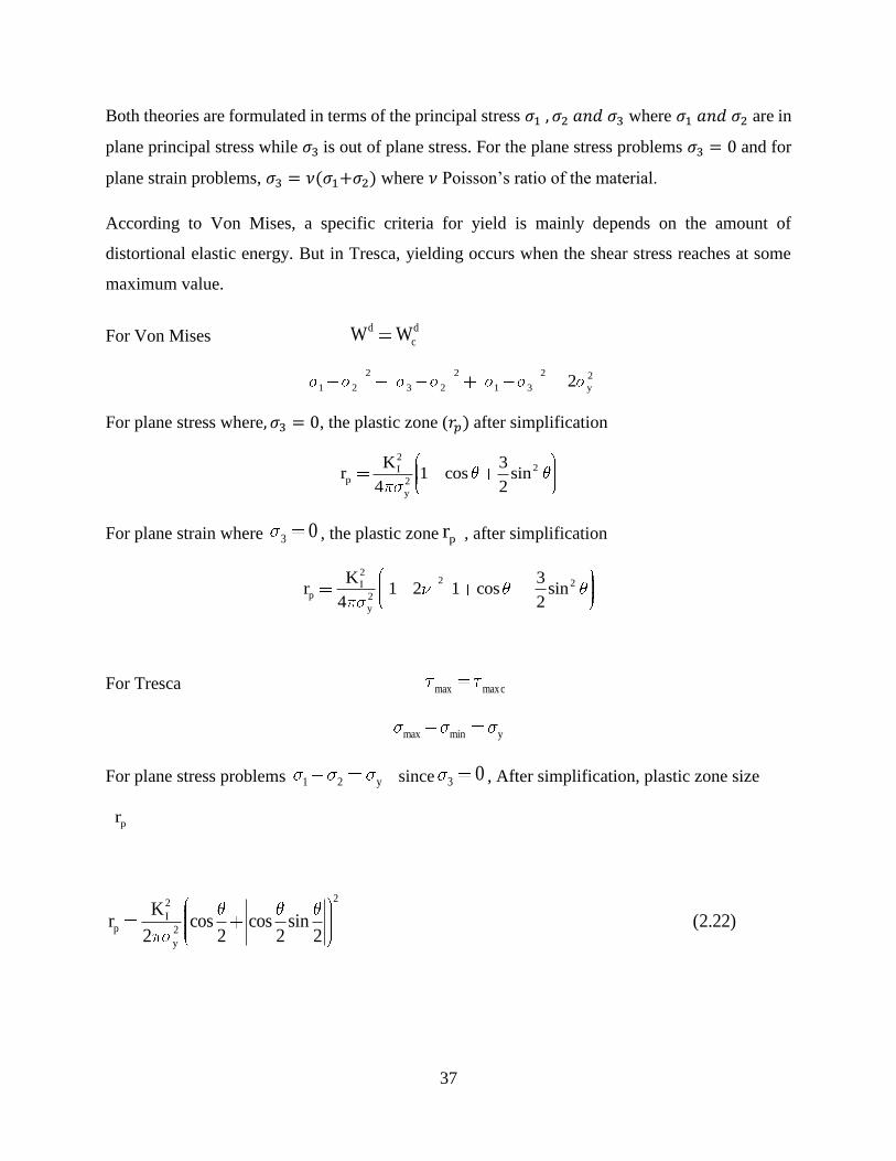
Both theories are formulated in terms of the principal stress 𝜎1 , 𝜎2 𝑎𝑛𝑑 𝜎3 where 𝜎1 𝑎𝑛𝑑 𝜎2 are in

plane principal stress while 𝜎3 is out of plane stress. For the plane stress problems 𝜎3 = 0 and for

plane strain problems, 𝜎3 = 𝜈(𝜎1+𝜎2) where 𝜈 Poisson’s ratio of the material.

According to Von Mises, a specific criteria for yield is mainly depends on the amount of

distortional elastic energy. But in Tresca, yielding occurs when the shear stress reaches at some

maximum value.

For Von Mises d d

cW W

2 2 2 2

1 2 3 2 1 3 y2

For plane stress where, 𝜎3 = 0, the plastic zone (𝑟𝑝) after simplification

22I

p 2

y

K 3r 1 cos sin

4 2

For plane strain where 3 0 , the plastic zone pr , after simplification

22 2I

p 2

y

K 3r 1 2 1 cos sin

4 2

For Tresca max maxc

max min y

For plane stress problems 1 2 y since 3 0 , After simplification, plastic zone size

pr

22

Ip 2

y

Kr cos cos sin (2.22)

2 2 2 2

38

For plane strain condition

Condition 1 where 1 2 3

22

Ip 2

y

Kr (1 2 )cos cos sin (2.23)

2 2 2 2

Condition 2 where 1 3 2

2

2Ip 2

y

Kr sin (2.24)

2

Stable and unstable crack propagation

Crack tip speed and its propagation mainly depends on the general energy balance. When crack is

subjected to mode I load with 𝛿 , resulting from external load applied at the edges far away from

the crack, the external work done will be zero when crack length changes.

Using energy balance

e a di kdu du dudu du

(2.25)da da da da da

If the dissipated energy is assumed to be very small and enough to be ignored, all the available

energy is going to be transformed in to surface energy and kinetic energy

e ddu du0 and 0

da da

For central crack in large plate with unloaded Elliptical area

Figure 2. 19: Plate subjected to far field stress, [2]

39

Surface energy a sU 4ab

as

dU4b

da

Internal energy

22

iU 2 a b2E

2

idU2 ab

da 2E

Total kinetic energy

22

yxdudu1

KE *V*2 dt dt

Where, is material density, V is material volume and yxdudu

anddt dt

are the material

velocity components. For constant thickness, b, V=bdxdy

22

yxdudu1

KE *b* dxdy2 dt dt

For material velocity, y y y yxdu du du dudu da

Sdt dt dt da dt da

Where,da

Sdt

, crack speed.

For plane stress of yu of crack face with

2

y2kdudu 1 d

S b dxdyda 2 da da

For the given crack shape 2

yu 2 2 a axE

Substitute the yu in to the above integral

2

2kdu 1S b aK a

da 2 E

40

Back to energy balance

222

s

2 a 14 S b aK a

E 2 E

Solve for crack speed S, s

2

2 E2 ES 1

K a

For c 2

2 Ea and

Ec

Finally, s will be

1

2ca

S 0.38c 1 (2.26)a

For a>> ac ,

S =0.38c

2.4 Section Capacity of Reinforced Concrete Elements

2.4.1 Stress and strain diagram

The subject of mechanics of materials involves analytical methods for determinations of the

strength, stiffness and stability of the various members in structural system. The behavior of

members depends on not only on the fundamental law that govern the equilibrium of force but also

on mechanical characteristics of the material.

This mechanical characteristics comes from laboratory, where materials are tested under

accurately known forces and their behavior is carefully observed and measured.

Reinforced Concrete Mechanical Characteristics

Stress: it is the intensity of Force acting on infitisimal area of section. Mathematically this can be

expressed as

A 0

Flim (2.27)

A

Figure 2. 20: Section body, [14]

41

For the sake of simplicity theses stress can be resolved in to two components, one is parallel the

cross section and is called shear stress (S) and the other is perpendicular to the section and is called

normal stress (N).

Figure 2. 21: Tractions decomposition, [14]

The state of the stress at any point can be described by using three components of stress on each

three mutually perpendicular direction. This term is called stress tensor.

Matrix representation of the stress tensor

xx xy xz

ij yx yy yz

zx zy zz

To satisfy equilibrium of moment stress tensor is symmetric i.e. ij ji

When the out of plane stress, stresses in the directions of 𝜎𝑧𝑧 = 𝜏𝑦𝑧 = 𝜏𝑥𝑧 = 0 or when all

elements in the 3rd column and 3rd rows are zeros, the 2D state is called plane stress problems.

However, if 𝜖𝑧𝑧 = 𝛾𝑦𝑧 = 𝛾𝑥𝑧 = 0, it is called plane strain problems.

For plane stress problems if 𝜎𝑧𝑧 = 0, Biaxial state of stress and if further 𝜎𝑦𝑦 =0, it is called

uniaxial state of stress.

When the stress are calculated in the original area of the member, they are referred as conventional

or engineering stress. However, if the member cross sections are assumed to be the actual, the

stress calculated is called true stress.

42

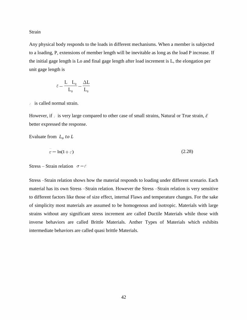
Strain

Any physical body responds to the loads in different mechanisms. When a member is subjected

to a loading, P, extensions of member length will be inevitable as long as the load P increase. If

the initial gage length is Lo and final gage length after load increment is L, the elongation per

unit gage length is

0

0 0

L L L

L L

is called normal strain.

However, if is very large compared to other case of small strains, Natural or True strain, 휀 ̅

better expressed the response.

Evaluate from 𝐿𝑜 𝑡𝑜 𝐿

ln(1 ) (2.28)

Stress – Strain relation

Stress –Strain relation shows how the material responds to loading under different scenario. Each

material has its own Stress –Strain relation. However the Stress –Strain relation is very sensitive

to different factors like those of size effect, internal Flaws and temperature changes. For the sake

of simplicity most materials are assumed to be homogenous and isotropic. Materials with large

strains without any significant stress increment are called Ductile Materials while those with

inverse behaviors are called Brittle Materials. Anther Types of Materials which exhibits

intermediate behaviors are called quasi brittle Materials.

43

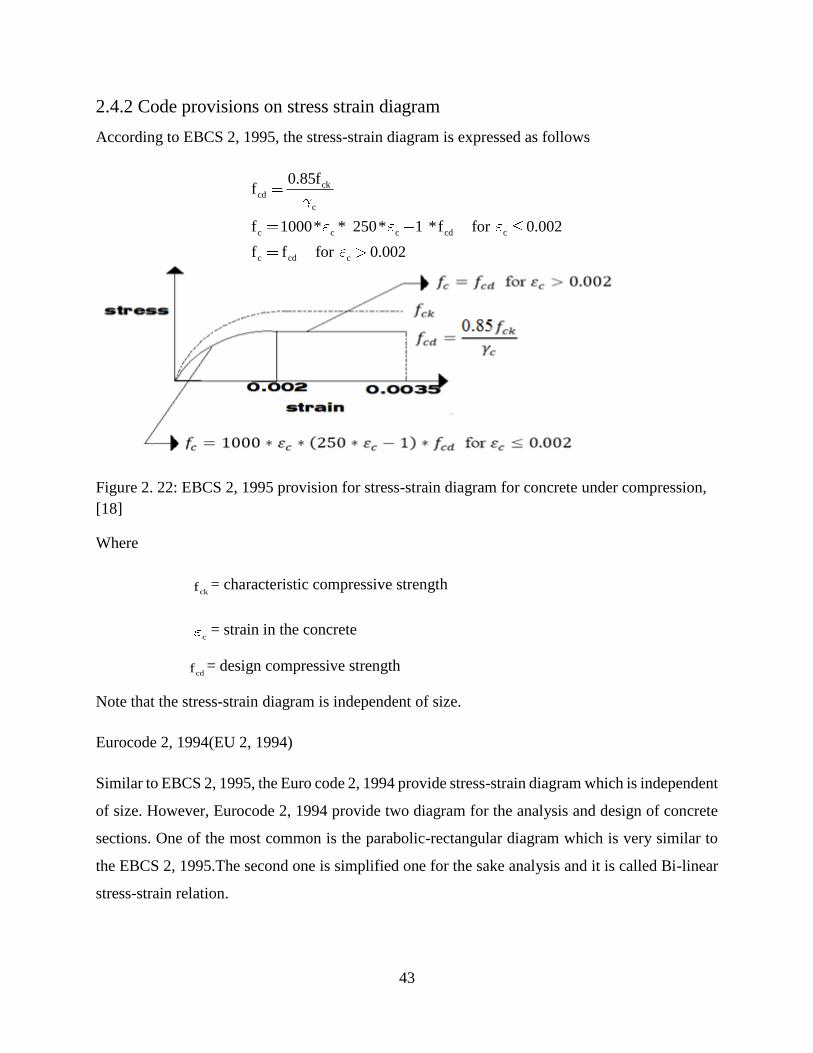
2.4.2 Code provisions on stress strain diagram

According to EBCS 2, 1995, the stress-strain diagram is expressed as follows

ckcd

c

c c c cd c

c cd c

0.85ff

f 1000* * 250* 1 *f for 0.002

f f for 0.002

Figure 2. 22: EBCS 2, 1995 provision for stress-strain diagram for concrete under compression,

[18]

Where

ckf = characteristic compressive strength

c

= strain in the concrete

cdf = design compressive strength

Note that the stress-strain diagram is independent of size.

Eurocode 2, 1994(EU 2, 1994)

Similar to EBCS 2, 1995, the Euro code 2, 1994 provide stress-strain diagram which is independent

of size. However, Eurocode 2, 1994 provide two diagram for the analysis and design of concrete

sections. One of the most common is the parabolic-rectangular diagram which is very similar to

the EBCS 2, 1995.The second one is simplified one for the sake analysis and it is called Bi-linear

stress-strain relation.

44

Figure 2. 23: EU 2, 1994, provision for Parabolic-rectangular stress-strain diagram for concrete

under compression, [17]

For Parabolic-rectangular stress-strain distribution

Where c1 2 0/00 and

c2 3.5 0/00

Figure 2. 24: EU 2, 1994, provision for bilinear stress-strain diagram for concrete under

compression, [17]

For Bi-linear stress-strain relation.

Where c3 1.75 0/00 and

c2 3.5 0/00

ACI 1999

The compressive strength of concrete (fc’) is determined by testing to failure 28-day-old 150mm

by 300mm concrete cylinder at specified rate of loading. Although concrete are available with the

28-day ultimate strength from 15 MPa (2.5 ksi) up to 70 MPa (10 ksi) to 140 MPa (20ksi), most

of the concrete used fall in to 20MPa (3ksi) to 48 MPa (7ksi).

ACI code for stress-strain curves show that the curves are roughly straight line while the load is

increased from zero to one-third to one-half of the concrete ultimate strength.

Beyond this range, the behavior of the concrete becomes nonlinear. The lack of linearity of

concrete stress-strain curves at higher stress causes some problems in the structural analysis.

45

The stress–strain curves from ACI code also shows that regardless of compressive strength, all

concrete reaches their ultimate strength at strain of 0.002 (20/00). From the graph it is clear that

concrete does not have definite yield strength.

Figure 2. 25: Typical Concrete stress-strain curve according to ACI provision, [10]

2.4.3 Effect of size on the stress strain diagram

The performance of concrete was assumed to be dependent on the concrete quality. However, real

life experiences shows that it is not only the concrete quality but also the size of the structure which

can control the failure mechanism. The behavior and strength of reinforced concrete member is

controlled by size and shape of the member and by the stress-strain properties of concrete and

reinforcement.

Figure 2. 26: Typical concrete stress-strain diagram under compression with different

compressive strength, [10]

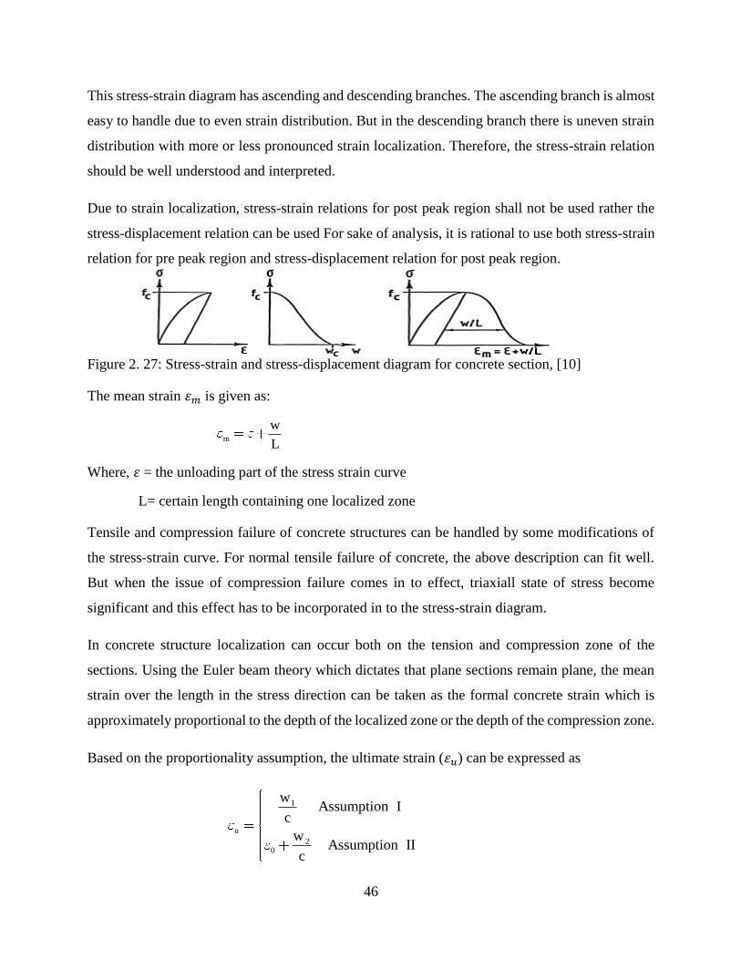
46

This stress-strain diagram has ascending and descending branches. The ascending branch is almost

easy to handle due to even strain distribution. But in the descending branch there is uneven strain

distribution with more or less pronounced strain localization. Therefore, the stress-strain relation

should be well understood and interpreted.

Due to strain localization, stress-strain relations for post peak region shall not be used rather the

stress-displacement relation can be used For sake of analysis, it is rational to use both stress-strain

relation for pre peak region and stress-displacement relation for post peak region.

Figure 2. 27: Stress-strain and stress-displacement diagram for concrete section, [10]

The mean strain 휀𝑚 is given as:

m

w

L

Where, 휀 = the unloading part of the stress strain curve

L= certain length containing one localized zone

Tensile and compression failure of concrete structures can be handled by some modifications of

the stress-strain curve. For normal tensile failure of concrete, the above description can fit well.

But when the issue of compression failure comes in to effect, triaxiall state of stress become

significant and this effect has to be incorporated in to the stress-strain diagram.

In concrete structure localization can occur both on the tension and compression zone of the

sections. Using the Euler beam theory which dictates that plane sections remain plane, the mean

strain over the length in the stress direction can be taken as the formal concrete strain which is

approximately proportional to the depth of the localized zone or the depth of the compression zone.

Based on the proportionality assumption, the ultimate strain (휀𝑢) can be expressed as

1

u

20

wAssumption I

c

wAssumption II

c

47

Where w1 and w2 are material properties while c is depth of the compression zone, [10].

Figure 2. 28: Dependency of the stress-strain diagram in the depth of compression zone, c, [10]

48

3 Fracture Mechanics of Concrete

In applying Fracture Mechanics to concrete, much was initially borrowed from the wealth of

information and research previously undertaken in conjunction with metals by metallurgists or

mechanical engineers. However, it quickly became evident that by its very heterogeneous nature,

concrete has some unique fracture characteristics, which required the alteration of existing models,

[28].

By now Fracture Mechanics is universally acknowledged as a viable tool of analysis for

investigation of concrete cracking. And after many years of development on numerous (plasticity

based) constitutive models for concrete, tensile cracking is not yet addressed well. For the most

part, even the simplest constitutive models appear to perform reasonably well under compressive

regimes, however their capabilities are seriously challenged under tensile stresses. This apparent

inability to properly model tensile cracking is of minor importance in reinforced concrete

structures in which the steel “takes over” the tensile stresses. However, for crack related failures,

the tensile strength should be properly determined for best approximation of response due to

different loadings.

3.1 Pre/Post-Peak Material Response of Steel and Concrete

As an introduction to concrete Fracture, the pre- and post-peak response of Rebar’s and concrete,

both obtained in a strain-controlled test of an un-cracked or un-notched specimen is shown below

Figure 3. 1: Stress-Strain Curves of reinforcement bars and Concrete, [28]

49

1. Pre-peak:

(a) Reinforcement exhibits a linear elastic response up to the yield stress σy, and an approximate

strain of 0.1%. Subsequently, due to internal dislocation and plastic deformation with strain up to

2.5% may result to be followed by strain hardening.

(b) Concrete under compression load exhibits a linear response while the load is increased from

zero to about one-third to one-half of the concrete ultimate strength and with strain of

approximately 0.2%. However, if the direction of the load is changed, when the load is Tensile,

the concrete responds in linear manner up to approximately 0.6ft’ subsequently internal micro

cracking induces a nonlinear response up to a peak stress f’ and a corresponding strain of

approximately 0.01%. Under load control, only the pre-peak response can be measured.

2. Post-peak:

(a) Reinforcement response in the post-peak zone is not yet well understood. Not only it is not of

practical usefulness, but also it is largely overshadowed by necking.

(b) Concrete response in the post-peak zone is most interesting, as it can exhibit additional strains.

The descending branch of the concrete response is an idealization of the average material response.

A more accurate description should account for the localization of the induced cracks. Thus away

from the localized crack there is an elastic unloading, and at the crack, since a strain cannot be

properly defined, a stress-crack opening displacement is a more appropriate model.

3.2 Stress versus crack opening displacement Diagram

It is clear that concrete softening is characterized by a stress-crack opening width curve (and not

stress-strain). The exact characterization of the softening response should ideally be obtained from

a uniaxial test of an un-cracked specimen. However, it has been found that not only those tests are

extremely sensitive, but drastically diff erent results can be obtained from diff erent geometries,

sizes, and testing machines. Hence, the softening curve is often indirectly determined by testing

notched specimens.

50

3.3 Concrete Models for Fracture Analysis

3.3.1 Fictitious crack model (Cohesive Crack Model)

The most referenced work in the nonlinear fracture of concrete literature, is Hillerborg Simple

and elegant model which has been used for long time till the initiation the Fracture concepts. Both

the experimental and theoretical Fracture concepts have been used to predict the nature of concrete

near to failure stage. As mentioned in the above one of the most well-known model is the Fictitious

crack model (FCM) developed by Hillerborg and co-workers. `

According to the FCM, any point on the material is in one of the three possible cases

Case 1: Undisturbed elastic state,

A point in this region is in elastic state and condition of compatibility satisfied.

Case 2: Fracture state (Fracture Zone),

The material in this region is softened by micro-cracking (Fictious Cracks) but stress can

transfer.

Case 3: No stress transformation state,

The material in this region lacks stress transfer and these are traction free surface.

All points outside the fracture zone can be handled by using the linear elastic theory. However, the

points in the fracture zone is handled by special constitutive relation, the so-called stress-crack

opening displacement relation, (𝜎 − 𝑤).

Since the traction free surface is with known boundary condition that is 𝜎𝜃𝜃 = 𝜏𝑟𝜃 = 0 and the

fracture zone is with 𝜎 − 𝑤 relation, it is rational to neglect the undisturbed elastic zone in

modeling. Therefore in this model, the crack is composed of two parts, these are

1. True or physical crack across which no stresses can be transmitted. Along this zone, there is

both displacement and stress discontinuities.

2. Fictitious crack, or Fracture Process Zone (FPZ) ahead of the previous one, characterized by:

a) Peak stress at its tip equal to the tensile strength of concrete

51

b) Decreasing stress distribution from ft at the tip of the fictitious crack to zero at the

tip of the physical crack. It should be noted that along the FPZ, there is displacement discontinuity

and stress continuity, [28].

Figure 3. 2: Hillerborg Fictitious Crack Model, [28]

3.3.2 Crack Band Model (CBM)

The crack band model has been the most widely used in practice for analyzing the distributed

cracking and fracture of concrete. Its main advantage over the FCM is it takes in to account tri-

axial stress in the Fracture process zone (FPZ), particularly the normal and shear stress acting in

the directions normal to crack plane.

The basic idea of CBM which was proposed by Bazant (1976)

Characterize material behavior in the FPZ in Smeared manner through strain softening

constitute relation

Impose fixed width of, wc, of the strain softening zone (crack band) representing material

properties.

The imposition of constant opening width, wc, is required in order to avoid spurious mesh

sensitivity and achieve objectivity, assuring that the energy dissipation due to the fracture per unit

length(and per width) is constant and equal to Fracture energy of the material.

52

Softening is cause by fracture strain (ef) which is superimposed to the elastic strain. Assuming all

the cracks to be parallel and smeared (continuously distributed) and choosing y to be normal to the

cracks(x-y plane)

xx xxxx xxyy xx

yy xxyy yyyy yy f

xy xyxy xy

c c 0 0

c c 0 e

c 00 0

Where C matrix is the compliance matrix

0 1 Shear retention factor

For isotropic material

xxxx yyyy '

1c c

E

yyxx xxyy '

'c c

E and xyxy

2 1 'c

E '

Where ,E ' E '

For plane stress condition' '

and

E

E ' 1For plane strain condition

'

1

Damage (w) is function of the strain normal to the crack, 휀𝑦𝑦. For no damage scenario, w = 0 and

for complete collapse damage, w = 1. Therefore, w is always between 0 and 1. The fracture

energy is obtained as follows

F c 22 f

0

G w de

The fracture strain, ef , can be incorporated Interms of damage (w)

yyyy

f yy

wce

1 w

New function Φ(휀𝑦𝑦) can be defined as

yy

w

1 w

53

The function Φ(휀𝑦𝑦) characterizes the uniaxial stress-strain softening. There are different options

in assuming Φ(휀𝑦𝑦). One of the most common is

pa

yy

t

Ee

f

Where a and 휀𝑝 are empirical constants.

The width of the crack band front can be assumed to be approximately wc = 3da. Where da is the

size of the maximum aggregate size. For CBM only two parameters are required and these are ft’

and GF. The effect of wc is very small, enough to be ignored. However, the effect of wc will be

pronounced when there are tension reinforcement (parallel cracks).

54

4 Application of Fracture Mechanics

4.1 Numerical Approach of Fracture Mechanics

In Fracture Mechanics only some problems have closed form solutions. This makes numerical

modeling to be indispensable tool in fracture analysis. This days advanced numerical techniques

are applied to study special problems like those of fracture at interface, dynamics of fracture and

ductile crack growth.

The stress and strain distribution in the body caused by external and internal load can be

determined in different ways. Only some of the problems have only closed form solution due to

the complex stress and strain distribution. In elastic problems, Westergaard and Williams used

different approaches to find stress caused by plane stress and plane strain loading.

Finite difference, Finite element and Boundary Integral Equations are well known in solid

mechanics. Finite elements are also known in Fracture Mechanics and with limited cases boundary

integral method can be used in Fracture analysis.

Numerical analysis are very important since they are the source of Fracture Mechanics parameters.

Two way of most common approach are point matching and energy method. In point matching,

stress or displacement fields are used to determine stress intensity factor (SIF). However in energy

method, Energy release rate is calculated and related to stress intensity factor.

Stress and displacement matching

For Mode I fracture type and at angle 𝜃 = 0

I 22

r 0K lim 2 r (4.1)

Where,22

is the stress acting perpendicular to the crack plane

r is the distance from the crack tip.

On the crack plane 0 , KI can be obtained by plotting the quantity in the square brackets against

from the crack tip and extrapolate to the point r 0 .

55

4.2 SIF and propagation criteria

In LEFM, analysis of cracked bodies depends on the SIF, for mode I type SIF (KI) can be expressed

as

I 22K a (4.2)

Where, a is initial crack length, is remote tensile stress and is factor considering crack

geometry. For the case of central crack with length of 2a in infinite plate where 1

IK a (4.3)

Since the KI describes the nature of the stress distribution at local level, better determinations of

KI will leads to more accurate determinations of the response.

Series of Hand books are available which are used for determination of SIF. Some of which are

Hand Books of SIF (Sih 1973), the stress analysis of crack Hand Book (Tada, 1971) and comparing

of SIF (Rook and Carting 1976).

As long as the local material is in a linear state, principle of superposition can be used. As long as

the location of the crack is fixed, SIF due to different loading can be super imposed while the

material is in the linear state.

Generally there are two solution techniques which are used to solve any 2D structural geometry or

loading situations. The first methods involves the generations of the stress for the un cracked body

part along the expected path of crack propagation. In the second method, generations of SIF via

integral calculation that employs the stress obtained from the un cracked body analysis. The Green

functions and the weight functions techniques can be used for integral calculation

Crack propagation

Mode I failure predominates for homogenous isotropic material. For conservative Fracture based

design, one needs to characterize the crack under mixed mode loading. In mixed mode type of

crack propagation, KI and KII, attains material independent critical value in space and this space is

called Fracture Surface. The fracture surface can be expressed as

56

1 I II IC IICf K ,K ,K ,K , 0 (4.4)

The function describing the failure surface can be expressed either by using polynomial or power

law and is expressed in non-dimensional form as follows

a b

I II

IC IIC

K K1

K K

Where a and b are obtained from material type.

However, if the energy principle is used for fracture surface function, the failure surface can be

expressed as follows

2 2

11 I 12 I II 22 IIa K 2a K K a K a

Where, 11a

12a and 22a are material dependent constants and a is real number constant.

Experimental evidences shows that most failure surface follow ellipse like distribution where a =

b = 2.

2 2

I II

IC IIC

K K1

K K

The most common crack propagation criteria are

Modified Griffith criteria

The concept of energy balance is extended to include energy release rates associated with all

mixed mode.

I IIG G G

Crack extends when

G

0 and

2

2

G0

57

Maximum Tangential stress criteria

When a cracked body is subjected to Mode I and Mode II loading, stress will develop in the

vicinity of the crack tip. According to this criteria, crack develops in the direction of maximum

tangential stress.

rr

11 21 31

I II

12 22 32

r

f f fK K

f f f

Where ijf f r,

Crack extends in a direction of θ where,

0 and

2

20

Strain energy density criteria

According to this criteria, stress will follow a direction of minimum strain energy density.

Energy density function, W

dU

WdV

Where, U is total elastic energy and V is total volume.

For linear 2D elasticity problems

2 2

11 22 11 22 12

1 k 1W 2

2E 4

Where,

3 4 for plane strain

k 3for plane stress

1

Crack propagates in a direction of minimum strain energy density

58

dW

0d

and

2

2

d W0

d

4.3 Proposed crack propagation model

From the first law of thermodynamics which states about conservation of energy

. . . . .1

e i a d kU U U U U [JS ]

For the case of static loading kU 0

Using variable change methods dx dx dA

dt dA dt

e a didu du dudu

dA dA dA dA

N.B: This equation is different from Griffith energy balance, since in this equation, energy lost in

the plastic zone is considered.

After some simplification

e d aidu du dudu

dA dA dA dA

For a very small incremental area, A, which is created due to External Loading can be

calculated using differential element. Then

)(abA

Where, a is small increment in crack length and b is small increment in thickness

baabA

For constant thickness b =0, and dAA , bdaab

bdaabdAA

After rearranging and simplifying, finally the first Law of Thermodynamics will take the

following format

59

e d aidu du dudu

bG 'dA dA dA dA

Where, G’ is modified Griffith energy release rate which consider the energy dissipated by

plastic deformation.

For the case of fixed grips where displacement is zero…… edu0

dA

This implies

di

du1 duG ' (4.5)

b da da

60

Typical example

Given

In through elliptic hole

Major and minor axis are 2a and 2b respectively

Tensile stress at far distance from the hole (flaws)

Figure 4. 1: Plate subjected to far field tensile stress with central hole,

a su 4ab Surface energy dissipated to create new surface

iU ……internal strain energy

2 2 2

i

v 0

1 2a bU d dV 2* *2a * a *b*

2 2E E

For thin plate n

2

2 2

i

a bU (4.6)

E

dU ……energy dissipated by plastic deformation

b

d ij ij ij

v 0

U d dv (4.7)

During collapse, strains are purely plastic and the section has two parts

61

The most outer part will be in plane stress mode with plastic zone of

2

2Iy

t

K1 3r 1 cos cos

4 f 2

While the most inner part will be in the plane strain mode with plastic zone of

2

2 2Iy

t

K1 3r (1 2 ) (1 cos ) sin

4 f 2 (4.8)

Figure 4. 2: The plane stress and plane strain plastic zone, [5]

The area of the plastic zone is assumed as the area of special curve which is shown below

Figure 4. 3: Area of special curve called Lemnsicate,

One problem with this type of special curve is the energy lost in the shaded region is not

captured.

Figure 4. 4: Approximate process zone beyond crack tip

62

Ignoring the shaded region is conservative in the design process and it will not cause any

overestimation of the maximum load to be carried by the structure.

The area of the lemnsicate is about

21A a

2 (4.9)

Where, For plane stress condition

2

I

t

K1a

4 f

For plane strain condition

2

2I

t

K1a 1 2

4 f

For the sake of simplicity, take linear variation of the Plane stress and Plane strain area

PSS PSN

i

A AV *b

2

Where, APSS = plane stress area ,APSN = plane strain area , b = width of specimens and Vi is total

volume plastic deformation considering the effect of poisons ratio.

Therefore,the energy dissipated by plastic deformation is

2

td

fU V

2E

And, finally

di

dUdU1G '

b da da (4.10)

This shows that the energy release will get higher value when plastic deformation is considered

and the issue of plastic stress and plastic strain is avoided.

63

Crack Initiation Load

Design codes give prescription on how to calculate the cracking load using the cracking Moment.

But the problem using the code prescription is that, crack can occur even below the expected

cracking load due to Size Effect. Therefore, there should be away to consider the Size Effect in

calculating the cracking load. For this reason, Fracture Mechanics concept will be used for

cracking load calculation.

From the first law of thermodynamics under constant temperature, amount of energy required for

a unit crack extension is

a FU G b da

Where, Ua is surface energy

GF = energy release rate

b = thickness of specimens

da = unit crack extensions

Given cross section

Figure 4. 5: Transverse and longitudinal section of three point bend beam

64

Required: The cracking Load which consider Size Effect

For the crack to nucleate, the following equilibrium condition should be satisfied

Where c is length of plastic zone, w is crack width and a is initial crack depth.

Energy dissipated by plastic deformation

2 2

t t PSS PSNd

f f A AU *V * *b

2E 2E 2 (4.11)

Internal strain energy

2

ti

v 0

fU d dV * W*c 2mac

2E

(4.12)

At the initial stage of cracking, m = 0 and volume of plastic zone will be

V b*c*w

Therefore the first law of thermodynamics will take the following form

2 2

't t PSS PSNF

f f A Ab* *W*c * G * a *b

2E 2E 2

(4.13)

After some simplification

3 2't t PSS PSN tF2

f *c*L f A A f LG *

8E 2E 2 8E

Rearranging the terms and after some simplification

65

2

t t

e Tf f * 0

c*L c (4.14)

Where e and T are material constants obtained from Experiments.

From the above equation it is clear that tensile strength is a function of plastic zone. But it is

possible to express the plastic zone size as a function of member depth as

c *D

Therefore, Equation 4.14 can be expressed as follows

2

t t

e Tf f * 0

*D*L *D (4.15)

Equation 4.15 shows that tensile strength of a material is a function of both member and cross

section. Qualitatively Equation 4.15 shows that both depth and member length have effect on the

tensile strength of the material. Therefore, Fracture is both section and member property.

Check the sensitivity of the Fracture to section and member length variation

Let,1

eb

DL and

2

eb

D

Equation 4.15 can be reduced to the following form

2

t t 1 2f f b b 0 (4.16)

To check the sensitivity of member effect

Take D to be constant and check for

tdf0

dL

Where 2

t t

e Tf f * 0

*D*L *D

Take the derivatives and after rearranging the terms

66

t t

2

t

df f *e

dL 2f DL eL

To check the sensitivity cross section effect

Take L to be constant and check for

tdf0

dD

Where , 2

t t

e Tf f * 0

*D*L *D

Take the derivatives and after rearranging the terms

t t

2

t

df f *e LT

dD 2f D L eD

Since 2 2

t t2f D L eD 2f DL eL , this shows that

t tdf df

dD dL

The physical interpretation of the above inequality is that the tensile strength is more sensitive to

the cross section than that of member length. Therefore crack nucleates whenever the applied

load cause ft amounts of tensile stress.

From the Elastic analysis for the three point bend beam

2 2

6M 3PL(4.17)

bD bD

Where, M is the actual design moment

b is width of the cross section

D is depth of the cross section

L is half of the member length

67

Using Bazant size effect Law

c t

1Bf

1

Where, B and β are parameters mainly depends on the geometry.

Equating Equation 4.17 and Bazant Size effect Law

t2

3PL 1Bf

bD 1

And solve for P

2

tcr

Bf bD 1P P

3L 1 (4.18)

Where,

P=Pcr is the cracking load which consider the Size Effect

ft is tensile strength of the material

b is width of the cross section

D is depth of the cross section

L is half length of the specimen

B is empirical constant obtained from experiment data analysis

β is brittleness number obtained from experiment data analysis

68

Crack Propagation

Figure 4. 6: Beam subjected to central loading

Crack follows a path where tensile strength at each element is greater than ft and it will follow

the direction of minimum tensile strength.

Figure 4. 7 : Beam part near the crack

At P=Pcr, crack nucleates and starts to propagate. There are two important situations occurring at

this point. These are

The existing Crack propagates

New crack surface will start to emerges at some distance from the existing Cracks

Closure look at the crack tip

Figure 4. 8: Magnified view in the vicinity of the crack

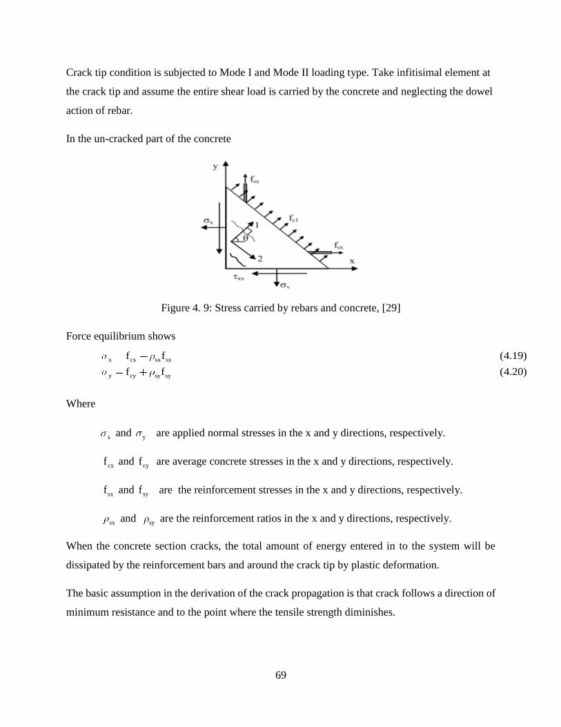
69

Crack tip condition is subjected to Mode I and Mode II loading type. Take infitisimal element at

the crack tip and assume the entire shear load is carried by the concrete and neglecting the dowel

action of rebar.

In the un-cracked part of the concrete

Figure 4. 9: Stress carried by rebars and concrete, [29]

Force equilibrium shows

x cx sx sx

y cy sy sy

f f (4.19)

f f (4.20)

Where

x and y are applied normal stresses in the x and y directions, respectively.

cxf and cyf are average concrete stresses in the x and y directions, respectively.

sxf and syf are the reinforcement stresses in the x and y directions, respectively.

sx and sy are the reinforcement ratios in the x and y directions, respectively.

When the concrete section cracks, the total amount of energy entered in to the system will be

dissipated by the reinforcement bars and around the crack tip by plastic deformation.

The basic assumption in the derivation of the crack propagation is that crack follows a direction of

minimum resistance and to the point where the tensile strength diminishes.

70

Therefore, once the crack nucleates then it will follow the direction of softening tensile stress. In

the post peak case, there are two sources for the tensile strength, these are tensile strength due to

Tension softening and Tension Stiffening. To be on the safe side and conservatives in the design,

the tensile strength due to tension softening is considered as the post cracking tensile stress.

On the way to crack propagation, some requirements should be satisfied and one of the basic

parameter in cracking process is Fracture Energy. In this Thesis the fracture Energy of the

concrete is taken as 75 N/M (This value is the default Value Of concrete Fracture Energy in

Most Fracture Analysis Finite Element Software).

Due to simplicity and ease of application, Linear Tension Softening Model is used.

Figure 4. 10: Simple linear softening Model, [28]

From the linear Tension Softening Model

c1 crts cr

ch cr

f f 1 (4. 21)

Where, fts is Tension softened tensile strength, fcr is tensile cracking stress, 휀𝑐1 𝑖𝑠 principal

tensile stress and 휀𝑐𝑟 Tensile cracking stress, 휀𝑐ℎ is characteristic strains of the tension softening

Curve.

Therefore the crack follows the directions where the maximum tensile stress reaches a value of

fts. The Tangential stress and shear stress in the polar coordinate

71

I II

r I II

2K 1 cos cos 3K sin cos

2 22 r

2K sin cos K (3cos 1)cos

2 22 r

Crack occurs in a direction of c ,where c tsf

c1 crI II cr

ch cr

2K 1 cos cos 3K sin cos f 1

2 22 r

In addition, when the crack starts in a direction of c , then r c 0 , this means Shear stress

diminishes in the crack plane. For the sake of simplicity, consider only Mode I loading in which

KII = 0.

I ts

2K 1 cos cos f

22 r

For crack to Propagate, KI = KIC, solving for c

ts3

c

IC

2f rcos 1

K

Therefore, as long as KIC, r and fts are known then the direction of the propagation can be

calculated.

4.4 Proposed section capacity model

Assumption

Water lost by evaporation from concrete structures cause additional flaws(internal micro

cracks)

Most of the fracture energy is lost in the post peak region

Some portion of the compression zone will not carry any compressive stress due to

localization

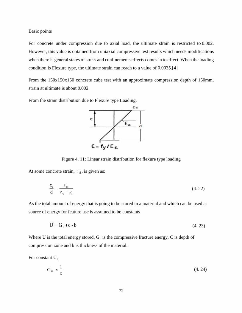
72

Basic points

For concrete under compression due to axial load, the ultimate strain is restricted to 0.002.

However, this value is obtained from uniaxial compressive test results which needs modifications

when there is general states of stress and confinements effects comes in to effect. When the loading

condition is Flexure type, the ultimate strain can reach to a value of 0.0035.[4]

From the 150x150x150 concrete cube test with an approximate compression depth of 150mm,

strain at ultimate is about 0.002.

From the strain distribution due to Flexure type Loading,

Figure 4. 11: Linear strain distribution for flexure type loading

At some concrete strain, ci , is given as:

cii

ci s

c

d (4. 22)

As the total amount of energy that is going to be stored in a material and which can be used as

source of energy for feature use is assumed to be constants

FU G c b (4. 23)

Where U is the total energy stored, GF is the compressive fracture energy, C is depth of

compression zone and b is thickness of the material.

For constant U,

F

1G

c (4. 24)

73

Since the Compressive Fracture energy is directly proportional to the ultimate strain, then

ci

1

c (4. 25)

This can be expressed as shown below

ci

n

c (4. 26)

Where, n is some constant.

For initial guess of n value, take the test result from the common compressive laboratory test

results where C=150mm and ci 0.002 . Solve for n

cin c 150*0.002 0.3

Therefore, the strain is expressed interms of compressive zone depth

Finally

ci

0.3

c (4. 27)

From force equilibriums

s yd cdA f f b c (4.28)

From strain distribution due to flexure type loading

cii

ci s

i

s

i

s

c

d

0.3

c c0.3d

c

c 0.3

d 0.3 c

Where, s is the strain in the reinforcement and Solve for c

74

s

s

0.3 0.09 1.2 dc

2 (4. 29)

The moment capacity for the given cross section is about

s ysM A f d 0.4 c (4. 30)

Where, M is design moment capacity which consider the Size Effect

fyd yield strength of reinforcement bars

As amount of reinforcement in the tension zone

d depth from most compression zone to the center of tension reinforcement bars

C depth of compression zone

4.5 Fracture Mechanics using Finite element software

Any experimental test requires lots of money, time and effort. In addition, handling of the

equipment’s and data recording is another critical issues. Therefore, simulations and modeling are

indispensable tools for response determination of structures subjected to different loading. These

simulations can be 2D or 3D. This days there are a lots of Finite Element (FE) software like those

of ANSYS, NASTRAN, ADINA, COSMOS and ABAQUS which have the ability of solving very

complex differential equation.

Due to the capability of predicting and displaying the pattern of crack propagation and crushing of

material, and material like that of concrete can be properly represented, for this reasons FE

software packages called ANSYS is selected for this study.

In ANSYS rebar’s can be modeled as bar or beam elements connected to concrete mesh nodes.

The concrete is modeled as SOLID 65 elements which has eight integration points. SOLID 65

elements has 3 Degree of Freedom (DOF): translation in X, Y and Z. Cracking, crushing and

plastic deformation can be represented by this elements.

Fracture Analysis is a combination of stress analysis and Fracture Mechanics parameters

calculation. Linear elastic or Non-linear elastic plastic methods can be used for stress analysis near

75

the crack tip. However, due to the high gradients of stress near the crack tips, Finite Element

modeling requires special attention.

In ANSYS modeling PLANE183, 8 node quadratic element is used for 2D fracture problems and

SOLID 65, 20 node brick elements is used for 3D fracture problems. In FE analysis of fracture

problems, there are some important parameters which plays important role in controlling the

response.

Some of the basic parameters in Fracture mechanics are

Stress Intensity Factor(SIF)

J integral

C* integral

T-stress

Material force

From the above Fracture mechanics parameters, SIF is selected due to its ability to express the

other parameters once it is accurately determined. In order for accurate calculation of SIF, there

are two methods at hands; the interaction integral method and displacement extrapolation methods.

76

4.6 Numerical Examples

Example 1:

Given Beam cross sections

Figure 4. 12: Beam subjected to two point Loading

Dimensional information (all in mm)

Table 4. 1: Geometric parameters of the test specimens

case D b a x L g

1 300 200 1800 750 4235 50

2 400 200 1800 750 4235 50

3 500 200 1800 750 4235 50

4 600 200 1800 750 4235 50

Reinforcement

Table 4. 2 : Reinforcement Design Data

Beam Bars Asb(mm2) stirrups

AA ∅ 16 600mm2 ------

For all cases, C-25 concrete is used.

Stress and strain diagram for the reinforcement

Figure 4. 13: Stress-strain diagram for reinforcement

77

Required

1. Calculate Cracking Load using EBCS 2, EU 2, ACI and Proposed Model

2. Calculate the maximum moments to be carried using EBCS 2, EU 2, ACI and Proposed Model

3. Use ANSYS to simulate the response

Solutions

1. Using EBCS 2

For C-25

fck=20 MPa fcd=11.33 MPa

Just before cracking, the transformed section

Where n is modular ratio expressed as shown below

s

c

E 200GPan 8

E 25GPa

The gross moment of inertia, the effective neutral axis depth from the most tensile zone:

3 32 2 2

g

8 2

g

300*200*150 4200*38y 142.67mm

300*200 4200

bh 200*300I Ad 300*200*(150 142.67) 4200*(142.67 38)

12 12

I 4.992*10 mm

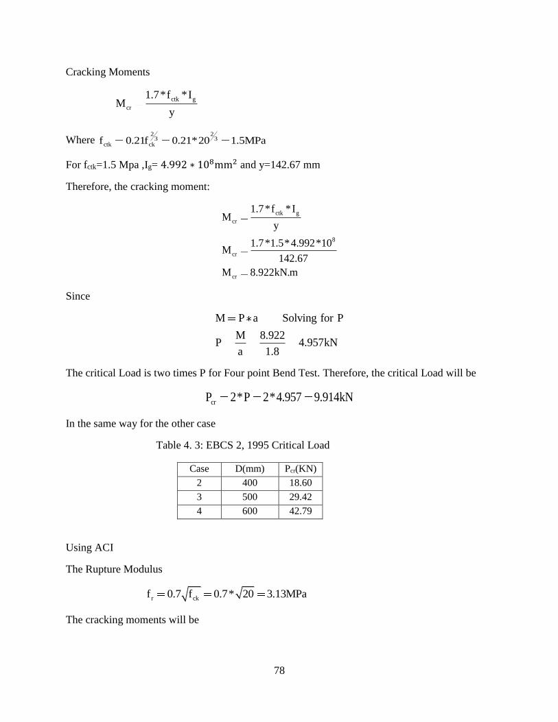
78

Cracking Moments

ctk g

cr

1.7*f *IM

y

Where 2 2

3 3ctk ckf 0.21f 0.21*20 1.5MPa

For fctk=1.5 Mpa ,Ig= 4.992 ∗ 108mm2 and y=142.67 mm

Therefore, the cracking moment:

ctk g

cr

8

cr

cr

1.7*f *IM

y

1.7*1.5*4.992*10M

142.67

M 8.922kN.m

Since

M P a Solving for P

M 8.922P 4.957kN

a 1.8

The critical Load is two times P for Four point Bend Test. Therefore, the critical Load will be

crP 2*P 2*4.957 9.914kN

In the same way for the other case

Table 4. 3: EBCS 2, 1995 Critical Load

Case D(mm) Pcr(KN)

2 400 18.60

3 500 29.42

4 600 42.79

Using ACI

The Rupture Modulus

r ckf 0.7 f 0.7* 20 3.13MPa

The cracking moments will be

79

8r g

cr

b

crcr

f *I 3.13*4.992*10M 10.88kN.m

y 142.67

2*M 2*10.88P 12.09kN.m

a 1.8

In the same way for the other case

Table 4. 4: ACI critical Load

Case D(mm) Pcr(KN)

2 400 22.10

3 500 35.00

4 600 50.90

Using EU 2

According to EU 2, the tensile strength is expressed as follows

ctm ctm

2.2

f max *fh1.6

1000

For h = 300 mm and fctm= 1.3*2.2 =2.86 MPa

The cracking moments will be

8

ctm g

cr

b

f *I 2.86*4.992*10M 10.007kN.m

y 142.67

The cracking load will be

crcr

2*M 2*10.007P 11.1kN

a 1.8

In the same way for the other case

Table 4. 5: EC 2, 2004 Critical Load

Case D(mm) Pcr(KN)

2 400 24.24

3 500 35.19

4 600 46.50

80

Using the Proposed Model

The critical Load according to the proposed model is

2

tcr

Bf bD 1P P

3L 1 For three Point Bend Test with span length of 2L.

Simplify the equation

2 2

tcr t

Bf bD 1 bD B 1P P * f

3L 3 L1 1

3 2bd bd dI

12 3 4 Multiply both sides by 2 where I is the gross moment of inertia and Yb is

the distance to most tension side from the Neutral axis.

3 2bd bd d2 I 2 2

12 3 4

Solve for

2bd

3 and use the approximations

2 2bd bD

3 3 and

b

d Dy

2 3

Finally use the approximations and rearrange, solve for Pcr

cr t

b

2 I B 1P f

y a 1

Given Values

D=300 mm I=4.992 *108 mm4 Yb=142.67 mm

According to Koeing ,[27]

ct

ff 2.12ln 1

10

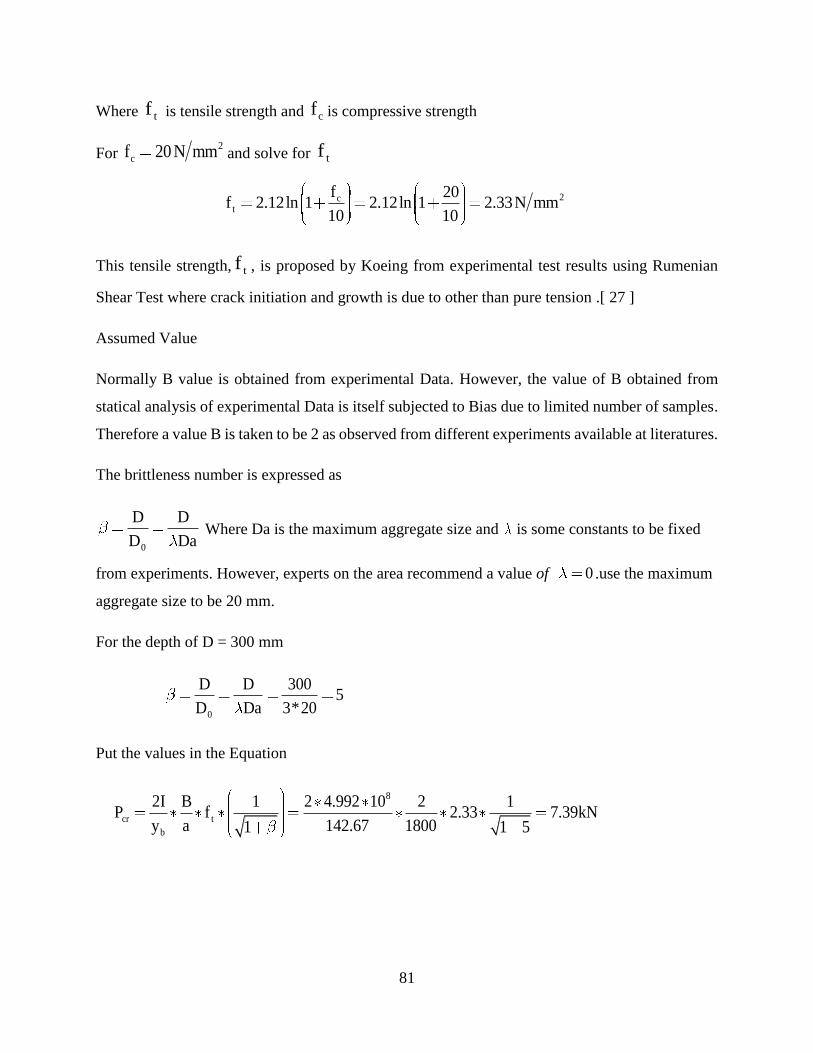
81

Where tf is tensile strength and cf is compressive strength

For 2

cf 20 N mm and solve for tf

2c

t

f 20f 2.12ln 1 2.12ln 1 2.33N mm

10 10

This tensile strength, tf , is proposed by Koeing from experimental test results using Rumenian

Shear Test where crack initiation and growth is due to other than pure tension .[ 27 ]

Assumed Value

Normally B value is obtained from experimental Data. However, the value of B obtained from

statical analysis of experimental Data is itself subjected to Bias due to limited number of samples.

Therefore a value B is taken to be 2 as observed from different experiments available at literatures.

The brittleness number is expressed as

0

D D

D Da Where Da is the maximum aggregate size and is some constants to be fixed

from experiments. However, experts on the area recommend a value of 0 .use the maximum

aggregate size to be 20 mm.

For the depth of D = 300 mm

0

D D 3005

D Da 3*20

Put the values in the Equation

8

cr t

b

2I B 1 2 4.992 10 2 1P f 2.33 7.39kN

y a 142.67 18001 1 5

82

Using the same procedure

Table 4. 6: Proposed Model Critical Load

b(mm) D(mm) Yb(mm) I(mm4) a=L(mm) B ft(Mpa) Pcr(KN)

200 300 142.67 499238130.8 1800 2 5 2.33 6.35

200 400 191.91 1072537022 1800 2 6.666 2.33 10.20

200 500 241.45 2091489727 1800 2 8.333 2.33 14.65

200 600 291.14 3610482935 1800 2 10 2.33 19.61

Flexural Section Capacity

ACI Design method

Nominal moment Strength calculation

For b=200mm D=300mm d’=40mm

d=D-d’=300-40=260 mm

From force equilibrium

T C

Where T is force carried by tension rebars while C is force carried by concrete under

compression. This shows that

'

s y ckA f 0.85f b a

Solving for a

s y

'

ck

A f 600 300a 42.4mm

0.85*f b 0.85 25 200

The nominal moment strength will be

n s y

a a 42.4M T d A f d 600 300 260 42.988kN.m

2 2 2

83

According ACI design code the strength reduction factor for flexure is about 0.9, therefore the

ultimate strength of the section will be

u nM 0.9*M 0.9*42.988kN.m 38.69kN.m

Using the same principle, for the other cases

Table 4. 7: ACI moment capacity

Case D(mm) Mu(KN.M)

2 400 54.89

3 500 71.09

4 600 87.29

Using EU 2

According to Eurocode 2, the ultimate design moment to be carried by the given cross section is

expressed as follows

2

ed cd

z zM f bd 1 *2

d d

After simplifications

ed

2

cd

M z z1 *2 K

f bd d d

From moment equilibrium

ed s ydM A f *z

This implies that eds yd

MA f 600*260 156000N

z

Using the following Equation

ed

2

cd

M d z* 1

f bd 2*z d

Solve for z, z 225.6mm

84

Therefore, the moment capacity is

ed s yd

ed

M A f *z 156000*225.6N.m

M 35.194kN.m

Similarly for the other cases

Table 4. 8: EU 2, 2004 Moment capacity

Case D(mm) Mu(KN.M)

2 400 52.55

3 500 68.11

4 600 83.11

Using EBCS 2, 1995

For concrete Grades of C-25……Case 1

Reinforcement ratio sA 6000.00115

bd 200*260

The ultimate moment will be

22

ydcded

cd

ff bdM 1 1

2 f

Put fcd=11.33 MPa ,b=200 mm d=260 mm fyd=260 MPa

The ultimate moment will be

edM 35.09kN.m

For the other cases

Table 4. 9: EBCS 2, 1995 Moment capacity

Case D(mm) Mu(kN.M)

2 400 50.79

3 500 66.39

4 600 81.99

85

Using the proposed model

The moment capacity of a given reinforced cross section is

u s ydM A f d 0.4*c

For As=600 mm2, fyd=260 MPa and d=260 mm

Calculate c, compression depth

s

s

0.3 0.09 1.2dc

2

0.3 0.09 1.2*260*0.002c

2*0.002

c 136.25mm

Calculating the Flexural section capacity

u s yd

u

u

M A f d 0.4*c

M 600*260* 260 0.4*136.25

M 32.058kN.m

For the other cases

Table 4. 10: Proposed Model moment capacity

Case D (mm) Mu (kN.m)

2 400 45.60

3 500 59.39

4 600 73.35

86

Example 2:

Given: Reinforced Concrete section with depth of 300mm and width of 200mm.

G = 75 N/M E = 30 GPa a = 50 mm fcr =2.55 Mpa 𝜙 = 16 mm As = 600 mm2

Req: Direction of the crack propagation using Proposed Model Crack propagation

Solution

For crack to propagate, the following criteria should be satisfied.

I ts

2K 1 cos cos f

22 r

For crack to Propagate, KI=KIC, solving for 𝜃c

ts3

c

IC

2f rcos 1

K

The critical stress intensity factor at the onset of crack propagation is, KIC

I C

I C

I C

K GE

K 75*30000

K 1500MPa mm

The post peak tensile strength is obtained from the linear tension softening model as shown

below.

c1 crts cr

ch cr

f f 1

Where, c1 0.0008 maximum cracking strain,

c1 0.0008 characteristic tensile strain

ch

cr

4G

Sf

For cracking stress, crf 2.55MPa , the cracking strain , 휀𝑐𝑟

87

crcr

cr

cr

f

E

2.55

30000

0.000085

According to EBCS 2, 1995, for humid environment, the characteristic crack width, wk, is

0.2mm. The average distance between the cracks, Srm, can be obtained from the equation shown

below.

rm 1 2

r

s 50 0.25k k

k1=0.8 , k2=0.5 , 𝜙 = 16 mm , 𝜌𝑟=0.030, put all values and obtain rms

rm

rm

16s 50 0.25*0.8*0.5*

0.03

s 103.33mm

The characteristic strain, ch

ch

cr

ch

ch

4G

Sf

4*75

0.103*255000

0.00114

Finally, put all values in the equation and solve for tsf

c1 crts cr

ch cr

ts

ts

f f 1

0.0008 0.000085f 2.55 1

0.00114 0.000085

f 2.55MPa

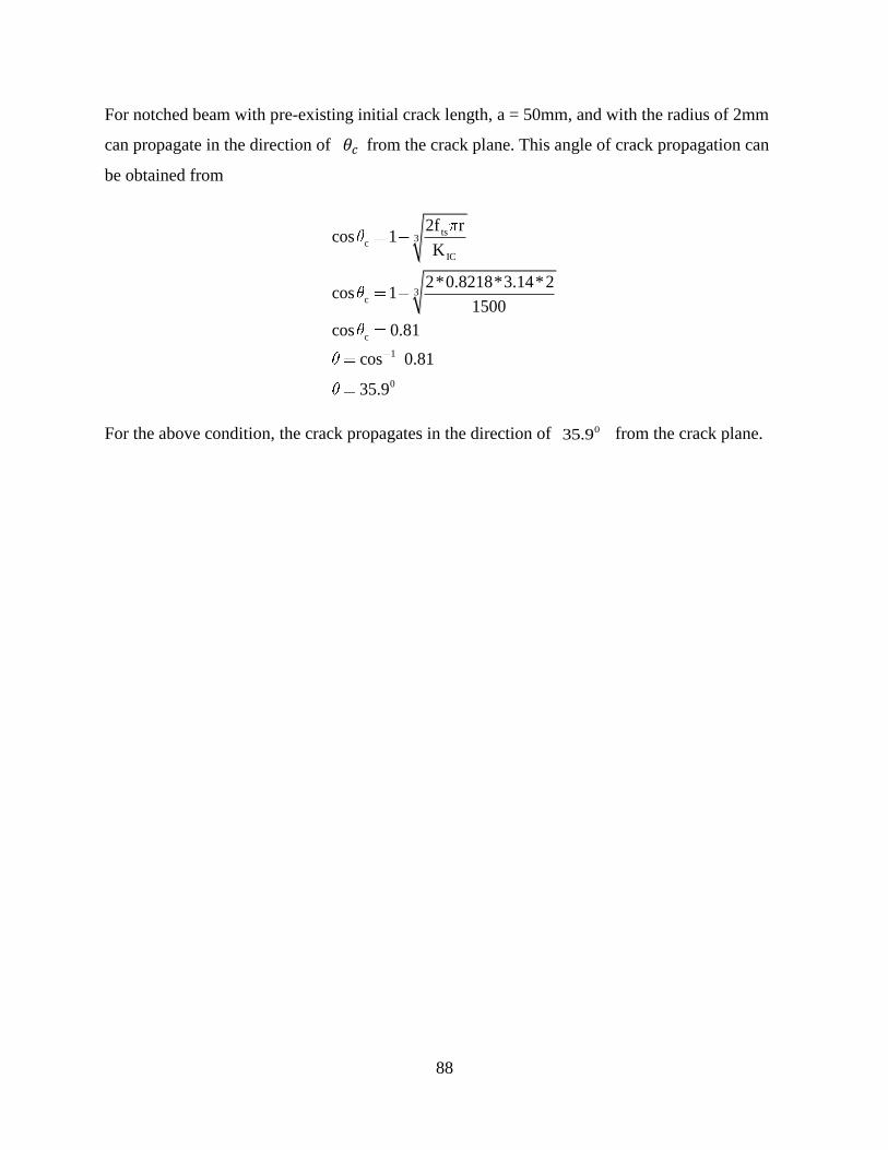
88

For notched beam with pre-existing initial crack length, a = 50mm, and with the radius of 2mm

can propagate in the direction of 𝜃𝑐 from the crack plane. This angle of crack propagation can

be obtained from

ts3

c

IC

3c

c

1

0

2f rcos 1

K

2*0.8218*3.14*2cos 1

1500

cos 0.81

cos 0.81

35.9

For the above condition, the crack propagates in the direction of 035.9 from the crack plane.

89

Crack Length a=

Width of Beam b= 100 mm

Length of Beam L= 1000 mm

Example 3:

Extraction of Stress intensity Factors and Energy release rate from notched specimens

Crack length=10mm,25mm,50mm,75mm,100mm,125mm,150mm and 175 mm

Table 4. 11: initial crack length, width and length of the specimens

b)

a)

c)

c)

d)

Fig: a) Notched specimen with known dimensions b) Meshing near in the vicinity of the crack

c) Stress distribution near the cracks d) Area of plastic zone near the crack

90

Table 4. 12: Stress intensity factors and energy release rate for plane stress and plane strain

conditions

PSS PSN

a/d

a

mm IK

MPa mm

IIK

MPa mm

J

N.mm

IK

MPa mm

IIK

MPa mm J

N.mm

J

N.mm

0.05 10 26.413 0.18577 0.023954 25.819 0.18751 0.023589

0.125 25 13.072 17.695 -6.1311E-08 13.072 17.698 2.475E-08

0.25 50 88.89 0.060035 0.27471 88.919 0.05794 0.26603

0.375 75 144.86 0.52992 0.72677 144.9 0.50838 0.7035

0.5 100 246.69 -0.27691 2.0391 246.73 -0.2768 1.9735

0.625 125 178.77 -1.2867 1.0397 179.51 -1.3145 1.015

0.75 150 209 -203.99 0.068824 208.89 -205.1 0.06805

0.875 175 636.91 -291.27 -0.23108 638.42 -294.61 -0.21803

PSS refers to plane stress condition while PSN represents plane strain conditions

91

0.00

10.00

20.00

30.00

40.00

50.00

3 0 0 4 0 0 5 0 0 6 0 0

CR

AC

KIN

G L

OA

D (

KN

)

SECION DEPTH (MM)

CRACKING LOAD VERSUS SECTION DEPTH

EBCS ACI EU PROPOSED

4.7 Comparisons and Discussions

Comparisons of Cracking Load

Table 4. 13: Cracking for different building codes under different cross section

Cracking Load in KN

Depth EBCS ACI EU PROPOSED

300 9.91 12.09 11.12 6.35

400 18.58 21.09 24.24 10.20

500 29.42 32.41 35.19 14.65

600 42.76 46.04 46.50 19.61

Figure 4. 14: Cracking loads versus size using different building codes and Proposed model

Discussions

From the table and the graph, it can be seen that the cracking load is proportional to the depth of

the beam. As the beam depth increase, the stiffness for bending also increase. The ACI code gives

relatively higher Cracking Load. One important point to be noticed here is that, almost all the

building codes neglect the size effect which can be the great source of brittle failure. In the codes,

the tensile strength is expressed independent of material size, this can cause an overestimation of

the strength which is the main reasons why many reinforced concrete structures fail before the

stress reaches to its peak value.

92

Comparisons of Section Moment Capacity

Table 4. 14: Moment capacity of a cross section under different building design codes and

Propose model

Section Moment Capacity (KN.M)

Depth(mm) EBCS ACI EU PROPOSED MODEL

300 35.189 38.9 35.194 30.64

400 50.79 54.89 52.5 43.68

500 66.39 71.09 68.11 57

600 81.99 87.29 83.71 70.54

Figure 4. 15: Section capacity varies with beam size using different building codes and Proposed

Model

Discussions

From the above data, it is clear that the moment capacity of a given beam is proportional to the

depth. As in the above case, ACI code predicts the highest section moment capacity. However, the

EBCS 2, 2013 and the EU 2, 2004 predicts almost the same moment capacity. But the problem

with the moment capacity determined by codes is that there is no any mechanisms which consider

the size effect. In the proposed model the size effect is included and the lowest section capacity is

determined.

0

20

40

60

80

100

0 100 200 300 400 500 600 700

Sect

iom

Mo

men

t C

apac

ity

(K

N.M

)

Beam Depth (mm)

Beam Depth Versus Moment Capacity

EBCS ACI EU PROPOSED

93

Discussion of crack propagations

When initially notched specimen is subjected to Mode I type loading, the stress intensity factor for

Mode I type of fracture will increase. The increment of the stress intensity Factor with the crack

length is limited to some values of crack length. When the crack length is beyond this particular

crack depth, the Mode I stress intensity factor will start to decrease and finally the specimen will

collapse.

If the given specimen is subjected to Mode II type of loading, which can cause sliding, the Mode

II stress intensity factor will not be effective quickly as the load is applied. However, as the effect

of the Mode I stress intensity factor diminished, the Mode II stress intensity factor will become

more pronounced with negative value. The negative value shows that crack occurs in the opposite

direction of the loading.

In the new proposed model, crack follows certain criteria to propagate. Once this criteria is

satisfied, Crack propagates otherwise it will not. The idea of crack propagation is not yet included

in many building codes. However, Using the Fracture Mechanics, it is possible to capture crack

propagation.

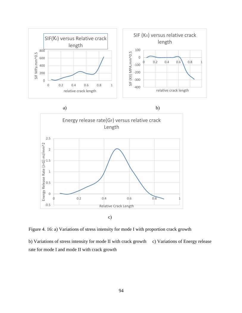
94

-400

-300

-200

-100

0

100

0 0.2 0.4 0.6 0.8 1

SIF

(KII

) M

PA

.mm

^0.5

relative crack length

SIF (KII) versus relative crack length

-0.5

0

0.5

1

1.5

2

2.5

0 0.2 0.4 0.6 0.8 1Ener

gy R

elea

se R

ate

(J=G

) m

J/m

m^

2

Relative Crack Length

Energy release rate(GF) versus relative crack Length

a) b)

c)

Figure 4. 16: a) Variations of stress intensity for mode I with proportion crack growth

b) Variations of stress intensity for mode II with crack growth c) Variations of Energy release

rate for mode I and mode II with crack growth

0

200

400

600

800

0 0.2 0.4 0.6 0.8 1

SIF

MP

a.m

m^0

.5

relative crack length

SIF(KI) versus Relative crack

length

95

5 Conclusion and Recommendations

5.1 Conclusions

Due to different reasons, the empirical formulas provided by Building codes do not include an

important phenomena called Size Effect. This days there are huge number of construction using

concrete structures in which some of them are already built and some are under constructions. As

long as the need for this huge number of construction using concrete structures increases, the

design principle should consider the size effect in order to have safe structure. Ignoring of size

effect in this huge construction using concrete can definitely cause brittle failure which can occur

at any time without any prior sign.

Real life experiences shows that as the size of the material increase, the amount of flaws and

internal micro cracks also increase. What happen in the region around these flaws and micro cracks

is, there will be high stress concentration, where this stress concentration around the flaws cause

the development of the micro cracks in to Macro cracks. In EBCS 2, EC2 AND ACI all the

empirical formulas given are independent of size which contradicts with the reality. Therefore, the

effect of size on material response should be included properly to have better prediction of the

response due subjected loads.

In this study, it has been also shown that Tensile Strength of reinforced concrete structure is

property of member length and section. In addition the stress-strain diagram under the

compressions loading is dependent on member length and section depth.

In this Thesis, there are two proposed model for Crack Propagation and Section Capacity

calculation. What makes this two model differ from what has been found in the building design

codes is that, the Size Effect is included in the both proposed model.

Finally, whenever the codes provisions are used, it is reasonable to assume that the codes

provisions overestimate the strength, and this is mainly due to ignoring of the size effect.

96

5.2 Recommendations

In this thesis, it has been shown that there are some material properties, particularly tensile and

compressive strength of concrete, which are assumed to be size independent. However,

experiences shows that these properties are rather size dependent and some modification is

mandatory when bigger section of these material is used. As long as the idea of fail-safe design is

critical issues, it is better to consider the size effect on the response of a material. And from results

the following recommendations are put forwarded by the Author

Codes prescription for crack propagations and section capacity is independent of size, this

will result brittle failure mode. Therefore, it is better to consider size whenever strength is

critical

Effect of size on strength and ductility of quasi brittle materials needs further study

Structure size and geometry should be included in factor of safety to be used for reliability

assessment for the design of reinforced concrete structures

Size independent Fracture Energy should be used for Analysis and Design purpose.

Pre-peak Fracture Energy contributions for new surface formations should be studied

For unreinforced concrete structures which are subjected to tensile cracking, plasticity

based model should be used with modification and if possible, Fracture Mechanics based

model is better.

97

References

[1] A.Hillerborg, M.Modeer, P.-E.Petersson: Analysis of Crack Formation and Crack

Growth in Concrete by means of Fracture Mechanics and Finite Elements, Cement and

Concrete Research, Vol. 6, 1976, pp 773-782.

[2] ACI Committee 446 on Fracture Mechanics (1992) (Bazant, Z.P. prine. author & chairman).

[3] A.R. Ingraffea. “Theory of Crack initiation and propagation in rock. In: Fracture Mechanics

of Roc”. Atkinson B.K. (Ed.), Academic Press, London, pp. 71-110,1987.

[4] American Concrete Institute Committee 318, “Building Code Requirements for Structural

Concrete”, ACI 318-08, American Concrete Institute, Detroit, MI, 2008.

[5] Anderson, D.T., Fracture Mechanics: Fundamentals and Applications. CRC

Press, Boca Raton (1991)

[6] Barenblatt, G.I. The mathematical theory of equilibrium cracks in brittle fracture. Advances

in Applied Mechanics, Vol 7, 1962, pp 55-129.

[7] Barsoum, R.S. On the use of isoparametric Finite Elements in Linear Fracture Mechanics.

Int. J. Numerical Methods in Engineering, Vol 10, 1976.

[8] Bazant ZP. Concrete Fracture Model: Testing And Practice Engineering Fracture Mechanics

69(2002)165 -205

[9] Bazant, Z.P. and Oh. B.H. (1983) Crack band theory for fracture of concrete. RILEM,

Materials and Structures, Vol 16, No 93, 155-177.

[10] Bazant, Z.P. and Pfeiffer, P.A. (1987), “Size Effect Method for Determining Fracture

Energy of Concrete from Maximum Loads of Specimens of Various Sizes”, Proposal for

RILEM Recommendations.

[11] Bazant, Z.P. (198.4), “Size Effect in Blunt Fracture: Concrete, Rock, Metals”, J. Eng.

Mech., ASCE, 110, pp. 518–538.

[12] Bazant, Z.P., 2002. “Concrete fracture models: testing and practice”. Engineering Fracture

Mechanics. Vol. 69, pp. 165-205

98

[13] Carpinteri, A. (1984) Stability of fracturing process in RC beams. Journal of Structural

Engineering (ASCE), 110,

[14] CEB-FIP Model Code 2010, Chapter 5, Code-type models for concrete

behavior (Draft); 2010.

[15] Dr.ir. P.J.G. Schreurs. ”Fracture Mechanics’’ Eindhoven University of Technology,

Department of Engineering, Materials Technology, September 13, 2011

[16] E. F. Rybicki and M. F. Kanninen. “Finite-element calculation of stress intensity factors by

a modified crack closure integral”. Engineering Fracture Mechanics, 9(4), pp. 931-938, 1977.

[17] Eurocode 2 - Design of Concrete Structures - Part 1 (Eurocode EC 2) - prEN 1992-1-1

November 2002 [ENG].

[18] EBCS 2,1995 - Design of Concrete Structures – Structural Use of Concrete-Addis

Ababa,Ethiopia, 1995.

[19] G.R. Irwin. “Plastic zone near a crack and fracture toughness”. Proc. 7th Sagamore

Conference, IV-63, New york, August 16-19, 1960.

[20] H. Tada, P.C. Paris and G.R. Irwin. “The Stress Analysis of Cracks Handbook”. Del

Research Corporation, Hellertown, Pennsylvania, 1973.

[21] H.A.W.Cornelissen, D.A.Hordijk, H.W.Reinhardt: Experiments and Theory for the

Application of Fracture Mechanics to Normal and Lightweight Concrete, Contributions

International Conference on Fracture Mechanics of Concrete, Lausane, 1-3 October, 1985.

[22] Hillerborg, A. (1985), “The Theoretical Basis of a Method to Determine the Fracture

Energy GF of Concrete” Materials and Structures,

[23]Hillerborg, A. (1988). Application of fracture mechanics to concrete: summary of a series of

lectures 1988. (Report TVBM; Vol. 3030). Division of Building Materials, LTH, Lund

University.

[24] Jenq, Y.S. and Shah, S.P. (1985), “A Two Parameter Fracture Model for Concrete”, J.

Eng. Mech. ASCE

99

[25] Karihaloo BL. Fracture Mechanics and Structural Concrete. Longman Pub Group. 1995

[26 ] Koing,G.,Grimn,R. and Remmel ,G,” shear behavior of longitudnaly reinforced concrete

members of HSC”, JCI international workshop on size effect in concrete structures,pp.63-74,1993

[27] P.A. Lagace. “Plane Stress and Plane Strain”. Lecture note Aeronautics & Astronautics

and Engineering Systems, MIT, 2001.

[28] Planas, J. and Elices, M. (1990), “A Nonlinear Analysis of a Cohesive Crack”, to be

published in J. Mech. and Phys. Of Solids.

[29] Wittman FH. Crack formation and fracture energy of normal and high strength

concrete. Sadhana 2002;27(4): 413–423.

[30] Wong,Trommels And F.J Vecchio,“ Vector2 & Formworks User’s Manual”,August 2013.

100

Appendix

Appendix A: Matlab code for plane strain and plane stress plastic zone

t = 0:.01:2*pi;nu=0.15%%%%% rp1=1+cos(t)+1.5*sin(t).*sin(t); %%%%%PLANE STRESS PLASTIC ZONE%%%%% rp2=(1-2*nu)^2.*(1+cos(t))+1.5*sin(t).*sin(t);%%PLANE STRAIN PLASTIC ZONE%%%%% polar(t,rp1); hold on polar(t,rp2);

The internal curved Area shows the plastic plane strain zone while the outside curved zone

shows zone of plastic plane stress

101

Appendix B: static structural simulations for two point bending

Code for concrete material

ET,MATID,SOLID65 ! Matarial definition for concrete

R,MATID,0,0,0,0,0,0

RMORE,0,0,0,0,0

MP,EX,MATID,30000 !young Modulus for concrete

MP,PRXY,MATID,0.15 ! poisson ratio for concrete

MPTEMP,MATID,22 !

TB,CONCR,MATID,1,10

TBTEMP,22

TBDATA,,0.3,0.5,2,20,0,0

TBDATA,,0,0,0.3,,,

TB,MISO,MATID,1,10,0

TBTEMP,22

TBPT,,0.0001,3

TBPT,,0.0002,6

TBPT,,0.0003,9

TBPT,,0.0004,12

TBPT,,0.0015,16

TBPT,,0.0022,28

TBPT,,0.0035,20

TBPT,,0.0038,17

TBPT,,0.0042,10

TBPT,,0.0045,0

Code for Reinforcement material

ET,MATID,LINK180 ! Matarial definition for rebars

MPDATA,EX,MATID,,2e5 ! young Modulus for rebars

MPDATA,PRXY,MATID,,0.3 !

TB,BISO,MATID,1,2

TBDATA,,280,0 !yield strength of rebars

R,MATID,8,,0!radius of rebars

Code for bonding between concrete and rebar (Reinforcement) elements

/PREP7

ESEL,S,ENAME,,65 !this ansys function connects all the rebars elements with the concrete

ESEL,A,ENAME,,180! Elements

ALLSEL,BELOW,ELEM !

CEINTF,0.001, !

ALLSEL,ALL !

/SOLU

OUTRES,ALL,ALL

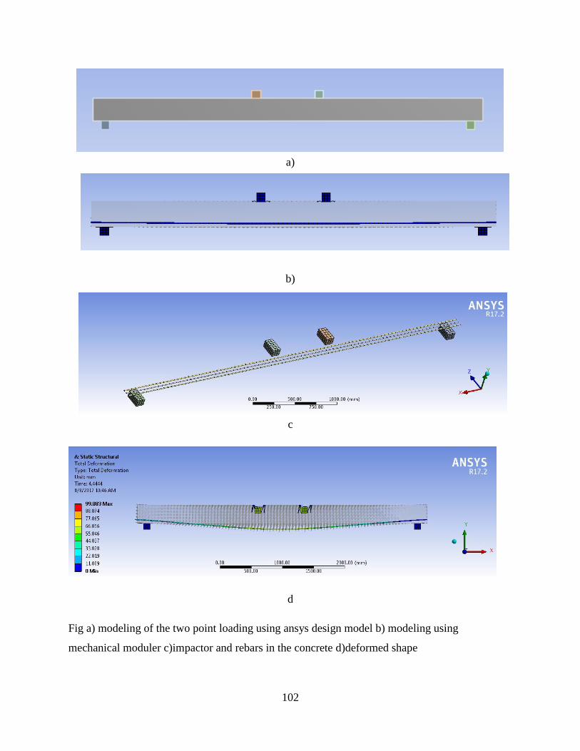
102

a)

b)

c

d

Fig a) modeling of the two point loading using ansys design model b) modeling using

mechanical moduler c)impactor and rebars in the concrete d)deformed shape

103

Appendix C: Explicit Dynamics simulations for Four point bending

Reinforced Concrete beam with the same dimension with the static structural beam.

A)

B)

C)

104

D)

E)

Fig R1 A) modeling for Explicit Dynamics B) Deformed shape of the beams with maximum

deflections C), D) and E) shows failure steps

105

DECLARATION

I hereby declare that the work presented in this thesis is my original work and has not been

presented for a degree in any other University and that all sources of material used for the thesis

have been duly acknowledged.

_____________________ _____________________

Andargchew Mekonen Date

(Candidate)

This is to certify that the above declaration made by the candidate is correct to the best of my

Knowledge.

_____________________ _____________________

Dr.Asnake Adamu Date

(Thesis Advisor)