Damage-based fracture with electro-magnetic coupling

P. Areiaso?∗, H.G. Silvao, N. Van Goethem+,M. Bezzeghoudo

24th April 2012

oDepartamento de Fısica

Universidade de Evora

Colegio Luıs Antonio Verney

Rua Romao Ramalho, 59

7002-554 Evora, Portugal

+CMAF, Universidade de Lisboa, Faculdade de Ciencias,

Departamento de Matematica

Centro de Matematica e Aplicacacoes Fundamentais

Av. Prof. Gama Pinto 2, 1649-003 Lisboa, Portugal?ICIST

Abstract

A coupled elastic and electro-magnetic analysis is proposed including finite displacementsand damage-based fracture. Piezo-electric terms are considered and resulting partial differentialequations include a non-classical wave equation due to the specific constitutive law. The resultingwave equation is constrained and, in contrast with the traditional solutions of the decoupledclassical electro-magnetic wave equations, the constraint is directly included in the analysis. Theabsence of free current density allows the explicitation of the magnetic field rate as a functionof the electric field and therefore, under specific circumstances, removal of the correspondingmagnetic degrees-of-freedom. A Lagrange multiplier field is introduced to exactly enforce thedivergence constraint, forming a three-field variational formulation (required to include the waveconstraint). No vector-potential is required or mentioned, eliminating the need for gauges. Theclassical boundary conditions of electromagnetism are specialized and a boundary conditioninvolving the electric field is obtained. A specific boundary finite element is introduced to dealwith this boundary condition. The spatial discretization makes use of mixed bubble-based(MINI-like) finite elements with displacement, electric field and Lagrange multiplier degrees-of-freedom. Three verification examples are presented with very good qualitative conclusions andmesh-independence.

KEYWORDS: Electro-magnetism, Maxwell’s equations, elasticity, piezo-electricity, mixed finiteelement methods

∗Corresponding Author. ISI search: areias p*; email: pmaa@uevora.pt, pareias@civil.ist.utl.pt, Ph.: +351 963496307, URL: http://evunix.uevora.pt/˜pmaa/

1

1 Introduction

Fundamental theoretical contributions for the analysis of continuum elastic dielectrics were made byLax and Nelson [21] and Maugin [26]. The latter text contains contributions with a detail beyondwhat is intended with this work. The purpose of it is to inaugurate a specific approach to electro-magnetic and elasticity coupling implemented with mixed finite elements to deal with fracture (withfinite strains). Piezo-electricity is also included, but mainly as a constitutive ingredient. Recentdiscussions on this topic, also with a continuum approach, are the works of Ericksen (cf. [13, 14])and Dorfmann and Ogden [12] albeit limited to strict dielectrics (without the magnetic field).Numerical calculations are sparse and mainly limited to magnetostatics (see, for example [7]) andpiezo-electricity. M. Kuna [20] performed a theoretical and experimental review of piezo-electricitywith classical fracture mechanics. In [19], the same author used a electromechanical contour integralto calculate energy release rates.

We perform finite displacements and rotations but small strains (in the sense of K.J. Bathe[6] p. 595 paragraph 6.6.3) in order to account for the rotation of the crack faces. The extensionto finite strains demands an in-depth study of the piezo-electric term in the total stress, beyondof the scope of this paper. Simulations of electro-magnetic fields including piezo-electricity areperformed. The total stress contains the Cauchy stress, the Maxwell stress, the piezo-electric stressand the polarization stress. The piezo-electric effect is characterized as a coupling between theelectric polarization of a given material and the (mechanical) stress field. It is crucial in sensors,actuators, smart materials among others. There is a significant variety of piezo-electric materials:crystals, e.g. quartz; ceramics, e.g. lead zirconate titanate (PZT); polymers, e.g. polyvinylidenefluoride (PVDF).

Taking into account that materials are subjected to frequent mechanical actions it is of funda-mental importance the study of fracture, in order to estimate their reliability to device applications.For that reason, many works have been focused on this topic, for a recent review the reader isreferred to [20]. Interestingly, the majority of them only consider the electrostatic limit where thecoupling of the electric and magnetic fields (present in Maxwell’s equations) can be neglected andthe analysis can be restricted to the electric field. Obviously, this constitutes an overall simplificationto the problem since in this case the electric field (vector), e, can be calculated from the electricpotential , φ, reducing a n-dimensional problem (2 or 3, typically) to a one-dimensional problem.

The basic equations considered in this paper are classical (Maxwell, piezoelectric polarization,etc) but their coupling with fracture propagation has not been studied much so far. So, thecontributions of this paper are the following:

• Numerical simulation of fracture incorporating magnetic and electric fields taking into accountpiezoelectric effects.

• A stable mixed formulation with Lagrange multipliers for imposing the null divergence of theelectric displacement.

• Non-standard formulation resulting in a uncoupled wave equation.

The remaining of this paper is composed of four sections. Section 2 contains the basic premisesof our work, as well as original derivations for the weak form and boundary conditions. Section 5

2

εmax

G

fc

Γt

Γuqs

e

(external charges)

Ω

Evolving crack

eext

n

Damage zone

µǫλ

Figure 1: Relevant ingredients for the coupled equilibrium/electromagnetic problem (currentconfiguration). The electric field equation holds in the interior and in the exterior of Ω withmatching of the external and internal values on every portion of the boundary where qs = 0.

briefly summarizes the discretization proposal and the mixed finite element. Section 6 presentsthree numerical applications where the new technique is successfully tested and in section 7 someconclusions are drawn.

2 Governing equations

2.1 Maxwell and equilibrium equations

We consider a linear elastic material with a damage evolution law, equilibrium with moderate strainsand finite displacements (ensuring the validity of Hooke’s law) and the classical electrodynamics ofcontinua (cf. [21, 26]).

The considered governing equations consist of:

• Cauchy equations of motion using the electromagnetic force as the only volume force.

• Mass conservation.

• Maxwell’s equations in S.I. units for dielectrics, in the absence of free charges and currents.

• Linear constitutive equations of electromagnetism, stress-strain relations and piezo-electricity.

Figure 1 shows the idealization of the typical problem to be solved and the three types of bound-ary conditions (essential for the displacement unknown and electric field and natural boundaryconditions).

3

The mass conservation principle for an impermeable continuum (open set Ω) is concisely givenby:

∂(Jρ)∂t

= 0 in Ω (1)

where ρ is the spatial mass density and J = detF where F is the deformation gradient (cf. [29]).The Cauchy equation of motion and Cauchy Lemma read:

∇ · σT + f = ρu in Ω (2)

σn = t in Γt (3)

where σ is the Cauchy stress tensor, u is the displacement vector and t ∈ [0, T ] is the time variable(not to be mistaken with t, the prescribed stress vector) and the term f is the body force field. Notethat, according to our notation, σij is the Cauchy stress component at facet j with the direction i.This is of course standard (e.g. [29, 25]) and shown here for completeness. A useful notion in elasticdielectricity is the one of total stress, here denoted as σ? which allows the rewriting of (2) as:

∇ · σ?T = ρu (4)

We consider ρu = 0 in remaining of this work. Maxwell’s equations in classical form1 in a domainΩ (cf. [15, 17, 14, 27]) are concisely written as:

∇× e+ b = 0 in Ω (5)

∇ · b = 0 in Ω (6)

∇× h− d = Jf in Ω (7)

∇ · d = qf in Ω (8)

where e is the electric field, b is the vector of magnetic induction, h is the magnetic field and d isthe electric displacement current (see, e.g. [26, 15]). The terms in the right-hand sides of (7) and(8) are the free external current (qf ) and charge (Jf ), respectively, and are related by the continuityequation: qf +∇ · Jf = 0. It is noticeable that the validity of (5-8) for a continuum described inthe spatial configuration is shown by Lax and Nelson [21]. Here, the following notation is adopted(see also [21]):

1S.I. units are adopted and lower-case is used for spatial quantities.

4

• = ∂•∂t

(9)

The inclusion of piezo-electricity in the system (5-8) can made by means of the polarizationvector or directly by introduction in a constitutive law for d. The latter is used here. As a matterof fact, for piezo-electric materials under consideration, we introduce a linear relation between theelectric displacement, the electric field and the Almansi strain ε:

d = εe+ A : ε (10)

where ε is the electric permitivity2 and A is a general third-order tensor. The Almansi strain isdefined in terms of the deformation gradient F by:

ε = 12(I − F−TF−1

)(11)

The choice of this strain is justified by the fact that, in contrast with the small strain measure (thesymmetric gradient of the displacement), allows large rotations of the crack faces without spuriousstress.

We specialize the general relation (10) by introducing the third-order piezo-electric tensor J :

A = −εI (12)

The tensor I is minor-symmetric in the two last indices, i.e. [I ]ijk = [I ]ikj . Relating thecontinuum and vacuum permitivity ε = (1 + χ)ε0 with χ being the electric susceptibility we obtainthe polarization as a constitutive relation:

p = ε0χe− εI : ε︸ ︷︷ ︸q

(13)

where ε0χe is the average electric dipole moment density and εI : ε is the piezo-electric polarizationterm. For notation simplicity, the electric displacement (10) is rewritten as:

d = ε (e− q) (14)

Our formulation is a particular case of M. Kuna approach [19] where we restrict to one dielectricconstant. In homogeneous linear isotropic continua, for which Lorentz relations hold, we can write(7) and (8) as:

∇× b = µJf + µε (e−I : ε) in Ω (15)

ε∇ · (e−I : ε) = qf in Ω (16)

where µ is the magnetic permeability. Both ε and µ can be related to the corresponding vacuumconstants. A direct manipulation results in the following second-order system:

2For our prototype model we assume a scalar permitivity.

5

∇× (∇× e) + µJf + µε (e− q) = 0 (17)

∇ · (e− q) = qfε

(18)

It is clear that ∇ · b = 0 is trivially satisfied in [0, T ] provided (∇ · b) (0) = 0 is satisfied. Moreover,the reader can verify that, contrary to traditional derivations in electromagnetic wave propagation,no Laplacian of e emerges in (17) since the classical condition ∇ · e = 0 does not hold, due to thepiezo-electric term in (18). An additional note is required: in the notation of Bustamante and Ogden[11], the polarization is determined differently. After direct specialization of the general boundaryconditions (cf. [21]), a final set of boundary conditions for piezo-electricity and electromagneticcoupling is obtained (see also [11, 9] for a comprehensive description):

[[ 1µb]]× n = Js in Γ (19)

[[e]]× n = 0 in Γ (20)

[[ε (e− q)]] · n = qs in Γ (21)

[[b]] · n = 0 in Γ (22)

We use the notation [[•]] for the “jump” of •: the difference between the external and internalvalues of • (see Figure 1). It can be proven that the condition [[b]] · n = 0 is trivially satisfied.Contrary to the charge surface density, qs, the surface current density Js is not directly imposed inthis framework (see also the recent paper by Linder et al. [24]). Since the magnetization vector ishere considered null, we can use the conclusions in reference [10] to write the enforced boundaryconditions:

[[b]] = 0 in Γ (23)

e = −qsεn in Γ (24)

For two-dimensional problems (23-24) results from (19-22) in the absence of surface current density.Note that the complete e is specified at Γ, in contrast with what occurs in piezo-electric reports.Typically (see [24]) the unknown field is d and not e since the magnetic field is seldom included innumerical simulations. For dielectrics (considered in this work) it follows that Jf = 0 and qf = 0(see, for example, the book of Maugin [26] page 157).

3 Coupled constitutive law

3.1 Total stress

We make use of the compressible Neo-Hookean hyperelastic model (cf. eq. (6.29) of [8]) as afunction of the deformation gradient F . The constitutive law for the total stress is given as3:

3In contrast with Chapter 4 of [26], we do not include electro-magnetic terms in the body forces.

6

σ? = (1− f)[G

J

(FF T − I

)+ λ

Jln JI

]︸ ︷︷ ︸

σe

+ 1µb⊗ b+ εe⊗ e− 1

2

(ε‖e‖2 + 1

µ‖b‖2

)I︸ ︷︷ ︸

σM

+ εe ·I︸ ︷︷ ︸σP E

(25)where σe is the elastic stress, σM is the Maxwell stress and σPE is the piezo-electric stress. Notethat the electric field already accounts for the piezo-electric effect in the global PDE in (17) andhence the reciprocal piezo-electric law is enforced at the global level. It is noticeable that thepolarization stress (see [26]) is not present in (25) for thermodynamically consistent Cauchy stresses(see [33] for this term and also [11] for a similar expression). Note that the transfer of bodyforces to the total stress has been an implicit practice in the literature (cf. Vu, Steinmann andPossart [33] equations (12) and (13)). In (25), the elastic stress contains the term (1− f) wheref is the void fraction, a constitutive variable accounting for material softening4. Note that thisapproach is standard (cf. [23], Chapter 7). We use a phenomenological model (see also [22]) whichis sufficient for this work’s purpose - the so-called damage variable in Lemaitre’s work is heredenoted void fraction. Also included in (25) is the third order piezo-electric tensor I . We mustremark that this damage model is unsuited for elastomer damage representation in the sense ofMullins [28]. In contrast with the works of Bustamante and Ogden in electroelasticity (see [11])and magnetoelasticity (see [9]), two differences are worth mentioning:

• The aforementioned Authors consider incompressible materials.

• We use only the dependence on b in the constitutive law for σe and therefore comparativelysmall strains are accounted.

3.2 Damage representation

Damage modeling includes a loading function and the loading/unloading conditions. The corre-sponding void fraction loading function is:

ϕ(ε) =[εmaxε1

(1 + α

ε1εmax

− α)]

exp[α

(1− ε1

εmax

)− 1

]− (1− f), (26)

where ε1 is the maximum principal strain and εmax is the maximum principal strain attainableduring the loading history at a given point before softening. Definition (26) precludes f of attaining1 for finite ε1 since ϕ(ε) ≤ 0. The parameter α in (26) is given as:

α =

1 ε1 ≤ εmaxllc

ε1 > εmax, (27)

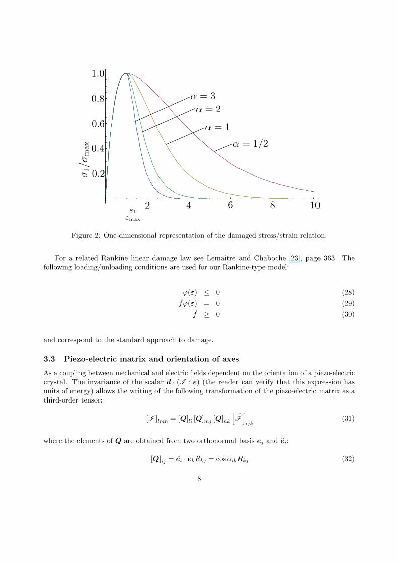
where the parameter l is the mesh size length and the lc is a characteristic length scale (cf. J.Oliver [30]). Figure 2 shows a representation of this prototype model. It is simple to prove that thesoftening energy is of course dependent on the length scale using α as calculated in (27).

4Material softening in the sense of Lemaitre [22], valid for small strains

7

2 4 6 8 10

0.2

0.4

0.6

0.8

1.0

ε1εmax

σ1/σ

max

α = 3

α = 2

α = 1

α = 1/2

Figure 2: One-dimensional representation of the damaged stress/strain relation.

For a related Rankine linear damage law see Lemaitre and Chaboche [23], page 363. Thefollowing loading/unloading conditions are used for our Rankine-type model:

ϕ(ε) ≤ 0 (28)

fϕ(ε) = 0 (29)

f ≥ 0 (30)

and correspond to the standard approach to damage.

3.3 Piezo-electric matrix and orientation of axes

As a coupling between mechanical and electric fields dependent on the orientation of a piezo-electriccrystal. The invariance of the scalar d · (I : ε) (the reader can verify that this expression hasunits of energy) allows the writing of the following transformation of the piezo-electric matrix as athird-order tensor:

[I ]lmn = [Q]li [Q]mj [Q]nk[I]ijk

(31)

where the elements of Q are obtained from two orthonormal basis ej and ei:

[Q]ij = ei · ekRkj = cosαikRkj (32)

8

where αij are the internal angles between the basis vectors and R is the rotation matrix, obtainedfrom the polar decomposition. It is obvious that minor-symmetry in the last two indices of [I ]allows some computational savings in (31). It is here assumed that the tabulated piezo-electric

properties correspond to the tensor components[I]

and αij are problem-dependent.

3.4 Frame invariance

Equation (25) is frame-invariant in the sense that [32] pp. 41-43:

x′ = c(t) +Q(t)x⇒ σ?

′ = Q(t)σ?Q(t)T (33)

where c(t) is a point and Q(t) is a unimodular orthogonal tensor. In equation (25), the first term(σe) is trivially frame-invariant since J

′ = J , f ′ = f , I = QQT and F ′F ′T = QFF TQT (witht omitted). The tensor products b ⊗ b = bbT and e ⊗ eT = eeT are also frame-invariant5. Thenorms of e and b are frame-invariant from orthogonality of Q. Finally, the only term that mayraise doubt is σPE which, from the definitions (32) and (31) can be proved to be frame-invariant.

4 Governing equations in reduced wave form

After the introduction of the previous derivations and considering a two-dimensional problem, thefinal equations to integrate are therefore dependent on σ? and independent of b:

c2 [∇× (∇× e)] + (e− q) = 0 in Ω (34)

∇ · σ?T = 0 in Ω (35)

∇ · (e− q) = 0 in Ω (36)

[[∇× e]] = 0 in Γ (37)

e = −qsεn in Γ (38)

σn = t in Γt (39)

5In the sense that material fields are obtained as E = F Te and B = F T b

9

u = u in Γu (40)

with c2 = 1/(µε) being the square of the light velocity in the continuum. Note that no explicitbody forces appear since the electro-magnetic field effect on the forces is completely includedin σ? (in equation (25)) and the Cauchy lemma retains its original form (in equation 39). Theweak form of the above equations is obtained by using a Lagrange multiplier field, λ ≡ λ(x) andperforming the customary projections and use of Green’s theorem. We introduce the spaces forthe test functions Vu = δui ∈ H1(Ω)|δu = 0 in Γu, Vd = δdi ∈ H1(Ω)|δd = 0 in Γ andP = δλ ∈ L2(Ω)|δλ = 0 in Γ and the sets for the trial functions Du = ui ∈ H1(Ω)|ui =ui in Γu, Dd = ei ∈ H1(Ω)|e = ei in Γ and P (the Lagrange multiplier space for testfunctions and set for trial functions coincide). The problem statement in weak form reads: findu ∈ Du, e ∈ De, and λ ∈ P such that the following holds (see [16] for this nomenclature andsymbols):

ˆΩc2(∇× e) · (∇× δd)dΩ +

ˆΓc2 [(∇× e)× δd] · n︸ ︷︷ ︸

−[(∇×e)×n]·δd=0

dΓ +ˆ

Ω(e− q) · δddΩ

+ˆ

Ωσ : ∇sδu dΩ−

ˆΓt

t · δudΓt

+ˆ

Ωλδ [∇ · (e− q)] dΩ

+ˆ

Ωδλ [∇ · (e− q)] dΩ = 0 (41)

∀δd ∈ Vd, ∀δu ∈ Vu, ∀δλ ∈ P. The test functions δd, δu and δλ in (41) can be seen asvariations of d, u and λ, respectively. We make use of the Acegen add-on [18] to the Mathematicasoftware [31] to accomplish the derivation of the discretized equilibrium equations and correspondinglinearization. The explicit expressions are omitted in this report. It is also noticeable that, in (41),

the symmetric spatial gradient of δu is adopted: ∇sδu =[∇δu+ (∇δu)T

]/2. Initial conditions

for (41) are given for both u and e (taken as homogeneous in this work). A remark concerning theconditioning of (41) is in order: for a Lead Zirconate Titanate (PZT) material, with µ = 1.256×10−6

Cm−2,ε = 6 × 10−9 Fm−1, E = 69.59 × 109 Nm−2, ν = 0.357 and ρ = 7500 Kg m−3, the ratiobetween the electromagnetic wave speed and the bulk wave speed

√κ/ρ , which corresponds to the

ratio between electrical and mechanical quantities in (41) is approximately 3500. Therefore, theproblem is well conditioned.

5 Discretization and time integration

We use a variant of the MINI element by D. Arnold (cf. [5]) which was previously used for theStokes equations to deal with the mixed problem (unknowns u− e− λ). We also used it before for

10

N4(ξ) = ξ1ξ2(1− ξ1 − ξ2)

uy1ex1ey1λ1

ux2uy2ex2ey2λ2

ex4

N1(ξ) = ξ1

ux1

ux3uy3ex3ey3λ3

N2(ξ) = ξ2N3(ξ) = 1− ξ1 − ξ2

ey4

Figure 3: Use of MINI element ([5]) for the mixed u− e− λ problem.

finite strain plasticity. Figure 3 shows the element degrees-of-freedom and the corresponding shapefunctions.

Time integration follows the backward-Euler method for first-order time integration appliedboth to degrees-of-freedom and their time-derivatives. If two consecutive time-steps are considered(n and n+ 1), the following expression results for an+1:

an+1 = an+1 − an∆t2 − an∆t (42)

where a contains degrees-of-freedom of all types (u, e and λ). The velocity is approximated asan+1 = (an+1 − an)/∆t. With the aforementioned assumptions, the magnetic field at step n+ 1can therefore be obtained as:

bn+1 = bn −∆t∇× en+1 (43)

The magnetic field (43) is of course necessary for the boundary conditions and constitutive lawand must be stored as an history variable. The relevant interpolated fields (with h as the mesh

11

characteristic length) in each element are obtained simply as:

uh =3∑

K=1NK(ξ)uK (44)

eh =4∑

K=1NK(ξ)eK (45)

λh =3∑

K=1NK(ξ)λK (46)

where NK(ξ) are the shape functions represented in Figure 3. After time integration, these are theonly degrees-of-freedom required to solve the coupled problem since b is written as a function of e.We keep track of the previous step (an and an) which is sufficient to calculate an at the elementlevel. The actual finite element implementation is too complex to be correctly and efficientlyhand-coded and we resort to the Acegen software by J. Korelc ([18]) to accomplish this undertaking.The tip remeshing algorithm [2] is used, with the electric field boundary conditions at the crackfaces reproducing the remaining boundary.

6 Numerical examples

6.1 Electric field pulling test

Surface electric charges (qs in the above equations) cause electro-magnetic waves and, of course,stress waves (this is due to both the Maxwell stress term and the piezo-electric effect). Notethat stress waves caused by the piezo-electric effect occur despite the absence of inertia (ρu = 0).With the purpose of obtaining a wave, we apply a time-constant electric charge at the surface ofa straight bar and analyze the produced effect (in terms. Figure 4 shows the relevant quantitiesfor this problem. A Lead Zirconate Titanate (PZT) material is considered, with properties shownin the same figure. Artificially large displacements are considered, with the goal of testing therobustness of implementation. Two meshes are tested: one containing 14298 elements and 7325nodes and another with 25374 elements and 12922 nodes. The displacement at point (A) is shownin Figure 5 for the two meshes. A slight difference is noticeable, a fact that does not occur indisplacement-controlled problems. The contour plots of interested are shown in Figure 6 for thefiner mesh.

6.2 Corner crack evolution

The following problem is considered: a reentrant corner with a pre-existing 5 mm diagonal crack hastwo edges clamped and is subject to a constant velocity applied in a corner point. Figure 7 showsthe relevant data of this problem. Again, a PZT material is considered with typical properties(except εm and Dc which are introduced here for verification purposes, a fact not affecting theconclusions). Three uniform-sized meshes are used to assert the sufficient independence of theresults: 5268, 11824 and 26620 mixed triangular elements. The same time step of ∆t = 2.5× 10−10

12

E = 69.59× 109 N/m2

ν = 0.357

ǫ = 6× 10−9 Fm−1µ = 1.256× 10−6 Hm−1

I111 = 15.08 Cm−2

ρ = 7500 Kg/m3

qs = 3 Cm−2

α11 = 0

A

e = 0

u

qs

uy = 0

10 mm

4mm

e = 0

Figure 4: PZT specimen with relevant properties and dimensions. The (artificially coarse) mesh isshown for illustrative purposes only.

Time (s)

-0.001

-0.0009

Fine mesh

-0.0008

-0.0007

-0.0006

-0.0005

-0.0004

-0.0003

-0.0002

-0.0001

0 2e-11 4e-11 6e-11 8e-11 1e-10 1.2e-10 1.4e-10 1.6e-10 1.8e-10

Point(A

)displacement

Coarse mesh

Figure 5: Displacement/time results for point A for two mesh densities.

13

-2.219e+09

-1.448e+09

-6.759e+08

9.576e+07

8.674e+08

E[X]

-7.084e+08

-3.582e+08

-7.983e+06

3.422e+08

6.925e+08

E[Y]

-2.000e+08

-1.000e+08

0.000e+00

1.000e+08

2.000e+08

H

-1.000e+20

-8.750e+19

-7.500e+19

-6.250e+19

-5.000e+19

LAGRANGE

Figure 6: Electric (e), magnetic (h) and Lagrange multiplier (λ) fields for t = 3.0× 10−8 s (notmagnified).

14

lc = 1× 10−3 m

E = 69.59× 109 N/m2

ν = 0.357

ǫ = 6× 10−9 Fm−1µ = 1.256× 10−6 Hm−1

I111 = 15.08 Cm−2

I122 = −5.207 Cm−2

I212 = 12.71 Cm−2

10 mm

5mm

Clamped

Clamped

u

Initial crack ρ = 7500 Kg/m3

qs = 0 Cm−2

u = 2× 104 ms−1

α11 = 0

εmax = 0.02fc = 0.2

Figure 7: Corner crack: relevant data.

s is used for all meshes. Besides the mechanical boundary conditions depicted in Figure 7 theelectric field is constrained with qs = 0 Cm−2. Now standard fracture algorithms (created by thefirst Author cf. [2, 4, 3]) are employed in this example with a insulating crack (see also [20]).

The reaction at the point of imposed displacement is monitored for the three meshes and theresults are shown in Figure 8. Close agreement occurs for the two finer meshes and very acceptableagreement is obtained in general. A comparison between the three crack paths is shown in Figure 9where adequate agreement can be observed. In addition, contour plots of relevant quantities for thefiner mesh are shown in Figure 10.

6.3 Three-point bending test

A version of the three-point bending beam is tested to assess the effect of the piezo-electric anglein the crack path curve and the load/displacement results. The relevant data for this problem isshown in Figure 11 which also shows the crack paths for α11 = 0, π/6, π/3 and π/2 radians. It isinteresting to observe that, although we have imposed displacement, the piezo-electric effect affectsthe crack path. The reaction corresponding to v is less affected by the angle α11 as Figure 13illustrates. The relevant contour plots of e, h and f are shown in Figure 12. It is also relevantto verify that the y-component of the electric field is anti-symmetric relative to a vertical plane,whereas other components follow geometrical symmetry. Of course there is some wave reflectionnear the null-charge boundaries.

15

Horizon

talreaction

26620 Elements

5268 Elements

Horizontal displacement (u)

0

200000

400000

600000

800000

1e+06

1.2e+06

1.4e+06

1.6e+06

0 5e-09 1e-08 1.5e-08 2e-08 2.5e-08 3e-08 3.5e-08

11824 Elements

Figure 8: Displacement/reaction results for the corner crack problem, comparing the three meshes.1 m depth is considered.

11824 Elements5268 Elements

26620 Elements

Figure 9: Crack path comparison between the three meshes.

16

-4.361e+05

-2.484e+05

-6.069e+04

1.270e+05

3.147e+05

E[X]

-3.298e+05

-1.163e+05

9.722e+04

3.107e+05

5.243e+05

E[Y]

1.796e-06

2.250e-01

4.500e-01

6.750e-01

9.000e-01

VOID_FRACTION

-9.491e+04

1.274e+04

1.204e+05

2.281e+05

3.357e+05

H

-8.027e+15

-5.327e+15

-2.627e+15

7.327e+13

2.773e+15

LAGRANGE

Figure 10: Electric (e), magnetic (h), Lagrange multiplier (λ) and void fraction (f) fields fort = 4.175 × 10−8 s. The mesh containing initially 11824 elements is adopted. No displacementmagnification is employed.

17

fc = 0.2

ρ = 7500 Kg/m3

qs = 0 Cm−2

εmax = 0.02v = 1× 105 ms−1

cl = 1× 10−3 m

I212 = 12.71 Cm−2I122 = −5.207 Cm−2I111 = 15.08 Cm−2ǫ = 6× 10−9 Fm−1µ = 1.256× 10−6 Hm−1ν = 0.357E = 69.59× 109 N/m2

0.01 m

0.03 m

v

0.102 m

0.002 m

α11 :

0

30

60

90

Figure 11: Three-point bending test: relevant data and crack path results. A mesh with 6585 nodesand with 12858 triangles is employed.

18

-4.257e+06

-2.145e+06

-3.246e+04

2.080e+06

4.192e+06

E[X]

-2.830e+06

-1.418e+06

-5.750e+03

1.406e+06

2.818e+06

E[Y]

-1.009e+06

-5.473e+05

-8.530e+04

3.767e+05

8.387e+05

H

1.796e-06

2.250e-01

4.500e-01

6.750e-01

9.000e-01

VOID_FRACTION

Figure 12: Three-point bending test: Electric (e), magnetic (h) and void fraction (f) fields fort = 8.38× 10−9 s and α11 = 0.

19

α11 =

100000

200000

300000

400000

500000

600000

700000

800000

0 0.0001 0.0002 0.0003 0.0004 0.0005 0.0006 0.0007

Verticalreaction

Vertical displacement (v)

0306090

0

Figure 13: Three-point bending test: vertical reaction as a function of v.

7 Discussion

Specialized derivations both in the strong and weak forms of electro-magnetic coupling of dielectricsincluding piezo-electricity were presented. New finite element formulations in both the continuumelement (with a variant of the MINI element) and the boundary condition element were shownand three verification numerical tests were presented. Compared with recent works on the sametheme (e.g. [27]) the inclusion of the magnetic field, the derivation of novel electro-magnetic waveequations and the generalization of the boundary conditions were the major contributions. Furtherimprovements in the number of ingredients and depth of numerical tests are being performed. Thequality of implementation and corresponding results holds great promises for further generalization,in particular the adoption of consistent models for finite strains (as shown recently by Bustamanteand co-workers [10] for the magnetic field). For imposed electric charge some mesh dependence wasnoted but is probably due to the basic time-integration algorithm.

Acknowledgments

The authors gratefully acknowledge financing from the “Fundacao para a Ciencia e a Tecnologia”under the Project PTDC/EME-PME/108751 and the Program COMPETE FCOMP-01-0124-FEDER-010267. The first author is grateful to Professor Philipe Geubelle and Dr. Scot Breitenfeld(University of Illinois) for support of SIMPLAS ([1]).

20

References

[1] P. Areias. Simplas. https://ssm7.ae.uiuc.edu:80/simplas.

[2] P. Areias, D. Dias-da-Costa, J. Alfaiate, and E. Julio. Arbitrary bi-dimensional finite straincohesive crack propagation. Comput Mech, 45(1):61–75, 2009.

[3] P. Areias, N. Van Goethem, and E.B. Pires. Constrained ale-based discrete fracture in shellswith quasi-brittle and ductile materials. In CFRAC 2011 International Conference, Barcelona,Spain, June 2011. CIMNE.

[4] P. Areias, N. Van Goethem, and E.B. Pires. A damage model for ductile crack initiation andpropagation. Comput Mech, 47(6):641–656, 2011.

[5] D.N. Arnold, F. Brezzi, and M. Fortin. A stable finite element for the Stokes equations. Calcolo,XXI(IV):337–344, 1984.

[6] K.-J. Bathe. Finite Element Procedures. Prentice-Hall, 1996.

[7] A. Belahcen and K. and Fonteyn. On numerical modeling of coupled magnetoelastic problem. InT. Kvamsdal, K.M. Mathisen, and B. Pettersen, editors, 21 Nordic Seminar on ComputationalMechanics, NSCM, Barcelona, 2008. CIMNE.

[8] J. Bonet and R.D. Wood. Nonlinear Continuum Mechanics for Finite Element Analysis.Cambridge University Press, Second edition, 2008.

[9] R. Bustamante, A. Dorfmann, and R.W. Ogden. Universal relations in isotropic nonlinearmagnetoelasticity. Q Jl Mech Appl Math, 59(3):435–450, 2006.

[10] R. Bustamante, A. Dorfmann, and R.W. Ogden. Numerical solution of finite geometryboundary-value problems in nonlinear magnetoelasticity. Int J Solids Struct, 48:874–883, 2011.

[11] R. Bustamante and R.W. Ogden. Universal relations for nonlinear electroelastic solids. Actamech, 182:125–140, 2006.

[12] A. Dorfmann and R.W. Ogden. Nonlinear electroelastic deformations. J Elasticity, 82(2):99–127,2006.

[13] J.L. Ericksen. On formulating and assessing continuum theories of electromagnetic fields inelastic materials. J Elasticity, 87:95–108, 2007.

[14] J.L. Ericksen. Theory of elastic dielectrics revisited. Arch Ration Mech An, 183:299–313, 2007.

[15] H.A. Haus and J.R. Melcher. Electromagnetic Fields and Energy. Prentice-Hall, 1989.

[16] T.J.R. Hughes. The Finite Element Method. Linear Static and Dynamic Finite ElementAnalysis. Dover Publications, 2000. Reprint of Prentice-Hall edition, 1987.

[17] J.D. Jackson. Classical Electrodynamics. John Wiley & Sons, Third edition, 1999.

21

[18] J. Korelc. Multi-language and multi-environment generation of nonlinear finite element codes.Eng Computation, 18(4):312–327, 2002.

[19] M. Kuna. Finite element analyses of cracks in piezoelectric structures: a survey. Arch ApplMech, 76:725–745, 2006.

[20] M. Kuna. Fracture mechanics of piezoelectric materials - Where are we right now? Eng FractMech, 77:309–326, 2010.

[21] M. Lax and D.F. Nelson. Maxwell equations in material form. Phys Rev B, 13(4):1777–1784,1976.

[22] J. Lemaitre. A Course on Damage Mechanics. Springer, second edition, 1996.

[23] J. Lemaitre and J.-L. Chaboche. Mechanics of Solid Materials. Cambridge University Press,1990.

[24] C. Linder, D. Rosato, and C. Miehe. New finite elements with embedded strong discontinuitiesfor the modeling of failure in electromechanical coupled solids. Comp Method Appl M, 200:141–161, 2011.

[25] J.E. Marsden and T.J.R. Hughes. Mathematical Foundations of Elasticity. Dover Publications,1994.

[26] G.A. Maugin. Continuum Mechanics of Electromagnetic Solids, volume 33 of Applied Mathe-matics and Mechanics. North-Holland, 1988.

[27] A. Mota and J.A. Zimmerman. A variational, finite-deformation constitutive model forpiezoelectric materials. Int J Numer Meth Eng, 85:752–767, 2011.

[28] L. Mullins. Softening of rubber by deformation. Rubber Chem. Technol., 42:339–362, 1969.

[29] R.W. Ogden. Nonlinear Elastic Deformations. Dover Publications, Mineola, New York, 1997.

[30] J. Oliver. A consistent characteristic length for smeared cracking models. Int J Numer MethEng, 28:461–474, 1989.

[31] Wolfram Research Inc. Mathematica, 2007.

[32] C. Truesdell and W. Noll. The non-linear field theories of mechanics. Springer, Third edition,2004.

[33] D.K. Vu, P. Steinmann, and G. Possart. Numerical modelling of non-linear electroelasticity.Int J Numer Meth Eng, 70:685–704, 2007.

22