Hydrological Sciences–Journal–des Sciences Hydrologiques, 53(1) February 2008

Open for discussion until 1 August 2008 Copyright © 2008 IAHS Press

81

Daily water stage estimated from satellite altimetric data for large river basin monitoring EMMANUEL ROUX1, MATHILDE CAUHOPE1, MARIE-PAULE BONNET1, STEPHANE CALMANT2, PHILIPPE VAUCHEL1 & FREDERIQUE SEYLER1

1 LMTG: UMR5563, UR154 (IRD, CNRS, Université Paul Sabatier), 14 Avenue Edouard Belin, F-31400 Toulouse, France emmanuel.roux@lmtg.obs-mip.fr

2 LEGOS: UMR5566 (IRD, CNRS, CNES, Université Paul Sabatier), 14 Avenue Edouard Belin, F-31400 Toulouse, France Abstract Satellite radar altimetry appears to be a highly promising method that could be used to comple-ment in situ limnimetric station surveys in remote river basins. However, a major drawback of satellite altimetry is its poor temporal resolution. The sampling period ranges from 10 to 35 days, depending on the satellite. This paper proposes a methodology for obtaining time series with a one-day sampling period. The method is based on a linear model exploiting data at a limited number of in situ limnimetric stations. Three parameter estimation methods are proposed: the least square (LS) and weighted least square (WLS) methods, and an optimization method based on a multi-objective criterion (OPT). The model and parameter estimation methods are evaluated by means of simulated altimetric time series whose characteristics are as realistic as possible. The absolute precision of the interpolation and its sensitivity to model structures, missing values and random noise are investigated. The RMS of the interpolation residuals ranges from 0.6 to 40.9 cm. Results show that taking into account more than one in situ reference station significantly decreases the RMS errors. Taking into account time shifts between stations improves the results too, reducing the RMS error by 16.4 cm (32.7%) in one case. In the ideal case, i.e. with no missing values and random noise, the OPT technique provides slightly better absolute results than the LS method, and significantly better results than the WLS approach. The OPT method is the least sensitive to missing values and random noise, two artefacts that systematically affect radar altimetric data. Key words satellite radar altimetry; Amazon basin; temporal resolution; interpolation; multi-objective optimization; simulation-based validation

Estimation de hauteurs d’eau journalières a partir de données d’altimétrie radar pour la surveillance des grands basins fluviaux Résumé L’altimétrie satellitaire radar semble être une solution particulièrement prometteuse afin de compléter les relevés limnimétriques in situ des bassins fluviaux difficiles d’accès. Cependant, un des inconvénients majeurs de l’altimétrie satellitaire est sa faible résolution temporelle, la période d’échantillonnage allant de 10 à 35 jours en fonction des satellites. Ainsi, cet article propose une méthodologie permettant d’interpoler les données d’altimétrie satellitaire et obtenir des séries temporelles au pas de temps journalier. La méthode se fonde sur un modèle linéaire exploitant les données d’un petit nombre de stations limnimétriques in situ. Trois méthodes d’estimation des paramètres du modèle sont proposées : les moindres carrés, les moindres carrés pondérés et une méthode d’optimisation multicritère. Le modèle et les méthodes d’estimation des paramètres sont évalués grâce à des séries temporelles altimétriques simulées dont les caractéristiques sont aussi réalistes que possible. La précision absolue de l’interpolation et sa sensibilité à la structure du modèle, aux données manquantes et à un bruit aléatoire sont étudiées. Les valeurs RMS des résidus d’interpolation s’échelonnent entre 0.6 et 40.9 cm. Les résultats montrent que la prise en compte de plus d’une station in situ de référence diminue les erreurs RMS de manière significative. La prise en compte de décalages temporels entre les stations améliore les résultats également, en réduisant, dans un cas, l’erreur RMS de 16.4 cm (32.7%). Dans le cas idéal, i.e. sans valeur manquante ni bruit aléatoire simulés, la méthode d’optimisation multicritère fournit des résultats sensiblement meilleurs que les moindres carrés et significativement meilleurs que les moindres carrés pondérés. Cette méthode s’avère être la moins sensible aux valeurs manquantes et au bruit aléatoire, deux artéfacts qui affectent systématiquement les données d’altimétrie radar. Mots clefs altimétrie radar satellitaire; basin Amazonien; résolution temporelle; interpolation; optimisation multicritère; validation à partir de données simulées INTRODUCTION

Installing and maintaining a dense operational network of in situ hydrological stations in remote basins is complicated and costly. Moreover, these difficulties lead to incomplete and unreliable data records. In this context, radar altimetry is a new and promising alternative for water-level monitoring in large river basins such as the Amazon basin in South America. Radar altimetry

Emmanuel Roux et al.

Copyright © 2008 IAHS Press

82

measures the distance between a satellite and instantaneous water surface. Orbitography provides satellite altitude relative to a reference ellipsoid. The difference between both distances is the instantaneous water-level height relative to the reference ellipsoid. Placed into a repeat orbit, the satellite altimeter flies over a given region at a regular time interval, called the repeat cycle, and with a ground track footprint; both vary depending on the satellite. The ability of radar altimeters to monitor stage elevation of continental water surfaces has been demonstrated (Birkett, 1998; Oliveira et al., 2001; Calmant & Seyler, 2006; Frappart et al., 2006). For the case of the Amazon basin, it has been found that satellite data very significantly increase the number of water stage measurement points. Indeed, the intersections between the river system and the satellite tracks form a network about 10 times denser than the actual in situ gauging network (Leon et al., 2008) (Fig. 1 represents the ENVISAT tracks crossing the Rio Negro and its major tributaries). Moreover, satellite altimetry already allows river discharge to be estimated by establishing rating curves using altimetric heights and either remotely-measured discharges (Coe & Birkett, 2004; Kouraev et. al., 2004), or local model-based discharge estimations (Leon et al., 2006). Also, lake heights can be predicted (Coe & Birkett, 2004) and flood-plain water storage estimated (Frappart et al., 2005). The exploitation of satellite altimeter data is performed by first defining “virtual limnimetric stations”. Basically, a “virtual station” can be defined as any intersection between a water body surface and a satellite track (see Fig. 1). For a given virtual station, the sampling period of the water-level time series is defined by the satellite cycle repeat period. It varies from 10 to 35 days, depending on the satellite (see an example of a water stage time series in Fig. 2). This poor temporal resolution is considered as one of the major drawbacks of altimetry for continental surface water study (Calmant & Seyler, 2006); it does not permit study of short-term events, or precise recording of water level at high and low water stages. Moreover, the resulting temporal resolution of the discharge time series obtained by applying rating curves is inadequate for hydro-

Fig. 1 Rio Negro River, its major tributaries and in situ limnimetric stations used for the interpolation method evaluation. Dotted lines represent the ENVISAT tracks. The arrow points to the virtual station used for illustrating the methodology throughout this paper. It is defined by the intersection between track 450 of ENVISAT and the Negro River; here it is referred to as VS450.

Daily water stage estimated from satellite altimetric data for large river basin monitoring

Copyright © 2008 IAHS Press

83

Fig. 2 Example of a water-level time series obtained at the virtual station VS450 (see Fig. 1).

graph separation and, thus, for a good understanding of hydrological processes. Finally, as virtual station time series are rarely synchronized, an interpolation method must be applied in order to level in situ limnimetric stations and estimate surface water slope. These applications of altimetric data are of decisive importance, particularly for most great tropical basins. Indeed, a limnimetric station provides the water-level variations with reference to the zero of its limnimetric scale, the absolute altitude of which is not known. Therefore, it is impossible to estimate water surface slope between two hydrometric stations. However, this slope is used as an approximation of the river bed slope, which is one of the key parameters in river geomorphology interpretation and which is required for running hydrodynamic models. Thus, effective interpolation methods are required to improve the temporal resolution of virtual station time series while synchronizing them. In this paper, an interpolation method is proposed to provide daily altimetric data at virtual stations by using daily water-level surveys at in situ adjacent limnimetric stations, referred to as reference stations. This method is based on a linear model. Three parameter estimation procedures, i.e. the least square (LS) and the weighted least square (WLS) methods and a multi-objective optimization technique, are evaluated. We propose to exploit the maximum amount of information and knowledge that is available on the phenomenon we want to estimate, i.e. the daily water heights at a “virtual station”, without requiring mathematical expressions (which non mathematicians sometimes find off-putting) of the a priori knowledge. In our case, daily time series are available for in situ gauges (see Fig. 1). We state that these data and the altimetric time series provided by the satellite contain most of the a priori information required for a reliable interpolation of the altimetric data. In this context, we do not need to define the mathematical expressions of some data and/or model properties, such as the spatio–temporal covariance of the interpolation residuals (Tarantola & Valette, 1982) and we adopt an empirical point of view. The basis of the method we propose is comparable to the Projection Onto Convex Sets (POCS) method that considers projection on the sets Mean, Spectrum and Data (Menke, 1991). Differences take place in the resolution methodology. In fact, we do not define a mathematical expression of the spectrum of the interpolated time series (Menke, 1991). We completely “construct” this spectrum by using those of the available time

Emmanuel Roux et al.

Copyright © 2008 IAHS Press

84

series at in situ gauges. Moreover, instead of constraining the solution by iteratively projecting candidate functions onto the sets, we define cost functions that integrate these constraints. These cost functions are then minimized by classical methods, i.e. least square, weighted least square and a gradient-based algorithm. The proposed methodology is applied to simulated altimetric data derived from the full in situ gauge records, allowing quantitative and absolute evaluation. The method’s sensitivity to model structure, to missing data (gaps in the altimetric time series) and to random noise is studied. Then, the application of the method to a “real” altimetric time series is performed. The paper is organized as follows: first the methodology is presented with the description of the proposed linear model and the parameter estimation procedures; then the evaluation method, based on simulated time series, is detailed. Evaluation results are given and the methodology is applied to a “real” case. The entire methodology is discussed and a conclusion is given along with future prospects. METHODS For a given virtual station, we intend to use the information provided by the nearest upstream and/or downstream in situ limnimetric stations. First, the model is presented, then three parameter estimation methods are proposed. Model Consider a virtual station and N in situ limnimetric stations located upstream and/or downstream. In the following, we note )(tx the centred and scaled version of the time series x(t) and )(ˆ tx the

estimate of x(t). The estimated altimetric time series at the virtual station is noted )(ˆ th , while Hi(t) is the water level time series for the ith in situ station (i∈[1,N]). Then we define the following linear model for the estimated time series at the virtual station:

∑∑Δ

Δ==

++⋅=Fi

Pik

iki,

N

i

bktHaθt,h 01

)()(ˆ (1)

{ } [ ] [ ]Fi

PikNiki ba

ΔΔ∈∈=

,,,10, ,θ being the vector of parameters, PiΔ ( 0≤ΔP

i ) and FiΔ ( 0≥ΔF

i ) the

minimum and maximum of the time shifts considered for the ith in situ station, respectively. Parameter estimation Three parameter estimation methods are proposed: the least square (LS) and weighted least square (WLS) methods and an optimization method (OPT) based on a multi-objective criterion. In the following, )( satth denotes the satellite altimetric time series.

Least square method (LS) This consists of minimizing the following cost function:

∑ ⎥⎦⎤

⎢⎣⎡ −=

2

satsat )(ˆ)()( ,θththθf (2)

The values obtained for θ at instants tsat are then used to estimate the complete time series at a daily resolution.

Weighted least square method (WLS) An alternative to the LS method is the minimization of the following function:

∑ ⎭⎬⎫

⎩⎨⎧

⎥⎦⎤

⎢⎣⎡ −⋅=

2

satsatsat )(ˆ)()()( ,θththtwθf (3)

w(tsat) being weights usually defined as the inverse of the standard deviation of h(tsat).

Daily water stage estimated from satellite altimetric data for large river basin monitoring

Copyright © 2008 IAHS Press

85

This method is called weighted least square (WLS), or, when the weights are defined with the standard deviation, the chi-square method. It is designed to make the LS method more robust to imprecision and uncertainty. It implies the estimation of the standard deviation of h(tsat). As shown in Fig. 2, the standard deviation of raw altimetric values can be computed for each satellite cycle. Thus, the chi-square method can be applied within the framework of altimetric data interpolation.

Optimization with multi-objective criteria (OPT) This method is based on the hypothesis that the spectral characteristics of the water stage time series depend on the location along the river and, in particular, that the spectral characteristics of stations located relatively close on the same river are comparable. Given h , iH , and the model (1), parameters are estimated by minimizing the following function:

( )[ ]44444444 344444444 214444 34444 21

component Spectral

2

1

component Amplitude

2

sasat )(log)(ˆlog)(ˆ)()( ∑∑ ⎥⎦⎤

⎢⎣⎡ −⎟

⎠⎞⎜

⎝⎛⋅+⎥⎦

⎤⎢⎣⎡ −⋅=

∈ ,NiiCCt tHSt,θhSβ,θththαθf (4)

where ( )CSlog is the logarithm of the spectral density estimate from autoregressive (AR) fit.

This spectrum estimation method provides a “smoothed” spectrum. Moreover, it shows good performances for “short” time series. |C indicates that only C points (C is the number of satellite cycles) of the spectrum, uniformly distributed along the frequency scale, are considered. This contributes to the definition of comparable weights for the amplitude and spectral components by fixing the same number of terms, C, for each component. Moreover:

( )[ ]

( )[ ]

[ ]∑ ∏∑ ∏

= ≠∈

= ≠∈

∈

⋅= N

i Nj j

N

i ijNj iCj

NiiCd

tHSdtHS

1 ij,,1

1 ,,1

,1

)(log)(log (5)

Equation (5) is the weighted average of the in situ time series spectra, using the distances between the virtual and in situ stations, di (I ∈ [1, N]), as weights. It is designed so that if the virtual station and one reference station j are located at the same place, only the jth reference station is considered in equation (5) (i.e. if there exists j with dj = 0, then:

( )[ ]

( )(t)HS(t)HS jC,NiiC loglog1

=∈

Then, by noting σ(x(t)) the standard deviation of the time series x(t), α and β are scaling

parameters set to ( )( ) 11 2sat =,θth/σ ( ( )satth being scaled) and ( )

[ ]

2

1)(log1 ⎟

⎠⎞⎜

⎝⎛

∈ ,NiiC tHS/σ ,

respectively. This also permits definition of a comparable contribution of the amplitude and spectral components in the optimization process. In this paper f(θ) is minimized by means of a gradient-based algorithm using the PORT (Portable, Outstanding, Reliable, and Tested) mathematical sub-routine library developed in Fortran77 (Gay, 1990) and implemented in R, a language and environment for statistical computing developed by the R Development Core Team (R Foundation for Statistical Computing, 2005; ISBN 3-900051-07-0, http://www.R-project.org) environment for statistical computing (R function nlminb). Finally, the optimal parameters θopt being found, we obtain ( )th using the following relationship:

( ) ( ) ( )( ) ( )( )satsatopt meanˆˆ ththσt,θhth +⋅= (6)

Emmanuel Roux et al.

Copyright © 2008 IAHS Press

86

EVALUATION

In this section, we objectively and quantitatively evaluate the proposed model and the three estimation methods in terms of the absolute precision and sensitivity to model structures, missing values and noise. For a given virtual station, estimated and measured values can only be compared at the instants for which satellite altimetric data are available. In other words, interpolated data do not have reference values that can be used for comparison purposes. So, we propose to simulate altimetric data from in situ water level surveys. Indeed, in situ water level surveys provide the reference values that allow the interpolation residuals to be computed. To transpose the results obtained with simulated data to the case of “real” altimetric data interpolation (see Application section), the characteristics of the simulated data have to be as close to the satellite records as possible. Altimetric data characteristics

In this study, the ENVISAT Geophysical Data Records (GDRs) are used as reference data. The sampling period of the ENVISAT time series is 35 days, i.e. the longest one. Consequently, ENVISAT defines an evaluation framework suited for the proposed interpolation methodology. Also, the altimeter ranges derived from the ICE-1 algorithm (or tracker), proposed in ENVISAT GDRs, have been found to be the most accurate (Frappart et al., 2006). Thirty-three ENVISAT cycles are currently available for the period between 18 October 2002 and 20 January 2006 (two cycles being separated by 35 days). Thus, satellite time series feature a 1121-sample length ((33 – 1) × 35 + 1 = 1121) with a 35-day sampling period. As each satellite cycle provides several values at a 18 Hertz sampling frequency, several statistics can be computed in order to characterize the water level relative to each cycle, including the average, median value and standard deviation (see Fig. 2). The standard deviation (cycle specific) can be used to define weights in the chi-square method previously described. Simulation method

This section first describes the method used to obtain realistic simulated time series comparable with ENVISAT altimetric data. Then we propose to simulate two noise contexts: missing values (“holes” in altimetric time series) and random noise. Indeed, several satellite cycles may be missing for a given virtual limnimetric station, and satellite data may feature dispersion (or noise) specific to a virtual station and a given cycle (see Fig. 2).

Time series simulation Consider an in situ limnimetric station and its water level time series H(t). This station is referred to as the evaluation station and H(t) is the initial time series. The adjacent in situ stations whose daily water levels are used for interpolation are referred to as reference stations. Then, the set of simulated time series is defined by:

( ) ( ) ( ) ( ){ }1120,,35,000

++= kkkk tHtHtHtS L (7)

with [ ]FPk Lt Δ−−+Δ∈ 1120,1

0 and [ ]Kk ,1∈

where L is the length of the initial time series, in days, ΔP and ΔF are the maximum time shifts in the interpolation model in the past and in the future, respectively (see Method section), and K is the number of simulated time series. Additionally, for a given evaluation station, two time series do not overlap by more than half of their length (i.e. by more than 16 time samples), so that simulated time series are significantly different from each other. As a result, K “virtual” time series made up of 33 samples and with a 35-day sampling period are obtained. This simulation principle is illustrated in Fig. 3. In this study, we produced at the most K = 200 simulated time series for each evaluation station. However, K depends on the lengths of the initial time series and on the simulation constraints previously presented.

Daily water stage estimated from satellite altimetric data for large river basin monitoring

Copyright © 2008 IAHS Press

87

Fig. 3 Illustration of the resampling method for the simulation of satellite altimetric time series. For ENVISAT, T = 35 and C = 33.

Missing value simulation For each simulated time series, m values were randomly and uniformly sampled and removed from the time series. Here, we considered four cases by choosing m in the set of values {1, 2, 5, 10}, i.e. by removing 3, 6, 15 and 30% of the initial values.

Random noise simulation Birkett (1998) found the mean RMS errors of the altimetric measurements performed by TOPEX/POSEIDON (T/P), for the Amazon flood plain and the Amazon River, to be ~25 cm and ~60 cm, respectively. According to Oliveira et al. (2001), on the Amazon River near Manaus (Fig. 1), the RMS of the differences between in situ and altimetric data provided by T/P is 45 cm. In Frappart et al. (2006), ENVISAT, coupled with the retracking algorithm ICE-1, appears to provide better results than T/P, with RMS differences between altimetric and in situ measurements less than 30 cm on the rivers and 50 cm on the wetlands. It is worth noting that these evaluation methods are based on comparisons between altimetric data and measurements at in situ stations that do not coincide with the virtual ones. So, even when consider-ing centred and scaled time series, we can suspect that nonlinear differences between the altimetric and in situ time series cause these errors to be overestimated. In this study, for each simulated time series and each one of the 33 time samples, we first fix the noise standard deviation, σk,t, using uniformly random sampling in the interval [0, σmax] where σmax is set to 1, 2, 5, 10, 20 and 50 cm. The inverse of noise standard deviation, 1/σk,t, will define the weight associated with cycle t of the kth simulated time series in the WLS method (see Method section). Then, the noise associated with each of the 33 time samples of the kth simulated time series, εk,t, is derived from a 0-mean and σk,t-standard deviation normal distribution.

In situ evaluation/reference stations In situ limnimetric stations used for the interpolation methodology evaluation are situated along the Negro River as shown in Fig. 1. Evaluation criteria

The interpolation methodology has been evaluated in terms of estimation precision and of sensitivity relative to model structure, missing values and random noise.

Emmanuel Roux et al.

Copyright © 2008 IAHS Press

88

First, the sensitivity of the results to the model structure is investigated with respect to both parameter estimation methods (OPT and LS). The model structure can be changed in two different ways: (i) by changing the set of reference in situ stations used for interpolation, and (ii) by changing the model “order”, i.e. the values of the time shifts P

iΔ and FiΔ defined for each

reference in situ station i. Sensitivity to the set of in situ reference stations has been evaluated with one evaluation station only (Sao Gabriel). This station appeared particularly interesting as it is located just downstream from one major Negro River tributary, the Uaupes River. As a result, the potential of the method when it comes to estimating the water stage by means of a reference station located on a major upstream tributary can be investigated. Three model structures have been tested by considering: (i) only the downstream station Curicuriari, (ii) the two upstream stations Taraqua (Rio Uaupes) and Sao Felipe (Rio Negro), and (iii) the three stations Curicuriari, Taraqua and Sao Felipe (Fig. 1). Sensitivity to model order has been evaluated with one station only (Barcelos), by using the Serrinha (241 km upstream from Barcelos) and the Manaus (453 km downstream from Barcelos) reference stations. For this application, we estimated water stage values with three model struc-tures: (i) ΔP = ΔF = 0 for the two reference stations, (ii) 2ΔSerrinha −=P , 0ΔSerrinha =F , 0ΔManaus =P and 2ΔManaus =F , and (iii) 3ΔSerrinha −=P , 0ΔSerrinha =F , 0ΔManaus =P and 5ΔManaus =F . It is worth noting that this application is only justified within this evaluation framework. Indeed, even if, as presented in the Results section, the method shows relatively good performances in such a situation, the limits of applicability are reached by considering such distances (241 and 453 km). Moreover, virtual stations are never so distant from in situ reference stations (Fig. 1). Then, we compared the results for the parameter estimation methods OPT, LS and WLS for an “nth-order” model structure (n > 0) (i.e. with ΔP > 0 and/or ΔF > 0 for at least one in situ station), as a function of the evaluation stations and of noise contexts. In the following, the index of interpolation quality is the root mean square (RMS) differences between estimated and initial values, computed between

0kt and 11200

+kt . The RMS error distributions for the K simulated time series are represented by boxplots. Boxplots represent the median and its confidence interval, the first and third quartiles, the maximum (minimum) value defined as the value just below (just above) the median plus (minus) two times the interquartile range. Values outside of the interval defined by the minimum and maximum are considered outliers and shown as points. RESULTS

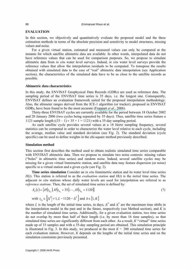
Figure 4 presents three representative examples of simulated time series interpolated with the OPT and LS methods. Figure 4(a) presents one of the worst cases. It is worth noting that even if the RMS errors of OPT and LS methods only differ by 5 cm, the LS method provides a less stable estimate with higher frequency variations that do not appear in the reference time series. By using the frequency distribution (spectrum) as an additional optimization criterion, the OPT method better reproduces the reference time series smoothness. In Fig. 4(b), the OPT and LS methods provide very similar results. Even the smoothness of the estimates is comparable. Thus, the relative evaluation of the OPT and LS approaches has to take another criterion into account. In fact, the two methods differ in their sensitivity to missing values and random noise (see below). Finally, Fig. 4(c) shows very good results for both methods. Figure 5 shows the sensitivity of the results to the set of in situ stations used as reference, for the evaluation station Sao Gabriel. The median of RMS errors diminishes when only the downstream station Curicuriari is taken into account and not the two stations upstream, Taraqua and Sao Felipe. It decreases by 6.4 cm (26.4%) and 8.5 cm (32%) with the OPT method and a 0- and nth-order model, respectively. The best results are obtained by considering all the adjacent reference stations, especially for the zero-

Daily water stage estimated from satellite altimetric data for large river basin monitoring

Copyright © 2008 IAHS Press

89

(a) Uaracu (–2,0) → Taraqua* → Sao Gabriel (0,2)

RMS error (cm): OPT: 32.92, LS: 37.93 (b) Sao Gabriel (–1,0) → Curicuriari* → Tapuruquara (0,2)

RMS error (cm): OPT: 12.51, LS: 12.94

- - ● - - - - - - .............

Reference time series Simulated altimetric time series Estimate provided by OPT Estimate provided by LS

(c) Tapuruquara (–1,0) → Serrinha* → Barcelos (0,2) RMS error (cm): OPT: 1.25, LS: 0.60

Fig. 4 Three examples of interpolation using OPT and LS methods. Model orders are given in brackets,

e.g. Uaracu (–2,0) means that 2ΔUaracu −=P and 0ΔUaracu

=F . The starred station corresponds to the evaluation station.

order model with LS (median of RMS errors equal to 16.0 cm) and the nth-order model with OPT (16.4 cm). Result variability appears to be more important with the zero-order model and OPT, and with the nth-order model and LS. Figure 6 shows the result sensitivity to the model order at evaluation station Barcelos. These results show that, for the OPT method, a ((–3,0),(0,5))-order model improves the results by 16.4 cm (32.7%) vs a 0-order model. Moreover, in the case of the OPT estimation method at Barcelos, increasing the model order from ((–2,0)(0,2)) to ((–3,0)(0,5)) tends to decrease the inter-polation residuals. However, the LS estimation approach appears to be less efficient when the model order becomes relatively important. In the following, the three estimation methods are compared. For each evaluation station, only one model structure has been considered. This structure has been chosen by considering the relative positions of the evaluation and reference stations (upstream, downstream), the a priori knowledge about water travel time between the evaluation and reference stations and about the water flow control type at the evaluation station (upstream or downstream). For Barcelos, the ((–2,0),(0,2))-order model has been chosen to evaluate the interpolation precision and its sensitivity to noise, whereas the distances between stations are large and the

Emmanuel Roux et al.

Copyright © 2008 IAHS Press

90

Fig. 5 Boxplots of the K absolute RMS interpolation errors at Sao Gabriel, obtained for different sets of in situ stations, for the parameter estimation methods OPT and LS and for different orders. Model orders are given in brackets, e.g. ((–2,0)(–2,0)) means that (( 2ΔTaraqua −=P , 0ΔTaraqua =F ),

( 2ΔSaoFelipe −=P , 0ΔSaoFelipe =F )).Numbers in brackets on the right correspond to the number K, of the simulated time series. The starred station corresponds to the evaluation station.

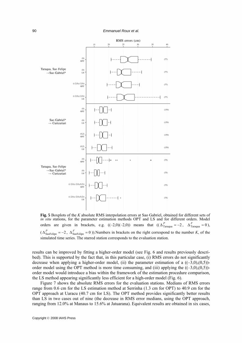
results can be improved by fitting a higher-order model (see Fig. 6 and results previously descri-bed). This is supported by the fact that, in this particular case, (i) RMS errors do not significantly decrease when applying a higher-order model, (ii) the parameter estimation of a ((–3,0),(0,5))-order model using the OPT method is more time consuming, and (iii) applying the ((–3,0),(0,5))-order model would introduce a bias within the framework of the estimation procedure comparison, the LS method appearing significantly less efficient for a high-order model (Fig. 6). Figure 7 shows the absolute RMS errors for the evaluation stations. Medians of RMS errors range from 0.6 cm for the LS estimation method at Serrinha (1.3 cm for OPT) to 40.9 cm for the OPT approach at Uaracu (40.7 cm for LS). The OPT method provides significantly better results than LS in two cases out of nine (the decrease in RMS error medians, using the OPT approach, ranging from 12.0% at Manaus to 15.6% at Jatuarana). Equivalent results are obtained in six cases,

Daily water stage estimated from satellite altimetric data for large river basin monitoring

Copyright © 2008 IAHS Press

91

Fig. 6 Boxplots of the K absolute RMS interpolation errors at Barcelos, obtained for different model orders and for the parameter estimation methods OPT and LS. Model orders are given in brackets (see Fig. 4).

with differences ranging from 0.0 to 0.6 cm. The LS method provides better results at Serrinha, with a 55.4% decrease corresponding to an absolute decrease of 0.7 cm only. The boxplots in Fig. 7 also show that the OPT method provides less variable errors in all cases except Serrinha. Figure 8 shows the distribution of differences between RMS errors obtained from the OPT and LS methods, as a function of the number of missing values. Thus, negative values are obtained when the RMS errors with LS are greater than those with OPT. It can be pointed out that when the number of missing values increases, the RMS errors increase more rapidly with the LS method than with the OPT one, except for Tapuruquara and Serrinha. This is evidenced by: (i) the decrease, according to the number of missing values, in the difference between RMS errors of the OPT and LS methods, and (ii) the skewed RMS error distributions towards negative values. For 10 missing values at Uaracu, Tapuruquara and Serrinha, medians of RMS errors are slightly higher for the OPT method (differences equal to 0.14, 0.05 and 1.28 cm, respectively). For all other eval-uation stations, the OPT approach provides better results, differences between its RMS error

Emmanuel Roux et al.

Copyright © 2008 IAHS Press

92

Fig. 7 Boxplots of the K absolute RMS interpolation errors for the evaluation stations. Model orders are given in brackets.

medians and the LS ones, for 10 missing values, ranging from –0.30 to –4.17 cm, and exceeding 30 cm for one trial at Jatuarana. Figure 9 shows the differences between RMS errors obtained from the OPT and LS methods, as a function of the standard deviation of the random noise added to the initial data. It clearly shows the higher sensitivity of the LS method to the maximum random noise range. In fact, the RMS errors for this estimation method increase more rapidly with the maximum noise range than the OPT method errors, in all the evaluation stations. For a maximum noise standard deviation equal to 50 cm, the difference at Uaracu is equal to 0.31 cm. For all other evaluation stations, the differences are negative (OPT is better than LS) and range from –0.78 (Barcelos) to –12.77 cm (Jatuarana). It is worth noting that the difference distributions present an important skewness towards negative values and that, if outliers are included, differences can exceed 50 cm (Jatuarana). Figure 10 shows the differences between RMS errors obtained from the OPT and WLS methods, as a function of the standard deviation of the random noise added to the initial data. Although the results are less marked than those of Fig. 9, they show that the WLS method is more

Daily water stage estimated from satellite altimetric data for large river basin monitoring

Copyright © 2008 IAHS Press

93

Fig. 8 Boxplots of the RMS error differences between OPT and LS estimation methods, as a function of the number of missing values and for each evaluation station.

sensitive to random noise than the OPT approach. Moreover, even with low noise standard deviations, WLS provides higher RMS error values than OPT, except for Serrinha, where the WLS yields better results up to a maximum noise standard deviation equal to 5 cm. However, in these cases, the difference between the medians of the OPT and the WLS RMS errors do not exceed 0.6 cm. For a maximum standard deviation of 50 cm, differences (of medians) between OPT and WLS range from –0.13 to –10.86 cm. The same remark as in the case of the results shown in Fig. 9 can be made: the asymmetry of distributions towards negative values is important and in specific cases, differences can exceed 50 cm (Jatuarana). Finally, the absolute RMS errors of the OPT method as a function of the number of missing values and of the random noise standard deviation were investigated. A significant increase in RMS errors can be observed for 10 missing values. However, these increases only range from 0.2 (Tapuruquara) to 1.8 cm (Uaracu). Additionally, no significant increase in result variability can be observed.

Emmanuel Roux et al.

Copyright © 2008 IAHS Press

94

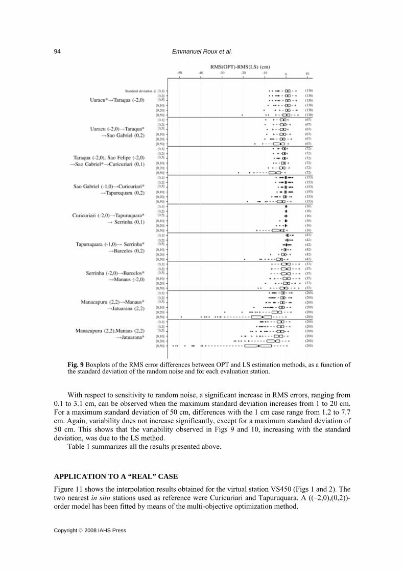
Fig. 9 Boxplots of the RMS error differences between OPT and LS estimation methods, as a function of the standard deviation of the random noise and for each evaluation station.

With respect to sensitivity to random noise, a significant increase in RMS errors, ranging from 0.1 to 3.1 cm, can be observed when the maximum standard deviation increases from 1 to 20 cm. For a maximum standard deviation of 50 cm, differences with the 1 cm case range from 1.2 to 7.7 cm. Again, variability does not increase significantly, except for a maximum standard deviation of 50 cm. This shows that the variability observed in Figs 9 and 10, increasing with the standard deviation, was due to the LS method. Table 1 summarizes all the results presented above.

APPLICATION TO A “REAL” CASE

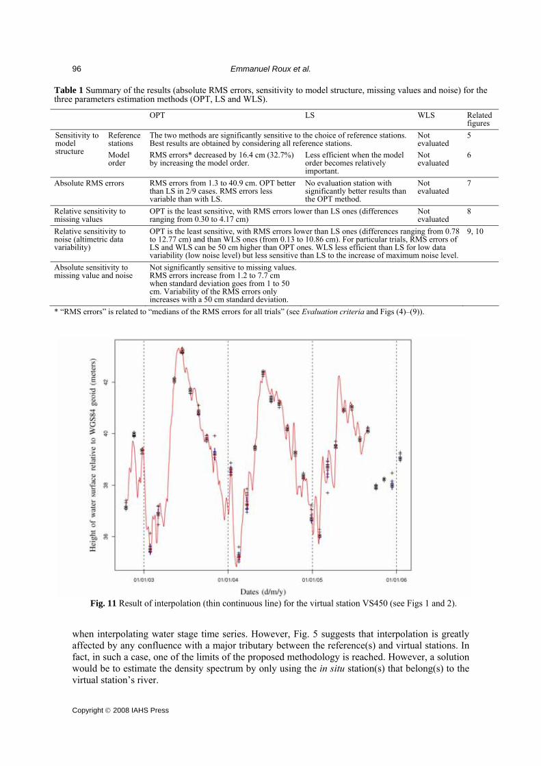
Figure 11 shows the interpolation results obtained for the virtual station VS450 (Figs 1 and 2). The two nearest in situ stations used as reference were Curicuriari and Tapuruquara. A ((–2,0),(0,2))-order model has been fitted by means of the multi-objective optimization method.

Daily water stage estimated from satellite altimetric data for large river basin monitoring

Copyright © 2008 IAHS Press

95

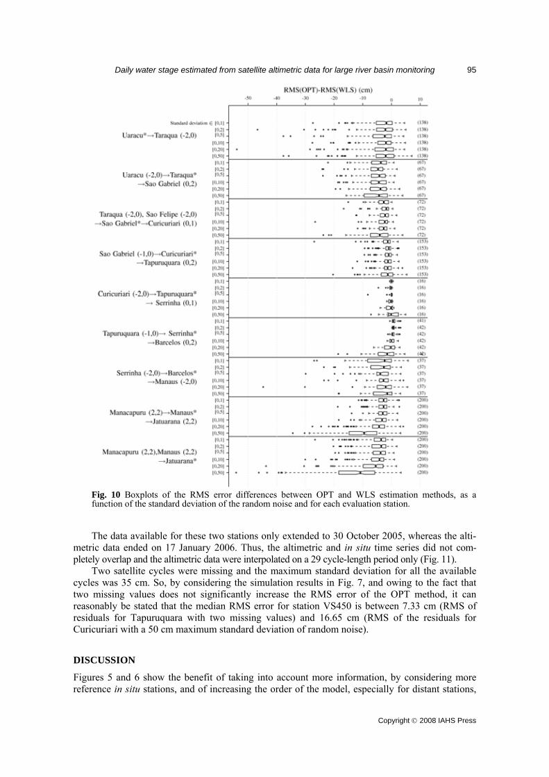
Fig. 10 Boxplots of the RMS error differences between OPT and WLS estimation methods, as a function of the standard deviation of the random noise and for each evaluation station.

The data available for these two stations only extended to 30 October 2005, whereas the alti-metric data ended on 17 January 2006. Thus, the altimetric and in situ time series did not com-pletely overlap and the altimetric data were interpolated on a 29 cycle-length period only (Fig. 11). Two satellite cycles were missing and the maximum standard deviation for all the available cycles was 35 cm. So, by considering the simulation results in Fig. 7, and owing to the fact that two missing values does not significantly increase the RMS error of the OPT method, it can reasonably be stated that the median RMS error for station VS450 is between 7.33 cm (RMS of residuals for Tapuruquara with two missing values) and 16.65 cm (RMS of the residuals for Curicuriari with a 50 cm maximum standard deviation of random noise). DISCUSSION

Figures 5 and 6 show the benefit of taking into account more information, by considering more reference in situ stations, and of increasing the order of the model, especially for distant stations,

Emmanuel Roux et al.

Copyright © 2008 IAHS Press

96

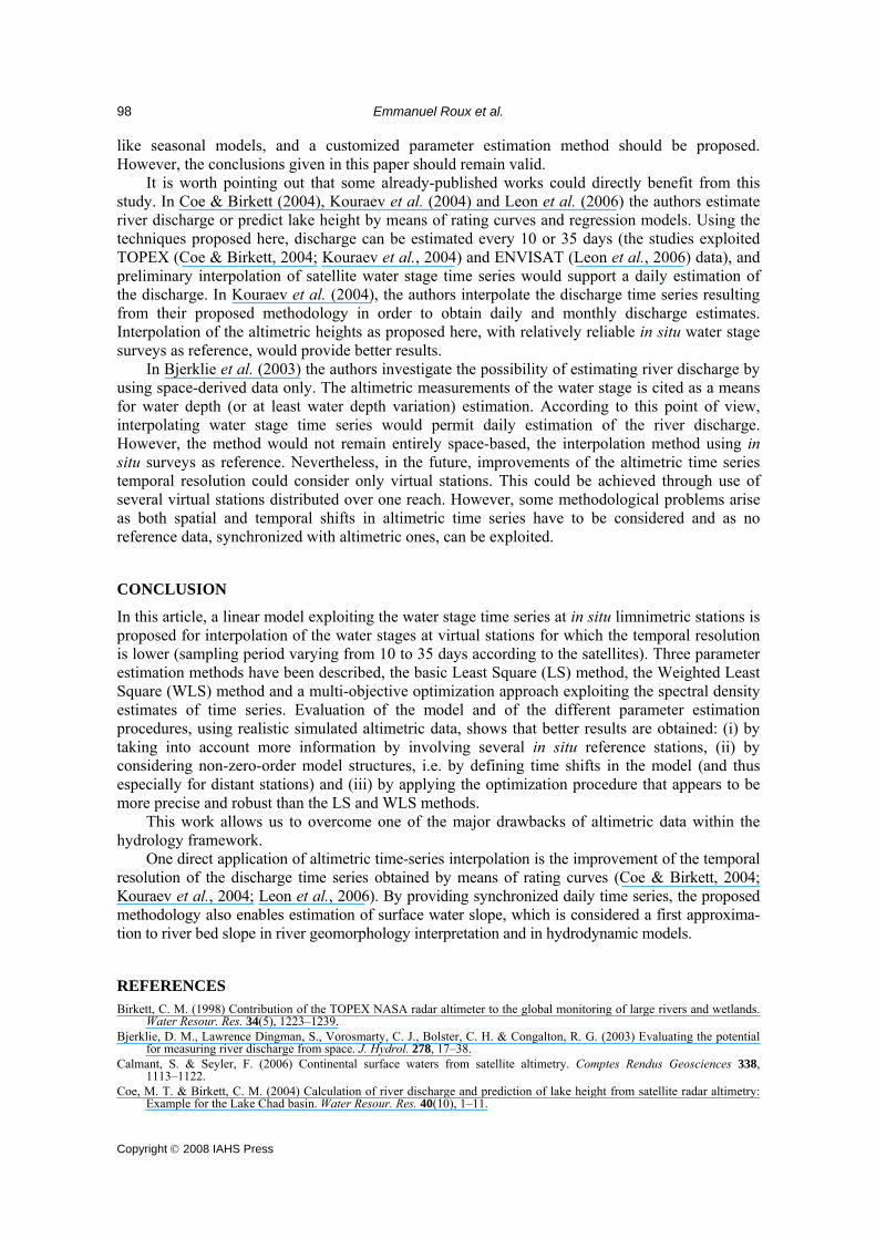
Table 1 Summary of the results (absolute RMS errors, sensitivity to model structure, missing values and noise) for the three parameters estimation methods (OPT, LS and WLS).

OPT LS WLS Related figures

Reference stations

The two methods are significantly sensitive to the choice of reference stations. Best results are obtained by considering all reference stations.

Not evaluated

5 Sensitivity to model structure Model

order RMS errors* decreased by 16.4 cm (32.7%) by increasing the model order.

Less efficient when the model order becomes relatively important.

Not evaluated

6

Absolute RMS errors RMS errors from 1.3 to 40.9 cm. OPT better than LS in 2/9 cases. RMS errors less variable than with LS.

No evaluation station with significantly better results than the OPT method.

Not evaluated

7

Relative sensitivity to missing values

OPT is the least sensitive, with RMS errors lower than LS ones (differences ranging from 0.30 to 4.17 cm)

Not evaluated

8

Relative sensitivity to noise (altimetric data variability)

OPT is the least sensitive, with RMS errors lower than LS ones (differences ranging from 0.78 to 12.77 cm) and than WLS ones (from 0.13 to 10.86 cm). For particular trials, RMS errors of LS and WLS can be 50 cm higher than OPT ones. WLS less efficient than LS for low data variability (low noise level) but less sensitive than LS to the increase of maximum noise level.

9, 10

Absolute sensitivity to missing value and noise

Not significantly sensitive to missing values. RMS errors increase from 1.2 to 7.7 cm when standard deviation goes from 1 to 50 cm. Variability of the RMS errors only increases with a 50 cm standard deviation.

* “RMS errors” is related to “medians of the RMS errors for all trials” (see Evaluation criteria and Figs (4)–(9)).

Fig. 11 Result of interpolation (thin continuous line) for the virtual station VS450 (see Figs 1 and 2).

when interpolating water stage time series. However, Fig. 5 suggests that interpolation is greatly affected by any confluence with a major tributary between the reference(s) and virtual stations. In fact, in such a case, one of the limits of the proposed methodology is reached. However, a solution would be to estimate the density spectrum by only using the in situ station(s) that belong(s) to the virtual station’s river.

Daily water stage estimated from satellite altimetric data for large river basin monitoring

Copyright © 2008 IAHS Press

97

The OPT method does not only provide better results than LS approach (see Fig. 7 and Results section). It also yields less variable results, being more robust than LS. This robustness is confirmed by the results in Figs 8, 9 and 10, in which one can observe that the OPT method is less sensitive to missing values and random noise. The WLS method, designed to be more robust than the LS, appears to be more sensitive than the OPT approach and yields higher RMS errors in almost all cases. Weights used in WLS define the relative contribution of each individual error to the total prediction error (see equation (3) and Menke, 1989). The WLS method weights the errors at time tsat by the inverse of the standard deviation of the data at the same time, tsat, so that the more the data are variable at a given time, the less the prediction error will contribute to the total error. Consequently, the greater the data variability at tsat, the less the estimated time series will attempt to be close to data at tsat. WLS can be viewed as a “relaxed” version of the LS method. This explains why WLS provides higher RMS errors than LS for a low maximum standard deviation. In fact, in this case, the standard deviations of the data are low and comparable from one cycle to another, thus the relative contributions of the individual errors are quite similar to the LS case, but the absolute errors are lower (“overall” relaxation). However, WLS is less sensitive to the increase of the maximum standard deviation of the noise. In fact, in such a case, the variability increases and differs from one cycle to another. The relative contributions of the individual errors in WLS are modified in order to minimize the contribution of errors provided by very variable data. In Figs 4 and 7, a decrease in RMS errors can be observed from Uaracu to Serrinha, i.e. when going downstream. This is not surprising as the water stage time series become smoother in that direction. Consequently, time series between two satellite cycles are less liable to high frequency variations and thus, predicting inter-cycle values becomes easier. The results at Barcelos, Manaus and Jatuarana can be explained by the very large distances between the stations (Barcelos) and their specific hydrological regimes. Indeed, Manaus and Jatuarana are known to be subject to a downstream control with strong backwater effects. Given the sampling period of the altimetric time series (35 days), high frequency flow dynamics comes from the nearby in situ gauges (Figs 4 and 11). However, the contribution of the altimetric data can be evaluated by looking at the sensitivity of the results to missing values (Fig. 8). Results show that a significant number of missing values decreases the interpolation accuracy, but in a proportion that depends on the parameter estimation method chosen (LS is more sensitive than OPT). The nth-order model structures proposed in this paper have been empirically defined. So, we could expect better results with an “optimal” model structure definition. This could be obtained by means of model comparison criteria such as the Akaike or Bayesian Information Criterion (BIC), that take into account a model’s accuracy and parsimony as two antagonistic objectives. With respect to the estimation of model parameters, another optimization method, dedicated to multi-objective criterion, could have been used. However, the sensitivity of the optimization results to weights α and β has been tested and no significant differences were found. Also, the algorithm used here is derived from the commonly-used R statistical software and based on the free Fortran PORT mathematical subroutine library (Gay, 1990), facilitating the application of the proposed methodology. In 1.2% of the cases studied, optimization did not converge and the results were not included in the study. However, non-convergences were due to the fact that the maximum number of cost function evaluations (the default is 200) was reached. In fact, when the optimization stopped due to non-convergence, the optimization parameters still gave good interpolation results. Non-convergences could be easily solved by slightly relaxing the stopping tolerances of the optimization algorithm. When exploiting the spectrum density estimated with Auto Regressive fit, the cost function, equation (4), assumes the stationarity of the time series characteristics, and consequently of the river flow characteristics. Nevertheless, the results presented in this paper imply that the proposed model and the parameter estimation method define suitable solutions for gradually varied unsteady flows, which apply to the Negro River and many other rivers in the basin. For rivers whose flow characteristics appear to be clearly unstationary, more sophisticated models could be considered,

Emmanuel Roux et al.

Copyright © 2008 IAHS Press

98

like seasonal models, and a customized parameter estimation method should be proposed. However, the conclusions given in this paper should remain valid. It is worth pointing out that some already-published works could directly benefit from this study. In Coe & Birkett (2004), Kouraev et al. (2004) and Leon et al. (2006) the authors estimate river discharge or predict lake height by means of rating curves and regression models. Using the techniques proposed here, discharge can be estimated every 10 or 35 days (the studies exploited TOPEX (Coe & Birkett, 2004; Kouraev et al., 2004) and ENVISAT (Leon et al., 2006) data), and preliminary interpolation of satellite water stage time series would support a daily estimation of the discharge. In Kouraev et al. (2004), the authors interpolate the discharge time series resulting from their proposed methodology in order to obtain daily and monthly discharge estimates. Interpolation of the altimetric heights as proposed here, with relatively reliable in situ water stage surveys as reference, would provide better results. In Bjerklie et al. (2003) the authors investigate the possibility of estimating river discharge by using space-derived data only. The altimetric measurements of the water stage is cited as a means for water depth (or at least water depth variation) estimation. According to this point of view, interpolating water stage time series would permit daily estimation of the river discharge. However, the method would not remain entirely space-based, the interpolation method using in situ surveys as reference. Nevertheless, in the future, improvements of the altimetric time series temporal resolution could consider only virtual stations. This could be achieved through use of several virtual stations distributed over one reach. However, some methodological problems arise as both spatial and temporal shifts in altimetric time series have to be considered and as no reference data, synchronized with altimetric ones, can be exploited. CONCLUSION

In this article, a linear model exploiting the water stage time series at in situ limnimetric stations is proposed for interpolation of the water stages at virtual stations for which the temporal resolution is lower (sampling period varying from 10 to 35 days according to the satellites). Three parameter estimation methods have been described, the basic Least Square (LS) method, the Weighted Least Square (WLS) method and a multi-objective optimization approach exploiting the spectral density estimates of time series. Evaluation of the model and of the different parameter estimation procedures, using realistic simulated altimetric data, shows that better results are obtained: (i) by taking into account more information by involving several in situ reference stations, (ii) by considering non-zero-order model structures, i.e. by defining time shifts in the model (and thus especially for distant stations) and (iii) by applying the optimization procedure that appears to be more precise and robust than the LS and WLS methods. This work allows us to overcome one of the major drawbacks of altimetric data within the hydrology framework. One direct application of altimetric time-series interpolation is the improvement of the temporal resolution of the discharge time series obtained by means of rating curves (Coe & Birkett, 2004; Kouraev et al., 2004; Leon et al., 2006). By providing synchronized daily time series, the proposed methodology also enables estimation of surface water slope, which is considered a first approxima-tion to river bed slope in river geomorphology interpretation and in hydrodynamic models. REFERENCES Birkett, C. M. (1998) Contribution of the TOPEX NASA radar altimeter to the global monitoring of large rivers and wetlands.

Water Resour. Res. 34(5), 1223–1239. Bjerklie, D. M., Lawrence Dingman, S., Vorosmarty, C. J., Bolster, C. H. & Congalton, R. G. (2003) Evaluating the potential

for measuring river discharge from space. J. Hydrol. 278, 17–38. Calmant, S. & Seyler, F. (2006) Continental surface waters from satellite altimetry. Comptes Rendus Geosciences 338,

1113–1122. Coe, M. T. & Birkett, C. M. (2004) Calculation of river discharge and prediction of lake height from satellite radar altimetry:

Example for the Lake Chad basin. Water Resour. Res. 40(10), 1–11.

Daily water stage estimated from satellite altimetric data for large river basin monitoring

Copyright © 2008 IAHS Press

99

De Oliveira Campos, I., Mercier, F., Maheu, C., Cochonneau, G., Kosuth, P., Blitzkow, D. & Cazenave, A. (2001) Temporal variations of river basin waters from Topex/Poseidon satellite altimetry. Application to the Amazon basin. C. R. Acad. Sci. Series IIA Earth and Planetary Science 333(10), 633–643.

Frappart, F., Seyler, F., Martinez, J.-M., Leon, J. G. & Cazenave, A. (2005) Floodplain water storage in the Negro River basin estimated from microwave remote sensing of inundation area and water levels. Remote Sens. Environ. 99(4), 387–399.

Frappart, F., Calmant, S., Cauhope, M., Seyler, F. & Cazenave, A. (2006) Preliminary results of ENVISAT RA-2-derived water levels validation over the Amazon basin. Remote Sens. Environ. 100, 252–264.

Gay, D. M. (1990) Usage summary for selected optimization routines. Technical report no. 153, AT&T Bell Laboratories. http://www.netlib.org/port.

Kouraev, A. V., Zakharova, E. A., Samain, O., Mognard, N. M. & Cazenave, A. (2004) Ob’ River discharge from TOPEX/Poseidon satellite altimetry (1992–2002). Remote Sens. Environ. 93(1–2), 238–245

Leon, J. G., Bonnet, M.-P., Cauhopé, M., Calmant, S. & Seyler, F. (2008) Distributed water flow estimates of the Upper Negro River using a Muskingum-Cunge routing model constrained by satellite altimetry. J. Hydrol. (submitted).

Leon, J. G., Calmant, S., Seyler, F., Bonnet, M.-P., Cauhopé, M., Frappart, F., Filizola, N. & Fraizy, P. (2006) Rating curves and estimation of average water depth at the upper Negro River based on satellite altimeter data and modeled discharges. J. Hydrol. 328(3–4), 481–496.

Menke, W. (1989) Geophysical Data Analysis: Discrete Inverse Theory. Academic Press, New York, USA. Menke, W. (1991) Applications of the POCS inversion method to interpolating topography and other geophysical fields.

Geophys. Res. Lett. 18(3), 435–438. Tarantola, A. & Valette, B. (1982) Generalized nonlinear problems solved using the Least Squares Criterion. Rev. Geophys.

Space Physics 20(2), 219–232. Received 15 December 2006; accepted 17 September 2007