CVA - E: A Conditional Variational Autoencoder With an ...

5676 IEEE TRANSACTIONS ON GEOSCIENCE AND REMOTE SENSING, VOL. 58, NO. 8, AUGUST 2020

CVA2E: A Conditional Variational AutoencoderWith an Adversarial Training Process for

Hyperspectral Imagery ClassificationXue Wang , Kun Tan , Senior Member, IEEE, Qian Du , Fellow, IEEE, Yu Chen,

and Peijun Du , Senior Member, IEEE

Abstract— Deep generative models such as the generativeadversarial network (GAN) and the variational autoencoder(VAE) have obtained increasing attention in a wide varietyof applications. Nevertheless, the existing methods cannot fullyconsider the inherent features of the spectral information, whichleads to the applications being of low practical performance.In this article, in order to better handle this problem, a novelgenerative model named the conditional variational autoencoderwith an adversarial training process (CVA2E) is proposed forhyperspectral imagery classification by combining variationalinference and an adversarial training process in the spectralsample generation. Moreover, two penalty terms are added topromote the diversity and optimize the spectral shape featuresof the generated samples. The performance on three different realhyperspectral data sets confirms the superiority of the proposedmethod.

Index Terms— Generative adversarial network (GAN), hyper-spectral image (HSI) classification, variational autoencoder(VAE).

I. INTRODUCTION

HYPERSPECTRAL image classification has recentlyattracted considerable attention in the field of Earth

observation as the contiguous spectral information can beutilized to discriminate different categories [1]. Discriminativemodels such as support vector machine (SVM) [2], multiplelogistic regression (MLR) [3], convolutional neural networks

Manuscript received October 4, 2019; revised November 17, 2019; acceptedDecember 24, 2019. Date of publication February 10, 2020; date of currentversion July 22, 2020. This work was supported in part by the National NaturalScience Foundation of China under Grant 41871337 and in part by the PriorityAcademic Program Development of Jiangsu Higher Education Institutions.(Xue Wang and Kun Tan contributed equally to this work.) (Correspondingauthor: Kun Tan.)

Xue Wang and Kun Tan are with the Key Laboratory of GeographicInformation Science (Ministry of Education), East China Normal University,Shanghai 200241, China, and also with the Key Laboratory for Land Envi-ronment and Disaster Monitoring of National Administration of Surveyingand Geoinformation (NASG), China University of Mining and Technology,Xuzhou 221116, China (e-mail: [email protected]).

Qian Du is with the Department of Electrical and Computer Engineering,Mississippi State University, Mississippi State, MS 39762 USA.

Yu Chen is with the Key Laboratory for Land Environment and DisasterMonitoring of National Administration of Surveying and Geoinformation(NASG), China University of Mining and Technology, Xuzhou 221116, China.

Peijun Du is with the Key Laboratory for Satellite Mapping Technol-ogy and Applications of National Administration of Surveying and Geoin-formation (NASG), Nanjing University, Nanjing 210023, China (e-mail:[email protected]).

Color versions of one or more of the figures in this article are availableonline at http://ieeexplore.ieee.org.

Digital Object Identifier 10.1109/TGRS.2020.2968304

(CNNs) [4], long short-term memory (LSTM) networks [5],and CapsuleNet [6] are advantageously used in classificationbecause of their sampling models and higher precision whencompared with generative models. However, the conditionaldistribution cannot describe the distribution characteristic anda priori knowledge of hyperspectral data. Moreover, obtain-ing enough labeled samples to train a classifier might notbe realistic because of the wide spatial coverage and thecostly field surveying and labeling. To address these issues,many generative models have been put forward in the lastfew years. Generative models explore a joint distributionand focus on high-order correlation rather than classificationboundaries only. However, the shallow generative models showa poor performance in optimization because of their limitedrepresentation ability for high-dimensional remote sensingdata sets. Motivated by deep learning, which has made greatprogress in many fields, deep generative models [7] have beenvery successful in computer vision tasks. The most impor-tant representative methods are the variational autoencoder(VAE) [8] and the generative adversarial network (GAN) [9].The principle of the VAE and the GAN is to learn a mappingfrom a latent distribution to a data space.

The difference between these two generative models is thatvariational inference is carried out to reduce the distancebetween different distributions in the VAE, while the GANtrades the complexity of sampling for the complexity ofsearching for a Nash equilibrium in minimax games. Bothmodels have a remarkable ability to generate samples that aresimilar to real samples, which have been successfully appliedin data augmentation. Before the deep generative models, dataaugmentation for remote sensing classification depended onthe following strategies: 1) sample transformation, such asrotation and translation and 2) label propagation, driven bydata or sample simulation based on a physical model, suchas spectral curve simulation under different illumination ofthe same ground field. However, these enhanced approachesare heavily reliant on the assumption of the data and thephysical environment. The VAE and the GAN have provideda new pathway for feature learning and sample augmentation,to address the issue of insufficient samples. Although the VAEhas worked well in generating reliable samples, the L2 normgives rise to blur in the generated samples. On the contrary,the GAN can create clear samples, but it suffers from model

0196-2892 © 2020 IEEE. Personal use is permitted, but republication/redistribution requires IEEE permission.See https://www.ieee.org/publications/rights/index.html for more information.

Authorized licensed use limited to: Qian Du. Downloaded on July 24,2020 at 04:14:59 UTC from IEEE Xplore. Restrictions apply.

https://orcid.org/0000-0002-6999-1362

https://orcid.org/0000-0001-6353-0146

https://orcid.org/0000-0001-8354-7500

https://orcid.org/0000-0002-2488-2656

WANG et al.: CVA2E FOR HYPERSPECTRAL IMAGERY CLASSIFICATION 5677

collapse and gradient vanishing, which can result in the sam-ples generated from the GAN being far from natural. To tacklethese defects, the structure of the VAE and the GAN has beenunceasingly perfected. Some works have used an adversarialtraining process for the VAE [10], [11] or an additionalnetwork [12] as the generator or discriminator, which havebeen proved to be effective ways to fix the blurring problemfor the VAE. For the model collapse and gradient vanishingof the GAN, the loss function has been modified, as in theWasserstein GAN [13] and the least-squares GAN [14]. Othertricks include batch normalization, distribution sampling, andthe choice of the optimizer, which are not considered in thisarticle. Moreover, considering the label information, the VAEand the GAN can be modified to perform supervised learningand semisupervised learning tasks.

Several articles have addressed classification in remotesensing images using the GAN [15]–[17]. Zhu et al. [18] putforward a hyperspectral image (HSI) classification algorithmbased on an auxiliary classifier GAN [19], where the samplesgenerated from the GAN are added to improve the perfor-mance of the classifier. Experiments on real hyperspectraldata sets confirmed the validity of the generated samples.However, the effect of the improvement was proven to belimited by Xu et al. [20], and the reason for the limitationis that the generated samples cannot cover all the featurespace. To solve the problem of the limited improvement, someworks have focused on the loss function and training samples.Wang et al. [21] proposed a removal strategy to weaken theside effects of data outliers and generate high-quality samples.Audebert et al. [22] introduced the Wasserstein distance toensure diversity of the generated samples, and the experimentsundertaken in this study showed that the cluster centers of thegenerated samples are consistent with those of real samples.ShiftingGAN [23] uses an “online-output” model to obtainmultiple generators, so that the generated samples are morediverse. Moreover, to keep the high quality of the generatedsamples, two additional shifting processes are added.

Although these works have proved that the generated sam-ples from the GAN can improve the performance of classifi-cation, the improvement is unstable because of the limitationin the enhancement of quantity and diversity.

Recently, there have been a few articles utilizing the VAEin remote sensing, instead of the GAN. For example, Gempet al. [24] proposed a deep semisupervised generative model,in which the VAE is employed to extract the spectra of theendmembers and retrieve the mineral spectra. Gong et al.[25] utilized the VAE for change detection in multispectralimagery, but the experiments indicated that the differenceimages were blurred because of the reconstruction loss of thetraining data in the VAE. Su et al. [26] proposed a VAE-basedhyperspectral unmixing method named the deep autoencodernetwork (DAEN), in which the VAE performs blind sourceseparation after the spectral signatures are extracted, and theVAE can ensure the nonnegativity and sum-to-one constraintswhen estimating the abundances.

Inspired by the adversarial autoencoder (AAE) [10] andthe conditional GAN (CGAN) [27], we propose a variationalGAN with label information named conditional variational

autoencoder with an adversarial training process (CVA2E). Thenew framework consists of a variational encoder to ensure thediversity when using the latent variable distribution, a gener-ator to reconstruct the samples from the latent variable distri-bution, and a discriminator to determine if the data are fromreal data or have a model distribution. Moreover, two fullyconnected layers are added in the discriminator to improvethe classification ability of the framework. Considering theinherent difference (hundreds of spectral bands in HSIs) in thespectral dimensionality between HSIs and the common imagesused in computer vision tasks, the spectral angle distance isused as one of the observation items.

The rest of this article is organized as follows. Section IIgives the background to this article. Section III details theCVA2E framework. Section IV describes the three real HSIsused in the experiments, the experimental results, and thecomparisons with other methods. Finally, the conclusions ofthis article are drawn in Section V.

II. PREVIOUS WORK

In this article, the main work is based on two kinds ofgenerative models: the GAN and the VAE. Therefore, in thissection, we briefly review these two models.

A. Generative Adversarial Network

The GAN uses deep neural networks to approximate anunknown data distribution and is typically composed of twonetworks named the generator and discriminator. The formeris aimed at learning the distribution characteristic of the dataand creating new data, and the discriminator learns to inferwhether the sample is from a model distribution or a realdistribution. When the training is over, the generator anddiscriminator converge to a Nash equilibrium, in which thediscriminator cannot distinguish whether the sample is realdata or generated data from the generator, i.e., the generatedsamples are indistinguishable from real samples. These tworoles are both deep neural networks, and the generator’straining target is a certain distribution pz(z) which is consistentwith the sample G(z)’s data space. The generator is denoted asG(z; θg), and θg represents the parameters of the deep neuralnetworks. For the discriminator, D(x; θd) represents a deepneural network with parameters θd . The training process is tosolve a minimax problem by a two-player game

minG

maxG

V (G, D) = Ex∼p(x)[logD(x)]+ Ez∼pz(z)[log(1 − D(G(z)))] (1)

where x ∼ p(x) is the real data distribution. The optimalmodel D(x) is p(x)/(p(x) + pg(x)), and the global equilib-rium of this two-player game is obtained when p(x) = pg(x).However, the prototype of the GAN model is difficult toconverge in the training stage, and the samples generatedfrom the GAN are often far from natural. To this end, manyworks have tried to improve the stability by modifying theloss function. For example, the Wasserstein GAN substitutesthe original Kullback–Leibler divergence and Jensen–Shannon



divergence for the Earth mover’s distance. The WassersteinGAN is aimed at solving the problem

maxw∈w

Ex∼p(x)[ fw(x)] − Ez∼pz(z)[ fw(gθ (z))] (2)

where w represents the parameters of function f , and w ∈ Wis a strong assumption akin to assuming that w meets the K-Lipschitz constraint ‖ f ‖w ≤ K when proving the consistencyof f . The Wasserstein GAN can improve the stability ofthe learning and get rid of problems such as mode collapse,whereas the range of the parameters of the discriminator islimited, to meet the K-Lipschitz constraint, which decreasesthe discriminative power.

B. Variational Autoencoder

The VAE uses a Kullback–Leibler divergence penalty tomake its hidden code vector like a prior distribution, i.e., theVAE performs efficient approximate inference and learningwith directed models using a continuous latent intractableposterior distribution. The reparameterization is carried outto yield a simple differentiable unbiased estimator of thevariational lower bound, whose Kullback–Leibler divergenceis straightforward to optimize using the standard stochasticgradient descent technique. The encoder Q of the autoencoderis used as the probabilistic function approximator qτ (z | x), andthe decoder P is used as the approximation of the posteriorof the generative model pθ (x, z). The parameters τ and θ areoptimized jointly with the objective function

V (P, Q) = −KL(qτ (z | x)‖pθ (z | x)) + Recost(x) (3)

where Recost() calculates the reconstruction loss of a givensample x through the VAE.

There have been many developments based on the VAEand the GAN. For example, combining the VAE and theGAN to construct a more powerful deep generative model[10], [11]. Introducing an adversarial training process to theautoencoder or using variational inference and elementwisemeasurement in the GAN’s observation function can alsoimprove the drawbacks of the original model. Furthermore,the VAE and the GAN can be modified to consider labelinformation and trained to conduct conditional generation,e.g., the conditional variational autoencoder (CVAE) and theCGAN.

III. PROPOSED METHOD

In this section, we describe the proposed CVA2E frameworkfor HSI classification and generation, which is illustratedin Fig. 1. First, we introduce the notations that are adoptedthroughout this article. If we suppose that a hyperspectral dataset with b spectral bands contains N labeled samples for Lclasses, and each is represented by {x1, x2, . . . , x N } ∈ R

1×b,then the corresponding label vector is Y = {y1, y2, . . . , yL} ∈R

1×L .As mentioned earlier, the GAN and the VAE have shown

good performances in data generation, whereas their latentvariables cannot learn the label knowledge during the adver-sarial training and variational inference process. Moreover,the intrinsic loss measurement of the VAE gives rise to blurry

generated samples, which result in defective pattern learningfor hyperspectral data. There will be various samples in thesame category in hyperspectral imagery, so the diversity ofthe generative model can be guaranteed. The GAN can createclear samples, which is an improvement over the VAE, butit always overfits on local properties, which leads to thegenerated spectra samples appearing disordered. To handle theabove problems, we propose CVA2E.

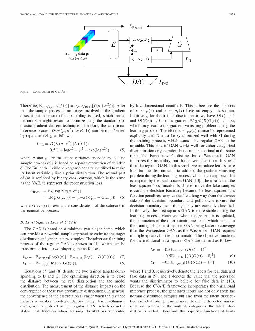
As shown in Fig. 1, the spectral feature vectors are utilizedas the input of CVA2E as we try to explore the individ-ual hyperspectral pixels with no spatial context. Inspired byLarsen et al. [12], the CVA2E framework consists of threenetworks: an encoder network E, a generator network G, anda discriminator network D. There are two connected parts ofdiscriminator network D, which execute the distinguishmentand the classification task, respectively. All the networks aredeep fully connected networks. For HSI classification, it iscritical to assign a high-dimensional spectral pixel with thecorrect label, which can be represented by the conditionaldistribution p(y | x). The input of E and G concatenates theoriginal spectral vector x with the 1-D categorical vector y.With the connection of the spectral and categorical features,the encoder network E maps x to a latent variable z throughthe probabilistic function approximator PE (z | x, y), where y isthe category of x . Following the encoder process, the sampledz is utilized to generate the fake data through the otherlearned probabilistic function approximator PG (x | z, y) in thegenerative network G. After this, D establishes whether thedata are real data or a model distribution, and G tries tolearn the real data distribution during the adversarial trainingprocess.

A. Variational Inference Process of CVA2E

The variational inference process in CVA2E is the sameas in the VAE, where the input data consider the categoryinformation. The principle of the VAE is to learn a distrib-ution which has a certain sampling space to sample the realdata distribution x . The learned distribution is described asz = N(μ, σ 2). The latent variable z is encoded by E(z, θg)and is sampled from this distribution, which is based onreparameterization, where θg represents the parameters of thedeep neural network. The objective is to minimize the distancebetween z and a given distribution (in this work, the givendistribution is a standard normal distribution). The distancecan be denoted as follows:

L = −D(N (μ, σ 2)||N (0, 1)) + EE [logP(x |μ, σ 2)] (4)

where μ and σ are obtained by the encoder network E.It is often possible to express a random variable z whichobeys the Gaussian distribution as a deterministic variablez = N(μ, σ 2), where μ and σ are obtained by feedfor-ward operation of the deep neural network in the VAE.The values of μ and σ can be calculated and taken asderivatives, whereas this is not possible for the sampleprocess. In this case, reparameterization is useful since itcan be used to rewrite the sample process as z = μ + σξ ,where ξ is an auxiliary noise variable and ξ = N (0, 1).



Fig. 1. Construction of CVA2E.

Therefore, Ez∼N (μ,σ 2)[ f (z)] = Eξ∼N (0,1)[ f (μ+σ 2ξ)]. Afterthis, the sample process is no longer involved in the gradientdescent but the result of the sampling is used, which makesthe model straightforward to optimize using the standard sto-chastic gradient descent technique. Therefore, the variationalinference process D(N (μ, σ 2)||N (0, 1)) can be transformedby reparametrizing as follows:

LKL = D(N (μ, σ 2)||N (0, 1))

= 0.5(1 + logσ 2 − μ2 − exp(logσ 2)) (5)

where σ and μ are the latent variables encoded by E. Thesample process of z is based on reparameterization of variableξ . The Kullback–Leibler divergence penalty is utilized to makeits latent variable z like a prior distribution. The second partof (4) is replaced by binary cross entropy, which is the sameas the VAE, to represent the reconstruction loss

LRecost = EE [logP(x |μ, σ 2)]= x log(G(z, y)) + (1−x)log(1 − G(z, y)) (6)

where G(z, y) represents the consideration of the category inthe generative process.

B. Least-Squares Loss of CVA2E

The GAN is based on a minimax two-player game, whichcan provide a powerful sample approach to estimate the targetdistribution and generate new samples. The adversarial trainingprocess of the regular GAN is shown in (1), which can betransformed into a two-player game as follows:

LD = −Ex∼p(x)[logD(x)]−Ez∼pz(z)[log(1−D(G(z)))] (7)

LG = −Ez∼pz(z)[log(D(G(z)))]. (8)

Equations (7) and (8) denote the two trained targets corre-sponding to D and G. The optimizing direction is to closethe distance between the real distribution and the modeldistribution. The measurement of the distance impacts on theconvergence of these two probability distributions. In general,the convergence of the distribution is easier when the distanceinduces a weaker topology. Unfortunately, Jensen–Shannondivergence is utilized in the regular GAN, which is not astable cost function when learning distributions supported

by low-dimensional manifolds. This is because the supportsof x ∼ p(x) and x ∼ pg(x) have an empty intersection.Intuitively, for the trained discriminator, we have D(x) → 1and D(G(z)) → 0, so the gradient ∂LG/∂(D(G(z))) → −∞,which may lead to the gradient-vanishing problem during thelearning process. Therefore, x ∼ pg(x) cannot be representedexplicitly, and D must be synchronized well with G duringthe training process, which causes the regular GAN to beunstable. This kind of GAN works well for either categoricaldiscrimination or generation, but cannot be optimal at the sametime. The Earth mover’s distance-based Wasserstein GANimproves the instability, but the convergence is much slowerthan the regular GAN. In this work, we introduce least-squareloss for the discriminator to address the gradient-vanishingproblem during the learning process, which is an approach thatis inspired by the least-squares GAN [13]. The idea is that theleast-squares loss function is able to move the fake samplestoward the decision boundary because the least-squares lossfunction penalizes samples that lie a long way from the correctside of the decision boundary and pulls them toward thedecision boundary, even though they are correctly classified.In this way, the least-squares GAN is more stable during thelearning process. Moreover, when the generator is updated,the parameters of the discriminator are fixed, which results inthe training of the least-squares GAN being faster to convergethan the Wasserstein GAN, as the Wasserstein GAN requiresmultiple updates for the discriminator. The objective functionsfor the traditional least-squares GAN are defined as follows:

LD = −0.5Ex∼p(x)[(D(x) − 1)2]− 0.5Ez∼pz(z)[(D(G(z)) − 0)2] (9)

LG = −0.5Ez∼pz(z)[(D(G(z)) − 1)2] (10)

where 1 and 0, respectively, denote the labels for real data andfake data in (9), and 1 denotes the value that the generatorwants the discriminator to believe for fake data in (10).Because the CVA2E framework incorporates the variationalinference process, the generated inputs are not only from thenormal distribution samples but also from the latent distribu-tion encoded from E. Furthermore, to create the deterministicrelationship between the multiple categories, the label infor-mation is added. Therefore, the objective functions of least-



squares loss are transformed as follows:

LD = −0.5Ex∼p(x)[(D(x |y) − 1)2]− 0.5Ez∼pz(z)[(D(G(z|y)) − 0)2]− 0.5Eξ∼N (0,1)[(D(G(ξ |y)) − 0)2] (11)

LG = −0.5Ez∼pz(z)[(D(G(z|y)) − 1)2]− 0.5Eξ∼N (0,1)[(D(G(ξ |y)) − 1)2] (12)

where G(z|y) denotes that the initial samples are sampled fromz ∼ N (μ, σ 2), and μ, σ are obtained by encoder networkE. G(ξ |y) denotes that the initial samples are sampled fromξ ∼ N (0, 1). The initial samples are then input into thegenerator network G to obtain the final fake data. Therefore,the discriminator network D should recognize if a sample isfrom the real data distribution or from the two fake distri-butions, which are described as the three parts of (11), andthe generator network should use both the conditional normaldistribution and the latent distribution to fool the discriminator.

C. Enhancement of Diversity and Spectral CharacteristicsWith CVA2E

The motivation of the CVA2E framework is to learn thespectral distribution characteristics of individual hyperspec-tral pixels. While the deep neural network is a remarkablefunction approximator, the inherent difference (hundreds ofspectral bands) in spectral dimensionality between HSIs andthe common images used in computer vision tasks shouldbe taken into account. Regular loss functions are generallybased on cross-entropy or least-squares loss, which focuseson the local feature matching. Here we introduce the spectralangle distance to match the generated samples based on thesimilarity of the curves of the spectra. The spectral angle matchmethod was proposed by Kruse [28]. This method regards thespectrum of an individual hyperspectral pixel in the image as ahigh-dimensional vector and measures the similarity betweenthe spectra by calculating the vectorial angle between thetwo high-dimensional vectors, where the smaller the angle,the more similar the two spectra are, and the more reliable thegenerator will be. Here we utilize cosine similarity to replacethe spectral angle

LSAD = 1

bs

∑[(G(z|y)Tx√

G(z|y)TG(z|y)√

x T x+ 1

)

+(

G(ξ |y)Tx√G(ξ |y)TG(ξ |y)

√xTx

+ 1

)](13)

where bs represents the batch size in the training process. Thespectral angles are calculated between the real spectra and thetwo kinds of generative spectra. Inspired by the spectral anglematch method, we utilize the vectorial angle measurement onan intermediate layer of the generator network. The differencein purpose is that we want the feature space of the generativesamples to be big enough to contain the entire training datadistribution, and thus reduce the likelihood of mode collapse,so the vectorial angle between pairwise features of an inter-mediate layer should be the maximum. The vectorial angle of

the features is calculated as follows:

LFVA

= 1

L

L∑l

1

Sl(Sl − 1)

×S∑m

lS∑

n =m

l F(zm | yl)T F(zn | yl)√

F(zm | yl)T F(zm | yl)

√F(zn | yl)

T F(zn | yl)+1

(14)

where bs represents the batch size in the training process, andF(·) denotes the features of an intermediate layer. In thiswork, the output of the penultimate layer of the generatornetwork is chosen as the compared features. The vectorialangle is calculated among the samples which belong to thesame category. Each F(z) should be calculated with the featurewhich is the same category in the ergodic case, except itself.After L iterations (L is the number of categories), the vectorialangle of the features is the cumulative sum in Sl (Sl − 1)Ltimes, and the average is obtained using division by thenumber of times. A larger LFVA means that the featuresare similar and that the generative model should have lowdiversity.

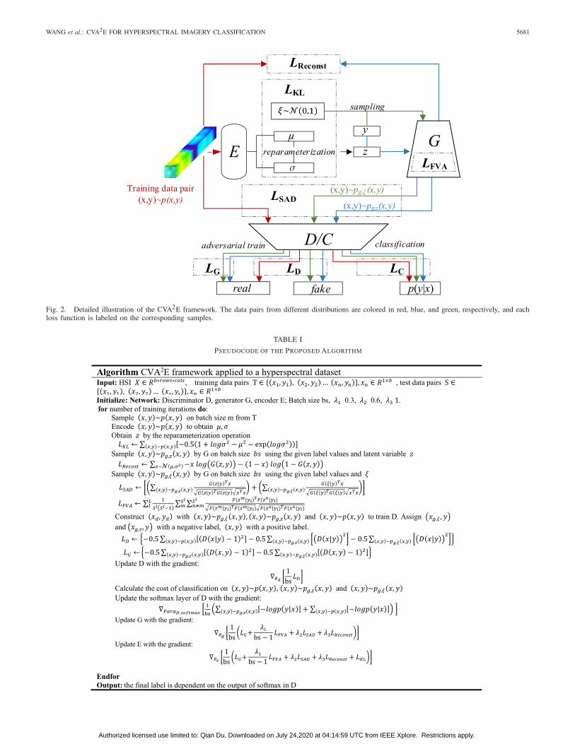
The final structure of CVA2E is shown in Fig. 2. Theinput of the discriminator network is the concatenation of thespectral and categorical vectors, which is used to estimatethe two joint probability distributions p(xg, y) and p(x, y).Moreover, the discriminator network is reused to executethe classification task. When the network plays the role ofclassifier, the categorical vector is replaced by a zero vector,so that the weights in the discriminator network correspondingto categorical features are disabled, and the last layer isreplaced by a softmax layer to obtain the posterior probabilityp(y|x) or p(y|xg).

Up until now, the final goal of CVA2E can be shown asfollows:

L = LD + LG + LC + LKL + λ1 LFVA+λ2 LSAD+λ3LRecost

(15)

where each part is given the explicit expression above. λ1,λ2, and λ3 are empirically set to 0.3, 0.6, and 1. As shownin Fig. 2, “red” means the data pair from the real distribu-tion, and “blue” and “green” denote the data pair from thegenerated distribution. The difference is that the “blue” datapairs are generated based on the latent distribution encodedby E, and the “green” data pairs are based on a certaindistribution. LD is related to the ability to distinguish betweenreal and fake data pairs, LG represents the ability of G tofool D, LC denotes the capability of the network to classifyspectra from different categories, LKL influences the latentdistribution encoded by E to obey a certain distribution,LRecost is related to the variational inference, LFVA improvesthe diversity of G, and LSAD considers the spectral similar-ity between the real spectrum and the generated spectrum.Finally, in order to summarize the whole training process,Table I gives a detailed description of the proposed learningalgorithm.



Fig. 2. Detailed illustration of the CVA2E framework. The data pairs from different distributions are colored in red, blue, and green, respectively, and eachloss function is labeled on the corresponding samples.

TABLE I

PSEUDOCODE OF THE PROPOSED ALGORITHM



Fig. 3. Implementation of each network in CVA2E. (a) Encoder network. (b) Discriminator network. (c) Generator network.

TABLE II

NUMBER OF TRAINABLE PARAMETERS AND MEMORY OVERHEAD IN CVA2E

IV. EXPERIMENTS

In order to demonstrate the performance of the proposedtechnique, three real HSIs were utilized. To explore thedistribution of the real spectra, the fully connected layerswere utilized to constitute the different compositions of themodel. In our experiments, the category information, whichwas transformed as a “one-hot vector,” was merged with thespectral vector. A “one-hot vector” is a vector with one single“1” and all the others as “0,” where the position of “1”indicates which category the pixel belongs to. The constructionof the three networks is shown in Fig. 3, where the encodernetwork E is a three-layer fully connected network, and theinput of each layer is merged by the spectral vector and “one-hot vector” in advance. μ and σ are from two different layers,and the rectified linear unit is utilized as the activation functionto obtain μ and σ . The discriminator D and generator Gconsist of four-layer fully connected networks. For D, whenit determines real or fake samples, the “one-hot” vector isapplied; otherwise, the categorical vector is set to zero, andthe softmax and sigmoid functions are utilized for the twooutputs. The former output is a posteriori probability of thecategories, and the latter is used for the loss calculation ofD in the adversarial training process. For G, the “one-hot”

vector determines the category of the generated sample, whichis represented by the results of the sigmoid function of the lastlayer. The number of neurons in each part of the network forthree different data sets is shown in Fig. 3, the mini-batchsize for training is set as 80, and the learning rate is set to0.0002. To exhibit the complexity referring to the previousresearch [29], the number of trainable parameters and memoryoverhead in CVA2E are given in Table II.

The experimental analysis starts with the generated samplesby the given generative models. The compared methods werechosen from the mainstream deep generative models. In orderto fairly compare each method, we used the same networkstructure to implement the different models. After verificationof the validity of the generated samples, the overall accuracy(OA) and kappa coefficient (kappa) are used to report the per-formance of all the models. To demonstrate the performanceof the proposed technique, three real HSIs were utilized. Thetraining samples in all the experiments were made up of 10%of the labeled data.

A. Data Set Description

1) Pavia University ROSIS Data Set: The Pavia Universitydata set was acquired by the Reflective Optics System Imaging



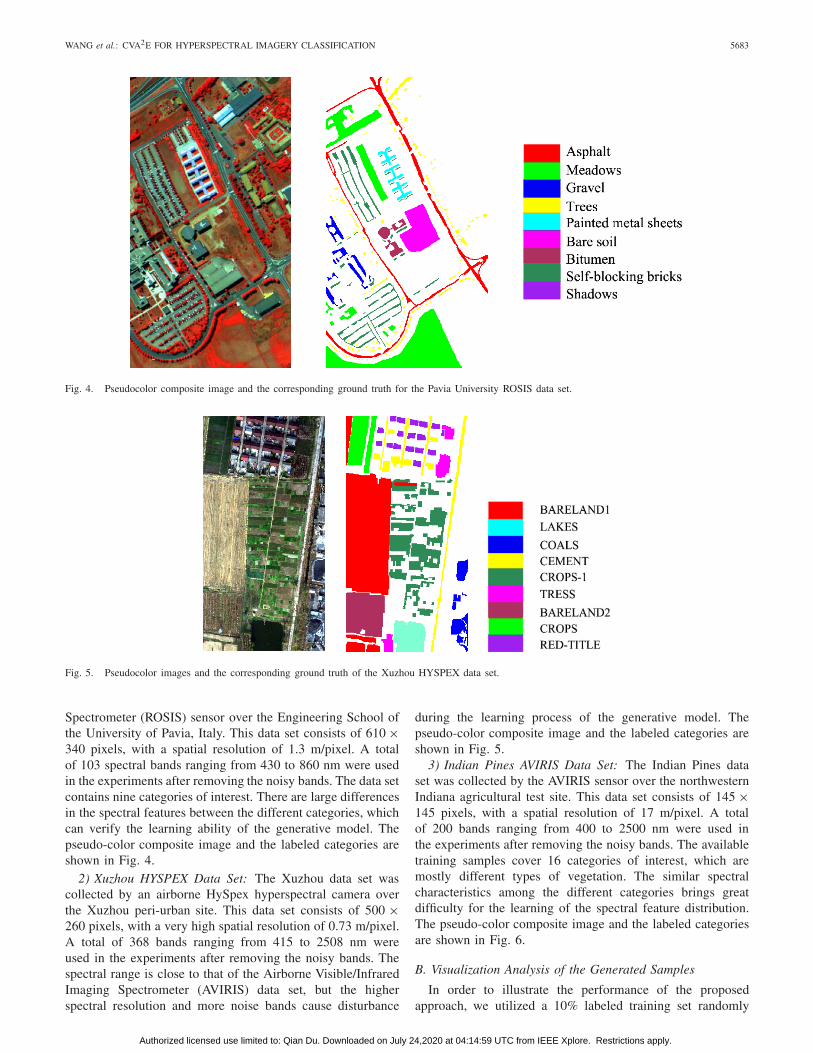
Fig. 4. Pseudocolor composite image and the corresponding ground truth for the Pavia University ROSIS data set.

Fig. 5. Pseudocolor images and the corresponding ground truth of the Xuzhou HYSPEX data set.

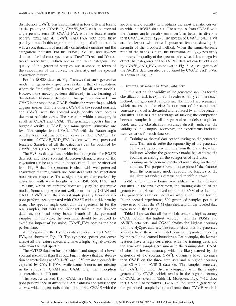
Spectrometer (ROSIS) sensor over the Engineering School ofthe University of Pavia, Italy. This data set consists of 610 ×340 pixels, with a spatial resolution of 1.3 m/pixel. A totalof 103 spectral bands ranging from 430 to 860 nm were usedin the experiments after removing the noisy bands. The data setcontains nine categories of interest. There are large differencesin the spectral features between the different categories, whichcan verify the learning ability of the generative model. Thepseudo-color composite image and the labeled categories areshown in Fig. 4.

2) Xuzhou HYSPEX Data Set: The Xuzhou data set wascollected by an airborne HySpex hyperspectral camera overthe Xuzhou peri-urban site. This data set consists of 500 ×260 pixels, with a very high spatial resolution of 0.73 m/pixel.A total of 368 bands ranging from 415 to 2508 nm wereused in the experiments after removing the noisy bands. Thespectral range is close to that of the Airborne Visible/InfraredImaging Spectrometer (AVIRIS) data set, but the higherspectral resolution and more noise bands cause disturbance

during the learning process of the generative model. Thepseudo-color composite image and the labeled categories areshown in Fig. 5.

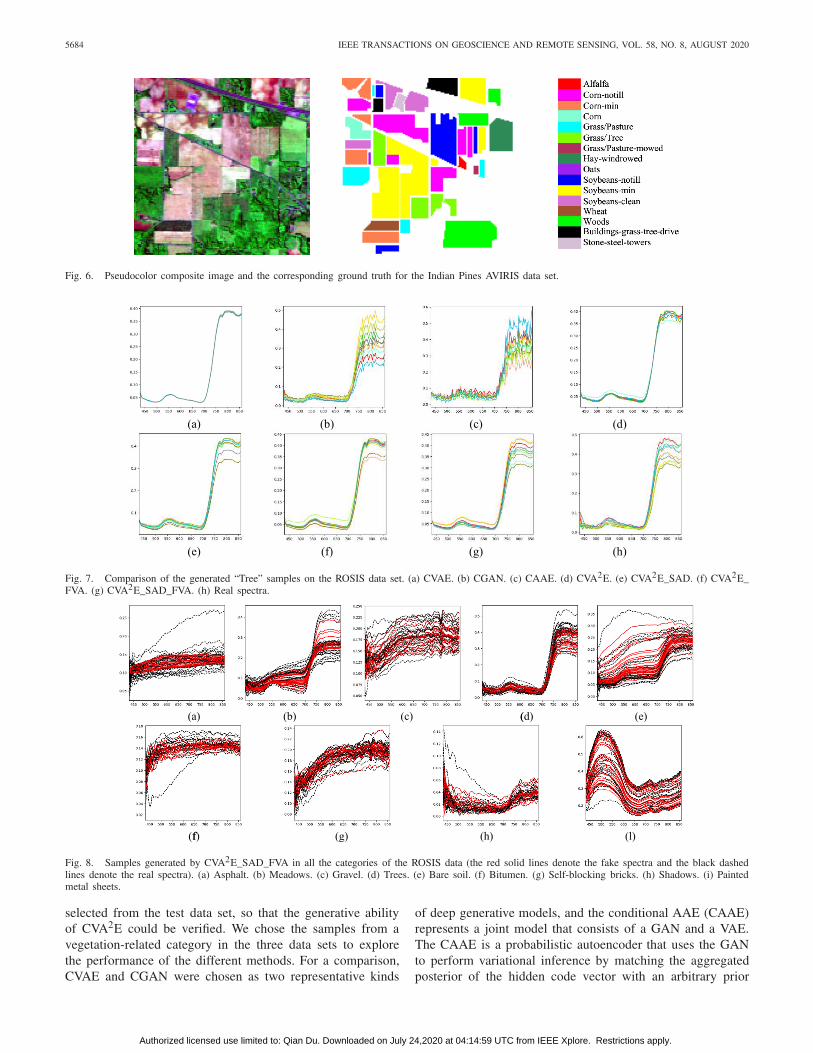
3) Indian Pines AVIRIS Data Set: The Indian Pines dataset was collected by the AVIRIS sensor over the northwesternIndiana agricultural test site. This data set consists of 145 ×145 pixels, with a spatial resolution of 17 m/pixel. A totalof 200 bands ranging from 400 to 2500 nm were used inthe experiments after removing the noisy bands. The availabletraining samples cover 16 categories of interest, which aremostly different types of vegetation. The similar spectralcharacteristics among the different categories brings greatdifficulty for the learning of the spectral feature distribution.The pseudo-color composite image and the labeled categoriesare shown in Fig. 6.

B. Visualization Analysis of the Generated Samples

In order to illustrate the performance of the proposedapproach, we utilized a 10% labeled training set randomly



Fig. 6. Pseudocolor composite image and the corresponding ground truth for the Indian Pines AVIRIS data set.

Fig. 7. Comparison of the generated “Tree” samples on the ROSIS data set. (a) CVAE. (b) CGAN. (c) CAAE. (d) CVA2E. (e) CVA2E_SAD. (f) CVA2E_FVA. (g) CVA2E_SAD_FVA. (h) Real spectra.

Fig. 8. Samples generated by CVA2E_SAD_FVA in all the categories of the ROSIS data (the red solid lines denote the fake spectra and the black dashedlines denote the real spectra). (a) Asphalt. (b) Meadows. (c) Gravel. (d) Trees. (e) Bare soil. (f) Bitumen. (g) Self-blocking bricks. (h) Shadows. (i) Paintedmetal sheets.

selected from the test data set, so that the generative abilityof CVA2E could be verified. We chose the samples from avegetation-related category in the three data sets to explorethe performance of the different methods. For a comparison,CVAE and CGAN were chosen as two representative kinds

of deep generative models, and the conditional AAE (CAAE)represents a joint model that consists of a GAN and a VAE.The CAAE is a probabilistic autoencoder that uses the GANto perform variational inference by matching the aggregatedposterior of the hidden code vector with an arbitrary prior



distribution. CVA2E was implemented in four different forms:1) the prototype CVA2E; 2) CVA2E_SAD with the spectralangle penalty term; 3) CVA2E_FVA with the feature anglepenalty term; and 4) CVA2E_SAD_FVA with both thesepenalty terms. In this experiment, the input of all the modelswas a concatenation of normally distributed sampling and thecategorical indicator. For the ROSIS, AVIRIS, and HySpexdata sets, the indicator vector was “Tree,” “Tree,” and “Grass-trees,” respectively, which are in the same category. Thequality of the generated samples was assessed in terms ofthe smoothness of the curves, the diversity, and the spectralabsorption features.

For the ROSIS data set, Fig. 7 shows that each generativemodel can generate a spectrum similar to that of vegetation,where the “red edge” was learned well by all seven models.However, the models perform differently in the learning ofthe detailed feature distribution. The spectrum derived fromCVAE is the smoothest. CAAE obtains the worst shape, whichappears noisier than the others. CGAN is the second noisiest,and CVA2E with the spectral angle penalty term obtainsthe most realistic curve. The variation within a category issmall in CGAN and CVAE. The generated spectra have abigger diversity in CAAE, but some spectral structures arelost. The samples from CVA2E_FVA with the feature anglepenalty term perform better in diversity than CVA2E. Thespectrum of CVA2E_SAD_FVA is clear with well-preservedfeatures. Samples of all the categories can be obtained byCVA2E_SAD_FVA, as shown in Fig. 8.

The HySpex data set has a wider band range than the ROSISdata set, and more spectral absorption characteristics of thevegetation can be explored in the spectrum. It can be observedfrom Fig. 9 that the spectrum is clear, with well-preservedabsorption features, which are consistent with the vegetationbiochemical response. These signatures are characterized byabsorption with wave troughs around 450, 550, 1450, and1950 nm, which are captured successfully by the generativemodel. Some samples are not well controlled by CGAN andCAAE. CVA2E with the spectral angle penalty term shows apoor performance compared with CVA2E without this penaltyterm. The spectral angle constrains the spectrum fit for thereal samples, but with the abundant noise in the HySpexdata set, the local noisy bands disturb all the generatedsamples. In this case, the constraint should be reduced toavoid the impact of the noise. CVA2E_FVA obtains the bestperformance.

All categories of the HySpex data are obtained by CVA2E_FVA, as shown in Fig. 10. The synthetic spectra can coveralmost all the feature space, and have a higher signal-to-noiseratio than the real spectra.

The AVIRIS data set has the widest band range and a lowerspectral resolution than HySpex. Fig. 11 shows that the absorp-tion characteristics at 450, 1450, and 1950 nm are successfullycaptured by CVA2E_FVA, while some features are missingin the results of CGAN and CAAE (e.g., the absorptioncharacteristic at 550 nm).

The spectra derived from CVAE are blurry and show apoor performance in diversity. CAAE obtains the worst shapecurves, which appear noisier than the others. CVA2E with the

spectral angle penalty term obtains the most realistic curves,as with the ROSIS data set. The samples from CVA2E withthe feature angle penalty term perform better in diversitythan CVA2E without LFVA. The spectra of CVA2E_SAD_FVAare the clearest, with the well-preserved features showing thestrength of the proposed method. When the signal-to-noiseratio of the bands is high, the utilization of LSAD positivelyimproves the quality of the spectra; otherwise, it has a negativeeffect. All categories of the AVIRIS data set can be obtainedby CVA2E_SAD_FVA, as shown in Fig. 5. All categories ofthe AVIRIS data can also be obtained by CVA2E_SAD_FVA,as shown in Fig. 12.

C. Training on Real and Fake Data Sets

In this section, the validity of the generated samples for theclassification task is explored. In order to fairly compare eachmethod, the generated samples and the model are separated,which means that the classification part of the conditionalgenerative model is discarded and replaced by an independentclassifier. This has the advantage of making the comparisonbetween samples from all the generative models straightfor-ward, and the classification accuracy directly indicates thevalidity of the samples. Moreover, the experiments includedtwo scenarios for each data set.

1) Training on the real data set and testing on the generateddata. This can describe the separability of the generateddata using hyperplane learning from the real data, whichindicates whether the generative model has captured theboundaries among all the categories of real data.

2) Training on the generated data set and testing on the realdata set. The purpose here is to explore if the featuresfrom the generative model support the features of thereal data set under a dimensional manifold space.

SVM with a linear kernel was utilized as the universalclassifier. In the first experiment, the training data set of thegenerative model was utilized to train the SVM classifier, and600 generated samples per class were used in the testing.In the second experiment, 600 generated samples per classwere used to train the SVM classifier, and all the labeled datawere used in the testing.

Table III shows that all the models obtain a high accuracy.CVAE obtains the highest accuracy with the ROSIS andAVIRIS data sets, and CGAN obtains the highest accuracywith the HySpex data set. The results show that the generatedsamples from these two models can be separated preciselyby the real-data learned boundaries. For example, the learnedfeatures have a high correlation with the training data, andthe generated samples are similar to the training data. CAAEobtains the lowest accuracy, which is likely caused by thedistortion of the spectra. CVA2E obtains a lower accuracythan CVAE on the three data sets and a higher accuracythan CGAN on AVIRIS data set. The samples generatedby CVA2E are more diverse compared with the samplesgenerated by CVAE, which results in the higher accuracyof CVAE as given in Table II. Moreover, Figs. 7–12 showthat CVA2E outperforms CGAN in the sample generation,the generated sample is more diverse than CVA2E while it



Fig. 9. Comparison of the generated “Tree” samples on the HySpex data set. (a) CVAE. (b) CGAN. (c) CAAE. (d) CVA2E. (e) CVA2E_SAD. (f) CVA2E_FVA. (g) CVA2E_SAD_FVA. (h) Real spectra.

Fig. 10. Samples generated by CVA2E_FVA in all categories of the HySpex data (the red solid lines denote the fake spectra and the black dashed linesdenote the real spectra). (a) Bare Land-1. (b) Lakes. (c) Coals. (d) Tree. (e) Cement. (f) Crops-1. (g) Bare Land-2. (h) Crops-2. (i) Red title.

TABLE III

TRAINING ON THE REAL DATA AND TESTING ON THE GENERATED DATA

is more anamorphic which caused that the difference betweenCVA2E and CGAN is not obvious in Table II. CVA2E withthe feature angle penalty term obtains a lower accuracy

than CVA2E without the penalty term on the ROSIS andAVIRIS data sets, where the feature angle penalty term forcesthe intermediate output of the generator to be different in



Fig. 11. Comparison of the generated “Grass-Tree” samples on the AVIRIS data set. (a) CVAE. (b) CGAN. (c) CAAE. (d) CVA2E. (e) CVA2E_SAD.(f) CVA2E_FVA. (g) CVA2E_SAD_FVA. (h) Real spectra.

Fig. 12. Samples generated by CVA2E_SAD_FVA in all categories of the AVIRIS data (the red solid lines denote the fake spectra and the black dashedlines denote the real spectra). (a) Alfalfa. (b) Corn-Notill. (c) Corn-Mintill. (d) Corn. (e) Grass-Pasture. (f) Grass–Trees. (g) Grass-Pasture-Mowed. (h) Hay-Windrowed. (i) Oats. (j) Soybean-Notill. (k) Soybean-Mintill. (l) Soybean-Clean. (m) Wheat. (n) Woods. (o) Buildings–Grass–Trees–Drives. (p) Stone–Steel–Towers.

TABLE IV

TRAINING ON THE GENERATED DATA AND TESTING ON THE REAL DATA



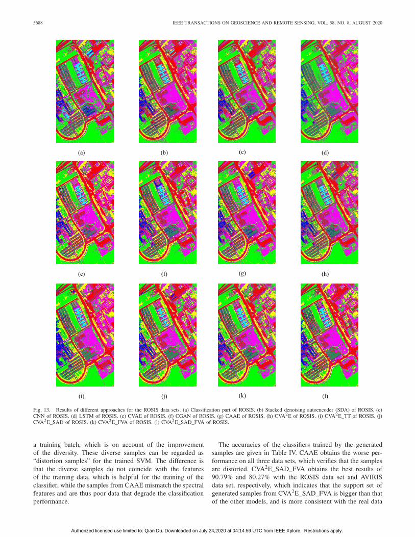
Fig. 13. Results of different approaches for the ROSIS data sets. (a) Classification part of ROSIS. (b) Stacked denoising autoencoder (SDA) of ROSIS. (c)CNN of ROSIS. (d) LSTM of ROSIS. (e) CVAE of ROSIS. (f) CGAN of ROSIS. (g) CAAE of ROSIS. (h) CVA2E of ROSIS. (i) CVA2E_TT of ROSIS. (j)CVA2E_SAD of ROSIS. (k) CVA2E_FVA of ROSIS. (l) CVA2E_SAD_FVA of ROSIS.

a training batch, which is on account of the improvementof the diversity. These diverse samples can be regarded as“distortion samples” for the trained SVM. The difference isthat the diverse samples do not coincide with the featuresof the training data, which is helpful for the training of theclassifier, while the samples from CAAE mismatch the spectralfeatures and are thus poor data that degrade the classificationperformance.

The accuracies of the classifiers trained by the generatedsamples are given in Table IV. CAAE obtains the worse per-formance on all three data sets, which verifies that the samplesare distorted. CVA2E_SAD_FVA obtains the best results of90.79% and 80.27% with the ROSIS data set and AVIRISdata set, respectively, which indicates that the support set ofgenerated samples from CVA2E_SAD_FVA is bigger than thatof the other models, and is more consistent with the real data



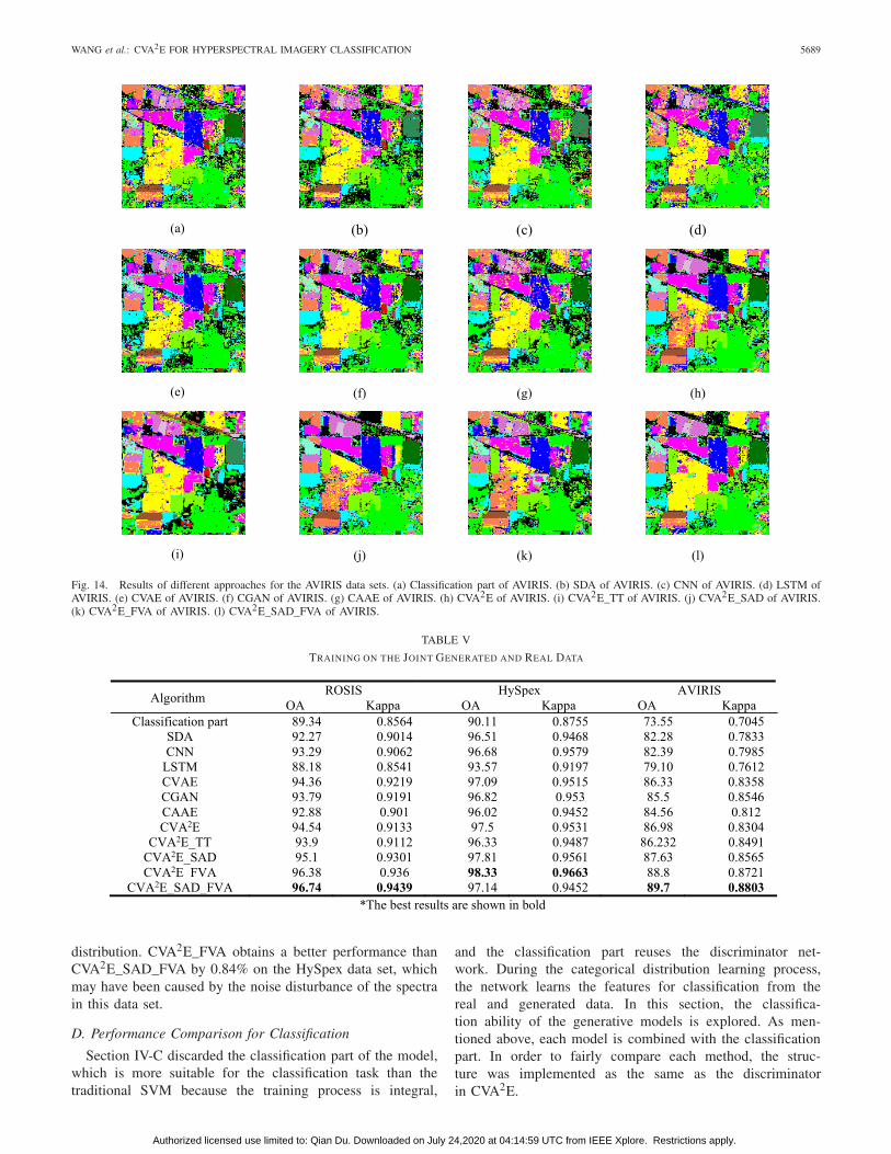
Fig. 14. Results of different approaches for the AVIRIS data sets. (a) Classification part of AVIRIS. (b) SDA of AVIRIS. (c) CNN of AVIRIS. (d) LSTM ofAVIRIS. (e) CVAE of AVIRIS. (f) CGAN of AVIRIS. (g) CAAE of AVIRIS. (h) CVA2E of AVIRIS. (i) CVA2E_TT of AVIRIS. (j) CVA2E_SAD of AVIRIS.(k) CVA2E_FVA of AVIRIS. (l) CVA2E_SAD_FVA of AVIRIS.

TABLE V

TRAINING ON THE JOINT GENERATED AND REAL DATA

distribution. CVA2E_FVA obtains a better performance thanCVA2E_SAD_FVA by 0.84% on the HySpex data set, whichmay have been caused by the noise disturbance of the spectrain this data set.

D. Performance Comparison for Classification

Section IV-C discarded the classification part of the model,which is more suitable for the classification task than thetraditional SVM because the training process is integral,

and the classification part reuses the discriminator net-work. During the categorical distribution learning process,the network learns the features for classification from thereal and generated data. In this section, the classifica-tion ability of the generative models is explored. As men-tioned above, each model is combined with the classificationpart. In order to fairly compare each method, the struc-ture was implemented as the same as the discriminatorin CVA2E.



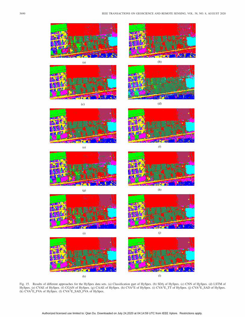
Fig. 15. Results of different approaches for the HySpex data sets. (a) Classification part of HySpex. (b) SDA of HySpex. (c) CNN of HySpex. (d) LSTM ofHySpex. (e) CVAE of HySpex. (f) CGAN of HySpex. (g) CAAE of HySpex. (h) CVA2E of HySpex. (i) CVA2E_TT of HySpex. (j) CVA2E_SAD of HySpex.(k) CVA2E_FVA of HySpex. (l) CVA2E_SAD_FVA of HySpex.



In this experiment, the training process of the classificationpart was divided into two stages. The first was with the vari-ational inference and the adversarial training process, wherethe classification part was trained with the real data. When thegame converged or the training epochs approached a certainnumber, the output from the generator was regarded as areliable data pair(x; y). The classification part was then trainedby the hybrid of the generated and real data. The mainstreamdeep learning algorithms such as SDA, LSTM, and CNNwere chosen as comparative methods. The “Classification part”was extracted as an independent network, which was trainedusing the real labeled data to carry out the classificationtask. Moreover, to verify the valid of augmented samplesfrom CVA2E, we include additional experiment “CVA2E_TT,”which trained on the real labeled data without any dataaugmentation.

Table V shows that CVA2E_SAD_FVA obtains the bestresults of 96.74% and 89.7% with the ROSIS data set andAVIRIS data set, respectively. CVA2E_FVA obtains the bestresult of 98.33% with the HySpex data set. HySpex andAVIRIS data sets. LSTM obtains the worst performance onROSIS data set. CVA2E with two training stages outperformsthat without any data augmentation, which demonstrates thatCVA2E can provide sufficient generative samples to improvethe classification performance. The results of each genera-tive model are better than those based on the traditionalSVM classifier as shown in Table III. This proves thatCVA2E_SAD_FVA is more effective at excavating efficientfeatures for classification. Figs. 13–15 show the results ofclassification by each model.

V. CONCLUSION

In this article, an innovative generative network namedCVA2E has been proposed, which combines variational infer-ence and an adversarial training process to obtain a morepowerful performance. From the visualization analysis onthree standard hyperspectral data sets, we showed that CVA2Ecan outperform the other methods in its capacity for spectralsynthesis. Moreover, to understand the fine-grained spectraldistribution characteristics of individual hyperspectral pixels,the spectral angle distance and vectorial angle measurementare introduced in the loss calculation of CVA2E. The improvedCVA2E showed a superior performance in the spectral synthe-sis of different categories. To demonstrate the ability of thegenerated samples for the classification task, three kinds ofscenarios were carried out, and all the results showed that theproposed model gave the best performance.

In our future work, spatial–spectral features will be takeninto account in CVA2E. In addition, the denoising abilitywill also be considered during the generative process for theapplications of low signal-to-noise ratio data.

ACKNOWLEDGMENT

The authors would like to thank Prof. D. Landgrebe andProf. P. Gamba for providing the data used in the experiments.

REFERENCES

[1] K. Tan, J. Zhu, Q. Du, L. Wu, and P. Du, “A novel tri-training techniquefor semi-supervised classification of hyperspectral images based ondiversity measurement,” Remote Sens., vol. 8, no. 9, p. 749, Sep. 2016.

[2] K. Tan, “Hyperspectral remote sensing image classification basedon support vector machine,” J. Infr. Millim. Waves, vol. 27, no. 2,pp. 123–128, Dec. 2008.

[3] D. Ou, K. Tan, Q. Du, J. Zhu, X. Wang, and Y. Chen, “A novel tri-training technique for semi-supervised classification of hyperspectralimages based on diversity measurement,” Remote Sens., vol. 11, no. 6,p. 654, 2019.

[4] A. Krizhevsky, I. Sutskever, and G. E. Hinton, “ImageNet classificationwith deep convolutional neural networks,” Commun. ACM, vol. 60, no. 6,pp. 84–90, May 2017.

[5] F. A. Gers, J. Schmidhuber, and F. Cummins, “Learning to forget:Continual prediction with LSTM,” in Proc. 9th Int. Conf. Artif. NeuralNetw. (ICANN), Edinburgh, U.K., 1999, pp. 850–855.

[6] X. Wang, K. Tan, Q. Du, Y. Chen, and P. Du, “Caps-TripleGAN: GAN-assisted CapsNet for hyperspectral image classification,” IEEE Trans.Geosci. Remote Sens., vol. 57, no. 9, pp. 7232–7245, Sep. 2019.

[7] K. Tan, F. Wu, Q. Du, P. Du, and Y. Chen,“A parallel Gaussian–Bernoullirestricted Boltzmann machine for mining area classification with hyper-spectral imagery,” IEEE J. Sel. Topics Appl. Earth Observ. Remote Sens.,vol. 12, no. 2, pp. 627–636, Feb. 2019.

[8] D. P. Kingma and M. Welling, “Auto-encoding variational Bayes,” 2013,arXiv:1312.6114. https://arxiv.org/abs/1312.6114

[9] I. Goodfellow et al., “Generative adversarial nets,” in Proc. Adv. NeuralInf. Process. Syst., 2014, pp. 2672–2680.

[10] A. Makhzani, J. Shlens, N. Jaitly, I. Goodfellow, and B. Frey,“Adversarial autoencoders,” 2015, arXiv:1511.05644. [Online]. Avail-able: https://arxiv.org/abs/1511.05644

[11] J. Bao, D. Chen, F. Wen, H. Li, and G. Hua, “CVAE-GAN: Fine-grainedimage generation through asymmetric training,” in Proc. IEEE Int. Conf.Comput. Vis. (ICCV), Oct. 2017, pp. 2764–2773.

[12] A. B. L. Larsen, S. K. Sønderby, H. Larochelle, and O. Winther,“Autoencoding beyond pixels using a learned similarity metric,” 2015,arXiv:1512.09300. [Online]. Available: https://arxiv.org/abs/1512.09300

[13] M. Arjovsky, S. Chintala, and L. Bottou, “Wasserstein GAN,” 2017,arXiv:1701.07875. [Online]. Available: https://arxiv.org/abs/1701.07875

[14] X. Mao, Q. Li, H. Xie, R. Y. Lau, Z. Wang, and S. P. Smolley,“Least squares generative adversarial networks,” in Proc. IEEE Int. Conf.Comput. Vis., Venice, Italy, Oct. 2017, pp. 2794–2802.

[15] J. Feng, H. Yu, L. Wang, X. Cao, X. Zhang, and L. Jiao, “Classificationof hyperspectral images based on multiclass spatial-spectral generativeadversarial networks,” IEEE Trans. Geosci. Remote Sens., vol. 57, no. 8,pp. 5329–5343, Mar. 2019.

[16] M. Zhang, M. Gong, Y. Mao, J. Li, and Y. Wu, “Unsupervised featureextraction in hyperspectral images based on Wasserstein generativeadversarial network,” IEEE Trans. Geosci. Remote Sens., vol. 57, no. 5,pp. 2669–2688, May 2019.

[17] Y. Duan, X. Tao, M. Xu, C. Han, and J. Lu, “GAN-NL: Unsupervisedrepresentation learning for remote sensing image classification,” in Proc.IEEE Global Conf. Signal Inf. Process. (GlobalSIP), Anaheim, CA,USA, Nov. 2018, pp. 375-379.

[18] L. Zhu, Y. Chen, P. Ghamisi, and J. A. Benediktsson, “Generativeadversarial networks for hyperspectral image classification,” IEEE Trans.Geosci. Remote Sens., vol. 56, no. 9, pp. 5046–5063, Sep. 2018.

[19] A. Odena, C. Olah, and J. Shlens, “Conditional image synthesis withauxiliary classifier GANs,” in Proc. 34th Int. Conf. Mach. Learn.,Sydney, NSW, Australia, vol. 70, 2017, pp. 2642–2651.

[20] Y. Xu, B. Du, and L. Zhang, “Can we generate good samples forhyperspectral classification?—A generative adversarial network basedmethod,” in Proc. IEEE Int. Geosci. Remote Sens. Symp. (IGARSS),Valencia, Spain, Jul. 2018, pp. 5752–5755.

[21] D. Wang et al., “Early tomato spotted wilt virus detection usinghyperspectral imaging technique and outlier removal auxiliary classifiergenerative adversarial nets (OR-AC-GAN),” in Proc. ASABE Annu. Int.Meeting, Detroit, MI, USA, 2018, p. 1.

[22] N. Audebert, B. L. Saux, and S. Lefèvre, “Generative adversarialnetworks for realistic synthesis of hyperspectral samples,” in Proc. IEEEInt. Geosci. Remote Sens. Symp. (IGARSS), Valencia, Spain, Jul. 2018,pp. 4359–4362.

[23] D. Ma, P. Tang, and L. Zhao, “SiftingGAN: Generating and siftinglabeled samples to improve the remote sensing image scene classificationbaseline in vitro,” IEEE Geosci. Remote Sens. Lett., vol. 16, no. 7,pp. 1046–1050, Jul. 2019.



[24] I. Gemp, I. Durugkar, M. Parente, M. D. Dyar, and S. Mahadevan,“Inverting variational autoencoders for improved generative accu-racy,” 2016, arXiv:1608.05983. [Online]. Available: https://arxiv.org/abs/1608.05983

[25] M. Gong, X. Niu, P. Zhang, and Z. Li, “Generative adversarial networksfor change detection in multispectral imagery,” IEEE Geosci. RemoteSens. Lett., vol. 14, no. 12, pp. 2310–2314, Dec. 2017.

[26] Y. Su, J. Li, A. Plaza, A. Marinoni, P. Gamba, and S. Chakravortty,“DAEN: Deep autoencoder networks for hyperspectral unmixing,” IEEETrans. Geosci. Remote Sens., vol. 57, no. 7, pp. 4309–4321, Jul. 2019.

[27] M. Mirza and S. Osindero, “Conditional generative adversar-ial nets,” 2014, arXiv:1411.1784. [Online]. Available: https://arxiv.org/abs/1411.1784

[28] F. A. Kruse, “Mapping spectral variability of geologic targets usingairborne visible/infrared imaging spectrometer (AVIRIS) data and acombined spectral feature/unmixing approach,” Proc. SPIE, vol. 2480,pp. 213–224, Jun. 1995.

[29] K. Simonyan and A. Zisserman, “Very deep convolutional networksfor large-scale image recognition,” 2014, arXiv:1409.1556. [Online].Available: https://arxiv.org/abs/1409.1556

Xue Wang received the B.S. degree in geographicinformation system and the Ph.D. degree in pho-togrammetric and remote sensing from the ChinaUniversity of Mining and Technology, Xuzhou,China, in 2014 and 2019, respectively.

He is currently a Post-Doctoral Researcher withEast China Normal University, Shanghai, China.His research interests include the hyperspectralimagery processing, deep learning, and ecologicalmonitoring.

Kun Tan (Senior Member, IEEE) received the B.S.degree in information and computer science fromthe Hunan Normal University, Changsha, China,in 2004, and the Ph.D. degree in photogrammetricand remote sensing from the China University ofMining and Technology, Xuzhou, China, in 2010.

From September 2008 to September 2009, he wasa Joint Ph.D. Candidate of remote sensing withthe Columbia University, New York, NY, USA.From 2010 to 2018, he was with the Departmentof Surveying, Mapping and Geoinformation, China

University of Mining and Technology. He is currently a Professor with theEast China Normal University, Shanghai, China. His research interests includehyperspectral image (HSI) classification and detection, spectral unmixing,quantitative inversion of land surface parameters, and urban remote sensing.

Qian Du (Fellow, IEEE) received the Ph.D. degreein electrical engineering from the University ofMaryland Baltimore County, Baltimore, MD, USA,in 2000.

She is currently the Bobby Shackouls Professorwith the Department of Electrical and ComputerEngineering, Mississippi State University, Missis-sippi State, MS, USA. Her research interests includehyperspectral remote sensing image analysis, patternrecognition, and machine learning.

Dr. Du served as a Co-Chair for the Data FusionTechnical Committee of the IEEE Geoscience and Remote Sensing Society(GRSS) from 2009 to 2013 and the Chair for the Remote Sensing and MappingTechnical Committee of the International Association for Pattern Recognition(IAPR) from 2010 to 2014. She currently serves as the Chief Editor of theIEEE JOURNAL OF SELECTED TOPICS IN APPLIED EARTH OBSERVATIONS

AND REMOTE SENSING.

Yu Chen received the master’s degree in photogram-metry and remote sensing from the China Universityof Mining and Technology (CUMT), Xuzhou, China,in 2012, and the Ph.D. degree in earth and planetaryscience from the University of Toulouse, Toulouse,France, in 2017.

She worked as an Assistant Researcher with theGéoscience Environnement Toulouse (GET) Labora-tory, French National Center for Scientific Research,Paris, France, in 2013. She is currently a Lecturerwith CUMT. Her research interest is synthetic aper-

ture radar (SAR) interferometry, with particular emphasis on its applicationfor geophysical studies.

Peijun Du (Senior Member, IEEE) is currently aProfessor of photogrammetry and remote sensingwith the Department of Geographic InformationSciences, Nanjing University, Nanjing, China, andalso the Deputy Director of the Key Laboratoryfor Satellite Surveying Technology and Applica-tions, National Administration of Surveying andGeoinformation. His research interests are remotesensing image processing and pattern recognition,remote sensing applications, hyperspectral remotesensing information processing, multisource geospa-

tial information fusion and spatial data handling, integration and applica-tions of geospatial information technologies, and environmental informationscience.

Prof. Du is an Associate Editor of IEEE GEOSCIENCE AND REMOTESENSING LETTERS.


CVA - E: A Conditional Variational Autoencoder With an ...

Documents

Transcript of CVA - E: A Conditional Variational Autoencoder With an ...