CSIRO-EPA Melbourne Aerosol Study. Final Report J.L. Gras ...
194
SYSTEM CSIRO-EPA Melbourne Aerosol Study. Final Report J.L. Gras, R.W. Gillett, S.T. Bentley, G.P. Ayers, and T. Firestone CSIRO Division of Atmospheric Research March 1992 C.S.I.RO. t^VlSsONOF ATfy^SPf-ERfC research aspendale VIC.
-
Upload
khangminh22 -
Category
Documents
-
view
1 -
download
0
Transcript of CSIRO-EPA Melbourne Aerosol Study. Final Report J.L. Gras ...

SYSTEM
CSIRO-EPA Melbourne Aerosol Study.
Final Report
J.L. Gras, R.W. Gillett, S.T. Bentley, G.P. Ayers,and T. Firestone
CSIRO Division of Atmospheric Research
March 1992
C.S.I.RO.t^VlSsONOF
ATfy^SPf-ERfCresearchaspendale
VIC.

This study report is presented as three sections:
Part A comprises a report on the ambient study design, results
and discussion.
Part B comprises a report on the design and results of a studyof aerosol sources.
Part C is a data summary.
LIBRARY
C.S1R.0.
DfVISIOfhlF
A"jM)SFl-EF!jCRESEA.F1CH
A^EhSALE
v'k;.

U9R^\RY
C.ai.flO.
OF
AT^)SP{-€R3C
REScAROI
ASF£?"i(}Ai£
VK).
Broadmeadows
MelbourneAirport
Preston
Heidelbero
;ALPHINGTONB Templestowe
Sunshiny
FOOTSCRAY^vvmelbourne Baiwyn
Nunawading
Richmond
Newport
St KildaAltona
BentleighBrighton
Springvale
Sandnngham
Dandenong
Mordialloc
•tAspendale
Map of Melbourne and surrounding suburban areas showing
the locations of the Alphington and Footscray sampling
sites.

PART A: AMBIENT STUDY AND INTERPRETATION
Contents page
Executive svimmary 4
Tables. 7
Figures 8
1. Introduction 13
2. Experiment description 13
2.1 Background-Pilot study 13
2.2 Study design 13
2.3 Sampling procedures
ambient sites, source studies and instrumentation 14
2.4 Analytical techniques 16
2.4.1 Chemical Measurements 16
2.4.2 Physical measurements 18
2.4.3 Particle sizing 19
2.4.4 Scattering coefficient (dry) Bsd 19
2.4.5 Data editing 19
3. Analyses and interpretation 20
3.1 Analytical techniques, intercomparisons,
data base 20
3.1.1 Comparison of Fluoropore and Nuclepore
collected mass 20
3.1.2 Comparison of PIXE elemental and soluble
ion concentrations 23
3.2 Scattering and Fine Particle Mass (FPM) 27
3.3 Fine Particle Mass (FPM) 32
3.3.1 Calculated and observed FPM - 32
3.3.2 Composition of FPM 35
3.4 Seasonal variation carbon 38
3.5 Bsd, Bap 45
3.5.1 Annual cycle of Bsd 45
3.5.2 Bap 4 5
3.6 Source contributions to the FPM and Bsd 45
3.7 Seasonal changes of source contributions 51
3.7.1 Aerosol acidity /Photochemistry /nss-S04 55
3.8 Late autumn early winter 64
3.9 Multiple linear regression models for FPM -
source contributions 72
3.10 Multiple linear regression models for Bsd -
source contributions 82
3.11 Organic trace compounds 90
3.12 Concluding.comments 93
4. Acknowledgements 95
5. References 96
APPENDIX 1, MLR model mass contributions 100
APPENDIX 2, MLR model Bsd contributions 108

Executive sxumnary
Ttie study
The Melbourne Aerosol Study was a collaborative projectcarried out by CSIRO Division of Atmospheric Research and the
Victorian EPA between April 1990 and February 1991. The studysought to understand the chemistry and microphysics of aerosol
particles responsible for periods of reduced visibility inMelbourne during this period. To achieve this, particles withradii less than 1.25 ^im radius were collected for analysis attwo field sites, Footscray and Alphington. In addition at
. Alphington, a laser particle size spectrometer was used to
measure the particle size distribution in the "opticallyactive" range between 0.045 and 1.5 ̂ m radius. From thesedistributions the size of particles responsible for visibilityreduction was determined to be typically 0.1 to 0.15 jimradius.
A self-contained source-sampling study was included to
characterise a range of aerosol sources known or thought to beimportant contributors to the Melbourne aerosol.
Aerosol samples from both the ambient and source studies were
analysed for fine particle mass (FPM), elemental and organiccarbon, and the concentration of sol;ible ions: hydrogen,
ammonium, calcium, potassium, chloride, nitrate, sulfate and
bromide. PIXE. (Proton Induced X-ray Emission) analyses werecarried out for the elements Al, As, Ba, Hi, Br, Ca, Cl, Cr, -Cu, Fe,- Ga, K, Mn, Ni, P, Pb, Rb, S, Si, Sr, Ti, V, Y and Zn.As well, a range of specific organic compounds (over 70) were
determined quantitatively as possible tracers for combustion
products in selected samples. Aerosol scatteringcoefficients, a range of trace gas concentrations and
meteorological variables were determined in parallel with theambient sampling program by the EPA.
Findings
The major finding of this study is that overall, 66% ofthe fine aerosol mass in Melbourne during the sampled
conditions was comprised of carbon. Elemental carbon, whichis produced only by primary combustion sources, accounts for
about 18% of that carbon. The aerosol carbon fraction is
large by international standards but in absolute concentration
terms the concentrations are reasonably typical of.thoseobserved in other large (developed) cities.
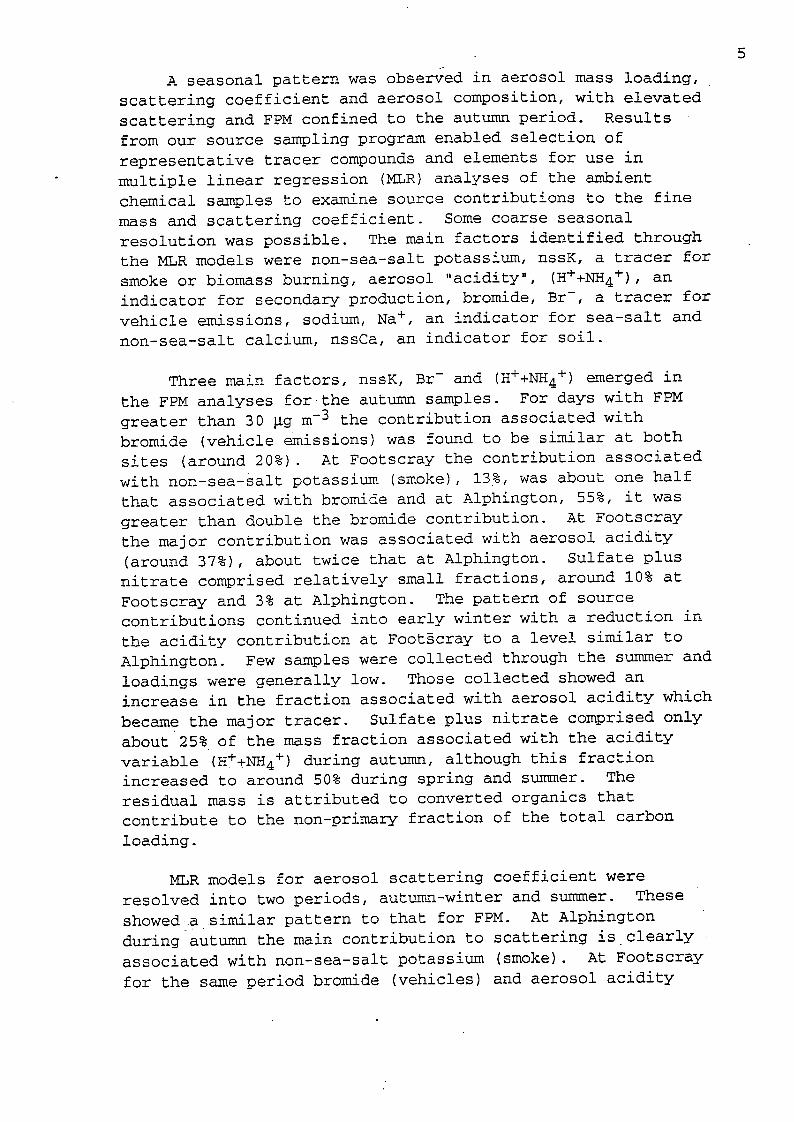
A seasonal pattern was observed in aerosol mass loading,scattering coefficient and aerosol composition, with elevatedscattering and FPM confined to the autumn period. Resultsfrom our source sampling program enabled selection ofrepresentative tracer compounds and elements for use inmultiple linear regression (MLR) analyses of the ambientchemical samples to examine source contributions to the finemass and scattering coefficient. Some coarse seasonalresolution was possible. The main factors identified throughthe MLR models were non-sea-salt potassium, nssK, a tracer forsmoke or biomass burning, aerosol "acidity", , anindicator for secondary production, bromide, Br , a tracer forvehicle emissions, sodium, Na"*", an indicator for sea-salt andnon-sea-salt calcium, nssCa, an indicator for soil.
Three main factors, nssK, Br and emerged in
the FPM analyses for the autumn samples. For days with FPMgreater than 3 0 |ig m"^ the contribution associated withbromide (vehicle emissions) was found to be similar at bothsites (around 20%). At Footscray the contribution associatedwith non-sea-salt potassium (smoke), 13%, was about one halfthat associated with bromide and at Alphington, 55%, it wasgreater than double the bromide contribution. At Footscraythe major contribution was associated with aerosol acidity(around 37%), about twice that at Alphington. Sulfate plusnitrate comprised relatively small fractions, around 10% atFootscray and 3% at Alphington. The pattern of sourcecontributions continued into early winter with a reduction inthe acidity contribution at Footscray to a level similar toAlphington. Few samples were collected through the summer andloadings were generally low. Those collected showed anincrease in the fraction associated with aerosol acidity whichbecame the major tracer. Sulfate plus nitrate comprised onlyabout 25% of the mass fraction associated with the acidityvariable (H'^+NH4"^) during autiomn, although this fractionincreased to around 50% during spring and summer. The
residual mass is attributed to converted organics thatcontribute to the non-primary fraction of the total carbonloading.
MLR models for aerosol scattering coefficient were
resolved into two periods, autumn-winter and summer. Theseshowed a similar pattern to that for FPM. At Alphingtonduring autumn the main contribution to scattering is clearlyassociated with non-sea-salt potassium (smoke). At Footscray
for the same period bromide (vehicles) and aerosol acidity

(secondary production) were major contributors, while massassociated with potassium was a minor component. During
summer the data for the sites were combined and showed that
the major contribution was from aerosol acidity (secondaryproduction) with a minor contribution from bromide (vehicles),potassium (smoke) was not significant.
Conclusions
Because of unusual meteorological conditions during the
study period, fewer widespread visibility-reducing events wereobserved than were expected from the historical record. Even
so, the present study has shown that reduced visibility inMelbourne is associated with fine aerosol mass and that the
major component of this is carbon. During autumn when reducedvisibility was most common the major contribution to theaerosol mass came from-organic carbon compounds.
MLR models were used to show that both the FPM and scattering-
coefficient increases at Alphington were predominantly
associated with non-sea-salt potassium, a smoke tracer. It
was not possible to distinguish unambiguously between possiblesources for the smoke aerosol that characterised the elevated
scattering in autumn. Both indirect evidence of the seasonal,and time of day, patterns of visibility events point todomestic wood burning. The ratios of organic carbon marker
compounds to elemental carbon are also indicative of a wood-burning source, as distinct from a general biomass burningsource. At Footscray the MLR models indicate that secondaryproduction and vehicle emissions were the main sources inautumn and winter. In summer at both locations secondary
production is the indicated major source of FPM and scatterwith a smaller contribution from vehicles. For this study
period visibility reduction appears to have been dominated byrelatively localised aerosol sources.
Tables.
Table 1. Alphington, 106 < day < 180 coefficients for
FPM multiple linear regression model 75
Table 2. Footscray, 106 < day < 180 coefficients for
FPM multiple linear regression model 76
Table 3. Alphington, 180 < day < 300 coefficients for
FPM multiple linear regression model 76
Table 4. Footscray, 180 < day < 300 coefficients for ■
FPM multiple linear regression model 76
Table 5. Alphington and Footscray, 300 < day < 425
coefficients for FPM multiple linear
regression model 76
Table 6. Alphington day < 300 coefficients for Bsd
multiple linear regression model 89
Table 7. Footscray day < 300 coefficients for Bsdmultiple linear regression model 89
Table 8. Alphington and Footscray, 300 < day < 425,
coefficients for Bsd multiple linear
regression model 89
Table 9. Concentration ratios of organic compounds,
with molecular weight mw, to elemental carbon
(compound / elC) 93
Figures
Figure 1. Ion balance plot for all valid soluble
extract samples. 21
Figure 2. Gravimetric mass concentration from
samples on Nuclepore and Fluoropore filters. 22
Figure 3. Bromide concentration determined using
PIXE on Nuclepore filters compared with bromide
concentration determined in soluble extracts from
Fluoropore filters. 24
Figure 4. Sulfur concentration determined using
PIXE on Nuclepore filters compared with sulfate
concentration determined in soluble extracts
from Fluoropore filters. 25
Figure 5. Potassium concentration determined using
PIXE on Nuclepore filters compared with potassium
concentration determined in soluble extracts from
Fluoropore filters. 26
Figure 6. Calcium concentration determined using
PIXE on Nuclepore filters compared v/ith calcium
concentration determined in soluble extracts from
Fluoropore filters. 28
Figure 7. Chloride concentration determined using
PIXE on Nuclepore filters compared with chloride
concentration determined in soluble extracts from
Fluoropore filters. 29
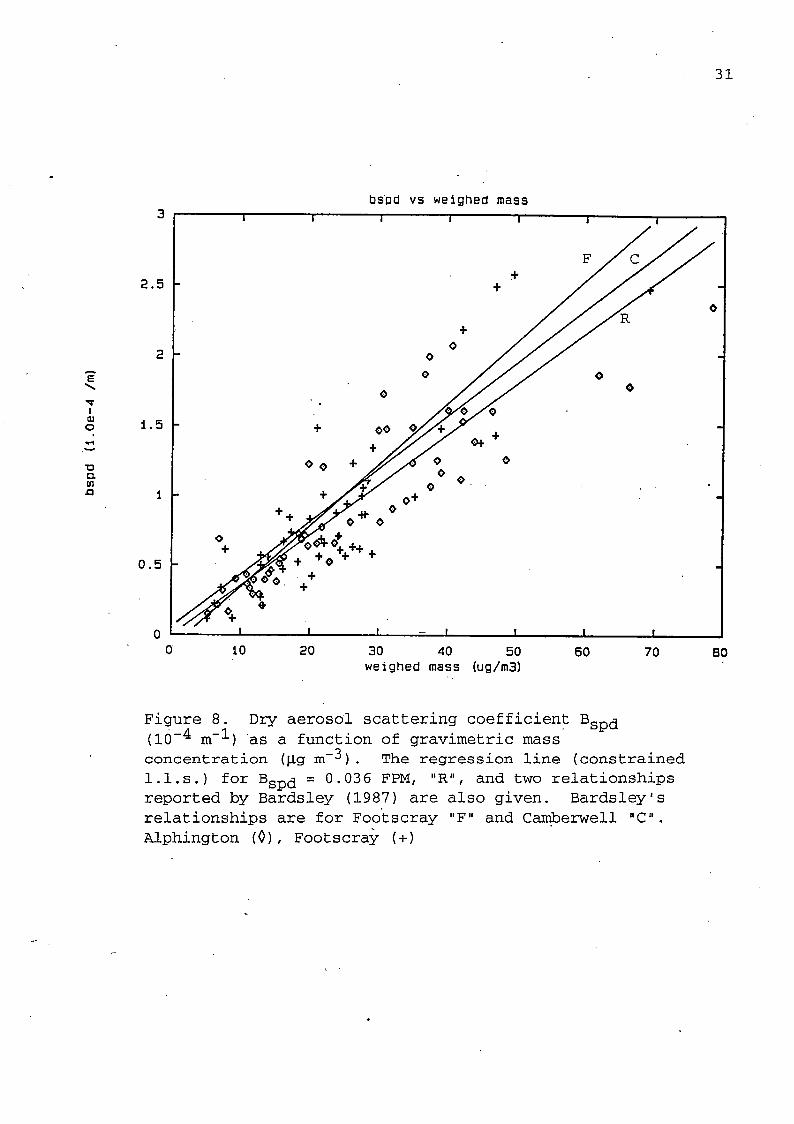
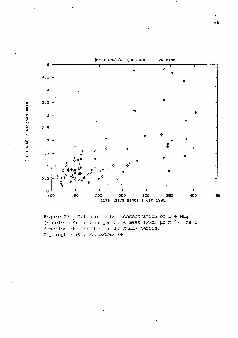
Figure 8. Dry aerosol scattering coefficient Bgp^as a function of gravimetric mass concentration. 31
Figure 9. Variation of scattering efficiency (Bgp,^/FPM) as a function of time during the study period. 33
Figure 10 . Comparison of simnmed fine aerosol
chemical component masses and gravimetric mass. 34
Figure 11. Total carbon mass concentration as a
function of gravimetric mass concentration. 36

9
Figure 12. Variation of total carbon mass concen
tration as a function of time during study period. 37
Figure 13. Elemental carbon mass concentration as
a function of gravimetric mass concentration. 39
Figure 14. Elemental carbon mass concentration as
a function of total carbon mass concentration. 40
Figure 15. Ratio of elemental carbon mass concen
tration to gravimetric mass concentration (Nuclepore
filter) as a function of time during study period. ' 41
Figure 16. Ratio of total carbon concentration to
elemental carbon concentration as a function of time
during study period. 42
Figure 17. Cumulative concentrations of inorganic
components, inorganic sum plus elemental carbon and
inorganic sum plus total carbon, as a function of
time during the study period, at Alphington. 43
Figure 18. Cumulative concentrations of inorganic
components, inorganic sum plus elemental carbon and
inorganic sum plus total carbon, as a function of
time during the study period, at Footscray. 44
Figure 19. Measured scattering coefficient Bg^ (airplus dry aerosol) as a function of time during
the study period. 46
Figure 20. Ratio of scattering coefficient to
aerosol absorption coefficient as a function of timeduring the study period. 47
Figure 21. Ratio of sea-salt mass to gravimetric
mass concentrations as a function of gravimetric
mass concentration. 48
Figure 22. Sea-salt mass loadings as a function
of time during the study period. 49
Figure 23. Ratio of sea-salt mass to gravimetricmass concentration as a function of time during the
study period. 50

10
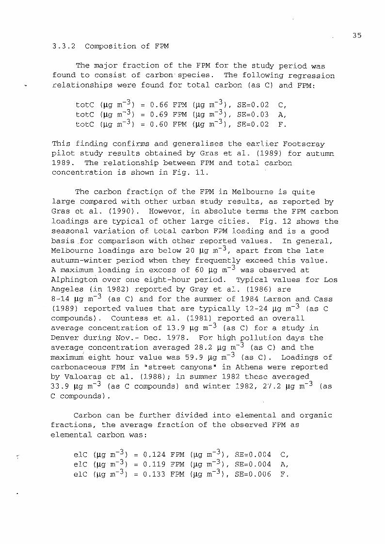
Figure 24. Crustal (soil) fraction of FPM (by mass)based on pixFe and pixSi concentrations, as afunction of gravimetric mass. 52
Figure 25. Crustal (soil) fraction of FPM (by mass)based on pixSi, pixAl and non-sea-salt pixCaconcentrations, as a function of time during the
study period. 53
Figure 26. Variation of non-sea-salt calciumconcentration, as a function of time during the
study period. 54
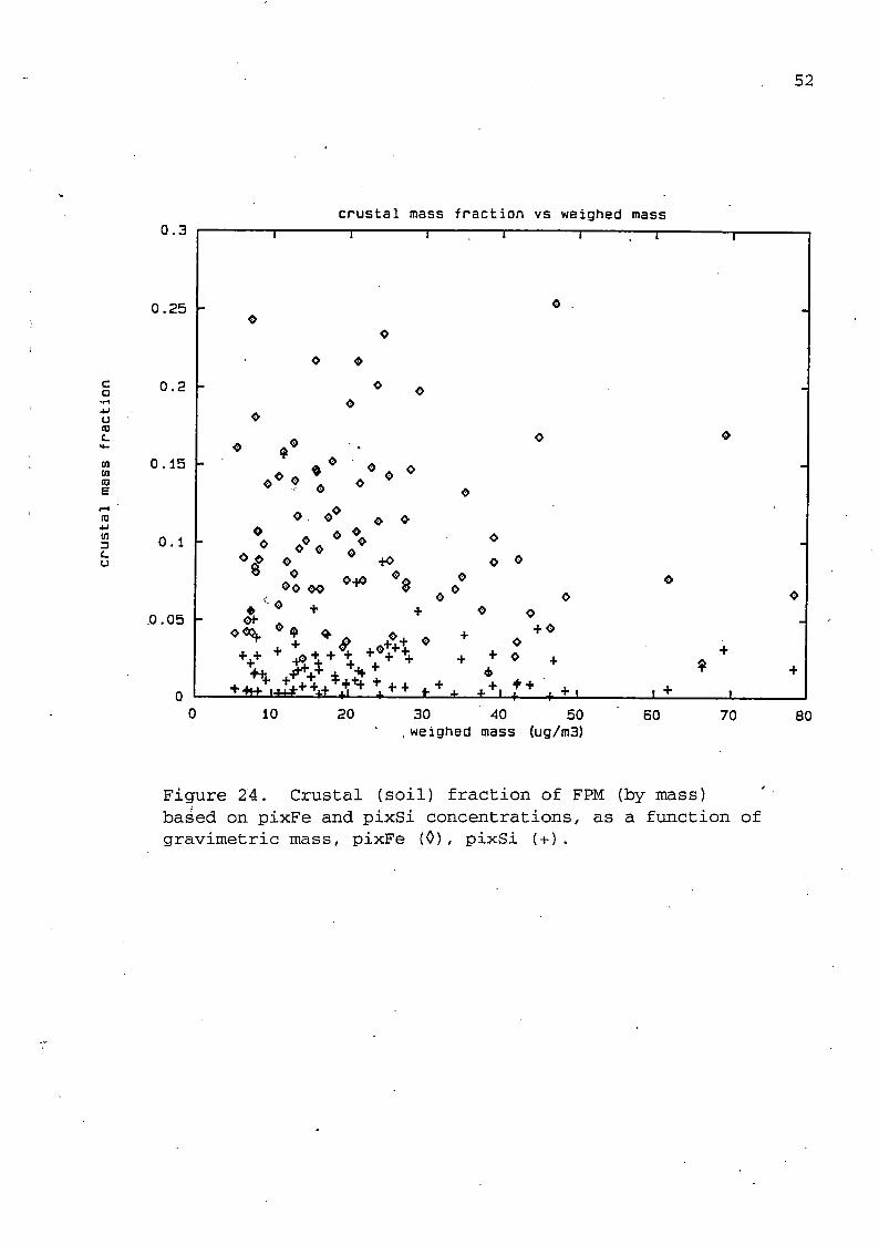
Figure 27. Ratio of molar concentration of H++ NH^"^to fine particle mas, as a function of time duringthe study period. . _ 56
Figure 28. NSS-SO4 mass concentration, as afunction of time during the study period. 57
Figure 29. Ozone concentration as a function of timeduring the study period. 58
Figure 30. Ratio of concentrations of NO2/NO, as afunction of time during the study period. 59
Figure 3L. Relationship between nss-S04 and H++ NH4"^in three time periods. These are: prior to July1990, August-October 1990, and after October 1990. 60
Figure 32. Concentration ratio (H"'"+ NH4'^)/ nss-S04^as a function of time during the study period. 61
Figure 33. Ratio of mass concentrations of nitrateto gravimetric mass, as a function of time during thestudy period. 62
Figure 34. Molar concentration ratios of bromide andlead (pixBr/pixPbl) as a function of time during thestudy period. 63
Figure 35. Concentration ratio of non-sea-saltpotassium and fine particle mass (Nuclepore filter)as a function of time during the study period. 65

11
Figure 36. Ratio of potassium concentration and
scattering coefficient as a function of time during
the study period. 66
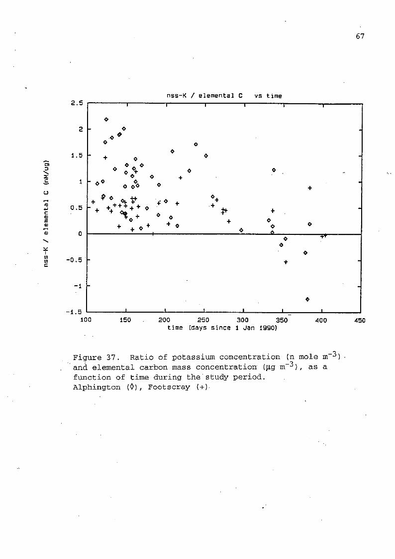
Figure 37. Ratio of potassium concentration and
elemental carbon mass concentration as a function of
time during the study period. 67
Figure 38. Ratio of potassium concentration and leadconcentration as a function of time during the study
period. 68
Figure 39. Ratio of potassium concentration and
sodium concentration as a function of time during the
study period. 69
Figure 40. Ratio of chloride concentration and
sodium concentration as a function of time during the
study period. 70
Figure 41. Mass concentration ratio of phosphorous
to gravimetric mass concentration, as a function of
time during the study period. 71
Figure 42. Ratio of magnesium concentration and
sodium concentration, as a function of time during
the study period. 73
Figure 43. Molar concentration of magnesium as a
function of time during the study period. 74
Figure 44. Calculated cumulative contributions to
fine particle mass at Footscray, as a function oftime during the study period. 78
Figure 45. Calculated cumulative contributions to
fine particle mass at Alphington, as a function of
time during the study period. 79
Figure 46. Calculated cumulative contributions to .
the dry scattering coefficient, Bg^j, at Footscray,as a function of time during the study period. 83
Figure 47. Calculated cumulative contributions to
the dry scattering coefficient, Bg^, at Alphington,as a function of time during the study period. 84

12
Figure 48. Calculated cumulative contributions to
the diry scattering coefficient, at Footscray,
as a function of time during the study period. 85
Figure 49. Calculated cumulative contributions to
the dry scattering coefficient, at Alphington,
as a function of time during the study period. 86
Figure 50. Individual calculated contributions to
the dry scattering coefficient, Bg^, at Footscray,as a function of time during the study period. 87
Figure 51. Individual calculated contributions to
the dry scattering coefficient, Bg^, at Alphington,as a function of time during the study period. 88

13
1. Introduction
This report describes a study of atmospheric aerosol and
visibility reduction in Melbourne conducted in collaboration
by CSIRO Division of Atmospheric Research (DAR) and the EPAV.
Ambient samples were collected for the Melbourne Aerosol Study
during the period April 1990 to February 1991. The main
product of this study is a data set of fine particle chemical
and physical properties linked to ambient air quality data
obtained by the EPAV during the sampling periods. The data
set comprises ambient data obtained at two locations,
Footscray and Alphington and an associated data set of source
chemical compositions obtained under essentially the same
sampling conditions as those used for the ambient sampling.
2. Experiment description
2.1 Background-Pilot study
Widespread reduced visibility events occur quite
frequently in Melbourne in association with stable atmospheric
conditions. The highest frequency of these events is usually
observed during autumn. During these events, visibility is
reduced because of increased light extinction by small aerosol
particles. Both scattering and absorption contribute to this
extinction.
A pilot study examining the relationship between the fine
fraction aerosol (r < 1.25 |im) and visibility was carried out
in Melbourne during April-May 1989 (Gras et al. 1989) . This
short, single site study revealed that at Footscray, during
autumn 1989, carbon species on average constituted around 70%
of the fine aerosol mass. It also showed that the major
fraction of the carbon species was in fact organic and that
organic carbon constituted around 50% of the fine particle
mass during periods with pronounced visibility reduction.
These findings and others relating to the composition and
microphysics of the Melbourne aerosol and its relation to
visibility were reported by Gras et al. (1989) however these
initial findings must be qualified by the very short duration
and single location of the pilot study.
2.2 Study design
The present Melbourne Aerosol Study was planned to expand
on the findings of the pilot study by taking measurements at
two sites over a longer period. Based on the statistical

14
frequency of low visibility events a three months study was
designed for autumn 1990. During the actual study period it
became apparent that the conditions experienced in 1990 wereless settled than usual and consequently low visibility events
occurred less frequently than expected. In response, the
study period was extended to include almost a complete year of
observations.
It was evident from the pilot study that a better
understanding of local source composition profiles, compatiblewith the ambient sampling procedures, was required. Thus the
Melbourne Aerosol Study also incorporated a study of the
composition of aerosol from several selected sources. These
included vehicles using leaded fuel and vehicles using
unleaded fuel, light diesels, woodstoves and biomass burning(gum leaves and twigs,,and dry grass hay). A description ofthe source study and a summary of the results are given inPart B of this report.
The principal measurements for the ambient study are the(dry) volume scattering and aerosol absorption coefficientsand fine particle (r < 1.25 |im) chemical composition. Thiscomprises soluble inorganic species, elemental composition,total and elemental .carbon content and for a subset of samples
organic marker compounds. The source profiles are similar butexclude the scattering coefficient determination.
2.3 Sampling procedures: ambient sites, source studies andinstrumentation.
Sampling sites for the Melbourne aerosol visibility studywere located at Footscray and Alphington. These were selectedfor their locations relative to the main city area and a
previous record of high incidence of sustained visibilityreduction events. Footscray is an inner suburb approximately8 km west of the city centre, this was also the site of thepilot study. Alphington is located close (1 km) to the YarraRiver around 7.5 km north-east of the city centre, (see Map,
page 2). Instrumentation at Footscray was housed in the EPAVair quality monitoring station and at Alphington in a CSIROBAR mobile laboratory located within the EPAV air qualitymonitoring station site.
Particles were collected for chemical and physical
analyses using automated low volume samplers with a stackinlet height 4 m above ground level. The samplers used in the

15
Melbourne aerosol visibility study differed in several ways
from those used in previous studies, including the pilot
study. A new 75 mm diameter inlet stack system was
constructed to give a low Reynolds niomber at the design
sampling rate and thus minimise turbulent deposition. Other
improvements included reduction in the number of bends in the
inlet to two broad 90° bends. A single inlet impaction stagewas incorporated to provide a consistent cut size for the
different sampling filters; this was located at the inlet to a
large plenum from which all filter housings connected with
short, direct inlets.
As in the previous samplers the design allows for the
parallel collection on three different filters- simultaneously
and the separate logging of the three sample flows. Up to
five different sets of filters can be exposed sequentially.
The sampler is controlled by a personal computer (PC) which
receives the (dry) scattering coefficient signal from the EPAV
integrating nephelometer. The PC is also used to log the
operation of the sampler, flow rates, filter sequence,
pressure drop etc. At both locations the nephelometer used
was an MRI 1550B with a heated inlet, located within the air
quality monitoring station.
Aerosol samples were taken over eight hour periods. The
actual sample volumes depend on the filter substrate type.
These are typically 24 m^ for glass filters, 15 m^ for PTFEfilters and 12 m^ for Nuclepore filters, the actual integratedsample volumes are given in the main data file (as floF, floN
and floG for the Fluoropore, Nuclepore and glass filters
respectively, see Part C Table C2).
Only the fine aerosol fraction was collected (r < 1.25
pm) for analysis, the large fraction being removed by the
greased preimpaction stage. For this study each set of
filters comprised three 47mm diameter filters, a 1.0 [im
Fluoropore PTFE for inorganic analyses, a 1.0 )im Nuclepore
filter used for absorption coefficient, elemental carbon and
PIXE elemental analysis and a prebaked Gelman A/E glass fibre
filter for total carbon determination and organic marker
determination.
PTFE and Nuclepore filters were stored in sealed, plastic
petri dishes before and after collection and Glass filters
were stored in aluminium foil. After collection the filters
were refrigerated until analysis.

16
The sampler was operated automatically throughout the
study, selecting occasions where the measured scattering
coefficient was greater than 1.175 x lO""^ or LVD < 40 km.In addition, during the autumn-winter period, samples were
initiated manually when an automatic sample had not been taken
for one week. Approximately 10% of the loaded sample PTFE and
Nuclepore filters were removed from the sampler without being
exposed to act as field blanks. Glass filters were removed
after one week whether exposed or unexposed, unexposed filters
were used as blanks.
2.4 Analytical techniques
2.4.1 Chemical Measurements
(i) Soluble inorganic•ions
Soluble ion concentrations were determined in aqueous
extracts from the Fluoropore filters. Filters were
transported to and from the study site in clean, closed petri
dishes to avoid loss of material from the filters, or
contamination, during transport. For extraction, filters were
placed into clean polyethylene bags which were also used to
store the extract. Soluble ions were extracted using 20.0 mL
of Milli-Q (HPLC-grade) ̂water after first wetting the filter
with 250 p,L of AR grade methanol. Chloroform (200 p,L) was
added to the extract- to act as a bacteriocide.
The majority of the soluble ion analyses were carried out
by AGAL (Tas.). Atomic absorption spectrophotometry (AA) was
used for determination of sodium, potassium, magnesiijm and
calcium and suppressed ion chromatography (IC) (Dionex AS3
columns with carbonate-bicarbonate eluent) for anions:
chloride, nitrate, sulfate and bromide. Precision for a
single analysis ion concentration is rated at better than
±10%.
Ammonium ion concentration was determined using
colorimetry (indo-phenol blue method, Dal Pont et al. 1974) at
CSIRO DAR. The expected uncertainty for these determinations
is around ±20%. A combination Ross pH electrode was used at
DAR to determine pH; this was standardised at pH 4.10 and 6.97
using low ionic strength pH buffers.

17
(ii) PIXE
Proton induced X-Ray emission analysis (PIXE) was used to
obtain additional information on aerosol composition, in
particular to determine insoluble components such as lead and
other metals. This non-destructive technique provides a large
suite of element concentrations that should be useful for
source identification although in low volume samples such as
these the full suite of elements is not usually detectable.
PIXE analyses were performed by the "Nuclear Science
Application Group" at ANSTO.
Elemental concentrations were determined in the fine
particle mass collected on Nuclepore filters. Elements
determined using PIXE are: As, Ba(l), Br, Ca, Cl, Cr, Cu, Fe,
K, Mn, Ni, P, Pb(l), S, Si, Sr, Ti, and Zn. Not all
determinations include all these species. Where species were
not detected a .null result is indicated in the data tabulation
(see Part C) and reference should be made to Table C7 for
minimum detection limits for the particular species.
(iii) Total carbon
Total fine particle aerosol carbon was determined at
CSIRO DAR for particles collected on glass fibre filters.
These filters were precleaned by baking at 450 °C for six hours
and were then stored in individual aluminium foil packages.
Total carbon was determined by oxidation of the samples to CO2at 800 °C, followed by catalytic conversion to methane and FID
detection. Calibration was by injection of pure CO2.
(iv) Organic Speciation
Organic compounds have been used as vehicle tracers
(Hering.et al. 1984; Pyysalo et al. 1987), as tracers for
woodstoves and biomass burning (Standley and Simoneit, 1987;
Standley and Simoneit, 1990; Hawthorne et al. 1988; Hawthorne
et al. 1989; Edye and Richards, 1991), as tracers for the
natural organic fraction of the primary aerosol (Simoneit,
1985; Simoneit, 1989; Edgerton and Holdren, 1987) and as
tracers of material incorporated in rain (Simoneit and
Mazurek, 1989).
Specific organic compounds were determined on segments of
the same glass filters used to determine total carbon. For
analysis, the area of portions of the glass fibre filters cut
from the filter circle were determined gravimetrically. The
filter sections were then extracted in a 5 ml mixture of
benzene: ethanol: dichloromethane (4.5:1:1.5). Extractions

18
were carried out in glass flasks in an ultrasonic bath for 2
hours at 50 °C. After extraction the samples were evaporated
to about 1 ml and then transferred to a glass vial insert,
evaporated to dryness at ambient temperature and sealed with a
crimp top.
The source samples were analysed first to establish the
range of organic molecules present in the various sources.
Organic compounds were determined using gas chromatography
with a mass spectrometer detector (GCMS). Compounds were
separated in the gas chromatograph on a 25 meter 0.32 mm
diameter 0.17 |im film thickness HPl column using helium as thecarrier gas. Temperature programming was 40-290 °C at 10 °Cmin~^. A Finnigan Mass Selective Detector (MSB) was employed.These analyses were carried out by the Central Science
Laboratory at the University of Tasmania.
2.4.2 Physical measurements
Collected aerosol mass on the Fluoropore and Nuclepore
filters was determined using a microbalance at the EPAV. Both
pre-exposed and exposed filters were equilibrated in the
weighing room for at least 24 hours before each determination.
Weighing was only conducted when the relative humidity was
within a narrow range around 40% RH. Glass filters were not
weighed. This procedure is not appropriate for the glass
filters which shed fibres and lose mass due to clamping in the
filter"holders.
Aerosol light absorption (and elemental carbon
concentration) was determined using a CSIRO monochromatic
photometer at a wavelength of 565 nm, based on the integratingplate method of Lin et al. (1973) (with the "filter facetowards light source" modification). Nuclepore filters wereused, with the absorption of each filter determined before and
after exposure. The volume absorption coefficient wasdetermined from the measured change in filter absorption and
the measured flow through each filter. This method has been
reported to produce an over-estimate of absorption by around
35% (Lewis and Dzubay 1986, Horvath and Habenreich 1989).This must be considered in determination of the aerosol
absorption coefficient but does not impact on thedetermination of elemental carbon mass using this technique
since the mass-specific absorption was determined empiricallyusing the same measurement technique. This empiricalcalibration factor, 7.23 m^ g~^ was determined using pyrolisedacetylene and is similar to other reported values, for example

19
7-11 g~^ (Weiss and Waggoner 1982) and 9.1 and 12.8 g~^(Cowan et al. 1982).
2.4.3 Particle sizing.
Between May 23 - Oct 3 1990 at the Alphington site,
during the periods that filters were exposed, airborne
particles were sized using a Particle Measuring Systems ASASP-
X aerosol particle size spectrometer. A stainless steel tube- '
oven on the inlet, operating at 40 °C was used to dry the
aerosol before sizing. A small personal computer was used to
control the measurement of particle size and flow-rate and
storage of the data. '
Flow rate for the ASASP-X was typically 90 cm^ min~^.Four ranges of 15 size channels were recorded giving 60
channels overall with.nominal limits of 0.05 and 1.5 |im
radius.
Size calibration was by means of mono-disperse
polystyrene latex (PSL) particles at 6 sizes from 0.117 to 1.1
[im radius. The refractive index of these particles, m=l. 6 was
also assumed for atmospheric particles. This value is
consistent with a primarily organic composition. For a given
refractive index, sizing is expected to be accurate to about
5%.
2.4.4 Scattering coefficient (dry)
Scattering coefficients were determined as five - minute
integrations from the EPAV air quality station MRI 1550G
nephelometers at the respective sampling locations. These are
calibrated regularly using Freon 12, and automatic zero and
span checks are made daily. Scattering coefficients were
determined following the EPA procedure for API with no
subtraction of the molecular (air) component but used the 20 °C
calibration values for molecular air and Freon'12. The
calibration values used were 2.1 x 10"^ m~^ for air at 20 °Cand 3.31 x 10"^ m~^ for Freon 12 at 20 °C. The MRI 1550G is abroad band instrument with an effective wavelength of about
470 nm. An approximation to dry aerosol is made by heating
the inlet of the nephelometer to 50°C.
2.4.5 Data editing
Reported concentrations of soluble ions below the minimumdetection limit were replaced with a value of one half the /
minimum detection limit. Concentrations of all chemical

20
species were blank corrected using a subset of unexposed
filters; these were treated identically to sample filters.
The blank - corrected soluble ion concentrations were required
to pass an ion balance test. Ion balances were determined on
the assumption that the measured cations and anions
constituted the entire soluble species. A reduced major axis
regression of the cation and anion sum was calculated. Values
falling outside a ± 3 standard deviation limit were rejected.
The procedure was repeated to convergence. All samples that
had integrated flow values substantially below that expected
for a normal eight hour period were also rejected. The ion
balance for all the remaining samples is shown in Fig. 1.
3. Analyses and interpretation
3.1 Analytical techniques, intercomparisons, data base
The main data base comprising the ambient and source
chemical and physical data and supporting EPAV data is given
in two ASCII files, in PC format in the attached data disk.
Source data are also summarised in Tables B1-B8 (Part B of
this report) and ambient data in Tc.bles C1-C8 (Part C of this
report). Particle size distributions obtained at Alphington
are presented in Appendix 3 (in Part C).
3.1.1 Comparison of Fluoropore and Nuclepore collected mass
Some differences in the collec
different filter types is expected
sample the same size-selected parti
Fluoropore and glass filters are fi
the Nuclepore is a membrane filter,
particles predominantly by diffusic
by interception and impaction for
that for a given flow rate there i
where particles are not caught effi
used the collection efficiency of
been measured to be effectively abs
concentrations for the Fluoropore e
compared in Fig. 2. Regression of
Fluoropore blank-corrected aerosol
average mass collection efficiency
of 88.9 ± 0.9% (in this size range
rate). This 11% difference in coll
tion efficiencies of the
although all three types
cle population. The
bre type filters whereas
Membrane filters collect
n for small particles and
large particles. This means
a range of particle sizes
ciently. At the flow rates
tlhe Fluoropore filters has
olute. Gravimetric mass
nd Nuclepore filters are
the Nuclepore and
mass loadings indicates an
for the Nuclepore filters
and at the operating flow
ection efficiencies may

21
CTOJ
3
m
ca•IH
cin
350
300 -
250 -
200 -
150 -
100 -
50 -
ion balance - ambient samples
50 100 150 200
cations (ueq/1)250 300 350
Figure 1. Ion balance plot for all valid soluble extract
samples (micro equivalents per litre).

22
m
e
OI
D
Ul
enID
E
(U
L.□d0)
1—I
uD
BO
70 -
60 -
50 -
40 -
30 -
20 -
10 -
Nuclepare mass vs Fluropore mass
10 20 30 40 50Fluoropore mass (ug/m3)
60 70 80
Figure 2. Gravimetric mass concentration from samples onNuclepore and Fluoropore filters {|ig m~^) . Indicatedregression (constrained l.l.s.) has slope 0.889.Alphington (0). , Footscray ( + )
23
have some effect on comparison of elemental concentrations
determined using PIXE (on the Nuclepore filters) and elemental
carbon loadings which are also determined using these filters
with the soluble ion concentrations determined in extracts
from the Fluoropore filters. Actual differences will depend
on'the mass-size distribution for each species. In species
where the average particle size is small (compared to the
Nuclepore cutoff size) little difference should be observed.
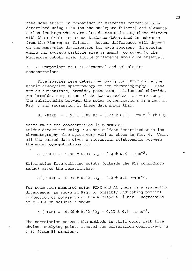
3.1.2 Comparison of PIXE elemental and soluble ion
concentrations
Five species were determined using both PIXE and either
atomic absorption spectroscopy or ion chromatography. These
are sulfur/sulfate, bromide, potassium, calcium and chloride.
For bromide, comparison of the two procedures is very good.
The relationship between the molar concentrations is shown in
Fig. 3 and regression of these data shows that:
Br (PIXE) = 0.96 ± 0.02 Br - 0.23 ± 0.1, nm m"^ (+ SE),
where nm is the concentration in nanomoles.
Sulfur determined using PIXE and sulfate determined with ion
chromatography also agree very well as shown in Fig. 4. Using
all the paired data gives a regression relationship between
the molar concentrations of:
S (PIXE) = 0.96 ± 0.03 SO4 - 0.2 ± 0.6 nm m"^.
Eliminating five outlying points (outside the 95% confidence
range) gives the relationship:
S '(PIXE) = 0.99 ± 0.02 SO4 -0.2+0.4 nm m"^.
For potassium measured using PIXE and AA there is a systematicdivergence, as shown in Fig. 5, possibly indicating partial
collection of potassium on the Nuclepore filter. Regressionof PIXE K on soluble K shows
K (PIXE) = 0.66+0.02 SO4 -0.13+0.9 nm m~3.
The correlation between the methods is still good, with five
obvious outlying points removed the correlation coefficient is0.97 (from 81 samples).

24
PIXE Br vs SQluble Br
T
cn
E
ZC
C.m
UJX
10 15 20
soluble Br (nM/m3)
Figure 3. Bromide concentration (n mole m 2). determinedusing PIXE on Nuclepore filters compared with bromideconcentration (n mole m~^) determined in soluble extractsfrom Fluoropore filters. Indicated,regression line: ■
pixBr = 0.96 sol. br - 0.23 (nmole m"^).Alphington (0), Footscray (+)

25
PIXE S vs soluble S04
T
me
zc
tn
UJX
©+0
30 40
soluble 504 (nM/m3)
Figure 4. Sulfur concentration (n mole m"^) determinedusing PIXE on Nuclepore filters .compared with sulfateconcentration. (n mole m"^) determined in soluble extractsfrom Fluoropore filters. Indicated regression line:
pixS = 0.99 sol. SO4 - 0.2 (nmole m~^).Alphington (0), Footscray (+)

26
PIXE K vs soluble K
T
m
E
C
IDX
6 a
soluble K (nM/m3)
Figure 5. Potassium concentration (n mole m~^).determined using PIXE on Nuclepore filters compared withpotassi\jm concentration (n mole m~^) determined insoluble extracts from Fluoropore filters. Indicatedregression line:
pixK = 0.66 sol. K + 0.13 (nmole m"^).Alphington (0), Footscray {+)

27
Comparison of calcium determined using PIXE and AA is
shown in Fig. 6. At low concentrations the data are noisy but
distributed about the 1:1 line, at higher levels PIXE derived
concentrations are larger. This suggests the presence of some
insoluble calcium probably associated with soil derived
particles.
Chloride concentrations determined using PIXE almost all
fall well below concentrations determined using ion
chromatography as shown in Fig. 7. The reason for this is not
clear, but we consider the soluble extract values to be more
reliable.
Lower concentrations of potassium and chloride obtained
from the Nuclepore-PIXE analyses may be related to size
discrimination in the.Nuclepore filter collections. Sea-salt
is a source of both aerosol potassium and chloride, and the
mass median radius of sea-salt is typically larger than 1 |im.This means that most sea-salt mass will be in the region where
the Nuclepore filters are likely to be size sensitive.
For analyses of the contributions to the fine particle
mass (FPM) and scattering coefficient given in this report,
PIXE derived concentrations for potassium and calcium and
soluble extract values for sulfate, bromide and chloride, have
been used.
3.2 Scattering and Fine Particle Mass (FPM)
Local visual distance (LVD) is an instr-umental measure of
the visual range due to scattering at a sampling point. It is
usually measured using dried sample to remove the major
effects of relative humidity on the ambient aerosol. This
allows a much more direct comparison of the scattering
coefficient with underlying physical and chemical parameters
in the aerosol than would be otherwise possible. LVD is
proportional to the reciprocal of the aerosol volume
scattering coefficient through what is known as Koschmieder's
relationship. Other factors that determine this relationship
are the target contrast ratio and wavelength. In the general
form the relationship is usually given as:
LVD (km)=0.0039/ Bg^ (m (at 550 nm).

28
m
E
ZC
10
o
UJX
Q.
PIXE Ca vs soluble Ca
3 4
soluble Ca (nM/tn3)
Figure 6. Calcium concentration (n mole m~^) determinedusing PIXE on Nuclepore filters compared with calciumconcentration (n mole m"^) determined in soluble extractsfrom Fluoropore filters. A 1:1 reference line isincluded.
Alphington (0), Footscray (+)

29
cn
E
U
lUXM
a
#ii»ni' iMir> © 1+ c»o
PIXE C1 vs soluble C1
r
j_ _L
30 40 50
soluble C1 (nM/m3)
60 70 80
Figure 7. Chloride concentration (n mole m~^.) determinedusing PIXE on Nuclepore filters compared with chlorideconcentration (n mole m~^) determined in soluble extractfrom Fluoropore filters. A 1:1 reference line isincluded.
Alphington (0) , Footscray { + )

30
For the instrumentation used during this study, an MRI 1550G
nephelometer, the relationship
LVD (km) =0.0047/ (m~l) (at 470 nm)
is used. Bg^ ~®spd ®mol' ®sd measured volumescattering coefficient at an effective wavelength of 470 nm.
It comprises a "dry" aerosol component, Bgp^^ (obtained byusing a heated 50 °C inlet) and the scattering coefficient of
®mol•
In the six week pilot study in Footscray (Gras et al.
1989), the aerosol particles responsible for essentially all
of the light scatter at visible wavelengths are shown to be
less than 1 |im in radius, and typically they are around 0.1 to0.2 |lm in radius. The _ same result has been found in thepresent extended study. This is shown in Appendix 3 (in Part
C) by the plots of differential scatter as a function of
particle radius obtained at Alphington from May to September
1990. These were derived by calculating the integrated
scattering coefficient from the aerosol size distribution
measured using a PMS ASASP-X aerosol size spectrometer, also
with a heated (40 °C) inlet. There is a recognised close
correlation between fine particle mass and scattering
coefficient in urban.environments, including Melbourne
(Waggoner and Weiss 1980, Dzubay et al. 1982, Bardsley 1987).
These close correlations are an indirect indication that fine
particles generally dominate aerosol scattering in these
environments. The expected close relationship between the
aerosol scattering coefficient and FPM was observed in the
present study as is shown in Fig. 8. For reference, similar
relationships reported by Bardsley (1987) for two suburban
Melbourne locations, Camberwell and Footscray, are also
included. Overall relationships obtained by (constrained)
linear least squares regression for the present study are:
FPM (|lg m"3) =26.2 Bgp^^ (10"^ m~l) , SE=0.7 [r2 = 0.93] C,FPM (|lg m~3) =27.2 Bgp^ (10~^m~l), SE=1.0 [r2 = 0.94] A,FPM (|lg m~3) =24.8 Bgp^ (10~^m~l), SE=1.0 [r2 = 0.92] F,
or
Bspd (10~^ m"^) = 0.036 FPM (p-g m~3) SE=0.001 C,Bgpd (10~^ m"l) = 0.034 FPM (M,g ) SE=0.001 A,Bgpd (10~^ m~l) = 0.037 FPM (|lg m"^) SE=0.002 F,
31
T
I
OJ
O
■aauia
2.5
2 -
1.5
0.5
bs'pd vs weighed massr~
10 20 30 40 50weighed mass (ug/m3)
60 70 80
Figure 8. Dry aerosol scattering coefficient Bgp^(10"'^ m~^) as a function of gravimetric massconcentration (|lg m"^) . The regression line (constrainedl.l.s.) for Bgpjj = 0.03 6 FPM, "R", and two relationshipsreported by Bardsley (1987) are also given. Bardsley'srelationships are for Footscray "F" and Camberwell "C".Alphington (0) , Footscray (+)

32
where A refers to Alphington, F to Footscray and C the two
sites combined and is the dry aerosol scatteringcoefficient.
Seasonal variation in the aerosol scattering efficiency(Bspd/FPM) is shown in Fig. 9. Relatively close clustering ofthe scattering efficiency points is evident in the late autumn
of 1990 when both Bgp^^ and FPM were elevated. This indicatesa more homogeneous aerosol in late autumn-winter than in
spring-summer when aerosol loadings were lower and possibly
derived from a wider mixture of sources.
3.3 Fine Particle Mass (FPM)
3.3.1 Calculated and observed FPM
Combining the masses of the soluble inorganic species,
total carbon and the most abundant elements (Pb,Zn,Fe,Si)
explains a substantial fraction of the observed FPM.
Constrained regressions give the following relationships
Sum (|lg m~^) = 0.85 FPM (|i.g m~^) , SE=0.02 C,Slim (|j.g m~^) = 0.84 FPM (|lg m~^), SE=0.03 A,Sum (|lg m~2) = 0.85 FPM (|lg m"^) , SE=0.02 F.
If allowance is made for known missing components,
particularly oxygen and hydrogen in organic carbon compounds
(assumed equal to 20% of the organic carbon mass) and
silicates in soils (assumed Si02),-this gives
Slum (|lg m~^) = 0.96 FPM (|lg m~^) , SE=0.02 CSum (|lg m~3) =0.96 FPM (p.g m~3), SE=0.04 ASum (|lg m~^) = 0.95 FPM (p.g m~^), SE=0.02 F.
Given that the particle mass is determined at approximately
40% RH and so some small fraction of water may be present in
the determined FPM, an effective mass closure can be
considered as established with no significant unaccounted
components.
The relationship between calculated mass (with allowance
for compounds) and observed FPM, for the combined data is
shown in Fig. 10.

33
0.11
oi
D\CME
I
0)
O
0101
m
E
•D01
ai•fi
013
TD01
n
100
bspd/welghed mass vs time
0.09
0.08
0.07
0.06
0.05
0.04
0.03
0.02
150 200 250 300 350
time (days since 1 Jan 1990)400 450
Figure 9. Variation of scattering efficiency (Bgp^j/FPM)(IC)^ g~^) as a function of time ciuring the stuciyperiod.
Alphington (0), Footsoray (+)

34
m
E
cn□
uiinIDE
13(UEEDUl
13OJ4Ju0)c.c.ou
go
80
70
60
50
40
30
20
10
corrected summed mass vs weighed mass1 1 1 \ 1 1 ^ 1
-
+
0
0
•
o
0 ̂
+ o^
-
0o
0 +
o
o-
-
1
O
I
0 0
< >
o
• 1 •
10 20 30 40 50
weighed mass (ug/m3)50 70 80
Figure 10. Comparison of summed fine aerosol chemicalcomponent masses and gravimetric mass (|ig m~^) . Organiccarbon is increased by a factor of 1.2 to account forcompounds and Si is assumed to be crustal and in the formSi02. The regression line (constrained l.l.s.) has aslope of 0.96.Alphington (0) , Footscray (+)
35
3.3.2 Composition of FPM
The major fraction of the FPM for the study period was
found to consist of carbon-species. The following regression
relationships were found for total carbon (as C) and FPM:
tote (|lg m~^) = 0.66 FPM (fig m~^), SE=0.02 C,tote (^lg m~3) = 0.69 FPM (^.g m"3) , SE=0.03 A,tote (|lg m~3) =0.60 FPM (|lg m"^) , SE=0.02 F.
This finding confirms and generalises the earlier Footscray
pilot study results obtained by Gras et al. (1989) for autumn
1989. The relationship between FPM and total carbon
concentration is shown in Fig. 11.
The carbon fractign of the FPM in Melbourne is quitelarge compared with other urban study results, as reported by
Gras et al. (1990). However, in absolute terms the FPM carbon
loadings are typical of other large cities. Fig. 12 shows the
seasonal variation of total carbon FPM loading and is a good
basis for comparison with other reported values. In general,
Melbourne loadings are below 2 0 |J.g m~^, apart from the lateautumn-winter period when they frequently exceed this value.
A maximum loading in excess of 60 p.g m"^ was observed atAlphington over one eight-hour period. lypical values for Los
Angeles (in 1982) reported by Gray et al. (1986) are
8-14 |lg m~2 (as G) and for the summer of 1984 Larson and Cass(1989) reported values that are typically 12-24 |lg m"^ (as Ccompounds). Countess et al. (1981) reported an overall
average concentration of 13.9 |lg m"^ (as C) for a study inDenver during Nov.- Dec. 1978. For high pollution days the
average concentration averaged 2 8.2 |ig m~^ (as C) and themaximum eight hour value was 59.9 |ig m~^ (as C) . Loadings ofcarbonaceous FPM in "street canyons" in Athens were reported
by Valoaras et al. (1988); in summer 1982 these averaged
33.9 ^ig m~2 (as C compounds) and winter 1982, 27.2 |ig m~^ (ase compounds).
Carbon can be further divided into elemental and organic
fractions, the average fraction of the observed FPM as
elemental carbon was:
elC (p,g m~3) ^ 0.124 FPM (|lgm~3), SE=0.004 C,elC (jig m~3) :::: 0.119 FPM (^ig m~3), SE=0.004 A,elC (fig m~3) = 0.133 FPM (|lgm~3), SE=0.006 F.

36
total aerosol C vs weighed mass
cn
s
01
D
U
o(/)
oC-03
(0
O4-1
70
60 -
50
40
30
20 -
10 -
10 20 30 40 50
weighed mass (ug/m3)60 70 80
Figure 11. Total carbon mass concentration as a functionof gravimetric mass concentration (FPM, jig m
Regression relationships (constrained l.l.s.) have slopes
of 0.69 for Alphington (A) and 0.60 for Footscray (F).
Alphington (0), Footscray (+)

37
tn
E
Ol
D
CJ
□inoc.lUm
70
60 -
50 -
40 -
30
20 -
10 -
100
total aerosol C vs time
150 200 250 300 350
time (days since 1 Jan 1990)400 450
Figure 12. Variation of total carbon mass concentration(p.g m~3) as a function of time during study period.Alphington (0) , Footscray (+)

38
The relationships for the data from both sites is shown in
Fig. 13. Considering the fraction of observed total carbon as
elemental carbon gave the following:
elC (jig m~3) = 0.177 totC (pigm'^), SE=0.007 C,elC (|lg m~3) = 0.158 totC (Jig m~3), SE=0 .009 A,elC (Jig m~3) = 0.220 totC (|ig m"^) , SE=0.006 F,
these are shown graphically in Fig. 14.
There are also seasonal changes in these ratios that help
in understanding the overall pattern of aerosol generation in
Melbourne.
3.4 Seasonal variation carbon
Elemental carbon is a primary combustion product, it is
not produced in secondary processes so its abundance is an
indicator of the fraction of primary combustion aerosol
present. Fig. 15 for example, is a plot of elemental carbon
as a fraction of particle mass; the primary combustion
component in the FPM is clearly much greater in autumn and
winter than summer, with intermediate spring levels. The
corollary of this relationship is that either secondary
aerosol or other non-combustion primary aerosol is relatively
more important over summer (absolute C loadings are a minimum
in summer, see Fig. 12). As we will show later, the evidence
suggests that the dominant cause is the increase in
photochemistry and hence secondary aerosol over summer. The
ratio of total carbon to elemental carbon. Fig. 16, also shows
a greater fraction of organic carbon over summer than during
winter although overall these summer ratios are similar to
values observed in autumn. In this case, this is probably the
result of a larger primary organic fraction in autumn and a
larger secondary organic fraction in summer. Enhanced levels
of organic carbon during days with increased FPM loadings in
autumn is demonstrated clearly in Figs. 17 and 18. The role
of the different sources responsible for producing this
organic contribution to the FPM will be discussed in
subsequent sections in relation to the abundance of other
(trace) species. (Note, Figs. 17 and 18 show the cumulativesum of the determined masses of inorganics, elemental carbon
and total carbon. This does not include oxygen or other
contributions to the organic fraction so will not equate
directly with observed FPM values).

40
elemental C vs total aerosol C
"T
cn
e
o»
u
c0)
(Ur-«
03
%
20 30 40 50
total aerosol C (ug/m3)
Figure 14. Elemental carbon mass concentration as a
function of total carbon mass concentration (}xg m~^) .Regression relationships (constrained l.l.s.) have slopes
of 0.16 for Alphington (A) and 0.22 for Footscray (F).
Alphington (0), Footscray (+)

41
elemental C mass fraction vs time
enen<0
E
"D0}
szD1•r-t
03
3:
03
C-o
a03I—1
u
3
cOJsOJ
0.3
0.25 -
0.2
0.15 -
0.1 -
0.05 -
100 150 200 250 300 350
time (days since 1 Jan 1990)400 450
Figure 15. Ratio of elemental carbon mass concentrationto gravimetric mass concentration (Nuclepore filter)(|ig m~3) as a function of time during study period.Alphington (0), Footscray (+)

42
n
u
c0)
e0)
u
IQ4J
a
total C / elemental C vs time
X
100 150 200 250 300 350
time (days since 1 Jan 1990)400 450
Figure 16. Ratio of total carbon concentration■toelemental carbon concentration (both [ig m as afunction of time during study period. The calculatedratio for all vehicles in the Melbourne region isindicated (totC/elC = 3.27, see report Part B) .Alphington (0) , Footscray (+)

eo
43
mass components vs time - Alphington
70 -
cn
oi
3
C0)c
o
aEOu
cn(n
(0
E
O0)
oc.0)
CD
60 -
50
40 -
30 -
20 -
10 -
□
^ %o □
°.+r
a
0^0 t o 0
1
100 150
+o
_L
200 250 300time (days since 1 Jan 1990)
§
+
350, 400
Figure 17. Cumulative concentrations (^ig m"^) of.inorganic components, inorganic sum plus elemental carbonand inorganic sum plus total carbon, as a function oftime during the study period, at Alphington.Inorganic sum (0) , inorganic sum plus elementalcarbon (+) , inorganic sum plus total carbon (square) .

44
mass components vs time - Footscray
nr
n£
oi
3
C0)
co
aE0u
V)01(0
E
o0)
ac.0)
03
+0 +-0
100 150 200 250 300 350
time (days since 1 Jan 1990)400 450
Figure 18. Cumulative concentrations (|lg m"^) ofinorganic components, inorganic sum plus elemental carbon
and inorganic sum plus total carbon, as a function oftime during the study period, at Footscray.
Inorganic sum (0), inorganic sum plus elementalcarbon (+), inorganic sum plus total carbon (square).

45
3.5 Bsd, Bap
3.5.1 Annual cycle of Bsd
Previous EPAV studies in Melbourne, for example (Bardsley
1987) and EPAV (1988) have shown that FPM and aerosol
scattering peak during the autumn-winter period (May - July).
The present study shows this expected pattern with more
frequent excedences of the sampling threshold (Bgp(j+Bj^Q2=l. 175X 10"^ m~^) and larger scattering coefficients. This is shownclearly in Fig. 19. The minimum frequency of excedences and
Bsd observed occurred during the late spring-summer period.
3.5.2 Bap
Reference to Fig. 20 which shows the annual variation of
Bsd/^ap indicates a systematic change in the scattering toabsorption coefficient ratios with a maximum in summer. This
is another indication -that the simmer aerosol either contains
a greater proportion of non-combustion primary material or a
greater fraction of secondary production.
3.6 Source contributions to the FPM and Bsd
Upper limits on the average contributions to the FPM from
some sources can be relatively easily determined using the
concentration of species of known abundance in these'sources.
Sea-salt and soil are two good examples. Using sodium and
magnesium as independent tracers for (primary) sea-salt,
whilst recognising that other sources maybe present (e.g.
soil) gives the overall estimated contributions shown in Fig.21. Elemental abundances for sea water from Millero (1974)
were used to estimate sea-salt mass. As shown in Fig. 21, for
low mass loadings, (FPM around 10 |ig m~^), the sea-saltcontribution is typically up to around 20%-25% of FPM. Thefraction falls with increasing FPM to less than 10% at 20 |lg
m~^ and less than 5% for FPM greater than 30 |J.g m~^.Estimated absolute loadings of sea-salt, based on sodium or
magnesiim show some seasonal variation (see Fig. 22) . On
average, loadings are lowest in autumn and highest in summeralthough a number of days in autumn and summer show enhanced
loadings (2 for sodium and magnesium, 4 for magnesium alone,
and 1 sodium alone. Where both species are elevated, sea-salt
is the likely cause. As a fraction of the FPM the sea-saltcontribution tends to be small in autumn (large cluster of
points) and relatively large and scattered in summer when lowFPM levels are observed (Fig. 23).

46
V
I01o
"Om
a
2.5 -
2 -
1.5 -
1 -
0.5 -
bsd vs time
100 150 200 250 300 350
time (days since.1 Jan 1990)400 450
Figure 19. Measured scattering coefficient Bg^ (air plusdry aerosol) (10"'^ as a function of time duringstudy period. (Calibration based on Freon 12,B = 3.31 lO"'^ m~^ at 20 °C) . The sampling threshold ofBgd=1.175 (10"4 m~l) is also shown.
Alphihgton (0), Footscray (+)

47
bsd/bap vs time
(/}
4J
c
3
a
n
•aen
D
100 150 200 250 300 350
time (days since 1 Jan 1990)400 450
Figure 20. Ratio of scattering coefficient to aerosolabsorption coefficient (Bg^/B^p) as a function of timeduring the study period.
Alphington (0), Footscray (+)

48
cQ
uto
c.
(00)
<T30)cn
0.45
0.4 -
0.35
0.3 -
0.25 -
0.2 -
0.15 -
0.1
0.05 -
sea salt mass fraction vs weighed mass
0 <^+I I O I ^
30 40 50
weighed mass
Figure 21. Ratio of sea-salt mass ([ig m"^) togravimetric mass concentrations (|ig m~^) as a function ofgravimetric mass concentration. Sea-salt concentration
determined from sodium (0) and determined from
magnesiiom- { + ) .

49
sea salt mass vs time
m
E
cn
3
cn
(n
(0
E
(D
cn
ro
Q)
(Si
0»-+ 00^
100 150 200 250 300 350
time (days since 1 Jan 1990)400 450
Figure 22. Sea-salt mass loadings (|ig m"^) as a functionof time during the study period. Sea-salt mass
determined from sodium concentration (0) and determinedfrom magnesium concentration (+).

50
co
u
10c.
03
cn
m
01U3
0.45
0.4 -
0.35 -
0.3 -
0.25 -
0.2 -
0.15
0.1 -
0.05 -
100
sea salt mass fraction vs time
log
150 200 250 300 350
time (days since 1 Jan 1990)400 450
Figure 23. Ratio of sea-salt mass (jig m 2) togravimetric mass concentration (FPM,_ |J,g m ■^) as afunction of time during the study period. Sea-saltmass determined from sodium concentration (0) anddetermined from magnesium concentration {+) .

51
There are number of elements that are potentially useful
as tracers for soil aerosol. The major constituents of
"average" crust are Si, 0, Al, Fe and Ca (Fairbridge 1972).
The estimated fraction of soil in the FPM using Si and Fe as
tracers, with abundances from Fairbridge (1972) is shown as a
function of FPM in Fig. 24. Clearly, iron is enhanced
relative to the average crust and either there is another
source of iron or the local soil composition (in the FPM size
range) doesn't match average crust. Iron was found in the
source studies in burning and vehicle exhaust samples (see
Part B), so its use as a soil tracer (using this simple
approach) appears compromised. Other measured species include
Al and non-sea-salt calcium (nss-Ca). Non-sea-salt
concentrations are determined by subtracting the proportion of
the observed variable attributable to sea-salt, based on the
measured sodium concentration and sea water concentration
ratios given by Millero (1974). The soil fraction in FPM
using Si, Al, and nss-Ca are plotted in Fig. 25. Nss-Ca shows
some enhancement over silicon at low FPM levels but otherwise
the fraction doesn't depend strongly on FPM. Estimated soil
fractions of FPM (medians) using the indicated elements and
average crustal abundances are 1.5% (Si), 2.4% (Al) and 1.4%
(nss-Ca). All three show soil contributions to FPM to be
quite small on average. The annual variation of nss-Ca is
plotted in Fig. 26, this shows some enhancement during autumn.
3.7 Seasonal changes of source contributions
Some indications of seasonal differences in FPM
composition have already been discussed. These include a
larger fraction of primary combustion aerosol mass (elemental
carbon) in late autumn - early winter, (Fig. 15) and increases
in total carbon to elemental carbon ratio in late autumn-early
winter and in summer (Fig. 16). Sodium and magnesium also
demonstrate small seasonal differences and possibly the
presence of some non-sea-salt source in autumn (Fig. 22).
Soil (crustal) aerosol also shows some possible systematic
change with season. This appears as a relative increase inautumn and appears to be greater at Footscray than Alphington.
Other evidence of seasonal change in the Melbourne FPM
has been observed in the present study; this is discussed inthe following sections.
52
co
u(D
C-
(n0}
<0
£
(0
DC.
u
0.3
0.25 -
crystal mass fraction vs weighed mass
0,2
0.15 -
0.1
.0.05 -
Oo oo
V ̂ + + o +t^^ A r* . *
30 40 50
weighed mass (ug/mB)
Figure 24, Crustal (soil) fraction of FPM (by mass)based on pixFe and pixSi concentrations, as a function of
gravimetric mass, pixFe (0) , pixSi ( + ) .

53
co
uro
c.
in
in(0
E
in
3C.u
0.2
0.15 -
0.1 -
0.05 -
crustal mass fraction vs weighed mass
-0.05
I m
10 20 30 40 50
weighed mass (ug/m3)60 70 SO
Figure 25. Crustal (soil) fraction of FPM (by mass)based on pixSi, pixAl and non-sea-salt pixCaconcentrations, as a function of time during the study
period, nss pixCa (0), pixSi (+), pixAl (square).

54
fn
E
Ol
D
10UI
inin
c
0.3
0.25 -
0.2 -
0.15 -
0.1 -
0.05 -
nss-Ca vs time
-0.05
100 150 200 250 300 350
time (days'since 1 Jan 1990)400 450
Figure 26. Variation of non-sea-salt calcium
concentration (n mole m~^), as a function'of time duringthe study period.
Alphington (0), Footscray (+)

55
3.7.1 Aerosol acidity /Photochemistry /nss-S04
Some of the changes discussed so far suggest a
photochemical origin. This includes the summer increase in
the ratio of organic to elemental carbon (Fig. 16) and the
closely related ratio of Bsd'^^ap which alsoincreases over summer.
Other changes include a general rise in FPM acidity over
summer as indicated in Fig. 27 by the ratio of the sum of the
concentrations of H"*" and NH4'^ (H+NH^) to aerosol FPM. Freeammonia in the atmosphere will rapidly titrate any free acid
in the aerosol and so this combined factor (H+NH^), gives abetter indication of the amount of aerosol acidity that has
been produced than H"*" alone. The increase in (H+NH^) oversiommer is broadly similar to increases in non-sea-salt sulfate
(nss-S04) and ozone concentrations as shown in Fig. 28 and 29,also to the photochemically-driven ratio of nitrogen dioxide
to nitric oxide (NO2/NO), shown in Fig. 30. The driving forcefor this seasonal change in acidity can be attributed to
photochemistry with increased conversion of both inorganic and
organic acids during simmer. Ayers et al. (1991) have shown
that loadings of natural nss-S04 in Southern Ocean maritimeair, observed in Tasmania during summer are typically around 2
nmole m"^ (200 ng m~^) and in winter about 0.2 n mole m~^ (20ng m~2). These concentrations are negligible compared withnss-SO^ concentrations observed in the Melbourne FPM; see, forexample. Fig. 31 which shows the relationship between nss-SO^and (H+NH4) for seasonally grouped data. Figure 32 gives theratio of (H+NH4)/nss-SO'^ as a function of time of year. Bothindicate the presence of two separate "modes". During autumn
and winter a substantial fraction (at times the main fraction)
of the acidity is not associated with sulfate whereas during
the remaining winter period through to summer nss-S04 and(H+NH4) are relatively well correlated (see Fig. 31).
The seasonal variation of aerosol nitrate. Fig. 33, is
different to that of sulfate. During autumn at Alphington the
relative nitrate levels in the FPM (mass fraction) are
typically less than at Footscray. This is consistent with
other evidence suggesting a larger contribution of vehicles to
the overall FPM at Footscray during autumn. The ratio of
nitrate/FPM at Footscray does not show any marked annual
variation whereas at Alphington there is possibly a slight
increase in this ratio during summer. At both locations there
is a systematic change in the ratio of bromide to lead, as
56
(n(/)(0
£
T30)
r:O)•fH
OJ3
■TIZ
+I
(H+ + NH4)/weighed mass
X
vs time
100 150- 200 250 300 350time (days since 1 Jan 1990)
400 450
Figure 27. Ratio of molar concentration of H''"+(n mole m"^) to fine particle mass (FPM, |ig m"^) , as afunction of time during the study period.Alphington (0) , Footscray (+)

57
nss-S04 vs time
m
£
OID
Ocn
(0ui
c
1 1 1 1 1
♦
1
0
+
++ +
+ + o
+ +
0
o
o
+
+ +
+ + + 0 ++<>0 ^ +
%>%$0 ^c +
r1
❖
0
I
100 150 200 250 " 300 350
time (days since 1 Jan 1990)400 450
Figure 28. Nss-SO^ mass concentration ([Ig m~^) , as afunction of time during the study period.
Alphington (0) , FootsCray ( + )

58
ozone vs time
enaa
01
coN
o
5 -
4 -
3 -
2 -
1 -
100 150 200 250 300 350
time (days since 1 Jan 1990)400 450
Figure 29. Ozone concentration (pphm), as a function of
time during the study period.
Alphington (0), Footscray (+)

59
18
N02 / NO
I
vs time
1
16 -
14 -
12 -
oz
10 -
fUoz
a -
6 -
4 -
2 - +
O
0+
+
oO o
o ̂
oL_
-
o -
+
100 150 200 250 300 350time (days since 1 Jan 1990)
400 450
Figure 30. Ratio of concentrations of NO2/NO, as afunction of time during the-study period.
Alphington (0), Footscray (+)_

60
80
60m
cuI—I
a
0
CO
1tn
tn
c
40
20
0
nss-S04 vs (H+NH4]date
, both sites, threegroups
1 ' ' 1 ' ' 1 '
• day < 180
1 1 1 1 1 1 1
M
1
+ 180 - 300
day > 300
+-
+
-
-
, + •
i .■ *< •
-
K 1^ 1
I I 1 I 1 I . I 1_ I I t , I I I I
0 30 12060 90
H + NH4 (n.Mole m-3)
Figure 31. Relationship between nss-S04 and H"''+ NH4+(n'mole in"^) in three time periods. These are: prior toJuly 1990, August-October 1990, and after October 1990.
150

(H + NH4)/nss-S04 vs time
61
T
0cn
U1
tn
cv.
1
+
I
5.5
5
4.5
4 -
3.5
3
2.5
2
1.5
1
0®
o S o
+ oo
+
+
+
O ̂ ,0
O %
o;5
-H- ^
+ +
o +
+
o
I '
+ +
J_
0
L
+oo
o
100 150 200 250 - 300 350
time (days since 1 Jan 1990)400 450
Figure 32. Concentration ratio (H"'"+ nss-S04^ as afunction of time during the study period.
Alphington (0), Footscray (+)

62
0)(n
03
B
T3OJ
szD)•rl
<U2\cn
oz
0.16
0. 14 -
0.12 -
0.1 -
o.oa -
0.05 -
0.04
0.02 -
100
N03/weaghed mass vs time
150 200 250 300 350
time (days since 1 Jan 1990)400 450
Figure 33. Ratio of mass concentrations of nitrate to
gravimetric mass ({ig m~^), as a function of time duringthe study period.
Alphington (0) , Footscray ( + )

Br / Pb vs time
63
n
a
LUX
c.m
LUX
i.a
1.6 -
1.4 -
1.2
o +
O CO*" *+ So oo o -y.
o
+ 0 0* 0 ^+ 3-
00
+
1 -
0.8 - + +
0.6
0.4 -
+
+ O
+
s +
0.2 -
_L J_ X
100 150 200 250 300 350
time (days since 1 Jan 1990)400 450
Figure 34. Molar concentration ratios of bromide and
lead (pixBr/pixPbl) (n mole m~^), as a function of timeduring the study period.
Alphington (0), Footscray (+)

64
shown in Fig. 34, indicating (greater?) volatilization of
bromide to bromine during the summer.
3 .8 Late autiimn early winter
Some significant changes are evident during the late
autumn-early winter period. The fraction of elemental carbon,
or primary combustion aerosol has been shown to be enhanced in
this period (Fig. 15) as is the ratio (H+NH^)/nss-SO^.Possibly the most obvious additional changes are in the
"biological" elements potassium, chloride and phosphorous,
particularly potassium (a known tracer for biomass burning,
see Part B, Source Studies) . The mass fraction of potassiiom
in the FPM is maximum in this period. Fig. 35, and the amount
of potassium for a given scattering coefficient is
correspondingly enhanced. Fig. 36. At Alphington in late
autumn there is enhancement of the ratio of potassium to
elemental carbon, as shown in Fig. 37. This ratio (K/elC)
gives one indication of the mixture of smoke carbon to vehicle
exhaust carbon which is clearly different at these two sites
during autiomn 1990 with relatively more smoke at Alphington.
Another indication of this is shown in Fig. 38 which is the
ratio of potassium to lead, with lead a good tracer for motor
vehicle emissions. This ratio also indicates a decreasing
fraction of smoke compared with vehicle emissions for
Alphington from autumn to summer. At Footscray there is a
slight (not statistically different from zero) increase in the
ratio from autumn to summer, suggesting no real change in the
■fraction of smoke relative to vehicle emissions.
In sea water the mole ratio for potassium/sodium is0.0219 (Millero 1974) . Calculation of the potassiiom to sodiummole ratio for the ambient samples is an effective procedurefor looking at enhancements of potassium. Ratios for theambient samples and the sea water ratio are given in Fig. 39.This figure indicates that potassium is enhanced above its seawater reference level in nearly all non-summer samples. Manylate autumn and winter samples show marked enhancement.Alphington shows the most cases of larger enhancement. Thesame procedure for the ratio of chloride to sodium. Fig. 40,also reveals a marked enhancement of chloride over the sea-
water ratio during the late autumn-winter period. Very fewsamples show a chloride to sodium ratio typical of sea water,chloride is usually either enhanced, (relative to sodium) ordepleted. Phosphorus was only observed above backgroundduring the late autumn period when potassium and chloride arestrongly enhanced. Fig. 41. All these elements are typical of

65
(n
en
COB
QiC.o
aOJ»—(
u
u
■a0)£1O)
OJz
I<nuic
0.012
0.01
0.008 -
0.006
0.004
0.002 -
nss-K / weighed mass
-0.002 -
-0.004100 150 200
time
250
(days since300 350
1 Jan 1990)400 450
Figure 35. Concentration ratio of non-sea-salt potassium(n'mole m"^) and fine particle mass (Nuclepore filter)(Jig m"3) , as a function of time during the study period.Alphington (0) , Footscray (+)

66
OJ
£
ZcX
■T03O
13tnn
100
K / bsd vs time
T
150 200 250 300 350time (days since 1 Jan 1990)
400 450
Figure 36. Ratio of potassium concentration (n mole m. . _A _1 .
and scattering coefficient (10 ^ m ■^) , as a function oftime during the study period.Alphington (0) , Footscray (+)
67
2.5
nss-K / elemental C vs time
T 1 1
2 -
□I3
ZC
u
c(Ue0)
Oo
❖
1.5 -
0.5
o
+ o
V. ^ ̂ O^ O
o o 4o ©
© ̂
■ + *+ <!** ̂^0+ ^ o+ 4.0+ ^ ©
I
inin
c
-0.5 -
-1 -
-1.5 JL J_
100 150 200 250 300 350
time (days since 1 Jan 1990)400 450
Figure 37. Ratio of potassium concentration (n mole m~^)and elemental carbon mass concentration (|ig m~^), as afunction of time during the study period.
Alphington (0), Footscray (+)

68
Ol
D
ZC
n
a
LUX
IuiUl
c
6 -
3 -
-1 -
-2
nss-K / Pb vs time
100 150 200 250 300 350
time (days since 1 Jan 1990)400 450
Figure 38. Ratio of potassium concentration (n mole m""^)and lead concentration (n mole m~^), as a function oftime during the study period.
Alphington (0), Footscray (+)

69
K / Na vs time
(0
z
1.2
1 -
0.8 -
0.6
0.4 -
0.2 -
+ %\-f>
100 150 200 250 300 350
time (days since 1 Jan 1990)400 -450
Figure 39. Ratio of potassiiom concentration (n mole m~^)and sodium concentration (n mole m~^), as a function oftime during the study period. The sea water mole ratio0.0219 is indicated.
Alphington (0), Footscray (+)

70
C1 / Na vs time
la
z
u
5 -
4 -
3 -
2 -
1 -
100 150 200 250 300 350
time (days since 1 Jan 1990)400 450
Figure 40. Ratio of chloride concentration (n mole m~^)and sodium concentration (n mole m~^), as a function oftime during the study period. The sea water mole ratio
1.163, is. indicated.
Alphington (0), Footscray (+)

71
0.0025
P / weighed mass vs time
0.002
0.0015
0.001
0.0005
10 onoio<> awi—la ♦ oi——b »i in ♦» oig100 150 200 ■ 250 300 350
time (days since 1 Jan 1990)400 450
Figure 41. Mass concentration ratio of phosphorousto gravimetric mass concentration (jig m-3 , as a
function of time during the study period.Alphington (0) , Footscray (+)

72
biological material and are present in smoke (see source
profiles, report Part B). The ratio of magnesium to sodium
tends to the sea water value over summer; however, magnesium
shows some occasions with enhancement during autumn (and some
periods with deficiency relative to sea water), see Fig. 42.
Absolute loadings of magnesium. Fig. 43, show a greater
increase in autumn at Footscray. Magnesium is present with
similar mass fractions in vehicle emissions and fire emissions
(see source profiles) so the relative abundances at Footscray
and Alphington do not allow simple interpretation.
3.9 Multiple linear regression models for FPM - source
contributions
Determination of the contributions of the major sources
to the fine particle mass, or scattering, requires some form
of inversion on the ambient concentration data; the source
profiles described in Part B of this report were collected for
that purpose. However, the initial assessment described below
relies on the determination of multiple linear-regression
models and our consideration that enough (near) specific
tracer variables are present to broadly interpret the
calculated source contributions associated with these tracers.
In 'view of the very clear difference in trace, chemistry
during the late autumn period, as shown in Fig. 35-40 and the
possibility of enhanced photochemistry effects _over summer,
the data were arbitrarily divided into three "seasonal" groups
for examining contributions to the FPM. The three groups are
"autumn" from day 106 to 180, "winter", days 180-300 and
"summer" days 300-425, where days are numbered from the start
of 1990. For the autumn and winter groupings the data were
further segregated by collection site: Alphington and
Footscray. Insufficient events were recorded during summer to
justify any subdivision of the summer data based on site.
Many regression models were tested with the aim ofproducing the maximum correlation coefficient and the minimumunexplained contribution (constant term) in the resultingmodels. Another consideration was to choose variables that
had valid data for the largest number of events. Some
variables are practicably or potentially interchangeable, for
example the use of nitric oxide (NO) and bromide or lead as
tracers for vehicles (see report Part B). Generally there
were more cases with missing NO than bromide and the lead
record has more "outliers" than the bromide record so the

73
10
z
D1
Z
0.5
0.45 -
0.35 -
Mg / Na vs time
0.25
0.15
i
0.05 -
100 150 200 250 300 350
time (days since 1 Jan 1990)400 450
Figure 42. Ratio of magnesium concentration (n mole mand sodium concentration (n mole m~^), as a function oftime during the study period. The sea water mole ratio0.1134, is indicated.
Alphington (0), Footscray (+)

74
12
Mg vs time
-I r T
+
m
B
SC
O)
z:
10 -
a -
6 -
4 -
2
o
L+ +
^ * Oo
o
«>oOo
+<:«■♦ +o<> 0 0"^+0 O +
+
o o + +
J_
❖
Oo
0'
t
AOO 150 200 250 300 350
time (days since 1 Jan 1990)400 450
Figure 43. Molar concentration of magnesium (n mole
m~^), as a function of time during the study period.Alphington (0), Footscray (+)

75
latter has been used as a vehicle tracer. PIXE-derived
potassium was used in preference to soluble potassium as a
fire/smoke tracer.
Aerosol acidity, the combined concentration of (H+NH^),frequently was a highly-significant factor. This overall
indicator of aerosol acidity has been used an indicator for
photochemical processes.
PIXE-derived calcium has been used as a "soil" tracer.
In some of the FPM models a sea-salt calcium fraction, based
on the concentration of sodium has been subtracted to give
nss-Ca. Where it has not, calcium should be considered as
representing a combination of soil and sea-salt. Magnesium
has been used as a sea-salt tracer in some models and sodium
in others; the choice was made on the basis of improvement in
correlation coefficient and/or the constant term. Where
possible, the use of variables such as temperature has been
avoided. These can produce significant coefficients that may
be acting as surrogates for other unspecified (chemical)
variables. Wind speed is used in one Bg^ model.
The final set of multiple linear regression models for
FPM (|ig m~2) are given in Tables 1-5, (units for chemicalvariables are nmole m~^). It is evident from these tablesthat the relative contributions of bromide and .potassium at
Alphington and Footscray during autumn, and the sources that
these are taken to represent, vehicles and .smoke, were
different at these two locations. The winter models. Tables 3
and 4, show this even more strongly; bromide was not a
statistically significant factor at Alphington (and was
excluded from the model) and potassium was not significant at
Footscray (and was also excluded). Both species are present
in the combined-site summer model. Table 5, although bromide
is not statistically significant.
Table 1. Alphington, 106 < day < 180 coefficients for FPM
multiple linear regression model
independent variable coeff. st.error sig.level
constant 1.56 1.53 0.3188
h+nh4 0 .32
O
o
0.0025
br 0.91 0 .24 0.0009
pixK 3 .68 0.06 0.0000
pixCa -na*.0219 2 .40 1.63 0.1551
R-SQ (ADJ) 0.9658, 27 observations fitted.
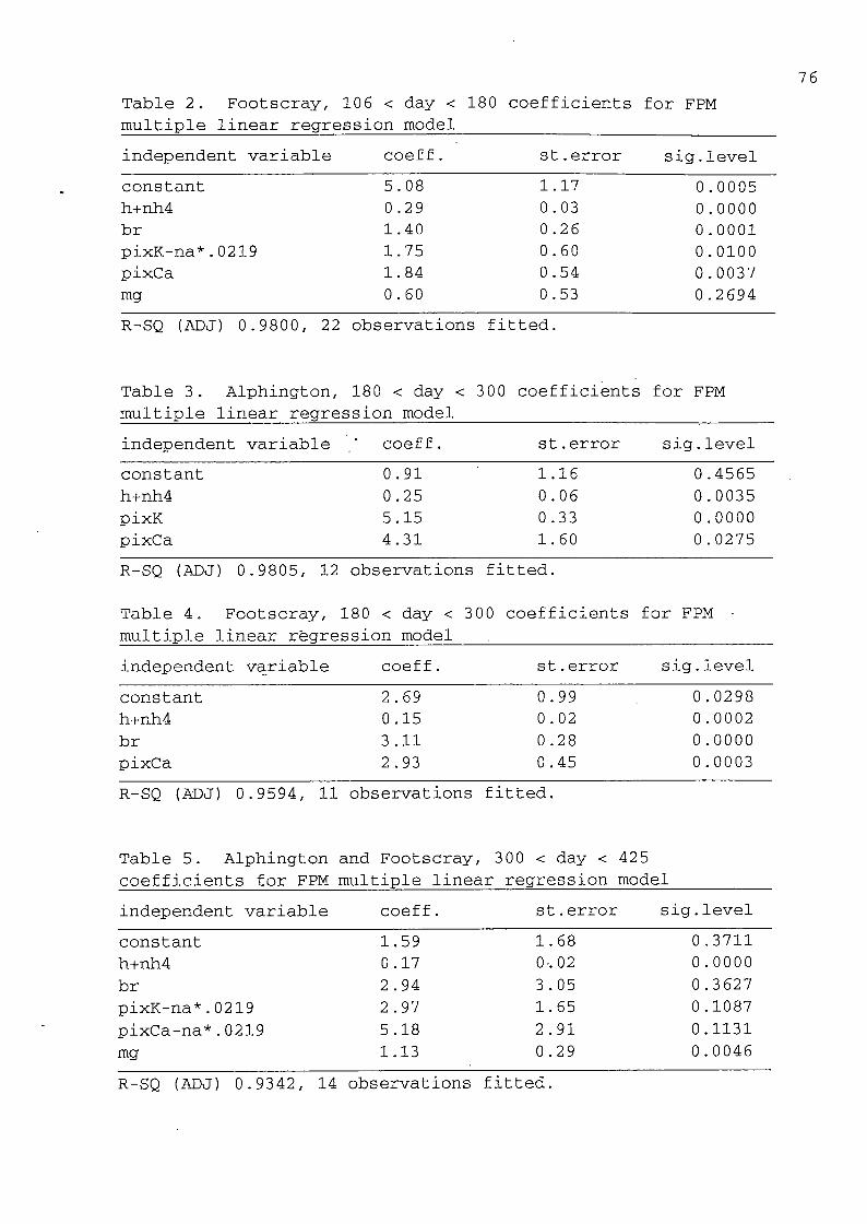
76
Table 2. Footscray, 106 < day < 180 coefficients for FPM
multiple linear regression model
independent variable coeff. St.error sig.level
constant 5.08 1.17 0.0005
h+nh4 0.29 0 .03 0.0000
br 1.40 0.26 0.0001
pixK-na*.0219 1.75 0.60 0.0100
pixCa 1.84 0 .54 0.0037
mg 0 . 60 0 .53 0.2694
R-SQ (ADJ) 0.9800, 22 observations fitted.
Table 3. Alphington, 180 < day < 300 coefficients for FPM
multiple linear regression model
independent variable coeff. St.error sig.level
constant 0.91 1.16 0.4565
h+nh4 0.25 0.06 0.0035
pixK 5.15 0 .33 0.0000
pixCa 4.31 1. 60 0.0275
R-SQ (ADJ) 0.9805, 12 observations fitted.
Table 4. Footscray, 180 < day < 300 coefficients for FPM -
multiple linear regression model
independent variable coeff. St.error sig.level
constant 2 .69 0 .99 0.0298
h+nh4 0 .15 0.02 0.0002
br 3 .11 0.28 0.0000
pixCa 2 .93 0.45 0.0003
R-SQ (ADJ) 0.9594, 11 observations fitted.
Table 5. Alphington and Footscray, 300 < day < 425
independent variable coeff. St.error sig.level
constant 1.59 1.68 0 .3711
h+nh4 0 .17 0-. 02 0.0000
br 2 .94 3 .05 0.3627
pixK-na*.0219 2 .97 1.65 0.1087
pixCa-na*.0219 5.18 2 .91 0 .1131
mg 1.13 0.29 0.0046
R-SQ (ADJ) 0.9342, 14 observations fitted.

77
Information on the contributions of different sources to
the FPM is given in Appendix 1, Tables A1-A5. The estimated
absolute contributions to the FPM are also shown as cumulative
component plots in Fig 44 for Footscray and Fig. 45 for
Alphington. Tables A1-A5 and Figs. 44-45 give the calculated
estimates for contributions to the FPM (in [ig m"^) for the MLRmodel appropriate to each sample assuming that the model
applies equally well to all samples in the set from which the
model was derived. The equivalent contributions for 1
standard error in the coefficient estimate from the MLR models
are given in Tables A1-A5 below each component mass estimate.
The measured sample FPM and sum of the estimated mass
associated with the different tracers are also included. The
variable "on" is the time in days since the start of 1990 that
the sample started and nF is the Fluoropore number of the
sample.'
Considering the "dirtier" days in the autumn grouping,
specifically those with FPM over 30 |J.g m"^ (nF = 23, 13, 32,33 and 14 at Footscray and nF=25, 29, 26, 20, 22, 35, 39,
47, 60, 36, 68 and 69 at Alphington), average fractional
contributions from the three "major" variables are as follows:
Footscray, (H+NH^) 37%, br 23% and pixK 13% and at Alphington(H+NH^) 21%, br 20% and pixK 55%. The estimate of the(average) absolute FPM associated with the bromide source is
similar for both sites for these selected samples; 10.5 |ig m~^at Footscray and 9.9 [ig m~^ at Alphington, but the estimatedmass (FPM) associated with potassium at Footscray is
5.7 |lg m~^ whereas at Alphington the corresponding estimate is24.6 }lg m~2 . (Footscray has a higher unexplained mass 5.1 |lgm~^, compared with 1.6 ^ig m~^ at Alphington, this is alsoshown in Figs. 44 and 45). Calculation of the fraction of
nss-S04 and N03~ in the FPM for these same samples isinstructive, at Footscray the average nss-SO^ fraction was4.5% and the nitrate fraction was 6% whereas at Alphington the
average nss-S04 fraction was 1.5% and the nitrate fraction1.6% of the FPM. In both cases it is clear that the acidity
indicator, (H+NH4) is not acting just as a surrogate forsulfuric and nitric acids. As well, any possible contribution
of natural nss-S04 during these events must be very minor.

78
80 -
Calculated FPM associated with variablesin MLR models. Footscray
'i' « J r~T r j r r " i —i—1"~ i "i ■ i—r*1 * I r—j I—I—I—I—I—]—I—I—I—I—p
cn 60 -
Dl
3
CLU_
CU
>• i-H
to1—1
3
e3
CJ
40
20 -
0 -
^ H+NH4
^ nss K
IZl Ca
Q Mgconst
-j I I \ j t i l l
^ y y ^ X X x' X 'x k_i « ' t t t 1 I t
100 150 200 250 300 , 350
Time (days from Jan 1 1990)400 450
Figure 44. Calculated cumulative contributions to fine
particle mass (|ig m~^) at Footscray, as a function oftime during the study period. Masses shown are those
associated with variables used in the selected multiple
linear regression, models.

79
i-n
C31
ZD
CLlJ_
03
>
toI—I
ZD
EU
u
100
80
60
40
20
0
Calculated FPM associated with variablesin MLR models, Alphington
■T I I I 1 ■ I I I ] I I I—r—]—I—I—I—T—]—r—I—I—I—I—I—I—I—I—p
S H+NH4. ̂ nss K
0 nss Caconst.
J 1 1 1 1 1 * 1 1 1 1 1 1 1 ! ! 1 1 1 I i t f . t I t t , » I . t . t I
100 150 200 . 250 300 350 400 450Time (days from Jan 1 1990)
Figure 45. Calculated cumulative contributions to fineparticle mass (jig m~^) at Alphington, as a function oftime during the study period. Masses shown are thoseassociated with variables used in the selected multiplelinear regression models.

The simpler models for the winter period give a
correspondingly simpler prediction of the fractional
contributions. For the winter period absolute loadings were
lower than in the autumn period, particularly at Footscray.
There were two events at Footscray with FPM in excess of 25 ^Lgm~^ (nF = 99, doy 190.85 and nF=124, doy=214.53). Theestimated fractions of FPM associated with the two variables
are:
(H+NH^) 14% and br 69%, (nF=99) and(H+NH^) 31% and br 29%, {nF=124).
Observed fractions of the FPM as nss-S04 and N03~corresponding to these are:
(nss-SO^) 4.3% and N03~ 3% (nF=99) and(nss-S04) 11% and N03~ 6% (nF=124).
At Alphington, samples with FPM in excess of 3 0 |J.g m~^ show aconsistent pattern of a large mass fraction associated with
■potassium. For these samples (nF= 79, 138, 145, and 148) theaverage FPM fraction associated with potassium was 72% andwith (H+NH4) was 22%. Corresponding FPM fractions were nss-SO4 2.4% and N03~ 3.9%. At Footscray one sample (nF=158, doy280.42) showed a high fraction of calcium, this is possiblyassociated with sea-salt since this model did not carry avariable directly related to a sea-salt source
At both sites later samples indicate an increase in thefraction associated with aerosol acidity (H+NH4) , although ingeneral the absolute FPM loadings decrease (see Figs. 44 and45) . Greater than 44% of estimated FPM was associated withthe acidity variable for nF=149, 151, 157 at Footscray andnF=155 (doy 296.52) at Alphington. For these spring samplesnss-S04 comprises 14% of the FPM and N03~ 9.3%.
An increase in the fraction of (H+NH4) is typical in thesummer samples. For samples with measured FPM in excess of 16p,g m~^ (nF=153, 154, at Alphington and 159, 189 and 191 atFootscray) the average estimated contribution of massassociated with (H+NH4) is 57% with only small fractionsassociated with primairy sources of potassium and bromide, 5%for each. The fraction associated with (H+NH4) is in factbiased down by sample nF= 191, this has a very large fractionevidently associated with magnesium (sea-salt) and acorresponding lower (H+NH4) fraction (only 29%) . On averagenss-S04 comprises 22% of the FPM in these samples and N03~ 5%,whereas for nF=191 the fractions are nss-S04 12.5% and N03~15.7%. In this one sample the estimated mass fraction

81
associated with acidity (29%) is similar to the observed mass
fraction of sulfate plus nitrate (28.2% of FPM), whilst in
general during winter and summer the observed fraction of
sulfate in the FPM is typically equivalent to about 30% of the
estimated mass fraction associated with (H+NH^) and nitrate isequivalent to close to 20% of this estimated mass fraction.
This indicates that even in summer, strong inorganic acids
only make up about 50% of the mass associated with this
secondary production indicator. During summer the total
inorganic mass fraction is also maximtom. The residual mass
associated with (H+NH^) is attributed to the photochemicallyconverted organics (hydrocarbons) that make up the non-primary
fraction of the total carbon loading. Sample nF=191 is also
noteworthy because it was collected during the period with the
highest hourly ozone for the period (and summer), 11.6 pphm.
This occurred during a sea-breeze when winds were southerly at
3 ms~^ (S. Ahmet, private communication).
The MLR models indicate that during autumn there are
similar contributions to the FPM from vehicles at Footscray
and Alphington but a much stronger contribution from smoke at
Alphington. At Footscray the contribution from smoke was
about one half that from vehicles whereas at Alphington it was
over twice the contribution of vehicles. Footscray on the
other hand shows a greater contribution associated with
aerosol acidity (secondary production) not associated with
identifiable primary sources (37% compared with 21%)._ The
pattern of attainment of the sampling threshold is consistent
with these contributions. There were an equal number of
sampling periods (six) initiated between midnight and noon at
the two sites. In the period noon to 6 pm, ten samples were
initiated at Footscray and five at Alphington whereas from 6
pm to midnight eight samples were initiated at Footscray and
eighteen at Alphington. This source contribution pattern
continued into the early part of winter with some reduction in
the fraction associated with acidity at Footscray to a level
similar to that at Alphington, just over 20%. The main
contribution to the FPM■during winter at Footscray wasassociated with primary emissions from motor vehicles whereasat Alphington the main source was smoke. The later samples inthe winter group are more typical of the summer samples wherethe mass fraction associated with secondary production thatcannot be associated with any one particular primary source isthe main contributor to the FPM. Summer samples can becharacterised as being associated predominantly with thesecondary production source on the dirtier days, whilst on
82
several of the days sampled with lower FPM values (typicallyFPM < 10 [ig but in one case FPM = 27 |ig ) sea-salt made
a considerable contribution to the FPM (nF=182, 187, 173,
191) .
3.10 Multiple linear regression models for Bsd - source
contributions
Procedures used to derive MLR models for the FPM were
also followed for deriving models of the scattering
coefficient In this case however the data were divided
into three groups, autumn and winter at Alphington (doy <
300), autumn and winter at Footscray, and summer at the
combined sites (doy > 300). The final MLR models are given in
Tables 6-8. One difference between the models for scattering
coefficient and those.for FPM is the constant fraction which
is due principally to the scattering coefficient of air, .
At the nephelometer wavelength, is 0.21 10"'^ m~^ at 20 °C.This value is within one standard deviation of the predicted
constant values. At Footscray the best model for autumn-
winter also included a coefficient (significant only at the
13% level) related to wind speed. The exact role of wind
speed is not clear but it may be acting as a surrogate for
coarse particles that are not collected in the chemical
sampling system.
Contributions to the- scattering coefficient were
calculated for each sample based on the MLR model applicable
for the time of collection and location. These contributions
are given in Tables A6-A8 (Appendix 2). The calculated
contributions to the scattering coefficient are also plotted
in Figs. 46-51. Figures 46 and 47 show absolute contributions
from ail the coefficients included in the MLR models. Overall
these figures show a similar pattern of contribution to those
for the corresponding FPM in Figs. 44 and 45. The maincontributing factors are potassium, bromide and acidity taken
to represent smoke (biomass burning), vehicles and secondary
production respectively. Figures 48 and 49 show the
contributions to Bg,^ of these main factors in cumulative formand Figs. 50 and 51 individually. At Alphington, during the
autumn periods with elevated scattering, the main contributionto the scattering coefficient is clearly associated with
potassium (biomass burning/smoke). At Footscray in the same
period bromide (vehicles) and aerosol acidity (secondary
production) were both significant contributors whereas the
potassium related factor (smoke) made a very minor

83
Io
■aa.cn
CQ
cu>
• rH
4-}ro
=3EZ3O
2.5
1.5
0.5
0
Calculated Bspd associated with MLRmodel variables. Footscray
-I—I—I—r 'I I '~i J I i I ' I I j *' I ' r 'T"*"! r~T—I I I ' I i j r j ■ I ' f ■"»' ' i j ■
H+NH4
nss K
nss Ca
H wind speedconst.
i ! 1 1 1 ! I I I I I I 1 I I 1 ' I ' '
100 150 200 250 300 350 400 450
■ Time (days from Jan 1 1990)
Figure 46. Calculated cxjmulative contributions to thedry scattering coefficient, (10~^ m~^) at Footscray,as a function of time during the study period.Contributed scattering coefficients shown are thoseassociated with variables used in the selected multiplelinear regression models.
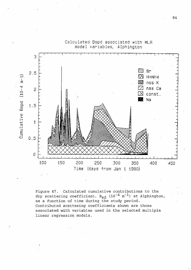
84
Io
■aCL03m
OJ>
• rH
-1-J(11
=JCJ
3 -
2.5
2 -
1.5 -
1 -
0.5
0 -
Calculated Bspd associated.with MLRmodel variables. Alphington
S H+NH4nss K
nss Ca
const.
100 150 200 250 300 350
Time (days from Jan 1 1990)400 450
Figure 47. Calculated cumulative contributions to thedry scattering coefficient, Bg,^ (10"'^ m~^) at Alphington,as a function of time during the study period.Contributed scattering coefficients shown are thoseassociated with variables used in the selected multiplelinear regression models.

85
"a
CL
in
CO
QJ
>•rH
4-1
ro
ZJCJ
i.a -
1.5 -
1.2
0.9
0.6
0.3
0 -
Calculated Bspd. associated with MLRmodel variables (selected]. Footscray
"I—I—I—I—I—1—I—I—I—I—I—I—I—I—[—I—I—I—I—I—I—I—I—I—]—1—I—I—1—[—I—1—I—r
^ H+NH4
nss K
100 150 200' 250 300 350
Time (days from, Jan 1 1990)
400 450
Figure 48. Calculated cumulative contributions to thedry scattering coefficient, (10~^ m~^) at Footscray,as a function of time during the study period.
Contributed scattering coefficients shown are those
associated with variables used in the selected multiple
linear regression models. This figure shows onlycontributions associated with the three "main" variables,
Br, nss-K and acidity (H+NH4).

86
Calculated Bspd associated with MLRmodel variables (selected], Alphington
2.4 -
I
o
TJ
CL
cn
in
OJ
>•rH
-M
(U
nu
1.6
1.2 -
0.8 -
0.4 -
0 -
Br
H+NH4
nss K
100 150 200 250 300 350
Time (days from Jan 1 1990]
400 450
Figure 49. Calculated cumulative contributions to the
dry scattering coefficient, (10~^ m~^) at Alphington,as a function of time during the study period.
Contributed scattering coefficients shown are those
associated with variables used in the selected multiple
linear regression models. This figure shows only'
contributions associated with the three "main" variables,
Br, nss-K and acidity (H+NH4).

1.2 -
87
Contributions to Bsd associated with MLR
model variables, Footscray
^ 1 -
Io
f
0.8 -
• H+NH4
+ br
5K pixK
co•fH
4-»
ZJX2•iH
c_4J
co
u
■aCDm
0.6 -
0.4 -
0.2 -
+
+
+
+
+ +
+« +
5K
0" -*1% i.** 14fef jJi
I ' ■ « ■ I ' ' ' ■ I ' ' ' I 1 I I : L. _1 I I 1 I I I I I I 1 I I I
+ ++
■w MAk'•nK
L
100 150 200 250 300 " 350
time (days since 1 Jan 1990)400 450
Figure 50. Individual calculated contributions to thedry scattering coefficient, (10~^ m~^) at Footscray,as a function of time during the study period.Contributed scattering coefficients are the same as thosein Figure 48 but are not summed.

88
Contributions to Bsd associated with MLRmodel variables, Alphington
1.5 --I—1—I—I—I—I—I—I—r- "1—I—1—I—I—]—I—1—I—I—p
-c-H
I
1o
co
♦ rH
4-)
=3
• iH
c_+J
co
u
X3
m
cn
1.2 -
— 0.9 -
0.6 -
0.3 -
*
3K
3fi
5fi
*
3K* ̂
3K
)K
3K
3K
3(f
0 -
+++5^ • 5^?*
J I I 1 I I I I I I L
3K
+
i I I i_ _i I I i_ 4 I I I L_
• H+NH4
+ br
^ pixK
■f+
m» » ' *
100 150 200 250 300 350
time (days since 1 Jan 1990)400 450
Figure 51. Individual calculated contributions to thedry scattering coefficient, (10"'^ m"^) at Alphington,as a function of time during the study period.Contributed scattering coefficients are the same as thosein Figure 49 but are not summed.

89
contribution. During winter at Alphington, potassium (smoke)
still comprised the major factor. At both sites in summer,
aerosol acidity (secondary production) assumes the major
contribution with a minor contribution from bromide (vehicles)
and an insignificant contribution associated with potassium
(smoke) (this was excluded from the MLR model as statistically
insignificant).
Table 6. Alphington day < 300 coefficients for multiple
linear regression model
independent variable coeff. St.err sig.level
constant 0 .266 0.051 ■ 0.0000
h+nh4 0.010 0 .002 0.0001
br 0.018 0.008 0 .0236
pixK-na*.0219 0 .123 0 .018 0.0000
pixCa 0 .114 0.059 0.0594
R-SQ (ADJ) 0.9421, 35 observations fitted.
Table 7. Footscray day < 300 coefficients for Bg^ multiplelinear regression model
independent variable coeff. St.err sig.level
constant 0 .151 0 .166 0.3725
h+nh4 0.009 0.002 0.0002
br ' 0.081 0 .023 0.0018
pixK-na*.0219 0.019 0.057 0.7373
pixCa-na*.0219 0.083 0.045 0.0764
sws 0.075 0 .042 0.0907
R-SQ (ADJ) 0.7634, 30 observations fitted.
Table 8. Alphington and Footscray, 300 < day < 425,
coefficients for 3^,^ multiple linear regression model
independent variable coeff. St.err sig.level
constant 0 .066 0 .130 0 . 6226
h+nh4 0.012 0.002 0.0000
br 0.396 0 .238 0.1275
pixCa-na*.0219 0.083 0 .147 0.5852
R-SQ (ADJ) 0.8571, 14 observations fitted.

90
3.11 Organic trace compounds
Source samples were analysed initially for specific
organic compounds with the Mass Sensitive Detector (MSB) in
the ion current mode to allow the widest possible range of
compounds to be determined. A range of organic compounds was
selected from these analyses. They were then analysed again
with the MSB in the selected ion monitoring mode (SIM). This
mode allows particular molecular weights.bo be targeted
thereby increasing the sensitivity by a factor of 100-1000.
Increased sensitivity is required for determination of the
concentration of organic compounds in the ambient samples.
The list of molecular weights targeted in the selected ion
monitoring mode is given in Table B9 (in Part B). Cresols
were included as possible tracers for secondary aerosol
■ although structures similar to cresols have been detected in
the aerosol from fires. Although 1-methyl Naphthalene and 2-
methyl Naphthalene were not detected in the scanning GC/MS
analysis they were included in the SIM runs because of their
previous use as tracers for petrol vehicles. The C22hydrocarbon was detected as a fragment of mass 85 (0113(0112)5)and was selected as a possible tracer of aerosol contributed
from diesel vehicles.
The output from the MSB is a series of peaks at given
retention times, which are subsequently integrated. A
problem, which is typical of mass spectrometers, is that the
respdnse of the MSB changes on time scales of less than one
day. To overcome this problem deuterated anthracite
(anthracite]_Q) was used as an internal standard. During thiswork 500 ng of the anthracite^o was added to the 5 ml of theextracting solution by adding 100 jiL of a solution of 0.5 mg
of anthracite^^Q per 100 ml. The use of mass spectrometrypresents a second problem in the quantification of the organic
compounds identified. This is that the response of the mass
spectrometer is not the same for all compounds so that the
response of an individual compound needs to be referred back
to the internal standard. During previous work the response
of a range of structurally similar individual compounds,
including anthracite2_Q, was determined. This enabled responsefactors to be determined for each compound.
The concentrations of compounds measured in the various
source samples are given in Table B8 (Part B). The most
obvious set of tracer compounds are those for biomass burning
(open fire dry grass hay, twigs and leaves). These are the

91
compounds in Table B8 which have masses between 152 and 196.
Such compounds have been previously identified as possible
tracers for such sources as woodstoves and biomass burning
(Edye and Richards, 1991; Gillett et al;, 1989; Hawthorne et
al. , 1988; Hawthorne et al. , 1989)'. Some of these compounds
are found in both the woodstove emissions and in biomass
burning but because they have significantly higher
concentrations in the biomass burning samples they may still
be suitable tracers for biomass burning. In particular these
are .3-methoxy-4-hydroxy benzaldehyde (vanillin), 2 , 6-dimethoxy
phenol, 3-methoxy-4-hydroxy-acetophenone and 3,5-dimethoxy-4-
hydroxy-acetophenone. Some other compounds appear to be
almost entirely confined to .the biomass burning source
samples. These are 3-methoxy-4-hydro>cy benzole acid,
2,6-dimethoxy-4-(2-propenyl)phenol^and the compound of
molecular weight 194 with a retention time of 11.917 min.
Two compounds with molecular weights of 218 were measured
in all the source samples investigated in this study but
concentrations measured in the woodstove source samples were
significantly higher than those measured in the other sources.
Both compounds appear to be possible tracers for woodstove-
type combustion. A second possible tracer for woodstoves is
the compound with a molecular weight of 206 and a retention
time of 17.224 min. This compound also was found almost
exclusively in the woodstove source samples.
Whilst GCMS analysis for organic compounds offers
considerable promise in identifying specific sources, the
number of samples actually analysed in this study was quite
small (14 source, 7 ambient). The principal reason for this
was logistic rather than technical. Within the time-frameallowed for analyses this was the maximum number that the
contracting laboratory could process. Because of the time
required to edit output files of the various mass components
these analyses are also relatively expensive.
Given the above discussion on possible source tracers the
ambient data, which were obtained for days with high carbon
loadings, can be examined to see whether these suggestions tiein with the other data. Ambient organic compound data which
include late autumn and winter samples are given in Table C8
(Part C). Three of the samples (nG=22 @ 1840 28/5/90 at
Alphington and nG=32 @ 1910 28/5/90 and nG=33 @ 0740 29/5/90
at Footscray) are associated with a single "event". Thesesamples show some interesting features. Over a wide range of

92
organic species the concentrations at Footscray are lower than
those at Alphington by a factor of around 3 or 4. One notable
exception is C22/ a possible tracer for diesel fuelledvehicles, which has similar concentrations at the two sites.
The MLR models for FPM predicts that for nG=22 (at
Alphington), the relative source contributions associated with
the main tracers are:
K 38%, Br 25% and (H+NH4) 20%.
This is equivalent to 63% from primary combustion sources and
20% secondary production. For the Footscray samples nG=32 the
model predicts the following associated FPM contributions:
K 8%, Br 12%, (H+NH4) 18%
giving 20% from primary combustion sources. For nG=33, taken
on the following morning, the MLR model predicts associated
contributions of:
K 8%, Br 10%, (H+NH4) 34%
giving 18% from primary combustion sources. The increase in
predicted secondary fraction .(associated with the (H+NH4)
variable) from nG=32 to nG=33 is interesting (whilst not
unexpected for a multi-day event), as is the ratio of close to
3 for the predicted primary combustion contributions at the
two sites, which is consistent with the ratio of observed
organic concentrations.
Compounds with molecular weights 218 and 206, which were
suggested as possible woodstove tracers, were only observed in
one ambient sample (nG=22). However, it would be premature to
claim that this meant woodfires were not implicated in the
other samples. The range of compounds with molecular weights
between 152 and 196 offers more clues. The concentrations of
several of these were observed to be considerably greater in
the open fire samples burning grass hay, leaves and twigs than
in the woodstove samples. This is consistent with the
observation that emission of primary organic material in
general (relative to elemental carbon) is considerably greater
in these samples (see report Part B). From the 152-196 range
of molecular weights, three compounds present in both the open
fire and woodstove samples were selected, they also had the
previously mentioned concentration difference. These
compounds have molecular weights of 152, 166 and 196. In

93
order to compare source and ambient samples it is necessary to
normalise the concentrations using a conservative component
such as elemental carbon. The range of concentration ratios
for compounds with the selected molecular weights and
elemental carbon are given below for the two sources and the
ambient samples.
Table 9. Concentration ratios of organic compounds, with
molecular weight mw, to elemental carbon (compound / elC)
(units all lE-4 ̂ ig/|ig)
mw ambient fire woodstove
152 0.27 -.2.3 2.4 - 91 0, 0.4,5
166 0.32 -0.79 57 - 390 1.6 - 9
196 0.48 - 29 18 - 240 0.85 - 4.6
These ratios give a clear indication that the ambient samples
are much more consistent with woodstove emissions than our
open fire source of burning grass hay, leaves and twigs.
This can not be taken as conclusive proof that woodstoves
dominate the primary carbon emissions during autumn and winter
(at Alphington), however it is suggestive. It also appears to
confirm that discrimination of these two potential sources is
possible using organic,tracers. Determination of the organicsin actual bushfire samples or controlled burn source aerosol
would be of value to supplement our open fire approximation to
general biomass burning.
3.12 Concluding comments
The presence of stable air over the Melbourne area during
autumn is clearly a predominant driving force for the
conditions that produce increased aerosol scattering at that
time. The present study shows that when these conditions
prevail the local sources of pollutants are most important and
that a region-wide uniform aerosol mix does not occur. It
should be noted however that because of meteorological
conditions, the expected frequency of widespread visibilityreducing events did not occur during the study period. The

I
94
main sources were determined to be motor vehicles at Footscray
and some form of burning/smoke at Alphington. The location of
Alphington close to the Yarra River may increase the
probability of advection of smoke from outlying rural and
semi-rural regions in the Yarra basin (or elsewhere) but the
source of the smoke may also be of local origin. The two main
possible local sources are the burning of leaves in autumn and
the use of woodfires for heating. . Unambiguous differentiation
between these potential sources has not been possible in this
study. However, the available data on the ratios of a number
of organic compounds to elemental carbon is strongly
suggestive of a wood burning source rather than a general
biomass burning source. Wood burning is a popular heating
source in Melbourne as reported by Todd et al. (1989) . Todd
et al. (1989) estimated that in 1988, 7.6% of Melbourne
households used wood as their main heating fuel and 10.7% used
wood for secondary heating. Their estimated consumption of
wood was 400,000 tonnes per year. Survey results showed
greater household consumption and more households using wood
in the outer suburbs. Both the timing of the peak in
scattering around the later part of autumn and early winter,
and 18 out of 29 excedences of our sampling threshold between
6 pm and midnight for April to June, compared with 5 between
noon and 6 pm, are consistent with wood burning as a major
aerosol source at Alphington.
The present visibility reduction study, carried out over
11 months at two Melbourne sites has shown that scattering
(and reduced visibility) is largely associated with the fine
particle mass. The major component of the FPM in Melbourne
was found to be carbon (organic plus elemental). During
autumn, when reduced visibility was most common, the major
contribution to the fine particle mass came from carbon
compounds and was mainly organic. During this period,
elements typical of "biological" origin were also considerably
enhanced.
We have also determined contributions to the FPM and Bg^using multiple linear regression procedures and from this have
broadly identified the main sources of aerosol related
visibility reduction during the 1990-1991 study period. We
have shown that the factors producing increased FPM and Bg^are different at the two sites which are only about 15 km
apart, but that they are similar for both FPM and Bg,^ at eachsite. The main sources for increased scattering (Bg^j) , in •autumn and winter at Footscray were vehicles and secondary

95
production. For the same period at Alphington the main source
was smoke. During summer at both locations secondary
production was the major source and primary emissions from
vehicles made a small contribution. Sources contributing tothe fine mass were similar to those for scattering but vehicle
primary emissions were not statistically significant in summer
and a small contribution came from smoke in summer.
4. Acknowledgements
We gratefully acknowledge the assistance of EPA
Environmental Studies and Technical Services Branches in
facilitating this study. Particular thanks go' to Trevor
Bardsley, and to David Whyte who assisted in the initial
stages of the field work and analysis.

96
5. References
Ayers G.P., J.P. Ivey and R.W. Gillett, Coherence between
seasonal cycles of dimethyl sulphide, methansulphonate and
sulphate in marine air. Nature, 349, 404-406, 1991
Bardsley T., Comparison of light scattering extinction
(Nephelometer) and fine particulate mass concentration
(Dichotomous sampler) in Melbourne aerosol. EPAV report SRS
87/001, 1987
Countess R.J., S.H. Cadle, P. Groblicki and G.T. Wolfe,
Chemical analysis of size segregated samples of Denver's
ambient particulate, JAPCA, 31, 247-252, 1981.'
Cowan S., D.S. Ensor and L.E. Sparks. Light absorption
measurements using the integrating plate method. In: Light
Absorption by Aerosol Particles, Eds. H.T. Gerber and E.E.
Hindman, Spectrum Press, 1982. ■
Dal Pont G., M. Hogan and B. Newell. Laboratory techniques in
marine chemistry (II). Determination of ammonia in sea-water
and the preservation of samples for nitrate analysis. CSIRO
Division of Fisheries and Oceanography, Report No. 55, 1974.
Dzubay T.G., R.K. Stevens, C.W. Lewis, D.H. Hern, W.J.
Courtney, J.W. Tesch and M.A. Mason, Visibility and aerosol
composition in~Houston, Texas, Environ. Sci. Technol., 16,"
514-525, 1982.
Edgerton S.A. and M.W. Holdren, Use of pattern recognition
techniques to characterise local sources of toxic organics in
the atmosphere. Environ. Sci. Technol., 21, 1102-1107, 1987.
Edye L.A. and G.N. Richards, Analysis of condensates from wood
smoke: Components derived from polysaccharides and lignins.
Environ. Sci. Technol., 25, 1133-1137, 1991.
EPAV, Air quality monitoring results 1986, Environment
Protection Authority, Victoria, Publication 263, 1988.
Fairbridge R.W. Ed. The Encyclopedia of Geochemistry and
Environmental Sciences. Van Nostrand Reinhold Company, 1972
Gillett R.W., Ayers G.P. and Mainwaring S.J., Source
contributions to atmospheric aerosols using organic tracers.

97
L.J. Brasser and W.C. Mulder (Eds.), Proceedings of the 8th
World Clean Air Conference, volume 3, Elsevier Science
Publishers B.V., Amsterdam, 1989.
Gras J.L., G. P. Ayers, R.W. Gillett and S.T. Bentley.
Atmospheric particles and visibility in Melbourne - a pilot
study. Report to EPAV Sept. 1989.
Gras J.L., G.P. Ayers, R.W. Gillett and S.T. Bentley.
Regional visibility and aerosol properties in South - Eastern
Australia. In proceedings of the 10th Clean Air Conference,
Clean Air Society of Australia and New Zealand, Auckland,
1990.
Gray H.A., G.R. Cass, J.J. Huntzicker, E.K. Heyerdahl and J.A.
Rau, Characteristics of atmospheric organic and elemental
carbon particle concentrations in Los Angeles, Environ. Sci.
Technol., 20, 580-589, 1986,
Hawthorne S.B., Frieger M.S., Miller D.J. and Barkley R.M.,
Methoxylated phenols as candidate tracers for atmospheric wood
smoke pollution. In; Proceedings of the 1988 EPA/APCA
international symposium on Measurement of Toxic and Related
Air Pollutants, Research Triangle Park, North Carolina, 1988.
Hawthorne S.B., Frieger M.S., Miller D.J. and Mathaison M.B.,
Collection and quantitation of methoxylated phenol tracers for
atmospheric pollution from residential wood stoves. Environ,
Sci. Technol., 23, 470-475, 1989.
Hering S.V., Miguel A.H. and Dod R.L., Tunnel measurements of
the PAH, carbon thermogram and elemental source signature for
vehicular exhaust, Sci. Tot. Environ., 36, 39-45, 1984.
Horvath H. and T.A. Habenreich. Absorption coefficient of the
Vienna Aerosols: comparison of two methods. Aerosol Sci. and
Tech., 10, 506-514, 1989.
Larson S.M. and G.M. Cass, Characteristics of summer midday
low-visibility events in the Los Angeles area. Environ. Sci.
Technol., 23, 281-289, 1989
Lewis C.W. and T.G. Dzubay. Measurement of light absorption
extinction in Denver. Aerosol Sci. and Tech., 5, 325-326,
1986.

98
Lin C.I., M. Baker and R.C. Charlson. Absorption coefficient
of atmospheric particles. Appl. Opt., 12, 1356-1363, 1973.
Millero F.J., The physical chemistry of sea-water. Ann. Rev.
Earth Plan. Sci., 2, 101-150, 1974.
Pyysalo H., Tuominen J., Wickstrom K., Skytta E., Tikkanen L.,
Salomaa S., Sorsa M., Nurmela T., Mattlia T. and Pohjola V.,
Polycyclic organic material (POM) in urban air.
Fractionation, chemical analysis and phenotoxicity of
particulate and vapour phases in an industrial town in
Finland, Atmos. Environ., 21, 1167-1180, 1987.
Simoneit B.R.T., Characterisation of Organic constituents in
aerosols in relation to their origin and transport: a review.
Int. J. Environ. Analyt. Cham., 23, 1985.
Simoneit B.R.T.', Organic matter in the troposphere - V:
Application of molecular marker analysis to biogenic emissions
in the troposphere for source reconciliations, J. Atmos.
Cham., 8, 251-275, 1989.
Simoneit B.R.T. and Mazurek M.A., Organic tracers in ambient
aerosols and rain. Aerosol Sci. Technol., 10, 267-291, 1989.
Standley L.J.- and Simoneit B.R.T., Characterisation of
extractable plant wax, resin and thermally matured compounds
in smoke particles from prescribed burns. Environ. Sci.
Technol., 21, 163-169, 1987.
Standley L.J. and Simoneit B.R.T., Preliminary correlation of
organic molecular tracers in residential wood smoke with the
source fuel, Atmos. Environ., 24B, 67-73, 1990.
Todd J.J, K.M. Craig and L.R. King, National Fuelwood Survey,
Final Report for Dept. of Primary Industries and Energy, 248
pp, 1989.
Valoaras G., J.J. Huntzicker and W.H. White, On the
contribution of motor vehicles to the Athenian "nephos": an
application of factor signatures. Atmos. Environ., 22, 212-
216, 1988.

99
Weiss R.E. and A.P. Waggoner (1982) . Optical measurements of
airborne soot in urban, rural and remote locations. In:
Particulate Carbon, Atmospheric Life Cycle. Eds. G.T. Wolff
and R.L. Klimisch, Plenum Press, New York.

100
APPENDIX 1, MLR model mass contributions
Table Al - Table A5, model calculations of fractional
contributions to fine particle mass using the variables in,
and coefficients from, multiple regression models described in
the main text, Tables 1-5.
Variables considered are:
N line number
on on time, as fractional day of year
nF Fluoropore filter number
massF observed fine mass from Fluoropore filters
SUM sum of mass components calculated for
considered variables and constant term,
h contribution associated with hydrogen ion
nh4 contribution associated with ammonium ion
br contribution associated with bromide ion
pixK contribution associated with PIXE derived potassium
na* contribution associated with sea-salt fraction of
preceding variable, either potassium or calcium
pixCa contribution associated with PIXE derived calcium
mg contribution associated with magnesium

101
Table Al, Alphington, 106 < day < 180. Fractional
contribution to FPM from different MLR variables, using model
in Table 1, with observed variable concentrations. First line
gives mass contributed (|ig m~^), second line mass equivalentto 1 standard error of variable coefficient from MLR model.
massF is the observed FPM, SUM is the summed mass for all
variable contributions (including constant). The missing data
code is -9.00.
N on nF massF SUM h nh4 br pixK pixCa na*
1 112.68 3 7.27 8.35 0.33 1.06 0.52 4.11 1.16 -0.40
0.10 0.31 0.14 0.66 0.79 -0.27
2 119.67 6 8.15 10.33 0.38 0.41 0.88 5.42 1.87 -0.20
0.11 0.12 0.23 0.88 1.27 -0.14
3 120.62 8 8.02 9.21 0.43 0.92 1.04 3.76 1.61 -0.10
0.13 0.27 0.27 0.61 1.10 -0.07
4 122.52 11 7.67 13.73 0.36 0.24 . 0.20 9.78 1.89 -0.30
0.10 0.07 0.05 1.58 1.29 -0.20
5 123.71 18 13.11 21.34 2.02 1.43 3.42 12.06 1.25 -0.40
0.59 0.42 0.89 1.95 0.85 -0.27
6 130.49 24 22.85 18.45 1.69 3.09 3.99 8.27 0.26 -0.42
0.50 0.91 1.04 1.34 0.17 -0.28
7 130.94 19 15.19 18.17 2.12 2.71 1.95 9.82 0.22 -0.21
0.62 0.79 0.51 1.59 0.15 -0.15
8 134.79 25 32.00 33.30 2.99 6.03 4.04 18.37 0.60 -0.29
0.88 1.77 1.05 2.97 0.41 -0.20
9 139.88 29 41.88 41.96 1.69 3.36 7.12 28.27 0.00 -0.04
0.50 0.98 1.85 4.57" 0.00 -0.03
10 140.90 26 30.19 28.33 2.77 5.51 2.01 16.76 0.00 -0.28
0.81 1.61 0.52 2.71 0.00 -0.19
11 143.94 30 11.77 8.70 1.46 0.97 2.18 2.71 0.22 -0.40
0.43 0.28 0.57 0.44 0.15 -0.27
12 144.82 31 16.24 18.18 1.70 1.17 4.76 8.40 0.99 -0.40
0.50 0.34 1.24 1.36 0.67 -0.27
13 145.93 20 38.41 37.96 2.91 5.55 5.31 22.96 0.00 -0.33
0.85 1.63 1.38 3.71 0.00 -0.23
14 147.36 21 21.02 21.41 1.84 6.36 2.72 5.63 3.53 -0.23
0.54 1.86 0.71 0.91 2.40 -0.15
15 147.78 22 78.32 84.94 4.77 15.43 24.85 37.75 1.05 -0.47
1.40 4.52 6.47 6.10 0.71 -0.32

102
Table Al continued.
N on nF massF SUM h nh4 br pixK pixCa na*
16 148.45 34 23.59 19.91 2.14 3.25 4.13 6.06 2.89 -0.12
0.63 0.95 1.08 0.98 1.96 -0.08
17 148.82 35 37.48 39.29 3.59 6.49 6.88 20.94 0.27 -0.44
1.05 1.90 1.79 3.38 0.19 -0.30
18 149.76 39 48.44 41.65 3.50 3.47 8.26 24.87 0.30 -0.32
1.03 1.02 2.15 4.02 0.20 -0.22
19 155.35 46 15.60 17.51 1.21 5.01 2.52 3.80 3.93 -0.52
0.35 1.47 0.66 0.61 2.67 -0.35
20 156.84 47 33.99 33.80 2.84 4.73 6.48 18.18 0.27 -0.25
0.83 1.39 1.69 2.94 0.18 -0.17
21 157.76 60 38.99 35.10 2.94 2.43 10.05 17.26 1.20 -0.34
0.86 0.71 2.61 2.79 0.81 -0.23
22 158.87 61 10.85 12:38 1.65 0.77 1.43 7.06 0.21 -0.31
0.48 0.23 0.37 1.14 0.15 -0.21
23 160.83 36 66.29 59.59 4.21 10.76 13.66 30.16 0.00 -0.76
1.24 3.15 3.56 4.87 0.00 -0.52
24 161.19 37 25.86 11.00 2.30 8.28 -9.00 8.25 0.00 -0.40
0.68 2.43 -9.00 1.33 0.00 -0.27
25 163.82 68 61.84 61.36 4.54 3.87 19.37 31.09 1.48 -0.55
1.33 1.14 5.04 5.02 1.01 -0.38
26 168.35 72 12.68 10.04 1.72 0.38 3.35 2.19 1.38 -0.55
0.50 0.11 0.87 0.35 0.94 -0.37
27 168.87 69 46.42 48.52 3.62 4.53 10.30 28.35 0.61 -0.45
1^06 1.33 2.68 4.58 0.41 -0.31
28 175.76 75 10.98 8.56 1.75 0.70 1.20 3.42 0.21 -0.28
0.51 0.20 0.31 0.55 0.15 -0.19
29 67.00 177 -2.11 1.56 -9.00 -9.00 -9.00 -9.00 -9.00 -9.00
-9.00 -9.00 -9.00 -9.00 -9.00 -9.00
constant =1.56
std.error=l.53

103
Table A2, Footscray, 106 < day < 180. Fractional contribution to
FPM from different MLR variables, using model in Table 2, with
observed variable concentrations. Other details as in Table Al.
N on nF massF SUM h nh4 br pixK na* pixCa mg
1 106.00 1 -9.00 5.08 -9.00 -9.00 -9.00 -9.00 -9.00 16.60 -9.00
-9.00 -9.00 -9.00 -9.00 -9.00 4.89 -9.00
2 107.52 2 17.74 21.06 0.72 4.33 4.58 2.39 -0.50 3.17 1.29
0.07 0.43 0.85 0.82 -0.17 0.93 1.13
3 112.63 4 7.87 9.41 0.33 0.85 0.34 1.07 -0.69 1.05 1.37
0.03 0.08 0.06 0.37 -0.24 0.31 1.20
4 119.64 7 10.77 11.64 0.44 0.74 0.62 1.75 -0.66 2.30 1.37
0.04 0.07 0.12 0.60 -0.23 0.68 1.20
5 120.66 9 -9.00 5.08 -9.00 -9.00 -9.00 -9.00 -9.00 16.60 -9.00
-9.00 -9.00 -9.00 -9.00 -9.00 4.89 -9.00
6 122.69 12 20.34 19.61 0.86 0.31 2.94 7.70 -0.67 1.09 2.28
0.08 0.03 0.55 2.64 -0.23 0.32 1.99
7 126.90 17 25.19 24.70 1.79 2.04 6.89 3.73 -0.74 2.99 2.91
0.18 0.20 1.28 1.28 -0.25 0.88 2.54
8 130.60 23 35.22 34.44 2.15 9.11 6."74 4.84 -1.07 6.47 1.12
0.21 0.90 1.25 1.66 -0.36 1.90 0.98
9 134.81 13 44.75 46.53 2.28 8.12 14.67 8.79 -2.44 8.46 1.56
0.22 0.80 2.73 3.01 -0.84 2.49 1.37 ,
10 140.52 27 13.23 13.01 1.08 1.11 1.56 0.79 -0.46 2.21 1.64
0.11 0.11 0.29 0.27 -0.16 0.65 1.43
11 141.46 28 21.69 21.12 1.56 3.77 2.42 4.49 -1.12 2.96 1.96
0.15 0.37 0.45 1.54 -0.38 0.87 1.71
12 147.80 32 46.87 46.09 3.02 14.59 12.25 7.49 -0.32 3.23 0.75
0.30 1.44 2.28 2.57 -0.11 0.95 0.65
13 148.32 33 69.10 69.32 3.83 30.95 10.43 7.50 -1.01 10.17 2.37
0.38 3.04 1.94 2.57 -0.35 3.00 2.07
14 148.68' 14 38.96 36.42 2.69 11.92 8.47 5.31 -0.46 2.66 0.74
0.26 1.17 1.58 1.82 -0.16 0.78 0.65
15 149.28 15 20.95 19.73 1.35 1.70 6.22 2.49 -0.19 2.45 0.62
0.13 0.17 1.16 0.85 -0.06 0.72 0.54
16 156.39 41 28.02 27.01 1.89 5.48 4.11 4.27 -0.46 5.21 1.43
0.19 0.54 0.77 1.46 -0.16 1.53 1.25
17 156.83 42 25.38 24.76 1.79 4.40 8.74 4.11 -0.22 0.47 0.39
0.18 0.43 1.63 1.41 -0.07 0.14 0.34
18 157.32 43 21.36 16.75 1.21 1.98 5.20 1.00 -0.39 1.89 0.77
0.12 0.19 0.97 0.34 -0.13 0.56 0.68
19 157.87 44 27.54 29.07 1.94 6.52 10.89 3.96 -0.21 0.40 0.49
0.19 0.64 2.03 1.35 -0.07 0.12 0.43

104
Table A2 continued.
N on nF massF SUM h nh4 br pixK na* pixCa mg
20 160.88 62 24.21 25 .36 1.89 4.61 7 .75 3 .77 -0 .88 2 .54 0 .59
0.19 0 .45 1.44 1.29 -0.30 0 .75 0 .52
21 161.50 . 63 12 .88 15.80 1.87 3 .50 2.00 2 .90 -0 .32 0 .18 0.58
0.18 0 .34 0 .37 0.99 -0 .11 0 . 05 0 .50
22 163.88 66 18.28 18.66 2.21 1.33 6.71 2.31 -0 .42 0.76 0.67
0.22 0 .13 1.25 0 .79 -0.14 0 .22 0 .59
23 164.88 67 23 .82 25.05 1.14 9.65 5.24 3 .43 -0 .33 0 .52 0-32
0 .11 0.95 0 .98 1.17 -0 .11 0 .15 0.28
24 177.53 77 8.86 7 .47 0 .84 0.00 0.39 0 .78 -0 .53 0.36 0 .55
0 .08 0.00 0.07 0 .27 -0 .18 0 .11 0 .48
constant =5.1
std.error=l.2

105
Table A3, Alphington, 180 < day < 300, Fractional
contribution to FPM from different MLR variables,
using model in Table 3, with observed variable
concentrations. Other details as in Table A1.
N on nF massF SUM h nh4 pixK pixCa
1 181.80 78 14.07 12 .09 1.80 0.69 8.70 0 .00
0 .44 0 .17 0 .55 0.00
2 190 .37 101 15.71 16.94 1.26 4.86 6.01 3.90
0.31 1.19 0.38 1.45
3 190.86 79 34.86 34.98 2 .51 8.25 22 .35 0 .97
0.61 2 .01 1.41 0.36
4 199.79 104 19 .73,18.20 1.47 0.79 12 .94 2 .08
0.36 0 .19 0 .82 0 .77
5 206.47 111 9 .32 8.50 1.11 0 .19 4.18 2 .12
0 .27 0.05 0.26 0.79
6 207.98 105 7 .42 11.39 1.12 0 .43 8.92 0.00
0 .27 0.11 0.56 0.00
7 214.87 129 6.72 5.45 1.39 1.38 1.77 0.00
0 .34 0 .34 0 .11 0.00
8 229.81 132 19 .28 19 .21 2.20 2 .58 12 .72 0.81
0 .54 0 .63 0.80 0.30
9 237.88 138 42 .12 43 .59 2 .82 2 .24 37.62 0.00
0.69 0 .55 2 .37 0.00
10 250.88 145 43 .83 42 .45 3 .59 4.5-6 33 .39 0.00
0 .88 1.11 2 .11 0 .00
11 259.82 148 42 .23 41.62 2 .32 8.06 24.06 -6.27
0 .57 1.97 1.52 2 .33
12 296.52 155 18.39 19.25 1.48 8.36 3 .97 4.54
0.36 2.04 0.25 1.69
constant =0.9
std.error=l.2

106
Table A4, Footscray, 180 < day < 300, Fractional
contribution to FPM from different MLR variables,
using model in Table 4, with observed variable
concentrations. Other details as in Table A1.
N on nF massF SUM h nh4 br pixCa
1 183.60 74 6.25 6.30 0 .66 0 .11 1.95 0 .89
0.09 0.02 0 .18 0 .14
2 190.85 99 27 .52 26.70 1.04 2.79 18 .40 1.79
0 .14 0.38 1.65 0 .27
3 191.34 100 -9.00 2 .69 -9 .00 -9.00 -9 .00 -9 . 00
-9 .00 -9.00 -9 .00 -9 . 00
4 203.43 102 7 .74 5.36 0 .48 0 .42 0.83 0.94
0.07 0 .06 0.07 0.14
5 214.53 124 2 9.11 28.17 0.98 7.97 8.09 8.44
0.13 1.09 0 .73 1.29
6 218.57 125 7 .16 7.76 0 .71 0 .16 2 .51 1.68
0.10 0.02 0.23 0.26
7 259.89 146 16.21 15.62 0.98 2 .98 7 . 61 ■ 1.37
0.13 0 .41 0.68 0.21
8 265.00 131 12 .87 15.50 0.98 1.13 9.66 1.05
0.13 0 .15 0 .87 0.16
9 272 .81 149 17.02 16.95 1.26 10.68 0.61 1.72
0 .17 1.46 0.06 0.26
10 273.21 151 15.48 16.71 0 .80 6.47 0.99 5.75
0 .11 0 .89 0.09 0 .88
11 276.52 157 17 .28 17 .46 0 .84 7.21 2 .79 3.93
0 .12 0.99 0.25 0.60
12 280.42 158 19.99 20.08 0.93 2 .61 3 .25 10.61
0 .13 0.36 0.29 1.62
13 297.36 160 -9 .00 -9 .00 -9.00 -9.00 -9 .00 8.68
-9.00 -9 .00 -9.00 1.33
constant =2.7
std.error=l.0

107
Table A5, Alphington and Footscray, 300 < day < 425, Fractional
contribution to FPM from different MLR variables, using model in Table 5,
with observed variable concentrations. Other details as in Table Al.
' N on nF massF SUM pixK na* h nh4 br mg pixCa na*
1 331.55 165 14.37 14.94 2.86 -1.48 0.89 4.50 2.25 2.32 4.60 -2.58
1.58 -0.82 0.10 0.51 2.33 0.60 2.58 -1.45
2 336.12 153 19.76 20.72 0.88 -0.68 0.93 15.02 1.81 1.26 1.10 -1.19
0.49 -0.38 0.11 1.71 1.88 0.32 0.62 -0.67
3 336.49 154 21.84 21.84 1.76 -0.97 1.45 11.67 1.14 1.70 5.19 -1.68
0.97 -0.54 0.17 1.33 1.18 0.44 2.92 -0.95
4 337.58 71 11.34 12.46 4.18 -0.18 1.29 1.17 1.20 0.83 2.68 -0.31
2.32 -0.10 0.15 0.13 1.25 0.21 1.51 -0.17
5 344.55 181 3.34-15.04 -9.00 -0.61 0.44 0.54 0.95 1.13 -9.00 -1.07
-9.00 -0.34 0.05 0.06 0.98 0.29 -9.00 -0.60
6 344.92 178 2.02-15.63 -9.00 -0.30 0.42 0.21 0.42 0.55 -9.00 -0.52
-9.00 -0.17 0.05 0.02 0.44 0.14 -9.00 -0.29
7 345.28 179 3.90-14.47 -9.00 -0.27 1.14 0.00 1.48 0.05 -9.00 -0.47
-9.00 -0.15 0.13 0.00 1.53 0.01 -9.00 -0.26
8 347.63 182 5.32 5.86 0.95 -1.23 0.46 0.25 1.66 2.06 2.27 -2.15
0.53 -0.68 0.05 0.03 1.72 0.53 1.28 -1.21
9 352.95 183 6.85 8.02 0.36 -0.54 0.70 4.64 1.39 0.82 0.00 -0.94
0.20 -0.30 0.08 0.53 1.44 0.21 0.00 -0.53
10 378.42 190 11.89 12.85 0.95 -1.69 0.93 7.73 0.76 2.57 2.97 -2.96
0.53 -0.94 0.11 0.88 0.78 0.66 1.67 -1.66
11 381.60 187 8.26 6.10 0.34 -1.44 0.53 1.38 1.06 2.71 2.45 -2.51
0.19 -0.80 0.06 0.16 1.10 0.70 1.37 -1.41
12 383.60 188 13.50 10.72 1.33 -1.00 1.16 3.49 1.72 1.54 2.64 -1.74
0.74 -0.55 0.13 0.40 1.78 0.40 1.49 -0.98
13 331.46 164 24.42 1.59 5.33 -9.00 -9.00 -9.00 -9.00 -9.00 19.29 -9.00
2.95 -9.00 -9.00 -9.00 -9.00 -9.00 10.84 -9.00
14 336.08 161 -9.00 1.59 1.16 -9.00 -9.00 -9.00 -9.00 -9.00 3.19 -9.00
0.64 -9.00 -9.00 -9.00 -9.00 -9.00 1.79 -9.00
15 336.45 159 26.21 24.91 2.71 -0.92 1.14 14.61 0.43 1.71 5.26 -1.61
1.50 -0.51 0.13 1.67 0.44 0.44 2.96 -0.91
16 353.55 173 5.20 5.83 0.00 -0.63 0.63 1.10 0.59 1.91 1.73 -1.09
0.00 -0.35 0.07 0.13 0.61 0.49 0.97 -0.61
17 383.51 189 16.12 14.36 2.68 -0.96 1.45 6.03 0.82 1.79 2.64 -1.68
1.48 -0.53 0.17 0.69 0.85 0.46 1.48 -0.94
18 399.55 191 27.29 27.20 7.22 -7.43 1.07 6.74 0.85 12.92 17.22-12.97
4.00 -4.12 0.12 0.77 0.88 3.33 9.68 -7.29
19 403.50 197 12.88 15.02 2.13 -2.18 0.79 5.89 0.54 3.44 6.62 -3.80
1.18 -1.21 0.09 0.67 0.56 0.89 3.72 -2.14
constant = 1.6
std.error= 1.7

108
APPENDIX 2, MLR model Bsd contributions
Table A6 - Table AS, model calculations of fractional
contributions to Bsd using the variables in, and coefficients
from, multiple regression models described in the main text.
Tables 6 - 8.
Variables considered are:
N line number
on on time, as fractional day of year
nF Fluoropore filter number
Bsd observed scattering coefficient
SUM sum of scattering coefficients calculated for
considered variables and constant term,
h contribution associated with hydrogen ion
nh4 contribution associated with ammonium ion
br contribution associated with bromide ion
pixK contribution associated with PIXF derived potassium
na* contribution associated with sea-salt fraction of
preceding variable, either potassium or calcium
pixCa contribution associated with PIXF derived calcium
sws contribution associated with wind speed
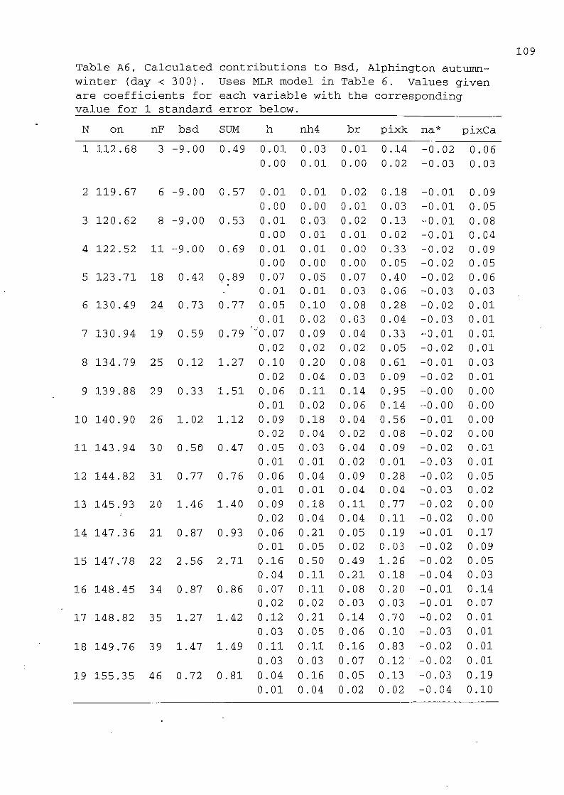
109
Table A6, Calculated contributions to Bsd, Alphington autumn-
winter (day < 300). Uses MLR model in Table 6. Values given
are coefficients for each variable with the correspondingvalue for 1 standard error below.
N on nF bsd SUM h nh4 br pixk na* pixCa
1 112.68 3 -9.00 0.49 0.01 0.03 0.01 0.14 -0.02 0.06
0.00 0.01 0.00 0.02 -0.03 0.03
2 119.67 6 -9.00 0.57 0.01 0.01 0.02 0.18 -0.01 0.09
0.00 0.00 0.01 0.03 -0.01 0.05
3 120.62 8 -9.00 0.53 0.01 0.03 0.02 0.13 -0.01 0.08
0.00 0.01 0.01 0.02 -0.01 0.04
4 122.52 11 -9.00 0.69 0.01 0.01 0.00 0.33 -0.02 0.09
0.00 0.00 0.00 0.05 -0.02 0.05
5 123.71 18 0.42 0.89 0.07 0.05 0.07 0.40 -0.02 0.06
0.01 0.01 0.03 0.06 -0.03 0.03
6 130.49 24 0.73 0.77 0.05 0.10 0.08 0.28 -0.02 0.01
0.01 0.02 0.03 0.04 -0.03 0.01
7 130.94 19 0.59 0.79 '"0.07 0.09 0.04 0.33 -0.01 0.010.02 0.02 0.02 0.05 -0.02 0.01
8 134.79 25 0.12 1.27 0.10 0.20 0.08 0.61 -0.01 0.03
0.02 0.04 0.03 0.09 -0.02 0.01
9 139.88 29 0.33 1.51 0.06 0.11 0.14 0.95 -0.00 0.00
0.01 0.02 0.06 0.14 -0.00 0.00
10 140.90 26 1.02 1.12 0.09 0.18 0.04 0.56 -0.01 0.00
0.02 0.04 0.02 0.08 -0.02 0.00
11 143.94 30 0.50 0.47 0.05 0.03 0.04 0.09 -0.02 0.01
0.01 0.01 0.02 0.01 -0.03 0.01
12 144.82 31 0.77 0.76 0.06 0.04 0.09 0.28 -0.02 0.05
0.01 0.01 0.04 0.04 -0.03 0.02
13 145.93 20 1.46 1.40 0.09 0.18 0.11 0.77 -0.02 0.00
0.02 0.04 0.04 0.11 -0.02 0.00
14 147.36 21 0.87 0.93 0.06 0.21 0.05 0.19 -0.01 0.17
0.01 0.05 0.02 0.03 -0.02 0.09
15 147.78 22 2.56 2.71 0.16 0.50 0.49 1.26 -0.02 0.05
0.04 0.11 0.21 0.18 -0.04 0.03
16 148.45 34 0.87 0.86 0.07 0.11 0.08 0.20 -0.01 0.14
0.02 0.02 0.03 0.03 -0.01 0.07
17 148.82 35 1.27 1.42 0.12 0.21 0.14 0.70 -0.02 0.01
0.03 0.05 0.06 0.10 -0.03 0.01
18 149.76 39 1.47 1.49 0.11 0.11 0.16 0.83 -0.02 0.01
0.03 0.03 0.07 0.12 ' -0.02 0.01
19 155.35 46 0.72 0.81 0.04 0.16 0.05 0.13 -0.03 0.19
0.01 0.04 0.02 0.02 -0.04 0.10
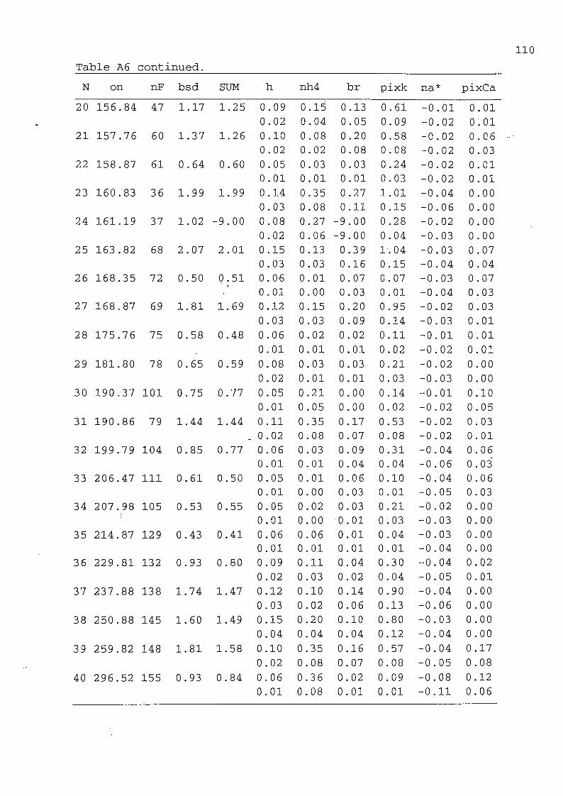
110
Table A6 continued.
N on nF bsd SUM h nh4 br pixk na* pixCa
20 156.84 47 1.17 1.25 0.09 0.15 0.13 0.61 -0.01 0.01
0.02 0.04 0.05 0.09 -0.02 0.01
21 157.76 60 1.37 1.26 0.10 0.08 0.20 0.58 -0.02 0.06
0.02 0.02 0.08 0.08 -0.02 0.03
22 158.87 61 0.64 0.60 0.05 0.03 0.03 0.24 -0.02 0.01
0.01 0.01 0.01 0.03 -0.02 0.01
23 160.83 36 1.99 1.99 0.14 0.35 0.27 1.01 -0.04 0.00
0.03 0.08 0.11 0.15 -0.06 0.00
24 161.19 37 1.02 -9.00 0.08 0.27 -9.00 0.28 -0.02 0.00
0.02 0.06 -9.00 0.04 -0.03 0.00
25 163.82 68 2.07 2.01 0.15 0.13 0.39 1.04 -0.03 0.07
0.03 0.03 0.16 0.15 -0.04 0.04
26 168.35 72 0.50 0.51 0.06 0.01 0.07 0.07 -0.03 0.07
0.01 0.00 0.03 0.01 -0.04 0.03
27 168.87 69 1.81 1.69 0.12 0.15 0.20 0.95 -0.02 0.03
0.03 0.03 0.09 0.14 -0.03 0.01
28 175.76 75 0.58 0.48 0.06 0.02 0.02 0.11 -0.01 0.01
0.01 0.01 0.01 0.02 -0.02 0.01
29 181.80 78 0.65 0.59 0.08 0.03 0.03 0.21 -0.02 0.00
0.02 0.01 0.01 0.03 -0.03 0.00
30 190.37 101 0.75 0.77 0.05 0.21 0.00 0.14 -0.01 0.10
0.01 0.05 0.00 0.02 -0.02 0.05
31 190.86 79 1.44 1.44 0.11 0.35 0.17 0.53 -0.02 0.03
_ 0.02 0.08 0.07 0.08 -0.02 0.01
32 199.79 104 0.85 0.77 0.06 0.03 0.09 0.31 -0.04 0.06
0.01 0.01 0.04 0.04 -0.06 0.03
33 206.47 111 0.61 0.50 0.05 0.01 0.06 0.10 -0.04 0.06
0.01 0.00 0.03 0.01 -0.05 0.03
34 207.98 105 0.53 0.55 0.05 0.02 0.03 0.21 -0.02 0.00
0.01 0.00 0.01 0.03 -0.03 0.00
35 214.87 129 0.43 0.41 0.06 0.06 0.01 0.04 -0.03 0.00
0.01 0.01 0.01 0.01 -0.04 0.00
36 229.81 132 0.93 0.80 0.09 0.11 0.04 0.30 -0.04 0.02
0.02 0.03 0.02 0.04 -0.05 0.01
37 237.88 138 1.74 1.47 0.12 0.10 0.14 0.90 -0.04 0.00
0.03 0.02 0.06 0.13 -0.06 0.00
38 250.88 145 1.60 1.49 0.15 0.20 0.10 0.80 -0.03 0.00
0.04 0.04 0.04 0.12 -0.04 0.00
39 259.82 148 1.81 1.58 0.10 0.35 0.16 0.57 -0.04 0.17
0.02 0.08 0.07 0.08 -0.05 0.08
40 296.52 155 0.93 0.84 0.06 0.36 0.02 0.09 -0.08 0.12
0.01 0.08 0.01 0.01 -0.11 0.06

Ill
Table A7, Footscray autumn-winter Bsd calculated contributions to Bsd
using MLR model given in Table 7. Values given are coefficients for each
variable with the corresponding value for 1 standard error below.
N on nF bsd SUM h nh4 br pixk na* pixCa na* sws
2 107.52 2 -9.00 0.84 0.02 0.14 0.26 0.03 -0.01 0.14 -0.02 0.12
0.01 0.03 0.08 0.08 -0.02 0.08 -0.01 0.07
3 112.63 4 -9.00 0.58 0.01 0.03 0.02 0.01 -0.01 0.05 -0.03 0.36
0.00 0.01 0.01 0.03 -0.02 0.03 -0.02 0.20
4 119.64 7 -9.00 0.74 0.01 0.02 0.04 0.02 -0.01 0.10 -0.03 0.43
0.00 0.01 0.01 0.06 -0.02 0.06 -0.02 0.25
6 122.69 12 0.63 0.67 0.03 0.01 0.17 0.09 -0.01 0.05 -0.03 0.22
0.01 0.00 0.05 0.25 -0.02 0.03 -0.02 0.12
7 126.90 17 0.78 0.93 0.06 0.07 0.40 0.04 -0.01 0.14 -0.04 0.13
0.01 0.02 0.11 0.12 -0.02 0.07 -0.02 0.07
8 130.60 23 1.20 1.33 , 0.07 0.29 0.39 0.05 -0.01 0.29 -0.05 0.14
.0.02 0.07 0.11 0.16 -0.03 0.16 -0.03 0.08
9 134.81 13 1.59 1.84 0.07 0.26 0.85 0.10 -0.03 0.38 -0.12 0.17
0.02 0.06 0.24 0.29 -0.08 0.21 -0.06 0.10
10 140.52 27 0.42 0.55 0.03 0.04 0.09 0.01 -0.01 0.10 -0.02 0.15
0.01 0.01 0.03 0.03 -0.02 0.05 -0.01 0.09
11 141.46 28 0.90 0.81 0.05 0.12 0.14 0.05 -0.01 0.13 -0.05 0.23
0.01 0.03 0.04 0.15 -0.04 0.07 -0.03 0.13
12 147.80 32 1.64 1.75 0.10 0.47 0.71 0.08 -0.00 0.15 -0.02 0.11
0.02 0.11 0.20 0.25-0.01 0.08 -0.01 0.06
13 148.32 33 2.68 2.48' 0.12 1.00 0.60 0.08 -0.01 0.46 -0.05 0.11
0.03 0.23 0.17 0.25 -0.03 0.25 -0.03 0.07
14 148.68 14 1.69 1.41 0.09 0.39 0.49 0.06 -0.01 0.12 -0.02 0.-14
0.02 0.09 0'.14 0.17 -0.01 0.06 -0.01 0.08
15 149.28 15 1.69 0.96 0.04 0.06 0.36 0.03 -0.00 0.11 -0.01 0.23
0.01 0.01 0.10 0.08 -0.01 0.06 -0.00 0.13
16 156.39 41 1.08 1.01 0.06 0.18 0.24 0.05 -0.01 0.23 -0.02 0.13
0.01 0.04 0.07 0.14 -0.02 0.13 -0.01 0.07
17 156.83 42 1.15 1.05 0.06 0.14 0.51 0.05 -0.00 0.02 -0.01 0.14
0.01 0.03 0.14 0.13 -0.01 0.01 -0.01 0.08
18 157.32 43 0.77 0.92 0.04 0.06 0.30 0.01 -0.00 0.09 -0.02 0.29
0.01 0.01 0.09 0.03 -0.01 0.05 -0.01 0.17
19 157.87 44 1.21 1.27 0.06 0.21 0.63 0.04 -0.00 0.-02 -0.01 0.16
0.01 0.05 0.18 0.13 -0.01 0.01 -0.01 0.09
20 160.88 62 0.92 0.99 0.06 0.15 0.45 0.04 -0.01 0.11 -0.04 0.08
0.01 0.03 0.13 0.12 -0.03 0.06 -0.02 0.04
21 161.50 63 0.78 0.72 0.06 0.11 0.12 0.03 -0.00 0.01 -0.02 0.26
0.01 0.03 0.03 0.10 -0.01 0.00 -0.01 0.15
22 163.88 66 0.73 0.79 0.07 0.04 0.39 0.03 -0.00 0.03 -0.02 0.11
0.02 0.01 0.11 0.08 -0.01 0.02 -0.01 0.06

112
Table A7 continued.
N on nF bsd SUM h nh4 br pixk na* pixCa na* sws
23 164.88 67 1.09 1.02 0.0^ 0.31 0.30 0.04 -0.00 0.02 -0.02 0.180.01 0.07 I).09 0.11 -0.01 0.01 -0.01 0.10
24 177.53 77 0.33 0.59 0.03 0.00 0.02 0.01 -0.01 0.02 -0.03 0.39
0.01 0.00 0.01 0.03 -0.02 0.01 -0.01 0.22
25 183.60 74 0.43 0.50 0.04 0.01 0.05 0.01 -0.01 0.03 -0.03 0.25
0.01 0.00 0.01 0.02 -0.02 0.01 -0.01 0.14
26 190.85 99 1.07 1.02 0.07 0.18 0.48 0.05 -0.01 0.05 -0.03 0.08
0.02 0.04 0.14 0.14 -0.02 0.03 -0.02 0.05
33 203.43 102 0.82 0.75 0.03 0.03 0.02 0.00 -0.00 0.03 -0.01 0.50
0.01 0.01 0.01 0.01 -0.00 0.01 -0.00 0.28
34 214.53 124 0.79 1.33 0.06 0.50 0.21 0.05 -0.00 0.24 -0.02 0.14
0.01 0.12 0.06 0.14 -0.01 0.13 -0.01 0.08
35 218.57 125 0.55 0.51 - .0.04 0.01 0.07 0.03 -0.00 0.05 -0.02 0.18
0.01 0.00 0.02 0.08 -0.01 0.03 -0.01 0.10
37 259.89 146 0.88 0.81 0.06 0.19 0.20 0.03 -0.00 0.04 -0.01 0.16
0.01 0.04 0.06 0.08 -0.01 0.02 -0.00 0.09
38 265.00 131 0.71 0.70. 0.06 0.07 0.25 0.03 -0.00 0.03 -0.01 0.12
0.01 0.02 0.07 0.08 -0.01 0.02 -0.01 0.07
39 272.81 149 1.05 1.07 0.08 0.67 0.02 0.01 -0.01 0.05 -0.03 0.13
0.02 0.15 0.00 0.03 -0.02 0.03 -0.02 0.07
40 273.21 151 1.10 0.98 0.05 0.41 0.03 0.02 -0.00 0.16 -0.02 0.19
0.01 0.09 0.01 0.05 -0.01 0.09 -0.01 0.11
41 276.52 157 0.94 1.04 0.05 0.45 0.07 0.02 -0.00 0.11 -0.01 0.19
0.01 0.10 0.02 0.05 -0.01 0.06 -0.01 0.11
42 280.42 158 1.04" 0.86 0.06 0.16 0.08 0.03 -0.01 0.30 -0.03 0.120.01 0.04 0.02 0.08 -0.02 0.16 -0.02 0.07

113
Table A8, Footscray and Alphington, suinmer (day > 300),
calculated contributions to Bsd using MLR model given in
Table A6.
N on nF bsd SUM h nh4 br pixCa na*
1 331.55 165 0.67 0.80 0.07 0.33 0.30 0.07 -0.04
0.01 0.04 0.18 0.13 -0.07
2 336.12 153 1.43 1.49 0.07 1.11 0.24 0.02 -0.02
0.01 0.13 0.15 0.03 -0.03
3 336.49 154 1.41 1.25 0.11 0.86 0.15 0.08 -0.03
0.01 0.10 0.09 0.15 -0.05
4 337.58 71 0.55 0.45 0.10 0.09 0.16 0.04 -0.00
0.01 0.01 0.10 0.08 -0.01
5 344.55 181 -9.00 -9.00 0.03 0.04 0.13 -9.00 -0.02
0.00 0.00 0.08 -9.00 -0.03
6 344.92 178 -9.00-9.00 0.03 0.02 0.06 -9.00 -0.01
0.00 0.00 0.03 -9.00 -0.01
7 345.28 179 -9.00 -9.00 0.08 0.00 0.20 -9.00 -0.01
0.01 0.00 0.12 -9.00 -0.01
8 347.63 182 0.36 0.34 0.03 0.02 0.22 0.04 -0.03
0.00 0.00 0.13 0.06 -0.06
9 352.95 183 0.90 0.63 0.05 0.34 0.19 0.00 -0.01
0.01 0.04 0.11 0.00 -0.03
10 378.42 190 0.61 0.81 0.07 0.57 0.10 0.05 -0.05
0.01 0.07 0.06 0.08 -0.08
11 381.60 187 0.38 0.35 0.04 0.10 0.14_ 0.04 -0.04
0.00 0.01 0.09 0.07 -0.07
12 383.60 188 0.61 0.66 0.09 0.26 0.23 0.04 -0.03
0.01 0.03 0.14 0.07 -0.05
13 331.46 164 0.82 -9.00 -9.00 -9.00 -9.00 0.31 -9.00
-9.00 -9.00 -9.00 0.55 -9.00
14 336.08 161 0.97 -9.00 -9.00 -9.00 -9.00 0.05 -9.00
-9.00 -9.00 -9.00 0.09 -9.00
15 336.45 159 1.44 1.35 0.08 1.08 0.06 0.08 -0.03
0.01 0.13 0.03 0.15 -0.05
16 353.55 173 0.32 0.28 0.05 0.08 0.08 0.03 -0.02
0.01 0.01 0.05 0.05 -0.03
17 383.51 189 0.68 0.75 0.11 0.45 0.11 0.04 -0.03
0.01 0.05 0.07 0.07 -0.05
18 399.55 191 0.83 0.83 0.08 0.50 0.11 0.28 -0.21
0.01 0.06 0.07 0.49 -0.37
19 403.50 197 0.48 0.68 0.06 0.44 0.07 0.11 -0.06
0.01 0.05 0.04 0.19 -0.11

114
CSIRO-EPA Melbourne Aerosol Study.
Final Report: Part B, Source Study

115
Contents, Part B: Source Study-
page
List of Tables 116
List of Figures 117
1. Source studies. 118
1.1 Results from source sampling 120
1.2 Carbon constituents, TC/elC, vehicles and
biomass 120
2. TC/EC ratios in vehicle emissions 120
3. TC/EC in biomass burning emissions 124
4. Source tracers - inorganic 125
5. Acknowledgements 130
6. References 131

list of Tables.
116
Table Bl. Source sampling summary.
Table B2. Medians of mass concentration ratios
(species/FPM) for indicated sources.
Table B3. Means of mass concentration ratios
(species/FPM) for indicated sources.
Table B4. Ratio of species mass to FPM for all
source samples.
Table B5. Concentrations of soluble inorganic
species in source samples.
Table B6. PIXE elemental concentrations, Al-Cr,
Table B7. Collected mass, sample flows, carbon
and FPM.
Table B8. Concentrations of organic compounds.
Table B9. GC/MS Target Compounds.
page
132
134
135
136
140
141
144
145
148

List of Figures
117
Figure Bl.
Figure B2.
Figure B3.
Figure B4.
Figure B5.
Figure B6.
Fine particle carbon and total
inorganic mass contributions to the
source FPM, (medians).
Fine particle elemental contributions
(PIXE analysis) to source FPM,(medians).
Fine particle soluble inorganic species
contributions to source FPM, (medians).
Relationship between ambient samples
lead concentration and bromide
concentration.
Relationship between ambient samples
lead concentration and nitric oxide (NO)
concentration.
Relationship between ambient samples
bromide concentration and nitric oxide
(NO) ooncentration.
page
121
122
123
127
128
129

118
1. Source studies.
An important aspect of the Melbourne Aerosol Study is the
characterisation of a number of different possible major
sources to the Melbourne (fine fraction) aerosol. A short
list of possible major sources includes both primary and
secondary particle production. Primary sources include sea-
salt, soil, stationary industrial sources, motor vehicle
emissions, domestic heating and incineration, and biomass
burning, either as controlled burns or wildfires. Additional
minor organic sources include natural emissions from plants
and waste products from meat cooking. Secondary fine aerosol
material is produced within the atmosphere from gaseous
precursors emitted along with primary emissions. The
association with these.primary emissions will be lost however
because of interposing meteorological and chemical conditions
which govern whether the potential for particle production is
realised and which also control the rate of particle
production. Examples of secondary production are the
conversion of NO^ and SO2 to nitric and sulfuric acids and arange of possible aerosol nitrates and sulfates and the
important case of conversion and condensation of volatile
organic .compounds into an aerosol phase.
Some of the possible primary sources require little
further characterisation, for example sodium is a frequently
used tracer for sea-salt aerosol and other constituents such
as magnesium may also be useful. Si, 0, Al, Fe and Ca are the
major crustal elements (Fairbridge, 1972), several of these
are frequently used for tracers of soil dust. For both of
these spurces the contributions to the reduced visibility and
fine aerosol mass in Melbourne are known to be quite small
(Gras et al. 1990 and Part A of this report). Some form of
combustion is associated with most other major sources.
In Melbourne during reduced visibility periods a very
high proportion of aerosol is comprised of carbon in both
organic and elemental forms. Elemental carbon can be
considered a general tracer for combustion processes but
cannot immediately be further subdivided with regard to its
possible origins. We have examined a number of primary
sources for additional constituents in the fine aerosol that
can be used as tracers for these sources. This includes known
tracers such as lead (and bromide) for motor vehicles but also
we have sought possible unique organic marker compounds in the

119
sources examined. These sources included vehicles using
leaded petrol, vehicles using unleaded petrol, light diesels,
woodstoves and biomass burning (approximated with gum leaves
and twigs, and dry grass hay).
Motor vehicle emissions were collected from in-service
vehicles operating on an "urban drive" cycle on the EPAV
vehicle test dynamometer at Altona after a standard cold
period. Vehicles using leaded and unleaded fuel were
considered separately. Collections were made in the start-up
period, usually the first one or two minutes and then over the
subsequent fifteen minutes. Air from the vehicle exhaust
system was diluted with filtered ambient air to assist in
drying the sample air and prevent clogging of the sampling
system. The collections were otherwise identical to those
made at the ambient sampling sites.
Diesel vehicles were sampled whilst static, after being
allowed to cool to ambient conditions. Samples were taken
during the start-up period and when warm, this was typically
for periods of about 10 seconds. A range of in-service light
diesels were considered including four-wheel drive passenger
vehicles and light trucks. Sampling procedures were otherwise
identical to those used for petrol fuelled vehicles.
Woodstove emissions were examined with the cooperation of
Coonara Heaters Pty. Ltd. in the Coonara test facility at
Fe~rntree Gully. This used a closed slow-combustion stove
burning dried split red-girm timber. The stove was operated
according to the draft Australian measurement standard for the
amount, size, moisture content and disposition of fuel in the
combustion chamber. A range of operating conditions were
examined including periods with the initial flaming combustion
and subsequent slow combustion when glowing coals were
present. The Coonara test facility incorporates a dilution
tunnel from which the aerosol samples were drawn. These were
further diluted with filtered air for size segregation and
collection.
Other possible biomass burning sources were examined by
constructing an open fire-box at CSIRO Division of AtmosphericResearch in which various fuels could be burnt. Fuels
considered in this study included dry grass hay and a mixture
of dry grass, eucalypt leaves and twigs. Aerosol samples were
collected during active flaming and smoking from a positionapproximately 60 cm above the combustion source. The sampled

120
material was diluted with filtered air before size segregation
and collection.
1.1 Results from source sampling
Source chemical data are summarised in Tables B2 - B4
which give the component mass fractions (component/ FPM) for
the five sources sampled. Comparable data for sea-salt from
Millero (1974) and "average crustal" composition (soil) from
Fairbridge (1972) are incorporated in Tables B2 and B3 for
reference. Table B2 is based on median concentrations and
Table B3 on means. Comparison of the two tables shows some
differences as can be expected for the relatively small number
of samples in each group and the range within groups. Table
B4 gives the individual sample mass loadings. Components of
the five sampled sources are also given in Figs. Bl - B3.
1.2 Carbon constituents, TC/elC, vehicles and biomass
The fractions of organic carbon in all five samples,
shown in Fig. Bl are relatively uniform with unleaded vehiclescontributing the lowest.fraction. This is expected since the
majority of the vehicles using unleaded fuel were relatively
new vehicles fitted with catalytic converters (required to
meet to Australian design Rule ADR 37 emission standard, - see
table Bl). Average ratios of total to elemental carbon
concentration for these sources are included in Table B3.
2. TC/EC ratios in vehicle emissions
Pratsinis et al. (1984) reported a ratio of TC/EC = 2.3
for fresh vehicle emissions in Los Angeles. The
concentrations of TC and EC for (post 1985 manufacture)
vehicles using unleaded fuel, (pre 1986) vehicles using leaded
fuel, and light diesels were determined individually in thepresent study. Average TC/EC values were determined for thethree vehicle types, giving:
TC/EC= 3.4, unleaded,
TC/EC= 5.1, leaded and
TC/EC= 2.8, diesel.
To derive an overall average ratio, these individual ratioswere weighted using estimated PMIO emissions for all petrol
fuelled vehicles and all diesel fuelled vehicles in the Port
Phillip Control Region (PPCR), from the EPA emission inventory
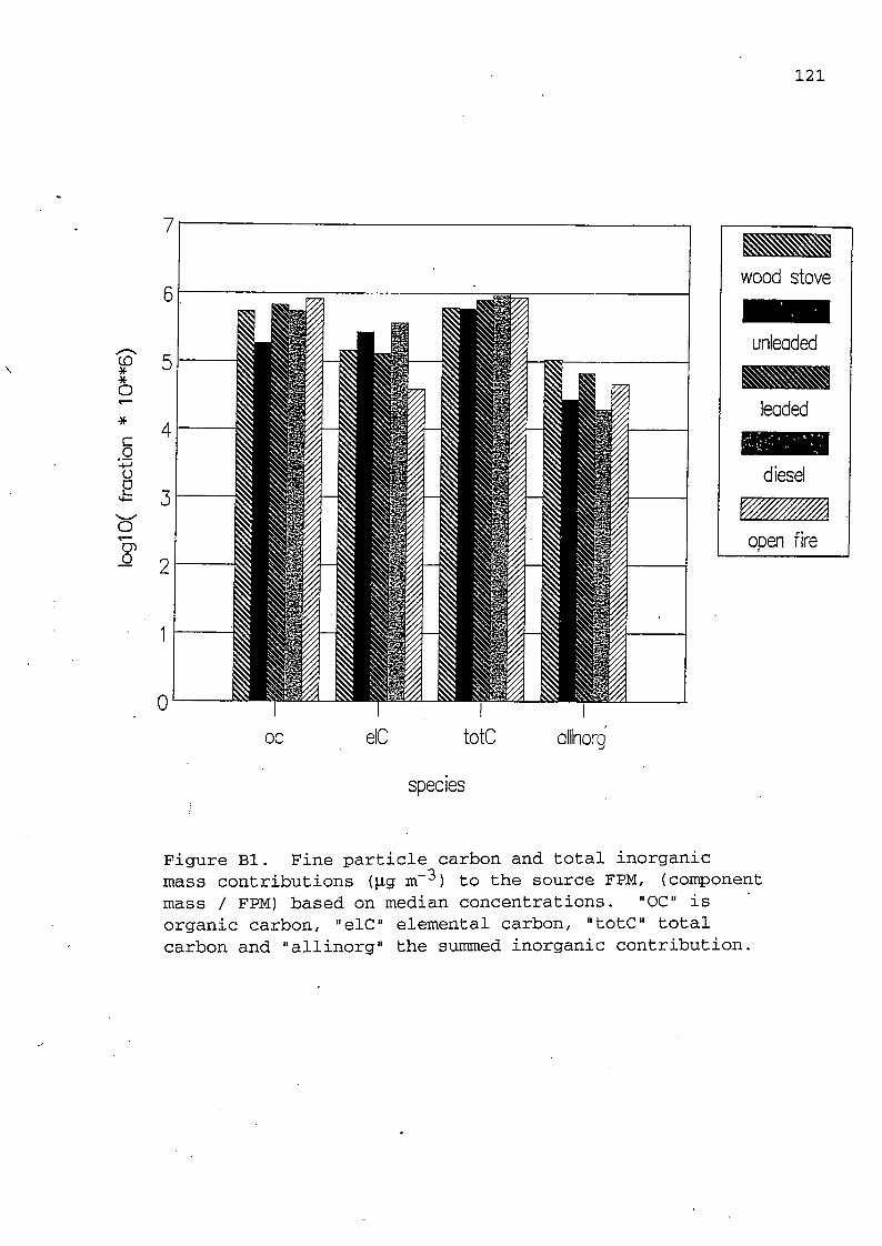
121
to**
o
*
Co
■-4-Jo□
cnO
wood stove
unleaded
open fire
00 elC tote aillnoro
species
Figure Bl. Fine particle carbon and total inorganicmass contributions (p.g m~^) to the source FPM, (componentmass / FPM) based on median concentrations. "OC" isorganic carbon, "elC" elemental carbon, "totC" totalcarbon and "allinorg" the summed inorganic contribution.

122
CD**
O
c,0
o
.2
o
'oio
pixSi pixS pixK plxCr pixFe pjxCu pixBr pixBdpixr pixCI pixCa pixMn pixNi pixZn pixSr pixPbl
species
wood stove
unleaded
leaded
^Hidiesel
open fire
Figure B2. Fine particle elemental contributions(PIXE analysis) to.source FPM, (element mass / FPM) based
on median concentrations.

123
CD**
o
c.O
u□
0
01O
wood stove
unleaded
open fire
no
nh4 mgcl CO
k
speciesno3
br"so4
Figure B3. Fine particle soluble inorganic speciescontributions to source FPM, (species mass / FPM) , baseddn median concentrations.

124
(EPA 19 91) . The petrol fuelled vehicle contribution was
divided into two parts, 70% for leaded and 30% for unleaded
vehicles, based on the 1990 fleet ratio. The fraction of
vehicle kilometers driven in arterial/freeway, over-dimension
roads, residential and minor roads was also taken into
account. The resulting weightings were, unleaded vehicle
7.8%, leaded vehicle 18.3% and (all) diesel 73.9% (motor
cycles and LPG fuelled vehicles were ignored). With these
weightings the overall estimated vehicle exhaust TC/EC ratio
is 3.3, somewhat larger than the value measured by Pratsinis
et al. (1984) for Los Angeles, but consistent with the minimixm
observed values of TC/EC in the ambient part of the Melbourne
Aerosol Study, as shown in (Part A) Fig. 16. It is also very
similar to the basin-wide primary emission TC/EC ratio
estimate of 3.2 for 1980 Los Angeles (which is also dominated
by diesel vehicles), as reported by Gray et al. (1986) .
3. TC/EC in biomass burning emissions
Much larger TC/EC ratios are reported as typical in
emissions from burning plant material, particularly in
bushfires or wildfires. Ambient measurements in suspected
fire-impacted air in Arizona with a TC/EC ratio of 30 were
reported by Marcias et al. (1981). Milne et al. (1983) report
a TC/EC value of 16.1 for Australian bushfire smoke and
similar values have been reported elsewhere. Andreae et al.
(1988) reported TC/EC ratios in smoke plumes from biomass
burning in Brazil; in the plume, ratios of 3.3, 876 and 7.7
were observed with general sampling in the impacted boundary
layer air giving ratios of 12.6 ± 8.7.
Our source samples for combustion stoves were obtained in
a variety of flaming and glowing coals conditions and have a
fairly wide range of TC/EC ratios (see comments Table Bl).
These range from 1.2 for sample nF=57 with active flamingusing mixed wood, to 41.9 for sample nF=55 with a moderate
flame burning redgum, the average TC/EC ratio excluding sample
nF=55 is 6.6 (median 4.1 from 10 samples). The open fire pit,
burning hay and eucalypt twigs and leaves gave TC/EC ratiosfrom 4.7 to 41.4 with an average ratio of 24.5 (median 24.7
from 6 samples). This latter case gives an approximation to abiomass burning source and is in agreement with the reported
ambient measurements from similar sources.

125
4. Source tracers - inorganic
The mass fractions of soluble ions in the source FPMs are
shown in Fig. B2 and elemental concentrations using PIXE
analysis in Fig. B3. These show that for vehicle sources lead
and/or bromide should provide near unique markers. Whilst the
use of bromide or lead strictly applies only to vehicles using
leaded fuel, providing the mixture of vehicles does not change
substantially with either time or location these tracers can
be used to represent the contribution of all vehicles. The
relationships between lead, bromide and nitric oxide (NO) in
the ambient samples were found by regression, they were:
pixPbl = 0.54 ± 0.01 pixBr + 0.35 + 0.04, r^=0.99, nm m"^
(± 1 std. error), from 86 samples, two outlying points
(outside the 95% confidence limits) removed.
pixPbl = 0.51 ± 0.01 br + 0.22 ± 0.08, r2=0.97 , nm m"^
using soluble bromide, for 82 samples (two outliers removed).
Corresponding mole ratios in the source samples for vehicles
using leaded fuel were:
lead = 0.65 bromide, nm m ,
for both pixBr (6 points) and soluble br (4 points, one-
suspect br value deleted). Some bromide was also observed in
emissions from vehicles using unleaded fuel (Tables B2-B4)
which probably accounts for the difference in the source and
ambient mole ratios. The relationship between lead and NO in
the ambient samples was:
pixPbl = 0.26 ± 0.01 NO + 0.27 ± 0.06, r2=0.98 ,
lead in nm m~^ and NO in pphm, from 66 points, (one outlierdeleted). For bromide the relationship with NO was:
pixBr = 0.49 ± 0.01 NO - 0.1 ± 0.1, r2=0.98 ,
bromide in nm m~^ and NO in pphm, from 65 points, (2 outliersdeleted). Clearly any of these three variables would
represent vehicles quite satisfactorily. We used soluble
bromide as this consistently gave the largest nuxnber of events
and usually resulted in slight improvements in multipleregression model correlation coefficients. The inter-

126
relationships between lead, bromide and NO in the ambient
samples (using PIXE lead and soluble br) is shown in Figs. B4-
B6.
Potassium, a known indicator for biomass combustion shows
strongly in both the woodstove and open fire samples, chloride
is also prominent in these samples. Phosphorous was only
detected in the woodstove samples. Chloride is also the major
component in sea-salt so the chloride concentration is less
specific for detection of burning. Potassium is present in
sea-salt at the 1% level which is comparable with combustion
sources however the use of the non-sea-salt potassium (based
on sodium concentration) together with the general pattern of
its abundance enables its very effective use as a biomass
burning tracer. We have used PIXE derived potassi-um as the
main indicator for smoke/biomass burning type aerosol. We
also used GCMS analysis of extractable organic material to
examine specific organic compounds that are potentially useful
as smoke/biomass burning indicators. Some of these appear to
offer prospects for differentiating between smokes from lower
temperature biomass burning, where the organic content is high
and may contain a greater fraction of distillation products,
and the high temperature combustion of diy eucalypt wood
typical of woodstoves (this is also discussed in Part A
section 3.11).
Aerosol acidity, expressed as the combination of the
concentrations of hydrogen ion and ammonium (H+NH4) is a
factor that frequently gave very significant coefficients in
our MLR models of FPM and Bg^. This factor shares a similarseasonal cycle to other constituents that are known to be
photochemically driven. In our MLR models we have interpreted
aerosol acidity as a measure of secondary production. This
variable may contain some contribution from primary acidic
aerosol emitted directly by stationary industrial sources,
however, in the lack of large smelting operations and high
sulfur fuel power stations in the Melbourne region this
fraction is assumed to be small.

127
Pb vs Br
cn
E
na
18
16
14
12
10
1 1
+
,,1
0
r
0
+0
-
0 0
0
-
o
* O 0^.
+ O^r ■><>
t *P 0 . 1 1 •
10 15Br (nM/m3)
20 25. 30
Figure B4. Relationship between ainbient samples leadconcentration (n mole m~^) and bromide concentration(n mole m"^) .
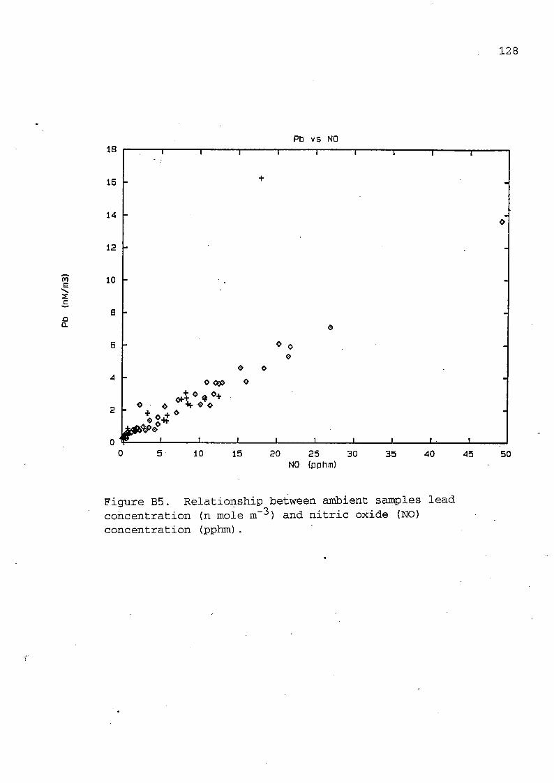
128
Pb vs NO
m
zc
£3
a
O <K&
20 25 30
NO (pphm)
Figure B5. Relationship between ambient samples leadconcentration (n mole iri"^) and nitric oxide (NO)concentration (pphm).
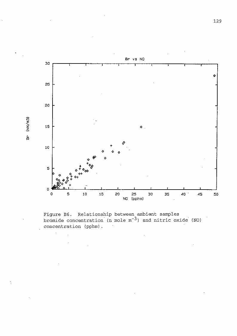
129
Bn vs NO
m
E
ZC
C.cu
30
25
20
15
10
1 1 I I 1 1 1 1 1
0
0
0 O o
O ̂ ^
^ o %0* ̂ce>•H-
0+
-
o I 1 I 1 1 1 I 1 1
10 15 20 25 30
NO (pphm)35 40 45 50
Figure B6. Relationship between ambient samples
bromide concentration (n mole m~^) and nitric oxide (NO)concentration (pphm).

130
5. Acknowledgements
We gratefully acknowledge the willing assistance of staff
at the EPAV Vehicle Testing Facility in our collection of
vehicle emission samples. We thank the Engineering Department
of Chelsea Council, CSIRO Chemicals and Polymers Division,
Janice Bathols and Patrick Bradley of CSIRO Atmospheric
Research for the use of their vehicles for emission testing.
We also thank Coonara International for allowing us the use of
their woodstove test facility. Special thanks go to David
Whyte for assistance in the sample collections.

131
6. References
Andreae E.E., E.V. Browell, M. Garstang, G.L. Gregory, R.C.
Harriss, G.F. Hill, D.J. Jacob,. M.C. Pereira, G.W. Sachse,
A.W. Setzer, P.L. Silva Bias, R.W. Talbot, A.L. Torres and
S.C. Wofsey, Biomass-burning emissions and associated haze
layers over Amezonia, J. Geophys. Res.,93, 1509-1527, 1988.
EPAV, Air emissions inventory. Port Phillip Control region.
Planning for the Future, EPAV SRS 91/001,1991.
Fairbridge R.W. Ed. The Encyclopedia of Geochemistry and
Environmental Sciences. Van Nostrand Reinhold Company, 1972
Gras J.L., G.P. Ayers, R.W. Gillett and S.T. Bentley.
Regional visibility and aerosol properties in South - Eastern
Australia. In proceedings of the 10th Clean Air Conference,
Clean Air Society of Australia and New Zealand, Auckland,
1990 .
Gray H.A., G.R. Cass, J.J. Huntzicker, E.K. Heyerdahl and J.A.
Rau, Characteristics of atmospheric organic and elemental
carbon particle concentrations in Los Angeles, Environ. Sci.
Technol., 20, 580-589, 1986.
Marcias E.S., J.O. Zwicker, J.R. Ouimette, S.V. Bering, S.K.
Friedlander, T.A. Cahill, G.A. Kuhlmey and L.W. Richards,
Regional haze case studies in the Southwestern U.S.- 1.
Aerosol chemical composition. Atmos. Environ., 15, 1971-1986,
1981.
Millero F.J., The physical chemistry of sea-water. Ann. Rev.
Earth Plan. Sci., 2. 101-150, 1974.
Milne J.W.,D.B. Roberts, S.J. Walker and D.J. Williams,
Sources of Sydney Brown Haze. In The Urban Atmosphere -
Sydney a case study. Eds. J.N Carras and G.N. Johnson, CSIRO.
PP181-197, 1983.
Pratsinis S.,T. Novakov, E.C. Ellis, and S.K. Friedlander, The
carbon containing component of the Los Angeles aerosol: source
apportionment and contributions to the visibility budget.
JAPC.A, 34, 643-650, 1984.

132
Table B1. Source sampling summary
nF nN nG description
woodstoves burning dry timber48 48 52 2. 45 kg redgum vigorously flaming and some
coals at start, subsided, 4.6 kg redgum addedmid sample, (17 min. sample)
.49 49 53 3.25 kg from previous load at start, stillflaming , no visible smoke, (7 min.)
50 50 54 1.5 kg coals from previous load at start.6 kg redgum added mid sample, (3 min.)
51 51 55 5.5 kg flaming wood and coals from previousload, hose slipped off
52 52 56 4.6 kg flaming wood and coals from previousload, Fluoropore filter leaked
53 53 57 3.25 kg wood and coals remaining, moderatelyactive flame (7 min 40 sec.)
54 54 58 2.45 kg remaining mostly coals, little flame.(15 min.)
55 55 59 1.1 kg coals remaining after last sample,4.1 kg new redgum added 6 min. beforesampling, (1 min. 30 sec.)
56 56 60 4.5 kg remaining from last load, moderateflame, (6 min.)
57 57 61 3.5 kg heavy bed of coals remaining. Added4.3 kg mixed wood, bark, packing case.New load 7.3 kg, actively flaming at start ofsampling, (2 min.)
58 58 62 6.35 kg actively flaming still with previous ■load of mixed wood pieces at start.(1 min. 15 sec.)
59 59 63 4.45 kg actively flaming still with previous-mixed load at start. 3.45 kg at end.no visible smoke, all effectively coals(10 min.)
vehicles - unleaded fuel
80 81 91 Nissan Maxima, cold start, new car81 83 92 Nissan Maxima, hot run.82 84 93 Nissan Pulsar GX, cold start, new car83 85 93 b- Nissan Pulsar GX, hot run.84 86 94 Nissan Pulsar GX, stabilized hot run.85 87 95 Holden Camira, MWJ 224, 10/1988, 2400 km.
cold start
86 88 96 Holden Camira, MWJ 224, hot run87 89 97 Nissan Pintara wagon, MWL 326, 11/1989, 7276
km, cold start
88 90 98 Falcon wagon, MWQ 955, 7/1989, 29198 km, coldstart
89 91 99 Falcon wagon, MWQ 955, hot run90 92 100 CSIRO Magna wagon, ZCE 561, 11/1989, 9995 km.
cold start
91 93 102 CSIRO Magna wagon, ZCE 561, hot run92 94 103 Mitsubishi Colt, MWL 146, 12/1988, 24578 km.
cold start

133
Table Bl cont. Source sampling summary.
93 95 104 ToYOta 4WD, no catalytic converter, 66907 km,cold start.
94 96 105 Toyota 4WD, 66907 km, hot run98 100 106 CSIRO Falcon wagon, ZCE 304, 4/1989, 23928
km, cold start95 97 107 CSIRO Falcon wagon, ZCE 304, hot run
vehicles - leaded fuel
117 119 130 CSIRO Toyota Landcruiser, ZCD 251, 78958 km,cold start
118 120 13 CSIRO Toyota Landcruiser, ZCD 251, hot run119 121 132 Datsun 1200, ECQ 125, 29677 miles, cold start
burning oil120 123 133 Datsun 1200, ECQ 125.96 98 108 Mazda 929, CKJ716, 125000 km, cold start97 99 109 Mazda 929, CKJ716, hot run114 116 134 Mazda 929, CKJ716, stabilized hot run115 117 135 Daihatsu Charade, BEW 438, 217000 km, cold
start
116 118 136 Daihatsu Charade, BBW 438, hot run121 125 137 Toyota Corona, BFH 509, 74215 km, cold start,
sample damaged in storage122 126 138 Toyota Corona, BFH 509, hot run
sample damaged in storage123 128 139 Toyota Corona, BFH 509, stabilized hot run
vehicles - diesel
133 149 165 Toyota Landcruiser, AWP 597, 180000 km,cold start
134 148 166 Toyota Landcruiser, AWP 597, hot run135 147 167 Toyota Landcruiser, AWP 597, second hot
run
136 146 168 Landcruiser, CDC 070, 95606 km, cold start137 145 169 Landcruiser, CDC 070, hot run139 143 174 Toyota Hilux truck, DKD 670, 40932 km, cold
start
140 142 175 Toyota Hilux truck, DKD 670, hot run141 140 176 Mazda T3500 small tip-truck, DCT 779, 42790
km, cold start142 141 177 Mazda T3500 small tip-truck, DCT779, hot run143 151 178 Ford Trader 0811 small tip-truck, PMJ 793,
19250 km, cold start144 152 179 Ford Trader 0811 small tip-truck, PMJ 793,
hot run
fire in open pit205 209 347 hay 2 min206 210 348 hay, twigs, leaves 2.5 min207 211 349 hay 1.5 min208 212 350 hay, twigs, grass, leaves 1.5 min209 213 351 hay, twigs, leaves 1.5 min210 214 352 twigs leaves 1.5 min

134
Table B2. Medians of mass concentration ratios (species/FPM) for indicated sources.
Corresponding values are given for seawater (Millero, 1974) and for crust
(Fairbridge, 1972) .
species woodstove unleaded leaded diesel open fire sea crust
pixSi 2.771e-04 4.663e-04 2.864e-04 1.179e-02 l.Olle-04 -2.820e-01
pixP 2.216e-04 0.OOOe+00 0 . OOOe+00 0 . OOOe+00 0.OOOe+00 -1.050e-03
pixS 5.384e-04 1.952e-04 2.072e-03 1.869e-03 7.362e-04 -2.600e-04
pixCl 2.133e-02 5.579e-02 9.082e-03 5.627e-04 1.151e-02 5.503e-01 1.300e-04
pixK 1.483e-02 1.145e-03 0 . OOOe+00 0. OOOe+00 1.178e-02 1.135e-02 2.090e-02
pixCa 0.OOOe+00 0.OOOe+00 4.589e-04 0.OOOe+00 0.OOOe+00 1.171e-02 4.150e-02
pixCr 4.304e-05 0.OOOe+00 0. OOOe+00 0 . OOOe+00 0 . OOOe+00 -l.OOOe-04
pixMn 4.432e-05 0.OOOe+00 0.OOOe+00 0.OOOe+00 0.OOOe+00 - 9.500e-04
pixFe 5.318e-05 1.926e-03 2.540e-04 1.360e-04 2.667e-05 -5.630e-02
pixNi 3.202e-05 5.558e-05 3.262e-05 2.435e-05 0 . OOOe+00 - 7 .500e-05
pixCu 3.639e-05 2.991e-05 3.268e-05 0.OOOe+00 0.OOOe+00 - 5.500e-05
pixZn 6.886e-04 1.996e-04' 1.035e-03 5.751e-05 1.881e-05 - 7.000e-05
pixBr 8.2330-05 5.770e-05 1.188e-01 0.OOOe+00 1.2820-04 1.916e-03 2.500e-06
pixSr 1.959e-04 3.298e-04 0 . OOOe+00 1.956e-04 0.OOOe+00 2.246e-04 3 .750e-04
pixBal 0.OOOe+00 0.OOOe+00 0.OOOe+00 0.OOOe+00 0.OOOe+00 - 4.250e-04
pixPbl 0.OOOe+00 0.OOOe+00 1.845e-01 0.OOOe+00 0.OOOe+00 - 1.250e-05
oc 5.354e-01 1.829e-01 6.733e-01 5.426e-01 8.257e-01 - -
elC 1.440e-01 2.684e-01 1.297e-01 3.612e-01 3 .849e-02 - -
tote 6.094e-01 5.798e-01 7.835e-01 1.007e+00 8.584e-01 - 2.000e-04
alllnorg 1.054e-01 2.743e-02 6.713e-02 1.964e-02 4.678e-02 - -
h 2.179e-04 2.829e-04 6.545e-05 3.365e-04 1.655e-04 - -
nh4 2.485e-03 1.930e-04 2 .588e-04 1.040e-03 4.594e-05 - -
na 1.054e-02 3.534e-03 -1.257e-03 3.920e-03 4.477e-03 3.061e-01 2 .360e-02
mg 3.207e-04 1.042e-03 1.478e-03 9.508e-04 3.536e-04 3 .680e-02 2 .330e-02
cl 5.523e-02 3.080e-03 2.670e-03 1.233e-03 2.584e-02 5.503e-01 1.300e-04
k 2.275e-02 1.005e-03 2.760e-04 1.144e-03 1.193e-02 1.135e-02 2.090e-02
ca 6.461e-04 2.526e-03 1.548e-03 1.343e-03 7.265e-04 1.171e-02 4.150e-02
no3 3 .'6536-03 2.374e-03 5.586e-04 2.488e-03 4.277e-04 - -
br 1.853e-04 3.897e-04 5.308e-02 1.953e-03 0.OOOe+00 1.916e-03 2.500e-06
so4 4.967e-03 3.284e-03 4.014e-03 8.832e-03 4.730e-03 7 .712e-02 -

Table B3. Means of mass concentration ratios (species/FPM) for indicated
Corresponding values are given for seawater (Millero, 1974) and for crust
(Fairbridge, 1972]
135
sources.
species woodstove unleaded leaded diesel open fire sea crust
pixSi 3.397e-04 2.609e-03 2.9470-04 1.1190-02 1.6190-04 -2.8200-01
pixP 2.807e-04 5.925e-05 0.OOOe+00 0.OOOe+00 0 . OOOe+OO -1.0500-03
pixS 3.697e-03 6 .441e-04 6.579e-03 2.1020-03 6.3140-04 - 2.6000-04
pixCl 4.014e-02 8 .143e-Q2 9.8220-03 2.3230-03 1.2190-02 5.5030-01 1.3000-04
pixK 3.677e-02 3.816e-Q3 0.OOOe+00 0.OOOe+OO 1.1520-02 1.1350-02 2.0900-02
pixCa 8.222e-06 0.OOOe+00 5.2150-04 6.4010-06 0.OOOe+OO 1.1710-02 4.1500-02
pixCr 4.685e-05 0.OOOe+00 2.7250-05 2.6920-06 0.OOOe+OO - 1.0000-04
pixMn 1.202e-04 0.OOOe+00 0.OOOe+00 0.OOOe+OO 1.0540-05 - 9 .5000-04
pixFe 8.581e-05 2.758e-03 1.283e-03 1.2720-04 9.4450-05 - 5 .6300-02
pixNi 3.023e-05 1.171e-04 4.388e-05 4.4710-05 1.2820-05 - 7.5000-05
pixCu 8.744e-05 5.266e-05 3.3810-05 1.5220-06 0.OOOe+OO - 5.5000-05
pixZn 1.026e-03 4.8216-04* 9.9440-04 6.9160-05 2.7300-05 - 7.0000-05
pixBr 3.819e-04 8.353e-05 1.1920-01 9.1490-05 1.3000-04 " 1.9160-03 2 .5000-06
pixSr 2.827e-04 9.6270-04 0.OOOe+00 2.5620-04 0.OOOe+OO 2.2460-04 3.7500-04
pixBal 1.381e-04 0.OOOe+00 0.OOOe+00 0.OOOe+OO 0.OOOe+OO - 4.2500-04
pixPbl 0.OOOe+00 1.428e-04 1.7670-01 1.3230-04 0.OOOe+OO - 1.2500-05
oc 1.210e+00 9.269e-01 5.9210-01 6.0800-01 1.2120+00 - -
elC 1.471e-01 2.799e-01 1.436e-01 3.4250-01 4.1480-02 - -
tote 1.357e+00 9.3780-01 7.3250-01 9.5320-01 1.2540+00 - 2.0000-04
alllnorg 1.992e-01 5.088e-02 1.087e-01 2.3450-02 5.0200-02 - -
h 2.635e-04 5.430e-04 1.9810-04 4.0970-04 1.8900-04 - -
nh4 3.752e-03 3.1100-03 2.4770-03 1.1450-03 1.1090-04 -
na 2.373e-02 5.1200-03 2.9520-03 3.9060-03 5.5000-03 3 .0610-01 2 .3600-02
mg 6.977e-04 1.367e-03 1.5660-03 1.3000-03 6.6910-04 3 .6800-02 2 .3300-02
cl 7.508e-02 1.225e-02 1.0920-02 1.9400-03 2.4930-02 5.5030-01 1.3000-04
k 5.748e-02 1.632e-03 2.2710-03 1.6320-03 1.2380-02 1.1350-02 2.0900-02
ca 2.983e-03 3.4836-03 1.6770-03 2.4970-03 1.1410-03 1.1710-02 4.1500-02
no3 4.'5486-03 3.426e-03 8.187e-04 2.6640-03 4.8090-04 - -
br 5.912e-04 9.8800-03 9.4740-02 2.3300-03 0.OOOe+OO 1.9160-03 2.5000-06
so4 2.753e-02 9.1910-03 5.4550-03 1.0400-02 4.3650-03 7.7120-02 -
TC/EC 6. 6**
9.2*
3.4 5.1 2.8 30.2
note, * this average biased by one large value (41.88 for nF=55)
* ★ this average has nF=55 deleted

136
Table B4. Ratio of species mass ho FPM for all source samples (see Table C1 for
key to variable names)
nF type tote pixZn pixSr pix:Si pixS pixPbl
48 c 2.958e-01 9 . 6080-04 8.7570-05 1.2390-04 1.0130-04 0.0000+00
49 c 8 .433e-01 1.0820-03 1.4910-04 2.1090-04 4.6010-04 0 . OOOe+OO
50 c 8.023e-01 4.3910-05 5.7990-05 8 .2010-05 2.4270-04 0.0000+00
53 c 5.782e-01 7.8540-04 8.3190-04 5.7590-04 1.4770-02 0.0000+00
54 c 6.406e-01 5.918e-04 2.1910-04 3 .1000-04 1.8230-02 0 .0000+00
55 c 6.731e-01 2.257e-05 1.1280-04 1.5960-04 1.3060-04 0.OOOe+OO
56 c 8.367e+00 2 .242e-.04 1.9620-04 2 .7750-04 6.1660-04 0.OOOe+OO
57 c 3.106e-01 2 .8790-04 1.9560-04 2.7670-04 2.2640-04 0.0000+00
58 c 6.939e-01 1.0730-03 7.7440-04 1.0950-03 8.9610-04 0.OOOe+OO
59 c 3.695e-01 5.1900-03 2.0220-04 2.8590-04 1.2970-03 0.0000+00
80 V - - - - - -
81 V - - - - - -
82 V - - - - - -
83 V 1.235e-01 1.4160-04 0.OOOe+OO 2.5960-04 0. OOOe+OO 0.OOOe+OO
84 V 5.800e-01 2 .2040-03 2.7640-04 3.9100-04 0.OOOe+OO 8.5690-04
85 V . - 0.OOOe+00 2.1790-03 3.0820-03 2.5220-03 0 . OOOe+OO
86 V 3 .093e+00 0.OOOe+00 2.6610-03 1.0990-02 0.OOOe+OO 0 . OOOe+OO
87 V 7 .947e-01 2.8920-04 3.3740-04 4.7710-04 3 .9030-04 0.OOOe+OO
88 V 1.1420+00 2.5760-04 3.2210-04 4.5550-04 9.5230-04 0 . OOOe+OO
89 V - - - - - -
90 V 8.776e-01 - - - - -
91 V - - - - - -
93 V 5.796e-01 - - - - -
94 V 4.943e-01 - - - -
98 V 7 .551e-01 - - - - -
95 V - - - - - -
117. V 9 .533e-01 1.9290-03 0.OOOe+OO 1.8190-04 2 .3040-03 6.7420-02
118 V - - - - - -
119 V 7.913e-01 1.2000-03 0.OOOe+OO 1.0590-04 1.8400-03 2.6610-02
120 V - - - - - -
96 V 8.690e-01 4.9290-04 O.OOOe+OO 5.3040-04 4.3390-04 1.5720-01
97 V 7 .757e-01 8.6970-04 0.0000+00 0.OOOe+OO 1.9290-02 3 .8100-01
115 V 3.146e-01 1.2830-03 0.OOOe+OO 3.9080-04 1.4670-02 2.1590-01
123 V 6.909e-01 1.9190-04 0.OOOe+OO 5.5890-04 9.3720-04 2.1180-01
133 V 1.022e+00 0 . OOOe+00 2.1090-04 1.4040-02 3 .3000-03 0.OOOe+OO
134 V 1.076e+00 0.OOOe+00 1.8030-04 1.4200-02 2 .7320-03 0.OOOe+OO
13 5 ■' V - - - - - -
136 V 9.877e-01 O.OOOe+OO 0.OOOe+OO 9.2390-03 1.0590-03 6.8380-04
137 V 1.242e+00 2.5860-04 8.7860-05 1.5750-03 1.346e-03 6.389e-04
139 V 1.052e+00 0.OOOe+OO 0.OOOe+OO 2.4470-02 1.0410-03 0.OOOe+OO
140 V 9.929e-01 1.0510-04 5.2550-04 1.3160-02 3.5880-03 0.OOOe+OO
141 V 4.120e-01 1.6390-05 0.OOOe+OO 2.6060-03 8.3930-04 0.OOOe+OO
142 V 7.283e-01 9.8630-05 4.9320-04 1.0500-02 2.0290-03 0 . OOOe+OO
143 V 9.185e-01 1.0180-04 5.0890-04 1.3090-02 1.7080-03 0.0000+00
144 V l.lOle+00 1.1110-04 5.5560-04 9.0080-03 3.3730-03 0.OOOe+OO
205 o 9.635e-01 1.3250-05 0.OOOe+OO 9.3700-05 7.8550-04 0.OOOe+OO
206 o 7.7980-01 4.9070-05 0.OOOe+OO 1.0560-04 9.1730-04 0.OOOe+OO
207 o 8.695e-01 0.0000+00 0.0000+00 8.9590-05 6.8680-04 0.OOOe+OO
208 o 8.473e-01 2.4370-05 0.OOOe+OO 1.7230-04 8.7710-04 0.OOOe+OO
209 o 3.0750+00 0.OOOe+OO 0.OOOe+OO 4.1350-04 3 .3830-04 0.OOOe+OO
210 o 9.8700-01 7.7100-05 O.OOOe+OO 9.6620-05 1.8350-04 0.OOOe+OO

137
Table B4 continued (1).
pixP pixNi pixMn pixK pixFe pixCu pixCr pixel
126e-04
917e-04
455e-05
236e-04
0 . OOOe+00
1.4510-04
2.522e-04
2 .515e-04
9 .9570-04
2 .5990-04
1.626e-05
2 .7700-05
1.0770-05
7 .5660-05
4.0690-05
2.0960-05
3 .6430-05
3 . 6330-05
0 . OOOe+00
3 .7540-05
252e-05
833e-05
4910-05
0030-04
6320-04
9020-05
0440-05
031e-05
0 .0000+00
1.3280-04
2 .759e-
2.960e-
2.869e-
8.4790-
8.7370-
2.3210-
2.881e-
5.495e-
2.4170-
1.275e-
03
02
03
02
02
04
03
03
02
01
,377e-
,0480-
.1420-
.9090-
.9480-
,0630-
,325e-
,3100-
,102e-
,490e-
05
05
05
04
05
05 0
05 3
05 3
04 0
05 3
.6260-05
.2990-04
.0770-05
.5620-05
.8790-04
.0000+00
, 645e-05
,6330-05
, 0000+00
,812e-04
2.878e-05
4.9000-05
1.9050-05
1.3380-04
7.2010-05
3 .7080-05
6.4470-05
6.4280-05
0.OOOe+00
0.OOO0+OO
2.5350-03
5.5050-02
3.6300-03
4.6110-02
3 .5860-02
1.1930-04
2.0740-04
6.8050-03
6.0770-02
1.9030-01
O.OOOe+00 3.4070-05 O.OOOe+00 O.OOO0+OO 3.3570-04 O.OOOe+00 O.OOO0+OO 2.7990-01
3.5550-04 5.1360-05 O.OOO0+OO O.OOO0+OO 8.0370-03 1.935e-04 O.OOO0+OO 7.IIO0-O2
O.OOOe+00 O.OOOe+00 O.OOOe+00 1.6750-02 4.234e-03 O.OOOe+OO O.OOO0+OO 4.0470-02
O.OOO0+OO 4.9450-04 O.OOO0+OO O.OOO0+OO 2.3190-03 O.OOOe+OO O.OOOe+00 7.431e-02
O.OOO0+OO 6.2590-05 O.OOO0+O6 2.2890-03 1.532e-03 6.2620-05 O.OOO0+OO 1.7690-02O.OOOe+OO 5.9800-05 O.OOOe+OO 3.8550-03 8.7410-05 5.9810-05 O.OOO0+OO 5.0840-03
O.OOO0+OO O.OOO0+OO O.OOOe+OO O.OOO0+OO 6.3880-03 5.144e-05 1.6350-04 6.1530-03
O.OOOe+OO 1.3910-05 O.OOOe+OO O.OOOe+OO 6.311e-04 1.3910-05 O.OOOe+OO 2.4400-03
O.OOOe+OO 6.9650-05 O.OOO0+OO O.OOO0+OO I.OI80-O4 6.964e-05 O.OOOe+OO 1.948e-02
O.OOO0+OO 1.284e-04 O.OOOe+OO O.OOO0+OO 7.1560-05 6.7890-05 O.OOO0+OO I.2OI0-O2
O.OOO0+OO 5.1330-05 O.OOO0+OO O.OOO0+OO 2.3690-04 O.OOO0+OO O.OOO0+OO 1.2000-03
O.OOO0+OO O.OOO0+OO O.OOOe+OO O.OOOe+OO 2.7100-04 O.OOO0+OO O.OOO0+OO 1.7650-02
O.OOO0+OO 3.9170-05 O.OOO0+OO O.OOO0+OO 3.0740-04 O.OOOe+OO O.OOO0+OO 4.5200-04
O.OOO0+OO 3.3480-05 O.OOO0+OO O.OOO0+OO 4.8930-05 O.OOO0+OO O.OOO0+OO 2.8280-03
0.OOOe+00
0 . OOO0+OO
0.OOOe+00
0 . OOOe+00
0.OOOe+00
0. OOO0+OO
0.OOO0+OO
0 . OOOe+OO
0.OOO0+OO
0 . OOOe+OO
0 . OOO0+OO
0 . OOO0+OO
O.OOOe+OO
0 .OOOe+OO
0.OOOe+OO
0.OOO0+OO
1.6710-04
9.7590-05
1.5220-05
0.OOOe+OO
9 .4510-05
0.OOOe+OO
0.OOOe+OO
0.OOOe+OO
0 .OOOe+OO
2 .2620-05
5.4290-05
0.OOO0+OO
0.OOO0+OO
0.OOO0+OO
0.OOO0+OO
0.OOO0+OO
0.OOO0+OO
0.OOOe+OO
0.OOOe+OO
0.OOOe+OO
0.OOOe+OO
4.6930-05
1.6290-05
0.OOO0+OO
0.OOO0+OO
0.OOO0+OO
O.OOO0+OO
0.OOO0+OO
0.OOO0+OO
0.OOO0+OO
0.OOO0+OO
0.OOO0+OO
0.OOOe+OO
0.OOOe+OO
1.9480-02
1.5860-02
7.4560-03
1.3990-02
9.5760-03
2.7280-03
5.9870-05
2.3850-05
2.4430-04
1.4260-04
2.2240-05
1.3390-04
1.3810-04
1.5080-04
1.7980-05
2.0270-05
6.3340-05
3.3060-05
4.1350-04
1.8540-05
O.OOOe+OO 0,
O.OOO0+OO 0,
O.OOO0+OO 0.
O.OOO0+OO 0,
1.5220-05 2,
O.OOO0+OO 0.
O.OOO0+OO 0.
O.OOOe+OO 0.
O.OOOe+OO 0.
O.OOOe+OO 0.
O.OOO0+OO 0.
O.OOOe+OO 0.
O.OOOe+OO 0.
O.OOO0+OO 0.
OOOe+OO
OOO0+OO
OOOe+OO
OOO0+OO
6920-05
OOOe+OO
OOOe+OO
OOOe+OO
OOOe+OO
OOOe+OO
OOO0+OO
OOO0+OO
OOOe+OO
OOOe+OO
2.3130-03
9 .2880-05
9 .4760-03
6.3360-03
8.6620-05
5.2130-04
5.3800-04
5.8730-04
0830-02
944e-02
2050-03
5100-02
8.1150-03
2 .4370-03

138
Table B4 continued (2)
pixCa pixBr pixBal elC br so4 no3 cl
0 . OOOe+00
0 . OOOe+00
0 .BOOe+00
0 . OOOe+00
0 . OOOe+00
8 .222e-05
0 . OOOe+00
0.OOOe+00
0.OOOe+00
0. OOOe+00
5.505e-05
9 .373e-05
3.645e-05
8.494e-04
5.761e-04
7.093e-05
0.OOOe+00
4.360e-04
0.OOOe+00
1.701e-03
O.OOOe+00 1.154e-04
O.OOOe+00 1.738e-04
O.OOOe+00 O.OOOe+00
O.OOOe+00 O.OOOe+00
O.OOOe+00 2.120e-04
O.OOOe+00 O.OOOe+00
OOOe+00
OOOe+00
OOOe+00
167e-04
OOOe+00
709e-04
971e-04 7
963e-04 2
OOOe+00 1
OOOe+00 1
OOOe+00
OOOe+00
OOOe+00
OOOe+OQ
OOOe+00
OOOe+00
.167e-
.589e-
.758e-
.390e-
.235e-
. 634e-
.707e-
.617e-
,413e-
,466e-
.256e-
.603e-
.803e-
.693e-
.442e-
.008e-
■01
01
01
02
02
02
02
01
01
01
03
02
01
03
01
01
1.549e-03 3.592e-02 O.OOOe+00 1.022e-01
3.059e-04 1.219e-02 O.OOOe+OO 1.635e-01
O.OOOe+00 1.018e-01
6.624e-04 2.890e-01
6.119e-04 1.408e-01
O.OOOe+00 1.357e-01
O.OOOe+00 O.OOOe+00
O.OOOe+00 O.OOOe+00
0.OOOe+00
6.401e-05
0.OOOe+00
0 . OOOe+000.OOOe+00
0 . OOOe+00
0.OOOe+00
0.OOOe+00
0 . OOOe+OO
0.OOOe+OO
0.OOOe+OO
0.OOOe+OO
0.OOOe+OO
0 . OOOe+OO
0. OOOe+OO
0 . OOOe+OO
5.657e-04
0 . OOOe+OO
0 . OOOe+OO
0.OOOe+OO
0.OOOe+OO
492e-04
798e-04
571e-04
982e-05
657e-05
838e-04
4.294e-05
OOOe+OO
OOOe+OO
OOOe+OO
OOOe+OO
OOOe+OO
OOOe+OO
OOOe+OO
OOOe+OO
OOOe+OO
OOOe+OO
OOOe+OO
OOOe+OO
OOOe+OO
OOOe+OO
OOOe+OO
OOOe+OO
OOOe+OO
OOOe+OO
OOOe+OO
OOOe+OO
1,
1,
3 .
2.
4.
5.
3 ,
1,
9 ,
4.
5.
1.
1.
4.
4.
2.
5.
2.
4.
6.
3 .
422e-
172e-
339e-
613e-
904e-
855e-
150e-
473e-
094e-
074e-
133e-
580e-
745e-
271e-
576e-
484e-
980e-
141e-
404e-
585e-
294e-
01
01
01
03
01
01
01
01
02
01
01
01
01
01
01
02
02
02
02
02
02
2 . "7776-
1.422e-
5.295e-
4.902e-
2.513e-
1.353e-
2.283e-
1.371e-
9.627e-
3.483e-
2.423e-
2.820e-
7.963e-
■05
04
05
04
04
04
04
04
04
03
04
04
05
623e-
462e-
876e-
097e-
218e-
837e-
972e-
516e-
472e-
204e-
589e-
939e-
979e-
03 2,
03 4,
04 1,
01 9.
01 1.
04
03
03
03
02
04
03
03
OOOe-
987e-
348e-
967e-
213e-
175e-
173e-
319e-
241e-
OOle-
714e-
043e-
483e-
03 1
03 8
03 9
03
02
04
03
03
03 8
03 2
04 6
03 4
03 2
.047e-02
.647e-02
.435e-03
.213e-01
.362e-02
.968e-03
.801e-02
.657e-02
.388e-02
.971e-01
.719e-04
.087e-03
.214e-03
3 .302e-04
3.632e-04
5.100e-04
3.004e-04
2.987e-04
5.448e-04
9.219e-04
3.965e-02
4.161e-04
9.756e-02
9.913e-04
5.707e-03
4.069e-02
6.547e-02
1.310e-02
3.030e-02
1.193e-01
2.461e-03
1.921e-02
7.767e-03
3.395e-03
3.172e-03
3.930e-03
1.219e-02
5.923e-02
2.802e-03
5.333e-03
2.670e-03
9.333e-03
5.830e-03
2.839e-03
2.311e-03
3.581e-03
4.447e-03'
076e-03
765e-03
499e-03
005e-03
409e-04
919e-03
458e-03
2 .704e-03
8.397e-03
2 .973e-03
6.155e-04
3 .543e-03
3.272e-04
1.666e-04
1.865e-04
1.608e-03
1.083e-03
052e-01
289e-02
961e-02
052e-03
590e-03
668e-03
227e-03
945e-03
2.031e-03
3 .718e-04
1.056e-03
1.418e-02
8.418e-04
5 .857e-03
9.062e-04
1.953e-03
1.053e-02
1.303e-01 1.346e-02 7.899e-04 3.387e-032.640e-01 5.716e-03 1.570e-03 5.295e-02
1.092e-03 9.450e-03 1.355e-03 9.686e-049.334e-04 7.183e-03 1.449e-03 6.625e-04
3.357e-03 2.099e-02 2.084e-03 4.171e-039.312e-04 7.166e-03 2.891e-03 8.263e-044.756e-03 1.144e-02 2.953e-03 3.376e-03
2.813e-03 1.137e-02 3.494e-03 1.498e-038.685e-04 5.012e-03 1.078e-03 4.624e-04
3.050e-03 8.214e-03 4.734e-03 3.247e-033.171e-03 1.281e-02 3.937e-03 2.251e-030.OOOe+OO 5.998e-03 3.527e-04 3.733e-020.OOOe+OO 5.718e-03 6.217e-04 3.644e-02
0.OOOe+OO 3.151e-03 1.190e-04 1.334e-02
0.OOOe+OO 5.105e-03 3.887e-04 2 .720e-020.OOOe+OO 4.354e-03 9.368e-04 2.448e-02
0.OOOe+OO 1.864e-03 4.666e-04 1.081e-02
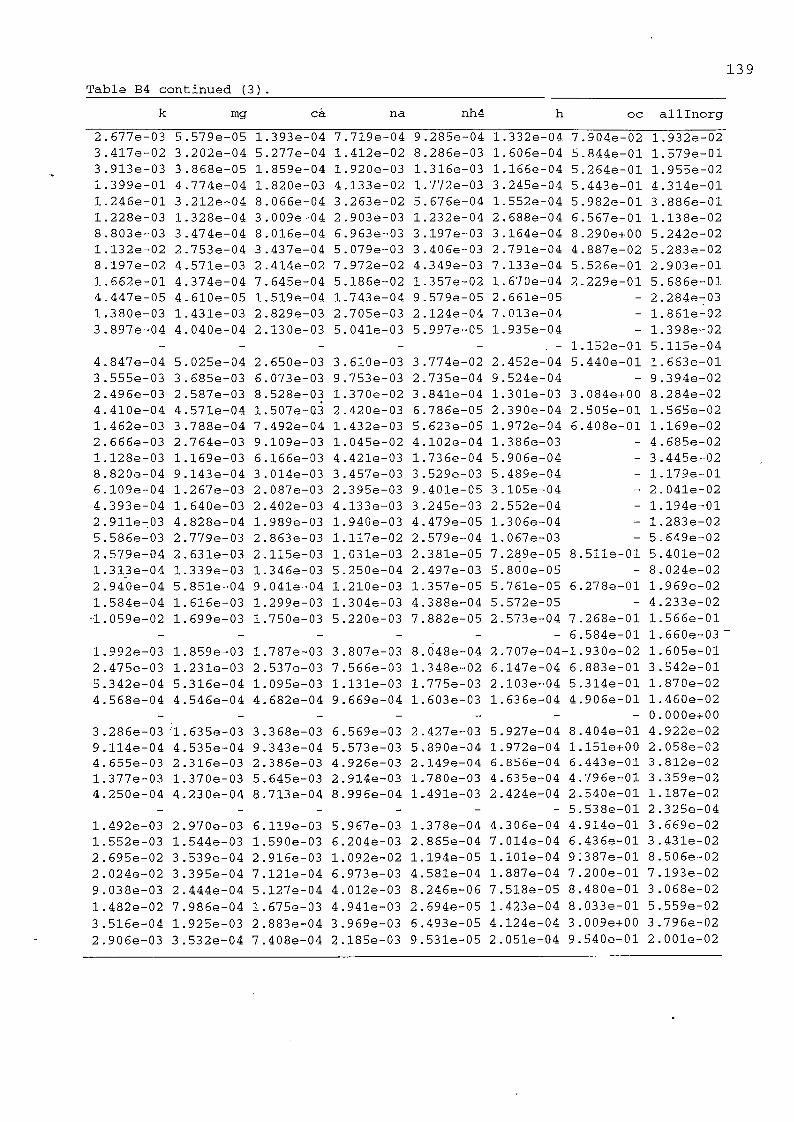
139
Table B4 continued (3).
k mg ca na nh4 h oc alllnorg
2.677e-03 5.579e-05 1.393e-04 7.719e-04 9.285e-04 1.332e-04 7.904e-02 1.932e-02
3.4170-02 3.202e-04 5.277e-04 1.412e-02 8.286e-03 1.606e-04 5.844e-01 1.579e-Ql
3.913e-03 3.868e-05 1.859e-04 1.920e-03 1.316e-03 1.166e-04 5.264e-01 1.955e-02
1.399e-01 4.774e-04 1.820e-03 4.133e-02 1.772e-03 3.245e-04 5.443e-01 4.314e-01
1.246e-01 3.212e-04 8.066e-04 3.263e-02 5.676e-04 1.552e-04 5.982e-01 3.886e-01
1.228e-03 1.328e-04 3.009e-04 2.903e-03 1.232e-04 2.688e-04 6.567e-01 1.138e-02
8.803e-03 3.474e-04 8.016e-04 6.963e-03 3.197e-03 3.164e-04 8.290e+00 5.242e-02
1.132e-02 2.753e-04 3.437e-04 5.079e-03 3.406e-03 2.791e-04 4.887e-02 5.283e-02
8.197e-02 4.571e-03 2.414e-02 7.972e-02 4.349e-03 7.133e-04 5.526e-01 2.903e-01
1.662e-01 4.374e-04 7.645e-04 5.186e-02 1.357e-02 1.670e-04 2.229e-01 5.686e-01
4.447e-05 4.610e-05 1.519e-04 1.743e-04 9.579e-05 2.661e-05 - 2.284e-03
1.380e-03 1.431e-03 2.829e-03 2.705e-03 2.124e-04 7.013e-04 - 1.861e-02
3.897e-04 4.040e-04 2.130e-03 5.041e-03 5.997e-05 1.935e-04 - 1.398e-02
- . - 1.152e-01 5.115e-04
4.847e-04 5.025e-04 2.650e-03 3.610e-03 3.774e-02 2.452e-04 5.440e-01 1.663e-01
3.555e-03 3.685e-03 6.073e-03 9.753e-03 2.735e-04 9.524e-04 - 9.394e-02
2.496e-03 2.587e-03 8.528e-03 1.370e-02 3.841e-04 1.301e-03 3.084e+00 8.284e-02
4.410e-04 4.571e-04 1.507e-03 2.420e-03 6.786e-05 2.390e-04 2.505e-01 1.565e-02
1.462e-03 3.788e-04 7.492e-04 1.432e-03 5.623e-05 1.972e-04 6.408e-01 1.169e-02
2.e66e-03 2.764e-03 9.109e-03 1.045e-02 4.102e-04 1.386e-03 - 4.685e-02
1.128e-03 1.169e-03 6.166e-03 4.421e-03 1.736e-04 5.906e-04 - 3.445e-02
8.820e-04 9.143e-04 3.014e-03 3.457e-03 3.529e-03 5.489e-04 - 1.179e-01
6.109e-04 1.267e-03 2.087e-03 2.395e-03 9.401e-05 3.105e-04 - 2.041e-02
4.393e-04 1.640e-03 2.402e-03 4.133e-03 3.245e-03 2.552e-04 - 1.194e-01
2.911e-03 4.828e-04 1.989e-03 1.940e-03 4.479e-05 1.306e-04 - 1.283e-02
5.5860-03 2.779e-03 2.863e-03 1.117e-02 2.579e-04 1.067e-03 - 5.649e-02
2.579e-04 2.631e-03 2.115e-03 1.031e-03 2.381e-05 7.289e-05 8.511e-01 5.401e-02
1.313e-04 1.339G-03 1.346e-03 5.250e-04 2.497e-03 5.800g-05 - 8.024e-02
2.940e-04 5.851e-04 9.041e-04 1.210e-03 1.357e-05 5.761e-05 6.278e-01 1.969e-02
1.584e-04 1.616e-03 1.299e-03 1.304e-03 4.388e-04 5.572e-05 - 4.233e-02
-1.059e-02 1.699e-03 1.750e-03 5.220e-03 7.882e-05 2.573e-04 7.268e-01 1.566e-01
- 6.584e-01 1.660e-03"
1.992e-03 1.859e-03 1.787e-03 3.807e-03 8.048e-04 2.707e-04-l.930e-02 1.605e-01
2.475e-03 1.231e-03 2.537e-03 7.566e-03 1.348e-02 6.147e-04 6.883e-01 3.542e-01
5.342e-04 5.316e-04 1.095e-03 1.131e-03 1.775e-03 2.103e-04 5.314e-01 1.870e-02
4.568e-04 4.546e-04 4.682e-04 9.669e-04 1.603e-03 1.636e-04 4.906e-01 1.460e-02
- - - - - - - O.OOOe+00
3.286e-03 '1.6350-03 3.368e-03 6.569e-03 2.427e-03 5.927e-04 8.404e-01 4.922e-02
9.1140-04 4.535e-04 9.343e-04 5.573e-03 5.8900-04 1.9720-04 1.1510+00 2.0580-02
4.6550-03 2.3150-03 2.386e-03 4.926e-03 2.149e-04 6.856e-04 6.443e-01 3.812e-02
1.3770-03 1.3700-03 5.645e-03 2.914e-03 1.780e-03 4.635e-04 4.796e-01 3.359e-02
4.2500-04 4.2300-04 8.713e-04 8.996e-04 1.491e-03 2.424e-04 2.540e-01 1.187e-02
.- 5.5380-01 2.3250-04
1.4920-03 2.9700-03 6.1190-03 5.967e-03 1.378e-04 4.3060-04 4.9140-01 3.6690-02
1.5520-03 1.5440-03 1.590e-03 6.2040-03 2.8650-04 7.0140-04 6.4360-01 3.4310-02
2.6950-02 3.5390-04 2.9160-03 1.092e-02 1.1940-05 l.lOle-04 9.387e-01 8.506e-02
2.0240-02 3.395e-04 7.121e-04 6.973e-03 4.581e-04 1.8870-04 7.2000-01 7.193e-02
9.0380-03 2.444e-04 5.127e-04 4.012e-03 8.246e-06 7.5180-05 8.480e-01 3.068e-02
1.4820-02 7.9860-04 1.675e-03 4.941e-03 2.694e-05 1.423e-04 8.033e-01 5.559e-02
3.516e-04 1.925e-03 2.883e-04 3.969e-03 6.493e-05 4.1240-04 3.009e+00 3.796e-02
2.906e-03 3.532e-04 7.408e-04 2.185e-03 9.531e-05 2.051e-04 9.540e-01 2.001e-02

140
Table B5. Concentrations of soluble inorganic species in source samples
(n mole m~^), nF is Fluoropore filter number.
row nF h nh4 na ca mg k cl no3 so4 br
1 48 1403 548 357 37 24 729 3145 343 180 4
2 49 435 1257 1682 36 36 2394 6680 220 184 5
3 50 2111 1333 1527 85 29 1830 4868 398 131 12
4 53 234 72 1310 33 14 2607 2494 117 832 4
5 54 117 24 1084 15 10 2432 2016 149 968 2
5 55 3513 90 1667 99 72 414 1477 68 135 23
7 56 665 376 643 42 30 478 1079 177 154 6
8 57 2304 1574 1843 72 94 2415 6252 312 132 14
9 58 1535 524 7534 1309 408 4555 5141 79 79 26
10 59 215 976 2928 25 23 5520 10881 105 298 57
11 80 223 45 64 32 16 10 161 51 40 26
12 81 552 9 93 56 47 28 92 26 24 3
13 82 2424 42 2773 672 210 126 790. 303 261 13
14 83 -9 -9 -9 -9 -9 -9 -9 -9 -9 -9
15 84 213 1831 137 58 18 11 2598 15 22 4
16 85 331 5 ,149 53 53 32 128 38 70 2
17 86 66 1 . 31 11 5 3 29 8 4 0
18 87 97 2 43 15 8 5 24 13 14 2
19 88 895 14 286 86 71 171 206 40 151 17
20 89 127 2 42 21 10 6 25 9 4 1
21 90 1584 26 521 417 130 78 323 151 344 31
22 91 135 48 37 19 9 6 '28 11 153 123
23 93 173 6 29 588 294 294 88 324 765 165 29
24 94 131 93 93 31 35 6 5 25 34 63 4
25 98 1440 28 939 552 221 829 331 110 309 138
26 95 13 6 2 63 9 15 18 52 7 13 9
27 117 1455 27 904 1064 2181 133 479 106 1223 10266
28 118 256 617 102 150 246 15 737 12 132 3655
29 119 2749 36 2536 1087 1159 362 1232 145 1159 7899
30 120 415 183 427 244 500 30 414 195 280 2852
31 96 1160 20 1034 199 318 1233 1352 80 211 6799
32 97 -9 -9 -9 -9 -9 -9 -9 -9 -9 -9
33 115 1170 195 723 195 334 223 417 56 612 7121
34 123 493 605 267 51 41 51 1211 21 48 2678
35 133 5081 2400 1200 667 533 333 667 533 2400 333
36 13 4 2296 1258 596 166 265 166 265 331 1060 166
37 135 -9 -9 -9 -9 -9 -9 -9 -9 ' -9 -9
38 136 8313 1905 4048 1190 952 1190 1667 476 3095 595
39 137 8547 1429 10612 1020 816 1020 1020 2041 3265 510
40 139 10559 185 3333 926 1481 1852 1481 741 1852 926
41 140 5767 1239 1593 1770 708 442 531 708 1487 442
42 141 15774 5429 2571 1429 1143 714 857 1143 3429 714
43 142 -9 -9 -9 -9 -9 -9 -9 -9 -9 -9
44 143 13963 250 8500 5000 4000 1250 3000 2500 2800 1250
45 144 21876 500 8500 1250 2000 1250 2000 2000 4200 1250
46 205 2177 13 9485 1453 291 13765 21030 114 1247 0
47 206 3990 542 6477 379 298 11057 21951 214 1271 0
48 207 3152 19 7389 542 426 9787 15938 81 1389 0
49 208 1680 18 2562 498 391 4520 9146 75 633 0
50 209 1944 17 822 34 377 43 3288 72 216 0
51 210 7431 193 3478 676 531 2720 11159 275 710 0
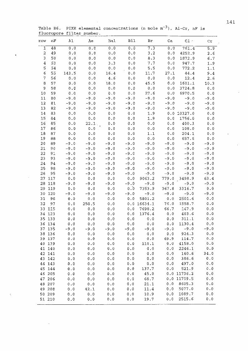
141
Table B6. PIXE elemental concentrations (n mole m 3) , Al-Cr, nF is
fluoropore filter number.
row nF A1 As Bal Bil Br Ca C1 ' Cr
1 48 0.0 0.0 0.0 0.0 7.3 0.0 761.4 5.9
2 49 0.0 0.0 0.0 0.0 3.2 0.0 4252 .9 2.6
3 50 0.0 0.0 0.0 0.0 8.3 0.0 1872 .9 6.7
4 53 0.0 0.0 3.3 0.0 7.7 0.0 947 .7 1.9
5 54 0.0 0.0 0.0 0.0 5.5 0.0 772 .2 1.1
6 55 143 .5 0.0 16.4 0.0 11.7 27.1 44.4 9.4
7 56 0.0 0.0 4.6 0.0 0.0 0.0 12.4 2.6
8 57 0.0 0.0 18.0 0.0 45.5 0.0 1601.1 10 .3
9 58 0.0 0.0 0.0 0.0 0.0 0.0 3724.8 0.0
10 59 0.0 0.0 0.0 0.0 27.6 0.0 6970 .5 0.0
11 80 -9.0 -9.0 -9.0 -9.0 -9.0 -9.0 -9.0 -9.0
12 81 -9.0 -9.0 -9.0 -9.0 -9.0 -9.0 -9.0 -9.0
13 82 -9.0 -9.0 -9.0 -9.0 -9.0 -9.0 -9.0 -9.0
14 83 0.0 0.0 0.0 0.0 1.9 0.0 10327.0 0.0
15 84 0.0 0.0 0.0 0.0 1.9 0.0 1756.0 0.0
16 85 0.0 22.1 . _ 0.0 0.0 0.0 0.0 400 .3 0.0
17 86 0 . 0 0.0 0.0 0.0 0.0 0.0 108.0 0.0
18 87 0.0 0.0 0.0 0.0 1.1 0.0 204.1 0.0
19 88 0.0 0.0 0.0 0.0 0.0 0.0 657 . 6 0.0
20 89 -9.0 -9.0 -9.0 -9.0 -9.0 -9.0 -9.0 -9.0
21 90 -9.0 -9.0 -9.0 -9.0 -9.0 -9.0 -9.0 -9.0
22 91 -9.0 -9.0 -9.0 -9.0 -9.0 -9.0 -9 . 0 -9.0
23 93 -9.0 -9.0 -9.0 -9.0 -9.0 -9.0 -9.0 -9.0
24 94 -9.0 -9.0 -9.0 -9.0 -9.0 -9.0 -9.0 -9.0
25 98 -9.0 -9.0 -9.0 -9.0 -9.0 -9.0 -9.0 -9.0
26 95 -9.0 -9.0 -9.0 -9.0 -9.0 -9.0 -9.0 -9.0
27 117 0.0 0.0 0.0 0.0 9063.2 779 .0 3498.9 63 .4
28 118 -9.0 -9.0 -9.0 -9.0 -9.0 -9.0 -9.0 -9.0
29 119 0.0 0.0 0.0 0 .0 7353 .9 367.8 3316.7 0.0
30 120 -9.0 -9.0 -9.0 -9.0 -9.0 -9.0 -9.0 -9.0
31 96 0.0 0.0 0.0 0.0 5801.2 0.0 2501.6 0.0
32 97 0.0 250.5 0.0 0.0 16634.1 76.0 1558 .7 0.0
33 115 0.0 0.0 0.0 0.0 7698.2 66.7 147 .9 0.0
34 123 0.0 0.0 0.0 0.0 1376.4 0.0 403 .6 0.0
35 133 0.0 0.0 0.0 0.0 0.0 0.0 311.1 0.0
36 13 4 0.0 0.0 0.0 0.0 0.0 0.0 1130.4 0.0
37 135 -9.0 -9.0 -9.0 -9.0 -9.0 -9.0 -9.0 -9.0
38 136 0.0 0.0 0.0 0.0 0.0 0.0 924.3 0.0
39 137 0 .0 0.0 0.0 0 .0 0 .0 69 .9 114 .7 0 .0
40 139 0.0 0.0 0.0 0.0 110 .1 0 . 0 4158.0 0 . 0
41 140 0.0 0.0 0.0 0.0 0.0 0.0 2246.1 0.0
42 141 0.0 0.0 0.0 0.0 0.0 0.0 160.6' 34.0
43 142 0.0 0.0 0.0 0.0 0.0 0.0 386.6 0.0
44 143 0.0 0.0 0.0 0.0 0.0 0.0 497.0 0.0
45 144 0.0 0.0 0.0 0.0 137 .7 0.0 521.9 0.0
46 205 0.0 0.0 0.0 0.0 45.0 0.0 11736.2 0.0
47 206 0.0 0.0 0.0 0.0 68.7 0.0 11709.5 0.0
48 207 0.0 0.0 0.0 0.0 21.1 0.0 8505.3 0.0
49 208 0.0 42.1 0.0 0.0 11.4 0.0 5077.0 0.0
50 209 0.0 0.0 0.0 0.0 10 .9 0.0 1089.7 0.0
51 210 0.0 0.0 0.0 0.0 19 .7 0.0 2515.6 0.0

Table B6 cont. PIXE elemental concentrations (nmole m
is Fluoropore filter number.Cu - Pb, nF
142
row nF Cu Fe Ga K Mn Ni P Pbl
1 48 2.7 4.5 0.0 . 750 .9 4.4 2.9 38.7 0.0
2 49 5.6 2.0 0 . 0 2073.2 1.9 1.3 17.0 0.0
3 50 3.1 13 .6 0.0 1341.9 5.0 3.4 44.0 0.0
4 53 0.9 3.8 0.0 1580.1 6.6 0.9 12.3 0.0
5 54 2.3 0.8 0.0 1705.7 5.0 0.5 0.0 0.0
6 55 0.0 7.2 0.0 78.4 7.0 4.7 61.8 0.0
7 56 1.2 2.0 0.0 156.5 2.0 1.3 17 .3 0.0
8 57 4.8 7.9 0.0 1172.1 7.6 5.2 67 .7 0.0
9 58 0.0 8.2 0.0 1343 .3 0.0 0.0 69.9 0.0
10 59 7.8 1.3 0.0 4232.8 3.1 0.8 10 .9 0.0
11 80 -9.0 -9.0 -9.0 -9.0 -9.0 -9.0 -9.0 -9.0
12 81 -9.0 -9.0 -9.0 -9.0 -9.0 -9.0 -9.0 -9.0
13 82 -9.0 -9.0 -9.0 -9.0 -9.0 -9,. 0 -9.0 -9.0
14 83 0.0 7.9 0.0 0.0 0.0 0.8 0.0 0.0
15 84 2.7 126.0 0.0 0.0 0.0 0.8 10.0 3.6
16 85 0.0 26.6 . 0.0 150.2 0.0 0.0 0.0 0.0
17 86 0.0 2.1 0.0 0.0 0.0 0.4 0.0 0.0
18 87 0.4 11.2 0.0 23 .9 0.0 0.4 0.0 0.0
19 88 4.3 7.2 0.0 452.2 0.0 4.7 0.0 0.0
20 89 -9.0 -9.0 -9.0 -9.0 -9.0 -9.0 -9.0 -9.0
21 90 -9.0 -9.0 -9.0 -9.0 -9.0 -9.0 -9.0 -9.0
22 91 -9.0 -9.0 -9.0 -9.0 -9.0 -9.0 -9.0 -9.0
23 93 -9.0 -9.0 -9.0 -9.0 -9.0 -9.0 -9.0 -9.0
24 94 -9.0 -9.0 -9.0 -9.0 -9.0 -9.0 -9.0 -9.0
25 98 -9.0 -9.0 -9.0 -9.0 -9.0 -9.0 -9.0 -9.0
26 95 -9.0 -9.0 -9.0 -9.0 -9.0 -9.0 -9.0 -9.0
27 117 16.3 2305.8 0.0 0.0 0.0 0.0 0.0 6559.8"
28 118 -9.0 -9^0 -9.0 -9.0 -9.0 -9.0 -9.0 -9.0
29 119 10 .5 544.5 0.0 0.0 0.0 11.4 0.0 6189 .3
30 120 -9.0 - -9.0 -9.0 -9.0 -9.0 -9.0 -9.0 -9.0
31 96 5.0 8.3 0.0 0.0 0.0 5.4 0.0 3454.3
32 97 4.9 5.9 0.0 0.0 0.0 10 .1 6.0 8456.2
33 115 0.0 18.5 0.0 0.0 0.0 3.8 0.0 4550.1
34 123 0.0 3.9 0.0 0.0 0.0 0.0 0.0 828.8
35 133 0.0 13 4.3 0.0 0.0 0.0 16.3 0.0 0.0
36 134 0.0 12.4 0.0 0.0 0.0 8.1 0.0 0.0
37 135 -9.0 -9.0 -9.0 -9.0 -9.0 -9.0 -9.0 -9.0
38 136 0.0 , 15.2 0.0 0.0 0.0 0.0 0.0 46.8
39 137 0 .0 18.7 0 .0 0 .0 0 .0 0 .0 0 .0 135 . 0
40 139 0.0 68.0 0.0 0.0 0.0 44.3 0.0 0 . 0
41 140 0.0 32.1 0.0 0.0 0.0 20.9 0.0 0.0
42 141 15.7 26.2 0.0 0.0 0.0 17.0 0.0 0.0
43 142 0.0 63 .0 0.0 0.0 0.0 0.0 0.0 0.0
44 143 0.0 81.0 0.0 0.0 0.0 52 .7 0 . 0 0.0
45 144 0.0 85.0 0.0 0.0 0.0 0.0 0.0 0.0
46 205 0.0 6.4 0.0 9953.2 0.0 0.0 0.0 0.0
47 206 0.0 7.7 0.0 8663.0 18.2 0.0 0.0 0.0
48 207 0.0 48.0 0.0 8073 .4 12.6 0.0 0.0 0.0
49 208 0.0 7.1 0.0 4265.6 0.0 4.6 0.0 0.0
50 209 0.0 35.2 0.0 1165.9 0.0 4.4 0.0 0.0
51 210 0.0 12.1 0.0 2553.0 0.0 0.0 0.0 0.0

143
Table 36 conh. PIXE elemental concentrations (nmole m ^), Rb - Zn, nFis Fluoropore filter number.
row nF Rb s Si Sr Ti V Y Zn
0 0 0.0 0.0 0 . 0 0.0 0.0 0.0 0.0 0.0
1 48 0.0 33 .6 46.9 10 .6 10.8 8.1 0.0 156.4
2 49 0.0 39.3 20.6 4.7 4.8 0.0 0.0 45.3
3 50 0.0 138.5 53 .4 12.1 0.0 9.2 0.0 12.3
4 53 0.0 335.7 14.9 6.9 3.5 0.0 0.0 8.8
5 54 0.0 434.1 8.4 1.9 0.0 0.0 0.0 6.9
6 55 0.0 53 .8 75.0 17.0 0.0 • 0.0 0.0 4.6
7 56 0.0 40 .8 21.0 4.8 4.8 0.0 0.0 7.3
8 57 0.0 58.9 82 .2 18.6 0.0 14.2 0.0 36.7
9 58 0.0 60 .7 84.7 19 .2 0.0 0.0 0.0 35.7
10 59 0.0 52 .5 13 .2 3.0 3.1 2.3 0.0 103 .1
11 80 -9.0 -9.0 -9.0 -9.0 -9.0 -9.0 -9.0 -9.0
12 81 -9.0 -9.0 -9.0 -9.0 -9.0 -9.0 -9.0 -9 . 0
13 82 -9.0 -9.0 -9.0 -9.0 -9.0 -9.0 -9.0 -9.0
14 83 0.0 0.0 12 .1 0.0 0.0 0.0 0.0 2.8
15 84 0.0 0.0 12.2 2.8 0.0 0.0 0.0 29 .5
16 85 0.0 27 .6 38.5 8.7 0.0 0.0 0.0 0.0
17 86 0.0 0.0 20 .1 1.6 0.0 0.0 0.0 0.0
18 87 0.0 5.0 6.9 1.6 0.0 0.0 0.0 1.8
19 88 0.0 13 6.2 74.4 16.9 0.0 0.0 0.0 18.1
20 89 -9.0 -9.0 -9 . 0 -9.0 -9.0 -9.0 -9.0 -9.0
21 90 -9.0 -9.0 -9.0 -9.0 -9.0 -9.0 -9.0 -9.0
22 91 -9.0 -9.0 -9.0 -9.0 -9.0 -9.0 -9.0 -9.0
23 93 -9.0 -9.0 -9.0 -9.0 -9.0 -9.0 -9.0 -9.0
24 94 -9.0 -9.0 -9.0 -9.0 -9.0 -9.0 -9.0 -9.0
25 98 -9.0 -9.0 -9.0 -9.0 -9.0 -9.0 -9.0 -9.0
26 95 -9.0 -9.0 -9.0 -9.0 -9.0 -9.0 -9.0 -9.0
27 117 0.0 1448.7 130 .5 0.0 0.0 0.0 0.0 594.8
28 118 -9.0 -9.0 -9.0 -9.0 -9.0 -9.0 -9.0 -9.0
29 119 0.0 2765.4 181.7 0.0 0.0 0.0 0.0 884.6
30 120 -9.0 -9.0 -9.0 - -9.0 -9.0 -9^.0 -9.0 -9.0
31 96 0 . 0 61.6 86.0 0.0 0.0 0.0 0.0 34.3
32 97 0.0 2767.2 0.0 0.0 0.0 0.0 0.0 61.2
33 115 0.0 1998.4 60 .8 0.0 0.0 0.0 0.0 85.7
34 123 0.0 23 .7 16.1 0.0 0.0 0.0 0.0 2.4
35 133 0.0 2511.4 12198.2 58.7 0.0 0.0 0.0 0.0
36 134 0.0 1207.8 7162.8 29.2 0.0 0.0 0.0 0.0
37 135 -9.0 -9.0 -9 . 0 -9.0 -9.0 -9.0 -9.0 -9.0
38 136 0.0 467.9 4659.8 0.0 0.0 0.0 0 .0 0 .0
39 137 0.0 1837 .2 2454.8 43 .9 0.0 0.0 0.0 173 .1
40 139 0.0 505.3 13549 .3 0 . 0 0.0 0 . 0 0.0 0 . 0
41 140 0.0 1406.6 5887.4 75.4 0.0 0.0 0.0 20.2
42 141 0.0 1720 .3 6095.8 0.0 0.0 0.0 0.0 16.5
43 142 0.0 1663.5 9829.5 147 .9 0.0 0.0 0.0 39.7
44 143 0.0 1745.2 15265.6 190.2 0.0 0.0 0.0 51.0
45 144 0.0 3314.1 10101.5 199 .7 0.0 0.0 0.0 53 .5
46 205 0.0 489 .4 66.6 0.0 0.0 0.0 0.0 4.0
47 206 0.0 611.0 80.3 0.0 0.0 0.0 0.0 16.0
48 207 0.0 907.1 135.0 0.0 0.0 0.0 0.0 0.0
49 208 0.0 326.2 73.1 0.0 0.0 0.0 0.0 4.4
50 209 0.0 50.2 70.1 0.0 0.0 0.0 0.0 0.0
51 210 0.0 209 .4 125.9 0.0 0.0 0.0 0.0 43 .2

144
Table B7. Collected mass, sample flows, carbon and FPM (see Table
C1 for label names and units).
row nF nN nG floF f loN floG massF massN elC tote FPM
1 48 48 52 0 .270 0.075 0.671 2877 946 2306.9 3148 10644
2 49 49 53 0.205 0 .171 0.444 562 387 709 .0 2310 2739
3 50 50 54 0.083 0.066 0 .181 1509 1115 5045.2 14674 18291
4 53 53 57 0 .224 0.236 0 .456 163 101 24.7 421 729
5 54 54 58 0.417 0.418 0 .872 318 197 32 .3 489 763
6 55 55 59' 0.044 0.047 0.093 586 461 215.7 8883 13198
7 56 56 60 0.165 0 .168 0.022 350 192 163 .7 17769 2124
8 57 57 61 0.070 0.043 0 .391 583 364 2183.0 2591 8341
9 58 58 62 0 .038 0.042 0 .073 83 59 307.0 1508 2173
10 59 59 63 0 .283 0 .267 0.601 367 272 190 .3 480 1298
11 80 81 91 0 .311 0 .343 0 .594 2638 -9 -9.0 -9 8477
12 81 83 92 0 .107 0.045 0.176 85 -9 -9.0 -9 794
13 82 84 93 0.024 0.099 0.043 301 -9 -9.0 -9 12647
14 83 85 93 0 .398 0.292 0 .985 520 249 10 .8 162 1308
15 84 86 94 0.276 0 .289 0 .522 242 125 31.5 508 876
16 85 87 95 0 .188.9.092 0.108 66 49 203 .5 -9 351
17 86 88 96 0.912.6.511 0.505 47 34 0.5 159 52
18 87 89 97 0.650 0.507 1.229 266 186 222.5 325 409
19 88 90 98 0.070 0.047 0.117 321 207 2296.3 5235 4586
20 89 91 99 0.477 0.473 0 .854 44 27 -9.0 -9 92
21 90 92 100 0.038 0.031 0.065 104 64 -9.0 2377 2708
22 91 93 102 0 .537 0 .416 0 .962 133 84 -9.0 -9 248
23 93 95 104 0 .034 0 .028 0 .064 192 135 -9.0 3273 5647
24 94 96 105 0.514 0.469 0.968 267 203 -9.0 257 520
25 98 100 106 0.036 0.028 0.062 403 -9 -9.0 8406 11133
26 95 97 107 0.542 0 .397 0 .978 70 -9 -9.0 -9 129
27 117 119 13 0 0.038 0.027 0.070 758 485 2060.1 19218 20160
28 118 120 131 0 .334 0 .359 1.147 1489 -9 -9.0 -9 4461
29 119 121 132 0.028 0 .019 0 .074 1330 722 7879.0 38131 48188
30 120 123 133 0.164 0.089 0.587 1234 - -9 -9.0 -9 7520
31 96 98 108 0.050 0.041 0 .089 229 159 647.3 3956 4553
32 97 99 109 0 .296 0.119 0.742 1360 742 539.1 3567 4599
33 115 117 135 0.072 0.058 0 .348 314 236 1458.4 1374 4367
34 123 128 139 0 .195 0 .219 0.492 158 95 2.1 560 811
35 133 149 165 0.015 0.014 0.036 366 271 11964.8 24930 24400
36 134 148 166 0.030 0.027 0.060 428 340 8297.3 15251 14172
37'135 147 167 0.008 0 .008 0.016 213 127 7987.4 -9 25357
38 136 146 168 0.008 0.022 0.017 119 80 2087.0 13993 14167
39 137 145 169 0 .010 0 .018 0 .010 429 290 3981.1 54354 43776
40 139 143 174 0.005 0.005 0 .010 84 53 6338 . 0 16361 15556
41 140 142 175 0.011 0.011 0.022 142 123 6450.9 12478 12566
42 141 140 176 0 .007 0.013 0.012 460 281 10383.4 27072 65714
43 142 141 177 0.007 0.005 0 .011 184 96 4587.8 19145 26286
44 143 151 178 0.004 0.004 0.008 131 124 13986.7 30080 32750
45 144 152 179 0.004 0 .004 0.007 126 120 14414.1 34688 31500
46 205 209 347 0.076 0 .053 0.139 1512 845 496.1 19245 19974
47 206 210 348 0.074 0.044 0.180 1576 738 1277.1 16652 21355
48 207 211 349 0 .052 0.026 0.107 2189 1045 906.6 36813 42340
49 208 212 350 0.056 0.048 0 .100 670 488 525.1 10101 11922
50 209 213 351 0.058 0.050 0.098 278 211 313 .4 14637 4760
51 210 214 352 0.041 0 .028 0.108 1515 828 1205.6 36117 36594

Table B8. Co
ncen
trat
ions
of organic c
ompo
unds
(pg m"^).
Retention
Molecular
Name
GF54
GF53
GF81
GF348
GF352
GF350
GF97
GF105
GF135
GF109
GF132
GF168
GF176
GF165
Time
weight
Coonara
Coonara
Coonara
Fire
Fire
Fire
Unleaded
Unleaded
Leaded
Leaded
Leaded
Diesel
Diesel
Diesel
7.962
142
0.20
0.18
1
0.06
0.05
8.721
142
'
0.13
13.817
178
Phenanthrene
189.65
3.90
3.32
4.04
10.48
21.34
0.07
0.09
0.48
3.82
85.71
1.64
13.926
178
Anthracene
17.10
0.33
0.29
0.92
2.48
5.37
0.02
0.01
22.62
13.277
180
9-H fluorene-9-one
71.59
5.51
3.95
1.17
2.03
6.35
0.08
0.54
0.67
2.41
14.927
180
1-H phenalene-1-one
155.68
36.43
9.39
1.52
2.48
4.77
0.03
2.30
0.19
16.702
202
PAH
598.81
107.29
39.60
7.24
8.81
25.14
1.41
0.61
89.10
14.22
198.45
37.02
296.63
34.61
16.896
202
Fluoranthene
148.75
16.84
7.96
3.75
5.10
12.30
0.26
0.06
23.04
1.79
88.47
6.87
81.29
4.91
17.167
202
Pyrene
625.78
108.00
43.16
7.79
9.13
25.59
1.45
0.89
118.05
20.08
261.68
62.12
613.38
48.88
15.848
204
2-phenyl Naphthalene
50.73
3.98
3.04
1.06
1.69
4.48
0.22
0.11
4.67
2.48
27.32
1.93
15.93
5.92
16.438
204
cyci
o penta(d,e,f)Phenanthrene
90.68
35.90
7.00
0.66
0.93
0.08
3.19
1.19
1.42
3.78
1.87
16.334
206
PAH
0.09
0.13
6.38
3.01
25.93
4.58
20.69
19.34
16.5CB
206
PAH
0.09
0.09
5.16
2.24
18.52
5.76
29.93
22.18
16.597
206
PAH
0.08
0.06
2.99
1.22
10.01
2.97
19.17
10.13
16.687
208
PAH
0.06
0.06
3.93
1.57
12.:^
2.60
12.75
10.05
17.224
208
PAH
10.37
2.54
0.51
0.01
15.34
208
PAH
15.666
208
9,10 anthracene dione
27.32
10.74
2.74
0.80
0.47
1.82
0.30
0.14
3.03
2.27
9.59
11.22
16.943
208
PAH
17.388
218
PAH
17.469
216
PAH
18.039
218
PAH
18.083
218
PAH
45.52
8.50
3.79
2.03
2.83
8.22
0.82
0,17
33.46
4.56
40.99
3.40
42.98
6.65
18.257
218
PAH
2.77
1.38
1.30
1.00
1.37
3.71
0.17
8.52
1.41
28.50
13.47
0.67
18.297
216
PAH
12.97
3.18
1.25
0.56
0.69
2.62
0.43
0.20
18.80
2.77
14.71
2.49
27.68
4.07
18.499
218
PAH
15.93
3.33
1.34
0.82
1.13
2.96
0.35
0.10
11.98
1.92
10.33
3.10
25.57
4.14
18.563
218
PAH
15.30
3.47
1.35
0.73
0.98
2.33
0.33
0.07
13.84
1.64
10.44
2.32
29.22
4.08
17.301
218
benzo(b)naphthol(2,3d)Furan
70.92
23.04
5.68
0.73
0.82
2.44
0.14
0.08
1.71
0.86
2.03
0.91
7.34
2.10
M ili'
(Jl

Table B8
continued. Co
ncen
trat
ions
of org
anic
com
poun
ds (p
g m"
3).
Retention
Molecular
Name
GF54
GF53
GF61
GF348
GF352
GF350
GF97
GF105
GF135
GF109
GF132
GF166
GF176
GF165
Time
weight
Coonara
Coonara
Coonara /
Fire
Fire
Fire
Unleaded
Unleaded
Leaded
Leaded
Leaded
Diesel
Diesel
Diesel
17.581
218
PAH
28.45
10.72
2.51
0.37
1.08
0.05
0.01
0.91
1.55
0.58
1.44
19.62
226
PAH
146.64
49.26
9.85
1.90
1.93
4.91
4.18
0.69
71.24
9.56
68.45
16.27
220.72
16.05
20.03
226
PAH
58.02
6.22
1.74
3.38
3.83
11.36
2.16
0.13
19.00
3.23
204.91
2.34
115.22
1.93
20.125
228
benz(a)Anthracena
120.00
24.99
7.52
2.56
3.28
7.55
4.16
0.39
32.74
5.47
49.82
59.71
4.35
20.194
228
Chiysene
192.12
81.80
15.08
4.07
5.73
11.51
9.14
1.00
102.65
13.01
65.80
14.54
201.17
17.14
19.245
230
terphenyl Isomer
1.99
0.75
30.12
6.67
10.13
2.26
4.00
19.742
230
terphenyl Isomer
54.02
23.88
4.62
78.45
2.10.
1.00
31.18
6.58
5.04
1.36
2.63
20.395
230
terphenyl isomer
135.44
42.10
10.59
1.17
138.34
1.72
0.32
12.07
4.17
14.62
1.26
3.83
22.596
252
benzo(e)Pyrene
326.49
8.17
23.33
3.35
3.48
9.22
14.86
1.15
143.86
21.64
79.46
17.29
267.22
22.52
22.79
252
PAH
45.19
8.03
2.65
1.28
1.50
1.69
2.41
20.01
1.62
25.83
2.48
34.97
3.41
23.092
252
benz
o(a)
Pyre
ne106.08
26.51
8.16
1.01
1.42
2.86
4.00
0.49
62.20
10.56
30.97
7.65
154.31
11.82
23.193
252
Peiylene
174.85
22.54
11.58
2.10
2.42
5.38
5.77
0.12
51.48
5.18
52.20
5.98
130.70
16.92
23.114
254
PAH
133.53
32.61
11.06
0.90
0.85
2.49
1.12
0.21
10.36
7.38
20.26
3.01
14.63
3.56
25.221
276
PAH
42.61
5.29
3.84
0.46
0.78
1.22
1.77
15.81
2.43
14.54
25.368
276
PAH
117.67
1.83
11.65
0.84
1.09
3.42
4.98
0.17
51.13
9.02
40.48
2.11
16.80
3.10
25.803
276
PAH
112.02
22.14
11.05
1.19
0.95
2.85
4.92
0.59
88.64
21.61
82.52
213.29
8.17
26.057
276
PAH
27.71
22.46
0.49
0.84
0.01
19.69
9.63
0.11
25.18
278
PAH
12.49
2.40
1.20
0.30
0.39
4.29
0.52
2.58
25.703
278
PAH
11.18
0.86
7.19
1.31
4.32
28.415
300
Coronene
19.52
1.43
0.22
37.99
9.036
152
0.13
9.136
152
0.14
1.01
0.17
9.184
152
3-methoxy-4-hydroxy Be
nzal
dehy
de0.22
0.36
3.03
10.93
15.70
8.683
154
2,6 di
meth
oxy Phenol
0.09
0.20
2.50
13.86
21.18
8.996
154
0.30
0.86
1.48
9.11
154
BIphenyl
0.08
0.27
0.03
0.42
9.232
166
0.33
10.342
166
3-methoxy-4-hydroxy Acetophenone
0.83
0.40
1.96
2.55
6.89
20.22
i->
CTl

Table B8
con
tinu
ed. Co
ncen
trat
ions
of o
rgan
ic com
poun
ds (p
g m"3).
Retention
Molecular
Name
GF54
GF53
GF61
GF348
GF352
GF350
GF97
GF105
GF135
GF109
GF132
GF166
GF176
GF165
Time
weight
Coonara
Coonara
Coonara
Fire
Fire
Fire
Unleaded
Unleaded
Leaded
Leaded
Leaded
Diesel
Diesel
Diesel
10.472
166
0.23
0.11
-
10.866
166
0.24
0.12
9.967
168
3-methoxy-4-hydroxy lienzolc Acid
0.07
2.83
12.30
10.058
168
0.48
10.79
168
0.03
0.34
11.917
194
0.92
3.29
3.12
12.33
194
0.30
,
12.478
194
0.02
0.53
13.044
194
2,6 dimethoxy -4-(2-propenyl) Ph
enol
0.06
0.75
3.48
3.79
11.136
196
0.05
12.036
196
0.33
0.90
1.86
13.266
18.62
196
85
3,5-dlmethoxy-4-hydroxy
Acetophenone
022 Hyd
roca
rlxj
n
0.43
1.51
0.15
5.87
1.01
0.59
2.25
6.39
5.29
23.97
12.41
45.16
4.33
2.29
21.03
18.23
146.13
917.37
297.26
<i

148
Table B9. GC/MS Target compounds
Compound Molecular Weight
C22 hydrocarbon 85
Cresols 108
1-methyl Naphthalene 142
2-methyl Naphthalene 142
Phenanthrene 178
Anthracene 178
IH Phenalen-l-one 180
9H Huorene-l-one 180
Anthracene-djo 188
Cyclopentaphenanthrene 190
PAH 192
PAH 202
2-Phenylacenaphthalene 204
Cyclopenta(d,e,f)phenanthrene 204
PAH 206
9,10 Anthracenedione 208
Benzo(b)naphtho(2,3d)furan 218
PAH 216
PAH 226
PAH 228
PAH 230
PAH 252
PAH 254
PAH 276
PAH 278
PAHcu
PAH 302
2,6 Dimethoxy phenol 154
Biphenyl 154
3-methoxy-4-hydroxy Benzaldehyde 152
3-methoxy-4-hydroxy Benzole Acid 168
3-methoxy-4-liydroxy Acetqphenone 166
2,6-dimethoxy-4-(2-propenyl) Phenol 194
3,5-dimethoxy-4-hydroxy Acetophenone 196
3,5-dimethoxy-4-hydroxy Benzaldehyde 182

149
CSIRO-EPA Melbourne Aerosol Study.
Final Report: Part C, Data Suirttnary

150
Data summary
The data suininary given in this part of the report parallelsthe main ambient data file on the PC format data disk. It alsoincludes some data on organic constituents that are not includedon the data disk (Table C8 and Appendix 3). The data aresummarised in eight data tables.
These tables are:
page
Table Cl. Key to field names used in other tables. 151
Table C2. Filter number, site, sample flows and masses. 153
Table C3. Concentration of soluble inorganic species. 155
Table C4. FIXE elemental concentrations. 157
Table C5. Bsd, Bap, carbon mass, FPM - Alphington. 163
Table C6. EPA air quality data, mean values for
sampling periods. 165
Table C7. PIXE detection limits and statistics. 167
Table C8. Concentrations of organic compounds. 168
Appendix 3: Size distributions and differential
scatter plots for Alphington 170

151
Table C1. Key to field names used in other tables.
nF
nN
nG
on
off
site
type
floF
f loN
floG
massF
massN
h
nh4
na
ca
mg
k
cl
no3
so4
br
Fluoropore filter numberNuclepore filter numberglass filter numbertime of start of ambient exposure, yyitimddhhmm AESTtime of start of ambient exposure, yymmddhhinin AESTsampling site a=Alphington, f^Footscraysample type c=woodstove, v=vehicle, o=:open fire pitflow through Fluoropore filter (m~^)flow through Nuclepore filter (m~^)flow through glass filter (m~-^)aerosol mass, Fluoropore filter (|ig)aerosol mass, Nuclepore' filter (|ig)cone. of soluble H"'" (nmole m 2), Fluoropore filtercone.
cone,
cone,
cone,
cone.
cone.
cone.
cone.
cone.
of
of
of
NHsoluble
soluble Na^ (nmolesoluble Ca^"*"
(nmole Fluoropore filterm 3)
(nmole m ;^) , Fluoropore filterFluoropore filter
of soluble Mg^"^ (nmole m"^), Fluoropore filterof soluble K"^ (nmole m~^), Fluoropore filter
Cl~ (nmole m~^), Fluoropore filtersoluble6 '
(nmole m ,of
totlnorg mass304-2-,bapelC
pixAlpixAspixBalpixBilpixBrpixCapixClpixCrpixCupixFepixGapixKpixMnpixNipixPpixPblpixRbpixSpixSipixSrpixTipix'VpixYpixZntote
bspdbsd
CO
o3
cone
dry a
soluble
soluble
solubleT +
^2-(nmole m-2) ,(nmole m'^)SO4
Br (nmole m -^ ) ,+ i\T=i + r" =. 2 +
Fluoropore filter, Fluoropore filterFluoropore filter2; 10ns n- , NH4"^, Na"^, Ca-_,
Fluoropore filter ()ig m-2)m
Mg
L)
+ CI NQ-:
.
cone.
cone.
cone.
cone.
cone.
cone.
cone.
cone.
cone.
cone.
cone.
cone.
cone.
cone.
cone.
cone.
cone.
cone.
cone.
cone.
cone.
cone.
cone.
total
(nmole m 2)
of soluble NO^
of
of
of ions H
and Br"
absorption coefficient il.OE-5elemental carbon (|lg m~^)
of Al determined by PIXEof As determined by PIXE (nmole m"-^)of Ba (L-line) determined by PIXE (nmole m-2)of Bi (L-line) determined by PIXE (nmole m-2)of Br determined by PIXE (nmole m-2 )of Ca determined by PIXE (nmole m-2)of Cl determined by PIXEof Cr determined by PIXEof Cu determined by PIXEof Fe determined by PIXEof Ga determined by PIXEof K determined by PIXE (nmole m"-^)of Mn determined by PIXE (nmole m-2)of Ni determined by PIXE (nmole m-2)of P determined by PIXE (nmole m-2)of Pb (L-line) determined by PIXE (nmole mof Rb determined by PIXE (nmole m-2)
(nmole m-2)(nmole m-2)(nmole m~^)(nmole m-2)(nmole m-2)
-3
of S determined by PIXE (nmole m -^1I
r3(nmole mof Si determined by PIXE
of Sr determined by PIXE (nmole mof Ti determined by PIXE (nmole m.
-3-
-3:
of V determined by PIXE (nmole m";:)of Y determined by PIXE (nmole m-3)of Zn determined by PIXE (nmole m-3)carbon (|ig m~^)
m 3-)m-1'
erosol scattering coefficient (l.OE-4dry scattering coefficient (includes air) (l,0E-4mean CO over ambient exposure as measured by EPA (ppm)mean O3 over ambient exposure as measured by EPA (pphm)

152
Table C1 continued.
no mean NO over ambient exposure as measured by EPA (pphm)no2 mean N02 over ambient exposure as measured by EPA (pphm)api mean API over ambient exposure measured by EPA (1.OE-4 m~^)so2 mean S02 over ambient exposure as measured by EPA (pphm)nmhc mean NMHC over ambient exposure as measured by EPA (ppm)tsr mean TSR over ambient exposure as measured by EPA (W m"^)uv mean UV over ambient exposure as measured by EPA (W m~^)dbt mean DBT over ambient exposure as measured by EPA (deg C)sws mean SWS over ambient exposure as measured by EPA (m sec~^)FPM fine particle mass (|lg m~^)

153
Table C2. Filter number, site, sample flows and masses
row nF nN nG date on site floF f loN floG massF massN
0 3 3 3 900423 1615 a 43 , 86 35.49 63 .13 319 217
1 6 6 6 900430 1558 a 46.62 37.18 73 .10 380 253
2 8 8 8 900501 1455 a 48.40 41.45 71.15 388 240
3 11 11 11 900503 1235 a 49 .41 36.71 81.32 379 354
4 18 18 18 900504 1655 a 14.71 13 .88 23.56 193 127
5 24 24 24 900511 1145 a 15.79 13 .02 22 .16 361 216
6 19 19 19 900511 2230 a 16.39 13 .90 23 .55 249 156
7 25 25 25 900515 1900 a 15.62 11.31 23 .26 500 303
8 29 29 29 900520 2100 a 14.75 11.53 23 .80 618 393
9 26 26 26 900521 2130 a 15.93 13 .50 22 .64 481 300
10 30 30 30 900524 2230 a 16.40 13 .65 23 .48 193 115
11 31 31 31 900525 1945 a 19 .02 11.88 22 .52 309 214
12 20 20 20 900526 2225 a 15 .33 12 .39 26 .22 589 383
13 21 21 21 900528 0840 a 15.12 11.98 23 .14 318 223
14 22 22 22 900528 1840 a 13 .27 6.77 24.69 1040 518
15 34 34 34 900529 1045 a 15.26 13 .07 22 .94 360 244
16 35 35 35 900529 1945 a 16.62 11.14 22 .93 623 378
17 39 39 39 900530-*1815 a 15.38 10 .29 24.36 745 388
18 46 46 46 900605 0830 a 16.34 12 .43 23 .80 255 187
19 47 47 48 900606 2010 a 16 .50 11.21 24.52 561 359
20 60 60 " 64 900607 1810 a 16.10 10 .47 24.24 628 344
21 61 61 65 900608 2050 a 17 .23 14 .27 23 .77 187 137
22 36 36 49 900610 1950 a 15.19 9 .53 24.82 1007 602
23 37 37 50 900611 0440 a 14.81 13 .90 23 .94 383 244
24 68 68 72 900613 1940 a 14.95 6.89 25.34 '925 402
25 72 72 76 900618 0830 a 16.09 11.81 24.72 204 144
26 69 69 73 900618 2055 a 16.07 10 .11 24.38 746 454
27 75 75 79 900625 1815 a 15.30 14.27 24.53 168 135
28 78 79 86 900701 1915 a 15 .21 14.51 24.15 214 155
29 101 103 115 900710 0850 a 15.78 12 .77 23 .97 248 147
30 79 80 116 900710 2035 a 15.71 11.20 24.43 548 344
31 104 106 125 900719 1850 a 15.76 11.78 24.50 311 206
32 111 113 141 900726 1120 a 16.40 13 .71 26.39 153 113
33 105 107 142 900727 2330 a 15 .23 14.78 23 .23 113 92
34 129 134 153 900803 2050 a 13 .99 14.16 26.99 94 70
35 132 139 161 900818 1920 a 14.72 13 .86 26.33 284 207
36 138 144 170 900826 2110 a 15.66 11.20 24.27 660 400
37 145' 155 184 900908 2100 a 11.22 11.01 23 .48 492 375
38 148 154 192 900917 1945 a 15.22 9.32 23 .80 643 404
39 155 160 208 901024 1235 a 14.46 14 .10 23 . 02 266 209
40 165 171 240 901128 1305 a 17.04 13 .21 22.78 245 185
41 153 161 241 901203 0255 a 15.99 13 .17 23 .27 316 278
42 154 162 242 901203 1140 a 14.51 14.90 24.46 317 333
43 71 71 243 901204 1355 a 15.25 14.71 22 .36 173 167
44 177 181 254 -9 a -9 -9 -9 19 49
45 181 185 258 901211 1315 a 21.86. 14.02 21.99 73 -9
46 178 182 255 901211 22 00 a 21.24 14.14 22.03 43 -9
47 179 183 256 901212 0645 a 8.45 6.28 9.66 33 -9
48 182 186 262 901214 1510 a 19 .18 13 .47 22 .19 102 89
49 183 187 263 901219 2255 a 20 .87 11.60 22 .38 143 104
50 190 194 286 910114 1000 a 15.72 11.16 23 .39 187 127
51 187 191 287 910117 1425 a 15.60 12.32 23 .81 129 87
52 188 192 288 910119 1430 a 14.81 12.07 23 .71 200 139

154
Table C2. contd. Filter, site, sample flows and masses
row nF nN nG date on site floF f loN floG massF massN
53 1 1 1 900417 0000 f -9 -9 -9 276 179
54 2 2 2 900418 1230 f 33 .94 38.30 57 .45 602 405
55 4 4 4 900423 1505 f 45.63 40 .83 75.46 359 231
56 7 7 7 900430 1520 f 38.43 32 .04 60 .63 414 235
57 9 9 9 900501 1555 f -9 -9 -9 383 245
58 12 12 12 900503 1630 f 13 .81 12 .28 22 .09 281 198
59 17 17 17 900507 2130 f 9 .96 12 .50 23.01 251 ■ 253
60 23 23 23 900511 1430 f 13 .94 10 .96 22 .30 491 310
61 13 13 13 900515 1930 f 15.37 9.09 22 .63 688 404
62 27 27 27 900521 1235 f 15.26 12 .76 21.78 202 132
63 28 28 28 900522 1110 f 14.52 10 .58 22 .52 315 209
64 32 32 32 900528 1910 f 14.29 9 .32 22 .85 670 410
65 33 33 33 900529 0740 f 13 .30 9 .10 22 .28 919 553
66 14 14 14 900529 1620 f 15.71 10.66 21.19 612 386
67 15 15 15 900530 0640 f 14.65 11.51 22 .20 307 210
68 41 41 41 900606 0925 f 15.34 10 .80 22 .43 430 258
69 42 42 42 900606.'2000 f 13 .63 11.73 23 .11 346 253
70 43 43 43 900607 0745 f 13 .20 11.04 22 .46 282 215
71 44 44 44 900607 2045 f 13 .76 12 .05 22 .62 379 275
72 62 62 66 900610 2100 f 15.36 12 .31 22 .20 372 222
73 63 63 67 900611 1200 f 13 .34 12.90 21.98 172 123
74 66 66 70 900613 2115 f 13 .56 12 .43 22 .53 248 199
75 67 67 71 900614 2110 f 13 .64 11.50 23 .01 325 245
76 77 77 81 900627 1240 f 14.55 13 .77 21.99 129 89
77 74 74 82 900703 1420 f 14.40 13 .56 22 .25 90 89
78 99 101 110 900710 2030 f 15.04 11.80 22 .10 414 222
79 100 102 111 900711 0810 f -9 -9 -9 1697 749
80 112 114 145 -9 f -9 -9 -9 675 -9
81 113 115 146 -9 f -9 -9 -9 -9 -9
82 64 64 147 -9 f -9 -9 - -9 -9 -9
83 65 65 148 -9 f -9 -9 -9 -9 -9
84 45 45 124 -9 f -9 -9 -9 -9 -9
85 102 104 120 900723 1015 f 15.12 14.59 21.26 117 62
86 124 129 140 900803 1245 f 13 .46 11.96 24.08 392 287
87 125 130 149 900807 1345 f 13 .68 13 .50 22 .26 98 93
88 130 137 157 -9 f -9 -9 -9 30 48
89 146' 153 188 900917 2120 f 15.05 12 .59 22 .12 244 227
90 131 138 189 900922 2355 f 13 .20 12 .33 22 . 66 170 146
91 149 157 192 900930 1930 f 13 .39 13 . 64 21.57 228 208
92 151 158 193 901001 0505 f 13 .30 13 .23 22 .30 206 207
93 157 163 200 901004 1230 f 14.52 12 .63 21.60 251 194
94 158 164 201 901008 1010 f 14.40 11.14 21.99 288 228
95 160 166 212 901025 0835 f 13 .89 12 .28 21.22 -9 243
96 163 169 228 -9 f -9 -9 -9 -9 164
97 164 170 236 901128 1105 f 13 .63 13 .06 21.37 333 281
98 161 167 237 901203 0200 f 12 .82 13 .67 21.71 -9 258
99 159 165 238 901203 1045 f 12.78 13 .43 21.09 335 291
100 173 178 266 901220 1310 f 19 .24 12 .59 20.30 100 102
101 189 193 282 910119 1215 f 13 .76 10 .52 21.46 222 156
102 191 195 298 910204 1315 f 13 .26 9.84 22 . 62 362 275
103 197 201 306 910208 1200 f 14.44 13 .06 21.83 186 167

155
Table C3. Concentration of soluble inorganic species (n mole in~^).
na ca mg k cl no3 so4 br
17.60 0.481 2 .562 1.71 12 .96 STTS 4732 OTFT13.80 0.774 1.879 2.10 9.40 6.08 2.85 0.97
11.99 1.196 1.471 2.18 8.83 3.48 4.00 1.14
5.72 0.164 0.842 1.98 1.17 3.17 1.35 0.22
67.59 2.915 8.195 11.52 30.96 29.53 11.52 3.747.97 0.892 1.798 2.99 3.36 7.28 8.91 4.37
4.08 0.000 0.732 2.70 0.47 3.83 6.60 2.14
5.49 0.000 0.871 7.08 13.90 10.28 8.83 4.42
10.83 0.006 1.707 12.18 28.14 12.17 3.84 7.80
5.34 0.000 0.703 7.43 13.62 12.29 6.95 2.20
7.62 0.000 0.829 1.26 6.08 2.84 5.11 2.38
7.53 0.000 0.284 2.22 6.30 3.05 5.18 5.21
6.34 0.000 0.939 10.22 18.07 11.79 8.53 5.81
4.30 0.932 0.899 2.25 1.23 3.61 14.81 2.98
8.95 0.760 1.340 13.34 44.89 28.62 16.10 27.19
2.32 0.661 1.114 2.19 1.38 4.78 9.36 4.52
8.35 0.000 0.722 9.58 24.65 9.99 6.86 7.52
6.."04 0.721 1.534 9.02 15.11 9.93 4.72 9.049.83 0.617 1.040 1.54 2.83 2.73 16.11 2.76
4.84 0.006 0.582 9.18 22.71 8.12 4.82 7.09
6.37 1.508 1.291 8.10 13.42 6.77 6.51 10.99
5.84 0.000 0.650 2.18 3.33 2.46 3.56 1.57
14.53 0.000 1.975 13.18 73.33 11.13 9.74 14.95
7.62 0.303 0.702 5.40 7.62 12.49 16.80 -9.00
10.53 0.675 1.685 11.57 39.69 8.45 5.95 21.20
10.41 0.627 1.566 0.00 11.92 4.00 2.67 3.67
8.55 0.628 0.448 10.39 31.84 7.24 8.53 11.27
5.32 0.268 0.470 0.00 6.25 2.77 2.68 1.31
6.41 0.000 0.868 3.62 6.16 2.79 2.83 1.65
5.03 1.146 0.836 0.82 3.91 2.31 14.00 0.26
6.20 0.000 0.840 6.04 16.02 15.17 15.46 9.10
16.08 1.148 1.852 4.12 20.54 5.61 2.85 4.76
13.37 0.493 1.780 1.40 13.51 1.85 2.62 3.35
7.58 0.000 0.866 0.85 4.84 2.78 2.69 1.51
10.68 0.000 0.943 0.21 7.41 1.60 13.79 0.79
13.68 0.000 0.896 4.41 8.27 9.67 13.10 2.1116.17 0.000 0.842 10.02 25.51 12.02 4.66 7.47
10.28 0.000 1.176 7.57 8.35 19.46 7.22 5.62
13.76 1.188 1.117 4.44 17.85 31.29 15.17 8.8329.00 1.071 2.476 0.97 4.49 7.55 26.07 0.87
22.73 0.886 2.053 1.51 0.00 6.49 26.46 0.77
10.48 0.344 1.113 0.49 0.40 11.56 66.23 0.6214.84 0.833 1.502 1.03 0.00 2.20 55.74 0.39
2.72 0.400 0.734 1.29 0.00 1.17 7.23 0.41
-9.00-9.000 -9.000 -9.00 -9.00 -9.00 -9.00 -9.00
9.40 0.279 0.997 0.01 7.59 1.21 4.69 0.32
4.58 0.023 0.489 0.00 3.64 (i.77 3.60 0.144.10 0.000 0.047 0.00 2.74 0.42 2.32 0.50
18.95 0.422 1.825 0.57 14.17 3.01 5.81 0.57
8.24 0.000 0.728 0.57 0.25 2.57 23.81 0.47
26.04 1.176 2.277 0.24 1.55 12.39 33.77 0.26
22.13 0.390 2,396 0.04 11.43 7.26 10.22 0.36
15.35 0.303 1.363 1.12 2.37 6.79 17.07 0.58
row nF h nh4
0 3 1.03 3.26
1 6 1.18 1.27
2 8 1.32 2 .83
3 11 1.10 0 .75
4 18 6.24 4.42
5 24 5.22 9 .56
6 19 6.55 8.36
7 25 9 .23 18.63
8 29 5.22 10 .37
9 26 8 .57 17.01
10 30 4.52 2 .99
11 31 5.24 3 . 63
12 20 8.98 17 .15
13 21 5.68 19.63
14 22 14.72 47.67
15 34 6.61 10.02
16 35 11.10 20.03
17 39 10 .82 10 .73
18 46 3 .73 15.48
19 47 8.78 14.60
20 60 9.08 7 .51
21 61 5 .10 2.38
22 36 13 .02 33 .25
23 37 7 .12 25.59
24 68 14.03 11.97
25 72 •5.30 1.18
26 69 11.19 14.00
27 75 5.40 2 .16
28 78 7.33 2 .83
29 101 5.14 19 .83
30 79 10 .22 33 .-66
31 104 6.02 3 .23
32 111 4.52 0 .79
33 105 4.58 1.77
34 129 5.68 5.65
35 132 8 .97 10 .52
36 138 11.51 9 .13
37 145 14.65 18.62
38 148 9 .47 32 .90
39 155 6 . 04 34 . 09
40 165 5.34 26.93
41 153 5 .59 89.87
42 154 8.67 69 .79
43 71 7 .74 7.02
44 177 -9.00 -9.00
45 181 2 .63 3.25
46 178 2 .50 1.27
47 179 6.84 0.00
48 182 2 .73 1.51
49 183 4.18 27 .74
50 190 5 .55 46.23
51 187 3.20 8.26
52 188 6.95 20 .85

Table C3 contd.. Soluble inorganic species (n mole m
156
row nF h nh4
53 1 -9.00 -9 .00
54 2 2 .51 15 .11
55 4 1.15 2.96
56 7 1.53 2 .58
57 9 -9.00 -9.00
58 12 3 .00 1.09
59 17 6.24 7.12
60 23 7 .49 31.77
61 13 7 .95 28.30
62 27 3 .75 3 .87
63 28 5.44 13 .15
64 32 10 .54 50 .86
65 33 13 .34 107 .89
66 14 9 .37 41.57
67 15 4 .71 5.94
68 41 6.59 19.09
69 42 6.26 15 .33
70 43 4.21 6.89
71 44 6.77 22 .74
72 62 6.60 16.08
73 63 6.51 12 .21
74 66 7.70 4.64
75 67 3 .99 33 .64
76 77 2 .94 0.00
77 74 4.49 0.76
78 99 7.07 18.94
79 100 -9.00 -9 .00
80 112 -9.00 -9 .00
81 113 -9.00 -9.00
82 64 -9 .00 -9.00
83 65 -9.00 -9.00
84 45 -9.00 -9.00
85 102 3 .28 2 .84
86 124 6.65 54.13
87 125 4 .84 1.10
88 130 -9.00 -9.00
89 146 6.63 20.26
90 131 6.63 7.65
91 149 8.53 72 .48
92 151 5.43 43 .96
93 157 5.73 48.95
94 158 6.33 17.70
95 160 -9.00 -9 .00
96 163 -9.00 -9 .00
97 164 -9.00 -9 .00
98 161 -9 .00 -9.00
99 159 6.80 87 .40
100 173. 3 .77 6.60
101 189 8.67 36.10
102 191 6.37 40 .33
103 197 4.75 35.24
na ca mg
-9.000
2 .145
cl no3 so4 br
-9
13
17
17
-9
17
19
27
63
12
29
8
26
11
4
12
5
10-
5
23
8
10
8
13
13
15
-9
-9
-9
-9
-9
-9
3
11
9
-9
4
7
15
8
6
17
-9
-9
-9
-9
14
9
14
114
33
.00-9
.13 3
.98 0
.37 0
.00-9
.42 0
.43 0
.86 2
.79 2
.07 0
.26 1
.50 0
.39 6
.94 1
.92 0
.11 1
.72 0
.12 0
.61 0
.02 1
.26 0
.87 0
.75 0
.84 0
.99 0,
. 65 1,
.00-9.
.00-9,
.00-9,
,00-9.
.00-9.
.00-9.
.00 0.
.10 2,
.60 0.
.00-9,
.89 0.
.09 0.
49 0,
61 1.
98 0.
73 3.
00-9 .
00-9 .
00-9 .
00-9 .
20 0.
64 0.
78 0.
24 3.
47 1.
,000
.179
.624
.845
.000
.513
,551
.115
.725
,491
342
594
984
241
825
401
000
265
000
438
262
744
300
000
000
203
000
000
000
000
000
000
535
086
000
000
073
113
000
164
970
464
000
000
000
000
712
472
472
233
253
-9
3
2
2
-9
3
4
1
2
2
3 .
1.
3 .
283
279
000
792
836
865
602
725
263
245
940
1.235
1.037
2 .385
0.646
1.288
0.814
0 .989
0.959
1.120
0 .528
0.907
0 .917
0 .877
-9.000
00 -9
26 6
0.75 12
1.11 10
9.00 -9
6.53 11.
2.73 18.
0.89 2.
1.51 55.
1.02 5.
00 10.
41 13.
62 20.
95 4.
1.2.70
3 .11 8
3.51 21
1.53 9
4.33 23
2.37 12
2.13 1
0.00 6
0.00 9
1.58 10
0.21 9
2
9
00
99 9
00 -9
-9.000 -9.
-9.000 -9.00 -9
-9.000 -9.00 -9
-9.000 -9.00 -9
-9.000 -9000 00
00 -9
24 11
43 6
99 8.59
00 -9
53 11
98 9.61
51 15
66 14
03 7
78 11
12 48
85136
63 42
92 2
34 19
22 7
81 3
36 8
51 10
75 4
76 7
07 28
01 1
29 2
15 11
00 -9
-9
-9
-9
-9
.00
00
00
00
00
.19
.53
.27
.47
-9
.56 13
. 65 4
00
82
25
53
.00 -9.00
.71 3.52
8.59
.26 30.76
.56 14.55
.55 5.90
.14 19.36
.71 19.35
.18 33.32
.90 16.35
.43 5.92
.29 12.07
-9.00
■3 .270 .240 .44
-9.002 .10
9281
56
509111
16.66.01 13.47.69 4.05.76 18.69.54 3.23.39 2.99.33 13.23.00 -9.00.00 -9.00.00 -9.00
99
0000
0000
0 .8730.9800.380
-9.0000 .5850 .7271.6271.1420 .4821.125
0.202 .601.68
.00 -9
.25 1
.88 28
.66 2-9.00 -9.00 -92.351.790 .631.701.14
18
4.0 .0 .0 .0.1.
02 1395 708 160600
33
97 15-9.000 -9.00 -9.00 -9
29
-9.000 -9.00 -9.00-9.000 -9.00 -9.00-9.000 -9.00 -9.001.518 1.33 0.571.694 1.92 9.061.583 1.95 2.55 12.
11.443 2.83 35.56 68.3.046 0.65 7.20 20.
-9.-9 .-9 .3 .5.
000000
10 .481.121.728.757 .456.054.442 .946.243.717.785.541.434.793 .740.280.635.92
-9.00-9-9-9
000000
00 -9.0035 2.8439 32.89
8700
51 300 -918 12.3851 8.7200 51.5838 36.8948 35.0558 19.0900 -9.0000 -900 -900 -985 66.7446 8.9429 25.0678 42.2910 31.09
-9.00-9.00
0 .272.600 .81
-9.002 .453 .110.200 .32
0.901.04
-9.00-9.00-9.00-9.00
0 .140.200.280.290.18

Table C4. PIXE elemental concentrations (n mole m~^), Al-Crrow nF Al As Bal Bi Br Ca C1 Cr
0 3 0.190 0.000 0.000 0.000 0.384 0.483 7.927 0.012
1 6 0.678 0.055 0.000 0.000 0.835 0.777 5.789 0.012
2 8 1.018 0.049 0.019 0.042 0.872 0.671 3.848 0.011
3 11 1.357 0.055 0.021 0.000 1.177 0.788 4.239 0.0124 18 0.486 0.000 0.056 0.000 0.493 0.519 0.150 0.032
5 24 2.273 0.400 0.000 0.000 3.601 1.107 0.160 0.034
6 19 0.485 0.146 0.000 0.000 1.018 0.092 0.000 0.0327 25 1.766 0.000 0.068 0.000 4.219 0.251 0.185 0.039
8 29 3.076 0.000 0.067 0.000 6.147 0.000 8.088 0.038
9 26 0.499 0.150 0.000 0.000 1.324 0.000 0.155 0.033
10 30 0.494 0.000 0.057. 0.000 1.030 0.093 0.153 0.032
11 31 2.257 0.171 0.000 0.000 5.280 0.413 0.176 0.037
12 20 0.544 0.164 0.062 0.000 4.576 0.000 0.168 0.036
13 21 0.563 0.169 0.000 0.000 2.428 1.469 0.174 0.03714 22 21.102 0.994 0.114 0.000 25.205 0.438 9.882 0.065
15 34 2.143 0.000 0.000 0.000 3.474 1.202 0.160 0.11616 35 3.871 0.182 0.069 0.000 6.187 0.114 0.187 0.04017 39 4.851 0.406 0..'075 0.000 7.889 0.124 0.203 0.04318 46 0.542 0.163 0.000 0.000 1.919 1.637 0.168 0.036
19 47 3.717 0.181 0.069 0.000 6.350 0.113 0.186 0.039
20 60 7.370 0.403 0.074 0.000 9.352 0.498 0.199 0.04221 61 0.473 0.000 0.054 0.000 1.207 0.089 0.146 0.03122 36 7.322 0.535 0.000 0.000 12.471 0.000 22.852 0.046
23 37 0.000 0.146 0.056 0.000 1.266 0.000 0.150 0.03224 68 17.782 0.294 0.000 0.000 22.599 0.616 10.402 0.064
25 72 1.569 0.000 0.065. 0.000 3.818 0.573 1.089 0.037
26 69 6.713 0.201 0.000 0.000 11.132 0.252 7.471 0.04427 75 0.000 0.142 0.000 0.000 0.895 0.089 0.146 0.031
28 78 0.000 0.000 0.000 0.000 1.070 0.000 1.131 0.00029 101 0.000 0.000 0.000 0.000 1.613 0.904 1.144 0.00030 79 0.000 0.000 0.000 0.000 8.954 0.225 1.946 O.OOO31 104 0.000 0.000 0.000 0.000 4.534 0.483 13.732 0.00032 111 0.000 0.000 0.000 0.000 3.215 0.491 11.745 0.09733 105 0.000 0.000 0.000 0.000 1.139 0.000 5.949 0.00034 129 0.000 0.000 0.000 0.000 0.483 0.000 1.130 0.00035 132 0.000 0.000 0.000 0.000 1.440 0.187 0.151 0.00036 138 0.000 0.536 0.000 0.000 6.878 0.000 12.523 0.00037 145 b.OOO 0.000 0.000 0.000 5.760 0.000 1.405 0.00038 148 0.000 0.000 0.000 0.000 9.274 1.454 4.585 0.00039 155 0.000 0.000 0.055 0.000 0.712 1.052 3.868 0.00040 165 0.000 0.000 0.000 0.000 0.368 0.887 0.158 0.00041 153 0.000 0.000 0.000 0.000 0.310 0.212 1.685 0.00042 154 0.,000 0.000 0.000 0.000 0.338 1.001 0.821 0.00043 71 0.000 0.000 0.000 0.000 0.258 0.517 5.435 0.00044 177 -9.000 -9.000 -9.000 -9.000 -9.000 -9.000 -9.000 -9.000
45 181 -9.000 -9.000 -9.000 -9.000 -9.000 -9.000 -9.000 -9.00046 178 -9.000 -9.000 -9.000 -9.000 -9.000 -9.000 -9.000 ,-9.00047 179 -9.000 -9.000 -9.000 -9.000 -9.000 -9.000 -9.000 -9.00048 182 0.000 0.000 0.000 0.000 0.384 0.439 10.806 0.00049 183 0.000 0.000 0.000 0.000 0.047 0.000 0.797 0.03850 190 0.000 0.000 0.000 0.000 0.147 0.574 0.187 0.00051 187 0.000 0.000 0.000 0.000 0.262 0.472 2.181 0.03652 188 0.000 0.000 0.000 0.000 0.285 0.510 2.032 0.037
157

158
Table C4 contd. PIXE elemental concentrations (n mole m ̂ ), Al-Cr
row nF A1 As Bal Bi Br Ca C1 Cr
53
54
55
56
57
58
59
60
61
62
63
64
65
66
67
68
69
70
71
72
73
74
75
76
77
78
1
2
4
7
9
12
17
23
13
27
28
32
33
14
15
41
42
43
44
62
63
66
67
77
74
99
83
84
-9.000
1.488
0.165
0 .210
-9.000
0 .549
1.402
0.615
8 .534
0 .528
0 . 000
7 .207
5.435
1.436
1.507
0 .625
1.955
0 . 611
2 .810
1.192
0 . 000
1.356
0 .586
0.000
0.000
0.000
79 100
80 112
81 113
82 64
65
45
85 102
86 124
87 125
88 130
89 146
90 131
91 149
92 151
93 157
94 158
95 160
96 163
97 164
98 161
99 159
100 173
101 189
102 191
103 197
-9 .000
0.053
0.050
0.000
-9.000
0 .165
0 .162
0.000
0 .487
0 .159
0 .192
0 .000
0 .223
0.190
0 .176
0 .188
0 .173
0 .184
0 .168
0 .165
0 .157
0 .163
0 .000
0 .147
0 .150
0 .000
000
000
000
000
0-00
000
0 . 000
0 .000
0.000
-9 .000
0.000
d.ooo0.000
0 .000
0.000
0.000
0.000
-9.000
0.000
0.000
0.000
0.000
0.000
0.000
0.000
-9.000
0.02 0'
0.000
0.000
-9 .000
0 .000
0.000
0.000
0.000
0.000
0.000
0.000
0.000
0.072\
0.000
0 .000
0.000
o.'ooo0.000
0.000
0.000
0.000
0 .067'
0 .000
0.000
0.000
-9.000
0.000
0.000
0.000
-9.000
0.000
0.000
0.000
0.000
0.000
0.000
0.000
0.000
0.000
0.000
0.000
0.000
0.000
0.000
0.000
0.000
0.000
0.000
0.000
0.000
0.000
000
000
000
000
000
000
0.000
0.000
0.000
9.000
0 .161
0.000
0.000
0 .000
0 .161
0.000
0.000
9 .000
0.000
0.000
0.000
0.000
0.000
0.000
0.000
000 -9.000
000
000
-9
-9
-9
-9
-9
-9
0.000
0.000
0 .000
000
000
000
-9.000
000 -9.000
000 -9.000
0.000
0.000
0.000
-9.000 -9.000
0.000 0.000
0.000
0 .000
0 .000
0 .000
0.000
0.251
0.000
0.000
0 .000
0 .000
0.000
0.000
-9.000 -9.000
0 .323
0.000
0.338
0.000
0.000
0.000
0.000
0.000
0.000
0.000
0.000
0.000
0.000
0 .000
-9.000
1.791
0 .180
0 .439
-9
1
4
4
.000
,772
.659
.749
11.200
0 .976
1.621
10 .300
7 .557
4
3
2
4
3 .
5,
3 ,
.317
.928
.648
,423
,910
,335
,957
0 .955
3 .926
2 .734
0 .270
0.477
086
000
5
-9
-9.000
-9
-9
-9
-9
000
000
000
000
0 .256
2 .667
0 .779
-9.000
2 .059
2 .464
0 .166
0.280
0 .913
1.165
0.396
-9.000
0 .267
0 .147
0 .156
0 .109
0 .278
0 .356
0.109
-9.000
1.718
0 .571
1.247
-9 .000
0 .591
1.624
3 .507
4.590
1.196
-9
1
1
5
1
1
2
,605
,750
,517
,442
,330
,825
0 .253
1.025
0 .219
1.378
0 .099
0 .411
0 .282
0 .197
0 .302
0 .609
000
000
000
000
000
000
0.321
2 .876
0.574
000
0.466
0 .358
0 .585
-9
-9
-9
-9
-9
-9
-9
961
339
615
958
000
723
0.615
1.016
0 .333
0.509
3 .324
1.278
000
0.054
5 .372
7 .804
000
468
238
-9
3
4
0 .190
31.589
0 .163
0 .197
0 .224
0 .229
0 .196
0 .181
0 .193
3 .084
0 .189
0 .173
0 .170
0 .162
0.168
0 .181
9 .421
7.038
4:933
-9.000
-9.000
-9.000
-9.000
000
000
1.027
1.535
590
000
0 .166
0 .169
0.153
0 .158
0 .000
0 .187
3 .083
-9.000
1.773
5.900
0 .155
2 .639
0 .555
10.641
0.160
-9
-9
4
-9
-9.000
0 .012
0.011
0.014
,000
.036
.035
. 040
.049
.035
.122
.047
.112
.041
. 038
.151
.038
.040
.037
. 036
.104
.036
.038
.000
,000
,000
.000
,000
000
,000
,000
000
000
000
033
000
000
000
000
000
000
000
000
000
000
032
000
000
100
000
000
/\ \r<. 2.qi^ 0-U^ o-c)c,T Q-0^(f8

159
Table C4 contd. PIXE elemental concentrations (n mole in~^), Cu-Pb
row nF Cu Fe Ga K Mn Ni P Pbl
0 3 0.016 0.409 0.000 1.118 0.025 0.0061 6 0.006 0.876 0.000 1.474 0.051 0.0062 8 0.122 0.864 0.000 1.022 0.047 0.005
3 11 0.025 1.395 0.000 2.658 0.046 0.0064 18 0.015 0.928 0.000 3.279 0.024 0.0165 24 0.138 3.409 0.000 2.248 0.137 0.0176 19 0.015 1.069 0.000 2.670 0.024 0.0167 25 0.018 2.089 0.000 4.994 0.029 0.0428 29 0.018 1.118 0.000 7.684 0.028 0.0199 26 0.015 1.114 0.000 4.556 0.024 0.016
10 30 0.015 0.852 0.000 0.736 0.064 0.01611 31 0.017 1.145 0.000 2.283 0.028 0.019
12 20 0.017 0.607 0.000 6.243 0.026 0.01813 21 0.129 4.585 0.000 1.530 0.128 0.01814 22 0.030 5.289 0.089 10.263 0.116 0.033
15 34 0.088 4.780 0.000 1.647 0.106 0.01716 35 0.018 2.137 ,0.054 5.693 0.070 0.02017 39 0.055 3.184 0.000 6.762 0.032 0.022
18 46 0.044 2.304 0.000 1.032 0.026 0.01819 47 0.104 2.394 0.000 4.941 0.063 0.02020 60 0.071 3.435 0.000 4.692 0.031 0.02121 61 0.035 0.652 0.000 1.919 0.023 0.01622 36 0.097 1.502 0.000 8.198 0.034 0.000
23 37 0.015 1.030 0.000 2.242 0.024 0.01624 68 0.190 4.781 0.087 8.451 0.098 0.03225 72 0.017 2.092 0.000 0.596 0.028 0.01926 69 0.020 2.106 0.000 7.707 0.032 0.00027 75 0.014 0.502 0.000 0.930 0.023 0.01628 78 0.000 0.352 0.000 1.689 0.000 0.01529 101 0.033 2.298 0.000 1.167 0.118 0.00030 79 0.018 2.739 0.000 4.340 0.067 0.00031 104 0.335 1.504 0.000 2.513 0.000 O.OOO32 111 0.015 1.290 0.000 0.811 0.000 0.00033 105 0.000 0.312 0.000 1.732 0.000 0.00034 129 0.000 0.287 0.000 0.343 0.000 0.01635 132 0.000 0.628 0.000 2.470 0.000 0.01636 138 0.260 1.528 0.000 7.305 0.029 0.02037 145 0.019 2.421 0.000 6.483 0.000 0.02038 148 0.062 3.798 0.000 4.671 0.035 0.02439 155 0.038 1.937 0.000 0.771 0.075 0.01640 165 0.040 1.464 0.000 0.962 0.000 0.00041 153 0.000 0.718 0.000 0.297 0.000 0.00042 154 0.014 1.665 0.000 0.592 0.022 0.00043 71 0.014 1.808 0.000 1.407 0.022 0.00044 177 -9.000 -9.000 -9.000 -9.000 -9.000 -9.00045 181 -9.000 -9.000 -9.000 -9.000 -9.000 -9.00046 178 -9.000 -9.000 -9.000 -9.000 -9.000 -9.00047 179 -9.000 -9.000 -9.000 -9.000 -9.000 -9.00048 182 0.000 0.861 0.000 0.319 0.000 0.00049 183 0.018 0.341 0.000 0.121 0.028 O.OOQ50 190 0.018 1.049 0.000 0.321 0.000 0.00051 187 0.000 0.740 0.000 0.114 0.000 0.00052 188 0.000 1.303 0.000 0.449 0.000 0.000
0 .000 0 .315
0.000 0 . 676
0.000 0 . 686
0.000 0 .897
0.000 0 .298
0.000 2 .369
0.209 0 .869
0 .257 2 .789
0 .000 3 .704
0 .215 0 .923
0 .213 0 .787
0 .549 3 .009
0.000 2 .311
0.000 1.844
0.000 13.621
0.000 2 .638
0.000 3 . 649
0 .282 4.605
0.000 1.551
0.000 3 .732
0.000 5 .330
0.204 0 .741
0.000 7 .110
0.000 0.965
0 .000 12.092
0 .246 2 .228
0 .287 5.927
0 .204 0 .739
0 . 000 0 .793
0.000 1.358
0.000 4.621
0.000 2 .992
0 .000 2 .331
0 .000 0.800
0.000 0 .420
0.000 1.126
0.000 3 .786
0 .000 3 .695
0.000 6.101
0 .000 0 .767
0.000 0 . 688
0.000 0 .579
0.000 0 .546
0 .000 0 .492
-9 .000 -9.000
-9.000 -9.000
-9 .000 -9.000
-9.000 -9.000
0 .000 0 .313
0.000 0 .250
0 . 000 0 .295
•0.000 0 .269
0.000 0 .450

Table C4 contd. PIXE elemental concentrations (n mole m 3), Cu-Pb160
row nF Cu Fe Gs. K Mn Ni Pbl
-9.000 -9.000 -9.000
1.368 0.075 0.012
0.611 0.008
1.003 0.068
0.005
0.007
53
54
55
56
57
58
59
60
61
62
63
64
65
66
67
68
69
70
71
72
73
74
75
76
77
78
1
2
4
7
9
12
17
23
13
27
28
32
33
14
15
41
42
43
44
62
63
66
67
77
74
99
79 100
80 112
81 113
82 64
83
84
65
45
85 102
86 124
87 125
88 130
89 146
90 131
91 149
92 151
93 157
94 158
95 160
96 163
97 164
98 161
99 159
100 173
101 189
102 191
103 197
-9.000
0 .089
0.094
0 .229
-9.000
0 .150
0.064
0 .166
0 .346
0 .229
0 . 052
0.181
1.353
0 .168
0 . 086
0 .207
0 .091
0 .524
0 .205
0.061
0.016
0.016
0 .103
0 .117
0.077
0 . 060
-9.000
-9.000
-9.000
-9.000
-9.000
-9.000
0 .030
0 .114
0.047
-9.000
0.040
0.000
0.015
0 .061
0.000
0 .175
0 .038
-9.000
0 .076
0.015
0.000
0 .000
0.000
0.000
0.000
-9 .000
2 .716
0 .640
1.542
-9.000
1.909
3 .622
4.685
7 .560
1.557
2 .199
11.964
11.820
.048
.255
.144
.258
.966
.065
0 .756
0 .555
2 .217
2 .723
0 .881
0 .567
1.966
4
2
4
2
2
2
,000
,000
-9 .000
-9 .000
.000
.000
0.655
5.789
1.754
-9 .000
2 .193
1.036
0 .708
3 .383
2 .017
3 ;811
4.536
-9 .000
5 .757
1.388
2 .090
0 .216
1.549
3 .153
.1.810
-9 .000
0.000
0.000
0 .000
-9.000
0.000
0.000
0.000
0.066
0 .000
0.000
0 .065
0.066
0.000
0.000
0.000
,0.000
.0.055
0.000
0 .000
0.000
0 .000
0.000
0.000
0.000
0 .000
-9.000
-9.000
-9.000
-9.000
-9.000
-9.000
0.000
0.000
0.000
-9.000
0 .000
0.000
0 .000
0 .000
0.000
0.000
0 .000
-9.000
0 .000
0.000
0.000
0.000
0.000
0.000
0.000
-9.000 -9.000
4.414
2 .139
2 .772
5.034
0 .453
2 .573
,293
,298
,044
,426
,448
,356
0 .574
2 .266
2 .158
1.663
1.322
1.965
0 .446
0 .305
2 .479
4
4
3
1
2
2
0 .067
0 .127
0.229
0 .262
0.054
0 .101
0 .490
0 .746
0 .082
0.028
0 .335
0.079
0 .168
0 .163
0 .027
0.025
0.026
0 .158
0.024
0.024
0.066
-9.000
0.018
0 .018
0 .053
0.000
0 .017
0.021
0 .024
0.024
0.021
0.019
0.021
0 .019
0.020
0 . 018
0 .018
0.017
0.018
0.019
0.016
0 .000
0 .019
-9 .000
0 .000
0 .071
0.091
-9.000
0.000
0 .000
1. 057
0 .000
0 .228
0 .275
0 .312
0.000
0.000
0 .000
0 . 000
0 .248
0.000
0.000
1.190
0.000
0 .000
0.000
0.000
0.000
0.000
-9.000 -9.000 -9.000 -9.000
-9.000 -9.000 -9.000 -9.000
000
000
-9.000 -9.000 -9.000
-9.000 -9.000 -9.000
-9
-9
-9.000
-9 .000
0 .217
2 .467
1.386
-9 .000
1.440
1.405
0 .560
0 .835
0.913
1.377
1.034
-9 .000
1.794
0 .391
0.912
0 .000
0.901
2 .428
0 .717
000 -9.000
000 -9.000
0.000
0.019
0.000
-9
-9
0.000
0 .307
0.050
-9.000 -9.000
0.066
0.027
0.071
0 .054
0 .026
0 .154
0 .120
-9 .000
0 .117
0 .024
0.000
0.026
0.000
0.000
0.000
0.000
0 . 000
0 .016
0.000
0 .018
0.020
0.000
-9.000
0.000
0.016
0.000
0.0,00
0.000
0.000
0.000
-9 .000
-9.000
0.000
0.000
0.000
-9 .000
0.000
0.000
0.000
0 . 000
0 .000
0 . 000
0.000
-9 .000
0.000
0.000
0 .000
0.000
0.000
0.000
0.000
-9 .000
1.342
0 .223
0 .549
-9.000
1.814
2 .751
3 .914
16.263
0 .763
1.578
6.547
6
3
2
2
2
3
2
2
,905
.265
,555
.675
. 674
, 075
,870
,398
0 .820
2 .203
2 .303
0 .350
0 .259
836
000
000
2
-9
-9
-9.000
-9.000
-9.000
-9.000
0 .205
2 .311
0 .727
-9.000
1.329
1.688
0 .226
0 .455
0 .856
1.390
0 .724
-9 . 000
0 .505
0 .166
0.343
0 .000
0 .280
0.360
0.248
f\ \J^ O'(0l , ■2.2^? a-oU o-on OoiH' 0-itl 2 21^

rH
aIS]I
CCi
ro1fi
(U
1—i
oCO
ao-HJJ
(0
4JaQ)uaou(0jj
a0g0wXHa^
Tijj
aouu01—I
XI0
Eh
aNl
r-
ro rH
rH
O O O H
o o o o
o o o o
o o o o
o o o o
>•HEh
CO
-H
CO
CO
XoiaoEl
LT)o
CNo
CMoO
r*Hl>l> I>
LT)\oCOtH
if)o
\—1
rHoo
inro'LD
LT)
CN]
t—1
roo
roCNogLDinl>
ro
ro
ro o
COo
LDCMo
CO
LT)O
rHCOt>rooo
roCD
Oo
\—1roLOCN
'=cf<<N
COo
CM
LT)
rH
intHo
(N
rHrorH
LT)LDro
OcnCN
oCN
0
o
1
0
1
1
0
1
2
1,0 ,1.1.0.
•0
■0
1.
■0
■I
■0
1. ■0
•0
2.
•0
\—1
*0
•0
*0
•0
Oooooooooooooooooooooooooooooooooooo
oooooooooooooooooooooooooooooooooooo
oooooooooooooooooooooooooooooooooooo
oooo
0
0
0
0
0
0
0
0
'0
0.
■0
0.
■0
■0
■0
•0
•0
0.
■0
■0
•0
•0
•0
0.
•0
•0
•0
•0
0*•0
•0
•0
OrHooooocriChcrio-iooooo
I I
I I
ooooooooooooo
ooooooooooooo
ooooooooooooo
ooooocTicricriooooo
I I
I I
oLT)ooo
oroLO
LT)T—1ooooooooo
roo
COCNoooooooooo
oT—1ooo
oLT)
inoooo
LOooo
KOo
COLOooooooooo
ooooooooooooooooooooooooooooooooooo
ooooo
0
0
o
0
0
0,0,
0
■0
'0
0.
■0
■0
■0
0.
•0
•0
•0
■0
0.0.
•0
0.
•0
•0
0.0.0.
•0
•0
CNLOLOo
(No
CN
t—1oo
COo
T—1o
CNroo
LDo
COl>LDo
COo
orHoooooo
CN
r--LDm
LT)
r--
r--"O
NDCDo
CNVDr-
r--o
l>
LT)COLOrH
VX)COLDooo
oooo
oooo
\—1ooooooo
\—1rHooooooooo
rHoooo
CNo
rHoooo
ooooooo
0
0
0
0
0,
0
'0
'0'0
■0
■0
■0
•0
•0
•0
■0
■0
•0
•00,0.
•0
•0
0.0.0.
■0
•0
oo
o o
ooooooooooooooo
ooooooooooooooo
ooooooooooooooo
0
'0'0
0.
■0
■0
9,9
.9.9 ,0.0,0.0.0.
I I
I
ooooooooooooo
COoooooooooooo
ooooooooooooo
'0
■0
■0
■0
■0
0.9 ,9
,9.9
.
■0
•0
•0
oo
o o
I I
I I
rOCDCriCNCOOI>-vHOOCril>^t^CXDrH*HOO'^Og'^CD'^t>I>CX5rOCDLr)rOvHCX)CX)"=:i<CDCX3
rHrOoqooOOOOOOOOOOO
CNOrHCNLnCOLOt^OLDLnCDOO^—ICDOC^CDLD*—ILncOLnt^CDC^LnLnOt^OLpLDLDLnC^r^T—lOOOOOOOOOOOOO
OOOOOr^OOOOOOOO^^OCNOOOqCNOOOCNO^^OOOOOOOOOO~~"~~~~~~^" - -
CNooooooooooooo
oooooooooooooooooooooooo
o
rHoooooooooooooo
CNoooooooooooooo
0
■00
'0
0,
■0
9.9
,9,
0.0.0,
■0
•0
II
I I
rH
CNCOONo^oooo
CNo
LDrH
LDroCO
CO\>oooo
LDo
LT)CO
\—1
oo
LDI>rooooo
CNroCNCNCO
CN
CNrHroo
ON
C7N
CTiONoo
\—1o
CN
rH
11
I1
oo
COLD00LOCNLOLD
LT)
LOO
CNLD
(ONrHr-
(ON
CONo
^—[COCOo
CM00
CONO
I>COCOLDCO
IT)LOLDo
CNCO
IT)I>1>CO
3
2
3
3
,4,
o
7 .
o
4.6,4,7
.9
.
I>COCN
^—1
rH
rHrHrH
C3NLDLO
rHCO
LOO
\—!
CON(ONOO
LOLOLOCN
(ONrHCOC-CO
t—1LOOOOO
CO^\—1CN
CONO
COCNrHLOCOCOLDrHCOO
LOCNr-rHrH
^—1COLDLDO
LDLDCOr-LO
CNCOOOOO
COCOLO
\—1
LOLO
T—1(ONCOrHLDO
I>rHLDCN
LDCNCNO
COCNI>COO
CONr-CO
CONCOLDOOOO
CONo
I>CN
\—!
COLDrHLO
COONLOCOl>
CNrH
CNLOO
rHO
COLDCNLO
CN00
l>LO
(ON
CON(ON
CONCO
CONCOCOCN
CN
rH
rHrH
rH
CNrHLDLO
11
11
rHCN
\—!
o o o o
o o o o
o o o o
o o o o
Oooo
COoooooooooooooooooooooooooooooooooo
Oooo
LOoooooooooooooooooooooooooooooooooo
oooo
CNoooooooooooooooooooooooooooooooooo
oooo
0
0
o
0
0
0
0
0
0
'0
■0
0,
'0'0
0.
■0
■0
•0
•0
0.0.
•0
0.0.
•0
0.
•0
•0
•0
•0
•0
•0
0.
•0
0.
oooooooooo
oooooooooo
oooooooooo
oooooooooo
I I
I I
COLDCO
^—1CO
CONLO
CONLDO
rHO
rHCN
LO
CONLDC^O
rHLDI>COCN
(ONLOCOrHo^
rHLO
(ONCNCO LO00
LOLOCO
rHI>rHCO
CONCNCOo
CO
T—1\—1CN
\—1CNCNCNCOCOCN
CNCNCOCOCO
LDLDCOCOLDI>LDI>r-o
orHO
CNCOCO ̂
LOLDLOLOl>
COI>t>COCO
CONCOCO
rH
rHrHrHrHrHrH rHrHrHrHrHrH
rHrH
\—1rH
^—1
T—1
X—1rH
X—1
orHCNCO
LT)LD1>CO
CONO
rH
CNro
LOLDl>CO
CONO
rHCNCO
LOLD
00
C7NO
^—1CNCO
LOLD I>CO
(ONO
rHCNCO
LOLDr-COONO
T—1CN
rH
\—1rH
\—1rHrH
\—1rHrHrHCN
CNCNCN
CNCNCNCNCNCNCOCOCOCOCOCOCO COCOCO
LOLOLO
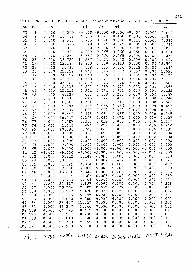
162
Table C4 contd. PIXE elemental concentrations (n mole Rb-Zn
Ti V Y Znrow nF Rb s Si Sr
0.020 0.015 0.000 0.817
0.025 0.000 0.000 0.714
-9.000 -9.000 -9.000 -9.000
0.066 0.050 0.000 4.851
0.065 0.000 0.000 1.236
0.152 0.206 0.000 2.447
0.413 0.000 0.000 12.502
0.064 0.048 0.000 1.644
0.077 0.057 0.000 1.698
0.235 0.065 0.000 2.434
0.466 0.000 0.289 7.710
0.076 0.000 0.000 1.683
0.071 0.053 0.000 1.866
0.982 0.000 0.000 3.423
0.253 0.000 0.000 4.287
0.497 0.000 0.000 6.944
0.213 0.000 0.000 3.462
0.066 0.049 0.000 0.457
0.063 0.047 0.000 0.716
0.065 0.049 0.000 0.845
0.071 0.000 0.000 3.427
0.000 0.000 0.000 1.437
0.000 0.000 0.000 0.210
0.000 0.000 0.000 0.695
-9.000 -9.000 -9.000 -9.000
-9.000 -9.000 -9.000 -9.000
-9.000 -9.000 -9.000 -9.000
-9.000 -9.000 -9.000 -9.000
-9.000 -9.000 -9.000 -9.000
-9.000--9.000 -9.000 -9.000
0.000 0.000 0.000 0.530
0.414 0.000 0.000 4.021
0.060 0.000 0.000 0.402
-9.000 -9.000 -9.000 -9.000
0.065 0.000 0.000 2.236
0.000 0.000 0.000 0.259
0.000 0.000 0.000 0.891
0.200 0.000 0.000 1.208
0.177 0.000 0.000 0.467
0.189 0.000 0.000 1.862
0.000 0.000 0.000 1.382
-9.000 -9.000 -9.000 -9.000
0.000 0.000 0.000 1.376
0.000 0.000 0.000 1.504
0.000 0.000 0.000 0.647
0.000 0.000 0.000 0.000
0.000 0.000 0.000 0.328
0.000 0.000 0.000 0.356
0.000 0.000 0.000 0.114
0-10 O-OZf
53 1 -9.000 -9.000 -9 .000 -9 .000
54 2 0 .000 10.469 4.803 0.021
55 4 0.000 2 .587 1.233 0.020
56 7 0.000 3 .478 3 .220 0 .025
57 9 -9.000 -9.000 -9.000 -9.000
58 12 0.000 3 .969 4.289 0.065
59 17 0.000 9.070 8.687 0.064
60 23 0.000 36.722 14.287 0 .073
61 13 0.000 12.285 19.970 0.088
62 27 0.000 5.792 3 .028 0 . 063
63 28 0 .000 21.359 1.749 0.075
64 32 0.000 24 .759 11.248 0.086
65 33 0 .000 42 .916 21.788 0 .371
66 14 0.000 23.163 10 .859 0.075
67 15 0.000 8.333 2 .251 0 . 069
68 41 0.000 15.112 6.984 0.074
69 42 0.000 6.138 . 6.665 0.068
70 43 0 .000 8.838 3.645 0 .072
71 44 0.000 8.860 1.781 0.151
72 62 0.000 15.791 0 .286 0.065
73 63 0.000 13.897 0 .602 0.062
74 66 0 .000 5.642 2 .476 0.064
75 67 0.000 18.817 2 .376 0.069
76 77 0.000 1.487 1.300 0 .058
77 74 0.000 1.448 1.674 0.059
78 99 0 .000 10 .896 8 .243 "0.068
79 100 -9.000 -9.000 -9.000 -9.000
80 112 -9.000 -9.000 -9.000 -9 . 000
■ 81 113 -9.000 -9.000 -9.000 -9.000
82 64 -9.000 -9.000 -9.000 -9.000
83 65 -9.000 -9.000 -9.000 -9.000
84 45 -9 .000 -9.000 -9.000 -9.000
85 102 o.ooO 0 .842 1.142 0 . 0|^586 124 0.000 30.091 16.322 0.067
87 125 0.000 1.399 4.024 0.059
88 130 -9.000 -9.000 -9.000 -9.000
89 146 0.000 10.808 2 .847 0.063
90 131 ■ 0.000 7 .195 . 1.867 0 .065
91 149 0.000 46.983 0.704 0.059
92 151 0 .000 37 .417 8 .897 0 .060
93 157 0 .000 35.566 7 . 002 0 .063
94 158 0.000 18.597 5 .478 0 . 072
95 160 0.000 23.163 15.245 0.000
96 163 -9.000 -9.000 -9.000 -9.000
97 164 0.000 23.447 21.457 0.000
98 161 0.000 46.207 3 .046 0.000
99 159 0.000 64.793 8.459 0.000
100 173 0.000 5.551 0 .280 0.000
101 189 0.000 19.010 3 .506 0 .000
102 191 0.000 29.760 9.865 0.000
103 197 0 . 000 19 .960 5.310 0 . 000
ae-
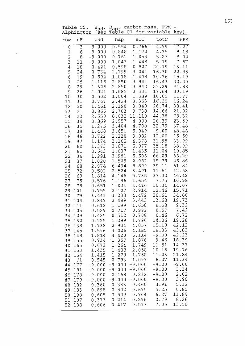
163
Table C5. Bg^, B^p, carbon mass, FPM -Alphington (see Table C1 for variable key).
row nF bsd bap elC totC FPM
0 3 -9.000 0.554 0.766 4799 TTTT1 6 -9.000 0.848 1.172 4.35 8.15
2 8 -9.000 0.761 1.053 5.27 8.02
3 11 -9.000 1.047 1.448 5.19 7.674 18 0.421 0.598 0.827 20.79 13.11
5 24 0.734 2.199 3.041 16.30 22.85
6 19 0.592 1.018 1.408 10.36 15.197 25 1.116 2.850 3.941 16.43 32.00
8 29 1.326 2.850 3.942 23.29 41.88
9 26 1.021 1.685 2.331 17.64 30.1910 30 0.502 1.004 1.389 10.65 11.7711 31 0.767 2.424 3.353 16.25 16.24
12 20 1.461 2.198 3.040 26.74. 38.41
13 21 0.866 2.703 3.738 14.66 21.02
14 22 2.558 8.032 11.110 44.38 78.32
15 34 0..869 2.957 4.090 20.39 23.5916 35 1.275 3.404 4.708 32.79 37.48
17 39 1.468 3.651 5.049 -9.00 48.44
18 46 0.722 2.228 3.082 12.00 15.6019 47 1.174 3.165 4.378 31.95 33.9920 60 1.373 3.671 5.077 35.18 38.9921 61 0.643 1.037 1.435 11.04 10.8522 36 1.991 3.981 5.506 66.09 66.29
23 37 1.020 1.505 2.082 19.79 25.8624 68 2.074 6.434 8.899 39.11 61.84
25 72 0.502 2.524 3.491 11.61 12.6826 69 1.814 4.146 5.735 37.32 46.4227 75 0.576 1.196 1.654 7.75 10.98
28 78 0.651 1.024 1.416 10.34 14.0729 101 0.755 2.107 2.914 12.46 15.7130 79 1.443 3.233 4.472 20.61 34.8631 104 0.849 2.489 3.443 13.68 19.7332 111 0.612 1.199 1.658 8.58 9.3233 105 0.529 0.717 0.992 8.57 7.4234 129 0.425 0.512 0.708 6.46 6.7235 132 0.925 1.299 1.796 14.06 19.2836 138 1.738 2.934 4.057 15.10 42.1237 145 1.596 3.026 4.185 19.33 43.8338 148 1.814 4.420 6.114 -9.00 42.2339 155 0.934 1.357 1.876 9.46 18.39
40 165 0.673 1.264 1.749 11.51 14.3741 153 1.435 1.488 2.058 10.16 19.7642 154 1.415 1.278 1.768 11.23 21.8443 71 0.545 0.793 1.097 6.27 11.3444 177 -9.000 -9.000 -9.000 -9.00 -9.0045 181 -9.000 -9.000 -9.000 -9.00 3.3446 178 -9.000 0.168 0.232 -9.00 2.0247 179 -9.000 -9.000 -9.000 -9.00 3.9048 182 0.360 0.333 0.460 3.91 5.3249 183 0.898 0.502 0.695 5.25 6.8550 190 0.605 0.509 0.704 6.27 11.8951 187 0.377 0.214 0.296 2.79 8.2652 188 0.606 0.417 0.577 7.06 13.50

164
Table C5 contd. Bg^j, B^p, elemental andtotal carbon mass, FPM - Footscray (seeTable C1 for key to variable names andunits)
bsd bap elC totC FPM
-9.000 -9.000 -9.000 -9.00 -9 .00
-9.000 1.286 1.778 8.80 17.74
-9.000 0.354 0.490 3.87 7.87
-9.000 0.663 0.917 5.68 10.77
-9.000 -9.000 -9.000 -9.00 -9.00
0.633 2.007 2.776 13.31 20.34
0.776 2.498 3.456 11.89 25.19
1.201 3.613 4.997 17.08 35.22
1.587 4.782 6.614 30.85 44.75
0.420 0.982 1.359 9.47 13.23
0.899 2.589 3.580 13.83 . 21.69
1.642 4.913 6.795 32.14 46.87
2.684 7.247 10.024 44.94 69.10
1..688 3.770 5.214 -9.00 38.96
1.691 2.990 4.136 -9.00 20.95
1.076 3.244 4.486 15.17 28.02
1.149 2.382 3.294 15.32 25.38
0.773 3.165 4.378 15.26 21.36
1.207 2.523 3.490 15.30 27.54
0.922 1.776 2.457 14.37 24.21
0.780 0.901 1.246 7.17 12.88
0.734 2.347 3.246 13.83 18.28
1.085 2.454 3.395 14.88 23.82
0.329 0.635 0.878 2.85 8.86
0.434 0.595 0.823 5.03 6.25
1.072 2.623 3.628 16.42 27.52
-9.000 -9.000 -9.000 -9.00 -9.00
-9.-000 -9.000 -9.000 -9 .00 -9.00
-9.000 -9.000 -9.000 -9.00 -9.00
-9.000 -9.000 -9.000 -9.00 -9.00
-9.000 -9.000 -9.000 -9.00 -9.00
-9.000 -9.000 -9.000 -9.00 -9.00
0.824 0.568 0.785 4.50 7.74
0.791 2.751 3.805 15.76 29.11
0.548 0.790 1.093 8.59 7.16
-9.000 -9.000 -9.000 -9.00 -9.000.880 1.766 2.443 12.00 16.21
0.710 1.382 1.912 10.85 12.87
1.053 0.394 0.545 -9.00 17.02
1.097 1.001 1.384 -9.00 15.48
0.945 1.221 1.689 8.71 17.28
1.043 2.955 4.087 15.84 19.990.973 1.633 2.258 11.42 -9.00
-9.000 -9.000 -9.000 -9.00 -9.00
0.818 1.298 1.795 11.07 24.420.967 0.608 0.841 6.36 -9.001.440 0.965 1.334 9.79 26.210.325 0.287 0.398 5.85 5.200.682 0.470 0.650 6.43 16.12
0.828 1.240 1.715 9.50 27.29
0.481 0.568 0.785 5.86 12.88
row nF
53 1
54 2
55 4
56 7
57 9
58 12
59 17
60 23
61 13
62 27
63 28
64 32
65 33
66 14
67 15
68 41
69 42
70 43
• 71 44
72 62
73 63
74 66
75 67
76 77
77 74
78 99
79 100
80 112
81 113
82 64
83 65
84 45
85 102
86 124
87 125
88 130
89 146
90 131
91 149
92 151
93 157
94 158
95 160
96 163
97 164
98 161
99 159
100 173
101 189
102 191
103 197

165
Table C6. EPA air quality data, mean values for sampling periods (seeTable C1 for key to variable labels and units) .
row nF CO o3
0 3 0.36 -9.00
1 6 0 . 61 -9.00
2 8 -9.00 -9.00
3 11 0.56 -9.00
4 18 0 .40 -9.00
5 24 1.95 -9.00
6 19 0 .51 -9.00
7 25 1.93 -9.00
8 29 2.14 0.00
9 26 0 .90 0.01
10 30 0 .53 0 .49
11 31 2.13 0.19
12 20 2.21 0 .00
13 21 1.39 0 .45
14 22 7 .17 0.00
15 34 1.62 0.80
16 35 2.16 0.00
17 39 3 .16 0.00
18 46 0 .85 0 .50
19 47 2.00 0 .01
20 60 3 .39 0.00
21 61 0.61 0.73
22 36 4.16 0.00
23 37 0.77 0.27
24 68 5.81 0.00
25 72 0 .95 1.25
26 69 3.39 0.03
27 75 0 .89 -9.00
28 78 1.06 -9.00
29 101 0 .81 -9.00
30 79 2.36 -9.00
31 104 1.70 -9.00
32 111 ,0.57 1.08
33 105 0.67 0.51
34 129 0.36 1.23
35 132 1.21 0.44
36 138 2.74 0 .00
37 145 2.27 0.00
38 148 3 .74 0.01
39 155 0 .74 1.47
40 165 1.12 2.47
41 153 0 .56 -9.00
42 154 0.69 2 .80
43 71 0 .71 3 .78
44 177 -9.00 -9.00
45 181 0 .25 0.20
46 178 0.04 0.66
47 179 0.30 0.63
48 182 -9.00 -9 .00
49 183 0.33 0.60
50 190 0.47 2.55
51 187 0.34 1.31
52 188 0.57 2.94
no- no2 api so2 nmhc tsr uv dbt sws
0.51
1.65
1.77
1.95
0.33
10.11
2.09
10 .64
12.94
3 .49
1.49
11.83
11.36
7.01
49 .09
7 .22
12.50
18.33
4.62
10.92
21.50
2.31
26.90
2.75
-9.00
5.50
21.73
3 .04
4.21
3 .59
15.27
9.44
2 .28
1.71
-9.00
4.63
16.03
12.09
20 .24
2 .22
0 .77
1.22
0 .94
0.38
-9.00
0.90
0 .24
1.50
-9.00
0.63
-9.00
-9.00
-9.00
1.21
1.11
1.69,
1.49
1.23
2.86
0.83
2.03
,00
,41
,64
,67
,69
,06
0.56
2.67
'l.071.39
-9.00
0.54
1. 09
1.27
0.54
1.34
-9.00
2.09
1.21
1.74
1.34
2.39
0.59
96
23
67
00
11
01
13
39
92
39
1.80
2.39
2 .24
-9.00
1.35
0.51
0.80
0.43
0 .43
0.46
0.62
0.48
0 .82
0 .56
1.33
1.50
1.10
0.47
0 .88
1.60
0 .94
2.90
0 .99
1.49
1.70
0.70
1.30
1.61
0.68
3 .02
1.21
2 .32
0 .51
2.24
0.70
0 .80
0 .83
1.59
0 .94
0.46
0.47
0.44
16
96
67
89
0.95
0 .75
1.61
1.51
0 .58
00
27
00
00
00
,00
,00
,00
,00
,00
0.68
-9.00
-9 . 00
0.58
0.00
0.01
0.01
0.01
0.00
0.14
0.00
0.09
0.06
0.01
0.01
0.10
0.07
0 .25
0.23
0 .15
0.07
0 .13
0.21
0.06
0.11
0 .00
0.13
0.00
0.19
0.05
0.14
0.03
0.01
0.17
0.07
0.09
0.10
0.01
0.01
0.00
0.00
0.01
0 .13
0 .16
0 .17
0.00
0 .12
0.00
-9 .00
0 .10
0.01
0.07
-9 .00
0.04
0.15
0.07
0.12
-9.00 -9 .00
-9.00 -9.00
-9.00 -9.00
-9.00 -9.00
-9.00 -9.00
-9.00 -9.00
-9.00 -9.00
-9.00 -9.00
-9.00 -9.00
-9.00 -9.00
-9.00 -9.00
-9.00 -9.00
-9 .00 -9.00
-9.00 -9.00
-9.00 -9.00
-9.00 -9.00
-9.00 -9.00
-9.00 -9.00
-9.00 -9.00
-9.00 -9.00
-9.00 -9.00
1
Oo -9.00
-9.00 -9.00
1
oO
-9 .00
-9.00 -9 .00
-9.00 -9.00
-9 . 00 -9.00
-9.00 -9.00
-9.00 -9.00
-9.00 -9.00
-9.00 -9.00
-9.00 -9.00
1
Oo
-9.00
-9.00 -9.00
-9.00 -9.00
1
oo
-9.00
-9.00 -9.00
-9.00 -9.00
-9 .00 -9.00
-9.00 -9.00
-9.00 -9.00
-9.00 -9.00
-9.00 -9.00
-9.00 -9.00
-9.00 -9.00
-9.00 -9 .00
-9.00 -9.00
-9.00 -9.00
-9.00 -9 . 00
-9.00 -9.00
-9.00 -9.00
-9.00 -9.00
-9.00 -9.00
00
00
00
00
00
00
00
00
00
00
00
00
00
00
do00
00
00
-9.00
-9.00
-9.00
-9.00
-9.00
-9.00
17.95
13 .01
-9.00
-9 .00
-9,
-9,
-9 ,
00
00
00
00
00
00
00
00
00
00
00
00
00
00
00
00
00
00
00
00
00
00
00
00
00
00
00
00
00
00
00
00
00
00
00
00
00
10.59
11.10
10 .74
13 .31
6.12
15.96
6.27
12.01
12.71
6.05
8.32
8.60
6.17
8.64
5.61
11.35
7.90
7 .75
7.94
13 .39
6.51
6.91
12.56
7.04
11.02
9 .29
2.71
5.36
7.10
18.25
20 .94
17.84
23 .65
32 .84
-9.00
16.20
14.34
15.03
-9.00
16.59
25.92
17 .90
24.75
-9 ,
-9,
-9 ,
1,
3 ,
1,
1.
1,
1,
1,
1,
2 ,
1,
1,
1,
1,
2 ,
1,
00
00
00
49
27
51
11
29
85
87
05
05
02
89
35
20
06
21
1.29
2.16
0 .86
1.24
0 .92
3 .01
0.92
2.91
2,
1,
1,
1,
3 ,
1,
3 ,
2,
86
54
17
90
74
54
19
27
0.91
1.15
1.37
2.76
3 .25
1.37
4.17
3.21
-9.00
2 .80
3.30
4.90
00
11
41
69
01

166
Table C6 contd.. EPA air quality data, mean values for sampling periods
row nF co o3 no no2 api so2 nmhc tsr uv . dbt sws
~53 i 0.06 0.70 -9.00 -9.00 o'TTt 0.12 0.11 -9.00 2.50 15.76 TTtT54 2 0.61 0.47 -9.00 -9.00 0.73 0.18 1.59 -9.00 4.09 14.99 1.60
55 4 0.20 -9.00 0.47 -9.00 0.39 0.00 0.05 -9.00 1.68 16.99 4.79
56 7 0.22 -9.00 0.98 -9.00 0.39 0.00 0.03 -9.00 5.12 17.24 5.80
57 9 0.38 -9.00 1.23 -9.00 0.42 0.05 0.19 -9.00 2.11 17.87 3.62
58 12 0.76 -9.00 3.31 2.47 0.63 0.06 0.24 -9.00 0.00 16.55 2.92
59 17 1.33 -9.00 8.31 2.17 0.79 0.10 0.75 -9.00 0.00 6.97 1.72
60 23 2.00 -9.00 -9.00 -9.00 1.23 1.02 1.01 -9.00 0.88 16.15 1.91
61 13 2.53 -9.00 17.83 2.47 1.62 0.24 0.98 -9.00 0.00 10.87 2.29
62 27 I 0.37 -9.00 -9.00 -9.00 0.45 0.05 0.09 -9.00 3.25 13.45 2.05
63 28 0.77 -9.00 -9.00 -9.00 1.00 0.22 0.24 64.00 5.75 13.42 3.05
64 32 3.10 -9.00 -9.00 -9.00 1.87 0.23 1.52 -9.00 0.00 7.26 1.45
65 33 2.97 -9.00 -9.00 -9.00 2.45 0.60 1.10 -9.00 7.63 14.57 1.54
66 14 1.74 -9.00 -9.00 -9.00 1.96 0.31 0.61 -9.00 0.13 10.82 1.91
67 15 1.46 -9.00 -9.00 -9.00 1.24 0.30 0.92 -9.00 6.63 15.07 3.04
68 41 1.35 0.69 7.62 3.30 1.11 0.30 0.42 -9.00 8.50 15.00 1.77
69 42 1.26 0.00 10.67 .'1.80 1.03 0.04 0.47 -9.00 0.00 7.67 1.9470 43 1.42 0.96 8.19 1.91 0.79 0.11 0.37 -9.00 9.38 15.51 3.95
71 44 1.46 0.00 12.49 1.80 1.11 0.06 0.57 -9.00 0.00 8.84 2.17
72 62 1.36 0.00 8.47 2.06 1.00 0.07 0.69 -9.00 0.00 8.75 1.05
73 63 0.45 0.91 1.75 1.91 0.82 0.01 0.07 -9.00 5.38 14.40 3.49
74 66 1.47 0.00 -9.00 -9.00 0.86 0.04 0.84 -9.00 0.00 7.64 1.41
75 67 1.29 0.04 8.80 2.00 1.27 0.07 0.57 -9.00 0.00 6.71 2.40
76 77 0.11 1.20 -9.00 -9.00 0.33 0.07 0.50 -9.00 1.25 7.89 5.25
77 74 0.40 0.81 -9.00 -9.00 0.40 0.00 0.08 -9.00 0.88 11.07 3.39
78 99 1.73 0.00 -9.00 -9.00 1.16 0.17 1.21 -9.00 0.00 8.24 1.12
79 100 2.55 0.00 -9.00-9.00 1.78 0.20 0.99 -9.00 3.50 6.95 1.75
80 112 -9.00 -9.00 -9.00 -9.00 -9.00 -9.00 -9.00 -9.00 -9.00 -9.00 -9.00
81 113 -9.00 -9.00 -9.00 -9.00 -9.00 -9.00 -9.00 -9.00 -9.00 -9.00 -9.00
82 64 -9.00 -9.00 -9.00 -9.00 -9.00 -9.00 -9.00 -9.00 -9.00 -9.00 -9.00
83 65 -9.00--9.00 -9.00 -9.00 -9.00 -9.00 -9.00 -9.00 -9.00 -9.00 -9.00
84 45 -9.00 -9.00 -9.00 -9.00 -9.00 -9.00 -9.00 -9.00 -9.00 -9.00 -9.00
85 102 0.20 1.05 -9.00 -9.00 -9.00 0.00 0.02 -9.00 9.63 15.76 6.69
86 124 1.45 0.56 -9.00 -9.00 -9.00 0.49 0.64 -9.00 3.88 13.59 1.89
87 125 0.25 0.75 -9.00 -9.00 0.37 0.00 0.32 -9.00 2.38 12.30 2.45
88 130 -9.00 -9.00 -9.00 -9.00 -9.00 -9.00 -9.00 -9.00 -9.00 -9.00 -9.00
89 146 0.97 0.06 5.74 2.56 1.02 0.11 0.32 -9.00 0.00 8.54 2.14
90 131 1.04 0.06 5.81 1.33 0.73 0.03 0.37 -9.00 0.75 6.16 1.66
91 149 0.13 2.34 0.00 1.14 1.18 0.13 0.06 -9.00 0.00 12.56 1.71
92 151 0.27 1.85 0.81 1.50 1.20 0.10 0.03 -9.00 14.50 16.54 2.51
93 157 0.41 1.96 0.74 2.35 0.98 0.16 0.18 -9.00 8.38 17.12 2.57
94 158 0.91 0.37 5.39 3.37 1.12 0.45 0.41 -9.00 4.75 12.95 1.56
95 160 -9.00 3.17 1.06 2.21 0.98 0.10 0.17 -9.00 20.38 25.14 2.95
95 163 -9.00 -9.00 -9.00 -9.00 -9.00 -9.00 -9.00 -9.00 -9.00 -9.00 -9.00
97 164 0.51 4.31 0.39 2.11 0.84 0.39 0.12 -9.00 12.13 22.94 3.72
98 161 0.21 1.42 0.21 0.91 0.98 0.00 0.05 -9.00 2.13 17.81 1.81
99 159 0.33 4.28 0.25 1.18 1.24 0.48 0.05 -9.00 21.13 23.81 4.30
100 173 0.21 1.42 0.27 0.88 0.32 0.11 0.01 -9.00 12.25 20.90 5.49
101 189 0.21 4.69 0.06 1.06 0.77 0.19 -9.00 -9.00 17.63 25.77 3.11
102 191 0.37 5.25 0.16 2.12 0.89 0.97 -9.00 -9.00 12.13 26.49 3.39
103 197 0.20 3.14 0.21 -9.00 0.51 0.24 -9.00 -9.00 16.75 23.82 3.39

167
Table C7. PIXE detection limits and
statistics
species no. mean min max
pixAl 47 0.3644 0 .304 0 .417
pixAs 47 0 .3032 0 .027 1.642
pixBal 30 0.2125 0.181 0 .239
pixBil 1 0.7360 0 .736 0 .736
pixBr 124 0.0874 0 .041 0.396
pixCa 95 0.1010 0 .080 0.135
pixCl 151 0.1470 0 .114 0.247
pixCr 77 0.0465 0.038 0 .058
pixCu 96 0.0262 0.013 0.050
pixFe 153 0.0384 0.020 ■ 0.054
pixGa 7 0.0841 0.053 0 .135
pixK 117 0.1097 0.090 0 .134
pixMn 93 0.0365 0.028 0.051
pixNi 104 0.0266 0.015 0.042
pixP 34 0.1801 0 .154 0 .225
pixPbl 102 0.4335 0.113 2 .458
pixRb 1 0.5070 0 .507 0 .507
pixS 137 0.1616 0 .129 0 .235
pixSi 152 0.1987 0 .167 0 .255
pixSr 108 0.1403 0 .000 0 .220
pixTi 70 0.0783 0.067 0.093
pixV 30 0.0624 0.054 0 . 072
pixY 1 0.4680 0 .468 0 .468
pixZn 128 0.0284 0.013 0.065
MDL (minimum detection limits) are in unitsof |ig per filter. "no." is the number offilters use to calculate the MDL statistics
mean= mean of MDLs
min=minimum MDL
max=maximum MDL
In the tables of PIXE results an element
concentration of 0.0 indicates that no
concentration was reported by ANSTO.

168
Table C8. Concentrations of organic compounds (ng m"^).Retention Molecular Name GF22 GF32 GF33 GF49 QF64 GF72 GF73
Time weight Alph Foots Foots Alph Alph Alph Alph
28/5/90 28/5/90 29/5/90 10/6/90 7/6/90 13/6/90 18/6/90
7.962 142
8.721 142
13.817 178 Phenanthrene 0.41 0.26 0.40 0.27 0.23 0.34 0.26
13.926 178 Anthracene 0.09 0.06 0.10 0.06 0.17 0.06 0.16
13.277 180 9-H fluorene-O-one 1.10 0.51 0.25 1.91 0.87 1.52 0.96
14.927 180 1-H phenaiene-1-one 0.69 0.09 0.22 0.76 0.20 0.58 0.20
16.702 202 PAH 2.34 0.65 0.85 0.66 0.39 1.11 0.62
16.896 202 Huoranthene 0.66 0.23 0.42 0.33 0.19 0.43 0.26
17.167 202 Pyrene . 2.98 1.23 1.66 1.21 0.77 1.71 1.30
15.846 204 2-phenyl Naphthalene 0.20 0.19 0.18 0.20 0.14 0.20 0.18
16.438 204 cyclo penta(d,e,f)Phenpnthrene 0.30 0.14 0.16 0.08 0.18 0.12
16.334 206 PAH 0.08 0.11
16.506 206 PAH 0.11 0.20 0.06 0.06 0.10
16.597 206 PAH 0.06 0.07
16.687 206 PAH 0.30
17.224 206 PAH 0.33
15.34 208 PAH 1.52 0.43 2.90 0.75 Z06 ^02
15.666 208 9,10 anthracene dione 0.17 0.40 0.28 0.20 0.26 0.24
16.943 208 PAH 1.78 0.96 0.35 0.51 0.32 0.76
17.388 216 PAH 0.09 0.13 0.22 0.14 0.11
17.469 216 PAH 0.03 0.04 1.05
18.039 216 PAH 0.04
18.083 216 PAH 0.76 0.17 0.30 0.55 0.20 0.59 0.35
18.257 216 PAH 0.07 0.10 0.24 0.08 0.26 0.15
18.297 216 PAH 0.10 0.16 0.21 0.09 0.23 0.15
18.499 216 PAH 0.13 0.14 0.25 0.13 0.30 0.18
18.563 216 PAH 0.09 0.11 0.21 0.08 0.22 0.14
17.301 218 benzo(b)naphthol(2,3d)Furan 0.27 0.05 0.12
17.581 218 PAH 0.12
19.62 226 PAH 3.97 1.08 1.63 2.79 1.09 2.93 1.50
20.03 226 PAH 9.28 1.75 5.38 2.02 6.52 2.71
20.125 228 benz(a)Anthracene &) 1.24 0.87 (6 '̂ &> (&1? Ci?20.194 228 Chrysene 15.12 5.26 3.13 12.46 4.32 10.77 6.05
19.245 230 terpheny! isomer 2.58 0.60 0.73 1.99 0.73 2.09 1.17
19.742 230 terpheny! isomer 4.54 0.51 0.97 3.93 2.10 3.99 2.91
20.395 230 terpheny! isomer 10.94 3.67 1.71 9.23 4.48 9.03 6.52
22.596 252 benzo(e)PyrBne 51.03 17.86 11.19 36.33 17.45 34.46 25.41
22.79 252 PAH 11.97 3.99 1.35 9.71 4.38 9.20 5.86
23.092 252 benzo(a)PyrBne 21.85 7.55 5.33 13.62 7.18 13.98 10.01
23.193 252 Petylene 28.48 9.10 4.02 21.10 10.54 21.23 14.71
23.114 254 PAH 12.36 2.63 2.99 8.83 1.10 7.09

169
Table C8 continued. Concentrations of organic compounds (ng m"3).Retention Molecular Name GF22 GF32 GF33 GF49 GF64 GF72 GF73
Time weight Alph Foots Foots Alph Alph Alph Alph
28/5/90 28/5/90 29/5/90 10/6/90 7/6/90 13/6/90 18/6/90
25.221 276 PAH 6.49 5.14 2.14 5.32 3.60
25.368 276 PAH 20.15 1.88 1.50 15.91 7.17 14.78 11.47
25.803 276 PAH 33.13 8.62 8.07 21.86 12.21 25.03 17.59
26.057 276 PAH 10.18 0.02 7.03 ^83 6.32 5.07
25.16 278 PAH 0.76 0.27 0.33 0.60 0.58 0.% 0.51
25.703 278 PAH 2.79 0.49 0.37 2.68 0.69 ^35 1.48
28.415 300 Coronene 9.58 1.82 1.90 5.30 ^37 7.62 4.72
9.036 152 0.27 0.19
9.136 152 0.19
9.184 152 3-methoxy-4-hydroxy BenzaWehyde 1.03 0.55 0.27 1.24 0.92 1.22 0.96
8.663 154 2,6 dimethoxy Phenol 1.26 0.37 0.16 1.07 0.69 1.57 1.12
8.996 154
9.11 154 Biphenyt 0.22 0.11 0.11 0.13 0.15 0.25 0.08
9.232 166
10.342 166 3-methoxy-4-hydroxy Acetophenone 0.35 0.32 0.36 0.60 0.45
10.472 166
10.866 166 0.37
9.967 168 3-methoxy-4-hydroxy benzole Acid 0.98 0.92 0.30 1.52 1.22 1.22 1.41
10.058 168 0.05
10.79 168
11.917 194 0.08 0.04 0.06 0.06
12.33 194
12.478 194 0.07 0.08
13.044 194 2,6 dimethoxy -4-(2-propenyl) Phenol 1.79 0.32 0.21 1.20 0.34 1.10 1.66
11.136 196
1Z036 196 0.07 0.03 0.11 0.09 0.11
13.266 196 3,5dlmethoxy-4-hydroxy 7.55 3.64 0.48 16.12 6.65 11.78 7.24
Acetophenone18.62 85 022 Hydrocartjon 16.45 17.50 15.90 11.69 6.79 10.70 10.52

170
APPENDIX 3
This appendix contains plots of particle size
distribution and differential scattering coefficient
determined at Alphington from May to September 1990.
Particles were sized using a PMS ASASP-X size spectrometer
with a heated inlet. Data for the plots typically represent
integrals over eight hours sampling concurrent with a chemical
filter sample. The ASASP-X file write-times and the
corresponding filter (Fluoropore number) are indicated on each
plot. A refractive index of m = 1.6 - Oi was used for the
size distributions. Differential scatter was calculated from
the measured size distributions using the relationship:
d(scatter)/dlog r = Q.A.dN/dlog r
where Q is the calculated Mie scattering efficiency at the
Nephelometer wavelength of 470 nm and particle radius, A is
the particle cross-sectional area and dN/dlog r the
(differential) particle concentration.
Size distribution samples were initiated in parallel with
filter samples and are thus biased to lower visibility
conditions. For all distributions the peak in scattering
consistently occurs between about 0.1 and 0.2 |im radius. This
demonstrates a strong dynamic influence maintaining the shape
of the aerosol size distribution in this size region.

m I E U DC cn
o I—I
■Q
Siz
e
dis
trib
utio
n
an
d
ca
lcu
late
d
sca
tte
r a
t 4
70
nm
Alp
hin
gto
n.
May
24
2
52
9 -
May
25
0
63
0
nF
30
1 I
I 1
11
11
1 I—
1
1 I
11
11
4-
3-
2 1
2 0
-cn 5
-1 _2
[-
- 3
1—J
I I
t I I
tt
J \
I I
I I
I I
I
. 0
2.
1 1
Ra
diu
s (/J
in)
□:
cn
o I—I
"O -p m u in cn
o _J
4 3 2 1 0
- 1
-2
-3
1 I
I I
11
11
"1 I
I I
1 I
I I
I
I I
II
I i
ll
J I
I I
I 1
11
1
. 0
21
1R
ad
ius
(/um
)<
1

cn I
■
E U □C cn
o I—I
"□ cn
o _1
Siz
e
dis
trib
utio
n
an
d
ca
lcu
late
d
sca
tte
r
at
47
0
nm
Alp
hin
gto
n.
May
2
5
20
43
-
May
2
6
03
43
n
F3
1
51
I I
I I
I I
4 3 2 1 0
-
1
-2
1 I
I I
I I
i I
. 0
2I
I I
II
I I
I 1
11
1 1
Ra
diu
s
i^m
]
q: cn
□ I—I
4J ra u in cn
o
51
I 1
I I
I 111
I I
I I
I I 1
11
4 3 2 1 0 1 2
-3
. 0
2I
I I
I 1
11 1
j I
I I
I I
11
1 1R
ad
ius
(/u m
)-j
to

cn I E U CT cn
□ I—I
"a z CD
□
Siz
e
dis
trib
utio
n
an
d
ca
lcu
late
d
sca
tte
r a
t 4
70
nm
Alp
hin
gto
n,
May
2
6
23
19
-
May
27
0
61
9
nF
20
5|
T I
I I
I I I
I I
I I
1 I
I I I
I
4 2 1 0
-
1
-2
-3
j I
I I
I 1
11
I I
±L
02
. 1
1R
ad
ius
(/um
)
cr CD
□ I—1
4-1 m u CO "D CD
□
5|
I I
I I
I 11
4 3 2 1 0 1
-2
"1
1 I
I I
I I
I I
I I
I 1
1j
I I
I 1
1
. 0
2.
1 1
Ra
diu
s
(/jm
)<
1LO

□c cn
o rH oi
O
Siz
e
dis
trib
utio
n
an
d
ca
lcu
late
d
sca
tte
r a
t 4
70
nm
Alp
hin
gto
n,
Ju
ne
5
08
37
-
16
25
n
F4
6
m 4
I ̂
E U
2 1
-a
0
-
1
-2
-3
I I
I I
I1
I I
I I
I 1
11
J—I
I I
I I
I I
I I
I I
M
I I
I0
2. 1 Ra
diu
s (^
im)
q: oi
□ I—1
u -p ra u m D)
o
5[
I I
I I 1
111
4 3 2 1 0 1
-2
-
3'
' '
■ ■ '
. 0
2
1 r
I I
11
1
j I
I I
I I
I
Ra
diu
s
(^m
)<
1

mI E u
(Z cn
o I—I
JD cn
o _J
Size distribution and calculated scatter at 470 nm
Alphington, June 6 2008 - June 7 0356 nF47
51
I I
I I
111
4 3 2 1 0
- 1
-2
"1
rI
I 1
11
02
\
I I
11
I 1
11
1
1 1
Radius
(^im
)2
□c cn
D I—I
ID -P m u m cn
D
5|
I CT
"
4 3 2 1 0 1 2
- 3
1 I
I I
I I
11
1
j I
I I
I 1
11
02
1 1
Ra
diu
s
ipm
)U
1

cn I E U □: D1
□ I—1
ID TJ cn
□
Siz
e
dis
trib
utio
n,
an
d
ca
lcu
late
d
sca
tte
r a
t 4
70
nm
Alp
hin
gto
n,
Ju
ne
7
18
14
-
Ju
ne
8
02
02
nF
BO
4 3 2 1 0
-
1
-2
1 I
I I
11
11
j I
I I
02
"1 I
I I
I
j I
I I
I 1
1
. 1
. 1
2R
ad
ius
(/jm
)
cr cn
□ I—I
4-> ra u CO "□ cn
o _J
Ra
diu
s
i^m
)<
1C
Tl

m
I E U cr en
o I—i
TD
z
cn
□ _J
Siz
e
dis
trib
utio
n
an
d
ca
lcu
late
d
sca
tte
r a
tA
lph
ing
ton
. Ju
ne
B
20
54
-
Jun
e
9 0
44
2
nF
Bl
47
0
nm
4 2 1 0
-
1
- 2
1 I
I I
11
i I
. 0
2. 1
1R
ad
ius
[^m
]
cr cn
□ I—I
"D -U fd U cr
ID O)
o
1 I
I I
I 1
1 i
1 I
I I
I I
I
4 3 2 1 0 1
j I
I I
I 1
11
J 1
I !
I I
I I
I0
2.
1 Ra
diu
s
(/jm
)i-
»-J

mI E U d Dl
□ I 1
TD
T3 cn
O
Siz
e
dis
trib
utio
n
and
ca
lcu
late
d
sca
tte
r a
t 47
0 nm
Alp
hin
gto
n.
Ju
ne
10
1
95
8
- Ju
ne
11
0
34
6
nF
3B
I M
I
I I
I
. 0
2. 1
1R
ad
ius
[pm
]
oc cn
o I—I
TD\ 4-
1 ra u in cn
D
51
I I
I I 1
111
4 3 2 1 0 1
1 I
TT
T
_ 3I
1
I I
I0
2J
I I
I I
I I
I I
Ra
diu
s
(/um
)<
1C
O
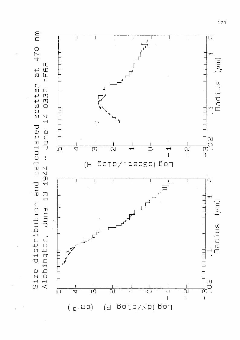
Size distribution and calculated scatter at 470 nm
Alphington, June 13 1944 - June 14 0332 nFBB
mI E U □c CD
0 1 1
"O ID CD
O
I I
I M
I
M Ra
diu
s
CE CD
□ I—1
~o
4-1 fD U CO ID CD
O _J
(A^m
)
Mi
ll Ra
diu
s(/^
m)

m 1 E U □C Dl
□ I—I
"D U D)
O
Siz
e
dis
tnib
utio
n
an
d
ca
1cu
1 a
ted
sca
tte
r a
t 4
70
nm
Alp
hin
gto
n.
Ju
ne
18
0
83
5
-16
23
n
F7
2
4 3 2 1 0
-
1
-2
1 I
I I
I 1
11
1
V
J I
I I
IJ
I I
II
I 1
11
. 0
2.
1 1
Ra
diu
s
(^im
)
5|
I I
I I
1111
□c cn
o r-H
T3
-P OD U CO CD
O
4 3 2 1 0
-
1
-2
1 I
I I
I 1
1
J I
I I
I M
IJ
I I
I I
I I
. 0
2.
1 Ra
diu
s
i^m
)0
0o

cn I E U □C C
DD I
1
"a CD
o
Siz
e
dis
trib
utio
n
an
d
ca
lcu
late
d
sca
tte
r
at
47
0
nm
Alp
hin
gto
n,
Ju
ne
1
8
21
03
-
Ju
ne
1
9
04
51
n
F6
9
51
I I
I I
1111
4 3 2 1 0
-
1
-2
I I
I 1
11
. 0
2j
I I
I 1
11
1j
I I
I I
I
1 1
2R
ad
ius
(/um
)
□c CD
□ 1—I
"□ -p ra u cn CD
□
51
I I
I 1
I I I
I I
I \
TT
4 3 2 1 0 1 2
-3 .
02
_1_L
J I
I I
I I
I I
. 1
1R
ad
ius
i^m
)C
O

Size distribution and calculated scatter at 470 nm
Alphington, June 25 1821 - June 26 0209 nF75
TTT
1 I
I I
I I
I I
I
mI E U CE CD
□ I 1
"D CD
□ _1
4-
3-
2 1
u 0
-
- 1
-
2-
3I
I I
I I I
I I I
I L
i_L
I I
I I
I I
I1
I I
I I
I I
I I
. 0
2. 1
12
Ra
diu
s
ipm
)
□c CD
o I—I
■a
-n CD u in "□ CD
o
4 3 2 1 0 1
-3
j I
I I
J L
02
1 1
Ra
diu
s
(y^m
)0
0C
O

cn I E U cr cn
□ I—I
"□ z cn
o _J
Siz
e
dis
trib
utio
n
an
d
ca
lcu
late
d
sca
tte
r
at
47
0
nm
Alp
hin
gto
n,
Ju
ly
1 1
91
9 -
Ju
ly
2 0
30
7
nF
78
51
I I
I I
1111
I I
I I
I 11
11
4 2 1 0
-
1
-2
j I
I I
11
11
. 0
2J
I L
. 1
1R
ad
ius
if^m
)
oc cn
□ I—I
"D 4-1 fD U in □n
o
5|
I I
I I
1111
I—I—
I I
I 11
11
4 3 2 1 0 1
-2
-3
. 0
2I
MIN
I
1 1
Ra
diu
s
(/um
)0
0(j
J

Size distribution and calculated scatter at 470 nm
Alphington, July 10 0854 -1642 nFlOl
m I E u CE CD
O I—1
■n CD
□ _l
4 2 1
-□
0
- 1
-2
-3
1 1
i I
11
1 I
I I
I 1
11
1
j I
I I
11
11
j I
I I
I 1
11
1
02
. 1 R
ad
ius
□c CD
o I—I
-p m u in CD
o
4 3 2 1 0
- 1
-2
1 I
I I
11
1 I
I I
I 1
11
1
. 0
2J
I I
I 1
11
1J
I
1 1
Ra
diu
s
if^m
)H
'C
O

cn I E U CE cn
o I—I
TD
\ Z
CD
Q
Size distribution and calculated scatter at 470 nm
Alphingten. July 10 2106 - July 11 0436 nF79
4 2 1 0 1
-3
1 I
I I
11
11
1 I
I I
11
1
\
j I
I I
11
j I
I I
I 1
1
. 02
. 1
1
Radius (^m)
□c CD
o I—I
"D 4-)
fD U cn TJ CD
D _J
1 I
I I
I I
I I
"I \
I I
I I
I I
I
4-
3 2 1 0 1
-2 .
02
J I
MIN
IJ
1 I
MIN
I
. 1 Ra
diu
s0
00
1

cn I E U OC CD
O I—I
TO
z "O cn
o _l
Size distribution and calculated scatter at 470 nm
Alphington, July 19 1854 - July 20 0242 nF104
4-
2 1 0 1
-2 . 02
3
TTT
1 I
I I
I I
I I
V
1 I
I I
I I
IJ
I I
I I
I 1
11
1 1
Radius
(/um
)
cr cn
o I—I
TD
-M fO
U CD CD
O
I I
I I
I I
I~I
I
I I
I I
4 3 2 1 0
- 1
-2-
- 3I—' ' ' '
02
j I
I I
I 1
1
Radius
(/jm
)1
00
CTl

cn I E U CE CD
□ r-H
"D z "O CD
O
Siz
e
dis
trib
utio
n
and
ca
lcu
late
d
sca
tte
r a
t 47
0 nm
Alp
hin
gto
n,
Ju
ly
26
1
12
5
- 1
91
3 n
Flll
51
I I
I I 1
111
4 2 1 0
-
1
-2
- 3
. 0
2j
I I
I 1
1j
I I
I I
11
. 1
1R
ad
ius
[pm
)
CL CD
□ I—I
TJ
-U ra u in CD
o
I I
I I
I 1
11
4 3 2 1 0 1
-2
- 3
1 I
I I
I 11
110
2
1 I
I I
I 1
11
1
J I
I I
11
1 Ra
diu
s
ipm
)H
'0
0<
1

m 1 E U □C □ rH z "D cn
□
Siz
e
dis
trlb
utia
n
and
ca
lcu
late
d
sca
tte
r a
t 47
0 nm
Alp
hin
gto
n,
Ju
ly
27
2338
-
Ju
ly
28
0726
nF
105
1 I
I I
I I
I I
"1 I
I I
I I
I I
I
4-
3-
2 1 0 1 2-
31—
I I
I I
11.1
1. 0
2.
1 Ra
d iu
s(/J
m)
1 I
I I
11
11
1 I
I I
I 1
11
1
cr cn
o I—I
"□ -M fO U in "D cn
o
4 3 2 1 0
- 1
-2
-3 .
02
J I
I I
I M
. 1
1R
ad
ius
i^m
)C
O0
0

cn 1 E U □C c
n□ I—
I
"□ cn
o _J
Siz
e
dis
trib
utio
n
an
d
ca
lcu
late
d
sca
tte
r
at
47
0
nm
Alp
hin
gto
n,
Aug
3
20
54
-
Aug
4
04
42
n
F1
29
51
' I
I I
1111
I I
I I
I 11
11
4 3 2 1 0 1 2
j I
I I
11
11
I I
I I
I 1
11
1
. 0
2.
1 .
1R
ad
ius
(/^m
)
□:
cn
□ I—I
"□ -p fD U LO 2 cn
D
Ra
diu
s
-2
-
(/^m
)0
0(£
1

cn I E U □C D
1□ I
1
"□ 2 CD
Q _J
Siz
e
dis
trib
utio
n
and
ca
lcu
late
d
sca
tte
r a
t 4
70
nm
Alp
hin
gto
n.
Aug
IB
19
28 -
Aug
19
03
16
nF13
2
5|
I I
I I
1111
I I
I I
I 11
11
4 3 2 1 0 1 2
J—
I I
I I
I 1
1 I
I I
I I
I I n
. 0
2.
1 ,1
Ra
diu
s
(/jm
)
cr CD
o (—I
-n (D u CD
o
51
' I
I I
I 111
I I
I 1
III
II
4 3 2 1 0
- 1
-2
-3
/
J—
I I
I I
II
I I
I I
I I
11
11
02
. 1 Ra
diu
so

cn I E U OC Ol
o I—I
"C O
Size distribution and calculated scatter at 470 nm
Alphington, Aug 26 2118 - Aug 27 0506 nF138
51
I i
II
111
1
4 3 2 1 0
- 1
-2
-3
1 I
I I
I 1
11
I I
I I
11
11
j I
I I
I
. 02
1 Radius ipm)
2
cr cn
□ I—I
-M fD U cn cn
o _J
5|
I—I
I I
1111
4 3 2 1 0
- 1
-2
-3
1 1
—I
I M
il
l
J i
I I
I I n
J I
I I
I I
I I
I
02
1 1
Ra
diu
s
(/jm
)

mI E U q:
CD
□ I—I
TD CD
O
Siz
e
dis
trib
utio
n
an
d
ca
lcu
late
d
sca
tte
r
at
47
0
nm
Alp
hin
gtc
n,
Au
g
31
1
22
6
- 1
70
5
nF
3B
4 3 2 1 0
-
1
-2
I I
I 1
1"1
—\—
r
J I
I I
MJ
I L
_L
LL
02
. 1
1R
ad
ius
(fim
)
CE CD
o I—i
"□ -p ra u in CD
o
5i
I—I
I I
1111
4 3 2 1 0 1
-2
-3
I M
I
02
T—
I I
I I
I I
I
Jl 1
J I
I I
I I
I I
I
1 Ra
diu
s
(/um
)to

mI E u DC cn
□ I—1
TD
"O CD
O _J
Siz
e
dis
trib
utio
n
an
d
ca
lcu
late
d
sca
tte
r a
t 4
70
nm
Alp
hin
gto
n,
Se
pt
8 2
10
4
- S
ep
t 9
04
52
n
F1
45
51
> I
I I
1111
4 3 2 1 0 1
-3
1—
I I
I 1
11
1
J 1
I I
I I
I I
I I
I I
I I
M I
. 0
21
1R
ad
ius
(/jm
)
□:
CD
o I—I
-p ro u in TD CD
o
5|
i I
Mi
ll
4 3 2 1 0 1
1—
I—I
I I
11
1
-2
-
- 3I
\
I I
I I I
n I
II
I. 0
2.
1 1
Ra
diu
s
(^im
)C
O

cn I E U CE O)
□ I 1
2 CJ)
o
Siz
e
dis
trib
utio
n
an
d
ca
lcu
late
d
sca
tte
r a
t 4
70
nm
Alp
hin
gto
n,
Se
pt
17
1952
-
Se
pt
18
03
40
n
F1
48
1 I
I I
I 1
11
1
3 2 1 0
_J -1 -2
-3 .
02
J_L
LJ
I I
I I
I I
I I
. 1 Ra
diu
s
(^im
)
DC D)
□ rH TD
-P ra u cn 2 cn
□
4 3 2 1 0 1 2
-3 .
02
1 1
1 1
1 1
11
11
1 1
11
11
1
;■V
;1
1 1
11
11
1 1
1 t
1 1
11
11
. 1
1R
ad
ius
(^m
)ID