Science Research Journal - (Interdisciplinary) Volume I, Issue I
Upload
khangminh22Category
view
3download
0
Pilbara Marine Conservation Partnership – Final Report
Volume 1
Gorgon Barrow Island Net Conservation Benefits Program
Final Report
December 2017
ISBN 978‐1‐4863‐1170‐5
CSIRO Oceans and Atmosphere
Citation
Babcock R, Donovan A, Collin S and Ochieng‐Erftemeijer C (2017) Pilbara Marine Conservation Partnership – Final Report. Brisbane: CSIRO
Copyright and disclaimer
© 2017 CSIRO To the extent permitted by law, all rights are reserved and no part of this publication covered by copyright may be reproduced or copied in any form or by any means except with the written permission of CSIRO.
Important disclaimer
CSIRO advises that the information contained in this publication comprises general statements based on scientific research. The reader is advised and needs to be aware that such information may be incomplete or unable to be used in any specific situation. No reliance or actions must therefore be made on that information without seeking prior expert professional, scientific and technical advice. To the extent permitted by law, CSIRO (including its employees and consultants) excludes all liability to any person for any consequences, including but not limited to all losses, damages, costs, expenses and any other compensation, arising directly or indirectly from using this publication (in part or in whole) and any information or material contained in it.
Metadata
Year of publication: 2017
Contributing Authors: Babcock RC, Bancroft K, Barnes P, Bearham D, Bennett K, Berry O, Bessey C, Birt MJ, Boddington D, Bond T, Bornt KR, Boschetti F, Bryce M, Candland L, Clarke H, Colberg F, Collin SP, Collins DL, Cuttler M, Depczynski M, D’Olivo JP, Donovan A, Dorji P, Doropoulos C, Drost E, Du Y, Ellis N, Evans R, Evans SN, Evensen NR, Fearns R, Feng M, Field S, Fisher R, Falter J, Fromont J, Fry G, Gershwin L‐A, Gomez O, Gómez‐Lemos LA, Grol MG, Haberstroh J, Hansen J, Hara A, Hardman‐Mountford N, Harvey ES, Haywood MDE, Hoell A, Holmes TH, Hosie A, Huisman J, Hurley T, Ingram B, Ivey GN, Jackson G, Jones NL, Keesing JK, Kendrick GA, Kirkendale L, Kuret AJ, Lan J, Langlois TJ, Liu D, Lough JM, Lowe RJ, Lozano‐Montes HM, Marin M, Marsh L, Mattio L, McCulloch MT, McInnes A, McLean DL, McLeod I, Miller M, Mitchell JD, Moore G, Morello B, Morrison S, Mortimer N, Moustaka M, Myers J, Naughton K, Newman SJ, Nguyen HM, O’Hara T, O’Loughlin M, Olsen YS, Partridge JC, Perez AZ, Piggott C, Pillans RD, Pitcher CR, Prunera K, Rankenburg K, Ricca V, Richards SA, Richards Z, Rochester WA, Rountrey AN, Rule M, Shedrawi G, Slawinski D, Speed C, Stoddart J, Strzelecki J, Taylor MD, Taylor S, Thompson A, Thomson DP, Trapon M, Travers MJ, van Hees DH, Vanderklift MA, Waite AM, Wakefield CB, Whisson C, Wijffels SE, Wilson S, Xu J, Zavala Perez A, Zhang N, Zhang Z, Zinke J.
Corresponding author and institution: Babcock RC – CSIRO Oceans and Atmosphere, GPO Box 2583, Brisbane, Qld 4001, Australia.
Front cover image: Pilbara coastline (Source: R. Babcock)

List of authors and their affiliation
Authors Affiliation
Babcock RC CSIRO
Bancroft K WA Department of Biodiversity, Conservation and Attractions
Barnes P WA Department of Biodiversity, Conservation and Attractions
Bearham D The University of Western Australia
Bennett K WA Department of Water
Berry O CSIRO
Bessey C CSIRO
Birt MJ The University of Western Australia
Boddington D WA Department of Primary Industries and Regional Development
Bond T The University of Western Australia
Bornt KR The University of Western Australia
Boschetti F CSIRO
Bryce M WA Museum
Candland L The University of Western Australia
Clarke H The University of Western Australia
Colberg F CSIRO *
Collin SP The University of Western Australia
Collins DL The University of Western Australia
Cuttler M The University of Western Australia
Depczynski M Australian Institute of Marine Science
D’Olivo JP The University of Western Australia
Donovan A CSIRO
Dorji P AIMS
Doropoulos C CSIRO
Drost E The University of Western Australia
Du Y South China Sea Institute of Oceanology
Ellis N CSIRO *
Evans R WA Department of Biodiversity, Conservation and Attractions
Evans SN WA Department of Primary Industries and Regional Development
Evensen NR University of Queensland
Fearns P AIMS
Feng M CSIRO
Field SN WA Department of Biodiversity, Conservation and Attractions
Fisher R AIMS
Falter J The University of Western Australia
Fromont J WA Museum
Fry G CSIRO
Gershwin L‐A CSIRO
Gomez O WA Museum
Gómez‐Lemos LA Griffith University
Grol MG CSIRO *
Haberstroh J The University of Western Australia
Hansen J The University of Western Australia
Hara A WA Museum
Hardman‐Mountford N CSIRO

Authors Affiliation
Harvey ES Curtin Uversity
Haywood MDE CSIRO
Hoell A University of California
Holmes TH WA Department of Biodiversity, Conservation and Attractions
Hosie A WA Museum
Huisman J Murdoch uni
Hurley T O2 Marine
Ingram B Griffith University
Ivey GN The University of Western Australia
Jackson G WA Department of Primary Industries and Regional Development
Jones NL The University of Western Australia
Keesing JK CSIRO
Kendrick GA The University of Western Australia
Kirkendale L WA Museum
Kuret AJ The University of Western Australia
Lan J Ocean University of China
Langlois TJ The University of Western Australia
Liu D East China Normal University
Lough JM James Cook University
Lowe RJ The University of Western Australia
Lozano‐Montes HM CSIRO
Marin M University Pierre and Marie Curie
Marsh L WA Museum
Mattio L The University of Western Australia
McCulloch MT The University of Western Australia
McInnes A Griffith University
McLean DL The University of Western Australia
McLeod I CSIRO *
Miller M CSIRO
Mitchell JD The University of Western Australia
Moore G WA Museum
Morello E CSIRO
Morrison S WA Museum
Mortimer N CSIRO
Moustaka M The University of Western Australia
Myers J CSIRO
Naughton K Museums Victoria
Newman SJ WA Department of Primary Industries and Regional Development
Nguyen HM The University of Western Australia
O’Hara T Museums Victoria
O’Loughlin M Museums Victoria
Olsen YS The University of Western Australia
Partridge JC The University of Western Australia
Perez AZ The University of Western Australia
Piggott C The University of Western Australia
Pillans RD CSIRO
Pitcher CR CSIRO

Authors Affiliation
Prunera K Paris Institute of Technology for Life
Rankenburg K The University of Western Australia
Ricca V The University of Western Australia
Richards SA CSIRO
Richards Z WA Museum
Rochester WA CSIRO
Rountrey AN University of Michigan
Rule M WA Department of Biodiversity, Conservation and Attractions
Shedrawi G WA Department of Biodiversity, Conservation and Attractions
Slawinski D CSIRO
Speed C Australian Institute of Marine Science
Stoddart J MScience
Strzelecki J CSIRO
Taylor MD The University of Western Australia
Taylor S WA Department of Primary Industries and Regional Development
Thompson A Australian Institute of Marine Science
Thomson DP CSIRO
Trapon M CSIRO
Travers MJ WA Department of Primary Industries and Regional Development
van Hees DH The University of Western Australia
Vanderklift MA CSIRO
Waite AM The University of Western Australia *
Wakefield CB WA Department of Primary Industries and Regional Development
Whisson C WA Museum
Wijffels SE CSIRO
Wilson S WA Department of Biodiversity, Conservation and Attractions
Xu J The University of Western Australia
Zavala Perez A The University of Western Australia
Zhang N Ocean University of China
Zhang Z The University of Western Australia
Zinke J Australian Institute of Marine Science *
* formerly affiliated with this institution
i | PMCP – Final Report
1 ContentsEXECUTIVE SUMMARY ............................................................................................................................... VI IMPLICATIONS FOR MANAGEMENT ............................................................................................................. VII KNOWLEDGE GAPS.................................................................................................................................. VIII
PART I OVERVIEW ....................................................................................................................... 2
1. PMCP ....................................................................................................................................... 3
1.1 STRUCTURE ................................................................................................................................. 3
2. SYNTHESIS ............................................................................................................................... 5
2.1 BIODIVERSITY .............................................................................................................................. 5 2.1.1 Summary ............................................................................................................................. 5 2.1.2 Implications for management ............................................................................................ 7 2.1.3 Knowledge gaps .................................................................................................................. 8
2.2 CONNECTIVITY ............................................................................................................................. 9 2.2.1 Summary ............................................................................................................................. 9 2.2.2 Implications for management .......................................................................................... 10 2.2.3 Knowledge gaps ................................................................................................................ 12
2.3 ENVIRONMENTAL DRIVERS ........................................................................................................... 14 2.3.1 Summary ........................................................................................................................... 14 2.3.2 Implications for management .......................................................................................... 15 2.3.3 Knowledge gaps ................................................................................................................ 17
2.4 CORAL REEF HEALTH ................................................................................................................... 18 2.4.1 Summary ........................................................................................................................... 18 2.4.2 Implications for management .......................................................................................... 21 2.4.3 Knowledge gaps ................................................................................................................ 21
2.5 HERBIVORY AND PREDATION ........................................................................................................ 23 2.5.1 Summary ........................................................................................................................... 23 2.5.2 Implications for management .......................................................................................... 24 2.5.3 Knowledge gaps ................................................................................................................ 25
2.6 MACROALGAE ........................................................................................................................... 26 2.6.1 Summary ........................................................................................................................... 26 2.6.2 Implications for management .......................................................................................... 27 2.6.3 Knowledge gaps ................................................................................................................ 27
2.7 FISH AND SHARKS ....................................................................................................................... 29 2.7.1 Summary ........................................................................................................................... 29 2.7.2 Implications for management .......................................................................................... 31 2.7.3 Knowledge gaps ................................................................................................................ 32
PART II ENVIRONMENTAL PRESSURES ........................................................................................ 33
3. BIODIVERSITY ........................................................................................................................ 34
3.1 REGIONAL BIODIVERSITY — PILBARA SEABED BIODIVERSITY MAPPING & CHARACTERISATION ................ 34 Abstract .......................................................................................................................................... 34 3.1.1 Introduction ...................................................................................................................... 36 3.1.2 Methods ............................................................................................................................ 37 3.1.3 Results ............................................................................................................................... 38 3.1.4 Discussion ......................................................................................................................... 61 3.1.5 Acknowledgements ........................................................................................................... 65 3.1.6 References ......................................................................................................................... 65 3.1.7 Appendices ........................................................................................................................ 67 Appendix 1. List of mapped environmental variables ................................................................ 67
ii | PMCP – Final Report
Appendix 2. Maps of regional environmental variables ............................................................ 68 Appendix 3. Map of previous biological survey sites ................................................................. 69 Appendix 4. Map of preliminary regional characterisation ....................................................... 70 Appendix 5. Relationships between change in species composition and environmental
variables. ................................................................................................................ 71 Appendix 6. Graphical summaries of composition of assemblages. .......................................... 72 Appendix 7. Predicted species distribution maps. ...................................................................... 75
3.2 PILBARA REEF BIODIVERSITY MAPPING & CHARACTERISATION .......................................................... 97 Abstract .......................................................................................................................................... 97 3.2.1 Introduction ...................................................................................................................... 98 3.2.2 Methods ............................................................................................................................ 99 3.2.3 Results ............................................................................................................................. 102 3.2.4 Discussion ....................................................................................................................... 120 3.2.5 Acknowledgements ......................................................................................................... 122 3.2.6 References ....................................................................................................................... 122 3.2.7 Appendices ...................................................................................................................... 125 Appendix 1. List of mapped environmental variables .............................................................. 125 Appendix 2. Maps of environmental variables ........................................................................ 127 Appendix 3. Gradient forest diagnostic figures ....................................................................... 141 Appendix 4. Turnover curves per species ................................................................................. 146 Appendix 5. Boxplots of biota measurements per assemblage ............................................... 151 Appendix 6. Maps of predicted species distributions ............................................................... 154
3.3 STRANDINGS OF RARE GIANT IRUKANDJI SEA JELLY; KEESINGIA GIGAS GERSHWIN 2014 (CNIDARIA: CUBOZOA: CARYBDEIDA: ALATINIDAE) ........................................................................................ 210
Abstract ........................................................................................................................................ 210 3.3.1 Introduction .................................................................................................................... 211 3.3.2 Methods .......................................................................................................................... 211 3.3.3 Results ............................................................................................................................. 215 3.3.4 Discussion ....................................................................................................................... 218 3.3.5 Acknowledgements ......................................................................................................... 219 3.3.6 References ....................................................................................................................... 219
4. CONNECTIVITY ..................................................................................................................... 221
4.1 OCEAN CIRCULATION DRIVES HETEROGENEOUS RECRUITMENTS AND CONNECTIVITY AMONG CORAL
POPULATIONS ON THE NORTH WEST SHELF OF AUSTRALIA ............................................................. 221 Abstract ........................................................................................................................................ 221 4.1.1 Introduction .................................................................................................................... 222 4.1.2 Methods .......................................................................................................................... 223 4.1.3 Results ............................................................................................................................. 228 4.1.4 Discussion ....................................................................................................................... 236 4.1.5 Acknowledgements ......................................................................................................... 238 4.1.6 References ....................................................................................................................... 238 4.1.7 Supplementary material ................................................................................................. 243
4.2 SETTING PRIORITIES FOR CONSERVATION INITIATIVES AT THE INTERFACE BETWEEN OCEAN CIRCULATION, LARVAL CONNECTIVITY, AND POPULATION DYNAMICS ..................................................................... 245
Abstract ........................................................................................................................................ 245 4.2.1 Introduction .................................................................................................................... 246 4.2.2 Methods .......................................................................................................................... 247 4.2.3 Results ............................................................................................................................. 252 4.2.4 Discussion ....................................................................................................................... 255 4.2.5 Acknowledgements ......................................................................................................... 257 4.2.6 References ....................................................................................................................... 257

iii | PMCP – Final Report
4.2.7 Appendices ...................................................................................................................... 261 Appendix 1. Regional carrying capacity ................................................................................... 261 Appendix 2. Yearly variation in connectivity ............................................................................ 262 Appendix 3. Impact and recovery analysis ‐ Yearly variability ................................................. 263 Appendix 4. Model parameterisation and sensitivity analysis ................................................ 265
4.3 CONNECTIVITY IN A MARINE FISH META‐POPULATION IS STRONGLY INFLUENCED BY LARVAL BEHAVIOUR .. 269 Abstract ........................................................................................................................................ 269 4.3.1 Introduction .................................................................................................................... 270 4.3.2 Methods .......................................................................................................................... 271 4.3.3 Results ............................................................................................................................. 274 4.3.4 Discussion ....................................................................................................................... 282 4.3.5 Acknowledgements ......................................................................................................... 285 4.3.6 References ....................................................................................................................... 285 4.3.7 Supplementary material ................................................................................................. 289
4.4 INTRA‐ANNUAL VARIABILITY OF THE NORTH WEST SHELF OF AUSTRALIA AND ITS IMPACT ON THE HOLLOWAY
CURRENT: EXCITEMENT AND PROPAGATION OF COASTAL KELVIN WAVES ........................................... 300 Abstract ........................................................................................................................................ 300 4.4.1 Introduction .................................................................................................................... 301 4.4.2 Methods .......................................................................................................................... 302 4.4.3 Results ............................................................................................................................. 305 4.4.4 Discussion ....................................................................................................................... 314 4.4.5 Acknowledgement .......................................................................................................... 316 4.4.6 References ....................................................................................................................... 316 4.4.7 Appendix ......................................................................................................................... 321
4.5 SEASONAL AND INTERANNUAL VARIATIONS OF MIXED LAYER SALINITY IN THE SOUTHEAST TROPICAL INDIAN OCEAN .................................................................................................................................. 325
Abstract ........................................................................................................................................ 325 4.5.1 Introduction .................................................................................................................... 326 4.5.2 Methods .......................................................................................................................... 327 4.5.3 Results ............................................................................................................................. 329 4.5.4 Discussion ....................................................................................................................... 338 4.5.5 Acknowledgments ........................................................................................................... 341 4.5.6 References ....................................................................................................................... 341 4.5.7 Supplementary material ................................................................................................. 346
4.6 CORAL RECORD OF SOUTHEAST INDIAN OCEAN MARINE HEAT WAVES WITH INTENSIFIED WESTERN PACIFIC TEMPERATURE GRADIENT .......................................................................................................... 350
Abstract ........................................................................................................................................ 350 4.6.1 Introduction .................................................................................................................... 351 4.6.2 Methods .......................................................................................................................... 352 4.6.3 Results ............................................................................................................................. 357 4.6.4 Discussion ....................................................................................................................... 362 4.6.5 Acknowledgement .......................................................................................................... 363 4.6.6 References ....................................................................................................................... 364 4.6.7 Supplementary Information ............................................................................................ 368
5. ENVIRONMENTAL DRIVERS .................................................................................................. 369
5.1 CRITICAL TIME AND SPACE SCALES OF CHLOROPHYLL‐A AND SEA SURFACE TEMPERATURE VARIATION OFF THE
NORTHWEST COAST OF AUSTRALIA ............................................................................................. 369 Abstract ........................................................................................................................................ 369 5.1.1 Introduction .................................................................................................................... 370 5.1.2 Results and Discussion .................................................................................................... 371 5.1.3 Experimental Section ...................................................................................................... 377
iv | PMCP – Final Report
5.1.4 Acknowledgments ........................................................................................................... 379 5.1.5 References ....................................................................................................................... 379
5.2 IMPACT OF A TROPICAL CYCLONE ON A FRINGING REEF COASTLINE .................................................... 382 Abstract ........................................................................................................................................ 382 5.2.1 Introduction .................................................................................................................... 383 5.2.2 Data and methods .......................................................................................................... 384 5.2.3 Results ............................................................................................................................. 386 5.2.4 Discussion and conclusions ............................................................................................. 389 5.2.5 Acknowledgements ......................................................................................................... 391 5.2.6 References ....................................................................................................................... 391 5.2.7 Appendices ...................................................................................................................... 395
5.3 TEMPORAL DISCONNECT OF REEF CALCIFIERS AND THE SEDIMENT RESERVOIR: IMPLICATIONS FOR SHORELINE
MORPHOLOGY OF A FRINGING REEF SYSTEM ................................................................................. 402 Abstract ........................................................................................................................................ 402 5.3.1 Introduction .................................................................................................................... 403 5.3.2 Data and methods .......................................................................................................... 405 5.3.3 Results ............................................................................................................................. 408 5.3.4 Discussion ....................................................................................................................... 413 5.3.5 Acknowledgements ......................................................................................................... 416 5.3.6 References ....................................................................................................................... 416
5.4 OCEAN TRANSPORT PATHWAYS TO A WORLD HERITAGE FRINGING CORAL REEF: NINGALOO REEF, WESTERN
AUSTRALIA ............................................................................................................................. 420 Abstract ........................................................................................................................................ 420 5.4.1 Introduction .................................................................................................................... 421 5.4.2 Methods .......................................................................................................................... 423 5.4.3 Results ............................................................................................................................. 428 5.4.4 Discussion ....................................................................................................................... 435 5.4.5 Appendices ...................................................................................................................... 440 Appendix 1. Sensitivity of the random displacement module .................................................. 440 Appendix 2. Sensitivity of the transport pathways to particle initializaiton time .................... 441 5.4.6 Acknowledgements ......................................................................................................... 442 5.4.7 References ....................................................................................................................... 443 5.4.8 Supplementary material ................................................................................................. 447
5.5 CONTRASTING HEAT BUDGET DYNAMICS DURING TWO LA NIÑA MARINE HEAT WAVE EVENTS ALONG
NORTHWESTERN AUSTRALIA ...................................................................................................... 449 Abstract ........................................................................................................................................ 449 5.5.1 Introduction .................................................................................................................... 450 5.5.2 Methods .......................................................................................................................... 452 5.5.3 Results ............................................................................................................................. 457 5.5.4 Discussion ....................................................................................................................... 465 5.5.5 Acknowledgements ......................................................................................................... 467 5.5.6 References ....................................................................................................................... 467

v | PMCP – Final Report
vi | PMCP – Final Report
Executive Summary
The program of research completed by the Pilbara Marine Conservation Partnership (PMCP), funded by the Gorgon Barrow Island Net Conservation Benefit Fund (NCB), has addressed a wide range of fundamental strategic and tactical questions of direct relevance to the current and future management of coral reefs in the Pilbara and northern Ningaloo regions.
The key findings of the PMCP include new insights about immediate and urgent threats to the marine biodiversity values of the Pilbara, and strategic underpinning understanding about the climatic and oceanographic processes that determine species distribution and abundance. As a result of work conducted by the PMCP, the role and importance of hydrodynamics and wave action as ecological drivers in the region are better understood than ever before. Field measurements have highlighted the importance of reefs in protecting shorelines from cyclone generated waves and the strong role of wave dynamics in the ecology of Ningaloo reefs, in contrast to reefs in the Pilbara which usually experience much lower wave energy and lower levels of water exchange as a consequence. Research also highlighted that global‐scale extreme climate states (e.g. El Niño Southern Oscillation variability) exacerbate local weather conditions, causing marine heatwaves in the region. The increased frequency and intensity of these extreme climate events is likely to lead to decreased time for the recovery of Pilbara’s coral reefs between impacts. This disturbance regime appears to already be occurring, with impaired recovery of badly affected reefs, such as Bundegi, and twice‐per‐decade bleaching.
The PMCP has also characterised, in greater detail than ever before, the ways that assemblages of marine animals, plants and fish are distributed across the region from Ningaloo to the Dampier Archipelago. This work has shown how the distribution of habitats determine which species are found where, and that some key species (including highly‐valued fish) use different habitats at different times in their lives. Knowledge of these patterns is now available for managers to use in future decisions, whether for marine park planning or for assessing developments in the region.
Largely as a consequence of successive coral bleaching events throughout the region, there have been changes in species composition of coral communities and also a strong declining trend in the percentage cover of living corals in the Pilbara and northern Ningaloo—in many parts of the region, healthy coral cover is at historically low levels. In some regions recovery from bleaching (and post‐bleaching mortality) has been much slower than recovery following past disturbances including cyclones, and is being slowed even further by outbreaks of crown‐of‐thorns starfish (COTS). Surveys of COTS have shown that they are present at higher densities (well above outbreak levels), and have persisted for longer (since 2009) further south than has been previously appreciated. In addition to an improved understanding of the risks from COTS in the region, the PMCP has also developed outbreak thresholds of Drupella snails, another potentially important predator of corals on reefs, particularly at Ningaloo.
As a consequence of the loss of coral, the abundance of butterflyfish (obligate coral feeders) at northern Ningaloo has declined over the past decade. Declines in other fish species have also been noted, but these are likely to be the result of fishing pressure at Ningaloo. While a variety of datasets have indicated that Sanctuary Zones have greater abundances or biomass of targeted fish than areas open to fishing, there remains an overall decline in the abundance of some key targeted fish species in both fished and unfished zones, implying urgent action is required. Despite these declines, the Pilbara and Ningaloo regions possess high fish diversity with >350 species recorded in the nearshore, higher than the Kimberley, for example.
Improved models of oceanography in the region have provided the basis for understanding the connections among reefs of the region, whereby larvae spawned on one reef contribute to
vii | PMCP – Final Report
populations on the next, sustaining regional reef networks. Such connections are vital for the replenishment of populations of fish and coral, particularly those that have been affected by impacts such as bleaching. Field measurements support the accuracy of these models, giving high confidence that they can be effectively used for coastal marine planning and risk assessment. Such models would assist in designing effective marine protected area networks for the region, taking advantage of reef networks as means of increasing the resilience of the region to multiple pressures from climate as well as the growing local population.
Implications for management
Pilbara reefs exchange water more slowly with the surrounding ocean (i.e. have longer residence times) than those at Ningaloo, which can make these reefs more likely to experience extreme water temperatures due to local atmospheric heating or cooling anomalies, limit the ocean‐reef exchange of material (e.g. nutrients and larvae), and make them more susceptible to other changes in water quality. This finding implies that managers should be aware that activities which affect water quality might be exacerbated by poor water exchange.
Ocean warming patterns within the Pilbara’s coastal and shelf waters are caused by a combination of large scale climate state and local weather patterns. Forecasting marine heatwaves in the region will require more sophisticated climate downscaling that incorporates both these processes to predict regional patterns of variability in sea temperatures.
Declines in coral cover and changes in coral community structure, combined with predictions of warming climate and more extreme climate events mean that actions need to be taken to manage and bolster system‐wide resilience of coral populations and coral reefs in the Ningaloo and west Pilbara regions. The range of possible options should be evaluated.
High densities of COTS are likely to slow the rate of recovery of reef‐building coral assemblages in the region. Active control of COTS populations is one option that should be considered, particularly given the relatively modest cost of controlling COTS numbers on the few reefs in the Barrow and Montebello Islands group, which still have significant levels of live hard coral.
COTS control may be important in order to interrupt their spread to Ningaloo as sea temperatures warm and become more suitable for COTS larvae. Outbreaks of COTS have been reported previously in the Dampier Archipelago in the 1970’s and 1980s, but this study recorded the first outbreak reported in the Montebello and Barrow islands region.
Reef ecological functionality and physical structural integrity of reefs provided by coral need to be retained, by protecting and enhancing coral assemblages, in order to sustain other reef organisms, particularly fish, which are dependent on them. We are already seeing some impacts on fish taxa (e.g. butterflyfishes) due to the loss of coral. Actions to protect and enhance current levels of coral reef resilience are required (such actions would include COTS control as mentioned above, but perhaps also restoration of degraded reefs).
Further steps need to be taken to understand and stem the decline in abundance of reef fish, particularly targeted species, as these may be important in controlling coral predators, such as COTS and Drupella snails, and competitors such as macroalgae. A range of options are available, and we recommend that tradeoffs in costs and benefits of these options be quanitified to further assist managers who will need to make difficult decisions in the near future.
Priority areas for focussing biodiversity and fisheries management effort outside existing/proposed marine parks and management areas include; the offshore islands of the southern Pilbara which possessed the highest diversity of fish and cover of hard corals, soft corals and macroalgae, and shallow macroalgae fish nursery habitats in the northern Pilbara region.
The detailed knowledge now compiled by the PMCP on patterns of biodiversity in the region, presents an unparalleled opportunity to consider spatial management measures, including rezoning of marine management areas and the declaration of new marine parks. It also allows the assessment of potential impacts of new development proposals, as well as the cumulative
viii | PMCP – Final Report
impacts of existing activities over the entire region.
Connectivity models of the region highlight the particular importance of some areas as likely sources of larvae that support populations of species in distant areas. These models are now available to inform conservation or development decisions. Because they incorporate network dynamics, they can be used to make decisions that ensure that these areas are protected (e.g. through conservation measures or by limiting development), enhancing the likelihood that coral reefs throughout the region can recover from disturbances, including marine heatwaves.
Knowledge gaps
Extended ecological time series are needed to allow managers to remain vigilant about the most urgent threats to the values of the region, and enable better understand variability in reef dynamics throughout the system, particularly targeted observations relating to regional variations in coral growth and survival. Such time series are essential to provide the observations of how the system is changing in response to the pressures exerted by a changing climate and increasing human use. They also will enable us to better parameterise the models of reef ecosystems that enable us to better predict and evaluate potential reef futures, as well as providing a basis for adaptive management.
Ongoing surveys of COTS abundance and distribution are required in order to assess outbreak status and feasibility of COTS control. These are also needed to monitor trends in coral cover. COTS surveys need to include the Dampier Archipelago, where numerous COTS were observed in 2017. This area has the highest coral cover remaining in the region, which would provide a growth platform for new COTS outbreaks, as well as a badly needed source of larval supply to help drive regional coral recovery.
A GIS resource that incorporates biodiversity values, ecological properties such as connectivity, environmental risk factors such as cyclone and bleaching susceptibility, and human pressures such as oil and gas infrastructure, ports, shipping and anchorages. This information provides the basic information for spatially‐explicit risk assessments that are needed to inform future decisions about coastal planning and management actions that could include modified protected area networks that are designed to incorporate optimal connectivity properties, location of coastal development projects, changed fishing regulations (e.g. reduced bag limits), and restoration of impacted reefs using assisted coral recruitment.
Systematic and continuous in situ measurements of key environmental parameters such as temperature and turbidity will benefit a range of applications, including our ability to attribute changes on reefs to specific causes (i.e. bleaching or some other factors).
Downscaled predictions of future climate in the region could be achieved as an extension of previous Kimberley and Ningaloo climate downscaling conducted under WAMSI. Such predictions would allow assessment of the probability distribution of future network connectivity (which we have shown is essential to the prioritisation of management interventions), and inform predictions of direct temperature effects on adult biota, the pelagic larval durations of key species, and other larval behaviours.
Information on cryptic fishing pressure (i.e. fishing from small vessels or from shore, which does not utilise major boat ramps, including unlanded bycatch such as bait fish), information which is currently unavailable, is likely key to understanding the causes of declining fish abundance. There are essentially no available regional estimates of impact rates of human activities on reefs or the seabed. It is essential that such measures match the scales of ecological monitoring and sampling programs, so that they can be used in a Driver‐Pressure‐State‐Impact‐Response (DPSIR) framework.
Genomic analysis of genetic variability between reefs and observations of larval supply and recruitment are crucial for a validation of the overall network approach in the region to increase

ix | PMCP – Final Report
confidence levels in decision making.
Enhanced collaboration between scientists and managers to develop specific scenarios relating to anticipated regimes of impact; small or large scale, chronic or acute, as well as potential management responses, in order to accurately target future simulations for evaluation of these management strategies.
Information on fish assemblages and habitats in depths >60 m is sparse for the west Pilbara region. Fish and habitat surveys are required at these depths to inform fisheries management and biodiversity conservation at depths where commercial fisheries, and significant offshore oil and gas production, coexist.
The role of different macrophytes as food and shelter. Studies at Ningaloo have demonstrated an important role of inshore macroalgae as nursery areas for juvenile fish. Rates of grazing at some places are also high. However, the region‐wide importance of macrophytes (macroalgae and seagrass) as food and shelter is poorly known.
Additional detailed information on results, relevance to management, and knowledge gaps, can be found in Part 1. Overview summaries below.


2 | PMCP – Final Report
Part I Overview
3 | PMCP – Final Report
1. PMCP
Structure The Pilbara Marine Conservation Partnership (PMCP) has enhanced the net conservation benefits of the globally‐significant coral reef ecosystems of the Pilbara by providing an assessment of the condition and trajectory of key ecological values. The project has also strengthened the understanding of causal linkages between ecological Key Performance Indicators (KPIs) and the processes that affect them. These assessments will inform and complement existing governance and management arrangements. Throughout the PMCP we have consulted with decision‐makers in government and industry to ensure that our research is relevant, and our research findings will continue to be used to provide ongoing advice and assessment for conservation efforts in the region, providing lasting benefits.
The PMCP concept is based on three core ecological components, namely:
Coral Reef Health; concentrating mainly on habitat forming primary producers,
Fish and Sharks; their community structure, interactions and impacts on lower trophic levels, and
Environmental Pressures; physical and anthropogenic factors that influence the condition of reefs and associated biota.
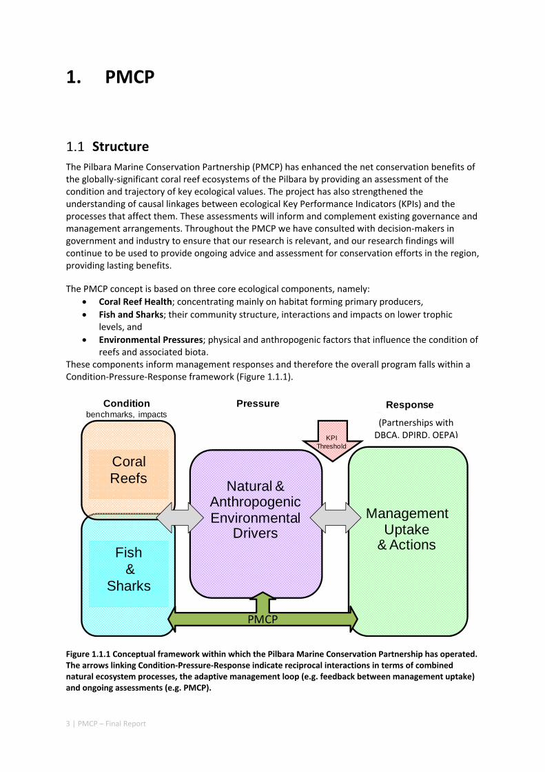
These components inform management responses and therefore the overall program falls within a Condition‐Pressure‐Response framework (Figure 1.1.1).
Figure 1.1.1 Conceptual framework within which the Pilbara Marine Conservation Partnership has operated. The arrows linking Condition‐Pressure‐Response indicate reciprocal interactions in terms of combined natural ecosystem processes, the adaptive management loop (e.g. feedback between management uptake) and ongoing assessments (e.g. PMCP).
Fish&
Sharks
Conditionbenchmarks, impacts
Response(Partnerships with DPaW, DoF, EPA)
Pressure
Natural & Anthropogenic Environmental
Drivers
Coral Reefs
Management Uptake
& Actions
PMCP
KPIThreshold
(Partnerships with DBCA, DPIRD, OEPA)

4 | PMCP – Final Report
The PMCP model was achieved through a program structure that broadly reflects the conceptual framework above (Figure 1.1.2). The Environmental Pressures Project was composed of three subcomponents, each of which had quite different logistical and conceptual approaches. These projects were therefore allocated their own budget lines in the PMCP program structure (Figure 1.1.2). The Coral Reef Health and Fish and Sharks projects also had subcomponents but these shared logistical and methodological similarities and interdependencies, as well as intimate conceptual linkages, and each was therefore encompassed within an overarching project structure. Outputs from all programs were linked through data collection, dissemination and storage activities that also facilitated external linkages (e.g. with the Department of Biodiversity, Conservation and Attractions and the Department of Primary Industries and Regional Development Fisheries Division) in the Condition‐Pressure‐Response framework.
Figure 1.1.2 PMCP program structure. Projects with separate budget lines are outlined in bold, principal project leaders (in parentheses) are indicated for each project.
5 | PMCP – Final Report
2. Synthesis
Biodiversity
2.1.1 SUMMARY
The Pilbara shelf is an important area of ecological and development significance. Activities such as offshore gas and petroleum extraction and processing, shipping and major port developments, and commercial and recreational fishing overlap with conservation areas and distributions of threatened and endangered species. The goal of the PMCP Biodiversity Project was to provide uniform, region‐wide information on habitats, biodiversity distribution and risks that can be used to help ensure these activities can coexist sustainably. While some prior data on demersal species distribution was available for the broader Pilbara region, this was mostly for fishes and some mobile invertebrates and did not include sessile invertebrates or habitats. Further, most existing information was only available for locations outside the specific shelf area of interest. Thus, there were significant spatial and taxonomical gaps for seabed habitats. While shallow water assemblages on coral reef habitats were better known, they had not been studied systematically and classified.
Between 2012 and 2015, the Pilbara Seabed Biodiversity Mapping and Characterisation Project, as part of the Pilbara Marine Conservation Program, mapped habitats and their associated biodiversity across the length and breadth of the west Pilbara shelf (0–50 m) to provide information that will help managers with regional spatial planning and management, in order that they could better ensure that human uses of the region are ecologically sustainable, as required by environmental protection legislation. Comprehensive information on the biodiversity of the seabed was acquired by visiting 125 sites, representing a wide range of known environments, during a month‐long voyage on each of two vessels and deploying several sampling devices including: towed video and digital cameras, an epibenthic sled and a research trawl to collect samples for more detailed data about plants, invertebrates and fishes on the seabed. Data from ~63 km of towed video, and from sorting and identification of 1,469 benthic samples and 382 demersal fish samples were collected and processed. The project has analysed this information and produced all of the outputs originally proposed including:
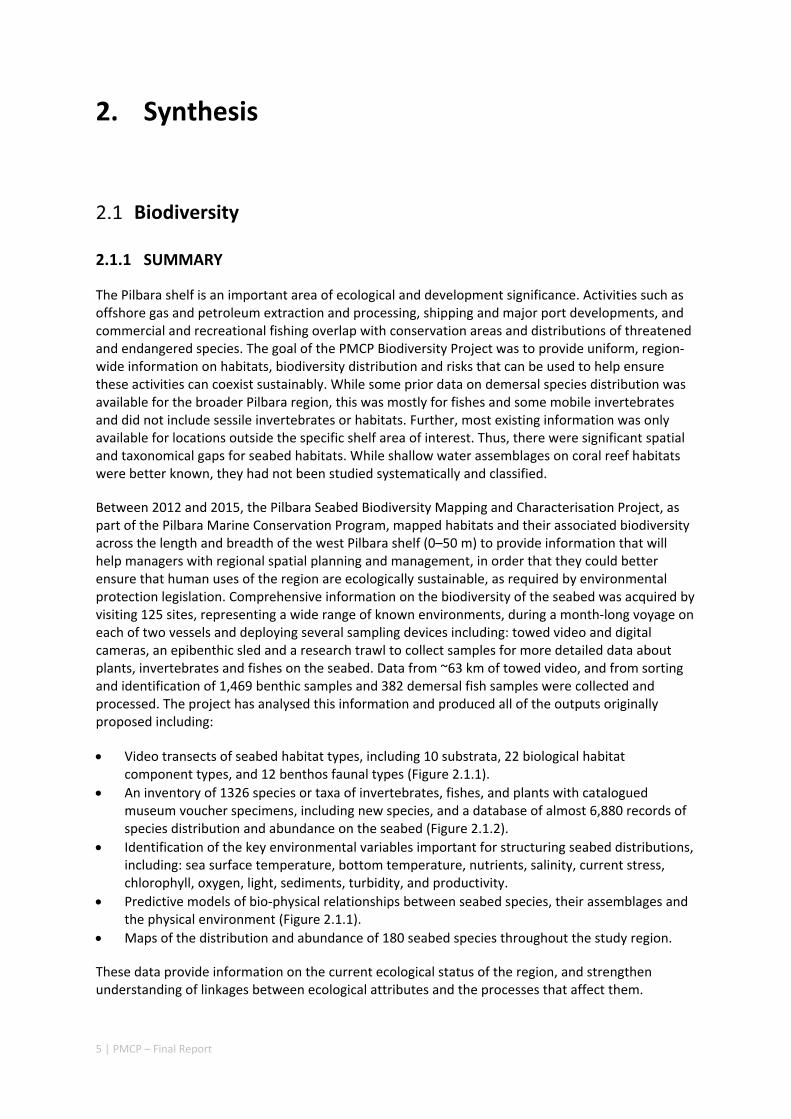
Video transects of seabed habitat types, including 10 substrata, 22 biological habitat component types, and 12 benthos faunal types (Figure 2.1.1).
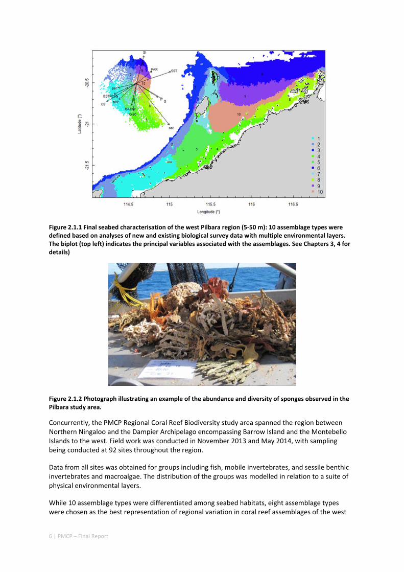
An inventory of 1326 species or taxa of invertebrates, fishes, and plants with catalogued museum voucher specimens, including new species, and a database of almost 6,880 records of species distribution and abundance on the seabed (Figure 2.1.2).
Identification of the key environmental variables important for structuring seabed distributions, including: sea surface temperature, bottom temperature, nutrients, salinity, current stress, chlorophyll, oxygen, light, sediments, turbidity, and productivity.
Predictive models of bio‐physical relationships between seabed species, their assemblages and the physical environment (Figure 2.1.1).
Maps of the distribution and abundance of 180 seabed species throughout the study region.
These data provide information on the current ecological status of the region, and strengthen understanding of linkages between ecological attributes and the processes that affect them.
6 | PMCP – Final Report
Figure 2.1.1 Final seabed characterisation of the west Pilbara region (5‐50 m): 10 assemblage types were defined based on analyses of new and existing biological survey data with multiple environmental layers. The biplot (top left) indicates the principal variables associated with the assemblages. See Chapters 3, 4 for details)
Figure 2.1.2 Photograph illustrating an example of the abundance and diversity of sponges observed in the Pilbara study area.
Concurrently, the PMCP Regional Coral Reef Biodiversity study area spanned the region between Northern Ningaloo and the Dampier Archipelago encompassing Barrow Island and the Montebello Islands to the west. Field work was conducted in November 2013 and May 2014, with sampling being conducted at 92 sites throughout the region.
Data from all sites was obtained for groups including fish, mobile invertebrates, and sessile benthic invertebrates and macroalgae. The distribution of the groups was modelled in relation to a suite of physical environmental layers.
While 10 assemblage types were differentiated among seabed habitats, eight assemblage types were chosen as the best representation of regional variation in coral reef assemblages of the west
7 | PMCP – Final Report
Pilbara. There was rough agreement in the spatial arrangement of these assemblages, with differences prominent in terms of the presence of distinct deeper water assemblages in the seafloor habitats as well as latitudinal gradients. However, a greater level of spatial differentiation in assemblages was evident in the shallow reef assemblages of the Dampier when compared to the seabed habitat types. These classifications are important in light of the likely future need to prioritise areas of the Pilbara for development or conservation (e.g. Table 2.1.1).
Existing marine management layers do not represent the full range of biological assemblages, either for seabed assemblages or for coral reefs, with under‐representation particularly notable for near‐shore areas. Established principles of Comprehensive, Adequate and Representative conservation zoning and levels of protection for marine conservation suggest that further steps should be taken to ensure adequate protection of key habitat types within the region (e.g. Table 2.1.1).
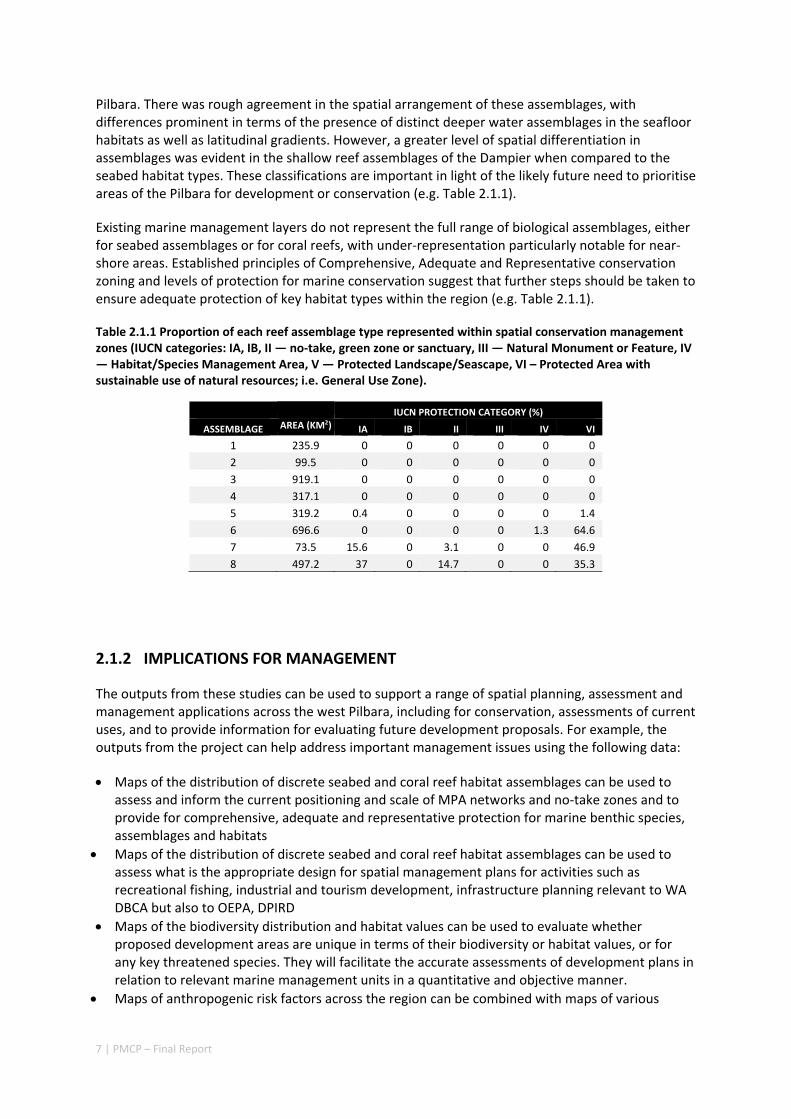
Table 2.1.1 Proportion of each reef assemblage type represented within spatial conservation management zones (IUCN categories: IA, IB, II — no‐take, green zone or sanctuary, III — Natural Monument or Feature, IV — Habitat/Species Management Area, V — Protected Landscape/Seascape, VI – Protected Area with sustainable use of natural resources; i.e. General Use Zone).
IUCN PROTECTION CATEGORY (%)
ASSEMBLAGE AREA (KM2) IA IB II III IV VI
1 235.9 0 0 0 0 0 0
2 99.5 0 0 0 0 0 0
3 919.1 0 0 0 0 0 0
4 317.1 0 0 0 0 0 0
5 319.2 0.4 0 0 0 0 1.4
6 696.6 0 0 0 0 1.3 64.6
7 73.5 15.6 0 3.1 0 0 46.9
8 497.2 37 0 14.7 0 0 35.3
2.1.2 IMPLICATIONS FOR MANAGEMENT
The outputs from these studies can be used to support a range of spatial planning, assessment and management applications across the west Pilbara, including for conservation, assessments of current uses, and to provide information for evaluating future development proposals. For example, the outputs from the project can help address important management issues using the following data:
Maps of the distribution of discrete seabed and coral reef habitat assemblages can be used to assess and inform the current positioning and scale of MPA networks and no‐take zones and to provide for comprehensive, adequate and representative protection for marine benthic species, assemblages and habitats
Maps of the distribution of discrete seabed and coral reef habitat assemblages can be used to assess what is the appropriate design for spatial management plans for activities such as recreational fishing, industrial and tourism development, infrastructure planning relevant to WA DBCA but also to OEPA, DPIRD
Maps of the biodiversity distribution and habitat values can be used to evaluate whether proposed development areas are unique in terms of their biodiversity or habitat values, or for any key threatened species. They will facilitate the accurate assessments of development plans in relation to relevant marine management units in a quantitative and objective manner.
Maps of anthropogenic risk factors across the region can be combined with maps of various

8 | PMCP – Final Report
habitats and biodiversity values, including marine parks, to facilitate systematic decision making
The project’s outputs will enable spatial analyses of the overlap of human uses with multiple levels of biodiversity (e.g. species, habitat types), permitting ecological risk assessments and, for some types of uses, fully quantitative assessments of their sustainability. The outputs will also support design of spatial aspects of monitoring in relation to biodiversity attributes and human use factors. The methods and data developed by the project can potentially be used to help predict the distribution of other regional biodiversity assets such as certain Threatened/Endangered/Protected species (e.g. dugongs), which although not directly sampled, are dependent on particular habitat types, which are incorporated in our species distribution maps.
2.1.3 KNOWLEDGE GAPS
1) The level of relative rarity of species samples in the Pilbara shelf seabed was very high, which suggests that more species, possibly many more, remain to be discovered by further sampling in the region. Furthermore, several taxonomic groups (e.g. Annelida, Brachiopoda, Bryozoa, Ascidiacea, Hydrozoa) were not identified further due to limited resources for identifications.
2) The datasets and maps developed as part of the biodiversity projects have the potential to be combined with other independent datasets, such as the distribution of TEPS (Threatened, Endangered or Protected Species) or fisheries data, to provide deeper understanding of the processes underpinning the overall distribution of species of interest.
3) The project provides a snapshot mapping of the region’s seabed biodiversity at one point in time, but we have little direct information on variability and dynamics over time. Sampling of spatio‐temporal changes will help our understanding of how the region’s seabed ecosystems may change with major environmental shifts and disturbances.
4) There are essentially no spatially explicit local or regional estimates of impact rates of human activities such as commercial or recreational fishing on either reefs or seafloor habitats. There area no estimates of seafloor biodiversity recovery rates following impacts. Gaps in these areas combine to make estimates of relative risk to natural resources difficult or virtually impossible to estimate.
9 | PMCP – Final Report
Connectivity
2.2.1 SUMMARY
The Pilbara marine environment consists of a huge diversity of habitats including coral reefs, seagrass meadows and sponge gardens. Many of these habitats have patchy distributions, and organisms must travel long distances through “hostile” conditions to reach favourable environments. Little is known about the patterns of larval connection among the major habitats in the Pilbara.
Ordinarily, this dispersal activity occurs in the first days or months of life when larvae swim or float in the water column as microscopic plankton. This phase receives a great deal of attention from scientists and environmental managers because it connects the fates of distant populations and has the potential to profoundly affect their resilience to human or natural perturbations. Yet, dispersal is extremely difficult to measure in marine environments because larvae are tiny and the ocean is vast, and also variable on multiple timescales.
Shelf circulation on the North West Shelf (NWS) of Australia is dominated by seasonal variations of the Holloway Current, forced by the monsoonal winds. The Holloway Current, with a mean annual transport rate of ~1 Sv (106 m3s‐1), is stronger during the austral autumn but is less consistent during the rest of the year. Strong inter‐annual and intra‐annual variations of sea level, ocean temperature, and alongshore currents have been previously observed along the NWS. In this project, we have also documented shorter‐term, intra‐seasonal variations of the coastal currents, which are important for the alongshore dispersal and cross‐shelf exchanges of nutrients and marine biota. Whereas the inter‐annual variability in the region is mostly forced remotely by tropical Pacific processes, the Holloway Current is stronger during a La Niña event and weaker during an El Niño event. The intra‐seasonal and semiannual signals are mostly driven by variations of regional winds off the northern coast of Australia, highlighting the role of regional weather regimes in driving processes in the NWS. The dominant intra‐annual variability of the alongshore current on the NWS are at intra‐seasonal and semiannual frequencies and are due to the excitation and propagation of coastally trapped Kelvin waves forced by Madden‐Julian Oscillations (MJO; intra‐seasonal) and semiannual wind anomalies. Therefore, the intra‐annual wind variability plays a major role in defining the highly variable state of the Holloway Current. This variability has important implications for the dispersal of coral and fish larvae.
Working with corals, we estimated networks of connectivity among coral populations on fringing coral reefs in the NWS of Australia and evaluated how this is likely to vary across the region and through time. We did so by combining four types of knowledge and technology: extensive habitat mapping, 3‐dimensional modelling of ocean currents, a particle tracking model based on shelf circulation, and an ecological model of sub‐population dynamics of corals on individual reefs.
We obtained several results of conservation significance. First, the dynamics of the ecological network results from the interplay between network connectivity and ecological processes on individual reefs: local population dynamics impose a significant non‐linearity on the role an individual reef plays within the overall dynamics of the network, and thus on the impact of conservation interventions on specific reefs. Conversely, the role an individual reef plays within these network dynamics changes considerably depending on the overall state of the system: a reef’s role in system maintenance can be different from the same reef’s role in system recovery. Local and regional ecological processes are thus inextricably interlinked. Second, patterns of network connectivity change significantly as a function of yearly shelf circulation trends, and non‐linearity in network dynamics make mean connectivity a poor representation of yearly variations. Regional
10 | PMCP – Final Report
oceanographic variability leads to both regional and local ecological variability. Finally, yearly shelf circulation trends affect the system’s potential for recovery more than system maintenance.
Our study has highlighted the importance of incorporating yearly variability when investigating dynamic systems, rather than simply investigating averages. When considering source‐sink dynamics and spatial planning, stochastic events can be important drivers of rare connectivity events rather than simply outliers. In our study system, variability in oceanic transport and its interactions with the annual lunar progression in the timing of coral mass spawning also drive dynamic patterns of ecological connectivity. Oceanographic drivers changed considerably among the years 2004‐2009, significantly affecting coral connectivity in different parts of the region, subsequently affecting the role local reefs play in overall regional coral cover. Thus, average connectivity values can overlook key components of dynamic systems. Nevertheless, we attempted to distinguish areas that would consistently make significant contributions to system maintenance and recovery. There were important areas in the south central region adjacent to Onslow, as well as in the south Barrow, Montebello and Dampier regions.
Connectivity among fish populations was also examined using spangled emperor Lethrinus nebulosus, which is an important commercial and angling species throughout north‐western Australia. Results indicate that larval connectivity is mainly on the scale of 100s of km. Furthermore, it suggests that, on these scales, larval retention averages between 22% and 30%, regardless of whether larvae are modelled as passive or with a variety of swimming behaviours. These values are similar to those derived empirically for other pelagic spawning reef fishes. Independent studies using a combination of population genetics and population modelling approaches conclude that dispersal distances ≤100 km are most likely for populations on the northwest Australian coast.
Furthermore our model has been able to reproduce, for swimming larvae, a positive relationship between oceanographic conditions (SOI) and Lethrinus sp. recruitment similar to that recently shown through field recruitment surveys at Ningaloo. We may, therefore, be reasonably confident that spatial management inferences based on our models will have significant utility. In this regard, the northern area, centred on the Dampier Archipelago stands out as having high potential conservation value as both a source and sink area, as well as having relatively high levels of larval retention.
Currently, planning of a Marine Park in the Dampier Archipelago is well advanced, although reserves are not yet declared and other areas within the region have been suggested as being of potential conservation interest. The relationship between larval dispersal and retention and population resilience in other existing marine parks at Ningaloo and the Montebello Islands is less clear and likely requires further investigation with fine scale variability and some very low recruitment areas present at these locations. There was little direct congruence in the results of the coral and fish models in terms of the likely optimal areas for protection as part of an integrated marine conservation program, although there were some general overlaps.
2.2.2 IMPLICATIONS FOR MANAGEMENT
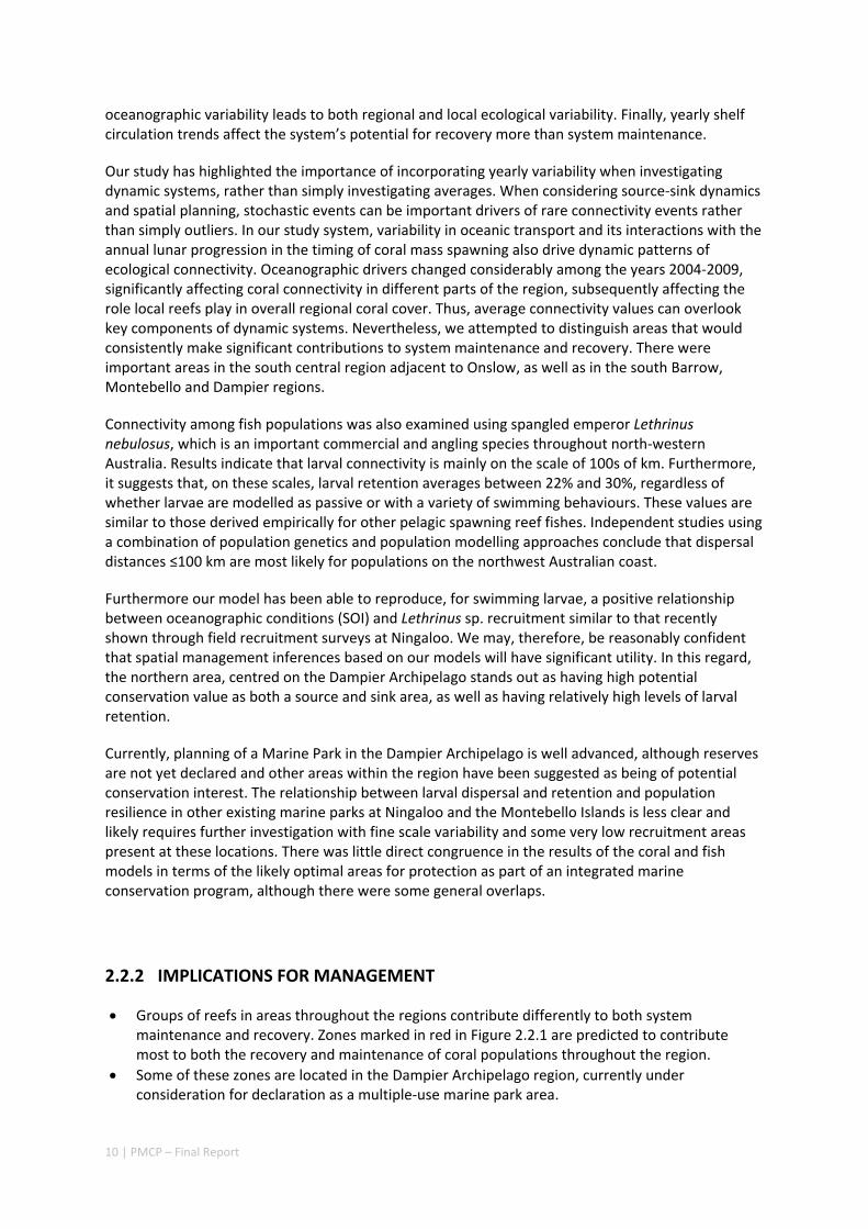
Groups of reefs in areas throughout the regions contribute differently to both system maintenance and recovery. Zones marked in red in Figure 2.2.1 are predicted to contribute most to both the recovery and maintenance of coral populations throughout the region.
Some of these zones are located in the Dampier Archipelago region, currently under consideration for declaration as a multiple‐use marine park area.

11 | PMCP – Final Report
Zones in the central part of the region also appear frequently as having both high impact on system maintenance and quick recovery for corals. Given recent coral bleaching in the Pilbara, the importance of these zones for the recovery and resilience of the overall region assumes broader importance and potentially greater urgency.
In contrast, zones marked in blue in Figure 2.2.1 appear to make relatively small contributions to system resilience so might receive lower priority for conservation measures, or higher priority as potential development sites, all other variables being equal. That said, care is needed when assessing the contribution of zones 1–3 because they are located close to the domain border.
Figure 2.2.1 Coral population network properties. Zones with high impact value and fast recovery time (red) and zones with low impact value and slower recovery time (dark blue). The eight highest and lowest ranked zones are shaded. Other ranks are in grey.
Ecological connectivity is not static: rather than thinking in terms of ‘a single’ connectivity pattern, it is important to consider the range of connectivity patterns the region may support. While this makes system prediction harder, model simulations suggest that variability in connectivity patterns lead to a much higher potential for system recovery compared to static connectivity. This may provide opportunities for flexible management approaches, which can adapt to regional climate variations.
Similarly, system resilience is not a single property, rather it represents robustness to at least three processes: i) local, relatively frequent natural and anthropogenic disturbances leading to variable local conditions, which can be balanced by larvae supplied from other areas (system maintenance); ii) occasional major and potentially catastrophic regional disturbances affecting a significant section of the region (system recovery) and iii) larger scale biophysical processes or climate change, which may lead to yearly or decadal variability in climatic and ecological regimes.
Zones which offer larger contributions to system maintenance do not necessarily have the same level of importance for system recovery or under different disturbance regimes.
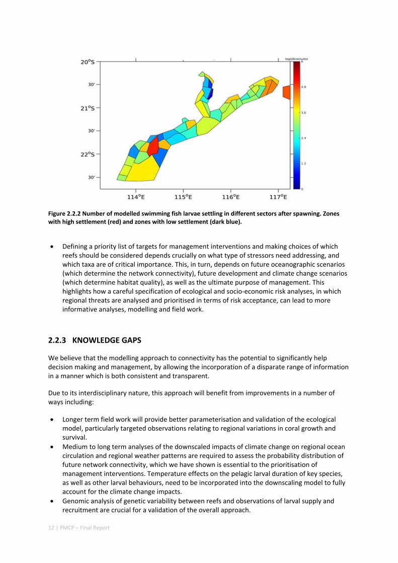
Zones which offer larger contributions to system maintenance and recovery for one taxa do not necessarily have the same level of importance for other different species (e.g. corals versus fish Figure 2.2.2).
12 | PMCP – Final Report
Figure 2.2.2 Number of modelled swimming fish larvae settling in different sectors after spawning. Zones with high settlement (red) and zones with low settlement (dark blue).
Defining a priority list of targets for management interventions and making choices of which reefs should be considered depends crucially on what type of stressors need addressing, and which taxa are of critical importance. This, in turn, depends on future oceanographic scenarios (which determine the network connectivity), future development and climate change scenarios (which determine habitat quality), as well as the ultimate purpose of management. This highlights how a careful specification of ecological and socio‐economic risk analyses, in which regional threats are analysed and prioritised in terms of risk acceptance, can lead to more informative analyses, modelling and field work.
2.2.3 KNOWLEDGE GAPS
We believe that the modelling approach to connectivity has the potential to significantly help decision making and management, by allowing the incorporation of a disparate range of information in a manner which is both consistent and transparent.
Due to its interdisciplinary nature, this approach will benefit from improvements in a number of ways including:
Longer term field work will provide better parameterisation and validation of the ecological model, particularly targeted observations relating to regional variations in coral growth and survival.
Medium to long term analyses of the downscaled impacts of climate change on regional ocean circulation and regional weather patterns are required to assess the probability distribution of future network connectivity, which we have shown is essential to the prioritisation of management interventions. Temperature effects on the pelagic larval duration of key species, as well as other larval behaviours, need to be incorporated into the downscaling model to fully account for the climate change impacts.
Genomic analysis of genetic variability between reefs and observations of larval supply and recruitment are crucial for a validation of the overall approach.

13 | PMCP – Final Report
Critically, there is a need for scientists and managers to work collaboratively to develop specific scenarios relating to anticipated regimes of impact, whether they be small or large scale, chronic or acute, as well as potential management responses, in order to accurately target future simulations for evaluation of these management strategies.
Modelling of a broader suite of organisms representing the full range of life history types present in key groups such as fishes, corals and mobile invertebrates, in order to broaden the generality of connectivity data that could be used in decision making.
14 | PMCP – Final Report
Environmental drivers
2.3.1 SUMMARY
A focus of the Environmental Drivers project was to assess and predict the processes that generate extreme conditions in the coastal ocean of the Pilbara region, particularly tropical cyclones and marine heatwaves that are known to severely impact coastal ecosystems in the region (including coral reefs). Data obtained from a combination of long term field monitoring of key physical variables (e.g. waves, water levels and temperature) across a large number of sites across the Ningaloo‐Pilbara region, as well as a number of intensive (process‐focused) field studies, were used to quantify the dominant ocean processes and variability over the study period and the responses to extreme events.
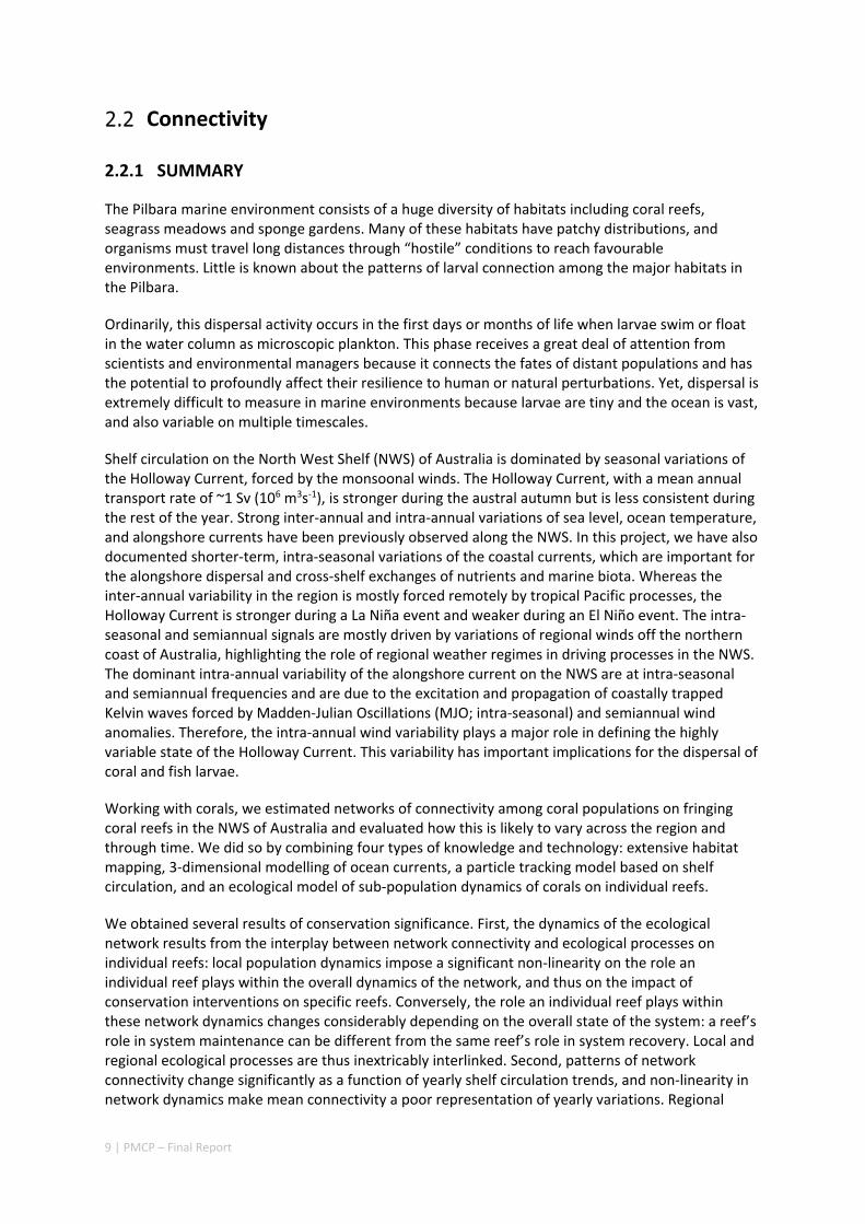
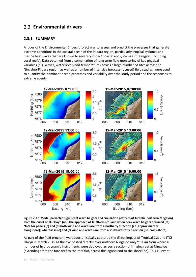
Figure 2.3.1 Model‐predicted significant wave heights and circulation patterns at Jurabbi (northern Ningaloo) from the onset of TC Olwyn (ab), the approach of TC Olwyn (cd) and when peak wave heights occurred (ef). Note for panels (c) and (d) both wind and waves are from a northerly direction (i.e. approximately alongshore); whereas in (e) and (f) wind and waves are from a south‐westerly direction (i.e. cross‐shore).
As part of the field program, we opportunistically captured the direct impact of Tropical Cyclone (TC) Olwyn in March 2015 as the eye passed directly over northern Ningaloo only ~10 km from where a number of hydrodynamic instruments were deployed across a section of fringing reef at Ningaloo (extending from the fore reef to the reef flat, across the lagoon and to the shoreline). This TC event
15 | PMCP – Final Report
not only provided insight into hydrodynamic conditions that are generated over fringing reefs in the region, but also the impacts to shoreline habitats (including understanding how effective reefs are at reducing extreme beach erosion). These insights were observed through beach topographic surveys that were conducted before and after the TC. The field observations revealed that despite the wave heights reaching 6 m and local winds reaching 140 km hr‐1, average beach volume loss in the lee of the reef was remarkably small (only ‐3 m3 m‐1).
Through the development and application of a coupled wave‐circulation model, we investigated the conditions within the reef during the TC. The model results revealed that the minimal erosion that was observed was primarily a result of locally‐generated wind waves within the lagoon, rather than the offshore waves that were primarily dissipated on the reef crest (Figure A5.2.5). Therefore, without the extreme wind conditions generated with the passage of the eye region within only 10s of kilometers from a given study site, the extreme waves generated by TCs offshore would be expected to have led to negligible coastal impacts. More broadly, when we compared these observed rates of beach erosion to observations of TC impacts along nearby exposed sandy beaches (lacking reefs), we observed one to two orders of magnitude less beach erosion in the presence of reefs. Overall, these results show a remarkable capacity for fringing reefs in the region to protect reef and shoreline habitats from TC storm damage.
Thermal stress caused by marine heatwaves in the Pilbara region can have widespread and rapid impacts to its marine ecosystem, especially on its coral reefs when mass coral bleaching events occur. Over the past decade, several marine heatwaves have occurred along Western Australia, including across the Ningaloo‐Pilbara region. In particular, two marine heatwaves linked to strong La Niña conditions (during the alternate austral summer periods of 2010/11 and 2012/13), led to the most severe bleaching that had ever been documented in the Ningaloo‐Pilbara region. Although these two heatwaves were forced by similar large‐scale climate drivers (i.e. triggered by the La Niña conditions), the warming patterns differed substantially between events. The Ningaloo region (south of ~22o S) experienced greater warming in 2010/11, whereas the Pilbara region to the north experienced greater warming in 2012/13.
Although these climate drivers establish conditions favourable for heatwaves to occur, regional ocean processes and weather processes can greatly influence the regional warming patterns (and hence coral bleaching patterns) that occur. To investigate how oceanic and atmospheric processes drove these different spatial patterns, an analysis of the ocean heat budget was conducted by integrating remote sensing observations, in situ mooring data, and a high resolution (~1 km) ocean circulation model. The results revealed substantial spatial differences in the relative contributions made by heat advection and air‐sea heat exchange between the two heatwave events. During 2010/11, anomalous warming driven by heat advection was present throughout the region, but was much stronger south of 22o S, where the poleward‐flowing Leeuwin Current tends to strengthen. During 2012/13, local air‐sea heat exchange had a positive (warming) influence on sea surface temperatures (especially in the northwest) and, when combined with the positive contribution of heat advection in the north, this can explain the regional differences in warming between these two La Niña‐associated heatwave events. The results of this study reveal that large‐scale climate status alone is not sufficient to predict the potential impacts of marine heatwaves along the Ningaloo‐Pilbara coast.
2.3.2 IMPLICATIONS FOR MANAGEMENT
Results from the field and numerical modelling studies have revealed that many of the dominant
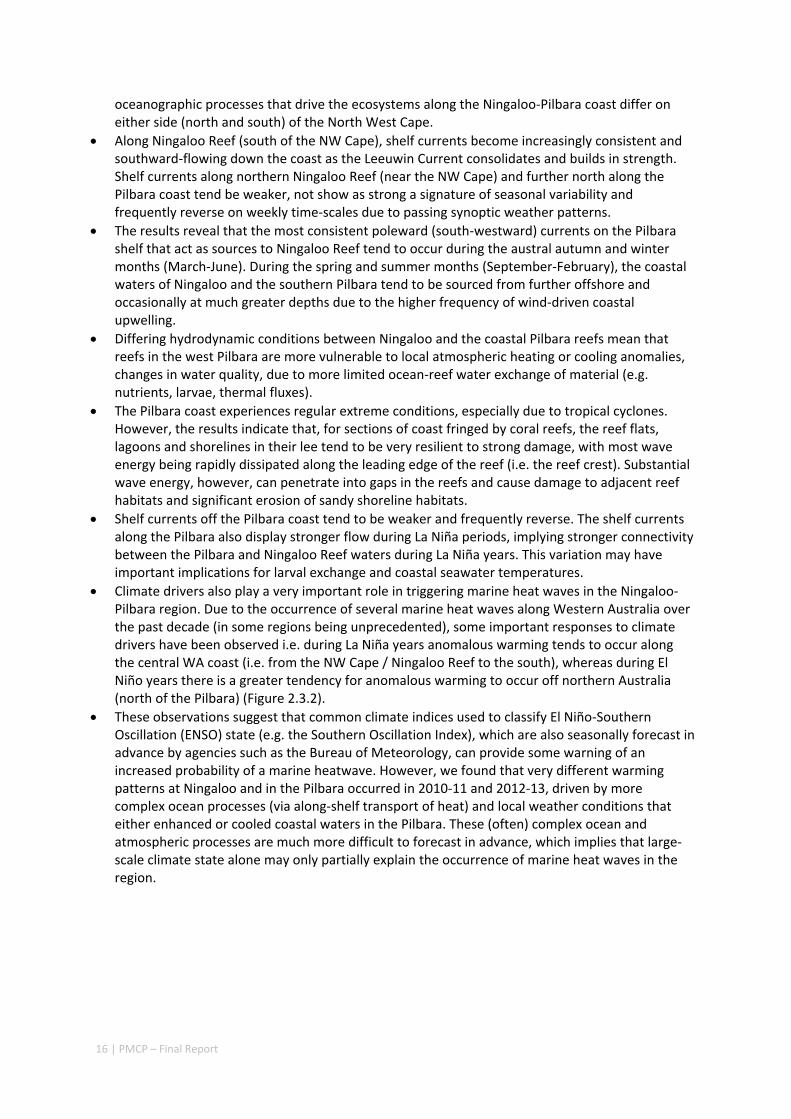
16 | PMCP – Final Report
oceanographic processes that drive the ecosystems along the Ningaloo‐Pilbara coast differ on either side (north and south) of the North West Cape.
Along Ningaloo Reef (south of the NW Cape), shelf currents become increasingly consistent and southward‐flowing down the coast as the Leeuwin Current consolidates and builds in strength. Shelf currents along northern Ningaloo Reef (near the NW Cape) and further north along the Pilbara coast tend be weaker, not show as strong a signature of seasonal variability and frequently reverse on weekly time‐scales due to passing synoptic weather patterns.
The results reveal that the most consistent poleward (south‐westward) currents on the Pilbara shelf that act as sources to Ningaloo Reef tend to occur during the austral autumn and winter months (March‐June). During the spring and summer months (September‐February), the coastal waters of Ningaloo and the southern Pilbara tend to be sourced from further offshore and occasionally at much greater depths due to the higher frequency of wind‐driven coastal upwelling.
Differing hydrodynamic conditions between Ningaloo and the coastal Pilbara reefs mean that reefs in the west Pilbara are more vulnerable to local atmospheric heating or cooling anomalies, changes in water quality, due to more limited ocean‐reef water exchange of material (e.g. nutrients, larvae, thermal fluxes).
The Pilbara coast experiences regular extreme conditions, especially due to tropical cyclones. However, the results indicate that, for sections of coast fringed by coral reefs, the reef flats, lagoons and shorelines in their lee tend to be very resilient to strong damage, with most wave energy being rapidly dissipated along the leading edge of the reef (i.e. the reef crest). Substantial wave energy, however, can penetrate into gaps in the reefs and cause damage to adjacent reef habitats and significant erosion of sandy shoreline habitats.
Shelf currents off the Pilbara coast tend to be weaker and frequently reverse. The shelf currents along the Pilbara also display stronger flow during La Niña periods, implying stronger connectivity between the Pilbara and Ningaloo Reef waters during La Niña years. This variation may have important implications for larval exchange and coastal seawater temperatures.
Climate drivers also play a very important role in triggering marine heat waves in the Ningaloo‐Pilbara region. Due to the occurrence of several marine heat waves along Western Australia over the past decade (in some regions being unprecedented), some important responses to climate drivers have been observed i.e. during La Niña years anomalous warming tends to occur along the central WA coast (i.e. from the NW Cape / Ningaloo Reef to the south), whereas during El Niño years there is a greater tendency for anomalous warming to occur off northern Australia (north of the Pilbara) (Figure 2.3.2).
These observations suggest that common climate indices used to classify El Niño‐Southern Oscillation (ENSO) state (e.g. the Southern Oscillation Index), which are also seasonally forecast in advance by agencies such as the Bureau of Meteorology, can provide some warning of an increased probability of a marine heatwave. However, we found that very different warming patterns at Ningaloo and in the Pilbara occurred in 2010‐11 and 2012‐13, driven by more complex ocean processes (via along‐shelf transport of heat) and local weather conditions that either enhanced or cooled coastal waters in the Pilbara. These (often) complex ocean and atmospheric processes are much more difficult to forecast in advance, which implies that large‐scale climate state alone may only partially explain the occurrence of marine heat waves in the region.
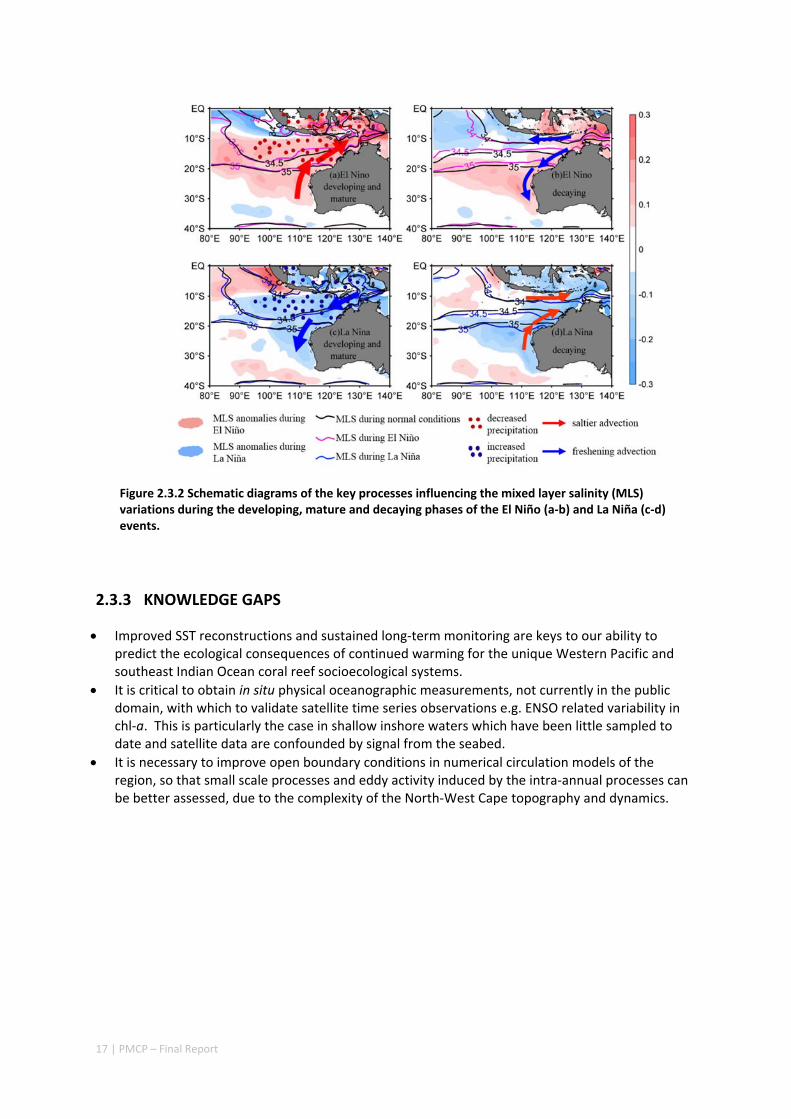
17 | PMCP – Final Report
Figure 2.3.2 Schematic diagrams of the key processes influencing the mixed layer salinity (MLS) variations during the developing, mature and decaying phases of the El Niño (a‐b) and La Niña (c‐d) events.
2.3.3 KNOWLEDGE GAPS
Improved SST reconstructions and sustained long‐term monitoring are keys to our ability to predict the ecological consequences of continued warming for the unique Western Pacific and southeast Indian Ocean coral reef socioecological systems.
It is critical to obtain in situ physical oceanographic measurements, not currently in the public domain, with which to validate satellite time series observations e.g. ENSO related variability in chl‐a. This is particularly the case in shallow inshore waters which have been little sampled to date and satellite data are confounded by signal from the seabed.
It is necessary to improve open boundary conditions in numerical circulation models of the region, so that small scale processes and eddy activity induced by the intra‐annual processes can be better assessed, due to the complexity of the North‐West Cape topography and dynamics.
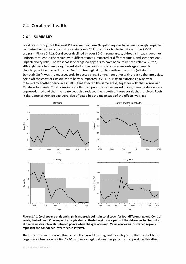
18 | PMCP – Final Report
Coral reef health
2.4.1 SUMMARY
Coral reefs throughout the west Pilbara and northern Ningaloo regions have been strongly impacted by marine heatwaves and coral bleaching since 2011, just prior to the initiation of the PMCP program (Figure 2.4.1). Coral cover declined by over 80% in some areas, although impacts were not uniform throughout the region, with different areas impacted at different times, and some regions impacted very little. The west coast of Ningaloo appears to have been influenced relatively little, although there has been a significant shift in the composition of coral assemblages towards bleaching resistant growth forms. Reefs at Bundegi, along the north‐eastern side (within the Exmouth Gulf), was the most severely impacted area. Bundegi, together with areas to the immediate north off the coast of Onslow, were heavily impacted in 2011 during an extreme La Niña year, followed by another heatwave in 2013 that affected the same areas, together with the Barrow and Montebello islands. Coral cores indicate that temperatures experienced during these heatwaves are unprecedented and that the heatwaves also reduced the growth of those corals that survived. Reefs in the Dampier Archipelago were also affected but the magnitude of the effects was less.
Dampier
Year
1985 1990 1995 2000 2005 2010 2015
Co
ver
(%)
10
20
30
40
50
60
70
Barrow and Montebello Is.
Year
2006 2008 2010 2012 2014 2016
Co
ver
(%)
0
10
20
30
40
50
60
Bundegi
Year
1990 1995 2000 2005 2010 2015
Co
ver
(%)
0
20
40
60
80
100
Ningaloo
Year
1980 1985 1990 1995 2000 2005 2010 2015
Co
ral C
ove
r (%
)
0
20
40
60
80
Figure 2.4.1 Coral cover trends and significant break points in coral cover for four different regions. Control levels; dashed lines, Change point analysis charts. Shaded regions are parts of the data expected to contain all the values for intervals between points when changes occurred. Values on y‐axis for shaded regions represent the confidence level for each interval.
The extreme climate events that caused the coral bleaching and mortality were the result of both large scale climate variability (ENSO) and more regional weather patterns that produced localised
19 | PMCP – Final Report
temperature extremes in the Pilbara in 2013. Successive warming events such as this are unmatched in the region, but climate predictions indicate that they are likely to become more common in the future. Extreme climate events can also include more intense cyclones and heavy rainfall. However, even though reefs in Ningaloo and the Pilbara have experienced several cyclones over the past five years, these appear to have had relatively minor, undetectable impacts on coral cover, either as a result of wave damage or freshwater inputs.
The ability of coral reefs to recover from episodic disturbances, such as severe coral bleaching, relies on recruitment: the settlement and growth of coral larvae from unaffected reefs. Studies of coral recruitment patterns show that connectivity models have considerable skill in predicting spatial and temporal patterns in recruitment, validating the models’ approach as a tool for management. They also suggest an additional impact of temperature stress on coral reefs as recruitment levels were depressed for up to two years after the heatwaves, even in the least affected Dampier region.
Experimental studies of the factors that influence the amount of successful coral recruitment success in the region suggest that larval density can have significant effects on the numbers of settlers, with positive feedback between settlement and initial larval density. Experiments also reveal variability in density‐dependent settlement among corals with distinct functional traits (e.g. fast versus slow growing) as well as those with similar functional forms. This positive density‐dependency may hamper recruitment on affected reefs. At the same time, field experiments have provided information on key factors such as algal cover, grazing and reef shape that affect the survival of juvenile corals and knowledge that may be useful in the near future when active restoration of reefs may be required.
Coral reef fish are key to the health of reef ecosystems and as such, were also included in the coral reef health program. We surveyed coral reef fishes inhabiting shallow reef flats in Mandu Sanctuary Zone (SZ) and adjacent Recreation Zones (RZ) in the NMP between 2007 and 2016, and simultaneously quantified the percentage cover of major benthic habitats (living hard coral, algae, non‐living substrate). There was greater density and biomass in the SZ than in the RZ in most years for emperors, wrasses, parrotfishes and surgeonfishes, but never higher density or biomass in the RZ (Figure 2.4.2). However, over the decade of surveys there was a decrease in the density and biomass of emperors, wrasses and butterflyfishes, but no evidence for a similar decrease in the density or biomass of parrotfishes, surgeonfishes and rabbitfishes. The highest rates of decline in emperor biomass occurred in the SZ (range 2–37%), but analyses indicated that there was an overall downward trend common to both SZ and RZ. The most abundant species of emperor inhabiting the reef flat, Lethrinus atkinsoni, also declined significantly in both abundance and biomass during this time. This pattern was mirrored in the large‐bodied wrasse, Coris aygula. These declines are consistent with an effect of fishing, as both species readily take baited hooks, although neither feature strongly in regional catch statistics. In contrast, observed downward trends in the abundance and biomass of butterflyfishes were most likely associated with declines in coral cover, since these fish are obligate coral feeders. There was some evidence in a decline in counts, but not biomass, of the rabbitfish Siganus nebulosus (0–50% per year), but estimates of rabbitfish abundance were very variable because of their schooling behaviour, and there was no strong evidence of overall trends for the family Siganidae.
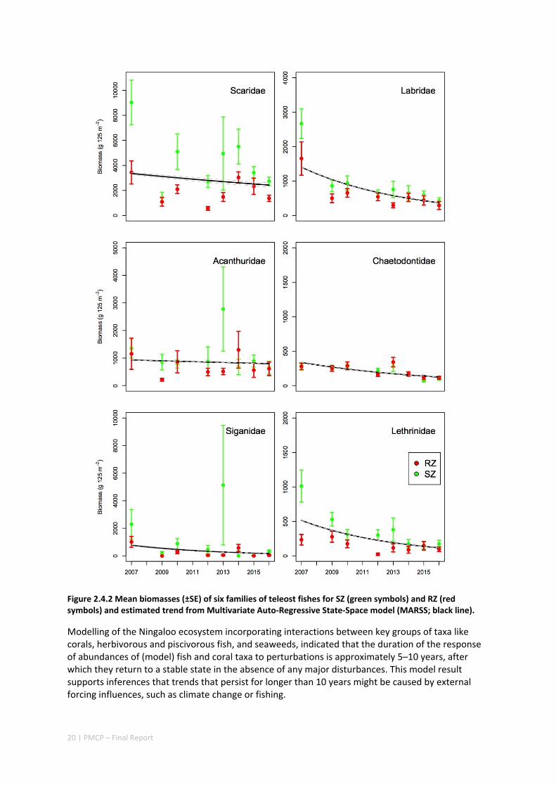
20 | PMCP – Final Report
Figure 2.4.2 Mean biomasses (±SE) of six families of teleost fishes for SZ (green symbols) and RZ (red symbols) and estimated trend from Multivariate Auto‐Regressive State‐Space model (MARSS; black line).
Modelling of the Ningaloo ecosystem incorporating interactions between key groups of taxa like corals, herbivorous and piscivorous fish, and seaweeds, indicated that the duration of the response of abundances of (model) fish and coral taxa to perturbations is approximately 5–10 years, after which they return to a stable state in the absence of any major disturbances. This model result supports inferences that trends that persist for longer than 10 years might be caused by external forcing influences, such as climate change or fishing.
21 | PMCP – Final Report
2.4.2 IMPLICATIONS FOR MANAGEMENT
Given the predicted increase in average seawater temperature due to global warming, and the likely increase in intensity and frequency of extreme climate events, there is a high likelihood that reefs in the west Pilbara and Ningaloo regions will experience more frequent bleaching and mortality events in the future. It is likely that we are already seeing the effects of this trend, with changes in the composition of coral assemblages at Ningaloo and declines in coral cover throughout the region since 2013.
At least one of these sites, Bundegi, may show impaired ability to recover, relative to previous observations. These observations are consistent with trends in other parts of the world where repeated severe bleaching impacts have led to changes in the composition of coral reef species assemblages and to the ability of coral reefs to recover from disturbance.
It is predicted that World Heritage Sites, such as Ningaloo, will experience severe bleaching twice per decade as early as 2041. While such predictions may appear pessimistic, the region immediately to the north and east has already experienced this.
The west coast of Ningaloo might be buffered from bleaching to some extent, due to favourable upwelling during summer, but the west Pilbara coastal waters do not have this advantage and may be affected even earlier by ocean warming. In this case the Pilbara may rely on larvae from Ningaloo for recolonization.
Actions need to be taken to manage and bolster system‐wide resilience of coral populations and coral reefs in the Ningaloo and west Pilbara region, which is arguably the most important coral reef province on Australia’s west coast. These actions could include modified protected area networks that are designed to incorporate optimal connectivity properties, and restoration of impacted reefs using assisted coral recruitment.
There is evidence of declining trends in fish abundance—measured as counts of individuals and biomass—inside the Mandu SZ, and in adjacent areas of Ningaloo Marine Park. Some of these declines might be caused by influences that are outside the direct control of park managers (e.g. declines in butterflyfish related to loss of coral cover caused by warming with global origins), others, such as declines in lethrinids, might be due to fishing, which is a pressure that can be managed by modified catch regulations.
Although the design of NMP follows ‘best practice’ recommendations to include a high representation of ‘no‐take’ sanctuary zones, modified management arrangements are likely needed to adequately conserve some species in order to achieve the goals outlined in NMP’s management plan. Fish species targeted by fishing may be important in controlling coral predators, such as crown‐of‐thorns starfish and Drupella snails, and competitors such as macroalgae.
2.4.3 KNOWLEDGE GAPS
Managing reefs of the Pilbara and Ningaloo into the future requires understanding both current and future threats. These threats include both growing local human use of the ecosystems, development of the coastline and climate change. Gaps in our understanding of the effects and the trajectory of how reefs will respond to these pressures include:
Extend time series in space and time to better understand variability in reef dynamics throughout the system, and to parameterise models of reef ecosystems that will enable us to better predict and evaluate potential reef futures.
More systematic and extensive in‐water environmental records (temperature, turbidity) throughout the region, in order to increase our ability to attribute changes on reefs to specific causes (i.e. bleaching or some other factors)

22 | PMCP – Final Report
Downscaled predictions of future climate in the region. These could be achieved as an extension of previous Kimberley and Ningaloo climate downscaling conducted under the Western Australian Marine Science Institution (WAMSI)
Better understanding of coral stock‐recruitment relationships, and factors that affect juvenile coral survival.
Information on cryptic fishing pressure (i.e. fishing from small vessels or from shore, which does not utilise major boat ramps, including un‐landed bycatch, such as fish used for bait).
Information on interactions between targeted and non‐targeted fish species that may help understand and predict complex indirect effects.
23 | PMCP – Final Report
Herbivory and predation
2.5.1 SUMMARY
Herbivory and predation can significantly influence coral populations and the ecology of coral reefs. Both processes can be affected by human activities so it is important to be able to evaluate their importance in order to best manage coral reef resources. Herbivory, here defined as grazing on macroalgae by fishes and invertebrates, can positively influence corals by reducing the level of competition between algae and corals. Predation can also work indirectly on corals, when the abundance of predators on coral feeders are reduced (e.g. fish that eat coral predators), or directly, as in the case of coral feeding snails (Drupella) or the crown‐of‐thorns starfish (COTS or Acanthaster).
In terms of herbivory, the abundance of important grazers such as fish can be influenced by environmental gradients in turbidity and sedimentation, which often decrease further from shore. In the Dampier Archipelago, we found no simple inshore‐offshore patterns in grazing rates on Sargassum marginatum, but there was an interaction between inshore‐offshore location, season (April versus October) and the standing crop of algae (high or low). Consumption was around three times higher in April at offshore sites with low biomass than any other time or location. These sites had high numbers of herbivorous fish, but herbivore abundance was not a good predictor of grazing rates. While there were seasonal patterns in phenolic composition and nitrogen content of algae, we observed no differences in the chemical composition of algae between inshore and offshore sites that could explain the patterns in grazing. A cross‐shelf transplant experiment also suggested that the origin of the algal fronds (inshore versus offshore) did not impact rates of consumption by herbivores.
Growth of three species of Sargassum measured alongside the grazing experiments at Dampier Archipelago showed high variability among fronds resulting in no significant spatial or temporal trends and no measurable differences among species. For the majority of sites, top‐down control of Sargassum by grazers (rates of herbivory) is likely to equal or exceed the growth of macroalgae in both seasons. There will, however, be sites and times with non‐existent grazing when macroalgal biomass can accumulate and bottom‐up forces, such as nutrient availability and light, control net growth of Sargassum. In contrast, in early autumn (April) when we observed localised heavy grazing offshore, consumption of macroalgae greatly exceeded our estimated rates of macroalgal growth. This indicates that there are times and locations when top‐down control may overwhelm growth rates of Sargassum. The Dampier Archipelago likely experiences seasonal shifts in the conditions that regulate both bottom‐up and top‐down controls, but these drivers are currently poorly understood in the area.
Direct predation on corals has become an important factor on some reefs in the region, particularly at the Montebello and Barrow Islands, where outbreak levels of COTS have been present on reefs since at least 2009 and are widespread around the eastern sides of the islands. In 2014, we recorded densities as high as 320 ±58.3 COTS ha‐1 in the region. The region was subjected to anomalously high water temperatures during the summers of 2012 and 2013, which resulted in the mortality of almost 70% of the live coral. We hypothesise that the observed high densities of COTS are the result of the starfish aggregating in response to a depleted food resource, rather than an intensification of the existing outbreak. Nevertheless, given that the coral cover has been reduced so substantially, the high densities of COTS still represent a significant threat to the recovery of the coral communities of the region, particularly since the COTS prefer to feed on coral taxa such as Acropora that are also most vulnerable to bleaching. Thus, the outbreak will exacerbate change in the composition of coral assemblages in the region. This change may be irreversible given that many of the corals now being
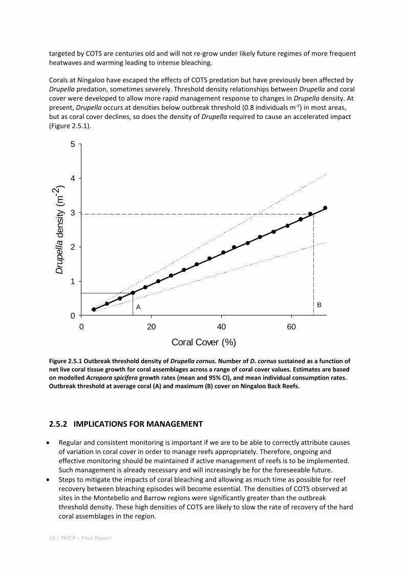
24 | PMCP – Final Report
targeted by COTS are centuries old and will not re‐grow under likely future regimes of more frequent heatwaves and warming leading to intense bleaching.
Corals at Ningaloo have escaped the effects of COTS predation but have previously been affected by Drupella predation, sometimes severely. Threshold density relationships between Drupella and coral cover were developed to allow more rapid management response to changes in Drupella density. At present, Drupella occurs at densities below outbreak threshold (0.8 individuals m‐2) in most areas, but as coral cover declines, so does the density of Drupella required to cause an accelerated impact (Figure 2.5.1).
Figure 2.5.1 Outbreak threshold density of Drupella cornus. Number of D. cornus sustained as a function of net live coral tissue growth for coral assemblages across a range of coral cover values. Estimates are based on modelled Acropora spicifera growth rates (mean and 95% CI), and mean individual consumption rates. Outbreak threshold at average coral (A) and maximum (B) cover on Ningaloo Back Reefs.
2.5.2 IMPLICATIONS FOR MANAGEMENT
Regular and consistent monitoring is important if we are to be able to correctly attribute causes of variation in coral cover in order to manage reefs appropriately. Therefore, ongoing and effective monitoring should be maintained if active management of reefs is to be implemented. Such management is already necessary and will increasingly be for the foreseeable future.
Steps to mitigate the impacts of coral bleaching and allowing as much time as possible for reef recovery between bleaching episodes will become essential. The densities of COTS observed at sites in the Montebello and Barrow regions were significantly greater than the outbreak threshold density. These high densities of COTS are likely to slow the rate of recovery of the hard coral assemblages in the region.
Coral Cover (%)
0 20 40 60
Dru
pella
den
sity
(m
-2)
0
1
2
3
4
5
A B
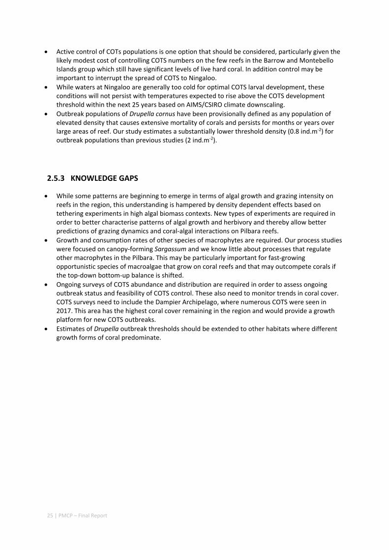
25 | PMCP – Final Report
Active control of COTs populations is one option that should be considered, particularly given the likely modest cost of controlling COTS numbers on the few reefs in the Barrow and Montebello Islands group which still have significant levels of live hard coral. In addition control may be important to interrupt the spread of COTS to Ningaloo.
While waters at Ningaloo are generally too cold for optimal COTS larval development, these conditions will not persist with temperatures expected to rise above the COTS development threshold within the next 25 years based on AIMS/CSIRO climate downscaling.
Outbreak populations of Drupella cornus have been provisionally defined as any population of elevated density that causes extensive mortality of corals and persists for months or years over large areas of reef. Our study estimates a substantially lower threshold density (0.8 ind.m‐2) for outbreak populations than previous studies (2 ind.m‐2).
2.5.3 KNOWLEDGE GAPS
While some patterns are beginning to emerge in terms of algal growth and grazing intensity on reefs in the region, this understanding is hampered by density dependent effects based on tethering experiments in high algal biomass contexts. New types of experiments are required in order to better characterise patterns of algal growth and herbivory and thereby allow better predictions of grazing dynamics and coral‐algal interactions on Pilbara reefs.
Growth and consumption rates of other species of macrophytes are required. Our process studies were focused on canopy‐forming Sargassum and we know little about processes that regulate other macrophytes in the Pilbara. This may be particularly important for fast‐growing opportunistic species of macroalgae that grow on coral reefs and that may outcompete corals if the top‐down bottom‐up balance is shifted.
Ongoing surveys of COTS abundance and distribution are required in order to assess ongoing outbreak status and feasibility of COTS control. These also need to monitor trends in coral cover. COTS surveys need to include the Dampier Archipelago, where numerous COTS were seen in 2017. This area has the highest coral cover remaining in the region and would provide a growth platform for new COTS outbreaks.
Estimates of Drupella outbreak thresholds should be extended to other habitats where different growth forms of coral predominate.
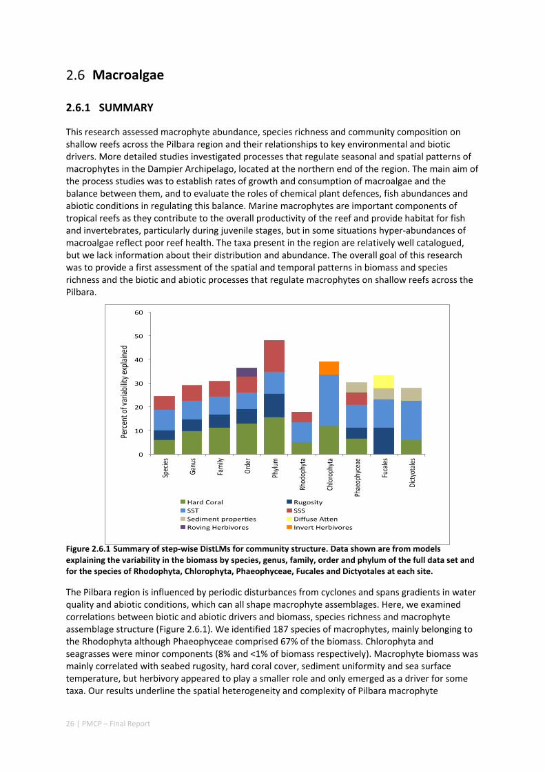
26 | PMCP – Final Report
Macroalgae
2.6.1 SUMMARY
This research assessed macrophyte abundance, species richness and community composition on shallow reefs across the Pilbara region and their relationships to key environmental and biotic drivers. More detailed studies investigated processes that regulate seasonal and spatial patterns of macrophytes in the Dampier Archipelago, located at the northern end of the region. The main aim of the process studies was to establish rates of growth and consumption of macroalgae and the balance between them, and to evaluate the roles of chemical plant defences, fish abundances and abiotic conditions in regulating this balance. Marine macrophytes are important components of tropical reefs as they contribute to the overall productivity of the reef and provide habitat for fish and invertebrates, particularly during juvenile stages, but in some situations hyper‐abundances of macroalgae reflect poor reef health. The taxa present in the region are relatively well catalogued, but we lack information about their distribution and abundance. The overall goal of this research was to provide a first assessment of the spatial and temporal patterns in biomass and species richness and the biotic and abiotic processes that regulate macrophytes on shallow reefs across the Pilbara.
Figure 2.6.1 Summary of step‐wise DistLMs for community structure. Data shown are from models explaining the variability in the biomass by species, genus, family, order and phylum of the full data set and for the species of Rhodophyta, Chlorophyta, Phaeophyceae, Fucales and Dictyotales at each site.
The Pilbara region is influenced by periodic disturbances from cyclones and spans gradients in water quality and abiotic conditions, which can all shape macrophyte assemblages. Here, we examined correlations between biotic and abiotic drivers and biomass, species richness and macrophyte assemblage structure (Figure 2.6.1). We identified 187 species of macrophytes, mainly belonging to the Rhodophyta although Phaeophyceae comprised 67% of the biomass. Chlorophyta and seagrasses were minor components (8% and <1% of biomass respectively). Macrophyte biomass was mainly correlated with seabed rugosity, hard coral cover, sediment uniformity and sea surface temperature, but herbivory appeared to play a smaller role and only emerged as a driver for some taxa. Our results underline the spatial heterogeneity and complexity of Pilbara macrophyte
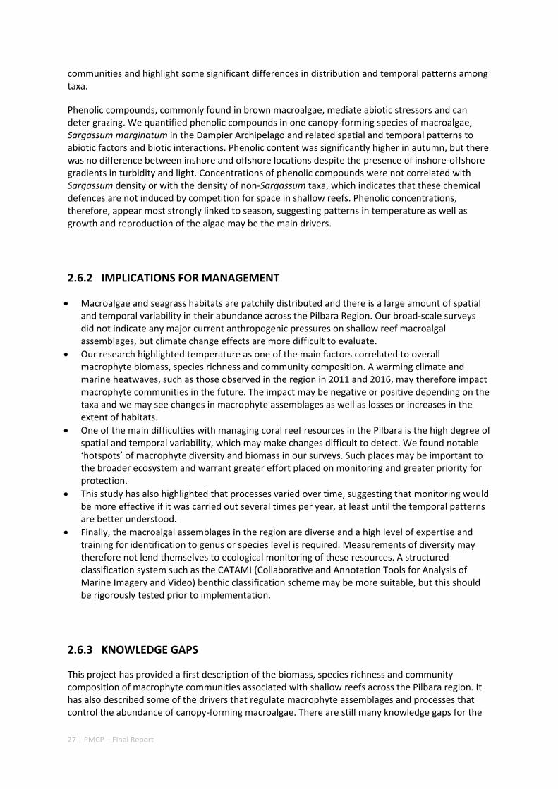
27 | PMCP – Final Report
communities and highlight some significant differences in distribution and temporal patterns among taxa.
Phenolic compounds, commonly found in brown macroalgae, mediate abiotic stressors and can deter grazing. We quantified phenolic compounds in one canopy‐forming species of macroalgae, Sargassum marginatum in the Dampier Archipelago and related spatial and temporal patterns to abiotic factors and biotic interactions. Phenolic content was significantly higher in autumn, but there was no difference between inshore and offshore locations despite the presence of inshore‐offshore gradients in turbidity and light. Concentrations of phenolic compounds were not correlated with Sargassum density or with the density of non‐Sargassum taxa, which indicates that these chemical defences are not induced by competition for space in shallow reefs. Phenolic concentrations, therefore, appear most strongly linked to season, suggesting patterns in temperature as well as growth and reproduction of the algae may be the main drivers.
2.6.2 IMPLICATIONS FOR MANAGEMENT
Macroalgae and seagrass habitats are patchily distributed and there is a large amount of spatial and temporal variability in their abundance across the Pilbara Region. Our broad‐scale surveys did not indicate any major current anthropogenic pressures on shallow reef macroalgal assemblages, but climate change effects are more difficult to evaluate.
Our research highlighted temperature as one of the main factors correlated to overall macrophyte biomass, species richness and community composition. A warming climate and marine heatwaves, such as those observed in the region in 2011 and 2016, may therefore impact macrophyte communities in the future. The impact may be negative or positive depending on the taxa and we may see changes in macrophyte assemblages as well as losses or increases in the extent of habitats.
One of the main difficulties with managing coral reef resources in the Pilbara is the high degree of spatial and temporal variability, which may make changes difficult to detect. We found notable ‘hotspots’ of macrophyte diversity and biomass in our surveys. Such places may be important to the broader ecosystem and warrant greater effort placed on monitoring and greater priority for protection.
This study has also highlighted that processes varied over time, suggesting that monitoring would be more effective if it was carried out several times per year, at least until the temporal patterns are better understood.
Finally, the macroalgal assemblages in the region are diverse and a high level of expertise and training for identification to genus or species level is required. Measurements of diversity may therefore not lend themselves to ecological monitoring of these resources. A structured classification system such as the CATAMI (Collaborative and Annotation Tools for Analysis of Marine Imagery and Video) benthic classification scheme may be more suitable, but this should be rigorously tested prior to implementation.
2.6.3 KNOWLEDGE GAPS
This project has provided a first description of the biomass, species richness and community composition of macrophyte communities associated with shallow reefs across the Pilbara region. It has also described some of the drivers that regulate macrophyte assemblages and processes that control the abundance of canopy‐forming macroalgae. There are still many knowledge gaps for the

28 | PMCP – Final Report
region and key among those are:
Long‐term baseline: Studies elsewhere have shown dramatic changes to macrophyte communities in response to external pressures, e.g. warming and heat waves. We do not have a clear understanding of longer‐term trends in producer communities in the Pilbara, which would be necessary to detect responses to climate change. Long‐term baseline data would also allow for assessment of human impacts on shallow reef systems e.g. effects of turbidity on macrophytes including interactions between nutrient enrichment and light limitation.
Detailed seasonal patterns at representative reefs: Evidence for gradients in biomass, species richness and community composition were weak, contrasting somewhat with the results of surveys conducted through the Biodiversity Theme. This is probably due to high levels of spatial variability on small scales and the fact that we did not return to exactly the same locations in both seasons.
Growth and consumption of other species of macrophytes: Our process studies were focused on canopy‐forming Sargassum and we know little about processes that regulate other macrophytes in the Pilbara. This may be particularly important for fast‐growing opportunistic species of macroalgae that grow on coral reefs and that may outcompete corals if the top‐down bottom‐up balance is shifted.
Macrophytes on sandy habitats and deeper reefs: Our work was restricted to shallow reef areas, but macrophytes may be important components of other habitats in the region. Seagrasses are known to form extensive (although sometimes sparse) meadows in both shallow sandy lagoons and in deeper sandy areas. These habitats may be of great importance to marine fauna such as dugongs that feed on seagrasses. The extent of and temporal patterns of these communities are not well documented across the Pilbara.
The role of different macrophytes as food and shelter: Studies at Ningaloo have demonstrated an important role of inshore macroalgae as nursery areas for juvenile fish. Rates of grazing at some places are also high. However, the region‐wide importance of macrophytes (macroalgae and seagrass) as food and shelter is poorly known. Given that macrophytes are likely to support iconic threatened and protected species, like sea turtles and dugongs, this should be a high priority.

29 | PMCP – Final Report
Fish and sharks
2.7.1 SUMMARY
The Pilbara region hosts fish and shark assemblages characterised by high diversity and economically important, but low productivity, fisheries. Historically, the deeper waters (>30 m) of the Pilbara were heavily exploited by foreign and domestic trawl fleets from the 1970’s to late 1990’s, which resulted in the destruction of well‐developed epibenthic habitat dominated by sponges and gorgonians and large decreases in catches of high value snappers, emperors and groupers. Mineral and petrochemical exploitation of the Pilbara commenced in earnest in the 1960’s but have increased since the 1990’s resulting in rapid coastal development at multiple locations throughout the region. This development has the potential to directly impact the biodiversity and productivity of vulnerable nearshore ecosystems via dredging, construction, pollution, shipping and other indirect pressures associated with increased human populations (e.g. fishing). In addition, to the south of the region the Ningaloo Marine Park is a popular destination for both extractive and non‐extractive recreational activities. Management is challenged with finding a balance between the economic benefits of non‐renewables, sustainable development of both recreational and commercial fisheries, sustainable use for non‐extractive recreation, and maintenance of biodiversity and ecosystem services. Knowledge of the patterns and processes that support the productivity and biodiversity of these nearshore marine ecosystems is therefore essential for informing management decisions.
Figure 2.7.1 Distance‐based redundancy (dbRDA) bubble plot illustrating the DISTLM model based on individual Lethrinus punctulatus size classes and the fitted environmental variables with their vector. The length and direction of vectors indicates the direction and strength of these relationships, respectively. Relative abundance of each species is shown by the size of bubbles.
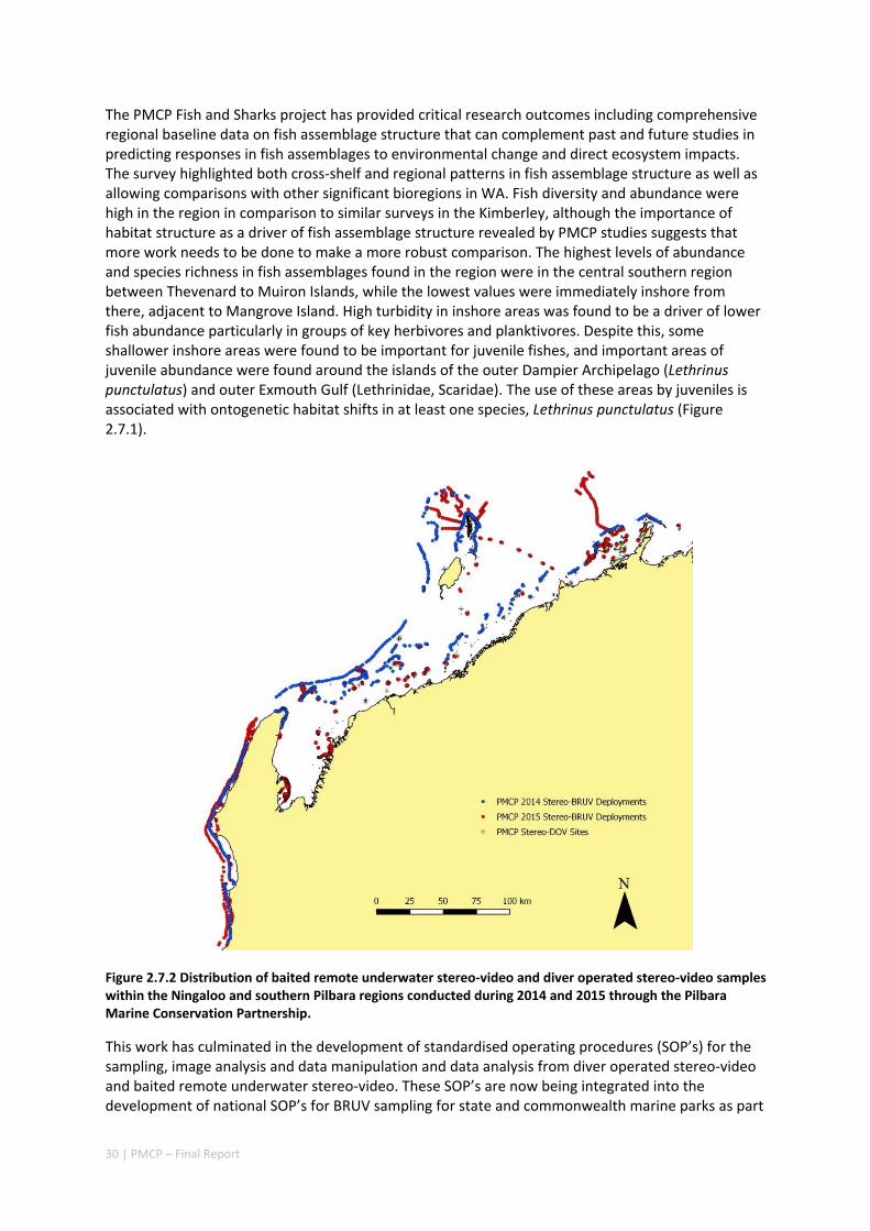
30 | PMCP – Final Report
The PMCP Fish and Sharks project has provided critical research outcomes including comprehensive regional baseline data on fish assemblage structure that can complement past and future studies in predicting responses in fish assemblages to environmental change and direct ecosystem impacts. The survey highlighted both cross‐shelf and regional patterns in fish assemblage structure as well as allowing comparisons with other significant bioregions in WA. Fish diversity and abundance were high in the region in comparison to similar surveys in the Kimberley, although the importance of habitat structure as a driver of fish assemblage structure revealed by PMCP studies suggests that more work needs to be done to make a more robust comparison. The highest levels of abundance and species richness in fish assemblages found in the region were in the central southern region between Thevenard to Muiron Islands, while the lowest values were immediately inshore from there, adjacent to Mangrove Island. High turbidity in inshore areas was found to be a driver of lower fish abundance particularly in groups of key herbivores and planktivores. Despite this, some shallower inshore areas were found to be important for juvenile fishes, and important areas of juvenile abundance were found around the islands of the outer Dampier Archipelago (Lethrinus punctulatus) and outer Exmouth Gulf (Lethrinidae, Scaridae). The use of these areas by juveniles is associated with ontogenetic habitat shifts in at least one species, Lethrinus punctulatus (Figure 2.7.1).
Figure 2.7.2 Distribution of baited remote underwater stereo‐video and diver operated stereo‐video samples within the Ningaloo and southern Pilbara regions conducted during 2014 and 2015 through the Pilbara Marine Conservation Partnership.
This work has culminated in the development of standardised operating procedures (SOP’s) for the sampling, image analysis and data manipulation and data analysis from diver operated stereo‐video and baited remote underwater stereo‐video. These SOP’s are now being integrated into the development of national SOP’s for BRUV sampling for state and commonwealth marine parks as part
31 | PMCP – Final Report
of the National Environmental Science Program. A data synthesis tool (globalarchive.org) has also been developed to enable comparison of the state and condition of fish assemblages in the Pilbara with those around Australia and internationally and is now being supported nationally by IMOS and the NECTAR Cloud facilities.The project completed 2912 baited remote underwater stereo‐video surveys, 558 diver‐operated stereo‐video transects, 574 underwater visual census transects in depths of between 1 and 60 m between Coral Bay and the Dampier Archipelago (Figure 2.7.2).
Assessments of the impacts of fishing were an important part of the project. Boat ramp interviews showed that fishing indirectly affected target species through depredation by sharks, where between 7 and 14% of teleost fishes hooked are taken by sharks. These fish are not reported in standard catch statistics thus the impacts of fishing are likely to be systematically under‐reported. Comparison of composition, abundance, size‐structure and biomass of fishes in areas open and closed to fishing showed that levels of abundance for the locally important target species Lethrinus nebulosus were approximately three times higher in no‐take areas than outside them, with fish also larger inside protected areas.
The importance of survey methodology and technology was highlighted by studies of MPA effectiveness, which showed that while Baited Remote Underwater Video (BRUV) was effective in demonstrating the difference between fished and unfished areas, Diver Operated Video (DOV) was not. The utility of a range of video approaches for quantifying habitat characteristics, and the use of this data in understanding patterns in the distribution and abundance of fish was also validated, with the potential to add significant value to future studies by improving cost effectiveness in data collection.
2.7.2 IMPLICATIONS FOR MANAGEMENT
In the Pilbara and Ningaloo regions, conservation and fisheries management is challenged with finding a balance between a broad range of extractive and non‐extractive uses. These pressures arise from i) the historical growth in both coastal population and infrastructure development for mineral and petrochemical industries, ii) the associated recreational fishing activities in the region iii) the pressure for the sustained use by the commercial fishing industry, including trawling, traps and longline based fisheries. Implications for management include:
The Fish and Sharks project has been able to collect and formulate useful benchmarks on the condition of fish assemblages with respect to environmental gradients across the region. The highest levels of abundance and species richness in fish assemblages found in the region were in the central southern region between Thevenard to Muiron Islands.
Some shallower inshore areas were found to be important for juvenile fish, and important areas of juvenile abundance were found around the islands of the outer Dampier Archipelago (Lethrinus punctulatus) and outer Exmouth Gulf (Lethrinidae, Scaridae). The use of these areas by juveniles is associated with ontogenetic habitat shifts in at least one species, Lethrinus punctulatus. These areas should be considered in management decisions such as development or conservation.
This study demonstrated a negative relationship between species richness, and abundance of key functional groups and suspended sediment in the fish assemblage of the nearshore Pilbara region, adjacent to development activities at Onslow.
In collaboration with the Department of Biodiversity, Conservation and Attractions, studies of the status of fish assemblages inside and outside no‐take areas within the Ningaloo Marine Park have

32 | PMCP – Final Report
provided useful information that could be used to evaluate whether management zoning provides adequate monitoring on the condition of fish assemblages.
Shark depredation may add between 7 and 14% additional mortality to reported catches, which should be accounted for in future management.
2.7.3 KNOWLEDGE GAPS
There are no data on the trends in abundance and biomass of fish populations outside Marine Parks and other areas in the Ningaloo and west Pilbara regions. It is particularly important to understand these trends in areas close to population centres, where there may be a focus of fishing activity, or where major infrastructure is located such as around oil and gas production infrastructure.
Spatially explicit data on fishing pressure, that match the scales of ecological observation from monitoring and sampling programs, are lacking. Although very detailed studies have previously been conducted at scales within the Ningaloo Marine Park this information does not exist for the Pilbara region as a whole and due to the variable nature of recreational fishing pressure the existing data sets within the Ningaloo Marine Park do not directly match up with the scales of ecological observation from monitoring and sampling programs.
Evaluation is needed of the adequacy of existing or proposed monitoring programs to detect likely changes due to changes in environmental variables or pressure gradients using a formal statistical power analysis for the monitoring of fish assemblages in existing marine parks.
To effectively manage the impact of anthropogenic activities that elevate suspended sediment levels (such as dredging), local exposure thresholds for both intensity and duration of suspended sediment elevation must be identified for key functional groups.
Data collection methods, whether employed for quantifying fishes or benthos, need to be fit for purpose but this will require the effective cross‐calibration of methods in order to enable the effective formulation and testing of hypotheses across environmental settings and projects.

33 | PMCP – Final Report
Part II Environmental Pressures
34 | PMCP – Final Report
3. Biodiversity
Regional Biodiversity — Pilbara Seabed Biodiversity Mapping & Characterisation
Authors: Pitcher CR, Miller M, Morello B, Fry G, Strzelecki J, McLeod I, Slawinski D, Ellis N, Thomson D, Bearham D, Keesing J, Donovan A, Babcock R, Mortimer N. — CSIRO Oceans & Atmosphere
Fromont J, Gomez O, Hosie A, Hara A, Moore G, Morrison S, Kirkendale L, Whisson C, Richards Z, Bryce M, Marsh L — Western Australian Museum
Naughton K, O’Loughlin M, O’Hara T — Museum Victoria
Boddington D — Western Australian Fisheries
Huisman J — Murdoch University
ABSTRACT
Between 2012 and 2015, the Pilbara Seabed Biodiversity Mapping & Characterisation Project, as part of the Pilbara Marine Conservation Program, mapped habitats and their associated biodiversity across the length and breadth of the west Pilbara shelf (0–50 m) to provide information that will help managers with regional planning and management, and to help ensure that human uses of the region are ecologically sustainable, as required by environmental protection legislation. Comprehensive information on the biodiversity of the seabed was acquired by visiting 125 sites, representing a wide range of known environments, during a ~month‐long voyage on each of two vessels and deploying several types of sampling devices including: towed video and digital cameras, an epibenthic sled and a research trawl to collect samples for more detailed data about plants, invertebrates and fishes on the seabed. Data were collected and processed from ~63 km of towed video, and from sorting and identification of 1,469 benthic samples and 382 demersal fish samples. The project has analysed this information and produced all of the outputs as originally proposed; these included:
• Video transects of seabed habitat types, including 10 substratum, 22 biological habitat component types, and 12 benthos faunal types
• An inventory of 1326 species or taxa of invertebrates, fishes, and plants with catalogued museum voucher specimens, including new species, and a database of almost 6,880 records of species distribution and abundance on the seabed.
• Identification of the key environmental variables important for structuring seabed distributions, and predictive models of bio‐physical relationships between seabed species, their assemblages and the physical environment.
• Maps of the distribution and abundance of 180 seabed species throughout the study region.

35 | PMCP – Final Report
These data provide information on the current ecological status of the region, and strengthen understanding of linkages between ecological attributes and the processes that affect them. The outputs from this study can be used to support a range of spatial planning, assessment and management applications across the west Pilbara, including for conservation, assessments of current uses, and to provide information for evaluating future development proposals — thus providing lasting benefits.

36 | PMCP – Final Report
3.1.1 INTRODUCTION
Planning, assessment and management of the marine environment requires an essential base level of understanding about the distribution of habitats and biodiversity. It is also critical for developing an effective sampling program for Key Performance Indicators (KPIs). Habitat is a key determinant of population structure and having a stratified sampling regime is vital to obtaining precise estimates of population parameters and properly identifying drivers of biological response. Consequently, the initial phase of the project included a component to compile all relevant existing available information relating to biodiversity and habitat variation in the region. Since the sea is a dynamic and three‐dimensional environment, habitat descriptions included benthic mapping, and key water column properties related to fish and biotic health, linking to satellite data for ground‐truthing. In order to plan the biodiversity sampling program we therefore capitalised on existing holdings of national scale environmental and biodiversity data sets, acquired additional regional datasets, and analysed these data to provide an initial regional characterisation and stratification prior to any fieldwork.
The regional seabed biodiversity study area spanned the region between Northern Ningaloo and the Dampier Archipelago encompassing Barrow Island and the Montebello Islands west to depths of approximately 50 m. In addition to video transects and photographs, extractive sampling using an epibenthic sled and a research trawl was planned in order to provide detailed biodiversity assessments rather than simple descriptions of coarse habitat types. The first year of the project collated and analysed existing available data to provide the preliminary characterisation of the region and stratification for the sampling design. Sampling was designed to representatively sample all known important environmental‐driver gradients in the region and to ensure that areas for which there were low levels of data or poor ability to accurately predict habitat and biodiversity would be sampled. Field work was conducted at the end of the first year of the project in order to inform sampling in other PMCP programs, but detailed processing of samples, analysis and reporting continued into subsequent years.
A primary determinant of the nature and complexity of ecological interactions is the composition and diversity of ecological communities. Accordingly we aimed to acquire information on regional biodiversity and habitat structure for the purposes of planning, assessment and management, as well as for use in the design of other ongoing sampling in the PMCP Coral Reef Health and Fish and Sharks projects. The Biodiversity and Habitat Project’s goal was to provide a region wide characterisation of biodiversity and habitat patterns as its key objective.
The key specific objectives are:
1. Acquire available existing data, conduct an initial biophysical characterisation of the west Pilbara region, including initial identification of environmental drivers, and produce a preliminary bioregional map for survey design and for departmental purposes.
2. Survey and sample spatial patterns of biodiversity of benthic ecosystems across the entire west Pilbara region, using towed video transects, an epibenthic sled and a research trawl.
3. From survey data, characterise biodiversity of the west Pilbara region including identification of key environmental drivers of biodiversity patterns, and produce a final bioregional map to inform the design of future ecological sampling program and for departmental planning and management purposes.
37 | PMCP – Final Report
3.1.2 METHODS
Environmental datasets
The environmental data layers collated and used for the biophysical analysis and mapping of biodiversity included:
Bathymetry DEM: depth, slope, aspect — the model bathymetry is based on several sources. The data set uses the Geoscience Australia (GA) GA2009 250m bathymetric product as a background. The WA state’s official coastline (mean tide) was used to define 0 depth and islands. Commercial partners provided bathymetric data based upon LiDAR/LADS surveys and CSIRO and GA provided surveys based on acoustic systems. AHO and WA DPI provided historical soundings. These were integrated and processed in swath mapper processing software by Gordon Keith into a 0.01 degree gridded product.
Sediment: gravel, sand, mud, carbonate — sediment properties where derived from dbSEABED (http://instaar.colorado.edu/~jenkinsc/dbseabed/, Chris Jenkins) gridded at 0.01°.
Seabed current stress — Data sourced from the CSIRO RIBBON Model (http://www.emg.cmar.csiro.au/www/en/emg/projects/‐Ribbon‐‐Model.html ).
Bottom water attributes (annual average and seasonal range): temperature, salinity, oxygen, nitrate, phosphate, silicate — Data sourced from the CSIRO Atlas of Regional Seas (CARS) (http://www.marine.csiro.au/~dunn/cars2009/ )
NASA Ocean colour (SeaWiFS & MODIS): chlorophyll, light attenuation, SST, surface PAR — satellite derived datasets were processed by IMOS (Edward King), gridded at 0.01°.
Derived variables: benthic irradiance, primary productivity, exported POC — calculated from ocean colour variables using published algorithms.
Terrain morphology probabilities: ridge, channel, peak, depression, pass, plane — generated from bathymetric data by Vanessa Lucieer, University of Tasmania.
Human use layers: fishing (e.g. trawl effort), mining, infrastructure, spatial management — datasets provided by WA DPIRD and DBCA.
See Appendix 1 for descriptions of environmental variables used in project analyses, and see Appendix 2 for maps of each variable.
Initial characterisation & stratification
To achieve the initial regional scale characterisation, existing benthic biodiversity data from locations well distributed across the study area were acquired and used to integrate with environmental data and analyse relationships between species distributions and their environment. Additional biological data were collated from past CSIRO trawl surveys, WA Fisheries surveys and WA DEC reefs surveys with seven datasets available in total (see Appendix 3). An integrative analysis method, ‘gradientForest’ (Ellis et al 2012, Pitcher et al 2012), was used to obtain evidence‐based relationships between species compositional change and multiple environmental gradients that were then used to transform all environmental layers to the same ‘biological’ scale. These transformed layer were mapped to provide an initial characterisation, which was also the basis for the most biologically relevant stratification for regional scale benthic sampling completed in mid–2013.
Field sampling
Previous studies have demonstrated that different sampling gears largely sample different species and different assemblage patterns, generating different species compositions & spatial patterns and confirming that data from multiple devices must be combined in order to comprehensively describe

38 | PMCP – Final Report
the biodiversity of an area (e.g. Pitcher et al. 2002 & 2007). For example the assemblage data generated from video alone is much less similar to benchmark datasets (all three gears combined) than either trawl or sled data alone. This stems from the different selectivity of sampling devices as well as the considerable difficulty in identifying and quantifying organisms from video as well as the limited observability resulting from variable visibility and camera movement in rough sea conditions.
To ensure the sampling of the benthic biodiversity of the Pilbara region was as comprehensive as possible, this study deployed a variety of sampling gears including towed underwater video, a 1.5 m epibenthic sled and an ~8‐fathom research trawl. The biodiversity mapping voyages in the Pilbara were conducted in June 2013 on the research vessels RV Naturaliste (Western Australia Fisheries; trawl and sled sampling) and RV Linneaus (CSIRO Oceans & Atmosphere; video transects and some sled sampling).
Sorting & identification of samples
Initial Operational Taxonomic Unit (OTU) level sorting of the new samples collected by the June 2013 Pilbara seabed biodiversity sampling trip was carried out by CSIRO staff at Floreat (WA). Following this initial sorting, most specimens were sent to expert staff at the Western Australian Museum (WAM) with CSIRO staff providing assistance — or for some groups, to the Museum of Victoria, and marine plants to the WA Herbarium. At these laboratories, detailed identification of specimens was completed as well as collation and storage of voucher samples and description of new species. As previously advised, the sponges were particularly abundant and diverse, and completion of identifications for sponges required more time than expected, delaying final analyses. All data were transferred to a secure Oracle database at CSIRO and checked.
Analyses of new sample data
Data arising directly from the June 2013 field survey were mapped. These comprised (i) habitat data recorded during towed video camera transects, and (ii) biomass data of the major sorting groups of fishes and benthos derived from primary sorting of trawl and sled samples on vessels at sea.
After species sorting and identification of the new sled and trawl samples was completed, basic biodiversity indices were examined and species richness was modelled and mapped. Selected individual species (those sufficiently frequently occurring for analysis, and with successful prediction models) were also modelled and mapped. Univariate modelling was conducted using Random Forests (Breiman 2001), a bootstrapped tree‐based method recognised for its prediction modelling power.
The initial regional scale characterisation was updated by integrating the new sled and trawl sample data in a combining analysis with the data previously collated from other sources. Relationships between species distributions and their environment were again analysed using ‘gradientForest’, to provide a final biophysical characterisation and map of patterns of biodiversity composition for the region.
3.1.3 RESULTS
Initial characterisation & stratification
The relationships between species distributions in existing datasets and their environment, as determined by the gradientForest analysis are shown in Figure 3.1.1. These indicate the cumulative
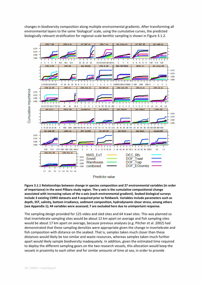
39 | PMCP – Final Report
changes in biodiversity composition along multiple environmental gradients. After transforming all environmental layers to the same ‘biological’ scale, using the cumulative curves, the predicted biologically relevant stratification for regional scale benthic sampling is shown in Figure 3.1.2.
Figure 3.1.1 Relationships between change in species composition and 37 environmental variables (in order of importance) in the west Pilbara study region. The y‐axis is the cumulative compositional change associated with increasing values of the x‐axis (each environmental gradient). Seabed biological surveys include 3 existing CSIRO datasets and 4 acquired prior to fieldwork. Variables include parameters such as depth, SST, salinity, bottom irradiance, sediment composition, hydrodynamic shear stress, among others (see Appendix 1); 44 variables were assessed; 7 are excluded here due to unimportant response.
The sampling design provided for 125 video and sled sites and 64 trawl sites. This was planned so that invertebrate sampling sites would be about 12 km apart on average and fish sampling sites would be about 17 km apart on average, because previous analyses (e.g. Pitcher et al. 2002) had demonstrated that these sampling densities were appropriate given the change in invertebrate and fish composition with distance on the seabed. That is, samples taken much closer than these distances would likely be too similar and waste resources, whereas samples taken much further apart would likely sample biodiversity inadequately. In addition, given the estimated time required to deploy the different sampling gears on the two research vessels, this allocation would keep the vessels in proximity to each other and for similar amounts of time at sea, in order to provide
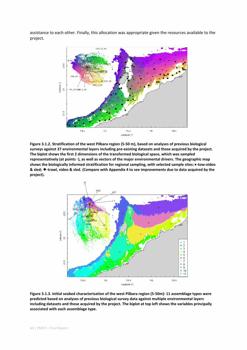
40 | PMCP – Final Report
assistance to each other. Finally, this allocation was appropriate given the resources available to the project.
Figure 3.1.2. Stratification of the west Pilbara region (5‐50 m), based on analyses of previous biological surveys against 37 environmental layers including pre‐existing datasets and those acquired by the project. The biplot shows the first 2 dimensions of the transformed biological space, which was sampled representatively (at points ◦), as well as vectors of the major environmental drivers. The geographic map
shows the biologically informed stratification for regional sampling, with selected sample sites: ‐tow‐video & sled; ‐trawl, video & sled. (Compare with Appendix 4 to see improvements due to data acquired by the project).
Figure 3.1.3. Initial seabed characterisation of the west Pilbara region (5‐50m): 11 assemblage types were predicted based on analyses of previous biological survey data against multiple environmental layers including datasets and those acquired by the project. The biplot at top left shows the variables principally associated with each assemblage type.

41 | PMCP – Final Report
A key initial output from the project was a map of the initial characterisation. Preliminary analyses of the existing biological survey data suggested that approximately 11 clusters were statistically justifiable for management purposes. These represent predicted biological assemblages at ~1 km resolution (with ~1‐10 km utility, at full regional extent ~18,700s sq kms, see Figure 3.1.3). The expectation is that assemblage composition would differ from cluster to cluster corresponding to distance apart in the biplot — some assemblages are more heterogeneous than others (e.g. in Figure 3.1.3, clusters 3 and 7 are each more heterogeneous than clusters 2 and 6 together).
Field sampling
The seabed biodiversity sampling voyages in the Pilbara were successfully completed in June 2013, using the research vessels RV Naturaliste (WA Fisheries) and RV Linneaus (CSIRO). In total, 125 sites were sampled with towed‐video and digital stills for seabed habitat, 111 sites with an epibenthic sled for sessile and mobile invertebrates and 43 with a research trawl net for fishes and mobile invertebrates. A number of sites were unsuitable for sampling by sled and/or trawl. Many sled and trawl samples were dominated by a large abundance and diversity of sponges (e.g. see Figure 3.1.4).
Figure 3.1.4 Photograph illustrating an example of the abundance and diversity of sponges observed in the Pilbara study area.
The biomass, by taxonomic group, sampled during the voyages is shown in Figure 3.1.5 and Figure 3.1.6, for benthic sled and trawl respectively. Overall, sponges dominated the sled samples — and fish dominated the trawl samples. The substratum types observed during video transects are shown in Figure 3.1.7 indicating that sand dominates the sampled area and most seabed reef areas were found around Barrow Island and the Montebello Islands. The biological habitat types observed during video transects are shown in Figure 3.1.8 indicating macro‐vegetated habitats in the vicinity of Barrow Island, and either gorgonian or sponge dominated habitats (or a mixture) scattered through much of the region; however, much of the seabed was bare of biological habitat, or bioturbated towards the NE.
Sorting & identification of samples
The samples collected showed high diversity of all groups examined in detail, noting that several groups (e.g. Annelida, Brachiopoda, Bryozoa, Ascidiacea, Hydrozoa) were not identified further in the laboratory due to resource constraints. Table 3.1.1 summarises the results of sorting of benthic sled and demersal trawl samples from the June 2013 trip. The diversity of the sponge communities was particularly high — and this required significantly more time for identifications. Data from
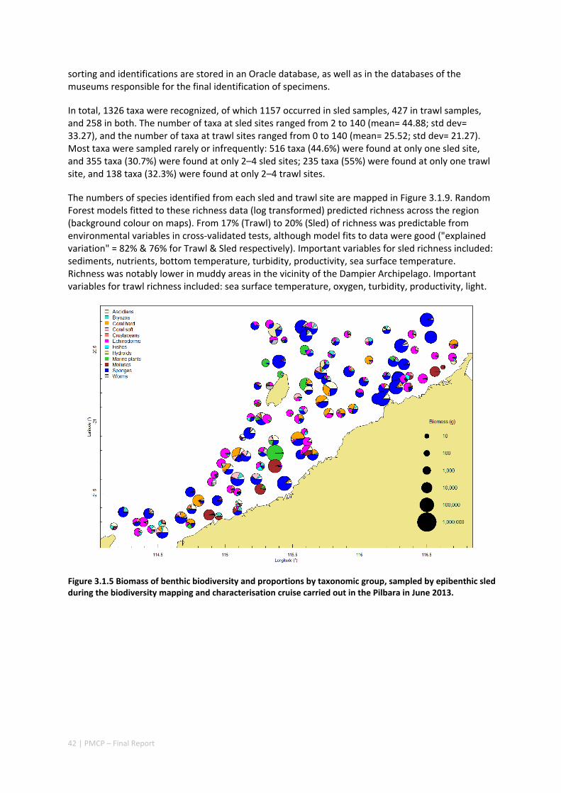
42 | PMCP – Final Report
sorting and identifications are stored in an Oracle database, as well as in the databases of the museums responsible for the final identification of specimens.
In total, 1326 taxa were recognized, of which 1157 occurred in sled samples, 427 in trawl samples, and 258 in both. The number of taxa at sled sites ranged from 2 to 140 (mean= 44.88; std dev= 33.27), and the number of taxa at trawl sites ranged from 0 to 140 (mean= 25.52; std dev= 21.27). Most taxa were sampled rarely or infrequently: 516 taxa (44.6%) were found at only one sled site, and 355 taxa (30.7%) were found at only 2–4 sled sites; 235 taxa (55%) were found at only one trawl site, and 138 taxa (32.3%) were found at only 2–4 trawl sites.
The numbers of species identified from each sled and trawl site are mapped in Figure 3.1.9. Random Forest models fitted to these richness data (log transformed) predicted richness across the region (background colour on maps). From 17% (Trawl) to 20% (Sled) of richness was predictable from environmental variables in cross‐validated tests, although model fits to data were good ("explained variation" = 82% & 76% for Trawl & Sled respectively). Important variables for sled richness included: sediments, nutrients, bottom temperature, turbidity, productivity, sea surface temperature. Richness was notably lower in muddy areas in the vicinity of the Dampier Archipelago. Important variables for trawl richness included: sea surface temperature, oxygen, turbidity, productivity, light.
Figure 3.1.5 Biomass of benthic biodiversity and proportions by taxonomic group, sampled by epibenthic sled during the biodiversity mapping and characterisation cruise carried out in the Pilbara in June 2013.
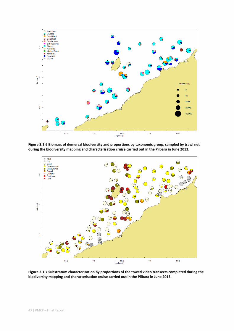
43 | PMCP – Final Report
Figure 3.1.6 Biomass of demersal biodiversity and proportions by taxonomic group, sampled by trawl net during the biodiversity mapping and characterisation cruise carried out in the Pilbara in June 2013.
Figure 3.1.7 Substratum characterisation by proportions of the towed video transects completed during the biodiversity mapping and characterisation cruise carried out in the Pilbara in June 2013.
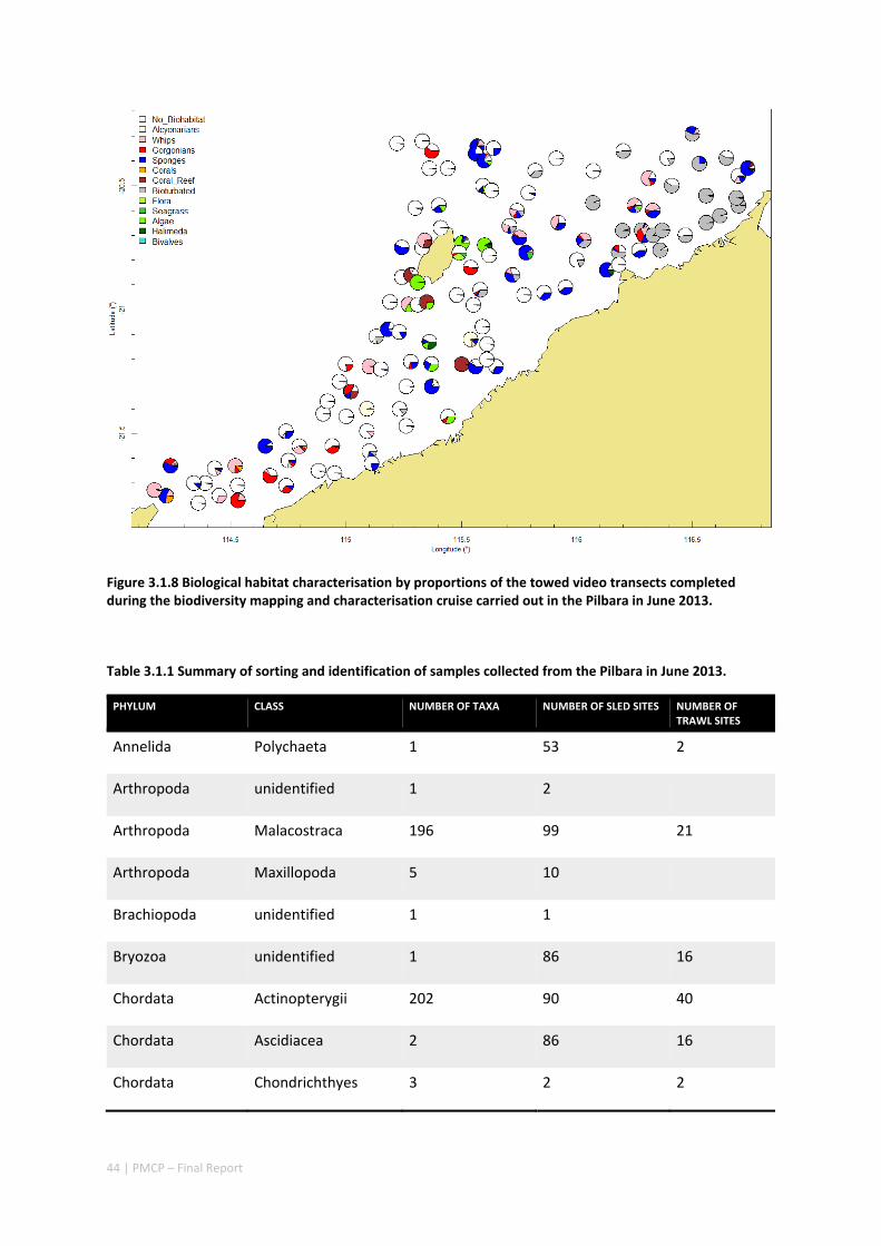
44 | PMCP – Final Report
Figure 3.1.8 Biological habitat characterisation by proportions of the towed video transects completed during the biodiversity mapping and characterisation cruise carried out in the Pilbara in June 2013.
Table 3.1.1 Summary of sorting and identification of samples collected from the Pilbara in June 2013.
PHYLUM CLASS NUMBER OF TAXA NUMBER OF SLED SITES NUMBER OF TRAWL SITES
Annelida Polychaeta 1 53 2
Arthropoda unidentified 1 2
Arthropoda Malacostraca 196 99 21
Arthropoda Maxillopoda 5 10
Brachiopoda unidentified 1 1
Bryozoa unidentified 1 86 16
Chordata Actinopterygii 202 90 40
Chordata Ascidiacea 2 86 16
Chordata Chondrichthyes 3 2 2
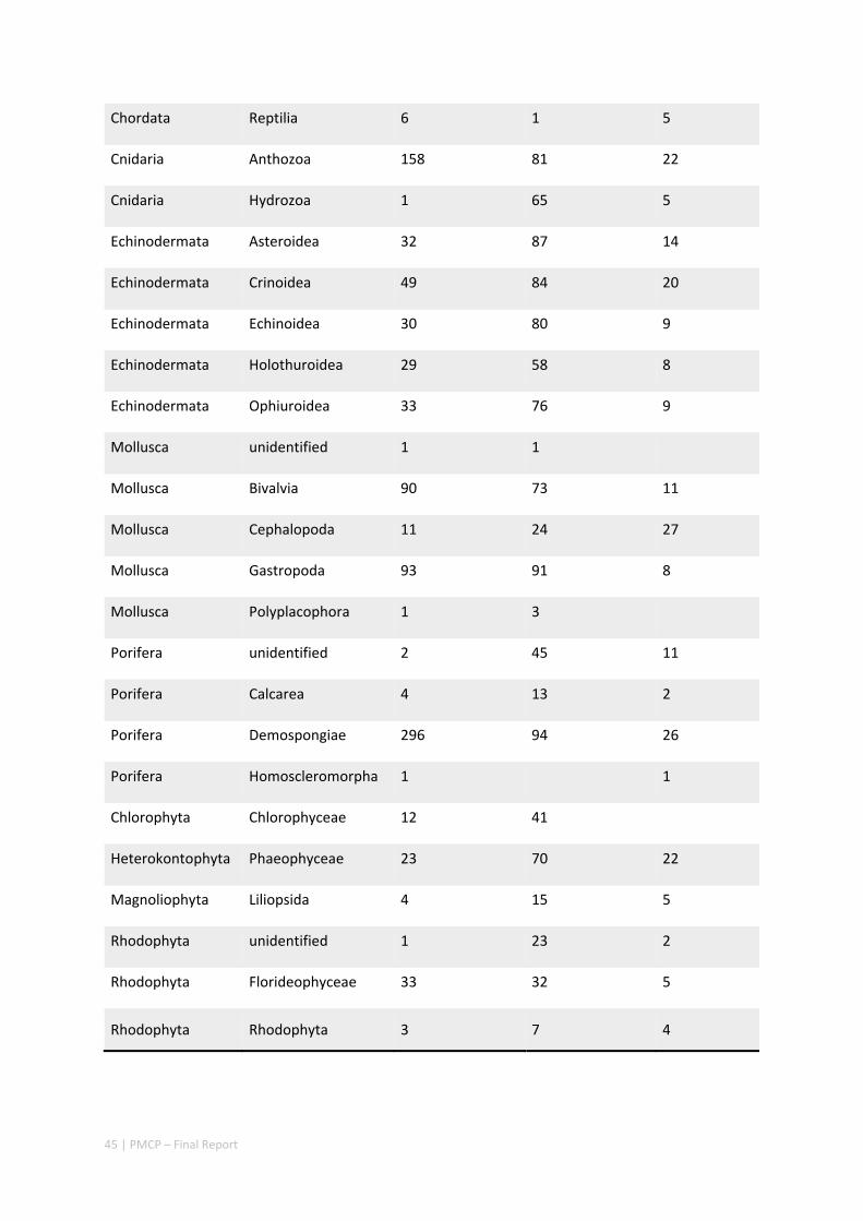
45 | PMCP – Final Report
Chordata Reptilia 6 1 5
Cnidaria Anthozoa 158 81 22
Cnidaria Hydrozoa 1 65 5
Echinodermata Asteroidea 32 87 14
Echinodermata Crinoidea 49 84 20
Echinodermata Echinoidea 30 80 9
Echinodermata Holothuroidea 29 58 8
Echinodermata Ophiuroidea 33 76 9
Mollusca unidentified 1 1
Mollusca Bivalvia 90 73 11
Mollusca Cephalopoda 11 24 27
Mollusca Gastropoda 93 91 8
Mollusca Polyplacophora 1 3
Porifera unidentified 2 45 11
Porifera Calcarea 4 13 2
Porifera Demospongiae 296 94 26
Porifera Homoscleromorpha 1 1
Chlorophyta Chlorophyceae 12 41
Heterokontophyta Phaeophyceae 23 70 22
Magnoliophyta Liliopsida 4 15 5
Rhodophyta unidentified 1 23 2
Rhodophyta Florideophyceae 33 32 5
Rhodophyta Rhodophyta 3 7 4
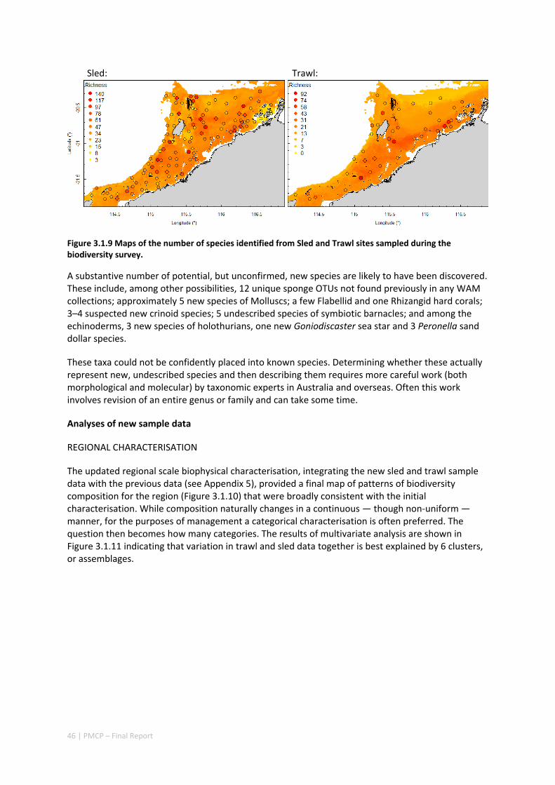
46 | PMCP – Final Report
Sled: Trawl:
Figure 3.1.9 Maps of the number of species identified from Sled and Trawl sites sampled during the biodiversity survey.
A substantive number of potential, but unconfirmed, new species are likely to have been discovered. These include, among other possibilities, 12 unique sponge OTUs not found previously in any WAM collections; approximately 5 new species of Molluscs; a few Flabellid and one Rhizangid hard corals; 3–4 suspected new crinoid species; 5 undescribed species of symbiotic barnacles; and among the echinoderms, 3 new species of holothurians, one new Goniodiscaster sea star and 3 Peronella sand dollar species.
These taxa could not be confidently placed into known species. Determining whether these actually represent new, undescribed species and then describing them requires more careful work (both morphological and molecular) by taxonomic experts in Australia and overseas. Often this work involves revision of an entire genus or family and can take some time.
Analyses of new sample data
REGIONAL CHARACTERISATION
The updated regional scale biophysical characterisation, integrating the new sled and trawl sample data with the previous data (see Appendix 5), provided a final map of patterns of biodiversity composition for the region (Figure 3.1.10) that were broadly consistent with the initial characterisation. While composition naturally changes in a continuous — though non‐uniform — manner, for the purposes of management a categorical characterisation is often preferred. The question then becomes how many categories. The results of multivariate analysis are shown in Figure 3.1.11 indicating that variation in trawl and sled data together is best explained by 6 clusters, or assemblages.
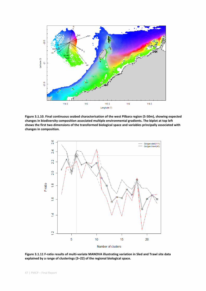
47 | PMCP – Final Report
Figure 3.1.10. Final continuous seabed characterisation of the west Pilbara region (5‐50m), showing expected changes in biodiversity composition associated multiple environmental gradients. The biplot at top left shows the first two dimensions of the transformed biological space and variables principally associated with changes in composition.
Figure 3.1.11 F‐ratio results of multi‐variate MANOVA illustrating variation in Sled and Trawl site data explained by a range of clusterings (3–22) of the regional biological space.
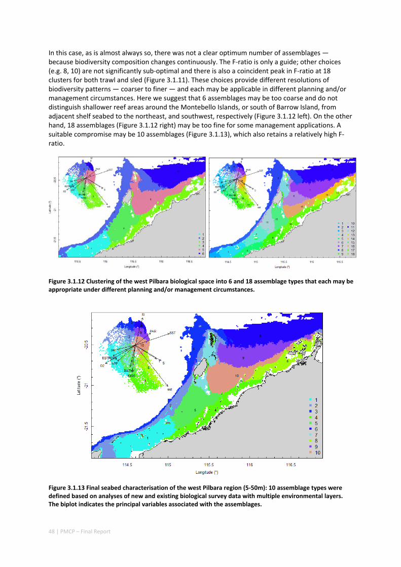
48 | PMCP – Final Report
In this case, as is almost always so, there was not a clear optimum number of assemblages — because biodiversity composition changes continuously. The F‐ratio is only a guide; other choices (e.g. 8, 10) are not significantly sub‐optimal and there is also a coincident peak in F‐ratio at 18 clusters for both trawl and sled (Figure 3.1.11). These choices provide different resolutions of biodiversity patterns — coarser to finer — and each may be applicable in different planning and/or management circumstances. Here we suggest that 6 assemblages may be too coarse and do not distinguish shallower reef areas around the Montebello Islands, or south of Barrow Island, from adjacent shelf seabed to the northeast, and southwest, respectively (Figure 3.1.12 left). On the other hand, 18 assemblages (Figure 3.1.12 right) may be too fine for some management applications. A suitable compromise may be 10 assemblages (Figure 3.1.13), which also retains a relatively high F‐ratio.
Figure 3.1.12 Clustering of the west Pilbara biological space into 6 and 18 assemblage types that each may be appropriate under different planning and/or management circumstances.
Figure 3.1.13 Final seabed characterisation of the west Pilbara region (5‐50m): 10 assemblage types were defined based on analyses of new and existing biological survey data with multiple environmental layers. The biplot indicates the principal variables associated with the assemblages.

49 | PMCP – Final Report
The important variables associated with compositional patterns in the combined trawl and sled data included: sea surface temperature, bottom temperature, nutrients, salinity, current stress, chlorophyll, oxygen, light, sediments, turbidity, and productivity.
The composition of each assemblage is described in relative terms as follows, with reference to Figure 3.1.13, Figure 3.1.14, Figure 3.1.15 and Appendix 6 (environmental variables, sled and trawl composition).
Figure 3.1.14 Boxplot summaries of biotic habitat components observed by towed‐video, for each Assemblage in the west Pilbara study region. The box indicates the first and third quartiles and the horizontal bar indicates the median value; the whiskers indicate the ‘normal’ range of the data and small circles indicate outlying values.
Figure 3.1.15 Boxplot summaries of richness and biomass, sampled by the sled and the trawl, for each Assemblage in the west Pilbara study region. The box indicates the first and third quartiles and the horizontal bar indicates the median value; the whiskers indicate the ‘normal’ range of the data and small circles indicate outlying values.

50 | PMCP – Final Report
Assemblage 1: is moderately shallow (Depth: 3.9–16.2 m) with low average sea surface temperature (SST: 25.5–26.1°C), moderately low seabed temperature (24.1–25.3°C) with narrow seasonal range (4.6–5.7°C), moderately low salinity (35.1–35.4‰), high oxygen (4.77–4.82 mL L⁻¹) with moderately narrow seasonal range (0.4–0.48 mL L⁻¹), moderately high seabed stress (0.4–1.9e⁻⁴ Nm⁻²), moderately low slope (0–0.4°), moderately high light attenuation (K490: 0.11–0.29 m⁻¹) with moderately wide seasonal range (0.03–0.1 m⁻¹), moderately high net primary production (NPP) (VGPM: 1249–1471 mg C m⁻² d⁻¹), moderately high gravel (2.4–82.6 %), moderately low sand (5.7–96.5 %) and low mud (0–24.9 %). Other variables had about median range.
The habitat was typically bare seabed interspersed with moderately high cover of gorgonians (0–67.3%) and whips (0–46%), median cover of sponges (0–9%), low corals (0–8.1%) and ~no cover of other habitat forming biota.
The sled samples were of median richness (20.4–77.4 species) and biomass (22.2–842.1 kg Ha⁻¹), and comprised relatively high biomass of Polychaeta (0–9.2), Malacostraca (0.2–8.3), Cephalopoda (0–2.8), and Chlorophyceae (0–1.3); moderately high biomass of Bivalvia (0–183.8), Gastropoda (0–65.7), Crinoidea (0–17.6), Hydrozoa (0–10.6), Phaeophyceae (0–7.2), Ophiuroidea (0–2.5); Liliopsida (0–0.013) and Florideophyceae (0–0.025) were present whereas Calcarea sponges were ~absent and other groups had about median biomass.
Trawl samples had moderately low richness (5.3–31.2 species) but moderately high biomass (1.3–52.8 kg Ha⁻¹), and comprised relatively high biomass of Reptilia (0–50.9), Malacostraca (0–0.65), Echinoidea (0–0.25), Phaeophyceae (0–0.13), Gastropoda (0–0.011); moderately high biomass of Cephalopoda (0.03–0.2) and Crinoidea (0.006–0.08), whereas Holothuroidea, Hydrozoa, Ophiuroidea, Anthozoa, Asteroidea, Ascidiacea, Bivalvia were ~absent and other groups had about median biomass.
Assemblage 2: has median depth (12.0–36.6 m) and relative steep slope (0.04–0.73°), moderately low sea surface temperature (SST: 25.5–26.6°C) with narrow seasonal range (5.6–7.2°C) and median seabed temperature with moderately narrow seasonal range (4.35–6.25°C), moderately low salinity (35.02–35.28 ‰), moderately wide oxygen seasonal range (0.39–0.54 mL L⁻¹), moderately high seabed stress (0.6–4.2e⁻⁴ Nm⁻²), moderately narrow K490 seasonal range (0.017–0.073 m⁻¹), moderately narrow NPP seasonal range (VGPM: 482.2–978.8 mg C m⁻² d⁻¹), moderately high gravel (0–91.4 %), moderately low sand (0–99.4 %) and moderately high carbonate (28.4–99.75 %). Other variables had about median range.
The habitat was typically bare seabed interspersed with moderately high cover of whips (0–95.6%), median gorgonians (0–12.4%) and median sponges (0–73.4%), some cover of algae (0–25%), and low cover of alcyonarians (0–2.2%), corals (0–6.8%), coral reef (0–5.4%), bioturbation (0–13.4%) and halimeda (0–0.8%), and ~no cover of seagrass.
The sled samples were of median richness (5.4–125.9) and biomass (13.4–1568.2 kg Ha⁻¹), and comprised relatively high biomass of Phaeophyceae (0–48.01), Calcarea (0–13.25), Chlorophyceae (0–7.25), Polychaeta (0–6.3) and Florideophyceae (0–2.54), moderately high biomass of Ascidiacea (0–123.6), Crinoidea (0–26.7), Bivalvia (0–19.9), Hydrozoa (0–11.9), Holothuroidea (0–7.9) and Ophiuroidea (0–1.7). Liliopsida (0–0.07) and Cephalopoda (0–2.8) were sampled, and other groups had about median biomass.
The trawl samples were of moderately low richness (6.6–45.6) biomass (0.1–25.4 kg Ha⁻¹), and comprised relatively high biomass of Phaeophyceae (0–0.19), moderately high biomass of Demospongiae (0–18.01) and Ascidiacea (0–0.04), and low biomass of Holothuroidea (0–0.008). Ophiuroidea (0–0.014) and Crinoidea (0–0.25) were sampled, whereas Reptilia, Asteroidea, Bivalvia, Echinoidea, Gastropoda, Hydrozoa were ~absent and other groups had about median biomass.
51 | PMCP – Final Report
Assemblage 3: is deep (27.3–48.9 m) with moderately steep slope (0.04–0.78 °), and has moderately high seabed temperature (24.98–25.89 °C) with narrow seasonal range (4.2–5.42 °C) and narrow SST seasonal range (5.68–6.31 °C), low salinity (34.98–35.15 ‰)with moderately narrow seasonal range (0.15–0.26 ‰), moderately low oxygen (4.54–4.65 mL L⁻¹) with narrow seasonal range (0.34–0.44 mL L⁻¹), moderately low light attenuation (K490: 0.048–0.079 m⁻¹) with narrow seasonal range (0.015–0.0415 m⁻¹), moderately low NPP (VGPM: 989.8–1237.4 mg C m⁻² d⁻¹) with narrow seasonal range (378.3–724.1 mg C m⁻² d⁻¹), moderately high gravel (0–74.02 %) and low mud (0–4.632 %). Other variables had about median range.
The habitat was typically bare seabed interspersed with moderately high cover of gorgonians (0–34.5%) and whips (0–29.8%); median cover of sponges (0–64%); moderately low coral reef (0–38.5%); low alcyonarians (0–1.2%) and seagrass (0–0.8%); and ~no cover of corals, bioturbation, algae and halimeda.
The sled samples were of median richness (10–107.4) and biomass (12.1–26580.8 kg Ha⁻¹), and comprised relatively high biomass of Crinoidea (0.24–747.7), Ophiuroidea (0–51.6), Polychaeta (0–21.9), Florideophyceae (0–1.02); moderately high biomass of Asteroidea (0–1512.7), Hydrozoa (0–872.1), Malacostraca (0.001–17.2) and Phaeophyceae (0–10.3). Liliopsida (0–0.023), Cephalopoda (0–0.61) and Calcarea (0–3.6) were sampled and other groups had about median biomass.
The trawl samples were of moderately low richness (8.6–30) and biomass (0.6–4.7 kg Ha⁻¹), and comprised relatively high biomass of Asteroidea (0–2.16), Ophiuroidea (0–0.038); moderately high biomass of Demospongiae (0.032–2.34), Ascidiacea (0–0.08), Phaeophyceae (0.001–0.04), Crinoidea (0.002–0.05), Actinopterygii (0.197–1.424), Reptilia (0–0.42), Echinoidea (0–0.004), Hydrozoa (0–0.002). Anthozoa (0.001–0.054) and Malacostraca (0–0.003) were sampled whereas Bivalvia, Holothuroidea, Gastropoda were ~absent and other groups had about median biomass.
Assemblage 4: is shallow (1.3–9.3 m) and flat (slope: 0–0.37 °) and has moderately low SST (24.701–26.705 °C) with relatively wide seasonal range (9.35–10.87 °C), low seabed temperature (24.11–25.36 °C) with wide seasonal range (5.74–6.82 °C), high salinity (35.12–35.61 ‰) with moderately narrow seasonal range (0.12–0.3 ‰), moderately high oxygen (4.69–4.81 mL L⁻¹), moderately high seabed stress (0.3–2.7e⁻⁴ Nm⁻²), high light attenuation (K490: 0.184–0.374 m⁻¹) with wide seasonal range (0.05–0.11 m⁻¹), wide NPP seasonal range (VGPM: 787.3–1536.1 mg C m⁻² d⁻¹), moderately low sand (3.8–95.6%), relatively high mud (0–33.9%) and moderately high carbonate (13.8–98.8 %). Other variables had about median range
The habitat was mostly bare seabed interspersed with median cover of sponges (0–50.8%) and gorgonians (0–7.9%); some cover of algae (0–19.5%), seagrass (0–6.5%), bioturbation (0–7.8%), alcyonarians (0–4%), whips (0–1.9%); and ~ no cover of coral reef, corals, halimeda.
The Sled samples were of median richness (11.4–66.7) and biomass (12–3931.6 kg Ha⁻¹), and comprised relatively high biomass of Cephalopoda (0–1.06); moderately high biomass of Anthozoa (0–234.3), Echinoidea (0–92.2), Ascidiacea (1.239–76.6), Bivalvia (0.484–60.7), Gastropoda (0.213–7.3), Hydrozoa (0–6.4), Actinopterygii (0.037–5.99), Holothuroidea (0–5.17), Florideophyceae (0–3.48), Ophiuroidea (0–1.31), Polychaeta (0–0.76), Chlorophyceae (0–0.57). Phaeophyceae were sampled (0–26.093) whereas Calcarea and Liliopsida were ~absent and other groups had about median biomass.
The Trawl sample was of median richness (17) and biomass (3.2 kg Ha⁻¹), and comprised relatively high biomass of Malacostraca (0.66), Cephalopoda (0.32), Echinoidea (0.42),Bivalvia (0.02), Ophiuroidea (0.01), whereas Asteroidea, Ascidiacea, Phaeophyceae, Crinoidea, Holothuroidea, Gastropoda, Hydrozoa, Reptilia, were ~absent and other groups had about median biomass.
52 | PMCP – Final Report
Assemblage 5: is moderately shallow (4.5–18.3 m) and flat (slope 0–0.31 °) and has moderately low SST (25.89–26.414 °C) with wide seasonal range (7.48–9.46 °C), low seabed temperature (24.25–24.88 °C) with moderately wide seasonal range (5.76–6.71 °C), moderately high salinity (35.22–35.48 ‰) with narrow seasonal range (0.12–0.2 ‰), moderately high oxygen (4.74–4.79 mL L⁻¹) with moderately wide seasonal range (0.47–0.53 mL L⁻¹), high seabed stress (0.7–4.8e⁻⁴ Nm⁻²), moderately high light attenuation (K490: 0.1203–0.212 m⁻¹) with wide seasonal range (0.0523–0.0985 m⁻¹), high NPP (VGPM: 1335.2–1488.4 mg C m⁻² d⁻¹) with moderately wide seasonal range (801.7–1152.3 mg C m⁻² d⁻¹), and low mud (0–0.38 %). Other variables had about median range.
The habitat was mostly bare seabed interspersed with median cover of sponges (0–40.5%) and algae (0–52.8%); moderately low cover of alcyonarians (0–82.7%) and whips (0–10.6%); low cover of coral_reef (0–30%), halimeda (0–8.7%), bioturbation (0–4.2%), gorgonians (0–2.4%), and ~ no cover of corals and seagrass.
The Sled samples were of moderately high richness (27.8–107) and biomass (44.1–7039.8 kg Ha⁻¹), and comprised relatively high biomass of Phaeophyceae (0–28.42), Polychaeta (0–8.53), Cephalopoda (0–2.31); moderately high biomass of Actinopterygii (0.32–11.48), Anthozoa (0.045–987.1), Ascidiacea (0–137.5), Bivalvia (0–1308.1), Echinoidea (0.091–99.56), Gastropoda (0.188–2.68), Holothuroidea (0.059–29.51), Hydrozoa (0–3.24), Malacostraca (0.359–2.42), Ophiuroidea (0–3.08). Chlorophyceae (0–2.84), Calcarea (0–1.17), Liliopsida (0–0.064), Florideophyceae (0–0.355) were sampled and other groups had about median biomass.
The Trawl samples were of high richness (25.4–81.6) and moderately high biomass (5.7–54.8 kg Ha⁻¹), and comprised relatively high biomass of Actinopterygii (3.01–38.82), Anthozoa (0.001–14.91), Demospongiae (0.91–7.51), Bivalvia (0–0.543), Phaeophyceae (0.006–0.76), Holothuroidea (0–0.59), Gastropoda (0–0.031); moderately high biomass of Echinoidea (0–0.032), Ascidiacea (0–0.174), Cephalopoda (0–0.477), Crinoidea (0–0.103). Asteroidea (0–0.015), Hydrozoa (0–0.175), Malacostraca (0–0.352) were sampled whereas Ophiuroidea and Reptilia were ~absent and other groups had about median biomass.
Assemblage 6: is deep (34.3–49.1 m) and flat (slope 0–0.2200392 °) and has high SST (26.65–27.11 °C) with moderately narrow seasonal range (6.195–7.164 °C), median seabed temperature with moderately narrow seasonal range (4.86–5.58 °C), low oxygen (4.54–4.58 mL L⁻¹) with narrow seasonal range (0.3–0.44 mL L⁻¹), low seabed stress (0.3–1.0e⁻⁴ Nm⁻²), low light attenuation (K490: 0.043–0.064 m⁻¹) with moderately narrow seasonal range (0.0298–0.0432 m⁻¹), low NPP (VGPM: (936.6–1102.3 mg C m⁻² d⁻¹) with narrow seasonal range (486.71–886.48 mg C m⁻² d⁻¹), moderately high sand (67.4–99.3 %), low mud (0–1.9 %) and low carbonate (7.8–53.1 %). Other variables had about median range.
The habitat was mostly bare seabed with moderately high levels of bioturbation (0–68.6%), median cover of sponges (0–26%), moderately low cover of gorgonians (0–4.6%), low cover of algae (0–0.6%), presence of whips (0–42.4%) and no cover of corals, coral reef, flora, seagrass, alimeda, alcyonarians.
The Sled samples were of median richness (14.5–104.2) and biomass (9.5–2525.8 kg Ha⁻¹), and comprised relatively high biomass of Florideophyceae (0–1.614); moderately high biomass of Hydrozoa (0.332–6.591) and Malacostraca (0.082–0.671). Calcarea (0–1.134), Cephalopoda (0–0.552), Phaeophyceae (0–0.049) were sampled whereas Chlorophyceae and Liliopsida were ~absent and other groups had about median biomass.
The Trawl samples were of low richness (2.9–25.4) and moderately low biomass (0.3–15.9 kg Ha⁻¹), and comprised relatively high biomass of Cephalopoda (0.006–0.397), Gastropoda (0–0.014), Hydrozoa (0–0.029); moderate biomass of Malacostraca (0–0.041), Bivalvia (0–0.019), Crinoidea (0–
53 | PMCP – Final Report
0.071). Anthozoa, Echinoidea, Holothuroidea, Ophiuroidea and Reptilia were ~absent and other groups had about median biomass.
Assemblage 7: is shallow (1.174–11.522 m) with moderately low SST (25.57–26.76 °C) but high seabed temperature (24.89–25.94 °C) with moderately wide seasonal range (6.2–6.46 °C), low salinity (35.01–35.25 ‰) with moderately wide seasonal range (0.14–0.37 ‰), high seabed stress (0.8–4.3e⁻⁴ Nm⁻²), high light attenuation (K490: 0.13–0.229 m⁻¹), high NPP (VGPM: 1239.9–1573.5 mg C m⁻² d⁻¹), low gravel (0–29.3 %), moderately high sand (0–100 %), low mud (0–19.684 %) and high carbonate (80.26–100 %). Other variables had about median range.
The seabed had relatively less area of bare seabed and higher cover of algae (0–69.6%) and coral reef (0–61.5%); median cover of sponges (0–62.9%) and gorgonians (0–4.2%); moderately low cover of whips (0–2.5%) and no cover of alcyonarians, corals, bioturbation, flora, seagrass and Halimeda.
The single Sled sample was of low richness (10) and median biomass (109 kg Ha⁻¹), and comprised relatively high biomass of Echinoidea (102.813–102.813) and Phaeophyceae (5.484–5.484); moderately high biomass of Chlorophyceae (0.028–0.028) and median biomass of Gastropoda. All other groups were not sampled and no trawl samples were possible.
Assemblage 8: is shallow GorgBATHY (1.55–15.08 m) and flat (slope 0–0.275 °), and has moderately high SST (26.45–27.44 °C) with wide seasonal range (7.68–9.99 °C), high seabed temperature (25.32–26.32 °C) with moderately wide seasonal range (6.17–6.52 °C), high salinity (35.49–35.66 ‰) with wide seasonal range (0.3–0.46 ‰), moderately narrow oxygen seasonal range (0.44–0.47 mL L⁻¹), moderately high seabed stress (0.3–2.19e⁻⁴ Nm⁻²), moderately high light attenuation (K490: 0.115–0.262 m⁻¹) with wide seasonal range (0.065–0.121 m⁻¹), moderately high NPP (VGPM: 1227.1–1505.2 mg C m⁻² d⁻¹) with wide seasonal range (892.5–1395.6 mg C m⁻² d⁻¹), moderately low gravel (0–34.5 %) and sand (0–97.8 %) sediments with high mud (0–99.3 %) and carbonate (29.5–100 %). Other variables had about median range.
The habitat was mostly bare seabed with large areas of bioturbation (0–98.4%); median cover of sponges (0–51.2%); low cover of whips (0–6.4%), gorgonians (0–5.6%), Halimeda (0–5.2%), algae (0–1.4%), seagrass (0–1%) and no cover of alcyonarians, corals, coral reef.
The sled samples were of moderately low richness (3.2–99.4) and median biomass (2.7–2856.2 kg Ha⁻¹), and comprised relatively high biomass of Cephalopoda (0–1.953); moderately high biomass of Bivalvia (0–105.403), Echinoidea (0–92.057), Holothuroidea (0–17.598), Asteroidea (0–13.686), Actinopterygii (0–9.612), Malacostraca (0–3.881), Ophiuroidea (0–2.783) and Polychaeta (0–1.024), whereas Calcarea (0–2.431), Florideophyceae (0–0.058), Liliopsida (0–0.016), Chlorophyceae (0–0.109) were sampled and other groups had about median biomass.
The trawl samples were of moderately high richness (10–63.5) and biomass (0.7–61.4 kg Ha⁻¹), and comprised relatively high biomass of Anthozoa (0–11.35), Malacostraca (0–1.34), Ascidiacea (0–0.86), Cephalopoda (0.001–0.34), Holothuroidea (0–0.035); moderately high biomass of Actinopterygii (0.201–15.94), Demospongiae (0–3.79), Crinoidea (0–0.093), Phaeophyceae (0–0.052), Asteroidea (0–0.011), Ophiuroidea (0–0.003); moderately low biomass of Gastropoda (0–0.005). Bivalvia (0–0.128), Echinoidea (0–0.057), Reptilia (0–33.413) were sampled, whereas Hydrozoa were absent and other groups had about median biomass.
Assemblage 9: is moderately deep (21.16–33.14 m) and (0–0.261 °), and has moderately high SST (26.36–26.95 °C) and seabed temperature (25.15–25.6 °C), moderately wide salinity seasonal range (0.27–0.36 ‰), moderately low oxygen (4.58–4.65 mL L⁻¹) with moderately wide seasonal range (0.45–0.52 mL L⁻¹), low seabed stress (0.2–0.9e⁻⁴ Nm⁻²), moderately low light attenuation (K490:
54 | PMCP – Final Report
0.056–0.0821 m⁻¹) with moderately narrow seasonal range (0.0291–0.0633 m⁻¹), moderately low NPP (VGPM: 1033.2–1216.7 mg C m⁻² d⁻¹), moderately low gravel (0.08–69.9 %) and carbonate (7.14–99.8 %) sediments with moderately high sand (28.1–99.6 %) and low mud (0–31.5 %). Other variables had about median range.
The habitat was mostly bare seabed with moderately large areas of bioturbation (0–94.6%); relatively high cover of whips (0–44.4%) and sponges (0.6–64.6%); moderately high cover of gorgonians (0–6.4%); moderately low cover of algae (0–5.2%); low cover of halimeda (0–2%) and seagrass (0–1%) and no cover of alcyonarians, corals, or coral reef.
The sled samples were of median richness (11.1–100.9) and biomass (17.1–1037.5 kg Ha⁻¹), and comprised relatively high biomass of Florideophyceae (0–16.515), Calcarea (0–1.36), Liliopsida (0–0.105); moderately high biomass of Hydrozoa (0–15.116), Holothuroidea (0–2.903), Cephalopoda (0–0.232), Chlorophyceae (0–0.258); and other groups had about median biomass.
The trawl samples were of moderately low richness (6–17.9) and biomass (0.6–3.7 kg Ha⁻¹), and comprised relatively high biomass of Echinoidea (0–0.069), Hydrozoa (0–0.042); moderately high biomass of Demospongiae (0.002–1.027), Anthozoa (0–0.886), Malacostraca (0–0.05), Crinoidea (0.001–0.044), Bivalvia (0–0.029); moderately low biomass of Reptilia (0–0.739), Cephalopoda (0–0.037), Gastropoda (0–0.003) and Asteroidea (0–0.001). Phaeophyceae, Holothuroidea, Ophiuroidea were absent and other groups had about median biomass.
Assemblage 10: is moderately shallow (7.1–20.1 m) and flat (slope: 0–0.283 °), and has moderately wide SST seasonal range (7.34–9.11 °C), moderately low seabed temperature (24.72–25.83 °C) with wide seasonal range (6.2–6.66 °C), moderately high salinity (35.14–35.51 ‰) with moderately wide seasonal range (0.23–0.43 ‰), moderately wide oxygen seasonal range (0.46–0.53 mL L⁻¹) and K490 seasonal range (0.041–0.089 m⁻¹), wide NPP seasonal range (VGPM: 955.52–1309.19 mg C m⁻² d⁻¹) and low mud (0–30.5 %).
The habitat was mostly bare seabed with moderately large areas of bioturbation (0–84%); moderate cover of gorgonians (0–41%), whips (0–16.8%) and sponges (0–47.2%); low cover of seagrass (0–4.5%), algae (0–21%) and low Halimeda (0–2.5%); and ~no cover of alcyonarians, corals and coral reef.
The sled samples were of median richness (8.8–98.2) biomass (22.7–2476.5 kg Ha⁻¹), and comprised relatively high biomass of Anthozoa (0–798.75), Phaeophyceae (0–192.048), Asteroidea (0.013–38.464), Chlorophyceae (0–12.414), Holothuroidea (0–10.148), Liliopsida (0–0.087); moderately high biomass of Florideophyceae (0–3.345), Echinoidea (0–42.805), Gastropoda (0–3.533), Malacostraca (0–4.41), Polychaeta (0–4.337); and Cephalopoda (0–0.341) were sampled. Calcarea were absent and other groups had about median biomass.
The trawl samples were of moderately high richness (12.8–77.4) and biomass (1–36.8 kg Ha⁻¹), and comprised relatively high biomass of Anthozoa (0.002–10.487), Asteroidea (0–1.403), Bivalvia (0–1.007), Ascidiacea (0–0.741), Holothuroidea (0–0.243); moderately high biomass of Actinopterygii (0.642–24.909), Malacostraca (0–0.744), Gastropoda (0–0.289), Echinoidea (0–0.15), Crinoidea (0–0.111), Ophiuroidea (0–0.08), Phaeophyceae (0–0.058); and low biomass of Reptilia (0–0.517). Hydrozoa (0–0.018) were sampled and other groups had about median biomass.
SPECIES DISTRIBUTIONS
Successful species distribution models and maps were generated for 183 species of 340 that met the minimum occurrence criterion of being sampled at ≥4 sites. Note that the majority of species (Sled: 75.3%; Trawl: 87.6%) were too rare for analyses (see section 3.1.3 – Sorting and identification of samples). A successful model is defined as being able to predict held‐out data better than random in cross‐validation tests. This is not the same as model fit to the data or "explained variation", which
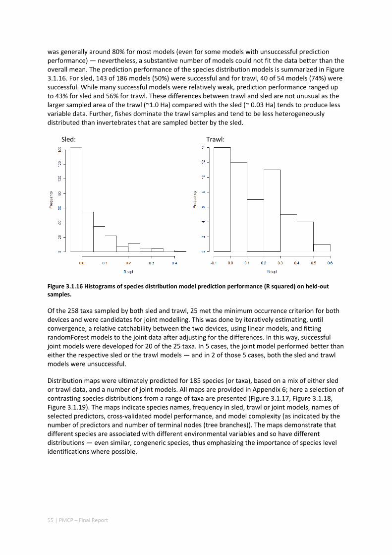
55 | PMCP – Final Report
was generally around 80% for most models (even for some models with unsuccessful prediction performance) — nevertheless, a substantive number of models could not fit the data better than the overall mean. The prediction performance of the species distribution models is summarized in Figure 3.1.16. For sled, 143 of 186 models (50%) were successful and for trawl, 40 of 54 models (74%) were successful. While many successful models were relatively weak, prediction performance ranged up to 43% for sled and 56% for trawl. These differences between trawl and sled are not unusual as the larger sampled area of the trawl (~1.0 Ha) compared with the sled (~ 0.03 Ha) tends to produce less variable data. Further, fishes dominate the trawl samples and tend to be less heterogeneously distributed than invertebrates that are sampled better by the sled.
Sled: Trawl:
Figure 3.1.16 Histograms of species distribution model prediction performance (R squared) on held‐out samples.
Of the 258 taxa sampled by both sled and trawl, 25 met the minimum occurrence criterion for both devices and were candidates for joint modelling. This was done by iteratively estimating, until convergence, a relative catchability between the two devices, using linear models, and fitting randomForest models to the joint data after adjusting for the differences. In this way, successful joint models were developed for 20 of the 25 taxa. In 5 cases, the joint model performed better than either the respective sled or the trawl models — and in 2 of those 5 cases, both the sled and trawl models were unsuccessful.
Distribution maps were ultimately predicted for 185 species (or taxa), based on a mix of either sled or trawl data, and a number of joint models. All maps are provided in Appendix 6; here a selection of contrasting species distributions from a range of taxa are presented (Figure 3.1.17, Figure 3.1.18, Figure 3.1.19). The maps indicate species names, frequency in sled, trawl or joint models, names of selected predictors, cross‐validated model performance, and model complexity (as indicated by the number of predictors and number of terminal nodes (tree branches)). The maps demonstrate that different species are associated with different environmental variables and so have different distributions — even similar, congeneric species, thus emphasizing the importance of species level identifications where possible.
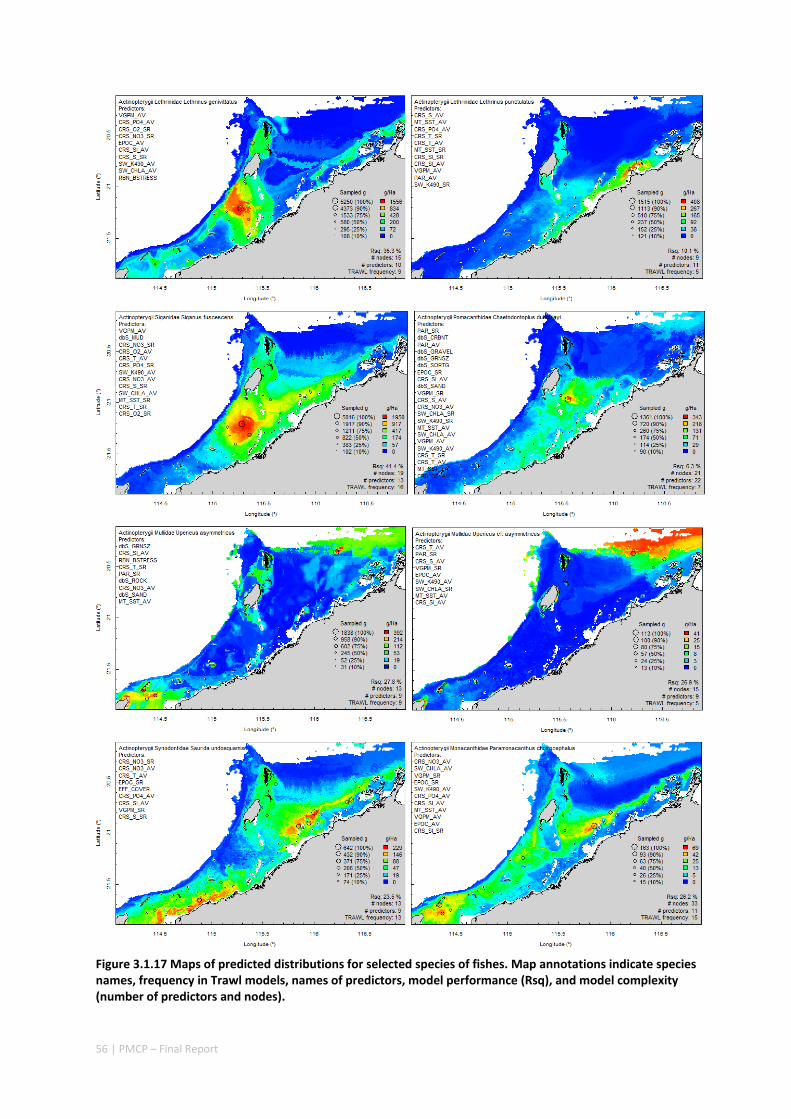
56 | PMCP – Final Report
Figure 3.1.17 Maps of predicted distributions for selected species of fishes. Map annotations indicate species names, frequency in Trawl models, names of predictors, model performance (Rsq), and model complexity (number of predictors and nodes).
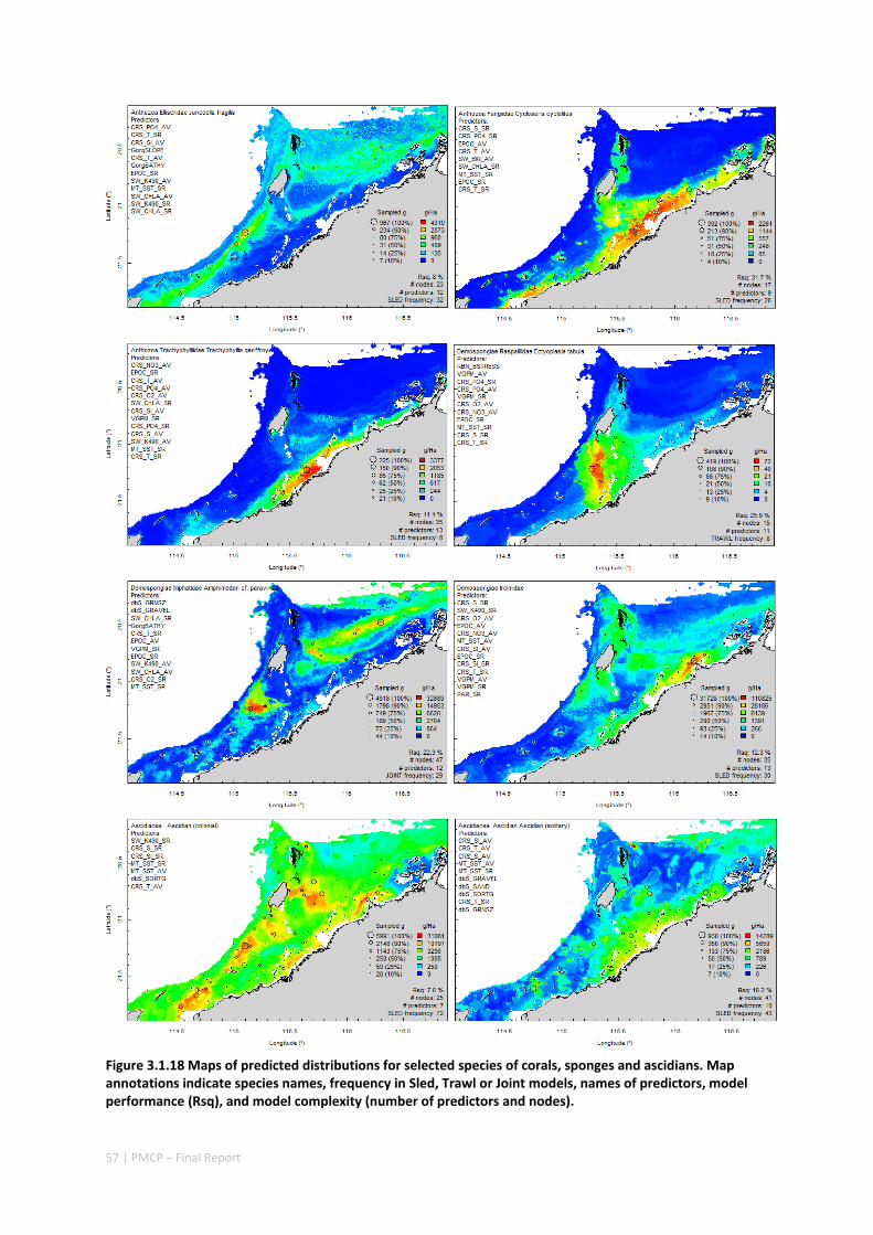
57 | PMCP – Final Report
Figure 3.1.18 Maps of predicted distributions for selected species of corals, sponges and ascidians. Map annotations indicate species names, frequency in Sled, Trawl or Joint models, names of predictors, model performance (Rsq), and model complexity (number of predictors and nodes).
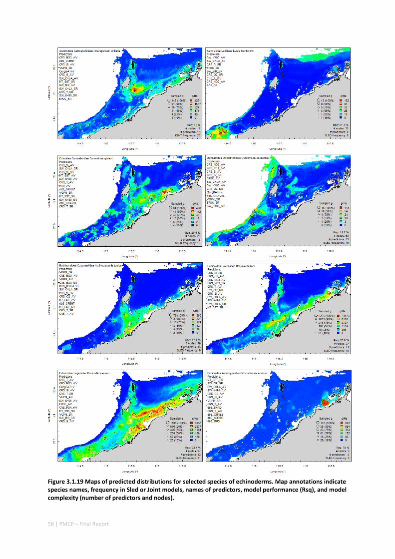
58 | PMCP – Final Report
Figure 3.1.19 Maps of predicted distributions for selected species of echinoderms. Map annotations indicate species names, frequency in Sled or Joint models, names of predictors, model performance (Rsq), and model complexity (number of predictors and nodes).
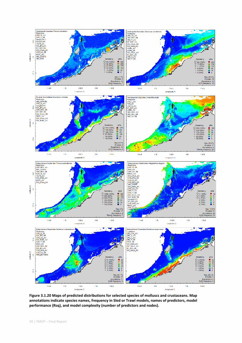
59 | PMCP – Final Report
Figure 3.1.20 Maps of predicted distributions for selected species of molluscs and crustaceans. Map annotations indicate species names, frequency in Sled or Trawl models, names of predictors, model performance (Rsq), and model complexity (number of predictors and nodes).
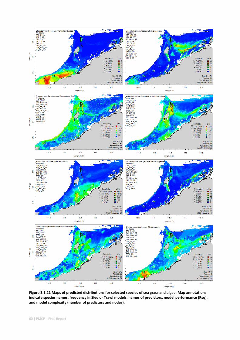
60 | PMCP – Final Report
Figure 3.1.21 Maps of predicted distributions for selected species of sea grass and algae. Map annotations indicate species names, frequency in Sled or Trawl models, names of predictors, model performance (Rsq), and model complexity (number of predictors and nodes).
61 | PMCP – Final Report
The distribution of Lethrinus gennivittatus (Figure 3.1.17) is considered to be associated with marine plants and has some correspondence with the distributions of some Sargassid species (Figure 3.1.21) and contrasts with congeneric L. punctulatus which corresponds with a number of sponges (e.g. Irciniidae), ascidians and some crinoids (Figure 3.1.18 and Figure 3.1.19). Siganus is a herbivore, and also corresponds with some Sargassid taxa. Chaetodontoplus is a popular aquarium species. The two goatfish (Upeneus, Figure 3.1.17) are very similar species with apparently contrasting distributions. The lizard fish (Saurida) and file fish (Paramonocanthus) are common on sandy seabeds.
Corals, sponges and ascidians (Figure 3.1.18) include some of the highest biomass taxa. Trachyphyllia and Cycloseris are likely to be species collected by the coral aquarium fishery. The seawhip, Junceella, along with many other gorgonians and sponges are potential habitat forming species.
Echinoderms (Figure 3.1.19) are a diverse group. Astropecten and Luidia are common sea‐stars on sandy shelf seabeds, but with contrasting distributions. Crinoids (e.g. Comanthus) are often found attached in elevated positions on habitat forming benthos (e.g. at Cape Preston). Numerous other crinoids have a deeper offshore distribution similar to the brittle star Ophiomaza, which lives only on different kinds of crinoids. The sea cucumber (Actinocucumis) and heart urchin (Breynia) have inshore distributions and feed on sedimentary deposits. Echinodiscus and Peronella are both sand dollars but have very different distributions. The gastropod Phalium (Figure 3.1.21) is a known predator of Echinodiscus and their distributions appear to be clearly associated.
Chicoreus is a spectacular spiky gastropod with a central inshore distribution (Figure 3.1.21); the spiny bivalve Spondylus also has an inshore distribution and may be its prey. The common squid Uroteuthis and the bug lobster Thenus are both potential commercial by‐product species. The squat lobster Allogalathea has a deeper offshore distribution. The congeneric hermit crabs Dardanus have strongly contrasting distributions.
The region may be a transition for seagrass species, with the temperate Amphibolis antarctica appearing at the edge of its range in the south of the study area, and the tropical Halophila spinulosa in the north of the study area (Figure 3.1.21). The biomass and cover of seagrass was low, but they are considered important food sources for turtles and dugongs. Most algal taxa were distribution towards the central part of the region and are considered important habitat (e.g. Sargassid species) for fishes and other species, and have been implicated in lethrinid recruitment. Algae are diverse and include browns (e.g. Sargassaceae sps.), coraline rhodoliths, reds (e.g. Desikacharyella), calcified greens (e.g. Halimeda), and other greens (e.g. Udotea).
3.1.4 DISCUSSION
The project has demonstrated substantial biodiversity on seabed of the Pilbara region, and has filled in data gaps for the majority of the ~18,700 km² study area, much of which had no pre‐existing data. Most of the prior biological knowledge about the region comes from fisheries surveys largely outside the immediate vicinity of the study area. The completed sorting and identification of samples has revealed new species and provided valuable specimens accessioned into the WA Museum that comprise an important biodiversity and genetic resource for WA. These new data and analyses have also documented the important relationships between sampled species distributions and environmental gradients that have been used to predict patterns of seabed assemblages and if species distributions at regional scale. These maps of regional biodiversity are more comprehensive and more detailed than available previously.
62 | PMCP – Final Report
The Pilbara shelf seabed is a complex mix of physical environments. The biological assemblages were observed to respond significantly to the multiple interacting physical gradients and few of these gradients have simple trends in geographic space. Some of the environmental gradients most associated with driving patterns of biodiversity composition include: seasonal range in sea surface temperature, which is greater in shallower and inshore areas; average annual sea surface temperature, which is higher in the NE of the region cf. the SW; seasonal range in salinity, which is greater in the NE coastal areas and lowest in central areas; seasonal range in bottom temperature, which is greater in central and NE inshore areas and lowest in deeper offshore area; seabed current stress, which is higher in central areas and around North West Cape; bottom water oxygen, which is higher on SW shelf areas and decreasing to the NE and with depth; and turbidity, which is higher in inshore areas. Other variables also are associated with biodiversity patterns but are increasingly less important overall, including those related to light, productivity, nutrients, and sediment types. These gradients in the Pilbara are perhaps not as strong as in some other areas such as the Torres Strait and parts of the Great Barrier Reef region, where sediment types and seabed current stress are strong drivers.
The epibenthic sled and research trawl both sampled a diverse seabed biota of about 12 phyla and 1326 species, of which almost 20% were sampled by both devices; 899 (78%) were unique to the sled and 169 (40%) to the trawl. The sled samples were rich with more than ~45 taxa per site on average, whereas the trawl samples averaged about 25 taxa per site. This site richness is somewhat lower than other similar tropical demersal/benthic surveys in the Torres Strait and the Great Barrier Reef regions (e.g. Pitcher et al. 2007ab: TS: sled: ~49, trawl: ~76; GBR: sled: ~41, trawl: ~76 — excluding Bryozoans), particularly for the trawl samples. Nevertheless, the trawl sampled fishes more consistently and representatively, whereas the Sled sampled all other biota better, though with greater variability due to its much smaller swept area. These devices provided specimens that could be properly identified, showed that otherwise inseparable taxa could have strikingly different distribution patterns, and revealed the biodiversity of the region (even at sites where no biota were observed in video). The level of relative rarity of species in the samples was also high: ~76% of sled species were found at <5 sled sites, and >87% of trawl species were found <5 trawl sites. This rarity was somewhat higher than other similar tropical demersal/benthic surveys (e.g. Pitcher et al. 2007ab: TS: sled: ~76%, trawl: ~75%; GBR: sled: ~62%, trawl: ~65%), particularly for the trawl samples. This suggests that more species, possibly many more, remain to be discovered by further sampling in the region.
As is typical of biological sampling, a large proportion of taxa were sampled at only one or a very few sites. This suggests that many more seabed species remain to be discovered in the shelf seabed of the region. Compared with the total number of species sampled, relatively fewer species were considered frequent enough for analyses (at ≥5 sites). Nevertheless, there were about 315 species that meet this criterion, including 25 that were sampled by both devices. The randomForest method provided a robust and flexible approach for modelling statistical relationships between the biological data and environmental gradients, and for identifying the important variables and predicting distributions. Ultimately, accounting for species modelled from both devices and joint modelling, 180 taxa had ‘successful’ models. Species with unsuccessful models had no statistically predictable relationship with the environmental variables. For the majority of species, i.e. those occurring at <5 sites, no individual analyses or modelling was possible, although the sample data are available. While the environmental variables have demonstrable utility for predicting the regional distribution of many species with adequate frequency of occurrence, not all the successful models could predict well even if they fitted the site data well. That is, they do not often account for the majority of observed variation in local biomass — other factors, including stochastic processes such as recruitment and mortality, biological interactions, and random sampling effects typically outweigh deterministic environmental relationships, or habitat preferences, at the local site biomass scale. Nevertheless, the regional scale patterns of distribution are representative.

63 | PMCP – Final Report
The multitude of species sampled, modelled and mapped respond in different, overlapping and varying ways to the multiple interacting environmental variables, which as noted above do not have simple trends in geographic space. Different species were associated with different variables, and some positively and others negatively to the same variables. Overall, the important variables for species were largely in line with the environmental variables associated with assemblage patterns.
Integration with other PMCP projects and sub‐projects
The datasets collated by this project have been used by the Hydrodynamic Model & Connectivity Project of the PMCP, and the characterisation of benthic habitats and assemblages in the Pilbara region, have been used to inform the sampling locations for the broad‐scale sampling that is being carried out within the scope of the Coral Health and Reef and Sharks projects of the PMCP.
Planning and management implications
The outputs from this study are intended to support a range of spatial planning, assessment and management applications across the west Pilbara, including for conservation, assessments of current uses, and to provide information for evaluating future development proposals. Such applications of the project’s outputs will be developed in an ongoing fashion as part of continuing dialogue with government stakeholders.
The outputs from the project can support important management questions:
Is the current positioning and scale of MPA networks and no‐take zones providing comprehensive, adequate and representative protection for marine benthic species, assemblages and habitats?
What is the CAR performance of spatial management at multiple levels, including habitats, assemblages and for hundreds of species?
What should be the size and location of spatial management zones in the region?
What is the appropriate design for spatial management plans for activities such as recreational fishing, industrial and tourism development, infrastructure planning relevant to WA DPIRD but also to OEPA and DPIRD
Are proposed development areas unique in terms of their biodiversity and habitat values, or for any key threatened species?
How can biodiversity be taken into account in assessments of development plans in relation to relevant marine management units in a quantitative and objective manner?
How do anthropogenic risk factors map across various habitats and biodiversity values in the region, including marine parks?
The project’s outputs will enable spatial analyses of the overlap of human uses with multiple levels of biodiversity, permitting ecological risk assessments and, for some types of uses, fully quantitative assessments of their sustainability. The outputs will also support design of spatial aspects of monitoring in relationship to biodiversity attributes and human use factors.
As an example, we quantified the representation of the 10 assemblages defined for the west Pilbara shelf (Figure 3.1.13) in the region’s Marine Park areas (both State and Commonwealth, Figure 3.1.22) and their exposure to regional trawl fisheries (Table 3.1.2). Highly protected areas (IUCN IA) ranged from 0−19% of each Assemblage, and trawl footprints ranged from 0−10.3%. Analogous quantification is possible for fishery closure areas and major marine infrastructure development, among others. Further, the representation of habitats, commercial species, species of conservation concern and other species in Marine Park zoning or other closure areas, and their exposure to major uses such as fishing pressure and infrastructure development can be similarly quantified.
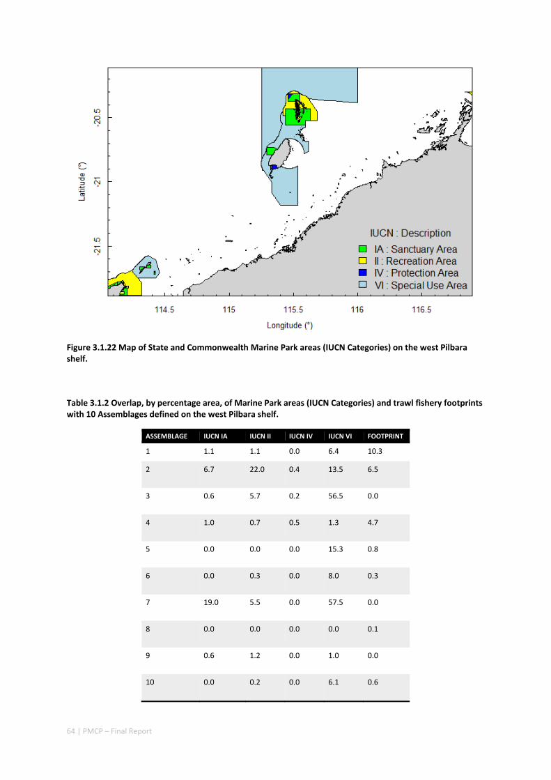
64 | PMCP – Final Report
Figure 3.1.22 Map of State and Commonwealth Marine Park areas (IUCN Categories) on the west Pilbara shelf.
Table 3.1.2 Overlap, by percentage area, of Marine Park areas (IUCN Categories) and trawl fishery footprints with 10 Assemblages defined on the west Pilbara shelf.
ASSEMBLAGE IUCN IA IUCN II IUCN IV IUCN VI FOOTPRINT
1 1.1 1.1 0.0 6.4 10.3
2 6.7 22.0 0.4 13.5 6.5
3 0.6 5.7 0.2 56.5 0.0
4 1.0 0.7 0.5 1.3 4.7
5 0.0 0.0 0.0 15.3 0.8
6 0.0 0.3 0.0 8.0 0.3
7 19.0 5.5 0.0 57.5 0.0
8 0.0 0.0 0.0 0.0 0.1
9 0.6 1.2 0.0 1.0 0.0
10 0.0 0.2 0.0 6.1 0.6
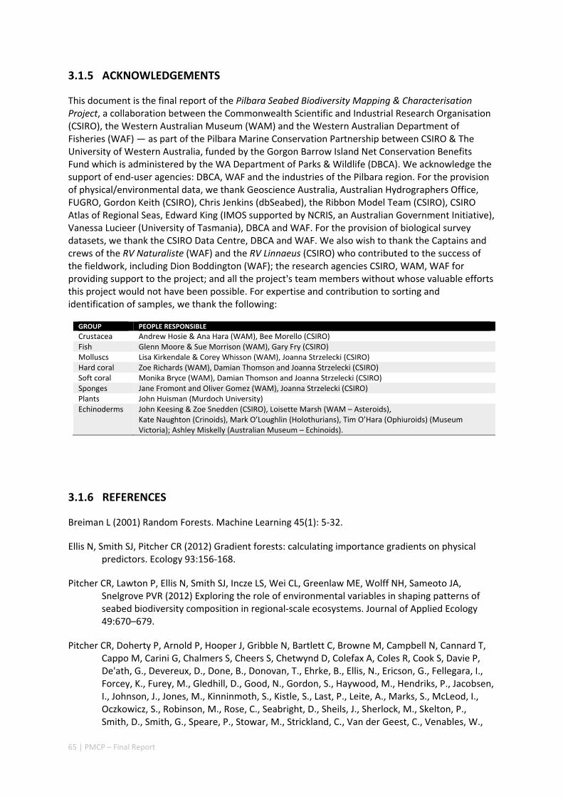
65 | PMCP – Final Report
3.1.5 ACKNOWLEDGEMENTS
This document is the final report of the Pilbara Seabed Biodiversity Mapping & Characterisation Project, a collaboration between the Commonwealth Scientific and Industrial Research Organisation (CSIRO), the Western Australian Museum (WAM) and the Western Australian Department of Fisheries (WAF) — as part of the Pilbara Marine Conservation Partnership between CSIRO & The University of Western Australia, funded by the Gorgon Barrow Island Net Conservation Benefits Fund which is administered by the WA Department of Parks & Wildlife (DBCA). We acknowledge the support of end‐user agencies: DBCA, WAF and the industries of the Pilbara region. For the provision of physical/environmental data, we thank Geoscience Australia, Australian Hydrographers Office, FUGRO, Gordon Keith (CSIRO), Chris Jenkins (dbSeabed), the Ribbon Model Team (CSIRO), CSIRO Atlas of Regional Seas, Edward King (IMOS supported by NCRIS, an Australian Government Initiative), Vanessa Lucieer (University of Tasmania), DBCA and WAF. For the provision of biological survey datasets, we thank the CSIRO Data Centre, DBCA and WAF. We also wish to thank the Captains and crews of the RV Naturaliste (WAF) and the RV Linnaeus (CSIRO) who contributed to the success of the fieldwork, including Dion Boddington (WAF); the research agencies CSIRO, WAM, WAF for providing support to the project; and all the project's team members without whose valuable efforts this project would not have been possible. For expertise and contribution to sorting and identification of samples, we thank the following:
GROUP PEOPLE RESPONSIBLE
Crustacea Andrew Hosie & Ana Hara (WAM), Bee Morello (CSIRO) Fish Glenn Moore & Sue Morrison (WAM), Gary Fry (CSIRO) Molluscs Lisa Kirkendale & Corey Whisson (WAM), Joanna Strzelecki (CSIRO) Hard coral Zoe Richards (WAM), Damian Thomson and Joanna Strzelecki (CSIRO) Soft coral Monika Bryce (WAM), Damian Thomson and Joanna Strzelecki (CSIRO) Sponges Jane Fromont and Oliver Gomez (WAM), Joanna Strzelecki (CSIRO) Plants John Huisman (Murdoch University) Echinoderms John Keesing & Zoe Snedden (CSIRO), Loisette Marsh (WAM – Asteroids),
Kate Naughton (Crinoids), Mark O’Loughlin (Holothurians), Tim O’Hara (Ophiuroids) (Museum Victoria); Ashley Miskelly (Australian Museum – Echinoids).
3.1.6 REFERENCES
Breiman L (2001) Random Forests. Machine Learning 45(1): 5‐32.
Ellis N, Smith SJ, Pitcher CR (2012) Gradient forests: calculating importance gradients on physical predictors. Ecology 93:156‐168.
Pitcher CR, Lawton P, Ellis N, Smith SJ, Incze LS, Wei CL, Greenlaw ME, Wolff NH, Sameoto JA, Snelgrove PVR (2012) Exploring the role of environmental variables in shaping patterns of seabed biodiversity composition in regional‐scale ecosystems. Journal of Applied Ecology 49:670–679.
Pitcher CR, Doherty P, Arnold P, Hooper J, Gribble N, Bartlett C, Browne M, Campbell N, Cannard T, Cappo M, Carini G, Chalmers S, Cheers S, Chetwynd D, Colefax A, Coles R, Cook S, Davie P, De'ath, G., Devereux, D., Done, B., Donovan, T., Ehrke, B., Ellis, N., Ericson, G., Fellegara, I., Forcey, K., Furey, M., Gledhill, D., Good, N., Gordon, S., Haywood, M., Hendriks, P., Jacobsen, I., Johnson, J., Jones, M., Kinninmoth, S., Kistle, S., Last, P., Leite, A., Marks, S., McLeod, I., Oczkowicz, S., Robinson, M., Rose, C., Seabright, D., Sheils, J., Sherlock, M., Skelton, P., Smith, D., Smith, G., Speare, P., Stowar, M., Strickland, C., Van der Geest, C., Venables, W.,
66 | PMCP – Final Report
Walsh, C., Wassenberg, T., Welna, A., Yearsley, G. (2007a) Seabed Biodiversity on the Continental Shelf of the Great Barrier Reef World Heritage Area. AIMS/CSIRO/QM/QDPI Final Report to CRC Reef Research. 320 pp. ISBN 978‐1‐921232‐87‐9 http://fish.gov.au/reports/Documents/Pitcher_et_al_2007a_GBR_Seabed_Biodiversity_Final_Report.pdf
Pitcher CR, Haywood M, Hooper J, Coles R, Bartlett C, Browne M, Cannard T, Carini G, Carter A, Cheers S, Chetwynd D, Colefax A, Cook S, Davie P, Ellis N, Fellegara I, Forcey K, Furey M, Gledhill D, Hendriks P, Jacobsen I, Johnson J, Jones M, Last P, Marks S, McLeod I, Sheils J, Sheppard J, Smith G, Strickland C, Van der Geest C, Venables W, Wassenberg T, Yearsley G (2007b) Mapping and Characterisation of Key Biotic & Physical Attributes of the Torres Strait Ecosystem. CSIRO/QM/QDPI Task Final Report to CRC Torres Strait. 142pp. ISBN 978‐1‐921232‐89‐3 http://www.cmar.csiro.au/e‐print/open/2007/pitchercr_a.pdf
Pitcher CR, Venables W, Ellis N, McLeod I, Pantus F, Austin M, Cappo M, Doherty P, Gribble N (2002) GBR Seabed Biodiversity Mapping Project: Phase 1 Report to CRC‐Reef. CSIRO/AIMS/QDPI Report, pp. 192.
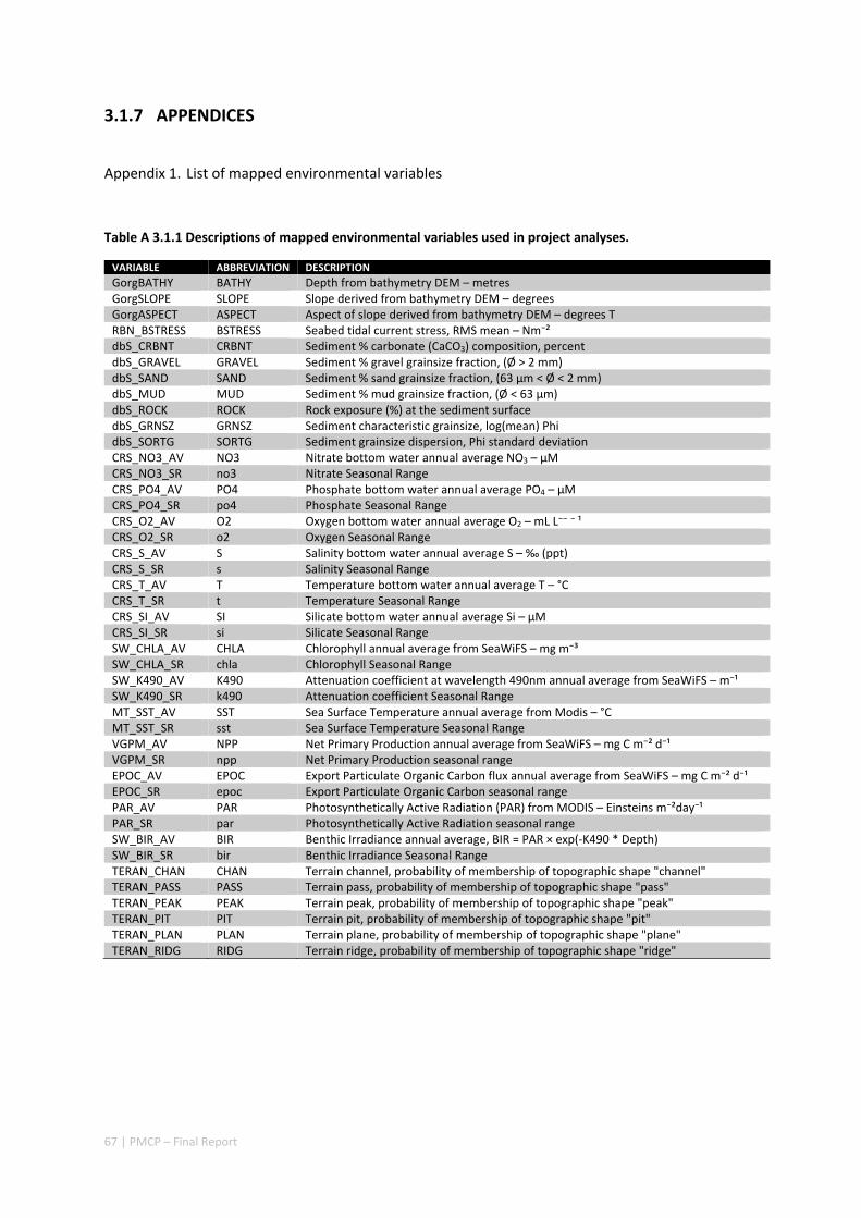
67 | PMCP – Final Report
3.1.7 APPENDICES
Appendix 1. List of mapped environmental variables
Table A 3.1.1 Descriptions of mapped environmental variables used in project analyses.
VARIABLE ABBREVIATION DESCRIPTION
GorgBATHY BATHY Depth from bathymetry DEM – metres GorgSLOPE SLOPE Slope derived from bathymetry DEM – degrees GorgASPECT ASPECT Aspect of slope derived from bathymetry DEM – degrees T RBN_BSTRESS BSTRESS Seabed tidal current stress, RMS mean – Nm⁻² dbS_CRBNT CRBNT Sediment % carbonate (CaCO3) composition, percent dbS_GRAVEL GRAVEL Sediment % gravel grainsize fraction, (Ø > 2 mm) dbS_SAND SAND Sediment % sand grainsize fraction, (63 μm < Ø < 2 mm) dbS_MUD MUD Sediment % mud grainsize fraction, (Ø < 63 μm) dbS_ROCK ROCK Rock exposure (%) at the sediment surface dbS_GRNSZ GRNSZ Sediment characteristic grainsize, log(mean) Phi dbS_SORTG SORTG Sediment grainsize dispersion, Phi standard deviation CRS_NO3_AV NO3 Nitrate bottom water annual average NO3 – μM CRS_NO3_SR no3 Nitrate Seasonal Range CRS_PO4_AV PO4 Phosphate bottom water annual average PO4 – μM CRS_PO4_SR po4 Phosphate Seasonal Range CRS_O2_AV O2 Oxygen bottom water annual average O2 – mL L⁻⁻ ⁻ ¹ CRS_O2_SR o2 Oxygen Seasonal Range CRS_S_AV S Salinity bottom water annual average S – ‰ (ppt) CRS_S_SR s Salinity Seasonal Range CRS_T_AV T Temperature bottom water annual average T – °C CRS_T_SR t Temperature Seasonal Range CRS_SI_AV SI Silicate bottom water annual average Si – μM CRS_SI_SR si Silicate Seasonal Range SW_CHLA_AV CHLA Chlorophyll annual average from SeaWiFS – mg m⁻³ SW_CHLA_SR chla Chlorophyll Seasonal Range SW_K490_AV K490 Attenuation coefficient at wavelength 490nm annual average from SeaWiFS – m⁻¹ SW_K490_SR k490 Attenuation coefficient Seasonal Range MT_SST_AV SST Sea Surface Temperature annual average from Modis – °C MT_SST_SR sst Sea Surface Temperature Seasonal Range VGPM_AV NPP Net Primary Production annual average from SeaWiFS – mg C m⁻² d⁻¹ VGPM_SR npp Net Primary Production seasonal range EPOC_AV EPOC Export Particulate Organic Carbon flux annual average from SeaWiFS – mg C m⁻² d⁻¹ EPOC_SR epoc Export Particulate Organic Carbon seasonal range PAR_AV PAR Photosynthetically Active Radiation (PAR) from MODIS – Einsteins m⁻²day⁻¹ PAR_SR par Photosynthetically Active Radiation seasonal range SW_BIR_AV BIR Benthic Irradiance annual average, BIR = PAR × exp(‐K490 * Depth) SW_BIR_SR bir Benthic Irradiance Seasonal Range TERAN_CHAN CHAN Terrain channel, probability of membership of topographic shape "channel" TERAN_PASS PASS Terrain pass, probability of membership of topographic shape "pass" TERAN_PEAK PEAK Terrain peak, probability of membership of topographic shape "peak" TERAN_PIT PIT Terrain pit, probability of membership of topographic shape "pit" TERAN_PLAN PLAN Terrain plane, probability of membership of topographic shape "plane" TERAN_RIDG RIDG Terrain ridge, probability of membership of topographic shape "ridge"

68 | PMCP – Final Report
Appendix 2. Maps of regional environmental variables
Bathymetry m Slope ° Carbonate % Gravel % Sand %
Mud % Rock exposure % Grainsize phi Current stress average Nitrate average
Nitrate seasonal range Phosphate average Phosphate season range Oxygen average Oxygen seasonal range
Salinity average Salinity seasonal range Temperature average Temperature seas range Silicate average
Silicate seasonal range K490 average K490 seasonal range Chlorophyll average Chlorophyll seas range
SSTemp average SST seasonal range Benthic Irradiance avg Benthic Irradiance rng Primary production av
Primary production rng Light (PAR) average PAR seasonal range Exported POC average EPOC seasonal range
Figure A 3.1.1 Maps of regional environmental variables.
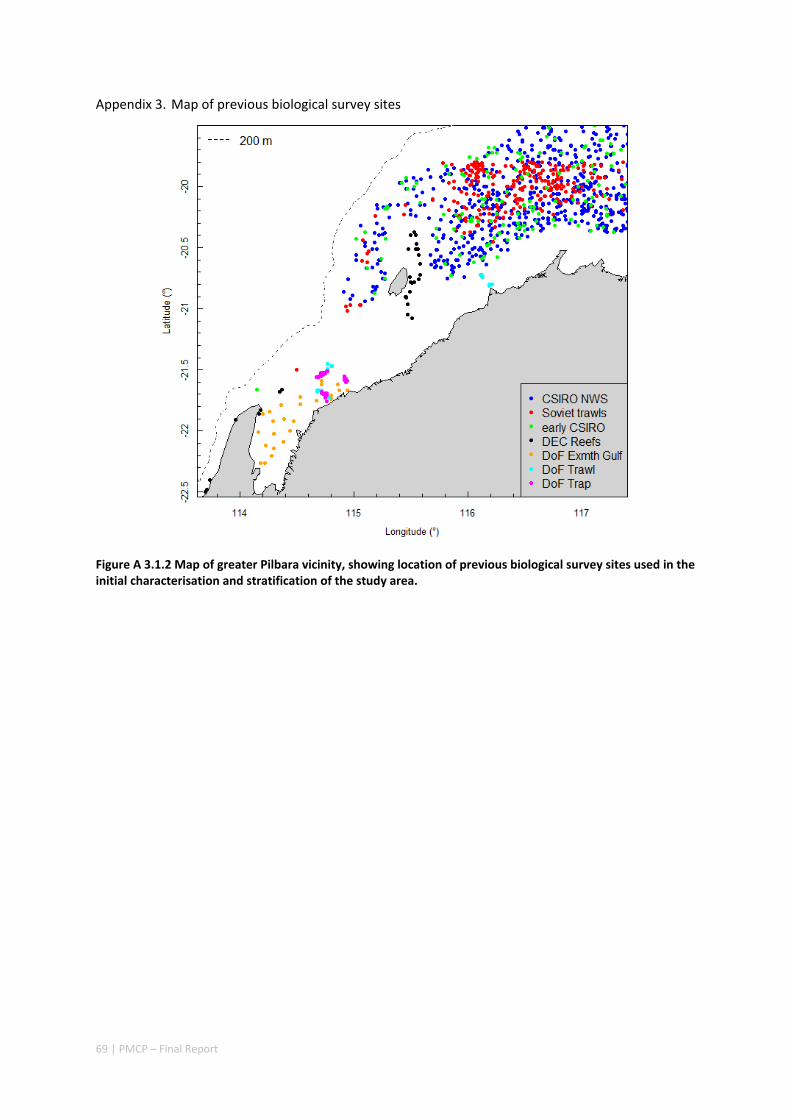
69 | PMCP – Final Report
Appendix 3. Map of previous biological survey sites
Figure A 3.1.2 Map of greater Pilbara vicinity, showing location of previous biological survey sites used in the initial characterisation and stratification of the study area.

70 | PMCP – Final Report
Appendix 4. Map of preliminary regional characterisation
Figure A 3.1.3 Results of preliminary analyses of pre‐existing CSIRO fish survey data on multiple environmental data coverages, prior to acquisition by the project of additional biological and environmental datasets and finer resolution ocean‐colour derived datasets.
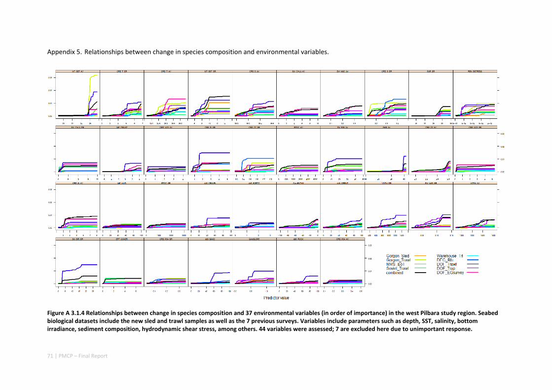
71 | PMCP – Final Report
Appendix 5. Relationships between change in species composition and environmental variables.
Figure A 3.1.4 Relationships between change in species composition and 37 environmental variables (in order of importance) in the west Pilbara study region. Seabed biological datasets include the new sled and trawl samples as well as the 7 previous surveys. Variables include parameters such as depth, SST, salinity, bottom irradiance, sediment composition, hydrodynamic shear stress, among others. 44 variables were assessed; 7 are excluded here due to unimportant response.
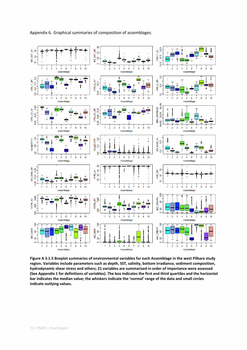
72 | PMCP – Final Report
Appendix 6. Graphical summaries of composition of assemblages.
Figure A 3.1.5 Boxplot summaries of environmental variables for each Assemblage in the west Pilbara study region. Variables include parameters such as depth, SST, salinity, bottom irradiance, sediment composition, hydrodynamic shear stress and others; 21 variables are summarized in order of importance were assessed (See Appendix 1 for definitions of variables). The box indicates the first and third quartiles and the horizontal bar indicates the median value; the whiskers indicate the ‘normal’ range of the data and small circles indicate outlying values.
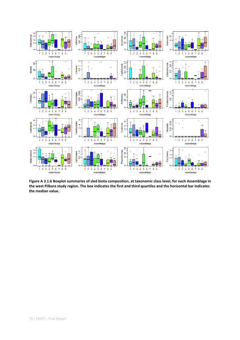
73 | PMCP – Final Report
Figure A 3.1.6 Boxplot summaries of sled biota composition, at taxonomic class level, for each Assemblage in the west Pilbara study region. The box indicates the first and third quartiles and the horizontal bar indicates the median value.
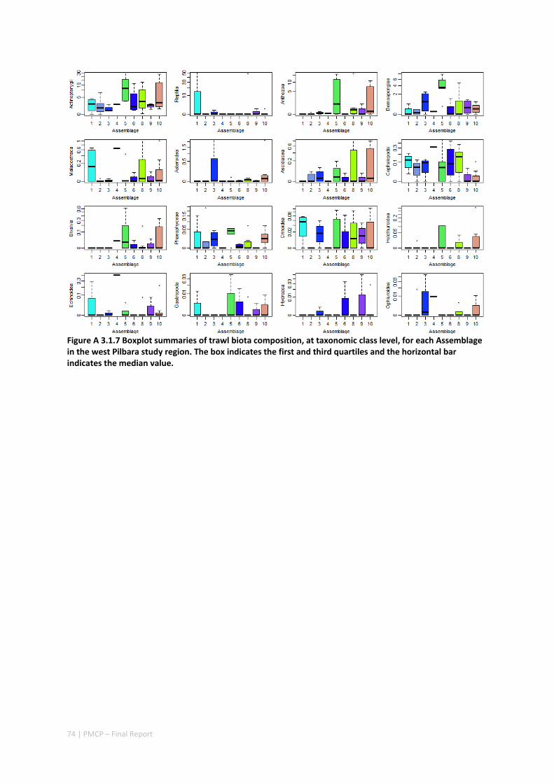
74 | PMCP – Final Report
Figure A 3.1.7 Boxplot summaries of trawl biota composition, at taxonomic class level, for each Assemblage in the west Pilbara study region. The box indicates the first and third quartiles and the horizontal bar indicates the median value.

75 | PMCP – Final Report
Appendix 7. Predicted species distribution maps.
Actinopterygii (fishes):
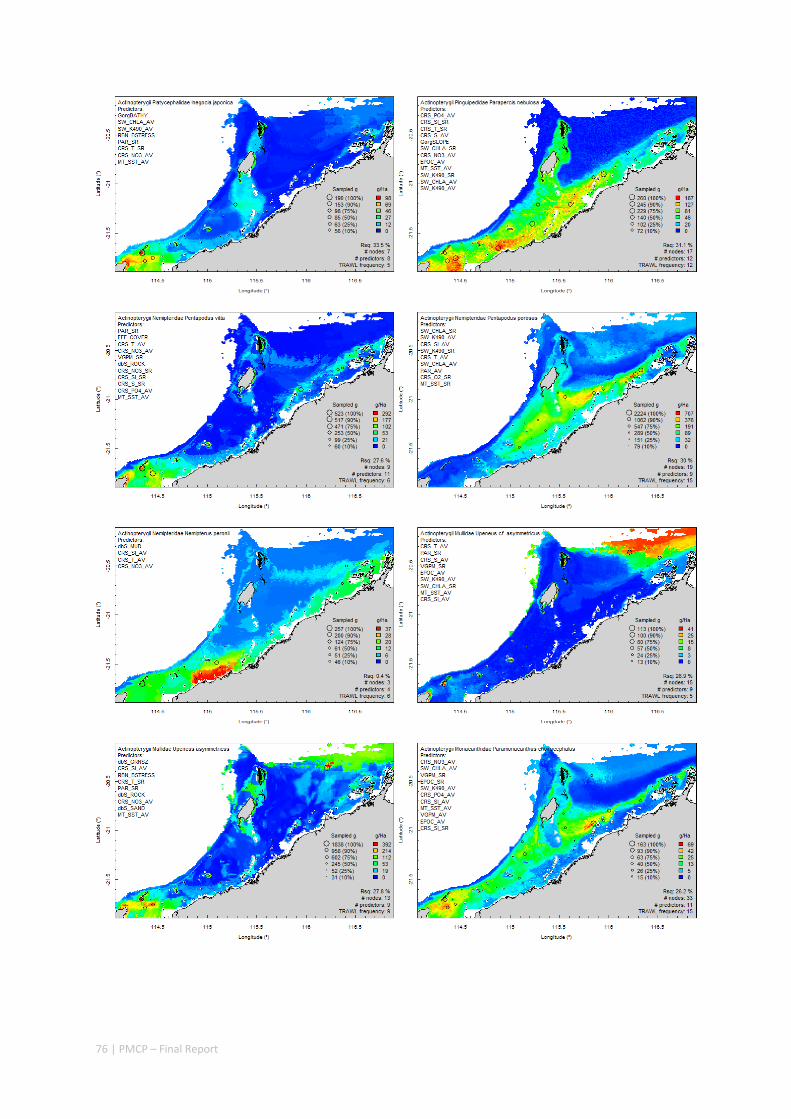
76 | PMCP – Final Report
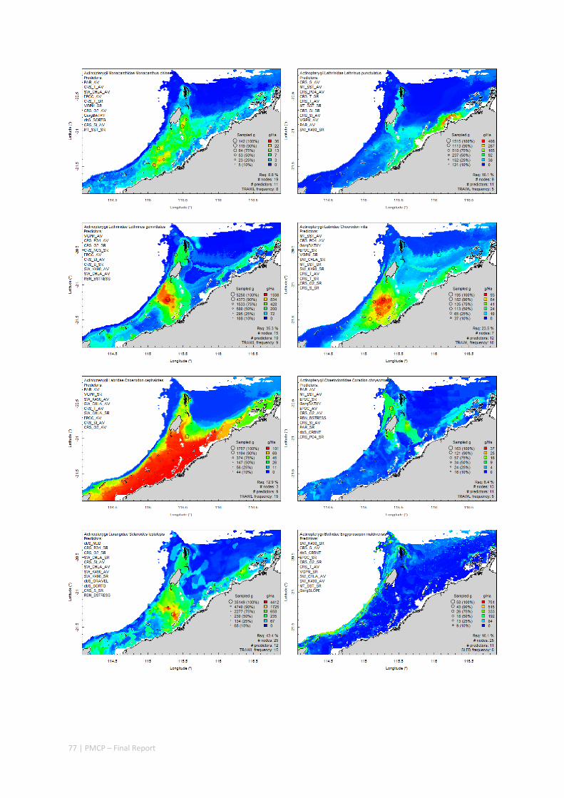
77 | PMCP – Final Report
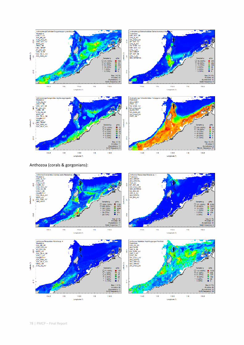
78 | PMCP – Final Report
Anthozoa (corals & gorgonians):
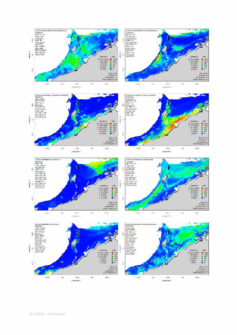
79 | PMCP – Final Report
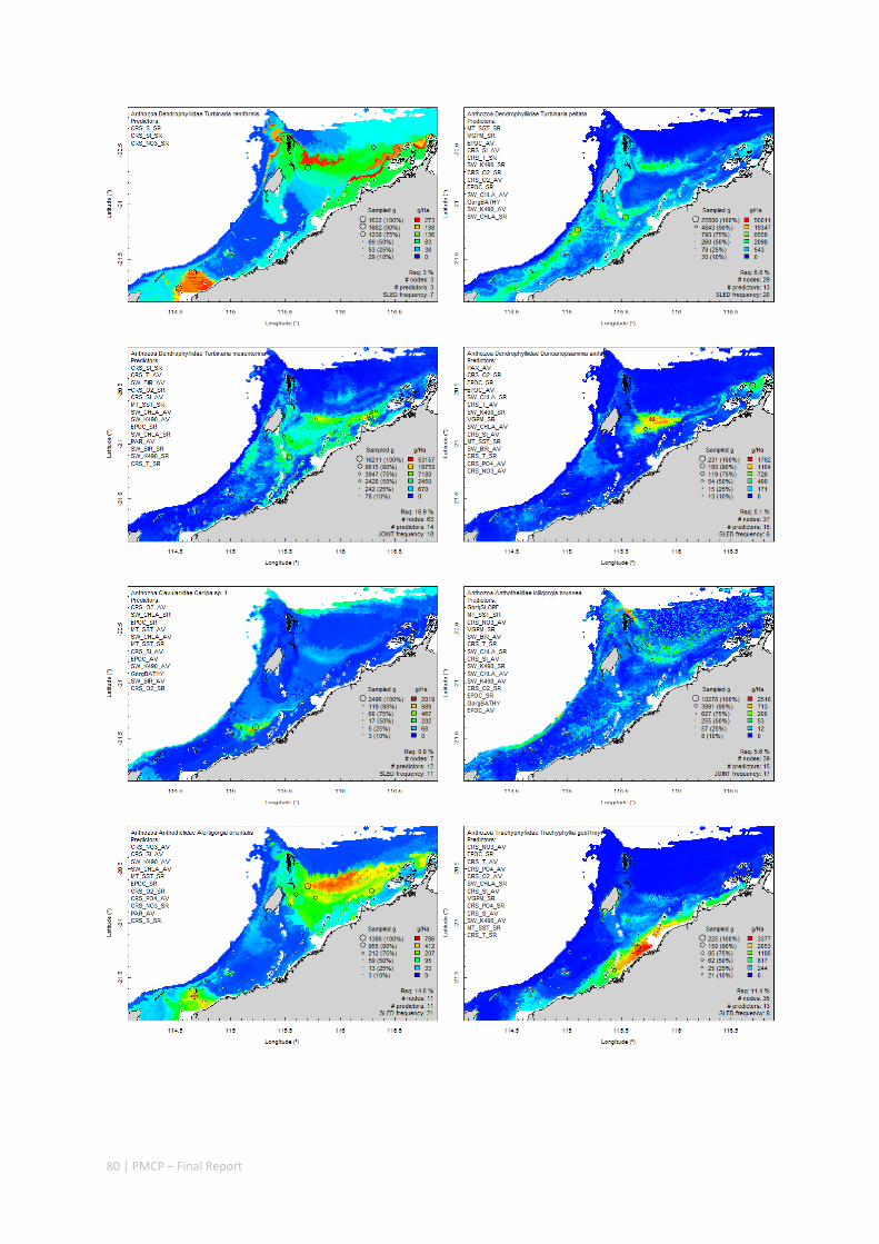
80 | PMCP – Final Report
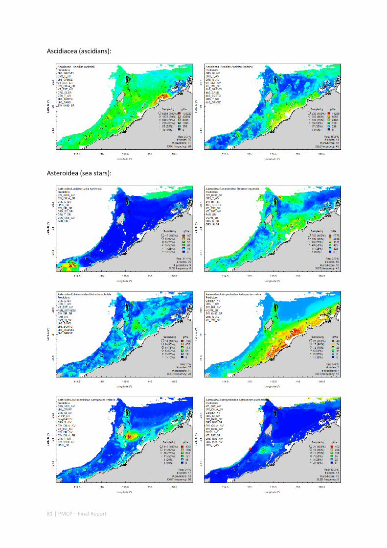
81 | PMCP – Final Report
Ascidiacea (ascidians):
Asteroidea (sea stars):
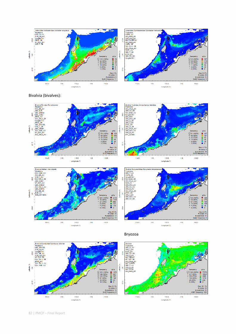
82 | PMCP – Final Report
Bivalvia (bivalves):
Bryozoa
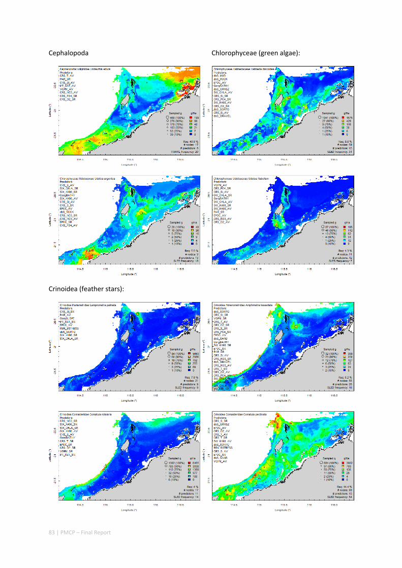
83 | PMCP – Final Report
Cephalopoda Chlorophyceae (green algae):
Crinoidea (feather stars):
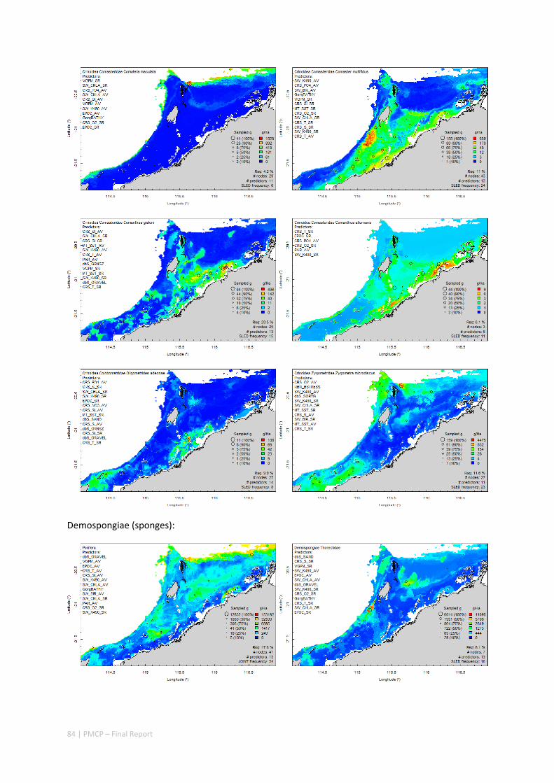
84 | PMCP – Final Report
Demospongiae (sponges):
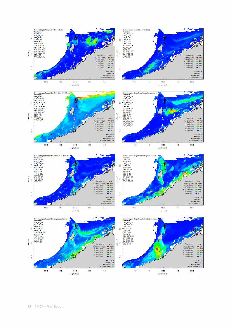
85 | PMCP – Final Report
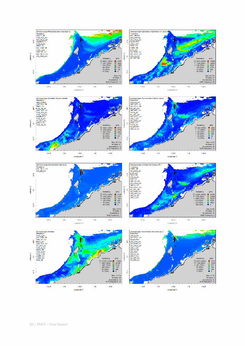
86 | PMCP – Final Report
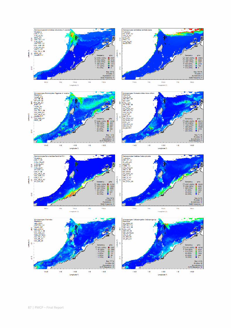
87 | PMCP – Final Report
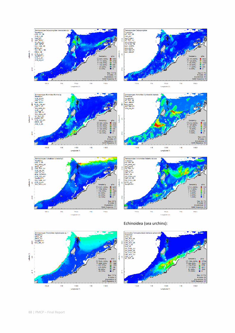
88 | PMCP – Final Report
Echinoidea (sea urchins):
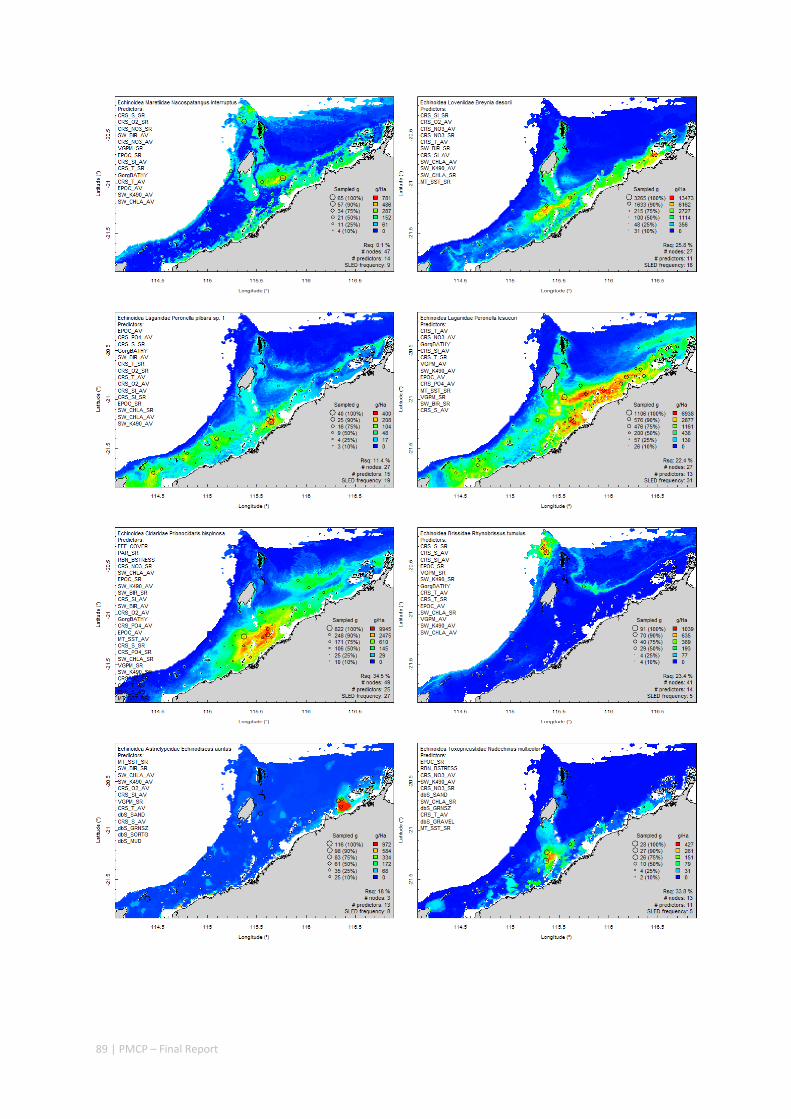
89 | PMCP – Final Report
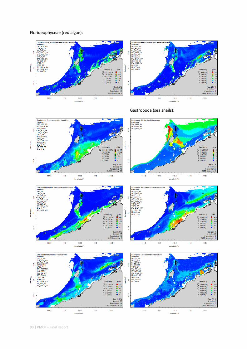
90 | PMCP – Final Report
Florideophyceae (red algae):
Gastropoda (sea snails):
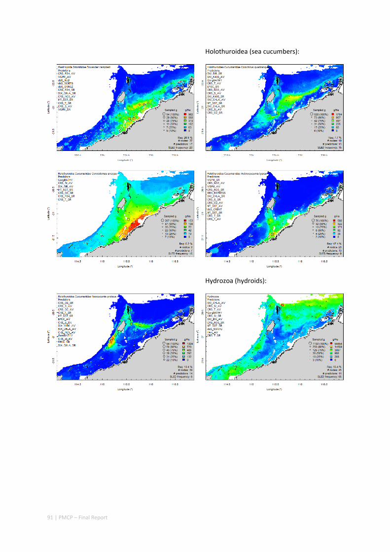
91 | PMCP – Final Report
Holothuroidea (sea cucumbers):
Hydrozoa (hydroids):
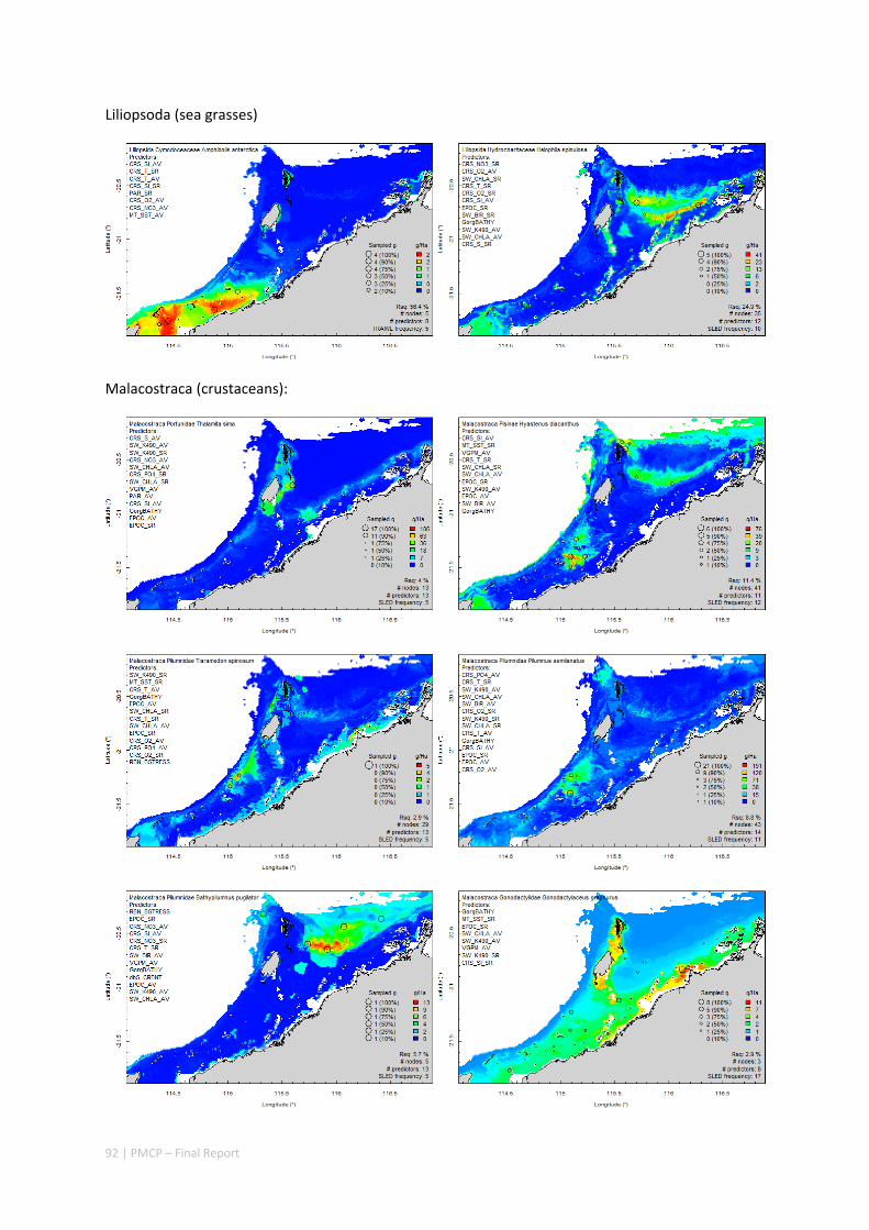
92 | PMCP – Final Report
Liliopsoda (sea grasses)
Malacostraca (crustaceans):
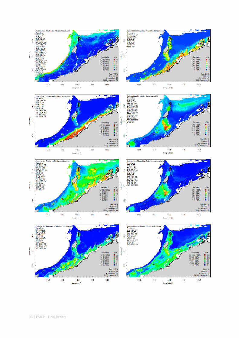
93 | PMCP – Final Report
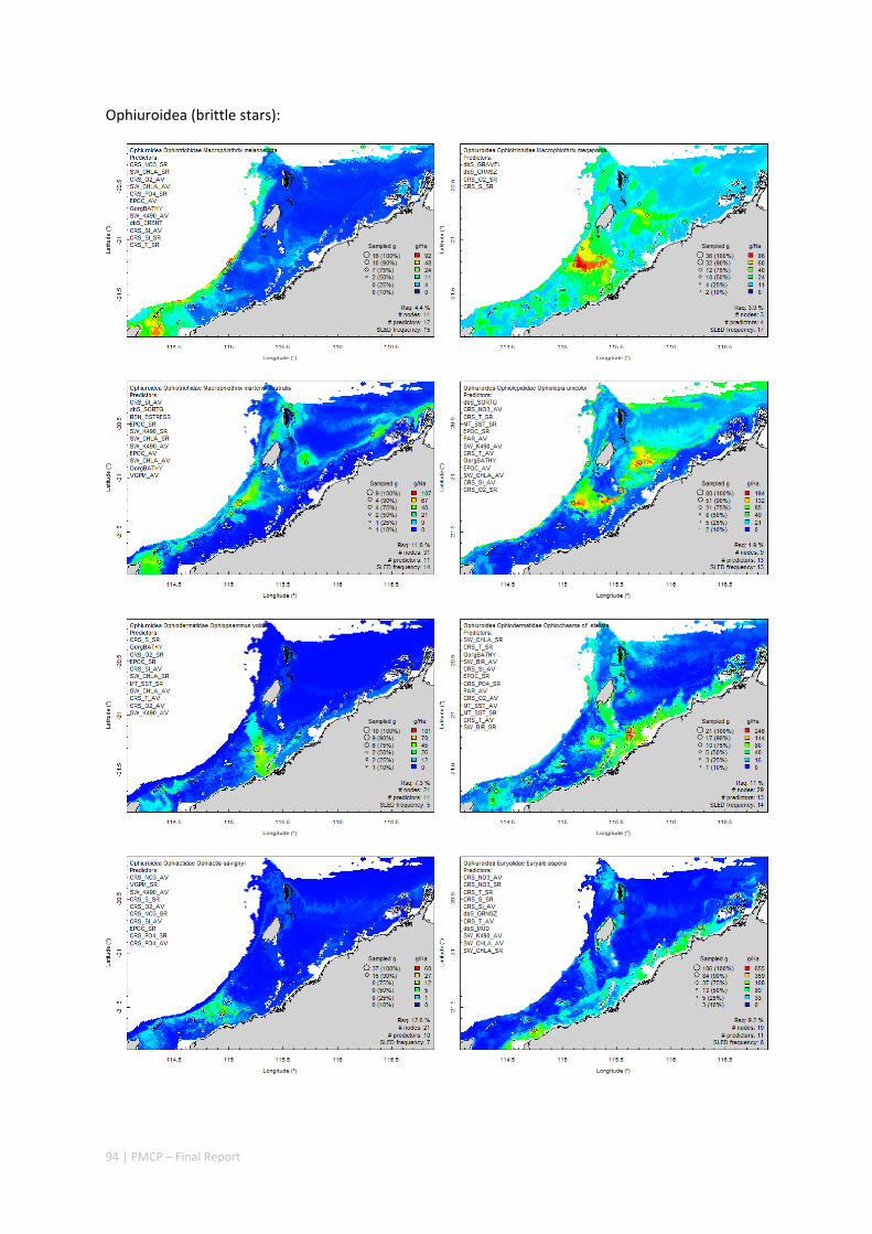
94 | PMCP – Final Report
Ophiuroidea (brittle stars):

95 | PMCP – Final Report
Phaeophyceae (brown algae):

96 | PMCP – Final Report
Figure A 3.1.8 Predicted species distribution maps of various species.
97 | PMCP – Final Report
Pilbara Reef Biodiversity Mapping & Characterisation
Authors: Ellis N, Babcock R, Donovan A, Grol M, Haywood M, Keesing J, Mattio L, McLeod I, Miller M, Olsen YS, Pillans R, Pitcher R, Thomson D, Zavala Perez A.
ABSTRACT
Reefs of the west Pilbara in northwestern Australia between the Dampier Archipelago and northern Ningaloo were surveyed to provide information on a range of reef organisms that would allow any patterns in reef assemblage structure to be determined. Data from 92 sites was obtained for groups including fish, mobile invertebrates, and sessile benthic invertebrates and macroalgae. The distribution of the groups was modelled in relation to a suite of physical environmental layers. Eight assemblage types were chosen as the best representation of regional variation in reef assemblages of the west Pilbara. The assemblages showed latitudinal trends as well as inshore–offshore variation. Existing marine management reserves do not adequately represent the full range of biological assemblages, with only two assemblages protected by no‐take reserves. To better support principles of Comprehensive, Adequate and Representative zoning for marine conservation, further steps could be taken to ensure adequate protection of key habitat types within the region

98 | PMCP – Final Report
3.2.1 INTRODUCTION
Planning, assessment and management of the marine environment requires an essential base level of understanding about the distribution of habitats and biodiversity (Day et al. 2002). It is also critical for developing an effective sampling program for Key Performance Indicators (KPIs) such as fish and corals (CALM 2005). Habitat is a key determinant of population structure and having a stratified sampling regime is vital to obtaining precise estimates of population parameters and properly identifying drivers of biological response (Pelletier et al. 2014, Mumby et al. 2016). Consequently, the initial phase of the project included a component to compile all relevant existing available information relating to biodiversity and habitat variation in the region. Since the sea is a dynamic and three‐dimensional environment, habitat descriptions included benthic mapping, and key water column properties related to fish and coral reef health, linking to satellite data for ground‐truthing (Pitcher et al. 2007b, Pitcher 2012).
A primary determinant of the nature and complexity of ecological interactions is the composition and diversity of ecological communities. Accordingly we aimed to acquire information on regional biodiversity and habitat structure for the purposes of planning, assessment and management, as well as for use in the design of other ongoing sampling in the PMCP Coral Reef Health and Fish and Sharks projects. The Biodiversity and Habitat Project’s goal was to provide a region wide characterisation of biodiversity and habitat patterns as its key objective. Sampling for the project had to serve the dual purposes of providing a broad scale overview of reef biodiversity as well as setting up baseline data and sites that could be used as the basis for longer term monitoring of the coral reefs in the region.
The West Pilbara Shelf is located in the southeast Indian Ocean between North West Cape and Dampier Archipelago of Australia. The region features a number of important marine reserves, including the Montebello/Barrow Island Marine Protected Areas (MBIMPAs) and the Ningaloo Marine Park (Figure 1), and significant fisheries resources closely juxtaposed with an increasing number of oil and gas facilities, shipping traffic, and large scale port infrastructure. It is topographically complex, being composed of numerous coral shoals and reefs fringing over 1000 rocky islands and submerged reefs (Wilson 2013). Much of the shelf is composed of Pleistocene limestone extending to around 15 meters depth with a mosaic of reefs ranging from limestone outcrops and biogenic reefs and limestone pavements covered with sand or sediment veneers (Semeniuk 1992).
The key specific objectives are:
1. Acquire available existing data, conduct an initial biophysical characterisation of the west Pilbara region, including initial identification of environmental drivers, and produce a preliminary bioregional map for survey design and for departmental purposes.
2. Survey and sample spatial patterns of biodiversity of benthic ecosystems across the entire west Pilbara region, using towed video transects, an epibenthic sled and a research trawl.
3. From survey data, characterise biodiversity of the west Pilbara region including identification of key environmental drivers of biodiversity patterns, and produce a final bioregional map to inform the design of future ecological sampling program and for departmental planning and management purposes.

99 | PMCP – Final Report
3.2.2 METHODS
Biological data sets
The regional coral reef biodiversity study area spanned the region between Northern Ningaloo and the Dampier Archipelago encompassing Barrow Island and the Montebello Islands to the west (Figure 3.2.1). Field work was conducted in November 2013 and May 2014, with sampling being conducted at 92 sites throughout the region. As far as possible, methods followed were those employed in regional coral reef monitoring programs by DBCA and CSIRO, such that sites could also serve as baseline data that would add to the potential for longer term monitoring in the region.
Figure 3.2.1 West Pilbara region. Coastal bathymetry and Conservation zoning.
The biological data sets representing the biodiversity within the reef area included:
• Habitat surveys, in which benthic cover was quantified using a sequence of photographic images taken every 0.5 m along 25 m transects were analysed. To ensure replicates were independent, photographs were randomly selected within each transect (32 photographs) and the habitat lying under a fixed set of points within each image (Transect Measure™; www.seagis.com.au),were classified into broad groups and into a finer classification referred to as an operational taxonomic unit or OTU. The proportion of counts within each class represents a measure of coverage.
• Algal biomass was measured by harvesting all macroalgae from six random 25×25 cm quadrats sampled over 4 trips in 2013 and 2014. The wet weights of the samples were measured in the laboratory; Algae were classified to family and OTU, where possible.
• Macroinvertebrates were counted within narrow strip transects (25 m 1 m) along the photographic transects over two trips (16 and 25) in 2013–14. They were classified to taxonomic levels family and species, where possible.
100 | PMCP – Final Report
Fish were sampled in all 6 trips (16, 24–26, 31, 33) by divers using long and short underwater visual census (UVC) transects. The long transects (100m 10m) focussed on larger fish species, particularly those targeted by commercial or recreational fishers as well as major herbivorous fish groups (scarids, acanthurids, siganids, kyphosids). The short transects (25 m 5 m) focused on counts of both these larger fish and smaller species (excluding cryptic groups such as gobies). All fish were classified to species. Coverage of corals, algae and seagrass were assessed semi‐quantitatively by divers as part of the long transect UVC, using (UVC) method on long transects. Algae and corals were classified to family and category (e.g. Acropora, tabular) respectively.
Environmental data sets
The environmental data sets are described in Pitcher et al. (2016), and maps of these are provided in Appendix 2 of that report. For completeness, we repeat the description of those data layers here. The same data layers are used in this reef analysis as for the seabed analysis of Pitcher et al. (2016), except that the variable are restricted to the reef areas. The reef area was defined by digitizing polygons of shallow areas from nautical bathymetric charts of the region (Hydrographic Office, 1992–3).
The environmental data layers collated and used for the biophysical analysis and mapping of biodiversity included:
• Bathymetry DEM: depth, slope, aspect — the model bathymetry is based on several sources. The data set uses the Geoscience Australia (GA) GA2009 250 m bathymetric product as a background. The WA state’s official coastline (mean tide) was used to define 0 depth and islands. Commercial partners provided bathymetric data based upon LiDAR/LADS surveys and CSIRO and GA provided surveys based on acoustic systems. AHO and WA DPI provided historical soundings. These were integrated and processed in swath mapper processing software by Gordon Keith into a 0.01 degree gridded product.
• Sediment: gravel, sand, mud, carbonate — sediment properties were derived from dbSEABED (http://instaar.colorado.edu/~jenkinsc/dbseabed/, Chris Jenkins) gridded at 0.01∘.
• Seabed current stress — Data sourced from the CSIRO RIBBON Model (http://www.emg.cmar.csiro.au/www/en/emg/projects/‐Ribbon–Model.html).
• Bottom water attributes (annual average and seasonal range): temperature, salinity, oxygen, nitrate, phosphate, silicate ‐ Data sourced from the CSIRO Atlas of Regional Seas (CARS) (http://www.marine.csiro.au/~dunn/cars2009/)
• NASA Ocean colour (SeaWiFS & MODIS): chlorophyll, light attenuation, SST, surface PAR — satellite derived datasets were processed by IMOS (Edward King), gridded at 0.01∘.
• Derived variables: benthic irradiance, primary productivity, exported POC — calculated from ocean colour variables using published algorithms.
• Terrain morphology probabilities: ridge, channel, peak, depression, pass, plane ‐ generated from bathymetric data by Vanessa Lucieer, University of Tasmania.
The gradient forest approach
The approach used in this report is the gradient forest method (Ellis et al. 2012; Pitcher et al. 2012). This is an integrative approach that uses random forest models of biota against multiple environmental gradients to obtain relationships of compositional change or `turnover’ along those gradients. These turnover curves are used to transform the multidimensional environment space into a corresponding biological space. Places that are close in biological space are expected to be similar in composition. A region in space having similar composition is called an assemblage. The method allows us to partition biological space into a convenient number of assemblages, which can be mapped, and provide a set of reference areas for conservation management.

101 | PMCP – Final Report
Each survey data set undergoes a separate gradient forest analysis. Species that have high quality random forest models in the sense of good predictive ability (high out‐of‐bag ) contribute more to the overall biological turnover. Moreover, predictors that are more influential on species distribution (in the sense of random forest accuracy importance) are associated with more biological turnover; that is, their turnover curves have a greater magnitude. Because the turnover curves all represent a common quantity (i.e. compositional turnover) they can be combined across multiple surveys. This combination is achieved by averaging across surveys using weighting that accounts for the relative quality of each survey. It is this combined turnover curve, one for each predictor, that is used to obtain the biological space as described above.
The question of how many assemblages to partition biological space into is of practical importance to management. Too many, and management might become unwieldy; too few, and assemblages might be too compositionally diverse for management at the assemblage level to be effective. The ideal is to have assemblages that are internally homogenous but that capture important variation in composition among assemblages. We use two strands of evidence: 1) multivariate regression tree (MRT) models of each survey to provide a minimum number of assemblages; and 2) constrained ordination of the species Bray‐Curtis dissimilarity data using the proposed assemblage labelling as the explanatory variable. The MRT method allows the optimal number of nodes of the regression tree to be obtained by cross‐validation, so this provides an objective measure of the minimum number of assemblages that are present in each survey. Typically MRT produces 2 to 5 nodes. With the ordination approach, biological space first is partitioned in to 2, 3, …, 30 assemblages using a clustering technique (PAM—partitioning around medoids). Each partition labelling is used as a categorical explanatory variable in the ordination for each survey, and the F ratio, which is a measure of the explanatory power of the labelling is recorded. The partitioning having the highest F ratio across all surveys (geometric mean) and that satisfies the minimum number criterion is the candidate for preferred number of assemblages.
Having decided on the desired number of assemblages, they can be mapped geographically and also described in terms of the environments expected there. As an indication of the mix of biota in each assemblage, summaries of broad taxonomic levels observed at the sites within each assemblage are also shown.
Individual species distributions
The gradient forest method affords a broad analysis over all sampled biodiversity that is derived from random forest models of each taxon. The method attempts to arrive at a set of predictors that describe the biota within each survey as a whole; for example, predictors having no influence on any taxa are removed and the gradient forests are refit. However, this approach does not guarantee that the best random forest model has been found for each separate taxon. Therefore, for individual species distributions a refined multi‐stage model approach is used:
1. Drop uninfluential predictors: starting with all predictors, fit a RF; if any predictors are uninfluential ( 0), drop them and refit; repeat until all remaining predictors have 0.
2. Drop weak predictors: examine the influence of the weakest predictor (smallest ) and, if this is less than 5% of the total influance of all predictors, drop it and refit the RF. Repeat until no weak predictors remain.
3. Optimize number of nodes: using the remaining predictors fit a sequence of RFs having maxnode parameter set over a range from 2 to /5 , and choose the value that maximizes
. By default, random forests do not limit how many terminal nodes a tree can have, which is what this parameter specifies.
4. Final refitting: the RF is refit with the optimal maxnode value (to avoid over‐fitting due to selection of the best ) and step 1 is repeated.
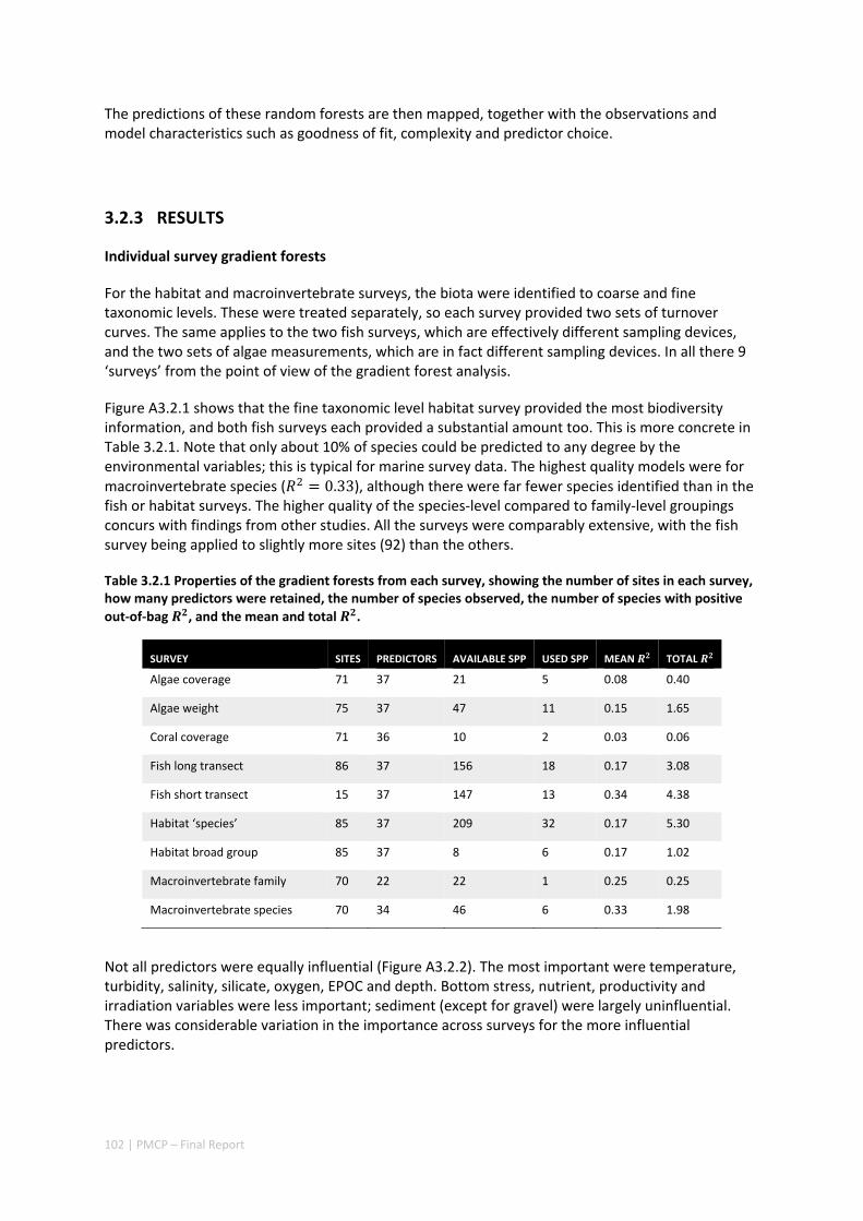
102 | PMCP – Final Report
The predictions of these random forests are then mapped, together with the observations and model characteristics such as goodness of fit, complexity and predictor choice.
3.2.3 RESULTS
Individual survey gradient forests
For the habitat and macroinvertebrate surveys, the biota were identified to coarse and fine taxonomic levels. These were treated separately, so each survey provided two sets of turnover curves. The same applies to the two fish surveys, which are effectively different sampling devices, and the two sets of algae measurements, which are in fact different sampling devices. In all there 9 ‘surveys’ from the point of view of the gradient forest analysis.
Figure A3.2.1 shows that the fine taxonomic level habitat survey provided the most biodiversity information, and both fish surveys each provided a substantial amount too. This is more concrete in Table 3.2.1. Note that only about 10% of species could be predicted to any degree by the environmental variables; this is typical for marine survey data. The highest quality models were for macroinvertebrate species ( 0.33), although there were far fewer species identified than in the fish or habitat surveys. The higher quality of the species‐level compared to family‐level groupings concurs with findings from other studies. All the surveys were comparably extensive, with the fish survey being applied to slightly more sites (92) than the others.
Table 3.2.1 Properties of the gradient forests from each survey, showing the number of sites in each survey, how many predictors were retained, the number of species observed, the number of species with positive
out‐of‐bag , and the mean and total .
SURVEY SITES PREDICTORS AVAILABLE SPP USED SPP MEAN TOTAL
Algae coverage 71 37 21 5 0.08 0.40
Algae weight 75 37 47 11 0.15 1.65
Coral coverage 71 36 10 2 0.03 0.06
Fish long transect 86 37 156 18 0.17 3.08
Fish short transect 15 37 147 13 0.34 4.38
Habitat ‘species’ 85 37 209 32 0.17 5.30
Habitat broad group 85 37 8 6 0.17 1.02
Macroinvertebrate family 70 22 22 1 0.25 0.25
Macroinvertebrate species 70 34 46 6 0.33 1.98
Not all predictors were equally influential (Figure A3.2.2). The most important were temperature, turbidity, salinity, silicate, oxygen, EPOC and depth. Bottom stress, nutrient, productivity and irradiation variables were less important; sediment (except for gravel) were largely uninfluential. There was considerable variation in the importance across surveys for the more influential predictors.
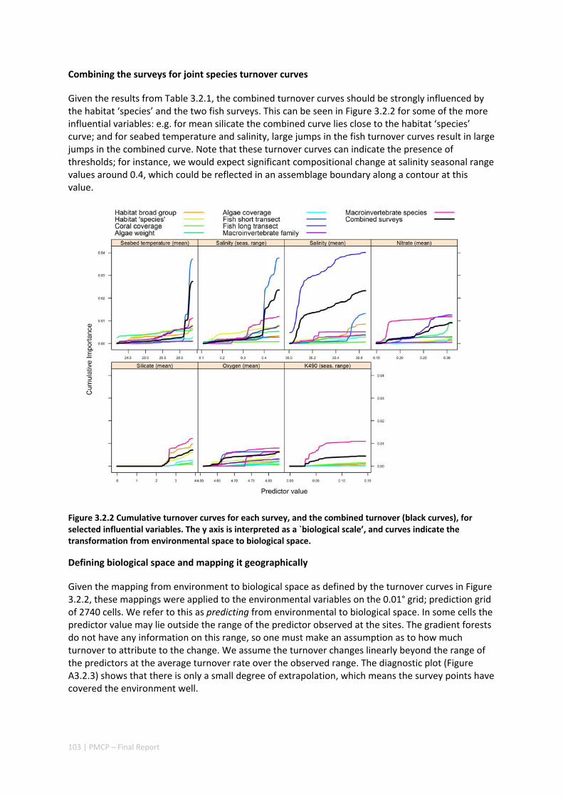
103 | PMCP – Final Report
Combining the surveys for joint species turnover curves
Given the results from Table 3.2.1, the combined turnover curves should be strongly influenced by the habitat ‘species’ and the two fish surveys. This can be seen in Figure 3.2.2 for some of the more influential variables: e.g. for mean silicate the combined curve lies close to the habitat ‘species’ curve; and for seabed temperature and salinity, large jumps in the fish turnover curves result in large jumps in the combined curve. Note that these turnover curves can indicate the presence of thresholds; for instance, we would expect significant compositional change at salinity seasonal range values around 0.4, which could be reflected in an assemblage boundary along a contour at this value.
Figure 3.2.2 Cumulative turnover curves for each survey, and the combined turnover (black curves), for selected influential variables. The y axis is interpreted as a `biological scale’, and curves indicate the transformation from environmental space to biological space.
Defining biological space and mapping it geographically
Given the mapping from environment to biological space as defined by the turnover curves in Figure 3.2.2, these mappings were applied to the environmental variables on the 0.01° grid; prediction grid of 2740 cells. We refer to this as predicting from environmental to biological space. In some cells the predictor value may lie outside the range of the predictor observed at the sites. The gradient forests do not have any information on this range, so one must make an assumption as to how much turnover to attribute to the change. We assume the turnover changes linearly beyond the range of the predictors at the average turnover rate over the observed range. The diagnostic plot (Figure A3.2.3) shows that there is only a small degree of extrapolation, which means the survey points have covered the environment well.
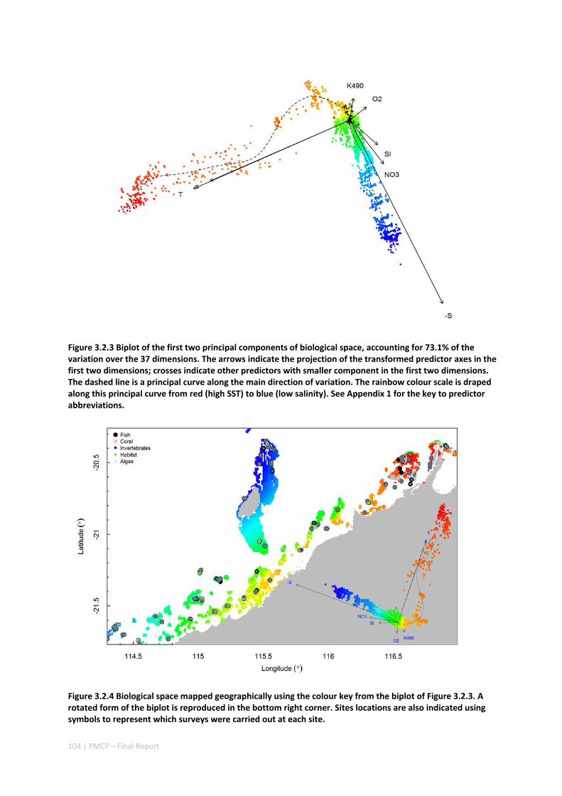
104 | PMCP – Final Report
Figure 3.2.3 Biplot of the first two principal components of biological space, accounting for 73.1% of the variation over the 37 dimensions. The arrows indicate the projection of the transformed predictor axes in the first two dimensions; crosses indicate other predictors with smaller component in the first two dimensions. The dashed line is a principal curve along the main direction of variation. The rainbow colour scale is draped along this principal curve from red (high SST) to blue (low salinity). See Appendix 1 for the key to predictor abbreviations.
Figure 3.2.4 Biological space mapped geographically using the colour key from the biplot of Figure 3.2.3. A rotated form of the biplot is reproduced in the bottom right corner. Sites locations are also indicated using symbols to represent which surveys were carried out at each site.
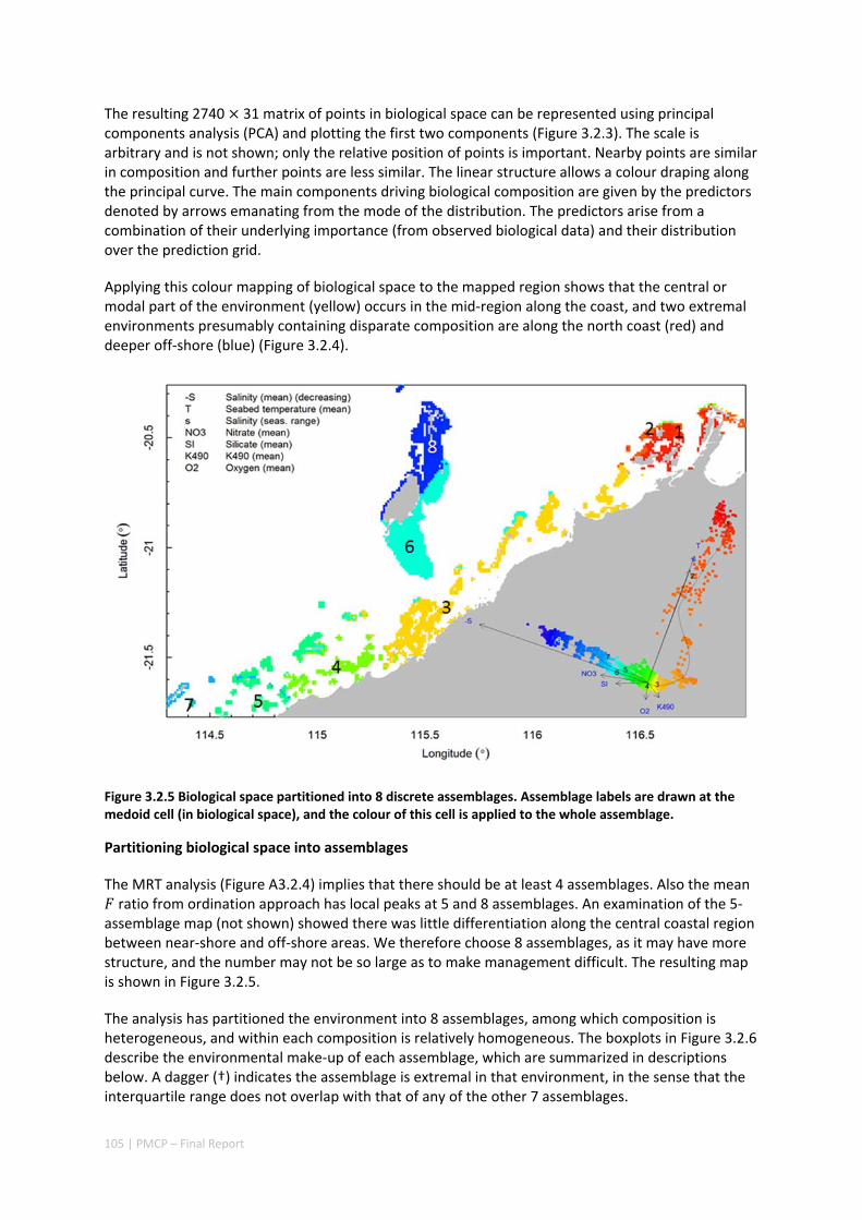
105 | PMCP – Final Report
The resulting 2740 31 matrix of points in biological space can be represented using principal components analysis (PCA) and plotting the first two components (Figure 3.2.3). The scale is arbitrary and is not shown; only the relative position of points is important. Nearby points are similar in composition and further points are less similar. The linear structure allows a colour draping along the principal curve. The main components driving biological composition are given by the predictors denoted by arrows emanating from the mode of the distribution. The predictors arise from a combination of their underlying importance (from observed biological data) and their distribution over the prediction grid.
Applying this colour mapping of biological space to the mapped region shows that the central or modal part of the environment (yellow) occurs in the mid‐region along the coast, and two extremal environments presumably containing disparate composition are along the north coast (red) and deeper off‐shore (blue) (Figure 3.2.4).
Figure 3.2.5 Biological space partitioned into 8 discrete assemblages. Assemblage labels are drawn at the medoid cell (in biological space), and the colour of this cell is applied to the whole assemblage.
Partitioning biological space into assemblages
The MRT analysis (Figure A3.2.4) implies that there should be at least 4 assemblages. Also the mean ratio from ordination approach has local peaks at 5 and 8 assemblages. An examination of the 5‐
assemblage map (not shown) showed there was little differentiation along the central coastal region between near‐shore and off‐shore areas. We therefore choose 8 assemblages, as it may have more structure, and the number may not be so large as to make management difficult. The resulting map is shown in Figure 3.2.5.
The analysis has partitioned the environment into 8 assemblages, among which composition is heterogeneous, and within each composition is relatively homogeneous. The boxplots in Figure 3.2.6 describe the environmental make‐up of each assemblage, which are summarized in descriptions below. A dagger (†) indicates the assemblage is extremal in that environment, in the sense that the interquartile range does not overlap with that of any of the other 7 assemblages.
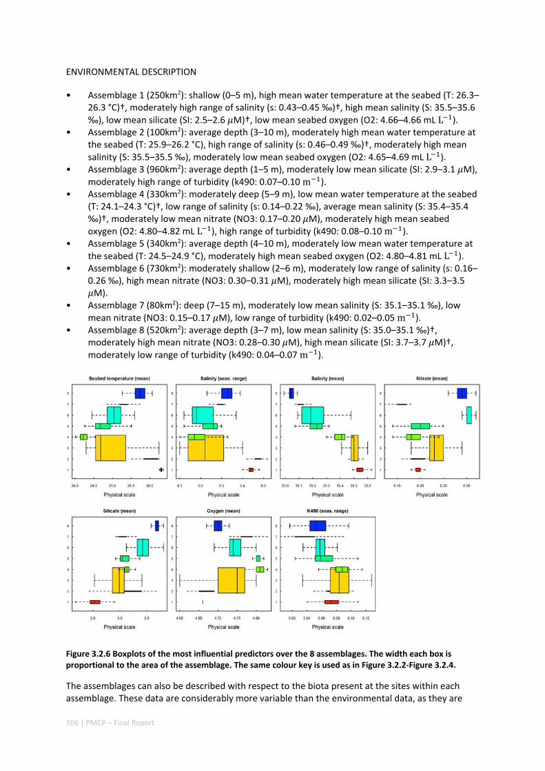
106 | PMCP – Final Report
ENVIRONMENTAL DESCRIPTION
• Assemblage 1 (250km2): shallow (0–5 m), high mean water temperature at the seabed (T: 26.3–26.3 °C)†, moderately high range of salinity (s: 0.43–0.45 ‰)†, high mean salinity (S: 35.5–35.6 ‰), low mean silicate (SI: 2.5–2.6 M)†, low mean seabed oxygen (O2: 4.66–4.66 mL L ).
• Assemblage 2 (100km2): average depth (3–10 m), moderately high mean water temperature at the seabed (T: 25.9–26.2 °C), high range of salinity (s: 0.46–0.49 ‰)†, moderately high mean salinity (S: 35.5–35.5 ‰), moderately low mean seabed oxygen (O2: 4.65–4.69 mL L ).
• Assemblage 3 (960km2): average depth (1–5 m), moderately low mean silicate (SI: 2.9–3.1 M), moderately high range of turbidity (k490: 0.07–0.10 m ).
• Assemblage 4 (330km2): moderately deep (5–9 m), low mean water temperature at the seabed (T: 24.1–24.3 °C)†, low range of salinity (s: 0.14–0.22 ‰), average mean salinity (S: 35.4–35.4 ‰)†, moderately low mean nitrate (NO3: 0.17–0.20 M), moderately high mean seabed oxygen (O2: 4.80–4.82 mL L ), high range of turbidity (k490: 0.08–0.10 m ).
• Assemblage 5 (340km2): average depth (4–10 m), moderately low mean water temperature at the seabed (T: 24.5–24.9 °C), moderately high mean seabed oxygen (O2: 4.80–4.81 mL L ).
• Assemblage 6 (730km2): moderately shallow (2–6 m), moderately low range of salinity (s: 0.16–0.26 ‰), high mean nitrate (NO3: 0.30–0.31 M), moderately high mean silicate (SI: 3.3–3.5 M).
• Assemblage 7 (80km2): deep (7–15 m), moderately low mean salinity (S: 35.1–35.1 ‰), low mean nitrate (NO3: 0.15–0.17 M), low range of turbidity (k490: 0.02–0.05 m ).
• Assemblage 8 (520km2): average depth (3–7 m), low mean salinity (S: 35.0–35.1 ‰)†, moderately high mean nitrate (NO3: 0.28–0.30 M), high mean silicate (SI: 3.7–3.7 M)†, moderately low range of turbidity (k490: 0.04–0.07 m ).
Figure 3.2.6 Boxplots of the most influential predictors over the 8 assemblages. The width each box is proportional to the area of the assemblage. The same colour key is used as in Figure 3.2.2‐Figure 3.2.4.
The assemblages can also be described with respect to the biota present at the sites within each assemblage. These data are considerably more variable than the environmental data, as they are
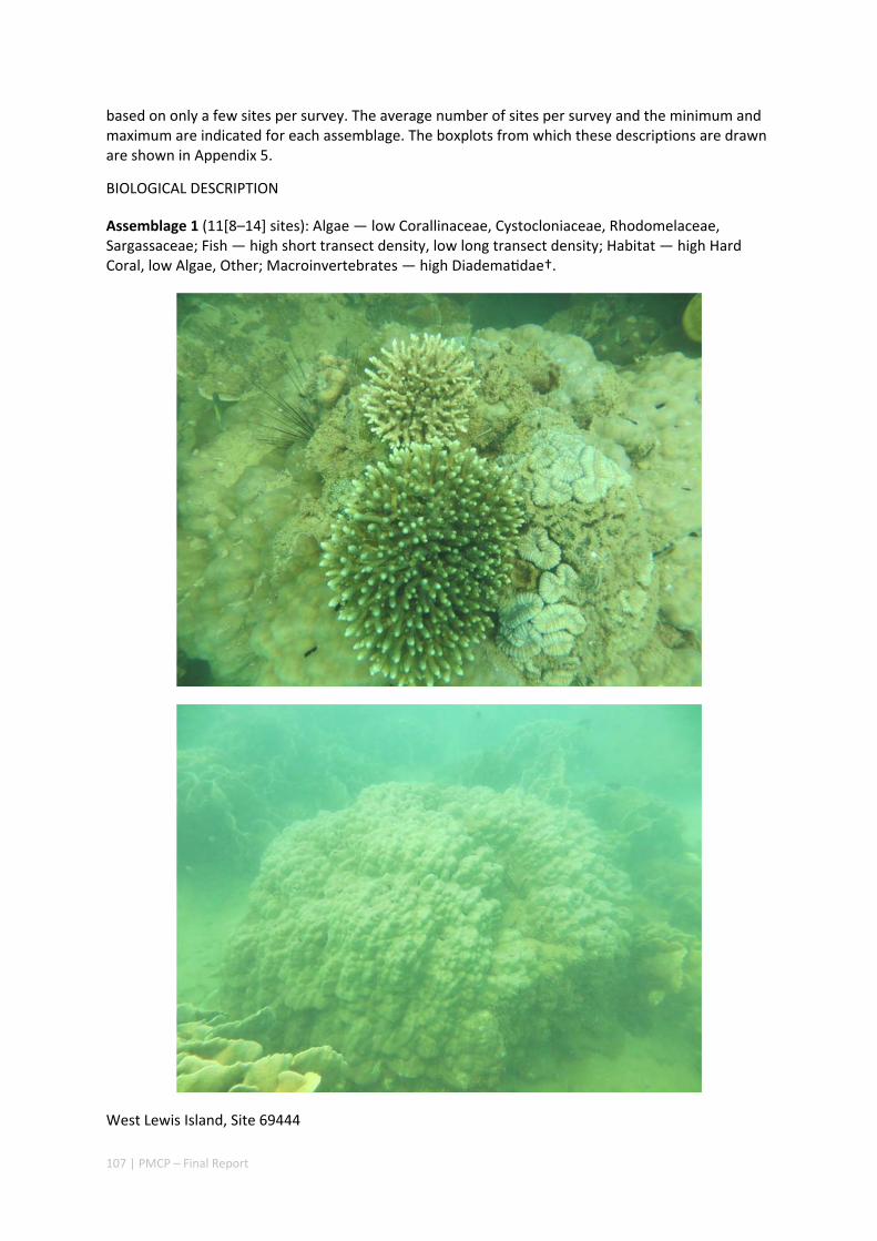
107 | PMCP – Final Report
based on only a few sites per survey. The average number of sites per survey and the minimum and maximum are indicated for each assemblage. The boxplots from which these descriptions are drawn are shown in Appendix 5.
BIOLOGICAL DESCRIPTION
Assemblage 1 (11[8–14] sites): Algae — low Corallinaceae, Cystocloniaceae, Rhodomelaceae, Sargassaceae; Fish — high short transect density, low long transect density; Habitat — high Hard Coral, low Algae, Other; Macroinvertebrates — high Diadema dae†.
West Lewis Island, Site 69444
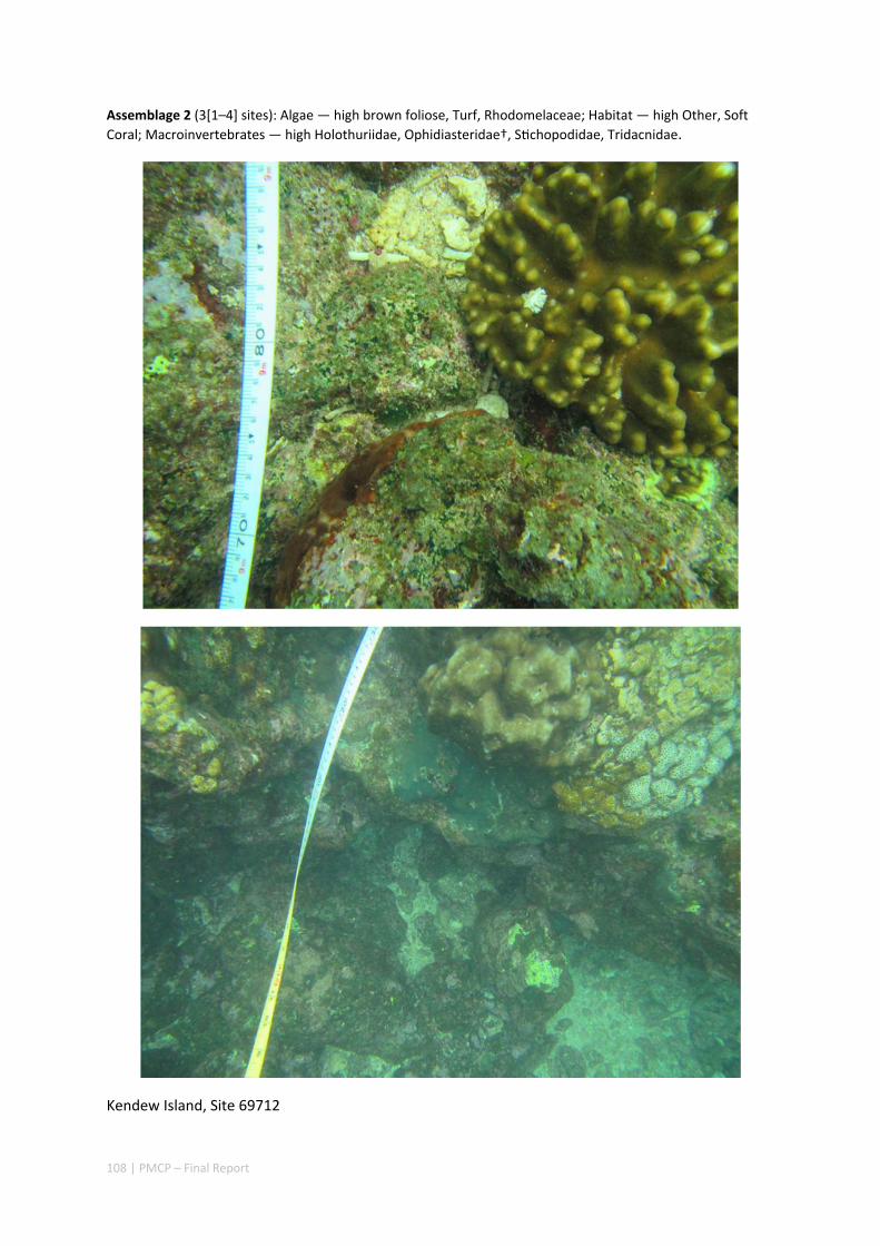
108 | PMCP – Final Report
Assemblage 2 (3[1–4] sites): Algae — high brown foliose, Turf, Rhodomelaceae; Habitat — high Other, Soft
Coral; Macroinvertebrates — high Holothuriidae, Ophidiasteridae†, S chopodidae, Tridacnidae.
Kendew Island, Site 69712
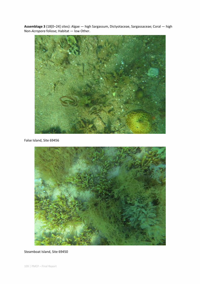
109 | PMCP – Final Report
Assemblage 3 (18[0–24] sites): Algae — high Sargassum, Dictyotaceae, Sargassaceae; Coral — high Non‐Acropora foliose; Habitat — low Other.
False Island, Site 69456
Steamboat Island, Site 69450
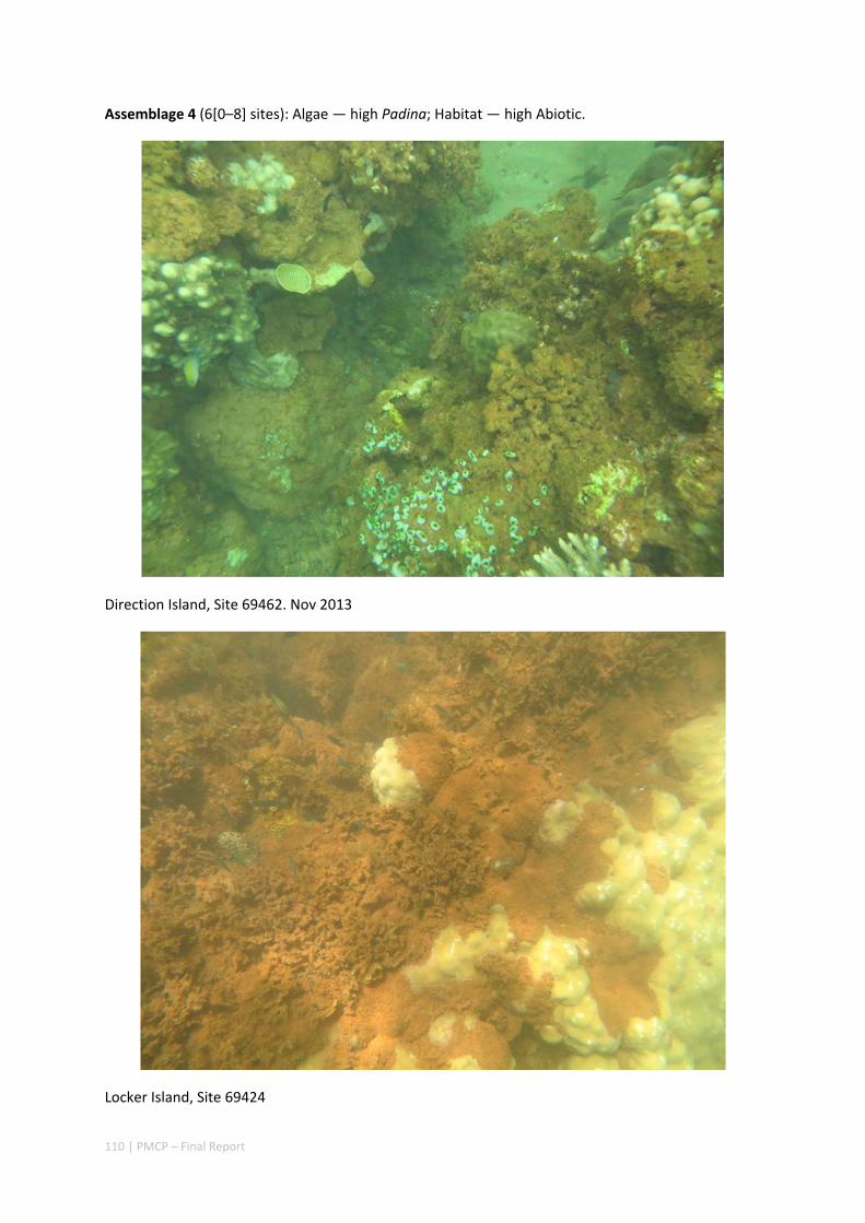
110 | PMCP – Final Report
Assemblage 4 (6[0–8] sites): Algae — high Padina; Habitat — high Abiotic.
Direction Island, Site 69462. Nov 2013
Locker Island, Site 69424
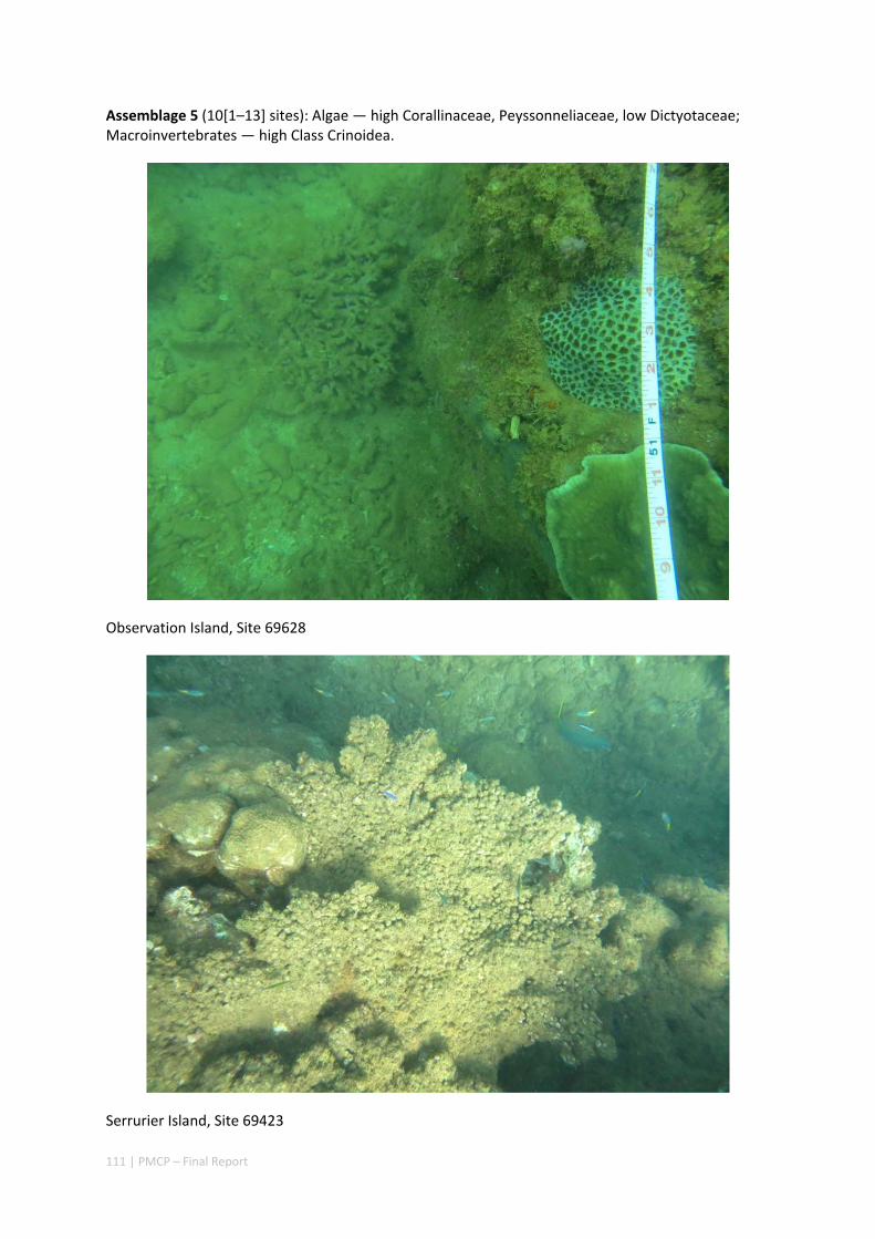
111 | PMCP – Final Report
Assemblage 5 (10[1–13] sites): Algae — high Corallinaceae, Peyssonneliaceae, low Dictyotaceae; Macroinvertebrates — high Class Crinoidea.
Observation Island, Site 69628
Serrurier Island, Site 69423
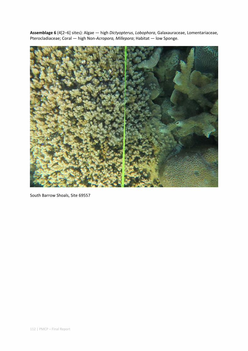
112 | PMCP – Final Report
Assemblage 6 (4[2–6] sites): Algae — high Dictyopterus, Lobophora, Galaxauraceae, Lomentariaceae, Pterocladiaceae; Coral — high Non‐Acropora, Millepora; Habitat — low Sponge.
South Barrow Shoals, Site 69557
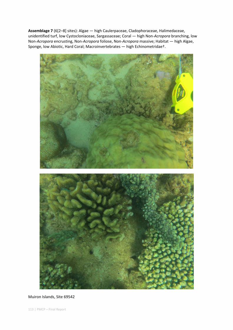
113 | PMCP – Final Report
Assemblage 7 (6[2–8] sites): Algae — high Caulerpaceae, Cladophoraceae, Halimedaceae, unidentified turf, low Cystocloniaceae, Sargassaceae; Coral — high Non‐Acropora branching, low Non‐Acropora encrusting, Non‐Acropora foliose, Non‐Acropora massive; Habitat — high Algae, Sponge, low Abiotic, Hard Coral; Macroinvertebrates — high Echinometridae†.
Muiron Islands, Site 69542
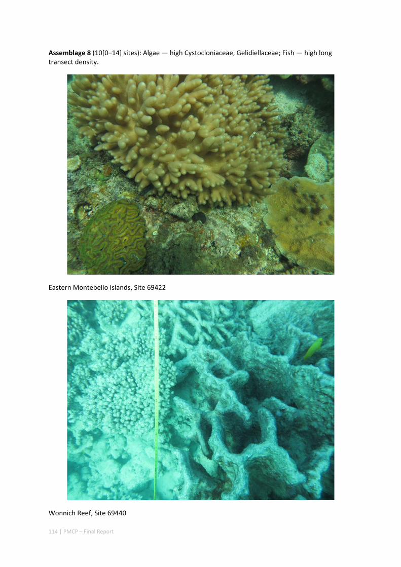
114 | PMCP – Final Report
Assemblage 8 (10[0–14] sites): Algae — high Cystocloniaceae, Gelidiellaceae; Fish — high long transect density.
Eastern Montebello Islands, Site 69422
Wonnich Reef, Site 69440

115 | PMCP – Final Report
Species distribution models
All taxa were analysed and the optimal random forest model was found. A range of transformations of the observed response variable were tried. The resulting models are listed in Table 3.2.2. Maps of these are shown in Appendix 6. For all other species, either there were not sufficient samples to model them or there were no influential predictors. As is typical of biological sampling, a large proportion of taxa were sampled at only one or a very few sites. However, compared with the total number of species sampled (698), relatively fewer species were considered frequent enough for analyses (at ≥5 sites). Nevertheless, there were about 233 species/taxa that met this criterion, including 15 that were sampled by both devices. The randomForest method provided a robust and flexible approach for modelling statistical relationships between the biological data and environmental gradients, and for identifying the important variables and predicting distributions. Ultimately, accounting for species modelled from both devices and joint modelling, 143 taxa had ‘successful’ models. Species with unsuccessful models had no statistically predictable relationship with the environmental variables. For the majority of species, i.e. those occurring at <5 sites, no individual analyses or modelling was possible, although the sample data are available. While the environmental variables have demonstrable utility for predicting the regional distribution of many species with adequate frequency of occurrence, not all the successful models could predict well even if they fitted the site data well. That is, they do not often account for the majority of observed variation in local biomass—other factors, including stochastic processes such as recruitment and mortality, biological interactions, and random sampling effects typically outweigh deterministic environmental relationships, or habitat preferences, at the local site biomass scale. Nevertheless, the regional scale patterns of distribution are representative.
Table 3.2.2 Properties of the individual random forest models. is the prevalence, is the transformation applied to the raw species data, and is the goodness of fit statistic based on the out‐of‐bag observations. The taxonomic levels of family and species are self‐explanatory; the operational taxonomic unit (OTU) is usually species, but may be some other convenient grouping (e.g. unidentified turf ‐ red); coral is classified in broad categories, and some habitat in broad groups; all fish are identified to species.
SURVEY DEVICE LEVEL TAXON
Algae coverage long transect Family Caulerpa / 9 0.140
Algae coverage long transect Family red foliose log 9 0.244
Algae coverage long transect Family Halimeda / 20 0.222
Algae coverage long transect Family Sargassum log 25 0.307
Algae coverage long transect Family Padina log 27 0.247
Algae weight 25cm quadrat OTU Sporochnus comosus / 5 0.208
Algae weight 25cm quadrat OTU Laurencia sp9 / 5 0.258
Algae weight 25cm quadrat OTU Hypnea sp4 / 6 0.219
Algae weight 25cm quadrat OTU Colpomenia sinuosa / 6 0.314
Algae weight 25cm quadrat OTU Portieria sp. / 6 0.264
Algae weight 25cm quadrat OTU Hydroclathrus clathratus 7 0.649
Algae weight 25cm quadrat OTU Leveillea jungermannioides / 7 0.339
Algae weight 25cm quadrat OTU Hypnea nidifica 7 0.466
Algae weight 25cm quadrat OTU Lomentaria sp1 / 8 0.133
Algae weight 25cm quadrat OTU Champia parvula / 8 0.177
Algae weight 25cm quadrat OTU Rhodymenia sp. / 8 0.269
Algae weight 25cm quadrat OTU Valonia ventricosa / 9 0.209
Algae weight 25cm quadrat OTU Bornetella sphaerica / 9 0.158
Algae weight 25cm quadrat OTU Sargassum unidentified 6 / 9 0.403
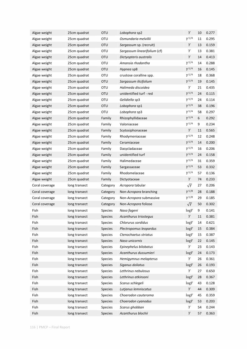
116 | PMCP – Final Report
Algae weight 25cm quadrat OTU Lobophora sp2 10 0.277
Algae weight 25cm quadrat OTU Osmundaria melvillii / 11 0.295
Algae weight 25cm quadrat OTU Sargassum sp. (recruit) 13 0.159
Algae weight 25cm quadrat OTU Sargassum linearifolium (cf) 13 0.381
Algae weight 25cm quadrat OTU Dictyopteris australis 14 0.413
Algae weight 25cm quadrat OTU Amansia rhodantha / 14 0.288
Algae weight 25cm quadrat OTU Hypnea sp8 / 16 0.145
Algae weight 25cm quadrat OTU crustose coralline spp. / 18 0.368
Algae weight 25cm quadrat OTU Sargassum ilicifolium / 19 0.145
Algae weight 25cm quadrat OTU Halimeda discoidea 21 0.435
Algae weight 25cm quadrat OTU unidentified turf ‐ red / 24 0.115
Algae weight 25cm quadrat OTU Gelidiella sp3 / 24 0.114
Algae weight 25cm quadrat OTU Lobophora sp1 / 38 0.196
Algae weight 25cm quadrat OTU Lobophora sp3 / 58 0.297
Algae weight 25cm quadrat Family Rhizophyllidaceae / 6 0.292
Algae weight 25cm quadrat Family Valoniaceae / 9 0.234
Algae weight 25cm quadrat Family Scytosiphonaceae 11 0.565
Algae weight 25cm quadrat Family Rhodymeniaceae / 12 0.248
Algae weight 25cm quadrat Family Ceramiaceae / 14 0.200
Algae weight 25cm quadrat Family Dasycladaceae / 16 0.206
Algae weight 25cm quadrat Family unidentified turf / 24 0.158
Algae weight 25cm quadrat Family Halimedaceae / 31 0.359
Algae weight 25cm quadrat Family Sargassaceae / 53 0.332
Algae weight 25cm quadrat Family Rhodomelaceae / 57 0.136
Algae weight 25cm quadrat Family Dictyotaceae 74 0.233
Coral coverage long transect Category Acropora tabular √ 27 0.206
Coral coverage long transect Category Non‐Acropora branching / 28 0.188
Coral coverage long transect Category Non‐Acropora submassive / 29 0.185
Coral coverage long transect Category Non‐Acropora foliose √ 50 0.302
Fish long transect Species Naso fageni log 9 0.141
Fish long transect Species Acanthurus triostegus 11 0.381
Fish long transect Species Chlorurus sordidus log 14 0.621
Fish long transect Species Plectropomus leopardus log 15 0.384
Fish long transect Species Ctenochaetus striatus log 15 0.387
Fish long transect Species Naso unicornis log 22 0.145
Fish long transect Species Epinephelus bilobatus 23 0.143
Fish long transect Species Acanthurus dussumieri log 24 0.173
Fish long transect Species Hemigymnus melapterus 26 0.361
Fish long transect Species Siganus doliatus log 26 0.193
Fish long transect Species Lethrinus nebulosus 27 0.650
Fish long transect Species Lethrinus atkinsoni log 28 0.367
Fish long transect Species Scarus schlegeli log 43 0.128
Fish long transect Species Lutjanus lemniscatus 44 0.309
Fish long transect Species Choerodon cauteroma log 45 0.359
Fish long transect Species Choerodon cyanodus log 53 0.203
Fish long transect Species Scarus ghobban 54 0.244
Fish long transect Species Acanthurus blochii 57 0.363
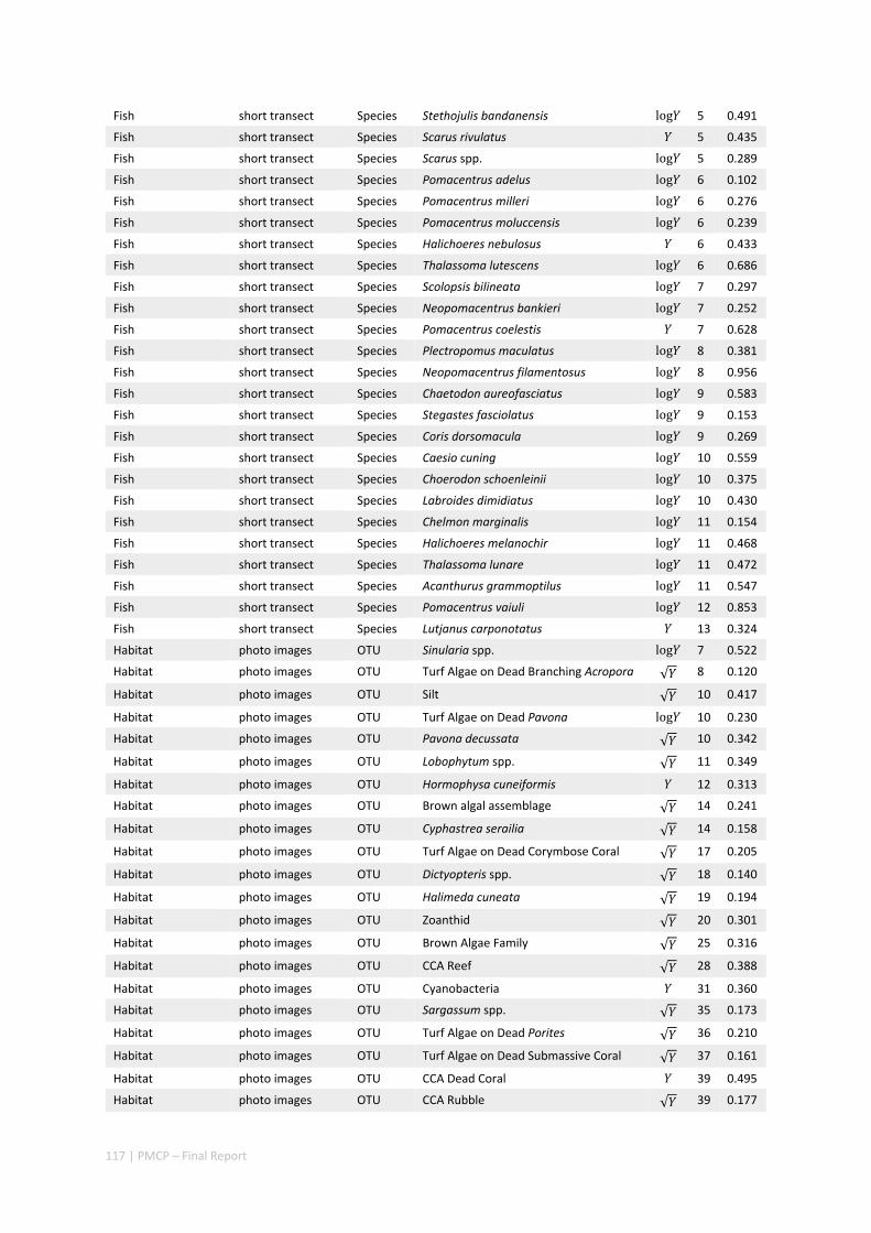
117 | PMCP – Final Report
Fish short transect Species Stethojulis bandanensis log 5 0.491
Fish short transect Species Scarus rivulatus 5 0.435
Fish short transect Species Scarus spp. log 5 0.289
Fish short transect Species Pomacentrus adelus log 6 0.102
Fish short transect Species Pomacentrus milleri log 6 0.276
Fish short transect Species Pomacentrus moluccensis log 6 0.239
Fish short transect Species Halichoeres nebulosus 6 0.433
Fish short transect Species Thalassoma lutescens log 6 0.686
Fish short transect Species Scolopsis bilineata log 7 0.297
Fish short transect Species Neopomacentrus bankieri log 7 0.252
Fish short transect Species Pomacentrus coelestis 7 0.628
Fish short transect Species Plectropomus maculatus log 8 0.381
Fish short transect Species Neopomacentrus filamentosus log 8 0.956
Fish short transect Species Chaetodon aureofasciatus log 9 0.583
Fish short transect Species Stegastes fasciolatus log 9 0.153
Fish short transect Species Coris dorsomacula log 9 0.269
Fish short transect Species Caesio cuning log 10 0.559
Fish short transect Species Choerodon schoenleinii log 10 0.375
Fish short transect Species Labroides dimidiatus log 10 0.430
Fish short transect Species Chelmon marginalis log 11 0.154
Fish short transect Species Halichoeres melanochir log 11 0.468
Fish short transect Species Thalassoma lunare log 11 0.472
Fish short transect Species Acanthurus grammoptilus log 11 0.547
Fish short transect Species Pomacentrus vaiuli log 12 0.853
Fish short transect Species Lutjanus carponotatus 13 0.324
Habitat photo images OTU Sinularia spp. log 7 0.522
Habitat photo images OTU Turf Algae on Dead Branching Acropora √ 8 0.120
Habitat photo images OTU Silt √ 10 0.417
Habitat photo images OTU Turf Algae on Dead Pavona log 10 0.230
Habitat photo images OTU Pavona decussata √ 10 0.342
Habitat photo images OTU Lobophytum spp. √ 11 0.349
Habitat photo images OTU Hormophysa cuneiformis 12 0.313
Habitat photo images OTU Brown algal assemblage √ 14 0.241
Habitat photo images OTU Cyphastrea serailia √ 14 0.158
Habitat photo images OTU Turf Algae on Dead Corymbose Coral √ 17 0.205
Habitat photo images OTU Dictyopteris spp. √ 18 0.140
Habitat photo images OTU Halimeda cuneata √ 19 0.194
Habitat photo images OTU Zoanthid √ 20 0.301
Habitat photo images OTU Brown Algae Family √ 25 0.316
Habitat photo images OTU CCA Reef √ 28 0.388
Habitat photo images OTU Cyanobacteria 31 0.360
Habitat photo images OTU Sargassum spp. √ 35 0.173
Habitat photo images OTU Turf Algae on Dead Porites √ 36 0.210
Habitat photo images OTU Turf Algae on Dead Submassive Coral √ 37 0.161
Habitat photo images OTU CCA Dead Coral 39 0.495
Habitat photo images OTU CCA Rubble √ 39 0.177
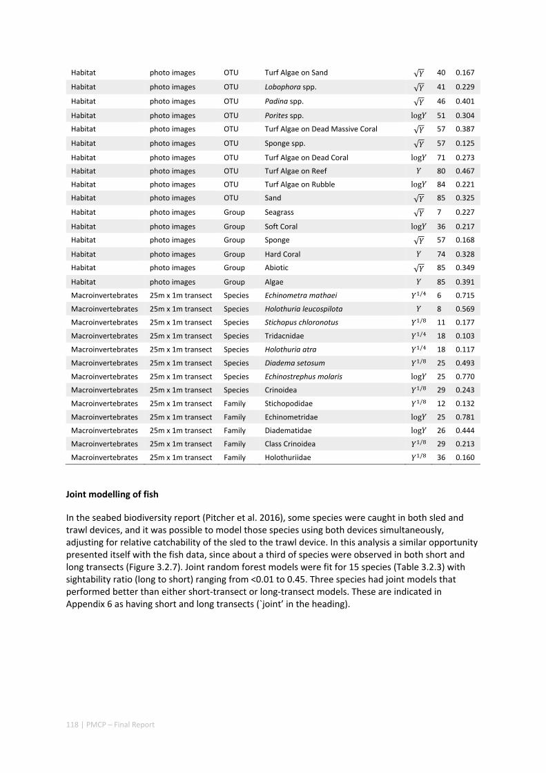
118 | PMCP – Final Report
Habitat photo images OTU Turf Algae on Sand √ 40 0.167
Habitat photo images OTU Lobophora spp. √ 41 0.229
Habitat photo images OTU Padina spp. √ 46 0.401
Habitat photo images OTU Porites spp. log 51 0.304
Habitat photo images OTU Turf Algae on Dead Massive Coral √ 57 0.387
Habitat photo images OTU Sponge spp. √ 57 0.125
Habitat photo images OTU Turf Algae on Dead Coral log 71 0.273
Habitat photo images OTU Turf Algae on Reef 80 0.467
Habitat photo images OTU Turf Algae on Rubble log 84 0.221
Habitat photo images OTU Sand √ 85 0.325
Habitat photo images Group Seagrass √ 7 0.227
Habitat photo images Group Soft Coral log 36 0.217
Habitat photo images Group Sponge √ 57 0.168
Habitat photo images Group Hard Coral 74 0.328
Habitat photo images Group Abiotic √ 85 0.349
Habitat photo images Group Algae 85 0.391
Macroinvertebrates 25m x 1m transect Species Echinometra mathaei / 6 0.715
Macroinvertebrates 25m x 1m transect Species Holothuria leucospilota 8 0.569
Macroinvertebrates 25m x 1m transect Species Stichopus chloronotus / 11 0.177
Macroinvertebrates 25m x 1m transect Species Tridacnidae / 18 0.103
Macroinvertebrates 25m x 1m transect Species Holothuria atra / 18 0.117
Macroinvertebrates 25m x 1m transect Species Diadema setosum / 25 0.493
Macroinvertebrates 25m x 1m transect Species Echinostrephus molaris log 25 0.770
Macroinvertebrates 25m x 1m transect Species Crinoidea / 29 0.243
Macroinvertebrates 25m x 1m transect Family Stichopodidae / 12 0.132
Macroinvertebrates 25m x 1m transect Family Echinometridae log 25 0.781
Macroinvertebrates 25m x 1m transect Family Diadematidae log 26 0.444
Macroinvertebrates 25m x 1m transect Family Class Crinoidea / 29 0.213
Macroinvertebrates 25m x 1m transect Family Holothuriidae / 36 0.160
Joint modelling of fish
In the seabed biodiversity report (Pitcher et al. 2016), some species were caught in both sled and trawl devices, and it was possible to model those species using both devices simultaneously, adjusting for relative catchability of the sled to the trawl device. In this analysis a similar opportunity presented itself with the fish data, since about a third of species were observed in both short and long transects (Figure 3.2.7). Joint random forest models were fit for 15 species (Table 3.2.3) with sightability ratio (long to short) ranging from <0.01 to 0.45. Three species had joint models that performed better than either short‐transect or long‐transect models. These are indicated in Appendix 6 as having short and long transects (`joint’ in the heading).

119 | PMCP – Final Report
Figure 3.2.7 Density of fish species at sites observed in long and short transects. The species towards the middle are observed in both types of transect, whereas species to the sides are all specific to one transect or the other. In the overlapping region, sites are plotted twice for each species, with short transects above long transects. Densities tend to be higher in short transects. The dashed rectangle indicates the 15 species for which joint modelling was applied and the sites at which both methods were deployed. The 3 species for which the joint model was the best model are within the solid rectangle; species to the left of this had preferred models using long transects, and species to the right preferred short transects.
Table 3.2.3 Fish species that could be modelled using both short and long transect data. The factor is the estimated catchability of the long transect relative to the short transect. For joint models, the data are combined by multiplying the long transect data by this factor. is the number of sites at which the species was observed in both surveys.
SPECIES FACTOR
Acanthurus grammoptilus 0.00 11 5 4 0.55 ‐0.14 ‐0.06
Caesio cuning 0.00 10 8 5 0.56 0.03 0.08
Scolopsis bilineata 0.00 7 8 3 0.30 0.04 0.04
Parupeneus indicus 0.00 9 20 13 0.07 0.07 0.11
Acanthurus triostegus 0.04 6 11 3 0.11 0.38 0.25
Choerodon schoenleinii 0.06 10 38 24 0.37 ‐0.04 ‐0.04
Scarus NA 0.07 5 19 6 0.29 0.25 0.20
Scarus rivulatus 0.10 5 29 8 0.43 0.41 0.47
Scarus ghobban 0.17 12 54 41 0.14 0.24 0.15
Hemigymnus melapterus 0.19 8 26 12 0.08 0.36 0.29
Choerodon cyanodus 0.21 9 53 30 0.10 0.20 0.17
Plectropomus maculatus 0.25 8 47 25 0.38 0.20 0.19
Lutjanus lemniscatus 0.27 11 44 30 0.06 0.31 0.25
Choerodon cauteroma 0.37 7 45 19 0.03 0.36 0.41
Lutjanus carponotatus 0.45 13 62 51 0.32 0.19 0.01
120 | PMCP – Final Report
3.2.4 DISCUSSION
The project has demonstrated substantial biodiversity on seabed of the Pilbara region, and has filled in data gaps for the majority of the reefs in the study area, much of which had no pre‐existing data. Most of the prior biological knowledge about the region comes from surveys within existing and proposed marine parks and from largely unpublished reports conducted as part of development approval and monitoring requirements. These new data and analyses have documented the important relationships between sampled species distributions and environmental gradients that have been used to predict patterns of coral reef assemblages and if species distributions at regional scale. These maps of regional biodiversity are more comprehensive and more detailed than available previously (e.g. Lyne et al. 2006).
The Pilbara shelf seabed is a complex mix of physical environments. The biological assemblages were observed to respond significantly to the multiple interacting physical gradients and few of these gradients have simple trends in geographic space. Some of the environmental gradients most associated with driving patterns of biodiversity composition include: average annual sea surface temperature, which is higher in the NE of the region cf. the SW; seasonal range in salinity, which is greater in the NE coastal areas and lowest in central areas; seasonal range in bottom temperature, which is greater in central and NE inshore areas and lowest in deeper offshore area; mean nitrate, which is low in the southwest, and higher offshore at Barrow and the Montebello Islands; bottom water oxygen, which is higher on SW shelf areas and decreasing to the NE and with depth; mean silicate, which is low in the central Dampier Archipelago and high offshore at Barrow and the Montebellos; and turbidity, which is higher in inshore areas. Other variables also are associated with biodiversity patterns but are increasingly less important overall, including those related to light, productivity, and sediment types. These gradients in the Pilbara are perhaps not as strong as in some other areas such as the Torres Strait and parts of the Great Barrier Reef region, where sediment types and seabed current stress are strong drivers (Pitcher et al. 2002, 2007a, b).
The multitude of species sampled, modelled and mapped respond in different, overlapping and varying ways to the multiple interacting environmental variables, which as noted above do not have simple trends in geographic space. Different species were associated with different variables, and some positively and others negatively to the same variables. Overall, the important variables for species were largely in line with the environmental variables associated with assemblage patterns.
Biological assemblages showed both inshore ‐ offshore gradients and latitudinal gradients from the northeast to the southwest. The results confirm and extend the observations of cross‐shelf trends in reef building coral assemblages on the Pilbara shelf (Radford 2005) with distinct inshore and offshore assemblages of coral reef biota both within the Dampier Archipelago and across the shelf from coastal areas through the eastern areas of Barrow Island and offshore to the Montebello Islands. In contrast to the differentiation between seafloor assemblages north and south of Barrow Island, there was a continuity of habitat on inshore reefs from Eaglehawk Island north of Cape Preston to Maryanne Reef northeast of Onslow. This assemblage roughly corresponds with the Robe region described by the Wilson report (Wilson 1994). The level of resolution in biological assemblages achieved in this study is considerably greater than previous classifications such as the IMCRA bioregionalisation which proposed an Inshore Pilbara zone and an Offshore Pilbara zone in the region. Our analysis has revealed five distinct assemblages in the inshore areas between northern Ningaloo and the Dampier Archipelago, with the offshore area comprised of three areas including the Muiron Islands, eastern Barrow and Lowendahl Islands, and the Montebello Islands. In many respects it has validated the heuristic conclusions of the Wilson Report which suggested the same three offshore zones and four inshore zones (Dampier, Robe, Thevenard and Exmouth Gulf (Wilson 1994). The zones outlined by Wilson were not continuous so this analysis constitutes a significantly higher level of detail beyond its empirical foundations.
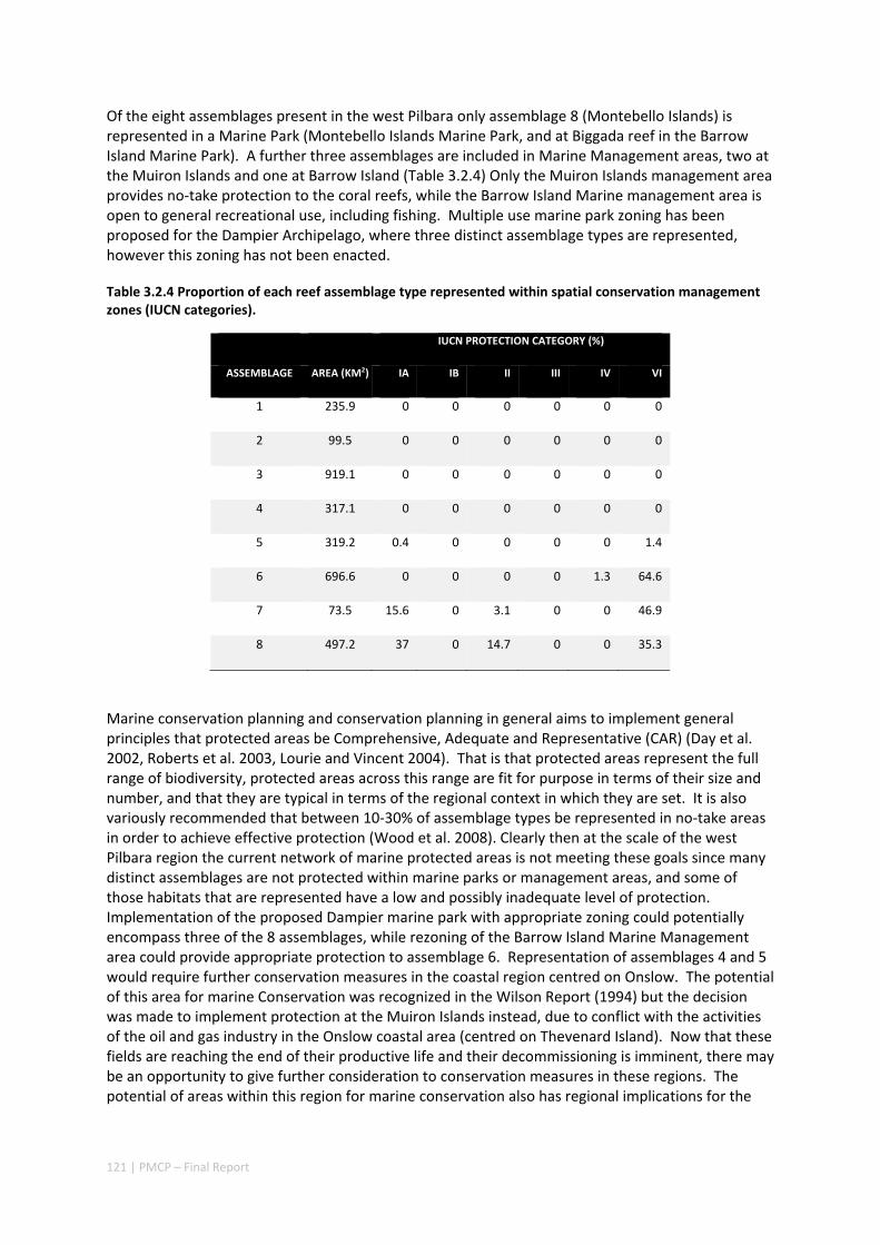
121 | PMCP – Final Report
Of the eight assemblages present in the west Pilbara only assemblage 8 (Montebello Islands) is represented in a Marine Park (Montebello Islands Marine Park, and at Biggada reef in the Barrow Island Marine Park). A further three assemblages are included in Marine Management areas, two at the Muiron Islands and one at Barrow Island (Table 3.2.4) Only the Muiron Islands management area provides no‐take protection to the coral reefs, while the Barrow Island Marine management area is open to general recreational use, including fishing. Multiple use marine park zoning has been proposed for the Dampier Archipelago, where three distinct assemblage types are represented, however this zoning has not been enacted.
Table 3.2.4 Proportion of each reef assemblage type represented within spatial conservation management zones (IUCN categories).
IUCN PROTECTION CATEGORY (%)
ASSEMBLAGE AREA (KM2) IA IB II III IV VI
1 235.9 0 0 0 0 0 0
2 99.5 0 0 0 0 0 0
3 919.1 0 0 0 0 0 0
4 317.1 0 0 0 0 0 0
5 319.2 0.4 0 0 0 0 1.4
6 696.6 0 0 0 0 1.3 64.6
7 73.5 15.6 0 3.1 0 0 46.9
8 497.2 37 0 14.7 0 0 35.3
Marine conservation planning and conservation planning in general aims to implement general principles that protected areas be Comprehensive, Adequate and Representative (CAR) (Day et al. 2002, Roberts et al. 2003, Lourie and Vincent 2004). That is that protected areas represent the full range of biodiversity, protected areas across this range are fit for purpose in terms of their size and number, and that they are typical in terms of the regional context in which they are set. It is also variously recommended that between 10‐30% of assemblage types be represented in no‐take areas in order to achieve effective protection (Wood et al. 2008). Clearly then at the scale of the west Pilbara region the current network of marine protected areas is not meeting these goals since many distinct assemblages are not protected within marine parks or management areas, and some of those habitats that are represented have a low and possibly inadequate level of protection. Implementation of the proposed Dampier marine park with appropriate zoning could potentially encompass three of the 8 assemblages, while rezoning of the Barrow Island Marine Management area could provide appropriate protection to assemblage 6. Representation of assemblages 4 and 5 would require further conservation measures in the coastal region centred on Onslow. The potential of this area for marine Conservation was recognized in the Wilson Report (1994) but the decision was made to implement protection at the Muiron Islands instead, due to conflict with the activities of the oil and gas industry in the Onslow coastal area (centred on Thevenard Island). Now that these fields are reaching the end of their productive life and their decommissioning is imminent, there may be an opportunity to give further consideration to conservation measures in these regions. The potential of areas within this region for marine conservation also has regional implications for the
122 | PMCP – Final Report
resilience of reefs within the region as they contribute disproportionately as sources and sinks of coral larvae (Feng et al. 2016, Boschetti et al. 2017).
Conclusions
The outputs from this study are intended to support a range of spatial planning, assessment and management applications across the west Pilbara, including for conservation, assessments of current uses, and to provide information for evaluating future development proposals. Such applications of the project’s outputs will be developed in an ongoing fashion as part of continuing dialogue with government stakeholders.
The outputs from the project support the current key management questions:
Is the current positioning and scale of MPA networks and no‐take zones providing comprehensive, adequate and representative protection for marine benthic species, assemblages and habitats?
What is the CAR performance of spatial management at multiple levels, including habitats, assemblages and for hundreds of species?
What should be the size and location of spatial management zones in the region?
What is the appropriate design for spatial management plans for activities such as recreational fishing, industrial and tourism development, infrastructure planning relevant to WA DPIRD but also to OEPA and DPIRD?
Are proposed development areas unique in terms of their biodiversity and habitat values, or for any key threatened species?
How can biodiversity be taken into account in assessments of development plans in relation to relevant marine management units in a quantitative and objective manner?
How do anthropogenic risk factors map across various habitats and biodiversity values in the region, including marine parks?
The project’s outputs will enable spatial analyses of the overlap of human uses with multiple levels of biodiversity, permitting ecological risk assessments and, for some types of uses, fully quantitative assessments of their sustainability. The outputs will also support design of spatial aspects of monitoring in relationship to biodiversity attributes and human use factors.
3.2.5 ACKNOWLEDGEMENTS
This research was financially supported as part of the Pilbara Marine Conservation Partnership funded by the Gorgon Barrow Island Net Conservation Benefits Fund which is administered by the WA Department of Biodiversity, Conservation and Attractions (DBCA).
3.2.6 REFERENCES
Boschetti F, Babcock RC, Doropoulos C, Thomson DP, Feng M, Slawinski D, Berry O, Vanderklift MA. (2017) Setting priorities for conservation initiatives at the interface between ocean circulation, larval connectivity, and population dynamics Journal of Applied Ecology (in review)
123 | PMCP – Final Report
Breiman L (2001) Random Forests, Machine Learning 45(1), 5‐32.
CALM (2005) Management Plan for the Ningaloo marine park And Muiron islands Marine Management Area 2005 – 2015 Management Plan Number 52. WA Dept. of Conservation and Land Management, Perth Western Australia. 115 pp.
Day J, Fernandes L, Lewis A, De'ath G, Slegers S, Barnett B, Kerrigan B, Breen D, Innes J, Oliver J, Ward T (2002) The representative areas program for protecting biodiversity in the Great Barrier Reef World Heritage Area. In Proceedings of the Ninth International Coral Reef Symposium, Bali, 23‐27 October 2000, (Vol. 2, pp. 687‐696).
Ellis N, Smith SJ, Pitcher CR (2012) Gradient forests: calculating importance gradients on physical predictors. Ecology 93:156‐168.
Feng M, Colberg F, Slawinski D, Berry O, Babcock R. (2016) Ocean circulation drives heterogeneous recruitments and connectivity among coral populations on the North West Shelf of Australia. J.Mar Systems 164:1‐12
Haywood MDE, Pitcher CR,Ellis N, Wassenberg TJ, Smith G, Forcey K, McLeod I, Carte A, Strickland C, Coles R (2008) Mapping and characterisation of the inter‐reefal benthic assemblages of the Torres Strait Continental Shelf Research 28: 2304‐2316
Interim Marine and Coastal Regionalisation for Australia Technical Group (1998) Interim Marine and Coastal Regionalisation for Australia: an ecosystem‐based classification for marine and coastal environments. Version 3.3. Environment Australia, Commonwealth Department of Environment. Canberra.
Lourie SA, Vincent AC (2004) Using biogeography to help set priorities in marine conservation. Conservation Biology 18:1004‐1020.
Lyne V, Fuller M, Last P, Butler A, Martin M, Scott R (2006) Ecosystem characterization of Australia’s North West Shelf. Technical report no. 12. 79 pp. CSIRO Marine and Atmospheric Research. North West Shelf Joint Environmental Management Study. Perth, Western Australia.
Mumby PJ (2016) Stratifying herbivore fisheries by habitat to avoid ecosystem overfishing of coral reefs. Fish Fish, 17: 266–278. doi:10.1111/faf.12078
Pelletier D, Mallet D, Powel A, Roman W (2014) Disentangling the Effects of Habitat and Protection on Coral Reef Fish Communities in Long‐Established Marine Reserves. In: Fages F, Piazza C (eds) Formal Methods in Macro‐Biology. FMMB 2014. Lecture Notes in Computer Science, vol 8738. Springer, Cham
Pitcher CR, Lawton P, Ellis N, Smith SJ, Incze LS, Wei CL, Greenlaw ME, Wolff, NH, Sameoto JA, Snelgrove PVR (2012) Exploring the role of environmental variables in shaping patterns of seabed biodiversity composition in regional‐scale ecosystems. Journal of Applied Ecology 49:670–679.
Pitcher CR, Doherty P, Arnold P, Hooper J, Gribble N, Bartlett C, Browne M, Campbell N, Cannard T, Cappo M, Carini G, Chalmers S, Cheers S, Chetwynd D, Colefax A, Coles R, Cook S, Davie P, De'ath G, Devereux D, Done B, Donovan T, Ehrke B, Ellis N, Ericson G, Fellegara I, Forcey K, Furey M, Gledhill D, Good N, Gordon S, Haywood M, Hendriks P, Jacobsen I, Johnson J, Jones M, Kinninmoth S, Kistle S, Last P, Leite A, Marks S, McLeod I, Oczkowicz S, Robinson M, Rose C, Seabright D, Sheils J, Sherlock M, Skelton P, Smith D, Smith G, Speare P, Stowar M, Strickland C, Van der Geest C, Venables W, Walsh C, Wassenberg T, Welna A, Yearsley G
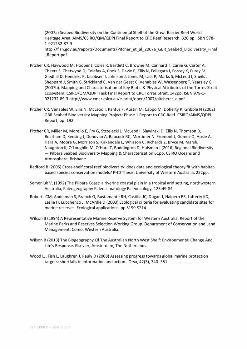
124 | PMCP – Final Report
(2007a) Seabed Biodiversity on the Continental Shelf of the Great Barrier Reef World Heritage Area. AIMS/CSIRO/QM/QDPI Final Report to CRC Reef Research. 320 pp. ISBN 978‐1‐921232‐87‐9 http://fish.gov.au/reports/Documents/Pitcher_et_al_2007a_GBR_Seabed_Biodiversity_Final_Report.pdf
Pitcher CR, Haywood M, Hooper J, Coles R, Bartlett C, Browne M, Cannard T, Carini G, Carter A, Cheers S, Chetwynd D, Colefax A, Cook S, Davie P, Ellis N, Fellegara I, Forcey K, Furey M, Gledhill D, Hendriks P, Jacobsen I, Johnson J, Jones M, Last P, Marks S, McLeod I, Sheils J, Sheppard J, Smith G, Strickland C, Van der Geest C, Venables W, Wassenberg T, Yearsley G (2007b). Mapping and Characterisation of Key Biotic & Physical Attributes of the Torres Strait Ecosystem. CSIRO/QM/QDPI Task Final Report to CRC Torres Strait. 142pp. ISBN 978‐1‐921232‐89‐3 http://www.cmar.csiro.au/e‐print/open/2007/pitchercr_a.pdf
Pitcher CR, Venables W, Ellis N, McLeod I, Pantus F, Austin M, Cappo M, Doherty P, Gribble N (2002) GBR Seabed Biodiversity Mapping Project: Phase 1 Report to CRC‐Reef. CSIRO/AIMS/QDPI Report, pp. 192.
Pitcher CR, Miller M, Morello E, Fry G, Strzelecki J, McLeod I, Slawinski D, Ellis N, Thomson D, Bearham D, Keesing J, Donovan A, Babcock RC, Mortimer N. Fromont J, Gomez O, Hosie A, Hara A, Moore G, Morrison S, Kirkendale L, Whisson C, Richards Z, Bryce M, Marsh, Naughton K, O’Loughlin M, O’Hara T, Boddington D, Huisman J (2016) Regional Biodiversity — Pilbara Seabed Biodiversity Mapping & Characterisation 61pp. CSIRO Oceans and Atmosphere, Brisbane
Radford B (2005) Cross‐shelf coral reef biodiversity: does data and ecological theory fit with habitat‐based species conservation models? PHD Thesis, University of Western Australia, 252pp.
Semeniuk V, (1992) The Pilbara Coast: a riverine coastal plain in a tropical arid setting, northwestern Australia, Paleogeography Paleoclimatology Paleoecology, 123:49‐84.
Roberts CM, Andelman S, Branch G, Bustamante RH, Castilla JC, Dugan J, Halpern BS, Lafferty KD, Leslie H, Lubchenco J, McArdle D (2003) Ecological criteria for evaluating candidate sites for marine reserves. Ecological applications, pp.S199‐S214.
Wilson B (1994) A Representative Marine Reserve System for Western Australia: Report of the Marine Parks and Reserves Selection Working Group. Department of Conservation and Land Management, Como, Western Australia.
Wilson B (2013) The Biogeography Of The Australian North West Shelf: Environmental Change And Life's Response. Elsevier, Amsterdam, The Netherlands.
Wood LJ, Fish L, Laughren J, Pauly D (2008) Assessing progress towards global marine protection targets: shortfalls in information and action. Oryx, 42(3), 340–351
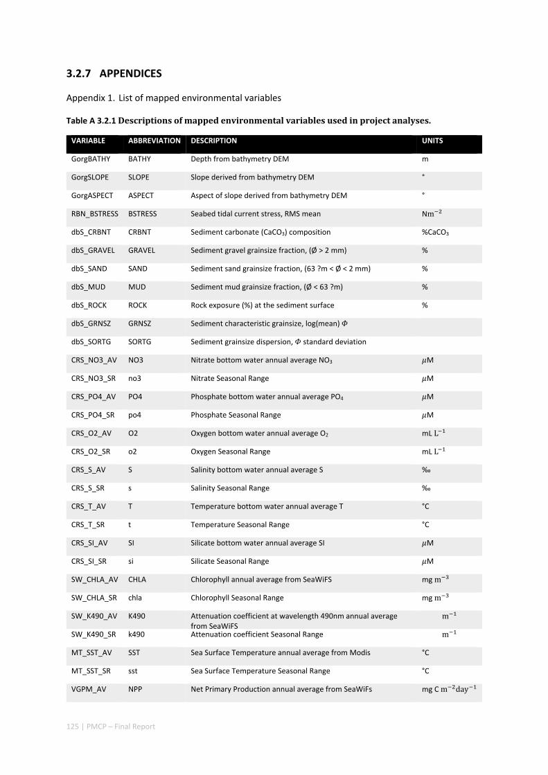
125 | PMCP – Final Report
3.2.7 APPENDICES
Appendix 1. List of mapped environmental variables
Table A 3.2.1Descriptionsofmappedenvironmentalvariablesusedinprojectanalyses.
VARIABLE ABBREVIATION DESCRIPTION UNITS
GorgBATHY BATHY Depth from bathymetry DEM m
GorgSLOPE SLOPE Slope derived from bathymetry DEM °
GorgASPECT ASPECT Aspect of slope derived from bathymetry DEM °
RBN_BSTRESS BSTRESS Seabed tidal current stress, RMS mean Nm
dbS_CRBNT CRBNT Sediment carbonate (CaCO3) composition %CaCO3
dbS_GRAVEL GRAVEL Sediment gravel grainsize fraction, (Ø > 2 mm) %
dbS_SAND SAND Sediment sand grainsize fraction, (63 ?m < Ø < 2 mm) %
dbS_MUD MUD Sediment mud grainsize fraction, (Ø < 63 ?m) %
dbS_ROCK ROCK Rock exposure (%) at the sediment surface %
dbS_GRNSZ GRNSZ Sediment characteristic grainsize, log(mean)
dbS_SORTG SORTG Sediment grainsize dispersion, standard deviation
CRS_NO3_AV NO3 Nitrate bottom water annual average NO3 M
CRS_NO3_SR no3 Nitrate Seasonal Range M
CRS_PO4_AV PO4 Phosphate bottom water annual average PO4 M
CRS_PO4_SR po4 Phosphate Seasonal Range M
CRS_O2_AV O2 Oxygen bottom water annual average O2 mL L
CRS_O2_SR o2 Oxygen Seasonal Range mL L
CRS_S_AV S Salinity bottom water annual average S ‰
CRS_S_SR s Salinity Seasonal Range ‰
CRS_T_AV T Temperature bottom water annual average T °C
CRS_T_SR t Temperature Seasonal Range °C
CRS_SI_AV SI Silicate bottom water annual average SI M
CRS_SI_SR si Silicate Seasonal Range M
SW_CHLA_AV CHLA Chlorophyll annual average from SeaWiFS mg m
SW_CHLA_SR chla Chlorophyll Seasonal Range mg m
SW_K490_AV K490 Attenuation coefficient at wavelength 490nm annual average from SeaWiFS
m
SW_K490_SR k490 Attenuation coefficient Seasonal Range m
MT_SST_AV SST Sea Surface Temperature annual average from Modis °C
MT_SST_SR sst Sea Surface Temperature Seasonal Range °C
VGPM_AV NPP Net Primary Production annual average from SeaWiFs mg C m day
126 | PMCP – Final Report
VGPM_SR npp Net Primary Production seasonal range mg C m day
EPOC_AV EPOC Export Particulate Organic Carbon flux annual average from SeaWiFs
mg C m day
EPOC_SR epoc Export Particulate Organic Carbon seasonal range mg C m day
PAR_AV PAR Photosynthetically Active Radiation (PAR) from MODIS Einstein m day
PAR_SR par Photosynthetically Active Radiation seasonal range Einstein m day
SW_BIR_AV BIR Benthic Irradiance annual average, BIR = PAR × $e^{‐\text{K490}\times\textDepth}$
Einstein m day
SW_BIR_SR bir Benthic Irradiance Seasonal Range Einstein m day
TERAN_CHAN CHAN Terrain channel, probability of membership of topographic shape “channel”
TERAN_PASS PASS Terrain pass, probability of membership of topographic shape “pass”
TERAN_PEAK PEAK Terrain peak, probability of membership of topographic shape “peak”
TERAN_PIT PIT Terrain pit, probability of membership of topographic shape “pit”
TERAN_PLAN PLAN Terrain plane, probability of membership of topographic shape “plane”
TERAN_RIDG RIDG Terrain ridge, probability of membership of topographic shape “ridge”

127 | PMCP – Final Report
Appendix 2. Maps of environmental variables
The following maps show the predictor variables used in the analysis. All predictors are defined on a 0.01° spatial grid. See Appendix 1 for definition of the abbreviations.
3.2.7.1 Sediment variables
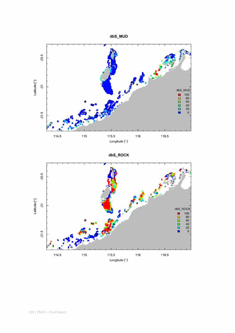
128 | PMCP – Final Report
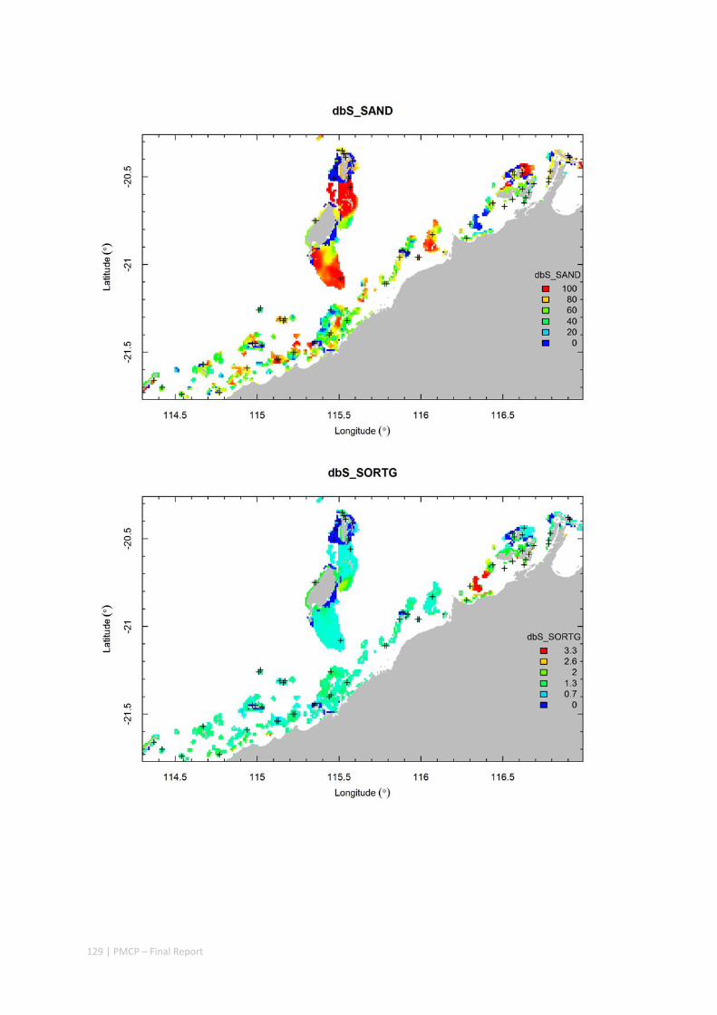
129 | PMCP – Final Report
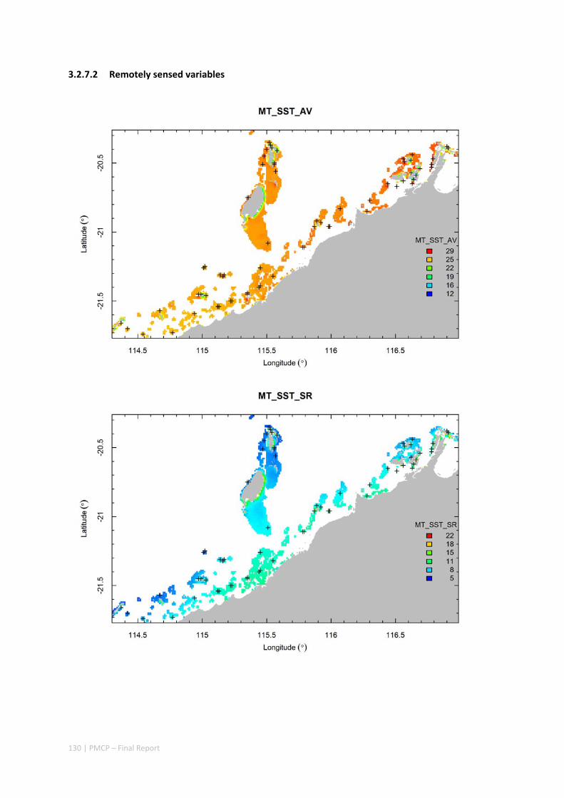
130 | PMCP – Final Report
3.2.7.2 Remotely sensed variables
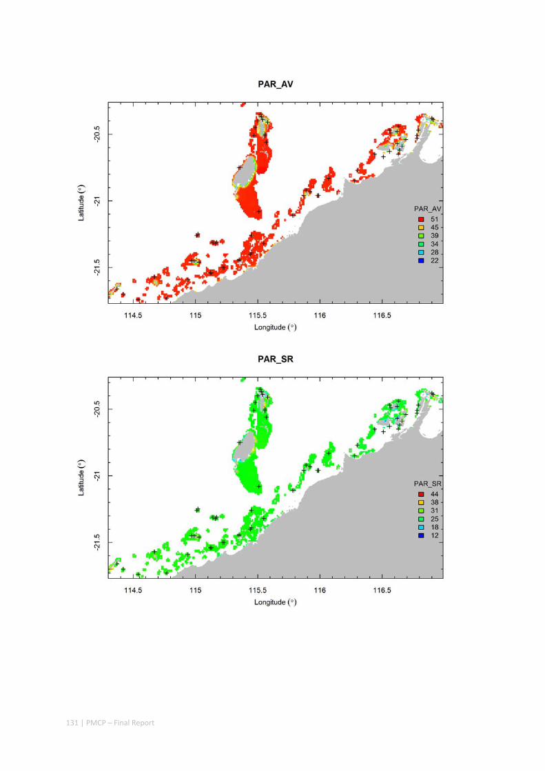
131 | PMCP – Final Report
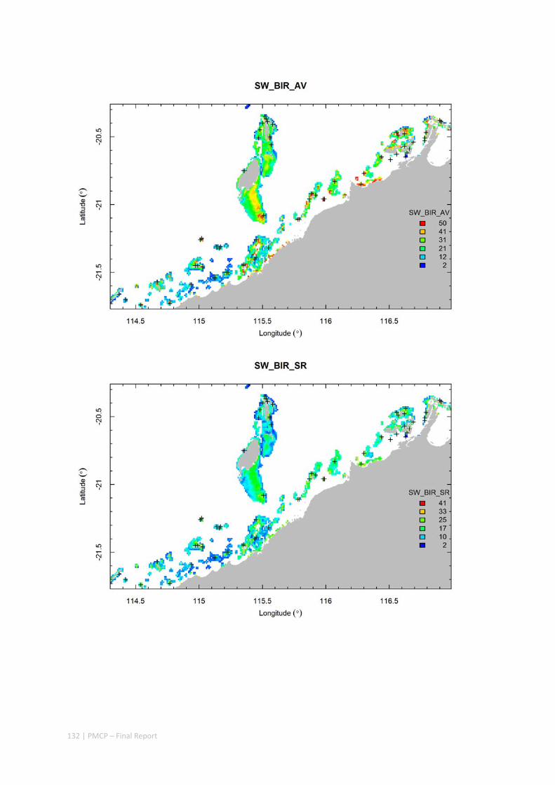
132 | PMCP – Final Report
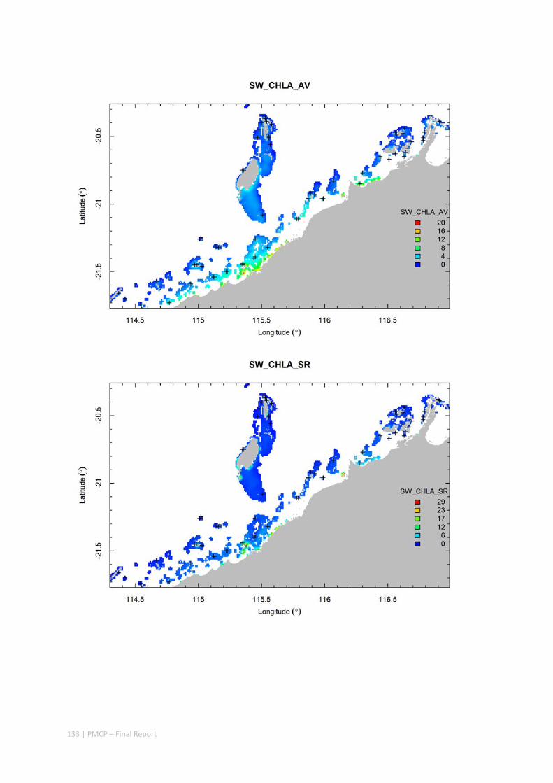
133 | PMCP – Final Report
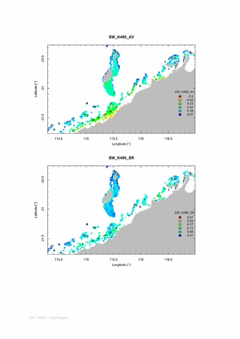
134 | PMCP – Final Report
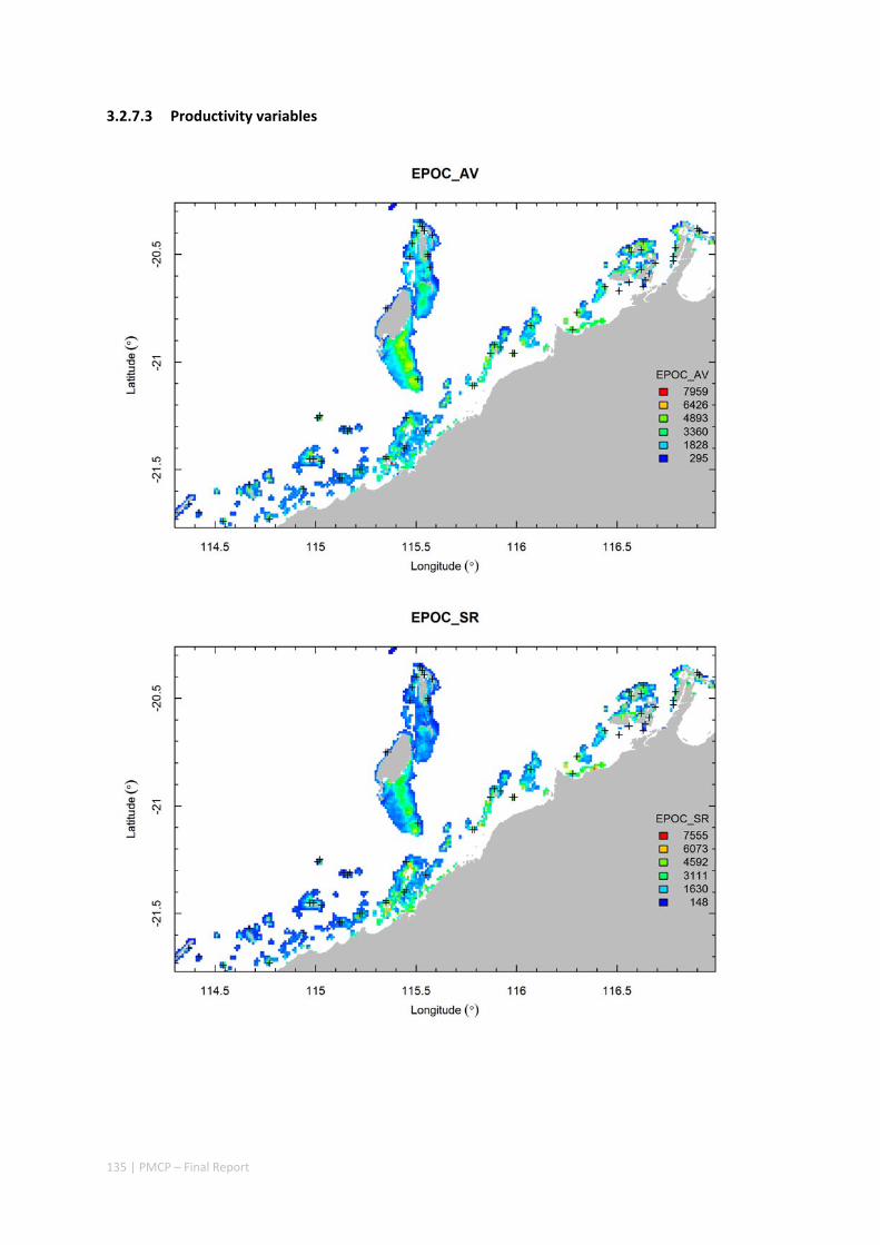
135 | PMCP – Final Report
3.2.7.3 Productivity variables
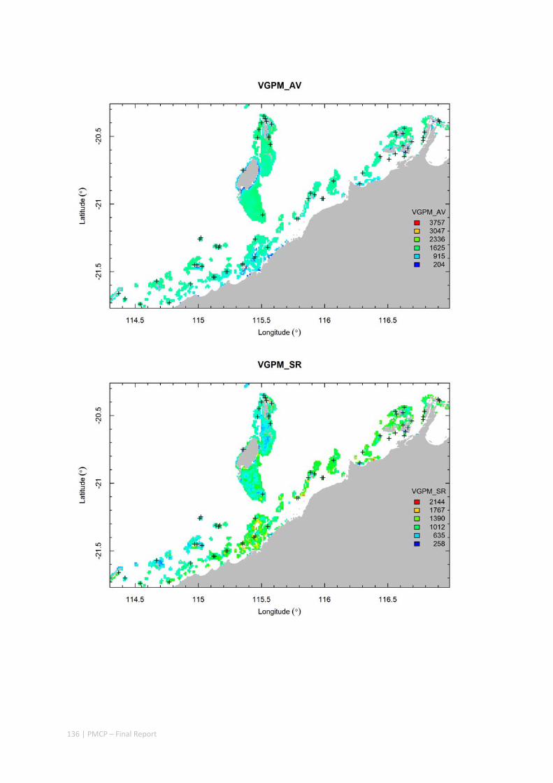
136 | PMCP – Final Report
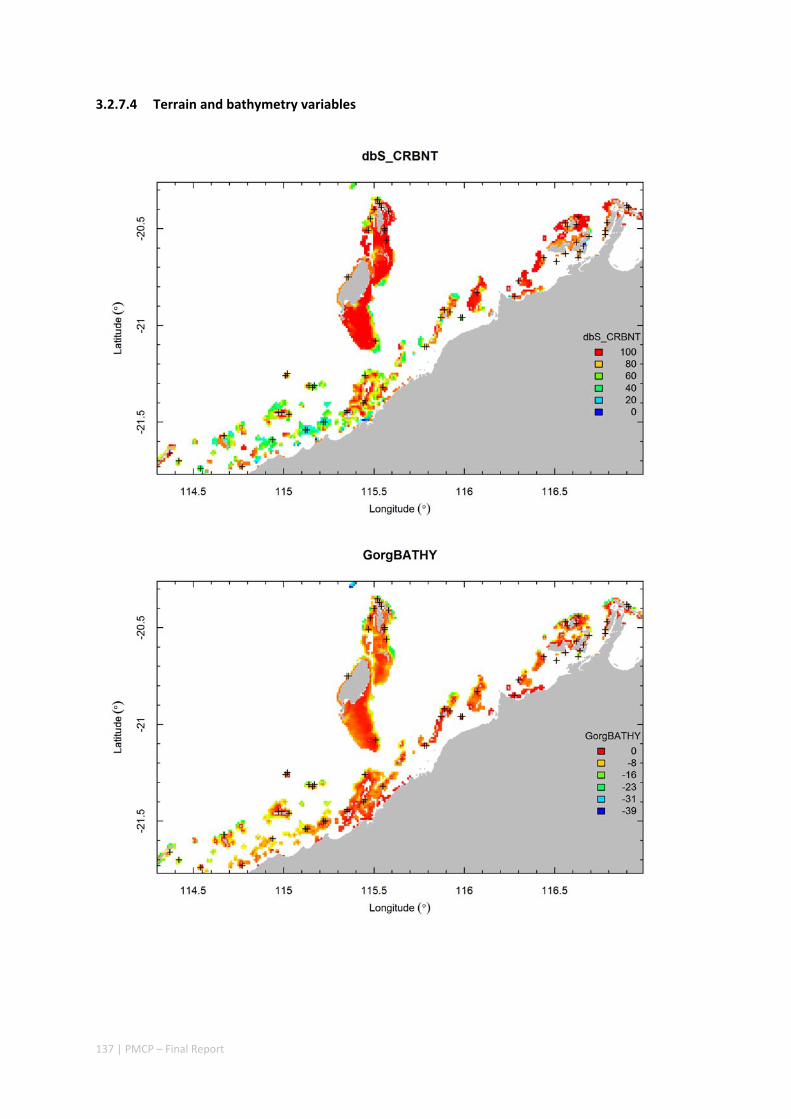
137 | PMCP – Final Report
3.2.7.4 Terrain and bathymetry variables
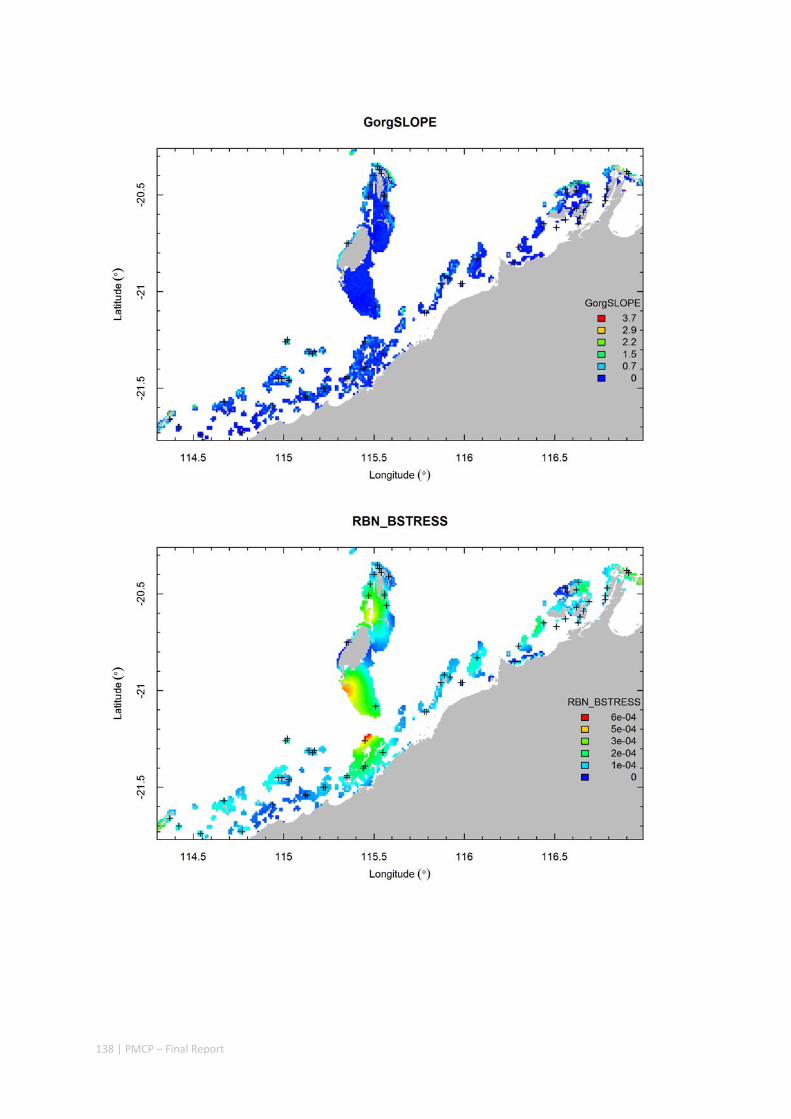
138 | PMCP – Final Report

139 | PMCP – Final Report
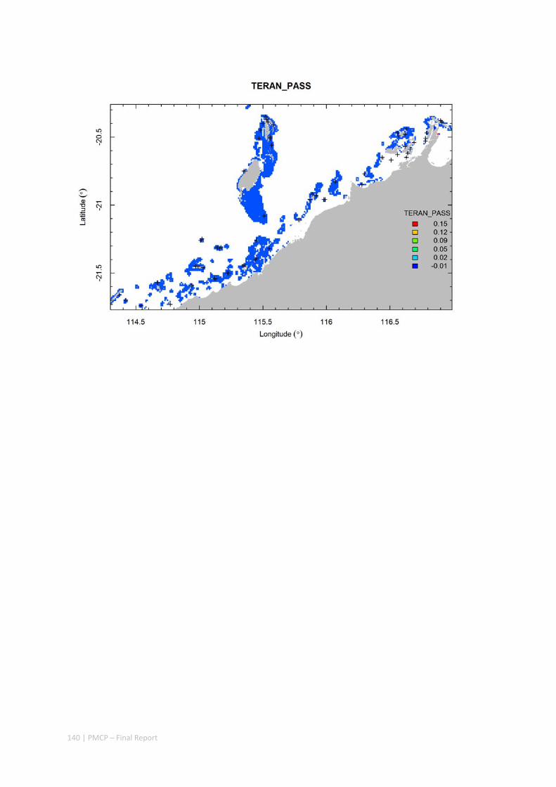
140 | PMCP – Final Report
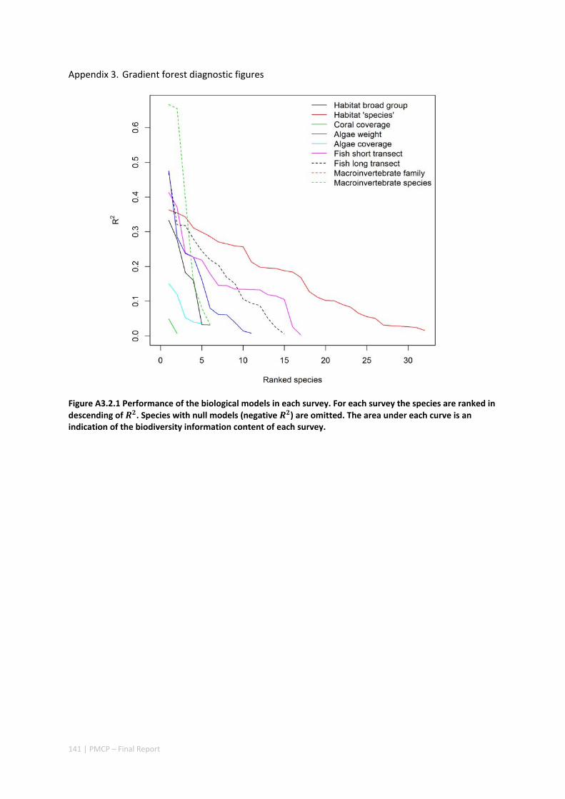
141 | PMCP – Final Report
Appendix 3. Gradient forest diagnostic figures
Figure A3.2.1 Performance of the biological models in each survey. For each survey the species are ranked in descending of . Species with null models (negative ) are omitted. The area under each curve is an indication of the biodiversity information content of each survey.
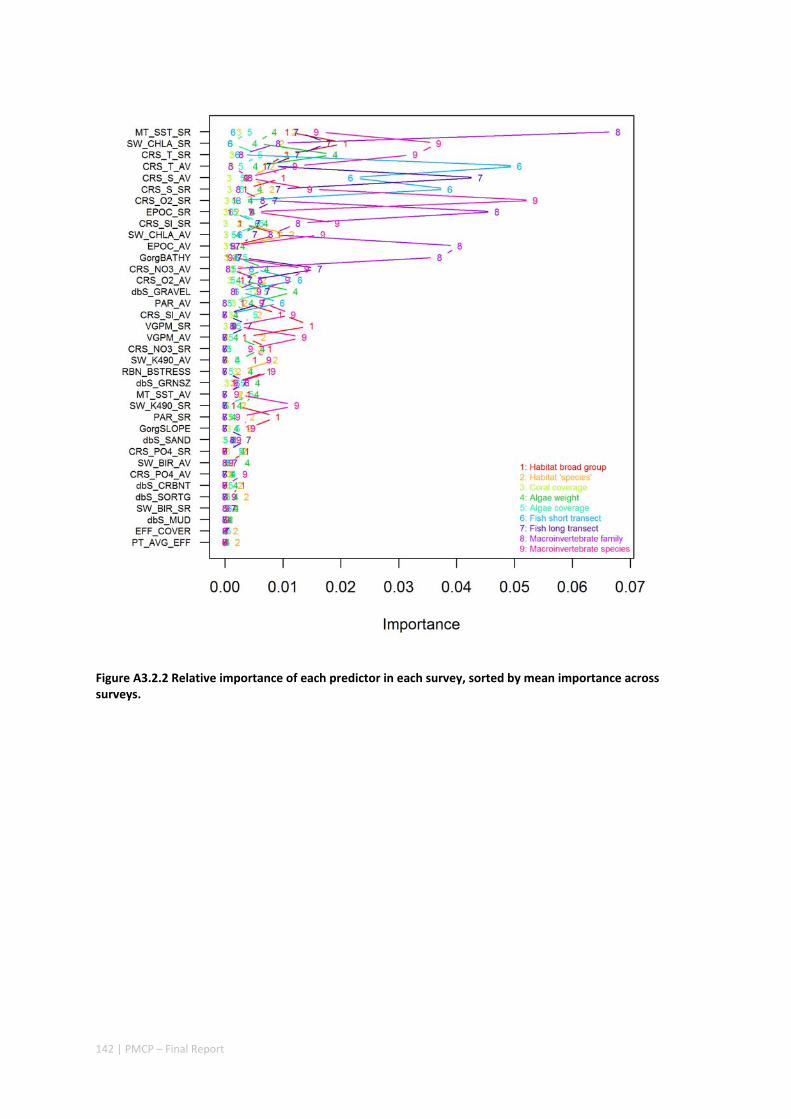
142 | PMCP – Final Report
Figure A3.2.2 Relative importance of each predictor in each survey, sorted by mean importance across surveys.
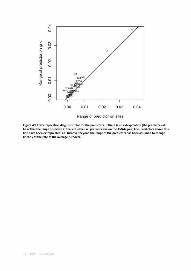
143 | PMCP – Final Report
Figure A3.2.3 Extrapolation diagnostic plot for the predictors. If there is no extrapolation (the predictors all lie within the range observed at the sites) then all predictors lie on the 45°ree; line. Predictors above this line have been extrapolated; i.e. turnover beyond the range of the predictors has been assumed to change linearly at the rate of the average turnover.
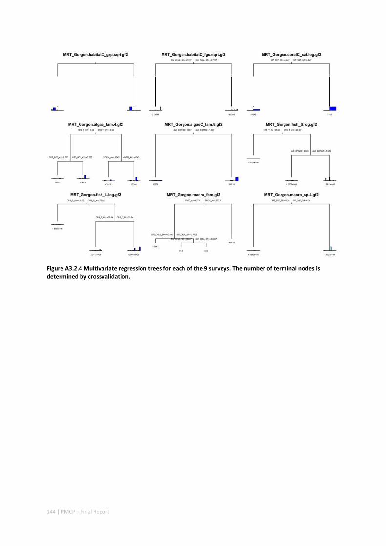
144 | PMCP – Final Report
Figure A3.2.4 Multivariate regression trees for each of the 9 surveys. The number of terminal nodes is determined by crossvalidation.
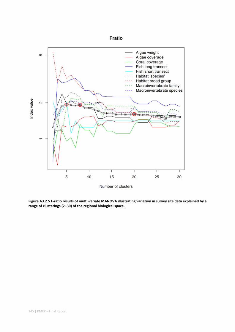
145 | PMCP – Final Report
Figure A3.2.5 F‐ratio results of multi‐variate MANOVA illustrating variation in survey site data explained by a range of clusterings (2–30) of the regional biological space.
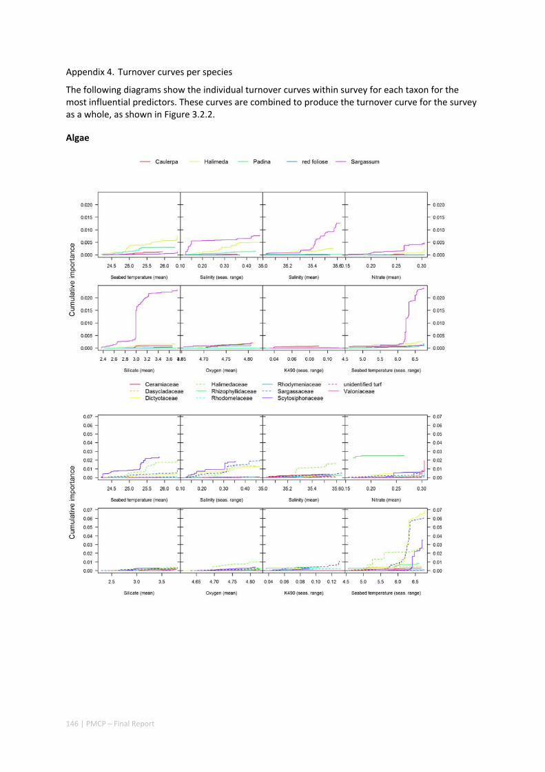
146 | PMCP – Final Report
Appendix 4. Turnover curves per species
The following diagrams show the individual turnover curves within survey for each taxon for the most influential predictors. These curves are combined to produce the turnover curve for the survey as a whole, as shown in Figure 3.2.2.
Algae
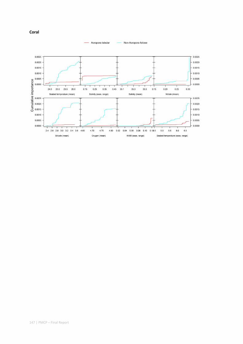
147 | PMCP – Final Report
Coral

148 | PMCP – Final Report
Fish
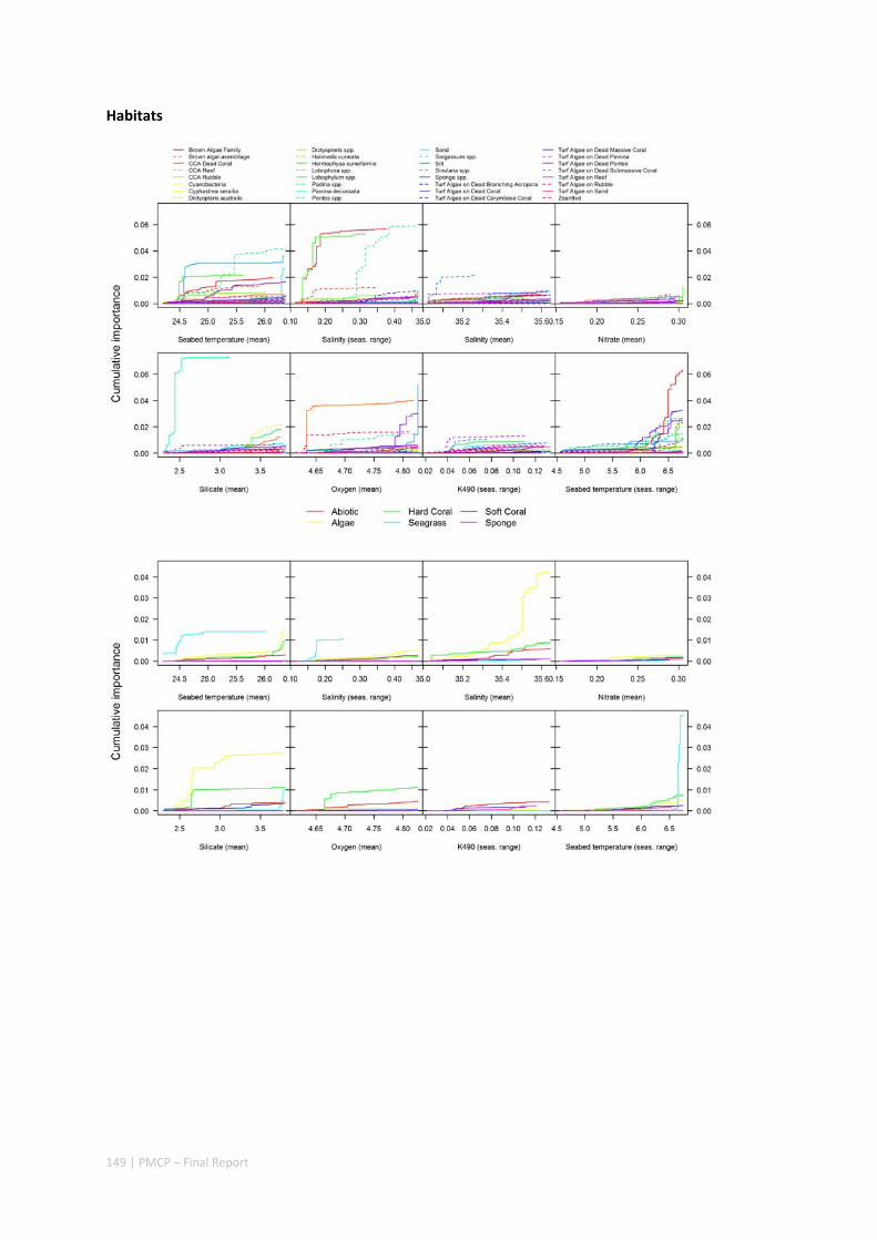
149 | PMCP – Final Report
Habitats
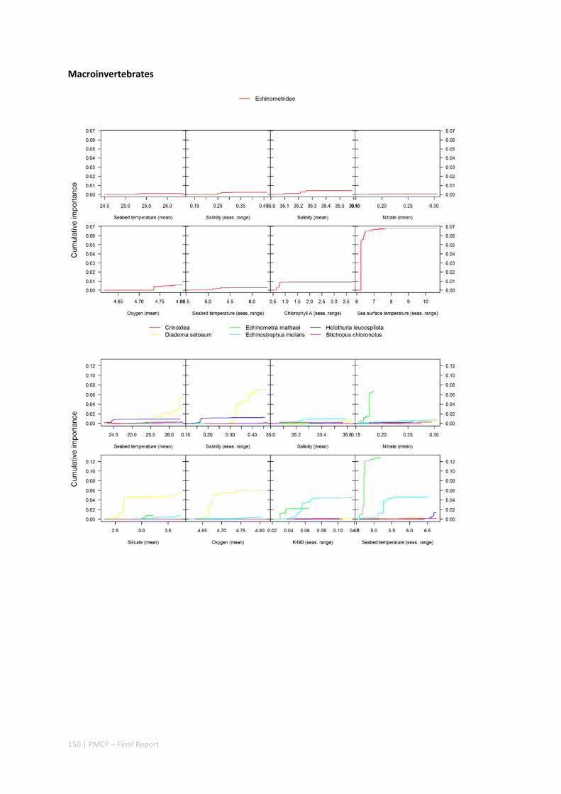
150 | PMCP – Final Report
Macroinvertebrates

151 | PMCP – Final Report
Appendix 5. Boxplots of biota measurements per assemblage
The following diagrams are box plots of observed biota measurements per assemblage across the surveys, analogous to Figure 5 for environmental predictors. Only the most abundant biota are included. The width of each bar is proportional to the number of sites in each assemblage. The number of sites per assemblage ranges as follows: Algae 2–23, Coral 4–17, Habitat 4–21, Fish (long transects) 4–24, Fish (short transects) 0–9, and Macroinvertebrates 3–18.
Algae

152 | PMCP – Final Report
Coral
Habitats
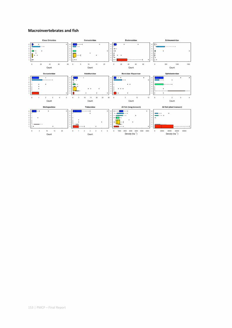
153 | PMCP – Final Report
Macroinvertebrates and fish

154 | PMCP – Final Report
Appendix 6. Maps of predicted species distributions
The following maps show the observed measurements (circles) and predictions (background colour) for all biological groups (OTUs, species, families, categories, habitat groups). The observations and predictions within each map use the same colour scale. The influential variables (in order of influence) are shown in the top left corner. In the bottom right corner are characteristics of the model fit: the out‐of‐bag (goodness of fit), the maximum number of nodes in any regression tree in the random forest (model complexity), the number of predictors in the model, and the number of sites at which the biota was observed. The title shows the name of the biota, the transformation applied to the observations before fitting (sqrt–square root, 4–4th root, 8–8th root, log–natural logarithm, id–no transformation) and the taxonomic level (fam–family, cat–coral category, grp–broad habitat group, fgs–fine habitat group (‘family genus species’)). For fish species the type of transect (long/short) is indicated.
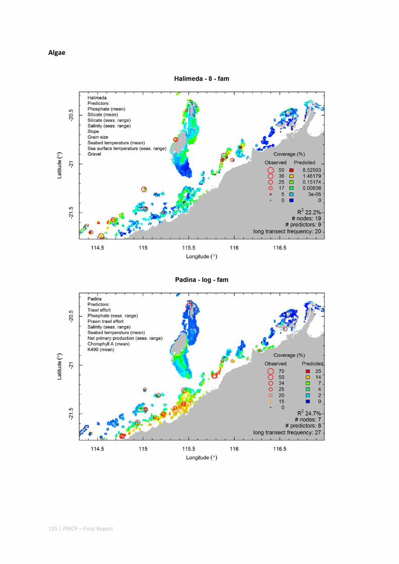
155 | PMCP – Final Report
Algae
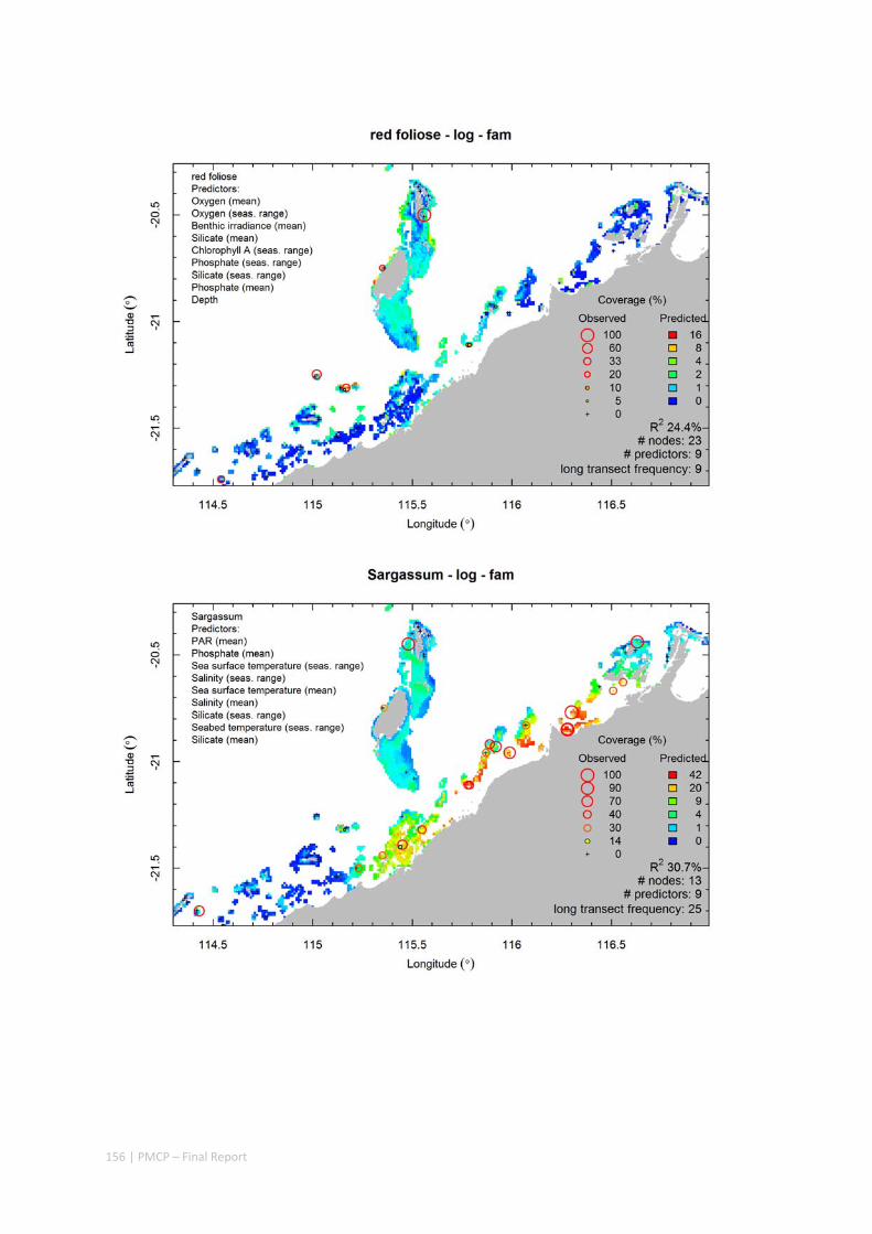
156 | PMCP – Final Report
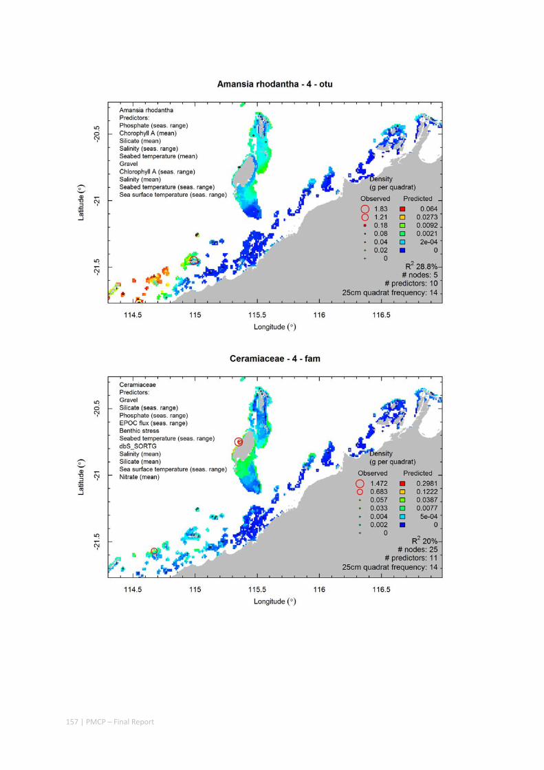
157 | PMCP – Final Report
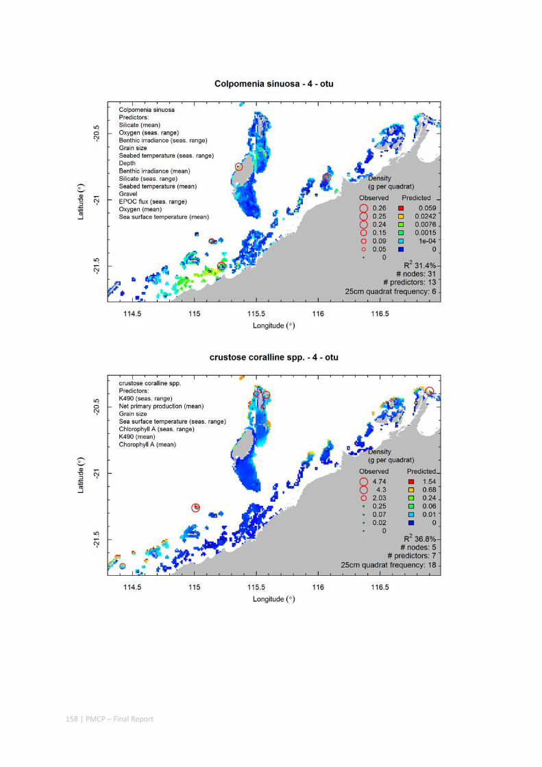
158 | PMCP – Final Report
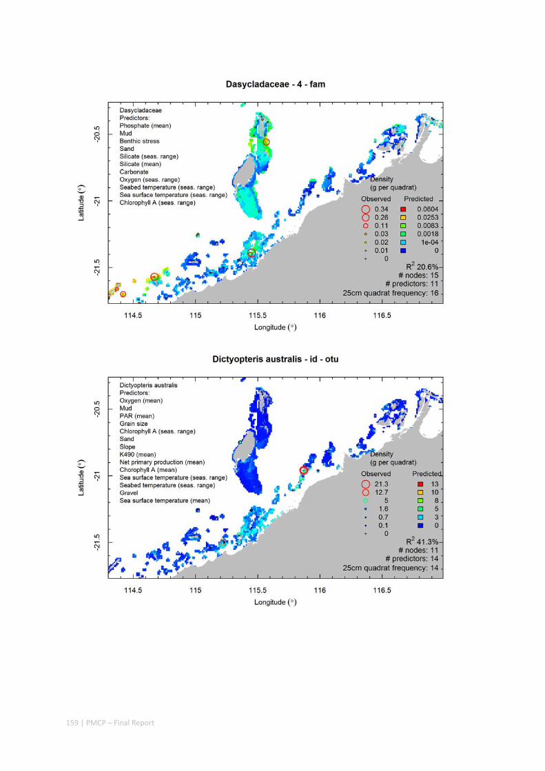
159 | PMCP – Final Report

160 | PMCP – Final Report
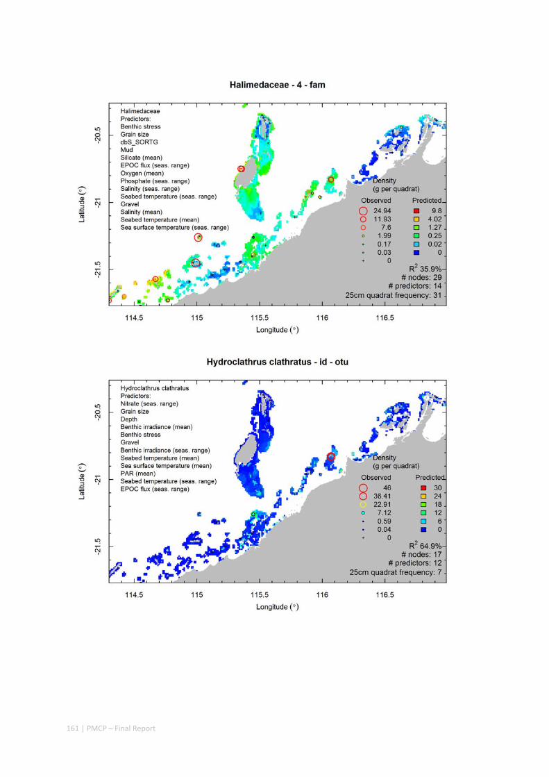
161 | PMCP – Final Report
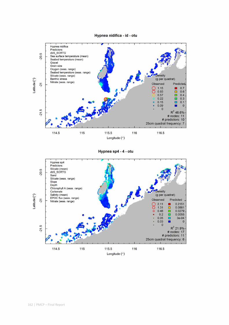
162 | PMCP – Final Report
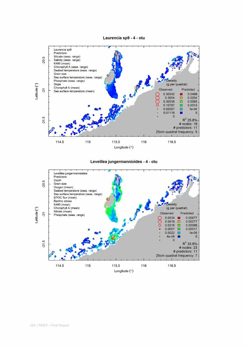
163 | PMCP – Final Report

164 | PMCP – Final Report
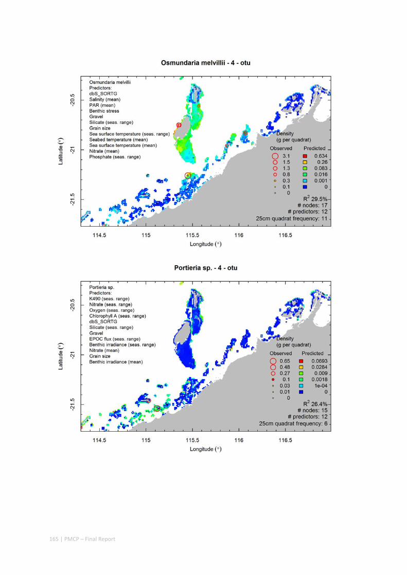
165 | PMCP – Final Report
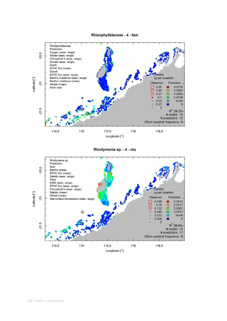
166 | PMCP – Final Report
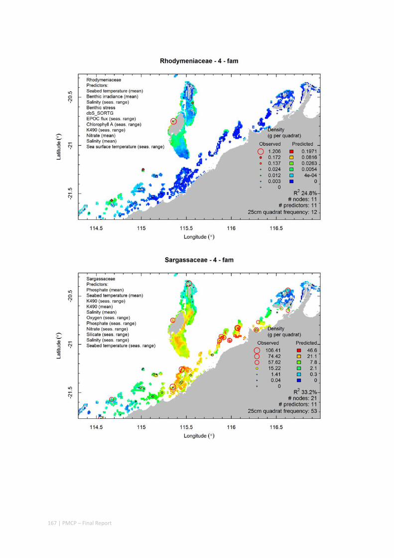
167 | PMCP – Final Report
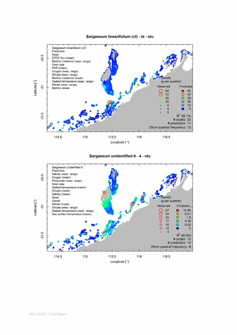
168 | PMCP – Final Report
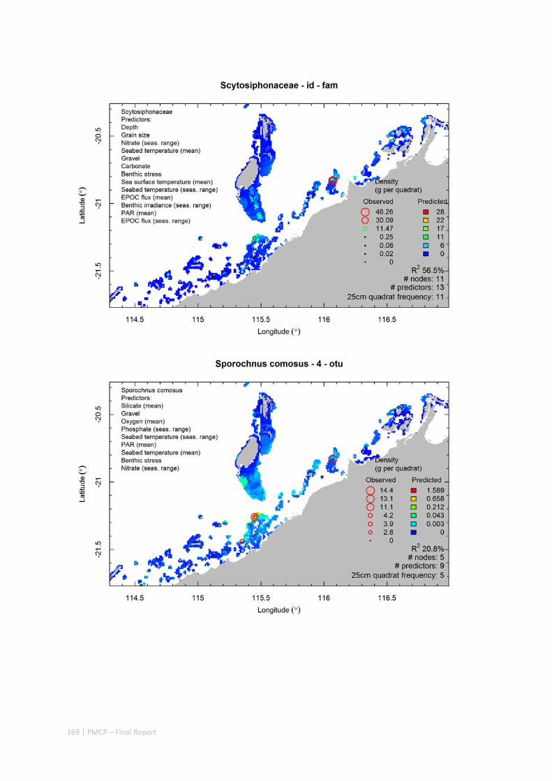
169 | PMCP – Final Report
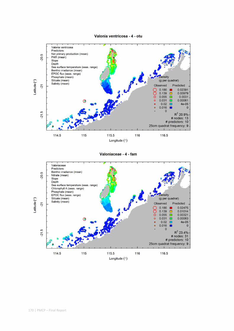
170 | PMCP – Final Report
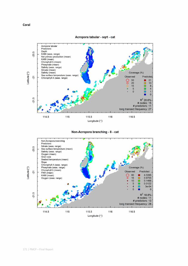
171 | PMCP – Final Report
Coral

172 | PMCP – Final Report

173 | PMCP – Final Report
Fish

174 | PMCP – Final Report
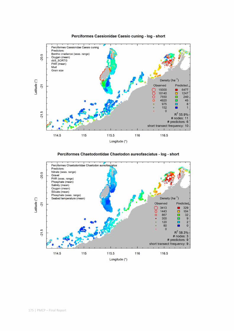
175 | PMCP – Final Report
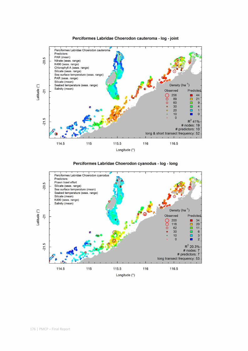
176 | PMCP – Final Report
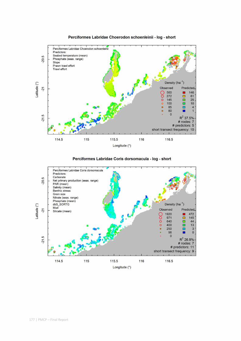
177 | PMCP – Final Report
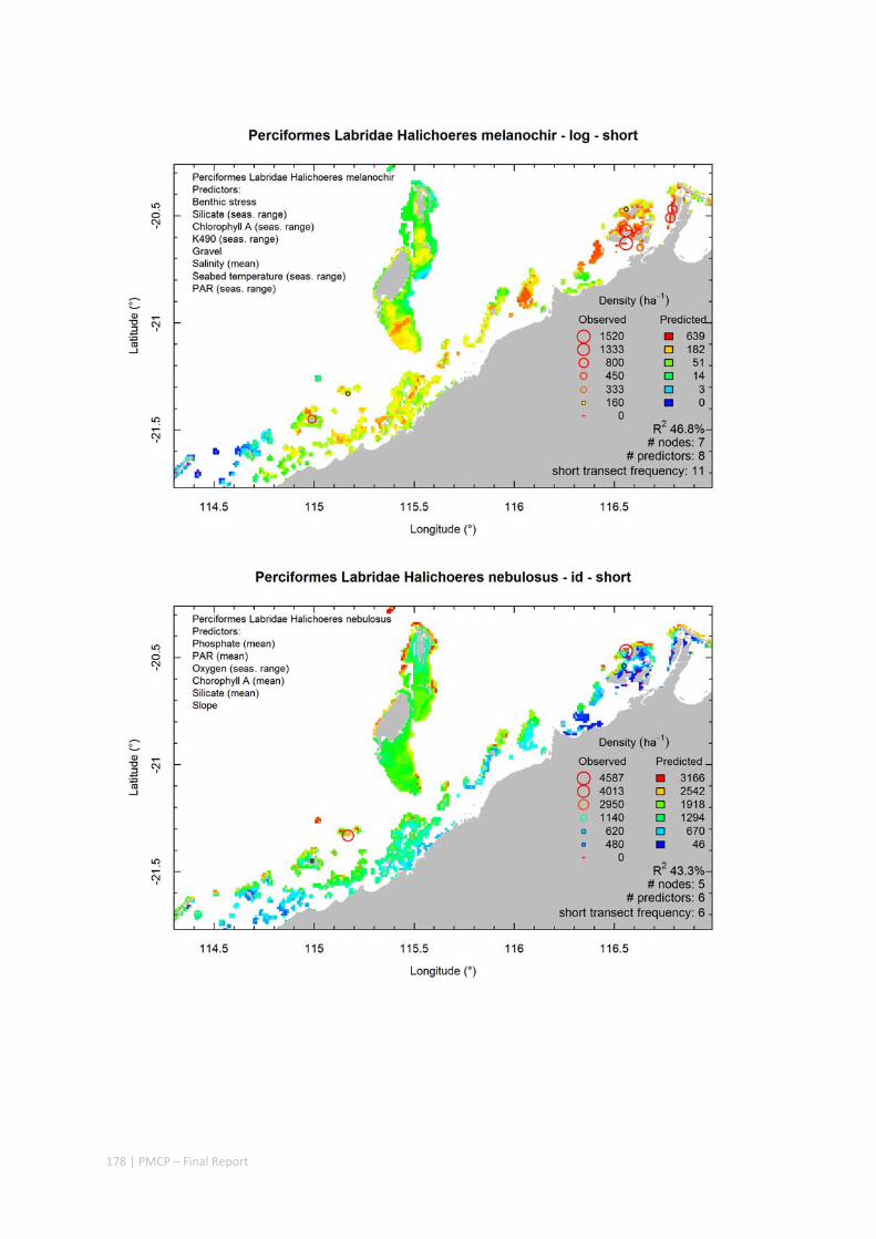
178 | PMCP – Final Report

179 | PMCP – Final Report
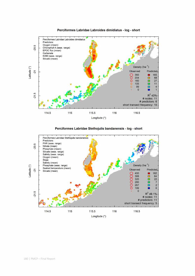
180 | PMCP – Final Report
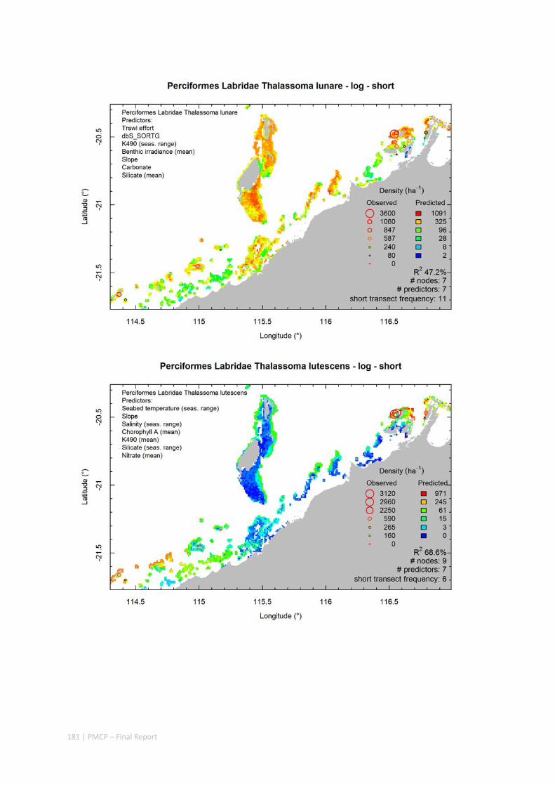
181 | PMCP – Final Report

182 | PMCP – Final Report

183 | PMCP – Final Report
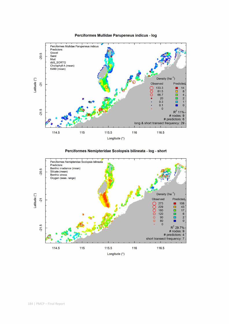
184 | PMCP – Final Report
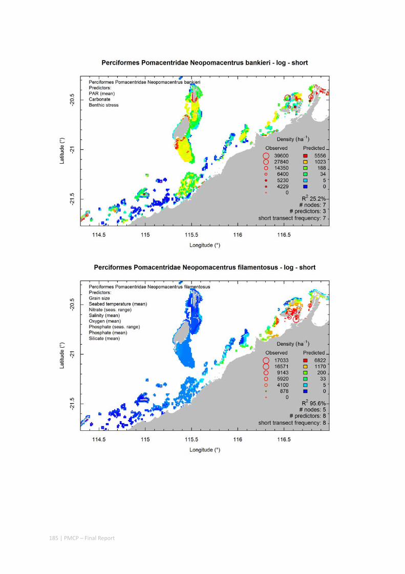
185 | PMCP – Final Report

186 | PMCP – Final Report
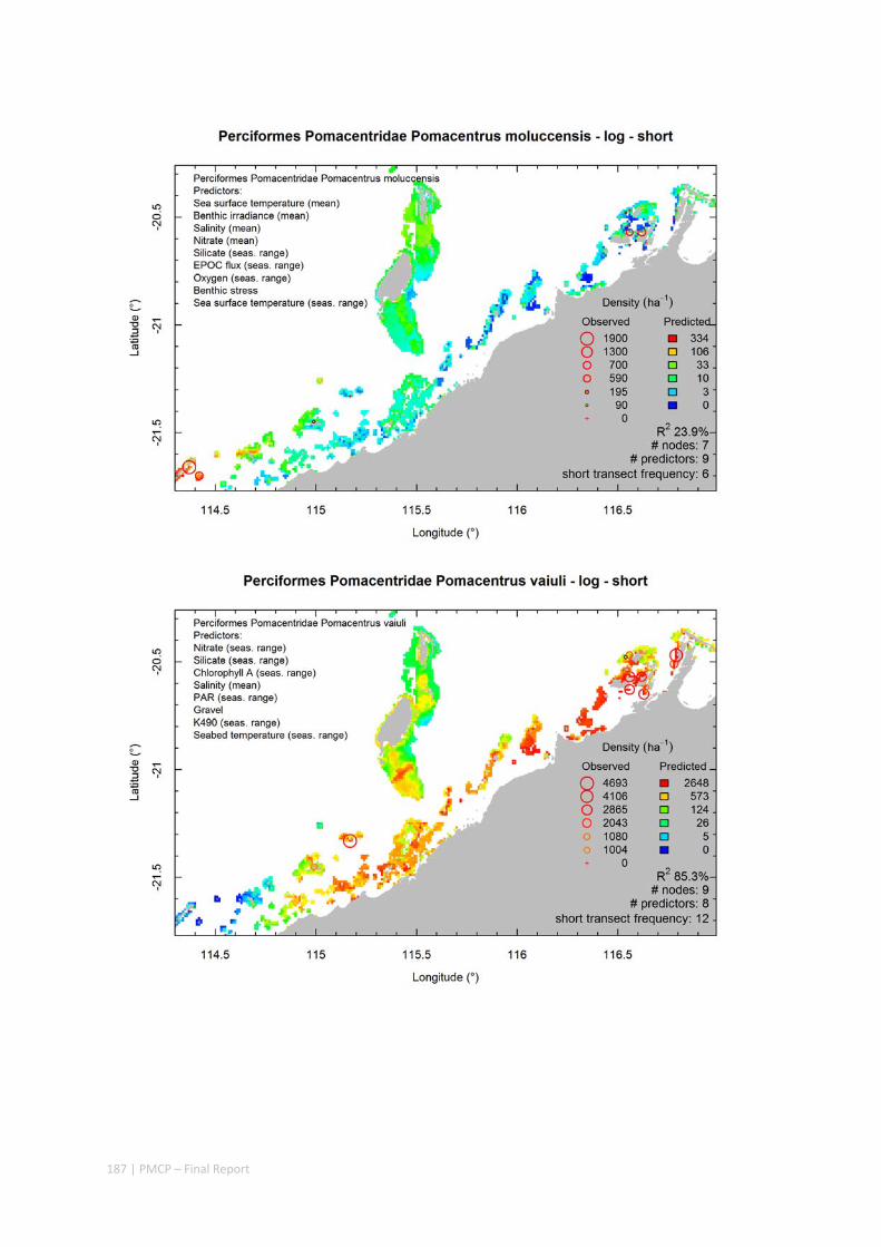
187 | PMCP – Final Report
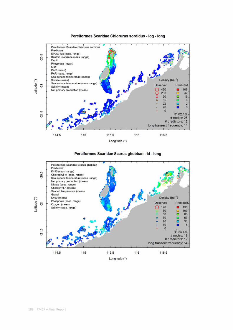
188 | PMCP – Final Report
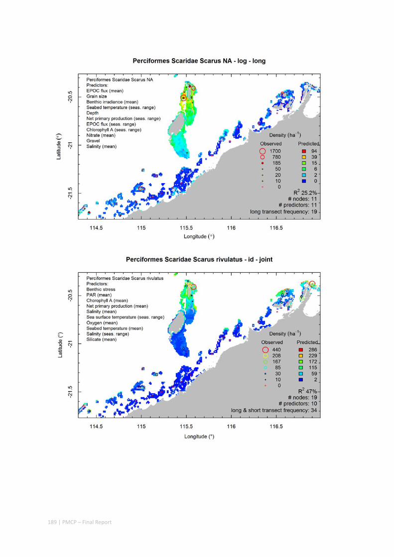
189 | PMCP – Final Report
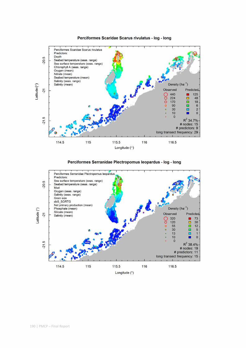
190 | PMCP – Final Report
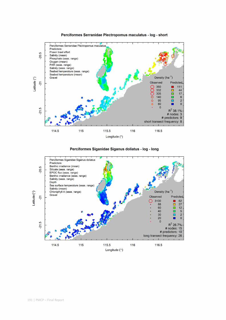
191 | PMCP – Final Report

192 | PMCP – Final Report
Habitats
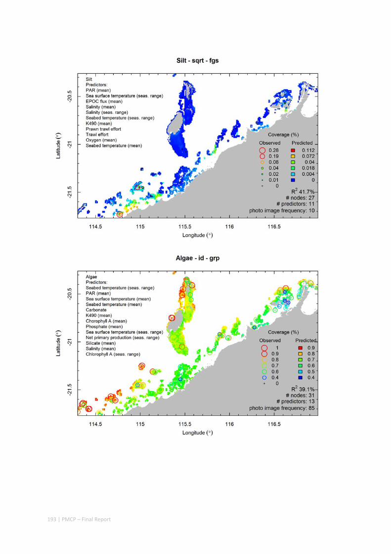
193 | PMCP – Final Report
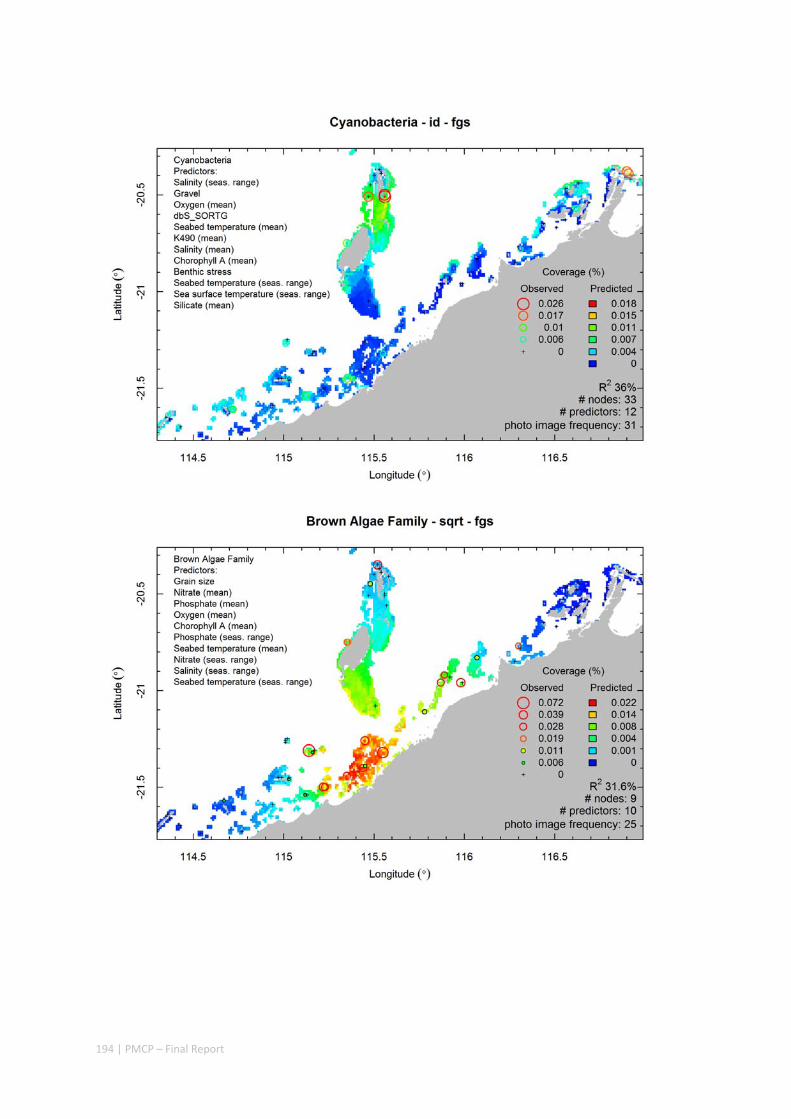
194 | PMCP – Final Report
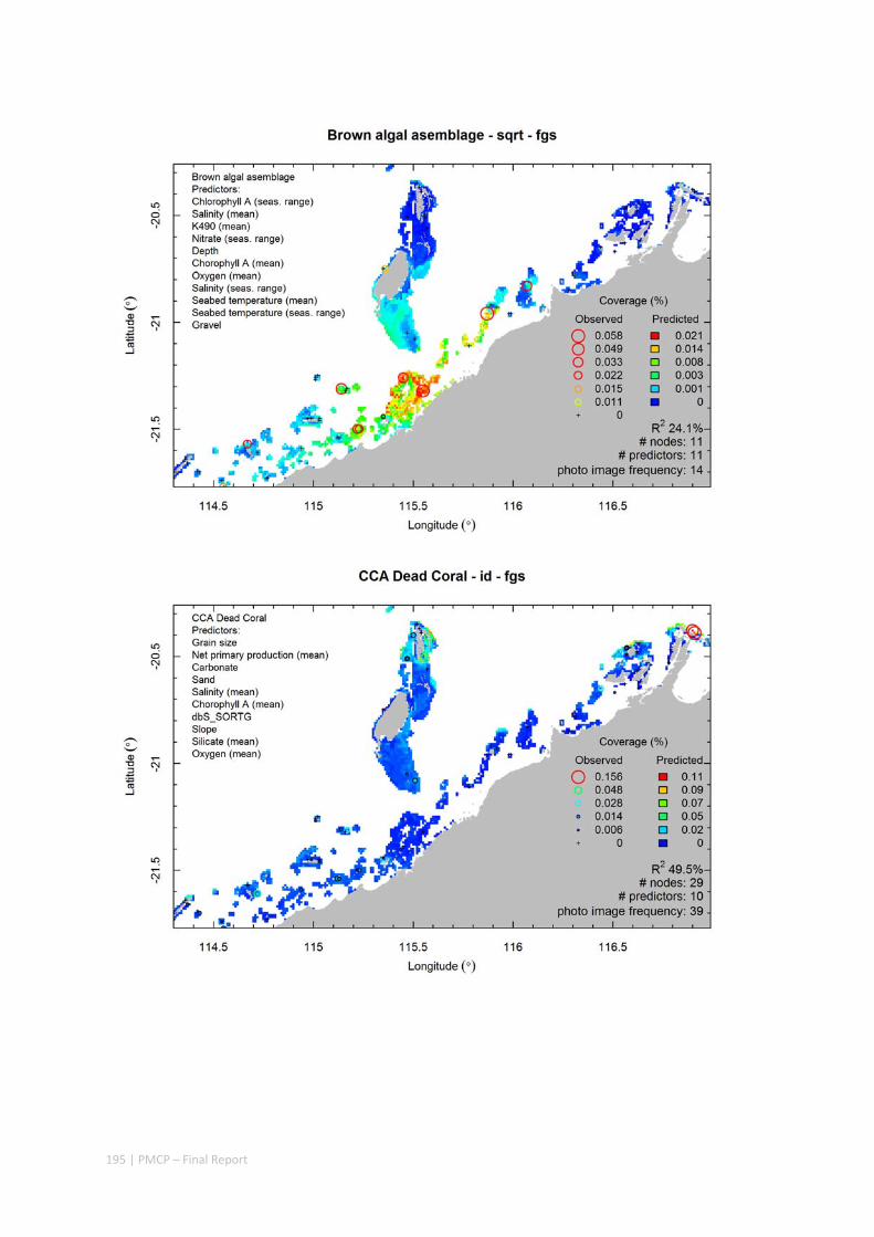
195 | PMCP – Final Report
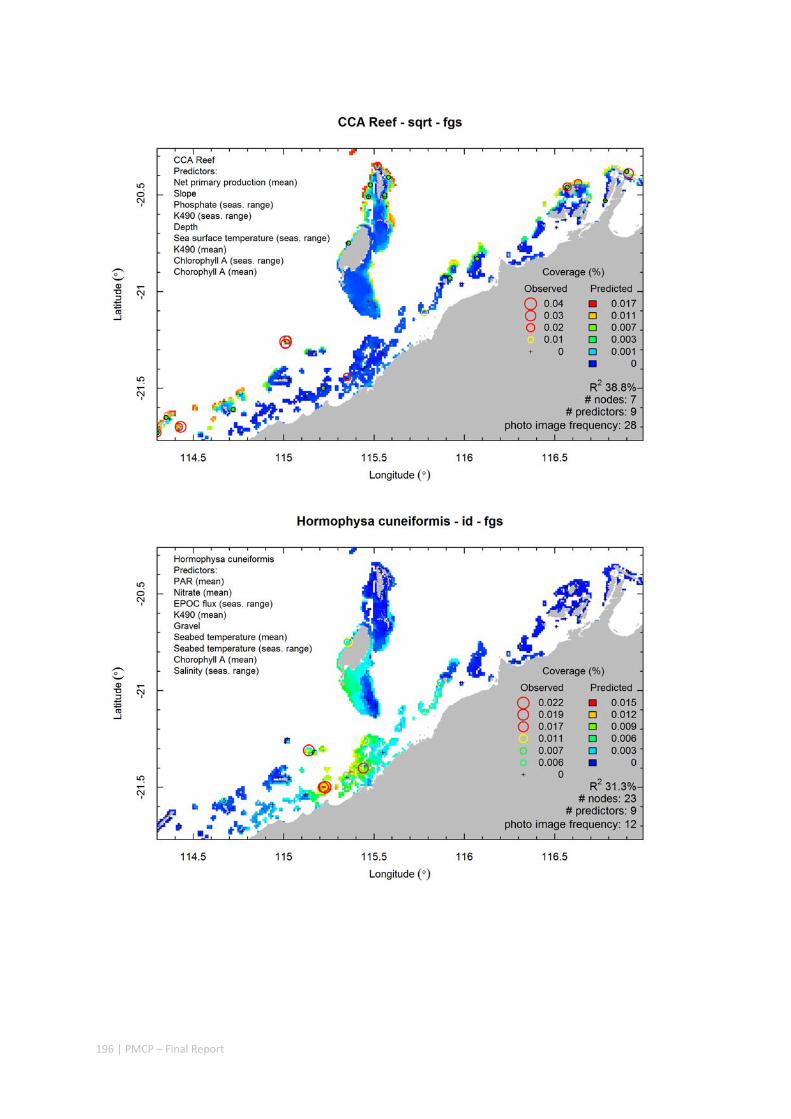
196 | PMCP – Final Report

197 | PMCP – Final Report
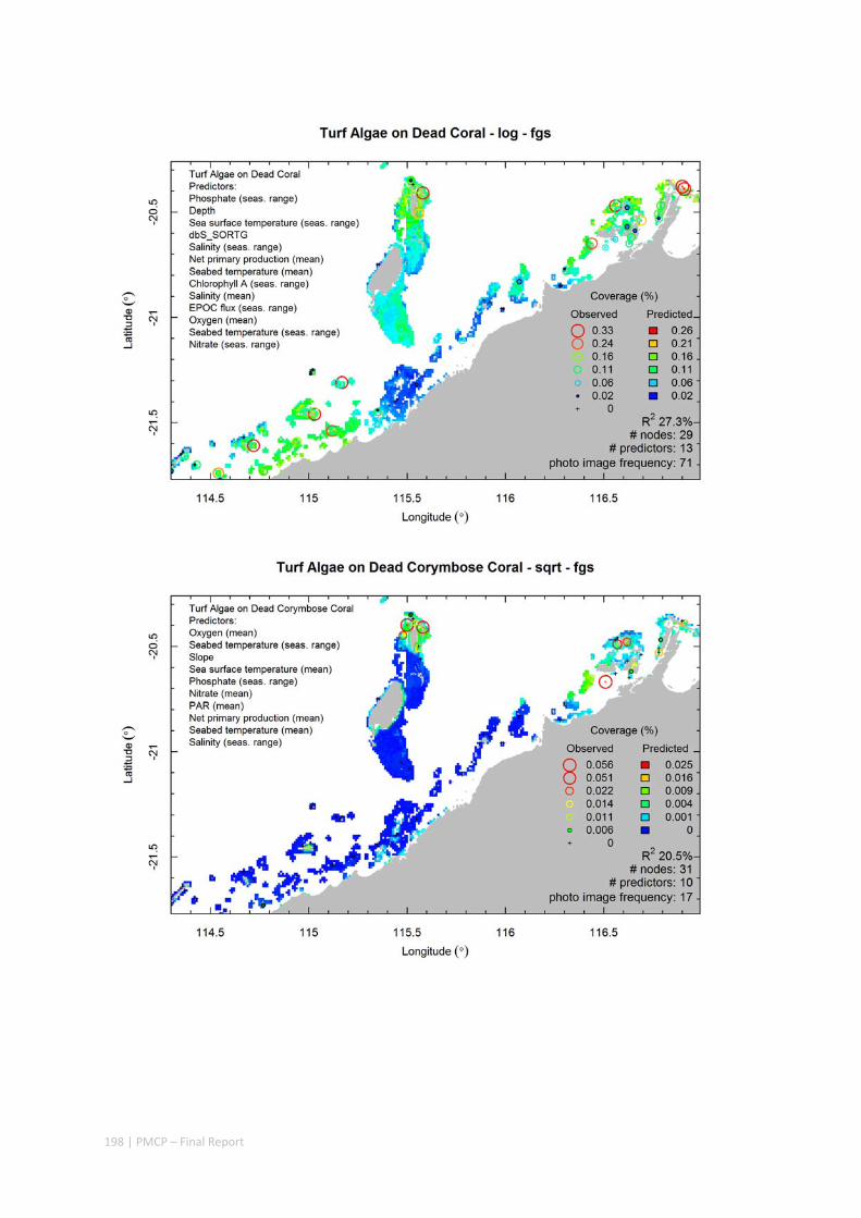
198 | PMCP – Final Report
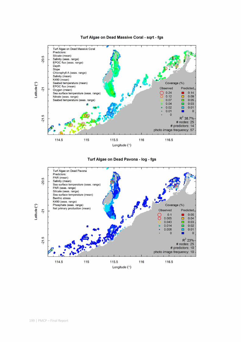
199 | PMCP – Final Report
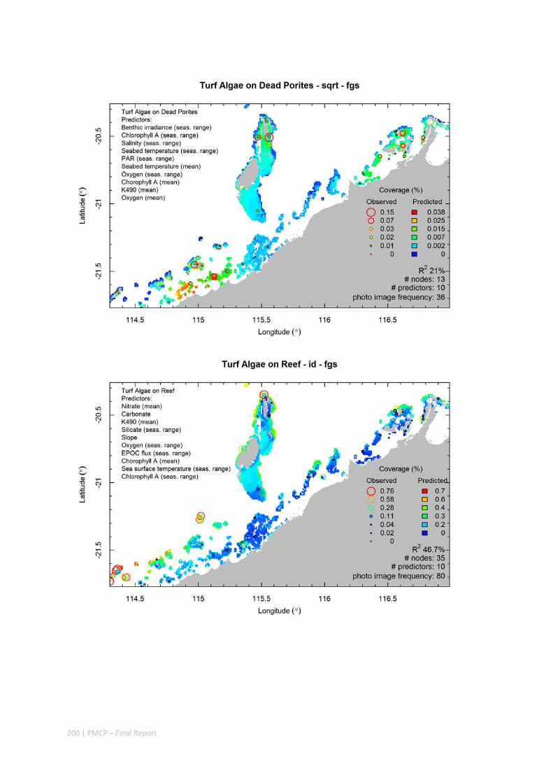
200 | PMCP – Final Report

201 | PMCP – Final Report

202 | PMCP – Final Report
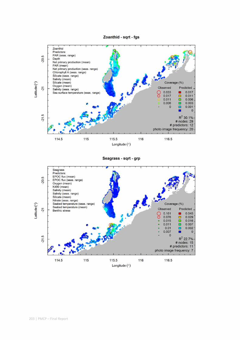
203 | PMCP – Final Report
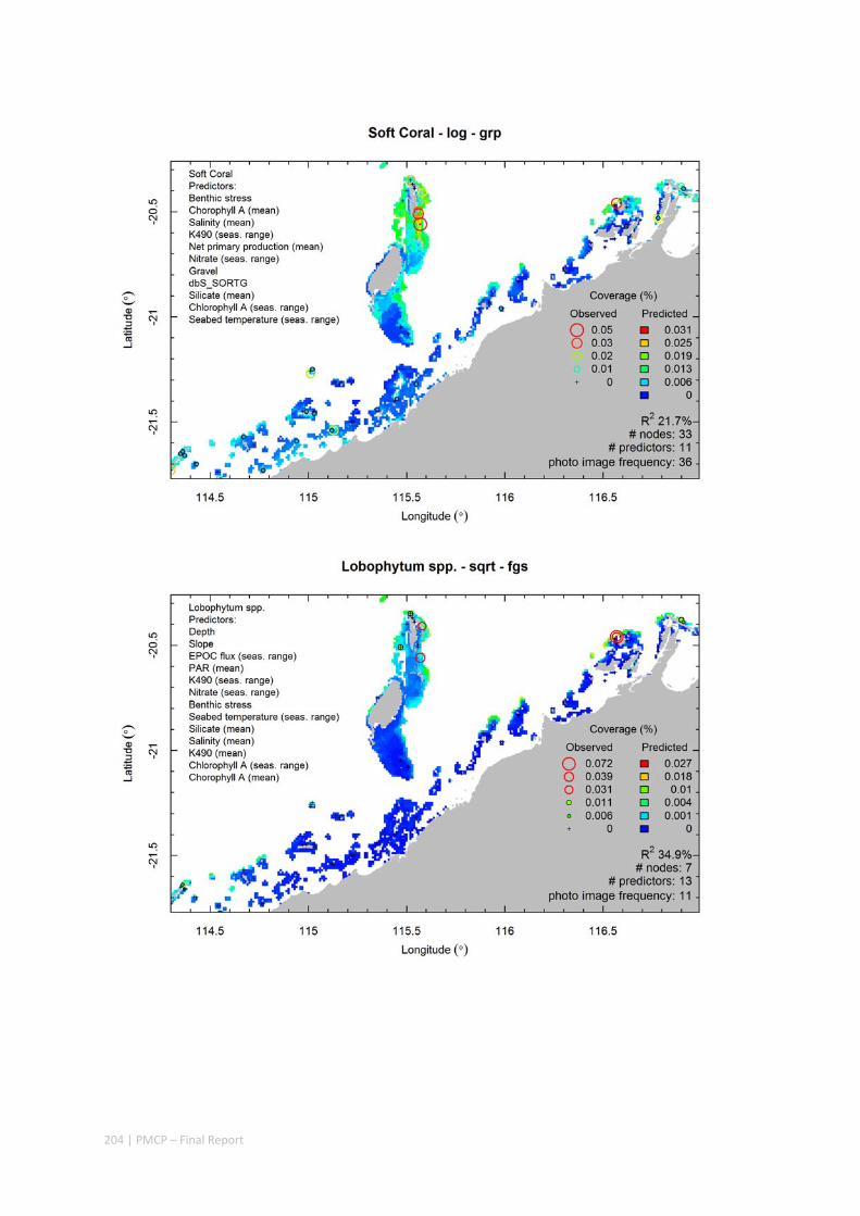
204 | PMCP – Final Report
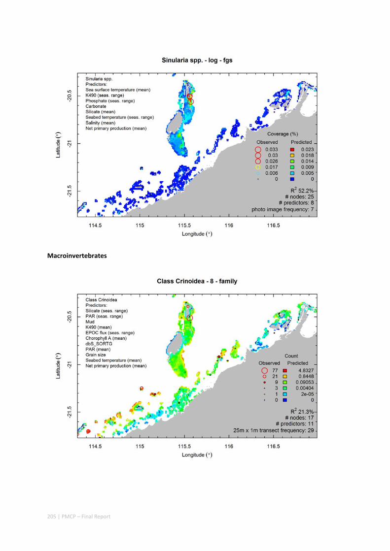
205 | PMCP – Final Report
Macroinvertebrates
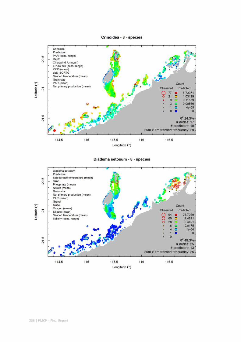
206 | PMCP – Final Report
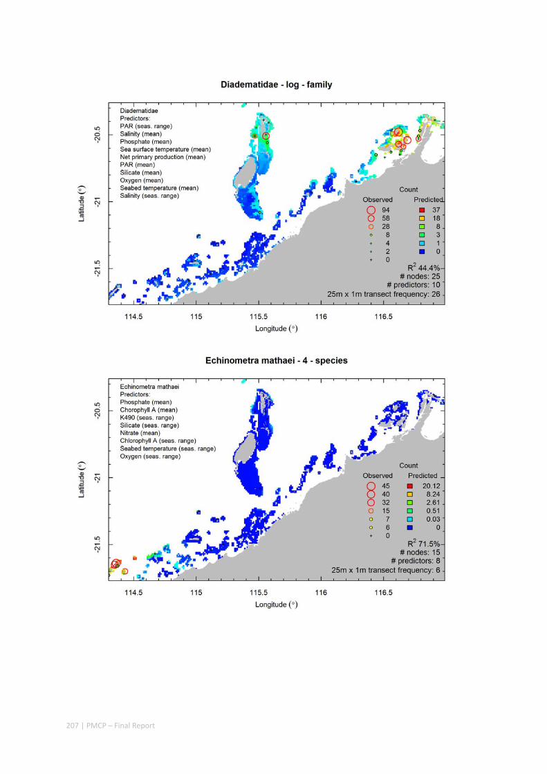
207 | PMCP – Final Report
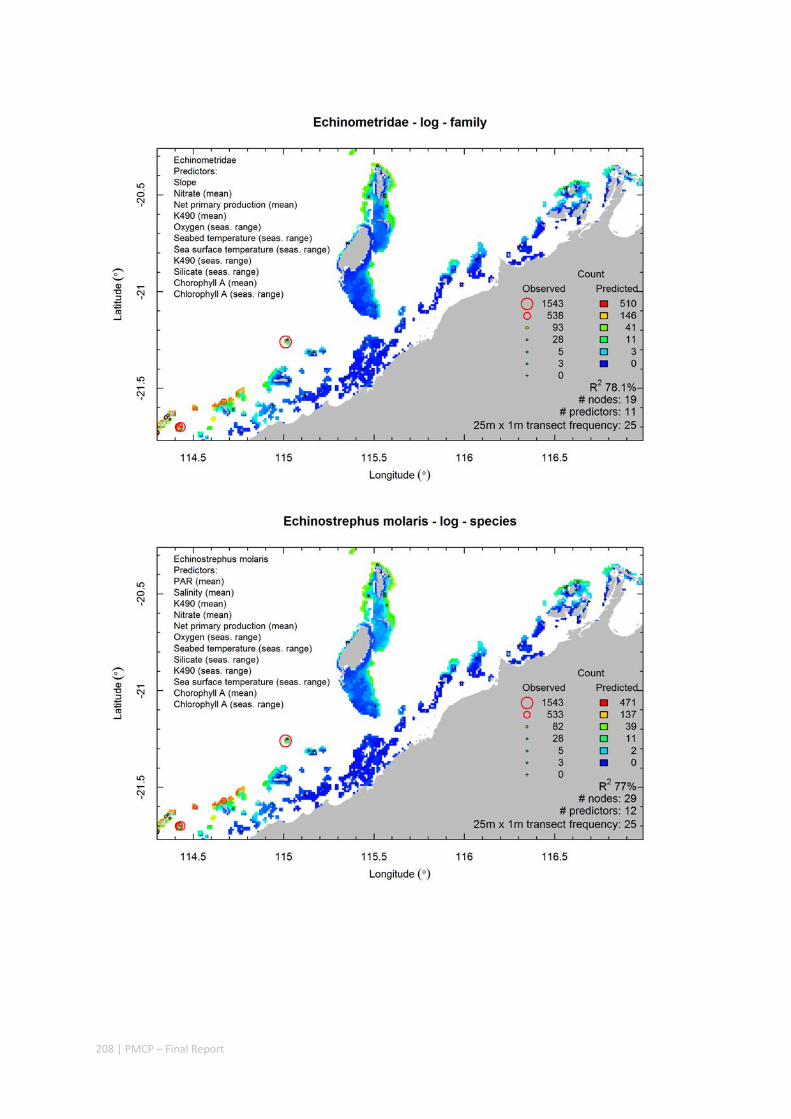
208 | PMCP – Final Report
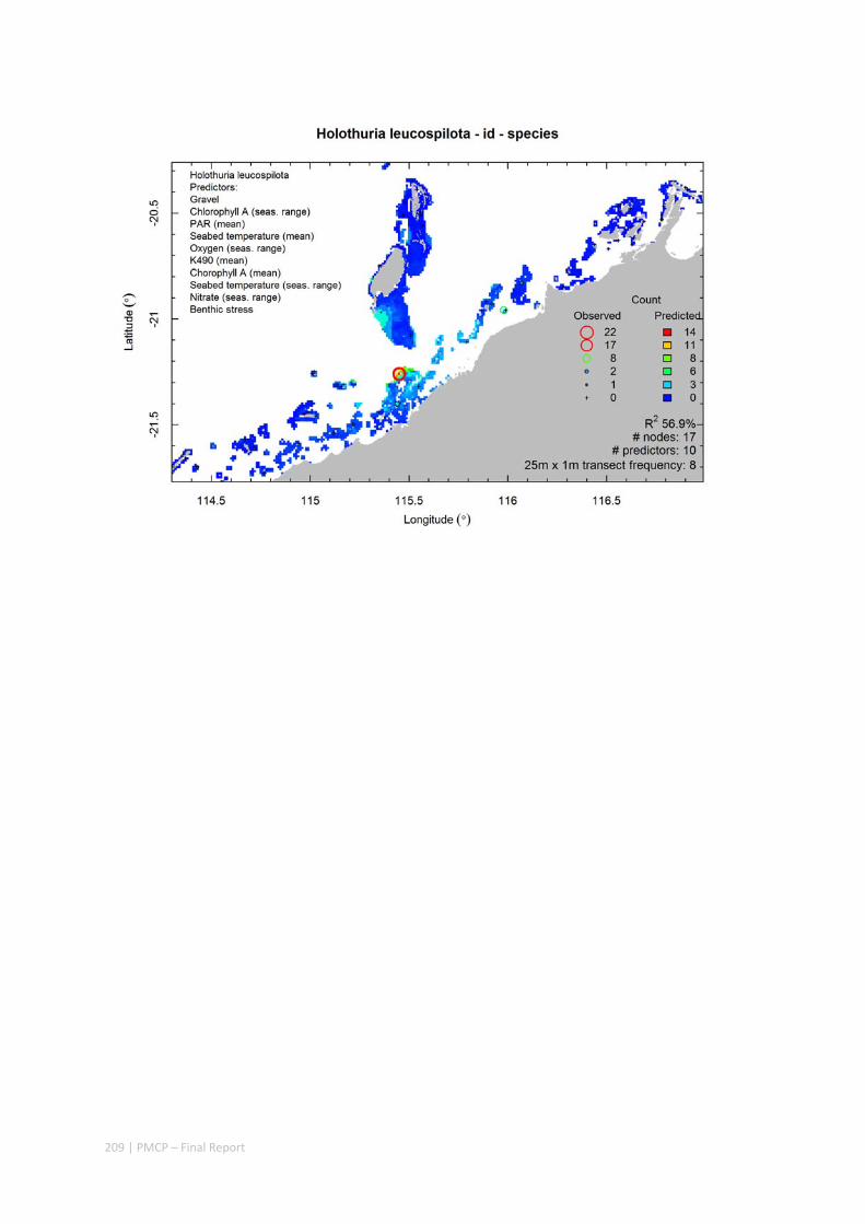
209 | PMCP – Final Report
210 | PMCP – Final Report
Strandings of rare giant irukandji sea jelly; Keesingia gigas Gershwin 2014 (Cnidaria: Cubozoa: Carybdeida: Alatinidae)
Authors: Keesing JK, Barnes P, Ingram B, Gershwin L‐A, Liu D, Slawinski D.
Abstract
Beach strandings of 31 rare giant irukandji sea jelly; Keesingia gigas Gershwin 2014 occurred in Exmouth Gulf, north‐western Australia between 16 and 25 March 2016, with 17 strandings recorded in just two days. These events provided an opportunity to examine this species as the only previously collected specimen was the holotype (off Shark Bay, north‐western Australia). A plankton net survey and visual surveys offshore failed to catch or observe any others. Of 19 specimens collected and/or photographed on the beach, overall medusa length ranged from 190 to 320 mm except for two 80 mm individuals. All but one of the smallest lacked tentacles, consistent with the original description of the species. The tentacles observed on the smallest animal examined may represent ontogentic variability. Clusters of nematocysts were observed on the base (near the skirt) of the bell. Three confirmed envenomations of adult people did not result in them developing symptoms of irukandji syndrome. Confirmed reports of K. gigas were also received from the ocean side of North West Cape indicating distribution was not solely restricted to Exmouth Gulf. Prevailing winds in the lead up to strandings also suggest the jellies had been transported from the ocean north of Exmouth and not from within Exmouth Gulf. All known sightings of K. gigas have been made in the March to May period in four separate years. A public awareness campaign by the Shire of Exmouth was successful in raising awareness of the potential threat to swimmers and beach users and also proved effective in obtaining reports of the distribution of K. gigas.
211 | PMCP – Final Report
3.3.1 INTRODUCTION
Box jellies or cubozoans are a common feature of the plankton in tropical coastal zones including in Australia where they include the highly venomous sea wasp, Chironex fleckeri and a range of species which cause irukandji syndrome (Hartwick 1991; Kingsford et al. 2012; Gershwin et al. 2013; Gershwin 2014; Keesing et al. 2015). The giant irukandji sea jelly; Keesingia gigas Gershwin 2014 was previously only known from the holotype collected off Dirk Hartog Island, Shark Bay in 2012, two underwater photographs and some anecdotal reports of stingings (Marsh and Slack‐Smith 2010; Gershwin 2014). Thus almost nothing is known of its distribution, habitat, biology and ecology and it had hitherto been considered extremely rare.
Reports were received of the stranding of two specimens on the beach at Exmouth in Exmouth Gulf on 16 March 2016. One of these specimens resulted in envenomation of the finder when handled. On the days that followed further strandings and two other stingings were reported (PB personal observations) following a public awareness campaign by local government officials to warn residents and tourists of the resultant danger to beach walkers and swimmers.
The purpose of this paper is to record the occurrence and extent of these strandings and envenomations, update the known distribution of K. gigas and to document the only ever observations made on live and recently dead specimens of this species.
3.3.2 METHODS
Beach surveys
Following the first report on 16 March 2016, beach surveys were conducted by Rangers either from the Shire of Exmouth (SoE) or the Western Australian Government’s Department of Biodiversity, Conservation and Attractions (DBCA). On one occasion one of the authors (JK) also took part in the surveys. The surveys were conducted by driving slowly (about 10 km per hour) along the beach between the high and low water mark in a four‐wheel drive vehicle with one or two observers watching ahead and to the side of vehicle. Due to the large size of the K. gigas, it was easy to see them if they were on the beach or at the immediate water’s edge as the water near the shore was clear. The SoE surveys were conducted once or twice daily between 19 and 28 March at approximately 07:30 and 13:00 hours from north to south over a distance of 4.8 km along the beach to the Exmouth Harbour and then for another 1.7 km south of the harbour (see Figure 3.3.1). Additional surveys were made beyond the main area of focus by both DBCA and SoE. These additional surveys were conducted on 19 and 20 March and included sites to the north (Bundegi) and south (Pebble Beach and Learmonth jetty) of the main focus area as well as at Turquoise Bay and Sandy Bay on the western coast of North‐West Cape (see Figure 3.3.1). Any jellies observed were photographed in situ with a ruler to obtain size information and then collected. Seven of the K. gigas collected were retained for the Western Australian Museum collection and they were fixed in 4% formaldehyde in seawater buffered with sodium tetraborate and samples from some specimens were also preserved in 100% ethanol for possible future genetic analyses. Other reports from known credible sources made to the DBCA and SoE of stranded K. gigas and envenomations by them around the same time were also included in this study. In addition, a photograph of a beach stranded K. gigas from Exmouth taken almost exactly a year before on 18 March 2015 was also provided by a member of the public.
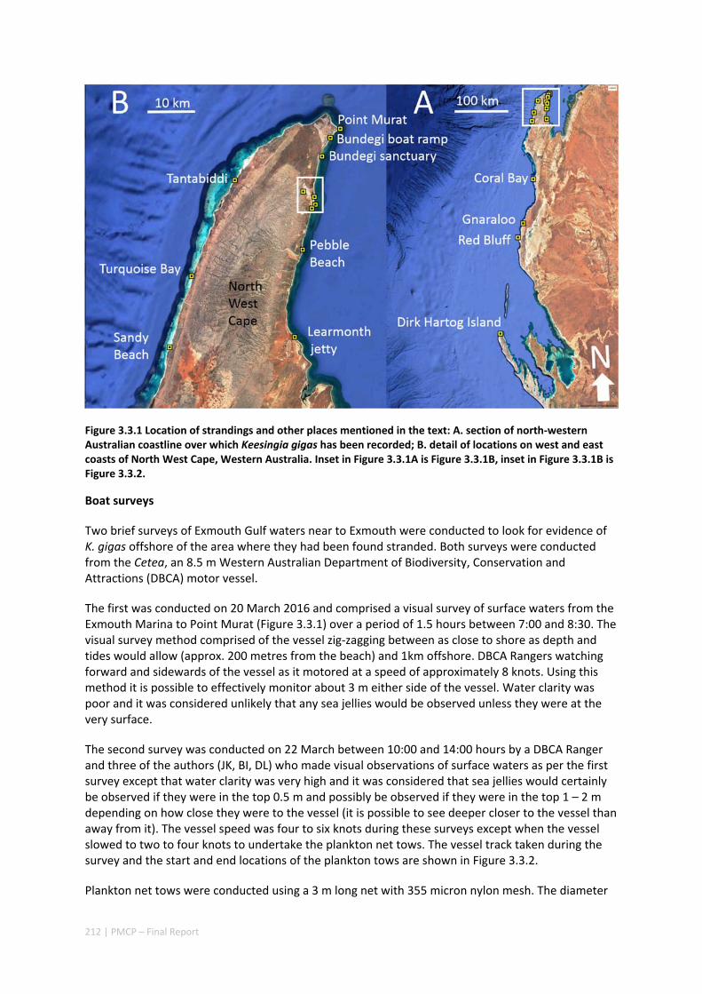
212 | PMCP – Final Report
Figure 3.3.1 Location of strandings and other places mentioned in the text: A. section of north‐western Australian coastline over which Keesingia gigas has been recorded; B. detail of locations on west and east coasts of North West Cape, Western Australia. Inset in Figure 3.3.1A is Figure 3.3.1B, inset in Figure 3.3.1B is Figure 3.3.2.
Boat surveys
Two brief surveys of Exmouth Gulf waters near to Exmouth were conducted to look for evidence of K. gigas offshore of the area where they had been found stranded. Both surveys were conducted from the Cetea, an 8.5 m Western Australian Department of Biodiversity, Conservation and Attractions (DBCA) motor vessel.
The first was conducted on 20 March 2016 and comprised a visual survey of surface waters from the Exmouth Marina to Point Murat (Figure 3.3.1) over a period of 1.5 hours between 7:00 and 8:30. The visual survey method comprised of the vessel zig‐zagging between as close to shore as depth and tides would allow (approx. 200 metres from the beach) and 1km offshore. DBCA Rangers watching forward and sidewards of the vessel as it motored at a speed of approximately 8 knots. Using this method it is possible to effectively monitor about 3 m either side of the vessel. Water clarity was poor and it was considered unlikely that any sea jellies would be observed unless they were at the very surface.
The second survey was conducted on 22 March between 10:00 and 14:00 hours by a DBCA Ranger and three of the authors (JK, BI, DL) who made visual observations of surface waters as per the first survey except that water clarity was very high and it was considered that sea jellies would certainly be observed if they were in the top 0.5 m and possibly be observed if they were in the top 1 – 2 m depending on how close they were to the vessel (it is possible to see deeper closer to the vessel than away from it). The vessel speed was four to six knots during these surveys except when the vessel slowed to two to four knots to undertake the plankton net tows. The vessel track taken during the survey and the start and end locations of the plankton tows are shown in Figure 3.3.2.
Plankton net tows were conducted using a 3 m long net with 355 micron nylon mesh. The diameter

213 | PMCP – Final Report
at the mouth was 0.5 m and at the cod end was 0.1 m. The net was towed 12 m behind the vessel with the top of the net positioned approximately 0.5 m below the surface. A total of ten tows between 4 and 10 minutes duration were made, for a total of 5557 m towed. The volume of the cod end was 2 l and at the end of each tow the contents were emptied into a 45 l black sorting tray to examine for the presence of any medusa. All medusa were then transferred to smaller containers and later fixed in 4% formaldehyde in seawater buffered with sodium tetraborate. The vessel speed, position, track, location of plankton tow start and end points as well as water temperature was recorded on a Garmin GPS/Sounder plotter. The location of the tows is shown in Figure 3.3.2.Wind speed and direction data during the period of the study was obtained from the Bureau of Meteorology (www.bom.gov.au).
Figure 3.3.2 Location of Keesingia gigas strandings and survey sites around Exmouth, Western Australia. Yellow line shows survey track made on 22 March 2016 with start (e.g. 1S) and end (e.g. 1E) points of plankton tows undertaken.
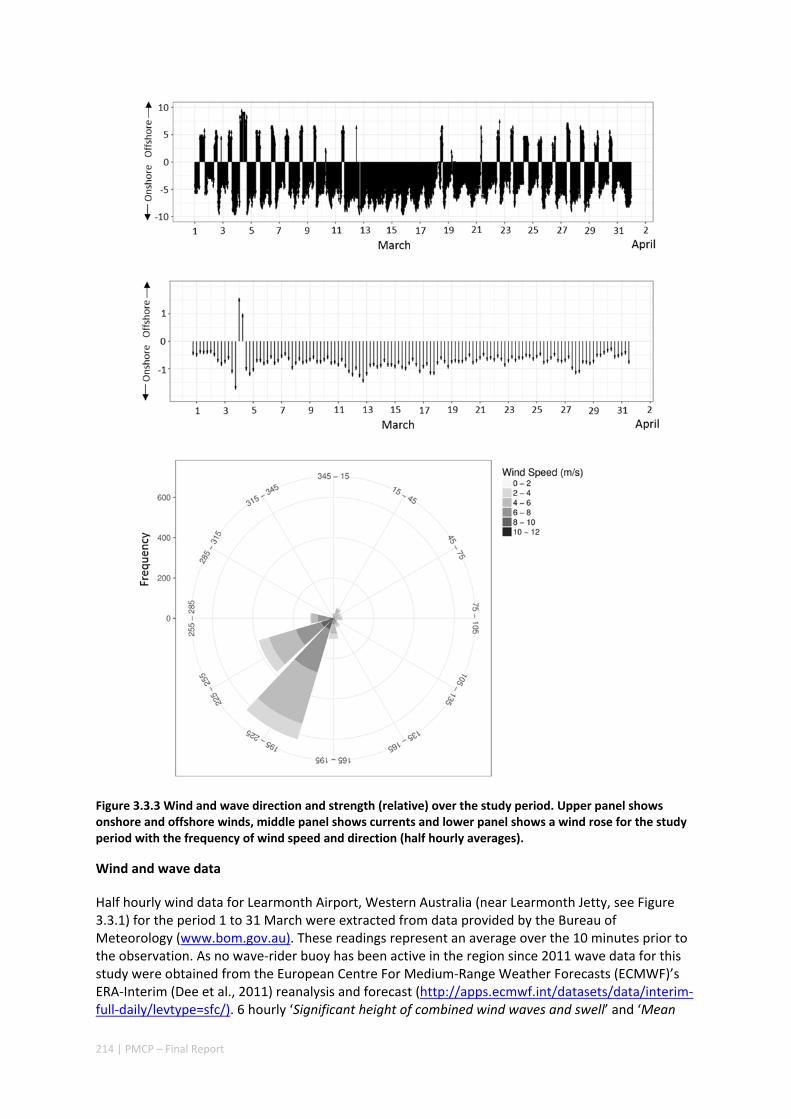
214 | PMCP – Final Report
Figure 3.3.3 Wind and wave direction and strength (relative) over the study period. Upper panel shows onshore and offshore winds, middle panel shows currents and lower panel shows a wind rose for the study period with the frequency of wind speed and direction (half hourly averages).
Wind and wave data
Half hourly wind data for Learmonth Airport, Western Australia (near Learmonth Jetty, see Figure 3.3.1) for the period 1 to 31 March were extracted from data provided by the Bureau of Meteorology (www.bom.gov.au). These readings represent an average over the 10 minutes prior to the observation. As no wave‐rider buoy has been active in the region since 2011 wave data for this study were obtained from the European Centre For Medium‐Range Weather Forecasts (ECMWF)’s ERA‐Interim (Dee et al., 2011) reanalysis and forecast (http://apps.ecmwf.int/datasets/data/interim‐full‐daily/levtype=sfc/). 6 hourly ‘Significant height of combined wind waves and swell’ and ‘Mean

215 | PMCP – Final Report
wave direction’ were extracted at 0.125 x 0.125 degree grids for the region 112o E to 116o E and 20o S to 24o S. The nearest grid cell to the stranding (111.0967o E, 22.2406o S) was used.
Onshore winds shown in Figure 3.3.3 are defined as winds blowing between 180o and 300o clockwise from east. The length of the arrows represents the strength of winds based on windspeed in m/s. The same criteria for onshore vs offshore was applied to the wave data. The length of the wave data arrows represents the strength of the wave based on significant wave height in meters.
The wind rose plot in Figure 3.3.3 bins wind data into 30o segments. The frequency of wind strength is binned at 2 m/s bins.
3.3.3 RESULTS
Beach surveys and other reports of beach strandings
Table 3.3.1 Reports and results of beach surveys for Keesingia gigas. *credible reports to Shire of Exmouth; ** 8 collected by SoE on survey, 5 others reported to SoE. *** collected by DBCA officer.
SOURCE SHIRE OF EXMOUTH (SoE) SURVEYS OTHER CREDIBLE REPORTS TO DBCA
LOCATION DATE
TO 4.8 KM NORTH OF HARBOUR
McLEOD’S BEACH GOLF COURSE TO BUNDEGI
TOTAL
16 March 2* No survey ‐ 2
17 March No survey No survey ‐ ‐
18 March No survey No survey ‐ ‐
19 March 13** 0 ‐ 13
20 March 2 2 ‐ 4
21 March 0 0 ‐ 0
22 March 2 0 5 7
23 March 0 1*** 1 2
24 March 1 0 1 2
25 March 1 1
Observed strandings of K. gigas on the Exmouth Gulf side of North West Cape were restricted to the Exmouth town beach and McLeod’s beach in an area 2 km north and 1 km south of Exmouth Harbour. Surveys of other sites to the north and south did not reveal any strandings of K. gigas. The majority (17 of 31) occurred on March 19 and 20 (see Table 3.3.1) and no sightings occurred between March 25 and 28 when the surveys were ceased. A specimen of K. gigas stranded on McLeod’s Beach is shown in Figure 3.3.4. Following the strandings near Exmouth, Parks and Wildlife Rangers searched beaches at Turquoise Bay, Sandy Bay, Bundegi Beach adjacent to Bundegi Boat ramp and along the beach from Bundegi Sanctuary Zone to the Exmouth Town Beach (Figure 3.3.1 and Figure 3.3.2) on the 19th March, but no K. gigas were observed. Although the searches conducted on the west coast of North West Cape did not reveal any K. gigas, there were three verified reports further south between Coral Bay and Red Bluff (Figure 3.3.1) over the same period

216 | PMCP – Final Report
as our study. A local resident of Coral Bay provided a reliable description of a single K. gigas estimated to be approximately 20cm long stranded at Skeleton Beach just north of Coral Bay on the 10th or 11th March 2016. Residents of Red Bluff photographed and collected video of a single K. gigas stranded on a beach at Red Bluff on the 11th April 2016. The specimen was estimated to be between 30 cm and 40 cm. A single K. gigas measuring approximately 40 cm was collected by a tour operator near North Passage north of Coral Bay on the 14th April 2016. In addition, a Parks and Wildlife Ranger received reports from visitors to Gnaraloo of a ‘squid like jellies being seen’ around the 11th April 2016. After a public awareness campaign by SoE a photograph of a single K. gigas stranded on the beach near Point Murat on the 18th March 2015 was provided by an Exmouth local resident. The size of 19 stranded K. gigas ranged from 80 to 320 mm with 17 animals between 190 and 320 mm and two much smaller specimens measuring just 80 mm.
Figure 3.3.4 Specimen of Keesingia gigas (345 mm) stranded on McLeod’s Beach 23 March 2016. Note the small paddle like pedalium. The white patches are sand inside the bell.
Boat surveys
No K. gigas were observed during either of the boat surveys. Distances traversed during the surveys were approximately 16 km on the first survey and 17 km on the second survey. This is an approximate area of 50,000 m2 searched during both surveys. Three of the ten plankton net tows contained medusa of Liriope tetraphylla and/or Aequorea sp., however no K. gigas were caught despite the net filtering 1091 m3 of water.
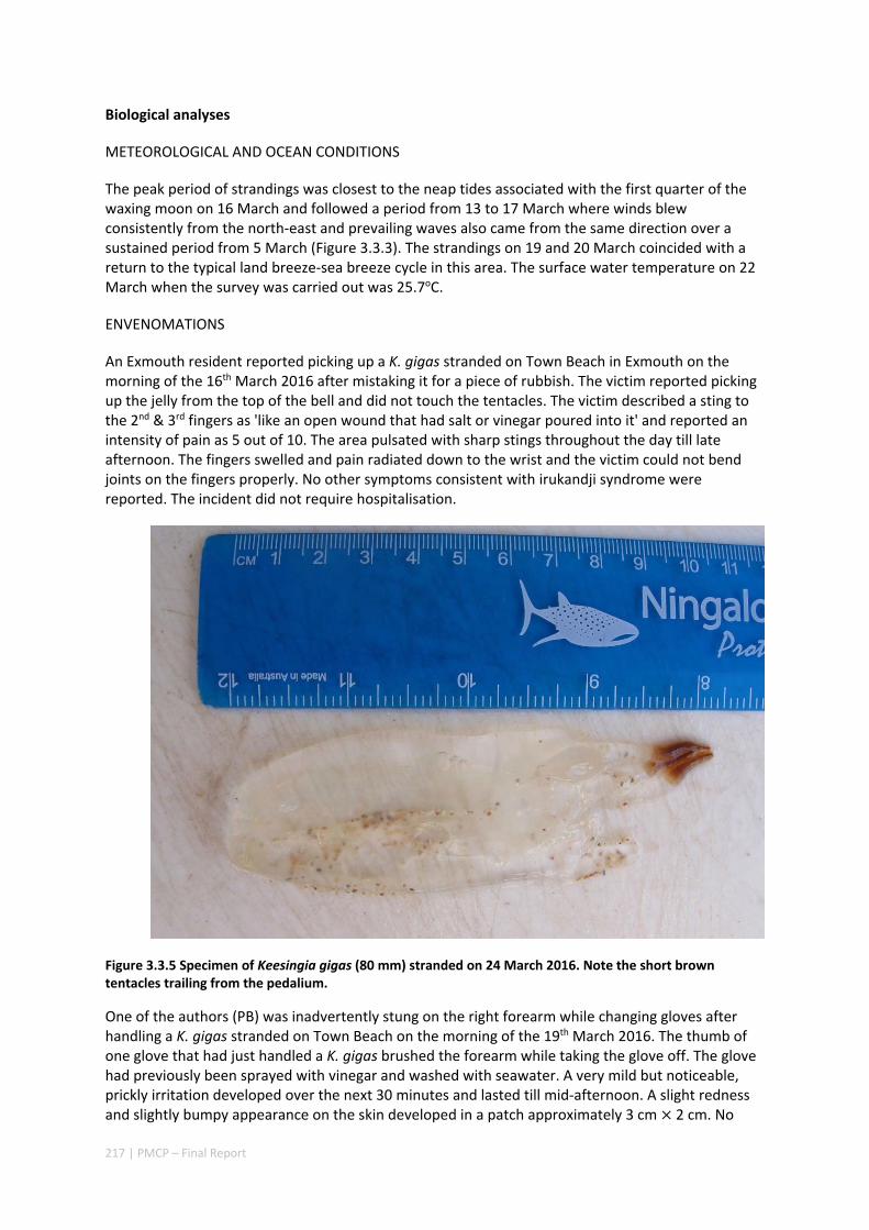
217 | PMCP – Final Report
Biological analyses
METEOROLOGICAL AND OCEAN CONDITIONS
The peak period of strandings was closest to the neap tides associated with the first quarter of the waxing moon on 16 March and followed a period from 13 to 17 March where winds blew consistently from the north‐east and prevailing waves also came from the same direction over a sustained period from 5 March (Figure 3.3.3). The strandings on 19 and 20 March coincided with a return to the typical land breeze‐sea breeze cycle in this area. The surface water temperature on 22 March when the survey was carried out was 25.7oC.
ENVENOMATIONS
An Exmouth resident reported picking up a K. gigas stranded on Town Beach in Exmouth on the morning of the 16th March 2016 after mistaking it for a piece of rubbish. The victim reported picking up the jelly from the top of the bell and did not touch the tentacles. The victim described a sting to the 2nd & 3rd fingers as 'like an open wound that had salt or vinegar poured into it' and reported an intensity of pain as 5 out of 10. The area pulsated with sharp stings throughout the day till late afternoon. The fingers swelled and pain radiated down to the wrist and the victim could not bend joints on the fingers properly. No other symptoms consistent with irukandji syndrome were reported. The incident did not require hospitalisation.
Figure 3.3.5 Specimen of Keesingia gigas (80 mm) stranded on 24 March 2016. Note the short brown tentacles trailing from the pedalium.
One of the authors (PB) was inadvertently stung on the right forearm while changing gloves after handling a K. gigas stranded on Town Beach on the morning of the 19th March 2016. The thumb of one glove that had just handled a K. gigas brushed the forearm while taking the glove off. The glove had previously been sprayed with vinegar and washed with seawater. A very mild but noticeable, prickly irritation developed over the next 30 minutes and lasted till mid‐afternoon. A slight redness and slightly bumpy appearance on the skin developed in a patch approximately 3 cm 2 cm. No

218 | PMCP – Final Report
other symptoms consistent with Irukandji Syndrome were observed.
A local Exmouth resident reported being stung by what appeared to be a K. gigas while wading in shallow water directly south of Exmouth Marina on the weekend of the 19th and 20th March 2016. The patient reported the pain to be localised and intense, but subsided after approximately 10 minutes. The above cases are consistent with our observations of nematocyst clusters present towards the base of the bell.
3.3.4 DISCUSSION
Keesingia gigas was described by Gershwin (2014) on the basis of a single individual captured offshore of Shark Bay by one of the authors (JK) on 7 May 2012. At the time there were also two known photographs of the same species taken offshore of Ningaloo Reef (Marsh and Slack‐Smith 2010). These three records and the large size of K. gigas suggested it was both very rare and/or may be an oceanic species. The strandings on Exmouth beach in Exmouth Gulf reported in this study show that it may occur on the coast, but is probably transported there from offshore by wind and wave driven currents and may be present seasonally with observations made in both March 2015 and 2016. The species was also photographed offshore of Ningaloo in April 2013 (see Figure 3 in Gershwin 2014). Thus all known observations of this species have occurred within the mid‐March to early May period.
The specimen described by Gershwin (2014) was 190 mm long and the specimens measured in our study were 80 to 320 mm. Gershwin (2014) commented on the absence of tentacles in the holotype and in the earlier underwater photographs she had seen. Most of the specimens we collected from the beach lacked tentacles but these could have been lost when the jellies were stranded. However, we found one small specimen, which may have been a juvenile, with tentacles. This individual (Figure 3.3.5) had one tentacle each on three of the four pedalia. The tentacles were comprised of bands of nematocysts and were contracted. The appearance is similar to that of the tentacles in Alatina grandis (see Figure 1a in Straehler‐Pohl and Gul 2017). All other specimens we collected lacked tentacles, although it is possible these may have lost their tentacles when they became stranded on the beach. However the absence of tentacles in the holotype, in the beach stranded specimens we collected in this study, the photographs examined by Gershwin (2014) and a report of a large swimming specimen without tentacles at Coral Bay reported to DBCA during this study suggests that the absence of tentacles in large individuals is typical.
The predominantly north‐westerly, onshore winds and waves (towards the shores of the western coast of Exmouth Gulf) largely unbroken five day period may explain how K. gigas were transported close to the shore on the eastern side of North West Cape and then brought on shore. This accumulation of sea jellies in near shore areas, often termed “swarming”, caused by a combination of wind and tides is a common feature with beach strandings or increased incidence of stinging of beach users (Gershwin et al 2014; Keesing et al. 2015).
Of significant interest is that despite three envenomations, none of the victims went on to develop any of the symptoms of Irukandji syndrome (see Gershwin et al. 2013) and did not require hospitalisation. However, this does not mean K. gigas does not cause Irukandji Syndrome as the stingings may have been minor, thus the species should still be regarded with caution pending further interactions, especially as the stranded specimens handled by those who were stung may have lost their tentacles or the majority of them and Gershwin (2014) cites cases of stingings of K. gigas causing Irukandji Syndrome.
219 | PMCP – Final Report
It is worth noting the value of the public awareness campaign coordinated by the SoE. Members of the public were prompted to provide photographs or observations after reading descriptions and seeing photographs on social media and being able to recognise K. gigas. The awareness campaign provided not only valuable public safety messages, but observations from the public that would have been unlikely previously reported including a report from previous years and from locations almost 300 km from the first observations in Exmouth Gulf.
3.3.5 ACKNOWLEDGEMENTS
We thank Matt Smith and Huw Dilley (DBCA) and David George (SoE) for carrying out the beach and vessel surveys and Joanna Strzelecki and Ryan Crossing (CSIRO) for constructing the plankton net at short notice. This research was financially supported as part of the Pilbara Marine Conservation Partnership funded by the Gorgon Barrow Island Net Conservation Benefits Fund which is administered by the WA Department of Biodiversity, Conservation and Attractions (DBCA).
3.3.6 REFERENCES
Dee DP, Uppala SM, Simmons AJ, Berrisford P, Poli P, Kobayashi S, Andrae U, Balmaseda MA, Balsamo G, Bauer P, Bechtold P, Beljaars ACM, van de Berg L, Bidlot J, Bormann N, Delsol C, Dragani R, Fuentes M, Geer AJ, Haimberger L, Healy SB, Hersbach H, Hólm EV, Isaksen L, Kållberg P, Köhler M, Matricardi M, McNally AP, Monge‐Sanz BM, Morcrette J‐J, Park B‐K, Peubey C, de Rosnay P, Tavolato C, Thépaut J‐N, Vitart F (2011) The ERA‐Interim reanalysis: configuration and performance of the data assimilation system. Q.J.R. Meteorol. Soc. 137:553–597. doi: 10.1002/qj.828.
Gershwin L (2014) Two new species of box jellies (Cnidaria: Cubozoa: Carybdeida) from the central coast of Western Australia, both presumed to cause Irukandji syndrome. Records of the Western Australian Museum 29:10–19.
Gershwin LA, Richardson AJ, Winkel KD, Fenner PJ, Lippmann J, Hore R, Avila‐Soria G, Brewer D, Kloser R.J, Stevens A, Condie S (2013) Biology and ecology of Irukandji jellyfish (Cnidaria: Cubozoa). Adv. Mar. Biol. 66:1–85.
Gershwin L, Condie SA, Mansbridge JV, Richardson AJ (2014). Dangerous jellyfish blooms are predictable. J Roy Soc Interface 11(96):20131168. doi: 10.1098/rsif.2013.1168.
Hartwick RF (1991). Distribution ecology and behaviour of the early life stages of the box‐jellyfish Chironex fleckeri. Hydrobiologia 216:181–188.
Keesing JK, Gershwin LA, Trew T, Strzelecki J, Bearham D, Liu D, Wang Y, Zeidler W, Onton K, Slawinski D (2016) Role of winds and tides in timing of beach strandings, occurrence, and significance of swarms of the jellyfish Crambione mastigophora Mass 1903 (Scyphozoa: Rhizostomeae: Catostylidae) in north‐western Australia. Hydrobiologia 768(1):19–36.
Keesing JK, Strzelecki J, Stowar M, Wakeford M, Miller KJ, Gershwin LA, Liu D (2016) Abundant box jellyfish, Chironex sp. (Cnidaria: Cubozoa: Chirodropidae), discovered at depths of over 50 m on western Australian coastal reefs. Scientific Reports 6:22290. doi: 10.1038/srep22290

220 | PMCP – Final Report
Kingsford MJ, Seymour JE, O’Callaghan MD (2012) Abundance patterns of cubozoans on and near the Great Barrier Reef. Hydrobiologia 690:257–268.
Marsh LM, Slack‐Smith SM (2010) Field guide to the sea stingers and other venomous and poisonous marine invertebrates of Western Australia. Perth, Western Australian Museum, 245 pp.
Straehler‐Pohl I, Gul S (2017) Rediscovery and description of the cubomedusa Alatina grandis (Agassiz & Mayer, 1902) (Cnidaria: Cubozoa: Alatinidae) from Pakistani waters. Plankton and Benthos Research 12(1):1–14.
221 | PMCP – Final Report
4. Connectivity
Ocean circulation drives heterogeneous recruitments and connectivity among coral populations on the North West Shelf of Australia
Authors: Feng M, Colberg F, Slawinski D, Berry O, Babcock R.
Pubilshed in Journal of Marine Systems 164(2016):1‐12.
Abstract
The North West Shelf (NWS) of Australia features extensive and globally‐significant fringing coral reef ecosystems with high levels of endemism and consequently has received significant conservation efforts in the form of Marine Parks. The shelf circulation on the NWS is dominated by the southwestward‐flowing Holloway Current during austral autumn‐winter and by the northeastward monsoonal currents during austral summer. Madden‐Julian Oscillation and short‐term wind variability also drive advection processes on the NWS. These circulation processes are likely to determine demographic inter‐dependencies among reef systems in the region, but the extent and spatial variability of the inter‐dependence is not well understood. Here, we use a 3‐dimensional, hydrostatic, primitive equations model, to simulate the shelf circulation at 1 km horizontal resolution during 2004‐2009. We then use a particle tracking model based on the shelf circulation model to understand larval dispersal in a representative coral species, Acropora millepora, among the 3430 coral reefs on the NWS during its autumn mass spawning. Model predicts that settling larvae typically reach suitable reef within 10 days of spawning, with a predominantly southwestward tendency of transport. There was significant spatial heterogeneity in larval settlements, and this also varied among years. By aggregating the reefs into 47 subregions we estimated that the mean rate of self‐seeding (as a proportion of total supply) was 22% (range from 99% to <1%). Subregions with high retention (as a proportion of total egg production) were not necessarily those with the highest levels of overall larval settlements. Such high “sink” subregions were also some of the most important “source” subregions. The majority of the five most important source and sink subregions were found to be outside existing marine parks, however, marine parks did contain subregions with some of the highest levels of self‐seeding and larval retention.

222 | PMCP – Final Report
4.1.1 INTRODUCTION
Coral reefs are one of the most highly impacted marine ecosystems on earth by human activities (Halpern et al. 2008), and the threats to reefs under anthropogenic climate change are likely to be extreme (Hoegh‐Guldberg et al. 2007). Consideration of how such threats might be mitigated and managed has motivated attempts to understand how levels of ecological and genetic connectivity among meta‐populations may confer these ecosystems with some degree of resilience to human impacts (Botsford et al. 2001, 2009; Cowen et al. 2007). Disruption of natural patterns of larval retention and connectivity may be one of the key factors contributing to the demise of coral reef populations in the coming century (Munday et al. 2009, Steneck et al. 2009; Gilmour et al. 2013).
A significant proportion of the effort devoted to understanding the role of connectivity in the conservation of coral reefs has focused on the role that networks of marine protected areas (MPA) may play in ensuring the resilience of ecosystems and the persistence of populations (Botsford et al. 2009, Bode et al. 2006, Kaplan et al. 2006, 2009). Publications aimed at providing management advice for conservation planners often advocate consideration of connectivity in planning MPA networks (Fernandes et al. 2012), including particular scale or spacing of coral reef MPA networks based on these principles (Gaines et al. 2010, Sale et al. 2010). Meta‐population models of connectivity suggest that the local retention of larvae is a key factor in population persistence (Kaplan et al. 2006, 2009) though the protection of important larval source (sources of larvae settling on other reefs) and sink (destinations of larvae) areas has also been advocated (Jones et al. 2009, Gaines et al. 2010, Sale et al. 2010). Realistically, understanding the interdependencies of any network of meta‐populations, including optimising any network of protected areas, will rely on a broader understanding of ecological processes, as well as source‐sink dynamics and larval retention (Burgess et al. 2014).
The North West Shelf (NWS) is located in the southeast Indian Ocean between North West Cape and Dampier Archipelago of Australia (Figure 4.1.1). The NWS supports extensive and globally‐significant fringing coral reef ecosystems with high levels of endemism (Roberts et al. 2002), and these reefs form a complex topography composed of numerous coral shoals and reefs fringing the 2100 rocky islands of sedimentary and igneous origin. These reef ecosystems are located off an arid coast that receives little terrestrial runoff, thereby facilitating exceptionally high levels of coral growth for a continental margin (Veron 2000). The region features a number of significant marine reserves, including the Montebello/Barrow Island marine protected areas (MBIMPAs) and the Ningaloo Marine Park (Figure 4.1.1), and fisheries resources, closely juxtaposed with an increasing number of oil and gas facilities and growing shipping traffic servicing onshore mining facilities. The region also supports several large port infrastructure developments. Currently planning of a Marine Park in the Dampier Archipelago is well advanced, although reserves are not yet declared and other areas within the region have been suggested as being of potential conservation interest (DPaW 2013). The NWS is one of the source regions of the Leeuwin Current, a poleward‐flowing eastern boundary current in the southeast Indian Ocean. The shelf circulation on the NWS is dominated by the southwestward‐flowing Holloway Current that feeds into the Leeuwin Current during austral autumn and winter (Holloway and Nye 1985; Holloway 1995); and by the Australian monsoonal wind‐driven northeastward currents over the inner‐ and mid‐shelf during austral summer (Condie and Andrewartha 2008). Madden‐Julian Oscillation also drives significant coastal currents on intraseasonal time scales (Marshall and Hendon 2014). Tidal currents and tropical cyclones are important factors in driving horizontal and vertical mixing processes on the shelf and in the nearshore environment. The region is susceptible to the influence of Pacific climate variability, transmitted along the coastal waveguide that drives the interannual variability of the Leeuwin Current (Feng et al. 2003; Wijffels and Meyers 2004). During the consecutive Ningaloo Niño – marine heatwave events in 2011‐2013 (Feng et al. 2015), the NWS experienced coral bleaching in various locations (Depczynski et al. 2013; Moore et al. 2012). Thus, the resilience of coral reef ecosystems to
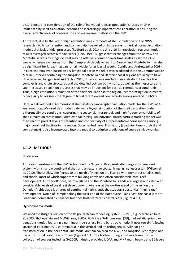
223 | PMCP – Final Report
disturbance, and consideration of the role of individual reefs as population sources or sinks, influenced by shelf circulation, becomes an increasingly important consideration in ensuring the overall effectiveness of conservation and management efforts on the NWS.
At present, due to the lack of high resolution measurements of shelf circulation on the NWS, research into larval retention and connectivity has relied on large scale numerical ocean circulation models that lack of tidal processes (Radford et al. 2014). Using a 10‐km resolution regional model, results averaged across 6 model years (1994–1999) suggest that exchanges from the Barrow and Montebello reefs to Ningaloo Reef may be relatively common over time‐scales as short as 1–2 weeks, whereas exchanges from the Dampier Archipelago reefs to Barrow and Montebello may also be significant for larvae that can remain viable for at least 2 weeks (Condie and Andrewartha 2008). In contrast, however, based on a 9‐km global ocean model, it was predicted that the Commonwealth Marine Reserves containing the Ningaloo‐Montebello and Dampier coast regions are likely to have little larval exchange (Kool and Nichol 2015). These coarse resolution models do not resolve the complex island chain structures and the detailed bottom bathymetry, as well as the mesoscale and sub‐mesoscale circulation processes that may be important for particle retentions around reefs. Thus, a high resolution simulation of the shelf circulation in the region, incorporating tidal currents, is necessary to reassess the degree of larval retention and connectivity among reefs of the NWS.
Here, we developed a 3‐dimensional shelf‐scale oceanographic circulation model for the NWS at 1‐km resolution. We used this model to deliver a 6‐year simulation of the shelf circulation under different climate conditions, capturing the seasonal, interannual, and high frequency variability of shelf circulation that is modulated by tidal forcing. An individual‐based particle tracking model was then used to predict levels of retention and connectivity of a representative coral species among major coral reef habitats in the region. Documented larval life‐history (spawning time, survival and competency) is also incorporated into the model to optimise predictions of source‐sink dynamics.
4.1.2 METHODS
Study area
At its southwestern end the NWS is bounded by Ningaloo Reef, Australia’s largest fringing reef system with a narrow continental shelf and an extensive coastal fringing reef ecosystem (Wilson et al. 2010). The shallow shelf areas to the north of Ningaloo are littered with numerous small islands and shoals, most of which support reef building corals and often considerable coral reef development. Further offshore, Barrow Island and the Montebello Islands are large islands also with considerable levels of coral reef development; whereas at the northern end of the region the Dampier Archipelago is an area of continental high islands that support substantial fringing reef development. North of Dampier along the west end of the Roebourne Plains East, the coast is more linear and dominated by beaches but does host scattered coastal reefs (Figure 4.1.1).
Hydrodynamic model
We used the Rutgers version of the Regional Ocean Modelling System (ROMS, e.g. Marchesiello et al. 2003; Shchepetkin and McWilliams, 2005). ROMS is a 3‐dimensional (3D), hydrostatic, primitive equations model, featuring a non‐linear free‐surface in the barotropic mode. It uses terrain following stretched‐coordinates (S‐coordinates) in the vertical and an orthogonal curvilinear grid transformation in the horizontal. The model domain covered the NWS and Ningaloo Reef region and has a horizontal resolution of ~1 km (Figure 4.1.1). The bottom topography was taken from a collection of sources including GA2009, industry provided LIDAR and MNF multi beam data. 30 levels
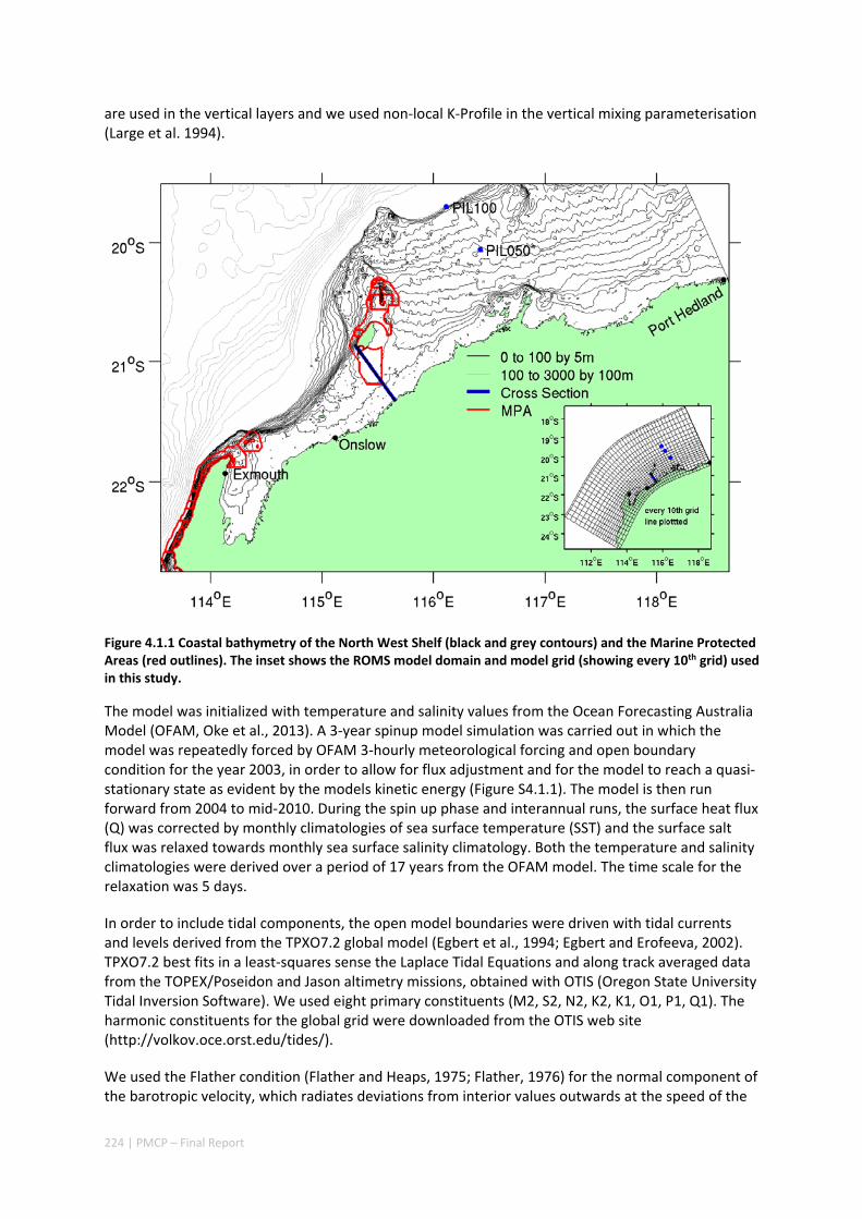
224 | PMCP – Final Report
are used in the vertical layers and we used non‐local K‐Profile in the vertical mixing parameterisation (Large et al. 1994).
Figure 4.1.1 Coastal bathymetry of the North West Shelf (black and grey contours) and the Marine Protected Areas (red outlines). The inset shows the ROMS model domain and model grid (showing every 10th grid) used in this study.
The model was initialized with temperature and salinity values from the Ocean Forecasting Australia Model (OFAM, Oke et al., 2013). A 3‐year spinup model simulation was carried out in which the model was repeatedly forced by OFAM 3‐hourly meteorological forcing and open boundary condition for the year 2003, in order to allow for flux adjustment and for the model to reach a quasi‐stationary state as evident by the models kinetic energy (Figure S4.1.1). The model is then run forward from 2004 to mid‐2010. During the spin up phase and interannual runs, the surface heat flux (Q) was corrected by monthly climatologies of sea surface temperature (SST) and the surface salt flux was relaxed towards monthly sea surface salinity climatology. Both the temperature and salinity climatologies were derived over a period of 17 years from the OFAM model. The time scale for the relaxation was 5 days.
In order to include tidal components, the open model boundaries were driven with tidal currents and levels derived from the TPXO7.2 global model (Egbert et al., 1994; Egbert and Erofeeva, 2002). TPXO7.2 best fits in a least‐squares sense the Laplace Tidal Equations and along track averaged data from the TOPEX/Poseidon and Jason altimetry missions, obtained with OTIS (Oregon State University Tidal Inversion Software). We used eight primary constituents (M2, S2, N2, K2, K1, O1, P1, Q1). The harmonic constituents for the global grid were downloaded from the OTIS web site (http://volkov.oce.orst.edu/tides/).
We used the Flather condition (Flather and Heaps, 1975; Flather, 1976) for the normal component of the barotropic velocity, which radiates deviations from interior values outwards at the speed of the
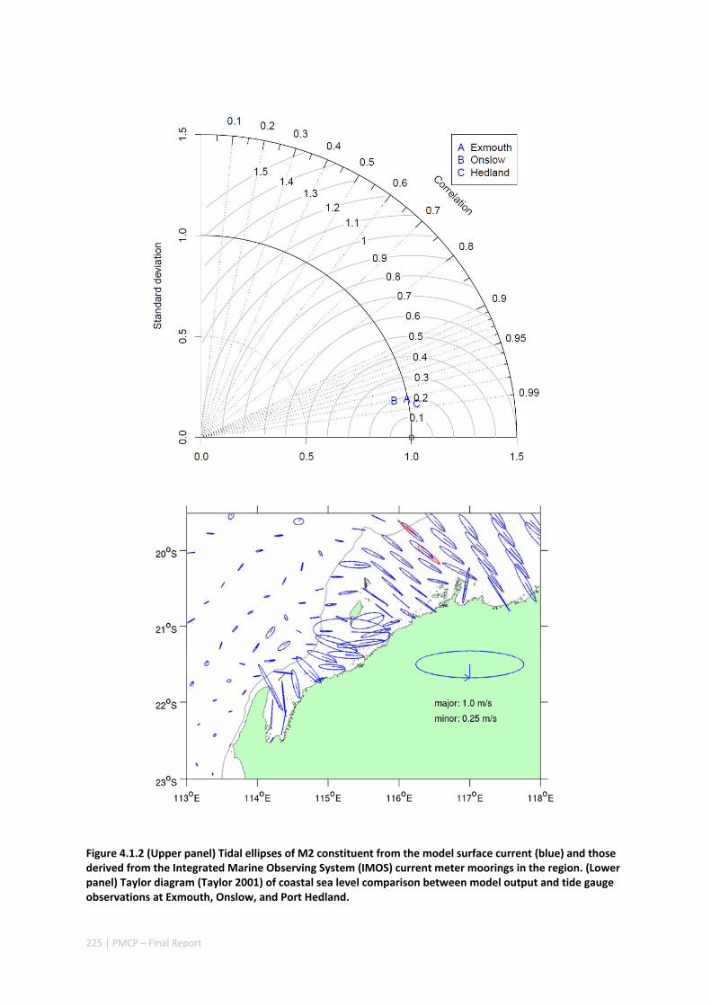
225 | PMCP – Final Report
Figure 4.1.2 (Upper panel) Tidal ellipses of M2 constituent from the model surface current (blue) and those derived from the Integrated Marine Observing System (IMOS) current meter moorings in the region. (Lower panel) Taylor diagram (Taylor 2001) of coastal sea level comparison between model output and tide gauge observations at Exmouth, Onslow, and Port Hedland.
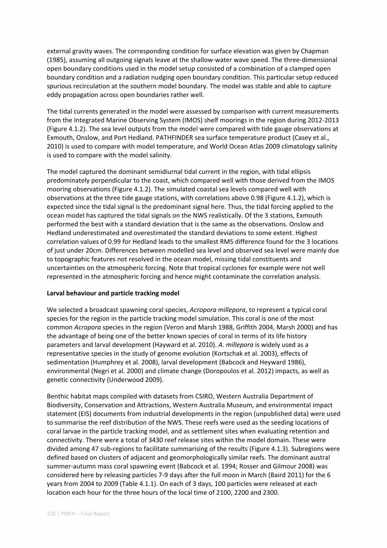
226 | PMCP – Final Report
external gravity waves. The corresponding condition for surface elevation was given by Chapman (1985), assuming all outgoing signals leave at the shallow‐water wave speed. The three‐dimensional open boundary conditions used in the model setup consisted of a combination of a clamped open boundary condition and a radiation nudging open boundary condition. This particular setup reduced spurious recirculation at the southern model boundary. The model was stable and able to capture eddy propagation across open boundaries rather well.
The tidal currents generated in the model were assessed by comparison with current measurements from the Integrated Marine Observing System (IMOS) shelf moorings in the region during 2012‐2013 (Figure 4.1.2). The sea level outputs from the model were compared with tide gauge observations at Exmouth, Onslow, and Port Hedland. PATHFINDER sea surface temperature product (Casey et al., 2010) is used to compare with model temperature, and World Ocean Atlas 2009 climatology salinity is used to compare with the model salinity.
The model captured the dominant semidiurnal tidal current in the region, with tidal ellipsis predominately perpendicular to the coast, which compared well with those derived from the IMOS mooring observations (Figure 4.1.2). The simulated coastal sea levels compared well with observations at the three tide gauge stations, with correlations above 0.98 (Figure 4.1.2), which is expected since the tidal signal is the predominant signal here. Thus, the tidal forcing applied to the ocean model has captured the tidal signals on the NWS realistically. Of the 3 stations, Exmouth performed the best with a standard deviation that is the same as the observations. Onslow and Hedland underestimated and overestimated the standard deviations to some extent. Highest correlation values of 0.99 for Hedland leads to the smallest RMS difference found for the 3 locations of just under 20cm. Differences between modelled sea level and observed sea level were mainly due to topographic features not resolved in the ocean model, missing tidal constituents and uncertainties on the atmospheric forcing. Note that tropical cyclones for example were not well represented in the atmospheric forcing and hence might contaminate the correlation analysis.
Larval behaviour and particle tracking model
We selected a broadcast spawning coral species, Acropora millepora, to represent a typical coral species for the region in the particle tracking model simulation. This coral is one of the most common Acropora species in the region (Veron and Marsh 1988, Griffith 2004, Marsh 2000) and has the advantage of being one of the better known species of coral in terms of its life history parameters and larval development (Hayward et al. 2010). A. millepora is widely used as a representative species in the study of genome evolution (Kortschak et al. 2003), effects of sedimentation (Humphrey et al. 2008), larval development (Babcock and Heyward 1986), environmental (Negri et al. 2000) and climate change (Doropoulos et al. 2012) impacts, as well as genetic connectivity (Underwood 2009).
Benthic habitat maps compiled with datasets from CSIRO, Western Australia Department of Biodiversity, Conservation and Attractions, Western Australia Museum, and environmental impact statement (EIS) documents from industrial developments in the region (unpublished data) were used to summarise the reef distribution of the NWS. These reefs were used as the seeding locations of coral larvae in the particle tracking model, and as settlement sites when evaluating retention and connectivity. There were a total of 3430 reef release sites within the model domain. These were divided among 47 sub‐regions to facilitate summarising of the results (Figure 4.1.3). Subregions were defined based on clusters of adjacent and geomorphologically similar reefs. The dominant austral summer‐autumn mass coral spawning event (Babcock et al. 1994; Rosser and Gilmour 2008) was considered here by releasing particles 7‐9 days after the full moon in March (Baird 2011) for the 6 years from 2004 to 2009 (Table 4.1.1). On each of 3 days, 100 particles were released at each location each hour for the three hours of the local time of 2100, 2200 and 2300.
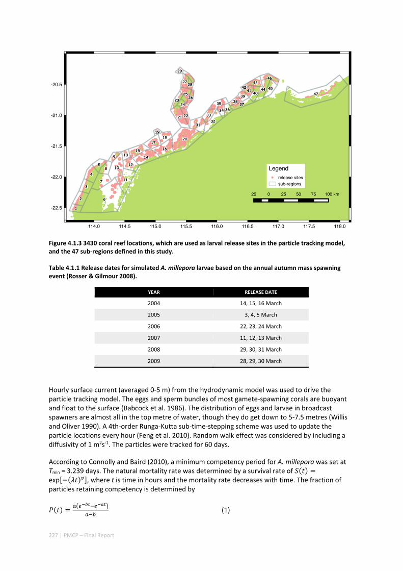
227 | PMCP – Final Report
Figure 4.1.3 3430 coral reef locations, which are used as larval release sites in the particle tracking model, and the 47 sub‐regions defined in this study.
Table 4.1.1 Release dates for simulated A. millepora larvae based on the annual autumn mass spawning event (Rosser & Gilmour 2008).
YEAR RELEASE DATE
2004 14, 15, 16 March
2005 3, 4, 5 March
2006 22, 23, 24 March
2007 11, 12, 13 March
2008 29, 30, 31 March
2009 28, 29, 30 March
Hourly surface current (averaged 0‐5 m) from the hydrodynamic model was used to drive the particle tracking model. The eggs and sperm bundles of most gamete‐spawning corals are buoyant and float to the surface (Babcock et al. 1986). The distribution of eggs and larvae in broadcast spawners are almost all in the top metre of water, though they do get down to 5‐7.5 metres (Willis and Oliver 1990). A 4th‐order Runga‐Kutta sub‐time‐stepping scheme was used to update the particle locations every hour (Feng et al. 2010). Random walk effect was considered by including a diffusivity of 1 m2s‐1. The particles were tracked for 60 days.
According to Connolly and Baird (2010), a minimum competency period for A. millepora was set at Tmin = 3.239 days. The natural mortality rate was determined by a survival rate of exp , where t is time in hours and the mortality rate decreases with time. The fraction of particles retaining competency is determined by
(1)
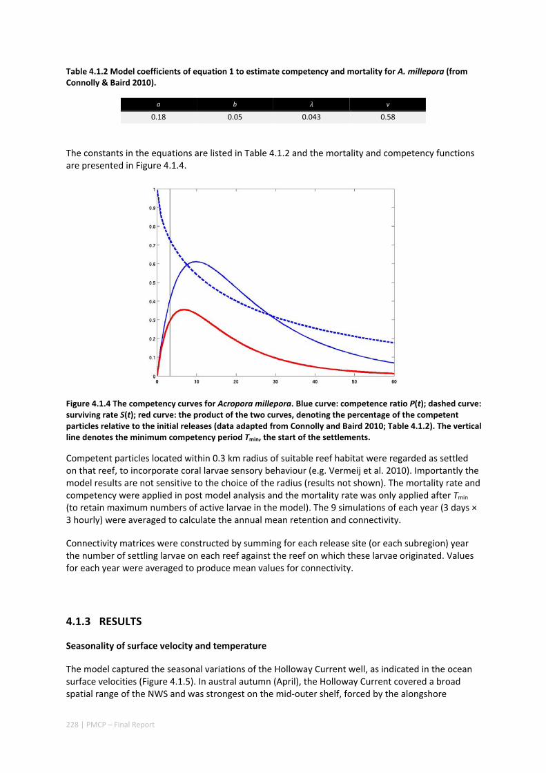
228 | PMCP – Final Report
Table 4.1.2 Model coefficients of equation 1 to estimate competency and mortality for A. millepora (from Connolly & Baird 2010).
a b v
0.18 0.05 0.043 0.58
The constants in the equations are listed in Table 4.1.2 and the mortality and competency functions are presented in Figure 4.1.4.
Figure 4.1.4 The competency curves for Acropora millepora. Blue curve: competence ratio P(t); dashed curve: surviving rate S(t); red curve: the product of the two curves, denoting the percentage of the competent particles relative to the initial releases (data adapted from Connolly and Baird 2010; Table 4.1.2). The vertical line denotes the minimum competency period Tmin, the start of the settlements.
Competent particles located within 0.3 km radius of suitable reef habitat were regarded as settled on that reef, to incorporate coral larvae sensory behaviour (e.g. Vermeij et al. 2010). Importantly the model results are not sensitive to the choice of the radius (results not shown). The mortality rate and competency were applied in post model analysis and the mortality rate was only applied after Tmin (to retain maximum numbers of active larvae in the model). The 9 simulations of each year (3 days × 3 hourly) were averaged to calculate the annual mean retention and connectivity.
Connectivity matrices were constructed by summing for each release site (or each subregion) year the number of settling larvae on each reef against the reef on which these larvae originated. Values for each year were averaged to produce mean values for connectivity.
4.1.3 RESULTS
Seasonality of surface velocity and temperature
The model captured the seasonal variations of the Holloway Current well, as indicated in the ocean surface velocities (Figure 4.1.5). In austral autumn (April), the Holloway Current covered a broad spatial range of the NWS and was strongest on the mid‐outer shelf, forced by the alongshore
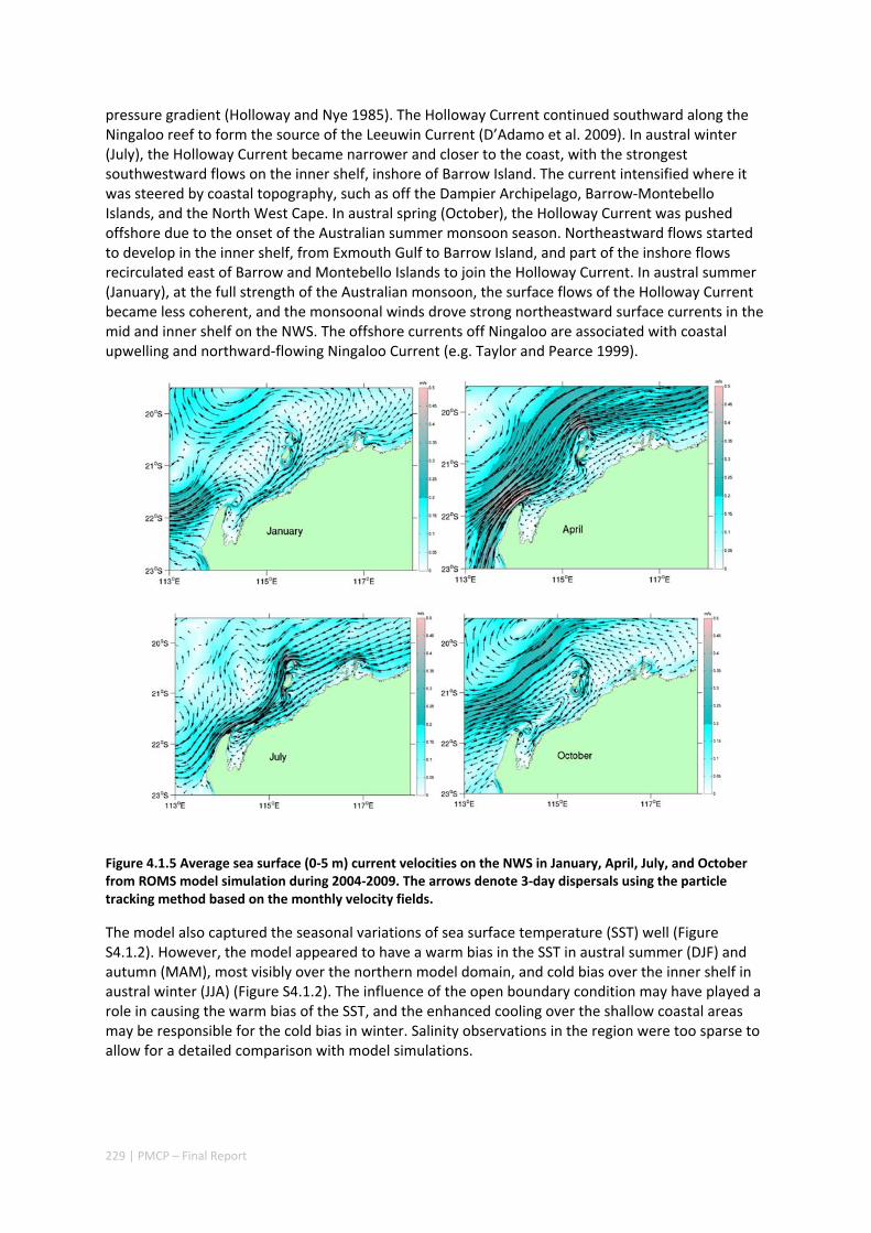
229 | PMCP – Final Report
pressure gradient (Holloway and Nye 1985). The Holloway Current continued southward along the Ningaloo reef to form the source of the Leeuwin Current (D’Adamo et al. 2009). In austral winter (July), the Holloway Current became narrower and closer to the coast, with the strongest southwestward flows on the inner shelf, inshore of Barrow Island. The current intensified where it was steered by coastal topography, such as off the Dampier Archipelago, Barrow‐Montebello Islands, and the North West Cape. In austral spring (October), the Holloway Current was pushed offshore due to the onset of the Australian summer monsoon season. Northeastward flows started to develop in the inner shelf, from Exmouth Gulf to Barrow Island, and part of the inshore flows recirculated east of Barrow and Montebello Islands to join the Holloway Current. In austral summer (January), at the full strength of the Australian monsoon, the surface flows of the Holloway Current became less coherent, and the monsoonal winds drove strong northeastward surface currents in the mid and inner shelf on the NWS. The offshore currents off Ningaloo are associated with coastal upwelling and northward‐flowing Ningaloo Current (e.g. Taylor and Pearce 1999).
Figure 4.1.5 Average sea surface (0‐5 m) current velocities on the NWS in January, April, July, and October from ROMS model simulation during 2004‐2009. The arrows denote 3‐day dispersals using the particle tracking method based on the monthly velocity fields.
The model also captured the seasonal variations of sea surface temperature (SST) well (Figure S4.1.2). However, the model appeared to have a warm bias in the SST in austral summer (DJF) and autumn (MAM), most visibly over the northern model domain, and cold bias over the inner shelf in austral winter (JJA) (Figure S4.1.2). The influence of the open boundary condition may have played a role in causing the warm bias of the SST, and the enhanced cooling over the shallow coastal areas may be responsible for the cold bias in winter. Salinity observations in the region were too sparse to allow for a detailed comparison with model simulations.
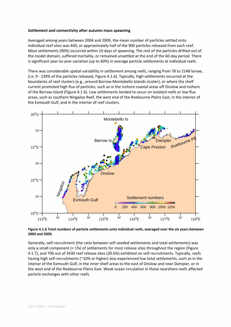
230 | PMCP – Final Report
Settlement and connectivity after autumn mass spawning
Averaged among years between 2004 and 2009, the mean number of particles settled onto individual reef sites was 440, or approximately half of the 900 particles released from each reef. Most settlements (90%) occurred within 10 days of spawning. The rest of the particles drifted out of the model domain, suffered mortality, or remained unsettled at the end of the 60‐day period. There is significant year‐to‐year variation (up to 60%) in average particle settlements at individual reefs.
There was considerable spatial variability in settlement among reefs, ranging from 78 to 2148 larvae, (i.e. 9 ‐ 239% of the particles released, Figure 4.1.6). Typically, high settlements occurred at the boundaries of reef clusters (e.g., around Barrow‐Montebello Islands cluster), or where the shelf current promoted high flux of particles, such as in the inshore coastal areas off Onslow and inshore of the Barrow Island (Figure 4.1.6). Low settlements tended to occur on isolated reefs or low flux areas, such as southern Ningaloo Reef, the west end of the Roebourne Plains East, in the interior of the Exmouth Gulf, and in the interior of reef clusters.
Figure 4.1.6 Total numbers of particle settlements onto individual reefs, averaged over the six years between 2004 and 2009.
Generally, self‐recruitment (the ratio between self‐seeded settlements and total settlements) was only a small component (< 1%) of settlements for most release sites throughout the region (Figure 4.1.7), and 706 out of 3430 reef release sites (20.6%) exhibited no self‐recruitments. Typically, reefs having high self‐recruitments (~10% or higher) also experienced low total settlements, such as in the interior of the Exmouth Gulf, in the inner shelf areas to the east of Onslow and near Dampier, or in the west end of the Roebourne Plains East. Weak ocean circulation in these nearshore reefs affected particle exchanges with other reefs.
113oE 30’ 114oE 30’ 115oE 30’ 116oE 30’ 117oE 30’ 118oE
23oS
30’
22oS
30’
21oS
30’
20oS
Exmouth Gulf
Onslow
Cape Preston
DampierBarrow Is
Montebello Is
Nin
galo
o
Roebourne PE
0 200 400 600 800 1000 1200
Settlement numbers
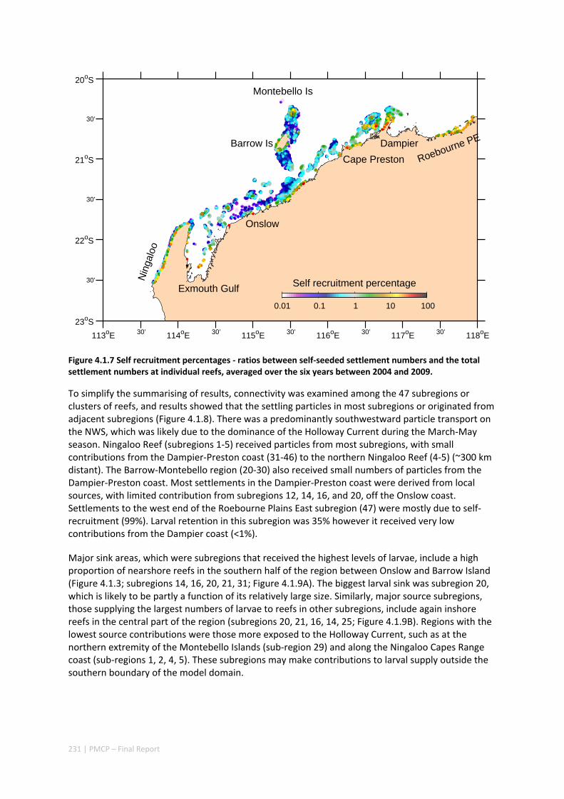
231 | PMCP – Final Report
Figure 4.1.7 Self recruitment percentages ‐ ratios between self‐seeded settlement numbers and the total settlement numbers at individual reefs, averaged over the six years between 2004 and 2009.
To simplify the summarising of results, connectivity was examined among the 47 subregions or clusters of reefs, and results showed that the settling particles in most subregions or originated from adjacent subregions (Figure 4.1.8). There was a predominantly southwestward particle transport on the NWS, which was likely due to the dominance of the Holloway Current during the March‐May season. Ningaloo Reef (subregions 1‐5) received particles from most subregions, with small contributions from the Dampier‐Preston coast (31‐46) to the northern Ningaloo Reef (4‐5) (~300 km distant). The Barrow‐Montebello region (20‐30) also received small numbers of particles from the Dampier‐Preston coast. Most settlements in the Dampier‐Preston coast were derived from local sources, with limited contribution from subregions 12, 14, 16, and 20, off the Onslow coast. Settlements to the west end of the Roebourne Plains East subregion (47) were mostly due to self‐recruitment (99%). Larval retention in this subregion was 35% however it received very low contributions from the Dampier coast (<1%).
Major sink areas, which were subregions that received the highest levels of larvae, include a high proportion of nearshore reefs in the southern half of the region between Onslow and Barrow Island (Figure 4.1.3; subregions 14, 16, 20, 21, 31; Figure 4.1.9A). The biggest larval sink was subregion 20, which is likely to be partly a function of its relatively large size. Similarly, major source subregions, those supplying the largest numbers of larvae to reefs in other subregions, include again inshore reefs in the central part of the region (subregions 20, 21, 16, 14, 25; Figure 4.1.9B). Regions with the lowest source contributions were those more exposed to the Holloway Current, such as at the northern extremity of the Montebello Islands (sub‐region 29) and along the Ningaloo Capes Range coast (sub‐regions 1, 2, 4, 5). These subregions may make contributions to larval supply outside the southern boundary of the model domain.
113oE 30’ 114oE 30’ 115oE 30’ 116oE 30’ 117oE 30’ 118oE
23oS
30’
22oS
30’
21oS
30’
20oS
Exmouth Gulf
Onslow
Cape Preston
DampierBarrow Is
Montebello Is
Nin
galo
oRoebourne PE
0.01 0.1 1 10 100
Self recruitment percentage
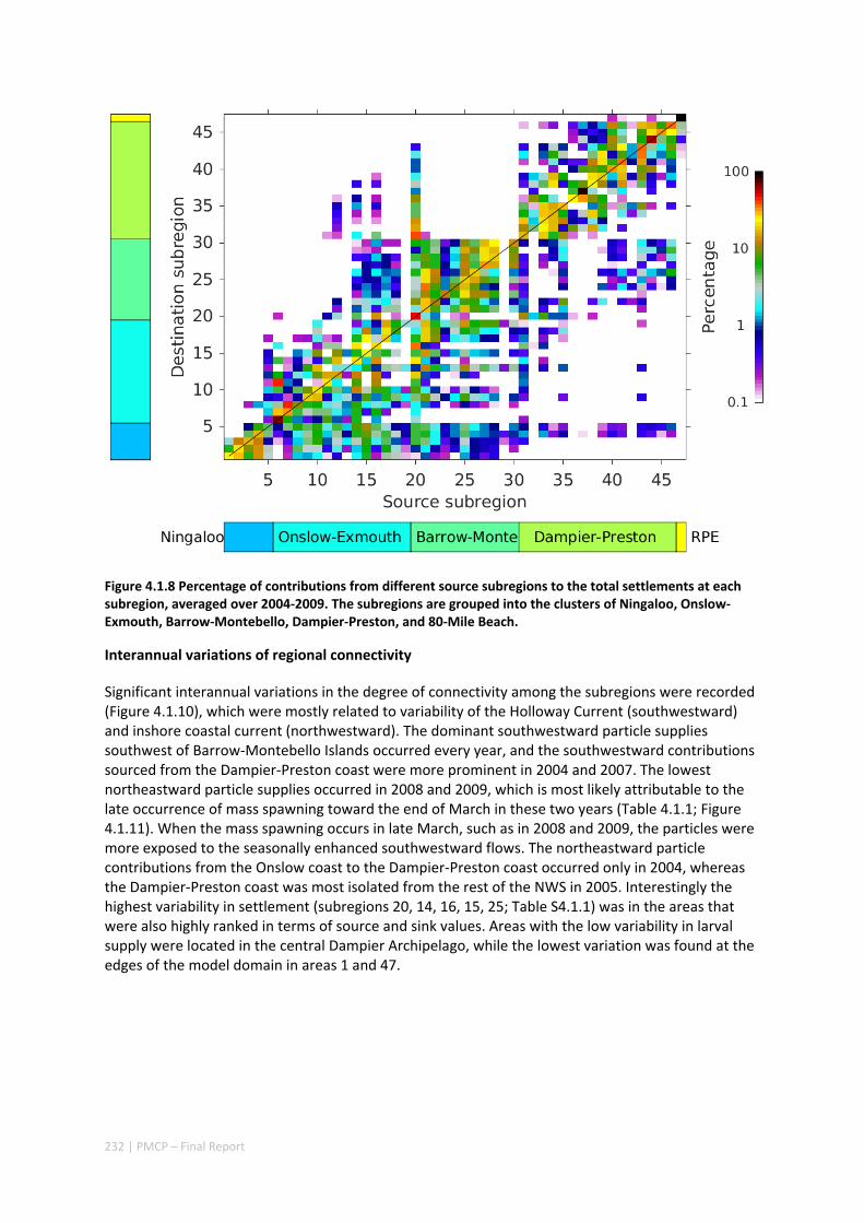
232 | PMCP – Final Report
Figure 4.1.8 Percentage of contributions from different source subregions to the total settlements at each subregion, averaged over 2004‐2009. The subregions are grouped into the clusters of Ningaloo, Onslow‐Exmouth, Barrow‐Montebello, Dampier‐Preston, and 80‐Mile Beach.
Interannual variations of regional connectivity
Significant interannual variations in the degree of connectivity among the subregions were recorded (Figure 4.1.10), which were mostly related to variability of the Holloway Current (southwestward) and inshore coastal current (northwestward). The dominant southwestward particle supplies southwest of Barrow‐Montebello Islands occurred every year, and the southwestward contributions sourced from the Dampier‐Preston coast were more prominent in 2004 and 2007. The lowest northeastward particle supplies occurred in 2008 and 2009, which is most likely attributable to the late occurrence of mass spawning toward the end of March in these two years (Table 4.1.1; Figure 4.1.11). When the mass spawning occurs in late March, such as in 2008 and 2009, the particles were more exposed to the seasonally enhanced southwestward flows. The northeastward particle contributions from the Onslow coast to the Dampier‐Preston coast occurred only in 2004, whereas the Dampier‐Preston coast was most isolated from the rest of the NWS in 2005. Interestingly the highest variability in settlement (subregions 20, 14, 16, 15, 25; Table S4.1.1) was in the areas that were also highly ranked in terms of source and sink values. Areas with the low variability in larval supply were located in the central Dampier Archipelago, while the lowest variation was found at the edges of the model domain in areas 1 and 47.
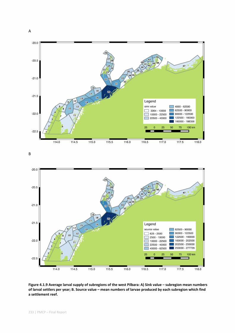
233 | PMCP – Final Report
A
B
Figure 4.1.9 Average larval supply of subregions of the west Pilbara: A) Sink value – subregion mean numbers of larval settlers per year; B. Source value – mean numbers of larvae produced by each subregion which find a settlement reef.
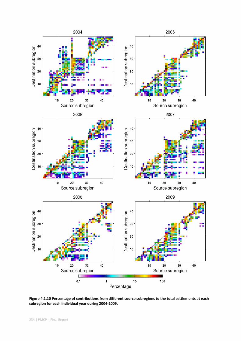
234 | PMCP – Final Report
Figure 4.1.10 Percentage of contributions from different source subregions to the total settlements at each subregion for each individual year during 2004‐2009.
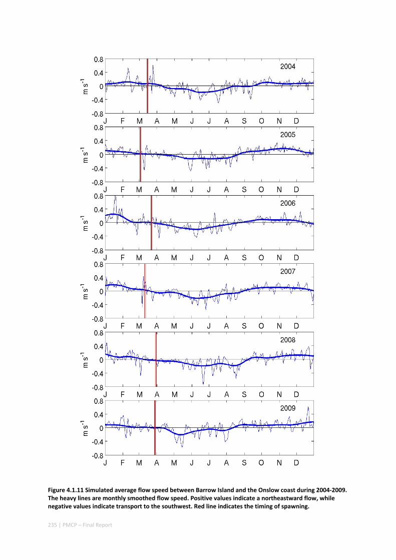
235 | PMCP – Final Report
Figure 4.1.11 Simulated average flow speed between Barrow Island and the Onslow coast during 2004‐2009. The heavy lines are monthly smoothed flow speed. Positive values indicate a northeastward flow, while negative values indicate transport to the southwest. Red line indicates the timing of spawning.
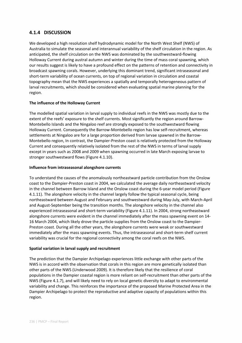
236 | PMCP – Final Report
4.1.4 DISCUSSION
We developed a high resolution shelf hydrodynamic model for the North West Shelf (NWS) of Australia to simulate the seasonal and interannual variability of the shelf circulation in the region. As anticipated, the shelf circulation on the NWS was dominated by the southwestward‐flowing Holloway Current during austral autumn and winter during the time of mass coral spawning, which our results suggest is likely to have a profound effect on the patterns of retention and connectivity in broadcast spawning corals. However, underlying this dominant trend, significant intraseasonal and short‐term variability of ocean currents, on top of regional variation in circulation and coastal topography mean that the NWS experiences a spatially and temporally heterogeneous pattern of larval recruitments, which should be considered when evaluating spatial marine planning for the region.
The influence of the Holloway Current
The modelled spatial variation in larval supply to individual reefs in the NWS was mostly due to the extent of the reefs’ exposure to the shelf currents. Most significantly the region around Barrow‐Montebello Islands and the Ningaloo reef are strongly exposed to the southwestward flowing Holloway Current. Consequently the Barrow‐Montebello region has low self‐recruitment, whereas settlements at Ningaloo are for a large proportion derived from larvae spawned in the Barrow‐Montebello region, In contrast, the Dampier‐Preston coast is relatively protected from the Holloway Current and consequently relatively isolated from the rest of the NWS in terms of larval supply except in years such as 2008 and 2009 when spawning occurred in late March exposing larvae to stronger southwestward flows (Figure 4.1.10).
Influence from intraseasonal alongshore currents
To understand the causes of the anomalously northeastward particle contribution from the Onslow coast to the Dampier‐Preston coast in 2004, we calculated the average daily northeastward velocity in the channel between Barrow Island and the Onslow coast during the 6‐year model period (Figure 4.1.11). The alongshore velocity in the channel largely follow the typical seasonal cycle, being northeastward between August and February and southwestward during May‐July, with March‐April and August‐September being the transition months. The alongshore velocity in the channel also experienced intraseasonal and short‐term variability (Figure 4.1.11). In 2004, strong northeastward alongshore currents were evident in the channel immediately after the mass spawning event on 14‐16 March 2004, which likely drove the particle supplies from the Onslow coast to the Dampier‐Preston coast. During all the other years, the alongshore currents were weak or southwestward immediately after the mass spawning events. Thus, the intraseasonal and short‐term shelf current variability was crucial for the regional connectivity among the coral reefs on the NWS.
Spatial variation in larval supply and recruitment
The prediction that the Dampier Archipelago experiences little exchange with other parts of the NWS is in accord with the observation that corals in this region are more genetically isolated than other parts of the NWS (Underwood 2009). It is therefore likely that the resilience of coral populations in the Dampier coastal region is more reliant on self‐recruitment than other parts of the NWS (Figure 4.1.7), and will likely need to rely on local genetic diversity to adapt to environmental variability and change. This reinforces the importance of the proposed Marine Protected Area in the Dampier Archipelago to protect the reproductive and adaptive capacity of populations within this region.
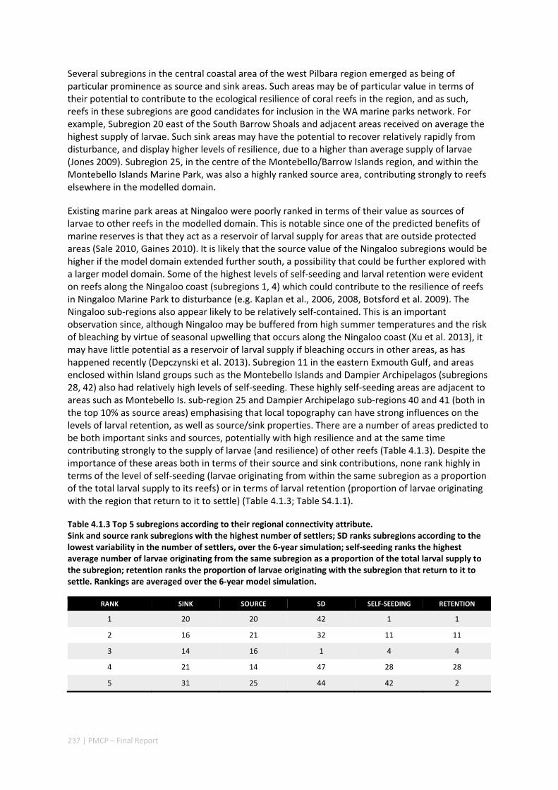
237 | PMCP – Final Report
Several subregions in the central coastal area of the west Pilbara region emerged as being of particular prominence as source and sink areas. Such areas may be of particular value in terms of their potential to contribute to the ecological resilience of coral reefs in the region, and as such, reefs in these subregions are good candidates for inclusion in the WA marine parks network. For example, Subregion 20 east of the South Barrow Shoals and adjacent areas received on average the highest supply of larvae. Such sink areas may have the potential to recover relatively rapidly from disturbance, and display higher levels of resilience, due to a higher than average supply of larvae (Jones 2009). Subregion 25, in the centre of the Montebello/Barrow Islands region, and within the Montebello Islands Marine Park, was also a highly ranked source area, contributing strongly to reefs elsewhere in the modelled domain.
Existing marine park areas at Ningaloo were poorly ranked in terms of their value as sources of larvae to other reefs in the modelled domain. This is notable since one of the predicted benefits of marine reserves is that they act as a reservoir of larval supply for areas that are outside protected areas (Sale 2010, Gaines 2010). It is likely that the source value of the Ningaloo subregions would be higher if the model domain extended further south, a possibility that could be further explored with a larger model domain. Some of the highest levels of self‐seeding and larval retention were evident on reefs along the Ningaloo coast (subregions 1, 4) which could contribute to the resilience of reefs in Ningaloo Marine Park to disturbance (e.g. Kaplan et al., 2006, 2008, Botsford et al. 2009). The Ningaloo sub‐regions also appear likely to be relatively self‐contained. This is an important observation since, although Ningaloo may be buffered from high summer temperatures and the risk of bleaching by virtue of seasonal upwelling that occurs along the Ningaloo coast (Xu et al. 2013), it may have little potential as a reservoir of larval supply if bleaching occurs in other areas, as has happened recently (Depczynski et al. 2013). Subregion 11 in the eastern Exmouth Gulf, and areas enclosed within Island groups such as the Montebello Islands and Dampier Archipelagos (subregions 28, 42) also had relatively high levels of self‐seeding. These highly self‐seeding areas are adjacent to areas such as Montebello Is. sub‐region 25 and Dampier Archipelago sub‐regions 40 and 41 (both in the top 10% as source areas) emphasising that local topography can have strong influences on the levels of larval retention, as well as source/sink properties. There are a number of areas predicted to be both important sinks and sources, potentially with high resilience and at the same time contributing strongly to the supply of larvae (and resilience) of other reefs (Table 4.1.3). Despite the importance of these areas both in terms of their source and sink contributions, none rank highly in terms of the level of self‐seeding (larvae originating from within the same subregion as a proportion of the total larval supply to its reefs) or in terms of larval retention (proportion of larvae originating with the region that return to it to settle) (Table 4.1.3; Table S4.1.1).
Table 4.1.3 Top 5 subregions according to their regional connectivity attribute. Sink and source rank subregions with the highest number of settlers; SD ranks subregions according to the lowest variability in the number of settlers, over the 6‐year simulation; self‐seeding ranks the highest average number of larvae originating from the same subregion as a proportion of the total larval supply to the subregion; retention ranks the proportion of larvae originating with the subregion that return to it to settle. Rankings are averaged over the 6‐year model simulation.
RANK SINK SOURCE SD SELF‐SEEDING RETENTION
1 20 20 42 1 1
2 16 21 32 11 11
3 14 16 1 4 4
4 21 14 47 28 28
5 31 25 44 42 2
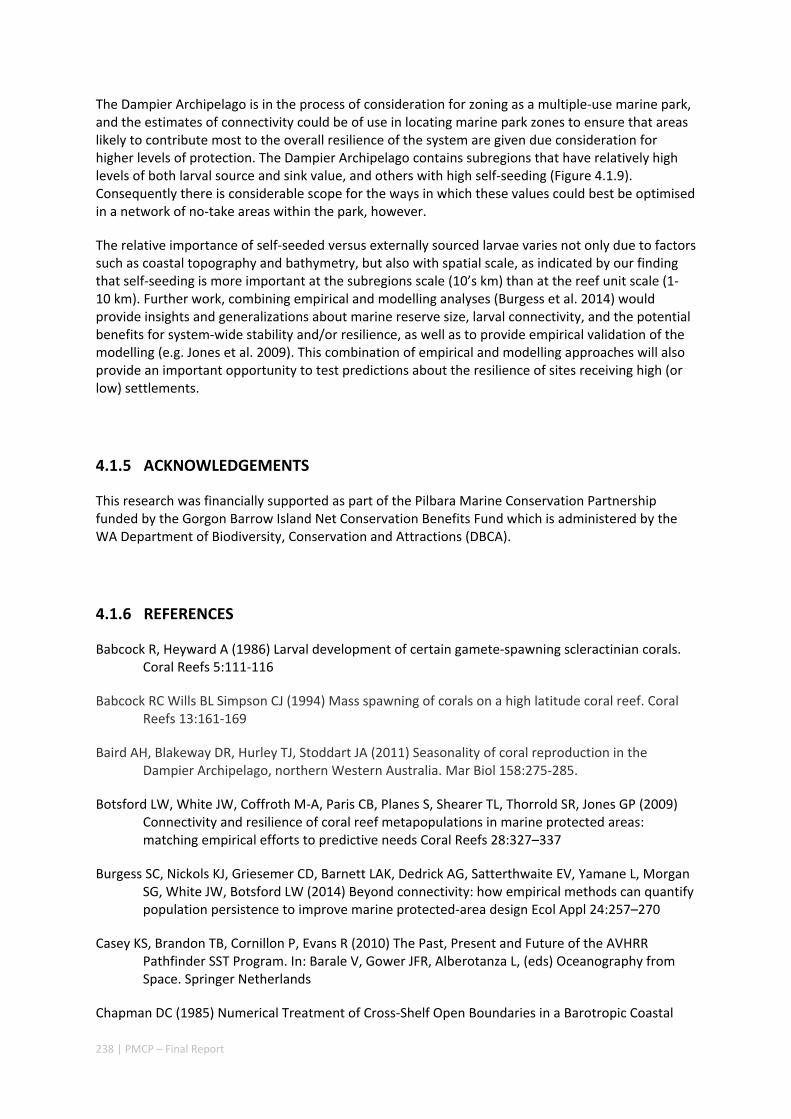
238 | PMCP – Final Report
The Dampier Archipelago is in the process of consideration for zoning as a multiple‐use marine park, and the estimates of connectivity could be of use in locating marine park zones to ensure that areas likely to contribute most to the overall resilience of the system are given due consideration for higher levels of protection. The Dampier Archipelago contains subregions that have relatively high levels of both larval source and sink value, and others with high self‐seeding (Figure 4.1.9). Consequently there is considerable scope for the ways in which these values could best be optimised in a network of no‐take areas within the park, however.
The relative importance of self‐seeded versus externally sourced larvae varies not only due to factors such as coastal topography and bathymetry, but also with spatial scale, as indicated by our finding that self‐seeding is more important at the subregions scale (10’s km) than at the reef unit scale (1‐10 km). Further work, combining empirical and modelling analyses (Burgess et al. 2014) would provide insights and generalizations about marine reserve size, larval connectivity, and the potential benefits for system‐wide stability and/or resilience, as well as to provide empirical validation of the modelling (e.g. Jones et al. 2009). This combination of empirical and modelling approaches will also provide an important opportunity to test predictions about the resilience of sites receiving high (or low) settlements.
4.1.5 ACKNOWLEDGEMENTS
This research was financially supported as part of the Pilbara Marine Conservation Partnership funded by the Gorgon Barrow Island Net Conservation Benefits Fund which is administered by the WA Department of Biodiversity, Conservation and Attractions (DBCA).
4.1.6 REFERENCES
Babcock R, Heyward A (1986) Larval development of certain gamete‐spawning scleractinian corals. Coral Reefs 5:111‐116
Babcock RC Wills BL Simpson CJ (1994) Mass spawning of corals on a high latitude coral reef. Coral Reefs 13:161‐169
Baird AH, Blakeway DR, Hurley TJ, Stoddart JA (2011) Seasonality of coral reproduction in the Dampier Archipelago, northern Western Australia. Mar Biol 158:275‐285.
Botsford LW, White JW, Coffroth M‐A, Paris CB, Planes S, Shearer TL, Thorrold SR, Jones GP (2009) Connectivity and resilience of coral reef metapopulations in marine protected areas: matching empirical efforts to predictive needs Coral Reefs 28:327–337
Burgess SC, Nickols KJ, Griesemer CD, Barnett LAK, Dedrick AG, Satterthwaite EV, Yamane L, Morgan SG, White JW, Botsford LW (2014) Beyond connectivity: how empirical methods can quantify population persistence to improve marine protected‐area design Ecol Appl 24:257–270
Casey KS, Brandon TB, Cornillon P, Evans R (2010) The Past, Present and Future of the AVHRR Pathfinder SST Program. In: Barale V, Gower JFR, Alberotanza L, (eds) Oceanography from Space. Springer Netherlands
Chapman DC (1985) Numerical Treatment of Cross‐Shelf Open Boundaries in a Barotropic Coastal
239 | PMCP – Final Report
Ocean Model. J. Phys. Oceanogr 15:1060‐1075
Condie S, Andrewartha J (2008) Circulation and connectivity on the Australian North West Shelf. Cont Shelf Res 28:1724–1739
Connolly SR, Baird AH (2010) Estimating dispersal potential for marine larvae: dynamic models applied to scleractinian corals. Ecology 91:3572‐3583.
Cowen RK, Gawarkiewicz G, Pineda J, Thorrold SR, Werner FE (2007) Population connectivity in marine systems: An overview. Oceanography 20:14–21
D'Adamo ND, Fandry C, Buchan S, Domingues C (2009) Northern Sources of the Leeuwin Current and the “Holloway Current” on the North West Shelf. J Roy Soc Western Australia 92:53–66
Depczynski M, Gilmour JP, Ridgway T, Barnes H, Heyward AJ, Holmes TH, Moore JAY, Radford BT, Thomson DP, Tinkler P, Wilson SK (2013) Bleaching, coral mortality and subsequent survivorship on a West Australian fringing reef. Coral Reefs 32:233–238
Doropoulos C, Ward S, Diaz‐Pulido G, Hoegh‐Guldberg O, Mumby PJ (2012) Ocean acidification reduces coral recruitment by disrupting intimate larval‐algal settlement interactions. Ecol Lett 15:338‐346
DPaW (2013) http://www.dpaw.wa.gov.au/management/marine/marine‐parks‐and‐reserves/69‐new‐and‐proposed‐marine‐parks‐and‐reserves
Egbert GD, Bennett AF, Foreman MGG (1994) TOPEX/POSEIDON tides estimated using a global inverse model. J Geophys Res 99:24,821‐24,852.
Egbert GD, Erofeeva S (2002) Efficient inverse modelling of barotropic ocean tides. J Atmos Ocean Technol 19:183–204
Feng M, Meyers G, Pearce A, Wijffels S (2003) Annual and Interannual Variations of the Leeuwin Current at 32° S. J Geophys Res 108:3355
Feng M, Slawinski D, Beckley L, Keesing J (2010) Retention and dispersal of shelf waters influenced by interactions of ocean boundary current and coastal geography.Mar Freshwater Res 61:1259‐1267
Fernandes L, Green A, Tanzer J, White A, Alino PM, Jompa J, Lokani P, Soemodinoto A, Knight M, Pomeroy B, Possingham H, Pressey B (2012) Biophysical principles for designing resilient networks of marine protected areas to integrate fisheries, biodiversity and climate change objectives in the Coral Triangle. Report prepared by The Nature Conservancy for the Coral Triangle Support Partnership 152 pp
Feng M, Hendon HH, Xie S‐P, Marshall AG, Schiller A, Kosaka Y, Caputi N, Pearce A (2015) Decadal increase in Ningaloo Niño since the late 1990s. Geophys Res Lett 42:104‐112
Flather RA, Heaps NS (1975) Tidal Computations for Morecambe Bay. Geophys J Roy Astronomical Soc 42:489–517
Flather RA (1976) A tidal model of the north‐west European continental shelf. Mem Soc Roy Sci Liege 6:141–164
240 | PMCP – Final Report
Gaines SD, White C, Carr MH, Palumbi SR (2010) Designing marine reserve networks for both conservation and fisheries management. Proc Natl Acad Sci USA107:18286‐18293
Gilmour JP, Smith LD, Heyward AJ, Baird AH, Pratchett MS (2013) Recovery of an isolated coral reef system following severe disturbance. Science 340:69‐71
Griffith JK (2004) Scleractinian corals collected during 1998 from the Dampier Archipelago, Western Australia. In: Jones D (ed) Marine biodiversity of the Dampier Archipelago, Western Australia 1998‐2002, Book 2002. Western Australian Museum, Perth
Halpern BS, Walbridge S, Selkoe KA, Kappel CV, Micheli F, D’Agrosa C, Bruno JF, Casey KS, Ebert C, Fox HE, Fujita R, Heinemann D, Lenihan HS, Madin EMP, Perry MT, Selig ER, Spalding M, Steneck R, Watson R (2008) A global map of human impact on marine ecosystems. Science 319:948–952
Hastings A, Botsford LW (2006) Persistence of spatial populations depends on returning home. Procs Natl Acad Sci USA 103:6067–6072
Heyward AJ, Negri AP. (2010) Plasticity of larval pre‐competency in response to temperature: observations on multiple broadcast spawning coral species. Coral Reefs 29:631‐636
Hoegh‐Guldberg O, Mumby PJ, Hooten AJ, Steneck RS, Greenfield P, Gomez E, Harvell CD, Sale PF, Edwards AJ, Caldeira K, Knowlton N, Eakin CM, Iglesias‐Prieto R, Muthiga N, Bradbury RH, Dubi A, Hatziolos ME (2007) Coral reefs under rapid climate change and ocean acidification. Science 318:1737–1742.
Holloway PE, Nye HC (1985) Leeuwin Current and wind distributions on the southern part of the Australian Northwest Shelf between January 1982 and July 1983. Aust J Mar Freshwater Res 36:123‐137
Holloway PE (1995) Leeuwin Current observations on the Australian North West Shelf, May‐June 1993. Deep‐Sea Res. I 42:285‐305.
Humphrey C, Weber M, Lott C, Cooper T, Fabricius K (2008) Effects of suspended sediments, dissolved inorganic nutrients and salinity on fertilisation and embryo development in the coral Acropora millepora (Ehrenberg, 1834). Coral Reefs 27:837‐850
Jones GP, Ablan Lagman MC, Alcala AC, Almany GR, Botsford L, Doherty PJ, Green A, McCook LJ, Munday PL, Planes S, Russ GR, Sale PF, Steneck RS, Thorrold SR, Treml EA, Van Oppen MJH, and Willis BL (2008) Connectivity and the design of marine protected area networks in the Coral Triangle. In: Fernandes L (ed) Coral Triangle Initiative: draft issue papers Version 2. ARC Centre of Excellence for Coral Reef Studies and the Australian Institute of Marine Science, Townsville. pp 63‐68
Kaplan DM, Botsford LW, Jorgensen S (2006) Dispersal‐per‐recruit: an efficient method for assessing sustainability in networks of marine reserves. Ecol Appl 16:2248–2263
Kaplan DM, Botsford LW, O’Farrel MR, Gaines SD, Jorgensen S (2009) Model‐based assessment of persistence in proposed marine protected area designs for the central California coast. Ecological Applications, 19:433–448
Kool JT, Nichol SL (2015) Four‐dimensional connectivity modelling with application to Australia’s north and northwest marine environments. Environ Model Softw 65:67–78
241 | PMCP – Final Report
Kortschak RD, Samuel G, Saint R, Miller DJ (2003) EST Analysis of the Cnidarian Acropora millepora Reveals Extensive Gene Loss and Rapid Sequence Divergence in the Model Invertebrates. Curr Biol 13:2190‐2195
Large WG, McWilliams JC, Doney SC (1994) Oceanic vertical mixing: a review and a model with a nonlocal boundary layer parameterization. Rev Geophys 32:363‐403
Marchesiello P, McWilliams JC, Shchepetkin A (2003) Equilibrium structure and dynamics of the California Current System. J Phys Oceanogr 33:753‐783
Marsh L (2000) Scleractinian Corals of the Montebello Islands. Rec Western Australian Mus Suppl 59:15‐19
Marshall AG, Hendon HH (2014) Impacts of the MJO in the Indian Ocean and on the Western Australian coast. Clim Dyn 42:579–595.
Munday PL, Leis JM, Lough JM, Paris CB, Kingsford MJ, Berumen ML, Lambrechts J (2009) Climate change and coral reef connectivity Coral Reefs 28:379–395
Moore JA, Bellchambers LM, Depczynski MR, Evans RD, Evans SN, Field SN, Friedman KJ, Gilmour JP, Holmes TH, Middlebrook R, Radford BT (2012) Unprecedented Mass Bleaching and Loss of Coral across 12° of Latitude in Western Australia in 2010–11. PLoS ONE 7(12): e51807. doi:10.1371/journal.pone.0051807
Negri AP, Heyward AJ (2000) Inhibition of fertilization and larval metamorphosis of the coral Acropora millepora (Ehrenberg, 1834) by petroleum products. Mar Pollut Bull 41:420‐427
Oke P, Griffin DA, Schiller A, Matear RJ, Mansbridge J, Lenton A, Cahill M, Chamberlain MA, and Ridgway K (2013) Evaluation of a near‐global eddy‐resolving ocean model. Geosci Model Dev 6:591615
Radford B, Babcock R, Niel K, Done T (2014) Are cyclones agents for connectivity between reefs? J Biogeog 41:1367‐1378
Roberts CM, McClean CJ, Veron JE, Hawkins JP, Allen GR, McAllister DE, Mittermeier CG, Schueler FW, Spalding M, Wells F, Vynne C (2002) Marine biodiversity hotspots and conservation priorities for tropical reefs. Science 295:1280–1284
Rosser NL, Gilmour J P (2008) New insights into patterns of coral spawning on Western Australian reefs Coral Reefs 27:345‐349
Sale PF, Van Lavieren H, Ablan Lagman MC, Atema J, Butler M, Fauvelot C, Hogan JD, Jones GP, Lindeman KC, Paris CB, Steneck RS, Stewart HL (2010) Preserving reef connectivity: a handbook for marine protected area managers. Coral Reef Targeted Research and Capacity Building for Management Program, Ontario
Shchepetkin AF, JC McWilliams (2005) The Regional Ocean Modeling System: A split‐explicit, free‐surface, topography following coordinates ocean model, Ocean Modelling, 9:347‐404
Steneck RS, Paris CB, Arnold SN, Ablan‐Lagman MC, Alcala AC, Butler MJ, McCook LJ, Russ GR, Sale PF (2009) Thinking and managing outside the box: coalescing connectivity networks to build region‐wide resilience in coral reef ecosystems. Coral Reefs 28:367‐378
242 | PMCP – Final Report
Taylor JG Pearce AF (1999) Ningaloo Reef currents; implications for coral spawn dispersal, zooplankton and whale shark abundance. J. Roy Soc Western Australia 82:57‐65
Taylor KE (2001) Summarizing multiple aspects of model performance in a single diagram .J Geophys Res 106:7183‐7192, 2001
Underwood JN (2009) Genetic diversity and divergence among coastal and offshore reefs in a hard coral depend on geographic discontinuity and oceanic currents. Evol Appl 2:222–233
Vermeij MJA, Marhaver KL, Huijbers CM, Nagelkerken I, Simpson SD (2010) Coral larvae move toward reef sounds. PloS one 5:e10660.
Veron J, Marsh L (1988) Hermatypic corals of Western Australia. Records and annotated species list. Supplement. Records of the Western Australian Museum 29:1‐136
Veron J (2000) Corals of the World. Vols 1‐3. Australian Inst Mar Sci. 1 382pp.
Wilson SK, Depczynski M, Fisher R, Holmes TH, O’leary RA, Tinkler P (2010) Habitat Associations of Juvenile Fish at Ningaloo Reef, Western Australia: The Importance of Coral and Algae. PLoS ONE 5(12): e15185. doi:10.1371/journal.pone.0015185
Wijffels S, Meyers G (2004) An intersection of oceanic waveguides: Variability in the Indonesian Throughflow region. J. Phys. Oceanogr.,34:1232–1253
Willis BL, Oliver JK, (1990) Direct tracking of coral larvae: Implications for dispersal studies of planktonic larvae in topographically complex environments. Ophelia 32:1‐2
Xu J, Lowe,RJ, Ivey G, Pattiaratchi C, Jones N, Brinkman R (2013) Dynamics of the summer shelf circulation and transient upwelling off Ningaloo Reef, Western Australia J Geophys Res Oceans 118:1099–1125

243 | PMCP – Final Report
4.1.7 SUPPLEMENTARY MATERIAL
Figure S4.1.1 Mode kinetic energy averaged over the model domain. The blue line denotes the spin up phase, and the green line denotes the interannual simulation phase.
Figure S4.1.2 Seasonal average of the sea surface temperature. Upper panels: ROMS. Lower panels: PATHFINDER SST product.
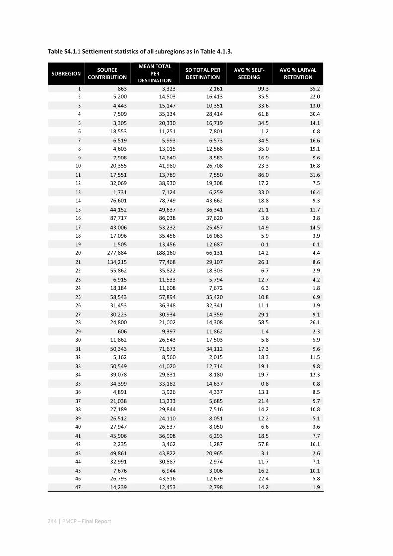
244 | PMCP – Final Report
Table S4.1.1 Settlement statistics of all subregions as in Table 4.1.3.
SUBREGION SOURCE
CONTRIBUTION
MEAN TOTAL PER
DESTINATION
SD TOTAL PER DESTINATION
AVG % SELF‐SEEDING
AVG % LARVAL RETENTION
1 863 3,323 2,161 99.3 35.2
2 5,200 14,503 16,413 35.5 22.0
3 4,443 15,147 10,351 33.6 13.0
4 7,509 35,134 28,414 61.8 30.4
5 3,305 20,330 16,719 34.5 14.1
6 18,553 11,251 7,801 1.2 0.8
7 6,519 5,993 6,573 34.5 16.6
8 4,603 13,015 12,568 35.0 19.1
9 7,908 14,640 8,583 16.9 9.6
10 20,355 41,980 26,708 23.3 16.8
11 17,551 13,789 7,550 86.0 31.6
12 32,069 38,930 19,308 17.2 7.5
13 1,731 7,124 6,259 33.0 16.4
14 76,601 78,749 43,662 18.8 9.3
15 44,152 49,637 36,341 21.1 11.7
16 87,717 86,038 37,620 3.6 3.8
17 43,006 53,232 25,457 14.9 14.5
18 17,096 35,456 16,063 5.9 3.9
19 1,505 13,456 12,687 0.1 0.1
20 277,884 188,160 66,131 14.2 4.4
21 134,215 77,468 29,107 26.1 8.6
22 55,862 35,822 18,303 6.7 2.9
23 6,915 11,533 5,794 12.7 4.2
24 18,184 11,608 7,672 6.3 1.8
25 58,543 57,894 35,420 10.8 6.9
26 31,453 36,348 32,341 11.1 3.9
27 30,223 30,934 14,359 29.1 9.1
28 24,800 21,002 14,308 58.5 26.1
29 606 9,397 11,862 1.4 2.3
30 11,862 26,543 17,503 5.8 5.9
31 50,343 71,673 34,112 17.3 9.6
32 5,162 8,560 2,015 18.3 11.5
33 50,549 41,020 12,714 19.1 9.8
34 39,078 29,831 8,180 19.7 12.3
35 34,399 33,182 14,637 0.8 0.8
36 4,891 3,926 4,337 13.1 8.5
37 21,038 13,233 5,685 21.4 9.7
38 27,189 29,844 7,516 14.2 10.8
39 26,512 24,110 8,051 12.2 5.1
40 27,947 26,537 8,050 6.6 3.6
41 45,906 36,908 6,293 18.5 7.7
42 2,235 3,462 1,287 57.8 16.1
43 49,861 43,822 20,965 3.1 2.6
44 32,991 30,587 2,974 11.7 7.1
45 7,676 6,944 3,006 16.2 10.1
46 26,793 43,516 12,679 22.4 5.8
47 14,239 12,453 2,798 14.2 1.9
245 | PMCP – Final Report
Setting priorities for conservation initiatives at the interface between ocean circulation, larval connectivity, and population dynamics
Authors: Boschetti F, Babcock RC, Doropoulos C, Thomson DP, Feng M, Slawinski D, Berry O, Vanderklift MA.
Submitted to Journal of Applied Ecology.
ABSTRACT
Population persistence in the marine environment is driven by patterns of ocean circulation, larval dispersal, and ecological interactions. For habitat forming organisms in particular, understanding the relationship between larval connectivity and meta‐population dynamics aids in planning for marine spatial management. Here, we estimate networks of connectivity between fringing coral reefs in the North West Shelf of Australia by combining a particle tracking model based on shelf circulation with models of sub‐population dynamics of individual reefs. Coral cover data were used as a proxy for overall habitat quality, which can change as a result of natural processes, human‐driven processes, and management initiatives. We obtain three major results of conservation significance. First, the dynamics of the ecological network results from the interplay between network connectivity and ecological processes on individual reefs: density‐dependence imposes a significant non‐linearity on the role an individual reef plays within the dynamics of the network, and thus on the impact of conservation interventions on specific reefs. Second, the role an individual reef plays within these network dynamics changes considerably depending on the overall state of the system: a reef’s role in system maintenance can be different from the same reef’s role in system recovery. Third, patterns of network connectivity change significantly as a function of yearly shelf circulation trends, and non‐linearity in network dynamics make mean connectivity a poor representation of yearly variations. From a management perspective, the central message is that when defining a priority list of targets for management interventions the choice of which reefs should be considered depends crucially on what type of stressors need addressing. This in turn depends on future oceanographic scenarios (which determine the network connectivity), future development and climate change scenarios (which determine habitat quality), as well as the ultimate purpose of management.
246 | PMCP – Final Report
4.2.1 INTRODUCTION
Connectivity has major consequences for the ability of populations to persist and sustain themselves as a network, or regional meta‐population. A network’s ability to maintain its functioning under variable local conditions and recover from occasional major regional disturbances, both key components of resilience, relies on the input and exchange of new individuals from remnant neighbouring populations (Cowen et al. 2006, Treml et al. 2008). Connectivity is particularly important for marine organisms that generally display bi‐partite life histories, with a dispersive larval phase following reproduction before transitioning to a more sedentary benthic phase. Ocean currents are a major driver of larval transport, and larvae can disperse from meters to thousands of kilometres from their natal reef (Cowen & Sponaugle 2009, Jones et al. 2009). Thus, understanding connectivity is a particularly important consideration in the management of marine natural resources (Gaines et al. 2010).
The consideration of connectivity in management is especially prominent in the conservation of coral reefs and marine reserves (e.g. Almany et al. 2009, Krueck et al. 2016). Both are usually somewhat isolated and discrete areas of habitat that are connected by larval transport over ecological and evolutionary timescales. Coral reefs are subject to a number of threats from anthropogenic sources, both local and global. These include but are not limited to overfishing, habitat destruction, coastal development, sedimentation, eutrophication and tropical storms, as well as the global impacts of climate change (Harborne et al. 2017). Given this array of disturbances and the fragmented geography of coral reef habitats there is a clear need for active efforts to ensure the persistence of coral reef ecosystems.
Spatial management approaches are a common tool employed to protect the resilience and persistence of coral reefs at a regional scale, and the idea of networks of marine reserves is being applied globally (Mora et al. 2006). Yet, because coral reefs support the livelihoods of millions, decisions regarding which reefs to protect and how to balance conservation with more immediate human needs, are difficult (Klein et al. 2008, Halpern et al. 2013). Consequently, connectivity based approaches to prioritising reefs and optimising conservation outcomes are increasingly common and include studies of larval behaviour, genetics and numerical hydrodynamic modelling (Ovaskainen & Hanski 2003, Werner et al. 2007, Figueira 2009, Jones et al. 2009, Jacobi & Jonsson 2011a). In order to understand the implications of this knowledge however, they must be combined and viewed in a network or meta‐population context.
Modelling approaches including the use of connectivity matrices and network analysis have increasingly been used for conservation prioritization (e.g. Ovaskainen & Hanski 2003, Figueira 2009, Jacobi & Jonsson 2011a, Kininmonth et al. 2011, Treml & Halpin 2012, Hock et al. 2014). These uses include marine reserves, but network analysis can also be used to prioritize reefs for the eradication of undesirable species such as crown‐of‐thorns starfish (Hock et al. 2014). While consideration of single reefs would suggest that larval retention is key to their persistence, it is clear that there is a need to include networks of populations in order to manage marine populations at appropriate scales. Such analyses have highlighted that prioritising areas on the basis of either sink or source characteristics alone is relatively ineffective (Jacobi & Jonsson 2011b) and that the key components of a network, in terms of its ability to recover from disturbances and ultimately to persist, are those nodes of the network that both supply and receive substantial numbers of larvae. Such nodes have been variously termed gateway reefs (Bode et al. 2006) or superspreaders (Hock et al. 2014).
While representations of connectivity such as betweenness centrality (Holstein et al. 2014) have been used to rank habitat components in terms of their input to persistence, it is increasingly recognised that such prioritizations need to incorporate multigenerational and dynamic aspects of populations at each node in order to include realistic representations of habitat quality. Variations in

247 | PMCP – Final Report
habitat quality or population parameters have been shown to have strong influences on the relative ranking of high priority sites, potentially altering priorities that might be made based on connectivity alone. For example, local demography becomes increasingly important under conditions of high larval retention where demographic variability can turn sources into sinks (Figueira 2009), and spatial variations in habitat quality can change network dynamics (Watson et al. 2011). These variations find their fullest expressions in the contrasting network characteristics of different species within the same region (Watson et al. 2011, Holstein et al. 2014). Hydrodynamic variability can potentially also have important influences on network properties (Bode et al. 2006, Golbuu et al. 2012).
Here we focus on a regional network of coastal reefs on the Pilbara Coast of north‐west Australia with a view to informing management approaches in the region to address multiple stake‐holder use. The region is the focus of significant industrial activity (oil, gas) and major port developments (Hanley 2011), well‐established conservation initiatives including several large multiple‐use marine parks and a World Heritage Area at Ningaloo Reef (CALM & MPRA 2005), as well as recreational and commercial fishing (Fletcher & Santoro 2009). Using a 6‐year time series of hydrodynamic models we have estimated connectivity among coral reefs in the region. We then used a meta‐population model, based on regional measurements of model coral populations, to study the interplay between local population dynamics and regional connectivity.
In setting up a regional management plan for the conservation of marine resources, a manager needs to address a number of stakeholder aspirations, but also to ensure that the system is resilient to three types of disturbances: i) local, relatively frequent natural and anthropogenic disturbances leading to variable local conditions which can be balanced by larvae supplied from other areas (we term this ‘system maintenance’ from hereon); ii) occasional major and potentially catastrophic regional disturbances affecting a significant section of the region (we term this ‘system recovery’) and iii) larger scale biophysical processes or climate change, which may lead to yearly or decadal variability in climatic and ecological regimes. The main result of this study is to show that zones which offer larger contributions to system maintenance do not necessarily have the same level of importance for system recovery or under different disturbance regimes. This finding is of both regional importance and general significance and represents robust advice across a range of management sectors.
4.2.2 METHODS
Methodological overview
We firstly describe the study region, data collection, and analysis which provide the estimated current coral cover and carrying capacity used in the meta‐population model. We then describe the hydrodynamic model which provides the connectivity data and meta‐population model used to study changes in coral cover as a function of both connectivity and local population dynamics. Next, we describe the modelling approach used to study the three types of disturbances. First, we employ an impact analysis to assess how much each zone contributes to system maintenance – i.e., preserving coral biomass in the overall region. Second, we explore the role each zone plays in system recovery following regional system collapse. Finally, we describe how yearly variability in network connectivity is analysed and its role on impact and recovery.
Study area
The Pilbara consists of over 300 low islands (<6 m above sea‐level) with most having well developed

248 | PMCP – Final Report
fringing coral reefs. The region is characterised by a large tidal range (3 m spring tides) and a wide, gently sloping continental shelf, resulting in strong tidal flows throughout the region (0.4 knts). Average annual rainfall is low (mean = 306 mm), however during the austral summer months (November to March) cyclones are common (mean 0.6 per year; BOM http://www.bom.gov.au/climate/maps/averages/tropical‐cyclones/) and have resulted in large declines of coral cover within Acropora dominated assemblages (Marsh & Marsh 2000). Most fringing coral reefs in the region are dominated by macroalgae (Sargassum, Turbinaria, Padina), however diverse assemblages of hard corals and invertebrates are common throughout (Richards & Rosser 2012, Pitcher et al. 2016).
Benthic communities were surveyed using 50 m photo‐transects (English et al. 1997). A total of over 1200 transects were completed between November 2013 and May 2015 with transects distributed evenly throughout the model sub‐regions. Sub‐regions were defined based on clusters of adjacent and geomorphologically similar reefs. To quantify the current coral cover and the coral carrying capacity for each sub‐region, the mean percent cover of live and recently dead coral were obtained from photo‐transects (Ridgway et al. 2016, Lafratta et al. 2017). Photos were captured at 0.5 m intervals along the transect and randomly selected for analysis with the genus of any scleractinian corals recorded for 6 fixed points per photograph using Transect Measure™ (i.e. 180 pts per 50 m transect). The coral cover was calculated as the mean coral cover of transects within that sub region (Figure 4.2.1). Estimated coral carrying capacity was based on observed coral cover and recently dead coral cover and adjusted according to local knowledge and where necessary by referring to estimates in adjacent zones.
Figure 4.2.1 West Pilbara model domain, zone locations and labels (as in Feng et al. 2016). Colours map coral cover. The 10 zones with highest coral cover are (in decreasing order) 44, 40, 39, 3, 22, 31, 2, 28, 41, 12.
Connectivity data
Connectivity data were obtained by simulating larval release and diffusion by tracking particle movement on the studied area forced by oceanic data recorded in the years 2004 to 2009. The particle tracking is based on hydrodynamic model outputs from model simulations using Rutgers version of the Regional Ocean Modelling System (Feng et al. 2016) and was run with ~1 km horizontal resolution. The bottom topography was taken from a collection of sources including GA2009, industry provided LIDAR and MNF multi beam data. Reef distribution was summarised by compiling benthic habitat maps from CSIRO, Western Australia Department of Biodiversity, Conservation and Attractions, Western Australia Museum, and environmental impact statement documents from industrial developments in the region. Reefs were used as the seeding locations of coral larvae in the particle tracking model, and as settlement sites when evaluating retention and
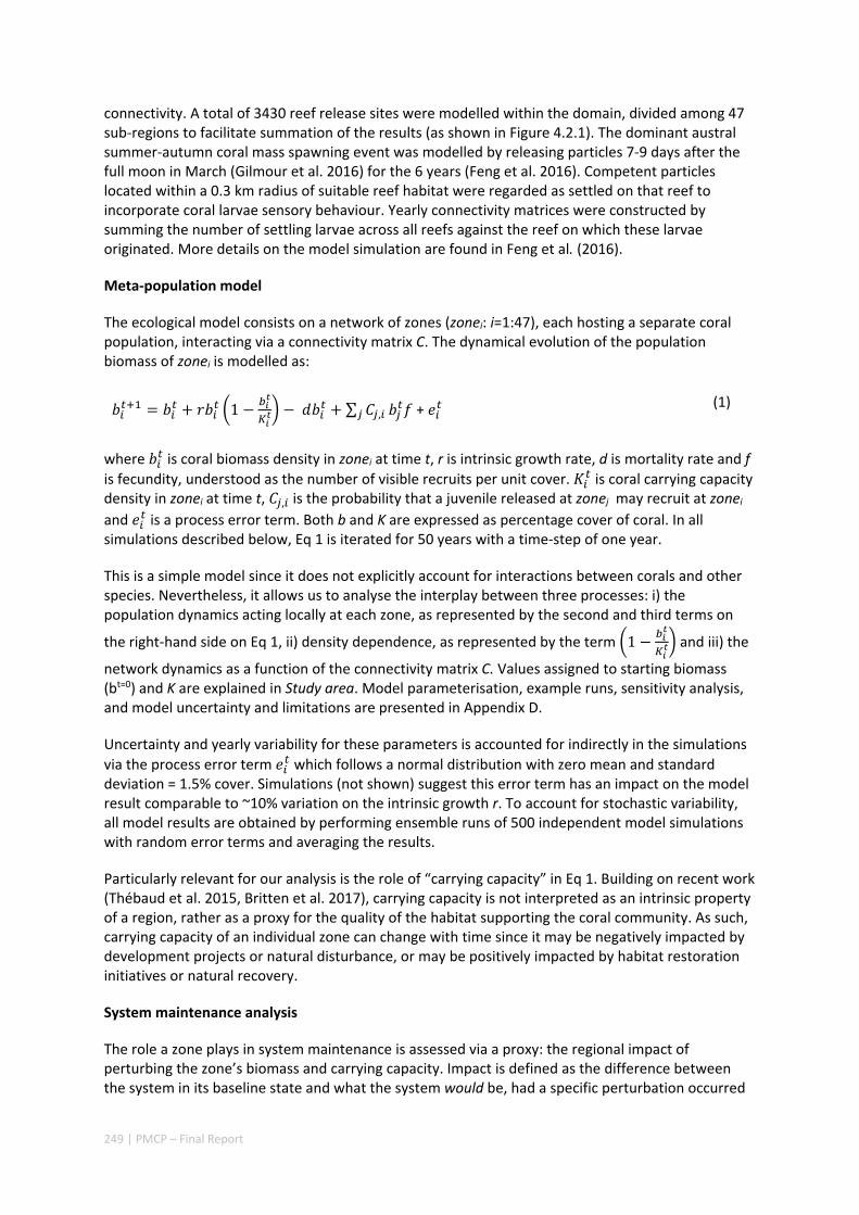
249 | PMCP – Final Report
connectivity. A total of 3430 reef release sites were modelled within the domain, divided among 47 sub‐regions to facilitate summation of the results (as shown in Figure 4.2.1). The dominant austral summer‐autumn coral mass spawning event was modelled by releasing particles 7‐9 days after the full moon in March (Gilmour et al. 2016) for the 6 years (Feng et al. 2016). Competent particles located within a 0.3 km radius of suitable reef habitat were regarded as settled on that reef to incorporate coral larvae sensory behaviour. Yearly connectivity matrices were constructed by summing the number of settling larvae across all reefs against the reef on which these larvae originated. More details on the model simulation are found in Feng et al. (2016).
Meta‐population model
The ecological model consists on a network of zones (zonei: i=1:47), each hosting a separate coral population, interacting via a connectivity matrix C. The dynamical evolution of the population biomass of zonei is modelled as:
1 ∑ , + (1)
where is coral biomass density in zonei at time t, r is intrinsic growth rate, d is mortality rate and f
is fecundity, understood as the number of visible recruits per unit cover. is coral carrying capacity density in zonei at time t, , is the probability that a juvenile released at zonej may recruit at zonei
and is a process error term. Both b and K are expressed as percentage cover of coral. In all simulations described below, Eq 1 is iterated for 50 years with a time‐step of one year.
This is a simple model since it does not explicitly account for interactions between corals and other species. Nevertheless, it allows us to analyse the interplay between three processes: i) the population dynamics acting locally at each zone, as represented by the second and third terms on
the right‐hand side on Eq 1, ii) density dependence, as represented by the term 1 and iii) the
network dynamics as a function of the connectivity matrix C. Values assigned to starting biomass (bt=0) and K are explained in Study area. Model parameterisation, example runs, sensitivity analysis, and model uncertainty and limitations are presented in Appendix D.
Uncertainty and yearly variability for these parameters is accounted for indirectly in the simulations
via the process error term which follows a normal distribution with zero mean and standard deviation = 1.5% cover. Simulations (not shown) suggest this error term has an impact on the model result comparable to ~10% variation on the intrinsic growth r. To account for stochastic variability, all model results are obtained by performing ensemble runs of 500 independent model simulations with random error terms and averaging the results.
Particularly relevant for our analysis is the role of “carrying capacity” in Eq 1. Building on recent work (Thébaud et al. 2015, Britten et al. 2017), carrying capacity is not interpreted as an intrinsic property of a region, rather as a proxy for the quality of the habitat supporting the coral community. As such, carrying capacity of an individual zone can change with time since it may be negatively impacted by development projects or natural disturbance, or may be positively impacted by habitat restoration initiatives or natural recovery.
System maintenance analysis
The role a zone plays in system maintenance is assessed via a proxy: the regional impact of perturbing the zone’s biomass and carrying capacity. Impact is defined as the difference between the system in its baseline state and what the system would be, had a specific perturbation occurred
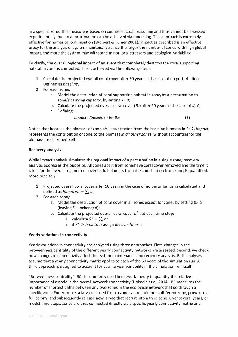
250 | PMCP – Final Report
in a specific zone. This measure is based on counter‐factual reasoning and thus cannot be assessed experimentally, but an approximation can be achieved via modelling. This approach is extremely effective for numerical optimisation (Wolpert & Tumer 2001). Impact as described is an effective proxy for the analysis of system maintenance since the larger the number of zones with high global impact, the more the system may withstand minor local stressors and ecological variability.
To clarify, the overall regional impact of an event that completely destroys the coral supporting habitat in zonei is computed. This is achieved via the following steps:
1) Calculate the projected overall coral cover after 50 years in the case of no perturbation. Defined as baseline.
2) For each zonei: a. Model the destruction of coral supporting habitat in zonei by a perturbation to
zonei’s carrying capacity, by setting Ki=0; b. Calculate the projected overall coral cover (B‐i) after 50 years in the case of Ki=0; c. Defining
impacti=(baseline ‐ bi ‐ B‐i) (2)
Notice that because the biomass of zonei (bi) is subtracted from the baseline biomass in Eq 2, impacti represents the contribution of zonei to the biomass in all other zones, without accounting for the biomass loss in zonei itself.
Recovery analysis
While impact analysis simulates the regional impact of a perturbation in a single zone, recovery analysis addresses the opposite. All zones apart from zonei have coral cover removed and the time it takes for the overall region to recover its full biomass from the contribution from zonei is quantified. More precisely:
1) Projected overall coral cover after 50 years in the case of no perturbation is calculated and defined as ∑
2) For each zonei: a. Model the destruction of coral cover in all zones except for zonei, by setting b‐i=0
(leaving K‐i unchanged);
b. Calculate the projected overall coral cover ; at each time‐step:
i. calculate ∑ ii. if assign RecoverTimei=t
Yearly variations in connectivity
Yearly variations in connectivity are analysed using three approaches. First, changes in the betweenness centrality of the different yearly connectivity networks are assessed. Second, we check how changes in connectivity affect the system maintenance and recovery analysis. Both analyses assume that a yearly connectivity matrix applies to each of the 50 years of the simulation run. A third approach is designed to account for year to year variability in the simulation run itself.
“Betweenness centrality” (BC) is commonly used in network theory to quantify the relative importance of a node in the overall network connectivity (Holstein et al. 2014). BC measures the number of shortest paths between any two zones in the ecological network that go through a specific zone. For example, a larva released from a zone can recruit into a different zone, grow into a full colony, and subsequently release new larvae that recruit into a third zone. Over several years, or model time‐steps, zones are thus connected directly via a specific yearly connectivity matrix and
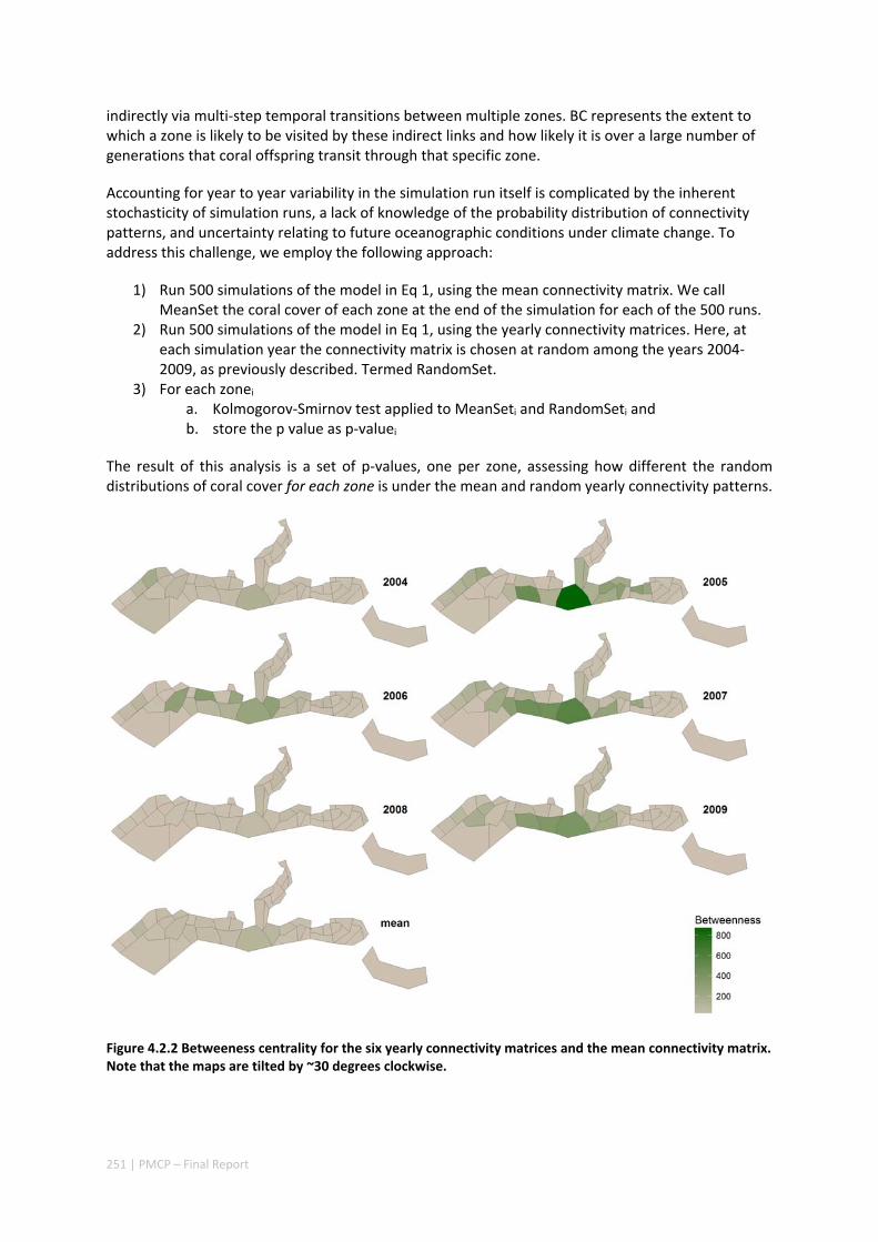
251 | PMCP – Final Report
indirectly via multi‐step temporal transitions between multiple zones. BC represents the extent to which a zone is likely to be visited by these indirect links and how likely it is over a large number of generations that coral offspring transit through that specific zone.
Accounting for year to year variability in the simulation run itself is complicated by the inherent stochasticity of simulation runs, a lack of knowledge of the probability distribution of connectivity patterns, and uncertainty relating to future oceanographic conditions under climate change. To address this challenge, we employ the following approach:
1) Run 500 simulations of the model in Eq 1, using the mean connectivity matrix. We call MeanSet the coral cover of each zone at the end of the simulation for each of the 500 runs.
2) Run 500 simulations of the model in Eq 1, using the yearly connectivity matrices. Here, at each simulation year the connectivity matrix is chosen at random among the years 2004‐2009, as previously described. Termed RandomSet.
3) For each zonei a. Kolmogorov‐Smirnov test applied to MeanSeti and RandomSeti and b. store the p value as p‐valuei
The result of this analysis is a set of p‐values, one per zone, assessing how different the random distributions of coral cover for each zone is under the mean and random yearly connectivity patterns.
Figure 4.2.2 Betweeness centrality for the six yearly connectivity matrices and the mean connectivity matrix. Note that the maps are tilted by ~30 degrees clockwise.
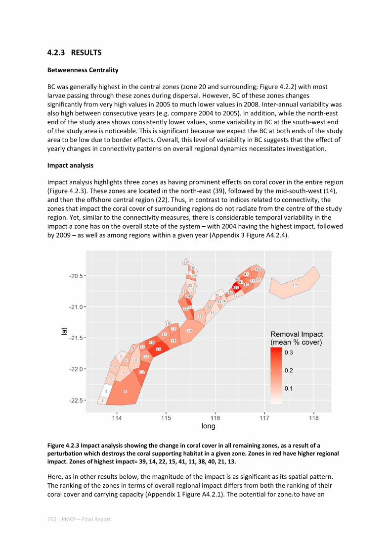
252 | PMCP – Final Report
4.2.3 RESULTS
Betweenness Centrality
BC was generally highest in the central zones (zone 20 and surrounding; Figure 4.2.2) with most larvae passing through these zones during dispersal. However, BC of these zones changes significantly from very high values in 2005 to much lower values in 2008. Inter‐annual variability was also high between consecutive years (e.g. compare 2004 to 2005). In addition, while the north‐east end of the study area shows consistently lower values, some variability in BC at the south‐west end of the study area is noticeable. This is significant because we expect the BC at both ends of the study area to be low due to border effects. Overall, this level of variability in BC suggests that the effect of yearly changes in connectivity patterns on overall regional dynamics necessitates investigation.
Impact analysis
Impact analysis highlights three zones as having prominent effects on coral cover in the entire region (Figure 4.2.3). These zones are located in the north‐east (39), followed by the mid‐south‐west (14), and then the offshore central region (22). Thus, in contrast to indices related to connectivity, the zones that impact the coral cover of surrounding regions do not radiate from the centre of the study region. Yet, similar to the connectivity measures, there is considerable temporal variability in the impact a zone has on the overall state of the system – with 2004 having the highest impact, followed by 2009 – as well as among regions within a given year (Appendix 3 Figure A4.2.4).
Figure 4.2.3 Impact analysis showing the change in coral cover in all remaining zones, as a result of a perturbation which destroys the coral supporting habitat in a given zone. Zones in red have higher regional impact. Zones of highest impact= 39, 14, 22, 15, 41, 11, 38, 40, 21, 13.
Here, as in other results below, the magnitude of the impact is as significant as its spatial pattern. The ranking of the zones in terms of overall regional impact differs from both the ranking of their coral cover and carrying capacity (Appendix 1 Figure A4.2.1). The potential for zonei to have an
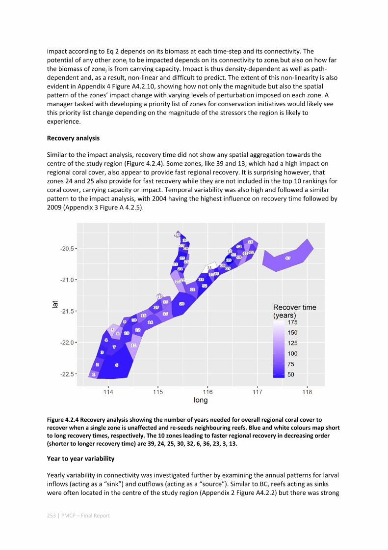
253 | PMCP – Final Report
impact according to Eq 2 depends on its biomass at each time‐step and its connectivity. The potential of any other zonej to be impacted depends on its connectivity to zonei but also on how far the biomass of zonej is from carrying capacity. Impact is thus density‐dependent as well as path‐dependent and, as a result, non‐linear and difficult to predict. The extent of this non‐linearity is also evident in Appendix 4 Figure A4.2.10, showing how not only the magnitude but also the spatial pattern of the zones’ impact change with varying levels of perturbation imposed on each zone. A manager tasked with developing a priority list of zones for conservation initiatives would likely see this priority list change depending on the magnitude of the stressors the region is likely to experience.
Recovery analysis
Similar to the impact analysis, recovery time did not show any spatial aggregation towards the centre of the study region (Figure 4.2.4). Some zones, like 39 and 13, which had a high impact on regional coral cover, also appear to provide fast regional recovery. It is surprising however, that zones 24 and 25 also provide for fast recovery while they are not included in the top 10 rankings for coral cover, carrying capacity or impact. Temporal variability was also high and followed a similar pattern to the impact analysis, with 2004 having the highest influence on recovery time followed by 2009 (Appendix 3 Figure A 4.2.5).
Figure 4.2.4 Recovery analysis showing the number of years needed for overall regional coral cover to recover when a single zone is unaffected and re‐seeds neighbouring reefs. Blue and white colours map short to long recovery times, respectively. The 10 zones leading to faster regional recovery in decreasing order (shorter to longer recovery time) are 39, 24, 25, 30, 32, 6, 36, 23, 3, 13.
Year to year variability
Yearly variability in connectivity was investigated further by examining the annual patterns for larval inflows (acting as a “sink”) and outflows (acting as a “source”). Similar to BC, reefs acting as sinks were often located in the centre of the study region (Appendix 2 Figure A4.2.2) but there was strong

254 | PMCP – Final Report
inter‐annual variability in larval supply to surrounding regions in both the north‐east and south‐west (Appendix 2 Figure A4.2.3). Sources of larval outflow were also dominated by reefs in the centre of the region. Additionally, connectivity in system maintenance and recovery shows that yearly variability is significant (Appendix 3).
A quantitative assessment of the year to year variability was obtained by simulation runs in which the connectivity matrix is chosen randomly at each time‐step (Figure 4.2.5). Thirty‐one of the forty‐seven zones in the model have highly significant p‐values (<0.01), suggesting that local biomass resulting from random yearly variations in connectivity are significantly different from the ones resulting from the mean connectivity. We further tested this following current recommendations about overreliance on p‐value significance (Halsey et al. 2015, Altman & Krzywinski 2017) by bootstrapping p‐values and comparing the above distribution against 200 different distributions, obtained by comparing 200 sets of 500 simulation runs that use the mean connectivity matrix and different random seeds for the error term. No comparison had a single p‐value <0.01, showing that patterns of connectivity in any given year and for the mean connectivity lead to simulation results that are statistically significant. Overall, this suggests that even over the time span of a 50‐year simulation the mean connectivity matrix is not a good approximation of yearly variability in ecological connectivity.
Figure 4.2.5 Comparison of model results between 500 simulation using the mean connectivity matrix vs using random yearly connectivity matrices. Colours map the p‐values of the Kolmogorov‐Smirnov test of the two distributions for each zone.
Joint analysis of impact and recovery
Because of their complexity, the findings are summarised to be useful for decision making. For each connectivity matrix in the years 2004‐2009, plus the mean connectivity, we select the zones in the top six ranks in either the system maintenance or recovery analysis yearly connectivity matrices (Appendix 3 Figure A4.2.6). Few zones show high values for both system maintenance and recovery, and do so for a maximum of only two yearly connectivity matrices. As for the mean connectivity
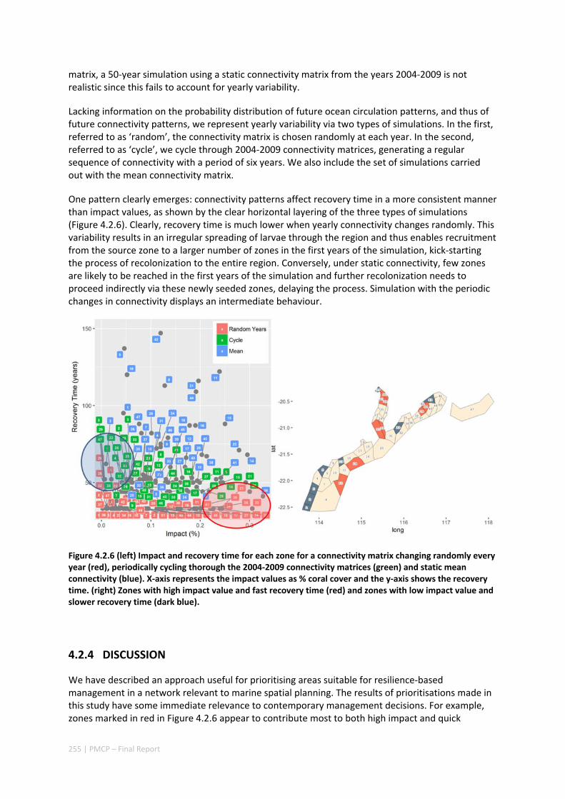
255 | PMCP – Final Report
matrix, a 50‐year simulation using a static connectivity matrix from the years 2004‐2009 is not realistic since this fails to account for yearly variability.
Lacking information on the probability distribution of future ocean circulation patterns, and thus of future connectivity patterns, we represent yearly variability via two types of simulations. In the first, referred to as ‘random’, the connectivity matrix is chosen randomly at each year. In the second, referred to as ‘cycle’, we cycle through 2004‐2009 connectivity matrices, generating a regular sequence of connectivity with a period of six years. We also include the set of simulations carried out with the mean connectivity matrix.
One pattern clearly emerges: connectivity patterns affect recovery time in a more consistent manner than impact values, as shown by the clear horizontal layering of the three types of simulations (Figure 4.2.6). Clearly, recovery time is much lower when yearly connectivity changes randomly. This variability results in an irregular spreading of larvae through the region and thus enables recruitment from the source zone to a larger number of zones in the first years of the simulation, kick‐starting the process of recolonization to the entire region. Conversely, under static connectivity, few zones are likely to be reached in the first years of the simulation and further recolonization needs to proceed indirectly via these newly seeded zones, delaying the process. Simulation with the periodic changes in connectivity displays an intermediate behaviour.
Figure 4.2.6 (left) Impact and recovery time for each zone for a connectivity matrix changing randomly every year (red), periodically cycling thorough the 2004‐2009 connectivity matrices (green) and static mean connectivity (blue). X‐axis represents the impact values as % coral cover and the y‐axis shows the recovery time. (right) Zones with high impact value and fast recovery time (red) and zones with low impact value and slower recovery time (dark blue).
4.2.4 DISCUSSION
We have described an approach useful for prioritising areas suitable for resilience‐based management in a network relevant to marine spatial planning. The results of prioritisations made in this study have some immediate relevance to contemporary management decisions. For example, zones marked in red in Figure 4.2.6 appear to contribute most to both high impact and quick
256 | PMCP – Final Report
recovery. Some of these zones are located in the Dampier Archipelago region, currently under consideration for declaration as a multiple‐use marine park area. Zones in the central part of the region also appear frequently as both high impact and quick recovery. Given recent coral bleaching in the Pilbara (Ridgway et al. 2016, Lafratta et al. 2017) the importance of these zones for the recovery and resilience of the overall region assumes broader importance and potentially greater urgency. In contrast, zones marked in blue in Figure 4.2.6 appear to make relatively small contributions to system resilience so might receive lower priority for conservation measures, or higher priority as potential development sites, all other things being equal. That said, care is needed when assessing the contribution of zones 1‐3 because they are located close to the domain border.
Somewhat surprisingly, our study has highlighted how a single reef can have differing contributions to habitat maintenance and recovery, both of which are key attributes of resilience (Mumby & Steneck 2008). We find zones that provide large contributions to system maintenance may not necessarily do so for system recovery. Some zones show high contributions for either maintenance or recovery, but not both. Moreover, the ranking of a zones’ impact can change as a function of the magnitude of the perturbation and its sign (Appendix 4 Figure A4.2.9). Only zones 38 and 39 ranked reasonably high for both maintenance and recovery, with similar but weaker contributions across both factors for zones 21, 22 and 12.
Our study has highlighted the importance of incorporating yearly variability when investigating dynamic systems, rather than simply investigating averages. When considering source‐sink dynamics and spatial planning, stochastic events can be important drivers of rare connectivity events rather than simply outliers (e.g. Golbuu et al. 2012). In our study system, variability in oceanic transport and its interactions with the annual lunar progression in the timing of coral mass spawning (Gilmour et al. 2016) also drives dynamic patterns of ecological connectivity. Connectivity patterns changed considerably among the years 2004‐2009, significantly affecting coral connectivity in different parts of the region, subsequently affecting the role they play in overall regional coral cover. Thus, average connectivity values can overlook key components of dynamic systems.
Differing hydrodynamic conditions emerge as a strong driver of the properties of the overall system if it were to experience long‐term change into conditions represented by the regime of a particular year (Appendix 3 Figure A4.2.6). For example, persistent conditions typical of year 2005 would produce the quickest recovery times, with such results being possible with recovery sourced from multiple reefs (Appendix 3 Figure A4.2.6). Conditions in 2005 were characterised by north to south flow yet relatively low connectivity between areas around Dampier in the north and the rest of the system (Feng et al. 2016). In contrast, recovery times appeared to be almost twice as long under conditions representative of 2004, when currents flowed mainly south to north.
Broad scale changes to coastal and oceanic circulation and seasonality in the eastern Indian Ocean may be experienced under changing climate and are likely to influence hydrodynamic regimes and therefore overall network dynamics. Random variation in hydrodynamic connectivity appears to promote the most rapid recovery of the system (Figure 4.2.6), with longer recovery times when hydrodynamic regimes cycle – such a phenomenon may be experienced under increased frequency of ENSO conditions in the south‐east Indian Ocean (Cai et al. 2015, Zinke et al. 2015). These changes may also impact rates of coral bleaching and other disturbances. Therefore, changing climate will have multiple paths to impact the resilience of Pilbara coral reefs.
The role of coral population dynamics in each zone was also evident, wherein contributions to system resilience were influenced not only by levels of connectivity but also by differing carrying capacities. For the same system, assessments of system resilience based on connectivity alone (i.e., rank contribution of a zone as a source and/or sink) produced a list of zones potentially important to resilience that was quite different (Feng et al. 2016) to those developed in the current analysis.
257 | PMCP – Final Report
Broad scale data on carrying capacity and dynamic aspects of populations is highly valuable in this context and given apparent sensitivity of the system to properties such as growth and mortality continued efforts to obtain relevant demographic data across appropriate spatial scales should be a high priority for management.
The presented approach can provide valuable input to management decision‐making in ranking the relative values of discrete areas based on agreed sets of prioritised attributes. By showing that even a single species logistic equation can lead to extremely complex behaviour when embedded in a network of 47 interacting nodes as described in this work, we highlight that different purposes of conservation initiatives (system maintenance and system recovery) can result in very different management recommendations. This brings attention to how a careful specification of management questions can lead to more informative analyses, modelling and field work. In addition, we show that yearly variability in connectivity is poorly captured by time‐averaged mean connectivity, even for a simulation spanning five decades. In this case, developing conservation initiative at the regional level can be extremely challenging especially under large ecological uncertainty. In these situations, field work spanning long time series as well as more realistic modelling could be carried out with foresight aimed at identifying possible regional scenarios and conservation priorities that can in turn inform further field work and modelling in an iterative and adaptive manner.
4.2.5 ACKNOWLEDGEMENTS
This project was funded by the Gorgon Barrow Island Net Conservation Benefits Fund, which is administered by the Western Australian Department of Biodiversity, Conservation and Attractions.
4.2.6 REFERENCES
Almany GR, Connolly SR, Heath DD, Hogan JD, Jones GP, McCook LJ, Mills M, Pressey RL, Williamson DH (2009) Connectivity, biodiversity conservation and the design of marine reserve networks for coral reefs. Coral Reefs 28:339‐351
Altman N, Krzywinski M (2017) Points of significance: P values and the search for significance. Nature Methods 14:3–4
Babcock RC, Gilmour J, Thomson D (2017) Measurement and modelling of key demographic processes in corals of the Dampier Archipelago. In: Report of Theme 4 – Project 47, prepared for the Dredging Science Node. WAMSI
Bode M, Bode L, Armsworth PR (2006) Larval dispersal reveals regional sources and sinks in the Great Barrier Reef. Marine Ecology Progress Series 308:17‐25
Britten GL, Dowd M, Kanary L, Worm B (2017) Extended fisheries recovery timelines in a changing environment. Nature Communications 8:15325
Cai W, Wang G, Santoso A, McPhaden MJ, Wu L, Jin F‐F, Timmermann A, Collins M, Vecchi G, Lengaigne M (2015) Increased frequency of extreme La Niña events under greenhouse warming. Nature Climate Change 5:132‐137

258 | PMCP – Final Report
CALM, MPRA (2005) Management Plan for the Ningaloo Marine Park and Muiron Islands Marine Management Area 2005‐2015. In: Management Plan Number 52, Book 52
Cowen RK, Paris CB, Srinivasan A (2006) Scaling of connectivity in marine populations. Science 311:522‐527
Cowen RK, Sponaugle S (2009) Larval Dispersal and Marine Population Connectivity. Annual Review of Marine Science 1:443‐466
English SS, Wilkinson CC, Baker VV (1997) Survey manual for tropical marine resources, Vol. Australian Institute of Marine Science
Feng M, Colberg F, Slawinski D, Berry O, Babcock R (2016) Ocean circulation drives heterogeneous recruitments and connectivity among coral populations on the North West Shelf of Australia. Journal of Marine Systems 164:1‐12
Figueira WF (2009) Connectivity or demography: Defining sources and sinks in coral reef fish metapopulations. Ecological Modelling 220:1126‐1137
Fletcher W, Santoro K (2009) State of the fisheries report 2008/09. WA Department of Fisheries, Perth
Gaines SD, White C, Carr MH, Palumbi SR (2010) Designing marine reserve networks for both conservation and fisheries management. Proceedings of the National Academy of Sciences 107:18286‐18293
Gilmour J, Speed CW, Babcock R (2016) Coral reproduction in Western Australia. PeerJ 4:e2010
Golbuu Y, Wolanski E, Idechong JW, Victor S, Isechal AL, Oldiais NW, Idip Jr D, Richmond RH, van Woesik R (2012) Predicting coral recruitment in Palau’s complex reef archipelago. PLoS ONE 7:e50998
Halpern BS, Klein CJ, Brown CJ, Beger M, Grantham HS, Mangubhai S, Ruckelshaus M, Tulloch VJ, Watts M, White C (2013) Achieving the triple bottom line in the face of inherent trade‐offs among social equity, economic return, and conservation. Proceedings of the National Academy of Sciences 110:6229‐6234
Halsey LG, Curran‐Everett D, Vowler SL, Drummond GB (2015) The fickle P value generates irreproducible results. Nature methods 12:179–185
Hanley J (2011) Environmental monitoring programs on recent capital dredging projects in the Pilbara (2003–10): a review. Australian Petroleum Production & Exploration Association (APPEA) 51:273‐294
Harborne AR, Rogers A, Bozec Y‐M, Mumby PJ (2017) Multiple Stressors and the Functioning of Coral Reefs. Annual Review of Marine Science 9:445‐468
Hock K, Wolff NH, Condie SA, Anthony KRN, Mumby PJ (2014) Connectivity networks reveal the risks of crown‐of‐thorns starfish outbreaks on the Great Barrier Reef. Journal of Applied Ecology
Holstein DM, Paris CB, Mumby PJ (2014) Consistency and inconsistency in multispecies population network dynamics of coral reef ecosystems. Marine Ecology Progress Series 499:1‐18

259 | PMCP – Final Report
Jacobi MN, Jonsson PR (2011a) Optimal networks of nature reserves can be found through eigenvalue perturbation theory of the connectivity matrix. Ecological Applications 21:1861–1870
Jacobi MN, Jonsson PR (2011b) Optimal networks of nature reserves can be found through eigenvalue perturbation theory of the connectivity matrix. Ecol Appl 21:1861‐1870
Jones G, Almany G, Russ G, Sale P, Steneck R, van Oppen M, Willis B (2009) Larval retention and connectivity among populations of corals and reef fishes: history, advances and challenges. Coral Reefs 28:307‐325
Kininmonth S, Beger M, Bode M, Peterson E, Adams VM, Dorfman D, Brumbaugh DR, Possingham HP (2011) Dispersal connectivity and reserve selection for marine conservation. Ecological Modelling 222:1272‐1282
Klein C, Chan A, Kircher L, Cundiff A, Gardner N, Hrovat Y, Scholz A, Kendall B, Airame S (2008) Striking a balance between biodiversity conservation and socioeconomic viability in the design of marine protected areas. Conservation Biology 22:691‐700
Krueck NC, Ahmadia GN, Green A, Jones GP, Possingham HP, Riginos C, Treml EA, Mumby PJ (2016) Incorporating larval dispersal into MPA design for both conservation and fisheries. Ecological Applications
Lafratta A, Fromont J, Speare P, Schönberg C (2017) Coral bleaching in turbid waters of north‐western Australia. Marine and Freshwater Research 68:65‐75
Marsh L, Marsh L (2000) Scleractinian corals of the Montebello Islands
Echinoderms of the Montebello Islands. Survey of the marine Fauna of the Montebello Islands, Western Australia and Christmas Island, Indian Ocean Records of the Western Australian Museum Supplement 59:21‐27
Mora C, Andréfouët S, Costello MJ, Kranenburg C, Rollo A, Veron J, Gaston KJ, Myers RA (2006) Coral reefs and the global network of marine protected areas. Science 2006:1750
Mumby PJ, Steneck RS (2008) Coral reef management and conservation in light of rapidly evolving ecological paradigms. Trends in Ecology & Evolution 23:555‐563
Ovaskainen O, Hanski I (2003) How much does an individual habitat fragment contribute to metapopulation dynamics and persistence? Theoretical Population Biology 64:481‐495
Pitcher R, Miller MW, Morello B, Fry G (2016) Pilbara seabed biodiversity mapping & characterisation. In: CSIRO Oceans & Atmosphere (ed), Brisbane
Richards Z, Rosser N (2012) Abundance, distribution and new records of scleractinian corals at Barrow Island and Southern Montebello Islands, Pilbara (Offshore) Bioregion. Journal of the Royal Society of Western Australia 95:155‐165
Ridgway T, Inostroza K, Synnot L, Trapon M, Twomey L, Westera M (2016) Temporal patterns of coral cover in the offshore Pilbara, Western Australia. Marine Biology 163:182
Thébaud O, Boschetti F, Jennings S, Smith AD, Pascoe S (2015) Of sets of offsets: cumulative impacts and strategies for compensatory restoration. Ecological Modelling 312:114‐124

260 | PMCP – Final Report
Treml EA, Halpin PN (2012) Marine population connectivity identifies ecological neighbors for conservation planning in the Coral Triangle. Conservation Letters 5:441‐449
Treml EA, Halpin PN, Urban DL, Pratson LF (2008) Modeling population connectivity by ocean currents, a graph‐theoretic approach for marine conservation. Landscape Ecology 23:19‐36
van Woesik R (2013) Quantifying uncertainty and resilience on coral reefs using a Bayesian approach. Environmental Research Letters 8:044051
Watson JR, Siegel DA, Kendall BE, Mitarai S, Rassweiller A, Gaines SD (2011) Identifying critical regions in small‐world marine metapopulations. Proceedings of the National Academy of Sciences 108:E907‐E913
Werner FE, Cowen RK, Paris CB (2007) Coupled biological and physical models: present capabilities and necessary developments for future studies of population connectivity. Oceanography 20:54‐69
Wolpert D, Tumer K (2001) Optimal payoff functions for members of collectives. Advances in Complex Systems 4:265‐279
Zinke J, Hoell A, Lough J, Feng M, Kuret A, Clarke H, Ricca V, Rankenburg K, McCulloch M (2015) Coral record of southeast Indian Ocean marine heatwaves with intensified Western Pacific temperature gradient. Nature communications 6:8562
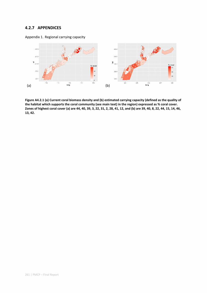
261 | PMCP – Final Report
4.2.7 APPENDICES
Appendix 1. Regional carrying capacity
(a) (b)
Figure A4.2.1 (a) Current coral biomass density and (b) estimated carrying capacity (defined as the quality of the habitat which supports the coral community (see main text) in the region) expressed as % coral cover. Zones of highest coral cover (a) are 44, 40, 39, 3, 22, 31, 2, 28, 41, 12, and (b) are 39, 40, 8, 22, 44, 15, 14, 46, 13, 42.

262 | PMCP – Final Report
Appendix 2. Yearly variation in connectivity
Figure A4.2.2 Inflows for the different yearly connectivity matrices (top) and for the mean connectivity (bottom left). It shows the mean probability that a specific zone may recruit larvae from any other zone – i.e., act as a ‘sink’.
Figure A4.2.3 Outflows for the different yearly connectivity matrices (top) and for the mean connectivity (bottom left). It shows the mean probability that a specific zone may recruit larvae to any other zone – i.e., act as a ‘source’.
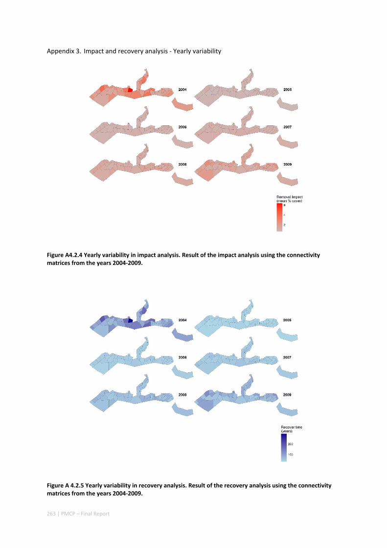
263 | PMCP – Final Report
Appendix 3. Impact and recovery analysis ‐ Yearly variability
Figure A4.2.4 Yearly variability in impact analysis. Result of the impact analysis using the connectivity matrices from the years 2004‐2009.
Figure A 4.2.5 Yearly variability in recovery analysis. Result of the recovery analysis using the connectivity matrices from the years 2004‐2009.

264 | PMCP – Final Report
In Figure A4.2.6, for each connectivity matrix in the years 2004‐2009 plus the mean connectivity, we
select the zones in the top 6 ranks in either the system maintenance or recovery analysis for that
yearly connectivity matrix. We then plot these zones in a 2D plane where the X axis shows the
impact values (as % coral cover) and the Y axis shows the recovery time (high to low recovery time
from the bottom). Zones are coloured according to the yearly connectivity matrices. Notice that a
zone may be displayed multiple times with different colours if it has high rank in more than one year.
Zones with high impact and fast recovery times are plotted on the top right of Figure A4.2.6. These
are the zones which contribute to both system maintenance and system recovery, and thus are ideal
conservation targets. Only few zones show high values for both system maintenance and system
recovery (38, 39, 21, 22 and 12) and each do so for only at most two yearly connectivity matrices.
Zones 6, 8, 14‐15 show high impact values on the 2004 connectivity matrix, but slow recovery times.
A number of zones show fast recovery times in the years 2005‐2007, but low impact values.
Figure A4.2.6 Zones in the top 6 ranks in either the impact or recovery analysis for each of the connectivity matrices in the years 2004‐2009, plus the mean connectivity. X axis represents the impact values as % coral cover and the Y axis shows the recovery time (inverted, slow recovery time at the bottom). Zones are coloured according to the yearly connectivity matrices.
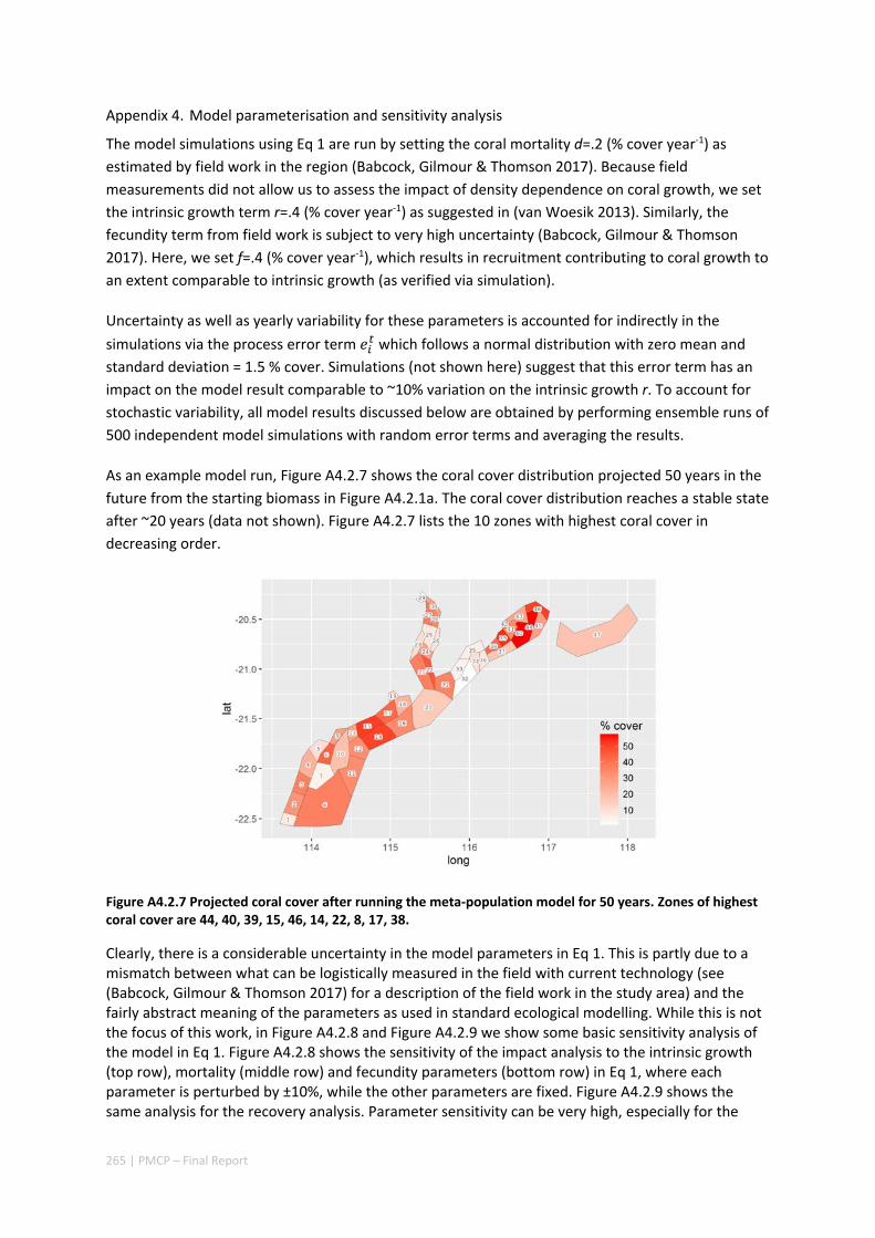
265 | PMCP – Final Report
Appendix 4. Model parameterisation and sensitivity analysis
The model simulations using Eq 1 are run by setting the coral mortality d=.2 (% cover year‐1) as
estimated by field work in the region (Babcock, Gilmour & Thomson 2017). Because field
measurements did not allow us to assess the impact of density dependence on coral growth, we set
the intrinsic growth term r=.4 (% cover year‐1) as suggested in (van Woesik 2013). Similarly, the
fecundity term from field work is subject to very high uncertainty (Babcock, Gilmour & Thomson
2017). Here, we set f=.4 (% cover year‐1), which results in recruitment contributing to coral growth to
an extent comparable to intrinsic growth (as verified via simulation).
Uncertainty as well as yearly variability for these parameters is accounted for indirectly in the
simulations via the process error term which follows a normal distribution with zero mean and
standard deviation = 1.5 % cover. Simulations (not shown here) suggest that this error term has an
impact on the model result comparable to ~10% variation on the intrinsic growth r. To account for
stochastic variability, all model results discussed below are obtained by performing ensemble runs of
500 independent model simulations with random error terms and averaging the results.
As an example model run, Figure A4.2.7 shows the coral cover distribution projected 50 years in the
future from the starting biomass in Figure A4.2.1a. The coral cover distribution reaches a stable state
after ~20 years (data not shown). Figure A4.2.7 lists the 10 zones with highest coral cover in
decreasing order.
Figure A4.2.7 Projected coral cover after running the meta‐population model for 50 years. Zones of highest coral cover are 44, 40, 39, 15, 46, 14, 22, 8, 17, 38.
Clearly, there is a considerable uncertainty in the model parameters in Eq 1. This is partly due to a mismatch between what can be logistically measured in the field with current technology (see (Babcock, Gilmour & Thomson 2017) for a description of the field work in the study area) and the fairly abstract meaning of the parameters as used in standard ecological modelling. While this is not the focus of this work, in Figure A4.2.8 and Figure A4.2.9 we show some basic sensitivity analysis of the model in Eq 1. Figure A4.2.8 shows the sensitivity of the impact analysis to the intrinsic growth (top row), mortality (middle row) and fecundity parameters (bottom row) in Eq 1, where each parameter is perturbed by ±10%, while the other parameters are fixed. Figure A4.2.9 shows the same analysis for the recovery analysis. Parameter sensitivity can be very high, especially for the
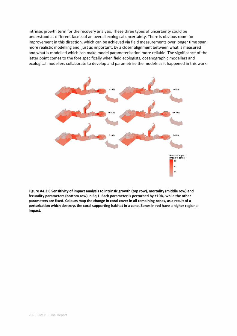
266 | PMCP – Final Report
intrinsic growth term for the recovery analysis. These three types of uncertainty could be understood as different facets of an overall ecological uncertainty. There is obvious room for improvement in this direction, which can be achieved via field measurements over longer time span, more realistic modelling and, just as important, by a closer alignment between what is measured and what is modelled which can make model parameterisation more reliable. The significance of the latter point comes to the fore specifically when field ecologists, oceanographic modellers and ecological modellers collaborate to develop and parametrise the models as it happened in this work.
Figure A4.2.8 Sensitivity of impact analysis to intrinsic growth (top row), mortality (middle row) and fecundity parameters (bottom row) in Eq 1. Each parameter is perturbed by ±10%, while the other parameters are fixed. Colours map the change in coral cover in all remaining zones, as a result of a perturbation which destroys the coral supporting habitat in a zone. Zones in red have a higher regional impact.

267 | PMCP – Final Report
Figure A4.2.9 Sensitivity of recovery analysis to intrinsic growth (top row), mortality (middle row) and fecundity parameters (bottom row) in Eq 1. Each parameter is perturbed by ±10%, while the other parameters are fixed. Colours map the number of years needed for the overall regional coral cover to recover when a single zone is unaffected and re‐seeds the reefs. Blue and white colours map short and long recover time, respectively).
Finally, to highlight the level of non‐linearity in both Eq 1 and in the impact analysis Figure A4.2.10 shows the calculation the zones’ impact, as above, for perturbation of varying magnitude. While in Figure 4.2.2 in the main document we assume a zone’s carrying capacity is completely destroyed (perturbation = ‐100%), in Figure A4.2.10 we simulate three perturbation levels: i) a perturbation which reduces a zone’s carrying capacity to 25% of its original value (top), ii) which halves the carrying capacity (middle) and iii) a restoration initiative which improves the local habitat by 50% (bottom). Not only the magnitudes but also the spatial pattern of the zones’ impact change with varying levels of perturbation. A manager tasked with developing a priority list of zones for conservation initiatives would likely see this priority list change depending on the magnitude of the stressors the region is likely to undergo.
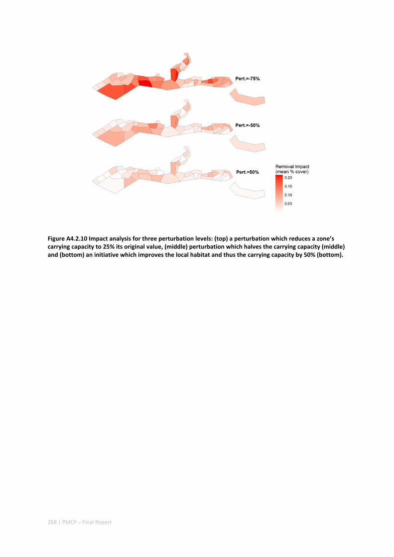
268 | PMCP – Final Report
Figure A4.2.10 Impact analysis for three perturbation levels: (top) a perturbation which reduces a zone’s carrying capacity to 25% its original value, (middle) perturbation which halves the carrying capacity (middle) and (bottom) an initiative which improves the local habitat and thus the carrying capacity by 50% (bottom).

269 | PMCP – Final Report
Connectivity in a marine fish meta‐population is strongly influenced by larval behaviour
Authors: Berry O, Slawinski D, Feng M, Colberg F, Babcock R.
ABSTRACT
Ocean currents can be important drivers of demographic and genetic cohesion among populations of marine organisms. Many marine species have a dispersive larval phase in which the larvae are small and with limited locomotor capacity, but some marine fish larvae have remarkable swimming capacity. This ability has the potential to significantly influence dispersive potential, patterns of settlement, and recruitment dynamics, but the quantitative effects of such behaviours are difficult to measure. Here, we use particle tracking simulations to show that realistic swimming behaviour in larval fishes, in a topographically and hydrodynamically complex marine region of north‐western Australia, is likely to significantly increase the probability of settlement and reduce the distance larvae are transported. Simulations of Lethrinus nebulosus, an important harvested species from the Indo‐pacific, show that larvae undertaking diurnal vertical migration on average travelled 6% further before settlement than non‐swimming larvae, but the probability of reaching suitable settlement habitat was similar. In contrast, larvae with realistic swimming capacity and ability to orient towards suitable settlement habitat had an order of magnitude higher chance of reaching settlement habitat, and on average travelled significantly shorter distances than non‐swimming larvae before settling (average 118 km vs. 148 km). Swimming reduced the influence of seasonal hydrodynamic variation, but spawning date nevertheless affected the distance and direction of transport in swimming larva (56% maximum seasonal difference). Our results demonstrate that despite their small size, swimming by larval fish potentially increases local recruitment significantly, underscoring the importance of including this biological attribute in particle tracking simulations for organisms. The relative importance of different reef zones as destinations or larval sinks, varied substantially depending on the degree of active larval behaviour and larval retention in the spawning region averaged between 17 and 26 %, but was highly variable. Areas in the north of the region featured as important larval source and sink areas, and potentially making a disproportionate contribution to resilience of regional populations, however rank importance as sinks varied according to larval behaviour.
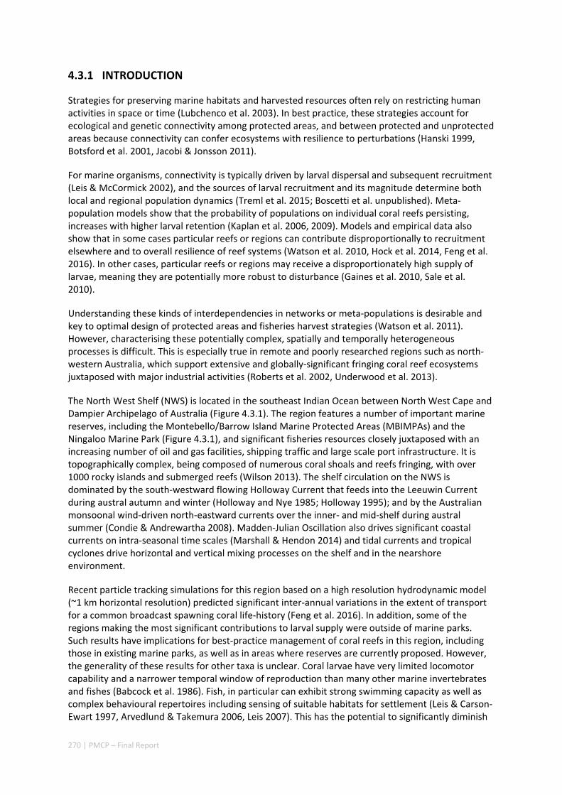
270 | PMCP – Final Report
4.3.1 INTRODUCTION
Strategies for preserving marine habitats and harvested resources often rely on restricting human activities in space or time (Lubchenco et al. 2003). In best practice, these strategies account for ecological and genetic connectivity among protected areas, and between protected and unprotected areas because connectivity can confer ecosystems with resilience to perturbations (Hanski 1999, Botsford et al. 2001, Jacobi & Jonsson 2011).
For marine organisms, connectivity is typically driven by larval dispersal and subsequent recruitment (Leis & McCormick 2002), and the sources of larval recruitment and its magnitude determine both local and regional population dynamics (Treml et al. 2015; Boscetti et al. unpublished). Meta‐population models show that the probability of populations on individual coral reefs persisting, increases with higher larval retention (Kaplan et al. 2006, 2009). Models and empirical data also show that in some cases particular reefs or regions can contribute disproportionally to recruitment elsewhere and to overall resilience of reef systems (Watson et al. 2010, Hock et al. 2014, Feng et al. 2016). In other cases, particular reefs or regions may receive a disproportionately high supply of larvae, meaning they are potentially more robust to disturbance (Gaines et al. 2010, Sale et al. 2010).
Understanding these kinds of interdependencies in networks or meta‐populations is desirable and key to optimal design of protected areas and fisheries harvest strategies (Watson et al. 2011). However, characterising these potentially complex, spatially and temporally heterogeneous processes is difficult. This is especially true in remote and poorly researched regions such as north‐western Australia, which support extensive and globally‐significant fringing coral reef ecosystems juxtaposed with major industrial activities (Roberts et al. 2002, Underwood et al. 2013).
The North West Shelf (NWS) is located in the southeast Indian Ocean between North West Cape and Dampier Archipelago of Australia (Figure 4.3.1). The region features a number of important marine reserves, including the Montebello/Barrow Island Marine Protected Areas (MBIMPAs) and the Ningaloo Marine Park (Figure 4.3.1), and significant fisheries resources closely juxtaposed with an increasing number of oil and gas facilities, shipping traffic and large scale port infrastructure. It is topographically complex, being composed of numerous coral shoals and reefs fringing, with over 1000 rocky islands and submerged reefs (Wilson 2013). The shelf circulation on the NWS is dominated by the south‐westward flowing Holloway Current that feeds into the Leeuwin Current during austral autumn and winter (Holloway and Nye 1985; Holloway 1995); and by the Australian monsoonal wind‐driven north‐eastward currents over the inner‐ and mid‐shelf during austral summer (Condie & Andrewartha 2008). Madden‐Julian Oscillation also drives significant coastal currents on intra‐seasonal time scales (Marshall & Hendon 2014) and tidal currents and tropical cyclones drive horizontal and vertical mixing processes on the shelf and in the nearshore environment.
Recent particle tracking simulations for this region based on a high resolution hydrodynamic model (~1 km horizontal resolution) predicted significant inter‐annual variations in the extent of transport for a common broadcast spawning coral life‐history (Feng et al. 2016). In addition, some of the regions making the most significant contributions to larval supply were outside of marine parks. Such results have implications for best‐practice management of coral reefs in this region, including those in existing marine parks, as well as in areas where reserves are currently proposed. However, the generality of these results for other taxa is unclear. Coral larvae have very limited locomotor capability and a narrower temporal window of reproduction than many other marine invertebrates and fishes (Babcock et al. 1986). Fish, in particular can exhibit strong swimming capacity as well as complex behavioural repertoires including sensing of suitable habitats for settlement (Leis & Carson‐Ewart 1997, Arvedlund & Takemura 2006, Leis 2007). This has the potential to significantly diminish
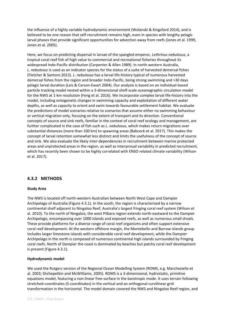
271 | PMCP – Final Report
the influence of a highly variable hydrodynamic environment (Wolanski & Kingsford 2014), and is believed to be one reason that self‐recruitment remains high, even in species with lengthy pelagic larval phases that provide significant opportunities for advection away from reefs (Jones et al. 1999, Jones et al. 2005).
Here, we focus on predicting dispersal in larvae of the spangled emperor, Lethrinus nebulosus, a tropical coral reef fish of high value to commercial and recreational fisheries throughout its widespread Indo‐Pacific distribution (Carpenter & Allen 1989). In north‐western Australia, L. nebulosus is used as an indicator species for the status of a suite of harvested demersal fishes (Fletcher & Santoro 2013). L. nebulosus has a larval life‐history typical of numerous harvested demersal fishes from the region and broader Indo‐Pacific, being strong swimming and >30 days pelagic larval duration (Leis & Carson‐Ewart 2004). Our analysis is based on an individual‐based particle tracking model nested within a 3‐dimensional shelf‐scale oceanographic circulation model for the NWS at 1‐km resolution (Feng et al. 2016). We incorporate complex larval life‐history into the model, including ontogenetic changes in swimming capacity and exploitation of different water depths, as well as capacity to orient and swim towards favourable settlement habitat. We evaluate the predictions of model scenarios relative to scenarios that assume either no swimming behaviour or vertical migration only, focusing on the extent of transport and its direction. Conventional concepts of source and sink reefs, familiar in the context of coral reef ecology and management, are further complicated in the case of fish such as L. nebulosus, which makes return migrations over substantial distances (more than 100 km) to spawning areas (Babcock et al. 2017). This makes the concept of larval retention somewhat less distinct and limits the usefulness of the concept of source and sink. We also evaluate the likely inter‐dependencies in recruitment between marine protected areas and unprotected areas in the region, as well as interannual variability in predicted recruitment, which has recently been shown to be highly correlated with ENSO related climate variability (Wilson et al. 2017).
4.3.2 METHODS
Study Area
The NWS is located off north‐western Australian between North West Cape and Dampier Archipelago of Australia (Figure 4.3.1). In the south, the region is characterised by a narrow continental shelf adjacent to Ningaloo Reef, Australia’s largest fringing coral reef system (Wilson et al. 2010). To the north of Ningaloo, the west Pilbara region extends north‐eastward to the Dampier Archipelago, encompassing over 1000 islands and exposed reefs, as well as numerous small shoals. These provide platforms for a diverse range of coral reef organisms and often support extensive coral reef development. At the western offshore margin, the Montebello and Barrow islands group includes larger limestone islands with considerable coral reef development, while the Dampier Archipelago in the north is composed of numerous continental high islands surrounded by fringing coral reefs. North of Dampier the coast is dominated by beaches but patchy coral reef development is present (Figure 4.3.1).
Hydrodynamic model
We used the Rutgers version of the Regional Ocean Modelling System (ROMS, e.g. Marchesiello et al. 2003; Shchepetkin and McWilliams, 2005). ROMS is a 3‐dimensional, hydrostatic, primitive equations model, featuring a non‐linear free‐surface in the barotropic mode. It uses terrain following stretched‐coordinates (S‐coordinates) in the vertical and an orthogonal curvilinear grid transformation in the horizontal. The model domain covered the NWS and Ningaloo Reef region, and
272 | PMCP – Final Report
has a horizontal resolution of ~1 km (Figure 4.3.1). The bottom topography was taken from a collection of sources including GA2009, industry provided LIDAR and MNF multi beam data. Thirty levels are used in the vertical layers and we used non‐local K‐Profile in the vertical mixing parameterisation (Large et al. 1994).
Figure 4.3.1 Map of the study region. Offshore coloured sections are modelled spawning zones. Numbered grey‐blue coastal regions are settlement sites. Marine reserves are indicated by red sections.
The model was initialized with temperature and salinity values from the Ocean Forecasting Australia Model (OFAM, Oke et al. 2013). A 3‐year spinup model simulation was carried out in which the model was repeatedly forced by OFAM 3‐hourly meteorological forcing and open boundary condition for the year 2003, in order to allow for flux adjustment and for the model to reach a quasi‐stationary state as evident by the models kinetic energy (Figure S4.3.1). The model is then run forward from 2004 to mid‐2010. During the spin up phase and interannual runs, the surface heat flux (Q) was corrected by monthly climatologies of sea surface temperature (SST) and the surface salt flux was relaxed towards monthly sea surface salinity climatology. Both the temperature and salinity climatologies were derived over a period of 17 years from the OFAM model. The time scale for the relaxation was 5 days.
In order to include tidal components, the open model boundaries were driven with tidal currents and levels derived from the TPXO7.2 global model (Egbert et al., 1994; Egbert and Erofeeva, 2002). TPXO7.2 best fits in a least‐squares sense the Laplace Tidal Equations and along track averaged data from the TOPEX/Poseidon and Jason altimetry missions, obtained with OTIS (Oregon State University Tidal Inversion Software). We used eight primary constituents (M2, S2, N2, K2, K1, O1, P1, Q1). The harmonic constituents for the global grid were downloaded from the OTIS web site (http://volkov.oce.orst.edu/tides/). See Feng et al. (2016) for more details about the model set up.
Larval behaviour and particle tracking simulations
Unlike many fishes that inhabit coral reef and associated habitats as adults, Lethrinids are pelagic spawners (Boehlert 1996). The precise environments where spawning occurs, however, are unclear.
273 | PMCP – Final Report
Aggregations of spawning‐ready fish are sometimes encountered on outer reef slopes (Salem 1999, SCRFA 2004, Nakamura et al. 2009), but the best available evidence for north‐western Australia is that they move further offshore to spawn at depths of >35 m (Babcock et al. 2017; R. Marriott, Dept. Fisheries, Western Australia pers. comm.). We selected a band between the 50 m and 90 m bathymetric lines as suitable spawning locations, and for practicality sub‐divided this into five distinct spawning regions (Figure 4.3.1) whose dimensions corresponded to the scale of L. nebulosus spawning migrations (Babcock et al. 2017). Spawning was modelled as occurring during the summer period (September‐March), based on evidence from gonad development (R. Marriott, Dept. Fisheries, Western Australia pers. comm.; Moran et al. 1993, Marriott et al. 2010) and observed spawning movements (Babcock et al. 2017). We modelled a pelagic larval duration of between 25 and 32 days based on the field analysis of Nakamura et al. (2012). Larval releases were simulated in an evenly spread manner throughout these regions, since we do not know the precise locations of spawning aggregation sites. In addition, the number of larvae released in each zone was weighted by the amount of reef habitat located within the catchment of each spawning zone (Figure 4.3.2). Modelled larvae were permitted to settle if they encountered suitable settlement habitat during days 25–32, based on evidence that there is some flexibility in settlement time in this species (Nakamura et al. 2010). The potential settlement area was subdivided into 47 sub‐regions (Figure 4.3.1) of suitable habitat, delineated by distribution and presence of reefs. Lethrinids settle in a diverse range of habitats and have been recorded recruiting into stands of Sargassum and other brown macroalgae in lagoons of Ningaloo and other reefs in the region (Wilson et al. 2010, Evans et al. 2014). Elsewhere, based on light‐trapping, L. nebulosus larvae settle on reefs with and without seagrass (Nakamura et al. 2009).
Figure 4.3.2 Map of the catchment area reefs for each spawning zone. Shading indicates spawning zone association. Dark Green; northern zone, Purple; Barrow Island East zone, Brown; Barrow Island West zone, Grey; Pilbara zone, Light Green; Ningaloo zone.
Three larval behaviour scenarios were modelled: 1) non‐swimming; 2) vertical migration; and 3) swimming, vertical migration and orienting towards suitable settlement habitat. Under all scenarios larvae were spawned at the surface (Akazaki et al. 1989, Leis & Rennis 2004) and exhibited no swimming or buoyancy change during the first 5 days of development corresponding to the pre‐
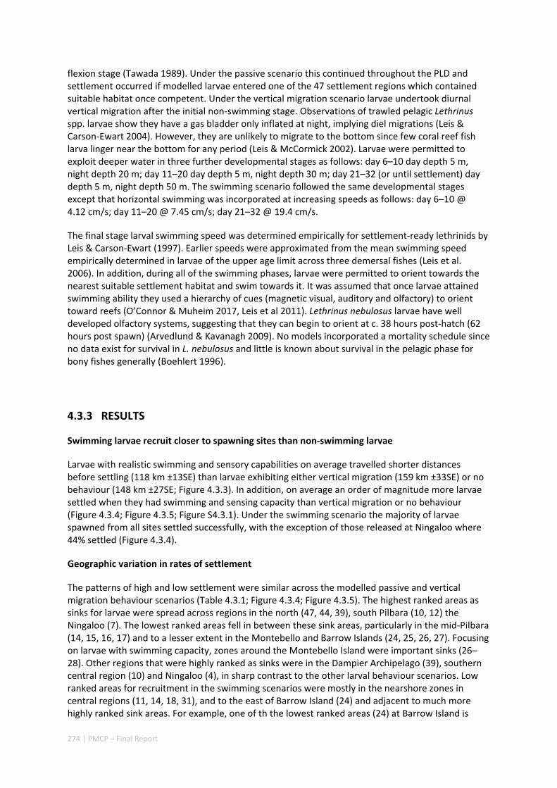
274 | PMCP – Final Report
flexion stage (Tawada 1989). Under the passive scenario this continued throughout the PLD and settlement occurred if modelled larvae entered one of the 47 settlement regions which contained suitable habitat once competent. Under the vertical migration scenario larvae undertook diurnal vertical migration after the initial non‐swimming stage. Observations of trawled pelagic Lethrinus spp. larvae show they have a gas bladder only inflated at night, implying diel migrations (Leis & Carson‐Ewart 2004). However, they are unlikely to migrate to the bottom since few coral reef fish larva linger near the bottom for any period (Leis & McCormick 2002). Larvae were permitted to exploit deeper water in three further developmental stages as follows: day 6–10 day depth 5 m, night depth 20 m; day 11–20 day depth 5 m, night depth 30 m; day 21–32 (or until settlement) day depth 5 m, night depth 50 m. The swimming scenario followed the same developmental stages except that horizontal swimming was incorporated at increasing speeds as follows: day 6–10 @ 4.12 cm/s; day 11–20 @ 7.45 cm/s; day 21–32 @ 19.4 cm/s.
The final stage larval swimming speed was determined empirically for settlement‐ready lethrinids by Leis & Carson‐Ewart (1997). Earlier speeds were approximated from the mean swimming speed empirically determined in larvae of the upper age limit across three demersal fishes (Leis et al. 2006). In addition, during all of the swimming phases, larvae were permitted to orient towards the nearest suitable settlement habitat and swim towards it. It was assumed that once larvae attained swimming ability they used a hierarchy of cues (magnetic visual, auditory and olfactory) to orient toward reefs (O’Connor & Muheim 2017, Leis et al 2011). Lethrinus nebulosus larvae have well developed olfactory systems, suggesting that they can begin to orient at c. 38 hours post‐hatch (62 hours post spawn) (Arvedlund & Kavanagh 2009). No models incorporated a mortality schedule since no data exist for survival in L. nebulosus and little is known about survival in the pelagic phase for bony fishes generally (Boehlert 1996).
4.3.3 RESULTS
Swimming larvae recruit closer to spawning sites than non‐swimming larvae
Larvae with realistic swimming and sensory capabilities on average travelled shorter distances before settling (118 km ±13SE) than larvae exhibiting either vertical migration (159 km ±33SE) or no behaviour (148 km ±27SE; Figure 4.3.3). In addition, on average an order of magnitude more larvae settled when they had swimming and sensing capacity than vertical migration or no behaviour (Figure 4.3.4; Figure 4.3.5; Figure S4.3.1). Under the swimming scenario the majority of larvae spawned from all sites settled successfully, with the exception of those released at Ningaloo where 44% settled (Figure 4.3.4).
Geographic variation in rates of settlement
The patterns of high and low settlement were similar across the modelled passive and vertical migration behaviour scenarios (Table 4.3.1; Figure 4.3.4; Figure 4.3.5). The highest ranked areas as sinks for larvae were spread across regions in the north (47, 44, 39), south Pilbara (10, 12) the Ningaloo (7). The lowest ranked areas fell in between these sink areas, particularly in the mid‐Pilbara (14, 15, 16, 17) and to a lesser extent in the Montebello and Barrow Islands (24, 25, 26, 27). Focusing on larvae with swimming capacity, zones around the Montebello Island were important sinks (26–28). Other regions that were highly ranked as sinks were in the Dampier Archipelago (39), southern central region (10) and Ningaloo (4), in sharp contrast to the other larval behaviour scenarios. Low ranked areas for recruitment in the swimming scenarios were mostly in the nearshore zones in central regions (11, 14, 18, 31), and to the east of Barrow Island (24) and adjacent to much more highly ranked sink areas. For example, one of th the lowest ranked areas (24) at Barrow Island is
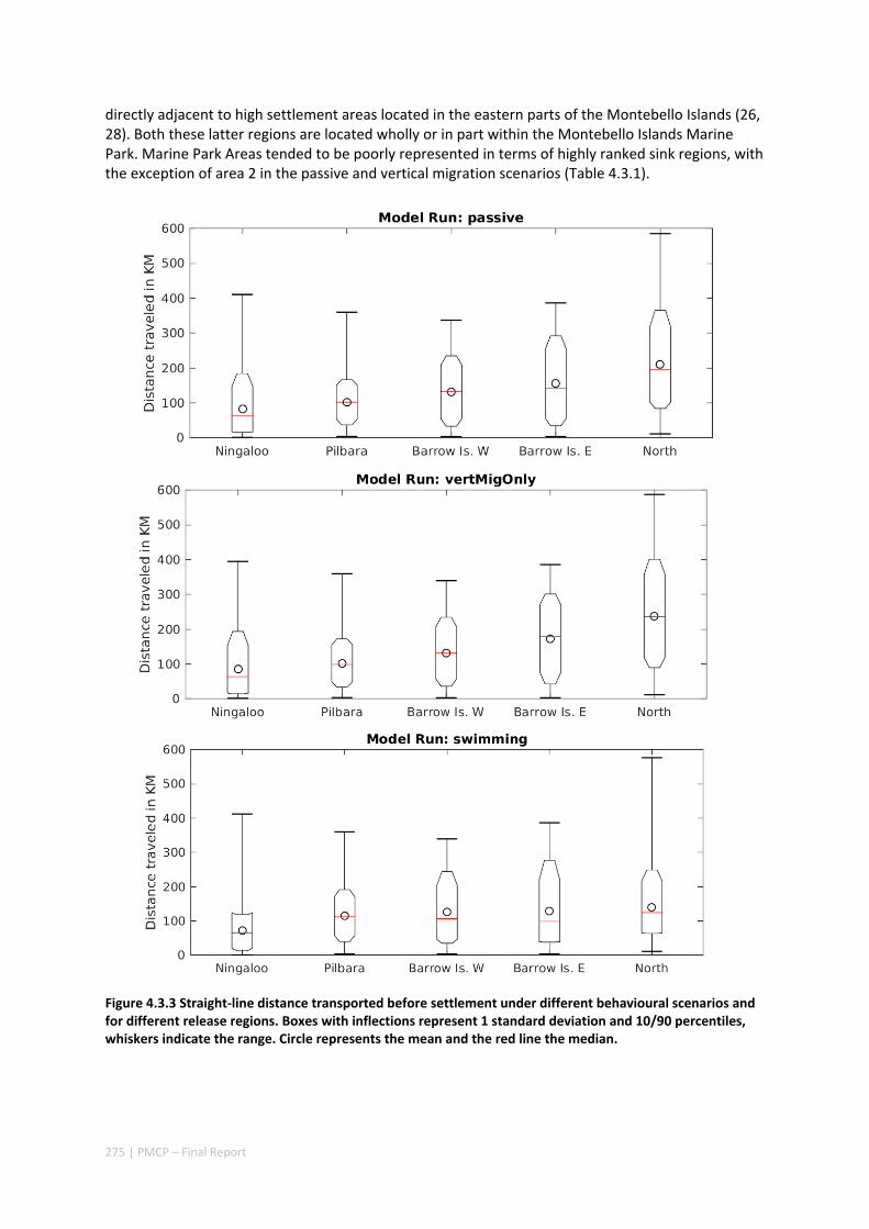
275 | PMCP – Final Report
directly adjacent to high settlement areas located in the eastern parts of the Montebello Islands (26, 28). Both these latter regions are located wholly or in part within the Montebello Islands Marine Park. Marine Park Areas tended to be poorly represented in terms of highly ranked sink regions, with the exception of area 2 in the passive and vertical migration scenarios (Table 4.3.1).
Figure 4.3.3 Straight‐line distance transported before settlement under different behavioural scenarios and for different release regions. Boxes with inflections represent 1 standard deviation and 10/90 percentiles, whiskers indicate the range. Circle represents the mean and the red line the median.
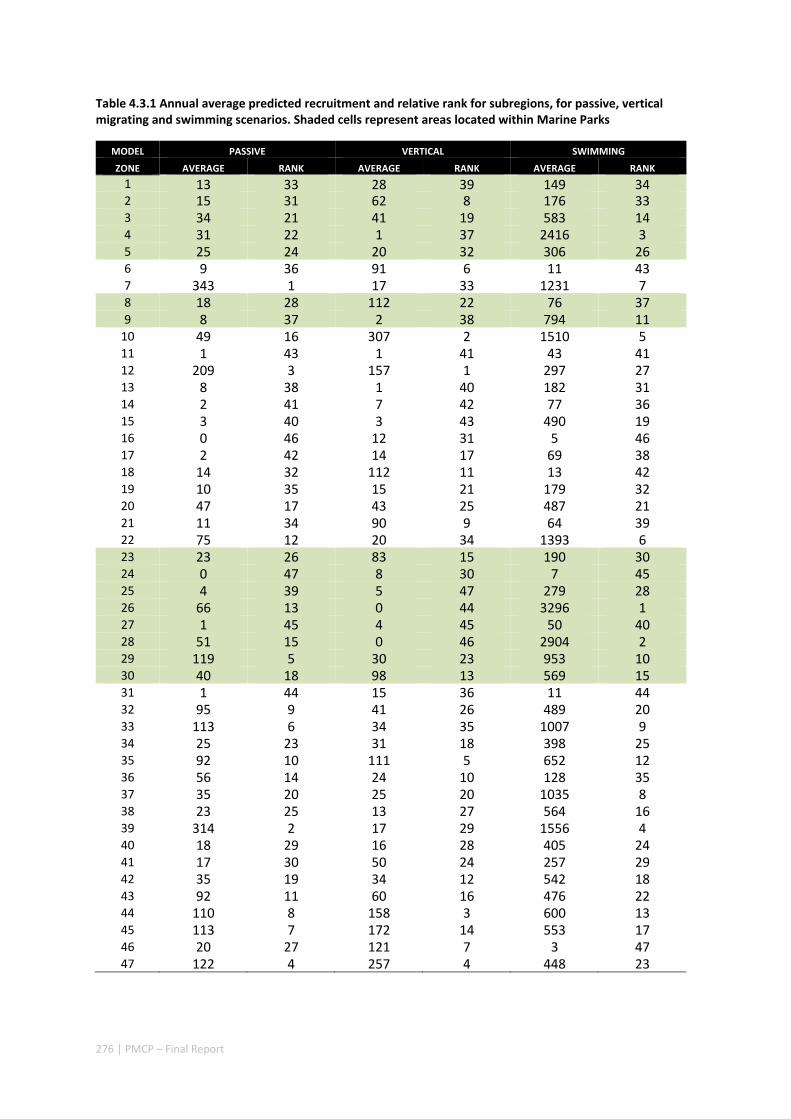
276 | PMCP – Final Report
Table 4.3.1 Annual average predicted recruitment and relative rank for subregions, for passive, vertical migrating and swimming scenarios. Shaded cells represent areas located within Marine Parks
MODEL PASSIVE VERTICAL SWIMMING
ZONE AVERAGE RANK AVERAGE RANK AVERAGE RANK
1 13 33 28 39 149 34 2 15 31 62 8 176 33 3 34 21 41 19 583 14 4 31 22 1 37 2416 3 5 25 24 20 32 306 26 6 9 36 91 6 11 43 7 343 1 17 33 1231 7 8 18 28 112 22 76 37 9 8 37 2 38 794 11 10 49 16 307 2 1510 5 11 1 43 1 41 43 41 12 209 3 157 1 297 27 13 8 38 1 40 182 31 14 2 41 7 42 77 36 15 3 40 3 43 490 19 16 0 46 12 31 5 46 17 2 42 14 17 69 38 18 14 32 112 11 13 42 19 10 35 15 21 179 32 20 47 17 43 25 487 21 21 11 34 90 9 64 39 22 75 12 20 34 1393 6 23 23 26 83 15 190 30 24 0 47 8 30 7 45 25 4 39 5 47 279 28 26 66 13 0 44 3296 1 27 1 45 4 45 50 40 28 51 15 0 46 2904 2 29 119 5 30 23 953 10 30 40 18 98 13 569 15 31 1 44 15 36 11 44 32 95 9 41 26 489 20 33 113 6 34 35 1007 9 34 25 23 31 18 398 25 35 92 10 111 5 652 12 36 56 14 24 10 128 35 37 35 20 25 20 1035 8 38 23 25 13 27 564 16 39 314 2 17 29 1556 4 40 18 29 16 28 405 24 41 17 30 50 24 257 29 42 35 19 34 12 542 18 43 92 11 60 16 476 22 44 110 8 158 3 600 13 45 113 7 172 14 553 17 46 20 27 121 7 3 47 47 122 4 257 4 448 23
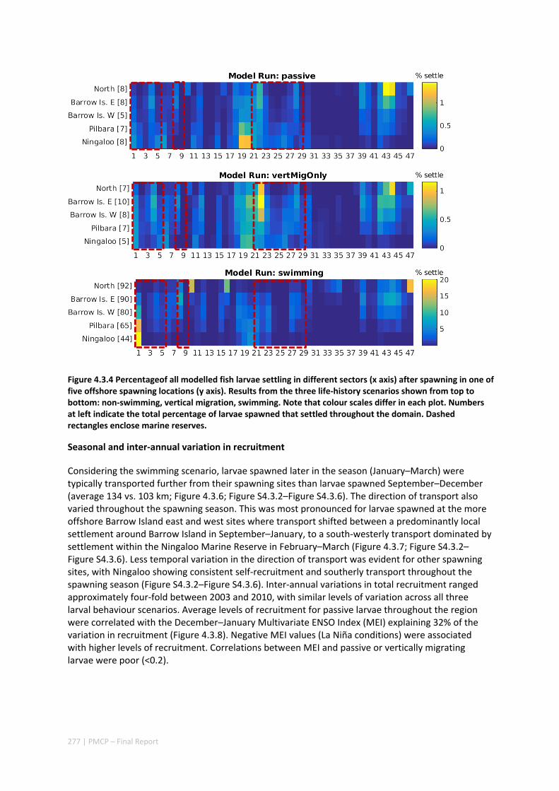
277 | PMCP – Final Report
Figure 4.3.4 Percentageof all modelled fish larvae settling in different sectors (x axis) after spawning in one of five offshore spawning locations (y axis). Results from the three life‐history scenarios shown from top to bottom: non‐swimming, vertical migration, swimming. Note that colour scales differ in each plot. Numbers at left indicate the total percentage of larvae spawned that settled throughout the domain. Dashed rectangles enclose marine reserves.
Seasonal and inter‐annual variation in recruitment
Considering the swimming scenario, larvae spawned later in the season (January–March) were typically transported further from their spawning sites than larvae spawned September–December (average 134 vs. 103 km; Figure 4.3.6; Figure S4.3.2–Figure S4.3.6). The direction of transport also varied throughout the spawning season. This was most pronounced for larvae spawned at the more offshore Barrow Island east and west sites where transport shifted between a predominantly local settlement around Barrow Island in September–January, to a south‐westerly transport dominated by settlement within the Ningaloo Marine Reserve in February–March (Figure 4.3.7; Figure S4.3.2–Figure S4.3.6). Less temporal variation in the direction of transport was evident for other spawning sites, with Ningaloo showing consistent self‐recruitment and southerly transport throughout the spawning season (Figure S4.3.2–Figure S4.3.6). Inter‐annual variations in total recruitment ranged approximately four‐fold between 2003 and 2010, with similar levels of variation across all three larval behaviour scenarios. Average levels of recruitment for passive larvae throughout the region were correlated with the December–January Multivariate ENSO Index (MEI) explaining 32% of the variation in recruitment (Figure 4.3.8). Negative MEI values (La Niña conditions) were associated with higher levels of recruitment. Correlations between MEI and passive or vertically migrating larvae were poor (<0.2).
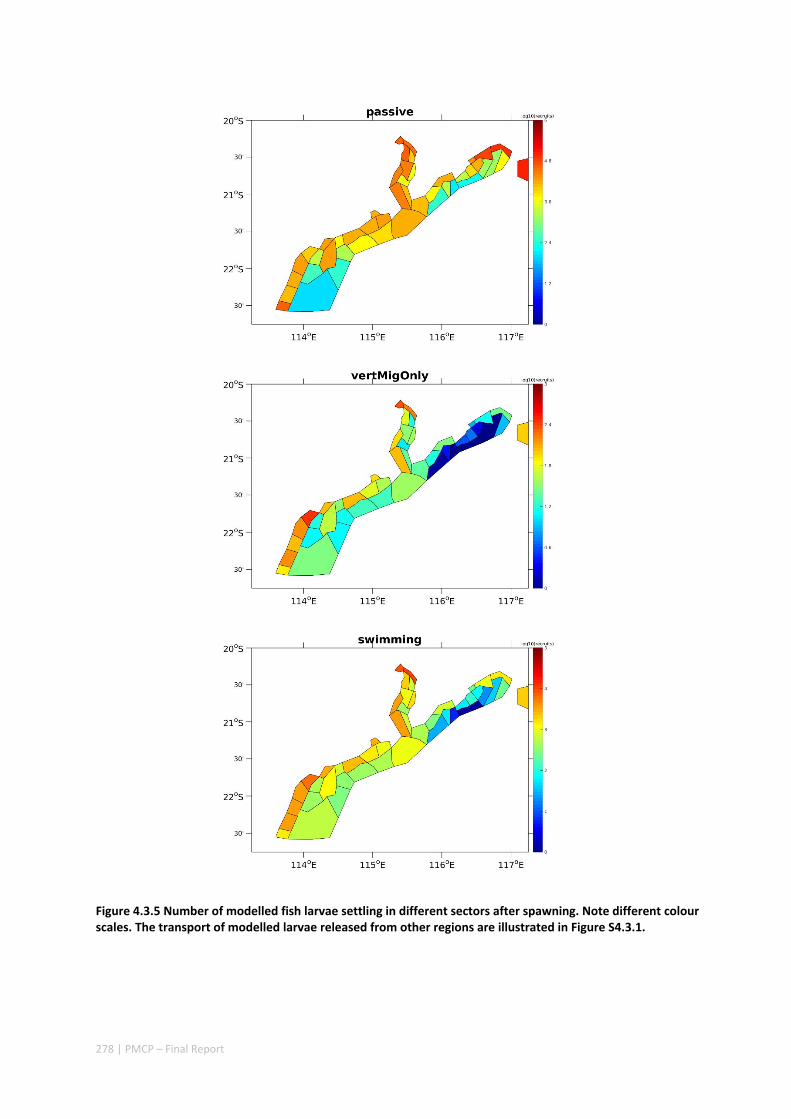
278 | PMCP – Final Report
Figure 4.3.5 Number of modelled fish larvae settling in different sectors after spawning. Note different colour scales. The transport of modelled larvae released from other regions are illustrated in Figure S4.3.1.

279 | PMCP – Final Report
Figure 4.3.6 Total distance travelled for swimming larvae spawned during different months. Data are from spawnings in each of the different spawning regions, and averaged for all larvae.
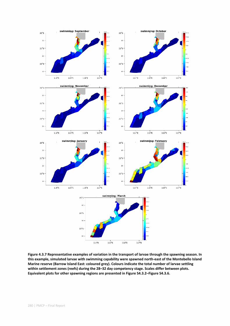
280 | PMCP – Final Report
Figure 4.3.7 Representative examples of variation in the transport of larvae through the spawning season. In this example, simulated larvae with swimming capability were spawned north‐east of the Montebello Island Marine reserve (Barrow Island East: coloured grey). Colours indicate the total number of larvae settling within settlement zones (reefs) during the 28–32 day competency stage. Scales differ between plots. Equivalent plots for other spawning regions are presented in Figure S4.3.2–Figure S4.3.6.

281 | PMCP – Final Report
Figure 4.3.8 Relationship between average regional recruitment (swimming scenario) and Southern Oscillation Index values (September–March).
Table 4.3.2 Average annual contribution of spawning zones to overall settlement throughout the region, 2003–2010.
MODEL PASSIVE VERTICAL SWIMMING
ZONE PARTICLES RANK PARTICLES RANK PARTICLES RANK
Barrow East 7.42E+03 4 9.34E+03 3 8.35E+04 3
Barrow West 1.16E+04 2 1.80E+04 2 1.67E+05 2
Ningaloo 1.50E+03 5 5 7.76E+03 5
North 5.23E+04 1 4.70E+04 1 5.73E+05 1
Pilbara 8.76E+03 3 8.16E+03 4 7.71E+04 4
TOTAL 8.16E+04
8.34E+04 9.08E+05
The contributions of different spawning regions to settlement
The relative (rank) annual contribution to settlement among spawning regions was similar under all scenarios in that the greatest contribution was always made by the North region, and the least by Ningaloo (Table 4.3.2; Figure 4.3.4). Under the swimming scenario contributions declined from east to west with easternmost spawning site “North” contributing around 9 times the number of successful settling larvae as the westernmost spawning site “Ningaloo”. The level of larval retention or “self‐seeding” where larvae spawned within a zone return to settle on reefs within the catchment of that zone, varied substantially among spawning zones, from less than 1% of total settling larvae to more than 30% (Table 4.3.3). The overall averages of larval retention ranged between 0.15% and 6.04% (Table 4.3.3). Simulations of swimming larvae resulted in higher levels of larval retention on average than for passive or vertically migrating larvae, although this was not significant due to high levels of variability around these values. The rank importance of spawning zones in terms of larval retention was quite different than their rank importance as overall larval sources, with the North spawning zone ranked highest in terms of larval retention. Apart from this, larval retention varied according to larval behaviour, but was next highest in the Barrow West spawning zone for swimming
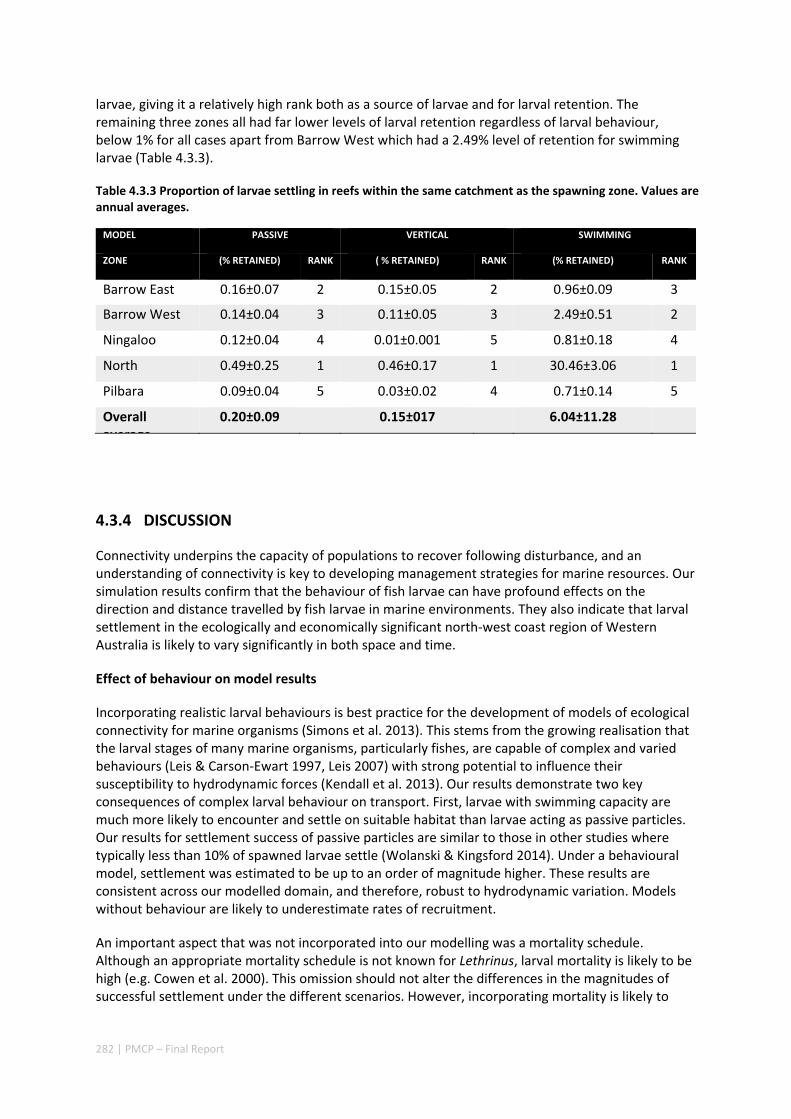
282 | PMCP – Final Report
larvae, giving it a relatively high rank both as a source of larvae and for larval retention. The remaining three zones all had far lower levels of larval retention regardless of larval behaviour, below 1% for all cases apart from Barrow West which had a 2.49% level of retention for swimming larvae (Table 4.3.3).
Table 4.3.3 Proportion of larvae settling in reefs within the same catchment as the spawning zone. Values are annual averages.
MODEL PASSIVE VERTICAL SWIMMING
ZONE (% RETAINED) RANK ( % RETAINED) RANK (% RETAINED) RANK
Barrow East 0.16±0.07 2 0.15±0.05 2 0.96±0.09 3
Barrow West 0.14±0.04 3 0.11±0.05 3 2.49±0.51 2
Ningaloo 0.12±0.04 4 0.01±0.001 5 0.81±0.18 4
North 0.49±0.25 1 0.46±0.17 1 30.46±3.06 1
Pilbara 0.09±0.04 5 0.03±0.02 4 0.71±0.14 5
Overall average
0.20±0.09 0.15±017 6.04±11.28
4.3.4 DISCUSSION
Connectivity underpins the capacity of populations to recover following disturbance, and an understanding of connectivity is key to developing management strategies for marine resources. Our simulation results confirm that the behaviour of fish larvae can have profound effects on the direction and distance travelled by fish larvae in marine environments. They also indicate that larval settlement in the ecologically and economically significant north‐west coast region of Western Australia is likely to vary significantly in both space and time.
Effect of behaviour on model results
Incorporating realistic larval behaviours is best practice for the development of models of ecological connectivity for marine organisms (Simons et al. 2013). This stems from the growing realisation that the larval stages of many marine organisms, particularly fishes, are capable of complex and varied behaviours (Leis & Carson‐Ewart 1997, Leis 2007) with strong potential to influence their susceptibility to hydrodynamic forces (Kendall et al. 2013). Our results demonstrate two key consequences of complex larval behaviour on transport. First, larvae with swimming capacity are much more likely to encounter and settle on suitable habitat than larvae acting as passive particles. Our results for settlement success of passive particles are similar to those in other studies where typically less than 10% of spawned larvae settle (Wolanski & Kingsford 2014). Under a behavioural model, settlement was estimated to be up to an order of magnitude higher. These results are consistent across our modelled domain, and therefore, robust to hydrodynamic variation. Models without behaviour are likely to underestimate rates of recruitment.
An important aspect that was not incorporated into our modelling was a mortality schedule. Although an appropriate mortality schedule is not known for Lethrinus, larval mortality is likely to be high (e.g. Cowen et al. 2000). This omission should not alter the differences in the magnitudes of successful settlement under the different scenarios. However, incorporating mortality is likely to
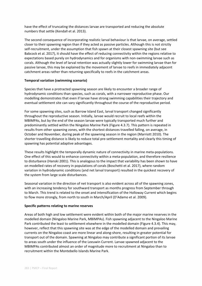
283 | PMCP – Final Report
have the effect of truncating the distances larvae are transported and reducing the absolute numbers that settle (Kendall et al. 2013).
The second consequence of incorporating realistic larval behaviour is that larvae, on average, settled closer to their spawning region than if they acted as passive particles. Although this is not strictly self‐recruitment, under the assumption that fish spawn at their closest spawning site (but see Babcock et al. 2017), it should have the effect of reducing connectivity within the regions relative to expectations based purely on hydrodynamics and for organisms with non‐swimming larvae such as corals. Although the level of larval retention was actually slightly lower for swimming larvae than for passive larvae, this may be explained by the movement of larvae to reefs in immediately adjacent catchment areas rather than returning specifically to reefs in the catchment areas.
Temporal variation (swimming scenario)
Species that have a protracted spawning season are likely to encounter a broader range of hydrodynamic conditions than species, such as corals, with a narrower reproductive phase. Our modelling demonstrates that even if larvae have strong swimming capabilities their trajectory and eventual settlement site can vary significantly throughout the course of the reproductive period.
For some spawning sites, such as Barrow Island East, larval transport changed significantly throughout the reproductive season. Initially, larvae would recruit to local reefs within the MBIMPAs, but by the end of the season larvae were typically transported much further and predominantly settled within the Ningaloo Marine Park (Figure 4.3.7). This pattern is repeated in results from other spawning zones, with the shortest distances travelled falling, on average, in October and November, during peak of the spawning season in the region (Marriott 2010). The shorter travelling distance is likely to reduce total pre‐settlement mortality and clearly this timing of spawning has potential adaptive advantages.
These results highlight the temporally dynamic nature of connectivity in marine meta‐populations. One effect of this would to enhance connectivity within a meta‐population, and therefore resilience to disturbance (Hanski 2001). This is analogous to the impact that variability has been shown to have on modelled rates of recovery in populations of corals (Boschetti et al. 2017), where random variation in hydrodynamic conditions (and net larval transport) resulted in the quickest recovery of the system from large scale disturbances.
Seasonal variation in the direction of net transport is also evident across all of the spawning zones, with an increasing tendency for southward transport as months progress from September through to March. This trend is related to the onset and intensification of the Holloway Current which begins to flow more strongly, from north to south in March/April (D’Adamo et al. 2009).
Specific patterns relating to marine reserves
Areas of both high and low settlement were evident within both of the major marine reserves in the modelled domain (Ningaloo Marine Park, MBIMPAs). Fish spawning adjacent to the Ningaloo Marine Park contributed the least to settlement elsewhere in the modelled domain (Figure 4.3.4). This may, however, reflect that this spawning site was at the edge of the modelled domain and prevailing currents on the Ningaloo coast are more linear and along‐shore, resulting in greater potential for transport out of the domain. Spawning at Ningaloo may contribute a significant portion of its larvae to areas south under the influence of the Leeuwin Current. Larvae spawned adjacent to the MBIMPAs contributed almost an order of magnitude more to recruitment at Ningaloo than to recruitment within the Montebello Islands Marine Park.

284 | PMCP – Final Report
Comparison to the coral results
The same model applied to a typical coral larval life‐history with a narrower reproductive window, shorter PLD, and without swimming capacity yielded significant spatial as well as temporal heterogeneity in larval transport (Feng et al. 2016). Patterns of variation in areas that were important sinks for coral were broadly similar from those for passive or vertically migrating L. nebulosus larvae, though recruitment was less focused on the central areas of the region than for corals. For actively swimming larvae, patterns were quite different however, with major sinks for recruitment spread throughout the area, particularly in the south central areas and the Dampier Archipelago.
Implications for management
Currently, management of the fishery for L. nebulosus is based on limited knowledge of larval dispersal and spatial ecology of adults. Mark recapture studies at Ningaloo have indicated that individuals move relatively small distances (<6 nautical miles) from the point of capture, though larger movements of the order of up to 100 km were recorded (Moran et al. 1993). This aligns with findings from acoustic tagging and tracking which showed that although some individuals are relatively sedentary, a substantial proportion move larger distances, including long‐distance spawning migrations (Pillans et al. 2014, Babcock 2017). The majority of connectivity mediated by adult movements, appears to be on the scale of tens of kilometres, and occasionally hundreds.
This study was undertaken to provide information on the extent of larval connectivity in L. nebulosus throughout north‐western Australia, so that it might better inform the spatial management of this species. It indicated that larval connectivity is mainly on the scale of 100s of km. Furthermore, it suggests that on these scales, larval retention averages around 6% for swimming larvae but is highly variable among regions and is highly dependent on larval behaviour (i.e. whether larvae are modelled as passive or with a variety of swimming behaviours). These values are within the lower range of those derived empirically for other pelagic spawning reef fishes (41.2 ±19.9%, reviewed in Herrera et al. 2017). While Herrera et al. (2017) urge caution when using “seascape and life history” to infer self‐recruitment, there are independent means with which to evaluate the effectiveness of our models for estimating larval transport of L. nebulosus in this region. Using a combination of population genetics and modelling approaches we conclude that dispersal distances ≤100 km are most likely for populations on the north‐west Australian coast (Berry et al. 2012). Furthermore our model has been able to reproduce, for swimming larvae, a positive relationship between oceanographic conditions (MEI) and Lethrinus recruitment similar to that recently shown through field recruitment surveys at Ningaloo (Wilson et al. 2017). We may therefore, be reasonably confident that spatial management inferences based on our models will have significant utility. In this regard, the northern area, centred on the Dampier Archipelago stands out as having high potential value as both a source and sink area, as well as having relatively high levels of larval retention. Currently planning of a Marine Park in the Dampier Archipelago is well advanced, although reserves are not yet declared and other areas within the region have been suggested as being of potential conservation interest (DPAW 2005). The relationship between larval dispersal, retention and population resilience in other existing marine parks at Ningaloo and the Montebello Islands is less clear and likely requires further investigation with fine scale variability evident and some very low recruitment areas featuring at these locations.
285 | PMCP – Final Report
4.3.5 ACKNOWLEDGEMENTS
This research was financially supported as part of the Pilbara Marine Conservation Partnership funded by the Gorgon Barrow Island Net Conservation Benefits Fund which is administered by the WA Department of Biodiversity, Conservation and Attractions (DBCA).
4.3.6 REFERENCES
Akazaki M, Tokito A, Takamatsu S, Nakajima H, Kawahara H (1989) Spawning behavior, embryonic development and metamorphosis of larvae of the lethrinid fish, Lethrinus nebulosus. Bulletin of the Faculty of Agriculture‐Miyazaki University 36
Arvedlund M, Kavanagh K (2009) The senses and environmental cues used by marine larvae of fish and decapod crustaceans to find tropical coastal ecosystems. Ecological Connectivity among Tropical Coastal Ecosystems. Springer
Arvedlund M, Takemura A (2006) The importance of chemical environmental cues for juvenile Lethrinus nebulosus Forsskål (Lethrinidae, Teleostei) when settling into their first benthic habitat. Journal of Experimental Marine Biology and Ecology 338:112‐122
Babcock R, Bull G, Harrison P, Heyward A, Oliver J, Wallace C, Willis B (1986) Synchronous spawnings of 105 scleractinian coral species on the Great Barrier Reef. Marine Biology 90:379‐394
Babcock RC, Pillans RD, ., Rochester W (2017) Environmental and individual effects on the behaviour and spawning movements of Lethrinus nebulosus on a coral reef. Marine and Freshwater Research
Berry O, England P, Marriott RJ, Burridge CP, Newman SJ. (2012) Understanding age‐specific dispersal in fishes through hydrodynamic modelling, genetic simulations and microsatellite DNA analysis. Molecular Ecology. 21(9):2145‐59.
Boehlert GW (1996) Larval dispersal and survival in tropical reef fishes. Reef fisheries. Springer
Boschetti F, Babcock RC, Doropoulos C, Thomson DP, Feng M, Slawinski D, Berry O, Vanderklift MA. (2017) Setting priorities for conservation initiatives at the interface between ocean circulation, larval connectivity, and population dynamics Journal of Applied Ecology (in review)
Botsford LW, Hastings A, Gaines SD (2001) Dependence of sustainability on the configuration of marine reserves and larval dispersal distance. Ecology Letters 4:144‐150
Carpenter KE, Allen GR (1989) FAO species catalogue, Vol 9. FAO
Condie S, Andrewartha J (2008) Circulation and connectivity on the Australian North West shelf. Continental Shelf Research 28:1724‐1739
Cowen RK, Lwiza KMM, Sponaugle S, Paris CB, Olson DB (2000) Connectivity of Marine Populations: Open or Closed? Science 287:857‐859

286 | PMCP – Final Report
DPAW (2005) Indicative management plan for the proposed Dampier Archipelago Marine Park and Cape Preston Marine Management Area. Dept. of Conservation and Land Management, Fremantle, W.A. 146 p.
Evans R, Wilson S, Field S, Moore J (2014) Importance of macroalgal fields as coral reef fish nursery habitat in north‐west Australia. Marine biology 161:599‐607
Feng M, Colberg F, Slawinski D, Berry O, Babcock R (2016) Ocean circulation drives heterogeneous recruitments and connectivity among coral populations on the North West Shelf of Australia. Journal of Marine Systems 164:1‐12
Fletcher W, Santoro K (2013) Status reports of the fisheries and aquatic resources of Western Australia 2012/13: the state of the fisheries. Department of Fisheries, Western Australia, Perth
Gaines SD, White C, Carr MH, Palumbi SR (2010) Designing marine reserve networks for both conservation and fisheries management. Proceedings of the National Academy of Sciences 107:18286‐18293
Hanski I (1999) Metapopulation Ecology. Oxford University Press, Oxford
Hanski I (2001) Population dynamic consequences of dispersal in local populations and in metapopulations. In: Clobert J, Dhondt AA, Nichols JD (eds) Dispersal. Oxford University Press, Oxford
Hock K, Wolff NH, Condie SA, Anthony KRN, Mumby PJ (2014). Connectivity networks reveal the risks of crown‐of‐thorns starfish outbreaks on the Great Barrier Reef. Journal of Applied Ecology 51:1188‐1196.
Jacobi MN, Jonsson PR (2011) Optimal networks of nature reserves can be found through eigenvalue perturbation theory of the connectivity matrix. Ecological Applications 21:1861‐1870
Jones G, Milicich M, Emslie M, Lunow C (1999) Self‐recruitment in a coral reef fish population. Nature 402:802‐804
Jones GP, Planes S, Thorrold SR (2005) Coral Reef Fish Larvae Settle Close to Home. Current Biology 15:1314‐1318
Kendall MS, Poti M, Wynne TT, Kinlan BP, Bauer LB (2013) Consequences of the life history traits of pelagic larvae on interisland connectivity during a changing climate. Marine Ecology Progress Series 489:43‐59
Leis J, Carson‐Ewart B (2004) The larvae of Indo‐Pacific coastal fishes: a guide to identification. Fauna Malesiana Handbook 2
Leis JM (2007) Behaviour as input for modelling dispersal of fish larvae: behaviour, biogeography, hydrodynamics, ontogeny, physiology and phylogeny meet hydrography. Marine Ecology Progress Series 347:185‐193
Leis JM, Carson‐Ewart BM (1997) In situ swimming speeds of the late pelagic larvae of some Indo‐Pacific coral‐reef fishes. Marine Ecology Progress Series 159:165‐174

287 | PMCP – Final Report
Leis JM, Hay AC, Trnski T (2006) In situ ontogeny of behaviour in pelagic larvae of three temperate, marine, demersal fishes. Marine Biology 148:655‐669
Leis JM, McCormick MI (2002) The Biology, Behavior and Ecology of the Pela ic Larval Stage of Coral Reef Fishes. Coral reef fishes: dynamics and diversity in a complex ecosystem:171
Leis JM, Rennis DS (2004) Lethrinidae (Emperors and Large‐eye breams. In: Leis JM, Carson‐Ewart B (eds) The Larvae of Indo‐Pacific Coastal Fishes. Brill
Leis JM, Siebeck U, Dixson DL (2011) How Nemo finds home: the neuroecology of dispersal and of population connectivity in larvae of marine fishes. Integrative and Comparative Biology 51:826‐843.
Lubchenco J, Palumbi SR, Gaines SD, Andelman S (2003) Plugging a hole in the ocean: the emerging science of marine reserves. Ecological applications 13:S3‐S7
Marriott RJ, Jarvis NDC, Adams DJ, Gallash AE, Norriss J, Newman SJ (2010) Maturation and sexual ontogeny in the spangled emperor Lethrinus nebulosus. Journal of Fish Biology 76:1396‐1414
Marshall A, Hendon H (2014) Impacts of the MJO in the Indian Ocean and on the Western Australian coast. Climate dynamics 42:579‐595
Moran M, Edmonds J, Jenke J, Cassels G, Burton C (1993) Fisheries Biology of Emperors (Lethrinidae) in North‐West Australian Coastal Waters. FRDC Project 89/20 Final Report. Fisheries Department of Western Australia, Perth.
Nakamura Y, Shibuno T, Lecchini D, Watanabe Y (2009) Habitat selection by emperor fish larvae. Aquat Biol 6:61‐65
Nakamura Y, Shibuno T, Suzuki N, Nakamori J, Kanashiro K, Watanabe Y (2010) Interspecific variations in age and size at settlement of 8 emperor fishes (Lethrinidae) at the southern Ryukyu Islands, Japan. Fisheries Science 76:503‐510
Nakamura Y, Shibuno T, Yamaoka K (2012) Relationship between pelagic larval duration and abundance of tropical fishes on temperate coasts of Japan. Journal of Fish Biology 80:346‐357
O’Connor J, Muheim R (2017) Pre‐settlement coral‐reef fish larvae respond to magnetic field changes during the day. Journal of Experimental Biology 220, 2874‐2877 doi:10.1242/jeb.159491
Roberts CM, McClean CJ, Veron JE, Hawkins JP, Allen GR, McAllister DE, Mittermeier CG, Schueler FW, Spalding M, Wells F (2002) Marine biodiversity hotspots and conservation priorities for tropical reefs. Science 295:1280‐1284
Sale P, Van Lavieren H, Lagman MA, Atema J, Butler M, Fauvelot C, Hogan J, Jones G, Lindeman K, Paris C (2010) Preserving reef connectivity: A handbook for marine protected area managers. Connectivity Working Group. Coral Reef Targeted Research & Capacity Building for Management Program, UNU‐INWEH
Salem M (1999) Management of fishing in the Ras Mohammed National Park with special reference to the fishery for Lethrinus nebulosus (Forsskal, 1775). University of York,

288 | PMCP – Final Report
SCRFA (2004) Spawning aggregation global database. . Accessed 09/05/2013.
Simons RD, Siegel DA, Brown KS (2013) Model sensitivity and robustness in the estimation of larval transport: A study of particle tracking parameters. Journal of Marine Systems 119‐120:19‐29
Tawada S (1989) Development of eggs, larvae and juveniles of the Lethrinus nebulosus (Forsskal) reared in the hatchery. Suisanzoshoku 37
Treml EA, Ford JR, Black KP, Swearer SE (2015) Identifying the key biophysical drivers, connectivity outcomes, and metapopulation consequences of larval dispersal in the sea. Movement ecology 3:17
Underwood JN, Wilson SK, Ludgerus L, Evans RD (2013) Integrating connectivity science and spatial conservation management of coral reefs in north‐west Australia. Journal for Nature Conservation 21:163‐172
Watson JR, Mitarai S, Siegel DA, Caselle JE, Dong C, McWilliams JC (2010) Realized and potential larval connectivity in the Southern California Bight. Marine Ecology Progress Series 401:31‐48
Watson JR, Siegel DA, Kendall BE, Mitarai S, Rassweiller A, Gaines SD (2011) Identifying critical regions in small‐world marine metapopulations. Proceedings of the National Academy of Sciences 108:E907–E913
Wilson B (2013) The Biogeography Of The Australian North West Shelf: Environmental Change And Life's Response. Elsevier, Amsterdam, The Netherlands
Wilson SK, Depczynski M, Fisher R, Holmes TH, O'Leary RA, Tinkler P (2010) Habitat associations of juvenile fish at Ningaloo Reef, Western Australia: the importance of coral and algae. PLOS one 5:e15185
Wolanski E, Kingsford MJ (2014) Oceanographic and behavioural assumptions in models of the fate of coral and coral reef fish larvae. Journal of The Royal Society Interface 11:20140209
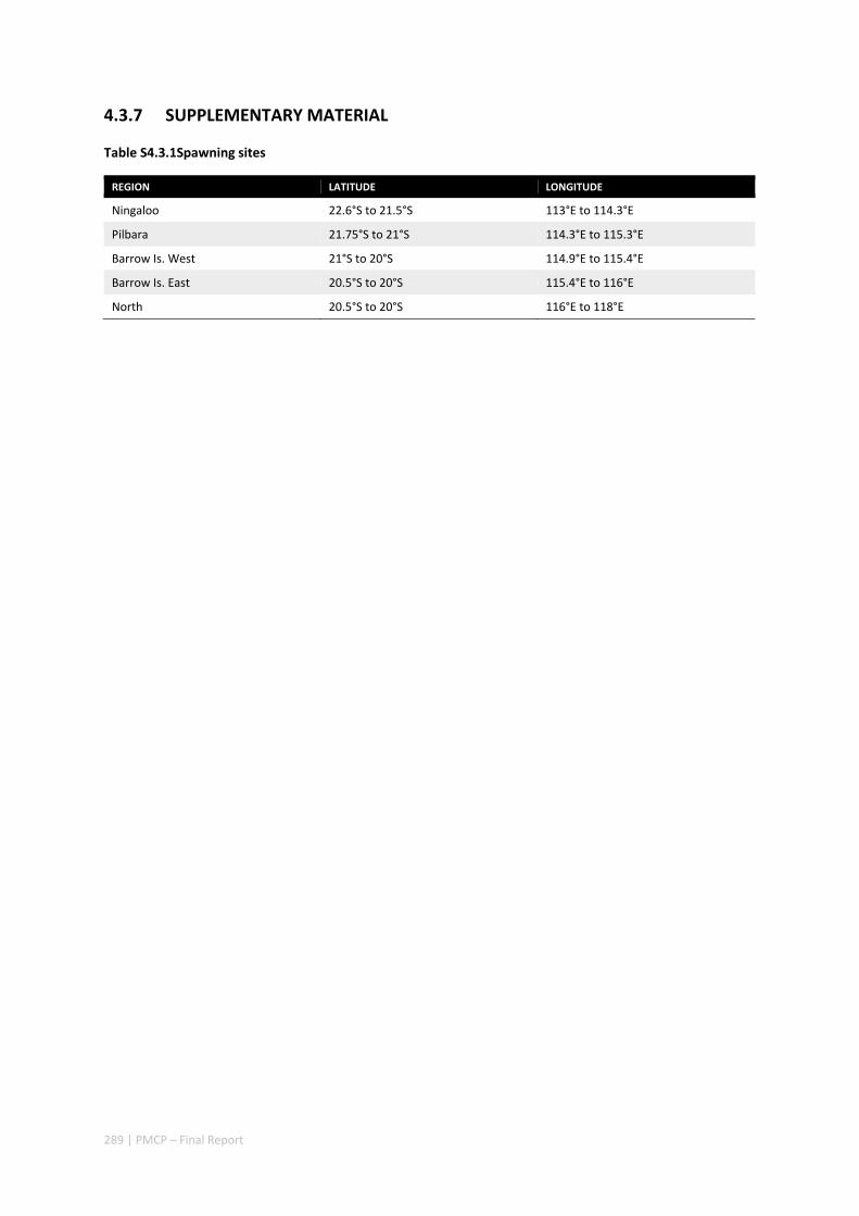
289 | PMCP – Final Report
4.3.7 SUPPLEMENTARY MATERIAL
Table S4.3.1Spawning sites
REGION LATITUDE LONGITUDE
Ningaloo 22.6°S to 21.5°S 113°E to 114.3°E
Pilbara 21.75°S to 21°S 114.3°E to 115.3°E
Barrow Is. West 21°S to 20°S 114.9°E to 115.4°E
Barrow Is. East 20.5°S to 20°S 115.4°E to 116°E
North 20.5°S to 20°S 116°E to 118°E
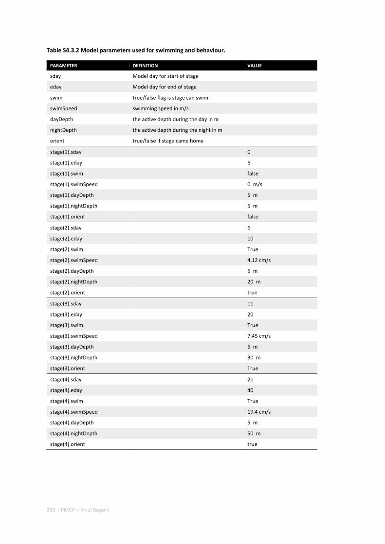
290 | PMCP – Final Report
Table S4.3.2 Model parameters used for swimming and behaviour.
PARAMETER DEFINITION VALUE
sday Model day for start of stage
eday Model day for end of stage
swim true/false flag is stage can swim
swimSpeed swimming speed in m/s
dayDepth the active depth during the day in m
nightDepth the active depth during the night in m
orient true/false if stage came home
stage(1).sday 0
stage(1).eday 5
stage(1).swim false
stage(1).swimSpeed 0 m/s
stage(1).dayDepth 5 m
stage(1).nightDepth 5 m
stage(1).orient false
stage(2).sday 6
stage(2).eday 10
stage(2).swim True
stage(2).swimSpeed 4.12 cm/s
stage(2).dayDepth 5 m
stage(2).nightDepth 20 m
stage(2).orient true
stage(3).sday 11
stage(3).eday 20
stage(3).swim True
stage(3).swimSpeed 7.45 cm/s
stage(3).dayDepth 5 m
stage(3).nightDepth 30 m
stage(3).orient True
stage(4).sday 21
stage(4).eday 40
stage(4).swim True
stage(4).swimSpeed 19.4 cm/s
stage(4).dayDepth 5 m
stage(4).nightDepth 50 m
stage(4).orient true
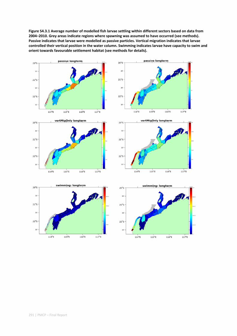
291 | PMCP – Final Report
Figure S4.3.1 Average number of modelled fish larvae settling within different sectors based on data from 2004–2010. Grey areas indicate regions where spawning was assumed to have occurred (see methods). Passive indicates that larvae were modelled as passive particles. Vertical migration indicates that larvae controlled their vertical position in the water column. Swimming indicates larvae have capacity to swim and orient towards favourable settlement habitat (see methods for details).
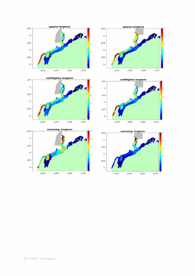
292 | PMCP – Final Report
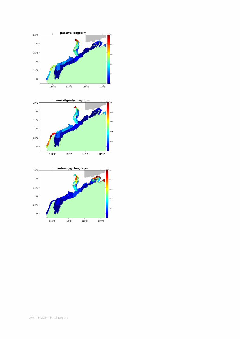
293 | PMCP – Final Report
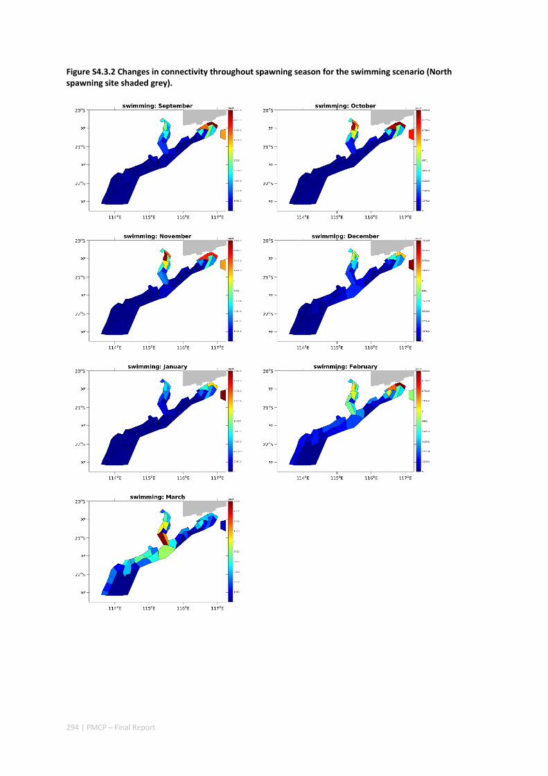
294 | PMCP – Final Report
Figure S4.3.2 Changes in connectivity throughout spawning season for the swimming scenario (North spawning site shaded grey).
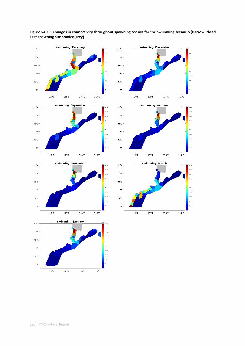
295 | PMCP – Final Report
Figure S4.3.3 Changes in connectivity throughout spawning season for the swimming scenario (Barrow Island East spawning site shaded grey).
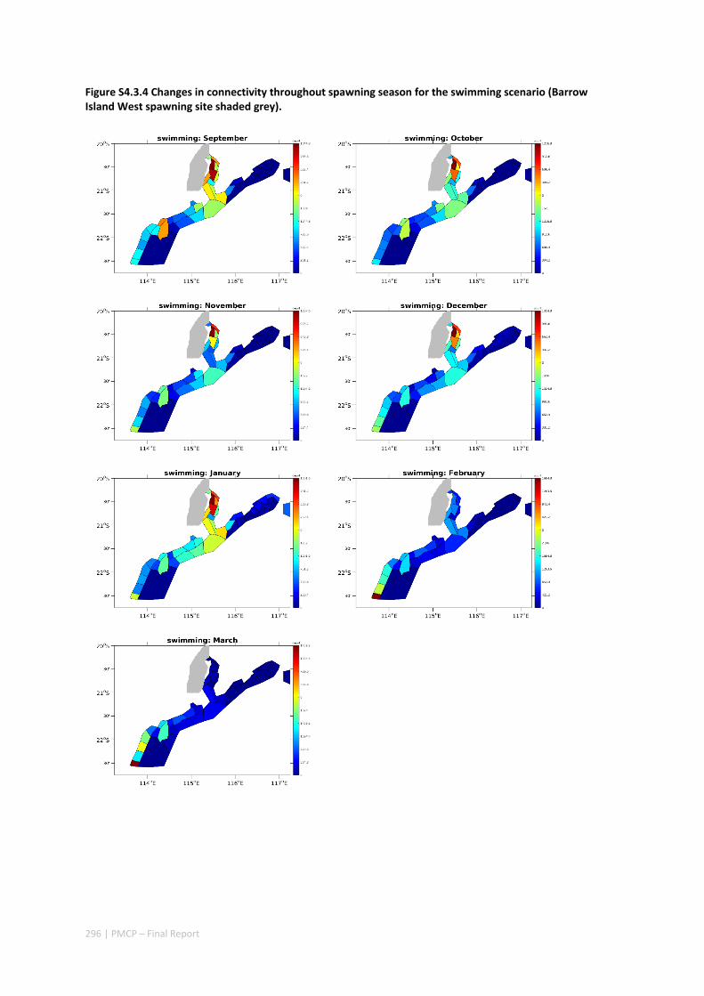
296 | PMCP – Final Report
Figure S4.3.4 Changes in connectivity throughout spawning season for the swimming scenario (Barrow Island West spawning site shaded grey).
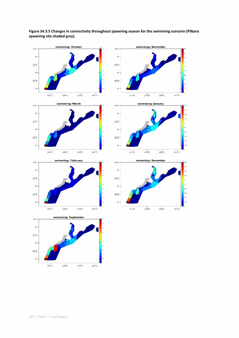
297 | PMCP – Final Report
Figure S4.3.5 Changes in connectivity throughout spawning season for the swimming scenario (Pilbara spawning site shaded grey).
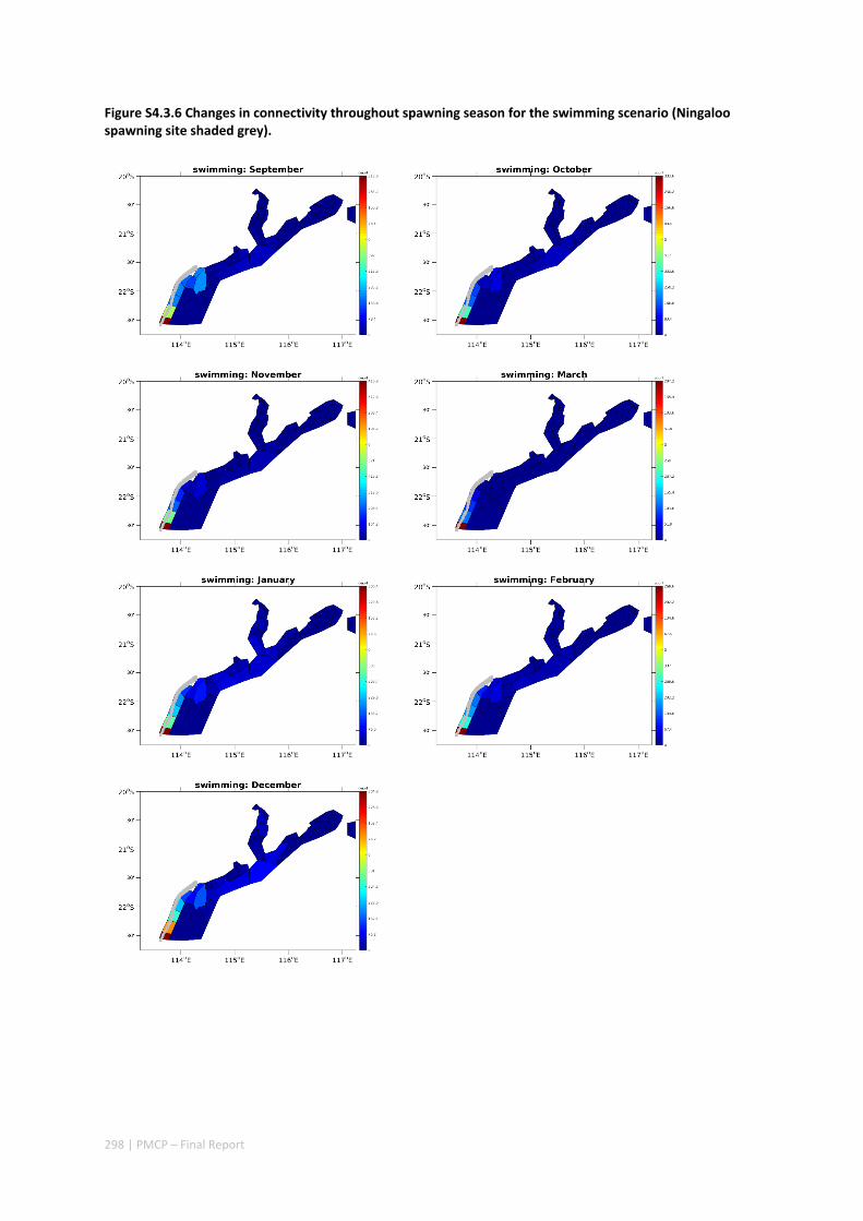
298 | PMCP – Final Report
Figure S4.3.6 Changes in connectivity throughout spawning season for the swimming scenario (Ningaloo spawning site shaded grey).
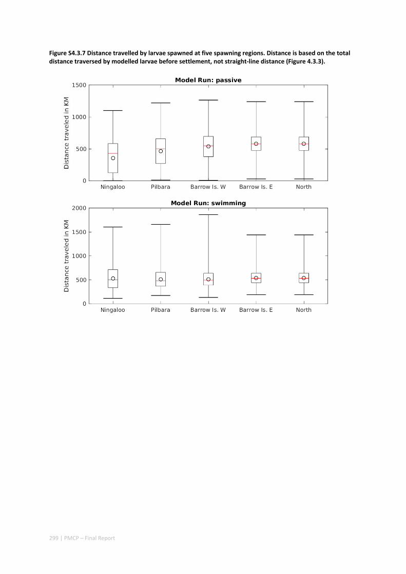
299 | PMCP – Final Report
Figure S4.3.7 Distance travelled by larvae spawned at five spawning regions. Distance is based on the total distance traversed by modelled larvae before settlement, not straight‐line distance (Figure 4.3.3).
300 | PMCP – Final Report
Intra‐annual variability of the North West Shelf of Australia and its impact on the Holloway Current: excitement and propagation of coastal Kelvin waves
Authors: Marin M, Feng M.
This work was conducted in partial fulfilment of the requirements for the degree of Master of Science at University Pierre and Marie Curie, France.
Abstract
Shelf circulation on the North West Shelf (NWS) of Australia is dominated by the seasonal variations of the Holloway Current, forced by the monsoonal winds. Strong inter‐annual and intra‐annual variations of sea levels, ocean temperatures, and alongshore current have been observed along NWS. Whereas the interannual variations of coastal currents have been well studied along the coast, the intra‐seasonal signals have yet to be evaluated. These intra‐seasonal variations of the coastal currents are important for the alongshore dispersal and cross‐shelf exchanges of nutrients and marine biota. Here, a combination of model outputs and 2 years of IMOS mooring time series data were used to analyse the intra‐annual variability of the shelf current on the NWS. Whereas the inter‐annual variability in the region is mostly forced remotely by tropical Pacific processes, the intra‐seasonal and semiannual signals are mostly driven by variations of regional winds off the northern coast of Australia. The Holloway Current, with a mean annual transport of ~1 Sv, is stronger during austral autumn but is less consistent during the rest of the year. The dominant intra‐annual variability of the alongshore current on the NWS were located at intra‐seasonal and semiannual frequencies. Bluelink ReANalysis (BRAN) sea level data revealed the existence of strong coastal sea level variability at both frequencies over the NWS of Australia. Moreover, the phase analysis of sea level anomalies indicated that the excitation and propagation of coastally trapped Kelvin waves are forced by Madden‐Julian Oscillations (MJO; intra‐seasonal) and semiannual wind anomalies. Intra‐seasonal Kelvin waves are excited over the eastern parts of the Kimberley shelf, whereas semiannual waves are generated further to the east, over the northern Australian coast. In both cases, strong alongshore wind anomalies drive cross‐shelf Ekman flows, inducing upwelling and downwelling near the coast, and exciting the propagation of coastally trapped Kelvin waves toward the south‐west. The Kelvin waves have a phase speed of ~1.9 m.s‐1 for both frequencies, characteristic of the first baroclinic mode. In addition to sea level anomalies, Kelvin waves also force velocity anomalies, as south‐westward/north‐eastward anomalies are associated with positive/negative anomalies in sea level. The fluctuations in the velocity field over the NWS translates into significant transport anomalies, ranging on average from ~0.3 Sv to ~0.4 Sv, for intra‐seasonal and semiannual frequency, respectively. South‐westward/north‐eastward intra‐seasonal transport anomalies peak during Phases 1 and 5 of the MJO on the Kimberley shelf, whereas the corresponding transport anomalies on the Pilbara shelf peak during Phases 3 and 7. Similar to intra‐seasonal transport anomalies, semiannual southwest‐ward/north‐eastward transport anomalies on the Kimberley shelf precede those in the Pilbara which peaks in April/January and then October/July on the Kimberley shelf and in May/February and then November/August on the Pilbara shelf. Therefore, the intra‐annual wind variability plays a major role in defining the highly variable state of the Holloway Current. Coral and fish larvae spawning may have been timed with the annual/semi‐annual variations of the coastal currents, but interrrupted by their intra‐seasonal variations.
301 | PMCP – Final Report
4.4.1 INTRODUCTION
Intra‐annual variability refers to processes which occur on a time scale of less than one year but more than one month, e.g. the semiannual variations and the intra‐seasonal oscillation. Intra‐annual variability in the oceans plays major roles in remotely or locally modifying marine environmental conditions which may in turn have potentially major impacts on regional climate and biological communities. An early study by Jacobs et al. (1992) demonstrated the extent of the spatial coverage of semiannual variability, observed all over the globe, with steric height anomalies exceeding 10 cm in various regions. The semiannual energy spectrum has also been found to be 3 times higher than the annual cycle in the Brazil-Malvinas current confluence region (Provost & Le Traon 1993). Intra‐seasonal variability of surface winds in the equatorial western Pacific generated eastward propagating Kelvin waves to influence temperature and circulation structures in the eastern Pacific and obscure the annual cycle (McPhaden & Taft 1988; Small et al. 2011). Anomalies of wind speed also excite westward propagation of Rossby waves which reflect on the Philippines coast as coastally trapped Kelvin waves, creating sea level anomalies of up to 3 cm (Chen et al. 2015). As datasets with better spatial coverage and temporal resolution are now being developed, it is important to study the intra‐annual variability thoroughly around the global oceans, especially in the coastal regions.
The NWS of Australia, is a place where the Indian and Pacific Ocean waters meet. It is divided into two specific shelf areas namely the Pilbara, extending west of North‐West Cape, and Kimberley shelves (Figure 4.4.1). NWS waters are one of the sources of the Leeuwin Current, the well‐studied Western Australian coastal current (D’Adamo et al. 2009), which is known to be an atypical poleward‐flowing eastern boundary current (Godfrey & Ridgway 1985), transporting warm tropical waters all the way to Southern Australia and Tasmania where it connects with the South Australia Current (Ridgway 2004). This anomalous flow is maintained by a strong meridional pressure gradient partly forced by intrusions of warm and low‐density Pacific waters through the Indonesian Islands (Godfrey & Ridgway 1985; D’Adamo et al. 2009), constituting the Indonesian Throughflow. The Leeuwin Current is also fed by warm tropical Indian Ocean waters (D’Adamo et al. 2009).
The Holloway Current (named by D’Adamo et al. 2009), is the seasonal, alongshore, south‐westward flow of water, which follows the north‐western coast of Australia (Holloway & Nye 1985; Cresswell et al. 1993; Kronberg 2004; Brink et al. 2007) and subsequently contributes to the Leeuwin Current. It is created by a rise in steric height along the north‐west Australian coast due to enhanced surface heating over the NWS and easing of monsoonal winds (Kronberg 2004), especially during late austral autumn (May–June). It is at this time that the Holloway Current is at its strongest, matching the Leeuwin Current maximum (Feng et al. 2003). Bahmanpour et al. (2016) used multi‐year mooring in‐situ current meter time series data to demonstrate that the Holloway Current flows south‐westward most of the year, with a mean transport of ~1 Sv, doubling during austral autumn. Rather than having a locally driven origin, the autumn intensification of the Holloway Current was found to be strongly related to the propagation of a coastally trapped Kelvin wave remotely forced by monsoonal winds over the Gulf of Carpentaria (GoC) (Ridgway & Godfrey 2015). Inter‐annual fluctuations of coastal currents in Western Australia are well correlated to El Nino/Southern Oscillation (ENSO) signals (Feng et al. 2003). The ENSO Pacific signal propagates poleward onto the Western Australia coast as a coastally trapped wave (Clarke & Liu 1994; Wijffels & Meyers 2004), consequently driving the inter‐annual variability of the Holloway Current.
Intra‐annual variability of shelf currents have also been observed on the NWS of Australia. Hidden behind intense meandering and eddy activity of the Leeuwin Current (Birol 1999; Birol & Morrow 2001), semiannual Rossby waves were observed from satellite altimeter data off the west coast of Australia, with a signature band situated between 150–180 days (Birol & Morrow 2001). Birol and Morrow (2003) further linked the genesis of those Rossby waves to baroclinic instabilities triggered by the interaction of the Leeuwin Current with a semiannual coastally trapped wave propagating

302 | PMCP – Final Report
from the NWS poleward along the Western Australian coast. The origin of such a semiannual coastal wave remains unknown. Potemra et al. (2002) identified strong semiannual signals in the straits between the Indonesian Sea and the eastern Indian Ocean and the signal was forced remotely from both the equatorial Indian Ocean, via the semiannual variations of the Wyrtki jets (Nagura & McPhaden 2010), and the equatorial Pacific (Qu et al. 2008). Still, it is not clear if the semiannual variability on the NWS of Australia is a response to this equatorial forcing.
The MJO (Madden & Julian 1971; Madden & Julian 1972) is the dominant mode of intra‐seasonal variability around the globe (Zhang 2005), especially in the tropical Indian and Pacific oceans. MJO are associated with zonal momentum flux and heat flux anomalies transferring into equatorial Rossby/Kelvin waves and sea surface temperature anomalies respectively, in both oceans (Hendon et al. 1998; Han et al. 2001; Fu 2007). Approaching the eastern Indian Ocean boundary, the equatorial Kelvin waves formed in the Indian Ocean become coastally trapped and propagate eastward following the south coast of Java and Sumatra (Zhou & Murtugudde 2010). Although a study by Webber et al. (2011) suggested that the coastally trapped waves would then transfer onto the north‐west coast of Australia and propagate poleward along the west coast of Australia, Marshall & Hendon (2014) hypothesise that intra‐seasonal variability in the Leeuwin Current is driven by wind and heat flux anomalies onto the NWS, piling up warm water onto the shelf and eventually generating a poleward propagating, coastally trapped wave. These intra‐seasonal variations of alongshore currents have been found to be important for the coral larval dispersal during their mass spawning events on the Pilbara shelf (Feng et al. 2016).
The present study aims at providing more insight on the dynamics of the intra‐annual variability of the ocean and atmospheric systems of the NWS of Australia and their influences on the Holloway Current at both semiannual and intra‐seasonal time scales. In particular, we seek to identify the origin of the semiannual signal observed in the Leeuwin Current, as well as evaluating the Marshall and Hendon (2014) theory on intra‐seasonal variability in Western Australia.
We primarily make use of two high resolution hydrodynamic models, namely the Regional Oceanic Modelling System (ROMS; Feng et al. 2016) applied to the Pilbara shelf and the Bluelink ReANalysis (BRAN; Oke et al. 2013), supported by in‐situ moorings data (from the Integrated Marine Observing System; IMOS) to quantify the intra‐annual variability modes and identify their origins. Gaining knowledge on the dynamics of the under‐studied Holloway Current is critical, as it is one of the main drivers of north‐west Australia’s ecosystem, and it also feeds into the Leeuwin Current, which is host to a unique marine ecosystem and biodiversity hotspot (Roberts et al. 2002).
4.4.2 METHODS
The BRAN is a multi‐year integration of a 1/10 degree horizontal resolution model with the BlueLink Ocean Data Assimilation System (BODAS; Oke et al. 2008), conducted from January 1993 to September 2012 (Oke et al. 2013). BRAN provides daily three dimensional outputs of temperature, salinity, and velocity (horizontal and vertical components), as well as sea level.
Observational data from the Australian Baseline Sea Level Monitoring Project run by the Australian Bureau of Meteorology (BoM) provided 15 years of hourly sea level data at the SEAFRAME Broome station (Figure 4.4.1), from 1991 to 2015. In addition, a European Centre for Medium‐Range Weather Forecasts (ECMWF) reanalysis of surface winds (ERA‐20C) was used to investigate the relationship between surface wind variability and the NWS variability. We also use observations from mooring arrays located on the Pilbara and Kimberley shelves (Figure 4.4.1). Those arrays are part of IMOS’s Australian national mooring network operated by the Australian Institute of Marine
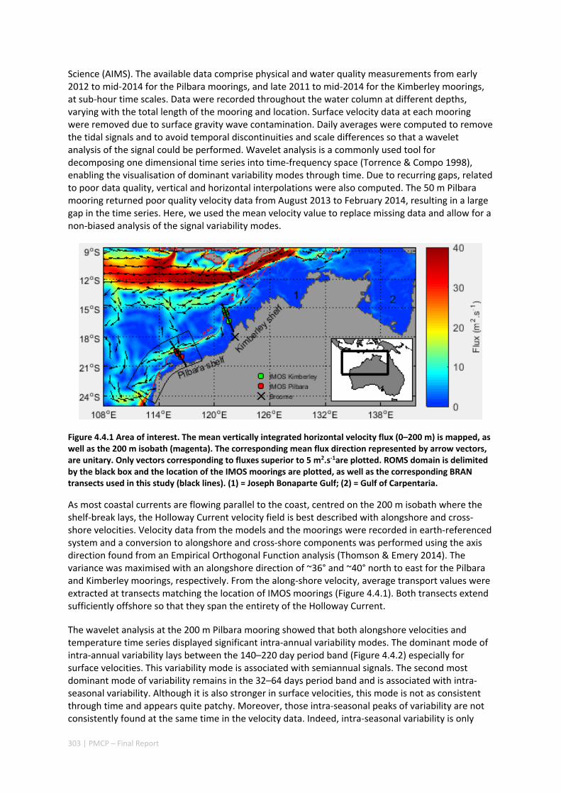
303 | PMCP – Final Report
Science (AIMS). The available data comprise physical and water quality measurements from early 2012 to mid‐2014 for the Pilbara moorings, and late 2011 to mid‐2014 for the Kimberley moorings, at sub‐hour time scales. Data were recorded throughout the water column at different depths, varying with the total length of the mooring and location. Surface velocity data at each mooring were removed due to surface gravity wave contamination. Daily averages were computed to remove the tidal signals and to avoid temporal discontinuities and scale differences so that a wavelet analysis of the signal could be performed. Wavelet analysis is a commonly used tool for decomposing one dimensional time series into time‐frequency space (Torrence & Compo 1998), enabling the visualisation of dominant variability modes through time. Due to recurring gaps, related to poor data quality, vertical and horizontal interpolations were also computed. The 50 m Pilbara mooring returned poor quality velocity data from August 2013 to February 2014, resulting in a large gap in the time series. Here, we used the mean velocity value to replace missing data and allow for a non‐biased analysis of the signal variability modes.
Figure 4.4.1 Area of interest. The mean vertically integrated horizontal velocity flux (0–200 m) is mapped, as well as the 200 m isobath (magenta). The corresponding mean flux direction represented by arrow vectors, are unitary. Only vectors corresponding to fluxes superior to 5 m2.s‐1are plotted. ROMS domain is delimited by the black box and the location of the IMOS moorings are plotted, as well as the corresponding BRAN transects used in this study (black lines). (1) = Joseph Bonaparte Gulf; (2) = Gulf of Carpentaria.
As most coastal currents are flowing parallel to the coast, centred on the 200 m isobath where the shelf‐break lays, the Holloway Current velocity field is best described with alongshore and cross‐shore velocities. Velocity data from the models and the moorings were recorded in earth‐referenced system and a conversion to alongshore and cross‐shore components was performed using the axis direction found from an Empirical Orthogonal Function analysis (Thomson & Emery 2014). The variance was maximised with an alongshore direction of ~36° and ~40° north to east for the Pilbara and Kimberley moorings, respectively. From the along‐shore velocity, average transport values were extracted at transects matching the location of IMOS moorings (Figure 4.4.1). Both transects extend sufficiently offshore so that they span the entirety of the Holloway Current.
The wavelet analysis at the 200 m Pilbara mooring showed that both alongshore velocities and temperature time series displayed significant intra‐annual variability modes. The dominant mode of intra‐annual variability lays between the 140–220 day period band (Figure 4.4.2) especially for surface velocities. This variability mode is associated with semiannual signals. The second most dominant mode of variability remains in the 32–64 days period band and is associated with intra‐seasonal variability. Although it is also stronger in surface velocities, this mode is not as consistent through time and appears quite patchy. Moreover, those intra‐seasonal peaks of variability are not consistently found at the same time in the velocity data. Indeed, intra‐seasonal variability is only
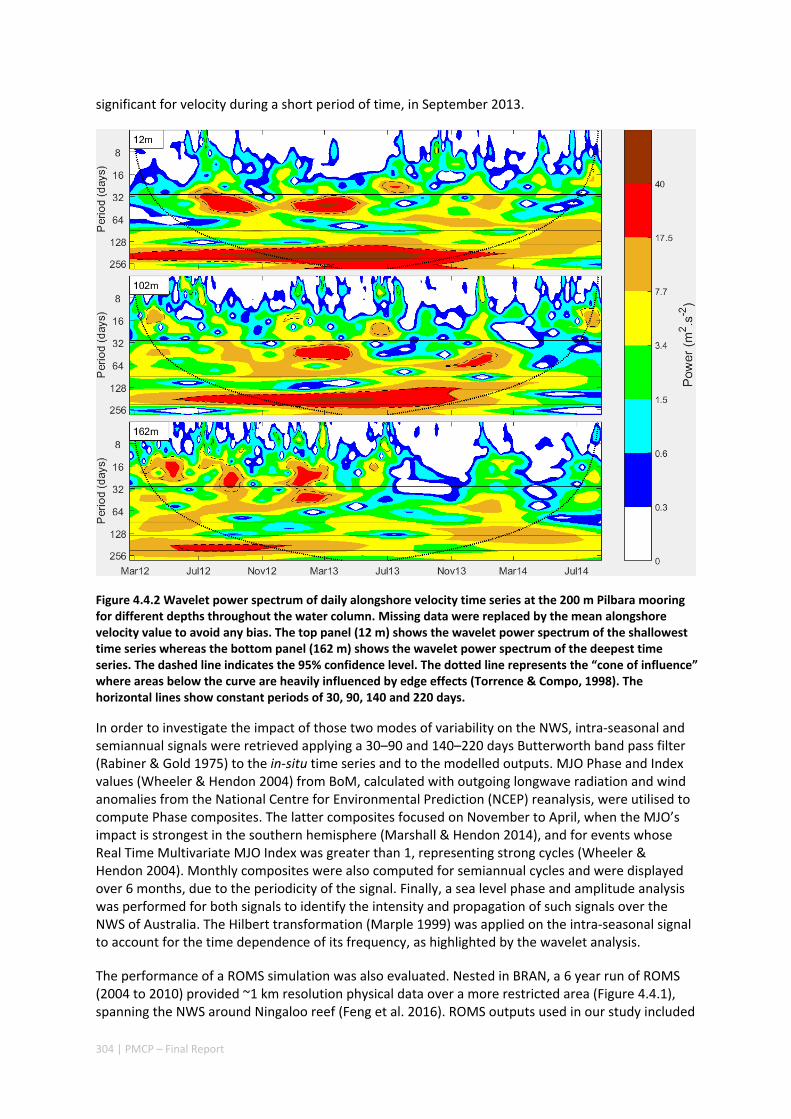
304 | PMCP – Final Report
significant for velocity during a short period of time, in September 2013.
Figure 4.4.2 Wavelet power spectrum of daily alongshore velocity time series at the 200 m Pilbara mooring for different depths throughout the water column. Missing data were replaced by the mean alongshore velocity value to avoid any bias. The top panel (12 m) shows the wavelet power spectrum of the shallowest time series whereas the bottom panel (162 m) shows the wavelet power spectrum of the deepest time series. The dashed line indicates the 95% confidence level. The dotted line represents the “cone of influence” where areas below the curve are heavily influenced by edge effects (Torrence & Compo, 1998). The horizontal lines show constant periods of 30, 90, 140 and 220 days.
In order to investigate the impact of those two modes of variability on the NWS, intra‐seasonal and semiannual signals were retrieved applying a 30–90 and 140–220 days Butterworth band pass filter (Rabiner & Gold 1975) to the in‐situ time series and to the modelled outputs. MJO Phase and Index values (Wheeler & Hendon 2004) from BoM, calculated with outgoing longwave radiation and wind anomalies from the National Centre for Environmental Prediction (NCEP) reanalysis, were utilised to compute Phase composites. The latter composites focused on November to April, when the MJO’s impact is strongest in the southern hemisphere (Marshall & Hendon 2014), and for events whose Real Time Multivariate MJO Index was greater than 1, representing strong cycles (Wheeler & Hendon 2004). Monthly composites were also computed for semiannual cycles and were displayed over 6 months, due to the periodicity of the signal. Finally, a sea level phase and amplitude analysis was performed for both signals to identify the intensity and propagation of such signals over the NWS of Australia. The Hilbert transformation (Marple 1999) was applied on the intra‐seasonal signal to account for the time dependence of its frequency, as highlighted by the wavelet analysis.
The performance of a ROMS simulation was also evaluated. Nested in BRAN, a 6 year run of ROMS (2004 to 2010) provided ~1 km resolution physical data over a more restricted area (Figure 4.4.1), spanning the NWS around Ningaloo reef (Feng et al. 2016). ROMS outputs used in our study included
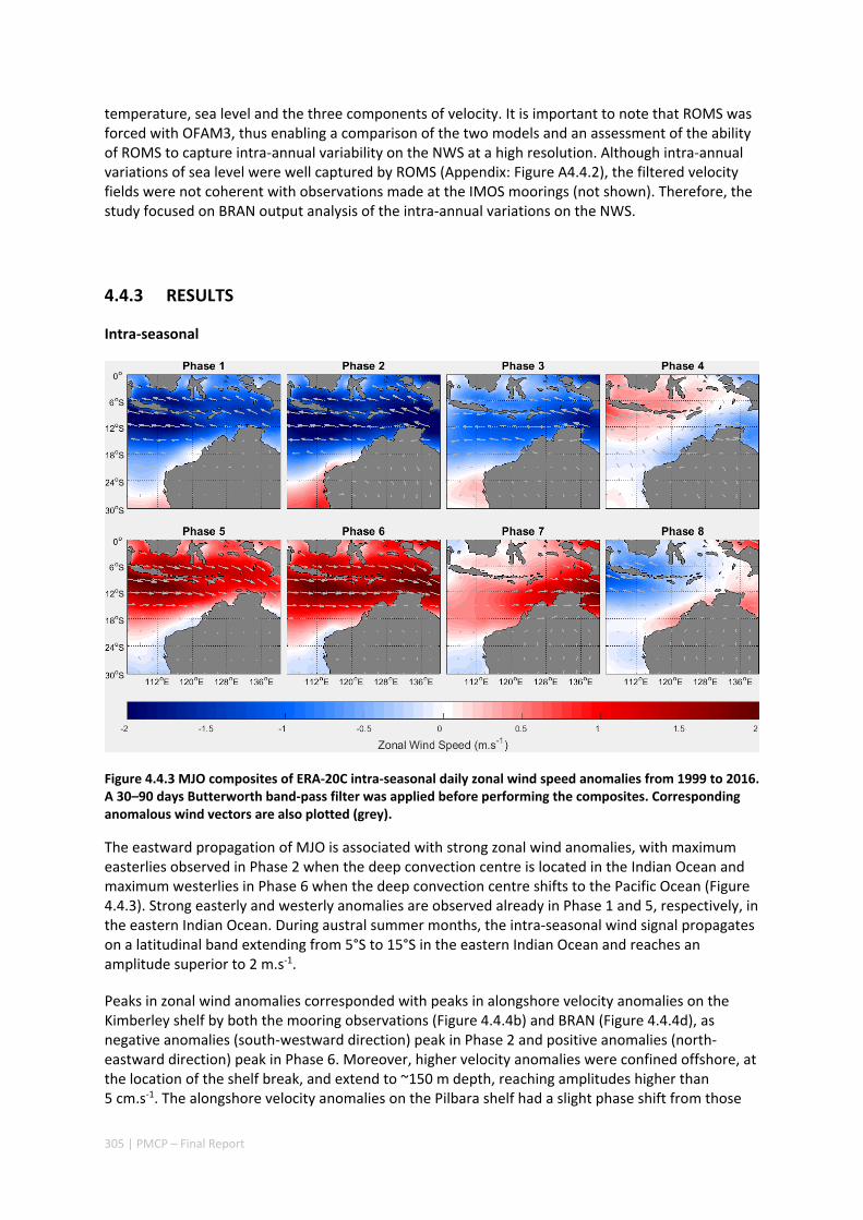
305 | PMCP – Final Report
temperature, sea level and the three components of velocity. It is important to note that ROMS was forced with OFAM3, thus enabling a comparison of the two models and an assessment of the ability of ROMS to capture intra‐annual variability on the NWS at a high resolution. Although intra‐annual variations of sea level were well captured by ROMS (Appendix: Figure A4.4.2), the filtered velocity fields were not coherent with observations made at the IMOS moorings (not shown). Therefore, the study focused on BRAN output analysis of the intra‐annual variations on the NWS.
4.4.3 RESULTS
Intra‐seasonal
Figure 4.4.3 MJO composites of ERA‐20C intra‐seasonal daily zonal wind speed anomalies from 1999 to 2016. A 30–90 days Butterworth band‐pass filter was applied before performing the composites. Corresponding anomalous wind vectors are also plotted (grey).
The eastward propagation of MJO is associated with strong zonal wind anomalies, with maximum easterlies observed in Phase 2 when the deep convection centre is located in the Indian Ocean and maximum westerlies in Phase 6 when the deep convection centre shifts to the Pacific Ocean (Figure 4.4.3). Strong easterly and westerly anomalies are observed already in Phase 1 and 5, respectively, in the eastern Indian Ocean. During austral summer months, the intra‐seasonal wind signal propagates on a latitudinal band extending from 5°S to 15°S in the eastern Indian Ocean and reaches an amplitude superior to 2 m.s‐1.
Peaks in zonal wind anomalies corresponded with peaks in alongshore velocity anomalies on the Kimberley shelf by both the mooring observations (Figure 4.4.4b) and BRAN (Figure 4.4.4d), as negative anomalies (south‐westward direction) peak in Phase 2 and positive anomalies (north‐eastward direction) peak in Phase 6. Moreover, higher velocity anomalies were confined offshore, at the location of the shelf break, and extend to ~150 m depth, reaching amplitudes higher than 5 cm.s‐1. The alongshore velocity anomalies on the Pilbara shelf had a slight phase shift from those
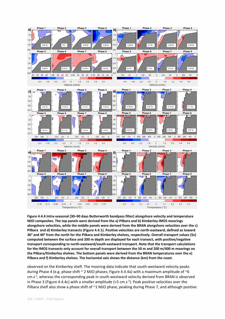
306 | PMCP – Final Report
Figure 4.4.4 Intra‐seasonal (30–90 days Butterworth bandpass filter) alongshore velocity and temperature MJO composites. The top panels were derived from the a) Pilbara and b) Kimberley IMOS moorings alongshore velocities, while the middle panels were derived from the BRAN alongshore velocities over the c) Pilbara and d) Kimberley transects (Figure 4.4.1). Positive velocities are north‐eastward, defined as toward 36o and 40o from the north for the Pilbara and Kimberley shelves, respectively. Overall transport values (Sv) computed between the surface and 200 m depth are displayed for each transect, with positive/negative transport corresponding to north‐eastward/south‐eastward transport. Note that the transport calculations for the IMOS transects only account for overall transport between the 50 m and 200 m/400 m moorings on the Pilbara/Kimberley shelves. The bottom panels were derived from the BRAN temperatures over the e) Pilbara and f) Kimberley shelves. The horizontal axis shows the distance (km) from the coast.
observed on the Kimberley shelf. The mooring data indicate that south‐westward velocity peaks during Phase 4 (e.g. phase shift ~ 2 MJO phases; Figure 4.4.4a) with a maximum amplitude of ~6 cm.s‐1, whereas the corresponding peak in south‐westward velocity derived from BRAN is observed in Phase 3 (Figure 4.4.4c) with a smaller amplitude (<5 cm.s‐1). Peak positive velocities over the Pilbara shelf also show a phase shift of ~1 MJO phase, peaking during Phase 7, and although positive
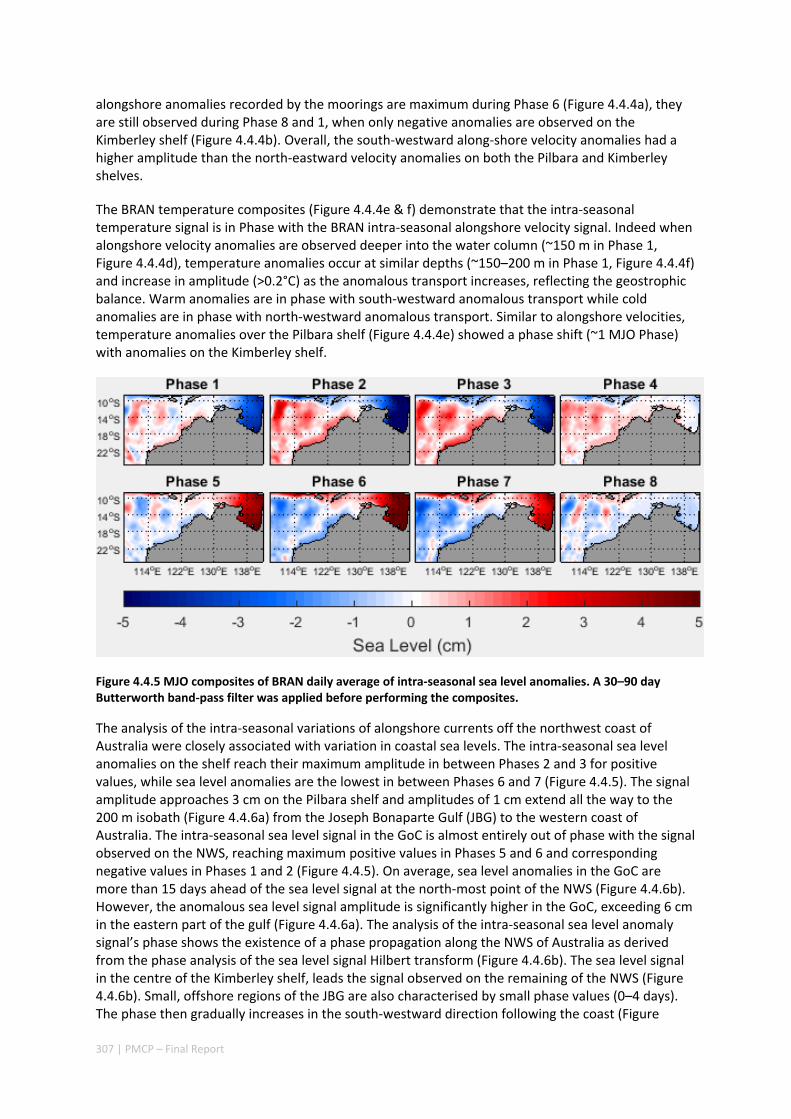
307 | PMCP – Final Report
alongshore anomalies recorded by the moorings are maximum during Phase 6 (Figure 4.4.4a), they are still observed during Phase 8 and 1, when only negative anomalies are observed on the Kimberley shelf (Figure 4.4.4b). Overall, the south‐westward along‐shore velocity anomalies had a higher amplitude than the north‐eastward velocity anomalies on both the Pilbara and Kimberley shelves.
The BRAN temperature composites (Figure 4.4.4e & f) demonstrate that the intra‐seasonal temperature signal is in Phase with the BRAN intra‐seasonal alongshore velocity signal. Indeed when alongshore velocity anomalies are observed deeper into the water column (~150 m in Phase 1, Figure 4.4.4d), temperature anomalies occur at similar depths (~150–200 m in Phase 1, Figure 4.4.4f) and increase in amplitude (>0.2°C) as the anomalous transport increases, reflecting the geostrophic balance. Warm anomalies are in phase with south‐westward anomalous transport while cold anomalies are in phase with north‐westward anomalous transport. Similar to alongshore velocities, temperature anomalies over the Pilbara shelf (Figure 4.4.4e) showed a phase shift (~1 MJO Phase) with anomalies on the Kimberley shelf.
Figure 4.4.5 MJO composites of BRAN daily average of intra‐seasonal sea level anomalies. A 30–90 day Butterworth band‐pass filter was applied before performing the composites.
The analysis of the intra‐seasonal variations of alongshore currents off the northwest coast of Australia were closely associated with variation in coastal sea levels. The intra‐seasonal sea level anomalies on the shelf reach their maximum amplitude in between Phases 2 and 3 for positive values, while sea level anomalies are the lowest in between Phases 6 and 7 (Figure 4.4.5). The signal amplitude approaches 3 cm on the Pilbara shelf and amplitudes of 1 cm extend all the way to the 200 m isobath (Figure 4.4.6a) from the Joseph Bonaparte Gulf (JBG) to the western coast of Australia. The intra‐seasonal sea level signal in the GoC is almost entirely out of phase with the signal observed on the NWS, reaching maximum positive values in Phases 5 and 6 and corresponding negative values in Phases 1 and 2 (Figure 4.4.5). On average, sea level anomalies in the GoC are more than 15 days ahead of the sea level signal at the north‐most point of the NWS (Figure 4.4.6b). However, the anomalous sea level signal amplitude is significantly higher in the GoC, exceeding 6 cm in the eastern part of the gulf (Figure 4.4.6a). The analysis of the intra‐seasonal sea level anomaly signal’s phase shows the existence of a phase propagation along the NWS of Australia as derived from the phase analysis of the sea level signal Hilbert transform (Figure 4.4.6b). The sea level signal in the centre of the Kimberley shelf, leads the signal observed on the remaining of the NWS (Figure 4.4.6b). Small, offshore regions of the JBG are also characterised by small phase values (0–4 days). The phase then gradually increases in the south‐westward direction following the coast (Figure

308 | PMCP – Final Report
4.4.6b) reaching 12 days into the MJO cycle at the western end of the Pilbara shelf. Note that a dramatic increase of the phase is observed from the JBG towards the GoC (Figure 4.4.6b). The sea level signal amplitudes simulated by BRAN, reflects the observed amplitude at Broome, even though the maximum values of sea level anomalies are observed during Phase 3 of the MJO (4.4.7a). This presents a slight phase shift with the results from BRAN, indicating a phase of 8 days into the MJO cycle, which corresponds to Phase 2 (Figure 4.4.6a).
Figure 4.4.6 Spatial structure of the intra‐seasonal cycle of BRAN sea level a) standard deviation and b) phase. The Phase was derived using the Hilbert transform to account for the changing frequency of MJO events. The average phase was computed using the mean period of intra‐seasonal cycles obtained from the transform (~43.7 days). Contour intervals are every 4 days (day 4 corresponding to the 4th day of an average MJO cycle). The 200 m isobath was plotted in black (a) and white (b).
As was observed at the moorings location, intra‐seasonal signals are also visible in the transport of South Java current in the eastern Indian Ocean (Figure 4.4.8a). Although the strongest anomalies in flux are located closer to the Indonesian coast, anomalies of 1.5 m2.s‐1 per 10 km grid are observed along the NWS of Australia, following the 200 m isobath (Figure 4.4.8a). Negative/positive (south‐westward/north‐westward) transport anomalies set from Phase 8–3/4–8 on the Kimberley shelf, peaking in Phase 1/5 (4.4.7a). A phase shift in the anomalous transport exists between the Kimberley and Pilbara shelves, corresponding to 1–2 MJO Phase, as negative transport anomalies on the Pilbara shelf only set in Phase 1 and positive anomalies in Phase 5, with delayed peaks in Phase 3 and 7 for negative and positive anomalies, respectively (4.4.7a). The maximum intra‐seasonal transport amplitude derived from BRAN is stronger on the Kimberley shelf, and of the order of ~0.35 Sv (4.4.7a), whereas transport on the Pilbara shelf peaks at ~0.3 Sv during the positive (positive sea level) phase and only ~0.2 Sv during the negative phase (4.4.7a).

309 | PMCP – Final Report
Figure 4.4.7 a) MJO composites of intra‐seasonal transport (black) over the Pilbara (solid) and Kimberley (dashed) shelves and Broome intra‐seasonal sea level transport anomalies (red). b) Monthly composites of semiannual transport (black) over the Pilbara (solid) and Kimberley (dashed) shelves and Broome semiannual sea level anomalies (red). 30–90 days and 140–220 days Butterworth filters were applied before performing the composites for intra‐seasonal and semiannual anomalies, respectively. The transport was calculated over the BRAN transects shown in Figure 4.4.1, from the surface to 200 m depth. Note the difference in axis scales for both frequencies.
Figure 4.4.8 Spatial structure of the a) intra‐seasonal and b) semiannual cycle of BRAN surface flux (0–50 m integration). 30–90 days and 140–220 days Butterworth bandpass filters were previously applied to velocity data for intra‐seasonal and semiannual cycles, respectively. The 200 m isobath was plotted in black.
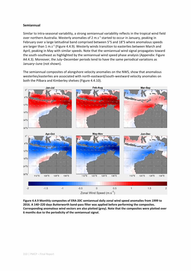
310 | PMCP – Final Report
Semiannual
Similar to intra‐seasonal variability, a strong semiannual variability reflects in the tropical wind field over northern Australia. Westerly anomalies of 2 m.s‐1 started to occur in January, peaking in February over a large latitudinal band comprised between 5°S and 18°S where anomalous speeds are larger than 1 m.s‐1 (Figure 4.4.9). Westerly winds transition to easterlies between March and April, peaking in May with similar speeds. Note that the semiannual wind signal propagates toward the south‐southeast as highlighted by the semiannual wind speed phase analysis (Appendix: Figure A4.4.3). Moreover, the July–December periods tend to have the same periodical variations as January–June (not shown).
The semiannual composites of alongshore velocity anomalies on the NWS, show that anomalous westerlies/easterlies are associated with north‐eastward/south‐westward velocity anomalies on both the Pilbara and Kimberley shelves (Figure 4.4.10).
Figure 4.4.9 Monthly composites of ERA‐20C semiannual daily zonal wind speed anomalies from 1999 to 2016. A 140–220 days Butterworth band‐pass filter was applied before performing the composites. Corresponding anomalous wind vectors are also plotted (grey). Note that the composites were plotted over 6 months due to the periodicity of the semiannual signal.

311 | PMCP – Final Report
Figure 4.4.10 Semiannual (140–220 days Butterworth bandpass filter) alongshore velocity and temperature monthly composites. The top panels were derived from the a) Pilbara and b) Kimberley IMOS moorings alongshore velocities, while the middle panels were derived from the BRAN alongshore velocities over the c) Pilbara and d) Kimberley transects (Figure 4.4.1). Positive velocities toward 36o and 40o north to east for the Pilbara and Kimberley shelves, respectively. Overall transport values (Sv) computed between the surface and 200 m depth are displayed for each transect, with positive/negative transport corresponding to north‐eastward/south‐eastward transport. Note that the transport calculations for the IMOS transects only account for overall transport between the 50 m and 200 m/400 m moorings on the Pilbara/Kimberley shelf. The bottom panels were derived from the BRAN temperatures over the e) Pilbara and f) Kimberley shelves. The horizontal axis shows the distance (km) from the coast.
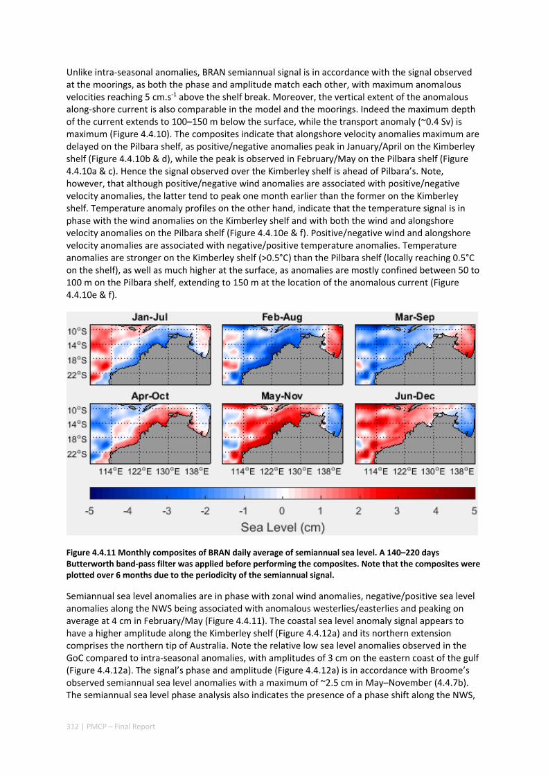
312 | PMCP – Final Report
Unlike intra‐seasonal anomalies, BRAN semiannual signal is in accordance with the signal observed at the moorings, as both the phase and amplitude match each other, with maximum anomalous velocities reaching 5 cm.s‐1 above the shelf break. Moreover, the vertical extent of the anomalous along‐shore current is also comparable in the model and the moorings. Indeed the maximum depth of the current extends to 100–150 m below the surface, while the transport anomaly (~0.4 Sv) is maximum (Figure 4.4.10). The composites indicate that alongshore velocity anomalies maximum are delayed on the Pilbara shelf, as positive/negative anomalies peak in January/April on the Kimberley shelf (Figure 4.4.10b & d), while the peak is observed in February/May on the Pilbara shelf (Figure 4.4.10a & c). Hence the signal observed over the Kimberley shelf is ahead of Pilbara’s. Note, however, that although positive/negative wind anomalies are associated with positive/negative velocity anomalies, the latter tend to peak one month earlier than the former on the Kimberley shelf. Temperature anomaly profiles on the other hand, indicate that the temperature signal is in phase with the wind anomalies on the Kimberley shelf and with both the wind and alongshore velocity anomalies on the Pilbara shelf (Figure 4.4.10e & f). Positive/negative wind and alongshore velocity anomalies are associated with negative/positive temperature anomalies. Temperature anomalies are stronger on the Kimberley shelf (>0.5°C) than the Pilbara shelf (locally reaching 0.5°C on the shelf), as well as much higher at the surface, as anomalies are mostly confined between 50 to 100 m on the Pilbara shelf, extending to 150 m at the location of the anomalous current (Figure 4.4.10e & f).
Figure 4.4.11 Monthly composites of BRAN daily average of semiannual sea level. A 140–220 days Butterworth band‐pass filter was applied before performing the composites. Note that the composites were plotted over 6 months due to the periodicity of the semiannual signal.
Semiannual sea level anomalies are in phase with zonal wind anomalies, negative/positive sea level anomalies along the NWS being associated with anomalous westerlies/easterlies and peaking on average at 4 cm in February/May (Figure 4.4.11). The coastal sea level anomaly signal appears to have a higher amplitude along the Kimberley shelf (Figure 4.4.12a) and its northern extension comprises the northern tip of Australia. Note the relative low sea level anomalies observed in the GoC compared to intra‐seasonal anomalies, with amplitudes of 3 cm on the eastern coast of the gulf (Figure 4.4.12a). The signal’s phase and amplitude (Figure 4.4.12a) is in accordance with Broome’s observed semiannual sea level anomalies with a maximum of ~2.5 cm in May–November (4.4.7b). The semiannual sea level phase analysis also indicates the presence of a phase shift along the NWS,
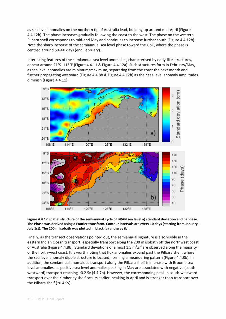
313 | PMCP – Final Report
as sea level anomalies on the northern tip of Australia lead, building up around mid‐April (Figure 4.4.12b). The phase increases gradually following the coast to the west. The phase on the western Pilbara shelf corresponds to mid‐end May and continues to increase further south (Figure 4.4.12b). Note the sharp increase of the semiannual sea level phase toward the GoC, where the phase is centred around 50–60 days (end February).
Interesting features of the semiannual sea level anomalies, characterised by eddy‐like structures, appear around 21°S–113°E (Figure 4.4.11 & Figure 4.4.12a). Such structures form in February/May, as sea level anomalies are minimum/maximum, separating from the coast the next month and further propagating westward (Figure 4.4.8b & Figure 4.4.12b) as their sea level anomaly amplitudes diminish (Figure 4.4.11).
Figure 4.4.12 Spatial structure of the semiannual cycle of BRAN sea level a) standard deviation and b) phase. The Phase was derived using a Fourier transform. Contour intervals are every 10 days (starting from January–July 1st). The 200 m isobath was plotted in black (a) and grey (b).
Finally, as the transect observations pointed out, the semiannual signature is also visible in the eastern Indian Ocean transport, especially transport along the 200 m isobath off the northwest coast of Australia (Figure 4.4.8b). Standard deviations of almost 1.5 m2.s‐1 are observed along the majority of the north‐west coast. It is worth noting that flux anomalies expand past the Pilbara shelf, where the sea level anomaly dipole structure is located, forming a meandering pattern (Figure 4.4.8b). In addition, the semiannual anomalous transport along the Pilbara shelf is in phase with Broome sea level anomalies, as positive sea level anomalies peaking in May are associated with negative (south‐westward) transport reaching ~0.2 Sv (4.4.7b). However, the corresponding peak in south‐westward transport over the Kimberley shelf occurs earlier, peaking in April and is stronger than transport over the Pilbara shelf (~0.4 Sv).
314 | PMCP – Final Report
4.4.4 Discussion
Coastal wave genesis and propagation
INTRA‐SEASONAL
The phase analysis of intra‐seasonal sea level anomalies indicate that a coastal phase propagation exists. Sea level anomalies associated with MJO first appear on the Kimberley shelf and parts of the JBG at the beginning of a MJO cycle. There was an absence of a coherent phase propagation from the Indonesian coast onto the Australian coast, as suggested by Webber et al. (2011). In addition, a lag correlation analysis between the intra‐seasonal sea level anomalies on the Pilbara shelf and the zonal wind anomalies (Appendix Figure A4.4.3a) also demonstrates that intra‐seasonal sea level variations are best correlated with zonal wind stress over northern Australia, and especially along the JBG and Kimberley shelf. Those results contradict Oliver & Thompson's (2011) hypothesis that intra‐seasonal variability over the NWS of Australia and the GoC originates from the Pacific Ocean. Note, however, that the GoC sea level, being almost entirely out of phase with the NWS, suggests that Oliver & Thompson’s (2011) theory may still apply for intra‐seasonal variability in the GoC itself.
Reinforcement of the easterlies in Phase 2 increases the spatial extent of sea level anomalies, spreading over the entire NWS. However, the sea level anomalies were “trapped” in the coastal waveguide. The phase speed along the north‐west coast is estimated to ~1.9 m.s‐1. This finding is consistent with the propagation speed found by Marshall & Hendon (2014) and corresponds to the typical speed of the first baroclinic Kelvin wave mode (Brink 1982). Our results tend to confirm the Marshall & Hendon (2014) theory that intra‐seasonal sea level coastal waves originating from the NWS, are forced by a wind‐driven Ekman flow associated with anomalous heat fluxes, and propagate along the western coast of Australia.
SEMIANNUAL
The analysis of semiannual sea level anomalies also shows a phase propagation along the north‐west coast of Australia. Considering only regions with standard deviations of the semiannual sea level exceeding 2 cm, peak anomalies are observed along the northern Australian coast (12oS–132oE) and in the JBG, around day 120 (e.g. late‐April/early‐May). Similar to intra‐seasonal cycles, semiannual northern Australia sea level anomalies are in phase with the onset of strong semiannual easterlies in the Arafura Sea, suggesting that positive coastal sea level anomalies are generated through wind‐driven Ekman advection onto the northern Australian coast and in the JBG. The shelf‐restricted phase shift along the north‐west coast demonstrate, once again, the generation and south‐westward propagation of a coastally trapped wave. The phase speed is also estimated to be ~1.9m.s‐1, indicating the domination of the first baroclinic mode (Brink, 1982).
A strong annual pulse of sea level was shown to originate from the GoC, driven by the local wind‐driven advection of water into the gulf and as the wind relaxed, the pulse would translate into a coastal wave travelling counter‐clockwise around Australia (Ridgway & Godfrey 2015). In the case of semiannual cycles, the sea level signal in the GoC leads the NWS signal. However, rather than progressively building‐up, the sea level signal phase propagates into the GoC from Papua at the end of January and rotates slowly in the gulf around an “amphridomic” point at 9oS 136oE. This point corresponds to the location of strongest eastward, semiannual wind anomalies (not shown) in January, switching to south‐east in February. As the wind anomalies rotate on a semiannual frequency, we suggest that the semiannual sea level cycles in the GoC are driven by the local wind forcing. The discontinuity of amplitude and slow phase changes suggest that the onset of the coastally trapped Kelvin waves on the northern Australian coast may not be related to the propagation of sea level within the GoC.
315 | PMCP – Final Report
The offshore sea level signal south of 20oS and west of 114oE appear to propagate westward at a much slower speed than the speed observed on the coast. The sea level anomaly propagation observed at 23oS, radiating away from the coast in phase with the coastal sea level signal, has an approximate speed of ~7 cm.s‐1. This phase speed correspond to the phase speed of Rossby waves at similar latitudes (Chelton & Schlax 1996) and confirms the excitation of semiannual Rossby waves by a semiannual coastally trapped wave travelling along the western coast of Australia (Birol & Morrow 2003).
Impact on the Holloway Current
The propagation of the coastally trapped Kelvin waves along the NWS has noticeable impacts on the alongshore Holloway Current. Kelvin waves mainly affect alongshore current variability. A downwelling (positive sea level) wave will create a difference in the pressure gradient, and associated geostrophic velocities, keeping higher pressures on the left in the Southern Hemisphere. In the case of the Holloway Current, a downwelling Kelvin wave will force south‐westward velocity anomalies and therefore intensify its transport. On the contrary, upwelling (negative sea level anomalies) Kelvin waves are associated with north‐westward anomalies and therefore, weaken the Holloway Current strength. The impact of both polarities of intra‐annual variability on the current’s transport over the Pilbara shelf was found to be relatively similar, ranging from 0.2 to 0.4 Sv at peak amplitude. Bahmanpour et al. (2016) estimated the mean annual transport of the Holloway Current on the Pilbara shelf to be ~1 Sv, peaking at ~2 Sv during austral autumn. Although the authors used transects extending only to the 300 m isobath, which covers a smaller distance than transects used here, intra‐annual variations in transport are significant. In fact, the annual component of sea level over the NWS was estimated at ~6 cm (Ridgway & Godfrey 2015) which is comparable with the intra‐seasonal (~2 cm) and semiannual (~3.5 cm) components of sea level over the shelf. We hypothesise that a strong upwelling favourable MJO event combined to a negative phase of a semiannual event (January/July to March/September) could almost entirely dampen the strength of the Holloway Current, as observed during summer and winter months (Bahmanpour et al. 2016).
Model Assessment
An indirect application of the above work focuses on the ability of BRAN to capture intra‐annual variability. Overall, both modes of variability are apparent in the dynamics simulated by BRAN, as values of current velocities and overall transport of the NWS match those observed by the moorings (Figure 4.4.4 and Figure 4.4.10). Although the semiannual sea level signal from BRAN and the moorings are in phase, the intra‐seasonal signal phase is different, as the phase described by the moorings lags the phase captured by BRAN (Figure 4.4.4). Such difference can be explained by the relatively short time‐length of the moorings data. Indeed, each mooring time series did not span more than 3 years of data, whereas BRAN outputs were derived from a ~20 years run. While the impact is minimised for the study of the highly periodical and consistent semiannual signal, it is of greater importance when focusing on the MJO, as its frequency and intensity constantly oscillate (Wheeler & Hendon 2004) in a manner that is still not well understood (Waliser 2006). Hence, the average frequency and strength of MJO events captured by the moorings between 2012 and 2014 are likely to differ from the mean state of MJO events over the 20 years spanned by BRAN.
Despite showing coherent sea level fluctuations on both intra‐annual scales, which is expected as it was forced by BRAN on the open boundaries, ROMS simulates weak intra‐annual currents (not shown). Although ROMS simulation of the semiannual signal is coherent, it has more difficulties capturing the phase of the intra‐annual variability. The lack of coherence can be an open boundary condition issue, which do not fully capture the remote influences (Feng et al. 2016). Both signals are generated by remote winds over the Arafura Sea and off the Kimberley coast for semiannual and intra‐seasonal variability, respectively. It is necessary to improve the open boundary conditions in
316 | PMCP – Final Report
the model, so that small scale processes and eddy activity induced by the intra‐annual processes can be better assessed (Feng et al. 2016), due to the complexity of the North‐West Cape topography and dynamics (Xu et al. 2013).
Summary
In this study, IMOS mooring observations and the BRAN reanalysis products were used to reveal the presence of semiannual and intra‐seasonal variability of coastal sea levels, ocean temperatures, and alongshore shelf currents on the NWS of Australia. These intra‐annual variabilities were in phase with alongshore wind anomalies. Anomalous westerlies were associated with negative sea level anomalies, cool subsurface temperature anomalies, and geostrophically balanced south‐westward shelf current over the NWS. In contrast, anomalous easterlies were associated with positive sea level anomalies, warm subsurface temperature anomalies, and geostrophically balanced north‐eastward shelf current. Sea level signals revealed the existence of a south‐westward phase propagation of intra‐annual anomalies along the NWS. Coastally trapped Kelvin waves were generated from the eastern end of the Kimberley shelf and the JBG, driven by MJO wind anomalies, and semiannual waves were generated further east, on the northern coast of Australia, driven by a strong semiannual wind signal in the Arafura Sea. Both signals propagated south‐westward along the shelf with a characteristic speed of ~1.9 m s‐1. The Kelvin waves further propagated to the west coast of Australia, influencing the poleward flowing Leeuwin Current, and on semiannual frequencies, forcing the westward propagation of Rossby waves into the Indian Ocean. The Holloway Current alongshore transport is under the strong influence of the intra‐annual Kelvin waves. With an average south‐westward annual transport of ~1 Sv, the Holloway Current transport fluctuates on intra‐seasonal and semiannual frequencies of ~0.3 and ~0.4 Sv, respectively.
4.4.5 ACKNOWLEDGEMENT
I would like to thank CSIRO for hosting me and providing the necessary tools for the completion of this study. I am also grateful of the CSIRO scientific community for their overwhelming welcome and support throughout my stay. I would also like to thank UPMC and the OACOS master responsible team for allowing the opportunity to travel to Australia. Finally, I am thankful to the French ministry of Superior Education (Ministère de l’Enseignement Supérieur) for their financial support.
This research was financially supported as part of the Pilbara Marine Conservation Partnership funded by the Gorgon Barrow Island Net Conservation Benefits Fund which is administered by the WA Department of Biodiversity, Conservation and Attractions (DBCA).
4.4.6 REFERENCES
Bahmanpour MH, Pattiaratchi C, Wijeratne EMS, Steinberg C, & D'Adamo N (2016) Multi‐Year Observation of Holloway Current along the Shelf Edge of North Western Australia. Journal of Coastal Research, 75(10 m):517–521.
Birol F (1999) Mecanismes de frocage dans l’ocean Indien sud‐est et etude de la reponse oceanique.University of Toulouse.
Birol F & Morrow R (2003) Separation of quasi‐semiannual Rossby waves from the eastern boundary
317 | PMCP – Final Report
of the Indian Ocean. Journal of Marine Research 61(6):707–723.
Birol F & Morrow R (2001) Source of the baroclinic waves in the southeast Indian Ocean. Journal of Geophysical Research: Oceans 106(C5):9145–9160. Available at: http://dx.doi.org/10.1029/2000JC900044.
Brink KH (1982) A comparison of long coastal trapped wave theory with observations off Peru. Journal of Physical Oceanography 12(8):897–913.
Brink KH, Bahr F & Shearman RK (2007) Alongshore currents and mesoscale variability near the shelf edge off northwestern Australia. Journal of Geophysical Research: Oceans 112(5):1–19.
Chelton DB & Schlax MG (1996) Global Observations of Oceanic Rossby Waves. Science 272(5259):234–238. Available at: http://science.sciencemag.org/content/272/5259/234.
Chen X, Qiu B, Cheng X, Qi Y & Du Y (2015) Intra‐seasonal variability of Pacific‐origin sea level anomalies around the Philippine Archipelago. Journal of Oceanography 71(3):239–249. Available at: http://dx.doi.org/10.1007/s10872‐015‐0281‐9.
Clarke AJ & Liu X (1994) Interannual Sea Level in the Northern and Eastern Indian Ocean. Journal of Physical Oceanography 24(6):1224–1235. Available at: http://dx.doi.org/10.1175/1520‐0485(1994)024<1224:ISLITN>2.0.CO.
Cresswell G, Frische A, Peterson J & Quadfasel D (1993) Circulation in the Timor Sea. Journal of Geophysical Research: Oceans 98(C8):14379–14389. Available at: http://dx.doi.org/10.1029/93JC00317.
D’Adamo N, Fandry C, Buchan S & Domingues C (2009) Northern sources of the Leeuwin Current and the “Holloway Current” on the North West Shelf. Journal of the Royal Society of Western Australia 92(2):53–66.
Feng M, Meyers G, Pearce A & Wijffels S (2003) Annual and interannual variations of the Leeuwin Current at 32°S. Journal of Geophysical Research 108(C11).
Feng M, Colberg F, Slawinski D, Berry O & Babcock R (2016) Ocean circulation drives heterogeneous recruitments and connectivity among coral populations on the North West Shelf of Australia. Journal of Marine Systems 164:1–12.
Fu L‐L (2007) Intraseasonal variability of the Equatorial Indian Ocean observed from sea surface height, wind, and temperature data. Journal of Physical Oceanography 37(2):188–202. Available at: http://dx.doi.org/10.1175/JPO3006.1.
Godfrey JS & Ridgway KR (1985) The large‐scale environment of the poleward‐flowing Leeuwin Current, Western Australia: longshore steric height gradients, wind stresses and geostrophic flow. Journal of Physical Oceanography 15(5):481–495. Available at: http://dx.doi.org/10.1175/1520‐0485(1985)015<0481:TLSEOT>2.0.CO.
Han W, Lawrence DM & Webster PJ (2001) Dynamical response of equatorial Indian Ocean to intraseasonal winds: zonal flow. Geophysical Research Letters 28(22):4215–4218. Available at: http://doi.wiley.com/10.1029/2001GL013701 (Accessed September 5, 2016).
Hendon HH, Liebmann B & Glick JD (1998). Oceanic Kelvin Waves and the Madden–Julian Oscillation. Journal of the Atmospheric Sciences 55(1):88–101. Available at:
318 | PMCP – Final Report
http://dx.doi.org/10.1175/1520‐0469(1998)055<0088:OKWATM>2.0.CO.
Holloway PE & Nye HC (1985) Leeuwin Current and wind distributions on the southern part of the Australian North West Shelf between January 1982 and July 1983. Marine and Freshwater Research 36(2):123–137. Available at: http://dx.doi.org/10.1071/MF9850123.
Jacobs GA, Born GH, Parke MD & Allen PC (1992) The global structure of the annual and semiannual sea surface height variability from Geosat altimeter data. Journal of Geophysical Research: Oceans 97(C11):17813–17828. Available at: http://doi.wiley.com/10.1029/92JC01708 (Accessed July 28, 2016).
Kronberg M (2004) Ocean circulation over the North West Shelf of Australia – Does it impact on the Leeuwin Current? University of Copenhagen, Denmark.
Madden RA & Julian PR (1971) Detection of a 40–50 Day Oscillation in the Zonal Wind in the Tropical Pacific. Journal of the Atmospheric Sciences 28(5):702–708. Available at: http://dx.doi.org/10.1175/1520‐0469(1971)028<0702:DOADOI>2.0.CO\n2.
Madden RA & Julian PR (1972) Description of global‐scale circulation cells in the tropics with a 40–50 day period. Journal of the Atmospheric Sciences 29(6):1109–1123.
Marple L (1999) Computing the discrete‐time “analytic” signal via FFT. IEEE Transactions on Signal Processing 47(9):2600–2603.
Marshall AG & Hendon HH (2014) Impacts of the MJO in the Indian Ocean and on the Western Australian coast. Climate Dynamics 42(3–4):579–595.
McPhaden MJ & Taft BA (1988) Dynamics of seasonal and intraseasonal variability in the eastern Equatorial Pacific. Journal of Physical Oceanography 18(11):1713–1732. Available at: http://dx.doi.org/10.1175/1520‐0485(1988)018<1713:DOSAIV>2.0.CO.
Nagura M & McPhaden MJ (2010) Wyrtki Jet dynamics: seasonal variability. Journal of Geophysical Research 115(C7):C07009. Available at: http://doi.wiley.com/10.1029/2009JC005922 (Accessed July 27, 2016).
Oke PR, Griffin DA, Schiller A, Matear RJ, Fiedler R, Mansbridge J, Lenton A, Cahill M, Chamberlain MA & Ridgway K (2013) Evaluation of a near‐global eddy‐resolving ocean model. Geoscientific Model Development 6(3):591–615. Available at: http://www.geosci‐model‐dev.net/6/591/2013/.
Oke P, Brassington GB, Griffin DA, Schiller A (2008) The Bluelink ocean data assimilation system (BODAS). Ocean Modelling 21(1):46–70.
Oliver ECJ & Thompson KR (2011) Sea level and circulation variability of the Gulf of Carpentaria: Influence of the Madden‐Julian Oscillation and the adjacent deep ocean. Journal of Geophysical Research: Oceans 116(2):C02019. Available at: http://doi.wiley.com/10.1029/2010JC006596 (Accessed August 11, 2016).
Potemra JT, Hautala SL, Sprintall J & Pandoe W (2002) Interaction between the Indonesian Seas and the Indian Ocean in Observations and Numerical Models*. Journal of Physical Oceanography 32(6):1838–1854.
Provost C & Le Traon P‐Y (1993) Spatial and temporal scales in altimetric variability in the Brazil‐
319 | PMCP – Final Report
Malvinas current confluence region: Dominance of the semiannual period and large spatial scales. Journal of Geophysical Research 98(C10):18037. Available at: http://doi.wiley.com/10.1029/93JC00693 (Accessed April 6, 2016).
Qu T, Gan J, Ishida A, Kashino Y & Tozuka T (2008). Semiannual variation in the western tropical Pacific Ocean. Geophysical Research Letters 35(16):L16602. Available at: http://doi.wiley.com/10.1029/2008GL035058 (Accessed July 27, 2016).
Rabiner LR & Gold B (1975) Theory and application of digital signal processing. Englewood Cliffs, N.J., Prentice‐Hall, Inc., 777 p.
Ridgway KR (2004) The 5500‐km‐long boundary flow off western and southern Australia. Journal of Geophysical Research 109(C4):C04017. Available at: http://doi.wiley.com/10.1029/2003JC001921 (Accessed July 28, 2016).
Ridgway KR & Godfrey JS (2015) The source of the Leeuwin Current seasonality. Journal of Geophysical Research: Oceans 120:6843–6864.
Roberts CM, McClean CJ, Veron JEN, Hawkins JP, Allen GR, McAllister DE, Mittermeier CG, Schueler FW, Spalding M, Wells F, Vynne C & Werner TB (2002) Marine biodiversity hotspots and conservation priorities for tropical reefs. Science 295(5558):1280–1284. Available at: http://science.sciencemag.org/content/295/5558/1280.
Small RJ, Xie SP, Maloney ED, de Szoeke SP & Miyama T (2011) Intraseasonal variability in the far‐east pacific: investigation of the role of air‐‐sea coupling in a regional coupled model. Climate Dynamics 36(5):867–890. Available at: http://dx.doi.org/10.1007/s00382‐010‐0786‐2.
Thomson RE & Emery WJ (2014) Data Analysis Methods in Physical Oceanography Third Edit., Boston: Elsevier. Available at: http://www.sciencedirect.com/science/article/pii/B9780123877826010012.
Torrence C & Compo GP (1998) A practical guide to wavelet analysis. Bulletin of the American Meteorological Society 79(1):61–78. Available at: http://dx.doi.org/10.1175/1520‐0477(1998)079<0061:APGTWA>2.0.CO.
Waliser DE (2006) Predictability of Tropical Intraseasaonal Variability. In T. Palmer & R. Hagedorn, eds. Predictability of Weather and Climate. Cambridge University Press.
Webber BGM, Stevens DP, Matthews AJ & Heywood KJ (2011) Dynamical ocean forcing of the Madden–Julian Oscillation at lead times of up to five months. Journal of Climate 25(8):2824–2842. Available at: http://dx.doi.org/10.1175/JCLI‐D‐11‐00268.1.
Wheeler MC & Hendon HH (2004) An all‐season real‐time multivariate MJO index: development of an index for monitoring and prediction. Monthly Weather Review 132(8):1917–1932. Available at: http://dx.doi.org/10.1175/1520‐0493(2004)132<1917:AARMMI>2.0.CO.
Wijffels S & Meyers G (2004) An intersection of oceanic waveguides: variability in the Indonesian Throughflow Region. Journal of Physical Oceanography 34(5):1232–1253.
Xu J, Lowe RJ, Ivey GN, Pattiaratchi C, Jones NL & Brinkman R (2013) Dynamics of the summer shelf circulation and transient upwelling off Ningaloo Reef, Western Australia. Journal of Geophysical Research: Oceans 118(3):1099–1125. Available at:

320 | PMCP – Final Report
http://dx.doi.org/10.1002/jgrc.20098.
Zhang C (2005) Madden‐Julian Oscillation. Reviews of Geophysics 43(2) p.n/a‐n/a. Available at: http://dx.doi.org/10.1029/2004RG000158.
Zhou L & Murtugudde R (2010) Influences of Madden–Julian Oscillations on the eastern Indian Ocean and the maritime continent. Dynamics of Atmospheres and Oceans 50(2):257–274.
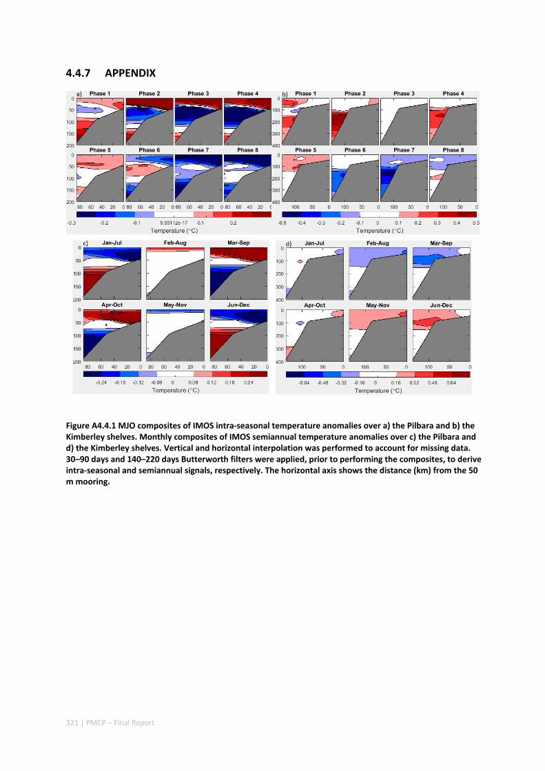
321 | PMCP – Final Report
4.4.7 APPENDIX
Figure A4.4.1 MJO composites of IMOS intra‐seasonal temperature anomalies over a) the Pilbara and b) the Kimberley shelves. Monthly composites of IMOS semiannual temperature anomalies over c) the Pilbara and d) the Kimberley shelves. Vertical and horizontal interpolation was performed to account for missing data. 30–90 days and 140–220 days Butterworth filters were applied, prior to performing the composites, to derive intra‐seasonal and semiannual signals, respectively. The horizontal axis shows the distance (km) from the 50 m mooring.
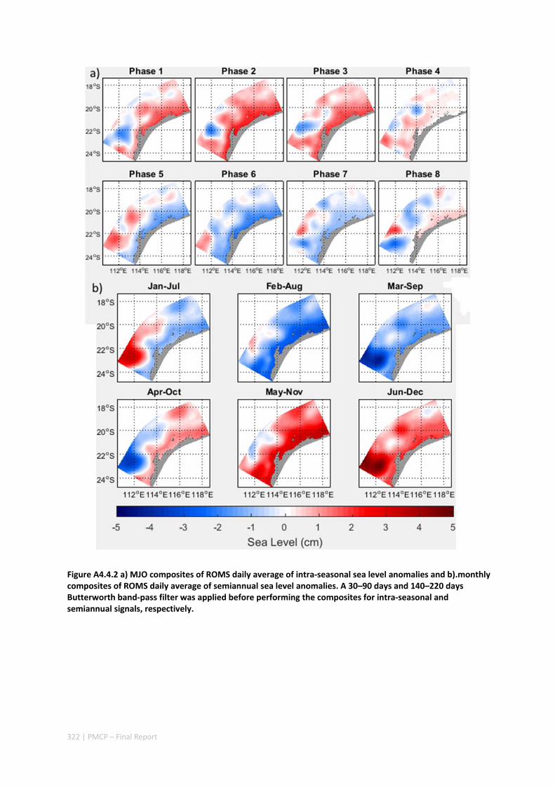
322 | PMCP – Final Report
Figure A4.4.2 a) MJO composites of ROMS daily average of intra‐seasonal sea level anomalies and b).monthly composites of ROMS daily average of semiannual sea level anomalies. A 30–90 days and 140–220 days Butterworth band‐pass filter was applied before performing the composites for intra‐seasonal and semiannual signals, respectively.
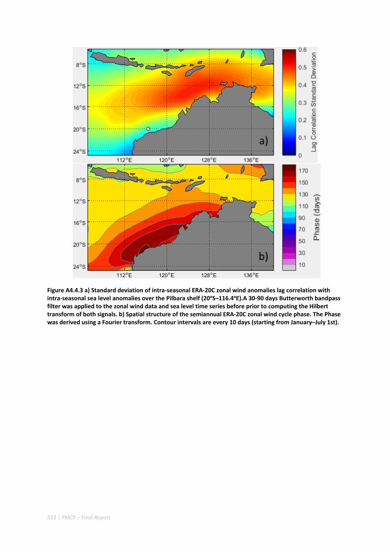
323 | PMCP – Final Report
Figure A4.4.3 a) Standard deviation of intra‐seasonal ERA‐20C zonal wind anomalies lag correlation with intra‐seasonal sea level anomalies over the Pilbara shelf (20oS–116.4oE).A 30‐90 days Butterworth bandpass filter was applied to the zonal wind data and sea level time series before prior to computing the Hilbert transform of both signals. b) Spatial structure of the semiannual ERA‐20C zonal wind cycle phase. The Phase was derived using a Fourier transform. Contour intervals are every 10 days (starting from January–July 1st).
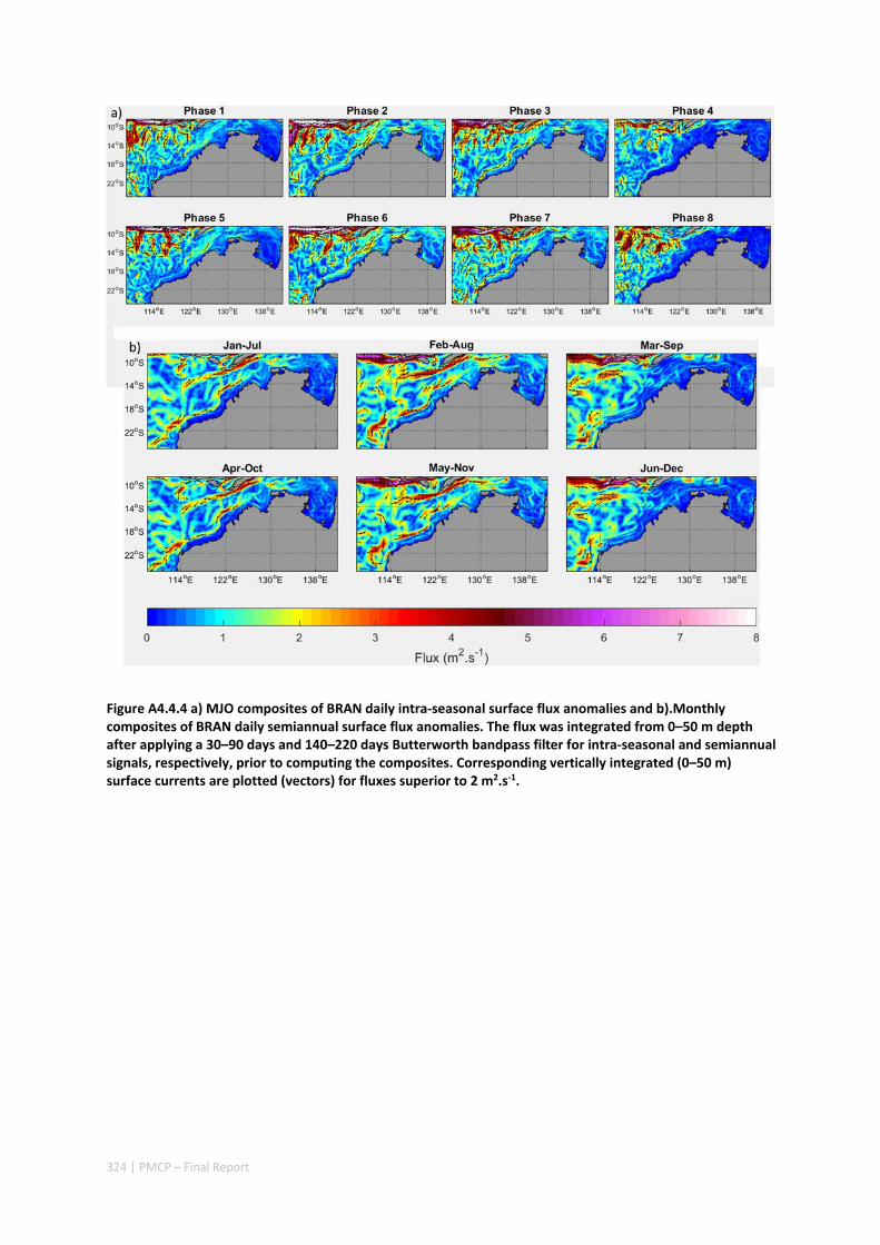
324 | PMCP – Final Report
Figure A4.4.4 a) MJO composites of BRAN daily intra‐seasonal surface flux anomalies and b).Monthly composites of BRAN daily semiannual surface flux anomalies. The flux was integrated from 0–50 m depth after applying a 30–90 days and 140–220 days Butterworth bandpass filter for intra‐seasonal and semiannual signals, respectively, prior to computing the composites. Corresponding vertically integrated (0–50 m) surface currents are plotted (vectors) for fluxes superior to 2 m2.s‐1.
325 | PMCP – Final Report
Seasonal and interannual variations of mixed layer salinity in the southeast tropical Indian Ocean
Authors: Zhang N, Feng M, Du Y, Lan J, Wijffels SE.
Published in J. Geophys. Res. Oceans 121 (2016): 4716–4731, doi:10.1002/2016JC011854..
Abstract
In this study, seasonal and interannual variations of the mixed layer salinity (MLS) in the southeast tropical Indian Ocean (SETIO) are analyzed using satellite observations, historical data sets, and data‐assimilating ocean model outputs. On the seasonal cycle, the MLS in the SETIO becomes fresher in austral winter and saltier in austral summer: between the Java‐Lesser Sunda coast and the South Equatorial Current (SEC, 12°S), where positive entrainment and fresh advections counterbalance each other, the annual cycle of the MLS closely follows the variation of the air‐sea freshwater forcing; off the northwest and west Australian coasts, the MLS variations are influenced by the annual cycles of the Indonesian Throughflow (ITF) and Leeuwin Current (LC) transports as well as the air‐sea freshwater forcing, with eddy fluxes acting to freshen the MLS along the SEC, the Eastern Gyral Current, and the LC. On the interannual‐scale, El Niño (La Niña) events are typically associated with saltier (fresher) MLS in the SETIO. Composite and budget analyses reveal that interannual variations in precipitations drive the MLS anomalies off the Java‐Lesser Sunda coast; between 12°S and the northwest Australian coast, the MLS variations are influenced by both advection anomalies and local precipitation anomalies; whereas anomalous meridional currents contribute to the MLS variations off the west Australian coast. Both enhanced local precipitations and the ITF transport anomalies have substantial contributions to the drastic freshening of the Indonesian‐Australian Basin between the Java‐Lesser Sunda coast and the northwest Australian coast during the extended La Niña events in 1999–2001 and 2010–2012.

326 | PMCP – Final Report
4.5.1 INTRODUCTION
The southeast tropical Indian Ocean (SETIO) is an important area of ocean‐atmosphere interaction and is also an intersection between the Indian Ocean (IO) and the Pacific Ocean through the Indonesian Throughflow (ITF) (Saji and Yamagata 2003; Wijffels and Meyers 2004; Qu and Meyers 2005a). The ITF transports low‐salinity tropical waters from the Pacific to the SETIO and upper ocean salinity in the SETIO shows strong interannual and decadal variability (Phillips et al. 2005; Durack and Wijffels 2010; Du et al. 2015; Feng et al. 2015). Salinity can affect stratification and mixing characteristics of the water column, and plays an important role in ocean dynamics and thermodynamics (Rao and Sivakumar 2003; Vinayachandran and Nanjundiah 2009; Ren et al. 2011; Grunseich et al. 2011). For instance, the anomalous low salinity in the southeast Indian Ocean during the 2010–2011 La Niña and Ningaloo Niño contributed 30% of the enhancement of the Leeuwin Current transport, resulting in unprecedented warming off the coast of Western Australia, causing widespread coral bleaching and fish kills (Pearce and Feng 2013; Feng et al. 2015). Decadal changes of the sea surface salinity (SSS) are often used as indicators for changes in global climate and hydrological cycle (Yu 2011; Katsura et al. 2013; Du et al. 2015).
The spatial distribution of the SSS in the SETIO is strongly shaped by air‐sea freshwater fluxes and regional ocean circulation. A maximum salinity zone extends zonally in the subtropical ocean, due to the intense evaporation (Toole and Warren 1993; Pokhrel et al. 2012). The contrast between the high subtropical SSS and the low salinity in the tropical IO, due to the outflows of the ITF and abundant local rainfall, forms great meridional salinity gradient (Figure 4.5.1) (Qu and Meyers 2005a). The surface‐intensified Timor throughflow contributes a large part to the ITF transport, which is carried westward in the South Equatorial Current (SEC), and is strongly surface intensified between 10°S and 15°S (Fieux et al. 1996; Gordon et al. 1997; Hautala et al. 2001; Wijffels et al. 2002, 2008). The Indonesian‐Australian Basin (IAB) acts as a “buffer,” collecting upper‐ocean water from the ITF from February to June and releasing it during the rest of the year (Meyers et al. 1995; Qu et al. 2008). Some ITF waters recirculate into the Eastern Gyral Current (EGC) and then transported southward in the LC. The South Java Current (SJC) transports low‐salinity tropical Indian Ocean waters into the SETIO. Ocean currents in the SETIO have significant seasonal and interannual variations, in response to the Asian‐Australian monsoon and the Indo‐Pacific climate variations (Wyrtki 1962; Pearce and Phillips 1988; Potemra 1999; Schott and McCreary 2001; Feng et al. 2003, 2008; Qu and Meyers 2005a).
Interannual and decadal variations of the SSS are to a large extent forced by air‐sea freshwater fluxes, with additional contributions from ocean dynamics such as advection, entrainment and diffusion (Rao and Sivakumar 2003; Ren et al. 2009, 2011). Interannual salinity variability in the Equatorial Indian Ocean (EIO) has been demonstrated to be closely related to the Indian Ocean Dipole (IOD) (Grunseich et al. 2011; Zhang et al. 2013; Nyadjro and Subrahmanyam 2014; Du and Zhang 2015), an important interannual climate mode in the IO (Saji and Yamagata 2003). Besides IOD, ENSO is another prominent interannual mode that affects the coupled ocean‐atmosphere processes in the IO (Schott et al. 2009). ENSO influences the SETIO mainly through the equatorial and coastal ocean waveguides via the Indonesian Archipelago (Clarke and Liu 1994; Meyers 1996; Wijffels and Meyers 2004; Feng et al. 2003, 2010), and the geostrophic transport of the ITF and the LC transports are closely related to ENSO, both stronger during La Niña events and weaker during El Niño events (Meyers 1996; Feng et al. 2003, 2008; England and Huang 2005; Liu et al. 2015). In addition, ENSO teleconnection also induces anticyclonic (cyclonic) atmospheric circulation anomalies in the SETIO when El Niño (La Niña) happens (Xie et al. 2002; Wang et al. 2003), such that the evolutions of ENSO are often associated with the development of the IOD.
The marine ecosystem and fisheries in the region are sensitive to the upper ocean variability (Caputi et al. 1996, 2001; Zinke et al. 2015). Variations of sea surface temperature (SST) in the SETIO have
327 | PMCP – Final Report
been well studied, such as along the Java‐Sumatra coast (Du et al. 2005) and off the west coast of Australia (Domingues et al. 2006; Feng et al. 2008). Despite the importance of salinity, quantitative study of the interannual variations of the mixed layer salinity (MLS) in the SETIO has not been carried out. In this study, we focus on the MLS variability and its budget in the SETIO on the seasonal and interannual time scales. Section 2 describes the data sets and methods used. In section 3, the annual cycles of the MLS budget are depicted. Interannual variations of the MLS associated with ENSO are presented in section 4. The relative contributions of the freshwater input from the Indonesian seas and the local precipitations to the MLS variations in the IAB are discussed in section 5, as well as a decomposition of the meridional advection anomalies. The final section summarizes the results.
4.5.2 METHODS
The Soil Moisture and Ocean Salinity (SMOS) mission launched in November 2009 provides global SSS observations for the first time and brings new era of the SSS research (Kerr et al., 2010). We use the monthly composite of the European Space Agency (ESA) level 3 SSS data at 1° × 1° spatial resolution from May 2010 to December 2014, to analyze the seasonal SSS variation and the evolution of SSS anomalies during the 2010‐2011 La Niña.
1°× 1° EN3 (v2a) salinity data from the Met Office Hadley Centre are used to assess salinity variations over longer time period. EN3 contains quality controlled measurements of subsurface ocean temperature and salinity (Ingleby and Huddleston, 2005). ECMWF Ocean Reanalysis System (ORAS4) salinity, potential temperature, mixed layer depth and current velocity model outputs, along with ERA Interim reanalysis evaporation and precipitation data (Dee et al., 2011) are used to conduct the MLS budget and composite analyses. Monthly data during January 1981‐ December 2013 are used. ORAS4 is based on the Nucleus for European Modeling of the Ocean (NEMO) model and the NEMOVAR ocean data assimilation system. The model is forced by atmospheric‐derived surface fluxes including solar radiation, total heat flux, evaporation‐minus‐precipitation and surface wind stress, derived from the ERA‐40 reanalysis from September 1957 to December 1989, the ERA Interim reanalysis from January 1989 to December 2009, and the ECMWF operational archive from January 2010 onwards (Balmaseda et al., 2013). ORAS4 assimilates the temperature and salinity profiles from the EN3 v2a database (XBT bias corrected) and altimeter‐derived sea‐level anomalies. Monthly Indian Ocean Dipole mode index (DMI) and Niño3.4 index since 1982 are obtained from the Ocean Observations Panel for Climate (OOPC). These indices have been calculated using the Reynolds OIv2 SST analysis. Gridded Argo float salinity data at 1° spatial resolution are obtained from the International Pacific Research Center (IPRC) to compare to the interannual variations of the EN3 salinity data.
One site (100°E, 25°S) of the Research Moored Array for African‐Asian‐Australian Monsoon Analysis and Prediction (RAMA) is in the SETIO. The SSS and surface freshwater flux during September 2012‐December 2013 are obtained from the RAMA mooring to validate the salinity and surface freshwater flux data used in this paper. The differences are small between the RAMA observations and the EN3, ORAS4 model outputs, and ERA Interim data (Figure S4.5.1), indicating the salinity and freshwater flux data used are reliable. On average, the SMOS SSS is around 0.2 psu saltier than the RAMA SSS at this site. The climatologically annual mean SSS distributions from the EN3 and SMOS data show similar patterns in the northern part of the SETIO (Figure 4.5.1). Along the west coast of Australia, the SMOS SSS resolves the LC well but may have fresh biases. The SMOS accuracy may still be within the general requirements for accuracy of the SSS observations: 1 psu in the area where coastal processes occur and 0.2 psu in the region where fronts or eddies exist (Kerr et al., 2010).
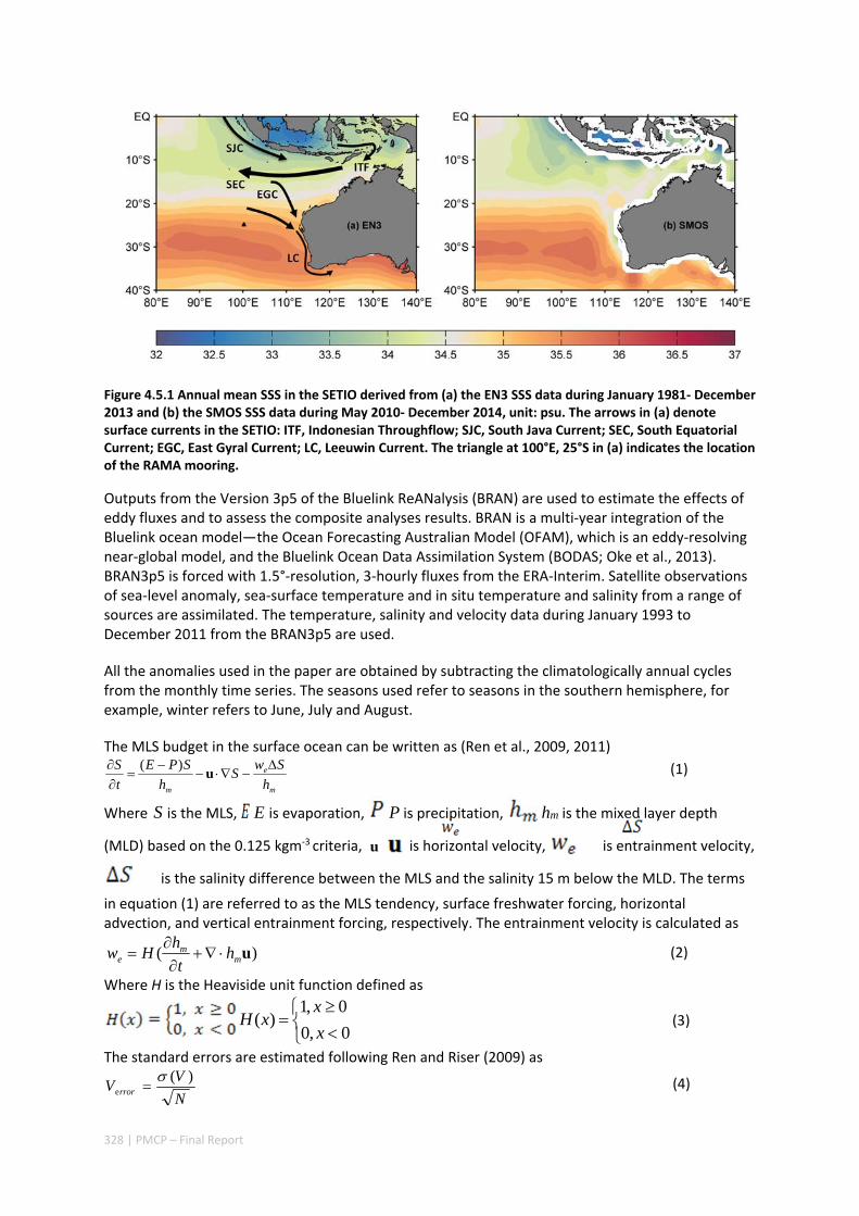
328 | PMCP – Final Report
Figure 4.5.1 Annual mean SSS in the SETIO derived from (a) the EN3 SSS data during January 1981‐ December 2013 and (b) the SMOS SSS data during May 2010‐ December 2014, unit: psu. The arrows in (a) denote surface currents in the SETIO: ITF, Indonesian Throughflow; SJC, South Java Current; SEC, South Equatorial Current; EGC, East Gyral Current; LC, Leeuwin Current. The triangle at 100°E, 25°S in (a) indicates the location of the RAMA mooring.
Outputs from the Version 3p5 of the Bluelink ReANalysis (BRAN) are used to estimate the effects of eddy fluxes and to assess the composite analyses results. BRAN is a multi‐year integration of the Bluelink ocean model—the Ocean Forecasting Australian Model (OFAM), which is an eddy‐resolving near‐global model, and the Bluelink Ocean Data Assimilation System (BODAS; Oke et al., 2013). BRAN3p5 is forced with 1.5°‐resolution, 3‐hourly fluxes from the ERA‐Interim. Satellite observations of sea‐level anomaly, sea‐surface temperature and in situ temperature and salinity from a range of sources are assimilated. The temperature, salinity and velocity data during January 1993 to December 2011 from the BRAN3p5 are used.
All the anomalies used in the paper are obtained by subtracting the climatologically annual cycles from the monthly time series. The seasons used refer to seasons in the southern hemisphere, for example, winter refers to June, July and August.
The MLS budget in the surface ocean can be written as (Ren et al., 2009, 2011)
m
e
m h
SwS
h
SPE
t
S
u)( (1)
Where S is the MLS, E is evaporation, P is precipitation, hm is the mixed layer depth
(MLD) based on the 0.125 kgm‐3 criteria, is horizontal velocity, is entrainment velocity,
is the salinity difference between the MLS and the salinity 15 m below the MLD. The terms
in equation (1) are referred to as the MLS tendency, surface freshwater forcing, horizontal advection, and vertical entrainment forcing, respectively. The entrainment velocity is calculated as
)( umm
e ht
hHw
(2)
Where H is the Heaviside unit function defined as
0,0
0,1)(
x
xxH (3)
The standard errors are estimated following Ren and Riser (2009) as
N
VV rror
)(e
(4)
u
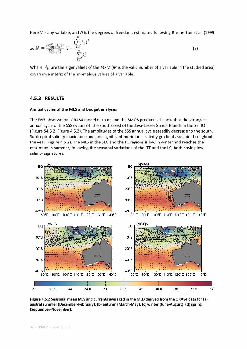
329 | PMCP – Final Report
Here V is any variable, and N is the degrees of freedom, estimated following Bretherton et al. (1999)
as
M
kk
M
kk
N
1
2
1
2)(
(5)
Where k are the eigenvalues of the M×M (M is the valid number of a variable in the studied area)
covariance matrix of the anomalous values of a variable.
4.5.3 RESULTS
Annual cycles of the MLS and budget analyses
The EN3 observation, ORAS4 model outputs and the SMOS products all show that the strongest annual cycle of the SSS occurs off the south coast of the Java‐Lesser Sunda Islands in the SETIO (Figure S4.5.2; Figure 4.5.2). The amplitudes of the SSS annual cycle steadily decrease to the south. Subtropical salinity maximum zone and significant meridional salinity gradients sustain throughout the year (Figure 4.5.2). The MLS in the SEC and the LC regions is low in winter and reaches the maximum in summer, following the seasonal variations of the ITF and the LC, both having low salinity signatures.
Figure 4.5.2 Seasonal mean MLS and currents averaged in the MLD derived from the ORAS4 data for (a) austral summer (December‐February); (b) autumn (March‐May); (c) winter (June‐August); (d) spring (September‐November).
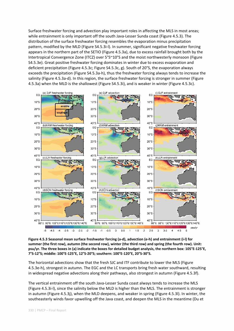
330 | PMCP – Final Report
Surface freshwater forcing and advection play important roles in affecting the MLS in most areas; while entrainment is only important off the south Java‐Lesser Sunda coast (Figure 4.5.3). The distribution of the surface freshwater forcing resembles the evaporation minus precipitation pattern, modified by the MLD (Figure S4.5.3i‐l). In summer, significant negative freshwater forcing appears in the northern part of the SETIO (Figure 4.5.3a), due to excess rainfall brought both by the Intertropical Convergence Zone (ITCZ) over 5°S~10°S and the moist northwesterly monsoon (Figure S4.5.3e). Great positive freshwater forcing dominates in winter due to excess evaporation and deficient precipitation (Figure 4.5.3c; Figure S4.5.3c, g). South of 20°S, the evaporation always exceeds the precipitation (Figure S4.5.3a‐h), thus the freshwater forcing always tends to increase the salinity (Figure 4.5.3a‐d). In this region, the surface freshwater forcing is stronger in summer (Figure 4.5.3a) when the MLD is the shallowest (Figure S4.5.3i), and is weaker in winter (Figure 4.5.3c).
Figure 4.5.3 Seasonal mean surface freshwater forcing (a‐d), advection (e‐h) and entrainment (i‐l) for summer (the first row), autumn (the second row), winter (the third row) and spring (the fourth row). Unit: psu/yr. The three boxes in (a) indicate the boxes for detailed budget analysis, the northern box: 105°E‐125°E, 7°S‐12°S; middle: 100°E‐125°E, 12°S‐20°S; southern: 100°E‐120°E, 20°S‐30°S.
The horizontal advections show that the fresh SJC and ITF contribute to lower the MLS (Figure 4.5.3e‐h), strongest in autumn. The EGC and the LC transports bring fresh water southward, resulting in widespread negative advections along their pathways, also strongest in autumn (Figure 4.5.3f).
The vertical entrainment off the south Java‐Lesser Sunda coast always tends to increase the MLS (Figure 4.5.3i‐l), since the salinity below the MLD is higher than the MLS. The entrainment is stronger in autumn (Figure 4.5.3j), when the MLD deepens, and weaker in spring (Figure 4.5.3l). In winter, the southeasterly winds favor upwelling off the Java coast, and deepen the MLS in the meantime (Du et
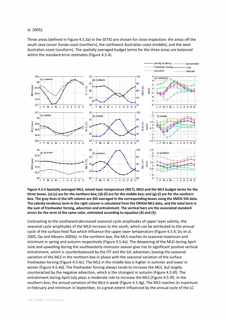
331 | PMCP – Final Report
al. 2005).
Three areas (defined in Figure 4.5.3a) in the SETIO are chosen for close inspection: the areas off the south Java‐Lesser Sunda coast (northern), the northwest Australian coast (middle), and the west Australian coast (southern). The spatially averaged budget terms for the three areas are balanced within the standard error estimates (Figure 4.5.4).
Figure 4.5.4 Spatially averaged MLS, mixed layer temperature (MLT), MLD and the MLS budget terms for the three boxes. (a)‐(c) are for the northern box; (d)‐(f) are for the middle box; and (g)‐(i) are for the southern box. The gray lines in the left column are SSS averaged in the corresponding boxes using the SMOS SSS data. The salinity tendency term in the right column is calculated from the ORAS4 MLS data, and the total term is the sum of freshwater forcing, advection and entrainment. The vertical bars are the associated standard errors for the term of the same color, estimated according to equation (4) and (5).
Contrasting to the southward‐decreased seasonal cycle amplitudes of upper layer salinity, the seasonal cycle amplitudes of the MLD increase to the south, which can be attributed to the annual cycle of the surface heat flux which influence the upper layer temperature (Figure 4.5.4; Du et al. 2005; Qu and Meyers 2005b). In the northern box, the MLS reaches its seasonal maximum and minimum in spring and autumn respectively (Figure 4.5.4a). The deepening of the MLD during April‐June and upwelling during the southeasterly monsoon season give rise to significant positive vertical entrainment, which is counterbalanced by the ITF and the SJC advection, leaving the seasonal variation of the MLS in the northern box in phase with the seasonal variation of the surface freshwater forcing (Figure 4.5.4c). The MLS in the middle box is higher in summer and lower in winter (Figure 4.5.4d). The freshwater forcing always tends to increase the MLS, but largely counteracted by the negative advection, which is the strongest in autumn (Figure 4.5.4f). The entrainment during April‐July plays a moderate role to increase the MLS (Figure 4.5.4f). In the southern box, the annual variation of the MLS is weak (Figure 4.5.4g). The MLS reaches its maximum in February and minimum in September, to a great extent influenced by the annual cycle of the LC
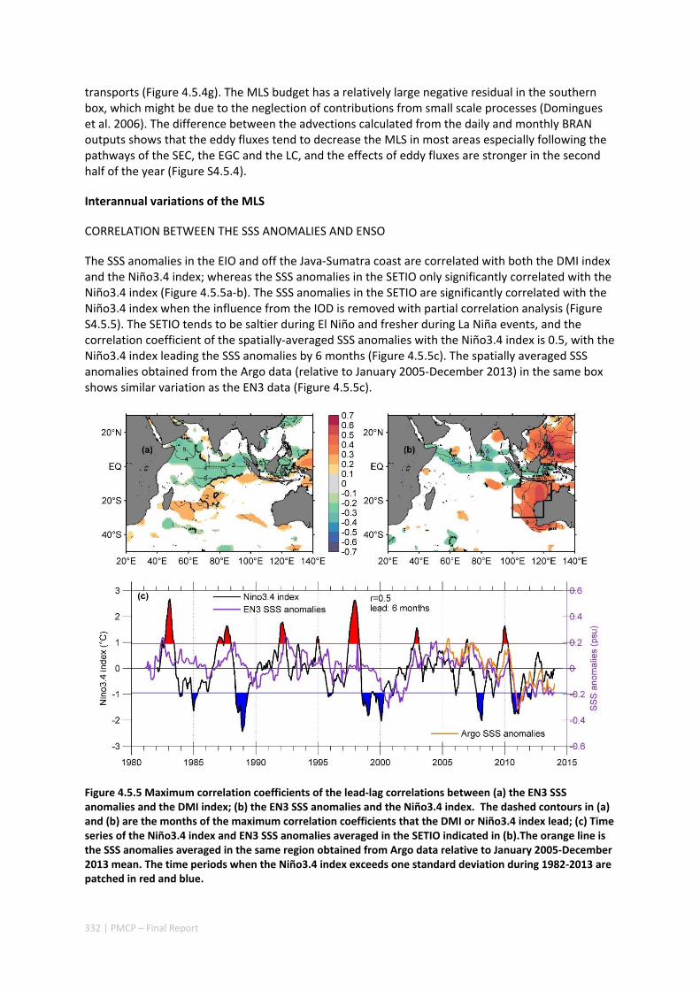
332 | PMCP – Final Report
transports (Figure 4.5.4g). The MLS budget has a relatively large negative residual in the southern box, which might be due to the neglection of contributions from small scale processes (Domingues et al. 2006). The difference between the advections calculated from the daily and monthly BRAN outputs shows that the eddy fluxes tend to decrease the MLS in most areas especially following the pathways of the SEC, the EGC and the LC, and the effects of eddy fluxes are stronger in the second half of the year (Figure S4.5.4).
Interannual variations of the MLS
CORRELATION BETWEEN THE SSS ANOMALIES AND ENSO
The SSS anomalies in the EIO and off the Java‐Sumatra coast are correlated with both the DMI index and the Niño3.4 index; whereas the SSS anomalies in the SETIO only significantly correlated with the Niño3.4 index (Figure 4.5.5a‐b). The SSS anomalies in the SETIO are significantly correlated with the Niño3.4 index when the influence from the IOD is removed with partial correlation analysis (Figure S4.5.5). The SETIO tends to be saltier during El Niño and fresher during La Niña events, and the correlation coefficient of the spatially‐averaged SSS anomalies with the Niño3.4 index is 0.5, with the Niño3.4 index leading the SSS anomalies by 6 months (Figure 4.5.5c). The spatially averaged SSS anomalies obtained from the Argo data (relative to January 2005‐December 2013) in the same box shows similar variation as the EN3 data (Figure 4.5.5c).
Figure 4.5.5 Maximum correlation coefficients of the lead‐lag correlations between (a) the EN3 SSS anomalies and the DMI index; (b) the EN3 SSS anomalies and the Niño3.4 index. The dashed contours in (a) and (b) are the months of the maximum correlation coefficients that the DMI or Niño3.4 index lead; (c) Time series of the Niño3.4 index and EN3 SSS anomalies averaged in the SETIO indicated in (b).The orange line is the SSS anomalies averaged in the same region obtained from Argo data relative to January 2005‐December 2013 mean. The time periods when the Niño3.4 index exceeds one standard deviation during 1982‐2013 are patched in red and blue.

333 | PMCP – Final Report
COMPOSITE ANALYSES
There are 9 El Niño (1982, 1986, 1987, 1991, 1994, 1997, 2002, 2006, and 2009) and 8 La Niña (1984, 1988, 1995, 1998, 1999, 2007, 2010, and 2011) events identified during 1981‐2013 (Meyers et al. 2007). Anomalies during the developing years (year 0) and the following years (year 1) are used to conduct composite analyses of the MLS and forcing anomalies.
Figure 4.5.6 (a)‐(h): Bimonthly composites of MLS anomalies (shaded, unit: psu) and surface currents anomalies (arrows, unit: m/s) from July/August of year 0 to September/October of year 1 during El Niño events. (i)‐(p): Bimonthly composites of freshwater flux (shaded, unit: m/yr) and MLD (m) anomalies (contours) during El Niño events. The statistical significances of the anomalies are tested by the two‐tailed t test. Anomalies exceeding 90% significance are plotted for the MLS and freshwater flux, and bold arrows for current anomalies exceeding 90% significance.
During El Niño events, positive MLS anomalies first appear off the south Java‐Lesser Sunda coast in July‐August of year 0 (Figure 4.5.6). The positive MLS anomalies extend southward and westward in subsequent months till January‐February of year 1, reaching a maximum of more than 0.2 psu (Figure 4.5.6a‐d). Weak positive MLS anomalies persist for several more months, off the northwest and west coast of Australia (Figure 4.5.6e‐h). Positive freshwater flux (E‐P) anomalies in the northern part of the SETIO directly contribute to increase the MLS during July‐August of year 0 to January‐February of year 1 (Figure 4.5.6i‐l). Positive freshwater flux anomalies first appear off the Java‐Lesser Sunda coast and in the Indonesian internal seas in July‐August of year 0 (Figure 4.5.6i); and gradually shift to the northwest Australia till January‐February of year 1 with a maximum of 0.5 m/yr (Figure 4.5.6j‐l); then reverse to negative in subsequent months (Figure 4.5.6m‐p). The positive freshwater flux anomalies mainly result from decreased precipitations. The Walker circulation weakens during El Niño events, and shifts its ascending branch eastward, thus suppresses the rainfall in the tropical IO (Pokhrel et al. 2012; Wu et al. 2012; Hasson et al. 2014).

334 | PMCP – Final Report
Off the south Java‐Lesser Sunda coast, anomalous westward currents start to appear in July‐August of year 0 and sustain through January‐February of year 1 (Figure 4.5.6a‐d), and then become eastward after the mature phase of El Niño (Figure 4.5.6e‐h). The anomalous westward currents are likely associated with the anomalous easterly winds along the EIO, which cause upwelling equatorial Kelvin waves that propagate eastward along the Java‐Sumatra coast as coastal Kelvin waves (Wijffels and Meyers 2004; Drushka et al. 2010). They contribute to shoal the thermocline, and lower the sea surface height off the Java coast, thus give rise to the westward geostrophic current anomalies. The subsequent anomalous eastward currents are mostly related to the Rossby waves radiated from the Australian coast, which originally propagates from the Pacific (Pearce and Phillips 1988; Meyers 1996; Feng et al. 2003; Liu et al. 2015). Off the northwest and west Australian coast, there are northeastward and northward current anomalies during the onset and mature phases of El Niño (Figure 4.5.6a‐e), due to the shallow thermocline anomalies transmitted from the tropical Pacific along the west Australian coast, which weakens the LC volume transports (Pearce and Phillips 1988; Meyers 1996; Feng et al. 2003). From May‐June of year 1, the current anomalies in the SETIO start to reverse (Figure 4.5.6f‐h). The MLD shoals off the south Java‐Lesser Sunda coast during September‐October of year 0 to July‐August of year 1, with peak anomalies of more than 12 m during January‐February of year 1 (Figure 4.5.6j‐o); the MLD shoals off the northwest and west Australian coasts during November‐December of year 1 to September‐October of year 1, with peak anomalies of more than 8 m during July‐August of year 1 (Figure 4.5.6k‐p).
Figure 4.5.7 Same as Figure 4.5.6, but for La Niña events.
The composites during La Niña events are almost opposite to those during El Niño events. Freshen MLS anomalies start to appear in the northern part of the SETIO off the south Java‐Lesser Sunda coast from September‐October of year 0 (Figure 4.5.7b). The MLS anomalies strengthen during September‐October to January‐February of year 1 and extend southward to the Australian coast in

335 | PMCP – Final Report
the meantime. In March‐April of year 1, the strongest MLS anomalies are located off the northwest coast of Australia, reaching the peak anomalies of more than 0.3 psu, extending southward along the west coast of Australia (Figure 4.5.7 c‐e). The MLS anomalies off the northwest and west Australian coasts sustain through September‐October of year 1 (Figure 4.5.7f‐h). The evolution of the anomalous freshening in the SETIO during the 2010‐2011 La Niña event is captured by the SMOS SSS data (Figure S4.5.7). Excessive precipitations in the SETIO have direct contributions to the evolution and southward shift of the fresh MLS anomalies north of 20°S (Figure 4.5.7i‐m). At the developing phase of La Niña, eastward surface current anomalies develop off the south Java‐Lesser Sunda coast and southward current anomalies off the northwest and west Australian coasts (Figure 4.5.7a‐f). The MLD deepens off the Java‐Lesser Sunda coast, the northwest and west Australian coasts (Figure 4.5.7j‐o).
During the El Niño events, due to the shoaling of the MLD (Klein et al. 1999; Schott et al. 2009) and the salinity increase, the barrier layer (defined as the difference between the isothermal depth (based on a temperature difference of 0.8°C from the sea surface) and the MLD) significantly reduces off the Java‐Lesser Sunda and north Australian coast Figure S4.5.6c‐e), which would increase vertical mixing (Qu and Meyers 2005b; Grunseich et al. 2011). The thickness of barrier layer off the Java‐Lesser Sunda and north Australian coast increases during La Niña, and thus decreases vertical mixing, sustaining the anomalous freshening in the SETIO for a longer period (Figure S4.5.6, Figure 4.5.7).
Figure 4.5.8 Bimonthly‐composites of of (a)‐(d) MLS tendency anomalies, (e)‐(h) surface freshwater forcing anomalies, (i)‐(l) advection anomalies, and (m)‐(p) entrainment anomalies during El Niño events for September‐October (first row), November‐December (second row), the following January‐February (third row), and the following March‐April (fourth row). Units: psu/yr.
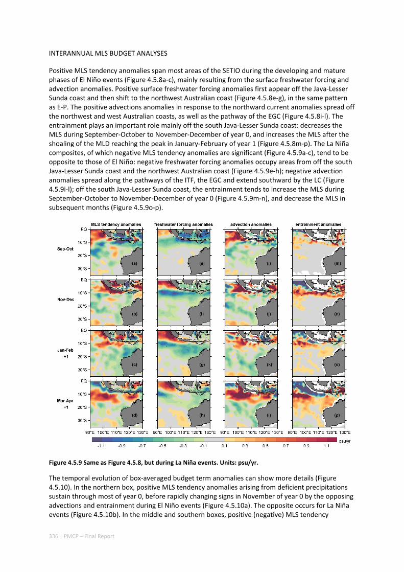
336 | PMCP – Final Report
INTERANNUAL MLS BUDGET ANALYSES
Positive MLS tendency anomalies span most areas of the SETIO during the developing and mature phases of El Niño events (Figure 4.5.8a‐c), mainly resulting from the surface freshwater forcing and advection anomalies. Positive surface freshwater forcing anomalies first appear off the Java‐Lesser Sunda coast and then shift to the northwest Australian coast (Figure 4.5.8e‐g), in the same pattern as E‐P. The positive advections anomalies in response to the northward current anomalies spread off the northwest and west Australian coasts, as well as the pathway of the EGC (Figure 4.5.8i‐l). The entrainment plays an important role mainly off the south Java‐Lesser Sunda coast: decreases the MLS during September‐October to November‐December of year 0, and increases the MLS after the shoaling of the MLD reaching the peak in January‐February of year 1 (Figure 4.5.8m‐p). The La Niña composites, of which negative MLS tendency anomalies are significant (Figure 4.5.9a‐c), tend to be opposite to those of El Niño: negative freshwater forcing anomalies occupy areas from off the south Java‐Lesser Sunda coast and the northwest Australian coast (Figure 4.5.9e‐h); negative advection anomalies spread along the pathways of the ITF, the EGC and extend southward by the LC (Figure 4.5.9i‐l); off the south Java‐Lesser Sunda coast, the entrainment tends to increase the MLS during September‐October to November‐December of year 0 (Figure 4.5.9m‐n), and decrease the MLS in subsequent months (Figure 4.5.9o‐p).
Figure 4.5.9 Same as Figure 4.5.8, but during La Niña events. Units: psu/yr.
The temporal evolution of box‐averaged budget term anomalies can show more details (Figure 4.5.10). In the northern box, positive MLS tendency anomalies arising from deficient precipitations sustain through most of year 0, before rapidly changing signs in November of year 0 by the opposing advections and entrainment during El Niño events (Figure 4.5.10a). The opposite occurs for La Niña events (Figure 4.5.10b). In the middle and southern boxes, positive (negative) MLS tendency
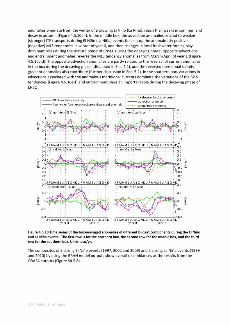
337 | PMCP – Final Report
anomalies originate from the winter of a growing El Niño (La Niña), reach their peaks in summer, and decay in autumn (Figure 4.5.10c‐f). In the middle box, the advection anomalies related to weaker (stronger) ITF transports during El Niño (La Niña) events first set up the anomalously positive (negative) MLS tendencies in winter of year 0, and then changes in local freshwater forcing play dominant roles during the mature phase of ENSO. During the decaying phase, opposite advections and entrainment anomalies reverse the MLS tendency anomalies from March/April of year 1 (Figure 4.5.10c‐d). The opposite advection anomalies are partly related to the reversal of current anomalies in the box during the decaying phase (discussed in Sec. 4.2), and the reversed meridional salinity gradient anomalies also contribute (further discussion in Sec. 5.2). In the southern box, variations in advections associated with the anomalous meridional currents dominate the variations of the MLS tendencies (Figure 4.5.10e‐f) and entrainment plays an important role during the decaying phase of ENSO.
Figure 4.5.10 Time series of the box‐averaged anomalies of different budget components during the El Niño and La Niña events.. The first row is for the northern box, the second row for the middle box, and the third row for the southern box. Units: psu/yr.
The composites of 3 strong El Niño events (1997, 2002 and 2009) and 2 strong La Niña events (1999 and 2010) by using the BRAN model outputs show overall resemblances as the results from the ORAS4 outputs (Figure S4.5.8).

338 | PMCP – Final Report
4.5.4 DISCUSSION
Relative contributions of advection and local precipitations on the MLS in the IAB
The upstream Indonesian seas are key regions for the salinity variations in the IAB (Phillips et al., 2005). In the Indonesian seas as well as off the south Java‐Lesser Sunda coast, E‐P shows great interannual variation (Figure 4.5.11a). The correlation between the E‐P anomalies and the Niño3.4 index in the Indonesian Seas can reach above 0.7 and there is deficient (excessive) rainfall during El Niño (La Niña) events. Following Phillips et al. (2005), the upper ocean salinity variations in the IAB
(outlined in black in Figure 4.5.11a) driven by the E‐P anomalies HtPESS /)(0 in the Indon box (outlined in blue in Figure 4.5.11a) are derived by integrating the E‐P anomalies over the previous year (see Phillips et al. 2005 for more details). The upper ocean salinity variations derived from the freshwater flux in the Indon box are in phase with the salinity variations in the IAB averaged between the EN3 and ORAS4 products (Figure 4.5.11b), which suggests that the freshwater advection from the Indonesian seas is an important contributor to the salinity change in the IAB. However, the amplitudes of the salinity variations derived from the Indonesian seas are smaller, which is especially true for the recent two freshening events in 1999‐2001 and 2010‐2012. This indicates that besides advections from the upstream, local precipitations in the IAB also affect the salinity variations, especially during the mature phase of ENSO, when the anomalous local rainfalls peak (Figure 4.5.8f‐g, Figure 4.5.9f‐g, Figure 4.5.10c‐d).
Figure 4.5.11 (a) Maximum correlation coefficients between the freshwater flux anomaly (E‐P) from the ERA Interim reanalysis products and the Niño3.4 index. The dashed contours indicate the months of the maximum correlation coefficients that the Niño3.4 index lead. (b) Surface layer salinity change derived from
the freshwater input in the Indon box (outlined by blue dashed lines in (a)), HtPESS /)(0 , using the ERA Interim products; and the surface layer salinity change in the IAB (outlined by black dashed lines in (a)) derived from the average of the EN3 and ORAS4 products. A 12‐points moving average is applied and the long‐term linear trend is removed from the two time series.
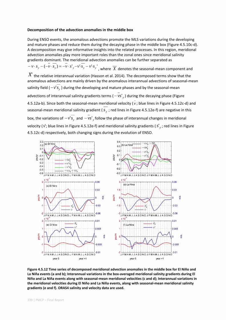
339 | PMCP – Final Report
Decomposition of the advection anomalies in the middle box
During ENSO events, the anomalous advections promote the MLS variations during the developing and mature phases and reduce them during the decaying phase in the middle box (Figure 4.5.10c‐d). A decomposition may give informative insights into the related processes. In this region, meridional advection anomalies play more important roles than the zonal ones since meridional salinity gradients dominant. The meridional advection anomalies can be further separated as
'''')( yyyyy svsvsvsvsv , where X denotes the seasonal‐mean component and
'X the relative interannual variation (Hasson et al. 2014). The decomposed terms show that the anomalous advections are mainly driven by the anomalous interannual advections of seasonal‐mean
salinity field ( ysv' ) during the developing and mature phases and by the seasonal‐mean
advections of interannual salinity gradients terms ( ysv ' ) during the decaying phase (Figure
4.5.12a‐b). Since both the seasonal‐mean meridional velocity ( v ; blue lines in Figure 4.5.12c‐d) and
seasonal‐mean meridional salinity gradient ( ys ; red lines in Figure 4.5.12e‐f) are negative in this
box, the variations of ysv' and ysv ' follow the phase of interannual changes in meridional
velocity ( 'v ; blue lines in Figure 4.5.12e‐f) and meridional salinity gradients ( ys' ; red lines in Figure
4.5.12c‐d) respectively, both changing signs during the evolution of ENSO.
Figure 4.5.12 Time series of decomposed meridional advection anomalies in the middle box for El Niño and La Niña events (a and b); Interannual variations in the box‐averaged meridional salinity gradients during El Niño and La Niña events along with seasonal‐mean meridional velocities (c and d); Interannual variations in the meridional velocities during El Niño and La Niña events, along with seasonal‐mean meridional salinity gradients (e and f). ORAS4 salinity and velocity data are used.
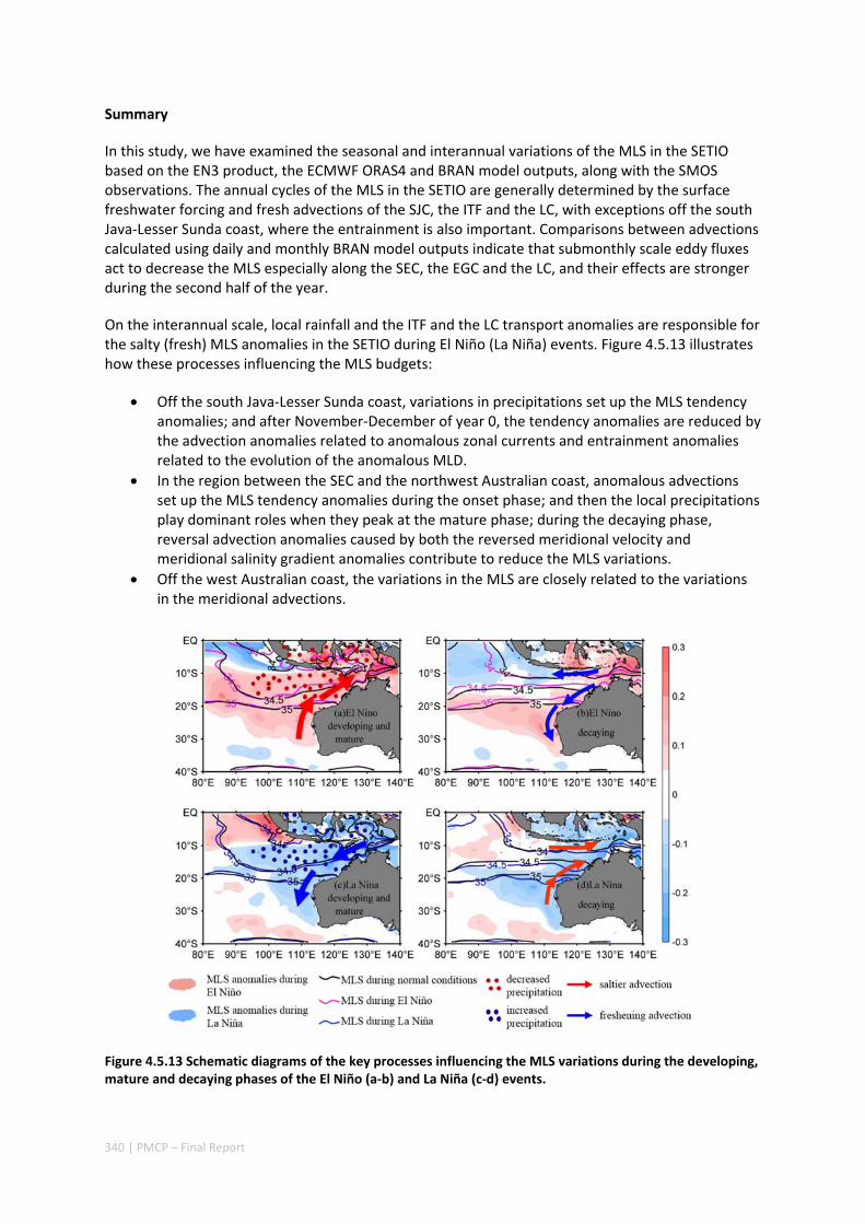
340 | PMCP – Final Report
Summary
In this study, we have examined the seasonal and interannual variations of the MLS in the SETIO based on the EN3 product, the ECMWF ORAS4 and BRAN model outputs, along with the SMOS observations. The annual cycles of the MLS in the SETIO are generally determined by the surface freshwater forcing and fresh advections of the SJC, the ITF and the LC, with exceptions off the south Java‐Lesser Sunda coast, where the entrainment is also important. Comparisons between advections calculated using daily and monthly BRAN model outputs indicate that submonthly scale eddy fluxes act to decrease the MLS especially along the SEC, the EGC and the LC, and their effects are stronger during the second half of the year.
On the interannual scale, local rainfall and the ITF and the LC transport anomalies are responsible for the salty (fresh) MLS anomalies in the SETIO during El Niño (La Niña) events. Figure 4.5.13 illustrates how these processes influencing the MLS budgets:
Off the south Java‐Lesser Sunda coast, variations in precipitations set up the MLS tendency anomalies; and after November‐December of year 0, the tendency anomalies are reduced by the advection anomalies related to anomalous zonal currents and entrainment anomalies related to the evolution of the anomalous MLD.
In the region between the SEC and the northwest Australian coast, anomalous advections set up the MLS tendency anomalies during the onset phase; and then the local precipitations play dominant roles when they peak at the mature phase; during the decaying phase, reversal advection anomalies caused by both the reversed meridional velocity and meridional salinity gradient anomalies contribute to reduce the MLS variations.
Off the west Australian coast, the variations in the MLS are closely related to the variations in the meridional advections.
Figure 4.5.13 Schematic diagrams of the key processes influencing the MLS variations during the developing, mature and decaying phases of the El Niño (a‐b) and La Niña (c‐d) events.

341 | PMCP – Final Report
4.5.5 ACKNOWLEDGMENTS
This research is partly supported by the Western Australian Marine Science Institution, the Gorgon Barrow Island Net Conservation Benefits Fund, which is administered by the WA Department of Biodiversity, Conservation and Attractions. Ningning Zhang is supported by the China Scholarship Council for her visit to CSIRO. Jian Lan is supported by National Natural Science Foundation of China (41276011). The Research is also partly supported by the CAS/SAFEA International Partnership Program for Creative Research Teams. We benefited from numerous data sets made freely available, including SMOS SSS data obtained from the Ocean Salinity Expertise Center (CECOS) of the Centre Aval de Traitemenent des Donnees SMOS (CATDS), EN3 SSS data (http://www.metoffice.gov.uk/hadobs/en3/), ECMWF ORAS4 salinity, potential temperature, mixed layer depth and current velocity data, IPRC Argo products made available at Asia‐Pacific data‐research center (APDRC, http://apdrc.soest.hawaii.edu/las/v6/dataset?catitem=5458), ERA Interim evaporation and precipitation data (http://apps.ecmwf.int/datasets/data/interim‐full‐mnth/), DMI and Nino 3.4 index (http://stateoftheocean.osmc.noaa.gov/sur/ind/dmi.php), RAMA data (http://www.pmel.noaa.gov/tao/disdel/frames/main.html), and BRAN3p5 data (http://wp.csiro.au/bluelink/global/data-access/).
4.5.6 REFERENCES
Balmaseda M A, Mogensen K and Weaver AT (2013) Evaluation of the ECMWF ocean reanalysis system ORAS4. Q. J. R. Meteorol. Soc. 139:1132–1161, doi: 10.1002/qj.2063.
Bretherton CS, Widmann M, Dymnikov VP, Wallace JM and Bladé I (1999) The effective number of Spatial Degrees of Freedom of a time‐varying field. J. Climate 12:1990–2009, doi: http://dx.doi.org/10.1175/1520‐0442(1999)012<1990:TENOSD>2.0.CO;2.
Caputi N, Chubb C and Pearce A (2001) Environmental effects on recruitment of the western rock lobster, Panulirus cygus. Mar. Freshwater Res. 52:1167‐1174, doi: 10.1071/MF01180.
Caputi N, Fletcher WJ, Pearce A and Chubb CF (1996) Effect of the Leeuwin Current on recruitment of fish and invertebrates along the Western Australian coast. Mar. Freshwater Res. 47:147‐155, doi: 10.1071/MF9960147.
Clarke AJ and Liu X (1994) Interannual sea level in the northern and eastern Indian Ocean. J. Phys. Oceanogr. 24:1224–1235. doi: http://dx.doi.org/10.1175/1520‐0485(1994)024<1224:ISLITN>2.0.CO;2.
Dee DP, Uppala SM, Simmons AJ, BerrisfordP , Poli P, Kobayashi S, Andrae U, Balmaseda MA, Balsamo G, Bauer P, Bechtold P, Beljaars ACM, van de Berg L, Bidlot J, Bormann N, Delsol C, Dragani R, Fuentes M, Geer AJ, Haimberger L, Healy SB, Hersbach H, Hólm EV, Isaksen L, Kållberg P, Köhler M, Matricardi M, McNally AP, Monge‐Sanz BM, Morcrette JJ, Park BK, Peubey C, de Rosnay P, Tavolato C, Thépaut JN and Vitart F (2011) The ERA‐Interim reanalysis: Configuration and performance of the data assimilation system. Q. J. R. Meteorol. Soc. 137:553–597, DOI: 10.1002/qj.828
Domingues CM, Wijffels SE, Maltrud ME, Church JA and Tomczak M (2006) Role of eddies in cooling the Leeuwin Current. Geophys. Res. Lett. 33:L05603, doi: 10.1029/2005GL025216.
Drushka K, Sprintall J, Gille ST and Brodjonegoro I (2010) Vertical structure of Kelvin waves in the

342 | PMCP – Final Report
Indonesian Throughflow exit passages. J. Phys. Oceanogr. 40:1965–1987, doi: http://dx.doi.org/10.1175/2010JPO4380.1.
Du Y, Qu T, Meyers G, Masumoto Y and Sasaki H (2005) Seasonal heat budget in the mixed layer of the southeastern tropical Indian Ocean in a high‐resolution ocean general circulation model. J. Geophys. Res. 110:C04012, doi:10.1029/2004JC002845.
Du Y and Zhang YH (2015) Satellite and Argo observed surface salinity variations in the topical Indian Ocean and their association with the Indian Ocean Dipole Mode. J. Clim. 28:695‐713, doi:10.1175/JCLI‐D‐14‐00435.1.
Du Y, Zhang Y, Feng M, Wang T, Zhang N and Wijffels S (2015) Decadal trends of the upper ocean salinity in the tropical Indo‐Pacific since mid‐1990s. Sci. Rep. 5:16050, doi: 10.1038/srep16050.
Durack P and Wijffels S (2010) Fifty‐year trends in global ocean salinities and their relationship to broad‐scale warming. J. Clim. 23:4342‐4362, doi: 10.1175/2010JCLI3377.1.
England MH and Huang F (2005) On the interannual variability of the Indonesian Throughflow and its linkage with ENSO. J. Clim. 18:1435–1444, doi: http://dx.doi.org/10.1175/JCLI3322.1.
Feng M, Meyers G, Pearce A and Wijffels S (2003) Annual and interannual variations of the Leeuwin Current at 32°S. J. Geophys. Res. 108(C11):3355, doi:10.1029/2002JC001763.
Feng M, Biastoch A, Böning C, Caputi N and Meyers G (2008) Seasonal and interannual variations of upper ocean heat balance off the west coast of Australia. J. Geophys. Res. 113:C12025, doi:10.1029/2008JC004908.
Feng M, McPhaden MJ and Lee T (2010) Decadal variability of the Pacific subtropical cells and their influence on the southeast Indian Ocean. Geophys. Res. Lett. 37:L09606, doi:10.1029/2010GL042796.
Feng M, Benthuysen J, Zhang N and Slawinski D (2015) Freshening anomalies in the Indonesian Throughflow and impacts on the Leeuwin Current during 2010‐11. Geophys. Res. Lett. 42:8555‐8562, doi:10.1002/2015GL065848.
Fieux F, Molcard R and Ilahude AG (1996) Geostrophic transport of the Pacific‐Indian Ocean Throughflow. J. Geophys. Res., 101(C5):12,421–12,432.
Gordon AL, Ma S, Olson DB, Hacker P, Ffield A, Talley LD, Wilson D and Baringer M (1997) Advection and diffusion of Indonesian Throughflow water within the Indian Ocean South Equatorial Current. Geophys. Res. Lett. 24:2573–2576.
Grunseich G, Subrahmanyam B, Murty VSN and Giese BS (2011) Sea surface salinity variability during the Indian Ocean Dipole and ENSO events in the tropical Indian Ocean. J. Geophys. Res. 116:C11013, doi:10.1029/2011JC007456.
Hasson A, Delcroix T, Boutin J, Dussin R and Ballabrera‐Poy J (2014) Analyzing the 2010–2011 La Niña signature in the tropical Pacific sea surface salinity using in situ data, SMOS observations, and a numerical simulation. J. Geophys. Res. Oceans 119:3855‐3867, doi:10.1002/2013JC009388.
Hautala S, Sprintall J, Potemra JT, Chong JC, Pandoe W, Bray N and Ilahude A (2001) Velocity
343 | PMCP – Final Report
structure and transport of the Indonesian Throughflow in the major straits restricting flow into the Indian Ocean. J. Geophys. Res. 106:19,527‐19,546, doi: 10.1029/2000JC000577.
Ingleby B. and Huddleston M (2005) Quality control of ocean temperature and salinity profiles‐historical and real‐time data. J. Marine Syst. 65:158‐175, doi: 10.1016/j.jmarsys.2005.11.019.
Katsura S, Oka E, Qiu B and Schneider N (2013) Formation and subduction of North Pacific tropical water and their interannual variability. J. Phys. Oceanogr. 43:2400‐2415, doi:10.1175/JPO‐D‐13‐031.1.
Kerr YH, Waldteufel P, Wigneron JP, Delwart S, Cabot F, Boutin J, Escorihuela MJ, Font J, Reul N, Gruhier C, Juglea SE, Drinkwater MR, Hahne A, Martin‐Neira M and Mecklenburg S (2010) The SMOS mission: new tool for monitoring key elements of the global water cycle. Proc. IEEE 98:666‐687, doi: 10.1109/JPROC.2010.2043032.
Klein SA, Soden BJ and Lau NC (1999) Remote sea surface temperature variations during ENSO: Evidence for a tropical atmospheric bridge. J. Clim. 12:917–932.
Liu QY, Feng M, Wang D and Wijffels S (2015) Interannual variability of the Indonesian Throughflow transport: A revisit based on 30 year expendable bathythermograph data. J. Geophys. Res. Oceans 120:8270–8282, doi:10.1002/2015JC011351.
Meyers G (1996) Variation of Indonesian Throughflow and the El Niño‐Southern Oscillation. J. Geophys. Res. 101:12255‐12263, doi:10.1029/95JC03729.
Meyers G, Bailey R and Worby A (1995) Geostrophic transport of Indonesian Throughflow. Deep‐Sea Res. PT I 42:1163‐1174, doi: 10.1016/0967‐0637(95)00037‐7.
Meyers G, Mcintosh P and Pigot L (2007) The years of El Niño, La Niña, and interactions with the tropical Indian Ocean. J. Clim. 20:2872‐2880, doi:10.1175/JCLI4152.1.
Nyadjro ES and Subrahmanyam B (2014) SMOS salinity mission reveals salinity structure of the Indian Ocean Dipole. IEEE Geoscience and Remote Sensing Letters 11:1564‐1568, doi: 10.1109/LGRS.2014.2301594.
Oke PR, Sakov P, Cahill ML, Dunn JR, Fiedler R, Griffin DA, Mansbridge JV, Ridgway KR and Schiller A (2013) Towards a dynamically balanced eddy‐resolving ocean reanalysis: BRAN3. Ocean Modelling 67:52‐70, doi:10.1016/j.ocemod.2013.03.008.
Pearce AF and Phillips BF (1988) ENSO events, the Leeuwin Current and larval recruitment of the western rock lobster. J. Cons. Int. Explor. Mer. 45:13–21.
Pearce AF and Feng M (2013) The rise and fall of the ‘‘marine heat wave’’ off Western Australia during the summer of 2010/11. J. Mar. Syst. 111–112:139–156, doi: 10.1016/j.jmarsys.2012.10.009.
Phillips HE, Wijffels SE and Fing M (2005) Interannual variability in the freshwater content of the Indonesian‐Australian Basin. Geophys. Res. Lett. 32:L03603, doi:10.1029/2004GL021755.
Pokhrel S, Rahaman H, Parekh A, Saha SK, Dhakate A, Chaudhari HS and Gairola RM (2012) Evaporation‐precipitation variability over Indian Ocean and its assessment in NCEP climate forecast system (CFSv2). Clim. Dyn. 39:2585‐2608, doi:10.1007/s00382‐012‐1542‐6.
344 | PMCP – Final Report
Potemra JT (1999) Seasonal variations of upper ocean transport from the Pacific to the Indian Ocean via Indonesian straits. J. Phys. Oceanogr. 29:2930‐2943, doi : 10.1175/1520‐0485(1999)029<2930:SVOUOT>2.0.CO;2.
Qu TD and Meyers G (2005a) Seasonal characteristics of circulation in the southeastern tropical Indian Ocean. J. Phys. Oceanogr. 35:244‐267, doi: http://dx.doi.org/10.1175/JPO‐2682.1.
Qu TD and Meyers G (2005b) Seasonal variation of barrier layer in the southeastern tropical Indian Ocean. J. Geophys. Res. 110 (C11):C11003, doi:10.1029/2004JC002816.
Qu TD, Du Y and McCreary Jr. JP (2008) Buffering effect and its related ocean dynamics in the Indonesian throughflow region. J. Phys. Oceanogr. 38:503‐516, doi: 10.1175/2007JPO3759.1.
Rao RR and Sivakumar R (2003) Seasonal variability of sea surface salinity and salt budget of the mixed layer of the north Indian Ocean. J. Geophys. Res. 108:3009, doi:10.1029/2001JC000907.
Ren L and Riser SC (2009) Seasonal salt budget in the northeast Pacific Ocean. J. Geophys. Res. 114:C12004, doi:10.1029/2009JC005307.
Ren L, Speer K and Chassignet EP (2011) The mixed layer salinity budget and sea ice in the Southern Ocean. J. Geophys. Res. 116:C08031, doi:10.1029/2010JC006634.
Saji NH and Yamagata t (2003) Structure of SST and surface wind variability during Indian Ocean Dipole mode events: COADS observations. J. Clim. 16:2735‐2751, doi:10.1175/1520‐0442(2003)016.
Schott FA and McCreary Jr. JP (2001) The monsoon circulation of the Indian Ocean. Prog. Oceanogr. 51:1‐123, doi:10.1016/S0079‐6611(01)00083‐0.
Schott FA, Xie SP and McCreary Jr. JP (2009) Indian Ocean circulation and climate variability. Rev. Geophys. 47:RG1002, doi:10.1029/2007RG000245.
Toole JM and Warren BA (1993) A hydrographic section across the subtropical South Indian Ocean. Deep‐Sea Res. PT I 40:1973–2019, doi:10.1016/0967‐0637(93)90042‐2.
Vinayachandran PN and Nanjundiah RS (2009) Indian Ocean sea surface salinity in a coupled model. Clim. Dyn. 33:245‐263, doi: 10.1007/s00382‐008‐0511‐6.
Wang B, Wu RG and Li T (2003) Atmosphere‐warm ocean interaction and its impacts on Asian‐Australian monsoon variation. J. Climate 16:1195‐1211, doi: 10.1175/1520‐0442(2003)16<1195:AOIAII>2.0.CO;2.
Wijffels S and Meyers G (2004) An intersection of oceanic waveguides: variability in the Indonesian Throughflow region. J. Phys. Oceanogr. 34:1232–1253, doi: http://dx.doi.org/10.1175/1520‐0485(2004)034<1232:AIOOWV>2.0.CO;2.
Wijffels S, Meyers G and Godfrey JS (2008) A 20‐yr average of the Indonesian Throughflow: regional currents and the interbasin exchange. J. Phys. Oceanogr. 38:1965–1978, doi: 10.1175/2008JPO3987.1.
Wijffels S, Sprintall J, Fieux M and Bray N (2002) The JADE and WOCE I10/IR6 throughflow sections in
345 | PMCP – Final Report
the southeast Indian Ocean. Part 1: Water mass distribution and variability. Deep Sea Res., Part II 49:1341–1362, doi:10.1016/S0967‐0645(01)00155‐2.
Wu B, Zhou TJ and Li T (2012) Two distinct modes of tropical Indian Ocean precipitation in boreal winter and their Impacts on equatorial western Pacific. J. Climate 25:921–938, doi: http://dx.doi.org/10.1175/JCLI‐D‐11‐00065.1.
Wyrtki K (1962) Geopotential topographies and associated circulation in the southeastern Indian Ocean. Aust. J. Mar. Freshw. Res. 13(1):1‐17.
Xie SP, Annamalai H, Schott FA and McCreary Jr. JP (2002) Structure and mechanisms of south Indian Ocean climate variability. J. Climate 15:864–878, doi: http://dx.doi.org/10.1175/1520‐0442(2002)015<0864:SAMOSI>2.0.CO;2.
Yu L (2011) A global relationship between the ocean water cycle and near‐surface salinity. J. Geophys. Res. 116:C10025, doi:10.1029/ 2010JC006937.
Zhang Y, Du Y, Zheng S, Yang Y and Cheng X (2013) Impact of Indian Ocean Dipole on the salinity budget in the equatorial Indian Ocean. J. Geophys. Res. 118:4911‐4923, doi:10.1002/jgrc.203.
Zinke J, Hoell A, Lough JM, Feng M, Kuret AJ, Clarke H, Ricca V, RankenburgK and McCulloch MT (2015) Coral record of southeast Indian Ocean marine heatwaves with intensified West Pacific temperature gradient. Nat. Commun. 6:8562, doi:10.1038/ncomms9562.

346 | PMCP – Final Report
4.5.7 SUPPLEMENTARY MATERIAL
Figure S4.5.1 Comparison between the RAMA data and data used in this paper during September 2012‐December 2013. (a) is for the SSS; (b) is for the freshwater flux (E minus P).
Figure S4.5.2 Standard deviation of annual cycle derived from (a) the EN3 SSS and (b) the SMOS SSS.

347 | PMCP – Final Report
Figure S4.5.3 Seasonal‐mean (a)‐(d) evaporation, (e)‐(h) precipitation, (i)‐(l) evaporation minus precipitation derived from the ERA Interim data. From top to bottom are for: DJF, MAM, JJA, and SON, respectively. Unit: m/yr. The contours in (i)‐(l) are the MLD from the ORAS4 data. The interval is 10 m for 0‐100 m and 50 m for those above 100 m. Unit: m.
Figure S4.5.4 (a) The difference between climatologically annual mean advection calculated from daily and monthly BRAN3p5 output (daily‐output‐calculated advection minus monthly‐calculated result). (b)‐ (d) are regionally mean difference in the three selected areas.
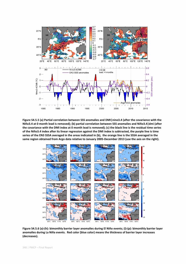
348 | PMCP – Final Report
Figure S4.5.5 (a) Partial correlation between SSS anomalies and DMI|nino3.4 (after the covariance with the Niño3.4 at 0 month lead is removed); (b) partial correlation between SSS anomalies and Niño3.4|dmi (after the covariance with the DMI index at 0 month lead is removed); (c) the black line is the residual time series of the Niño3.4 index after its linear regression against the DMI index is subtracted, the purple line is time series of the EN3 SSSA averaged in the areas indicated in (b), the orange line is the SSSA averaged in the same region obtained from Argo data relative to January 2005‐December 2013 (use the axis on the right).
Figure S4.5.6 (a)‐(h): bimonthly barrier layer anomalies during El Niño events; (i)‐(p): bimonthly barrier layer anomalies during La Niña events. Red color (blue color) means the thickness of barrier layer increases (decreases).
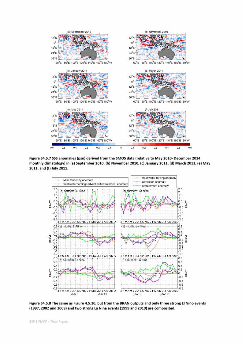
349 | PMCP – Final Report
Figure S4.5.7 SSS anomalies (psu) derived from the SMOS data (relative to May 2010‐ December 2014 monthly climatology) in (a) September 2010, (b) November 2010, (c) January 2011, (d) March 2011, (e) May 2011, and (f) July 2011.
Figure S4.5.8 The same as Figure 4.5.10, but from the BRAN outputs and only three strong El Niño events (1997, 2002 and 2009) and two strong La Niña events (1999 and 2010) are composited.
350 | PMCP – Final Report
Coral record of southeast Indian Ocean marine heat waves with intensified Western Pacific temperature gradient
Authors: Zinke J, Hoell A, Lough JM, Feng M, Kuret AJ, Clarke H, Ricca V, Rankenburg K, McCulloch MT.
Published in Nature Communications 6 (2015):8562.
Abstract
Increasing intensity of marine heatwaves has caused widespread mass coral bleaching events, threatening the integrity and functional diversity of coral reefs. Here we demonstrate the role of inter‐ocean coupling in amplifying thermal stress on reefs in the poorly studied southeast Indian Ocean (SEIO), through a robust 215‐year (1795–2010) geochemical coral proxy sea surface temperature (SST) record. We show that marine heatwaves affecting the SEIO are linked to the behaviour of the Western Pacific Warm Pool on decadal to centennial timescales, and are most pronounced when an anomalously strong zonal SST gradient between the western and central Pacific co‐occurs with strong La Niña. This SST gradient forces large‐scale changes in heat flux that exacerbate SEIO heatwaves. Better understanding of the zonal SST gradient in the Western Pacific is expected to improve projections of the frequency of extreme SEIO heatwaves and their ecological impacts on the important coral reef ecosystems off Western Australia.
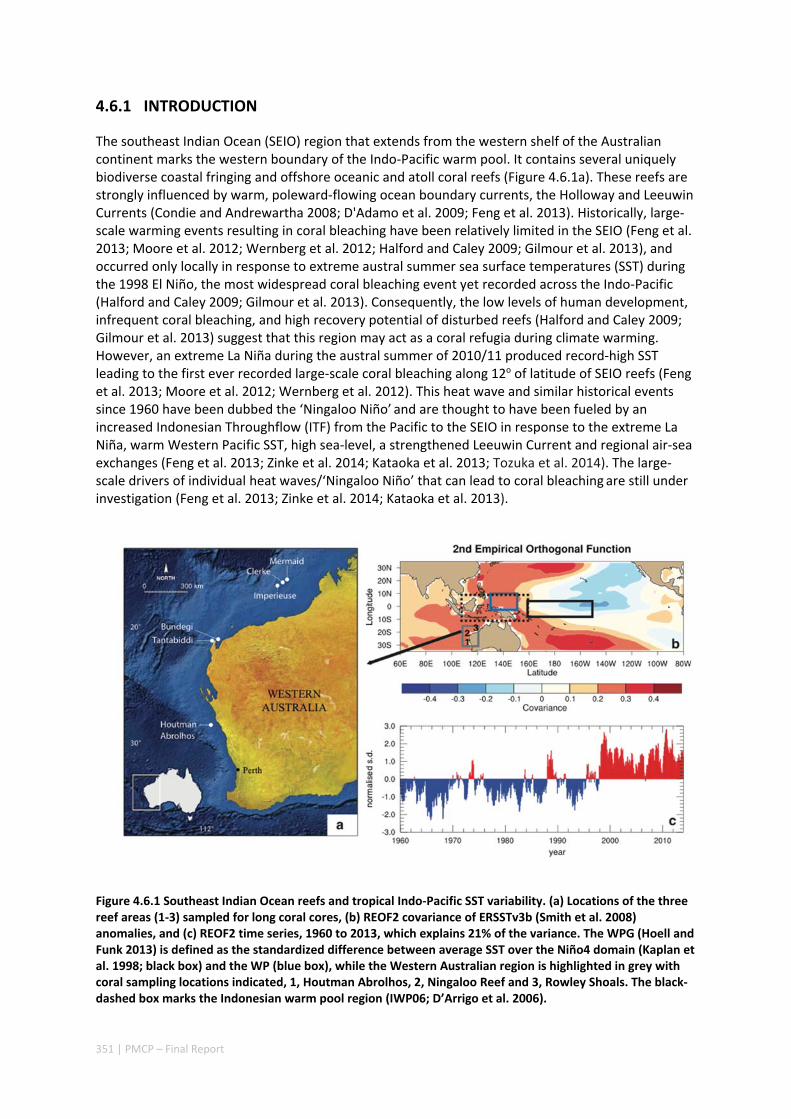
351 | PMCP – Final Report
4.6.1 INTRODUCTION
The southeast Indian Ocean (SEIO) region that extends from the western shelf of the Australian continent marks the western boundary of the Indo‐Pacific warm pool. It contains several uniquely biodiverse coastal fringing and offshore oceanic and atoll coral reefs (Figure 4.6.1a). These reefs are strongly influenced by warm, poleward‐flowing ocean boundary currents, the Holloway and Leeuwin Currents (Condie and Andrewartha 2008; D'Adamo et al. 2009; Feng et al. 2013). Historically, large‐scale warming events resulting in coral bleaching have been relatively limited in the SEIO (Feng et al. 2013; Moore et al. 2012; Wernberg et al. 2012; Halford and Caley 2009; Gilmour et al. 2013), and occurred only locally in response to extreme austral summer sea surface temperatures (SST) during the 1998 El Niño, the most widespread coral bleaching event yet recorded across the Indo‐Pacific (Halford and Caley 2009; Gilmour et al. 2013). Consequently, the low levels of human development, infrequent coral bleaching, and high recovery potential of disturbed reefs (Halford and Caley 2009; Gilmour et al. 2013) suggest that this region may act as a coral refugia during climate warming. However, an extreme La Niña during the austral summer of 2010/11 produced record‐high SST leading to the first ever recorded large‐scale coral bleaching along 12o of latitude of SEIO reefs (Feng et al. 2013; Moore et al. 2012; Wernberg et al. 2012). This heat wave and similar historical events since 1960 have been dubbed the ‘Ningaloo Niño’ and are thought to have been fueled by an increased Indonesian Throughflow (ITF) from the Pacific to the SEIO in response to the extreme La Niña, warm Western Pacific SST, high sea‐level, a strengthened Leeuwin Current and regional air‐sea exchanges (Feng et al. 2013; Zinke et al. 2014; Kataoka et al. 2013; Tozuka et al. 2014). The large‐scale drivers of individual heat waves/‘Ningaloo Niño’ that can lead to coral bleaching are still under investigation (Feng et al. 2013; Zinke et al. 2014; Kataoka et al. 2013).
Figure 4.6.1 Southeast Indian Ocean reefs and tropical Indo‐Pacific SST variability. (a) Locations of the three reef areas (1‐3) sampled for long coral cores, (b) REOF2 covariance of ERSSTv3b (Smith et al. 2008) anomalies, and (c) REOF2 time series, 1960 to 2013, which explains 21% of the variance. The WPG (Hoell and Funk 2013) is defined as the standardized difference between average SST over the Niño4 domain (Kaplan et al. 1998; black box) and the WP (blue box), while the Western Australian region is highlighted in grey with coral sampling locations indicated, 1, Houtman Abrolhos, 2, Ningaloo Reef and 3, Rowley Shoals. The black‐dashed box marks the Indonesian warm pool region (IWP06; D’Arrigo et al. 2006).
352 | PMCP – Final Report
Hoell and Funk (2013) and Hoell et al. (2014, 2015) showed that during both El Niño and La Niña events the global impacts, including the SEIO, in terms of SST, atmospheric circulation and precipitation, were more severe when the SST anomalies in the western Pacific were strongly opposing those in the central Pacific SST than when the western Pacific SST anomalies were near neutral. Hoell and Funk (2013) described this gradient between the western and central Pacific as the Western Pacific Gradient (WPG; Hoell and Funk 2013). The WPG (Hoell and Funk 2013) is defined as the standardized difference between the central Pacific (Niño4 region (Kaplan et al. 1998); 5°S‐5°N, 160‐210°E) and western Pacific SST (0‐10°N, 130‐150°E) between 1854 to 2010 from the 2° 2° gridded extended reconstructed SST from NOAA version 3b (Smith et al. 2008) (hereafter ERSST (Smith et al. 2008); Figure 4.6.1; Supplementary Fig. 1). These studies (Hoell and Funk 2013; Hoell et al. 2014; Hoell et al. 2015) show that the SST gradient between the central (Niño4 region) and the western Pacific was an important measure of interannual to multi‐decadal Pacific climate variability in addition to any previously derived metric of El Niño‐Southern Oscillation (ENSO; Kaplan et al. 1998) or combination of ENSO metrics (see Table 2 of Hoell and Funk 2013).
Due to the remoteness of SEIO reefs and sparseness of historical data, it is hard to quantify the magnitude of temperature stress during past ‘Ningaloo Niño’, La Niña and WPG events. It is also not well known whether SEIO heatwaves always have a close association with ENSO on decadal or centennial timescales and whether they preferentially occur during a La Niña‐like mean state in the Pacific.
Here we aim to explore historical SST variability and occurrence of warm events in the SEIO and, for the first time, the role of the recently identified SST gradient between the Western and Central Pacific, the WPG (Hoell and Funk 2013), as a large‐scale driver in exacerbating heatwaves in the SEIO. To overcome the limitations of short‐term instrumental observations, coral proxy records of SST were developed from ten long Porites spp. coral cores at three locations covering 11° of latitude (17–28°S) off the coast of Western Australia. Here we present a well‐replicated 215‐year reconstruction of annual SST for the SEIO based on coral Sr/Ca ratios and stable isotopes. The emergent long‐term SST trends and interannual to multi‐decadal variability highlight the key role of an increased WPG (Hoell and Funk 2013; Hoell et al. 2014; Hoell et al. 2015), often in concert with strong La Niña’s, in triggering extreme warm events in the SEIO. We trace the cause of historical heatwaves to large energy flux changes associated with an increased WPG (Hoell and Funk 2013) as a result of the western Pacific warming faster than the central Pacific, illustrated by the second rotated empirical orthogonal function of tropical Indo‐Pacific SST (Hoell and Funk 2013; Figure 4.6.1b,c; Supplementary Fig. 1). We show that the magnitude of the WPG varies independently between individual El Niño and La Niña events (Zinke et al. 2014; Kataoka et al. 2013; Tozuka et al. 2014; Hoell and Funk 2013; Hoell et al. 2014; Hoell et al. 2015) resulting in modification of the large‐scale tropical circulation and precipitation fields (Hoell and Funk 2013; Hoell et al. 2015) affecting the energy and heat flux terms, warm water ocean advection through the coastal waveguide and sea‐level pressure in the SEIO and ultimately the magnitude of SEIO marine heatwaves.
4.6.2 METHODS
Core locations and sampling
The Rowley Shoals are located in the eastern tropical Indian Ocean, on the edge of the northwest Australian shelf, forming an extended shelf region of tertiary carbonate composition bounded by shelf edge atolls (Babcock et al. 1994). Two cores were obtained in 2009 from Imperieuse Reef (Figure 4.6.1), the southernmost reef of the Rowley Shoals, and are part of an ongoing study into the
353 | PMCP – Final Report
climatological history of Australia’s coral reefs conducted by AIMS (Cooper et al. 2012). Each of the 90 mm diameter cores (IMP05A, 17°5196’S, 118°969’E; 8‐m water depth, 3.43‐m long) and IMP03A (17°5369’S, 118°974’E, 14‐m water depth, 3.11‐m long) were taken from bommies of Porites genus ~2‐km apart. Two 70‐mm diameter cores CLE09 (1.5‐m long, 10‐m water depth) and MER09 (1.5‐m long, 17‐m water depth) were obtained from Clerke (northernmost atoll) and Mermaid (halfway between Imperieuse and Clerke) reefs during research cruises of AIMS and the University of Western Australia (UWA), respectively, in 2009.
Ningaloo Reef extends over 300 km and includes the only example in the world of an extensive fringing coral reef on the west coast of a continent. Ningaloo Marine Park (NMP) was listed as a World Heritage site in 2013 (Depczynski et al. 2013). Tantabiddi Reef lies in the north‐western section of NMP and forms a narrow lagoon which provides rapid exchange with the open ocean and the Leeuwin Current (LC). Bundegi Reef lies in the north‐eastern section of the NMP, an area that extends into the shallow Exmouth Gulf. Coral cores (Porites spp.) from Tantabiddi (TNT07C; 21°91’S, 113°97’E; 2.5‐m water depth, 1.55 m long) and Bundegi (BUN05C; 21°87’S,114°17’E; 2‐m water depth; 1.78‐m long) were drilled in October 2008 by AIMS (Cooper et al. 2012). Both corals sampled were from inner reef environments located within 200–300 m of the shoreline. Growth rates for the corals were determined from the X‐ray photographs and were between 1–1.6 cm per year for Tantabiddi and 1.2–1.9 cm per year Bundegi. The published stable isotope record from Tantabiddi Reef extends from 1878 to 1994 (Kuhnert et al. 1999). A core of 2.8 m in length from 3‐m water depth was recovered in May 1995 (growth rate ranged between 1.04 and 1.36 cm per year). Coral cores from the Houtman Abrolhos Islands (HAI; cores HAB10A and HAB05B) are described in detail in Kuhnert et al. (2000) and Zinke et al. (2014). The HAI are a group of carbonate platforms lying approximately 50–60 km offshore of the western coast of Western Australia (WA), and is the southernmost true coral reef formation SouthEast Indian Ocean (SEIO; Veron and Marsh 1988). The HAI lie within the path of the LC, and support an astonishing diversity of corals for such a high latitude reef (28.5°S, 113°E). Given their latitude, the HAI are subject to relatively low seasonal SST variation of ~4°C, largely attributable to the LC (Abdo et al. 2012). The intra‐annual variation in salinity of ~0.4 p.s.u. is also low (Abdo et al. 2012). However, interannual variability of mean annual HAI SST is high, with La Niña years being significantly warmer (annual mean temperature in 2011 was 1.5°C above twentieth century average SST) than El Niño years (Abdo et al. 2012).
The cored colonies were all ≥1.5 m in height and on the leeward side of the reef. Cores were extracted using a hydraulic drill, and the hole was then sealed with a concrete plug to prevent microbial infection, colonization of the bore hole and to allow recolonization by the living tissue layer. The use of replicate cores from the same area allowed smoothing of any inconsistencies and minimizing the presence of false signals from localized environmental factors (Delong et al. 2011).
Following initial sectioning and preparation by AIMS and UWA, core slices were cut into sections ~500‐mm long using a Buehler IsoMet 1000 precision sectioning saw. Joints between subsections were cut on an interlocking angle to ensure appropriate sampling overlap, thus preserving the chronology. Slices were visually inspected aided by densitometry measurements (Cooper et al. 2012) for diagenesis along the growth axis, which may impart an artificial cooling/warming signal (Delong et al. 2011; Delong et al. 2013). The segments were then cut as needed to allow router access to the principal growth axis and exposing a ledge for milling. Using a Zenbot CNC controlled Hitachi router with a 4‐mm routing bit, the ledge was milled 2.5 mm inwards from the growth axis for each consecutive high and low‐density band comprising one coral growth year. This excess material was removed to ensure that any surface contaminants from handling could not contaminate the next sample.
Each slab was then cleaned with a reagent‐grade solution of sodium hypochlorite (NaOCl) and milli‐Q water at a 1:1 ratio for 24 h. This process removes excess organic material, particularly in the

354 | PMCP – Final Report
tissue layer, whilst preserving the trace element composition of the sample (Nagtegaal et al. 2012). Excess NaOCl and particulate matter were then removed from the slab by ultrasonic cleaning in deionized water for thirty minutes, with the water replaced at 10‐min intervals. Finally, the sections were dried in a Contherm Thermotec 2000 drying oven.
Skeletal density banding was prominent in all cores (visible in X‐rays) and were the dominant control for determining age relationships and the orientations of the growth axes given their established use as coral chronometers (Lough and Cooper 2011; Supplementary Figs 11–16). Luminescence banding was used to confirm the position/orientation of the growth axes where density banding was difficult to interpret in small sections of the cores. Density and luminescence banding on the whole cores showed excellent agreement and thus their combined use enabled the most accurate interpretation of the orientation of the growth axis.
Sr/Ca and stable isotope analysis.
Following the method of Zinke et al. (2014), annual samples of ~50 mg (mean 52.28 mg; s.d.±1.03 mg) of finely powdered core dust were homogenized and then weighed into thoroughly cleaned 5‐ml Eppendorf tubes, then dissolved in 2.1 ml of 0.562 N HNO3. The dissolved samples were first diluted to a calcium concentration of 100 p.p.m. by taking an aliquot of 30 µl from the primary dissolution and adding 2.7 ml of 2% HNO3. The final trace element aliquots were prepared at 10 p.p.m. by using a 30 µl aliquot of the first dilution and adding 2.7 ml of 2% HNO3 spiked with trace concentrations of scandium, bismuth, praseodymium and yttrium so that the sensitivity of the instruments could be scaled.
Samples were analysed for trace element concentration on a Thermo Scientific XSERIES 2 quadrupole inductively coupled plasma mass spectrometer. The standard reference material for calibration is the JCp‐1 Porites sp. standard prepared by the Geological Survey of Japan (Okai et al. 2002). All Sr/Ca data are normalized to JCp‐1 with Sr/Ca = 8.838 mmol.mol‐1. External reproducibility has been checked by repeated analysis (N = 150) of our in‐house coral (Porites sp.) standard Davies Reef (DR) which gives Sr/Ca = 8.953±0.34% (2σ).
The stable oxygen isotope (δ18O) ratios in Kuhnert et al. (1999; 2000) were analysed on a Finnigan MAT 251 mass spectrometer calibrated against NBS‐19. They are reported in per mil versus Vienna Pee Dee Belemnite isotope scale (‰ VPDB). Analytical errors of replicate measurements of an internal laboratory standard (Solnhofen limestone) are less than ±0.07 for δ18O. The δ18O analyses of the new HAB10A coral record was undertaken at the West Australian Biogeochemistry Centre (WABC) at UWA following the protocol of Paul and Skrzypek (Paul and Skrzypek 2006). δ18O was analysed using GasBench II coupled with Delta XL Isotope Ratio Mass Spectrometer (Thermo‐Fisher Scientific, Bremen, Germany). All results were expressed using the standard δ‐notation (δ18O) and reported in per mil (‰) after normalization to the Vienna Pee Dee Belemnite isotope scale (‰ VPDB). The multi‐point normalization was based on three international standards NBS18, NBS19 and L‐SVEC, each replicated twice (Paul et al. 2007). The analytical uncertainty was lower than ±0.10‰ (1σ) for δ18O. The proxy SST data from this study will be made available through NOAA paleoclimate database (www.ncdc.noaa.gov/paleo/).
Age models and reconstructions.
We developed all chronologies based on annual density banding assisted by luminescence banding. For the Abrolhos corals, we adopted a second step to assess the agreement between geochemical records where we had additional information based on a long higher resolution sampling (Kuhnert et al. 1999). The new cores HAB05B and HAB10A had some horizons where annual banding was not very clear in the X‐rays. Therefore, we used the COFECHA tool to cross‐date the individual

355 | PMCP – Final Report
Figure 4.6.2 Southeast Indian Ocean coral SST anomaly reconstruction and Western Pacific SST anomalies. (a) Reconstructed annual WA coral SST anomaly (red) with 95% confidence interval (grey shaded) based on the spread of both coral and ERSST standard deviations between 1961 to 1990 compared to Indonesian warm pool (D’Arrigo et al. 2006; IWP06; blue) and WP SST anomaly reconstructions (Smith et al. 2008; black). SST anomalies are relative to 1961‐1990 mean, (b) Number of coral cores through time, (c) Reconstruction skill statistics for WA coral SST against regional ERSST (Smith et al. 2008; 17‐28°S, 113‐119°E) are calculated over the validation period (1920‐1949) for each proxy nest, including the coefficient of determination (Rsq, magenta), the reduction of error (RE, orange), and the coefficient of efficiency (CE, black) and (d) Same as (a), but detrended time series.
geochemical records with the annualized high‐resolution record from Kuhnert et al. (1999; see Methods in Zinke et al. 2014). This indicated the critical time intervals in need of optimization in the Abrolhos records. For Ningaloo and Rowley Shoals, no adjustment was needed. Annual band counting for all cores was based on annually sampled records only and all agreed with the number of years in the geochemical records. A composite SST record was created by (i) normalizing (subtract mean and divide by s.d.) each individual coral geochemical record to its variance using the time period 1961–1990 shared by all cores, (ii) averaging all records to form a composite chronology for the three reef areas and (iii) averaging all three composite reef records to form a SEIO composite chronology (hereafter WA coral SST). We converted our normalized SEIO coral composite proxy record to SST by scaling it to the s.d. of ERSSTv3b (Smith et al. 2008; over the period 1961–1990), the longest and most reliable continuous SST dataset for the SEIO region, over the region 17–28°S, 113–
356 | PMCP – Final Report
119°E. To determine the accuracy of the long‐term composite record, we calculated the 95% confidence interval in the spread of the SST s.d. (grey shading in Figure 4.6.2a,d) for 1961–1990 in both WA coral SST and ERSSTv3b (Smith et al. 2008) and subsequently estimated the spread in the scaling coefficient. We used the maximum spread in the scaling coefficient as uncertainty bounds on our final coral record for both WA coral SST with trend (grey shading in Figure 4.6.2a) and for detrended data (grey shading in Figure 4.6.2d). To allow for the number of coral records decreasing backwards in time, reconstruction skill statistics (Cook et al. 1999) for each nest of SST reconstructions starting with 2 records and ending with the composite record of all 10 proxy time series were calculated over the validation period 1920–1949, including the coefficient of determination (Rsq), the reduction of error (RE), and CE (Figure 4.6.2c). Values of RE (CE) above zero indicate some statistical skill in that the reconstructed values over the validation period are better estimates of SST than the mean of the calibration (validation) period. The calibration period was 1950–2008 and comprised two‐thirds of the years that the proxy and instrumental SST time series with best data coverage shared in common, with the validation period (1920–1949) comprising the remaining one‐third. The choice of the validation period was largely based on the HadSST3 (Kennedy et al. 2011) data sets for the West Australia region (17–28°S, 113‐19°E) which showed large data gaps between 1870 and 1920.
Instrumental data
The reconstructed annual SST was verified against four SST data sets: (1) the NOAA 0.25° 0.25° gridded Advanced Very High‐Resolution Radiometer Optimally Interpolated SST (Reynolds et al. 2007; AVHRR OISSTv2 1981 to 2010); (2) the 2° 2° gridded extended reconstructed SST from NOAA version 3b (Smith et al. 2008); (3) the 1° 1° gridded HadISST (Rayner 2003; 1870–2010); and (4) 5° 5° gridded HadSST3 (Kennedy et al. 2011), the latter two from the UK Hadley Centre
(Supplementary Tables 1–4). We use the Western Pacific SST gradient (WPG; Hoell and Funk 2013) defined as the standardized difference between the central Pacific (Niño4 region14; 5°S–5°N, 160–210°E) and western Pacific SST (0–10°N, 130–150°E) between 1854 and 2010. All data sets were accessed via the Royal Netherlands Meteorological Institute (KNMI) online climate explorer (Trouet and van Oldenborgh 2013).
Paleo‐WPG from paleoclimate data
We extracted the mean annual Niño3.4 reconstructions from www.ncdc.noaa.gov/paleo/ (Wilson et al. 2010; Emile‐Geay et al. 2013). The Indonesian warm pool SST reconstruction (IWP06 (D’Arrigo et al. 2006)) was kindly provided by Rosanne D’Arrigo. We extracted La Niña events from two Niño 3.4 paleoreconstructions (Wilson et al. 2010; Emile‐Geay et al. 2013). For the Wilson et al. (2010) Niño 3.4 reconstruction we selected the negative anomalies that correspond with weak to extreme La Niña events. We computed a paleo‐WPG between 1795 and 1992 from the difference between annual mean IWP06 (Wood ruff et al. 2015) and a reconstruction of the annual mean Niño 3.4 index (Wilson et al. 2010). This differs from the observational WPG defined as the standardized difference between the central Pacific (Niño4 region (Kaplan et al. 1998); 5°S–5°N, 160–210°E) and western Pacific SST15 (0–10°N, 130–150°E). The IWP06 record does include the western Pacific region (0–10°N, 130–150°E), yet is of larger extent. Currently, no paleoclimatic reconstruction is available for the Niño4 region, so we relied on the Niño3.4 index of Wilson et al. (Wilson et al. 2010) which is significantly correlated with the Niño4 index (r = 0.82 (r =0.76–0.87, 95% confidence interval), P < 0.001, N = 138). The Niño3.4 region also represents the central tropical Pacific and shares a large amount of variance with the Niño4 region (r = 0.92, P < 0.001, N = 138) and is therefore considered the best available record to calculate a paleo‐WPG. We note that the standard deviation of IWP06 and the Niño3.4 reconstruction are of different magnitude than the observational indices for the WP SST and Niño3.4. Nevertheless, we verified our approach by directly comparing the observed WPG with our paleo‐WPG to ensure that the timing and relative magnitudes of anomalies were well

357 | PMCP – Final Report
matched with the observational record. The correlation between the (detrended) observed WPG and paleo‐WPG was significant (r = 0.67 (r = 0.57–0.75, 95% confidence interval), P < 0.001, N = 138). Considering only data after 1880, where SST observations are considered more reliable, resulted in a higher correlation between WPG and paleo‐WPG (r = 0.77 (r = 0.69–0.82, 95% confidence interval), P < 0.001, N = 112).
4.6.3 RESULTS
Coral geochemical proxy records of sea surface temperature
Porites coral cores were obtained from the Rowley Shoals (17°S, 119°E), Ningaloo Reef (21°S, 113°E) and the Houtman‐Abrolhos Islands (HAI; 28°S, 114°E) between 2008 and 2010 (Cooper et al. 2012; Figure 4.6.1a). Coral δ18O and Sr/Ca are widely used as robust proxies for SST (Corrège 2006; Pfeiffer et al. 2009; Lough 2004). While Sr/Ca is considered to be primarily controlled by SST, coral δ18O can be influenced by both SST and δ18O seawater through precipitation minus evaporation (P – E) influencing surface ocean salinity (Lough 2004). However, interannual changes in P – E at the Rowley Shoals, Ningaloo Reef and HAI are too small to noticeably affect coral δ18O. Therefore, the δ18O record primarily reflects variations in SST. We combine two previously published bimonthly‐resolved coral δ18O records (Kuhnert et al. 1999; Kuhnert et al. 2000) and two annually resolved Sr/Ca records from HAI8 with six new annually resolved Sr/Ca and δ18O records to reconstruct a robust and well‐replicated record of past SST variability in the SEIO (Figure 4.6.2; Supplementary Figs 1–4).
Coral proxy records of SST from three representative reefs of the SEIO were obtained for the period 1795–2010 (Figure 4.6.2; Supplementary Figs 1–2). Least squares linear regressions between individual coral SST reconstructions from the three representative reefs of the SEIO were significant and positive over the record length, typically sharing between 35 to 41% of variance (Supplementary Tables 1–4). The longest records from HAI and Rowley Shoals shared 45% variance between 1798 and 1850 on decadal timescales (>7 years), although the year‐to‐year variability was not always in phase. Subsequently, a composite annual mean SST record for the SEIO including the three reefs was created by (i) normalizing (subtract mean and divide by standard deviation) each individual coral record to its variance using the time period 1961–1990 shared by all cores, (ii) averaging all records to form a composite chronology for the three reef areas, and (iii) averaging all three composite reef records to form a SEIO composite chronology. We converted our normalized SEIO coral composite proxy record to SST (hereafter WA coral SST) by scaling it to the standard deviation (over the period 1961–1990) of the 2° 2° gridded ERSSTv3b (Smith et al. 2008) and ground‐truthed with the 1° 1° gridded HadISST (1870–2010; Rayner 2003) from the UK Hadley Centre (Supplementary Tables 1–7) for the SEIO region 17–28°S, 113–119°E (Figure 4.6.2; Supplementary Figs 3–5).
Least squares linear regression between WA coral SST and the modern SST reconstructions shows significant positive relationships that typically accounted for 20–40% of the SST variance over the entire record length (Supplementary Tables 1–7). Validation statistics show skill of the WA coral reconstruction for most of the record (Figure 4.6.2c). The WA coral SST composite shows long‐term warming (Figure 4.6.2a; Supplementary Fig. 3) with strong multi‐decadal variability superimposed before 1900 and after 1990. However, our WA coral SST record indicates overall cooler mean SST during the nineteenth century up to the mid‐twentieth century than any of the long‐term instrumental SST data for the west Australian shelf (Figure 4.6.2; Supplementary Figs 3 and 4). Although there are weaker long‐term relationships with ship‐based SST reconstructions, the multicore approach provides confidence in the proxy record that would be lacking if based on a single coral core ( Pfeiffer et al. 2009; Lough 2004). The excellent agreement between the coral core
358 | PMCP – Final Report
composite pre‐1900 implies that SST coverage in SST reconstruction data sets based on ICOADS (Wood ruff et al. 2015) ship‐of‐opportunity (Supplementary Figs 3–5) suffers from poor sampling and interpolation from increasingly distant data points.
To assess if mean annual SST capture the major warm events in the SEIO during Ningaloo Niño event years that are normally phase‐locked to austral summer and autumn, we evaluated the occurrence of warm anomalies in mean annual versus monthly time scale ERSSTv.3b (Smith et al. 2008) since 1950 (Supplementary Table 8). This confirmed that mean annual SST did capture the vast majority (18 out of 26 events) of Ningaloo Niño/Niña event years defined in Feng et al. (2013) and Kataoka et al. (2013) (Supplementary Table 8). Our detrended mean annual WA coral SST is also significantly correlated (r = 0.59; P = 0.0001; DF = 59) with the Ningaloo Niño index (Feng et al. 2015; Marshall et al. 2015) between 1948 and 2010, defined for January‐February averages (Supplementary Table 9).
The role of the Western Pacific warm pool for SEIO SST
To assess the role of the Indo‐Pacific warm pool on SEIO SST, we compared our WA coral SST reconstruction with SST proxy records from the Indonesian warm pool (detrended) derived from a multi‐proxy reconstruction (hereafter IWP06; D’Arrigo et al. 2006) and the western Pacific from instrumental data (hereafter WP SST; Smith et al. 2008; Supplementary Table 5). IWP06 extends from 1782 to 1992 and is a composite from annual tree ring and coral records for the Indonesian Archipelago (Figure 4.6.2). For the period 1795 to 1992, the IWP06 and WA coral SST were significantly correlated (r = 0.48, P < 0.001; DF = 195) and this relationship remained statistically significant after detrending (Supplementary Table 5). WA coral SST indicates overall cooler mean SST during the nineteenth century up to the mid‐twentieth century than IWP06. This is in agreement with a recent compilation of tropical coral SST reconstructions (Tierney et al. 2015) that also showed cooler SST in the Indian Ocean than in the Western Pacific for the entire nineteenth and early twentieth century. Both WA coral SST and IWP06 co‐vary on multi‐decadal timescales with highest amplitudes between 1795 and 1850 and post 1980 (Figure 4.6.2). The higher amplitude variations in WA coral SST between 1795 and 1850 are solely based on HAI and RS data sets (four cores). The coral records agree best on decadal timescales in this time interval, and show less agreement for year to year events. Our reconstruction skill statistics also revealed lowest skill for the period 1800–1840 with the coefficient of efficiency (CE) just above zero (Figure 4.6.2c). Thus, the absolute magnitude of SST anomalies between 1795 and 1850 in our reconstruction should be interpreted with caution.
WA coral SST was also significantly correlated with WP SST (r = 0.55; P < 0.001; DF = 154), and this relationship was statistically significant after detrending (Supplementary Table 5). The highest correlation between WA coral SST and WP SST was found after 1980 (r = 0.68; P < 0.001; DF = 28). The same holds for the correlation between WA coral SST and the Niño4 index (Kaplan et al. 1998; r = 0.68; P < 0.001; DF = 28). Post‐1980, WA coral SST was also significantly correlated with the WPG (Hoell and Funk 2013; (r = 0.69; P = 0.002; DF = 28); Figure 4.6.3a). These results indicate that post 1980, SST in the SEIO was most strongly connected with the western Pacific rather than the Indian Ocean, especially the warm pool and Niño4 region, and the WPG (Hoell and Funk 2013; Supplementary Tables 5–7; Supplementary Figs 7–9).
The role of the west pacific gradient for SEIO SST
To assess the importance of western Pacific forcing of SEIO warm events we used the WPG (Hoell and Funk 2013) defined as the standardized difference between the central Pacific (Niño4 region (Kaplan et al. 1998); 5°S–5°N, 160–210°E) and western Pacific SST (0–10°N, 130–150°E) between 1854 and 2010 from ERSST (Smith et al. 2008; Figure 4.6.1). We assessed the long‐term stability of the relationship between WA coral SST and the WPG and La Niña events using detrended data

359 | PMCP – Final Report
(Figure 4.6.3). We also computed a paleo‐WPG between 1795 and 1992 from the difference between IWP06 (D’Arrigo et al. 2006) and a proxy reconstruction of the Niño3.4 index (Wilson et al. 2010) and extracted La Niña events from both the instrumental Niño3.4 (Kaplan et al. 1998) index and a paleoreconstruction (Wilson et al. 2010; Figure 4.6.3). The paleo‐WPG reconstruction was shown to be insensitive to the choice of independent Nino3.4 reconstructions (Wilson et al. 2010; Wilson et al. 2010) (detrended) based on paleoclimate data (Supplementary Fig. 10).
Figure 4.6.3 Western Pacific Gradient—SEIO SST relationship. (a) WPG from observations (y axis inverted) compared to detrended WA coral SST, (b) paleo‐WPG based on the difference between IWP06 (D’Arrigo et al. 2006) and Niño3.4 reconstruction (Wilson et al. 2010), (c) Niño3.4 instrumental index (blue = La Niña; red = El Niño) and La Niña‐like anomalies in the Niño3.4 reconstruction (Wilson et al. 2010) superimposed (orange), and (d) 31‐year running correlations between detrended WA coral SST and paleo‐WPG (red solid line, red stippled 95% confidence interval based on a 1,000‐sample Monte Carlo simulation; Trouet and van Oldenborgh 2013) and WPG from observations (Hoell and Funk 2013; purple solid line, purple stippled 95% confidence interval). Grey shaded areas indicates periods with statistically significant correlations (>95%).
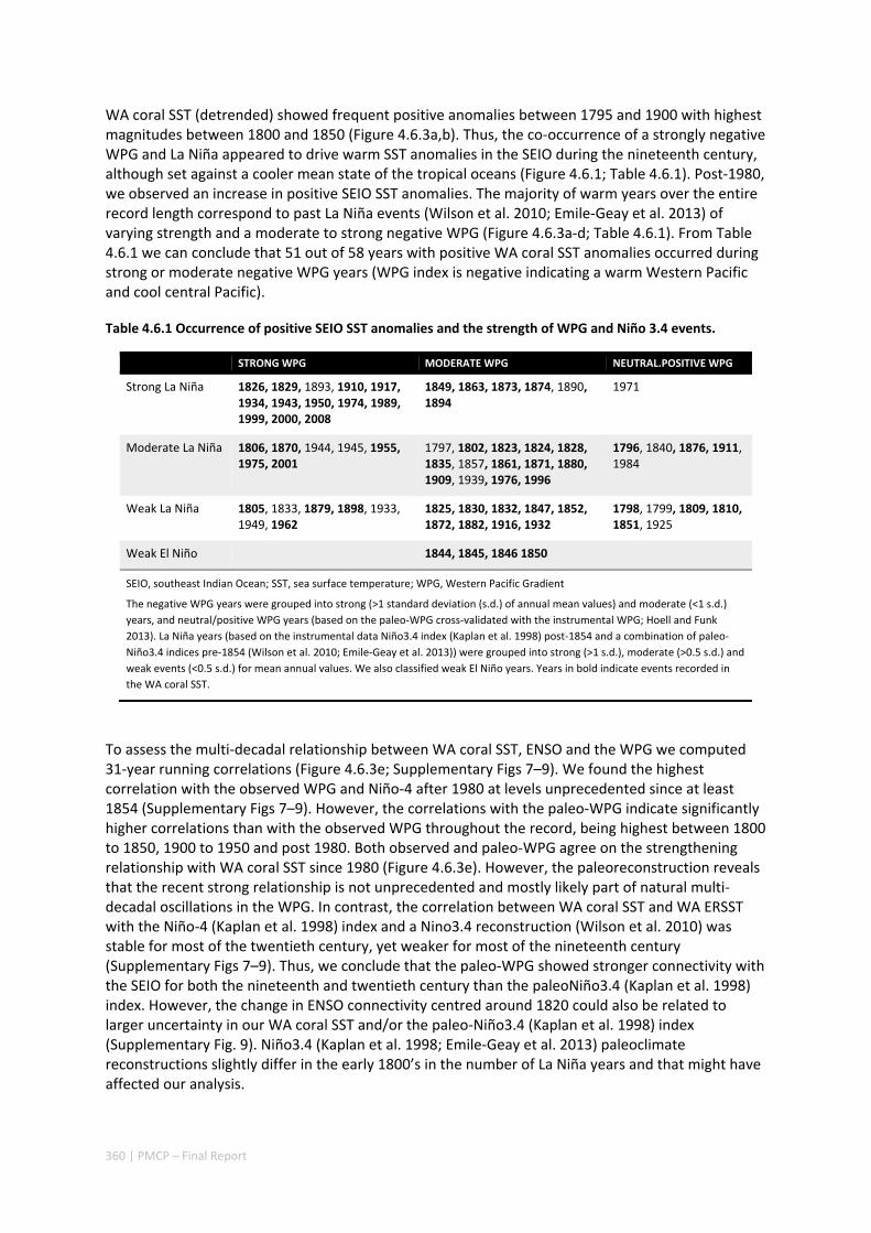
360 | PMCP – Final Report
WA coral SST (detrended) showed frequent positive anomalies between 1795 and 1900 with highest magnitudes between 1800 and 1850 (Figure 4.6.3a,b). Thus, the co‐occurrence of a strongly negative WPG and La Niña appeared to drive warm SST anomalies in the SEIO during the nineteenth century, although set against a cooler mean state of the tropical oceans (Figure 4.6.1; Table 4.6.1). Post‐1980, we observed an increase in positive SEIO SST anomalies. The majority of warm years over the entire record length correspond to past La Niña events (Wilson et al. 2010; Emile‐Geay et al. 2013) of varying strength and a moderate to strong negative WPG (Figure 4.6.3a‐d; Table 4.6.1). From Table 4.6.1 we can conclude that 51 out of 58 years with positive WA coral SST anomalies occurred during strong or moderate negative WPG years (WPG index is negative indicating a warm Western Pacific and cool central Pacific).
Table 4.6.1 Occurrence of positive SEIO SST anomalies and the strength of WPG and Niño 3.4 events.
STRONG WPG MODERATE WPG NEUTRAL.POSITIVE WPG
Strong La Niña 1826, 1829, 1893, 1910, 1917, 1934, 1943, 1950, 1974, 1989, 1999, 2000, 2008
1849, 1863, 1873, 1874, 1890, 1894
1971
Moderate La Niña 1806, 1870, 1944, 1945, 1955, 1975, 2001
1797, 1802, 1823, 1824, 1828, 1835, 1857, 1861, 1871, 1880, 1909, 1939, 1976, 1996
1796, 1840, 1876, 1911, 1984
Weak La Niña 1805, 1833, 1879, 1898, 1933, 1949, 1962
1825, 1830, 1832, 1847, 1852, 1872, 1882, 1916, 1932
1798, 1799, 1809, 1810, 1851, 1925
Weak El Niño 1844, 1845, 1846 1850
SEIO, southeast Indian Ocean; SST, sea surface temperature; WPG, Western Pacific Gradient
The negative WPG years were grouped into strong (>1 standard deviation (s.d.) of annual mean values) and moderate (<1 s.d.)
years, and neutral/positive WPG years (based on the paleo‐WPG cross‐validated with the instrumental WPG; Hoell and Funk
2013). La Niña years (based on the instrumental data Niño3.4 index (Kaplan et al. 1998) post‐1854 and a combination of paleo‐
Niño3.4 indices pre‐1854 (Wilson et al. 2010; Emile‐Geay et al. 2013)) were grouped into strong (>1 s.d.), moderate (>0.5 s.d.) and
weak events (<0.5 s.d.) for mean annual values. We also classified weak El Niño years. Years in bold indicate events recorded in
the WA coral SST.
To assess the multi‐decadal relationship between WA coral SST, ENSO and the WPG we computed 31‐year running correlations (Figure 4.6.3e; Supplementary Figs 7–9). We found the highest correlation with the observed WPG and Niño‐4 after 1980 at levels unprecedented since at least 1854 (Supplementary Figs 7–9). However, the correlations with the paleo‐WPG indicate significantly higher correlations than with the observed WPG throughout the record, being highest between 1800 to 1850, 1900 to 1950 and post 1980. Both observed and paleo‐WPG agree on the strengthening relationship with WA coral SST since 1980 (Figure 4.6.3e). However, the paleoreconstruction reveals that the recent strong relationship is not unprecedented and mostly likely part of natural multi‐decadal oscillations in the WPG. In contrast, the correlation between WA coral SST and WA ERSST with the Niño‐4 (Kaplan et al. 1998) index and a Nino3.4 reconstruction (Wilson et al. 2010) was stable for most of the twentieth century, yet weaker for most of the nineteenth century (Supplementary Figs 7–9). Thus, we conclude that the paleo‐WPG showed stronger connectivity with the SEIO for both the nineteenth and twentieth century than the paleoNiño3.4 (Kaplan et al. 1998) index. However, the change in ENSO connectivity centred around 1820 could also be related to larger uncertainty in our WA coral SST and/or the paleo‐Niño3.4 (Kaplan et al. 1998) index (Supplementary Fig. 9). Niño3.4 (Kaplan et al. 1998; Emile‐Geay et al. 2013) paleoclimate reconstructions slightly differ in the early 1800’s in the number of La Niña years and that might have affected our analysis.
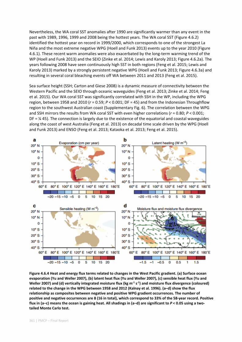
361 | PMCP – Final Report
Nevertheless, the WA coral SST anomalies after 1990 are significantly warmer than any event in the past with 1989, 1996, 1999 and 2008 being the hottest years. The WA coral SST (Figure 4.6.2) identified the hottest year on record in 1999/2000, which corresponds to one of the strongest La Niña and the most extreme negative WPG (Hoell and Funk 2013) events up to the year 2010 (Figure 4.6.1). These recent warm anomalies were also exacerbated by the long‐term warming trend of the WP (Hoell and Funk 2013) and the SEIO (Zinke et al. 2014; Lewis and Karoly 2013; Figure 4.6.2a). The years following 2008 have seen continuously high SST in both regions (Feng et al. 2015; Lewis and Karoly 2013) marked by a strongly persistent negative WPG (Hoell and Funk 2013; Figure 4.6.3a) and resulting in several coral bleaching events off WA between 2011 and 2013 (Feng et al. 2015).
Sea surface height (SSH; Carton and Giese 2008) is a dynamic measure of connectivity between the Western Pacific and the SEIO through oceanic waveguides (Feng et al. 2013; Zinke et al. 2014; Feng et al. 2015). Our WA coral SST was significantly correlated with SSH in the WP, including the WPG region, between 1958 and 2010 (r = 0.59; P < 0.001; DF = 45) and from the Indonesian Throughflow region to the southwest Australian coast (Supplementary Fig. 6). The correlation between the WPG and SSH mirrors the results from WA coral SST with even higher correlations (r = 0.80; P < 0.001; DF = ¼ 45). The connection is largely due to the existence of the equatorial and coastal waveguides along the coast of west Australia (Feng et al. 2013) on decadal time scale driven by the WPG (Hoell and Funk 2013) and ENSO (Feng et al. 2013; Kataoka et al. 2013; Feng et al. 2015).
Figure 4.6.4 Heat and energy flux terms related to changes in the West Pacific gradient. (a) Surface ocean evaporation (Yu and Weller 2007), (b) latent heat flux (Yu and Weller 2007), (c) sensible heat flux (Yu and Weller 2007) and (d) vertically integrated moisture flux (kg m‐1 s‐1) and moisture flux divergence (coloured) related to the change in the WPG between 1958 and 2012 (Kalnay et al. 1996). (a–d) show the flux relationship as composites between negative and positive WPG gradient occurrences. The number of positive and negative occurrences are 8 (16 in total), which correspond to 33% of the 58‐year record. Positive flux in (a–c) means the ocean is gaining heat. All shadings in (a–d) are significant to P < 0.05 using a two‐tailed Monte Carlo test.
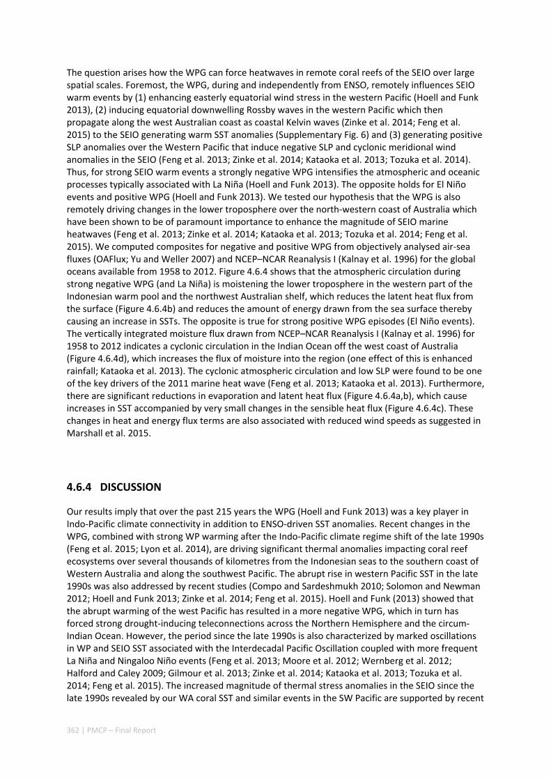
362 | PMCP – Final Report
The question arises how the WPG can force heatwaves in remote coral reefs of the SEIO over large spatial scales. Foremost, the WPG, during and independently from ENSO, remotely influences SEIO warm events by (1) enhancing easterly equatorial wind stress in the western Pacific (Hoell and Funk 2013), (2) inducing equatorial downwelling Rossby waves in the western Pacific which then propagate along the west Australian coast as coastal Kelvin waves (Zinke et al. 2014; Feng et al. 2015) to the SEIO generating warm SST anomalies (Supplementary Fig. 6) and (3) generating positive SLP anomalies over the Western Pacific that induce negative SLP and cyclonic meridional wind anomalies in the SEIO (Feng et al. 2013; Zinke et al. 2014; Kataoka et al. 2013; Tozuka et al. 2014). Thus, for strong SEIO warm events a strongly negative WPG intensifies the atmospheric and oceanic processes typically associated with La Niña (Hoell and Funk 2013). The opposite holds for El Niño events and positive WPG (Hoell and Funk 2013). We tested our hypothesis that the WPG is also remotely driving changes in the lower troposphere over the north‐western coast of Australia which have been shown to be of paramount importance to enhance the magnitude of SEIO marine heatwaves (Feng et al. 2013; Zinke et al. 2014; Kataoka et al. 2013; Tozuka et al. 2014; Feng et al. 2015). We computed composites for negative and positive WPG from objectively analysed air‐sea fluxes (OAFlux; Yu and Weller 2007) and NCEP–NCAR Reanalysis I (Kalnay et al. 1996) for the global oceans available from 1958 to 2012. Figure 4.6.4 shows that the atmospheric circulation during strong negative WPG (and La Niña) is moistening the lower troposphere in the western part of the Indonesian warm pool and the northwest Australian shelf, which reduces the latent heat flux from the surface (Figure 4.6.4b) and reduces the amount of energy drawn from the sea surface thereby causing an increase in SSTs. The opposite is true for strong positive WPG episodes (El Niño events). The vertically integrated moisture flux drawn from NCEP–NCAR Reanalysis I (Kalnay et al. 1996) for 1958 to 2012 indicates a cyclonic circulation in the Indian Ocean off the west coast of Australia (Figure 4.6.4d), which increases the flux of moisture into the region (one effect of this is enhanced rainfall; Kataoka et al. 2013). The cyclonic atmospheric circulation and low SLP were found to be one of the key drivers of the 2011 marine heat wave (Feng et al. 2013; Kataoka et al. 2013). Furthermore, there are significant reductions in evaporation and latent heat flux (Figure 4.6.4a,b), which cause increases in SST accompanied by very small changes in the sensible heat flux (Figure 4.6.4c). These changes in heat and energy flux terms are also associated with reduced wind speeds as suggested in Marshall et al. 2015.
4.6.4 DISCUSSION
Our results imply that over the past 215 years the WPG (Hoell and Funk 2013) was a key player in Indo‐Pacific climate connectivity in addition to ENSO‐driven SST anomalies. Recent changes in the WPG, combined with strong WP warming after the Indo‐Pacific climate regime shift of the late 1990s (Feng et al. 2015; Lyon et al. 2014), are driving significant thermal anomalies impacting coral reef ecosystems over several thousands of kilometres from the Indonesian seas to the southern coast of Western Australia and along the southwest Pacific. The abrupt rise in western Pacific SST in the late 1990s was also addressed by recent studies (Compo and Sardeshmukh 2010; Solomon and Newman 2012; Hoell and Funk 2013; Zinke et al. 2014; Feng et al. 2015). Hoell and Funk (2013) showed that the abrupt warming of the west Pacific has resulted in a more negative WPG, which in turn has forced strong drought‐inducing teleconnections across the Northern Hemisphere and the circum‐Indian Ocean. However, the period since the late 1990s is also characterized by marked oscillations in WP and SEIO SST associated with the Interdecadal Pacific Oscillation coupled with more frequent La Niña and Ningaloo Niño events (Feng et al. 2013; Moore et al. 2012; Wernberg et al. 2012; Halford and Caley 2009; Gilmour et al. 2013; Zinke et al. 2014; Kataoka et al. 2013; Tozuka et al. 2014; Feng et al. 2015). The increased magnitude of thermal stress anomalies in the SEIO since the late 1990s revealed by our WA coral SST and similar events in the SW Pacific are supported by recent
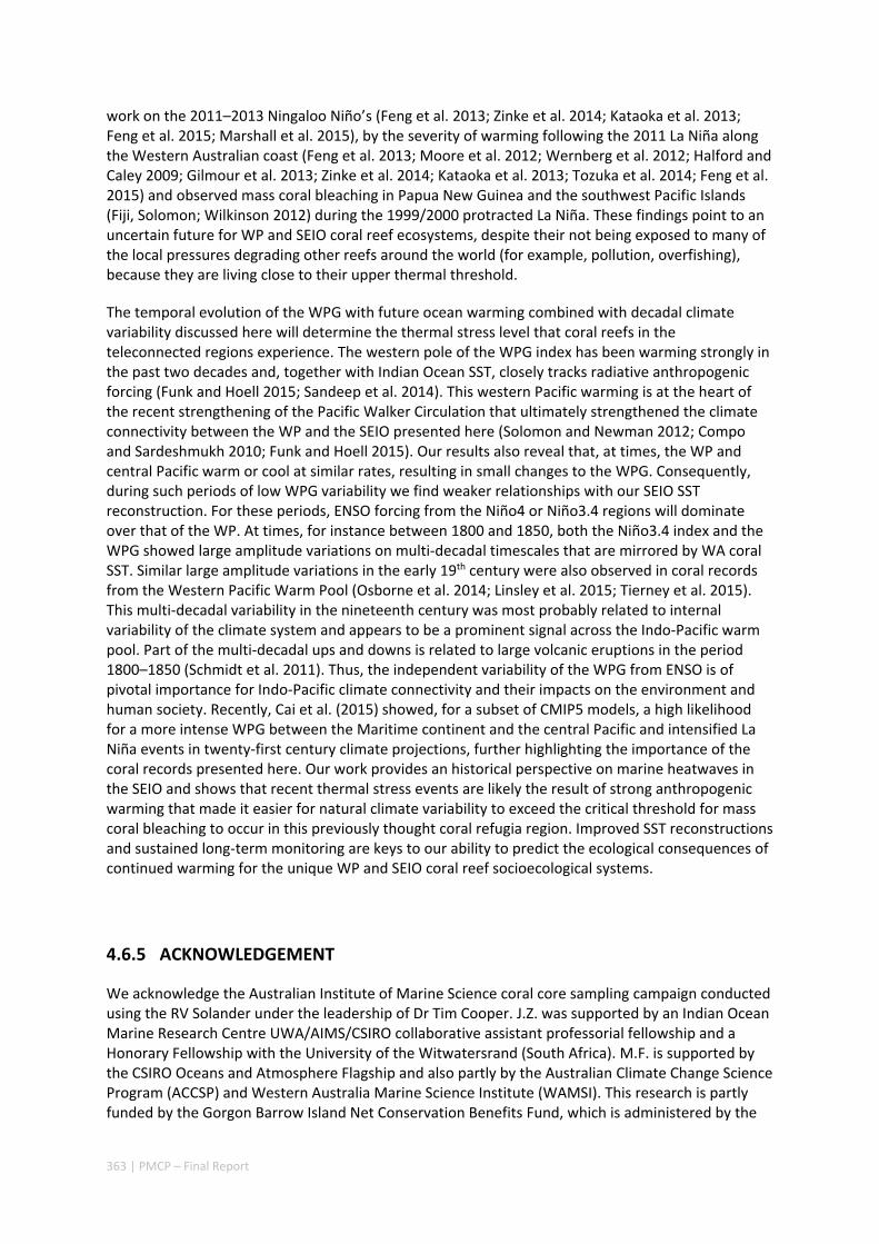
363 | PMCP – Final Report
work on the 2011–2013 Ningaloo Niño’s (Feng et al. 2013; Zinke et al. 2014; Kataoka et al. 2013; Feng et al. 2015; Marshall et al. 2015), by the severity of warming following the 2011 La Niña along the Western Australian coast (Feng et al. 2013; Moore et al. 2012; Wernberg et al. 2012; Halford and Caley 2009; Gilmour et al. 2013; Zinke et al. 2014; Kataoka et al. 2013; Tozuka et al. 2014; Feng et al. 2015) and observed mass coral bleaching in Papua New Guinea and the southwest Pacific Islands (Fiji, Solomon; Wilkinson 2012) during the 1999/2000 protracted La Niña. These findings point to an uncertain future for WP and SEIO coral reef ecosystems, despite their not being exposed to many of the local pressures degrading other reefs around the world (for example, pollution, overfishing), because they are living close to their upper thermal threshold.
The temporal evolution of the WPG with future ocean warming combined with decadal climate variability discussed here will determine the thermal stress level that coral reefs in the teleconnected regions experience. The western pole of the WPG index has been warming strongly in the past two decades and, together with Indian Ocean SST, closely tracks radiative anthropogenic forcing (Funk and Hoell 2015; Sandeep et al. 2014). This western Pacific warming is at the heart of the recent strengthening of the Pacific Walker Circulation that ultimately strengthened the climate connectivity between the WP and the SEIO presented here (Solomon and Newman 2012; Compo and Sardeshmukh 2010; Funk and Hoell 2015). Our results also reveal that, at times, the WP and central Pacific warm or cool at similar rates, resulting in small changes to the WPG. Consequently, during such periods of low WPG variability we find weaker relationships with our SEIO SST reconstruction. For these periods, ENSO forcing from the Niño4 or Niño3.4 regions will dominate over that of the WP. At times, for instance between 1800 and 1850, both the Niño3.4 index and the WPG showed large amplitude variations on multi‐decadal timescales that are mirrored by WA coral SST. Similar large amplitude variations in the early 19th century were also observed in coral records from the Western Pacific Warm Pool (Osborne et al. 2014; Linsley et al. 2015; Tierney et al. 2015). This multi‐decadal variability in the nineteenth century was most probably related to internal variability of the climate system and appears to be a prominent signal across the Indo‐Pacific warm pool. Part of the multi‐decadal ups and downs is related to large volcanic eruptions in the period 1800–1850 (Schmidt et al. 2011). Thus, the independent variability of the WPG from ENSO is of pivotal importance for Indo‐Pacific climate connectivity and their impacts on the environment and human society. Recently, Cai et al. (2015) showed, for a subset of CMIP5 models, a high likelihood for a more intense WPG between the Maritime continent and the central Pacific and intensified La Niña events in twenty‐first century climate projections, further highlighting the importance of the coral records presented here. Our work provides an historical perspective on marine heatwaves in the SEIO and shows that recent thermal stress events are likely the result of strong anthropogenic warming that made it easier for natural climate variability to exceed the critical threshold for mass coral bleaching to occur in this previously thought coral refugia region. Improved SST reconstructions and sustained long‐term monitoring are keys to our ability to predict the ecological consequences of continued warming for the unique WP and SEIO coral reef socioecological systems.
4.6.5 ACKNOWLEDGEMENT
We acknowledge the Australian Institute of Marine Science coral core sampling campaign conducted using the RV Solander under the leadership of Dr Tim Cooper. J.Z. was supported by an Indian Ocean Marine Research Centre UWA/AIMS/CSIRO collaborative assistant professorial fellowship and a Honorary Fellowship with the University of the Witwatersrand (South Africa). M.F. is supported by the CSIRO Oceans and Atmosphere Flagship and also partly by the Australian Climate Change Science Program (ACCSP) and Western Australia Marine Science Institute (WAMSI). This research is partly funded by the Gorgon Barrow Island Net Conservation Benefits Fund, which is administered by the
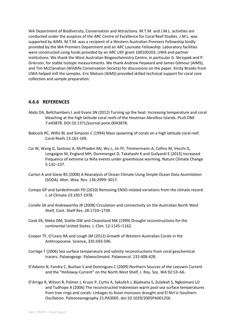
364 | PMCP – Final Report
WA Department of Biodiversity, Conservation and Attractions. M.T.M. and J.M.L. activities are conducted under the auspices of the ARC Centre of Excellence for Coral Reef Studies. J.M.L. was supported by AIMS. M.T.M. was a recipient of a Western Australian Premiers Fellowship kindly provided by the WA Premiers Department and an ARC Laureate Fellowship. Laboratory facilities were constructed using funds provided by an ARC LIEF grant 100100203, UWA and partner institutions. We thank the West Australian Biogeochemistry Centre, in particular G. Skrzypek and P. Grierson, for stable isotope measurements. We thank Andrew Heyward and James Gilmour (AIMS), and Tim McClanahan (Wildlife Conservation Society) for discussions on the paper. Kirsty Brooks from UWA helped mill the samples. Eric Matson (AIMS) provided skilled technical support for coral core collection and sample preparation.
4.6.6 REFERENCES
Abdo DA, Bellchambers L and Evans SN (2012) Turning up the heat: Increasing temperature and coral bleaching at the high latitude coral reefs of the Houtman Abrolhos Islands. PLoS ONE 7:e43878. DOI:10.1371/journal.pone.0043878.
Babcock RC, Willis BL and Simpson C (1994) Mass spawning of corals on a high latitude coral reef. Coral Reefs 13:161‐169.
Cai W, Wang G, Santoso A, McPhaden MJ, Wu L, Jin FF, Timmermann A, Collins M, Vecchi G, Lengaigne M, England MH, Dommenget D, Takahashi K and Guilyardi E (2015) Increased frequency of extreme La Niña events under greenhouse warming. Nature Climate Change 5:132–137.
Carton A and Giese BS (2008) A Reanalysis of Ocean Climate Using Simple Ocean Data Assimilation (SODA). Mon. Wea. Rev. 136:2999–3017.
Compo GP and Sardeshmukh PD (2010) Removing ENSO‐related variations from the climate record. J. of Climate 23:1957‐1978.
Condie SA and Andrewartha JR (2008) Circulation and connectivity on the Australian North West Shelf, Cont. Shelf Res. 28:1724–1739.
Cook ER, Meko DM, Stahle DW and Cleaveland MK (1999) Drought reconstructions for the continental United States. J. Clim. 12:1145–1162.
Cooper TF, O’Leary RA and Lough JM (2012) Growth of Western Australian Corals in the Anthropocene. Science, 335:593‐596.
Corrège T (2006) Sea surface temperature and salinity reconstructions from coral geochemical tracers. Palaeogeogr. Palaeoclimatol. Palaeoecol. 232:408‐428.
D'Adamo N, Fandry C, Buchan S and Domingues C (2009) Northern Sources of the Leeuwin Current and the "Holloway Current" on the North West Shelf, J. Roy. Soc. WA 92:53–66.
D’Arrigo R, Wilson R, Palmer J, Krusic P, Curtis A, Sakulich J, Bijaksana S, Zulaikah S, Ngkoimani LO and Tudhope A (2006) The reconstructed Indonesian warm pool sea surface temperatures from tree rings and corals: Linkages to Asian monsoon drought and El Nin o–Southern Oscillation. Paleoceanography 21:PA3005. doi:10.1029/2005PA001256.
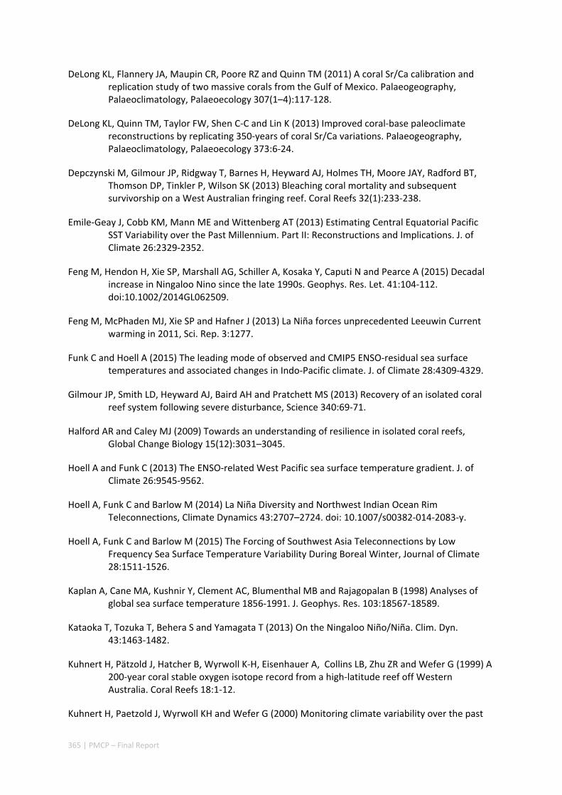
365 | PMCP – Final Report
DeLong KL, Flannery JA, Maupin CR, Poore RZ and Quinn TM (2011) A coral Sr/Ca calibration and replication study of two massive corals from the Gulf of Mexico. Palaeogeography, Palaeoclimatology, Palaeoecology 307(1–4):117‐128.
DeLong KL, Quinn TM, Taylor FW, Shen C‐C and Lin K (2013) Improved coral‐base paleoclimate reconstructions by replicating 350‐years of coral Sr/Ca variations. Palaeogeography, Palaeoclimatology, Palaeoecology 373:6‐24.
Depczynski M, Gilmour JP, Ridgway T, Barnes H, Heyward AJ, Holmes TH, Moore JAY, Radford BT, Thomson DP, Tinkler P, Wilson SK (2013) Bleaching coral mortality and subsequent survivorship on a West Australian fringing reef. Coral Reefs 32(1):233‐238.
Emile‐Geay J, Cobb KM, Mann ME and Wittenberg AT (2013) Estimating Central Equatorial Pacific SST Variability over the Past Millennium. Part II: Reconstructions and Implications. J. of Climate 26:2329‐2352.
Feng M, Hendon H, Xie SP, Marshall AG, Schiller A, Kosaka Y, Caputi N and Pearce A (2015) Decadal increase in Ningaloo Nino since the late 1990s. Geophys. Res. Let. 41:104‐112. doi:10.1002/2014GL062509.
Feng M, McPhaden MJ, Xie SP and Hafner J (2013) La Niña forces unprecedented Leeuwin Current warming in 2011, Sci. Rep. 3:1277.
Funk C and Hoell A (2015) The leading mode of observed and CMIP5 ENSO‐residual sea surface temperatures and associated changes in Indo‐Pacific climate. J. of Climate 28:4309‐4329.
Gilmour JP, Smith LD, Heyward AJ, Baird AH and Pratchett MS (2013) Recovery of an isolated coral reef system following severe disturbance, Science 340:69‐71.
Halford AR and Caley MJ (2009) Towards an understanding of resilience in isolated coral reefs, Global Change Biology 15(12):3031–3045.
Hoell A and Funk C (2013) The ENSO‐related West Pacific sea surface temperature gradient. J. of Climate 26:9545‐9562.
Hoell A, Funk C and Barlow M (2014) La Niña Diversity and Northwest Indian Ocean Rim Teleconnections, Climate Dynamics 43:2707–2724. doi: 10.1007/s00382‐014‐2083‐y.
Hoell A, Funk C and Barlow M (2015) The Forcing of Southwest Asia Teleconnections by Low Frequency Sea Surface Temperature Variability During Boreal Winter, Journal of Climate 28:1511‐1526.
Kaplan A, Cane MA, Kushnir Y, Clement AC, Blumenthal MB and Rajagopalan B (1998) Analyses of global sea surface temperature 1856‐1991. J. Geophys. Res. 103:18567‐18589.
Kataoka T, Tozuka T, Behera S and Yamagata T (2013) On the Ningaloo Niño/Niña. Clim. Dyn. 43:1463‐1482.
Kuhnert H, Pätzold J, Hatcher B, Wyrwoll K‐H, Eisenhauer A, Collins LB, Zhu ZR and Wefer G (1999) A 200‐year coral stable oxygen isotope record from a high‐latitude reef off Western Australia. Coral Reefs 18:1‐12.
Kuhnert H, Paetzold J, Wyrwoll KH and Wefer G (2000) Monitoring climate variability over the past
366 | PMCP – Final Report
116 years in coral oxygen isotopes from Ningaloo Reef, Western Australia. International Journal of Earth Sciences 88:725‐732.
Kalnay E, Kanamitsu M, Kistler R, Collins W, Deaven D, Gandin L, Iredell M, Saha S, White G, Woollen J, Zhu Y, Leetmaa A, Reynolds R, Chelliah M, Ebisuzaki W, Higgins W, Janowiak J, Mo KC, Ropelewski C, Wang J, Jenne R and Joseph D (1996) The NCEP/NCAR 40‐Year Reanalysis Project. Bull. Amer. Meteor. Soc. 77:437‐471.
Kennedy JJ, Rayner NA, Smith RO, Parker DE and Saunby M (2011) Reassessing biases and other uncertainties in sea‐surface temperature observations since 1850: 2. Biases and homogenisation. J. Geophys. Res. 116:D14104. doi:10.1029/2010JD015220.
Lewis SC and Karoly DJ (2013) Anthropogenic contributions to Australia’s record summer temperatures of 2013Geophysical Research Letters 40, 3705–3709.
Linsley BK, Wu HC, Dassié EP and Schrag DP (2015) Decadal changes in South Pacific sea surface temperatures and the relationship to the Pacific decadal oscillation and upper ocean heat content. Geophysical Research Letters 42:2358–2366.
Lough JM (2004) A strategy to improve the contribution of coral data to high‐resolution paleoclimatology. Palaeogeogr. Palaeoclimatol. Palaeoecol. 204:115‐143.
Lough JM and Cooper TF (2011) New insights from coral growth band studies in an era of rapid environmental change. Earth‐Science Reviews 108(3–4):170‐184.
Lyon B, Barnston AG and Dewitt DG (2014) Tropical pacific forcing of a 1998–1999 climate shift: observational analysis and climate model results for the boreal spring season. Climate Dynamics 43:893‐909.
Marshall AG, Hendon HH, Feng M and Schiller A (2015) Initiation and amplification of the Ningaloo Niño. Climate Dynamics 45:9‐10. doi:10.1007/s00382‐015‐2477‐5.
Moore JA, Bellchambers LM, Depczynski MR, Evans RD, Evans SN, Field SN, Friedman KJ, Gilmour JP, Holmes TH, Middlebrook R and Radford BT (2012) Unprecedented Mass Bleaching and Loss of Coral across 12° of Latitude in Western Australia in 2010–11. PLoS ONE 7(12): e51807.
Nagtegaal R, Grove CA, Kasper S, Zinke J, Boer W and Brummer G‐JA (2012) Spectral luminescence and geochemistry of coral aragonite: effects of whole‐core chemical treatments. Chemical Geology 318–319:6‐15.
Okai T, Suzuki A, Kawahata H, Terashima S and Imai N (2002) Preparation of a new geological survey of Japan geochemical reference material: Coral JCp‐1. Geostandards Newsletter 26(1):95‐99.
Osborne MC, Dunbar RB, Mucciarone DA, Druffel E and Sanchez‐Cabeza J‐A (2014) 215‐yr coral 18O time series from Palau records dynamics of the West Pacific Warm Pool following the end of the Little Ice Age. Coral Reefs 33:719–731.
Paul D and Skrzypek G (2006) Flushing time and storage effects on the accuracy and precision of carbon and oxygen isotope ratios of sample using the GasBench II technique. Rapid Commun. Mass Spectrom. 20:2033–2040.
Paul D, Skrzypek G and Forizs I (2007) Normalization of measured stable isotope composition to
367 | PMCP – Final Report
isotope reference scale – a review. Mass Spectrom. 21:3006‐3014.
Pfeiffer M, Dullo W‐C, Zinke J and Garbe‐Schönberg D (2009). Paired coral Sr/Ca and �18O records from the Chagos Archipelago: Late twentieth century warming affects rainfall variability in the tropical Indian Ocean. International Journal of Earth Sciences 98:53‐66. doi:10.007/s00531‐008‐0326‐z.
Rayner NA (2003) Global analyses of sea surface temperature, sea ice, and night marine air temperature since the late nineteenth century. Journal of Geophysical Research 108 (D14).
Reynolds RW, Smith TM, Liu C, Chelton DB, Casey KS and Schlax MG (2007) Daily High‐resolution Blended Analyses for sea surface temperature. J. Climate 20:5473‐5496.
Sandeep S, Stordal F, Sardeshmukh PD and Compo GP (2014) Pacific Walker Circulation variability in coupled and uncoupled climate models. J. of Climate 43:103–117.
Schmidt GA, Jungclaus JH, Ammann CM, Bard E, Braconnot P, Crowley TJ, Delaygue G, Joos F, Krivova NA, Muscheler R, Otto‐Bliesner B, Pongratz J, Shindell DT, Solanki SK, Steinhilber F and Vieira LEA (2011) Climate forcing reconstructions for use in PMIP simulations of the last millennium (v1.0), Geosci. Model Dev. 4:33–45.
Smith TM, Reynolds RW, Peterson TC and Lawrimore J (2008) Improvements to NOAA’s historical merged land–ocean surface temperature analysis (1880–2006), J. of Climate 21: 2283‐2296.
Solomon A and Newman M (2012) Reconciling disparate twentieth‐century Indo‐Pacific ocean temperature trends in the instrumental record. Nature Climate Change 2:691‐699.
Tierney JE, Abram NJ, Anchukaitis KJ, Evans MN, Giry C, Kilbourne KH, Saenger CP, Wu H and Zinke J (2015) Tropical sea‐surface temperatures for the past four centuries reconstructed from coral archives. Paleocenography 30:226‐252. doi:10.1002/2014PA002717.
Tozuka T, Kataoka T and Yamagata T (2014) Locally and remotely forced atmospheric circulation anomalies of Ningaloo Nino/Nina, Clim. Dyn. 43:2197‐2205.
Trouet V and van Oldenborgh GJ (2013) KNMI Climate Explorer: a web‐based research tool for high‐resolution paleoclimatology. Tree Ring Research 69(1):3‐13.
Veron JEN and Marsh LM (1988) Hermatypic corals of Western Australia: records and annotated species list. Records of the Western Australian Museum. Supplement 29:1–136.
Wernberg T, Smale DA, Tuya F, Thomsen MS, Langlois TJ, de Bettignies T, Bennett S and Rousseaux CS (2012) An extreme climate event alters marine ecosystem structure in a global biodiversity hotspot, Nature Climate Change 3:78–82.
Wilkinson CR (ed.) (2012) Status of Coral Reefs, GCRMN Report, Australian Institute of Marine Science, Townsville, 141‐159.
Wilson R, Cook E, D'Arrigo R, Riedwyl N, Evans MN, Tudhope A and Allan R (2010) Reconstructing ENSO: the influence of method, proxy data, climate forcing and teleconnections. Journal of Quaternary Science 25:62‐78.
Woodruff SD, Worley SJ, Lubker SJ, Ji Z, Freeman JE, Berry DI, Brohan P, Kent EC, Reynolds RW, Smith

368 | PMCP – Final Report
SR and Wilkinson C (2011) ICOADS Release 2.5: Extensions and enhancements to the surface marine meteorological archive. Int. J. Climatol. 31:951‐967.
Yu L and Weller RA (2007) Objectively analyzed air‐sea heat fluxes for the global ice‐free oceans (1981–2005). Bull. Ameri. Meteor. Soc. 88:527–539.
Zinke J, Rountrey A, Feng M, Xie S‐P, Dissard D, Rankenburg K, Lough JM and McCulloch MT (2014) Corals record long‐term Leeuwin Current variability during Ningaloo Niño/Niña since 1795, Nature Communications 5:3607. doi:10.1038/ncomms4607.
4.6.7 SUPPLEMENTARY INFORMATION
Supplementary information can be found at: https://www.nature.com/article‐assets/npg/ncomms/2015/151023/ncomms9562/extref/ncomms9562‐s1.pdf
369 | PMCP – Final Report
5. Environmental drivers
Critical time and space scales of chlorophyll‐a and sea surface temperature variation off the northwest coast of Australia
Authors: Rountrey AN, Collin SC, Hardman‐Mountford N, McInnes A, Nguyen HM, Partridge JC, Waite AM.
ABSTRACT
The northwest shelf of Australia is a tropical region of moderate productivity supporting a rich diversity of organisms, but the underlying drivers of productivity are not well understood. We conducted a time series analysis, spanning 1997 through 2012, of satellite‐derived chlorophyll‐a concentration data using seasonal decomposition analysis, principal components analysis, and correlative analysis to elucidate the spatiotemporal variation in chlorophyll‐a and highlight potential drivers of productivity. We identified four zones of variation in chlorophyll‐a. The most variable zone was Zone 1‐ areas shallower than 30 m north of Cape Range, where bottom reflectance and turbidity make interpretation difficult, but where clear seasonal variation is present. Zone 2‐ areas along the 50 m isobath ‐ shows strong correlations with the El Niño / Southern Oscillation. Zone 3, which exhibits a recurring autumn bloom, includes areas between the 50 m and 100 m isobaths from north of Barrow Island to northwest of Broome. The bloom may be associated with early seasonal deepening of the mixed layer in the region. While the majority of variance in the shelf system is attributable to seasonal patterns, there are spatially restricted, aperiodic modes of variation suggestive of upwelling events present in Zone 4, immediately adjacent to Ningaloo Reef.

370 | PMCP – Final Report
5.1.1 INTRODUCTION
In the Indian Ocean off Western Australia, marine productivity is driven by several, often counter‐acting, regional physical forces. The strength of the Indonesian Throughflow (ITF) and inputs from the Eastern Gyral Current (EC) determine regional inputs from the north (Domingues et al. 2007), as well as the pressure gradient driving the oligotrophic coastal boundary current, the Leeuwin Current (LC). Sporadic upwelling, driven by winds from the southwest, is seasonal and topographically constrained along the Australian west coast (Rossi et al. 2013 a and b). In addition, the oligotrophic nature of the region favours organisms that fix atmospheric nitrogen, freeing them from the immediate constraints of oligotrophy (Waite et al. 2014, Raes et al. 2015). On the shelf, the complex interactions between regional and local physical processes such as tides, river flow and cyclones are thought to control rates of pelagic primary production, but these are often difficult to resolve against a strong seasonal cycle occurring in the shelf/slope region (Rousseaux et al. 2012). This results in a complex network of drivers for shelf production, which has been shown to support both local reefs by Wyatt et al. (2012; 2010) and local fisheries (Griffin et al. 2001; Nguyen et al. 2015) off Western Australia. Although some baseline primary production data exists within shallow reef systems in the Ningaloo region (Waite, pers. comm), environmental variability within reefs along the broader coastal region of the Pilbara remains virtually unknown. A mechanistic understanding of productivity drivers is therefore critical to our understanding of ecosystem vulnerability, in an area where industrial development, including dredging, port construction, mine de‐watering, is extremely rapid.
Here, we aim to elucidate the spatial and temporal distributions of the dominant drivers of productivity in the Indian Ocean off Australia´s northwest using statistical analyses of satellite derived chlorophyll‐a (chl a) measurements and temperature records. We show that there are zones of coherent variation present, and their boundaries likely reflect the influences of different physical oceanographic drivers of production. Identification and understanding of these zones will assist in future management of regional ecosystem resources.
Figure 5.1.1 Mean background signal of chl a (in mg m‐3) across the study region over the study period (1998 ‐2002), superimposed on contours of bathymetry. The seasonal component of this background signal is shown in Figure 5.1.2.
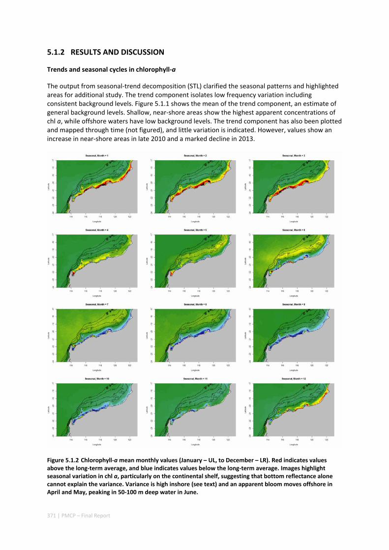
371 | PMCP – Final Report
5.1.2 RESULTS AND DISCUSSION
Trends and seasonal cycles in chlorophyll‐a
The output from seasonal‐trend decomposition (STL) clarified the seasonal patterns and highlighted areas for additional study. The trend component isolates low frequency variation including consistent background levels. Figure 5.1.1 shows the mean of the trend component, an estimate of general background levels. Shallow, near‐shore areas show the highest apparent concentrations of chl a, while offshore waters have low background levels. The trend component has also been plotted and mapped through time (not figured), and little variation is indicated. However, values show an increase in near‐shore areas in late 2010 and a marked decline in 2013.
Figure 5.1.2 Chlorophyll‐a mean monthly values (January – UL, to December – LR). Red indicates values above the long‐term average, and blue indicates values below the long‐term average. Images highlight seasonal variation in chl a, particularly on the continental shelf, suggesting that bottom reflectance alone cannot explain the variance. Variance is high inshore (see text) and an apparent bloom moves offshore in April and May, peaking in 50‐100 m deep water in June.
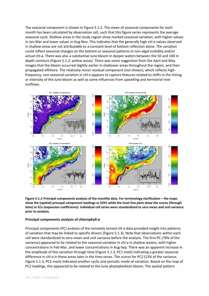
372 | PMCP – Final Report
The seasonal component is shown in Figure 5.1.2. The mean of seasonal components for each month has been calculated by observation cell, such that this figure series represents the average seasonal cycle. Shallow areas in the study region show marked seasonal variation, with higher values in Jan‐Mar and lower values in Aug‐Nov. This indicates that the generally high chl a values observed in shallow areas are not attributable to a constant level of bottom reflection alone. The variation could reflect seasonal changes on the bottom or seasonal patterns in non‐algal turbidity and/or actual chl‐a. There was also a substantial June bloom in deeper waters between the 50 and 100 m depth contours (Figure 5.1.2; yellow areas). There was some suggestion from the April and May images that the bloom occurred slightly earlier in shallower areas throughout the region, and then propagated offshore. The relatively minor residual component (not shown), which reflects high‐frequency, non‐seasonal variation in chl a appears to capture features related to shifts in the timing or intensity of the June bloom as well as some influences from upwelling and terrestrial river outflows.
Figure 5.1.3 Principal components analysis of the monthly data. For terminology clarification – the maps show the (spatial) principal component loadings or EOFs while the inset line plots show the scores (through time) or ECs (expansion coefficients). Individual cell series were standardized to zero mean and unit variance prior to analysis.
Principal components analysis of chlorophyll‐a
Principal components (PC) analysis of the remotely sensed chl a data provided insight into patterns of variation that may be linked to specific drivers (Figure 5.1.3). Note that observations within each cell were standardized to zero mean and unit variance before the analysis. The first PC (78% of the variance) appeared to be related to the seasonal variation in chl a in shallow waters, with higher concentrations in Feb‐Mar, and lower concentrations in Aug‐Sep. There was an apparent increase in the amplitude of this variation through time (Figure 5.1.3, PC1 inset) indicating a greater seasonal difference in chl a in these areas later in the time series. The scores for PC2 (13% of the variance, Figure 5.1.3, PC2 inset) indicated another cyclic and periodic mode of variation. Based on the map of PC2 loadings, this appeared to be related to the June phytoplankton bloom. The spatial pattern

373 | PMCP – Final Report
included Barrow Island and the Montebello Islands as well as areas around Dampier. The 3rd PC (5% of the variance) showed quasi‐periodic patterns in time, and extreme values during the Ningaloo Niño event in 2011. The 4th PC explained only 4% of the variance, but presented a spatial pattern that could be associated with upwelling. The temporal pattern for PC4 was not periodic (Figure 5.1.3, PC4 inset). The Montebello Island region seemed show connections with both “eastern influences” (PC2) and “western influences” (PC4).
Correlation of remotely sensed chlorophyll‐a with ENSO
Mean annual chl a concentrations just inside the 50 m isobath from Barrow Island northward were correlated strongly with El Niño/La Niña (Figure 5.1.4). The mean annual chl a tended to be higher when El Niño conditions occurred in Jan‐Apr (Feng et al. 2015). Some nearshore waters (e.g., Exmouth Gulf) showed consistent negative correlations with ENSO implying that El Niño (La Niña ) conditions at any time during the year lead to reduced (enhanced) apparent chl a (Figure 5.1.4).
Figure 5.1.4 Correlation of mean annual chl a with ENSO for each month. Positive values are represented by the warm (yellow‐red) colours, negative correlations are represented by the cold colours (blue‐purple).
Figure 5.1.5 Correlation of seasonally adjusted and de‐trended chl a with Maitland River discharge.
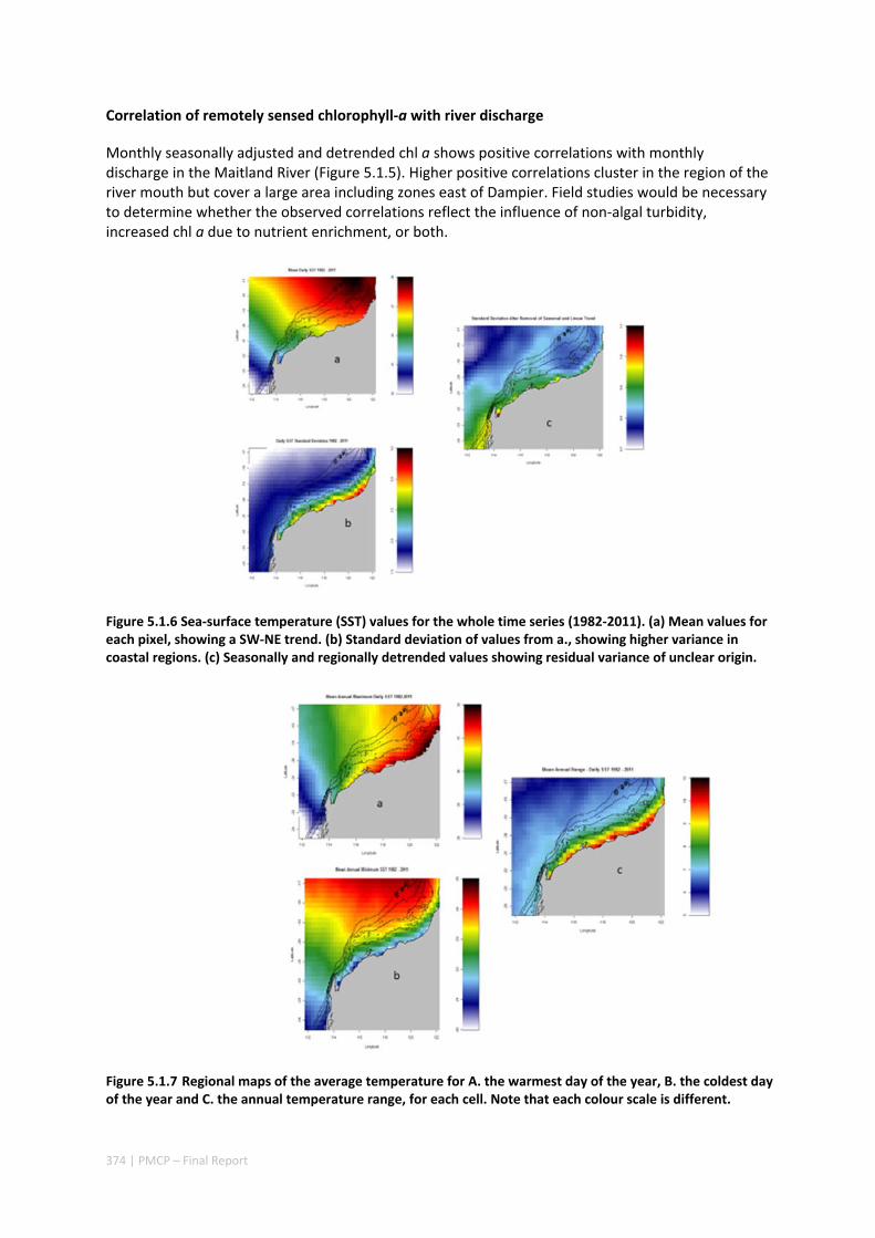
374 | PMCP – Final Report
Correlation of remotely sensed chlorophyll‐a with river discharge
Monthly seasonally adjusted and detrended chl a shows positive correlations with monthly discharge in the Maitland River (Figure 5.1.5). Higher positive correlations cluster in the region of the river mouth but cover a large area including zones east of Dampier. Field studies would be necessary to determine whether the observed correlations reflect the influence of non‐algal turbidity, increased chl a due to nutrient enrichment, or both.
Figure 5.1.6 Sea‐surface temperature (SST) values for the whole time series (1982‐2011). (a) Mean values for each pixel, showing a SW‐NE trend. (b) Standard deviation of values from a., showing higher variance in coastal regions. (c) Seasonally and regionally detrended values showing residual variance of unclear origin.
Figure 5.1.7 Regional maps of the average temperature for A. the warmest day of the year, B. the coldest day of the year and C. the annual temperature range, for each cell. Note that each colour scale is different.
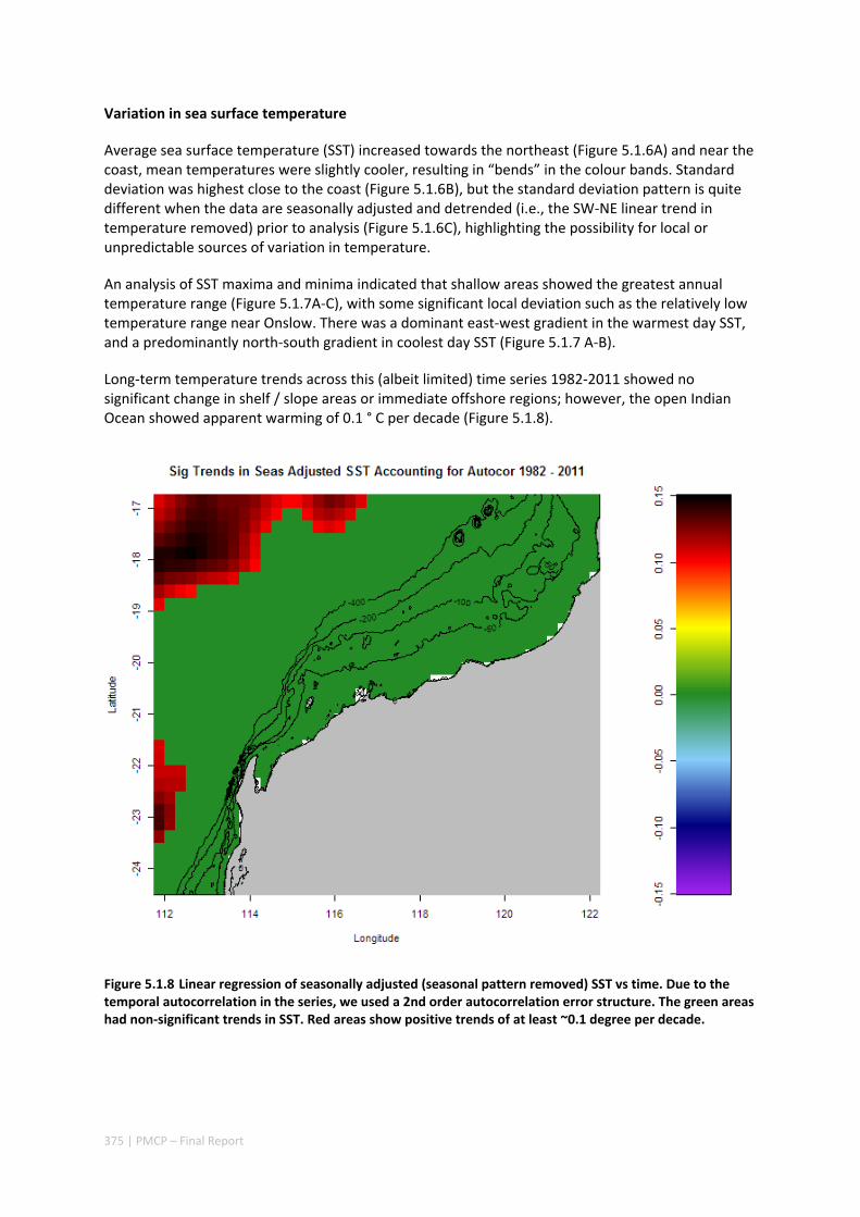
375 | PMCP – Final Report
Variation in sea surface temperature
Average sea surface temperature (SST) increased towards the northeast (Figure 5.1.6A) and near the coast, mean temperatures were slightly cooler, resulting in “bends” in the colour bands. Standard deviation was highest close to the coast (Figure 5.1.6B), but the standard deviation pattern is quite different when the data are seasonally adjusted and detrended (i.e., the SW‐NE linear trend in temperature removed) prior to analysis (Figure 5.1.6C), highlighting the possibility for local or unpredictable sources of variation in temperature.
An analysis of SST maxima and minima indicated that shallow areas showed the greatest annual temperature range (Figure 5.1.7A‐C), with some significant local deviation such as the relatively low temperature range near Onslow. There was a dominant east‐west gradient in the warmest day SST, and a predominantly north‐south gradient in coolest day SST (Figure 5.1.7 A‐B).
Long‐term temperature trends across this (albeit limited) time series 1982‐2011 showed no significant change in shelf / slope areas or immediate offshore regions; however, the open Indian Ocean showed apparent warming of 0.1 ° C per decade (Figure 5.1.8).
Figure 5.1.8 Linear regression of seasonally adjusted (seasonal pattern removed) SST vs time. Due to the temporal autocorrelation in the series, we used a 2nd order autocorrelation error structure. The green areas had non‐significant trends in SST. Red areas show positive trends of at least ~0.1 degree per decade.
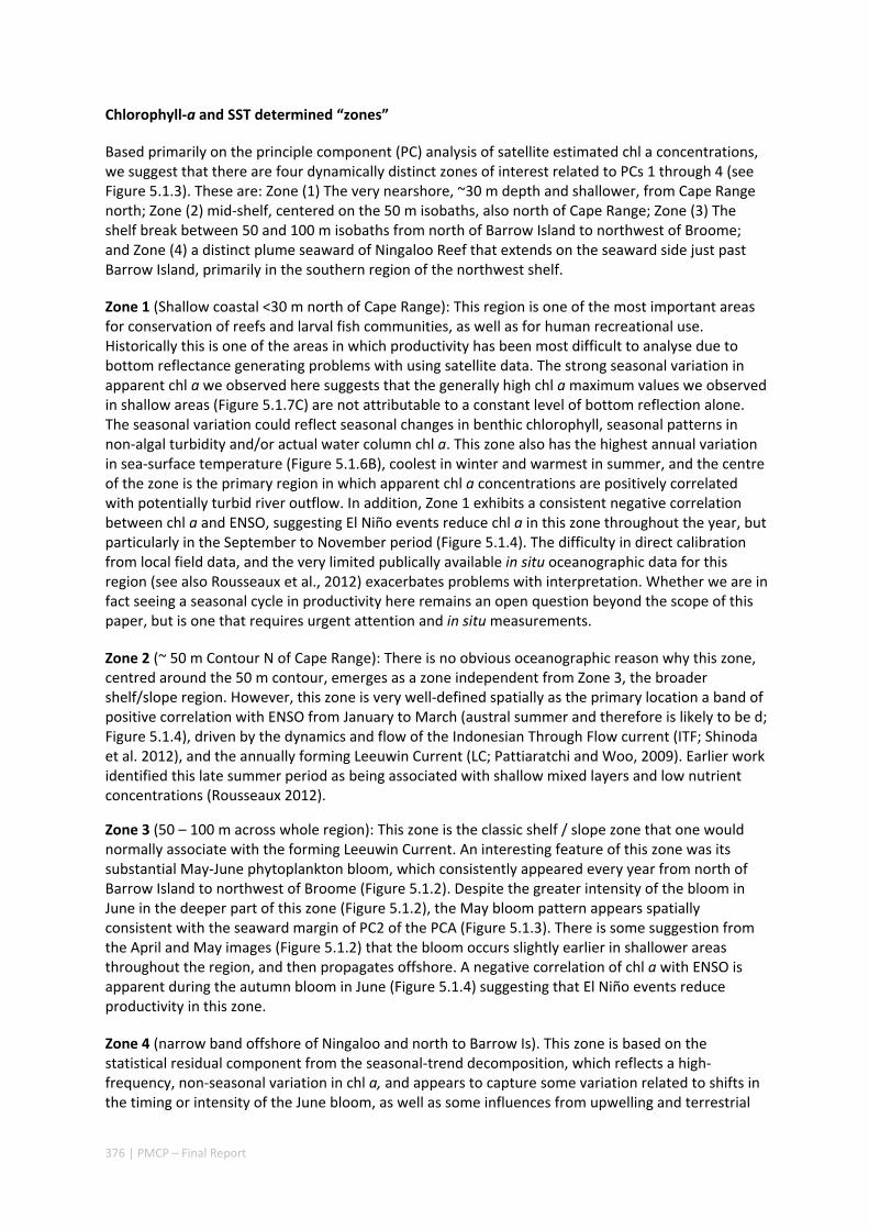
376 | PMCP – Final Report
Chlorophyll‐a and SST determined “zones”
Based primarily on the principle component (PC) analysis of satellite estimated chl a concentrations, we suggest that there are four dynamically distinct zones of interest related to PCs 1 through 4 (see Figure 5.1.3). These are: Zone (1) The very nearshore, ~30 m depth and shallower, from Cape Range north; Zone (2) mid‐shelf, centered on the 50 m isobaths, also north of Cape Range; Zone (3) The shelf break between 50 and 100 m isobaths from north of Barrow Island to northwest of Broome; and Zone (4) a distinct plume seaward of Ningaloo Reef that extends on the seaward side just past Barrow Island, primarily in the southern region of the northwest shelf.
Zone 1 (Shallow coastal <30 m north of Cape Range): This region is one of the most important areas for conservation of reefs and larval fish communities, as well as for human recreational use. Historically this is one of the areas in which productivity has been most difficult to analyse due to bottom reflectance generating problems with using satellite data. The strong seasonal variation in apparent chl a we observed here suggests that the generally high chl a maximum values we observed in shallow areas (Figure 5.1.7C) are not attributable to a constant level of bottom reflection alone. The seasonal variation could reflect seasonal changes in benthic chlorophyll, seasonal patterns in non‐algal turbidity and/or actual water column chl a. This zone also has the highest annual variation in sea‐surface temperature (Figure 5.1.6B), coolest in winter and warmest in summer, and the centre of the zone is the primary region in which apparent chl a concentrations are positively correlated with potentially turbid river outflow. In addition, Zone 1 exhibits a consistent negative correlation between chl a and ENSO, suggesting El Niño events reduce chl a in this zone throughout the year, but particularly in the September to November period (Figure 5.1.4). The difficulty in direct calibration from local field data, and the very limited publically available in situ oceanographic data for this region (see also Rousseaux et al., 2012) exacerbates problems with interpretation. Whether we are in fact seeing a seasonal cycle in productivity here remains an open question beyond the scope of this paper, but is one that requires urgent attention and in situ measurements.
Zone 2 (~ 50 m Contour N of Cape Range): There is no obvious oceanographic reason why this zone, centred around the 50 m contour, emerges as a zone independent from Zone 3, the broader shelf/slope region. However, this zone is very well‐defined spatially as the primary location a band of positive correlation with ENSO from January to March (austral summer and therefore is likely to be d; Figure 5.1.4), driven by the dynamics and flow of the Indonesian Through Flow current (ITF; Shinoda et al. 2012), and the annually forming Leeuwin Current (LC; Pattiaratchi and Woo, 2009). Earlier work identified this late summer period as being associated with shallow mixed layers and low nutrient concentrations (Rousseaux 2012).
Zone 3 (50 – 100 m across whole region): This zone is the classic shelf / slope zone that one would normally associate with the forming Leeuwin Current. An interesting feature of this zone was its substantial May‐June phytoplankton bloom, which consistently appeared every year from north of Barrow Island to northwest of Broome (Figure 5.1.2). Despite the greater intensity of the bloom in June in the deeper part of this zone (Figure 5.1.2), the May bloom pattern appears spatially consistent with the seaward margin of PC2 of the PCA (Figure 5.1.3). There is some suggestion from the April and May images (Figure 5.1.2) that the bloom occurs slightly earlier in shallower areas throughout the region, and then propagates offshore. A negative correlation of chl a with ENSO is apparent during the autumn bloom in June (Figure 5.1.4) suggesting that El Niño events reduce productivity in this zone.
Zone 4 (narrow band offshore of Ningaloo and north to Barrow Is). This zone is based on the statistical residual component from the seasonal‐trend decomposition, which reflects a high‐frequency, non‐seasonal variation in chl a, and appears to capture some variation related to shifts in the timing or intensity of the June bloom, as well as some influences from upwelling and terrestrial

377 | PMCP – Final Report
river outflows. As shown in Figure 5.1.3 (PC3 and PC4), it looks specifically associated with a typical upwelling signature that develops off Ningaloo in summer, which Rossi and coworkers (2013b) identified to be associated with a strong upwelling region here, centerd around 23°S.
Interestingly, The Montebello Islands seem show connections with both “eastern influences” (Zone 2) and “western influences (Zone 4). Also worth noting is the “pocket” just east of the Montebellos that shows unusual patterns of variation for its depth.
5.1.3 EXPERIMENTAL SECTION
Data
To maximize spatial and temporal coverage, merged data from multiple satellite observation systems including SeaWIFS (1997 – 2010), MERIS (2002 – 2012), and MODIS (2002 – 2012) were used. This allowed analysis of 16 consecutive years of observations. The merged product (with 4.6 km grid cells) was produced by the ESA using the GSM algorithm (Maritorena and Siegel 2005) as part of the GlobColour Project (www.globcolour.info). Data were downloaded in 2013, prior to the 2014 GlobColour reprocessing. We analysed the monthly averaged CHL1 dataset, which uses algorithms intended for “Case 1” waters. Case 1 waters are those in which the optical properties result predominantly from the presence of phytoplankton (Lee and Hu 2006). The northwest coast of Australia was categorized as Case 1 in the analysis of (Lee and Hu 2006); however, bottom reflectance likely influences the signal in shallow areas and conclusions reached for shallow water must therefore be regarded as strictly qualitative at this point.
For our correlation analyses, we used the Multivariate El Niño / Southern Oscillation Index (MEI) (Wolter and Timlin 1993), downloaded from http://www.esrl.noaa.gov/psd/enso/mei/. Data for mean monthly Maitland River discharge at Miaree Pool (Site 709004) were obtained from the Department of Water, Western Australia. Bathymetry contours shown in plots are based on the ETOPO1 dataset (Amante and Eakins 2009).
Two temperature datasets were used in the analyses, one providing a longer series at lower resolution, and the other providing a short series at higher resolution. For the low‐resolution set, we used the NOAA optimally interpolated (OI) 0.25‐degree daily SST (Reynolds et al., 2007). This gridded (0.25‐degree grid size) dataset is based on infrared satellite measurements of SST (AVHRR) as well as in situ ship and buoy data, and the series analysed runs from 1982 through 2011. For the high‐resolution set, we used the NASA‐JPL Multi‐scale Ultra‐high Resolution (MUR) daily SST dataset. This gridded dataset combines infrared and microwave (cloud penetrating) remote sensing SST measurements. It has a grid size of 0.01 degree (~1 km) and the series analysed runs from 2002 through 2012.
Extensive efforts were made to obtain both in situ SST and chl‐a data in order to validate satellite‐derived measurements. However, in situ information for this marine areas are very limited in the public domain at this time, the vast majority being currently held by industry and are of commercially valuable nature. Some in situ SST and chl‐a data obtained from the historical underway Solander (AIMs) cruises are available at the Pawsey centre RSDI.
378 | PMCP – Final Report
Statistical Analysis
We employed the seasonal‐trend decomposition method of Cleveland et al. (1990) to decompose the monthly chl‐a data from each grid cell into trend, seasonal, and residual components. The method uses the loess smoother, and it produces an additive decomposition. Importantly, missing values are acceptable and the method is able to accommodate changes in the seasonal pattern through time. Briefly, the decomposition is accomplished through a series of iterations of inner and outer loops. In the inner loop, a detrended overall series is computed, and then each cycle‐subseries (e.g., all January values through time) is smoothed. The resulting estimate of the seasonal series is filtered, and then a deseasonalized series is produced and smoothed. This will be the trend estimate for the next inner loop. In the outer loop which follows, robustness weights based on the residuals are calculated. These weights are then used in the smoothing steps of the next inner loop process (Cleveland et al. 1990).
While this seasonal decomposition method can handle missing data, we limited the analysis to grid cells with less than 20 missing (monthly) values. The span of the loess window for seasonal data for the first run was 12.
A principal components analysis was also performed on the (non‐decomposed) monthly chl a data. This is a rotation of the data that may allow reduction of dimensionality in subsequent analyses, and it can highlight patterns that account for large proportions of the variance in the system, which may elucidate causal mechanisms. Due to the large amount of data involved and its three dimensionality, a custom R function was written to perform the principal component analysis. This function first creates a two‐dimensional matrix in which each column represents a grid cell, and each row represents a time step (month). The series from each grid cell was standardized to zero mean and unit variance. Four or more approximate singular values and singular vectors of the matrix were then calculated using the Implicitly‐restarted Lanczos bi‐diagonalization method of the “irlba” package for R (Baglama and Reichel 2005) The custom function takes the loadings (singular vectors) from the irlba analysis and places them back in their original spatial configuration such that loadings maps can be visualized.
Correlation analyses were performed to determine the influence of ENSO status (as characterized by the Multivariate ENSO Index) and Maitland River discharge on remotely sensed chl a concentrations. Mean annual chl a series were calculated for each observation cell, and the (Pearson’s) correlations between each annual series and monthly ENSO series were calculated. Thus for each cell, 12 correlation coefficients were determined (mean annual chl a vs. Jan. ENSO Index values, mean annual chl a vs. Feb. ENSO Index values, etc.). Mapping of these correlation coefficients allows identification of coherent spatiotemporal patterns in the data. To assess the impact of Maitland River discharge, we used detrended, seasonally adjusted (trend and seasonal components removed by STL method, see above) monthly chl‐a, and monthly Maitland River discharge (at Miaree Pool; data from WA Dept. of Water). The correlation between discharge and seasonally adjusted, remotely sensed chl a was calculated for each observation cell, and a map of correlation coefficients was produced.
Remotely sensed chl a may be influenced by bottom reflection in shallow water and also by non‐algal turbidity. We attempted to identify the degree to which remotely sensed chl a data used in this study reflected chl a concentrations measured in the field using underway data from the RV Solander (provided by the Australian Institute for Marine Science). The data included temperature, fluorescence (converted to chl a concentration), depth, salinity, and turbidity, along with latitude, longitude, date, and time. There were over 3000 instances in which Solander data were collected in an observation cell on a day when satellite data were also obtained for that cell. All Solander

379 | PMCP – Final Report
observations in the matched cell were averaged for each matched observation day. Linear models and semiparametric regression (GAM) were used to investigate the relationships among variables.
We performed a variety of exploratory analyses of SST aimed at characterizing long term trends, recurrent spatial patterns, and modes of variation. For some analyses, seasonal‐trend decomposition using STL (see above) was utilized. For the OI‐0.25 dataset, we mapped mean temperature, standard deviation, standard deviation of detrended and seasonally adjusted values, mean annual maximum/minimum/range, mean number of days above 30 °C, significant linear trends (2nd‐order autocorrelation error structure), significant linear trends in number of extreme events, mean day of onset of seasonal warming, significant linear trends in onset of seasonal warming, principal components of seasonally adjusted values, correlation between seasonally adjusted values and ENSO status, and month‐by‐month correlation between seasonally adjusted values and ENSO status. For the MUR dataset, we produced maps of mean temperature, standard deviation, standard deviation of seasonally adjusted values, significant linear trends (2nd‐order autocorrelation error structure), and principal components of seasonally adjusted values. Note that we show and discuss only a subset of these analyses here.
Conclusions
The Northwest Shelf of Western Australia in the eastern Indian Ocean is positioned at the nexus of several ocean current systems, and characterized by highly complex oceanography. To understand core drivers of regional productivity, we analysed 15 years of satellite estimates of chl a, a proxy for plankton biomass, and sea‐surface temperature. Here we show that there are four key spatial zones associated with the most important temporal scales of variability in chl a. We identified these zones, and suggested the most likely drivers for the inferred patterns in productivity. We showed that while the region is dominated by seasonal forcing (and has been subject to a clear 0.1°C increase in offshore SST during the study period) there are important local sources of variation on the continental shelf that are local and aperiodic. In addition, we identified a shelf‐break autumn plankton bloom correlated with ENSO cycles? Further understanding of the productive in this bio‐diverse and ecologically sensitive region, which includes the globally important Ningaloo reef and Cape Range World Heritage Area and other sites of acknowledged special marine importance, is likely to be enhanced by the use of recent sources of satellite data such as ESA CCI for chl a, and MODIS or ESA AATSR for high resolution SST information. More critical, however, is access to in situ physical oceanographic measurements, not currently in the public domain, with which to validate the marked time series observations noted in this study.
5.1.4 ACKNOWLEDGMENTS
The authors would like to thank Gorgon Barrow Island Net Conservation Benefits Fund (www.ncb.org.au) who made this study possible.
5.1.5 REFERENCES
Amante C and Eakins BW (2009) Etopo1 1 arc‐minute global relief model: Procedures, data sources and analysis. US Department of Commerce, National Oceanic and Atmospheric Administration, National Environmental Satellite, Data, and Information Service, National Geophysical Data Center, Marine Geology and Geophysics Division.
380 | PMCP – Final Report
Baglama J and Reichel L (2005) Augmented implicitly restarted lanczos bidiagonalization methods. SIAM Journal on Scientific Computing 27:19‐42.
Cleveland RB, Cleveland WS, McRae JE, Terpenning I Stl (1990) A seasonal‐trend decomposition procedure based on loess. Journal of Official Statistics 6:3‐73.
Domingues CM, Maltrud ME, Wijffels SE, Church JA and Tomczak M (2007) Simulated lagrangian pathways between the leeuwin current system and the upper‐ocean circulation of the southeast indian ocean. Deep‐Sea Research Part II 54:797‐817.
Feng M, Hendon HH, Xie SP, Marshall AG andSchiller A… (2015) Decadal increase in Ningaloo Niño since the late 1990s. Geophysical Research Letters, 42(1):104‐112.
Griffin D, Wilkin J, Chubb C, Pearce A and Caputi N (2001) Ocean currents and the larval phase of australian western rock lobster panulirus cygnus. Mar. Freshw. Res. 52:1187‐1199.
http://www.rswa.org.au/publications/Journal/92(2)/ROY%20SOC%2092.2%20LEEUWIN%20221‐241.pdf
Lee Z and Hu C (2006) Global distribution of case‐1 waters: An analysis from seawifs measurements. Remote Sensing of Environment 101:270‐276.
Maritorena S and Siegel DA (2005) Consistent merging of satellite ocean color data sets using a bio‐optical model. Remote Sensing of Environment 94:429‐440.
Nguyen HM, Rountrey AN, Meeuwig JJ, Coulson PG, Feng M, Newman SJ, Waite AM, Wakefield CB and Meekan MG (2015) Growth of a deep‐water, predatory fish is influenced by the productivity of a boundary current system. Scientific Reports 5:9044.
Pattiaratchi C and Woo M. (2009) The mean state of the Leeuwin Current system between North West Cape and Cape Leeuwin. J Royal Soc WA 92:221‐241.
Raes EJ, Thompson PA, McInnes AS, Nguyen HM, Hardman‐Mountford N and Waite AM (2015) Sources of new nitrogen in the indian ocean. Glob. Biogeochem. Cycle 29:1283‐1295.
Rossi V, Feng M, Pattiaratchi C, Roughan M and Waite AM (2013a)Linking synoptic forcing and local mesoscale processes with biological dynamics off ningaloo reef. Journal of Geophysical Research‐Oceans 118:1211‐1225.
Rossi V, Feng M; Pattiaratchi C, Roughan M andWaite AM (2013b). On the factors influencing the development of sporadic upwelling in the leeuwin current system. Journal of Geophysical Research ‐ Oceans, 118:3608‐3621.
Rousseaux CSG, Lowe R, Feng M, Waite A and Thompson PA (2012) The role of the leeuwin current and mixed layer depth on the autumn phytoplankton bloom off ningaloo reef, western australia. Continental Shelf Research 32:22‐35.
Toshiaki S, Han W, Metzger EJ and Hurlburt HE (2012) Seasonal Variation of the Indonesian Throughflow in Makassar Strait. J. Phys. Oceanogr. 42:1099–1123.
Waite AM, Rossi V, Roughan M, Tilbrook B, Thompson PA, Feng M, Wyatt AS and Raes EJ (2014) Formation and maintenance of high‐nitrate, low ph layers in the eastern Indian Ocean and the role of nitrogen fixation. Biogeosciences 10:5691‐5702.

381 | PMCP – Final Report
Wolter K, Timlin MS (1993) In Monitoring enso in coads with a seasonally adjusted principal component index, Proc. of the 17th Climate Diagnostics Workshop, pp 52‐57.
Wyatt ASJ, Falter JL, Lowe RJ, Humpries S and Waite AM (2012) Oceanographic forcing of nutrient uptake and release over a fringing coral reef. Limnology and Oceanography.
Wyatt ASJ, Lowe RJ, Humphries S and Waite AM (2010) Particulate nutrient fluxes over a fringing coral reef: Relevant scales of phytoplankton production and mechanisms of supply. Mar. Ecol.‐Prog. Ser. 405:113‐130.
382 | PMCP – Final Report
Impact of a tropical cyclone on a fringing reef coastline
Authors: Cuttler M, Hansen J, Lowe R, Drost E.
Submitted to Geophysical Research Letters.
ABSTRACT
Tropical cyclones (TCs) generate extreme hazards along coastlines, often leading to losses of life and property. Although coral reefs exist in cyclone‐prone regions around the world, few studies have measured the hydrodynamic conditions and morphological responses of reef‐fronted coastlines to TCs. Here, we examine the impact of TC Olwyn on a section of Australia’s largest fringing reef (Ningaloo Reef) using in situ wave and water level observations, topographic surveys, and numerical modeling. Despite forereef significant wave heights reaching 6 m and local winds of 140 km hr‐1, average beach volume change was only ‐3 m3 m‐1. Numerical simulations indicate that this erosion was due to locally‐generated wind waves within the lagoon rather than the offshore waves that were dissipated on the reef crest. A comparison of these volume changes to observations of TC impacts along exposed sandy beaches quantitatively demonstrates the substantial coastal protection reefs can provide against extreme storms.

383 | PMCP – Final Report
5.2.1 INTRODUCTION
The coastal impacts of tropical cyclones (TCs) namely erosion flooding and habitat destruction have been well documented globally (Castillo et al. 2012; Woodruff et al. 2013). Existing studies of TC impacts on shorelines fringed by coral reefs have primarily focused on the impact to the coral communities (Harmelin‐Vivien 1994) the hydrodynamic conditions over the reefs (Péquignet et al. 2011; Roeber and Bricker 2015; Shimozono et al. 2015) or the fate of storm deposits (Scoffin 1993). However, few studies have focused on the hydrodynamic and morphodynamic processes driving observed changes in reef‐fringed beach morphology during a TC. In this study, we quantify the morphological change due to a direct cyclone impact along a reef‐fringed coast identify the physical mechanisms responsible for the observed beach erosion patterns and assess the coastal protection provided by the reef as compared to exposed sandy coasts experiencing similar extreme met‐ocean conditions.
Fringing reefs which can range from shore‐attached to several kilometers offshore are the most prevalent type of coral reef along tropical coasts (Hopley 2004). Reefs provide natural coastal protection by dissipating offshore wave energy through both wave breaking and bottom friction (Lowe et al. 2005). Despite the abundance of reef hydrodynamic studies few studies have extended the hydrodynamics to quantify coastal morphological changes particularly during TCs. Previous studies conducted under more typical (non‐TC) conditions have shown that shorelines fringed by reefs can experience morphological changes on short (weekly) to intermediate (seasonal) timescales due to changes in wind and wave direction (Eversole and Fletcher 2003; Kench and Brander 2006; Beetham and Kench 2014) and that reef‐fronted beaches are generally more stable than exposed beaches (Gallop et al. 2012; Ruiz de Alegria‐Arzaburu et al. 2013). The limited studies that have directly measured TC‐induced shoreline changes have suggested that shoreline response is inversely related to reef flat width with the magnitude of beach erosion decreasing with increasing reef flat width (Jeanson et al. 2013; Mahabot et al. 2016). These same studies have also suggested that the relative coastline orientation (i.e. in relation to local wind and wave direction) can influence the magnitude of coastal erosion. However, due to the episodic nature of TCs in general and more specifically the rarity of capturing a direct impact with in situ instrumentation (i.e. near the eye region with extreme local winds) there still remains a gap in understanding of how much coastal protection is offered by fringing reefs during extreme storms and moreover which factors specifically govern coastal responses.
Rigorously assessing the coastal protection afforded by reefs is particularly important given that a number of recent studies have suggested that the coastal protection offered by reefs is under threat due to both coral degradation (i.e. decreasing rates of net reef accretion) and sea level rise which will increase wave transmission across reefs and expose reef‐protected coastlines to larger waves (Storlazzi et al. 2011; Grady et al. 2013; Ruiz de Alegria‐Arzaburu et al. 2013; Quataert et al. 2015). Collectively these studies emphasize that it is critical to understand the modern drivers of morphological change in reef environments to better predict future changes to these coastlines. In this study we combine in situ measurements (wave heights water levels) repetitive topographic beach surveys and output from a coupled wave‐current numerical model (Delft3D/SWAN) to quantify the coastal response from the direct impact of TC Olwyn (2015) at Ningaloo Reef Western Australia.

384 | PMCP – Final Report
5.2.2 DATA AND METHODS
Study area
Ningaloo Reef is Australia’s largest fringing reef stretching ~270 km south from Australia’s North West Cape (Figure 5.2.1a). The morphology of Ningaloo is characterized by a steep (1:20) forereef slope a relatively narrow reef flat (~150 to 200 m) and a wide (1 to 5 km) but relatively shallow (less than 5 m deep) lagoon (Collins et al. 2003). The study area is located at the northern end of Ningaloo Reef at Tantabiddi (Figure 5.2.1c). This area is marked by the presence of a shoreline salient inland from the reef flat; which is a common feature along the reef‐fringed coastline of Western Australia including at Ningaloo (Sanderson and Eliot 1996). The local beach at the study site has a variable slope (β) ranging from β ~ 0.03 north of the salient to β ~ 0.14 south of the salient is relatively narrow (≤100 m) and is backed by an extensive dune system with heights from 3 to 10 m above mean sea level.
Figure 5.2.1 (a) Western Australia with the Ningaloo Peninsula in yellow; (b) the Ningaloo Peninsula with the boundaries of the ‘outer’ Delft3D‐FLOW and SWAN domain indicated in blue; (c) study site and bathymetry with the cross‐shore array of pressure sensors indicated by the white triangles the ‘inner’ Delft3D‐FLOW and SWAN domain show in grey and the ‘shore’ Delft3D‐FLOW grid shown in black. TC Olwyn track is the red line in (a) and (b). (d) Cross‐shore depth profile from the coastline to the forereef with the reef crest marked with a red ‘x’ and pressure sensors denoted by red triangles.
Ningaloo Reef is located along Australia’s Northwest Shelf which is the most cyclone prone region of Australia (Bureau of Meteorology 2016) being influenced on average by 1 to 2 TCs per year with the more severe cyclones (sustained winds > ~120 km hr‐1) increasing in likelihood later in the southern hemisphere cyclone season (March‐April) (Bureau of Meteorology 2016).
In order to opportunistically capture the impact of a TC on the morphodynamics of this fringing reef system a transect of five pressure sensors (Figure 5.2.1c, d) was deployed from December 2014 to May 2015 at Tantabiddi. On 11 March 2015 TC Olwyn developed off the northwest coast and tracked southward until crossing land on 13 March 2015 (Figure 5.2.1a–b). On 12 March 2015 its eye passed only ~10 km to the west (offshore) of the study area (Figure 5.2.1b) as a Category 3 (Australian tropical cyclone intensity scale) cyclone with an estimated central pressure of 965 hpa sustained winds of 140 km hr‐1 and gusts up to 200 km hr‐1 (Bureau of Meteorology 2017).
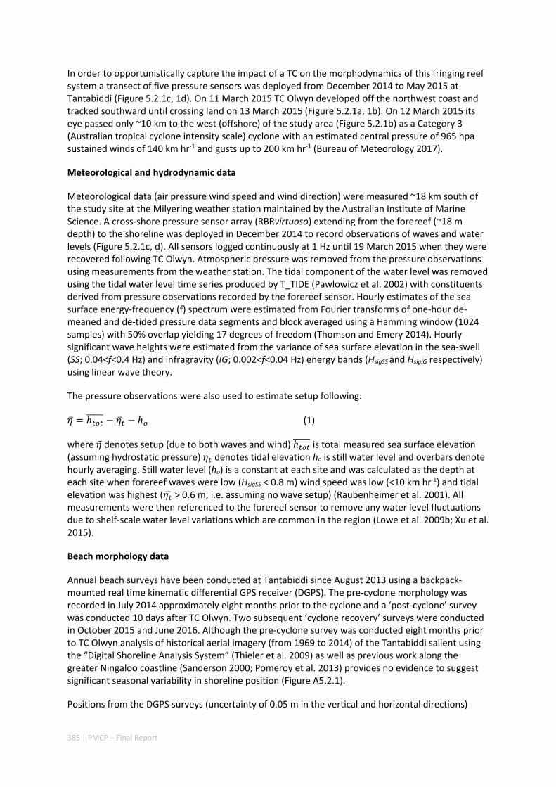
385 | PMCP – Final Report
In order to opportunistically capture the impact of a TC on the morphodynamics of this fringing reef system a transect of five pressure sensors was deployed from December 2014 to May 2015 at Tantabiddi (Figure 5.2.1c, 1d). On 11 March 2015 TC Olwyn developed off the northwest coast and tracked southward until crossing land on 13 March 2015 (Figure 5.2.1a, 1b). On 12 March 2015 its eye passed only ~10 km to the west (offshore) of the study area (Figure 5.2.1b) as a Category 3 (Australian tropical cyclone intensity scale) cyclone with an estimated central pressure of 965 hpa sustained winds of 140 km hr‐1 and gusts up to 200 km hr‐1 (Bureau of Meteorology 2017).
Meteorological and hydrodynamic data
Meteorological data (air pressure wind speed and wind direction) were measured ~18 km south of the study site at the Milyering weather station maintained by the Australian Institute of Marine Science. A cross‐shore pressure sensor array (RBRvirtuoso) extending from the forereef (~18 m depth) to the shoreline was deployed in December 2014 to record observations of waves and water levels (Figure 5.2.1c, d). All sensors logged continuously at 1 Hz until 19 March 2015 when they were recovered following TC Olwyn. Atmospheric pressure was removed from the pressure observations using measurements from the weather station. The tidal component of the water level was removed using the tidal water level time series produced by T_TIDE (Pawlowicz et al. 2002) with constituents derived from pressure observations recorded by the forereef sensor. Hourly estimates of the sea surface energy‐frequency (f) spectrum were estimated from Fourier transforms of one‐hour de‐meaned and de‐tided pressure data segments and block averaged using a Hamming window (1024 samples) with 50% overlap yielding 17 degrees of freedom (Thomson and Emery 2014). Hourly significant wave heights were estimated from the variance of sea surface elevation in the sea‐swell (SS; 0.04<f<0.4 Hz) and infragravity (IG; 0.002<f<0.04 Hz) energy bands (HsigSS
and HsigIG respectively) using linear wave theory.
The pressure observations were also used to estimate setup following:
(1)
where denotes setup (due to both waves and wind) is total measured sea surface elevation (assuming hydrostatic pressure) denotes tidal elevation ho is still water level and overbars denote hourly averaging. Still water level (ho) is a constant at each site and was calculated as the depth at each site when forereef waves were low (HsigSS < 0.8 m) wind speed was low (<10 km hr‐1) and tidal elevation was highest ( > 0.6 m; i.e. assuming no wave setup) (Raubenheimer et al. 2001). All measurements were then referenced to the forereef sensor to remove any water level fluctuations due to shelf‐scale water level variations which are common in the region (Lowe et al. 2009b; Xu et al. 2015).
Beach morphology data
Annual beach surveys have been conducted at Tantabiddi since August 2013 using a backpack‐mounted real time kinematic differential GPS receiver (DGPS). The pre‐cyclone morphology was recorded in July 2014 approximately eight months prior to the cyclone and a ‘post‐cyclone’ survey was conducted 10 days after TC Olwyn. Two subsequent ‘cyclone recovery’ surveys were conducted in October 2015 and June 2016. Although the pre‐cyclone survey was conducted eight months prior to TC Olwyn analysis of historical aerial imagery (from 1969 to 2014) of the Tantabiddi salient using the “Digital Shoreline Analysis System” (Thieler et al. 2009) as well as previous work along the greater Ningaloo coastline (Sanderson 2000; Pomeroy et al. 2013) provides no evidence to suggest significant seasonal variability in shoreline position (Figure A5.2.1).
Positions from the DGPS surveys (uncertainty of 0.05 m in the vertical and horizontal directions)
386 | PMCP – Final Report
were organised into a triangulated irregular network and converted to a grid to produce a 1 m cell‐size topographic surface of the surveyed beach (Hansen and Barnard 2010). Successive topographic surfaces were differenced to determine the location and extent of erosion or accretion. Cross‐shore transects were extracted at 50 m alongshore intervals from the survey grids to assess beach elevation and volume change.
Numerical model
The numerical model Delft3D‐FLOW (Lesser et al. 2004) coupled with the wave model SWAN (Booij et al. 1999) was used to simulate the coupled wave and hydrodynamic conditions during the cyclone. Delft3D solves the unsteady shallow‐water equations in two‐ or three‐dimensions (Lesser et al. 2004) and has been used effectively in coral reef environments under both non‐storm and storm conditions (Lowe et al. 2009a; Hoeke et al. 2015). Numerical details governing equations and underlying assumptions of Delft3D are described in detail in Lesser et al. (2004); brief details of the model resolution and settings used for this study are described below. Further details of model settings and validation are provided in Section 5.2.7.
Delft3D‐FLOW (version 6.02.02.5562M) was run in depth‐averaged mode and consisted of three domains (‘outer’ ‘inner’ ‘shore’) of varying resolution that were two‐way coupled using a “domain decomposition” technique (Hummel and de Goede 2000). The ‘outer’ domain had a 50x50 m resolution (Figure 5.2.1b blue box) the ‘inner’ domain had a 17x17 m resolution (Figure 5.2.1c grey box) and the ‘shore’ domain had a 5x5 m resolution (Figure 5.2.1c black box).
The hydrodynamic model was two‐way coupled with SWAN (version 40.72) over two nested domains that had the same resolutions as the ‘outer’ and ‘inner’ circulation domains. Spatially‐uniform offshore boundary conditions for TC Olwyn were derived from frequency‐directional spectra from a larger regional scale SWAN model (Drost et al. 2017). Although SWAN does not model IG energy (Buckley et al. 2014) which has been shown to be important to lagoonal processes in many reefs under non‐TC conditions (Pomeroy et al. 2012; Van Dongeren et al. 2013) we show below that SS energy was the dominant forcing mechanism adjacent to the shoreline during these TC conditions.
5.2.3 RESULTS
Field observations
The eye of TC Olwyn passed ~10 km offshore of the study site on 12 March 2015 at ~17:00 UTC (Figure 5.2.1b); this resulted in incident waves on the forereef reaching ~6 m (HsigSS) which is ~3 times larger than the average swell (HsigSS ~1‐2 m) observed at Ningaloo (Taebi et al. 2011). To place these TC Olwyn conditions in context of the typical hydrodynamics of the system the observed waves and water levels during the cyclone were compared to a ‘typical’ swell event (HsigSS =1.8 m) observed prior to TC Olwyn (Figure 5.2.2).
The cross‐shore distribution of wave heights and setup (due to both wind and waves) were considerably different during the cyclone compared to typical swell conditions. Under typical swell conditions after dissipation of incident wave energy commences near the reef crest HsigSS continues to decrease across the reef flat and lagoon towards shore; and HsigSS and HsigIG become comparable in magnitude (Figure 5.2.1b). However during the peak of TC Olwyn (19:00 UTC) although HsigSS was initially reduced by 89% due to wave dissipation at reef crest HsigSS increased across the lagoon towards the shoreline with HsigSS reaching 1.5 m (~1.5 times reef flat HsigSS) and thus substantially
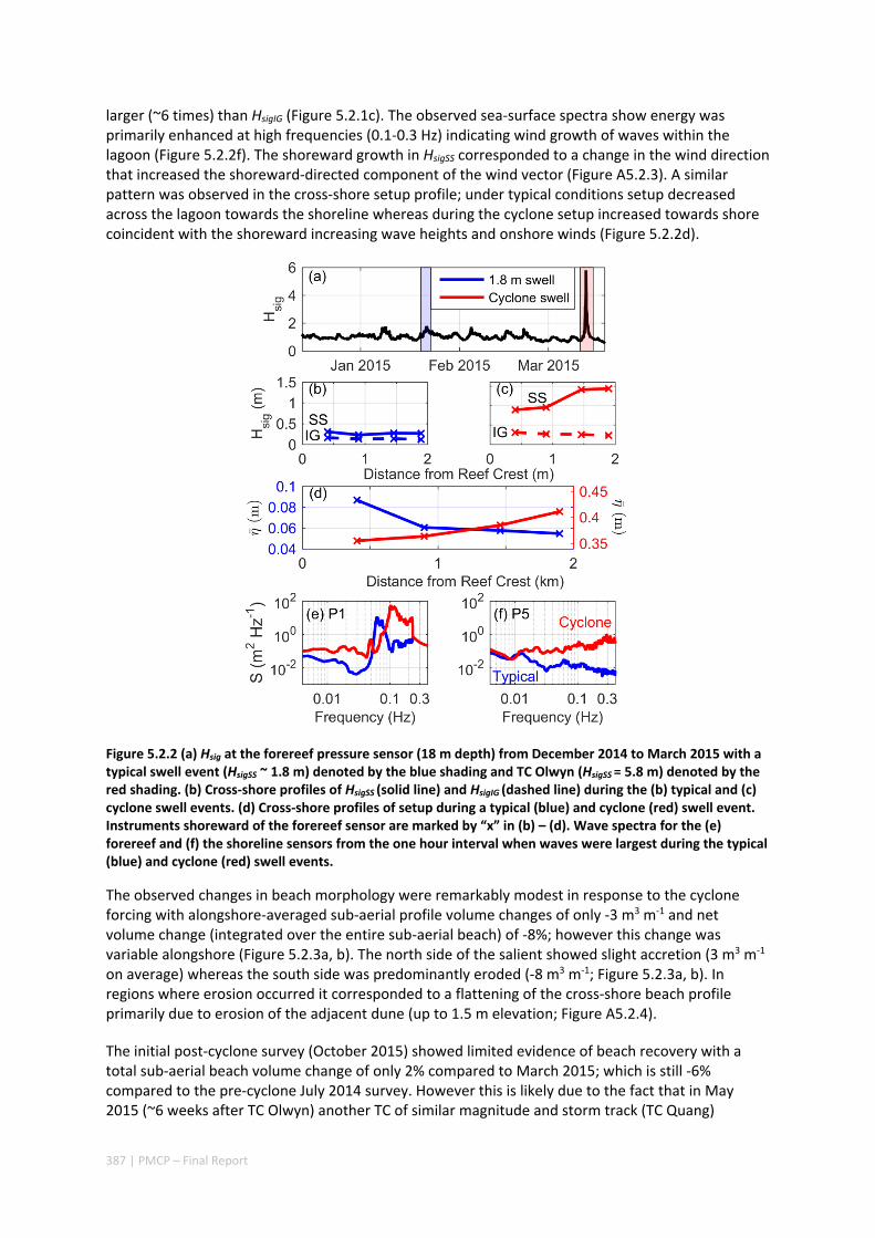
387 | PMCP – Final Report
larger (~6 times) than HsigIG (Figure 5.2.1c). The observed sea‐surface spectra show energy was primarily enhanced at high frequencies (0.1‐0.3 Hz) indicating wind growth of waves within the lagoon (Figure 5.2.2f). The shoreward growth in HsigSS corresponded to a change in the wind direction that increased the shoreward‐directed component of the wind vector (Figure A5.2.3). A similar pattern was observed in the cross‐shore setup profile; under typical conditions setup decreased across the lagoon towards the shoreline whereas during the cyclone setup increased towards shore coincident with the shoreward increasing wave heights and onshore winds (Figure 5.2.2d).
Figure 5.2.2 (a) Hsig at the forereef pressure sensor (18 m depth) from December 2014 to March 2015 with a typical swell event (HsigSS ~ 1.8 m) denoted by the blue shading and TC Olwyn (HsigSS = 5.8 m) denoted by the red shading. (b) Cross‐shore profiles of HsigSS (solid line) and HsigIG (dashed line) during the (b) typical and (c) cyclone swell events. (d) Cross‐shore profiles of setup during a typical (blue) and cyclone (red) swell event. Instruments shoreward of the forereef sensor are marked by “x” in (b) – (d). Wave spectra for the (e) forereef and (f) the shoreline sensors from the one hour interval when waves were largest during the typical (blue) and cyclone (red) swell events.
The observed changes in beach morphology were remarkably modest in response to the cyclone forcing with alongshore‐averaged sub‐aerial profile volume changes of only ‐3 m3 m‐1 and net volume change (integrated over the entire sub‐aerial beach) of ‐8%; however this change was variable alongshore (Figure 5.2.3a, b). The north side of the salient showed slight accretion (3 m3 m‐1 on average) whereas the south side was predominantly eroded (‐8 m3 m‐1; Figure 5.2.3a, b). In regions where erosion occurred it corresponded to a flattening of the cross‐shore beach profile primarily due to erosion of the adjacent dune (up to 1.5 m elevation; Figure A5.2.4).
The initial post‐cyclone survey (October 2015) showed limited evidence of beach recovery with a total sub‐aerial beach volume change of only 2% compared to March 2015; which is still ‐6% compared to the pre‐cyclone July 2014 survey. However this is likely due to the fact that in May 2015 (~6 weeks after TC Olwyn) another TC of similar magnitude and storm track (TC Quang)

388 | PMCP – Final Report
impacted the study area. Profiles on the north side of the salient showed slight accretion compared to the pre‐Olwyn (July 2014) survey (1 m3 m‐1; Figure A5.2.4). Although October 2015 surveys exhibited net erosion on the south side of the salient when compared to the July 2014 survey (‐3 m3 m‐1 on average) profiles between 0 and ‐600 m (i.e. locations of largest cyclone‐induced erosion) returned to pre‐cyclone volumes (~11 m3 m‐1 recovery from March 2015; Figure A5.2.4). The final recovery survey (June 2016) showed complete beach volume recovery with a total sub‐aerial beach volume change of 15% compared to the pre‐Olwyn survey. Furthermore profiles on both the north side and south side of the salient exhibited net accretion between October 2015 and June 2016 (Figure A5.2.4) consistent with the longer term accretionary trend measured since 1945 (Figure A5.2.1).
Figure 5.2.3 (a) Observed beach elevation change. (b) TC‐induced beach volume change and (c) pre‐storm beach slope (β) calculated between the 1 m contour and the furthest offshore position of the beach survey. R2 describes the relationship between β and beach volume change shown in (b). (d) Model‐predicted Hsig along the 2 m isobath (yellow dashed line in (a)) for a 1.8 m swell (solid line) and peak TC conditions with (dashed line) and without wind growth (dashed‐x line) enabled. (e) Disequilibrium wave heights (HsigTC/HsigTypical) predicted with (dashed) and without (dashed‐x) wind growth (i.e. ratio of black dashed or dashed‐x line in (c) to solid line in (c)). R2 describes the relationship between disequilibrium TC wave heights with wind growth (dashed line) and post‐cyclone beach volume change (data shown in (b)).
Model simulations
The cross‐reef wave observations indicate substantial wind growth occurred across the lagoon; to further investigate how the nearshore wave fields likely drove the observed spatial variability in the beach changes we used the numerical model to extend the in situ results over the entire study area. Modeled wave heights were extracted along the 2 m isobaths which is further offshore on the south side of the salient due to the southern portion of the lagoon generally being shallower than the north (Figure 5.2.3a).
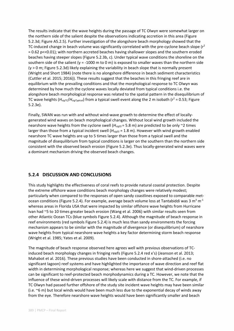
389 | PMCP – Final Report
The results indicate that the wave heights during the passage of TC Olwyn were somewhat larger on the northern side of the salient despite the observations indicating accretion in this area (Figure 5.2.3d; Figure A5.2.5). Further investigation of the alongshore beach morphology showed that the TC‐induced change in beach volume was significantly correlated with the pre‐cyclone beach slope (r2 = 0.62 p<<0.01); with northern accreted beaches having shallower slopes and the southern eroded beaches having steeper slopes (Figure 5.2.3b, c). Under typical wave conditions the shoreline on the southern side of the salient (y = ‐1000 m to 0 m) is exposed to smaller waves than the northern side (y > 0 m; Figure 5.2.3d) likely explaining the variability in beach slope that is normally present (Wright and Short 1984) (note there is no alongshore difference in beach sediment characteristics (Cuttler et al. 2015; 2016)). These results suggest that the beaches in this fringing reef are in equilibrium with the prevailing conditions and that the morphological response to TC Olwyn was determined by how much the cyclone waves locally deviated from typical conditions i.e. the alongshore beach morphological response was related to the spatial pattern in the disequilibrium of TC wave heights (HsigTC/HsigTypical) from a typical swell event along the 2 m isobath (r2 = 0.53; Figure 5.2.3e).
Finally, SWAN was run with and without wind‐wave growth to determine the effect of locally‐generated wind waves on beach morphological changes. Without local wind growth included the nearshore wave heights from the cyclone swell (HsigSS = 5.8 m) are predicted to be only ~2 times larger than those from a typical incident swell (HsigSS = 1.8 m). However with wind growth enabled nearshore TC wave heights are up to 5 times larger than those from a typical swell and the magnitude of disequilibrium from typical conditions is larger on the southern than the northern side consistent with the observed beach erosion (Figure 5.2.3e). Thus locally‐generated wind waves were a dominant mechanism driving the observed beach changes.
5.2.4 DISCUSSION AND CONCLUSIONS
This study highlights the effectiveness of coral reefs to provide natural coastal protection. Despite the extreme offshore wave conditions beach morphology changes were relatively modest; particularly when compared to the responses of open sandy coastlines exposed to comparable met‐ocean conditions (Figure 5.2.4). For example, average beach volume loss at Tantabiddi was 3 m3 m‐1 whereas areas in Florida USA that were impacted by similar offshore wave heights from Hurricane Ivan had ~5 to 10 times greater beach erosion (Wang et al. 2006) with similar results seen from other Atlantic Ocean TCs (blue symbols Figure 5.2.4). Although the magnitude of beach response in reef environments (red symbols Figure 5.2.4) is much less than sandy environments the forcing mechanism appears to be similar with the magnitude of divergence (or disequilibrium) of nearshore wave heights from typical nearshore wave heights a key factor determining storm beach response (Wright et al. 1985; Yates et al. 2009).
The magnitude of beach response observed here agrees well with previous observations of TC‐induced beach morphology changes in fringing reefs (Figure 5.2.4 red x’s) (Jeanson et al. 2013; Mahabot et al. 2016). These previous studies have been conducted in shore‐attached (i.e. no significant lagoon) reef systems and have highlighted the importance of wave direction and reef flat width in determining morphological response; whereas here we suggest that wind‐driven processes can be significant to reef‐protected beach morphodynamics during a TC. However, we note that the influence of these wind‐driven processes will likely scale with distance from the TC. For example, if TC Olwyn had passed further offshore of the study site incident wave heights may have been similar (i.e. ~6 m) but local winds would have been much less due to the exponential decay of winds away from the eye. Therefore nearshore wave heights would have been significantly smaller and beach
390 | PMCP – Final Report
volume changes likely would have been even less than those observed here.
Figure 5.2.4 Comparison of TC impacts on open sandy coasts (blue symbols) and reef‐fronted coasts (red symbols). For studies that did not report Hsig wave heights from WaveWatchIII hindcast model predictions (Tolman 2009; ftp://polar.ncep.noaa.gov/pub/history/waves/nww3/) were extracted at the grid cell nearest to the study location in ~20 m depth (magenta circles). Values for Mahabot et al. (2016) represent alongshore‐averaged values for transects where reef morphology is constant.
The results show that remotely‐generated incident waves were largely dissipated by the reef and played a minimal role in driving the beach changes. Instead locally‐generated wind waves played a critical role in determining the morphological change with these wind waves ultimately being much larger than the residual offshore waves that were transmitted across the reef. Our results suggest that even over the small scales (order 1 km) of a nearshore reef‐lagoon system local wind wave generation can play a dominant role in sediment transport and erosion responses during TC conditions a process traditionally neglected in nearshore model applications to predict beach response to extreme events (e.g. Xbeach). Furthermore because the reef geomorphology at Ningaloo (e.g. shallow reef crest that gradually deepens to a shallow lagoon) represents a ‘standard’ reef (Falter et al. 2013) accounting for the local wind growth of waves will be critical to determining beach response to TCs in reef systems worldwide.
Although future climate changes are likely to increase wave transmission over coral reefs primarily due to sea level rise but also due to degradation of reef habitats (Grady et al. 2013; Quataert et al. 2015) the results presented here show that while these structures still exist they can provide substantial natural coastal protection under extreme events. The results also suggest that lagoon width and depth will determine the importance of wind‐driven processes in driving beach morphodynamics during TCs as these factors will directly determine the disequilibrium of nearshore wave heights from typical conditions. Therefore future assessments of coastal hazards in fringing reef systems will need to account for the pre‐storm beach morphology and estimate the magnitude of disequilibrium of nearshore wave conditions associated with the passage of a TC to accurately predict beach responses.
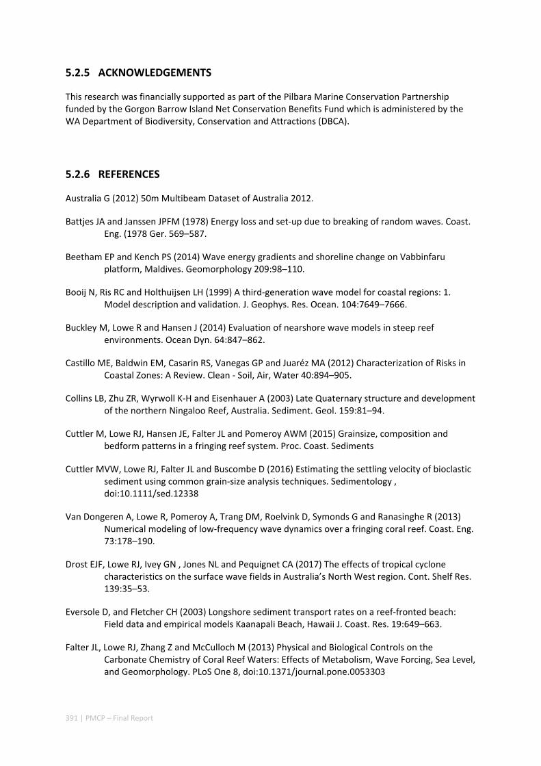
391 | PMCP – Final Report
5.2.5 ACKNOWLEDGEMENTS
This research was financially supported as part of the Pilbara Marine Conservation Partnership funded by the Gorgon Barrow Island Net Conservation Benefits Fund which is administered by the WA Department of Biodiversity, Conservation and Attractions (DBCA).
5.2.6 REFERENCES
Australia G (2012) 50m Multibeam Dataset of Australia 2012.
Battjes JA and Janssen JPFM (1978) Energy loss and set‐up due to breaking of random waves. Coast. Eng. (1978 Ger. 569–587.
Beetham EP and Kench PS (2014) Wave energy gradients and shoreline change on Vabbinfaru platform, Maldives. Geomorphology 209:98–110.
Booij N, Ris RC and Holthuijsen LH (1999) A third‐generation wave model for coastal regions: 1. Model description and validation. J. Geophys. Res. Ocean. 104:7649–7666.
Buckley M, Lowe R and Hansen J (2014) Evaluation of nearshore wave models in steep reef environments. Ocean Dyn. 64:847–862.
Castillo ME, Baldwin EM, Casarin RS, Vanegas GP and Juaréz MA (2012) Characterization of Risks in Coastal Zones: A Review. Clean ‐ Soil, Air, Water 40:894–905.
Collins LB, Zhu ZR, Wyrwoll K‐H and Eisenhauer A (2003) Late Quaternary structure and development of the northern Ningaloo Reef, Australia. Sediment. Geol. 159:81–94.
Cuttler M, Lowe RJ, Hansen JE, Falter JL and Pomeroy AWM (2015) Grainsize, composition and bedform patterns in a fringing reef system. Proc. Coast. Sediments
Cuttler MVW, Lowe RJ, Falter JL and Buscombe D (2016) Estimating the settling velocity of bioclastic sediment using common grain‐size analysis techniques. Sedimentology , doi:10.1111/sed.12338
Van Dongeren A, Lowe R, Pomeroy A, Trang DM, Roelvink D, Symonds G and Ranasinghe R (2013) Numerical modeling of low‐frequency wave dynamics over a fringing coral reef. Coast. Eng. 73:178–190.
Drost EJF, Lowe RJ, Ivey GN , Jones NL and Pequignet CA (2017) The effects of tropical cyclone characteristics on the surface wave fields in Australia’s North West region. Cont. Shelf Res. 139:35–53.
Eversole D, and Fletcher CH (2003) Longshore sediment transport rates on a reef‐fronted beach: Field data and empirical models Kaanapali Beach, Hawaii J. Coast. Res. 19:649–663.
Falter JL, Lowe RJ, Zhang Z and McCulloch M (2013) Physical and Biological Controls on the Carbonate Chemistry of Coral Reef Waters: Effects of Metabolism, Wave Forcing, Sea Level, and Geomorphology. PLoS One 8, doi:10.1371/journal.pone.0053303
392 | PMCP – Final Report
Fredsøe J (1984) Turbulent Boundary Layer in Wave‐current Motion. J. Hydraul. Eng. 110:1103–1120.
Gallop SL, Bosserelle C, Eliot I and Pattiaratchi CB (2012) The influence of limestone reefs on storm erosion and recovery of a perched beach. Cont. Shelf Res. 47:16–27.
Grady AE, Moore LJ, Storlazzi CD, Elias E and Reidenbach MA (2013) The influence of sea level rise and changes in fringing reef morphology on gradients in alongshore sediment transport. Geophys. Res. Lett. 40:3096–3101.
Hansen JE, and Barnard PL (2010) Sub‐weekly to interannual variability of a high‐energy shoreline Coast. Eng. 57:959–972.
Hansen JE, Raubenheimer B, List JH and Elgar S (2015) Modeled alongshore circulation and force balances onshore of a submarine canyon. J. Geophys. Res. Ocean. 120:1887–1903.
Harmelin‐Vivien ML (1994) The effects of storms and cyclones on coral reefs : A Review. J. Coast. Res. 211–231.
Hoeke R, McInnes M and O’Grady J (2015) Wind and Wave Setup Contributions to Extreme Sea Levels at a Tropical High Island: A Stochastic Cyclone Simulation Study for Apia, Samoa. J. Mar. Sci. Eng. 3:1117–1135.
Hopley D (2004) Coral Reefs, p. 343–349. In MA Schwarz [ed], Encyclopedia of Coastal Science. Springer.
Hummel S, and de Goede ED (2000) Domain decomposition with grid refinement for shallow water modeling. Proceedings of the 4th International Conference on Hydroinformatics. Iowa Institute of Hydraulic Research.
Jeanson M, Anthony EJ, Dolique F and Aubry A (2013) Wave characteristics and morphological variations of pocket beaches in a coral reef–lagoon setting, Mayotte Island, Indian Ocean. Geomorphology 182:190–209.
Kench PS, and Brander AW (2006) Response of reef island shorelines to seasonal climate oscillations: South Maalhosmadulu atoll , Maldives. J. Geophys. Res. 111:F01001.
Lesser GR, Roelvink JA, van Kester JATM and Stelling GS (2004) Development and validation of a three‐dimensional morphological model. Coast. Eng. 51:883–915.
Lowe RJ, Falter JL, Monismith SG and Atkinson MJ (2009a) Wave‐Driven Circulation of a Coastal Reef – Lagoon System. J. Phys. Oceanogr. 39:873–893.
Lowe RJ, Falter JL, Monismith SG and Atkinson MJ (2009b) A numerical study of circulation in a coastal reef‐lagoon system. J. Geophys. Res. 114:C06022.
Madsen OS, Poon Y and Graber HC (1988) Spectral wave attenuation by bottom friction: theory. Coast. Eng. 1988 492–504.
Mahabot M‐M, Pennober G, Suanez S, Troadec R and Delacourt C (2016) Effect of Tropical Cyclones on Short‐Term Evolution of Carbonate Sandy Beaches on Reunion Island, Indian Ocean. J. Coast. Res., doi:10.2112/JCOASTRES‐D‐16‐00031.1
Meteorology AB (of 2017) The Australian Tropical Cyclone Database.
393 | PMCP – Final Report
Meteorology B (of 2016) Climatology of Tropical Cyclones in Western Australia.
Murphy AH (1988) Skill Scores Based on the Mean Square Error and Their Relationships to the Correlation Coefficient. Mon. Weather Rev. 116:2417–2424.
Pawlowicz R, Beardsley B and Lentz S (2002) Classical tidal harmonic analysis including werror estimates in MATLAB using T_TIDE. Comput. Geosci. 28:929–937.
Péquignet AC, Becker JM, Merrifield MA and Boc SJ (2011) The dissipation of wind wave energy across a fringing reef at Ipan, Guam. Coral Reefs 30:71–82.
Pomeroy A, Lowe R, Symonds G, van Dongeren A and Moore C (2012) The dynamics of infragravity wave transformation over a fringing reef. J. Geophys. Res. 117:C11022.
Pomeroy AWM (2016) Tantabiddi Sediment Dynamics Experiment (Ninglaoo Reef): Hydrodynamic And Suspended Sediment Data. doi.org , doi:10.5281/ZENODO.126670
Pomeroy AWM, Lowe RJ, Bowyer C, Zhang Z, Falter JL, van Dongeren AR and Roelvink D (2013) The influence of hydrodynamic forcing on sediment transport pathways and shoreline evolution in a coral reef environment. Coast. Dyn. 1265–1276.
Quataert E, Storlazzi C, van Rooijen A, Cheriton O and van Dongeren A (2015) The influence of coral reefs and climate change on wave‐driven flooding of tropical coastlines. Geophys. Res. Lett. n/a‐n/a.
Ralston DK, Geyer WR, Lerczak JA, and Scully M (2010) Turbulent mixing in a strongly forced salt wedge estuary. J. Geophys. Res. Ocean. 115:1–21.
Raubenheimer B, Guza RT and Elgar S (2001) Field observations of wave‐driven setdown and setup. J. Geophys. Res. 106:4629–4638.
Roeber V, and Bricker JD (2015) Destructive tsunami‐like wave generated by surf beat over a coral reef during Typhoon Haiyan. Nat. Commun. 6:7854.
Ruiz de Alegria‐Arzaburu A, Mariño‐Tapia I, Enriquez C, Silva R and González‐Leija M (2013) The role of fringing coral reefs on beach morphodynamics. Geomorphology 198:69–83.
Sanderson PG (2000) A comparison of reef‐protected environments in Western Australia: The central west and Ningaloo coasts. Earth Surf. Process. Landforms 25:397–419.
Sanderson PG, and Eliot I (1996) Shoreline salients, cuspate forelands and tombolos on the coast of Western Australia. J. Coast. Res. 12:761–773.
Scoffin TP (1993) The geological effects of hurricanes on coral reefs and the interpretation of storm deposits. Coral Reefs 12:203–221.
Shimozono T, Tajima Y, Kennedy AB, Nobuoka H, Sasaki J and Sato S (2015) Combined infragravity wave and sea‐swell runup over fringing reefs by super typhoon Haiyan. J. Geophys. Res. Ocean. 120:4463–4486.
Storlazzi CD, Elias E, Field ME and Presto MK (2011) Numerical modeling of the impact of sea‐level rise on fringing coral reef hydrodynamics and sediment transport. Coral Reefs 30:83–96.

394 | PMCP – Final Report
Taebi S, Lowe RJ, Pattiaratchi CB, Ivey GN, Symonds G (2012) A numerical study of the dynamics of the wave‐driven circulation within a fringing reef system. Ocean Dyn. 62:585–602.
Taebi S, Lowe RJ, Pattiaratchi CB, Ivey GN, Symonds G and Brinkman R (2011) Nearshore circulation in a tropical fringing reef system. J. Geophys. Res. Ocean. 116:1–15.
Thieler ER, Himmelstoss EA, Zichichi JL and Ergul A (2009) The Digital Shoreline Analysis System (DSAS) Version 40‐An ArcGIS Extension for Calculating Shoreline Change. U.S. Geol. Surv. Open‐File Rep. 2008–1278.
Thomson RE, and Emery WJ (2014) Data Analysis Methods in Physical Oceanography.
Tolman HL (2009) User manual and system documentation of WAVEWATCH‐IIITM version 3.14. Tech. note 220.
Wang P, Kirby JH, Haber JD, Horwitz MH, Knorr PO and Krock JR (2006) Morphological and Sedimentological Impacts of Hurricane Ivan and Immediate Poststorm Beach Recovery along the Northwestern Florida Barrier‐Island Coasts. J. Coast. Res. 22:1382–1402.
van der Westhuysen AJ, Zijlema M and Battjes JA (2007) Nonlinear saturation‐based whitecapping dissipation in SWAN for deep and shallow water. Coast. Eng. 54:151–170.
Woodruff JD, Irish JL and Camargo SJ (2013) Coastal flooding by tropical cyclones and sea‐level rise. Nature 504:44–52.
Wright LD, and Short AD (1984) Morphodynamic variability of surf zones and beaches: a synthesis. Mar. Geol. 56:93–118.
Wright LD, Short AD and Green MO (1985) Short‐term changes in the morphodynamic states of beaches and surf zones: an empirical predictive model. Mar. Geol. 62.
Xu J, Lowe RJ, Ivey GN, Jones NJ and Brinkman R (2015) Observations of the shelf circulation dynamics along Ningaloo Reef, Western Australia during the austral spring and summer. Cont. Shelf Res. 95:54–73.
Yates ML, Guza RT and O’Reilly WC (2009) Equilibrium shoreline response: Observations and modeling. J. Geophys. Res. Ocean. 114:1–16.
395 | PMCP – Final Report
5.2.7 APPENDICES
Note this section is arranged to coincide with the order it is referenced in the above text (Section 5.2); this is different from the format in which it was submitted to Geophysical Research Letters.
Figure A5.2.1 (a) Net shoreline movement and (b) linear regression rate of shoreline change with 95% confidence intervals (red dashed lines) as determined from analysis of historical aerial imagery (1969 to 2013; 13 total photos) using the Digital Shoreline Analysis System (Thieler et al. 2009)
Numerical model
For the circulation model a water level boundary was prescribed along the offshore boundary (~80 m depth) based on the pressure record from the forereef sensor (P1 ~18 m depth) and Neumann boundaries were used along the two lateral boundaries (Figure 5.2.1 (a) Western Australia with the Ningaloo Peninsula in yellow; (b) the Ningaloo Peninsula with the boundaries of the ‘outer’ Delft3D‐FLOW and SWAN domain indicated in blue; (c) study site and bathymetry with the cross‐shore array of pressure sensors indicated by the white triangles the ‘inner’ Delft3D‐FLOW and SWAN domain show in grey and the ‘shore’ Delft3D‐FLOW grid shown in black. TC Olwyn track is the red line in (a) and (b). (d) Cross‐shore depth profile from the coastline to the forereef with the reef crest marked with a red ‘x’ and pressure sensors denoted by red triangles.b). A spatially‐varying bottom roughness (CD) was calculated using the White‐Colebrook friction formulation and a Nikuradse roughness length (kn) of 0.5 m (Lowe et al. 2009b). For the depths on the reef flat and in the lagoon (i.e. 0.5 m to 5 m) this kn corresponds to a CD of 0.007 to 0.026 which is well within the range of CD values reported for numerical and field investigations of reef environments (Lowe et al. 2009a; Péquignet et al. 2011; Taebi et al. 2012; Van Dongeren et al. 2013; Quataert et al. 2015). Enhancement of bed shear stresses due to waves was modelled as a function of the ratio of the near‐bed current to wave velocities using the formulation of Fredsoe (1984).
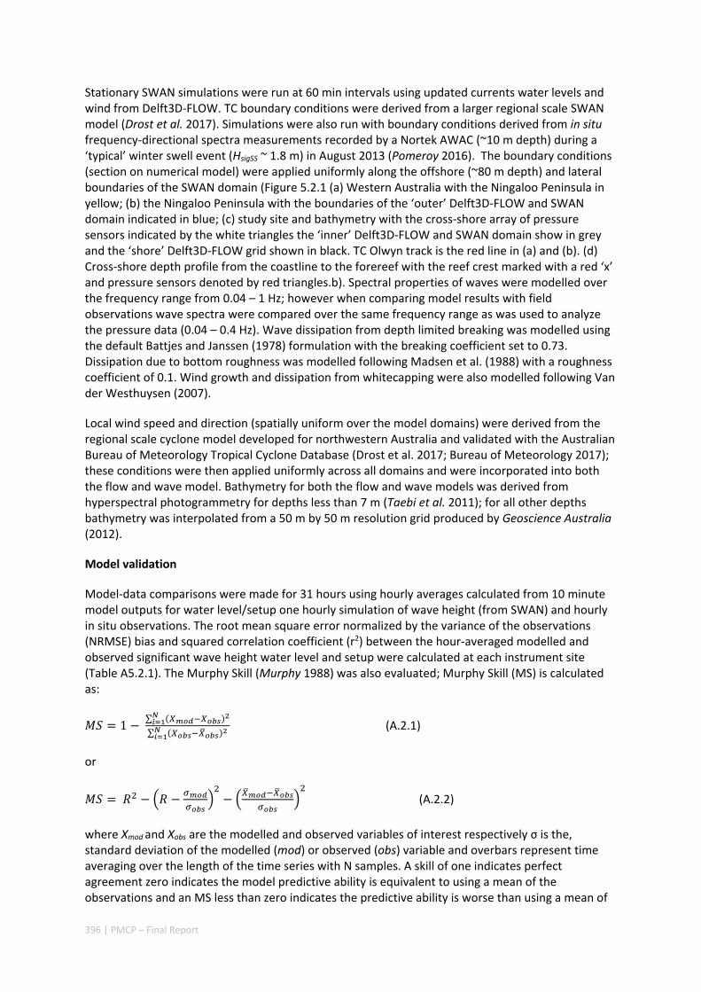
396 | PMCP – Final Report
Stationary SWAN simulations were run at 60 min intervals using updated currents water levels and wind from Delft3D‐FLOW. TC boundary conditions were derived from a larger regional scale SWAN model (Drost et al. 2017). Simulations were also run with boundary conditions derived from in situ frequency‐directional spectra measurements recorded by a Nortek AWAC (~10 m depth) during a ‘typical’ winter swell event (HsigSS ~ 1.8 m) in August 2013 (Pomeroy 2016). The boundary conditions (section on numerical model) were applied uniformly along the offshore (~80 m depth) and lateral boundaries of the SWAN domain (Figure 5.2.1 (a) Western Australia with the Ningaloo Peninsula in yellow; (b) the Ningaloo Peninsula with the boundaries of the ‘outer’ Delft3D‐FLOW and SWAN domain indicated in blue; (c) study site and bathymetry with the cross‐shore array of pressure sensors indicated by the white triangles the ‘inner’ Delft3D‐FLOW and SWAN domain show in grey and the ‘shore’ Delft3D‐FLOW grid shown in black. TC Olwyn track is the red line in (a) and (b). (d) Cross‐shore depth profile from the coastline to the forereef with the reef crest marked with a red ‘x’ and pressure sensors denoted by red triangles.b). Spectral properties of waves were modelled over the frequency range from 0.04 – 1 Hz; however when comparing model results with field observations wave spectra were compared over the same frequency range as was used to analyze the pressure data (0.04 – 0.4 Hz). Wave dissipation from depth limited breaking was modelled using the default Battjes and Janssen (1978) formulation with the breaking coefficient set to 0.73. Dissipation due to bottom roughness was modelled following Madsen et al. (1988) with a roughness coefficient of 0.1. Wind growth and dissipation from whitecapping were also modelled following Van der Westhuysen (2007).
Local wind speed and direction (spatially uniform over the model domains) were derived from the regional scale cyclone model developed for northwestern Australia and validated with the Australian Bureau of Meteorology Tropical Cyclone Database (Drost et al. 2017; Bureau of Meteorology 2017); these conditions were then applied uniformly across all domains and were incorporated into both the flow and wave model. Bathymetry for both the flow and wave models was derived from hyperspectral photogrammetry for depths less than 7 m (Taebi et al. 2011); for all other depths bathymetry was interpolated from a 50 m by 50 m resolution grid produced by Geoscience Australia (2012).
Model validation
Model‐data comparisons were made for 31 hours using hourly averages calculated from 10 minute model outputs for water level/setup one hourly simulation of wave height (from SWAN) and hourly in situ observations. The root mean square error normalized by the variance of the observations (NRMSE) bias and squared correlation coefficient (r2) between the hour‐averaged modelled and observed significant wave height water level and setup were calculated at each instrument site (Table A5.2.1). The Murphy Skill (Murphy 1988) was also evaluated; Murphy Skill (MS) is calculated as:
1 ∑
∑ (A.2.1)
or
(A.2.2)
where Xmod and Xobs are the modelled and observed variables of interest respectively σ is the, standard deviation of the modelled (mod) or observed (obs) variable and overbars represent time averaging over the length of the time series with N samples. A skill of one indicates perfect agreement zero indicates the model predictive ability is equivalent to using a mean of the observations and an MS less than zero indicates the predictive ability is worse than using a mean of

397 | PMCP – Final Report
the observations. Furthermore in Equation A.2.2 the first term is the squared correlation coefficient the second term quantifies the ability of the model to reproduce the variance in the observations and the third term represents the disagreement of the model and observational means (bias) and corresponds to the linear regression intercept (Murphy 1988; Ralston et al. 2010; Hansen et al. 2015). Here we consider 0.0<MS<0.5 to represent “moderate” skill scores with “high” and “poor” skills for higher and lower scores respectively (Hansen et al. 2015).
The model was able to reproduce the TC conditions with a high skill for nearly all variables and
instrument locations; average MS was 0.77 0.95 and 0.62 for HsigSS and respectively (Table A5.2.1). The lowest MS was for the reef flat sensor (P2) where HsigSS was under‐predicted but was slightly over‐predicted (except during the maximum setup); these discrepancies are likely due to the highly variable bathymetry associated with coral reef flats that the model was unable to reproduce as well as the wave dissipation formulation.
Table A5.2.1 Summary of Murphy (1988) skill score (MS) for modelled significant wave height (HsigSS) water level ( ) and setup ( ) at the instrument locations. For MS a score of 1 indicates perfect agreement between the model results and the observations.

398 | PMCP – Final Report
Figure A5.2.2 (a‐e) Comparison of observed significant wave heights (HsigSS) (f‐j) water level ( ) and (k‐o) setup ( ) with output from Delft3D‐FLOW and SWAN at the fore reef (P1) reef flat (P2) outer lagoon (P3) mid‐lagoon (P4) and inner lagoon (P5).
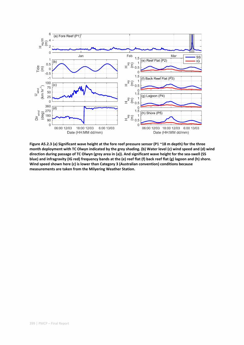
399 | PMCP – Final Report
Figure A5.2.3 (a) Significant wave height at the fore reef pressure sensor (P1 ~18 m depth) for the three month deployment with TC Olwyn indicated by the grey shading. (b) Water level (c) wind speed and (d) wind direction during passage of TC Olwyn (grey area in (a)). And significant wave height for the sea‐swell (SS blue) and infragravity (IG red) frequency bands at the (e) reef flat (f) back reef flat (g) lagoon and (h) shore. Wind speed shown here (c) is lower than Category 3 (Australian convention) conditions because measurements are taken from the Milyering Weather Station.
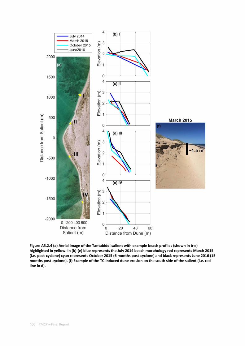
400 | PMCP – Final Report
Figure A5.2.4 (a) Aerial image of the Tantabiddi salient with example beach profiles (shown in b‐e) highlighted in yellow. In (b)‐(e) blue represents the July 2014 beach morphology red represents March 2015 (i.e. post‐cyclone) cyan represents October 2015 (6 months post‐cyclone) and black represents June 2016 (15 months post‐cyclone). (f) Example of the TC‐induced dune erosion on the south side of the salient (i.e. red line in d).
401 | PMCP – Final Report
Figure A5.2.5 Model‐predicted significant wave heights and circulation patterns from the onset of TC Olwyn (ab) the approach of TC Olwyn (cd) and when peak wave heights occurred (ef). Note for panels (c) and (d) both wind and waves are from a northerly direction (i.e. approximately alongshore); whereas in (e) and (f) wind and waves are from a south‐westerly direction (i.e. cross‐shore).
402 | PMCP – Final Report
Temporal disconnect of reef calcifiers and the sediment reservoir: implications for shoreline morphology of a fringing reef system
Authors: Cuttler M, Lowe R, Hansen J, McCulloch M.
ABSTRACT
Coral reefs are unique environments due to the strong link between ecological processes, the sediment reservoir, and the morphology of the adjacent coastline. Due to the linkages between the benthic community and the sediment reservoir in reef systems, the spatial distribution of sediment texture (or settling velocity) can be combined with measurements of the contemporary ecological community and the composition of the sediment reservoir to gain further insight into sediment transport pathways. Here, habitat mapping and thin section analysis revealed that living coral accounts for less than 5% of the benthic cover; however, coral was the dominant sediment constituent, accounting for up to 40% of deposits regardless of sub‐reef environment. Transport pathways through the system, inferred from the spatial distribution of D50, agree well with the predicted circulation for wave‐dominated fringing reefs (i.e. shore‐directed flow over the reef flat that diverges towards channels in the lagoon). However, due to the low coral cover on the reef crest, these pathways do not provide evidence of a modern source of coral‐rich sediment to the lagoon. Radiometric dating (238U/230Th) of coral fragments from the outer reef flat through the lagoon indicate that sediment is ~1000 to ~3500 years old, respectively; thus, the sediment reservoir is temporally disconnected from the modern calcifying community. These results suggest that the active sediment reservoir and calcifying community are temporally disconnected (i.e. sediments are derived from an older reef system), and therefore, despite the recent observations of rapid declines in net reef accretion, the sediment budget and shoreline morphology in this system may be more resilient to climate change induced declines in the contemporary reef ecology.

403 | PMCP – Final Report
5.3.1 INTRODUCTION
The sediments that form tropical beaches along coral reef coastlines are primarily derived from the calcium carbonate skeletal remains of organisms living within the diverse sub‐reef environments (Harney et al. 2000). Therefore, landforms in reef environments (e.g. reef islands or shorelines in the lee of fringing reefs) can be particularly sensitive to any ecological transitions that modify reef community composition as this will directly impact the source and supply of sediment to these formations (Perry et al. 2011, 2015a). Given that reef‐dwelling organisms (i.e. coral, crustose coralline algae, molluscs, Halimeda, etc.) break down into characteristic shapes and sizes [the ‘Sorby principle’; Sorby 1879], it is the length of time between the death of these organisms and when they are broken down to transportable‐sized (i.e. sand‐sized) material as well as the timescales of sediment transport processes that will determine the sensitivity of reef‐associated landforms to ecological community shifts.
Comparing the modern benthic community with the spatial distribution of sediment constituents can give insight into transport pathways through the system and ecological‐sedimentary links between sediment sources and sinks (Yamano et al. 2000; Perry et al. 2015a; Hamylton et al. 2016). For example, these data can identify key sediment producing regions and/or organisms that are key to landform development and maintenance (Kench 1997; Yamano et al. 2000; Dawson et al. 2012; Morgan and Kench 2016). Investigations into the links between reef ecology and reef‐associated landforms (primarily atoll islands), have relied upon radiometric dating of specific sediment constituents and/or bulk sediment samples to understand timescales of transport (Harney et al. 2000; Yamano et al. 2000; Dawson et al. 2012). For example, large benthic foraminifera have been dated with carbon‐14 (14C) to show transport from source (reef flat) to sink (reef island) takes place relatively quickly (i.e. ~60 years). In contrast, 14C dating of bulk sediment samples (i.e. all sediment constituents) from a fringing reef system in Hawaii showed that surface sediments throughout the system were older (~1000s years), thus suggesting longer timescales of transport from source (forereef) to sink (beach) (Harney et al. 2000). Apart from 14C, uranium‐series dating has been used to determine the age of coral pieces from core material in fringing reefs (Collins et al. 2003) as well as storm‐deposited coral boulders (Lau et al. 2016). However, radiometric dating provides little understanding of the sediment transport mechanisms (e.g. bedload or suspended load, storm‐induced versus fair‐weather wave driven) responsible for the observed age distributions and inferred transport pathways.
Suspended sediment transport has been studied in reefs for obvious reasons ‐ increased turbidity negatively impacts corals by decreasing the light availability and/or smothering them in sediments (Rogers 1990; Storlazzi et al. 2015). However, lagoon and beach sediment tend to be medium‐sized sand (Kench 1997; Morgan and Kench 2014, 2016) and therefore, unlikely to be suspended by typical mean currents. Bedforms are also common in these lower energy environments (e.g., lagoon and back‐reef; Storlazzi et al., 2004; Cuttler et al., 2015, 2016), suggesting the importance of bedload transport in these areas. Direct measurements of sediment transport (both bedload and suspended load) in reefs has relied upon the use of sediment traps (Kench and Mclean 2004; Storlazzi et al. 2004; Morgan and Kench 2014); however, where bedforms are present, migration rates can be used to calculate bedload sediment flux (e.g. Traykovski et al. 1999; Becker et al. 2007).
Linking reef ecology to sediment transport processes and geomorphic development is critical to determining the long‐term resilience of these landforms (Morgan and Kench 2014, 2016; Perry et al. 2015b). Reef associated landforms face significant erosion risk from sea level rise which has been hypothesized to increase wave transmission across reefs and therefore increase waves reaching the shoreline (Grady et al. 2013; Quataert et al. 2015; Cheriton et al. 2016). However, sediment supply has been suggested to be a more dominant control on geomorphic development in some systems (Woodroffe et al. 2007; Perry et al. 2015b). Identifying and quantifying the links between reef
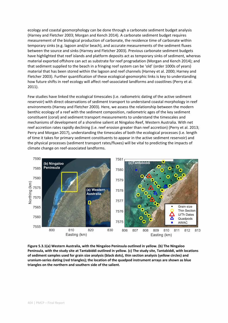
404 | PMCP – Final Report
ecology and coastal geomorphology can be done through a carbonate sediment budget analysis (Harney and Fletcher 2003; Morgan and Kench 2014). A carbonate sediment budget requires measurement of the biological production of carbonate, the residence time of carbonate within temporary sinks (e.g. lagoon and/or beach), and accurate measurements of the sediment fluxes between the source and sinks (Harney and Fletcher 2003). Previous carbonate sediment budgets have highlighted that reef islands and platform deposits act as temporary sinks of sediment, whereas material exported offshore can act as substrate for reef progradation (Morgan and Kench 2014); and that sediment supplied to the beach in a fringing reef system can be ‘old’ (order 1000s of years) material that has been stored within the lagoon and reef channels (Harney et al. 2000; Harney and Fletcher 2003). Further quantification of these ecological‐geomorphic links is key to understanding how future shifts in reef ecology will affect reef‐associated landforms and coastlines (Perry et al. 2011).
Few studies have linked the ecological timescales (i.e. radiometric dating of the active sediment reservoir) with direct observations of sediment transport to understand coastal morphology in reef environments (Harney and Fletcher 2003). Here, we assess the relationship between the modern benthic ecology of a reef with the sediment composition, radiometric ages of the key sediment constituent (coral) and sediment transport measurements to understand the timescales and mechanisms of development of a shoreline salient at Ningaloo Reef, Western Australia. With net reef accretion rates rapidly declining (i.e. reef erosion greater than reef accretion) (Perry et al. 2013; Perry and Morgan 2017), understanding the timescales of both the ecological processes (i.e. length of time it takes for primary sediment constituents to appear in the active sediment reservoir) and the physical processes (sediment transport rates/fluxes) will be vital to predicting the impacts of climate change on reef‐associated landforms.
Figure 5.3.1(a) Western Australia, with the Ningaloo Peninsula outlined in yellow. (b) The Ningaloo Peninsula, with the study site at Tantabiddi outlined in yellow. (c) The study site, Tantabiddi, with locations of sediment samples used for grain size analysis (black dots), thin section analysis (yellow circles) and uranium‐series dating (red triangles); the location of the quadpod instrument arrays are shown as blue triangles on the northern and southern side of the salient.
405 | PMCP – Final Report
5.3.2 DATA AND METHODS
Study area and field studies
Ningaloo Reef is Australia’s largest fringing reef, stretching ~270 km south from Australia’s North West Cape (Figure 5.3.1a). The morphology of Ningaloo is characterized by a steep (1:20) forereef slope, a relatively narrow reef flat (100s of m), and a wide (1 to 5 km), but shallow (< 5 m deep) lagoon (Collins et al. 2003). The study area, located at the northern extent of Ningaloo Reef at Tantabiddi (Figure 5.3.1), is marked by the presence of a shoreline salient inland from the reef flat. Salients, and other accretionary coastal landforms (e.g. dunes) are common features along the entire stretch of Ningaloo Reef and the greater Western Australian coastline (Sanderson and Eliot 1996; Sanderson 2000).
The field data presented here were collected over a period between August 2013 and June 2016, through several field experiments and surveys aimed at understanding the timescales and mechanisms linking sediment generation on the reef to development of the shoreline salient. In August 2013 field activities included collection of surficial sediment samples spanning the range of sub‐reef environments at Tantabiddi (e.g. forereef, reef flat, lagoon, and beach); these samples were used to determine sediment grain size, composition, and age. Benthic habitat surveys were collected in July 2014 for the reef flat and lagoon and in June 2016 for the reef crest and upper forereef (max ~11 m depth); these data were used to map the spatial coverage of reef calcifiers. Lagoon hydrodynamic and ripple migration rate data were collected between May 2016 and June 2016; these data was used to quantify the sediment transport mechanism supplying sediment to the salient.
Habitat data
In order to quantify the spatial coverage of modern reef calcifiers (i.e. the source of bioclastic sediments), diver‐recorded video transects were conducted at 15 locations encompassing the range of sub‐reef environments (e.g. reef crest, reef flat, and lagoon). At each location, five 50 m transects were recorded at ~0.5 m above the bed. Twenty still images were extracted from each video transect and imported into Coral Point Count with Excel Extensions (CPCe) to determine percent cover of individual benthic organisms (Kohler and Gill 2006). CPCe allows for randomisation of percent cover analysis by automatically generating a user‐defined number of points within an image; benthic organisms at the random points are then identified. Ten points were generated within each photo, yielding a total of 15,000 identification points (10 points per image x 20 images per transects x 5 transects per location x 15 locations); organisms were grouped into 11 categories to determine percent cover of the main calcifying organisms: coral, gorgonian, sponge, mollusc, macroalgae, other live, dead coral with algae, coralline algae, echinoid, sand/pavement/rubble, and unknown.
Sediment constituents and radiometric dating
To determine the spatial distribution of sediment texture (grain size, sorting, skewness) and composition, surficial sediment samples were collected from 57 locations across the study site (3 forereef, 16 reef flat, 24 lagoon, 10 channel, 4 beach; Figure 1); approximately 500 g of sediment was collected from the top 5‐7 cm of the seabed at each site (Cuttler et al. 2016). Standard wet sieve analysis was used to isolate gravel (>2 mm), sand (0.063 – 2 mm), and fine fractions (<0.063 mm). Hydraulic properties of sand‐sized sediment (0.063 – 2 mm) previously reported in (Cuttler et al. 2016) were converted to equivalent grain size distribution using Gibbs et al. (1971) and a site‐specific sediment density of 2580 kg m‐3 (Cuttler et al. 2016); and then combined with sieve results for the gravel fraction to determine the entire grain size distribution (Morgan and Kench 2016). Grain size statistics were then calculated using the graphical techniques of Folk and Ward (1957). Sub‐samples
406 | PMCP – Final Report
from the sand fraction at 35 sites were embedded in epoxy and thin‐sectioned; composition was determined by identifying a minimum of 300 grains using a petrographic microscope (Cuttler et al. 2016). Sediment were categorized as: coral, coralline algae (CCA), foraminifera, mollusc, echinoderm, quartz, framework, and other.
Coral sediment from 3 locations (Figure 5.3.1, red triangles) along a typical mean‐flow pathway through the lagoon (i.e. from outer reef flat towards the channel; Pomeroy, 2016a) were dated using uranium‐series isotope decay (238U – 234U – 230Th) and multi‐collector inductively coupled plasma mass spectrometry (MC‐ICPMS). This technique has been shown to be accurate for dating modern coral (100 to 102 years) as well as ancient (i.e. Last Interglacial) corals (~105 years) (McCulloch and Mortimer 2008). Coral sediment for radiometric dating was selected from the 0.25 – 0.5 mm sieve fraction by using a binocular microscope to select individual grains. This size fraction was used because it includes the median grain size (a common metric used for sediment transport studies) of each sample. Small sample sizes (≤ 50 mg) were used in order to minimize the number of grains contributing to each date (Harney et al. 2000); however, because samples contained 10s‐100s of individual grains, the ages presented here represent average ages of the sand‐sized material at the sample locations. Coral sediment from the most seaward (outer reef flat) site were also selected from the gravel fraction to gain more insight into the age distribution at the site theoretically closest to the source of coral (i.e. near the reef crest); however, gravel‐sized sediment age was measured on two individual pieces of coral due to the size and mass of these clasts.
Statistical and spatial analysis
Spatial interpolations of sediment texture (mean size and sorting) and composition were constructed in ArcGIS v10.3 using ordinary kriging methods. Statistical analysis of benthic cover and sediment composition and texture was conducted using the Fathom toolbox for Matlab (Jones 2015) to determine habitats and biosedmentary facies at Tantabiddi (Morgan and Kench 2016).
Agglomerative, hierarchical cluster analysis was conducted using the unweighted, pair group method with arithmetic mean. For habitat identification, a Bray‐Curtis (BC) dissimilarity matrix of square‐root transformed benthic cover data was used for cluster analysis; whereas, for determining biosedimentary facies, a BC matrix of square‐root transformed sediment texture (mean and sorting) and sediment composition was used (Kench 1997; Morgan and Kench 2016). Dissimilarity profile analysis (DISPROF) was used to identify statistically significant, unique habitats and facies from the resulting dendrograms (Clarke et al. 2008; Legendre and Legendre 2012). DISPROF is equivalent to similarity profile analysis (SIMPROF) proposed by Clarke et al. (2008); however, DISPROF is based on dissimilarity measures; both analyses provide an objective method for identifying members of “real” groups present in the results from clustering analysis (Jones 2015). Finally, canonical analysis of principal coordinates (CAP) was used to assess the driving factors behind the habitat and facies classifications.
Shoreline sediment supply: bedform migration rates and lagoon hydrodynamics
Sand ripples (~0.1 m height and ~0.5 m wavelength) are a common feature throughout the lagoon at Tantabiddi (Cuttler et al. 2015). Previous analysis of bed sediment at Tantabiddi has suggested that bedload transport is the primary transport mode through the lagoon (Cuttler et al. 2016) and that a key mechanism for sediment delivery to the shoreline could be the migration of sand ripples (Cuttler et al. 2015). To quantify ripple migration rates, which can be used as a proxy for bedload sediment flux, two instrument arrays were deployed in the inner lagoon on either side of the salient in ~3.5 m depth (north side) or ~2.5 m depth (south side) for four weeks in May‐June 2016 (Figure 5.3.1, blue triangles; Figure 5.3.2).
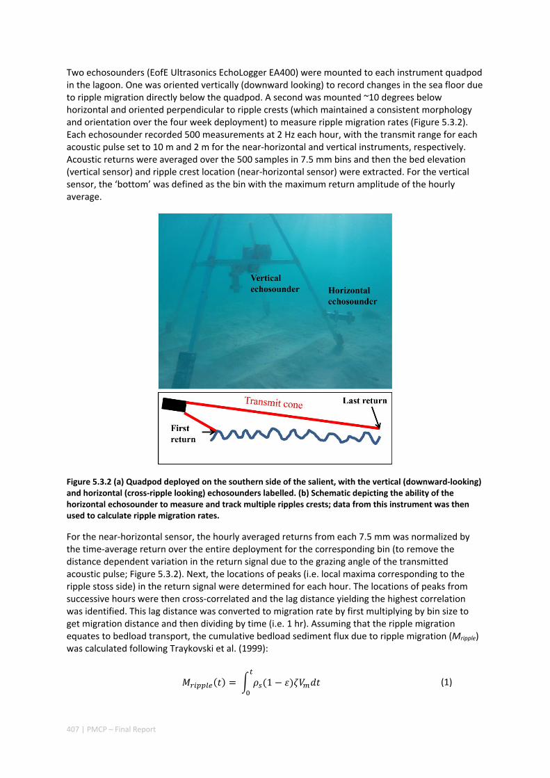
407 | PMCP – Final Report
Two echosounders (EofE Ultrasonics EchoLogger EA400) were mounted to each instrument quadpod in the lagoon. One was oriented vertically (downward looking) to record changes in the sea floor due to ripple migration directly below the quadpod. A second was mounted ~10 degrees below horizontal and oriented perpendicular to ripple crests (which maintained a consistent morphology and orientation over the four week deployment) to measure ripple migration rates (Figure 5.3.2). Each echosounder recorded 500 measurements at 2 Hz each hour, with the transmit range for each acoustic pulse set to 10 m and 2 m for the near‐horizontal and vertical instruments, respectively. Acoustic returns were averaged over the 500 samples in 7.5 mm bins and then the bed elevation (vertical sensor) and ripple crest location (near‐horizontal sensor) were extracted. For the vertical sensor, the ‘bottom’ was defined as the bin with the maximum return amplitude of the hourly average.
Figure 5.3.2 (a) Quadpod deployed on the southern side of the salient, with the vertical (downward‐looking) and horizontal (cross‐ripple looking) echosounders labelled. (b) Schematic depicting the ability of the horizontal echosounder to measure and track multiple ripples crests; data from this instrument was then used to calculate ripple migration rates.
For the near‐horizontal sensor, the hourly averaged returns from each 7.5 mm was normalized by the time‐average return over the entire deployment for the corresponding bin (to remove the distance dependent variation in the return signal due to the grazing angle of the transmitted acoustic pulse; Figure 5.3.2). Next, the locations of peaks (i.e. local maxima corresponding to the ripple stoss side) in the return signal were determined for each hour. The locations of peaks from successive hours were then cross‐correlated and the lag distance yielding the highest correlation was identified. This lag distance was converted to migration rate by first multiplying by bin size to get migration distance and then dividing by time (i.e. 1 hr). Assuming that the ripple migration equates to bedload transport, the cumulative bedload sediment flux due to ripple migration (Mripple) was calculated following Traykovski et al. (1999):
1 (1)
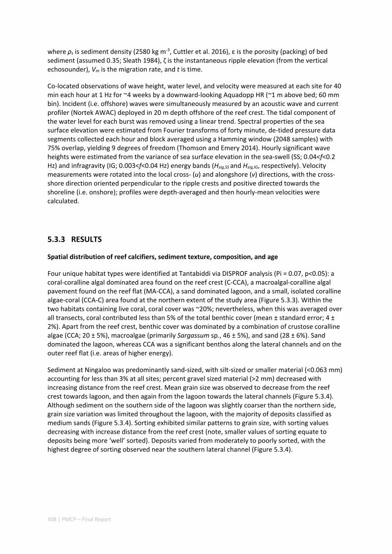
408 | PMCP – Final Report
where ρs is sediment density (2580 kg m‐3, Cuttler et al. 2016), ε is the porosity (packing) of bed sediment (assumed 0.35; Sleath 1984), ζ is the instantaneous ripple elevation (from the vertical echosounder), Vm is the migration rate, and t is time.
Co‐located observations of wave height, water level, and velocity were measured at each site for 40 min each hour at 1 Hz for ~4 weeks by a downward‐looking Aquadopp HR (~1 m above bed; 60 mm bin). Incident (i.e. offshore) waves were simultaneously measured by an acoustic wave and current profiler (Nortek AWAC) deployed in 20 m depth offshore of the reef crest. The tidal component of the water level for each burst was removed using a linear trend. Spectral properties of the sea surface elevation were estimated from Fourier transforms of forty minute, de‐tided pressure data segments collected each hour and block averaged using a Hamming window (2048 samples) with 75% overlap, yielding 9 degrees of freedom (Thomson and Emery 2014). Hourly significant wave heights were estimated from the variance of sea surface elevation in the sea‐swell (SS; 0.04<f<0.2 Hz) and infragravity (IG; 0.003<f<0.04 Hz) energy bands (Hsig,SS
and Hsig,IG, respectively). Velocity measurements were rotated into the local cross‐ (u) and alongshore (v) directions, with the cross‐shore direction oriented perpendicular to the ripple crests and positive directed towards the shoreline (i.e. onshore); profiles were depth‐averaged and then hourly‐mean velocities were calculated.
5.3.3 RESULTS
Spatial distribution of reef calcifiers, sediment texture, composition, and age
Four unique habitat types were identified at Tantabiddi via DISPROF analysis (Pi = 0.07, p<0.05): a coral‐coralline algal dominated area found on the reef crest (C‐CCA), a macroalgal‐coralline algal pavement found on the reef flat (MA‐CCA), a sand dominated lagoon, and a small, isolated coralline algae‐coral (CCA‐C) area found at the northern extent of the study area (Figure 5.3.3). Within the two habitats containing live coral, coral cover was ~20%; nevertheless, when this was averaged over all transects, coral contributed less than 5% of the total benthic cover (mean ± standard error; 4 ± 2%). Apart from the reef crest, benthic cover was dominated by a combination of crustose coralline algae (CCA; 20 ± 5%), macroalgae (primarily Sargassum sp., 46 ± 5%), and sand (28 ± 6%). Sand dominated the lagoon, whereas CCA was a significant benthos along the lateral channels and on the outer reef flat (i.e. areas of higher energy).
Sediment at Ningaloo was predominantly sand‐sized, with silt‐sized or smaller material (<0.063 mm) accounting for less than 3% at all sites; percent gravel sized material (>2 mm) decreased with increasing distance from the reef crest. Mean grain size was observed to decrease from the reef crest towards lagoon, and then again from the lagoon towards the lateral channels (Figure 5.3.4). Although sediment on the southern side of the lagoon was slightly coarser than the northern side, grain size variation was limited throughout the lagoon, with the majority of deposits classified as medium sands (Figure 5.3.4). Sorting exhibited similar patterns to grain size, with sorting values decreasing with increase distance from the reef crest (note, smaller values of sorting equate to deposits being more ‘well’ sorted). Deposits varied from moderately to poorly sorted, with the highest degree of sorting observed near the southern lateral channel (Figure 5.3.4).
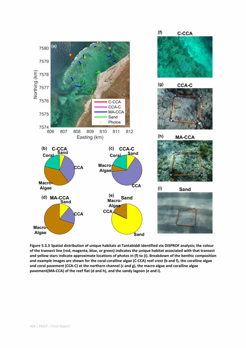
409 | PMCP – Final Report
Figure 5.3.3 Spatial distribution of unique habitats at Tantabiddi identified via DISPROF analysis; the colour of the transect line (red, magenta, blue, or green) indicates the unique habitat associated with that transect and yellow stars indicate approximate locations of photos in (f) to (i). Breakdown of the benthic composition and example images are shown for the coral‐coralline algae (C‐CCA) reef crest (b and f), the coralline algae and coral pavement (CCA‐C) at the northern channel (c and g), the macro algae and coralline algae pavement(MA‐CCA) of the reef flat (d and h), and the sandy lagoon (e and i).
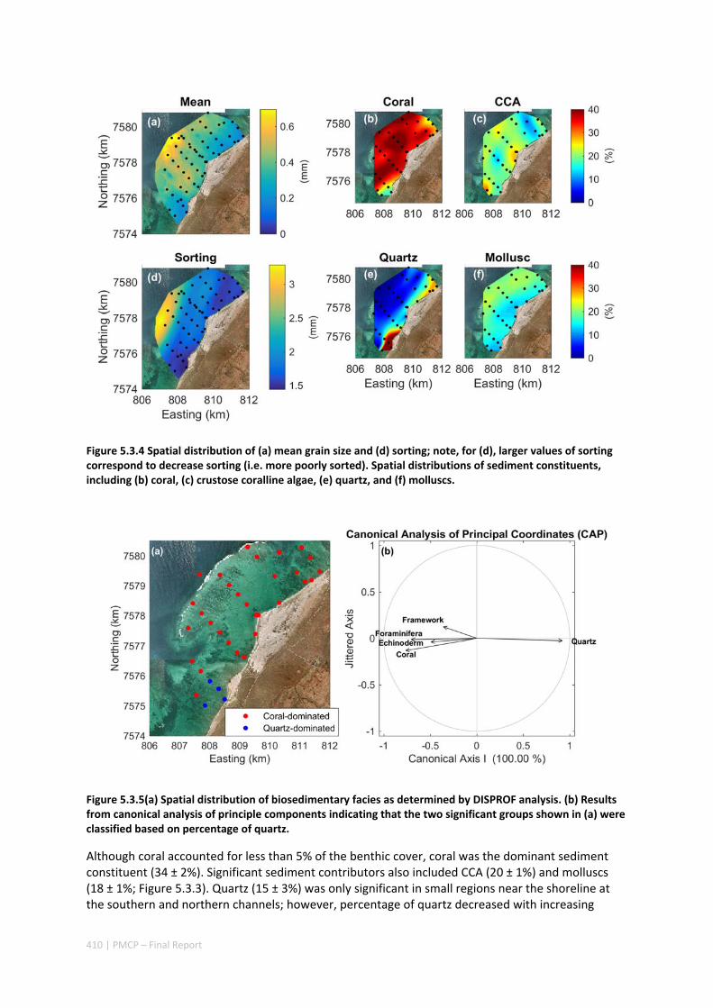
410 | PMCP – Final Report
Figure 5.3.4 Spatial distribution of (a) mean grain size and (d) sorting; note, for (d), larger values of sorting correspond to decrease sorting (i.e. more poorly sorted). Spatial distributions of sediment constituents, including (b) coral, (c) crustose coralline algae, (e) quartz, and (f) molluscs.
Figure 5.3.5(a) Spatial distribution of biosedimentary facies as determined by DISPROF analysis. (b) Results from canonical analysis of principle components indicating that the two significant groups shown in (a) were classified based on percentage of quartz.
Although coral accounted for less than 5% of the benthic cover, coral was the dominant sediment constituent (34 ± 2%). Significant sediment contributors also included CCA (20 ± 1%) and molluscs (18 ± 1%; Figure 5.3.3). Quartz (15 ± 3%) was only significant in small regions near the shoreline at the southern and northern channels; however, percentage of quartz decreased with increasing

411 | PMCP – Final Report
distance from the shoreline (Figure 5.3.4). DISPROF analysis showed only two significant groupings (Pi = 7.19, p<0.05) for bed sediment, primarily differentiated by the percentage of quartz (Figure 5.3.5); thus, suggesting minimal compositional differences between sediment from the reef crest, reef flat, lagoon, and beach.
Uranium‐series ages of coral sediment (i.e. the dominant sediment constituent) revealed that sediments are ‘old’, with the youngest sediments aged ~1400 years before present (1 ka BP; Table 5.3.1). Sediment age increased along a typical flow pathway from the reef flat to the channel (Figure 5.3.4), with the channel sands from this study dated to ~3.7 ka BP and the top of a lagoon core from Collins et al. (2003) dated to ~5 ka BP (also using U‐series dating). There was a limited range in age between the coarse (PJ028‐C1 and PJ028‐C2) and sand‐sized (PJ028‐S) material dated from the outer reef flat (~300 years).
Table 5.3.1 Summary of radiometric (Uranium‐series) analysis. Corrected age is calculated assuming initial, non‐radiogenic [230Th/232Th] = 1 ± 1; see McCulloch and Mortimer (2008) for further details of calculations.
Figure 5.3.6 Uranium‐series ages of coral sediment dated from surficial sediment samples collected for this study (red dots) from the outer reef flat (PJ028), back reef flat (PJ033), and lagoon (PJ039); note, C or S denotes that fragments were from the coarse (>2 mm) or sand (<2 mm) fractions, respectively. Uranium‐series age of coral fragment dated from the top of a lagoon sediment core (Collins et al. 2003). White arrows indicate the dominant mean wave‐driven circulation patterns from model results presented elsewhere.
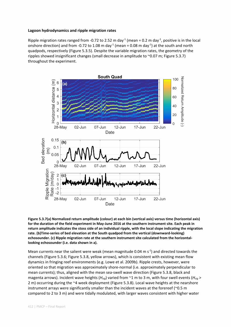
412 | PMCP – Final Report
Lagoon hydrodynamics and ripple migration rates
Ripple migration rates ranged from ‐0.72 to 2.52 m day‐1 (mean = 0.2 m day‐1, positive is in the local onshore direction) and from ‐0.72 to 1.08 m day‐1 (mean = 0.08 m day‐1) at the south and north quadpods, respectively (Figure 5.3.5). Despite the variable migration rates, the geometry of the ripples showed insignificant changes (small decrease in amplitude to ~0.07 m; Figure 5.3.7) throughout the experiment.
Figure 5.3.7(a) Normalized return amplitude (colour) at each bin (vertical axis) versus time (horizontal axis) for the duration of the field experiment in May‐June 2016 at the southern instrument site. Each peak in return amplitude indicates the stoss side of an individual ripple, with the local slope indicating the migration rate. (b)Time‐series of bed elevation at the South quadpod from the vertical (downward‐looking) echosounder. (c) Ripple migration rate at the southern instrument site calculated from the horizontal‐looking echosounder (i.e. data shown in a).
Mean currents near the salient were weak (mean magnitude 0.04 m s‐1) and directed towards the channels (Figure 5.3.6; Figure 5.3.8, yellow arrows), which is consistent with existing mean flow dynamics in fringing reef environments (e.g. Lowe et al. 2009b). Ripple crests, however, were oriented so that migration was approximately shore‐normal (i.e. approximately perpendicular to mean currents); thus, aligned with the mean sea‐swell wave direction (Figure 5.3.8, black and magenta arrows). Incident wave heights (Hsig) varied from ~1 m to 3 m, with four swell events (Hsig > 2 m) occurring during the ~4 week deployment (Figure 5.3.8). Local wave heights at the nearshore instrument arrays were significantly smaller than the incident waves at the forereef (~0.5 m compared to 2 to 3 m) and were tidally modulated, with larger waves consistent with higher water
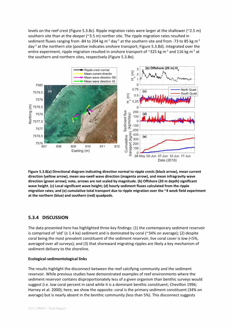
413 | PMCP – Final Report
levels on the reef crest (Figure 5.3.8c). Ripple migration rates were larger at the shallower (~2.5 m) southern site than at the deeper (~3.5 m) norther site. The ripple migration rates resulted in sediment fluxes ranging from ‐84 to 204 kg m‐1 day‐1 at the southern site and from ‐73 to 85 kg m‐1 day‐1 at the northern site (positive indicates onshore transport; Figure 5.3.8d). Integrated over the entire experiment, ripple migration resulted in onshore transport of ~325 kg m‐1 and 116 kg m‐1 at the southern and northern sites, respectively (Figure 5.3.8e).
Figure 5.3.8(a) Directional diagram indicating direction normal to ripple crests (black arrow), mean current direction (yellow arrow), mean sea‐swell wave direction (magenta arrow), and mean infragravity wave direction (green arrow); note, arrows are not scaled by magnitude. (b) Offshore (20 m depth) significant wave height. (c) Local significant wave height; (d) hourly sediment fluxes calculated from the ripple migration rates; and (e) cumulative total transport due to ripple migration over the ~4 week field experiment at the northern (blue) and southern (red) quadpods.
5.3.4 DISCUSSION
The data presented here has highlighted three key findings: (1) the contemporary sediment reservoir is comprised of ‘old’ (≥ 1.4 ka) sediment and is dominated by coral (~34% on average); (2) despite coral being the most prevalent constituent of the sediment reservoir, live coral cover is low (<5%, averaged over all surveys); and (3) that shoreward migrating ripples are likely a key mechanism of sediment delivery to the shoreline.
Ecological‐sedimentological links
The results highlight the disconnect between the reef calcifying community and the sediment reservoir. While previous studies have demonstrated examples of reef environments where the sediment reservoir contains disproportionately less of a given organism than benthic surveys would suggest (i.e. low coral percent in sand while it is a dominant benthic constituent; Chevillon 1996; Harney et al. 2000); here, we show the opposite: coral is the primary sediment constituent (34% on average) but is nearly absent in the benthic community (less than 5%). This disconnect suggests
414 | PMCP – Final Report
either a spatial disconnect from the source material (i.e. coral sediment is derived from outside the surveyed area) or a temporal decoupling from the source material (i.e. sediments are reflective of a relic reef community). It is unlikely that the sediment at Tantabiddi was imported from adjacent reef sections with higher coral cover due to the dominant circulation patterns (i.e. limited alongshore transport; Figure 5.3.4). Furthermore, regional hyperspectral mapping suggests that our results agree well with spatially‐averaged coral cover for the northern Ningaloo Reef (270 km2 mapped; Kobryn et al. 2013). Data used for calibrating the hyperspectral maps showed that the sanctuary zone immediately south of the study area has similar coral cover to that found here, and that it is not until Osprey Bay (~40 km to the south) that there is high (~40%) coral cover (Langdon 2012). Given that the ages of coral sediment were > 1 ka BP, the results presented here further support that sediments at Tantabiddi are derived from a reef community that was living ~1.4 to ~5 ka BP; and that these ‘old’ sediment are stored in surficial sand bodies (e.g. offshore areas and/or channels) and then transported into the lagoon by waves, similar to Hawaiian fringing reefs (Harney et al. 2000; Harney and Fletcher 2003).
The most recent (local) sea level high stand occurred 5.8 ka BP, when sea level was approximately 1 to 2 m higher than present (Collins et al. 2003). Prior to this time (~8 ka BP to 5.8 ka BP), reef growth had been in a rapid, ‘catch up’ phase (Twiggs and Collins 2010); and core data indicates that benthic cover during that time was dominated by corals (Collins et al. 2003; Twiggs and Collins 2010). Over the last ~5.8 ka, sea level has fallen to present levels and Ningaloo has been marked by a ‘detrital build up and aggradational’ phase (Twiggs and Collins 2010). It was during this time period that the modern sediment reservoir was likely created, as a decrease in local sea level would have exposed the coral‐dominated reef to increasing amounts of wave energy that would have eroded these communities and generated the sediment that is now slowly cycling through the system, with some of the oldest material (i.e. ~5 ka BP) still present near the channels.
Future changes to reef‐associated landforms will be governed by the effects of sea level rise and ocean warming/acidification on the reef ecology; with changing oceanic forcing determining the constituent assemblage and grain size of sediment available (Perry et al. 2011). For example, coral‐dominated landforms are expected to undergo major morphological change due to decreased availability of sand‐sized, coral material (Perry et al. 2011). Although rapid changes (i.e. over ~10 years) in sediment composition in response to changes in reef ecology have been observed (Perry 1996), the temporal disconnect between the modern benthic ecology and the active sediment reservoir shown here suggests that this system could be slower to respond to future shifts in the benthic ecology as sediment is stored in the active sediment reservoir (and therefore available for shoreline maintenance) for 1000s of years.
Implications for shoreline morphology and maintenance
Rouse (1937) numbers (P) are commonly used for predicting sediment transport mode (i.e. suspended load versus bedload); where P is the ratio of the sediment’s settling velocity to the shear velocity of the overlying flow (Rouse 1937). In agreement with P calculated from the settling velocities of bed sediment (Cuttler et al. 2016), bedload transport through the lagoon, via ripple migration, is suggested to be a significant mechanism for delivery of sediment to the shoreline. Spatial distributions of grain size agreed well with observed mean circulation patterns, suggesting that these currents are responsible for the larger scale distribution of sediment around the reef. However, in terms of sediment delivery to the shoreline, ripples were oriented so that migration was determined by mean the sea‐swell wave direction. Ripples have been shown to orient themselves so as to maximize transport rate (Gallagher et al. 1998), suggesting that the wave orbital motions are primarily responsible for the bedload transport with the local direction of transport determined by wave refraction around the reef edges and into the lagoon (Figure 5.3.8).

415 | PMCP – Final Report
In order for bedload transport via wave orbital motions to be responsible for building the shoreline salient at the study site, it must be operating at similar timescales to the supply of sediment to the lagoon (i.e. order 1000s of years). Assuming the coastline immediately behind the reef would be approximately straight if not for the shoreline salient, then the salient volume is approximately 6,400,000 m3 (Figure 5.3.9); using a mean sediment flux derived from ripple migration rates (averaged over both north and south sites) of 9 kg m‐1 day‐1, and a porosity of 0.35, ripple migration could have filled the salient volume in ~1.5 ka. However, this is likely a lower‐bound (i.e. most rapid in‐fill time) estimate, given that our migration rates are from a winter period where waves are more energetic; for example, if migration rates are halved, the estimated fill time increases to ~2.7 ka, which is similar to the age of lagoon sand.
Figure 5.3.9 Volume calculation of the shoreline salient at Tantabiddi used to determine in‐fill time given average rates of ripple migration. Elevations for onshore locations are derived from topographic light detecting and ranging (LiDAR) data flown for the region in October 2015.
Given that both the active sediment reservoir and the dominant mechanism of sediment delivery to the shoreline are operating on long (order 1000s of years) timescales, the results collectively imply that shoreline morphology in this environment will likely be resilient to future shifts in benthic community structure. However, changing environmental conditions may still pose a threat to these coastlines as the changing benthic community (i.e. decrease in coral cover) and decline in net reef accretion as well as sea level rise, could allow more wave energy to reach the coastline and directly impact the shoreline (Grady et al. 2013; Cheriton et al. 2016).
Conclusions
Coral reef environments are unique in that there is a strong link between the reef ecology and the sediment reservoir; however, these connections may increase the sensitivity of reef‐associated landforms (e.g. reef islands or fringing reef‐fronted coastlines) to changes in reef ecology. Data presented here highlights that for a section of Australia’s largest fringing reef, Ningaloo Reef, the benthic ecology (e.g. coral cover) and the active sediment reservoir are temporally disconnected; thus, the sediments are derived from a benthic community that occupied the reef ~1,400 to 5,000 years ago. Over this same timescale, bedload transport (in the form of migrating sand ripples) has

416 | PMCP – Final Report
been acting to build the large shoreline salient that is present in the lee of the reef. Together, these results indicate that reef systems similar to Ningaloo may be more resilient to future shifts in benthic ecology, with the supply of sediment decoupled from the modern benthic community; however, declines in net reef accretion still pose a threat, as any increase in wave transmission over the reef flat may result in direct wave attack of these coastlines.
5.3.5 ACKNOWLEDGEMENTS
This research was financially supported as part of the Pilbara Marine Conservation Partnership funded by the Gorgon Barrow Island Net Conservation Benefits Fund which is administered by the WA Department of Biodiversity, Conservation and Attractions (DBCA).
5.3.6 REFERENCES
Becker JM, Firing YL, Aucan J, Holman R, Merrifield M and Pawlak G (2007) Video‐based observations of nearshore sand ripples and ripple migration. J. Geophys. Res. Ocean. 112: 1–14.
Cheriton OM, Storlazzi CD, Rosenberger KJ (2016) Observations of wave transformation over a fringing coral reef and the importance of low‐frequency waves and offshore water levels to runup, overwash, and coastal flooding. J. Geophys. Res. Ocean. 3372–3380.
Chevillon C 1996. Skeletal composition of modern lagoon sediments in New Caledonia: coral, a minor constituent. Coral Reefs 199–207.
Clarke KR, Somerfield PJ and Gorley RN (2008) Testing of null hypotheses in exploratory community analyses: similarity profiles and biota‐environment linkage. J. Exp. Mar. Bio. Ecol. 366: 56–69.
Collins LB, Zhu ZR, Wyrwoll KH‐ and Eisenhauer A (2003) Late Quaternary structure and development of the northern Ningaloo Reef, Australia. Sediment. Geol. 159: 81–94.
Cuttler M, Lowe RJ, Hansen JE, Falter JL and Pomeroy AWM (2015) Grainsize, composition and bedform patterns in a fringing reef system. Proc. Coast. Sediments
Cuttler MVW, Lowe RJ, Falter JL and Buscombe D (2016) Estimating the settling velocity of bioclastic sediment using common grain‐size analysis techniques. Sedimentology.
Dawson JL, Hua Q and Smithers SG (2012) Benthic foraminifera : Their importance to future reef island resilience. Proc. 12th Int. Coral Reef Symp. Cairns, Aust.
Folk RL and Ward WC (1957) Brazos River Bar : A study in the significance of grain size parameters. J. Sediment. Petrol. 27: 3–26.
Gallagher EL, Elgar S and Thornton EB (1998) Megaripple migration in a natural surf zone. Nature 394: 165–168.
Gibbs RJ, Matthews MD and a Link D (1971). The relationship between sphere size and settling velocity. J. Sediment. Res. 41: 7–18.
417 | PMCP – Final Report
Grady AE, Moore EJ, Storlazzi CD, Elias E and Reidenbach MA (2013) The influence of sea level rise and changes in fringing reef morphology on gradients in alongshore sediment transport. Geophys. Res. Lett. 40: 3096–3101.
Hamylton SM, Carvalho RC, Duce S, Roelfsema CM and Vila‐Concejo A (2016) Linking pattern to process in reef sediment dynamics at Lady Musgrave Island, southern Great Barrier Reef C. Betzler [ed.]. Int. Assoc. Sedimentol. Spec. Publ. 63: 1634–1650.
Harney JN Fletcher CH (2003) A budget of carbonate framework and sediment production, Kailua Bay, Oahu, Hawaii. J. Sediment. Res. 73: 856–868.
Harney JN, Grossman EE, Richmond BM and Fletcher III CH (2000) Age and composition of carbonate shoreface sediments, Kailua Bay, Oahu, Hawaii. Coral Reefs 19: 141–154.
Jones DL (2015) Fathom Toolbox for Matlab: software for multivariate ecological and oceanographic data analysis.
Kench PS (1997) Contemporary sedimentation in the Cocos (Keeling) Islands, Indian Ocean: interpretation using settling velocity analysis. Sediment. Geol. 114: 109–130.
Kench PS, Mclean RF (2004) Hydrodynamics and sediment flux of hoa in an Indian Ocean atoll. Earth Surf. Process. Landforms 29: 933–953.
Kobryn HT, Wouters K, Beckley LE Heege T (2013) Ningaloo Reef: Shallow Marine Habitats Mapped Using a Hyperspectral Sensor. PLoS One 8: e70105.
Kohler KE, Gill SM (2006) Coral Point Count with Excel extensions (CPCe): A Visual Basic program for the determination of coral and substrate coverage using random point count methodology. Comput. Geosci. 32: 1259–1269.
Langdon MW (2012) The ecology of the grazing urchin Echinometra mathaei at Ningaloo Marine Park. Murdoch University.
Lau AYA, Terry JP, Ziegler AD, Switzer AD, Lee Y and Etienne S (2016) Understanding the history of extreme wave events in the Tuamotu Archipelago of French Polynesia from large carbonate boulders on Makemo Atoll, with implications for future threats in the central South Pacific Mar. Geol. , doi:10.1016/j.margeo.2016.04.018
Legendre P and Legendre (2012) Numerical Ecology, 3rd ed Elsevier Science BV
Lowe RJ, Falter JL, Monismith SG and Atkinson MJA (2009) Wave‐Driven Circulation of a Coastal Reef – Lagoon System. J. Phys. Oceanogr. 39: 873–893.
McCulloch MT and Mortimer GE (2008) The decay series to dating of fossil and modern corals using MC‐ICPMS. Aust. J. Earth Sci. 55: 955–965.
Morgan KM and Kench PS (2014) A detrital sediment budget of a Maldivian reef platform. Geomorphology 222: 122–131.
Morgan KM and Kench PS (2016) Reef to island sediment connections on a Maldivian carbonate platform: using benthic ecology and biosedimentary depositional facies to examine island‐building potential. Earth Surf. Process. Landforms , doi:10.1002/esp.3946
418 | PMCP – Final Report
Perry CT (1996) The rapid response of reef sediments to changes in community composition: implications for time averaging and sediment accumulation. J. Sediment. Petrol. 66: 459–467.
Perry CT, Kench PS, O’Leary MJ, Morgan KM and Januchowski‐Hartley F (2015a) Linking reef ecology to island building: Parrotfish identified as major producers of island‐building sediment in the Maldives. Geology 43: 503–506.
Perry CT, Kench PS O’Leary MJ, Morgan KM and Januchowski‐Hartley F (2015b) Linking reef ecology to island building: Parrotfish identified as major producers of island‐building sediment in the Maldives. Geology 43: 503–506.
Perry CT, Kench PS, Smithers SG, Riegl B, Yamano H and O’Leary MJ (2011) Implications of reef ecosystem change for the stability and maintenance of coral reef islands. Glob. Chang. Biol. 17: 3679–3696.
Perry CT and Morgan KM (2017) Bleaching drives collapse in reef carbonate budgets and reef growth potential on southern Maldives reefs. Sci. Rep. 7: 40581.
Perry CT, Murphy GN, Kench PS, Smithers SG, Edinger EN, Steneck RS and Mumby PJ (2013) Caribbean‐wide decline in carbonate production threatens coral reef growth. Nat. Commun. 4: 1402.
Pomeroy AWM (2016) Sediment transport in fringing coral reefs The University of Western Australia
Quataert E, Storlazzi C, van Rooijen A, Cheriton O and van Dongeren A (2015). The influence of coral reefs and climate change on wave‐driven flooding of tropical coastlines. Geophys. Res. Lett. n/a‐n/a.
Rogers CS (1990) Responses of coral reefs and reef organisms to sedimentation. Mar. Ecol. Prog. Ser. 62: 185–202.
Rouse H (1937) Modern conceptions of the mechanics or fluid turbulence. Trans. Am. Soc. Civ. Eng. 102: 463–505.
Sanderson PG (2000) A comparison of reef‐protected environments in Western Australia: The central west and Ningaloo coasts. Earth Surf. Process. Landforms 25: 397–419.
Sanderson PG and Eliot I (1996) Shoreline salients, cuspate forelands and tombolos on the coast of Western Australia. J. Coast. Res. 12: 761–773.
Sleath JFA (1984) Sea bed mechanics, John Wiley.
Sorby HC (1879) The structure and origin of limestones. Proc. Geol. Soc. London 35: 56–95.
Storlazzi CD, Norris BK and Rosenberger KJ (2015) The influence of grain size, grain color, and suspended‐sediment concentration on light attenuation: Why fine‐grained terrestrial sediment is bad for coral reef ecosystems. Coral Reefs 34: 967–975.
Storlazzi CD, Ogston a S, Bothner MH, Field ME and Presto MK (2004) Wave‐ and tidally‐driven flow and sediment flux across a fringing coral reef: Southern Molokai, Hawaii Cont. Shelf Res. 24: 1397–1419.
419 | PMCP – Final Report
Thomson RE and Emery WJ (2014) Data Analysis Methods in Physical Oceanography,
Traykovski PAE Hay, Irish JD and Lynch JF (1999) Geometry, migration, and evolution of wave orbital ripples at LEO‐15. J Geophys Res 104: 1505.
Twiggs EJ and Collins LB (2010) Development and demise of a fringing coral reef during Holocene environmental change, eastern Ningaloo Reef, Western Australia Mar Geol 275: 20–36.
Woodroffe CD, Samosorn B, Hua Q and Hart DE (2007) Incremental accretion of a sandy reef island over the past 3000 years indicated by component‐specific radiocarbon dating. Geophys Res Lett 34: L03602.
Yamano H, Miyajima T and Koike I (2000) Importance of foraminifera for the formation and maintenance of a coral sand cay: Green Island, Australia. Coral Reefs 19: 51–58.
420 | PMCP – Final Report
Ocean transport pathways to a World Heritage fringing coral reef: Ningaloo Reef, Western Australia
Authors: Xu J, Lowe RJ, Ivey GN, Jones NL, Zhang Z.
Published in PLoS ONE 11(2016):e0145822. doi:10.1371/journal.pone.0145822.
ABSTRACT
A Lagrangian particle tracking model driven by a regional ocean circulation model was used to investigate the seasonally‐varying connectivity patterns within the shelf circulation surrounding the 300 km long Ningaloo Reef in Western Australia (WA) during 2009‐2010. Forward‐in‐time simulations revealed that surface water was transported equatorward and offshore in summer due to the upwelling‐favorable winds. In winter, however, water was transported polewards down the WA coast due to the seasonally‐strong Leeuwin Current. Using backward‐in‐time simulations, the subsurface transport pathways revealed two main source regions of shelf water reaching Ningaloo Reef: (1) a year‐round source to the northeast in the upper 100 m of water column; and (2) during the summer, an additional source offshore and to the west of Ningaloo in depths between ~30 and ~150 m. Transient wind‐driven coastal upwelling, onshore geostrophic transport and stirring by offshore eddies were identified as the important mechanisms influencing the source water origins. The identification of these highly time‐dependent transport pathways and source water locations is an essential step towards quantifying how key material (e.g. nutrients, larvae, contaminants, etc.) is exchanged between Ningaloo Reef and the surrounding shelf ocean, and how this is mechanistically coupled to the complex ocean dynamics in this region.
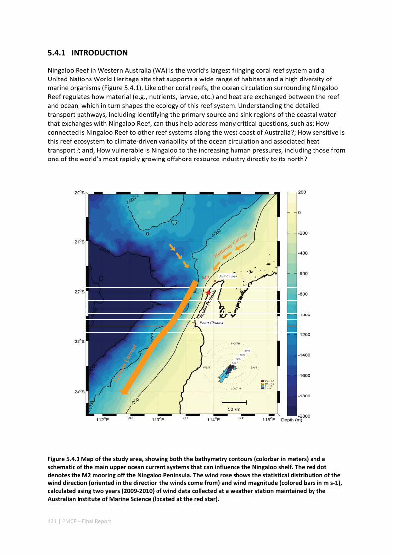
421 | PMCP – Final Report
5.4.1 INTRODUCTION
Ningaloo Reef in Western Australia (WA) is the world’s largest fringing coral reef system and a United Nations World Heritage site that supports a wide range of habitats and a high diversity of marine organisms (Figure 5.4.1). Like other coral reefs, the ocean circulation surrounding Ningaloo Reef regulates how material (e.g., nutrients, larvae, etc.) and heat are exchanged between the reef and ocean, which in turn shapes the ecology of this reef system. Understanding the detailed transport pathways, including identifying the primary source and sink regions of the coastal water that exchanges with Ningaloo Reef, can thus help address many critical questions, such as: How connected is Ningaloo Reef to other reef systems along the west coast of Australia?; How sensitive is this reef ecosystem to climate‐driven variability of the ocean circulation and associated heat transport?; and, How vulnerable is Ningaloo to the increasing human pressures, including those from one of the world’s most rapidly growing offshore resource industry directly to its north?
Figure 5.4.1 Map of the study area, showing both the bathymetry contours (colorbar in meters) and a schematic of the main upper ocean current systems that can influence the Ningaloo shelf. The red dot denotes the M2 mooring off the Ningaloo Peninsula. The wind rose shows the statistical distribution of the wind direction (oriented in the direction the winds come from) and wind magnitude (colored bars in m s‐1), calculated using two years (2009‐2010) of wind data collected at a weather station maintained by the Australian Institute of Marine Science (located at the red star).
20%
15%
10%
5%
WEST EAST
SOUT H
NORTH
0 − 55 − 1010 − 1515 − 20
M2
422 | PMCP – Final Report
The ocean circulation off Ningaloo Reef is shaped by the unique large‐scale ocean dynamics that also drive the shelf circulation along the broader coastline of WA (Lowe et al. 2012). In particular, the region experiences an unusually strong poleward‐directed meridional pressure gradient that opposes the dominant equatorward wind stresses (Figure 5.4.1), which is a unique phenomenon among the world’s major eastern boundary current systems (Cresswell et al. 1980; Smith et al. 1991; Feng et al. 2003). Historically, the shelf dynamics along WA have been most well‐studied in the southwest of Australia (Thompson 1984; Godfrey and Ridgway 1985; Holloway 1995; Feng et al. 2003; Domingues et al. 2007), located several hundred kilometres to the south of Ningaloo Reef. These studies have shown how the pressure gradient‐driven Leeuwin Current (hereafter referred as the LC) transports warm and low salinity water from the tropics downs the WA coast (Cresswell and Golding 1980; Godfrey and Ridgway 1985). Based on a large‐scale Langrangian particle tracking study of the entire eastern Indian Ocean using a global‐scale ocean model, Domingues et al. (2007) provided insight into the large‐scale source water origins that contribute to the formation of the LC. They argued that the northern source of the LC is largely from the tropical equatorial Indian Ocean via the south Java Current, with an additional component from the Pacific Ocean water via the Indonesian Throughflow. Measurements during May‐June 1993 reported by Holloway (1995) indicated that there may also be a significant south‐westward flow on the Australian North West Shelf (hereafter referred as NWS) towards Ningaloo Reef, which is now commonly referred to as the ‘Holloway Current’. Recent observations specifically off the Ningaloo Peninsula in spring (Xu 2015) have suggested that part of LC water originates from a local eastward‐directed onshore geostrophic flow, which in turn forms a poleward along‐shelf flow down the coast of the Ningaloo Peninsula (the region between the North West Cape and Point Cloates; Figure 5.4.1).
The wind patterns in the WA region are predominantly upwelling‐favourable (towards the northeast, see Figure 5.4.1), although they also display some seasonality: winds are on average strongly north‐eastward during the austral summer, weaker but still towards the northeast in spring and autumn, and weak and more variable in direction during winter (Domingues et al. 2007; Lowe et al. 2012). When local wind stresses are strong enough to overcome the persistent along‐shelf pressure gradients in the region, transient coastal upwelling over the full length of the Ningaloo Peninsula often occurs (Xu 2015). During summer months, coastal upwelling has been shown to substantially reduce water temperatures along Ningaloo Reef by on average 2‐3 oC relative to offshore during summer (Lowe et al. 2012), which may explain why Ningaloo has experienced only very limited thermal coral bleaching relative to other reefs in the eastern Indian Ocean. Over most of the year, the dominant equatorward winds also tend to interact with the opposing poleward pressure gradient, creating highly energetic mesoscale eddy fields that can encroach towards the coast (Feng et al. 2005; Meuleners et al. 2008). Both transient coastal upwelling and eddies are thought to provide substantial fluxes of deep‐water nutrients to Ningaloo Reef (Hanson et al. 2005; Wyatt et al. 2010) and also stimulate local phytoplankton blooms along the Ningaloo shelf; for example, frequent observations of a band of high chlorophyll‐a concentration (a proxy for phytoplankton biomass) adjacent to the Ningaloo shelf have been attributed to localized upwelling (Hansen et al. 2005). Vertical fluxes of nutrient have also been found to be enhanced within (sub)mesoscale eddies during opportunistic ship‐based transects off Ningaloo (Rossi et al. 2014a). However, due to the complex hydrodynamic processes that occur in the Ningaloo region, the mechanisms by which water masses (e.g. carrying nutrients) interact with this reef system still remain poorly quantified, yet are believed to be key to understanding why this fringing reef system is so productive along the generally oligotrophic coast of WA (Hansen et al. 2005; Wyatt 2010).
Langrangian particle tracking provides a useful approach to assess the connectivity pathways both to and from different oceanic regions (Rivas and Samelson 2005; Batchelder 2006). Using particle tracking driven by a regional ocean circulation model, this study focuses on identifying the key source regions of water that is advected both to and from Ningaloo Reef during different seasonal periods (specifically focusing on a period during 2009‐10), including how various hydrodynamic
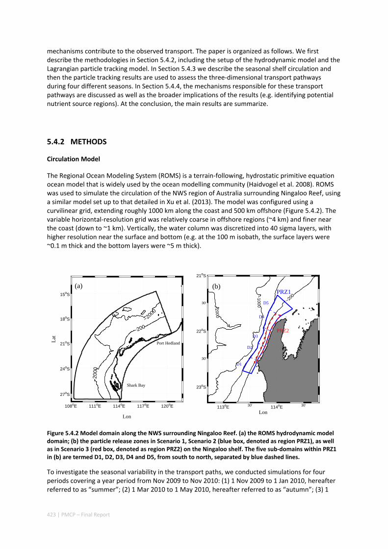
423 | PMCP – Final Report
mechanisms contribute to the observed transport. The paper is organized as follows. We first describe the methodologies in Section 5.4.2, including the setup of the hydrodynamic model and the Lagrangian particle tracking model. In Section 5.4.3 we describe the seasonal shelf circulation and then the particle tracking results are used to assess the three‐dimensional transport pathways during four different seasons. In Section 5.4.4, the mechanisms responsible for these transport pathways are discussed as well as the broader implications of the results (e.g. identifying potential nutrient source regions). At the conclusion, the main results are summarize.
5.4.2 METHODS
Circulation Model
The Regional Ocean Modeling System (ROMS) is a terrain‐following, hydrostatic primitive equation ocean model that is widely used by the ocean modelling community (Haidvogel et al. 2008). ROMS was used to simulate the circulation of the NWS region of Australia surrounding Ningaloo Reef, using a similar model set up to that detailed in Xu et al. (2013). The model was configured using a curvilinear grid, extending roughly 1000 km along the coast and 500 km offshore (Figure 5.4.2). The variable horizontal‐resolution grid was relatively coarse in offshore regions (~4 km) and finer near the coast (down to ~1 km). Vertically, the water column was discretized into 40 sigma layers, with higher resolution near the surface and bottom (e.g. at the 100 m isobath, the surface layers were ~0.1 m thick and the bottom layers were ~5 m thick).
Figure 5.4.2 Model domain along the NWS surrounding Ningaloo Reef. (a) the ROMS hydrodynamic model domain; (b) the particle release zones in Scenario 1, Scenario 2 (blue box, denoted as region PRZ1), as well as in Scenario 3 (red box, denoted as region PRZ2) on the Ningaloo shelf. The five sub‐domains within PRZ1 in (b) are termed D1, D2, D3, D4 and D5, from south to north, separated by blue dashed lines.
To investigate the seasonal variability in the transport paths, we conducted simulations for four periods covering a year period from Nov 2009 to Nov 2010: (1) 1 Nov 2009 to 1 Jan 2010, hereafter referred to as “summer”; (2) 1 Mar 2010 to 1 May 2010, hereafter referred to as “autumn”; (3) 1
108oE 111oE 114oE 117oE 120oE
27oS
24oS
21oS
18oS
15oS
−200
0
−2000
−200
Lon
Lat
(a)
Shark Bay
Port Hedland
(b)
D5
D4
D3
D2
D1
−2000
−1000
−200
PRZ1
PRZ2
113oE 30’ 114oE 30’
23oS
30’
22oS
30’
21oS
Lon
424 | PMCP – Final Report
May 2010 to 1 Jul 2010, hereafter referred to as “winter”; and (4) 1 Sep 2010 to 1 Nov 2010, hereafter referred to as “spring”. These periods were chosen since they cover the detailed field mooring data recorded on the Ningaloo shelf as described in Xu et al. (2015). Previous work by Xu et al. (2013) showed that, in the absence of data assimilation, model simulations over this duration ensured negligible long‐term model drift from their initial conditions. Separate ROMS runs were thus conducted for four separate seasonal simulations, and the resulting three‐dimensional velocity fields were used to drive the particle tracking models (described below) for each period.
Although the model was configured similarly to that described in Xu et al. (2013), for the present study we included the surface heat fluxes using atmospheric data obtained from the Climate Forecast System Reanalysis (CFSR) results archived at the National Operational Model Archive and Distribution System (NOMADS, http://nomads.ncdc.noaa.gov/) with 0.3o resolution. We initialized and drove the model at the lateral open boundaries using global hindcast reanalysis output from a hybrid coordinate ocean model (HYCOM, 1/12o, www.hycom.org (Chassignet et al. 2007)). This approach allows the large‐scale and remotely‐generated dynamics (including currents, temperature/salinity fields, and sea surface height) to drive the regional ROMS model. Nonetheless, we previously found HYCOM tended to over‐predict the strength of the poleward flow during Nov‐Dec 2009 simulation (Xu et al. 2013).Thus, we instead used direct satellite sea surface height observations from Australia’s Integrated Marine Observing System (IMOS, http://thredds.aodn.org.au/thredds/catalog/IMOS/OceanCurrent/GSLA/catalog.html) to initialize the surface elevation fields in the ROMS model. The three‐dimensional velocity outputs were, in turn, used to drive the particle tracking models (described below) for each period.
Particle Tracking Model
To simulate the time‐integrated transport pathways using particle tracking, we used the offline Larval Transport Lagrangian model (LTRANS (Schlag and North 2012), see http://northweb.hpl.umces.edu/LTRANS.htm). Although LTRANS was initially developed to simulate active and passive larval transport (North et al. 2008), it has since been successfully applied to a number of other applications; for example, to assess oil droplet dispersal from the Deep Water Horizon oil‐spill in Gulf of Mexico (North et al. 2011). LTRANS reads and interpolates ROMS three‐dimensional velocity vector fields onto particle positions at each hydrodynamic model output time steps (external time step). Based on these interpolated values, the model calculates particle movements and updates their positions in three‐dimensional space at each internal time step using a passive particle displacement algorithm that includes transport from both advection and turbulent diffusion, as:
1/211 2n n hx x u t R r K t ( 1 )
1/211 2n n hy y v t R r K t ( 2 )
1/211 2v
n n v
Kz z w t t R r K t
z
( 3 )
where vK and hK are the vertical and horizontal diffusivities derived from the ROMS model,
respectively; t is the internal time step for the Lagrangian particle tracking; R is a random number generator with mean = 0 and standard deviation r = 1; xn and yn denote the horizontal particle positions at the nth time step, and zn the vertical positions at the nth time step. The advection of particles was computed by numerically integrating the velocities using a 4th order Runge‐Kutta scheme. In our simulations, LTRANS read the ROMS output every 6 h (external time step), and

425 | PMCP – Final Report
predicted and updated the particle displacements every 3 minutes (internal time step). Like most particle tracking models, the built‐in random displacement module (Visser 1997, North et al. 2006) based on turbulent diffusivities from ROMS may not fully represent realistic turbulent mixing processes in the coastal ocean. We examined the influence of the random displacement module on particle trajectories separately, as detailed in Appendix 1. These results indicate that the dominant transport pathways are largely insensitive to sub‐grid scale turbulent diffusive processes, consistent with a much stronger role of advection on the overall transport.
On this basis, by reversing the input sequence in time and the direction of the velocity fields from the ROMS simulations, we ran LTRANS backwards in time to determine the source of the water parcels reaching Ningaloo Reef. The benefits of backward‐in‐time particle tracking (hereafter referred as BITT) (Batchelder 2006) become most apparent when the size of sink destinations in a model is significantly smaller than that of the potential sources ‐ as in the present application. Therefore, with a fixed number of particles within the sink destination region, we were able to track and identify the source region of each particle with much greater efficiency compared to applying conventional forward‐in‐time tracking (hereafter referred as FITT) over all grid cells within the entire domain. Since diffusion processes are irreversible, we switched off the particle turbulence sub‐grid scale model in order to track the particle movements due to advection alone. These advection‐only FITT and BITT simulations should be reversible, which was confirmed by a set of test runs (see Supporting Information, Figure S5.4.1).
Particle initialization, source tracking, and transport scenarios
Three particle tracking scenarios were considered in this study (see Table 5.4.1). Scenario 1 investigated the two‐dimensional horizontal surface flow pathways originating from Ningaloo Reef during the four different seasons. In this scenario, particles were released at the surface (0 m depth) and trajectories were calculated over 60 day simulations for each season. The Scenario 1 simulations were run forward as FITT simulations. Scenario 2 investigated the reverse dynamics, i.e., the source locations of water masses that reached the Ningaloo shelf during the different seasons. In these simulations, particles were released at two depths (10 m and 50 m below the surface) adjacent to the coast and were tracked backwards using BITT simulations for 60 days. Finally, in Scenario 3, the effects of shorter‐term (order weekly) local wind forcing events on vertical particle excursions were investigated using a series of shorter BITT simulations. Since the wind events responsible for driving transient upwelling or downwelling in the Ningaloo region tend to occur within a synoptic weather band with a period of ~10 days (Roughan 2003; Lowe et al. 2012; Rossi et al. 2013b; Xu et al. 2013), particles were initialized at a depth of 10 m near the coast, and six separate 10 day BITT simulations were conducted within each seasonal period.
Table 5.4.1 The configurations for the three particle tracking scenarios.
MODEL TYPE DURATION NUMBER OF SIMULATIONS
INITIAL DEPTH INITIAL DOMAIN
TURBULENT MODULE
Scenario 1 FITT 2 months 1 in each season Surface (0 m) PRZ1 RDM#
Scenario 2 BITT 2months 1 in each season 10 m 50 m
PRZ1 PRZ1
N/A N/A
Scenario 3 BITT 10 days 6 in each season 10 m PRZ2 N/A
# RDM denotes the random displacement module.
For Scenarios 1 and 2, particles were released within particle release zone 1 (hereafter PRZ1), denoted by the blue polygon in Figure 5.4.2, which extended along the entire Ningaloo peninsula
426 | PMCP – Final Report
with width ~20 km and an outer boundary at the 600 m isobath. For Scenario 3, we released particles within a narrower zone, with an outer boundary at the 200 m isobath (referred to as PRZ2, ~7 km width), denoted by the red polygon in Figure 5.4.2 that coincided with the typical coastal upwelling zone width at the site (Xu et al. 2013). The FITT model (in Scenario 1) was run with the random displacement module, but was disabled in the BITT simulations (in Scenarios 2 and 3). For all simulations, once a particle moved outside the model domain it was no longer tracked. Finally, to avoid confusion when reporting the tracking results below, we present the transport paths in the BITT simulations in a forward‐in‐time perspective, to maintain consistency among all three scenarios. Therefore, particles “originate” from the final model positions and arrive at their “initial” positions at the beginning of the BITT simulations.
Transport analysis
To determine the source origins of water transported to different areas along Ningaloo Reef for Scenario 2, we divided the particle release zone into five sub‐domains enclosed within the 600 m isobath (regions D1‐D5), and released ~7000 particles to examine the mean transport pathways to each sub‐domain (see Figure 5.4.2b). To investigate the vertical transport of particles due to coastal upwelling in Scenario 3, we calculated the average vertical migration of the particles over an inshore PRZ2 domain (Figure 5.4.2b) for each 10 day simulation period. These computed vertical displacements were then compared with those estimated from an analytical of coastal upwelling, where the mean vertical upwelling velocity w within an upwelling zone is (Cushman‐Roisin and Beckers 2010; Marchesiello and Estrade 2010):
0
geostrophicEkman
gxsv H
wfL L
(4)
Here 0 is the reference seawater density, xs denotes the along‐shelf wind stress with positive sign
directed equatorward (northeastward) along the Ningaloo peninsula (refer to Xu et al. 2013) and f is the Coriolis parameter (negative in the southern hemisphere). In Eq. (4), the first term is the vertical velocity contribution from the along‐shelf winds (i.e. coastal upwelling due to Ekman transport), which has been found to be a good description of wind‐driven cross‐shelf transport (after removing the background interior flow) along the Ningaloo shelf (Xu et al. 2013; 2015). The second term represents a geostrophic correction of the contribution from any background barotropic cross‐shelf flow. The real ocean barotopic cross‐shelf flow can be spatially‐complex and transient, e.g. due to eddies and meandering shelf currents with order daily‐weekly temporal variability. These higher‐frequency dynamics can only be resolved using three‐dimensional ocean circulation models, as in the present study. Alternatively, Marchesiello et al. (2010) proposed a simple model incorporating a climatological onshore geostrophic flow to estimate the impact of this barotopic cross‐shelf flow on the upwelling/downwelling transport in Eq. (4) in the absence of a numerical model. This method has been previously used to predict variability in upwelling/downwelling along the WA coast (including along Ningaloo Reef) by Rossi et al. (2013b), and although it has been shown to qualitatively capture a number of major historical upwelling events (i.e., as inferred from satellite imagery), it has not yet been verified with direct in situ observations or numerical model simulations of vertical transport. We thus used this analytical model as a framework to evaluate how different mechanisms contribute to upwelling/downwelling, and moreover, assessed how this simple analytical model (with only climatological information about the background geostrophic flow)
performed against our highly‐resolved 3D numerical simulations. Therefore, in Eq. (4) we treated gv
as the cross‐shelf geostrophic velocity (with positive velocity directed offshore), which was estimated by a downward integration of the pressure gradient above the 100 dbar reference level from CARS09 temperature and salinity seasonal climatological dataset (Rossi et al. 2013b), where H
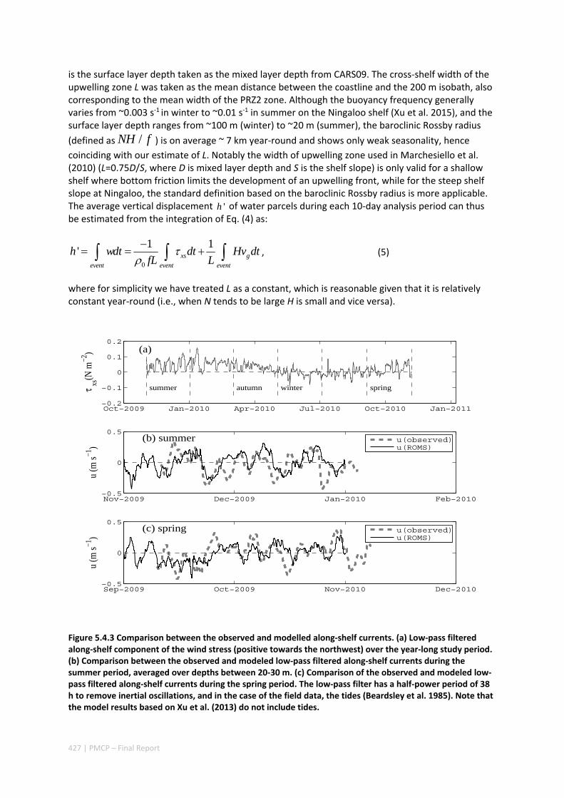
427 | PMCP – Final Report
is the surface layer depth taken as the mixed layer depth from CARS09. The cross‐shelf width of the upwelling zone L was taken as the mean distance between the coastline and the 200 m isobath, also corresponding to the mean width of the PRZ2 zone. Although the buoyancy frequency generally varies from ~0.003 s‐1 in winter to ~0.01 s‐1 in summer on the Ningaloo shelf (Xu et al. 2015), and the surface layer depth ranges from ~100 m (winter) to ~20 m (summer), the baroclinic Rossby radius
(defined as /NH f ) is on average ~ 7 km year‐round and shows only weak seasonality, hence
coinciding with our estimate of L. Notably the width of upwelling zone used in Marchesiello et al. (2010) (L=0.75D/S, where D is mixed layer depth and S is the shelf slope) is only valid for a shallow shelf where bottom friction limits the development of an upwelling front, while for the steep shelf slope at Ningaloo, the standard definition based on the baroclinic Rossby radius is more applicable. The average vertical displacement 'h of water parcels during each 10‐day analysis period can thus be estimated from the integration of Eq. (4) as:
0
1 1' xs g
event event event
h wdt dt Hv dtfL L
, (5)
where for simplicity we have treated L as a constant, which is reasonable given that it is relatively constant year‐round (i.e., when N tends to be large H is small and vice versa).
Figure 5.4.3 Comparison between the observed and modelled along‐shelf currents. (a) Low‐pass filtered along‐shelf component of the wind stress (positive towards the northwest) over the year‐long study period. (b) Comparison between the observed and modeled low‐pass filtered along‐shelf currents during the summer period, averaged over depths between 20‐30 m. (c) Comparison of the observed and modeled low‐pass filtered along‐shelf currents during the spring period. The low‐pass filter has a half‐power period of 38 h to remove inertial oscillations, and in the case of the field data, the tides (Beardsley et al. 1985). Note that the model results based on Xu et al. (2013) do not include tides.
Nov−2009 Dec−2009 Jan−2010 Feb−2010−0.5
0
0.5
u (m
s−1)
(b) summer u(observed)
u(ROMS)
Sep−2009 Oct−2009 Nov−2010 Dec−2010−0.5
0
0.5
u (m
s−1)
(c) spring u(observed)
u(ROMS)
Oct−2009 Jan−2010 Apr−2010 Jul−2010 Oct−2010 Jan−2011−0.2
−0.1
0
0.1
0.2
τ xs(N
m−2
) (a)
summer autumn winter spring
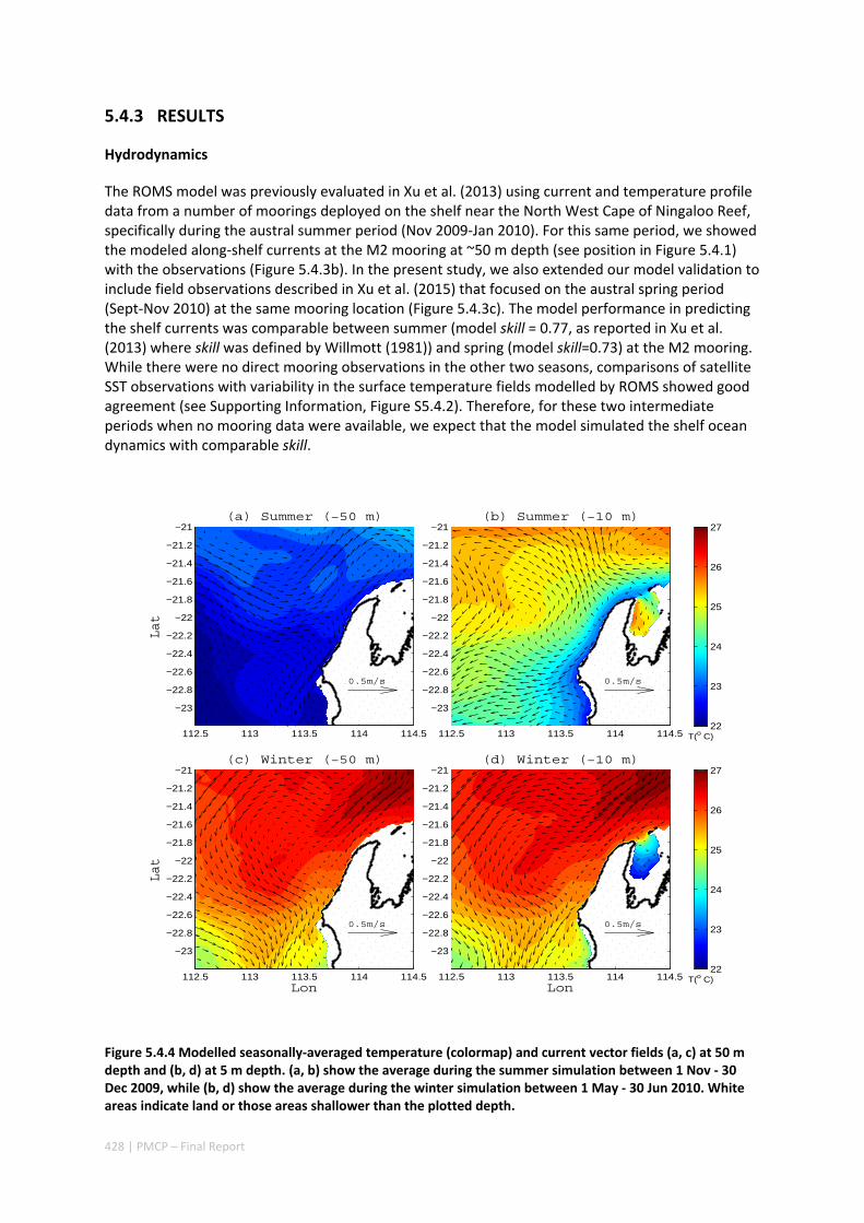
428 | PMCP – Final Report
5.4.3 RESULTS
Hydrodynamics
The ROMS model was previously evaluated in Xu et al. (2013) using current and temperature profile data from a number of moorings deployed on the shelf near the North West Cape of Ningaloo Reef, specifically during the austral summer period (Nov 2009‐Jan 2010). For this same period, we showed the modeled along‐shelf currents at the M2 mooring at ~50 m depth (see position in Figure 5.4.1) with the observations (Figure 5.4.3b). In the present study, we also extended our model validation to include field observations described in Xu et al. (2015) that focused on the austral spring period (Sept‐Nov 2010) at the same mooring location (Figure 5.4.3c). The model performance in predicting the shelf currents was comparable between summer (model skill = 0.77, as reported in Xu et al. (2013) where skill was defined by Willmott (1981)) and spring (model skill=0.73) at the M2 mooring. While there were no direct mooring observations in the other two seasons, comparisons of satellite SST observations with variability in the surface temperature fields modelled by ROMS showed good agreement (see Supporting Information, Figure S5.4.2). Therefore, for these two intermediate periods when no mooring data were available, we expect that the model simulated the shelf ocean dynamics with comparable skill.
Figure 5.4.4 Modelled seasonally‐averaged temperature (colormap) and current vector fields (a, c) at 50 m depth and (b, d) at 5 m depth. (a, b) show the average during the summer simulation between 1 Nov ‐ 30 Dec 2009, while (b, d) show the average during the winter simulation between 1 May ‐ 30 Jun 2010. White areas indicate land or those areas shallower than the plotted depth.
112.5 113 113.5 114 114.5
−23
−22.8
−22.6
−22.4
−22.2
−22
−21.8
−21.6
−21.4
−21.2
−21(a) Summer (−50 m)
Lat
0.5m/s
112.5 113 113.5 114 114.5
−23
−22.8
−22.6
−22.4
−22.2
−22
−21.8
−21.6
−21.4
−21.2
−21(b) Summer (−10 m)
0.5m/s
T(o C)22
23
24
25
26
27
112.5 113 113.5 114 114.5
−23
−22.8
−22.6
−22.4
−22.2
−22
−21.8
−21.6
−21.4
−21.2
−21(c) Winter (−50 m)
Lon
Lat
0.5m/s
112.5 113 113.5 114 114.5
−23
−22.8
−22.6
−22.4
−22.2
−22
−21.8
−21.6
−21.4
−21.2
−21(d) Winter (−10 m)
Lon
0.5m/s
T(o C)22
23
24
25
26
27
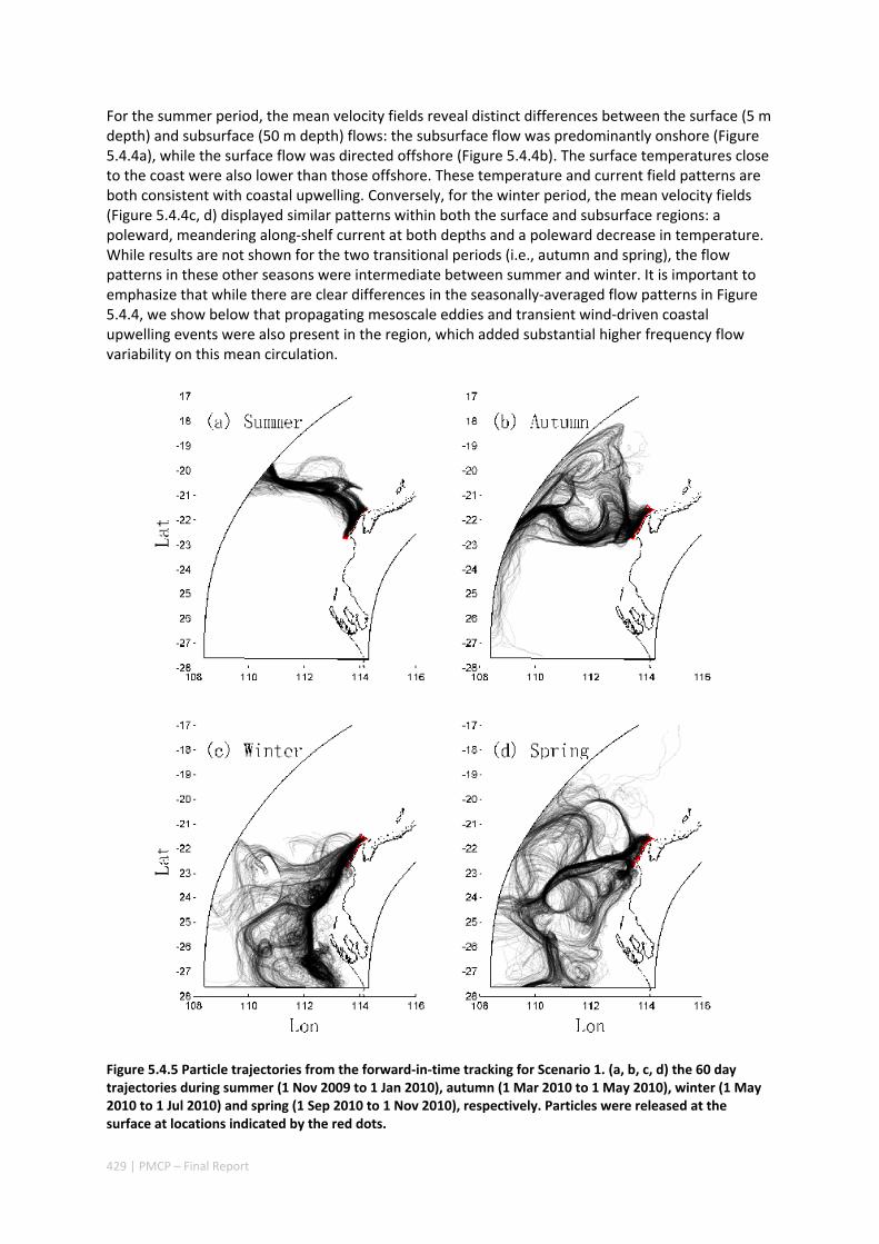
429 | PMCP – Final Report
For the summer period, the mean velocity fields reveal distinct differences between the surface (5 m depth) and subsurface (50 m depth) flows: the subsurface flow was predominantly onshore (Figure 5.4.4a), while the surface flow was directed offshore (Figure 5.4.4b). The surface temperatures close to the coast were also lower than those offshore. These temperature and current field patterns are both consistent with coastal upwelling. Conversely, for the winter period, the mean velocity fields (Figure 5.4.4c, d) displayed similar patterns within both the surface and subsurface regions: a poleward, meandering along‐shelf current at both depths and a poleward decrease in temperature. While results are not shown for the two transitional periods (i.e., autumn and spring), the flow patterns in these other seasons were intermediate between summer and winter. It is important to emphasize that while there are clear differences in the seasonally‐averaged flow patterns in Figure 5.4.4, we show below that propagating mesoscale eddies and transient wind‐driven coastal upwelling events were also present in the region, which added substantial higher frequency flow variability on this mean circulation.
Figure 5.4.5 Particle trajectories from the forward‐in‐time tracking for Scenario 1. (a, b, c, d) the 60 day trajectories during summer (1 Nov 2009 to 1 Jan 2010), autumn (1 Mar 2010 to 1 May 2010), winter (1 May 2010 to 1 Jul 2010) and spring (1 Sep 2010 to 1 Nov 2010), respectively. Particles were released at the surface at locations indicated by the red dots.
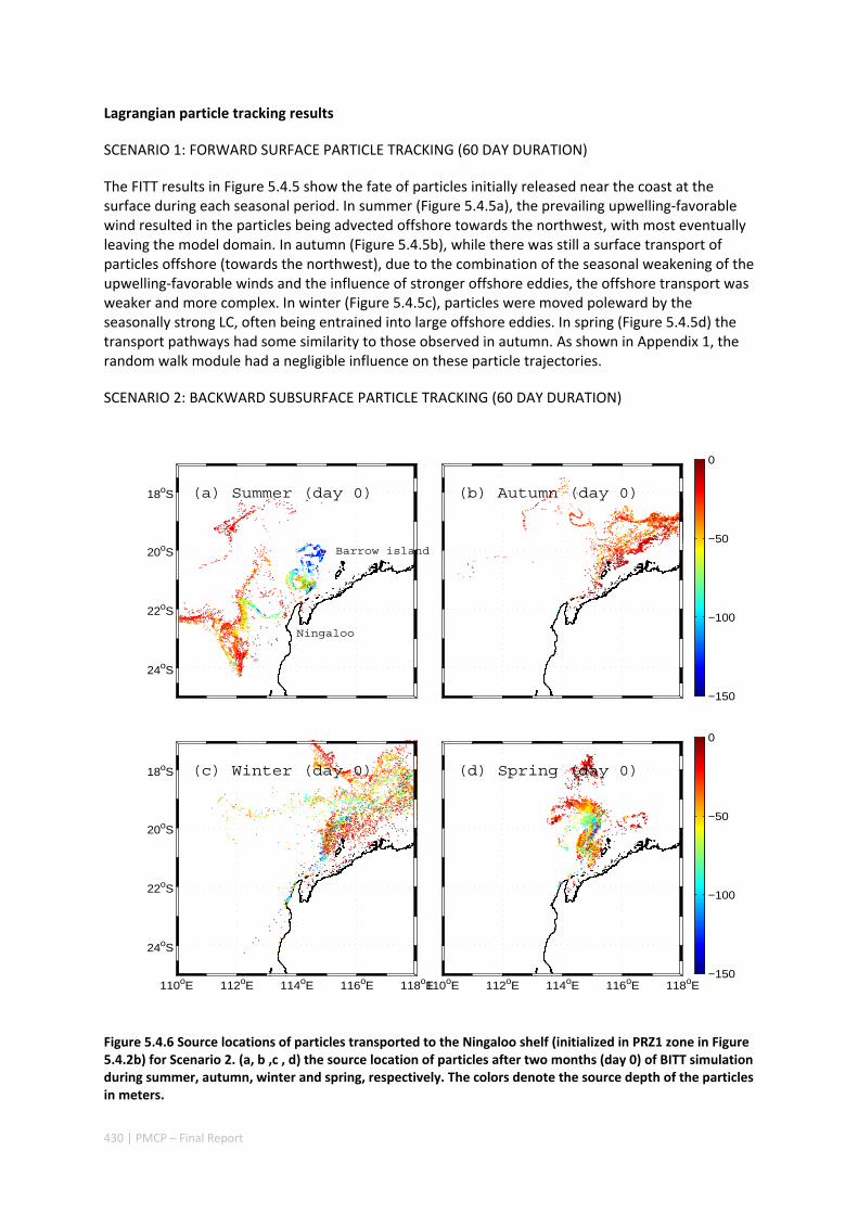
430 | PMCP – Final Report
Lagrangian particle tracking results
SCENARIO 1: FORWARD SURFACE PARTICLE TRACKING (60 DAY DURATION)
The FITT results in Figure 5.4.5 show the fate of particles initially released near the coast at the surface during each seasonal period. In summer (Figure 5.4.5a), the prevailing upwelling‐favorable wind resulted in the particles being advected offshore towards the northwest, with most eventually leaving the model domain. In autumn (Figure 5.4.5b), while there was still a surface transport of particles offshore (towards the northwest), due to the combination of the seasonal weakening of the upwelling‐favorable winds and the influence of stronger offshore eddies, the offshore transport was weaker and more complex. In winter (Figure 5.4.5c), particles were moved poleward by the seasonally strong LC, often being entrained into large offshore eddies. In spring (Figure 5.4.5d) the transport pathways had some similarity to those observed in autumn. As shown in Appendix 1, the random walk module had a negligible influence on these particle trajectories.
SCENARIO 2: BACKWARD SUBSURFACE PARTICLE TRACKING (60 DAY DURATION)
Figure 5.4.6 Source locations of particles transported to the Ningaloo shelf (initialized in PRZ1 zone in Figure 5.4.2b) for Scenario 2. (a, b ,c , d) the source location of particles after two months (day 0) of BITT simulation during summer, autumn, winter and spring, respectively. The colors denote the source depth of the particles in meters.
24oS
22oS
20oS
18oS (a) Summer (day 0)
Barrow island
Ningaloo
(b) Autumn (day 0)
−150
−100
−50
0
110oE 112oE 114oE 116oE 118oE
24oS
22oS
20oS
18oS (c) Winter (day 0)
110oE 112oE 114oE 116oE 118oE
(d) Spring (day 0)
−150
−100
−50
0
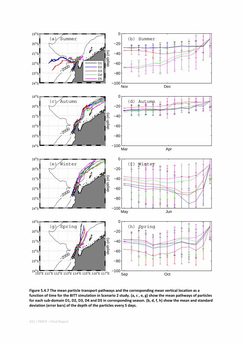
431 | PMCP – Final Report
Figure 5.4.7 The mean particle transport pathways and the corresponding mean vertical location as a function of time for the BITT simulation in Scenario 2 study. (a, c , e, g) show the mean pathways of particles for each sub‐domain D1, D2, D3, D4 and D5 in corresponding season. (b, d, f, h) show the mean and standard deviation (error bars) of the depth of the particles every 5 days.
24oS
23oS
22oS
21oS
20oS
19oS
−2000−20
0
(a) Summer
D1D2D3D4D5
Nov Dec−100
−80
−60
−40
−20
0
dept
h (m
)
(b) Summer
24oS
23oS
22oS
21oS
20oS
19oS
−2000−20
0
(c) Autumn
Mar Apr−100
−80
−60
−40
−20
0
dept
h (m
)
(d) Autumn
24oS
23oS
22oS
21oS
20oS
19oS
−2000−20
0
(e) Winter
May Jun−100
−80
−60
−40
−20
0
dept
h (m
)
(f) Winter
110oE 111oE 112oE 113oE 114oE 115oE 116oE 117oE 24oS
23oS
22oS
21oS
20oS
19oS
−2000−20
0
(g) Spring
Sep Oct−100
−80
−60
−40
−20
0
dept
h (m
)
(h) Spring
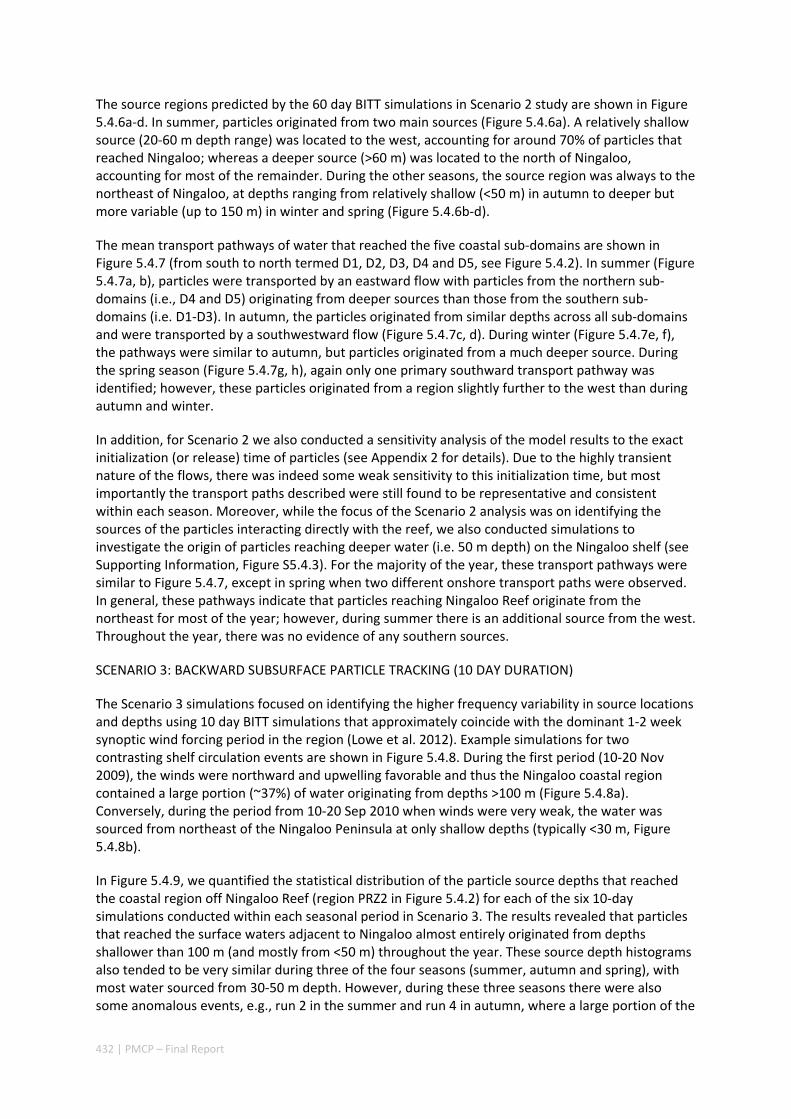
432 | PMCP – Final Report
The source regions predicted by the 60 day BITT simulations in Scenario 2 study are shown in Figure 5.4.6a‐d. In summer, particles originated from two main sources (Figure 5.4.6a). A relatively shallow source (20‐60 m depth range) was located to the west, accounting for around 70% of particles that reached Ningaloo; whereas a deeper source (>60 m) was located to the north of Ningaloo, accounting for most of the remainder. During the other seasons, the source region was always to the northeast of Ningaloo, at depths ranging from relatively shallow (<50 m) in autumn to deeper but more variable (up to 150 m) in winter and spring (Figure 5.4.6b‐d).
The mean transport pathways of water that reached the five coastal sub‐domains are shown in Figure 5.4.7 (from south to north termed D1, D2, D3, D4 and D5, see Figure 5.4.2). In summer (Figure 5.4.7a, b), particles were transported by an eastward flow with particles from the northern sub‐domains (i.e., D4 and D5) originating from deeper sources than those from the southern sub‐domains (i.e. D1‐D3). In autumn, the particles originated from similar depths across all sub‐domains and were transported by a southwestward flow (Figure 5.4.7c, d). During winter (Figure 5.4.7e, f), the pathways were similar to autumn, but particles originated from a much deeper source. During the spring season (Figure 5.4.7g, h), again only one primary southward transport pathway was identified; however, these particles originated from a region slightly further to the west than during autumn and winter.
In addition, for Scenario 2 we also conducted a sensitivity analysis of the model results to the exact initialization (or release) time of particles (see Appendix 2 for details). Due to the highly transient nature of the flows, there was indeed some weak sensitivity to this initialization time, but most importantly the transport paths described were still found to be representative and consistent within each season. Moreover, while the focus of the Scenario 2 analysis was on identifying the sources of the particles interacting directly with the reef, we also conducted simulations to investigate the origin of particles reaching deeper water (i.e. 50 m depth) on the Ningaloo shelf (see Supporting Information, Figure S5.4.3). For the majority of the year, these transport pathways were similar to Figure 5.4.7, except in spring when two different onshore transport paths were observed. In general, these pathways indicate that particles reaching Ningaloo Reef originate from the northeast for most of the year; however, during summer there is an additional source from the west. Throughout the year, there was no evidence of any southern sources.
SCENARIO 3: BACKWARD SUBSURFACE PARTICLE TRACKING (10 DAY DURATION)
The Scenario 3 simulations focused on identifying the higher frequency variability in source locations and depths using 10 day BITT simulations that approximately coincide with the dominant 1‐2 week synoptic wind forcing period in the region (Lowe et al. 2012). Example simulations for two contrasting shelf circulation events are shown in Figure 5.4.8. During the first period (10‐20 Nov 2009), the winds were northward and upwelling favorable and thus the Ningaloo coastal region contained a large portion (~37%) of water originating from depths >100 m (Figure 5.4.8a). Conversely, during the period from 10‐20 Sep 2010 when winds were very weak, the water was sourced from northeast of the Ningaloo Peninsula at only shallow depths (typically <30 m, Figure 5.4.8b).
In Figure 5.4.9, we quantified the statistical distribution of the particle source depths that reached the coastal region off Ningaloo Reef (region PRZ2 in Figure 5.4.2) for each of the six 10‐day simulations conducted within each seasonal period in Scenario 3. The results revealed that particles that reached the surface waters adjacent to Ningaloo almost entirely originated from depths shallower than 100 m (and mostly from <50 m) throughout the year. These source depth histograms also tended to be very similar during three of the four seasons (summer, autumn and spring), with most water sourced from 30‐50 m depth. However, during these three seasons there were also some anomalous events, e.g., run 2 in the summer and run 4 in autumn, where a large portion of the
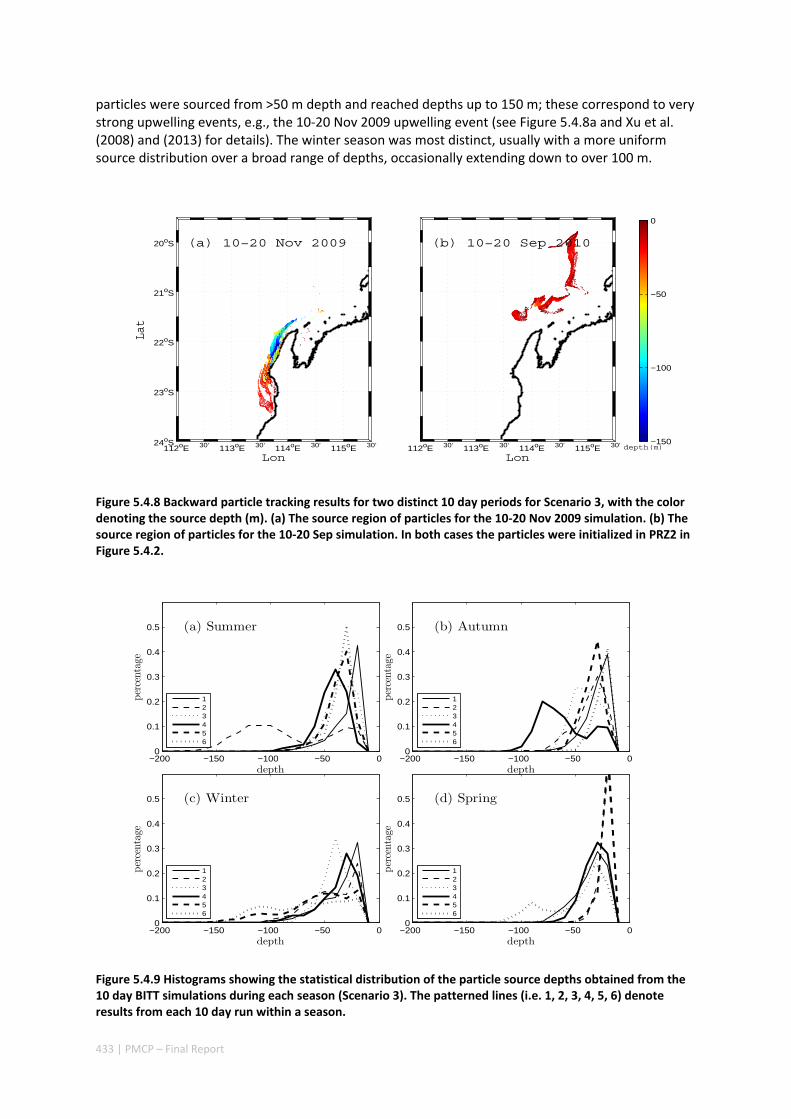
433 | PMCP – Final Report
particles were sourced from >50 m depth and reached depths up to 150 m; these correspond to very strong upwelling events, e.g., the 10‐20 Nov 2009 upwelling event (see Figure 5.4.8a and Xu et al. (2008) and (2013) for details). The winter season was most distinct, usually with a more uniform source distribution over a broad range of depths, occasionally extending down to over 100 m.
Figure 5.4.8 Backward particle tracking results for two distinct 10 day periods for Scenario 3, with the color denoting the source depth (m). (a) The source region of particles for the 10‐20 Nov 2009 simulation. (b) The source region of particles for the 10‐20 Sep simulation. In both cases the particles were initialized in PRZ2 in Figure 5.4.2.
Figure 5.4.9 Histograms showing the statistical distribution of the particle source depths obtained from the 10 day BITT simulations during each season (Scenario 3). The patterned lines (i.e. 1, 2, 3, 4, 5, 6) denote results from each 10 day run within a season.
(a) 10−20 Nov 2009
112oE 30’ 113oE 30’ 114oE 30’ 115oE 30’ 24oS
23oS
22oS
21oS
20oS
Lon
Lat
112oE 30’ 113oE 30’ 114oE 30’ 115oE 30’
(b) 10−20 Sep 2010
Londepth(m)
−150
−100
−50
0
−200 −150 −100 −50 00
0.1
0.2
0.3
0.4
0.5
depth
percentag
e
(a) Summer
123456
−200 −150 −100 −50 00
0.1
0.2
0.3
0.4
0.5
depth
percentag
e
(c) Winter
123456
−200 −150 −100 −50 00
0.1
0.2
0.3
0.4
0.5
depth
percentag
e
(d) Spring
123456
−200 −150 −100 −50 00
0.1
0.2
0.3
0.4
0.5
depth
percentag
e
(b) Autumn
123456
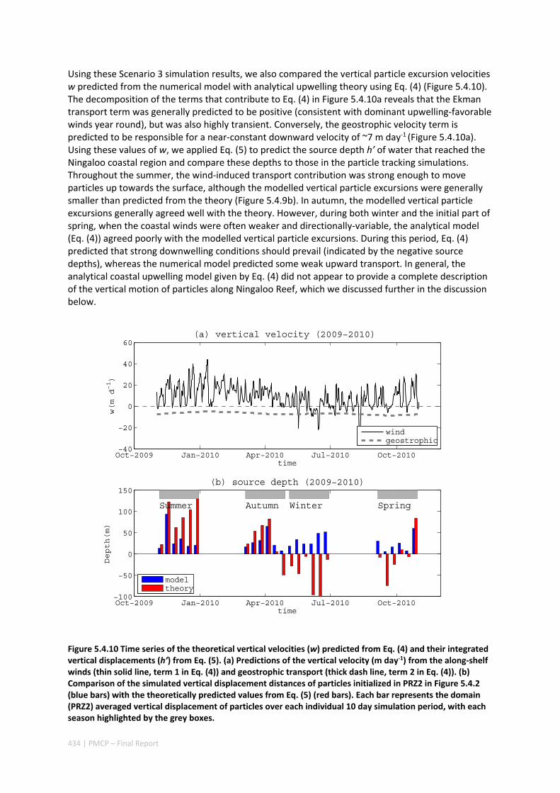
434 | PMCP – Final Report
Using these Scenario 3 simulation results, we also compared the vertical particle excursion velocities w predicted from the numerical model with analytical upwelling theory using Eq. (4) (Figure 5.4.10). The decomposition of the terms that contribute to Eq. (4) in Figure 5.4.10a reveals that the Ekman transport term was generally predicted to be positive (consistent with dominant upwelling‐favorable winds year round), but was also highly transient. Conversely, the geostrophic velocity term is predicted to be responsible for a near‐constant downward velocity of ~7 m day‐1 (Figure 5.4.10a). Using these values of w, we applied Eq. (5) to predict the source depth h’ of water that reached the Ningaloo coastal region and compare these depths to those in the particle tracking simulations. Throughout the summer, the wind‐induced transport contribution was strong enough to move particles up towards the surface, although the modelled vertical particle excursions were generally smaller than predicted from the theory (Figure 5.4.9b). In autumn, the modelled vertical particle excursions generally agreed well with the theory. However, during both winter and the initial part of spring, when the coastal winds were often weaker and directionally‐variable, the analytical model (Eq. (4)) agreed poorly with the modelled vertical particle excursions. During this period, Eq. (4) predicted that strong downwelling conditions should prevail (indicated by the negative source depths), whereas the numerical model predicted some weak upward transport. In general, the analytical coastal upwelling model given by Eq. (4) did not appear to provide a complete description of the vertical motion of particles along Ningaloo Reef, which we discussed further in the discussion below.
Figure 5.4.10 Time series of the theoretical vertical velocities (w) predicted from Eq. (4) and their integrated vertical displacements (h’) from Eq. (5). (a) Predictions of the vertical velocity (m day‐1) from the along‐shelf winds (thin solid line, term 1 in Eq. (4)) and geostrophic transport (thick dash line, term 2 in Eq. (4)). (b) Comparison of the simulated vertical displacement distances of particles initialized in PRZ2 in Figure 5.4.2 (blue bars) with the theoretically predicted values from Eq. (5) (red bars). Each bar represents the domain (PRZ2) averaged vertical displacement of particles over each individual 10 day simulation period, with each season highlighted by the grey boxes.
Oct−2009 Jan−2010 Apr−2010 Jul−2010 Oct−2010−40
−20
0
20
40
60
time
w(m d−1)
(a) vertical velocity (2009−2010)
windgeostrophic
Oct−2009 Jan−2010 Apr−2010 Jul−2010 Oct−2010−100
−50
0
50
100
150
time
Depth(m)
(b) source depth (2009−2010)
Summer Autumn Winter Spring
modeltheory
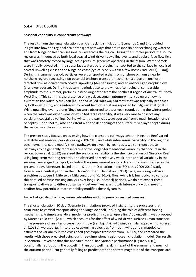
435 | PMCP – Final Report
5.4.4 DISCUSSION
Seasonal variability in connectivity pathways
The results from the longer‐duration particle tracking simulations (Scenarios 1 and 2) provided insight into how the regional‐scale transport pathways that are responsible for exchanging water to and from Ningaloo Reef can seasonally vary across the region. During the summer period, the source region was influenced by both local coastal wind‐driven upwelling events and a subsurface flow field that was remotely‐forced by large‐scale pressure gradients operating in the region. Water parcels were initially advected in the subsurface waters before being transported to the surface by localised coastal upwelling close to the Ningaloo coast (typically only within a few Rossby radii or O(10 km)). During this summer period, particles were transported either from offshore or from a nearby northern region, suggesting two potential onshore transport mechanisms: a bottom onshore‐directed flow associated with coastal upwelling (deeper source) and an onshore geostrophic flow (shallower source). During the autumn period, despite the winds often being of comparable amplitude to the summer, particles instead originated from the northeast region of Australia’s North West Shelf. This confirms the presence of a weak seasonal (autumn‐winter) poleward flowing current on the North West Shelf (i.e., the so‐called Holloway Current) that was originally proposed by Holloway (1995), and reinforced by recent field observations reported by Ridgway et al. (2015). While upwelling events along Ningaloo were observed to occur year‐round, during the winter period when the wind was either weak or exhibited large variability, it was very rare to observe any persistent coastal upwelling. During winter, the particles were sourced from a much broader range of depths (up to 150 m), also consistent with the deepening of the surface mixed layer depth during the winter months in this region.
The present study focuses on assessing how the transport pathways to/from Ningaloo Reef varied with different seasonal periods during 2009‐2010, and while inter‐annual variability in the regional ocean dynamics could modify these pathways on a year‐by‐year basis, we still expect these pathways to be generally representative of the longer‐term seasonal variability that occurs in the region. Lowe et al. (2012) assessed the seasonal variability in the shelf circulation off Ningaloo Reef using long‐term mooring records, and observed only relatively weak inter‐annual variability in the seasonally‐averaged transport, including the same general seasonal trends that we observed in the present study. Moreover, based on the Southern Oscillation Index (SOI), this 2009‐2010 study focused on a neutral period in the El Niño‐Southern Oscillation (ENSO) cycle, occurring within a transition between El Niño to La Niña conditions (Xu 2014). Thus, while it is impractical to conduct this detailed particle tracking analysis over long (i.e., decadal) periods, we do not expect these transport pathways to differ substantially between years, although future work would need to confirm how potential climate variability modifies these dynamics.
Impact of geostrophic flow, mesoscale eddies and buoyancy on vertical transport
The shorter‐duration (10 day) Scenario 3 simulations provided insight into the processes that contribute to vertical transport along the Ningaloo shelf, including the role of different forcing mechanisms. A simple analytical model for predicting coastal upwelling / downwelling was proposed by Marchesiello et al. (2010), which accounts for the effect of wind‐driven surface Ekman transport in the presence of an interior geostrophic flow (i.e., Eq. (4)). Following a similar approach to Rossi et al. (2013b), we used Eq. (4) to predict upwelling velocities from both winds and climatological estimates of variability in the cross‐shelf geostrophic transport from CARS09, and compared the results with those predicted using our three‐dimensional region ocean circulation model. Our results in Scenario 3 revealed that this analytical model had variable performance (Figure 5.4.10), occasionally reproducing the upwelling transport well (i.e. during part of the summer and much of the autumn period), but generally failing to predict both the correct magnitude of the transport and
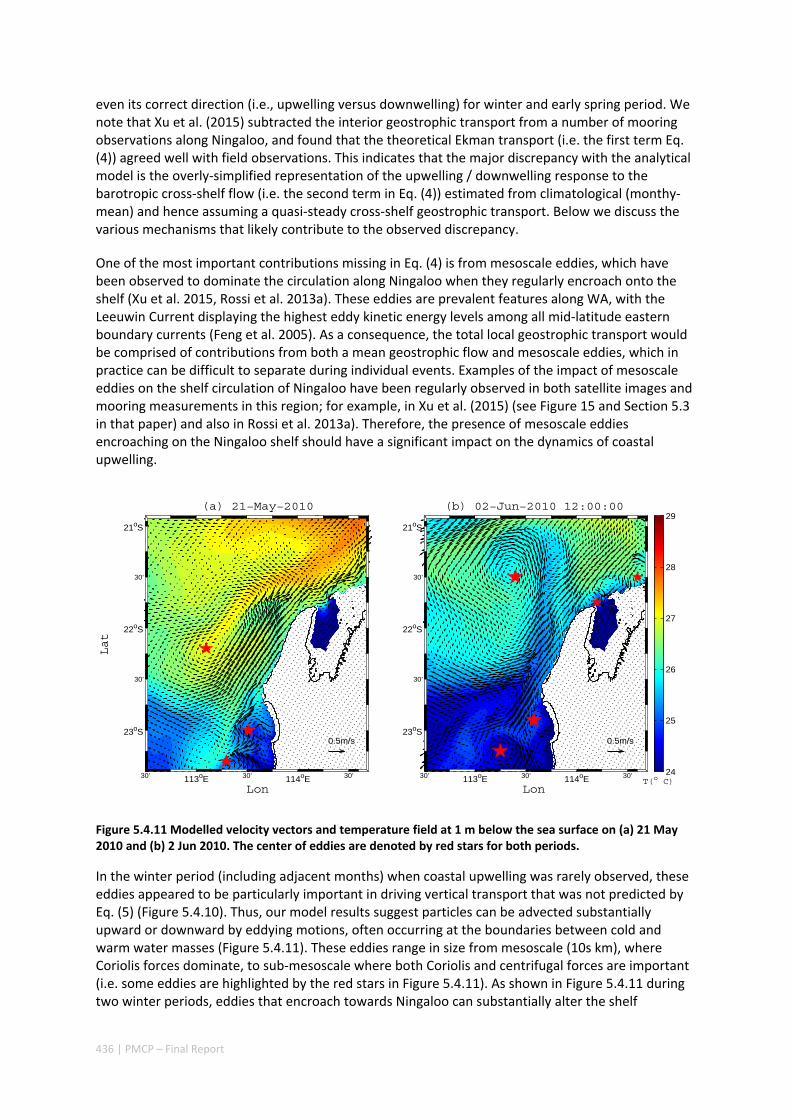
436 | PMCP – Final Report
even its correct direction (i.e., upwelling versus downwelling) for winter and early spring period. We note that Xu et al. (2015) subtracted the interior geostrophic transport from a number of mooring observations along Ningaloo, and found that the theoretical Ekman transport (i.e. the first term Eq. (4)) agreed well with field observations. This indicates that the major discrepancy with the analytical model is the overly‐simplified representation of the upwelling / downwelling response to the barotropic cross‐shelf flow (i.e. the second term in Eq. (4)) estimated from climatological (monthy‐mean) and hence assuming a quasi‐steady cross‐shelf geostrophic transport. Below we discuss the various mechanisms that likely contribute to the observed discrepancy.
One of the most important contributions missing in Eq. (4) is from mesoscale eddies, which have been observed to dominate the circulation along Ningaloo when they regularly encroach onto the shelf (Xu et al. 2015, Rossi et al. 2013a). These eddies are prevalent features along WA, with the Leeuwin Current displaying the highest eddy kinetic energy levels among all mid‐latitude eastern boundary currents (Feng et al. 2005). As a consequence, the total local geostrophic transport would be comprised of contributions from both a mean geostrophic flow and mesoscale eddies, which in practice can be difficult to separate during individual events. Examples of the impact of mesoscale eddies on the shelf circulation of Ningaloo have been regularly observed in both satellite images and mooring measurements in this region; for example, in Xu et al. (2015) (see Figure 15 and Section 5.3 in that paper) and also in Rossi et al. 2013a). Therefore, the presence of mesoscale eddies encroaching on the Ningaloo shelf should have a significant impact on the dynamics of coastal upwelling.
Figure 5.4.11 Modelled velocity vectors and temperature field at 1 m below the sea surface on (a) 21 May 2010 and (b) 2 Jun 2010. The center of eddies are denoted by red stars for both periods.
In the winter period (including adjacent months) when coastal upwelling was rarely observed, these eddies appeared to be particularly important in driving vertical transport that was not predicted by Eq. (5) (Figure 5.4.10). Thus, our model results suggest particles can be advected substantially upward or downward by eddying motions, often occurring at the boundaries between cold and warm water masses (Figure 5.4.11). These eddies range in size from mesoscale (10s km), where Coriolis forces dominate, to sub‐mesoscale where both Coriolis and centrifugal forces are important (i.e. some eddies are highlighted by the red stars in Figure 5.4.11). As shown in Figure 5.4.11 during two winter periods, eddies that encroach towards Ningaloo can substantially alter the shelf
30’ 113oE 30’ 114oE 30’
23oS
30’
22oS
30’
21oS
0.5m/s
Lon
Lat
(a) 21−May−2010
30’ 113oE 30’ 114oE 30’
23oS
30’
22oS
30’
21oS
0.5m/s
Lon
(b) 02−Jun−2010 12:00:00
T(o C)24
25
26
27
28
29

437 | PMCP – Final Report
circulation. Klein et al. (2009) provided a general review of the vertical exchange of material in the ocean associated with mesoscale and sub‐mesoscale eddies, and while focusing on the open ocean, they demonstrate how important eddies can be to localized vertical transport. In shelf regions, eddies have also been recognized for the important role they can play in vertical transport. For instance, Bassin et al. (2005) showed that eddies with time scales of 2‐6 days contribute a major source of vertical nutrient flux to the inner shelf region of the California shelf. For our study region, the relatively weak stratification in winter also appears to enhance vertical displacements of water from these eddies. This suggests that along coasts with consistent downwelling (e.g., along WA) transient eddies can still drive substantial upward transport on the shelf, especially during seasons when the stratification is weak.
Interactions between buoyancy effects and shelf slopes can also complicate the response of coastal upwelling predicted from the simple analytical model (MacCready and Rhines 1991; Garrett et al. 1993; Brink and Lentz 2010a; 2010b; Brink 2012). Buoyancy arrest effects can modify the cross‐shelf transport and vertical transport structure, and hence suppress vertical transport. Both the present model results and our prior field observations (Xu et al. 2015) indicate that this buoyancy arrest effect can be strong during the spring, summer and autumn seasons, when the Burger number (B=NH/f) consistently exceeds 2 along the majority of the Ningaloo shelf. For cases with large Burger numbers, the flow within the bottom boundary layer contributes to strengthening the vertical density gradient, and the cross‐shelf flow can be ‘shut down’ after a short adjustment time (Brink and Lentz 2010a; 2010b; Brink 2012) (approximately 1 day during summertime on the Ningaloo shelf, which equates to a small excursion length of <5 km on the shelf), as was shown in our previous observations at Ningaloo (Xu et al. 2013; 2015). The strong buoyancy gradient across the shelf can thus substantially reduce onshore bottom boundary layer flow, while still allowing for the development of onshore geostrophic flow in the interior of the water column. This is consistent with the two main water sources observed in our particle tracking results, i.e. a deep source associated with bottom boundary layer transport and a shallower source due to onshore geostrophic transport. The idealized upwelling model (Eq. (4)), will only predict the instantaneous vertical transport velocity just below the surface boundary layer, so it is clear that a simple integration of this velocity can overestimate the overall source depth by ignoring the actual vertical flow structure. This is also the reason why Lagrangian particle tracking can give more reasonable predictions of true vertical migration distances, since it continuously follows the position of particles as they move through this spatially‐varying flow field.
Implications for nutrient supply to Ningaloo Reef
Our connectivity study has important implications for identifying the regional transport pathways and source waters that supply nutrients to Ningaloo Reef in both dissolved and particulate forms. Based on phytoplankton grazing rates by shallow reef communities measured on a portion of the ~300 km long reef, Wyatt et al. (2010) proposed that the oceanic supply of nitrogen to the reef that is associated with phytoplankton must be drawn from a large offshore ‘ocean catchment’ in the region. From the seasonal transport pathways identified in this study (e.g. Figure 5.4.6 and Figure 5.4.7), there is clearly the potential for the regional ocean circulation to supply this reef with particulate nutrients originating from source regions that are remote from the reef itself.
In addition, examination of the seasonally and spatially‐varying dissolved nitrogen (nitrate, NO3) concentrations from historical archives (CSIRO Atlas of Regional Seas, CARS 2009) shows very low concentrations (~0 µM) in the upper 50 m of the water column throughout the region (Figure 5.4.12). However, concentrations increase sharply below 50 m, and tend to also increase towards the northeast, reaching ~10 µM at some northern locations at 100 m depth (Figure 5.4.12). According to these regional‐scale NO3 patterns and our estimation of the seasonal source water locations and depths (Scenario 2), it is apparent that water at the Ningaloo coast during most of the

438 | PMCP – Final Report
year (Mar‐Oct) is on average sourced from the surface waters (<50 m depth) where NO3 concentrations are very low. Some coastal upwelling may bring up deeper (NO3 rich) water from 50‐100 m depth to the surface in spring and summer; however, the strengthening of the poleward flow on the NWS would also advect higher NO3 concentration water southward towards Ningaloo Reef during the late‐summer and autumn periods. Although we acknowledge that dissolved nutrients such as NO3 do not behave as passive tracers, as they are taken up and transformed by planktonic communities, the results suggest that horizontal advection of nutrients may be an important source of nutrients to Ningaloo Reef during these seasons. Only during occasional major upwelling events (especially in summer), would coastal upwelling be able to bring up large volumes of deep water (100‐150 m) with high NO3 concentrations (> 5µM). Nevertheless, upwelling events would regularly deliver moderate‐depth water (~50‐80 m) towards the surface, where nitrate concentrations are typically ~1 µM and are thus still far greater than background surface water concentrations. This magnitude of NO3 variability (up to ~1 µM) associated with typical upwelling events at Ningaloo compares well with the observations from Wyatt et al. (2012), which attributed increases in NO3
concentrations from background levels of <0.3 µM to ~1 µM to periods of persistent upwelling favorable winds that most often occur in summer. However, there was no clear evidence of coastal upwelling in the winter; instead deep and hence nutrient rich water was transported upwards by coastal eddies. Thus, transient eddies propagating through this region can also be an important mechanism in supplying nutrients to the shallow waters of Ningaloo Reef.
Figure 5.4.12 A climatological snapshot of nutrient (as nitrate) distribution taken from CSIRO Atlas of Regional Seas (CARS) for 1 Nov (Ridgway et al. 2002). (a) the horizontal distribution of nitrate (NO3, in units of uM) at 100 m depth as denoted by the back dash line in (b); (b) the vertical profiles of nitrate concentration taken at six sites highlighted by the red stars in (a).
Conclusions
In this study we investigated the ocean transport pathways surrounding Ningaloo Reef during different seasonal periods, and how they are influenced by transient upwelling, the Leeuwin Current and energetic eddy fields in the region. Overall, two main source regions for water that interacts with Ningaloo Reef were identified: water from northeast on Australia’s North West Shelf (in all seasons); and water from the west and offshore of the Ningaloo shelf (particularly in summer). The
1
2
3
4 5
6
(a)
108oE 110oE 112oE 114oE 116oE 118oE 120oE
27oS
24oS
21oS
18oS
15oS
Lon
Lat
N(μ M)0
2
4
6
8
0 10 20 30−200
−180
−160
−140
−120
−100
−80
−60
−40
−20
0
N (μ M)
dept
h(m
)
(b)
123456

439 | PMCP – Final Report
poleward circulation associated with the Leeuwin Current dominated horizontal transport during most of the year, consistent with the predominant southward along‐shelf trajectories of particles that originated from the northeast. The offshore water source was generally only significant during the summer period, when the Leeuwin Current was comparatively weak and was located further offshore. The vertical position of source waters were influenced by transient coastal upwelling that was found to be important on the Ningaloo shelf during the spring, summer and autumn periods. Driven by local wind variability and also influenced by the prevailing onshore geostrophic transport, coastal upwelling episodically brought subsurface water (typically from 100 m depth, but occasionally from 150 m during major upwelling events) towards the surface along the Ningaloo Reef. The persistent onshore geostrophic flow had an important effect on the development of coastal upwelling year‐round, while transient eddies encroaching on the shelf also episodically contributed to the vertical advection of deep water to the reef, particularly in winter when the surface stratification was weakest. Overall, the results reveal how the complex ocean dynamics of the region determine the material transport pathways to Ningaloo Reef, which has important implications for understanding the mechanisms responsible for supplying nutrients to the reef that are required to support its high productivity.
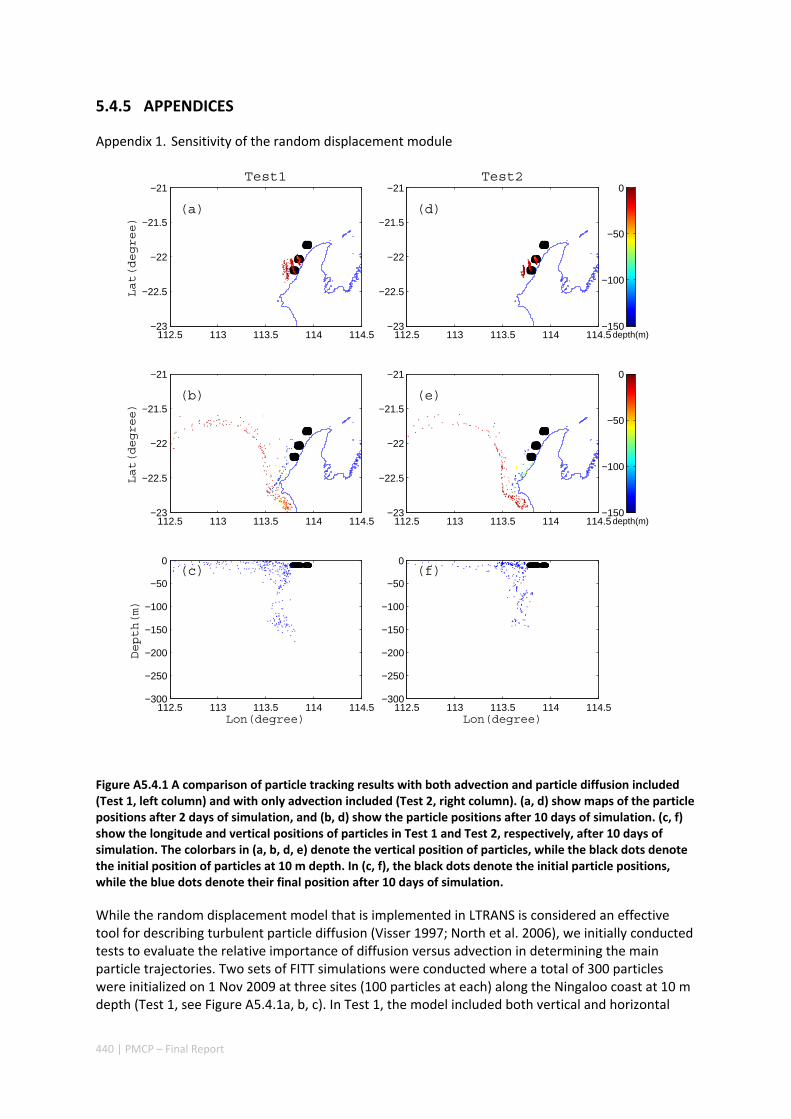
440 | PMCP – Final Report
5.4.5 APPENDICES
Appendix 1. Sensitivity of the random displacement module
Figure A5.4.1 A comparison of particle tracking results with both advection and particle diffusion included (Test 1, left column) and with only advection included (Test 2, right column). (a, d) show maps of the particle positions after 2 days of simulation, and (b, d) show the particle positions after 10 days of simulation. (c, f) show the longitude and vertical positions of particles in Test 1 and Test 2, respectively, after 10 days of simulation. The colorbars in (a, b, d, e) denote the vertical position of particles, while the black dots denote the initial position of particles at 10 m depth. In (c, f), the black dots denote the initial particle positions, while the blue dots denote their final position after 10 days of simulation.
While the random displacement model that is implemented in LTRANS is considered an effective tool for describing turbulent particle diffusion (Visser 1997; North et al. 2006), we initially conducted tests to evaluate the relative importance of diffusion versus advection in determining the main particle trajectories. Two sets of FITT simulations were conducted where a total of 300 particles were initialized on 1 Nov 2009 at three sites (100 particles at each) along the Ningaloo coast at 10 m depth (Test 1, see Figure A5.4.1a, b, c). In Test 1, the model included both vertical and horizontal
112.5 113 113.5 114 114.5−23
−22.5
−22
−21.5
−21
Lat(degree)
(a)
Test1
112.5 113 113.5 114 114.5−23
−22.5
−22
−21.5
−21
Lat(degree)
(b)
112.5 113 113.5 114 114.5−300
−250
−200
−150
−100
−50
0
Depth(m)
Lon(degree)
(c)
112.5 113 113.5 114 114.5−23
−22.5
−22
−21.5
−21
(d)
Test2
depth(m)−150
−100
−50
0
112.5 113 113.5 114 114.5−23
−22.5
−22
−21.5
−21
(e)
depth(m)−150
−100
−50
0
112.5 113 113.5 114 114.5−300
−250
−200
−150
−100
−50
0
Lon(degree)
(f)
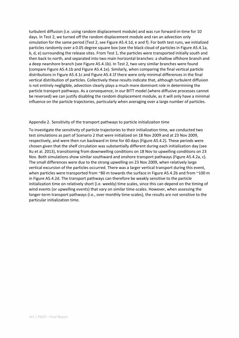
441 | PMCP – Final Report
turbulent diffusion (i.e. using random displacement module) and was run forward‐in‐time for 10 days. In Test 2, we turned off the random displacement module and ran an advection only simulation for the same period (Test 2, see Figure A5.4.1d, e and f). For both test runs, we initialized particles randomly over a 0.05 degree square box (see the black cloud of particles in Figure A5.4.1a, b, d, e) surrounding the release sites. From Test 1, the particles were transported initially south and then back to north, and separated into two main horizontal branches: a shallow offshore branch and a deep nearshore branch (see Figure A5.4.1b). In Test 2, two very similar branches were found (compare Figure A5.4.1b and Figure A5.4.1e). Similarly, when comparing the final vertical particle distributions in Figure A5.4.1c and Figure A5.4.1f there were only minimal differences in the final vertical distribution of particles. Collectively these results indicate that, although turbulent diffusion is not entirely negligible, advection clearly plays a much more dominant role in determining the particle transport pathways. As a consequence, in our BITT model (where diffusive processes cannot be reversed) we can justify disabling the random displacement module, as it will only have a minimal influence on the particle trajectories, particularly when averaging over a large number of particles.
Appendix 2. Sensitivity of the transport pathways to particle initializaiton time
To investigate the sensitivity of particle trajectories to their initialization time, we conducted two test simulations as part of Scenario 2 that were initialized on 18 Nov 2009 and at 23 Nov 2009, respectively, and were then run backward in time for 60 days (Figure A5.4.2). These periods were chosen given that the shelf circulation was substantially different during each initialization day (see Xu et al. 2013), transitioning from downwelling conditions on 18 Nov to upwelling conditions on 23 Nov. Both simulations show similar southward and onshore transport pathways (Figure A5.4.2a, c). The small differences were due to the strong upwelling on 23 Nov 2009, when relatively large vertical excursion of the particles occurred. There was a larger vertical transport during this event, when particles were transported from ~80 m towards the surface in Figure A5.4.2b and from ~100 m in Figure A5.4.2d. The transport pathways can therefore be weakly sensitive to the particle initialization time on relatively short (i.e. weekly) time scales, since this can depend on the timing of wind events (or upwelling events) that vary on similar time‐scales. However, when assessing the longer‐term transport pathways (i.e., over monthly time‐scales), the results are not sensitive to the particular initialization time.
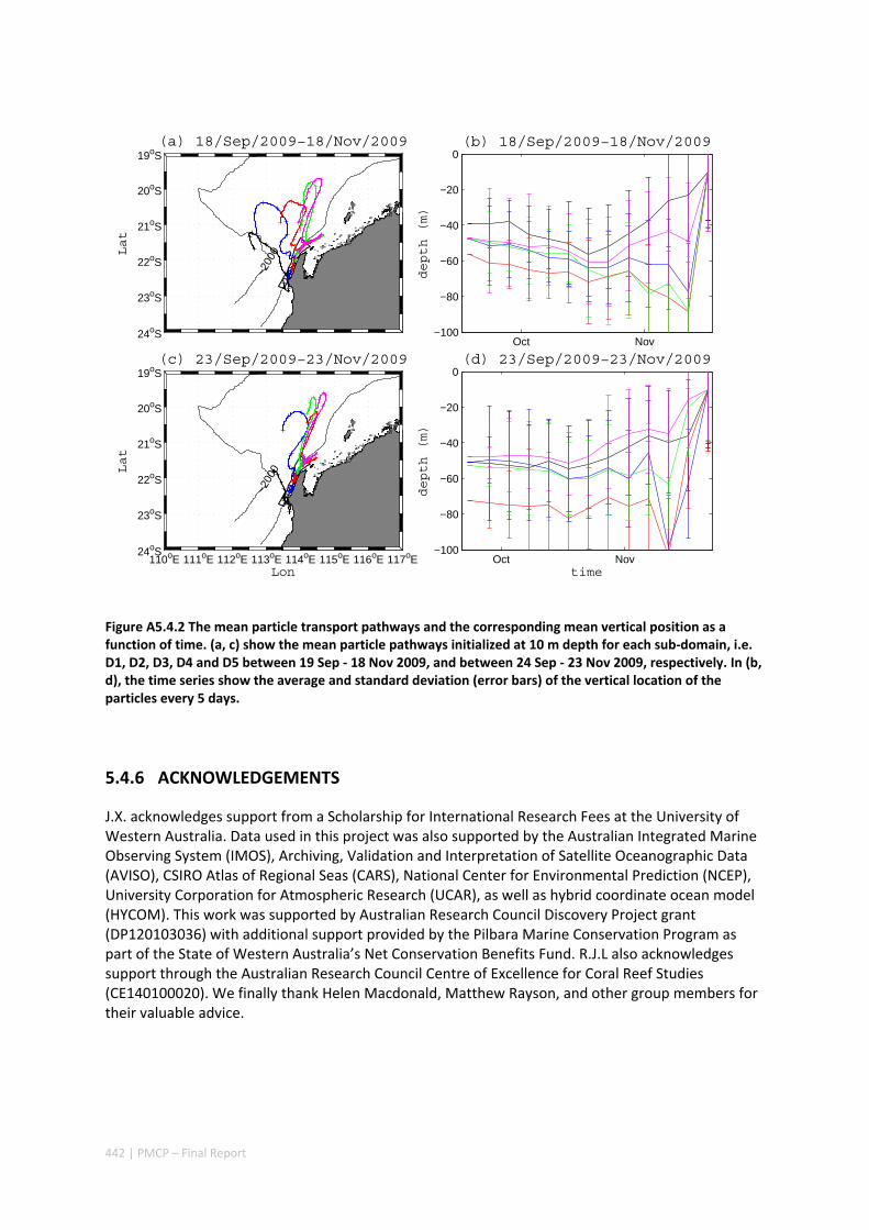
442 | PMCP – Final Report
Figure A5.4.2 The mean particle transport pathways and the corresponding mean vertical position as a function of time. (a, c) show the mean particle pathways initialized at 10 m depth for each sub‐domain, i.e. D1, D2, D3, D4 and D5 between 19 Sep ‐ 18 Nov 2009, and between 24 Sep ‐ 23 Nov 2009, respectively. In (b, d), the time series show the average and standard deviation (error bars) of the vertical location of the particles every 5 days.
5.4.6 ACKNOWLEDGEMENTS
J.X. acknowledges support from a Scholarship for International Research Fees at the University of Western Australia. Data used in this project was also supported by the Australian Integrated Marine Observing System (IMOS), Archiving, Validation and Interpretation of Satellite Oceanographic Data (AVISO), CSIRO Atlas of Regional Seas (CARS), National Center for Environmental Prediction (NCEP), University Corporation for Atmospheric Research (UCAR), as well as hybrid coordinate ocean model (HYCOM). This work was supported by Australian Research Council Discovery Project grant (DP120103036) with additional support provided by the Pilbara Marine Conservation Program as part of the State of Western Australia’s Net Conservation Benefits Fund. R.J.L also acknowledges support through the Australian Research Council Centre of Excellence for Coral Reef Studies (CE140100020). We finally thank Helen Macdonald, Matthew Rayson, and other group members for their valuable advice.
24oS
23oS
22oS
21oS
20oS
19oS
−200
0−2
00
Lat
(a) 18/Sep/2009−18/Nov/2009
Oct Nov−100
−80
−60
−40
−20
0
depth (m)
(b) 18/Sep/2009−18/Nov/2009
110oE 111oE 112oE 113oE 114oE 115oE 116oE 117oE 24oS
23oS
22oS
21oS
20oS
19oS
−200
0−2
00
Lon
Lat
(c) 23/Sep/2009−23/Nov/2009
Oct Nov−100
−80
−60
−40
−20
0
time
depth (m)
(d) 23/Sep/2009−23/Nov/2009
443 | PMCP – Final Report
5.4.7 REFERENCES
Bassin CJ, Washburn L, Brzezinski M and McPhee‐Shaw E (2005) Sub‐mesoscale coastal eddies observed by high frequency radar: A new mechanism for delivering nutrients to kelp forests in the Southern California Bight. Geophys Res Lett. 2005;32(12):L12604. doi: 10.1029/2005GL023017.
Brink KH (2012) Buoyancy Arrest and Shelf–Ocean Exchange. Journal of Physical Oceanography 42(4):644‐58. doi: 10.1175/JPO‐D‐11‐0143.1.
Batchelder HP (2006) Forward‐in‐Time‐/Backward‐in‐Time‐Trajectory (FITT/BITT) Modeling of Particles and Organisms in the Coastal Ocean*. J Atmos Ocean Tech. 23(5):727‐41. doi: 10.1175/JTECH1874.1.
Beardsley RC, Limeburner R and Rosenfeld LK (1985) Introduction to the CODE‐2 moored array and large‐scale data report. Woods Hole Oceanographic Institution.
Brink KH and Lentz SJ (2010a) Buoyancy Arrest and Bottom Ekman Transport. Part I: Steady Flow. Journal of Physical Oceanography 40(4):621‐35. doi: 10.1175/2009jpo4266.1. PubMed PMID: WOS:000276827700001.
Brink KH and Lentz SJ (2010b) Buoyancy Arrest and Bottom Ekman Transport. Part II: Oscillating Flow. Journal of Physical Oceanography 40(4):636‐55. doi: 10.1175/2009jpo4267.1. PubMed PMID: WOS:000276827700002.
Chassignet EP, Hurlburt HE, Smedstad OM, Halliwell GR, Hogan PJ, Wallcraft AJ, et al. (2007) The HYCOM (HYbrid Coordinate Ocean Model) data assimilative system. J Mar Syst. 65(1‐4):60‐83. doi: 10.1016/j.jmarsys.2005.09.016. PubMed PMID: WOS:000245003400005.
Cresswell GR and Golding TJ (1980) Observations of a south‐flowing current in the southeastern Indian Ocean. Deep‐Sea Research Part a‐Oceanographic Research Papers 27(6):449‐66. PubMed PMID: ISI:A1980KD83400004.
Cushman‐Roisin B and Beckers J‐M (2010) Introduction to Geophysical Fluid Dynamics. Hanover, New Hampshire 03755, USA: Academic Press. 768 p.
Domingues CM, Maltrud ME, Wijffels SE, Church JA and Tomczak M (2007) Simulated Lagrangian pathways between the Leeuwin Current System and the upper‐ocean circulation of the southeast Indian Ocean. Deep Sea Research Part II: Topical Studies in Oceanography 54(8–10):797‐817. doi: http://dx.doi.org/10.1016/j.dsr2.2006.10.003.
Feng M, Meyers G, Pearce A and Wijffels S (2003) Annual and interannual variations of the Leeuwin Current at 32 degrees S. Journal of Geophysical Research‐Oceans 108(C11):21. doi: 335510.1029/2002jc001763. PubMed PMID: ISI:000186899100004.
Feng M, Wijffels S, Godfrey S and Meyers G (2005) Do eddies play a role in the momentum balance of the Leeuwin Current? Journal of Physical Oceanography 35(6):964‐75. doi: 10.1175/jpo2730.1. PubMed PMID: WOS:000230580500004.
Garrett C, Maccready P and Rhines P (1993) Boundary mixing and arrested Ekman layers‐rotating stratified flow near a sloping boundary. Annu Rev Fluid Mech. 25:291‐323. doi: 10.1146/annurev.fluid.25.1.291. PubMed PMID: WOS:A1993KJ09800010.

444 | PMCP – Final Report
Godfrey JS and Ridgway KR (1985) The large‐scale environment of the poleward‐flowing Leeuwin Current, Western Australia: longshore steric height gradients, wind stresses and geostrophic flow. Journal of Physical Oceanography 15(5):481‐95. PubMed PMID: ISI:A1985AKU7800001.
Haidvogel DB, Arango H, Budgell WP, Cornuelle BD, Curchitser E, Di Lorenzo E, et al. (2008) Ocean forecasting in terrain‐following coordinates: Formulation and skill assessment of the Regional Ocean Modeling System. J Comput Phys. 227(7):3595‐624. doi: 10.1016/j.jcp.2007.06.016. PubMed PMID: ISI:000255005900009.
Hanson CE, Pattiaratchi CB and Waite AM (2005) Sporadic upwelling on a downwelling coast: Phytoplankton responses to spatially variable nutrient dynamics off the Gascoyne region of Western Australia. Cont Shelf Res. 25(12‐13):1561‐82. doi: 10.1016/j.csr.2005.04.003. PubMed PMID: ISI:000231045300007.
Holloway PE (1995) Leeuwin current observations on the Australian North West Shelf, May–June 1993. Deep Sea Research Part I: Oceanographic Research Papers 42(3):285‐305. doi: http://dx.doi.org/10.1016/0967‐0637(95)00004‐P.
Klein P and Lapeyre G (2009) The Oceanic Vertical Pump Induced by Mesoscale and Submesoscale Turbulence. Annual Review of Marine Science. 2009;1(1):351‐75. doi: doi:10.1146/annurev.marine.010908.163704. PubMed PMID: 21141041.
Lowe RJ, Ivey GN and Brinkman RM, Jones NJ (2012) Seasonal circulation and temperature variability near the North West Cape of Australia. Journal of Geophysical Research‐Oceans 117(C4). doi: 10.1029/2011JC007653.
MacCready P and Rhines PB (1991) Buoyant inhibition of Ekman transport on a slope and its effect on stratified spin‐up. J Fluid Mech. 223:631‐61.
Marchesiello P and, Estrade P (2010) Upwelling limitation by onshore geostrophic flow. J Mar Res. 68(1):37‐62. PubMed PMID: WOS:000283605000003.
Meuleners MJ, Ivey GN and Pattiaratchi CB (2008) A numerical study of the eddying characteristics of the Leeuwin Current System. Deep‐Sea Res Part I‐Oceanogr Res Pap. 55(3):261‐76. doi: 10.1016/j.dsr.2007.12.004. PubMed PMID: ISI:000254694200003.
North EW, Adams EE, Schlag Z, Sherwood CR, He R, Hyun KH, et al. (2011) Simulating Oil Droplet Dispersal From the Deepwater Horizon Spill With a Lagrangian Approach. Monitoring and Modeling the Deepwater Horizon Oil Spill: A Record‐Breaking Enterprise. Geophys. Monogr. Ser. 195. Washington, DC: AGU. p. 217‐26.
North EW, Hood RR, Chao SY and Sanford LP (2006) Using a random displacement model to simulate turbulent particle motion in a baroclinic frontal zone: A new implementation scheme and model performance tests. J Mar Syst. 60(3‐4):365‐80. doi: 10.1016/j.jmarsys.2005.08.003. PubMed PMID: WOS:000238331500012.
North EW, Schlag Z, Hood RR, Li M, Zhong L, Gross T, et al. (2008) Vertical swimming behavior influences the dispersal of simulated oyster larvae in a coupled particle‐tracking and hydrodynamic model of Chesapeake Bay. Marine Ecology Progress Series 359(99):115. doi: citeulike‐article‐id:10245453.
445 | PMCP – Final Report
Ridgway KR, Dunn JR and Wilkin JL (2002) Ocean Interpolation by Four‐Dimensional Weighted Least Squares—Application to the Waters around Australasia. J Atmos Ocean Tech. 19(9):1357‐75. doi: 10.1175/1520‐0426(2002)019<1357:oibfdw>2.0.co;2.
Ridgway KR and Godfrey JS (2015) The source of the Leeuwin Current seasonality. Journal of Geophysical Research: Oceans 120(10):6843‐64. doi: 10.1002/2015jc011049.
Rivas D and Samelson RM (2010) A Numerical Modeling Study of the Upwelling Source Waters along the Oregon Coast during 2005. Journal of Physical Oceanography 41(1):88‐112. doi: 10.1175/2010JPO4327.1.
Rossi V, Feng M, Pattiaratchi C, Roughan M and Waite AM (2013a) Linking synoptic forcing and local mesoscale processes with biological dynamics off Ningaloo Reef. Journal of Geophysical Research: Oceans 118(3):1211‐25. doi: 10.1002/jgrc.20110.
Rossi V, Feng M, Pattiaratchi C, Roughan M and Waite AM (2013b) On the factors influencing the development of sporadic upwelling in the Leeuwin Current system. Journal of Geophysical Research: Oceans 118(7):3608‐21. doi: 10.1002/jgrc.20242.
Roughan M, Oke PR and Middleton JH (2003) A Modeling Study of the Climatological Current Field and the Trajectories of Upwelled Particles in the East Australian Current. Journal of Physical Oceanography 33(12):2551‐64. doi: 10.1175/1520‐0485(2003)033<2551:AMSOTC>2.0.CO;2.
Schlag Z and North EW (2012) Larval TRANSport Lagrangian model (LTRANS) Users Guide. Cambridge, MD: University of Maryland Center for Environmental Science,Horn Point Laboratory, 2012 Report No.
Smith RL, Huyer A, Godfrey JS and Church JA (1991) The leeuwin current off Western Australia, 1986‐1987. Journal of Physical Oceanography 21(2):323‐45. PubMed PMID: ISI:A1991FB60400009.
Thompson RORY (1984) Observations of the Leeuwin Current off Western Australia. Journal of Physical Oceanography 14(3):623‐8. doi: 10.1175/1520‐0485(1984)014<0623:OOTLCO>2.0.CO;2.
Visser AW (1997) Using random walk models to simulate the vertical distribution of particles in a turbulent water column. Marine Ecology Progress Series 158:275‐81. doi: 10.3354/meps158275. PubMed PMID: WOS:A1997YK60700026.
Willmott CJ (1981) On the validation of models. Physical Geography 2:184‐194.
Wyatt ASJ, Falter JL, Lowe RJ, Humphries S and Waite AM (2012) Oceanographic forcing of nutrient uptake and release over a fringing coral reef. Limnol Oceanogr. 57(2):401‐19. doi: 10.4319/lo.2012.57.2.0401.
Wyatt ASJ, Lowe RJ, Humphries S and Waite AM (2010) Particulate nutrient fluxes over a fringing coral reef: relevant scales of phytoplankton production and mechanisms of supply. Mar Ecol‐Prog Ser. 405:113‐30. doi: 10.3354/meps08508. PubMed PMID: WOS:000278041300009.
Xu J (2014) Ocean dynamics and connectivity on the Ningaloo Shelf. 35 Striling HWY, Crawley,WA: the University of Western Australia.

446 | PMCP – Final Report
Xu J, Lowe RJ, Ivey GN, Jones NL and Brinkman R (2014) Observations of the shelf circulation dynamics along Ningaloo Reef, Western Australia during the austral spring and summer. Cont Shelf Res. 95(0):54‐73. doi: 10.1016/j.csr.2014.12.013.
Xu J, Lowe RJ, Ivey GN, Pattiaratchi C, Jones NL and Brinkman R (2013) Dynamics of the summer shelf circulation and transient upwelling off Ningaloo Reef, Western Australia. Journal of Geophysical Research‐Oceans 118(3):1099‐125. doi: Doi 10.1002/Jgrc.20098. PubMed PMID: WOS:000320323200004.
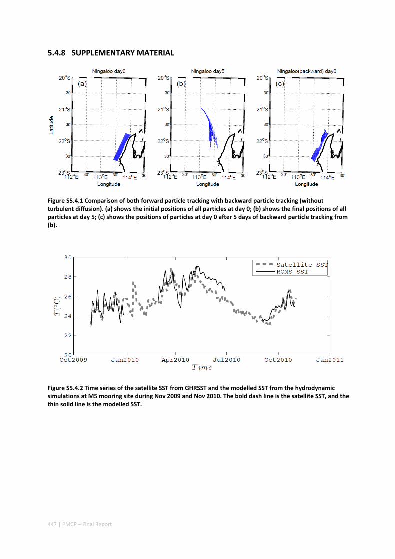
447 | PMCP – Final Report
5.4.8 SUPPLEMENTARY MATERIAL
Figure S5.4.1 Comparison of both forward particle tracking with backward particle tracking (without turbulent diffusion). (a) shows the initial positions of all particles at day 0; (b) shows the final positions of all particles at day 5; (c) shows the positions of particles at day 0 after 5 days of backward particle tracking from (b).
Figure S5.4.2 Time series of the satellite SST from GHRSST and the modelled SST from the hydrodynamic simulations at M5 mooring site during Nov 2009 and Nov 2010. The bold dash line is the satellite SST, and the thin solid line is the modelled SST.
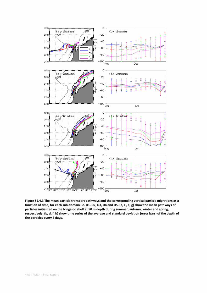
448 | PMCP – Final Report
Figure S5.4.3 The mean particle transport pathways and the corresponding vertical particle migrations as a function of time, for each sub‐domain i.e. D1, D2, D3, D4 and D5. (a, c , e, g) show the mean pathways of particles initialized on the Ningaloo shelf at 50 m depth during summer, autumn, winter and spring, respectively; (b, d, f, h) show time series of the average and standard deviation (error bars) of the depth of the particles every 5 days.

449 | PMCP – Final Report
Contrasting heat budget dynamics during two La Niña marine heat wave events along northwestern Australia
Authors: Xu J, Lowe RJ, Ivey GN, Jones NL.
Submitted to Journal of Geophysical Research
ABSTRACT
Two marine heat wave events occurred along Western Australia (WA) during the alternate austral summer periods of 2010/11 and 2012/13, both linked to strong La Niña conditions, which severely impacted marine ecosystems over >12 degrees of latitude, including unprecedented bleaching of many coral reefs. However, although these two heat waves were forced by similar large‐scale climate drivers, the warming patterns differed substantially between events, with the central coast of WA (south of 22o S) experiencing its greatest warming in 2010/11; whereas, the northwestern coast experienced greater warming in 2012/13. To investigate how oceanic and atmospheric processes drove these different spatial patterns, an analysis of the ocean heat budget was conducted by integrating remote sensing observations, in situ mooring data, and a high resolution (~1 km) ocean circulation model (Regional Ocean Modeling System). The results revealed substantial spatial differences in the relative contributions made by heat advection and air‐sea heat exchange between the two heat wave events. During 2010/11, anomalous warming by heat advection was present throughout the region, but was much stronger south of 22o S where the poleward‐flowing Leeuwin Current strengthens. During 2012/13, air‐sea heat exchange had a much more positive (warming) influence on sea surface temperature (especially in the northwest), and when combined with a more positive contribution of heat advection in the north, this can explain the regional differences in warming between these two La Niña‐associated heat wave events.
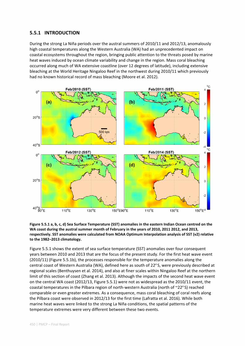
450 | PMCP – Final Report
5.5.1 INTRODUCTION
During the strong La Niña periods over the austral summers of 2010/11 and 2012/13, anomalously high coastal temperatures along the Western Australia (WA) had an unprecedented impact on coastal ecosystems throughout the region, bringing public attention to the threats posed by marine heat waves induced by ocean climate variability and change in the region. Mass coral bleaching occurred along much of WA extensive coastline (over 12 degrees of latitude), including extensive bleaching at the World Heritage Ningaloo Reef in the northwest during 2010/11 which previously had no known historical record of mass bleaching (Moore et al. 2012).
Figure 5.5.1 a, b, c, d) Sea Surface Temperature (SST) anomalies in the eastern Indian Ocean centred on the WA coast during the austral summer month of February in the years of 2010, 2011 2012, and 2013, respectively. SST anomalies were calculated from NOAA Optimum Interpolation analysis of SST (v2) relative to the 1982–2013 climatology.
Figure 5.5.1 shows the extent of sea surface temperature (SST) anomalies over four consequent years between 2010 and 2013 that are the focus of the present study. For the first heat wave event (2010/11) (Figure 5.5.1b), the processes responsible for the temperature anomalies along the central coast of Western Australia (WA), defined here as south of 22o S, were previously described at regional scales (Benthuysen et al. 2014), and also at finer scales within Ningaloo Reef at the northern limit of this section of coast (Zhang et al. 2013). Although the impacts of the second heat wave event on the central WA coast (2012/13, Figure 5.5.1) were not as widespread as the 2010/11 event, the coastal temperatures in the Pilbara region of north‐western Australia (north of ~22o S) reached comparable or even greater extremes. As a consequence, mass coral bleaching of coral reefs along the Pilbara coast were observed in 2012/13 for the first time (Lafratta et al. 2016). While both marine heat waves were linked to the strong La Niña conditions, the spatial patterns of the temperature extremes were very different between these two events.
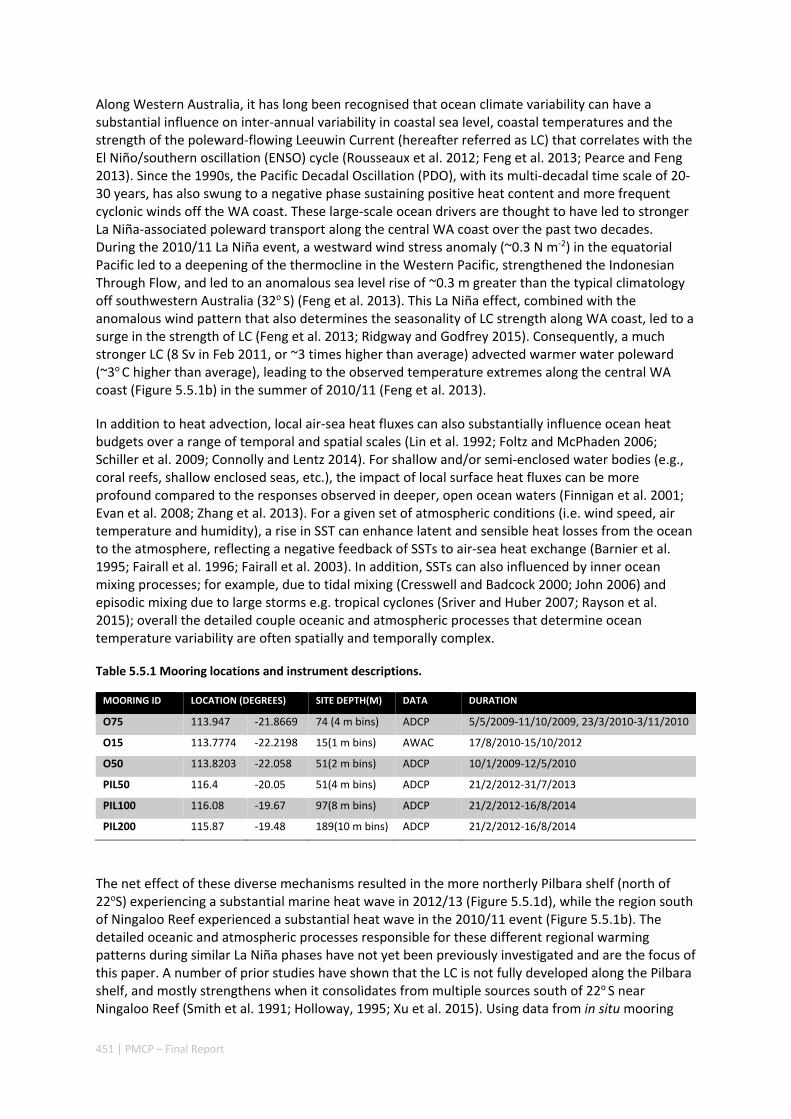
451 | PMCP – Final Report
Along Western Australia, it has long been recognised that ocean climate variability can have a substantial influence on inter‐annual variability in coastal sea level, coastal temperatures and the strength of the poleward‐flowing Leeuwin Current (hereafter referred as LC) that correlates with the El Niño/southern oscillation (ENSO) cycle (Rousseaux et al. 2012; Feng et al. 2013; Pearce and Feng 2013). Since the 1990s, the Pacific Decadal Oscillation (PDO), with its multi‐decadal time scale of 20‐30 years, has also swung to a negative phase sustaining positive heat content and more frequent cyclonic winds off the WA coast. These large‐scale ocean drivers are thought to have led to stronger La Niña‐associated poleward transport along the central WA coast over the past two decades. During the 2010/11 La Niña event, a westward wind stress anomaly (~0.3 N m‐2) in the equatorial Pacific led to a deepening of the thermocline in the Western Pacific, strengthened the Indonesian Through Flow, and led to an anomalous sea level rise of ~0.3 m greater than the typical climatology off southwestern Australia (32o S) (Feng et al. 2013). This La Niña effect, combined with the anomalous wind pattern that also determines the seasonality of LC strength along WA coast, led to a surge in the strength of LC (Feng et al. 2013; Ridgway and Godfrey 2015). Consequently, a much stronger LC (8 Sv in Feb 2011, or ~3 times higher than average) advected warmer water poleward (~3o C higher than average), leading to the observed temperature extremes along the central WA coast (Figure 5.5.1b) in the summer of 2010/11 (Feng et al. 2013).
In addition to heat advection, local air‐sea heat fluxes can also substantially influence ocean heat budgets over a range of temporal and spatial scales (Lin et al. 1992; Foltz and McPhaden 2006; Schiller et al. 2009; Connolly and Lentz 2014). For shallow and/or semi‐enclosed water bodies (e.g., coral reefs, shallow enclosed seas, etc.), the impact of local surface heat fluxes can be more profound compared to the responses observed in deeper, open ocean waters (Finnigan et al. 2001; Evan et al. 2008; Zhang et al. 2013). For a given set of atmospheric conditions (i.e. wind speed, air temperature and humidity), a rise in SST can enhance latent and sensible heat losses from the ocean to the atmosphere, reflecting a negative feedback of SSTs to air‐sea heat exchange (Barnier et al. 1995; Fairall et al. 1996; Fairall et al. 2003). In addition, SSTs can also influenced by inner ocean mixing processes; for example, due to tidal mixing (Cresswell and Badcock 2000; John 2006) and episodic mixing due to large storms e.g. tropical cyclones (Sriver and Huber 2007; Rayson et al. 2015); overall the detailed couple oceanic and atmospheric processes that determine ocean temperature variability are often spatially and temporally complex.
Table 5.5.1 Mooring locations and instrument descriptions.
MOORING ID LOCATION (DEGREES) SITE DEPTH(M) DATA DURATION
O75 113.947 ‐21.8669 74 (4 m bins) ADCP 5/5/2009‐11/10/2009, 23/3/2010‐3/11/2010
O15 113.7774 ‐22.2198 15(1 m bins) AWAC 17/8/2010‐15/10/2012
O50 113.8203 ‐22.058 51(2 m bins) ADCP 10/1/2009‐12/5/2010
PIL50 116.4 ‐20.05 51(4 m bins) ADCP 21/2/2012‐31/7/2013
PIL100 116.08 ‐19.67 97(8 m bins) ADCP 21/2/2012‐16/8/2014
PIL200 115.87 ‐19.48 189(10 m bins) ADCP 21/2/2012‐16/8/2014
The net effect of these diverse mechanisms resulted in the more northerly Pilbara shelf (north of 22oS) experiencing a substantial marine heat wave in 2012/13 (Figure 5.5.1d), while the region south of Ningaloo Reef experienced a substantial heat wave in the 2010/11 event (Figure 5.5.1b). The detailed oceanic and atmospheric processes responsible for these different regional warming patterns during similar La Niña phases have not yet been previously investigated and are the focus of this paper. A number of prior studies have shown that the LC is not fully developed along the Pilbara shelf, and mostly strengthens when it consolidates from multiple sources south of 22o S near Ningaloo Reef (Smith et al. 1991; Holloway, 1995; Xu et al. 2015). Using data from in situ mooring

452 | PMCP – Final Report
observations, remote sensing data, and ocean circulation modelling, we investigate how spatial differences in shelf circulation (heat advection) and air‐sea heat fluxes regulated the coastal heat budgets during these two events, to understand the causes of the different warming patterns.
5.5.2 METHODS
Study region and data sources
The study focuses on the ocean region off northwestern Australia, including the shelf region off Ningaloo Reef (near 22o S) to the south and the North West Shelf (hereafter referred to as NWS) off the Pilbara coast (Figure 5.5.2). Temperature, pressure and velocity data were measured at several moorings along the shelf (see Table 1 and the red dots in Figure 5.5.2). Daily SST fields were obtained from the Group for High‐Resolution Sea Surface Temperature (GHRSST, ~1 km resolution, see Reynolds et al. (2007)) global Level 4 products archived by the NOAA/National Climatic Data Center prior to 2010, and G1SST (Global 1 km Sea Surface Temperature, see Chao et al. (2009)) available from the NASA Jet Propulsion Laboratory after January 2010. These two data sets agree well with in situ SST measurements in the region (Zhang et al. 2013). Meteorological forcing (e.g., wind vectors, air temperature, air pressure, cloud cover and surface heat flux terms) were obtained from the Coupled Forecast System model version 2 (CFSv2, (Saha et al. 2013) ), and the European Centre for Medium‐Range Weather Forecasts (ECMWF, (Dee et al. 2011)). While there were occasionally small differences among these products (as we show below), these different products yielded only minor differences in the net surface heat fluxes imposed in the model.
Figure 5.5.2 Map of the study region. The regional model includes a large‐scale domain (ranging from 108oE to 122oE and from 14oS to 25oS) and a finer‐scale nested domain (highlighted by the solid black line). Mooring locations are denoted by the red dots. The blue dash lines enclose three coastal control volumes: Total_ControlV, PIL_ControlV (off Onslow) and CB_ControlV (off Coral Bay).

453 | PMCP – Final Report
Model configuration
The ocean circulation and thermodynamics were simulated using the Regional Ocean Modeling System (ROMS version 3.7, www.myroms.org), a hydrostatic primitive equation model using free surface terrain‐following vertical coordinates, and orthogonal curvilinear horizontal coordinates (Shchepetkin and McWilliams 2003; 2005). We utilized recent developments in two‐way nesting within ROMS, which included a large‐scale parent grid (~1000 km in each axis, 238 x 198 cells or ~4 km resolution) covering the broad region off northwestern Australia and a smaller‐scale child grid (~300 km, 270 x 186 cells or ~1 km resolution) that encompassed the coastal Pilbara region (see Figure 5.5.2). This on‐line nesting scheme had the advantage of accounting for both the large‐scale ocean dynamics that influence the region, while still achieving good spatial resolution in the main study area with reduced computational costs. For both grids, the vertical water column was simulated with 30 sigma layers, with the stretching designed to achieve higher resolutions near both
the surface and bottom (Vtransform =2, Vstretching =4, s = 5, b = 0.4). The model bathymetry was
based on the gridded 250 m resolution Geoscience Australia 2009 dataset. For the parent domain, a minimum model depth of 5 m was used. However, for the inner domain, a minimum model depth of 1 m was used with wetting/drying turned on to allow shallow grid points to come out of the water during low tide. Model bathymetries were matched in a buffer zone in the child grid (width of 30 grid cells), which were re‐masked to resolve a more highly‐resolved coastline relative to the parent grid. Note that the raw bathymetry data were interpolated and smoothed using LP_Bathymetry tools (Sikirić et al. 2009) to sustain a maximum Beckman and Haidvogel number (rx0) of 0.3 and a maximum Haney number (rx1) of 8.
Our regional model was initialized and driven by results from a global Hybrid Coordinate Ocean Model (HYCOM, ~1/12o global resolution) system as a hindcast reanalysis (Chassignet et al. 2007). Details of the open boundary and turbulent module configuration were identical to our previous ROMS model studies of the region (Xu et al. 2013; Xu et al. 2016). We activated the air‐sea interaction module‐bulk algorithm (Fairall et al. 1996; Fairall et al. 2003) to calculate the surface heat flux and momentum transfer rates. Atmospheric forcing variables, including wind, shortwave radiation, sea level pressure, air temperature and humidity, were derived from the coupled forecast system model (CFSv2) results (Saha et al. 2013). The solar radiation was applied exponentially over the depth assuming a first Jerlov water type relationship (Paulson and Simpson 1977). In addition, for an initial set of test simulations, the predicted heat fluxes derived from European Centre for Medium‐Range Weather Forecasts (ECMWF) (Dee et al. 2011) were also used in the ROMS model. Tidal forcing was obtained from the TPXO8 tidal atlas solution, a data assimilated tidal solution that has been significantly improved in shallow and coastal region (1/6o global resolution and 1/30o resolution in coastal regions), particularly in regions with strong non‐linear tide, such as the NWS of Australia (Egbert and Erofeeva 2002; Egbert et al. 2010; Stammer et al. 2014).
Heat budget analysis
The time evolution of the potential temperature field in ROMS is governed by the advection‐diffusive equation (Gan and Allen 2005):
(( ) ( ) ( ) ) ( ) ( ) ( )t x y z H x x H y y V z zT uT vT wT D T D T D T F (6)
Here T is temperature, x, y and z denotes the spatial coordinates, u, v, w denotes the corresponding velocity components, DH and DV are the horizontal and vertical eddy diffusivities, and F is the heat source term. In Eq. (6) the subscripts t, x, y, z denote partial derivatives with respect to these variables. Vertically‐integrating Eq. (6) over a surface layer (from a reference depth z=‐Z to the surface elevation z=η) gives:

454 | PMCP – Final Report
0
1 1(( ) ( ) ( ) ) /
rate advQ
t x y z net p diff
Z Z
T TT
T dz uT vT wT dz Q c H TH H
(7)
The overall temperature change rate Trate is therefore dependent on an advection term (Tadv ), a net air‐sea flux term (TQ) and a diffusion term (Tdiff). The net air sea heat flux Qnet consist of four individual terms (Zhang et al. 2013):
( )net sw ld lu lt sbQ Q Q Q Q Q (8)
where Qsw is the net shortwave (solar) radiation at the water surface (including both downward and upward short wave radiation), Qld and Qlu are the downward and upward longwave radiation (together defined as the net longwave radiation Qln), Qlt is the latent heat flux, and Qsb is the sensible heat flux. In this convention, a positive sign denotes a net flux of heat into the ocean.
To assess the net accumulation or loss of heat within a coastal region over a given time period, Eq. (7) can be spatially‐integrated within a control volume V0 and then integrated from an initial time t0 to an arbitrary time t. The temperature variability for given periods in the control volume then becomes
0 00
1 t
rate t
t Z S
T T dSdz dtV
(9)
Likewise, the heat advection and net air‐sea heat transfer terms can be expressed as
0 00
1(( ) ( ) ( ) )
t
adv x y z
t Z S
T uT vT wT dSdz dtV
(10)
and
0
00
1/
t
Q net p
t S
T Q c dSdtV
(11)
Here S represents the surface area of the control volume; Z0 denotes the depth where integration starts, taken as 100 m to include the layer above the seasonal thermocline in this region (see Xu et al. 2013); and t0 denotes the time when the integration commences. In this study we chose t0 to be the prior winter (1 July of each year), also coinciding with when the upper ocean heat content displays a minimum in inter‐annual variability; thus allowing heat budget variations to be cross‐compared between years.
To examine the heat transported along the coast, we locally computed the depth‐integrated along‐shelf heat advection, where the along‐shelf direction x’ was defined to run parallel to the isobaths (positive towards the northeast). Integrating this heat flux over the local water depth H yields:
'
1'along x
H
T u T dzH
(12)

455 | PMCP – Final Report
where u’ defines the projection of the velocity in the x’ direction. For this analysis we focused only on the continental shelf region (<200 m), where boundary currents are present and the depth‐integrated flow still tends to align with the local isobaths.
SST and surface heat flux anomalies
Anomalies of variables were only estimated for data that have long term records, e.g. the satellite SST data and the surface heat flux terms (for both CFSv2 and ECMWF). Given the good agreement between the satellite‐derived SST data and the model predictions (Bias<0.1 oC) shown below, we computed SST anomalies from the model output by subtracting the 2002‐2015 SST climatology (estimated from NOAA SST) from the modelled SSTs over the four consecutive years 2010‐2013. The surface heat flux anomalies (CFSv2, ECMWF) were estimated by subtracting the corresponding long term climatological data from the values that occurred over the four year study period. We note that anomalies in variables output from the ROMS model are not reported due to its relatively short record (only the four simulation years).
Figure 5.5.3 Vertical profiles comparing the model performance statistics in simulating the along‐shelf velocity profiles at selected moorings over the study period, i.e. at sites O50, PIL50, PIL100, PIL200, and O75, respectively (refer to Figure 2 for mooring locations). (a, b, c ,d ,e) profiles of model Bias. (f, g, h, i, j ) profiles of model Skill. The different profiles denote measurements for different periods when observations were available.

456 | PMCP – Final Report
Model evaluation
Similar ROMS models have previously been applied and validated for the northestern Australia region for different periods of time, which have included rigorous assessments of model performance; as detailed in Xu et al. (2013) and Xu et al. (2016). Here we provide some additional evaluation of the model over the period considered within the present study. Different measures of model performance were quantitatively compared to the field observations by computing a mean time‐averaged difference (Bias) and model Skill defined as (Willmott 1981):
2
21 model obs
model obs obs obs
X XSkill
X X X X
(13)
where X is the variable being compared with its time‐averaged value X . Perfect agreement between the model predictions and field observations yield a Skill=1, whereas complete disagreement yields a Skill=0. The model predictions of along‐shelf velocity profiles at 5 moorings are summarised in Figure 5.5.3. The bias at each mooring was within 0.05 m s‐1, except at the PIL200 mooring site, where the bias was within 0.1 m s‐1 and varied with depth. The Skill was over 0.6 at all sites and over 0.8 at the PIL50 site. Temperature variability across the study region was also accurately predicted by the model (Figure 5.5.4) where SSTs had Skill values of ~0.95. The Bias of the simulated SST was minor (within 0.1 oC) over the 4‐year simulation period. There were no continuous vertical temperature profile records over the 4‐year period; but in situ temperature observations at some discrete depths beneath the surface (Figure 5.5.4b, d) showed similar model performance as SST.
Figure 5.5.4 Comparison between the observed and modelled temperature time series. (a) Low‐pass filtered SST time series at the PIL100 mooring site derived from satellite observations (JPL SST; see section 2.1). (b) Low‐pass filtered temperature sampled at the PIL100 mooring at 20 m depth from the in situ mooring data. (c) Low‐pass filtered SST at O15 mooring site from satellite observations (JPL SST). (d) Low‐pass filtered temperature sampled in situ at O15 mooring site at 13 m depth. The low‐pass filter has a half‐power period of 38 h to remove tidal and inertial oscillations.
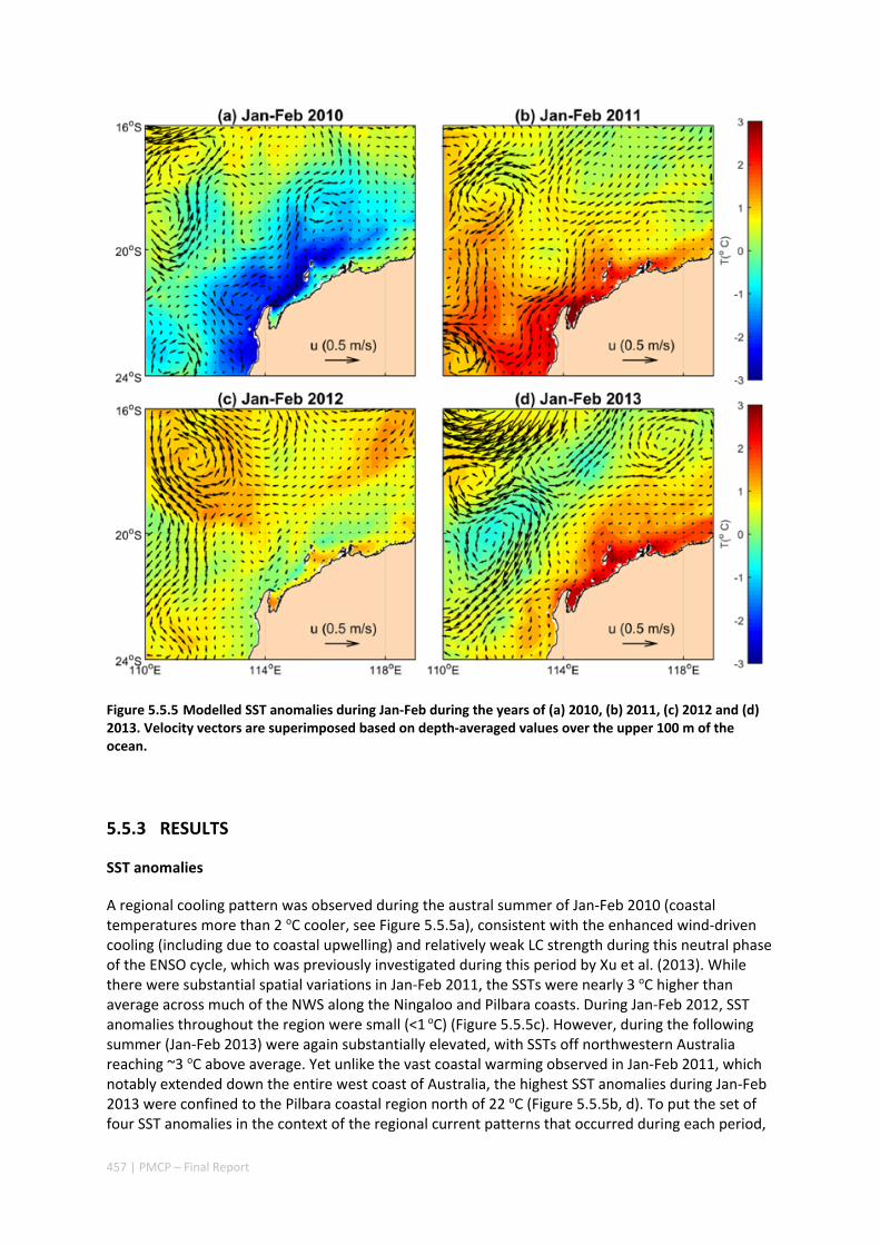
457 | PMCP – Final Report
Figure 5.5.5 Modelled SST anomalies during Jan‐Feb during the years of (a) 2010, (b) 2011, (c) 2012 and (d) 2013. Velocity vectors are superimposed based on depth‐averaged values over the upper 100 m of the ocean.
5.5.3 RESULTS
SST anomalies
A regional cooling pattern was observed during the austral summer of Jan‐Feb 2010 (coastal temperatures more than 2 oC cooler, see Figure 5.5.5a), consistent with the enhanced wind‐driven cooling (including due to coastal upwelling) and relatively weak LC strength during this neutral phase of the ENSO cycle, which was previously investigated during this period by Xu et al. (2013). While there were substantial spatial variations in Jan‐Feb 2011, the SSTs were nearly 3 oC higher than average across much of the NWS along the Ningaloo and Pilbara coasts. During Jan‐Feb 2012, SST anomalies throughout the region were small (<1 oC) (Figure 5.5.5c). However, during the following summer (Jan‐Feb 2013) were again substantially elevated, with SSTs off northwestern Australia reaching ~3 oC above average. Yet unlike the vast coastal warming observed in Jan‐Feb 2011, which notably extended down the entire west coast of Australia, the highest SST anomalies during Jan‐Feb 2013 were confined to the Pilbara coastal region north of 22 oC (Figure 5.5.5b, d). To put the set of four SST anomalies in the context of the regional current patterns that occurred during each period,
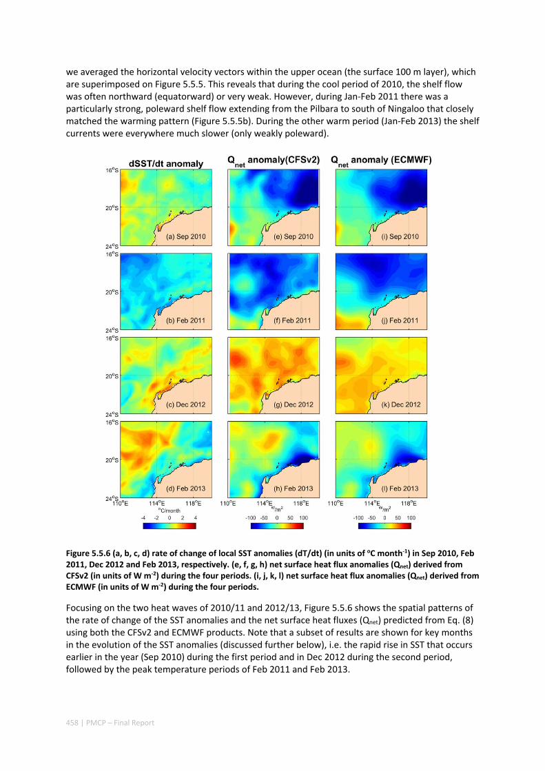
458 | PMCP – Final Report
we averaged the horizontal velocity vectors within the upper ocean (the surface 100 m layer), which are superimposed on Figure 5.5.5. This reveals that during the cool period of 2010, the shelf flow was often northward (equatorward) or very weak. However, during Jan‐Feb 2011 there was a particularly strong, poleward shelf flow extending from the Pilbara to south of Ningaloo that closely matched the warming pattern (Figure 5.5.5b). During the other warm period (Jan‐Feb 2013) the shelf currents were everywhere much slower (only weakly poleward).
Figure 5.5.6 (a, b, c, d) rate of change of local SST anomalies (dT/dt) (in units of oC month‐1) in Sep 2010, Feb 2011, Dec 2012 and Feb 2013, respectively. (e, f, g, h) net surface heat flux anomalies (Qnet) derived from CFSv2 (in units of W m‐2) during the four periods. (i, j, k, l) net surface heat flux anomalies (Qnet) derived from ECMWF (in units of W m‐2) during the four periods.
Focusing on the two heat waves of 2010/11 and 2012/13, Figure 5.5.6 shows the spatial patterns of the rate of change of the SST anomalies and the net surface heat fluxes (Qnet) predicted from Eq. (8) using both the CFSv2 and ECMWF products. Note that a subset of results are shown for key months in the evolution of the SST anomalies (discussed further below), i.e. the rapid rise in SST that occurs earlier in the year (Sep 2010) during the first period and in Dec 2012 during the second period, followed by the peak temperature periods of Feb 2011 and Feb 2013.
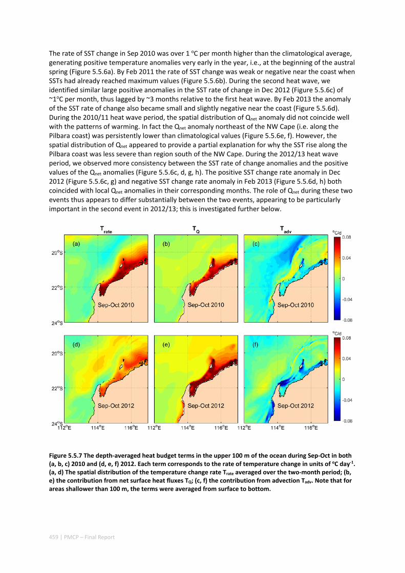
459 | PMCP – Final Report
The rate of SST change in Sep 2010 was over 1 oC per month higher than the climatological average, generating positive temperature anomalies very early in the year, i.e., at the beginning of the austral spring (Figure 5.5.6a). By Feb 2011 the rate of SST change was weak or negative near the coast when SSTs had already reached maximum values (Figure 5.5.6b). During the second heat wave, we identified similar large positive anomalies in the SST rate of change in Dec 2012 (Figure 5.5.6c) of ~1oC per month, thus lagged by ~3 months relative to the first heat wave. By Feb 2013 the anomaly of the SST rate of change also became small and slightly negative near the coast (Figure 5.5.6d). During the 2010/11 heat wave period, the spatial distribution of Qnet anomaly did not coincide well with the patterns of warming. In fact the Qnet anomaly northeast of the NW Cape (i.e. along the Pilbara coast) was persistently lower than climatological values (Figure 5.5.6e, f). However, the spatial distribution of Qnet appeared to provide a partial explanation for why the SST rise along the Pilbara coast was less severe than region south of the NW Cape. During the 2012/13 heat wave period, we observed more consistency between the SST rate of change anomalies and the positive values of the Qnet anomalies (Figure 5.5.6c, d, g, h). The positive SST change rate anomaly in Dec 2012 (Figure 5.5.6c, g) and negative SST change rate anomaly in Feb 2013 (Figure 5.5.6d, h) both coincided with local Qnet anomalies in their corresponding months. The role of Qnet during these two events thus appears to differ substantially between the two events, appearing to be particularly important in the second event in 2012/13; this is investigated further below.
Figure 5.5.7 The depth‐averaged heat budget terms in the upper 100 m of the ocean during Sep‐Oct in both (a, b, c) 2010 and (d, e, f) 2012. Each term corresponds to the rate of temperature change in units of oC day‐1. (a, d) The spatial distribution of the temperature change rate Trate averaged over the two‐month period; (b, e) the contribution from net surface heat fluxes TQ; (c, f) the contribution from advection Tadv. Note that for areas shallower than 100 m, the terms were averaged from surface to bottom.
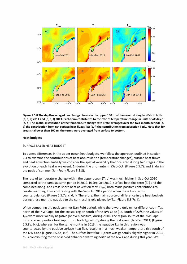
460 | PMCP – Final Report
Figure 5.5.8 The depth‐averaged heat budget terms in the upper 100 m of the ocean during Jan‐Feb in both (a, b, c) 2011 and (d, e, f) 2013. Each term contributes to the rate of temperature change in units of oC day‐1. (a, d) The spatial distribution of the temperature change rate Trate averaged over the two‐month period; (b, e) the contribution from net surface heat fluxes TQ; (c, f) the contribution from advection Tadv. Note that for areas shallower than 100 m, the terms were averaged from surface to bottom.
Heat budgets
SURFACE LAYER HEAT BUDGET
To assess differences in the upper ocean heat budgets, we follow the approach outlined in section 2.3 to examine the contributions of heat accumulation (temperature changes), surface heat fluxes and heat advection. Initially we consider the spatial variability that occurred during two stages in the evolution of each heat wave event: 1) during the prior autumn (Sep‐Oct) (Figure 5.5.7); and 2) during the peak of summer (Jan‐Feb) (Figure 5.5.8).
The rate of temperature change within the upper ocean (Trate) was much higher in Sep‐Oct 2010 compared to the same autumn period in 2012. In Sep‐Oct 2010, surface heat flux term (TQ) and the combined along‐ and cross‐shore heat advection term (Tadv) both made positive contributions to coastal warming, thus contrasting with the Sep‐Oct 2012 period when these two terms counterbalanced (Figure 5.5.7a, c, d, f). Therefore, the main source of difference in the heat budgets during these months was due to the contrasting role played by Tadv (Figure 5.5.7c, f).
When comparing the peak summer (Jan‐Feb) period, while there were only minor differences in Tadv north of the NW Cape, for the coastal region south of the NW Cape (i.e. south of 22oS) the values of Tadv were more weakly negative (or even positive) during 2010. The region south of the NW Cape thus received positive heat input from both Tadv and TQ during the first event (Jan‐Feb 2011) (Figure 5.5.8a, b, c); whereas, for the same months in 2013, the negative Tadv in this region was counteracted by the positive surface heat flux, resulting in a much weaker temperature rise south of the NW Cape (Figure 5.5.8d, e, f). The surface heat flux TQ term was generally slightly higher in 2013, thus contributing to the observed enhanced warming north of the NW Cape during this year. We
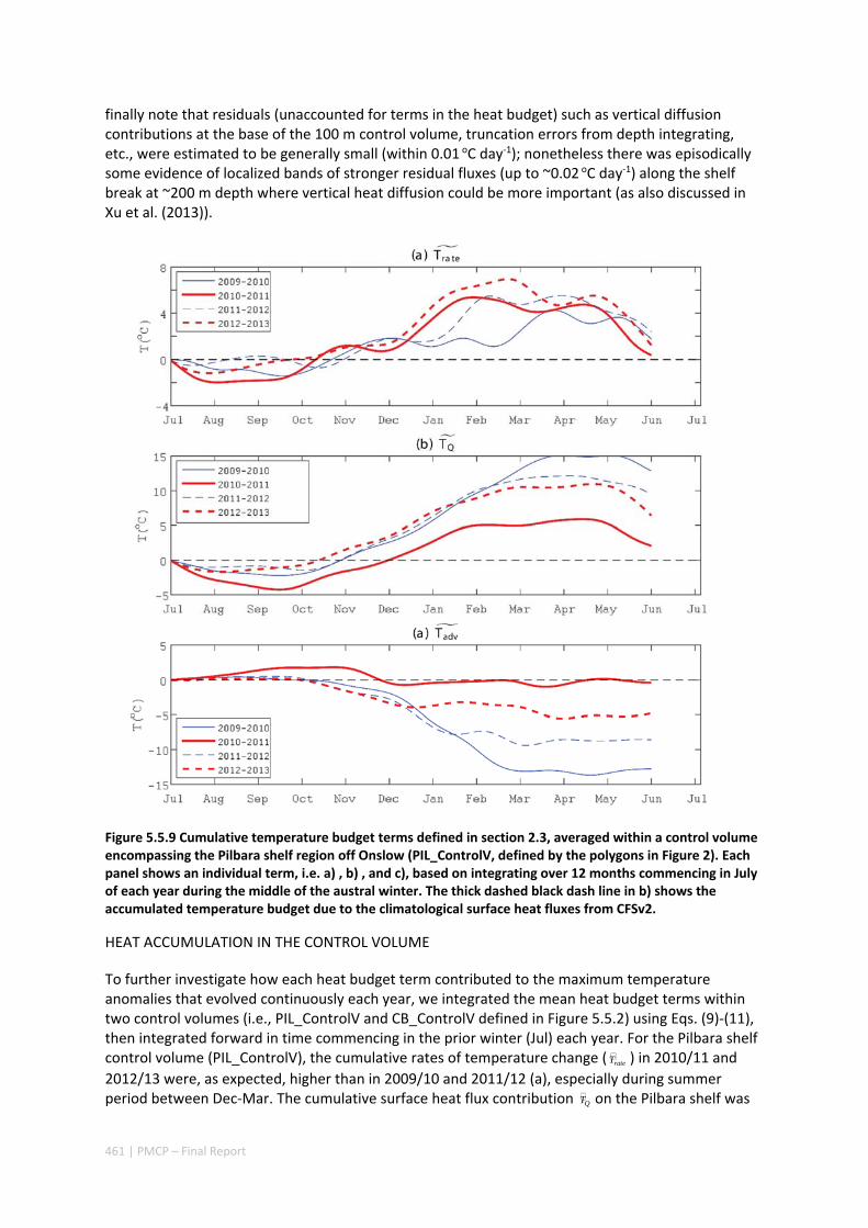
461 | PMCP – Final Report
finally note that residuals (unaccounted for terms in the heat budget) such as vertical diffusion contributions at the base of the 100 m control volume, truncation errors from depth integrating, etc., were estimated to be generally small (within 0.01 oC day‐1); nonetheless there was episodically some evidence of localized bands of stronger residual fluxes (up to ~0.02 oC day‐1) along the shelf break at ~200 m depth where vertical heat diffusion could be more important (as also discussed in Xu et al. (2013)).
Figure 5.5.9 Cumulative temperature budget terms defined in section 2.3, averaged within a control volume encompassing the Pilbara shelf region off Onslow (PIL_ControlV, defined by the polygons in Figure 2). Each panel shows an individual term, i.e. a) , b) , and c), based on integrating over 12 months commencing in July of each year during the middle of the austral winter. The thick dashed black dash line in b) shows the accumulated temperature budget due to the climatological surface heat fluxes from CFSv2.
HEAT ACCUMULATION IN THE CONTROL VOLUME
To further investigate how each heat budget term contributed to the maximum temperature anomalies that evolved continuously each year, we integrated the mean heat budget terms within two control volumes (i.e., PIL_ControlV and CB_ControlV defined in Figure 5.5.2) using Eqs. (9)‐(11), then integrated forward in time commencing in the prior winter (Jul) each year. For the Pilbara shelf control volume (PIL_ControlV), the cumulative rates of temperature change ( rateT ) in 2010/11 and
2012/13 were, as expected, higher than in 2009/10 and 2011/12 (a), especially during summer period between Dec‐Mar. The cumulative surface heat flux contribution QT on the Pilbara shelf was
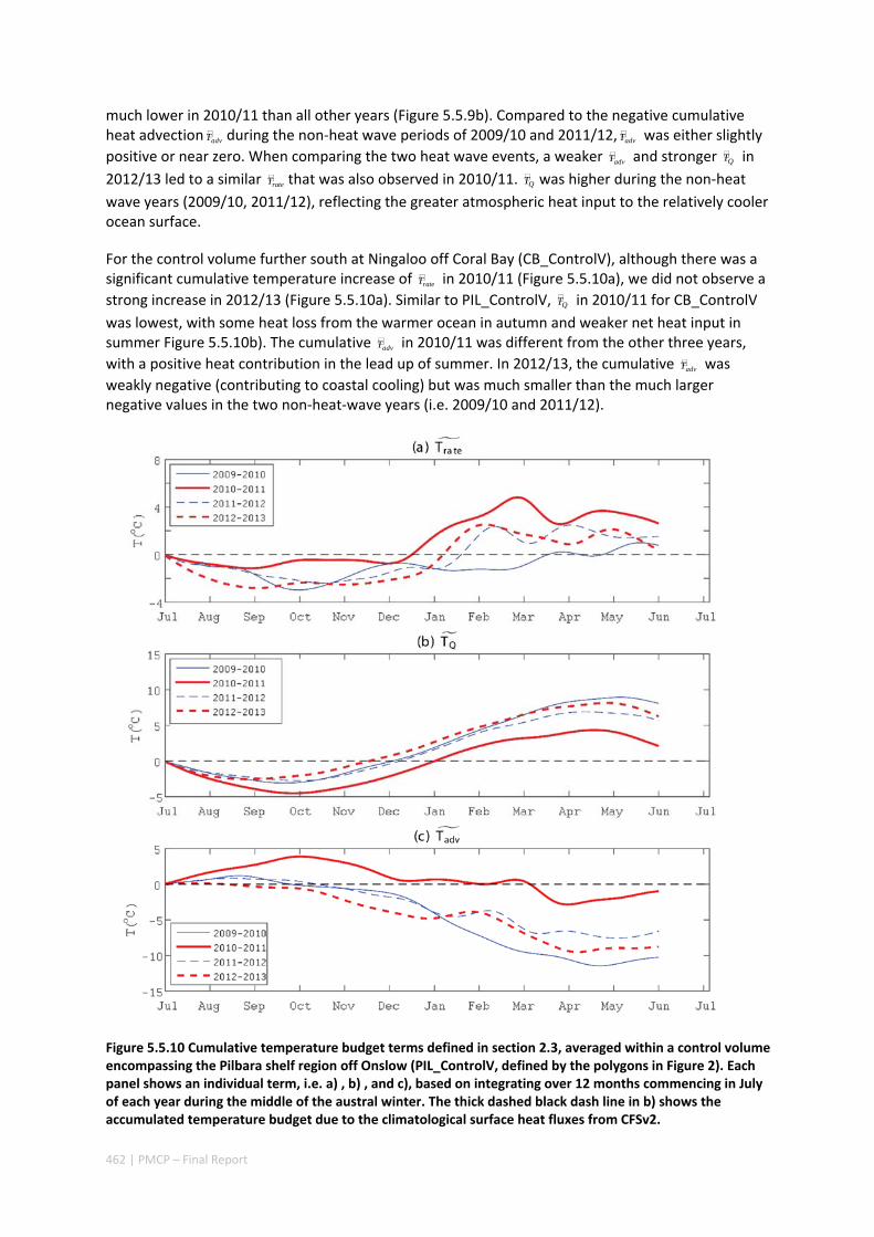
462 | PMCP – Final Report
much lower in 2010/11 than all other years (Figure 5.5.9b). Compared to the negative cumulative heat advection advT during the non‐heat wave periods of 2009/10 and 2011/12, advT was either slightly
positive or near zero. When comparing the two heat wave events, a weaker advT and stronger QT in
2012/13 led to a similar rateT that was also observed in 2010/11. QT was higher during the non‐heat
wave years (2009/10, 2011/12), reflecting the greater atmospheric heat input to the relatively cooler ocean surface.
For the control volume further south at Ningaloo off Coral Bay (CB_ControlV), although there was a significant cumulative temperature increase of rateT in 2010/11 (Figure 5.5.10a), we did not observe a
strong increase in 2012/13 (Figure 5.5.10a). Similar to PIL_ControlV, QT in 2010/11 for CB_ControlV
was lowest, with some heat loss from the warmer ocean in autumn and weaker net heat input in summer Figure 5.5.10b). The cumulative advT in 2010/11 was different from the other three years,
with a positive heat contribution in the lead up of summer. In 2012/13, the cumulative advT was
weakly negative (contributing to coastal cooling) but was much smaller than the much larger negative values in the two non‐heat‐wave years (i.e. 2009/10 and 2011/12).
Figure 5.5.10 Cumulative temperature budget terms defined in section 2.3, averaged within a control volume encompassing the Pilbara shelf region off Onslow (PIL_ControlV, defined by the polygons in Figure 2). Each panel shows an individual term, i.e. a) , b) , and c), based on integrating over 12 months commencing in July of each year during the middle of the austral winter. The thick dashed black dash line in b) shows the accumulated temperature budget due to the climatological surface heat fluxes from CFSv2.
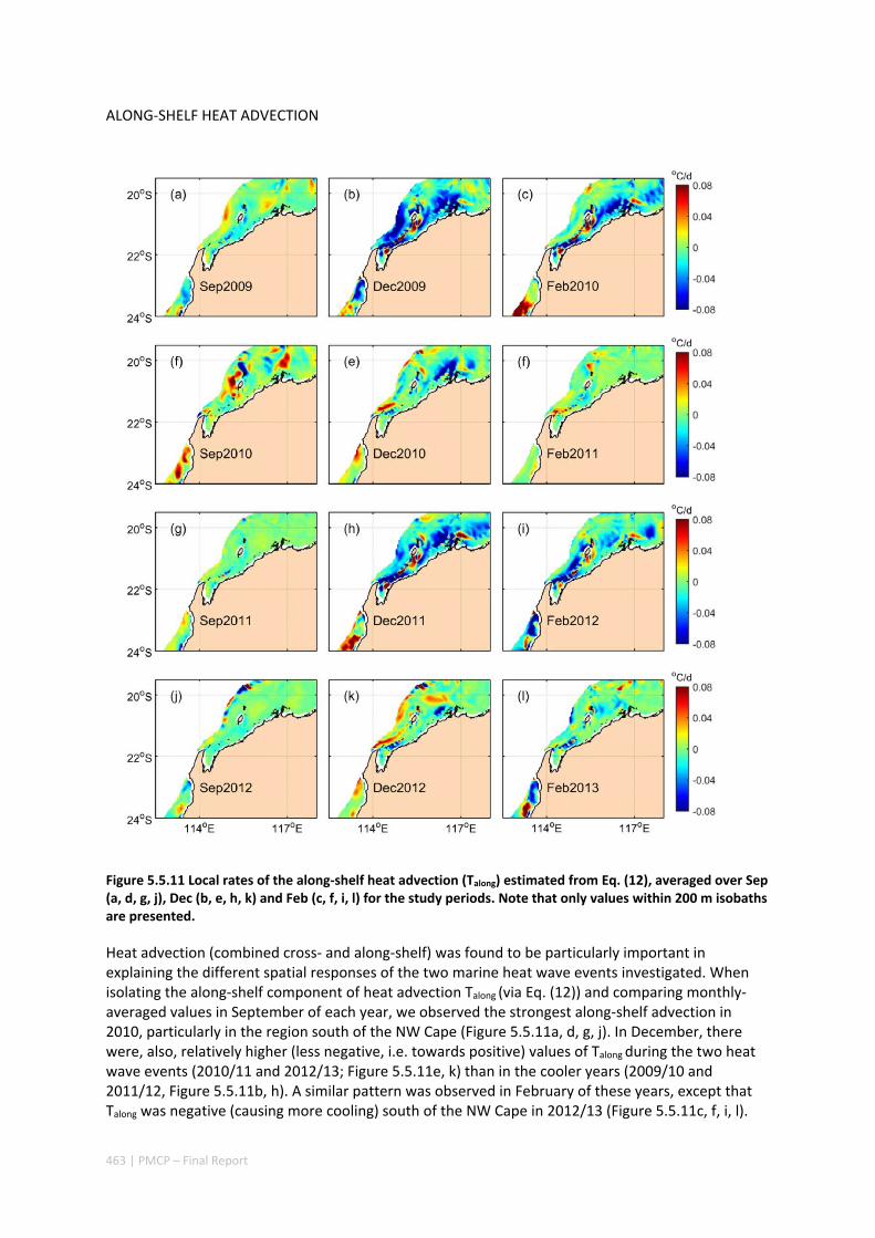
463 | PMCP – Final Report
ALONG‐SHELF HEAT ADVECTION
Figure 5.5.11 Local rates of the along‐shelf heat advection (Talong) estimated from Eq. (12), averaged over Sep (a, d, g, j), Dec (b, e, h, k) and Feb (c, f, i, l) for the study periods. Note that only values within 200 m isobaths are presented.
Heat advection (combined cross‐ and along‐shelf) was found to be particularly important in explaining the different spatial responses of the two marine heat wave events investigated. When isolating the along‐shelf component of heat advection Talong (via Eq. (12)) and comparing monthly‐averaged values in September of each year, we observed the strongest along‐shelf advection in 2010, particularly in the region south of the NW Cape (Figure 5.5.11a, d, g, j). In December, there were, also, relatively higher (less negative, i.e. towards positive) values of Talong during the two heat wave events (2010/11 and 2012/13; Figure 5.5.11e, k) than in the cooler years (2009/10 and 2011/12, Figure 5.5.11b, h). A similar pattern was observed in February of these years, except that Talong was negative (causing more cooling) south of the NW Cape in 2012/13 (Figure 5.5.11c, f, i, l).
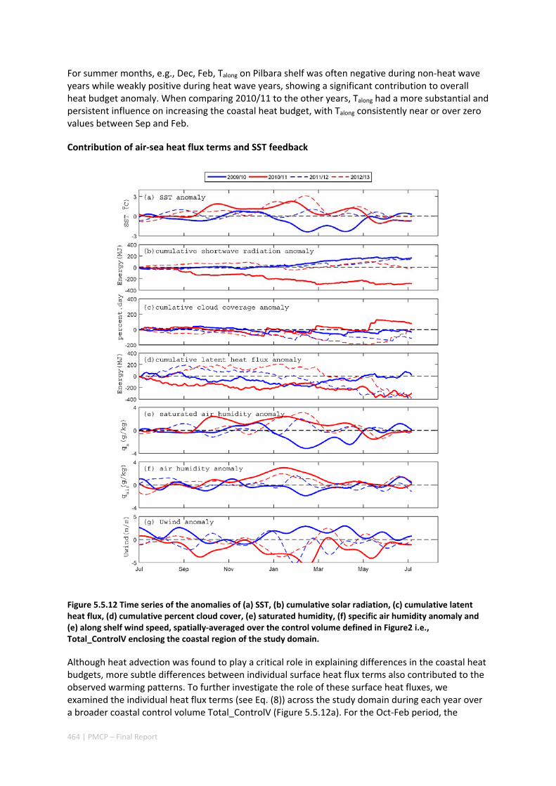
464 | PMCP – Final Report
For summer months, e.g., Dec, Feb, Talong on Pilbara shelf was often negative during non‐heat wave years while weakly positive during heat wave years, showing a significant contribution to overall heat budget anomaly. When comparing 2010/11 to the other years, Talong had a more substantial and persistent influence on increasing the coastal heat budget, with Talong consistently near or over zero values between Sep and Feb.
Contribution of air‐sea heat flux terms and SST feedback
Figure 5.5.12 Time series of the anomalies of (a) SST, (b) cumulative solar radiation, (c) cumulative latent heat flux, (d) cumulative percent cloud cover, (e) saturated humidity, (f) specific air humidity anomaly and (e) along shelf wind speed, spatially‐averaged over the control volume defined in Figure2 i.e., Total_ControlV enclosing the coastal region of the study domain.
Although heat advection was found to play a critical role in explaining differences in the coastal heat budgets, more subtle differences between individual surface heat flux terms also contributed to the observed warming patterns. To further investigate the role of these surface heat fluxes, we examined the individual heat flux terms (see Eq. (8)) across the study domain during each year over a broader coastal control volume Total_ControlV (Figure 5.5.12a). For the Oct‐Feb period, the
465 | PMCP – Final Report
spatially‐averaged SST anomalies during the 2010/11 heat wave event were up to 3oC higher than the climatological average. However, the cumulative shortwave radiation and latent heat flux anomalies over this year were the lowest among the four years investigated Figure 5.5.12b, c). These trends were in stark contrast to the terms during the 2012/13 heat wave when both shortwave radiation and latent heat flux positively contributed to the coastal warming.
The reduced shortwave radiation during the 2010/11 event is, to a large extent, due to increased cloud coverage in this year relative to 2012/13 (especially during the spring and early summer) (Figure 5.5.12c). In addition, we examined the conditions (individual variables) that contributed to
the latent heat fluxes in the bulk formulation, i.e. ( )lt air E wind s airQ C LU q q , where qs is
saturated humidity (which becomes higher when SST increases (Barnier et al. 1995; Fairall et al.
1996; Fairall et al. 2003)), qair is the specific air humidity, Uwind is the wind speed, air is the air
density, CE is the bulk transfer coefficient for latent heat, and L is the latent heat of vaporisation. Given that in 2010/11 the specific air humidity qair was higher and the wind speed Uwind was weaker than climatological averages (see Figure 5.5.12f, g), both variables would have only led to lower rates of evaporation and less latent heat loss; as a consequence the reduction of surface heat inputs were driven by an increase in the saturated humidity qs due to the highly elevated SST (Figure 5.5.12e). From This is consistent with Barnier et al. (1995), who showed that an SSTs increase of 1 oC in the tropical ocean can cause non‐solar surface heat fluxes to the ocean would typically decrease ~40 W m‐2 near the equator (which will reduce to ~20 W m‐2 at higher latitudes). This negative feedback between SSTs and the surface heat flux, together with the weaker shortwave radiation provide an explanation for the lower surface heat flux than climatology during the 2010/11 heat wave event. However, during the second heat wave in 2012/13, the latent heat flux anomaly clearly showed a positive contribution to regional warming due to the weaker winds and higher air humidity during this year.
5.5.4 DISCUSSION
The objective of this study was to investigate the coastal and shelf ocean heat budgets along northwestern Australia to isolate how various atmospheric and oceanic processes contributed to two extreme marine heat wave events during the austral summers of 2010/11 and 2012/13, with a particular focus on understanding the very different warming patterns between the two events despite occurring under similar La Niña conditions. During both heat wave events, poleward heat advection made key contributions to the coastal heat budgets that elevated SSTs relative to alternate cooler years. During La Niña phases of the ENSO cycle, the poleward transport associated with the Leeuwin Current down the Western Australia coast south of the NW Cape is known to be much stronger due to the enhanced along shelf pressure gradient (Feng et al. 2003; Ridgway and Godfrey 2015). While both the 2010/11 and 2012/13 heat wave events occurred during La Niña phases of the ENSO cycle, the 2010/11 La Niña was stronger, i.e. the Southern Oscillation Index (SOI) reached ~20 during 2010/11 versus ~10 in 2012/13.
In addition to the differences in the La Niña strength (and hence the strength of the Leeuwin Current), spatial differences in the wind conditions and surface (air‐sea) heat exchange also contributed to differences in the warming patterns observed between the two events. During the 2012/13 event, the along‐shelf winds averaged ~5 m s‐1 and were directed equatorward (opposing the Leeuwin Current) over the summer, which is comparable to normal climatological conditions. However, during the summer of 2010/11, the winds across the region were on average much weaker (~0 m s‐1), which would have also contributed to strengthening the poleward ocean transport and further enhanced the SSTs south of the NW Cape (22o S) during 2010/11 (Lowe et al. 2012). The
466 | PMCP – Final Report
results also indicate that the net surface heat fluxes during the austral spring and early‐summer (Sep‐Jan) that preceded the 2010/11 event were much more negative (heat loss to the atmosphere) than climatological mean conditions and also substantially lower than in the non‐heat wave years (Figure 5.5.9b, Figure 5.5.10b); this is in stark contrast to the nearly zero or weakly positive net surface heat fluxes observed during the second heat wave event of 2012/13, at rates even above the non‐heat wave years. These greater surface heat losses from the ocean to less local warming on the Pilbara shelf during the first 2010/11 event relative to the second 2012/13 event. Additional inspection of the individual terms that contributed to the net surface heat fluxes suggested that the higher heat losses to the atmosphere in 2010/11 were partially due to the negative feedback between ocean and atmosphere due to the warming ocean (mainly via latent heat fluxes) and partially due to the lower shortwave radiation due to higher cloud cover.
The spatial variability of the heat advection along the North West Shelf during the two heat wave events, including the differing importance of heat advection between the regions north and south of the NW Cape (22o S), are closely related to the bathymetric characteristics and coastline orientation that influence the shelf circulation patterns across the region. For the region south of the NW Cape, prior studies have shown how along‐shelf transport (and hence heat advection) is controlled by a balance between the along‐shelf pressure‐gradient‐driven Leeuwin Current flowing poleward (favoring transport of warmer water) and the opposing equatorward wind that both transports cooler water from the south via coastal currents and also can vertically transport cooler subsurface water via coastal upwelling (Xu et al. 2015). In 2010/11, the strong Leeuwin Current and weak equatorward winds led to a poleward transport of warm water south of the NW Cape that enhanced warming of this coastal region (Figure 5.5.1, Figure 5.5.12). Analysis by Benthuysen et al. (2014) focusing on the region south of the NW Cape (including the southwestern coast of WA) similarly found that this anomalous heat advection led to even more severe temperature anomalies in southwestern Australia (~5oC above averaged) as the Leeuwin Current strengthen down the central coast. However, in the Pilbara region to the northeast of the NW Cape, the continental shelf is much wider and shallower, with a coastline (and isobaths) oriented predominantly southwest to northeast direction. Within the shallower and wider continental shelf of Pilbara region any differences in net surface heat fluxes can have a more substantial influence in warming this coastal region relative to the steep shelf region south of the NW Cape; thus differences between the net surface heat fluxes between 2010/11 and 2012/13 had a more substantial influence on northern Pilbara shelf.
In summary, the objective of this this study was to investigate the oceanic and atmospheric processes (including feedback) that led to contrasting patterns of warming during two marine heat waves during the summers of 2010/11 and 2012/13 along northwestern Australia. Heat advection played an important role in driving the warming patterns in both events, but was stronger across the region during the 2010/11 event and was also consistently much stronger south of the NW Cape. Surface heat fluxes were found to be lower (less heat exchange into the ocean) relative to climatological mean conditions during the 2010/11 event due to a combination of reduced shortwave radiation due to higher cloud coverage and greater latent heat losses; however, during the 2012/13 these fluxes were similar to (or slightly higher than) climatology. Our heat budget analysis suggested a broadly negative (net cooling) role of surface heat flux during the first event while a positive role during the second event. The negative feedback of SST due to latent heat fluxes was found to be particularly important in reducing the surface heat flux during 2010/11. The substantial differences in the SST anomalies, separated to the north and south by the NW Cape, was also largely driven by spatial variability in heat advection. South of the NW Cape, along‐shelf heat advection tended to dominate the overall shelf heat budget, which was driven by the interaction between along shelf winds and along shelf circulation (e.g., the LC). For the northern Pilbara shelf region, both heat advection (e.g., coastal downwelling) and surface heat fluxes made substantial contributions to the coastal heat budget. Overall, the results highlight some of the challenges with predicting the patterns of extreme warming across coastal regions during marine heat waves; while
467 | PMCP – Final Report
large‐scale climate drivers can pre‐condition a region for a marine heat wave (i.e. strong La Niña conditions in the present case), the specific warming patterns that emerge depend on resolving complex coupled oceanic and atmospheric processes that regulate the warming responses.
5.5.5 ACKNOWLEDGEMENTS
We thank Zhenlin Zhang for providing input into the numerical modelling and heat budget analysis. This study used mooring data provided by the Australian National Mooring Network as part of the Integrated Marine Observing System (IMOS, www.imos.org.au), satellite SST data available from the NOAA/National Climatic Data Center (GHRSST) and from the NASA Jet Propulsion Laboratory (G1SST), meteorological forcing from the National Center for Environmental Prediction (CFSv2) and the European Centre for Medium‐Range Weather Forecasts, and global ocean model output from the hybrid coordinate ocean model (HYCOM, www.hycom.org). This research is funded by the Gorgon Barrow Island Net Conservation Benefits Fund, which is administered by the WA Department of Biodiversity, Conservation and Attractions, with additional support provided by the Australian Research Council Centre of Excellence for Coral Reef Studies (CE140100020).
5.5.6 REFERENCES
Barnier B, Siefridt L and Marchesiello P(1995) Thermal forcing for a global ocean circulation model using a three‐year climatology of ECMWF analyses Journal of Marine Systems 6(4):363‐380 doi:http://dx.doi.org/10.1016/0924‐7963(94)00034‐9.
Benthuysen J, Feng M and Zhong L (2014) Spatial patterns of warming off Western Australia during the 2011 Ningaloo Niño: Quantifying impacts of remote and local forcing, Continental Shelf Research 91(0):232‐246 doi:http://dx.doi.org/10.1016/j.csr.2014.09.014.
Chao YZ, Li J, Farrara D and Hung P (2009) Blending Sea Surface Temperatures from Multiple Satellites and In Situ Observations for Coastal Oceans, Journal of Atmospheric and Oceanic Technology, 26(7):1415‐1426 doi:doi:10.1175/2009JTECHO592.1.
Chassignet EP, Hurlburt HE Smedstad OM, Halliwell GR, Hogan PJ, Wallcraft AJ, Baraille R and Bleck R (2007) The HYCOM (HYbrid Coordinate Ocean Model) data assimilative system. Journal of Marine Systems 65(1‐4):60‐83 doi:10.1016/j.jmarsys.2005.09.016.
Connolly TP, and Lentz SJ (2014) Interannual variability of wintertime temperature on the inner continental shelf of the Middle Atlantic Bight. Journal of Geophysical Research: Oceans 119(9):6269‐6285 doi:10.1002/2014jc010153.
Cresswell GR and Badcock KA (2000) Tidal mixing near the Kimberley coast of NW Australia. Journal of Marine and Freshwater Research 51(7):641‐646 doi:http://dx.doi.org/10.1071/MF99154.
Dee DP et al. (2011) The ERA‐Interim reanalysis: configuration and performance of the data assimilation system, Quarterly. Journal of the Royal Meteorological Society 137(656):553‐597 doi:10.1002/qj.828.
Egbert GD and Erofeeva SY (2002) Efficient Inverse Modeling of Barotropic Ocean Tides. Journal of
468 | PMCP – Final Report
Atmospheric and Oceanic Technology 19(2):183‐204 doi:10.1175/1520‐0426(2002)019<0183:eimobo>2.0.co;2.
Egbert GD,Erofeeva SY and Ray RD (2010) Assimilation of altimetry data for nonlinear shallow‐water tides: Quarter‐diurnal tides of the Northwest European Shelf Continental Shelf Research 30(6):668‐679 doi:http://dx.doi.org/10.1016/j.csr.2009.10.011.
Evan W, Gary M and Itsara M (2008) A Climatology of Ocean–Atmosphere Heat Flux Estimates over the Great Barrier Reef and Coral Sea: Implications for Recent Mass Coral Bleaching Events. Journal of Climate 21(15):3853‐3871 doi:doi:10.1175/2007JCLI2085.1.
Fairall CW, Bradley EF, Hare JE, Grachev AA and Edson JB (2003) Bulk Parameterization of Air–Sea Fluxes: Updates and Verification for the COARE Algorithm. Journal of Climate 16(4):571‐591 doi:10.1175/1520‐0442(2003)016<0571:bpoasf>2.0.co;2.
Fairall CW, Bradley EF, Rogers DP, Edson JB and Young GS (1996) Bulk parameterization of air‐sea fluxes for Tropical Ocean Global Atmosphere Coupled Ocean Atmosphere Response. Experiment J. Geophys. Res. Oceans 101(C2):3747‐3764.
Feng M, McPhaden MJ, Xie S‐P and Hafner J (2013) La Niña forces unprecedented Leeuwin Current warming in 2011. Sci. Rep. 3.
Feng M, Meyers G, Pearce A and Wijffels S (2003) Annual and interannual variations of the Leeuwin Current at 32 degrees. S J. Geophys. Res.‐Oceans 108(C11) 21 doi:335510.1029/2002jc001763.
Finnigan TD, Winters KB and Ivey GN (2001) Response Characteristics of a Buoyancy‐Driven Sea. Journal of Physical Oceanography 31(9):2721‐2736 doi:10.1175/1520‐0485(2001)031<2721:rcoabd>2.0.co;2.
Foltz GR, and McPhaden MJ (2006) The Role of Oceanic Heat Advection in the Evolution of Tropical North and South Atlantic SST Anomalies. Journal of Climate 19(23):6122‐6138 doi:10.1175/jcli3961.1.
Gan J. P. and J. S. Allen (2005) Modeling upwelling circulation off the Oregon coast J. Geophys. Res.‐Oceans 110(C10) ‐ doi:Artn C10s07
Holloway P. E. (1995) Leeuwin current observations on the Australian North West Shelf May–June 1993, Deep Sea Research Part I: Oceanographic Research Papers 42(3) 285‐305 doi:http://dx.doi.org/10.1016/0967‐0637(95)00004‐P.
John LW (2006) The Summertime Heat Budget and Circulation of Southeast New England Shelf Waters, Journal of Physical Oceanography 36(11):1997‐2011 doi:doi:10.1175/JPO2968.1.
Lafratta A, Fromont J, Speare P and Schönberg CHL (2016) Coral bleaching in turbid waters of north‐western Australia. Marine and Freshwater Research ‐ doi:http://dx.doi.org/10.1071/MF15314.
Lin C, Higuchi AK and Michaud R (1992) Interannual variability of the surface heat budget over the northern North Atlantic and North Pacific Oceans Theoretical and Applied Climatology 45(3):161‐165 doi:10.1007/bf00866188.
Lowe RJ, Ivey GN, Brinkman RM and Jones NL (2012) Seasonal circulation and temperature variability
469 | PMCP – Final Report
near the North West Cape of Australia. Journal of Geophysical Research: Oceans 117(C4).
Moore JAY et al. (2012) Unprecedented Mass Bleaching and Loss of Coral across 12° of Latitude in Western Australia in 2010‐11. PLoS ONE 7(12):e51807.
Paulson CA and Simpson JJ (1977) Irradiance Measurements in the Upper Ocean Journal of Physical Oceanography 7(6):952‐956 doi:10.1175/1520‐0485(1977)007<0952:imituo>2.0.co;2.
Pearce AF and Feng M (2013) The rise and fall of the “marine heat wave” off Western Australia during the summer of 2010/2011. Journal of Marine Systems 111–112 139‐156 doi:http://dx.doi.org/10.1016/j.jmarsys.2012.10.009.
Rayson MD, Ivey GN Jones NL, Lowe RJ Wake GW and McConochie JD (2015) Near‐inertial ocean response to tropical cyclone forcing on the Australian North‐West Shelf. Journal of Geophysical Research: Oceans 120(12):7722‐7751 doi:10.1002/2015jc010868.
Reynolds RW, Smith T, Liu CM, Chelton DB, Casey KS and Schlax MG (2007) Daily High‐Resolution‐Blended Analyses for Sea Surface Temperature. Journal of Climate 20(22):5473‐5496 doi:doi:10.1175/2007JCLI1824.1.
Ridgway KR and Godfrey JS (2015) The source of the Leeuwin Current seasonality. Journal of Geophysical Research: Oceans, 120(10):6843‐6864 doi:10.1002/2015jc011049.
Rousseaux C, Lowe RJ, Feng M, Waite A and Thompson P(2012) The role of the Leeuwin Current and mixed layer depth on the autumn phytoplankton bloom off Ningaloo Reef, Western Australia. Continental Shelf Research 32 doi:10.1016/j.csr.2011.10.010.
Saha S et al. (2013) The NCEP Climate Forecast System Version 2. Journal of Climate 27(6):2185‐2208 doi:10.1175/jcli‐d‐12‐00823.1.
Schiller A, Ridgway KR, Steinberg CR and Oke PRCL (2009) Dynamics of three anomalous SST events in the Coral Sea. Geophysical Research Letters 36(6) n/a‐n/a doi:10.1029/2008gl036997.
Shchepetkin AF and McWilliams JC (2003) A method for computing horizontal pressure‐gradient force in an oceanic model with a nonaligned vertical coordinate J. Geophys. Res.‐Oceans 108(C3):34.
Shchepetkin AF and McWilliams JC (2005) The regional oceanic modeling system (ROMS): a split‐explicit, free‐surface, topography‐following‐coordinate oceanic model Ocean Model. 9(4):347‐404
Sikirić MD, Janeković I and Kuzmić M (2009) A new approach to bathymetry smoothing in sigma‐coordinate ocean models. Ocean Model. 29(2):128‐136
Smith RLA, Huyer JS, Godfrey and Church JA (1991) The leeuwin current off Western Australia 1986‐1987. Journal of Physical Oceanography 21(2):323‐345.
Sriver RL and Huber M (2007) Observational evidence for an ocean heat pump induced by tropical cyclones Nature 447(7144):577‐580.
Stammer D et al. (2014) Accuracy assessment of global barotropic ocean tide models Reviews of Geophysics 52(3):243‐282 doi:10.1002/2014rg000450.

470 | PMCP – Final Report
Willmott CJ (1981) On the validation of models. Physical Geography 2: 184‐194.
Xu J, Lowe RL, Ivey GN, Jones NL and Brinkman R (2015) Observations of the shelf circulation dynamics along Ningaloo Reef, Western Australia during the austral spring and summer Continental Shelf Research 95(0):54‐73 doi:10.1016/j.csr.2014.12.013.
Xu J, Lowe RL, Ivey GN, Jones NL and Zhang Z (2016) Ocean Transport Pathways to a World Heritage Fringing Coral Reef: Ningaloo Reef, Western Australia, PLoS ONE 11(1) e0145822.
Xu J, Lowe RL, Ivey GN, Pattiaratchi C, Jones NL and Brinkman R (2013) Dynamics of the summer shelf circulation and transient upwelling off Ningaloo Reef, Western Australia, J. Geophys. Res.‐Oceans 118(3):1099‐1125 doi: 10.1002/Jgrc.20098.
Zhang Z, Falter J, Lowe R, Ivey G and McCulloch M (2013) Atmospheric forcing intensifies the effects of regional ocean warming on reef‐scale temperature anomalies during a coral bleaching event. Journal of Geophysical Research: Oceans 118(9) 4600‐4616 doi:10.1002/jgrc.20338.
Copyright © 2022 FDOKUMEN