Australian Journal of Physics - CSIRO Publishing

C S I R O P U B L I S H I N G

Australian Journal of Physics

Volume 53, 2000© CSIRO 2000

A journal for the publication of original research in all branches of physics

w w w. p u b l i s h . c s i r o . a u / j o u r n a l s / a j p

All enquiries and manuscripts should be directed to Australian Journal of PhysicsCSIRO PUBLISHINGPO Box 1139 (150 Oxford St)Collingwood Telephone: 61 3 9662 7626Vic. 3066 Facsimile: 61 3 9662 7611Australia Email: [email protected]

Published by CSIRO PUBLISHINGfor CSIRO and

the Australian Academy of Science

http://www.publish.csiro.au/journals/ajp

http://www.publish.csiro.au

Aust. J. Phys., 2000, 53, 575–596

© CSIRO 2000 10.1071/PH00046 0004-9506/00/0400575$05.00

A Novel Constraint for the Simplified Description of Dispersion Forces*

John F. Dobson, Bradley P. Dinte, Jun Wang and Tim Gould

Faculty of Science and Technology, Griffith University, Kessels Road, Nathan, Qld 4111, Australia.

Abstract

We propose a novel use of an exact constraint in the construction of simple approximations for responsefunctions of interacting many-electron systems. Within its simplest local version, the resulting theorygives improved approximations for static atomic dipolar polarisabilities without the direct use ofwavefunctions or semi-empirical cutoffs. It leads to correct van der Waals energies between distant planarsystems, but over-corrects existing cutoff theories for the van der Waals C6 coefficient for atoms. It isargued that a nonlocal-response version of the constrained theory will do better.

1. Introduction

Dispersion or van der Waals (vdW) forces, though weak compared with other types ofintermolecular interaction, can play a crucial role in soft-matter and biophysical situations;for example, in the folding of proteins. An accurate ab initio description of these forcesrequires the inclusion of a long-ranged, geometry-dependent part of the electronic correl-ation energy, corresponding to the ‘vdW hole’ in the electronic pair distribution. Becausedispersion forces are typically strongest in very large systems for which standard quantumchemical energy calculations are impractical, one would naturally think of trying densityfunctional methods. Unfortunately, the usual local and local-gradient functionals miss thelong-ranged vdW interaction, although some gradient functionals have been found to givequite a good account of the vdW interaction between small rare-gas atoms near theirequilibrium separation (Zhang et al. 1997). For this it is only necessary to describe therelatively short-ranged correlations between the neighbouring parts of the two electronicclouds, and this is achieved quite well by the PBE functional (Perdew et al. 1996) amongothers. The R−6 interaction between distant rare gas atoms is wholly absent in the PBE andother generalised gradient functionals, however. Moreover, the gradient functionals do notperform particularly well for the larger, more polarisable rare gases even near the equil-ibrium separation (Patton and Pederson 1997), possibly because correlation between moredistant parts of the atoms is important. For chain-folding problems in large chemical andbiological systems, the long-ranged part governing interactions between non-contactingregions of the chains is even more important, so that there is a need for a simple butnonlocal functional to provide reliable energy surfaces.

The present paper addresses this problem via approximations for the dynamic density–density response function χ( r

→, r

→ ′, ω) or related tensor response functions. The philoso-

* Refereed paper based on a contribution to the Ninth Gordon Godfrey Workshop on Condensed Matterin Zero, One and Two Dimensions held at the University of New South Wales, Sydney, in November 1999.

576 J. F. Dobson et al.

phy of this approach is as follows. The ground-state correlation energy depends on thenontrivial part of the ground-state electron pair distribution, which describes how elec-trons avoid one another in the ground state. The avoidance between electrons in differentparts of a pair of separated systems gives rise to the van der Waals interaction.

This phenomenon can also be thought of in terms of transient fluctuations: if a zero-point fluctuation in electron density produces a dipole moment on one subsystem, thisinduces an opposing moment on the other system, and the Coulomb interaction betweenthese temporary charges gives a negative fluctuation (i.e. correlation) contribution to theground-state energy.

This way of viewing the van der Waals phenomenon leads naturally to the involvementof response functions which describe the process whereby a fluctuation in one regioninduces a response elsewhere. Several alternative nonlocal response functions contain thenecessary information: the nonlocal tensor conductivity σσσσ( r

→, r

→ ′, ω), the dynamicaltensor polarisability αααα( r

→, r

→′, ω), and the scalar density–density response function χ( r→

,r→′, ω). The van der Waals correlation energy is mathematically related to these response

functions through the fluctuation–dissipation theorem. This theorem is needed because theresponse functions describe how the system responds to specified external fields, whereasin the vdW process we are concerned with response to spontaneous internal fluctuations.

The accurate calculation of any one of these response functions is a many-bodyproblem with no closed exact solution, though evidence is emerging that the random phaseapproximation (RPA) may be an adequate approximation for vdW purposes, in many cir-cumstances. While it is now possible (Pitarke and Eguiluz 1998; Dobson and Wang 1999)to carry such RPA calculations through in full for large systems of very simple geometrysuch as metal slabs and possibly small molecules also, such a calculation would bedaunting in the extreme for cases of practical interest such as folded proteins. The presentpaper therefore concerns approximation schemes for the RPA (or higher) responsefunctions, intended to make this approach tractable for large systems of chemical andbiological interest.

A direct approximation for the full interacting response functions based on the localground state density can be shown (Dobson et al. 1998) to yield the ordinary LDA energy,which misses the long-ranged van der Waals interaction. Nevertheless, local approxi-mations can in principle yield sensible results. What is required is to recognise that thecalculation of the interacting response can be broken into two parts:• Step 1: calculation of the independent-particle response• Step 2: screening of the independent response to produce the interacting response,

a process which involves the long-ranged Coulomb interaction.The first step is amenable to local approximations in the van der Waals context, while

the second is not because of the long range of the Coulomb potential. The second step is,however, amenable to perturbation theory in many (but not all) cases. The purpose of thepresent work is to discuss a new approach in the generation of quasi-local approximationsfor Step 1. The paper is organised as follows.

In Section 2 we give basic equations which provide formally exact, and also perturb-ative, expressions for the ground-state correlation energy including the vdW energy.

In Section 3 we discuss some previous approaches and approximation schemes. The‘seamless’ theories satisfactorily describe vdW forces between two systems at all separ-ations right down to intimate contact. By contrast the asymptotic theories are valid onlyfor non-overlapping systems, but provide much simpler approximations than the seamlessapproaches. The response and correlation properties of the uniform electron gas can be

Simplified Description of Dispersion Forces 577

used to guide these theories, but in the case of small systems they still require quite drasticsemi-empirical cutoffs. They typically give gross overestimates of the vdW force withoutsuch cutoffs.

In Section 4 we propose an additional exact constraint in order to ‘tie down’ the elec-tronic response of finite systems, a phenomenon clearly lacking in the uniform-gas model.This replaces the somewhat arbitrary cutoffs of the simplest, most numerically tractable,existing vdW theories.

In Section 5 we discuss the performance of a highly simplified version of the newconstrained, cutoff-free theory. Its properties for the asymptotic van der Waals interactionbetween planar systems appear good. It gives improved static dipole polarisabilities formany atoms, compared with existing cutoff theories. The values of the van der Waals C6coefficient are over-corrected, however.

2. Basic Formulae

(2a) Ground State

The Kohn–Sham (1965) formulation of density functional theory shows that there is aone-particle Kohn–Sham (KS) potential VKS( r

→) such that the true ground-state electronic

number density n( r→

) is reproduced by a set of effective one-body Kohn–Sham orbitalsφj :

Here fj is the Fermi occupation factor and εj is the KS eigenvalue.The KS potential is a unique functional of the ground-state density, but the form of this

functional is unknown in general. For the remainder of this paper we will assume thatVKS ( r

→), n ( r

→) and φ j ( r

→) are given sufficiently accurately by currently popular

formalisms such as the local density approximation or the generalised gradient approxi-mation. For small finite systems we will also need orbital self-interaction corrections(SIC) in the ground state, resulting in an effective potential Vj

eff which can exhibit orbitaldependence beyond the KS format:

In atoms and other small systems, this refinement is essential in order to obtain the correctasymptotic form of orbitals and potentials far from the nucleus of a neutral atom, where anelectron ‘sees’ an effective Coulomb field due to a net charge + | e |, caused by theexclusion of its own charge as a source. By contrast, the standard local approximationsinclude the electron’s own charge as a source of potential, resulting in artificially weakbinding. This is important in the present context because the low-density outer tails of theorbitals contribute strongly to the polarisabilities which we will be using to generate thevdW interaction. In practice we have used the Perdew–Zunger (1981) form of Vj

eff , in

φ φ

φ φε

φ φε


which one starts with the local density approximation (LDA) but then subtracts the contri-bution of each orbital j to its own effective potential. Ideally one would use the optimisedeffective potential (OEP) method (Li et al. 1993) in which all orbitals feel the samepotential, but self-interaction correction is nevertheless achieved. Unfortunately, programsfor this approach are readily available only for the pure exchange case, so we preferred thePerdew–Zunger method which easily accommodates correlation as well as exchange.

The ground-state density- and orbital-functional formalisms mentioned above are usedbecause, unlike more standard many-body methods such as the configuration interaction(CI) approach, they remain tractable for large systems. None of them, however, correctlydescribes the long-ranged part of the vdW interaction. The present work aims to producerelatively simple formalisms which use the ground-state density and effective potential asinput, but nevertheless yield a correlation energy including the long ranged vdW inter-action (as well as the portion of the correlation energy already covered by the above-mentioned local methods).

One could argue that it is inconsistent to use ground-state properties from the abovestandard formalisms as input to our new functionals. Certainly, it would be ideal to useoptimised ground-state density, orbitals and potentials emerging from the new formalismitself. However, this distinction is a higher-order effect compared with the basic repro-duction of the distant vdW interaction by our formalism, a property entirely lacking in thestandard density functional methods. Furthermore, experience has shown that approximatedensities from the standard methods are usually rather accurate.

(2b) Dynamic Response Functions (Generalised Susceptibilities)

The density–density response function χλ( r→

, r→ ′, ω) is defined as the linear change in

electron density at position r→

, due to a small time-oscillating variation in externalpotential localised at point r

→ ′. If the change in potential is not localised but extends overall points r

→ ′, then by linearity the density change at r→

is

(1)

to first order in the external potential δV ext( r→

, ω)exp(−iωt). The subscript λ refers to aproblem in which the electron–electron interaction has been reduced by a factor λ lyingbetween 0 and 1, so that the pair potential is

The introduction of the factor λ is useful in obtaining the kinetic part of the ground-statecorrelation energy: see Section 2e below. Following standard practice we define the λ ≠ 1problem to be one in which an external potential Vλ( r

→) is applied so as to maintain the

ground-state density at the fully interacting value, so that nλ( r→

) = nλ=1( r→

).For an interacting (λ ≠ 0) inhomogeneous many-electron system, the exact calculation

of χλ is an insoluble many-body problem. Fortunately (Gross and Kohn 1985) the task canbe broken into two parts: calculation of the independent-particle response χ0 χKS, fol-lowed by dynamic screening to produce the interacting response χλ.

δ δω ω ωχ λ

λ λ


Linear response functions other than the scalar χλ will also prove useful. The inter-acting current–current response tensor χik,λ is the response of the current density j

→( r

→) to

a small externally-applied vector potential A→ ext( r

→ ′)exp(−iωt):

(2)

where the Einstein summation convention is assumed on the index k. In a gauge where thescalar potential is zero, the small external electric field is

(3)

We may also define an electronic displacement vector p→

such that

(4)

Then

(5)

where α is the dynamic polarisability tensor given by αααα = −ω−2χχχχ.By use of the continuity equation with (3) (see Dobson et al. 1998 where α is denoted

by A–

), one recovers the scalar density–density response from the dynamic polarisabilitytensor:

(6)

The relation (6) can be useful (Dobson and Dinte 1996) when making simple directapproximations for response functions. In particular, for finite systems by charge conser-vation we must have χλ( r

→, r

→ ′, ω)d r→

= 0, and furthermore χλ( r→

, r→ ′, ω) d r

→ ′ = 0because a constant potential produces no force. These conditions for αλ are guaranteed ifwe make direct approximations for αλ, and then use (6), provided that our approximationfor αλ vanishes at infinity. For this reason the approximation schemes outlined in Sections3 and 4 are couched in terms of the dynamic polarisability ααααλ rather than directly in termsof the density–density response χλ.

(2c) Independent-particle (Kohn–Sham, KS) Response

The KS response of a many-body system is the λ = 0 response: that is, the response ofelectrons with no mutual Coulomb repulsion, but experiencing an external potentialVλ=0 VKS( r

→) such that the true interacting ground-state density is maintained. From

one-electron perturbation theory one obtains the exact result

(7)

ω χ λ ω

ω

ω

ω α λ ω

χ λ ω ∂∂ ∂ α λ ω

χ ω ε ε ωφ φ φ φ


where φk,εk are the (real) eigenfunctions and eigenvalues of VKS( r→

), and fi is theFermi occupation factor. Equation (7) is readily computed for small or geometricallysimple systems, but one of our aims is to find approximations for χKS that are simpleenough to be carried through for large systems of arbitrary geometry. This means inpractice that one prefers not to use the Kohn–Sham eigenfunctions directly when approxi-mating χ0.

Like χλ, the interacting response functions χjk,λ and αjk,λ introduced above also havetheir Kohn–Sham versions χjk,0 and αjk,0. In particular, from (6) we get

(8)

2d Dynamic Screening Equation

The interacting response χλ as defined in (1) is related to the KS response (7) by theDyson-like screening equation (Gross and Kohn 1985):

(9)

(10)

These equations are exact, but the exchange-correlation kernel fxc of an inhomogeneousinteracting system is not known precisely. Setting fxc = 0 gives the usual random phaseapproximation (RPA), and various non-zero approximations are also available for fxc. Thekernel Q is long-ranged in space even when χ0 is not, because of the long range of theCoulomb potential in (10). This leads χλ≠0 to be long-ranged via equation (9). Specif-ically, χλ≠0 has a long-ranged van der Waals part connecting two isolated fragments ofmatter, even though χ0 has no such part because independent electrons cannot movebetween the isolated fragments. This last property has been termed the ‘no-flow condition’for χ0 (Dobson et al. 1998). These observations are the basis for using locally-basedapproximations for χ0 in constructing a ‘seamless’ vdW energy functional (Dobson1994a; Dobson et al. 1998; Dobson and Wang 1999). Solving (or suitably approximating)equation (9) then introduces a vdW tail into the response function. The final step inobtaining a vdW energy functional is to use the long-ranged interacting response with thefluctuation–dissipation theorem to produce a long-ranged van der Waals correlationenergy. This step is explained in the following two sections.

(2e) Adiabatic Connection and Fluctuation–Dissipation Theorems

For a general inhomogeneous system of Coulomb-interacting electrons, the ground-statecorrelation energy can be written exactly as

(11)

The frequency integral implements the zero-temperature fluctuation–dissipation theorem,which relates fluctuations (correlations) in the quantum ground state to the linear response

χ ω∂

∂ ∂α λ ω

χ λ ω χ ω ω χ λ ω

ω χ ω λ λ ω

λ π∞

χ λ χ


χλ to external perturbations. The formula (11) has the appearance of a potential energydue to correlation, but the integration over Coulomb coupling strength λ implements theadiabatic connection formula (Langreth and Perdew 1975; Gunnarsson and Lundqvist1976) which allows zero-point kinetic energy of correlation to be included also.

In (11), the response χλ is that of a system of electrons with pair interactionλe2| r

→ − r→ ′|, moving in an external potential Vλ( r

→) chosen so that the physical (λ = 1)

ground-state electron number density n( r→

) is the ground-state density at each particularλ. This implies that

Kohn, Meir and Makarov (KMM) (1998) have derived a variant of (11) in which the bareCoulomb potential is split into a long-ranged part and a short-ranged part, so that

Only the long-ranged part plays a direct role in the long-ranged part of the vdWinteraction. By replacing Ulr by λUlr to produce a total bare electron–electron interactionU~

λ , and then switching on λ from 0 to 1, KMM obtained an exact exchange-correlationenergy formula in the form Exc = Exc

(sr) − Ulr(0) + Epol. Here E xc(sr) is the exchange-

correlation energy with only Usr present, and the ‘polarisation energy’ is given by

(12)

Here χ~λ is calculated from the screening equation (9) with U~

λ in place of λe2| r→ − r

→ ′|−1.For vdW applications, E xc

(sr) can be evaluated by an LDA. KMM also proposed a time-domain method of evaluating Epol. In this approach two steps of the present approach wererolled into one set of time-dependent Schrödinger solutions: (i) evaluating χ0 and (ii)screening it to produce χ~λ . This is a very accurate method, but for large systems itrequires a large number of wavefunctions to be included. There are also some mixedmethods (Lein et al. 1999) involving wavefunctions plus some simplifying assumptions.Here we will be seeking formulae which approximate the van der Waals correlation energywithout summation over wavefunctions, in order to accommodate large systems in asimple fashion.

(2f) Perturbative vdW Energy Expression for Small Non-overlapping Systems

Consider two finite systems ‘a’ and ‘b’ with negligible overlap of ground-state electrondensity, so that electrons in the two subsystems may be considered distinguishable. Thenthe screening equation (9) may be solved by performing perturbation theory with respectto the part of the Coulomb interaction Vab

Coulomb which couples the two systems (Dobson1994a). This gives a second-order correlation energy

λ λ

λ π∞

χλ ω ω


(13)

Notice that there is now no integration over λ: the way in which the λ integration goesaway in the perturbation treatment is not straightforward and is treated in detail for theRPA case in Dobson (1994a). The same proof also applies when fxc is assumed to be localand proportional to λ. The formula (13) can also be obtained by direct perturbation theoryon many-body wavefunctions (Zaremba and Kohn 1976). Here χa includes the electron–electron interaction amongst the electrons within system a to all orders at full couplingstrength λ = 1, and similarly for χ. Equation (13) does however represent a second-orderperturbation result in terms of the inter-system interaction Vab

Coulomb.When the distance R between the systems greatly exceeds the size of either, (13) can be

expanded in powers of R. The leading term is obtained by writing χa in terms of apolarisability, χa( r→, r→ ′, ω) = −e−2∂i ∂j′α ij

(a)( r→

, r→′, ω), then integrating by parts. This

gives

(14)

where

and the dipole polarisability of system b is

(15)

For a spherically symmetric system, Aij(ω) = A(ω)δik and (14) gives the familiar result

(16)

The dipole polarisability A of small systems such as spherical atoms can of course becalculated quite accurately from a number of many-body techniques, and also from time-dependent density functional methods. We will use this information to test simplified vander Waals energy functionals which are sufficiently tractable numerically to be applied inmore complex situations.

×

π

∞χ λ λχ

π≈

δ

∞

α ω

π∞


3. Existing Approximate vdW Functionals

(3a) Seamless van der Waals Functionals

The term ‘seamless’ refers to a correlation energy formula which remains valid wheninteracting systems approach and overlap, as well as correctly giving the asymptotic vdWenergy when the systems are well separated. The random phase approximation (RPA) fallsinto this class, as do modifications of the RPA which make local approximations for fxc(rather than setting it to zero as in the RPA). The KMM approach outlined above is anefficient procedure for implementing such RPA-like formulae without approximation. Forlarge, complex systems one would like something simpler, based more directly on thedensity and not requiring the calculation of excited wavefunctions. Such formulae can bederived in principle by simplified uniform-gas-based approximations for χ0, followed bysolution of a screening equation. This approach has had some success for large systems(Dobson and Wang 1999) but tends to overestimate the interaction between small systemssuch as atoms.

(3b) Existing Asymptotic Functionals for Well-separated Systems

The exact second-order perturbation result (13) has been used (Dobson and Dinte 1996) togenerate a very simple but highly nonlocal density functional for the distant vdW inter-action between finite systems. The idea was to approximate the density–density responsefunctions χa and χb in (13) using only the ground-state electron density n(

→r ) as input.

The approximation proposed by Dobson and Dinte can be expressed as follows. In thesimplest hydrodynamic model with neglect of the zero-point pressure, the polarisability ofa homogeneous electron gas is

(17)

where n0 is the uniform electron number density and ωP(n0) = (4πn0e2/m)1/2 is the plasmafrequency. The space Fourier transform of (17) is

(18)

and the simplest generalisation to an inhomogeneous system is

(19)

where n(→r ) is the inhomogeneous ground-state electronic number density. Using (6) we

obtain

(20)

α ω δ ω ω

α ω δω ω

δ

α ω δω ω

δ

χ ωω ω

δ


Substituting (20) into (13), using integration by parts in the space integrations andperforming the imaginary frequency integral analytically, we find a simple and explicit buthighly nonlocal density functional for the van der Waals interaction:

(21)

An approximation similar to (21) was earlier obtained via quite different arguments byRapcewicz and Ashcroft (1991), who evaluated it for atoms and found a substantial over-estimation of the vdW interaction. For atoms, they were able to cure this problem in largepart by cutting off the space integrations in the outer tails wherever the wavenumberrepresenting the spatial variation of the density sufficiently exceeds the local Thomas–Fermi screening wavenumber. Specifically they set their integrand to zero whenever

(22)

For the fully spin-polarised case the cutoff

(23)

was proposed by Andersson et al. (1998). Andersson et al. (1996) modified theRapcewicz–Ashcroft formula slightly in order to accommodate some known limits, andobtained exactly the formula (21) proposed by Dobson and Dinte on different grounds.Once again, Andersson et al. found that considering the simplicity of the formula (21), itgave surprisingly good answers for the distant vdW interaction between atoms, but onlywhen used in conjunction with the cutoff (22). The cutoff is intended to express the factthat atomic electron gases respond less readily than the homogeneous electron gas, in thetails where their density is highly inhomogeneous. Unfortunately, the same cutoff does notappear so suitable for use in systems with large spatial extent.

4. Simple vdW Energy Functionals without Empirical Cutoffs

The purpose of the present paper is to explore ways to avoid the use of semi-empiricalcutoffs in simple asymptotic vdW formulae. The essential physics of our approach isstraightforward: a major reason for reduced response in small systems is that their elec-trons are tied down (pinned) by the same confining potential which causes the system tohave finite size. Thus, particularly at low driving frequency and long wavelength whereinertial confinement is ineffective, the lack of pinning in a homogeneous electron gasmakes that system a very poor model for the response of a finite or confined system. Thisvague idea is transformed into a precise constraint on response functions, by using a forcetheorem described in the following subsection.

(4a) Force Theorem

By viewing the ground state from a moving reference frame undergoing rigid simpleharmonic motion of small amplitude, one derives (see the Appendix) the following exact

π

π>

π>


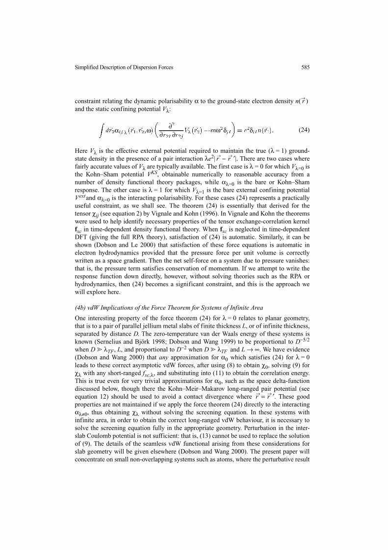
constraint relating the dynamic polarisability α to the ground-state electron density n(→r )

and the static confining potential Vλ:

(24)

Here Vλ is the effective external potential required to maintain the true (λ = 1) ground-state density in the presence of a pair interaction λe2| r

→ − r→ ′|. There are two cases where

fairly accurate values of Vλ are typically available. The first case is λ = 0 for which Vλ=0 isthe Kohn–Sham potential VKS, obtainable numerically to reasonable accuracy from anumber of density functional theory packages, while αλ=0 is the bare or Kohn–Shamresponse. The other case is λ = 1 for which Vλ=1 is the bare external confining potentialVext and αλ=0 is the interacting polarisability. For these cases (24) represents a practicallyuseful constraint, as we shall see. The theorem (24) is essentially that derived for thetensor χij (see equation 2) by Vignale and Kohn (1996). In Vignale and Kohn the theoremswere used to help identify necessary properties of the tensor exchange-correlation kernelfxc in time-dependent density functional theory. When fxc is neglected in time-dependentDFT (giving the full RPA theory), satisfaction of (24) is automatic. Similarly, it can beshown (Dobson and Le 2000) that satisfaction of these force equations is automatic inelectron hydrodynamics provided that the pressure force per unit volume is correctlywritten as a space gradient. Then the net self-force on a system due to pressure vanishes:that is, the pressure term satisfies conservation of momentum. If we attempt to write theresponse function down directly, however, without solving theories such as the RPA orhydrodynamics, then (24) becomes a significant constraint, and this is the approach wewill explore here.

(4b) vdW Implications of the Force Theorem for Systems of Infinite Area

One interesting property of the force theorem (24) for λ = 0 relates to planar geometry,that is to a pair of parallel jellium metal slabs of finite thickness L, or of infinite thickness,separated by distance D. The zero-temperature van der Waals energy of these systems isknown (Sernelius and Björk 1998; Dobson and Wang 1999) to be proportional to D−5/2

when D λTF, L, and proportional to D−2 when D λTF and L → ∞. We have evidence(Dobson and Wang 2000) that any approximation for α0 which satisfies (24) for λ = 0leads to these correct asymptotic vdW forces, after using (8) to obtain χ0, solving (9) forχλ with any short-ranged fxc,λ, and substituting into (11) to obtain the correlation energy.This is true even for very trivial approximations for α0, such as the space delta-functiondiscussed below, though there the Kohn–Meir–Makarov long-ranged pair potential (seeequation 12) should be used to avoid a contact divergence where r

→ = r→ ′. These good

properties are not maintained if we apply the force theorem (24) directly to the interactingαλ≠0, thus obtaining χλ without solving the screening equation. In these systems withinfinite area, in order to obtain the correct long-ranged vdW behaviour, it is necessary tosolve the screening equation fully in the appropriate geometry. Perturbation in the inter-slab Coulomb potential is not sufficient: that is, (13) cannot be used to replace the solutionof (9). The details of the seamless vdW functional arising from these considerations forslab geometry will be given elsewhere (Dobson and Wang 2000). The present paper willconcentrate on small non-overlapping systems such as atoms, where the perturbative result

α λ ω ω δ δλ∂

∂ ∂


(13) reduces the prediction of vdW forces to computation of the dynamic response of eachatom separately: see equations (14)–(16).

(4c) Local Approximation for αλ with Force-theorem Constraint

The principal result of the present paper is that the sum rule (24) is sufficient to determinethe response completely, if we assume, as in the asymptotic theories outlined in Section 3babove, that the polarisability is local in space, so that

(25)

Putting (25) into the constraint (24) we find

(26)

where

(27)

Note that there was no need to appeal to properties of the homogeneous electron gas: theassumption (25) of spatial locality, plus the exact force sum rule (24), are sufficient todetermine completely.

Defining Vij,λ( r→

) = ∂2Vλ/∂ri∂rj (a symmetric curvature tensor or Hooke’s law force-constant tensor at the point r

→), we can diagonalise Vij,λ at each space point r

→:

where m is the electron mass. The eigenvalues Λ(n)( r→

) = ω(n)2( r→

) can be thought of asthe squares of harmonic frequencies ω(n) matched to the local curvature of the potential,but note that λ(n) may be negative. The matrix B can then be inverted in general to give

(28)

Here ζ→

(n) and ω(n) both depend on the coupling strength λ, but for notational simplicitythis dependence has not been shown explicitly in (28). Equation (28) can be used to obtainthe dipolar polarisability as in equations (14)–(16). The spherical case is studied below.

(4d) Polarisability αλ of Spherical System with Local Force-theorem Ansatz

For spherical (or sphericalised) atoms the confining potential is a function of radius only[Vλ( r

→) Vλ(r)], and then (27) becomes

α ω δλ λ

λ

∂∂ ∂

ω δλ

λ ξ ξ

α λ ω δ ξ ξω ω

∂ λ ω δ∂ ∂

δλ λ ω δ


This can be written in the usual polar coordinates (r, θ, φ) as

where r∧

, θ∧

, φ∧ are the usual unit vectors and we have noted that r∧

r∧ + θ

∧θ∧

+ φ∧ φ∧ = I.Thus the tensor B( r

→) is diagonal in the orthonormal basis (r

∧, θ

∧, φ∧ ) ( ξ

→(1), ξ→(2), ξ

→(3))and so can be inverted immediately (see equation 28). Then (25) and (26) give for aspherical system

(29)

where

(4e) Dipole Polarisability of Spherical System with Local Force-theorem Ansatz for αλ

For a spherical system (29) and (15) give a dipole polarisability

where

Using

we obtain the dipole polarisability of a spherical system as

(30)

For ω = 0 this becomes

(31)

ω λ

ω λ λ

ω λ ω λ φφθθ

αλ ω δλ ω λ ω

φφθθ

λ λ

λ ωλ ω

Ω

Ωωλ

Ω φ θπ

Ω π Ωπ

λ ωπ ∞

λ ω λ ω

λ ωπ ∞

λ λ


while at high frequency Vλ″ and r−1Vλ′ are negligible beside mω2, so that

(32)

This is the response of N free electrons, as required by a version of the f-sum rule.

(4f) Test on Hooke’s Atom (Parabolic Quantum Dot)

Hooke’s atom is a simple model of N electrons confined by an isotropic harmonic externalpotential, Vext( r

→) = mω2

0 r2, and interacting amongst themselves via the usual Coulombpotential. For this system the harmonic potential theorem (HPT) (extended generalisedKohn theorem, Dobson 1994b) shows that, under the action of an oscillating spatiallyuniform electric field E

→0 cos(ωt), the ground-state density n( r

→) moves rigidly with

simple harmonic motion, yielding a density n( r→ − R

→(t)), where R

→(t) = −eE

→0 m−

[ω2 − ω 20 ]−1cos(ωt). This gives a dipole moment

The dynamic interacting dipole polarisability of Hooke’s atom is thus exactly

We now show that our constrained local approximation (30) for λ = 1 reproduces thisexact result. For this case, Vλ=1(r) = Vext(r) = mω 2

0 r2, so that (30) becomes

It is also readily shown that the present theory gives the exact dipole polarisability ofanisotropic Hooke’s atoms at all frequencies.

(4g) Dipole Polarisablity of Regular Atoms

We have also applied our formula (30) to regular atoms. In finite charge-neutral systemssuch as these it is important to obtain the density and Kohn–Sham potential from a self-interaction-corrected (SIC) formalism. This is because, in the local density approximation(LDA) (Kohn and Sham 1965) and related formalisms, the unphysical repulsion of theelectron in each orbital from its own orbital charge density causes VKS (r

→) to lack the

correct −e2/r behaviour at large distance r from the nucleus (Perdew and Zunger 1981).The outer orbitals are strongly affected, and hence so is the density in the outer region

λ ω ∞π

ω

∞

ω

∞π

ω

∞

ω

ω ωω

Hooke ω ωω

QED

λ ωπ ∞

ω ω ω ω

∞ π ω ω

∞π ω ω ω ω


where most of the polarisability is generated. We used an atomic code written by H. B.Shore and J. H. Rose, implementing the Perdew–Zunger (1981) LDA–SIC scheme. Inplace of the unknown exact (and therefore automatically SIC) KS potential, we used adensity-weighted combination of SIC potentials from the various orbitals i:

(33)

Very similar results were also obtained using, for all orbitals, the Vi from the last occupiedSIC orbital.

So far the static dipole polarisability has been investigated in detail using (31). Table 1shows atomic dipole polarisabilities in units of 10−24 cm3 (Gaussian cgs units). Note that10−24 cm3 6.7487 Hartree units.

For the elements from H to Na, the static polarisability data from Table 1 is also plottedin Figs 1 and 2. Fig. 1 shows the weakly polarisable elements (those with a full or nearly

λ

Table 1. Static dipolar polarisabilities of atomsUnits are 10-24 cm3 (Gaussian cgs). Column 2: accurate values of the interacting polarisabilityfrom Chemical Rubber Company Tables (CRC 1995). Column 3: predicted interacting polaris-abilities from the λ = 1 version of equation (31). Column 4: predicted bare polarisabilities from theλ = 0 version of equation (31), using orthogonalised SIC density and orbital-averaged potentialfrom (33) (results in brackets used the SIC potential Vj of the last occupied orbital). Column 5:predicted interacting polarisabilities from existing cutoff local theory, equations (21)

and (22) (results in brackets used spin-polarised cutoff, equation 23)

Atom Aλ=1exact(ω = 0)

CRC (1995)Aλ=1

force thm(ω = 0Eq. (31)

Aλ=1force thm(ω = 0)

Eq. (31)Vλ=0 from (33)(Brackets: Vi max)

Aλ=1cutoff(ω = 0)

Eq. (19),cutoff as in (22)(Brackets: cutoff from 23)

H 0.666793 0.556 0.556 [0.555] 1.55 (0.714)

He 0.204956 0.1406 0.2505 [0.250] 0.28638 (0.10467)

Li 24.3±2% 4.614 6.8927 [7.05] 27.67 (18.245)

Be 5.6±2% 1.1283 3.7747 [3.78] 9.093

B 3.03±2% 0.6873 2.4785 [2.47] 5.022

C 1.76±2% 0.41789 1.6310 [1.79] 3.089

N 1.1±2% 0.27138 1.1394 [1.309] 1.755

O 0.802±2% 0.1982 0.9248 [0.953] 1.136

F 0.557 0.1446 0.72927 [0.751] 0.743

Ne 0.3956±0.1% 0.1082 0.5825 [0.586] 0.499

Na 24.08±0.4% 0.76156 7.8466 [8.004] 32.14 (9.324)

Mg 10.6±2% 0.6485 6.178 [6.240] 15.45

. . .

Kr 2.4844±0.05% 0.1832 2.9241 [2.973]

Rb 47.3±2% 0.54199 15.8443 [16.72]

Sr 27.6±8% 0.57171 14.985 [15.15]

. . .

U 24.9±6% 0.3504 18.1503


Fig. 2. Dipole polarisabilities as in Fig. 1, but including highly polarisable atoms. The congested part ofthis figure is shown more clearly in Fig. 1.

Fig. 1. Dipole polarisabilities of weakly polarisable atoms, in units of 10−24 cm3 (Gaussian cgs). Thehorizontal axis orders elements by their interacting dipole polarisability from experiment or accuratetheory (CRC 1995). The vertical axis shows approximate polarisabilities for various theories. Solid line:accurate results from CRC (1995). Solid triangles: bare or Kohn–Sham values from equation (31) withλ = 0. Open squares: interacting values from (31) with λ = 1. Crosses: existing cutoff theory (spinunpolarised) from equations (19) and (22). Open circle: existing cutoff theory (spin polarised) fromequations (19) and (23) (shown only for hydrogen since inclusion of spin polarisation does not appear toimprove the other monovalent cases).


full outer shell). Here the exact interacting polarisability (solid line) is quite well repro-duced by the bare polarisability from the local force-theorem formula (31) with λ = 0(solid triangles). For these systems, the new formula does somewhat better than theprevious local formula (21) with the cutoff (22) (crosses). [Without the cutoff the previoustheory (20) gives an infinite polarisability at zero frequency.] Since Coulomb screening ofperturbations is weak in these tightly-bound systems, it is not surprising that an approxi-mate theory for the bare response gives results close to the interacting response. It seemsat first paradoxical, however, that the dipole polarisability is seriously underestimated(open squares) by the local-force-theorem approximation (31), applied directly for theinteracting response αλ=1. Since the force theorem is exact, the local assumption (25)would therefore seem to be less accurate for the interacting response αλ=1 than for the bareresponse αλ=0, in these systems. While the screening of a given bare response does notgreatly affect the dipole moment αλdr

→dr

→′ in tightly bound systems, the extranonlocality introduced into α by screening evidently does make a large difference in theapplication of the force theorem (24), where αλ is integrated with a rapidly varyingfunction ∇

→∇→

Vλ . The notion that a local approximation is better for a bare than for aninteracting polarisability is certainly in line with the philosophy of Dobson (1994a),Dobson and Wang (1999) and Dobson et al. (1998).

Fig. 2 plots the approximation (31) and other approximations as for Fig. 1, but for arange of more highly polarisable atoms with only one or two electrons present in the outershell. For the divalent metals Be and Mg, our new approximation (31) for the bareresponse (solid triangles) gets only about two-thirds of the exact interacting result, slightlybetter than the older local theory given by (18) and (22) which overestimates by 50% ormore. Only for the alkali metals Na and Li does the new theory do worse than the old,giving only about one-third of the correct polarisability. In these cases there is a near-degeneracy between the outer s orbital and a dipole-allowed excited p orbital, resulting in avery large dipole polarisability because of a small energy denominator in equation (7).With such an orbital-specific mechanism in force, it is unsurprising that a crude localtheory does poorly.

Once more, it is evident in Fig. 2 that the local-force-theorem approximation based onthe interacting response gives a severely under-estimated polarisability (open squares).

(4h) Dipole Response of Atoms at Finite Frequency: vdW C6 Coefficient

We have already noted that the high-frequency response is correct in our new theory basedon the force theorem (see equation 32), and we found in the previous section that the zero-frequency response for atoms is typically comparable to or better than that from the olderlocal theory, except for alkali metal atoms. One might therefore imagine that the responsewould be a good approximation at all finite complex frequencies. This is too much to askof such a simple theory, however, because the exact response must have poles on the realfrequency axis corresponding to discrete atomic excitation frequencies which are notpresent in the approximate theory. This in itself is not a problem for calculation of the vdWinteraction, because one can use analyticity to write the asymptotic vdW interaction as anintegral of the dipolar polarisability over imaginary frequencies, ω = is. On the imaginaryfrequency axis the exact susceptibility α is a real, smooth function of s: it is guaranteed tolack singularities on the imaginary axis because causality ensures it is analytic in the upperhalf frequency plane. In this connection the approximation (30) has a serious problem,because V ″(r) is typically negative for atoms, so that α has poles on the imaginary


frequency axis [as well as poles on the real axis from the r−1V ′(r) term]. These poles on theimaginary axis correspond to a lack of causality which can be traced back to the localassumption made in equation (25), and its effect in the force sum rule (24). Because of thepoles just described, one cannot in practice perform a numerical integral over imaginaryfrequency to obtain the vdW C6 coefficient. Instead, one can integrate along (for example)a contour at 45° to the real frequency axis, where there are no poles. Our preliminaryresults for this process have been disappointing, with predicted C6 values only about halfof the true answer, even for atoms where the new theory gave a good estimate of the staticpolarisability. The details will be described elsewhere when complete.

5. Summary and Discussion

In the context of van der Waals interactions, we have proposed a new approach usingconstrained approximations for dynamic response functions of inhomogeneous many-electron systems. The exact constraint used was the force theorem (24) for the dynamicpolarisability α(r

→, r

→ ′, ω). We outlined several paths to simplified vdW energy calcu-lations via approximations for response functions, in which the constraint could be useful.First we have given a brief discussion of the application of the force theorem in ‘seamless’vdW theory, valid for vdW-interacting systems at all separations, where the new constraintautomatically imposes the correct asymptotic vdW behaviour for distant parallel jelliumslabs. Our main emphasis, however, was on the simplified perturbative calculation of vdWeffects for finite well-separated systems. For the case of atoms, the correct results are ofcourse known from existing, more computationally intensive methods, providing a test ofour theory.

The simplest existing approximate theory for such cases (Rapcewicz and Ashcroft1991; Dobson and Dinte 1997; Andersson et al. 1996) assumed a local form for α, basedon the long-wavelength response of a uniform electron gas (see equations 19 and 21). Ifapplied verbatim to small bound systems such as atoms, this approach gives very poorresults including a divergent static dipolar polarisability, and grossly over-estimated vdWattraction. With use of a semi-empirical cutoff (Rapcewicz and Ashcroft 1991; Anderssonet al. 1996, 1998) in the low-density regions, however, the existing approach was found togive reasonable vdW C6 coefficients for a range of systems, with some tendency to over-estimation.

The principal aim of the present work was to remove the need for semi-empiricalcutoffs, while maintaining the simplicity of a local theory. We found that, with the localassumption (25), the force theorem (24) was sufficient to determine the polarisabilityαλ(r

→, r

→ ′, ω) completely, without the need for cutoffs or even the use of the responseproperties of a uniform electron gas (see equation 28). For the first twelve elements H–Mg, the resulting function αλ was used to compute the dipolar polarisability Aλ (equations30 and 31), from which the van der Waals coefficient C6 can also be obtained via (16).Two versions of this theory were tested.

The first (λ = 0) version of the theory expresses αλ=0 directly in terms of the ground-state density and the static Kohn–Sham potential (see equation 15). This theory gavereasonable values for A(ω = 0), slightly better than the previous theory with cutoff, for theweakly polarisable atoms (see Fig. 1). For the alkali metals, however, the new theory givesonly about one-third of the correct polarisability (see Fig. 2). These metals owe their veryhigh polarisability to a near-degeneracy of s- and p-orbitals, an effect probably not system-atically reproducible in a simple, non-wavefunction approach.


In contrast, for λ = 1, the new theory severely underestimated the static dipole polar-isability of most atoms. Since the force theorem is exact, the nonlocality of the Coulombscreening effects in the interacting polarisability αλ=1 must be the culprit, invalidating thelocal approximation in the context of the force theorem. Fortunately, the interacting dipolepolarisability Aλ=1 is close to the KS polarisability Aλ=0 for most atoms. (For atoms withsubstantially full outer shells, the binding is tight and the polarisability and screening aresmall, while for the monovalent elements the most polarisable outer electron cannot screenitself (SIC effect). It is mainly for the divalent atoms that screening strongly affects theoverall dipolar polarisability. The same argument, implying minimal effects of screening,cannot be made in the context of the force theorem, where α is integrated with a stronglyvarying function ∇

→∇→

V ext (there the nonlocality introduced by the screening term canoverride its small size).

Thus, fortunately, our λ = 0, ω = 0 theory can be used for most atoms, at the level ofaccuracy of these very simple theories.

In order to predict van der Waals forces, it is necessary to know A(ω) for finite as wellas zero frequency ω (see equations 14 and 16). Here our simplest force-constrained theorydid not do so well, underestimating the vdW C6 coefficient in our initial tests, despite itsrelatively good low-frequency and high-frequency properties. The problem appears to berelated to a lack of causality arising from imaginary pinning eigenfrequencies ω(n)

(negative principal values of the curvature tensor ∇→

∇→

V KS ) in equation (28). We believethat a simple nonlocal theory might do better, by averaging over regions of negative andpositive curvature: in some sense the latter must predominate if the system is overallbound. In this context, it is noteworthy that the kinetic pressure of the electron gas hasbeen ignored, both in the relatively successful cutoff vdW theory (equations 19 and 22),and also in our new theory. The pressure leads to dispersion of the plasmon pole inequation (18), and to a corresponding space nonlocality in the polarisability tensorαλ(r

→, r

→ ′, ω). Information from the homogeneous electron gas, not used in the local α0form of the present theory, can be inserted into the formalism at this level. We are cur-rently investigating this.

Acknowledgments

We thank David Langreth, Andreas Savin and Hardy Gross for useful discussions, and JimRose and Herb Shore for the use of their LDA–SIC atomic code. This work was supportedin part by a grant from the Australian Research Council.

ReferencesAndersson, Y., Langreth, D. C., and Lundqvist, B. I. (1996). Phys. Rev. Lett. 76, 102.Andersson, Y., et al. (1998). In ‘Electronic Density Functional Theory: Recent Progress and New

Directions’ (Eds J. F. Dobson et al.), pp. 243–60 (Plenum: New York).CRC (1995). ‘CRC Handbook of Chemistry and Physics’, 76th edn (Chemical Rubber Company: Cleve-

land).Dobson, J. F. (1994a). In ‘Topics in Condensed Matter Physics’ (Ed. M. P. Das), pp. 121–42 (Nova: New

York).Dobson, J. F. (1994b). Phys. Rev. Lett. 73, 2244.Dobson, J. F., and Dinte, B. P. (1996). Phys. Rev. Lett. 76, 1780.Dobson, J. F., and Le, H. M. (2000). Theochem. 501–2, 327.Dobson, J. F., and Wang, J. (1999). Phys. Rev. Lett. 82, 2123.Dobson, J. F., and Wang, J. (2000). Phys. Rev. B, submitted.


Dobson, J. F., Dinte, B. P., and Wang, J. (1998). In ‘Electronic Density Functional Theory: Recent Progressand New Directions’ (Eds J. F. Dobson et al.), pp. 261–84 (Plenum: New York).

Gross, E. K. U., and Kohn, W. (1985). Phys. Rev. Lett. 55, 2850.Gunnarsson, O., and Lundqvist, B. I. (1976). Phys. Rev. B 13, 4274.Kohn, W., and Sham, L. J. (1965). Phys. Rev. 140, A1133.Kohn, W., Meir, Y., and Makarov, D. E. (1998). Phys. Rev. Lett. 80, 4153.Langreth, D. C., and Perdew, J. P. (1975). Solid State Commun. 17, 1425.Lein, M., Dobson, J. F., and Gross, E. K. U. (1999). J. Comput. Chem. 20, 12.Li, Y., Krieger, J. B., and Iafrate, J. G. (1993). Phys. Rev. A 47, 165.Patton, D. C., and Pederson, M. R. (1997). Phys. Rev. A 56, 2495.Perdew, J., and Zunger, A. (1981). Phys. Rev. B 23, 5048.Perdew, J. P., Burke, K., and Ernzerhof, M. (1996). Phys. Rev. Lett. 77, 3865.Pitarke, J. M., and Eguiluz, A. G. (1998). Phys. Rev. B 57, 6329.Rapcewicz, K., and Ashcroft, N. W. (1991). Phys. Rev. B 44, 4032.Sernelius, B. E., and Björk, P. B. (1998). Phys. Rev. B 57, 6592.Vignale, G., and Kohn, W. (1996). Phys. Rev. Lett. 77, 2037.Zaremba, E., and Kohn, W. (1976). Phys. Rev. B 13, 2270.Zhang, Y., Pan, W., and Yang, W. (1997). J. Chem. Phys. 107, 7921.

Appendix: Derivation of Force Theorem for α

Consider a fictitious system with reduced pair interaction Uλ = λe2/|r→ −r

→ ′| in an externalone-electron potential Vλ(r

→) . For λ = 1, we have the true Coulomb problem and Vλ=1 is

defined to be the true external potential Vext(r→

), giving the true ground-state densityn(r

→). For each λ < 1, Vλ(r

→) is defined so that the ground-state density with Uλ and Vλ is

still the true ground-state density n( r→

). For λ = 0 we have independent electrons, forwhich the external potential producing n( r

→) is VKS , by definition of the Kohn-Sham

(1965) potential VKS ( r→

). Thus, we have

(34)

This construction of Vλ is the standard one for implementation of the exact adiabaticconnection formula (11). The external electric field corresponding to the externalpotential Vλ is

(35)

Now view the fictitious system, in its ground state | ψλ , from a (non-rotating, non-relativistic) frame whose moving origin O ′ is at position

relative to the original stationary frame. In this frame the position coordinate is r→ ′ = r

→ −X→

(t) , so that r→

= r→ ′+ X

→(t) . The density function in the moving frame is

λ λ λ λ∀

λ λ∇

ω


(36)

The external field seen in the accelerated frame includes a fictitious or inertial component:

(37)

where linearisation in X→

is used in the last line.Thus, the accelerated observer sees a zeroth order confining external field E

→λ (r

→ ′)the same as the stationary observer, and a linearised additional external driving field

(38)

where linearisation in X→

was used to replace ∇→

by ∇→

′.Since the accelerated observer is simply viewing the rest-frame ground state, he sees a

rigid displacement of the ground state with velocity −d X→

/ dt = ωsin(ωt) X→

and hencefrom (36) an electric current density

(39)

to linear order in X→

. Therefore, from (4), by time-integrating (39),

(40)

Since r→

and r→′ differ only by the space-independent displacement X

→(t) , the electron–

electron interaction in the accelerated frame is Uλ′(r→1′ , r→2′) = λe2/|r→1 − r→2 | = λe2/|r→1′− r→2′ |, of the same form as in the rest frame. Indeed all effects of the acceleration,including the fictitous force in equation (37), are accounted for by the linearised externaldriving field (38).

The field δE→

′ (equation 38) and polarisation δ p→ ′ (equation 40) are seen in the

accelerated frame as small departures about an equilibrium described by n(r→ ′) ,Eλ(r→ ′ ) = −∇

→′Vλ(r→ ′) . They must therefore be related by the corresponding polarisabil-

ity αλ( r→

1, r→′2 , ω = is), the same function as for the rest frame. Thus, from the definition

(5),

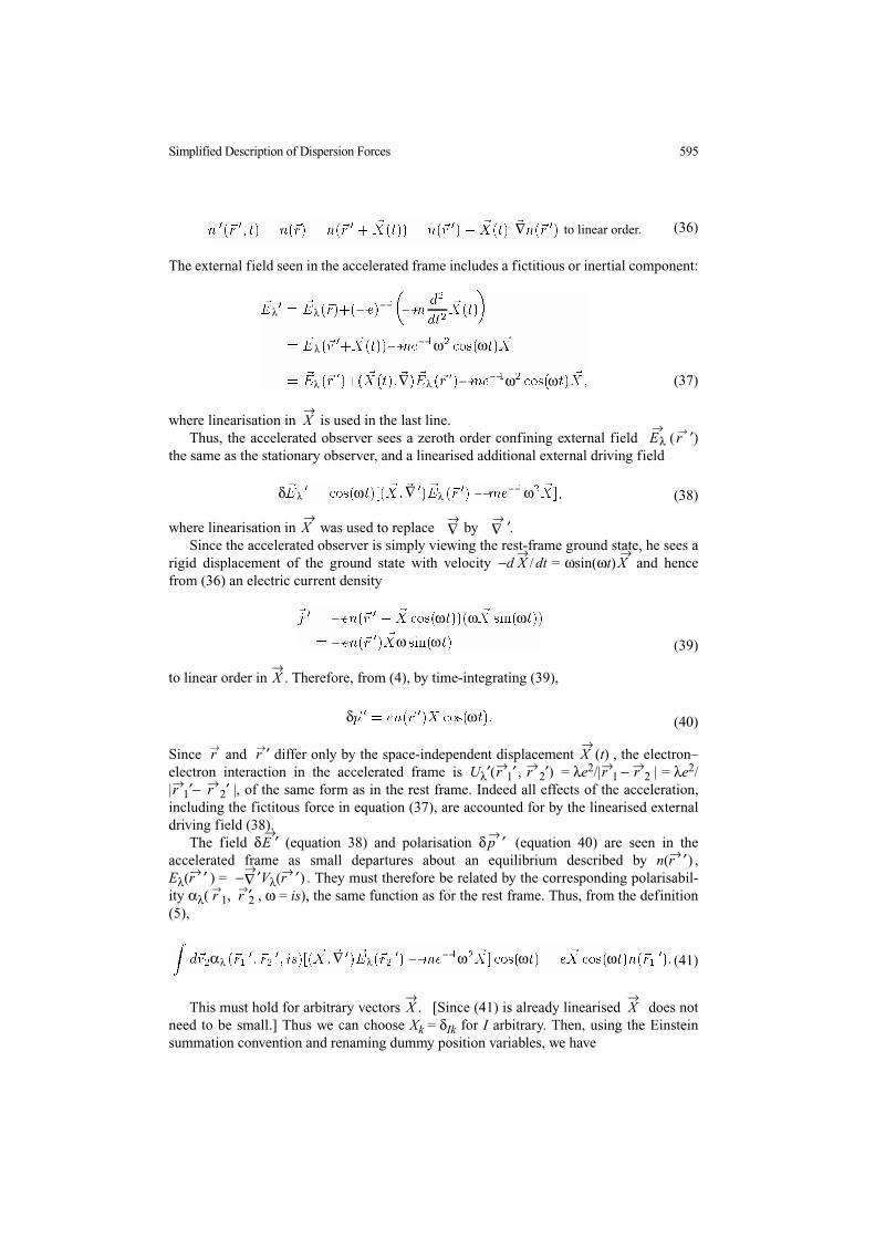
(41)

This must hold for arbitrary vectors X→

. [Since (41) is already linearised X→

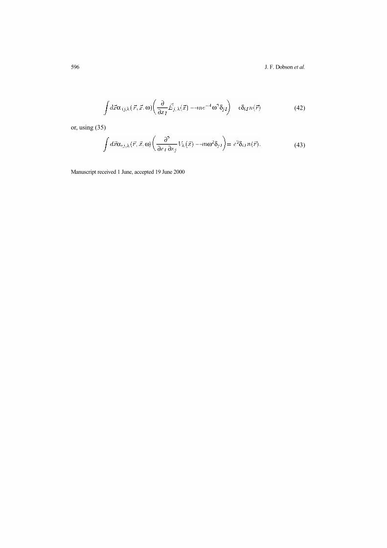
does notneed to be small.] Thus we can choose Xk = δIk for I arbitrary. Then, using the Einsteinsummation convention and renaming dummy position variables, we have

to linear order.∇

λ λ

λ ω ω

λ ∇ λ ω ω

δ λ ω ∇ λ ω

ω ω ωω ω

δ ω

αλ ∇ λ ω ω ω


(42)

or, using (35)

(43)

Manuscript received 1 June, accepted 19 June 2000

α λ ω ∂∂ λ ω δ δ

α λ ω ∂∂ ∂ λ ω δ δ

Australian Journal of Physics - CSIRO Publishing

Documents

Transcript of Australian Journal of Physics - CSIRO Publishing