GenCost 2020-21 - CSIRO
81
GenCost 2020-21 Consultation draft Paul Graham, Jenny Hayward, James Foster and Lisa Havas December 2020 Australia’s National Science Agency
-
Upload
khangminh22 -
Category
Documents
-
view
0 -
download
0
Transcript of GenCost 2020-21 - CSIRO

GenCost 2020-21 Consultation draft
Paul Graham, Jenny Hayward, James Foster and Lisa Havas December 2020
Australia’s NationalScience Agency

GenCost 2020-21 | i
Citation
Graham, P., Hayward, J., Foster J. and Havas, L.2020, GenCost 2020-21: Consultation draft, Australia.
Copyright
© Commonwealth Scientific and Industrial Research Organisation 2020. To the extent permitted by law, all rights are reserved and no part of this publication covered by copyright may be reproduced or copied in any form or by any means except with the written permission of CSIRO.
Important disclaimer
CSIRO advises that the information contained in this publication comprises general statements based on scientific research. The reader is advised and needs to be aware that such information may be incomplete or unable to be used in any specific situation. No reliance or actions must therefore be made on that information without seeking prior expert professional, scientific and technical advice. To the extent permitted by law, CSIRO (including its employees and consultants) excludes all liability to any person for any consequences, including but not limited to all losses, damages, costs, expenses and any other compensation, arising directly or indirectly from using this publication (in part or in whole) and any information or material contained in it.
CSIRO is committed to providing web accessible content wherever possible. If you are having difficulties with accessing this document please contact [email protected].

ii | CSIRO Australia’s National Science Agency
Contents
Forward vi
Executive summary ........................................................................................................................ vii
1 Introduction ........................................................................................................................ 9
1.1 Scope of the GenCost project and reporting......................................................... 9
1.2 CSIRO and AEMO roles .......................................................................................... 9
1.3 Incremental improvement and focus areas .......................................................... 9
2 Current technology costs .................................................................................................. 11
2.1 Current cost definition ........................................................................................ 11
2.2 Updates to current costs ..................................................................................... 11
2.3 Current generation technology capital costs ...................................................... 12
2.4 Current storage technology capital costs ............................................................ 13
3 Scenario narratives and data assumptions ....................................................................... 15
3.1 Scenario narratives .............................................................................................. 15
4 Projection results .............................................................................................................. 31
4.1 Global generation mix ......................................................................................... 31
4.2 Changes in capital cost projections ..................................................................... 32
4.3 Hydrogen electrolysers ........................................................................................ 48
5 Levelised cost of electricity analysis ................................................................................. 50
5.1 Overview of the new method .............................................................................. 50
5.2 LCOE estimates .................................................................................................... 52
Global and local learning model .......................................................................... 58
Data tables ........................................................................................................... 62
Shortened forms ........................................................................................................................... 74
References ............................................................................................................................. 76

GenCost 2020-21 | iii
Figures Figure 2-1 Comparison of current cost estimates with previous work ........................................ 12
Figure 2-2 Capital costs of storage technologies in $/kWh (total cost basis) ............................... 13
Figure 2-3 Capital costs of storage technologies in $/kW (total cost basis) ................................. 14
Figure 3-1 Projected EV sales share under the Central scenario .................................................. 21
Figure 3-2 Projected EV adoption curve (vehicle sales share) under the High VRE scenario ....... 22
Figure 3-3 Projected EV sales share under the Diverse technology scenario .............................. 22
Figure 3-4 Adoption curves for hydrogen technologies under the Central scenario ................... 23
Figure 3-5 Adoption curves for hydrogen technologies under the High VRE scenario ................ 24
Figure 3-6 Adoption curves for hydrogen technologies under the Diverse technology scenario 24
Figure 3-7 Projected carbon price trajectory under High VRE and Diverse technology scenarios, all regions ...................................................................................................................................... 26
Figure 3-8 Projected carbon price trajectory under the Central scenario by region ................... 27
Figure 4-1 Projected global electricity generation mix in 2030 and 2050 by scenario ................ 31
Figure 4-2 Projected capital costs for black coal supercritical by scenario compared to 2019-20 projections .................................................................................................................................... 33
Figure 4-3 Projected capital costs for black coal with CCS by scenario compared to 2019-20 projections .................................................................................................................................... 34
Figure 4-4 Projected capital costs for gas combined cycle by scenario compared to 2019-20 projections .................................................................................................................................... 35
Figure 4-5 Projected capital costs for gas with CCS by scenario compared to 2019-20 projections ....................................................................................................................................................... 36
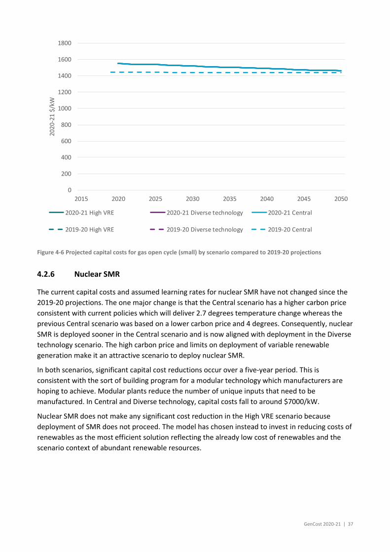
Figure 4-6 Projected capital costs for gas open cycle (small) by scenario compared to 2019-20 projections .................................................................................................................................... 37
Figure 4-7 Projected capital costs for nuclear SMR by scenario compared to 2019-20 projections ....................................................................................................................................................... 38
Figure 4-8 Projected capital costs for solar thermal with 8 hours storage by scenario compared to 2019-20 projections .................................................................................................................. 39
Figure 4-9 Projected capital costs for large scale solar PV by scenario compared to 2019-20 projections .................................................................................................................................... 40
Figure 4-10 Projected capital costs for rooftop solar PV by scenario compared to 2019-20 projections .................................................................................................................................... 41
Figure 4-11 Projected capital costs for onshore wind by scenario compared to 2019-20 projections .................................................................................................................................... 42

iv | CSIRO Australia’s National Science Agency
Figure 4-12 Projected capital costs for offshore wind by scenario compared to 2019-20 projections .................................................................................................................................... 43
Figure 4-13 Projected capital costs for batteries by scenario (battery pack only) ....................... 44
Figure 4-14 Projected capital costs for pumped hydro energy storage (12 hours) by scenario .. 45
Figure 4-15 Projected technology capital costs under the Central scenario compared to 2019-20 projections .................................................................................................................................... 46
Figure 4-16 Projected technology capital costs under the High VRE scenario compared to 2019-20 projections ............................................................................................................................... 47
Figure 4-17 Projected technology capital costs under the Diverse technology scenario compared to 2019-20 projections .................................................................................................................. 48
Figure 4-18 Projected technology capital costs for alkaline and PEM electrolysers by scenario . 49
Figure 5-1 Three types of electricity system models .................................................................... 52
Figure 5-2 Levelised costs of achieving 50%, 60%, 70%, 80% and 90% variable renewable energy shares in the NEM, NSW, VIC and QLD ......................................................................................... 54
Figure 5-3 Calculated LCOE by technology and category for 2020 ............................................... 56
Figure 5-4 Calculated LCOE by technology and category for 2030 ............................................... 56
Figure 5-5 Calculated LCOE by technology and category for 2040 ............................................... 57
Figure 5-6 Calculated LCOE by technology and category for 2050 ............................................... 57
Apx Figure A.1 Schematic of changes in the learning rate as a technology progresses through its development stages after commercialisation .............................................................................. 59
Apx Figure A.2 Schematic diagram of GALLM and DIETER modelling framework ....................... 60
Tables Table 3-1 Scenarios and their key drivers ..................................................................................... 17
Table 3-2: Assumed technology learning rates under the Central and High VRE scenarios ........ 18
Table 3-3 Hydrogen demand assumptions by scenario ................................................................ 25
Table 3-4 Renewable resource limits on generation in TWh in the year 2050. NA means the resource is greater than projected electricity demand. ............................................................... 27
Table 3-5 Assumed gas prices in $A/GJ ........................................................................................ 28
Table 3-6 Assumed black coal prices in $A/GJ .............................................................................. 29
Table 3-7 Assumed global oil price in $A/bbl ............................................................................... 30
Apx Table B.1 Current and projected generation technology capital costs under the Central scenario ......................................................................................................................................... 63
GenCost 2020-21 | v
Apx Table B.2 Current and projected generation technology capital costs under the High VRE scenario ......................................................................................................................................... 64
Apx Table B.3 Current and projected generation technology capital costs under the Diverse technology scenario ...................................................................................................................... 65
Apx Table B.4 One and two hour battery cost data by storage duration, component and total costs .............................................................................................................................................. 66
Apx Table B.5 Four and eight hour battery cost data by storage duration, component and total costs .............................................................................................................................................. 67
Apx Table B.6 Pumped hydro storage cost data by duration, all scenarios, total cost basis ....... 68
Apx Table B.7 Storage cost data by source, total cost basis ......................................................... 69
Apx Table B.8 Data assumptions for LCOE calculations ................................................................ 70
Apx Table B.9 Electricity generation technology LCOE projections data, 2020-21 $/MWh ......... 72
Apx Table B.10 Hydrogen electrolyser cost projections by scenario and technology, 2020-21 $/kW .............................................................................................................................................. 73

vi | CSIRO Australia’s National Science Agency
Forward
This consultation report is provided with the purpose of seeking feedback. Stakeholders are requested to provide feedback on the GenCost scenarios, approach and results via formal submissions to AEMO's consultation on the Draft 2021 Inputs, Assumptions and Scenarios (IASR) Report. Submissions close 1 February. Further details are available at https://aemo.com.au/consultations/current-and-closed-consultations/2021-planning-and-forecasting-consultation-on-inputs-scenarios-and-assumptions.
The consultation report has been improved by input from a stakeholder webinar in September 2020, comments provided in response to publication of draft scenario assumptions in October 2020 and the GenCost working group. Feedback received during the consultation phase will assist in finalising the report in early 2021.

GenCost 2020-21 | vii
Executive summary
GenCost is a collaboration between CSIRO and AEMO to deliver an annual process of updating electricity generation and storage costs with a strong emphasis on stakeholder engagement. This is the third update following the inaugural report in 2018 and a second report in 2019-20. The 2020-21 report incorporates updated current capital cost estimates commissioned by AEMO and delivered by Aurecon. Based on these updated current capital costs, projections of future changes in costs consistent with updated global electricity scenarios are also provided. Levelised costs of electricity (LCOEs) are also included and provide a simple summary of the relative competitiveness of generation technologies.
Capital cost projections
The projection methodology is grounded in a global electricity generation and capital cost projection model recognising that cost reductions experienced in Australia are largely a function of global technology deployment. Three scenarios are explored:
Central: Current stated global climate policy ambitions only, with the most likely assumptions for all other factors such as renewable resource constraints
High VRE: A world that is driving towards net zero emission by 2050 and where technical, social and political support for variable renewable generation is high
Diverse technology: A world where most developed countries are striving for net zero emissions by 2050 but others are lagging such that global net zero emissions is reached by 2070. Furthermore, there is lack of social, technical and political support for variable renewable generation and subsequently a greater role for other technologies.
Both the Central and High VRE scenarios reach high global renewable generation shares of 60% and 78% respectively by 2050. Wind and solar PV achieve the highest shares supported by battery and pumped hydro energy storage. Wind and solar PV are currently the lowest cost sources of low emission electricity generation for regions with good quality resources and this is projected to continue to be the case throughout the projection period to 2050
When access to wind and solar PV is assumed to be constrained in the Diverse technology scenario, generation from gas with carbon capture and storage fills the gap and is also used more commonly in hydrogen production. Nuclear small modular reactors could also play a role in the Diverse technology scenario so long as investors are willing to drive down costs through multiple deployments in the late 2020s and early 2030s.
The technology cost projections included in this report have been extended to include hydrogen electrolysers reflecting strong interest in this technology that, combined with low cost renewable generation could potentially underpin a low emission hydrogen fuel industry for export or Australian domestic consumption. The results indicate that substantial cost reductions are expected over the next few decades, with many demonstration projects underway worldwide.

viii | CSIRO Australia’s National Science Agency
Levelised cost of electricity
There have been concerns for many years that it is difficult to quantify the additional costs associated with variable renewable generation. Traditional approaches to calculating the levelised cost of electricity fail to include these additional costs, underestimating the full costs to the electricity system. The GenCost team has been seeking to address this issue since the first report in 2018 where we outlined this problem and reviewed a number of alternative solutions.
To calculate the additional costs CSIRO constructed an electricity system model that can calculate the required additional investment considering any existing resources in the system. The key additional investments required are in:
New transmission to access Renewable Energy Zones
Additional transmission to strengthen the grid so that dispersed renewable generation can reach key demand centres and expanded state interconnection so that connecting regions can provide more support for one another when renewable generation is low in one or more regions
Battery and pumped hydro storage to meet demand during low renewable generation periods.
The required amount of additional investment depends on the amount or share of variable renewable energy (VRE) generated. We calculated the additional costs of variable renewable generation for VRE shares from 50% to 90%1 for the National Electricity Market. We found that the additional costs to support a combination of solar PV and wind generation in 2030 is estimated at between $0 to $29/MWh depending on the VRE share and region of the NEM. When added to variable renewable generation costs and compared to other technology options, these new estimates indicate that wind and solar PV are the least cost generation technologies for the electricity system for any expected level of deployment.
ES Figure 0-1 Calculated LCOE by technology and category for 2030
1 90% is about as high as variable renewable deployment is likely to need to go as increasing it further would result in the undesirable outcome of shutting down existing non-variable renewable generation from biomass and hydroelectric sources.
0
50
100
150
200
250
300
350
400
Gas t
urbi
ne sm
all
Gas t
urbi
ne la
rge
Gas r
ecip
roca
ting
Blac
k coa
l
Brow
n co
al
Gas
Blac
k coa
l
Brow
n co
al
Gas
Blac
k coa
l
Brow
n co
al
Gas
Blac
k coa
l with
CCS
Brow
n co
al w
ith C
CS
Gas w
ith C
CS
Solar
ther
mal
8hr
s
Nucle
ar (S
MR)
Biom
ass (
small
scale
)
Win
d
Solar
PV
50%
VRE
shar
e
60%
VRE
shar
e
70%
VRE
shar
e
80%
VRE
shar
e
90%
VRE
shar
e
Carbon price No carbon priceor risk premium
No carbon price,5% risk premium
Carbon price Carbon price Standalone Wind & solar PV combined
Peaking 20% load Flexible 40-80% load, high emission Flexible 40-80% load, low emission Variable Variable with storage andnew transmission
2020
-21
A$/M
Wh

GenCost 2020-21 | 9
1 Introduction
Current and projected electricity generation and storage technology costs are a necessary and highly impactful input into electricity market modelling studies. Modelling studies are conducted by the Australian Energy Market Operator (AEMO) for planning and forecasting purposes. They are also widely used by electricity market actors to support the case for investment in new projects. Governments and regulators require modelling studies to assess alternative policies and regulations. There are substantial coordination benefits if all parties are using similar cost data sets for these activities or at least have a common reference point for differences.
1.1 Scope of the GenCost project and reporting
The GenCost project is a joint initiative of the CSIRO and AEMO to provide an annual process for updating electricity generation and storage cost data for Australia. The project is committed to a high degree of stakeholder engagement as a means of supporting the quality and relevancy of outputs.
The project is flexible about including new technologies of interest or, in some cases, not updating information about some technologies where there is no reason to expect any change, or if their applicability is limited. GenCost does not seek to describe the set of electricity generation and storage technologies included in detail.
1.2 CSIRO and AEMO roles
AEMO and the CSIRO jointly fund the GenCost project by combining their own in-kind resources. AEMO commissioned Aurecon to provide an update of current electricity generation and storage cost and performance characteristics (Aurecon, 2020). This update was initially shared with a wide range of stakeholders during a webinar in September 2020.
Project management, workshops, capital cost projections (presented in Section 4) and this final report are primarily the responsibility of the CSIRO.
1.3 Incremental improvement and focus areas
There are many assumptions, scope and methodological considerations underlying electricity generation and storage technology cost data. In any given year, we are readily able to change assumptions in response to stakeholder input. However, the scope and methods may take more time to change, and input of this nature may only be addressed incrementally over several years, depending on the priority.
In this report, we have improved our approach to calculating Levelised Costs of Electricity (LCOE) for renewables by employing a new modelling approach which is able to calculate additional costs to the system associated with variable renewable generation.

10 | CSIRO Australia’s National Science Agency
The report provides an overview of updates to current costs in Section 2. Further details on the Aurecon (2020) updates can be found in their report. The global scenarios narratives and data assumptions for the projection modelling are outlined in Section 3. Capital cost projection results are reported in Section 4 and LCOE results in Section 5. CSIRO’s cost projection methodology is discussed in Appendix A. Appendix B provides data tables for those projections which can also be downloaded from CSIRO’s data access portal.

GenCost 2020-21 | 11
2 Current technology costs
2.1 Current cost definition
Our preferred definition of current costs are the costs that have been demonstrated to have been incurred for projects completed in the current financial year (or within a reasonable period before). We do not wish to include in our definition of current costs, costs that represent quotes for delivery of projects in future financial years or project announcements.
While all data is useful in its own context, our preference reflects the objective that the data must be suitable for input into electricity models. The way most electricity models work is that investment costs are incurred either before (depending on construction time assumptions) or in the same year as a project is available to be counted as a new addition to installed capacity2. Hence, current costs and costs in any given year must reflect the costs of projects completed in that year. Quotes received now for projects to be completed in future years are only relevant for future years.
For technologies that are not frequently being constructed, the preference is to look overseas at the most recent projects constructed. This introduces several issues in terms of different construction standards and engineering labour costs which have been addressed by Aurecon (2020).
2.2 Updates to current costs
AEMO commissioned Aurecon (2020) to provide an update of current cost and performance data for existing and selected new electricity generation and storage technologies. This data is used in this report as the starting point for projections of capital costs to 2050 and for calculations of the levelised cost of electricity.
Compared to 2019-20, Aurecon has reviewed coal generation and included two gas open cycle unit sizes. CSIRO has updated costs for technologies which are more rarely deployed such as tidal/current and wave energy. Nuclear small modular reactor (SMR) costs have not been updated. Feedback from the 2019-20 report accepted that historical costs for completed SMR projects are high, that first of a kind plant in Australia would be high cost, but that future costs have the potential to be lower if there is significant global investment and the potential for modular construction is included (these future considerations are not part of our definition of current costs but are reflected in the projections). These views have not changed and there have been no major developments worldwide in SMR. Aurecon (2020) has included hydrogen electrolysers for the first time and these are separately reported.
2 This is not strictly true of all models but is most true of long-term investment models. In other models, investments costs are converted to an annuity (adjusted for different economic lifetimes) or additional capital costs may be added later in a project timeline for replacement of key components.

12 | CSIRO Australia’s National Science Agency
Pumped hydro has also not been updated by Aurecon (2020), but we have revised this data to be consistent with AEMO’s ISP 2020 which received further input from stakeholders on this technology.
2.3 Current generation technology capital costs
Figure 2-1 provides a comparison of current (2020-21) cost estimates (drawing primarily on the Aurecon (2020) update) for electricity generation technologies with the four most recent previous reports: GenCost 2012-20, GenCost 2018, Hayward and Graham (2017) (also CSIRO) and CO2CRC (2015) which we refer to as APGT (short for Australian Power Generation Technology report). All costs are expressed in real 2020-21 Australian dollars and represent overnight costs since it would not be possible to build and financially close projects before July 2021.
CSIRO’s estimate for 2020-21 rooftop solar PV cost is included in the “Aurecon/CSIRO” data as that technology was not part of Aurecon (2020). Rooftop solar PV costs are before subsidies from the Small-scale Renewable Energy Scheme. All data has been adjusted for inflation.
Figure 2-1 Comparison of current cost estimates with previous work
Coal generation capital costs have been revised upwards after not being significantly updated since the 2018 GHD analysis. The lack of Australian construction means there will always be a range of interpretations when converting overseas data to Australia. Solar thermal costs have increased on 2019-20 estimates reflecting inclusion of a first of a kind cost premium. Gas, wind and solar PV data have been relatively stable reflecting better data availability for Australian projects.
0
2000
4000
6000
8000
10000
12000
14000
16000
18000
2020
-21
$/kW
APGT 2015 CSIRO 2017 GHD/CSIRO 2018 Aurecon/CSIRO 2019-20 Aurecon/CSIRO 2020-21

GenCost 2020-21 | 13
2.4 Current storage technology capital costs
Updated and previous capital costs are provided on a total cost basis for various durations of battery and pumped hydro energy storage (PHES) in $/kW and $/kWh. Total cost basis means that the costs are calculated by taking the total project costs divided by the capacity in kW or KWh3. As the storage duration of a project increases then more batteries or larger reservoirs need to be included in the project, but the power components of the storage technology remain constant. As a result, $/kWh costs tend to fall with increasing storage duration (Figure 2-2). The downward trend flattens somewhat with batteries since its power component, mostly inverters, is relatively small compared to the hydro turbine on PHES.
Conversely, the costs in $/kW increase as storage duration increase because additional storage duration adds costs without adding any power rating to the project (Figure 2-3). These relationships are the reasons why batteries tend to be more competitive in low storage duration applications, while PHES is more competitive in high duration applications.
Figure 2-2 Capital costs of storage technologies in $/kWh (total cost basis)
Battery current costs have declined in Aurecon (2020) compared to their previous work. These are based on projects deployed. In contrast we have increased PHES costs by aligning with AEMO ISP July 2020 estimates. Feedback received during the ISP consultation indicated that PHES was under-estimated in previous assumptions. A new higher data point was included in the July 2020 ISP
3 Component costs basis is when the power and storage components are separately costed and must be added together to calculate the total project cost.
0
200
400
600
800
1000
1200
Battery(1hr)
Battery(2hrs)
Battery(4hrs)
PHES (6hrs) Battery(8hrs)
PHES(12hrs)
PHES(24hrs)
PHES(48hrs)
PHES(48hrs)
Tasmania
2020
-21
$/kW
h
Aurecon 2019 Aurecon 2020 Entura 2018 (higher 2 projects) AEMO ISP July 2020

14 | CSIRO Australia’s National Science Agency
inputs and assumptions workbook based on submissions and discussion with proponents and reputable consultants with experience in PHES deployments. Some escalation in costs is consistent with major infrastructure projects where cost increases occur after initial estimates. However, we have also added a separate category for Tasmania PHES with 48hrs duration. This area of Australia has had the most detailed analysis undertaken of its PHES costs and consequently warrants greater certainty that it can achieve project cost estimates without the same level of escalation.
Figure 2-3 Capital costs of storage technologies in $/kW (total cost basis)
0
1000
2000
3000
4000
5000
6000
Battery(1hr)
Battery(2hrs)
Battery(4hrs)
PHES (6hrs) Battery(8hrs)
PHES(12hrs)
PHES(24hrs)
PHES(48hrs)
PHES(48hrs)
Tasmania
2020
-21
$/kW
Aurecon 2019 Aurecon 2020 Entura 2018 (higher 2 projects) AEMO ISP July 2020

GenCost 2020-21 | 15
3 Scenario narratives and data assumptions
3.1 Scenario narratives
The global climate policy ambitions for the Central, High VRE and Diverse technology scenarios have been adopted from the International Energy Agency’s 2020 World Energy Outlook (IEA WEO 2020) scenarios matching to the Stated Policies scenario, Net Zero Emission by 2050 and Sustainable Development Scenario respectively. Other elements, such as the degree of vehicle electrification and hydrogen production, are also consistent with IEA WEO 2020. However, we also include other topics such as renewable resource constraints and the social and political acceptance and technical performance of renewables.
3.1.1 Central
The Central scenario applies a 2.7 degrees consistent climate policy (using a carbon price4) and includes current renewable energy policies with no extension beyond current targets5. This implies that current 2030 Paris Nationally Determined Commitments are met but that the planned ramping up of ambition to prevent a greater than 2 degrees increase in temperature does not occur. There are moderate constraints applied with respect to global renewable energy resources (based on currently available information). Technical approaches for managing balancing of variable renewable electricity are based on current technology. Demand growth is moderate with moderate electrification of transport.
3.1.2 High VRE
Under the High VRE scenario there is a strong climate policy consistent with maintaining temperature increases of 1.5 degrees and achieving net zero emissions by 2050 worldwide. Reflecting the low emission intensity of predominantly renewable electricity supply there is an emphasis on energy efficiency and high electrification across sectors such as transport, hydrogen-based industries and buildings leading to high electricity demand. Renewable energy resources are less constrained (both physically and socially) and balancing variable renewable electricity is less technically challenging.
4 The use of carbon prices does not mean that we expect this to be the favoured global policy tool. However, it is more efficient to use carbon prices in the modelling than to anticipate and implement all the potential future policy approaches. However, we have also included renewable energy targets because they are the exception to this rule.
5 To be consistent with the IEA World Energy Outlook 2020, this does not include recent announcements or changes of government. For example, the WEO 2020 includes Chian’s 2060 net zero emissions pledge in its sustainable development scenario which we use for Diverse technology but does not include recent announcements by Japan and South Korea, nor change of leadership in the United States. See Annex B of WEO 2020.

16 | CSIRO Australia’s National Science Agency
3.1.3 Diverse technology
The Diverse technology scenario assumes that physical and social constraints mean that access to variable renewable energy resources is more limited in most regions of the world. Governments subsequently limit their renewable targets below the threshold required for major deployment of balancing solutions. Consequently, there is a greater reliance on non-renewable technologies and a carbon price consistent with a 1.65 degrees climate policy ambition provides the investment signal necessary to deploy these technologies. Developed countries are still largely aiming for net zero emissions by 2050 but other countries are lagging such that worldwide net zero emissions are no achieved until 2070. Hydrogen trade (based mainly on gas with CCS and alkaline electrolysis) is relatively high allowing some regions with energy or CO2 storage resource limitations to access a low emission imported fuel.
The GenCost scenarios are described in general in Table 3-1 and expanded on in the sub-sections below. The scenario drivers are based on the themes identified by stakeholders at a workshop in August 2019, together with insights from the modelling team on what would most likely deliver a broad range of technology cost outcomes.
We acknowledge that there are potential wild card events that are not included in the scenarios such as completely new technologies and inter-regional high voltage interconnection. However, we chose to exclude wild cards. We also considered the possibility of aligning scenarios with other globally recognised scenarios. However, we found that drivers for other scenarios were not well targeted at producing changes in technology outcomes. In particular, experience has shown that climate change policy drivers alone do not result in major differences in technology adoption.

GenCost 2020-21 | 17
Table 3-1 Scenarios and their key drivers
Key drivers High VRE Diverse technology Central
IEA WEO 2020 scenario alignment
Net zero emission by 2050
Sustainable development scenario
Stated policies scenario
CO2 pricing / climate policy
Consistent with 1.5 degrees world, not requiring negative abatement technologies
Consistent with 1.65 degrees world (or 1.5 if negative abatement technologies deployed by 2070)
Consistent with 2.7 degrees world
Renewable energy targets and forced builds / accelerated retirement
High (reflecting confidence in VRE)
RE policies go to no more than 40%
Current RE policies
Demand / Electrification
High Medium Medium
Learning rates1 Higher for longer in solar and batteries
Normal maturity path Higher for longer in solar and batteries
Renewable resource & other renewable constraints
Less constrained More constrained than existing assumptions
Existing constraint assumptions2
Constraints around stability and reliability of variable renewables
New low-cost solutions
Conventional solutions but less demand for them
Conventional solutions
Decentralisation Less constrained rooftop solar photovoltaics (PV)
More constrained rooftop solar PV constraints2
Existing rooftop solar PV constraints2
1 The learning rate is the potential change in costs for each doubling of cumulative deployment, not the rate of change in costs over time. In a normal maturity path, learning rates fall over time as per Apx Figure A.1 2 Existing large-scale and rooftop solar PV renewable generation constraints are as shown in Table 3-4
3.1.4 Technologies and learning rates
As we explain further in Appendix A, we use two global and local learning models (GALLM). One is of the electricity sector (GALLME) and the other of the transport sector (GALLMT). GALLME projects the future cost and installed capacity of 31 different electricity generation and energy storage technologies. Where appropriate, these have been split into their components of which there are 48. Components have been shared between technologies; for example, there are two

18 | CSIRO Australia’s National Science Agency
carbon capture and storage (CCS) components – CCS technology and CCS construction – which are shared among all CCS plant technologies. The technologies are listed in Table 3-2 showing the relationship between generation technologies and their components and the assumed learning rates under the central scenario (learning is on a global (G) basis, local (L) to the region, or no learning (-) is associated).
The potential for local learning means that technology costs are different in different regions in the same time period. This has been of particular note for technology costs in China which can be substantially lower than other regions. GALLME will use current costs from Aurecon to calibrate 2020 Australian costs in GALLME. For technologies not commonly deployed in Australia these costs can be higher than other regions. However, the inclusion of local learning assumptions in GALLME means that they can quickly catch up to other regions if deployment occurs. However, they will not always fall to levels seen in China due to differences in production standards for some technologies. That is, to meet Australian standards, the technology product from China would increase in costs and align more with other regions. Regional labour construction and engineering costs also remain a source of differentiation.
Table 3-2: Assumed technology learning rates under the Central and High VRE scenarios
Technology Component LR 1 (%) LR 2 (%) References
Coal, pf - - -
Coal, IGCC G - 2 (International Energy Agency, 2008; Neij, 2008)
Coal/Gas/Biomass with CCS
G 10 5 (EPRI Palo Alto CA & Commonwealth of Australia, 2010; Rubin et al., 2007)
L 20 10 As above + (Grübler et al., 1999; Hayward & Graham, 2013; Schrattenholzer & McDonald, 2001)
Gas peaking plant - - -
Gas combined cycle - - -
Nuclear G - 3 (International Energy Agency, 2008)
SMR G 20 10 (Grübler et al., 1999; Hayward & Graham, 2013; Schrattenholzer & McDonald, 2001)
Diesel/oil-based generation
- - -
Reciprocating engines
- - -
Hydro - - -
Biomass G - 5 (International Energy Agency, 2008; Neij, 2008)
Concentrating solar thermal (CST)
G 14.6 7 (Hayward & Graham, 2013)

GenCost 2020-21 | 19
Technology Component LR 1 (%) LR 2 (%) References
Photovoltaics G 35 10 (Fraunhofer ISE, 2015; Hayward & Graham, 2013; Wilson, 2012)
L - 17.5 As above
Onshore wind G - 4.3 (Hayward & Graham, 2013)
L - 11.3 As above
Offshore wind G - 3 (Samadi, 2018) (van der Zwaan, Rivera-Tinoco, Lensink, & van den Oosterkamp, 2012) (Voormolen, Junginger, Sark, & M, 2016)
Wave G - 9 (Hayward & Graham, 2013)
CHP - - -
Conventional geothermal
G - 8 (Hayward & Graham, 2013)
L 20 20 (Grübler et al., 1999; Hayward & Graham, 2013; Schrattenholzer & McDonald, 2001)
Fuel cells G - 20 (Neij, 2008; Schoots, Kramer, & van der Zwaan, 2010)
Utility scale energy storage – Li-ion
G - 15 (Brinsmead, Graham, Hayward, Ratnam, & Reedman, 2015)
L - 7.5
Utility scale energy storage – flow batteries
G - 15 (Brinsmead et al., 2015)
L - 7.5
Pumped hydro G -
L - 20 (Grübler et al., 1999; Schrattenholzer & McDonald, 2001)
Electrolysis G 18 9 (Schmidt et al., 2017)
L 18 9
Steam methane reforming with CCS
G 10 5 (EPRI Palo Alto CA & Commonwealth of Australia, 2010; Rubin et al., 2007)
L 20 10 As above + (Grübler et al., 1999; Hayward & Graham, 2013; Schrattenholzer & McDonald, 2001)
Pf=pulverised fuel, IGCC=integrated gasification combined cycle, CHP=combined heat and power, SMR=small modular reactor Solar photovoltaics is listed as one technology with global and local components however there are three separate PV plant technologies in GALLME. Rooftop PV includes solar photovoltaic modules and the local learning component is the balance of plant (BOP). Large scale PV also include modules and BOP. However, a discount of 25% is given to the BOP to take into account economies of scale in building a large scale versus rooftop PV plant. PV with

20 | CSIRO Australia’s National Science Agency
storage has all the components including batteries. Inverters are not given a learning rate instead they are given a constant cost reduction, which is based on historical data. Li-ion batteries are a component that is used in both PV with storage and utility scale Li-ion battery energy storage. Installation BOP is a component of utility scale battery storage that is shared between both types of utility scale battery storage. Geothermal BOP includes the power generation. Shared technology components mean that when one of the technologies that uses that component is installed, the costs decrease not just for that technology but for all technologies that use that component.
The LR for PV BOP and li-ion batteries was adjusted for the Diverse technology scenario. Instead of continuing with a LR of 17.5% indefinitely, it was reduced to 10% for both technologies.
Compared to onshore wind, offshore wind has its own lower learning rate of 3%, based on findings in the literature (Samadi, 2018) (Voormolen, Junginger, Sark, & M, 2016) (van der Zwaan, Rivera-Tinoco, Lensink, & van den Oosterkamp, 2012). While this limits the potential for capital cost reductions, offshore wind farms have seen significant increases in capacity factor as larger turbines are used, which reduce the LCOE (IRENA, 2019). We have included an exogenous increase up to the year 2050 of 6% in lower resource regions, and 7% in higher resource regions, up to a maximum of 55%, in capacity factor.
Two types of reciprocating engines have been included in GALLME. The first type uses diesel as a fuel and the second, more expensive type uses hydrogen as fuel. They are considered to be mature technologies and therefore do not have a learning rate. They can be used as peaking or ‘baseload’ plant in the model.
3.1.5 Electricity demand and electrification
In GenCost 2020-21 we are seeking to improve our approach to electrification assumptions. Previously we had been reliant on existing published global scenarios to capture all demand effects. We are looking to provide more explicit road vehicle electrification assumptions whilst still using existing sources to set underlying global electricity demand. Underlying electricity demand is sourced from the IEA’s latest version of the World Energy Outlook (IEA, 2020). Demand data is provided for the Sustainable Development Scenario (SDS), which is used in our Diverse Technology scenario. The demand data from the Stated Policies (STEPS) scenario is used in our Central scenario. Detailed demand data was not provided for the Net Zero Emissions scenario. However, the text indicates that it is higher than SDS and comparable with STEPS and thus we have applied the STEPS scenario demand assumptions to our Diverse Technology scenario. Added to this is the electric vehicle electricity consumption (net of existing electrification assumptions in the IEA scenarios). The IEA demand data also includes electricity used to make hydrogen by scenario. We have therefore assumed the same level of hydrogen demand per scenario as the IEA’s World Energy Outlook.
Global vehicle electrification
Global adoption of electric vehicles (EVs) by scenario is projected using an adoption curve calibrated to a different shape to correspond to the matching IEA World Energy Outlook scenario sales shares to ensure consistency across electricity and hydrogen demand. The rate of adoption is highest in the VRE scenario, medium in the Diverse technology scenario and low in the Central scenario consistent with climate policy ambitions. The shape of the adoption curve varies by

GenCost 2020-21 | 21
vehicle type and by region, where countries that have significant EV uptake already, such as China, Western Europe, India, Japan, North America and rest of OECD Pacific, are leaders and the remaining regions are followers. Cars and light commercial vehicles (LCV) have faster rates of adoption, followed by medium commercial vehicles (MCV) and buses. The EV adoption curves for the Central, High VRE, Diverse technology scenarios are shown in Figure 3-1, Figure 3-2 and Figure 3-3 respectively. The adoption rate is applied to new vehicle sales shares.
Figure 3-1 Projected EV sales share under the Central scenario
0
0.1
0.2
0.3
0.4
0.5
0.6
0.7
0.8
0.9
1
2015 2020 2025 2030 2035 2040 2045 2050
Proj
ecte
d sa
les s
hare
Cars and LCVs Leaders Cars and LCVs Followers
MCVs and Buses Leaders MCVs and Buses Followers

22 | CSIRO Australia’s National Science Agency
Figure 3-2 Projected EV adoption curve (vehicle sales share) under the High VRE scenario
Figure 3-3 Projected EV sales share under the Diverse technology scenario
0
0.1
0.2
0.3
0.4
0.5
0.6
0.7
0.8
0.9
1
2015 2020 2025 2030 2035 2040 2045 2050
Proj
ecte
d sa
les s
hare
Cars and LCVs Leaders Cars and LCVs Followers
MCVs and Buses Leaders MCVs and Buses Followers
0
0.1
0.2
0.3
0.4
0.5
0.6
0.7
0.8
0.9
1
2015 2020 2025 2030 2035 2040 2045 2050
Proj
ecte
d sa
les s
hare
Cars and LCVs Leaders Cars and LCVs Followers
MCVs and Buses Leaders MCVs and Buses Followers

GenCost 2020-21 | 23
3.1.6 Hydrogen
In previous GenCost projections, GALLME used an exogenous hydrogen price which varied by scenario. Given the large role hydrogen could potentially play in decarbonisation across the whole of the energy and industry sectors, hydrogen production technologies, namely electrolysis and steam methane reforming with CCS, now have learning rates applied and contribute to global electricity demand. Their capital costs have been projected based on deployment required to meet demand for hydrogen projected by the IEA and the technology contributions to meeting that demand have been based on adoption curves which vary by scenario. The learning rates used are shown in Table 3-2 and the adoption curves are shown in Figure 3-4 to Figure 3-6. The adoption curves have been designed to provide a range of future technology costs which match each scenario. In the High VRE scenario proton-exchange membrane electrolysis (PEM) is the dominant technology as this works best with VRE. In the Central scenario Alkaline electrolysis (AE) is the dominant technology. In the Diverse Technology scenario steam methane reforming (SMR) with CCS dominates.
Figure 3-4 Adoption curves for hydrogen technologies under the Central scenario
0
0.1
0.2
0.3
0.4
0.5
0.6
0.7
0.8
0.9
1
2020 2025 2030 2035 2040 2045 2050
Proj
ecte
d ra
te o
f ado
ptio
n
AE PEM

24 | CSIRO Australia’s National Science Agency
Figure 3-5 Adoption curves for hydrogen technologies under the High VRE scenario
Figure 3-6 Adoption curves for hydrogen technologies under the Diverse technology scenario
0
0.1
0.2
0.3
0.4
0.5
0.6
0.7
0.8
0.9
1
2020 2025 2030 2035 2040 2045 2050
Proj
ecte
d ra
te o
f ado
ptio
n
AE PEM
0
0.1
0.2
0.3
0.4
0.5
0.6
0.7
0.8
0.9
1
2020 2025 2030 2035 2040 2045 2050
Proj
ecte
d ra
te o
f ado
ptio
n
AE PEM SMR with CCS

GenCost 2020-21 | 25
There is currently a greater installed capacity of AE which has been commercially available since the 1950’s, whereas PEM is a more recent technology. The current generation of AE are better suited to a steady and continuous supply of electricity whereas PEM can work with variable renewable supply. However, that balance has been changing with recent developments focussed on improving the performance of AE and reducing the cost of PEM.
The IEA have included demand for electricity from electrolysis into their scenarios. Given that we are assuming the same rate of hydrogen demand per scenario as the IEA we have made no changes to electricity demand assumptions to take into account hydrogen production. The assumed hydrogen demand assumptions for the year 2040 are shown in Table 3-3 and include existing demand, the majority of which is met by steam methane reforming. The reason for including existing demand is that in order to achieve emissions reductions the existing demand for hydrogen will also need to be replaced with low emissions sources of hydrogen production.
Table 3-3 Hydrogen demand assumptions by scenario
Scenario 2040 total hydrogen demand (Mt)
Central 80
High VRE 331
Diverse Technology 150
3.1.7 Government climate and renewable policies
GALLME contains government policies which act as incentives for technologies to reduce costs or limits their uptake. The key assumption about government policy that has an impact on results is a carbon price. The inclusion of carbon price should not be read to suggest this is the most likely global policy instrument6. It is the most efficient way of modelling a mix of climate policies. The carbon prices are based on those of Clarke et al. (2014).
The carbon price trajectory under the Diverse technology scenario has been designed to produce CO2 emissions from electricity generation at the same level as those of the IEA Sustainable Development Scenario (SDS) (Figure 3-7). The High VRE scenario has a carbon price trajectory 40% higher than the Diverse technology scenario to try to achieve net zero emissions by 2050 These carbon price trajectories are in some cases higher than what the IEA use in their modelling. However, the IEA have greater regional and country granularity and are better able to include individual country emissions reduction policies, which is not possible in GALLME due to our regional aggregation. This means the IEA model reduces emissions through a greater variety of levers and not just a high carbon price. We do include some regional policies where possible, such
6 However, it should be noted that China, the largest single country in greenhouse gas emissions, has indicated a preference to set up an emissions trading scheme.

26 | CSIRO Australia’s National Science Agency
as renewable energy targets and mandated construction of renewable technologies in countries like China.
The Central scenario uses a lower carbon price trajectory consistent with lower climate policy ambition as shown in Figure 3-8.
Figure 3-7 Projected carbon price trajectory under High VRE and Diverse technology scenarios, all regions
0
50
100
150
200
250
300
350
400
450
2020 2025 2030 2035 2040 2045 2050
Proj
ecte
d CO
2 pr
ice
(AU
D 2
020
/ tCO
2-e)
Diverse Technology High VRE

GenCost 2020-21 | 27
Figure 3-8 Projected carbon price trajectory under the Central scenario by region
3.1.8 Resource constraints
Constraints around the availability of suitable sites for renewable energy farms, available rooftop space for rooftop PV and sites for storage of CO2 generated from using CCS have been included in GALLME as a constraint on the amount of electricity that can be generated from these technologies (see Government of India, 2016, Edmonds, et al., 2013 and Hayward & Graham, 2017 for more information on sources). Constraints on key renewable technologies in the Central scenario are shown in Table 3-4. In the High VRE scenario, the resource constraint on renewables was removed. In the Diverse technology scenario, variable renewables will be limited to 40% of generation below the year 2060. However, this will not limit all renewables i.e. all forms of biomass-fuelled and hydrogen-fuelled generation, hydro and geothermal are not limited.
Table 3-4 Renewable resource limits on generation in TWh in the year 2050. NA means the resource is greater than projected electricity demand.
Region Rooftop PV Large scale PV CST Onshore wind
AFR 565 NA NA NA
AUS 113 NA NA NA
CHI 1913 NA NA NA
EUE 179 NA NA NA
0
10
20
30
40
50
60
70
2020 2025 2030 2035 2040 2045 2050
Proj
ecte
d CO
2 pr
ice
(AU
D 2
020
/ tCO
2-e)
EUW; PAO
AUS; CHI; JPN; NAM
IND; LAM; SEA
AFR; EUE; FSU; MEA

28 | CSIRO Australia’s National Science Agency
Region Rooftop PV Large scale PV CST Onshore wind
EUW 776 112 1155 2125
FSU 300 NA NA NA
IND 416 1732 1465 550
JPN 165 17 174 247
LAM 587 NA NA NA
MEA 531 NA NA NA
NAM 1901 NA NA NA
PAO 157 47 480 682
SEA 647 249 2566 974
3.1.9 Other data assumptions
GALLME international fossil fuel prices are based on (IEA, 2020) as shown in Table 3-5 for gas and Table 3-6 for black coal. Brown coal has a flat price of 0.6 $/GJ and there is one global oil price which is shown in Table 3-7.
Table 3-5 Assumed gas prices in $A/GJ
2019 2025 2040 2050
AFR 12 13 16 18
AUS7 6 5 5 5
CHI 12 12 13 13
EUE 10 10 12 14
EUW 10 10 12 14
FSU 10 10 12 14
IND 15 13 13 13
7 It should be noted that Australian gas prices have no impact on model outcomes. These prices are consistent with moderate to strong climate policy ambition across the scenarios.

GenCost 2020-21 | 29
2019 2025 2040 2050
JPN 15 13 13 13
LAM 12 12 13 13
MEA 4 5 6 7
NAM 4 5 6 7
PAO 15 13 13 13
SEA 10 10 12 14
Table 3-6 Assumed black coal prices in $A/GJ
2019 2025 2040 2050
AFR 5.1 4.7 4.7 4.7
AUS 2.9 2.7 2.7 2.7
CHI 5.6 5.0 4.8 4.6
EUE 3.7 4.0 4.2 4.3
EUW 3.7 4.0 4.2 4.3
FSU 2.8 3.2 3.0 2.9
IND 2.8 3.2 3.0 2.9
JPN 5.1 4.7 4.7 4.7
LAM 5.1 4.7 4.7 4.7
MEA 5.1 4.7 4.7 4.7
NAM 2.8 3.2 3.0 2.9
PAO 5.1 4.7 4.7 4.7
SEA 5.1 4.7 4.7 4.7

30 | CSIRO Australia’s National Science Agency
Table 3-7 Assumed global oil price in $A/bbl
2019 2025 2040 2050
Global price 91 103 123 139
Power plant technology operating and maintenance (O&M) costs, plant efficiencies and fossil fuel emission factors were obtained from (IEA, 2016) (IEA, 2015), capacity factors from (IRENA, 2015) (IEA, 2015) (CO2CRC, 2015) and historical technology installed capacities from (IEA , 2008) (Gas Turbine World, 2009) (Gas Turbine World, 2010) (Gas Turbine World, 2011) (Gas Turbine World, 2012) (Gas Turbine World, 2013) (UN, 2015) (UN, 2015) (US Energy Information Administration, 2017) (US Energy Information Administration, 2017) (GWEC) (IEA) (IEA, 2016) (World Nuclear Association, 2017) (Schmidt, Hawkes, Gambhir, & Staffell, 2017) (Cavanagh, et al., 2015).

GenCost 2020-21 | 31
4 Projection results
4.1 Global generation mix
The rate of technology deployment is the key driver for the rate of reduction in technology costs for all non-mature technologies. However, the generation mix is determined by technology costs. Recognising this, the projection modelling approach simultaneously determines the global generation mix and the capital costs. The projected generation mix consistent with the capital cost projection described in the next section is shown in Figure 4-1.
Figure 4-1 Projected global electricity generation mix in 2030 and 2050 by scenario The technology categories displayed are more aggregated than in the model to improve clarity. Solar includes solar thermal and solar photovoltaics.
Central scenario has the lowest electrification because it has the least climate policy ambition. However, it has the least energy efficiency and industry transformation8. For this reason, it has similar overall electricity demand to High VRE which has the most climate policy ambition, high vehicle electrification and high hydrogen electrolysis but also high energy efficiency and industry transformation which offsets these sources of new electricity demand growth. Diverse technology
8 Economies can reduce their emissions by reducing the activity of emission intensive sectors and increasing the activity of low emission sectors. This is not the same as improving the energy efficiency of an emission intensive sector. Industry transformation can also be driven by changes in consumer preferences away from emission intensive products.
0
10000
20000
30000
40000
50000
60000
Central scenario High VRE Diversetechnology
Central scenario High VRE Diversetechnology
2030 2050
Gen
erat
ion
(TW
h)
BECCS Coal Coal CCS Gas
Gas CCS Hydro Nuclear Oil
Solar Wind onshore Wind offshore Other renewables

32 | CSIRO Australia’s National Science Agency
also has stronger climate policy ambition than Central, but its hydrogen production is dominated by gas with CCS.
By design, Diverse technology has the lowest renewable share. Variable renewables such as wind and solar PV are limited to a 40% share and as a result total non-hydro renewable generation accounts for 57% of generation by 2050. Coal and gas with CCS are the main substitutes for lower renewables with gas being the most preferred CCS technology. A small amount of gas without CCS also remains in the mix. Nuclear has a proportionally higher role, although similar in magnitude to Central.
The Central scenario has the least climate policy ambition which we implement as a lower carbon price and as a result it has the highest amount of coal, gas and oil-based generation in 2030 and 2050. The non-hydro renewable share of generation is 60% by 2050 with a strong focus on solar and wind rather than other renewables which tend to require higher carbon prices to compete.
The High VRE scenario is near zero emission by 2050 with a non-hydro renewable share of 78% by 2050. In 2030 it has the highest retirement of existing coal, gas and oil-based generation with earlier deployment of solar and wind generation. Other renewables also feature strongly in this scenario, supported by high carbon prices. Nuclear generation is the lowest in High VRE consistent with the dominance of renewables with high social, political and technical support.
4.2 Changes in capital cost projections
This section discusses the changes in cost projections to 2050 compared to the 2019-20 projections. For mature technologies, where the current costs have not changed and the assumed improvement rate is very similar, their projection pathways often overlap. The assumed annual rate of cost reduction for mature technologies is 0.2% in this report. This is faster than the 0.01% calculated in GenCost 2019-20. The method for calculating the reduction rate for mature technologies is outlined in Appendix A. Data tables for the full range of technology projections are provided in Appendix B.
4.2.1 Black coal supercritical
The 2019-20 black coal generation capital costs were based on GHD (2018). For the 2020-21 projections, Aurecon (2020) has increased the current cost by around $1000/kW. However, the assumed rate of improvement in mature technologies is faster which leads to a modest amount of convergence in the projections over time.

GenCost 2020-21 | 33
Figure 4-2 Projected capital costs for black coal supercritical by scenario compared to 2019-20 projections
4.2.2 Coal with CCS
The 2019-20 black coal with CCS current capital costs were based on GHD (2018) and have been updated by Aurecon (2020) for the 2020-21 projections. Consequently, these projections begin from a higher starting point of just over $9000/kW. This higher current cost estimate makes a minor contribution to more delayed deployment of CCS compared to the 2019-20 projections, particularly in the Central and High VRE scenarios. Overall black coal with CCS is not a large share of the generation mix in any scenario with cost reductions mainly reflecting co-learning from deployment of gas with CCS.
Given assumed lower confidence in the deployment of variable renewables, the Diverse technology scenario has the earliest and highest deployment of CCS in both the generation sector and in gas-based hydrogen production. Substantial deployment commences from around 2030 which is around five years later than in the 2019-20 projections. In 2019-20, diverse technology and High VRE scenarios shared the same carbon price. However, in the 2020-21 projections High VRE has a much higher carbon price consistent with near zero net emissions by 2050 and consequently CCS technologies which have residual uncaptured emissions have only limited deployment.
Brown coal with CCS is included in the Appendix B data tables. It experiences a similar cost trajectory to black coal with CCS whereby cost reduction are due to co-learning from deployment of gas with CCS rather than any significant deployment of its own.
0
500
1000
1500
2000
2500
3000
3500
4000
4500
5000
2015 2020 2025 2030 2035 2040 2045 2050
2020
-21
$/kW
2020-21 High VRE 2020-21 Diverse technology 2020-21 Central
2019-20 High VRE 2019-20 Diverse technology 2019-20 Central

34 | CSIRO Australia’s National Science Agency
Figure 4-3 Projected capital costs for black coal with CCS by scenario compared to 2019-20 projections
4.2.3 Gas combined cycle
Gas combined cycle is classed as a mature technology for projection purposes and as a result its change in capital cost is governed by our assumed cost improvement rate for mature technologies. Consequently, the rate of improvement is constant across the Central, High VRE and Diverse technology scenarios. The current capital cost for gas combined cycle was updated by Aurecon (2020) and is only slightly higher than in 2019-20. The faster assumed reduction in mature technology costs in the 2020-21 projections results in a convergence with 2019-20 projections by 2040.
0
1000
2000
3000
4000
5000
6000
7000
8000
9000
10000
2015 2020 2025 2030 2035 2040 2045 2050
2020
-21
$/kW
2020-21 High VRE 2020-21 Diverse technology 2020-21 Central
2019-20 High VRE 2019-20 Diverse technology 2019-20 Central

GenCost 2020-21 | 35
Figure 4-4 Projected capital costs for gas combined cycle by scenario compared to 2019-20 projections
4.2.4 Gas with CCS
The current cost for gas with CCS has been revised slightly upwards for the 2020-21 projections based on Aurecon (2020). Given assumed lower confidence in the deployment of variable renewables, the Diverse technology scenario has the earliest and highest deployment of gas with CCS in both the generation sector and in gas-based hydrogen production. Coal with CCS, to a lesser extent, also contributes to co-learning between these three CCS technologies. Substantial deployment commences from around 2030 which is around five years later than in the 2019-20 projections.
High VRE does not deploy CCS in the 2020-21 projections to the same degree as the 2019-20 projections. This is because a higher carbon price is used for High VRE in the 2020-21 projections consistent with achieving near zero global emissions by 2050. The residual emissions from fossil CCS plant are inconsistent with this change in the scenario design and are penalised more strongly by the higher carbon price to limit their uptake in the modelling. In 2019-20, High VRE had previously applied the same carbon price to diverse technology.
0
200
400
600
800
1000
1200
1400
1600
1800
2000
2015 2020 2025 2030 2035 2040 2045 2050
2020
-21
$/kW
2020-21 High VRE 2020-21 Diverse technology 2020-21 Central
2019-20 High VRE 2019-20 Diverse technology 2019-20 Central

36 | CSIRO Australia’s National Science Agency
Figure 4-5 Projected capital costs for gas with CCS by scenario compared to 2019-20 projections
4.2.5 Gas open cycle (small)
The 2020-21 projections include results for both large- and small-scale gas open cycle generation. However, only small scale is shown in Figure 4-6 because only small was included in the 2019-20 projections. Both projections are provided in Appendix B with large open cycle starting at around $900/kW. Open cycle gas is classed as a mature technology for projection purposes and as a result its change in capital costs is governed by our assumed cost improvement rate for mature technologies. Consequently, the rate of improvement is constant across the scenarios. The faster rate of cost reduction for mature technologies assumed in the 2020-21 projections means that the projection converges towards the 2019-20 projections by 2050.
Aurecon (2020) reports that current gas open cycle costs are impacted by global over supply and so there is some risk that costs will be adjusted upward if future conditions allow.
0
500
1000
1500
2000
2500
3000
3500
4000
4500
5000
2015 2020 2025 2030 2035 2040 2045 2050
2020
-21
$/kW
2020-21 High VRE 2020-21 Diverse technology 2020-21 Central
2019-20 High VRE 2019-20 Diverse technology 2019-20 Central
GenCost 2020-21 | 37
Figure 4-6 Projected capital costs for gas open cycle (small) by scenario compared to 2019-20 projections
4.2.6 Nuclear SMR
The current capital costs and assumed learning rates for nuclear SMR have not changed since the 2019-20 projections. The one major change is that the Central scenario has a higher carbon price consistent with current policies which will deliver 2.7 degrees temperature change whereas the previous Central scenario was based on a lower carbon price and 4 degrees. Consequently, nuclear SMR is deployed sooner in the Central scenario and is now aligned with deployment in the Diverse technology scenario. The high carbon price and limits on deployment of variable renewable generation make it an attractive scenario to deploy nuclear SMR.
In both scenarios, significant capital cost reductions occur over a five-year period. This is consistent with the sort of building program for a modular technology which manufacturers are hoping to achieve. Modular plants reduce the number of unique inputs that need to be manufactured. In Central and Diverse technology, capital costs fall to around $7000/kW.
Nuclear SMR does not make any significant cost reduction in the High VRE scenario because deployment of SMR does not proceed. The model has chosen instead to invest in reducing costs of renewables as the most efficient solution reflecting the already low cost of renewables and the scenario context of abundant renewable resources.
0
200
400
600
800
1000
1200
1400
1600
1800
2015 2020 2025 2030 2035 2040 2045 2050
2020
-21
$/kW
2020-21 High VRE 2020-21 Diverse technology 2020-21 Central
2019-20 High VRE 2019-20 Diverse technology 2019-20 Central

38 | CSIRO Australia’s National Science Agency
Figure 4-7 Projected capital costs for nuclear SMR by scenario compared to 2019-20 projections
4.2.7 Solar thermal with 8 hours storage
The current capital cost of solar thermal generation was revised upwards for the 2020-21 projections reflecting escalation in Australian project cost estimates. Cost reductions across the scenarios proceed at a faster and steady pace across the scenarios compared to the 2019-20 projections reflecting generally higher climate policy ambitions – implemented as higher carbon prices sooner in the modelling. However, the overall scale of capital cost reduction, around $2000/kW, is less than previously projected. This reflects greater deployment of other renewables such as wind and solar PV whose current capital cost estimates continue to fall each year in contrast to solar thermal.
0
2000
4000
6000
8000
10000
12000
14000
16000
18000
2015 2020 2025 2030 2035 2040 2045 2050
2020
-21
$/kW
2020-21 High VRE 2020-21 Diverse technology 2020-21 Central
2019-20 High VRE 2019-20 Diverse technology 2019-20 Central

GenCost 2020-21 | 39
Figure 4-8 Projected capital costs for solar thermal with 8 hours storage by scenario compared to 2019-20 projections
4.2.8 Large scale solar PV
As was the case in the 2019-20 projections, the 2020-21 projections for large-scale solar continue to track their historical learning rate with current capital costs updated to a lower level of around $1400/kW. For future years, the capital cost projections are reasonably aligned with the 2019-20 projections. Under Diverse technology, variable renewables are limited so that solar PV deployment is lower and as a result less learning occurs, and capital costs are at a higher level. Central and High VRE have greater deployment and subsequent learning with High VRE, as the name suggests, achieving the most deployment.
0
1000
2000
3000
4000
5000
6000
7000
8000
2015 2020 2025 2030 2035 2040 2045 2050
2020
-21
$/kW
2020-21 High VRE 2020-21 Diverse technology 2020-21 Central
2019-20 High VRE 2019-20 Diverse technology 2019-20 Central

40 | CSIRO Australia’s National Science Agency
Figure 4-9 Projected capital costs for large scale solar PV by scenario compared to 2019-20 projections
4.2.9 Rooftop solar PV
Rooftop solar PV capital costs have been adjusted to align with a 6.6kW system size given the increasing popularity of this system size. The 2019-20 assumption was 5kW. This change to larger systems which have economies of scale in installation costs together with general cost reductions across all system sizes means that the projection starts with a significant reduction in capital costs.
The current costs for rooftop solar system are sourced from historical data published by Solar Choice. However, they note that there are significantly discounted rooftop solar system prices available at any time and so their data is best interpreted as a mean and may not align with the lowest cost systems available.
Rooftop solar PV benefits from co-learning in the components in common with large scale PV generation and is also impacted by the same drivers for variable renewable generation deployment across scenarios. As a result, we can observe similar trends in the rate of capital cost reduction in each scenario as for large-scale solar PV.
0
200
400
600
800
1000
1200
1400
1600
2015 2020 2025 2030 2035 2040 2045 2050
2020
-21
$/kW
2020-21 High VRE 2020-21 Diverse technology 2020-21 Central
2019-20 High VRE 2019-20 Diverse technology 2019-20 Central

GenCost 2020-21 | 41
Figure 4-10 Projected capital costs for rooftop solar PV by scenario compared to 2019-20 projections
4.2.10 Onshore wind
The current capital cost for onshore wind remains similar to 2019-20 projections and this is consistent with observations that the capital cost learning rate of wind is slowing, at around 4% for each doubling of cumulative global capacity. However, while capital costs are falling slower for wind than solar PV, it is making improvements in its capacity factor which continue to make this technology one of the lowest cost available.
Capital costs fall the slowest in Diverse technology reflecting limitations on variable renewable generation in that scenario. Central and High VRE achieve similar reductions in wind capital costs over time.
0
200
400
600
800
1000
1200
1400
1600
1800
2000
2015 2020 2025 2030 2035 2040 2045 2050
2020
-21
$/kW
2020-21 High VRE 2020-21 Diverse technology 2020-21 Central
2019-20 High VRE 2019-20 Diverse technology 2019-20 Central

42 | CSIRO Australia’s National Science Agency
Figure 4-11 Projected capital costs for onshore wind by scenario compared to 2019-20 projections
4.2.11 Offshore wind
Offshore wind plays an important role globally in countries with good wind resources, relatively shallow coastal depths and strong competition for land use onshore. The current capital cost of offshore wind has been revised downwards based on Aurecon (2020). Like onshore wind, the learning rate of offshore wind is low, at around 3% for each doubling of cumulative capacity. Consistent with this learning rate the capital cost reductions are low over time. However, offshore wind has a high potential to improve its capacity factor since very large turbines can be built without impinging on the amenity of neighbouring land uses. These high capacity factors ensure offshore wind is a competitive technology globally.
Capital cost reductions are highest in High VRE which has the greatest deployment as expected. Cost reduction are lowest in Diverse technology where it is assumed variable renewable generation technologies are more limited in their deployment.
0
500
1000
1500
2000
2500
2015 2020 2025 2030 2035 2040 2045 2050
2020
-21
$/kW
2020-21 High VRE 2020-21 Diverse technology 2020-21 Central
2019-20 High VRE 2019-20 Diverse technology 2019-20 Central

GenCost 2020-21 | 43
Figure 4-12 Projected capital costs for offshore wind by scenario compared to 2019-20 projections
4.2.12 Battery storage
Like solar PV, batteries are another technology which has been able to sustain high cost reduction rates over time which justifies the assumption of a 15% cost reduction for each doubling of cumulative capacity. The cost reductions have been achieved through deployment mainly in industries other than electricity such as in consumer electronics and electric vehicles. However, small- and large-scale stationary electricity system applications are growing globally from a small base. Under the three global scenarios, batteries have a large future role to play supporting variable renewables alongside other storage and flexible generation options and in growing electric vehicle deployment. Aurecon (2020) has revised the current capital cost of batteries downwards to around $300/kWh. Based on this current cost, the projected future change in battery pack costs is shown in Figure 4-13 (total costs are in Appendix B).
Battery deployment is strongest in the High VRE scenario reflecting stronger deployment of variable renewables increasing electricity sector storage requirements and stronger uptake of electric vehicles to support achieving near zero emission by 2050. Diverse technology and Central have more delayed uptake of electric vehicles and stationary storage but after a period of around five years they begin to follow a parallel course of cost reduction. Diverse technology achieves stronger cost reduction from around the late 2020s reflecting the stronger climate policy ambition assumed in this scenario and it maintains higher deployment, mainly because of higher electric vehicle adoption rather than stationary energy as the lower deployment of variable renewables in this scenario means relatively lower stationary storage requirements. Central scenario battery costs remain relatively higher cost through to the end of the projection period, closing the gap
0
1000
2000
3000
4000
5000
6000
7000
2015 2020 2025 2030 2035 2040 2045 2050
2020
-21
$/kW
2020-21 High VRE 2020-21 Diverse technology 2020-21 Central
2019-20 High VRE 2019-20 Diverse technology 2019-20 Central

44 | CSIRO Australia’s National Science Agency
slightly with the other scenarios as its variable renewable deployment and subsequent demand for stationary battery storage increases.
The complete costs for various storage durations including balance of plant are provided in Appendix B.
Figure 4-13 Projected capital costs for batteries by scenario (battery pack only)
4.2.13 Pumped hydro energy storage
Pumped hydro energy storage is assumed to be a mostly mature technology with only a small proportion of site drilling/piping having the potential to improve with deployment9. Given the strong deployment of variable renewables in all scenarios and subsequent need for storage, this component of learning is maximised in all scenarios so that their cost trajectory is identical over time. The increase in costs compared to the 2019-20 projections is due to the change in sources from Entura (2018) to AEMO’s July 2020 ISP assumptions. Appendix B includes the costs of pumped hydro energy storage at different durations. We also assume that Tasmania 24 hour pumped hydro storage is 46% the cost of the mainland owing to greater confidence in Tasmanian project cost estimates (and consistent with the AEMO ISP).
9 This improvement occurs generically for the capital cost of pumped hydro energy storage. However, any capital cost estimate is a mean of projects that may have a wide distribution of costs due to site conditions. It is possible that poorer site conditions may offset cost savings from improved drilling productivity.
0
50
100
150
200
250
300
350
400
450
2015 2020 2025 2030 2035 2040 2045 2050
2020
-21
$/kW
h
2019-20 Central 2019-20 Diverse technology 2019-20 High VRE
2020-21 Central 2020-21 Diverse technology 2020-21 High VRE

GenCost 2020-21 | 45
Figure 4-14 Projected capital costs for pumped hydro energy storage (12 hours) by scenario
4.2.14 Other technologies
There are several technologies that are not commonly deployed in Australia but may be important from a global energy resources perspective or as emerging technologies. These additional technologies are included in the projections for completeness and discussed below. They are each influenced by revisions to current costs. While the estimate for wave electricity generation has not changed all other technologies have. Biomass with CCS has been revised upwards to be consistent with the proportional costs of CCS in coal generation (which increased due to Aurecon (2020) updates). Tidal/current technology updates to capital costs have been sourced from AUSTEn (2020) and reflect more in-depth analysis. Fuel cell updates were included in Aurecon (2020) and mainly reflect a smaller assumed average plant size.
Central scenario
Biomass with CCS is not adopted in the Central scenario because the climate policy ambition and subsequent carbon price is not strong enough to incentivise deployment. Cost reductions reflect co-learning from other CCS technologies which are deployed. Fuel cell cost improvements are mainly a function of deployment and co-learning in the vehicle sector rather than electricity generation. There are modest cost reductions in tidal/current mainly reflecting a limited number of quality sites in various regions of world. Wave generation achieves the greatest cost reduction reflecting a higher assumed learning rate due to its relative immaturity. Earlier deployment compared to the 2019-20 projection reflects higher climate policy ambition in the 2020-21 Central scenario assumptions.
0
500
1000
1500
2000
2500
3000
2015 2020 2025 2030 2035 2040 2045 2050
2020
-21
$/kW
2020-21 High VRE 2020-21 Diverse technology 2020-21 Central
2019-20 High VRE 2019-20 Diverse technology 2019-20 Central
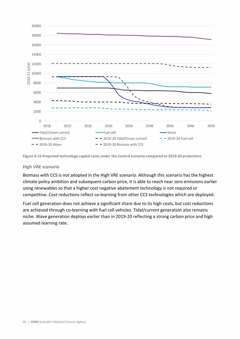
46 | CSIRO Australia’s National Science Agency
Figure 4-15 Projected technology capital costs under the Central scenario compared to 2019-20 projections
High VRE scenario
Biomass with CCS is not adopted in the High VRE scenario. Although this scenario has the highest climate policy ambition and subsequent carbon price, it is able to reach near zero emissions earlier using renewables so that a higher cost negative abatement technology is not required or competitive. Cost reductions reflect co-learning from other CCS technologies which are deployed.
Fuel cell generation does not achieve a significant share due to its high costs, but cost reductions are achieved through co-learning with fuel cell vehicles. Tidal/current generation also remains niche. Wave generation deploys earlier than in 2019-20 reflecting a strong carbon price and high assumed learning rate.
0
2000
4000
6000
8000
10000
12000
14000
16000
18000
20000
2018 2022 2026 2030 2034 2038 2042 2046 2050
2020
-21
$/kW
Tidal/Ocean current Fuel cell Wave
Biomass with CCS 2019-20 Tidal/Ocean current 2019-20 Fuel cell
2019-20 Wave 2019-20 Biomass with CCS

GenCost 2020-21 | 47
Figure 4-16 Projected technology capital costs under the High VRE scenario compared to 2019-20 projections
Diverse technology scenario
Biomass with CCS is deployed in the Diverse technology scenario reflecting the assumed limitations on variable renewable generation. This result is also consistent with the scenario climate policy ambition. Biomass with CCS benefits from co-learning from the significant deployment of gas and coal with CCS generation and hydrogen production from gas with CCS in this scenario.
Wave generation is relatively delayed in this scenario reflecting assumed limitations on variable renewables which are slightly tighter than that assumed in the 2019-20 assumptions. Tidal/current generation is deployed the fastest in this scenario reflecting the greater need for alternative energy sources. However, both tidal/current and fuel cell generation remains niche.
0
2000
4000
6000
8000
10000
12000
14000
16000
18000
20000
2018 2022 2026 2030 2034 2038 2042 2046 2050
2020
-21
$/kW
Tidal/Ocean current Fuel cell WaveBiomass with CCS 2019-20 Tidal/Ocean current 2019-20 Fuel cell2019-20 Wave 2019-20 Biomass with CCS

48 | CSIRO Australia’s National Science Agency
Figure 4-17 Projected technology capital costs under the Diverse technology scenario compared to 2019-20 projections
4.3 Hydrogen electrolysers
Alkaline electrolysers are currently lower cost than Proton-exchange membrane (PEM) electrolysers and they have a common learning rate applied in the modelling. However, we assume that PEM electrolysers are more suited to varying their daily output which makes them more suited to matching their production to low cost variable renewable generation. As the costs of both technologies fall, energy input costs increase in proportion making it increasingly more efficient to sacrifice electrolyser capacity utilisation for lower energy costs. Hence PEM electrolysers are projected to be lower cost over the long term.
Electrolyser deployment is being supported by a substantial number of hydrogen supply and end-use trials globally and in Australia. Experience with other emerging technologies indicates that this type of globally coincident technology deployment activity can lead to a scaleup in manufacturing which supports cost reductions through economies of scale. Very low costs, at the bottom end of the projections here, have been reported in China. However, differences in engineering and operating and maintenance costs mean these are not able to be immediately replicated in other regions. They do indicate, however, a likely achievable level for other regions over the longer term.
Cost reductions are projected to be greatest in the High VRE scenario where global hydrogen production is assumed to be the largest. There is also substantial hydrogen production in Diverse technology but gas with CCS takes a greater share of hydrogen production leading to lower deployment of electrolysers. The Central scenario achieves the least reduction in costs owing to lower global demand for hydrogen consistent with less climate policy ambition in this scenario.
0
2000
4000
6000
8000
10000
12000
14000
16000
18000
20000
2018 2022 2026 2030 2034 2038 2042 2046 2050
2020
-21
$/kW
Tidal/Ocean current Fuel cell Wave
Biomass with CCS 2019-20 Tidal/Ocean current 2019-20 Fuel cell
2019-20 Wave 2019-20 Biomass with CCS

GenCost 2020-21 | 49
Figure 4-18 Projected technology capital costs for alkaline and PEM electrolysers by scenario
0
500
1000
1500
2000
2500
3000
3500
4000
2020 2025 2030 2035 2040 2045 2050
2020
-21
$/kW
Central PEM Diverse technology PEM High VRE PEM
Central Alkaline Diverse technology Alkaline High VRE Alkaline

50 | CSIRO Australia’s National Science Agency
5 Levelised cost of electricity analysis
Levelised cost of electricity (LCOE) data is an electricity generation technology comparison metric. Modelling studies such as AEMO’s Integrated System Plan do not require or use LCOE data. LCOE is a simple screening tool for quickly determining the relative competitiveness of electricity generation technologies. It is not a substitute for detailed project cashflow analysis or electricity system modelling which both provide more realistic representations of electricity generation project operational costs and performance. Furthermore, in the GenCost 2018 report and a supplementary report on methods for calculating the additional costs of renewables (Graham, 2018), we described several issues and concerns in calculating and interpreting levelised cost of electricity. These include:
LCOE does not take account of the additional costs associated with each technology and in particular variable renewable electricity generation technologies
LCOE applies the same discount rate across all technologies even though fossil fuel technologies face a greater risk of being impacted by the introduction of new state or commonwealth climate change policies.
LCOE does not recognise that electricity generation technologies have different roles in the system. In particular, some technologies are operated less frequently, increasing their costs, but are valued for their ability to quickly make their capacity available at peak times.
In Graham (2018), after reviewing several alternatives from the global literature, we proposed a new method for addressing the first dot point – inclusion of balancing and other costs unique to variable renewables costs. That new method has now been implemented and we include those results in the projected LCOEs.
To address other issues not associated with additional cost of renewables, when we present LCOE information we:
Separate and group together peaking technologies, flexible technologies and variable technologies
Include additional LCOE data on fossil fuel technologies which includes additional risk premiums or carbon prices10 on fossil fuel technologies.
5.1 Overview of the new method
Options considered
Graham (2018) reviewed the methods of seven published studies which were relevant in developing a method for taking account of additional costs of variable renewables. Some of the
10 A carbon price is used as a proxy for any policy which may be introduced to reduce high emission activities. This is not a statement of either likely or preferred policy mechanisms.
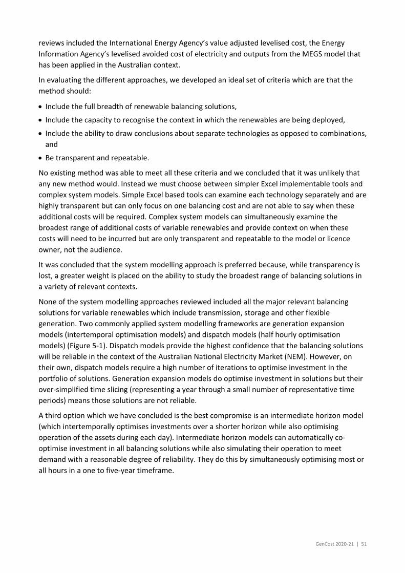
GenCost 2020-21 | 51
reviews included the International Energy Agency’s value adjusted levelised cost, the Energy Information Agency’s levelised avoided cost of electricity and outputs from the MEGS model that has been applied in the Australian context.
In evaluating the different approaches, we developed an ideal set of criteria which are that the method should:
Include the full breadth of renewable balancing solutions,
Include the capacity to recognise the context in which the renewables are being deployed,
Include the ability to draw conclusions about separate technologies as opposed to combinations, and
Be transparent and repeatable.
No existing method was able to meet all these criteria and we concluded that it was unlikely that any new method would. Instead we must choose between simpler Excel implementable tools and complex system models. Simple Excel based tools can examine each technology separately and are highly transparent but can only focus on one balancing cost and are not able to say when these additional costs will be required. Complex system models can simultaneously examine the broadest range of additional costs of variable renewables and provide context on when these costs will need to be incurred but are only transparent and repeatable to the model or licence owner, not the audience.
It was concluded that the system modelling approach is preferred because, while transparency is lost, a greater weight is placed on the ability to study the broadest range of balancing solutions in a variety of relevant contexts.
None of the system modelling approaches reviewed included all the major relevant balancing solutions for variable renewables which include transmission, storage and other flexible generation. Two commonly applied system modelling frameworks are generation expansion models (intertemporal optimisation models) and dispatch models (half hourly optimisation models) (Figure 5-1). Dispatch models provide the highest confidence that the balancing solutions will be reliable in the context of the Australian National Electricity Market (NEM). However, on their own, dispatch models require a high number of iterations to optimise investment in the portfolio of solutions. Generation expansion models do optimise investment in solutions but their over-simplified time slicing (representing a year through a small number of representative time periods) means those solutions are not reliable.
A third option which we have concluded is the best compromise is an intermediate horizon model (which intertemporally optimises investments over a shorter horizon while also optimising operation of the assets during each day). Intermediate horizon models can automatically co-optimise investment in all balancing solutions while also simulating their operation to meet demand with a reasonable degree of reliability. They do this by simultaneously optimising most or all hours in a one to five-year timeframe.

52 | CSIRO Australia’s National Science Agency
Figure 5-1 Three types of electricity system models
Development of STABLE
CSIRO has developed an intermediate horizon model called STABLE: Spatial Temporal Analysis of Balancing Levelised-cost of Energy. STABLE has drawn on the open source DIETER model for its basic design and been modified substantially to incorporate the details of the National Electricity Market. Time is represented hourly for one year. Most underlying data is based on the July 2020 AEMO ISP inputs and assumptions workbook and various other data (such as renewable energy production traces) published as part of the Integrated System Planning process. Demand is solved at the transmission zone level and Renewable Energy Zones are the smallest spatial supply regions associated with each transmission zone.
5.2 LCOE estimates
5.2.1 Calculating additional costs of variable renewables
We implement STABLE by selecting a future year of interest, 203011, imposing a required variable renewable energy (VRE) share and running the model to determine the optimal investment to support the VRE share. In practice, although wave, current, solar thermal and offshore wind are available as variable renewable technologies, onshore wind and large-scale solar PV are the only variable renewables deployed in the modelling due to their cost competitiveness12.
11 This year makes the most sense within the framework applied because there is enough time to plausibly reach high VRE shares but variable renewable shares are still expected to be at or below 50% in the larger states. In the 2040s and 2050s, much of the existing flexible capacity in the system will retire due to end of asset life and be replaced with variable renewables (see AEMO ISP and other long-term modelling). As such, most of the additional costs will already be incurred in the counterfactual.
12 This does not preclude other types of projects proceeding in reality but is a reflection of modelling inputs.
Intermediate horizon model
Dispatch model
Generation expansion
model
STABLE
Co-optimised generation, storage and transmission investment (annual steps to 2050 and beyond with limited sub-annual time-slices)
Co-optimised investment and operation for reliability and security (one to several hours time steps for one to five years)
Operation of existing capacities to the reliability standard is optimised each five minutes to half hour. Partial investment optimisation can be achieved through model iteration.
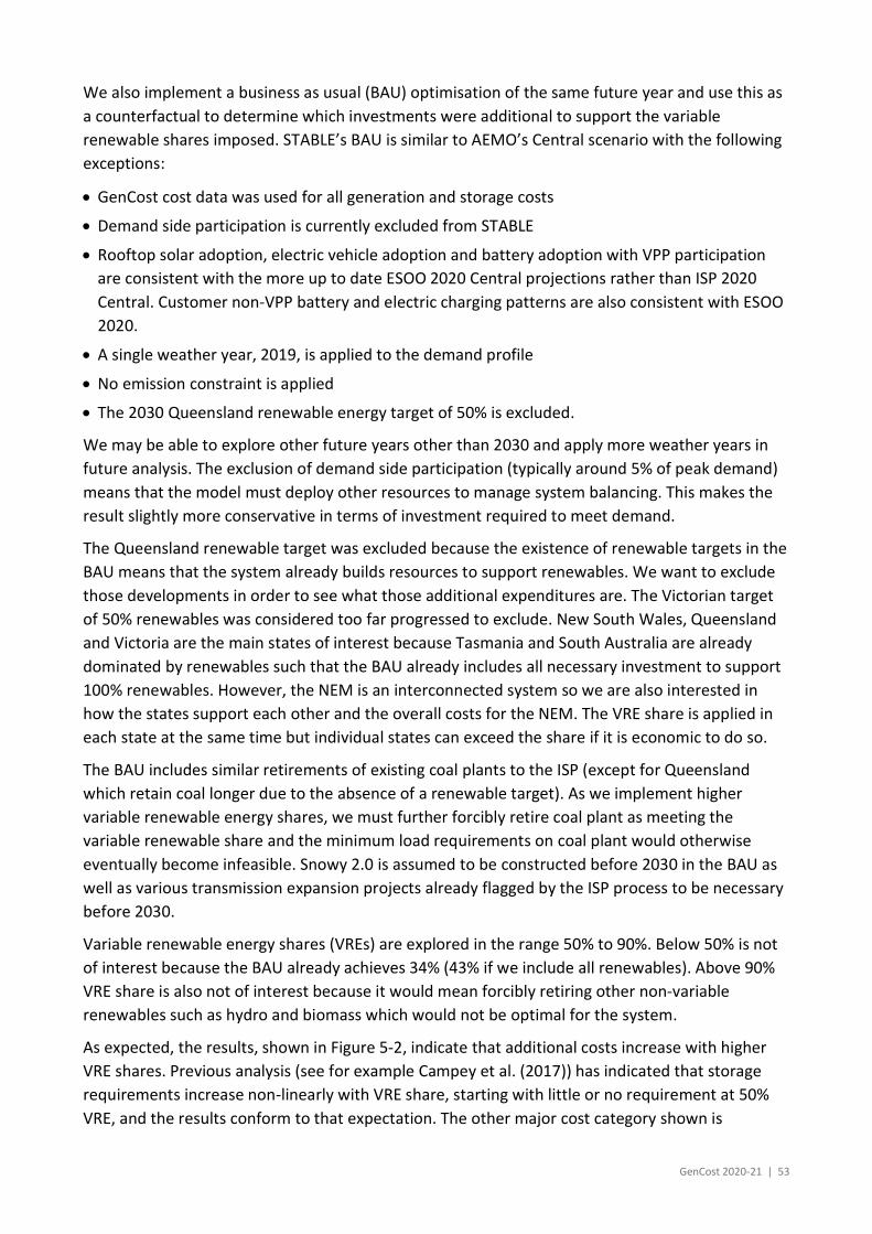
GenCost 2020-21 | 53
We also implement a business as usual (BAU) optimisation of the same future year and use this as a counterfactual to determine which investments were additional to support the variable renewable shares imposed. STABLE’s BAU is similar to AEMO’s Central scenario with the following exceptions:
GenCost cost data was used for all generation and storage costs
Demand side participation is currently excluded from STABLE
Rooftop solar adoption, electric vehicle adoption and battery adoption with VPP participation are consistent with the more up to date ESOO 2020 Central projections rather than ISP 2020 Central. Customer non-VPP battery and electric charging patterns are also consistent with ESOO 2020.
A single weather year, 2019, is applied to the demand profile
No emission constraint is applied
The 2030 Queensland renewable energy target of 50% is excluded.
We may be able to explore other future years other than 2030 and apply more weather years in future analysis. The exclusion of demand side participation (typically around 5% of peak demand) means that the model must deploy other resources to manage system balancing. This makes the result slightly more conservative in terms of investment required to meet demand.
The Queensland renewable target was excluded because the existence of renewable targets in the BAU means that the system already builds resources to support renewables. We want to exclude those developments in order to see what those additional expenditures are. The Victorian target of 50% renewables was considered too far progressed to exclude. New South Wales, Queensland and Victoria are the main states of interest because Tasmania and South Australia are already dominated by renewables such that the BAU already includes all necessary investment to support 100% renewables. However, the NEM is an interconnected system so we are also interested in how the states support each other and the overall costs for the NEM. The VRE share is applied in each state at the same time but individual states can exceed the share if it is economic to do so.
The BAU includes similar retirements of existing coal plants to the ISP (except for Queensland which retain coal longer due to the absence of a renewable target). As we implement higher variable renewable energy shares, we must further forcibly retire coal plant as meeting the variable renewable share and the minimum load requirements on coal plant would otherwise eventually become infeasible. Snowy 2.0 is assumed to be constructed before 2030 in the BAU as well as various transmission expansion projects already flagged by the ISP process to be necessary before 2030.
Variable renewable energy shares (VREs) are explored in the range 50% to 90%. Below 50% is not of interest because the BAU already achieves 34% (43% if we include all renewables). Above 90% VRE share is also not of interest because it would mean forcibly retiring other non-variable renewables such as hydro and biomass which would not be optimal for the system.
As expected, the results, shown in Figure 5-2, indicate that additional costs increase with higher VRE shares. Previous analysis (see for example Campey et al. (2017)) has indicated that storage requirements increase non-linearly with VRE share, starting with little or no requirement at 50% VRE, and the results conform to that expectation. The other major cost category shown is

54 | CSIRO Australia’s National Science Agency
transmission which includes transmission cost to connect Renewable Energy Zones to the grid and other transmission which includes state interconnectors and general expansion of existing lines. REZ expansion costs appear to be required at similar levels for each additional 10% increase. Other transmission expenditure, not already in the BAU, is only required in significant levels in NSW likely reflecting its position in the middle of the NEM.
Storage requirements are also highest in NSW. This reflects existing flexible resources and the quality of the variable renewable resources. Queensland has a wind resource which tends to be stronger at night which is therefore well suited to filling in the gaps left by solar PV. The reduced coincidence of wind and solar means less storage is necessary. Queensland also has around 430MW additional existing flexible gas and diesel than NSW in 2030.
The proximity to Tasmania’s hydro resources means Victoria does not have to build as many storage resources locally. Also, in 2030 Victoria has 360MW of additional existing flexible gas and diesel compared to NSW. Without these existing assets more storage or other flexible generation would likely need to be built in Queensland and Victoria.
Figure 5-2 Levelised costs of achieving 50%, 60%, 70%, 80% and 90% variable renewable energy shares in the NEM, NSW, VIC and QLD
There are no additional costs of meeting a 50% VRE share in Victoria because all those costs are already in the BAU which includes a 50% target. Across the NEM, the cost of REZ transmission expansion adds around $4/MWh. Other transmission adds between $0.1 to $1.8/MWh. Storage adds between $0 to $14/MWh. For these latter two, the share of VRE targeted is crucial in determining the relevant point in that range. The region of the NEM is another key source of variation.
0
10
20
30
40
50
60
70
80
50% VRE 60% VRE 70% VRE 80% VRE 90% VRE
$/M
Wh
Generation Storage REZ transmission Other transmission
NEM
0
10
20
30
40
50
60
70
80
50% VRE 60% VRE 70% VRE 80% VRE 90% VRE
$/M
Wh
Generation Storage REZ transmission Other transmission
NSW
0
10
20
30
40
50
60
70
80
50% VRE 60% VRE 70% VRE 80% VRE 90% VRE
$/M
Wh
Generation Storage REZ transmission Other transmission
VIC
0
10
20
30
40
50
60
70
80
50% VRE 60% VRE 70% VRE 80% VRE 90% VRE
$/M
Wh
Generation Storage REZ transmission Other transmission
QLD

GenCost 2020-21 | 55
5.2.2 Variable renewables with and without storage and transmission
The results for the additional costs for increasing variable renewable shares are used to update and extend our LCOE estimates. We expand the results for 2030 to include a combined wind and solar PV category for different VRE shares. We have also removed the wind plus storage and solar PV plus storage categories that were included in GenCost 2018 and GenCost 2019-20. These were always designed to be temporary estimate until a better approach was available. In GenCost 2019-20, for 2030, the simple approach of adding 2 or 6 hours storage added $19 to $106/MWh to the cost of variable renewables for an unspecified share of generation. With the new approach the additional costs to support renewables are estimated at $0 to $29/MWh depending on the VRE share (Figure 5-4). As such, the previous approach was too conservative. While it did not consider transmission, which is an important additional cost, it over-estimated the need for storage and, in total, over-estimated the additional costs that might be associated with variable renewable generation.
Variable renewables (wind and solar PV) without transmission or storage costs are the lowest cost generation technology by a significant margin. From 2030, the new estimates on additional costs associated with increasing variable renewable generation confirms that they are also competitive when transmission and storage costs are included up to any relevant VRE share.
5.2.3 Peaking technologies
The peaking technology category includes two sizes for gas turbines and a gas reciprocating engine. Fuel comprises the majority of costs, but the lower capital costs of the larger gas turbine make it the most competitive. Reciprocating engines have higher efficiency and consequently, for applications with relatively higher capacity factors and where a smaller unit size is required, they can be the lower cost choice.
5.2.4 Flexible technologies
Evaluated purely on their energy costs, black coal, brown coal and gas-based generation technologies that are designed to deliver energy for 40 to 80% of the year are the next most competitive generation technologies after variable renewables (with or without transmission and storage). It is difficult to say which fossil fuel is more competitive as it depends very much on whether gas generation can secure gas supply at the lower end of the fuel cost range (just under $6/GJ).
New fossil fuel generation faces the risk of higher costs over time because all states in Australia have either legislated or aspirational net zero emission targets. There is also bipartisan commitment to the Paris agreement which is aiming for net zero emissions in the second half of the century. We address these risks in the cost estimations in two ways: directly adding a carbon price from our global scenario range and indirectly by imposing a 5% risk premium on borrowing costs. The results show that a carbon price would result in lower costs for black and brown coal over the next two decades than adding a 5% risk premium but this switches by 2050 reflecting the non-linear growth in the assumed carbon price range. Natural gas-based generation is less impacted by either a carbon price or risk premium because of its lower emission fuel, higher thermal efficiency and lower capital cost. However, it is at greater risk of facing high fuel prices.
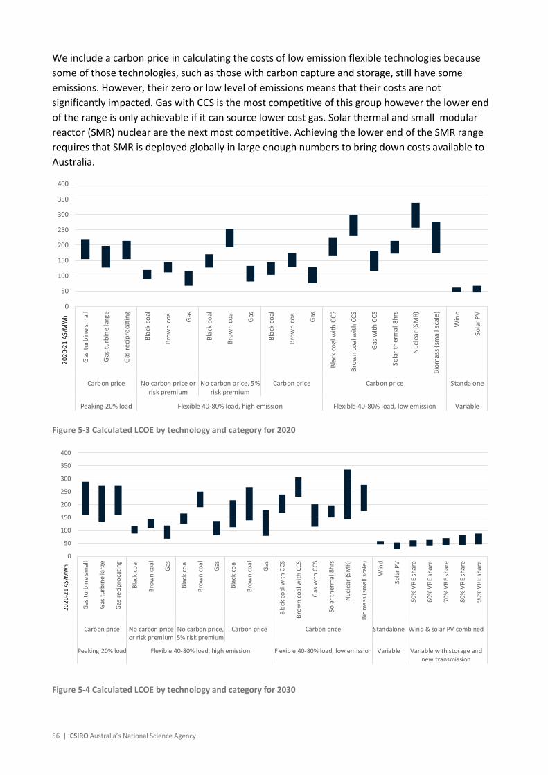
56 | CSIRO Australia’s National Science Agency
We include a carbon price in calculating the costs of low emission flexible technologies because some of those technologies, such as those with carbon capture and storage, still have some emissions. However, their zero or low level of emissions means that their costs are not significantly impacted. Gas with CCS is the most competitive of this group however the lower end of the range is only achievable if it can source lower cost gas. Solar thermal and small modular reactor (SMR) nuclear are the next most competitive. Achieving the lower end of the SMR range requires that SMR is deployed globally in large enough numbers to bring down costs available to Australia.
Figure 5-3 Calculated LCOE by technology and category for 2020
Figure 5-4 Calculated LCOE by technology and category for 2030
0
50
100
150
200
250
300
350
400
Gas
turb
ine
smal
l
Gas
turb
ine
larg
e
Gas
reci
proc
atin
g
Blac
k co
al
Brow
n co
al
Gas
Blac
k co
al
Brow
n co
al
Gas
Blac
k co
al
Brow
n co
al
Gas
Blac
k co
al w
ith C
CS
Brow
n co
al w
ith C
CS
Gas
with
CCS
Sola
r the
rmal
8hr
s
Nuc
lear
(SM
R)
Biom
ass (
smal
l sca
le)
Win
d
Sola
r PV
Carbon price No carbon price orrisk premium
No carbon price, 5%risk premium
Carbon price Carbon price Standalone
Peaking 20% load Flexible 40-80% load, high emission Flexible 40-80% load, low emission Variable
2020
-21
A$/M
Wh
0
50
100
150
200
250
300
350
400
Gas
turb
ine
smal
l
Gas
turb
ine
larg
e
Gas
reci
proc
atin
g
Blac
k co
al
Brow
n co
al
Gas
Blac
k co
al
Brow
n co
al
Gas
Blac
k co
al
Brow
n co
al
Gas
Blac
k co
al w
ith C
CS
Brow
n co
al w
ith C
CS
Gas
with
CCS
Sola
r the
rmal
8hr
s
Nuc
lear
(SM
R)
Biom
ass (
smal
l sca
le)
Win
d
Sola
r PV
50%
VRE
shar
e
60%
VRE
shar
e
70%
VRE
shar
e
80%
VRE
shar
e
90%
VRE
shar
e
Carbon price No carbon priceor risk premium
No carbon price,5% risk premium
Carbon price Carbon price Standalone Wind & solar PV combined
Peaking 20% load Flexible 40-80% load, high emission Flexible 40-80% load, low emission Variable Variable with storage andnew transmission
2020
-21
A$/M
Wh

GenCost 2020-21 | 57
Figure 5-5 Calculated LCOE by technology and category for 2040
Figure 5-6 Calculated LCOE by technology and category for 2050
0
50
100
150
200
250
300
350
400
Gas
turb
ine
smal
l
Gas
turb
ine
larg
e
Gas
reci
proc
atin
g
Blac
k co
al
Brow
n co
al
Gas
Blac
k co
al
Brow
n co
al
Gas
Blac
k co
al
Brow
n co
al
Gas
Blac
k co
al w
ith C
CS
Brow
n co
al w
ith C
CS
Gas
with
CCS
Sola
r the
rmal
8hr
s
Nuc
lear
(SM
R)
Biom
ass (
smal
l sca
le)
Win
d
Sola
r PV
Carbon price No carbon price orrisk premium
No carbon price, 5%risk premium
Carbon price Carbon price Standalone
Peaking 20% load Flexible 40-80% load, high emission Flexible 40-80% load, low emission Variable
2020
-21
A$/M
Wh
0
50
100
150
200
250
300
350
400
450
500
Gas
turb
ine
smal
l
Gas
turb
ine
larg
e
Gas
reci
proc
atin
g
Blac
k co
al
Brow
n co
al
Gas
Blac
k co
al
Brow
n co
al
Gas
Blac
k co
al
Brow
n co
al
Gas
Blac
k co
al w
ith C
CS
Brow
n co
al w
ith C
CS
Gas
with
CCS
Sola
r the
rmal
8hr
s
Nuc
lear
(SM
R)
Biom
ass (
smal
l sca
le)
Win
d
Sola
r PV
Carbon price No carbon price orrisk premium
No carbon price, 5%risk premium
Carbon price Carbon price Standalone
Peaking 20% load Flexible 40-80% load, high emission Flexible 40-80% load, low emission Variable
2020
-21
A$/M
Wh
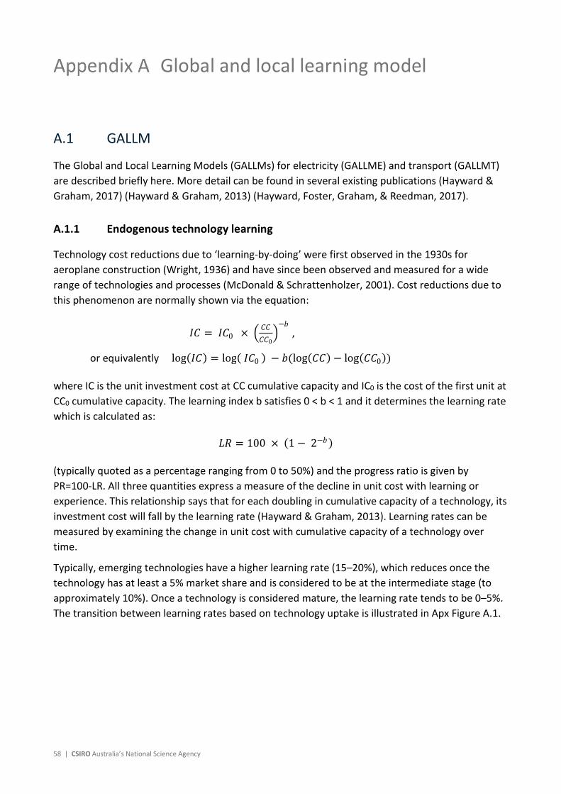
58 | CSIRO Australia’s National Science Agency
Global and local learning model
A.1 GALLM
The Global and Local Learning Models (GALLMs) for electricity (GALLME) and transport (GALLMT) are described briefly here. More detail can be found in several existing publications (Hayward & Graham, 2017) (Hayward & Graham, 2013) (Hayward, Foster, Graham, & Reedman, 2017).
A.1.1 Endogenous technology learning
Technology cost reductions due to ‘learning-by-doing’ were first observed in the 1930s for aeroplane construction (Wright, 1936) and have since been observed and measured for a wide range of technologies and processes (McDonald & Schrattenholzer, 2001). Cost reductions due to this phenomenon are normally shown via the equation:
where IC is the unit investment cost at CC cumulative capacity and IC0 is the cost of the first unit at CC0 cumulative capacity. The learning index b satisfies 0 < b < 1 and it determines the learning rate which is calculated as:
(typically quoted as a percentage ranging from 0 to 50%) and the progress ratio is given by PR=100-LR. All three quantities express a measure of the decline in unit cost with learning or experience. This relationship says that for each doubling in cumulative capacity of a technology, its investment cost will fall by the learning rate (Hayward & Graham, 2013). Learning rates can be measured by examining the change in unit cost with cumulative capacity of a technology over time.
Typically, emerging technologies have a higher learning rate (15–20%), which reduces once the technology has at least a 5% market share and is considered to be at the intermediate stage (to approximately 10%). Once a technology is considered mature, the learning rate tends to be 0–5%. The transition between learning rates based on technology uptake is illustrated in Apx Figure A.1.
𝐼𝐶 = 𝐼𝐶0 × 𝐶𝐶
𝐶𝐶0
−𝑏 ,
or equivalently log(𝐼𝐶) = log( 𝐼𝐶0 ) − 𝑏(log(𝐶𝐶) − log(𝐶𝐶0))
𝐿𝑅 = 100 × (1 − 2−𝑏 )

GenCost 2020-21 | 59
Apx Figure A.1 Schematic of changes in the learning rate as a technology progresses through its development stages after commercialisation
However, technologies that do not have a standard unit size and can be used in a variety of applications tend to have a higher learning rate for longer (Wilson, 2012). This is the case for solar photovoltaics and historically for gas turbines.
Technologies are made up of components and different components can be at different levels of maturity and thus have different learning rates. Different parts of a technology can be developed and sold in different markets (global vs. regional/local) which can impact on the cost reductions as each region will have a different level of demand for a technology and this will affect its uptake.
5.2.5 The modelling framework
In order to project the future cost of a technology using experience curves, the future level of cumulative capacity/uptake needs to be known. However, this is dependent on the costs. The GALLMs solve this problem by simultaneously projecting both the cost and uptake of the technologies. The optimisation problem includes constraints such as government policies, demand for electricity or transport, capacity of existing technologies, exogenous costs such as for fossil fuels and limits on resources (e.g. rooftops for solar photovoltaics). The models have been divided into 13 regions and each region has unique assumptions and data for the above listed constraints. The regions have been based on Organisation for Economic Co-operation Development (OECD) regions (with some variation to look more closely at some countries of interest) and are: Africa, Australia, China, Eastern Europe, Western Europe, Former Soviet Union, India, Japan, Latin America, Middle East, North America, OECD Pacific, Rest of Asia and Pacific.
The objective function of the model is to minimise the total system costs while meeting demand and all constraints. The model is solved as a mixed integer linear program. The experience curves are segmented into step functions and the location on the experience curves (i.e. cost vs.

60 | CSIRO Australia’s National Science Agency
cumulative capacity) is determined at each time step. See (Hayward & Graham, 2013) and (Hayward, Foster, Graham, & Reedman, 2017) for more information. Both models run from the year 2006 to 2100. However, results are only reported from the present year to 2050.
A.1.2 Mature technologies and the “basket of costs”
There are three main drivers of mature technology costs: imported materials and equipment, domestic materials and equipment, and labour. The indices of these drivers over the last 20 years (ABS data) combined with the split in capital cost of mature technologies between imported equipment, domestic equipment and labour (Bureau of Resource and Energy Economics (BREE), 2012) was used to calculate an average rate of change in technology costs: - 0.2%. This value has been applied as an annual capital cost reduction factor to mature technologies and to operating and maintenance costs.
A.1.3 Variable Renewables and Energy Storage
The Dispatch and Investment Evaluation Tool with Endogenous Renewables (DIETER) is an open source model which has been designed to model the cost of electricity generation systems with high shares of variable renewables (PV, onshore and offshore wind and ocean renewables) and energy storage (http://www.diw.de/dieter). DIETER contains hourly renewable resource and load data for one calendar year, and because of this granularity, it is better able to optimise variable renewable and storage combinations than GALLME in any one year.
Apx Figure A.2 Schematic diagram of GALLM and DIETER modelling framework
DIETER has been used in this study to determine the new capacity of variable renewables and storage technologies in the years that DIETER is solved, and this data has then been included back in GALLME to update the cumulative capacity and thus the capital cost of these technologies. A schematic of the interaction between GALLME and DIETER is shown in Apx Figure A.2.

GenCost 2020-21 | 61
The model interactions are as follows:
1. GALLME is solved without DIETER to calculate cost and uptake of all technologies
2. GALLME cost data, installed capacity of non-variable renewable technologies and upper and lower bounds on demand for electricity satisfied by variable renewables are used as inputs into DIETER
3. DIETER is solved for each region in 5-yearly intervals, beginning in 2025.
4. The new installed capacity of variable renewables and storage is included in GALLME and GALLME is solved.

62 | CSIRO Australia’s National Science Agency
Data tables
The following tables provide data behind the figures presented in this document.

GenCost 2020-21 | 63
Apx Table B.1 Current and projected generation technology capital costs under the Central scenario
Black coal
Black coal with CCS
Brown coal
Brown coal with CCS
Gas combined cycle
Gas open cycle (small)
Gas open cycle (large)
Gas with CCS
Gas reciprocating
Hydrogen reciprocating
Biomass (small scale)
Biomass with CCS (large scale)
Large scale solar PV
Rooftop solar panels
Solar thermal (8 hrs)
Wind Offshore wind
Wave Nuclear (SMR)
Tidal/ocean current
Fuel cell
Integrated solar and battery (2 hrs)
$/kW $/kW $/kW $/kW $/kW $/kW $/kW $/kW $/kW $/kW $/kW $/kW $/kW $/kW $/kW $/kW $/kW $/kW $/kW $/kW $/kW $/kW
2020 4450 9311 6868 14293 1801 1550 961 4461 1567 1750 8619 18438 1408 1439 7411 1951 5771 9384 16487 6971 9333 2139
2021 4441 9297 6854 14269 1797 1546 959 4457 1564 1746 8613 18406 1272 1304 7331 1937 5727 9384 16487 6954 9144 1990
2022 4432 9283 6841 14245 1793 1543 957 4453 1561 1743 8609 18373 1178 1211 7291 1925 5687 9384 16487 6945 8951 1885
2023 4423 9269 6827 14221 1790 1540 955 4448 1558 1739 8606 18341 1128 1162 7290 1915 5641 9384 16487 6945 8766 1814
2024 4414 9255 6813 14197 1786 1537 954 4444 1555 1736 8606 18309 1084 1118 7283 1908 5599 9384 16487 6945 8600 1730
2025 4406 9241 6800 14173 1783 1534 952 4439 1551 1732 8606 18277 1041 1076 7263 1904 5557 9384 14705 6945 8460 1637
2026 4397 9227 6786 14149 1779 1531 950 4435 1548 1729 8606 18245 1002 1036 7212 1901 5536 9384 12908 6945 8342 1543
2027 4388 9213 6773 14125 1775 1528 948 4430 1545 1725 8606 18213 964 998 7111 1899 5512 9384 11110 6945 8248 1455
2028 4379 9199 6759 14102 1772 1525 946 4426 1542 1722 8606 18181 931 964 6978 1896 5498 9384 9312 6945 8179 1374
2029 4370 9185 6746 14078 1768 1522 944 4422 1539 1718 8606 18149 901 933 6842 1894 5476 9384 7465 6945 8110 1273
2030 4362 9171 6732 14054 1765 1519 942 4417 1536 1715 8606 18117 874 905 6732 1892 5458 8365 7415 6945 8064 1189
2031 4353 9158 6719 14031 1761 1516 940 4413 1533 1711 8606 18086 852 882 6641 1889 5437 6976 7333 6798 8032 1123
2032 4344 9144 6705 14007 1758 1513 938 4408 1530 1708 8606 18054 835 863 6564 1878 5424 5443 7251 6652 8030 1099
2033 4336 9130 6692 13984 1754 1510 936 4404 1527 1705 8606 18022 822 849 6499 1864 5417 4794 7251 6506 8028 1079
2034 4327 9116 6678 13960 1751 1507 935 4400 1524 1701 8606 17991 810 835 6443 1841 5415 4428 7251 6506 8026 1060
2035 4318 9103 6665 13937 1747 1504 933 4395 1521 1698 8606 17959 790 815 6395 1826 5411 4152 7251 6467 8024 1035
2036 4310 9089 6652 13913 1744 1501 931 4391 1518 1694 8606 17928 773 797 6352 1812 5408 3978 7251 6419 8023 1012
2037 4301 9075 6638 13890 1740 1498 929 4387 1515 1691 8606 17896 756 779 6314 1807 5404 3734 7251 6369 8021 990
2038 4292 9061 6625 13867 1737 1495 927 4382 1512 1688 8606 17865 748 771 6281 1802 5389 3536 7251 6358 7891 977
2039 4284 9048 6612 13844 1733 1492 925 4378 1509 1684 8606 17834 739 761 6251 1797 5360 3282 7251 6357 7663 964
2040 4275 9034 6599 13820 1730 1489 923 4374 1505 1681 8606 17803 727 749 6224 1792 5323 3146 7248 6357 7406 949
2041 4267 9021 6585 13797 1726 1486 922 4370 1502 1678 8606 17772 710 732 6177 1786 5291 2983 7246 6357 7255 930
2042 4258 9007 6572 13774 1723 1483 920 4365 1499 1674 8606 17741 689 711 6112 1781 5269 2912 7244 6330 7199 907
2043 4250 8994 6559 13751 1720 1480 918 4361 1496 1671 8606 17710 669 691 6031 1778 5249 2867 7244 6296 7167 885
2044 4241 8980 6546 13728 1716 1477 916 4357 1493 1667 8606 17679 650 672 5956 1776 5231 2855 7244 6163 7155 864
2045 4233 8967 6533 13705 1713 1474 914 4353 1491 1664 8606 17648 632 654 5888 1774 5212 2843 7244 6049 7143 843
2046 4224 8953 6520 13682 1709 1471 912 4348 1488 1661 8606 17617 617 639 5825 1771 5197 2841 7244 5943 7132 827
2047 4216 8872 6507 13591 1706 1468 911 4276 1485 1657 8606 17518 606 628 5767 1766 5184 2837 7244 5938 7122 814
2048 4207 8755 6494 13464 1702 1465 909 4169 1482 1654 8606 17383 597 619 5714 1759 5176 2832 7244 5938 7114 804
2049 4199 8609 6481 13309 1699 1462 907 4034 1479 1651 8606 17220 589 611 5665 1750 5166 2826 7244 5846 7105 794
2050 4195 8553 6474 13248 1697 1461 905 3982 1477 1649 8606 17155 585 607 5641 1745 5162 2823 7244 5800 7101 789

64 | CSIRO Australia’s National Science Agency
Apx Table B.2 Current and projected generation technology capital costs under the High VRE scenario
Black coal
Black coal with CCS
Brown coal
Brown coal with CCS
Gas combined cycle
Gas open cycle (small)
Gas open cycle (large)
Gas with CCS
Gas reciprocating
Hydrogen reciprocating
Biomass (small scale)
Biomass with CCS (large scale)
Large scale solar PV
Rooftop solar panels
Solar thermal (8 hrs)
Wind Offshore wind
Wave Nuclear (SMR)
Tidal/ocean current
Fuel cell
Integrated solar and battery (2 hrs)
$/kW $/kW $/kW $/kW $/kW $/kW $/kW $/kW $/kW $/kW $/kW $/kW $/kW $/kW $/kW $/kW $/kW $/kW $/kW $/kW $/kW $/kW
2020 4450 9311 6868 14293 1801 1550 961 4461 1567 1750 8619 18438 1408 1439 7411 1951 5771 9384 16487 6971 9333 2139
2021 4441 9297 6854 14269 1797 1546 959 4457 1564 1746 8613 18406 1209 1244 7243 1944 5723 9384 16487 6954 9314 1848
2022 4432 9283 6841 14245 1793 1543 957 4453 1561 1743 8609 18373 1067 1106 7108 1937 5668 9384 16487 6945 9294 1628
2023 4423 9269 6827 14221 1790 1540 955 4448 1558 1739 8606 18341 994 1034 7008 1931 5613 9384 16487 6945 9275 1480
2024 4414 9255 6813 14197 1786 1537 954 4444 1555 1736 8606 18309 927 968 6893 1926 5561 9384 16487 6945 9257 1355
2025 4406 9241 6800 14173 1783 1534 952 4439 1551 1732 8606 18277 885 926 6762 1923 5522 9384 16487 6798 9242 1262
2026 4397 9227 6786 14149 1779 1531 950 4435 1548 1729 8606 18245 857 898 6622 1920 5491 9384 16487 6652 9230 1200
2027 4388 9213 6773 14125 1775 1528 948 4430 1545 1725 8606 18213 833 873 6507 1918 5467 9384 16487 6506 9222 1150
2028 4379 9199 6759 14102 1772 1525 946 4426 1542 1722 8606 18181 813 851 6412 1914 5446 9384 16487 6506 9216 1109
2029 4370 9185 6746 14078 1768 1522 944 4422 1539 1718 8606 18149 796 833 6332 1907 5429 9384 16487 6506 8864 1060
2030 4362 9171 6732 14054 1765 1519 942 4417 1536 1715 8606 18117 780 816 6264 1899 5414 8349 16487 6506 8490 1030
2031 4353 9158 6719 14031 1761 1516 940 4413 1533 1711 8606 18086 770 803 6205 1891 5406 7015 16487 6506 8098 1008
2032 4344 9144 6705 14007 1758 1513 938 4408 1530 1708 8606 18054 754 786 6153 1884 5402 5584 16487 6506 8037 1001
2033 4336 9130 6692 13984 1754 1510 936 4404 1527 1705 8606 18022 742 773 6108 1877 5402 4978 16487 6506 7987 984
2034 4327 9116 6678 13960 1751 1507 935 4400 1524 1701 8606 17991 726 756 6068 1870 5388 4568 16487 6506 7945 965
2035 4318 9103 6665 13937 1747 1504 933 4395 1521 1698 8606 17959 703 732 6032 1863 5362 4189 16487 6467 7912 938
2036 4310 9089 6652 13913 1744 1501 931 4391 1518 1694 8606 17928 681 709 6000 1857 5327 3987 16487 6419 7885 913
2037 4301 9075 6638 13890 1740 1498 929 4387 1515 1691 8606 17896 649 678 5971 1852 5296 3731 16487 6369 7861 880
2038 4292 9061 6625 13867 1737 1495 927 4382 1512 1688 8606 17865 624 652 5945 1848 5269 3524 16487 6358 7839 852
2039 4284 9048 6612 13844 1733 1492 925 4378 1509 1684 8606 17834 597 626 5919 1844 5246 3331 16487 6357 7820 823
2040 4275 9034 6599 13820 1730 1489 923 4374 1505 1681 8606 17803 582 611 5874 1842 5225 3246 16487 6357 7806 807
2041 4267 9021 6585 13797 1726 1486 922 4370 1502 1678 8606 17772 576 604 5813 1835 5206 3124 16487 6357 7795 799
2042 4258 9007 6572 13774 1723 1483 920 4365 1499 1674 8606 17741 571 598 5740 1828 5190 3005 16487 6330 7790 791
2043 4250 8994 6559 13751 1720 1480 918 4361 1496 1671 8606 17710 567 593 5672 1811 5175 2917 16487 6296 7787 785
2044 4241 8980 6546 13728 1716 1477 916 4357 1493 1667 8606 17679 565 591 5610 1798 5162 2884 16487 6263 7787 781
2045 4233 8937 6533 13675 1713 1474 914 4323 1491 1664 8606 17618 563 588 5552 1785 5149 2864 16487 6176 7787 777
2046 4224 8838 6520 13566 1709 1471 912 4234 1488 1661 8606 17501 561 586 5499 1782 5138 2860 16487 6097 7787 773
2047 4216 8696 6507 13416 1706 1468 911 4103 1485 1657 8606 17342 556 581 5450 1779 5128 2849 16487 6018 7786 767
2048 4207 8563 6494 13272 1702 1465 909 3979 1482 1654 8606 17191 552 576 5404 1776 5119 2840 16487 6018 7786 761
2049 4199 8465 6481 13165 1699 1462 907 3891 1479 1651 8606 17076 547 571 5362 1773 5111 2809 16487 5939 7785 754
2050 4195 8426 6474 13121 1697 1461 905 3857 1477 1649 8606 17028 546 569 5341 1772 5106 2797 16487 5900 7784 752
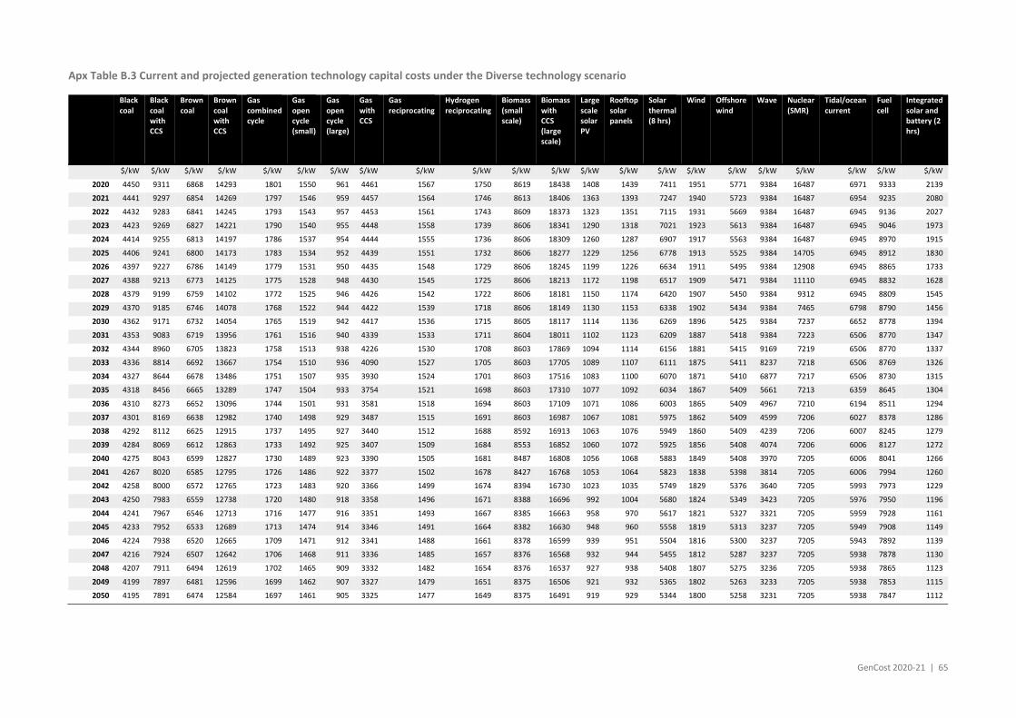
GenCost 2020-21 | 65
Apx Table B.3 Current and projected generation technology capital costs under the Diverse technology scenario
Black coal
Black coal with CCS
Brown coal
Brown coal with CCS
Gas combined cycle
Gas open cycle (small)
Gas open cycle (large)
Gas with CCS
Gas reciprocating
Hydrogen reciprocating
Biomass (small scale)
Biomass with CCS (large scale)
Large scale solar PV
Rooftop solar panels
Solar thermal (8 hrs)
Wind Offshore wind
Wave Nuclear (SMR)
Tidal/ocean current
Fuel cell
Integrated solar and battery (2 hrs)
$/kW $/kW $/kW $/kW $/kW $/kW $/kW $/kW $/kW $/kW $/kW $/kW $/kW $/kW $/kW $/kW $/kW $/kW $/kW $/kW $/kW $/kW
2020 4450 9311 6868 14293 1801 1550 961 4461 1567 1750 8619 18438 1408 1439 7411 1951 5771 9384 16487 6971 9333 2139
2021 4441 9297 6854 14269 1797 1546 959 4457 1564 1746 8613 18406 1363 1393 7247 1940 5723 9384 16487 6954 9235 2080
2022 4432 9283 6841 14245 1793 1543 957 4453 1561 1743 8609 18373 1323 1351 7115 1931 5669 9384 16487 6945 9136 2027
2023 4423 9269 6827 14221 1790 1540 955 4448 1558 1739 8606 18341 1290 1318 7021 1923 5613 9384 16487 6945 9046 1973
2024 4414 9255 6813 14197 1786 1537 954 4444 1555 1736 8606 18309 1260 1287 6907 1917 5563 9384 16487 6945 8970 1915
2025 4406 9241 6800 14173 1783 1534 952 4439 1551 1732 8606 18277 1229 1256 6778 1913 5525 9384 14705 6945 8912 1830
2026 4397 9227 6786 14149 1779 1531 950 4435 1548 1729 8606 18245 1199 1226 6634 1911 5495 9384 12908 6945 8865 1733
2027 4388 9213 6773 14125 1775 1528 948 4430 1545 1725 8606 18213 1172 1198 6517 1909 5471 9384 11110 6945 8832 1628
2028 4379 9199 6759 14102 1772 1525 946 4426 1542 1722 8606 18181 1150 1174 6420 1907 5450 9384 9312 6945 8809 1545
2029 4370 9185 6746 14078 1768 1522 944 4422 1539 1718 8606 18149 1130 1153 6338 1902 5434 9384 7465 6798 8790 1456
2030 4362 9171 6732 14054 1765 1519 942 4417 1536 1715 8605 18117 1114 1136 6269 1896 5425 9384 7237 6652 8778 1394
2031 4353 9083 6719 13956 1761 1516 940 4339 1533 1711 8604 18011 1102 1123 6209 1887 5418 9384 7223 6506 8770 1347
2032 4344 8960 6705 13823 1758 1513 938 4226 1530 1708 8603 17869 1094 1114 6156 1881 5415 9169 7219 6506 8770 1337
2033 4336 8814 6692 13667 1754 1510 936 4090 1527 1705 8603 17705 1089 1107 6111 1875 5411 8237 7218 6506 8769 1326
2034 4327 8644 6678 13486 1751 1507 935 3930 1524 1701 8603 17516 1083 1100 6070 1871 5410 6877 7217 6506 8730 1315
2035 4318 8456 6665 13289 1747 1504 933 3754 1521 1698 8603 17310 1077 1092 6034 1867 5409 5661 7213 6359 8645 1304
2036 4310 8273 6652 13096 1744 1501 931 3581 1518 1694 8603 17109 1071 1086 6003 1865 5409 4967 7210 6194 8511 1294
2037 4301 8169 6638 12982 1740 1498 929 3487 1515 1691 8603 16987 1067 1081 5975 1862 5409 4599 7206 6027 8378 1286
2038 4292 8112 6625 12915 1737 1495 927 3440 1512 1688 8592 16913 1063 1076 5949 1860 5409 4239 7206 6007 8245 1279
2039 4284 8069 6612 12863 1733 1492 925 3407 1509 1684 8553 16852 1060 1072 5925 1856 5408 4074 7206 6006 8127 1272
2040 4275 8043 6599 12827 1730 1489 923 3390 1505 1681 8487 16808 1056 1068 5883 1849 5408 3970 7205 6006 8041 1266
2041 4267 8020 6585 12795 1726 1486 922 3377 1502 1678 8427 16768 1053 1064 5823 1838 5398 3814 7205 6006 7994 1260
2042 4258 8000 6572 12765 1723 1483 920 3366 1499 1674 8394 16730 1023 1035 5749 1829 5376 3640 7205 5993 7973 1229
2043 4250 7983 6559 12738 1720 1480 918 3358 1496 1671 8388 16696 992 1004 5680 1824 5349 3423 7205 5976 7950 1196
2044 4241 7967 6546 12713 1716 1477 916 3351 1493 1667 8385 16663 958 970 5617 1821 5327 3321 7205 5959 7928 1161
2045 4233 7952 6533 12689 1713 1474 914 3346 1491 1664 8382 16630 948 960 5558 1819 5313 3237 7205 5949 7908 1149
2046 4224 7938 6520 12665 1709 1471 912 3341 1488 1661 8378 16599 939 951 5504 1816 5300 3237 7205 5943 7892 1139
2047 4216 7924 6507 12642 1706 1468 911 3336 1485 1657 8376 16568 932 944 5455 1812 5287 3237 7205 5938 7878 1130
2048 4207 7911 6494 12619 1702 1465 909 3332 1482 1654 8376 16537 927 938 5408 1807 5275 3236 7205 5938 7865 1123
2049 4199 7897 6481 12596 1699 1462 907 3327 1479 1651 8375 16506 921 932 5365 1802 5263 3233 7205 5938 7853 1115
2050 4195 7891 6474 12584 1697 1461 905 3325 1477 1649 8375 16491 919 929 5344 1800 5258 3231 7205 5938 7847 1112

66 | CSIRO Australia’s National Science Agency
Apx Table B.4 One and two hour battery cost data by storage duration, component and total costs
Battery storage (1 hr)
Battery storage (2 hrs)
Total
Battery
BOP
Total
Battery
BOP
Central Diverse
technology
High VRE Central Diverse technology
High VRE Central Diverse technology
High VRE
Central Diverse technology
High VRE Central Diverse technology
High VRE Central Diverse technology
High VRE
$/kWh $/kWh $/kWh $/kWh $/kWh $/kWh $/kWh $/kWh $/kWh
$/kWh $/kWh $/kWh $/kWh $/kWh $/kWh $/kWh $/kWh $/kWh
2020 827 827 827 300 300 300 527 527 527
542 542 542 300 300 300 242 242 242
2021 817 817 779 294 294 254 523 523 524
534 534 495 294 294 254 240 240 241
2022 809 810 727 289 290 205 520 520 522
528 529 445 289 290 205 239 239 240
2023 801 804 701 285 287 181 516 517 520
522 524 419 285 287 181 237 237 239
2024 777 780 661 264 266 143 513 514 518
499 502 381 264 266 143 235 236 238
2025 744 764 635 234 253 119 509 511 516
468 487 356 234 253 119 234 235 237
2026 716 715 621 210 207 108 506 508 514
442 441 343 210 207 108 232 233 236
2027 686 675 606 184 170 95 502 505 511
414 402 330 184 170 95 231 232 235
2028 659 642 596 160 140 86 499 502 509
389 370 320 160 140 86 229 230 234
2029 637 620 589 142 121 81 496 498 507
369 350 314 142 121 81 227 229 233
2030 630 613 584 138 117 79 492 495 505
364 345 311 138 117 79 226 227 232
2031 623 606 580 134 114 77 489 492 503
359 340 308 134 114 77 224 226 231
2032 616 600 576 131 111 75 485 489 501
354 336 305 131 111 75 223 224 230
2033 609 594 572 127 108 73 482 486 499
349 331 302 127 108 73 221 223 229
2034 602 588 568 124 105 71 478 483 496
344 327 299 124 105 71 220 222 228
2035 596 582 564 121 102 69 475 480 494
339 323 296 121 102 69 218 220 227
2036 589 576 560 118 100 68 471 477 492
334 318 293 118 100 68 216 219 226
2037 583 570 556 115 97 66 468 474 490
329 314 291 115 97 66 215 217 225
2038 576 565 552 112 94 64 464 470 488
325 310 288 112 94 64 213 216 224
2039 570 559 548 109 92 62 461 467 486
320 306 285 109 92 62 212 214 223
2040 563 553 544 106 89 61 458 464 484
316 302 283 106 89 61 210 213 222
2041 557 548 541 103 87 59 454 461 481
312 298 280 103 87 59 208 212 221
2042 551 542 537 100 84 58 451 458 479
307 295 278 100 84 58 207 210 220
2043 545 537 533 98 82 56 447 455 477
303 291 275 98 82 56 205 209 219
2044 539 532 530 95 80 55 444 452 475
299 287 273 95 80 55 204 207 218
2045 533 526 526 93 78 53 440 449 473
295 284 270 93 78 53 202 206 217
2046 527 521 522 90 76 52 437 445 471
291 280 268 90 76 52 201 204 216
2047 521 516 519 88 74 50 433 442 468
287 277 266 88 74 50 199 203 215
2048 516 511 516 86 72 49 430 439 466
283 273 263 86 72 49 197 202 214
2049 510 506 512 83 70 48 427 436 464
279 270 261 83 70 48 196 200 213
2050 504 501 509 81 68 47 423 433 462
275 266 259 81 68 47 194 199 212

GenCost 2020-21 | 67
Apx Table B.5 Four and eight hour battery cost data by storage duration, component and total costs
Battery storage (4 hrs)
Battery storage (8 hrs)
Total
Battery
BOP
Total
Battery
BOP
Central Diverse
technology
High VRE Central Diverse technology
High VRE Central Diverse technology
High VRE
Central Diverse technology
High VRE Central Diverse technology
High VRE Central Diverse technology
High VRE
$/kWh $/kWh $/kWh $/kWh $/kWh $/kWh $/kWh $/kWh $/kWh
$/kWh $/kWh $/kWh $/kWh $/kWh $/kWh $/kWh $/kWh $/kWh
2020 446 446 446 300 300 300 146 146 146
421 421 421 300 300 300 121 121 121
2021 439 439 399 294 294 254 145 145 145
414 414 374 294 294 254 120 120 120
2022 433 434 350 289 290 205 144 144 144
408 409 325 289 290 205 119 119 120
2023 428 430 325 285 287 181 143 143 144
403 405 300 285 287 181 118 118 119
2024 406 409 287 264 266 143 142 142 143
381 384 262 264 266 143 117 118 119
2025 375 394 262 234 253 119 141 141 143
351 370 238 234 253 119 117 117 118
2026 350 348 250 210 207 108 140 140 142
326 324 225 210 207 108 116 116 118
2027 323 310 236 184 170 95 139 140 141
299 286 212 184 170 95 115 116 117
2028 298 279 227 160 140 86 138 139 141
274 255 203 160 140 86 114 115 117
2029 279 259 222 142 121 81 137 138 140
255 235 198 142 121 81 114 114 116
2030 274 254 219 138 117 79 136 137 140
251 231 195 138 117 79 113 113 116
2031 270 250 216 134 114 77 135 136 139
246 227 192 134 114 77 112 113 115
2032 265 246 214 131 111 75 134 135 139
242 223 190 131 111 75 111 112 115
2033 261 243 211 127 108 73 133 134 138
238 219 187 127 108 73 110 111 114
2034 256 239 209 124 105 71 132 134 137
234 216 185 124 105 71 110 111 114
2035 252 235 206 121 102 69 131 133 137
230 212 183 121 102 69 109 110 113
2036 248 231 204 118 100 68 130 132 136
226 209 180 118 100 68 108 109 113
2037 244 228 201 115 97 66 129 131 136
222 205 178 115 97 66 107 108 112
2038 240 224 199 112 94 64 128 130 135
218 202 176 112 94 64 106 108 112
2039 236 221 197 109 92 62 128 129 134
214 199 174 109 92 62 106 107 111
2040 232 218 195 106 89 61 127 128 134
211 195 172 106 89 61 105 106 111
2041 229 214 192 103 87 59 126 128 133
207 192 169 103 87 59 104 106 110
2042 225 211 190 100 84 58 125 127 133
204 189 167 100 84 58 103 105 110
2043 221 208 188 98 82 56 124 126 132
200 186 165 98 82 56 102 104 109
2044 218 205 186 95 80 55 123 125 131
197 183 163 95 80 55 102 103 109
2045 215 202 184 93 78 53 122 124 131
194 180 162 93 78 53 101 103 108
2046 211 199 182 90 76 52 121 123 130
190 178 160 90 76 52 100 102 108
2047 208 196 180 88 74 50 120 122 130
187 175 158 88 74 50 99 101 107
2048 205 193 178 86 72 49 119 121 129
184 172 156 86 72 49 99 101 107
2049 201 190 176 83 70 48 118 121 128
181 170 154 83 70 48 98 100 106
2050 198 187 174 81 68 47 117 120 128
178 167 152 81 68 47 97 99 106
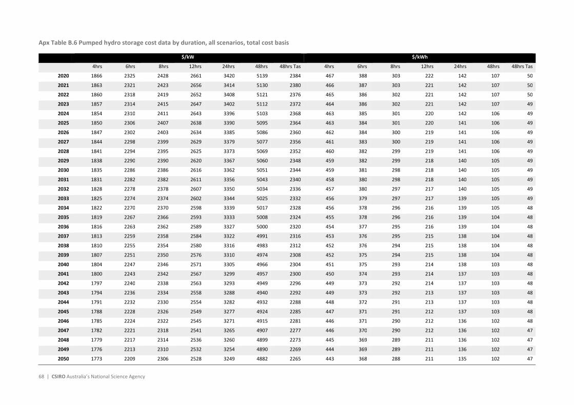
68 | CSIRO Australia’s National Science Agency
Apx Table B.6 Pumped hydro storage cost data by duration, all scenarios, total cost basis
$/kW $/kWh
4hrs 6hrs 8hrs 12hrs 24hrs 48hrs 48hrs Tas 4hrs 6hrs 8hrs 12hrs 24hrs 48hrs 48hrs Tas
2020 1866 2325 2428 2661 3420 5139 2384 467 388 303 222 142 107 50
2021 1863 2321 2423 2656 3414 5130 2380 466 387 303 221 142 107 50
2022 1860 2318 2419 2652 3408 5121 2376 465 386 302 221 142 107 50
2023 1857 2314 2415 2647 3402 5112 2372 464 386 302 221 142 107 49
2024 1854 2310 2411 2643 3396 5103 2368 463 385 301 220 142 106 49
2025 1850 2306 2407 2638 3390 5095 2364 463 384 301 220 141 106 49
2026 1847 2302 2403 2634 3385 5086 2360 462 384 300 219 141 106 49
2027 1844 2298 2399 2629 3379 5077 2356 461 383 300 219 141 106 49
2028 1841 2294 2395 2625 3373 5069 2352 460 382 299 219 141 106 49
2029 1838 2290 2390 2620 3367 5060 2348 459 382 299 218 140 105 49
2030 1835 2286 2386 2616 3362 5051 2344 459 381 298 218 140 105 49
2031 1831 2282 2382 2611 3356 5043 2340 458 380 298 218 140 105 49
2032 1828 2278 2378 2607 3350 5034 2336 457 380 297 217 140 105 49
2033 1825 2274 2374 2602 3344 5025 2332 456 379 297 217 139 105 49
2034 1822 2270 2370 2598 3339 5017 2328 456 378 296 216 139 105 48
2035 1819 2267 2366 2593 3333 5008 2324 455 378 296 216 139 104 48
2036 1816 2263 2362 2589 3327 5000 2320 454 377 295 216 139 104 48
2037 1813 2259 2358 2584 3322 4991 2316 453 376 295 215 138 104 48
2038 1810 2255 2354 2580 3316 4983 2312 452 376 294 215 138 104 48
2039 1807 2251 2350 2576 3310 4974 2308 452 375 294 215 138 104 48
2040 1804 2247 2346 2571 3305 4966 2304 451 375 293 214 138 103 48
2041 1800 2243 2342 2567 3299 4957 2300 450 374 293 214 137 103 48
2042 1797 2240 2338 2563 3293 4949 2296 449 373 292 214 137 103 48
2043 1794 2236 2334 2558 3288 4940 2292 449 373 292 213 137 103 48
2044 1791 2232 2330 2554 3282 4932 2288 448 372 291 213 137 103 48
2045 1788 2228 2326 2549 3277 4924 2285 447 371 291 212 137 103 48
2046 1785 2224 2322 2545 3271 4915 2281 446 371 290 212 136 102 48
2047 1782 2221 2318 2541 3265 4907 2277 446 370 290 212 136 102 47
2048 1779 2217 2314 2536 3260 4899 2273 445 369 289 211 136 102 47
2049 1776 2213 2310 2532 3254 4890 2269 444 369 289 211 136 102 47
2050 1773 2209 2306 2528 3249 4882 2265 443 368 288 211 135 102 47

GenCost 2020-21 | 69
Apx Table B.7 Storage cost data by source, total cost basis
$/kWh
$/kW Aurecon 2019 Aurecon 2020 Entura 2018
(higher 2 projects)
AEMO ISP July 2020
Aurecon 2019 Aurecon 2020 Entura 2018 (higher 2 projects)
AEMO ISP July 2020
Battery (1hr) 988 827 - - 988 827 - - Battery (2hrs) 622 542 - - 1244 1083 - - Battery (4hrs) 491 446 - - 1964 1783 - - PHES (6hrs) - - 308 388 - - 1850 2325 Battery (8hrs) 446 421 - - 3564 3365 - - PHES (12hrs) - - 177 222 - - 2118 2661 PHES (24hrs) - - 131 142 - - 3139 3420 PHES (48hrs) - - 73 107 - - 3517 5139 PHES (48hrs) Tasmania
- - - 50 - - - 2384

70 | CSIRO Australia’s National Science Agency
Apx Table B.8 Data assumptions for LCOE calculations
Constant Low assumption High assumption
Economic life Construction time Efficiency O&M fixed O&M variable CO2 storage Capital Fuel Capacity factor Emission factor Carbon price Capital Fuel Capacity factor Emission factor Carbon price
Years Years
$/kW $/MWh $/MWh
$/kW $/GJ
ktCO2e/PJ $/tCO2e
$/kW $/GJ
ktCO2e/PJ $/tCO2e
2020
Gas with CCS 25 1.5 0.44 16.4 7.2 1.9 4461 5.8 0.80 10.3 18.1 4461 11.3 0.60 19.9 30.7
Gas combined cycle 25 1.5 0.51 10.9 3.7 0.0 1801 5.8 0.80 56.0 18.1 1801 11.3 0.60 65.6 30.7
Gas open cycle (small) 25 1.3 0.36 12.6 4.1 0.0 1550 5.8 0.20 57.0 18.1 1550 11.3 0.20 66.6 30.7
Gas open cycle (large) 25 1.1 0.33 10.2 2.4 0.0 961 5.8 0.20 57.0 18.1 961 11.3 0.20 66.6 30.7
Gas reciprocating 25 1.0 0.41 24.1 7.6 0.0 1567 5.8 0.20 57.4 18.1 1567 11.3 0.20 67.0 30.7
Black coal with CCS 30 2.0 0.30 77.8 8.0 4.1 9311 2.8 0.80 8.5 18.1 9311 4.1 0.60 15.4 30.7
Black coal 30 2.0 0.40 53.2 4.2 0.0 4450 2.8 0.80 88.0 18.1 4450 4.1 0.60 88.0 30.7
Brown coal with CCS 30 4.0 0.21 101.6 11.6 4.7 14293 0.6 0.80 5.8 18.1 14293 0.7 0.60 5.8 30.7
Brown coal 30 4.0 0.32 69.0 5.3 0.0 6868 0.6 0.80 85.0 18.1 6868 0.7 0.60 85.0 30.7
Biomass (small scale) 30 2.0 0.23 131.6 8.4 0.0 8619 0.5 0.60 0.0 18.1 8619 2.0 0.40 0.0 30.7
Nuclear (SMR) 30 3.0 0.30 200.0 20.0 0.0 16487 0.5 0.80 0.0 18.1 16487 0.7 0.60 0.0 30.7
Large scale solar PV 25 0.5 1.00 17.0 0.0 0.0 1408 0.0 0.32 0.0 18.1 1408 0.0 0.22 0.0 30.7
Solar thermal (8hrs) 25 1.8 1.00 142.5 0.0 0.0 7411 0.0 0.52 0.0 18.1 7411 0.0 0.42 0.0 30.7
Wind 25 1.0 1.00 25.0 0.0 0.0 1951 0.0 0.44 0.0 18.1 1951 0.0 0.35 0.0 30.7
2030
Gas with CCS 25 1.5 0.44 16.4 7.2 1.9 4417 5.8 0.80 10.3 29.5 4417 11.8 0.60 19.9 129.0
Gas combined cycle 25 1.5 0.51 10.9 3.7 0.0 1765 5.8 0.80 56.0 29.5 1765 11.8 0.60 65.6 129.0
Gas open cycle (small) 25 1.3 0.36 12.6 4.1 0.0 1519 5.8 0.20 57.0 29.5 1519 11.8 0.20 66.6 129.0
Gas open cycle (large) 25 1.1 0.33 10.2 2.4 0.0 942 5.8 0.20 57.0 29.5 942 11.8 0.20 66.6 129.0
Gas reciprocating 25 1.0 0.41 24.1 7.6 0.0 1536 5.8 0.20 57.4 29.5 1536 11.8 0.20 67.0 129.0
Black coal with CCS 30 2.0 0.30 77.8 8.0 4.1 9171 2.9 0.80 8.5 29.5 9171 3.8 0.60 15.4 129.0
Black coal 30 2.0 0.40 53.2 4.2 0.0 4362 2.9 0.80 88.0 29.5 4362 3.8 0.60 88.0 129.0
Brown coal with CCS 30 4.0 0.21 101.6 11.6 4.7 14054 0.7 0.80 5.8 29.5 14054 0.7 0.60 5.8 129.0
Brown coal 30 4.0 0.32 69.0 5.3 0.0 6732 0.7 0.80 85.0 29.5 6732 0.7 0.60 85.0 129.0
Biomass (small scale) 30 2.0 0.23 131.6 8.4 0.0 8606 0.5 0.60 0.0 29.5 8606 2.0 0.40 0.0 129.0
Nuclear (SMR) 30 3.0 0.35 200.0 20.0 0.0 7237 0.5 0.80 0.0 29.5 16487 0.7 0.60 0.0 129.0
Large scale solar PV 25 0.5 1.00 17.0 0.0 0.0 780 0.0 0.32 0.0 29.5 874 0.0 0.19 0.0 129.0
Solar thermal (8hrs) 25 1.8 1.00 142.5 0.0 0.0 6264 0.0 0.52 0.0 29.5 6732 0.0 0.42 0.0 129.0
Wind 25 1.0 1.00 25.0 0.0 0.0 1899 0.0 0.46 0.0 29.5 1892 0.0 0.35 0.0 129.0

GenCost 2020-21 | 71
2040
Gas with CCS 25 1.5 0.44 16.4 7.2 1.9 3390 5.8 0.80 10.3 48.1 4374 11.8 0.60 19.9 220.3
Gas combined cycle 25 1.5 0.51 10.9 3.7 0.0 1730 5.8 0.80 56.0 48.1 1730 11.8 0.60 65.6 220.3
Gas open cycle (small) 25 1.3 0.36 12.6 4.1 0.0 1489 5.8 0.20 57.0 48.1 1489 11.8 0.20 66.6 220.3
Gas open cycle (large) 25 1.1 0.33 10.2 2.4 0.0 923 5.8 0.20 57.0 48.1 923 11.8 0.20 66.6 220.3
Gas reciprocating 25 1.0 0.41 24.1 7.6 0.0 1505 5.8 0.20 57.4 48.1 1505 11.8 0.20 67.0 220.3
Black coal with CCS 30 2.0 0.30 77.8 8.0 4.1 8043 2.9 0.80 8.5 48.1 9034 3.8 0.60 15.4 220.3
Black coal 30 2.0 0.40 53.2 4.2 0.0 4275 2.9 0.80 88.0 48.1 4275 3.8 0.60 88.0 220.3
Brown coal with CCS 30 4.0 0.21 101.6 11.6 4.7 12827 0.7 0.80 5.8 48.1 13820 0.7 0.60 5.8 220.3
Brown coal 30 4.0 0.32 69.0 5.3 0.0 6599 0.7 0.80 85.0 48.1 6599 0.7 0.60 85.0 220.3
Biomass (small scale) 30 2.0 0.23 131.6 8.4 0.0 8606 0.5 0.60 0.0 48.1 8606 2.0 0.40 0.0 220.3
Nuclear (SMR) 30 3.0 0.40 200.0 20.0 0.0 7205 0.5 0.80 0.0 48.1 16487 0.7 0.60 0.0 220.3
Large scale solar PV 25 0.5 1.00 17.0 0.0 0.0 582 0.0 0.32 0.0 48.1 727 0.0 0.19 0.0 220.3
Solar thermal (8hrs) 25 1.8 1.00 142.5 0.0 0.0 5874 0.0 0.52 0.0 48.1 6224 0.0 0.42 0.0 220.3
Wind 25 1.0 1.00 25.0 0.0 0.0 1842 0.0 0.48 0.0 48.1 1792 0.0 0.35 0.0 220.3
2050
Gas with CCS 25 1.5 0.44 16.4 7.2 1.9 3325 5.8 0.80 10.3 64.6 3982 11.8 0.60 19.9 386.7
Gas combined cycle 25 1.5 0.51 10.9 3.7 0.0 1697 5.8 0.80 56.0 64.6 1697 11.8 0.60 65.6 386.7
Gas open cycle (small) 25 1.3 0.36 12.6 4.1 0.0 1461 5.8 0.20 57.0 64.6 1461 11.8 0.20 66.6 386.7
Gas open cycle (large) 25 1.1 0.33 10.2 2.4 0.0 905 5.8 0.20 57.0 64.6 905 11.8 0.20 66.6 386.7
Gas reciprocating 25 1.0 0.41 24.1 7.6 0.0 1477 5.8 0.20 57.4 64.6 1477 11.8 0.20 67.0 386.7
Black coal with CCS 30 2.0 0.30 77.8 8.0 4.1 7891 2.9 0.80 8.5 64.6 8553 3.8 0.60 15.4 386.7
Black coal 30 2.0 0.40 53.2 4.2 0.0 4195 2.9 0.80 88.0 64.6 4195 3.8 0.60 88.0 386.7
Brown coal with CCS 30 4.0 0.21 101.6 11.6 4.7 12584 0.7 0.80 5.8 64.6 13248 0.7 0.60 5.8 386.7
Brown coal 30 4.0 0.32 69.0 5.3 0.0 6474 0.7 0.80 85.0 64.6 6474 0.7 0.60 85.0 386.7
Biomass (small scale) 30 2.0 0.23 131.6 8.4 0.0 8606 0.5 0.60 0.0 64.6 8606 2.0 0.40 0.0 386.7
Nuclear (SMR) 30 3.0 0.45 200.0 20.0 0.0 7205 0.5 0.80 0.0 64.6 16487 0.7 0.60 0.0 386.7
Large scale solar PV 25 0.5 1.00 17.0 0.0 0.0 546 0.0 0.32 0.0 64.6 585 0.0 0.19 0.0 386.7
Solar thermal (8hrs) 25 1.8 1.00 142.5 0.0 0.0 5341 0.0 0.52 0.0 64.6 5641 0.0 0.42 0.0 386.7
Wind 25 1.0 1.00 25.0 0.0 0.0 1772 0.0 0.50 0.0 64.6 1745 0.0 0.35 0.0 386.7
Notes: Wind is onshore. Large-scale solar PV is single axis tracking. Emission factors include fugitive emissions associated with the fuel. The low emission factor is from the lowest state average and the high from the highest emission state. The discount rate used for all technologies is 5.99%.

72 | CSIRO Australia’s National Science Agency
Apx Table B.9 Electricity generation technology LCOE projections data, 2020-21 $/MWh
Category Assumption Technology 2020 2030 2040 2050 Low High Low High Low High Low High Peaking 20% load Carbon price Gas open cycle (small) 154 219 159 289 168 348 176 458 Gas open cycle (large) 127 198 133 274 144 339 153 458
Gas reciprocating 155 213 159 274 167 327 174 423 Flexible 40-80% load, high emission No carbon price or risk premium Black coal 89 120 88 116 87 114 86 113 Brown coal 112 145 111 143 110 142 108 139
Gas 68 115 67 118 67 117 67 117 No carbon price, 5% risk premium Black coal 127 171 126 166 124 163 122 161
Brown coal 193 254 190 249 188 246 184 242 Gas 82 133 81 136 80 135 80 134
Carbon price Black coal 103 144 111 218 125 289 137 419 Brown coal 129 175 139 268 156 354 170 512
Gas 75 129 79 178 86 220 92 296 Flexible 40-80% load, low emission Carbon price Black coal with CCS 167 226 167 238 156 253 156 276
Brown coal with CCS 230 299 229 305 216 311 214 318 Gas with CCS 114 181 115 201 104 215 104 236
Solar thermal 8hrs 172 213 150 197 143 185 133 171 Nuclear (SMR) 258 338 143 336 142 335 141 335
Biomass (small scale) 175 277 175 277 175 277 175 277 Variable Standalone Wind 48 61 45 59 42 57 39 55
Solar photovoltaic 46 68 28 52 23 45 22 38

GenCost 2020-21 | 73
Apx Table B.10 Hydrogen electrolyser cost projections by scenario and technology, 2020-21 $/kW
Central High VRE Diverse technology Alkaline PEM Alkaline PEM Alkaline PEM
2020 2516 3510 2516 3510 2516 3510 2021 2066 2760 1847 2716 2062 2743 2022 1773 2239 1631 2164 1771 2212 2023 1580 1868 1491 1771 1583 1836 2024 1458 1607 1409 1493 1467 1571 2025 1390 1432 1374 1305 1406 1393 2026 1346 1303 1350 1164 1370 1260 2027 1305 1188 1315 1041 1337 1143 2028 1264 1086 1280 932 1307 1039 2029 1225 998 1246 840 1280 950 2030 1185 919 1208 758 1253 870 2031 1147 852 1169 689 1224 796 2032 1108 792 1127 628 1194 731 2033 1068 738 1080 574 1161 674 2034 1028 691 1031 527 1125 622 2035 989 649 982 485 1088 577 2036 950 612 931 449 1048 538 2037 914 581 883 417 1009 504 2038 882 554 838 390 972 475 2039 853 531 797 367 937 450 2040 828 513 760 347 905 429 2041 808 497 728 330 868 405 2042 791 484 699 315 834 385 2043 777 474 674 302 804 367 2044 766 466 652 291 776 352 2045 757 459 632 282 750 338 2046 750 454 614 273 727 326 2047 744 449 598 265 705 315 2048 739 446 582 258 684 305 2049 735 443 568 251 665 295 2050 732 441 555 245 647 287

74 | CSIRO Australia’s National Science Agency
Shortened forms
Abbreviation Meaning
AE Alkaline electrolysis
AEMO Australian Energy Market Operator
bbl Barrel
BOP Balance of plant
CCS Carbon capture and storage
CHP Combined heat and power
CO2 Carbon dioxide
CO2e Carbon dioxide equivalent
CSIRO Commonwealth Scientific and Industrial Research Organisation
CSP Concentrated solar power
DIETER Dispatch and investment evaluation tool with endogenous renewables
EV Electric vehicle
GALLME Global and Local Learning Model Electricity
GALLMs Global and Local Learning Models
GALLMT Global and Local Learning Model Transport
hrs Hours
IEA International Energy Agency
IGCC Integrated gasification combined cycle
ISP Integrated System plan
kW Kilowatt
kWh Kilowatt hour

GenCost 2020-21 | 75
Abbreviation Meaning
LCOE Levelised Cost of Electricity
LCV Light commercial vehicle
MCV Medium commercial vehicle
Li-ion Lithium-ion
LR Learning Rate
MW Megawatt
MWh Megawatt hour
O&M Operations and Maintenance
OECD Organisation for Economic Cooperation and Development
PEM Proton-exchange membrane electrolysis
pf Pulverised fuel
PHES Pumped hydro energy storage
PV Photovoltaic
SDS Sustainable Development Scenario
SMR Small modular reactor
STABLE Spatial Temporal Analysis of Balancing Levelised-cost of Energy
t tonne
TWh Terawatt hour
VRE Variable Renewable Energy
WEO World Energy Outlook

76 | CSIRO Australia’s National Science Agency
References
ACIL ALLEN 2018, Opportunities for Australia from Hydrogen Exports. ACIL ALLEN Consulting for ARENA.
Aurecon 2020, 2020 costs and technical parameter review, AEMO.
AUSTEn 2020 Tidal Energy in Australia - Assessing resource and feasibility for Australia's future energy mix. Milestone 4 report to ARENA
Australian Electricity Market Operator (AEMO) 2020, Input and assumptions workbook v1 5 Jul 20, AEMO.
BNEF 2020, Hydrogen Economy Outlook, March 2020.
Brinsmead, T., Graham, P. and Qiu, J. 2017. Economic benefits of the Electricity Network Transformation Roadmap: Technical report, CSIRO report for the Energy Networks Australia, Australia.
Brinsmead T.S., Graham, P., Hayward, J., Ratnam, E.L., and Reedman, L. 2015, Future Energy Storage Trends: An Assessment of the Economic Viability, Potential Uptake and Impacts of Electrical Energy Storage on the NEM 2015-2035, AEMC, Australia.
Brinsmead, T., Rendall, A., Baynes, T., Butler, C., Kelly, R., Adams, P., . . . Yu, Y. 2019, Australian National Outlook 2019 Technical Report, CSIRO, Australia, https://publications.csiro.au/rpr/pub?pid=csiro:EP183813
Bruce, S., Temminghoff, M., Hayward, J., Schmidt, E., Munnings, C., Palfreyman, D., and Hartley, P. 2018, National Hydrogen Roadmap, CSIRO, Australia, https://www.csiro.au/en/Do-business/Futures/Reports/Hydrogen-Roadmap
Campey, T., Bruce, S., Yankos, T., Hayward, J., Graham, P., Reedman, L., Brinsmead, T., Deverell, J. 2017, Low Emissions Technology Roadmap, CSIRO, Australia.
Cavanagh, K., Ward, J. K., Behrens, S., Bhatt, A. R., E, O., & J, H. 2015, Electrical energy storage: technology overview and applications. CSIRO for AEMC.
Clarke L., K. Jiang, K. Akimoto, M. Babiker, G. Blanford, K. Fisher-Vanden, J.-C. Hourcade, V. Krey, E. Kriegler, A. Löschel, D. McCollum, S. Paltsev, S. Rose, P. R. Shukla, M. Tavoni, B. C. C. van der Zwaan, and D.P. van Vuuren, 2014, Assessing Transformation Pathways. In: Climate Change 2014: Mitigation of Climate Change. Contribution of Working Group III to the Fifth Assessment Report of the Intergovernmental Panel on Climate Change [Edenhofer, O., R. Pichs-Madruga, Y. Sokona, E. Farahani, S. Kadner, K. Seyboth, A. Adler, I. Baum, S. Brunner, P. Eickemeier, B. Kriemann, J. Savolainen, S. Schlömer, C. von Stechow, T. Zwickel and J.C. Minx (eds.)]. Cambridge University Press, Cambridge, United Kingdom and New York, NY, USA.
CO2CRC 2015, Australian Power Generation Technology Report, CO2CCRC, Canberra.

GenCost 2020-21 | 77
Deloitte 2019, Australian and Global Hydrogen Demand Growth Scenario Analysis. COAG Energy Council – National Hydrogen Strategy Taskforce.
Edmonds, J., Lucknow, P., Calvin, K., Wise, M., Dooley, J., Kyle, P., . . . Clarke, L. 2013, Can radiative forcing be limited to 2.6Wm(-2) without negative emissions from bioenergy and CO2 capture and storage? Climatic Change, 118(1), 29-43 SI. doi:10.1007/s10584-012-0678.2
Electric Power Research Institute (EPRI) 2010, Australian Electricity Generation Technology Costs – Reference Case 2010. Department of Resources, Energy and Tourism, Canberra.
Entura 2018, Pumped hydro cost modelling, AEMO, https://www.aemo.com.au/-/media/Files/Electricity/NEM/Planning_and_Forecasting/Inputs-Assumptions-Methodologies/2019/Report-Pumped-Hydro-Cost-Modelling.pdf
Fraunhofer ISE, 2015. Current and Future Cost of Photovoltaics. Long-term Scenarios for Market Development, System Prices and LCOE of Utility-Scale PV Systems, s.l.: Study on behalf of Agora Energiewende
Gas Turbine World 2009, Gas Turbine World Handbook.
Gas Turbine World 2010, Gas Turbine World Handbook.
Gas Turbine World 2011, Gas Turbine World Handbook.
Gas Turbine World 2012, Gas Turbine World Handbook.
Gas Turbine World 2013, Gas Turbine World Handbook.
GHD 2018, AEMO costs and technical parameter review: Report final Rev 4 9110715, AEMO, Australia.
Government of India. 2016, A new dawn in renewable energy. India: Ministry of new and renewable energy. Retrieved from http://pib.nic.in/newsite/PrintRelease.aspx?relid=155612
Graham, P., Hayward, J., Foster, J. and Havas, L. 2020, GenCost 2019-20, Australia.
Graham, P.W., Hayward, J, Foster, J., Story, O. and Havas, L. 2018, GenCost 2018, CSIRO, Australia.
Graham, P. 2018, Review of alternative methods for extending LCOE calculations to include balancing costs. CSIRO, Australia.
Grübler, A., Nakicenovic, N., & Victor, D. G. 1999, Dynamics of energy technologies and global change. Energy Policy, 27(5), 247-280.
GWEC. (n.d.). Global Wind Report Series 2006 to 2016. Global Wind Energy Council.
Hayward, J. A., Foster, J. D., Graham, P. W., & Reedman, L. J. 2017. A Global and Local Learning Model of Transport (GALLM-T). In Syme, G., Hatton MacDonald, D., Fulton, B. and Piantadosi, J. (eds) MODSIM2017, 22nd International Congress on Modelling and Simulation. Modelling and Simulation Society of Australia and New Zealand, December 2017, pp. 818-824. ISBN: 978-0-9872143-7-9. https://www.mssanz.org.au/modsim2017/F1/hayward.pdf [accessed 18 December 2018]
Hayward, J.A. and Graham, P.W. 2017, Electricity generation technology cost projections: 2017-2050, CSIRO, Australia, https://publications.csiro.au/rpr/download?pid=csiro:EP178771&dsid=DS2

78 | CSIRO Australia’s National Science Agency
Hayward, J. and Graham, P. 2013, A global and local endogenous experience curve model for projecting future uptake and cost of electricity generation technologies, Energy Economics, 40, 537-548.
International Energy Agency (IEA) 2008, Electricity Information 2008 Edition. Paris, France: IEA.
International Energy Agency (IEA) 2008, World Energy Outlook. Paris, France: IEA.
International Energy Agency (IEA) 2015,. Projected costs of Generating Electricity . Paris, France: OECD.
International Energy Agency (IEA) 2016, CSP Projects Around the World. Retrieved from SolarPACES: http://www.solarpaces.org/csp-technology/csp-projects-around-the-world
International Energy Agency (IEA) 2016, World Energy Outlook . Paris, France: OECD.
International Energy Agency (IEA) 2017, World Energy Outlook . Paris: OECD.
International Energy Agency (IEA) 2018, World Energy Outlook . Paris: OECD.
International Energy Agency (IEA) 2020, World Energy Outlook . Paris: OECD.
International Energy Agency (IEA) n.d. Trends in Photovoltaic Applications Series from 2007 to 2016. Paris, France: IEA.
IPCC, 2014, Climate Change 2014: Mitigation of Climate Change. Contribution of Working Group III to the Fifth Assessment Report of the Intergovernmental Panel on Climate Change. Cambridge, United Kingdom and New York, NY, USA: Cambridge University Press.
IRENA 2019, Renewable Power Generation Costs in 2018. IRENA.
Jacobs 2017, Report to the Independent Review into the Future Security of the National Electricity Market: Emission mitigation policies and security of supply, Department of Energy and Environment, Canberra.
McDonald, A., & Schrattenholzer, L. 2001, Learning rates for energy technologies. Energy Policy, 29, 255-261.
Neij, L. 2008, Cost development of future technologies for power generation-A study based on experience curves and complementary bottom-up assessments. Energy Policy, 36(6), 2200-2211.
Rubin, E. S., Yeh, S., Antes, M., Berkenpas, M., & Davison, J. (2007). Use of experience curves to estimate the future cost of power plants with CO2 capture. International Journal of Greenhouse Gas Control, 1(2), 188-197.
Samadi, S. 2018, The experience curve theory and its application in the field of electricity generation technologies, Renewable & Sustainable Energy Reviews, Vol. 82 , pp 2346-2364
Schmidt, O., Hawkes, A., Gambhir, A., & Staffell, I. 2017, The future cost of electrical energy storage based on experience rates. Nature Energy, 2, 17110.
Schoots, K., Kramer, G.J. and Zwaan, B. 2010, Technology Learning for Fuel Cells: An Assessment of Past and Potential Cost Reductions, Energy Policy, vol. 38, pp. 2887-2897
Schrattenholzer, L., and McDonald, A. 2001 Learning rates for energy technologies. Energy Policy, 29, 255-261.

GenCost 2020-21 | 79
UN 2015. Energy Statistics Yearbook 2012. New York, USA: United Nations.
UN 2015. Energy Statistics Yearbook 2013. New York, USA: United Nations.
US Energy Information Administration 2017, World installed liquids-fired generating capacity by region and country. Retrieved from https://www.eia.gov/outlooks/aeo/data/browser/#/?id=17-IEO2016®ion=0-0&cases=Reference&start=2010&end=2016&f=A&linechart=Reference-d021916a.2-17-IEO2016&sourcekey=0
US Energy Information Administration 2017, World installed natural-gas-fired generating capacity by region and country. Retrieved from https://www.eia.gov/outlooks/aeo/data/browser/#/?id=18-IEO2016®ion=0-0&cases=Reference&start=2010&end=2016&f=A&sourcekey=0
Voormolen, J.A., Junginger, H.M. and van Sark, W.G.J.H.M., 2016. Unravelling historical cost developments of offshore wind energy in Europe, Energy Policy, Elsevier, vol. 88(C), pp 435-444.
Wilson, C. (2012). Up-scaling, formative phases, and learning in the historical diffusion of energy technologies. Energy Policy, 50(0), 81-94, http://dx.doi.org/10.1016/j.enpol.2012.04.077
World Nuclear Association 2017, World Nuclear Power Reactors and Uranium Requirements. Retrieved from www.world-nuclear.org: http://www.world-nuclear.org/information-library/facts-and-figures/world-nuclear-power-reactors-and-uranium-requireme.aspx
Wright, T. P. 1936, Factors Affecting the Cost of Airplanes. Journal of the Aeronautical Sciences, 3, 122-128.
Zwaan, B., Rivera Tinoco, R., Lensink, S. and Van den oosterkamp, P. 2012, Cost reductions for offshore wind power: Exploring the balance between scaling, learning and R&D, Renewable Energy, pp389-393

80 | CSIRO Australia’s National Science Agency
The GenCost project is a partnership of CSIRO and AEMO.
As Australia’s national science agency and innovation catalyst, CSIRO is solving the greatest challenges through innovative science and technology.
CSIRO. Unlocking a better future for everyone.
Contact us
1300 363 400 +61 3 9545 2176 [email protected] csiro.au
For further information
Energy Paul Graham +61 2 4960 6061 [email protected] csiro.au/energy