
Baseline - CSIRO Research Publications Repository
93
Baseline 2001-2002 ATMOSPHERIC PROGRAM (Australia) 2001-2002
-
Upload
khangminh22 -
Category
Documents
-
view
5 -
download
0
Transcript of Baseline - CSIRO Research Publications Repository

Baseline 2001-2002
ATMOSPHERIC PROGRAM (Australia) 2001-2002

Bureau of Meteorology and
CSIRO Atmospheric Research
Baseline Atmospheric Program Australia 2001-2002
Edited by J M Cainey, N Derek and P B Krummel
2004
Cover: Images showing views of, and from Cape Grim Baseline Air Pollution Station. Photos by Paul Krummel© (bottom panel); Bim Graham© (top left and right panels)

ii
©Copyright: Commonwealth of Australia, 2004 Published for the Bureau of Meteorology and CSIRO Atmospheric Research, Melbourne ISBN 0 643 06890 2 https://doi.org/10.4225/08/585974b9791e4

Foreword
iii
FOREWORD
Science is totally reliant on its empirical basis. Al-though formal approaches to the development of science often stress the need to formulate and test hypotheses, history suggests that the genesis of most major advances in scientific understanding has generally been in careful observation of the world around us. Whether it be Darwin’s painstaking documentation of patterns in biological systems, or Joe Farman and his colleagues identifying the totally unanticipated Antarctic Ozone Hole, observation is the first step in scientific discovery.
The importance of careful observations has been demonstrated many times in the development of our understanding of global scale atmospheric chemistry. Early measurements of carbon monoxide concentra-tions in the atmosphere led to a recognition that at-mospheric oxidation must be much more rapid than estimates based on known chemistry at the time. Similarly, the first precise measurements of carbon dioxide by Dave Keeling revealed a previously unsus-pected repeating seasonal cycle in concentration and opened the door to insights into the interactions be-tween the biosphere and the atmosphere which are still expanding. The discovery of the Antarctic Ozone Hole, already mentioned, not only led to a much richer understanding of stratospheric chemistry, but also provided a clear stimulus for policy on the manage-ment of ozone depleting substances.
This link to policy introduces additional responsi-bilities as well as a sense of urgency for observa-tional programmes in atmospheric chemistry. The atmosphere has never before been in its present state and the rate of change in its composition is both unprecedented and clearly due to human activi-ties. While our ability to predict the future effects of these changes remains limited, we do know that changes in atmospheric chemistry have the potential to affect human welfare now and increasingly in the future. It is worth recalling that in just over 50 years, i.e. less than two generations of atmospheric scien-tists, we have gone from not really knowing whethercarbon dioxide was increasing in the atmosphere toan extensive intergovernmental process to considerfuture management options for reducing that in-crease in the future.
The central role played by observations in global atmospheric chemistry has been successful because it has been carried out in a research context. From time to time senior research managers suggest that measurements of atmospheric composition might be put on an operational basis and run as an adjunct of traditional meteorological measurement networks. In a limited number of cases this might be valid but, for most of the species we measure, the required preci-sion and coverage remains challenging or elusive with present technology, particularly when it is necessary to merge data from different networks. So there are sound technical reasons why measurement of atmos-pheric composition should be conducted as a re-search activity. But more importantly rooting meas-
urement programmes in an active research context has provided them with a rapidly evolving sense of purpose and with the drive for the precision and spa-tial coverage required to resolve key questions.
The atmospheric research programme at the Cape Grim station has from its outset been an outstanding example of an atmospheric programme devoted to comprehensive state of the art measurements and conducted with clear research goals. As can be seen from this report of activities in 2001 and 2002, the sta-tion is a key site for international networks such as AGAGE and the WMO Global Atmosphere Watch. The large amounts of data generated within these networks are used widely throughout the international atmospheric science community and are fundamental to tracking ongoing global change. The importance of the research based drive for such measurements is shown very clearly here in the efforts being taken to improve network precision with the LoFlo CO2 ana-lyser, and to measure new species being used as substitutes for CFCs using gas chromatograph mass spectrometer instrumentation.
A strong focus on new research questions is also shown here in the broad ranging interdisciplinary study of emissions from marine ecosystems which provides initial information for unravelling the myriad of relationships between ecosystem structure, nutri-ent availability, and the species released to the at-mosphere. Such detailed process studies are nec-essary if we are to understand biogeochemical feedbacks in climate change and they gain consid-erable strength from the infrastructure and baseline data at the Cape Grim station. The analyses pre-sented here of the ‘Melbourne plume’ and regional emissions are also fascinating because they dem-onstrate the enormous power of high frequency sampling and measurement of multiple species in combination with quantitative information on wind shifts and back trajectories. The unique geographic situation of the Cape Grim station allows methods such as these for determining regional emissions to be tested thoroughly in a relatively simple setting be-fore being considered in more complex situations of multiple or dispersed source regions.
These new studies of possible climate change feedbacks and regional emissions bring us back to the increasing policy relevance of careful and pre-cise measurements of atmospheric composition. The Cape Grim station has the staff, resources and research focus needed to continue to play a major role in this area and, along with my colleagues around the world, I look forward to seeing the high standards of atmospheric research shown in this re-port continued throughout the foreseeable future.
Dr Martin R. Manning Director
IPCC Working Group I Support Unit
August, 2004

Preface
iv
PREFACE
Baseline 2001-2002 reports on the activities and scientific program at the Cape Grim Baseline Air Pollution Station in North West Tasmania, Australia, for the two calendar years of 2001 and 2002. In-cluded are scientific papers, based on research at Cape Grim, as well as operational reports on the various experiments and monitoring conducted at the station over the two year period.
For this edition of Baseline, we are fortunate to have a ‘Foreword’ provided by Dr Martin Manning, Director of the Technical Support Unit for the Inter-Governmental Panel on Climate Change, Working Group I (The Physical Basis of Climate Change). Prior to moving to NOAA, Boulder, USA to take up this important position, supporting the co-chair Susan Solomon, Martin was the Director of the Tro-pospheric Physics and Chemistry Group at the Na-tional Institute of Water and Atmospheric Research (NIWA), Wellington, NZ
NIWA run the Baring Head Clean Air Station, situated south east of Wellington, atop 90 m cliffs and while a smaller operation than the Cape Grim Station, Baring Head still provides and has provided significant quality data for a number of atmospheric species over many years. NIWA measurements of carbon dioxide in clean on-shore ‘baseline’ air com-menced in 1970 and at Baring Head from 1973. This
record for carbon dioxide is the longest in the South-ern Hemisphere, eclipsing even the record at Cape Grim. Martin was instrumental in setting up this measurement program and is ideally placed to comment on the role such measurements have in determining both research and policy directions.
Following the style of recent issues of Baseline, the layout of this edition includes both research pa-pers and reports from the various scientific pro-grams in operation at the Cape Grim station. Pro-gram reports contain the status of the research pro-grams for only the two year period. The research papers are stand-alone scientific articles that may present research results and data up to the final time of submission. The research papers have been scientifically peer-reviewed by at least two inde-pendent referees before being considered for publi-cation.
The research papers follow the American Geo-physical Union (AGU) publications formatting and referencing styles. Limited numbers of reprints of these papers are available from the lead author of each paper.
J M Cainey, N Derek and P B Krummel
June 2004

Contents
v
CONTENTS
1. STATION SPECIFICATION
1.1 General .......................................................................................................................... 1
1.2 Site plan ......................................................................................................................... 2
1.3 Program summary ......................................................................................................... 3 2. OFFICER-IN-CHARGE’S REPORT
2.1 Introduction .................................................................................................................... 5
2.2 Buildings and maintenance ............................................................................................ 5
2.3 Staff and students .......................................................................................................... 6
2.4 International activities and visitors ................................................................................. 6
2.5 Operational budget ........................................................................................................ 7 3. RESEARCH PAPERS
A preliminary investigation of the phytoplankton ecology and marine biogenic trace gas production near Cape Grim, Tasmania G Corno, A McMinn, G Sturrock, R Parr, N Tindale, L Porter, R Gillett, P Fraser, N Derek, C Reeves and S Penkett .............................................................................................................................. 8
Oil and gas activities near Cape Grim: implications for the atmospheric program D M Etheridge, C P Meyer and G O’Brien ....................................................................................... 15
Sulfur hexafluoride at Cape Grim: long term trends and regional emissions P J Fraser, L W Porter, S B Baly, P B Krummel, B L Dunse, L P Steele, N Derek, R L Langenfelds, I Levin, D E Oram, J W Elkins, M K Vollmer and R F Weiss ............................................................. 18
4. PROGRAM REPORTS (CALENDAR YEARS 2001-2002)
4.1 Introduction .................................................................................................................... 24
General 4.2 Data management – R P Wheaton .................................................................................. 24
4.3 Meteorology/Climatology – A Downey and M Tully .......................................................... 26
4.4 Radon and radon daughters – W Zahorowski ................................................................. 33
Trace gases 4.5 Baseline carbon dioxide monitoring – L P Steele, P B Krummel, D A Spencer, L W Porter,
S B Baly, R L Langenfelds, L N Cooper, M V van der Schoot and G A Da Costa .................... 36
4.6 δ13C and δ18O of CO2 in baseline Cape Grim air: 2001-2002 – C E Allison, L N Cooper, S A Coram and R J Francey .............................................................................................. 41
4.7 Continuous measurements of 14C in atmospheric CO2 at Cape Grim, 1997-2002 – I Levin, B Kromer, R J Francey and L W Porter ................................................................... 44

Contents
vi
4.8 Atmospheric methane, carbon dioxide, hydrogen, carbon monoxide and nitrous oxide from Cape Grim flask air samples analysed by gas chromatography – R L Langenfelds, L P Steele, M V van der Schoot, L N Cooper, D A Spencer and P B Krummel ........................ 46
4.9 SF6 from flask sampling – I Levin, R Heinz, J. Ilmberger, R L Langenfelds, R J Francey, L P Steele and D A Spencer .............................................................................................. 48
4.10 Archiving of Cape Grim air – R L Langenfelds, P J Fraser, L P Steele and L W Porter ........ 48
4.11 Halocarbons, nitrous oxide, methane, carbon monoxide and hydrogen: The AGAGE program, 1993-2002 – P B Krummel, P J Fraser, L P Steele, N Derek, L W Porter, B L Dunse and R L Langenfelds ......................................................................................................... 50
4.12 HCFCs, HFCs, halons, minor CFCs, PCE and halomethanes: the AGAGE in situ GC-MS program at Cape Grim, 1998-2002 – P B Krummel, L W Porter, P J Fraser, S B Baly, B L Dunse and N Derek ...................................................................................... 57
4.13 Sulfur hexafluoride in situ program at Cape Grim, 2001-2002 – L W Porter, P B Krummel, S B Baly, P J Fraser, L P Steele, N Derek and B L Dunse .................................................... 63
4.14 Phytoplankton dynamics and the production of methyl bromide at Cape Grim: 2001-2002 – A McMinn, J Cainey, C Lane, G Sturrock, C Parr, N Tindale, L, Porter, R Gillett, P Fraser, C Reeves and S Penkett ..................................................................................... 64
4.15 Studies of ozone, NOx and VOCs in near surface air at Cape Grim, 2002 – I E Galbally, C P Meyer and S T Bentley ............................................................................................... 67
Precipitation, particles and multi-phase species 4.16 Particles – J L Gras ......................................................................................................... 69
4.17 Fine particle sampling at Cape Grim – D D Cohen, D Garton, E Stelcer and O Hawas ....... 71
4.18 Precipitation chemistry – R W Gillett, G P Ayers and P W Selleck ...................................... 72
4.19 High volume aerosol sampler – M D Keywood, B Graham, R W Gillett , J L Gras and P W Selleck ..................................................................................................................... 74
4.20 Measurement of natural levels of tritium in precipitation – C Tadros, D Hill and D Stone... 78
Radiation 4.21 Spectral solar radiation – S R Wilson and B W Forgan ..................................................... 79
4.22 Passive solar radiation – S R Wilson ............................................................................... 80 APPENDICES
A. Publications .................................................................................................................... 81
B. Personnel ....................................................................................................................... 85
C. Definitions ...................................................................................................................... 86

Station specification - Site plan
1
1. STATION SPECIFICATION
1.1 GENERAL
Name Cape Grim Baseline Air Pollution Station
Latitude 40o 41’ 00” (40.383o) S
Longitude 144o 41’ 22” (144.689o) E (DATUM GDA94)
Roofdeck elevation 94 metres
Air intake elevations 104 metres (10-m intake) 164 metres (70-m intake)
WMO station classification Baseline (global)
Status Fully operational
Station ID indices WMO station code 94954 WMO index number A2000 101 WMO turbidity code number 03 050 WMO ozone code number 230 AWS station code 94954
Time zone Australian Eastern Standard Time (AEST) (AEST = UTC + 10 hours; the station operates on AEST year-round)
Office hours 0845-1700 local time (AEST plus 1 hour in summer)
Telephone Smithton office (03) 6452 1629 International dialling 61 3 6452 1629 Station (03) 6452 2181 Facsimile Smithton (03) 6452 2600 Facsimile Station (03) 6452 2582
E-mail [email protected]
Postal address P.O. Box 346, Smithton, Tasmania 7330, Australia
Freight address 159 Nelson Street, Smithton, Tasmania 7330, Australia

Station specification - Site plan
2
1.2 SITE PLAN
Site Plan
1. Baseline ERNI 2. Continuous ERNI 3. Raindrop sensor 4. Tipping-bucket rain gauge 5. Standard 203 mm rain gauge 6. Stevenson screen 7. Station exhausts 8. Telstra tower (74 m) 9. 70-m intake
10. Wind vane and anemometer (50 m)
11. 50-m Temperature sensor 12. Wind vane and anemometer
(30 m) 13. Radon detector (HURD2) 14. Concrete slab & power box for
containers 15. NIES flask sampling
Solar Radiation Instruments
16. Global pyranometer 17. Sunphotometer (SPO-1A) 18. Direct pyrheliometer 19. Diffuse pyranometer 20. Sunphotometer (SPO-2) 21. Long wave radiometer
(Pyrgeometer) 22. Spectral radiometer (SRAD)
Roof deck plan
1. UV-B radiometer 2. UV pyranometer 3. Barometer static head and DOE
transmitter 4. Elemental carbon LVS 5. DOE HVS 6. CSIRO ‘Goldtop’ HVS 7. ‘Particulate’ rain gauge 8. 10-m anemometer and wind vane 9. 10-m air intake
10. 10-m anemometer 11. ANSTO ASP sampler 12. ANU precipitation collector 13. Ecotech A HVS 14. Dioxin sampler 15. Dual flow aerosol sampler 16. MOUDI aerosol Sampler
STATION SPECIFICATION - Program summary
3
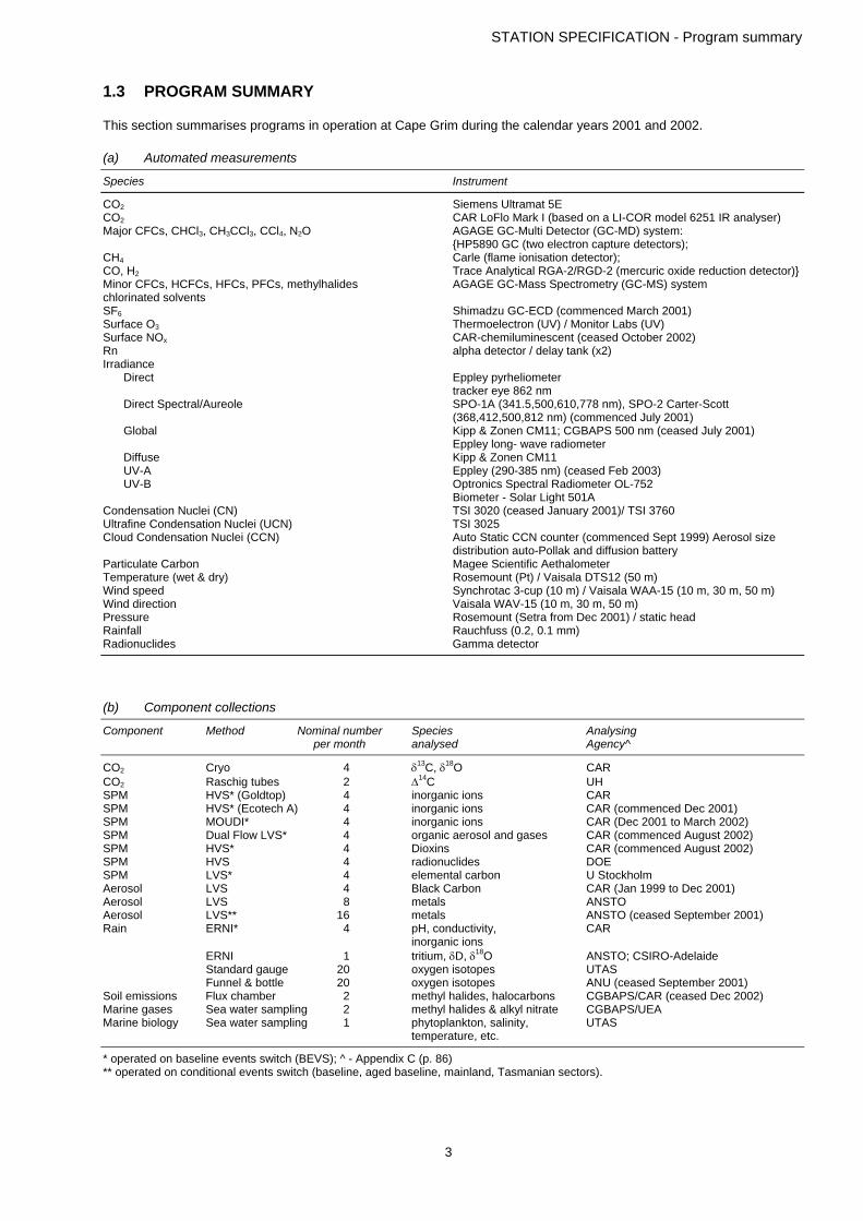
1.3 PROGRAM SUMMARY
This section summarises programs in operation at Cape Grim during the calendar years 2001 and 2002.
(a) Automated measurements
Species Instrument
CO2 Siemens Ultramat 5E CO2 CAR LoFlo Mark I (based on a LI-COR model 6251 IR analyser) Major CFCs, CHCl3, CH3CCl3, CCl4, N2O AGAGE GC-Multi Detector (GC-MD) system: {HP5890 GC (two electron capture detectors); CH4 Carle (flame ionisation detector); CO, H2 Trace Analytical RGA-2/RGD-2 (mercuric oxide reduction detector)} Minor CFCs, HCFCs, HFCs, PFCs, methylhalides AGAGE GC-Mass Spectrometry (GC-MS) system chlorinated solvents SF6 Shimadzu GC-ECD (commenced March 2001) Surface O3 Thermoelectron (UV) / Monitor Labs (UV) Surface NOx CAR-chemiluminescent (ceased October 2002) Rn alpha detector / delay tank (x2) Irradiance Direct Eppley pyrheliometer tracker eye 862 nm Direct Spectral/Aureole SPO-1A (341.5,500,610,778 nm), SPO-2 Carter-Scott (368,412,500,812 nm) (commenced July 2001) Global Kipp & Zonen CM11; CGBAPS 500 nm (ceased July 2001) Eppley long- wave radiometer Diffuse Kipp & Zonen CM11 UV-A Eppley (290-385 nm) (ceased Feb 2003) UV-B Optronics Spectral Radiometer OL-752 Biometer - Solar Light 501A Condensation Nuclei (CN) TSI 3020 (ceased January 2001)/ TSI 3760 Ultrafine Condensation Nuclei (UCN) TSI 3025 Cloud Condensation Nuclei (CCN) Auto Static CCN counter (commenced Sept 1999) Aerosol size distribution auto-Pollak and diffusion battery Particulate Carbon Magee Scientific Aethalometer Temperature (wet & dry) Rosemount (Pt) / Vaisala DTS12 (50 m) Wind speed Synchrotac 3-cup (10 m) / Vaisala WAA-15 (10 m, 30 m, 50 m) Wind direction Vaisala WAV-15 (10 m, 30 m, 50 m) Pressure Rosemount (Setra from Dec 2001) / static head Rainfall Rauchfuss (0.2, 0.1 mm) Radionuclides Gamma detector
(b) Component collections
Component Method Nominal number Species Analysing per month analysed Agency^
CO2 Cryo 4 δ13C, δ18O CAR CO2 Raschig tubes 2 ∆14C UH SPM HVS* (Goldtop) 4 inorganic ions CAR SPM HVS* (Ecotech A) 4 inorganic ions CAR (commenced Dec 2001) SPM MOUDI* 4 inorganic ions CAR (Dec 2001 to March 2002) SPM Dual Flow LVS* 4 organic aerosol and gases CAR (commenced August 2002) SPM HVS* 4 Dioxins CAR (commenced August 2002) SPM HVS 4 radionuclides DOE SPM LVS* 4 elemental carbon U Stockholm Aerosol LVS 4 Black Carbon CAR (Jan 1999 to Dec 2001) Aerosol LVS 8 metals ANSTO Aerosol LVS** 16 metals ANSTO (ceased September 2001) Rain ERNI* 4 pH, conductivity, CAR inorganic ions ERNI 1 tritium, δD, δ18O ANSTO; CSIRO-Adelaide Standard gauge 20 oxygen isotopes UTAS Funnel & bottle 20 oxygen isotopes ANU (ceased September 2001) Soil emissions Flux chamber 2 methyl halides, halocarbons CGBAPS/CAR (ceased Dec 2002) Marine gases Sea water sampling 2 methyl halides & alkyl nitrate CGBAPS/UEA Marine biology Sea water sampling 1 phytoplankton, salinity, UTAS temperature, etc.
* operated on baseline events switch (BEVS); ^ - Appendix C (p. 86) ** operated on conditional events switch (baseline, aged baseline, mainland, Tasmanian sectors).

STATION SPECIFICATION - Program summary
4
(c) Whole air collections – episodes+
Flask type Pressure Drying Nominal number Species analysed Analysing Laboratory^ (litre) (kPa) per month*
G (0.5) 100 p Dehydrite 4 CO2, CO, CH4, H2, N2O δ13C and δ18O of CO2 CAR 50 p Dehydrite 4 O2/N2, CO2, CO, CH4, H2, N2O δ13C and δ18O of CO2 CAR G (2.5) 100 p Cryo 4 CO2, CO, CH4, H2 δ13C and δ18O of CO2 CMDL 0 p Cryo 4 O2/N2, CO2 U Princeton 0 p Cryo 2 O2/N2, CO2 (Automated sampler) U Princeton (from Aug 2001) 0 p Cryo 2 O2/N2, CO2 CAR G (5) 0 p Cryo 2 O2/N2, CO2 SIO G (5) 0 p Cryo 2 O2/N2, CO2 CAR SS (0.8/2.5/3.0) 280 p - 4 N2O, halocompounds CMDL G (2.5) 150 p - 1 N2O, halocompounds CMDL SS (35) 3000 c - (6) archive / AGAGE standards CAR/CGBAPS SS (3.2) 500 p - (6) halocarbons by GC-MS UEA SS (1.6) 100 p Dehydrite 1 SF6 [also G (0.5) CAR species] CAR/UH SS (6.0) 150 p - 2 Methyl halides, SF6, Halocarbons, N2O SIO G (2.0) 100 p Dehydrite 1 CO2 CFR SS (1.0) 100 p Dehydrite 1 CO2 U Tohoku SS (6.0) 100 p - 2 Methyl halides NIES SS (35) 3000 p - 2 O and N isotopes of N2O UCSD (ceased September 2001) SS (3.2) 150 p - 2 methyl halides and alkyl nitrates CGBAPS/UEA
p - pump; c - cryogenic trap; * () indicates per year,+each episode may include multiple flask traps; ^ - Appendix C (p. 86)
(d) Discrete sampling
Parameter Method Occasion
Temperature (wet & dry) Mercury-in-glass 1/day Temperature (max & min) Mercury-in-glass 1/day Condensation Nuclei (CN) Manual Pollak 4/day Cloud Condensation Nuclei (CCN) Thermal Diffusion (5 supersaturations) 3/day Rainfall Standard 203 mm rain gauge 1/day

OiC’s report
5
2. OFFICER-IN-CHARGE’S REPORT 2.1. INTRODUCTION
One of the significant events of 2001-2002 was the commencement of construction and the opening of phase one of the Woolnorth Wind Farm. In the planning phase, there was much consultation to ensure that neither the planned construction nor the operation would impact adversely on Cape Grim operations. Construction of the sealed road out to the turn-off to the wind farm site commenced in October 2001 and construction of the gravel roads on lots 1 and 2 of the wind farm site commenced in December 2001. The latter resulted in a great deal of dust generation, but this did not appear to affect the station. Footings for the first six wind turbines were laid in March 2002 and also at this time Hydro mooted the construction of a major visitor facility at the wind farm. The proposed facility would have toilets, a kitchen and a meeting room. Such a facility indicated that traffic to and from the area, and consequent contamination to air measured at the station may be far more considerable than was first envisaged. Discussions with Hydro were undertaken in March and April of 2002 to express concerns at the impact this proposed facility could have on Cape Grim operations and seek a mutually acceptable compromise. In April 2002, the first turbine tower wended its way through Smithton to much local celebration. Finally, the view across Valley Bay looked very different to how it looked when Cape Grim started 26 years ago, with 6 turbines generating a total 10.8 MW, with the official opening ceremony in October 2002. An additional 31 turbines are planned for Lot 2 and these should be in position by mid-2004. It is pleasing to think that this ‘progress’ towards greener energy generation may be, in part, a response to the measurements made at Cape Grim and it is a reminder that things never stay the same.
There were no major measurement campaigns in 2001-2002 at Cape Grim. However, two lead scientists departed. Reinout Boers left CSIRO to take up the position as head of Atmospheric Research at the Royal Netherlands Meteorological Institute (KNMI, Netherlands). With Reinout’s departure the lidar and liquid water radiometer (LWR) program at Cape Grim ceased operation. The lidar commenced January 1995 and the LWR, and associated AUSLIG GPS water vapour measurements, commenced in January 1994, both ceased operation in October 2000. The LWR container was removed from its prime position, beside the station, in May 2001.
Stewart Whittlestone, who started the radon measurements in February 1980, and was appointed lead scientist of the radon program in June 1984, left ANSTO, bringing to an end a long, fruitful association. Wlodek Zahorowski, who had assisted with the radon program, took over the lead scientist role in 2001.
Tasmania Police vessel MV Van Dieman (March 2001), and Australian Customs Service patrol boat
MV Botany Bay (January 2002) provided opportunities for Bob Parr and University of Tasmania staff to undertake surface seawater, air and biological sampling, directly offshore from Cape Grim and out approximately 50 km, to the edge of the continental shelf, as part of the phytoplankton project.
2001 ended with somewhat of a bang, when lightning (possibly) struck the 10-m stack on Christmas Eve. The lightning strike took out most of the network at the station and the network to the outside world. Some instruments were damaged, although most of the problems were related to the loss of communications and the failure of the data acquisition system. Laurie Porter and Stuart Baly put in a huge effort and Randall Wheaton assisted by telephone, as he was on leave. A great deal of assistance was provided by the networking staff at the Bureau’s Head Office and by Telstra in restoring wider communications rapidly. Problems were still being discovered and fixed well into January 2002.
Several measurement projects ceased operation in 2001-2002 including the collection of rainwater samples for Pauline Treble (ANU) when the study concluded in September 2001. Collection of air samples for Martin Whalen (UCSD) for nitrogen isotopes measurements and the operation of a 4-channel sector switched sampler run for ANSTO, primarily for metals data analyses, both ceased in September 2001. Operation of the dual filter omni-directional sampler continues. The nitrogen oxides (NOx) analyser has not operated since October 2002, when it was ‘mothballed’ due to problems with its ozone generator, UV lamp and power supply. In March 2001, a gas chromatograph instrument, configured to measure sulfur hexafluoride (SF6) as part of the AGAGE program, commenced operation.
2.2. BUILDINGS AND MAINTENANCE
Apart from the routine maintenance of the building, systems and surrounds, the Telstra tower dominated 2001-2002. Discussions with Telstra continued regarding the state of the tower and plans for refurbishment. In the interim, there were several visits by the Telstra contractor, NDC, to replace and tighten nuts. Towards the end of 2001, after a strut was seen dangling precariously from the tower, a safety fence was installed around the base, to prevent access under the tower, by unsuspecting members of the public or staff.
Early in 2001 Macrocom indicated that they wished to install a 100-m communication tower in the vicinity of Cape Grim. Meetings were held with interested parties to alert them to possible impacts on Cape Grim. However this proposal never became reality.
As part of the refurbishment plans Laurie and Randall attended a paint trial at Telstra’s site in the north-east, Waterhouse Point. Telstra have undertaken to use a water-based paint in response to the sensitivities of solvent use around the station. The grand plan is to grind off the rust and paint the

OiC’s report
6
four main legs, at each corner of the tower and replace all the steelwork elsewhere. Telstra plan to commence work in summer 2002-2003.
Occupational health and safety continued to be a priority at Cape Grim and at the office in Smithton. The issue with safe handling of heavy freight at the office, identified in an OHS&E risk assessment, was addressed with the purchase of a lifter in December 2002. Problems with the safe storage of gas cylinders at the station were also identified in the assessment. A new gas cylinder store is proposed for the station, to meet the current Australian Standards and plans are being drawn up in the Bureau’s Head Office.
In June 2002, the copper communications cable running from the station to the radiation enclosure was replaced with optic fibre. It was believed that the cable contributed to distributing the damage caused by the lightning strike in December 2001 far and wide. Other than the lightning strike the other major incident was a total power failure at the station caused by a faulty phase relay switch continually switching, causing as many as 120 power failures, resulting in the generator starting a total of 25 times. The starter battery on the generator eventually failed causing a total loss of power. After Aurora had confirmed that the external power supply was not at fault, the problem was traced to the starter battery and the generator was then jump-started using the Toyota truck. It took some considerable time to bring all the instruments back up and this process was complicated by the failure of some software on the Raid array. The faulty relay was eventually diagnosed, bypassed to allow use of mains power and the faulty relay was replaced a week later, but not before batteries in the Telstra area discharged, bringing down the microwave link between Cape Grim, the station and King Island.
2.3. STAFF AND STUDENTS
There were number of promotions over the period 2001-2002. Firstly Jan Britton was promoted from ASO3 to ASO4 in recognition of the increasingly important role the office manager plays in Station operations. Also in recognition of the increasing workload and to provide leave relief Sheree Maguire was employed on a non-ongoing part-time basis, as an ASO3, to assist Jan in the office. Brian Weymouth, SITO-C, left Cape Grim in August 2001 after 7 and a half years (March 1994) at Cape Grim. Brian contributed greatly to the development of the CGBAPS data archive and processing. He also oversaw much of the modernisation and improvement of the Cape Grim computer network and equipment. Randall Wheaton who had been ITO2 was promoted to the SITO-C position in November 2002. There was a considerable battle to replace the ITO2 and eventually in May 2002 Stuart Baly was promoted to this position. However, Stuart could not fully take up the role until his current position, the TO3 at the Station, was replaced. The recruitment process was well underway with a
selection made for a new TO3 in December 2002, so hopefully Stuart can move into his new role in early 2003.
Craig McCulloch left in December 2002, at the expiry of his 3 year part time contract with CAR as a technical assistant supporting the GCMS project. He had worked at Cape Grim on and off over about 6 years in a variety of technical roles that contributed significantly to operations at the Station. Neil Tindale, the Officer-in-Charge left in December 2002, after 4 and a half years, to take up a temporary position at the Bureau of Meteorology’s Research Centre in Melbourne, before finally moving to Maroochydore and a lectureship at the University of the Sunshine Coast. Jill Cainey commences as the new Officer-in-Charge in January 2003. Neil presided over SOAPEX-II, a major international photochemistry experiment run at Cape Grim in January 1999. Neil was also instrumental in setting up ANZ-SOLAS and represented Australia on the international SOLAS scientific steering committee.
Guido Corno, a student at the University of Tasmania, who visited Cape Grim frequently to work on the Phytoplankton Project, as part of his honours thesis, left Tasmania to take up a postgraduate position at Oregon State University, USA.
Sadly Joyce, Brian Weymouth’s longstanding partner and wife, died in November 2002, after a battle with cancer.
Randall Wheaton married Karin in September 2002 and Chad Dick (OiC 1993-1997) married his long-time partner and mother to James and Arran, Kaye Robinson, in New Zealand in December 2002.
And finally the last word must go to Laurie Porter who not only achieved 30 years of service with the Bureau in February 2001, over 17 years of that spent at Cape Grim, but also was awarded a National Australia Day Medal at the Cape Grim Annual Science Meeting in Hobart, in February 2002. The Parliamentary Secretary Sharman Stone presented Laurie with his medal, which included the following citation: ‘For his outstanding personal contribution to the exemplary standards of observation and extremely high international reputation of the Bureau of Meteorology-CSIRO Cape Grim Baseline Air Pollution Station, that celebrated the 25th anniversary of its first observations in July 2001’.
Congratulations must go to Laurie for his many years of dedicated service to the Bureau and to the Cape Grim station. Laurie’s efforts have largely secured the good reputation of the station, locally and internationally, and have ensured a smooth running operation over many years.
2.4. INTERNATIONAL ACTIVITIES AND VISITORS
While there was no international campaign there was still a large number of visitors to the Station in 2001-2002. These included Kazuta Suda (Japan Meteorological Association), Georgina Sturrock (UEA), Carolyn Lindley (CalTech), Bradley Hall and

OiC’s report
7
Pat Sheridan (NOAA-CMDL) and Caroline Simmonds (Bowdoin College, Maine, USA), who came to install an automated sampler for the Princeton University O2/N2 project.
There were several significant groups of overseas visitors including Mukai Hitoski and Dr Katsumoto of NEIS (Japan), who were given a guided tour by Paul Fraser (CAR), with a party of 7 scientists from the Japan Meteorological Association. In March 2002 a group of 12 scientists from the World Climate Research Program visited the station. One of the party included Chad Dick (OiC 1993-1997) who assisted with providing guided tours.
In November 2002 Dr Christoph Zellweger and Dr. Stefan Reimann, of World Meteorological Organization-Swiss Federal Laboratories for Materials Testing and Research (WMO-EMPA, Switzerland), visited the Station to audit ozone, methane and carbon monoxide equipment and to perform inter-calibrations with the standard EMPA instruments. The EMPA report concluded ‘The global GAW station Cape Grim is a well established site within the GAW programme, and long time series of high quality are available for ozone, carbon monoxide, methane and other parameters. An excellent platform for extensive atmospheric research is available at the site’. The inter-comparisons showed good agreement between WCC-EMPA and station instruments for ozone (~2% difference) and methane (0.1% difference). Results for carbon monoxide showed more significant (~6%) differences in the scales and the report recommended further investigation is needed to resolve this problem.
Local visitors to Cape Grim included Pauline Treble (Australian National University) winding up her rainwater sampling project, a delegation of 11 members of the Legislative Council (Tasmania’s Upper House) led by the local MLC, the Honourable Tony Fletcher and a group of 8 Hobart Ports Authority Directors.
October 2002 was a busy month for local visitors encouraged to the area by the opening of Stage 1 of the Woolnorth Wind Farm. A group from McCain, the local vegetable processing factory, visited the Station as did the Air Quality Group from the Tasmanian Government’s Department of Primary Industries, Water and Environment. Noel Hunt (Area General Manager Northern Tasmania, Telstra Country Wide) and a small party from Telstra visited the Station in late October.
The Cape Grim Annual Science Meetings were held at IASOS, University of Tasmania, Hobart (6-7 February 2002) and at CSIRO Atmospheric Research, Aspendale (7-8 November 2002). Both meetings were well attended with over 100 attendees in total and more than 20 papers presented at each. Quite a number of posters were also presented, most coming from overseas. In Hobart, there was also a special display of posters that had been presented at The Sixth International Carbon Dioxide Conference, in Sendai, Japan (1-5 October 2001). NOAA-CMDL was represented at
both meetings, Brad Hall (Hobart) and Patrick Sheridan (Aspendale). Roger Dargaville (Laboratoire des Science du Climat et de l’Environnement, France) also made a presentation at the Aspendale meeting. Awards were given for Best Student Presentation, in Hobart the winner was Salah Jimi, and in Aspendale, Cecelia MacFarling. A discussion paper was presented in Hobart on the possible impact of oil exploration in newly acquired leases, to the west of Cape Grim. It was resolved to seek to have discussions with Santos regarding the impact of such activities on the measurements made at Cape Grim and to encourage Santos to visit the station as soon as practical.
Laurie Porter represented Cape Grim at four meetings of AGAGE Scientists, the 23rd Meeting at Galway, Ireland, May 2001, 24th Meeting at Queenstown, New Zealand, December 2001, 25th Meeting at Pago Pago, American Samoa, May 2002 and 26th Meeting at Scripps Institution of Oceanography, University of California, San Diego, California, USA, November 2002. The last of these included a visit to the laboratories of Prof. Ray Weiss, Scripps Institution of Oceanography for familiarisation training on a new GC-MS system under development for AGAGE.
Finally, the OiC attended several international meetings during 2001-2002 including the NOAA-CMDL Annual Meeting, in Boulder, Colorado, in May 2001 and the American Geophysical Union Fall Meeting in San Francisco, in December 2001. Several SOLAS related meetings were attended, both local and international. In July 2001 the second ANZ-SOLAS was held in Townsville and in December 2001, in San Francisco, a SOLAS-Scientific Steering Committee Meeting was attended as the Australian representative, Mike Harvey (NIWA) represented New Zealand at the same meeting. In June 2002 the OiC represented Australia at an Executive Committee and National Representatives meeting held in Amsterdam.
2.5. OPERATIONAL BUDGET
The Cape Grim program expenditure allocations for the financial years 2000-2001, 2001-2002 and 2002-2003 are detailed below. Staff salaries, road and building maintenance are not included as they are covered by other parts of the Bureau of Meteorology budget. Personnel costs of staff at CAR assisting with Cape Grim related research are included in the Research allocation.
2000-2001 2001-2002 2002-2003 $ $ $ Station operation 177,690 177,000 184,740 Research 524,310 413,447 517,260 Equipment 200,000 201,000 178,000 Total 902,000 791,447 880,000
Compiled by J. M. Cainey

BASELINE ATMOSPHERIC (AUSTRALIA) 2001-2002, PAGES 8-14, SEPTEMBER 2004
8
A PRELIMINARY INVESTIGATION OF THE PHYTOPLANKTON ECOLOGY AND MARINE BIOGENIC TRACE GAS PRODUCTION NEAR CAPE GRIM, TASMANIA
G Corno1, A McMinn1, G Sturrock2, R Parr3,4, N Tindale4, L Porter4, R Gillett3, P Fraser3, N Derek3, C Reeves2 and S Penkett2
1Institute of Antarctic and Southern Ocean Studies, University of Tasmania, Hobart, Tasmania 7001, Australia
2School of Environmental Science, University of East Anglia, Norwich NR4 7TJ, UK 3CSIRO Atmospheric Research, Aspendale, Victoria 3195, Australia
4Cape Grim Baseline Air Pollution Station, Bureau of Meteorology, Smithton, Tasmania 7330, Australia
1. Introduction
Atmospheric measurements of several biogenic trace gases (e.g. dimethyl sulphide (DMS), DMS de-rivatives and methyl halides) are made at Cape Grim, Tasmania (41°S), but there have been few at-tempts to relate these measurements to the phyto-plankton ecology and biogenic trace gas production processes in the adjacent ocean waters. During ACE-1 [Aerosol Characterisation Experiment-1: Bates et al., 1998; Jones et al., 1998 and Griffiths et al., 1999] the relationships between phytoplankton abundance, chemical oceanography and DMS levels in the sub-Antarctic region south of Tasmania were studied. Gabric et al. [1998] also modelled the effect of climate change on the ocean-air flux of DMS as-sociated with phytoplankton blooms in the Southern Ocean.
In this paper, we investigate the ecology of the marine surface mixed layer close to Cape Grim dur-ing the period spring 2000 to autumn 2001. We re-port physical and chemical properties of the oceanic mixed layer (temperature, light levels, salinity, nutri-ent concentrations), phytoplankton ecology (bio-mass, nutrient limitation, photosynthetic parameters and species composition) and oceanic and/or at-mospheric concentrations of marine biogenic gases - methyl bromide (CH3Br), methyl iodide (CH3I) and methane sulphonic acid (MSA, CH3SO2H). The rela-tionships between marine biogenic gases and eco-logical processes are investigated. A more compre-hensive treatment of the phytoplankton ecology will be presented in a future paper.
Marine temperate phytoplankton communities are typically comprised of around 300 species from up to six algal divisions (e.g. Bacillariophyta (diatoms), Di-nophyta (dinoflagellates), Prymnesiophyta (cocco-lithophoroids, Phaeocystis), Cyanobacteria, Crypto-phyta, Raphidophyta). Under changing environ-mental conditions, different species will be most competitive at different times, giving rise to annual species successions or sequences. The most impor-tant factors controlling these successions are light, temperature and the nutrient supply, most particu-larly nitrogen (ammonium, nitrate and nitrite), phos-phorus (phosphate), silica and trace micronutrients such as iron, manganese and vitamins. The primary resource for phytoplankton is light, but in marine ecosystems the amount of light reaching a cell is principally controlled by how rapidly each cell is moved around in the water column by wind and
wave induced vertical mixing. Deep mixing will take cells below the euphotic zone, i.e. the zone in which there is sufficient light for photosynthesis to occur, usually considered to be 1% of surface irradiance. The mixed layer depth (MLD) is therefore a primary factor for phytoplankton growth, particularly in a re-gion such as Cape Grim and the Tasmanian west coast, which is exposed to strong and persistent winds. In many coastal areas, spring phytoplankton blooms deplete nutrient levels to the point where fur-ther growth is limited [Harris, 1986]. Thus, knowl-edge of nutrient levels and supply is important in un-derstanding local bloom dynamics.
The photosynthetic yield (FV/FM) was determined by measuring chlorophyll in vivo fluorescence and is an indication of environmental and photosynthetic stress.
We use this information, in combination with physical and chemical oceanographic data, to char-acterise the major influences on the phytoplankton biomass, speciation and photosynthetic physiology.
2. Methods
All seawater samples, physical and chemical meas-urements were obtained approximately 9 km off-shore from Couta Rocks, 50 km south of Cape Grim, on the northwest coast of Tasmania. Salinity and temperature measurements were made using a Platypus Instruments CTD (for conductivity, tem-perature and depth measurements). The stratifica-tion index was derived from the difference in tem-perature between 0 and 50 m. Light was measured with a LI-COR submersible PAR (photosynthetically-available radiation) radiometer. Nutrients (phos-phate, silicate and nitrite + nitrate) were measured on an Alpkem Autoanalyser following standard methods [Alpkem, 1992].
Phytoplankton biomass was determined by measuring the chlorophyll a (chl a) concentration. One-litre ocean water samples were filtered onto 42 mm diameter, glass fibre filters, which were then ex-tracted in methanol for 8 hours. Chlorophyll was measured by the acidification method [Holm-Hansen and Riemann, 1978] using a Turner Instruments 10AU digital fluorometer. Cell counts were per-formed on a Zeiss Televar inverted microscope, us-ing Utermohl settling chambers. Additional samples were collected using a phytoplankton net for the identification of less common taxa. Photosynthetic parameters were measured using a Chelsea Instru-

Corno et al : Biogenic trace gas emissions
9
ments Fast Repetition Rate Fluorometer (FRRF). The FRRF is a non-invasive, in situ method of ob-taining information on how well the photosynthetic apparatus of the phytoplankton cells are coping with their current environmental conditions.
Air and seawater samples for CH3Br and CH3I analyses were collected at the same time as the phytoplankton collections and measurements. Ide-ally samples were only to be taken during baseline conditions (wind direction 190°-280°) - however, this was achieved on about 50% of sampling trips, be-cause boat availability was weather dependent (of-ten winds were too strong under baseline conditions for safe sampling). Analysis by GC with electron capture detection (ECD) is described in Sturrock et al. [2003].
Aerosol samples were collected using a Hi-vol sampler (10" x 8" Pallflex filters) on the air sampling deck at Cape Grim Baseline Air Pollution Station (CGBAPS) at about 100 m above sea level. These were collected every week from November 1 2000 to until March 31 2001, when local wind direction and cloud condensation nuclei (CCN) concentration cri-teria (wind direction between 190° and 280°; CCN concentration < 600 cm-3) defined the air mass as unpolluted marine ‘baseline’ air [Ayers et al., 1991]. These conditions occur on average about 30% of the time at Cape Grim. After collection, the Pallflex filters were shipped within a few days to CSIRO-Atmospheric Research at Aspendale, Victoria, for analysis. There, a 1 cm2 section was removed from the filter and placed into a clean polyethylene bag. To this was added 12 cm3 of Milli-Q water to extract the soluble ions. The extracts were then analysed for Na+, NH4
+, K+, Mg2+, Ca2+, Cl-, Br-, NO2-, NO3
-, SO4
2-, -O2CCO2-, HCO2
-, CH3SO3-, PO4
3- and CH3CO2
-. Analysis was by suppressed ion chroma-tography (Dionex model DX500) with an anion gra-dient method using an AS-11 column and ASRS-1 suppressor, and a cation isocratic method using a CS-12 column.
3. Results
3.1. Temperature, salinity, stratification and light
The physical characteristics of the water column are shown in Figure 1. Temperature and salinity are the column average from the surface to 20 m. The water column temperature rose steadily through the sum-mer, starting at 16°C in December, reaching just over 18°C in early March, and then declining to be-low 16°C in autumn. Two significant changes were observed in salinity - a rise from spring to summer (34.6 to 34.9 psu) and a fall from summer to autumn (34.9 to 34.7 psu). The MLD was about 10 m during November-December, increasing to about 40 m by January through to March. A major decrease in MLD occurred during March (6 m on 26 March), but by April-May the MLD had returned to 30-40 m.
Nov-00 Dec-00 Jan-01 Feb-01 Mar-01 Apr-01 May-01Date
34.4
34.6
34.8
35.0
35.2
salinity (psu)
0
20
40
60
Temp
eratu
re (°
C) M
LD, E
ZD (m
) * temperature’ salinity# euphotic zone depth& mixed layer depth
Figure 1. Physical characteristics of the water column 9 km off Couta Rocks, 50 km south of Cape grim, Tasmania: MLD Mixed Layer Depth (m); EZD = Euphotic Zone Depth (m); surface salinity; surface temperature.
The euphotic zone depth (EZD) is the depth to which 1% of surface irradiance penetrates and is generally assumed to be the maximum depth for phytoplankton photosynthesis. During the summer of 2000/2001 at Cape Grim, the EZD was relatively uniform, varying between 20 and 30 m, with no evi-dence of a summer increase in depth.
3.2. Nutrients Surface nutrient (nitrate, silicate, phosphate) con-centrations were generally higher in spring, lower in summer, and rising again in autumn (Figure 2). Ni-trate levels were at a minimum during summer (0.6 µmol l-1), with higher levels in spring and autumn (1.5 µmol l-1) and a maximum level (2.3 µmol l-1) seen in late March. Silicate and phosphate levels showed less seasonal variability, with summer con-centrations averaging 0.6 and 0.2 µmol l-1 respec-tively and autumn/spring levels averaging 0.8 and 0.3 µmol l-1 respectively. Maximum levels of silicate (1.0 µmol l-1) were observed in November and late March and phosphate (0.3-0.4 µmol l-1) in January and March. The N:P ratio was always less than the typical phytoplankton nutrient uptake ratio of 15 [Myklestad, 1977], indicating that conditions were always at least mildly nitrate limiting. Ratio values varied between a minimum of 1.9 on 16 January to a maximum of 7.5 on 28 March (Figure 3).
Nov-00 Dec-00 Jan-01 Feb-01 Mar-01 Apr-01 May-01Date
0.1
0.2
0.3
0.4
0.5
phosphate (micromol l -1)
0.0
0.5
1.0
1.5
2.0
2.5
Chl a
(mg m
-3);
nitra
te, si
licate
(micr
omol
l -1)
, Chl a+ phosphate- nitrate/ silicate
Figure 2. Chlorophyll a, nitrate, silicate and phosphate concentration off Couta Rocks, 2000/2001.
Corno et al : Biogenic trace gas emissions
10
Nov-00 Dec-00 Jan-01 Feb-01 Mar-01 Apr-01 May-01Date
0
4
8
12
Chl a (x10; mg m-3); N:P
0
100
200
300
400
CH3B
r (pp
t)
, Chl aA N:P (0 m)C CH3Br
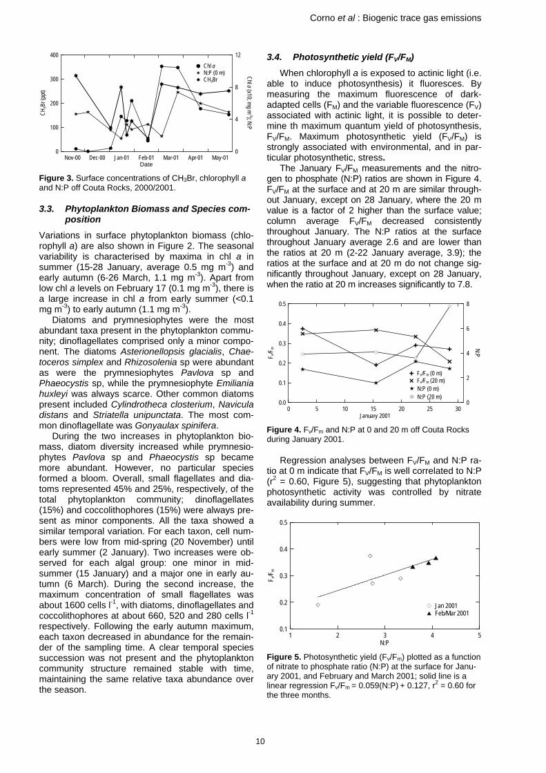
Figure 3. Surface concentrations of CH3Br, chlorophyll a and N:P off Couta Rocks, 2000/2001.
3.3. Phytoplankton Biomass and Species com-position
Variations in surface phytoplankton biomass (chlo-rophyll a) are also shown in Figure 2. The seasonal variability is characterised by maxima in chl a in summer (15-28 January, average 0.5 mg m-3) and early autumn (6-26 March, 1.1 mg m-3). Apart from low chl a levels on February 17 (0.1 mg m-3), there is a large increase in chl a from early summer (<0.1 mg m-3) to early autumn (1.1 mg m-3).
Diatoms and prymnesiophytes were the most abundant taxa present in the phytoplankton commu-nity; dinoflagellates comprised only a minor compo-nent. The diatoms Asterionellopsis glacialis, Chae-toceros simplex and Rhizosolenia sp were abundant as were the prymnesiophytes Pavlova sp and Phaeocystis sp, while the prymnesiophyte Emiliania huxleyi was always scarce. Other common diatoms present included Cylindrotheca closterium, Navicula distans and Striatella unipunctata. The most com-mon dinoflagellate was Gonyaulax spinifera.
During the two increases in phytoplankton bio-mass, diatom diversity increased while prymnesio-phytes Pavlova sp and Phaeocystis sp became more abundant. However, no particular species formed a bloom. Overall, small flagellates and dia-toms represented 45% and 25%, respectively, of the total phytoplankton community; dinoflagellates (15%) and coccolithophores (15%) were always pre-sent as minor components. All the taxa showed a similar temporal variation. For each taxon, cell num-bers were low from mid-spring (20 November) until early summer (2 January). Two increases were ob-served for each algal group: one minor in mid-summer (15 January) and a major one in early au-tumn (6 March). During the second increase, the maximum concentration of small flagellates was about 1600 cells l-1, with diatoms, dinoflagellates and coccolithophores at about 660, 520 and 280 cells l-1 respectively. Following the early autumn maximum, each taxon decreased in abundance for the remain-der of the sampling time. A clear temporal species succession was not present and the phytoplankton community structure remained stable with time, maintaining the same relative taxa abundance over the season.
3.4. Photosynthetic yield (FV/FM) When chlorophyll a is exposed to actinic light (i.e.
able to induce photosynthesis) it fluoresces. By measuring the maximum fluorescence of dark-adapted cells (FM) and the variable fluorescence (FV) associated with actinic light, it is possible to deter-mine th maximum quantum yield of photosynthesis, FV/FM. Maximum photosynthetic yield (FV/FM) is strongly associated with environmental, and in par-ticular photosynthetic, stress.
The January FV/FM measurements and the nitro-gen to phosphate (N:P) ratios are shown in Figure 4. FV/FM at the surface and at 20 m are similar through-out January, except on 28 January, where the 20 m value is a factor of 2 higher than the surface value; column average FV/FM decreased consistently throughout January. The N:P ratios at the surface throughout January average 2.6 and are lower than the ratios at 20 m (2-22 January average, 3.9); the ratios at the surface and at 20 m do not change sig-nificantly throughout January, except on 28 January, when the ratio at 20 m increases significantly to 7.8.
0 5 10 15 20 25 30January 2001
0.0
0.1
0.2
0.3
0.4
0.5
F v/F
m
0
2
4
6
8
N:P
" Fv/Fm (0 m)> Fv/Fm (20 m)A N:P (0 m)? N:P (20 m)
Figure 4. Fv/Fm and N:P at 0 and 20 m off Couta Rocks during January 2001.
Regression analyses between FV/FM and N:P ra-tio at 0 m indicate that FV/FM is well correlated to N:P (r2 = 0.60, Figure 5), suggesting that phytoplankton photosynthetic activity was controlled by nitrate availability during summer.
1 2 3 4 5N:P
0.1
0.2
0.3
0.4
0.5
F v/F
m
# Jan 2001/ Feb/Mar 2001
Figure 5. Photosynthetic yield (Fv/Fm) plotted as a function of nitrate to phosphate ratio (N:P) at the surface for Janu-ary 2001, and February and March 2001; solid line is a linear regression Fv/Fm = 0.059(N:P) + 0.127, r2 = 0.60 for the three months.

Corno et al : Biogenic trace gas emissions
11
3.5. Methyl halides 3.5.1. Methyl bromide
Figure 3 shows CH3Br concentrations in seawater during this study (mean 196±98 pmol l-1, 1 standard deviation). These seawater concentrations were not correlated (r2 = 0.02) with atmospheric concentra-tions of CH3Br, measured in air samples (mean of 12.2±3.2 ppt), collected at the ocean sampling site at the same time of collection of the water samples. The atmospheric samples were collected under both on-shore (baseline) and off-shore conditions, and the results show the variability associated with re-gional coastal/land based sources and baseline, oceanic air [Cox, 2001; Sturrock et al., 2001].
The relationship between seawater CH3Br con-centrations and phytoplankton biomass (Figure 3) and species abundance were examined during the summer-early autumn period of enhanced biological activity (January – March). The correlation coeffi-cients are shown in Table 1, and are considered in-dicative (though not necessarily statistically signifi-cant) of biological relationships when r2 exceeds 0.5 [Zar, 1984]. The best correlation over this period was between CH3Br and dinoflagellates (r2 = 0.74), and good correlations were also found with small flagellates (r2 = 0.67), diatoms (r2 = 0.60) and phyto-plankton biomass (r2 = 0.62). The major (8-fold) phytoplankton increase between February and March was associated with a 5-fold increase in CH3Br, dinoflagellates and small flagellates and a doubling in diatoms.
Table 1. Correlations (r2) between CH3Br, CH3I and nitrate concentrations and N:P ratios in seawater off the Tasma-nian west coast and MSA at Cape Grim with associated phytoplankton abundance and ocean chemistry data dur-ing January – March 2001. Parameter CH3Br CH3I MSA nitrate N:P phytoplankton 0.62 0.003 0.62 diatom 0.60 0.65 dinoflagellate 0.74 0.79 0.65 0.54 small flagellate 0.67 0.84 0.61 Coccolithophore 0.76 Nitrate 0.70 - - Phosphate 0.83 - - N:P 0.92 - -
Seawater CH3Br concentrations were closely re-lated to surface N:P ratios as seen in Figure 3. They show a strong inverse relationship during the period of high biomass (r2 = 0.92). During early January, CH3Br increased to 270 ppt while nitrate availability was low (N:P = 1.6); similarly, the large CH3Br in-crease observed in early autumn to 280 ppt oc-curred at low nitrate availability (N:P = 1.9). These results suggest that CH3Br was produced by phyto-plankton when N:P was low.
No other good correlations were observed be-tween CH3Br concentrations and any other chemical or physical parameters, including phytoplankton photosynthetic activity (FV/FM).
3.5.2. Methyl iodide
Figure 6 shows CH3I concentrations in seawater (mean 234±106 ppt). Again, these were not signifi-cantly related to atmospheric concentrations (r2 = 0.01), showing a different temporal pattern and more variation than atmospheric data (mean of 1.3±0.4 ppt).
Seawater CH3I concentrations were well corre-lated with phytoplankton biomass (r2 = 0.92) during January - March, and also with diatom, flagellate and coccolithophore abundance (Table 1). Increases in phytoplankton biomass in mid-summer (0.6 chl a mg m-3) and early autumn (0.9 chl a mg m-3) were accompanied by simultaneous increases (about 200 ppt) in CH3I concentrations and associated growths in flagellates, diatoms and coccolithophores, reach-ing peak levels in early autumn (520, 660, 1600 and 280 cells l-1 for dinoflagellates, diatoms, small flagel-lates and coccolithophores respectively).
As observed for CH3Br, these results suggest that phytoplankton were an important source of CH3I in coastal waters off Cape Grim during summer-autumn 2001. No other significant correlation was found with phytoplankton taxa or photosynthetic activity.
Seawater CH3I concentrations were inversely correlated (r2 = 0.70) to surface nitrate concentrations (Figure 6). When nitrate levels decreased in mid-summer to 0.49 µmol l-1, CH3I concentrations reached 350 ppt. A second minimum in nitrate concentrations (0.36 µmol l-1) in early autumn was associated with the largest CH3I concentrations observed (440 ppt). These results suggest that maximum phytoplankton production of CH3I occurred when nitrate concentrations are low (<0.5 µmol l-1).
No other strong correlations were observed be-tween CH3I concentrations and any other chemical or physical parameters.
Nov-00 Dec-00 Jan-01 Feb-01 Mar-01 Apr-01 May-01Date
0
4
8
12 Chl a (x10; mg m-3); nitrate (micromol l -1)
0
100
200
300
400
500
CH3I
(ppt)
, Chl a- nitrateB CH3I
Figure 6. Surface concentrations of CH3I, chlorophyll a and nitrate off Couta Rocks, 2000/2001.
3.6. Methane Sulfonic Acid (MSA) Atmospheric MSA concentrations, measured at Cape Grim under baseline conditions, decreased throughout spring-summer 2000/2001, with the ex-ception of a single large increase, to 2.1 nmol m-3, in mid-summer (Figure 7). Background levels de-creased from 0.60 nmol m-3 in November to 0.15 nmol m-3 in April. MSA concentrations at Cape Grim were not significantly related to phytoplankton bio-

Corno et al : Biogenic trace gas emissions
12
mass, specific taxa or photosynthetic activity meas-ured during ocean water sampling off Cape Grim. The only chemical or physical oceanic factor that is correlated to MSA concentrations at Cape Grim was phosphate at the surface during January to March (r2
= 0.83, F test=0.01). The basis of this correlation is unknown.
Nov-00 Dec-00 Jan-01 Feb-01 Mar-01 Apr-01 May-01Date
0.0
0.2
0.4
0.6
0.8
1.0
1.2 Chl a (mg m-3); phosphate (micromol l -1)
0.0
0.5
1.0
1.5
2.0
2.5
MSA
(nmo
les m
-3)
, Chl a# MSA+ phosphate
Figure 7. Surface concentrations of chlorophyll a, phos-phate off Couta Rocks, and methane sulfonic acid (MSA) at Cape Grim, 2000/2001.
4. Discussion
This investigation describes the phytoplankton community structure and species composition in wa-ters off Cape Grim during November 2000 to May 2001. As found by Jones et al. [1998], small flagel-lates and diatoms dominated the phytoplankton community, making up 45% and 25% of the total community respectively, while dinoflagellates (15%) and coccolithophores (15%) were observed at lower levels. An earlier model study of this area, based on satellite images, suggested that the prymnesio-phytes comprised the bulk of the phytoplankton community [Gabric et al., 1996]. The data reported here show greater species diversity compared with the model results.
The seasonal phytoplankton variation at Cape Grim, with a dominant autumn bloom, differed from typical temperate phytoplankton biomass cycles in not having a major spring bloom followed by a smaller autumn bloom. The spring bloom may have been depressed by limiting environmental factors, such as increased mixing due to elevated wind and wave stress, grazing, nutrient limitation and light. However, previous analyses of archival satellite im-agery also failed to show a well-defined spring bloom event [Gabric et al., 1996], although spring-summer phytoplankton biomass was still much greater than during winter [Gabric et al., 1998].
Phytoplankton biomass measurements from this study are compared with other values, both meas-ured and model derived, from around Tasmania in Table 2. The concentrations observed are similar to those reported for the open ocean off Cape Grim [0.2 to 0.7 mg m-3, November 1995, Griffiths et al., 1999]. They are lower than those reported from other Tasmanian coastal areas (less open ocean in-fluence) during the same period of the year, and fall in the lower half of the range estimated in the model study, based on satellite images from 1996/1997 [Gabric et al., 1998]. These lower phytoplankton lev-els are likely due to the more open-ocean nature, with greater exposure to wind and swell, of the sam-pling site off Cape Grim, compared to other Tasma-nian coastal sites.
With the exception of nitrate, phytoplankton taxa were not strongly correlated with any chemical or physical parameters of the water column. However, a peak in small flagellates abundance (1590 cells l-1) in early autumn was linked to the gradual increase of turbulence of the water column, confirmed by a deepening of the MLD. This relationship has also been described in previous studies from a variety of environments [Margalef, 1958]. In early autumn, in-creasing diatom abundance (670 cells l-1) was also linked to a continuous increase in silicate.
Chemical and physical parameters of the water column are similar to previously reported values from off northern west Tasmania [Gibbs et al., 1983; Grif-fiths et al., 1999]. The EZD, which averaged 25 m, was shallower than would be expected (50-75 m) for coastal waters at this latitude during spring-summer [Harris, 1986]. This is probably due to higher concen-trations of suspended organic and inorganic matter. A deep MLD (40 m) and a shallow EZD (25 m) during spring-early summer contributed to the low phyto-plankton biomass (0.10 mg chl a m-3). Deep mixing reduces the time that each algal cell spends in the euphotic zone, lowering growth and photosynthetic rates as a consequence.
The first minor phytoplankton increase (to 0.6 mg chl a m-3) occurred when the EZD deepened to 32 m, the same as the MLD; nitrate concentration de-creased slightly (to 0.5 µmol l-1). In early autumn, the second (major) phytoplankton increase (to 1.0 mg chl a m-3) was again accompanied by a small nitrate decrease (to 0.4 µmol l-1), and a slight deepening of the EZD. The large nitrate increase (to 2.3 µmol l-1) occurred after a major increase in phytoplankton biomass, when the MLD decreased (6 m) compared to the EZD (30 m).
Table 2. Observed and modelled biomass concentrations in Tasmanian waters from recent studies Type of data Location Duration of study Biomass References (mg chl a m-3) observations near Cape Grim spring to autumn 0.05 to 1.1 This work observations near Cape Grim summer 0.6 to 1.2 Jones et al. 1998; Griffiths et al. 1999 model results near Cape Grim spring to autumn 0.1 to 2.5 Gabric et al. 1998 observations Storm Bay, southern Tasmania 3 years 0.7 to 6.0 Clementson et al. 1989 observations east coast Tasmania 2 years 0.6 to 2.5 Harris et al. 1987 observations Derwent and Huon estuaries, 20 years 1 to 3 (background) G. Hallegraeff and A. McMinn, southern Tasmania 7 to 15 (blooms) (unpublished data)

Corno et al : Biogenic trace gas emissions
13
MSA concentrations in the air at CGBAPS were found to decrease constantly during spring-autumn 2000/2001 with the exception of one large increase in mid-summer. This temporal trend is in agreement with previous investigations where MSA was found to in-crease only in summer and to then decrease for the rest of the year [Ayers et al., 1995]. Background MSA concentrations reported in this paper for 2000/2001 are similar to those reported earlier from the same site by Ayers and Gras [1991], although their maxi-mum concentration reported was 0.5 nmol m-3, com-pared to 2.1 nmol m-3 observed in mid-summer 2001.
MSA concentrations in the air at Cape Grim were not correlated with changes in phytoplankton bio-mass in the surrounding coastal waters. This finding is contrary to the model data of Gabric et al. [1996, 1998] where phytoplankton biomass and specific taxa, namely prymnesiophytes, were related to MSA concentrations in the air. During spring-autumn 2000/2001, although the prymnesiophyte Phaeocys-tis sp was relatively abundant, the prymnesiophyte E. huxleyi abundance was low. However, in either case, no relationship was found with MSA concen-trations. Part of the reason for these poor correla-tions is probably related to the different locations of the MSA measurements and the seawater sample sites because phytoplankton biomass and commu-nity structure may vary considerably between differ-ent locations along the coast. MSA and phosphate levels were correlated during January-March, but the reason for the correlation is unknown.
In both air and seawater samples, the CH3Br concentrations fell in the range of data previously measured in the same area [Sturrock et al. 2001; G. Sturrock unpublished data]. The CH3Br concentra-tions in seawater were not related to atmospheric concentrations, although there is a net flux from the water to the air [Sturrock et al. 2003]. Atmospheric CH3Br concentrations are influenced by long-range and regional transport (i.e. additional sources), as well as the underlying ocean, with complex interac-tions between solar radiation, temperature and wind speed. Correlations between seawater CH3Br con-centration and phytoplankton biomass and taxa (Ta-ble 1) were statistically significant at the 93% or bet-ter level.
An inverse correlation was found between CH3Br concentrations in seawater and N:P ratio (r2 = 0.92, 99% significant) indicating a relationship between CH3Br concentration and increasing nitrate limitation (ie decreasing N:P ratio). Nitrate limiting conditions occur when the N:P ratio is below that required (i.e.15) for active marine phytoplankton growth [Myk-lestad 1977]. The low N:P values recorded at Cape Grim, i.e. less than 2, imply acute nitrate limitation. No significant correlations were observed with ni-trate or phosphate levels. During the sampling pe-riod, CH3Br was produced or released by phyto-plankton at low photosynthetic activity and under ni-trate limiting conditions.
The ecological and physiological role of CH3Br in phytoplankton is still poorly understood. Possible roles have included the elimination of toxic halogens
from the cell and as protection from herbivore feed-ing [Krysell 1991]. Our results suggest that produc-tion of CH3Br from phytoplankton may be in re-sponse to nitrate limiting conditions (i.e. nitrate defi-ciency) causing low phytoplankton activity. Previ-ously, high values of CH3Br have been observed when the senescence of phytoplankton occurs [Scarratt and Moore, 1998; Baker et al., 1999].
In both air and seawater samples, the CH3I con-centrations fell within the range reported for the Cape Grim region [Cohan et al., 2003; G. Sturrock, unpublished data]. Seawater CH3I concentrations were not significantly related to atmospheric concen-trations – again, not unexpected, given the influence of various local source regions [Cohan et al., 2003]. Seawater CH3I concentrations were significantly re-lated to phytoplankton biomass, with the abundance of flagellates, coccolithophores and diatoms all showing significant correlation with CH3I concentra-tions (Table 1). These results suggest that these species are sources of CH3I in coastal waters off Cape Grim.
Seawater CH3I concentrations are inversely cor-related to nitrate concentrations (r2 = 0.70) implying an increase in CH3I concentration associated with a reduction in nitrate concentration. This suggests that CH3I is produced by phytoplankton during low nutri-ent conditions. The natural function of CH3I in phyto-plankton physiology and ecology is not clear [Night-ingale et al., 1995]. Possible functions suggested in-clude as an antimicrobial compound, a grazing de-terrent and warning signal [Manley and Dastoor, 1988; Nightingale et al., 1995]. From our study in coastal waters off Cape Grim, the production of CH3I and CH3Br may be a response to nitrate limiting conditions. However, further field and laboratory re-search is needed to assess and confirm these re-sults.
5. Summary
This investigation has contributed information on phytoplankton biomass and species in coastal wa-ters off Cape Grim, Tasmania, which remains a much under-studied region. A clear temporal spe-cies succession was not present and the phyto-plankton community structure remained constant over time. The sampling interval was coarse, how-ever, and phytoplankton peaks could have been missed. Small flagellates and diatoms dominated the phytoplankton community, making up 45% and 25% of the total community respectively, while dinoflagel-lates (15%) and coccolithophores (15%) were ob-served at lower levels. Other prymnesiophytes were not present to any significant extent.
Oceanic CH3I and CH3Br levels are clearly re-lated to phytoplankton growth in summer and early autumn. Phytoplankton growth appears to be in-versely related to nitrate availability.

Corno et al : Biogenic trace gas emissions
14
References ALPKEM, Methodology manual, the flow solution, Wilsonville,
Oregon: ALPKEM Corporation, 1992. Ayers, G. P., and J. L. Gras, Seasonal relationship between con-
densation nuclei and aerosol methanesulfonate in marine air, Nature, 353, 834-835, 1991.
Ayers, G. P., S. T. Bentley, J. P. Ivey, and B.W. Forgan, Di-methylsulphide in marine air at Cape Grim, 41°S, J. Geophys. Res., 100, 21,013-21,021, 1995.
Baker, J. M., C. E. Reeves, P. D. Nightingale, S. A. Penkett, S. W. Gibb, and A. D. Hatton, Biological production of methyl bro-mide in the coastal waters of the North Sea and open ocean of the northeast Atlantic, Mar. Chem., 64, 267-285, 1999.
Bates, T. S., B. J. Huebert, J. L. Gras, F. B. Griffiths, and D. A. Durkee, International Global Atmospheric Chemistry (IGAC) First Aerosol Characterisation Experiment (ACE-1): Overview, J. Geophys Res., 103, 16297-16318, 1998.
Cohan, D. S., G. A. Sturrock, A. P. Biazar, and P. J. Fraser, At-mospheric Methyl Iodide at Cape Grim, Tasmania, from AGAGE Observations, J. Atmos. Chem., 44, 131-150, 2003.
Cox, M. L., A regional study of the natural and anthropogenic sources and sinks of the major halomethanes, Ph.D. Thesis, School of Mathematical Sciences, Monash University, Clayton, Australia, 188 p., 2001.
Clementson, L. A., G. P. Harris, F. B. Griffiths, and D. W. Rimmer, Seasonal and inter-annual variability in chemical and biological parameters in Storm Bay, Tasmania I, Physics, chemistry and biomass components of the food chain, Aust. J. Mar. Fresh. Res., 28, 105-115, 1989.
Gabric, A. J., G. Ayers, C. N. Murray, and J. Parslow, Use of re-mote sensing and mathematical modelling to predict flux of di-methylsulfide to the atmosphere in the Southern Ocean, Adv. Space Res., 18, 117-128, 1996.
Gabric, A. J., P. H. Whetton, R. Boers, and G. Ayers, The impact of simulation climate change on the air sea flux of dimethylsul-fide in the subantarctic Southern Ocean, Tellus, 50, 388-399, 1998.
Gibbs, C.F., R. A. Cowdell, and A. R. Logmore, Studies of the chemical oceanography of Bass Strait 1979-1980, Internal CSIRO Report 49, 1-42, 1983.
Griffiths, F. B., T. S. Bates, P. K. Quinn, L. A. Clemenston, and J.S. Parslow, Oceanographic context of the First Aerosol Char-acterisation Experiment (ACE 1): A physical, chemical and bio-logical overview, J. Geophys. Res., 104, 21,649-21671, 1999.
Harris, G. P., Phytoplankton Ecology, Chapman Hill, Cambridge, 1986.
Harris, G. P., G. G. Gant, and D. P. Tomas, Productivity, growth rates and cell size distributions of phytoplankton in SW Tasman Sea: implications for carbon metabolism in the photic zone, J. Plank. Res., 9, 1003-1030, 1987.
Holm-Hansen, O., and B. Riemann, Chlorophyll a determination: improvements in methodology, Oikos, 30, 438-447, 1978.
Jones, G. B., M. A. Curran, H. B. Swan, R. M. Greene, F. B. Grif-fiths, and L. A. Clementson, Influence of different water masses and biological activity on dimethylsulphide and dimethylsul-phiopropionate in the subantarctic zone of the Southern Ocean during ACE-1, J. Geophys. Res., 103, 16,691-16701, 1998.
Krysell, M., Bromoform in the Nansen Basin in the Arctic Ocean, Mar. Chem., 33, 188-197, 1991.
Manley, S. L., and M. N. Dastoor, Methyl iodide production by kelp and associated microbes, Mar. Biol., 98, 477-482, 1988.
Margalef, R., Temporal succession and spatial heterogeneity in phytoplankton, in Perspectives in Marine Biology, edited by Buzzati-Traverso, A. A., California Press, Berkley, 322-349, 1958.
Myklestad, S., Production of carbohydrates by marine phytoplank-tonic diatoms. II. Influence of the N/P ratio in the growth me-dium on the assimilation ratio, growth rate and production of cellular and extracellular carbohydrates by Chaetoceros affinis va. Willei (Gran.) Hustedt and Skeletonema costatum (Grev.) Cleve., J. Exp. Mar. Ecol., 29, 161-197, 1977.
Nightingale, P. D., Low molecular weight halocarbons in sea-water, PhD thesis, University of East Anglia, Norwich, UK, 1995.
Scarratt, M. G., and R. M. Moore, Production of methyl bromide and methyl chloride in laboratory cultures of marine phytoplank-ton II, Mar. Chem., 59, 311-320, 1998.
Sturrock, G.A., L. W. Porter, and P. J. Fraser, In situ measure-ment of CFC replacement chemicals and other halocarbons at Cape Grim: the AGAGE GC-MS Program, in Baseline Atmos-pheric Program (Australia) 1997-1998, edited by N. W. Tindale, N. Derek, and R. J. Francey, Bureau of Meteorology and CSIRO Atmospheric Research, Melbourne, Australia, Baseline 1997/98, 43-49, 2001.
Sturrock, G. A., C. R. Parr, C. E. Reeves, S. A. Penkett, P. J. Fra-ser, and N. W. Tindale, Methyl bromide saturations in surface seawater off Cape Grim, in Baseline Atmospheric Program (Australia) 1999-2000, edited by N. W. Tindale, N. Derek, and P. J. Fraser, Bureau of Meteorology and CSIRO Atmospheric Research, Melbourne, Australia, 85-86, 2003.
Zar, J. H., Biostatistical Analysis, Prentice Hall, New Jersey, 1984.

BASELINE ATMOSPHERIC (AUSTRALIA) 2001-2002, PAGES 15-17, SEPTEMBER 2004
15
OIL AND GAS ACTIVITIES NEAR CAPE GRIM: IMPLICATIONS FOR THE ATMOSPHERIC PROGRAM
D Etheridge1, C P Meyer1 and G O’Brien2 1 CSIRO Atmospheric Research, Aspendale, Victoria 3195, Australia
2 National Centre for Petroleum Geology and Geophysics, University of Adelaide, South Australia 5005, Australia
1. Background
Exploration and production of oil and gas has re-cently been proposed for several areas offshore Northwest Tasmania. This is part of a large increase in the development of reserves expected in the South East Australian region. Emissions from these activities could affect the measurements of atmos-pheric compounds at the Cape Grim Baseline Air Pollution Station, which was established there be-cause of the remoteness from significant local an-thropogenic emissions.
An open forum on this issue was held during the 2002 Cape Grim annual science meeting. This re-port outlines some of the information presented and the discussion that ensued.
2. Oil and gas areas near Cape Grim and their development
There are several stages in the development of potential oil and gas tenements. These are: 1. Open: there are no exploration or production ac-
tivities in the area. 2. Advertised or released: areas are gazetted by
government (usually state) inviting resource companies or consortia to bid (Details of the pro-posed exploration activities must be supplied).
3. Exploration: if a bid is successful, the company or consortium is awarded an exploration permit (typically lasting about 6 years) allowing exclu-
sive rights to that area. Exploration activities of-ten require an environment impact statement.
4. Production: If exploration proves successful and the company decides the area is commercially viable, it can apply for a production license to ex-tract the oil and/or gas. An EIS (Environmental Impact Statement) process ensues. Alternatively, if the area is estimated to be commercial at some later time, a retention lease may be applied for.
Figure 1 shows areas of oil and gas exploration and production in Victorian and Tasmanian waters and their stage of activity. Exploration and produc-tion licenses that might impact on Cape Grim are those in the Otway, Sorell and Bass basins (to the North West, West and North of Cape Grim respec-tively). Exploration and production are likely to in-crease in these areas in the next few years. The Ot-way Basin is considered the new ‘hot’ exploration area, the Sorrel Basin much less so. Within these areas are two recently advertised developments of significance. These are: • Increases in exploration activity in areas V01-2 and
V02-3 in the Sorell Basin (also called Vic/P51 and Vic/P52), and T32 and T33 under permits issued to a consortium headed by Santos Ltd in 2001. (Ex-pected cost is $170 million).
• Production proposed in areas Vic/P43 and T/30P (the Geographe and Thylacine gas fields) by the Otway Gas Project (Woodside Energy Ltd and partners Origin Energy Resources Ltd). (Expected cost is $1 billion).
Figure 1. Oil and gas exploration and production tenements in the Victorian (left) and Tasmanian (right) regions. Adapted from Department of Natural Resources and Environment, Victoria and Department of Infrastructure, Energy and Resources, Tasmania.

Etheridge et al: Oil and gas near Cape Grim
16
3. Implications for the Cape Grim Science Program
Emissions to the atmosphere are likely from a range of sources as a result of oil and gas exploration and production activities in these areas. Whether these may be detected in measurements at Cape Grim will depend on their amount and location.
Emissions could be expected from wells by direct gaseous emissions, gas flaring, produced formation waters (PFWs) and from infrastructure (eg. pipe-lines, engine exhausts, fuels and other industrial compounds associated with rigs, ships and aircraft).
The types of compounds we might expect to be emitted include hydrocarbons (especially methane), carbon dioxide, carbon monoxide, sulfur gases, ni-trogen oxides, radon, industrial compounds (eg. halocarbons) and aerosols.
The Santos program is of particular concern, be-ing located nearby and in the baseline wind sector. It involves seismic sounding and the drilling of wells. The Santos exploration program is probably the first significant industrial activity in the baseline sector since the beginning of CGBAPS. Atmospheric com-position measurements in the baseline sector are the most sensitive and the most easily corrupted by such industrial sources. The Otway Gas Project pro-posed for the Geographe and Thylacine fields would be the closest production activity to Cape Grim. Al-though not in the baseline sector, it could have ef-fects, for example, on the measurements of the emissions coming from mainland Australia. How-ever, it is not yet known whether the amounts of emissions would be sufficient to have significant ef-fects on measurements in any sector.
Emissions from similar activities have been de-tected at other atmospheric monitoring stations. For example, methane, carbon dioxide and nitrogen ox-ide emissions from Prudhoe Bay, Alaska were de-tected at Barrow (about 300 km away) and quanti-fied [Jaffe et al., 1995]. Emissions of methane from oil production activities in the North Sea were identi-fied as the likely cause of an underestimated source detected in NW Europe [Janssen et al. 1999]. Al-though the Prudhoe Bay and North Sea operations are much larger than those expected near Cape Grim, they are much further from the stations that measured their emissions (the Sorell and Otway tenements are about 50 and 220 km respectively from CGBAPS at their nearest points). They also re-lease into air that is less pristine compared to Cape Grim. Emissions from shipping associated with ex-ploration and production may also be important for the Cape Grim Science Program, for example, through aerosols and their ability to modify cloud properties [e.g. Durkee et al. 2000].
4. Is there existing evidence of industry or natural emissions?
Before these recent developments, there were only small programs of exploration near Cape Grim, in-cluding in the baseline sector, involving seismic sur-veys from ships and the drilling of wells. Scrutiny of
the Cape Grim record for key compounds may re-veal events coinciding with these activities.
Hydrocarbon formations are prone to natural seepage of liquids and gases. Leakage from marine basins may reach the water surface depending on their amount, the depth of the water column and its ability to consume these compounds [MacDonald et al. 2002]. Large seeps have been observed to reach the surface in NW Australia [O’Brien et al. 2002]. They coincide with high dissolved methane levels in deep waters. Large seeps have been documented in the Gippsland Basin. The Otway Basin appears to seep less and the Bass Basin seems to seep rela-tively little.
The seeps can be largely continuous and can also be triggered by seismic activity that disturbs the sealing formation. Satellite data (Synthetic Aperture Radar) studies off West Tasmania have revealed lit-tle liquid hydrocarbon (i.e. oil) seepage. It is likely, from a range of geological observations, that the seeps near Cape Grim will be either dry gas (meth-ane-rich; low in ethane and heavier hydrocarbons) or condensate. The baseline sector methane record at Cape Grim may contain evidence of such re-leases, although a cursory inspection of one year of methane data by Paul Krummel suggests that if such enhancements have occurred they are proba-bly very small (less than about 10 ppb).
5. Opportunities
The existence of oil and gas in these areas and their exploration and production may present issues of mutual interest and opportunity for the Cape Grim Science Program and for the resource companies. These include: • Scoping studies, such as placing expected sources
in a transport model, may indicate the extent (if any) that emissions would affect the measurements at Cape Grim;
• Reanalysis of the Cape Grim record to establish if there is useful information regarding natural hydro-carbon releases from offshore areas.
• Quantification of emissions. It may be possible to quantify the emissions from the exploration and production activities (eg. for compliance reasons) by monitoring at Cape Grim, combined with trans-port modelling. (CSIRO-AR has done consultancies with Woodside on greenhouse gas emissions from the North West shelf).
Adaptation of monitoring activities may be necessary (e.g. detection of signature species to identify af-fected air masses, adding such a parameter in base-line selection criteria). Relocation of monitoring ac-tivities would need to be investigated if the impacts are found to be unacceptable.
Assistance or support for some of the above ac-tions may be requested from the resource compa-nies.

Etheridge et al: Oil and gas near Cape Grim
17
6. Follow up studies and action
Work has commenced to see if there are noticeable methane emissions (in the form of spikes in concen-tration) in the Cape Grim record since 1978 coinci-dent with earthquakes recorded in the Cape Grim baseline sector (Paul Krummel, David Etheridge, Geoff O’Brien). This should provide some under-standing about natural emissions, if any, from seeps.
There has been some dialogue between CSIRO Atmospheric Research (Willem Bouma and Graeme Pearman) and Santos (Oleg Morozow, Manager, Environment) regarding the possible impact of their activities. This is likely to continue. Santos has in-formed Bruce Forgan of recent exploration activity details in the area.
Engagement in an official process has begun: A submission to the Otway Gas Project, Draft guide-lines for Environmental Impact Statement (EIS) and Environmental Effects Statement (EES), has been prepared on behalf of the Cape Grim program (writ-ten by D. Etheridge and M. Meyer). This has been used by Bruce Forgan to help inform Environment Australia of the issues.
It is acknowledged that the situation regarding oil and gas operations could provide an opportunity to assess and review the Cape Grim program. For ex-ample, the monitoring program may benefit from in-strumentation that is more modular, mobile and self-supporting to allow relocation. Relocation may need to be preceded by a period of overlap with meas-urements at both sites. However, monitoring of some species would need to continue at Cape Grim, even if the bulk of the measurements ultimately were transferred to another site.
Given the potential for these issues to have im-pacts on the CGBAPS Science Program, policy de-cisions and interaction with the oil and gas industry, the forum recommended that the CGBAPS Man-agement Group be briefed and be requested to pro-vide direction to the CGBAPS Working Group on any further action, particularly action involving con-tact with the industry or other government depart-ments and agencies.
References Durkee, P. A., K. J. Noone, and R. T. Bluth, The Monterey Area
Ship Track Experiment J. Atmos. Sci., 57, 2523-2541, 2000. Jaffe, D. A., R. E. Hornrath, D. Furness, T. J. Conway, E.
Dlugokencky, and L. P. Steele, A determination of the CH4, NOx, and CO2 emissions from the Prudhoe Bay, Alaska oil de-velopment, J. Atmos. Chem., 20, 213-227, 1995.
Janssen, L. H. J. M.; J. G. J. Olivier, and A. R. van Amstel, Com-parison of CH4 emission inventory data and emission estimates from atmospheric transport models and concentration meas-urements, Environ. Sci. and Pol., 2, 295-314, 1999.
MacDonald, I. R., I. Leifer, R. Sassen, P. Stine, R. Mitchell, and N. Guinasso Jr., Transfer of hydrocarbons from natural seeps to the water,column and atmosphere, Geofluids, 2, 95-107, 2002.
O'Brien, G. W., K. Glenn, G. Lawrence, A. K. Williams, M. Web-ster, S. Burns, and R. Cowley, Influence of hydrocarbon migra-tion and seepage on benthic communities in the Timor Sea, Australia, APPEA Journal, 42, 225-240, 2002.

BASELINE ATMOSPHERIC (AUSTRALIA) 2001-2002, PAGES 18-23, SEPTEMBER 2004
18
SULFUR HEXAFLUORIDE AT CAPE GRIM: LONG TERM TRENDS AND REGIONAL EMISSIONS
P J Fraser1, L W Porter2, S B Baly2, P B Krummel1, B L Dunse1, L P Steele1, N Derek1, R L Langenfelds1, I Levin3, D E Oram4, J W Elkins5, M K Vollmer6,7 and R F Weiss8
1CSIRO Atmospheric Research, Aspendale, Victoria 3195, Australia 2Cape Grim Baseline Air Pollution Station, Commonwealth Bureau of Meteorology,
Smithton, Tasmania 7330, Australia 3 Institut fur Umweltphysik, University of Heidelberg, D-69120 Heidelberg, Germany
4 School of Environmental Sciences, University of East Anglia, Norwich, UK 5 Climate Monitoring and Diagnostics Laboratory, NOAA, Boulder, Colorado 80305, USA
6Swiss Federal Laboratories for Material Testing and Research, EMPA, Dubendorf, Switzerland 7Max Planck Institute for Chemistry, Biogeochemistry, Mainz, Germany
8 Scripps Institution of Oceanography, University of California at San Diego, La Jolla, California, 92093-0244, USA
Abstract
Sulfur hexafluoride (SF6) has been measured at Cape Grim since 1978 via a combination of in situ and flask measurements, including measurements on the Cape Grim air archive. The long-term growth rate of SF6 as observed at Cape Grim has increased from 0.1 ppt yr-1 in the late 1970s to 0.24 ppt yr-1 in the mid-1990s. Since then the growth rate has remained relatively constant at 0.23±0.02 ppt yr-1, indicating relatively con-stant global emissions (±10 %) since 1995. Pollution episodes at Cape Grim have been used to estimate re-gional (Melbourne and environs) and Australian emissions of SF6 at 3±1.5 and 15±7.5 tonnes yr-1 during 2001-2003.
1. Introduction
Sulfur hexafluoride (SF6) is a very long-lived trace gas with an atmospheric lifetime in excess of 3,000 years and a Global Warming Potential (GWP) in ex-cess of 15,000 [Montzka and Fraser, 2003]. Sulfur hexafluoride, which is used mainly in high voltage electrical switching equipment, was first identified in the atmosphere in 1970 at background levels of 0.03 ppt [parts per trillion (1012) molar; Lovelock, 1971]. Since then, its atmospheric levels have grown stead-ily, reaching levels of 4.7 ppt in 2000 [Montzka and Fraser, 2003]. Global atmospheric SF6 levels have been measured by satellite showing an annual growth rate (2002-2003) of 5-8% yr-1 [Burgess et al., 2004].
Although it is present in the background atmos-phere in very low concentrations, it has been in-cluded in the Kyoto Protocol because of its large GWP and persistent growth rate [4-5% per year, Montzka and Fraser, 2003]. A more extensive global program of atmospheric SF6 measurements has been recommended to review and verify SF6 emis-sion inventories provided by national governments [Harnisch and Hohne, 2002]. By 2100, SF6 is esti-mated to reach 60 ppt or more in the background atmosphere [Nakicenovic, 2000].
Sulfur hexafluoride has proved invaluable as a stable tracer in studies of exchange processes be-tween different water masses within lakes, between the atmosphere and the oceans, between air and the firn-ice system and between the troposphere and the stratosphere [Harnisch, 1999].
Sulfur hexafluoride measurements have been made on air samples from the Cape Grim air archive (collection commenced in 1978) and from stainless
steel flasks filled at Cape Grim for the University of Heidelberg [UH; Maiss et al., 1996; Maiss and Brenninkmeijer, 1998; Levin et al., 2003 and earlier Baseline reports], for the University of East Anglia [UEA; Oram, 1999], for the Scripps Institution of Oceanography [SIO; Vollmer and Weiss, 2002] and for NOAA-CMDL [Geller et al., 1997; Hall et al., 2002].
Based on UH atmospheric observations from Cape Grim and other background locations, global annual emissions of SF6 were calculated to peak in 1995 at 6,700 tonnes, declining to 5,600 tonnes in 1996 and less than 5,000 tonnes in 1998 [Maiss and Brenninkmeijer, 2000]. Similar global emissions of 5,900 tonnes in 1996 have been reported [Geller et al., 1997], based on observations from the NOAA-CMDL global network. Further analysis of data from the NOAA-CMDL network suggests that global emissions may have increased in 2002-2003 com-pared to 1998-2001 [Thompson et al., 2004]. Using inter-species correlation techniques, in situ SF6 and perchloroethylene (C2Cl4) measurements from a 500-metre tower in North Carolina, USA, have been used to estimate North American SF6 emissions of 2400±500 tonnes in 1995 [Bakwin et al., 1997], about 35% of global emissions.
Emissions are dominated by releases from elec-trical equipment (75%), with 7% from magnesium production, 6% from adiabatic applications (tyres and shoes), 5% from aluminium degassing, 4% from the electronics industry and 3% from insulated win-dows. By the mid-1990s, global sales of SF6 had reached about 8,500 tonnes yr-1, with 75% of sales in the 1990s being released to the atmosphere and 25% banked in electrical equipment and insulating

Fraser et al : SF6 trends and emissions
19
windows. Within the global electrical equipment sec-tor (more likely to represent the use pattern of SF6 in Australia), 32% of annual SF6 sales is banked into equipment and 68% of sales is used to replace SF6 that has escaped from electrical equipment [Maiss and Brenninkmeijer, 1998].
Cape Grim in situ measurements on the AGAGE (Advanced Global Atmospheric Gases Experiment) GC-MS-ADS [Prinn et al., 2000] commenced in June 2000, with the aim being to produce a more precise record, through higher sampling frequency, compared to those obtained from the various flask records. In addition, it was planned to derive regional emissions of SF6 from data collected when air masses reached Cape Grim after passing over regional SF6 sources such as Melbourne and environs, an urban complex of 3.5 million people, 250 km north of Cape Grim.
Unfortunately, the AGAGE GC-MS-ADS data proved to be noisy and unreliable because of poor repeatability of trapping on the adsorption-desorption system (ADS) used. It was then decided in 2001 to initiate another in situ SF6 measurement project using GC-ECD (gas chromatography with electron capture detection), a widely used and reli-able technique for this species. A new instrument (GC-MS-Medusa), which can measure SF6 with im-proved precision, was installed at Cape Grim in January 2004. It is planned to run this new instru-ment in parallel with the GC-ECD instrument for six months or more during 2004 to obtain a reliable in-strument inter-comparison.
2. Instrument design and methodologies
A GC system designed to measure SF6 was assem-bled and commenced measurements in late March 2001. The instrument is based on a Shimadzu model GC-14A, fitted with a 63Ni 370 MBq ECD. The ECD is operated at 325°C in constant current, vari-able frequency mode, with the current set at 1.0 nA.
The sample loop volume is nominally 3 ml and dry air samples are injected directly to a 1 m x 3/16” O.D. stainless steel column packed with a 60-80 mesh 5A molecular sieve to separate SF6 from air. The column oven temperature is 40°C (isothermal). The carrier gas is high purity nitrogen (BOC grade 4.0), further purified by a 5A molecular sieve trap at room tem-perature and a Supelco high capacity gas purifier, model #23801. Carrier gas flow-rate is 40 ml min-1.
Two Valco valves with electric actuators are used, the first (EQ36 – 2 position, 3 port) selecting either ambient air from the main 10-m air intake stack via a metal bellows pump (MB-21E), or working standard air from a pressurised stainless steel tank. Both air streams are dried by passage through a cartridge type Nafion® dryer [Folger and Simmonds, 1979], and then fed to the second valve (E4C10P) which switches the sample loop between ‘load’ and ‘inject’ positions. The sample loop is flushed with the se-lected air stream for 30 seconds at 60 ml min-1. For ambient measurements the flush pump is switched on and purged for 60 seconds prior to the loop flush.
The valves, air pump and a HP3396A integrator are controlled by a PC (Samsung 386), via its paral-lel port and a custom-built relay interface unit. The ECD output analogue signal is connected to the in-tegrator, which digitises the chromatographic data. Initially the integrator was used to process the chro-matograms with the resulting report files being col-lected by the PC via a serial communications link. Since July 2001 the PC also acquires and stores the raw data for each chromatogram from the integrator, which are later imported by the AGAGE chromatog-raphy software on a separate computer for batch in-tegration and processing.
3. Standard gases
Dry ambient air SF6 mole fractions are obtained by comparison to working standards. The operating se-quence alternates between standard and ambient measurements. The current sequence is for a sample injection every 15 minutes, i.e. an ambient air sample every 30 minutes. In the past, the instrument has been programmed at various times for injections at intervals of 12, 13, 15 and 20 minutes.
The working standard gases used (Table 1) are supplied from an internally-electropolished 15-litre or 35-litre stainless steel tank, refilled as required at Cape Grim under baseline conditions. The working standards are calibrated against a secondary stan-dard, J-042, a sample of compressed, natural air, contained in a 35-litre internally-electropolished stainless steel tank, filled at Trinidad Head, California [Prinn et al., 2000]. A comparison of J-042 against another secondary standard, J-064, in September 2002 allowed the whole SF6 data set to be directly referenced to the Scripps Institution of Oceanography SIO-1998 scale, using the SIO assigned concentra-tion for J-064. J-064 was assigned an SF6 concentra-tion of 4.698±0.012 ppt by indirect comparison with SIO primary standards on 5 June 2002.
Table 1. Natural air secondary and working standards used in the calibration of SF6 in situ measurements at Cape Grim. Mole fractions are listed in the SIO-1998 scale. Standards are wet, baseline air, cryo-trapped (-196°C) at Cape Grim into an evacuated, electropolished 15 L stainless steel tank. Tank # Date On SF6 (ppt) J-064 4.698 J-042 4.436 CG010319 22 Mar 2001 4.530 CG010618 01 Jul 2001 4.584 CG011108 12 Nov 2001 4.635 CG020328 03 Apr 2002 4.707 CG020620 21 Jun 2002 4.771 CG021022 22 Oct 2002 4.884 CG030117 20 Jan 2003 4.918 G-094 14 May 2003 4.837 (35 litre tank) GR-097 26 Jun 2003 4.909 (Rix pump filled 35 litre tank) CG300404 14 May 2004 5.203 interim; # to be relabelled G-109 11 Aug 2004 5.310 interim

Fraser et al : SF6 trends and emissions
20
Figure 1 shows comparisons of AGAGE in situ SF6 data with flask data from SIO, UH, UEA and NOAA-CMDL at Cape Grim. The average ratios of AGAGE in situ data to flask data are: SIO/AGAGE, 1.01±0.02 (23); UH/AGAGE, 1.01±0.01 (19); UEA/AGAGE, 1.04±0.03 (7) and NOAA-CMDL/AGAGE, 1.01±0.01 (113). The AGAGE in situ data agree to within 1% of SIO, UH and NOAA-CMDL flask data and to within 4% of UEA data.
2001 2002 2003 2004 2005
0.95
1.00
1.05
SIOe
cd/A
GAGE
ecd
0.95
1.00
1.05
UHec
d/AGA
GEec
d
1.00
1.05
1.10
UEAm
s/AGA
GEec
d
0.95
1.00
1.05
NOAA
ecd/A
GAGE
ecd
sulfur hexafluoride (SF6)
1.010±0.011 (113)
1.042±0.027 (7)
1.012±0.009 (19)
1.010±0.017 (23)
Figure 1. Comparisons of AGAGEecd in situ SF6 data with flask data from SIOecd, UHecd, UEAms and NOAA-CMDLecd at Cape Grim. The subscripts indicate the respective measurement techniques employed by the different labo-ratories. Mean ratios shown are calculated using solid symbol data; open symbol data have been removed after applying a 2σ filter to detrended data.
The in situ and SIO flask data are reported in the same gravimetric calibration scale [SIO-1998; Prinn et al., 2000], which is estimated to have an absolute accuracy of 2% for SF6 [Vollmer and Weiss, 2002]. The UH data are reported in an independent calibra-tion scale, based on a primary standard, with an es-timated absolute accuracy of ±1.1%, which was pre-pared by gravimetric dilution of a commercial gra-vimetric standard [Maiss et al., 1996]. The NOAA-CMDL data are reported in an independent scale prepared by gravimetric dilution of pure SF6 [Geller et al., 1997]. The UEA data are reported in a scale based on a NOAA-CMDL standard [Oram, 1999]. NOAA-CMDL have prepared two gravimetric SF6 calibration scales, the first called the 1994 scale [Geller et al., 1997] and the second the 2000 scale, which agrees with the 1994 scale to within 2% [Hall et al., 2002]. The NOAA-CMDL data reported here are in the 2000 scale. The cause of the difference (4%) between UEA (presumably reported in the NOAA-CMDL 1994 scale) and NOAA-CMDL data
reported for Cape Grim in this paper is unknown, but it is possible that some of the difference is due to changes in the NOAA-CMDL SF6 calibration scale.
SIO and UH measurements of SF6 at Cape Grim have been independently reported to agree to within 1% [Vollmer and Weiss, 2002]. The NOAA-CMDL 1994 and UH SF6 calibration scales have also been reported to agree within 1% [UH/NOAA-CMDL 1994 = 1.01±0.03; Geller et al., 1997]. From the Cape Grim data above, UH/NOAA-CMDL 2000 = 1.00± 0.01.
During the measurement period (2001-2003), SF6 concentrations have grown by more than 10% (0.6 ppt), and the comparison with UH measure-ments over the same period shows no evidence of concentration dependent differences, suggesting that, over the concentration range measured, the re-spective instruments are behaving linearly. The maximum enhancements of SF6 during pollution epi-sodes at Cape Grim are about 5% (0.3 ppt), so the assumption of linearity in assigning concentrations during these pollution episodes should be sound.
4. Data
4.1. Identification of pollution The identification of ‘non-baseline’ periods is carried out by AGAGE personnel at Georgia Institute of Technology (GIT), using an objective, automated al-gorithm [Prinn et al., 2000]. The algorithm considers a 4-month period centred on each observation. After removal of a second-order polynomial fit to the data in this period, the algorithm seeks to identify a statisti-cally normal distribution of unpolluted (baseline) mole fractions over this period. This is achieved by itera-tively removing (and labelling as pollution) those mole fractions which exceed the median plus 2.5 standard deviations. Simultaneously, the algorithm fits a normal distribution to these baseline values to produce a mean and standard deviation of the distribution. Fur-ther checks, using standard synoptic analyses and back trajectory calculations, ensure that the pollution events so identified are meteorologically reasonable.
4.1.1. Baseline data
The monthly mean baseline SF6 data (pollution epi-sodes removed) for 2001-2003 are presented in Ta-ble 2. Figure 2 shows all (baseline monthly means and non-baseline) instrumentally valid data. Data were not obtained for two extended periods: 24 De-cember 2001 to 5 February 2002, due to loss of the integrator program after a lightning strike, and 14 April to 23 May 2003 due to a variety of instrumental problems. The average annual growth rates in SF6 observed at Cape Grim from the AGAGE program over the period 2001 to 2003 are listed in Table 2. The growth rates are calculated using the curve fit-ting techniques of Thoning et al. [1989], by finding a long-term trend curve with 650-day smoothing and seasonal cycles removed. The derivative of the long-term trend curve is then taken to give an instantane-ous growth rate curve. The annual average growth rates are then produced from such curves.
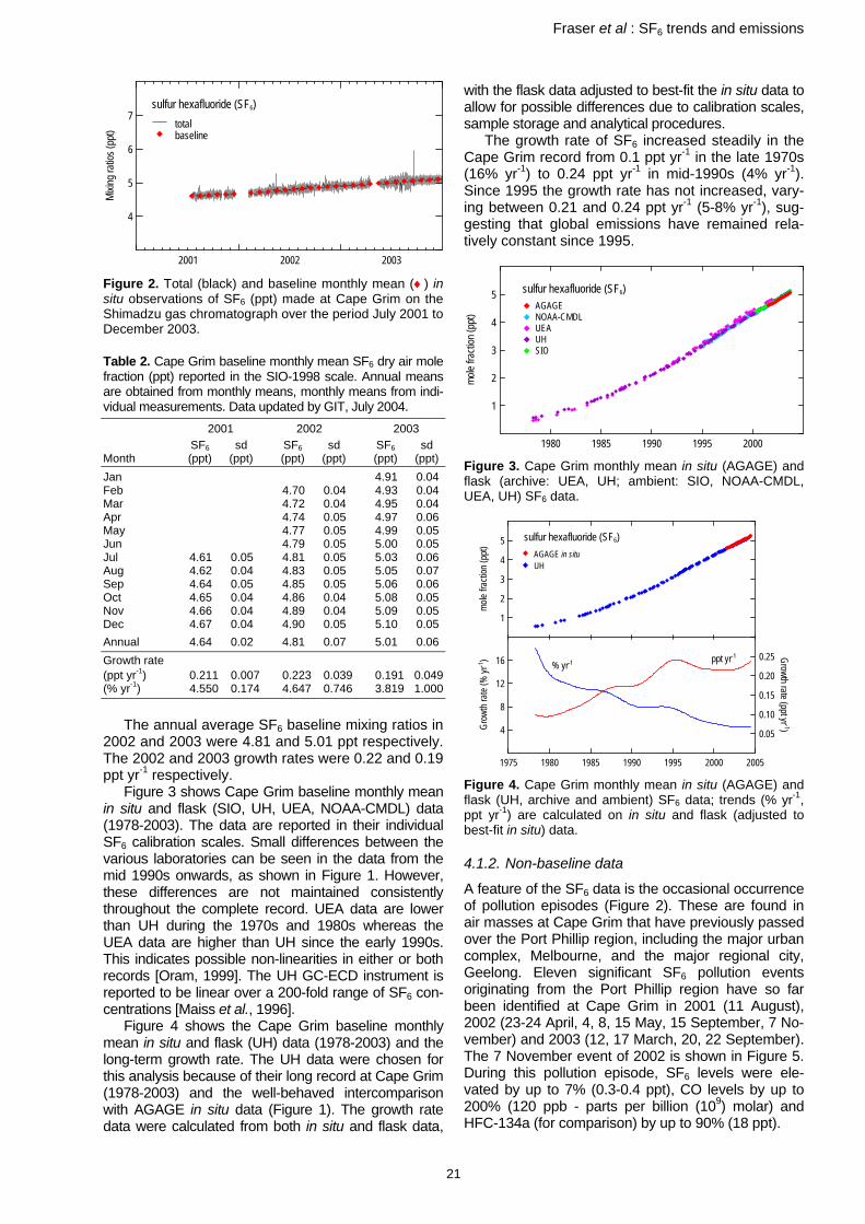
Fraser et al : SF6 trends and emissions
21
4
5
6
7Mi
xing r
atios
(ppt)
sulfur hexafluoride (SF6)totalbaseline
2001 2002 2003 Figure 2. Total (black) and baseline monthly mean (♦) in situ observations of SF6 (ppt) made at Cape Grim on the Shimadzu gas chromatograph over the period July 2001 to December 2003.
Table 2. Cape Grim baseline monthly mean SF6 dry air mole fraction (ppt) reported in the SIO-1998 scale. Annual means are obtained from monthly means, monthly means from indi-vidual measurements. Data updated by GIT, July 2004. 2001 2002 2003 SF6 sd SF6 sd SF6 sd Month (ppt) (ppt) (ppt) (ppt) (ppt) (ppt) Jan 4.91 0.04 Feb 4.70 0.04 4.93 0.04 Mar 4.72 0.04 4.95 0.04 Apr 4.74 0.05 4.97 0.06 May 4.77 0.05 4.99 0.05 Jun 4.79 0.05 5.00 0.05 Jul 4.61 0.05 4.81 0.05 5.03 0.06 Aug 4.62 0.04 4.83 0.05 5.05 0.07 Sep 4.64 0.05 4.85 0.05 5.06 0.06 Oct 4.65 0.04 4.86 0.04 5.08 0.05 Nov 4.66 0.04 4.89 0.04 5.09 0.05 Dec 4.67 0.04 4.90 0.05 5.10 0.05 Annual 4.64 0.02 4.81 0.07 5.01 0.06 Growth rate (ppt yr-1) 0.211 0.007 0.223 0.039 0.191 0.049 (% yr-1) 4.550 0.174 4.647 0.746 3.819 1.000
The annual average SF6 baseline mixing ratios in 2002 and 2003 were 4.81 and 5.01 ppt respectively. The 2002 and 2003 growth rates were 0.22 and 0.19 ppt yr-1 respectively.
Figure 3 shows Cape Grim baseline monthly mean in situ and flask (SIO, UH, UEA, NOAA-CMDL) data (1978-2003). The data are reported in their individual SF6 calibration scales. Small differences between the various laboratories can be seen in the data from the mid 1990s onwards, as shown in Figure 1. However, these differences are not maintained consistently throughout the complete record. UEA data are lower than UH during the 1970s and 1980s whereas the UEA data are higher than UH since the early 1990s. This indicates possible non-linearities in either or both records [Oram, 1999]. The UH GC-ECD instrument is reported to be linear over a 200-fold range of SF6 con-centrations [Maiss et al., 1996].
Figure 4 shows the Cape Grim baseline monthly mean in situ and flask (UH) data (1978-2003) and the long-term growth rate. The UH data were chosen for this analysis because of their long record at Cape Grim (1978-2003) and the well-behaved intercomparison with AGAGE in situ data (Figure 1). The growth rate data were calculated from both in situ and flask data,
with the flask data adjusted to best-fit the in situ data to allow for possible differences due to calibration scales, sample storage and analytical procedures.
The growth rate of SF6 increased steadily in the Cape Grim record from 0.1 ppt yr-1 in the late 1970s (16% yr-1) to 0.24 ppt yr-1 in mid-1990s (4% yr-1). Since 1995 the growth rate has not increased, vary-ing between 0.21 and 0.24 ppt yr-1 (5-8% yr-1), sug-gesting that global emissions have remained rela-tively constant since 1995.
1
2
3
4
5
mole
fracti
on (p
pt)
1980 1985 1990 1995 2000
sulfur hexafluoride (SF6)& AGAGE& NOAA-CMDL& UEA& UH& SIO
Figure 3. Cape Grim monthly mean in situ (AGAGE) and flask (archive: UEA, UH; ambient: SIO, NOAA-CMDL, UEA, UH) SF6 data.
1
2
3
4
5
mole
fracti
on (p
pt)
sulfur hexafluoride (SF6)
4
8
12
16
Grow
th ra
te (%
yr-1
)
1975 1980 1985 1990 1995 2000 2005
0.05
0.10
0.15
0.20
0.25 Growth rate (ppt yr -1)
% yr-1 ppt yr-1
UHAGAGE in situ
Figure 4. Cape Grim monthly mean in situ (AGAGE) and flask (UH, archive and ambient) SF6 data; trends (% yr-1, ppt yr-1) are calculated on in situ and flask (adjusted to best-fit in situ) data.
4.1.2. Non-baseline data
A feature of the SF6 data is the occasional occurrence of pollution episodes (Figure 2). These are found in air masses at Cape Grim that have previously passed over the Port Phillip region, including the major urban complex, Melbourne, and the major regional city, Geelong. Eleven significant SF6 pollution events originating from the Port Phillip region have so far been identified at Cape Grim in 2001 (11 August), 2002 (23-24 April, 4, 8, 15 May, 15 September, 7 No-vember) and 2003 (12, 17 March, 20, 22 September). The 7 November event of 2002 is shown in Figure 5. During this pollution episode, SF6 levels were ele-vated by up to 7% (0.3-0.4 ppt), CO levels by up to 200% (120 ppb - parts per billion (109) molar) and HFC-134a (for comparison) by up to 90% (18 ppt).

Fraser et al : SF6 trends and emissions
22
15
20
25
30
35ppt
80
120
160
ppb4.8
4.9
5.0
5.1
5.2ppt
5-Nov 6-Nov 7-Nov 8-Nov 9-Nov2002
HFC-134a
CO
SF6
Figure 5. Port Phillip region pollution events for SF6, HFC-134a and CO observed at Cape Grim on 7 November 2002.
The process of estimating SF6 emissions in-volved first identifying pollution episodes in the Cape Grim record that were attributed to air masses that passed over the Port Phillip region before travelling across Bass Strait to Cape Grim. Pollution markers (CFC-12, CH2Cl2 and HFC-134a) were used to iden-tify episodes caused by Port Phillip emissions. These ‘pollution episodes’ were extracted, and cor-relations between the trace species in the polluted air masses were derived. Linear regressions applied to the data were performed using a Reduced Major Axis (RMA) regression procedure [Davis, 1986]. These correlations and an estimate of CO emissions from Port Phillip were used to deduce the mass of Port Phillip emissions.
Figure 6 shows back-trajectories for the eleven pollution episodes, indicating that the air passed over or near Melbourne some 6-12 hours before arriving at Cape Grim. Figure 7 shows the elevation in SF6 lev-els compared to CO levels for the eleven identified SF6 pollution episodes at Cape Grim.
Emissions of SF6 (3.0±1.5 tonnes yr-1) from the Port Phillip region were deduced from these episodes during 2001-2003, assuming CO emissions from this region of 680,000 tonnes yr-1 [EPA, 1998; NPI, 2003], which include an assumed 25% uncertainty in CO emissions. This is the first measurement-based esti-mate of regional SF6 emissions in Australia. The Port Phillip region contains 20±1% of Australia’s popula-tion [EPA, 1998] and, assuming SF6 emissions are proportional to population, leads to an estimate of Australian SF6 emissions during 2001-2003 of 15±7.5 tonnes yr-1, or 0.75 tonnes per million people. In GWP terms the SF6 emissions are equivalent to 0.18-0.54 M tonnes of CO2 [< 0.1% of Australia’s total green-house gas emissions in 2000; AGO, 2002].
Figure 6. HYSPLIT [Draxler and Rolph, 2003] back-trajectories for the 11 identified SF6 pollution episodes at Cape Grim. All the trajectories were run with an endpoint height at Cape Grim of 100 m.
Figure 7. The elevation in SF6 levels compared to CO levels for the 11 identified SF6 pollution episodes at Cape Grim. The best-fit slope (SF6-ppt/CO-ppb) is 0.00084 ± 0.00022.
The only SF6 emissions listed currently in the Australian National Greenhouse Gas Inventory (NGGI) are 0.1 tonnes in 2000 from metal produc-tion [AGO, 2002]. Australian SF6 emissions from the electricity transmission and distribution sector have been estimated to be as high as 75 tonnes in 1996/1997, based on US SF6 emission factors (4.1 tonnes of SF6 per million people) [AGO, 2000], but these estimates have not yet been included in the NGGI. Since 1996/1997 US SF6 emission factors for this sector have declined by a factor of 2 [2.1 tonnes per million people in 2002, US EPA 2004]. Applying the latter emission factor to Australia would imply Australian emissions from this sector of about 40 tonnes yr-1 in 2002. The UK, New Zealand and the EU have reported SF6 emissions factors for the elec-tricity transmission and distribution sector of 0.2, 0.4 and 0.7 tonnes per million people respectively [AGO, 2000; NZGGI 2000], significantly lower than the US factors. The possible reasons for these differences between nations are not obvious.

Fraser et al : SF6 trends and emissions
23
5. Conclusions
Long-term observations of SF6 at Cape Grim have shown a growth rate that increased from 0.1 ppt yr-1 in the late 1970s to 0.24 ppt yr-1 in the mid-1990s. Since then, the SF6 growth rate has remained rela-tively constant at 0.23 ± 0.02 ppt yr-1. These data suggest that global emissions of SF6 have been rela-tively constant (±10%) over the past 5 years.
An analysis of SF6 pollution episodes at Cape Grim suggests that SF6 emissions in the Port Phillip region were 3±1.5 tonnes yr-1 during 2001-2003, which have been extrapolated to estimate Australian emissions of 15±7.5 tonnes yr-1, indicating an overall SF6 emission factor for Australia of 0.75 tonnes per million people. This emission factor is near the mid-dle of the range reported by the US, UK, EU and NZ (0.2 to 2.1 tonnes of SF6 per million people).
Continued monitoring of SF6 at Cape Grim, using a higher precision instrument (AGAGE GC-MS-Medusa), which was installed in early 2004, should lead to more accurate estimates of regional SF6 emissions.
Acknowledgment
The authors gratefully acknowledge the NOAA Air Resources Laboratory (ARL) for the provision of the HYSPLIT transport and dispersion model and/or READY website used in this publication: http://www.arl.noaa.gov/ready.html
References AGO, Synthetic Gas Use in Non-Montreal Protocol Industries,
Australian Greenhouse Office, Canberra, Australia, 68 p., 2000. AGO, National Greenhouse Gas Inventory 2000, Australian
Greenhouse Office, Canberra, Australia, 350 p., 2002. Bakwin, P. S., D. F. Hurst, P. P. Tans and J. W. Elkins, Anthropo-
genic sources of halocarbons, sulfur hexafluoride, carbon mon-oxide and methane in the southeastern United States, J. Geo-phys. Res., 102, 15915-15925, 1997.
Burgess, A. B., R. G. Grainger, A. Dudhia, V. H. Payne and V. L. Jay, MIPAS measurement of sulphur hexafluoride (SF6), Geophys. Res. Letts., 31, L05112, doi: 10.1029/2003GL019143, 2004.
Davis, J. C., Statistics and Data Analysis in Geology, New York, John Wiley & Sons, 1986.
Draxler, R. R. and Rolph, G. D., HYSPLIT (HYbrid Single-Particle Lagrangian Integrated Trajectory) Model access via NOAA ARL READY website (http://www.arl.noaa.gov/ready/hysplit4.html). NOAA Air Resources Laboratory, Silver Spring, MD, 2003.
Dunse, B. L., L. P. Steele, P. J. Fraser and S. R. Wilson, An analysis of Melbourne pollution episodes observed at Cape Grim from 1995-1998, in Baseline Atmospheric Program (Aus-tralia) 1997-98, edited by N. W. Tindale, N. Derek and R. J. Francey, Bureau of Meteorology and CSIRO Atmospheric Re-search, Melbourne, Australia, 34-42, 2001.
Dunse, B. L., Investigation of urban emissions of trace gases by use of atmospheric measurements and a high-resolution at-mospheric transport model, Ph.D. Thesis, University of Wollon-gong, Wollongong, Australia, 298 p., 2002.
EPA, Air Emissions Inventory – Port Phillip Region, Environment Protection Agency, Melbourne, Australia, 48p., 1998.
Folger, B. E. and P. G. Simmonds, Drier for field use in the de-termination of trace atmospheric gases, Anal. Chem., 51, 1089, 1979.
Geller, L. S., J. W. Elkins, J. M. Lobert, A. D. Clarke, D. F. Hurst, J. H. Butler and R. C. Myers, Tropospheric SF6: observed lati-tudinal distribution and trends, derived emissions and inter-hemispheric exchange time, Geophys. Res. Letts., 24, 675-678, 1997.
Hall, B. D. (ed.), J. H. Butler, A. D. Clarke, G. S. Dutton, J. W. El-kins, D. F. Hurst, D. B. King, E. S. Kline, J. Lind, L. T. Lock, D.Mondeel, S. A. Montzka, F. L. Moore, J. D. Nance, E. A. Ray, P. A. Romashkin and T. M. Thompson, Halocarbons and Other Atmospheric Trace Species, Chapter 5 in CMDL Summary Re-port No. 26, 2000-2001, edited by D. B. King, R. C. Schnell, R. M. Rosson and C. Sweet, NOAA/US Department of Com-merce, Boulder, USA, 106-135, 2002.
Harnisch, J., Reactive Fluorine Compounds, Chapter 3 in The Handbook of Environmental Chemistry Volume 4 Part E, Reac-tive Halogen Compounds in the Atmosphere, edited by P. Fa-bian and O. N. Singh, Springer-Verlag, Berlin Heidelberg, Ger-many, 81-111, 1999.
Harnisch, J., and N. Hohne, Comparison of emission estimates derived from atmospheric measurements with national estimate of HFCs, PFCs and SF6, Env. Sci. & Pollut. Res., 9(5), 315-320, 2003.
Levin, I., R. Heinz, R. L. Langenfelds, R. J. Francey, L. P. Steele and D. A. Spencer, SF6 from Flask Sampling, Section 4.9 in Baseline 1999-2000, edited by N. W Tindale, N. Derek and P. J. Fraser, Bureau of Meteorology and CSIRO, Melbourne, Aus-tralia, 79, 2003.
Lovelock, J. E., Atmospheric fluorine compounds as indicators of air movements, Nature, 230, 379, 1971.
Maiss, M., L. P. Steele, R. J. Francey, P. J. Fraser, R. L. Lan-genfelds, N. B. A. Trivett and I. Levin, Sulfur hexafluoride – a powerful new atmospheric tracer, Atmos. Environ., 30, 1621-1629, 1996.
Maiss, M. and C. A. M. Brenninkmeijer, Atmospheric SF6: trends, sources and prospects, Environ. Science and Technol., 32, 3077-3068, 1998.
Maiss, M. and C. A. M. Brenninkmeijer, A reversed trend in emis-sions of SF6 into the atmosphere? in Non-CO2 Greenhouse Gases: Scientific Understanding, Control and Implementation, Kluwer Academic Publishers, The Netherlands, 199-204, 2000.
Montzka, S. A. and P. J. Fraser (Lead Authors), Controlled Sub-stances and Other Source gases, Chapter 1 in Scientific Assess-ment of Ozone Depletion: 2002, WMO Global Ozone Research and Monitoring Project – Report No. 47, WMO/UNEP/NOAA/EU/ NASA, Geneva, Switzerland, 1.1-1.83, 2003.
Nakicenovic, N. (Lead Author), Special Report on Emissions Scenarios, Intergovernmental Panel on Climate Change, Cam-bridge University Press, Cambridge, UK, 599 p., 2000.
NPI, National Pollutant Inventory: Carbon monoxide emissions report for the Port Phillip Region, [Web Page], available at http://www.npi.gov.au/, Department of Environment and Heri-tage, Canberra, Australia, 2003.
NZGGI, New Zealand Greenhouse Gas Inventory 2000, http://www.climatechange.govt.nz/resources/reports/nir-apr04/index.html
Oram, D. E., Trends of long–lived anthropogenic halocarbons in the Southern Hemisphere and model calculations of global emissions, PhD thesis, U. East Anglia, Norwich UK, 1999.
Prinn, R. G., R. F. Weiss, P. J. Fraser, P. G. Simmonds, D. M. Cun-nold, F. N. Alyea, S. O’Doherty, P. Salameh, B. R. Miller, J. Huang, R. H. J. Wang, D. E. Hartley, C. Harth, L. P. Steele, G. Sturrock, P. M. Midgley, and A. McCulloch, A history of chemically and radia-tively important gases in air deduced from ALE/GAGE/AGAGE, J. Geophys. Res., 105, 17,751-17,792, 2000.
Thompson, T. M. (ed.), J. H. Butler, B. C. Daube, G. S. Dutton, J. W. Elkins, B. D. Hall, D. F. Hurst, D. B. King, E. S. Kline, B. G. Lafleur, J. Lind, S. Lovitz, D.Mondeel, S. A. Montzka, F. L. Moore, J. D. Nance, J. L. New, P. A. Romashkin, A. Scheffer, and W. J. Snible, Halocarbons and Other Atmospheric Trace Species, Chapter 5 in CMDL Summary Report No. 27, 2002-2003, NOAA/US Department of Commerce, Boulder, USA, 115-135, 2004.
Thoning, K. W., P. P. Tans and W. D. Komhyr, Atmospheric car-bon dioxide at Mauna Loa Observatory, 2, Analysis of the NOAA/GMCC data, 1974 - 1985, J. Geophys. Res., 94, 8549-8565, 1989.
US EPA, Inventory of U.S. Greenhouse Gas Emissions and Sinks: 1990-2002, U.S. Environmental Protection Agency, Washington, DC, USA, EPA 430-R-04-003, 2004.
Vollmer, M. K. and R. F. Weiss, Simultaneous determination of sulfur hexafluoride and three chlorofluorocarbons in water and air, Marine Chem., 78, 137-148, 2002.

PROGRAM REPORTS - General
4. PROGRAM REPORTS 4.1. INTRODUCTION
The Program Reports section documents the status and preliminary results of the scientific experiments and measurements at Cape Grim during the years 2001 and 2002. There are essentially three types of measurement programs at Cape Grim.
The first and main group are the Cape Grim Pro-grams which are long-term and provide the core measurements of compounds monitored in the at-mosphere at Cape Grim. The Lead Scientists for these programs collectively form the Cape Grim ‘Working Group’, essentially the scientific steering committee, and are responsible for maintaining the continuity and quality of the core data from Cape Grim.
The second group of scientific programs are the short-term, more research orientated, studies la-belled as ‘Pilot Projects’. Generally these studies only last from one to three years and are designed to develop and test new sampling techniques and/or equipment, or for short-term intensive measure-ments of compounds that are difficult to measure routinely.
The final group of programs includes all the Col-laborative Programs, primarily the longer-term inter-national collaborations where samples and data are collected and shared with international colleagues. Some of these collaborative studies form part of global surveys and Cape Grim provides assistance and samples to outside researchers. Sometimes in-cluded in the collaborative program reports are the short-term intensive studies made by scientists and research students who are visiting Cape Grim to take advantage of the sampling facilities and support at the Cape Grim station.
Cape Grim reports
The Program, Pilot Project and Collaborative reports included in this edition of Baseline are categorised into four groupings: General (including climatology and transport tracers, and the report on the Cape Grim database and data management) Trace Gases (radiatively or chemically active gases) Multi-phase (including precipitation, particles and multi-phase studies and Radiation (electromagnetic radiation monitoring).
Missing reports
A brief summary is included below of the Cape Grim and collaborative programs that have not submitted reports for 1999-2000, but were in operation during at least some of this period.
Isotopes in precipitation; Approximately 24 monthly ‘continuous’ samples were collected for analysis of oxygen isotopes and deuterium in rain water. The rain water samples are initially sent to ANSTO, with a subsample forwarded to the CSIRO-Division of Soils. The data ultimately end up ar-
chived at, and available from, the International Atomic Energy Agency (IAEA) in Vienna, Austria.
Other precipitation samples were collected from the manual rain gauge on a daily basis, and from the weekly ERNI ‘Baseline’ collector, for the University of Tasmania for isotope analysis.
Aerosol radionuclides; Weekly hi-volume aerosol filter samples are collected and counted for radionu-clide radiation. Data are then directly transmitted by satellite to the Department of Energy (DOE), USA. Filters and data backups are sent approximately every month.
Elemental carbon; Weekly low-volume aerosol fil-ters are collected and sent to the University of Stockholm, Sweden, for the analysis of particulate elemental carbon.
4.2. DATA MANAGEMENT
R P Wheaton Cape Grim Baseline Air Pollution Station, Bureau of Meteorology, Smithton, Tasmania 7330, Australia Introduction
Data is collected at Cape Grim Baseline Air Pollution Station (CGBAPS) from 2 broad sources: the analog Data Acquisition System (DAS) and instrument con-trol PCs.
The DAS consists of an HP3497A 60-channel scanning DVM controlled over HP-IB interface by custom software on an HP9000/715 HP workstation ('Jacob'). The DAS samples voltages from each channel 10 times per minute and reduces these 10 raw readings to mean, max, min, standard deviation and first reading for each minute. The resulting data is stored in a daily binary-format file. All 60 channels are sampled, although not all are in use at any given time.
Newer experiments at CGBAPS have tended to use a decentralised approach in which an instrument is controlled by a dedicated PC. The controlling PC typically accesses a central file server over the net-work to archive its data. Instrument control software and hardware are developed elsewhere by the re-sponsible scientist. Due to the development being left to the individual a wide range of software and operating systems is in use at CGBAPS. Older In-strument PCs communicate with the central server using PC-NFS or LANMAN network client software while newer machines use their built-in SMB clients to access our 'samba' service.
System Operation
The Data Acquisition System lost 4002 minutes in 2001 (a success rate of 99.23%) and 222 minutes in 2000 (99.96%). A major disruption to data acquisi-tion occurred on Christmas Eve 2001 when lightning struck the station after staff had left for their Christ-mas break. A large number of systems, including data acquisition, were rendered inoperative until staff returned on the 27 December. Other notable disruptions were due to mains power outages.
24

PROGRAM REPORTS - General
25
Modifications were made to the Data Acquisition System to allow the production of a third 'baseline' signal. Baseline #3 is similar to baseline #2 but has a seasonally-variable CN threshold instead of the fixed value for baseline #2. The daily CN threshold value is derived from the 90th percentile of in-sector CN readings over the last 5 years. CN values are obtained monthly and interpolated to daily values us-ing a cubic spline.
The FTP service (ftp.baps.bom.gov.au) at Cape Grim was migrated from 'wilhelm' to 'pampero'.
A couple of hard disk failures were encountered on the station file server 'mauka' but the operation of the RAID5 array meant no interruption to service. The only significant outage on the file server was caused by a failed operating system upgrade - nor-mal service was resumed within 24 hours.
A new linux-based file server was purchased for the Smithton office. The machine is an Intel-based ‘Gateway 7400’ server with redundant power supply and disk arrays. This server 'shamal' is used as the mail, printer and file server for the Smithton office as well as mirroring data from the Cape Grim servers. This frees 'virazon' to run the Oracle database.
A new HP (now Agilent) 34970A scanning volt-meter was purchased as a replacement for the reli-able but ageing HP3497A currently in use. Unfortu-nately development work on the new Data Acquisi-tion System 'DAS2' stalled due to staff shortages in the IT section.
The Cape Grim communications infrastructure was upgraded with the addition of about 100 new LAN connection points throughout the station. This allows for the inevitable future expansion of net-worked devices at the station.
The 'Lynx 1500' UPS that powers the database and mail servers in the Smithton Office had its bat-teries replaced after 5 years of operation.
The ageing and increasingly unreliable Sun workstations 'agage' and 'msgrim' were replaced by a new Intel/Linux workstation 'agage2'.
The introduction of a number of PCs running Windows 2000 required some updating and recon-figuration of the file servers - this was accomplished with minimal impact on data acquisition.
Data Processing
A preliminary merged data set of Cape Grim Radon data commenced automatic production: this is a ‘best of’ compilation of the data from HURD1 and HURD2. Reviewed radon data from 1999 was re-turned from the radon Lead Scientist, Stewart Whit-tlestone.
The recovery of ancient GRIMCO I datasets stored on magnetic tape continued slowly with the kind assistance of Clive Elsum (CSIRO Atmospheric Research).
The Annual Meteorology Reports were ported from Grimco1 and scheduled for automatic genera-tion and e-mail on the first day of each year.
Hourly results processing was amended to allow Lo-Flo CO2 data to optionally replace BASGAM in
the published hourly results. Station staff manually control switching between sources. At this stage BASGAM is still the preferred source, however Lo-Flo data was used between 18 November 2002 and 30 December 2002 whilst BASGAM was unservica-ble.
After a prolonged hiatus, the ozone processing software was ported from GRIMCO-I and the ozone dataset brought up to date in preparation for the WMO ozone audit. Thanks to Simon Bentley (CSIRO Atmospheric Research) for his invaluable contribution to this effort.
Dr Stewart Whittlestone's analyses of minutely wind data revealed some problems with the algo-rithm used to compute standard deviation of wind direction. Corrections will be required once the prob-lem is fully understood.
Software Development
Flask sampling record sheets were progressively transferred online. All routine flask sampling pro-grams conducted at Cape Grim now have an online record sheet that automates the extraction of sup-porting data and archives the results electronically. Electronic data exchange was initiated with some partner organisations to reduce manual handling and transcription errors.
Improvements were made to our external website (http://www.bom.gov.au/inside/cgbaps/) including links to associated sites.
An email to SMS gateway service was purchased from RedRock communications. This allows station monitoring systems to page staff via their mobile phone if urgent action is required.
A web-based sign-in book was developed for the station to address OH&S concerns.
Slow progress was made on the next-generation Data Acquistion System (DAS2) hampered by con-tinued staff shortages.
Other Significant news
IT manager Brian Weymouth departed Cape Grim in August 2001 for the warmer climes of Newcastle University. Brian worked at Cape Grim for 7 years and was the driving force behind GRIMCO II and the modernisation of Cape Grim data processing. His contribution cannot be understated. Randall Whea-ton was appointed to fill the vacancy left by Brian and Stuart Baly subsequently joined the IT team in Randall's old position.

PROGRAM REPORTS - General
26
4.3. METEOROLOGY/CLIMATOLOGY 2001-2002
A Downey and M Tully Bureau of Meteorology Melbourne, Victoria 3001, Australia [Supported by CGBAPS research funds]
Introduction
Tables 1 to 11 present a summary of the Cape Grim meteorological conditions for 2001 and 2002.
Tables 1, 2, 3, and 4 contain mean values for 0000, 0300, 0600, 0900, 1200, 1500, 1800, 2100 (AEST) and monthly means for each month of the year. These are computed using, for example, the mean of hours 2, 3 and 4 to represent 0300.
In Table 5, extreme max is the highest of all of minute means for the month. Mean daily max is the mean of the daily maxima for the month. Similarly for mean daily min and extreme min.
Table 6 shows the monthly and annual rainfall in millimetres.
Table 7 is derived from month-to-date and year-to-date counts of the number of minutes during which the 'baseline switch' was on. Baseline condi-tions are said to exist if wind direction is between 190° and 280° and the count of condensation nuclei is less than 600 cm-3.
Tables 8-11 are derived from the hourly mean vector wind speed and direction from the 10-m and 50-m levels.
Figures 1 to 12 are derived from (raw) minute data. The monthly means presented are the mean of every minute that month. The mean monthly maxima and minima shown are the monthly means of daily maxima, and minima from the wind speeds aver-aged over one minute (wind speeds are recorded every six seconds).
Much of the overview description below is drawn from the excellent monthly climate summaries pre-pared by the Climate and Consultancy Section of the Tasmanian Regional office of the Bureau [Com-monwealth Bureau of Meteorology, 2002].
Overviews of 2001 and 2002
In summer, the circulation is typically dominated by a weak circulation pattern associated with the migra-tion of high-pressure systems from west to east along the subtropical ridge (STR). This was the case in January 2001. Much of the state had also re-ceived lower than normal rainfall and in the dry con-ditions a number of bushfires were started by light-ning and over 10,000 ha were burned. February continued the trend and was drier and warmer than normal. In autumn low pressure systems usually start to influence the state and that was the case in March, which remained warmer than normal but was also wetter. By late autumn, westerly winds usually dominate. This autumn however found the state un-der the influence of high-pressure systems that caused below normal rainfall across the state. In June the westerlies returned and there was above
normal rainfall in most areas. The system embedded in the westerlies can make June a windy month. A gust of 172 km hr-1 was recorded at Maatsuyker Is-land, in the Southern Ocean. Rainfall across the state was above normal. However, in July the gen-eral weather pattern became quite anomalous. There were high-pressure systems near and even to the south of the state for much of the month. This led to light and even easterly winds and very low rainfall, with some areas recording their lowest monthly rainfalls on record in August. However, things returned to normal and there was above nor-mal rainfall. In September there was more than the usual northerly component to the wind and it was generally warmer than normal. In October the state was dominated by low-pressure systems making it warmer and wetter than normal. By November, the STR has normally migrated pole-wards enough to be a significant influence. That was the case in No-vember and December.
In January 2002 a low pressure system domi-nated the weather pattern and there was signifi-cantly higher rainfall in most areas. By February things had returned to normal. After a relatively cool summer, March was relatively warm across the state (though not at Cape Grim). Interestingly enough there were no records set for any element at any site (this is quite unusual). April is the month where more reliable rainfall starts. April 2002 was drier than nor-mal with low rainfall records set at quite a number of sites. This was mainly due to the influence of high-pressure systems, which lingered in the region. This pattern continued into May with rainfall across the state below normal and temperatures above normal. In June rainfall generally increases as it did in 2002. In fact, quite a few stations set monthly rainfall re-cords and some of these were substantial increases. Zeehan (on the south-west coast) for example, had a record 456 mm for the month, up from 394 mm, set some 25 years ago. July continued the above normal rainfall in the west of the state but in the east it was below normal caused by predominantly north-westerly winds. By August flow had returned to nor-mal. In September the state was under the influence of strong westerly winds. These caused large swells. The Spirit of Tasmania was forced to return to Mel-bourne in the face of a 7 m swell. In October things returned to close to normal. By November and De-cember however, the influence of high-pressure sys-tems led to below normal rainfalls.
Temperature Higher-than-normal temperatures were observed early in 2001. In February, Burnie (about 120 km east of Cape Grim) recorded its highest mean daily maximum (23.2°C) and Wynyard Airport (about 100 km east of Cape Grim) reported its highest mean daily maximum for any month (22.8°C). Marrawah (about 50 km south of Cape Grim) also recorded its highest minimum temperature for February (19.8°C). In March Wynyard Airport reported its highest daily minimum (18.9°C). In July, Burnie (8.1°C) and Wyn-

PROGRAM REPORTS - General
27
yard Airport (13.6°C) recorded their highest mean daily minima. Most of the state had monthly mean maxima well above normal. In September higher than normal temperatures continued with Marrawah (15.2°C) and Wynyard Airport (15.6°C) recording re-cord mean daily maxima and Burnie (9.3°C) and Marrawah (9.1°C) recording highest mean daily min-ima. Marrawah (18.5°C) and Wynyard Airport (20.6°C) recorded their highest September tempera-tures on record. Figure 1 shows the monthly mean temperature anomaly at Cape Grim during 2001. The year starts off warmer than usual and is gener-ally warmer throughout the year except for the end of the year. This is compatible with the overview and with the temperature summary above.
Figure 1. Monthly mean temperature anomaly during 2001 (2001 temperatures – long term [1987-2000] means).
Due to above normal rainfall, 2002 began with below normal maxima and above normal minima. No temperature records were set until April when Wyn-yard Airport (19.0°C) reported record highest mean daily maxima. In May Wynyard Airport (16.0°C) re-corded its highest mean daily maximum tempera-tures for the month. Marrawah recorded a record high may temperature of 22°C. In June Wynyard Airport set its lowest ever temperature (-3.3°C). In July Marrawah (8.1°C ) reported its highest mean daily minimum and Wynyard Airport which is appar-ently no stranger to records reported its lowest July daily minimum (-4.0°C). In September Wynyard Air-port reported its highest September temperature (20.6°C). In November Wynyard has its highest temperature for that month (28.4°C). Wynyard also set a record highest mean daily minimum tempera-ture for December (17.8°C). Figure 2 shows the monthly mean temperature anomaly at Cape Grim during 2002. The systems which caused slightly lower than normal temperatures in December 2001 persist and the 2001/2002 summer is a cool one with a higher than normal rainfall. For the rest of 2002 however, temperatures are above normal at the station (as they were through much of the State).
Figure 2. Monthly mean temperature anomaly during 2002 (2002 temperatures – long term [1987-2000] means).
Pressure 2001 began with average to slightly below average pressure at the Cape Grim (Figure 3 shows the monthly mean pressure anomaly at Cape Grim dur-ing 2001). July and August are contrasting months with a strong positive anomaly in July reversing to a strong negative anomaly in August. This is reflected in the broadscale patterns, especially in July, which was notable for the presence of high-pressure sys-tem sometimes even to the south of the station.
Figure 3. Mean monthly barometric pressure anomaly for 2001. (2001 pressures – long term [1987-2000] means).
2002 began with slightly below normal pressure Figure 4 shows the monthly mean pressure anomaly at Cape Grim during 2002). Of most interest how-ever are the two strong negative anomalies in June and September. The influence of low-pressure sys-tems can be seen in both periods with June setting rainfall records and September’s high winds.
Figure 4. Mean monthly barometric pressure anomaly for 2002 (2002 pressures – long term [1987-2000] means).

PROGRAM REPORTS - General
28
Rainfall In 2001 rainfall totals around the state were mixed, with some months above normal and some below. July was a significant month because some sites re-corded lowest-ever rainfall on record. Burnie, for ex-ample, received 26.4 mm against a long-term aver-age of 130 mm, setting a record in the 56 years of records. Cape Grim (shown in Table 6) received 775.4 mm against a long-term average of 806mm [Downey and Tully, 2002]. This is the fifth year of be-low average rainfall. The last year the station re-ceived rainfall above the long-term average was 1996, when 934 mm were recorded.
2002 started with below normal rainfalls across most of the state, especially in April and March where record low rainfall records were reported. In April, Burnie received just 24 mm against a long-term average of 77 mm and Marrawah received its lowest April rainfall on record (33.2 mm). At Cape Grim, the station received its lowest annual rainfall (610 mm, shown in Table 6) since the drought, which culminated in 1982 (when 571.8 mm was re-corded).
Baseline time 2001 had an average for the year of 21.4% (as shown in Table 7). This compares with a long-term average of 32% but it is an increase on the 20.1% recorded in 2000. The weak circulation patterns in summer led to some low values there and the anomalous circulation patterns in July led to some quite low values for those months.
2002 recorded a mean baseline average of 28.2% for the year, up from the previous year but still below the long-term average. The largest values are normally recorded in spring and that was the case here.
Wind There is a 70-m tower to the south-east of the measuring device for the 50-m anemometer and wind vane and to the north-east for the 10-m and there is a 70-m cliff to the west of the instruments, so caution should be taken in interpreting values for winds from these directions.
Tables 8 and 10 show the wind speed and direc-tion at the 10-m and 50-m level during 2001. This can be seen in Figures 5 and 6, which show the fre-quency distribution at 10 m and 50 m respectively for 2001. Figures 7 and 8 show the monthly means of daily maxima, means and minima one-minute wind speeds at both heights for 2001 and 2002 re-spectively. As is usual the greatest percentage of the wind is from between the south and west.
Figure 5. Frequency distribution of the 10-m wind for 2001.
Figure 6. Frequency distribution of 50-m wind for 2001.
Figure 7. Monthly average wind speeds at 10 m for 2001. Top line is mean maximum, middle is mean and bottom line is mean minimum.
Figure 8. Monthly average wind speeds at 50 m for 2001. Top line is mean maximum, middle is mean and bottom line is mean minimum.

PROGRAM REPORTS - General
29
Tables 9 and 11 show the wind speed and direc-tion at the 10-m and 50-m level during 2002. This can be seen graphically in Figures 9 and 10 which show the frequency distribution at 10 and 50-m re-spectively for 2002. Figures 11 and 12 show the monthly means of daily maxima, means and minima one-minute wind speeds at both heights for 2002.
Once again most of the wind came from the south to west sector. September shows some quite strong averages and maxima. This was a very windy month across the north of the State (recall that the Spirit of Tasmania had to hide in Melbourne be-cause of the large swell).
Figure 9. Frequency distribution of 10-m wind for 2002.
Figure 10. Frequency distribution of 50-m wind for 2002.
Figure 11. Monthly average wind speeds at 10 m for 2002. Top line is mean maximum, middle is mean and bot-tom line is mean minimum.
Figure 12. Monthly average wind speeds at 50 m for 2002. Top line is mean maximum, middle is mean and bot-tom line is mean minimum.
Acknowledgement
The authors would like to thank Laurie Porter, Stuart Baly, Randall Wheaton and the other Cape Grim staff for their dedicated efforts in maintaining instru-mentation and records and supplying data.
References Bureau of Meteorology, Monthly Weather Review Tasmania
(January to December 2002), Commonwealth of Australia, 2002.
Downey, A., and M. Tully, Meteorology/Climatology 1999/2000 in Baseline Atmospheric Program (Australia) 1999-2000, edited by N. W. Tindale, N. Derek, and P. J. Fraser, Bureau of Meteorology and CSIRO Atmospheric Research, Melbourne, Australia, 64-70, 2003.

PROGRAM REPORTS - General
30
Table 1. Monthly mean dry bulb temperature (°C) for 2001 and 2002. 2001 Jan Feb Mar Apr May Jun Jul Aug Sep Oct Nov Dec Mean 0000 15.6 16.2 15.3 13.0 11.7 11.8 10.0 10.2 11.4 11.0 11.4 12.2 12.5 0300 15.3 16.1 15.2 12.8 11.4 11.6 9.8 10.1 11.1 11.0 11.2 11.9 12.3 0600 15.8 16.4 15.0 12.9 11.1 10.8 9.6 10.0 11.2 11.3 11.7 12.5 12.3 0900 17.8 18.5 16.9 14.3 12.5 11.4 10.6 10.9 12.8 12.8 13.4 14.2 13.8 1200 18.9 19.6 18.0 15.4 14.3 12.8 11.9 11.7 13.7 13.5 14.3 15.0 14.9 1500 18.1 19.4 17.5 14.9 13.5 12.5 11.9 11.5 13.2 13.0 13.8 14.7 14.4 1800 16.9 17.5 16.1 13.8 12.1 11.9 10.8 10.7 11.8 11.5 12.5 13.5 13.2 2100 15.9 16.4 15.5 13.3 11.8 11.9 10.3 10.5 11.5 11.1 11.9 12.6 12.7 Mean 16.8 17.5 16.2 13.8 12.3 11.8 10.6 10.7 12.1 11.9 12.5 13.3 13.3 2002 Jan Feb Mar Apr May Jun Jul Aug Sep Oct Nov Dec Mean 0000 13.9 14.6 14.0 13.4 11.7 11.5 11.1 10.3 10.6 10.8 11.4 12.9 12.1 0300 13.6 14.4 13.9 13.2 11.5 11.4 11.0 10.1 10.6 10.6 11.4 12.7 12.0 0600 14.0 14.6 14.0 13.0 11.4 11.2 11.2 10.1 10.5 10.9 12.1 13.5 12.2 0900 15.8 16.4 15.8 14.7 12.6 11.8 11.4 11.0 11.6 12.4 13.7 15.3 13.5 1200 16.5 17.6 16.8 16.4 14.0 12.6 11.8 12.2 12.3 13.3 14.6 16.0 14.5 1500 16.4 17.2 16.2 16.0 13.8 12.2 11.7 11.7 11.9 12.8 14.1 15.5 14.1 1800 15.3 15.8 14.8 14.3 12.3 11.7 11.2 10.7 11.0 11.4 12.6 14.2 12.9 2100 14.4 14.9 14.3 13.7 11.9 11.6 11.2 10.4 10.8 11.0 11.8 13.4 12.4 Mean 15.0 15.7 15.0 14.3 12.4 11.7 11.3 10.8 11.2 11.7 12.7 14.2 13.0
Table 2. Monthly mean relative humidity (%) for 2001 and 2002. 2001 Jan Feb Mar Apr May Jun Jul Aug Sep Oct Nov Dec Mean 0000 83.0 81.0 81.5 77.5 81.1 80.4 85.1 81.7 81.2 81.4 79.0 77.1 80.9 0300 84.5 81.3 81.5 77.8 81.7 82.1 84.2 81.5 81.3 81.6 79.1 77.6 81.3 0600 83.8 80.9 82.3 77.0 83.5 82.2 83.6 81.4 80.1 78.9 77.6 74.3 80.6 0900 76.0 73.2 75.6 73.1 79.2 79.9 81.4 80.0 74.8 73.0 72.7 69.9 75.8 1200 70.5 68.0 71.7 69.7 72.4 78.3 77.2 76.6 70.6 70.4 70.5 68.9 72.1 1500 73.6 67.4 73.2 72.3 76.2 78.4 78.5 78.3 71.5 73.1 73.5 70.1 73.9 1800 78.2 75.3 79.0 76.1 81.7 80.9 84.8 82.0 78.0 78.7 77.5 74.1 78.9 2100 81.8 79.1 81.6 77.2 81.5 81.8 85.2 80.6 79.8 80.8 79.8 76.7 80.6 Mean 78.9 75.8 78.3 75.1 79.6 80.5 82.5 80.2 77.1 77.2 76.2 73.6 78.0 2002 Jan Feb Mar Apr May Jun Jul Aug Sep Oct Nov Dec Mean 0000 83.7 79.3 81.3 86.3 79.2 78.3 79.0 78.5 76.8 80.7 80.8 83.3 80.6 0300 84.0 78.0 79.8 85.7 80.7 78.6 79.4 79.2 76.0 81.4 80.2 84.1 80.5 0600 82.0 76.8 80.1 84.1 80.6 79.3 76.7 79.3 75.4 80.8 77.7 81.2 79.5 0900 76.3 71.5 72.5 78.2 77.5 77.2 76.4 76.2 71.6 74.7 73.6 74.0 74.9 1200 75.0 67.5 69.7 70.7 72.2 73.7 73.0 70.9 69.2 71.2 70.4 71.1 71.2 1500 75.5 70.0 72.7 73.7 72.7 74.9 74.6 72.8 73.0 73.8 71.8 72.0 73.1 1800 79.7 76.4 78.7 83.0 79.3 76.6 77.9 75.4 76.0 79.6 77.4 76.5 78.0 2100 83.4 78.3 82.0 85.2 79.0 78.1 78.5 77.0 76.8 81.2 80.2 80.1 79.9 Mean 79.9 74.7 77.1 80.9 77.6 77.1 77.0 76.2 74.4 77.9 76.5 77.8 77.2
Table 3. Monthly mean absolute humidity (gm-3) for 2001 and 2002. 2001 Jan Feb Mar Apr May Jun Jul Aug Sep Oct Nov Dec Mean 0000 11.2 11.3 10.8 8.9 8.6 8.6 8.0 7.8 8.4 8.2 8.2 8.4 9.0 0300 11.2 11.3 10.8 8.9 8.5 8.7 7.8 7.8 8.3 8.2 8.1 8.3 9.0 0600 11.4 11.4 10.8 8.8 8.5 8.6 7.7 7.8 8.2 8.1 8.2 8.3 9.0 0900 11.6 11.7 11.0 9.1 8.8 8.7 8.0 8.1 8.4 8.3 8.5 8.6 9.2 1200 11.5 11.6 11.1 9.3 9.0 8.9 8.4 8.2 8.5 8.4 8.8 8.9 9.3 1500 11.5 11.5 11.1 9.3 9.0 8.7 8.4 8.1 8.3 8.3 8.8 8.9 9.3 1800 11.4 11.4 11.0 9.2 8.9 8.6 8.4 8.1 8.3 8.2 8.6 8.7 9.2 2100 11.2 11.2 11.0 9.0 8.6 8.7 8.2 7.9 8.3 8.2 8.6 8.5 9.1 Mean 11.4 11.4 10.9 9.1 8.7 8.7 8.1 8.0 8.3 8.3 8.5 8.6 9.2 2002 Jan Feb Mar Apr May Jun Jul Aug Sep Oct Nov Dec Mean 0000 10.2 10.1 9.9 10.1 8.3 8.1 8.0 7.6 7.5 8.1 8.4 9.5 8.8 0300 10.0 9.8 9.7 9.9 8.4 8.1 8.0 7.6 7.5 8.0 8.3 9.5 8.7 0600 10.0 9.8 9.8 9.7 8.4 8.1 7.8 7.6 7.4 8.1 8.4 9.7 8.7 0900 10.4 10.1 9.9 10.0 8.6 8.2 7.9 7.7 7.5 8.2 8.8 9.9 8.9 1200 10.7 10.3 10.1 10.0 8.8 8.2 7.9 7.7 7.6 8.3 8.9 9.8 9.0 1500 10.7 10.4 10.1 10.1 8.7 8.1 7.9 7.7 7.8 8.3 8.8 9.7 9.0 1800 10.5 10.4 10.1 10.3 8.7 8.1 7.9 7.4 7.7 8.3 8.7 9.5 8.9 2100 10.5 10.2 10.2 10.2 8.5 8.2 8.0 7.5 7.6 8.2 8.5 9.5 8.9 Mean 10.4 10.1 10.0 10.0 8.6 8.2 7.9 7.6 7.6 8.2 8.6 9.6 8.9

PROGRAM REPORTS - General
31
Table 4. Monthly mean barometric pressure (hPa) for 2001 and 2002. 2001 Jan Feb Mar Apr May Jun Jul Aug Sep Oct Nov Dec Mean 0000 1004.6 1003.9 1005.0 1009.6 1007.9 1008.0 1011.1 999.5 1004.7 998.0 1002.9 999.1 1004.7 0300 1003.8 1003.2 1004.3 1008.9 1007.5 1007.6 1010.9 998.9 1004.0 997.1 1002.5 998.4 1004.1 0600 1004.5 1003.8 1004.9 1009.4 1007.9 1007.7 1011.1 999.3 1004.5 997.7 1003.3 999.0 1004.6 0900 1005.3 1004.4 1005.7 1010.3 1008.6 1008.6 1011.8 1000.6 1005.1 998.3 1003.8 999.4 1005.4 1200 1004.9 1004.0 1005.2 1009.8 1007.9 1007.9 1011.0 999.7 1004.5 997.8 1003.2 999.4 1004.8 1500 1004.3 1003.4 1004.5 1009.1 1007.4 1007.3 1010.2 999.0 1003.8 997.3 1002.5 998.7 1004.1 1800 1004.4 1003.6 1004.9 1009.6 1007.9 1007.8 1010.5 999.5 1004.4 998.0 1002.7 998.9 1004.6 2100 1005.3 1004.3 1005.6 1010.1 1008.3 1008.2 1010.9 1000.0 1005.0 998.7 1003.4 999.5 1005.1 Mean 1004.6 1003.8 1005.0 1009.6 1007.9 1007.9 1010.9 999.6 1004.5 997.9 1003.0 999.1 1004.7 2002 Jan Feb Mar Apr May Jun Jul Aug Sep Oct Nov Dec Mean 0000 1000.0 1003.0 1005.5 1010.2 1007.4 1001.5 1002.4 1006.8 998.0 1000.1 1004.7 1003.6 1003.7 0300 999.1 1002.3 1004.7 1009.6 1007.0 1001.2 1002.0 1006.1 997.1 999.5 1004.0 1002.9 1003.0 0600 999.9 1002.9 1005.2 1010.1 1007.3 1001.3 1002.1 1006.3 997.5 1000.0 1004.8 1003.6 1003.5 0900 1000.6 1003.6 1006.1 1010.9 1007.9 1002.3 1002.8 1007.3 998.4 1000.6 1005.5 1004.0 1004.2 1200 1000.5 1003.1 1005.9 1010.3 1007.2 1001.5 1002.3 1006.8 997.8 1000.2 1005.2 1003.7 1003.8 1500 1000.2 1002.4 1005.2 1009.6 1006.6 1000.8 1001.9 1006.3 997.4 999.3 1004.5 1003.1 1003.2 1800 1000.3 1002.5 1005.5 1010.1 1007.2 1001.2 002.5 1006.9 998.2 999.8 1004.8 1003.1 1003.6 2100 1001.1 1003.3 1006.3 1010.7 1007.7 1001.7 1002.9 1007.3 998.7 1000.4 1005.5 1003.9 1004.2 Mean 1000.2 1002.9 1005.5 1010.2 1007.3 1001.4 1002.4 1006.7 997.9 1000.0 1004.9 1003.5 1003.6
Table 5. Monthly temperature data (°C) 2001 and 2002. 2001 Jan Feb Mar Apr May Jun Jul Aug Sep Oct Nov Dec Extreme max 24.9 28.7 23.5 20.3 19.4 21.8 15.2 15.6 19.5 17.2 19.8 20.1 Mean daily max 20.3 21.2 19.2 16.8 15.7 14.1 13.1 13.0 14.9 14.7 16.1 15.9 Extreme min 10.1 11.4 9.9 5.9 6.0 6.2 6.7 4.1 5.2 5.6 5.2 8.7 Mean daily min 14.2 14.8 13.4 11.0 9.9 10.1 8.4 8.4 9.9 9.5 10.0 10.8 2002 Jan Feb Mar Apr May Jun Jul Aug Sep Oct Nov Dec Extreme max 22.6 23.0 23.2 20.9 20.8 16.4 14.9 15.2 19.9 18.2 21.0 22.5 Mean daily max 17.9 18.9 17.9 17.7 15.2 13.6 13.1 13.1 13.7 14.4 15.7 17.0 Extreme min 9.2 9.0 9.6 6.9 6.6 3.9 2.9 5.6 5.8 6.2 6.6 7.0 Mean daily min 12.6 13.0 12.7 11.8 10.1 9.5 9.2 8.9 8.6 9.4 9.9 11.4
Table 6. Monthly rainfall (mm) 2001 and 2002. Jan Feb Mar Apr May Jun Jul Aug Sep Oct Nov Dec Total 2001 37.4 22.0 84.4 31.4 23.2 98.0 51.0 113.8 82.6 125.6 62.8 43.2 775.4 2002 28.4 27.4 5.6 23.8 56.8 106.6 116.8 76.8 53.2 61.0 20.6 33.0 610.0
Table 7. Monthly baseline time (%) 2001 and 2002. Jan Feb Mar Apr May Jun Jul Aug Sep Oct Nov Dec Total 2001 5.4 14.6 17.0 22.8 19.7 30.5 19.6 35.0 23.3 25.5 14.2 29.2 21.4 2002 15.4 18.2 26.0 9.0 22.8 36.4 36.9 37.4 33.9 37.9 28.0 35.8 28.2
Table 8. 10-m vector wind summary 2001 (%).
Jan Feb Mar Apr May Jun Jul Aug Sep Oct Nov Dec Mean Speed Summary (km hr-1), Range [a,b) meaning less than b and equal to or greater than a. [0,10) 3.8 4.3 11.6 6.4 13.4 4.9 12.0 5.9 8.2 12.0 6.0 7.5 8.0 [10,20) 13.2 10.9 17.9 23.5 33.7 12.4 29.4 12.1 14.2 18.0 16.8 17.4 18.4 [20,30) 23.8 17.1 17.5 24.6 20.6 24.9 21.0 20.8 31.2 24.5 21.4 27.7 22.9 [30,40) 22.2 21.7 14.4 18.2 15.3 22.6 13.0 19.0 26.2 17.5 22.1 31.0 20.1 [40,50) 19.9 29.5 16.1 19.2 13.6 12.8 13.0 14.2 13.6 14.2 16.7 9.1 15.9 [50,60) 14.2 14.6 14.7 5.4 3.1 10.7 8.3 9.8 4.0 9.9 11.4 3.0 9.1 [60,70) 2.3 1.9 5.5 0.7 0.3 7.1 3.1 8.4 1.2 2.6 2.8 2.2 3.2 [70,..) 0.7 0.0 2.4 2.1 0.0 4.7 0.1 9.8 1.2 1.3 2.9 1.9 2.3 Direction Summary (°), Range [a,b) meaning less than b and equal to or greater than a. [0,45) 0.8 2.2 2.6 6.9 10.1 7.2 6.7 12.9 13.7 6.5 4.2 2.4 6.4 [45,90) 21.9 22.6 15.7 4.2 18.5 8.8 13.4 9.0 16.8 4.0 10.6 5.7 12.6 [90,135) 24.5 17.6 18.5 10.7 17.3 9.2 37.2 5.8 13.3 5.1 12.5 6.9 15.0 [135,180) 5.9 3.0 4.8 10.0 10.9 0.8 7.7 4.4 1.1 2.2 7.6 5.7 5.4 [180,225) 23.7 29.2 23.1 12.4 14.0 11.1 13.6 11.3 9.4 17.1 26.8 25.2 17.9 [225,270) 14.4 16.7 22.8 26.1 17.1 20.6 14.1 24.8 16.0 29.8 22.8 35.4 21.6 [270,315) 7.8 6.8 8.7 19.9 5.9 27.6 3.4 18.6 18.6 25.0 11.4 15.1 14.1 [315,360) 1.1 1.9 3.6 9.9 6.2 14.7 3.9 13.1 11.0 10.3 4.2 3.6 7.0

PROGRAM REPORTS - General
32
Table 9. 10-m vector wind summary 2002 (%). Jan Feb Mar Apr May Jun Jul Aug Sep Oct Nov Dec Mean Speed Summary (km hr-1), Range [a,b) meaning less than b and equal to or greater than a. [0,10) 3.4 1.6 4.9 9.7 12.1 2.4 1.3 4.1 1.5 3.8 2.2 4.8 4.3 [10,20) 10.1 10.0 10.0 25.7 20.8 11.3 6.9 18.9 9.1 15.5 9.3 14.2 13.5 [20,30) 15.1 17.0 11.1 25.0 31.6 21.7 22.6 29.3 17.1 19.6 15.7 19.0 20.4 [30,40) 23.9 25.0 24.3 17.4 18.3 13.1 28.7 21.4 19.5 19.2 16.5 13.2 20.0 [40,50) 21.9 19.0 28.6 15.1 7.3 18.8 24.8 11.1 18.2 14.2 17.2 19.5 18.0 [50,60) 15.9 18.2 16.7 6.9 3.3 17.2 9.0 5.5 14.3 15.5 25.1 15.7 13.6 [60,70) 7.2 6.4 4.4 0.1 6.0 11.0 4.6 6.2 9.8 9.0 13.1 8.5 7.2 [70,..) 2.6 2.8 0.1 0.0 0.7 4.6 2.2 3.5 10.4 3.2 0.8 5.1 3.0 Direction Summary (°), Range [a,b) meaning less than b and equal to or greater than a. [0,45) 0.7 0.9 0.8 5.8 15.6 6.3 12.0 7.4 9.1 6.0 2.1 4.4 6.0 [45,90) 14.7 16.7 16.4 22.2 4.6 0.6 1.3 10.3 3.8 7.3 13.2 13.7 10.4 [90,135) 19.0 23.1 8.2 23.9 11.8 4.2 0.4 3.4 0.6 9.4 10.1 13.3 10.5 [135,180) 3.2 6.1 3.1 5.7 13.2 5.1 1.1 4.5 1.8 3.5 2.5 1.7 4.3 [180,225) 28.7 21.0 34.2 21.4 21.4 9.3 3.6 13.8 7.9 17.6 25.3 28.5 19.4 [225,270) 25.4 27.1 30.3 10.7 17.9 29.5 33.0 30.9 34.9 32.1 31.8 26.6 27.5 [270,315) 7.0 5.1 6.2 7.4 7.9 31.3 26.2 20.9 28.9 17.6 13.2 7.4 14.9 [315,360) 1.2 0.1 0.7 2.9 7.6 13.8 22.3 8.8 13.0 6.5 1.8 4.3 7.0
Table 10. 50-m vector wind summary 2001 (%).
Jan Feb Mar Apr May Jun Jul Aug Sep Oct Nov Dec Mean Speed Summary (km hr-1), Range [a,b) meaning less than b and equal to or greater than a. [0,10) 6.0 4.0 12.1 6.7 14.2 4.2 12.6 5.7 3.8 4.7 4.6 7.2 7.2 [10,20) 19.0 15.1 22.0 22.3 30.6 15.1 26.4 10.0 20.0 18.2 17.0 15.5 19.3 [20,30) 27.3 26.1 20.2 21.1 18.6 15.3 24.3 15.6 31.2 25.9 28.0 31.3 23.7 [30,40) 28.9 30.1 16.6 23.2 18.2 23.2 13.7 20.1 20.4 20.4 22.4 30.3 22.2 [40,50) 11.7 18.9 12.5 17.4 14.2 17.9 12.9 16.5 11.8 20.2 18.6 9.2 15.2 [50,60) 5.2 5.1 12.4 6.1 3.4 12.6 7.4 13.4 9.2 7.1 5.4 3.4 7.6 [60,70) 1.6 0.7 2.6 1.4 0.7 7.8 2.6 8.4 2.7 2.2 2.9 2.4 3.0 [70,..) 0.3 0.0 1.6 1.8 0.1 4.0 0.0 10.3 0.7 1.3 1.1 0.7 1.9 Direction Summary (°), Range [a,b) meaning less than b and equal to or greater than a. [0,45) 0.8 3.6 3.4 6.8 13.9 7.0 8.4 12.9 14.8 6.3 4.3 2.2 7.1 [45,90) 39.9 37.9 28.3 8.2 20.4 13.5 19.1 11.2 23.8 11.5 20.3 7.9 20.2 [90,135) 6.9 1.3 5.5 7.6 11.9 3.3 30.6 2.4 4.3 0.7 3.6 5.2 7.0 [135,180) 11.2 6.3 9.3 11.8 15.0 3.2 7.3 7.9 1.5 5.9 13.4 10.3 8.6 [180,225) 23.3 30.6 26.5 13.4 13.9 12.3 16.9 10.8 13.6 18.5 28.7 34.1 20.1 [225,270) 11.7 13.3 16.2 26.1 16.3 22.7 9.2 27.8 14.1 27.8 16.4 25.9 19.0 [270,315) 5.2 5.2 6.5 15.6 2.9 22.5 3.2 12.9 16.4 19.4 8.5 10.3 10.7 [315,360) 1.1 1.9 4.3 10.4 5.7 15.5 5.4 14.1 11.2 10.0 4.9 4.0 7.4
Table 11. 50-m vector wind summary 2002 (%). Jan Feb Mar Apr May Jun Jul Aug Sep Oct Nov Dec Mean Speed Summary (km hr-1), Range [a,b) meaning less than b and equal to or greater than a. [0,10) 3.8 3.0 5.5 12.6 14.4 2.6 1.7 3.8 0.7 4.4 2.8 3.6 4.9 [10,20) 18.4 14.1 11.7 31.7 18.0 7.8 3.4 12.8 5.8 12.6 12.6 17.9 13.9 [20,30) 22.0 26.8 15.1 19.4 25.1 17.7 14.9 31.2 13.5 20.6 18.6 21.9 20.5 [30,40) 25.8 27.2 27.2 18.3 21.3 16.3 26.5 22.3 18.8 26.3 20.8 21.1 22.7 [40,50) 16.1 14.7 28.5 13.0 10.9 14.9 25.1 11.8 18.8 15.5 19.9 17.6 17.3 [50,60) 7.9 7.4 9.8 5.2 6.2 20.7 17.2 7.4 16.6 12.0 21.0 9.9 11.8 [60,70) 4.8 5.2 2.2 0.0 4.1 12.8 8.3 7.5 12.5 6.5 4.2 4.4 6.0 [70,..) 1.1 1.5 0.0 0.0 0.0 7.2 2.8 3.2 13.3 2.2 0.1 3.5 2.9 Direction Summary (°), Range [a,b) meaning less than b and equal to or greater than a. [0,45) 0.9 1.0 0.9 6.8 14.2 6.0 12.2 8.1 8.4 5.5 1.4 5.2 5.9 [45,90) 30.9 34.8 21.9 33.8 7.1 1.8 1.3 11.3 3.9 12.0 21.2 22.6 16.8 [90,135) 2.8 5.5 2.7 11.3 7.5 3.3 0.1 1.3 0.0 6.2 2.4 3.9 3.9 [135,180) 7.5 9.1 4.8 9.3 19.0 8.2 2.0 5.9 3.1 3.5 5.4 5.8 7.0 [180,225) 29.7 22.2 42.7 22.6 22.4 8.6 7.3 18.1 10.0 21.2 29.3 31.9 22.2 [225,270) 20.2 22.3 20.9 4.9 13.0 25.0 29.0 26.9 31.7 28.2 27.9 19.5 22.5 [270,315) 6.2 4.9 5.2 8.2 7.2 32.3 24.3 19.5 28.4 16.4 10.0 6.7 14.1 [315,360) 1.7 0.1 0.8 3.1 9.6 14.7 23.7 8.9 14.5 7.0 2.4 4.4 7.6

PROGRAM REPORTS - General
33
4.4. RADON AND RADON DAUGTHERS
W Zahorowski ANSTO, Menai, NSW 2234, Australia [Supported by CGBAPS research funds]
Introduction
In the reporting period, radon continued to be re-corded at CGBAPS simultaneously by two radon de-tectors: HURD and HURD-2. As for 1999-2000 data in the Cape Grim database have been taken pre-dominantly from HURD-2, with HURD serving as a backup instrument. This dual recording system has ensured not only a very good data recovery rate (99.9% in 2001 and 99.3% in 2002), but also en-abled calibration, background estimates, and other activities to be completed without loss of data. In 2001 it was decided to replace the aging HURD with a new detector of the dual flow loop two-filter type, which proved to be more stable than HURD and easier to maintain. Construction of all essential parts of the replacement detector was completed at the end of 2002 and the new detector was scheduled to
be deployed at Cape Grim in 2003. Re-installation of a re-designed radon and thoron daughter detector has been postponed and progress will depend on availability of funds and program’s priorities.
Data summary
The most prominent feature of the radon record at Cape Grim has been its very prominent anisotropic angular distribution with a strong signal in the non-baseline sector. The angular distribution does not change a lot from year to year as is evidenced in Figures 1 and 2 that show the annual distributions for 2001 and 2002. Tables 1 and 2 show monthly summaries of radon for 2001 and 2002. Overall, the results are similar to those in previous years. To-gether, they provide an easy comparison of the in-ter-annual variability of the monthly radon means in baseline and non-baseline sectors, as well as per-centage of samples in the baseline wind sector af-fected by recent land contact resulting in radon con-centrations higher than 100 mBq m-3. The effect of including the 600 cm-3 baseline criterion of the ultra-fine particles, is also documented.
Table 1. Monthly mean radon concentrations (mBq m-3) in 2001 and 2002. The baseline criterion is wind speed > 2 m s-1, wind direction between 190° and 280°, with wind persisting in the sector for at least two hours. Month Non- Baseline Non- Baseline baseline All ultra-fine particles Ultra-fine particles baseline All ultra-fine particles Ultra-fine particle Rn ≤ 600 cm-3 Rn ≤ 600 cm-3 Rn hours hours Rn hours hours Rn hours hours Rn hours hours 2001 Rn>100 Rn>100 2002 Rn>100 Rn>100 Jan 606 259 246 96 45 43 5 396 55 290 43 58 120 27 Feb 1099 149 278 67 61 126 17 396 65 270 34 32 129 7 Mar 816 207 294 104 114 139 42 483 79 383 50 46 196 15 Apr 1251 98 291 45 75 189 29 1053 262 138 29 29 69 4 May 1282 296 195 132 159 157 95 1619 200 194 77 86 171 58 Jun 2251 145 269 68 117 258 58 2020 34 254 5 22 246 2 Jul 1019 115 178 35 80 168 25 1553 51 254 13 51 254 13 Aug 1591 123 276 62 125 267 61 1314 132 305 72 132 298 70 Sep 1054 138 206 40 90 178 29 1045 66 286 72 67 240 62 Oct 763 59 370 47 37 225 16 826 81 340 70 66 287 60 Nov 430 72 328 61 58 116 17 519 156 367 168 115 213 97 Dec 322 39 346 26 23 223 6 609 41 325 20 24 268 7
Figure 1. Angular radon concentration distribution in 2001 characterised by 25, 50, and 75 percentiles.
Figure 2. Angular radon concentration distributions in 2002 characterised by 25, 50, and 75 percentiles.

PROGRAM REPORTS - General
34
Oceanic fetch Table 2 shows monthly radon concentration distribu-tions in the baseline wind sector characterised by the 25, 50, and 75 percentiles for 2001 and 2002. Concentrations are very low compared to those in air coming from land. Also, no distinctive seasonal pattern is evident. Similarly, no distinctive pattern is evident in the angular radon concentration distribu-tions in the sector (Table 3). These data suggest that radon recorded in the baseline wind sector (ex-cluding a subset recorded within the first two hours in the sector and those events corresponding to a wind speed lower than 2 m s-1) is relatively free of recent land influence. However, as shown in Figure 3, wind needs to persist in the baseline sector for more than 2 hours for the radon signal to reach lev-els characteristic of the least perturbed oceanic air. The same can be concluded from Table 4, which shows angular radon distribution (medians) in the
baseline wind sector for the first 24 hours after change to the sector. On average, median radon concentrations become lower than 100 mBq m-3 only after 6 hours.
Figure 3. Radon concentration means in consecutive composite periods of 1 hour after the sector change to baseline. Based on the 2001-2002 radon dataset.
Table 2. Monthly radon concentrations (mBq m-3) in the baseline wind sector in 2001 and 2002, where wind speed > 2 m s-1, wind direction between 190° and 280°, persist-ing in the sector for at least two hours. Month 2001 2002 25th Median 75th 25th Median 75th percentile percentile percentile percentile Jan 24 38 318 12 21 62 Feb 28 38 95 15 24 32 Mar 42 55 191 21 29 42 Apr 25 35 69 11 18 38 May 56 172 291 28 55 169 Jun 35 45 100 9 25 43 Jul 35 43 54 21 29 44 Aug 31 43 84 27 41 87 Sep 24 36 76 16 60 101 Oct 18 25 38 13 42 90 Nov 15 23 71 26 91 207 Dec 14 20 30 12 18 25
Table 3. Angular radon concentration (mBq m-3) distribu-tions in the baseline wind sector in 2001 and 2002 charac-terised by the 25, 50, and 75 percentiles, where wind speed > 2 m s-1, wind direction between 190° and 280°, persisting in the sector for at least two hours. Sub-sector 2001 2002 in Baseline 25th Median 75th 25th Median 75th Sector (°) percentile percentile percentile percentile 180-190 68 126 151 21 28 60 190-200 38 82 194 19 36 126 200-210 32 59 290 17 30 71 210-220 28 39 111 18 30 87 220-230 20 32 50 19 35 87 230-240 21 30 53 20 30 79 240-250 19 31 53 15 29 70 250-260 22 36 69 8 27 52 260-270 25 37 76 3 24 44 270-280 23 36 72 7 26 49
Table 4. Angular radon concentration (mBq m-3) distribution in the baseline wind sector in 2001 and 2002 characterised by their median values, where wind speed > 2 m s-1, wind direction between 190° and 280°.
Hour after change Sub-sectors in the baseline sector (°) to baseline sector 190-200 200-210 210-220 220-230 230-240 240-250 250-260 260-270 270-280 Average 1 194 248 376 502 575 406 1436 235 103 453 2 133 414 334 479 340 476 629 96 58 329 3 146 265 292 505 360 266 110 93 51 232 4 122 259 121 345 119 142 51 44 66 141 5 194 142 103 162 60 102 107 36 39 105 6 162 89 59 338 63 85 36 39 49 102 7 86 69 42 91 64 47 35 36 37 56 8 57 67 32 68 35 48 37 44 34 47 9 49 53 29 46 28 37 42 26 41 39 10 52 47 32 34 30 29 30 36 28 35 11 60 28 42 32 39 24 31 35 30 36 12 49 30 38 48 28 28 28 25 32 34 13 58 37 28 32 31 27 26 35 38 35 14 39 67 35 27 31 26 27 31 33 35 15 36 49 31 25 42 30 30 33 31 34 16 39 43 41 31 29 31 24 34 25 33 17 44 34 35 31 35 37 25 26 24 32 18 34 35 31 29 40 27 26 29 22 30 19 41 32 39 25 29 40 25 47 31 34 20 35 30 39 19 103 28 39 29 29 39 21 56 31 29 26 61 17 36 32 30 35 22 43 29 25 28 53 27 22 36 26 32 23 48 26 40 24 26 35 22 40 30 32 24 45 34 36 23 29 26 33 22 29 31

PROGRAM REPORTS - General
35
Continental fetch Table 5 shows monthly radon concentration distribu-tions in the mainland wind sector characterised by the 25, 50, and 75 percentiles for 2001 and 2002. There is a characteristic broad maximum centred in June and May, in 2001 and 2002, respectively. The angular radon concentration distributions (Table 6) show in detail what has already been indicated in Figures 1 and 2, namely, a well centred maximum centred on the geographic North. Another character-istic feature of mainland radon is a period of a steady increase of radon concentrations after change to the sector before a maximum is reached. This is evident in Figure 4 which shows mean radon concentrations as a function of time after change to the mainland sector. The period in question is about 30 hours long.
Table 5. Monthly radon concentrations (mBq m-3) in the mainland wind sector in 2001 and 2002, where wind speed > 2 m s-1, wind direction between 190° and 280°, persisting in the sector for at least two hours. Month 2001 2002 25th Median 75th 25th Median 75th percentile percentile percentile percentile Jan 151 276 730 94 187 384 Feb 215 613 2091 138 264 442 Mar 188 376 830 104 221 438 Apr 206 728 2547 293 682 1570 May 430 614 1380 506 3175 4633 Jun 183 1724 4167 30 1311 3578 Jul 485 939 2117 122 996 2670 Aug 251 951 2740 231 968 2205 Sep 155 461 1507 45 212 1737 Oct 125 304 812 64 216 1133 Nov 105 189 453 83 235 751 Dec 88 163 310 142 229 937
Table 6. Angular radon concentration (mBq m-3) distribu-tions in the mainland wind sector in 2001 and 2002 char-acterised by the 25, 50, and 75 percentiles, where wind speed > 2 m s-1, wind direction between 280° and 90°, persisting in the sector for at least two hours. Sub-sector 2001 2002 in Baseline 25th Median 75th 25th Median 75th Sector (°) percentile percentile percentile percentile 280-290 34 87 293 24 67 566 290-300 44 248 817 21 66 378 300-310 96 397 925 32 144 856 310-320 202 559 1436 99 518 2246 320-330 260 586 1591 161 653 2242 330-340 182 899 2606 260 1260 2607 340-350 317 1628 3696 419 1736 3481 350-360 293 570 3019 641 2341 4145 0-10 294 1116 2978 573 1553 3688 10-20 407 1429 3134 555 2032 4464 20-30 330 1126 3364 699 2349 4214 30-40 326 744 2753 234 1284 3160 40-50 298 725 1485 291 965 1542 50-60 317 594 1128 246 578 1522 60-70 185 465 847 202 349 729 70-80 185 420 1084 193 272 725 80-90 198 406 1576 123 232 633
Figure 4. Radon concentration means in consecutive composite periods of 1 hour after the sector change to mainland. Based on the 2001-2002 radon dataset.
Acknowledgements
The author would like to thank the Cape Grim staff for their support in the running of the radon program at CGBAPS. Contributions made by Scott Cham-bers, Ot Sisoutham, and Sylvester Werczynski, of ANSTO, are also gratefully acknowledged.

PROGRAM REPORTS – Trace gases
36
4.5. BASELINE CARBON DIOXIDE MONITORING
L P Steele1, P B Krummel1, D A Spencer1, L W Por-ter2, S B Baly2, R L Langenfelds1, L N Cooper1, M V van der Schoot1, and G A Da Costa1, 3 1CSIRO Atmospheric Research,
Aspendale, Victoria 3195, Australia 2Cape Grim Baseline Air Pollution Station, Bureau of
Meteorology, Smithton, Tasmania 7330, Australia 3Now at Invetech, Mount Waverley, Victoria 3149,
Australia [Supported by CGBAPS and CSIRO research funds]
The continuous monitoring of atmospheric carbon dioxide continued at Cape Grim during 2001-2002.
BASGAM
Over the two years 2001-2002, the continuous measurement of atmospheric carbon dioxide (CO2) in air drawn from the 70-m intake continued with the Siemens ULTRAMAT 5E (serial number X08-397) infrared gas analyser system known as BASGAM. Shown in Figure 1 are the hourly CO2 values for this period with corresponding baseline data. The top panel shows all instrumentally valid hourly values, with baseline data shown in red and non-baseline data shown in blue, illustrating the large number of departures of CO2 both above and below the base-line values. As noted previously, the largest negative departures from baseline levels occur predominantly in the winter months of each year, while the largest positive excursions occur in the summer months.
In the second panel are shown hourly baseline data only (see Steele et al. 2003 for details of the baseline selection technique). Also shown in this panel is the 80-day smooth curve (blue) and 650-day trend curve found using the filtering techniques of Thoning et al. [1989]. A change in the way these CO2 data are reported here is the use of units of µmol mol-1 instead of parts per million, as recom-mended by the International Union of Pure and Ap-plied Chemistry (IUPAC), and described by Schwartz and Warneck [1995].
The change to the BASGAM CO2 monitoring pro-gram introduced from the beginning of 1997 (the use of high-span, low-span, and reference gases prepared in CSIRO GASLAB from dry natural air) continued through 2001-2002.
The salient details of the high-span, low-span, and reference gases used for BASGAM monitoring during 2001-2002 are given in Table 1. The dates and times specified are Australian Eastern Standard Time (AEST). The Universal Analysis Number (UAN) is a unique identifier for each air sample measured in GASLAB. It avoids possible confusion over the identity of any of the calibration gases, even when the same cylinder is re-filled several times. All span and reference gases are measured for CO2 (and some other trace species) in GASLAB, prior to despatch to Cape Grim, and on return to Aspendale.
Figure 1. The Cape Grim in situ (BASGAM) carbon diox-ide (CO2) record for 2001 to 2002 inclusive. Top: all in-strumentally valid hourly CO2 values, with baseline data shown in red and non-baseline shown in blue. Bottom: hourly baseline data only, with 80-day smooth curve (blue) and 650-day long-term trend curve (green). CO2 values are expressed in micromoles of CO2 per mole of dry air (µmol mol-1). Missing data in November-December 2002 are due to instrumental problems (see text).
The monthly average, and annual average base-line CO2 values derived from the BASGAM system during 2001-2002 are tabulated in Table 2. Included are summaries of the number of CO2 baseline hours, and the proportion of hours when instrumentally valid CO2 data were obtained. A notable feature in Table 2, and in Figure 1, is the reduced number of hours of data in November and December 2002. The loss of data was due to an excessively noisy de-tector signal from the Ultramat 5E analyser. Numer-ous attempts to diagnose the cause of the excessive noise were not successful, and the analyser recov-ered, apparently spontaneously. Again the CO2 val-ues in Table 2 are reported to 3 digits after the decimal (rather than 2 digits after the decimal). While not warranted at this stage, it is being done in anticipation of improvements in CO2 measurements.
A change that was introduced previously [Steele et al., 2003] in the method used to calculate the monthly average baseline CO2 values is continued for the 2001-2002 data. The evaluation of possible improvements to the definition of CO2 baseline at Cape Grim will be provided elsewhere.
The long term record of CO2 at Cape Grim has been updated with the results presented here for 2001-2002, and is shown in the top panel of Figure 2. The variation of the growth rate of CO2 over the period 1976-2002 is shown in the bottom panel of Figure 2.
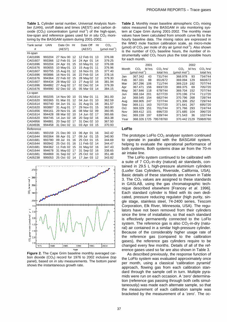
PROGRAM REPORTS – Trace gases
37
Table 1. Cylinder serial number, Universal Analysis Num-ber (UAN), on/off dates and times (AEST) and carbon di-oxide (CO2) concentration (µmol mol-1) of the high-span, low-span and reference gases used for in situ CO2 moni-toring by the BASGAM system during 2001-2002. Tank serial UAN Date On Hr Date Off Hr CO2 # (AEST) (AEST) (µmol mol-1) Hi-span CA01696 993204 27 Nov 00 12 12 Feb 01 13 376.08 CA01607 993366 12 Feb 01 14 24 Apr 01 14 379.25 CA01696 993204 24 Apr 01 15 10 May 01 12 376.08 CA01676 993655 10 May 01 13 15 Aug 01 11 376.96 CA01607 993755 15 Aug 01 12 16 Nov 01 15 377.40 CA01696 993886 16 Nov 01 16 22 Feb 02 14 378.16 CA01676 994364 22 Feb 02 15 28 May 02 12 379.30 CA01607 994434 28 May 02 13 27 Aug 02 16 381.94 CA01696 994882 27 Aug 02 17 02 Dec 02 14 379.39 CA01676 994990 02 Dec 02 15 05 Mar 03 14 384.15 Lo-span CA01614 993205 14 Nov 00 10 01 Mar 01 11 361.00 CA01620 993365 01 Mar 01 12 04 Jun 01 10 362.59 CA01614 993740 04 Jun 01 11 31 Aug 01 16 361.57 CA01620 993887 31 Aug 01 17 29 Nov 01 15 363.80 CA01656 994161 29 Nov 01 16 08 Mar 02 09 360.95 CA01614 994428 08 Mar 02 10 14 Jun 02 17 365.66 CA01620 994745 14 Jun 02 18 20 Sep 02 16 363.38 CA04956 994881 20 Sep 02 17 31 Dec 02 10 367.50 CA04936 994458 31 Dec 02 11 03 Apr 03 15 370.93 Reference CA01681 993159 21 Dec 00 13 06 Apr 01 16 342.42 CA01644 993364 06 Apr 01 17 09 Jul 01 15 340.90 CA01681 993780 09 Jul 01 16 25 Oct 01 15 344.69 CA01644 993942 25 Oct 01 16 11 Feb 02 14 344.47 CA01681 994362 11 Feb 02 15 31 May 02 16 347.43 CA01644 994678 31 May 02 17 31 Sep 02 16 338.65 CA01681 994869 31 Sep 02 17 25 Oct 02 13 351.48 CA05238 995053 25 Oct 02 14 17 Jan 03 12 343.82
Figure 2. The Cape Grim baseline monthly averaged car-bon dioxide (CO2) record for 1976 to 2002 inclusive (top panel), based on in situ measurements. The bottom panel shows the instantaneous growth rate.
Table 2. Monthly mean baseline atmospheric CO2 mixing ratios measured by the BASGAM in situ monitoring sys-tem at Cape Grim during 2001-2002. The monthly mean values have been calculated from smooth curve fits to the hourly baseline data. The mixing ratios are expressed in the WMO mole fraction calibration scale, as micro-mole (µmol) of CO2 per mole of dry air (µmol mol-1). Also shown is the number of CO2 baseline hours, the number of in-strumentally valid CO2 hours plus the total possible hours for each month. 2001 2002 Month CO2 bl hrs CO2 hrs/ CO2 bl hrs CO2 hrs/ (µmol mol-1) total hrs (µmol mol-1) total hrs Jan 367.342 43 731/744 368.978 93 734/744 Feb 367.331 88 651/672 369.094 129 660/672 Mar 367.296 106 711/744 369.219 192 707/744 Apr 367.471 156 693/720 369.375 69 705/720 May 367.846 118 678/744 369.704 152 707/744 Jun 368.164 201 627/720 370.196 274 711/720 Jul 368.545 154 682/744 370.796 268 728/744 Aug 368.905 247 727/744 371.306 252 729/744 Sep 369.111 163 707/720 371.641 267 695/720 Oct 369.329 151 701/744 371.766 293 724/744 Nov 369.412 101 696/720 371.685 104 396/720 Dec 369.159 197 639/744 371.543 36 102/744 Year 368.326 1725 7957/8760 370.442 2129 7598/8760
LoFlo
The prototype LoFlo CO2 analyser system continued to operate in parallel with the BASGAM system, helping to evaluate the operational performance of both systems. Both systems draw air from the 70-m air intake line.
The LoFlo system continued to be calibrated with a suite of 7 CO2-in-dry (natural) air standards, con-tained in 29.5 L high-pressure aluminium cylinders (Luxfer Gas Cylinders, Riverside, California, USA). Basic details of these standards are shown in Table 3. The CO2 values are assigned to these standards in GASLAB, using the gas chromatographic tech-nique described elsewhere [Francey et al. 1996]. Each standard cylinder is fitted with its own dedi-cated, pressure reducing regulator (high purity, sin-gle stage, stainless steel, 74-2400 series, Tescom Corporation, Elk River, Minnesota, USA). The regu-lators have not been removed from their cylinders since the time of installation, so that each standard is effectively permanently connected to the LoFlo system. The reference gas is also CO2-in-dry (natu-ral) air contained in a similar high-pressure cylinder. Because of the considerably higher usage rate of the reference gas (compared to the calibration gases), the reference gas cylinders require to be changed every few months. Details of all of the ref-erence gases used so far are also shown in Table 3.
As described previously, the response function of the LoFlo system was evaluated approximately once per month, using a classical ‘calibration pyramid’ approach, flowing gas from each calibration stan-dard through the sample cell in turn. Multiple pyra-mids were run on each occasion. A ‘zero’ determina-tion (reference gas passing through both cells simul-taneously) was made each alternate sample, so that the measurement of each calibration sample was bracketed by the measurement of a ‘zero’. The oc-

PROGRAM REPORTS – Trace gases
38
casions of these response function determinations are given in Table 4. In each such calibration ex-periment, the response function of the analyser sys-tem is determined (a shallow quadratic function), as well as the CO2 value of the reference gas (see last column of Table 4), relative to the suite of seven calibration standards. These are then deemed to de-fine the response of the analyser during ambient air measurements, until the time of the next calibration experiment. Shown in Figure 3 are the changes in CO2 values of each reference gas, as a function of the cylinder pressure at the time of each determina-tion. The CO2 mixing ratio mostly tends to increase slightly as the pressure drops, although there is a puzzling exception.
All of the instrumentally valid, hourly-average CO2 data from the LoFlo system during 2001-2002 are shown in Figure 4. Most of the gaps in the re-cord correspond to the times when calibration ex-periments were being run. Some extended periods of missing data occurred during July-August 2002, when several intermittent hardware faults devel-oped. These included a stream selection valve and actuator which did not always respond faithfully to commands, and a faulty hard disc in the computer which caused the analyser system to hang. The se-lection of instrumentally valid data is based primarily on the behaviour of the parameters such as differen-tial pressure. The performance of the LoFlo system over this period continues to be encouraging. Monthly average, and annual average baseline CO2 values from the LoFlo system during 2001-2002 are given in Table 5.
Table 3. Details of the CO2-in-air calibration suite used on the LoFlo CO2 analyser system, as well as those of all of the CO2-in-air reference gases to the end of 2002. ID Installation Cyl. # UAN Starting GASLAB Date Pressure CO2 (psig) (µmol mol-1) CAL1 20000510 CA01666 980773 1870 338.96 CAL2 20000510 CA01687 980772 1950 350.24 CAL3 20000510 CA01647 970830 1750 360.68 CAL4 20000510 CA01688 980771 1890 369.99 CAL5 20000510 CA01634 970337 1790 380.37 CAL6 20000510 CA01640 970338 1780 388.47 CAL7 20000510 CA01622 970339 1740 400.15 REF1 20000510 CA01686 991782 1400 367.39 REF2 20000607 CA01605 991071 1860 365.23 REF3 20001011 CA01698 992447 1880 366.59 REF4 20010214 CA03130 993362 1880 367.64 REFTemp 20010622 CA01605 993363 367.06 REF5 20010625 CA03122 993756 1910 367.47 REF6 20011024 CA03130 993943 1860 368.41 REF7 20020222 CA03122 994363 1980 369.52 REF8 20020823 CA03130 994746 1960 369.42
Table 4. Basic details of the calibration experiments con-ducted on the LoFlo CO2 analyser system, during 2001-2002. Dates (yyyymmdd) and times (hhmm) are in AEST. The reference gas is assigned a CO2 value (last column) on the basis of each calibration experiment. CAL Start Finish REF CO2 # Date Time Date Time µmol mol-1 REF3 13 20010115 1138 20010117 1603 366.556 14 20010213 1308 20010215 1046 366.570 REF4 15 20010215 1111 20010216 1435 367.616 16 20010316 1446 20010319 1150 367.619 17 20010410 1809 20010412 1602 367.614 18 20010501 1320 20010504 0213 367.618 19 20010601 1614 20010604 1146 367.621 20 20010621 1106 20010622 1604 367.625 REFTemp 21 20010622 1625 20010625 0249 367.038 REF 5 22 20010625 1454 20010627 0106 367.408 23 20010713 1513 20010716 1131 367.406 24 20010803 1826 20010807 1453 367.401 25 20010828 1632 20010830 1436 367.397 26 20010830 1445 20010831 1454 367.398 27 20011002 1559 20011004 1526 367.404 28 20011022 1238 20011024 1416 367.422 REF 6 30 20011024 1442 20011026 1503 368.379 31 20011121 1344 20011123 1312 368.377 32 20020102 1510 20020104 1431 368.375 33 20020130 1421 20020201 1418 368.377 34 20020219 1422 20020222 0440 368.386 REF 7 35 20020222 1027 20020225 0143 369.477 36 20020322 1510 20020325 1413 369.469 37 20020426 1637 20020429 1632 369.473 38 20020603 1622 20020607 1534 369.477 39 20020722 1615 20020724 1543 369.479 40 20020819 1410 20020821 1955 369.489 REF 8 41 20020823 1626 20020826 1318 369.390 42 20021014 1023 20021016 0929 369.367 43 20021122 1600 20021126 1058 369.381
-0.02
0.00
0.02
CO2 c
hang
e (µm
ol mo
l-1)
0 400 800 1200 1600 2000Pressure (psig)
Ref 1Ref 2Ref 3Ref 4
Ref 5Ref 6Ref 7Ref 8
Figure 3. LoFlo reference tank CO2 assignment for each calibration experiment as a function of cylinder pressure. Shown in the figure is the change in CO2 concentration from the first measurement of each reference tank.

PROGRAM REPORTS – Trace gases
39
Figure 4. Cape Grim LoFlo in situ carbon dioxide (CO2) record for 2001 to 2002 inclusive. First panel: all instru-mentally valid hourly CO2 values, with baseline data shown in red and non-baseline shown in blue. Second panel: hourly baseline data only, with 80-day smooth curve (blue) and 650-day long-term trend curve (green).
Table 5. Monthly mean baseline atmospheric carbon diox-ide mixing ratios measured by the LoFlo in situ monitoring system at Cape Grim during 2001-2002. The monthly mean values have been calculated from smooth curve fits to the hourly baseline data (see text for details). The mix-ing ratios are expressed in the WMO mole fraction calibra-tion scale, as micro-mole (µmol) of CO2 per mole of dry air (µmol mol-1). Also shown is the number of CO2 baseline hours, the number of instrumentally valid CO2 hours plus the total possible hours for each month, and a summary for each year. 2001 2002 Month CO2 bl hrs CO2 hrs/ CO2 bl hrs CO2 hrs/ (µmol mol-1) total hrs (µmol mol-1) total hrs Jan 367.315 42 651/744 369.134 54 508/744 Feb 367.297 62 520/672 369.223 62 433/672 Mar 367.335 95 641/744 369.328 135 458/744 Apr 367.506 125 555/720 369.470 66 526/720 May 367.794 131 633/744 369.693 48 264/744 Jun 368.112 114 474/720 370.075 102 300/720 Jul 368.532 108 454/744 370.693 37 80/744 Aug 369.018 91 307/744 371.276 37 113/744 Sep 369.238 141 614/720 371.588 38 168/720 Oct 369.348 146 543/744 371.665 82 258/744 Nov 369.494 96 597/720 371.569 140 467/720 Dec 369.322 191 656/744 371.435 156 381/744 Year 368.359 1342 6645/8760 370.429 957 3956/8760
It continues to be a revealing exercise to com-pare the ambient CO2 data from the BASGAM and LoFlo analyser systems. Differences between the hourly average data from the two analyser systems (LoFlo minus BASGAM) for 2001 and 2002 are shown in Figure 5, using only instrumentally valid data from both systems. As noted previously (Steele et al., 2003) systematic offsets between the data from the two systems continue to be observed. The
frequent changes in working standards on BASGAM continue to be associated with step changes in the CO2 differences between the analysers. Some out-lier points in Figure 5 have been statistically clipped, so that they do not unduly influence the overall re-sult. The clipping is carried out by first calculating a running mean (with a width of 401 points) for the full record. The running mean is then subtracted from the data, and a standard deviation of the residuals calculated. In the first clip, any data points lying out-side two standard deviations are flagged as being clipped. This entire exercise is then repeated once again. Finally, the running mean for the retained data is determined, and this is shown as the solid green line in Figure 5. All those points identified by the clipping process are shown as orange crosses in Figure 5.
Figure 5. Difference between LoFlo and BASGAM hourly carbon dioxide (CO2) data for all matching times during the overlap period January 2001 to December 2002 as a function of time. The top panel shows results for 2001, and the bottom panel shows those for 2002. Vertical lines indi-cate calibration and reference tank changes on the BASGAM system: Dashed black - reference tanks; Or-ange - high-span tanks; Blue - low-span tanks. The orange crosses represent those ∆CO2 points that have been sta-tistically clipped (see text). The solid green lines show the running mean of the retained points.

PROGRAM REPORTS – Trace gases
40
Comparison between BASGAM and CO2 flask data
The comparison between the in situ BASGAM CO2 data and the Cape Grim flask samples measured for CO2 in GASLAB are shown in Figure 6, for the 6-year period 1997-2002 inclusive. The requirements on both types of data are the same as those de-scribed previously by Steele et al. (2003). The CO2 mean difference between the two records remains at 0.1 ± 0.15 µmol mol-1. Factors which might help ex-plain these observed differences between in situ and flask CO2 measurements have been mentioned be-fore (Steele et al., 2003).
Figure 6. Comparison of CSIRO (GASLAB) flask CO2 and hourly BASGAM in situ CO2 records for Cape Grim for 1997 to 2002 inclusive. First panel: shows both of the full data sets as time series (Flask - red; in situ - blue). Sec-ond panel: shows only the matched data points as time series (match window is flask fill time ± 30 minutes). Third panel: shows the difference between the matched flask and in situ records as a function of time; orange dots indi-cate data that lie outside 2 standard deviations about a 31 point running mean (green line).
References Francey, R. J., L. P. Steele, R. L. Langenfelds, M. P. Lu-
carelli, C. E. Allison, D. J. Beardsmore, S. A. Coram, N. Derek, F. R. de Silva, D. M. Etheridge, P. J. Fraser, R. J. Henry, B. Turner, E. D. Welch, D. A Spencer, and L. N. Cooper, Global atmospheric sampling laboratory (GASLAB): supporting and extending the Cape Grim trace gas programs, in Baseline Atmospheric Program (Australia) 1993, edited by R. J. Francey, A. L. Dick, and N. Derek, Bureau of Meteorology and CSIRO Division of Atmospheric Research, Melbourne, Australia, 8-29,1996.
Langenfelds, R. L., R. J. Francey, B. C. Pak, L. P. Steele, J. Lloyd, C. M. Trudinger and C. E. Allison, Interannual growth rate variations of atmospheric CO2 and its δ13C, H2, CH4 and CO between 1992 and 1999 linked to bio-mass burning, Glob. Biogeochem. Cycles, 16, 1048, doi:10.1029/2001GB001466, 2002a.
Langenfelds, R. L., L. P. Steele, L. N. Cooper, D. A. Spencer, P. B. Krummel and B. L. Dunse, Atmospheric methane, carbon dioxide, hydrogen, carbon monoxide and nitrous oxide from Cape Grim flask air samples ana-lysed by gas chromatography, in Baseline Atmospheric Program (Australia) 1999-2000, edited by N. W. Tindale, N. Derek, and P. J. Fraser, Bureau of Meteorology and CSIRO Atmospheric Research, Melbourne, Australia, 76-77, 2003.
Schwartz, S. E. and P. Warneck, Units for use in atmos-pheric chemistry, Pure & Appl. Chem., 67, 1377-1406, 1995.
Steele, L. P., P. B. Krummel, G. A. Da Costa, D. A. Spencer, L. W. Porter, S. B. Baly, R. L. Langenfelds, and L. N. Cooper, Baseline carbon dioxide monitoring, in Baseline Atmospheric Program (Australia) 1999-2000, edited by N. W. Tindale, N. Derek, and P. J. Fraser, Bu-reau of Meteorology and CSIRO Atmospheric Research, Melbourne, Australia, 80-84, 2003.
Tans, P. P., P. S. Bakwin, L. Bruhwiler, T. J. Conway, E. J. Dlugoklencky, D. W. Guenther, D. R. Kitzis, P. M. Lang, K. A. Masarie, J. B. Miller, P. C. Novelli, K. W. Thoning, B. H. Vaughn, J. W. C. White, and C. Zhao, Carbon Cy-cle, Chapter 2 in Climate Monitoring and Diagnostics Laboratory Summary Report No. 26 2000-2001, edited by D. B. King and R. C. Schnell, NOAA, Boulder, Colo-rado, USA, 28-50, 2002.
Thoning, K. W., P. P. Tans and W. D. Komhyr, Atmos-pheric carbon dioxide at Mauna Loa observatory, 2, Analysis of the NOAA/GMCC data, 1974-1985, J. Geo-phys. Res., 94, 8549-8565, 1989.

PROGRAM REPORTS – Trace gases
41
4.6. δ13C AND δ18O OF CO2 IN BASELINE CAPE GRIM AIR: 2001-2002
C E Allison, L N Cooper, S A Coram and R J Francey CSIRO Atmospheric Research Aspendale, Victoria 3195, Australia [Supported by CGBAPS research funds]
CSIRO Atmospheric Research (CAR) operates two programs at Cape Grim to measure the isotopic com-position of atmospheric carbon dioxide (CO2). The in situ program (CIA), where CO2 is extracted from baseline air at Cape Grim and sent to CAR for stable isotope (13C and 18O) analysis, has been operating since 1977 [Allison et al., 1994; Francey et al., 1995]. The flask program (CGA), where samples of air are collected in 0.5 litre glass flasks and returned to CAR for analysis as part of the global flask network oper-ated by CAR, has been in operation since 1991. Both programs sample air from the 70-m intake. Results from these two programs for 2001 and 2002 are summarised here and data from both programs are available through the Cape Grim data archive.
Baseline Selection
The criteria used to select baseline air are that (1) air originates from the marine sector, 190° to 280°, (2) the ‘in situ’ CO2 concentration is steady, variation < 0.2 ppm hr-1, and (3) the condensation nuclei (CN) count is less than a seasonally variable threshold based on the 90th percentile of CN hourly medians for this day-of-year over the previous 5 years [Allison et al., 2003]. Collected samples that fail any of the criteria are retained but identified as non-baseline.
In situ Program (CIA)
There were no serious disruptions to the CIA sam-pling recorded in the logbook.
Ninety-eight CO2 samples were collected and analysed: CGIS (Cape Grim in situ) CGIS#980 - CGIS#1077, with an average sampling interval of 10±6 days. Two of these (CGIS#988 and CGIS#997) were contaminated with air and one flask (containing sample CGIS#1020) was broken prior to analysis. Twenty-three of the remaining samples were collected from high-pressure cylinders of air (see below: Air Standards) and one sample was collected under marginal baseline conditions leaving 71 samples considered to be characteristic of marine air. Of these, three samples exceeded the CN rejection criteria based on the 90th percentile.
The CIA δ13C and δ18O records are presented in Figure 1 and 2 respectively as dashed black lines, generated by initially fitting a quadratic and four harmonic functions to the data [Thoning et al., 1989]. Samples that failed the CN threshold test are plotted separately (x). Rejected, non-baseline, samples are not plotted. A summary of the collection and storage details for the CIA samples is presented in Table 1.
Flask Program (CGA)
There were no serious disruptions to the CGA sam-pling recorded in the logbook.
One hundred and sixty-two CGA samples were collected for the stable isotope program. Of these, five were not analysed and one was rejected due to poor analysis. The one hundred and fifty-six remain-ing samples were collected at an average sampling interval of 9±5 days. Two samples were collected in non-baseline wind directions and are not considered further here. Of the one hundred and fifty-four re-maining samples, including five that were collected under marginal baseline wind conditions, twelve had CN counts greater than the 90th percentile threshold for the collection day.
The CGA δ13C and δ18O records are presented in Figures 1 and 2 as solid grey lines, generated using the same fitting procedure used for the CIA data. For both δ13C and δ18O, samples collected under condi-tions of high CN are plotted separately (+). The col-lection and storage details for all CGA samples are presented in Table 1.
2001.0 2001.5 2002.0 2002.5 2003.0Date
-8.2
-8.1
-8.0
-7.9
δ13C V
PDB (
per m
ill, ‰
)
CIACIA high CNCGACGA high CN
Figure 1. Smoothed fit to the 2001-2002 Cape Grim δ13C records for CIA (---) and CGA (―). Samples collected when CN exceeded the 90th percentile threshold are shown as (x) for CIA and (+) for CGA. The actual data are also included as small symbols: CIA (O), CGA ( ).
2001.0 2001.5 2002.0 2002.5 2003.0Date
0.5
1.0
1.5
2.0
δ18O V
PDB (
per m
ill, ‰
)
CIACIA high CNCGACGA high CN
Figure 2. Smoothed fit to the 2001-2002 Cape Grim δ18O records for CIA (---) and CGA (―). Samples collected when CN exceeded the 90th percentile threshold are shown as (x) for CIA and (+) for CGA. The actual data are also included as small symbols: CIA (O), CGA ( ).

PROGRAM REPORTS – Trace gases
42
Table 1. Average collection details and storage times for the CIA and CGA samples. Also presented are the num-bers of analyses from each of the air standards at Cape Grim (CIA) and at CSIRO Atmospheric Research (CGA) in the period 2001-2002. CIA CGA No. of retained samples 71 154 Average sampling frequency (days) 10 ± 6 9 ± 5 Average storage time prior to analysis 25 ± 17 55 ± 43 Average wind direction (°N) 246 ± 24 246 ± 23 Average wind speed (m s-1) 13 ± 5 13 ± 5 No. of samples with CN above 90th percentile 3 12 No. of CO2 samples extracted from CA03142 12 28 No. of CO2 samples extracted from CA04606 10 44
CO2 and N2O concentration
The concentrations (mixing ratios) of both CO2 and nitrous oxide (N2O) are used to correct for mass spectrometric interference from N2O that is co-trapped with the CO2 [Francey and Goodman, 1985]. The CO2 and N2O concentrations of all CGA sam-ples are measured at GASLAB [Langenfelds et al., 2004] while for CIA samples the average CO2 con-centration during the CO2 trap is obtained from the in situ CO2 program [Steele et al., 1999] and N2O con-centration is obtained using an interpolation proce-dure described previously [Allison et al., 2001]. If no CO2 concentration data are available for either an in situ or flask sample, the CO2 concentration is esti-mated by interpolation of the 0.5 L flask data over the period 1992 through 2002 using the fitting pro-cedure of Thoning et al. [1989].
Reporting scale for the δ13C and δ18O
The δ13C and δ18O values are reported on the VPDB-CO2 scale [Coplen, 1995], requiring an assignment of isotopic values to both pure CO2 and CO2-in-air in-house standards on the VPDB-CO2 scale. We have just completed a comprehensive revision of previous assignments, including our initial assignment to the VPDB-CO2 scale, HC453 (1987) [Francey and Good-man, 1988] and our principal assignment of stable iso-topic composition to our CO2-in-air standards, CG92 [Allison and Francey, 1999], based on an improved treatment of the systematic effects that influence the measurements. The result is a new CAR2003 proce-dure [Allison and Francey, in preparation] that provides a consistent traceable assignment (with uncertainties) for both types of in-house standards.
Comparison of the records: δ13C and δ18O
Using the CAR2003 procedures and assignments, the two Cape Grim stable isotope records, CIA and CGA, are in excellent agreement for both δ13C and δ18O. The bias of about 0.1‰ between the two δ13C records, and between the two δ18O records, that was first observed in 1998 and reported in a previous edition of Baseline, [Allison et al., 2003], has been removed, mostly as a result of improved assignment to the CO2-in-air stan-dards in use at the time. The mean difference between the CIA and CGA δ13C records for 2001-2002 is 0.003‰. The mean δ18O difference is 0.011‰. Both
these are well within the uncertainty estimates for our measurements of 0.03‰ and 0.05‰, respectively.
CIA air standards
Independent confirmation of the effectiveness of the CAR2003 procedures comes from the introduction of cylinder air extractions carried out on the CIA extrac-tion line at Cape Grim. Two cylinders of air have been prepared and analysed at CSIRO GASLAB and sent to Cape Grim for use as air standards. The first cylinder, CA03142, was sent to Cape Grim in August 2000 and connected to the in situ extraction line where CO2 was extracted using the same proto-cols used to extract CIA samples (flow rate, trapping time, etc). Preliminary results from this analysis con-firmed the bias between the CIA and CGA records [Allison et al., 2003]. The second cylinder, CA04606, was sent to Cape Grim in February 2002 to overlap with the first cylinder that was nearing exhaustion (< 2000 kPa). Cylinder CA03142 was returned to CSIRO in May 2002 for re-analysis. Table 1 summa-rises the number of samples extracted from each of the air standards at CSIRO Atmospheric Research (CGA) and at Cape Grim (CIA).
The measured δ13C and δ18O for both air standards are shown in Figures 3 and 4 respectively. Lines have been fitted to the CIA analyses of each standard and extrapolated through the corresponding CGA analyses. There is no significant difference between the mean levels of δ13C for the CIA and CGA measurements of either air standard. There appear to be small jumps in the δ18O records for each air standard that most likely arise as a consequence of changing or re-fitting regula-tors to the cylinders. For cylinder CA03142, this oc-curred when the cylinder was returned to Aspendale in mid-2002, and for cylinder CA04606, a new regulator was fitted just prior to the final analyses before ship-ping the cylinder to Cape Grim in late 2001.
2001.0 2001.5 2002.0 2002.5 2003.0Date
-8.2
-8.1
-8.0
-7.9
-7.8
-7.7
δ13C V
PDB
(per
mill,
‰)
, CA03142 (CGA) + CA03142 (CIA)/ CA04606 (CGA) - CA04606 (CIA)
Figure 3. Individual δ13C analyses in 2001-2002 of the air standards used at Cape Grim. The circles represent the first air standard, cylinder CA03142, and the triangles rep-resent the second air standard, cylinder CA04606. Open symbols represent measurements on CO2 extracted at Cape Grim; filled symbols represent measurements on CO2 extracted at CAR, Aspendale. The horizontal lines are lines of best fit to the CIA extractions, extrapolated through the CGA extractions performed at CSIRO Atmos-pheric Research.

PROGRAM REPORTS – Trace gases
43
2001.0 2001.5 2002.0 2002.5 2003.0Date
-0.5
0.0
0.5
1.0δ18
O VPD
B (p
er m
ill, ‰
), CA03142 (CGA) + CA03142 (CIA)/ CA04606 (CGA) - CA04606 (CIA)
Figure 4. Individual δ18O analyses in 2001-2002 of the air standards at Cape Grim. Details are as for Figure 3.
Conclusion
Implementation of the CAR2003 procedure has re-solved the previously reported discrepancy between the CIA and CGA records at Cape Grim. There are presently no significant differences between the CIA and CGA records for δ13C or δ18O at Cape Grim.
For the period 2001-2002, δ13C decreased at a rate of -0.051‰ yr-1 from a starting value of -7.99‰ to -8.09‰. This is twice the rate at which δ13C de-creased over the previous 10 years (-0.026‰ yr-1) but is consistent with the strong link between CO2 concentration and δ13C on interannual timescales. For the same period, δ18O remained relatively con-stant at approximately 1.26‰, not significantly dif-ferent from the average value for the previous 10 years of 1.41‰, although a slight increase of 0.2‰ over the two years is observed.
Acknowledgements
We would like to thank Laurie Porter, Stuart Baly and Craig McCulloch for their expertise in maintain-ing both the CIA and CGA programs over many years. We specially thank Laurie Porter for his assis-tance in incorporating the air standard into the CIA sampling program. We also thank the GASLAB staff (Ray Langenfelds, Paul Steele, Marcel van der Schoot, Darren Spencer and Paul Krummel) for pro-viding the CO2 and N2O concentration data.
References Allison, C. E., L. N. Cooper, and R. J. Francey, δ13C of CO2
in baseline Cape Grim air: 1997-98, Baseline Atmos-pheric Program (Australia) 1996, edited by N. W. Tindale, N. Derek, and R. J. Francey, Bureau of Meteorology and CSIRO Atmospheric Research, Melbourne, 67-69, 2001.
Allison, C. E., L. N. Cooper, and R. J. Francey, δ13C of CO2 in baseline Cape Grim air: 1999-2000, Baseline Atmospheric Program (Australia) 1999-2000, edited by N. W. Tindale, N. Derek, and P. J. Fraser, Bureau of Meteorology and CSIRO Atmospheric Research, Melbourne, 71-73, 2003.
Allison, C. E., and R. J. Francey, δ13C of atmospheric CO2 at Cape Grim: The in situ record, the flask record, air standards and the CG92 reference scale, in Baseline At-mospheric Program (Australia) 1996, edited by J. L. Gras, N. Derek, N. W. Tindale and A. L. Dick, Bureau of Mete-
orology and CSIRO Atmospheric Research, Melbourne, 44-56, 1999.
Allison, C. E., R. J. Francey, R. L. Langenfelds, and E. D. Welch, Comparison of high precision Cape Grim CO2 iso-tope measurements using two mass spectrometers, in Baseline Atmospheric Program (Australia) 1991, edited by A. L. Dick and J. L. Gras, Bureau of Meteorology and CSIRO, Division of Atmospheric Research, Melbourne, 10-19, 1994.
Coplen T. B., Reporting of stable carbon, hydrogen, and oxygen isotopic abundances, in Reference and intercom-parison materials for stable isotopes of light elements, proceedings of a consultants meeting, Vienna (IAEA-TECDOC-825). Vienna, Austria: International Atomic En-ergy Agency, 31-34, 1995.
Francey, R. J. and H. S. Goodman, Systematic error in, and selection of, in situ δ13C, in Baseline Atmospheric Program (Australia) 1983-1984, edited by R. J. Francey and B. W. Forgan, Bureau of Meteorology and CSIRO, Division of Atmospheric Research, Melbourne, Australia, 27-36, 1985.
Francey, R. J., and H. S. Goodman, The DAR stable isotope reference scale for CO2, in Baseline Atmospheric Program (Australia) 1986, edited by B. W. Forgan and P. J. Fraser, Bureau of Meteorology and CSIRO, Division of Atmos-pheric Research, Melbourne, Australia, 40-46, 1988.
Francey, R. J., C. E. Allison, and E. D. Welch, The 11-year high precision in situ CO2 stable isotope record from Cape Grim, 1982-1992, in Baseline Atmospheric Program (Aus-tralia) 1992, edited by A. L. Dick and P. J. Fraser, Bureau of Meteorology and CSIRO, Division of Atmospheric Re-search, Melbourne, Australia, 16-25, 1995.
Langenfelds, R. L., L. P. Steele, M. V. van der Schoot, L. N. Cooper, D. A. Spencer, and P. B. Krummel, Atmospheric methane, carbon dioxide, hydrogen, carbon monoxide and nitrous oxide from Cape Grim flask air samples ana-lysed by gas chromatography in Baseline Atmospheric Program (Australia) 2001-2002, edited by J. M. Cainey, N. Derek and P. B. Krummel, Bureau of Meteorology and CSIRO Atmospheric Research, Melbourne, 46-47, 2004.
Steele, L. P., D. J. Beardsmore, G. A. Da Costa and G. I. Pearman, Baseline carbon dioxide monitoring, in Baseline Atmospheric Program (Australia) 1996, edited by J. L. Gras, N. Derek, N. W. Tindale and A. L. Dick, Bureau of Meteorology and CSIRO, Division of Atmospheric Re-search, Melbourne, 88-89, 1999.
Thoning, K. W., P. P. Tans, and W. D. Komhyr, Atmospheric carbon dioxide at Mauna Loa observatory, 2, Analysis of the NOAA/GMCC data, 1974-1985, J. Geophys. Res., 94, 8549-8565, 1989.

PROGRAM REPORTS – Trace gases
44
4.7. CONTINUOUS MEASUREMENTS OF 14C IN ATMOSPHERIC CO2 AT CAPE GRIM, 1997-2002
I Levina, B Kromera, R J Franceyb and L W Porterc aInstitut für Umweltphysik, University of Heidelberg,
Im Neuenheimer Feld 229, D-69120 Heidelberg, Germany
bCSIRO Atmospheric Research, Aspendale, Victoria 3195, Australia
cCape Grim Baseline Air Pollution Station, Bureau of Meteorology, Smithton, Tasmania 7330, Australia
[Cooperative Research report]
The collection of atmospheric carbon dioxide at Cape Grim for analysis of its 14CO2 started in April 1987 as part of a world wide network [Levin et al., 1992]. During 1997-2002, two-week integrated at-mospheric CO2 sampling for this project continued.
The atmospheric CO2 is collected from about 15 m3 of air by quantitative absorption in sodium hy-droxide solution. After shipping of the bottles of ex-posed sodium hydroxide solution to the Heidelberg laboratory, CO2 is extracted from the solution in a vacuum system by adding hydrochloric acid [Levin et al., 1980]. For 14C analysis, the CO2 gas is puri-fied over activated charcoal and counted in a high-precision proportional counter system [Kromer and Münnich, 1992]. The 13C/12C ratio is measured, as δ13C, by mass spectrometry from small aliquots of the pure CO2 gas and is only used for the fractiona-tion correction of the 14C data; the δ13C values (‰) are given relative to the international V-PDB scale. The 14C activity is expressed as per mil deviation
(∆14C (‰)) from the US National Institute of Stan-dards and Technology (formerly National Bureau of Standards) oxalic acid, activity corrected for decay [Stuiver and Polach, 1977]. The precision (1σ of a single analysis) is typically ∆14C = ±3 to 4‰.
All samples collected in 1997-2002 are listed in Table 1. Those samples analysed so far in the Hei-delberg 14C laboratory are listed in Table 1 and shown in Figure 1. Not all samples have been ana-lysed due to restrictions on funding. It is expected that the stored samples will be analysed when the financial restrictions are resolved.
The results from this program have been dis-cussed in Levin et al. [1992].
References Kromer, B. and K. O. Münnich, CO2 gas proportional
counting in Radiocarbon Dating - Review and perspec-tive, in Radiocarbon after four decades: An interdiscipli-nary perspective, edited by R. E. Taylor, A. Long and R. S. Kra, pp. 184-197, Springer-Verlag, New York, 1992.
Levin, I., R. Bösinger, G. Bonani, R. Francey, B. Kromer, K. O. Münnich, M. Suter, N. B. A. Trivett and W. Wölfli, Radiocarbon in atmospheric carbon dioxide and meth-ane: Global distributions and trends, in Radiocarbon af-ter four decades: An interdisciplinary perspective, edited by R. E. Taylor, A. Long and R. S. Kra, pp. 503-517, Springer-Verlag, New York, 1992.
Levin, I., K. O. Münnich and W. Weiss, The effect of an-thropogenic CO2 and 14C sources on the distribution of 14C in the atmosphere, in Proceedings of 10th Interna-tional 14C Conference, edited by M. Stuiver and R. S. Kra, Radiocarbon, 22, 379-391, 1980.
Stuiver, M. and H. A. Polach, Discussion: Reporting of 14C data, Radiocarbon, 19, 355-363, 1977.
80
100
120
140
160
180
200
∆14C
(per
mil,
‰)
1990 1995 2000Year
Figure 1. ∆14C in atmospheric CO2 measured with the CG-MAIN sampler for the period 1987-2002 at Cape Grim.

PROGRAM REPORTS – Trace gases
45
Table 1. 14C activity in atmospheric CO2 at Cape Grim during 1997 - 2002. Missing data (-) indicate samples have not been analysed.
Sample Sampling Period δ13C ∆14C σ Sample Sampling Period δ13C ∆14C σ No. Start Stop (‰) (‰) (‰) No. Start Stop (‰) (‰) (‰) 333 02 Jan 97 16 Jan 97 -8.20 98 3 408 18 Nov 99 02 Dec 99 - - - 334 16 Jan 97 30 Jan 97 -8.12 105 3 409 02 Dec 99 16 Dec 99 - - - 335 31 Jan 97 13 Feb 97 - - - 410 16 Dec 99 30 Dec 99 - - - 336 13 Feb 97 27 Feb 97 -8.21 107 3 411 30 Dec 99 13 Jan 00 - - - 337 27 Feb 97 13 Mar 97 -8.09 101 3 412 13 Jan 00 27 Jan 00 - - - 338 13 Mar 97 27 Mar 97 -8.14 114 4 413 27 Jan 00 10 Feb 00 - - - 339 27 Mar 97 10 Apr 97 - - - 414 10 Feb 00 24 Feb 00 - - - 340 10 Apr 97 24 Apr 97 -8.08 106 3 415 25 Feb 00 09 Mar 00 - - - 341 24 Apr 97 08 May 97 - - - 416 09 Mar 00 23 Mar 00 - - - 342 08 May 97 22 May 97 -8.09 112 3 417 23 Mar 00 06 Apr 00 - - - 343 22 May 97 05 Jun 97 - - - 418 06 Apr 00 20 Apr 00 - - - 344 05 Jun 97 19 Jun 97 -8.86 107 3 419 20 Apr 00 04 May 00 - - - 345 19 Jun 97 04 Jul 97 - - - 420 04 May 00 18 May 00 - - - 346 04 Jul 97 17 Jul 97 -8.80 110 3 421 18 May 00 01 Jun 00 - - - 347 17 Jul 97 31 Jul 97 - - - 422 01 Jun 00 15 Jun 00 - - - 348 31 Jul 97 14 Aug 97 -8.12 99 2 423 15 Jun 00 29 Jun 00 - - - 349 14 Aug 97 28 Aug 97 - - - 424 29 Jun 00 13 Jul 00 - - - 350 28 Aug 97 11 Sep 97 -8.33 112 3 425 13 Jul 00 27 Jul 00 - - - 351 11 Sep 97 25 Sep 97 - - - 426 27 Jul 00 10 Aug 00 - - - 352 25 Sep 97 09 Oct 97 -8.81 103 2 427 10 Aug 00 24 Aug 00 - - - 353 09 Oct 97 23 Oct 97 - - - 428 24 Aug 00 07 Sep 00 - - - 354 23 Oct 97 06 Nov 97 -9.05 106 3 429 07 Sep 00 21 Sep 00 - - - 355 06 Nov 97 20 Nov 97 - - - 430 21 Sep 00 05 Oct 00 - - - 356 20 Nov 97 04 Dec 97 -8.93 106 3 431 05 Oct 00 19 Oct 00 - - - 357 04 Dec 97 18 Dec 97 - - - 432 19 Oct 00 02 Nov 00 - - - 358 18 Dec 97 02 Jan 98 -9.10 109 3 433 02 Nov 00 16 Nov 00 - - - 359 02 Jan 98 15 Jan 98 - - - 434 16 Nov 00 30 Nov 00 - - - 360 15 Jan 98 29 Jan 98 -9.04 105 3 435 30 Nov 00 14 Dec 00 - - - 361 29 Jan 98 12 Feb 98 - - - 436 14 Dec 00 28 Dec 00 - - - 362 12 Feb 98 26 Feb 98 -8.90 104 2 437 28 Dec 00 11 Jan 01 - - - 363 26 Feb 98 12 Mar 98 - - - 438 11 Jan 01 25 Jan 01 - - - 364 12 Mar 98 26 Mar 98 -8.91 101 3 439 25 Jan 01 08 Feb 01 - - - 365 26 Mar 98 09 Apr 98 - - - 440 08 Feb 01 22 Feb 01 - - - 366 09 Apr 98 23 Apr 98 -8.68 104 3 441 22 Feb 01 08 Mar 01 - - - 367 23 Apr 98 07 May 98 - - - 442 08 Mar 01 22 Mar 01 - - - 368 07 May 98 21 May 98 -8.89 98 2 443 22 Mar 01 05 Apr 01 - - - 369 21 May 98 04 Jun 98 - - - 444 05 Apr 01 19 Apr 01 - - - 370 04 Jun 98 18 Jun 98 -9.16 102 3 445 19 Apr 01 03 May 01 - - - 371 18 Jun 98 02 Jul 98 - - - 446 03 May 01 17 May 01 - - - 372 02 Jul 98 16 Jul 98 -8.68 99 3 447 17 May 01 31 May 01 - - - 373 16 Jul 98 30 Jul 98 - - - 448 31 May 01 14 Jun 01 - - - 374 30 Jul 98 13 Aug 98 -9.01 103 5 449 14 Jun 01 28 Jun 01 - - - 375 13 Aug 98 28 Aug 98 - - - 450 28 Jun 01 12 Jul 01 - - - 376 28 Aug 98 10 Sep 98 -8.94 100 3 451 12 Jul 01 26 Jul 01 - - - 377 10 Sep 98 24 Sep 98 - - - 452 26 Jul 01 09 Aug 01 - - - 378 24 Sep 98 08 Oct 98 -8.95 100 3 453 09 Aug 01 23 Aug 01 - - - 379 08 Oct 98 22 Oct 98 -8.62 101 3 454 23 Aug 01 06 Sep 01 - - - 380 22 Oct 98 06 Nov 98 -8.94 95 2 455 29 Nov 01 13 Dec 01 - - - 381 06 Nov 98 19 Nov 98 - - - 456 13 Dec 01 27 Dec 01 - - - 382 19 Nov 98 03 Dec 98 -8.95 96 2 457 27 Dec 01 10 Jan 02 - - - 383 03 Dec 98 17 Dec 98 - - - 458 10 Jan 02 24 Jan 02 - - - 384 17 Dec 98 31 Dec 98 -9.03 97 2 459 24 Jan 02 07 Feb 02 - - - 385 31 Dec 98 14 Jan 99 - - - 460 07 Feb 02 21 Feb 02 - - - 386 14 Jan 99 28 Jan 99 -8.83 93 2 461 21 Feb 02 07 Mar 02 - - - 387 28 Jan 99 11 Feb 99 - - - 462 07 Mar 02 21 Mar 02 - - - 388 11 Feb 99 25 Feb 99 -8.65 98 2 463 21 Mar 02 04 Apr 02 - - - 389 25 Feb 99 11 Mar 99 - - - 464 04 Apr 02 18 Apr 02 - - - 390 11 Mar 99 25 Mar 99 -8.86 97 2 465 18 Apr 02 02 May 02 - - - 391 25 Mar 99 08 Apr 99 - - - 466 02 May 02 16 May 02 - - - 392 08 Apr 99 22 Apr 99 -8.27 93 2 467 16 May 02 30 May 02 - - - 393 22 Apr 99 06 May 99 - - - 468 30 May 02 13 Jun 02 - - - 394 06 May 99 20 May 99 -8.32 97 2 469 13 Jun 02 27 Jun 02 - - - 395 20 May 99 03 Jun 99 - - - 470 27 Jun 02 11 Jul 02 - - - 396 03 Jun 99 17 Jun 99 - - - 471 11 Jul 02 25 Jul 02 - - - 397 17 Jun 99 01 Jul 99 - - - 472 25 Jul 02 08 Aug 02 - - - 398 01 Jul 99 15 Jul 99 - - - 473 08 Aug 02 22 Aug 02 - - - 399 15 Jul 99 29 Jul 99 - - - 474 22 Aug 02 05 Sep 02 - - - 400 29 Jul 99 12 Aug 99 - - - 475 05 Sep 02 19 Sep 02 - - - 401 12 Aug 99 26 Aug 99 - - - 476 19 Sep 02 03 Oct 02 - - - 402 26 Aug 99 09 Sep 99 - - - 477 03 Oct 02 17 Oct 02 - - - 403 09 Sep 99 23 Sep 99 - - - 478 17 Oct 02 31 Oct 02 - - - 404 23 Sep 99 07 Oct 99 - - - 479 31 Oct 02 14 Nov 02 - - - 405 07 Oct 99 21 Oct 99 - - - 480 14 Nov 02 28 Nov 02 - - - 406 21 Oct 99 05 Nov 99 - - - 481 28 Nov 02 12 Dec 02 - - - 407 05 Nov 99 18 Nov 99 - - - 482 12 Dec 02 30 Dec 02 - -

PROGRAM REPORTS – Trace gases
46
4.8. ATMOSPHERIC METHANE, CARBON DIOXIDE, HYDROGEN, CARBON MONOXIDE AND NITROUS OXIDE FROM CAPE GRIM FLASK AIR SAMPLES ANALYSED BY GAS CHROMATOGRAPHY
R L Langenfelds, L P Steele, M V van der Schoot, L N Cooper, D A Spencer and P B Krummel CSIRO Atmospheric Research, Aspendale, Victoria 3195, Australia [Supported by CGBAPS research funds]
Air samples are regularly collected at Cape Grim in glass and stainless steel flasks, and returned to CSIRO Atmospheric Research’s (CAR) Global At-mospheric Sampling Laboratory (GASLAB) for analy-sis of trace gas composition [Francey et al., 1996; 2003a; 2003b]. Gas chromatographic (GC) meas-urements of methane (CH4), carbon dioxide (CO2) and carbon monoxide (CO) commenced in 1980 [Fraser and Hyson, 1986; Fraser et al., 1986; 1994]. Introduction of new and upgraded instrumentation in 1991/92 as part of the GASLAB development led to improved precision and calibration of previously measured species, and measurement of two addi-tional species, hydrogen (H2) and nitrous oxide (N2O).
Figure 1 shows time series and growth rates for CH4 and CO through 2002. Figure 2 shows CO2, H2 and N2O. Data are displayed for all flask samples with different symbols used to distinguish retained and rejected data. Causes of rejection are described by Steele et al. [1996] and Cooper et al. [1999].
Measurements of the important greenhouse gases, CO2 and N2O, show their mixing ratios to be steadily increasing in the atmosphere with mean growth rates in 2001/02 of 2.1 ppm yr-1 and 0.7 ppb yr-1 respectively. On the other hand, the mixing ratio of CH4, another greenhouse gas, has stabilised over the last 3 years. Its growth rate has been trending downward since the start of the record in 1984 and
has been near-zero since 2000. These observations are consistent with the results of Dlugokencky et al. [2003], which show the declining CH4 growth rate to be a global phenomenon. The mixing ratio of CO has also been stable in recent years, maintaining a near-zero, long-term growth rate since the start of the re-cord in 1985. Recent interannual variability of CO has been modest relative to earlier years, for example the El Niño years of 1997/98 where exceptionally high growth rates of CO (and other species including CO2, CH4 and H2) were linked to major biomass burning events [Langenfelds et al., 2002]. The H2 data show an increasing trend to have resumed in 2001/02. This followed about 2 years of negative growth rates that at least partly reflected a response to elevated emis-sions in 1997/98 [Langenfelds et al., 2002]. The full 11-year record shows an increasing H2 trend with a mean growth rate of 1.2 ppb yr-1.
Most of these data are available from the follow-ing international archives: World Data Center for Greenhouse Gases (WDCGG; http://gaw.kishou.go.jp/wdcgg.html) Carbon Dioxide Information Analysis Center (CDIAC; http://cdiac.esd.ornl.gov) and CSIRO Atmospheric Research ftp site (CAR; ftp://gaspublic:[email protected]/data/gaslab/)The CO2 and CH4 data are contributed regularly to the ‘Globalview’ data sets generated by integration of measurements from participating international laboratories [Globalview-CH4, 2001; Globalview-CO2, 2002].
Recent publications using GASLAB GC data have addressed interannual growth rate variability of multiple trace gas species during the 1990s [Lan-genfelds, 2002] and have used Cape Grim surface data as a benchmark for interpreting vertical profiles in the troposphere above Cape Grim, in relation to mean seasonal behaviour and episodic influence of tropical biomass burning plumes [Pak et al., 2003; Langenfelds, 2002].
1984 1988 1992 1996 2000
-8
-4
0
4
8
grow
th ra
te (p
pb yr
-1)
40
60
80
100
ppbCO
0
5
10
15
grow
th ra
te (p
pb yr
-1)
1600
1650
1700
ppb
1984 1988 1992 1996 2000
CH4
Figure 1. Top panels: Atmospheric CH4 and CO in ppb (mole fraction in parts per 109 in dry air). CSIRO data are from individual Cape Grim flask air samples and are shown as retained (diamonds) or rejected (crosses), based on selection for baseline conditions and analytical quality assessment. The solid curves indicate long-term trends obtained from the curve fitting routine described by Thoning et al. [1989]. Bottom panels: Growth rate curves as given by the first derivative of the long-term trends.

PROGRAM REPORTS – Trace gases
47
1992 1994 1996 1998 2000 2002
0.2
0.4
0.6
0.8
1.0
grow
th ra
te (p
pb yr
-1)
310
312
314
316
318ppb
N2O
1992 1994 1996 1998 2000 2002-8
-4
0
4
8
grow
th ra
te (p
pb yr
-1)
510
520
530
540
550ppb
H2
1992 1994 1996 1998 2000 2002
1.0
1.5
2.0
2.5
grow
th ra
te (p
pm yr
-1)
355
360
365
370
ppmCO2
Figure 2. Top panels: Cape Grim records of CO2, H2 and N2O. Results from all individual flask air samples are classified as retained (diamonds) or rejected (crosses). Solid curves indicate long-term trends. Bottom panels: Growth rate curves as given by the first derivative of the long-term trends.
References Cooper, L. N., L. P. Steele, R. L. Langenfelds, D. A.
Spencer, and M. P. Lucarelli, Atmospheric methane, car-bon dioxide, hydrogen, carbon monoxide and nitrous ox-ide from Cape Grim flask air samples analysed by gas chromatography, in Baseline Atmospheric Program (Aus-tralia) 1996, edited by J. L. Gras, N. Derek, N. W. Tindale and A. L. Dick, Bureau of Meteorology and CSIRO At-mospheric Research, Melbourne, Australia, 98-102, 1999.
Dlugokencky, E. J., S. Houweling, L. Bruhwiler, K. A. Ma-sarie, P. M. Lang, J. B. Miller and P. P. Tans, Atmos-pheric methane levels off: Temporary pause or a new steady-state?, Geophys. Res. Lett., 30(19), 1992, doi:10.1029/2003GL018126, 2003.
Francey, R. J., L. P. Steele, R. L. Langenfelds, M. P. Lu-carelli, C. E. Allison, D. J. Beardsmore, S. A. Coram, N. Derek, F. R. de Silva, D. M. Etheridge, P. J. Fraser, R. J. Henry, B. Turner, E. D. Welch, D. A. Spencer, and L. N. Cooper, Global Atmospheric Sampling Laboratory (GASLAB): supporting and extending the Cape Grim trace gas programs, Baseline Atmospheric Program (Aus-tralia) 1993, edited by R. J. Francey, A. L. Dick and N. Derek, Bureau of Meteorology and CSIRO Division of Atmospheric Research, Melbourne, Australia, 8-29, 1996.
Francey, R. J., L. P. Steele, D. A. Spencer, R. L. Lan-genfelds, R. M. Law, P. B. Krummel, P. J. Fraser, D. M. Etheridge, N. Derek, S. A. Coram, L. N. Cooper, C. E. Allison, L. Porter, and S. Baly, The CSIRO (Australia) measurement of greenhouse gases in the global atmos-phere, Baseline Atmospheric Program (Australia) 1999-2000, edited by N. W. Tindale, N. Derek and P. J. Fra-ser, Bureau of Meteorology and CSIRO Atmospheric Research, Melbourne, Australia, 42-53, 2003a.
Francey, R. J., L. P. Steele, D. A. Spencer, R. L. Lan-genfelds, R. M. Law, P. B. Krummel, P. J. Fraser, D. M. Etheridge, N. Derek, S. A. Coram, L. N. Cooper, C. E. Al-lison, L. Porter, and S. Baly, The CSIRO (Australia) measurement of greenhouse gases in the global atmos-phere, report of the 11th WMO/IAEA Meeting of Experts on Carbon Dioxide Concentration and Related Tracer Measurement Techniques, Tokyo, Japan, September 2001, S.Toru and S. Kazuto (editors), World Meteorologi-cal Organization Global Atmosphere Watch, 97-111, 2003b.
Fraser, P., and P. Hyson, Methane, carbon monoxide and methylchloroform in the Southern Hemisphere, J. At-mos. Chem., 4, 3-42, 1986.
Fraser, P., P.Hyson, and S.Coram, Carbon monoxide in the Southern Hemisphere, Proceedings of the Seventh World Clean Air Congress, Sydney, Australia, 341-352, 1986.
Fraser, P., S. Coram, and N. Derek, Atmospheric meth-ane, carbon monoxide and carbon dioxide by gas chro-matography, Baseline Atmospheric Program (Australia) 1991, edited by A. L. Dick and J. L. Gras, Bureau of Me-teorology and CSIRO Division of Atmospheric Re-search, Melbourne, Australia, 60-64, 1994.
GLOBALVIEW-CH4: Cooperative Atmospheric Data Inte-gration Project - Methane. CD-ROM, NOAA CMDL, Boulder, Colorado [Also available on Internet via anonymous FTP to ftp.cmdl.noaa.gov, Path: ccg/ch4/GLOBALVIEW], 2001.
GLOBALVIEW-CO2: Cooperative Atmospheric Data Inte-gration Project - Carbon Dioxide. CD-ROM, NOAA CMDL, Boulder, Colorado [Also available on Internet via anonymous FTP to ftp.cmdl.noaa.gov, Path: ccg/co2/GLOBALVIEW], 2002.
Langenfelds, R. L., Studies of the global carbon cycle using atmospheric oxygen and associated tracers, PhD thesis, University of Tasmania, Hobart, Australia, 320 p., 2002.
Langenfelds, R. L., R. J. Francey, B. C. Pak, L. P. Steele, J. Lloyd, C. M. Trudinger and C.E. Allison, Interannual growth rate variations of atmospheric CO2 and its δ13C, H2, CH4 and CO between 1992 and 1999 linked to bio-mass burning, Global Biogeochem. Cycles, 16(3), 1048, doi:10.1029/2001GB001466, 2002.
Pak, B. C., R. L. Langenfelds, S. A. Young, R. J. Francey, C. P. Meyer, L. M. Kivlighon, L. N. Cooper, B. L. Dunse, C. E. Allison, L. P. Steele, I. E. Galbally, and I. A. Weeks, Measurements of biomass burning influences in the troposphere over southeast Australia during the SAFARI 2000 dry season campaign, J. Geophys. Res., 108(D13), 8480, doi:10.1029/2002JD002343, 2003.
Steele, L. P., R. L, Langenfelds, M. P. Lucarelli, P. J. Fra-ser, L. N. Cooper, D. A. Spencer, S. Chea, and K. Broadhurst, Atmospheric methane, carbon dioxide, car-bon monoxide, hydrogen and nitrous oxide from Cape Grim flask samples analysed by gas chromatography, in Baseline Atmospheric Program (Australia), 1994-95, ed-ited by R. J. Francey, A. L. Dick and N. Derek, Bureau of Meteorology and CSIRO Division of Atmospheric Re-search, Melbourne, Australia, 107-110, 1996.
Thoning, K. W., P. P. Tans, and W. D. Komhyr, Atmos-pheric carbon dioxide at Mauna Loa Observatory, Analysis of the NOAA/GMCC data, 1974 - 1985, J. Geophys. Res., 94, 8549-8565, 1989.

PROGRAM REPORTS – Trace gases
48
4.9. SF6 FROM FLASK SAMPLING
I Levin1, R Heinz1, J Ilmberger1, R L Langenfelds2, R J Francey2, L P Steele2 and D A Spencer2 1Institut für Umweltphysik, University of Heidelberg,
Im Neuenheimer Feld 229, D-69120 Heidelberg, Germany
2CSIRO Atmospheric Research, Aspendale, Victoria 3195, Australia
[Cooperative Research report]
Sulfur hexafluoride (SF6) is a man-made trace gas used predominantly in gas insulated switchgear. Be-cause of its well known, largely northern hemi-spheric source distribution and long lifetime of over 3000 years, it is a useful tracer of atmospheric circu-lation and exchange between the atmosphere and linked reservoirs. It is also a strong greenhouse gas with radiative forcing 36000 times that of CO2 on a per molecule basis.
A high precision record of its accumulation in the atmosphere between 1978 and 1994 was recon-structed from measurements made at University of Heidelberg (UH-IUP) of subsamples of the Cape Grim Air Archive [Maiss et al., 1996]. This record has subsequently been strengthened and extended by analysis of additional pre-1996 archived air and by regular, direct flask sampling of baseline air in 1.6L, stainless steel flasks since November 1995 [Levin et al., 2001; 2003]. The full Cape Grim record, now spanning 25 years, is displayed in Figure 1.
SF6
1980 1985 1990 1995 2000
1
2
3
4
5
Mixin
g rati
o (pp
t)
Figure 1. SF6 at Cape Grim from measurements of the Cape Grim Air Archive and direct flask sampling since 1995. Data are available on request, e-mail: [email protected]
References Levin, I., R. Heinz, V. Walz, R. L. Langenfelds, R. J.
Francey, L. P. Steele and D. A. Spencer, SF6 from flask sampling, in Baseline Atmospheric Program (Australia) 1997-98, edited by N. W. Tindale, N. Derek, and R. J. Francey, Bureau of Meteorology and CSIRO Atmos-pheric Research, Melbourne, Australia, 87-88, 2001.
Levin, I., R. Heinz, V. Walz, R. L. Langenfelds, R. J. Francey, L. P. Steele and D. A. Spencer, SF6 from flask sampling, in Baseline Atmospheric Program (Australia)
1999-2000, edited by N. W. Tindale, N. Derek, and P. J. Fraser, Bureau of Meteorology and CSIRO Atmospheric Research, Melbourne, Australia, 80, 2003.
Maiss, M., L. P. Steele, R. J. Francey, P. J. Fraser, R. L. Langenfelds, N. B. A. Trivett and I. Levin, Sulfur hexafluoride - a powerful new atmospheric tracer, At-mos. Environ., 30, 1621-1629, 1996.
4.10. ARCHIVING OF CAPE GRIM AIR
R L Langenfelds1, P J Fraser1, L P Steele1 and L W Porter2 1CSIRO Atmospheric Research,
Aspendale, Victoria 3195, Australia 2Cape Grim Baseline Air Pollution Station, Bureau of
Meteorology, Smithton, Tasmania, 7330, Australia [Supported by CGBAPS research funds]
Regular collection of Cape Grim air in high pressure metal cylinders for the purpose of maintaining an ar-chive of atmospheric composition has continued since 1978. A history of sampling events, protocols, techniques and reconstruction of atmospheric trace gas records through 1995 has been given previously [Langenfelds et al., 1996 and references therein] and updated through 2000 [Langenfelds et al., 2003 and references therein].
Recent publications using Cape Grim air archive data have established or extended atmospheric re-cords of numerous greenhouse and ozone-depleting gases from measurements of air in Antarctic firn [Sturrock et al., 2002; Trudinger et al., 2002]. Air ar-chive records provided critical constraints of firn dif-fusion processes for these studies. The record of atmospheric O2/N2 based on air archive measure-ments was extended and re-evaluated by Lan-genfelds [2002].
Primary sampling
Ten cylinders were filled during 2001-2002 (Table 1), including 7 filled specifically to be used as cali-bration standards at CGBAPS for measurement programs maintained by the Advanced Global At-mospheric Gases Experiment (AGAGE) and the University of East Anglia (UEA).
Subsampling
Table 2 lists collection details of two archive sub-samples prepared during 2001-2002 for analysis of the isotopic composition of N2O at the Max Planck Institute for Chemistry (MPI), Mainz, Germany in 2 litre, stainless steel flasks provided by MPI.
Acknowledgements
We thank the CGBAPS and CAR personnel who have assisted in the collection, management and analysis of these samples.

PROGRAM REPORTS – Trace gases
49
Table 1. Collection and status details for primary archive samples filled at Cape Grim. Samples are listed against UAN (a number unique to each sample, assigned at CAR), Tank ID (a label unique to each individual sample container) and Ar-chive ID (a sample identifier commonly used before 1992). Wind data represent estimated averages over the period of collection. They are calculated either from collection records or from Cape Grim hourly average data. UAN Tank Archive Collection Sampling Drying Wind Pressure Current ID ID Date Methoda,b Methodc Speed Direction Fill Current Statusd,e (GMT) (m s-1) (°) (kPa abs) S35L-C70 CG150101A 15 Jan 01 cryo wet 20 216 4680 0 exhausted 993563 S35L-B05 CG150101B 15 Jan 01 cryo wet 17 215 3730 3310 CAR S35L-C53 CG040399 2 Apr 01 cryo wet 12 191 4490 0 exhausted 994885 S35L-C70 CG190701 19 Jul 01 cryo wet 15 209 4550 4490 CAR S34L-F06 CG100801 10 Aug 01 cryo wet 6 261 4420 0 exhausted S35L-C53 CG180202 18 Feb 02 cryo wet 8 206 3590 0 exhausted S34L-F06 CG220502 22 May 02 cryo wet 15 182 4860 0 exhausted 994886 S35L-C53 CG200602 20 Jun 02 cryo wet 16 266 3310 3170 CAR S34L-F01 CG110902 11 Sep 02 cryo wet 9 247 4660 100 AGAGE S34L-F06 CG281102 28 Nov 02 RIX wet 5 226 6210 5170 AGAGE acryo immersion in liquid nitrogen bRIX oil-free compressor cwet no drying dCAR managed and stored at CAR eAGAGE used as a standard in the AGAGE program Table 2. Preparation and status details for subsamples of primary archive samples. Current status entries denote the in-stitute managing the sample. Subsample Fill Current Subsample Parent Archive Preparation Pressure Pressure Current Status UAN Tank ID UAN Date Date kPa abs kPa abs 993609 011 860001 6 Feb 86 11 Apr 01 350 MPI 993610 502 993563 15 Jan 01 11 Apr 01 350 MPI
References Langenfelds, R. L., P. J. Fraser, R. J. Francey, L. P.
Steele, and L. W. Porter, The Cape Grim Air Archive: the first seventeen years, 1978 - 1995, in Baseline At-mospheric Program (Australia), 1994-95, edited by R. J. Francey, A. L. Dick and N. Derek, Bureau of Meteorol-ogy and CSIRO Division of Atmospheric Research, Mel-bourne, 53-70, 1996.
Langenfelds, R. L., Studies of the global carbon cycle us-ing atmospheric oxygen and associated tracers, PhD thesis, University of Tasmania, Hobart, Australia, 320 p., 2002.
Langenfelds, R. L., P. J. Fraser, L. P. Steele and L. W. Porter, Archiving of Cape Grim air, in Baseline Atmos-
pheric Program (Australia), 1999-2000, edited by N. W. Tindale, N. Derek and P. J. Fraser, Bureau of Meteorol-ogy and CSIRO Atmospheric Research, Melbourne, 78-79, 2003.
Sturrock, G. A., D. M. Etheridge, C. M. Trudinger and P. J. Fraser, Atmospheric histories of halocarbons from analysis of Antarctic firn air: Major Montreal Protocol species, J. Geophys. Res., 107(D24), 4765, doi:10.1029/2002JD002548, 2002.
Trudinger, C. M., D. M. Etheridge, P. J. Rayner, I. G. Enting, G. A. Sturrock and R. L. Langenfelds, Recon-structing atmospheric histories from measurements of air composition in firn, J. Geophys. Res., 107(D24), 4780, doi:10.1029/2002JD002545, 2002.

PROGRAM REPORTS - Trace gases
50
4.11. HALOCARBONS, NITROUS OXIDE, METHANE, CARBON MONOXIDE AND HYDROGEN: THE AGAGE PROGRAM, 1993–2002
P B Krummel1, P J Fraser1, L P Steele1, N Derek1, L W Porter2, B L Dunse1 and R L Langenfelds1 1CSIRO Atmospheric Research, Aspendale, Victoria 3195, Australia
2Cape Grim Baseline Air Pollution Station, Bureau of Meteorology, Smithton, Tasmania 7330, Australia
[Supported by CGBAPS, CSIRO and MIT research funds]
Introduction
This report summarises in situ observations at Cape Grim of ten trace gases that are involved in strato-spheric ozone depletion, climate change and tropo-spheric chemistry. Measurements of CFC-11 (CCl3F), CFC-12 (CCl2F2), CFC-113 (CCl2FCClF2), chloroform (CHCl3), methyl chloroform (CH3CCl3), carbon tetrachloride (CCl4), nitrous oxide (N2O), methane (CH4), carbon monoxide (CO) and hydro-gen (H2) have been made at Cape Grim during 1993-2002, using a composite instrument compris-ing a Hewlett-Packard gas chromatograph (HP5890 GC) with two electron capture detectors (ECDs), a Carle Series 100 GC with a flame ionization detector (FID) and a Trace Analytical RGA2/RGD2 GC with a mercuric oxide reduction detector (MRD), as part of the Advanced Global Atmospheric Gases Experi-ment (AGAGE) program. Collectively this instrument is called AGAGE2.
The instrument design and methodologies used to make these observations are described in Base-line 94-95 [Fraser et al., 1996; Steele et al., 1996] and Prinn et al. [2000]. Data on all AGAGE species except CO have been published [Prinn et al., 2000
and references therein; Simmonds et al., 2000; O’Doherty et al., 2001; Cunnold et al., 2002]; all AGAGE data, including CO and H2, are available from CDIAC (Carbon Dioxide Information Analysis Center, Oak Ridge National Laboratory, Oak Ridge, Tennessee, USA). The data can be accessed on the web at http://cdiac.ornl.gov/ndps/alegage.html. To access the Atmospheric Lifetime Experiment (ALE), Global Atmospheric Gases Experiment (GAGE) or AGAGE data, select the appropriate directory. The AGAGE data presented in this report (including CO and H2) were updated by the Georgia Institute of Technology (GIT) in January 2004.
Standard gases
The concentrations of all species are based on comparisons of ambient air to working standards (G- and J-series, Table 1). The concentrations of all trace gases (Table 2), except CH4, CO and H2, are reported in the SIO98 scale [Prinn et al., 2000]. The AGAGE CH4 data are ultimately referenced to a gra-vimetrically prepared CH4-in-air calibration scale de-veloped by T. Nakazawa and co-workers at Tohoku University, Sendai, Japan [Cunnold et al., 2002]. The link to this scale was established using meas-urements in CSIRO GASLAB of standards obtained from Tohoku University, even though CSIRO main-tain a different CH4 scale, that is derived from, and almost identical to, the NOAA-CMDL CH4 scale. The AGAGE CO data are referenced to a CSIRO scale closely linked to a CO gravimetric scale developed by NOAA-CMDL [Novelli et al., 1991]. The AGAGE H2 data are referenced to a calibration scale devel-oped by CSIRO GASLAB, boot-strapped from a gra-vimetrically prepared CH4 scale [Simmonds et al., 2000]. Further details of the origin of CSIRO calibra-tion scales are described by Francey et al., [2003].
Table 1. Natural air standards used in the AGAGE program (updated by SIO, April 2004) up to the end of 2002. Tank On CFC-11 CFC-12 CFC-113 CHCl3 CH3CCl3 CCl4 N2O CH4 H2 CO Scale SIO98 SIO98 SIO98 SIO98 SIO98 SIO98 SIO98 CSIRO94 CSIRO94 CSIRO94 Units ppt ppt ppt ppt ppt ppt ppb ppb ppb ppb G-016a Aug 93 260.79 499.09 77.22 11.34 117.69 102.01 309.43 1683.37 492.20 60.40 G-023Db Sep 93 262.86 506.71 79.41 6.63 112.89 95.16 309.40 1670.64 512.90 48.70 G-011Db Feb 94 259.49 493.83 74.44 7.02 119.96 91.96 310.38 1670.60 513.90 69.20 G-025b Mar 94 262.86 508.38 80.28 8.89 116.50 101.44 309.83 1682.43 508.50 59.10 G-029b Jul 94 263.23 512.29 81.31 6.07 109.09 101.06 309.86 1654.92 518.40 42.30 G-031b Nov 94 262.76 512.68 81.31 5.77 108.37 100.75 309.77 1662.68 518.90 43.50 G-035 Apr 95 264.11 517.78 81.94 5.42 105.49 100.39 310.75 1679.56 529.20 53.90 G-039 Sep 95 263.08 519.22 82.09 12.03 99.96 100.14 310.47 1670.13 523.10 47.10 J-005c Apr 96 268.23 537.53 84.04 12.12 124.81 101.47 312.46 1787.55 531.60 176.20 J-011 Nov 96 267.79 536.23 83.91 12.37 102.13 101.56 312.22 1794.74 530.10 148.30 J-018 Aug 97 267.50 535.60 84.29 12.88 100.45 101.40 312.05 1782.63 502.20 156.40 J-023 May 98 265.94 542.73 83.53 13.58 72.49 99.55 314.13 1816.49 506.50 178.70 J-029 Jan 99 265.63 542.15 83.59 12.92 72.55 99.53 313.72 1819.16 512.90 165.40 J-036 Oct 99 265.65 542.10 83.43 13.07 72.64 99.54 313.92 1815.03 501.86 165.68 J-047 Jun 00 262.20 545.63 82.00 10.93 49.02 97.32 316.04 1825.91 542.20 153.00 G-085 Dec 00 257.95 539.20 81.71 6.53 44.07 94.68 315.20 1720.77 522.10 58.80 J-053 Feb 01 262.18 545.62 81.97 11.09 49.22 97.28 316.07 1826.27 541.32 155.12 J-059 Nov 01 262.36 545.69 81.94 12.50 49.27 97.10 316.13 1828.87 534.41 149.21 J-064 Jul 02 262.33 545.97 81.96 11.04 48.55 97.18 316.36 1828.02 548.40 150.10 a G series standards are wet, baseline air, cryo-trapped (-196°C) at Cape Grim into evacuated, welded, electropolished 35 L stainless steel tanks; D indicates a cryogenically dried (-78°C) air standard.
b Standards used on GAGE and AGAGE simultaneously. c J series standards are natural air from Trinidad Head, California, compressed (Rix pump) into evacuated, welded, electropolished 35 L stainless steel tanks and dried to 10 torr of water vapour.

PROGRAM REPORTS – Trace gases
51
Table 2. AGAGE monthly mean halocarbon, N2O, CH4, CO and H2 mixing ratios for 1993-2002, with pollution episodes re-moved statistically. Annual means are obtained from monthly means, monthly means from individual measurements. The halocarbon and N2O data are in the SIO98 scale and the CO and H2 data are in calibration scales maintained by CSIRO GASLAB (see text). Data were updated by GIT in July 2004. The CH4 data are expressed in the Tohoku University CH4 scale (see text). month Jan Feb Mar Apr May Jun Jul Aug Sep Oct Nov Dec mean
CFC-11; CCl3F (ppt) 1993 263.5 263.6 263.8 263.8 263.8 1994 263.8 263.3 263.0 263.2 263.2 263.3 263.6 263.8 263.9 264.0 264.0 263.9 263.6 1995 263.8 263.6 263.8 262.8 262.8 263.0 263.0 263.2 263.3 263.4 263.4 263.4 263.3 1996 263.2 262.9 262.9 263.3 264.0 263.5 263.4 263.4 263.3 263.2 263.1 263.0 263.3 1997 262.9 262.6 262.5 262.5 262.5 262.6 262.6 262.7 262.6 262.4 262.3 262.0 262.5 1998 261.7 261.3 261.1 260.9 261.2 261.5 261.7 261.6 261.6 261.5 261.4 261.3 261.4 1999 261.1 260.8 260.4 260.2 260.1 260.0 260.0 260.1 259.9 259.7 259.6 259.5 260.1 2000 259.3 259.2 258.9 258.7 258.6 258.6 258.7 258.7 258.7 258.6 258.5 258.2 258.7 2001 257.5 257.3 257.2 256.8 256.8 257.0 257.1 257.0 256.9 256.7 256.6 256.5 256.9 2002 256.3 256.0 255.7 255.5 255.3 255.2 255.2 255.2 255.0 254.8 254.5 254.2 255.2 CFC-12; CCl2F2 (ppt) 1993 509.4 509.7 510.2 510.8 511.2 1994 511.6 512.7 512.8 513.6 514.1 514.6 515.2 516.0 516.9 517.6 518.1 518.7 515.2 1995 519.1 519.1 519.5 519.6 520.5 520.9 521.4 522.2 522.7 523.0 523.5 523.8 521.3 1996 524.0 524.1 524.6 524.7 526.1 526.1 526.4 527.0 527.5 528.1 528.4 528.7 526.3 1997 529.0 529.2 529.6 530.2 530.8 531.5 531.8 532.3 532.7 532.9 533.0 533.0 531.3 1998 533.0 532.9 533.0 533.1 533.5 533.7 534.6 535.0 535.5 535.6 535.9 536.2 534.3 1999 536.3 536.2 536.2 536.5 536.8 536.8 537.3 537.9 538.0 538.0 538.0 538.3 537.2 2000 538.3 538.4 538.4 538.6 538.9 539.2 539.2 539.6 539.7 540.0 540.2 540.0 539.2 2001 539.6 539.5 539.5 539.3 539.7 540.2 540.8 541.0 541.2 541.3 541.3 541.2 540.4 2002 541.2 541.1 541.0 541.0 540.8 541.0 541.3 541.9 541.9 541.9 541.7 541.6 541.3 CFC-113; CCl2FCClF2 (ppt) 1993 80.9 80.5 80.3 80.4 80.4 1994 80.4 80.6 81.0 81.1 81.2 81.3 81.6 81.8 82.0 82.0 82.1 82.0 81.4 1995 82.0 82.0 82.2 82.1 82.0 82.1 82.2 82.2 82.4 82.4 82.4 82.5 82.2 1996 82.4 82.4 82.4 82.6 82.7 82.7 82.8 82.8 82.8 82.9 82.9 82.8 82.7 1997 82.8 82.6 82.6 82.6 82.6 82.6 82.7 82.9 83.2 83.2 83.2 83.1 82.9 1998 83.1 83.0 82.9 82.8 82.7 82.7 82.8 82.8 82.8 82.8 82.8 82.8 82.8 1999 82.8 82.6 82.5 82.4 82.3 82.3 82.3 82.3 82.3 82.1 82.1 82.0 82.3 2000 81.9 81.8 81.8 81.8 81.8 81.8 81.5 81.6 81.6 81.6 81.6 81.6 81.7 2001 81.5 81.3 81.1 81.0 81.0 81.0 81.0 81.0 81.0 81.0 81.0 80.9 81.1 2002 80.8 80.7 80.6 80.5 80.4 80.4 80.4 80.3 80.2 80.2 80.2 80.2 80.4
Chloroform; CHCl3 (ppt) 1993 7.1 1994 6.9 6.7 5.8 5.4 5.8 6.2 6.4 6.5 6.5 6.5 6.2 6.2 6.2 1995 6.0 5.4 5.6 5.4 5.6 6.0 6.1 6.4 6.5 7.1 6.8 5.8 6.1 1996 5.7 5.3 5.1 5.4 6.8 7.0 7.0 6.9 6.9 6.7 6.1 5.6 6.2 1997 5.2 5.0 5.0 5.2 5.7 6.1 6.4 6.7 6.9 6.6 6.1 5.7 5.9 1998 5.3 5.1 5.0 5.3 5.7 6.4 6.7 7.1 7.0 6.9 6.5 5.9 6.1 1999 5.6 5.1 5.2 5.2 5.8 6.4 6.7 6.8 6.9 6.5 6.7 5.6 6.0 2000 5.2 5.2 5.1 5.3 5.8 6.1 6.5 6.7 6.6 6.4 5.9 5.4 5.8 2001 4.9 4.8 4.8 5.0 5.7 6.0 6.2 6.4 6.5 6.2 5.8 5.3 5.6 2002 5.2 4.8 4.8 5.1 5.8 6.1 6.2 6.1 6.1 6.0 5.7 5.1 5.6 Methyl chloroform; CH3CCl3 (ppt) 1993 115.4 115.1 115.2 114.7 114.1 1994 112.8 111.6 109.8 109.2 109.2 109.0 108.3 107.9 107.4 106.5 105.5 103.9 108.4 1995 102.3 101.1 100.1 100.0 99.7 99.4 99.2 98.6 97.9 96.8 95.5 93.8 98.7 1996 92.0 90.9 89.6 89.3 88.7 88.5 87.8 86.9 86.2 85.1 83.7 82.5 87.6 1997 80.7 79.0 78.2 77.2 76.6 76.0 75.4 74.8 74.1 73.0 71.9 70.7 75.6 1998 69.3 68.2 66.5 65.9 65.2 64.6 64.1 63.5 62.7 61.9 60.8 59.5 64.3 1999 58.3 57.0 56.3 55.5 54.8 54.5 53.9 53.2 52.6 52.0 51.4 50.3 54.2 2000 49.1 48.1 47.6 46.8 46.2 45.7 45.3 44.9 44.5 43.7 42.8 42.2 45.6 2001 40.9 40.1 39.5 39.1 38.6 38.2 37.8 37.5 37.2 36.7 36.1 35.2 38.1 2002 34.3 33.7 33.0 32.6 32.3 32.0 31.7 31.3 31.0 30.6 30.1 29.3 31.8 Carbon tetrachloride; CCl4 (ppt) 1993 101.5 101.5 101.4 101.4 101.5 1994 101.5 101.5 101.3 101.2 101.1 100.8 100.7 100.5 100.4 100.4 100.4 100.4 100.8 1995 100.4 100.3 100.2 100.0 100.1 99.9 99.8 99.7 99.6 99.6 99.6 99.7 99.9 1996 99.6 99.5 99.5 99.1 99.2 99.0 98.8 98.7 98.5 98.5 98.5 98.5 98.9 1997 98.6 98.5 98.5 98.4 98.4 98.3 98.2 98.1 98.1 98.0 97.9 97.9 98.2 1998 97.7 97.5 97.5 97.3 97.2 97.1 97.1 96.9 96.9 96.8 96.8 96.8 97.1 1999 96.8 96.7 96.6 96.4 96.3 96.1 96.0 96.0 95.8 95.7 95.6 95.7 96.1 2000 95.7 95.7 95.6 95.5 95.3 95.3 95.1 95.0 94.8 94.8 94.9 94.8 95.2 2001 94.7 94.6 94.5 94.2 94.2 94.2 94.2 94.1 94.0 94.0 93.8 93.6 94.2 2002 93.6 93.6 93.5 93.4 93.3 93.1 93.1 93.1 92.8 92.8 92.7 92.6 93.1

PROGRAM REPORTS – Trace gases
52
Table 2. continued…. month Jan Feb Mar Apr May Jun Jul Aug Sep Oct Nov Dec mean
Nitrous oxide; N2O (ppb) 1993 309.9 309.9 310.0 310.1 310.1 1994 310.2 310.0 310.1 310.2 310.2 310.2 310.2 310.2 310.5 310.6 310.7 310.9 310.3 1995 310.9 310.7 310.5 310.6 310.8 310.8 310.8 311.0 311.1 311.3 311.4 311.5 310.9 1996 311.5 311.5 311.5 311.3 311.4 311.5 311.7 311.8 311.9 312.0 312.1 312.3 311.7 1997 312.4 312.3 312.3 312.3 312.3 312.5 312.6 312.8 313.0 313.0 313.1 313.2 312.6 1998 313.2 313.1 312.8 312.8 312.9 313.0 313.3 313.5 313.7 313.8 313.9 314.1 313.3 1999 314.2 314.1 314.0 314.0 314.0 314.0 314.2 314.4 314.5 314.5 314.6 314.7 314.3 2000 314.8 314.8 314.7 314.7 314.7 314.8 315.0 315.1 315.3 315.4 315.6 315.6 315.0 2001 315.5 315.4 315.4 315.2 315.4 315.6 315.9 316.0 316.1 316.2 316.3 316.5 315.8 2002 316.5 316.5 316.3 316.2 316.1 316.1 316.3 316.7 316.8 316.9 316.9 316.9 316.5
Methane; CH4 (ppb) 1993 1701.3 1701.8 1700.8 1696.0 1688.4 1994 1680.7 1675.0 1675.2 1681.2 1687.8 1695.5 1701.7 1705.6 1708.3 1707.5 1703.8 1697.1 1693.3 1995 1691.2 1685.9 1685.4 1688.8 1696.1 1702.1 1706.1 1710.8 1714.1 1714.5 1711.3 1702.0 1700.7 1996 1692.1 1687.2 1686.9 1690.2 1698.1 1703.8 1708.9 1712.3 1713.8 1713.2 1709.4 1702.3 1701.5 1997 1695.1 1691.1 1692.9 1700.2 1709.1 1716.0 1720.9 1725.6 1726.8 1724.4 1720.5 1712.2 1711.2 1998 1704.0 1698.9 1698.6 1702.3 1710.8 1719.3 1726.5 1732.8 1734.6 1733.9 1730.1 1722.2 1717.8 1999 1715.1 1710.2 1711.1 1717.5 1724.5 1730.7 1736.2 1740.5 1742.7 1740.7 1736.4 1727.7 1727.8 2000 1718.6 1713.1 1713.8 1718.7 1726.2 1732.5 1738.7 1742.3 1742.6 1740.6 1735.2 1726.8 1729.1 2001 1717.8 1711.4 1712.9 1716.4 1726.2 1733.0 1739.0 1741.1 1742.7 1740.2 1734.1 1725.0 1728.3 2002 1717.3 1712.2 1712.3 1717.9 1726.7 1733.2 1738.1 1742.2 1743.2 1740.5 1735.2 1726.5 1728.8
Carbon monoxide; CO (ppb) 1993 61.6 66.9 68.3 58.9 46.8 1994 40.9 38.7 39.9 43.2 46.5 50.5 52.4 55.4 59.3 61.5 57.8 51.3 49.8 1995 45.7 41.3 40.0 40.7 44.6 47.8 53.0 58.4 65.3 76.2 67.7 54.8 52.9 1996 42.1 37.0 35.7 41.9 46.4 49.9 54.1 56.1 59.4 60.0 54.8 47.2 48.7 1997 40.4 36.5 37.4 41.2 47.1 52.0 56.4 60.0 63.9 64.9 61.2 54.7 51.3 1998 47.2 42.3 42.0 44.9 50.9 58.4 63.5 69.3 71.3 69.8 63.1 53.2 56.3 1999 45.2 41.4 41.1 44.3 47.1 51.9 56.8 60.3 67.2 70.0 63.2 51.0 53.3 2000 44.5 41.1 41.3 44.4 49.3 52.9 57.3 59.9 59.7 58.4 54.2 47.3 50.8 2001 40.2 40.0 43.4 46.0 51.9 55.8 62.0 64.6 67.8 68.0 62.0 52.7 54.5 2002 48.1 43.4 46.6 49.8 54.2 58.5 62.6 66.4 68.5 63.2 54.9 46.5 55.2
Hydrogen; H2 (ppb) 1993 503.6 506.9 513.1 516.6 518.6 1994 521.8 520.8 520.8 517.6 514.0 509.3 508.4 509.0 511.3 517.5 522.2 526.9 516.6 1995 526.2 528.1 528.8 524.4 516.4 516.6 515.7 514.3 515.9 521.5 527.4 532.6 522.3 1996 533.7 534.0 530.9 526.6 522.2 516.7 514.2 514.7 515.2 520.1 523.4 527.0 523.2 1997 528.3 528.3 528.0 525.7 522.2 516.7 515.8 515.5 517.1 522.5 527.3 532.5 523.3 1998 537.0 539.3 538.6 536.4 532.2 528.3 526.3 524.1 527.9 532.4 534.0 540.2 533.1 1999 539.3 539.5 539.3 535.4 531.2 527.0 524.8 524.8 525.4 531.5 534.2 535.5 532.3 2000 537.5 534.6 534.2 531.0 528.3 523.1 521.2 520.4 522.9 524.5 528.0 531.5 528.1 2001 531.3 532.6 530.8 529.1 523.5 519.7 516.6 517.5 519.0 523.2 526.7 533.4 525.3 2002 531.6 532.8 530.9 525.2 522.0 517.8 516.9 518.5 521.2 524.0 530.1 534.6 525.5
Table 3. Average annual growth rates in CCl3F, CCl2F2, CCl2FCClF2, CHCl3, CH3CCl3, CCl4, N2O, CH4, CO and H2 ob-served at Cape Grim from the AGAGE program for 1993 to 2002. The uncertainties are one standard deviation. Year CFC-11 CFC-12 CFC-113 CHCl3 CH3CCl3 CCl4 N2O CH4 CO H2 (ppt yr-1) (ppt yr-1) (ppt yr-1) (ppt yr-1) (ppt yr-1) (ppt yr-1) (ppb yr-1) (ppb yr-1) (ppb yr-1) (ppb yr-1) (% yr-1) (% yr-1) (% yr-1) (% yr-1) (% yr-1) (% yr-1) (% yr-1) (% yr-1) (% yr-1) (% yr-1) 1993 0.16±0.11 7.30±0.10 1.27±0.17 -0.34±0.03 -10.67±0.49 -0.94±0.03 0.71±0.02 7.17±0.05 -1.19±2.41 3.85±0.34 0.06±0.04 1.43±0.02 1.58±0.21 -5.02±0.48 -9.28±0.33 -0.92±0.03 0.23±0.01 0.43±0.00 -2.26±4.56 0.75±0.07 1994 0.08±0.32 7.05±0.42 1.40±0.32 -0.66±0.15 -9.25±0.21 -1.06±0.05 0.59±0.04 8.24±0.47 -1.84±3.77 5.09±1.24 0.03±0.12 1.37±0.09 1.72±0.39 -10.10±2.27 -8.54±0.24 -1.05±0.05 0.19±0.01 0.49±0.03 -3.57±7.41 0.99±0.24 1995 -0.36±0.27 5.23±0.43 0.39±0.10 0.29±0.25 -10.22±0.46 -0.84±0.07 0.72±0.05 3.14±3.16 2.92±3.66 4.60±2.20 -0.14±0.10 1.00±0.09 0.47±0.12 4.64±3.92 -10.37±0.77 -0.84±0.07 0.23±0.01 0.19±0.19 5.60±6.96 0.88±0.42 1996 -0.20±0.36 5.19±0.25 0.37±0.11 -0.25±0.33 -11.84±0.35 -0.95±0.14 0.89±0.08 4.46±4.38 -4.86±2.63 -2.91±1.23 -0.08±0.14 0.99±0.05 0.44±0.13 -3.91±5.22 -13.55±0.91 -0.96±0.13 0.29±0.03 0.26±0.26 -9.50±5.09 -0.56±0.24 1997 -1.12±0.09 4.01±0.85 0.14±0.04 -0.17±0.34 -11.74±0.26 -0.80±0.16 0.82±0.12 8.62±2.54 6.88±1.99 7.05±3.78 -0.43±0.03 0.75±0.16 0.17±0.05 -2.74±5.60 -15.53±0.35 -0.81±0.16 0.26±0.04 0.50±0.15 13.21±3.61 1.35±0.72 1998 -0.96±0.15 2.89±0.17 -0.26±0.16 0.35±0.17 -10.95±0.30 -1.07±0.05 0.86±0.09 9.90±2.73 0.17±3.24 4.23±3.72 -0.37±0.06 0.54±0.03 -0.31±0.19 5.66±2.72 -17.03±0.40 -1.10±0.04 0.28±0.03 0.58±0.16 0.30±5.75 0.80±0.70 1999 -1.55±0.08 2.41±0.39 -0.66±0.06 -0.22±0.07 -9.26±0.54 -1.04±0.02 0.75±0.08 5.44±4.12 -2.25±0.60 -2.05±0.61 -0.60±0.03 0.45±0.07 -0.80±0.08 -3.50±1.08 -17.09±0.17 -1.08±0.02 0.24±0.03 0.32±0.24 -4.11±1.07 -0.39±0.11 2000 -1.55±0.12 1.43±0.18 -0.66±0.02 -0.35±0.05 -8.13±0.26 -0.96±0.01 0.76±0.04 -0.90±0.17 -2.05±2.22 -4.12±0.23 -0.60±0.05 0.27±0.03 -0.81±0.02 -5.84±0.80 -17.87±0.38 -1.01±0.01 0.24±0.01 -0.05±0.01 -3.90±4.26 -0.78±0.04 2001 -1.60±0.08 1.27±0.11 -0.59±0.03 -0.01±0.11 -6.75±0.42 -1.00±0.03 0.85±0.06 -0.07±0.32 6.59±1.42 -3.02±1.36 -0.62±0.03 0.24±0.02 -0.73±0.03 -0.22±1.84 -17.74±0.22 -1.06±0.04 0.27±0.02 0.00±0.02 12.04±2.58 -0.58±0.26 2002 -2.15±0.17 0.52±0.16 -0.72±0.07 -0.13±0.07 -5.72±0.27 -1.03±0.10 0.58±0.07 0.64±0.29 -8.39±7.39 6.07±2.22 -0.84±0.07 0.10±0.03 -0.89±0.09 -2.23±1.27 -17.94±0.12 -1.11±0.11 0.18±0.02 0.04±0.02 -15.60±14.12 1.15±0.42

PROGRAM REPORTS – Trace gases
53
Significant Events
The WMO/EMPA audit of Cape Grim carbon monox-ide and methane measurements was conducted in November 2002 by Christoph Zellweger and Stefan Reimann. Eight EMPA standards (CO and CH4 in air) in high-pressure cylinders were analysed on AGAGE2, typically five aliquots each. These tank measurements were carried out while regular ambi-ent air measurements continued from the 10 m inlet. An additional feature of this audit experiment was the operation of an AeroLaser (AL5001) system (provided by EMPA) to continuously measure at-mospheric CO by the technique of VUV (vacuum ul-traviolet) fluorescence. Most of the time the Aer-oLaser measured ambient air, but it was also used to measure the CO values in the AGAGE2 standard tank (J-064), and the low, medium and high CO standards. The detailed results of the audit experi-ment will be provided in a formal report from EMPA.
Instrument maintenance/modifications
2001 In February and March the H2 generator (GC-FID) was serviced in an attempt to repair a ‘sticky’ non-return valve.
In April the H2 generator was modified to remove the non-return valve plate to prevent it from sticking; the generator works satisfactorily without the non-return function. The molecular sieve trap in the N2 carrier gas line (GC-FID) was replaced in April. The 10-m ambient air pump was modified in April back to its original (pre-Oct 1996) configuration using a back-pressure regulator in place of the ‘cracking valve’ and isolation coil (the 70 m pump had been similarly modified in Nov 2000).
In May and December the Trace Analytical UV lamp was replaced (GC-MRD). The copper line be-tween the nitrogen tank and molecular sieve trap was found to have split in May and was replaced (GC-FID).
In June the molecular sieve trap in the zero air carrier gas line for the GC-MRD was replaced and the two clean-up traps in the argon/CH4 carrier gas line (GC-ECD) were baked out.
In August, the mercury scrubber on the Trace Analytical detector was replaced (GC-MRD).
The station compressed air supply (and hence the input for the zero air generator and the Trace Analytical carrier gas) was lost in September due to a failure in the air compressor. Also in September, variability in the sample flushing rates was noted and found to date from the replacement of the stream select valve actuator in December 2000. The problem was resolved by re-adjusting the valve port alignment. Data quality appears to have not been affected by this problem.
The molecular sieve trap for the Trace Analytical carrier gas was changed in October (GC-MR). Also, the station compressed air supply (and hence the input for the zero air generator) was lost, due to a failed solenoid valve. The valve was replaced. Later
in October, the station air compressor was replaced with a new higher capacity pump. The pressure set-point was increased to allow a higher input pressure to the zero-air generator (GC-FID), to improve its ef-ficiency and increase the methane measurement precision.
2002 The station compressed air supply (and hence the input for the zero air generator) was lost in January, due to a jammed solenoid valve. The valve was fixed.
The poor precision problems with the Trace Ana-lytical RGD2 detector (GC-MRD), that had persisted since the UV lamp was replaced in December 2001, were resolved in February by replacing the refer-ence light guide optical aperture. The old aperture (made of plastic) had partially disintegrated after years of exposure to UV light and heat. The new ap-erture has been made from aluminium sheeting. Also in February, the Sun Unix workstation was re-tired and replaced with a PC running Linux and up-dated AGAGE software.
The molecular sieve trap for the Trace Analytical carrier gas was changed in April (GC-MRD).
In May, some CH4 data were lost after the H2 generator shut down after a desiccant change. The PC Uninterruptible Power Supply (UPS) encoun-tered an error after some mains power failures. This caused the GC to stop operating as the PC had re-booted. The UPS was subsequently tested and lasted only five minutes as the batteries were past their use-by date. The PC was shifted to the GC UPS.
The CO system blank was measured in June and October using zero air, with there being no signifi-cant change in the size of the blank.
In August the Trace Analytical UV lamp was re-placed (GC-MRD) and the 50Hz lamp ballast trans-former was reinstalled (this replaced a 60Hz unit that had been installed in January 2002 as a test).
A set of nine air samples in 4.6 litre stainless steel flasks, prepared at CSIRO-GASLAB, were analysed in September to determine the detector re-sponse functions for CO and H2. These samples also contain N2O and CH4, and so also provide addi-tional information about detector responses for these species.
The molecular sieve trap in the N2 carrier gas line (GC-FID) was replaced in October. Various adjust-ments and modifications were made to the GC-MRD system in October in an attempt to improve the pre-cision of the H2 and CO measurements, including a change in the sample loop size from 1 cc to 2 cc (1/16” O.D.). This improved the precision of the CO measurements but little improvement was seen in the H2 precision (due to broader peak shape). Later, to try and improve the H2 precision, the 2 cc 1/16” O.D. loop was replaced with a 2 cc 1/8” O.D. loop. However, the H2 peak was even broader with this loop, so the change was reversed. The ‘in-house’ made reference light guide optical aperture (GC-

PROGRAM REPORTS – Trace gases
54
MRD) that was placed in the system in February, was replaced by a genuine one in October. The in-jection valve rotor for CH4 and CO/H2 was found to be heavily stained and was replaced. This resulted in the CO blank being no longer detectable.
In November a new medium CO standard was connected (CO concentration of 93.14 ppb, cylinder serial # CA03122, and UAN 994991).
In December, the series of nine CAR prepared flask samples were analysed again following their return from Mace Head, to re-assess the instrument response functions for CO and H2. This was needed because the CO ‘blank’ problem had been fixed since the previous assessment in September.
AGAGE data
Identification of pollution The identification of ‘non-baseline’ periods in the AGAGE data is achieved using an objective, auto-mated algorithm [Prinn et al. 2000]. The algorithm considers a 4-month period centred on each obser-vation. After removal of a second-order polynomial fit to the data in this period, the algorithm seeks to identify a statistically normal distribution of unpol-luted (baseline) mole fractions over this period. This is achieved by iteratively removing (and labelling as pollution) the mole fractions that exceed the median plus 2.5 standard deviations. Simultaneously, the algorithm fits a normal distribution to these baseline values to produce a mean and standard deviation of the distribution. Further checks using standard syn-optic analyses and back trajectory calculations en-sure that the pollution events so identified are mete-orologically reasonable.
The data
The AGAGE monthly mean halocarbon, N2O, CH4, CO and H2 baseline data (pollution episodes re-moved) for 1993-2002 are presented in Table 2. Figures 1 - 4 show AGAGE total (baseline monthly means and non-baseline) instrumentally valid data. The average annual growth rates in CCl3F, CCl2F2, CCl2FCClF2, CHCl3, CH3CCl3, CCl4, N2O, CH4, CO and H2 observed at Cape Grim from the AGAGE program over the period 1993 to 2002 are listed in Table 3. The growth rates are calculated using curve fitting techniques of Thoning et al., [1989], by finding a long-term trend curve with 650-day smoothing and seasonal cycles removed. The derivative of the long-term trend curve is then taken to give an instantane-ous growth rate curve. The annual average growth rates are then found from such curves.
Chlorofluorocarbons CFC-11 (CCl3F)
The annual average CCl3F baseline mixing ratios in 2001 and 2002 were 257.0 and 255.3 ppt respec-tively. The 2001 and 2002 growth rates were -1.6 and -2.0 ppt yr-1 respectively. These are the largest annual decreases (0.6 – 0.8% yr-1) in CCl3F ob-
served at Cape Grim. Larger decreases are ex-pected in the future, up to 2% per year when global emissions are near zero.
A distinct feature of the pre-1995 total data was the occurrence of CCl3F (Figure 1a) pollution epi-sodes, particularly in winter. These are largely found in air masses at Cape Grim that had previously passed over Melbourne. The data suggest that the emissions of CCl3F into the Melbourne atmosphere have declined significantly since 1994, in line with the Montreal Protocol total phase-out of the con-sumption of CFCs from the beginning of 1996. Mel-bourne emissions of CCl3F for 2001 were about 30 tonnes yr-1 found using the tracer-ratio technique as discussed in Dunse [2002].
CFC-12 (CCl2F2)
The annual average CCl2F2 baseline mixing ratios in 2001 and 2002 were 540.4 and 541.5 ppt respec-tively and the 2001 and 2002 growth rates were 1.3 and 0.8 ppt yr-1 respectively. These are the smallest annual increases in CCl2F2 observed at Cape Grim and continue a slow-down in growth of CCl2F2 first observed in 1988-89. The data indicate that CCl2F2 levels should stop growing in 1 - 2 years. The inten-sities of CCl2F2 pollution episodes at Cape Grim have declined, but not disappeared, compared to the mid-1980s (Figure 1b). There are remaining emis-sions of CCl2F2 in Melbourne, presumably from old refrigeration and auto-air conditioning systems. Mel-bourne emissions of CCl2F2 for 2001 were about 60 tonnes yr-1 found using the tracer-ratio technique as discussed in Dunse [2002].
CFC-113 (CCl2FCClF2)
The annual average CCl2FCClF2 baseline mixing ra-tios in 2001 and 2002 were 81.1 and 80.5 ppt re-spectively and the 2001 and 2002 growth rates were both approximately -0.6 ppt yr-1. The data indicate that the levels of CCl2FCClF2 in the atmosphere are declining at about 0.8% per year. Emissions of CCl2FCClF2 in Melbourne appear to be small (less than 10 tonnes yr-1) after 1995, based on the CCl2FCClF2 pollution episode data observed at Cape Grim (Figure 1c) [Dunse et al., 2001, 2002].
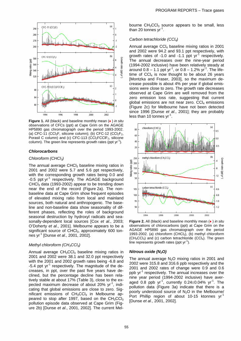
PROGRAM REPORTS – Trace gases
55
1994 1996 1998 2000 2002
80
84
88
-1
0
1
2CFC-113 (CCl2FCClF2) (c)
520
540
560
580
Mixin
g rati
os (p
pt)
0
4
8
Growth rates (ppt yr -1)
CFC-12 (CCl2F2) (b)
260
270
280
290
-2
-1
0
1CFC-11 (CCl3F) (a)
Figure 1. All (black) and baseline monthly mean (♦) in situ observations of CFCs (ppt) at Cape Grim on the AGAGE HP5890 gas chromatograph over the period 1993-2002. (a) CFC-11 (CCl3F, silicone column); (b) CFC-12 (CCl2F2, Porasil C column) and (c) CFC-113 (CCl2FCClF2, silicone column). The green line represents growth rates (ppt yr-1).
Chlorocarbons Chloroform (CHCl3)
The annual average CHCl3 baseline mixing ratios in 2001 and 2002 were 5.7 and 5.6 ppt respectively, with the corresponding growth rates being 0.0 and -0.5 ppt yr-1 respectively. The AGAGE background CHCl3 data (1993-2002) appear to be trending down near the end of the record (Figure 2a). The non-baseline data at Cape Grim show frequent episodes of elevated mixing ratio from local and mainland sources, both natural and anthropogenic. The base-line and non-baseline data show seasonality of dif-ferent phases, reflecting the roles of background seasonal destruction by hydroxyl radicals and sea-sonally-dependent local sources [Cox et al., 2003; O’Doherty et al., 2001]. Melbourne appears to be a significant source of CHCl3, approximately 600 ton-nes yr-1 [Dunse et al., 2001, 2002].
Methyl chloroform (CH3CCl3)
Annual average CH3CCl3 baseline mixing ratios in 2001 and 2002 were 38.1 and 32.0 ppt respectively with the 2001 and 2002 growth rates being -6.8 and -5.4 ppt yr-1 respectively. The magnitude of the de-creases, in ppt, over the past five years have de-clined, but the percentage decline has been rela-tively stable at about 17% (Table 3), close to the ex-pected maximum decrease of about 20% yr-1, indi-cating that global emissions are close to zero. Sig-nificant emissions of CH3CCl3 in Melbourne ap-peared to stop after 1997, based on the CH3CCl3 pollution episode data observed at Cape Grim (Fig-ure 2b) [Dunse et al., 2001, 2002]. The current Mel-
bourne CH3CCl3 source appears to be small, less than 20 tonnes yr-1.
Carbon tetrachloride (CCl4)
Annual average CCl4 baseline mixing ratios in 2001 and 2002 were 94.2 and 93.1 ppt respectively, with growth rates of -1.0 and -1.1 ppt yr-1 respectively. The annual decreases over the nine-year period (1994-2002 inclusive) have been relatively steady at around 0.8 – 1.1 ppt yr-1, or 0.8 – 1.2% yr-1. The life-time of CCl4 is now thought to be about 26 years [Montzka and Fraser, 2003], so the maximum de-crease possible is about 4% per year if global emis-sions were close to zero. The growth rate decreases observed at Cape Grim are well removed from the zero emission loss rate, suggesting that current global emissions are not near zero. CCl4 emissions (Figure 2c) for Melbourne have not been detected since 1996 [Dunse et al., 2001]; they are probably less than 10 tonnes yr-1.
1994 1996 1998 2000 2002
90
95
100
105
-1.2
-1.0
-0.8
-0.6carbon tetrachloride (CCl4) (c)
50
100
150
200
250
Mixin
g rati
os (p
pt)
-12
-8
-4
Growth rates (ppt yr -1)
methyl chloroform (CH3CCl3) (b)
20
40
60
80
-0.5
0.0
0.5chloroform (CHCl3) (a)
Figure 2. All (black) and baseline monthly mean (♦) in situ observations of chlorocarbons (ppt) at Cape Grim on the AGAGE HP5890 gas chromatograph over the period 1993-2002. (a) chloroform (CHCl3), (b) methyl chloroform (CH3CCl3) and (c) carbon tetrachloride (CCl4). The green line represents growth rates (ppt yr-1).
Nitrous oxide (N2O) The annual average N2O mixing ratios in 2001 and 2002 were 315.8 and 316.6 ppb respectively and the 2001 and 2002 rates of change were 0.9 and 0.6 ppb yr-1 respectively. The annual increases over the nine year period (1994-2002 inclusive) have aver-aged 0.8 ppb yr-1, currently 0.24±0.04% yr-1. The pollution data (Figure 3a) indicate that there is a poorly understood source of N2O in the Melbourne/ Port Phillip region of about 10-15 ktonnes yr-1 [Dunse et al., 2001, 2002].

PROGRAM REPORTS – Trace gases
56
Methane (CH4) The annual average CH4 mixing ratios in 2001 and 2002 were 1728.6 and 1728.8 ppb respectively with the 2001 and 2002 annual changes being 0.0 and -0.6 ppb respectively. The growth rates for the three year period 2000-2002 inclusive (-0.8, 0.0 and 0.3 ppb yr-1) represent the period of sustained lowest growth rates since systematic measurements began. There are significant CH4 pollution events observed at Cape Grim (Figure 3b), largely in air influenced by Melbourne CH4 sources (such as land-fills, sewer-age treatment, natural gas). Emissions from Mel-bourne appear to be increasing (around 150 ktonnes yr-1 in 1995-1996) to 300 ktonnes in 2001 [Dunse et al., 2001, 2002].
1994 1996 1998 2000 2002
1700
1800
1900
0
5
10
15methane (CH4) (b)
305
310
315
320
Mixin
g rati
os (p
pb)
0.4
0.8
1.2
Growth rates (ppb yr -1)
nitrous oxide (N2O) (a)
Figure 3. All (black) and baseline monthly mean (♦) in situ observations of (a) nitrous oxide (N2O; ppb) measured on the Porasil C column of the HP5890 gas chromatograph and (b) methane (CH4; ppb) measured on the molecular sieve 5A column of the Carle gas chromatograph at Cape Grim over the period 1993-2002. The green line repre-sents growth rates (ppb yr-1). Note that the CH4 values here are expressed in the Tohoku University CH4 scale (see text).
Carbon monoxide (CO) The annual average CO baseline mixing ratio was 54.9 ppb in 2001 and 55.6 ppb in 2002. The general features of the data (Figure 4a) are: (i) a distinct seasonality with a minimum concentration in late summer, reflecting enhanced destruction by hy-droxyl radical and (ii) the regular observation of CO pollution episodes at Cape Grim, usually associated with air that had previously passed over Melbourne. The average intensity (peak CO values) of the pollu-tion events appears to be approximately constant in time, which is consistent with Melbourne (Port Phillip air-shed) CO emissions estimates of 670±10 million tonnes per year from 1995 to 2002 [EPA, 1998; NPI, 2003].
Hydrogen (H2) The annual average H2 baseline mixing ratio was 524.9 ppb in 2001 and 525.2 ppb in 2002. The gen-eral features of the data (Figure 4b) are: (i) a distinct seasonality with a minimum concentration in winter and a maximum in late summer, reflecting the major
photochemical H2 source in the atmosphere [Sim-monds et al., 2000], (ii) the regular observation of elevated, with respect to baseline, H2 levels at Cape Grim, usually associated with air that had previously passed over Melbourne (unidentified source, 5-15 ktonnes yr-1) [Dunse et al., 2001, 2002] and (iii) the regular observation of reduced, with respect to base-line, H2 levels at Cape Grim, usually associated with air that had previously passed over the rural mainland (soil H2 sink).
1994 1996 1998 2000 2002
400
500
600
700
-5
0
5
10hydrogen (H2) (b)
200
400
600
800
Mixin
g rati
os (p
pb)
-5
0
5
Growth rates (ppb yr -1)
carbon monoxide (CO) (a)
Figure 4. All (black) and baseline monthly mean (♦) in situ observations of (a) carbon monoxide (CO; ppb) and (b) hydrogen (H2; ppb) measured on the molecular sieve 5A column of the Trace Analytical gas chromatograph at Cape Grim over the period 1993-2002. The green line represents growth rates (ppb yr-1).
References Cox, M. L., G. A. Sturrock, P. J. Fraser, S. T. Siems, P. B.
Krummel, and S. O’Doherty, Regional sources of methyl chloride, chloroform and dichloromethane identified from AGAGE observations at Cape Grim, Tasmania, 1998-2000, J. Atmos. Chem., 45, 79-99, 2003.
Cunnold, D. M., L. P. Steele, P. J. Fraser, P. G. Simmonds, R. G. Prinn, R. F. Weiss, L. W. Porter, S. O'Doherty, R. L. Langenfelds, P. B. Krummel, H. J. Wang, L. Emmons. X. X. Tie, and E. J. Dlugokencky, In situ measurements of at-mospheric methane at GAGE/AGAGE sites during 1985–2000 and resulting source inferences, J. Geophys. Res., 107, doi:10.1029/2001JD001226, 2002.
Dunse, B. L., L. P. Steele, P. J. Fraser and S. R. Wilson, An analysis of Melbourne pollution episodes observed at Cape Grim from 1995-1998, in Baseline Atmospheric Program (Australia) 1997-98, edited by N. W. Tindale, N. Derek and R. J. Francey, Bureau of Meteorology and CSIRO Atmos-pheric Research, Melbourne, Australia, 34-42, 2001.
Dunse, B. L., Investigation of urban emissions of trace gases by use of atmospheric measurements and a high-resolution atmospheric transport model, Ph.D. Thesis, Uni-versity of Wollongong, Wollongong, Australia, 303 p., 2002.
EPA, Air Emissions Inventory: Port Phillip Region, Publication 632, Environment Protection Authority, Melbourne, Victoria, 1998.
Francey, R. J., L. P. Steele, D. A. Spencer, R. L. Lan-genfelds, R. M. Law, P. B. Krummel, P. J. Fraser, D. M. Etheridge, N. Derek, S. A. Coram, L.N. Cooper, C. E. Alli-son, L. Porter and S. Baly, The CSIRO (Australia) meas-urement of greenhouse gases in the global atmosphere, in Baseline Atmospheric Program (Australia) 1999-2000, ed-ited by N. W. Tindale, N. Derek and P. J. Fraser, Bureau of

PROGRAM REPORTS – Trace gases
57
Meteorology and CSIRO Atmospheric Research, Mel-bourne, Australia, 42-53, 2003.
Fraser, P. J., N. Derek and L. W. Porter, Halocarbons, nitrous oxide and methane – the GAGE program, 1994-, in Base-line Atmospheric Program (Australia) 1994-95, edited by R. J. Francey, A. L. Dick, and N. Derek, Bureau of Meteorol-ogy and CSIRO Atmospheric Research, Melbourne, Aus-tralia, 119-113, 1996.
NPI, National Pollutant Inventory: Carbon monoxide emis-sions report for the Port Phillip Region, [Web Page], Avail-able at http://www.npi.gov.au/, Department of Environment and Heritage, Canberra, Australia, 2003.
Montzka, S. A. and P. J. Fraser, Controlled Substances and Other Source Gases, Chapter 1 in: Scientific Assessment of Ozone Depletion: 2002, Global Ozone Research and Monitoring Project – Report No. 47, 1.1-1.83, WMO/UNEP/NOAA/NASA/EC, Geneva, Switzerland, 2003.
Novelli, P. C., J. W. Elkins, and L. P. Steele, The develop-ment and evaluation of a gravimetric reference scale for measurements of atmospheric carbon monoxide, J. Geo-phys. Res., 96, 13,109-13,121, 1991.
O'Doherty, S., P. G. Simmonds, D. M. Cunnold, H. J. Wang, G. A. Sturrock, P. J. Fraser, D. Ryall, R. G. Derwent, R. F. Weiss, P. Salameh, B. R. Miller, and R. G. Prinn, In situ chloroform measurements at Advanced Global Atmos-pheric Gases Experiment atmospheric research stations from 1994 to 1998, J. Geophys. Res., 106, 20,429-20,444, 2001.
Prinn, R. G., R. F. Weiss, P. J. Fraser, P. G. Simmonds, D. M. Cunnold, F. N. Alyea, S. O’Doherty, P. Salameh, B. R. Miller, J. Huang, R. H. J. Wang, D. E. Hartley, C. Harth, L. P. Steele, G. Sturrock, P. M. Midgley, and A. McCulloch, A history of chemically and radiatively important gases in air deduced from ALE/GAGE/AGAGE, J. Geophys. Res., 105, 17,751-17,792, 2000.
Simmonds, P. G., R. G. Derwent, S. O'Doherty, D. B. Ryall, L. P. Steele, R. L. Langenfelds, P. Salameh, H. J. Wang, C. H. Dimmer, and L. E. Hudson, Continuous high-frequency observations of hydrogen at the Mace Head baseline at-mospheric monitoring station over the 1994-1998 period. J. Geophys. Res., 105, 12,105-12,121, 2000.
Steele, L. P., M. P. Lucarelli, P. J. Fraser, N. Derek and L. W. Porter, Halocarbons, nitrous oxide, methane, carbon mon-oxide and hydrogen – the AGAGE program, 1993-1995, in Baseline Atmospheric Program (Australia) 1994-95, edited by R. J. Francey, A. L. Dick, and N. Derek, Bureau of Me-teorology and CSIRO Atmospheric Research, Melbourne, Australia, 134-140, 1996.
Thoning, K. W., P. P. Tans and W. D. Komhyr, Atmospheric carbon dioxide at Mauna Loa Observatory, 2, Analysis of the NOAA/GMCC data, 1974 - 1985, J. Geophys. Res., 94, 8549-8565, 1989.
4.12. HCFCS, HFCS, HALONS, MINOR CFCS, PCE AND HALOMETHANES: THE AGAGE IN SITU GC-MS PROGRAM AT CAPE GRIM, 1998-2002
P B Krummel1, L W Porter2, P J Fraser1, S B Baly2, B L Dunse1 and N Derek1 1CSIRO Atmospheric Research, Aspendale, Victoria 3195, Australia
2Cape Grim Baseline Air Pollution Station, Bureau of Meteorology, Smithton, Tasmania 7330, Australia
[Supported by CGBAPS, CSIRO and MIT research funds]
Introduction
Gas chromatography-mass spectrometry (GC-MS) instruments were installed at Mace Head, Ireland, and Cape Grim, Tasmania, in late-1997 as part of the AGAGE global GC-MS program for the meas-urement of chlorofluorocarbon (CFC) replacements – hydrochlorofluorocarbons (HCFCs) and hydro-fluorocarbons (HFCs) – as well as halons, minor CFCs, perchloroethylene (PCE) and halomethanes. The Cape Grim instrument, its installation and op-eration, are discussed in detail in Sturrock et al. [2001a, b], along with initial observations of these halocarbon species. A summary of the AGAGE GC-MS program has been published in Prinn et al. [2000]. The AGAGE halomethane data (methyl chlo-ride, CH3Cl; methyl iodide, CH3I; dichloromethane, CH2Cl2; chloroform, CHCl3) have been published [Cox, 2001; O’Doherty et al., 2001; Cohan et al., 2003; Cox et al., 2003a, b]. The major HFC/HCFCs AGAGE data have been published [O’Doherty et al., 2004].
This report summarises the major instrumental problems encountered in the AGAGE GC-MS pro-gram at Cape Grim during 2001-2002 and presents and discusses the HCFC, HFC, halon, minor CFCs, PCE and halomethane data for 1998-2002.
Standard gases
AGAGE GC-MS data are reported in a number of standard scales (Table 1). SIO98 is the long-term AGAGE standard scale and UB98 is an interim AGAGE standard scale. The origin and propagation of these scales are described in Prinn et al. [2000] and Sturrock et al. [2001a, b]. At present AGAGE has adopted the NOAA-CMDL standard scale for HCFC-123 and PCE, and the UEA standard scale for CH3I. The concentrations of all species are based on comparisons of ambient air to working standards (G-series, Table 1), and comparisons of working standards to ‘GOLD’ standards. Previously, GOLD standards were calibrated at UB and SIO for appli-cable gases, and via flask or tank comparisons lo-cally to transfer scales from UEA and NOAA-CMDL.
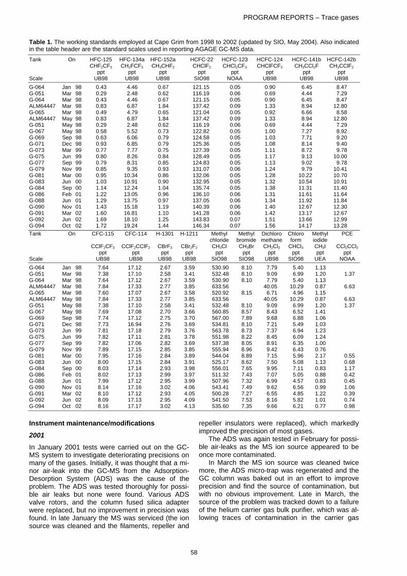
PROGRAM REPORTS – Trace gases
58
Table 1. The working standards employed at Cape Grim from 1998 to 2002 (updated by SIO, May 2004). Also indicated in the table header are the standard scales used in reporting AGAGE GC-MS data. Tank On HFC-125 HFC-134a HFC-152a HCFC-22 HCFC-123 HCFC-124 HCFC-141b HCFC-142b CHF2CF3 CH2FCF3 CH3CHF2 CHClF2 CHCl2CF3 CHClFCF3 CH3CCl2F CH3CClF2 ppt ppt ppt ppt ppt ppt ppt ppt Scale UB98 UB98 UB98 SIO98 NOAA UB98 UB98 UB98 G-064 Jan 98 0.43 4.46 0.67 121.15 0.05 0.90 6.45 8.47 G-051 Mar 98 0.29 2.48 0.62 116.19 0.06 0.69 4.44 7.29 G-064 Mar 98 0.43 4.46 0.67 121.15 0.05 0.90 6.45 8.47 ALM64447 Mar 98 0.83 6.87 1.84 137.42 0.09 1.33 8.94 12.80 G-065 Mar 98 0.49 4.79 0.65 121.04 0.05 0.92 6.66 8.58 ALM64447 May 98 0.83 6.87 1.84 137.42 0.09 1.33 8.94 12.80 G-051 May 98 0.29 2.48 0.62 116.19 0.06 0.69 4.44 7.29 G-067 May 98 0.58 5.52 0.73 122.82 0.05 1.00 7.27 8.92 G-069 Sep 98 0.63 6.06 0.79 124.58 0.05 1.03 7.71 9.20 G-071 Dec 98 0.93 6.85 0.79 125.36 0.05 1.08 8.14 9.40 G-073 Mar 99 0.77 7.77 0.75 127.39 0.05 1.11 8.72 9.78 G-075 Jun 99 0.80 8.26 0.84 128.49 0.05 1.17 9.13 10.00 G-077 Sep 99 0.79 8.31 0.85 124.83 0.05 1.13 9.02 9.78 G-079 Nov 99 0.85 9.35 0.93 131.07 0.06 1.24 9.79 10.41 G-081 Mar 00 0.95 10.34 0.86 132.06 0.05 1.28 10.22 10.70 G-083 Jun 00 1.03 10.91 0.90 132.95 0.05 1.32 10.54 10.91 G-084 Sep 00 1.14 12.24 1.04 135.74 0.05 1.38 11.31 11.40 G-086 Feb 01 1.22 13.05 0.96 136.10 0.06 1.31 11.61 11.64 G-088 Jun 01 1.29 13.75 0.97 137.05 0.06 1.34 11.92 11.84 G-090 Nov 01 1.43 15.18 1.19 140.39 0.06 1.40 12.67 12.30 G-091 Mar 02 1.60 16.81 1.10 141.28 0.06 1.42 13.17 12.67 G-092 Jun 02 1.69 18.10 1.25 143.83 0.07 1.51 13.66 12.99 G-094 Oct 02 1.72 19.24 1.44 146.34 0.07 1.56 14.17 13.28 Tank On CFC-115 CFC-114 H-1301 H-1211 Methyl Methyl Dichloro Chloro Methyl PCE chloride bromide methane form iodide CClF2CF3 CClF2CClF2 CBrF3 CBr2F2 CH3Cl CH3Br CH2Cl2 CHCl3 CH3I CCl2CCl2 ppt ppt ppt ppt ppt ppt ppt ppt ppt ppt Scale UB98 UB98 UB98 UB98 SIO98 SIO98 UB98 SIO98 UEA NOAA G-064 Jan 98 7.64 17.12 2.67 3.59 530.90 8.10 7.79 5.40 1.13 G-051 Mar 98 7.38 17.10 2.58 3.41 532.48 8.10 9.09 6.99 1.20 1.37 G-064 Mar 98 7.64 17.12 2.67 3.59 530.90 8.10 7.79 5.40 1.13 ALM64447 Mar 98 7.84 17.33 2.77 3.85 633.56 40.05 10.29 0.87 6.63 G-065 Mar 98 7.60 17.07 2.67 3.58 520.92 8.15 6.71 4.96 1.15 ALM64447 May 98 7.84 17.33 2.77 3.85 633.56 40.05 10.29 0.87 6.63 G-051 May 98 7.38 17.10 2.58 3.41 532.48 8.10 9.09 6.99 1.20 1.37 G-067 May 98 7.69 17.08 2.70 3.66 560.85 8.57 8.43 6.52 1.41 G-069 Sep 98 7.74 17.12 2.75 3.70 567.00 7.89 9.68 6.88 1.06 G-071 Dec 98 7.73 16.94 2.76 3.69 534.81 8.10 7.21 5.49 1.03 G-073 Jun 99 7.81 17.18 2.79 3.76 563.78 8.73 7.37 6.94 1.23 G-075 Jun 99 7.82 17.11 2.81 3.78 551.98 8.22 8.45 6.09 1.24 G-077 Sep 99 7.82 17.06 2.82 3.69 537.38 8.05 8.91 6.35 1.00 G-079 Nov 99 7.89 17.15 2.85 3.85 555.94 8.96 9.42 6.43 0.76 G-081 Mar 00 7.95 17.16 2.84 3.89 544.04 8.89 7.15 5.96 2.17 0.55 G-083 Jun 00 8.00 17.15 2.84 3.91 525.17 8.62 7.50 5.08 1.13 0.68 G-084 Sep 00 8.03 17.14 2.93 3.98 556.01 7.65 9.95 7.11 0.83 1.17 G-086 Feb 01 8.02 17.13 2.99 3.97 511.32 7.43 7.07 5.05 0.88 0.42 G-088 Jun 01 7.99 17.12 2.95 3.99 507.96 7.32 6.99 4.57 0.83 0.45 G-090 Nov 01 8.14 17.16 3.02 4.06 543.41 7.49 9.62 6.56 0.99 1.06 G-091 Mar 02 8.10 17.12 2.93 4.05 500.28 7.27 6.55 4.85 1.22 0.39 G-092 Jun 02 8.09 17.13 2.95 4.09 541.50 7.53 8.16 5.82 1.01 0.74 G-094 Oct 02 8.16 17.17 3.02 4.13 535.60 7.35 9.66 6.21 0.77 0.98
Instrument maintenance/modifications
2001 In January 2001 tests were carried out on the GC-MS system to investigate deteriorating precisions on many of the gases. Initially, it was thought that a mi-nor air-leak into the GC-MS from the Adsorption-Desorption System (ADS) was the cause of the problem. The ADS was tested thoroughly for possi-ble air leaks but none were found. Various ADS valve rotors, and the column fused silica adapter were replaced, but no improvement in precision was found. In late January the MS was serviced (the ion source was cleaned and the filaments, repeller and
repeller insulators were replaced), which markedly improved the precision of most gases.
The ADS was again tested in February for possi-ble air-leaks as the MS ion source appeared to be once more contaminated.
In March the MS ion source was cleaned twice more, the ADS micro-trap was regenerated and the GC column was baked out in an effort to improve precision and find the source of contamination, but with no obvious improvement. Late in March, the source of the problem was tracked down to a failure of the helium carrier gas bulk purifier, which was al-lowing traces of contamination in the carrier gas

PROGRAM REPORTS – Trace gases
59
through to the GC-MS. It was replaced and the con-tamination problems ceased.
The MS ion source was cleaned and one MS fila-ment was replaced in June.
In July the MS electron multiplier was replaced with a new ETP type AF617 electron multiplier. Later the MS ion source was cleaned and the repeller was replaced again, due to contamination of the ion source when the electron multiplier was changed.
In September a Supelco OMI-2 indicating purifier unit was installed in the helium carrier gas line, after the Hewlett-Packard bulk purifier. Late in September the GC capillary column was found to have broken and was repaired.
During October new AGAGE software was in-stalled and a blown MS ion source filament was re-placed. Later in October, the complete ion source assembly was replaced with a new ultra-clean unit.
In December MS maintenance was carried out; both MS ion sources were cleaned and tested, the repeller was cleaned and the Peltier coolers were dried and re-sealed.
2002 In January 2002 the high vacuum turbo-pump failed and was replaced with a refurbished pump from Agilent.
During February the ADS power supply devel-oped a fault and the ADS main circuit board suffered a failure. Both were replaced with spares.
The MS ion source was replaced with the spare cleaned one in March.
In April a new pair of Peltier cooling units was in-stalled improving the trapping temperature. A new micro-trap was installed at the same time.
During May water ingress into the cooler housing caused erratic temperatures and chromatograms. The cooler units were dried and resealed. Also in May, the trap desorption temperature was found to be somewhat low, due to the negative 5 volt wire having been inadvertently left disconnected. This was reconnected and the temperatures and data re-turned to normal.
In July the ADS trap temperature made a step change due to the trap having over heated, which changed its resistance characteristics. The tempera-ture measurement calibration was reset, but some degradation in chromatography was noted for the early eluting peaks.
In August the ADS trap was replaced with a spare to overcome the chromatography problems experienced since late July. Also in August the MS ion source and fore-line vacuum pump oil were changed.
In October the BOC Grade 5 helium carrier gas cylinder was changed for a trial of higher purity Matheson Grade 6 helium.
The helium carrier gas purifier was replaced with a new Agilent Big Universal Trap in November.
In December the MS ion source was changed.
The data
The monthly and annual mean baseline data for HCFCs, HFCs, halons, minor CFCs, halomethanes and PCE from 1998 to 2002 are listed in Table 2. Figure 1 shows the HFCs: (a) HFC-125, CHF2CF3; (b) HFC-134a, CH2FCF3; (c) HFC-152a, CH3CHF2); Figure 2 shows the HCFCs: (a) HCFC-22, CHClF2; (b) HCFC-123, CHCl2CF3; (c) HCFC-124, CHClFCF3; (d) HCFC-141b, CH3CCl2F; (e) HCFC-142b, CH3CClF2; Figure 3 shows minor CFCs: (a) CFC-114†, CClF2CClF2 and CCl2FCF3; (b) CFC-115, CClF2CF3; Figure 4 shows the halons: (a) H-1211, CBrClF2; (b) H-1301, CBrF3 and Figure 5 shows the halomethanes: (a) methyl chloride, CH3Cl; (b) methyl bromide, CH3Br; (c) methyl iodide, CH3I; (d) chloro-form, CHCl3; (e) dichloromethane, CH2Cl2. Figure 6 shows perchloroethylene, PCE, CCl2CCl2. †CFC-114 as listed here is a combination of CFC-114 (CClF2CClF2) and its isomer CFC-114a (CCl2FCF3). The contribution from CFC-114a is unknown but it has an atmospheric abundance of about 10% of that of CFC-114 [Oram, 1999; Montzka and Fraser, 2003].
Temporal trends and annual cycles
Several of the AGAGE GC-MS species show clear evidence of annual cycles at Cape Grim, see the baseline monthly mean data in Figures 1 – 6. Also shown are the instantaneous growth rates in ppt yr-1 for each species. The annual mean trends in ppt yr-1 and % yr-1 are listed in Table 3.
Regional pollution
The AGAGE in situ data show clear evidence of lo-cal urban sources (largely Melbourne) of HCFC-22 (refrigeration/air conditioning), HCFC-141b (foams), HFCs-125, -134a and -152a (refrigeration), PCE (solvent) and H-1211. The influence of local and re-gional biogenic sources and sinks (vegetation, soils, tidal flats) are also evident in the records of ha-lomethane species.
References Cohan, D. S., G. A. Sturrock, A. P. Biazar, and P. J. Fraser,
Atmospheric methyl iodide at Cape Grim, Tasmania, from AGAGE observations, J. Atmos. Chem., 44, 131-150, 2003.
Cox, M. L., A regional study of the natural and anthropogenic sources and sinks of the major halomethanes, PhD Thesis, Monash University, Clayton, Australia, 188 p., 2001.
Cox, M. L., G. A. Sturrock, P. J. Fraser, S. T. Siems, P. B. Krummel, and S. O’Doherty, Regional sources of methyl chloride, chloroform and dichloromethane identified from AGAGE observations at Cape Grim, Tasmania, 1998-2000, J. Atmos. Chem., 45, 79-99, 2003a.
Cox, M., S. Siems, P. Fraser, P. Hurley, and G. Sturrock, TAPM modelling studies of AGAGE dichloromethane ob-servations at Cape Grim, in Baseline Atmospheric Program (Australia) 1999-2000, edited by N. W. Tindale, N. Derek and P. J. Fraser, Bureau of Meteorology and CSIRO At-mospheric Research, Melbourne, Australia, 25-30, 2003b.
O'Doherty, S., P. G. Simmonds, D. M. Cunnold, H. J. Wang, G. A. Sturrock, P. J. Fraser, D. Ryall, R. G. Derwent, R. F. Weiss, P. Salameh, B. R. Miller, and R. G. Prinn, In situ chloroform measurements at Advanced Global Atmos-

PROGRAM REPORTS – Trace gases
60
pheric Gases Experiment atmospheric research stations from 1994 to 1998, J. Geophys. Res., 106, 20,429-20,444, 2001.
O’Doherty, S., D. M. Cunnold, A. Manning, B. R. Miller, R. H. J. Wang, P. B. Krummel, P. J. Fraser, P. G. Simmonds, A. McCulloch, R. F. Weiss, P. Salameh, L. W. Porter, R. G. Prinn, J. Huang, G. Sturrock, D. Ryall, R. G. Derwent and S. A. Montzka, Rapid growth of HFC-134a, HCFC-141b, HCFC-142b and HCFC-22 from AGAGE observations at Cape Grim, Tasmania and Mace Head, J. Geophys. Res., 109, D06310, doi:10. 2004.
Oram, D. E., Long-Lived Halocarbons in the Southern Hemi-sphere, Ph.D. Thesis, University of East Anglia, Norwich, UK, 270 pp., 1999.
Montzka, S. A and P. J. Fraser, Controlled Substances and Other Source Gases, Chapter 1 in: WMO Scientific As-sessment of Ozone Depletion, p. 1.1-1.83, Geneva, Swit-zerland, 2003.
Prinn, R. G., R. F. Weiss, P. J. Fraser, P. G. Simmonds, D. M. Cunnold, F. N. Alyea, S. O’Doherty, P. Salameh, B. R. Miller, J. Huang, R. H. J. Wang, D. E. Hartley, C. Harth, L.
P. Steele, G. Sturrock, P. M. Midgley, and A. McCulloch, A history of chemically and radiatively important gases in air deduced from ALE/GAGE/AGAGE, J. Geophys. Res., 105, 17,751-17,792, 2000.
Sturrock, G. A., L. W. Porter, and P. J. Fraser, In situ meas-urement of CFC replacement chemicals and other halo-carbons at Cape Grim: The AGAGE GC-MS program, in Baseline Atmospheric Program (Australia) 1997-98, edited by N. W. Tindale, N. Derek, and R. J. Francey, Bureau of Meteorology and CSIRO Atmospheric Research, Mel-bourne, Australia, 43-49, 2001a.
Sturrock, G. A., L. W. Porter, P. J. Fraser, N. Derek and P. B. Krummel, HCFCs, HFCs, minor CFCs and halomethanes – The AGAGE in situ GC-MS pogram, 1997-1998, and re-lated measurements on flask air samples collected at Cape Grim, in Baseline Atmospheric Program (Australia) 1997-98, edited by N. W. Tindale, N. Derek, and R. J. Francey, Bureau of Meteorology and CSIRO Atmospheric Research, Melbourne, Australia, 97-100, 2001b.
Table 2. AGAGE monthly mean HFC, HCFC, minor CFC, halomethane and PCE mixing ratios for 1998-2002, with pollu-tion episodes removed statistically. Annual means are obtained from monthly means, monthly means from individual measurements. The data were updated by GIT in July 2004. Month Jan Feb Mar Apr May Jun Jul Aug Sep Oct Nov Dec Mean
HFC-125; CHF2CF3 (ppt) 1998 0.52 0.56 0.60 0.62 0.65 0.68 0.70 0.72 0.74 0.75 0.65 1999 0.76 0.79 0.81 0.84 0.88 0.90 0.91 0.92 0.91 0.91 0.92 0.93 0.87 2000 0.96 0.99 1.04 1.07 1.09 1.14 1.17 1.20 1.18 1.21 1.26 1.27 1.13 2001 1.32 1.33 1.37 1.38 1.43 1.46 1.47 1.50 1.53 1.57 1.58 1.59 1.46 2002 1.62 1.66 1.72 1.77 1.84 1.81 1.85 1.92 2.00 1.95 1.95 1.93 1.83 HFC-134a; CH2FCF3 (ppt) 1998 5.1 5.4 5.6 5.8 6.0 6.3 6.6 6.7 6.9 7.1 6.2 1999 7.4 7.6 7.9 8.2 8.6 8.8 9.0 9.3 9.4 9.7 9.9 10.1 8.8 2000 10.3 10.6 10.8 11.2 11.6 11.8 12.1 12.3 12.4 12.7 13.1 13.2 11.8 2001 13.6 13.7 14.1 14.4 14.7 15.1 15.3 15.5 15.8 16.1 16.4 16.5 15.1 2002 16.7 17.1 17.5 17.9 18.4 18.6 18.9 19.3 19.6 20.0 20.2 20.4 18.7 HFC-152a; CH3CHF2 (ppt) 1998 0.71 0.73 0.76 0.80 0.84 0.85 0.87 0.86 0.85 0.84 0.81 1999 0.84 0.82 0.81 0.82 0.87 0.90 0.95 0.98 0.97 0.98 0.95 0.93 0.90 2000 0.91 0.90 0.91 0.93 0.95 1.01 1.04 1.07 1.08 1.09 1.09 1.05 1.00 2001 1.05 1.02 1.05 1.07 1.11 1.15 1.19 1.20 1.24 1.24 1.23 1.20 1.15 2002 1.17 1.13 1.08 1.13 1.25 1.31 1.37 1.43 1.47 1.48 1.48 1.43 1.31 HCFC-22; CHClF2 (ppt) 1998 122.1 122.5 123.0 123.5 124.3 125.1 125.6 126.0 126.1 126.3 124.5 1999 126.6 126.9 127.5 128.3 129.1 129.7 130.6 131.5 131.5 131.8 132.1 131.8 129.8 2000 131.9 132.2 132.8 133.4 134.3 135.0 135.6 136.3 136.2 136.5 137.3 137.0 134.9 2001 136.9 136.7 137.5 137.8 139.0 139.9 140.6 140.8 141.4 141.7 141.9 141.8 139.7 2002 141.8 141.9 142.4 143.6 144.5 145.0 145.5 146.2 146.8 147.5 147.8 147.4 145.0 HCFC-123; CF3CHCl2 (ppt) 1998 0.046 0.046 0.048 0.048 0.051 0.051 0.051 0.051 0.050 0.049 0.049 1999 0.043 0.042 0.043 0.042 0.045 0.047 0.055 0.057 0.056 0.056 0.052 0.050 0.049 2000 0.047 0.047 0.047 0.048 0.053 0.051 0.047 0.054 0.054 0.053 0.050 0.049 0.050 2001 0.049 0.051 0.051 0.053 0.054 0.061 0.061 0.066 0.064 0.058 0.055 0.057 2002 0.053 0.049 0.054 0.057 0.057 0.060 0.062 0.064 0.067 0.064 0.058 0.054 0.058 HCFC-124; CHClFCF3 (ppt) 1998 0.95 0.98 1.00 1.02 1.06 1.08 1.10 1.09 1.10 1.12 1.05 1999 1.12 1.15 1.13 1.15 1.21 1.23 1.26 1.27 1.25 1.25 1.25 1.29 1.21 2000 1.29 1.30 1.33 1.35 1.36 1.40 1.43 1.44 1.39 1.38 1.39 1.40 1.37 2001 1.43 1.33 1.36 1.40 1.41 1.43 1.42 1.45 1.48 1.46 1.45 1.44 1.42 2002 1.45 1.45 1.46 1.49 1.53 1.57 1.59 1.59 1.61 1.61 1.58 1.60 1.54 HCFC-141b; CH3CCl2F (ppt) 1998 7.0 7.1 7.3 7.4 7.6 7.8 8.0 8.1 8.2 8.3 7.7 1999 8.4 8.6 8.7 8.9 9.1 9.3 9.5 9.7 9.8 9.8 10.0 10.0 9.3 2000 10.1 10.2 10.4 10.6 10.8 11.0 11.2 11.3 11.4 11.5 11.7 11.7 11.0 2001 11.8 11.8 12.0 12.1 12.3 12.5 12.7 12.8 12.9 13.0 13.0 13.1 12.5 2002 13.1 13.2 13.4 13.6 13.8 13.9 14.0 14.1 14.3 14.4 14.4 14.4 13.9

PROGRAM REPORTS – Trace gases
61
Table 2. continued ……… Month Jan Feb Mar Apr May Jun Jul Aug Sep Oct Nov Dec Mean
HCFC-142b; CH3CClF2 (ppt) 1998 8.8 8.8 8.9 9.0 9.1 9.2 9.4 9.4 9.5 9.5 9.2 1999 9.6 9.7 9.8 9.9 10.0 10.1 10.2 10.4 10.4 10.5 10.5 10.6 10.1 2000 10.6 10.7 10.8 10.9 11.0 11.1 11.3 11.4 11.4 11.4 11.5 11.6 11.1 2001 11.7 11.8 11.8 12.0 12.1 12.2 12.3 12.4 12.5 12.5 12.5 12.6 12.2 2002 12.6 12.7 12.8 12.9 13.0 13.1 13.2 13.2 13.3 13.4 13.4 13.4 13.1 CFC-115; CClF2CF3 (ppt) 1998 7.7 7.6 7.7 7.7 7.7 7.8 7.8 7.8 7.8 7.8 7.7 1999 7.8 7.8 7.8 7.9 7.8 7.9 7.9 7.9 7.8 7.8 7.8 7.9 7.8 2000 7.9 7.9 8.0 8.0 8.0 8.0 8.0 8.1 8.1 8.1 8.1 8.1 8.0 2001 0.0 8.1 8.0 8.0 8.0 8.1 8.0 8.0 8.0 8.0 8.1 8.2 7.4 2002 8.2 8.1 8.1 8.1 8.2 8.1 8.2 8.1 8.1 8.2 8.3 8.2 8.2 CFC-114; CClF2CClF2 and CCl2FCF3 (ppt) 1998 17.1 17.1 17.1 17.1 17.1 17.1 17.2 17.1 17.1 17.1 17.1 1999 17.1 17.2 17.2 17.2 17.2 17.2 17.2 17.2 17.1 17.2 17.2 17.1 17.2 2000 17.2 17.2 17.2 17.2 17.2 17.1 17.2 17.2 17.1 17.0 17.0 17.1 17.1 2001 17.2 17.2 17.2 17.3 17.2 17.2 17.2 17.2 17.3 17.1 17.1 17.1 17.2 2002 17.2 17.1 17.1 17.2 17.2 17.2 17.2 17.1 17.1 17.2 17.2 17.2 17.2 H-1301; CBrF3 (ppt) 1998 2.7 2.7 2.7 2.7 2.7 2.7 2.8 2.8 2.8 2.8 2.7 1999 2.8 2.8 2.8 2.8 2.8 2.8 2.8 2.9 2.9 2.9 2.9 2.9 2.8 2000 2.9 2.9 2.9 2.9 2.9 2.9 2.9 2.9 2.9 2.9 2.9 3.0 2.9 2001 3.0 3.0 3.0 3.0 3.0 3.0 3.0 3.0 3.0 3.0 3.0 3.0 2002 3.1 3.0 3.0 2.9 3.0 3.0 3.0 3.0 3.0 3.0 3.0 3.0 3.0 H-1211; CBrClF2 (ppt) 1998 3.6 3.6 3.7 3.7 3.7 3.7 3.7 3.7 3.7 3.7 3.7 1999 3.7 3.8 3.8 3.8 3.8 3.8 3.8 3.9 3.9 3.9 3.9 3.9 3.8 2000 3.9 3.9 3.9 3.9 3.9 4.0 4.0 4.0 4.0 4.0 4.0 4.0 4.0 2001 4.0 4.0 4.0 4.0 4.0 4.0 4.1 4.1 4.1 4.1 4.1 4.1 4.0 2002 4.1 4.1 4.1 4.1 4.1 4.1 4.1 4.1 4.2 4.2 4.2 4.1 4.1 Methyl chloride; CH3Cl (ppt) 1998 527.7 534.1 540.5 548.7 562.3 570.7 576.6 568.4 564.4 554.1 545.2 553.9 1999 539.5 532.7 533.9 537.4 555.5 569.7 569.9 573.0 566.0 558.3 554.7 537.5 552.3 2000 522.0 515.9 514.5 522.8 540.1 551.0 562.4 561.7 546.8 537.8 531.7 528.2 536.2 2001 516.0 510.5 510.5 522.8 538.5 549.0 551.1 545.8 538.7 525.1 512.1 529.1 2002 505.5 498.9 502.3 514.2 539.7 539.2 541.8 543.1 540.3 536.7 522.4 525.8 Methyl bromide; CH3Br (ppt) 1998 0.0 8.2 8.4 8.3 8.4 8.5 8.6 8.0 8.0 8.0 8.0 7.5 1999 8.6 8.5 8.4 8.4 8.3 8.4 8.0 8.1 8.2 8.2 8.3 8.2 8.3 2000 8.2 8.1 8.0 8.1 8.1 8.2 8.2 8.3 8.0 7.8 8.0 7.8 8.1 2001 7.9 7.7 7.7 7.5 7.6 7.5 7.7 7.7 7.5 7.5 7.4 7.4 7.6 2002 7.4 7.4 7.5 7.5 7.6 7.5 7.4 7.4 7.2 7.4 7.5 7.5 7.4 Dichloromethane; CH2Cl2 (ppt) 1998 7.0 7.2 7.5 8.2 8.9 9.6 10.2 10.1 9.7 9.0 8.2 8.7 1999 7.5 7.3 7.3 7.6 8.4 9.0 9.5 10.0 10.1 9.7 9.0 7.9 8.6 2000 7.4 7.1 7.1 7.6 8.3 9.0 9.6 9.9 10.0 9.5 8.9 8.1 8.5 2001 7.5 6.8 7.0 7.5 8.2 8.9 9.7 9.9 10.0 9.6 8.8 7.9 8.5 2002 7.3 7.0 7.1 7.6 8.4 8.9 9.3 9.8 9.8 9.5 9.0 8.1 8.5 Chloroform; CHCl3 (ppt) 1998 5.6 5.2 5.4 5.7 6.6 6.9 7.2 7.5 7.3 6.9 6.3 6.4 1999 5.6 5.3 5.3 5.3 5.8 6.4 6.8 7.0 7.0 6.8 6.4 5.8 6.1 2000 5.3 5.2 5.2 5.4 5.9 6.1 6.5 6.7 6.9 6.8 6.1 5.7 6.0 2001 5.2 4.9 5.0 5.2 5.8 6.2 6.3 6.4 6.5 6.3 6.0 5.5 5.8 2002 5.3 4.9 4.9 5.2 6.0 6.3 6.3 6.3 6.2 5.9 5.4 5.7 Methyl iodide; CH3I (ppt) 1998 1.57 1.71 1.75 1.76 1.64 1.65 1.51 1.45 1.69 1.98 1.67 1999 2.17 2.04 1.65 1.70 1.70 1.67 1.49 1.25 1.22 1.24 1.18 1.43 1.56 2000 1.55 1.61 1.64 1.52 1.51 1.47 1.44 1.31 1.31 1.19 1.59 1.57 1.48 2001 1.78 1.79 1.83 1.90 1.86 1.87 1.47 1.26 1.19 1.19 1.30 1.32 1.56 2002 1.47 1.62 1.65 1.83 1.75 1.91 1.84 1.47 1.32 1.25 1.34 1.39 1.57 Perchloroethylene (PCE); CCl2CCl2 (ppt) 1998 1999 2000 1.18 1.24 1.12 0.95 0.74 0.58 2001 0.42 0.49 0.58 0.75 0.88 1.06 1.08 1.00 0.85 0.71 0.55 0.76 2002 0.46 0.42 0.54 0.68 0.85 0.90 0.97 1.01 1.01 0.87 0.76 0.56 0.75

PROGRAM REPORTS – Trace gases
62
Table 3. The annual mean trends for HFCs, HCFCs, minor CFCs, halons, halomethanes and PCE. Year HFC-125 HFC-134a HFC-152a HCFC-22 HCFC-123 HCFC-124 HCFC-141b HCFC-142b CHF2CF3 CH2FCF3 CH3CHF2 CHClF2 CHCl2CF3 CHClFCF3 CH3CCl2F CH3CClF2 (ppt yr-1) (ppt yr-1) (ppt yr-1) (ppt yr-1) (ppt yr-1) (ppt yr-1) (ppt yr-1) (ppt yr-1) (% yr-1) (% yr-1) (% yr-1) (% yr-1) (% yr-1) (% yr-1) (% yr-1) (% yr-1) 1998 0.27±0.02 2.81±0.10 0.11±0.01 5.91±0.13 0.000±0.001 0.202±0.005 1.87±0.03 1.136±0.031 41.46±3.32 45.98±3.59 13.24±1.12 4.75±0.05 -0.13±1.70 19.31±0.58 24.43±1.81 12.43±0.71 1999 0.21±0.02 2.95±0.01 0.09±0.01 5.63±0.37 0.003±0.001 0.180±0.013 1.74±0.05 1.030±0.029 24.47±3.22 33.61±3.29 10.32±1.86 4.34±0.34 6.65±2.54 14.71±1.70 18.70±1.54 10.17±0.59 2000 0.31±0.02 3.14±0.08 0.14±0.03 4.78±0.06 -0.001±0.002 0.090±0.041 1.62±0.03 1.034±0.024 27.11±1.17 26.56±1.36 13.50±2.16 3.54±0.07 -1.12±4.29 6.60±3.12 14.76±0.90 9.27±0.05 2001 0.36±0.03 3.35±0.11 0.11±0.02 5.00±0.24 0.008±0.002 0.073±0.042 1.44±0.06 0.986±0.054 24.40±0.38 22.22±0.80 9.81±2.01 3.58±0.14 14.54±3.05 5.05±2.86 11.48±0.86 8.11±0.63 2002 0.32±0.04 3.89±0.14 0.26±0.05 5.20±0.43 0.002±0.001 0.130±0.031 1.28±0.04 0.782±0.061 17.77±3.08 20.81±0.59 19.77±3.32 3.59±0.33 2.90±1.63 8.44±2.20 9.23±0.55 5.99±0.57 Year CFC-115 CFC-114 H-1301 H-1211 Methyl Methyl Dichloro Chloro Methyl PCE chloride bromide methane form iodide CClF2CF3 CClF2CClF2 CBrF3 CBr2F2 CH3Cl CH3Br CH2Cl2 CHCl3 CH3I CCl2CCl2 (ppt yr-1) (ppt yr-1) (ppt yr-1) (ppt yr-1) (ppt yr-1) (ppt yr-1) (ppt yr-1) (ppt yr-1) (ppt yr-1) (ppt yr-1) (% yr-1) (% yr-1) (% yr-1) (% yr-1) (% yr-1) (% yr-1) (% yr-1) (% yr-1) (% yr-1) (% yr-1) 1998 0.18±0.02 0.10±0.02 0.12±0.01 0.14±0.01 5.53±4.37 -0.11±0.09 0.12±0.03 0.002±0.126 0.22±0.15 2.33±0.31 0.60±0.08 4.21±0.15 3.80±0.32 1.00±0.79 -1.25±1.07 1.37±0.37 0.03±1.97 13.05±8.57 1999 0.12±0.03 0.01±0.05 0.08±0.03 0.13±0.01 -10.70±8.76 -0.07±0.04 -0.06±0.07 -0.29±0.05 -0.36±0.11 1.57±0.37 0.04±0.31 2.76±0.91 3.48±0.15 -1.94±1.59 -0.88±0.48 -0.68±0.83 -4.71±0.75 -22.08±7.08 2000 0.16±0.06 0.00±0.04 0.12±0.04 0.12±0.02 -10.04±5.76 -0.32±0.12 -0.09±0.03 -0.132±0.014 0.18±0.12 -0.12±0.01 1.95±0.76 0.02±0.26 3.98±1.19 3.01±0.53 -1.86±1.05 -3.97±1.49 -1.05±0.37 -2.20±0.23 11.89±7.58 -14.45±0.67 2001 0.02±0.04 0.01±0.04 0.03±0.07 0.075±0.002 -8.88±2.36 -0.47±0.08 -0.05±0.01 -0.16±0.04 -0.07±0.07 -0.03±0.03 0.28±0.45 0.03±0.24 1.13±2.30 1.86±0.06 -1.67±0.45 -6.13±0.99 -0.57±0.15 -2.67±0.65 -4.41±4.55 -4.20±4.40 2002 0.09±0.03 -0.01±0.04 0.01±0.06 0.05±0.02 2.58±3.72 0.19±0.28 0.03±0.08 -0.12±0.15 -0.04±0.17 -0.002±0.013 1.10±0.37 -0.04±0.22 0.22±1.84 1.12±0.45 0.49±0.70 2.53±3.66 0.40±0.91 -2.14±2.59 -2.72±10.92 -0.33±1.70
1999 2000 2001 2002
0.8
1.2
1.6
2.0
0.0
0.1
0.2
0.3
0.4HFC-152a (CH3CHF2) (c)
10
20
30
Mixin
g rati
os (p
pt)
2.5
3.0
3.5
4.0
Growth rates (ppt yr -1)
HFC-134a (CH2FCF3) (b)
1
2
3
4
0.2
0.3
0.4
0.5HFC-125 (CHF2CF3) (a)
Figure 1. All (black) and baseline monthly mean (♦) in situ observations of HFCs (ppt) made at Cape Grim on the AGAGE GC-MS over the period 1998-2002. The green line represents growth rates (ppt yr-1). (a) HFC-125 (CHF2CF3); (b) HFC-134a (CH2FCF3,); (c) HFC-152a (CH3CHF2). 1999 2000 2001 2002
10
12
14
0.8
1.2HCFC-142b (CH3CClF2) (e)
10
15
1.5
2.0HCFC-141b (CH3CCl2F) (d)
2
4
6
Mixin
g rati
os (p
pt)
0.0
0.1
0.2
0.3
Growth rates (ppt yr -1)
HCFC-124 (CHClFCF3) (c)
0.20.40.60.81.0
-0.008
0.000
0.008
0.016HCFC-123 (CHCl2CF3) (b)
120
140
160
180
4
5
6
7HCFC-22 (CHClF2) (a)
Figure 2. All (black) and baseline monthly mean (♦) in situ observations of HCFCs (ppt) made at Cape Grim on the AGAGE GC-MS over the period 1998-2002. The green line represents growth rates (ppt yr-1). (a) HCFC-22 (CHClF2); (b) HCFC-123 (CHCl2CF3); (c) HCFC-124 (CHClFCF3); (d) HCFC-141b (CH3CCl2F); (e) HCFC-142b (CH3CClF2).

PROGRAM REPORTS – Trace gases
63
1999 2000 2001 2002
7.5
8.0
8.5
9.0
-0.2
0.0
0.2
0.4CFC-115 (CClF2CF3) (b)
16.8
17.2
17.6Mi
xing r
atios
(ppt)
-0.1
0.0
0.1
0.2
0.3
Growth rates (ppt yr -1)
CFC-114 (CClF2CClF2) (a)
Figure 3. All (black) and baseline monthly mean (♦) in situ observations of minor CFCs (ppt) made at Cape Grim on the AGAGE GC-MS over the period 1998-2002. The green line represents growth rates (ppt yr-1). (a) CFC-114 (CClF2CClF2 and CCl2FCF3); (b) CFC-115 (CClF2CF3).
1999 2000 2001 2002
30
60
90
120
-0.2
0.0
0.2dichloromethane (CH2Cl2) (e)
20
40
60
-0.3
0.0
0.3chloroform (CHCl3) (d)
5
10
15
20
Mixin
g rati
os (p
pt)
-0.5
0.0
0.5
Growth rates (ppt yr -1)
methyl iodide (CH3I) (c)
10
20
30
40
-0.5
0.0
0.5methyl bromide (CH3Br) (b)
500
1000
1500
2000
-20-1001020methyl chloride (CH3Cl) (a)
Figure 5. All (black) and baseline monthly mean (♦) in situ observations of the halomethanes (ppt) made at Cape Grim on the AGAGE GC-MS over the period 1998-2002. The green line represents growth rates (ppt yr-1). (a) Methyl chloride (CH3Cl); (b) methyl bromide (CH3Br); (c) methyl iodide (CH3I); (d) chloroform (CHCl3); (e) dichloro-methane (CH2Cl2).
1999 2000 2001 2002
3
4
5
6
-0.1
0.0
0.1
0.2
0.3(b)H-1301 (CBrF3)
4
5
6
7
Mixin
g rati
os (p
pt) 0.0
0.1
0.2
Growth rates (ppt yr -1)
H-1211 (CBrClF2) (a)
Figure 4. All (black) and baseline monthly mean (♦) in situ observations of halons (ppt) made at Cape Grim on the AGAGE GC-MS over the period 1998-2002. The green line represents growth rates (ppt yr-1). (a) H-1211 (CBrClF2); (b) H-1301 (CBrF3).
1999 2000 2001 2002
4
8
12
16
Mixin
g rati
os (p
pt)
-0.2
-0.1
0.0
0.1 Growth rates (ppt yr -1)
PCE (CCl2CCl2)
Figure 6. All (black) and baseline monthly mean (♦) in situ observations of perchloroethylene (PCE, CCl2CCl2, ppt) made at Cape Grim on the AGAGE GC-MS over the period 1998-2002. The green line represents growth rates (ppt yr-1).

PROGRAM REPORTS – Trace gases
64
4.13. SULFUR HEXAFLUORIDE IN SITU PROGRAM AT CAPE GRIM, 2001-2002
L W Porter1, P B Krummel2, S B Baly1, P J Fraser2, L P Steele2, N Derek2 and B L Dunse2. 1Cape Grim Baseline Air Pollution Station, Bureau of Meteorology, Smithton, Tasmania 7330, Australia
2CSIRO Atmospheric Research, Aspendale, Victoria 3195, Australia
[Supported by CGBAPS, CSIRO and MIT research funds]
Introduction
This report summarises the in situ sulfur hexafluoride (SF6) program at Cape Grim, as a tem-porary subsidiary to the Advanced Global Atmos-pheric Gases Experiment (AGAGE) program, until the installation of the new AGAGE GC-MS Medusa system in early 2004.
A gas chromatograph system with electron cap-ture detector (GC-ECD) was setup and commenced measurements of atmospheric SF6 in late March 2001. The instrument used is a Shimadzu model GC-14A, fitted with dual 63Ni 370 MBq electron cap-ture detectors, one of which is used for this program. A full description of the system design and method-ologies, standards gases, data and interpretation of results is given in Fraser et al. [2004].
Instrument maintenance/modifications
2001 March - the system was configured and commission-ing tests were done. On 22 March data collection commenced, with a sample injection every 15 min-utes. April - tests were performed with different ECD tem-peratures and the cycle time was changed to a sample injection every 20 minutes. May - the column was baked out. June - the Nafion dryer was changed and the col-umn baked out. Approximately two weeks of data were lost due to a shortage of a working standard gas. Also in June, the ambient sample line pre-flush duration was increased from 30 to 60 seconds. July - the program in the Hewlett-Packard model 3396 integrator was altered to allow transmission of raw chromatogram data to the controlling computer. This change allowed subsequent data to be inte-grated, processed, archived, transmitted and ana-lysed using regular AGAGE software and proce-dures. October - the cycle time was changed to a sample injection every 15 minutes.
2002 June - the GC controller stalled after a power failure and was reset. September - the Nafion dryer was changed. October - the GC controller was corrupted. The power was cycled to reset it.
References Fraser, P. J., L. W. Porter, S. B. Baly, P. B. Krummel, B. L.
Dunse, L. P. Steele, N. Derek, R. L. Langenfelds, I. Levin, D. E. Oram, J. H. Butler and M. Vollmer, Sulfur hexafluoride at Cape Grim: Long-term trends and regional emissions, in Baseline Atmospheric Program (Australia) 2001-2002, edited by J. M. Cainey, N. Derek, and P. B. Krummel, Bureau of Meteorology and CSIRO Atmospheric Research, Melbourne, Australia, 18-23, 2004.
4.14. PHYTOPLANKTON DYNAMICS AND THE PRODUCTION OF METHYL BROMIDE AT CAPE GRIM: 2001-2002
A McMinn1, J Cainey2, C Lane1, G Sturrock3, C Parr2,3, N Tindale2, L, Porter2, R Gillett3, P Fraser3, C Reeves4 and S Penkett4 1Institute of Antarctic and Southern Ocean Studies, University of Tasmania, Hobart, Tasmania 7001, Australia
2Cape Grim Baseline Air Pollution Station, Bureau of Meteorology, Smithton, Tasmania 7330, Australia
3CSIRO Atmospheric Research, Aspendale, Victoria 3195, Australia
4University of East Anglia, Norwich, UK [Supported by CGBAPS research funds]
An investigation of the relationship between phyto-plankton ecology and methyl halide production at Couta Rocks, south of Cape Grim in 2000/2001 [Corno et al., 2004; Sturrock et al., 2003], showed that there was a significant relationship between ni-trate limitation and methyl bromide (CH3Br) produc-tion in coastal waters. It also showed that diatoms are just as likely as prymnesiophytes such as Phaeocys-tis to be responsible for most of the methyl halide production. Here, we have continued to investigate the same relationships with the objective of enlarging the database of measurements and beginning to as-sess the extent of inter-annual variability.
Sampling at Couta Rocks
Sampling of air and surface seawater samples, 5 nautical miles offshore from Couta Rocks, com-menced in March/May 2000, with supporting meas-urements of phytoplankton parameters by Institute of Antarctic and Southern Ocean Studies (IASOS), University of Tasmania.
Couta Rocks is a small fishing community, ap-proximately 50 km south of Cape Grim. Sampling trips are made when sea state and weather are suit-able and when a boat and master is available. In 2001, 14 trips were made out from Couta Rocks and 10 trips in 2002 (data up to September 2001 were reported in Sturrock et al., [2003]).
Air samples of methyl halides
A 6 L stainless steel can was first flushed and then filled to a pressure of 1.6 bar with a battery operated pump. The samples were analysed on a gas-chromatograph, with electron capture detection (GC-

PROGRAM REPORTS – Trace gases
65
ECD) and the details of the method can be found in Sturrock et al., [2003].
Methyl bromide levels ranged from 10 to 50 pptv in the near surface atmosphere and methyl iodide (CH3I) 2 to 6 pptv in the same air sample (Figure 1).
21/11/01 14/12/01 5/01/02 18/01/02 8/03/02 23/03/02 15/04/02 29/04/02Sample Date
0
10
20
30
40
50
CH3 Br (pptv)
0
1
2
3
4
5
6
CH3I
(pptv
)
& CH3I# CH3Br
Figure 1. Methyl bromide (CH3Br) and methyl iodide (CH3I) in near surface air collected off Couta Rocks during 2001-2002.
Surface seawater samples of methyl halides
A seawater sample was obtained using a large yellow bucket and two 100 ml glass syringes were flushed with seawater from this bucket, before being filled and sealed. The syringes were kept on ice until analysis on return to the laboratory in Smithton, Tasmania.
The highest concentration of CH3Br, 509 ppb, was at the beginning of spring (21 November 2001). It subsequently declined but with smaller peaks on 18 January 2002 (267 ppt) and 23 March 2002 (359 ppt). The lowest value, 107 ppt, was recorded on 5 January 2002 (Figure 2).
Methyl iodide shows a quite different pattern. The lowest concentration, 117 ppt, is at the beginning of the season (21 November 2001) with the highest values, 264, 280 ppt, on 8 and 23 March respec-tively (Figure 3).
21/11/01 14/12/01 5/01/02 18/01/02 8/03/02 23/03/02 15/04/02 29/04/02Sample Date
0
100
200
300
400
500
600
CH3 Br (ppb)
0
4
8
12
16
N:P
ratio
; integ
rated
Chl
a
’ integrated Chl a* N:P ratio# sea water CH3Br
Figure 2. Variation of methyl bromide (CH3Br) with chlo-rophyll a (chl a) and N:P ratio.
21/11/01 14/12/01 5/01/02 18/01/02 8/03/02 23/03/02 15/04/02 29/04/02Sample Date
0
50
100
150
200
250
300
CH3 I (ppb)
0
4
8
12
16
N:P
ratio
; integ
rated
Chl
a
’ integrated Chl a* N:P ratio& sea water CH3I
Figure 3. Variation of methyl iodide (CH3I) with chlorophyll a (chl a) and N:P ratio.
Biological sampling
Conductivity and temperature measurements were made with a Platypus Instruments CTD, to a maxi-mum depth of 20 m. Underwater light transmittance was determined using a Secchi disc. Seawater samples were collected in Niskin bottles at various depths, to a maximum of 20 m. Sub-samples of these seawater samples were then assessed for nu-trients, including phosphate, nitrate, nitrite and sili-cate, using an ALPKEM Autoanalyser.
Phytoplankton biomass was determined by measuring the chlorophyll a (chl a) concentration. A further sub-sample 1 L of seawater from the Niskin bottle samples were filtered onto 42 mm GF/F glass fibre filters and then extracted in methanol for 8 hours. Chlorophyll was measured by the acidification method [Holm-Hansen and Riemann, 1978] using a Turner Instruments 10AU digital fluorometer. Cell counts were performed on a Zeiss Televar inverted microscope using Utermolh settling chambers.
Additional samples were collected using a 20 µm phytoplankton net for the identification of less com-mon taxa.
Temperature, Salinity, Light, Stratification Sea surface temperature (Figure 4) showed a steady rise over the season to a maximum of 16.41 on 29 April 2002. There was a single small drop down to 15.48 (15 April) in late March and early April. The temperature at 20 m closely followed sea surface temperate but was consistently lower by ap-proximately 0.6. This temperature gap disappeared in late march (25 March) and then followed the drop in temperature seen at the surface.
Sea water salinity (Figure 4) at 20 m stayed in a tight band, between 34.50 and 34.80 throughout the season. Sea surface salinity, however, was constant between 34.56 and 34.6 until mid December but then showed a strong drop down to 32.16 by 18 January. It remained significantly lower than the sa-linity at 20 m until 25 March.

PROGRAM REPORTS – Trace gases
66
21/11/01 14/12/01 5/01/02 18/01/02 8/03/02 23/03/02 15/04/02 29/04/02Sample Date
13
14
15
16
17
18
Temperature (°C)
30
32
34
36
38
40
Salin
ity
+ Salinity, Temperature
Figure 4. Temperature and salinity during 2001-2002.
There is a general trend of increasing light transmittance (Figure 5) throughout the season. However, there is one major increase centred on 18 January where the Secchi disk depth increased from 6.2 m to 11.0 m and then subsequently decreased to 8.6 m.
21/11/01 14/12/01 5/01/02 18/01/02 8/03/02 23/03/02 15/04/02 29/04/02Sample Date
0.0E+000
2.0E+010
4.0E+010
6.0E+010
8.0E+010
1.0E+011
Integrated cell numbers
0
4
8
12
16
Integ
rated
Chl
a; Se
cchi
depth
(m) ’ Integrated Chl a
" Secchi depth> Integrated cell numbers
Figure 5. Cell numbers, chlorophyll a (chl a) and Secchi depth (Light Transmittance Depth) during 2001-2002.
Nutrients Nitrate, phosphate and silicate concentrations (Fig-ure 6) show similar trends to each other and also to between the surface and 20 m concentrations. In general the seasonal pattern is stoichiometric with few clear trends. Surface nitrate, phosphate and sili-cate concentrations are relatively high in November (i.e. 1.98, 1.12, 0.24 mMol L-1 respectively), drop sharply in December and early January (i.e. 0.17, 0.25, 0.11 mMol L-1) and then rise to peaks in mid-January (2.20, 1.37, 0.24 mMol L-1) and mid-March (3.03, 1.50, 0.29 mMol L-1).
The N:P ratio follows a similar succession to the nu-trients themselves. Overall, nitrate was the limiting nu-trient, with a value less than 15, throughout the whole season. Ratio values at both 0 m and 20 m were mostly between 5 and 10. The maximum was 11.45 on 18 January and the minimum was 1.40 on 5 January.
21/11/01 14/12/01 5/01/02 18/01/02 8/03/02 23/03/02 15/04/02 29/04/02Sample Date
0.0
0.5
1.0
1.5
2.0
2.5
3.0
3.5
Conc
entra
tion (
mML-1
)
- Nitrate/ Silicate5 Phosphate
Figure 6. Variation in nutrients during 2001-2002.
Chlorophyll a and cell abundance Chlorophyll a (chl a) concentration (Figure 5) does not show clear seasonal trends, although there is a strong relationship between concentrations at 0 m and 20 m. After moderate levels at the surface in De-cember (0.486 mg chl a L-1), there is a drop to 0.109 mg chl a L-1 in early January. There is then a general rising trend with peaks at 18 January (0.488) and 29 April (0.792). Integrated chl a shows a similar pattern with peaks at 18 January (14.445 mg chl a m-2) and 29 April (10.215 mg chl a m-2).
The cell abundance data (Figure 5) is also noisy with little discernable trend. Abundances drop from 3.32 x10⁶ cells L-1 in November to 3.55 x10⁵ cells L-1 by 18 January. There are subsequent peaks at 8 March (4.42 x10⁶ cells L-1) and 15 April (2.54 x 10⁶ cells L-1).
Phytoplankton composition The taxonomic composition of the phytoplankton community throughout the season was overwhelm-ingly dominated by small flagellates, predominantly Phaeocystis pouchettii. Dinoflagellates and diatoms together never comprised more than 10% of the total cell numbers, reaching a maximum of only 9% on the 15th April. Coccolithophoroids were consistently present but never comprised more than 1% of cells.
The spring diatom flora was dominated by Gui-nardia, Laudaria Leptocylindrus, Chaetoceros spp., Cylindrotheca cloisterium, Rhizosolenia castranei, Skelotenema costatum, Thalassiosira rotula, Pseu-doNitzschia pungens and Asteriopsis.
The dinoflagellate flora was dominated by auto-trophic forms, mainly Ceratium fusus, Ceratium furca, Ceratium tripos, Scrippsiella, Dinophysis fortii with less common Protoperidiniun spp.
Copopod numbers peaked in January and Feb-ruary and declined in April. Protozoans, principally tintinids, by contrast continued to increase through-out the season.
Discussion
The composition of the phytoplankton off Couta Rocks in 2001/2002 was very different from that in 2000/2001 [Corno et al., 2004]. In 2000/2001 the species compostion was dominated by diatoms with smaller contributions from dinoflagellates and small flagellates, mostly Phaeocystis spp. In 2001/2002

PROGRAM REPORTS – Trace gases
67
the species composition was overwhelmingly domi-nated by colonies of Phaeocystis. Prymnesiophyte taxa, including Phaeocystis and coccolithophoroids such as Emilliana huxleyi, have been widely re-ported to be associated with high methyl halide pro-duction and so their occurrence with high levels of methyl halides in 2001/2002 was much less surpris-ing than the high methyl halide concentrations asso-ciated with diatom blooms in 2000/2001.
Corno et al. [2004] suggested that there was a correlation between the N:P ratio and methyl halide concentration. However, regression correlations be-tween methyl halide concentrations and major oceanographic and ecological variables in 2001/2002 are consistently poor. There are good, although unsurprising, correlations between inte-grated cell numbers and chl a (Figure 5) and be-tween the different nutrient concentrations (Figure 6). If the season is broken up, there is a good corre-lation between methyl bromide and the N:P ratio for most of the season (21 November 2001 to 8 March 2002) but this breaks down in late March. With CH3I, there is an inverse relationship with N:P between all dates except 18 January 2002; at all other dates when N:P rises, methyl halide falls and vice versa.
Conclusion
At this stage it is hard to perceive a seasonal rela-tionship between biology and levels of either CH3Br and CH3I in seawater or air. The relationship be-tween the gases and biology is not consistent. The water off Couta Rocks is normally supersaturated with both CH3Br and CH3I suggesting the ocean is a net source to the atmosphere at this location.
Work will continue to extend the time series of measurements and an additional air sample will be taken at the Cape Grim Station, to coincide with the collection of the sample at Couta Rocks. This will better allow the Couta Rock measurements to be re-lated to the continuous AGAGE measurements made routinely at the Cape Grim Station.
In addition we hope to perform sampling from a small boat, in the waters directly around Cape Grim and we will also take additional surface water sam-ples at Couta Rocks for biological and gas analysis to determine spatial variation at this site on a given day.
Acknowledgements
We would like to thank Graham Airey for supporting this work at Couta Rock, through providing his boat and skills and Clare Reeves and the University of East Anglia, UK for providing the GC-ECD on which the analytical work for the methyl halides is per-formed.
References Corno, G., A. McMinn, G. Sturrock, R. Parr, N. Tindale, T.
Porter, R. Gillett, P. Fraser, N. Derek, C. Reeves, and S. C. Penkett, A Preliminary investigation of the phytoplankton ecology and marine biogenic trace gas production near Cape Grim, Tasmania, in Baseline Atmospheric Program
(Australia) 2001-2002, edited by C. M. Cainey, N. Derek, and P. B. Krummel, Bureau of Meteorology and CSIRO Atmospheric Research, Melbourne, 8-14, 2004.
Holm-Hansen, O., and B. Riemann, Chlorophyll a determina-tion: improvements in methodology, Oikos, 30, 438-447, 1978.
Sturrock, G. A., C. R. Parr, C. E. Reeves, S. A. Penkett, P. J. Fraser and N. W. Tindale, L. N. Cooper, Methyl Bromide Saturations in Surface Seawater off Cape Grim, in Baseline Atmospheric Program (Australia) 1999-2000, edited by N. W. Tindale, N. Derek, and P. J Fraser, Bureau of Meteorol-ogy and CSIRO Atmospheric Research, Melbourne, 85-86, 2003.
4.15. STUDIES OF OZONE, NOX AND VOCs IN NEAR SURFACE AIR AT CAPE GRIM, 2002
I E Galbally, C P Meyer and S T Bentley CSIRO Atmospheric Research Aspendale, Victoria, 3195, Australia [Supported by CGBAPS research funds.]
The units used in this program report are mole (mol) fractions with respect to dry air, specifically µmol mol-1 (10-6 mol mol-1), nmol mol-1 (10-9 mol mol-1) and pmol mol-1 (10-12 mol mol-1) [Schwartz and Warneck, 1995].
Ozone
Ozone measurements were made on ambient air drawn from 10 m above the laboratory roof through the main station stainless steel inlet, using the abso-lute ozone monitor designated as TECO 2 (Model 49, Thermo Instruments, USA) for the whole period. Quality control was carried out during the data analysis using protocols previously described [Gal-bally and Elsworth, 1984; Elsworth et al., 1985]. Cor-rections were made for measured ozone losses in the inlet system. The absolute accuracy of the ozone monitor was checked regularly against a Thermoe-lectron Model 49PS ozone calibrator. Automatic calibrations are currently performed approximately every two weeks. Detailed sensitivity tests under-taken in 1988 and 1989 confirmed that TECO 2 was not sensitive to water vapour concentration [Meyer et al., 1991]. The surface ozone monthly mean con-centrations for all conditions for January to Decem-ber 2000 to 2002 are presented in Table 1.
Recently the Cape Grim ozone data set has been used to determine an anomalous loss of ozone at sunrise that may be due to halogen chemistry [Gal-bally, Bentley and Meyer, 2000].
A system and performance audit was conducted at the Global Atmosphere Watch station Cape Grim from 26 November to 3 December 2002 by the World Calibration Centre (WCC) for surface ozone, carbon monoxide and methane. It was the first audit by WCC-EMPA at Cape Grim.

PROGRAM REPORTS – Trace gases
68
The results of the audit can be summarised as follows: ‘Audit of the surface ozone measurement
The inter-comparison, consisting of three multi-point runs between the WCC transfer standard and main ozone instrument of the station, demonstrated good agreement between the station analyser and the transfer standard. The recorded differences ful-filled the defined assessment criteria as ‘good’ over the tested range from 10 to 100 ppb’. ‘The lower readings of the station analyser compared to the WCC-EMPA transfer standard confirmed a compari-son of the instrument performed at NIST in 1986. Since then no further comparisons of the instrument with external standards were performed. Further in-ter-comparisons were made with the station calibra-tor (TEI 49PS #AOC-10687) and the second ozone analyser (ML 9810 #327B-125). The results ob-tained with these instruments were similar as for the main ozone instrument, although a poorer stability was observed for the Monitor Labs instrument’. ‘The station calibrator TEI 49PS fulfils the assessment criteria of ‘good’ over the tested range between 10 and 100 ppb ozone. However, the observed differ-
ences are relatively large. Agreement between the station analyser and the station calibrator is good.’
References Elsworth, C. M., I. E. Galbally, and M. D. Douglas, Uncertain-
ties in ozone measurements in clean air, in Proceedings of Quadrennial Ozone Symposium, Halkidiki Greece, Sep-tember 1984, edited by C. S. Zeferos and A. Ghazi, D. Reidel Publishing Company, Netherlands, 809–814, 1985.
Galbally, I. E and C.M. Elsworth, Rationale and methodology for the measurement of ozone in the lower atmosphere, in Baseline Atmospheric Program (Australia) 1981-82, edited by R. J. Francey, Department of Science and Technology and CSIRO Division of Atmospheric Research, Melbourne, Australia, 37-42, 1984.
Galbally, I. E., S. T. Bentley, and C. P. Meyer, Mid-Latitude marine boundary-layer ozone destruction at visible sunrise observed at Cape Grim, Tasmania 41°S, Geophys. Res. Letts.; 27(23),3841-3844, 2000.
Meyer, C. P., C. M. Elsworth, and I.E. Galbally, Water vapour interference in the measurement of ozone in ambient air by ultraviolet absorption, Rev. Sci. Inst., 62, 223–228, 1991.
Schwartz, S. E. and P. Warneck, Units for use in atmospheric chemistry, Pure & Appl. Chem., 67(8/9), 1,377–1,406, 1995.
Table 1. Cape Grim surface ozone (nmol mol-1), all observations; instrument = TECO 2. Month Mean sd Hourly Hourly # of Mean sd Hourly Hourly # of Mean sd Hourly Hourly # of Min Max Hours Min Max Hours Min Max Hours 2000 2001 2002 Jan 15.1 2.4 8.7 25.0 697 18.8 5.0 9.3 49.4 692 16.1 3.2 9.5 38.4 694 Feb 19.2 7.5 8.2 54.7 697 21.1 6.9 11.2 58.6 629 17.1 3.2 9.9 32.3 631 Mar 21.4 5.4 13.1 50.4 674 20.7 4.1 9.2 44.6 701 18.7 3.7 9.4 34.9 678 Apr 25.5 4.0 14.2 41.5 674 24.6 3.9 14.4 41.0 658 23.8 4.1 11.7 43.6 652 Ma 28.2 3.7 13.2 35.8 690 26.4 4.0 12.0 34.9 694 27.4 3.7 11.1 42.3 682 Jun 29.2 3.7 16.7 35.8 674 29.4 4.2 13.2 35.5 678 29.9 4.1 14.9 38.5 672 Jul 30.5 4.0 15.6 39.4 693 29.1 4.3 15.5 39.1 644 31.6 4.1 13.6 36.2 632 Aug 30.6 3.9 14.7 38.0 682 32.2 3.9 14.7 42.9 696 33.0 2.6 18.4 36.9 688 Sep 31.1 3.6 14.4 46.1 666 32.7 3.6 19.8 47.3 678 32.5 2.6 19.8 45.5 581 Oct 28.4 3.4 14.5 42.3 684 30.1 2.9 21.4 43.4 640 30.0 3.7 13.5 47.7 654 Nov 22.4 3.9 12.5 34.0 637 23.0 3.3 10.5 33.7 678 25.1 4.0 14.7 45.2 624 Dec 19.3 3.1 12.1 38.7 678 17.6 3.5 5.5 33.8 517 19.6 4.7 11.4 41.9 678

PROGRAM REPORTS – Multi-phase
69
4.16. PARTICLES
J L Gras CSIRO Atmospheric Research, Aspendale, Victoria 3195, Australia [Supported by CGBAPS research funds]
Introduction: Program and instrumentation
The Cape Grim particles program operated through 2001-2002 with measurements of particle number concentration (CN and UCN), cloud condensation nucleus (CCN) concentration, indirect determination of the particle size distribution of CN using a diffu-sion battery, and aerosol optical absorption (inter-preted as elemental carbon). From August 2002 a twelve month study of toxic dioxins, furans and di-oxin-like PCBs in ambient air was added as part of a national dioxin measurement program. Instrumenta-tion used during the two year period is listed in Ta-ble 1.
Data summary
In keeping with previous Baseline ‘Particles’ reports, data presented here should be considered provi-sional and may be subject to further editing and re-
vision. Only ‘baseline’ data obtained when the wind at 10 m is in the 190°-280° ‘baseline’ sector are re-ported. No other criteria have been applied for base-line data selection.
Particle number concentration, D > 3 nm and D > 11 nm (UCN and CN) Atmospheric concentrations, for particles with a minimum diameter of approximately 3 nm and 11 nm, determined using TSI 3025 and TSI 3760 counters, are shown in Figure 1 for the 2001-2002 time period. As shown in previous Baseline reports for concentrations of particles with D > 3 nm, deter-mined using Nolan Pollak CN counters, particle con-centrations for both size ranges show a pronounced annual cycle with a summer concentration maximum and winter minimum. Concentrations of particles were also determined continuously using the auto-mated Nolan Pollak counter. From 25 September 2002 the TSI 3760 (CN) counter was out of service for participation in the 2002 WMO GAW CPC inter-comparison workshop.
Table 1. Instrumentation for Particles program, 2001-2002. CN counters Manual Nolan-Pollak, CSIRO #2, operated daily. Automated Nolan-Pollak, CSIRO #1, quasi-continuous (3 diffusion battery cycles per hour, includes 15 direct CN samples per hour). TSI 3020, continuous (until 18/1/2001). TSI 3025, continuous. TSI 3760, continuous. CCN (1) Static thermal gradient counter, 5 supersaturations, nominal values 0.25%, 0.5%, 0.7%, 1% and 1.2%. Operated manually, 3 spectra daily. ASCCN Automated static thermal gradient counter. Operated quasi-continuously 0.5% supersaturation with some spectra. Particle size Diffusion battery, CSIRO #8. Automatic operation, three cycles per hour in conjunction with Nolan-Pollak CSIRO #1. Aerosol optical absorption Bap - aethalometer, Magee scientific. Continuous, 30 minute measurement cycle. Dioxin sampler Combined gas/particle trapping system using custom designed medium-volume sampler (1 m3 min-1)
J F M A M J J A S O N D J F M A M J J A S O N D101
102
103
104
Conc
entra
tion (
cm-3)
2001 2002
UCNCN
Figure 1. Baseline hourly average UCN and CN concentrations for 2001-2002.

PROGRAM REPORTS – Multi-phase
70
CCN concentration CCN concentration data presented here were de-termined using the manually operated thermal gra-dient CCN counter. Data shown in Figure 2, for 1981-2002, are for aerosol particles that activate at 1.2%, 0.96%, 0.71%, 0.47% and 0.23% supersatu-ration. These are monthly median concentrations for baseline conditions only. Criteria used for selecting baseline are the same as those for CN concentra-tion. Daily mean spectra are calculated from a mini-mum of three daily spectra, and the monthly medi-
ans are determined from the daily means. For some months the number of baseline spectra is small; a factor that should be taken into account when using these data.
CCN concentrations show a marked annual cycle with a superimposed longer-period cyclic inter-annual modulation. This is evident in both the sum-mer (maxima) and winter (minima) concentrations.
Concentrations determined with the automated CCN counter will be reported in the next edition of Baseline.
1983 1985 1987 1989 1991 1993 1995 1997 1999 2001101
102
103
CCN
(cm-3)
0.25%0.5%0.75%1%1.25%
Figure 2. Median concentrations for CCN active at nominal values of 0.25%, to 1.25% supersaturation, for baseline con-ditions, 1981-2001.
Aethalometer At Cape Grim, aerosol light absorption is determined using a Magee Scientific Aethalometer, with the ab-sorption values interpreted as black carbon concen-tration. Equivalent black carbon loadings are plotted in Figure 3 for baseline sector winds (190°-280°). No other baseline selection criteria have been applied. Values plotted are determined from hourly absorption measurements, interpreted as aerosol optical absorp-tion per cubic metre of air that has passed through the filter, converted to equivalent elemental carbon (EC) concentration using the manufacturer’s recom-mended mass absorption coefficient of 19 m2 g-1. Data are recorded as 30-minute integrals and a three point running average has been applied before the hourly average was taken. Values plotted in Figure 3 are daily means determined from hourly absorp-tion/carbon values. All hourly values of absorp-tion/carbon concentration are included in the aver-ages irrespective of the sign (positive or negative).
Sample air for the aethalometer is taken from the main 10-m inlet stack.
Logbook summary (2001-2002)
Most instrumentation operated with only minor prob-lems during the 2001-2002 period. The TSI 3020 was removed from service on 19 January 2001. The determination of number concentration was contin-ued with both the TSI 3025 and the TSI 3760. Both manual and automated CCN counters were oper-ated during 2001-2002 with calibration of both counters conducted in June 2001. A lightning strike destroyed the aethalometer flow controller on 24 December 2001 and the instrument was out of op-eration until 9 January 2002. A count limitation prob-lem with the TSI 3760 was corrected in June 2002 by installation of a new eprom in its logger. A me-dium volume sampler for dioxin-like species was in-stalled on the roof deck near the existing high-volume samplers on 6 August 2002. This subse-quently operated in baseline-only collection mode with monthly samples. On 25 September the TSI 3760 was removed from service to take part in a WMO-GAW CPC workshop in Leipzig. It remained out of service for the rest of the year.

PROGRAM REPORTS – Multi-phase
71
J F M A M J J A S O N D J F M A M J J A S O N D10-1
100
101
102
103
Blac
k car
bon c
once
ntrati
on (n
g m-3)
2001 2002 Figure 3. Aethalometer output for baseline sector winds (190°-280°) for 2001-2002. Inferred black carbon (BC) concen-trations assume a mass absorption coefficient of 19 m2 g-1.
4.17. FINE PARTICLE SAMPLING AT CAPE GRIM
D D Cohen, D Garton, E Stelcer and O Hawas ANSTO, Environment, Menai, NSW 2234, Australia [Cooperative Research report]
Fine particles (PM2.5) are being sampled at Cape Grim using a cyclone sampler with a 50% cut-off point for a flow rate 22 L min-1. Samples are col-lected on 220 µg m-2 stretched-Teflon filters of 25 mm diameter. Two, 24 hour (midnight-midnight) samples per week are obtained.
These stretched-Teflon filters are ideal for multi-elemental analysis using the accelerator based ion beam analysis IBA techniques at Australian Nuclear Science Technology Organisation (ANSTO). Cur-rently the following elements can be detected at lev-els around or below 10 ng m-3 of air sampled; H, C,
N, O, F, Na, Al, Si, P, S, Cl, K, Ca, Ti, Cr, Mn, Fe, Co, Cu, Ni, Zn, Br, and Pb. Measured average an-nual concentrations for many of these species for the twelve month period from January to December 2000 are given in Table 1. The annual averages are calculated from all the 24 hour samples and contain components from the baseline sector as well as all other sectors (conti-nental and Tasmanian sectors).
Elemental carbon estimates were obtained by standard He/Ne laser absorption methods, pre- and post- filter exposure and show that at Cape Grim elemental carbon is only about 6% of the total aver-age annual fine mass.
Organic matter was estimated from the hydrogen not associated with ammonium ions and assumed the average organic particle was composed of 9% H, 20% O and 71% C. It corresponds to about 8% of the annual average fine particle mass.
Table 1. Monthly average concentrations (ng m-3, except where indicated) of selected species and some derived pa-rameters in the sub 2.5 µm size fraction at Cape Grim in 2000, based on 2 day per week, 24 hour average, non-sectored sampling. 2000 Jan Feb Mar Apr May Jun Jul Aug Sep Oct Nov Dec Average s.d. Weight 3695 5943 7964 6020 7279 4182 5561 3551 8039 6106 4145 6945 5786 1603 Ammonia sulphate 879 1100 1042 1087 903 751 745 913 1164 1109 1001 1497 1016 205 Organics 36 122 224 244 102 73 137 490 473 322 47 614 241 194 Soil 84 102 130 140 107 78 95 76 129 93 80 113 102 22 Elemental carbon 240 324 304 361 209 186 202 210 269 240 233 278 255 54 Salt 1505 2653 2188 1618 5159 2641 3485 1580 5617 3476 2029 3691 2970 1364 K 26 24 38 35 47 30 37 31 57 35 27 38 35 9 Fe 3 4 7 9 2 2 3 3 2 1 3 3 3 2 Zn 0 0 1 1 0 1 1 1 0 0 0 0 0 0 Pb 1 0 2 2 1 1 1 1 1 0 1 0 1 0

PROGRAM REPORTS – Multi-phase
72
4.18. PRECIPITATION CHEMISTRY
R W Gillett, G P Ayers and P W Selleck CSIRO Atmospheric Research, Aspendale, Victoria, 3195 Australia [Supported by CGBAPS research funds]
Tables 1 and 2 show the results of the chemical analysis of rainwater collected at Cape Grim under baseline conditions. Samples are collected in an ERNI wet only sampler as described by Ayers and Ivey [1990]. The sampler opens after activation from the baseline event switch (BEVS) when the wind di-rection is between 190° and 280° and the condensa-tion nucleus (CN) concentration is < 600 cm-3.
Samples were collected on a weekly basis. As suggested by Gillett and Ayers [1991], and further quantified by Ayers et al., [1998], thymol was added to the collection bottle before sampling, to inhibit bio-logical degradation of ions such as organic acids and ammonia.
After collection samples were sent to CSIRO At-mospheric Research (CAR) where the chemical analysis was carried out. Anion and cation concen-trations were measured by suppressed ion chroma-tography (IC) using a Dionex DX500 gradient ion chromatograph. Anions were determined using a
Dionex AS11 column, a Dionex ARSUltra supressor and a gradient eluent of sodium hydroxide. Cations were determined using a Dionex CS12 column and a Dionex CRSUltra supressor with a 20 millimolar methanesulfonic acid eluent. Conductivity was measured in a flow system using a Waters auto-sampler to inject samples into a Milli-Q water stream; detection was done using a Dionex conduc-tivity detector. pH measurements were carried out using an Orion Ross pH electrode calibrated with Orion low ionic strength buffers.
The data set presented here is raw and has not been subjected to more than preliminary quality checks. The cation anion balance is a useful quality control check since the total number of cation equivalents should equal the total number of anion equivalents because electroneutrality is assumed.
References Ayers G. P., and J. P. Ivey, Methanesulfonate in rainwater
at Cape Grim, Tasmania, Tellus, 428, 217-222, 1990. Gillett, R. W, and G. P. Ayers, The use of thymol as a bac-
teriocide in rain water samples, Atmos. Environ., 25a, 2677-2681, 1991.
Ayers G. P., N. Fukuzaki, R. W. Gillett, P. W. Selleck, J.C. Powell and H. Hara, Thymol as a biocide in Japanese rainwater, J. Amos. Chem., 30, 301-310, 1998.
Table 1. Baseline rainfall (mm) and anion concentrations (µmol l-1) in precipitation collected at Cape Grim. Sample Date Time Date Time rain Cl- Br- NO3
- SO42- C2O4
2- CH3COO- HCOO- CH3SO3- Total
Anions On GMT Off GMT mm [ µmol l-1 ] µeq l-1
634 12/09/00 0000 19/09/00 0000 0.6 6284 9.8 1.0 321 3.9 <0.1 2.7 6937 635 19/09/00 0000 03/10/00 0000 3.5 6639 9.6 5.9 355 3.5 <0.1 12.5 7375 636 03/10/00 0000 10/10/00 0000 0.9 4111 6.0 2.5 223 3.4 <0.1 1.0 4568 637 10/10/00 0000 17/10/00 0000 6.7 1339 1.9 1.1 75 1.5 2.0 5.5 0.1 1499 638 05/12/00 0000 12/12/00 0000 0.9 1928 2.5 4.2 129 9.1 16.5 45.4 1.0 2271 639 12/12/00 0000 02/01/01 0000 1.6 4403 6.6 0.6 268 10.4 <0.1 0.7 4961 640 02/01/01 0000 06/02/01 0000 0.5 2581 2.8 17.1 175 14.1 <0.1 82.2 3058 641 06/02/01 0000 13/03/01 0000 2.8 2207 2.6 5.4 134 7.3 1.8 9.6 2507 642 13/03/01 0000 20/03/01 0000 7.1 606 0.6 3.2 36 2.0 1.0 2.1 68 643 20/03/01 0000 27/03/01 0000 7.5 924 1.1 1.1 50 2.0 2.2 4.3 0.5 103 644 27/03/01 0000 03/04/01 0000 1.2 2480 4.4 0.8 127 2.0 12.5 21.1 2772 645 03/04/01 0000 17/04/01 0000 2.5 1833 2.4 1.5 103 4.1 1.7 6.1 2057 646 17/04/01 0000 01/05/01 0000 1.8 2047 2.8 2.0 111 4.7 11.1 20.7 2312 647 01/05/01 0000 22/05/01 0000 2.5 2748 4.0 3.8 146 3.6 <0.1 7.8 3059 648 22/05/01 0000 29/05/01 0000 1.8 945 1.4 2.0 47 2.8 5.2 14.2 106 649 29/05/01 0000 05/06/01 0000 1.6 851 1.2 2.4 45 1.7 4.4 11.5 96 650 05/06/01 0000 12/06/01 0000 0.4 514 0.4 5.8 24 4.8 7.2 17.2 60 651 12/06/01 0000 19/06/01 0000 4.1 1887 2.5 1.0 98 1.7 2.5 6.9 2097 652 19/06/01 0000 26/06/01 0000 6.6 2761 3.8 0.9 147 2.0 <0.1 6.8 3067 653 26/06/01 0000 03/07/01 0000 1.9 2348 3.0 1.3 129 2.7 <0.1 11.8 2624 654 03/07/01 0000 17/07/01 0000 8.8 896 1.1 0.6 45 1.4 1.6 3.1 99 655 17/07/01 0000 24/07/01 0000 2.3 1765 2.9 0.2 91 1.2 5.2 11.6 1966 656 24/07/01 0000 07/08/01 0000 10.9 1282 1.8 1.1 65 1.3 1.8 4.7 1422 657 07/08/01 0000 14/08/01 0000 5.5 1651 2.2 0.8 82 0.9 1.5 4.5 1824 658 14/08/01 0000 21/08/01 0000 9.6 4657 6.6 4.2 246 1.7 <0.1 0.9 5159 659 21/08/01 0000 28/08/01 0000 4.7 1123 1.7 0.8 59 0.7 2.8 5.9 125 660 28/08/01 0000 04/09/01 0000 0.4 604 0.8 3.8 31 2.5 5.5 17.6 69 661 04/09/01 0000 11/09/01 0000 0.8 1498 2.2 8.5 83 3.9 7.5 21.6 1710 662 11/09/01 0000 02/10/01 0000 0.8 0 22.6 20.7 744 0.9 <0.1 <0.1 663 02/10/01 0000 16/10/01 0000 12.0 511 0.6 3.3 27 1.6 2.1 7.8 0.2 58 664 16/10/01 0000 23/10/01 0000 4.7 1125 1.7 0.5 58 0.9 3.0 6.5 0.1 125 665 23/10/01 0000 30/10/01 0000 0.8 1049 1.3 2.8 59 2.6 3.3 10.2 0.2 118 666 30/10/01 0000 06/11/01 0000 1.7 3216 4.9 1.8 178 2.8 <0.1 15.8 3595 667 06/11/01 0000 13/11/01 0000 2.9 649 1.0 0.5 44 2.1 2.4 6.7 0.2 75 668 13/11/01 0000 27/11/01 0000 1.9 1192 1.5 2.2 100 4.2 4.4 20.2 0.6 142 669 27/11/01 0000 11/12/01 0000 0.8 4152 7.3 2.1 254 7.0 0.0 28.8 1.0 4707

PROGRAM REPORTS – Multi-phase
73
Table 1. continued…. Sample Date Time Date Time rain Cl- Br- NO3
- SO42- C2O4
2- CH3COO- HCOO- CH3SO3- Total
Anions On GMT Off GMT mm [ µmol l-1 ] µeq l-1
670 11/12/01 0000 18/12/01 0000 0.9 1777 5.4 0.1 105 4.4 1.8 10.3 1.6 2009 671 05/02/02 0000 26/02/02 0000 1.0 9810 13.0 6.3 494 12.4 8.9 37.4 0.8 10876 672 26/02/02 0000 05/03/02 0000 0.5 6564 10.0 2.0 331 5.7 6.3 25.8 1.1 7273 673 05/03/02 0000 19/03/02 0000 1.7 2165 2.1 4.8 135 3.4 11.9 24.2 1.1 2484 674 03/04/02 0000 30/04/02 0000 0.9 3751 3.0 18.3 219 8.7 15.3 50.2 0.7 4290 675 30/04/02 0000 14/05/02 0000 0.7 6498 7.8 12.2 323 7.0 3.8 17.4 0.3 7191 676 14/05/02 0000 21/05/02 0000 6.8 587 0.4 1.5 36 2.0 0.7 3.4 0.2 67 677 21/05/02 0000 04/06/02 0000 2.5 1207 1.1 2.0 68 3.3 5.8 13.3 0.1 1372 678 04/06/02 0000 11/06/02 0000 13.8 3036 4.1 1.2 168 1.9 1.3 2.6 3382 679 11/06/02 0000 18/06/02 0000 16.0 773 0.9 1.1 41 0.5 1.5 858 680 18/06/02 0000 25/06/02 0000 9.8 1530 1.9 0.3 83 0.3 0.6 1.6 1700 681 25/06/02 0000 02/07/02 0000 4.8 3225 4.6 0.1 179 0.8 2.0 5.3 3592 682 02/07/02 0000 09/07/02 0000 31.2 1188 1.7 0.1 61 0.4 0.5 1.5 1313 683 09/07/02 0000 16/07/02 0000 4.3 3802 5.6 0.5 202 1.0 2.7 4.8 4216 684 16/07/02 0000 23/07/02 0000 9.2 1130 1.3 0.2 60 0.5 1.6 3.3 1257 685 23/07/02 0000 30/07/02 0000 0.5 5172 7.2 3.8 284 4.0 5.6 26.4 5783 686 30/07/02 0000 06/08/02 0000 0.2 5081 7.0 6.0 244 4.3 4.6 52.2 5640 687 06/08/02 0000 13/08/02 0000 9.6 1932 2.3 0.6 105 1.1 1.3 3.3 2150 688 13/08/02 0000 20/08/02 0000 3.9 991 1.7 0.6 54 1.2 2.2 5.8 1110 689 20/08/02 0000 27/08/02 0000 4.0 866 0.9 0.7 48 0.6 2.6 5.7 973 690 27/08/02 0000 10/09/02 0000 2.0 10295 16.4 1.9 481 4.8 3.3 17.4 11290 691 10/09/02 0000 17/09/02 0000 2.6 3033 3.7 1.7 170 2.1 5.5 11.9 3396 692 17/09/02 0000 24/09/02 0000 1.8 8229 12.7 1.5 415 4.4 1.8 11.5 9083 693 24/09/02 0000 01/10/02 0000 2.0 3254 4.6 1.2 194 2.1 4.0 10.6 3663 694 01/10/02 0000 15/10/02 0000 6.5 1835 2.2 1.4 104 1.6 2.8 6.5 2057 695 15/10/02 0000 22/10/02 0000 3.9 2308 2.8 6.2 130 0.9 3.4 9.0 0.2 2590 696 22/10/02 0000 29/10/02 0000 8.8 810 0.8 1.9 45 0.5 2.3 5.5 0.1 911 697 29/10/02 0000 05/11/02 0000 0.9 5027 6.9 2.6 296 3.1 7.4 17.9 5654 698 05/11/02 0000 10/12/02 0000 4.0 5467 6.8 3.3 312 3.4 0.1 1.8 6103 699 10/12/02 0000 17/12/02 0000 2.2 1823 2.3 0.7 107 1.6 8.1 17.5 0.9 2067 700 17/12/02 0000 24/12/02 0000 0.4 2361 2.2 2.0 176 4.2 6.0 18.5 0.5 2748 701 24/12/02 0000 31/12/02 0000 1.8 1455 1.8 1.7 95 2.7 8.6 13.8 0.5 1675 702 31/12/02 0000 17/01/03 0000 1.8 2857 3.8 3.3 176 4.6 0.9 3.4 2.5 3228
Table 2. Baseline cation concentrations and pH and conductivity in precipitation collected at Cape Grim. Sample Date Time Date Time pH H+ Na+ NH4
+ K+ Mg2+ Ca2+ Total Conductivity Cations Meas. Calc. On GMT Off GMT [ µmol l-1 ] µeq l-1 [ µs cm-1 ]
634 12/09/00 0000 19/09/00 0000 6.5 0.3 5428 4.2 94 574 159 6991 784 891 635 19/09/00 0000 03/10/00 0000 6.6 0.3 5679 2.4 97 593 165 7295 802 939 636 03/10/00 0000 10/10/00 0000 6.3 0.5 3395 3.7 65 362 116 4420 511 578 637 10/10/00 0000 17/10/00 0000 6.4 0.4 1195 2.2 26 112 25 1498 183 192 638 05/12/00 0000 12/12/00 0000 6.5 0.3 1684 5.3 34 199 90 2301 271 292 639 12/12/00 0000 02/01/01 0000 6.9 0.1 3905 2.0 68 292 139 4837 550 629 640 02/01/01 0000 06/02/01 0000 6.1 0.8 2274 6.9 52 228 123 3036 352 390 641 06/02/01 0000 13/03/01 0000 6.2 0.7 1905 3.1 38 174 81 2457 287 319 642 13/03/01 0000 20/03/01 0000 6.2 0.7 544 0.9 12 42 12 667 87 87 643 20/03/01 0000 27/03/01 0000 6.0 1.0 807 1.8 17 67 17 996 123 131 644 27/03/01 0000 03/04/01 0000 6.1 0.8 2056 4.7 38 206 79 2669 301 349 645 03/04/01 0000 17/04/01 0000 6.3 0.5 1650 2.0 32 135 38 2032 233 262 646 17/04/01 0000 01/05/01 0000 6.1 0.8 1781 5.6 35 164 57 2262 262 293 647 01/05/01 0000 22/05/01 0000 5.8 1.8 2230 8.2 45 250 72 2927 333 385 648 22/05/01 0000 29/05/01 0000 5.4 4.0 788 5.9 19 83 25 1033 125 136 649 29/05/01 0000 05/06/01 0000 5.4 4.0 697 5.7 17 84 21 933 114 123 650 05/06/01 0000 12/06/01 0000 5.5 3.6 469 6.4 14 40 15 602 77 78 651 12/06/01 0000 19/06/01 0000 5.9 1.4 1629 3.4 31 141 36 2018 238 264 652 19/06/01 0000 26/06/01 0000 5.9 1.2 2255 3.7 44 223 58 2867 337 382 653 26/06/01 0000 03/07/01 0000 6.1 0.9 1966 4.5 46 188 48 2491 289 329 654 03/07/01 0000 17/07/01 0000 5.9 1.4 770 3.6 20 68 15 960 116 126 655 17/07/01 0000 24/07/01 0000 5.7 2.1 1469 5.4 31 151 36 1883 222 248 656 24/07/01 0000 07/08/01 0000 5.8 1.7 1080 2.6 22 106 23 1366 160 179 657 07/08/01 0000 14/08/01 0000 6.2 0.7 1400 2.3 25 128 36 1756 207 230 658 14/08/01 0000 21/08/01 0000 6.3 0.5 3640 6.9 74 385 99 4690 548 636 659 21/08/01 0000 28/08/01 0000 6.1 0.7 962 2.6 23 91 19 1209 143 158 660 28/08/01 0000 04/09/01 0000 5.8 1.6 521 5.5 12 51 15 673 85 88 661 04/09/01 0000 11/09/01 0000 5.4 4.2 1273 10.5 29 132 36 1651 196 217 662 11/09/01 0000 02/10/01 0000 6.3 0.5 12240 11.4 128 1174 361 15450 1509 911 663 02/10/01 0000 16/10/01 0000 5.7 2.0 447 2.0 11 39 9 557 69 74 664 16/10/01 0000 23/10/01 0000 6.0 1.0 947 2.6 20 87 23 1191 137 157 665 23/10/01 0000 30/10/01 0000 5.6 2.7 908 5.2 19 79 24 1141 134 150 666 30/10/01 0000 06/11/01 0000 6.4 0.4 2576 5.4 49 261 94 3339 379 447

PROGRAM REPORTS – Multi-phase
74
Table 2. continued…. Sample Date Time Date Time pH H+ Na+ NH4
+ K+ Mg2+ Ca2+ Total Conductivity Cations Meas. Calc. On GMT Off GMT [ µmol l-1 ] µeq l-1 [ µs cm-1 ]
667 06/11/01 0000 13/11/01 0000 6.3 0.6 588 2.4 15 45 15 725 87 95 668 13/11/01 0000 27/11/01 0000 6.5 0.4 1070 5.6 25 96 42 1376 158 180 669 27/11/01 0000 11/12/01 0000 6.4 0.4 3450 8.9 62 258 110 4257 473 579 670 11/12/01 0000 18/12/01 0000 6.2 0.6 1511 5.0 33 140 52 1934 218 253 671 05/02/02 0000 26/02/02 0000 6.2 0.6 8099 5.5 135 845 335 10598 1326 1378 672 26/02/02 0000 05/03/02 0000 5.7 1.9 5590 8.1 101 609 212 7343 868 935 673 05/03/02 0000 19/03/02 0000 5.5 3.1 1926 3.6 45 187 70 2491 297 319 674 03/04/02 0000 30/04/02 0000 5.4 4.4 3224 8.3 65 351 151 4306 518 551 675 30/04/02 0000 14/05/02 0000 5.4 4.5 5490 8.8 92 623 209 7258 854 925 676 14/05/02 0000 21/05/02 0000 5.9 1.2 536 0.9 12 40 17 664 86 86 677 21/05/02 0000 04/06/02 0000 5.6 2.8 1065 2.2 24 105 36 1377 173 176 678 04/06/02 0000 11/06/02 0000 6.3 0.5 2706 3.2 52 241 81 3406 405 434 679 11/06/02 0000 18/06/02 0000 6.2 0.6 685 1.6 15 59 17 854 106 110 680 18/06/02 0000 25/06/02 0000 6.2 0.6 1322 0.7 28 130 39 1688 213 217 681 25/06/02 0000 02/07/02 0000 6.4 0.4 2840 1.4 57 288 86 3646 430 463 682 02/07/02 0000 09/07/02 0000 6.4 0.4 1049 0.7 23 94 28 1316 165 168 683 09/07/02 0000 16/07/02 0000 6.4 0.4 3436 1.6 65 297 89 4276 504 542 684 16/07/02 0000 23/07/02 0000 6.3 0.5 986 0.9 23 95 28 1255 152 161 685 23/07/02 0000 30/07/02 0000 6.2 0.7 4443 4.9 87 535 148 5900 688 746 686 30/07/02 0000 06/08/02 0000 6.4 0.4 4399 9.8 74 475 150 5733 680 726 687 06/08/02 0000 13/08/02 0000 6.3 0.6 1697 1.1 36 170 47 2169 265 276 688 13/08/02 0000 20/08/02 0000 6.1 0.7 858 1.1 19 89 26 1108 136 142 689 20/08/02 0000 27/08/02 0000 6.1 0.8 750 1.4 15 74 25 966 119 124 690 27/08/02 0000 10/09/02 0000 6.5 0.3 8806 3.1 129 947 290 11411 1312 1450 691 10/09/02 0000 17/09/02 0000 6.0 1.0 2665 3.3 58 269 85 3435 401 437 692 17/09/02 0000 24/09/02 0000 6.0 1.0 7865 3.0 109 494 162 9289 1081 1170 693 24/09/02 0000 01/10/02 0000 6.0 1.0 2898 2.2 63 286 91 3717 437 472 694 01/10/02 0000 15/10/02 0000 6.0 1.0 1613 1.8 37 155 49 2062 246 264 695 15/10/02 0000 22/10/02 0000 6.0 1.0 2019 2.0 41 201 71 2606 309 333 696 22/10/02 0000 29/10/02 0000 6.0 1.0 725 2.6 17 62 21 911 111 117 697 29/10/02 0000 05/11/02 0000 6.0 1.0 4390 3.3 74 461 187 5764 681 730 698 05/11/02 0000 10/12/02 0000 6.0 1.0 4900 3.2 88 447 175 6236 741 789 699 10/12/02 0000 17/12/02 0000 6.0 1.0 1593 2.3 37 163 54 2067 245 265 700 17/12/02 0000 24/12/02 0000 6.0 1.0 2176 6.5 43 182 103 2796 325 355 701 24/12/02 0000 31/12/02 0000 6.0 1.0 1314 5.4 35 114 49 1681 204 215 702 31/12/02 0000 17/01/03 0000 6.0 1.0 2528 2.9 54 244 99 3273 385 416
4.19. HIGH VOLUME AEROSOL SAMPLER
M D Keywood, B Graham, R W Gillett, J L Gras and P W Selleck CSIRO Atmospheric Research, Aspendale, Victoria 3195, Australia [Supported by CGBAPS research funds]
The data presented in Table 1 were obtained with the ‘Goldtop sampler’ commissioned in November 1988 [Ayers et al., 1990]. The data are for January 1999 to August 2001. Table 2 shows data for August 2001 to December 2002, when gravimetric mass measurements were also made. The ‘Goldtop sam-pler’ is activated by the baseline event switch 1 (BEVS1) when the wind direction is between 190° and 280° and the condensation nucleus (CN) con-centration is < 600 cm-3. The sampler has a PM10 (particle diameter < 10 µm) inlet, which excludes particles > 10 µm in diameter. Particles are collected on 254 mm x 203 mm Pallflex filters (EMSB TX 4OH, 120-WW), with filters being exchanged weekly. After sample collection, filters were sent to CSIRO Atmospheric Research where all analyses were per-formed. Gravimetric mass measurements were per-formed on the filters using a Mettler MT5 ultra-microbalance at < 20% relative humidity. Electro-
static charging was reduced by the presence of ra-dioactive static discharge sources within the balance chamber. The resolution of the balance is 0.0001 mg (0.1 µg). Each filter was weighed repeatedly, both before and after sampling, until three weights within 0.001 mg were obtained. After mass determination, a 6.25 cm2 section of the filter was removed and wetted with methanol before being extracted in 5 ml of MQ-grade water. The sample was then preserved using 1% chloroform. Anion and cation concentra-tions were determined by suppressed ion chroma-tography (IC) using a Dionex DX500 gradient ion chromatograph. Anions were determined using an AS11 column and an ASRS ultra-suppressor. Cations were determined using a CS12 column and a CSRS ultra-suppressor. The data displayed are raw data and have not been subjected to more than preliminary data quality checks.
Reference Ayers, G. P., J. Ivey, and R. Gillett, High volume samplers
in Baseline Atmospheric Program (Australia) 1988, ed-ited by S. R. Wilson and G. P. Ayers, CSIRO Atmos-pheric Research and Bureau of Meteorology, Mel-bourne, Australia, 45, 1990.
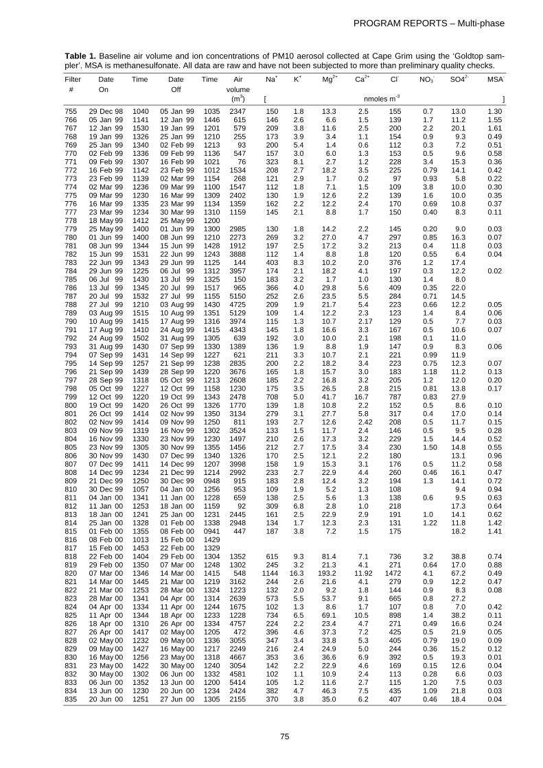
PROGRAM REPORTS – Multi-phase
75
Table 1. Baseline air volume and ion concentrations of PM10 aerosol collected at Cape Grim using the ‘Goldtop sam-pler’. MSA is methanesulfonate. All data are raw and have not been subjected to more than preliminary quality checks. Filter Date Time Date Time Air Na+ K+ Mg2+ Ca2+ Cl- NO3
- SO42- MSA- # On Off volume (m3) [ nmoles m-3 ]
755 29 Dec 98 1040 05 Jan 99 1035 2347 150 1.8 13.3 2.5 155 0.7 13.0 1.30 766 05 Jan 99 1141 12 Jan 99 1446 615 146 2.6 6.6 1.5 139 1.7 11.2 1.55 767 12 Jan 99 1530 19 Jan 99 1201 579 209 3.8 11.6 2.5 200 2.2 20.1 1.61 768 19 Jan 99 1326 25 Jan 99 1210 255 173 3.9 3.4 1.1 154 0.9 9.3 0.49 769 25 Jan 99 1340 02 Feb 99 1213 93 200 5.4 1.4 0.6 112 0.3 7.2 0.51 770 02 Feb 99 1336 09 Feb 99 1136 547 157 3.0 6.0 1.3 153 0.5 9.6 0.58 771 09 Feb 99 1307 16 Feb 99 1021 76 323 8.1 2.7 1.2 228 3.4 15.3 0.36 772 16 Feb 99 1142 23 Feb 99 1012 1534 208 2.7 18.2 3.5 225 0.79 14.1 0.42 773 23 Feb 99 1139 02 Mar 99 1154 268 121 2.9 1.7 0.2 97 0.93 5.8 0.22 774 02 Mar 99 1236 09 Mar 99 1100 1547 112 1.8 7.1 1.5 109 3.8 10.0 0.30 775 09 Mar 99 1230 16 Mar 99 1309 2402 130 1.9 12.6 2.2 139 1.6 10.0 0.35 776 16 Mar 99 1335 23 Mar 99 1134 1359 162 2.2 12.2 2.4 170 0.69 10.8 0.37 777 23 Mar 99 1234 30 Mar 99 1310 1159 145 2.1 8.8 1.7 150 0.40 8.3 0.11 778 18 May 99 1412 25 May 99 1200 779 25 May 99 1400 01 Jun 99 1300 2985 130 1.8 14.2 2.2 145 0.20 9.0 0.03 780 01 Jun 99 1400 08 Jun 99 1210 2273 269 3.2 27.0 4.7 297 0.85 16.3 0.07 781 08 Jun 99 1344 15 Jun 99 1428 1912 197 2.5 17.2 3.2 213 0.4 11.8 0.03 782 15 Jun 99 1531 22 Jun 99 1243 3888 112 1.4 8.8 1.8 120 0.55 6.4 0.04 783 22 Jun 99 1343 29 Jun 99 1125 144 403 8.3 10.2 2.0 376 1.2 17.4 784 29 Jun 99 1225 06 Jul 99 1312 3957 174 2.1 18.2 4.1 197 0.3 12.2 0.02 785 06 Jul 99 1430 13 Jul 99 1325 150 183 3.2 1.7 1.0 130 1.4 8.0 786 13 Jul 99 1345 20 Jul 99 1517 965 366 4.0 29.8 5.6 409 0.35 22.0 787 20 Jul 99 1532 27 Jul 99 1155 5150 252 2.6 23.5 5.5 284 0.71 14.5 788 27 Jul 99 1210 03 Aug 99 1430 4725 209 1.9 21.7 5.4 223 0.66 12.2 0.05 789 03 Aug 99 1515 10 Aug 99 1351 5129 109 1.4 12.2 2.3 123 1.4 8.4 0.06 790 10 Aug 99 1415 17 Aug 99 1316 3974 115 1.3 10.7 2.17 129 0.5 7.7 0.03 791 17 Aug 99 1410 24 Aug 99 1415 4343 145 1.8 16.6 3.3 167 0.5 10.6 0.07 792 24 Aug 99 1502 31 Aug 99 1305 639 192 3.0 10.0 2.1 198 0.1 11.0 793 31 Aug 99 1430 07 Sep 99 1330 1389 136 1.9 8.8 1.9 147 0.9 8.3 0.06 794 07 Sep 99 1431 14 Sep 99 1227 621 211 3.3 10.7 2.1 221 0.99 11.9 795 14 Sep 99 1257 21 Sep 99 1238 2835 200 2.2 18.2 3.4 223 0.75 12.3 0.07 796 21 Sep 99 1439 28 Sep 99 1220 3676 165 1.8 15.7 3.0 183 1.18 11.2 0.13 797 28 Sep 99 1318 05 Oct 99 1213 2608 185 2.2 16.8 3.2 205 1.2 12.0 0.20 798 05 Oct 99 1227 12 Oct 99 1158 1230 175 3.5 26.5 2.8 215 0.81 13.8 0.17 799 12 Oct 99 1220 19 Oct 99 1343 2478 708 5.0 41.7 16.7 787 0.83 27.9 800 19 Oct 99 1420 26 Oct 99 1326 1770 139 1.8 10.8 2.2 152 0.5 8.6 0.10 801 26 Oct 99 1414 02 Nov 99 1350 3134 279 3.1 27.7 5.8 317 0.4 17.0 0.14 802 02 Nov 99 1414 09 Nov 99 1250 811 193 2.7 12.6 2.42 208 0.5 11.7 0.15 803 09 Nov 99 1319 16 Nov 99 1302 3524 133 1.5 11.7 2.4 146 0.5 9.5 0.28 804 16 Nov 99 1330 23 Nov 99 1230 1497 210 2.6 17.3 3.2 229 1.5 14.4 0.52 805 23 Nov 99 1305 30 Nov 99 1355 1456 212 2.7 17.5 3.4 230 1.50 14.8 0.55 806 30 Nov 99 1430 07 Dec 99 1340 1326 170 2.5 12.1 2.2 180 13.1 0.96 807 07 Dec 99 1411 14 Dec 99 1207 3998 158 1.9 15.3 3.1 176 0.5 11.2 0.58 808 14 Dec 99 1234 21 Dec 99 1214 2992 233 2.7 22.9 4.4 260 0.46 16.1 0.47 809 21 Dec 99 1250 30 Dec 99 0948 915 183 2.8 12.4 3.2 194 1.3 14.1 0.72 810 30 Dec 99 1057 04 Jan 00 1256 953 109 1.9 5.2 1.3 108 9.4 0.94 811 04 Jan 00 1341 11 Jan 00 1228 659 138 2.5 5.6 1.3 138 0.6 9.5 0.63 812 11 Jan 00 1253 18 Jan 00 1159 92 309 6.8 2.8 1.0 218 17.3 0.64 813 18 Jan 00 1241 25 Jan 00 1231 2445 161 2.5 22.9 2.9 191 1.0 14.1 0.62 814 25 Jan 00 1328 01 Feb 00 1338 2948 134 1.7 12.3 2.3 131 1.22 11.8 1.42 815 01 Feb 00 1355 08 Feb 00 0941 447 187 3.8 7.2 1.5 175 18.2 1.41 816 08 Feb 00 1013 15 Feb 00 1429 817 15 Feb 00 1453 22 Feb 00 1329 818 22 Feb 00 1404 29 Feb 00 1304 1352 615 9.3 81.4 7.1 736 3.2 38.8 0.74 819 29 Feb 00 1350 07 Mar 00 1248 1302 245 3.2 21.3 4.1 271 0.64 17.0 0.88 820 07 Mar 00 1346 14 Mar 00 1415 548 1144 16.3 193.2 11.92 1472 4.1 67.2 0.49 821 14 Mar 00 1445 21 Mar 00 1219 3162 244 2.6 21.6 4.1 279 0.9 12.2 0.47 822 21 Mar 00 1253 28 Mar 00 1324 1223 132 2.0 9.2 1.8 144 0.9 8.3 0.08 823 28 Mar 00 1341 04 Apr 00 1314 2639 573 5.5 53.7 9.1 665 0.8 27.2 824 04 Apr 00 1334 11 Apr 00 1244 1675 102 1.3 8.6 1.7 107 0.8 7.0 0.42 825 11 Apr 00 1344 18 Apr 00 1233 1228 734 6.5 69.1 10.5 898 1.4 38.2 0.11 826 18 Apr 00 1310 26 Apr 00 1334 4757 224 2.2 23.4 4.7 271 0.49 16.6 0.24 827 26 Apr 00 1417 02 May 00 1205 472 396 4.6 37.3 7.2 425 0.5 21.9 0.05 828 02 May 00 1232 09 May 00 1336 3055 347 3.4 33.8 5.3 405 0.79 19.0 0.09 829 09 May 00 1427 16 May 00 1217 2249 216 2.4 24.9 5.0 244 0.36 15.2 0.12 830 16 May 00 1256 23 May 00 1318 4667 353 3.6 36.6 6.9 392 0.5 19.3 0.01 831 23 May 00 1422 30 May 00 1240 3054 142 2.2 22.9 4.6 169 0.15 12.6 0.04 832 30 May 00 1302 06 Jun 00 1332 4581 102 1.1 10.9 2.4 113 0.28 6.6 0.03 833 06 Jun 00 1352 13 Jun 00 1200 5414 105 1.2 11.6 2.7 115 1.20 7.5 0.03 834 13 Jun 00 1230 20 Jun 00 1234 2424 382 4.7 46.3 7.5 435 1.09 21.8 0.03 835 20 Jun 00 1251 27 Jun 00 1305 2155 370 3.8 35.0 6.2 407 0.46 18.4 0.04

PROGRAM REPORTS – Multi-phase
76
Table 1. continued… Filter Date Time Date Time Air Na+ K+ Mg2+ Ca2+ Cl- NO3
- SO42- MSA- # On Off volume (m3) [ nmoles m-3 ]
836 27 Jun 00 1310 04 Jul 00 1315 2042 112 1.4 11.0 2.1 119 0.5 6.8 0.04 837 04 Jul 00 1401 12 Jul 00 1523 2303 943 7.2 57.4 7.8 1004 1.6 22.4 838 12 Jul 00 1558 18 Jul 00 1245 914 233 2.8 22.4 4.3 250 0.7 12.8 0.03 839 18 Jul 00 1330 25 Jul 00 1252 2538 428 4.3 36.8 8.2 466 0.34 20.3 0.03 840 25 Jul 00 1318 01 Aug 00 1422 2132 120 1.5 12.4 2.2 129 0.48 7.4 0.06 841 01 Aug 00 1523 08 Aug 00 1330 842 08 Aug 00 1400 15 Aug 00 1221 5506 227 2.8 27.7 4.9 256 0.88 14.4 0.02 843 15 Aug 00 1250 22 Aug 00 1306 576 139 2.2 9.5 2.0 137 0.57 6.5 0.11 844 22 Aug 00 1430 29 Aug 00 1055 2011 78 1.1 6.6 1.4 81 0.68 4.5 0.05 845 29 Aug 00 1111 05 Sep 00 0943 2768 218 2.5 22.1 4.0 242 0.7 12.1 0.04 846 05 Sep 00 1005 12 Sep 00 1021 2288 296 3.2 30.6 6.9 330 0.5 17.7 0.02 847 12 Sep 00 1040 19 Sep 00 1058 1276 338 4.0 33.8 6.9 373 0.85 20.1 0.05 848 19 Sep 00 1118 26 Sep 00 1020 1095 298 3.5 28.5 6.0 324 0.68 17.2 0.09 849 26 Sep 00 1037 03 Oct 00 1052 2311 683 4.8 52.2 11.8 739 1.32 29.9 850 03 Oct 00 1110 10 Oct 00 1211 772 294 3.9 28.9 5.9 317 1.77 17.6 0.08 851 10 Oct 00 1233 17 Oct 00 1152 2930 196 3.0 31.1 4.6 234 0.5 14.9 0.12 852 17 Oct 00 1214 24 Oct 00 1203 967 1019 8.0 77.9 12.6 1110 1.1 32.9 0.07 853 24 Oct 00 1217 31 Oct 00 1140 1635 166 2.2 16.4 3.0 180 1.0 10.5 0.21 854 31 Oct 00 1157 07 Nov 00 1115 818 105 2.0 6.9 1.6 82 2.5 6.4 0.40 855 07 Nov 00 1138 14 Nov 00 1203 172 199 3.8 4.1 1.2 145 1.9 9.3 0.42 856 14 Nov 00 1530 21 Nov 00 1115 163 205 4.0 4.1 1.3 157 2.31 8.9 0.44 857 21 Nov 00 1132 28 Nov 00 1056 1700 116 1.7 10.8 2.4 120 1.31 9.4 0.60 858 28 Nov 00 1114 05 Dec 00 1101 5 859 05 Dec 00 1119 12 Dec 00 1213 840 129 2.2 9.8 2.2 131 0.66 8.8 0.58 860 12 Dec 00 1235 19 Dec 00 1336 190 174 3.2 3.4 1.0 126 1.25 9.1 0.59 861 19 Dec 00 1356 26 Dec 00 0937 113 425 7.2 15.0 3.9 370 2.07 19.4 0.69 862 26 Dec 00 1031 02 Jan 01 1323 1673 208 2.7 19.7 3.8 227 0.91 13.3 0.41 863 02 Jan 01 1400 09 Jan 01 1300 8 864 09 Jan 01 1400 16 Jan 01 1438 56 361 7.0 2.3 0.9 204 2.79 13.5 865 16 Jan 01 1508 23 Jan 01 1357 1748 241 3.4 25.4 4.6 258 1.50 19.4 2.05 866 23 Jan 01 1431 30 Jan 01 1228 236 269 4.8 12.9 2.7 240 1.25 14.8 0.85 867 30 Jan 01 1252 06 Feb 01 1210 250 186 3.7 7.0 1.6 156 2.65 9.7 0.43 868 06 Feb 01 1233 13 Feb 01 1221 2493 237 2.9 24.1 4.6 258 1.04 16.6 0.72 869 13 Feb 01 1245 20 Feb 01 1205 1857 123 1.7 12.1 2.3 133 0.59 8.2 0.27 870 20 Feb 01 1220 27 Feb 01 1111 459 181 3.0 10.8 2.3 176 1.60 10.8 0.35 871 27 Feb 01 1132 06 Mar 01 1019 182 209 3.5 5.8 1.5 165 2.19 10.1 0.38 872 06 Mar 01 1039 13 Mar 01 1112 486 195 3.1 12.8 2.8 195 0.56 9.5 0.28 873 13 Mar 01 1126 20 Mar 01 1057 1929 199 2.4 19.0 4.1 214 0.73 12.3 0.24 874 20 Mar 01 1118 27 Mar 01 1029 2369 149 2.0 15.6 3.0 161 1.31 11.3 0.20 875 27 Mar 01 1040 03 Apr 01 1124 2861 155 2.1 18.7 3.1 177 0.43 10.8 0.30 876 03 Apr 01 1203 10 Apr 01 1241 2796 270 3.5 32.4 5.4 303 1.35 17.6 0.32 877 10 Apr 01 1323 17 Apr 01 1231 2678 371 4.1 41.6 8.3 417 0.89 23.4 0.36 878 17 Apr 01 1313 24 Apr 01 1052 526 204 2.8 15.6 3.3 207 0.41 10.3 0.21 879 24 Apr 01 1117 01 May 01 1251 1309 167 1.8 14.3 2.9 179 0.44 8.8 0.09 880 01 May 01 1325 08 May 01 1211 881 08 May 01 1407 15 May 01 1150 882 15 May 01 1210 22 May 01 1141 3472 77 2.2 8.7 2.1 81 0.66 6.8 0.06 883 22 May 01 1221 29 May 01 1420 3048 125 2.8 11.4 2.4 131 0.39 7.5 0.06 884 29 May 01 1436 05 Jun 01 1155 2335 195 4.5 21.6 3.3 210 0.87 11.4 0.13 885 05 Jun 01 1230 12 Jun 01 1344 125 272 10.9 3.9 1.8 144 6.9 886 12 Jun 01 1410 19 Jun 01 1216 3528 188 3.9 19.6 3.2 208 0.34 10.3 887 19 Jun 01 1232 26 Jun 01 1302 4249 146 3.2 14.2 8.4 158 0.15 14.4 888 26 Jun 01 1323 03 Jul 01 1105 2161 202 4.3 18.5 5.5 211 1.53 14.1 0.08 889 03 Jul 01 1125 10 Jul 01 1244 106 890 10 Jul 01 0109 17 Jul 01 1211 2552 72 2.0 9.9 3.4 79 0.08 7.7 891 17 Jul 01 1228 24 Jul 01 1210 3534 196 4.2 19.8 2.8 217 0.42 9.7 892 24 Jul 01 1225 31 Jul 01 1226 1119 221 6.0 21.8 3.4 228 1.68 12.7 0.06 893 31 Jul 01 1251 07 Aug 01 1212 4252 264 6.2 34.0 4.5 320 1.68 17.5 894 07 Aug 01 1222 14 Aug 01 1127 2333 191 4.3 20.2 5.9 208 0.61 14.3 895 14 Aug 01 1141 21 Aug 01 1255 4913 184 4.9 30.0 6.9 228 0.40 17.5 896 21 Aug 01 1311 28 Aug 01 1254 2207 179 4.3 19.8 3.6 194 0.84 11.2 0.05 897 28 Aug 01 1323 04 Sep 01 1236 978 178 4.8 13.6 2.9 174 1.01 9.7 0.06 898 04 Sep 01 1256 11 Sep 01 1410 1617 203 5.1 21.1 3.5 214 0.96 12.4 0.08 899 11 Sep 01 1433 18 Sep 01 1314 2212 362 6.7 32.1 8.8 403 0.81 21.6 0.02 900 18 Sep 01 1404 25 Sep 01 1317 1813 208 4.9 23.1 4.9 225 0.75 14.3 0.08

PROGRAM REPORTS – Multi-phase
77
Table 2. Baseline gravimetric mass, air volume and ion concentrations of PM10 aerosol at Cape Grim collected using the ‘Goldtop sampler’. MSA is methanesulfonate. All data are raw and have not been subjected to more than preliminary quality checks. Filter Date Time Date Time Mass Air Na+ K+ Mg2+ Ca2+ Cl- NO3
- SO42- MSA-
# On Off volume (µg m-3) (m3) [ nmoles m-3 ]
901 25 Sep 01 1336 02 Oct 01 1337 33 2354 310 7.1 33.0 7.0 345 1.25 19.5 0.08 902 02 Oct 01 1400 16 Oct 01 1200 17 5298 216 4.5 21.0 3.8 250 1.24 11.9 902 02 Oct 01 1400 16 Oct 01 1200 17 5298 216 4.5 21.0 3.8 250 1.24 11.9 903 16 Oct 01 1230 23 Oct 01 1200 20 3141 184 4.3 19.9 4.1 203 0.38 11.3 904 23 Oct 01 1230 30 Oct 01 1208 19 537 210 7.3 13.4 2.1 190 1.28 11.5 0.24 905 30 Oct 01 1227 06 Nov 01 1324 36 1793 320 7.1 32.0 6.7 352 0.51 19.5 0.16 906 06 Nov 01 1349 20 Nov 01 1134 10 2636 99 2.5 9.2 1.8 102 0.39 6.3 0.20 907 20 Nov 01 1202 27 Nov 01 1151 26 685 223 7.2 16.4 3.4 208 3.02 14.0 0.48 908 27 Nov 01 1216 04 Dec 01 1152 28 1738 193 4.9 19.0 3.6 203 0.87 12.5 0.40 909 04 Dec 01 1227 11 Dec 02 1242 17 2009 156 4.0 14.9 2.9 162 0.96 10.7 0.67 910 11 Dec 01 1303 18 Dec 01 1040 12 7528 107 2.5 11.8 2.4 116 0.92 10.1 0.79 911 18 Dec 01 1150 02 Jan 02 1250 4 3589 35 1.2 2.5 0.5 32 0.20 2.9 0.32 912 02 Jan 02 1329 08 Jan 02 1007 21 3014 188 4.6 19.9 4.0 204 0.38 13.1 0.52 913 08 Jan 02 1120 15 Jan 02 1133 14 842 142 4.9 9.2 1.6 129 0.77 10.2 1.20 914 15 Jan 02 1308 22 Jan 02 1045 13 378 157 6.9 5.4 0.6 113 13.4 2.16 915 22 Jan 02 1240 29 Jan 02 1228 15 748 165 5.6 11.3 2.0 147 15.8 1.53 916 29 Jan 02 1353 05 Feb 02 1202 14 1575 133 4.0 11.7 2.3 126 13.0 1.41 917 05 Feb 02 1418 12 Feb 02 1355 13 777 133 4.8 7.6 0.6 116 0.72 8.2 0.85 918 12 Feb 02 1539 19 Feb 02 1443 31 541 294 9.3 22.4 4.4 279 1.06 21.2 3.50 919 19 Feb 02 1552 26 Feb 02 1300 18 2798 159 3.9 16.2 3.3 129 0.27 8.1 0.36 920 26 Feb 02 1437 05 Mar 02 1300 18 4173 152 3.6 16.3 3.4 168 0.58 11.0 0.52 921 05 Mar 02 1415 12 Mar 02 1213 15 236 163 7.3 2.8 1.2 91 8.3 0.52 922 12 Mar 02 1344 19 Mar 02 1015 20 3260 155 3.8 15.5 3.0 160 1.14 13.4 0.90 923 19 Mar 02 1305 26 Mar 02 1203 19 553 138 5.1 5.9 0.4 113 7.5 0.24 924 26 Mar 02 1304 02 Apr 02 1541 19 3649 101 2.7 10.5 2.3 105 0.48 7.9 0.40 925 04 Apr 02 1341 09 Apr 02 1319 13 2251 85 2.4 8.2 1.8 86 0.47 6.0 0.23 926 09 Apr 02 1408 16 Apr 02 1113 22 612 171 5.7 13.0 3.0 155 1.22 10.1 0.41 927 16 Apr 02 1209 23 Apr 02 1158 12 928 23 Apr 02 1234 30 Apr 02 1204 25 338 225 9.0 13.5 4.2 189 3.14 11.8 0.28 929 30 Apr 02 1300 07 May 02 1241 10 2469 100 2.8 9.9 2.2 102 1.38 7.8 0.25 930 07 May 02 1307 14 May 02 1230 28 2387 271 6.0 29.1 6.1 288 0.51 17.6 0.04 931 14 May 02 1311 21 May 02 1248 14 2459 195 4.9 21.4 4.7 212 0.56 13.5 0.05 932 21 May 02 1332 28 May 02 1242 12 732 150 4.8 10.8 3.2 138 1.15 8.3 0.08 933 28 May 02 1423 04 Jun 02 1132 12 2904 129 3.5 13.4 2.8 134 1.50 9.6 0.11 934 04 Jun 02 1213 11 Jun 02 1509 44 3300 365 7.9 39.1 8.1 397 0.34 22.3 935 12 Jun 02 1310 18 Jun 02 1251 26 1511 497 10.7 56.4 16.2 542 0.53 38.3 0.03 936 18 Jun 02 1359 25 Jun 02 1206 36 3605 100 2.4 10.2 2.3 105 0.11 6.2 0.09 937 25 Jun 02 1234 02 Jul 02 1321 23 4284 101 3.2 15.9 4.3 114 0.55 10.9 0.04 938 02 Jul 02 1352 09 Jul 02 1206 37 4976 298 5.9 30.8 7.1 328 0.24 18.7 0.06 939 09 Jul 02 1312 16 Jul 02 1138 37 2344 261 5.8 27.4 7.4 280 0.26 18.5 0.08 940 16 Jul 02 1249 23 Jul 02 1358 34 3775 235 5.4 26.7 7.2 257 0.35 17.6 0.02 941 23 Jul 02 1441 30 Jul 02 1233 24 2502 194 4.3 18.8 4.8 206 0.75 12.6 0.14 942 30 Jul 02 1354 07 Aug 02 1228 31 1829 293 6.9 30.2 6.4 307 0.84 18.1 943 07 Aug 02 1711 13 Aug 02 1407 39 2663 329 7.0 34.5 7.5 357 0.69 21.0 0.11 944 13 Aug 02 1515 20 Aug 02 1340 16 6198 148 3.6 16.8 3.5 160 1.75 11.1 945 20 Aug 02 1551 27 Aug 02 1351 20 2351 189 4.5 20.2 4.4 201 0.53 12.6 0.04 946 27 Aug 02 1557 03 Sep 02 1208 21 1247 212 6.2 20.6 4.7 212 1.75 14.6 0.50 947 09 Mar 02 1452 10 Sep 02 1239 47 1973 394 8.7 41.9 9.0 425 0.86 24.8 0.07 948 10 Sep 02 1410 17 Sep 02 1338 30 3160 66 1.5 7.1 1.5 246 1.01 14.2 0.09 949 17 Sep 02 1445 24 Sep 02 1056 34 4510 275 5.6 28.6 6.3 303 0.50 17.3 950 24 Sep 02 1200 01 Oct 02 1234 25 2750 218 5.2 23.3 4.9 235 0.53 14.2 0.03 951 01 Oct 02 1615 08 Oct 02 1153 40 154 391 19.4 21.4 7.2 303 8.91 15.9 0.27 952 08 Oct 02 1314 15 Oct 02 1219 28 2861 187 4.0 18.3 4.2 192 1.40 11.2 0.03 953 15 Oct 02 1434 22 Oct 02 1216 30 4876 270 5.2 27.9 5.9 292 1.98 17.2 0.23 954 22 Oct 02 1342 29 Oct 02 1219 17 5894 143 2.9 15.4 3.2 164 0.41 9.4 0.13 955 29 Oct 02 1337 05 Nov 02 1415 39 2563 347 7.2 36.8 7.6 398 0.94 22.5 0.29 956 05 Nov 02 1551 12 Nov 02 1105 34 1820 305 5.8 30.7 6.0 350 1.17 20.6 0.35 957 12 Nov 02 1325 19 Nov 02 1357 16 1977 314 6.6 35.0 7.5 362 0.71 21.0 0.26 958 19 Nov 02 1547 26 Nov 02 1119 17 2008 161 4.1 15.4 3.5 177 1.62 12.2 0.31 959 26 Nov 02 1310 03 Dec 02 1138 25 2867 218 4.9 23.1 4.8 247 1.57 16.7 1.52 960 03 Dec 02 1329 10 Dec 02 1221 27 4294 237 4.9 27.7 5.5 268 0.79 15.8 0.30 961 10 Dec 02 1415 17 Dec 02 1010 21 5470 164 3.4 18.7 3.5 187 0.77 12.4 0.44 962 17 Dec 02 1103 24 Dec 02 1401 16 2242 140 3.2 13.4 3.0 153 1.22 12.2 0.68 963 24 Dec 02 1520 31 Dec 02 1252 14 1727 104 2.8 9.0 2.5 111 0.65 8.7 0.87

PROGRAM REPORTS – Multi-phase
78
4.20. MEASUREMENT OF NATURAL LEVELS OF TRITIUM IN PRECIPITATION
C Tadros, D Hill and D Stone ANSTO Environment, Menai, NSW 2234, Australia [Cooperative Research report]
Introduction
Tritium denoted using the symbol 3H or T is the only radioactive isotope of hydrogen and has a half-life of 12.33 years. Tritium concentrations are expressed as a ratio using tritium units; TU, where one TU cor-responds to one 3H atom per 1018 atoms of hydro-gen or 0.11919 ± 0.00021 Bq kg-1.
Chemically, tritium behaves similar to stable hy-drogen and is usually found attached to molecules in place of hydrogen. Of all naturally occurring hydro-gen, tritium is produced in low abundance. Measur-able amounts of natural tritium are produced in the earths crust from the spontaneous fission of uranium which provides neutrons for the neutron capture reaction of 6Li in rocks;
238U + n → 3H + products 6Li + n → 3H + 4He
and in the upper atmosphere by nuclear reactions of cosmic rays with atmospheric atoms [Kaufman and Libby, 1983];
14N + n → 3H +12C 16O + n → 3H +14N 14N + p → 3H + products 16O + p → 3H + products.
Once in the atmosphere, tritium is readily
incorporated into water and reaches the earth‘s surface in rainwater, snow and atmospheric moisture. Monthly precipitation samples have been collected from various weather stations throughout Australia including Cape Grim, for the Australian Nuclear Science and Technology Organisation (ANSTO), as part of the Global Network of Isotopes in Precipitation project. This global project is con-ducted by the International Atomic Energy Agency (IAEA) in cooperation with the World Meteorological Organisation (WMO).
Sampling and tritium analysis
Monthly precipitation samples collected from Cape Grim are analysed for tritium at ANSTO, which has the only facility in Australia capable of low level trit-ium analysis.
An accepted methodology for the determination of low level tritium in environmental water samples is a process referred to as electrolytic enrichment followed by Liquid Scintillation Counting. This is an established technique being employed by ANSTO and numerous laboratories worldwide.
A subsample of the monthly precipitation re-ceived from each weather station is supplied to CSIRO Land and Water, Isotope Analysis Service, Waite Rd, Urrbrae, South Australia 5064, for deute-rium and oxygen-18 analysis.
Results
Tritium activity in precipitation from Cape Grim for the period 2001–2002 is presented in Table 1. The yearly mean for tritium, weighted by the total amount of precipitation has been calculated according to the formula: yearly weighted mean = [ ]( ) ( )P/TP Σ×Σ ; where P = monthly precipitation and [T] = monthly tritium con-centration.
During 2001 insufficient samples were supplied, as such the yearly weighted mean for tritium could not be calculated.
Table 1. Monthly tritium precipitation data for the Cape Grim sampling station during 2001 and 2002. 2001 2002 January 38 mm 28.6 mm 2.7 ± 01 TU 4.1 ± 0.1 TU February 21.4 mm 27.4 mm 3.3 ± 0.2 TU 2.1 ± 0.1 TU March 64.4 mm 5.4 mm * * April 29.4 mm 23.6 mm 3.0 ± 0.2 TU 2.0 ± 0.1 TU May 23.8 mm 55.6 mm 4.3 ± 0.3 TU 2.5 ± 0.1 TU June 85.5 mm 106.6 mm * 2.3 ± 0.4 TU July 38.8 mm 113.6 mm * 2.8 ± 0.4 TU August 121.2 mm 76.4 mm 3.1 ± 0.3 TU 1.8 ± 0.3 TU September 79.6 mm 52.6 mm * 2.3 ± 0.4 TU October 128.4 mm 61.6 mm 3.4 ± 0.2 TU 4.2 ± 0.4 TU November 63.4 mm 21.4 mm 5.0 ± 0.2 TU 3.4 ± 0.4 TU December * 25.4 mm 3.0 ± 0.1 TU 3.6 ± 0.4 TU
Weighted mean 2.2 ± 0.2 TU # 2.1 ± 0.3 TU # 61.3 %^ 99.1 %^ * Tritium levels in TU for these months are not available, monthly
precipitation in mm are indicated were data was supplied # Yearly weighted mean for tritium (TU), weighted by the total
amount of precipitation ^ Percentage of the total precipitation for which tritium data are
available to calculate the weighted mean References
Kaufman, S. and W. F. Libby, The natural distribu-tion of tritium, Physical Review, 93(6), 1337-1344, 1983.
Acknowledgments
We would like to acknowledge the staff at the Cape Grim Baseline Air Pollution Station who collected the samples and the Bureau of Meteorology for supply-ing the relevant precipitation values.

PROGRAM REPORTS - Radiation
79
4.21. SPECTRAL SOLAR RADIATION
S R Wilson1 and B W Forgan2 1University of Wollongong, Wollongong, NSW 2522, Australia
266 Haversham Avenue, Wheelers Hill, Victoria 3150, Australia
[Supported by CGBAPS research funds]
Reported here are the data from the Spectral Radia-tion program, which includes measurements of spectral irradiance and turbidity.
Optical depth
The operation of this system was relatively trouble free for the two years. On 15 June 2001 the direct sun spectral radiometer (SPO1A) control box was replaced with a dual controller to allow installation of a second spectral radiometer on the southern tracker. The second spectral radiometer is an SPO2 (Carter-Scott Design #1029), with 4 independent in-terference filtered silicon diode detectors channel. Unlike the SPO1A the channels of the SPO2 are not temperature stabilized, but as they use 1” and 10 nm FWHM filters combined with Hamamatsu detectors the impact of ambient temperature on the signals is insignificant. The wavelengths measured by the two spectral radiometers are summarised in Table 1. Communication (via RS485) became erratic follow-ing this change. The problems were finally resolved in September 2001. Following the lightning strike on 24 December 2001 the system was out of action un-til 7 February 2002. On 27 February 2002 it was noted that the two controllers for the spectral radi-ometers were swapped during the repair, and this was corrected.
On 8 August 2002 a spare instrument mount was removed from the northern instrument pole that was shading the SPO1A near solar noon.
Spectral irradiance
This section reports on measurements from two in-struments; a spectral radiometer (SRAD) (Optronics Laboratories OL-752), and a broad band UV-B de-tector (Solar Light model 501 UV-Biometer). In-cluded in this section are changes of note that oc-curred during the two years.
Communication with SRAD was problematic dur-ing the two years. On 10 and 11 April 2001 the in-strument repeatedly failed, and this was traced to corrosion in various locations in the controller, which was overcome on 7 May 2001. However, the system failed completely on 15 May 2001 and was returned to the manufacturer for repair. The spectrometer was returned to service on 17 December 2001. On 24 December 2001 lightning damaged the commu-nications equipment (short-haul modems and Light-ning sponges), which failed intermittently. These were finally identified and replaced and the system returned to operation on 18 March 2002. On 15 May the touch screen on the controller was replaced to assist in system fault finding. The original display had failed several years earlier. On June 4 2002 the controller failed to read the CMOS memory following a power disruption, and returned to factory settings. This reduced the photomultiplier gain and hence the system calibration significantly. A similar event oc-curred on 29 September 2002, although the decision to leave the system at the factory default voltage meant that this lead to no significant change to the calibration.
The Biometer system ran reliably through this en-tire period, with the data collected by the main data collection system.
Table 1. Details of the sunphotometers operating at Cape Grim since 1990. The SPO sunpho-tometers were purchased from Carter Scott. Name Operation dates Wavelengths Quantities measured (nm) WMO#1 1985 -10 Dec 1997 368,500,778,862 direct beam SPO1a (#1007) 12 Dec 1997- 341,500,610,778,862 Direct beam & aureole SPO2 (#1029) 15 June 2001- 368,412,500,867,862 Direct beam

PROGRAM REPORTS - Radiation
80
4.22. PASSIVE SOLAR RADIATION
S R Wilson University of Wollongong, Wollongong, NSW 2522, Australia [Supported by CGBAPS research funds]
The Passive Solar Radiation monitoring program continued throughout 1999-2000 The Regional In-strument Centre the Bureau of Meteorology is re-sponsible for the maintenance and calibration of the instruments and data processing of all irradiance quantities apart from UV.
Continuous measurements of global, direct, dif-fuse, and terrestrial measurements continued in 2001-2002. The trackers were overhauled on 20-22 March 2001, and the tracker computer replaced with two stepper-motor controllers. On 2 March 2001 the direct pyrheliometer was realigned. On 12 Novem-ber 2001 the shading arms were cleaned to remove salt build-up on the joints. The lightning strike on 24 December 2001 halted both power and communica-tions to the radiation enclosure. The various dam-aged components were identified and replaced, and the system returned to operation on 7 February 2002. On 10 – 12 July 2002 a fibre optics cable was commissioned for communication with the radiation enclosure to reduce the likelihood of failures due to lightning striking the communications tower. At this time the controlling computer and the diffuse pyranometer were also replaced. Cable faults
caused problems for the diffuse measurements be-tween 8 – 16 August, and intermittently for the long-wave measurements from sometime in August 2002 through to 11 October 2002
Data processing is largely automated. Daily ex-posure and irradiance data were edited to exclude those days when instrument failures or data acquisi-tion errors were evident from system logs or trace examination. Daily data are excluded from the monthly averages when quality control and assur-ance tests reject more than 2 minutes in a day. Ta-bles 1 and 2 provide monthly statistics of the proc-essed quantities.
Table 1. Monthly mean daily terrestrial (long wave) irradi-ance for 2001-2002. The sample estimate of the standard deviation and number of days included in the average is given in brackets for each month. Month Terrestrial Irradiance Terrestrial Irradiance (W m-2) s.d n (W m-2) s.d n 2001 2002 Jan 351.02 24.15 31 0 Feb 349.59 22.96 28 346.72 25.24 19 Mar 347.17 19.59 26 338.71 21.17 31 Apr 335.39 24.42 30 335.34 22.12 30 May 326.00 17.71 31 322.78 25.79 31 Jun 336.26 17.85 30 326.43 20.39 30 Jul 319.45 17.10 31 326.54 15.19 28 Aug 325.16 18.81 30 315.41 18.34 29 Sept 329.15 22.79 30 314.47 23.15 2 Oct 324.85 19.54 31 322.03 16.83 8 Nov 330.21 22.14 30 326.06 21.09 30 Dec 332.59 17.33 22 337.29 22.45 31
Table 2. Monthly mean daily solar exposure and sunshine hours for 2001-2002. Exposure Sunshine Direct s.d # days Global s.d # days Diffuse s.d # days # hr s.d # days (MJ m-2) /month (MJ m-2) /month (MJ m-2) /month /day /month Jan 01 18.94 12.27 28 23.80 8.24 31 9.60 2.71 28 7.75 4.44 28 Feb 01 18.96 11.20 28 22.28 5.93 28 9.14 3.08 28 7.75 3.82 28 Mar 01 14.96 11.42 20 16.91 6.36 22 7.17 2.67 20 6.32 4.18 20 Apr 01 8.53 6.19 30 10.54 3.25 30 6.20 1.51 30 4.12 2.70 30 May 01 10.01 6.68 31 8.20 2.35 31 4.08 1.24 31 4.54 2.59 31 Jun 01 4.17 3.81 25 5.09 1.95 30 3.75 1.49 30 2.26 1.82 25 Jul 01 5.88 4.50 22 6.77 2.02 28 5.15 1.92 31 2.85 1.95 22 Aug 01 6.71 6.13 29 8.37 3.62 30 5.19 1.73 30 3.31 2.71 29 Sep 01 10.01 7.96 30 13.19 4.81 30 7.38 2.00 30 4.83 3.26 30 Oct 01 14.85 9.04 27 19.49 5.67 31 9.68 3.67 31 6.15 3.27 27 Nov 01 15.46 9.70 28 23.01 6.66 30 11.45 2.86 28 6.51 3.37 28 Dec 01 16.92 12.53 17 24.69 8.40 22 11.86 3.27 16 6.77 4.34 17 Jan 02 0 0 9.95 2.91 12 0 Feb 02 13.75 9.86 12 21.10 5.24 19 7.45 2.52 31 6.15 3.53 12 Mar 02 15.67 10.55 31 17.19 5.21 31 5.72 1.85 30 6.49 3.69 31 Apr 02 12.45 7.49 30 12.21 3.25 30 3.62 1.28 31 5.86 2.99 30 May 02 10.89 8.57 31 7.39 2.91 25 3.21 1.04 30 4.83 3.28 31 Jun 02 7.12 6.78 30 5.32 2.03 26 3.84 0.76 28 3.64 2.79 30 Jul 02 4.97 5.01 28 5.94 2.22 28 5.09 1.42 25 2.83 2.53 28 Aug 02 9.85 6.13 31 9.94 2.52 28 6.83 1.62 29 4.71 2.27 31 Sep 02 11.45 6.67 29 14.18 4.05 29 9.35 2.91 30 5.44 2.54 29 Oct 02 13.25 9.44 31 19.11 5.07 30 10.78 3.23 29 5.73 3.28 31 Nov 02 16.04 10.87 29 23.53 6.38 30 9.73 3.68 31 6.87 3.83 29 Dec 02 20.41 13.57 31 25.82 8.18 31 9.95 2.91 12 7.93 4.40 31

Appendix A - Publications
81
APPENDICES Appendix A - PUBLICATIONS
(Peer-reviewed research papers in international journals are listed first with ‘project leader’ names in bold. Conference presentations and proceedings are listed next, followed by other significant publications).
International Journal Papers Ankilov, A., A. Baklanov, M. Colhoun, K.-H. Enderle, J. L.
Gras, Yu. Julanov, D. Kaller, A. Lindner, A. A. Lush-nikov, R. Mavliev, F. McGovern, A. Mirme, T. C. O'Con-nor, J. Podzimek, O. Preining, G. P. Reischl, R. Rudolf, G. J. Sem, W. W. Szymanski, E. Tamm, A. E. Vrtala, P. E. Wagner, W. Winklmayr, and V. Zagaynov, Intercom-parison of number concentration measurements by vari-ous aerosol particle counters, Atmos. Res., 62(3-4), 177-207, 2002.
Ankilov, A., A. Baklanov, M. Colhoun, K.-H. Enderle, J. L. Gras, Yu. Julanov, D. Kaller, A. Lindner, A. A. Lush-nikov, R. Mavliev, F. McGovern, T. C. O'Connor, J. Pod-zimek, O. Preining, G. P. Reischl, R. Rudolf, G. J. Sem, W. W. Szymanski, A. E. Vrtala, P. E. Wagner, W. Winklmayr, and V. Zagaynov, Particle size dependent response of aerosol counters, Atmos. Res., 62(3-4), 209-237, 2002.
Cihlar, J., S. Denning, F. Ahern, O. Arino, A. Belward, F. Bretherton, W. Cramer, G. Dedieu, C. Field, R. J. Francey, R. Gommes, J., K. Hibbard, T. Igarashi, P. Ka-bat, D. Olson, S. Plummer, I. Rasool, M. R. Raupach, R. Scholes, J. Townshend, R. Valentini, and D. Wickland, Initiative to quantify terrestrial carbon sources and sinks, Eos, 83(1), 1,6-7, 2002.
Cunnold, D. M., L. P. Steele, P. J. Fraser, P. G. Sim-monds, R. G. Prinn, R. F. Weiss, L. W. Porter, S. O'Do-herty, R. L. Langenfelds, P. B. Krummel, H. J. Wang, L. Emmons. X. X. Tie,and E. J. Dlugokencky, In situ meas-urements of atmospheric methane at GAGE/AGAGE sites during 1985-2000 and resulting source inferences, J. Geophys. Res., 107(D14): 10.1029/2001JD001226, 2002.
Gabric, A. J., R. Cropp, G. P. Ayers, G. McTainsh, and R. Braddock, Coupling between cycles of phytoplankton biomass and aerosol optical depth as derived from SeaWiFS time series in the Subantarctic Southern Ocean, Geophys. Res. Letts., 29(7), 10.1029/2001GL013545, 2002.
Galbally, I. E., and W. Kirstine,The production of metha-nol by flowering plants and the global cycle of methanol, J. Atmos. Chem., 43(3),195-229, 2002.
Gras, J. L., J. Podzimek, T. C. O'Connor, and K.-H. En-derle, Nolan-Pollak type CN counters in the Vienna aerosol workshop, Atmos. Res., 62(3-4): 239-254, 2002.
Langenfelds, R. L., R. J. Francey, B. C. Pak, L. P. Steele, J. Lloyd, C. M. Trudinger, and C. E. Allison, Interannual growth rate variations of atmospheric CO2 and its δ13C , H2 ,CH4 , and CO between 1992 and 1999 linked to bio-mass burning, Global Biogeochemical Cycles, 16(3), 1048, doi:10.1029/2001GB001466, 2002.
Law, R. M., P. J. Rayner, L. P. Steele, and I. G. Enting, Using high temporal frequency data for CO2 inversions, Global Biogeochemical Cycles, 16(4), 1053, DOI 10.1029/2001GB001593, 2002.
Masarie, K. A., R. L. Langenfelds, C. E. Allison, T. J. Con-way, E. J. Dlugokencky, R. J. Francey, P. C. Novelli, L. P. Steele, P. P. Tans, B. Vaughn, and J. W. C. White,
NOAA/CSIRO Flask Air Intercomparison Experiment: A strategy for directly assessing consistency among at-mospheric measurements made by independent labora-tories, J. Geophys. Res., 106(D17), 20445-20464, 2001.
O'Doherty, S., P. G. Simmonds, D. M. Cunnold, H. J. Wang, G. A. Sturrock, P. J. Fraser, D. Ryall, R. G. Der-went, R. F. Weiss, P. Salameh, B. R. Miller, and R. G. Prinn, In situ chloroform measurements at Advanced Global Atmospheric Gases Experiment atmospheric re-search stations from 1994 to 1998, J. Geophys. Res., 106(D17): 20429-20444, 2001.
Prinn, R. G., J. Huang, R. F. Weiss, D. M. Cunnold, P. J. Fraser, P. G. Simmonds, A. McCulloch, C. Harth, P. Salameh, S. O'Doherty, R. H. J. Wang, L. W. Porter, and B. R. Miller, Evidence of substantial variations of atmos-pheric hydroxyl radicals in the past two decades, Sci-ence, 292(5523): 1882-1888, 2001.
Sturrock, G. A., D. M. Etheridge, C. M. Trudinger, P. J. Fraser, and A. M. Smith, tropospheric histories of halo-carbons from analysis of Antarctic firn air: major Mont-real Protocol species, J. Geophys. Res. 107(D24): 10.1029/2002JD002548, 2002.
Conferences Environmental research in the Arctic 2000 [Proceed-ings of the Second International Symposium on En-vironmental Research in the Arctic and Fifth Ny-Alesund Scientific Seminar], 23-25 February 2000, Tokyo, Japan, edited by O. Watanabe and T. Yama-nouchi, (Memoirs of National Institute of Polar Re-search Special Issue, 54), National Institute of Polar Research, Tokyo, Japan, 2001
Francey, R. J., M. Groening, K. Holmén, K. R. Kim, J. Miller, P. Tans, and N. Trivett, Global quality control for long-lived trace gas measurements, 81-90.
Millennium Symposium on Atmospheric Chemistry: past, present, and future of atmospheric chemistry [preprints], 14-19 January 2001, Albuquerque, New Mexico, USA, American Meteorological Society, Boston, Massachusetts, USA, 2001
Dunse, B. L., L. P. Steele, P. J. Fraser, P. J. Hurley, P. B. Krummel, and S. R. Wilson, Estimating emissions of a range of trace gases from a large city (Melbourne, Aus-tralia) by analysing and modeling measurements made about 250 km downwind at the Cape Grim Baseline Air Pollution Station, 92-95.
AMOS 2001: 8th National AMOS Conference incor-porating the 6th Australasian Conference on the Physics of Remote Sensing of Atmosphere and Ocean [abstracts], 5-7 February, 2001 University of Tasmania (AMOS Publication, 17), AMOS Confer-ence Committee, Hobart, Australia, 2001
Francey, R. J., Atmospheric CO2 measurements for the next decade, 27.

Appendix A - Publications
82
International Workshop ‘Emissions of chemical spe-cies and aerosols into the atmosphere’ [abstracts], 19-22 June 2001, Paris, France, POET European Project, Paris, France, 2001
Galbally, I. E., W. Zahorowski, C. P. Meyer, and S. Whit-tlestone, A comparison of the regionally averaged sur-face exchange rates of trace gases made through at-mospheric concentration observations, 1 p.
Meyer, C. P., G. Cook, K. G. Tolhurst, I. E. Galbally, and R. D. Graetz, A spatially explicit inventory of trace gas emissions from wildfires and controlled burning over Australia,1 p.
Oram, D. E., C. E. Reeves, G. A. Sturrock, S. A. Penkett, P. J. Fraser, C. A. M. Brenninkmeijer, and A. Zahn, Es-timates of global and regional halocarbon emissions from measurements on the Cape Grim Air Archive and from the CARIBIC aircraft experiment, 1 p.
Challenges of a changing earth [abstracts of scien-tific papers and posters presented at the Global Change Open Science Conference], 10-13 July 2001, Amsterdam, Netherlands, Congrex Holland BV, Amsterdam, Netherlands, 2001. Cihlar, J., S. Denning, O. Arnio, F. Bretherton, W. Cramer,
G. Dedieu, C. Field, R. Gommes, J. Gosz, K. Hibbard, T. Igarashi, P. Kabat, R. Olson, S. Plummer, I. Rasool, M. R. Raupach, S. Scholes, J. Townshend, R. Valentini, D. Wickland, and R. J. Francey, Terrestrial carbon obser-vation: an integrated satellite - in situ strategy, 90.
Raupach, M. R., D. Barrett, P. Briggs, H. Cleugh, D. Ea-mus, I. G. Enting, G. Farquhar, R. J. Francey, I. E. Gal-bally, R. Gifford, R. D. Graetz, D. Griffith, L. Hutley, H. Keith, M. Kirschbaum, R. Leuning, J. L. McGregor, B. Medlyn, I. Noble, J. Raison, P. J. Rayner, J. Skjemstad, L. P. Steele, and Y. P. Wang, The Australian Carbon Cycle Project, 94.
Sixth International Carbon Dioxide Conference [ex-tended abstracts], 1-5 October 2001, Sendai, Japan, Organizing Committee of the 6th Conference, Sen-dai, Japan, 2001
Allison, C. E., R. J. Francey, and P. J. Rayner, Stable iso-topes of atmospheric carbon dioxide from the CSIRO Global Flask Sampling Network [poster], AT07, 81-84.
Ciais, P., R. J. Francey, P. Balkwin, K. A. Masarie, and P. P. Tans, Atmospheric CO2 and tracers measurements to monitor the carbon cycle and its future evolution [oral presentation], AT81, 1-4.
Francey, R. J., C. E. Allison, P. Ciais, and G. Hoffmann, The interannual variation in the δ18O in atmospheric CO2 over the last 25 years [poster], AT56, 190-193.
Francey, R. J., C. E. Allison, C. M. Trudinger, P. J. Rayner, I. G. Enting, and L. P. Steele, The interannual variation in global atmospheric δ13C and its link to net terrestrial exchange [oral presentation], AT55, 43-46.
Langenfelds, R. L., R. J. Francey, B. Pak, L. P. Steele, J. Lloyd, C. M. Trudinger, and C. E. Allison, The use of multi-species measurements for interpreting interannual variability in the carbon cycle [oral presentation], AT44, 9-11.
Le Quéré, C., O. Aumont, L. P. Bopp, P. Bousquet, P. Ciais, R. J. Francey, M. Heimann, H. S. Kheshgi, P. Peylin, S. C. Piper, I. C. Prentice, and P. J. Rayner, Two decades of ocean CO2 sink and variability [poster], MC07, 919-922.
Peylin, P., P. Ciais, P. P. Tans, and R. J. Francey, Monthly estimates of terrestrial photosynthesis and res-piration from atmospheric measurements of 18O/16O ra-tion in CO2 [oral presentation], MA18, 731-734.
Roy, T., P. J. Rayner, R. J. Matear, and R. J. Francey, Comparison of Southern Hemisphere ocean CO2 flux estimates with atmospheric inversion results [oral pres-entation], MC22,1035-1038.
Steele, L. P., G. A. Da Costa, D. A. Spencer, P. B. Krum-mel, R. J. Francey, J. W. Bennett., B. S. Petraitis, R. T. Howden, C. Smith, S. B. Baly, and L. W. Porter, Future directions in atmospheric CO2 measurement methods [poster], AT45, 172-175.
Trudinger, C. M., I. G. Enting, P. J. Rayner, and R. J. Francey, A Kalman filter double deconvolution of ice core CO2 and δ13 data [poster], MC04, 907-910.
Cape Grim Baseline Air Pollution Station, Annual Scientific Meeting 2001 [abstracts], 6-7 February 2002, Antarctic CRC, University of Tasmania, Hobart, Tasmania, edited by N. W. Tindale, and N. Derek, CSIRO Atmospheric Research and Bureau of Meteorology, Melbourne, Australia, 2002.
Allison, C., R. Francey, and L. Porter, Future CO2 isotope monitoring at Cape Grim, 11.
Ayers, G., CSIRO‘s commitment to Cape Grim in a world of BHAGs, Emerging science and IP revaluation, 26.
Cox, M., S. Siems, P. Fraser, P. Hurley, and G. Sturrock, TAPM modelling studies of Cape Grim dichloromethane, 30.
Etheridge, D., C. Trudinger, R. Langenfelds, D. Lowe, A. Smith, G. Sturrock, P. Steele, P. Fraser, R. Francey, L. Porter, A. Elcheick, and M. Battle, Atmospheric composi-tion changes during the past century from firn air from two Antarctic Sites, 25.
Francey, R., C. Allison, C. Trudinger, P. Rayner, I. Enting, P. Steele, L. Cooper, and Cape Grim staff, The interan-nual variation in global atmospheric δ13C and its link to net terrestrial CO2 exchange, 10.
Fraser, P., B. Dunse, P. Steele, S. Wilson, M. Cox, S. O’Doherty, P. Simmonds, and N. Derek, Trace gas emissions from melbourne and europe deduced from AGAGE observations at Cape Grim and Mace Head, 14.
Fraser, P., D. Etheridge, C. Trudinger,L. Porter, M. Cox, S. O’Doherty, P. Simmonds,B. Miller, R. Weiss, and N. Derek, Recent changes in the global abundance of methyl bromide from AGAGE and SIO measurements, 15.
Granek, H., J. Gras, and D. Paterson, The aerosol trans-mission efficiency of the Cape Grim 10-m inlet, 7
Jimi, S., J. Gras, S. Siems, and P. Krummel, Observation of Ultrafine aerosol particles in the marine environment of southeastern Australia, 8.
Meyer, M., I. Galbally, G. Cook, D. Barrett, D. Graetz, and K. Tolhurst, A spatially explicit inventory of trace gas emissions from wildfires and controlled burning over Australia, 29.
Steele, L. P., G. Pearman, D. Beardsmore, F. de Silva, P. Krummel, R. Langenfelds, and Cape Grim Staff, The 25-year Cape Grim in situ CO2 record, 9.
Steele, L. P., D. Spencer, P. Krummel, R. Francey, R. Law, G. Da Costa, CSIRO Engineering Staff, and Cape Grim Staff, The future of CO2 measurement at Cape Grim, 12.
Tully, M., and A. Downey, Air mass origin – some sources of error, 24.

Appendix A - Publications
83
Wilson, S., D. Griffith, T. Naylor, J. Menegazzo, and F. Turatti, Isotopic fractionation in sources of atmospheric N2O, 22.
Zahorowski, W., S. Chambers, S. Werczynski, and A. Henderson-Sellers, A brief review of key characteristics of radon measurements at Cape Grim 1987-2001, 6.
AMOS 2002: 9th National AMOS Conference incor-porating the 6th Australasian Conference on the Physics of Remote Sensing of Atmosphere and Ocean [abstracts], 18-20 February, 2002 University of Melbourne (AMOS Publication, 18), AMOS Con-ference Committee, Melbourne, Australia, 2002
Ayers, G. P., Chemistry of dimethylsulfide in marine air, 13.
Geophysical Research abstracts: 27th General As-sembly, 21-26 April 2002, Nice, France, European Geophysical Society, Katlenburg-Lindau, Germany, 2002 Etheridge, D. M., C. M. Trudinger, D. C. Lowe, K. R.
Lassey, A. M. Smith, L. P. Steele, R. L. Langenfelds, R. J. Francey, and M. Battle, Evolution of atmospheric methane during the anthropocene from methane isotopic measurements of firn air from two Antarctic sites, OA25, Abstract: EGS 02-A-05157.
7th South Pacific Environmental Radioactivity Asso-ciation Conference, [program and abstracts], 13-17 May, 2002, Sydney, Australia, 2002.
Zahorowski, W. S. Chambers, and A. Henderson-Sellers, characterisation of air mass origin using atmospheric ra-don concentration measurements, 10.
2002 Spring Meeting, 28-31 May 2002, Washington, D. C., USA, (supplement to EOS, Transactions, American Geophysical Union, 83(19), American Geophysical Union, Washington, D. C., USA, 2002
Wilson, S. R., D. W. T. Griffith, J. M. Menegazzo, T. Nay-lor, and F. Turatti, Isotopic Signatures of some anthro-pogenic nitrous oxide sources [abstract],
Western Pacific Geophysics Meeting [abstract], 9-12 July 2002, Wellington, New Zealand, (supplement to EOS, Transactions, American Geophysical Union, 83(22), American Geophysical Union, Washington, D. C., USA, 2002
Wilson, S.R., D. Griffith, and T. Naylor, Isotopic signa-tures of N2O from wastewater sites, A31A-04.
Proceedings of the 16th International Clean Air & Environment Conference, 18-22 August 2002, Christchurch, New Zealand, Clean Air Society of Australia and New Zealand, Christchurch, New Zea-land, 2002
Manins, P. C., T. Beer, P. J. Fraser, P. N. Holper, R. Sup-piah, and K. J. E. Walsh, Australia State of Environment Report 2001 Atmosphere, 536-541.
Joint International Symposium on Atmospheric Chemistry within the Earth System [program and abstracts], 18-25 September, 2002, Hersonissos, Crete, IAMAS/CACGP/IGAC, Hersonissos, Crete, 2002.
Ayers, G. P., M. D. Keywood, and R. W. Gillett, The DMS - climate connection: is there empirical evidence in time se-ries data from Cape Grim, Tasmania?, 41.
Cunnold, D. M., R. G. Prinn, R. F. Weiss, P. G. Simmonds, P. J. Fraser, L. W. Porter, R. L. Langenfelds, S. O'Do-herty, B. R. Miller, and A. McCulloch, Emission estimates and total tropospheric chlorine time series derived from 20+ years of ground-based measurements 53.
Oram, D. E., C. E. Reeves, S. A. Penkett, and P. J. Fra-ser, Recent changes in the global abundance, growth rates and emissions of anthropogenic halocarbons: im-plications for ozone depletion and global warming, 13-14.
Proceedings of the 4th APEX International Workshop [ab-stracts], 26-28 September 2002, Kyoto, Japan, Japan Science & Technology Corp., Kyoto, Japan, 2002.
Jensen, J. B., S. Siems, J. Hacker, J. L. Gras, C. M. Tivendale, and J. R. Peter, A summary of King-Air ob-servations during APEX-E2/ACE-Asia with special em-phasis on giant aerosol particles, 111-114.
Cape Grim Baseline Air Pollution Station, Annual Science Meeting 2002 [abstracts], 7-8 November 2002, CSIRO Atmospheric Research, Aspendale, Victoria, edited by N. W. Tindale, and N. Derek, CSIRO Atmospheric Research and Bureau of Mete-orology, Melbourne, Australia, 2002.
Allison, C., and R. Francey, The Cape Grim stable iso-topes in atmospheric CO2 measurement program, 5.
Baly, S., L. Porter, P. Fraser, P. Krummel, and N. Derek, In situ SF6 measurements at Cape Grim, 14.
Dunse, B., P. Fraser, P. Krummel, N. Derek, L. Porter, and D. Oram, CFC measurements at Cape Grim, 1978-2002, 13.
Etheridge, D., K. Lassey, A. Smith, D. Lowe, C. Trudinger, and P. Steele, Can we explain the causes of methane changes from isotopic information?, 26.
Francey, R., and P. Steele, CO2 measurement in the Aus-tralian region – the next decade, 4.
Fraser, P., B. Dunse, P. Krummel, L. Porter, and N. Derek, Halon-1211 emissions from Melbourne, 12.
Jimi, S. I., J. L. Gras, S. T. Siems, and P. B. Krummel, Nano-particles at Cape Grim, Tasmania, 21.
Krummel, P., M. Tully, A. Downey, L. Porter, J. Gras, R. Wheaton, and P. Steele, Cape Grim statistics and their use in indicators of baseline conditions, 1.
Law, R., P. Rayner, E. Kowalczyk, Y-P. Wang, and P. Steele, Estimating CO2 sources from continuous meas-urements: Australia as a test case, 6.
MacFarling, C., D. Etheridge, I. Levin, J. Harnisch, M. Vollmer, C. Trudinger, A. Smith, P. Steele, and P Fra-ser, Natural and anthropogenic SF6 and CF4 in the atmosphere, 25.
van der Schoot, M., R. Langenfelds, D. Spencer, R. Francey, P. Steele, M. Schmidt, C. Allison, and H. Mu-kai, Modification of trace gas concentrations by diffusive and surface processes, 24.
Zahorowski, W., S. Chambers, and A. Henderson-Sellers, Estimating regional oceanic radon flux, 11.

Appendix A - Publications
84
Other Significant Publications Allison, C. E., R. J. Francey, and L. P. Steele, The Inter-
national Atomic Energy Agency circulation of laboratory air standards for stable isotope comparison: aims, preparation and preliminary results, in Isotope aided studies of atmospheric carbon dioxide and other green-house gases Phase II, (IAEA-TECDOC; 1269), Interna-tional Atomic Energy Agency, Vienna, Austria, 5-23, 2002. Bhattacharrya, S. K., R. A. Jani, D. V. Borole, R. J. Francey, C. E. Allison, L. P. Steele, and K. A. Masarie, Monsoon signatures in trace gas records from Cape Rama, India, in Isotope aided studies of atmospheric carbon dioxide and other greenhouse gases Phase II, (IAEA-TECDOC; 1269), International Atomic Energy Agency, Vienna, Austria, 81-89, 2002.
Chambers, S., K. J. Harle, S. Sharmeen, W. Zahorowski, D. Cohen, H. Heijnis, and A. Henderson-Sellers, in Hu-man Activity and Climate Variability Project. Annual Re-port 2002, ANSTO E-Report, 25-56, November 2002.
Francey, R. J., P. J. Rayner, and C. E. Allison, Constrain-ing the global carbon budget from global to regional scales - the measurement challenge, 25-35, 2002.
Francey, R. J., P. J. Rayner, and C. E. Allison, Constrain-ing the global carbon budget from global to regional scales - the measurement of change, in Global biogeo-chemical cycles in the climate system, edited by E.-D. Schulze, and others, Academic Press, San Diego, Cali-forinia, USA, 245-252, 2001.
Meyer, C. P., I. E. Galbally, Y. P. Wang, I. A. Weeks, I. M. Jamie, and D. W. T. Griffith, Two automatic chamber techniques for measuring soil-atmosphere exchanges of trace gases and results of their use in the oasis field ex-periment [electronic publication;: http://www.dar.csiro.au/publications/meyer_2001a.pdf], (CSIRO Atmospheric Research technical paper; no. 51),
CSIRO Atmospheric Research, Melbourne, Australia, 30 p., 2001.
Meyer, C. P., R. W. Gillett, and I. E. Galbally, The atmos-pheric nitrogen cycle over Australia, in Nitrogen work-shop 2000: sources, transformations, effects and man-agement of nitrogen in freshwater ecosystems, Monash University, edited by B. T. Hart, and M. R. Grace, (Occa-sional Paper (Land and Water Resources Research and Development Corporation (Australia)), 10/00), Canberra: Land and Water Australia [and others], 65-73, 2001.
Prinn, R. G., R. F. Weiss, D. M. Cunnold, P. J. Fraser, and P. G. Simmonds, Advanced Global Atmospheric Gases Experiment (AGAGE) in Climate Monitoring and Diagnostics Laboratory No.25 Summary Report 1998-99, edited by R. C. Schnell, D. B. King, and R. M. Rosson, National Oceanic and Atmospheric Administration, Boul-der, Colorado, USA, 140-142, 2001.
Weeks, I. A., I. E. Galbally, M. A. Hooper, L. M. Kivlighon, and S. T. Bentley, Survey and characterization of hydro-carbons related to ozone air pollution problems in Bang-kok, prepared for Air & Waste Technology Co Ltd, Bang-kok, Thailand [restricted access], CSIRO Atmospheric Research, Melbourne, Australia, 76 p. + 1 compact disk, 2001.
White, J. W. C., D. F. Ferretti, B. H. Vaughn, R. J. Francey, and C. E. Allison, Stable isotope measure-ments of atmospheric CO2, in Stable isotope measure-ment techniques for atmospheric greenhouse gases, (IAEA-TECDOC; 1268), International Atomic Energy Agency, Vienna, Austria, 3-23, 2002.
Zahorowski, W., S. Whittlestone, and J. Harries, Radon measurement for atmospheric tracing, in Environmental Changes and Radioactive Tracers, edited by J.-M. Fer-nandez and R. Fichez, IRD Editions, Paris,France, 279-298, 2002.

Appendix B - Personnel
85
Appendix B - PERSONNEL
Station Staff Officer-in-Charge Neil Tindale Computing systems officers Randall Wheaton Technical officers Laurie Porter, Stuart Baly Administrative services officer Jan Britton Temporary staff Ellen Porter, Daniel Evenhuis, Craig McCulloch, Bob Parr
Lead Scientists Greg Ayers Multiphase Atmospheric Chemistry CAR Reinout Boers Remote Sensing of Clouds CAR Arthur Downey Meteorology/Climatology BoM John Gras Particles CAR Roger Francey Carbon isotopes and air archives CAR Paul Fraser Halocarbons, nitrous oxide and air archives CAR Ian Galbally Ozone/NOx and air archives CAR (No Lead Scientist) Precipitation chemistry/High Volume aerosol Paul Steele Carbon dioxide CAR Paul Steele Methane, carbon monoxide, hydrogen CAR Wlodek Zahorowski Radon ANSTO Stephen Wilson Radiation (spectral) UoW
CGBAPS Funded Research Personnel Lisa Cooper Technical officer CAR Grant Da Costa Research engineer CAR Nada Derek Technical officer CAR Paul Krummel Project scientist CAR Paul Selleck Technical officer CAR
Management Group Bill Downey Deputy Director (Research and Systems) BoM Graeme Pearman Chief, CSIRO Atmospheric Research CAR
List of Working Group Attendees Colin Allison CAR Paul Krummel CAR Greg Ayers CAR Ray Langenfelds CAR Stuart Baly CAR Andrew McMinn UTAS Reinout Boers CAR Mick Meyer CAR Willem Bouma CAR Bob Parr CGBAPS/CAR Jan Britton CGBAPS Laurie Porter CGBAPS Guido Corno UTAS Peter Price BoM Arthur Downey BoM Steve Siems Monash Uni Bill Downey BoM Paul Steele CAR Bruce Forgan BoM Neil Tindale CGBAPS Roger Francey CAR Matt Tully BoM Paul Fraser CAR Randall Wheaton CGBAPS Ian Galbally CAR Stephen Wilson UoW John Gras CAR Wlodek Zahorowski ANSTO

Appendix C - Definitions
86
Appendix C - DEFINITIONS
(Most frequently used acronyms and symbols in this issue)
AGAGE Advanced Global Atmospheric Gases Experiment AGAL Australian Government Analytical Laboratories, Hobart, Tasmania ANSTO Australian Nuclear Science and Technology Organisation, Menai, NSW BoM Bureau of Meteorology, Melbourne, Victoria CGBAPS Cape Grim Baseline Air Pollution Station, Smithton, Tasmania CMDL Climate Monitoring and Diagnostics Laboratory, NOAA, Boulder, USA CSIRO Commonwealth Scientific and Industrial Research Organisation, Australia CAR CSIRO Atmospheric Research, Aspendale, Victoria GASLAB Global Atmospheric Sampling Laboratory, CAR IASOS Institute of Antarctic and Southern Ocean Studies, Hobart, Tasmania MPI Max Planck Institute for Chemistry, Mainz, Germany NIES National Institute for Environmental Studies, Tsukuba, Japan NIST National Institute of Standards and Technology, USA NIWA National Institute of Water & Atmospheric research, New Zealand NOAA National Oceanic and Atmospheric Administration, USA PU Princeton University, Princeton, New Jersey, USA SIO Scripps Institution of Oceanography, La Jolla, California, USA SOLAS Surface Ocean – Lower Atmosphere Study UB University of Bristol, Bristol, England, UK UCSD University of California at San Diego, La Jolla, California, USA UEA University of East Anglia, Norwich, England, UK UH University of Heidelberg, Heidelberg, Germany UW University of Wollongong, Wollongong, NSW UTAS University of Tasmania, Hobart, Tasmania WMO World Meteorological Organization
AEST Australian Eastern Standard Time BEVS Baseline Events Switch CCN Cloud CN CN Condensation Nuclei δ13C relative isotopic ratio 13C/12C GC Gas Chromatograph GRIMCO CGBAPS computing system HP Hewlett Packard NDIR Non-Dispersive InfraRed UV Ultraviolet
ppm parts per 106 ppb parts per 109 ppt parts per 1012 ‰ per mil, parts per 103
V-PDB international scale for expressing C and O isotopic composition relative to PDB carbonate