Crystal Plasticity Simulation of the Thermo-mechanical ...
142
UNIVERSIDAD POLITÉCNICA DE MADRID ESCUELA TÉCNICA SUPERIOR DE INGENIEROS DE CAMINOS, CANALES Y PUERTOS Crystal Plasticity Simulation of the Thermo-mechanical Behavior in Polycrystalline Metals TESIS DOCTORAL Jifeng Li Ingeniero de Materiales
-
Upload
khangminh22 -
Category
Documents
-
view
4 -
download
0
Transcript of Crystal Plasticity Simulation of the Thermo-mechanical ...

UNIVERSIDAD POLITÉCNICA DE MADRID
ESCUELA TÉCNICA SUPERIOR DE
INGENIEROS DE CAMINOS, CANALES Y PUERTOS
Crystal Plasticity Simulation of theThermo-mechanical Behavior in
Polycrystalline Metals
TESIS DOCTORAL
Jifeng Li
Ingeniero de Materiales


UNIVERSIDAD POLITÉCNICA DE MADRID
ESCUELA TÉCNICA SUPERIOR DE
INGENIEROS DE CAMINOS, CANALES Y PUERTOS
Crystal Plasticity Simulation of theThermo-mechanical Behavior in
Polycrystalline Metals
TESIS DOCTORAL
Jifeng Li
Ingeniero de Materiales
Directores: Prof. Javier Segurado
Prof. Ignacio Romero


The journey ahead for seeking truth is long and tough, but I will search highand low till the end of my life.
— Qu, Yuan (Famous ancient chinese poet.)


Acknowledgement
Firstly, I would like to express my sincere gratitude to my advisors Prof. JavierSegurado and Prof. Ignacio Romero for their continuous support of my Ph.Dstudy and related research, for their patience, encouragement, motivation, andimmense knowledge. Their guidance helped me in all the time of research andwriting of this thesis.My sincere thanks also goes to Prof. Pedro Arrazola and Dr. Mikel Saez-de-
Buruaga from Mondragon University for providing me with the experimental dataand giving me guidance in the orthogonal cutting simulation of ferrite-pearlitesteels.Thanks for the financial support from China Scholarship Council with con-
tact No: 20150489009 and my home institute in China, Institute of ComputerApplication, China Academy of Engineering Physics.Finally, I must express my very profound gratitude to my wife for providing
me with unfailing support and continuous encouragement throughout my yearsof study and through the process of researching and writing this thesis. Thanksalso goes to my kids who motivated me to walk forward every time I got stuckand felt frustrated during these years.This accomplishment would not have been possible without them. Thank you
all.


Abstract
Metals and alloys play an important role in our society. Hence, understand-ing and further predicting their behavior, and in particular under machiningprocesses, is of great scientific and industrial interest. Such an understandingwill prove instrumental for the optimization of machining conditions, which willfurther lead to a reduction of cost and an increase of productivity. Under thermo-mechanical processes including the machining process, polycrystalline metals usu-ally undergo large deformations, high strain rates and high temperatures. Theresponse of metals in these processes is very complex since their mechanical be-havior is often strongly coupled with thermal phenomena. Accurate simulationsof such processes require a fully coupled modeling framework that can accu-rately describe both the mechanical and the thermal behavior of the material,as well as their interaction. Such a complex multi-physics nonlinear frameworkcould be established with the commonly used finite element method (FEM). InFEM, the simulation accuracy is largely dependent on the constitutive model em-ployed. Conventional constitutive models are usually phenomenological and lackthe description of the plasticity anisotropy and microstructure heterogeneity thatpolycrystalline metals exhibit, limiting their simulation accuracy. To address thisissue, in this research an elasto-visco-thermo-plastic constitutive model based oncrystal plasticity theory is developed for single crystals, which could connect themacroscopic plastic deformation behavior with the dislocation glide along slipsystems and crystal reorientation.
Actual engineering metals and alloys are usually polycrystalline materials,made of numerous single crystals. Each macroscopic material point may rep-resent a huge amount of grains, up to millions. For this reason it is difficultto precisely capture the detailed shapes and orientations of all the grains in amacroscopic point, and even more difficult to reproduce this microstructure ina finite element simulation due to the prohibitively computational cost. To linkthe macroscopic response of a material point and the underlying microstructure,homogenization approaches need to be constructed. In this research, the compu-tational homogenization approach, which represents a macroscopic material pointwith a representative element volume (RVE) of the microstructure and obtainsthe macroscopic response and microscopic field distribution solving a boundaryvalue problem on the RVE, is employed to study the response of polycrystallinemetals during deformation. The modeling approach accounts for thermal strains,heat generation and conduction at the microscale, and the effect that this mi-croscopic temperature field has on the crystal response through a temperaturedependent crystal plasticity model.

Machining is one of the most commonly used manufacturing operations. Dueto its crucial importance in modern industry, an in-depth understanding of themechanisms and an accurate predictive simulation framework that could link themachining parameters with output variables could optimize the machining con-ditions and finally lead to notable enhancement of product quality, improvementof manufacturing productivity and reduction of economical cost. A machiningprocess is a complicated nonlinear multiphysics problem as it usually involvescontact, large deformations, fracture, as well as heat generation and conduction.Such a complex problem is usually resolved with the finite element method. Inthis study, the orthogonal cutting process of low carbon steel C45, a typicalferrite-pearlite steel, under various machining conditions is simulated. As theaccuracy of a finite element analysis is mainly dependent on the constitutive re-lation employed, to better describe the material behavior of ferrite-pearlite steelsubjected to large strain, high strain rate and high temperature and account forits plastic anisotropy and microstructure heterogeneity features, a microstructureinformed elasto-visco-thermo-plastic constitute model based on the crystal plas-ticity model is proposed and integrated into ABAQUS/Explicit as a user definedsubroutine VUMAT. A pure Lagrangian method with element deletion techniqueis adopted. The numerical results show acceptable agreement with experimentaldata and it could also capture the heterogeneous distribution of stress in the con-tact face due to the use of microstructure based constitutive model, which couldnot be observed with other conventionally used models, such as Jonhson-Cook’s.

Resumen
Los metales y sus aleaciones juegan un papel importante en nuestra sociedadpor lo que la comprensión y la predicción de su comportamiento, y en particularen los procesos de mecanizado, es de interés tanto científico como industrial. Elresultado en este último caso debe conducir a la optimización del proceso, y enúltima instancia a una reducción de costes y aumento de productividad.
En los procesos termo-mecánicos que tienen lugar durante el mecanizado demetales, estos experimentan grandes deformaciones, altas velocidades de defor-mación y temperaturas. La respuesta de los metales en estas condiciones esmuy compleja y se complica aún más debido al fuerte acoplamiento entre losfenómenos mecánicos y térmicos. Para simular con precisión dicha respuesta esnecesario un entorno de simulación multi-campo que represente fielmente la re-spuesta mecánica, la térmica y también su interacción. Tal entorno se puedeconstruir empleando el método de los elementos finitos (MEF).
Cuando se emplea el MEF, la precisión depende en gran medida del modeloconstitutive empleado. De hecho, los modelos constitutivos habitualmente em-pleados para modelar la respuesta de metales son, a menudo, fenomenológicos,ignorando la anisotropía propia de la plasticidad y la heterogeniedad debida ala microestructura de los policristales. Estas simplificaciones limitan, a priori, laprecisión de las simulaciones que los emplean. Para subsanar estas limitaciones,en esta tesis se desarrolla un modelo termo-elasto-visco-plástico basado en plas-ticidad cristalina de metales. Con este modelo, formulado para monocristales, sepodrá relacionar la deformación macroscópica con los procesos microscópicos dedeslizamiento de dislocaciones y de reorientación cristalográfica.
Los metales y aleaciones que se usan habitualmente en ingeniería son materi-ales policristalinos, formados por numerosos cristales. Cada punto macroscópicopuede representar un gran número de granos cristalinos, del orden de un millón.Es difícil representar la compleja geometría de estos granos y sus orientación,incluso para un único punto macroscópico, así que su modelado preciso medianteel MEF es imposible. Para relacionar la respuesta macroscópica de un puntomaterial y su comportamiento microestructural han de emplearse técnicas dehomogeneización. En este trabajo se desarrollan modelos homogeneizados com-putacionalmente. En ellos, cada punto material macroscópico se simula con unelemento de volumen representativo (RVE) de la microestructura. En este ele-mento, que incluye un gran número de granos cristalinos, se resuelve un problemade valores de contorno y se obtiene tanto la respuesta global como la de los cam-pos microscópicos. El modelo empleado tiene en cuenta los fenómenos mecánicosy también las deformaciones de origen térmico, el calor generado por la plastici-

dad, la conducción en la micro-escala y los efectos que la temperatura tiene sobrelas propiedades plásticas de los cristales.El mecanizado es una de las técnicas de fabricación más comunes. Debido
a su importancia crucial en la industria moderna, es interesante conocer conprofundidad los mecanismos de deformación que ocurren en las piezas que sonmecanizadas y, para ello, construir un entorno de simulación predictivo, capazde relacionar parámetros materiales con propiedades finales. Si esto se lograra,se podría emplear para optimizar las condiciones del mecanizado, mejorar lacalidad de las piezas fabricadas de esta manera y, en última instancia, lograrreducción de costes. Sin embargo, el proceso de mecanizado es extremadamentecomplejo, y desde el punto de vista de simulación involucra el modelado del con-tacto, de grandes deformaciones, de fractura, plasticidad y de calor generado pordeformación plástica. Usando las técnicas desarrolladas en la primera parte dela tesis doctoral y el MEF se estudiará en la parte final el corte ortogonal deun acero ferrítico-perlítico C45 con bajo contenido de carbono. Para describireste acero se desarrollará un modelo constitutivo específico que tendrá en cuentalas heterogeneidades microestructurales del mismo, y se integrará en una sub-rutina VUMAT de Abaqus/Explicit. Empleando una discretización puramenteLagrangiana con eliminación de elementos e integración explícita se simulará elproceso de corte. Los resultados numéricos obtenidos muestran una concordan-cia aceptable con medidas experimentales del proceso y además proporcionaninformación microestructural (de tensiones, deformación plástica, etc.) que nopueden analizarse con modelos fenomenológicos habituales (por ejemplo, el mod-elo de Johnson-Cook).

Contents
1 Introduction and Objectives 11.1 Motivation . . . . . . . . . . . . . . . . . . . . . . . . . . . . . . . 11.2 Thermo-mechanical material modeling . . . . . . . . . . . . . . . 51.3 Crystal plasticity based mechanical models . . . . . . . . . . . . . 6
1.3.1 Polycrystalline Homogenization . . . . . . . . . . . . . . . 71.4 Simulation of Machining Process . . . . . . . . . . . . . . . . . . . 101.5 Objectives . . . . . . . . . . . . . . . . . . . . . . . . . . . . . . . 14
2 Thermo-Mechanically Coupled Crystal Plasticity Finite ElementFramework 152.1 Finite Element Method for Fully Coupled Thermal-Mechanical
Analysis . . . . . . . . . . . . . . . . . . . . . . . . . . . . . . . . 162.1.1 Problem Statement . . . . . . . . . . . . . . . . . . . . . . 162.1.2 Finite Element Discretization . . . . . . . . . . . . . . . . 202.1.3 Solution Procedures . . . . . . . . . . . . . . . . . . . . . . 302.1.4 Concluding Remarks . . . . . . . . . . . . . . . . . . . . . 43
2.2 Crystal Plasticity Constitutive Model for Single Crystal . . . . . . 452.2.1 Crystal Plasticity Model . . . . . . . . . . . . . . . . . . . 452.2.2 Numerical Schemes . . . . . . . . . . . . . . . . . . . . . . 512.2.3 Validation . . . . . . . . . . . . . . . . . . . . . . . . . . . 57
3 Application to Polycrystal Homogenization 633.1 Polycrystalline Homogenization . . . . . . . . . . . . . . . . . . . 64
3.1.1 Taylor model . . . . . . . . . . . . . . . . . . . . . . . . . 643.2 Computational homogenization . . . . . . . . . . . . . . . . . . . 65
3.2.1 Generation of the Representative Volume Elements . . . . 673.2.2 Periodic Boundary Conditions . . . . . . . . . . . . . . . . 69
3.3 Numerical Methods . . . . . . . . . . . . . . . . . . . . . . . . . . 723.4 Numerical Analysis on Uniaxial Traction of Polycrystalline Tantalum 73
3.4.1 Effect of initial orientation . . . . . . . . . . . . . . . . . . 763.4.2 Effect of initial temperature . . . . . . . . . . . . . . . . . 78
I

CONTENTS
3.4.3 Effect of strain rate . . . . . . . . . . . . . . . . . . . . . . 793.4.4 Effects of considering heat conduction at the microscale . . 803.4.5 Comparison with Taylor homogenization model . . . . . . 81
4 Application to Orthogonal Cutting of Ferrite-pearlite Steel 854.1 Motivation . . . . . . . . . . . . . . . . . . . . . . . . . . . . . . . 854.2 Microstructure informed constitutive model for ferrite-pearlite steels 87
4.2.1 Microstructure of ferrite-pearlite steels . . . . . . . . . . . 874.2.2 Constitutive Model for Single Crystalline Ferrite . . . . . . 894.2.3 Constitutive Model for Cementite . . . . . . . . . . . . . . 894.2.4 Constitutive Model for Pearlite Colonies . . . . . . . . . . 904.2.5 Model Parameters Calibration . . . . . . . . . . . . . . . . 93
4.3 Simulations on orthogonal turning of ferrite-pearlite steels . . . . 964.3.1 Orthogonal Turning Process . . . . . . . . . . . . . . . . . 964.3.2 Setup of finite element model for orthogonal cutting simu-
lation . . . . . . . . . . . . . . . . . . . . . . . . . . . . . 964.4 Simulation Results and Discussion . . . . . . . . . . . . . . . . . . 99
5 Conclusions and Future work 1075.1 Summary . . . . . . . . . . . . . . . . . . . . . . . . . . . . . . . 1075.2 Future Work . . . . . . . . . . . . . . . . . . . . . . . . . . . . . . 108
II

List of Figures
1.1 Some applications of metals and alloys. . . . . . . . . . . . . . . . 1
1.2 Illustration on the (a). Pure Lagrangian approach, (b). ALE ap-proach and (c). CEL approach . . . . . . . . . . . . . . . . . . . . 13
2.1 Illustration of the connectivity of a node I and its associated ele-ments. . . . . . . . . . . . . . . . . . . . . . . . . . . . . . . . . . 23
2.2 Mapping from a 3D 8-node element to the isoparametric element. 25
2.3 Flowchart for fully coupled thermal-mechanical analysis with im-plicit finite element method . . . . . . . . . . . . . . . . . . . . . 36
2.4 Flowchart for fully coupled thermal-mechanical analysis with ex-plicit finite element method . . . . . . . . . . . . . . . . . . . . . 41
2.5 Illustration on decomposition of deform gradient into the thermal,plastic and elastic parts. . . . . . . . . . . . . . . . . . . . . . . . 46
2.6 Comparative numerical results on (a). temperature increase rate,(b). plastic shearing rate, (c). resolved shear stress, (d). uniaxialCauchy stress for uniaxial tension of a single crystal under differentcases. . . . . . . . . . . . . . . . . . . . . . . . . . . . . . . . . . . 59
2.7 Comparisons on numerical results obtained from explicit and im-plicit schemes for (a). uniaxial stress-strain and (b). temperature-strain curves of a single BCC crystal under uniaxial traction. . . . 60
2.8 Comparisons on numerical results obtained with various mass scal-ing factors for (a). uniaxial stress-strain and (b). temperature-strain curves of a single BCC crystal under uniaxial traction. . . . 61
3.1 Illustration of Taylor homogenization model. . . . . . . . . . . . . 65
3.2 Illustration of computational homogenization model. . . . . . . . 66
3.3 Flowchart for generating a RVE with grain size following experi-mental distribution. . . . . . . . . . . . . . . . . . . . . . . . . . . 68
3.4 Demonstration on a periodic RVE generated following the experi-mental grain size distribution. . . . . . . . . . . . . . . . . . . . . 69
III

LIST OF FIGURES
3.5 (a). Error evolution and (b). comparison on grain size distributionbetween the generated RVE and the experimental data . . . . . . 70
3.6 Example of a cubic RVE generated with the voxel-based method. 71
3.7 Representative volume element of BCC Ta containing 400 randomly-oriented crystals discretized with 8000 cubic finite elements. . . . 74
3.8 Mesh convergence check on (a). uniaxial stress-strain and (b).Temperature elevation-strain curves with 203, 253 and 303 elementswithin the RVE. . . . . . . . . . . . . . . . . . . . . . . . . . . . . 75
3.9 Mesh convergence check on distributions of (a). Von Mises stresswith 203 elements, (b). Von Mises stress with 303 elements, (c).Temperature with 203 elements, and (d). Temperature with 303
elements within the RVE models. . . . . . . . . . . . . . . . . . . 76
3.10 Mesh convergence check on (a). uniaxial stress-strain and (b).Temperature elevation-strain curves with RVE model containing400 grains and 800 grains. . . . . . . . . . . . . . . . . . . . . . . 77
3.11 Comparison of experimental and predicted stress-strain responsesof BCC Ta during uniaxial traction. . . . . . . . . . . . . . . . . . 78
3.12 (a). Uniaxial stress-strain and (b). Temperature change-straincurves of single crystalline BCC Ta during uniaxial traction atvarious crystallographic directions . . . . . . . . . . . . . . . . . . 79
3.13 (a). Stress- (b). Temperature change-strain curves of BCC Taduring uniaxial traction at various initial temperatures . . . . . . 79
3.14 (a). Stress- (b). Temperature change-strain curves of BCC Taduring uniaxial traction tests at various engineering strain rates . 80
3.15 Temperature distributions of BCC Ta during uniaxial traction testsat ε = 5.0 · 103 s−1 under cases (a). with heat transfer and (b).without heat conduction . . . . . . . . . . . . . . . . . . . . . . . 82
3.16 Comparison of stress-strain curves obtained by computational ho-mogenization approach and Taylor model of BCC Ta during uniax-ial tensile tests at various engineering strain rates and isothermalconditions. (a). ε = 5.0 ·103 s−1 (b). ε = 5.0 s−1 (c). ε = 5.0 ·10−3
s−1 . . . . . . . . . . . . . . . . . . . . . . . . . . . . . . . . . . . 83
3.17 Comparison of stress-strain curves obtained by computational ho-mogenization approach and Taylor model of BCC Ta during uni-axial tensile tests at various engineering strain rates and adiabaticconditions. (a). ε = 5.0 · 103 s−1 (c). ε = 5.0 s−1 (e). ε = 5.0 · 10−3
s−1 . . . . . . . . . . . . . . . . . . . . . . . . . . . . . . . . . . . 84
4.1 Microstructures of (a) ferrite-pearlite steel and (b) pearlite block . 87
IV

LIST OF FIGURES
4.2 Illustration of microstructure of pearlite colony . . . . . . . . . . . 884.3 Fitting of model parameters for ferrite-pearlite steels . . . . . . . 954.4 (a). Illustration of an orthogonal turning process. (b). Oblique
view and (c) Front view on a simplified model of turning process . 974.5 Finite element model for simulations of turning processes of C45.
(a). Distributions of grains and blocks and (b). Distribution ofphases (Blue for ferrite crystals and Red for pearlite blocks) in theworkpiece. . . . . . . . . . . . . . . . . . . . . . . . . . . . . . . . 98
4.6 Time histories on cutting forces during cutting process. . . . . . . 994.7 Comparison on numerical and experimental results of specific cut-
ting forces for cases (a). Vc=100m/min, f=0.1mm, (b). Vc=100m/min,f=0.2mm, (c). Vc=200m/min, f=0.1mm and (d). Vc=200m/min,f=0.2mm . . . . . . . . . . . . . . . . . . . . . . . . . . . . . . . 100
4.8 Chip form at cutting length of 0.45 mm for (a). Vc=100m/min,f=0.1mm, (b). Vc=100m/min, f=0.2mm, (c). Vc=200m/min,f=0.1mm and (d). Vc=100m/min, f=0.2mm. . . . . . . . . . . . 101
4.9 Distributions of effective plastic strain in the workpiece at cuttinglength of (a). 0.05mm, (b). 0.15mm, (c). 0.3 mm and (d). 0.45mmfor cutting speed of 200m/min and feed of 0.1mm. . . . . . . . . . 102
4.10 Distributions of Von. Mises stress in the workpiece at cuttinglength of (a). 0.05mm, (b). 0.15mm, (c). 0.3mm and (d). 0.45mmfor cutting speed of 200m/min and feed of 0.1mm. . . . . . . . . . 103
4.11 Distributions of temperature in the workpiece at cutting lengthof (a). 0.05mm, (b). 0.15mm, (c). 0.3mm and (d). 0.45mm forcutting speed of 200m/min and feed of 0.1mm. . . . . . . . . . . . 104
V

LIST OF FIGURES
VI

List of Tables
2.1 Integration Points in C3D8T Isoparametric Element . . . . . . . . 252.2 Slip Systems for FCC Crystals . . . . . . . . . . . . . . . . . . . . 462.3 Slip Systems for BCC Crystals . . . . . . . . . . . . . . . . . . . . 472.4 Slip Systems for a Simple Single Crystal . . . . . . . . . . . . . . 572.5 Material Properties of a Simple Single Crystal . . . . . . . . . . . 582.6 Material Properties of a BCC single crystal . . . . . . . . . . . . . 602.7 Comparison on computational efficiency for explicit and implicit
analysis . . . . . . . . . . . . . . . . . . . . . . . . . . . . . . . . 61
3.1 Material Properties of BCC Ta . . . . . . . . . . . . . . . . . . . 773.2 Maximum, minimum, and average local temperatures considering
heat diffusion (full model) or a microscopic adiabatic condition (nodiffusion) . . . . . . . . . . . . . . . . . . . . . . . . . . . . . . . 81
3.3 Comparison of Temperature Distribution in Polycrystal Obtainedby Taylor and Computational Homogenization . . . . . . . . . . . 83
4.1 Thermal Material Properties for Ferrite-pearlite Steels . . . . . . 944.2 Material Properties of Ferrite-pearlite Steels . . . . . . . . . . . . 95
VII

LIST OF TABLES
VIII

CHAPTER 1
Introduction and Objectives
1.1 Motivation
Metals and their alloys have been playing a crucial role in the formation anddevelopment of technology since the Bronze age, dating back to about five thou-sand years, when humans started to use metals to fabricate tools. Since then,metallic materials have been behind almost any technological development, fromthe basis of agriculture tools as sickles, passing through their fundamental rolein the industrial revolution, to their central role in the aerospace industry. Inthe present, even with the progressive introduction of composites or high perfor-mance polymers, metallic alloys still play the most prominent role as structuralmaterials due to their good performance and relative low cost. Moreover, there noalternatives to replace metals when a combination of high strength, high workingtemperature and ductility is required as for example in engine blocks, turbines,nuclear applications, etc. Some applications of metals and alloys are illustratedin Fig. 1.1.
Fig. 1.1: Some applications of metals and alloys.
1

CHAPTER 1. INTRODUCTION AND OBJECTIVES
Due to the importance of metals and alloys in our society, it is of great sci-entific and industrial interest to understand and further predict the behaviorof metallic material. In particular, understanding the behavior under extremeconditions (high strain rates, high temperature, large applied deformations) isspecially helpful for the manufacturing industry since these are the typical condi-tions achieved during the solid-state processing of metallic parts by either rolling,drawing, machining, etc.
The introduction of a new metallic alloy in any technological application orthe validation of its performance under the particular working condition (tem-perature, strain rate, level of stresses, etc) have been classically accounted byexperimental testing. These tests range from lab test of the uniaxial materialresponse to the very complex crash tests need to assess the safety of new de-signed automobiles or drop test in electronics industry to evaluate the durabilityof electronic appliances. Since the mechanical response depends on these con-ditions and also on the alloy microstructure (precipitation, presence of secondphases, grain shape, size and orientation distribution, surface conditions, etc),the number of test needed and their associated cost implies the use of largelyconservative assumptions during design and slows down the introduction of newalloys for a particular application. This limitations are maximized in the case ofthe behavior under extreme conditions where testing becomes more difficult andexpensive.
To overcome these difficulties, reduce the production cost and improve the useor processing with a given alloy, it is fundamental the development of mathe-matical models able to predict the alloy response under any particular workingcondition and including the effect of the microstructure. Analytical models havethe benefit of being simple and easy to be evaluated, allowing the parametricstudy of the model inputs. However, analytical approaches usually imply strongsimplifications of the actual physics behind the problem and many times are notuseful to provide accurate and quantitative predictions. An alternative approachis the development of complex physically based models of the mechanical be-havior which requires numerical simulations to be evaluated. The objective ofthese computational approaches is to provide accurate predictions of the mate-rial response accounting for the physical mechanisms occurring at different lengthscales, from the atomistic scale to the macroscale, and including the effect of themicrostructure on those predictions. The computational cost of this strategy be-comes prohibitive in many cases and this fact has limited its application awayfrom academic examples. Recent advances in simulation techniques, increase ofcomputational power, and the development of new multiscale modeling strate-gies are rapidly overcoming this limitation. This new paradigm to quantitatively
2

CHAPTER 1. INTRODUCTION AND OBJECTIVES
predict the metal response for a given combination microstructure and workingconditions is allowing the virtual testing of materials for any new condition ormicrostructure as well as its performance during a particular processing route,strongly reducing the number of tests needed and therefore reducing the time andcost of the introduction of a material in a particular application.
Focusing on the behavior of a metallic material under a thermo-mechanicalprocessing route, it is common that they undergo large plastic deformation undera wide range of strain rates and at high temperature. The response of metals inthese processes is very complex since their mechanical behavior is often stronglycoupled with thermal phenomena. In one direction, the temperature influencesthe mechanical response. For example, the thermal variations may produce affectthe mechanical behavior as the result of thermal expansion and/or contraction.Also temperature changes may notably affect the mechanical response as manymechanical material properties, such as the elastic modulus, are temperature de-pendent and their non-linear regime (yield and post-yielding behavior) is stronglytemperature dependent. As an illustration of the temperature dependent elasticresponse and its modeling, the stiffness constants of single crystalline aluminumare temperature dependent [1], and this dependency can be approximated with apolynomial expression as function of the absolute temperature θ (in K) as follows([1]):
c11 = 123.323− 7.8788× 10⁻³θ − 1.1342× 10⁻⁴θ2 + 6.7008× 10⁻⁸θ3,
c12 = 70.6512 + 3.9992× 10⁻³θ − 7.5498× 10⁻⁵θ2 + 4.4105× 10⁻⁸θ3,
c44 = 31.2071− 8.3274× 10⁻³θ − 1.2136× 10⁻⁵θ2 + 7.0477× 10⁻⁸θ3.
(1.1)
Away from the elastic response, temperature changes may even more significantlymodify the metal response. As an example, the flow stress usually decreases withtemperature (thermal softening), and the strain-rate dependency of the metalis strongly coupled with temperature. Moreover, temperature changes may evencause microstructural changes as solid state transformations (nucleation or trans-formation of the present phases) or grain structure changes as coarsening or re-crystallization. These microstructural transformations can remarkably changethe overall material response. On the contrary direction, the mechanical de-formation itself can influence the temperature of the material through the heatgeneration caused by plastic work dissipation. Thus, accurate simulations ofthermo-mechanical processes require a fully coupled modeling framework thatcan describe with precision both the mechanical and the thermal behavior ofthe material, as well as their interaction. In addition, the simulation of theseprocesses imply the use of accurate constitutive equations that accounts for the
3

CHAPTER 1. INTRODUCTION AND OBJECTIVES
material response under mechanical and thermal fields and depending on themicrostructure.
The fully coupled modeling framework for thermomechanical processes will bebased on the balance equations of linear momentum and thermal energy thatgovern the mechanical and the thermal fields, respectively. A thermo-mechanicalprocess can then be mathematically described by a coupled set of second orderpartial differential equations with given boundary and initial conditions. Suchan initial-boundary value problem could be resolved by a variety of numericalapproaches such as the finite difference method, the boundary element method,the finite element method and meshfree methods. Among these numerical meth-ods, the finite element method (FEM) has been extensively studied and widelyused in both academia and industry due to its capability of dealing with com-plicated boundary conditions. In finite element method, the weak form formu-lations for the balance equations of linear momentum and thermal energy arespatially discretized into a nonlinear system of algebraic equations and furthersolved for the nodal displacements and temperatures with iterative method in animplicit scheme or separately with the central difference method for the mechan-ical field and the forward difference method for the thermal field in an explicitscheme. All these procedures are standard in computational continuum mechan-ics and have been implemented in generalist commercial finite element code suchas ABAQUS[2].
Contrary to the general thermomechanical framework, constitutive equationsaccounting for the material response under mechanical and thermal fields aremuch less developed and, with the exception of simple phenomenological ap-proaches such as Jonson-Cook [3] , and not included in general commercial codes.Moreover, it is very hard to find in the scientific literature any material mod-els/computational strategy that account for the influence of the microstructurein the material thermo-mechanical response of a polycrystalline metallic alloy.The reason for the small number of studies proposing microstructure dependentmodels for the thermo-mechanical behavior of polycrystals is the complexity ofthe processes involved. It is well known that during plastic deformation polycrys-talline metals exhibit a notable anisotropic response at the macro-scale, drivenby the orientation dependent behavior of the single crystalline grains formingthe polycrystal. The plastic accommodation of finite strains leads to the re-orientation of the grains (texture evolution) that also anisotropically influencesthe response. To further complicate the process, the heterogeneous plastic defor-mation at the grain level could lead to a heterogeneous distribution of temperaturefield, which strongly influences the crystal response.
As a summary of the above arguments, the accurate simulation of thermo-
4

CHAPTER 1. INTRODUCTION AND OBJECTIVES
mechanical processing routes in polycrystalline metals require the development ofelasto-visco-thermo-plastic constitutive models able to model the microstructuredependent mechanical response and its coupling with temperature.
1.2 Thermo-mechanical material modeling
The vast majority of the constitutive models for the thermo-mechanical re-sponse of metals for engineering applications are phenomenological, lacking thedescription of material behavior at the microscopic level. Among them, the mostwidely used constitutive model for metallic materials in industrial field is theJohnson-Cook’s model [3]. This model assumes that the flow stress σy of the al-loy is determined by the plastic strain rate (εp) and temperature (θ) as well as bythe material history, given by the accumulated plastic strain εp. The expressionof this relation gives
σy =(A+Bεnp
) [1 + Cln
(εpε0
)][1−
(θ − θrefθm − θref
)m](1.2)
where A, B, C, n, m are material parameters measured at the reference tem-perature θref , ε0 is the reference strain rate and θm is the melting temperature.These material parameters can be generally determined by performing a series ofsplit Hopkinson pressure bar (SHPB) tests under various temperatures and strainrates. This phenomenological model could favorably predict responses of metallicmaterials under low and moderate temperatures while for elevated temperatureit may yield notable prediction inaccuracies compared to experimental observa-tions, which may be caused by its uncoupled nature of strain rate hardening effectand thermal softening effect [4].
Another constitutive model is the dislocation mechanics based Zerilli-Armstrongmodel [5]. In the model the effects of strain rate and temperature are determinedbased on the theory of thermal activation processess. Contrary to Johnson-Cook’smodel [3], Zerilli-Armstrong model has a (weak) microscopical basis since its re-sponse depends on the lattice of the material under study. For bcc crystals, theZerilli-Armstrong model is expressed as
σy = C0 + C1exp (−C3θ + C4θln ˙ε) + C5εn (1.3)
while for fcc crystals it is given by
σy = C0 + C2ε12 exp (−C3θ + C4θln ˙ε) (1.4)
5

CHAPTER 1. INTRODUCTION AND OBJECTIVES
where C0 ∼ C5 are model parameters determined from dislocation dynamics anal-ysis. The Zerilli-Armstrong model could give more accurate predictions at highertemperature compared to the Johnson-Cook model, but it is more complicatedand still lacks the description of the plastic anisotropy and microstructure evo-lution required for accurate predictions of responses of polycrystalline metals asmentioned above.The incorporation of the plastic anisotropy in the mechanical response can be
introduced using anisotropic phenomenological models([6, 7, 8, 9]) However, theresulting models are very complex and they usually include a large number ofparameters to account for the anisotropic yielding and its evolution during theplastic deformation. Moreover, a large number of tests are required to obtainthose parameters, being some of them considerably complex since they implydifferent triaxialities or strain path changes.
1.3 Crystal plasticity based mechanical models
An alternative to phenomenological anisotropic plasticity is the use of ap-proaches based on the single crystal plastic behavior, given by the crystal plastic-ity (CP) model [10, 11, 12, 13]. These models imply the individual representationof each grain and, therefore, can only be applied to the response of small volumescontaining a relative small number of grains. The use of this models for macro-scopic simulations can be achieved directly in the case where the grain size iscomparable to the macroscopic domain under study [14]. On other more generalcases, CP should first be combined with some homogenization technique to aver-age the behavior of a representative set of grains. This can be achieved with eithersimplified mean-field models [15, 16, 17] or using polycrystalline computationalhomogenization [18, 19]. The response obtained under homogenization will di-rectly represent the response under simple homogeneous macroscopic states. Forgeneral heterogeneous simulations, multiscale models are need which couple ho-mogenization approaches at the microscale with FE models at the macroscale.This has been done using mean-field homogenization at the microscale [20, 21] orusing more expensive FE2 [22, 23] or FE-FFT[24, 25] models.The crystal plasticity (CP) model was developed in [10, 11, 12, 13] based on
the model envisioned by Taylor in the 30s. Since then, the model has been widelyused in finite element frameworks as a constitutive equation for single crystallinemetals, being this type of models known as CPFEM approaches. The crystal plas-ticity model considers the single crystalline plastic response by taking into accountthe plastic slip caused by moving dislocations through the slip planes characteris-tic of its lattice. Due to the verified predictive capacity, CPFEM has been exten-
6

CHAPTER 1. INTRODUCTION AND OBJECTIVES
sively applied for the direct modeling and simulating of some problems or phenom-ena at the microscale such as the nanoindentation testing [26, 27, 28], micro-pillartesting [29, 30] and microscale cutting [31, 32]. In addition, when adopting ho-mogenization approaches as will be introduced in the next section, the model hasbeen employed for predicting the mechanical responses of polycrystalline metalsat the macroscale under monotonic loading [33, 34, 35, 36, 37, 38, 39], cyclicloading [40, 41, 42] and fatigue response [43, 44, 45, 46, 47] or simulating formingprocesses such as rolling [48, 49, 50, 51].
It must be noted however, that the models based on CP are usually puremechanical models and with the exception of a few recent works, they neglect theeffect of temperature on the mechanical response or/and the heat generation dueto plastic deformation. As the first objective of this research, as will be describedin Chapter 2, we will develop a finite element framework for predictions of thermo-mechanical behavior of polycrystalline metals by incorporating a temperaturedependent physically based crystal plasticity model as constitutive equation.
1.3.1 Polycrystalline Homogenization
Actual engineering metals and alloys are usually polycrystalline materials,formed by numerous single crystals. As mentioned before, for the macroscopicapplication of the CPFEM to polycrystalline metals, every material point shouldbe associated with a collection of single crystals being each one characterized byits shape and orientation. The behavior of a macroscopic material point can beextracted by the collective responses of all the associated single crystals whereasthe behavior for each single crystal is determined by the CP model.
Since the typical mesh size in finite element model in a macroscopic applicationcan be around 1.0 mm and the typical grain size is about 10 µm, the number ofgrains per each macroscopic material point may comprise a huge amount of grains,up to million of grains. Even with high resolution experimental techniques, it isstill difficult to precisely capture the detailed shapes and orientations of all thegrains in a macroscopic point and even more difficult would be the use of this mi-crostructure in a finite element simulation due to the prohibitively computationalcost caused from the huge number of degrees of freedom. To link the macroscopicresponses of a material point and the underlying microstructure (grain shape andorientation distributions), homogenization approaches are adopted. In essence,the main task of a polycrystalline homogenization approach is to construct a ho-mogenized constitutive relation at the macroscale based on the collective behaviorof a statistically representative sample of grains while the response of each grainis described with the CP model. Thus, a homogenization model implies first a
7

CHAPTER 1. INTRODUCTION AND OBJECTIVES
statistically representative simplified description of the microstructure and sec-ond an approach to relate the relevant quantities between the macroscopic scaleand the microscopic scale. Commonly used homogenization approaches could beclassified into two categories: mean-field homogenization approaches and full fieldhomogenization approaches.
Mean-field homogenization approaches assume a uniform distribution of themicroscopic fields in each of the grains consider to statistically represent themicrostructure. Therefore, the complex shape of stress and strain fields at themicrostructure are replaced by a discrete set of values characterizing the state ofeach grain. The objective of any mean-field homogenization approach is providinga macroscopic strain-stress tensorial relation by assuming some hypothesis abouthow these fields are distributed in the different grains depending on their partic-ular shape and orientation. The simplest mean-field homogenization model is theTaylor model [52], which assumes that the deformation gradient in each grain isidentical to the deformation gradient of the macroscopic material point. Inter-actions between neighboring grains are neglected. The macroscopic quantities ofthe material point is then extracted by simply averaging the corresponding quan-tities in all the associated grains. In thermo-mechanical cases under the Taylormodel, it is assumed that heat generated from plastic dissipation only contributesto the local temperature rise in each grain while heat transfer between neighboringrains is neglected due to the absence of their interactions. Taylor approach pro-vides a very simple method to predict the macroscopic response but if mightbe inaccurate, specially when predicting the macroscopic response under largestrains, since the model does not capture adequately the grain reorientation (tex-ture evolution). the most commonly used mean-field homogenization approachis the viscoplastic self-consistent (VPSC) model [15, 16, 17], in which the plas-tic strain of each grain is linked to the applied macroscopic strain based on itsparticular orientation. In order to obtain this localization (the relation betweenthe microscopic fields with the macroscopic one based on the particular size andorientation), an Eshelby [53] based approach is used. Due to the accuracy andrelative simplicity, the VPSC model can be used as a constitutive equation for apolycrystal in multiscale macroscopic simulations [20].
The full field homogenization approach, which is also known as computationalhomogenization, represents a macroscopic material point with a representativeelement volume (RVE) of the microstructure and obtains the macroscopic re-sponse and microscopic field distribution solving a boundary value problem onthe RVE in which boundary conditions, usually periodic, are used to introducethe macroscopic state [18, 19]. The RVE consists in a material volume containingan explicit representation of a number of grains representative of the distribution
8

CHAPTER 1. INTRODUCTION AND OBJECTIVES
of shapes, sizes and orientations (ODF) found in the actual polycrystalline alloy.In this case, each grain is represented by a subset of microscopic material pointsin order to resolve the microfield distribution within the grain. Compared tomean-field approaches, computational homogenization is computationally moreexpensive but more accurate due to the very precise representation of microstruc-ture details and to the resolution of the microfields. This precise microstructurereproduction allows to account for the effect of the grain orientation and alsothe surrounding atmosphere of each grain, neglected in mean-field approaches,and fundamental to get an accurate description of the deformation and textureevolution.
At the end of the previous section some examples were given on the appli-cations of CPFEM under homogenization frameworks to the prediction of me-chanical behavior of polycrystalline metals under various loading. Regarding thetemperature effect, some studies can be found [54, 55, 56] which adopt the com-putational homogenization framework to extract the mechanical response of anRVE of the polycrystal as function of the temperature and a purely mechanicalCP finite element framework. In these works, temperature appears in the crys-tal plasticity model as a parameter, through which the mechanical response ofthe crystal was affected. This parameter was set constant to consider isothermalsimulations and heat generation from plastic dissipation, heat conduction andtemperature field evolution were not considered. The incorporation of heatingdue to plastic dissipation was considered in [57, 58] using the Taylor model toextract the thermo-mechanical response of a polycrystal. In these works eachgrain contributed to the local temperature rise based on its plastic deformation.Since the Taylor approach considers individual grain orientations, the effect ofthe texture evolution in the thermo-mechanical response was accounted. On theother hand, the state of each grain was represented by a single value for each fieldvariable and all the grains shared the same deformation gradient, limiting theaccuracy of the models. Heat conduction at the microscale was not considered asneighboring grains do not interact with each other.
More recently, computational polycrystalline homogenization based on FEMhas been used to simulate the thermo-mechanical response of a polycrystal con-sidering a detailed representation of the microstructure and resolving the fullmicrofields within the grains. Most of the studies use microscopic adiabatic con-ditions and therefore neglect thermal transport phenomena at the microscale, re-sulting in a very heterogeneous temperature distribution due to the differences inplastic dissipation in different points of the microstructure. In the last years, twofully coupled models for crystal plasticity have been presented that include heatdiffusion at the microscale. In [59], a fully coupled thermodynamical framework
9

CHAPTER 1. INTRODUCTION AND OBJECTIVES
using the FEM with implicit integration scheme is developed. The model includesheat generation and thermal strains but the crystal plastic behavior was assumedto be independent of the temperature. An alternative thermo-mechanical cou-pled framework was proposed recently for FCC materials [60] including a morephysical description of the plastic flow in the crystal plasticity model, but for-mulated using explicit time integration scheme. It must be noted, finally, thatnone of the works reviewed proposing coupled thermo-mechanical frameworks forpolycrystals considers the use of periodic boundary conditions for both thermaland mechanical fields, limiting the accuracy of the schemes proposed due to theinaccuracies near the RVE surfaces.As the second objective in this research, the thermo-mechanical coupled crys-
tal plasticity finite element framework described in Chapter 2 will be applied,together with the computational homogenization, to study the response of poly-crystalline metals during deformation (Chapter 3). The modeling approach willaccount for thermal strains, heat generation and conduction at the microscale,and the effect that this microscopic temperature field has on the crystal responsethrough a temperature dependent crystal plasticity model.
1.4 Simulation of Machining Process
As mentioned in the motivation section, the micromechanical modeling thepolycrystalline response under extreme conditions opens the door to simulatethermo-mechanical processes accounting for the effect of the microstructure. Theaccurate modeling of these processes will lead to their better understanding andoptimization for the particular material studied, with the corresponding materialand energy savings. Among the different industrial processes to produce finalparts for engineering applications, machining, or metal cutting, is maybe oneof the most important operations since the resulting products of many otherprocessing routes as casting or rolling, will require a further adaptation to theactual shape of the part under production.Machining can be defined as a set of manufacturing operations that transform
raw metallic materials into final products with desired shapes by removal of mate-rial from the workpiece. It was estimated that in developed countries in the year2000 the machining expenditures contributed to as high as 5% of the GDP [61]and this number may have increased since then. Due to the economic impact ofmachining, many efforts have been invested in achieving a comprehensive under-standing of the process and in developing predictive simulation frameworks thatlink the machining parameters such as the cutting speed, feed rate and cuttingdepth, to the output variables including the cutting forces, temperature field and
10

CHAPTER 1. INTRODUCTION AND OBJECTIVES
chip morphology. These models could be the key for a notable enhancement of themanufacturing productivity, improvement of the product quality and reductionof the economic costs.
The machining process is an extremely complicated thermo-mechanically cou-pled process involving contact, very large non-linear deformations and fractureas well as heat generation and conduction. The material of the workpiece that isprocessed is subjected, in the region near the cutting edge, to high temperature,at high strain rates and suffering large deformations leading to fracture. Thiscomplex problem is classically solved using coupled multiphysics finite elementmethod. Typically three different finite element approaches are used for simulat-ing the machining process, namely the Lagrangian method, Arbitrary LagrangianEulerian (ALE) method and Coupled Eulerian Lagrangian (CEL) method, as willbe introduced below.
Lagrangian method is probably the most commonly used finite element methodto simulate the machining process. In this method, the workpiece and the cuttingtool are straightforwardly modeled with the conventional Lagrangian mesh. Thematerial points in the workpiece and the cutting tool always coincide with thenodes and integration points in the mesh during deformation process, enabling aneasy and natural way for dealing with the boundary conditions and visualizationof the motion of the material. However, machining processes usually involve largedeformation and fracture. Pure Lagrangian method for simulations of such pro-cesses, as illustrated in Fig. 1.2(a) usually suffer from excessive element distortion,leading to the degradation of element aspect ratios, loss of simulation accuracy,reduction of the size of stable time increment or even the termination of the entireanalysis. In order to address this problem, a failure criterion is usually definedto delete severe distorted elements before they cause computational difficulties.This element deletion technique allows to simulate the formation of chip andseparation of chip from the workpiece. However, element removal technique isjust a numerical approximation without a robust physical ground that violatesthe conservation of mass due to the removal of material and its use may intro-duce a pathological dependency of the simulation results on the finite elementdiscretization. Although machining simulations using the Lagrangian approachwith element removal constitute an interesting approach to simulate the problemin some circumstances, the results are dependent on some non-physical simula-tion parameters, as element removal criterion, so simulations need to be carefullyadjusted and benchmarked with experimental results or other approaches.
ALE (Adaptative Lagrangian Eulerian) method uses an adaptive meshing tech-nique to maintain a high quality mesh throughout the analysis by dynamicallyrelocating nodal positions to reduce element distortions. In this method, the
11

CHAPTER 1. INTRODUCTION AND OBJECTIVES
domain where the workpiece interacts with the cutting tool is pre-defined as anadaptive meshing domain, where most distorted elements are located and thusnew refined mesh needs to be generated. Conventional Lagrangian computationsare performed in every time increment followed by the possible execution of twoextra tasks in specified time increments at a given frequency: adaptive mesh-ing and remapping. In the adaptive meshing process, a new mesh with goodelement aspect ratios is created by iteratively sweeping over the domain and re-locating the position of the nodes based on the mesh smoothing method applied,as illustrated in Fig. 1.2(b). In this process the mesh topology (elements andconnectivity) is not changed. The new mesh is built simply by moving nodesin the old mesh to proper new position, without deleting or adding any node orelement. The remapping process transfers solution dependent variables (SDVs)such as the stress, temperature, internal variables from the old mesh to the newone. These SDVs are conserved in an integral sense during the remapping pro-cess, which implies that their integrals over the domain in the new mesh equal tothat in the old mesh. The mass, momentum and energy of the system are alsoconserved. Compared to the pure Lagrangian method with element deletion, theALE method can usually give more accurate simulation results, since it does notrequire the use of any non-physical failure criterion. However, the computationalcost of ALE method is usually very high due to the frequent and costly mesh-ing and remapping operations, limiting its applications mainly to simulations ofmachining processes under two dimensional cases.
CEL (Coupled Eulerian Lagrangian) is the most recently developed numericalapproach for simulating machining processes. In this method, the cutting toolis usually discretized with pure Lagrangian mesh and the workpiece is placedin a large Eulerian mesh. At the initial time, the workpiece occupies a partialregion of the Eulerian mesh while the rest of the mesh is empty, i.e. does nothave any material point associated. The CEL method involves the evolution oftwo phases in each time increment: a Lagrangian phase and an Eulerian phase.In the Lagrangian phase, nodes in the Eulerian region are assumed to be tem-porarily fixed within the material occupying the region. Their new positions aredetermined by a Lagrangian computation. Then in the Eulerian phase, thesenodes are remapped to their original positions, thus it seems that the nodes inthe Eulerian region are fixed in space and the mesh never moves, as illustratedin Fig. 1.2(c). Unlike in ALE method where every element is always occupiedby a single material, in CEL method, an element could be empty or occupied byvarious materials. Every increment, each element will update the volume fractionof all associated materials within it. The sum of volume fractions for all materialsin an element always equal to one. As the material flows independently in the
12

CHAPTER 1. INTRODUCTION AND OBJECTIVES
Eulerian mesh, it is not possible to determine the material boundary directly fromthe mesh but trace it by computation of the volume fraction in all the elementsin the Eulerian mesh. The CEL method is generally computational costly com-pared to the pure Lagrangian method with element deletion but behaves betterand does not require unphysical assumptions as shown in Fig. 1.2.
(a)
(b)
(c)
Fig. 1.2: Illustration on the (a). Pure Lagrangian approach, (b). ALE approachand (c). CEL approach
As we have argued previously, the constitutive relation is the key ingredientresponsible for the accuracy of a finite element analysis. The most common consti-tutive model used for simulating the machining processes of polycrystalline metalsis the Johnson-Cook model coupled with heat generation due to plastic dissipa-tion. However, this phenomenological model will yield notable error at moderate
13

CHAPTER 1. INTRODUCTION AND OBJECTIVES
to high temperatures. Moreover, since it is phenomenological macroscopic ap-proach, it does not account for the microstructure heterogeneity, preventing itsuse to study the effect of the heterogeneity of the material in the workpiece in themachining process. Since many metallic alloys subjected to machining presentdifferent phases with very different strength and stiffness (for example, ferritic-perlitic steels or Ti6Al4- alloys), their study cannot be accurately aforded usingthis simple constitutive model.Therefore, as the third objective of this research, the thermo-mechanically cou-
pled crystal plasticity finite element framework described in Chapter 2 will beused together with a crystal plasticity based constitutive equation to study theeffect of the microstructure heterogeneity of the workpiece material during anorthogonal cutting process. The material under study will be a ferrite-pearlitesteel. Due to the problems of using an heterogeneous material combined withCEL or ALE methods caused by the inappropriate remapping of internal vari-ables at integration points, a simple Lagrangian method with element deletionwill be adopted.
1.5 Objectives
As a brief summary of the above discussion, the main objectives for this researchare listed below:1). Development of a fully coupled finite element framework incorporating a
temperature dependent and physically based crystal plasticity model as constitu-tive equation for the simulation of the response of polycrystalline metals duringthermo-mechanical processes.2). Application of the coupled finite element framework under implicit inte-
gration with computational homogenization to study the themo-mechanical re-sponse of polycrystalline metals during uniaxial traction at different strain ratesand temperatures.3). Adaptation of the coupled finite element framework to investigate the
machining process in polycrystalline alloys explicitly accounting for heteroge-neous microstructure. In particular, a crystal plasticity model will be developedfor ferrite-pearlite and the orthogonal cutting process will be analyzed using aLagrangian approach with element deletion technique.
14

CHAPTER 2
Thermo-Mechanically Coupled Crystal Plasticity
Finite Element Framework
This chapter serves as the theoretic framework of this dissertation. We presenta finite element framework incorporating the crystal plasticity constitutive modelfor fully coupled analysis of the response of crystalline materials during thermo-mechanical processes. We start from a systematic and comprehensive discus-sion of the implementation of a general thermo-mechanical coupled finite elementframework, followed by the introduction of the crystal plasticity model and theincorporation of this constitutive model into the general framework through userdefined material subroutines. First the weak formulation for thermo-mechanicallycoupled problems is constructed based on the balance equation of linear momen-tum that governs the evolution of the mechanical field and the balance equationof thermal energy that determines the evolution of the thermal field, as well asthe initial and boundary conditions. Then the weak form is spatially discretizedinto a coupled system of nonlinear equations of the nodal displacements and tem-peratures with the finite element method. This system of equations is continuousin the time domain and is further discretized into a series of time increments andsolved for the nodal displacements and temperatures at the end of each time in-crement by using an implicit or an explicit time integration scheme. Finally, thecrystal plasticity model is introduced and integrated into the general frameworkdiscussed previously through user defined material subroutines. The implemen-tation of this constitutive model is described in detail followed by some simplenumerical examples for validation of the entire framework.
15

CHAPTER 2. THERMO-MECHANICALLY COUPLED CRYSTALPLASTICITY FINITE ELEMENT FRAMEWORK
2.1 Finite Element Method for Fully Coupled Thermal-
Mechanical Analysis
2.1.1 Problem Statement
For fully coupled thermo-mechanical analyses of the response of a deformablebody to be studied, both the mechanical field and the thermal field need tobe solved simultaneously for any time of interest during the loading process.An accurate solution of the coupled fields first requires a precise mathematicaldescription of the corresponding initial boundary value problem for the thermalmechanical process, which is established in this subsection based on the governingequations and the initial and boundary conditions of the thermal and mechanicalfields as introduced below.
Mathematical Description of the Mechanical Field
Considering a deformable body and let X be the coordinates of a materialpoint in the reference configuration which occupies a domain B0, bounded by thesurface ∂B0 in three-dimensional space R3, and x(t) denote the correspondingcoordinates at time t in the current configuration occupying a domain B, boundedby the surface ∂B. The reference configuration is usually chosen to be the initialundeformed configuration (at t = 0).The motion of the body could be described by a one-to-one, continuously dif-
ferentiable mapping
ϕ(X, t) : X ∈ B0 7−→ x(t) ∈ B. (2.1)
The deformation gradient tensor F could be derived from this mapping as
F =∂x
∂X. (2.2)
The displacement field u(X, t) := x(X, t) − X is governed by the balanceequation of linear momentum, which is generally written as
∇ · σ + ρb = ρu (2.3)
where ρ is the mass density, σ is the Cauchy stress tensor, b is the body force perunit volume in the deformed configuration, ∇· is the spatial divergence operatorand u is the second time derivative of u.For thermo-mechanical coupled problems, it is generally assumed that the stress
16

CHAPTER 2. THERMO-MECHANICALLY COUPLED CRYSTALPLASTICITY FINITE ELEMENT FRAMEWORK
tensor depends on the deformation gradient F , its rate F , the local value of thetemperature θ and, possibly, some internal variables denoted collectively as ψ.That is,
σ = σ(F , F , θ, ψ
). (2.4)
The boundary of the current configuration ∂B can be split into two disjointparts denoted by ∂uB and ∂tB as
∂uB ∩ ∂tB = ∅,
∂uB ∪ ∂tB = ∂B,(2.5)
The displacement and tractions on the boundary are constrained as
u = u, on ∂uB, (2.6a)
σ · n = t, on ∂tB, (2.6b)
where n is the outer normal to the boundary, u and t are known fields ofdisplacement and surface tractions, respectively. Eq. (2.6a) is usually called theessential boundary condition or the Dirichlet boundary condition, and Eq. (2.6b)is called the natural boundary condition or the Neuwmann boundary condition.
Due to the presence of the inertial term in Eq. (2.3) which has the secondderivative of the displacement with respect to time, to close the description ofthe mechanical field, two initial conditions need to be specified
u(X, 0) = u0(X),
v(X, 0) = v0(X),(2.7)
where v := u is the velocity of the material point.
The initial values for the internal variables in the constitutive equation Eq. (2.4)are assumed to be known, which is expressed as
ψ(X, 0) = ψ0(X). (2.8)
The weak form of the momentum equation expressed in Eq. (2.3) could beconstructed by multiplication with the test function δv and integration over thecurrent configuration ∫
Bδv (∇ · σ + ρb− ρv) dV = 0. (2.9)
The test function δv could be chosen as the virtual velocity field, which isarbitrary but satisfies the essential boundary condition given in Eq. (2.6a) and
17

CHAPTER 2. THERMO-MECHANICALLY COUPLED CRYSTALPLASTICITY FINITE ELEMENT FRAMEWORK
has sufficient continuity.Applying integration by parts, using Gauss’s theorem and taking into consider-
ation the boundary conditions, we could obtain the virtual power equation fromEq. (2.9)∫
Bσ : ∇δvdV −
∫Bδv · ρbdV −
∫∂tB
δv · tdS +
∫Bδv · ρvdV = 0. (2.10)
Mathematical Description of the Thermal Field
Analogously, the temperature field θ(X, t) of the body is governed by thebalance equation of thermal energy. This equation reads
ρcθ = ∇ · q +Q, (2.11)
where ρ is the mass density as mentioned before in the momentum equationEq. (2.3), c is the specific heat capacity, Q is the volumetric heat generation rate,q is the heat flux per unit surface.For most solids the heat conduction is assumed to follow Fourier’s law, which
relates the heat flux with the temperature gradient as
q = −k · ∇θ, (2.12)
where k is the spatial thermal conductivity tensor.Substituting Eq. (2.12) into Eq. (2.11) yields
ρcθ +∇ · (k · ∇θ)−Q = 0. (2.13)
For thermo-mechanical coupled problems, the heat supply Q is mainly con-tributed from the mechanical dissipation due to the power of the stress conjugatedwith the viscoplastic strains. The efficiency of the conversion of mechanical intothermal energy is not perfect because some energy may be stored in microstruc-tural transformations at the dislocation level for metallic materials. However,considering this phenomena from a physical view point implies the introductionof constitutive hypotheses that are material dependent (see, e.g., the discretedislocation model presented by Benzerga et. al. for copper [62]). For simplic-ity, the model proposed by Taylor and Quinney is usually used, which takes theconversion efficiency to be constant. The internal heat generation could then becustomarily expressed as
Q = χW p = χσεp (2.14)
where W p is the plastic power, εp is the plastic strain rate, χ is the so-called
18

CHAPTER 2. THERMO-MECHANICALLY COUPLED CRYSTALPLASTICITY FINITE ELEMENT FRAMEWORK
Taylor-Quinney parameter, usually selected in the range 0.85 ≤ χ ≤ 1.0.
For the thermal field, the boundary of the current configuration ∂B, as hasbeen similarly described in the mechanical field, could also be split into two partsdenoted by ∂θB and ∂hB
∂θB ∩ ∂hB = ∅,
∂θB ∪ ∂hB = ∂B.(2.15)
In the boundary ∂θB, the prescribed temperature condition is defined, which isgiven by
θ = θ, on ∂θB, (2.16)
where θ is the known temperature.
In the boundary ∂hB, the boundary conditions may be applied in three differentforms, namely the specified heat flux condition, the convection condition and theradiation condition. The specified heat flux condition reads
q · n = q, on ∂hB, (2.17)
where q is the prescribed surface heat flux. The convection condition is given by
q · n = h(θ − θe), on ∂hB (2.18)
where h is the film coefficient and θe is the environment temperature. The radi-ation condition is given by
q · n = A(θ4 − θ4
e
), on ∂hB (2.19)
where A is the radiation constant. Eq. (2.16) is the essential boundary condi-tion and Eq. (2.17) ∼ Eq. (2.19) are the natural boundary conditions. In whatfollows, for brevity and clarity of the formulations for the thermal field, we onlyconsider the specified heat flux condition but ignore the convection and radiationconditions. It is rather straightforward to include these two boundary conditionsin relevant formulations if one wants to take them into consideration.
Finally, the initial conditions need to be specified to complete the descriptionof the thermal field due to the presence of the first derivative of temperature withrespect to time in Eq. (2.13), which is given by
θ(X, 0) = θ0(X). (2.20)
The weak form of the balance equation of energy Eq. (2.13) could be estab-
19

CHAPTER 2. THERMO-MECHANICALLY COUPLED CRYSTALPLASTICITY FINITE ELEMENT FRAMEWORK
lished by multiplying it with the test function δθ and integrating over the currentconfiguration ∫
Bδθ(ρcθ +∇ · (k · ∇θ)−Q
)dV = 0. (2.21)
The test function δθ is an arbitrary field satisfying the essential boundary condi-tions given in Eq. (2.16).Using Gauss’s theorem and the boundary conditions defined in Eq. (2.16) and
Eq. (2.17), the weak form of the balance equation of energy Eq. (2.21) could berewritten as∫
BδθρcθdV +
∫B∇δθ · (k · ∇θ) dV −
∫∂hB
δθqdS −∫BδθQdV = 0. (2.22)
Box 2.1 Weak Form Formulation for FullyCoupled Thermal Mechanical Problems
Find the velocity field v ∈ V and the temperature field θ ∈ T such that∫B σ : ∇δvdV −
∫B δv · ρbdV −
∫∂tB δv · tdS +
∫B δv · ρvdV = 0, ∀δv ∈ V0∫
B δθρcθdV +∫B∇δθ·(k · ∇θ) dV −
∫∂hB
δθqdS−∫B δθQ(σ)dV = 0, ∀δθ ∈ T0
where
V = v ∈ C0(X), v = ˙u on ∂uB, V0 = δv ∈ C0(X), δv = 0 on ∂uB,
T = θ ∈ C0(X), θ = θ on ∂θB, T0 = δθ ∈ C0(X), δθ = 0 on ∂θB.
Coupling Effects between the Mechanical and the Thermal Fields
It is obviously seen that the mechanical field and the thermal field are closelycoupled. Temperature changes will induce thermal strains, and changes in me-chanical properties such as the elastic constants and other physical quantitiesin the constitutive equation as indicated in Eq. (2.4), which will affect the stressfield and the deformation field. In turn, changes in the stress and strain fields willresult in the changes of the internal heat generation Q as described in Eq. (2.14),and changes in the deformation field will lead to changes of the domain andboundary of the thermal problem. All these could affect the distribution andevolution of the temperature field.
2.1.2 Finite Element Discretization
The finite element method is a powerful and efficient numerical tool that isextensively used in engineering and mathematical physics for finding the approx-
20

CHAPTER 2. THERMO-MECHANICALLY COUPLED CRYSTALPLASTICITY FINITE ELEMENT FRAMEWORK
imation solution to partial differential equations. In this section, the coupled setof integral equations derived in previous subsection is spatially discretized into acoupled system of nonlinear equations of the nodal temperatures and displace-ments with the finite element method for future use.
Discretization of the Mechanical Field
In the finite element method, the current configuration B is geometrically par-titioned by a mesh consisting of a set of elements. Each element occupies asubdomain Be and contains a given number of vertices named nodes. For anymaterial point X, its velocity v at time t could be approximated as the interpo-lation of velocities of all nodes in the mesh, which is expressed by
v(X, t) =
nN∑I=1
NI(X)vI(t) := NIvI = NV , (2.23)
where nN is the total number of nodes in the mesh, V is the global nodal velocityvector defined as
V := (v1x, v1y, v1z, v2x, · · · , vnNx, vnNy, vnNz)T . (2.24)
with vI denoting the velocity of node I and N is the interpolation matrix for themechanical field given by
N =
N1 0 0 N2 0 0 · · · NnN0 0
0 N1 0 0 N2 0 · · · 0 NnN0
0 0 N1 0 0 N2 · · · 0 0 NnN
. (2.25)
with NI being the global shape function for node I.
Following the standard Galerkin method, the virtual velocity field could beapproximated by the same shape functions as used for the approximation of thevelocity field. That is
δv(X, t) = NIδvI = NδV . (2.26)
By substituting Eq. (2.26) into the virtual power equation Eq. (2.10) and usingthe arbitrariness of δvI , the discretized version of the virtual power equationcould be formulated as∫
Bσ · ∇NIdV −
∫BNIρbdV −
∫∂tB
NI tdS +
∫BNIρNJ vJdV = 0. (2.27)
By differentiating Eq. (2.23) with respect to the coordinates at the current
21
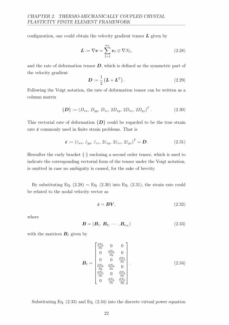
CHAPTER 2. THERMO-MECHANICALLY COUPLED CRYSTALPLASTICITY FINITE ELEMENT FRAMEWORK
configuration, one could obtain the velocity gradient tensor L given by
L := ∇v =
nN∑I=1
vI ⊗∇NI , (2.28)
and the rate of deformation tensor D, which is defined as the symmetric part ofthe velocity gradient
D :=1
2
(L+LT
). (2.29)
Following the Voigt notation, the rate of deformation tensor can be written as acolumn matrix
D := (Dxx, Dyy, Dzz, 2Dxy, 2Dxz, 2Dyz)T . (2.30)
This vectorial rate of deformation D could be regarded to be the true strainrate ε commonly used in finite strain problems. That is
ε := (εxx, εyy, εzz, 2εxy, 2εxz, 2εyz)T = D. (2.31)
Hereafter the curly bracket · enclosing a second order tensor, which is used toindicate the corresponding vectorial form of the tensor under the Voigt notation,is omitted in case no ambiguity is caused, for the sake of brevity.
By substituting Eq. (2.28) ∼ Eq. (2.30) into Eq. (2.31), the strain rate couldbe related to the nodal velocity vector as
ε = BV , (2.32)
whereB = (B1, B2, · · · ,BnN
) (2.33)
with the matrices BI given by
BI =
∂NI
∂x0 0
0 ∂NI
∂y0
0 0 ∂NI
∂z∂NI
∂y∂NI
∂x0
∂NI
∂z0 ∂NI
∂x
0 ∂NI
∂z∂NI
∂y
. (2.34)
Substituting Eq. (2.33) and Eq. (2.34) into the discrete virtual power equation
22

CHAPTER 2. THERMO-MECHANICALLY COUPLED CRYSTALPLASTICITY FINITE ELEMENT FRAMEWORK
Eq. (2.27), and using Voigt notation of the Cauchy stress tensor defined as
σ := (σxx, σyy, σzz, σxy, σxz, σyz)T , (2.35)
one could obtain the discrete momentum equation in matrix form as
MU = fext − f int (2.36)
where M is the consistent mass matrix expressed as
M =
∫BρNTNdV, (2.37)
fext and f int are the external and internal nodal force vectors, respectively,which are given by
fext =
∫BρNTbdV +
∫∂tBNT tdS, (2.38a)
f int =
∫BBTσdV. (2.38b)
For quasi-static problems, the inertial term in the left hand of the discretemomentum equation Eq. (2.36) vanishes, which is reduced to the equilibriumequation as
fext − f int = 0. (2.39)
Fig. 2.1: Illustration of the connectivity of a node I and its associated elements.
The global shape functions NI have nonzero values only in elements associatedwith the node I. Thus, the computations of the global consistent mass matrixMIJ , internal nodal force f intI and external nodal force fextI for node I are in
23

CHAPTER 2. THERMO-MECHANICALLY COUPLED CRYSTALPLASTICITY FINITE ELEMENT FRAMEWORK
practice performed by adding the corresponding contributions from the associatedelements. As illustrated in Fig. 2.1, the node I is shared by eight elements denotedby e1 ∼ e8. The global internal force of node I could then be computed as
f intI =
∫BBTI σdV =
e8∑e=e1
∫BeBekTσdV , (2.40)
where k is the local number of node I in element e, which is 5 in element e3
in Fig. 2.1, Be denotes the elemental interpolation matrix of element e, which issimilar to the global interpolation matrix B but defined in the domain of elemente as
Be = (Be1, B
e2, · · · ,Be
m) (2.41)
with m denoting the number of nodes in element e, and
Bek =
∂Nek
∂x0 0
0∂Ne
k
∂y0
0 0∂Ne
k
∂z∂Ne
k
∂y
∂Nek
∂x0
∂Nek
∂z0
∂Nek
∂x
0∂Ne
k
∂z
∂Nek
∂y
. (2.42)
with N ek being the element shape functions. The superscript e in Be and N e may
be dropped off when no indices confusion is caused, for the sake of brevity.In a finite element code, it is more practical to build the global internal force
vector with a so-called assembly procedure, which loops through all the elementsin the mesh, and for each element computes the elementary internal force vec-tor and assemble it to the proper components of the global vector. The globalconsistent matrix and external force vector could be computed analogously.The computation of such elementary quantities requires the integration over the
element domain, which is usually very difficult to perform analytically. To achievethis, it is convenient to transform the integrals over the element domain at thecurrent configuration to the integrals over the domain of a standard isoparametricelement as illustrated in Fig. 2.2, and perform the integration numerically, whichis expressed as∫
Be
f(x)dVe =
∫Bs
f(x (ξ))JξdVs =∑l
wlJξf(x (ξl)), (2.43)
where x is the spatial coordinates of a material point in the element domainBs, ξ is the corresponding coordinates of x at the isoparametric element domainBs or usually being called the natural coordinates, Jξ is the Jacobian of the
24

CHAPTER 2. THERMO-MECHANICALLY COUPLED CRYSTALPLASTICITY FINITE ELEMENT FRAMEWORK
transformation defined as the determinant of the transformation matrix Fξ givenby
Fξ =
∂x∂ξ
∂x∂η
∂x∂ζ
∂y∂ξ
∂y∂η
∂y∂ζ
∂z∂ξ
∂z∂η
∂z∂ζ
, (2.44)
f is a function defined in the element domain, wl and ξl are, respectively, theweight and the location of an integration point l within the isoparametric element.
Fig. 2.2: Mapping from a 3D 8-node element to the isoparametric element.
Now we could evaluate the integrals over the element domain as describedin Eq.(2.43) with the commonly used Gaussian quadrature scheme. An n-pointGaussian quadrature scheme could yield an exact result for a 2n−1 order polyno-mial. For the C3D8T element used in this work, there are two integration pointsin each axis in the 3D space, so there are eight integration points in total withinthe element. For these integration points the weights are equally taken as 1.0and the locations are tabulated in Table 2.1. This 2 × 2 × 2− points Gaussian
Table 2.1: Integration Points in C3D8T Isoparametric Element
Intg. Pt. Natural Coordinates Intg. Pt. Natural Coordinates1 1√
3(−1, −1, −1) 5 1√
3(−1, −1, +1)
2 1√3
(+1, −1, −1) 6 1√3
(+1, −1, +1)
3 1√3
(+1, +1, −1) 7 1√3
(+1, +1, +1)
4 1√3
(−1, +1, −1) 8 1√3
(−1, +1, +1)
quadrature scheme could give exact results if the integrands of the integral termscomputed at the element level are cubic or lower order polynomial functions ofthe natural coordinates.Sometimes, the reduced integration elements may be used for computational
efficiency. For example for the C3D8RT element, which is also a three dimen-
25

CHAPTER 2. THERMO-MECHANICALLY COUPLED CRYSTALPLASTICITY FINITE ELEMENT FRAMEWORK
sional eight nodes structural-thermal coupled continuum element as the C3D8Telement, there is only a single integration point located at the center of the el-ement. The weight and natural coordinates of this integration point in are 8.0and (0.0, 0.0, 0.0), respectively. Compared to the full integration element that haseight integration points, this reduced integration point could reduce the time costfor the computation of quantities in the element, including the Cauchy stress, theelement internal force vector and the element stiffness matrix, by about 87.5%,which is a huge save of the computational time. Nevertheless, the reduced inte-gration element usually means the reduced computational accuracy. Compromiseshould be made between the efficiency and the accuracy. In addition, the use ofthe reduced integration element may give rise to the spurious hourglass mode,which will result in large amount of unphysical element distortion. This hourglassmode could be suppressed by some hourglass control approaches. In this work,for implicit analysis which will be introduced in later sections, the full integra-tion element C3D8T is adopted while for explicit the reduced integration elementC3D8RT is used.
Using Eq. (2.32), the strain increment ∆ε in the time interval could be relatedto the nodal displacement increment ∆U by
∆ε = ε∆t = BV ∆t = Be∆U = Be (Un+1 −Un) . (2.45)
The stress increment in this time interval could then be evaluated from a rateform constitutive model by
∆σ :=σ∆t = ∆σ (σn, ∆ε, θn, θn+1, ψn) (2.46)
whereσ represents an objective stress rate. Two types of objective stress rate
measures are commonly used in finite element analysis, namely the Jaumannrate of Cauchy stress and the Green-Naghdi rate of Cauchy stress. The former isdefined as
5σ = σ + σ ·w −w · σ (2.47)
where w is the skew symmetric part of the velocity gradient
w =1
2
(L−LT
), (2.48)
and the latter is given by
4σ = σ + σ ·Ω−Ω · σ (2.49)
26

CHAPTER 2. THERMO-MECHANICALLY COUPLED CRYSTALPLASTICITY FINITE ELEMENT FRAMEWORK
whereΩ = RRT , (2.50)
with the rotation matrix R determined by the polar decomposition of the defor-mation gradient as
F = V R = RU , (2.51)
and U and V being symmetric stretch tensors. Both w and Ω are in essencemeasures of the rigid rotation during this time interval.
With the the stress increment obtained above, the Cauchy stress at time tn+1
could then be updated in a corotational framework by
σn+1 = Rn+1RTnσnRnR
Tn+1 + ∆σ (2.52)
Sometimes, it is more convenient to describe the constitutive behavior of thematerial to be studied directly with the second Piola-Kirchhoff stress S, whichcould be written as
Sn+1 = S(En+1, En+1, θn, θn+1, ψn
). (2.53)
Here E is the Green strain, which is the conjugate strain measure of the secondPiola-Kirchhoff stress and given by
E =1
2
(F TF − I
)(2.54)
with I being the second order identity tensor. The Cauchy stress is the pushforward of the second Piola-Kirchhoff stress to the current configuration, whichcould be evaluated by
σn+1 = (detFn+1)−1 Fn+1Sn+1FTn+1. (2.55)
With the Cauchy stress evaluated here from Eq. (2.52) or Eq. (2.55), and theelementary interpolation matrix Be obtained from Eq. (2.42) for each integrationpoint, the element internal nodal force could be computed by Eq. (2.40).
Based on the above discussion, the procedures for computation of the globalconsistent mass matrix, the global external nodal force vector and the globalexternal nodal force vector in the discrete momentum equation Eq. (2.36) arebriefly summarized in Box 2.2
27

CHAPTER 2. THERMO-MECHANICALLY COUPLED CRYSTALPLASTICITY FINITE ELEMENT FRAMEWORK
Box 2.2 Procedures for Computation of Global ConsistentMass Matrix, External and Internal Nodal Force Vectors
Given the global nodal displacement and temperature vectors at time tn+1,1. Initialization: M = 0, fext = 0, f int = 0.
2. Loop for each element e:(1). Initialization: Me = 0, fexte = 0, f inte = 0.
(2). For each integration point l in element e:a). Compute F (ξl), N (ξl) and B(ξl).b). Me += wlρN
TN ,
c). fexte += wlρNTb, modify it following boundary conditions.
d). Update the stress σ from the constitutive model.e). f inte += wlB
Tσ.
(3). Assemble elementary matrix and vectors to the global counterparts.
Discretization of the Thermal Field
Similarly as discussed for the mechanical field, the temperature field θ(X, t), itsrate θ(X, t) and its variation δθ(X) could be approximated by the interpolationsof corresponding nodal values, which reads
θ(X, t) = NIθI = NΘ,
θ(X, t) = NI θI = NΘ,
δθ(X, t) = NIδθI = NδΘ.
(2.56)
whereN := (N1, N2, · · · , NnN
) (2.57)
is the interpolation matrix for the thermal field and
Θ := (θ1, θ2, · · · , θnN)T (2.58)
denotes the nodal temperature vector. Substituting Eq. (2.56) into the weak formof the thermal energy balance equation Eq. (2.22), and using the arbitrariness ofthe virtual nodal temperature δθI , we could obtained the discretized version ofthe thermal energy balance equation∫
BρcNINJ θJdV +
∫B∇NI · (k · ∇NJθJ) dV −
∫∂hB
NI qdS −∫BNIQdV = 0.
(2.59)
28

CHAPTER 2. THERMO-MECHANICALLY COUPLED CRYSTALPLASTICITY FINITE ELEMENT FRAMEWORK
This set of equations could be rewritten in matrix form as
CΘ +KthΘ = fth, (2.60)
where C and Kth are the temperature dependent heat capacity matrix andconductivity matrix, respectively, which read
C =
∫BρcNTNdV, (2.61a)
Kth =
∫B∇NT ·
(k · ∇N
)dV, (2.61b)
and fth is the nodal heat supply vector given by
fth =
∫BNTQdV +
∫∂hBNT qdS. (2.62)
As discussed in the mechanical field, the procedures for computation of the globalheat capacity matrix, the conductivity matrix and the heat supply vector can bedescribed in Box 2.3.
Box 2.3 Procedures for Computation of Global Heat Ca-pacity and Conductivity Matrices, and Heat Supply Vector
Given the global nodal displacement and temperature vectors at time tn+1,1. Initialization: C = 0, Kth = 0, fth = 0.
2. Loop for each element e:(1). Initialization: Ce = 0, Kth
e = 0, fthe = 0.
(2). For each integration point l in element e:a). Compute N (ξl) and ∇N (ξl).b). Ce += wlρN
TN ,
c). Kthe += wl∇NT ·
(k · ∇N
)d). fthe += wlN
TQ.
(3). Assemble elementary matrix and vectors to the global counterparts.
As a brief summary, in this subsection, the weak form formulation for fullycoupled analysis of thermal mechanical processes is spatially discretized with thefinite element method into a coupled system of nonlinear equations of the nodaldisplacements and nodal temperatures, which is stated in Box 2.4:
29

CHAPTER 2. THERMO-MECHANICALLY COUPLED CRYSTALPLASTICITY FINITE ELEMENT FRAMEWORK
Box 2.4 Finite Element Formulation forThermo-Mechanical Coupled Problems
Solve the system of nonlinear equations
MU = fext − f int
CΘ +KthΘ = fth
for the nodal displacement vector U and temperature vector Θ, where
M =∫B ρN
TNdV, fext =∫B ρN
TbdV +∫∂tBN
T tdS,
f int =∫BB
Tσ(Θ)dV, C =∫B ρcN
TNdV,
Kth =∫B∇N
T ·(k · ∇N
)dV, fth =
∫B N
TQ(σ)dV +∫∂hBNT qdS.
Numerical evalutaions of these global matrices and vectors as function of
U and Θ are described in Box 2.2 and Box 2.3.
It is shown that this nonlinear system of equations explicitly contains the timederivatives of the nodal displacements and temperatures. In addition, accordingto the constitutive equation described in Eq. (2.4), the stress is in general depen-dent on the strain rate as well as the history of the internal variables. Thus thesystem of equations described in Box 2.4 is actually a nonlinear set of ordinarydifferential equations in time and should be first discretized in the time domainbefore it could be finally solved numerically for the nodal displacements and tem-peratures at a give time. This time discretization and solution procedures will bediscussed in detail in the following section.
2.1.3 Solution Procedures
In this section, the spatially discretized system of nonlinear differential equa-tions given in Box 2.4 will be further discretized in the time domain to solve thenodal displacements and temperatures and to compute other solution dependentvariables at a given time. Both implicit and explicit time integration schemes areintroduced in detail.The time domain for the loading process [0, tend] could be split into a series of
time intervals as
[0, tend] = [t0, t1] ∪ (t1, t2] ∪ · · · ∪ (tnT−1, tnT], t0 = 0, tnT
= tend. (2.63)
Each interval is called a time increment defined as
(tn, tn+1], 0 ≤ n < nT . (2.64)
30

CHAPTER 2. THERMO-MECHANICALLY COUPLED CRYSTALPLASTICITY FINITE ELEMENT FRAMEWORK
∆tn+1 is also used to represent the time increment size as
∆tn+1 = tn+1 − tn, 0 ≤ n < nT , (2.65)
in this thesis depending on the context.At the initial time t = 0, the nodal values of the displacements and temper-
atures as well as the values of internal variables for each integration point areobtained from the initial conditions given in Eq. (2.7), Eq. (2.20) and Eq. (2.8).For a typical time increment ∆tn+1 we assume that at the beginning of the in-crement t = tn the solution to the system of nonlinear algebraic equations givenin Box 2.4 is known, which means that all necessary information at t = tn in-cluding the nodal displacements, temperatures, and all other solution dependentvariables including the stress, deformation gradient and internal variables at eachintegration point have been already solved or evaluated. If the values for thesequantities at the end of the increment t = tn+1 could be obtained based on theirknown values at time t = tn following a specific procedure, we could then marchin the time domain by repeating the procedure from one increment to the nextuntil the solution at every discrete time t = tk (1 ≤ k ≤ nT ) is incrementally de-termined. This procedure of advancing the solution of the system of equations,described in Box 2.4 from the beginning of an increment t = tn to the end ofthe increment t = tn+1, is usually called the time integration procedure, which isbriefly summarized in Box 2.5 for the sake of clarity.
Box 2.5 Time Integration Procedure forThermal-Mechanical Coupled Problems
1. At t = 0, apply the initial conditions Eq. (2.7), Eq. (2.20) and Eq. (2.8)
U0(XI) = u0(XI), Θ0(XI) = θ0(XI), ∀ node I,
ψ0(Xl) = ψ0(Xl), ∀ integration point l.
2. For time increment (tn, tn+1] (0 ≤ n < nT ), given
Un(XI), Θn(XI), ∀I and ψn(Xl), ∀l,
determine
Un+1(XI), Θn+1(XI), ∀I and ψn+1(Xl), ∀l,
by solving the system of equations in Box 2.4 at time t = tn+1.
Typically there are two types of time integration algorithm, namely implicittime integration scheme and explicit time integration schemes. Both schemes havetheir own advantages in specific application scenarios and will be introduced indetail here.
31

CHAPTER 2. THERMO-MECHANICALLY COUPLED CRYSTALPLASTICITY FINITE ELEMENT FRAMEWORK
Implicit Time Integration Schemes
For fully coupled thermal-mechanical analysis with the implicit time integra-tion scheme, the inertial effect is usually neglected [2], i.e. the mechanical processis assumed to be quasi-static, which could be described with the discrete equi-librium equation given by Eq. (2.39). Taking such assumption and using thebackward-Euler scheme for the temperature rate, the nonlinear system of equa-tions described in Box 2.4 could be formulated at a typical time increment ∆tn+1
as
Ru(U , Θ) = f int (U , Θ)− fext = 0, (2.66a)
Rθ(U , Θ) = CΘ−Θn
∆t+KthΘ− fth (U , Θ) = 0. (2.66b)
Here the subscript n + 1, which is used to represent the values of quantities attime tn+1, is dropped off for brevity. That is
U := Un+1, Θ := Θn+1, ψ := ψn+1, ∆t := ∆tn+1. (2.67)
At the beginning of this increment t = tn, as stated in Box 2.5 all necessary infor-mation including the nodal displacements, nodal temperatures and the internalvariables for all integration points is known. Let Y := (U , Θ)T denote the vectorof unknowns of Eq.(2.66), which could be rewritten in compact residual form as
R(Y ) :=
(Ru (Y )
Rθ (Y )
)= 0 (2.68)
The total number of unknowns, the degree of freedom in the model, is 4nN . Thisnonlinear system of algebraic equations could be solved by using the well knownNewton-Raphson iterative solution scheme as introduced below.
Let Yk be the approximation of Y at the k-th iteration. The residual vector ofEq. (2.68) at the next iteration could be derived by expanding the Taylor seriesin the neighborhood of Yk as
R (Yk+1) = R (Yk −∆Yk) = R (Yk)−∂R (Yk)
∂Yk∆Yk +O
(∆Y 2
k
)(2.69)
By neglecting the second and higher order terms in Eq. (2.69) and setting theresidual vector to zero, the following iterative relation could be derived:
K∆Yk = R (Yk) , (2.70a)
Yk+1 = Yk −∆Yk, (2.70b)
32
CHAPTER 2. THERMO-MECHANICALLY COUPLED CRYSTALPLASTICITY FINITE ELEMENT FRAMEWORK
where K is the global tangent stiffness matrix obtained by differentiating theresidual vector with respect to the vector of unknowns as
K =∂R (Yk)
∂Yk. (2.71)
The initial values for the vector of unknowns and the internal variables duringthe iterative process could be taken as the corresponding known values at timetn. That is
Y0 = (Un, Θn) , ψ0 = ψn. (2.72)
This iterative procedure expressed in Eq.(2.70) could then be repeated until thenorm of the residual vector gets smaller than a given tolerance, which is writtenas
‖R (Yk)‖ 5 εtol. (2.73)
This Newton-Raphson iterative method will converge at a quadratic rate as longas the initial guess for the unknowns falls into the radius of convergence.
The key task for an iteration is to determine the correction to the vector ofunknowns by solving the linear system of algebraic equations given by Eq. (2.70a),which first requires the computation of the global residual vector and the globaltangent stiffness matrix as will be discussed in detail as below.
By rewriting the global stiffness matrix in partitioned form, the linear systemof equations Eq. (2.70a) could be reformulated as(
Kuu Kuθ
Kθu Kθθ
)(∆Uk
∆Θk
)=
(Ru (Uk, Θk)
Rθ (Uk, Θk)
). (2.74)
Following the procedures described in Box 2.2 and Box 2.3, the residual vectorsin the displacement field Ru and the temperature field Rθ could be evaluatedstraightforwardly. The computation of the submatrices of the global tangentstiffness matrix is discussed as below.
The submatrix Kuu could be derived from Eq. (2.66a) and further be dividedinto the three parts as
Kuu :=∂Ru
∂U=∂f int
∂U− ∂f ext
∂U= Kuu,mat +Kuu,geo +Kuu,load, (2.75)
where Kuu,mat is the material tangent stiffness matrix, which can be computedby using Eq. (2.52) and Eq. (2.45) as
Kuu,mat =
∫BBT ∂σ
∂UdV =
∫BBT ∂∆σ
∂∆ε
∂∆ε
∂UdV =
∫BBT ∂∆σ
∂∆εB, (2.76)
33

CHAPTER 2. THERMO-MECHANICALLY COUPLED CRYSTALPLASTICITY FINITE ELEMENT FRAMEWORK
Kuu,geo is the geometric tangent stiffness matrix, which is given here withoutproven as
Kuu,geo =
∫B
∂N
∂Xσ∂N
∂XdV, (2.77)
and Kuu,load is the contribution from the external load that is dependent on thedeformation field. In case that this part of the stiffness matrix is absent, Kuu
would be symmetric.
The submatrix Kuθ could be computed by introducing the interpolation formfor the temperature field given in Eq. (2.56) to Eq. (2.66a)
Kuθ :=∂Ru
∂Θ=
∫BBT ∂∆σ
∂∆θ
∂∆θ
∂ΘdV =
∫BBT ∂∆σ
∂∆θNdV. (2.78)
The submatrix Kθu could be derived from Eq. (2.66b) by using Eq. (2.45) as
Kθu :=∂Rθ
∂U= −
∫BNT ∂Q
∂UdV = −
∫BNT ∂∆Q
∂∆εBdV. (2.79)
Finally,the submatrix Kθθ could be derived from Eq. (2.66b) directly as
Kθθ :=∂Rθ
∂Θ=
∫B
[ρc
∆tNTN +∇NT ·
(k · ∇N
)+∂∆Q
∂∆θNTN
]dV
+
∫B
[θk − θn
∆t
∂ρc
∂θNTN +∇NT ·
(∂k
∂θ· ∇θkN
)]dV.
(2.80)
The second integral in Kθθ is the contribution from the change of the materialthermal properties including the heat capacity and thermal conductivity. It isusually neglected as the derivatives of thermal properties with respect to temper-ature are relatively small. In this case, the submatrix Kθθ becomes symmetric.
It could be observed that although the diagonal submatricesKuu andKθθ maybe symmetric under some assumptions, the full global stiffness matrix K is stillasymmetric as the off-diagonal submatricesKuθ andKθu are not symmetric andKuθ 6= KθuT . However, it is shown from the component form of the submatricesexpressed above that, due to the nodal support property of the global shapefunctions, the global stiffness matrix is sparse as its component KIJ only hasnonzero value when node I and node J are associated with the same element.Thus an asymmetric sparse matrix storage format could be used for the globalstiffness matrix.
With the obtained residual vector and the global stiffness matrix discussedabove, the estimated vector of unknowns at the next iteration could be updatedwith the correction vector ∆Yk determined by solving the linear system of equa-tions with a sparse linear solver, as described in Eq. (2.70). This iterative process
34

CHAPTER 2. THERMO-MECHANICALLY COUPLED CRYSTALPLASTICITY FINITE ELEMENT FRAMEWORK
is repeated until the converged solution to the nodal displacement vector andnodal temperature vector at the end of the time increment are determined. As abrief summary, the main procedures for performing thermo-mechanically coupledanalysis with implicit finite element method are illustrated in Fig. 2.3.
Box 2.6 Staggered Solution Scheme for Implicit FiniteElement Analysis of Thermal-Mechanical Coupled Problems
1. Initialization: k = 0, Uk = Un, Θk = Θn, ψk = ψn.
2. Solution to mechanical field:
a). Compute Kuu (Uk, Θk) and Ru (Uk, Θk),
b). Update Qk+1 and ψk+1 from constitutive model.
c). Solve Eq.(2.82a) for ∆Uk,
d). Update displacement field: Uk+1 = Uk −∆Uk.
3. Solution to thermal field:
a). Compute Kθθ (Uk+1, Qk+1, Θk) and Rθ (Uk+1, Qk+1, Θk),
b). Solve Eq.(2.82b) for ∆Θk,
c). Update Θk+1 = Θk −∆Θk,
d). Check convergence for thermal and mechanical field.
In the previous discussion, we have discussed the implementation of the fullycoupled thermomechanical problem. The displacement field and the tempera-ture field are updated simultaneously in each iteration. However, as discussedpreviously, the global stiffness matrix is unsymmetric, which requires the use ofunsymmetric matrix storage. Solving such linear system of equations also needsa more costly solution scheme compared to the one with symmetric stiffness ma-trix. This full implementation of the global stiffness matrix is more suitable forproblems where the coupling effects between the mechanical field and the thermalfield are strong. In cases that the coupling effects are weak, the linear system ofequations given in Eq. (2.74) could be approximated as(
Kuu 0
0 Kθθ
)(∆Uk
∆Θk
)=
(Ru (Uk, Θk)
Rθ (Uk, Θk)
), (2.81)
which in essence divides the original fully coupled system of equations into two
35

CHAPTER 2. THERMO-MECHANICALLY COUPLED CRYSTALPLASTICITY FINITE ELEMENT FRAMEWORK
Global initialization: t=0,n=0. Apply initial conditions.
Check termination: t<tend?
Initialization of increment: k = 0. Yk :=(Uk,Θk)|k=0 = (Un,Θn), ψk=0 = ψn.
Compute auxiliary quantities: N , B,N , ∆N , ∆ε, F ,...at integration point.
Evaluate σ, Q, ψ, ∂∆σ∂∆ε
, ∂∆σ∂∆θ
, ∂∆Q∂∆ε
,∂∆Q∂∆θ
from the constitutive model.
Compute M , C, Kth, f ext,f int and f th for each element.
Compute the elemental residual vec-tor Re
k and stiffness matrix Ke.
Assemble the global residual vec-tor Rk and stiffness matrix K.
Check convergence: ‖Rk‖ 5 εtol?
New increment:(Un+1,Θn+1) = Yk.n = n+ 1, t = t+ ∆t.
Solve Eq. K∆Yk = Rk for ∆Yk.
New iteration: Yk+1 = Yk−∆Yk. k = k+ 1.
Analysis termination
yes
no
no
yes
Fig. 2.3: Flowchart for fully coupled thermal-mechanical analysis with implicitfinite element method
36

CHAPTER 2. THERMO-MECHANICALLY COUPLED CRYSTALPLASTICITY FINITE ELEMENT FRAMEWORK
separated sets of equations as
Kuu∆Uk = Ru, (2.82a)
Kθθ∆Θk = Rθ. (2.82b)
The mechanical field and the thermal field at each iteration could now beupdated in a staggered way as described in Box 2.6.In this staggered solution scheme, if the load contribution to the stiffness ma-
trix Kuu and the contribution to Kθθ caused by thermal property changes isnegligible, both the mechanical problem and the thermal problem have symmet-ric stiffness matrix and fewer unknowns, which can yield a reduction in storageand computational costs compared to the concurrent scheme where the two fieldsare solved simultaneously. Nevertheless, although the computational cost in eachiteration is reduced, the staggered scheme usually needs more iterations beforereaching convergence for both the mechanical and the thermal fields.As long as the converged solution is obtained, the solution accuracy is not
affected whether the staggered scheme or the concurrent scheme is chosen, sinceit is only determined by the given tolerance.
Explicit Time Integration Scheme
For fully coupled thermal-mechanical analysis with an explicit time integrationscheme, the mechanical field and the thermal field are updated in a staggeredfashion at each time increment. First for the mechanical field, the inertial effectnow needs to be taken into consideration but the consistent mass matrix is usuallyreplaced by the lumped mass matrix for the sake of computational efficiency. Theelemental lumped mass matrix could be obtained by distributing the total massof the element equally to each associated node as
M lumpe =
1
m
∫BeρdVe diag I1, I2, ..., Im (2.83)
where m is the number of nodes in the element and I1 ∼ Im are 3 × 3 identitymatrices. By the assembly procedure of the elemental lumped mass matrix, theglobal lumped mass matrix could be formulated. As the nodal mass does notchange in time, this global lumped mass matrix only needs to be computed onceat the beginning of the analysis. It is diagonal and can be trivially inverted.The displacement field could then be updated by using the central differenceintegration scheme as follows.At the beginning of time increment n+ 1, the external and internal nodal force
37

CHAPTER 2. THERMO-MECHANICALLY COUPLED CRYSTALPLASTICITY FINITE ELEMENT FRAMEWORK
vectors are first computed following the procedures described in Box 2.2. Thenodal acceleration vector could then be computed from the discretized balanceequation of linear momentum given in Eq. (2.36) as
Un = M−1(f extn − f int
n
). (2.84)
The nodal velocity vector at the middle of the increment could be obtained by
Un+ 12
= Un− 12
+1
2(∆tn+1 + ∆tn) Un, (2.85)
Finally, the nodal displacement vector at the end of the increment could bedetermined by
Un+1 = Un + Un+ 12∆tn+1. (2.86)
Actually the above equations Eq. (2.84) ∼ Eq. (2.86) are decoupled and is inpractice solved node by node without the formulation and storage of the globalmass matrix, the external and internal force vectors.
After the integration of the mechanical field, the new configuration of the bodyB are determined and the volumetric internal heat generation rate Q is evaluated.With the obtained information from the mechanical field, the thermal field couldthen be updated by using the explicit forward difference integration scheme asfollows.
First, the consistent heat capacity matrix is replaced by the diagonal lumpedheat capacity matrix as is done to the mass matrix in the mechanical field. Dueto the temperature dependency, this matrix may need to be updated at the be-ginning of each increment. The procedures for computation of this heat capacitymatrix, the thermal conductivity matrix Kth and the heat supply vector f th aredescribed in Box 2.3. The nodal temperature rate vector could then be computedfrom the discretized balance equation of thermal energy given in Eq. (2.60) as
Θn = C−1(f thn − f int(Θn)
). (2.87)
Finally, the nodal temperature vector at the end of the increment could be eval-uated as
Θn+1 = Θn + Θn∆tn+1. (2.88)
As discussed above, for each time increment, the mechanical field and the ther-mal field are updated explicitly by using the central difference integration schemeand the forward difference scheme, respectively. In contrast to the implicit timeintegration scheme as discussed in detail previously, this explicit time integrationscheme does not require the expensive Newton-Raphson iteration process, which
38

CHAPTER 2. THERMO-MECHANICALLY COUPLED CRYSTALPLASTICITY FINITE ELEMENT FRAMEWORK
means that neither the formation of the global tangent stiffness matrix nor thesolution to the linear system of equations are required. However, both the centraldifference integration scheme and the forward difference scheme are conditionallystable. For every time increment, the increment size ∆t, which is usually calledthe stable time increment, should be smaller than a critical value. It could beproved that for the central difference operator and the forward difference opera-tor, the stability limit is determined by
∆t ≤ min (∆tm, ∆tt) := min(
2
ωmax,
2
λmax
), (2.89)
where ∆tm and ∆tt are the stability limit determined by the mechanical andthermal fields, respectively, ωmax is the highest frequency in the system of equa-tions for the mechanical response and λmax is the largest eigenvalue in the systemof equations for the thermal response. To avoid solving eigenvalue problems, inpractice the stability limit for the mechanical field is usually chosen such thatthe time increment is too small for the dilatational wave to travel through anyelement in the mesh, which is written as
∆tm ≈Lmin
cd(2.90)
where Lmin is the smallest characteristic length of the elements and cd is thedilatational wave speed given by
cd =
√λ+ 2µ
ρ(2.91)
with λ and µ being the effective Lamé’s constants, and the stability limit for thethermal field is usually estimated by
∆tt ≈ρcL2
min
2k(2.92)
where k is the thermal conductivity.
In most cases the stability limit is governed by the mechanical field unlesshuge amount of mass scaling is used. Mass scaling is a practical technique forimproving the computational efficiency of explicit finite element analysis. Theactual stable time increment calculated from Eqs. (2.90) and (2.92) is typicallyvery small, which means a large number of time increments are required for thewhole analysis. For some particular problems, the density could be treated asa parameter. By intentionally increasing the density, which is usually calledmass scaling, the stable time increment could be increased accordingly as given
39
CHAPTER 2. THERMO-MECHANICALLY COUPLED CRYSTALPLASTICITY FINITE ELEMENT FRAMEWORK
by Eq. (2.90) and Eq. (2.91). The computational costs could then be reducedsignificantly while causing little effect on the solution accuracy of the problems.Two typical problems the mass scaling technique may apply to are the quasi-staticanalysis or transit response simulations of a model consisting a few very smallelements that dominate the stability limit. For quasi-static analysis, the inertialeffect is weak and the fixed mass scaling approach is usually performed, whichapplies an appropriate and fixed mass scaling factor uniformly to the entire model.For example, a mass scaling factor of 100 may be applied to each element in themodel, leading to an increase of the stable time increment by a factor of 10 andthus a reduction of the total computational time by about 90%. For the transitanalysis, the inertial effect plays a crucial role in the response of the material.In this case the variable mass scaling approach may be used, which only scalesthe mass of a few elements with very small characteristic length that govern thestability limit. This could increase the stable time increment notably but yielda negligible effect on the overall response of the entire model. In practice, theeffect of the mass scaling on the solution accuracy could be indicated by the ratioof the kinetic energy to the total strain energy in the model. It is believed thatthe increases of the mass and consequent inertial forces do not alter the solutionsignificantly when the ratio remains under 5% throughout the analysis.For the sake of clarity, the main procedures for performing thermo-mechanically
coupled analysis with explicit finite element method are illustrated in Fig. 2.4.
Comparison between Implicit and Explicit Time Integration Schemes
In this subsection, both the implicit and explicit time integration schemes havebeen introduced in detail for updating the thermal and the mechanical fields inthe model for each time increment. Comparisons between these two schemes aresummarized as below.First, the implicit time integration scheme determines the nodal temperatures
and displacements at the end of each increment by solving a nonlinear system ofalgebraic equations with the Newton-Raphson iterative method. Typically tensof iterations may be required in each increment before the converged solutions areobtained for both the temperature field and the displacement field. In each itera-tion, a linear system of equations with a total number of 4nN unknowns is solvedwith a sparse linear solver to determine the correction to the nodal temperaturesand displacements. Prior to the solution of this linear system of equations, theleft hand section and the right hand section, which are the global tangent stiff-ness matrix and the global residual vector, respectively, need to be formulated.The two fields could also be updated in each increment in a staggered way bysolving one linear system of equations with a total number of 3nN unknowns for
40

CHAPTER 2. THERMO-MECHANICALLY COUPLED CRYSTALPLASTICITY FINITE ELEMENT FRAMEWORK
Global initialization: t=0,n=0. Apply initial conditions.
Check termination: t<tend?
Compute N , B, ∆ε, F at inte-gration point for mechanical field.
Compute σn, Qn, ψn fromthe constitutive model.
Compute elemental f extn and f int
n
and assemble to global counterparts.
Compute Un, Un+ 12, and Un+1 sequen-
tially with central difference scheme.
Compute N and ∆N at inte-gration point for thermal field.
Compute elemental C, Kthn and f th
n
and assemble to global counterparts.
Compute Θn and Θn+1 sequentiallywith forward difference scheme.
Determine stable time increment ∆tn+1.
New increment: t = t+ ∆tn+1, n = n+ 1
Analysis termination
yes
no
Fig. 2.4: Flowchart for fully coupled thermal-mechanical analysis with explicitfinite element method
41

CHAPTER 2. THERMO-MECHANICALLY COUPLED CRYSTALPLASTICITY FINITE ELEMENT FRAMEWORK
the mechanical field and another liner system of equations with nN unknowns forthe thermal field sequentially. In contrast, the implicit time integration schemeupdates the mechanical field and the thermal field in a staggered fashion. Foreach increment, first the temperature field is frozen and the nodal displacementsand other relevant quantities including the volumetric internal heat generationcontributed from the mechanical dissipation are updated explicitly by using thecentral difference integration scheme. Then with the updated mechanical field,the temperature field can be updated straightforwardly with the forward differ-ence integration scheme. No iteration is needed in each increment and thereforeno need for formulation of the global tangent stiffness matrix and solution of thelinear system of equations compared to the implicit scheme.
Second, for the implicit time integration scheme, the constitutive model needsto evaluate the Cauchy stress σ, the volumetric internal heat generation Q, theinternal variables ψ as well as the derivatives of the increments of σ and Q
with respect to the strain increment and the temperature increment. While forthe explicit scheme, as the global tangent stiffness matrix is not needed, theconstitutive model only has to compute σ, Q, and ψ, which is much more simplefor implementation.
Third, the implicit time integration scheme unconditional stable for linear prob-lems and large time increments may be used in the simulation, while the explicitscheme is conditionally stable. To get a stable and reliable solution, the chosentime increments should not exceed the stability limit determined by the mesh sizeand material properties. Typically the time increment used in implicit schemecould be larger that in explicit scheme by three to five orders of magnitude.However, as the Newton-Raphson iterations performed in one increment in theimplicit analysis are much more expensive than the central difference scheme andthe forward different scheme applied in the explicit analysis, the explicit inte-gration scheme may be more computational efficient than the implicit scheme,especially in cases where there is a huge number of degrees of freedom in themodel or the mass scaling technique is adopted.
Fourth, for some quasi-static problems with high nonlinearity, in particular forprocesses where contact between different parts of the model is involved, for theimplicit time integration scheme it may be difficult to achieve convergence in anincrement with the Newton-Raphson iterative method. In these cases, the ex-plicit time integration scheme might be preferred as it does not have convergencedifficulties. And for some transient problems where the detailed history of theevolution of the mechanical and the thermal fields during the loading process isof interest, for instance the impact process or the machining process, the explicittime integration scheme may also be the first choice as it uses small time in-
42

CHAPTER 2. THERMO-MECHANICALLY COUPLED CRYSTALPLASTICITY FINITE ELEMENT FRAMEWORK
crement and could give high resolution solution of the coupled fields in the timedomain. Aside from these cases the implicit scheme might be adopted. As will beseen later, in chapter 3, the implicit finite element method is applied to study theplastic deformation behavior of polycrystalline metallic materials with the com-putational homogenization approach and in chapter 4, the explicit finite elementmethod is adopted to study the thermal mechanical responses of ferrite-pearlitesteels during machining processes.
2.1.4 Concluding Remarks
In section 2.1, we have introduced systematically and comprehensively a gen-eral finite element framework for fully coupled thermal mechanical analysis. Firstwe started from the construction of the weak form formulation for fully coupledthermal mechanical problems in the form of coupled integral equations, basedon the balance equations of linear energy and thermal energy that govern theevolution of the involved mechanical and thermal fields as well as the initialand boundary conditions as described in Box 2.1. Then, with the finite elementmethod, we spatially discretized the weak form formulation derived before into acoupled system of nonlinear equations of the nodal displacements and tempera-tures as shown in Box 2.4. As each equation in this coupled system is actuallyan ordinary differential equation of time, we split the total time duration of theanalysis into a series of time increments and temporally discretized the nonlinearsystem of ordinary differential equations accordingly, which were finally solvedfor the nodal displacements and temperatures at each increment by using the im-plicit or explicit time integration scheme, as summarized in Fig. 2.3 and Fig. 2.4,respectively.
It should be pointed out that all the procedures mentioned in the flowchartsfor the implicit and explicit finite element analysis and as shown in Fig. 2.3 andFig. 2.4 are standard. These fundamental procedures in finite element analysishave been implemented in most mature finite element codes such as the com-mercial FE codes ABAQUS, ANSYS and the research-centered FE codes Iris.For example, in Abaqus/standard there is a built-in element type C3D8R thatis responsible for the computation of the element residual force and the elementtangent stiffness matrix, and the assembly of these elemental quantities into theglobal counterparts. The Newton-Raphson iterative approach has been imple-mented to solve the discrete nonlinear set of balance equations for the thermaland the mechanical fields in each time increment, and linear sparse solvers havebeen implemented to solve the linear system of equations for the correction tothe unknowns in each iteration. In Abaqus/explicit, the central difference inte-
43

CHAPTER 2. THERMO-MECHANICALLY COUPLED CRYSTALPLASTICITY FINITE ELEMENT FRAMEWORK
grator and the forward difference integrator are developed for integration of thedisplacement field and the temperature field, respectively. All these built-in el-ement types, nonlinear and linear solvers and integrators in ABAQUS could becommonly found in other FE codes. All these well developed FE codes shouldhave similar performance in computational accuracy and efficiency for the samenumerical example. Nevertheless, it should be emphasized that the key ingredi-ent for the accuracy of a thermo-mechanically coupled finite element analysis isthe accuracy of the Cauchy stress as well as other related quantities evaluatedfrom the constitutive relation. Different material may have very different consti-tutive behavior in a thermal-mechanical process. Although most FE code mayprovide a material model library with tens of commonly used constitutive models,it is still not enough for these built-in constitutive models to accurately describethe constitutive behavior of all materials due to the diversity. Luckily, many fi-nite element codes are well designed so that users could readily define their ownconstitutive relation. For instance, in ABAQUS user defined constitutive modelcould be integrated into ABAQUS/standard for an implicit analysis through theuser subroutine UMAT, and ABAQUS/explict for an explicit analysis throughthe user subroutine VUMAT. And in Iris, the material constitutive models areintegrated as an open source library named Muesli. It is written in C++ andcould be easily extended due to its well-designed code structure. Users couldeasily define one new constitutive model by deriving, in the terminology of ob-ject oriented programming, a pair of sub-classes from the appropriate base classand overloading a handful of essential virtual functions to update the relevantenergies, Cauchy stress and material tangent stiffness matrix.
Regarding metallic materials we are interested in, in the material model li-brary of these FE codes several constitutive models such as the Johnson-Cook’s[3] and Zerilli-Armstrong [5] may be found. However, these constitutive modelsare phenomenological and could not capture the anisotropic plasticity behaviorof metallic material during deformation. As the macroscopic behavior of mate-rials is largely determined by the underlying microstructure, in order to get themost reliable possible model for metallic materials, in this work a microstruc-ture based crystal plasticity model is employed in which the macroscopic plasticflow is connected to the crystallographic slip at the grain level. A general finiteelement framework for fully coupled thermal mechanical analysis of metallic ma-terials will be developed by integrating the crystal plasticity constitutive modelinto ABAQUS/standard and ABAQUS/explicit through user defined subroutinesUMAT and VUMAT, which will be applied to study the plastic deformation be-havior of polycrystalline metals and the responses of ferrite-pearlite steels duringmachining processes as will shown in later chapters. In the next section, the
44

CHAPTER 2. THERMO-MECHANICALLY COUPLED CRYSTALPLASTICITY FINITE ELEMENT FRAMEWORK
introduction, implementation and validation of the crystal plasticity model willbe presented.
2.2 Crystal Plasticity Constitutive Model for Sin-
gle Crystal
2.2.1 Crystal Plasticity Model
For finite strain inelastic mechanics of single crystal plasticity the deforma-tion gradient F is assumed to be multiplicatively decomposed into its elastic andplastic parts as F = F eF p [63]. The elastic and plastic deformation gradientsdefine two different local deformed configurations: one intermediate configura-tion described by F p, and the final deformed configuration locally determined byF eF p. For a thermo-mechanical problem, as illustrated in Fig. 2.5, a third con-figuration is introduced accounting for thermal deformations [64]. The resultingdecomposition reads
F = F eF pF θ, detF e > 0, detF p = 1, detF θ > 0. (2.93)
where F θ now represents the thermal part of the deformation gradient. The elas-tic deformation gradient embodies the elastic distortions of the lattice, and therigid body motions; the plastic part, F p, describes the irreversible deformationsof the lattice, associated with plastic shearing along crystallographic planes; fi-nally, the thermal contribution F θ includes the lattice distortion due solely tothermal effects. The local configuration defined by F pF θ is hereafter called theintermediate configuration, and can be regarded as being obtained by a pureelastic unloading from the current configuration.
The constitutive model relates the three parts of the deformation gradient withthe stress and temperature, or their evolution. In particular, the evolution of thethermal deformation gradient of any metal can be expressed respect its latticesymmetry axis as
F θF θ−1= θβ, (2.94)
where β is a diagonal tensor of anisotropic thermal expansion coefficients
β = diag (β1, β2, β3) . (2.95)
Assuming that the plastic deformation takes place purely through dislocationglide, the evolution of the plastic deformation gradient could be expressed as a
45

CHAPTER 2. THERMO-MECHANICALLY COUPLED CRYSTALPLASTICITY FINITE ELEMENT FRAMEWORK
Fig. 2.5: Illustration on decomposition of deform gradient into the thermal,plastic and elastic parts.
combination of the slip rate γα in every slip system α as in
Lp := F pF p−1 =∑α
γαSα0 , (2.96)
where Lp is the plastic velocity gradient and, for every slip system α, Sα0 =
sα0⊗mα0 is the Schmidt tensor, sα0 andmα
0 are unit vectors along the slip directionand normal to the slip plane, respectively. For FCC crystals crystallographic slipoccurs along the <1 1 0> direction in 1 1 1 planes and for BCC crystals slipoccurs in three different slip sets: <1 1 1> 1 1 0, <1 1 1> 1 1 2 and <1 1 1>1 2 3. Usually the slip systems in the <1 1 1> 1 1 2 set are neglected forsimplicity. Here for the sake of completeness the slip systems for FCC and BCCcrystals are listed in Table 2.2 and Table 2.3, respectively.
Table 2.2: Slip Systems for FCC Crystals
α s0 m0 α s0 m0
1 1√2
(0 1 1) 1√3
(1 1 1) 7 1√2
(1 1 0) 1√3
(1 1 1)
2 1√2
(1 1 0) 1√3
(1 1 1) 8 1√2
(0 1 1) 1√3
(1 1 1)
3 1√2
(1 0 1) 1√3
(1 1 1) 9 1√2
(1 0 1) 1√3
(1 1 1)
4 1√2
(1 1 0) 1√3
(1 1 1) 10 1√2
(1 1 0) 1√3
(1 1 1)
5 1√2
(0 1 1) 1√3
(1 1 1) 11 1√2
(0 1 1) 1√3
(1 1 1)
6 1√2
(1 0 1) 1√3
(1 1 1) 12 1√2
(1 0 1) 1√3
(1 1 1)
46

CHAPTER 2. THERMO-MECHANICALLY COUPLED CRYSTALPLASTICITY FINITE ELEMENT FRAMEWORK
Table 2.3: Slip Systems for BCC Crystals
α s0 m0 α s0 m0
1 1√3
(1 1 1) 1√2
(0 1 1) 13 1√3
(1 1 1) 1√6
(2 1 1)
2 1√3
(1 1 1) 1√2
(1 0 1) 14 1√3
(1 1 1) 1√6
(1 1 2)
3 1√3
(1 1 1) 1√2
(1 1 0) 15 1√3
(1 1 1) 1√6
(1 1 2)
4 1√3
(1 1 1) 1√2
(0 1 1) 16 1√3
(1 1 1) 1√6
(1 1 2)
5 1√3
(1 1 1) 1√2
(1 0 1) 17 1√3
(1 1 1) 1√6
(1 2 1)
6 1√3
(1 1 1) 1√2
(1 1 0) 18 1√3
(1 1 1) 1√6
(1 2 1)
7 1√3
(1 1 1) 1√2
(0 1 1) 19 1√3
(1 1 1) 1√6
(1 2 1)
8 1√3
(1 1 1) 1√2
(1 0 1) 20 1√3
(1 1 1) 1√6
(1 2 1)
9 1√3
(1 1 1) 1√2
(1 1 0) 21 1√3
(1 1 1) 1√6
(1 2 1)
10 1√3
(1 1 1) 1√2
(1 1 0) 22 1√3
(1 1 1) 1√6
(2 1 1)
11 1√3
(1 1 1) 1√2
(1 0 1) 23 1√3
(1 1 1) 1√6
(2 1 1)
12 1√3
(1 1 1) 1√2
(0 1 1) 24 1√3
(1 1 1) 1√6
(2 1 1)
In the intermediate configuration, the elastic Green-Lagrange strain Ee, whichis the work conjugate to the second Piola-Kirchhoff tensor S∗, is defined as
Ee =1
2
(F eTF e − I
), (2.97)
where I is the second order identity tensor. Ee and S∗ are assumed to beconnected with an elastic constitutive relation given by
S∗ = L : Ee, (2.98)
where L is the fourth-order elasticity tensor.The Cauchy stress is the push forward of the stress S∗ to the current configu-
ration, that isσ = (detF e)−1 F eS∗F eT . (2.99)
To close the mechanical constitutive law, the evolution of the plastic slip γα
must be specified for every slip plane. In a viscoplastic model for strain ratesensitive materials as metals, the slip rate is expressed with the flow model
γα = ˆγα (τα, sα, θ) , (2.100)
where τα is the resolved shear stress in slip system α, defined as
τα = detF θ(F θTS∗F θ−T
)· Sα0 , (2.101)
and sα is the slip resistance [64]. In this equation and below, the dot productrefers to the full contraction of vectors or tensors over all their indices. The
47

CHAPTER 2. THERMO-MECHANICALLY COUPLED CRYSTALPLASTICITY FINITE ELEMENT FRAMEWORK
quantity sα evolves following the hardening model
sα =∑β
hαβ∣∣γβ∣∣, (2.102)
wherehαβ = hαqαβ (2.103)
represents the hardening modulus, hα stands for the self hardening modulus andqαβ denotes the latent hardening coefficients. qαβ is usually taken to be 1.4 if theslip systems α and β are non-coplanar and 1.0 if they are co-planar.
Power Law Type Flow Model
Several flow and hardening models have been proposed in the literature and areintroduced here for the sake of completeness of our framework. Two flow models,one a phenomenological power law type model and the other a physically basedmodel, are commonly used. The power law type flow model was first proposedby [65] and is given by
γα = γ0
∣∣∣∣ταsα∣∣∣∣m sign(τα) (2.104)
where γ0 is the reference shearing rate, the exponent m is the strain rate sensitiv-ity. This flow model is very simple, easy to implement in the user subroutine dueto the simplicity of the formulation and easy for calibrating the model parame-ters as only two model parameters are involved. What is more, this flow modelis computational very efficient compared to the physically based flow model thatwill be introduced later. However, this flow model also has some disadvantages.First it is phenomenological without clear physical meaning behind the formu-lation, which limits its reliability for description of flow mechanisms from themicroscopic scale and hence the accuracy of the numerical analysis. Second, thisflow model does not take into consideration the temperature effect, which is im-portant in the fully coupled thermal mechanical problems we are studying. Inorder to get more accurate numerical results, the physically based flow model isusually adopted, which is discussed below.
Physically Based Flow Model
Assume that the slip resistance sα could be decomposed as
sα = sαat + sαt , (2.105)
48
CHAPTER 2. THERMO-MECHANICALLY COUPLED CRYSTALPLASTICITY FINITE ELEMENT FRAMEWORK
where st and sat denote the thermal and athermal parts due to thermally activatedobstacles and athermal obstacles, respectively [57]. The resolved shear stress ata slip system α needs to overcome the athermal part of the slip resistance beforeslip starts. Beyond that value of the resolved shear stress, the thermal energyrequired to overcome the obstacle depends on the effective resolved shear stressταeff , defined as
ταeff = |τα| − sαat. (2.106)
According to the flow model proposed by Frost and Ashby[65], the slip rate ina slip system α controlled by some thermal activation process can be obtainedfrom the Orowan equation
γα = ραmbαLνα(ταeff , θ). (2.107)
where ραm denotes the mobile dislocation density, bα is the Burgers vector of thatsystem and L is a characteristic length of the distance between obstacles. να isthe average frequency of jumping events across the obstacles. It depends on boththe effective resolved stress and the current temperature and is obtained by usingthe theory of thermally activated processes. If all the constants in the previousequation are grouped, a single parameter independent of the temperature γα0 , thereference slip rate, can be defined as
γα0 ≈ ραmbαLν0, (2.108)
where ν0 is the Debye frequency. Using this value, the shear rate can finally beexpressed as
γα =
0, ταeff ≤ 0,
γα0 exp(−∆Gα
kBθ
)sign (τα) , 0 < ταeff ≤ sαt ,
(2.109)
where kB is Boltzmann’s constant and ∆Gα is the activation enthalpy. The lattercan be obtained with the expression
∆Gα = ∆Fα
[1−
( |ταeff |sαt
)p]q, (2.110)
with ∆Fα being the activation energy at 0 K, p and q denoting model parameterswith values 0 < p < 1 and 1 < q < 2.
The flow model based on thermal activation is valid for any alloy in whichdislocation glide is controlled by thermal activation. In BCC crystals, the latticefriction is the main energy barrier and it is usually assumed that the thermal
49

CHAPTER 2. THERMO-MECHANICALLY COUPLED CRYSTALPLASTICITY FINITE ELEMENT FRAMEWORK
part of the slip resistance sαt is constant [57]. For FCC crystals, the short rangedislocation-dislocation interactions are the main thermal process and it was inves-tigated experimentally [66] that both the thermal and athermal parts of the slipresistance evolve with the deformation but their ratio sαt /sαat could be regardedas a constant over a broad range of strains.The self hardening modulus hα in Eq. (2.103) for describing the evolution of
the slip resistance is given by the hardening models. The most commonly usedhardening models are all phenomenological and briefly introduced below.
Assaro-Needleman Hardening Model
This hardening model was presented by Assaro and Needleman [67]. The self-hardening modulus in different slip systems are considered to be identical as:
h = h0sech2
(h0Γ
ss − s0
)(2.111)
where h0 is the initial hardening modulus, s0 and ss are the initial and thesaturation value of the slip system resistance, Γ is the accumulated shear strainon all the active slip systems.
Voce-Tome Hardening Model
This hardening model was first proposed by Voce [68] and later modified byTome. It is also assumed that the self-hardening modulus in all slip systems areidentical as:
h = h0 +
(h0 − hs +
h0hsss
)exp (−h0Γ/ss) (2.112)
where h0 and hs are initial and saturation hardening modulus, respectively, ss isthe saturation value of the slip system resistance and Γ is the accumulated shearstrain.
Voce-Kock Hardening Model
This hardening model was presented by Kock [69] by making some modificationto the Voce-type hardening model. In this model the self-hardening moduli atslip system α is expressed as
hα = h0ss − sα
ss − s0
(2.113)
where h0 is the initial hardening modulus, s0 is the initial value of slip systemresistance and ss is the saturated value of slip system which evolves with the sum
50

CHAPTER 2. THERMO-MECHANICALLY COUPLED CRYSTALPLASTICITY FINITE ELEMENT FRAMEWORK
of shearing rate at all slip systems as:
ss = hs0
(∑β |γβ|γs0
)kbθ/A(2.114)
where Kb is the Boltzmann constant, hs0, γs0 and A are model parameters.
Brown Hardening Model
This hardening model was proposed by Brown[70]. In this model the self-hardening modulus at slip system α is give by
hα = hα0 (1− sα/sαs )r1sign (1− sα/sαs ) . (2.115)
where hα0 is the initial hardening moduli, r1 is a model parameter and sαs is thesaturation value of sα.Finally, to close the description of this crystal plasticity constitutive model,
the volumetric heat generation contributed from plastic work dissipation definedin Eq. (2.14) can be evaluated by
Q = χ∑α
ταγα. (2.116)
2.2.2 Numerical SchemesIn this subsection, we will discuss the numerical schemes for implementing
the crystal plasticity constitutive model discussed in the previous subsection inABAQUS/standard through the user subroutine UMAT for an implicit finiteelement analysis, and in ABAQUS/explicit through the user subroutine VUMATfor an explicit analysis.
Numerical Schemes in Implicit AnalysisAs discussed before in section 2.1.3, in an implicit finite element analysis, the
nodal displacements Un, nodal temperatures Θn and the internal variables ψn atthe beginning of a typical time increment n are known. And for each iteration inthis increment in the Newton-Raphson iterative process, the best estimation of thenodal temperature Θn+1 and displacements Un+1 at the end of the increment arealso known. The corresponding values of these quantities at the integration pointscould obtained easily. The value of the deformation gradient at the beginning ofthe increment Fn and the estimated value at the end of the increment Fn+1 at eachintegration point could be computed from the estimated nodal displacements.
51

CHAPTER 2. THERMO-MECHANICALLY COUPLED CRYSTALPLASTICITY FINITE ELEMENT FRAMEWORK
Now the key task for the user defined material subroutine UMAT may be statedas follows: Given Fn, Fn+1, θn, θn+1 and ψn, update the Cauchy stress σ, theinternal volumetric heat generation contributed from plastic dissipation Q, theirderivatives with respect to strain increments and temperature increments ∆σ/∆ε,∆Q/∆ε, ∆σ/∆θ, ∆Q/∆ε, as well as the internal variables ψ, at each iteration.
Update of Cauchy Stress
During each iteration, the thermal deformation gradient can be calculated di-rectly from Eq. (2.94) as
F θn+1 = exp (∆θβ)F θ
n ≈ (I + ∆θβ)F θn , (2.117)
with ∆θ = θn+1 − θn. Next, using Eq. (2.93), the plastic deformation gradientcan be evaluated with the expression
F pn+1 = exp
(∆t∑α
γαSα0
)F pn ≈
(I + ∆t
∑α
γαSα0
)F pn . (2.118)
Replacing Eqs. (2.117) and (2.118) in Eq. (2.93), the elastic deformation gradientcan be also obtained as
F en+1 = Fn+1F
θn+1
−1F pn−1
(I −∆t
∑α
γαSα0
). (2.119)
This expression can be rewritten as
F en+1 − Fn+1F
θn+1
−1F pn−1
(I −∆t
∑α
γαSα0
)= 0. (2.120)
Using a backward-Euler scheme, the increment of the accumulated shear strainis given by
∆γα = γα∆t. (2.121)
Combining Eqs. (2.120) and (2.121), a set of nonlinear equations is formed, andthe elastic deformation gradient F e
n+1 and the increment of the accumulated shearstrain ∆γα can be solved simultaneously, at the level of the quadrature point, withNewton-Raphson’s iterative method as detailed below.For simplicity, the subindex n + 1 is omitted, which implies that F e := F e
n+1,∆γα := ∆γαn+1, γα := γαn+1, τα := ταn+1, sα = sαn+1 and θ := θn+1.Let X := (vec(F e), ∆γ)T be the vector of unknowns of the nonlinear equa-
tions, wherevec (Amn) = (A11, A12, ..., A1n, ..., Amn)T (2.122)
52

CHAPTER 2. THERMO-MECHANICALLY COUPLED CRYSTALPLASTICITY FINITE ELEMENT FRAMEWORK
is the function that converts the matrix A to a vector by stacking the rows ofthe matrix on top of one another sequentially. Let ns be the number of slipsystems, the dimension of the unknown vector X will be 9+ns, which is 21 forFCC crystals and 33 for BCC crystals.
The residual vector R (X) := (RF e , R∆γ)T is given by
RF e = vec
(F e − Faux
(I −∆t
∑α
γα (τα, sα, θ) · Sα0
))R∆γ = ∆γα − γα∆t
(2.123)
whereFaux := Fn+1F
θn+1
−1F pn−1 (2.124)
The non-linear system of equations consist then in finding X such that
RF e(X) = 0
R∆γ(X) = 0.(2.125)
The linearization of the equation 2.125 around the last iteration of Xk leads tothe Newton-Raphson iterative procedure where the new iteration of the solutionXk+1 is given by
Xk+1 = Xk − δX. (2.126)
The vector δX is the solution of a linear system of equations
JδX = R (Xk)
in which J is the jacobian matrix, that can be written in block form as
J =∂R
∂X=
[J11 J12
J21 J22
](2.127)
where
J11IJ =
∂ (RF e)I∂ (vec (F e))J
= δIJ + ∆t∑α
vec (FauxSα0 )I
∂γα∂vec (F e)J
, I, J = 1, ..., 9
J12IJ =
∂ (RF e)I∂∆γJ
= ∆t∑α
vec (FauxSα0 )I
∂γα∂∆γJ
, I = 1, ..., 9; J = 1, ..., ns
J21IJ =
∂ (R∆γ)I∂ (vec (F e))J
= −∆t∂γI
∂vec (F e)J, I = 1, ..., ns; J = 1, ..., 9
J22IJ =
∂ (R∆γ)I∂ (vec (F e))J
= δIJ −∂γI
∂∆γJ, I, J = 1, ..., ns
(2.128)
53

CHAPTER 2. THERMO-MECHANICALLY COUPLED CRYSTALPLASTICITY FINITE ELEMENT FRAMEWORK
Some auxiliary quantities used in Eq. (2.128) are given by
∂γα
∂F e=∂γα
∂τα∂τα
∂F e=∂γα
∂τα
(∂S∗
∂F e: Sα0
)∂S∗
∂F e=∂ (L : Ee)
∂F e= L :
∂Ee
∂F e=
1
2L :
∂(F eTF e
)∂F e
∂γα
∂∆γβ=∂γα
∂sα∂sα
∂γβsign
(γβ)
(2.129)
The derivatives of the slip rate γα with respect to the slip resistance sα, and theslip resistance rate sα with respective to the slip rate γβ could be evaluated fromEqs. (2.100) and (2.102), respectively.
The initial value of the vector of unknowns is taken as
X0 = (vec (F en) , 0)T (2.130)
and Eq. (2.126) is updated until the norm of the residual given by Eq. (2.123) issmaller than the given tolerance.
Once the elastic deformation gradient of the current increment is obtained,the Cauchy stress is updated with Eqs. (2.97) ∼ (2.99). The internal volumetricheat generation Q is calculated with Eq. (2.116). The internal variables for ourcrystal plasticity model, the plastic deformation gradient F p, the plastic defor-mation gradient Lp and the slip resistance sα, are automatically updated to thelatest values obtained in the iteration. Now, we will discuss how to calculatethe derivatives of stress increment and heat generation increment with respect tostrain increment and temperature increment.
Calculation of the material Jacobian matrix
In order to formulate the element tangent stiffness matrix at each iteration,the following Jacobian matrices should be provided by the constitutive relation:
JMe : =∂∆σ
∂∆ε, Jhe :=
∂∆Q
∂∆ε,
JMt : =∂∆σ
∂∆θ, Jht :=
∂∆Q
∂∆θ.
(2.131)
Due to the complexity, it is usually very difficult to give analytical expressionsof these matrices from the constitutive relation. Thus a numerical procedure isemployed in this work to evaluate these matrices as described below.
According the previous discussion the procedures for computation of Cauchystress and internal heat generation rate could be literally represented by the
54

CHAPTER 2. THERMO-MECHANICALLY COUPLED CRYSTALPLASTICITY FINITE ELEMENT FRAMEWORK
following equations
σn+1 = σ (Fn, Fn+1, θn, θn+1, ψn) ,
Qn+1 = Q (Fn, Fn+1, θn, θn+1, ψn) .(2.132)
Employing Voigt notation, the stress and strain in Eq. (2.131) could be writtenas 6-dimensional vectors. That is
σ = (σ11, σ22, σ33, σ12, σ13, σ23)T
ε = (ε11, ε22, ε33, ε12, ε13, ε23)T .(2.133)
At the end of increment n + 1, the stress and the volumetric heat generationrate are known as σn+1 and Qn+1, respectively. Giving a small increment ∆ε
to the i-th component of the strain vector in Eq. (2.133) and keeping the othercomponents fixed, the corresponding increment to the strain tensor is given by
∆Ei =
∆εei ⊗ ei if i = 1, 3
12∆εe1 ⊗ e2 + 1
2∆εe2 ⊗ e1 if i = 4
12∆εe1 ⊗ e3 + 1
2∆εe3 ⊗ e1 if i = 5
12∆εe2 ⊗ e3 + 1
2∆εe3 ⊗ e2 if i = 6
(2.134)
and the total deformation gradient at this new configuration is calculated as
F newi = (I + ∆Ei)Fn+1. (2.135)
The value of the Cauchy stress and the volumetric heat generation rate at thisnew configuration, σ∆ε
i and Q∆εi , are obtained from Eq. (2.132) by following the
procedure for computation of Cauchy stress and heat generation rate discussedin detail previously as
σ∆εi = σ (Fn, F
newi , θn, θn+1, ψn) ,
Q∆εi = Q (Fn, F
newi , θn, θn+1, ψn) .
(2.136)
The i-th column of the matrix JMe and the i-th component of Jhe could then becomputed using numerical differentiation as
JMe:,i =
∂∆σ
∂∆εi|n+1=
σ∆εi − σn+1
∆εi
Jhei =∂∆Q
∂∆εi|n+1=
Q∆εi −Qn+1
∆εi
(2.137)
Similarly, giving a small increment ∆θ to the temperature at the end of theincrement and keeping others quantities fixed, the corresponding stress and in-
55

CHAPTER 2. THERMO-MECHANICALLY COUPLED CRYSTALPLASTICITY FINITE ELEMENT FRAMEWORK
ternal heat generation rate could be calculated from Eq. (2.132) by following theprocedure for computation of Cauchy stress and heat generation rate discussedin detail previously as
σ∆θ = σ (Fn, Fn+1, θn, θn+1 + ∆θ, ψn) ,
Q∆θ = Q (Fn, Fn+1, θn, θn+1 + ∆θ, ψn) .(2.138)
The i-th column of the matrix JMt and the i-th component of Jht could then becomputed using numerical differentiation as
JMt =∂∆σ
∂∆θ|n+1=
σ∆θ − σn+1
∆θ
Jht =∂∆Q
∂∆θ|n+1=
Q∆θ −Qn+1
∆θ
(2.139)
Numerical Schemes in Explicit AnalysisSimilarly to what discussed for the implcit analysis, in an explicit finite element
analysis, the key task for the user defined material subroutine VUMAT could bestated as follows: Given Fn, Fn+1, θn, θn+1 and ψn, update the Cauchy stressσn+1, the internal volumetric heat generation contributed from plastic dissipationQn+1, as well as the internal variables ψn+1 at the end of each time increment.Compared to the UMAT used in the implicit analysis, in VUMAT there is noneed to calculate the material Jacobian matrices. In the UMAT we developedfor the crystal plasticity model, the elastic deformation gradient F e
n+1 at the endof the increment n + 1 was obtained by solving a nonlinear system of equationswith the Newton-Raphson iterative method, while in this VUMAT designed tobe used in an explicit finite analysis with a huge number of time increments, it isvery computational costly to use the iterative method to determine F e
n+1 in eachincrement. Here it is computed in an explicit manner.The thermal deformation gradient at the end of the increment F θ
n+1 could bedirectly from Eq.(2.117). Using the forward Euler scheme, the plastic deformationgradient at the end of the increment could be approximated from Eq. (2.96) as
F pn+1 = F p
n + F pnL
pn∆t (2.140)
The elastic deformation gradient could then be explicitly determined from Eq. (2.93)by
F en+1 = Fn+1
(F pn+1F
θn+1
)−1 (2.141)
The Cauchy stress then could be evaluated from Eqs. (2.97) ∼ (2.99). From thedefinition given in Eq.(2.101), the resolved shear stress ταn+1 could be determined
56

CHAPTER 2. THERMO-MECHANICALLY COUPLED CRYSTALPLASTICITY FINITE ELEMENT FRAMEWORK
and the slip rate can be evaluated from Eq. (2.100) by
γαn+1 = ˆγα(ταn+1, s
αn, θn+1
). (2.142)
The slip resistance now is updated from Eq. (2.102) by
sαn+1 = sαn +∑β
hαβ|γβ|∆t, (2.143)
and the plastic velocity gradient Lp could be updated using Eq. (2.96). F p,Lp and sα are stored as the internal variables for further use in the next incre-ment. Finally, the internal volumetric heat generation Qn+1 is calculated withEq. (2.116).
2.2.3 Validation
In this subsection, several simple numerical examples are presented to validatethe thermal-mechanically coupled crystal plasticity finite element framework wehave developed.For the first numerical example, let’s consider a single crystal with only two
slip systems as shown in Table 2.4: Numerical simulations for uniaxial tension of
Table 2.4: Slip Systems for a Simple Single Crystal
α s0 m0 α s0 m0
1 1√2
(0 1 1) 1√2
(0 1 1) 2 1√2
(0 1 1) 1√2
(0 1 1)
the crystal in the (0, 1, 0) direction under a constant true strain rate of 1.0 s−1 atan initial temperature of 300 K were carried out in the following different cases.a) (Case 1). The elastic modulus of the crystal is temperature independent
and the thermal expansion is not considered.b) (Case 2). The elastic modulus (in GPa) of the crystal is a linear function of
temperature given by:
c11 = 110.0− 0.20θ
c12 = 60.0− 0.10θ
c14 = 22.0− 0.04θ
(2.144)
but the thermal expansion is not considered.c). (Case 3). The elastic modulus of the crystal is temperature independent but
the thermal expansion is now taken into consideration. The thermal expansioncoefficient is taken to be 10−3K−1.
57

CHAPTER 2. THERMO-MECHANICALLY COUPLED CRYSTALPLASTICITY FINITE ELEMENT FRAMEWORK
The power law type flow model and the Brown type hardening law as introducedin section 2.2.1 are used in the simulations. The other model parameters andmaterial properties are arbitrarily chosen as listed in Table 2.5.
Table 2.5: Material Properties of a Simple Single Crystal
Model Parameter Valueγ0 1.0 s−1
m 0.02r1 2.0s0 200 MPass 210 MPah0 100 MPaρ 1.0E+03 Kg/m3
c 1.0E+03 J/(Kg ·K)χ 0.9
For case 1, some analytic results could be obtained. The resolved shear stressesin the two slip systems are identical and as the deformation proceeds it firstincreases from 0.0 to the initial slip resistance 200 MPa and then equals to the slipresistance, which slowly increases to reach the saturated value of 210 MPa. Theplastic shearing rate increases from 0.0 to 1.0 according to the flow model. Thetemperature increase rate can be approximated from Eq. (2.13) and Eq. (2.116)by:
θ =Q
ρc=χ∑
α γατα
ρc≈ 0.9× 2× 1.0× 200× 106
1.0× 103 × 1.0× 103= 360K/s (2.145)
The numerical results are shown in Fig. 2.6. It can be seen that for case 1 thenumerical results are in good agreement with the analytic solutions. For case 2with a temperature dependent elastic properties, as the traction proceeds, thetemperature increases and the elastic modulus decreases accordingly. Comparedto case 1, the resolved shear stress is a little smaller, thus the Cauchy stressin the tension direction, the plastic shearing rate and the temperature increaserate is smaller than those in case 1. For case 3 with thermal expansion but notemperature dependency of elastic modulus, due to the presence of thermal strain,the resolved shear stress is a bit smaller than the other two cases. Therefore theplastic shearing rate and the temperature increase rate also gets smaller. Asoftening in the Cauchy stress is also observed in this case.This simple example shows that the framework we have developed could give
reasonable numerical results, which to some extent validated the reliability of ourframework.For the second numerical example, let’s consider a BCC single crystal. The
elastic modulus (in GPa) of the crystal is taken to be linearly dependent on the
58

CHAPTER 2. THERMO-MECHANICALLY COUPLED CRYSTALPLASTICITY FINITE ELEMENT FRAMEWORK
0.00 0.05 0.10 0.15 0.20time (s)
050
100150200250300350400450
T (K
/s)
case1 case2 case3
(a)
0.00 0.05 0.10 0.15 0.20time (s)
0.0
0.2
0.4
0.6
0.8
1.0
1.2case1 case2 case3
(b)
0.00 0.05 0.10 0.15 0.20time (s)
180
185
190
195
200
205
210
(MPa
)
case1 case2 case3
(c)
0.00 0.05 0.10 0.15 0.20time (s)
0
100
200
300
400
500
(MPa
)
case1 case2 case3
(d)
Fig. 2.6: Comparative numerical results on (a). temperature increase rate, (b).plastic shearing rate, (c). resolved shear stress, (d). uniaxial Cauchy stress foruniaxial tension of a single crystal under different cases.
absolute temperature θ given by:
c11 = 268.2− 0.24θ
c12 = 159.6− 0.011θ
c14 = 87.1− 0.015θ
(2.146)
The physically based flow model and the Brown hardening law as introduced insection 2.2.1 are used. The model parameters and necessary material propertiesare listed in Table 2.6.A pair of comparative simulations, one using the explicit finite element method
and the other one using the implicit method, are performed to study the responsesof the crystal under uniaxial traction in the (0, 0, 1) crystalline direction undera constant engineering strain rate of 1.0 s−1 at an initial temperature of 300 K.The C3D8R and C3D8RT element types are chosen for the implicit analysis andthe explicit analysis, respectively. For the implicit analysis, the staggered solu-tion technique as introduced in section 2.1.3 is adopted for solving the coupledfields. The numerical results on the uniaxial stress and the temperature during
59

CHAPTER 2. THERMO-MECHANICALLY COUPLED CRYSTALPLASTICITY FINITE ELEMENT FRAMEWORK
Table 2.6: Material Properties of a BCC single crystal
Model Parameter Value∆Fα 2.77 · 10−19 Jγ0 1.732 · 107 s−1
h0 181 MPass 121 MPar1 1.10p 0.28q 1.40sat,0 50.0 MPast,0 445 MPaα 6.3 · 10−6
ρ 1.669 · 10−8
c 57.5χ 0.9
traction are shown in Fig. 2.7. It is shown in Fig. 2.7 that the numerical results
0.0 0.2 0.4 0.6True Strain
0
50
100
150
200
250
300
350
True
Stre
ss [M
Pa]
ExplicitImplicit
(a)
0.0 0.2 0.4 0.6True Strain
300
320
340
360
380
Tem
p [K
]
ExplicitImplicit
(b)
Fig. 2.7: Comparisons on numerical results obtained from explicit and implicitschemes for (a). uniaxial stress-strain and (b). temperature-strain curves of asingle BCC crystal under uniaxial traction.
obtained with the implicit method and the explicit method are in good accor-dance, especially for the temperature-strain curve. This accordance could also tosome extent cross validate the thermo-mechanically coupled implicit and explicitcrystal plasticity finite element framework we have developed.The computational efficiency of the explicit method and implicit method is
also compared as shown in Table 2.7. For the implicit analysis, the initial andmaximum time increment are given as 10−4s and 10−2s while for the explicitanalysis, the time increment is automatically determined by the stability limitcalculated at each increment. Although this comparison is rather coarse as wedid not make an absolute equivalent conditions for the two method, we could stillget some conclusions from Table 2.7. It is shown that the time increment size in
60

CHAPTER 2. THERMO-MECHANICALLY COUPLED CRYSTALPLASTICITY FINITE ELEMENT FRAMEWORK
Table 2.7: Comparison on computational efficiency for explicit and implicitanalysis
Implicit Analysis Explicit AnalysisTotal Increments 133 7.5 MillionMin Inc. Size 1.0E-4 s 1.2E-7 sMax Inc. Size 1.0E-2 s 1.5E-7 s
Normalized Time Cost 1.0 28.4
the explicit analysis may be typically smaller by three to five orders of magnitudethan that in the implicit analysis, thus the total increments for the former mayaccordingly be three to five orders of magnitude greater than that for the lattercase. In this quasi-static problem, the total time cost for the explicit analysis isabout 30 times longer than that for the implicit analysis, but in other cases theformer one may be more efficient than the latter one, depending on the specificproblem we are solving.For explicit finite element analysis, the mass scaling technique may be applied
to improve the computational efficiency. Here, a series of explicit analysis withmass scaling factors of 1.0, 103 and 105 are performed to study the effect ofthe mass scaling technique on the accuracy and efficiency of explicit analysis.The numerical results for the uniaxial stress-strain curve and the temperature-strain curve are plotted in Fig. 2.8. As shown in Fig. 2.8, for this quasi-static
0.0 0.2 0.4 0.6True Strain
0
50
100
150
200
250
300
350
True
Stre
ss [M
Pa]
MSF=1.0MSF=1.0E3MSF=1.0E5
(a)
0.0 0.2 0.4 0.6True Strain
300
320
340
360
380
Tem
p [K
]
MSF=1.0MSF=1.0E3MSF=1.0E5
(b)
Fig. 2.8: Comparisons on numerical results obtained with various mass scalingfactors for (a). uniaxial stress-strain and (b). temperature-strain curves of asingle BCC crystal under uniaxial traction.
problem the numerical simulation performed with a mass scaling factor of ashigh as 105 yields little accuracy loss compared to the one conducted withoutthe use of mass scaling technique while achieve huge computational efficiencygain as the total increments greatly drops from about 7.5 million to 20 thousand,corresponding to a sharp decrease of the total computational time by 99.8%. In
61

CHAPTER 2. THERMO-MECHANICALLY COUPLED CRYSTALPLASTICITY FINITE ELEMENT FRAMEWORK
order to improve the computational efficiency, the mass scaling technique may beadopted in explicit analysis performed in later chapters.
62

CHAPTER 3
Application to Polycrystal Homogenization
In the previous chapter, a thermo-mechanically coupled finite element frame-work was developed that incorporates the crystal plasticity constitutive modelfor single crystals and which could be directly applied to study the thermal-mechanical responses of crystalline materials at the grain scale. However, froma practical viewpoint, it is necessary to obtain the response at the macroscale asfunction of the microstructure, and this response should be based on the behaviorat the grain scale. This scale bridging will help to better model thermomechanicalprocess and improve the efficiency and reduce the costs in engineering applica-tions.An engineeering alloy is in general a polycrystalline agregate of grains with
sizes usually ranging 10 − 200µm. The polycrystalline alloy microstructure isthen characterized by the grain size, shape and orientation distributions. As thegrain scale is usually several orders of magnitude smaller than the macroscale,determining the macroscopic behavior explicitely modelling all the grains con-tained in the component under study is not possible due to high computationalcost.The scale gap between the microscopic and the macroscopic responses can
be strongly simplified considering scale separation in the problem. Under thisapproach, macroscopic fields gradients can be considered negligible at the micro-scopic level, and the material point behavior can then be studied as the collectiveresponse of a set grains representing the microstructure subjected to homogeneousstress/strain states. Homogenization theories are used then to obtain the macro-scopic or effective response of the polycrystal from the behavior of the grains,given by the crystal plasticity model, and the microstructure, characterized bythe grain size, shape and orientation distributions.In this chapter, we will first present the main aspects of the Taylor homoge-
nization approach and the framework of finite element based computational ho-mogenization. Then, the crystal plasticity finite element framework developedin the previous chapter will be combined with computational homogenization to
63

CHAPTER 3. APPLICATION TO POLYCRYSTAL HOMOGENIZATION
study the thermo-mechanical behavior of polycrystalline Tantalum in uniaxialtraction process under various initial temperatures and strain rates. To validatethe model, simulations will be compared with experiments and with the resultsprovided by a simpler Taylor homogenization model.
3.1 Polycrystalline Homogenization
The main task for a homogenization approach in a thermo-mechanical problemis to establish a homogenized constitutive relation between the macroscopic defor-mation gradient F , temperature θ and the stress σ for a material point x in thecurrent configuration B, from the statistical average of the corresponding defor-mation gradient field F , temperature field θ and stress field σ in the underlyingmicrostructure of x. Thus, a homogenization model consists of the following twoaspects: first, how to establish a microstructure to represent the material pointx in a statistical sense and second, how to link the relevant quantities betweenthe macroscopic scale and the microscopic scale.
3.1.1 Taylor model
Typically there are two types of homogenization approaches, namely the mean-field homogenization approach and the full field homogenization approach. Mean-field homogenization approaches assume a uniform distribution of the microscopicfields in each of the grains. In this work, the Taylor model [52], will be consid-ered. In this model, a macroscopic material point is represented by a polycrystalconsisting of a collection of grains and each grain is considered to be an inde-pendent single crystal with prescribed initial volume and orientation, while theshape of each grain and interactions between neighboring grains are neglected.The model assumes that the local deformation gradient in each grain is constantand identical to the deformation gradient F of the macroscopic material point,independently on the grain orientation respect the loading axes.The macroscopic response of the material point is extracted simply by averaging
the responses of all the associated grains as illustrated in Fig. 3.1, where k labelsa grain and φk denotes the initial orientation of grain k.In the adaptation of the Taylor model to the thermo-mechanical case, it is
assumed that there is no heat transfer between neighboring grains and the tem-perature evolution of each grain evolves as function of the local plastic workassuming an adiabatic condition. These conditions emulate very fast heatingwhere the time associated to heat transfer from grain to grain is much largerthan the time of the process under study. Under these approaches, the micro-
64

CHAPTER 3. APPLICATION TO POLYCRYSTAL HOMOGENIZATION
Fig. 3.1: Illustration of Taylor homogenization model.
and macro- fields are related as
F = F (k)
σ =1
Nc
Nc∑k=1
σ(k)
θ =1
Nc
Nc∑k=1
θ(k)
(3.1)
where Nc is the total number or grains/orientations in the representative poly-crystal.More complex mean-field models allow that each grain deforms independently
based on its actual orientation. The viscoplastic self-consistent model (VPSC)is the most common approach within mean-field approaches [15, 16, 17] and dueto its accuracy and relative simplicity can be used as constitutive equation of apolycrystal in macroscopic simulations [20]. However, mean-field approaches arenot accurate enough for some purposes and full field homogenization schemes arepreferred.
3.2 Computational homogenization
The full field homogenization approach is also called the computational ho-mogenization approach. For polycrystalline materials, the computational ho-mogenization approach is based on the numerical resolution of the governingequations at the microscopic level in a representative volume element (RVE) ofthe polycrystalline microstructure [18, 19]. Finite elements ([71, 72]) or othersimulation approaches as FFT based algorithms ([73, 74, 75]) are used to solvethe boundary value problemAs illustrated in Fig. 3.2, the RVE typically contains hundreds of grains, each
65

CHAPTER 3. APPLICATION TO POLYCRYSTAL HOMOGENIZATION
one with an assigned initial orientation and represented by a subset of microscalematerial points which define its shape. The collection of grains in the RVE is syn-thetically generated to be representative of the orientation distribution function(ODF) and the distribution of the grain sizes experimentally measured.The macroscopic fields are obtained as the volume average of the microscopic
fields obtained by the numerical resolution of a boundary value problem in theRVE. Compared to mean-field approaches, the computational homogenizationapproach is usually computationally more expensive but it accounts for a moredetailed description of the microstructure and its evolution and the full resolutionof the fields at the microscale result in a more accurate prediction of the macro-scopic behavior of the material. For these reasons, this is the approach adoptedin this chapter to study the response of polycrystalline Tantalum under uniaxialtraction.
Fig. 3.2: Illustration of computational homogenization model.
The computational homogenization framework used here is based on solvingnumerically the weak form of the balance equation of linear momentum and thebalance equation of thermal energy as given in Box 2.1 in the previous chap-ter, with periodic boundary conditions using the finite element method. Thestress tensor and the temperature of a macroscopic material point are calculated,respectively, with the averages:
F =1
V
∫FdV =
∑Ni
l=1 F(l)V (l)∑Ni
l=1 V(l)
,
σ =1
V
∫σ dV =
∑Ni
k=1 σ(k)V (k)∑Ni
k=1 V(k)
θ =1
V
∫θdV =
∑Ni
k=1 θ(k)V (k)∑Ni
k=1 V(k)
,
(3.2)
where Ni is the total number of integration points within the RVE and V (l) is thevolume associated to the l-th integration point, which is obtained from its weighwithin the associated element and the volume of that element.
66

CHAPTER 3. APPLICATION TO POLYCRYSTAL HOMOGENIZATION
3.2.1 Generation of the Representative Volume El-ements
Under the computational homogenization approach, one of the key ingredientsfor an accurate prediction of the behavior of polycrystalline materials is the pre-cise reproduction of the associated microstructure with the RVE. RVE shouldcontain a statistical sample of the actual grain size, shape and orientation dis-tribution. The number of grains in the RVE should be sufficiently large to berepresentative of the grain size distribution and the orientation density function(ODF), providing the same symmetry in the mechanical response as the macro-scopic material (i.e. isotropic response for a polycrystal with random texture).
Grain shapes in a polycrystal are well represented by a Voronoi tessellation inwhich the seeds can be set to mimic a target grain size distribution [33], which canbe experimentally measured using optical microscopy or EBSD data. The pro-cedure followed consists first in generating randomly Nc seed points in the RVEand then use these seed points to generate a Voronoi tessellation (performed hereusing the open source code Voro++ [76]) to divide the RVE into nc subdomainswith each one representing a grain. With the volumes of these polyhedra, the nu-merical grain size distribution is obtained, as well as the quadratic error betweenthis distribution and the target distribution. In a second step, a Monte Carlo pro-cess is used to modify the locations of the seed points until the error gets smallerthan a given tolerance as summarized in a flowchart in Fig. 3.3. An example ofa periodic RVE generated following the procedure introduced above is shown inFig. 3.4. The error evolution during the Monte-Carlo process and the comparisonof the grain size distribution in the generated RVE with the experimental one arealso represented in Fig. 3.5.
Once the geometry is generated, the orientation of each grain, represented bythree Euler angles as φ = (φ1, φ2, φ3), is randomly selected such that the RVEtexture well represents the experimental ODF, usually obtained by X-ray diffrac-tion or electron backscatter diffraction (EBSD) data [77, 78, 79]. In the case ofuniform/isotropic texture (no preferencial directions in the crystal orientations),the initial crystalline orientations are randomly distributed in the orientationspace SO3.
The Finite Element model is constructed from the geometry generated by theVoronoi procedure. Two type of FE discretization have been considered, adapta-tive meshes and voxelized models. The first approach (Fig. 3.2) is used to rep-resent the microstructure during the machining process (chapter 4). In this casethe generated optimal Voronoi tessellation is exported and an unstructured meshis generated with Gmsh [80] using triangular/tetrahedral in the cases of 2D/3D.
67

CHAPTER 3. APPLICATION TO POLYCRYSTAL HOMOGENIZATION
Randomly generate nc seed points
Generate voronoi tessellation todivide the RVE into nc grains
Calculate error of grain size distribution
Error less than tolerance?
Modify seed points with MonteCarlo method based on the error
Output the optimal generated geometry
Generate finite element mesh
no
yes
Fig. 3.3: Flowchart for generating a RVE with grain size following experimentaldistribution.
68

CHAPTER 3. APPLICATION TO POLYCRYSTAL HOMOGENIZATION
Fig. 3.4: Demonstration on a periodic RVE generated following the experimentalgrain size distribution.
The second approach, voxelized models, is performed by the discretizing the RVEin a regular array of hexahedral elements and rastering the Voronoi tessellationgenerated. This type of discretization is used in this chapter to simulate thethermomechanical response of polycrystals under uniaxial tension. Usually eachgrain is represented by tens or hundreds of elements. An example of a voxel-basedRVE with 400 randomly distributed grains discretized by 303 elements is shownin Fig. 3.6. It must be noted that for any of the two discretization approachesconsidered, mesh convergence tests usually need to be performed to check theeffect of the mesh size and the number of grains on the numerical results.
3.2.2 Periodic Boundary ConditionsThe microstructure of a polycrystalline material can be idealized as an infinite
periodic arrangement of RVEs. Under this approach, periodic boundary condi-tions need to be imposed to enforce shape compatibility between adjacent de-formed RVEs as periodic boundary conditions reproduce exactly the deformationof an infinite media constructed by a periodic arrangement of the RVE. Moreover,it has been observed that, among the different boundary conditions that fulfillthe Hill-Mandel condition, periodic boundary conditions give solutions that con-verge faster than any other to the solution of an infinite RVE [81]. For a cubic
69

CHAPTER 3. APPLICATION TO POLYCRYSTAL HOMOGENIZATION
(a) (b)
Fig. 3.5: (a). Error evolution and (b). comparison on grain size distributionbetween the generated RVE and the experimental data
RVE, let P+i be an arbitrary node lying on a boundary surface S+
i , and P−i be its
counterpart lying on surface S−i , where S+i and S−i are a pair of surfaces perpen-
dicular to the Xi axis. According to the requirement of periodicity and continuityof boundary conditions, the deformations of nodes P+
i and P−i are linked by themultiple point constraints given by [82],
u(P+i )− u(P−i ) = (F − I)Li = u(Mi)− u(O) (i = 1, 2, 3), (3.3)
where F is the deformation gradient of the corresponding macroscopic materialpoint, Li is a vector with the length of the cubic RVE along the Xi axis and Oand Mi being its two associated vertices. The vertex O is called the referencepoint and its deformation u(O) is set to zero for convenience.
In the case of the thermal problem, the use of periodic boundary conditions ontemperature in the RVE also provides the microscopic temperature distributionin an idealized medium formed as an infinite periodic arrangement of the RVE.In this case, the corresponding equations are
θ(P+i )− θ(P−i ) = ∇θi ·Li = θ(Mi)− θ(O) (i = 1, 2, 3), (3.4)
where ∇θ is the temperature gradient of the macroscopic material point andLi,Mi, O are as before.
From the macroscopic view point, two cases of interest can be analyzed withthe periodic RVE, namely, adiabatic and isothermal processes. In the case of anadiabatic process the average temperature gradient ∇θ is equal to zero. In thiscase, Eq. (3.4) is reduced to
θ(P+i )− θ(P−i ) = 0 (i = 1, 2, 3). (3.5)
70

CHAPTER 3. APPLICATION TO POLYCRYSTAL HOMOGENIZATION
Fig. 3.6: Example of a cubic RVE generated with the voxel-based method.
In standard constitutive models at the macroscale, the adiabatic condition as-sumes that the plastic work contributes to the macroscopic temperature increaselocally and that its effect on the mechanical response is instantaneous. On thecontrary when two scales are considered, the heat generation at the micro-scaleis not uniform due to the inhomogeneous distributions of the stress, plastic strainand temperature fields caused by the heterogeneity of the microstructure. In thiscase thermal conduction exists between grains at the microscopic level even undermacroscopic adiabatic conditions and the mechanical effect of the temperature atthe macro-scale might not be instantaneous. Such a detailed description of thedistribution and evolution of the temperature field within the RVE is obtained inthis work by solving the thermo-mechanically coupled problem under the periodicboundary conditions given in Eqs. (3.3) and (3.5). The additional complexity ofthe coupled problem leads to a better prediction of the material behavior duringthermo-mechanical processes, as compared to the conventional approaches.
The second case of interest is a macroscopic isothermal process. In this case, toensure that the temperature of the macroscopic material point does not changein time, the average temperature increase of the associated RVE should be keptequal to zero at all times. This could be implemented simply by setting equal tozero the Taylor-Quinney factor χ defined in Eq. (2.14).
71

CHAPTER 3. APPLICATION TO POLYCRYSTAL HOMOGENIZATION
3.3 Numerical Methods
Under Taylor’s homogenization model, the macroscopic deformation is pre-scribed and it is assumed that its value is equal to the deformation gradient ofeach crystal. Hence, there is no need to solve any boundary value problem atthe microscale. The problem is reduced to solve, for each time increment, thesystem of non-linear equations defined by the constitutive equations as discussedin section 2.1.3, and the Taylor approach given by Eq. (3.1).
To obtain the macroscopic stress and temperature as function of the currentdeformation gradient, the backward Euler method is used to integrate the equa-tions in time. The time interval of interest is divided into subintervals of size ∆t.Let Fn+1 be the prescribed macroscopic deformation gradient at time t = tn+1
and σ(k) the stress in the k-th grain of the polycrystal. The problem to solve con-sists in finding for each grain k its stress σ(k), temperature, θ(k) and the internalvariables ψ(k) that satisfy the constitutive equation (2.4) at time tn+1, that is,
σ(k) = σ(F (k), F (k), θ(k), ψ(k)
)= σ
(Fn+1,
˙F n+1, θ(k), ψ(k)
). (3.6)
The numerical scheme for updating the local stress of each grain in Eq. (3.6) isdiscussed in detail in Section 2.2.2.
The temperature at each grain, θ(k) in Eq. (3.6) is computed from the localtemperature at time tn and its increment from tn to tn+1, denoted as ∆θ(k), usingthe thermal balance equation and neglecting heat conduction between grains.The resulting temperature of each grain reads
θ(k) = θ(k)n + ∆θ(k) = θ(k)
n +Q(k)(σ(k),ψ(k))∆t/ (ρc) . (3.7)
A fixed-point iteration algorithm is used to solve, for each grain, the system ofnon-linear equations (3.6) and (3.7). The values of θ(k) and ψ(k) are initializedat the beginning of the time step with the corresponding values at the previoustime and are updated iteratively. This iterative procedure is repeated until thedifferences of the stress and temperature between two consecutive iterations arebelow the given tolerances.
Once the non-linear equations are solved, the macroscopic stress σ and thetemperature θ at the material point are computed as the average of the values in
72

CHAPTER 3. APPLICATION TO POLYCRYSTAL HOMOGENIZATION
each grain as
σ =1
Nc
Nc∑k=1
σ(k)
θ =1
Nc
Nc∑k=1
θ(k)
(3.8)
For the computational homogenization approach, the stress field and the tem-perature field within the RVE are obtained from the thermo-mechanically coupledcrystal plasticity finite element framework proposed in the previous chapter, andthe deformation gradient F , the Cauchy stress σ and the temperature θ at themacroscopic material point are calculated by the volumetric averages of the cor-responding quantities in the RVE as given in Eq. (3.2).
3.4 Numerical Analysis on Uniaxial Traction of
Polycrystalline Tantalum
The computational homogenization framework combined with the implicit ver-sion of the thermo-mechanically coupled crystal plasticity finite element frame-work proposed in the previous chapter is applied to study the thermo-mechanicalresponses of a polycrystalline alloy under uniaxial traction. In this chapter,pure BCC tantalum is selected as a benchmark to validate the model since afull thermo-mechanical experimental campaign is available on the literature [83],which was also modelled using a Taylor model in [57].The results obtained with this numerical framework will be compared at the
end of this section with the response obtained using the Taylor homogenizationapproach.A RVE with 400 randomly oriented grains is defined and discretized in hexahe-
dral finite elements, as illustrated in Fig. 3.7. To determine the size of the modelsa mesh sensitivity study was done. In particular, simulations considering themacroscopic adiabatic condition were conducted using meshes containing 203, 253
and 303 elements to check the effects of mesh. The comparative results on themacroscopic uniaxial stress and temperature in a tension process are shown inFig. 3.8. It is observed that the difference of both the macroscopic temperature-strain curves and the stress-strain curves between the model with 203 mesh and303 mesh are below 1%. In addition, the distributions of the Von Mises stressand the temperature within the RVE models with 203 mesh and 303 mesh arealso compared as shown in Fig. 3.9. It could be observed that the mechanicaland thermal fields at the microscopic scale were also very similar. These results
73

CHAPTER 3. APPLICATION TO POLYCRYSTAL HOMOGENIZATION
Fig. 3.7: Representative volume element of BCC Ta containing 400 randomly-oriented crystals discretized with 8000 cubic finite elements.
suggest that the mesh containing 203 elements is accurate enough, and this sizeis then used for the following part of this thesis. Moreover, to check the effectof the total number of grains in the RVE model on the numerical results, a pairof simulations were conducted, both using meshes containing 203 elements butone was divided with 400 grains and the other with 800 grains. The simulationresults are plotted in Fig. 3.10. It is shown that the difference of the macro-scopic temperature-strain curves and the stress-strain curves between the modelwith 400 grains and 800 grains are below 1% and 3%, respectively. This goodagreement suggests that 400 is a number sufficiently large to provide statisti-cally representative results and isotropic response, having also a better in-grainresolution.
The elastic moduli (in GPa) of this metallic material is approximated by alinear function of the temperature θ as follows [84]:
c11 = 268.2− 0.024 θ,
c12 = 159.6− 0.011 θ,
c44 = 87.1− 0.015 θ.
(3.9)
The density, the specific heat, the thermal conductivity and the thermal expansion
74

CHAPTER 3. APPLICATION TO POLYCRYSTAL HOMOGENIZATION
0.00 0.05 0.10 0.15 0.20 0.25True Strain
0
100
200
300
400
500
600
700
800
True
Stre
ss [M
Pa]
Mesh : 203
Mesh : 253
Mesh : 303
(a)
0.00 0.05 0.10 0.15 0.20 0.25True Strain
0
10
20
30
40
50
Tem
pera
ture
Elev
ation
[K]
Mesh : 203
Mesh : 253
Mesh : 303
(b)
Fig. 3.8: Mesh convergence check on (a). uniaxial stress-strain and (b). Tem-perature elevation-strain curves with 203, 253 and 303 elements within the RVE.
are taken to be 16.69× 10³ Kg/m3, 1.506× 10⁸ J/(Kg · K), 57.5 W/(m · K) and6.3× 10−6 K−1, respectively.
Regarding the plastic response, in BCC metals three sets of slip systems arenormally responsible of the plastic deformation, 〈1 1 1〉 1 1 0, 〈1 1 1〉 1 1 2 and〈1 1 1〉 1 2 3. In this work, only the first two slip sets are taken into considerationas proposed in [57] and the corresponding slip systems are listed in Table 2.3 inthe previous chapter.
The experimental behavior of Tantalum was taken from [83], where an en-hanced compression recovery split Hopkinson bar technique was used to obtainthe plastic flow in wide range of strains, strain rates, and temperatures duringuniaxial compression. In particular, the model parameters defining both flow andhardening models were adjusted to fit the stress-strain response of the polycrys-talline RVE with the experimental result for uniaxial traction under isothermalcondition in [83].
This fitting procedure used in the study started using as an initial guess theset of parameters for the flow and hardening model in [57], who model theseexperiments using a Taylor approach and a similar crystal plasticity model. Itmust be noted that the resulting parameters using computational homogenizationare different to the ones obtained in [57] because Taylor model gives an upperbound for the stress predictions. The resulting set of parameters obtained arelisted in Table 3.1.
To assess the validity of the fitting procedure, the parameters listed in Table 3.1(fitted using isothermal experiments) are used in the numerical framework topredict the stress-strain response of the RVE under an adiabatic condition. Thenumerical results and corresponding experimental values obtained from [83] areplotted in Fig. 3.11. It is shown that the numerical predictions provided by the
75

CHAPTER 3. APPLICATION TO POLYCRYSTAL HOMOGENIZATION
(a) (b)
(c) (d)
Fig. 3.9: Mesh convergence check on distributions of (a). Von Mises stress with203 elements, (b). Von Mises stress with 303 elements, (c). Temperature with203 elements, and (d). Temperature with 303 elements within the RVE models.
current work are in good agreement with the experimental results, which validatesthe reliability of the framework proposed.
3.4.1 Effect of initial orientation
To study the effect of the initial orientation on the response of single crystalTa, a single crystal RVE is created and discretized into 20 × 20 × 20 regularfinite elements, as in the first simulation. The solid is strained at three differentcrystalline directions [1 0 0], [1 1 0] and [1 1 1]. The uniaxial stress-strain curvesand the temperature changes at these directions during traction processes underadiabatic condition are plotted in Fig. 3.12.It is shown that the response of the single crystal is strongly dependent on
the traction direction, being the strength obtained when loading in direction [11 1] the highest of all the three cases. In the model, the same value of sat and
76

CHAPTER 3. APPLICATION TO POLYCRYSTAL HOMOGENIZATION
0.00 0.05 0.10 0.15 0.20 0.25True Strain
0
100
200
300
400
500
600
700
800
True
Stre
ss [M
Pa]
Grains : 400Grains : 800
(a)
0.00 0.05 0.10 0.15 0.20 0.25True Strain
0
10
20
30
40
50
Tem
pera
ture
Elev
ation
[K]
Grains : 400Grains : 800
(b)
Fig. 3.10: Mesh convergence check on (a). uniaxial stress-strain and (b). Tem-perature elevation-strain curves with RVE model containing 400 grains and 800grains.
Table 3.1: Material Properties of BCC Ta
Model Parameter Value∆Fα 2.77 · 10−19 Jγ0 1.732 · 107 s−1
h0 181 MPass 121 MPar1 1.10p 0.28q 1.40sat,0 50.0 MPast,0 445 MPa
st are chosen for all the slip systems so the result obtained is simply due to theSchmidt factor of the systems. In particular, when loading in a [1 1 1] directionthe Schmidt factor of the best oriented planes is lower than in the other twoloading directions and therefore, the material plastifies at a larger applied stress.
The effect of loading direction in the thermal response of the single crystal canbe observed in Fig. 3.12. The temperature rises faster when loading in the [111]direction and this is due to the higher strength in this direction. Heat genera-tion is proportional to the plastic dissipation which rate depends on the sum ofthe product of resolved stress and shear rates on all the systems (Eq. (2.116)).Because the accumulated plastic shear is the same for all the three loading direc-tions, the temperature increases faster when pulling in the [111] direction due toits larger strength.
77

CHAPTER 3. APPLICATION TO POLYCRYSTAL HOMOGENIZATION
0.00 0.05 0.10 0.15 0.20 0.25True Strain
0
100
200
300
400
500
600
700
800
True
Stre
ss [M
Pa]
Isothermo, Numerical(Fitted)Adiabatic, Numerical(Predicted)Isothermo, experimentalAdiabatic, experimental
Fig. 3.11: Comparison of experimental and predicted stress-strain responses ofBCC Ta during uniaxial traction.
3.4.2 Effect of initial temperature
To study the effect of the initial temperature on the thermo-mechanical be-havior of polycrystalline Ta, the RVE is strained at three different initial tem-peratures: 298 K, 398 K, and 498 K with an engineering strain rate of 5000 s−1.Two sets of simulations are performed, under isothermal conditions and underadiabatic conditions in order to quantify the effect of considering heat generationduring the test. The numerical results of the mechanical response of both typeof tests are plotted in Fig. 3.13(a). It can be observed that the effect of theinitial temperature is a decrease in the material strength. In the isothermal case,all the three curves are proportional and hardening is not affected by the ini-tial temperature. Under adiabatic conditions, the material plastifies at the samestress than as in the corresponding isothermal case but the stress-strain curvedeviates with the strain showing less hardening. Moreover, in contrast with theisothermal case, the effective hardening rate increases when decreasing the initialtemperature. The reason of this behavior can be found in the heat generationdue to plastic dissipation. As it can be observed in Fig. 3.13(b) the temperaturerise is higher for the lowest temperature due to the higher value of the strength(as it happened when analyzing the effect of loading direction). This tempera-ture increase produces a softening of the material that is more evident for thelower initial temperature where the differences between isothermal and adiabaticcases are maximal. The resulting behavior is in agreement with the experimentalobservations showing a reduction of the strength for BCC Ta as a function of theinitial temperature.
78

CHAPTER 3. APPLICATION TO POLYCRYSTAL HOMOGENIZATION
0.00 0.05 0.10 0.15 0.20 0.25True Strain
0
200
400
600
800
1000
True
Stre
ss [M
Pa]
[1 0 0][1 1 0][1 1 1]
(a)
0.00 0.05 0.10 0.15 0.20 0.25True Strain
0
10
20
30
40
50
60
70
Tem
pera
ture
Elev
ation
[K]
[1 0 0][1 1 0][1 1 1]
(b)
Fig. 3.12: (a). Uniaxial stress-strain and (b). Temperature change-strain curvesof single crystalline BCC Ta during uniaxial traction at various crystallographicdirections
0.00 0.05 0.10 0.15 0.20 0.25True Strain
0
100
200
300
400
500
600
700
800
True
Stre
ss [M
Pa]
0=298K, adia0=298K, iso0=398K, adia0=398K, iso0=498K, adia0=498K, iso
(a)
0.00 0.05 0.10 0.15 0.20 0.25True Strain
0
10
20
30
40
50
60Te
mpe
ratu
re E
levati
on[K
]0=298K0=398K0=498K
(b)
Fig. 3.13: (a). Stress- (b). Temperature change-strain curves of BCC Ta duringuniaxial traction at various initial temperatures
3.4.3 Effect of strain rate
To study the effect of the strain rate on the behavior of polycrystal Ta, the RVEis strained at three different engineering strain rates: 5 · 10−3, 5, and 5 · 103 s−1,all of them at 298K and under adiabatic conditions. The stress-strain response ofthe polycrystal for the three strain rates considered are plotted in Fig. 3.14(a). Inthis figure the effect of the strain rate can be clearly observed, the strength of thepolycrystal increases when increasing the strain rate applied. These results arein quantitative agreement with the experimental results in [83]. The hardeningeffect is due to the elasto-visco-plastic nature of the CP selected and shows thatincreasing the strain rate is equivalent to reducing the temperature. The largedifferences found in the initial yield indicate a high strain rate sensitivity of themodel for the energy parameters chosen even at room temperature. The effectof the strain rate in the thermal response of the polycrystal can be observed
79

CHAPTER 3. APPLICATION TO POLYCRYSTAL HOMOGENIZATION
in Fig. 3.14(b) where the temperature increase is represented as a function ofthe applied strain for the three strain rates considered. The larger strain ratesresult in higher values of the effective strength and, as a consequence, the plasticdissipation increases and the temperature increases faster. It is interesting tonote that the current framework is able to reproduce the analogous effect ofdecreasing the applied strain rate or increasing the initial temperature in boththe mechanical response and in the temperature evolution.
0.00 0.05 0.10 0.15 0.20 0.25True Strain
0
100
200
300
400
500
600
700
800
True
Stre
ss [M
Pa]
= 5. 0e 3= 5. 0e + 0= 5. 0e + 3
(a)
0.00 0.05 0.10 0.15 0.20 0.25True Strain
0
10
20
30
40
50
60
Tem
pera
ture
Elev
ation
[K]
= 5. 0e 3= 5. 0e + 0= 5. 0e + 3
(b)
Fig. 3.14: (a). Stress- (b). Temperature change-strain curves of BCC Ta duringuniaxial traction tests at various engineering strain rates
3.4.4 Effects of considering heat conduction at themicroscale
Conventional approaches of thermo-mechanical coupled crystal plasticity oftenneglect the heat transfer. To study the effect of heat transfer on the responsesof BCC Ta, comparative simulations were carried out to study the responses ofthe RVE during uniaxial traction tests, under macroscopic adiabatic conditions.Two different cases are considered, one where heat conduction at the microscaleis considered and a second one where heat transfer is disabled also at the mi-croscopic level. The maximum, minimum, and average value of the microscopictemperature field obtained for the three strain rates considered are given in Ta-ble 3.2. When heat diffusion is considered, it can be observed that for the twosmallest strain rates, namely 5s−1 and 5·10−3s−1, the temperature distribution onthe microstructure is homogeneous. In contrast, when microscopic heat conduc-tion is not allowed (microscopic adiabatic condition), temperature distributionsare heterogeneous and the differences between the maximum and minimum localtemperatures are 83 K and 63 K, respectively, for the two strain rates. In contrast,for the highest strain rate (5·103s−1) the full model with diffusion predicts an het-
80

CHAPTER 3. APPLICATION TO POLYCRYSTAL HOMOGENIZATION
ε = 5000 s−1 ε = 5 s−1 ε = 0.005 s−1
No diff. Full model No diff. Full model No diff. Full modelTmin (K) 304.2 316.3 302.3 333.2 300.9 324.5Tmax (K) 422.8 401.2 385.1 333.5 364.0 324.5Tave (K) 349.1 349.1 333.2 333.3 324.4 324.5
Table 3.2: Maximum, minimum, and average local temperatures consideringheat diffusion (full model) or a microscopic adiabatic condition (no diffusion)
erogeneous temperature distribution. This is an important result of the modelbecause it shows that a characteristic time scale is introduced. Then, when strainrates are low, temperature becomes homogeneous, while for fast deformations thematerial behaves almost as microscopic-adiabatic.To further analyze this behavior, the temperature field distribution at the end
of the tensile simulation for the case at a nominal strain rate of 5000 s−1 is plottedin Fig. 3.15(a) for the case in which thermal conduction is considered and (b) forthe microscopic-adiabatic case. Both figures show an heterogeneous distributionof the temperature due to the non-homogeneous distribution of the plastic defor-mation within the RVE. In both cases, the temperature hot-spots are the pointsin which plastic dissipation is maximum and correspond to the regions in whichplastic strain is localized, near grain boundary or triple points. The comparisonbetween the two figures suggests that the heat transfer plays a smoothing role,as expected. Allowing heat transfer at the microscale diffuses the temperaturenear the hottest points of the microstructure and the temperature gradients inFig. 3.15(a) are reduced in comparison to the case without transfer, as shownin Fig. 3.15(b). This redistribution is very incipient here (time is 5·10−5s) andtemperature heterogeneities are still significant, but the heterogeneities disap-pear for larger times, as it happens at the end of the tests at 5s−1 and 5·10−3s−1
(Table 3.2).
3.4.5 Comparison with Taylor homogenization model
To illustrate the difference between the results obtained using the full-fieldcomputational homogenization approach proposed in this work and the Taylormodel, the cases studied in the previous sections are now simulated using thislast approximation. In particular, the model was used to simulate uniaxial tensiletests performed at nominal strain rates of 0.005, 5.0 and 5000 s−1, under bothmacroscopic adiabatic and isothermal conditions. The initial temperature waschosen to be 298 K in all cases.The polycrystal was represented using 400 grains and the orientations of these
grains were exactly the same as those in the RVE. The model parameters were
81

CHAPTER 3. APPLICATION TO POLYCRYSTAL HOMOGENIZATION
(a) (b)
Fig. 3.15: Temperature distributions of BCC Ta during uniaxial traction testsat ε = 5.0 · 103 s−1 under cases (a). with heat transfer and (b). without heatconduction
also the same as in previous simulations. The results under isothermal conditionsare represented in Fig. 3.16. It can be observed that, for all the strain ratesconsidered, the Taylor model produces a stiffer stress-strain response comparedwith the results obtained by the computational homogenization approach. Thestiffer response of the Taylor model is well known and is due to the iso-strainassumption. This approach imposes that grains badly oriented for accommodat-ing the plastic deformation deform identically to well oriented grains, artificiallyincreasing their elastic strain level and therefore their contribution to the macro-scopic stress. It must be noted that in the isothermal case the temperature doesnot play any role and the differences between (a), (b) and (c) are only due to thestrain rate sensitivity of the crystal plasticity model.The results obtained for macroscopic adiabatic conditions are represented in
Fig. 3.17. It is shown that, similar to the isothermal case, under an adiabaticcondition Taylor model still gives stiffer stress-strain response compared withthe computational homogenization approach. However, the difference in strengthbetween Taylor model and computational homogenization for this adiabatic con-dition is slightly smaller than the difference obtained under isothermal conditions.This small weakening of the Taylor model respect the computational homogeniza-tion approach may be due to higher heat generated from overestimated stressresponse, which further produces a higher temperature and in return softens thestress response.More interesting is the comparison of the temperatures obtained using the two
homogenization approaches at the end of the simulation as listed in Table 3.3.First, as pointed out in the previous section, it can be observed that allowing heatdiffusion at the microscale influences the local temperature distribution. This re-
82

CHAPTER 3. APPLICATION TO POLYCRYSTAL HOMOGENIZATION
0.00 0.05 0.10 0.15 0.20 0.25True Strain
0
100
200
300
400
500
600
700
800
Stre
ss(M
Pa)
Computational homogenizationTaylor modelExperimental
(a)
0.00 0.05 0.10 0.15 0.20 0.25True Strain
0
100
200
300
400
500
600
Stre
ss(M
Pa)
Computational homogenizationTaylor model
(b)
0.00 0.05 0.10 0.15 0.20 0.25True Strain
0
50
100
150
200
250
300
350
400
Stre
ss(M
Pa)
Computational homogenizationTaylor model
(c)
Fig. 3.16: Comparison of stress-strain curves obtained by computational ho-mogenization approach and Taylor model of BCC Ta during uniaxial tensile testsat various engineering strain rates and isothermal conditions. (a). ε = 5.0 · 103
s−1 (b). ε = 5.0 s−1 (c). ε = 5.0 · 10−3 s−1
distribution of temperature has an effect on the local behavior and therefore onthe actual macroscopic response. In contrast with this effect, it can be observedthat in the Taylor approach temperature differences persist for every strain rate.This is due to the grain-adiabatic condition used in the Taylor model that does notallow heat redistribution within the grains, similarly to what happened when mi-croscopic adiabatic condition was used in the computational model. In summary,the use of a Taylor approach results in a stiffer response and in a time-independentartificial temperature heterogeneity that might influence the mechanical results.
Table 3.3: Comparison of Temperature Distribution in Polycrystal Obtained byTaylor and Computational Homogenization
ε = 5000 s−1 ε = 5 s−1 ε = 0.005 s−1
Taylor Comp. Taylor Comp. Taylor Comp.Tmin (K) 340.7 316.3 327.4 333.2 319.8 324.5Tmax (K) 368.8 401.2 347.3 333.5 335.4 324.5Tave (K) 353.8 349.1 336.7 333.3 327.2 324.5
83

CHAPTER 3. APPLICATION TO POLYCRYSTAL HOMOGENIZATION
0.00 0.05 0.10 0.15 0.20 0.25True Strain
0
100
200
300
400
500
600
700
800
Stre
ss(M
Pa)
Computational homogenizationTaylor modelExperimental
(a)
0.00 0.05 0.10 0.15 0.20 0.25True Strain
0
100
200
300
400
500
600
Stre
ss(M
Pa)
Computational homogenizationTaylor model
(b)
0.00 0.05 0.10 0.15 0.20 0.25True Strain
0
50
100
150
200
250
300
350
400
Stre
ss(M
Pa)
Computational homogenizationTaylor model
(c)
Fig. 3.17: Comparison of stress-strain curves obtained by computational ho-mogenization approach and Taylor model of BCC Ta during uniaxial tensile testsat various engineering strain rates and adiabatic conditions. (a). ε = 5.0 · 103 s−1
(c). ε = 5.0 s−1 (e). ε = 5.0 · 10−3 s−1
84

CHAPTER 4
Application to Orthogonal Cutting of
Ferrite-pearlite Steel
4.1 Motivation
Machining, or metal cutting, is one of the most commonly used manufacturingoperations for producing industrial components with high-precision dimensionsand smooth surfaces by the removal of unwanted material from a metallic work-piece. Due to its crucial importance in modern industry, many attempts have beenmade to gain an in-depth understanding of the mechanisms behind this process.Moreover, there is a big scientific and technological interest in developing predic-tive simulation frameworks which allows to link the machining parameters withoutput variables such as cutting and feed forces, temperature on the cutting zone,contact length and chip morphology. These frameworks will help to optimize themachining conditions leading to a notable enhancement of the product quality,an improvement of manufacturing productivity and the reduction of economicalcost.
The typical simulation approach for the machining process is based on coupledthermo-mechanical implementations of the finite element method due to their ca-pacity to account for contact, large deformations, fracture as well as heat genera-tion and conduction. Three different approaches are usually followed for simulat-ing the machining process, namely the Lagrangian method, Arbitrary LagrangianEulerian (ALE) method and Coupled Eulerian Lagrangian (CEL) method, ashave been comparatively introduced in Chapter 1. The pure Lagrangian methodrequires an element deletion criterion to delete excessive distorted elements andenable the formation of chip but the results of the simulations might depend onthe specific expressions and parameters of the chosen criterion. The ALE methodis based on remeshing of elements with poor aspect ratio and in CEL method thematerial of the workpiece independently flows on the fixed Eulerian mesh avoidingdistortion. However, ALE and CEL method are computationally more complex
85

CHAPTER 4. APPLICATION TO ORTHOGONAL CUTTING OFFERRITE-PEARLITE STEEL
and expensive and simulations are generally limited to 2D cases.
Under any of these three approaches, the improvement of the fidelity and pre-dictive capacity of the simulations implies the use of realistic constitutive modelsspecially suited for the raw material under study. In particular, the incorpora-tion of the effect of the material micro-heterogeneity on the process is crucial forthe improvement of the simulation accuracy. Only a few recent studies can befound in this direction. In [85] the microstructure of a ferrite-pearlite dual-phasesteel was explicitly introduced in the simulations using differentiated propertiesfor each phase and CEL approach. The model was able to account for the ef-fect microstructure in the tool wear, but the material model considered for bothphases was a phenomenological macroscopic approach and the possible effect ofthe anisotropy of the perlite was not considered. In [86], a similar approachwas followed for austempered ductile iron, while in [87], a two-phase steel AISI1045 was studied also considering the microstructure explicitly, but using sim-ple Johson-cook models for the two phases. The use of more physically basedconstitutive models is also taking interest in the simulation of machining. Forexample in [88] a physically based model was used to model the flow stress of aferrite-perlite steel including strain hardening, thermal softening and strain ratehardening based on microstructure parameters and mechanisms. This study isa first important step in linking microscopic deformation mechanisms with theresponse during machining but due to the complex response, microstructure isnot explicitly considered. To account for the possible influence of microstruc-tural heterogeneities, recently the crystal plasticity theory has been applied tothe simulation of cutting processes. For instance, In [89] a 2D cutting simulationin small deformation was carried out and in [90] the crystal plasticity theory wasapplied to study the cutting process of Ti alloys.
In this chapter, the crystal plasticity thermo-mechanical simulation frameworkproposed in previous chapters will be used to simulate the orthogonal cutting ofa low carbon steel C45, a typical ferrite-pearlite steel under various machiningconditions. A Lagrangian method will be employed and the alloy microstructurewill be considered explicitly. Finally, as first time in this type of simulation, aphysically based crystal plasticity approach will be used for the mechanical be-havior of the two phases. The crystal plasticity model will account for the elasticand plastic anisotropy in the deformation of each phase considering large strains,high strain rates and the effect of temperature on their mechanical response. Thethermo-mechanical model is introduced into ABAQUS/Explicit as a user definedsubroutine VUMAT. Some of the simulation results will be compared with theexperimental ones reported by Mikel et.al. [91].
86

CHAPTER 4. APPLICATION TO ORTHOGONAL CUTTING OFFERRITE-PEARLITE STEEL
4.2 Microstructure informed constitutive model
for ferrite-pearlite steels
4.2.1 Microstructure of ferrite-pearlite steelsThe microstructure of ferrite-pearlite steel is experimentally characterized as
pearlite blocks surrounded by ferrite crystal grains. A pearlite block containsseveral lamella-structured pearlite colonies composed by cementite phase andferrite phase and the mechanical behavior of a pearlite colony is dependent on thenumber of lamellas and the inter-lamella spacing. This hierarchial microstructureis shown in Fig. 4.1 [92].
(a) (b)
Fig. 4.1: Microstructures of (a) ferrite-pearlite steel and (b) pearlite block
The typical length scale for the geometry model in a finite element simulation ofmachining process is about 1.0 mm and the element size is about 10 µm, which iscomparable to the actual grain size of ferrite crystals or pearlite colonies. Thus inthe model, the workpiece will be divided into a set of ferrite grains and pearliteblocks following the experimentally observed microstructure of ferrite-pearlitesteel in a statistical sense. Ferrite grains will be considered as single crystals witha BCC lattice and their behavior will be accounted using a CP model. Pearlitecolonies will be modeled using a homogenization approach in which the behaviorof the full multilayered phase will be represented by a lamella of cementite andone lamella of ferrite, as illustrated in Fig. 4.2. The orientation of the BCClattice of the ferrite grains will be randomly generated. The orientation of theperlite block, considered as the normal to the ferrite/cementite lamellas, will alsobe set randomly, but the orientation of the ferrite within the perlite colony isdetermined by the crystalline orientation relationship between ferrite phase and
87

CHAPTER 4. APPLICATION TO ORTHOGONAL CUTTING OFFERRITE-PEARLITE STEEL
cementite phase [92]
(0, 0, 1)c // (2, 1, 1)f , [1, 0, 0]c // (0, 1, 1)f , [0, 1, 0]c // (1, 1, 1)f (4.1)
Fig. 4.2: Illustration of microstructure of pearlite colony
Let V c be the volume fraction of the cementite phase in the pearlite colony.According to the steel-carbon equilibrium diagram, the overall carbon content inthe pearlite colony is estimated to be about wt. 0.76%, and from the chemicalcomposition of the cementite (Fe3C), the resulting carbon content in cementitephase is about wt. 6.69%. Thus a carbon equilibrium equation can be written as,
0.76[(1.0− V c) ρf + V cρc
]= 6.69V cρc (4.2)
whereρf = 7.85g/cm3, ρc = 7.68g/cm3 (4.3)
are the densities of ferrite phase and cementite phase, respectively. By solvingEq. (4.2) and Eq. (4.3), the resulting volume fraction of the cementite phase inpearlite colony V c is determined to be around 11.6%.
Once the microstructure of the steel and its approximation for the present sim-ulations are described, constitutive equations for each of the materials or phasesconsidered should be derived. As mentioned above, the hierarchial microstructureof ferrite-peartlite steel is composed by two phases, the pearlite colony and theferrite grains being the former composed by two materials, ferrite and cementite.Therefore, the constitutive equations for the ferrite and the cementite will bepresented together with the homogenization approach to obtain the response ofthe perlite colony from the other two materials.
88

CHAPTER 4. APPLICATION TO ORTHOGONAL CUTTING OFFERRITE-PEARLITE STEEL
4.2.2 Constitutive Model for Single Crystalline Fer-rite
The crystal plasticity consitutive model implemented in Chapter 2 is directlyemployed here to describe the constitutive relation of single crystalline ferrite andthe ferrite phase in the pearlite colony. As the ferrite grain has a BCC structure,the slip systems listed in Table. 2.3 are also used here. The physically basedflow rule and the Brown’s hardening law are employed. Numerical scheme forupdate of Cauchy stress and volumetric heat generation could be found in detailin section 2.2.2.
4.2.3 Constitutive Model for Cementite
For simplicity, cementite phase is described with the Mises plasticity modelwith isotropic hardening. In elastic stage, the stress increment ∆σ is expressedin terms of strain increment ∆ε as,
∆σ = 2µ∆ε+ λtr (∆ε) (4.4)
where λ and µ are Lame constants and can be derived from the Young’s modulusEc and the shear modulus Gc by
λ =Gc(Ee − 2GG)
3Gc − Ec, µ = G (4.5)
The yield stress σy is expressed in terms of the effective plastic strain εp as,
σy = σ0 + Epεp (4.6)
where σ0 is the initial yield stress and Ep is the hardening modulus.
The conventional elastic prediction and radial return scheme is employed forupdate of stress at each time increment n+1. First, an elastic response is assumedand a trial stress is predicted as,
σpr = σn + 2µ∆ε+ λtr (∆ε) (4.7)
The deviatoric trial stress is calculated as:
Spr = σpr − tr (σpr) I (4.8)
89

CHAPTER 4. APPLICATION TO ORTHOGONAL CUTTING OFFERRITE-PEARLITE STEEL
Then the yield function is given as,
f = σ − σyn (4.9)
whereσ =
1
2Spr : Spr (4.10)
is the Von. Mises stress.
If the yield function is less than zero, which indicates that the material pointlies in the elastic regime, the plastic strain increment is zero and the predictedstress is accepted as the stress measure at the new time step as
σn+1 = σpr. (4.11)
Otherwise, the effective plastic strain increment is determined by
∆εp =σ − σyn
3µ+ Ep, (4.12)
and the yield stress is updated from the newly obtained effective plastic strainincrement as,
σyn+1 = σyn + Ep∆εp. (4.13)
The deviatoric stress can then be calculated by scaling the predicted one back tothe yield surface as,
Sn+1 =σn+1
σn+1 + 3µ∆εpSpr (4.14)
Finally, The stress is calculated by
σn+1 = Sn+1 + tr (σpr) I. (4.15)
The volumetric heat generation rate contributed from plastic dissipation canbe calculated from Eq. (2.14) by,
Qc = χσ : εp (4.16)
where εp is the plastic strain rate and is calculated during the above stress updateprocedure.
4.2.4 Constitutive Model for Pearlite Colonies
As previously mentioned, the behavior of a full pearlite colony will be accountedby homogenization. The pearlite is represented as a perfect layered structure, and
90

CHAPTER 4. APPLICATION TO ORTHOGONAL CUTTING OFFERRITE-PEARLITE STEEL
the macroscopic stress and strains of the colony will be obtained as the volumeaverage of their counterparts in the ferrite and cementite phases. The distributionof the fields in each phase will be obtained exactly by solving the stress equilibriumand deformation compatibility of a two-layer structure with a perfect interface(iso-stress or iso-strain conditions depending on the field component), as describedbelow.
Let σc and σf respectively be the stresses of the cementite phase and the ferritephase in a material point of pearlite colony and σ be its overall stress, and εc,εf and ε be the corresponding strain measures. The overall stress and strainincrements of pearlite colony could be approximated as the volumetric averageof the corresponding stress and strain increments of cementite phase and ferritephase as
∆σ = V c∆σc + (1− V c) ∆σf , (4.17a)
∆ε = V c∆εc + (1− V c) ∆εf . (4.17b)
Under a cartesian coordinate systems Ox1x2x3 defined in the corotational con-figuration as illustrated in Fig. 4.2, for thermo-viscoplastic constitutive models,assuming that the constitutive models for both cementite phase and ferrite phasecould be generally written in an incremental form as
∆σc = Dc∆εc + ∆σct, (4.18a)
∆σf = Df∆εf + ∆σft, (4.18b)
where Dc and Df are the elastic plastic stiffness matrices of cementite phaseand ferrite phase, respectively, ∆σct and ∆σft are thermal stress increments forthe two phases. These four quantities are updated at every time increment bycorresponding constitutive models of the two phases as will be discussed later.
Under this corotational coordinates system, where the interface of the twophases is parallel to the Ox1x2 plane, the tangential and normal components ofstress and strain measures of pearlite colony could be written as
Y‖ := (Y11, Y22, Y12)T , Y⊥ := (Y33, Y13, Y23)T (4.19)
where Y can represent σc, σct, σf , σft, σ, εc, εf or ε.
On the interface of the two phases, to avoid relative sliding, the strain compo-nents along the interface plane need to be compatible as,
dεc‖ = dεf‖ (4.20)
91

CHAPTER 4. APPLICATION TO ORTHOGONAL CUTTING OFFERRITE-PEARLITE STEEL
And to avoid relative separation of the two phases, the stress components alongthe normal direction of the plane should satisfy,
dσc⊥ = dσf⊥ (4.21)
For each material point, the overall strain increment dε is known, while theoverall stress increment dσ as well as both the strain increment and stress in-crement of ferrite phases and the cementite phase are unknown, which leaves us6× 5 = 30 independent unknowns in total. Eqs. (4.17a)-Eqs. (4.21) provide a setof exactly 30 linear equations. Thus the overall stress increment of the pearlitecolony could be obtained as below.First, Eq. (4.18a) could be rearranged as,
∆σc‖∆σc⊥
=
[Ac1 Ac2
A3c A4
c
]∆εc‖∆εc⊥
+
∆σct‖∆σct⊥
(4.22)
where
Ac1 =
Dc1111 Dc
1122 Dc1112
Dc2211 Dc
2222 Dc2212
Dc1211 Dc
1222 Dc1212
,Ac2 =
Dc1133 Dc
1123 Dc1131
Dc2233 Dc
2223 Dc2231
Dc1233 Dc
1223 Dc1231
,Ac3 =
Dc3311 Dc
3322 Dc3312
Dc2311 Dc
2322 Dc2312
Dc3111 Dc
3122 Dc3112
,Ac4 =
Dc3333 Dc
3323 Dc3331
Dc2333 Dc
2323 Dc2331
Dc3133 Dc
3123 Dc3131
.
(4.23)
Remembering that∆σc⊥ = ∆σ⊥, ∆εc‖ = ∆ε‖, (4.24)
Eq. (4.22) could be rewritten as,∆σc‖∆εc⊥
= Bc
∆σ⊥
∆ε‖
+Rc (4.25)
where
Bc =
[Ac2 (Ac4)−1 Ac1 − Ac2 (Ac4)−1Ac3
(Ac4)−1 − (Ac4)−1 Ac3
],Rc =
∆σct‖ − Ac2 (Ac4)−1 ∆σct⊥
− (Ac4)−1 ∆σct⊥
(4.26)
92

CHAPTER 4. APPLICATION TO ORTHOGONAL CUTTING OFFERRITE-PEARLITE STEEL
Similarly, for ferrite phase, four matrix blocks Af equivalent to eqs. (4.23) canbe defined from the tangent behavior. Using the same orientation considerationsthan in the case of cementite, we have
∆σf‖∆εf⊥
= Bf
∆σ⊥
∆ε‖
+Rf (4.27)
where
Bf =
Af2 (Af4)−1
Af1 − Af2
(Af4
)−1
Af3(Af4
)−1
−(Af4
)−1
Af3
,Rf =
∆σft‖ − Af2
(Af4
)−1
∆σft⊥
−(Af4
)−1
∆σft⊥
(4.28)
Combining Eq. (4.25) and Eq. (4.27) and making use of Eq. (4.17a) andEq. (4.17b), we have
∆σ‖
∆ε⊥
= B
∆σ⊥
∆ε‖
+R (4.29)
where
B = V cBc + (1− V c)Bf ,
R = V cRc + (1− V c)Rf .(4.30)
which finally leads to the expression of the increment of the overall stress withthe increment of the overall strain as,
∆σ‖
∆σ⊥
=
[B2 −B1B
−13 B4 B1B
−13
−B−13 B4 B−1
3
]∆ε‖
∆ε⊥
+
[I −B1B
−13
0 B−13
]R. (4.31)
The overall heat generation rate, which will be contributed as a heat source tothe temperature field, could be approximated as the volume average of the heatgeneration rate of the two phases as,
Q = V cQc + (1− V c)Qf . (4.32)
For each phase the heat generation rate could be obtained by the correspondingconstitutive model, as previously discussed.
4.2.5 Model Parameters Calibration
The elastic behavior for both the ferrite phase and the cementite phase aretemperature dependent. However, a detailed characterization of this tempera-ture dependency is not available for the two phases, so for simplicity the elastic
93

CHAPTER 4. APPLICATION TO ORTHOGONAL CUTTING OFFERRITE-PEARLITE STEEL
behavior is considered temperature independent. In the case of cementite theYoung’s Modulus and shear modulus are taken as [93]
Ec = 210GPa, Gc = 80GPa. (4.33)
For the single crystals of ferrite phase, the components of elastic modulus atroom temperature are used as representative of all the temperature range, andare taken from the database [84]
Cf11 = 230GPa, Cf
12 = 130GPa, Cf44 = 110GPa. (4.34)
The plastic response of the cementite phase, as mentioned above, is representedwith the Mises plasticity model with isotropic hardening. For simplicity, it isconsidered that this response is also temperature independent so the initial yieldstress and the hardening modulus are taken constant with values σ0 = 2200MPa
and Ep = 600MPa, which are estimated from the stress-strain curves in [94].It is expected that these assumptions will not have a strong influence in themachining simulations, since the elastic response has a limited effect for the largestrains reached. The thermal material properties are considered identical for thetwo phases and temperature dependent as [91]
Table 4.1: Thermal Material Properties for Ferrite-pearlite Steels
Material Properties Valueρ (Kg ·m−3) 7765(293K), 7685(473K), 7535(973K)K (W ·m−1 ·K−1) 32.2(293K), 34.3(473K), 20.7(973K)Cp (J ·Kg−1 ·K−1) 395(293K), 545(473K), 800(973K)
Finally, the parameters of the CP model used for the ferrite phase are obtainedusing an inverse optimization procedure, following the procedure given in [35], tofit the numerical results obtained in the simulation of uniaxial compression tests ofpolycrystals with the actual experimental results [88]. For efficiency, the referenceshear strain rate is taken to be 1.73 · 106 s−1, the exponent r1 in the hardeninglaw is taken to be 1.1. The rest of the model parameters are obtained fromthe curve fitting procedure. The final parameters obtained model are listed inTable 4.2. The validity of the parameters used for the mechanical simulation canbe analyzed in Fig. 4.3 where the result of isothermal polycrystalline simulationsat two different temperatures and a strain rate of 50 s−1 are compared withthe corresponding experimental stress-strain curves. It can be observed thatmodel reproduces well the experiments for both temperatures. Nevertheless, itshould be remarked that since this set of parameters have been obtained withlimited experimental data and neglecting the temperature dependency of elastic
94

CHAPTER 4. APPLICATION TO ORTHOGONAL CUTTING OFFERRITE-PEARLITE STEEL
Table 4.2: Material Properties of Ferrite-pearlite Steels
Model Parameter Value∆Fα 2.77 · 10−19 Jγ0 1.73 · 106 s−1
h0 200 MPass 120 MPar1 1.10p 0.20q 1.40sat,0 60.0 MPast,0 380 MPa
constants, the temperatures and strain rates in which the model can be appliedshould near the testing data. In order to improve the model adjustment in futuredevelopments, experimental results of pure ferrite crystals would help to identifythe parameter of its phase. From those results, the cementite properties couldthen be obtained using inverse fitting procedure with the ferrite-pearlite steel,from the set of tests here presented. The newly calibrated model parameters mayhopefully fits experimental results better in a much wider range of strain ratesand temperatures, as observed in metal cutting processes.
Fig. 4.3: Fitting of model parameters for ferrite-pearlite steels
95

CHAPTER 4. APPLICATION TO ORTHOGONAL CUTTING OFFERRITE-PEARLITE STEEL
4.3 Simulations on orthogonal turning of ferrite-
pearlite steels
4.3.1 Orthogonal Turning Process
In this section, the orthogonal turning process of C45 will be simulated andcompared with the experimental results given in [91]. In a turning process, thecutting tool is fixed and the workpiece, which is usually a cylindrical tube, rotatesat a given angular velocity as depicted in Fig. 4.4(a), where Vc is the linearvelocity of the outer radius of the workpiece. Since the typical length scale for thestudy of such cutting process is several millimeters, much more smaller than theradius of the workpiece, this process could be simply modeled as in Fig. 4.4(b)and Fig. 4.4(c), where f is called the feed, ap is the cutting depth, tc is thechip thickness, α, β and γ are the rake angle, clearance angle and shear angle,respectively. The surface in the tool that contacts with the chip is called therake face and the other bottom face in the tool that contact with the workpieceis called the frank face. In an orthogonal turning experiment, the cutting forceand feed force can be measured by a dynamometer; the temperature at the sideface of the cutting tool can be obtained with an infrared (IR) camera, and basedthis measurement the temperature in the contact face could be estimated; thechip thickness and contact length can be measured with a microscope IR and aprofilometer, respectively.
4.3.2 Setup of finite element model for orthogonalcutting simulation
A finite element model was established to simulate the orthogonal cutting ofC45 as illustrated in Fig. 4.5. The length, width and depth of the workpiece in themodel are taken as 1.2mm, 0.5mm, and 0.3mm, respectively. The microstructureof the workpiece is represented by about 3000 grains discretized into about 300,000hexagonal elements with each grain being either a ferrite crystal or a pearliteblock. The initial orientations of these grains are assumed to be random. Theactual orientations and distributions of grains within the workpiece are slightlydifferent for simulations with different feed due to the randomness of the graingeneration process, but this is expected to have minor effect on the simulationresults. The volume fraction of the ferrite single crsytals in the model is taken tobe 0.25 as in the specimen of the experiments [91]. The cutting tool is deformablewith a radius of 40 µm of the cutting edge, and a rake and clearance angles of 5
96

CHAPTER 4. APPLICATION TO ORTHOGONAL CUTTING OFFERRITE-PEARLITE STEEL
(a)
(b) (c)
Fig. 4.4: (a). Illustration of an orthogonal turning process. (b). Oblique viewand (c) Front view on a simplified model of turning process
97

CHAPTER 4. APPLICATION TO ORTHOGONAL CUTTING OFFERRITE-PEARLITE STEEL
and 6, respectively. A Coulomb friction law is employed to describe the frictionalbehavior between the tool and the chip and the friction coefficient is taken to be0.50. The bottom face of the workpiece is fixed.
(a)
(b)
Fig. 4.5: Finite element model for simulations of turning processes of C45. (a).Distributions of grains and blocks and (b). Distribution of phases (Blue for ferritecrystals and Red for pearlite blocks) in the workpiece.
The pure Lagrangian method is adopted to study the thermo-mechanical be-havior of C45 during turning process. In this method, an element deletion crite-rion is needed to remove the excessively distorted elements and enable the forma-tion and evolution of chips. For simplicity, the maximum effective plastic strain
98

CHAPTER 4. APPLICATION TO ORTHOGONAL CUTTING OFFERRITE-PEARLITE STEEL
criteria is employed. An element will be removed when its effective plastic strainreaches a critical value of 1.6. It should be pointed out that this parameters willaffect the simulation results notably and was chosen after several times of trial.If it is too large, the analysis may be terminated due to the excessive distortedelements. While if it is too small, the workpiece may behaves too fragile andtoo much mass loss will be found, which leads to a reduction of the simulationaccuracy.
4.4 Simulation Results and Discussion
A series of simulations were carried out with cutting speed of 100m/min and200m/min and feed of 0.1mm and 0.2mm to study the thermo-mechanical be-havior of C45 under orthogonal turning processes. The cutting length for allthese simulations are taken to be 0.5mm. Thus, for cases with cutting speedof 200m/min, the cutting time simulated is one half of that for cutting speed of100m/min. The time histories of cutting forces for these cases, which are obtainedas the total contact forces on the rake face of the tool in the cutting direction, areplotted in Fig. 4.6. It is shown that the cutting forces first increase rapidly and
Fig. 4.6: Time histories on cutting forces during cutting process.
then oscillate around corresponding mean values after cutting time of about 0.1ms, indicating that steady cutting states have been reached. The cutting forcechanges slightly as the cutting speed increases, but it rises almost proportionallyas the feed rises, since the cutting area and the amount of material to be removed
99

CHAPTER 4. APPLICATION TO ORTHOGONAL CUTTING OFFERRITE-PEARLITE STEEL
in this case increases accordingly. The specific cutting force Ksc, which is definedas
Ksc = Fc/apf (4.35)
where Fc is the average cutting force at steady state, ap is the cutting depth andf is the feed, is compared to the experimental results given in [91] as shown inFig. 4.7. It is shown that the model follows the same trends than the experiments
Fig. 4.7: Comparison on numerical and experimental results of specific cuttingforces for cases (a). Vc=100m/min, f=0.1mm, (b). Vc=100m/min, f=0.2mm,(c). Vc=200m/min, f=0.1mm and (d). Vc=200m/min, f=0.2mm
in terms of the dependency of Ksc with the cutting speed and the feed. Quanti-tatively, the difference between the numerical and experimental results are about20% to 40%, which suggests that our proposed numerical framework is reasonableaccurate, considering the complexity of the problem and the lack of fitting datafor the material response.The chip forms at a cutting length of 0.45 mm for the four cases are given in
Fig. 4.8. It can be observed that the simulated chip forms are in good agreementwith experimental observations [91]. In order to observe how the chip is separatedfrom the workpiece and how the chip form evolves, the distribution of the effectiveplastic strain within the workpiece at various cutting length for the case withcutting speed of 200m/min and feed of 0.1mm are shown in Fig.4.9. It can beobserved that the material in contact with the cutting edge is the one first failsdue to the large shear deformations that has to accommodate. Moreover, themodel clearly reproduces the typical shear band formed from the tool edge to
100

CHAPTER 4. APPLICATION TO ORTHOGONAL CUTTING OFFERRITE-PEARLITE STEEL
(a) (b)
(c) (d)
Fig. 4.8: Chip form at cutting length of 0.45 mm for (a). Vc=100m/min,f=0.1mm, (b). Vc=100m/min, f=0.2mm, (c). Vc=200m/min, f=0.1mm and(d). Vc=100m/min, f=0.2mm.
101

CHAPTER 4. APPLICATION TO ORTHOGONAL CUTTING OFFERRITE-PEARLITE STEEL
(a) (b)
(c) (d)
Fig. 4.9: Distributions of effective plastic strain in the workpiece at cuttinglength of (a). 0.05mm, (b). 0.15mm, (c). 0.3 mm and (d). 0.45mm for cuttingspeed of 200m/min and feed of 0.1mm.
102
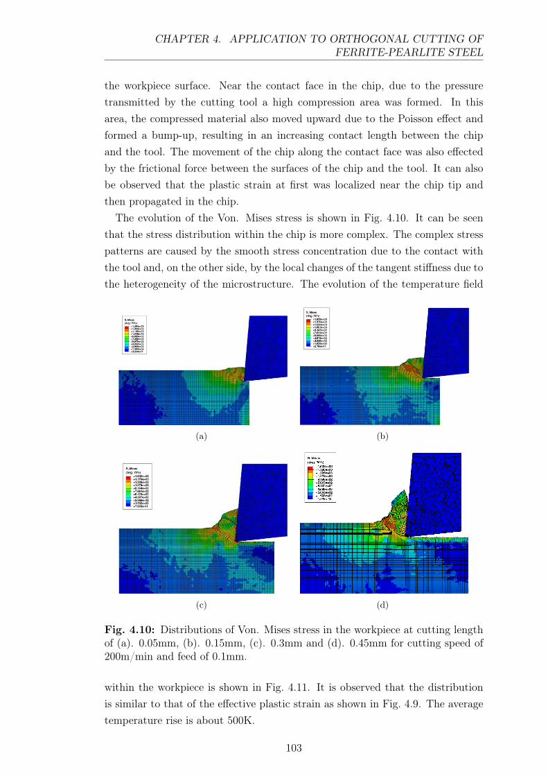
CHAPTER 4. APPLICATION TO ORTHOGONAL CUTTING OFFERRITE-PEARLITE STEEL
the workpiece surface. Near the contact face in the chip, due to the pressuretransmitted by the cutting tool a high compression area was formed. In thisarea, the compressed material also moved upward due to the Poisson effect andformed a bump-up, resulting in an increasing contact length between the chipand the tool. The movement of the chip along the contact face was also effectedby the frictional force between the surfaces of the chip and the tool. It can alsobe observed that the plastic strain at first was localized near the chip tip andthen propagated in the chip.The evolution of the Von. Mises stress is shown in Fig. 4.10. It can be seen
that the stress distribution within the chip is more complex. The complex stresspatterns are caused by the smooth stress concentration due to the contact withthe tool and, on the other side, by the local changes of the tangent stiffness due tothe heterogeneity of the microstructure. The evolution of the temperature field
(a) (b)
(c) (d)
Fig. 4.10: Distributions of Von. Mises stress in the workpiece at cutting lengthof (a). 0.05mm, (b). 0.15mm, (c). 0.3mm and (d). 0.45mm for cutting speed of200m/min and feed of 0.1mm.
within the workpiece is shown in Fig. 4.11. It is observed that the distributionis similar to that of the effective plastic strain as shown in Fig. 4.9. The averagetemperature rise is about 500K.
103

CHAPTER 4. APPLICATION TO ORTHOGONAL CUTTING OFFERRITE-PEARLITE STEEL
(a) (b)
(c) (d)
Fig. 4.11: Distributions of temperature in the workpiece at cutting length of(a). 0.05mm, (b). 0.15mm, (c). 0.3mm and (d). 0.45mm for cutting speed of200m/min and feed of 0.1mm.
104

CHAPTER 4. APPLICATION TO ORTHOGONAL CUTTING OFFERRITE-PEARLITE STEEL
As a brief summary, in this chapter, we successfully applied the thermo-mechanicallycoupled crystal plasticity framework into the study of the machining process offerrite-pearlite steel and obtained acceptable cutting forces and chip forms con-sidering the limited data used to calibrate the model parameters. The modelingframework is a first step into the simulation of the cutting process as functionof the microstructure using precise CP models and opens the door to study theeffect of the raw material texture or dual microstructure in the process. Theexplicit representation of the microstructure allows to go behind this simulationand investigate in next studies the effect of the microstructure in the tool wear.The improvement of the model calibration with more experimental data as
well as the extension of the model to more accurate CEL or ALE simulationframeworks will improve the accuracy of the simulations. In addition, from aphysical point of view, the model can be improved by introducing recrystallizationduring the cutting process.
105

CHAPTER 4. APPLICATION TO ORTHOGONAL CUTTING OFFERRITE-PEARLITE STEEL
106

CHAPTER 5
Conclusions and Future work
5.1 Summary
Metals and alloys play a crucial role in our society. Due to their importancein industry, an in-depth understanding and accurate prediction of their behaviormay lead to notable economic benefits. Theoretical and numerical models haveexisted for decades now, but accuracy demands from complex manufacturingprocesses require more sophisticated models than the standard ones. The newmodels must incorporate precise descriptions of the physics that metals undergoduring thermomechanical processes, and provide information about the state atwhich they end after being subjected to extreme conditions.
Metallic materials usually undergo large strain, high strain rate and high tem-perature, and their deformation is usually thermally coupled. They also exhibitplastic anisotropy and microstructure heterogeneity. To better describe theirbehavior, in this work a thermo-mechanically coupled finite element frameworkincorporating a crystal plasticity constitutive model has been developed to pre-dict the behavior of metallic material during thermo-mechanical processes. Thismodel is physics-based and physics-informed, minimizing the number of parame-ters that are obtained from experiments. At the same time, it holds much moreinformation than phenomenological plasticity models, thus serving the purposeto feed highly accurate information to analysts and engineers.
Real metallic materials are polycrystalline. Each macroscopic material pointrepresents numerous single crystals. To extract the macroscopic behavior of poly-crystalline metals from its associated single crystals in the microstructure, anhomogenization approach is usually needed. In this study, a computational ho-mogenization approach is adopted and applied to study the plastic deformationof polycrystalline metals by combining with the previous proposed coupled finiteelement crystal plasticity framework. This combination can predict the behaviorof polycrystals under various initial temperatures and strain rates. It could also
107

CHAPTER 5. CONCLUSIONS AND FUTURE WORK
reveal the effect of heat transfer at the grain level on the distribution of stressand temperature field at the microstructural scale.Finally, we have employed the model developed for the simulation of an ex-
tremely complex thermomechanical process, namely, that of high-speed machin-ing. This is one of the most important manufacturing operations in modernindustry but so complex that very few true plasticity models have been able tosimulate it. In this research, a microstructure informed constitutive model is firstdeveloped for low carbon steel C45, based on crystal plasticity theory. Then, itis integrated into a thermo-mechanical coupled Lagrangian framework to studythe orthogonal cutting process of C45. The numerical results are in acceptableagreement with experimental observations. In addition, our model captures theheterogeneous distribution of stress, temperature in the chip and the contactforce on the rake face of the cutting tool, which may not be observed with theconventional Johnson-Cook model.
5.2 Future Work
In the future, we could extend the work presented in this dissertation withregard to the following aspects:
1. Develop thermo-mechanically coupled frameworks based on other, more ef-ficient alternative approaches, instead of the finite element method. Forlarge scale problems which usually need parallel computing, the finite ele-ment method usually exhibits poor parallel efficiency, limiting its applica-tion to large scale engineering problems in rapidly advancing supercomput-ers. There some other numerical approaches that may have good parallelperformance, such as the FFT based homogenization and the peridynamicsapproaches.
2. Improve the numerical framework we have established for the simulation ofcutting process of ferrite-pearlite steel. Currently, and for the sake of sim-plicity, we have taken many assumptions and simplifications. In the future,we could improve the simulation accuracy by finding better material proper-ties for the ferrite and cementite phases, performing curve fitting proceduresto obtain parameters in the constitutive models that could reproduce ex-perimental results at much wider range of temperatures and strain rates. Ina similar topic, the solutions obtained have been proven to be fairly sensibleto the element deletion criterion, and further analysis of the latter mightresult in overall improvements.
108

CHAPTER 5. CONCLUSIONS AND FUTURE WORK
3. Apply the proposed numerical framework to the cutting simulation of othercommonly used engineering materials such as Ti6Al4V. Due to the general-ity of our framework, only minor modifications and extensions are neededto develop a similar microstructure informed constitutive model for thisdual-phase metal.
4. Explore the feasibility of using the ALE method and CEL method in thesimulation of cutting processes based on our proposed constitutive model.These two approaches could potentially give better simulation accuracy asthey do not use the non-physical element deletion criteria that could degradethe accuracy.
5. Introducing the size effect in our constitutive model, study the micro-cuttingprocess of tiny size metallic components, with application in various fieldssuch as the biomedical, optical, and mold/die industries.
109

CHAPTER 5. CONCLUSIONS AND FUTURE WORK
110

CHAPTER 5. CONCLUSIONS AND FUTURE WORK
111

CHAPTER 5. CONCLUSIONS AND FUTURE WORK
112

Bibliography
[1] S. Balasubramanian and L. Anand. Elasto-viscoplastic constitutive equationsfor polycrystalline fcc materials at low homologous temperatures. Journalof the Mechanics and Physics of Solids, 50(1):101 – 126, 2002.
[2] ABAQUS. ABAQUS User’s Manual, Version 6.16. Dassault Systèmes, 2016.
[3] G.R. Johnson and W.H. Cook. A constitutive model and data for metalssubjected to large strains, high strain rates, and high temperatures. InProceedings of 7th International Symposium on Ballistics, pages 541–547,1983.
[4] Zohreh Akbari, Hamed Mirzadeh, and Jose-Maria Cabrera. A simple consti-tutive model for predicting flow stress of medium carbon microalloyed steelduring hot deformation. Materials & Design, 77:126 – 131, 2015.
[5] F.J. Zerilli and R.W. Armstrong. Dislocation-mechanics-based constitutiverelations for material dynamics calculations. Journal of Applied Physics,61(5):1816–1825, 1987.
[6] R. Hill. Theoretical plasticity of textured aggregates. Mathematical Proceed-ings of the Cambridge Philosophical Society, 85(1):179–191, 1979.
[7] Frédéric Barlat, Daniel J. Lege, and John C. Brem. A six-componentyield function for anisotropic materials. International Journal of Plastic-ity, 7(7):693 – 712, 1991.
[8] Do-Nyun Kim, Francisco Javier Montáns, and Klaus-Jürgen Bathe. Insightinto a model for large strain anisotropic elasto-plasticity. ComputationalMechanics, 44(5):651–668, Oct 2009.
[9] B. Plunkett, R.A. Lebensohn, O. Cazacu, and F. Barlat. Anisotropic yieldfunction of hexagonal materials taking into account texture development andanisotropic hardening. Acta Materialia, 54(16):4159 – 4169, 2006.
113

BIBLIOGRAPHY
[10] R. Hill. Generalized constitutive relations for incremental deformation ofmetal crystals by multislip. Journal of the Mechanics and Physics of Solids,14(2):95 – 102, 1966.
[11] J.R. Rice. Inelastic constitutive relations for solids: An internal-variabletheory and its application to metal plasticity. Journal of the Mechanics andPhysics of Solids, 19(6):433 – 455, 1971.
[12] R.J. Asaro and J.R. Rice. Strain localization in ductile single crystals. Jour-nal of the Mechanics and Physics of Solids, 25(5):309 – 338, 1977.
[13] D. Peirce, R.J. Asaro, and A. Needleman. Material rate dependence andlocalized deformation in crystalline solids. Acta Metallurgica, 31(12):1951 –1976, 1983.
[14] Marc G. D. Geers, Ron H. J. Peerlings, Johan P. M. Hoefnagels, and YuriyKasyanyuk. On a proper account of first- and second-order size effects incrystal plasticity. Advanced Engineering Materials, 11(3):143–147, 2009.
[15] A. Molinari, G.R. Canova, and S. Ahzi. A self consistent approach of thelarge deformation polycrystal viscoplasticity. Acta Metallurgica, 35(12):2983– 2994, 1987.
[16] R.A. Lebensohn and C.N. Tomé. A self-consistent anisotropic approachfor the simulation of plastic deformation and texture development of poly-crystals: Application to zirconium alloys. Acta Metallurgica et Materialia,41(9):2611 – 2624, 1993.
[17] C.N. Tomé and R.A. Lebensohn. Self Consistent Homogenization Methodsfor Texture and Anisotropy, chapter 23, pages 473–499. Wiley-Blackwell,2005.
[18] F. Roters, P. Eisenlohr, T.R. Bieler, and D. Raabe. Homogenization, chap-ter 7, pages 93–108. Wiley-Blackwell, 2010.
[19] J. Segurado, R.A. Lebensohn, and J. Llorca. Computational homogenizationof polycrystals. Advances in Applied Mechanics, 51:1–114, 04 2018.
[20] J. Segurado, R.A. Lebensohn, J. LLorca, and C.N. Tomé. Multiscale model-ing of plasticity based on embedding the viscoplastic self-consistent formula-tion in implicit finite elements. International Journal of Plasticity, 28(1):124– 140, 2012.
114
BIBLIOGRAPHY
[21] Ricardo A. Lebensohn, Carlos N. Tomé, and Pedro Ponte Castañeda. Self-consistent modelling of the mechanical behaviour of viscoplastic polycrystalsincorporating intragranular field fluctuations. 2007.
[22] T. Herwig and W. Wagner. On a robust fe2 model for delamination analysisin composite structures. Composite Structures, 201:597 – 607, 2018.
[23] E. Tikarrouchine, G. Chatzigeorgiou, F. Praud, B. Piotrowski, Y. Chemisky,and F. Meraghni. Three-dimensional fe2 method for the simulation of non-linear, rate-dependent response of composite structures. Composite Struc-tures, 193:165 – 179, 2018.
[24] Felix Selim Göküzüm, Lu Trong Khiem Nguyen, and Marc-André Keip. Amultiscale fe-fft framework for electro-active materials at finite strains. Com-putational Mechanics, 64(1):63–84, Jul 2019.
[25] Julian Kochmann, Stephan Wulfinghoff, Lisa Ehle, Joachim Mayer, BobSvendsen, and Stefanie Reese. Efficient and accurate two-scale fe-fft-basedprediction of the effective material behavior of elasto-viscoplastic polycrys-tals. Computational Mechanics, 61(6):751–764, Jun 2018.
[26] Y. Wang, D. Raabe, C. Klueber, and F. Roters. Orientation dependence ofnanoindentation pile-up patterns and of nanoindentation microtextures incopper single crystals. Acta Materialia, 52(8):2229–2238, 2004.
[27] O. Casals and S. Forest. Finite element crystal plasticity analysis of sphericalindentation in bulk single crystals and coatings. Computational MaterialsScience, 45(3):774 – 782, 2009. Proceedings of the 17th International Work-shop on Computational Mechanics of Materials.
[28] Mao Liu, Cheng Lu, and Anh Kiet Tieu. Crystal plasticity finite elementmethod modelling of indentation size effect. International Journal of Solidsand Structures, 54:42 – 49, 2015.
[29] Zhen Zhang, Tea-Sung Jun, T Britton, and Fionn Dunne. Intrinsicanisotropy of strain rate sensitivity in single crystal alpha titanium. ActaMaterialia, 118:317, 07 2016.
[30] Qiang Liu, Anish Roy, and Vadim Silberschmidt. Size-dependent crystalplasticity: from micro-pillar compression to bending. Mechanics of Materials,100:31 – 40, 6 2016.
[31] Qiang Liu, Anish Roy, Shoichi Tamura, Takashi Matsumura, and VadimSilberschmidt. Micro-cutting of single-crystal metal: Finite-element analysis
115

BIBLIOGRAPHY
of deformation and material removal. International Journal of MechanicalSciences, 118:135–143, 11 2016.
[32] Murat Demiral, Anish Roy, and Vadim V. Silberschmidt. Strain-gradientcrystal-plasticity modelling of micro-cutting of b.c.c. single crystal. Mecca-nica, 51(2):371–381, Feb 2016.
[33] A. Cruzado, B. Gan, M. Jiménez, D. Barba, K. Ostolaza, A. Linaza, J.M.Molina-Aldareguia, J. Llorca, and J. Segurado. Multiscale modeling of themechanical behavior of IN718 superalloy based on micropillar compressionand computational homogenization. Acta Materialia, 98:242 – 253, 2015.
[34] C. Zhang, H. Li, P. Eisenlohr, W. Liu, C.J. Boehlert, M.A. Crimp, and T.R.Bieler. Effect of realistic 3d microstructure in crystal plasticity finite elementanalysis of polycrystalline Ti-5Al-2.5Sn. International Journal of Plasticity,69:21 – 35, 2015.
[35] V. Herrera-Solaz, J. LLorca, E. Dogan, I. Karaman, and J. Segurado. Aninverse optimization strategy to determine single crystal mechanical behaviorfrom polycrystal tests: Application to AZ31 Mg alloy. International Journalof Plasticity, 57:1 – 15, 2014.
[36] G. Zhou, M.K. Jain, P. Wu, Y. Shao, D. Li, and Y. Peng. Experiment andcrystal plasticity analysis on plastic deformation of az31b mg alloy sheetunder intermediate temperatures: How deformation mechanisms evolve. In-ternational Journal of Plasticity, 79:19 – 47, 2016.
[37] A. Shahba and S. Ghosh. Crystal plasticity FE modeling of Ti alloys fora range of strain-rates. Part I: A unified constitutive model and flow rule.International Journal of Plasticity, 87:48 – 68, 2016.
[38] S. Ghosh, A. Shahba, X. Tu, E.L. Huskins, and B.E. Schuster. Crystal plas-ticity FE modeling of Ti alloys for a range of strain-rates. Part II: Image-based model with experimental validation. International Journal of Plastic-ity, 87:69 – 85, 2016.
[39] R. Yuan, I.J. Beyerlein, and C. Zhou. Homogenization of plastic deformationin heterogeneous lamella structures. Materials Research Letters, 5(4):251–257, 2017.
[40] J. Luo, G. Kang, and M. Shi. Simulation to the cyclic deformation of poly-crystalline aluminum alloy using crystal plasticity finite element method.International Journal of Computational Materials Science and Engineering,02:1350019, 2013.
116

BIBLIOGRAPHY
[41] W. Muhammad, A.P. Brahme, J. Kang, R.K. Mishra, and K. Inal. Exper-imental and numerical investigation of texture evolution and the effects ofintragranular backstresses in aluminum alloys subjected to large strain cyclicdeformation. International Journal of Plasticity, 93:137 – 163, 2017.
[42] A. Cruzado, J. LLorca, and J. Segurado. Modeling cyclic deformation ofinconel 718 superalloy by means of crystal plasticity and computational ho-mogenization. International Journal of Solids and Structures, 122-123:148 –161, 2017.
[43] F.P.E. Dunne, D. Rugg, and A. Walker. Length scale-dependent, elasticallyanisotropic, physically-based hcp crystal plasticity: Application to cold-dwellfatigue in Ti alloys. International Journal of Plasticity, 23:1061 – 1083, 2007.
[44] F. Bridier, D.L. McDowell, P. Villechaise, and J. Mendez. Crystal plasticitymodeling of slip activity in ti6al4v under high cycle fatigue loading. Inter-national Journal of Plasticity, 25(6):1066 – 1082, 2009.
[45] A. Rovinelli, M.D. Sangid, H. Proudhon, Y. Guilhem, R.A. Lebensohn, andW. Ludwig. Predicting the 3d fatigue crack growth rate of small cracksusing multimodal data via bayesian networks: In-situ experiments and crys-tal plasticity simulations. Journal of the Mechanics and Physics of Solids,115:208 – 229, 2018.
[46] A. Cruzado, S. Lucarini, J. LLorca, and J. Segurado. Microstructure-basedfatigue life model of metallic alloys with bilinear coffin-manson behavior.International Journal of Fatigue, 107:40 – 48, 2018.
[47] B. Chen, J. Jiang, and F.P.E. Dunne. Is stored energy density the primarymeso-scale mechanistic driver for fatigue crack nucleation? InternationalJournal of Plasticity, 101:213 – 229, 2018.
[48] G.B. Sarma and B. Radhakrishnan. Modeling microstructural effects on theevolution of cube texture during hot deformation of aluminum. MaterialsScience and Engineering: A, 385(1):91 – 104, 2004.
[49] T. Walde and H. Riedel. Modeling texture evolution during hot rolling ofmagnesium alloy az31. Materials Science and Engineering: A, 443(1-2):277– 284, 2007.
[50] J.R. Mayeur, I.J. Beyerlein, C.A. Bronkhorst, and H.M. Mourad. Incorpo-rating interface affected zones into crystal plasticity. International Journalof Plasticity, 65:206 – 225, 2015.
117

BIBLIOGRAPHY
[51] A. Gupta, M.B Bettaieb, F. Abed-Meraim, and S.R. Kalidindi. Computa-tionally efficient predictions of crystal plasticity based forming limit diagramsusing a spectral database. International Journal of Plasticity, 103:168 – 187,2018.
[52] G.I. Taylor. Plastic strain in metals. Journal of the Institute of Metals,62:307–324, 1938.
[53] John Douglas Eshelby and Rudolf Ernst Peierls. The determination of theelastic field of an ellipsoidal inclusion, and related problems. Proceedings ofthe Royal Society of London. Series A. Mathematical and Physical Sciences,241(1226):376–396, 1957.
[54] K.S. Cheong, E.P. Busso, and A. Arsenlis. A study of microstructural lengthscale effects on the behaviour of fcc polycrystals using strain gradient con-cepts. International Journal of Plasticity, 21:1797 – 1814, 2005.
[55] D. Rodríguez-Galán, I. Sabirov, and J. Segurado. Temperature and strainrate effect on the deformation of nanostructured pure titanium. InternationalJournal of Plasticity, 70:191–205, 2015.
[56] P. Hu, Y. Liu, Y. Zhu, and L. Ying. Crystal plasticity extended modelsbased on thermal mechanism and damage functions: Application to multi-scale modeling of aluminum alloy tensile behavior. International Journal ofPlasticity, 86:1 – 25, 2016.
[57] M. Kothari and L. Anand. Elasto-viscoplastic constitutive equations forpolycrystalline metals: Application to tantalum. Journal of the Mechanicsand Physics of Solids, 46(1):51 – 83, 1998.
[58] P. Hakansson, M.Wallin, and M. Ristinmaa. Prediction of stored energyin polycrystalline materials during cyclic loading. International Journal ofSolids and Structures, 45(6):1570 – 1586, 2008.
[59] R. Seghir, E. Charkaluk, P. Dufrnoy, and L. Bodelot. Thermomechanicalcouplings in crystalline plasticity under fatigue loading. Procedia Engineer-ing, 2(1):1155 – 1164, 2010. Fatigue 2010.
[60] E.D. Cyr, M. Mohammadi, R.K. Mishra, and K. Inal. A three dimensional(3d) thermo-elasto-viscoplastic constitutive model for fcc polycrystals. In-ternational Journal of Plasticity, 70:166 – 190, 2015.
118

BIBLIOGRAPHY
[61] R. W. Ivester, M. Kennedy, M. Davies, R. Stevenson, J. Thiele, R. Fur-ness, and S. Athavale. Assessment of machining models: progress report.Machining Science and Technology, 4(3):511–538, 2000.
[62] A.A. Benzerga, Y. Brechet, A. Needleman, and E. Van der Giessen. Thestored energy of cold work: Predictions from discrete dislocation plasticity.Acta Materialia, 53(18):4765 – 4779, 2005.
[63] E.H. Lee and D.T. Liu. Finite-strain elastic—plastic theory with applicationto plane-wave analysis. Journal of Applied Physics, 38(1):19–27, 1967.
[64] F.T. Meissonnier, E.P. Busso, and N.P. O’Dowd. Finite element implemen-tation of a generalised non-local rate-dependent crystallographic formulationfor finite strains. International Journal of Plasticity, 17(4):601 – 640, 2001.
[65] H.J. Frost and M.F. Ashby. Deformation Mechanism Maps: the plasticityand creep of metals and ceramics. Pergamon Press, 1982.
[66] A. Cotterell and R. Stokes. Effects of temperature on the plastic proper-ties of aluminium crystals. Proceedings of the Royal Society of London A:Mathematical, Physical and Engineering Sciences, 233(1192):17–34, 1955.
[67] R.J. Asaro and A. Needleman. Texture development and strain hardeningin rate dependent polycrystals. Acta Metallurgica, 33(6):923 – 953, 1985.
[68] E. Voce. The relationship between stress and strain for homogeneous defor-mations. 1948.
[69] U. F. Kocks. Laws for Work-Hardening and Low-Temperature Creep. Jour-nal of Engineering Materials and Technology, 98(1):76–85, 01 1976.
[70] S.B. Brown, K.H. Kim, and L. Anand. An internal variable constitutivemodel for hot working of metals. International Journal of Plasticity, 5(2):95– 130, 1989.
[71] Fabrice Barbe, Luc Decker, Dominique Jeulin, and Georges Cailletaud. In-tergranular and intragranular behavior of polycrystalline aggregates. part 1:F.e. model. International Journal of Plasticity, 17(4):513 – 536, 2001.
[72] Fabrice Barbe, Samuel Forest, and Georges Cailletaud. Intergranular andintragranular behavior of polycrystalline aggregates.part 2: Results. Inter-national Journal of Plasticity, 17(4):537 – 563, 2001.
[73] R. A. Lebensohn. N-site modeling of a 3d viscoplastic polycrystal using fastfourier transform. Acta Materialia, 49(14):2723 – 2737, 2001.
119

BIBLIOGRAPHY
[74] P. Eisenlohr, M. Diehl, R.A. Lebensohn, and F. Roters. A spectral methodsolution to crystal elasto-viscoplasticity at finite strains. International Jour-nal of Plasticity, 46:37 – 53, 2013. Microstructure-based Models of PlasticDeformation.
[75] S. Lucarini and J. Segurado. On the accuracy of spectral solvers for microme-chanics based fatigue modeling. Computational Mechanics, 63(2):365–382,Feb 2019.
[76] Chris H. Rycroft. Voro++: A three-dimensional voronoi cell library in c++.Chaos: An Interdisciplinary Journal of Nonlinear Science, 19(4):041111,2009.
[77] Lei-Ting Li, Y. C. Lin, Ling Li, Lu-Ming Shen, and Dong-Xu Wen. Three-dimensional crystal plasticity finite element simulation of hot compressivedeformation behaviors of 7075 al alloy. Journal of Materials Engineeringand Performance, 24(3):1294–1304, Mar 2015.
[78] Ralf Hielscher and Helmut Schaeben. A novel pole figure inversion method:Specification of the mtex algorithm. Journal of Applied Crystallography - JAPPL CRYST, 41:1024–1037, 12 2008.
[79] Ling Li, Luming Shen, and Gwénaëlle Proust. A texture-based representativevolume element crystal plasticity model for predicting bauschinger effectduring cyclic loading. Materials Science and Engineering: A, 608:174 – 183,2014.
[80] Christophe Geuzaine and Jean-François Remacle. Gmsh: A 3-d finite ele-ment mesh generator with built-in pre- and post-processing facilities. Inter-national Journal for Numerical Methods in Engineering, 79(11):1309–1331,2009.
[81] H.J. Böhm. A Short Introduction to Continuum Micromechanics. Springer-Verlag Wien, 2004.
[82] J. Segurado and J. Llorca. Simulation of the deformation of polycrystallinenanostructured Ti by computational homogenization. Computational Mate-rials Science, 76:3 – 11, 2013.
[83] S. Nemat-Nasser and J.B. Isaacs. Direct measurement of isothermal flowstress of metals at elevated temperatures and high strain rates with applica-tion to ta and taw alloys. Acta Materialia, 45(3):907 – 919, 1997.
120
BIBLIOGRAPHY
[84] G. Simmons and H. Wang. Single Crystal Elastic Constants and CalculatedAggregate Properties: A Handbook. The MIT Press, Cambridge, 1971.
[85] Mikel Saez-de Buruaga, Ibon Poveda, and Pedro José Arrazola. Tool wearprediction in machining process using a microstructure-based finite elementmodel. In Material Forming ESAFORM 2015, volume 651 of Key Engineer-ing Materials, pages 1229–1234. Trans Tech Publications Ltd, 8 2015.
[86] Anil Meena and Mohamed El Mansori. Microstructure induced wear mech-anisms of pvd-coated carbide tools during dry drilling of newly producedadi. In Material Forming ESAFORM 2015, volume 651 of Key EngineeringMaterials, pages 1271–1276. Trans Tech Publications Ltd, 8 2015.
[87] Mustapha Abouridouanea, Fritz Klockea, Dieter Lunga, and Drazen Veselo-vaca. The mechanics of cutting: In-situ measurement and modelling. In 15thCIRP Conference on Modelling of Machining Operations, Key EngineeringMaterials, pages 246–251. Trans Tech Publications Ltd, 2015.
[88] M. Saez de Buruaga, P. Aristimuño, D. Soler, E. D’Eramo, A. Roth, and P.J.Arrazola. Microstructure based flow stress model to predict machinabilityin ferrite–pearlite steels. CIRP Annals, 68(1):49 – 52, 2019.
[89] Y. Zhang, T. Mabrouki, D. Nelias, C. Courbon, J. Rech, and Y. Gong.Cutting simulation capabilities based on crystal plasticity theory and discretecohesive elements. Journal of Materials Processing Technology, 212(4):936 –953, 2012.
[90] H.B. Boubaker, C. Mareau, Y. Ayed, G. Germain, and F. Guerin. Devel-opment of a hyperelastic constitutive model based on the crystal plasticitytheory for the simulation of machining operations. Procedia CIRP, 82:20– 25, 2019. 17th CIRP Conference on Modelling of Machining Operations(17th CIRP CMMO).
[91] Mikel Echeandia, D. Soler, Patxi Aristimuño, Jon Esnaola, and Pedro Arra-zola. Determining tool/chip temperatures from thermography measurementsin metal cutting. Applied Thermal Engineering, 145:305–314, 09 2018.
[92] I. Watanabe, D. Setoyama, N. Nagasako, N. Iwata, and K. Nakanishi. Mul-tiscale prediction of mechanical behavior of ferrite–pearlite steel with nu-merical material testing. International Journal for Numerical Methods inEngineering, 89(7):829–845, 2012.
[93] George Langford. Deformation of pearlite. Metallurgical Transactions A,8(6):861–875, Jun 1977.
121

BIBLIOGRAPHY
[94] X. Peng, J. Fan, and J. Zeng. Microstructure-based description for themechanical behavior of single pearlitic colony. International Journal of Solidsand Structures, 39(2):435 – 448, 2002.
122