Creating composite indicators with DEA and robustness analysis: the case of the Technology...
13
Journal of the Operational Research Society (2008) 59, 239--251 2008 Operational Research Society Ltd. All rights reserved. 0160-5682/08 $30.00 www.palgrave-journals.com/jors Creating composite indicators with DEA and robustness analysis: the case of the Technology Achievement Index L Cherchye 1 ∗ , W Moesen 1 , N Rogge 1 , T Van Puyenbroeck 1 , M Saisana 2 , A Saltelli 2 , R Liska 2 and S Tarantola 2 1 Catholic University of Leuven, Belgium; and 2 Joint Research Centre, European Commission, Italy Composite indicators (CIs) are often used for benchmarking countries’ performance, but they frequently stir controversies about the unavoidable subjectivity in their construction. Data Envelopment Analysis helps to overcome some key limitations, as it does not need any prior information on either the normalization of sub-indicators or on an agreed unique set of weights. Still, subjective decisions remain, and such modelling uncertainty propagates onto countries’ CI scores and rankings. Uncertainty and sensitivity analysis are therefore needed to assess the robustness of the final outcome and to analyse how much each source of uncertainty contributes to the output variance. The current paper reports on these issues, using the Technology Achievement Index as an illustration. Journal of the Operational Research Society (2008) 59, 239 – 251. doi:10.1057/palgrave.jors.2602445 Published online 27 June 2007 Keywords: Data Envelopment Analysis; composite indicator construction; robustness analysis 1. Introduction Organizations such as the United Nations, the European Com- mission, and others have developed and used composite in- dicators (CIs) in which sub-indicators are aggregated into one number, with a view to provide comparisons of coun- tries in complex and sometimes elusive policy issues. These measures are increasingly recognized as a tool for policy making and, especially, public communications on countries’ relative performance in wide ranging fields from environ- ment, economy to technological development. More dis- cussions on various CIs can be found in the information server: http://farmweb.jrc.cec.eu.int/ci/ provided by the Joint Research Centre of European Commission. A CI is much like a mathematical or computational model. Just as for models, the justification for a CI lays in its fitness to the intended purpose and peer acceptance, while its con- struction owes more to craftsmanship than to universally ac- cepted scientific rules for encoding. The construction of CIs involves stages that need subjective judgments: the selection of sub-indicators, the treatment of missing values, the choice of the aggregation model, the weights of the sub-indicators, and so on. These choices can, however, be used to manipu- late the results. It is, thus, important to identify the sources of subjective assessment and data errors and use uncertainty and sensitivity analysis to gain insight during the process of ∗ Correspondence: L Cherchye, Catholic University of Leuven, Campus Kortrijk, E. Sabbelaan 53; B-8500 Kortrijk, Belgium. E-mail: [email protected] CI building, including an appraisal of the reliability of coun- tries’ ranking. These considerations are a central theme of the current paper. The construction methodology that is used in the present paper is rooted in data envelopment analysis (DEA). The orig- inal question in the DEA literature is how one could measure each decision-making unit’s relative efficiency, given obser- vations on input and output quantities in a sample of peers and, often, no reliable information on prices (Charnes and Cooper, 1985). One immediately appreciates the conceptual similarity between that original problem and the one of con- structing CIs. In the latter case, quantitative sub-indicators for overall benchmarking are available, but as a rule there is only disparate expert opinion available about the appropri- ate weights to be used in an aggregation function. On the other hand, there are differences between the two settings; for example, a notable difference is that CIs typically look at ‘achievements’ without taking into account the input-side, though there are some interesting exceptions, for example the work of the European Commission (2005) on the Summary Innovation Index. A well-known feature of DEA is that it looks for en- dogenous (possibly constrained) weights, which maximize the overall score for each decision-making unit given a set of other observations. This quality explains a major part of the appeal of DEA-based CIs in real policy-related settings. For example, several European policy issues entail an intri- cate balancing act between supra-national concerns and the country-specific policy priorities of member states. If one
-
Upload
independent -
Category
Documents
-
view
1 -
download
0
Transcript of Creating composite indicators with DEA and robustness analysis: the case of the Technology...
Journal of the Operational Research Society (2008) 59, 239 --251 2008 Operational Research Society Ltd. All rights reserved. 0160-5682/08 $30.00
www.palgrave-journals.com/jors
Creating composite indicators with DEA androbustness analysis: the case of the TechnologyAchievement IndexL Cherchye1∗, W Moesen1, N Rogge1, T Van Puyenbroeck1, M Saisana2, A Saltelli2,R Liska2 and S Tarantola21Catholic University of Leuven, Belgium; and 2Joint Research Centre, European Commission, Italy
Composite indicators (CIs) are often used for benchmarking countries’ performance, but they frequently stircontroversies about the unavoidable subjectivity in their construction. Data Envelopment Analysis helps toovercome some key limitations, as it does not need any prior information on either the normalization ofsub-indicators or on an agreed unique set of weights. Still, subjective decisions remain, and such modellinguncertainty propagates onto countries’ CI scores and rankings. Uncertainty and sensitivity analysis are thereforeneeded to assess the robustness of the final outcome and to analyse how much each source of uncertaintycontributes to the output variance. The current paper reports on these issues, using the Technology AchievementIndex as an illustration.Journal of the Operational Research Society (2008) 59, 239–251. doi:10.1057/palgrave.jors.2602445Published online 27 June 2007
Keywords: Data Envelopment Analysis; composite indicator construction; robustness analysis
1. Introduction
Organizations such as the United Nations, the European Com-mission, and others have developed and used composite in-dicators (CIs) in which sub-indicators are aggregated intoone number, with a view to provide comparisons of coun-tries in complex and sometimes elusive policy issues. Thesemeasures are increasingly recognized as a tool for policymaking and, especially, public communications on countries’relative performance in wide ranging fields from environ-ment, economy to technological development. More dis-cussions on various CIs can be found in the informationserver: http://farmweb.jrc.cec.eu.int/ci/ provided by the JointResearch Centre of European Commission.
A CI is much like a mathematical or computational model.Just as for models, the justification for a CI lays in its fitnessto the intended purpose and peer acceptance, while its con-struction owes more to craftsmanship than to universally ac-cepted scientific rules for encoding. The construction of CIsinvolves stages that need subjective judgments: the selectionof sub-indicators, the treatment of missing values, the choiceof the aggregation model, the weights of the sub-indicators,and so on. These choices can, however, be used to manipu-late the results. It is, thus, important to identify the sourcesof subjective assessment and data errors and use uncertaintyand sensitivity analysis to gain insight during the process of
∗Correspondence: L Cherchye, Catholic University of Leuven, CampusKortrijk, E. Sabbelaan 53; B-8500 Kortrijk, Belgium.E-mail: [email protected]
CI building, including an appraisal of the reliability of coun-tries’ ranking. These considerations are a central theme ofthe current paper.
The construction methodology that is used in the presentpaper is rooted in data envelopment analysis (DEA). The orig-inal question in the DEA literature is how one could measureeach decision-making unit’s relative efficiency, given obser-vations on input and output quantities in a sample of peersand, often, no reliable information on prices (Charnes andCooper, 1985). One immediately appreciates the conceptualsimilarity between that original problem and the one of con-structing CIs. In the latter case, quantitative sub-indicatorsfor overall benchmarking are available, but as a rule there isonly disparate expert opinion available about the appropri-ate weights to be used in an aggregation function. On theother hand, there are differences between the two settings;for example, a notable difference is that CIs typically lookat ‘achievements’ without taking into account the input-side,though there are some interesting exceptions, for example thework of the European Commission (2005) on the SummaryInnovation Index.
A well-known feature of DEA is that it looks for en-dogenous (possibly constrained) weights, which maximizethe overall score for each decision-making unit given a setof other observations. This quality explains a major part ofthe appeal of DEA-based CIs in real policy-related settings.For example, several European policy issues entail an intri-cate balancing act between supra-national concerns and thecountry-specific policy priorities of member states. If one
240 Journal of the Operational Research Society Vol. 59, No. 2
opts to compare the multi-dimensional performance of EUmember states by subjecting them to a fixed set of weights,this may prevent acceptance of the entire exercise. To take anexample: with reference to European social inclusion policy,Atkinson et al (2002) remark that ‘in the context of the EU,there are evident difficulties in reaching agreement on suchweights, given that each member state has its own nationalspecificity.’ As the essence of DEA is that it yields mostfavourable, country-specific weights, it may help to counter-act such problems. However, the standard DEA set-up thatonly requires the non-negativity of weights does not sufficeto guarantee peer acceptance. Often, expert opinion about themost appropriate weights is available, and such informationshould be considered in the DEA model.
DEA-based CIs have inter alia been used to assess labourmarket policy (Storrie and Bjurek, 2000), social inclusionpolicy (Cherchye et al, 2004), and internal market policy(Cherchye et al, 2007). A similar model has been tested toassess progress towards achieving the so-called Lisbon ob-jectives (European Commission, 2004, pp. 376–378). Sim-ilarly, some authors have proposed a DEA-based model forthe well-known Human Development Index (Mahlberg andObersteiner, 2001; Despotis, 2005).
In this paper, we will illustrate our approach using theTechnology Achievement Index, which together with theHuman Development Index, was developed by the United Na-tions and included in the 2001 Human Development Report(United Nations, 2001). A further incentive to use the TAI isthat it was extensively studied in the JRC-OECD Handbookon Constructing Composite Indicators (Nardo et al, 2005a,b).We will complement the handbook’s results by providing amore in-depth application of the DEA approach. We willstart in Section 2 by briefly discussing the TAI as well as theavailable information on possible sets of weights obtainedfrom a panel of informed individuals. Section 3 presents thebasic model and discusses its similarities and differences fromconventional DEA models. We then address uncertainty andsensitivity analysis associated with our DEA model in Section4. The current mainstream literature on sensitivity analysisfor DEA-models is primarily concerned with the sensitivityof (in)efficiency scores induced by data perturbations for agiven selection of inputs and outputs (Cooper et al, 2004). Inthe case of CIs, however, one is further concerned with theimpact on the results of adding or deleting sub-indicators,altering expert information, and so on. Such issues havebeen addressed rather infrequently in the DEA literature(Valdmanis, 1992; Wilson, 1995; Banker et al, 1996; Simarand Wilson, 1998; Simar, 2003). Even here the parallelbetween CIs and mathematical models is useful. In mathe-matical models of natural or man-made systems uncertaintyand sensitivity analysis related to modelling assumptions orscenarios have been studied (see Saltelli et al, 2004, for areview). The methodology that we present in Section 4 maytherefore be valuable for a broader DEA audience as well.Section 5 concludes and offers some final remarks.
2. The Technology Achievement Index and expertopinion
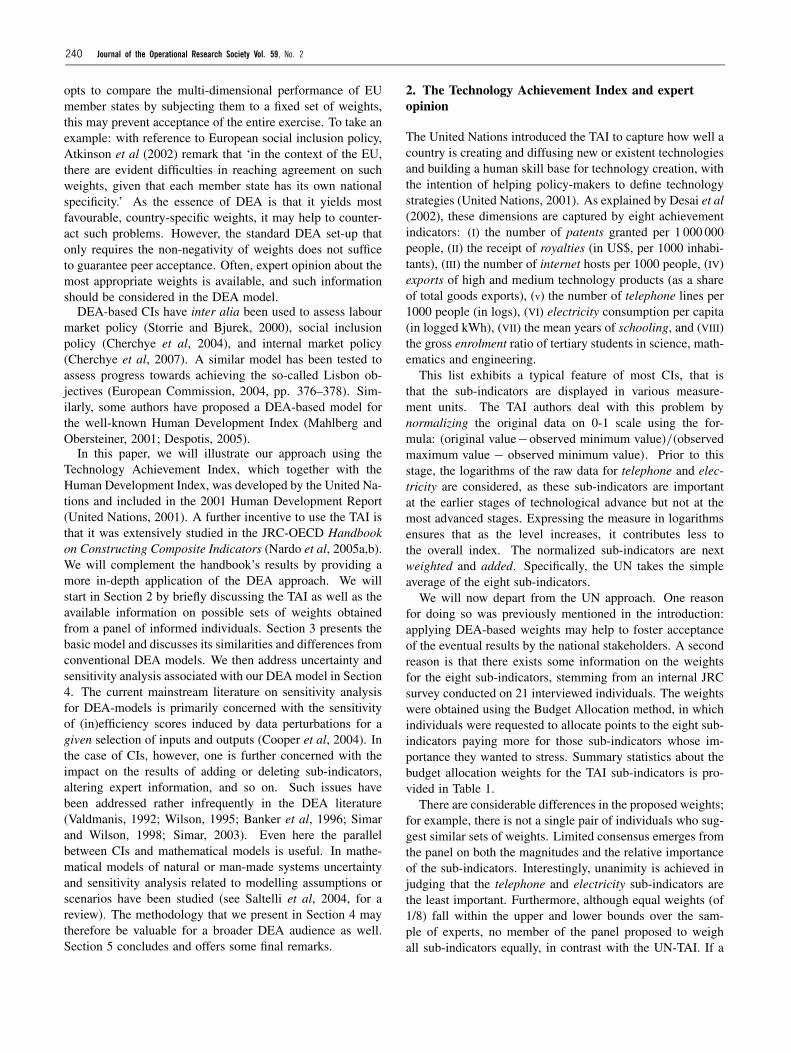
The United Nations introduced the TAI to capture how well acountry is creating and diffusing new or existent technologiesand building a human skill base for technology creation, withthe intention of helping policy-makers to define technologystrategies (United Nations, 2001). As explained by Desai et al(2002), these dimensions are captured by eight achievementindicators: (I) the number of patents granted per 1 000 000people, (II) the receipt of royalties (in US$, per 1000 inhabi-tants), (III) the number of internet hosts per 1000 people, (IV)exports of high and medium technology products (as a shareof total goods exports), (v) the number of telephone lines per1000 people (in logs), (VI) electricity consumption per capita(in logged kWh), (VII) the mean years of schooling, and (VIII)the gross enrolment ratio of tertiary students in science, math-ematics and engineering.
This list exhibits a typical feature of most CIs, that isthat the sub-indicators are displayed in various measure-ment units. The TAI authors deal with this problem bynormalizing the original data on 0-1 scale using the for-mula: (original value−observed minimum value)/(observedmaximum value − observed minimum value). Prior to thisstage, the logarithms of the raw data for telephone and elec-tricity are considered, as these sub-indicators are importantat the earlier stages of technological advance but not at themost advanced stages. Expressing the measure in logarithmsensures that as the level increases, it contributes less tothe overall index. The normalized sub-indicators are nextweighted and added. Specifically, the UN takes the simpleaverage of the eight sub-indicators.
We will now depart from the UN approach. One reasonfor doing so was previously mentioned in the introduction:applying DEA-based weights may help to foster acceptanceof the eventual results by the national stakeholders. A secondreason is that there exists some information on the weightsfor the eight sub-indicators, stemming from an internal JRCsurvey conducted on 21 interviewed individuals. The weightswere obtained using the Budget Allocation method, in whichindividuals were requested to allocate points to the eight sub-indicators paying more for those sub-indicators whose im-portance they wanted to stress. Summary statistics about thebudget allocation weights for the TAI sub-indicators is pro-vided in Table 1.
There are considerable differences in the proposed weights;for example, there is not a single pair of individuals who sug-gest similar sets of weights. Limited consensus emerges fromthe panel on both the magnitudes and the relative importanceof the sub-indicators. Interestingly, unanimity is achieved injudging that the telephone and electricity sub-indicators arethe least important. Furthermore, although equal weights (of1/8) fall within the upper and lower bounds over the sam-ple of experts, no member of the panel proposed to weighall sub-indicators equally, in contrast with the UN-TAI. If a
L Cherchye et al—Robustness of DEA composite indicators 241
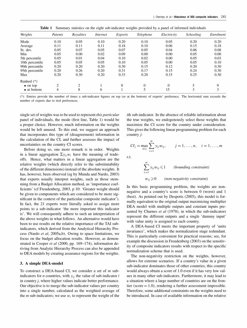
Table 1 Summary statistics on the eight sub-indicator weights provided by a panel of informed individuals
Weights Patents Royalties Internet Exports Telephone Electricity Schooling Enrolment
Mode 0.10 0.05 0.10 0.20 0.10 0.05 0.20 0.20Average 0.11 0.11 0.11 0.18 0.10 0.06 0.15 0.18St. dev. 0.05 0.07 0.05 0.07 0.05 0.04 0.06 0.08Min 0.05 0.00 0.02 0.09 0.00 0.00 0.05 0.005th percentile 0.05 0.01 0.04 0.10 0.02 0.00 0.05 0.0310th percentile 0.05 0.05 0.05 0.10 0.05 0.00 0.05 0.1090th percentile 0.20 0.20 0.20 0.30 0.15 0.12 0.20 0.3095th percentile 0.20 0.26 0.20 0.31 0.17 0.15 0.24 0.30Max 0.20 0.30 0.20 0.33 0.20 0.15 0.25 0.30
Ranked (*)• on top 2 2 1 8 0 0 5 9• at bottom 4 8 6 1 5 15 3 3
(*): Entries provide the number of times a sub-indicator figures on top (or at the bottom) of experts’ preference. The horizontal sum exceeds thenumber of experts due to tied preferences.
single set of weights was to be used to represent this particularpanel of individuals, the mode (first line, Table 1) would bea proper choice. However, much information on the weightswould be left unused. To this end, we suggest an approachthat incorporates this type of (disagreement) information inthe calculation of the CI, and further assesses the impact ofuncertainties on the country CI scores.
Before doing so, one more remark is in order. Weightsin a linear aggregation �yijwi have the meaning of trade-offs. Hence, what matters in a linear aggregation are therelative weights (which directly refer to the substitutabilityof the different dimensions) instead of the absolute weights. Ithas, however, been observed (eg by Munda and Nardo, 2003)that experts usually interpret weights, such as those stem-ming from a Budget Allocation method, as ‘importance coef-ficients’ (cf Freudenberg, 2003, p 10: ‘Greater weight shouldbe given to components which are considered to be more sig-nificant in the context of the particular composite indicator’).In fact, the 21 experts were literally asked to assign morepoints to a sub-indicator ‘the more important this indicatoris’. We will consequently adhere to such an interpretation ofthe above weights in what follows. An alternative would havebeen to use results on the relative importance of the TAI sub-indicators, which derived from the Analytical Hierarchy Pro-cess (Nardo et al, 2005a,b). Owing to space limitations, wefocus on the budget allocation results. However, as demon-strated in Cooper et al (2000, pp. 169–174), information de-riving from Analytic Hierarchy Process can also be appendedto DEA models by creating assurance regions for the weights.
3. A simple DEA-model
To construct a DEA-based CI, we consider a set of m sub-indicators for n countries, with yij the value of sub-indicator iin country j, where higher values indicate better performance.Our objective is to merge the sub-indicator values per countryinto a single number, calculated as the weighted average ofthe m sub-indicators; we use wi to represent the weight of the
ith sub-indicator. In the absence of reliable information aboutthe true weights, we endogenously select those weights thatmaximize the CI score for the country under consideration.This gives the following linear programming problem for eachcountry j:
CI j = maxwi j
m∑
i=1
yijwi j , j = 1, . . . , n, i = 1, . . . ,m
s.t.m∑
i=1
yijwi j �1 (bounding constraint)
wi j �0 (non-negativity constraint)
In this basic programming problem, the weights are non-negative and a country’s score is between 0 (worst) and 1(best). As pointed out by Despotis (2005), this model is for-mally equivalent to the original output maximizing multiplierDEA model with multiple outputs and constant inputs pre-sented by Charnes et al (1978), in which the sub-indicatorsrepresent the different outputs and a single ‘dummy input’with value unity is assigned to each country.
A DEA-based CI meets the important property of ‘unitsinvariance’, which makes the normalization stage redundant.This is particularly convenient for practical reasons; see, forexample the discussion in Freudenberg (2003) on the sensitiv-ity of composite indicators results with respect to the specificnormalization scheme that is used.
The non-negativity restriction on the weights, however,allows for extreme scenarios. If a country’s value in a givensub-indicator dominates those of other countries, this countrywould always obtain a score of 1.0 even if it has very low val-ues in many other sub-indicators. Furthermore, it may lead toa situation where a large number of countries are on the fron-tier (score= 1.0), rendering a further assessment impossible.Therefore, some additional constraints on the weights need tobe introduced. In case of available information on the relative
242 Journal of the Operational Research Society Vol. 59, No. 2
importance of the sub-indicators, as in the present case, thisneeds to be considered in the development of the DEA model.
The issue of imposing additional a prioriweight restrictionshas attracted considerable attention in the DEA literature (seeThanassoulis et al (2004) for a survey). In the present context,restrictions regarding the pie shares are particularly interestingas these (i) do not depend on measurement units and (ii)directly reveal how the respective pie shares contribute to aCI score. Formally, the ith pie share for country j is given asthe product yijwi j . Clearly, the sum of the pie shares equalsthe CI j . In what follows, we focus on pie share constraints(for each sub-indicator i) of the type
Li �yijwi j∑mi=1yijwi j
�Ui (pie share constraint)
with Li and Ui the respective lower and upper bounds (Wongand Beasley, 1990).
The resulting CI j remains invariant to the measurementunits. An alternative would have been to bound the weightsacross countries by imposing that weights cannot vary (toomuch) over different country observations (Kao and Tung,2005; Cherchye and Kuosmanen, 2006). We will refrain frompursuing this further in this paper, and instead build explic-itly on the information provided by the panel. The available(budget allocation) information on the pie shares in the spe-cific TAI case is consistent with formulating such upper andlower bounds.
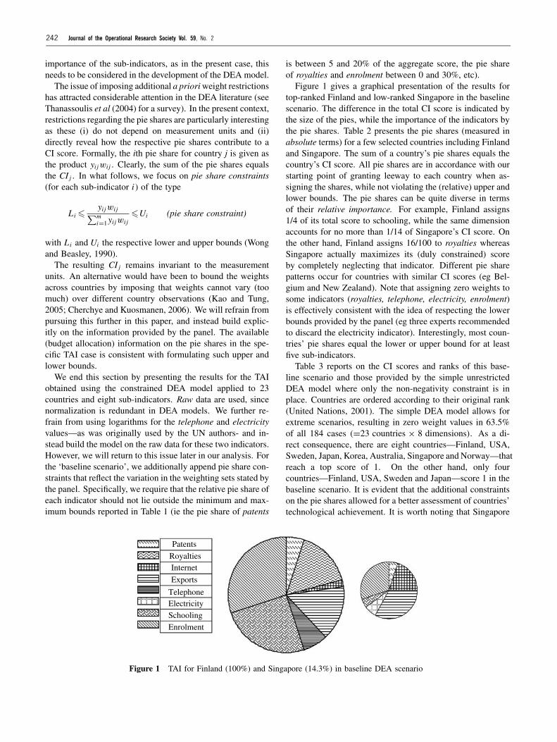
We end this section by presenting the results for the TAIobtained using the constrained DEA model applied to 23countries and eight sub-indicators. Raw data are used, sincenormalization is redundant in DEA models. We further re-frain from using logarithms for the telephone and electricityvalues—as was originally used by the UN authors- and in-stead build the model on the raw data for these two indicators.However, we will return to this issue later in our analysis. Forthe ‘baseline scenario’, we additionally append pie share con-straints that reflect the variation in the weighting sets stated bythe panel. Specifically, we require that the relative pie share ofeach indicator should not lie outside the minimum and max-imum bounds reported in Table 1 (ie the pie share of patents
Patents
RoyaltiesInternet
Exports
TelephoneElectricitySchooling
Enrolment
Figure 1 TAI for Finland (100%) and Singapore (14.3%) in baseline DEA scenario
is between 5 and 20% of the aggregate score, the pie shareof royalties and enrolment between 0 and 30%, etc).
Figure 1 gives a graphical presentation of the results fortop-ranked Finland and low-ranked Singapore in the baselinescenario. The difference in the total CI score is indicated bythe size of the pies, while the importance of the indicators bythe pie shares. Table 2 presents the pie shares (measured inabsolute terms) for a few selected countries including Finlandand Singapore. The sum of a country’s pie shares equals thecountry’s CI score. All pie shares are in accordance with ourstarting point of granting leeway to each country when as-signing the shares, while not violating the (relative) upper andlower bounds. The pie shares can be quite diverse in termsof their relative importance. For example, Finland assigns1/4 of its total score to schooling, while the same dimensionaccounts for no more than 1/14 of Singapore’s CI score. Onthe other hand, Finland assigns 16/100 to royalties whereasSingapore actually maximizes its (duly constrained) scoreby completely neglecting that indicator. Different pie sharepatterns occur for countries with similar CI scores (eg Bel-gium and New Zealand). Note that assigning zero weights tosome indicators (royalties, telephone, electricity, enrolment)is effectively consistent with the idea of respecting the lowerbounds provided by the panel (eg three experts recommendedto discard the electricity indicator). Interestingly, most coun-tries’ pie shares equal the lower or upper bound for at leastfive sub-indicators.
Table 3 reports on the CI scores and ranks of this base-line scenario and those provided by the simple unrestrictedDEA model where only the non-negativity constraint is inplace. Countries are ordered according to their original rank(United Nations, 2001). The simple DEA model allows forextreme scenarios, resulting in zero weight values in 63.5%of all 184 cases (=23 countries × 8 dimensions). As a di-rect consequence, there are eight countries—Finland, USA,Sweden, Japan, Korea, Australia, Singapore and Norway—thatreach a top score of 1. On the other hand, only fourcountries—Finland, USA, Sweden and Japan—score 1 in thebaseline scenario. It is evident that the additional constraintson the pie shares allowed for a better assessment of countries’technological achievement. It is worth noting that Singapore
L Cherchye et al—Robustness of DEA composite indicators 243
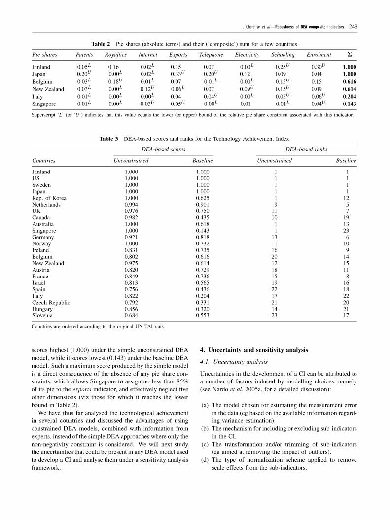
Table 2 Pie shares (absolute terms) and their (‘composite’) sum for a few countries
Pie shares Patents Royalties Internet Exports Telephone Electricity Schooling Enrolment R
Finland 0.05L 0.16 0.02L 0.15 0.07 0.00L 0.25U 0.30U 1.000Japan 0.20U 0.00L 0.02L 0.33U 0.20U 0.12 0.09 0.04 1.000Belgium 0.03L 0.18U 0.01L 0.07 0.01L 0.00L 0.15U 0.15 0.616New Zealand 0.03L 0.00L 0.12U 0.06L 0.07 0.09U 0.15U 0.09 0.614Italy 0.01L 0.00L 0.00L 0.04 0.04U 0.00L 0.05U 0.06U 0.204Singapore 0.01L 0.00L 0.03U 0.05U 0.00L 0.01 0.01L 0.04U 0.143
Superscript ‘L’ (or ‘U’) indicates that this value equals the lower (or upper) bound of the relative pie share constraint associated with this indicator.
Table 3 DEA-based scores and ranks for the Technology Achievement Index
DEA-based scores DEA-based ranks
Countries Unconstrained Baseline Unconstrained Baseline
Finland 1.000 1.000 1 1US 1.000 1.000 1 1Sweden 1.000 1.000 1 1Japan 1.000 1.000 1 1Rep. of Korea 1.000 0.625 1 12Netherlands 0.994 0.901 9 5UK 0.976 0.750 11 7Canada 0.982 0.435 10 19Australia 1.000 0.618 1 13Singapore 1.000 0.143 1 23Germany 0.921 0.818 13 6Norway 1.000 0.732 1 10Ireland 0.831 0.735 16 9Belgium 0.802 0.616 20 14New Zealand 0.975 0.614 12 15Austria 0.820 0.729 18 11France 0.849 0.736 15 8Israel 0.813 0.565 19 16Spain 0.756 0.436 22 18Italy 0.822 0.204 17 22Czech Republic 0.792 0.331 21 20Hungary 0.856 0.320 14 21Slovenia 0.684 0.553 23 17
Countries are ordered according to the original UN-TAI rank.
scores highest (1.000) under the simple unconstrained DEAmodel, while it scores lowest (0.143) under the baseline DEAmodel. Such a maximum score produced by the simple modelis a direct consequence of the absence of any pie share con-straints, which allows Singapore to assign no less than 85%of its pie to the exports indicator, and effectively neglect fiveother dimensions (viz those for which it reaches the lowerbound in Table 2).
We have thus far analysed the technological achievementin several countries and discussed the advantages of usingconstrained DEA models, combined with information fromexperts, instead of the simple DEA approaches where only thenon-negativity constraint is considered. We will next studythe uncertainties that could be present in any DEAmodel usedto develop a CI and analyse them under a sensitivity analysisframework.
4. Uncertainty and sensitivity analysis
4.1. Uncertainty analysis
Uncertainties in the development of a CI can be attributed toa number of factors induced by modelling choices, namely(see Nardo et al, 2005a, for a detailed discussion):
(a) The model chosen for estimating the measurement errorin the data (eg based on the available information regard-ing variance estimation).
(b) The mechanism for including or excluding sub-indicatorsin the CI.
(c) The transformation and/or trimming of sub-indicators(eg aimed at removing the impact of outliers).
(d) The type of normalization scheme applied to removescale effects from the sub-indicators.
244 Journal of the Operational Research Society Vol. 59, No. 2
(e) The amount of missing data and the choice of a particularimputation algorithm for replacing these missing data.
(f) The choice of the weighting scheme (eg equal weights,weights derived from a DEA-based approach, etc).
(g) The level of aggregation, if more than one level is used(eg at the indicator level or at the sub-indicator level).
(h) The choice of the aggregation scheme (eg additive aggre-gation, multiplicative aggregation, or aggregation basedon multi-criteria analysis).
All these choices may influence the countries’ CI scoresand should be taken into account before attempting anyinterpretation of the results. Saisana et al (2005) studied theuncertainties in the Technology Achievement Index, focusingon the type of normalization for the sub-indicators, the wayof eliciting information from the experts on the weight issueand the sub-indicators’ weights.
In the previous section, we discussed the use of a suit-able DEA model that incorporates expert opinion on the rel-ative importance of the different dimensions of a CI. Still,this baseline scenario is effectively characterized by specificmodelling choices. We focus on two points (see point (c) and(f) in the list above) that could introduce uncertainty in thecountries’ CI scores:
• the consideration of logarithms for telephone and electricityindicators, as applied in the original version of the TAI, and
• the weights (pie shares in our case) provided by experts,together with the corresponding pie share constraints forthe DEA model.
The remaining types of uncertainty listed above are either non-applicable or non-relevant in our case. There is no informationabout the measurement error in the data (point (a)), the typeof normalization has no impact on the results due to the units’invariance feature of DEA models (point (d)), there are nomissing data in the dataset (point (e)), and finally, the UNauthors selected one level of aggregation for the indicators inTAI (point (g)). The inclusion/exclusion of an indicator (point(b)) is already inherent in our second source of uncertainty,
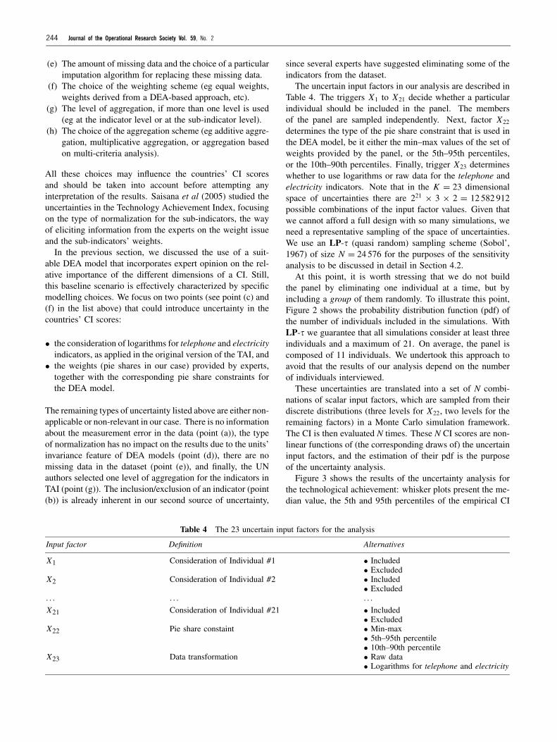
Table 4 The 23 uncertain input factors for the analysis
Input factor Definition Alternatives
X1 Consideration of Individual #1 • Included• Excluded
X2 Consideration of Individual #2 • Included• Excluded
. . . . . . . . .
X21 Consideration of Individual #21 • Included• Excluded
X22 Pie share constaint • Min-max• 5th–95th percentile• 10th–90th percentile
X23 Data transformation • Raw data• Logarithms for telephone and electricity
since several experts have suggested eliminating some of theindicators from the dataset.
The uncertain input factors in our analysis are described inTable 4. The triggers X1 to X21 decide whether a particularindividual should be included in the panel. The membersof the panel are sampled independently. Next, factor X22
determines the type of the pie share constraint that is used inthe DEA model, be it either the min–max values of the set ofweights provided by the panel, or the 5th–95th percentiles,or the 10th–90th percentiles. Finally, trigger X23 determineswhether to use logarithms or raw data for the telephone andelectricity indicators. Note that in the K = 23 dimensionalspace of uncertainties there are 221 × 3 × 2 = 12 582 912possible combinations of the input factor values. Given thatwe cannot afford a full design with so many simulations, weneed a representative sampling of the space of uncertainties.We use an LP-� (quasi random) sampling scheme (Sobol’,1967) of size N = 24 576 for the purposes of the sensitivityanalysis to be discussed in detail in Section 4.2.
At this point, it is worth stressing that we do not buildthe panel by eliminating one individual at a time, but byincluding a group of them randomly. To illustrate this point,Figure 2 shows the probability distribution function (pdf) ofthe number of individuals included in the simulations. WithLP-� we guarantee that all simulations consider at least threeindividuals and a maximum of 21. On average, the panel iscomposed of 11 individuals. We undertook this approach toavoid that the results of our analysis depend on the numberof individuals interviewed.
These uncertainties are translated into a set of N combi-nations of scalar input factors, which are sampled from theirdiscrete distributions (three levels for X22, two levels for theremaining factors) in a Monte Carlo simulation framework.The CI is then evaluated N times. These N CI scores are non-linear functions of (the corresponding draws of) the uncertaininput factors, and the estimation of their pdf is the purposeof the uncertainty analysis.
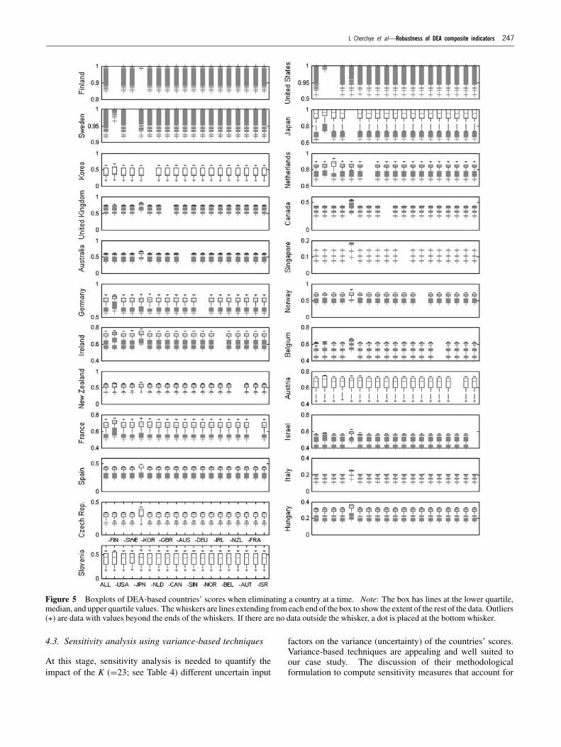
Figure 3 shows the results of the uncertainty analysis forthe technological achievement: whisker plots present the me-dian value, the 5th and 95th percentiles of the empirical CI
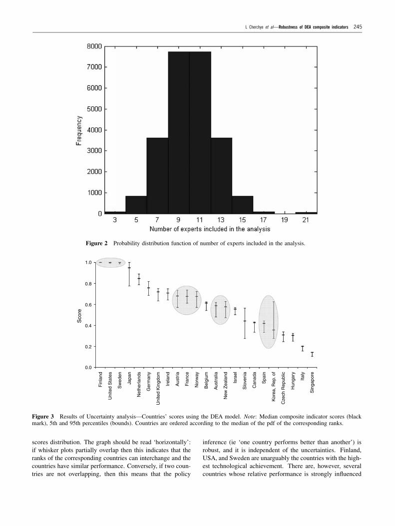
L Cherchye et al—Robustness of DEA composite indicators 245
Figure 2 Probability distribution function of number of experts included in the analysis.
Fin
land
Uni
ted
Sta
tes
Sw
eden
Japa
n
Net
herla
nds
Ger
man
y
Uni
ted
Kin
gdom
Ir
elan
d
Aus
tria
Fran
ce
Nor
way
Bel
gium
Aus
tral
ia
New
Zea
land
Isra
el
S
love
nia
Can
ada
Spa
in
Kor
ea, R
ep. o
f
Cze
ch R
epub
lic
Hun
gary
Italy
Sin
gapo
re
Sco
re
1.0
0.8
0.6
0.4
0.2
0.0
Figure 3 Results of Uncertainty analysis—Countries’ scores using the DEA model. Note: Median composite indicator scores (blackmark), 5th and 95th percentiles (bounds). Countries are ordered according to the median of the pdf of the corresponding ranks.
scores distribution. The graph should be read ‘horizontally’:if whisker plots partially overlap then this indicates that theranks of the corresponding countries can interchange and thecountries have similar performance. Conversely, if two coun-tries are not overlapping, then this means that the policy
inference (ie ‘one country performs better than another’) isrobust, and it is independent of the uncertainties. Finland,USA, and Sweden are unarguably the countries with the high-est technological achievement. There are, however, severalcountries whose relative performance is strongly influenced

246 Journal of the Operational Research Society Vol. 59, No. 2
Figure 4 Uncertainty analysis of the DEA-derived TAI scores for Korea and Slovenia.
by the assumptions in the DEA model, with the most notablebeing Korea and Slovenia. The distributions of their empiricalCI scores are plotted in Figure 4. Korea’s score can range be-tween 0.276 (5th percentile) and 0.625 (95th percentile), whilefor Slovenia the performance is estimated between 0.275 and0.564.
Going back to the overlap in the countries’ CI scores,as shown in Figure 3, an evident question is: which coun-tries have significantly different performance in technologicaldevelopment? Can we argue that France (median score =0.676) performs better than Norway (0.675), or that Canada’slevel of technological achievement (0.426) is superior to thatof Spain (0.420)? An hypothesis test could provide the an-swer. We applied the Wilcoxon signed rank test on the mediandifferences in paired TAI scores. The test, also known as theWilcoxon matched pairs test, is the non-parametric equivalentof the paired t-test (see Conover, 1980). The assumption thatthe differences follow a normal distribution (as needed for thet-test) was not confirmed in our case. In contrast, the only as-sumption required for the Wilcoxon test, that the distributionof the differences is symmetric, was confirmed. Applying thistest we identify four groups of countries for which no distinc-tion can be made in terms of their technological achievementlevel. The groups are shaded in grey in Figure 3. The firstgroup contains the top three performing countries Finland(1.000), USA (1.000) and Sweden (1.000). The second groupis composed of Austria (0.680), France (0.676) and Norway(0.675). Australia (0.587) and New Zealand (0.576) belong tothe third group. Finally, Slovenia (0.443) and Canada (0.426)belong to the fourth group. Note that, although the medianscore for Spain is 0.420, which is very close to that of Canada(0.426), the performance of the two countries can be clearlydistinguished.
We next complement our uncertainty analysis with a sen-sitivity analysis. We first investigate sensitivity of the coun-tries’ scores with respect to outlier countries that define the
frontier of the DEA model. We then use variance-based tech-niques to apportion the variance in the countries’ scores tothe two major sources of uncertainty in our analysis.
4.2. Sensitivity analysis due to outlier countries
Procedures that randomly omit some observations (in our casecountries; for example one randomly excludes one country ata time) have been suggested in the DEA literature as a wayto correct for the impact of outlier observations (eg Wilson,1995; Cazals et al, 2002; Simar, 2003). To assess such animpact on the countries’ scores, we have repeated the MonteCarlo approach described above, after eliminating one coun-try at a time from the set of 23 countries. The N = 24 576CI scores are estimated for each group of 22 countries. Thecorresponding box plots are presented in Figure 5. The left-most box plot in each graph represents the CI score distribu-tion that is obtained for the given country when using the fullsample of countries (compare with Figure 3); the followingbox plots (left to right) represent the CI distribution obtainedafter eliminating one country from the sample, starting fromFinland (second box plot), USA (third box plot) to France(penultimate box plot) and Israel (final, rightmost box plot).The two countries that have the greatest impact on the coun-tries’ scores are Japan and Finland. When Japan is elimi-nated from the set, the countries that improve their score are:Finland, United Kingdom, Australia, Ireland, Spain, CzechRepublic, Canada, Singapore, Norway, Belgium, Israel, Italyand Hungary. When Finland is eliminated from the set, thecountries that improve their score are: Sweden, United States,Korea, Germany, France, and to a lesser degree Japan. Elimi-nating any of the remaining countries does not have a notableimpact on the countries’ scores. This result suggests that, forthis application, the DEA model is quite robust with respectto outlier observations. Consequently, we do not explicitlyaccount for outlier countries in the remaining analysis.
L Cherchye et al—Robustness of DEA composite indicators 247
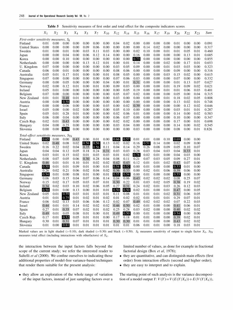
Figure 5 Boxplots of DEA-based countries’ scores when eliminating a country at a time. Note: The box has lines at the lower quartile,median, and upper quartile values. Thewhiskers are lines extending from each end of the box to show the extent of the rest of the data. Outliers(+) are data with values beyond the ends of the whiskers. If there are no data outside the whisker, a dot is placed at the bottom whisker.
4.3. Sensitivity analysis using variance-based techniques
At this stage, sensitivity analysis is needed to quantify theimpact of the K (=23; see Table 4) different uncertain input
factors on the variance (uncertainty) of the countries’ scores.Variance-based techniques are appealing and well suited toour case study. The discussion of their methodologicalformulation to compute sensitivity measures that account for
248 Journal of the Operational Research Society Vol. 59, No. 2
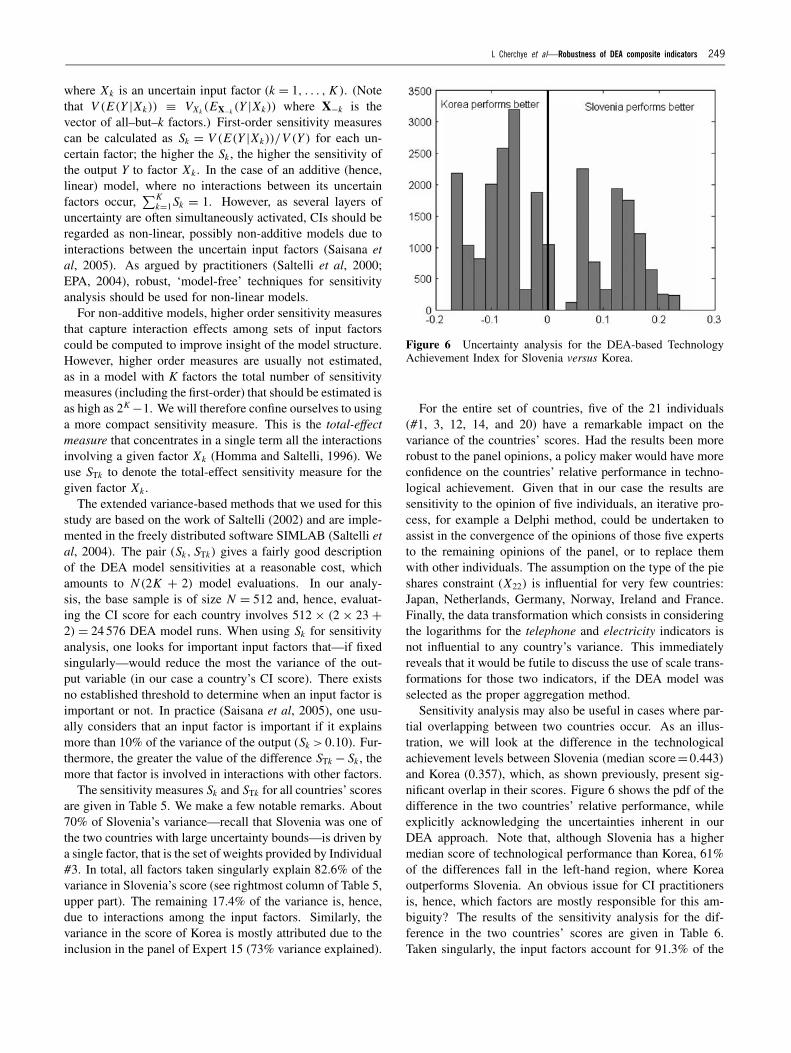
Table 5 Sensitivity measures of first order and total effect for the composite indicators scores
Marked values are in light shaded (> 0.10), dark shaded (> 0.30) and black (> 0.50). Sk measures sensitivity of output to single factor Xk , STkmeasures total effect (including interactions with otherfactors) of Xk .
the interaction between the input factors falls beyond thescope of the current study; we refer the interested reader toSaltelli et al (2000). We confine ourselves to indicating thoseadditional properties of model-free variance-based techniquesthat render them suitable for the present analysis:
• they allow an exploration of the whole range of variationof the input factors, instead of just sampling factors over a
limited number of values, as done for example in fractionalfactorial design (Box et al, 1978);
• they are quantitative, and can distinguish main effects (firstorder) from interaction effects (second and higher order);
• they are easy to interpret and to explain.
The starting point of such analysis is the variance decomposi-tion of a model output Y: V (Y )=V (E(Y |Xk))+E(V (Y |Xk)),
L Cherchye et al—Robustness of DEA composite indicators 249
where Xk is an uncertain input factor (k = 1, . . . , K ). (Notethat V (E(Y |Xk)) ≡ VXk (EX−k (Y |Xk)) where X−k is thevector of all–but–k factors.) First-order sensitivity measurescan be calculated as Sk = V (E(Y |Xk))/V (Y ) for each un-certain factor; the higher the Sk , the higher the sensitivity ofthe output Y to factor Xk . In the case of an additive (hence,linear) model, where no interactions between its uncertainfactors occur,
∑Kk=1Sk = 1. However, as several layers of
uncertainty are often simultaneously activated, CIs should beregarded as non-linear, possibly non-additive models due tointeractions between the uncertain input factors (Saisana etal, 2005). As argued by practitioners (Saltelli et al, 2000;EPA, 2004), robust, ‘model-free’ techniques for sensitivityanalysis should be used for non-linear models.
For non-additive models, higher order sensitivity measuresthat capture interaction effects among sets of input factorscould be computed to improve insight of the model structure.However, higher order measures are usually not estimated,as in a model with K factors the total number of sensitivitymeasures (including the first-order) that should be estimated isas high as 2K −1. We will therefore confine ourselves to usinga more compact sensitivity measure. This is the total-effectmeasure that concentrates in a single term all the interactionsinvolving a given factor Xk (Homma and Saltelli, 1996). Weuse STk to denote the total-effect sensitivity measure for thegiven factor Xk .
The extended variance-based methods that we used for thisstudy are based on the work of Saltelli (2002) and are imple-mented in the freely distributed software SIMLAB (Saltelli etal, 2004). The pair (Sk, STk) gives a fairly good descriptionof the DEA model sensitivities at a reasonable cost, whichamounts to N (2K + 2) model evaluations. In our analy-sis, the base sample is of size N = 512 and, hence, evaluat-ing the CI score for each country involves 512 × (2 × 23 +2) = 24 576 DEA model runs. When using Sk for sensitivityanalysis, one looks for important input factors that—if fixedsingularly—would reduce the most the variance of the out-put variable (in our case a country’s CI score). There existsno established threshold to determine when an input factor isimportant or not. In practice (Saisana et al, 2005), one usu-ally considers that an input factor is important if it explainsmore than 10% of the variance of the output (Sk > 0.10). Fur-thermore, the greater the value of the difference STk − Sk , themore that factor is involved in interactions with other factors.
The sensitivity measures Sk and STk for all countries’ scoresare given in Table 5. We make a few notable remarks. About70% of Slovenia’s variance—recall that Slovenia was one ofthe two countries with large uncertainty bounds—is driven bya single factor, that is the set of weights provided by Individual#3. In total, all factors taken singularly explain 82.6% of thevariance in Slovenia’s score (see rightmost column of Table 5,upper part). The remaining 17.4% of the variance is, hence,due to interactions among the input factors. Similarly, thevariance in the score of Korea is mostly attributed due to theinclusion in the panel of Expert 15 (73% variance explained).
Figure 6 Uncertainty analysis for the DEA-based TechnologyAchievement Index for Slovenia versus Korea.
For the entire set of countries, five of the 21 individuals(#1, 3, 12, 14, and 20) have a remarkable impact on thevariance of the countries’ scores. Had the results been morerobust to the panel opinions, a policy maker would have moreconfidence on the countries’ relative performance in techno-logical achievement. Given that in our case the results aresensitivity to the opinion of five individuals, an iterative pro-cess, for example a Delphi method, could be undertaken toassist in the convergence of the opinions of those five expertsto the remaining opinions of the panel, or to replace themwith other individuals. The assumption on the type of the pieshares constraint (X22) is influential for very few countries:Japan, Netherlands, Germany, Norway, Ireland and France.Finally, the data transformation which consists in consideringthe logarithms for the telephone and electricity indicators isnot influential to any country’s variance. This immediatelyreveals that it would be futile to discuss the use of scale trans-formations for those two indicators, if the DEA model wasselected as the proper aggregation method.
Sensitivity analysis may also be useful in cases where par-tial overlapping between two countries occur. As an illus-tration, we will look at the difference in the technologicalachievement levels between Slovenia (median score=0.443)and Korea (0.357), which, as shown previously, present sig-nificant overlap in their scores. Figure 6 shows the pdf of thedifference in the two countries’ relative performance, whileexplicitly acknowledging the uncertainties inherent in ourDEA approach. Note that, although Slovenia has a highermedian score of technological performance than Korea, 61%of the differences fall in the left-hand region, where Koreaoutperforms Slovenia. An obvious issue for CI practitionersis, hence, which factors are mostly responsible for this am-biguity? The results of the sensitivity analysis for the dif-ference in the two countries’ scores are given in Table 6.Taken singularly, the input factors account for 91.3% of the
250 Journal of the Operational Research Society Vol. 59, No. 2
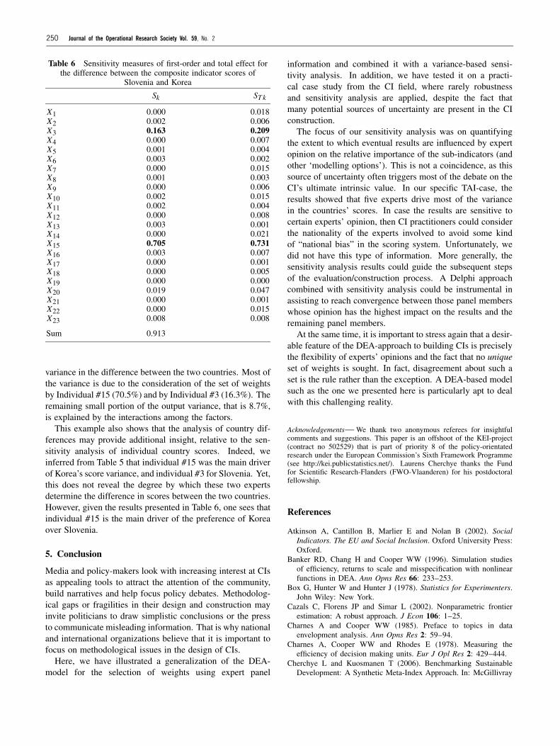
Table 6 Sensitivity measures of first-order and total effect forthe difference between the composite indicator scores of
Slovenia and Korea
Sk ST k
X1 0.000 0.018X2 0.002 0.006X3 0.163 0.209X4 0.000 0.007X5 0.001 0.004X6 0.003 0.002X7 0.000 0.015X8 0.001 0.003X9 0.000 0.006X10 0.002 0.015X11 0.002 0.004X12 0.000 0.008X13 0.003 0.001X14 0.000 0.021X15 0.705 0.731X16 0.003 0.007X17 0.000 0.001X18 0.000 0.005X19 0.000 0.000X20 0.019 0.047X21 0.000 0.001X22 0.000 0.015X23 0.008 0.008
Sum 0.913
variance in the difference between the two countries. Most ofthe variance is due to the consideration of the set of weightsby Individual #15 (70.5%) and by Individual #3 (16.3%). Theremaining small portion of the output variance, that is 8.7%,is explained by the interactions among the factors.
This example also shows that the analysis of country dif-ferences may provide additional insight, relative to the sen-sitivity analysis of individual country scores. Indeed, weinferred from Table 5 that individual #15 was the main driverof Korea’s score variance, and individual #3 for Slovenia. Yet,this does not reveal the degree by which these two expertsdetermine the difference in scores between the two countries.However, given the results presented in Table 6, one sees thatindividual #15 is the main driver of the preference of Koreaover Slovenia.
5. Conclusion
Media and policy-makers look with increasing interest at CIsas appealing tools to attract the attention of the community,build narratives and help focus policy debates. Methodolog-ical gaps or fragilities in their design and construction mayinvite politicians to draw simplistic conclusions or the pressto communicate misleading information. That is why nationaland international organizations believe that it is important tofocus on methodological issues in the design of CIs.
Here, we have illustrated a generalization of the DEA-model for the selection of weights using expert panel
information and combined it with a variance-based sensi-tivity analysis. In addition, we have tested it on a practi-cal case study from the CI field, where rarely robustnessand sensitivity analysis are applied, despite the fact thatmany potential sources of uncertainty are present in the CIconstruction.
The focus of our sensitivity analysis was on quantifyingthe extent to which eventual results are influenced by expertopinion on the relative importance of the sub-indicators (andother ‘modelling options’). This is not a coincidence, as thissource of uncertainty often triggers most of the debate on theCI’s ultimate intrinsic value. In our specific TAI-case, theresults showed that five experts drive most of the variancein the countries’ scores. In case the results are sensitive tocertain experts’ opinion, then CI practitioners could considerthe nationality of the experts involved to avoid some kindof “national bias” in the scoring system. Unfortunately, wedid not have this type of information. More generally, thesensitivity analysis results could guide the subsequent stepsof the evaluation/construction process. A Delphi approachcombined with sensitivity analysis could be instrumental inassisting to reach convergence between those panel memberswhose opinion has the highest impact on the results and theremaining panel members.
At the same time, it is important to stress again that a desir-able feature of the DEA-approach to building CIs is preciselythe flexibility of experts’ opinions and the fact that no uniqueset of weights is sought. In fact, disagreement about such aset is the rule rather than the exception. A DEA-based modelsuch as the one we presented here is particularly apt to dealwith this challenging reality.
Acknowledgements—We thank two anonymous referees for insightfulcomments and suggestions. This paper is an offshoot of the KEI-project(contract no 502529) that is part of priority 8 of the policy-orientatedresearch under the European Commission’s Sixth Framework Programme(see http://kei.publicstatistics.net/). Laurens Cherchye thanks the Fundfor Scientific Research-Flanders (FWO-Vlaanderen) for his postdoctoralfellowship.
References
Atkinson A, Cantillon B, Marlier E and Nolan B (2002). SocialIndicators. The EU and Social Inclusion. Oxford University Press:Oxford.
Banker RD, Chang H and Cooper WW (1996). Simulation studiesof efficiency, returns to scale and misspecification with nonlinearfunctions in DEA. Ann Opns Res 66: 233–253.
Box G, Hunter W and Hunter J (1978). Statistics for Experimenters.John Wiley: New York.
Cazals C, Florens JP and Simar L (2002). Nonparametric frontierestimation: A robust approach. J Econ 106: 1–25.
Charnes A and Cooper WW (1985). Preface to topics in dataenvelopment analysis. Ann Opns Res 2: 59–94.
Charnes A, Cooper WW and Rhodes E (1978). Measuring theefficiency of decision making units. Eur J Opl Res 2: 429–444.
Cherchye L and Kuosmanen T (2006). Benchmarking SustainableDevelopment: A Synthetic Meta-Index Approach. In: McGillivray

L Cherchye et al—Robustness of DEA composite indicators 251
M and Clarke M (eds). Understanding Human Well-being. UnitedNations University Press: Tokyo, pp 139–168.
Cherchye L, Moesen W and Van Puyenbroeck T (2004).Legitimately diverse yet comparable: On synthesizing socialinclusion performance in the EU. J Common Market Stud 42:919–955.
Cherchye L, Knox Lowell CA, Moesen W and Van PuyenbroeckT (2007). One market, one number? A composite indicatorassessment of EU internal market dynamics. Eur Econ Rev 51:749–779.
Conover WJ (1980). Practical Nonparametric Statistics. John Wiley:New York.
Cooper WW, Seiford L and Tone K (2000). Data EnvelopmentAnalysis. Kluwer Academic Publishers: Boston.
Cooper WW, Shanling L, Seiford LM and Zhu J (2004). Sensitivityanalysis in DEA. In: Cooper WW, Seiford LM and Zhu J(eds). Handbook on Data Envelopment Analysis. Kluwer AcademicPublishers: Boston, pp 75–97.
Desai M, Fukuda-Parr S, Johansson C and Sagasti F (2002).Measuring the technology achievement of nations and the capacityto participate in the network age. J Human Dev 3: 95–122.
Despotis DK (2005). A reassessment of the human development indexvia data envelopment analysis. J Opl Res Soc 56: 969–980.
EPA (2004). Council for Regulatory Environmental Modeling,‘Draft Guidance on the Development, Evaluation, andApplication of Regulatory Environmental Models’, http://www.epa.gov/osp/crem/library/CREM%20Guidance%20Draft%2012 03.pdf.
European Commission (2004). The EU Economy Review 2004.European Economy, vol. 6, Office for Official Publications of theEC: Luxembourg.
European Commission (2005). European innovation scoreboard2005—Comparative analysis of innovation performance, http://trendchart.cordis.lu/scoreboards/scoreboard2005/pdf/EIS%202005.pdf.
Freudenberg M (2003). Composite indicators of country performance:A critical assessment, STI Working Paper 2003/16, OECD, Paris.
Homma T and Saltelli A (1996). Importance measures in globalsensitivity analysis of nonlinear models. Reliab Eng Syst Safety 52:1–17.
Kao C and Tung HT (2005). Data envelopment analysis with commonweights: The compromise solution approach. J Opl Res Soc 56:1196–1203.
Mahlberg B and Obersteiner M (2001). Remeasuring the HDIby data envelopment analysis. IIASA interim report IR-01-069,Luxemburg.
Munda G and Nardo M (2003). On the methodological foundationsof composite indicators used for ranking countries. Mimeo,Universitat Autonoma de Barcelona.
Nardo M, Saisana M, Saltelli A and Tarantola S (2005a). Toolsfor composite indicators building. EUR 21682 EN, EuropeanCommission-Joint Research Centre.
Nardo M, Saisana M, Saltelli A, Tarantola S, Hoffman A andGiovannini E (2005b). Handbook on constructing compositeindicators: methodology and user’s guide, OECD StatisticsWorking Paper, JT00188147.
Saisana M, Saltelli A and Tarantola S (2005). Uncertainty andsensitivity analysis techniques as tools for the quality assessmentof composite indicators. J Roy Stat Soc 168: 307–323.
Saltelli A (2002). Making best use of model evaluations to computesensitivity indices. Comput Phys Commu 145: 280–297.
Saltelli A, Chan K and Scott M (2000). Sensitivity Analysis.Probability and Statistics Series, John Wiley & Sons: New York.
Saltelli A, Tarantola S, Campolongo F and Ratto M (2004). SensitivityAnalysis in Practice. A Guide to Assessing Scientific Models.Wiley: England.
Simar L (2003). Detecting outliers in frontier models: A simpleapproach. J Prod Anal 20: 391–424.
Simar L and Wilson P (1998). Sensitivity of efficiency scores: Howto bootstrap in Nonparametric frontier models. Mngt Sci 44:49–61.
Sobol IM (1967). On the distribution of points in a cube and theapproximate evaluation of integrals. USSR Comput Math Phys 7:86–112.
Storrie D and Bjurek H (2000). Benchmarking European labourmarket performance with efficiency frontier techniques, CELMSDiscussion paper, Goteborg University.
Thanassoulis E, Portela MC and Allen R (2004). Incorporating valuejudgments in DEA. In: Cooper WW, Seiford LM and Zhu J(eds). Handbook on Data Envelopment Analysis. Kluwer AcademicPublishers: Dordrecht, pp 99–138.
United Nations (2001). Annex 2.1: The technology achievementindex: A new measure of countries’ ability to participate in thenetwork age.Human Development Report, Oxford University Press:United Kingdom, http://www.undp.org.
Valdmanis V (1992). Sensitivity analysis for DEA models: Anempirical example using public vs. NFP hospitals. J Public Econ48: 185–205.
Wilson PW (1995). Detecting influential observations in dataenvelopment analysis. J Prod Anal 6: 27–46.
Wong Y-HB and Beasley JE (1990). Restricting weight flexibility indata envelopment analysis. J Opl Res Soc 47: 136–150.
Received January 2006;accepted April 2007 after three revisions