Contracting For Educational Achievement Maria Marta Ferreyra Pierre Jinghong Liang Carnegie Mellon University Carnegie Mellon University

January 29, 20091

Very Preliminary and Incomplete

Please Do Not Cite Without Permission

Abstract We argue that the lack of academic proficiency in K-12 education is due to information asymmetry between the policy-maker, households, and schools. The policy-maker is thus unable to write down efficient contracts to ensure proficiency, and must incur agency costs which, in turn, generate other distortions. We develop a theoretical equilibrium model where schools and households choose their efforts in response to the policy-maker’s incentives. We model public schools as one possible response to informational failures. Unlike private schools, public schools separate the roles of financing and consuming education, thus creating rents for public schools. We develop a computational version of the model that allows us to illustrate the distortions and effects from alternative contracts.

1 We thank the Berkman Faculty Development Fund at Carnegie Mellon for financial support. We are grateful to Jane Cooley, Dennis Epple, David Figlio, Randy Reback, Rich Romano and Patrick Wolf for helpful conversations and comments. We also benefited from comments from session participants at the 2008 AEFA conference, the 2008 APPAM Fall conference, and the 2009 Winter meetings of the Econometric Society. Andrea Cinkovic and Abby Clay Turner provided excellent research assistance, and Jeff Reminga assisted us with the computational aspects of the project. All errors are ours.

1. Introduction

An educated population is a fundamental ingredient for a well-functioning democracy as

well as a key driver for growth in the modern economy. Thus, education has both private

returns that accrue to the individual, and public returns that accrue to society. For this

reason, the policy-maker often has a minimum goal of basic academic proficiency for

every student in the economy. While some households invest in their children’s education

and meet the policy-maker’s goal, others do not. Therefore, the educational achievement

of some children is lower than the policy-maker’s desired minimum, even after policy

interventions in the marketplace for education such as the establishment and funding of

public schools.

In this paper we focus on an information-based explanation for academic

achievement, namely the contracting frictions due to the information asymmetry among

the policy-maker, households, and schools. In consonance with the No Child Left Behind

legislation, we focus on a policy-maker who sets an achievement floor for every student

in the population. If the policy-maker were able to observe all the relevant information –

for instance, household income, students’ ability, schools’ productivity, students’ and

schools’ effort - he would achieve his goal by providing the exact incentives to

households and schools. In other words, he would be able to write down efficient, first-

best contracts. In reality, however, the policy-maker only has imperfect information, and

can only write down inefficient contracts. For instance, since he cannot observe schools’

effort he must contract with schools based on some indirect signal of effort, such as

enrollment count. A contract based on enrollment count is likely a poor substitute for a

contract based on school effort.

Relative to efficient contracts, these inefficient arrangements are necessarily more

costly. In addition, these inefficient arrangements have the potential to trigger other,

unintended effects when they are implemented large-scale. For example, a mechanism

that rewards public schools proportionally to their enrollment gives them no direct

incentive to exert high effort. Low school effort will directly hurt public school students.

Moreover, some students may switch into private schools to obtain higher school effort.

If these students are the most motivated and able, the quality of the student body at public

2

schools will suffer, which may further hurt the performance of public school students. In

other words, these contracts not only affect the behavior of the immediate parties, but

also have equilibrium effects. These equilibrium effects may hinder the primary goal of

the policy-maker when designing the contract.

Hence, in this paper we develop a theoretical model of student achievement,

school quality, and household choice of schools, that relies on a contracting approach and

is embedded in an equilibrium framework. We develop a computational version of the

model, and use it to simulate alternative contracts. Information asymmetry is at the root

of other economic problems facing policy-makers and market participants, such as the

regulation of natural monopolies, and managerial contracts in corporate settings.2 While

researchers have used a contracting framework to study these problems, they have not

done so for education. In contrast, we adopt this framework because it allows us to study

the consequences of inefficient contracting on the behavior of households, schools, and

teachers. This helps us compare alternative policies that seek to address the

underachievement problem, and informs the design of more efficient mechanisms. This

perspective will yield more insights of theoretical and policy interest as we add

institutional features to the basic framework that we have currently developed.

In our model, we assume that the production of achievement requires two inputs -

school and household effort- and that it is increasing in the school’s peer quality, defined

as the school’s average student ability. Importantly, we assume that school and household

effort are complementary. This means that if a student attends a school that provides low

effort, she will optimally choose to provide low effort as well. We start our analysis by

considering an economy in which all students attend private schools, and all households

can observe the effort exerted by all the schools. The fact that households can observe

school effort subjects private schools to market discipline – if they try to extract rents,

free-entry will force them out of the market. Left to their own devices, households with

low income and/or ability consume too low a school effort, provide too low a student

effort, and fall short of the policy-maker’s goal. If the policy-maker knew the income and

ability of each household, he would be able to provide it with the exact subsidy to induce

2 See, for instance, Laffont and Tirole (1983), and Laffont and Martimort (2002).

3

it to choose the school and student effort that meet the policy-maker’s goal. While the

attainment of this goal would come at the cost of income redistribution among

households, the subsidies would be economically efficient in the sense that the funds

involved would only be used to enhance the achievement of the underperforming

households. This perfect-information solution can be viewed as efficient, first-best

contracting.

Since the informational requirements needed to attain the efficient solution are

very high, we then turn to cases with lower, more realistic informational requirements.

For instance, the policy-maker may only know the range of the income and ability

distributions across households. Thus, the first informational asymmetry we analyze is

between the policy-maker and the households. In this case, the policy-maker can procure

a fixed level of school effort and make it available to all interested households for free. In

this arrangement, the effort supplied is exactly the level needed by the lowest-performing

household to reach the policy-maker’s desired minimum achievement. While this

solution achieves the policy objective at a lower informational requirement, it is

necessarily more costly than the efficient solution. This is because households other than

the lowest-performing can now choose between a private school and a publicly funded

school effort. Moreover, the policy-maker can pool all the students that take up his offer

of a fixed school effort in one single school. This mixing benefits low-ability students by

exposing them to higher-ability peers. In so doing, it lowers the fiscal cost of raising

achievement for the low-performing segment because some school effort can be

substituted for peer quality, thus reducing the demand for school effort. The mixing,

however, hurts high-ability students. In addition, the entry and formation of public

schools is decided by the policy-maker, not the market. Hence, public schools are not

subject to market discipline as private schools are.

Besides lacking information on the households, the policy-maker may also lack

information on the schools. Since the policy-maker does not consume education, he does

not observe the actual effort provided by public schools. This is akin to the classic

incentive problem in government procurements (Laffont and Tirole 1993). Thus, the

policy-maker designs procurement contracts that rely on variables related to school

effort, but not on school effort directly. For instance, he may set up a contract with the

4

school to pay a fixed amount per child enrolled.3 This type of contract not only gives too

much or too little school effort to some households relative to the amount they need in

order to meet the achievement target, but also gives public schools incentives to extract

rents and under-provide effort. This perverse incentive is aggravated by the fact that

public schools are not subject to market discipline, and that some households who might

want to switch into private schools do not have the means to do so. Low public school

effort will lead public school students to provide low effort as well, further aggravating

the problem.

A number of mechanisms have been debated and/or implemented in order to

address the inefficiency of this contract. Broadly speaking, these mechanisms rely either

on contracts, or on markets, or on a combination of both. For instance, public school

accountability relies on contracts, private school vouchers rely on markets, and private

school vouchers for children attending public schools of poor performance rely on both.

In our computational study we simulate and compare some of these mechanisms. An

important finding from our simulations is that given the pervasiveness of the

informational problem, a combination of contracts and markets may be more effective

than any of these mechanisms alone. In other words, contracts and markets work best

when used as complements rather than substitutes.4

Throughout we make the following contributions. First, we explicitly model

household and school effort. While school effort and/or public school rent-seeking

behavior have been modeled before (Chakrabarti 2007, McMillan 2003, Neal and

Schanzenbach 2007), student effort has not. If student and school effort are indeed

complementary, omitting student effort leads to underestimating the total impact of an

increase in school effort because of its multiplier effect on household effort. Second, we

are the first to address theoretically the issues introduced by information asymmetry

between the policy-maker and the schools and households, and to theoretically

investigate the trade-offs involved in alternative policies aimed at attenuating these

3 For children enrolled in private schools, this contract takes the form of a universal voucher. Depending on the voucher amount, the policy-maker may or may not be able to attain the desired achievement for all students. In this type of voucher program, some households may receive too low or too high a voucher relative to their needs, yet competition among private schools ensures the efficient use of the voucher provided households can observe private school effort. 4 See Neal (2008) for further discussion of this issue.

5

issues. We do so by adopting a contracting framework. Third, because the existence of

public schools may itself be viewed as a response to the underachievement problem, we

do not simply assume that public schools exist in the economy; rather, we motivate them

through informational arguments and analyze settings in which either they do not exist, or

coexist with private schools. Fourth, our contracting setup is embedded in an equilibrium

framework, where students sort across public and private schools, households and

schools choose effort, and school qualities and fiscal costs are determined endogenously.

Since the nature of this model limits our ability to study it analytically, we develop a

computational version that enables us to quantify the relevant trade-offs of alternative

contracts.

Findings from our preliminary simulations suggest that a combination of contracts

and markets may be more successful than any of these tools alone. If the policy-maker is

committed to the existence of public schools, accountability-based contracts are needed

to raise public school effort. Our findings also suggest that when public schools are risk-

averse, a higher noisiness in achievement tests can actually raise their effort.

However, in our simulations the effectiveness of public school accountability is

limited, because the very existence of public schools separates the roles of consuming

and financing education. Private school vouchers re-unite these roles, by giving

households -who directly consume education- the means to pay for it. Nonetheless,

private school vouchers are not necessarily efficient. If parents cannot observe private

school effort, then private schools enjoy an informational rent. The less able the parent is

to monitor the school, the greater the rent enjoyed by the school. If, as is plausible,

parents of lowest-performing children are the least able to monitor school effort, then part

of their vouchers will simply provide rents to private schools unless private schools are

held accountable. In other words, a combination of contracts and markets in public and

private schools may be needed in the presence of pervasive asymmetric information

among the parties.

The remainder of this paper is organized as follows: section 2 presents the model,

and section 3 describes the computational version and results. Section 4 concludes and

describes extensions to our basic framework.

6

2. The Model

Our objective in this section is to illustrate the basic trade-offs faced by the policy-maker.

We begin by analyzing a benchmark economy, where all households attend private

schools. Left to their own devices, some households in this economy do not attain the

target achievement. We then analyze a variety of settings which differ in the

informational constraints faced by the policy-maker. These, in turn, shape the set of

available incentives for schools and households and the cost of attaining the desired goal.

Private School Benchmark

In the model, the economy is populated by a continuum of households. Each household

has one child who must go to school. All schools are private; we describe private schools

in further detail below. Households are heterogeneous in income, y, and child ability, μ.

There are a finite number of income types, I, and also a finite number of ability types, M.

Thus, there are household types, each one representing an (income, ability)

combination. Without loss of generality, we assume that each type exists with measure

one. Hence, the total measure of households in the economy equals H. Parents and

students form a single decision-making unit, the household. We refer to parents,

households, and students interchangeably.

H I M= ×

Household preferences are described by the following utility function:

(1) 2

2aU c sβ

μ= −

where c is numeraire consumption, s is school achievement, a is household effort spent in

generating achievement (the production of achievement is described below), and 0β > .5

Notice that households suffer disutility from exerting effort, and this disutility is related

to their ability. Thus, effort is more costly for lower μ (i.e., lower ability) households.

Households seek to maximize utility (1) subject to the following budget constraint:

(2) y c T= +

5 We normalize the coefficient on school achievement in the utility function to one to facilitate the calculations. Changing this coefficient simply amounts to re-scaling the other parameters.

7

where T is school tuition.

The production of child achievement, s, is as follows:

(3) 1 2s e q aη η=

where e is teacher effort at the school, q is the school’s peer quality (defined as the

school’s average ability), and 1 2, 0η η > . Because the inputs in the production of

achievement are complementary, a household will exert greater effort when attending a

school where teachers work more, and where the other students are more able.

Teachers derive utility from salary W, and disutility from effort e. Since the

teacher labor market is competitive, for a given effort teachers are paid a salary which

leaves them indifferent between working and not. Thus:

(4) W Aeλ=

where A is a monotonic transformation of teacher reservation utility, and λ > 1. Note that

the marginal cost of teacher effort is positive and increasing. All schools in the economy

hire teachers from the same pool and pay the same price for a given amount of effort.

Private schools are competitive firms that set admission criteria and cater to

specific household types. While a private school would like to attract the highest possible

income and ability types, free entry guarantees that these households can always find a

provider that caters to them exclusively. In equilibrium, these households attend a school

where all the students come from the same household type. Since the argument applies to

each household type, it follows that in equilibrium, a private school formed by

households of ability μ has q = μ. Within a given private school, all households pay the

same tuition, equal to the market salary of a teacher who provides the effort level that is

optimal for the household. That is, a household chooses a school that offers the level of

school effort e which maximizes the household utility (1) subject to the budget constraint

(2), the production function (3), and the condition T = W(e). The optimal choices of

household effort, school effort, and household consumption are related as follows:

(5) 2 1i i i ia c q eη ηβ

iμ=

(6) ( ) 1 ii i

cT e Aeλ ηβλ

= =

Equation (5) results from the complementarities in achievement production, and shows

that a household attending a school that exerts greater effort and has higher peer quality

8

will choose to exert higher effort. In addition, a more able household will choose to exert

greater effort as well.

Incorporating the budget constraint allows us to solve for the optimal choices as

follows:

(7) 1

i ic yβλβλ η

=+

(8) 1

1i iT yη

η βλ=

+

(9) ( )

1

1

1i ie y

A

ληη βλ

⎛ ⎞= ⎜ ⎟⎜ ⎟+⎝ ⎠

(10) ( )

1

2 1

1 1i i i i ia q y y

A

ηβ λ

η ηβλμβλ η η βλ

⎛ ⎞⎛ ⎞= ⎜ ⎟⎜ ⎟ ⎜ ⎟+ +⎝ ⎠ ⎝ ⎠

Notice that optimal consumption and tuition (and hence school effort) are proportional to

household income yet do not depend on household ability, whereas optimal household

effort depends (positively) on household income and ability.6 The achievement resulting

from these optimal choices is as follows:

(11) ( )

1

2

2

2 1

1 1i i i i is q y y

A

ηβ λ

η ηβλμβλ η η βλ

⎛ ⎞⎛ ⎞= ⎜ ⎟⎜ ⎟ ⎜ ⎟+ +⎝ ⎠ ⎝ ⎠

An equilibrium in this model is a partition of the population into private schools,

and a vector of private school qualities, such that private schools achieve zero profits, the

teacher market clears, and households cannot gain utility by changing schools or

household effort.

As (11) makes clear, the achievement of a household depends on its income,

ability, and school peer quality. In what follows we assume that the policy-maker’s goal

is that every household attains at least a minimum achievement equal to s .7 Our choice

6 The reason ability does not enter into consumption or tuition spending is that household effort does not enter into the household’s budget constraint. In a more general model, ability affects consumption and tuition if households must choose between working to generate income and working to improve their achievement. 7 Alternative objective functions, of course, are possible for the policy-maker. For instance, he might wish to maximize the aggregate future income of the economy, which is related to current student achievement, or he might wish to maximize aggregate welfare. See Costrell (1994) for an analysis of standard-setting

9

of objective function is inspired by the No Child Left Behind legislation, whose goal is

that every child be proficient by the school year 2013/14. It is possible, particularly for

sufficiently high levels of s , that some households do not reach the desired threshold,

either because their income, or their ability, or their school peer quality is not sufficiently

high.8 We assume that s is such that at least one household type does not meet the

threshold in the private school benchmark.

Faced with the problem that is < s for some households, the policy-maker must

devise a mechanism to induce the under performing households to attain an achievement

of at least s . In a totalitarian regime, the policy-maker could simply force these

households to purchase the right amount of school effort, and to produce the right amount

of household effort, in order to meet the threshold. In a free society, however, the policy-

maker must provide economic incentives for households to rationally choose to meet the

threshold. Given that the socially optimal achievement is greater than the private

optimum for the underperforming households, the policy-maker must subsidize their

production of achievement.

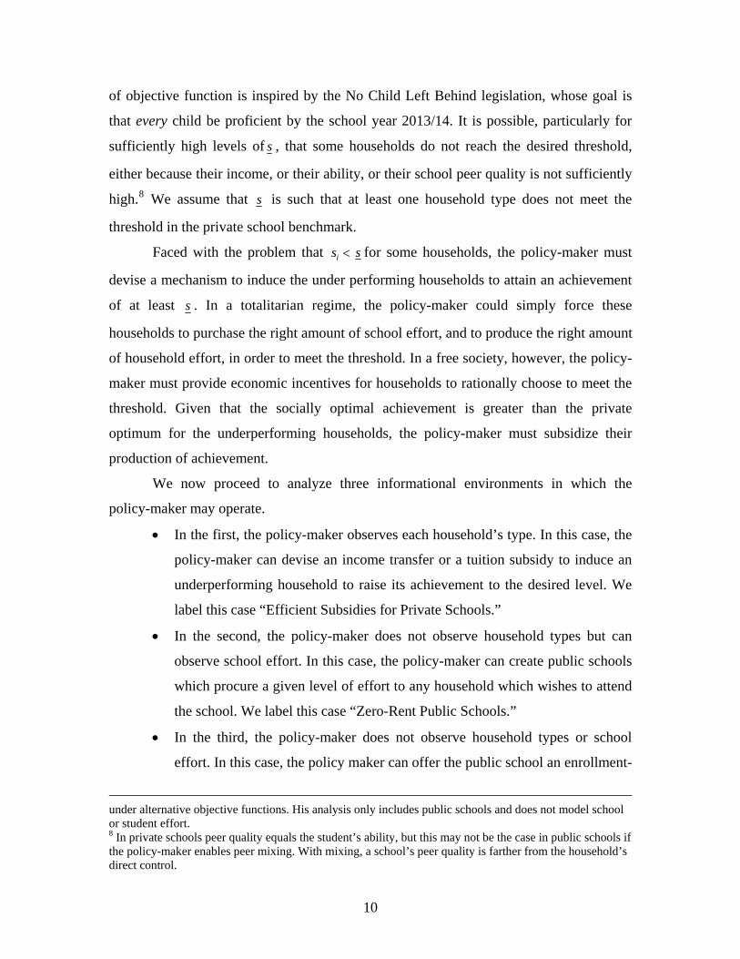
We now proceed to analyze three informational environments in which the

policy-maker may operate.

• In the first, the policy-maker observes each household’s type. In this case, the

policy-maker can devise an income transfer or a tuition subsidy to induce an

underperforming household to raise its achievement to the desired level. We

label this case “Efficient Subsidies for Private Schools.”

• In the second, the policy-maker does not observe household types but can

observe school effort. In this case, the policy-maker can create public schools

which procure a given level of effort to any household which wishes to attend

the school. We label this case “Zero-Rent Public Schools.”

• In the third, the policy-maker does not observe household types or school

effort. In this case, the policy maker can offer the public school an enrollment-

under alternative objective functions. His analysis only includes public schools and does not model school or student effort. 8 In private schools peer quality equals the student’s ability, but this may not be the case in public schools if the policy-maker enables peer mixing. With mixing, a school’s peer quality is farther from the household’s direct control.

10

based contract which leads to inefficiencies in the procurement of school

effort. We label this case “Rent-seeking public schools.”

Efficient Subsidies for Private Schools

Knowing each household’s type gives the policy-maker a great deal of flexibility. As (11)

suggests, in this case the policy-maker can provide the exact subsidy so that the

household’s optimal choice of e and a yields s . He can, for instance, provide each

household with a transfer and thus raise the household’s disposable income.

Alternatively, he can subsidize tuition. Below we study both types of subsidies. To

finance them, the policy-maker raises an income tax rate that is constant across

households. Although these incentives come at the cost of redistributing money across

households, they are used efficiently in the sense that no money is wasted.

From the point of view of the policy-maker, the optimal income transfer to under-

performing household i solves the following equation:

(12) ( ) ( ) ( )1

2

2

2 1

1 1

1 1i i z i i z i is q t z y t z yA

ηβ λ

η ηβλμβλ η η βλ

⎛ ⎞⎛ ⎞= − + − +⎜ ⎟⎜ ⎟ ⎜ ⎟+ +⎝ ⎠ ⎝ ⎠

where is the transfer to household i, expressed as a proportion of its income, and is

the income tax rate required to finance all the income transfers. Households whose

achievement is above the threshold receive transfers of zero. Notice that the implicit

transfer rate depends on household ability and income: the lower the ability, the greater

the transfer rate; and the lower the income, the greater the transfer rate. The state sets the

income tax rate to the level required to balance its budget constraint, equal to:

iz zt

zt

(13) z ii

t Y z y= ∑ i

z

i

i

where Y is total household income in the economy. Provided , the income transfer

increases household i’s disposable income, which is now equal to .

Substituting for in (7) and (9), it is clear that the household will increase

its consumption and purchase more school effort thanks to the transfer. Furthermore, it

will also produce more effort, as indicated by equation (5).

iz t>

(1 )z it z y− +

iy (1 )z it z y− +

11

Instead of income transfers, the policy-maker can provide tuition subsidies to

under-performing households. When household i receives a tuition subsidy, the

household’s expenditure in tuition equals ( )1

1

(1 ) (1 ) 1i i i v iv T v t yηη βλ

− = − −+

, where is the

tuition subsidy rate, chosen by the policy-maker to solve the following equation:

iv

(14) ( ) ( ) ( )1 1

2

2 2

2 1

1 1

11 11i i v i v is q t y t y

A v

η ηβ λ λη ηβλμβλ η η βλ

⎛ ⎞⎛ ⎞ ⎛ ⎞= − −⎜ ⎟⎜ ⎟ ⎜ ⎟⎜ ⎟+ + ⎝ ⎠⎝ ⎠ ⎝ ⎠ −

i

In this equation, is the income tax rate required to finance all the tuition subsidies, and

is set by the state to balance the following state budget constraint:

vt

(15) v ii

t Y v T= ∑

Once again, the implicit tuition subsidy rate is higher for lower-income, lower-ability

households.

In the presence of a tuition subsidy, household i will choose to buy school effort

for the following total cost:

(16) 1

1

(1 )(1 )

vi i

i

tT yv

ηη βλ

−=

+ −

Provided , the household will choose a higher school effort than in the private

school benchmark, as can be seen by comparing (16) and (8). Although the household’s

consumption will not change, the complementarity between school and household effort

will induce the household to produce greater effort (see (5)). Thus, although directly

aimed at school effort, the tuition subsidy has a multiplier effect on achievement through

the complementarity between school and household effort.

iv t> v

From a fiscal perspective, a combination of income and tuition subsidies allows

the policy-maker to minimize the cost of attaining his goal. This is because the income

subsidy is the less costly option for households whose transfer is greater than their

equilibrium tax bill, and the tuition subsidy is the less costly option for households whose

subsidy is lower than their equilibrium tax bill. Thus, providing income transfers to some

households and tuition subsidies to others minimizes the goal of attaining the desired

achievement.

12

Zero-Rent Public School

Now we assume that the policy-maker does not observe household types; instead, he

observes the range of income and ability. Among the different policies that the policy-

maker could adopt, we focus on the following: a full subsidy for the purchase of a type-

invariant school effort, for which all households are eligible.9 In other words, households

have a choice between attending a school whose teacher effort is fully funded by the

policy-maker but cannot be altered by the household, and a private school whose cost is

fully born by the household yet whose teacher effort is freely chosen by the household.

We call the first choice “zero-rent public school without mixing.”

This school derives its public character from the full funding of teacher effort,

which makes the school tuition-free,10 and from the fact that households in the school are

not allowed to supplement school effort. The school, however, retains some aspects of

private schools, because it continues to cater to specific ability types. This is because

mixing types would invite the more able student to leave her school for another with the

same teacher effort yet a higher peer quality.

The effort E necessary for the lowest-achievement type m to reach the threshold is

found by solving the following equation:

(17) 1 12 22 2

1(1 )m i m m ms E q a E q t y

βη ηη η βλμ

βλ η⎛ ⎞

= = −⎜ ⎟+⎝ ⎠

where t denotes the income tax rate needed to fund this program. The income tax rate t is

set to balance the following state budget constraint:

(18) ( ) ( )tY W E N E=

where ( )W E is the teacher salary required to obtain E, and ( )N E is the number of

households who choose public schools in equilibrium.

9 Given that he does not observe household types, the policy-maker cold set up revelation mechanisms asking each household to send him messages. The policy-maker would then make household-specific offers conditional on these messages. We abstract away from such mechanisms for two reasons. First, these mechanisms require some elements, such as cost of signaling and information acquisition, which are currently not included in our model. Second, these mechanisms may not be implementable in large-scale. Therefore, we choose a mechanism, zero-rent public schools, that serves as a bridge between the subsidy-based solution in the private school-world, and the rent-seeking public school solution. 10 Of course, the school is not literally free in equilibrium, as households must pay taxes to support it.

13

These public schools cannot reap rents because E is procured exactly at the

market value, without any kind of waste. However, the policy is not efficient for two

reasons. First, some underperforming household types (but not the lowest-performing) do

not need as much school effort as household type m. Second, since the policy-maker

makes E available to all households, some over-performing households switch into public

schools. Nonetheless, the policy-maker incurs these costs precisely because of his

informational constraints.

One way of reducing the fiscal cost of public schools is to allow them it to mix

students of different abilities. Thus, we consider another case, the “zero-rent public

school with mixing.” When mixing is allowed, all public schools attain the same peer

quality, which is equivalent to having only one public school that pools all public school

students. In this school, peer quality is equal to Q μ= , where the average is calculated

over the households with children in the public school. Mixing reduces the cost of

attaining s because raising the peer quality for the lowest-performing students raises their

achievement, thus lowering their need for school effort. This regime still contains the

same kind of inefficiencies as the zero-rent public school without mixing, although

mitigated by the fact that the mixing reduces the level of E that is needed to reach the

achievement threshold.

Agency Costs

So far we have assumed that schools can be monitored, namely that their effort choices

can be observed. In the case of private schools, this assumption ensures that households

can perfectly observe teacher effort. In particular, households can identify situations in

which schools try to derive a rent, by not spending all of its tuition revenue purchasing

teacher effort. Perfect monitoring, coupled with perfect competition among private

schools, ensure that households can always find a school that derives zero rent and meets

their needs. In the case of public schools, perfect monitoring means that the policy-maker

can observe public school effort.

The assumption of perfect monitoring may not be descriptive of the informational

setting in which families and schools operate. Hence, we now relax it by introducing

14

agency costs. We assume that households do not observe school effort, either at public or

private schools. In the case of public schools, we further assume that the policy-maker

does not observe school effort either. These informational constraints give rise to rents on

the part of the schools.

We begin with private schools. The more able the household is to monitor the

school, the less rent the school will collect, and the more efficiently it will use its tuition

revenue. Thus, we modify equation (6), reflective of private school tuition, as follows:

(19) λμii eAeT /1)( =

This equation reflects the fact that the greater the household ability, the lower the

monitoring cost, and hence the more efficient use of tuition.

Public procurement of school effort separates the provision and consumption of

school effort, thus rendering the policy-maker incapable of perfectly monitoring the

school. In addition, as we saw above, households are not capable to monitoring the

school either.11 Thus, we assume that the policy-maker only observes a noisy measure of

household and school effort, namely, the number of children enrolled in public schools.

In this case, the policy-maker chooses a level of funding per student, X, and provides the

school with a total revenue equal to X times the observed public school enrollment. In the

current version we take X as given, although in future versions we will model the choice

of X. Thus, the public school chooses effort E to maximize the following objective

function:

(20) ( )( ) ( ) ( )B E X W E N E= −

subject to B(E)>0. In this objective function, ( )( )X W E− is the per-student rent, and N is

the measure of households choosing public schools. This objective function captures the

trade-offs faced by the public school when choosing effort. On the one hand, the school

wishes to maximize its per-student rent by minimizing their effort. On the other hand, a

11 In reality, monitoring public schools may be harder than monitoring private schools because of the institutional distance between the household and the school’s decision-maker. In particular, it may be easier, and more effective, to talk with a private school principal than with the board of education of a public school district.

15

high effort helps the school attract more students and raise the peer quality of its student

body, which further attracts students.12

The existence of the public school creates an agency cost to the policy-maker,

because the policy-maker does not observe the agent’s actions and can only contract upon

a noisy signal. Thus, he overpays for public school effort. From an empirical perspective,

one way of interpreting the rents is as frictions in the public school teacher labor market

(union contracts, barriers to entry, etc.).13

Rent-seeking public schools have some negative effects. On the one hand, the rent

has a fiscal cost, which requires higher taxes and hence more redistribution. On the other

hand, the under-provision of school effort leads households to under-provide effort as

well. In other words, the fiscal cost is higher, and the achievement outcomes lower, for

the rent-seeking public school than for the efficient-with-mixing public school.

Increasing Efficiency under Agency Costs

The inefficiencies created by public schools are related to the fact that public schools

separate the consumption and financing of education. One way of reuniting these is

through private school vouchers. Vouchers are tuition subsidies for private schools. We

focus on universal vouchers. We assume that they are funded by the state through income

taxes, and that the dollar amount of the voucher is the same for all households. Under

vouchers, the household budget constraint changes as follows:

(21) ( ) )0,max(1 vTcyty −+=−

where ty is the state income tax rate needed to fund both vouchers for private schools and

spending at public schools, and v is the dollar amount of the voucher.

Another way of limiting the inefficiencies created by public schools is through

accountability for public schools, which attaches consequences to public schools’

outcomes and aims at eliciting greater effort on their part. To measure those outcomes,

12 More generally, we could model the public school as attempting to maximize an objective function that combines school rents and student achievement. Simulations conducted with this alternative objective function show that the results presented in the text are qualitatively robust. 13 Although we model a competitive teacher market, we can interpret the rents as being distributed among the teachers, such that a public school teacher’s total compensation exceeds that of a private school teacher for the same amount of effort.

16

the policy-maker usually designs an assessment test, and establishes the threshold score

that children must meet to pass the test. The test is a noisy measure of the child’s

achievement, s. Thus, we assume that the test score of a child in public schools is given

by:

(22) ε+= ss

where ε denotes achievement measurement error. We assume that ε e is independent

among students, and follows a normal distribution with mean 0 and variance 2~σ .

After the test is taken, the policy-maker observes the proportion of children who

meet the desired achievement threshold and hence pass the test. Let p denote this

proportion, or passing rate. We assume that the policy-maker aims at having a passing

rate equal to p*. Thus, one mechanism to elicit effort on the part of schools consists of

rewarding with extra funding those schools whose passing rate exceeds the target, s , and

removing some funding from those who fail to meet the target. The presence of this

mechanism changes the school’s objective function as follows:

(23) ( ) ( ) ( )*)()( pEpENEWXEEB −+−= φ

where EB(.) denotes the expected value of the school’s objective function, which is now

random because test scores, and hence passing rates, are random. The second term of the

objective function reflects the school’s extra incentive to exert effort in order to

maximize the probability of meeting the target passing rate. In this objective function,

φ >0 represents the dollar amount of money that the school receives (loses) for each

percentage point that its passing rate is above (below) the target.

Test-based accountability introduces randomness in the realization of the school’s

objective function. The school, in particular, may be risk-averse, and hence dislike

volatility in outcomes. For instance, the school may not want to make adjustments to its

operations based on fluctuations in test scores. Modeling a risk-averse public school

changes equation (23) as follows:

(24) ( ) ( ) ( ) 2*)()( γσφ −−+−= pEpENEWXEEB

where γ>0 represents the disutility incurred by the risk-averse public school when

participating in an accountability system that relies on stochastic test scores and passing

17

rates, and represents the volatility of passing rates given the volatility of test scores, 2σ2~σ .

To summarize, in this section we have analyzed mechanisms available to the

policy-maker under alternative informational constraints. Since the model does not have a

closed-form solution, we compute the equilibrium numerically to gain insight on these

mechanisms. The next section provides details on the computational analysis and its

results.

3. Computational Analysis

In this section we first lay out the details of the computational version of our model, and

then analyze our computational results. We construct a computational representation of

the economy, and calibrate the model’s parameters to reproduce certain aspects of

relevant data. We are currently working on improving our calibration and providing

sensitivity analyses with respect to our parameter values. Thus, the results presented here

should be viewed as merely illustrative.

Our computational representation of the economy includes five income types,

whose incomes equal the 10th, 30th, 50th, 70th and 90th percentile of the 2000 household

income distribution in the United States. All dollar amounts are expressed in dollars of

2000. We include six ability levels, and assume that income and ability are independently

distributed.14 In this model, it can be shown that the scaling of ability is irrelevant to the

results. For simplicity, we choose to use six ability types, ranging between 0.5 and 1. Our

setting of income and ability types yields thirty household types. Thus, the total measure

of households in the economy is H=30.

We set the utility function coefficient on consumption, β, equal to 6 based on

Ferreyra (2007), who estimated a model with a Cobb-Douglas utility function including,

among others, consumption and schooling. In that model, the coefficient on consumption

14 Since some evidence points to the fact that income and ability might be positively correlated (see Solon 1992 and Zimmerman 1992), in future versions we will explore the implications of assuming positive correlation.

18

was about six times as large as the coefficient on school quality. Given that we set our

coefficient on school quality equal to 1, it follows that β must be set equal to 6.

To calibrate the labor market portion of the model, we chose A=1.5. We choose

values of λ, 1η and 2η that help us match (approximately) certain features of the

predicted equilibrium for rent-seeking public schools to actual 2000 US data. These

features are the 2000 chools, the fraction of households in

public schools, and the average household income for households with children in private

schools. Thus, w

average tuition in private s

e use 2λ = , 1 0.73η = , and 2 0.5η = . Finally, we choose X=$7,000, which

is appr

um for a given tax rate. In the outer loop, the income tax rate is adjusted to meet

e state budget constraint. The outcome of the outer loop is a full equilibrium for the

oximately equal to the 1999/2000 nationwide average spending per student in

public schools.

To compute the equilibrium for each regime, we use an algorithm which consists

of two nested loops. In the inner loop, schools and households make their optimal choices

conditional on a given tax rate. In the case of public schools with peer mixing, the inner

loop computes the public school peer quality as well. The outcome of the inner loop is an

equilibri

th

model.

Private School Benchmark Table 1 portrays some characteristics of the equilibrium in alternative informational

settings.15 All these settings, however, assume that parents do not perfectly observe effort

in private schools. The private school benchmark, reported in Column 1, is the

equilibrium of the model without any kind of policy intervention. Throughout, we assume

that the achievement target, s , is equal to 10, which is equal to the 23rd percentile of the

equilibrium achievement distribution. Thus, in equilibrium the passing rate (i.e., the

proportion of households with achievement no lower than the threshold) equals 0.77. We

assume

that the policy-maker sets a target passing rate for the economy equal to 0.85.

Clearly, in the private school benchmark equilibrium, this target is not met.

15 We omit the presentation of results for optimal subsidies and efficient public schools here. Results are available upon request.

19

Across households, large variation exists in school effort (and tuition), peer

quality, household effort, and achievement. Under-performing households belong to the

lowest income segment. Although some of these households also have high ability, their

lack of income prevents them from purchasing more school effort and providing more

rthermore,

ss

into the

household effort. Since the policy-maker does not intervene in this economy, the income

tax rate is zero.

While we do not present results for the optimal subsidies and the efficient public

schools,16 we summarize the results below. By design, income transfers induce

households to choose the school and household effort that leads them to exactly meet the

threshold. This is evidenced by the increase in the minimum school and household effort

in the economy. Although the income transfers raise achievement for the lower tail of the

distribution, they lower it for the rest because over-performing households bear the

largest share of the fiscal cost of the program. Since the program reduces their disposable

income, they purchase less school effort and provide less household effort. Fu

the decline in average achievement relative to the private school benchmark is due to the

negative fiscal effect on the households who financially support the program.

A tuition subsidy is considerably more expensive than the income transfers, as the

income tax rate required to fund it is several times higher. The reason is that an income

transfer, by raising disposable income, increases the production of household effort. In

addition, it stimulates the purchase of school effort, which furthers the production of

household effort. While the tuition subsidy leads to the purchase of additional school

effort and thus to the production of more household effort than in the private school

benchmark, it does not directly affect the production of household effort. By tapping le

potential of household effort and relying more on the input that must be bought

on the market, tuition subsidies are necessarily more expensive than income transfers.

Relative to income transfers, tuition subsidies make the under performing

households consume more school effort, whereas the over performing households

consume less give the higher fiscal cost of tuition subsidies. By having less disposable

income, over performing households consume less school effort, produce less household

effort, and have lower achievement. However, all households are worse off under tuition

16 Detailed results are available upon request.

20

subsidies than income transfers; over-performing households are worse off because of

their higher fiscal burden, and under-performing households are worse off because tuition

subsidi

ur calibration choices, they nonetheless illustrate the fact that

offering to every household that which is needed by the least-performing one can indeed

costly.17

ing this case with the private school benchmark

provide

es do not raise their disposable income (and hence their consumption) as income

transfers do.

When the policy-maker only observes the distribution of types, he can calculate

the amount of school effort needed to lift the type with the lowest income and ability up

to the achievement threshold. The policy-maker makes this school effort available to all

households and provides it for free, although he does not allow them to supplement it. In

our simulations, however, the zero-rent public school without peer mixing is

prohibitively expensive given that the school effort needed to lift up the least-performing

household is very high, and making it available to all households (some of which achieve

above the threshold and hence do not need it) only increases the cost of the program.

Allowing public schools to mix households of different abilities reduces the school effort

requirement. However, the resulting increase in peer quality is not enough, in these

simulations, to render the zero-rent public school with peer mixing viable. While our

results are sensitive to o

be prohibitively

Agency Costs

We now turn to the case of agency costs, in which households have imperfect monitoring

of private schools, and public schools are rent-seeking. The equilibrium for this case is

reported in Column 2 of Table 1. Compar

s a sense of the distortions induced by imperfect information. We view this case

as a benchmark representation of reality.

Under agency costs, 87 percent of the households enroll in public schools, and the

income tax rate required to fund public schools is 12 percent. Relative to the private

school benchmark, the households that attend private schools are the most able among

17 These results echo the adequate spending simulations conducted by Ferreyra (2008), who concludes that funding schools to reach a meaningful achievement floor for all households can be fiscally prohibitive.

21

those with the highest income. All other households attend public schools. Households

from the bottom and middle portions of the income distribution are better off under

agency costs than in the private benchmark because public schools allow them to mix

with higher ability types. Only high-income, high-ability households remain in private

schools. This is because the existence of public schools generates a fiscal burden on

households, who thus have less disposable income to pay for tuition. Monitoring costs at

private schools also mean that part of the tuition is not used productively, yet lower-

ability households are more affected by this inefficiency than higher-ability households.

Househ

than their private schools in the benchmark private

equilib

r by rents

that acc

private schools lose the opportunity to mix with other peers, the greater school effort, and

olds that switched into public schools and hence lost some (private) lower their

provision of effort.

In addition, the public school provides low-income households with more school

effort and higher peer quality

rium. As a result, the average passing rate in the economy is higher than in the

benchmark private equilibrium.

As column 2 shows, the spending per student is higher under agency costs than in

the private benchmark. Although the households that remain in private schools spend less

now, for most households the public school spending is higher than their own in the

private benchmark. However, most of the spending per student is accounted fo

rue to the public school because of informational problems. These rents, which

are a source of inefficiency, motivate the analysis that we carry out in Table 2.

Column 1 of Table 2 simply reproduces results for agency costs, for convenience.

The goal of this table is to explore mechanisms to reduce public school rents and increase

efficiency. Column 2 presents results for universal vouchers whose dollar amount equal

the public school spending per student. The dollar amount of the voucher is larger than

the tuition paid by any household under agency costs, and all households take up the

voucher. Thus, in equilibrium, all households attend private schools. Although spending

per student would be the same for public and private schools under this mechanism,

private schools are more efficient, which means that the effort purchased by that given

dollar amount is higher in private schools. Higher school effort leads to higher household

effort, which leads to higher achievement. While households switching from public into

22

the greater induced household effort, more than compensate for the peer quality losses.

From a fiscal perspective, this program is more expensive than the agency cost

benchm

. This suggests that lifting the lower

segmen

the households that leave public

schools

e, have the highest monitoring costs), are

particu

ark, because all households are funded at a rate equal to the voucher amount.

Column 3 presents results for a universal voucher of half the size of per-pupil

spending in public schools. In this case, not everybody takes up the voucher; only the

highest ability students do. These are the students who gain by separating from their

peers in public school, and who incur the lowest monitoring costs in private schools.

Average achievement is not as high as under the higher voucher. However, neither the

higher voucher nor this one can raise the passing rate beyond 0.8. Even though they raise

the lower tail of the achievement distribution, they do not manage to lift the lowest-

performing students up to the target threshold

t of the distribution may be quite costly.18

An important effect of the $3,500 voucher is that it motivates the public school to

exert greater effort (and earn lower rents) than in the agency cost benchmark, which in

turn leads households to exert greater effort and leads to higher achievement. The reason

is that to prevent the loss of students, the public school must raise their effort, and give up

some of the rents it would otherwise earn. From a fiscal perspective, this program is less

costly than the original agency cost equilibrium, because

require a funding of $3,500 rather than $7,000.

As mentioned before, vouchers reunite the functions of consuming and financing

education, by giving households the means to fund (at least partially) their education at

the school of their choice. The fact that the agent who consumes education also finances

it (and has the effective choice of leaving the school if he wishes to do so), reduces

inefficiencies in the economy. However, the inefficiencies do not disappear completely,

because households cannot monitor private schools perfectly either. In other words, there

is a floor level of inefficiency in the economy that may be hard to eliminate, and low-

ability households (which, we assum

larly subject to such inefficiency.

18 See Ferreyra (2008) for simulations using structural estimates that speak to the prohibitively high cost of lifting the lower tail of the distribution.

23

In column 4 we present the results from our public school accountability

simulation assuming that the school is risk-neutral (i.e., γ = 0). In the simulation we

calibrate φ so that for every percentage point that the passing rate falls below the target

passing rate, the school loses $2,100. This amount is equal to 1 percent of the total

funding that the public school would receive if all households were enrolled in public

schools. Clearly, the effects of this accountability policy depend on the value of φ , and in

future versions we will conduct sensitivity analyses with respect to this parame this

simulat

ter. In

ion, and those that follow, we use the same value for 2~σ , the variance of the

achievement test.

Public school accountability forces public schools to make greater effort than in

the agency costs benchmark. This, in turn, attracts more households into public schools.

These households are more able than the original public school households, which in turn

raises public school peer quality. In contrast, vouchers lower public school peer quality.

However, the accountability incentives are not strong enough to force the public school to

meet th

of the passing rate

equal to

simply stronger for risk-averse schools. Further simulations (not

reporte

e target passing rate. While they somewhat lift the lower tail of the achievement

distribution, they do so to a lesser extent than the $3,500-voucher.

In Column 5 we explore the notion that the public school may be risk-averse. We

calibrate the risk aversion parameter γ so that a standard deviation

0.01 causes a disutility of about $500. While this disutility may not seem large, it

helps us highlight some features of the risk-averse school behavior.

Intuitively, when there is much uncertainty about test outcomes, schools’ optimal

response is to exert more effort. This is precisely what the simulation shows. Thus, risk-

averse schools respond more strongly to accountability incentives. The effects shown for

risk-neutral schools are

d here) show that the greater the variance of the outcome, the greater the effort

exerted by the school.

Finally, in column 6 we explore the implications of combining accountability (for

risk-averse public schools) and private school vouchers for those attending private

schools. This combination makes more students go to private schools than a mere

accountability regime, although not as many than the mere $3,500 voucher. This is the

policy that accomplishes the greatest effort on the part of public schools. As a result, it

24

leads to the greatest average achievement in public schools. It also the most effective tool

to reduce public school rents, because it combines direct pressure on public schools

through accountability, with competition from private schools enabled through vouchers.

The most able students, however, continue to exit towards private schools, even more so

than under a pure accountability regime. At roughly the same cost as the mere

accountability regime, it leads to better average outcomes in public schools, and is more

efficien

er might want to

impose some form of accountability on private schools as well. It remains to be explored,

uld respond to that kind of regulation.

likely to combine elements from each approach. We have built a simple model to

t. Furthermore, this combination of accountability and vouchers is no more costly

than the agency cost benchmark, and it is certainly more efficient.

To summarize, in this section we have computationally analyzed the theoretical

settings presented in section 2. As the simulations show, each mechanism has equilibrium

effects that can strengthen or undermine the policy-maker’s original purpose. Thus, a

proper investigation of achievement incentives must rely both on an understanding of the

policy-maker’s informational constraints, and on a careful modeling of equilibrium

effects. Our current findings suggest that a combination of public school accountability

and private school choice may be more successful than a policy that merely relies on

accountability or vouchers. They also suggest that a reasonable degree of measurement

error in achievement can actually encourage harder work on the part of public schools.

Finally, it is also possible that if monitoring costs in private schools are sufficiently large,

strict accountability may be preferable to vouchers to raise the achievement of the lower

tail of the distribution. The presence of monitoring costs in private schools suggests that

were a large-scale voucher program to be implemented, the policy-mak

however, how private schools wo

6. Conclusions and Extensions

In this paper we have argued that the primary cause of the underachievement problem is

the information asymmetry among the policy-maker, households, and schools. The

pervasive asymmetry implies that neither a complete market-based solution nor a

complete contract-based solution is the answer to the problem. Rather, the solution is

25

highlight the various frictions in this problem. We have also built a computational version

of the model, which has enabled us to quantify distortions and inefficiencies in alternative

informa

ve that

extendi

cational setting has unique features that add

richnes

apable teachers. This,

in turn,

tional environments.

We view our theoretical and computational model as a first step towards a

comprehensive and systematic investigation of the problems facing a policy-maker in a

system including public and private schools. We believe that a contracting perspective

will shed light on the problem and its possible solutions. In particular, we belie

ng our model in the directions indicated below will be particularly useful.

First, a good school accountability system should reward the value added by the

school, which could be very high despite low student achievement. The issue, then, is

how to measure value added. Furthermore, achievement test scores are a noisy measure

of the underlying element of interest, intellectual skills. These skills may not be fully

realized in the short run, yet achievement tests are usually administered in the short run.

This creates an incentive for schools to focus on the short-term skills measured by the

tests, possibly in detriment of more valuable long-term skills. These measurement

problems have famously produced dysfunctional incentives when not properly accounted

for in the design of reward systems based on performance metrics (Holmstrom and

Milgrom 1991). Further, when measurements are subject to manipulation by the very

economic entity being measured, they invite performance management (akin to earnings

management in corporate settings). Monitoring and measurement problems have been

studied in other settings, such as managerial performance evaluation and firm equity

valuation (Holmstron 1982, Huddart and Liang 2003 and 2005, Legros and Matthews

1993, Miller 1997). However, the edu

s and complexity to the problem.

Teacher heterogeneity is also an important element to consider, because the

reforms have the potential of adversely affecting teacher sorting across schools. For

instance, in the absence of good value-added measurement, a school attended by low-

performing students will face considerable difficulties attracting c

will only aggravate the initial underachievement problem.

Engaging students and their parents seems to be a fundamental task of education

reform, and we wish to explore what kind of incentives can be provided to this end. In

26

addition, we wish to explore the notion that some schools may have an advantage in

eliciting student effort and hence attaining high performance. If this is indeed the case,

then inducing low-effort students to attend those schools may be more desirable than

providing them with short-term incentives, because those schools can help the students

develop work habits that enhance their human capital in the long run. Furthermore, if

peer quality were a function of a school’s average household ability and effort, the school

might succeed at implementing an environment where students work hard in response to

the har

studied before (Costrell 1994), they have not been explored in

a settin

e to contribute to the understanding of this

problem and to the design of its solutions.

d work of their peers.19

Another important extension concerns the choice of the socially desired

achievement level – who chooses it and how. Furthermore, what would be the

equilibrium implications of decentralizing the choice by school district? While some of

these problems have been

g as rich as ours.

In closing, we reiterate our view that understanding the achievement problem in

public schools requires a firm grasp of the existing frictions between the policy-maker,

households and students, the incentives implied by alternative mechanisms that address

the frictions, and the equilibrium effects of the large-scale implementation of these

mechanisms. Through our work we hop

19 See Cooley (2007) for an empirical model of peer effects which depend on endogenous choices of student effort.

27

References Chakrabarti, Rajashri. “Can Increasing Private School Participation and Monetary Loss in a Voucher Program Affect Public School Performance? Evidence from Milwaukee (2007)”. Forthcoming, Journal of Public Economics. Cooley, Jane. 2007. “Desegregation and the Achievement Gap: Do Diverse Peers Help”, Mimeo, University of Wisconsin-Madison. Costrell, Robert. 1994. “A Simple Model of Educational Standards”. American Economic Review, 84: 956-971.

Ferreyra, Maria M. 2008. “An empirical Framework for Large-Scale Policy Evaluation, with an Application to School Finance Reform in Michigan”. Forthcoming, American Economic Journal: Policy. Holmstrom, Bengt. 1982. “Moral Hazard in Teams.” Bell Journal of Economics, 13: 313-392. Holmstrom, Bengt and Paul Milgron. 1991. “Multitask Principal-Agent Analyses: Incentive Contracts, Asset Ownership, and Job Desing”. Journal of Law, Economics and Organization, 7: 24-52. Huddart, Steve and Pierre Liang. 2003. “Accounting in Partnerships.” American Economic Review, 93: 410-414. Huddart, Steve and Pierre Liang. 2005. “Profit Sharing and Monitoring in Partnerships.” Journal of Accounting and Economics, 40(1-3): 153-187. Laffont, Jean-Jacques and David Martimort. 2002. “The Theory of Incentives: the principal-agent model.” Princeton University Press. Laffont, Jean-Jacques and Jean Tirole. 1993. “A Theory of Incentives in Procurement and Regulation”. MIT Press. Legros, Patric and Steven A. Matthews. 1992. “Efficient and Nearly Efficient Partnerships”. Review of Economic Studies. McMillan, Robert. 2005. “Competition, Incentives, and Public School Productivity.” Journal of Public Economics, 89: 1131-1154. Miller, Nolah. 1997. “Efficiency in partnerships with joint monitoring.” Journal of Economic Theory 77. 285-299 Neal, Derek (2008). “Designing Incentive Systems for Schools.” Forthcoming in Spring, Matthew (ed.), Performance Incentives: Their Growing Impact on American K-12 Education. Brookings Institution Press. Neal, Derek and Diane Schanzenbach. 2007. “Left Behind by Design: Proficiency Counts and Test-Based Accountability.” Forthcoming, Review of Economics and Statistics.

28

Nechyba, Thomas. 1999. “School Financed Induced Migration Patterns: The Case of Private School Vouchers”. Journal of Public Economic Theory, 1(1): 5-50.

Sappington, David. 1983. "Limited liability contracts between principal and agent," Journal of Economic Theory, 29(1): 1-21. Solon, Gary. 1992. “Intergenerational Income Mobility in the United States.” American Economic Review, 82(3): 393-409. Zimmerman, David. 1992. “Regression Toward Mediocrity in Economic Stature.” American Economic Review, 82(3)” 409-29.

29

TABLE 1 Equilibrium without Agency Costs under Alternative Scenarios

Private School

Benchmark (1)

Agency Costs (2)

Fraction of Hhs. in Public School

0 0.87

Passing Rate 0.77 0.8 Public n/a 0.77 Private 0.77 1 Achievement (avg.)

6.46 2.64

Achievement in Public Schools Average n/a 1.20 Minimum n/a 2.1e-5 Maximum n/a 6.57 Achievement in Private Schools Average 6.46 15.04 Minimum 1e-5 0.74 Maximum 65.83 28.20 Peer Quality (avg.) 0.70 0.70 Peer Quality in Public

n/a 0.68

Peer Quality in Private Schools Average 0.70 0.89 Minimum 0.5 0.71 Maximum 1 1 School Effort (avg.)

0.38 0.35

School Effort in Public Schools

n/a 0.32

School Effort in Private Schools Average 0.38 0.55 Minimum 0.19 0.46 Maximum 0.65 0.61 Household Effort (avg.)

1.07 0.50

Household Effort in Public Schools Average n/a 0.21 Minimum n/a 5.80e-6 Maximum n/a 4.05 Household Effort in Private Schools Average 1.07 2.37 Minimum 5e-6 0.13 Maximum 9.03 4.05

31

TABLE 1 (cont.) Equilibrium without Agency Costs under Alternative Scenarios

Private School Benchmark

(1)

Agency Costs (2)

Spending per student (avg.)

0.29 0.67

Spending per Student in Public Schools

n/a 0.7

Spending per Student in Private Schools Average 0.29 0.50 Minimum 0.08 0.32 Maximum n/a 0.56 Public School Rent per Student

0.00 0.55

Income Tax Rate 0 0.12 For ease of exposition, achievement is expressed in 10,000, and household effort is expressed in 100,000. Spending per student, and income and tuition subsidies are expressed in $10,000. Target passing rate is equal to 0.85. To pass, achievement must be greater than or equal to 0.001.

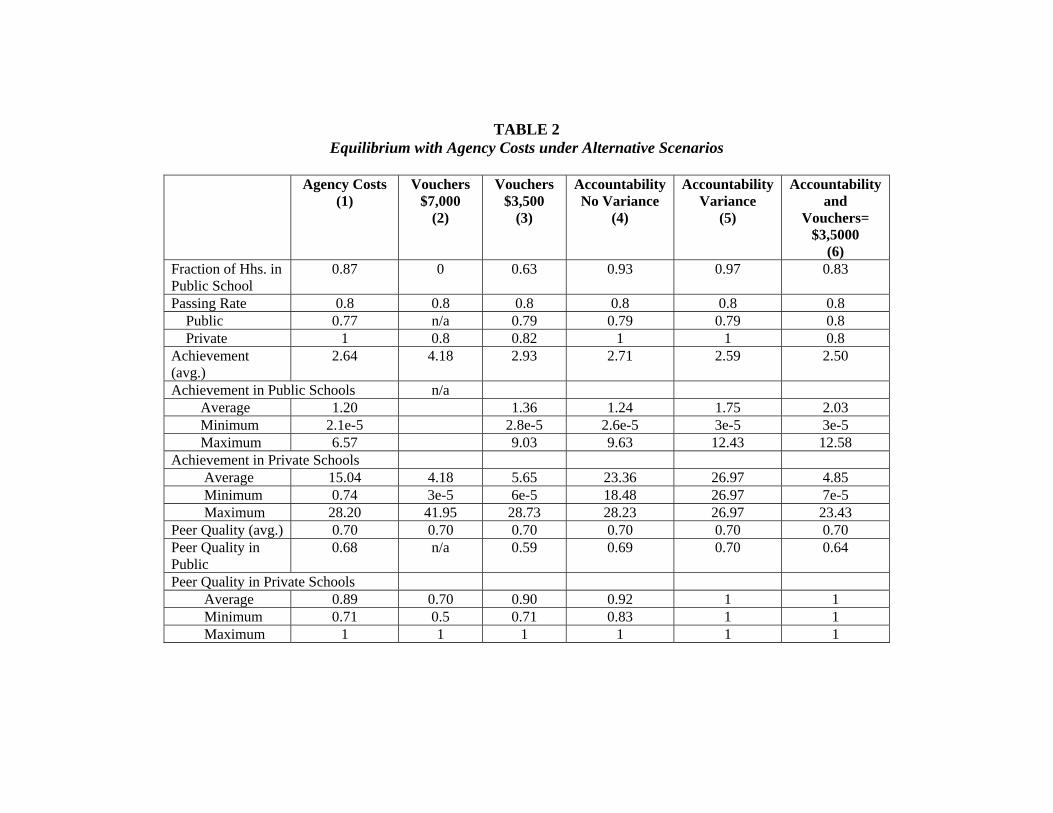
TABLE 2 Equilibrium with Agency Costs under Alternative Scenarios

Agency Costs

(1) Vouchers

$7,000 (2)

Vouchers $3,500

(3)

AccountabilityNo Variance

(4)

AccountabilityVariance

(5)

Accountability and

Vouchers= $3,5000

(6) Fraction of Hhs. in Public School

0.87 0 0.63 0.93 0.97 0.83

Passing Rate 0.8 0.8 0.8 0.8 0.8 0.8 Public 0.77 n/a 0.79 0.79 0.79 0.8 Private 1 0.8 0.82 1 1 0.8 Achievement (avg.)

2.64 4.18 2.93 2.71 2.59 2.50

Achievement in Public Schools n/a Average 1.20 1.36 1.24 1.75 2.03 Minimum 2.1e-5 2.8e-5 2.6e-5 3e-5 3e-5 Maximum 6.57 9.03 9.63 12.43 12.58 Achievement in Private Schools Average 15.04 4.18 5.65 23.36 26.97 4.85 Minimum 0.74 3e-5 6e-5 18.48 26.97 7e-5 Maximum 28.20 41.95 28.73 28.23 26.97 23.43 Peer Quality (avg.) 0.70 0.70 0.70 0.70 0.70 0.70 Peer Quality in Public

0.68 n/a 0.59 0.69 0.70 0.64

Peer Quality in Private Schools Average 0.89 0.70 0.90 0.92 1 1 Minimum 0.71 0.5 0.71 0.83 1 1 Maximum 1 1 1 1 1 1

TABLE 2 (cont.) Equilibrium with Agency Costs under Alternative Scenarios

(threshold achievement = 2e-4)

Agency Costs (1)

Vouchers $7,000

(2)

Vouchers $3,500

(3)

AccountabilityNo Variance

(4)

AccountabilityVariance

(5)

Accountability and

Vouchers= $3,5000

(6) School Effort 0.35 0.62 0.52 0.39 0.41 0.56 School Effort in Public Schools

0.32 n/a 0.51 0.37 0.41 0.57

School Effort in Private Schools Average 0.55 0.62 0.52 0.60 0.61 0.52 Minimum 0.46 0.56 0.46 0.58 0.61 0.48 Maximum 0.61 0.68 0.66 0.61 0.61 0.66 Household Effort (avg.)

0.50 0.67 0.49 0.52 0.52 0.38

Household Effort in Public Schools Average 0.21 n/a 0.29 0.31 0.41 0.38 Minimum 5.80e-6 6e-6 7e-6 7e-6 6e-6 Maximum 4.05 1.90 2.39 3.88 2.35 Household Effort in Private Schools Average 2.37 0.66 0.84 3.53 3.88 0.66 Minimum 0.13 6.64e-06 1e-5 3.00 3.88 1e-5 Maximum 4.05 5.54 3.90 4.06 3.88 3.18

33

TABLE 2 (cont.) Equilibrium without Agency Costs under Alternative Scenarios

Agency Costs (1)

Vouchers $7,000

(2)

Vouchers $3,500

(3)

AccountabilityNo Variance

(4)

AccountabilityVariance

(5)

Accountability and

Vouchers= $3,5000

(6) Spending per student (avg.)

0.67 0.70 0.59 0.69 0.7 0.65

Spending per Student in Public Schools

0.7 n/a 0.7 0.7 0.7 0.7

Spending per Student in Private Schools Average 0.50 0.70 0.41 0.56 0.55 0.38 Minimum 0.32 0.70 0.35 0.56 0.45 0.35 Maximum 0.56 0.70 0.55 0.56 0.45 0.54 Public School Rent per Student

0.55 n/a 0.30 0.44 0.39 0.14

Income Tax Rate 0.12 0.14 0.11 0.12 0.12 0.12 For ease of exposition, achievement is expressed in 10,000, and household effort is expressed in 100,000. Spending per student, and income and tuition subsidies are expressed in $10,000. Target passing rate is equal to 0.85. To pass, achievement must be greater than or equal to 0.001.

34