Relational Contracting in Ghana versus the UK
91
NBER WORKING PAPER SERIES WHEN NO BAD DEED GOES PUNISHED: RELATIONAL CONTRACTING IN GHANA VERSUS THE UK Elwyn Davies Marcel Fafchamps Working Paper 23123 http://www.nber.org/papers/w23123 NATIONAL BUREAU OF ECONOMIC RESEARCH 1050 Massachusetts Avenue Cambridge, MA 20138 February 2017, Revised July 2018 We would like to thank Johannes Abeler, Alan Beggs, Douglas Bernheim, Stefano Caria, Johannes Haushofer, Karine Marazyan, Fola Malomo, Muriel Niederle, Simon Quinn, Yogita Shamdasani, Hannah Uckat as well as participants of the Oxford Firms and Development Research Group, the Stanford Behavioral and Experimental Lunch, the CSAE-iiG Conference, the Stanford Development Workshop, the CSAE Research Workshop, the Paris DIAL conference, the World Bank Poverty and Applied Micro Seminar, NEUDC, PacDev and SEEDEC for helpful comments. Many thanks to Vaclav Tehle for excellent research assistance, and thanks to Andrew Kerr and Denise Gray for their assistance during trial sessions of this experiment. Furthermore, we would like to thank Moses Awoonor-Williams for his role in helping out with logistics, as well as our local team in the field, in particular Eric Agyekum and Bismark Owusu Tetteh Nortey. This research belongs to a wider study of Ghanaian entrepreneurship funded by the UK Department for International Development (DFID) as part of the iiG, a research programme to study how to improve institutions for pro-poor growth in Africa and South-Asia. Elwyn Davies gratefully acknowledges additional funding from the Economic and Social Research Council (ESRC). The findings, interpretations, and conclusions expressed in this paper are entirely those of the authors. They do not necessarily represent the views of DFID, the International Bank for Reconstruction and Development/World Bank and its affiliated organizations, or those of the Executive Directors of the World Bank, the governments they represent, or the National Bureau of Economic Research. At least one co-author has disclosed a financial relationship of potential relevance for this research. Further information is available online at http://www.nber.org/papers/w23123.ack NBER working papers are circulated for discussion and comment purposes. They have not been peer-reviewed or been subject to the review by the NBER Board of Directors that accompanies official NBER publications. © 2017 by Elwyn Davies and Marcel Fafchamps. All rights reserved. Short sections of text, not to exceed two paragraphs, may be quoted without explicit permission provided that full credit, including © notice, is given to the source.
-
Upload
khangminh22 -
Category
Documents
-
view
0 -
download
0
Transcript of Relational Contracting in Ghana versus the UK

We would like to
Uckat as well as
NBER WORKING PAPER SERIES
WHEN NO BAD DEED GOES PUNISHED:RELATIONAL CONTRACTING IN GHANA VERSUS THE UK
Elwyn DaviesMarcel Fafchamps
Working Paper 23123http://www.nber.org/papers/w23123
NATIONAL BUREAU OF ECONOMIC RESEARCH1050 Massachusetts Avenue
Cambridge, MA 20138February 2017, Revised July 2018
We would like to thank Johannes Abeler, Alan Beggs, Douglas Bernheim, Stefano Caria, Johannes Haushofer, Karine Marazyan, Fola Malomo, Muriel Niederle, Simon Quinn, Yogita Shamdasani, Hannah Uckat as well as participants of the Oxford Firms and Development Research Group, the Stanford Behavioral and Experimental Lunch, the CSAE-iiG Conference, the Stanford Development Workshop, the CSAE Research Workshop, the Paris DIAL conference, the World Bank Poverty and Applied Micro Seminar, NEUDC, PacDev and SEEDEC for helpful comments. Many thanks to Vaclav Tehle for excellent research assistance, and thanks to Andrew Kerr and Denise Gray for their assistance during trial sessions of this experiment. Furthermore, we would like to thank Moses Awoonor-Williams for his role in helping out with logistics, as well as our local team in the field, in particular Eric Agyekum and Bismark Owusu Tetteh Nortey. This research belongs to a wider study of Ghanaian entrepreneurship funded by the UK Department for International Development (DFID) as part of the iiG, a research programme to study how to improve institutions for pro-poor growth in Africa and South-Asia. Elwyn Davies gratefully acknowledges additional funding from the Economic and Social Research Council (ESRC). The findings, interpretations, and conclusions expressed in this paper are entirely those of the authors. They do not necessarily represent the views of DFID, the International Bank for Reconstruction and Development/World Bank and its affiliated organizations, or those of the Executive Directors of the World Bank, the governments they represent, or the National Bureau of Economic Research. At least one co-author has disclosed a financial relationship of potential relevance for this research. Further information is available online at http://www.nber.org/papers/w23123.ack
NBER working papers are circulated for discussion and comment purposes. They have not been peer-reviewed or been subject to the review by the NBER Board of Directors that accompanies official NBER publications.
© 2017 by Elwyn Davies and Marcel Fafchamps. All rights reserved. Short sections of text, not to exceed two paragraphs, may be quoted without explicit permission provided that full credit, including © notice, is given to the source.

When No Bad Deed Goes Punished: Relational Contracting in Ghana versus the UK Elwyn Davies and Marcel FafchampsNBER Working Paper No. 23123February 2017, Revised July 2018JEL No. D2,J41,O12
ABSTRACT
Experimental evidence to date supports the double theoretical prediction that parties transacting repeatedly punish bad contractual performance by reducing future offers, and that the threat of punishment disciplines opportunistic breach. We conduct a repeated gift-exchange experiment with university students in Ghana and the UK. The experiment is framed as an employment contract. Each period the employer makes an irrevocable wage offer to the worker who then chooses an effort level. UK subjects behave in line with theoretical predictions and previous experiments: wage offers reward high effort and punish low effort; this induces workers to choose high effort; and gains from trade are shared between workers and employers. We do not find such evidence among Ghanaian subjects: employers do not reduce wage offers after low effort; workers often choose low effort; and employers earn zero payoffs on average. These results also hold if we use a strategy method to elicit wage offers. Introducing competition or reputation does not significantly improve workers' effort. Using a structural bounds approach, we find that the share of selfish workers in Ghana is not substantially different from the UK or earlier experiments. We conclude that strategic punishment in repeated labor transactions is not a universally shared heuristic.
Elwyn DaviesDepartment of EconomicsUniversity of OxfordManor Road, Oxford OX1 3UQUnited [email protected]
Marcel FafchampsFreeman Spogli InstituteStanford University616 Serra StreetStanford, CA 94305and [email protected]

1 Introduction
Worker performance is a key determinant of firm productivity. In many sub-Saharan African
countries worker productivity is low, even after accounting for differences in physical and human
capital (Hall and Jones, 1999; Caselli and Coleman, 2006). Firm surveys and other studies have
shown that employers in developing countries have substantial difficulties in managing their
workers and making sure that their employees perform (e.g. Bloom and Reenen, 2010; Fafchamps
and Soderbom, 2006). At the same time, competition for jobs is high: employers often face many
applicants per opening (e.g. Falco and Teal, 2012). This seems at odds with predictions from
labor market models (Shapiro and Stiglitz, 1984; Bowles, 1985), as well as empirical studies in
the United States and the United Kingdom (Green and Weisskopf, 1990; Wadhwani and Wall,
1991), in which competition for jobs and threat of dismissal drive higher worker performance.
Relationships and reputation are important when the enforcement of formal contracts is
problematic: legal institutions are often weak and wage contracts incomplete due to the com-
plexity of labor tasks. This means that employers have to rely on other incentives. Repeated
interaction can provide a viable alternative: if both parties gain enough value out of a relation-
ship, the threat of losing the relationship – or having its value reduced – provides an incentive to
perform. This is the essence of relational contracting. Many studies documented its importance,
especially in a developing country context (e.g, McMillan and Woodruff, 1999; Macchiavello and
Morjaria, 2015). Similarly, the ability to develop a public reputation can work as an enforcement
mechanism: if individuals gain enough value from having a good reputation, the fear of losing
it can deter cheating (Milgrom et al., 1990; Greif, 2000).
This paper looks at relational contracting in Ghana, West Africa, and compares it with the
United Kingdom. To this effect we conduct a lab experiment to assess the use of repeated
contracting and the reliance on reputation in a gift-exchange game framed as a labor contract.
In this experiment based on the design of Fehr et al. (1993) and Brown et al. (2004), university
students are randomly assigned the role of worker or employer, and they interact in a principal-
agent setting: employers start out by making an offer to a worker, specifying a wage in return for
effort. The worker then chooses to accept or reject this offer and what effort to exert. Crucially,
the employer cannot condition the wage on effort. The worker and employer interact repeat-
edly, however, and the employer can adjust wage offers in subsequent periods. We investigate
whether, as in Fehr et al. (1993) and Brown et al. (2004), employers rely on a trigger strategy
to discipline shirking workers, and whether worker reputation and competition across workers
2

create additional incentives to exert effort. This is achieved by combining five treatments that
vary market size, contractual completeness, and the information available to employers about
past worker performance.
In both the UK and in Ghana we find a substantial group of workers choosing low effort
despite high average wages. This finding is in line with earlier experiments (e.g. Brown et al.,
2004, 2012). The behavior of employers, however, is different. While low effort is punished
in the UK, in line with previous experiments and theoretical predictions, we find no evidence
of punishment strategies in Ghana. Similarly, in the UK high effort is rewarded but not in
Ghana. The findings for Ghana are odds with earlier experimental evidence from developed
countries, and they deviate from relational contracting models where low effort is punished
either by terminating the relationship or by initiating a punishment stage during which the other
player’s payoff is lowered (see e.g. Shapiro and Stiglitz, 1984; Kranton, 1996; Ghosh and Ray,
1996). Furthermore, the Ghanaian findings remain even when we introduce worker reputation
or competition between players.
This paper contributes to an emerging literature on how norms, preferences and strategic
behavior differ across cultures (Henrich et al., 2006; Cardenas and Carpenter, 2008; Henrich
et al., 2010). The most extensive work in this area, the Global Preference Survey conducted by
Falk et al. (2015), shows large differences in preferences across representative samples from 76
countries. Not only do they find large differences between countries, but also within countries.
While they elicit preferences through simple survey questions, we compare behavior in a more
extensive lab game, where players interact repeatedly and can respond to each other’s behavior.
Our experiment aims to capture labor market heuristics reflecting prevailing norms and
expectations. Compared to high income countries, the labor market in Ghana is characterized
by a large degree of informality. Self-employment and working in a family firm are more common
than wage employment: in 2012-13 only 20.2 percent of the country’s working population and
32.5 percent of its urban working population was wage employed (Ghana Statistical Service,
2014). The lower incidence of wage employment may influence the expectations of both workers
and employers in wage relationships. Understanding labor market norms and expectations in a
developing country is crucial, especially when, such as in Ghana, steady growth has occurred
and the share of wage employment has been rising over time. Our results show that punishment
strategies predicted by repeated game theory – such as lowering the wage after low effort to
deter shirking – do not naturally come to the mind of Ghanaian subjects. This finding resonates
3

with earlier empirical findings showing labor management to be problematic in many developing
countries (Bloom et al., 2014; Fafchamps and Soderbom, 2006).
The paper is structured as follows: Section 2 discusses related experiments. Section 3 presents
the experiment and predictions based on the theory. Section 4 presents the results and tests the
predictions. Section 5 concludes and discusses possible explanations for the behavior found in
this experiment.
2 Related literature
Gift-exchange games have been used widely to study informal labor market institutions (Char-
ness and Kuhn, 2011; Fehr et al., 2009).1 The first gift-exchange lab experiment was conducted
by Fehr et al. (1993). It consisted of one-shot interactions between workers and employers who
were randomly rematched at the end of each period. Despite the lack of explicit incentives or
future interaction, the authors show that employers offer wages above the market clearing level
and that workers exert a higher level of effort in return for this higher wage. This provides
evidence for the fair wage-effort hypothesis formulated by Akerlof (1982) to explain involuntary
employment, i.e., employers and workers engage in a “gift exchange”. This pattern can arise
even when there are more workers than employers and workers bid for wage contracts: Fehr and
Falk (1999) find that some employers refuse to hire employees who undercut wages, possibly
because they fear that they are more likely to shirk.
In a repeated interaction, these concerns can be reinforced. Gachter and Falk (2002) in-
troduce a treatment of the gift-exchange game experiment in which an employer repeatedly
interacts with the same worker for ten periods. They find that a repeated interaction makes the
positive wage-effort relation stronger, compared to a treatment in which workers and employers
are randomly rematched every period. They further find that repeated interaction functions
as a disciplining device: “selfish” workers imitate “reciprocal” types in the first periods of the
game. This is in line with the predictions of Kreps et al. (1982) and Fehr and Schmidt (1999)
on cooperation in finite games.
In Brown et al. (2004) this is taken further, by introducing multiple employers and workers
1The gift-exchange game is closely related to the trust game (Glaeser et al., 2000; Karlan, 2005; Bohnet et al.,
2010) in that trust plays an important role (see Berg et al., 1994; Camerer and Weigelt, 1988). The main difference
is that in the gift-exchange game the size of the surplus is determined by the choice of effort by the receiver (i.e.,
the worker), instead of the sender.
4

who can contract with each other in the same marketplace. The authors allow the employers to
make public offers, made to all workers and visible to all participants, as well as private offers,
only made to a specific worker. They show that relational contracting emerges naturally in this
environment: employers keep offering high wages to workers that exerted high effort in the past.
This leads to a higher effort than in a treatment in which the identity of workers and employers
are scrambled every period, so that employers cannot recognize their past workers. Follow-up
experiments have replicated these results (see e.g. Brown et al., 2012; Altmann et al., 2014; Wu
and Roe, 2007). In all these experiments, when employers are faced with low effort, they choose
to either terminate the relationship (contingent contract renewal) or to lower the wage in the
next period.2 This threat of reduced payoff is what incentivizes workers to exert effort, resulting
in higher average payoffs for both workers and employers.
The above-mentioned studies only reveal past worker performance to the past employer,
only allowing for bilateral reputation. Falk et al. (2005) introduce a treatment in which the
past performance of workers is made publicly available to all employers. They find that effort in
this new treatment is higher than in the absence of public reputation. The effect of reputation
is limited, however: bilateral relationships still play an important role. Charness et al. (2011)
similarly finds evidence of reputation effects in the trust game.
In these experiments contractual incompleteness on one-sided: the worker is always ensured
of receiving the promised wage. Other experiments have introduced the possibility of ex post
wage adjustments, such as giving a bonus to a worker or reducing the promised wage ex post
(see e.g. Fehr et al., 1997, 2007; Wu and Roe, 2007; Falk et al., 2008). This is generally effective:
Falk et al. (2008) find that bonus systems work of a substitute for long-term contracts, while
Wu and Roe (2007) observe that trading patterns is close to complete contracts.
Gift-exchange experiments has been conducted in numerous OECD countries: Austria (Fehr
et al., 1993, 1997); Germany (Abeler et al., 2010; Altmann et al., 2014; Falk et al., 2008; Fehr
et al., 2007); Switzerland (Fehr and Falk, 1999; Brown et al., 2004; Falk et al., 2005); the
Netherlands (Van Der Heijden et al., 2001); Portugal (Pereira et al., 2006); Spain (Brandts and
Charness, 2004); the United Kingdom (Gachter et al., 2016); and California, Ohio and Florida
in the United States (Charness, 2004; Cooper and Lightle, 2013; Wu and Roe, 2007). All these
2Brown et al. (2012) show that on their 10-point scale of effort, a one point increase in effort leads to an
increase of the wage of 5.527 (Table 4, column 6). This is significant at a 1 percent level. Their wage is bounded
between 1 and 100.
5

experiments have found the same general pattern of high effort in return for high wages. Similar
results have been found in experiments in former communist countries, such as Hungary (Falk
et al., 1999) and Russia (Fehr et al., 2014). To the best of our knowledge, however, few gift-
exchange experiments have been conducted in developing countries3 and none in sub-Saharan
Africa.
3 Experimental design
The experiment is a multi-period gift exchange game based on Brown et al. (2004) and the
original gift-exchange game of Fehr et al. (1993). The game is framed as a labor contract in a
principal agent setting. At the beginning of the experiment, participants are randomly assigned
the role of worker or employer. This game is played for five periods, after which employers and
workers are rematched for another game. Each participant plays four games of five periods.4
Each game involves either two or six players. The two player variant involves one worker
and one employer (1-on-1 treatment). The six player variant has three workers and three em-
ployers (3-on-3 treatment). The sequencing of play is similar in the two variants, but the 3-on-3
treatment includes more steps.
The 1-on-1 treatment is similar to a gift exchange game. The sequence of moves is as follows:
• Contracting: At the beginning of first period t = 1, the employer makes a wage offer
wt ≥ 0 and specifies a desired effort level et; the worker then either accepts or rejects
the offer; if the worker rejects the offer, the game moves to the next period and a new
contracting stage begins. The employer can also decide not to offer any contract, or to
offer a zero wage. In both cases, both employer and worker earn a zero payoff in that
period.
At the beginning of periods t = 2 to 5, the offer made by the employer is normally
determined by the decisions made at the rehiring stage of the previous period – see below.
If there was no rehiring stage, the contracting stage starts afresh as described above.
• Effort choice: If the worker accepts the offer, he/she then decides an effort level et. This
3Siang et al. (2011) conducted a bilateral gift exchange experiment in Malaysia.4A worker-employer pair (in the one-on-one treatment) or group (in the three-on-three treatment) stays the
same during the five periods of a game. Participants can recognize workers and employers by their randomly
generated identifier (i.e., a letter) assigned at the beginning of each game.
6

effort costs c(e) to the worker with c′(e) ≥ 0 – additional effort is increasingly costly to the
worker. Effort can take one of three possible values: low, medium, or high (e ∈ {L,M,H}).
The employer collects a revenue b(e) with b′(e) > 0 – effort benefits the employer. The
payoffs to the employer πE,t and to the worker πW,t at time t are given by:
πE,t = b(et)− wt (1)
πW,t = wt − c(et) (2)
Mutual gains are possible if b(e) > c(e) for any e, which we impose throughout. We also
select functions c(.) and b(.) such that b(L) − c(L) < b(M) − c(M) < b(H) − c(H), i.e.,
high effort generates larger gains from trade. The main research question is whether these
gains can be achieved in a sustainable and equitable manner.
• Rehiring: In this stage we elicit subjects’ choices using a strategy method. Before moving
to the next period, we ask the employer to make a contingent choice for contract renewal
in the next period. At this stage the employer does not yet know the effort level chosen by
the worker. For each possible effort choice et ∈ {L,M,H} we ask the employer to specify
a conditional wage offer wt+1(et) and desired effort level et+1(et). The purpose of this step
is to verify that subjects intentionally pursue a trigger strategy, i.e., that they intend to
punish a worker who has chosen an effort level lower than stipulated in the contract – i.e.,
et < et.
We also ask the worker to specify a reservation wage rt+1 below which the worker reject
the contract. If the realized contract offer wt+1 ≥ rt+1, the worker is regarded as accepting
the offer. The purpose of this step is to investigate whether the worker anticipates a lower
offer if et < et, i.e., whether the worker has internalized the possibility of retaliation by
the employer.
Following a rehiring stage, the contracting stage of period t+1 is automatic if wt+1 ≥ rt+1:
it implements the conditional offer {wt+1(et), et+1(et)} that corresponds to the actual effort
level et. The game then moves to the effort choice of the worker as above before moving
to the next rehiring stage. If wt+1 < rt+1, the conditional offer is not implemented and
period t+ 1 starts with the offer stage as explained above: the employer can make a fresh
offer and the worker can choose to accept or reject this offer, as before.
7

• Rematching: The above three steps are repeated in sequence until t = 5, a which points
the game ends. Workers and employers are then rematched for a new game – often with
a different treatment. More about this later.
In the 3-on-3 treatment, the sequence of moves is similar, except that it allows for multiple
actions by employers and workers. The order of play is as follows:
• Contracting: At the beginning of period t = 1, employers and workers contract with
each other in a virtual marketplace. Each of the workers is listed with their identification
number clearly visible. This stage consists of three steps:
– First, each employer j makes offers to each individual worker i. An offer by employer
j to worker i specifies the payment that the employer will make to the worker wijt
and the effort level eijt desired from the worker. The employer can also decide not to
make an offer to a particular worker. Employers make these choices without seeing
the choices made by other employers. At this stage, choices are private, i.e., they are
not yet seen by workers and other employers.
– Second, when all employers have finished selecting offers to all three workers, the
selected offers are revealed to all three employers. Having seen the offers of the other
employers, each employer then has one chance to revise his offers to each of the three
workers. All these initial offers are not shown to the workers.
– Third, when all employers have finished revising their initial offers, workers are al-
lowed to see the three offers made to them. This is done in a randomly determined
sequential order. One of the three workers is selected at random; that worker sees
all the offers made to him/her; the worker either accepts one of them or none. It is
then the next worker’s turn, and so on. If a worker rejects all offers or no offer was
made, the worker receives a zero payoff for that period. Once an offer by employer j
is accepted by a worker i, no subsequent worker can accept an offer from employer j.
This ensures that each worker has at most one employer and that each employer has
at most one worker.
• Effort choice: If a worker has accepted an offer, he/she then decides an effort level et.
The rest is as in the one-on-one treatment.
8

• Rehiring. Before moving to the next period, we ask each employer i matched with a
worker i to choose a contract offer for next period. As in the one-on-one treatment, this
contract {wijt+1(eit), eijt+1(eit)} is contingent on the effort level of worker i. We also ask
worker i to specify a reservation wage rijt+1 for employer j.
The game then moves to the contracting stage of period t+ 1. If employer j was matched
with worker i at period t, the contingent offer {wijt+1(eit), eijt+1(eit)} is automatically
made to that worker. If worker i also stipulates a reservation wage rijt+1 below wijt+1(eit),
the offer is deemed accepted and the employer-worker pair is removed from set of subjects
yet to be matched. The purpose of this construct is to allow employer and worker to form
a long-term bond, free of the vagaries of the randomized order in which workers accept
employer offers. If the worker’s stipulated reservation wage is higher than the offered wage,
the offer is deemed rejected. All unmatched employers then make offers to the unmatched
workers, as described in the contracting stage above.
• Rematching: The above three steps are repeated in sequence until t = 5, a which points
the game ends. Workers and employers are then rematched for a new game, possibly with
a different treatment. In total, each subject plays four different games of five periods.
Their precise sequence is discussed more in detail below.
The number of effort levels is limited to three to simplify strategy elicitation in the rehiring
stage.5 The values of c(e) and b(e) are as follows. High effort costs the worker 6 points and
gives the employer a benefit of 40 points. Medium effort costs the worker 2 points and give the
employer 20 points. Low effort is costless to the worker but only gives the employer 5 points.
High effort maximizes joint surplus but requires trust: offering a high wage exposes the employer
to shirking (i.e., low effort) by the worker.
While our experimental design is largely inspired by that of Brown et al. (2004), it differs
from it in several important ways. The rehiring stage is novel to our experiment. The strategy
method allows to investigate whether subjects explicitly pursue conditional strategies: does the
employer intentionally reduce the wage offer after low effort by the worker; does the worker
intentionally accept a contract conditional on the wage offered? This aspect is important to test
the existence of punishment strategies capable of deterring deter opportunistic behavior. We
also allow subjects – under certain conditions – to revisit their strategy after the action of the
5The effort levels are equal to three out of the ten effort levels in Brown et al. (2004).
9

other player has been revealed. The purpose of this aspect of the design is to test whether the
intent to punish is self-commitment-proof, i.e., do players stick to their guns and carry through
their punishment strategy, or do they cave in when the desired result fails to materialize. These
two features of our experimental design will prove useful in the empirical analysis.
To elicit information about the conditional strategies of employers and workers, our design
must depart from that of Brown et al. (2004) in other, less essential ways: since it is not possible
to elicit conditional play in continuous time, contracting takes place in discrete stages, not
continuously; we reduce the number of effort levels to three to reduce the number of conditional
play decisions for employers; and in the multiple workers/multiple employers treatment, we
limit the number of workers and employers to three in order to simplify the range of conditional
strategies subjects can choose from.
Although these changes are forced upon the experiment by the strategy method design, they
nonetheless enhance the experiment in a number of ways. First, when played in continuous time,
the experiment tends to reward technical ability, something that puts less experienced subjects
at a disadvantage and may create artificial differences across subject pools. Continuous play
may also distract subjects from adopting simple conditional strategies, e.g., punishment for low
effort. Secondly, we do not introduce excess labor demand or supply in the multiple workers and
employer treatment. This stands in contrast with Brown et al. (2004) who originally combined
7 employers and 10 workers in an effort to make unemployment more costly for workers. The
literature has however shown that this complication is not required for relational contracting to
emerge. A follow-up study has indeed shown that excess labor does not affect the prevalence
and pattern of relational contracting; it only affects the division of surplus (Brown et al., 2012).
Third, we reduce the number of periods in each game from 15 or 20 to only five so that we
could subject participants to different treatments, to be detailed below. A within-subject design
increases power and gives more opportunities for subjects to learn the value of conditional play.
Whether five periods are sufficient for repeated game reasoning to kick in is an issue we examine
in detail in the empirical section. There we also discuss a follow-up experiment in which the
number of periods was increased without affecting our main findings (Davies and Fafchamps
2016).
The last difference with earlier work is framing. The original experimental design of Brown
et al. (2004) seeks to use a neutral language, describing work as a ”good”, employers as ”buyers”
and workers as ”sellers”. We did try using such neutral terms in our Ghana pilot. But we found
10

that they decreased the understanding of the game – an interpretation confirmed by answers to
questions on the understanding of the game by our subjects. In particular, subjects found coun-
terintuitive that the buyer would make a take-it-or-leave-it price offer, since it contradicts what
subjects observe in their everyday purchases where the price is set by the seller. Understanding
improved considerably by framing the experiment as an interaction between an employer and a
worker, probably because doing so triggered heuristics more in line with the strategic structure
of the game. There is evidence that framing is not a major concern for this type of game: in
a gift-exchange game experiment with Munich students, Fehr et al. (2007) found that using a
neutral frame or a labor market frame does not not produce different behavior. We revisit this
issue in the empirical section.
While we have argued that each of these changes, taken individually, should not have a
dramatic effect on subjects’ behavior, taken together they make the game simpler and more
intuitive. This in turn should make subjects more likely to follow heuristics and behavioral norms
with which they are already familiar. Indeed, we are not interested in how our subjects would
behave in a highly unusual and unintuitive setting. On the contrary we wish the experiment to
reveal, in a way least contaminated by experimental artifacts, how the subjects would naturally
tend to behave in a labor relationship.
We are particularly keen to ascertain the generality of the type of conditional play strategies
documented in European student populations in Brown et al. (2004) and subsequent papers.
Many of the simplications we have introduced should make conditional play more salient, a
feature that we deliberately set to reinforce. We nevertheless remained concerned that our
findings may be driven by design differences with earlier work. It is to address this concern that
we have repeated the experiment with two distinct populations of college students: in Ghana and
in the United Kingdom. As we will show later in the paper, our results with United Kingdom
students are very similar to earlier experiments conducted in OECD countries. This provides
reassurance that making conditional play more salient in our design does not have the inherent
but paradoxical consequence of making it less common.
3.1 Other treatments
In addition to the 1-to-1 and 3-to-3 treatments described above, we vary whether contract
compliance is enforced (treatment C) or not (treatment E); and whether information about the
past actions of workers is automatically shared among all employers (treatment S). Since the
11

latter treatment only applies in the 3-to-3 treatment and is only relevant when the contract is
not externally enforced, there is a total of five possible treatment configurations.
The control treatment is when the contract is externally enforced, which means that the
worker can only choose the level of effort stipulated in the employer’s offer. The 1-on-1 and 3-
on-3 versions are denoted 1C and 3C, respectively. These treatments are essentially a modified
version of an ultimatum game: the worker can only accept or reject the division of gains from
trade proposed by the employer, and refusal yields a null payoff for both.
Treatments 1E and 3E are as described in the previous sub-section: after accepting a contract,
the worker is free to choose any of the three effort levels. Treatment 1E is similar to a bilateral
gift-exchange game with a fixed partner (see e.g., Kirchler et al., 1996; Gachter and Falk, 2002).
In contrast, the 3-on-3 treatment 3E allows competition between employers and workers. It is
closest to the multilateral gift-exchange games conducted by Brown et al. (2004). Treatment
3ES only differs from 3E in that information about the past actions of each worker is available
to all three employers. Treatment (3ES) allows for a multilateral reputation mechanism, while
3E and 1E only allow for bilateral reputation/relational contracting.
Each participant plays four games of five periods. Table A2 shows the seven treatments
sequences used in the experiment and the number of participants for each. This setup is designed
to allow comparisons within and between subjects and to facilitate the gradual introduction of
more complicated treatments. These treatments allow us to compare the impact of imperfect
enforcement, the role of competition (increasing the number of employers and workers) and the
role of sharing information between employers. In treatment (1C) and (3C) the worker has
to comply with the demanded effort. Comparing these treatments with treatments (1E) and
(3E) estimates the impact of imperfect enforcement on effort choice. In treatments (3C), (3E)
and (3ES), there is competition between workers and and between employers. Comparing these
treatments with treatment (1C) and (1E) estimates the impact of having a larger market on wage
offers and on effort. Finally, comparing treatments (3E) and (3ES) tests whether information on
past effort results in a reputational equilibrium in which employers offer higher wages to workers
who have supplied higher effort to other employers in the past.6
6In the United Kingdom, we only conduct the three treatment sequences that are most relevant to demonstrate
the comparability of our findings with the literature.The purpose of the UK sessions is to test whether differences
in findings between our Ghana and earlier experiments can be ascribed to variation in design. To achieve this,
we only need to replicate in the UK the effort choice treatments with exactly the same design as in Ghana. See
Table A2 for a treatment summary.
12

3.2 Implementation
The participants to the study reported here were recruited among students from colleges and
universities in Accra, Ghana, and Oxford, United Kingdom. In Ghana a total 16 sessions were
held, with 18 to 20 participants each and a total of 304 participants. In the UK we held 13
sessions, with 192 participants in total. Sessions lasted between 1.5 and 2 hours. The points
earned during the session were converted to Ghana cedis or British pounds at the end of each
session, with an exchange rate of 0.05 Ghana cedi and 0.03 British pound for every point.
Including the show-up fee, average earnings are 32 Cedis (about 10 British pounds) in Ghana
and 18 pounds in the UK.
For the experiments we developed our own tablet-based mobile lab, LabBox. This platform
can operate completely independently from electricity mains and existing network structures.
The experiments run on 7-inch Android tablets with a custom-built app. This app collects
user input and communicates with a LabBox server using a wireless connection. Each session
starts with a 15 minute instruction on how to use the touch screen of the tablet, followed by
an extensive demonstration of how the game is played. The experiment is entirely conducted in
English, which is the language of instruction in the higher education system of both countries.
To make sure that participants are always fully cognizant of the payoff implications of their
actions, we provide visual on-screen aids that display to participants the prospective earnings of
the choices they are about to make (such as making a job offer or setting an effort level). This
is to ensure that differences in behavior between subjects are not driven by differences in their
ability to calculate payoffs or memorize game rules.
The experimental sessions in Ghana were held in September 2013 in the central Osu neigh-
borhood of Accra. The UK sessions took place at the Oxford CESS lab in November 2015 and
between January and May 2016. These sessions were preceded by an extensive pilot held in
Ghana in April 2013 and involving 4 sessions with 48 students and 20 small entrepreneurs. This
pilot served to test the visual interface used in the experiment and to refine the experimental de-
sign. As a result of the pilot, changes were made to make the game easier to understand. These
improvements did not eliminate the main finding of this paper which is that Ghanaian subjects
do not punish low effort by reducing subsequent wage offers: this finding is also apparent in the
pilot, both with student subjects and with small entrepreneurs.
13

4 Empirical results
When introducing the experimental design we have already outlined the testing strategy behind
most of the design choices we have made. In Appendix we formally derive testable hypotheses
from a conceptual framework based on the theoretical literature on relational contracting and
on the experimental literature on gift exchange. Since these predictions are probably familiar
to most readers, we directly move to the empirical results.
We are interested in testing three main hypotheses: (1) do employers offer wages higher
than what is predicted for finitely repeated games such as ours; (2) do workers reciprocate con-
ditionally by exerting high effort when receiving a high wage; and (3) do employers reciprocate
conditionally by offering a high wage following high effort. The first hypothesis relates to a large
literature showing that experimental subjects placed in a finitely repeated game are capable
of improving on the Nash equilibrium of the stage game. In our experiment, this equilibrium
is low effort and low wage. The other two hypotheses come from the literature on relational
contracting: by conditioning high wage on high effort and vice versa, players can establish an
incentive structure that sustains cooperation.
Before delving into the analysis proper, it is useful to take a look at Table 1 which provides a
summary of average play for all treatments in the United Kingdom and Ghana. The Table shows
the average offered wage, the share of accepted individual offers, compliance with demanded
effort, and the average earnings. We find little difference across the two experimental populations
in terms of wage offers, share of accepted offers, and worker payoff. But in all treatments where
workers choose their effort level (i.e., 1E, 3E and 3ES), there is a difference between the Ghana
and UK results in terms of effort compliance and, even more strikingly, in terms of employer
payoffs: the employer’s average payoff is close to zero in Ghana and much lower than in the UK
sessions. What drives this difference is the focus of the rest of our analysis.
4.1 Contract offers
We start by investigating our first hypothesis, namely, that employers offer a wage above the
subgame perfect equilibrium of finitely repeated games, which is 0 or 1 point in treatment 1E.
Figure 1 shows, for each of the three 1E games played by subjects in group II (see Table A2), the
average wage offer in each periods for both Ghana and the UK. In game 2 the average wage is
14.9 points in Ghana and 12.9 in the UK, with a slight downward trend across the five periods.
14

This drops in games 3 and 4 to an average offer of 12.6 and 12.8 points in Ghana and 13.6 and
13.9 in the UK, with little noticeable trend over time. The differences between the Ghanaian
and UK sessions are mostly non-significant.7
Average offers are significantly higher than the Nash equilibrium of the stage game, which is
0 or 1 point. This finding is in line with findings from earlier bilateral gift-exchange experiments
(e.g., Kirchler et al., 1996; Fehr et al., 1998; Gachter and Fehr, 2001). We also find no drop in
wage offers in the last period of each game, suggesting that the short duration of each game
is unlikely to drive any of our results. Finally we note that average offers are higher than the
employer’s revenue with low effort, which is 5 points. Hence unless the worker chooses high or
medium effort, the employer suffers a net loss: b(e)−w < 0. A high wage may induce a worker
to reciprocate with high effort, but it leaves the employer vulnerable if reciprocation does not
occur. This feature is at the heart of trust games and gift exchange games.
The averages reported so far pool data from all periods and therefore partially incorporate
the employer’s response to the worker’s choices. In contrast, the wage offered in period 1 cannot,
by construction, depend on worker effort and is therefore more informative of the employer’s
initial expectation regarding effort. We do not, however, find different results if we limit our
attention to wage offers in period 1 of game 1E: initial wage offers in Ghana are on average 16.2,
12.9 and 13.6 in periods 2, 3 and 3, respectively; in the UK, they are 13.9, 14.1 and 13.9. None
of the differences between the UK and Ghana are statistically significant.8
Figure A1 shows the distribution of wage offers in treatment 1E. In the UK the distribution
is multimodal, with peaks around 3, 11 and 23 points – wage levels that roughly correspond
to equal payoffs for employer and worker when the worker chooses low, medium or high effort,
respectively. In Ghana the distribution of wage offers is more spread out than in the UK. Non-
parametric tests of equality of distribution nonetheless show that these differences are mostly
insignificant.9
7A t-test for game 2 yields a p-value of 0.066. For games 3 and 4 the corresponding p-values are 0.878 and
0.738. All p-values are corrected for clustering at the individual level.8The offer in period 1 of game 2 is 2.3 points higher in Ghana than in the United Kingdom, but this difference
is only marginally significant (the p-value of the t-test is 0.107). In later games the differences are smaller and
definitely not significant.9Both the Kolmogorov-Smirnov and the Mann-Whitney U rank-sum tests fail to reject the null hypothesis of
equal distributions (e.g., in game 2, the Kolmogorov-Smirnov test gives p = 0.393 and the U-test gives p = 0.234,
with Z = −1.189). The tests are conducted with unmatched data pairs. The offer is averaged across the five
periods for each employer such that each employer counts as one observation. Wherever appropriate, the tests
15

We also find that average wage offers in treatment 1E are lower than in treatment 1C when
workers cannot choose effort: wage offers are on average 19.8 in Ghana and 18.6 in the UK for
treatment 1C, compared to 14.9 in Ghana and 12.9 in the UK for treatment 1E. These differences
between treatment 1C and 1E are significant for both countries, with p-values smaller than
0.001.10 This is in line Brown et al. (2004)’s findings, which the authors interpret as suggesting
that contractual incompleteness leads to lower offers.
Next we examine the effort levels requested by employers. Figure A2a shows the effort
demanded by employers in treatment 1E. For 51% of the offers in both Ghana and the UK,
employers demand high effort. A substantial fraction of employers nonetheless request low
effort: 12.3% of offers in Ghana and 14.2% in the UK. In most cases this occurs in combination
with a low wage offer, and indicates a lack of trust in the worker. Although low wage/low effort
is the Nash equilibrium of the stage game, in principle the employer could have requested a high
wage knowing that worker can adjust his effort downwards anyway. The data however shows
that UK workers tend to reject low wage offers asking for high effort, even though the requested
effort is not binding.11 To examine these patterns more in detail, we turn to the choices made
by workers.
4.2 Acceptance and effort choice
We first test our second hypothesis, i.e., conditional reciprocity: do workers reciprocate a high
wage with high effort, and do they respond to a low wage offer either by rejecting the offer or
applying low effort. We start with acceptances and then turn to effort choice.
Figure A2b presents a breakdown of rejection and effort choice in treatment 1E for both
countries. Across all periods and games, the proportion of rejected offers is 12.3% in Ghana and
19.5% in the UK. Figure 2 displays non-parametric regressions of the acceptance and compliance
rates on the wage offered. We see that workers are more likely to reject low wage offers than
high wage offers: offers of five points or less are rejected 23.6% of the time by Ghana subjects
are two-sided and exact t statistics are used.10In Appendix Section D we calculate the effect of imperfect enforcement using within-subject, between-subject,
and difference-in-difference approaches. Most tests confirm that the difference in wage offers between treatment
1E and 1C is statistically significant.11There is some evidence of this in the UK. For wage offers of five points or less, workers reject 64.5% of the
offers asking for high effort, but 51.4% and 28.6% of the offers asking for low and medium effort, respectively. We
find no such differences in Ghana: rejection rates for low wage offers asking for low, medium and high effort are
24.0%, 21.2% and 25.0%, respectively.
16

and 45.7% of the time by UK subjects. In Table 2 we present the results of a linear probability
model of acceptance and compliance on wage. They confirms that the relation between wage
offer and acceptance is positive and that it is stronger for UK than Ghana subjects: a wage
increase of one point increases the acceptance probability 0.96 percentage points in Ghana and
2.20 percentage points in the UK. The difference between Ghana and the UK is significant at
the 1% level, as indicated by the interaction term in Column (7) of Table 2 shows. This confirms
that high wage offers are more likely to be accepted, a result in line with conditional reciprocity.
Turning to effort levels, we show in Figure A2b the frequency of non-compliance with the
employer’s requested effort level – i.e., when the worker chose an effort lower than what the
employer demanded. As the Figure shows (dashed area), there is considerable non-compliance
in both Ghana and the UK in treatment 1E. But as shown in Table 1, compliance is higher among
UK than Ghana subjects: in Ghana compliance levels are around 40% throughout; in the UK
they rise steadily from 56% to 72% between games 2 and 4, suggesting increased coordination
on the efficient effort level.
To summarize, we find some evidence of conditional reciprocity among workers. The positive
correlation between wage offer and effort choice corresponds to findings from earlier studies. We
similarly find a positive relationship between wage and effort compliance – in the non-parametric
regressions of Figure 2 as well as in the linear probability model of Table 2.12 According to
the latter, a one point wage increase is associated with a 1.6 percentage point increase in the
probability of compliance in Ghana, and 2.6 percentage points in the UK. Both coefficients are
significantly different from zero at the 5% level but the difference between subject pools is not
significant, as shown by the interaction terms in Column (9) (p = 0.196).
4.3 Revision of wage offers by employers
Having found evidence of conditional reciprocity in the behavior of workers, we now ask whether
employers also condition their wage offers on past effort levels, i.e., reward high effort with a
high wage offer next period, or punish low effort with a low wage offer – or no offer at all. As
argued in models of relational contract, such behavior creates an incentive for workers to exert
high effort, thereby increasing efficiency.
12As can be seen in Figure 2, the relationship between wage and compliance has an inverted U-shape. This result
is only driven by a few observations above 35 points, and is mainly driven by low effort choices following offers
of 40 points. Such high wage offers are difficult to rationalize since, even when with high effort, the employer’s
payoff is zero.
17

We first focus on wage revision in the period following a wage offer above the median of 15
points. For these cases Table 3 shows the employer’s response in treatment 1E to low, medium
and high effort. Panel A only includes wages offered in the second period, conditional on effort;
Panel B pools data from periods 2 to 5.
The Table highlights two main differences between the UK and Ghana subjects. First,
Ghanaian subjects are less likely than UK subjects to decrease their final wage offer following
low effort: 41% of Ghana subjects lower their wage offer in period 2 following low effort in period
1; the corresponding figure for UK subjects is 71%.13 When we pool periods 2 to 5, these figures
are respectively 51% and 70%. Second, after high effort, UK subjects are more likely to keep
their wage offer unchanged: 85% of UK employers offer the same wage compared to 36% among
Ghanaian subjects. If anything, Ghanaian employers are more likely to lower their wage offer
after high effort: 55% lower their wage offer in period 2 after high effort, compared to 10% in
the UK.
As shown in Table 4, similar findings are obtained using regressions. Among UK subjects
compliance with a high effort request is associated with a 6.26 points increase in wage offer, a
result that is significant at the 1% level. In Ghana the corresponding coefficient is 0.28 and it is
not statistically significant. Furthermore the difference between the two estimates is significant
at the 1% level, as shown by the interaction term between compliance and a country dummy
in the last two columns of Table 4. These results confirm that UK subjects are more likely to
lower their wage offer following low effort and to keep their wage offer unchanged after high
effort. Neigher of these behavioral patterns is present among Ghanaian subjects, rejecting the
conditional reciprocity hypothesis as it applies to wage offers. The fact that Ghana subjects do
not naturally adopt a punishment-and-reward strategy to discipline workers stands in a stark
contrast with other experiments conducted in developed countries, including our own replication
in the UK.14
Could it be that Ghanaian employers initially intend to punish low effort but cave in when
13To account for the use of a touch screen, we follow Table 3 in adopting a 2 point difference for an offer to be
regarded as the “same” wage. The results do not change qualitatively when no margin or a margin of 1 point are
used.14For example, in Brown et al. (2012) the coefficient on the relation between effort chosen and the subsequent
rent that is offered is positive and significant (Table 4, Column 6). The coefficient has a magnitude of 5.527 and
is significant at the 1% level. In their experiment, effort can take 10 values and offered wages can vary between
0 and 100. This coefficient is based on data from both the ICF-S and ICF-D treatments. The data for the ICF-S
treatment, with an excess supply of labour, is the same data as used in Brown et al. (2004).
18

the worker refuses a low wage offer? To throw light on this question, we recall that, before
employers observe the effort level selected by the worker in round t (i.e., low, medium, or high),
they state whether they would reemploy the worker and, in that case, are asked to stipulate a
period t+ 1 wage offer for each of these effort levels. This is the so-called strategy method.
Answers, shown in Table 5, confirm the stark difference between Ghanaian and UK subjects.
In the UK, most employers follow a deliberate trigger strategy: re-employment frequencies and
wage offers increase steadily in effort level in all three treatments 1E, 3E and 3ES. In contrast,
Ghanaian subjects are much less likely to stipulate a conditional wage offer: less than 20% of
them are willing to specify a wage even after high effort, compared to 60-70% of UK subjects.
Furthermore, when Ghanaian subjects do make a conditional wage offer, the wage offered varies
much less by effort than the offers made by UK subjects: average offers in Ghana range from 11-
13 units after low effort, to 13-19 units after high effort, compared with offers ranging from 2-4
units for low effort to 19-20 units for high effort in the UK. To confirme the statistical significant
of these differences, we report in Table 6 an employer fixed-effect regression of wage offers on
hypothetical effort level for each of the three treatments in Ghana and the UK. Results for Ghana
show some evidence of conditional offers only in treatment 1E – when there is no competition
with other employers. In contrast, UK subjects show strong evidence of conditional play in all
three treatments. Furthermore, even in treatment 1E where Ghanaian subjects do condition
on effort, the range of offers they make is narrower than those of UK subjects. From this we
conclude that Ghanaian subjects assigned the role of employer are more reluctant to condition
wage on effort than their UK counterparts. Put differently, it is not the case that Ghanaian
subjects intend to punish low effort but subsequently cave in when the worker demands a high
wage; rather, they show little a priori desire to punish workers for low effort.
What about workers? Do they anticipate being punished for low effort and thus are more
likely to subsequently accept a low offer? To examine this issue, we rely on the fact that,
after choosing an effort level, workers are asked to stipulate a reservation wage above which an
employer’s offer is automatically accepted. Table 5 also reports the automatic acceptance rate
of offers made by employers, conditional on effort. We see that, in Ghana, the acceptance rate
is low for all effort level: even though Ghanaian employers offer higher wages after low effort
than UK subjects, there is no evidence that these wages are more likely to be accepted. In fact,
in treatments 3E and 3ES the opposite is true: UK employers make very low offers, but these
offers are above the worker’s reservation wage in 30-43% of the cases – suggesting that workers
19

anticipate being penalized for low effort. In Ghana the frequencies are a much lower 6-13%. In
the UK, we also observe that workers accept the majority of conditional wage offers made after
high effort – suggesting some kind of convergence towards a mutually acceptable remuneration
for high effort. The same is not true in Ghana where workers overwhelmingly set a reservation
wage above the conditional offers made after high effort. Workers seem intent on receiving a
wage that is high and does not depend on their effort level – with no evidence of convergence
towards a mutually acceptable wage level.
4.4 Consequences on effort and earnings
We now show that the absence of punishment strategy in Ghana has consequences on worker
effort, payoffs, and efficiency. In Table A5 we contrast the transition matrix of effort for treat-
ment 1E for both Ghana and the United Kingdom. Observations from period 5 are omited to
eliminate possible final period effects. In the UK there are few transitions away from high effort:
of the workers who chose high effort in one period, 74% choose it again in the following period.
The corresponding figure for Ghana is 49%, implying that Ghana subjects assigned the role of
employer are less able to maintain high effort provision by their workers than UK subjects. This
is undoubtedly related to the fact that Ghana employers often reduce their wage offer after high
effort.
Figure A4 presents a graphical representation of transition patterns between effort levels. The
size of a bubble (and the number inside it) represent the share of workers choosing that level of
effort in that period. The thickness of a line denotes the relative strengths of transitions across
periods, while their shading indicates whether the wage offer increases (dark grey), decreases
(black) or remains the same (light grey). The graph confirms that, apart from period 5, there
are few transitions out of high effort in the UK sessions. The light gray lines further indicate
that, with the exception of the last period, high effort is almost always followed by high effort
in the next period. We also note that a higher wage offer tends to increase effort while a lower
wage decreases it. A similar pattern is present in Ghana in terms of workers’ responses to wage
offers, but Ghana employers are less likely to reward high effort by keep the wage high. As a
result, fewer workers in Ghana exert high effort. The graphs also show a fall in effort in the last
period, again suggesting that workers respond to incentives: since workers cannot be rewarded
for high effort or punished for low effort after period 5, they have less reason to choose high
effort. The fall in effort is strongest among UK subjects, bringing the share of low effort to
20

similar levels in the two subject pools – i.e., 44% versus 47%.
Differences in effort levels between the two subject pools have dramatic consequences for the
earnings of employers and workers in our experiment. As shown in Table 1, under treatment 1C
(perfect enforcement) the earnings of workers and employers are nearly equal, especially in later
games. Imperfect enforcement (treatment 1E) significantly reduces employers’ average earnings:
between treatment 1C in game 1 and treatment 1E in game 2, employer earnings fall from 12 to
0.6 points in Ghana and from 17 to 6 points in the UK. These differences between games 1 and 2
are highly significant, as shown in Appendix Table A9. Furthermore, the difference in employer
earnings between UK and Ghana subjects in treatment 1E in game 2 is also significant. This
difference even increases in later games: in Ghana, employer’s earnings fall further in games 3
and 4 (to −1.0 and −0.6 points, respectively), while they increase slightly in the UK (to 6.3 and
9.7 points, respectively). These differences between UK and Ghana subjects are all significant.
In contrast, we do not observe significant differences in worker’s earnings, both between
treatments 1E and 1C, and between UK and Ghana subjects. Workers’ earnings are slightly
lower in 1E than 1C in both subject pools, but this difference is not significant (see Table 1 and
Appendix Table A9). This indicates that it is Ghana employers who are ”paying the price” of
lower effort.
4.5 Competition and reputation
So far we have only considered 1-on-1 games. Can the situation be improved by introducing
competition among workers and employers? To investigate this possibility, we compare treat-
ments perfect and imperfect enforcement treatments 1C to 1E to their 3-to-3 counterparts 3C
and 3E.
We first compare wages across 1-on-1 and 3-on-3 treatments. Since employers make the first
move, competition between them for workers may increase the wages they offer. We indeed find
some evidence in Ghana that wage offers are higher in 3C compared to 1C. This is in particular
beneficial to workers who capture a larger share of the surplus – see Davies and Fafchamps
(2016) for details.
Turning to imperfect enforcement treatments 1E and 3E, we find no evidence that wage
offers differ between them. For example, in game 3 when treatment 3E is first introduced, the
average wage offer is 14.3 points in Ghana and 12.9 in the UK, while in game 3 of treatment
1E the average is 12.6 in Ghana and 13.6 in the UK (see Table 1). Unsurprisingly, these small
21

differences between treatments are not statistically significant in within-subject, between-subject
or difference-in-difference comparisons (see Appendix Tables A8, A9 and A10 for details). As
shown in Figure A3, there is also no noticeable difference in the dispersion of wage offers in either
of the two study populations, and non-parametric tests similarly find no significant difference in
the offer distribution between the two treatments.
We do, however, find a significant difference in offer levels between the UK and Ghana in
treatment 3E: average wage offers are lower in the United Kingdom and non-parametric tests
reject the null hypothesis of equal offer distribution in Ghana and the UK.15
Next we examine the data for evidence that, in treatment 3E, employers offer higher wages
to individual workers who have supplied high effort to them in the past. Evidence of this kind
of behavior was found by Brown et al. (2004). In their experiment employers could make public
offers to all workers as well as private offers to individual workers. They found that private
offers were on average higher than public offers and that employers tailored their wage offers to
past effort levels. We examine whether we find similar behavior in our experiment, in spite of
the difference in design – in our design all offers are a specific worker, but employers can make
different offers to different workers.
We first look for evidence of higher wages in repeated intertactions. Table 7 shows how wage
offers vary with the number of past interactions with a worker, regardless of past effort level. For
UK subjects we find a pattern of wage offers similar to that of Brown et al. (2004). But not in
Ghana. In the UK wage offers are increasing in the number of past interactions, suggesting that
repeated contracting is associated with more beneficial exchange for employers. For example,
in period 5, the wage offer is 4.85 points higher when an employer has interacted with a worker
for three periods. In contrast, among Ghana subjects we find no significant correlation between
wage offer and the number of past interactions.
Similar findings are obtained if we control for whether the worker complied with the requested
effort level in the past. Columns (1) and (3) of Table 8 present fixed effects regressions of wage
offer on whether the employer contracted with this worker in the past period and whether
the worker complied with the requested effort level. We find a significant coefficient for past
compliance among UK subjects, but not in Ghana. In the UK past compliance is associated
with a 7.5 points increase in wage offer in the subsequent period. The corresponding coefficient
15The Kolmogorov-Smirnov test rejects the null for both game 3 (p = 0.093) and 4 (p = 0.000). The rank-sum
test similarly rejects the null for game 4 (Z = 2.90, p = 0.004), but not for game 3 (Z = −0.986, p = 0.324).
22

for Ghana is small (1 point) and not significant at a 10% level. These findings confirm that
our UK subjects behave in a way similar to that documented by Brown et al. (2004) for Swiss
subjects. But Ghanaian subjects behave differently. This suggests that populations differ in
the kind of heuristics they bring to contractual situations: punishing and rewarding workers for
low and high effort is not something that comes naturally to Ghanaian college students, while
it does for students in the UK and, from the literature, in other developed economies.
Why is this the case? One possibility is that Ghanaian subjects find 1-on-1 punishment
problematic but expect reputation to discipline workers. Testing this hypothesis is the object
of treatment 3ES which, within each game, introduces public information about the past effort
choices of each worker, irrespective of which employer hired them. The existing literature has
found that introducing reputation in this way does act as an additional (albeit weak) incentive
for workers to provide high effort in subjects populations from developed countries. Is this also
true in our Ghana sample?
We first compare average wage offers between treatments 3E and 3ES. As in earlier experi-
ments, we find some evidence that reputation increases wages in the UK, but no such effect in
Ghana. This is shown in Table 9 which compares 3ES to 3E for a number of outcome variables,
using a within subject and difference-in-difference approaches (see also Appendix Section D).
For Ghana, the within-subject estimator shows a significant drop in wage as a result of infor-
mation sharing but in the diff-in-diff regression where we control for a time trend, the effect
disappears. In contrast, for the UK the within-subject, diff-in-diff and fixed effects results all
show a positive and significant effect of information sharing on wage offer.
We also find that UK subjects modulate their wage offer on the information provided on
past effort. We find no such evidence for Ghanaian subjects. This is shown in columns 2
and 4 of Table 8: compliance with another’s employer’s requested effort is associated with a
significant wage increase of 4 points in the UK, while in Ghana the corresponding coefficient
is less than half a point and is not significant. Ghanaian subjects do not appear to rely on a
reputation mechanism to incentivize workers. We also find that UK subjects reward more a
worker’s compliance with them than with another employer: compliance to oneself is associated
with a wage increase of 7.9 points, almost double that for compliance with another employer’s
requested effort. UK employers thus reward more strongly a worker’s compliant behavior with
their own contract than with other employers. This could be because they value compliance
more when it benefits them – and wish to reward it more. Another possibility is that employers
23

have more detailed information for own workers – they know the wage they paid, not the wage
paid by other employers. Consequently, they are in a better position to assess who was ‘at
fault’ for non-compliance: a worker may not be expected to provide high effort when the wage
is unreasonably low. None of these patterns are present among Ghanaian subjects, however.
So far we have examined whether employers reward workers for compliance with other em-
ployers effort requests. But do reputational incentives induce workers to comply more – i.e., is
reputation effective in deterring shirking? We do not find strong evidence that this is the case.
From Table 1 we see that the rate of effort compliance in Ghana is higher (50%) in treatment
3ES than in treatment 3E (43%), even though employers do not modulate wage offers based on
past compliance with other employers. This difference, however, is not statistically significant
(see Table 9). In contrast, in the UK where employers do vary wage offers to reflect compliance
with others, the compliance rate in treatment 3ES in game 4 is identical to treatment 3E in
game 4 – 76% in both cases.16
If we also control for the wage offered, we again fail to find that having a reputation mecha-
nism significantly increases compliance. Table A7 presents a linear probability model of accep-
tance and compliance as a function of wage offer and being in treatment 3ES. As before we find
that the wage coefficient is positive and significant in both Ghana and the UK. But the coeffi-
cient on treatment 3ES is mostly not significant. This suggests that multilateral reputation is
not a stronger disciplining mechanism compared to bilateral reputation/relational contracting,
even though it leads to higher wage offers.
4.6 Robustness analysis
We have found striking differences between UK and Ghanaian subjects in the behavior of subjects
assigned the role of employer: in the UK – but not in Ghana – employers make a higher wage
offers following compliance with a high effort request by self or other employers; in Ghana –
but not in the UK – employers reduce their wage offer following high effort. Since the Ghana
findings differ from previous evidence from developed countries, we check their robustness to
other specifications and we subject them to out-of-sample validation.
In Appendix Table A13 we present two alternative specifications for the Ghana regression
16This is a between-subject comparison. The within-subject treatment effect estimate for compliance is positive:
compliance of workers in treatment 3ES in game 4 is 11 percentage points higher than the compliance rate of
these workers in treatment 3E in game 3.
24

of wage offer on past compliance: in the first specification we add the lagged value of the wage,
to allow for the possibility that low effort in the previous period was seen by employers as a
response to low wage. Adding this control does not change our main finding. In the same spirit
of controlling for past wage, we estimate a model in which the dependent variable is the change
in wage relative to the last period – rather than the wage level. This again does not change the
magnitude or significance of the coefficient of past compliance among Ghana subjects.
In Appendix Table A14 we regress the offered wage on past effort and whether the chosen
effort was a positive or negative “surprise” (i.e., higher or lower than demanded). This spec-
ification is similar to that of Brown et al. (2012) with German subjects.17 We find that both
Ghana and UK employers reward higher effort with a higher wage in the next period. But the
coefficient is significantly higher for UK subjects. The response to negative surprises is also
different: in the UK, a negative surprise lowers the offered wage of −2.1 points; in Ghana it
raises the offered wageby 1.7 points. Ths difference is statistically significant, confirming again
that the two subject populations behave differently when assigned the role of employer.
We also worry that our Ghana results are a ‘fluke’, that is, they apply to one particular set
of experimental sessions but do not replicate to other sessions with similar or different Ghanaian
subjects. To this effect we compare our findings to those of an experiment run in Ghana by
Davies and Fafchamps (2017) and designed to test whether allowing employers to send messages
of praise or criticism to workers can alleviate the incentive issues outlined in this paper. The
basic design of the experiment is a simplified version of ours: it only allows two effort levels
(instead of three) and makes high effort the default contractual setting.18 If anything these
changes should make rewards and punishment even more salient. In total 31 sessions were
held with a total of 559 students from the same Ghanaian universities, to which are added 61
entrepreneurs recruited from small and medium-size enterprises.
In Table 10 we use data from those sessions to replicate our regression of wage offer on past
compliance. Results are slightly more encouraging: past compliance is now associated with a
statistically significant 2 point increase in wage offer. The magnitude of the coefficient is however
small relative to the employer’s loss from low effort – which ranges between 25 and 30 points.
We also find that entrepreneur subjects display a stronger willingness to condition wage offer on
past compliance: for them, the estimated coefficient is 3.5 and is significantly higher than for
17See columns (4) and (5) of Table 4 of Brown et al. (2012).18The payoff function is the same as ours, except that some sessions the employer’s earning from low effort is
raised from 5 to 10 or 15 points.
25

student subjects. These estimates nevertheless remain well below what we find for UK subjects:
as shown in Table 4, an equivalent regression for UK sessions yields a wage increase of 10.2
points for compliance with high effort.
5 Worker heterogeneity
We have found striking differences in contracting patterns between UK and Ghana experimental
subjects. We would like to know why. One possibility that we explore in this Section is that
workers have different distributional preferences in the UK and Ghana, and these differences
translate in different effort levels. This could arise, for instance, out of a sense of entitlement:
very few Ghanaians go to university, and those who do may believe they deserve to be paid
even if they do not work hard. Alternatively, they may perceive employers as ‘rich’ and feel
justified to distort payoffs to their advantage by shirking. Although employers in the experiment
are just other students and the choice of high effort does not require any actual effort, subjects
may nonetheless apply heuristics that reflect how they would tend to behave in realistic situa-
tions. To investigate this idea, we examine whether Ghanaian workers in the experiment exhibit
distributional preferences that are significantly different from those of UK subjects.
To do this, we estimate a structural model of effort choices that categorizes workers according
to their distributional preferences. The starting point of our estimation is the model of inequality
aversion proposed by Fehr and Schmidt (1999) whereby the utility that individual i derives from
his own payoff xi and the payoff of another player j is:
Ui(xi, xj) = xi − αi max (xj − xi, 0)− βi max (xi − xj , 0) (3)
where the key parameters of interest are: βi which represents ‘altruism’ or, more precisely, the
disutility from advantageous inequality (i.e., when i has a higher payoff than j); and αi which
represents ‘envy’ or, more precisely, the disutility from disadvantageous inequality (i.e., when i
has a lower payoff than j). A fully rational self-interested agent has parameters αi = βi = 0;
an inequality averse agent has αi > 0 and βi > 0. We discuss this model more in detail in the
Appendix. The key identifying assumptions are workers set their effort level in each period to
maximize U(xi, xj), and that parameters βi and αi are constant throughout the experiment for
individual i. The latter assumption rules out strategic motives on the part of workers – see the
Appendix for a discussion.
26
We endeavor to obtain estimates of βi and αi for each experimental subject, based on all
the decisions made over all games and periods. Relative to self-interested agents, workers with
a high βi choose an effort level that reduces the earnings gap between themselves and the
employer. As noted by Charness and Haruvy (2002), in a gift-exchange game most of the
worker’s choices involve payoff distributions where the worker earns more than the employer,
i.e., faces advantageous inequality. These choices are therefore more informative about βi than
about αi, for which we are naturally underpowered.
In order to obtain estimates of βi and αi, we rely on two different methods: a set identification
approach that brackets the values of αi and βi that are consistent with the choices made by i;
and the maximum likelihood estimation of a multinomial logit model. ML estimtes yield point
estimates of βi and αi that predict the data best, while set identification yields bounds on the
values of βi and αi that are allowed by observed choices.
5.1 Set identification
In the set identification method, we proceed as follows. First we calculate, for each realized effort
choice, the set of values of αi and βi for which this choice maximizes utility. Second, for each
worker in each five-period game we calculate the overlap in the sets for each of the five periods.
For 34% of Ghana workers and 24% of UK workers the sets overlap in all five periods. For 71%
of Ghana workers and 61% of UK workers the sets overlap in at least four of the five periods.
These are the subjects we focus on in the rest of the analysis presented in this sub-section.19
Using the above set overlaps, we construct the potential range of cumulative distribution
functions (CDFs) for αi and βi. Figure 3 shows the potential CDFs for βi. In the Appendix E
we report the corresponding CDFs of αi but as noted before, our experiment is not particularly
informative about this parameter, so we do not discuss it further. These CDFs indicate that
there is substantial heterogeneity in βi’s in both countries.
From Figures 3a and 3b we see that 45% of Ghana workers have a value of βi of 0.13 or higher.
The corresponding share in the United Kingdom is 67%. These workers can be characterized as
reciprocal: they choose medium or high effort if the wage is sufficiently high. For 33% of the
workers in Ghana and 12% of the workers in the UK βi is lower than 0.13. This corresponds to a
19In both countries there is a group of workers for whom we cannot bound the βi parameter: either their
behaviour is not captured by the Fehr-Schmidt model; or the employer’s wage offer does not allow the identification
of βi.
27

low effort choice even for high wages. Subjects with these preferences can thus be characterized
as selfish. These results therefore suggest that the proportion of workers acting reciprocally is
larger among UK than Ghanaian subjects.
This analysis, however, conflates two types of motivations: pure inequality aversion; and a
strategic reciprocation motive, i.e., high effort to get a high wage reward or to avoid a low wage
punishment. In a repeated game setting, selfish workers may act reciprocally for a while. But
they should act selfishly in the last period when the shadow of the future no longer incentivizes
them to choose high effort.20 This means that pure preferences for distribution are only revealed
in period 5.
Figures 3c and 3d display estimates of βi that are based solely on period 5 behavior. The
differences between UK and Ghana subjects disappear. If anything, the pattern is reversed: 44%
of Ghana subjects have a βi of 0.14 or higher, and 17% a βi of 0.13 or lower. For the UK, these
figures are respectively 36% and 23%. The findings suggest that for 31% (=67% - 36%) of UK
subjects, reciprocal behavior is driven by strategic play: these workers choose high effort only
in response to incentives. Similarly, the proportion of selfish play among UK subjects increases
from 12% to 23% in period 5, again suggesting that 11% of subjects act less selfishly for strategic
reasons.
In contrast, in Ghana the proportion of workers who stop acting reciprocal in period 5 is
only 1% (=45% - 44%). Furthermore, the proportion of workers who act selfishly drops from
33% to 17% in period 5, instead of increasing. These suggest that Ghanaian subjects do not, as
a rule, act strategically, thereby confirming our earlier results. It follows that if Ghana workers
are not responding to incentives, and employers correctly anticipate that, they may rationally
choose not to introduce rewards and punishment in their choice of wage offers.
5.2 Maximum likelihood
To further check the robustness of our set indentification findings, we derive ML point estimates
of αi and βi using a random utility model with multinomial logit choice probabilities. The choice
probabilities are based on the four options that a worker has: rejecting an offer or accepting it
and choosing low, medium or high effort.
Table 11 presents ML population estimates of α and β for both countries. While the es-
20Remember that, by experimental design, subjects never play two games with (some of) the same subjects.
There is also no information sharing across games, thereby ruling out any repeated game motive across games.
28

timated value of α is not significantly different from zero at the 5% level, estimates for β are
significantly greater than zero in both subject pools. Point estimates for β are 0.147 in Ghana
and at 0.213 in the UK, indicating significantly more reciprocal play by UK subjects. But the
difference between the two subject pools is smaller in period 5.
We repeat the estimation for each worker individually, using the observations from all five
periods of the game.21 Figure 4 shows the distribution of estimated βi for both Ghana and the
UK. Just like for the CDFs obtained by set identification, estimated βi values tend to be higher
in the UK than in Ghana, again consistent with more reciprocal behavior among UK subjects –
a feature that set identification has shown to be driven more by strategic play than by aversion
to inequality per se. It remains that in both countries we find a probability mass of workers
with a positive βi significantly different from zero.
5.3 Response of employers
As a final check, we examine whether the behavior of employers varies according to whether a
worker is reciprocal or selfish. To this effect, we classify workers with a low βi as selfish and
those with a high βi as reciprocal and we look at the offers made by employers to these two
types of workers. Figure 5 shows wage offers and employer earnings depending on whether they
are matched with a high or low βi worker.
We see that in UK subjects assigned the role of employer offer lower wages after period 2
while in Ghana wage offers remain high in all periods. In other words, UK employers seem
able to identify those workers willing to work for lower pay; Ghanaian employers do not, again
indicating that they do not act strategically. We also find that worker types are associated with
differences in employer earnings (see Figure 5c and d). In the UK sessions, employers facing a
low βi type tend to increase their earnings after period 2 – e.g., by reducing the wage they offer.
In contrast, Ghanaian employers matched with such workers keep making losses until the end
of the game.22
21There is not enough variation in the data to identify a point estimate of βi for a particular subject in a given
period.22In this analysis, reverse causality is a potential issue: a low wage offer in the first period could encourage
more selfish behavior by the worker. We can find some evidence for this in the UK: workers that we identify as
having a low βi tend to have received a lower wage in the first period. We can circumvent this problem, by taking
the estimated βi value of an earlier game and look at the response of a new employer. We find a very similar
pattern.
29

6 Conclusion
Experiments with gift-exchange games in developed countries have provided support for coop-
erating behavior based on conditional reciprocity. Our results in the UK support this as well.
We do, however, find markedly different behavior among Ghanaian subjects, in spite of the fact
that they are selected among university students as in earlier experiments.
In experimental sessions involving Ghanaian subjects, we find that subjects assigned the
role of worker tend to choose a lower level of effort, even after receiving a fair wage offer. This
contrasts with UK subjects, who behave reciprocally more often. A large fraction of UK subjects,
however, act reciprocal not because they are more inequality averse, but rather because they
act stratetically and respond to incentives.
A similar contrast is found in the behavior of subjects assigned the role of employer. While
UK subjects tend to keep offering high wage following high effort and reduce their wage offer
otherwise, Ghanaian employers do not act in a way that rewards workers for good behavior and
penalizes low effort. For instance, Ghanaian employers are often observed making high wage
offers in spite of facing repeated low effort by the worker. As a result, Ghanaian subjects acting
as employers have average earnings that are much lower than those of workers. We also find
that employer subjects in the UK offer higher wages to workers with a good reputation, in line
with the result of Charness et al. (2011) in the trust game and of Falk et al. (2005) in the
gift-exchange game. No such effect is observed in Ghana.
The low level of effort observed in our Ghana experiment may resonate with firms surveys
documenting low worker productivity in developing countries. But what is truly surprising
is that college students acting as employers lack a natural understanding of how to discipline
workers using reward and punishment strategies, even though these strategies are automatically
adopted by a majority of student subjects in developed countries. Indeed, just like in our UK
sessions, subjects assigned an employer role in Brown et al. (2004) and Brown et al. (2012)
punish poorly performing workers, even in situations of shortage of labor. What makes these
findings troubling is that, in their professional life, many of the Ghanaian university students
who participated in our experiment will end up supervising and monitoring workers either as
business owners or as middle managers in civil service and the private sector. Their inability to
incentivize workers augurs badly of their future performance in labor management.
What could account for our findings? A first possibility – that is often raised when using
subjects from developing countries – is lack of understanding. We do not believe that poor
30

understanding explains our Ghana results. First, much fewer Ghanaians attend university,
which implies that university students are, if anything, more strongly selected on ability in
Ghana than university students in developed countries.23 Secondly, we introduced a number of
simplications in the design to reduce possible sources of confusion. Thirdly, we do not require
subjects to make any numerical calculation to infer how their effort choice will affect their payoff:
all calculations are instantaneously made for them and displayed on their screen. Fourth, at the
rehiring stage we explicitly ask employers to make conditional offers based on the effort chosen
of the worker. This should encourage employers to think strategically about wage offers. Yet,
in spite of this, we find little if any evidence of conditional reciprocity by employers.
Could it be that our experiment reflects the different nature of employment in developing
countries such as Ghana? As noted in the introduction, the Ghanaian economy is characterized
by a large proportion of self-employment. Recruitment in formal jobs often happens through
social networks, perhaps making it harder for employers to punish workers for low performance.
Wage employment may also be seen as serving a redistributive social function. Some studies
suggest that recruitment through social networks can increase effort (e.g., Montgomery, 1991;
Bandiera et al., 2009). Others have shown that performance pay – i.e., incentives for high effort
– can be demoralizing. For example, in a field experiment in India, Breza et al. (2015) find that
effort fell after workers started receiving wages (weakly) based on their past effort. By setting
incentives, employers de facto peg workers against each other, and the extra effort of one worker
imposes a negative externality on others (Bandiera et al., 2005). One interpretation of our result
is that Ghanaian subjects internalize this norm much more than UK subjects.
Another interpretation relates to the sense of entitlement or responsibility that comes with
social status. Our games were explicitly framed in labor market terms. The purpose of doing
this was to encourage subjects to apply relevant heuristics. In the context of Ghana, there may
exist strong cultural connotations of employers providing a living for their employees. Giving a
subject the role of employer and another the role of worker may well have triggered these cultural
connotations, making it morally less acceptable for employers to reward or punish workers.24
These findings leave open the question of what alternative incentives can be brought to bear
23Our UK students subjects are not only University of Oxford students, but also include students from other
universities in the Oxford area – e.g., Oxford Brookes University, a former polytechnical school.24Further support for this interpretation comes from the observation that, in a pilot, we switched roles halfway
through the experiment. We found no difference in behavior between those who were employers before or after
the switch, a result consistent with the idea that subjects applied behavioral norms specific to their assigned role.
31

to discipline workers. One possibility is firing. Although the firing of workers is not explicitly
incorporated in our experimental design, it can nonetheless be approximated by the employer not
making any offer to a worker, or by only offering a very low wage. This option is more attractive
when employers can choose between multiple workers, as in the 3-on-3 treatments. But we did
not find evidence that competition between workers in Ghana induced more punishment and
higher effort. Furthermore results from the gift-exchange experiment of Brown et al. (2012)
indicate that even when there is excess demand for labor (and firing is relatively unattractive),
there is little difference in contracting patterns compared to treatments with an excess supply of
labor. It therefore remains to be seen whether making firing a more attractive or salient option
could generate stronger incentives to exert high effort.
Another possibility is to introduce non-monetary incentives – e.g., by allowing employers to
praise or criticize workers based on their choice of effort. This avenue is explored in Davies and
Fafchamps (2017), but did not lead to a significant increase in effort.
References
Abeler, Johannes, Steffen Altmann, Sebastian Kube, and Matthias Wibral (2010) “Gift-exchange and
worker’s fairness concerns: when equality is unfair,” Journal of the European Economic Association,
Vol. 8, pp. 1299–1324.
Akerlof, George A. (1982) “Labor contracts as partial gift exchange,” The Quarterly Journal of Eco-
nomics, Vol. 97, pp. 543–569.
Altmann, Steffen, Armin Falk, Andreas Grunewald, and David Huffman (2014) “Contractual Incom-
pleteness, Unemployment, and Labour Market Segmentation,” Review of Economic Studies, Vol. 81,
pp. 30–56, URL: http://restud.oxfordjournals.org/lookup/doi/10.1093/restud/rdt034, DOI:
http://dx.doi.org/10.1093/restud/rdt034.
Andreoni, James and John H Miller (1993) “Rational Cooperation in the Finitely Repeated Prisoner’s
Dilemma: Experimental Evidence,” Economic Journal, Vol. 103, pp. 570–585.
Axelrod, Robert (1984) The Evolution of Co-operation, New York, NY: Basic Books.
Bandiera, Oriana, Iwan Barankay, and Imran Rasul (2005) “Social preferences and the response to
incentives: Evidence from personnel data,” Quarterly Journal of Economics, Vol. 120, pp. 917–962,
DOI: http://dx.doi.org/10.1162/003355305774268192.
32

(2009) “Social Connections and Incentives in the Workplace: Evidence From Personnel
Data,” Econometrica, Vol. 77, pp. 1047–1094, URL: http://doi.wiley.com/10.3982/ECTA6496{\%
}5Cnhttp://eprints.ucl.ac.uk/17098/, DOI: http://dx.doi.org/10.3982/ECTA6496.
Berg, Joyce, John Dickhaut, and Kevin McCabe (1994) “Trust, reciprocity and social history,” Games
and Economic Behavior, Vol. 10, pp. 122–142.
Bloom, Nicholas, Renata Lemos, Raffaella Sadun, Daniela Scur, and John Van Reenen (2014) “JEEA-
FBBVA Lecture 2013: The new empirical economics of management,” Journal of the European Eco-
nomic Association, Vol. 12, pp. 835–876, DOI: http://dx.doi.org/10.1111/jeea.12094.
Bloom, Nicholas and John Van Reenen (2010) “Why Do Management Practices Differ across Firms and
Countries ?,” Journal of Economic Perspectives, Vol. 24, pp. 203–224.
Bohnet, Iris, Benedikt Herrmann, and Richard J Zeckhauser (2010) “Trust and the reference points
for trustworthiness in Gulf and Western countries,” Quarterly Journal of Economics, Vol. 125, pp.
811–828, DOI: http://dx.doi.org/10.1162/qjec.2010.125.2.811.
Bowles, Samuel (1985) “The Production Process in a Competitive Economy: Walrasian, Marxian, and
Neo-Hobbesian Models.,” American Economic Review, Vol. 76, pp. 16–36.
Brandts, Jordi and Gary Charness (2004) “Do Labour Market Conditions Affect Gift Exchange?
Some Experimental Evidence,” The Economic Journal, Vol. 114, pp. 684–708, URL: http://
onlinelibrary.wiley.com/doi/10.1111/j.1468-0297.2004.00237.x/full.
Breza, Emily, Supreet Kaur, and Yogita Shamdasani (2015) “The Morale Effects of Pay Inequality,”
Mimeo.
Brown, Martin, Armin Falk, and Ernst Fehr (2004) “Relational Contracts and the Nature of Market
Interactions,” Econometrica, Vol. 72, pp. 747–780.
(2012) “Competition and Relational Contracts: the Role of Unemployment As a Dis-
ciplinary Device,” Journal of the European Economic Association, Vol. 10, pp. 887–907,
URL: http://doi.wiley.com/10.1111/j.1542-4774.2011.01058.x, DOI: http://dx.doi.org/
10.1111/j.1542-4774.2011.01058.x.
Camerer, Colin and Keith Weigelt (1988) “Experimental Tests of a Sequential Equilibrium Reputation
Model,” Econometrica, Vol. 56, pp. 1–36, URL: http://www.jstor.org/stable/1911840?origin=
crossref, DOI: http://dx.doi.org/10.2307/1911840.
Cardenas, Juan Camilo and Jeffrey Carpenter (2008) “Behavioural Development Economics: Lessons
from Field Labs in the Developing World,” Journal of Development Studies, Vol. 44, pp. 311–338.
33

Caselli, Francesco and Wilbur John II Coleman (2006) “The World Technology Frontier,” American
Economic Review, Vol. 96, pp. 499–522.
Charness, Gary (2004) “Attribution and Reciprocity in an Experimental Labor Market,” Journal of Labor
Economics, Vol. 22, pp. 665–688, DOI: http://dx.doi.org/10.1086/383111.
Charness, Gary, Ninghua Du, and Chun-Lei Yang (2011) “Trust and trustworthiness reputations
in an investment game,” Games and Economic Behavior, Vol. 72, pp. 361–375, URL: http:
//linkinghub.elsevier.com/retrieve/pii/S0899825610001429, DOI: http://dx.doi.org/10.
1016/j.geb.2010.09.002.
Charness, Gary and Ernan Haruvy (2002) “Altruism, equity, and reciprocity in a gift-exchange ex-
periment: an encompassing approach,” Games and Economic Behavior, Vol. 40, pp. 203–231, URL:
http://linkinghub.elsevier.com/retrieve/pii/S0899825602000064, DOI: http://dx.doi.org/
10.1016/S0899-8256(02)00006-4.
Charness, Gary and Peter Kuhn (2011) “Lab Labor: What Can Labor Economists Learn from the Lab?,”
in Handbook of Labor Economics, Vol. 4: Elsevier Inc. pp. 229–330, URL: http://dx.doi.org/10.
1016/S0169-7218(11)00409-6, DOI: http://dx.doi.org/10.1016/S0169-7218(11)00409-6.
Cooper, David J. and John P. Lightle (2013) “The gift of advice: Communication in a bilateral gift
exchange game,” Experimental Economics, Vol. 16, pp. 443–477, DOI: http://dx.doi.org/10.1007/
s10683-012-9347-3.
Davies, Elwyn and Marcel Fafchamps (2016) “Who gains from competition? The ultimatum game in
a labour market setting in Ghana,” in Social Economics (CESifo Conference Volume): MIT Press,
Chap. 3.
(2017) “Pledging, Praising, Shaming: Experimental Labour Markets in Ghana,” IZA Discussion
Paper.
Fafchamps, Marcel and Mans Soderbom (2006) “Wages and Labor Management,” Journal of Human
Resources, Vol. 41, pp. 346–379.
Falco, Paolo and Francis Teal (2012) “Unemployment, Not Working and Jobs for the Young in Urban
Africa: Evidence from Ghana,” Mimeo.
Falk, Armin, Anke Becker, Thomas Dohmen, Benjamin Enke, David Huffman, and Uwe Sunde (2015)
“The Nature and Predictive Power of Preferences: Global Evidence,” IZA Discussion Paper, Vol. 9504.
Falk, Armin, Ernst Fehr, and Christian Zehnder (2005) “Reputation and Performance,” Mimeo.
34

Falk, Armin, Simon Gachter, and Judit Kovacs (1999) “Intrinsic motivation and extrinsic incentives in
a repeated game with incomplete contracts,” Journal of Economic Psychology, Vol. 20, pp. 251–284,
DOI: http://dx.doi.org/10.1016/S0167-4870(99)00009-4.
Falk, Armin, David Huffman, and W. Bentley MacLeod (2008) “Institutions and Contract Enforcement,”
IZA Discussion Paper, Vol. 3435, URL: http://www.nber.org/papers/w13961.
Fehr, Ernst, Martin Brown, and Christian Zehnder (2009) “On reputation: A microfoundation of contract
enforcement and price rigidity,” Economic Journal, Vol. 119, pp. 333–353, DOI: http://dx.doi.org/
10.1111/j.1468-0297.2008.02240.x.
Fehr, Ernst and Armin Falk (1999) “Wage rigidity in a competitive incomplete contract market,” Journal
of Political Economy, Vol. 107, pp. 106–134, URL: http://www.jstor.org/stable/10.1086/250052.
Fehr, Ernst, Simon Gachter, and Georg Kirchsteiger (1997) “Reciprocity as a Contract Enforcement
Device: Experimental Evidence,” Econometrica, Vol. 65, pp. 833–860, URL: http://www.jstor.org/
stable/2171941{\%}5Cnhttp://www.jstor.org/stable/pdfplus/2171941.pdf?acceptTC=true,
DOI: http://dx.doi.org/10.2307/2171941.
Fehr, Ernst, Erich Kirchler, Andreas Weichbold, and Simon Gachter (1998) “When Social Norms Over-
power Competition: Gift Exchange in Experimental Labor Markets,” Journal of Labor Economics,
Vol. 16, pp. 324–351, DOI: http://dx.doi.org/10.1086/209891.
Fehr, Ernst, Georg Kirchsteiger, and Arno Riedl (1993) “Does Fairness Prevent Market Clear-
ing? An Experimental Investigation,” The Quarterly Journal of Economics, Vol. 108, pp. 437–
459, URL: http://www.jstor.org/stable/2118338http://www.jstor.org/stable/2118338{\%
}5Cnhttp://www.jstor.org/stable/pdfplus/2118338.pdf?acceptTC=true, DOI: http://dx.doi.
org/10.2307/2118338.
Fehr, Ernst, Alexander Klein, and Klaus M. Schmidt (2007) “Fairness and Contract Design,” Economet-
rica, Vol. 75, pp. 121–154.
Fehr, Ernst and Klaus Schmidt (2002) “Theories of Fairness and Reciprocity - Evidence and Economic
Applications,” in M. Dewatripont, L. Hansen, and S. Turnovsky eds. Advances in Economics and
Econometrics, Cambridge: Cambridge University Press.
Fehr, Ernst and Klaus M. Schmidt (1999) “A Theory of Fairness, Competition, and Cooperation,” Quar-
terly Journal of Economics, Vol. 114, pp. 817–868.
Fehr, Ernst, Elena Tougareva, and Urs Fischbacher (2014) “Do high stakes and competition undermine
fair behaviour? Evidence from Russia,” Journal of Economic Behavior and Organization, Vol. 108,
35

pp. 354–363, URL: http://dx.doi.org/10.1016/j.jebo.2013.09.005, DOI: http://dx.doi.org/
10.1016/j.jebo.2013.09.005.
Fudenberg, D and E Maskin (1986) “The Folk Theorem in repeated games with discounting or with
incomplete information,” Econometrica, Vol. 54, pp. 533–554, URL: http://www.jstor.org/stable/
1911307.
Gachter, Simon and Armin Falk (2002) “Reputation and Reciprocity: Consequences for the Labour
Relation,” Scandinavian Journal of Economics, Vol. 104, pp. 1–27, DOI: http://dx.doi.org/10.
2307/3441139.
Gachter, Simon and Ernst Fehr (2001) “Fairness in the Labour Market A Survey of Experimental
Results,” Surveys in Experimental Economics. Bargaining, Cooperation and Election Stock Markets.
Gachter, Simon, Lingbo Huang, and Martin Sefton (2016) “Combining ”Real Effort” with induced effort
costs: the ball-catching task,” Experimental Economics, Vol. 19, pp. 687–712, DOI: http://dx.doi.
org/10.1007/s10683-015-9465-9.
Ghana Statistical Service (2014) “Ghana Living Standards Survey Round 6 (GLSS 6). Labour Force
Report,”Technical report.
Ghosh, Parikshit and Debraj Ray (1996) “Cooperation in Community Interaction without Information
Flows,” The Review of Economic Studies, Vol. 63, pp. 491–519, URL: http://www.jstor.org/stable/
2297892, DOI: http://dx.doi.org/10.2307/2297892.
Glaeser, Edward L., David I Laibson, Jose A. Scheinkman, and Christine L. Soutter (2000) “Measuring
trust,” Quarterly Journal of Economics, Vol. 115, pp. 811–846, DOI: http://dx.doi.org/10.1162/
003355300554926.
Green, Francis and Thomas E Weisskopf (1990) “The worker discipline effect: A disaggregative analysis,”
The Review of Economics and Statistics, Vol. 72, pp. 241–249, URL: http://www.jstor.org/stable/
10.2307/2109713.
Greif, Avner (2000) “The fundamental problem of exchange: A research agenda in Historical Institu-
tional Analysis,” European Review of Economic History, Vol. 4, pp. 251–284, URL: http://ereh.
oxfordjournals.org/cgi/doi/10.1017/S1361491600000071, DOI: http://dx.doi.org/10.1017/
S1361491600000071.
Greif, Avner, Paul Milgrom, and Barry Weingast (1994) “Coordination, Commitment, and Enforcement:
The Case of the Merchant Guild,” Journal of Political Economy, Vol. 102, pp. 745–776, DOI: http:
//dx.doi.org/10.1086/261953.
36

Hall, Robert E. and Charles I. Jones (1999) “Why do some countries produce so much more output per
worker than others?,” Quarterly Journal of Economics, Vol. 114, pp. 83–116, URL: http://www.nber.
org/papers/w6564, DOI: http://dx.doi.org/10.1162/003355399555954.
Henrich, Joseph, Steven J Heine, and Ara Norenzayan (2010) “The weirdest people in the world?,” The
Behavioral and Brain Sciences, Vol. 33, pp. 61–83; discussion 83–135, DOI: http://dx.doi.org/10.
1017/S0140525X0999152X.
Henrich, Joseph, Richard McElreath, Abigail Barr, Jean Ensminger, Clark Barrett, Alexander Bolyanatz,
Juan Camilo Cardenas, Michael Gurven, Edwins Gwako, Natalie Henrich, Carolyn Lesorogol, Frank
Marlowe, David Tracer, and John Ziker (2006) “Costly punishment across human societies,” Science,
Vol. 312, pp. 1767–70, URL: http://www.ncbi.nlm.nih.gov/pubmed/16794075, DOI: http://dx.
doi.org/10.1126/science.1127333.
Karlan, Dean S (2005) “Using Experimental Economics to Measure Social Capital and Predict Financial
Decisions,” American Economic Review, Vol. 95, pp. 1688–1699.
Kirchler, Erich, Ernst Fehr, and Robert Evans (1996) “Social exchange in the labor market: Reciprocity
and trust versus egoistic money maximization,” Journal of Economic Psychology, Vol. 17, pp. 313–341,
DOI: http://dx.doi.org/10.1016/0167-4870(96)00013-X.
Kranton, Rachel E. (1996) “Reciprocal Exchange: A Self-Sustaining System,” American Economic Re-
view, Vol. 86, pp. 830–851.
Kreps, David M, Paul Milgrom, John Roberts, and Robert Wilson (1982) “Rational Cooperation in the
Finitely Dilemma Repeated Prisoners’ Dilemma,” Journal of Economic Theory, Vol. 252, pp. 245–252.
Macchiavello, Rocco and Ameet Morjaria (2015) “The value of relational contracts : evidence from a
supply shock to Kenyan flower exporters,” American Economic Review, Vol. 105, pp. 2911–2945, URL:
http://wrap.warwick.ac.uk/45494/.
McMillan, J. and Christopher Woodruff (1999) “Interfirm Relationships and Informal Credit in Vietnam,”
Quarterly Journal of Economics, Vol. 114, pp. 1285–1320, URL: http://qje.oxfordjournals.org/
cgi/doi/10.1162/003355399556278, DOI: http://dx.doi.org/10.1162/003355399556278.
Milgrom, Paul R., Douglass C. North, and Barry R. Weingast (1990) “The Role of Institutions in the
Revival of Trade: the Law Merchant, Private Judges, and the Champagne Fairs,” Economics and Pol-
itics, Vol. 2, pp. 1–23, URL: http://doi.wiley.com/10.1111/j.1468-0343.1990.tb00020.x, DOI:
http://dx.doi.org/10.1111/j.1468-0343.1990.tb00020.x.
Montgomery, J.D. (1991) “Social networks and labor-market outcomes: Toward an economic analysis,”
American Economic Review, Vol. 81, pp. 1408–1418, URL: http://www.jstor.org/stable/2006929.
37

Pereira, Paulo T., Nuno Silva, and Joao Andrade e Silva (2006) “Positive and negative reciprocity in the
labor market,” Journal of Economic Behavior and Organization, Vol. 59, pp. 406–422, DOI: http:
//dx.doi.org/10.1016/j.jebo.2004.03.015.
Selten, Reinhard and Rolf Stoecker (1986) “End behavior in sequences of finite Prisoner’s Dilemma
supergames. A learning theory approach,” Journal of Economic Behavior & Organization, Vol. 7,
pp. 47–70, URL: http://linkinghub.elsevier.com/retrieve/pii/0167268186900211, DOI: http:
//dx.doi.org/10.1016/0167-2681(86)90021-1.
Shapiro, Carl and Joseph E Stiglitz (1984) “Equilibrium as a Worker Unemployment Discipline Device,”
American Economic Review, Vol. 74, pp. 433–444.
Siang, Ch’ng Kean, Till Requate, and Israel Waichman (2011) “On the role of social wage comparisons in
gift-exchange experiments,” Economics Letters, Vol. 112, pp. 75–78, URL: http://dx.doi.org/10.
1016/j.econlet.2011.03.024, DOI: http://dx.doi.org/10.1016/j.econlet.2011.03.024.
Van Der Heijden, Eline C M, Jan H M Nelissen, Jan J M Potters, and Harrie A A Verbon (2001)
“Simple and complex gift exchange in the laboratory,” Economic Inquiry, Vol. 39, pp. 280–297, DOI:
http://dx.doi.org/10.1093/ei/39.2.280.
Wadhwani, Sushil B and Martin Wall (1991) “A Direct Test of the Efficiency Wage Model Using UK
Micro-Data,” Oxford Economic Papers, Vol. 43, pp. 529–548.
Wu, Steven Y. and Brian Roe (2007) “Contract enforcement, social efficiency, and distribution: Some
experimental evidence,” American Journal of Agricultural Economics, Vol. 89, pp. 243–258, DOI:
http://dx.doi.org/10.1111/j.1467-8276.2007.00996.x.
Wu, Steven Y and Brian E Roe (2007) “Discretionary Latitude and Relational Contracting,” IZA Dis-
cussion Paper, Vol. 2879.
38

● ●● ● ●
● ● ●●
●● ● ●
●●□ □ □ □ □
□ □ □ □ □□ □
□ □□
(1E) (1E) (1E)
Period
5
10
15
20
25
Amount offered
● Ghana □ UK
1 5 1 5 1 5 1 5
Game 1 Game 2 Game 3 Game 4
Figure 1: Average wage offers in treatment (1E) in Ghana and the UK.
39

0.2.4.6.81
0 10 20 30 40
Wage
Acceptance
0.2.4.6.81
0 10 20 30 40
Wage
Compliance with medium effort
Treatment (1E)
Ghana
0.2.4.6.81
0 10 20 30 40
Wage
Compliance with high effort
0.2.4.6.81
0 10 20 30 40
Wage
Acceptance
0.2.4.6.81
0 10 20 30 40
Wage
Compliance with medium effort
Treatment (1E)
United Kingdom
0.2.4.6.81
0 10 20 30 40
Wage
Compliance with high effort
Figure 2: The Figure shows the relationship between the wage offered and acceptance, compli-ance with offers demanding medium effort, and compliance with offers demanding high effort.Only games 2-4 of treatment (1E) are used for this Figure. Compliance is defined as chosing alevel of effort equal or greater than that demanded by the employer. The figures include datafrom all periods in each game. The size of the bubbles represents the number of offers made atthis wage level. The solid line is a non-parametric local polynomial regression of the outcomevariable on the wage, together with 95% confidence intervals.
40

Ghana
0.0 0.2 0.4 0.6 0.8 1.00.0
0.2
0.4
0.6
0.8
1.0
β (advantageous inequality)
CD
F
(a) All periods
United Kingdom
0.0 0.2 0.4 0.6 0.8 1.00.0
0.2
0.4
0.6
0.8
1.0
β (advantageous inequality)
CD
F
(b) All periods
Ghana
0.0 0.2 0.4 0.6 0.8 1.00.0
0.2
0.4
0.6
0.8
1.0
β (advantageous inequality)
CD
F
(c) Period 5 only
United Kingdom
0.0 0.2 0.4 0.6 0.8 1.00.0
0.2
0.4
0.6
0.8
1.0
β (advantageous inequality)
CD
F
(d) Period 5
Figure 3: The Figure presents the cumulative distribution of βi in treatment (1E). The dashedline represents the cumulative distribution of the βi value of the geometric centre (i.e., thetwo-dimensional average) of each choice set.
41

Ghana
0
.2
.4
.6
.8
1
CD
F o
f Bet
a
-.2 0 .2 .4 .6 .8 1
Beta
United Kingdom
0
.2
.4
.6
.8
1
CD
F o
f Bet
a
-.2 0 .2 .4 .6 .8 1
Beta
Figure 4: Cumulative distribution function of the estimated βi using maximum likelihood esti-mation, based on treatment (1E).
42

Ghana
0
5
10
15
20
25
Am
ount
offe
red
1 2 3 4 5
Period within treatment
Beta > 0.13Beta < 0.13Not classified
(a) Amount offered
United Kingdom
0
5
10
15
20
25
Am
ount
offe
red
1 2 3 4 5
Period within treatment
Beta > 0.13Beta < 0.13Not classified
(b) Amount offered
Ghana
-15
-10
-5
0
5
10
15
20
25
Pay
off e
mpl
oyer
1 2 3 4 5
Period within treatment
Beta > 0.13Beta < 0.13Not classified
(c) Per period employer’s earnings
United Kingdom
-15
-10
-5
0
5
10
15
20
25
Pay
off e
mpl
oyer
1 2 3 4 5
Period within treatment
Beta > 0.13Beta < 0.13Not classified
(d) Per period employer’s earnings
Figure 5: The amount offered by the employer and the per period employer’s earnings whenfacing the “fair” type (βi ≥ 0.13) and the “selfish” type (βi < 0.13). Not classified are workersfor whom the potential range of βi includes values that are below 0.13 as well as above 0.13, orworker for whom we could not find an overlapping set for αi and βi in four out of five periods.
43

Table 1: The average wage, the share accepted, compliance and the average earnings in thevarious treatments.
Ghana United Kingdom
Average Share Average Average Average Average Share Average Average AverageTreatment wage accepted compli- employer’s worker’s wage accepted compli- employer’s worker’s
offer ance payoff payoff offer ance payoff payoff
(1C) Game 1-4 20.0 78% 100% 12.8 16.2 18.6 78% 100% 17.0 14.3(1E) Game 2-4 14.0 87% 41% 0.0 13.1 13.2 81% 60% 6.7 12.3(3C) Game 2-4 20.1 30% 100% 12.2 17.0(3E) Game 3-4 13.4 30% 43% 0.3 13.3 13.1 30% 66% 7.6 12.7
(3ES) Game 4 12.3 31% 50% 1.5 12.3 13.2 29% 76% 9.4 12.7
Note: The above figures pool observations from all games. Compliance is defined as whether a worker chose the level of effort that wasdemanded, or a higher level of effort. For the multilateral treatments, Share accepted indicates the share of offers that were taken up,regardless of whether that offer was presented to any of the workers. As employers can make offers to three workers and only one can be takenup, this figure is likely to be smaller in the multilateral treatments.
Table 2: Compliance and acceptance in relation to the wage in treatment (1E).
Ghana United Kingdom Both countries (pooled)
(1) (2) (3) (4) (5) (6) (7) (8) (9)Acceptance Compliance Compliance Acceptance Compliance Compliance Acceptance Compliance Compliance
(medium (high (medium (high (medium (highdemand) demand) demand) demand) demand) demand)
Wage 0.00959∗∗ 0.0100 0.0156∗∗ 0.0220∗∗∗ 0.0322∗∗ 0.0260∗∗∗ 0.00959∗∗∗ 0.0100 0.0156∗∗∗
(0.00239) (0.00717) (0.00495) (0.00235) (0.0136) (0.00628) (0.00224) (0.00678) (0.00460)
Wage×UK 0.0124∗∗∗ 0.0221 0.0104(0.00322) (0.0150) (0.00775)
Constant 0.784∗∗∗ 0.398 −0.0330 0.527∗∗∗ 0.178 0.0519 0.778∗∗∗ 0.356∗∗ −0.0944(0.0395) (0.244) (0.154) (0.0389) (0.201) (0.161) (0.0512) (0.145) (0.105)
N 478 160 224 763 217 358 1241 377 582Adjusted R2 0.225 0.513 0.297 0.316 0.398 0.450 0.238 0.235 0.433Fixed effects Worker Worker Worker Worker Worker Worker Worker Worker WorkerPeriod
dummies Yes Yes Yes Yes Yes Yes Yes† Yes† Yes†
∗ p < 0.1, ∗∗ p < 0.05, ∗∗∗ p < 0.01† These regressions also include the interaction of the period dummies with the country dummy.
Note: This is a fixed effects linear probability model regression of acceptance and compliance on the wage offered. Acceptance isan indicator variable equal to one if the worker accepts the offer. Compliance is an indicator variable equal to one if the workerchooses an effort level equal or higher than that specified by the employer. In the Compliance (medium demand) and Compliance(high demand) columns, the regression only includes observations where medium or high effort is demanded by the employer. Theregression specifications in Table 2 include worker fixed effects and therefore control for individual differences in the likelihood ofaccepting or complying. The coefficients should therefore be interpreted as the worker’s response to wage variations faced duringthe experiment. Excluding fixed effects in the regression does lead to a significant difference in the size of the coefficient betweenGhana and the UK, as can be seen in Appendix Table A11. Columns (7), (8) and (9) also include interaction terms betweenperiod dummies and a country dummy. Standard errors are clustered by session.
44

Table 3: Response to the previous period’s effort for above median wages in treatment (1E)
Ghana United Kingdom
Worker’s effort in period t− 1 Worker’s effort in period t− 1for above median wages (wt−1 ≥ 15) for above median wages (wt−1 ≥ 15)
Low Medium High All Low Medium High All
Panel A. Response in period 2Share of effort in period 1 37.0% 39.1% 23.9% 100.0% 10.1% 33.3% 56.5% 100.0%
Employer’s response in period t = 2Decrease wage 41.2% 38.9% 54.6% 43.5% 71.4% 60.9% 10.3% 33.3%Same wage (±2 points) 29.4% 38.9% 36.4% 34.8% 0.0% 26.1% 84.6% 56.5%Increase wage 29.4% 16.7% 9.1% 19.6% 14.3% 8.7% 5.1% 7.3No offer 0.0% 5.6% 0.0% 2.2% 14.3% 4.4% 0.0% 2.9%
Panel B. Response in periods 2 to 5Share of effort in period t− 1 41.3% 32.3% 26.4% 100.0% 11.0% 20.9% 68.1% 100.0%
Employer’s response in period tDecrease wage 50.7% 29.6% 45.5% 42.5% 70.0% 70.2% 6.5% 26.7%Same wage (±2 points) 24.6% 46.3% 47.7% 37.7% 10.0% 19.3% 88.2% 65.2%Increase wage 21.7% 20.4% 4.6% 16.8% 13.3% 8.8% 4.3% 6.2%No offer 2.9% 3.7% 2.3% 3.0% 6.7% 1.8% 1.1% 1.8%
Note: Panel B includes the responses from periods 2-5. Only responses to effort following above median wages are included in thistable. Rejected offers are not included in this table. We use a 2 point margin in the wage classification. Wages that are more than2 points lower are classified as a wage decrease, and wage increases of more than 2 points are classified as a wage increase. Wageswithin a 2 points margin as classified as being the same wage for the purpose of this Table.
45

Table 4: Linear regression of wage offers on past rejection and compli-ance by the worker – treatment (1E).
Ghana United Kingdom
Dependent variable:Wage offer in period t (1) (2) (3) (4)
Rejection in period t− 1? −1.192 −1.087 2.487∗∗∗ 2.645∗∗∗
(1.376) (1.339) (0.773) (0.811)
Compliance in period t− 1? 0.283 6.260∗∗∗
(0.902) (1.228)
Compliance in period t− 1? 0.744 10.21∗∗∗
(high effort demanded) (2.356) (1.460)
Compliance in period t− 1? 0.875 4.906∗∗∗
(medium effort demanded) (0.945) (1.384)
Constant 16.79∗∗∗ 16.66∗∗∗ 11.05∗∗∗ 10.45∗∗∗
(1.239) (1.414) (0.828) (0.631)
Observations 380 380 608 608Adjusted R2 0.0136 0.0132 0.139 0.249Fixed effects Employer Employer Employer EmployerPeriod dummies Yes Yes Yes Yes
∗ p < 0.1, ∗∗ p < 0.05, ∗∗∗ p < 0.01
Note: The Table presents a fixed effects regression of the wage offered on previouscompliance and rejection. Rejection is an indicator variable equal to one if the workerrejected the offer. Compliance is an indicator variable equal to one if the workerchose an effort level equal to or higher than that demanded by the employer. Onlywage offers in period 2-5 are included. Standard errors are clustered at the sessionlevel.
46

Table 5: Conditional wages offered in the rehiring stage (strategy method)
Ghana United Kingdom
Suppose effort is... Suppose effort is...Low Medium High N Low Medium High N
Treatment (1E)Would re-offer? 6.4% 11.5% 18.1% 409 10.8% 36.7% 61.3% 499Mean offered wage 13.0 16.9 19.4 2.7 10.9 19.4Pre-acceptance rate 5.6% 10.5% 5.3% 0.0% 15.9% 51.1%
Treatment (3E)Would re-offer? 11.2% 12.9% 19.3% 518 10.9% 38.1% 69.6% 339Mean offered wage 11.7 12.0 13.8 3.8 11.1 19.6Pre-acceptance rate 13.3% 5.6% 16.7% 42.8% 24.1% 52.1%
Treatment (3ES)Would re-offer? 16.2% 19.2% 19.2% 198 13.2% 24.3% 66.9% 136Mean offered wage 11.2 13.8 13.2 2.7 10.3 20.0Pre-acceptance rate 5.8% 25.0% 33.3% 30.7% 6.7% 54.0%
Note: The Table presents summary statistics on the conditional wage offers made by employers at therehiring stage, before the effort level chosen by the worker is revealed. N refers to the number of cases inwhich employers could select a conditional wage for the next period. Would reoffer? is the percentage ofemployers who re-offer a wage to the worker. Mean offered wage is the average wage offered, conditional onre-offering. Pre-acceptance rate is the percentage of offers that are above the minimum reservation wagespecified by the worker; these offers are automatically implemented at the beginning of the next period.
Table 6: Linear regression of conditional wage offer on effort (strategy method)
Ghana United Kingdom
Dependent variable: (1) (2) (3) (4) (5) (6)Conditional wage offer (1E) (3E) (3ES) (1E) (3E) (3ES)
High effort 7.789∗∗ 0.296 -0.496 14.23∗∗∗ 15.46∗∗∗ 9.310∗
(2.729) (0.347) (1.393) (1.198) (1.335) (4.341)
Medium effort 4.555∗∗ 0.285 0.913 7.183∗∗∗ 8.838∗∗∗ 4.310∗
(1.267) (0.481) (1.724) (0.905) (0.687) (1.946)
Constant 12.06∗∗∗ 12.52∗∗∗ 12.66∗∗∗ 4.459∗∗∗ 3.499∗∗∗ 8.588∗∗
(1.667) (0.242) (0.724) (0.954) (0.955) (3.218)
Observations 147 225 108 543 402 142Adjusted R2 0.570 0.732 0.788 0.686 0.701 0.796Fixed effect Employer Employer Employer Employer Employer Employer
∗p < 0.1, ∗∗ p < 0.05, ∗∗∗ p < 0.01Note: The Table presents OLS regressions of the conditional wage offers made by employers at therehiring stage, before the effort level chosen by the worker is revealed. The constant term can beinterpreted as the average wage offer conditional on low effort. The high effort and medium effortcoefficients represent the additional wage offered conditional on high or medium effort, respectively.Standard errors are clustered at the session level.
47
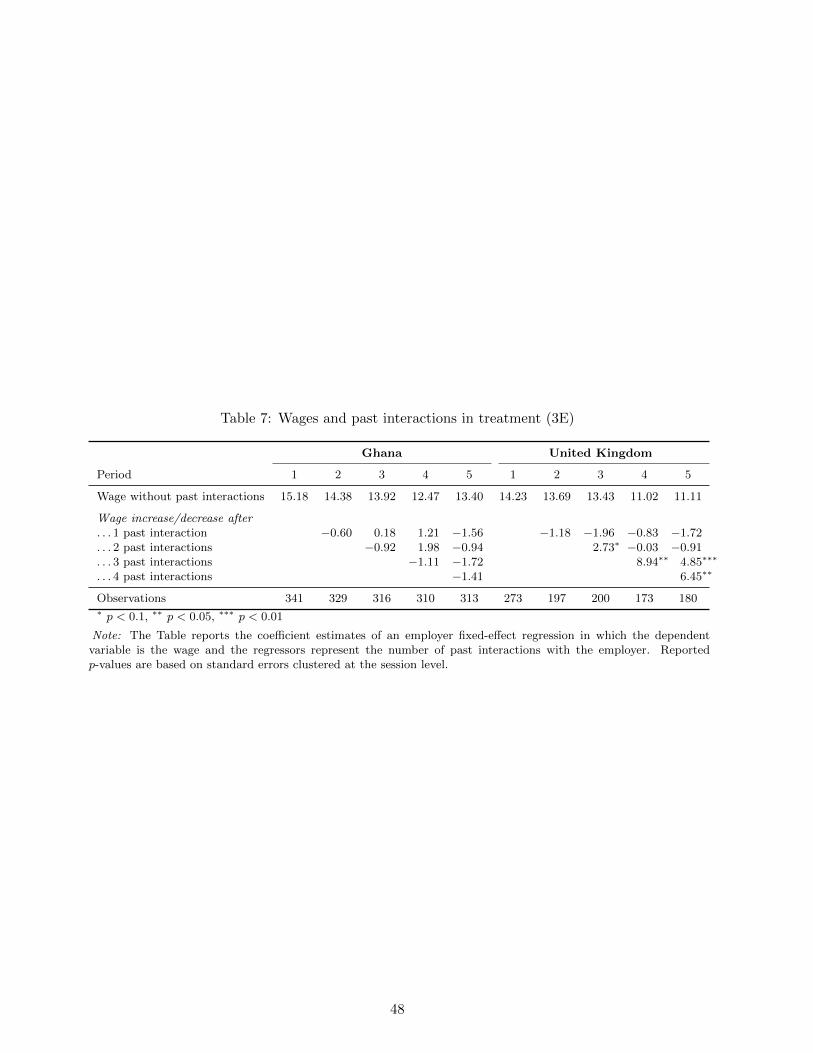
Table 7: Wages and past interactions in treatment (3E)
Ghana United Kingdom
Period 1 2 3 4 5 1 2 3 4 5
Wage without past interactions 15.18 14.38 13.92 12.47 13.40 14.23 13.69 13.43 11.02 11.11
Wage increase/decrease after. . . 1 past interaction −0.60 0.18 1.21 −1.56 −1.18 −1.96 −0.83 −1.72. . . 2 past interactions −0.92 1.98 −0.94 2.73∗ −0.03 −0.91. . . 3 past interactions −1.11 −1.72 8.94∗∗ 4.85∗∗∗
. . . 4 past interactions −1.41 6.45∗∗
Observations 341 329 316 310 313 273 197 200 173 180∗ p < 0.1, ∗∗ p < 0.05, ∗∗∗ p < 0.01
Note: The Table reports the coefficient estimates of an employer fixed-effect regression in which the dependentvariable is the wage and the regressors represent the number of past interactions with the employer. Reportedp-values are based on standard errors clustered at the session level.
48

Table 8: Wage offers in treatment (3E) and (3ES)
Ghana United Kingdom
Dependent variable: (1) (2) (3) (4)Wage offer by employer i in period t Treatment Both Treatment Both
(3E) only treatments (3E) only treatments
Contracted with employer i at t− 1 −0.872 −0.682 −3.070∗∗∗ −3.292∗∗∗
(0.837) (0.892) (0.885) (0.951)
Contracted with another employer at t− 1 −0.614 −0.442 0.525 0.518(0.830) (0.877) (0.913) (0.950)
Complied with i’s requested effort at t− 1 0.965 0.813 7.512∗∗∗ 7.851∗∗∗
(0.630) (0.743) (1.039) (0.981)
Complied with another employer’s requested effort at t− 1 0.543 0.401 −0.0199 0.103(0.467) (0.484) (0.765) (0.748)
Treatment (3ES)? 0.133 2.085(1.658) (1.655)
× Contracted with employer i at t− 1 −0.307 1.618(0.955) (0.973)
× Contracted with another employer at t− 1 −0.662 −0.925(0.965) (1.127)
× Complied with i’s requested effort in t− 1 0.102 0.0279(1.245) (0.995)
× Complied with other employer’s requested effort at t− 1 0.414 4.060∗∗∗
(1.020) (0.981)
Constant 14.92∗∗∗ 15.14∗∗∗ 12.43∗∗∗ 11.67∗∗∗
(0.719) (0.799) (0.499) (0.576)
N. Observations 1268 1795 750 1038Adjusted R-sq 0.687 0.681 0.572 0.592Fixed effects Employer Employer Employer EmployerPeriod dummies Yes Yes Yes Yes∗ p < 0.1, ∗∗ p < 0.05, ∗∗∗ p < 0.01
Note: The Table presents coefficient estimates of a linear regression using the wage offered by employer i in periodt as dependent variable. All regressors are indicator variables and relate to period t − 1, i.e., the period before theoffer. Standard errors are clustered at the session level.
49

Table 9: The effect of the reputation treatment on experimental outcomes
Ghana United Kingdom
(1) (2) (3) (4)Withing subject Across subject Withing subject Across subject
Offered wage(3ES) vs. (3E) −2.067∗∗∗ 0.293 1.678∗∗∗ 3.007
(0.406) (2.731) (0.403) (2.517)Acceptance(3ES) vs. (3E) −0.00892 −0.0125 0.0192 0.0448
(0.0100) (0.0196) (0.0197) (0.0610)Compliance(3ES) vs. (3E) 0.0380 0.00701 0.114∗∗∗ −0.0292
(0.0227) (0.109) (0.0270) (0.0944)Surplus(3ES) vs. (3E) 0.189 1.140 3.718∗∗∗ 2.785
(1.057) (3.073) (0.708) (4.292)Employer’s earnings(3ES) vs. (3E) 1.870∗ 0.910 2.723∗∗∗ 0.0712
(1.008) (2.173) (0.375) (2.424)Worker’s earnings(3ES) vs. (3E) −2.200∗∗∗ 0.288 −2.101∗ 2.002
(0.718) (6.141) (1.009) (3.112)
Note: Each cell of the Table corresponds to a separate regression. The reported coefficient is the treatmenteffect of 3ES relative to 3E. Each row corresponds to a different dependent variable, defined as in earlierTables. The ’Within subject’ regressions are subject-fixed-effect linear regressions using only those subjectsincluded in both treatments 3E and 3ES; it compares outcomes within subjects across games played atdifferent times in the same session. The ’Across subject’ regressions compare subjects from differentsessions, some of whom are assigned to treatment 3ES and some are not. These regressions include adummy equal to 1 if subject i is assigned to treatment 3ES and 0 otherwise, as well as a game orderdummy. Observations from games other than 3E and 3ES are omitted throughout. Standard errorsclustered at the session level are given in parentheses.
50

Table 10: Wage offer as a function of past effort and past offer rejection intreatment (1E) in additional experiments conducted in Ghana.
Students Entrepreneurs Both groups (pooled)
Dependent variable:Wage offer in period t (1) (2) (3) (4)
High effort in period t− 1? 1.762∗∗∗ 3.523∗∗ 1.976∗∗∗ 1.762∗∗∗
(0.381) (0.855) (0.377) (0.380)
Rejection in period t− 1? 1.788∗∗∗ 0.805 1.602∗∗∗ 1.788∗∗∗
(0.407) (0.825) (0.370) (0.406)
Entrepreneur?
× High effort in period t− 1? 1.762∗∗
(0.858)
× Rejection in period t− 1? −0.983(0.846)
Constant 15.30∗∗∗ 12.39∗∗∗ 14.68∗∗∗ 14.69∗∗∗
(0.278) (0.382) (0.273) (0.270)
Observations 2496 458 2954 2954Adjusted R2 0.0207 0.0272 0.0197 0.0212Fixed effects Employer Employer Employer EmployerPeriod dummies Yes Yes Yes Yes
∗ p < 0.1, ∗∗ p < 0.05, ∗∗∗ p < 0.01
Note: The Table presents coefficient estimates from a fixed effects regression of wage offeredon previous high effort and rejection, using data from the additional experiments conductedin Ghana (see text for details). Rejection is an indicator variable equal to one if the workerrejects the offer. High effort is an indicator variable and equal to one if the worker chooseshigh effort. Entrepreneur is a dummy equal to 1 if the subject is an entrepreneur, and 0 if thesubject is a university student. Only wage offers in period 2-5 are included. Standard errorsare clustered at the session level.
Table 11: Maximum likelihood population estimates of α and β of the Fehr-Schmidt model inGhana and the United Kingdom
Ghana United Kingdom Both countries (pooled)
(1) (2) (3) (4) (5) (6) (7) (8) (9)All periods Period 1 Period 5 All Period 1 Period 5 All periods Period 1 Period 5
α (disadvantageous −0.0291∗ −0.0195 −0.0393 0.0238 −0.00935 0.0263 −0.0291∗ −0.0195 −0.0393inequality aversion) (0.0171) (0.0285) (0.0296) (0.0165) (0.0303) (0.0194) (0.0163) (0.0271) (0.0281)
UK? 0.0529∗∗ 0.0101 0.0656∗
(0.0230) (0.0403) (0.0340)
β (advantageous 0.147∗∗∗ 0.158∗∗∗ 0.141∗∗∗ 0.213∗∗∗ 0.208∗∗∗ 0.181∗∗∗ 0.147∗∗∗ 0.158∗∗∗ 0.141∗∗∗
inequality aversion) (0.00777) (0.0106) (0.0117) (0.00886) (0.0125) (0.0125) (0.00738) (0.0101) (0.0111)
UK? 0.0663∗∗∗ 0.0497∗∗∗ 0.0399∗∗
(0.0114) (0.0159) (0.0166)
Observations 562 115 108 763 155 153 1325 270 261
∗ p < 0.1, ∗∗ p < 0.05, ∗∗∗ p < 0.01Note: The parameters have been estimated using a random utility multinomial logit model, using all available observationsover the entire subject pool. Positive numbers indicate inequality aversion.
51

Online appendix
A Instructions to experimental subjects
Below is an excerpt of the script used in the experiment for our British sessions. For our
Ghanaian sessions the same script was used, with the exception of the references to the currency
used for payment.
“Good morning. / Good afternoon. My name is Elwyn Davies. I am a researcher at the
University of Oxford. This is [...], who will be helping out today.
Welcome to this session of the experiment. This experiment is part of a wider study done by
the University of Oxford on entrepreneurship and firms. The goal is to see how people behave in
a virtual marketplace. Please remain silent during the entire duration of the experiment. Please
turn off any mobile phones.
During this session you will earn points. These points will be converted to pounds at the
end of the session. 100 points is equal to 3 pounds. You will receive this amount in private at
the end of the session. You will also receive a show-up payment of 4 pounds. All earnings will
be rounded up to the next 10p.
I will explain more about this experimental session later on. First, I will talk about how to
use the tablet. You will use the tablet to make choices in this experiment. Please have a look
at your tablet and read the message. If you are done reading, press OK.
Make sure to touch the screen gently. Do not press it too hard.
If, at any point, you have a question about the experiment, please raise your hand and we
will come to your desk to answer your question in private.
(Wait.)
We are now going to practice how to make offers. In this game you will be either an employer
or a worker. Employers make offers to the workers. I will talk about that more later on. First
we will practice how to make an offer.
Please press the green Make Offer button. You will see a new screen in which you can make
an offer. You always have to indicate two things. First you always need to select the level of
effort you demand from the worker, by pressing Low, Medium or High.
Please press Low, Medium or High.
Your selected choice becomes yellow.
52

Now try to change your choice. For example: from High to Low, and from Low to Medium.
Second, you need to select an amount of compensation, on the right part of the screen. Please
touch here, and select a number. The number has to be between 0 and 40. After selecting a
number, please change the number, for example from 0 to 5, or from 32 to 37. And then change
the number again.
On the bottom left of the screen you can see graphs. These graphs show you how much you
can earn if the worker accepts the offer. Please change the number on the right hand side, and
see how the graphs change as well. Yellow means that you are earning money, gray means that
points will be deducted.
Click on OK if you want to make the offer. You can also click on Cancel, or on Delete offer,
if you don’t want to make an offer to the worker. After clicking on OK, you will see the offer
you have made. If you want to change the offer, click on Change offer.
If you have any questions, please ask them. We will come to your desk to answer them.
(Wait until everybody is done.)
I will now talk about the experiment itself and what we are going to do.
Some of you will be employers, some of you will be workers. We will determine by chance
which role you get.
Each period the employers start by making offers to the workers. Each offer must specify a
level of effort and an amount of compensation. The workers then choose to accept or reject an
offer. If they reject an offer, both get zero points.
If the worker accepts the offer, the worker will work for the employer. This work gives a
profit to the employer, but working hard is tiring for the worker, so the worker will get less.
There are three levels of effort: high, medium and low.
• High effort means that the employer gets 40 points. The worker will lose 6 points.
• Medium effort means that the employer gets 20 points. The worker will lose 2 points.
• Low effort means that the employer gets only 5 points, but the worker will not lose any-
thing.
We will hand out a paper to remind you about this. You can also use the graphs to help
you with the calculation.
The effort level chosen is the same as what the employer demanded: the worker can only
choose the effort level demanded by the employer.
53
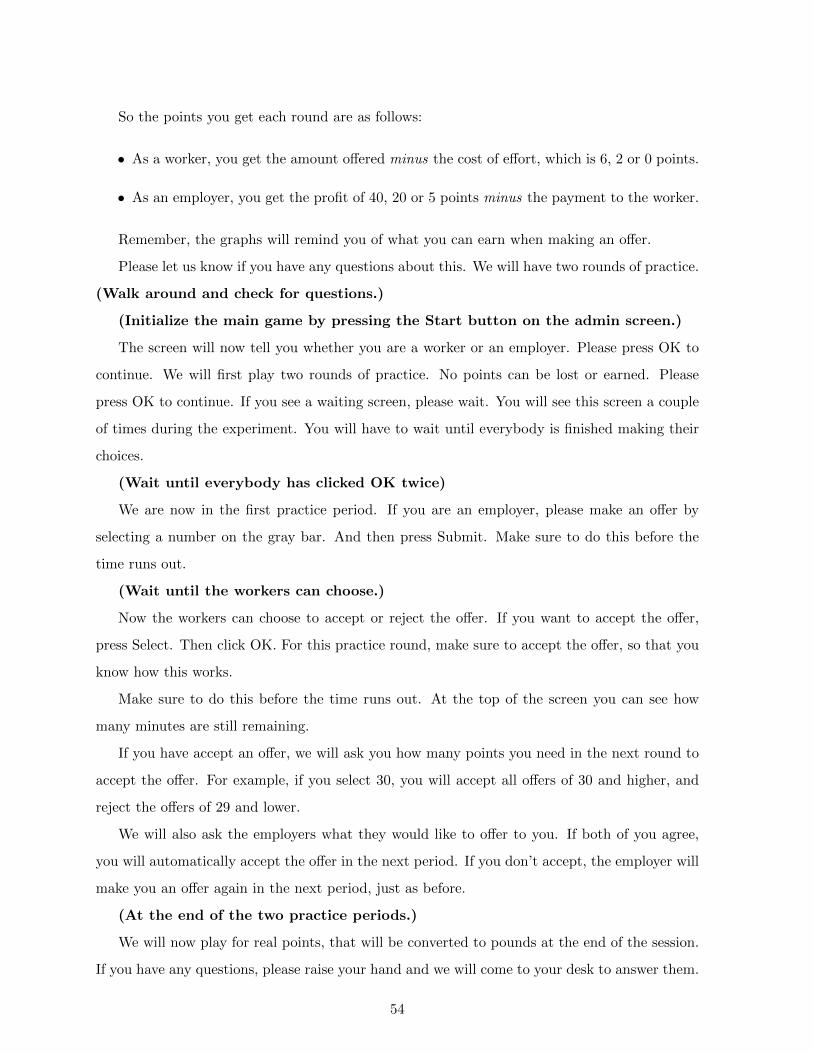
So the points you get each round are as follows:
• As a worker, you get the amount offered minus the cost of effort, which is 6, 2 or 0 points.
• As an employer, you get the profit of 40, 20 or 5 points minus the payment to the worker.
Remember, the graphs will remind you of what you can earn when making an offer.
Please let us know if you have any questions about this. We will have two rounds of practice.
(Walk around and check for questions.)
(Initialize the main game by pressing the Start button on the admin screen.)
The screen will now tell you whether you are a worker or an employer. Please press OK to
continue. We will first play two rounds of practice. No points can be lost or earned. Please
press OK to continue. If you see a waiting screen, please wait. You will see this screen a couple
of times during the experiment. You will have to wait until everybody is finished making their
choices.
(Wait until everybody has clicked OK twice)
We are now in the first practice period. If you are an employer, please make an offer by
selecting a number on the gray bar. And then press Submit. Make sure to do this before the
time runs out.
(Wait until the workers can choose.)
Now the workers can choose to accept or reject the offer. If you want to accept the offer,
press Select. Then click OK. For this practice round, make sure to accept the offer, so that you
know how this works.
Make sure to do this before the time runs out. At the top of the screen you can see how
many minutes are still remaining.
If you have accept an offer, we will ask you how many points you need in the next round to
accept the offer. For example, if you select 30, you will accept all offers of 30 and higher, and
reject the offers of 29 and lower.
We will also ask the employers what they would like to offer to you. If both of you agree,
you will automatically accept the offer in the next period. If you don’t accept, the employer will
make you an offer again in the next period, just as before.
(At the end of the two practice periods.)
We will now play for real points, that will be converted to pounds at the end of the session.
If you have any questions, please raise your hand and we will come to your desk to answer them.
54

You will have the same worker or employer for the next five periods. The letter
on your screen does not correspond to the letter on the desk: they are different. You cannot tell
who in the room your worker or employer is.
You can check your number of points by pressing the Show history button during the
experiment. You can then also see what has happened in the previous rounds.
Press I am ready to continue.
(Part 2: Treatment (1E))
We have now finished the first set of five periods.
For the next part of the experiment, we are going to do the same thing. However, now the
workers can choose their level of effort. They do not have to do what you demanded as an
employer. So for example, if you ask for high effort, the worker can also choose medium or low
effort. If you ask for low effort, the worker can also choose medium or high effort.
As an employer you will now see graphs for all the three options.
During the making of an offer, you will see bullets indicating what the worker has done in
previous rounds. Gray means that the worker rejected the offer. Green means that the worker
chose the level of effort that was demanded, or higher. Red means that the worker choose a
lower level of effort than you demanded.
You will have a different worker than before. You will have the same worker or employer for
the next five periods.
(Part 3: Treatment (3E))
For the next five periods, workers can still choose their level of effort. However, some of the
employer can now make offers to three workers at the same time. Similarly, workers can accept
offers from different employers. Every worker can only choose one offer. An employer can only
have one worker.
Workers will take turns in choosing their offer. Sometimes you might be the first one, and
have all the offers available. Sometimes you might be the last one, and there might be fewer
offers available. We will determine the order in which you choose by chance.
As an employer, when you make your first offer, this will be shared with the other employers
that can offer to this worker.
Again, as an employer, you can see what the workers have done in the previous periods
when they were working for you. You cannot see what workers did when they were working for
55

someone else.
(Part 4: Treatment (3E))
For the next five periods, you will have new workers or employers. There is no practice
period.
(Part 4: Treatment (3ES))
For the next five periods, you will have new workers or employers. There is no practice
period.
As an employer, you can now see what the workers have done in the previous periods, not
only when they were working for you, but also what they did when they were working for
someone else.
(Questionnaire)
Ok, we are now almost done with the experiment. Please fill in the questions in the ques-
tionnaire. In the meantime we will prepare your payment. We will call you when we are done
with making the payments.”
56

B Conceptual framework for the gift-exchange game
We start by discussing the standard conceptual framework that is behind our experiment. The
gift-exchange game is a sequential prisoner’s dilemma game. The game is sequential in the sense
that the worker makes a choice only after observing the employer’s choice. In infinite games, the
Folk Theorem tells us that grim trigger strategies can sustain cooperation. Also other strategies,
such as tit-for-tat strategies can sustain cooperation in games like these (see e.g. Axelrod, 1984).
The main difference between the grim trigger and the tit-for-tat strategy is that tit-for-tat allows
for redemption, while for the grim trigger the punishment lasts forever. However, conditional
reciprocity is an element of both: a player will only cooperate if the other player cooperated in
the past as well.
Our experiment is a finite period game. Backwards induction, assuming that players only
maximize their own earnings, predicts non-cooperation as the subgame perfect equilibrium: in
the last period workers will choose low effort, regardless of the wage offered by the employer.
Anticipating this, employers will choose a minimum wage of zero, such that the worker is indif-
ferent between accepting or rejecting the offer. By backwards induction, the subgame perfect
equilibrium is that the employer offers a wage of zero points in every period, regardless of past
behavior of the worker, and that the worker chooses low effort in every round, regardless of the
amount offered by the employer: cooperation unravels.
However, many experimental studies have shown that cooperation is possible in a finite
game. Selten and Stoecker (1986) and Andreoni and Miller (1993) show that in a finite period
prisoner’s dilemma game subjects tend to cooperate for some period of time, until the last couple
of periods, when people defect. Theoretical models have tried to explain this, for example by
assuming that players have incomplete information on the other player’s options or motivations.
Kreps et al. (1982) show that if a player has a belief that there is a small probability that another
player is acting “irrationally”, i.e., not playing according to the subgame perfect equilbrium,
but for example to a tit-for-tat strategy instead, cooperation can be feasible in a finite game.
Fudenberg and Maskin (1986) use a similar argument to show that in a finite repeated game an
equilibrium is possible where in the first periods of the game the game is played like an infinitely
repeated game, and where players play a cooperation with punishment strategy, while switching
to behavior consistent with backward induction in the last periods of the game.
A similar result as Kreps et al. (1982) can also be achieved by incorporating other-regarding
preferences, such as inequity aversion and fairness concerns into the utility function of some
57

of the players. In the Appendix we present a model in which there are two types, a social
type (S-type) and a rational self-interested type (R-type). The S-type’s effort choice is solely
dependent on the wage offered: higher wages attract higher levels of effort. The R-type is purely
self-interested and aims to achieve the highest payoff. In the Appendix we show that when the
share of S-types in the population is high enough, a Perfect Bayesian equilibrium exists in which
the R-type’s optimal response is to mimic the S-type until the second to last period and for
the employer to keep offering a high wage as long as the worker chooses high effort. In the last
period the R-type will choose low effort. If the worker chooses low effort, the employer infers
that the worker must be the R-type and will subsequently offer a zero wage. This punishment
by the employer following low effort provides an incentive for the R-type to choose high effort,
as long as the high wage outweighs the cost of high effort. In this equilibrium, the R-type tries
to build a reputation for being a S-type, allowing him or her to capture parts of the surplus of
exerting high effort.
Depending on the wage parameters and the distribution of types in the population, other
types of Perfect Bayesian equilibria are possible as well, for example in which the employer offers
high wages in the first periods of the game and then a medium-level wage in the last period or
in which the employer offers medium level wages throughout.
The behavior of the social type can be rationalised by other-regarding preferences, such as
models of altruism or inequality aversion. For example, in the Fehr-Schmidt model of inequality
aversion (Fehr and Schmidt, 2002) players receive a disutility from both earning more than the
other player (advantageous inequality) or from earning less than the other player (disadvanta-
geous inequality). The utility function in the two-player case can be written as
Ui(x) = xi − αi max {xj − xi, 0} − βi max {xi − xj , 0} .
In this equation αi represents the disutility from disadvantageous inequality and βj represents
the disutility from advantageous inequality. Generally, it is assumed that αi ≥ βi: a player has
a higher disutility from disadvantageous inequality than from advantageous inequality. We will
use the Fehr-Schmidt model of inequality aversion later in this paper to structurally estimate
the reciprocity parameters of our participants in Ghana and the UK.
B.1 Competition and reputation
In treatments (3C), (3E) and (3ES) there are three workers and three employers. In our setup
there is no market imbalance, as each worker can in principle find an employer and vice versa.
58

A purely self-interested profit-maximizing principal will prefer to hire a worker that is willing to
exert high effort for a low wage. If employers had full information, they would compete with each
other to hire this worker, which can result in increasing the wages to outbid the other employers.
In Davies and Fafchamps (2016) we show that if there is heterogeneity in the minimum wage
that a worker needs to accept an offer, competition between employers to hire the worker with
the lowest minimum wage will lead to employers increasing the wages offered to these workers
to the level of the worker with the highest minimum wage.
Introducing reputation in treatment (3ES) can have multiple effects. First, by revealing past
compliance, an employer can identify more reliable workers, which can lead to increased com-
petition to hire this worker and therefore to wage increases. Second, the sharing of information
on compliance can also function as an incentive, if employers use this information in their offers.
Non-compliance for a worker can now become more costly: not only will the employer who he
or she was working for lower their offer, also other employers will lower their offers. Greif et al.
(1994) argue that such a multilateral reputation mechanism can function as an enforcement
device and deter cheating.
B.2 Predictions
On the basis of the theoretical model as well as the results from earlier experiments, we predict
three main patterns of contracting to happen.
First, we expect employers to offer high wages in the initial periods, rather than the zero
wage predicted by the subgame perfect equilibrium of purely self-interested rational agents. The
theoretical model shows that if there is a sizeable group of reciprocating workers, offering a high
wage is rationally the optimal choice for the employer.
Second, we expect conditional reciprocity on behalf of the workers. Workers will reciprocate
high wages with high effort. This behavior is for example implied by other-regarding models of
altruism or inequality aversion. As we show in the Appendix, according to the Fehr-Schmidt
model of inequality aversion, a worker with inequality aversion coefficients of αi = 0.5 and βi =
0.5 will choose high effort when the wage is 19 points or higher, choose medium effort for wage
offers between 8 and 19 points and choose low effort for lower offers. This positive reciprocity
by the workers has been shown consistently across many gift-exchange game experiments and
happens even when there are no future interactions present (Fehr et al., 1997, 1993, 1998; Fehr
and Falk, 1999).
59

Third, we expect conditional reciprocity on behalf of the employers. This means that we
expect employers to reduce wages of workers choosing low effort or to cut the relationship
completely. In the finite period theoretical model with types, this is the outcome of screening,
as low effort reveals the type of the worker. The threat of lowering the wage provides an
incentive even for rationally self-interested workers to exert high effort (provided their incentive
compatibility constraint is satisfied).
Earlier gift-exchange game experiments have confirmed this presence of conditional reci-
procity on behalf of employers. In the experiment of (Brown et al., 2004, 2012) employers
implemented a strategy of contingent contract renewal, in which they were more likely to renew
contracts of workers choosing high effort. Workers choosing low effort were either fired or saw
their wage reduced. These three predictions can be tested by analyzing the contracting behavior
in treatment (1E), where one employer can make an offer to one worker only, and where the
worker can choose effort.
Furthermore, we anticipate that introducing competition will increase wages, due to the
wage pushing up effect of bidding. This can be tested by comparing wage offers in treatment
(3E) with wage offers in treatment (1E). Moreover, we anticipate that sharing information on
the past workers’ actions increases compliance as the availability of a multilateral reputation
mechanism increases the scope for collective punishment. This can be tested by comparing wage
offers following low and high effort in treatment (3ES) with wage offers in treatment (3E).
60

C A model of cooperation with types
We now introduce a model in which players differ in their propensity to cooperate. We start
with a basic model of cooperation inspired by the literature, before modifying this model to suit
our needs.
C.1 Basic model of cooperation
For our model, we follow Kreps et al. (1982) as well as the Appendix of Brown et al. (2004).
Let w be the wage offer. We assume there are two types in the population, a social type and a
purely self-interested type:
Assumption 1 There exist two types, a “social” type S(wM , wH) and a rationally self-interestedtype R. The share of social types in the population is σ. The social type S-type will choose
• high effort if w ≥ wH ,
• medium effort if wM ≤ w < wH ,
• and low effort if w < wM .
The threshold wages wH and wM are fixed and wH > wM > 0.The rationally self-interested R-type will maximize monetary earnings across the game. The
utility function of earnings in a particular period is
πW (w, e) = w − c(e), (A1)
with c(e) the cost of effort. We assume no discounting.
The employers are risk-neutral:
Assumption 2 Employers are risk-neutral and maximize their monetary earnings, i.e. choosethe wage w such that their payoff πE(w, e) is maximized, with
πE(w, e) = Π(e)− w. (A2)
Furthermore, we assume full knowledge of the relevant parameters:
Assumption 3 The share social types σ and the threshold wages wH and wM are public knowl-edge.
C.1.1 High effort equilibrium
Proposition 4 Under certain conditions, a perfect Bayesian equilibrium exists in which theemployer offers wH in all periods, unless the worker deviates from the S-type behavior, afterwhich the employer will offer wL = 0. The S-type worker chooses effort according to the offeredwage throughout. The R-type mimics the actions of an S-type in all periods except for the finalperiod, in which the R-type will choose low effort.
61

We can use backward induction to prove the existence of such an equilibrium under certain
conditions:
• In the last period, T , the R-type will choose low effort and the S-type will choose effort
dependent on the offered wage, as described above. When offered a wage of zero, both
types of workers accept the offer, as they are indifferent between rejection and acceptance,
and both types will choose low effort.
• In the last period, the employer will choose the wage that gives the highest expected payoff.
Let XT be the history of play up until period T . The expected employer’s payoff when
offering w is
P (S|XT )Π(H) + (1− P (S|XT ))Π(L)− w if w ≥ wH ,
P (S|XT )Π(M) + (1− P (S|XT ))Π(L)− w if wM ≤ w < wH ,
Π(L)− w if w < wM ,
0 if no offer is made.
In the above PT (S|XT ) is the probability that the worker is a social type given history
XT .
If the R-type mimics the social type until this period, the belief of the employer that the
worker is of the S-type equals PT (S|XT ) = σ. (For any other behavior PT (S|XT ) = 0 and
the employer will offer wL = 0.) The lowest wage possible to encourage high effort from
the S-type is wH and the lowest wage to encourage medium effort from the S-type is wM .
The employer will offer wH over wM if
Π(H)−Π(M) ≥ wH − wM
σ, (A3)
and over wL = 0 if
Π(H)−Π(L) ≥ wH − wL
σ=wH
σ. (A4)
If the employer is presented with a worker that does not choose according to how an S-type
chooses, PT (S|XT ) = 0, and the employer will offer a wage of wL = 0.
• In period T−1 the R-type worker will mimic the actions of the S-type if the sum of payoffs
in period T − 1 and period T of doing so outweighs the payoffs of choosing low effort. The
62

incentive compatibility constraint for the R-type worker in period T − 1 becomes, when
wH is offered,
wH − c(H) + wH − c(L) ≥ wH − c(L) + wL − c(L).
so
wH ≥ c(H).25 (A5)
• Given that the R-type will mimic the S-type in period T − 1, the earnings in this period
are respectively Π(H) − wH , Π(M) − wM and Π(L) when offering wH , wM and wL = 0.
The employer will offer wH if
Π(H)−Π(M) ≥ wH − wM and Π(H)−Π(L) ≥ wH (A6)
Note that these conditions are satisfied when conditions (A3) and (A4) are satisfied.
• We can repeat this exercise for the earlier periods and show that conditions (A5) and (A6)
need to hold in these periods as well.26
Provided conditions (A3), (A4), (A5) and (A6) hold, the Perfect Bayesian equilibrium as
described in Proposition 4 holds.
C.1.2 Alternative Perfect Bayesian equilibria
For other conditions, other Perfect Bayesian equilibria exist, for example in which the employer
offers wH in the first periods and then offers wM in the last period, or in which the employer
offers wM throughout.
The equilibrium in which wM is offered in the last period, and wH in the periods before that,
can exist under the following conditions:
• In the final period, the employer will offer wM provided this yields a higher payoff than
offering wH or zero, so if
Π(H)−Π(M) ≤ wH − wM
σand Π(M)−Π(L) ≥ wM
σ, (A7)
25When this condition holds, the worker will also mimic the S-type when offered wM in this period, because ifc(H) > c(M),
wM − c(M) + wH − c(L) ≥ wM − c(L) + wL − c(L).
26E.g., the R-type worker in period t will choose high effort if
wH − c(H) + (T − t)wH − (T − t− 1)c(H) − c(L) ≥ wH − c(L) + (T − t)wL − (T − t− 1)c(L) − c(L),
which is equivalent towH ≥ c(H).
63

• In period T − 1, the R-type worker will mimic the S-type worker and choose high effort
following wH if
wH − c(H) + wM − c(L) ≥ wH − c(L) + wL − c(L),
wM > c(H). (A8)
and choose medium effort following wM if
wM − c(M) + wM − c(L) ≥ wM − c(L) + wL − c(L),
wM > c(M). (A9)
• In period T − 1 wH is the optimal wage if
Π(H)−Π(M) ≥ wH − wM and Π(H)−Π(L) ≥ wH (A10)
• For periods t < T − 1 the R-type will choose high effort following wH if
wH − c(H) + (T − t− 1)(wH − c(H)) + wM − c(L) ≥ wH − c(L) + (T − t)(wL − c(L)),
⇒ wH ≥(T − t)c(H)− wM
T − t− 1, (A11)
which is implied by condition (A8).27
Proposition 5 Under conditions (A7), (A8) and (A10) a Perfect Bayesian equilibrium is pos-sible in which the employer offers wH in all but the final period and wM in the final period toworkers that choose according to the wage-effort schedule of the S-type and zero to other workers.R-type workers will choose according to the S-type schedule up until the second to last periodand choose low effort in the last period.
The main difference between the all high wage equilibrium and this equilibrium is that the
expected payoff in the last period from offering wH is not high enough, for example if there are
too few S-types in the population. Offering wM in the last period will yield a higher payoff
in expectation. In the periods before that offering wH is - in expectation - the most profitable
choice, as both the R- and the S-type will reciprocate this with high effort (see condition (A10)).
There are also equilibria possible where the employer offers wM throughout. This will be
the case when condition (A10) is violated, and the wage differential wH − wM is higher than
the profit differential Π(H) − Π(M). For these wage levels, even if the entire population were
S-types, offering wM would be more profitable than offering wH .
27We can rewrite the left had side of (A11) using condition (A8):
(T − t− 1)wH + wM
T − t− 1>
(T − t− 1)wM + wM
T − t− 1=
(T − t)wM
T − t− 1≥ (T − t) c(H)
T − t− 1
64

C.2 Microfoundations of other-regarding behavior
The model above does not provide a microfoundation for the behavior of the social S-type,
but rather assumed that this type would choose according to a schedule. A common model
to provide such a microfoundation is the Fehr-Schmidt model of inequality aversion, where the
individual utility function is defined by
Ui(xi, xj) = xi − αi max (xj − xi, 0)− βi max (xi − xj , 0) .
In this equation αi represents the disutility from having a lower payoff than the other player
and βj represents the disutility of having a higher payoff than the other player. Generally,
it is assumed that αi ≥ βi: a player has a higher disutility from disadvantageous inequality
(represented by αi) than from advantageous inequality (represented by βi).
Figure A5 shows the relation between βi and the threshold wages wM and wH , taking αi
fixed at 0.5 and using the parameters from our experiment. When both αi and βi are fixed at
0.5, the corresponding threshold wages are wM = 8 and wH = 19.
Other classes of utility functions exist that result in similar threshold wages. For example,
a model of altruism with a linear weighting of individual utility functions, e.g.,
Ui(xi, xj) = γv(xi) + (1− γ)v(xj)
will lead to the worker choosing high effort for high wages, medium effort for medium-level
wages and low effort for low wages, provided the individual value functions v(xi) are sufficiently
concave.28
C.3 Screening and incentives
In the Perfect Bayesian equilibrium an employer observing low effort following a wage offer of
wM or wH will infer from this that the worker is a R-type worker and subsequently reduce the
wage to zero. This reduction of the wage following low effort provides the basis of the incentive
compatibility constraint (A5). The screening mechanism used by the employer provides the
incentive for the R-type worker to exert high effort.
In the model, screening is perfect and instant: if the worker chooses low effort following a
high wage, the worker is singled out as an R-type and will be offered zero wages for the remaining
28Given that the payoff functions for both the worker and employer are linear in w, using a linear value functioninstead of a convex value function will result in either always the same effort choice, regardless of wage, or in acorner solution, or in indifference between two effort levels for all wages.
65

periods. There is no rationale for still offering a high wage following low effort. Such a rationale
could be provided by models where the effort choice is not perfect. Suppose we introduce a
small margin of error in the decision of the S-type.
Assumption 6 With probability ρ < 1 each period, a S-type worker will choose low effort.
For simplicity, assume we play the game for only two periods. Suppose that in period 1 the
worker received a high wage, wH , but chose low effort. The probability that the worker is a
S-type is
P (S|wH , L) =P (L|wH , S)P (S|wH)
P (L|wH , S)P (S|wH) + P (L|wH , R)P (R|wH)=
ρσ
ρσ + P (L|R, wH)(1− σ).
Now suppose the R-type always chooses low effort, so P (L|R, wH) = 1, does it make sense
to offer wH again? The employer will offer a high wage if
wH − wM ≤ ρσ
ρσ + (1− σ)(1− ρ) (Π(H)−Π(M)),
and wH ≤ ρσ
ρσ + (1− σ)(1− ρ) (Π(H)−Π(L)).
If ρ and σ are sufficiently high and wH sufficiently low, these conditions indeed hold, and it
is optimal for the employer to offer high effort following low effort. Given this, it is optimal for
the R-type to choose low effort in the first period.
If we add another period to the model, and look at whether it is still rational to offer high
wage following two choices of low effort, we see that the conditions become even stricter: we
require a higher level for ρ and σ and a lower level for wH :
wH − wM ≤ ρ2σ
ρ2σ + (1− σ)(1− ρ) (Π(H)−Π(M)),
and wH ≤ ρ2σ
ρ2σ + (1− σ)(1− ρ) (Π(H)−Π(L)).
Figure A6 shows these conditions graphically, with σ = 0.8 and wM = 10, for the two-period
game (solid line), the three-period game (dashed line), the four-period game (dot-dashed line)
and the five-period game (dotted line), using the payoff parameters of our game. From the graph
it can be seen that the maximum level of wH that supports such an equilibrium is low for low
values of ρ (if an employer sees low effort, the probability is high that the worker is an R-type),
66
then increases for medium levels of ρ and finally decreases again (for high values of ρ offering
wH becomes to risky, because the probability that S-types choose low effort is high).
The Figure shows that when σ = 0.8, wM = 10, the highest level of wH that can sustain
offering wH following low effort in a 2-period game is 13, if ρ = 0.3. As discussed earlier, most
other-regarding models point to values of wH that are higher than this and therefore cannot
sustain an equilibrium where high wages are offered following low effort. The equilibria where
employers offer high effort following two instances of low effort require high values of ρ (i.e., the
probability that an S-type makes a mistake must be high) and also wH must be low (S-types
are willing to exert high effort following a low wage).
Other equilibria exist, for example in which the employer lowers the wage from wH to wM
following low effort. These equilibria can exist for higher levels of wM and wH and lower levels
of ρ and σ.
67
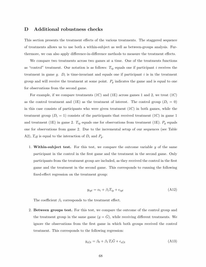
D Additional robustness checks
This section presents the treatment effects of the various treatments. The staggered sequence
of treatments allows us to use both a within-subject as well as between-groups analysis. Fur-
thermore, we can also apply difference-in-difference methods to measure the treatment effects.
We compare two treatments across two games at a time. One of the treatments functions
as “control” treatment. Our notation is as follows: Tig equals one if participant i receives the
treatment in game g. Di is time-invariant and equals one if participant i is in the treatment
group and will receive the treatment at some point. Pg indicates the game and is equal to one
for observations from the second game.
For example, if we compare treatments (1C) and (1E) across games 1 and 2, we treat (1C)
as the control treatment and (1E) as the treatment of interest. The control group (Di = 0)
in this case consists of participants who were given treatment (1C) in both games, while the
treatment group (Di = 1) consists of the participants that received treatment (1C) in game 1
and treatment (1E) in game 2. Tig equals one for observations from treatment (1E). Pg equals
one for observations from game 2. Due to the incremental setup of our sequences (see Table
A2), Tig is equal to the interaction of Di and Pg.
1. Within-subject test. For this test, we compare the outcome variable y of the same
participant in the control in the first game and the treatment in the second game. Only
participants from the treatment group are included, as they received the control in the first
game and the treatment in the second game. This corresponds to running the following
fixed-effect regression on the treatment group:
yigt = αi + β1Tig + εigt (A12)
The coefficient β1 corresponds to the treatment effect.
2. Between groups test. For this test, we compare the outcome of the control group and
the treatment group in the same game (g = G), while receiving different treatments. We
ignore the observations from the first game in which both groups received the control
treatment. This corresponds to the following regression:
yiGt = β0 + β1 TiG+ εiGt (A13)
68

3. Difference-in-difference. In the difference-in-difference test we correct for the com-
mon time trend of both groups across the two games. This corresponds to the following
regression:
yigt = β0 + β1 Tig + β2 Pg + β3Di + εigt (A14)
Here Di is a time-invariant indicator on whether an individual is in the treatment group,
Pg is an indicator for the second game. Note that in our setup, Tig = Di × Pg.
4. Fixed effects. The fixed-effects regression is in its essence similar to the difference-
in-difference regression, but exploits the full panel dimension of the data by controlling
for individual characteristics. This approach has potentially more power. Just like in the
difference-in-difference regression we rely on a common trend assumption for our estimation
of the treatment effect. This corresponds to the following regression:
yigt = αi + β1 Tig + β2 Pg + εigt (A15)
The main difference between this equation and Equation (A14) is that in Equation (A14)
β0 and β3 are estimated on the basis of the entire sample, while in this equation αi is
estimated for each individual separately.
Tables A8, A9 and A10 present the effects of the treatments on the offered wages, surplus,
the earnings of the worker and the employer, the rate of acceptance and the rate of compliance.
69

E Classifying worker types
This appendix section provides more detailed information on the estimation of the structural
model of other-regarding preferences for workers. As starting point, we assume that, in every
period, the worker chooses an effort level to maximize Fehr-Schmidt preferences of the type:
Ui(x) = xi − αi max (xj − xi, 0)− βi max (xi − xj , 0)
Figure A8 shows, for three different wage values, the effort level predicted by a worker holding
Fehr-Schmidt preferences with parameters αi and βi. The full set of graphs for all possible wage
values is shown in Figure A9. These Figures can be used to identify sets of values of αi and βi
that are consistent with observed effort choices under the maintained assumption that workers
act as if in a one-shot (i.e., unconditional) one-sided PD game and have Fehr-Schmidt preferences
with preference parameters αi and βi.
This calculation is first done separately for each worker in each period of each game, as
illustrated in Figure A10. Next, we overlap the shared areas i with each other to identify the
set of values of αi and βi that are consistent with at least four out of the five effort choices
made by a worker. This is illustrated in Figure A11 for the same worker as in Figure A10. By
repeating this process for each worker, we derive bounds for the distribution of αi and βi across
all workers. These bounds are those shown in Figure 3.
70

F Appendix Tables and Figures0
.1.2
0 10 20 30 40Wage
All periods
0 10 20 30 40Wage
Period 1
Treatment (1E)Ghana
0 10 20 30 40Wage
Period 5
0.1
.2
0 10 20 30 40Wage
All periods
0 10 20 30 40Wage
Period 1
Treatment (1E)United Kingdom
0 10 20 30 40Wage
Period 5
Figure A1: The Figure shows histograms of wage offers for Ghana and the UK. Only observationsfrom treatment (1E), games 2-4, are used to construct the histogram. The line represents a non-parametric density estimate calculated using a Epanechnikov kernel.
71
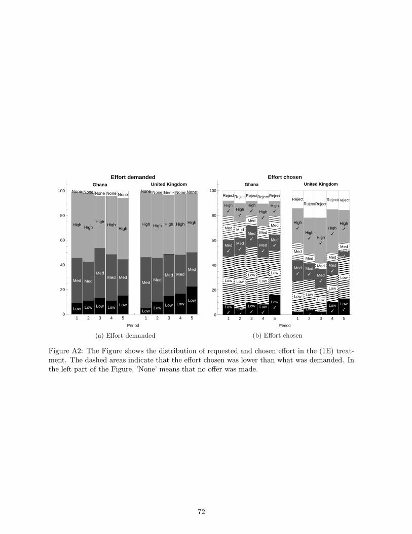
Low
Med
High
None
Low
Med
High
None
Low
Med
High
None
Low
Med
High
None
Low
Med
High
None
Low
Med
High
None
Low
Med
High
None
Low
Med
High
None
Low
Med
High
None
Low
Med
High
None
1 2 3 4 5 1 2 3 4 50
20
40
60
80
100
Period
Effort demandedGhana United Kingdom
(a) Effort demanded
Low✓
Low
Med✓
Med
High✓
Reject
Low✓
Low
Med✓
Med
High✓
Reject
Low✓
Low
Med✓
Med
High✓
Reject
Low✓
Low
Med✓
Med
High✓
Reject
Low✓
Low
Med✓
Med
High✓
Reject
Low✓
Low
Med✓
Med
High✓
Reject
Low✓
Low
Med✓
Med
High✓
Reject
Low✓
Low
Med✓
Med
High✓
Reject
Low✓
Low
Med✓
Med
High✓
Reject
Low✓
Low
Med✓
Med
High✓
Reject
1 2 3 4 5 1 2 3 4 50
20
40
60
80
100
Period
Effort chosenGhana United Kingdom
(b) Effort chosen
Figure A2: The Figure shows the distribution of requested and chosen effort in the (1E) treat-ment. The dashed areas indicate that the effort chosen was lower than what was demanded. Inthe left part of the Figure, ’None’ means that no offer was made.
72

0.1
.2
0 10 20 30 40Wage
Treatment (1E)
0 10 20 30 40Wage
Treatment (3E)
(Game 4 only)Ghana
0 10 20 30 40Wage
Treatment (3ES)
0.1
.2
0 10 20 30 40Wage
Treatment (1E)
0 10 20 30 40Wage
Treatment (3E)
(Game 4 only)United Kingdom
0 10 20 30 40Wage
Treatment (3ES)
Figure A3: The Figure shows histograms of wage offers in treatment (1E), (3E) and (3ES), inGhana and the United Kingdom. To allow for comparison, only game 4 data is included becausetreatment (3ES) is only conducted as game 4. The line represents a non-parametric densityestimate calculated using a Epanechnikov kernel.
73

Ghana
37 42 49 37 44
39 24 22 24 31
14 19 12 24 14
1 2 3 4 5
Loweffort
Mediumeffort
Higheffort
Period
% Effort chosen (percentage) Wage is increased Same wage (within ±2 points) Wage is decreased
United Kingdom
27 30 20 34 47
32 23 20 16 10
25 23 32 31 23
1 2 3 4 5
Loweffort
Mediumeffort
Higheffort
Period
% Effort chosen (percentage) Wage is increased Same wage (within ±2 points) Wage is decreased
Figure A4: The Figure presents a visual summary of transitions between effort levels in game2 of treatment (1E). The number and the size of the circle indicate the percentage of workerschoosing this effort level in a particular period. The thickness of the line indicates the percentageof transitions between effort levels over all subjects. The shading of the lines indicates whetherthe employer increases the wage by more than 2 points, keeps it the same (within a ±2 pointrange) or decreases the wage by more than 2 points. Rejections are not included in this graph.
74

0.0 0.2 0.4 0.6 0.8 1.0βi0
10
20
30
40wH,wM
αi = 0.5
wH
wM
Figure A5: The levels of wH and wM as a function of βi in the Fehr-Schmidt framework (usingαi = 0.5 and the parameters from the game).
0.0 0.2 0.4 0.6 0.8 1.0ρ0
10
20
30
40wH
σ = 0.8, wM = 10
2-period game (after observing L)
3-period game (after observing LL)
4-period game (after observing LLL)
5-period game (after observing LLLL)
Figure A6: The maximum level of wH for which it is rational for an employer to offer this wage,after observing low effort for one period (solid line), two periods (dashed line), three periods(dot-dashed line) and four periods (dotted line), as a function of ρ.
75

Employer
Worker
0 40
selects w between 0 and 40, andspecifies desired effort
Worker
acceptreject
(0, 0)(40 − w, w − 6) (5 − w, w)
high
low
* payoffs if employer makes no offer: (0, 0)payoff notation: (employer, worker)
(20 − w, w − 2)
medium
Figure A7: Extensive-form representation of the game
0.0 0.5 1.0 1.5 2.00.0
0.5
1.0
1.5
2.0
α (disadvantageous)
β(a
dvan
tage
ous)
w = 7
REJECTchoose
MEDIUM
chooseLOW
0.0 0.5 1.0 1.5 2.00.0
0.5
1.0
1.5
2.0
α (disadvantageous)
β(a
dvan
tage
ous)
w = 19
REJECT
chooseHIGH
chooseMEDIUM
choose LOW
0.0 0.5 1.0 1.5 2.00.0
0.5
1.0
1.5
2.0
α (disadvantageous)
β(a
dvan
tage
ous)
w = 27
choose HIGH
choose MEDIUMchoose LOW
Figure A8: Expected behaviour by worker in the fairness model for different parameters of αi
and βi, as response to the wage w offered by the employer.
76

0.0
0.5
1.0
1.5
2.0
0.0
0.5
1.0
1.5
2.0
α(d
isad
vant
ageo
us)
β(advantageous)
w=
1
0.0
0.5
1.0
1.5
2.0
0.0
0.5
1.0
1.5
2.0
α(d
isad
vant
ageo
us)
β(advantageous)
w=
2
0.0
0.5
1.0
1.5
2.0
0.0
0.5
1.0
1.5
2.0
α(d
isad
vant
ageo
us)
β(advantageous)
w=
3
0.0
0.5
1.0
1.5
2.0
0.0
0.5
1.0
1.5
2.0
α(d
isad
vant
ageo
us)
β(advantageous)
w=
4
0.0
0.5
1.0
1.5
2.0
0.0
0.5
1.0
1.5
2.0
α(d
isad
vant
ageo
us)
β(advantageous)
w=
5
0.0
0.5
1.0
1.5
2.0
0.0
0.5
1.0
1.5
2.0
α(d
isad
vant
ageo
us)
β(advantageous)
w=
6
0.0
0.5
1.0
1.5
2.0
0.0
0.5
1.0
1.5
2.0
α(d
isad
vant
ageo
us)
β(advantageous)
w=
7
0.0
0.5
1.0
1.5
2.0
0.0
0.5
1.0
1.5
2.0
α(d
isad
vant
ageo
us)
β(advantageous)
w=
8
0.0
0.5
1.0
1.5
2.0
0.0
0.5
1.0
1.5
2.0
α(d
isad
vant
ageo
us)
β(advantageous)
w=
9
0.0
0.5
1.0
1.5
2.0
0.0
0.5
1.0
1.5
2.0
α(d
isad
vant
ageo
us)
β(advantageous)
w=
10
0.0
0.5
1.0
1.5
2.0
0.0
0.5
1.0
1.5
2.0
α(d
isad
vant
ageo
us)
β(advantageous)
w=
11
0.0
0.5
1.0
1.5
2.0
0.0
0.5
1.0
1.5
2.0
α(d
isad
vant
ageo
us)
β(advantageous)
w=
12
0.0
0.5
1.0
1.5
2.0
0.0
0.5
1.0
1.5
2.0
α(d
isad
vant
ageo
us)
β(advantageous)
w=
13
0.0
0.5
1.0
1.5
2.0
0.0
0.5
1.0
1.5
2.0
α(d
isad
vant
ageo
us)
β(advantageous)
w=
14
0.0
0.5
1.0
1.5
2.0
0.0
0.5
1.0
1.5
2.0
α(d
isad
vant
ageo
us)
β(advantageous)
w=
15
0.0
0.5
1.0
1.5
2.0
0.0
0.5
1.0
1.5
2.0
α(d
isad
vant
ageo
us)
β(advantageous)
w=
16
0.0
0.5
1.0
1.5
2.0
0.0
0.5
1.0
1.5
2.0
α(d
isad
vant
ageo
us)
β(advantageous)
w=
17
0.0
0.5
1.0
1.5
2.0
0.0
0.5
1.0
1.5
2.0
α(d
isad
vant
ageo
us)
β(advantageous)
w=
18
0.0
0.5
1.0
1.5
2.0
0.0
0.5
1.0
1.5
2.0
α(d
isad
vant
ageo
us)
β(advantageous)
w=
19
0.0
0.5
1.0
1.5
2.0
0.0
0.5
1.0
1.5
2.0
α(d
isad
vant
ageo
us)
β(advantageous)
w=
20
0.0
0.5
1.0
1.5
2.0
0.0
0.5
1.0
1.5
2.0
α(d
isad
vant
ageo
us)
β(advantageous)
w=
21
0.0
0.5
1.0
1.5
2.0
0.0
0.5
1.0
1.5
2.0
α(d
isad
vant
ageo
us)
β(advantageous)
w=
22
0.0
0.5
1.0
1.5
2.0
0.0
0.5
1.0
1.5
2.0
α(d
isad
vant
ageo
us)
β(advantageous)
w=
23
0.0
0.5
1.0
1.5
2.0
0.0
0.5
1.0
1.5
2.0
α(d
isad
vant
ageo
us)
β(advantageous)
w=
24
0.0
0.5
1.0
1.5
2.0
0.0
0.5
1.0
1.5
2.0
α(d
isad
vant
ageo
us)
β(advantageous)
w=
25
0.0
0.5
1.0
1.5
2.0
0.0
0.5
1.0
1.5
2.0
α(d
isad
vant
ageo
us)
β(advantageous)
w=
26
0.0
0.5
1.0
1.5
2.0
0.0
0.5
1.0
1.5
2.0
α(d
isad
vant
ageo
us)
β(advantageous)
w=
27
0.0
0.5
1.0
1.5
2.0
0.0
0.5
1.0
1.5
2.0
α(d
isad
vant
ageo
us)
β(advantageous)
w=
28
0.0
0.5
1.0
1.5
2.0
0.0
0.5
1.0
1.5
2.0
α(d
isad
vant
ageo
us)
β(advantageous)
w=
29
0.0
0.5
1.0
1.5
2.0
0.0
0.5
1.0
1.5
2.0
α(d
isad
vant
ageo
us)
β(advantageous)
w=
30
0.0
0.5
1.0
1.5
2.0
0.0
0.5
1.0
1.5
2.0
α(d
isad
vant
ageo
us)
β(advantageous)
w=
31
0.0
0.5
1.0
1.5
2.0
0.0
0.5
1.0
1.5
2.0
α(d
isad
vant
ageo
us)
β(advantageous)
w=
32
0.0
0.5
1.0
1.5
2.0
0.0
0.5
1.0
1.5
2.0
α(d
isad
vant
ageo
us)
β(advantageous)
w=
33
0.0
0.5
1.0
1.5
2.0
0.0
0.5
1.0
1.5
2.0
α(d
isad
vant
ageo
us)
β(advantageous)
w=
34
0.0
0.5
1.0
1.5
2.0
0.0
0.5
1.0
1.5
2.0
α(d
isad
vant
ageo
us)
β(advantageous)
w=
35
0.0
0.5
1.0
1.5
2.0
0.0
0.5
1.0
1.5
2.0
α(d
isad
vant
ageo
us)
β(advantageous)
w=
36
0.0
0.5
1.0
1.5
2.0
0.0
0.5
1.0
1.5
2.0
α(d
isad
vant
ageo
us)
β(advantageous)
w=
37
0.0
0.5
1.0
1.5
2.0
0.0
0.5
1.0
1.5
2.0
α(d
isad
vant
ageo
us)
β(advantageous)
w=
38
0.0
0.5
1.0
1.5
2.0
0.0
0.5
1.0
1.5
2.0
α(d
isad
vant
ageo
us)
β(advantageous)
w=
39
0.0
0.5
1.0
1.5
2.0
0.0
0.5
1.0
1.5
2.0
α(d
isad
vant
ageo
us)
β(advantageous)
w=
40
Fig
ure
A9:
Eac
hgr
aph
show
s,fo
ra
give
nth
ew
age
level
,th
eeff
ort
choi
cep
red
icte
dby
aon
e-sh
ot
inte
ract
ion
mod
elw
ith
Feh
r-S
chm
idt
pre
fere
nce
sp
aram
eter
sαi
andβi.
Th
esh
adin
gre
pre
sents
diff
eren
teff
ort
level
s(s
eeal
soF
igu
reA
8).
77

α (disadvantageous)
β(a
dvan
tage
ous)
Period 1
α (disadvantageous)
β(a
dvan
tage
ous)
Period 2
α (disadvantageous)β(a
dvan
tage
ous)
Period 3
α (disadvantageous)
β(a
dvan
tage
ous)
Period 4
α (disadvantageous)
β(a
dvan
tage
ous)
Period 5
Figure A10: The value sets of αi and βi consistent with the choice made by one worker in thefive periods of a game.
α (disadv.)
β(a
dv)
Overlaps
⇒ α (disadv.)
β(a
dv)
Overlap of minimal 4
Figure A11: The overlapping area of αi and βi for one worker.
78

Table A1: The number of participants in each treatment in each part of the sequence.
Ghana United Kingdom
Treatment Game Game Game Game Game Game Game Game1 2 3 4 1 2 3 4
(1C) 304 28 28 28 192 − − −(1E) − 138 48 48 − 192 60 60(3C) − 138 30 30 − − − −(3E) − − 198 90 − − 132 54(3ES) − − − 108 − − − 78
Total 304 304 304 304 192 192 192 192
Table A2: The seven treatment sequences of the experiment.
Ghana UK
Game 1 Game 2 Game 3 Game 4 No. of No. of(5 periods) (5 periods) (5 periods) (5 periods) subjects subjects
I (1C) (1C) (1C) (1C) 28 −II (1C) (1E) (1E) (1E) 48 60III (1C) (1E) (3E) (3E) 36 54IV (1C) (1E) (3E) (3ES) 54 78V (1C) (3C) (3C) (3C) 30 −VI (1C) (3C) (3E) (3E) 54 −VII (1C) (3C) (3E) (3ES) 54 −
Total 304 192
Note: After each game of five periods, employers and workers are rematched ran-domly.
79

Table A3: The average wage, the share accepted, compliance and the average earnings in thevarious treatments.
Ghana United Kingdom
Average Share Average Average Average Average Share Average Average AverageTreatment wage accepted compli- employer’s worker’s wage accepted compli- employer’s worker’s
offer ance payoff payoff offer ance payoff payoff
(1C) Game 1 19.8 76.8% 100.0% 11.6 16.4 18.6 77.9% 100.0% 17.0 14.3(1C) Game 2 20.0 75.7% 100.0% 18.3 14.2 - - - - -(1C) Game 3 20.2 87.1% 100.0% 16.1 15.3 - - - - -(1C) Game 4 21.4 84.3% 100.0% 16.1 17.1 - - - - -
(1E) Game 2 14.9 86.1% 41.0% 0.6 13.8 12.9 78.8% 56.1% 5.9 12.4(1E) Game 3 12.6 90.9% 41.2% −1.0 11.9 13.6 80.7% 60.3% 6.3 12.7(1E) Game 4 12.8 87.5% 39.0% −0.6 12.2 13.9 86.0% 72.1% 9.7 11.7
(3C) Game 2 20.1 29.8% 100.0% 12.4 16.9 - - - - -(3C) Game 3 20.6 29.3% 100.0% 12.0 17.5 - - - - -(3C) Game 4 19.8 28.9% 100.0% 11.4 17.3 - - - - -
(3E) Game 3 14.3 30.5% 43.3% −0.1 14.0 12.9 30.4% 62.5% 6.5 12.6(3E) Game 4 11.5 30.3% 43.1% 1.4 11.8 13.5 29.9% 76.0% 10.3 13.0
(3ES) Game 4 12.3 30.6% 50.0% 1.5 12.3 13.2 29.4% 75.6% 9.4 12.7
Note: The figures presented in the Table represent averages over the five periods of each game. Compliance equals 1 if the worker chosethe level of effort equal or higher than what is demanded by the employer. In multilateral treatments 3C, 3E and 3ES, ’Share accepted’represents the share of offers that are taken up. No all offers are seen by workers since, once an offer has been accepted, other offers are notshown. Since employers can make offers to all three workers but only one can be taken up, the Share accepted is naturally smaller in themultilateral treatments.
80

Table A4: Linear regression of wage offers on past rejection and compliance by the worker –treatment (1E).
Ghana United Kingdom Both countries (pooled)
Dependent variable:Wage offer in period t (1) (2) (3) (4) (5) (6)
Rejection in period t− 1? −1.192 −1.087 2.487∗∗∗ 2.645∗∗∗ −1.172 −1.043(1.376) (1.339) (0.773) (0.811) (1.309) (1.292)
Compliance in period t− 1? 0.283 6.260∗∗∗ 0.221(0.902) (1.228) (0.923)
Compliance in period t− 1? 0.744 10.21∗∗∗ 0.678(high effort demanded) (2.356) (1.460) (2.285)
Compliance in period t− 1? 0.875 4.906∗∗∗ 0.822(medium effort demanded) (0.945) (1.384) (0.973)
UK × Rejection in period t− 1? 3.684∗∗ 3.676∗∗
(1.521) (1.528)
× Compliance in period t− 1? 6.092∗∗∗
(1.502)
× Compliance in period t− 1? 9.544∗∗∗
(high effort demanded) (2.750)
× Compliance in period t− 1? 4.047∗∗
(medium effort demanded) (1.689)
Constant 16.79∗∗∗ 16.66∗∗∗ 11.05∗∗∗ 10.45∗∗∗ 13.25∗∗∗ 12.85∗∗∗
(1.239) (1.414) (0.828) (0.631) (0.662) (0.629)
Observations 380 380 608 608 988 988R2 0.0475 0.0496 0.158 0.266 0.0669 0.0882Adjusted R2 0.0136 0.0132 0.139 0.249 0.0545 0.0742Fixed effects Employer Employer Employer Employer Employer EmployerPeriod dummies Yes Yes Yes Yes Yes Yes
∗ p < 0.1, ∗∗ p < 0.05, ∗∗∗ p < 0.01
Note: The Table presents a fixed effects regression of the wage offered on previous compliance and rejection. Rejectionis an indicator variable equal to one if the worker rejected the offer. Compliance is an indicator variable equal to oneif the worker chose an effort level equal to or higher than that demanded by the employer. Only wage offers in period2-5 are included. Standard errors are clustered at the session level.
81

Table A5: Evolution of effort in treatment (1E)
Ghana United Kingdom
↓ t−1t→ Low Medium High
Nooffer Rejected
Low 69.6 10.9 5.4 4.3 9.8
Medium 25.9 37.0 22.2 5.6 9.3
High 24.2 24.2 48.5 0.0 3.0
No offer 37.5 25.0 25.0 12.5 0.0
Rejected 30.0 20.0 5.0 10.0 35.0
↓ t−1t→ Low Medium High
Nooffer Rejected
Low 47.3 12.2 6.8 4.1 29.7
Medium 23.6 38.9 20.8 2.8 13.9
High 11.7 9.1 74.0 1.3 3.9
No offer 40.0 40.0 20.0 0.0 0.0
Rejected 30.0 16.7 8.3 1.7 43.3
Note: The Table shows (right) stochastic transition matrices. The numbers represent percentages. Each row adds upto 100%). Data from period 5 has been omitted. The rows represent the choices made in period t− 1 and the columnsrepresent the choice made in the following period t.
Table A6: Comparison of treatments 3ES and 3E
Ghana United Kingdom
(1) (2) (3) (4) (5) (6) (7) (8)Within Between Across FE Within Between Across FE
Offered wage(3ES) vs. (3E) −2.067∗∗∗ 0.858 0.293 0.387 1.678∗∗∗ −0.343 3.007 3.243∗∗∗
(0.406) (2.093) (2.731) (0.654) (0.403) (1.805) (2.517) (0.678)Acceptance(3ES) vs. (3E) −0.00892 −0.00403 −0.0125 −0.0127 0.0192 0.0289 0.0448 0.0410
(0.0100) (0.0160) (0.0196) (0.0105) (0.0197) (0.0473) (0.0610) (0.0262)Compliance(3ES) vs. (3E) 0.0380 0.0683 0.00701 −0.00279 0.114∗∗∗ −0.00382 −0.0292 −0.0386
(0.0227) (0.0819) (0.109) (0.0455) (0.0270) (0.0406) (0.0944) (0.0501)Surplus(3ES) vs. (3E) 0.189 0.764 1.140 1.140 3.718∗∗∗ −1.377 2.785 2.785∗∗
(1.057) (1.950) (3.073) (1.234) (0.708) (2.927) (4.292) (1.055)Employer’s earnings(3ES) vs. (3E) 1.870∗ 0.162 0.910 0.910 2.723∗∗∗ −0.943 0.0712 0.0712
(1.008) (0.999) (2.173) (1.084) (0.375) (1.373) (2.424) (0.608)Worker’s earnings(3ES) vs. (3E) −2.200∗∗∗ 0.204 0.288 −0.204 −2.101∗ −3.488 2.002 2.286
(0.718) (4.558) (6.141) (1.109) (1.009) (1.927) (3.112) (2.470)
Note: Each cell of the Table corresponds to a separate regression. The reported coefficient is the treatment effect of3ES relative to 3E. Each row corresponds to a different dependent variable, defined as in earlier Tables. The ’Within’regressions are subject-fixed-effect linear regressions using only those subjects included in both treatments 3E and 3ES; itcompares outcomes within subjects across games played at different times in the same session. The ’Between’ regressionscompare subjects from different sessions, some of whom are assigned to treatment 3ES and some are not. Regressions’Across’ are similar, except that they also include a dummy equal to 1 if subject i is assigned to treatment 3ES and 0otherwise, as well as a game order dummy. The ’FE’ regressions combine both within and across subject comparisons;they include subject fixed effects as well as a game order dummy. Observations from games other than 3E and 3ES areomitted throughout. Standard errors clustered at the session level are given in parentheses.
82

Table A7: Acceptance and compliance in treatments 3E and 3ES
Ghana United Kingdom
(1) (2) (3) (4) (5) (6)Acceptance Compliance Compliance Acceptance Compliance Compliance
(medium (high (medium (highdemand) demand) demand) demand)
Wage 0.00579∗∗∗ 0.0137∗ 0.0101∗∗ 0.0187∗∗∗ 0.0548∗∗∗ 0.0229∗∗
(0.000924) (0.00703) (0.00424) (0.00203) (0.0157) (0.00887)
Treatment (3ES) ? −0.00566 0.217∗ 0.127 −0.00719 0.145 −0.0264(0.0194) (0.104) (0.100) (0.0288) (0.0936) (0.111)
Constant 0.226∗∗∗ 0.437∗∗ 0.188 0.0329 0.190 0.235(0.0256) (0.151) (0.120) (0.0411) (0.174) (0.158)
Observations 2270 288 396 1423 186 352R-squared 0.0283 0.617 0.664 0.153 0.779 0.643Adjusted R-sq −0.0137 0.445 0.559 0.106 0.645 0.549Fixed effects Worker Worker Worker Worker Worker WorkerPeriod dummies Yes Yes Yes Yes Yes Yes∗ p < 0.1, ∗∗ p < 0.05, ∗∗∗ p < 0.01
Note: The Table presents coefficient estimates from a linear probability regression of acceptance and compli-ance on the wage offered. Only data from games 3 and 4 in treatments (3E) and (3ES) is used. Acceptance isan indicator variable equal to one if the worker accepts the offer. Compliance is an indicator variable equalto one if the worker chooses an effort level equal or above that specified by the employer. Treatment (3ES) isan indicator variable equal to one if the treatment is (3ES). The medium demand and high demand columnsonly include observations where medium or high effort is demanded by the employer. Worker fixed effects areincluded throughout. Standard errors are clustered by session.
83

Table A8: Treatment effects.
Ghana United Kingdom
(1) (2) (3) (4) (5) (6) (7) (8)Within Between Across FE Within Between Across FE
Panel A. Offered wage
(1E) vs. (1C)Game 2 / Game 1 −4.025∗∗ −4.624∗ −2.207 −1.891 −5.698∗∗∗
(1.526) (2.309) (2.027) (2.110) (0.862)Game 3 / Game 1 −7.033∗∗∗ −6.896∗∗ −5.383∗∗∗ −5.140∗∗∗ −4.406∗∗
(1.184) (2.354) (1.282) (1.448) (1.473)Game 4 / Game 1 −7.128∗∗∗ −8.235∗∗ −6.722∗ −6.402∗ −4.406∗∗
(1.711) (2.873) (3.059) (3.274) (1.473)(3C) vs. (1C)Game 2 / Game 1 0.452 0.444 2.030 2.585
(0.795) (2.112) (1.580) (1.646)Game 3 / Game 1 −2.513∗∗∗ 0.439 −1.309 −0.621
(0.570) (4.702) (0.632) (0.738)Game 4 / Game 1 −3.097 −1.587 −3.335 −2.372
(1.952) (3.429) (2.081) (2.163)(3E) vs. (1E)Game 3 / Game 2 −0.617 1.428 1.903 1.765 0.911 −0.712 0.585 1.190
(0.457) (1.836) (1.815) (1.350) (0.958) (1.460) (1.572) (1.643)Game 4 / Game 2 −2.079 −1.380 0.892 0.368 1.547 −0.386 0.862 1.653
(1.705) (3.057) (2.835) (1.785) (1.245) (1.180) (1.606) (1.753)(3E) vs. (3C)Game 3 / Game 2 −5.146∗∗∗ −5.908 −5.374∗∗∗ −4.752∗∗∗
(0.951) (4.503) (1.196) (1.045)Game 4 / Game 2 −6.998∗∗∗ −8.028∗∗ −7.187∗∗ −6.392∗∗
(1.448) (2.838) (2.445) (2.604)(3ES) vs. (3E)Game 4 / Game 3 −2.145∗∗∗ 1.506 −0.306 −0.262 1.681∗∗ −0.305 3.040∗∗∗ 3.264∗∗∗
(0.653) (2.309) (0.902) (0.984) (0.573) (1.837) (0.926) (0.962)
Panel B. Surplus
(1E) vs. (1C)Game 2 / Game 1 −7.675∗∗∗ −11.96∗∗ −9.017 −9.017 −10.06∗∗∗
(1.803) (4.397) (6.493) (6.835) (0.845)Game 3 / Game 1 −10.57∗∗∗ −16.97∗∗∗ −14.74∗∗∗ −14.74∗∗∗ −8.087∗∗∗
(1.285) (1.528) (1.577) (1.658) (1.297)Game 4 / Game 1 −11.06∗∗∗ −18.00∗∗∗ −15.77∗∗∗ −15.77∗∗∗ −8.087∗∗∗
(1.098) (1.462) (1.639) (1.723) (1.297)(3C) vs. (1C)Game 2 / Game 1 4.313∗∗∗ 1.577 2.970 2.970
(0.954) (4.105) (6.469) (6.811)Game 3 / Game 1 4.387 −1.522 0.215 0.215
(3.874) (1.889) (4.810) (5.055)Game 4 / Game 1 3.293∗ −3.158 −1.421 −1.421
(1.746) (2.503) (2.665) (2.800)(3E) vs. (1E)Game 3 / Game 2 −1.949∗∗ 2.683∗ 1.144 −0.789 3.258∗∗ 2.127 2.604 2.604
(0.826) (1.295) (2.639) (2.625) (1.395) (2.403) (2.305) (2.427)Game 4 / Game 2 −2.544 2.324 0.189 −0.894 6.267∗∗∗ 2.433 2.527 2.527
(1.910) (2.091) (3.860) (3.071) (2.010) (2.136) (2.585) (2.721)(3E) vs. (3C)Game 3 / Game 2 −12.47∗∗∗ −12.76∗∗∗ −17.21∗∗∗ −15.54∗∗∗
(1.576) (2.553) (3.456) (3.831)Game 4 / Game 2 −13.23∗∗∗ −12.52∗∗∗ −16.29∗∗∗ −15.21∗∗∗
(2.855) (2.509) (2.281) (3.580)(3ES) vs. (3E)Game 4 / Game 3 0.283 1.214 1.022 1.022 3.718∗∗∗ −1.377 2.785∗ 2.785
(1.710) (2.171) (1.971) (2.076) (1.018) (2.909) (1.452) (1.528)
∗ p < 0.1, ∗∗ p < 0.05, ∗∗∗ p < 0.01Note: Each cell of the Table corresponds to a separate regression. The reported coefficient is the difference in valuebetween two treatments. Each row corresponds to a different dependent variable, defined as in earlier Tables. The’Within’ regressions are subject-fixed-effect linear regressions using only those subjects included in both treatments; itcompares outcomes within subjects across games played at different times in the same session. The ’Between’ regressionscompare subjects from different sessions, some of whom are assigned to one treatment and some are not. Regressions’Across’ are similar, except that they also include a dummy equal to 1 if subject i is assigned to the treatment and 0otherwise, as well as a game order dummy. The ’FE’ regressions combine both within and across subject comparisons;they include subject fixed effects as well as a game order dummy. Observations from other treatments/games are omittedthroughout. Standard errors clustered at the session level are given in parentheses.
84

Table A9: Treatment effects (continued).
Ghana United Kingdom
(1) (2) (3) (4) (5) (6) (7) (8)Within Between Across FE Within Between Across FE
Panel C. Employer’s earnings
(1E) vs. (1C)Game 2 / Game 1 −7.939∗∗∗ −13.70∗∗∗ −12.30∗∗∗ −12.30∗∗∗ −8.652∗∗∗
(1.326) (2.617) (3.034) (3.194) (0.590)Game 3 / Game 1 −8.350∗∗∗ −15.05∗∗∗ −12.88∗∗∗ −12.88∗∗∗ −7.480∗∗∗
(0.522) (2.195) (1.271) (1.337) (0.677)Game 4 / Game 1 −8.730∗∗∗ −14.96∗∗∗ −12.79∗∗∗ −12.79∗∗∗ −7.480∗∗∗
(1.229) (2.556) (1.741) (1.830) (0.677)(3C) vs. (1C)Game 2 / Game 1 2.103∗∗∗ −3.279 −2.254 −2.254
(0.652) (2.594) (3.162) (3.329)Game 3 / Game 1 5.627 −3.537 1.098 1.098
(3.982) (3.630) (4.953) (5.205)Game 4 / Game 1 4.960∗ −3.732 0.903 0.903
(2.621) (2.379) (1.404) (1.475)(3E) vs. (1E)Game 3 / Game 2 −2.703∗∗∗ 0.983 −2.522 −3.843 1.218 0.897 0.498 0.498
(0.750) (2.100) (3.606) (3.571) (0.877) (1.461) (1.432) (1.508)Game 4 / Game 2 −2.256∗∗ 2.764 −2.310 −3.016 4.059∗∗∗ 0.855 0.0459 0.0459
(0.765) (2.618) (2.819) (2.729) (0.890) (1.194) (1.712) (1.801)(3E) vs. (3C)Game 3 / Game 2 −10.76∗∗∗ −10.53∗∗ −15.71∗∗∗ −14.56∗∗∗
(1.569) (4.028) (2.769) (3.234)Game 4 / Game 2 −10.06∗∗∗ −8.459∗∗∗ −13.89∗∗∗ −13.19∗∗∗
(2.387) (1.897) (1.552) (2.472)(3ES) vs. (3E)Game 4 / Game 3 1.996 0.156 1.179 1.179 2.723∗∗∗ −0.943 0.0712 0.0712
(1.625) (1.200) (1.697) (1.787) (0.538) (1.365) (0.836) (0.880)
Panel D. Worker’s earnings
(1E) vs. (1C)Game 2 / Game 1 −0.520 4.455 1.164 1.205 −2.410
(0.630) (3.657) (3.368) (3.957) (1.882)Game 3 / Game 1 −3.421 7.279 −3.051 −4.265 1.354
(3.698) (5.142) (3.342) (3.787) (4.015)Game 4 / Game 1 −2.483 4.035 −3.216 −4.779 1.354
(2.451) (4.227) (4.096) (3.419) (4.015)(3C) vs. (1C)Game 2 / Game 1 2.641∗ 5.771 4.969 4.365
(1.294) (3.327) (3.287) (3.283)Game 3 / Game 1 1.321 9.840 0.428 0.478
(2.463) (3.670) (4.914) (3.970)Game 4 / Game 1 0.818 7.111∗∗ 1.023 −1.478
(6.853) (1.534) (4.804) (7.535)(3E) vs. (1E)Game 3 / Game 2 0.840 −2.620 1.602 2.036 3.015 −0.290 0.139 0.261
(2.461) (3.164) (4.295) (5.360) (2.111) (3.411) (3.680) (3.724)Game 4 / Game 2 0.996 −4.343 −3.295 −0.329 5.821∗∗ 2.760 8.113 7.706
(1.786) (5.453) (4.775) (2.544) (2.014) (3.428) (4.599) (5.101)(3E) vs. (3C)Game 3 / Game 2 −1.250 −5.181 1.963 1.042
(1.960) (6.178) (1.552) (2.074)Game 4 / Game 2 −4.221∗∗∗ −7.419 −2.008 −3.683
(0.616) (5.339) (5.379) (4.536)(3ES) vs. (3E)Game 4 / Game 3 −0.278 1.072 1.651 2.543 −1.916 −2.644 2.139 0.623
(1.349) (5.109) (2.208) (2.271) (1.346) (1.838) (2.681) (2.889)
∗ p < 0.1, ∗∗ p < 0.05, ∗∗∗ p < 0.01Note: Each cell of the Table corresponds to a separate regression. The reported coefficient is the difference in valuebetween two treatments. Each row corresponds to a different dependent variable, defined as in earlier Tables. The’Within’ regressions are subject-fixed-effect linear regressions using only those subjects included in both treatments; itcompares outcomes within subjects across games played at different times in the same session. The ’Between’ regressionscompare subjects from different sessions, some of whom are assigned to one treatment and some are not. Regressions’Across’ are similar, except that they also include a dummy equal to 1 if subject i is assigned to the treatment and 0otherwise, as well as a game order dummy. The ’FE’ regressions combine both within and across subject comparisons;they include subject fixed effects as well as a game order dummy. Observations from other treatments/games are omittedthroughout. Standard errors clustered at the session level are given in parentheses.
85

Table A10: Treatment effects (continued).
Ghana United Kingdom
(1) (2) (3) (4) (5) (6) (7) (8)Within Between Across FE Within Between Across FE
Panel E. Acceptance
(1E) vs. (1C)Game 2 / Game 1 0.132∗∗∗ 0.144 0.185 0.176 0.0153
(0.0343) (0.140) (0.198) (0.207) (0.0189)Game 3 / Game 1 0.137∗ 0.0417 0.0497 0.0476 0.0376
(0.0686) (0.0522) (0.0674) (0.0687) (0.0358)Game 4 / Game 1 0.101∗ 0.0551 0.0631 0.0664 0.0376
(0.0501) (0.0388) (0.0735) (0.0776) (0.0358)(3C) vs. (1C)Game 2 / Game 1 −0.436∗∗∗ −0.399∗∗ −0.408∗ −0.393
(0.0185) (0.141) (0.205) (0.210)Game 3 / Game 1 −0.460∗∗∗ −0.564∗∗∗ −0.569∗∗ −0.549∗∗
(0.0797) (0.0257) (0.0823) (0.0951)Game 4 / Game 1 −0.455∗∗∗ −0.511∗∗ −0.516∗∗ −0.490∗∗
(0.0453) (0.0585) (0.0740) (0.0826)(3E) vs. (1E)Game 3 / Game 2 −0.533∗∗∗ −0.597∗∗∗ −0.539∗∗∗ −0.534∗∗∗ −0.361∗∗∗ −0.401∗∗∗ −0.379∗∗∗ −0.361∗∗∗
(0.0232) (0.0202) (0.0354) (0.0373) (0.0428) (0.0388) (0.0529) (0.0558)Game 4 / Game 2 −0.517∗∗∗ −0.554∗∗∗ −0.492∗∗∗ −0.478∗∗∗ −0.406∗∗∗ −0.499∗∗∗ −0.510∗∗∗ −0.484∗∗∗
(0.0465) (0.0284) (0.0546) (0.0554) (0.0730) (0.0379) (0.0580) (0.0611)(3E) vs. (3C)Game 3 / Game 2 −0.0235 0.00854 −0.0201 −0.0187
(0.0170) (0.0312) (0.0377) (0.0399)Game 4 / Game 2 −0.0158 0.0122 −0.00618 −0.0171
(0.0207) (0.0314) (0.0344) (0.0270)(3ES) vs. (3E)Game 4 / Game 3 −0.0112 −0.0125 −0.0143 −0.0144 0.0178 0.0267 0.0443 0.0409
(0.0149) (0.0164) (0.0145) (0.0160) (0.0235) (0.0433) (0.0295) (0.0313)
Panel F. Compliance
(1E) vs. (1C)Game 2 / Game 1 −0.585∗∗∗ −0.579∗∗∗ −0.579∗∗∗ −0.585∗∗∗ −0.443∗∗∗
(0.0401) (0.0325) (0.0325) (0.0399) (0.0334)Game 3 / Game 1 −0.590∗∗∗ −0.598∗∗∗ −0.598∗∗∗ −0.590∗∗∗ −0.413∗∗∗
(0.0971) (0.0884) (0.0886) (0.0935) (0.0629)Game 4 / Game 1 −0.617∗∗∗ −0.614∗∗∗ −0.614∗∗∗ −0.617∗∗∗ −0.413∗∗∗
(0.0919) (0.0829) (0.0831) (0.0885) (0.0629)(3E) vs. (1E)Game 3 / Game 2 −0.0353 0.0512 −0.0980 −0.113 0.0431 0.0213 −0.0473 −0.0524
(0.0643) (0.0958) (0.157) (0.168) (0.0410) (0.0672) (0.0811) (0.0830)Game 4 / Game 2 −0.178 0.0161 −0.209 −0.232 0.186∗∗∗ 0.0394 −0.0167 −0.0168
(0.145) (0.0964) (0.159) (0.175) (0.0262) (0.0538) (0.0682) (0.0736)(3E) vs. (3C)Game 3 / Game 2 −0.521∗∗∗ −0.547∗∗∗ −0.547∗∗∗ −0.521∗∗∗
(0.0632) (0.0421) (0.0421) (0.0627)Game 4 / Game 2 −0.584∗∗∗ −0.598∗∗∗ −0.598∗∗∗ −0.584∗∗∗
(0.157) (0.0729) (0.0731) (0.156)(3ES) vs. (3E)Game 4 / Game 3 0.0529 0.136 0.0643 0.0517 0.113∗∗ −0.00452 −0.0310 −0.0406
(0.0304) (0.0813) (0.0526) (0.0598) (0.0379) (0.0406) (0.0643) (0.0686)
Note: Each cell of the Table corresponds to a separate regression. The reported coefficient is the difference in valuebetween two treatments. Each row corresponds to a different dependent variable, defined as in earlier Tables. The’Within’ regressions are subject-fixed-effect linear regressions using only those subjects included in both treatments; itcompares outcomes within subjects across games played at different times in the same session. The ’Between’ regressionscompare subjects from different sessions, some of whom are assigned to one treatment and some are not. Regressions’Across’ are similar, except that they also include a dummy equal to 1 if subject i is assigned to the treatment and 0otherwise, as well as a game order dummy. The ’FE’ regressions combine both within and across subject comparisons;they include subject fixed effects as well as a game order dummy. Observations from other treatments/games are omittedthroughout. Standard errors clustered at the session level are given in parentheses.
86

Table A11: Acceptance and compliance in treatment (1E), no fixed effects
Ghana United Kingdom Both countries (pooled)
(1) (2) (3) (4) (5) (6) (7) (8) (9)Acceptance Compliance Compliance Acceptance Compliance Compliance Acceptance Compliance Compliance
(medium (high (medium (high (medium (highdemand) demand) demand) demand) demand) demand)
Wage 0.00688∗∗ 0.0145∗∗ 0.0139∗∗ 0.0205∗∗∗ 0.0371∗∗∗ 0.0453∗∗∗ 0.00688∗∗∗ 0.0145∗∗∗ 0.0139∗∗∗
(0.00183) (0.00482) (0.00424) (0.00215) (0.00983) (0.00361) (0.00171) (0.00449) (0.00395)
UK −0.244∗∗∗ −0.130 −0.374∗∗∗
(0.0589) (0.211) (0.127)
Wage × UK 0.0136∗∗∗ 0.0226∗ 0.0314∗∗∗
(0.00273) (0.0108) (0.00534)
Constant 0.803∗∗∗ 0.317 −0.0512 0.559∗∗∗ 0.187 −0.425∗∗∗ 0.809∗∗∗ 0.314∗∗∗ −0.125∗
(0.0490) (0.168) (0.0830) (0.0373) (0.142) (0.101) (0.0384) (0.0842) (0.0700)
N 478 160 224 763 217 358 1241 377 582Adjusted R2 0.225 0.513 0.297 0.316 0.398 0.450 0.238 0.235 0.433Fixed effects None None None None None None None None NonePeriod
dummies Yes Yes Yes Yes Yes Yes Yes† Yes† Yes†
∗ p < 0.1, ∗∗ p < 0.05, ∗∗∗ p < 0.01† Columns (7), (8) and (9) also include the interaction of the period dummies with the country dummy.Note: This is a linear probability model regression of acceptance and compliance on the wage offered, without fixed effects (seeTable 2 for the table with fixed effects). Acceptance is an indicator variable and is equal to one if the worker accepted the offer.Compliance is an indicator variable and is equal to one if the worker chooses the effort level specified by the employer, or ahigher effort level. For the Compliance (medium demand) and Compliance (high demand) columns the regression only includesobservations where medium or high effort was demanded by the employer. Standard errors are clustered by session.
87

Table A12: Linear regression of wage offers on rejection and previous compliance in treatment(1E), without fixed effects.
Ghana United Kingdom
Dependent variable:Wage offer in period t (1) (2) (3) (4)
Rejection in period t− 1? −1.195 −1.093 1.677∗∗ 1.690∗
(1.448) (1.397) (0.712) (0.944)
Compliance in period t− 1? 0.789 7.558∗∗∗
(0.807) (1.034)
Compliance in period t− 1? 1.799 13.01∗∗∗
(high effort demanded) (2.357) (1.000)
Compliance in period t− 1? 1.252 5.308∗∗∗
(medium effort demanded) (0.969) (1.314)
Constant 13.82∗∗∗ 13.12∗∗∗ 8.602∗∗∗ 7.572∗∗∗
(2.640) (3.521) (1.319) (1.021)
Observations 380 380 608 608Adjusted R2 0.0136 0.0132 0.139 0.249Fixed effects None None None NonePeriod dummies Yes Yes Yes Yes
∗ p < 0.1, ∗∗ p < 0.05, ∗∗∗ p < 0.01
Note: This is a linear regression of wage offered on previous complianceand rejection, without fixed effects. Rejection is an indicator variable andequal to one if the worker rejected the offer. Compliance is an indicatorvariable and equal to one if the worker chose the effort level demanded bythe employer, or a higher level. Only wage offers in period 2-5 are included.Standard errors are clustered on the session level.
88

Table A13: Alternative specifications of Table 4
Ghana United Kingdom
(1) (2) (3) (4)Waget ∆ Waget Waget ∆ Waget
Wage in period t− 1 0.0850 0.326∗∗∗
(0.0995) (0.0740)
Compliance in period t− 1? 0.254 −0.653 6.065∗∗∗ 5.582∗∗∗
(0.896) (1.599) (1.073) (1.188)
Rejection in period t− 1? −0.767 5.198∗∗ 4.751∗∗∗ 9.855∗∗∗
(1.772) (1.612) (1.116) (1.522)
Constant 15.46∗∗∗ 0.0808 6.145∗∗∗ −3.998∗∗∗
(2.878) (1.227) (1.126) (0.685)
Observations 371 371 595 595Adjusted R-sq 0.0224 0.0221 0.221 0.187Employer fixed effects Yes Yes Yes YesPeriod dummies Yes Yes Yes Yes
∗ p < 0.1, ∗∗ p < 0.05, ∗∗∗ p < 0.01
Note: The Table presents a fixed effects regression of the wage offered onprevious compliance and rejection. Rejection is an indicator variable equal toone if the worker rejected the offer. Compliance is an indicator variable equalto one if the worker chose an effort level equal to or higher than that demandedby the employer. Only wage offers in period 2-5 are included. Standard errorsare clustered at the session level.
89

Table A14: Alternative specifications of Table 4
Ghana United Kingdom Both countries (pooled)
Dependent variable: (1) (2) (3) (4) (5) (6)Wage offer in period t
Medium effortt−1 2.502∗ 3.167∗∗ 3.989∗∗∗ 3.072∗∗ 2.502∗∗ 3.167∗∗∗
(1.065) (0.916) (1.195) (1.110) (0.995) (0.856)
High effortt−1 2.951 4.231∗ 9.583∗∗∗ 7.823∗∗∗ 2.951 4.231∗∗
(1.831) (1.791) (1.275) (1.508) (1.711) (1.673)
Positive surpriset−1 0.887 0.270 0.887(1.043) (1.985) (0.974)
Negative surpriset−1 1.725∗∗∗ −2.132∗∗ 1.725∗∗∗
(0.339) (0.976) (0.317)
UK × Medium effortt−1 1.487 −0.0950(1.545) (1.392)
× High effortt−1 6.632∗∗∗ 3.592(2.126) (2.242)
× Positive surpriset−1 −0.616(2.193)
× Negative surpriset−1 −3.857∗∗∗
(1.017)
Constant 14.49∗∗∗ 13.34∗∗∗ 5.677∗∗∗ 7.416∗∗∗ 9.221∗∗∗ 9.796∗∗∗
(2.197) (2.106) (1.447) (1.499) (1.189) (1.188)
Observations 416 416 619 619 1035 1035Adjusted R-sq 0.0369 0.0402 0.243 0.251 0.156 0.162Employer fixed effects Yes Yes Yes Yes Yes YesPeriod dummies Yes Yes Yes Yes Yes Yes
Standard errors in parentheses∗ p < 0.1, ∗∗ p < 0.05, ∗∗∗ p < 0.01
Note: The Table presents a fixed effects regression of the wage offered on previous compliance andrejection. Rejection is an indicator variable equal to one if the worker rejected the offer. Compliance is anindicator variable equal to one if the worker chose an effort level equal to or higher than that demandedby the employer. Only wage offers in period 2-5 are included. Standard errors are clustered at the sessionlevel.
90