The International Journal of Biostatistics Classification of Stationary Signals with Mixed Spectrum
Upload
independentCategory
view
0download
0
0
AMOUD UNIVERSITY
FACULTY OF AGRICULTURE AND ENVIRONMENTAL
COURSE: BIO 206
BIOSTATISTICS
Mr. Mohamed A. OsmanDean, Faculty of Agriculture and Environmental
Amoud University, Borama, Somaliland+252634505067
Instructor: Ismail I Hussein
Tell: 63-4523-122 and 63-4459-176

I
n
t
r
o
d
u
c
t
i
o
n
Statistics for Agriculture and Biology sciences (206) is a second semester
course. It is a two credit unit compulsory course which all students
offering Bachelor of Science (BSc) in Biology must take.
Statistics is a familiar and accepted part of modern world that is concern
with obtaining an insight into the real word by means of the analysis of
numerical relationships. It is used in amost all fields of human endevour. It
is applied in sports, public health, education, surveys, operations research,
quality control, estimation and prediction.
Since this course Statistics for Agriculture and Biology sciences entails
analysis of numerical relationships, we will focus on the meaning of
statistics and biostatistics(collections of quantitative information and
method of handling such data,drawing inferences on the basis of
observation), also frequency of distribution,probability,
hypothesis,correlation and regression,covariance, ANOVA and the use of
statistical package.
What you will learn in this course
In this course, you have the course units and a course guide. The course
guide will tell you briefly what the course is all about. It is a general
overview of the course materials you will be using and how to use those
materials. It also helps you to allocate the appropriate time to each unit so
that you can successfully complete the course within the stipulated time
limit.
The course guide also helps you to know how to go about your Tutor-
Marked-Assignment which will form part of your overall assessment at
the end of the course. Also, there will be tutorial classes that are related to
this course, where you can interact with your facilitators and other
students. Please I encourage you to attend these tutorial classes.
This course exposes you data collection, management and analysis, the
knowledge will be helpful during your project data collection and analysis,
it is indeed very interesting field of Biology.
Course Aims

This course aims to enable you to know/understand the use of different
statistical and biostatistical analysis and packages for biological sciences
and agricultural data interpretations and inference.
Course Objectives
To achieve the aim set above, there are objectives. Each unit has a set of
objectives presented at the beginning of the unit. These objectives will
give you what to concentrate and focus on while studying the unit and
during your study to check your progress.
The Comprehensive Objectives of the Course are given below. At the end
of the course/after going through this course, you should be able to:
Discuss the use of statistics in area of biology, agriculture and
medicine
Discuss the different sampling methods and understand the
purpose and importance of sampling
Mention type of frequency distribution.
Organise data using frequency distribution.
Explain the normal, poisson and binomial distributions
Computethe probabilies in poisson and binomial probability
distributions
State the null and alternative statistical hypothesis
Determine the level of confidence in a biological data
Explain the relationship between type I and II errors
Explain the purpose of goodnessof fit test
Compute correlation and regression
Explain types of correlation and Regression
Explain the principle of experimental design
Define Anova and test statistical hypothesis using Anova
Compute the spear rank correlation coefficient
Give the difference between non-parametric and parametric test
Describe the applications of SPSS and MINITAB in different
statistical procedures
Mention example of statistical tools in the statistical packages.

Working through the Course
To successfully complete this course. You are required to read each study
unit, read the textbooks and other materials provided by the National Open
University.
Reading the reference materials can also be of great assistance.
Each unit has self –assessment exercise which you are advised to do. At
certain periods during the course you will be required to submit your
assignments for the purpose of assessment.
There will be a final examination at the end of the course. The course
should take you about17 weeks to complete.
This course guide provides you with all the components of the course,
how to go about studying and how you should allocate your time to each
unit so as to finish on time and successfully.
The Course Materials
The main components of the course are:
1 The Study Guide
2 Study Units
3 Reference/ Further Readings
4 Assignments
5 Presentation Schedule
Study Units
The study units in this course are given below:
BIO 206 Statistics for Agriculture and Biology sciences (2 UNITS)
Unit 1: Use of Statistics in Biology and Agriculture
Unit 2: Frequency distribution
Unit 3: Probability distributions
Unit 4: Estimation and hypothesis testing
Unit 5: Contigency tables
Unit 6: Correlation , Regression and covariance
Unit 7: Simple Experimental design and Analysis of Variance (ANOVA)
Unit 8: Non-Parametric Tests
Unit 9: Use of statistical packages

In unit one, the mening of statistics and biostatistics, the application of
statistics in biology-related fields and the limitation of such applications
Unit two and three explain frequency distribution types,and how it can be
use to organise data.Also types of probability distribution; normal, poisson
and binomial.
Unit four and five are concerned with estimation and hypothesis testing;
null and alternative hypotheses,level of confidence in biological data,Test
hypotheses involving means using z and t tests.Also, contigency
tables;chi-square distribution and goodness of fit test.
Unit six deals with correlation and regression and covariance; bivariate
distribution and scatter diagram.
Unit seven and eight explain simple experimental design and analysis of
variance (ANOVA);principle of experimentation and Anova and test
statistical hypothesis. Also, Non-parametric tests; Sign test and Kruskal
Wallis test.
Unit nine discusses the SPSS(Statistical Package for Social Sciences) and
MINITAB
Each unit will take a week or two lectures, will include an introduction,
objectives, reading materials, self assessment question(s), conclusion,
summary, tutor-marked assignments (TMAs), references and other reading
resources.
There are activities related to the lecture in each unit which will help your
progress and comprehension of the unit. You are required to work on these
exercises which together with the TMAs will enable you to achieve the
objective of each unit.
Presentation Schedule
There is a time-table prepared for the early and timely completion and
submissions of your TMAs as well as attending the tutorial classes. You
are required to submit all your assignments by the stipulated date and
time. Avoid falling behind the schedule time.
Assessment
There are three aspects to the assessment of this course.
The first one is the self-assessment exercises. The second is the tutor-
marked assignments and the third is the written examination or the
examination to be taken at the end of the course.
Do the exercises or activities in the unit applying the information and
knowledge you acquired during the course. The tutor-marked assignments
must be submitted to your facilitator for formal assessment in accordance

with the deadlines stated in the presentation schedule and the assignment
file.
The work submitted to your tutor for assessment will account for 30% of
your total work.
At the end of this course you have to sit for a final or end of course
examination of about a three hour duration which will account for 70% of
your total course mark.
Tutor Marked Assignment
This is the continuous assessment component of this course and it
accounts for 30% of the total score. You will be given four (4) TMAs by
your facilitator to answer. Three of which must be answered before you
are allowed to sit for the end of the course examination.
These answered assignments must be returned to your facilitator.
You are expected to complete the assignments by using the information
and material in your reading references and study units.
Reading and researching into the references will give you a wider view
point and give you a deeper understanding of the subject.
1 Make sure that each assignment reaches your facilitator on or
before the deadline given in the presentation schedule and
assignment file. If for any reason you are not able to complete your
assignment, make sure you contact your facilitator before the
assignment is due to discuss the possibility of an extension.
Request for extension will not be granted after the due date unless
there is an exceptional circumstance.
2 Make sure you revise the whole course content before sitting for
examination. The self-assessment activities and TMAs will be
useful for this purposes and if you have any comments please do
before the examination. The end of course examination covers
information from all parts of the course.
Course Marking Scheme
Assignment Marks
Assignment 1-4 Four assignments, best three
marks of the four count at 10%
each - 30% of course marks.
End of course examination 70% of overall course marks
Total 100% of course materials

Facilitators/ Tutors and Tutorials
Sixteen (16) hours are provided for tutorials for this course. You will
be notified of the dates, times and location for these tutorial classes.
As soon as you are allocated a tutorial group, the name and phone
number of your facilitator will be given to you.
These are the duties of your facilitator:
• He or she will mark and comment on your assignment
• He will monitor your progress and provide any necessary
assistance you need.
• He or she will mark your TMAs and return to you as soon as
possible.
(You are expected to mail your tutored assignment to your facilitators at
least two days before the schedule date).
Do not delay to contact your facilitator by telephone or e-mail for
necessary assistance if
• You do not understand any part of the study in the course material.
• You have difficulty with the self assessment activities.
• You have a problem or question with an assignment or with the
grading of the assignment.
It is important and necessary you attend the tutorial classes because this is
the only chance to have face to face contact with your facilitator and to ask
questions which will be answered instantly. It is also a period where you
can point out any problem encountered in the course of your study.
Summary
Statistics for Agriculture and Biology sciences (206) deals with the ways
of collecting, organizing,summarizing and describing quantifiable data,
and methods of drawing inferences and generalizing upon them.
Also, this course has been able to explain the data collection and analysis
using statistical tools derived from the fields of biological sciences;
medicine, pharmacy, Biochemistry, Microbiology, agricultural sciences
and other biology-related areas
On the completion of this course, you will how and when a statistical
package is used for biological data. In addition you will be able to answer
the following questions:
What is sample size?
What is considered the goal of sampling?
List three incorrect methods that are often used to obtain a
sample

Names and three of frequency distributions
Outline the stages involved in the construction of a frequency
Ouline five characteristics of a normal curve
Construct a probability distribution for three patients given a
head ache relief tablet. The probabilities for 0.1.2 ro 3 success
are 0, 18, 0.52, 0,21, and 0.09, respecrively.
If the hypothesis of a population mean is 151 (i.eHO:
µ=151).List the three possible hypotheses
What is implication of committing a Type II error?
What is a right tailled test with α=50. If the sample of 36 had 6, x =
475. Conduct a two tailed test with α = 0.01.
Distinguished between Observed and Expected frequencies
Give two examples in nature of two variables that are
positively correlated and two that are negatively correlated
Outline and briefly discuss the principles involved in
experimental
The list of questions you are expected to answer is not limited to the above
list.
I believe you will agree with me that Statistics for Agriculture and Biology
sciences is a very interesting field of biology.
I wish you success in this course.

BIO 206 BIOSTATISTICS
15
NATIONAL OPEN UNIVERSITY OF NIGERIA
STATISTICS FOR BIOLOGY AND AGRICULTURE
BY
DR ILIYA S. NDAMS
AHMADU BELLO UNIVERSITY, ZARIA
UNIT ONE:
USE OF STATISTICS IN BIOLOGY & AGRICULTURE
1.1 INTRODUCTION
1.2 OBJECTIVES
1.3 MAIN CONTENTS
1.3.1 STATISTICS AND BIOSTATISTICS
1.3.2 USE OF STATISTICS IN BIOLOGY, AGRICULTURE AND
MEDICINE
1.3.3 DISCRETE AND CONTINUOUS VARIABLES
1.3.4 SAMPLING
1.3.5 SAMPLE
1.3.6 IMPORTANCE OF SAMPLE / SAMPLING
1.3.7 SAMPLING METHODS
1.3.8 RANDOM SAMPLING
1.3.9 STRATIFIED SAMPLING
1.3.10 CLUSTER SAMPLING
1.3.11 SYSTEMATIC OR SKIP SAMPLING
1.3.12 PROPORTIONATE SAMPLING
1.3.13 SAMPLING DISTRIBUTION
1.4 TUTOR MARKED ASSIGNMENT
1.5 REFERENCES

BIO 206 BIOSTATISTICS
16
UNIT TWO:
FREQUENCY DISTRIBUTION
2.1 INTRODUCTION
2.2 OBJECTIVES
2.3 MAIN CONTENT
2.3.1 THE FREQUENCY DISTRIBUTION
2.3.2 TYPES OF FREQUENCY DISTRIBUTION
2.3.3 UNGROUPED FREQUENCY DISTRIBUTION
2.3.4 GROUPED FREQUENCY DISTRIBUTION
2.3.5 OTHER FORMS OF DATA REPRESENTATIONS
2.4 TUTOR MARKED ASSIGNMENT
2.5 REFERENCES
UNIT THREE:
PROBABILITY DISTRIBUTIONS
3.1 INTRODUCTION
3.2 OBJECTIVE
3.3 MAIN CONTENTS
3.3.1 PROBABILITY DISTRIBUTION
3.3.2 THE NORMAL DISTRIBUTION
3.3.3 STANDARDIZING THE NORMAL CURVE
3.3.4 POISSON DISTRIBUTION
3.3.5 BINOMIAL DISTRIBUTION
3.4 TUTOR MARKED ASSIGNMENT
3.5 REFERENCES

BIO 206 BIOSTATISTICS
17
UNIT FOUR:
ESTIMATION AND HYPOTHESIS TESTING
4.1 INTRODUCTION
4.2 OBJECTIVES
4.3 MAIN CONTENT
4.3.1 ESTIMATION
4.3.2 TEST OF HYPOTHESIS
4.3.3 TESTING A HYPOTHESIS INVOLVING A MEAN
4.3.4 TESTING A HYPOTHESIS INVOLVING TWO MEANS 4.3.5 TWO-TAILED TEST
4.3.6 LEFT – TAILED TEST
4.3.7 STUDENT’S T-DISTRIBUTION (The t-test)
4.4 TUTOR MARKED ASSIGNMENT
4.5 REFERENCES
UNIT FIVE
CONTINGENCY TABLES
5.1 INTRODUCTION
5.2 OBJECTIVES
5.3 MAIN CONTENT
5.3.1 CHI-SQUARE DISTRIBUTION
5.4 TUTOR MARKED ASSIGNMENT
5.5 REFERENCES
UNIT SIX
CORRELATION AND REGRESSION AND COVARIANCE
6.1 INTRODUCTION

BIO 206 BIOSTATISTICS
18
6.2 OBJECTIVES
6.3 MAIN CONTENT
6.3.1 CORRELATION
6.3.2 REGRESSION
6.3.3 SCATTER DIAGRAM/PLOT
6.3.4 TYPES OF CORRELATION AND REGRESSION
6.3.5 SPURIOUS CORRELATION
6.3.6 CONVARIANCE
6.4 TUTOR MARKED ASSIGNMENT
6.5 REFERENCES
UNIT SEVEN
SIMPLE EXPERIMENTAL DESIGN AND ANALYSIS OF VARIANCE
(ANOVA)
7.1 INTRODUCTION
7.2 OBJECTIVES
7.3 MAIN CONTENT
7.3.1 EXPERIMENTAL DESIGN
7.3.2 PRINCIPLES INVOLVED IN EXPERIMENTATION
7.3.3 TYPES OF EXPERIMENTAL DESIGN
7.3.4 ANALYSIS OF VARIANCE (ANOVA)
7.4 TUTOR MARKED ASSIGNMENT
7.5 REFERENCES
UNIT EIGHT

BIO 206 BIOSTATISTICS
19
NON – PARAMETRIC TESTS
8.1 INTRODUCTION
8.2 OBJECTIVES
8.3 MAIN CONTENT
8.3.1 ADVANTAGES OF NON-PARAMETRIC TEST
8.3.2 DISADVANTAGES OF NON-PARAMETRIC TEST
8.3.3 DISTINCTION BETWEEN NON-PARAMETRIC AND
PARAMETRIC TESTS
8.3.4 THE SIGN TEST
8.3.5 KRUSKAL – WALLIS TEST
8.3.6 SPEARMAN RANK CORRELATION
8.4 TUTOR MARKED ASSIGNMENT
8.5 REFERENCES
UNIT NINE
USE OF STATISTICAL PACKAGES
9.1 INTRODUCTION
9.2 OBJECTIVES
9.3 MAIN CONTENT
9.3.1 SPSS
9.3.2 MINITAB
9.4 REFERENCES

BIO 206 BIOSTATISTICS
20
MODULE 1
UNIT ONE: USE OF STATISTICS IN BIOLOGY & AGRICULTURE
1.0 INTRODUCTION:
Statistics is a familiar and accepted part of modern world that is concern
with obtaining an insight into the real world by means of the analysis of numerical
relationships. It is used in almost all fields of human endeavour. It is applied in
sports, public health, education, surveys, operations research, quality control,
estimation and prediction.
This unit discusses the meaning of Statistics and Biostatistics, the
application of statistics in biology-related fields and the limitation of such
applications.
1.2 OBJECTIVES:
At the end of this unit, you should be able to:
i) Define the terms Statistics and Biostatistics.
ii) Discuss the use of statistics in areas of biology, agriculture and medicine.
iii) Discuss discrete and continuous variables
iv) Define a sample and sampling
v) Discuss the different sampling methods and understand the purpose and
importance of sampling and the advantages made possible by sampling
vi). Explain sampling distribution
1.3.1 STATISTICS AND BIOSTATISTICS
BIO 206 BIOSTATISTICS
21
The word statistics is used in two senses. It refers to collections of
quantitative information, and to methods of handling that sort of data i.e.
descriptive statistics. It also refers to the drawing of inferences about large groups
on the basis of observations made on smaller one i.e. inferential statistics.
Statistics, then, is to do with ways of collecting, organizing, summarizing
and describing quantifiable data, and methods of drawing inferences and
generalizing upon them. While the term Biostatistics is used when the data that
are being analysed using statistical tools, are derived from the fields of biological
sciences: Medicine, Pharmacy, Biochemistry, Microbiology, Agricultural Sciences
and other biology-related areas.
1.3.2 USE OF STATISTICS IN BIOLOGY, AGRICULTURE AND
MEDICINE.
Unlike other fields of science such as the physical sciences of chemistry
and physics, variation is regarded as a fundamental feature in natural sciences of
biology, agriculture and medicine. Biostatistics helps to explain this natural
variation inherent in these fields of natural sciences. For example, variation may
occur due to age of the population or may occur among individuals of a population
due to diseases or their genetic makeup. Experimental design is an important
aspect of biostatistics that describe on how to collect, organize, summarize and
analyze data such that valid and objective conclusions or decision about the
population can be drawn.
Therefore before applying statistics in research, a research must know:

BIO 206 BIOSTATISTICS
22
What technique to use for an investigation
What to be achieved
Rules of using the technique, using correctly the statistical
techniques for analysis of biological data
Statistical significance test for comparing one set of data with
another.
Determination of relationship between two variables either the use of
correlation or fitting the best straight line or curve on a graph.
1.3.3 DISCRETE AND CONTINUOUS VARIABLES
To gain knowledge about secondly haphazard events, statistician collect
information for variables which describe the event. Therefore, a variable is a
characteristics attribute that can assume different value.
Variables can be classified into two broad categories.
1. Qualitative variables
2. Quantitative variables
Qualitative variables are variables that can be placed into distinct
categories, according to some characteristic or attribute. For example, if subjects
are classified according to gender (i.e. male or female), then the variable gender is
qualitative.
Quantitative variables are numerical and can be ordered or ranked. For
example, the variable age is numerical, and people can be ranked according to the
value of their ages. Quantitative variables can be grouped into two:

BIO 206 BIOSTATISTICS
23
1. Discrete Variables – can be assigned values such as 0,1,2,3 (integers) and
are said to be variables that assume values that can be counted. Examples
include number of children in a family, number of birds in a pen, number of
trees in a garden, number of animals per litter etc.
2. Continuous variables – can assume all values between any specific values.
They are obtained by measuring. This applies to variables such as length,
weight, height, yield, temperature and time, that can be thought of as
capable of assuming any value in some interval of values.
Figure1.1 : Summary of classification of variables.
DATA
QUALITATIVE QUANTITATIVE
DISCRETE CONTINUOUS
NOTE: Data are the values (measurements and observations) that the variables
can assume
1.3.4 SAMPLING
When a set of observations is collected from a population, the population
mean (μ), population variance (σ2) and population standard deviation (σ) can be

BIO 206 BIOSTATISTICS
24
computed from it as the properties of the population. In the case of a sample, the
parameters that describe it are the sample mean (x), sample variance (s2) and
sample standard deviation (s). Since the sample is a portion of the population, the
parameters of the sample represent an estimate of the true parameters of the
population. Therefore, sampling is a random process of selecting a sample from a
population selected for study.
1.3.5 SAMPLE
A sample is a subgroup of the population selected for study. When a
sample is chosen at random from a population, it is said to be an unbiased sample.
That is, the sample for the most part, is representative of the population. But if a
sample is selected incorrectly, it may be a biased sample when some type of
systematic error has been made in the selection of the subjects. However, the
sample must be random in order to make valid inferences about the population.
1.3.6 IMPORTANCE OF SAMPLE / SAMPLING
A sample is used to get information about a population for several reasons:
1. It saves the researcher time and money.
2. It enables the researcher to get information that he or she might not be able
to obtain otherwise.
3. It enables the researcher to get more detailed information about a particular
subject.

BIO 206 BIOSTATISTICS
25
1.3.7 SAMPLING METHODS
In order to obtain unbiased samples, several sampling methods have been
developed. The most common methods are random, systematic, stratified, and
clustered sampling.
1.3.8 RANDOM SAMPLING
For a sample to be a random sample, every member of the population must
have an equal chance of being selected. Therefore, a random sample is one that
has the same chance as any other of being selected.
Randomness assists in avoiding various forms of conscious and
unconscious bias and can be achieved by these two ways:
1. Number each element of the population and then place the numbers on
cards. Place the cards in a hat or bowl, mix them, and then select the
sample by drawing the cards. You must ensure that the numbers are well
mixed.
2. The second and most preferred way of selecting a random sample is to use
random numbers e.g. Table of random numbers by Fisher and Yates. The
table comprises of a series of digits 0, 1, 2…. up to 9 arranged as such that
each number had the same chance of appearing in any given position.
1.3.9 STRATIFIED SAMPLING
A stratified sample is a sample obtained by dividing the population into
subgroups, called strata, according to various homogenous (alike) characteristics
and then selecting members from each stratum for the sample. For example, you

BIO 206 BIOSTATISTICS
26
can group the items on basis of their age, size, colour etc. The advantage of
stratified sampling is that it increases precision because all types of groups are
represented through stratification and a heterogeneous population is made into a
homogenous one.
1.3.10 CLUSTER SAMPLING
A cluster sample is a sample obtained by selecting a preexisting or natural
group, called a Cluster and using the members in the cluster for the sample. For
example a habitat, or a large area or field is divided into smaller units and a
number of such units are randomly selected and used as a sample.
There are three advantages to using a cluster sample instead of other types
of sample:
1. A cluster sample can reduce cost
2. It can simplify field work.
3. It is convenient.
The major disadvantage of cluster sampling is that the elements in a cluster
may not have the same variations in characteristics as elements selected
individually from a population.
1.3.11 SYSTEMATIC OR SKIP SAMPLING
This method involves taking an item as a sample from a larger population
at regular intervals. For example, when sampling from a poultry farm, every third

BIO 206 BIOSTATISTICS
27
or fifth or tenth chick coming out of the cage is taken and included in the sample.
This is done after the first number is selected at random for counting to start.
1.3.12 PROPORTIONATE SAMPLING
This type of sampling involves selecting a sample in proportion to the
different groups in the population under study. For example: Assuming in a given
terrestrial habitat there are the following different proportions of organism:
Trees - 100
Shrubs - 150
Vertebrates - 60
Invertebrates - 250
In sampling such a population, you may wish to pick 15 trees, 10 shrubs, 5
vertebrates, 20 invertebrates. These will form your sample.
In addition to the above sampling methods, other methods are sometimes
used.
In sequence sampling – successive units taken from production lines are
sampled to ensure that products meet certain standards set by the
manufacturing company. This is used in quality control.
In double sample, a very large population is given a questionnaire to
determine those who meet the qualifications for a study. After the
questionnaires are reviewed, a second, smaller population is defined. Then
a sample is selected from this group.
BIO 206 BIOSTATISTICS
28
In multistage sampling, the researcher uses a combination of sampling
methods.
1.3.13 SAMPLING DISTRIBUTION
If a sample of n observation is taken at random from a population, the
sample is expected to have a mean x. Suppose another sample also of n
observations is taken from the same population, it will similarly have a mean x (as
the first one). The numerical values of these means will differ slightly because
even though the samples are taken from the same population, the representative
members of the two samples differ. As you take samples from the same
population so will you get different numerical values for their means. This set of
numerical values is called the Sampling distribution of the mean and it is
determined by the nature of the population and the sample size. Therefore, a
sampling distribution is the distribution of values from a mass of samples, one
value per sample. If the sample size is large then the sampling distribution of the
mean approximates very closely to a normal curve. This implies that the mean of
the sampling distribution of means is equal to the population mean.
Examples
1. Identify the following as either discrete or continuous data:
(a) Number of patients coming to the hospital each day
(b) Lifetimes of micro organism in a certain pond
(c) Heights of 200 birds in a certain farm

BIO 206 BIOSTATISTICS
29
(d) Yearly salary of an agronomist
(e) Temperatures recorded every 30 minutes of a little boy suffering from
malaria fever
Answer
(a) Discrete (b) continuous (c) continuous (d) Discrete (e) continuous
2. Identify each of the following sampling methods.
(a) Every fish in a fish pond has equal chances of being included in a
sample
(b) Every corn plant that is 2m apart in a particular farm will be included in
a sample
(c) In surveying piggeries within a region, we choose to select 50 pig farms
blocks and then investigate every pigs within the selected blocks.
Ans
(a) Random (b) Systematic (c) Cluster
1.4 TUTOR MARKED ASSIGNMENT
1. Why do you need statistics in science based disciplines?
2. What is a sample size?
3. What is the purpose of sampling?
4. What is considered the goal of sampling?
5. In your opinion, which sampling method(s) provided the best sample to
represent a population of trees in a forest?
6. List three incorrect methods that are often used to obtain a sample.

BIO 206 BIOSTATISTICS
30
1.5 REFERENCES
Bailey, N.T.J. (1994). Statistical Methods in Biology. Third Edition. Cambridge
University Press. United Kingdom.
Bluman, A.G. (2004). Elementary Statistics. A Step by Step Approach. Fifth
Edition. McGraw-Hill Companies Incorporated. London.
Daniel, W.W. (1995). Biostatistics: a foundation for Analysis in Health sciences.
Sixth Edition. John Wiley and sons Incorporated. USA.
Fowler, J.A. and Cohen, L. Statistics for Ornithologist. British Trust for
Ornithology Guide 22.
Harper, W.M. (1991). Statistics. Sixth Edition. Pitman Publishing, Longman
Group, United Kingdom.
Hoel, P.G. (1976). Elementary Statistics. Four Edition. John Wiley and Sons
Incorporated, NewYork. Pp 151-204.
Mukhtar, F.B. (2003). An Introduction to Biostatistics. Samarib Publishers, Kano
Nigeria. Pp 1-112.
Sanders, D.H., Murph, A.F. and Eng, R.J. (1980). Statistics: A Fresh Approach.
McGraw-Hill Kogakusha, Limited. Kosaido Printing Company Limited,
Tokyo, Japan.
UNIT TWO: FREQUENCY DISTRIBUTION
2.1 INTRODUCTION:

BIO 206 BIOSTATISTICS
31
Measurements or counting gives rise to raw data. Raw data itself is
difficult to comprehend because it lacks organization, summarization, which
renders it meaningless. Thus, the raw data has to be put in some order through
classification and tabulation so as to reduce its volume and heterogeneity. To
describe situations, draw conclusions or make inferences about events, the
researcher must organize the data in some meaningful way. The most convenient
method of organizing data is to construct a frequency distribution.
2.2 OBJECTIVES:
At the end of this unit, you should be able to
i) Define frequency and frequency distribution.
ii) Mention the types of frequency distribution
iii) organize data using frequency distributions
iv) Give reasons for constructing distribution.
v) Represent data in methods other than frequency distribution.
2.3 MAIN CONTENTS
2.3.1 The Frequency distribution
Frequency is the number of occurrences of an element in a sample and is
symbolized by f. A frequency distribution is the organization of raw data in table
form, using classes and frequencies. When data are collected in original form, that
is as observed or recorded they are called raw data.
2.3.2 Types of Frequency Distribution

BIO 206 BIOSTATISTICS
32
Two types of frequency distributions that are most often used are the:
Categorical Frequency
This is used for data that can be placed in specific categories, such as
nominal or ordinal-level data. It is useful to know the proportion of values that
fall within a group, category or observation rather than the number of values or
frequencies. To get the relative frequency, the frequency of occurrence of each
number is divided by the total number of values and multiplied by hundred. This
can be expressed as follows:
f x 100%
n
Where f = Frequency of the category class and n = total number of values.
For example:
The data below represents the blood groups of 40 students in a Biostatistics class.
Construct a frequency distribution for the data.
A AB B O O A B AB A B
O O O A AB B B A O AB
A O O A AB B B A A B
AB A O B AB O A B A B

BIO 206 BIOSTATISTICS
33
SOLUTION:
Since the data are categorical, the blood groups: A, B, O and AB can be used as
the classes for the distribution.
Class Tally Frequency Percent
A /////,/////,// 12 30
B /////,/////,/ 11 27.5
O /////,///// 10 25
AB /////,// 7 17.5
TOTAL 100
Therefore, it can be concluded that in the sample more students have type A blood
group because its frequency is the highest.
2.3.3 UNGROUPED FREQUENCY DISTRIBUTION
This is a list of the figures in array form, occurring in the raw data, together
with the frequency of each figure, i.e. a frequency is constructed for a data based
on a single data values for each class.
For example: Given below, are the wing length measurements (to the nearest
whole millimeter) of 50 laughing doves.
76 73 75 73 74 74 72 75 76 73
68 72 78 74 75 72 76 76 77 70
78 72 70 74 76 75 75 79 75 74
75 70 73 75 70 74 76 74 75 74
78 74 75 74 73 74 71 72 71 79
Construct the frequency distribution of the above data.

BIO 206 BIOSTATISTICS
34
SOLUTION:
The measurements above are presented in the order in which the observations
were recorded. This can be represented in an ordered array so that the minimum
and maximum values can easily be read.
68 70 70 70 70 71 71 72 72 72
72 72 73 73 73 73 73 74 74 74
74 74 74 74 74 74 74 75 75 75
75 75 75 75 75 75 75 76 76 76
76 76 76 77 78 78 78 78 79 79
Find the range of the data: Highest value – lowest value (79 – 68 =11). Since the
range of the data is small, classes of single data values can be used.
Table 2.1: A tally of frequency of the wing length (mm) of 50 laughing doves.
Class limits Tally Frequency Cumulative
frequency
Relative
frequency
(%)
68 / 1 1 2
70 //// 4 5 8
71 // 2 7 4
72 ///// 5 12 10
73 ///// 5 17 10
74 /////,///// 10 27 20
75 /////,///// 10 37 20
76 /////,/ 6 43 12
77 / 1 44 2
78 //// 4 48 8
79 // 2 50 4
100

BIO 206 BIOSTATISTICS
35
Figures 2.1 (A-C): The frequency distribution of the wing length of 50 laughing
doves
(A)
0
2
4
6
8
10
12
68 70 71 72 73 74 75 76 77 78 79
frequency
winglength
Frequency distribution of winglength

BIO 206 BIOSTATISTICS
36
(B)
0
5
10
15
20
25
68 70 72 74 76 78 80
Fre
qu
en
cy
[winglength]
Histogram
Normal Fit
(Mean=74.2, …

BIO 206 BIOSTATISTICS
37
(C)
-3
-2
-1
0
1
2
3
68 70 72 74 76 78 80
No
rmal Q
uan
tile
(Z
)
winglength
Normality Plot (Q-Q)
Normal Fit
(Skewness=-0.17, …

BIO 206 BIOSTATISTICS
38
2.34 GROUPED FREQUENCY DISTRIBUTION
The heights in inches of commonly grown herbs are shown below. Organize the
data into a frequency distribution with six classes, and make useful suggestions.
18 20 18 18 24 10 15 12 29 36
13 20 18 24 18 16 16 20 7
Solution:
Find the range of the data: Highest value – lowest value (36 – 7 =29)
The class width is given by
=
= 4.8 (round it up to the nearest
whole number= 5)
Table 2.2: Frequency distribution for grouped data
Class
limits
Class
boundaries
Tally Frequency Cumulative
frequency
Relative
frequency
(%)
5 – 10 4.5 -10.5 // 2 2 10.5
11 -16 10.5 – 16.5 ///// 5 7 26.3
17 -22 16.5 – 22.5 /////,/// 8 15 42.1
23 – 28 22.5 – 28.5 // 2 17 10.5
29 -34 28.5 – 34.5 / 1 18 5.3
35 -40 34.5 -40.5 / 1 19 5.3
Total 100

BIO 206 BIOSTATISTICS
39
Rules to be followed in the construction of a frequency
1. There should be enough classes to clearly represent the data. Classes
between 5 and 20 are mostly suggested.
2. The class width should be an odd number. The class midpoint (Xm) is
given by
Xm = Lower boundary + Upper boundary OR Lower limit + Upper limit
2 2
Midpoint is the numeric location of the center of the class
3. The classes must not have overlapping class limits e.g.
Class But should be: Class
500-100 50-100
100-150 101-151
150-200 152-202
200-250 203-253
4. The classes must be continuous, even if there are no values in a class ie
there should be no gaps in the classes for lack of values.
5. Enough classes should be created to accommodate the whole data. i.e.
every value in the data must belong to a class. Note: If zero frequency is
the first or last, then it can be ignored.
6. The classes must be of equal width. In rule number 3 above, the class width
is 50. Here, it is important to note that some times in open ended
distribution i.e. distribution that has no specific beginning or ending value
as:

BIO 206 BIOSTATISTICS
40
Class Temperature oC
50-100 Below 5
101-151 6-10
152-202 11-15
203-253 16-20
254 and above 21-25
In the class distribution above any value above 254 is tallied in the last class while
in the distribution for temperature, simply means that any value below 5oC will be
tallied in the first class.
Effect of grouping
As a result of grouping, it is possible to detect a pattern in the figures but
grouping results in the loss of information i.e. calculations made from a grouped
frequency distribution can never be exact, and consequently excessive accuracy
can only result in spurious accuracy.
The reasons for constructing a frequency distribution are:
1. To organize the data in a meaningful, intelligible way.
2. To enable the reader to determine the nature and shape of the distribution.
3. To facilitate computational procedures for measures of average and spread.
4. To enable the researcher to draw charts and graphs for the presentation of
data.
5. To enable the reader to make comparisons among different data sets.

BIO 206 BIOSTATISTICS
41
2.3.5 OTHER FORMS OF DATA REPRESENTATIONS INCLUDE:
Figure 2.3: A bar chart of the nutrient content of a seed
4.17 5.04
21.9
4.61 1.41
62.87
0
10
20
30
40
50
60
70
PROTEIN MOISTURE LIPID FIBRE ASH C/HYDRATE

BIO 206 BIOSTATISTICS
42
Figure 2.4: A scatter plot or dot diagram of the wing length of 50 laughing doves
Figure 2.5: A cummulative frequency of the wing length of 50 laughing doves
0
2
4
6
8
10
12
66 68 70 72 74 76 78 80
Series1
0
10
20
30
40
50
60
66 68 70 72 74 76 78 80
CUMMULATIVE FREQUENCY

BIO 206 BIOSTATISTICS
43
Figure 2.6: A Pie chart showing the distribution of fruits in an orchard
2.4 TUTOR MARKED ASSIGNMENT
1. Name the three types of frequency distributions.
2. Outline the stages involved in the construction of a frequency.
3. The data below represents the number of bats trapped in mist net in 30
trials.
2 9 4 3 6
6 2 8 6 5
7 5 3 8 6
6 2 3 2 4
6 9 9 8 9
4 2 1 7 4
(a) Construct an ungrouped frequency distribution for the data.
(b) Construct a histogram for the data.
MANGO 18%
ORANGE 41%
BANANA 12%
GUAVA 29%

BIO 206 BIOSTATISTICS
44
2.5 REFERENCES
Bailey, N.T.J. (1994). Statistical Methods in Biology. Third Edition. Cambridge
University Press. United Kingdom.
Bluman, A.G. (2004). Elementary Statistics. A Step by Step Approach. Fifth
Edition. McGraw-Hill Companies Incorporated. London.
Daniel, W.W. (1995). Biostatistics: a foundation for Analysis in Health sciences.
Sixth Edition. John Wiley and sons Incorporated. USA.
Harper, W.M. (1991). Statistics. Sixth Edition. Pitman Publishing, Longman
Group, United Kingdom.
Helmut F. van Emden.(2008). Statistics for Terrified Biologists. Blackwell
Publishing Limited. USA.
Hoel, P.G. (1976). Elementary Statistics. Four Edition. John Wiley and Sons
Incorporated, NewYork. Pp 151-204.
Mukhtar, F.B. (2003). An Introduction to Biostatistics. Samarib Publishers, Kano
Nigeria. Pp 1-112.
Sanders, D.H., Murph, A.F. and Eng, R.J. (1980). Statistics: A Fresh Approach.
McGraw-Hill Kogakusha, Limited. Kosaido Printing Company Limited,
Tokyo, Japan.

BIO 206 BIOSTATISTICS
45
UNIT THREE: PROBABILITY DISTRIBUTIONS
3.1 INTRODUCTION
Probability is a branch of mathematics which as a general concept can be
defined as the chance of an event occurring. It is the basis of inferential statistics.
This unit looks at three particular distributions, the Normal, the Poisson and the
Binomial – all of which are important in sampling theory.
3.2 OBJECTIVES:
At the end of this unit, you should be able to
i) Distinguish between frequency and probability distributions
ii) Explain the Normal, Poisson and Binomial distributions
iii) Compute the probabilities in Poisson and binomial probability distributions.
3.3 MAIN CONTENTS
3.3.1 PROBABILITY DISTRIBUTION
A distribution is a scatter of related values, such as the assortment of
weights in a group of cattle. A frequency distribution shows us how many times
given values in a range of values occur. A Probability distribution is very similar
because it shows us how probable given random variable values in a range of such
values are. For example: if we toss two coins we can obtain 0, 1 or 2 ‘heads’. If
we prepare a table showing the probabilities of all the random variable values we
will have the probability distribution as shown below.

BIO 206 BIOSTATISTICS
46
Number of ‘heads’ Sequential event Probability
0 TT 0.5 x 0.5 = 0.25
1 {HT
{TH
0.5 x 0.5} = 0.50
0.5 x 0.5}
2 HH 0.5 x 0.5 = 0.25
Total 1.00
(Note that the sum of a probability distribution must be equals to 1)
Therefore a probability distribution is simply a complete listing of all possible
outcomes of an experiment, together with their probabilities.
3.3.2 THE NORMAL DISTRIBUTION
This is the most important distribution in statistics. It is also known as the
Gaussian distribution named after Gauss, a German astronomer who showed its
use in statistics. The normal distribution is defined by just two statistics, the mean
and the standard deviation. Normal distribution is concerned with results obtained
by taking measurements on continuous random variable (i.e the quantified value of
a random event) like weight, yield etc. The normal distribution is a particular
pattern of variation of numbers around the mean. It is symmetrical (hence we
express the standard deviation as ±) and the frequency of individual numbers falls
off equally away from the mean in both directions. In terms of human height,
progressively larger and smaller people than the average occur symmetrically with
decreasing frequency towards respectively giants or dwarfs. What is important

BIO 206 BIOSTATISTICS
47
about this distribution is not only that this kind of natural variation often occurs,
but also that it is the distribution which comes with the best statistical reference for
data analysis and testing of hypotheses. It so happens that the curve given by this
probabilities distribution approximates very closely to a Mathematical curve. This
curve is called the Normal curve.
In checking for normality, it is important to know whether an experimental
data is an approximate fit to a normal distribution. This is easily checked with
large samples. There should be roughly equal numbers of observations on either
side of the mean. Things are more difficult when we have only a few samples. In
experiments, it is not uncommon to have no more than three data per treatment.
However, even here we can get clues. If the distribution is normal, there should be
no relationship between the magnitude of the mean and its standard deviation.
Figure 3.1: Normal curve from a normal distribution
Y-axis
µ X- axis

BIO 206 BIOSTATISTICS
48
Properties of a Normal Curve
It is a Unimodal symmetrical curve
The mean, mode & median all coincide, thereby dividing the curve into two
equal parts
Most items on the curve are clustered around the mean
No kurtosis or skewness in the curve
The area beneath the curve is proportional to the observation associate with the
part.
Figure 3.2: Normal curve with standard deviations
Y-axis
-2σ -1σ µ +1σ +2σ X- axis

BIO 206 BIOSTATISTICS
49
Important Aspect or characteristics of the curve
The important aspect of the curve is the area in relationship with
probability, if perpendiculars are erected at a distance of 1σ from the mean and in
both directions, the area covered by these perpendiculars and the curve will be
about 68.26% of the total area. (It means that 68.26% of all the frequencies are
formed within one standard deviation of the mean). The total probability
encompassed by the area under the curve is 1 (100%).
Normal distribution is defined by;
)2/()( 22
2
1
uxy x
The measures of central tendency (µ = Population mean) and dispersion
(σ = Population standard deviation) are the parameters of the distribution and
once they have been estimated for a particular population, the shape of its
distribution curve can be worked out using the normal curve formula. Usually we
do not know the values of μ and σ and have to estimate them from a sample as
x and s. If the number of observations in the sample exceeds about 30, then x
and s are considered to be reliable estimates of the parameters.
3.3.3 STANDARDIZING THE NORMAL CURVE

BIO 206 BIOSTATISTICS
50
Any value of an observation X on the baseline of a normal curve can be
standardized as a number of standard deviation units, the observation is away from
the population mean, μ. This is called a z-score. To transform x into z the
formula is given by: z = (x – μ)
σ
If the population mean µ is larger than the sample mean x, the z is negative. But if
the sample size is more than about 30 observations, the sample mean (x) and
standard deviation (s) are considered to be good estimates of μ and σ, and z is
given by:
z = (x – μ)
s
If the calculated value of z is larger than 1.96 (i.e. P< 0.05 or 95% confidence
coefficient) then this is regarded as unlikely or statistically significant.
3.3.4 POISSON DISTRIBUTION
A Poisson distribution is a discrete probability distribution that is useful
when n is larger and p is small and when the independent variables occur over a
period of time. It can be used when a density of items is distributed over a given
area or volume, such as the number of plants growing per acre. It can also be used
to discover whether organisms are randomly distributed. For example, in
ecological studies, Poisson distribution is used to describe the spread of organisms
like insects, trees, and snails’ etc. by the following:
1. Divide the large area into small squares of equal size

BIO 206 BIOSTATISTICS
51
2. Count the particular animal or plant species under study in each square
3. You can also randomly select a number of squares, if the area is two large.
The probability of X occurrences in an interval of time, volume, area etc. for a
variable where λ (lambda) is the mean number of occurrences per unit (time,
volume, area etc) is given by:
!),(
xxP
x
....................,.........3,2,1,0xwhere
e = constant, approximately equal to 2.7183
For Example:
In a study on the distribution of tree-roosting birds, if there are 200 birds randomly
distributed on 500 trees, find the probability that a given tree contains exactly
three birds.
Solution:
First, find the mean number λ of birds on each tree
λ = 200 = 2 = 0.4
500 5
That is 0.4 birds per tree. Therefore λ = 0.4, while x = 3.
We can then substitute in the formular above.
P (3; 0.4) = (2.7183)- 0.4
(0.4)3 = 0.0072
3!

BIO 206 BIOSTATISTICS
52
Thus, there is less than a 1% probability that any given tree will contain exactly
three birds.
3.3.5 BINOMIAL DISTRIBUTION
A binomial experiment is a probability experiment that satisfies the
following four requirements:
1. Each trial can have only two outcomes or outcomes that can be reduced
to two outcomes. i.e these outcomes can either be success or failure. No
two events can occur simultaneously.
2. There must be a fixed number of trails.
3. The outcomes of each trial must be independent of each other.
4. The probability of a success must remain the same for each trial.
A binomial distribution is a special probability distribution that describes
the distribution of probabilities when there are only two possible outcomes for
each trial of an experiment.
Examples:
1. The answer to a multiple choice question (even though there are four or five
answer choices) can be classified as correct or incorrect.
2. When tossing a coin, you get either a head or a tail.

BIO 206 BIOSTATISTICS
53
3. In selecting individuals from human population you select either a male or
a female, a boy or a girl etc.
The binomial probability formula is given by:
xnnqpxxn
nxP
!)!(
!)(
Where: P = Numerical probability of a success = P(s)
q = Numerical probability of a failure = P(F)
n = Number of trials
x = The number of successes in n trials
! = Mathematical symbol called ‘factorial’. So n! means
multiple all the numbers in a count down from the total
number in the sample. For example:
7! =7 x 6 x 5 x 4 x 3 x 2 x 1, and 4! = 4 x 3 x 2 x 1
For Example:
1. A survey on birds showed that one out of five fire finch was trapped,
using mist net, in a given season. If 10 birds are selected at random,
find the probability that 3 of the birds were trapped in the previous
season.
Solution:
n = 10, x = 3, P = 1/5 and q =
4/5
Substituting these values in the formula above, we have
P (3) = 10! . (1/5)3(4/5)
7 = 0.201
(10 – 3)! 3!

BIO 206 BIOSTATISTICS
54
The mean (μ), variance (σ2) and standard deviation (σ) of a variable that has the
binomial distribution can be found by using the formular:
µ = n.p ; σ2 = n.p.q ; σ = √n.p.q
From our example above:
The mean, µ = 10 x 1/5 = 2
The variance, σ2 = 10 x ½ x
4/5 = 1.6
The Standard deviation, σ2
= √1.6 = 1.265
2. 40% of the snails breed by a certain farm are of the type reticulata,
determine the probability that, out of 12 snails chosen at random, (a) 2
(b) at most 3 will be of the type reticulate
Solution
0.4 is the probability of chosen reticulata breed, and 0.6 is the probability of
chosen a non reticulata breed.
(a) P (2 reticulata breed of 12 snails) = 102
12
2
)6.0()4.0(
(b) P (at most 3 reticulata snails breed) = P(0 reticulata) + P(1 reticulata) +
P(2 reticulata) + P(3 reticulata)
=
120
12
0
)6.0()4.0( 111
12
1
)6.0()4.0(
+
102
12
2
)6.0()4.0(
+ 93
12
3
)6.0()4.0(

BIO 206 BIOSTATISTICS
55
3.3.6 TUTOR MARKED ASSIGNMENT
1. What is a Normal Curve?
2. Outline any five characteristics of a normal curve.
3. Construct a probability distribution for three patients given a headache
relief tablet. The probabilities for 0, 1, 2 or 3 success are 0.18, 0.52, 0.21
and 0.09, respectively.
4. In a certain rabbit farm in the southern part of Nigeria 25% of the rabbit
breed are of the type bauscat, determine the probability that, out of 3 rabbits
chosen at random, (a) 1 (b) at most 4 will be of the type bauscat
REFERENCES
Bailey, N.T.J. (1994). Statistical Methods in Biology. Third Edition. Cambridge
University Press. United Kingdom.
Bluman, A.G. (2004). Elementary Statistics. A Step by Step Approach. Fifth
Edition. McGraw-Hill Companies Incorporated. London.
Daniel, W.W. (1995). Biostatistics: a foundation for Analysis in Health sciences.
Sixth Edition. John Wiley and sons Incorporated. USA.
Fowler, J.A. and Cohen, L. Statistics for Ornithologist. British Trust for
Ornithology Guide 22.
Harper, W.M. (1991). Statistics. Sixth Edition. Pitman Publishing, Longman
Group, United Kingdom.
Hoel, P.G. (1976). Elementary Statistics. Fourth Edition. John Wiley and Sons
Incorporated, NewYork. Pp 151-204.
Mukhtar, F.B. (2003). An Introduction to Biostatistics. Samarib Publishers, Kano
Nigeria. Pp 1-112.

BIO 206 BIOSTATISTICS
56
Sanders, D.H., Murph, A.F. and Eng, R.J. (1980). Statistics: A Fresh Approach.
McGraw-Hill Kogakusha, Limited. Kosaido Printing Company Limited,
Tokyo, Japan.
UNIT FOUR: ESTIMATION AND HYPOTHESIS TESTING
4.1 INTRODUCTION
Researchers are interested in answering many types of questions. For
example, a scientist might want to know whether the earth is warming up. A
physician might want to know whether a new medication will lower a person’s
blood pressure. An educator might wish to see whether a new teaching technique
is better than a traditional one. These types of questions can be addressed through
statistical hypothesis testing, which is a decision-making process for evaluating
claims about a population.
4.2 OBJECTIVES:
At the end of this unit, you should be able to:
1. Define estimation and statistical hypothesis
2. State the null and alternative statistical hypotheses
3. Distinguish the possible outcomes of a hypothesis test
4. Determine the level of confidence in a biological data
5. State the steps used in hypothesis testing
6. Explain the relationship between type I and type II errors

BIO 206 BIOSTATISTICS
57
7. Test hypotheses involving means using z and t tests.
4,3 MAIN CONTENTS
4.3.1 ESTIMATION
Estimation is the entire process of using an estimator to produce an
estimate of a parameter. Estimation and hypothesis testing are interrelated. An
estimate is any specific value of a statistic while an estimator is any statistic used
to estimate a parameter. For example, the sample mean x is used to estimate the
populations mean µ. A Point estimate is obtained when a single number is used to
estimate a population parameter. For example s = 30. An Interval estimate is
obtained when a range of values is used to estimate a population parameter. For
example, a range of values between 20 and 30 allows evaluation of the estimate
unlike the point estimate of a single value.
4.3.2 STATISTICAL HYPOTHESIS
A statistical hypothesis is a conjecture about a population parameter. This
conjecture may or may not be true.
There are two types of statistical hypotheses for each situation: the null
hypothesis and the alternative hypothesis.
NULL AND ALTERNATIVE HYPOTHESES
The null hypothesis, symbolized by Ho, is a statistical hypothesis that states
that there is no difference between a parameter and a specific value, or that there is
no difference between two parameters. It can be accepted or rejected as the case

BIO 206 BIOSTATISTICS
58
may be. If it conforms sufficiently closely in a statistical sense, it is accepted, if it
doesn’t, it is rejected. If the sample results do not support the null hypothesis then
the conclusion which is on the rejection of the null hypothesis is known as the
alternative hypothesis.
Alternative Hypothesis, symbolized by H1, is the conclusion to be drawn
contingent on the rejection of the null hypothesis i.e. it states that there is a
difference between a parameter and a specific value under study.
For example supposing we want to test the hypothesis that a population
mean (μ) is equal to 55. The hypothesis is that: Ho: μ = 55.
Where: μ is the true value and 55 is the assumed value
Therefore the three possible alternative hypotheses are
1. H1: μ ≠ 55 ⇒ expressed in Two-tailed test
2. H1: μ > 55 ⇒ expressed in Right-tailed test
3. H1: μ < 55 ⇒ expressed in Left-tailed test.
A statistical test uses the data obtained from a sample to make a decision
about whether the null hypothesis should be rejected.
A one-tailed test is either right- tailed when the inequality sign is > or
left-tailed when the inequality sign <. It indicates that the Ho should be rejected
when the test value is in the critical region on one side of the mean.

BIO 206 BIOSTATISTICS
59
In a two-tailed test, the null hypothesis should be rejected when the test
value (numerical value obtained from a statistical test) is in either of the two
critical regions.
THE LEVEL OF CONFIDENCE
The level of probability associated with an interval estimate is known as the
confidence level or degree of confidence or the confidence coefficient.
‘Confidence’ is applied or used because the probability is an indicator of the
degree of certainty that the particular method of estimation will produce an
estimate which includes µ. The most frequently used confidence levels employed
in interval estimation are 90, 95 and 99 percent as summarized below.
Table 4.1: Probability Levels and interval estimates
Probability
levels
Confidence
Coefficient
z- value Form of the interval estimate
0.1 90 1.64 x - 1.64σx < µ < x + 1.64σx
0.05 95 1.96 x - 1.96σx < µ < x + 1.96σx
0.01 99 2.58 x - 2.58σx < µ < x + 2.58σx
Where: x = Sample mean
µ = Population mean
σx = standard error of mean x.
Figure 4.1: Normal curve showing acceptance and rejection regions with a
significance level (α) of 0.05

BIO 206 BIOSTATISTICS
60
Y-axis
α= 0.95 (Noncritical region)
Do not reject Ho
LEFT-TAILED TEST RIGHT-TAILED TEST
α=0.025 (reject Ho) α=0.025 (critical region).
(critical region) reject Ho
µHo X-axis
-1.96 0 + 1.96
The significance difference is the degree of difference between sample mean (x) and
population mean (µHo) that leads to the rejection of the null hypothesis. This is because it
has only 5% or less chance of occurring.
In two-tailed test, once the Ho cannot be accepted, it is concluded that the hypothesized
value and the true value are not the same.
The critical or rejection region is the range of values of the test values that indicates
that there is significant difference and that the null hypothesis should be rejected. This
tells us that the degree of difference between the two means cannot wholly be explained
by chance.
Steps in Hypothesis Testing
Every hypothesis testing situation begins with the statement of hypothesis
Determine the type of data, that is whether the data is continuous or discrete
State the hypotheses. Be sure to state both the null and alternative hypotheses
Design the study. This step involves:

BIO 206 BIOSTATISTICS
61
Selecting the correct statistical test
Choosing a level of significance
Formulating a plan to carry out the study
Conduct the study and collect the data
Evaluate the data. Make the decision to reject or not reject the null hypothesis
Summarize the results.
Note:
1. It is important to establish a criterion for the rejection and acceptance of the null
hypothesis. In that regard, the level of risk you desire rejecting a null hypothesis is
the level of significance (α).
2. It is also worthy of note that theoretically a test never proves that a hypothesis is
true but merely provides statistical evidence for not rejecting a hypothesis.
When you reject the Null Hypothesis, the five possibilities are:
1. There is direct cause and effect between the variables. For example, increase in
height of an Okro plant brings about increase in its yield.
2. There is a reverse cause and effect relationship between the variables.
3. The relationship between the variables may be caused by a third variable
4. There may be a complexity of interrelationships among many variables.
5. The relationship may be coincidental.
TYPE I AND TYPE II ERRORS
In hypothesis testing situation, there are four possible outcomes. That is, two possibilities
of incorrect decisions, together with the two possibilities for correct decisions. These
are listed in the table 4.2 below.
Table 4.2
Ho ACCEPTED H1 ACCEPTED
Ho True Correct Decision Type I error
H1 True Type II error Correct Decision
A Type I error occurs if one rejects the null hypothesis when it is true or it is the risk
that a true hypothesis will be rejected.

BIO 206 BIOSTATISTICS
62
A Type II error occurs if you do not reject the null hypothesis when it is false or when a
false hypothesis is erroneously accepted as true.
4.3.3 TESTING A HYPOTHESIS INVOLVING A MEAN
1. Find the sample mean and standard deviations.
2. State the null hypothesis: Ho : x = μ
3. Use sample standard deviation (s) to estimate population standard deviation
(σ) and compute σx = S/√n
4. Find the range for μ ± z σ
5. Check it if the value of x falls within the range or not
6. If it does, then accept the Ho, and if it doesn’t, then reject the Ho.
EXAMPLES:
1. Assuming the following values of a sample are given: x = 454. n = 120,
standard deviation (S) = 27, μ = 460, α = 0.05 or 95 (confidence coeff.).
Solution:
State the null hypothesis.
Ho: x = µ (That is, there is no difference between the sample mean and the
population mean).
σx = 27/√120 = 2.46
Then calculate the range: µ + 1.96 x 2.46 TO µ - 1.96 x 2.46
460 + 1.96 x 2.46 TO 460 - 1.96 x 2.46
The range is: 465 TO 455

BIO 206 BIOSTATISTICS
63
So the sample mean, x = 454 does not fall within the range of 465 to 455.
Therefore, the null hypothesis is rejected. This implies that the sample mean
x and the population mean µ are significantly different.
2. The mean yield of tomato following fertilizer treatment from 10 plots
was 176.10 kg with standard deviation 3.88. Estimate the 95%
confidence limit for the mean yield of tomato.
Solution:
µ = 176.10kg, α = 0.05, n = 10, σ = 3.88
since the sample size (n = 10) is small i.e less than 30, the t-distribution is used
instead. µ ± tn-1 (σ / √n)
tn-1 = t10-1 = t9 ; check the value on the t-distribution table that correspond to
degrees of freedom (9) at 0.05 level. This value is 2,262.
Then σ / √n = 3.88 / √10 = 1.23
To fix the limits: L1 = µ - tn-1 (σ / √n) = 176.10 – 2.262 (1.23)
L1 = 173.318
L2 = µ + tn-1 (σ / √n) = 176.10 + 2.262 (1.23)
L2 = 178.882
At 95% confidence, the true population mean (µ), will lie between the limits,
173.318 and 178.882. The mean yield of tomato is 176.10kg and is within the
interval. Therefore, it is the true mean.
4.3.4 TESTING A HYPOTHESIS INVOLVING TWO MEANS

BIO 206 BIOSTATISTICS
64
A sample of 158 obese girls of average age 15 was analysed with respect to
various physical characteristics during early childhood. A control group of 94 non-
obese girls of similar age and socioeconomic background was also analysed. The
following table gives the sample means and standard deviations for two
characteristics of the two groups.
Obese group Non obese group
Birth weight x1 = 7.04, S1 = 1.2 x2 = 7.19, S2 = 0.9
One year weight x1 = 23.3, S1 = 2.8 x2 = 21.9, S2 = 3.0
(a) Use the data to test the null hypothesis : Ho : µ1 = µ2, at α = 0.05 for
i. Birth weight
ii. One year weight
(b) What conclusions can be drawn from the results in (a) i and ii?
SOLUTION:
State the null hypothesis: There is no difference between obese and non-obese girls at birth weight and one
year weight in the two populations.
The Z formula for testing two means is given by: Z = x1 - x2
√S12/n1 + S2
2/n2
Where: x1 – mean value of the first group
x2 - mean value of the second group
S1 – standard deviation of the first group

BIO 206 BIOSTATISTICS
65
S2 - standard deviation of the second group
n1 – number of the first sample (=158)
n2 – number of the second sample (=94)
Therefore,
(a) i. Birth weight: Z = 7.04 – 719 = - 0.15/0.133 = -1.13
√1.22/158 + 0.9
2/94
(a) ii. One year weight: Z = 23.3 – 21.9 = 1.4 = 3.67
√2.82/158 + 3.0
2/94 √0.145
Decision:
1. Since the Z – value (-1.13) for birth weight is within the non critical region (i.e
within the range of -1.96 to +1.96) (Figure 3.1), we accept the null hypothesis.
This signifies that the difference between obese and non-obese girls at birth
weight is statistically not significant.
2. The z value (3.67) for one year weight falls within the critical region (i.e outside
the range of -1.96 to +1.96). Therefore, we reject the null hypothesis because the
difference is statistically significant. This signifies that there was difference
between obese and non-obese girls at one year weight.
(b) Conclusion.
The conclusion that can be drawn from these decisions above is that, one
characteristic feature of obesity is large increase in weight during the first one
year of life in girls.
4.3.5 TWO-TAILED TEST – When σx is known (‘n’ more than 30)
Decision: The rejection of the null hypothesis is simply that the assumed value is not the
true value.
For Instance: If the mean of a population is assumed to be 500, with σ = 50. If a sample
of 36 had a mean of 475, conduct a two-tailed test with α =0.01.
Solution:

BIO 206 BIOSTATISTICS
66
The hypothesis are: Null Hypothesis, Ho : µ = 500
Alternative hypothesis : µ ≠ 500
With α = 0.01, the z- value is 2.58 (Table 4.1).
The decision rule is: Accept the Ho if the Critical ratio (CR) falls between ± 2.58. OR
Reject the Ho and accept the H1 if CR is greater than + 2.58 (CR > +2.58) or less than -
2.58 (CR < -2.58). Note that it is this two rejection regions that made this test a TWO
– TAILED TEST.
Compute the CR
CR = x - µHo = 475 – 500 = -3.00
σ/√n 50/√36
CONCLUSION:
Since the CR value (-3.00) is less than -2.58, we reject the Ho and accept the H1.
NOTE: z-distribution can only be used to determine the rejection regions when the
sample size (n) is more than 30. If the sample size is 30 or less, then the sampling
distribution takes shape of t-distribution.
4.3.6 TWO-TAILED TEST – When σx is unknown (‘n’ less than 30)
Assuming the following data is given: µ = 612, x = 608, S = 50, n = 13 and α =0.05.
Conduct a two-tailed test.
Solution:
The hypotheses are: Null Hypothesis, Ho: µ = 612
Alternative hypothesis: µ ≠ 612
With α = 0.05, since the n is less than 30 (i.e n =13), we us t-distribution.
First, we calculate the degrees of freedom (DF) = n – 1 i.e 13 – 1 = 12.
Using the t-distribution table, the t-value at 2 DF is 2.179 {expressed as (t0.05/2 = .025)
t.025 = 2.179}.
The decision rule is: Accept the Ho if the Critical ratio (CR) falls between ± 2.179. OR
Reject the Ho and accept the H1, if CR is greater than + 2.179 or less than -2.179.
σx = S/√n-1 5/√12 = 1.44.

BIO 206 BIOSTATISTICS
67
Therefore, CR = x - µHo = 608 - 612 = -2.77
S/√n-1 1.44
Conclusion:
Since CR is less than -2.179, we reject the Null Hypothesis and accept the Alternative
Hypothesis.
4.3.7 LEFT – TAILED TEST
Assuming that we are given the following null hypothesis; Ho : µ = 100. Conduct a left-
tailed test with α = 0.05, σ = 15, n = 36, x = 88.
Solution:
State the hypothesis: Ho : µ = 100 and H1 : µ < 100
With α = 0.05, the z-value is -1.64.
Decision rule: Accept the Ho, if CR ≥ -1.64 OR Reject Ho and accept H1 if CR < -1.64.
CR = 88 – 100 = -4.8
15/√36
Conclusion:
Since the CR value (-4.8) is less than -1.64, we reject the Ho and accept the H1.
4.3.8 STUDENT’S T-DISTRIBUTION (The t-test)
The t-distribution is characterized by the following properties, which are similar to that of
a standard normal distribution;
1. It is bell-shaped.
2. It is symmetric about the mean
3. The mean, median and mode are equal to 0 and are located at the center of the
distribution.
4. The curve never touches the x-axis.
While the properties below differentiate it from the standard normal distribution.
5. The variance is greater than 1.

BIO 206 BIOSTATISTICS
68
6. The t-distribution is a family of curves based on the sample size (n), with the
degrees of freedom n-1.
7. As the sample size increases, the t-distribution approaches the normal distribution.
The t-test
When the population standard deviation is unknown and the sample size is less than 30,
the z-test is inappropriate for testing hypotheses involving. The t-test is used instead.
The t-test is define as a statistical test for the mean of a population and is used
when the population is normally or approximately normally distribution, σ is unknown,
and n< 30.
Formula for t-test: tn-1 = x - µ
s/√n
Where: x = Sample mean.
µ = Population mean.
s = Sample standard deviation.
n = Sample size.
Testing of hypotheses using the t-test follows the same procedure as for the z-test, except
that you use the t- table instead.
4.4 TUTOR MARKED ASSIGNMENT
1. If the hypothesis for a population mean is 151 (i.e Ho: µ = 151). List the
three possible hypotheses.
2. A sample of 35 housefly wing lengths from a population has a mean of
44.8. Given that the population standard deviation is 3.90. Compute the
confidence limits at 95 and 99 %.
3. What is the implication of committing a Type II error?
4. What is a right-tailed test?
5. Assuming the population mean is 500, with σ = 50. If the sample of 36 had 6,
x = 475. Conduct a two-tailed test with α = 0.01.
4.5 REFERENCES
Bailey, N.T.J. (1994). Statistical Methods in Biology. Third Edition. Cambridge
University Press. United Kingdom.

BIO 206 BIOSTATISTICS
69
Bluman, A.G. (2004). Elementary Statistics. A Step by Step Approach. Fifth
Edition. McGraw-Hill Companies Incorporated. London.
Daniel, W.W. (1995). Biostatistics: a foundation for Analysis in Health sciences.
Sixth Edition. John Wiley and sons Incorporated. USA.
Fowler, J.A. and Cohen, L. Statistics for Ornithologist. British Trust for
Ornithology Guide 22.
Harper, W.M. (1991). Statistics. Sixth Edition. Pitman Publishing, Longman
Group, United Kingdom.
Helmut F. van Emden.(2008). Statistics for Terrified Biologists. Blackwell
Publishing Limited. USA.
Hoel, P.G. (1976). Elementary Statistics. Four Edition. John Wiley and Sons
Incorporated, NewYork. Pp 151-204.
Mukhtar, F.B. (2003). An Introduction to Biostatistics. Samarib Publishers, Kano
Nigeria. Pp 1-112.
Sanders, D.H., Murph, A.F. and Eng, R.J. (1980). Statistics: A Fresh Approach.
McGraw-Hill Kogakusha, Limited. Kosaido Printing Company Limited,
Tokyo, Japan.
UNIT FIVE: CONTINGENCY TABLES
5.1 INTRODUCTION
Contingency tables are usually constructed for the purpose of studying the
relationship between two or more variables of classification. One may wish to
know whether the two variables are independence or there is association between
them. By means of chi square (χ2) test it is possible to test the hypothesis that the
two variables are independent (Independence test).
5.2 OBJECTIVES:

BIO 206 BIOSTATISTICS
70
At the end of this unit, you should be able to:
1. Define chi-square distribution.
2. Mention the properties and steps in calculating chi-square.
3. Explain the purpose of goodness of fit test
4. Describe the steps in the goodness-of-fit test, and use them to arrive at
statistical decisions about the population.
5.3 MAIN CONTENT
5.3.1 CHI-SQUARE DISTRIBUTION
Chi-square (χ2) is the general method for testing compatibility based on a
measure of the extent to which the observed and expected frequencies agree. Chi-
square is also, referred to as test for homogeneity randomness, association,
independence and goodness of fit. The assumptions for the chi-square goodness-
of-fit test are:
1. The data are obtained from a random sample.
2. The expected frequency for each category must be 5 or more.
Chi-square is defined by the formula:
i
iik
i e
eo 2
1
2 )(
Where oi and ei denote the observed and expected frequencies, respectively, for
the ith cell, and k denotes the number of cells.

BIO 206 BIOSTATISTICS
71
The frequencies we observe are compared to those we expect on the basis
of some null hypotheses. If the differences between the observed and expected
frequencies are great and exceed the critical value at appropriate degrees of
freedom, we are then obliged to the reject the null hypothesis (Ho) and accept the
alternative hypothesis (H1).
PROPERTIES OF CHI-SQUARE
1. It is concerned with the sequences of normally distribution observations,
thereby estimating the variance.
2. Chi-square values tend to become normal as the sample size (n) increases.
Its degree of freedom is n - 1.
3. It is non-symmetrical
4. χ2 can take any value from zero to in infinity.
5. χ2 is additive and always positive.
6. Chi-square can be:
(a) One-way classification as in testing the goodness of fit of a
hypothesis, with two or more classes.
(b) Two-way classification as in determining association or differences
between two different classes or the test may involve more than two
classes.
CHI-SQUARE TESTING
Chi-square distributions are used in a procedure that involves the
comparison of the differences between the sample frequencies of occurrences or

BIO 206 BIOSTATISTICS
72
percentages that are actually observed and the hypothetical or theoretical
population frequencies of occurrences or percentages that are expected if the
hypothesis is true.
Steps in the general χ2 testing procedure
1. Formulate the null and alternative hypotheses.
2. Select the level of significance to be used in the particular testing situation.
3. Take random samples from the populations, and record the observed
frequencies that are actually obtained.
4. Compute the frequencies of percentages that would be expected if the null
hypothesis is true.
5. Use the observed and the expected frequencies to compute the χ2
.
6. Compare the value of χ2
computed in step 5 with the χ2
table value at the
specified level of significance (step 2).
For Example:
In an experiment to test the effectiveness of three different traps for
catching birds, the number of birds captured in each trap design over the study
period was recorded as follows:
Design A Design B Design C Total
10 27 15 52

BIO 206 BIOSTATISTICS
73
The observed frequencies are, of course, 10, 27 and 15. The question we are
interested in is “Does the observation that more birds were caught in trap
design B really reflect a genuine difference, or could the difference be due to
chance scatter or sampling error?” Another question could be “Is the
distribution of frequencies between the traps homogenous (i.e evenly spread)?”
From these, the hypotheses are:
Ho: The observed frequencies are homogenous and any departure can be
accounted for by chance scatter or sampling error;
H1: The observed frequencies depart from those expected of a homogenous
(even) distribution by an amount that cannot be explained by sampling error.
Then, what frequencies would have been expected if Ho is indeed true. That
means if the frequencies reflect a homogenous distribution, we would expect
the 52 birds to be equally distributed in all the three trap designs. That is 52/3
=17.33 birds in each design is our expected frequency. To calculate χ2, we can
summarize our frequencies as shown below.
Design Observed
frequency
Expected
frequency
Obs. – Exp. (Obs. – Exp.)2/Exp.
A 10 17.33 -7.33 3.10
B 27 17.33 9.67 5.40
C 15 17.33 -2.33 0.313
χ2 = 8.813
The calculated χ2 = 8.813 can then be compared with the critical or table χ
2
value at 0.05 or 0.01 levels of significance.

BIO 206 BIOSTATISTICS
74
The degrees of freedom = n – 1 ⇒ 3 – 1 = 2. From the χ2 table at 2 d.f, we
have 5.99 under the 0.05 (5%) level of significance and 9.21 under the
0.01(1%). Our calculated χ2
value of 8.813 is bigger than the first but smaller
than the second. We conclude that the difference between the observed and
expected frequencies is statistically ‘significant’ but not ‘highly significant’.
This simply means that “the trap of design B was shown in a trial to be
more effective in catching birds than the other two traps tested; χ2
(2d.f) =
8.813, P<0.05”.
Chi-square tests that require classification of observed frequencies in two
ways i.e two rows and two columns are presented in 2 x 2 contingency tables as
shown below:
Table 5.1: A general 2 x 2 contingency table.
Classification Characteristics
Present
Characteristics Absent Total
Sample A A B a + b
Sample B B D c + d
Total a + b b + d N
χ2
= N(ad – bc)2
(a+b) (a+c) (b+d) (c+d)
Where: N = a + b + c + d
The degrees of freedom = n – 1 ⇒ 2 – 1 = 1
Worked Examples:
1. Test for Goodness-of-Fit

BIO 206 BIOSTATISTICS
75
The offspring of a certain cross gave the following colours: Red, Black or
white in the ratio 9:3:4. Assuming the experiment gave 74, 32, and 38 offsprings
respectively in those categories, is the theory substantiated?
Red Black White Total
74 32 38 144
9 3 4 16
The expected frequencies are calculated as follows:
Red: 9/16 x 144 = 54
Black: 3/16 x 144 = 27
White: 4/16 x 144 = 36
χ2 = (74 – 54)
2 + (32 – 27)
2 + (38 – 36)
2 = 8.45
54 27 36
χ2 = 8.45
The D.F n – 1
3 – 1
= 2
The calculated χ2 of 8.45 is higher than the table χ2 value of 5.99 at α =
0.05 and d.f 2. Therefore, we conclude that the number of offsprings in the 3
colours is not compatible with the given ratios. i.e we reject the null hypothesis.

BIO 206 BIOSTATISTICS
76
2. Test for Independence
Two plant extracts are claimed to be effective in curing stomach ulcer were
tested on patients. The patients’ reactions to treatment were recorded in the table
below:
EXTRACTS
EFFICACY
HELPED HARMED NO EFFECT
Anona senegalensis 62 84 24
Bauhinia monandra 34 44 22
Test the data whether the two extracts have the same effects.
Solution:
Our null hypothesis (Ho): The two plant extracts have the same effect on the
patients.
First calculate the expected frequencies.
A. senegalensis
Helped Harmed No effect Total
62 84 24 170
B. monandra 34 44 22 100
Total 96 128 46 270
Frequencies of each category:
Helped: A. senegalensis: 170 x 96 ÷ 270 = 60.4
B. monandra: 100 x 96 ÷ 270 = 35.6
Harmed: A. senegalensis: 170 x 128 ÷ 270 = 80.4
B. monandra: 100 x 128 ÷270 = 47.4

BIO 206 BIOSTATISTICS
77
No effect: A. senegalensis: 170 x 46 ÷ 270 = 29.0
B. monandra: 10 0 x46 ÷ 270 = 17.0
Form a table of expected frequencies.
A. senegalensis
Helped Harmed No effect
60.4 80.6 29.0
B. monandra 35.6 47.4 17.0
96 128 46
χ2
= (62 – 60.4)2 + (84 – 80.6)
2 + …………. (22 – 17.0)
2 = 2.83
60.4 80.6 17.0
Therefore, χ2 = 2.83
Find the degrees of freedom (DF): Rows (r) = 2; Columns (c) = 3
DF = (r – 1) (c – 1)
= (2 – 1) (3 – 1) = 2
The table χ2 value at DF 2 is 5.99, at α = 0.05
Since our calculated χ2 value (2.83) is less than the χ
2 table value (5.99), it
shows that the effect of the extracts is not significant. Therefore, we accept our Ho
i.e the two extracts have the same effect on the patients.
Additional Example:
The table below is an outcome of a survey of Ahmadu Bello University Zaria
graduates working in Abuja. They were divided into four groups on the basis of
their classes of degree and their income in practice, ten years after graduation.

BIO 206 BIOSTATISTICS
78
Income
Class of degree High Medium Low
First 22 10 10
Second 10 13 7
Third 20 6 6
Pass 5 9 15
Determine the relationship between the class of degree and their income.
First, we state the hypotheses.
1. Null hypothesis (Ho): There is no significant relationship between the class
of degree and income of A.B.U. Zaria graduates in Abuja.
2. Alternative hypothesis (H1): There is significant relationship between the
class of degree and income of A.B.U. Zaria graduates in Abuja.
Compute the totals of the observed values.
Income
Class of degree High Medium Low Total
First 22 10 10 42
Second 10 13 7 30
Third 20 6 6 32
Pass 5 9 15 29
Total 57 38 38 133
Compute the expected frequencies.
First – High 42 x 57 / 133 = 18
First - Medium 42 x 38 / 133 = 12
First – Low 42 x 38 / 133 = 12
Second – High 30 x 57 / 133 = 12.9
Second – Medium 30 x 38 / 133 = 8.6

BIO 206 BIOSTATISTICS
79
Second – Low 30 x 38 / 133 = 8.6
Third – High 32 x 57 / 133 = 13.7
Third – Medium 32 x 38 / 133 = 9.1
Third – Low 32 x 38 / 133 = 9.1
Pass – High 29 x 57 / 133 = 12.4
Pass - Medium 29 x 38 / 133 = 8.3
First – Low 29 x 38 / 133 = 8.3
Place the computed expected values in the table of frequencies.
Income
High Medium Low
First 18 12 12
Second 12.9 8.6 8.6
Third 13.7 9.1 9.1
Pass 12.4 8.3 8.3
We can compute the chi square value using the χ2 formular.
χ2
= (22 - 18)2 + (10 -12)
2 + (10 – 12.9)
2……. (15 - 8.3)
2 = 19.65
18 12 12.9 8.3
Then determine the degrees of freedom (d.f).
d.f = (column -1)(row -1)
= (3-1)(4-1)
= 6
Check the value in the chi square table at d.f 6
At d.f 6, the value is 12.59
Conclusion:
Since the calculated value of 19.65 in higher than the table value of 12.59, it
shows that the relationship between the class of degree and income of the A.B.U.

BIO 206 BIOSTATISTICS
80
Zaria graduates in Abuja is significant. Therefore, we reject our null hypothesis
(Ho) and accept our alternative hypothesis (H1).
5.4 TUTOR MARKED ASSIGNMENT
1. Distinguish between Observed and Expected frequencies.
2. A scientist who claimed that eye colour is independent of coat colour in
rabbits obtained the following data. Analyse the data statistically and draw
suitable conclusion.
Eye colour/ Coat colour
White Brown Black
Red 15 5 15
Grey 20 10 30
Brown 25 15 25
3. In a cross involving two cowpea varieties (smooth white and rough brown),
a sample of 550 gave the following frequencies: 305 smooth white; 110
smooth brown; 105 rough white and 30 rough brown, in a ratio of 9:3:3:1.
Test whether the frequencies agree with the given ratio.
4. The offspring of a certain cross gave the following colours, red, black or
white in the ratio 9:3;4. If the experiment gave 74, 32 and 38 offsprings in
the categories respectively, can the theory be substantiated?
5.5 REFERENCES
Bailey, N.T.J. (1994). Statistical Methods in Biology. Third Edition. Cambridge
University Press. United Kingdom.
Bluman, A.G. (2004). Elementary Statistics. A Step by Step Approach. Fifth
Edition. McGraw-Hill Companies Incorporated. London.

BIO 206 BIOSTATISTICS
81
Daniel, W.W. (1995). Biostatistics: a foundation for Analysis in Health sciences.
Sixth Edition. John Wiley and sons Incorporated. USA.
Fowler, J.A. and Cohen, L. Statistics for Ornithologist. British Trust for
Ornithology Guide 22.
Harper, W.M. (1991). Statistics. Sixth Edition. Pitman Publishing, Longman
Group, United Kingdom.
Hoel, P.G. (1976). Elementary Statistics. Four Edition. John Wiley and Sons
Incorporated, NewYork. Pp 151-204.
Mukhtar, F.B. (2003). An Introduction to Biostatistics. Samarib Publishers, Kano
Nigeria. Pp 1-112.
Sanders, D.H., Murph, A.F. and Eng, R.J. (1980). Statistics: A Fresh Approach.
McGraw-Hill Kogakusha, Limited. Kosaido Printing Company Limited,
Tokyo, Japan.

BIO 206 BIOSTATISTICS
82
UNIT SIX: CORRELATION AND REGRESSION AND COVARIANCE
6.1 INTRODUCTION
Correlation and regression are other areas of inferential statistics which
involve determining whether a relationship between two or more numerical or
quantitative variables exists. This is when two characteristics are studied
simultaneously on each member of a population in order to examine whether they
are related. For instance, a researcher may be interested in finding out the
relationship between height and yield in okro plant or a zoologist may not to know
whether the birth weight of a certain animal is related to the life span. Therefore,
correlation and regression analyses are used to measure association between two
variables of a bivariate data.
6.2 OBJECTIVES:
At the end of this Unit, you should be able to:
1. Define correlation and regression and bivariate distribution.
2. Explain the types of correlation and regression
3. State possible relationships between variables
4. Draw a scatter diagram for a bivariate data
5. Compute correlation and regression.

BIO 206 BIOSTATISTICS
83
6.3 MAIN CONTENT
6.3.1 CORRELATION
Correlation is a statistical technique that measures the degree/strength of
linear relationship in a bivariate normal distribution where two continuous
variables drawn from the same population are compared.
The correlation coefficient computed from a sample data measures the
strength and direction of a linear relationship between two variables. The symbol,
r, represents samples correlation coefficient. While the Greek letter ρ (rho) is the
population correlation coefficient.
])(][)(
))((
2222 YYNXXN
YXXYNr
Where n is the number of data pairs (x,y)
OR
))(( 22 yx
xyr
Procedure for calculating simple linear correlation

BIO 206 BIOSTATISTICS
84
1. Compute the mean x and y, the corrected sum of squares, 2x and 2y ,
and the corrected sum of cross products xy , of the variables x and y.
2. Compute the r value.
3. Compare the absolute value of the computed r value to the tabular r values
with n-2 degrees of freedom at 5% and 1% levels of significance.
4. If the computed r value is greater than the tabular r value at 5% level but
smaller than the tabular r value at the 1% level, then the simple linear
correlation is significant at the 5% level of significance.
The range of ‘r’ value
The range of values for correlation coefficient is from -1 to +1 that is if there is
1. Strong positive linear relationship between the variables, the value or r will
be close to +1.
2. Strong negative linear relationship between the variables, the value of r will
be close to -1.
3. No linear relationship between the variables or only a weak relationship,
the value of r will be close to 0.
Figure 6.1: Strength of linear relationships
↑ ↑ ↑ Strong negative No linear relationship (0) Strong Positive

BIO 206 BIOSTATISTICS
85
6.3.2 REGRESSION
Regression is a statistical method used to describe the nature of the
relationships between variables, that is, positive or negative linear or non linear. It
tells us at what rate the two variables that are significantly correlated are
associated by means of a regression line.
A regression line (sometimes called the least-square line) is a line that best
fits the point in a scatter diagram, and it always passes through the point (X, Y). it
enables one to estimate or protect the value of one variable from a given value of
the other variable. The general equation for a fitted regression line is given as:
bXaY
Where:
Y = Dependent variable on the vertical axis
X = Independent variable on the horizontal axis
a = Intercept
b = Slope of the regression line or the correlation coefficient of
Y on X.
The intercept (a) is estimated as:
a = y - b x
where:
y = Mean of the dependent variable
x = Mean of the independent variable

BIO 206 BIOSTATISTICS
86
The regression coefficient is estimated as:
22 )()(
))(()(
xxn
yxxynb
OR
2x
xyb
A dependent variable (Y) is the variable in regression that cannot be
controlled or manipulated.
An independent variable (X) is the variable in regression that can be
controlled or manipulated.
NB: The determination of which variable is the dependent or independent is not
always clear and is sometimes an arbitrary decision.
For example: A researcher may be interested in studying the relationship
between amount of fertilizer applied and crop yield. Crop yield can be said to be
the dependent variable while amount of fertilizer applied as independent variable.
Procedure for calculating simple linear regression
1. Compute the mean x and y, the corrected sum of squares, 2x and 2y ,
and the corrected sum of cross products xy , of the variables x and y.

BIO 206 BIOSTATISTICS
87
2. Compute the estimates of the regression parameters α and β as α = y - β x
(α and β are considered as the estimates of a and b rather than parameters).
Therefore β = 2/ xxy
3. Then substitute the value of β in the linear equation: α = y - β x. Thus the
estimated linear regression is y = α + β x
4. Plot the observed points and draw a graphical representation of the
estimated linear regression equation above.
Plot the scatter diagram and compute: yminimum = α + β xminimum and
ymaximum = α + β x maximum.
Plot the two points ( xmin, ymin) and (xmax, ymax) and draw the line
between the two points.
Note that:
o The drawn line must be within the range xmin. and xmax.
o The line must pass through the mean point (x, y).
o The slope of the is β
o The line, if extended, must intersect the y-axis at the y value of α
(intercept).
5. Test the significance of β. First you calculate the residual mean square as:
2
/)( 222
.2
n
xxyyS xy
and compute the tβ value as:

BIO 206 BIOSTATISTICS
88
2.
2 / xSt
xy
6. The Conclusion.
The regression coefficient β is said to be significantly different if the calculated
t-value above is greater than the tabular value at the 5% and 1% levels of
significance.
6.3.3 SCATTER DIAGRAM/PLOT
A scatter diagram is a graph of the ordered pairs (x,y) of numbers
consisting of the independent variable X and the dependent variable Y. It is a
visual way to describe the nature of the relationship between x and y. i.e. it enable
us to see whether there is any pattern among the points. The more distinct a
pattern is, the more closely the two variables are related in some way. For
example: Construct a scatter diagram for the data.
Subject Age Pressure
(x) (y)
A 43 128
B 48 120
C 56 135
D 61 143
E 67 141
F 70 154
G 32 96

BIO 206 BIOSTATISTICS
89
Figure 6.2 Scatter diagram
6.3.4 TYPES OF CORRELATION AND REGRESSION
Correlation can be Simple or Multiple. In simple relationships, there are
only two variables under study. For example, a researcher may wish to study the
relationship between height and weight in a population of rats.
In Multiple relationships more than two variables are under study for
example, a zoologist may wish to investigate the relationship between growth in
snails and factors such as different feed protein levels, quantity of feed given per
day and hours of lighting per day.
Regression can be linear or curvilinear regression. Linear could be either
simple linear regression or multiple linear regressions. Curvilinear – could be
exponential, quadratic, and logarithmic etc.
0
20
40
60
80
100
120
140
160
0 20 40 60 80
PRESSURE
AGE
SCATTER DIAGRAM

BIO 206 BIOSTATISTICS
90
Simple relationships can also be Positive or Negative. A positive
relationship exists when the two variables under study increase or decrease at the
same time. In a negative relationship as one variable increases the other variable
decreases, and vice versa.
Generally, simple correlation and simple linear regression may be:
1. Positive correlation – when an increase in one variable is associated to a
greater or lesser extent with an increase in the other.
2. Negative correlation – when an increase in one variable is associated to a
greater or lesser extent with a decrease in the other.
3. Perfect correlation – when a change in one variable is exactly matched by
a change in the other variable. If both increase together, it is perfect
positive correlation: if one decreases as the other increases, it is perfect
negative correlation.
4. High correlation – When a change in one variable is almost exactly
matched by a change in the other.
5. Low correlation – when a change in one variable is to a small extent
matched by a change in the other.
6. Zero correlation – when the two variables are not in matched at all, and
there is no relationship between changes in one variable and changes in the
other.

BIO 206 BIOSTATISTICS
91
Figure 6.3 A perfect positive correlation
Figure 6.4 A perfect negative correlation
0
5
10
15
20
25
30
35
40
0 5 10 15 20 25 30 35 40
Y-AXIS
X - AXIS
Perfect positive correlation (r=+1)
0
5
10
15
20
25
30
35
0 5 10 15 20 25 30 35
Y-Axis
X-Axis
Perfect negative correlation (r= -1)

BIO 206 BIOSTATISTICS
92
Figure 6.5 A zero correlation
Figure 6.6 A curvilinear graph
0
5
10
15
20
25
30
35
0 5 10 15 20 25 30
Y-Axis
X-Axis
Zero correlation (r=0)
0
5
10
15
20
25
30
35
0 5 10 15 20 25
Y-Axis
X-Axis
Curvilinear relationship
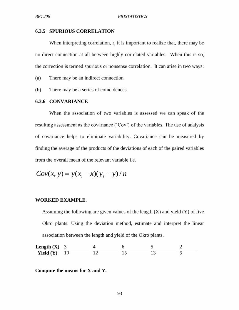
BIO 206 BIOSTATISTICS
93
6.3.5 SPURIOUS CORRELATION
When interpreting correlation, r, it is important to realize that, there may be
no direct connection at all between highly correlated variables. When this is so,
the correction is termed spurious or nonsense correlation. It can arise in two ways:
(a) There may be an indirect connection
(b) There may be a series of coincidences.
6.3.6 CONVARIANCE
When the association of two variables is assessed we can speak of the
resulting assessment as the covariance (‘Cov’) of the variables. The use of analysis
of covariance helps to eliminate variability. Covariance can be measured by
finding the average of the products of the deviations of each of the paired variables
from the overall mean of the relevant variable i.e.
nyyxxyyxCov ii /))((),(
WORKED EXAMPLE.
Assuming the following are given values of the length (X) and yield (Y) of five
Okro plants. Using the deviation method, estimate and interpret the linear
association between the length and yield of the Okro plants.
Length (X) 3 4 6 5 2
Yield (Y) 10 12 15 13 5
Compute the means for X and Y.

BIO 206 BIOSTATISTICS
94
Mean of X = 3 + 4 + 6 + 5 + 2 / 5 = 4
Mean of Y = 10 + 12 + 15 + 13 + 5 / 5 = 11
Compute the values of the deviates.
Deviation from mean Squares of deviates
Products
of deviates Length (X) Yield (Y) X Y x
2 y
2 xy
3 10 -1 -1 1 1 1
4 12 0 1 0 1 0
6 15 2 4 4 16 8
5 13 1 2 1 4 2
2 5 -2 -6 4 36 12
Total 10 58 23
Then we can compute the correlation (r) value.
))(( 22 yx
xyr
= . 23 = 23 = 0.954
√(10)(58) 24.1
The r value of 0.954 is high and positive. That means the longer the Okro plant the
more the yield.
The degrees of freedom (d.f) is given by:
d.f. = n – 2
where: n is the number of the bivariate data.
The d.f. = 5 – 2 =3
Then check the correlation table at d.f 3 and 95% level of significance = 0.878.
Since the absolute value of r (0.954) is greater than correlation table value (0.878)
at 5% probability level, the linear association between length and yield is
significant. That means that the longer the Okro plant, the more the yield in almost
95% of the population.

BIO 206 BIOSTATISTICS
95
6.4 TUTOR MARKED ASSIGNMENT
1. What is meant by the statement that two variables are related?
2. Give examples in nature of two variables that are positively correlation and
two that are negatively correlated.
3. The average normal daily temperature (oC) and the corresponding average
precipitate (inches) for the month of August for seven randomly selected
Local Government Areas in Plateau State are shown in the data below.
Av. daily temp. (x) 30 27 28 32 27 23 18
Av. mon. precip. (y) 3.4 1.8 3.5 3.6 3.7 1.5 0.2
(a). Draw a scatter plot for the variables.
(b). State the hypothesis.
(c). Compute the value of the correlation coefficient.
(d). Test the significance of the correlation coefficient at = 0.05.
(e). Give a brief explanation of the type of relationship.
4. The data of an experiment to apply sufficient quantities of fertilizer to optimize
vegetation growth (grass yield) and avoid excessive application that could lead to
runoff and nutrient enrichment of a nearby lake is shown in the table below.
Weight of fertilizer (g/
sq. m) (x).
25 50 75 100 125 150 175 200 225 250
Yield of grass (g/sq.
m) (y).
84 90 90 154 148 169 206 244 212 248
(a). Plot the scattergram for the data.
(b). determine the regression of y on x.

BIO 206 BIOSTATISTICS
96
6.5 REFERENCES
Bailey, N.T.J. (1994). Statistical Methods in Biology. Third Edition. Cambridge
University Press. United Kingdom.
Bluman, A.G. (2004). Elementary Statistics. A Step by Step Approach. Fifth
Edition. McGraw-Hill Companies Incorporated. London.
Clarke, G.M. (1971). Statistisc and Experimental Design. Edward Arnold
Publishers Limited. London.
Daniel, W.W. (1995). Biostatistics: a foundation for Analysis in Health sciences.
Sixth Edition. John Wiley and sons Incorporated. USA.
Fowler, J.A. and Cohen, L. Statistics for Ornithologist. British Trust for
Ornithology Guide 22.
Harper, W.M. (1991). Statistics. Sixth Edition. Pitman Publishing, Longman
Group, United Kingdom.
Hoel, P.G. (1976). Elementary Statistics. Four Edition. John Wiley and Sons
Incorporated, NewYork. Pp 151-204.
Mukhtar, F.B. (2003). An Introduction to Biostatistics. Samarib Publishers, Kano
Nigeria. Pp 1-112.
Sanders, D.H., Murph, A.F. and Eng, R.J. (1980). Statistics: A Fresh Approach.
McGraw-Hill Kogakusha, Limited. Kosaido Printing Company Limited,
Tokyo, Japan.
UNIT SEVEN: SIMPLE EXPERIMENTAL DESIGN AND ANALYSIS
OF VARIANCE (ANOVA)
7.1 INTRODUCTION
Over the years, an enormous range of experimental patterns has been
developed and designs are available to suit a wide variety of circumstances.
Experimental design may be considered under two main headings. The
first is the actual pattern of the experiment in which a correct of design depends

BIO 206 BIOSTATISTICS
97
partly on knowledge of the experimental material and partly on the kind of
question are wishes to ask. Secondly is the analysis of the data. As a rule, the
results of the kind of experimental can be summarized in an analysis of variance
(Anova) table. The design and analysis of an experiment obviously influence one
another very strongly. That is for a given design, there really one satisfactory way
of analyzing the data.
7.2 OBJECTIVES:
At the end of this unit, you should be able to:
1. Define experimental design.
2. Explain the principles of experimentation.
3. Mention and explain the different types of experimental design.
4. Define Anova and test statistical hypotheses using Anova.
7.3 MAIN CONTENT
7.3.1 EXPERIMENTAL DESIGN
Experimental design deals with the methods of constructing and analyzing
comparative experiments such as comparing the effect of different factors or
treatments. Planning experiments is made much more effective if you understand
the advantages and disadvantages of different experimental designs and how they
affect the “experimental error” against which we test our differences between
treatments. There is the need to understand how experimental design as well as
BIO 206 BIOSTATISTICS
98
treatment and replicate numbers impact on the “residual degrees of freedom” and
whether you should be looking at one-tailed or two-tailed statistical tables.
Experimental design ensures that maximum precision is achieved for the
amount of effort expended in an experiment. In every design, it is important that
the roles of the treatments should be well defined and the objectives of the
experiment properly understood.
An experiment is a systematic procedure for making observations under
controlled conditions in such a way that they can be used for arriving at general
conclusions regarding the population under study. An experimental unit is a plant
or animal or group of plants or animals making up a single replicate of a single
treatment. It is also called a plot.
7.3.2 PRINCIPLES INVOLVED IN EXPERIMENTATION
1. Randomization: This involves the allotting of treatments to the available
material at random.
2. Replication / Reproducibility: is the need for an experiment to be planned
in such a way that it can be replicated or reproduced. Replication is
important in reducing error and enhancing accuracy. (Note: An error is the
variation among varieties that cannot be accounted for by the variation due
to treatments, blocks and other factors controlled in the experiment).
Normally errors affecting any treatment tend to cancel out as the number of
replications is increased.

BIO 206 BIOSTATISTICS
99
3. Homogeneity/Sensitivity: A homogenous experimental setup is one that has
uniformity of materials and therefore does not require the control of local
variation. While sensitivity is to be able to estimate the effects of the
treatments so that valid conclusion can be drawn.
7.3.3 TYPES OF EXPERIMENTAL DESIGN
1. Completely Randomized Design (CRD): is the simplest type of
experimental design in which treatments are assigned at random to a set of
plots. It is applicable when homogenous (same) experimental material is
used on heterogeneous (different) experimental units or treatments, which
is replicated more than once. CRD ensures that treatments allotment is
completely random thereby avoiding biasness and minimizing inherent
differences in experimental units or treatment. For example, the CRD for
three replicates of six treatments is as follows.
A B A
A E B
D D E
C C C
F F E
F B D
A one-way analysis of variance is used in the analysis of CRD. Examples
of such simple experiment include: Effects of different fertilizers
(treatments) on yield of maize (experimental material), evaluating the
effects of a feed of different protein levels (treatments (experimental
material) on the growth of quails or fish of the same age, sex, size, etc.

BIO 206 BIOSTATISTICS
100
Advantages of CRD
a. The design is very flexible and can be used for any number of treatments.
b. The statistical analysis is comparatively easy and straightforward.
c. It is unaffected by missing observations for any treatment for some purely
random accidental reason.
Disadvantage of CRD
a. The design is inherently less informative than other more sophisticated
layouts.
2. Randomized Block Design (RBD): is an experimental design in which the
total area is divided into blocks and all of the treatments are arranged
within each block in a random order. It is the probably the most widely
used experimental design.
Block Plots
Fertility Trend
I A C B D
II B C A D
III D A C B
IV B D C A
There are two sources of variation (i.e Treatment and Blocks) in RBD and
therefore a two-way analysis of variance is used to analyze data obtained.
Examples include experiments to determine the response of quails of different age

BIO 206 BIOSTATISTICS
101
groups to different dietary protein levels, response of five variety of maize to three
levels Indole-Acetic-Acid (IAA), etc.
Advantages and Disadvantages of RBD
1. With heterogeneous material the residual variance can be reduced by
choosing blocks of plots such that the plots within the blocks are fairly
similar. i.e the design reduces the effect of heterogeneous material.
2. There is no restriction on the number of blocks or treatments, but in each
block there must be the same number of plots, one to each treatment.
3. If some yields are accidentally lost, the analysis is again without due
complications, although special modifications are required.
Procedure of a randomized block experiment
Phase 1
Total rows and columns, and check Grand total by adding both row and
column totals.
Calculate correction factor for experiment = Grand total2/number plots.
Calculate TOTAL sum of squares (added squares – correction factor!).
YOU HAVE NOW NO FURTHER USE FOR THE PLOT RESULT DATA
Phase 2
Construct the analysis of variance table with the headings: Source of
variation, d.f., Sum of squares, Mean square, F, and P.
Insert sources of variation as Treatments, Blocks, Residual, and Total.

BIO 206 BIOSTATISTICS
102
Allocate degrees of freedom as n − 1 for number of Treatments and
Replicates, and the product of these two d.f. for the Residual. Check that
the three d.f.’s add up to n−1 for the Total (i.e. one less than the number of
data in the experiment).
Square and add the TREATMENT totals to obtain the Treatments sum of
squares of deviations.
Square and add the REPLICATE totals to obtain the Replicates sum of
squares of deviations.
The “Residual” sum of squares of deviations is the remainder of the
“total” sum of squares of deviations.
YOU HAVE NOW USED ALL THE COLUMN AND ROW TOTALS
End Phase
Calculate mean square for “treatments,” “replicates,” and “residual” by
dividing each sum of squares of deviations by its own degrees of freedom.
3. Latin square: Is an experimental design in which the number of rows,
columns, and treatments are equal and each treatment occurs just once in
each row and column. As the name implies, a Latin square is a square
design in that it consists of the same number of plots (though these don’t
have to be square) in two dimensions, i.e. 4 × 4, 5 × 5, 6 × 6, etc. The
“dimension” of the square is the number of treatments in the experiment.
We’ll take as our example a Latin square with four treatments (A, B, C,and
D) – i.e. a 4×4 (16 plot) square.

BIO 206 BIOSTATISTICS
103
C B A D
D C B A
B A D C
A D C B
Simple Factorial Experiment
A factorial experiment is one where the treatments allocated to the
experimental plots are combinations of two or more factors (hence the term
“factorial”). For example, we might wish to test the effect on some measurement
of a NUMBER of different fertilizers on MORE THAN ONE plant variety. Each
plot would then be allocated the combination of one “level”of fertilizer (one of the
fertilizers) applied to one “level” of variety (one of the varieties).
7.3.4 ANALYSIS OF VARIANCE (ANOVA)
Analysis of variance (abbreviated as ANOVA) is a systematic procedure
for obtaining two or more estimate of variance and comparing them. Anova as a
technique enables the comparison of means and variances in an experiment that
involves more than two treatments. It estimates the value of the true variance of
the population (σ2) from which the sample is drawn.
Anova permits us to conclude whether or not all means of the population
under study are equal base upon the degree of variability in the sample data.
Therefore, it is extremely efficient and powerful technique for investigating
relationships between several groups of data.
ASSUMPTIONS IN ANOVA
In Anova, the following assumptions must be made or else its appropriateness
becomes questionable.

BIO 206 BIOSTATISTICS
104
1. Samples are drawn randomly and each sample is independent of the other
samples.
2. The populations under study have distribution which is approximately the
normal curve.
3. The populations from which the sample values are obtained, all have the
same population variance (σ2). That is (σ1
2 = σ2
2 = σ3
2 = ………….σk
2), the
variances of all the populations are equal.
HYPOTHESES IN ANOVA
1. The null hypothesis (Ho) in Anova is that the independent samples are
drawn from populations with the same means: Ho : µ1 = µ2 = µ3 =
…………….µk.
Where, k, is the number of populations under
study.
2. The alternative hypothesis (H1) in Anova is that, not all population means
are equal. That is, at least one mean is different from the others.
H1 : µ1 ≠ µ2 ≠ µ3 ≠ ……...µk.
THE CONCLUSIONS
Conclusions concerning Ho in Anova test are based on computed variance ratio,
sometimes called the F-ratio.
1. Accept the null hypothesis, Ho, if the F-ratio value is less than the table
value. That is, it is not significant.
2. Reject the null hypothesis, Ho, and accept the alternative hypothesis, H1, if
the F-ratio value is more than the table value. That is it is significant.
EXAMPLES:
1. The table below shows the number of seeds for five varieties of garden egg
to three level of Indo-acetic acid (IAA).

BIO 206 BIOSTATISTICS
105
IAA\varieties A B C D E
I 3 5 10 7 8
II 2 4 7 4 5
III 4 5 8 6 7
Solution:
State the null hypothesis: There is no significant difference between seed
number in five varieties of garden egg and levels of IAA.
Calculate the totals from the table as below:
IAA\varieties A B C D E Total
I 3 5 10 7 8 33
II 2 4 7 4 5 22
III 4 5 8 6 7 30
Total 9 14 25 17 20 GT=85
Then calculate the Correction Factor (CF) as:
CF = GT2/N = 85
2/15 = 481.7
Calculate the Mean Squares (SS)
BLOCKss = (332 + 22
2 + 30
2/5) – CF = 12.9
VARIETIESss = (92 + 14
2 +………..+ 20
2)/3 – CF = 48.6
TOTALss = (32 + 5
2 +………...+7
2) – CF = 65.3
ERRORss = TOTALss – (BLOCK + VARIETIESss) = 3.8
Then calculate:
BLOCKMS = BLOCKss/ BLOCKDF = 12.9/2 = 6.45
VARIETIESMS = VARIETIESss/VARIETIESDF = 48.6/4 = 12.15
Block F-value = BlockMS /ErrorMS = 6.45/0.475 = 13.58
Varieties F-value = VarietiesMS /ErrorMS = 12.15/0.475 = 25.58

BIO 206 BIOSTATISTICS
106
The calculated F-values are compared with the F-distribution table, using their
respective degrees of freedoms.
SOURCE DF SS MS F
Block 2 12.9 6.45 13.58**
Varieties 4 48.6 12.15 25.58**
Error 8 3.8 0.475
Total 14 65.3
** indicates that the values are highly significant.
Conclusion:
Since the F-values are highly significant, we reject the null hypothesis. It
means that the three levels of IAA have effect on the seed number of the five
varieties of garden egg.
2. Complete the Anova table below and draw your conclusions.
Source Sum of
squares (SS)
Degrees of
freedom
(DF)
Mean
squares (MS)
F-ratio
Varieties 123.44 * * *
Residual * 15 *
Total 210.21 18
RESIDUALss = 210.21 – 123.44 = 86.8
VARIETIESDF = 18 – 15 = 3
VARIETIESMS = 123.44/3 = 41.15
RESIDUALMS = 86.8/15 = 5.79
F- ratio = 41.15/5.79 = 7.11
The complete table is as shown below.
Source Sum of Degrees of Mean squares F-ratio

BIO 206 BIOSTATISTICS
107
squares (SS) freedom (DF) (MS)
Varieties 123.44 3 41.15 7.11
Residual 86.8 15 5.79
Total 210.21 18
Conclusion:
The observed variance ratio of 7.12 is greater than the table values at both
5% (3.29) and 1% (5.42). That means there is high significant difference
among the varieties. Therefore, we reject the null hypothesis that the varieties
are the same.
7.4 TUTOR MARKED ASSIGNMENT
1. What do you understand by ‘Experimental design’?
2. Which type of experimental design is most appropriate to use for the
following Anova. (a) One-way classification. (b) Two-way classification.
3. Outline and briefly discuss the principles involved in experimental.
4. What is the importance of using homogenous materials in an experiment?
5. From the Anova table below
Source of
variation
d.f. Sum of
Squares
Mean
Square
F
Block 2 16 8 11.94
Treatment 5 145.8 29.17 43.54
Residual/Error 10 6.67 0.67
Total 17 168.5
a. Name the type of design that was employed.
b. How many treatments were compared?
c. How many observations were analysed?
d. Draw your conclusions on the F-values.

BIO 206 BIOSTATISTICS
108
REFERENCES
Bailey, N.T.J. (1994). Statistical Methods in Biology. Third Edition. Cambridge
University Press. United Kingdom.
Bluman, A.G. (2004). Elementary Statistics. A Step by Step Approach. Fifth
Edition. McGraw-Hill Companies Incorporated. London.
Clarke, G.M. (1971). Statistisc and Experimental Design. Edward Arnold
Publishers Limited. London.
Daniel, W.W. (1995). Biostatistics: a foundation for Analysis in Health sciences.
Sixth Edition. John Wiley and sons Incorporated. USA.
Fowler, J.A. and Cohen, L. Statistics for Ornithologist. British Trust for
Ornithology Guide 22.
Harper, W.M. (1991). Statistics. Sixth Edition. Pitman Publishing, Longman
Group, United Kingdom.
Helmut F. van Emden.(2008). Statistics for Terrified Biologists. Blackwell
Publishing
Limited. USA.
Hoel, P.G. (1976). Elementary Statistics. Four Edition. John Wiley and Sons
Incorporated, NewYork. Pp 151-204.
Mukhtar, F.B. (2003). An Introduction to Biostatistics. Samarib Publishers, Kano
Nigeria. Pp 1-112.
Sanders, D.H., Murph, A.F. and Eng, R.J. (1980). Statistics: A Fresh Approach.
McGraw-Hill Kogakusha, Limited. Kosaido Printing Company Limited,
Tokyo, Japan.

BIO 206 BIOSTATISTICS
109
UNIT EIGHT: NON – PARAMETRIC TESTS
8.1 INTRODUCTION
Statistical test, such as mean, standard deviation, variance, Z, t and F- tests
are called parametric tests. This is because these assumptions are governed by the
distribution of the sampled population or populations that is/or are at least
approximately normal. But if the population in a particular hypothesis-testing
situation is not normally distributed, then the non-parametric or distribution – free
tests is used.
Non parametric test can also be used to test hypothesis that do not involve
specific population parameters such as μ, σ or P.
8.2 OBJECTIVES:
At the end of this unit, you should be able to
1. State the advantages and disadvantages of non parametric method.
2. Give the differences between non-parametric and parametric test.
3. Test hypotheses using non parametric tests such as Sign test and Kruskal-
Wallis test.
4. Compute the Spear rank correlation coefficient.
8.3 MAIN CONTENT
8.3.1 ADVANTAGES OF NON-PARAMETRIC TEST
There are five advantages that non parametric methods have over
parametric methods.

BIO 206 BIOSTATISTICS
110
1. They can be used to test population when the variable is not normally
distributed.
2. They can be used when the data are nominal or ordinal.
3. Can be used to test hypothesis that do not involve population parameters.
4. In most cases, computation is easier than in parametric.
5. They are easier to understand.
8.3.2 DISADVANTAGES OF NON-PARAMETRIC TEST
1. They are less sensitive than in parametric i.e larger differences are needed
before the null hypothesis can be rejected.
2. They tend to use less information than the parametric tests.
3. They are less efficient than their parametric counterparts when the
assumptions of the parametric are met.
NOTE:
The researcher should use caution in deciding whether to use non-
parametric or parametric methods. However, if the assumptions can be met, the
parametric methods are preferred.
DISTINCTION BETWEEN NON-PARAMETRIC AND PARAMETRIC
TESTS
NON – PARAMETRIC TESTS PARAMETRIC TEST
1 May be used with actual observations, or
with observations converted to ranks.
Are used only with actual
observations
2 May be used with observations on nominal,
ordinal and interval scales
Generally restricted to observations
on interval scales.
3 Compare medians Compare means and variances
4 Data are ‘distribute in free’ i.e must not be
normally distributed.
Data are required to be normally
distributed and to have similar
variances

BIO 206 BIOSTATISTICS
111
5 Are suitable for data which are counts Counts must be transformed
6 Are suitable for derived data e.g.
proportions, indices
Derived data may first have to be
transformed.
8.3.3 THE SIGN TEST
The simplest non-parametric test is the sign test for single samples. It is
used to test the value of a median for a specific sample. In using Sign test, you:
Hypothesize the specific value for the median of a population.
Select a sample of data and compare each value with the conjectured median.
Assign plus sign if the data value is above the conjectured median.
Assign minus sign if the data value is below the conjecture median.
And zero (0) if it is the same as the conjecture median.
Compare the number of plus and minus signs and ignore the zeros
If the null hypothesis (Ho) is true, the number of plus signs should be
approximately equal to the number of minus signs.
But if the Ho is not true, there will be disproportionate number of plus or
minus signs.
NB:
The test value is the smaller number of plus or minus signs obtained in a
sample. For example, if there are 12 plus signs and 5 minus signs, the test value is
5.

BIO 206 BIOSTATISTICS
112
For Example:
A chicken poultry owner hypothesizes that the median number of eggs he
gets per day is 40. A random sample of 20 days yields the following for the
number of eggs laid each day.
18 30 39 36 43
29 34 40 40 32
39 34 16 37 45
39 22 36 28 52
At α = 0.05, test the owner’s hypothesis
Solution:
State the hypotheses:
Ho: median = 40 – that is the claim
H1: median ≠ 40.
Find the critical value. Compare each value of data with the median
_ + 0 _ _
_ _ _ _ _
_ _ _ + _
_ 0 _ _ +
Then count the number of plus and minus signs, and ignore zero. This gives n =
18.

BIO 206 BIOSTATISTICS
113
Refer to Table of critical values for Sign test and α = 0.05 for a two-tailed test:
The critical value is 4.
Compute the test value.
Since there are 3 plus signs and 15 minutes sign, then the test value is 3. (Always
use the smaller value as the test value). The test value 3 is less than the critical
value 4 (3<4). Therefore, the null hypothesis is rejected.
In summary, there is enough evidence to reject the claim that the median number
of eggs layed per day is 40.
NB:
If the sample size is 25 or less, the table of critical values for Sign test is
used. But when the sample size is 26 or more, the standard normal distribution
table can be used to find the test value.
8.3.4 KRUSKAL – WALLIS TEST
The Kruskal – Wallis test, sometimes called the H - test is a non-
parametric test which can be used to compare three or more means, where the
assumptions for the ANOVA test: populations are normally distributed and the
population variances are equal, cannot be met. In Kruskal – Wallis test, each
sample size must be 5 or more with M-1 degrees of freedom, where m = number
of groups.
The distribution in kruskal – wallis can be approximated by the chi-square
distribution.

BIO 206 BIOSTATISTICS
114
Formula for Kruskal-Wallis Test
H = . 12 . ˟ (R12/n1+ R2
2/n2 + …….. + Rk
2/nk) – 3 (N + 1)
N(N+1)
Where:
R1 = Sum of ranks of sample 1
n1 = Size of sample 1
R2 = Sum of ranks of sample 2
n2 = Size of sample 2
Rk = Sum of ranks of sample K
nk = Size of sample k
N = n1 + n2 + ….. nk
k = number of samples
For Example:
A research was conducted to know the relationships of bill-length (mm) in three
bird species. The data below were obtained.
A B C
33.5 38.0 32.0
37.5 31.5 33.0
35.0 34.0 36.5
39.1 35.1 34.9
31.1 33.4 32.5
** At α = 0.05, is there enough evidence to reject the hypothesis that all the bird
species have the same bill length?

BIO 206 BIOSTATISTICS
115
Solution:
State the hypotheses
Ho: There is no difference in the bill length of the 3 bird species in the forest
reserve.
H1: There is a difference in the bill length of the 3 bird species in the forest
reserve.
Find the critical value using the chi-square distribution table at degrees of
freedom.
Df = m – 1 at α = 0.05, where m is the number of groups
df = 3 – 1 = 2: The critical value is 5.991
Arrange all the data from lowest to highest and rank each value
Bill - Length Species Rank
31.1 A 1
31.5 B 2
32.0 C 3
32.5 C 4
33.0 C 5
33.4 B 6
33.5 A 7
34.0 B 8
34.9 C 9
35.1 B 10
35.0 A 11
36.5 C 12
37.5 A 13
38.0 B 14
39.1 A 15

BIO 206 BIOSTATISTICS
116
Calculate the sum of the ranks of each bird species
Species A = 1 + 7 + 11 + 13 + 15 = 47
Species B = 2 + 6 + 8 + 10 + 14 = 40
Species C = 3 + 4 + 15 + 9 + 12 = 33
Substitute the Kruskal – Wallis Test formula
H = 12 (R2
1 + R2
2 + R2
3) – 3 (N + 1)
N(N+1) n1 n2 n3
Where:
N =15, R1 = 47, R2 = 40, R3 = 33 and n1 = n2 = n3 = 5
Therefore,
H = 12 (472 + 40
2 + 33
2) – 3 (15 + 1)
15(15+1) 5 5 5
= 0.05 (979.6) – 48
= 48.98 – 48
H = 0.98
Then deduce the decision.
Decision:
Since the test value 0.98 is less than the critical value 5.991, the decision is to
accept the null hypothesis. This simply means that there is no difference in the bill
length of the three bird species.
8.3.5 SPEARMAN RANK CORRELATION
The spearman rank correlation coefficient, denoted by rs, is the non-
parametric equivalent of the Pearson coefficient used for testing hypothesis when

BIO 206 BIOSTATISTICS
117
samples obtained are not normally distributed. It can be used when the data are
ranked. If the two sets of data have the same ranks, rs will be +1. If the ranks are
in exactly the opposite way, rs will be -1. If there is no relationship between the
rankings, then rs will be near 0.
The formula for spear rank correlation is given as:
)1(
)6(1
2
2
nn
drs
where: d = difference in ranks
n = number of data pairs
For Example:
The table below gives the number of horn bill nestlings ringed, and
juveniles captured in the same season, over a 6 year study period at a woodland
site. At α = 0.05, test the hypothesis that there is a linear correlation between the
nestlings ringed and juveniles captured.
Nestlings Ringed 16 9 1 7 13 5
Juveniles Captured 16 8 5 4 10 3
Solution:
State the hypothesis
Ho: ρ = 0 and H1: ρ ≠ 0

BIO 206 BIOSTATISTICS
118
Find the critical value using the table of critical values for the Rank correlation
coefficient.
And the value n = 6 and α = 0.05
The value is 0.886.
To find the test value, you first rank the data set.
Nestlings ringed Rank 1 Juveniles
captured
Rank 2
16 1 16 1
9 4 8 3
1 6 5 4
7 5 4 5
13 3 10 2
15 2 3 6
Then subtract the rankings for each season (R1 – R2) and square the differences.
R1 R2 d d2
1 1 0 0
4 3 -1 1
6 4 2 4
5 5 0 0
3 2 1 1
2 6 -4 16
222 d

BIO 206 BIOSTATISTICS
119
Substitute in the formula to find r.
)1(
)6(1
2
2
nn
drs
where n = the number of data pairs (n = 6)
rs = 1 – 6(22) = 0.371
6(62 – 1)
Make a decision.
Since the rs = 0.371, which is less than the critical value of 0.886, we accept
the null hypothesis. Therefore, there is no enough evidence to say that there is
a correlation between Nestlings ringed and Juveniles captured.
8.4 TUTOR MARKED ASSIGNMENT:
1. Why is the sign-test the simplest non-parametric test to use?
2. Ten patients suffering from severe muscle pains volunteered to try two new
analgesics and the time of relief were recorded in minutes for each patient
are as shown below.
Patient number 1 2 3 4 5 6 7 8 9 10
Analgesic A
(min.)
138 136 142 151 154 141 140 138 132 136
Analgesic B
(min.)
140 136 141 150 153 144 143 136 131 138
(a) State the hypotheses and identify the claim.
(b) Find the critical value and compute the test value.
(c) Make a decision based on your finding.

BIO 206 BIOSTATISTICS
120
3. A study was conducted on 10 adults to determine the effect of alcohol on
test scores. Each adult was given a test. Then for one week, each adult was
required to consume a certain amount of alcohol and then he or she was
retested. The results are shown below.
Adult Score before Score after
1 105 106
2 109 105
3 98 94
4 112 109
5 109 105
6 117 115
7 123 125
8 114 114
9 95 98
10 101 100
At α = 0.10, test the claim that alcohol does not affect a person’s test score.
8.5 REFERENCES
Bailey, N.T.J. (1994). Statistical Methods in Biology. Third Edition. Cambridge
University Press. United Kingdom.
Bluman, A.G. (2004). Elementary Statistics. A Step by Step Approach. Fifth
Edition. McGraw-Hill Companies Incorporated. London.
Daniel, W.W. (1995). Biostatistics: a foundation for Analysis in Health sciences.
Sixth Edition. John Wiley and sons Incorporated. USA.
Fowler, J.A. and Cohen, L. Statistics for Ornithologist. British Trust for
Ornithology Guide 22.
Harper, W.M. (1991). Statistics. Sixth Edition. Pitman Publishing, Longman
Group, United Kingdom.
Helmut F. van Emden.(2008). Statistics for Terrified Biologists. Blackwell
Publishing Limited. USA.

BIO 206 BIOSTATISTICS
121
Hoel, P.G. (1976). Elementary Statistics. Four Edition. John Wiley and Sons
Incorporated, NewYork. Pp 151-204.
Mukhtar, F.B. (2003). An Introduction to Biostatistics. Samarib Publishers, Kano
Nigeria. Pp 1-112.
Sanders, D.H., Murph, A.F. and Eng, R.J. (1980). Statistics: A Fresh Approach.
McGraw-Hill Kogakusha, Limited. Kosaido Printing Company Limited,
Tokyo, Japan.

BIO 206 BIOSTATISTICS
122
UNIT NINE: USE OF STATISTICAL PACKAGES
9.1 INTRODUCTION
In the past, statistical calculations were done with pencil and paper.
However, with the advent of calculators, numerical computations have become
much easier, especially where computers do all the numerical calculations. All
one does is to enter the data into the computer and use the appropriate command;
the computer will print the answer or display it on the screen. You should realize
that you are responsible for understanding and interpreting each statistical concept.
There are many statistical packages available. This unit discusses the SPSS
(Statistic al package for Social Sciences) and MINITAB.
9.2 OBJECTIVES:
At the end of this unit, you should be able to:
1. Describe the applications of SPSS and MINITAB in different statistical
procedures.
2. Mention examples of statistical tools in the statistical packages.
9.3 MAIN CONTENT
9.3.1 SPSS
This is a statistical package developed especially for the social sciences but
it has wide applicability in the areas of biology and agriculture. It can be used to
execute some statistical procedures such as summaries, custom tables, Anova
(Analysis of variance), correlation and regression analyses, non-parametric tests,

BIO 206 BIOSTATISTICS
123
time series, create charts (Bar, line, Pie, Area, Histogram, Scatter etc.) and lots
more.
The SPSS is a comprehensive package that is command based but
commands list can be generated from menus and interactive operations are
possible.
9.3.2 MINITAB
The MINITAB statistical software provides a wide range of statistical
analysis and graphical capabilities. Like the SPSS, it is also a comprehensive
command based statistical package. MINITAB can be used for various types of
statistical analysis ranging from editing and manipulating data, basic statistics,
arithmetic, regression, Anova, non parametric test, exploratory data analysis et.c.
9.4 REFERENCES
Bailey, N.T.J. (1994). Statistical Methods in Biology. Third Edition. Cambridge
University Press. United Kingdom.
Bluman, A.G. (2004). Elementary Statistics. A Step by Step Approach. Fifth
Edition. McGraw-Hill Companies Incorporated. London.
Mukhtar, F.B. (2003). An Introduction to Biostatistics. Samarib Publishers, Kano
Nigeria. Pp 1-112.

I
n
t
r
o
d
u
c
t
i
o
n
Statistics for Agriculture and Biology sciences (206) is a second semester
course. It is a two credit unit compulsory course which all students
offering Bachelor of Science (BSc) in Biology must take.
Statistics is a familiar and accepted part of modern world that is concern
with obtaining an insight into the real word by means of the analysis of
numerical relationships. It is used in amost all fields of human endevour. It
is applied in sports, public health, education, surveys, operations research,
quality control, estimation and prediction.
Since this course Statistics for Agriculture and Biology sciences entails
analysis of numerical relationships, we will focus on the meaning of
statistics and biostatistics(collections of quantitative information and
method of handling such data,drawing inferences on the basis of
observation), also frequency of distribution,probability,
hypothesis,correlation and regression,covariance, ANOVA and the use of
statistical package.
What you will learn in this course
In this course, you have the course units and a course guide. The course
guide will tell you briefly what the course is all about. It is a general
overview of the course materials you will be using and how to use those
materials. It also helps you to allocate the appropriate time to each unit so
that you can successfully complete the course within the stipulated time
limit.
The course guide also helps you to know how to go about your Tutor-
Marked-Assignment which will form part of your overall assessment at
the end of the course. Also, there will be tutorial classes that are related to
this course, where you can interact with your facilitators and other
students. Please I encourage you to attend these tutorial classes.
This course exposes you data collection, management and analysis, the
knowledge will be helpful during your project data collection and analysis,
it is indeed very interesting field of Biology.
Course Aims

This course aims to enable you to know/understand the use of different
statistical and biostatistical analysis and packages for biological sciences
and agricultural data interpretations and inference.
Course Objectives
To achieve the aim set above, there are objectives. Each unit has a set of
objectives presented at the beginning of the unit. These objectives will
give you what to concentrate and focus on while studying the unit and
during your study to check your progress.
The Comprehensive Objectives of the Course are given below. At the end
of the course/after going through this course, you should be able to:
Discuss the use of statistics in area of biology, agriculture and
medicine
Discuss the different sampling methods and understand the
purpose and importance of sampling
Mention type of frequency distribution.
Organise data using frequency distribution.
Explain the normal, poisson and binomial distributions
Computethe probabilies in poisson and binomial probability
distributions
State the null and alternative statistical hypothesis
Determine the level of confidence in a biological data
Explain the relationship between type I and II errors
Explain the purpose of goodnessof fit test
Compute correlation and regression
Explain types of correlation and Regression
Explain the principle of experimental design
Define Anova and test statistical hypothesis using Anova
Compute the spear rank correlation coefficient
Give the difference between non-parametric and parametric test
Describe the applications of SPSS and MINITAB in different
statistical procedures
Mention example of statistical tools in the statistical packages.

Working through the Course
To successfully complete this course. You are required to read each study
unit, read the textbooks and other materials provided by the National Open
University.
Reading the reference materials can also be of great assistance.
Each unit has self –assessment exercise which you are advised to do. At
certain periods during the course you will be required to submit your
assignments for the purpose of assessment.
There will be a final examination at the end of the course. The course
should take you about17 weeks to complete.
This course guide provides you with all the components of the course,
how to go about studying and how you should allocate your time to each
unit so as to finish on time and successfully.
The Course Materials
The main components of the course are:
1 The Study Guide
2 Study Units
3 Reference/ Further Readings
4 Assignments
5 Presentation Schedule
Study Units
The study units in this course are given below:
BIO 206 Statistics for Agriculture and Biology sciences (2 UNITS)
Unit 1: Use of Statistics in Biology and Agriculture
Unit 2: Frequency distribution
Unit 3: Probability distributions
Unit 4: Estimation and hypothesis testing
Unit 5: Contigency tables
Unit 6: Correlation , Regression and covariance
Unit 7: Simple Experimental design and Analysis of Variance (ANOVA)
Unit 8: Non-Parametric Tests
Unit 9: Use of statistical packages

In unit one, the mening of statistics and biostatistics, the application of
statistics in biology-related fields and the limitation of such applications
Unit two and three explain frequency distribution types,and how it can be
use to organise data.Also types of probability distribution; normal, poisson
and binomial.
Unit four and five are concerned with estimation and hypothesis testing;
null and alternative hypotheses,level of confidence in biological data,Test
hypotheses involving means using z and t tests.Also, contigency
tables;chi-square distribution and goodness of fit test.
Unit six deals with correlation and regression and covariance; bivariate
distribution and scatter diagram.
Unit seven and eight explain simple experimental design and analysis of
variance (ANOVA);principle of experimentation and Anova and test
statistical hypothesis. Also, Non-parametric tests; Sign test and Kruskal
Wallis test.
Unit nine discusses the SPSS(Statistical Package for Social Sciences) and
MINITAB
Each unit will take a week or two lectures, will include an introduction,
objectives, reading materials, self assessment question(s), conclusion,
summary, tutor-marked assignments (TMAs), references and other reading
resources.
There are activities related to the lecture in each unit which will help your
progress and comprehension of the unit. You are required to work on these
exercises which together with the TMAs will enable you to achieve the
objective of each unit.
Presentation Schedule
There is a time-table prepared for the early and timely completion and
submissions of your TMAs as well as attending the tutorial classes. You
are required to submit all your assignments by the stipulated date and
time. Avoid falling behind the schedule time.
Assessment
There are three aspects to the assessment of this course.
The first one is the self-assessment exercises. The second is the tutor-
marked assignments and the third is the written examination or the
examination to be taken at the end of the course.
Do the exercises or activities in the unit applying the information and
knowledge you acquired during the course. The tutor-marked assignments
must be submitted to your facilitator for formal assessment in accordance
with the deadlines stated in the presentation schedule and the assignment
file.
The work submitted to your tutor for assessment will account for 30% of
your total work.
At the end of this course you have to sit for a final or end of course
examination of about a three hour duration which will account for 70% of
your total course mark.
Tutor Marked Assignment
This is the continuous assessment component of this course and it
accounts for 30% of the total score. You will be given four (4) TMAs by
your facilitator to answer. Three of which must be answered before you
are allowed to sit for the end of the course examination.
These answered assignments must be returned to your facilitator.
You are expected to complete the assignments by using the information
and material in your reading references and study units.
Reading and researching into the references will give you a wider view
point and give you a deeper understanding of the subject.
1 Make sure that each assignment reaches your facilitator on or
before the deadline given in the presentation schedule and
assignment file. If for any reason you are not able to complete your
assignment, make sure you contact your facilitator before the
assignment is due to discuss the possibility of an extension.
Request for extension will not be granted after the due date unless
there is an exceptional circumstance.
2 Make sure you revise the whole course content before sitting for
examination. The self-assessment activities and TMAs will be
useful for this purposes and if you have any comments please do
before the examination. The end of course examination covers
information from all parts of the course.
Course Marking Scheme
Assignment Marks
Assignment 1-4 Four assignments, best three
marks of the four count at 10%
each - 30% of course marks.
End of course examination 70% of overall course marks
Total 100% of course materials

Facilitators/ Tutors and Tutorials
Sixteen (16) hours are provided for tutorials for this course. You will
be notified of the dates, times and location for these tutorial classes.
As soon as you are allocated a tutorial group, the name and phone
number of your facilitator will be given to you.
These are the duties of your facilitator:
• He or she will mark and comment on your assignment
• He will monitor your progress and provide any necessary
assistance you need.
• He or she will mark your TMAs and return to you as soon as
possible.
(You are expected to mail your tutored assignment to your facilitators at
least two days before the schedule date).
Do not delay to contact your facilitator by telephone or e-mail for
necessary assistance if
• You do not understand any part of the study in the course material.
• You have difficulty with the self assessment activities.
• You have a problem or question with an assignment or with the
grading of the assignment.
It is important and necessary you attend the tutorial classes because this is
the only chance to have face to face contact with your facilitator and to ask
questions which will be answered instantly. It is also a period where you
can point out any problem encountered in the course of your study.
Summary
Statistics for Agriculture and Biology sciences (206) deals with the ways
of collecting, organizing,summarizing and describing quantifiable data,
and methods of drawing inferences and generalizing upon them.
Also, this course has been able to explain the data collection and analysis
using statistical tools derived from the fields of biological sciences;
medicine, pharmacy, Biochemistry, Microbiology, agricultural sciences
and other biology-related areas
On the completion of this course, you will how and when a statistical
package is used for biological data. In addition you will be able to answer
the following questions:
What is sample size?
What is considered the goal of sampling?
List three incorrect methods that are often used to obtain a
sample

Names and three of frequency distributions
Outline the stages involved in the construction of a frequency
Ouline five characteristics of a normal curve
Construct a probability distribution for three patients given a
head ache relief tablet. The probabilities for 0.1.2 ro 3 success
are 0, 18, 0.52, 0,21, and 0.09, respecrively.
If the hypothesis of a population mean is 151 (i.eHO:
µ=151).List the three possible hypotheses
What is implication of committing a Type II error?
What is a right tailled test with α=50. If the sample of 36 had 6, x =
475. Conduct a two tailed test with α = 0.01.
Distinguished between Observed and Expected frequencies
Give two examples in nature of two variables that are
positively correlated and two that are negatively correlated
Outline and briefly discuss the principles involved in
experimental
The list of questions you are expected to answer is not limited to the above
list.
I believe you will agree with me that Statistics for Agriculture and Biology
sciences is a very interesting field of biology.
I wish you success in this course.

BIO 206 BIOSTATISTICS
15
NATIONAL OPEN UNIVERSITY OF NIGERIA
STATISTICS FOR BIOLOGY AND AGRICULTURE
BY
DR ILIYA S. NDAMS
AHMADU BELLO UNIVERSITY, ZARIA
UNIT ONE:
USE OF STATISTICS IN BIOLOGY & AGRICULTURE
1.1 INTRODUCTION
1.2 OBJECTIVES
1.3 MAIN CONTENTS
1.3.1 STATISTICS AND BIOSTATISTICS
1.3.2 USE OF STATISTICS IN BIOLOGY, AGRICULTURE AND
MEDICINE
1.3.3 DISCRETE AND CONTINUOUS VARIABLES
1.3.4 SAMPLING
1.3.5 SAMPLE
1.3.6 IMPORTANCE OF SAMPLE / SAMPLING
1.3.7 SAMPLING METHODS
1.3.8 RANDOM SAMPLING
1.3.9 STRATIFIED SAMPLING
1.3.10 CLUSTER SAMPLING
1.3.11 SYSTEMATIC OR SKIP SAMPLING
1.3.12 PROPORTIONATE SAMPLING
1.3.13 SAMPLING DISTRIBUTION
1.4 TUTOR MARKED ASSIGNMENT
1.5 REFERENCES

BIO 206 BIOSTATISTICS
16
UNIT TWO:
FREQUENCY DISTRIBUTION
2.1 INTRODUCTION
2.2 OBJECTIVES
2.3 MAIN CONTENT
2.3.1 THE FREQUENCY DISTRIBUTION
2.3.2 TYPES OF FREQUENCY DISTRIBUTION
2.3.3 UNGROUPED FREQUENCY DISTRIBUTION
2.3.4 GROUPED FREQUENCY DISTRIBUTION
2.3.5 OTHER FORMS OF DATA REPRESENTATIONS
2.4 TUTOR MARKED ASSIGNMENT
2.5 REFERENCES
UNIT THREE:
PROBABILITY DISTRIBUTIONS
3.1 INTRODUCTION
3.2 OBJECTIVE
3.3 MAIN CONTENTS
3.3.1 PROBABILITY DISTRIBUTION
3.3.2 THE NORMAL DISTRIBUTION
3.3.3 STANDARDIZING THE NORMAL CURVE
3.3.4 POISSON DISTRIBUTION
3.3.5 BINOMIAL DISTRIBUTION
3.4 TUTOR MARKED ASSIGNMENT
3.5 REFERENCES

BIO 206 BIOSTATISTICS
17
UNIT FOUR:
ESTIMATION AND HYPOTHESIS TESTING
4.1 INTRODUCTION
4.2 OBJECTIVES
4.3 MAIN CONTENT
4.3.1 ESTIMATION
4.3.2 TEST OF HYPOTHESIS
4.3.3 TESTING A HYPOTHESIS INVOLVING A MEAN
4.3.4 TESTING A HYPOTHESIS INVOLVING TWO MEANS 4.3.5 TWO-TAILED TEST
4.3.6 LEFT – TAILED TEST
4.3.7 STUDENT’S T-DISTRIBUTION (The t-test)
4.4 TUTOR MARKED ASSIGNMENT
4.5 REFERENCES
UNIT FIVE
CONTINGENCY TABLES
5.1 INTRODUCTION
5.2 OBJECTIVES
5.3 MAIN CONTENT
5.3.1 CHI-SQUARE DISTRIBUTION
5.4 TUTOR MARKED ASSIGNMENT
5.5 REFERENCES
UNIT SIX
CORRELATION AND REGRESSION AND COVARIANCE
6.1 INTRODUCTION

BIO 206 BIOSTATISTICS
18
6.2 OBJECTIVES
6.3 MAIN CONTENT
6.3.1 CORRELATION
6.3.2 REGRESSION
6.3.3 SCATTER DIAGRAM/PLOT
6.3.4 TYPES OF CORRELATION AND REGRESSION
6.3.5 SPURIOUS CORRELATION
6.3.6 CONVARIANCE
6.4 TUTOR MARKED ASSIGNMENT
6.5 REFERENCES
UNIT SEVEN
SIMPLE EXPERIMENTAL DESIGN AND ANALYSIS OF VARIANCE
(ANOVA)
7.1 INTRODUCTION
7.2 OBJECTIVES
7.3 MAIN CONTENT
7.3.1 EXPERIMENTAL DESIGN
7.3.2 PRINCIPLES INVOLVED IN EXPERIMENTATION
7.3.3 TYPES OF EXPERIMENTAL DESIGN
7.3.4 ANALYSIS OF VARIANCE (ANOVA)
7.4 TUTOR MARKED ASSIGNMENT
7.5 REFERENCES
UNIT EIGHT

BIO 206 BIOSTATISTICS
19
NON – PARAMETRIC TESTS
8.1 INTRODUCTION
8.2 OBJECTIVES
8.3 MAIN CONTENT
8.3.1 ADVANTAGES OF NON-PARAMETRIC TEST
8.3.2 DISADVANTAGES OF NON-PARAMETRIC TEST
8.3.3 DISTINCTION BETWEEN NON-PARAMETRIC AND
PARAMETRIC TESTS
8.3.4 THE SIGN TEST
8.3.5 KRUSKAL – WALLIS TEST
8.3.6 SPEARMAN RANK CORRELATION
8.4 TUTOR MARKED ASSIGNMENT
8.5 REFERENCES
UNIT NINE
USE OF STATISTICAL PACKAGES
9.1 INTRODUCTION
9.2 OBJECTIVES
9.3 MAIN CONTENT
9.3.1 SPSS
9.3.2 MINITAB
9.4 REFERENCES

BIO 206 BIOSTATISTICS
20
MODULE 1
UNIT ONE: USE OF STATISTICS IN BIOLOGY & AGRICULTURE
1.0 INTRODUCTION:
Statistics is a familiar and accepted part of modern world that is concern
with obtaining an insight into the real world by means of the analysis of numerical
relationships. It is used in almost all fields of human endeavour. It is applied in
sports, public health, education, surveys, operations research, quality control,
estimation and prediction.
This unit discusses the meaning of Statistics and Biostatistics, the
application of statistics in biology-related fields and the limitation of such
applications.
1.2 OBJECTIVES:
At the end of this unit, you should be able to:
i) Define the terms Statistics and Biostatistics.
ii) Discuss the use of statistics in areas of biology, agriculture and medicine.
iii) Discuss discrete and continuous variables
iv) Define a sample and sampling
v) Discuss the different sampling methods and understand the purpose and
importance of sampling and the advantages made possible by sampling
vi). Explain sampling distribution
1.3.1 STATISTICS AND BIOSTATISTICS

BIO 206 BIOSTATISTICS
21
The word statistics is used in two senses. It refers to collections of
quantitative information, and to methods of handling that sort of data i.e.
descriptive statistics. It also refers to the drawing of inferences about large groups
on the basis of observations made on smaller one i.e. inferential statistics.
Statistics, then, is to do with ways of collecting, organizing, summarizing
and describing quantifiable data, and methods of drawing inferences and
generalizing upon them. While the term Biostatistics is used when the data that
are being analysed using statistical tools, are derived from the fields of biological
sciences: Medicine, Pharmacy, Biochemistry, Microbiology, Agricultural Sciences
and other biology-related areas.
1.3.2 USE OF STATISTICS IN BIOLOGY, AGRICULTURE AND
MEDICINE.
Unlike other fields of science such as the physical sciences of chemistry
and physics, variation is regarded as a fundamental feature in natural sciences of
biology, agriculture and medicine. Biostatistics helps to explain this natural
variation inherent in these fields of natural sciences. For example, variation may
occur due to age of the population or may occur among individuals of a population
due to diseases or their genetic makeup. Experimental design is an important
aspect of biostatistics that describe on how to collect, organize, summarize and
analyze data such that valid and objective conclusions or decision about the
population can be drawn.
Therefore before applying statistics in research, a research must know:

BIO 206 BIOSTATISTICS
22
What technique to use for an investigation
What to be achieved
Rules of using the technique, using correctly the statistical
techniques for analysis of biological data
Statistical significance test for comparing one set of data with
another.
Determination of relationship between two variables either the use of
correlation or fitting the best straight line or curve on a graph.
1.3.3 DISCRETE AND CONTINUOUS VARIABLES
To gain knowledge about secondly haphazard events, statistician collect
information for variables which describe the event. Therefore, a variable is a
characteristics attribute that can assume different value.
Variables can be classified into two broad categories.
1. Qualitative variables
2. Quantitative variables
Qualitative variables are variables that can be placed into distinct
categories, according to some characteristic or attribute. For example, if subjects
are classified according to gender (i.e. male or female), then the variable gender is
qualitative.
Quantitative variables are numerical and can be ordered or ranked. For
example, the variable age is numerical, and people can be ranked according to the
value of their ages. Quantitative variables can be grouped into two:

BIO 206 BIOSTATISTICS
23
1. Discrete Variables – can be assigned values such as 0,1,2,3 (integers) and
are said to be variables that assume values that can be counted. Examples
include number of children in a family, number of birds in a pen, number of
trees in a garden, number of animals per litter etc.
2. Continuous variables – can assume all values between any specific values.
They are obtained by measuring. This applies to variables such as length,
weight, height, yield, temperature and time, that can be thought of as
capable of assuming any value in some interval of values.
Figure1.1 : Summary of classification of variables.
DATA
QUALITATIVE QUANTITATIVE
DISCRETE CONTINUOUS
NOTE: Data are the values (measurements and observations) that the variables
can assume
1.3.4 SAMPLING
When a set of observations is collected from a population, the population
mean (μ), population variance (σ2) and population standard deviation (σ) can be

BIO 206 BIOSTATISTICS
24
computed from it as the properties of the population. In the case of a sample, the
parameters that describe it are the sample mean (x), sample variance (s2) and
sample standard deviation (s). Since the sample is a portion of the population, the
parameters of the sample represent an estimate of the true parameters of the
population. Therefore, sampling is a random process of selecting a sample from a
population selected for study.
1.3.5 SAMPLE
A sample is a subgroup of the population selected for study. When a
sample is chosen at random from a population, it is said to be an unbiased sample.
That is, the sample for the most part, is representative of the population. But if a
sample is selected incorrectly, it may be a biased sample when some type of
systematic error has been made in the selection of the subjects. However, the
sample must be random in order to make valid inferences about the population.
1.3.6 IMPORTANCE OF SAMPLE / SAMPLING
A sample is used to get information about a population for several reasons:
1. It saves the researcher time and money.
2. It enables the researcher to get information that he or she might not be able
to obtain otherwise.
3. It enables the researcher to get more detailed information about a particular
subject.

BIO 206 BIOSTATISTICS
25
1.3.7 SAMPLING METHODS
In order to obtain unbiased samples, several sampling methods have been
developed. The most common methods are random, systematic, stratified, and
clustered sampling.
1.3.8 RANDOM SAMPLING
For a sample to be a random sample, every member of the population must
have an equal chance of being selected. Therefore, a random sample is one that
has the same chance as any other of being selected.
Randomness assists in avoiding various forms of conscious and
unconscious bias and can be achieved by these two ways:
1. Number each element of the population and then place the numbers on
cards. Place the cards in a hat or bowl, mix them, and then select the
sample by drawing the cards. You must ensure that the numbers are well
mixed.
2. The second and most preferred way of selecting a random sample is to use
random numbers e.g. Table of random numbers by Fisher and Yates. The
table comprises of a series of digits 0, 1, 2…. up to 9 arranged as such that
each number had the same chance of appearing in any given position.
1.3.9 STRATIFIED SAMPLING
A stratified sample is a sample obtained by dividing the population into
subgroups, called strata, according to various homogenous (alike) characteristics
and then selecting members from each stratum for the sample. For example, you

BIO 206 BIOSTATISTICS
26
can group the items on basis of their age, size, colour etc. The advantage of
stratified sampling is that it increases precision because all types of groups are
represented through stratification and a heterogeneous population is made into a
homogenous one.
1.3.10 CLUSTER SAMPLING
A cluster sample is a sample obtained by selecting a preexisting or natural
group, called a Cluster and using the members in the cluster for the sample. For
example a habitat, or a large area or field is divided into smaller units and a
number of such units are randomly selected and used as a sample.
There are three advantages to using a cluster sample instead of other types
of sample:
1. A cluster sample can reduce cost
2. It can simplify field work.
3. It is convenient.
The major disadvantage of cluster sampling is that the elements in a cluster
may not have the same variations in characteristics as elements selected
individually from a population.
1.3.11 SYSTEMATIC OR SKIP SAMPLING
This method involves taking an item as a sample from a larger population
at regular intervals. For example, when sampling from a poultry farm, every third

BIO 206 BIOSTATISTICS
27
or fifth or tenth chick coming out of the cage is taken and included in the sample.
This is done after the first number is selected at random for counting to start.
1.3.12 PROPORTIONATE SAMPLING
This type of sampling involves selecting a sample in proportion to the
different groups in the population under study. For example: Assuming in a given
terrestrial habitat there are the following different proportions of organism:
Trees - 100
Shrubs - 150
Vertebrates - 60
Invertebrates - 250
In sampling such a population, you may wish to pick 15 trees, 10 shrubs, 5
vertebrates, 20 invertebrates. These will form your sample.
In addition to the above sampling methods, other methods are sometimes
used.
In sequence sampling – successive units taken from production lines are
sampled to ensure that products meet certain standards set by the
manufacturing company. This is used in quality control.
In double sample, a very large population is given a questionnaire to
determine those who meet the qualifications for a study. After the
questionnaires are reviewed, a second, smaller population is defined. Then
a sample is selected from this group.

BIO 206 BIOSTATISTICS
28
In multistage sampling, the researcher uses a combination of sampling
methods.
1.3.13 SAMPLING DISTRIBUTION
If a sample of n observation is taken at random from a population, the
sample is expected to have a mean x. Suppose another sample also of n
observations is taken from the same population, it will similarly have a mean x (as
the first one). The numerical values of these means will differ slightly because
even though the samples are taken from the same population, the representative
members of the two samples differ. As you take samples from the same
population so will you get different numerical values for their means. This set of
numerical values is called the Sampling distribution of the mean and it is
determined by the nature of the population and the sample size. Therefore, a
sampling distribution is the distribution of values from a mass of samples, one
value per sample. If the sample size is large then the sampling distribution of the
mean approximates very closely to a normal curve. This implies that the mean of
the sampling distribution of means is equal to the population mean.
Examples
1. Identify the following as either discrete or continuous data:
(a) Number of patients coming to the hospital each day
(b) Lifetimes of micro organism in a certain pond
(c) Heights of 200 birds in a certain farm

BIO 206 BIOSTATISTICS
29
(d) Yearly salary of an agronomist
(e) Temperatures recorded every 30 minutes of a little boy suffering from
malaria fever
Answer
(a) Discrete (b) continuous (c) continuous (d) Discrete (e) continuous
2. Identify each of the following sampling methods.
(a) Every fish in a fish pond has equal chances of being included in a
sample
(b) Every corn plant that is 2m apart in a particular farm will be included in
a sample
(c) In surveying piggeries within a region, we choose to select 50 pig farms
blocks and then investigate every pigs within the selected blocks.
Ans
(a) Random (b) Systematic (c) Cluster
1.4 TUTOR MARKED ASSIGNMENT
1. Why do you need statistics in science based disciplines?
2. What is a sample size?
3. What is the purpose of sampling?
4. What is considered the goal of sampling?
5. In your opinion, which sampling method(s) provided the best sample to
represent a population of trees in a forest?
6. List three incorrect methods that are often used to obtain a sample.

BIO 206 BIOSTATISTICS
30
1.5 REFERENCES
Bailey, N.T.J. (1994). Statistical Methods in Biology. Third Edition. Cambridge
University Press. United Kingdom.
Bluman, A.G. (2004). Elementary Statistics. A Step by Step Approach. Fifth
Edition. McGraw-Hill Companies Incorporated. London.
Daniel, W.W. (1995). Biostatistics: a foundation for Analysis in Health sciences.
Sixth Edition. John Wiley and sons Incorporated. USA.
Fowler, J.A. and Cohen, L. Statistics for Ornithologist. British Trust for
Ornithology Guide 22.
Harper, W.M. (1991). Statistics. Sixth Edition. Pitman Publishing, Longman
Group, United Kingdom.
Hoel, P.G. (1976). Elementary Statistics. Four Edition. John Wiley and Sons
Incorporated, NewYork. Pp 151-204.
Mukhtar, F.B. (2003). An Introduction to Biostatistics. Samarib Publishers, Kano
Nigeria. Pp 1-112.
Sanders, D.H., Murph, A.F. and Eng, R.J. (1980). Statistics: A Fresh Approach.
McGraw-Hill Kogakusha, Limited. Kosaido Printing Company Limited,
Tokyo, Japan.
UNIT TWO: FREQUENCY DISTRIBUTION
2.1 INTRODUCTION:

BIO 206 BIOSTATISTICS
31
Measurements or counting gives rise to raw data. Raw data itself is
difficult to comprehend because it lacks organization, summarization, which
renders it meaningless. Thus, the raw data has to be put in some order through
classification and tabulation so as to reduce its volume and heterogeneity. To
describe situations, draw conclusions or make inferences about events, the
researcher must organize the data in some meaningful way. The most convenient
method of organizing data is to construct a frequency distribution.
2.2 OBJECTIVES:
At the end of this unit, you should be able to
i) Define frequency and frequency distribution.
ii) Mention the types of frequency distribution
iii) organize data using frequency distributions
iv) Give reasons for constructing distribution.
v) Represent data in methods other than frequency distribution.
2.3 MAIN CONTENTS
2.3.1 The Frequency distribution
Frequency is the number of occurrences of an element in a sample and is
symbolized by f. A frequency distribution is the organization of raw data in table
form, using classes and frequencies. When data are collected in original form, that
is as observed or recorded they are called raw data.
2.3.2 Types of Frequency Distribution

BIO 206 BIOSTATISTICS
32
Two types of frequency distributions that are most often used are the:
Categorical Frequency
This is used for data that can be placed in specific categories, such as
nominal or ordinal-level data. It is useful to know the proportion of values that
fall within a group, category or observation rather than the number of values or
frequencies. To get the relative frequency, the frequency of occurrence of each
number is divided by the total number of values and multiplied by hundred. This
can be expressed as follows:
f x 100%
n
Where f = Frequency of the category class and n = total number of values.
For example:
The data below represents the blood groups of 40 students in a Biostatistics class.
Construct a frequency distribution for the data.
A AB B O O A B AB A B
O O O A AB B B A O AB
A O O A AB B B A A B
AB A O B AB O A B A B

BIO 206 BIOSTATISTICS
33
SOLUTION:
Since the data are categorical, the blood groups: A, B, O and AB can be used as
the classes for the distribution.
Class Tally Frequency Percent
A /////,/////,// 12 30
B /////,/////,/ 11 27.5
O /////,///// 10 25
AB /////,// 7 17.5
TOTAL 100
Therefore, it can be concluded that in the sample more students have type A blood
group because its frequency is the highest.
2.3.3 UNGROUPED FREQUENCY DISTRIBUTION
This is a list of the figures in array form, occurring in the raw data, together
with the frequency of each figure, i.e. a frequency is constructed for a data based
on a single data values for each class.
For example: Given below, are the wing length measurements (to the nearest
whole millimeter) of 50 laughing doves.
76 73 75 73 74 74 72 75 76 73
68 72 78 74 75 72 76 76 77 70
78 72 70 74 76 75 75 79 75 74
75 70 73 75 70 74 76 74 75 74
78 74 75 74 73 74 71 72 71 79
Construct the frequency distribution of the above data.

BIO 206 BIOSTATISTICS
34
SOLUTION:
The measurements above are presented in the order in which the observations
were recorded. This can be represented in an ordered array so that the minimum
and maximum values can easily be read.
68 70 70 70 70 71 71 72 72 72
72 72 73 73 73 73 73 74 74 74
74 74 74 74 74 74 74 75 75 75
75 75 75 75 75 75 75 76 76 76
76 76 76 77 78 78 78 78 79 79
Find the range of the data: Highest value – lowest value (79 – 68 =11). Since the
range of the data is small, classes of single data values can be used.
Table 2.1: A tally of frequency of the wing length (mm) of 50 laughing doves.
Class limits Tally Frequency Cumulative
frequency
Relative
frequency
(%)
68 / 1 1 2
70 //// 4 5 8
71 // 2 7 4
72 ///// 5 12 10
73 ///// 5 17 10
74 /////,///// 10 27 20
75 /////,///// 10 37 20
76 /////,/ 6 43 12
77 / 1 44 2
78 //// 4 48 8
79 // 2 50 4
100

BIO 206 BIOSTATISTICS
35
Figures 2.1 (A-C): The frequency distribution of the wing length of 50 laughing
doves
(A)
0
2
4
6
8
10
12
68 70 71 72 73 74 75 76 77 78 79
frequency
winglength
Frequency distribution of winglength

BIO 206 BIOSTATISTICS
36
(B)
0
5
10
15
20
25
68 70 72 74 76 78 80
Fre
qu
en
cy
[winglength]
Histogram
Normal Fit
(Mean=74.2, …

BIO 206 BIOSTATISTICS
37
(C)
-3
-2
-1
0
1
2
3
68 70 72 74 76 78 80
No
rmal Q
uan
tile
(Z
)
winglength
Normality Plot (Q-Q)
Normal Fit
(Skewness=-0.17, …

BIO 206 BIOSTATISTICS
38
2.34 GROUPED FREQUENCY DISTRIBUTION
The heights in inches of commonly grown herbs are shown below. Organize the
data into a frequency distribution with six classes, and make useful suggestions.
18 20 18 18 24 10 15 12 29 36
13 20 18 24 18 16 16 20 7
Solution:
Find the range of the data: Highest value – lowest value (36 – 7 =29)
The class width is given by
=
= 4.8 (round it up to the nearest
whole number= 5)
Table 2.2: Frequency distribution for grouped data
Class
limits
Class
boundaries
Tally Frequency Cumulative
frequency
Relative
frequency
(%)
5 – 10 4.5 -10.5 // 2 2 10.5
11 -16 10.5 – 16.5 ///// 5 7 26.3
17 -22 16.5 – 22.5 /////,/// 8 15 42.1
23 – 28 22.5 – 28.5 // 2 17 10.5
29 -34 28.5 – 34.5 / 1 18 5.3
35 -40 34.5 -40.5 / 1 19 5.3
Total 100

BIO 206 BIOSTATISTICS
39
Rules to be followed in the construction of a frequency
1. There should be enough classes to clearly represent the data. Classes
between 5 and 20 are mostly suggested.
2. The class width should be an odd number. The class midpoint (Xm) is
given by
Xm = Lower boundary + Upper boundary OR Lower limit + Upper limit
2 2
Midpoint is the numeric location of the center of the class
3. The classes must not have overlapping class limits e.g.
Class But should be: Class
500-100 50-100
100-150 101-151
150-200 152-202
200-250 203-253
4. The classes must be continuous, even if there are no values in a class ie
there should be no gaps in the classes for lack of values.
5. Enough classes should be created to accommodate the whole data. i.e.
every value in the data must belong to a class. Note: If zero frequency is
the first or last, then it can be ignored.
6. The classes must be of equal width. In rule number 3 above, the class width
is 50. Here, it is important to note that some times in open ended
distribution i.e. distribution that has no specific beginning or ending value
as:

BIO 206 BIOSTATISTICS
40
Class Temperature oC
50-100 Below 5
101-151 6-10
152-202 11-15
203-253 16-20
254 and above 21-25
In the class distribution above any value above 254 is tallied in the last class while
in the distribution for temperature, simply means that any value below 5oC will be
tallied in the first class.
Effect of grouping
As a result of grouping, it is possible to detect a pattern in the figures but
grouping results in the loss of information i.e. calculations made from a grouped
frequency distribution can never be exact, and consequently excessive accuracy
can only result in spurious accuracy.
The reasons for constructing a frequency distribution are:
1. To organize the data in a meaningful, intelligible way.
2. To enable the reader to determine the nature and shape of the distribution.
3. To facilitate computational procedures for measures of average and spread.
4. To enable the researcher to draw charts and graphs for the presentation of
data.
5. To enable the reader to make comparisons among different data sets.

BIO 206 BIOSTATISTICS
41
2.3.5 OTHER FORMS OF DATA REPRESENTATIONS INCLUDE:
Figure 2.3: A bar chart of the nutrient content of a seed
4.17 5.04
21.9
4.61 1.41
62.87
0
10
20
30
40
50
60
70
PROTEIN MOISTURE LIPID FIBRE ASH C/HYDRATE

BIO 206 BIOSTATISTICS
42
Figure 2.4: A scatter plot or dot diagram of the wing length of 50 laughing doves
Figure 2.5: A cummulative frequency of the wing length of 50 laughing doves
0
2
4
6
8
10
12
66 68 70 72 74 76 78 80
Series1
0
10
20
30
40
50
60
66 68 70 72 74 76 78 80
CUMMULATIVE FREQUENCY

BIO 206 BIOSTATISTICS
43
Figure 2.6: A Pie chart showing the distribution of fruits in an orchard
2.4 TUTOR MARKED ASSIGNMENT
1. Name the three types of frequency distributions.
2. Outline the stages involved in the construction of a frequency.
3. The data below represents the number of bats trapped in mist net in 30
trials.
2 9 4 3 6
6 2 8 6 5
7 5 3 8 6
6 2 3 2 4
6 9 9 8 9
4 2 1 7 4
(a) Construct an ungrouped frequency distribution for the data.
(b) Construct a histogram for the data.
MANGO 18%
ORANGE 41%
BANANA 12%
GUAVA 29%

BIO 206 BIOSTATISTICS
44
2.5 REFERENCES
Bailey, N.T.J. (1994). Statistical Methods in Biology. Third Edition. Cambridge
University Press. United Kingdom.
Bluman, A.G. (2004). Elementary Statistics. A Step by Step Approach. Fifth
Edition. McGraw-Hill Companies Incorporated. London.
Daniel, W.W. (1995). Biostatistics: a foundation for Analysis in Health sciences.
Sixth Edition. John Wiley and sons Incorporated. USA.
Harper, W.M. (1991). Statistics. Sixth Edition. Pitman Publishing, Longman
Group, United Kingdom.
Helmut F. van Emden.(2008). Statistics for Terrified Biologists. Blackwell
Publishing Limited. USA.
Hoel, P.G. (1976). Elementary Statistics. Four Edition. John Wiley and Sons
Incorporated, NewYork. Pp 151-204.
Mukhtar, F.B. (2003). An Introduction to Biostatistics. Samarib Publishers, Kano
Nigeria. Pp 1-112.
Sanders, D.H., Murph, A.F. and Eng, R.J. (1980). Statistics: A Fresh Approach.
McGraw-Hill Kogakusha, Limited. Kosaido Printing Company Limited,
Tokyo, Japan.

BIO 206 BIOSTATISTICS
45
UNIT THREE: PROBABILITY DISTRIBUTIONS
3.1 INTRODUCTION
Probability is a branch of mathematics which as a general concept can be
defined as the chance of an event occurring. It is the basis of inferential statistics.
This unit looks at three particular distributions, the Normal, the Poisson and the
Binomial – all of which are important in sampling theory.
3.2 OBJECTIVES:
At the end of this unit, you should be able to
i) Distinguish between frequency and probability distributions
ii) Explain the Normal, Poisson and Binomial distributions
iii) Compute the probabilities in Poisson and binomial probability distributions.
3.3 MAIN CONTENTS
3.3.1 PROBABILITY DISTRIBUTION
A distribution is a scatter of related values, such as the assortment of
weights in a group of cattle. A frequency distribution shows us how many times
given values in a range of values occur. A Probability distribution is very similar
because it shows us how probable given random variable values in a range of such
values are. For example: if we toss two coins we can obtain 0, 1 or 2 ‘heads’. If
we prepare a table showing the probabilities of all the random variable values we
will have the probability distribution as shown below.

BIO 206 BIOSTATISTICS
46
Number of ‘heads’ Sequential event Probability
0 TT 0.5 x 0.5 = 0.25
1 {HT
{TH
0.5 x 0.5} = 0.50
0.5 x 0.5}
2 HH 0.5 x 0.5 = 0.25
Total 1.00
(Note that the sum of a probability distribution must be equals to 1)
Therefore a probability distribution is simply a complete listing of all possible
outcomes of an experiment, together with their probabilities.
3.3.2 THE NORMAL DISTRIBUTION
This is the most important distribution in statistics. It is also known as the
Gaussian distribution named after Gauss, a German astronomer who showed its
use in statistics. The normal distribution is defined by just two statistics, the mean
and the standard deviation. Normal distribution is concerned with results obtained
by taking measurements on continuous random variable (i.e the quantified value of
a random event) like weight, yield etc. The normal distribution is a particular
pattern of variation of numbers around the mean. It is symmetrical (hence we
express the standard deviation as ±) and the frequency of individual numbers falls
off equally away from the mean in both directions. In terms of human height,
progressively larger and smaller people than the average occur symmetrically with
decreasing frequency towards respectively giants or dwarfs. What is important

BIO 206 BIOSTATISTICS
47
about this distribution is not only that this kind of natural variation often occurs,
but also that it is the distribution which comes with the best statistical reference for
data analysis and testing of hypotheses. It so happens that the curve given by this
probabilities distribution approximates very closely to a Mathematical curve. This
curve is called the Normal curve.
In checking for normality, it is important to know whether an experimental
data is an approximate fit to a normal distribution. This is easily checked with
large samples. There should be roughly equal numbers of observations on either
side of the mean. Things are more difficult when we have only a few samples. In
experiments, it is not uncommon to have no more than three data per treatment.
However, even here we can get clues. If the distribution is normal, there should be
no relationship between the magnitude of the mean and its standard deviation.
Figure 3.1: Normal curve from a normal distribution
Y-axis
µ X- axis

BIO 206 BIOSTATISTICS
48
Properties of a Normal Curve
It is a Unimodal symmetrical curve
The mean, mode & median all coincide, thereby dividing the curve into two
equal parts
Most items on the curve are clustered around the mean
No kurtosis or skewness in the curve
The area beneath the curve is proportional to the observation associate with the
part.
Figure 3.2: Normal curve with standard deviations
Y-axis
-2σ -1σ µ +1σ +2σ X- axis

BIO 206 BIOSTATISTICS
49
Important Aspect or characteristics of the curve
The important aspect of the curve is the area in relationship with
probability, if perpendiculars are erected at a distance of 1σ from the mean and in
both directions, the area covered by these perpendiculars and the curve will be
about 68.26% of the total area. (It means that 68.26% of all the frequencies are
formed within one standard deviation of the mean). The total probability
encompassed by the area under the curve is 1 (100%).
Normal distribution is defined by;
)2/()( 22
2
1
uxy x
The measures of central tendency (µ = Population mean) and dispersion
(σ = Population standard deviation) are the parameters of the distribution and
once they have been estimated for a particular population, the shape of its
distribution curve can be worked out using the normal curve formula. Usually we
do not know the values of μ and σ and have to estimate them from a sample as
x and s. If the number of observations in the sample exceeds about 30, then x
and s are considered to be reliable estimates of the parameters.
3.3.3 STANDARDIZING THE NORMAL CURVE

BIO 206 BIOSTATISTICS
50
Any value of an observation X on the baseline of a normal curve can be
standardized as a number of standard deviation units, the observation is away from
the population mean, μ. This is called a z-score. To transform x into z the
formula is given by: z = (x – μ)
σ
If the population mean µ is larger than the sample mean x, the z is negative. But if
the sample size is more than about 30 observations, the sample mean (x) and
standard deviation (s) are considered to be good estimates of μ and σ, and z is
given by:
z = (x – μ)
s
If the calculated value of z is larger than 1.96 (i.e. P< 0.05 or 95% confidence
coefficient) then this is regarded as unlikely or statistically significant.
3.3.4 POISSON DISTRIBUTION
A Poisson distribution is a discrete probability distribution that is useful
when n is larger and p is small and when the independent variables occur over a
period of time. It can be used when a density of items is distributed over a given
area or volume, such as the number of plants growing per acre. It can also be used
to discover whether organisms are randomly distributed. For example, in
ecological studies, Poisson distribution is used to describe the spread of organisms
like insects, trees, and snails’ etc. by the following:
1. Divide the large area into small squares of equal size

BIO 206 BIOSTATISTICS
51
2. Count the particular animal or plant species under study in each square
3. You can also randomly select a number of squares, if the area is two large.
The probability of X occurrences in an interval of time, volume, area etc. for a
variable where λ (lambda) is the mean number of occurrences per unit (time,
volume, area etc) is given by:
!),(
xxP
x
....................,.........3,2,1,0xwhere
e = constant, approximately equal to 2.7183
For Example:
In a study on the distribution of tree-roosting birds, if there are 200 birds randomly
distributed on 500 trees, find the probability that a given tree contains exactly
three birds.
Solution:
First, find the mean number λ of birds on each tree
λ = 200 = 2 = 0.4
500 5
That is 0.4 birds per tree. Therefore λ = 0.4, while x = 3.
We can then substitute in the formular above.
P (3; 0.4) = (2.7183)- 0.4
(0.4)3 = 0.0072
3!

BIO 206 BIOSTATISTICS
52
Thus, there is less than a 1% probability that any given tree will contain exactly
three birds.
3.3.5 BINOMIAL DISTRIBUTION
A binomial experiment is a probability experiment that satisfies the
following four requirements:
1. Each trial can have only two outcomes or outcomes that can be reduced
to two outcomes. i.e these outcomes can either be success or failure. No
two events can occur simultaneously.
2. There must be a fixed number of trails.
3. The outcomes of each trial must be independent of each other.
4. The probability of a success must remain the same for each trial.
A binomial distribution is a special probability distribution that describes
the distribution of probabilities when there are only two possible outcomes for
each trial of an experiment.
Examples:
1. The answer to a multiple choice question (even though there are four or five
answer choices) can be classified as correct or incorrect.
2. When tossing a coin, you get either a head or a tail.

BIO 206 BIOSTATISTICS
53
3. In selecting individuals from human population you select either a male or
a female, a boy or a girl etc.
The binomial probability formula is given by:
xnnqpxxn
nxP
!)!(
!)(
Where: P = Numerical probability of a success = P(s)
q = Numerical probability of a failure = P(F)
n = Number of trials
x = The number of successes in n trials
! = Mathematical symbol called ‘factorial’. So n! means
multiple all the numbers in a count down from the total
number in the sample. For example:
7! =7 x 6 x 5 x 4 x 3 x 2 x 1, and 4! = 4 x 3 x 2 x 1
For Example:
1. A survey on birds showed that one out of five fire finch was trapped,
using mist net, in a given season. If 10 birds are selected at random,
find the probability that 3 of the birds were trapped in the previous
season.
Solution:
n = 10, x = 3, P = 1/5 and q =
4/5
Substituting these values in the formula above, we have
P (3) = 10! . (1/5)3(4/5)
7 = 0.201
(10 – 3)! 3!

BIO 206 BIOSTATISTICS
54
The mean (μ), variance (σ2) and standard deviation (σ) of a variable that has the
binomial distribution can be found by using the formular:
µ = n.p ; σ2 = n.p.q ; σ = √n.p.q
From our example above:
The mean, µ = 10 x 1/5 = 2
The variance, σ2 = 10 x ½ x
4/5 = 1.6
The Standard deviation, σ2
= √1.6 = 1.265
2. 40% of the snails breed by a certain farm are of the type reticulata,
determine the probability that, out of 12 snails chosen at random, (a) 2
(b) at most 3 will be of the type reticulate
Solution
0.4 is the probability of chosen reticulata breed, and 0.6 is the probability of
chosen a non reticulata breed.
(a) P (2 reticulata breed of 12 snails) = 102
12
2
)6.0()4.0(
(b) P (at most 3 reticulata snails breed) = P(0 reticulata) + P(1 reticulata) +
P(2 reticulata) + P(3 reticulata)
=
120
12
0
)6.0()4.0( 111
12
1
)6.0()4.0(
+
102
12
2
)6.0()4.0(
+ 93
12
3
)6.0()4.0(

BIO 206 BIOSTATISTICS
55
3.3.6 TUTOR MARKED ASSIGNMENT
1. What is a Normal Curve?
2. Outline any five characteristics of a normal curve.
3. Construct a probability distribution for three patients given a headache
relief tablet. The probabilities for 0, 1, 2 or 3 success are 0.18, 0.52, 0.21
and 0.09, respectively.
4. In a certain rabbit farm in the southern part of Nigeria 25% of the rabbit
breed are of the type bauscat, determine the probability that, out of 3 rabbits
chosen at random, (a) 1 (b) at most 4 will be of the type bauscat
REFERENCES
Bailey, N.T.J. (1994). Statistical Methods in Biology. Third Edition. Cambridge
University Press. United Kingdom.
Bluman, A.G. (2004). Elementary Statistics. A Step by Step Approach. Fifth
Edition. McGraw-Hill Companies Incorporated. London.
Daniel, W.W. (1995). Biostatistics: a foundation for Analysis in Health sciences.
Sixth Edition. John Wiley and sons Incorporated. USA.
Fowler, J.A. and Cohen, L. Statistics for Ornithologist. British Trust for
Ornithology Guide 22.
Harper, W.M. (1991). Statistics. Sixth Edition. Pitman Publishing, Longman
Group, United Kingdom.
Hoel, P.G. (1976). Elementary Statistics. Fourth Edition. John Wiley and Sons
Incorporated, NewYork. Pp 151-204.
Mukhtar, F.B. (2003). An Introduction to Biostatistics. Samarib Publishers, Kano
Nigeria. Pp 1-112.

BIO 206 BIOSTATISTICS
56
Sanders, D.H., Murph, A.F. and Eng, R.J. (1980). Statistics: A Fresh Approach.
McGraw-Hill Kogakusha, Limited. Kosaido Printing Company Limited,
Tokyo, Japan.
UNIT FOUR: ESTIMATION AND HYPOTHESIS TESTING
4.1 INTRODUCTION
Researchers are interested in answering many types of questions. For
example, a scientist might want to know whether the earth is warming up. A
physician might want to know whether a new medication will lower a person’s
blood pressure. An educator might wish to see whether a new teaching technique
is better than a traditional one. These types of questions can be addressed through
statistical hypothesis testing, which is a decision-making process for evaluating
claims about a population.
4.2 OBJECTIVES:
At the end of this unit, you should be able to:
1. Define estimation and statistical hypothesis
2. State the null and alternative statistical hypotheses
3. Distinguish the possible outcomes of a hypothesis test
4. Determine the level of confidence in a biological data
5. State the steps used in hypothesis testing
6. Explain the relationship between type I and type II errors

BIO 206 BIOSTATISTICS
57
7. Test hypotheses involving means using z and t tests.
4,3 MAIN CONTENTS
4.3.1 ESTIMATION
Estimation is the entire process of using an estimator to produce an
estimate of a parameter. Estimation and hypothesis testing are interrelated. An
estimate is any specific value of a statistic while an estimator is any statistic used
to estimate a parameter. For example, the sample mean x is used to estimate the
populations mean µ. A Point estimate is obtained when a single number is used to
estimate a population parameter. For example s = 30. An Interval estimate is
obtained when a range of values is used to estimate a population parameter. For
example, a range of values between 20 and 30 allows evaluation of the estimate
unlike the point estimate of a single value.
4.3.2 STATISTICAL HYPOTHESIS
A statistical hypothesis is a conjecture about a population parameter. This
conjecture may or may not be true.
There are two types of statistical hypotheses for each situation: the null
hypothesis and the alternative hypothesis.
NULL AND ALTERNATIVE HYPOTHESES
The null hypothesis, symbolized by Ho, is a statistical hypothesis that states
that there is no difference between a parameter and a specific value, or that there is
no difference between two parameters. It can be accepted or rejected as the case

BIO 206 BIOSTATISTICS
58
may be. If it conforms sufficiently closely in a statistical sense, it is accepted, if it
doesn’t, it is rejected. If the sample results do not support the null hypothesis then
the conclusion which is on the rejection of the null hypothesis is known as the
alternative hypothesis.
Alternative Hypothesis, symbolized by H1, is the conclusion to be drawn
contingent on the rejection of the null hypothesis i.e. it states that there is a
difference between a parameter and a specific value under study.
For example supposing we want to test the hypothesis that a population
mean (μ) is equal to 55. The hypothesis is that: Ho: μ = 55.
Where: μ is the true value and 55 is the assumed value
Therefore the three possible alternative hypotheses are
1. H1: μ ≠ 55 ⇒ expressed in Two-tailed test
2. H1: μ > 55 ⇒ expressed in Right-tailed test
3. H1: μ < 55 ⇒ expressed in Left-tailed test.
A statistical test uses the data obtained from a sample to make a decision
about whether the null hypothesis should be rejected.
A one-tailed test is either right- tailed when the inequality sign is > or
left-tailed when the inequality sign <. It indicates that the Ho should be rejected
when the test value is in the critical region on one side of the mean.

BIO 206 BIOSTATISTICS
59
In a two-tailed test, the null hypothesis should be rejected when the test
value (numerical value obtained from a statistical test) is in either of the two
critical regions.
THE LEVEL OF CONFIDENCE
The level of probability associated with an interval estimate is known as the
confidence level or degree of confidence or the confidence coefficient.
‘Confidence’ is applied or used because the probability is an indicator of the
degree of certainty that the particular method of estimation will produce an
estimate which includes µ. The most frequently used confidence levels employed
in interval estimation are 90, 95 and 99 percent as summarized below.
Table 4.1: Probability Levels and interval estimates
Probability
levels
Confidence
Coefficient
z- value Form of the interval estimate
0.1 90 1.64 x - 1.64σx < µ < x + 1.64σx
0.05 95 1.96 x - 1.96σx < µ < x + 1.96σx
0.01 99 2.58 x - 2.58σx < µ < x + 2.58σx
Where: x = Sample mean
µ = Population mean
σx = standard error of mean x.
Figure 4.1: Normal curve showing acceptance and rejection regions with a
significance level (α) of 0.05

BIO 206 BIOSTATISTICS
60
Y-axis
α= 0.95 (Noncritical region)
Do not reject Ho
LEFT-TAILED TEST RIGHT-TAILED TEST
α=0.025 (reject Ho) α=0.025 (critical region).
(critical region) reject Ho
µHo X-axis
-1.96 0 + 1.96
The significance difference is the degree of difference between sample mean (x) and
population mean (µHo) that leads to the rejection of the null hypothesis. This is because it
has only 5% or less chance of occurring.
In two-tailed test, once the Ho cannot be accepted, it is concluded that the hypothesized
value and the true value are not the same.
The critical or rejection region is the range of values of the test values that indicates
that there is significant difference and that the null hypothesis should be rejected. This
tells us that the degree of difference between the two means cannot wholly be explained
by chance.
Steps in Hypothesis Testing
Every hypothesis testing situation begins with the statement of hypothesis
Determine the type of data, that is whether the data is continuous or discrete
State the hypotheses. Be sure to state both the null and alternative hypotheses
Design the study. This step involves:

BIO 206 BIOSTATISTICS
61
Selecting the correct statistical test
Choosing a level of significance
Formulating a plan to carry out the study
Conduct the study and collect the data
Evaluate the data. Make the decision to reject or not reject the null hypothesis
Summarize the results.
Note:
1. It is important to establish a criterion for the rejection and acceptance of the null
hypothesis. In that regard, the level of risk you desire rejecting a null hypothesis is
the level of significance (α).
2. It is also worthy of note that theoretically a test never proves that a hypothesis is
true but merely provides statistical evidence for not rejecting a hypothesis.
When you reject the Null Hypothesis, the five possibilities are:
1. There is direct cause and effect between the variables. For example, increase in
height of an Okro plant brings about increase in its yield.
2. There is a reverse cause and effect relationship between the variables.
3. The relationship between the variables may be caused by a third variable
4. There may be a complexity of interrelationships among many variables.
5. The relationship may be coincidental.
TYPE I AND TYPE II ERRORS
In hypothesis testing situation, there are four possible outcomes. That is, two possibilities
of incorrect decisions, together with the two possibilities for correct decisions. These
are listed in the table 4.2 below.
Table 4.2
Ho ACCEPTED H1 ACCEPTED
Ho True Correct Decision Type I error
H1 True Type II error Correct Decision
A Type I error occurs if one rejects the null hypothesis when it is true or it is the risk
that a true hypothesis will be rejected.

BIO 206 BIOSTATISTICS
62
A Type II error occurs if you do not reject the null hypothesis when it is false or when a
false hypothesis is erroneously accepted as true.
4.3.3 TESTING A HYPOTHESIS INVOLVING A MEAN
1. Find the sample mean and standard deviations.
2. State the null hypothesis: Ho : x = μ
3. Use sample standard deviation (s) to estimate population standard deviation
(σ) and compute σx = S/√n
4. Find the range for μ ± z σ
5. Check it if the value of x falls within the range or not
6. If it does, then accept the Ho, and if it doesn’t, then reject the Ho.
EXAMPLES:
1. Assuming the following values of a sample are given: x = 454. n = 120,
standard deviation (S) = 27, μ = 460, α = 0.05 or 95 (confidence coeff.).
Solution:
State the null hypothesis.
Ho: x = µ (That is, there is no difference between the sample mean and the
population mean).
σx = 27/√120 = 2.46
Then calculate the range: µ + 1.96 x 2.46 TO µ - 1.96 x 2.46
460 + 1.96 x 2.46 TO 460 - 1.96 x 2.46
The range is: 465 TO 455

BIO 206 BIOSTATISTICS
63
So the sample mean, x = 454 does not fall within the range of 465 to 455.
Therefore, the null hypothesis is rejected. This implies that the sample mean
x and the population mean µ are significantly different.
2. The mean yield of tomato following fertilizer treatment from 10 plots
was 176.10 kg with standard deviation 3.88. Estimate the 95%
confidence limit for the mean yield of tomato.
Solution:
µ = 176.10kg, α = 0.05, n = 10, σ = 3.88
since the sample size (n = 10) is small i.e less than 30, the t-distribution is used
instead. µ ± tn-1 (σ / √n)
tn-1 = t10-1 = t9 ; check the value on the t-distribution table that correspond to
degrees of freedom (9) at 0.05 level. This value is 2,262.
Then σ / √n = 3.88 / √10 = 1.23
To fix the limits: L1 = µ - tn-1 (σ / √n) = 176.10 – 2.262 (1.23)
L1 = 173.318
L2 = µ + tn-1 (σ / √n) = 176.10 + 2.262 (1.23)
L2 = 178.882
At 95% confidence, the true population mean (µ), will lie between the limits,
173.318 and 178.882. The mean yield of tomato is 176.10kg and is within the
interval. Therefore, it is the true mean.
4.3.4 TESTING A HYPOTHESIS INVOLVING TWO MEANS

BIO 206 BIOSTATISTICS
64
A sample of 158 obese girls of average age 15 was analysed with respect to
various physical characteristics during early childhood. A control group of 94 non-
obese girls of similar age and socioeconomic background was also analysed. The
following table gives the sample means and standard deviations for two
characteristics of the two groups.
Obese group Non obese group
Birth weight x1 = 7.04, S1 = 1.2 x2 = 7.19, S2 = 0.9
One year weight x1 = 23.3, S1 = 2.8 x2 = 21.9, S2 = 3.0
(a) Use the data to test the null hypothesis : Ho : µ1 = µ2, at α = 0.05 for
i. Birth weight
ii. One year weight
(b) What conclusions can be drawn from the results in (a) i and ii?
SOLUTION:
State the null hypothesis: There is no difference between obese and non-obese girls at birth weight and one
year weight in the two populations.
The Z formula for testing two means is given by: Z = x1 - x2
√S12/n1 + S2
2/n2
Where: x1 – mean value of the first group
x2 - mean value of the second group
S1 – standard deviation of the first group

BIO 206 BIOSTATISTICS
65
S2 - standard deviation of the second group
n1 – number of the first sample (=158)
n2 – number of the second sample (=94)
Therefore,
(a) i. Birth weight: Z = 7.04 – 719 = - 0.15/0.133 = -1.13
√1.22/158 + 0.9
2/94
(a) ii. One year weight: Z = 23.3 – 21.9 = 1.4 = 3.67
√2.82/158 + 3.0
2/94 √0.145
Decision:
1. Since the Z – value (-1.13) for birth weight is within the non critical region (i.e
within the range of -1.96 to +1.96) (Figure 3.1), we accept the null hypothesis.
This signifies that the difference between obese and non-obese girls at birth
weight is statistically not significant.
2. The z value (3.67) for one year weight falls within the critical region (i.e outside
the range of -1.96 to +1.96). Therefore, we reject the null hypothesis because the
difference is statistically significant. This signifies that there was difference
between obese and non-obese girls at one year weight.
(b) Conclusion.
The conclusion that can be drawn from these decisions above is that, one
characteristic feature of obesity is large increase in weight during the first one
year of life in girls.
4.3.5 TWO-TAILED TEST – When σx is known (‘n’ more than 30)
Decision: The rejection of the null hypothesis is simply that the assumed value is not the
true value.
For Instance: If the mean of a population is assumed to be 500, with σ = 50. If a sample
of 36 had a mean of 475, conduct a two-tailed test with α =0.01.
Solution:

BIO 206 BIOSTATISTICS
66
The hypothesis are: Null Hypothesis, Ho : µ = 500
Alternative hypothesis : µ ≠ 500
With α = 0.01, the z- value is 2.58 (Table 4.1).
The decision rule is: Accept the Ho if the Critical ratio (CR) falls between ± 2.58. OR
Reject the Ho and accept the H1 if CR is greater than + 2.58 (CR > +2.58) or less than -
2.58 (CR < -2.58). Note that it is this two rejection regions that made this test a TWO
– TAILED TEST.
Compute the CR
CR = x - µHo = 475 – 500 = -3.00
σ/√n 50/√36
CONCLUSION:
Since the CR value (-3.00) is less than -2.58, we reject the Ho and accept the H1.
NOTE: z-distribution can only be used to determine the rejection regions when the
sample size (n) is more than 30. If the sample size is 30 or less, then the sampling
distribution takes shape of t-distribution.
4.3.6 TWO-TAILED TEST – When σx is unknown (‘n’ less than 30)
Assuming the following data is given: µ = 612, x = 608, S = 50, n = 13 and α =0.05.
Conduct a two-tailed test.
Solution:
The hypotheses are: Null Hypothesis, Ho: µ = 612
Alternative hypothesis: µ ≠ 612
With α = 0.05, since the n is less than 30 (i.e n =13), we us t-distribution.
First, we calculate the degrees of freedom (DF) = n – 1 i.e 13 – 1 = 12.
Using the t-distribution table, the t-value at 2 DF is 2.179 {expressed as (t0.05/2 = .025)
t.025 = 2.179}.
The decision rule is: Accept the Ho if the Critical ratio (CR) falls between ± 2.179. OR
Reject the Ho and accept the H1, if CR is greater than + 2.179 or less than -2.179.
σx = S/√n-1 5/√12 = 1.44.

BIO 206 BIOSTATISTICS
67
Therefore, CR = x - µHo = 608 - 612 = -2.77
S/√n-1 1.44
Conclusion:
Since CR is less than -2.179, we reject the Null Hypothesis and accept the Alternative
Hypothesis.
4.3.7 LEFT – TAILED TEST
Assuming that we are given the following null hypothesis; Ho : µ = 100. Conduct a left-
tailed test with α = 0.05, σ = 15, n = 36, x = 88.
Solution:
State the hypothesis: Ho : µ = 100 and H1 : µ < 100
With α = 0.05, the z-value is -1.64.
Decision rule: Accept the Ho, if CR ≥ -1.64 OR Reject Ho and accept H1 if CR < -1.64.
CR = 88 – 100 = -4.8
15/√36
Conclusion:
Since the CR value (-4.8) is less than -1.64, we reject the Ho and accept the H1.
4.3.8 STUDENT’S T-DISTRIBUTION (The t-test)
The t-distribution is characterized by the following properties, which are similar to that of
a standard normal distribution;
1. It is bell-shaped.
2. It is symmetric about the mean
3. The mean, median and mode are equal to 0 and are located at the center of the
distribution.
4. The curve never touches the x-axis.
While the properties below differentiate it from the standard normal distribution.
5. The variance is greater than 1.

BIO 206 BIOSTATISTICS
68
6. The t-distribution is a family of curves based on the sample size (n), with the
degrees of freedom n-1.
7. As the sample size increases, the t-distribution approaches the normal distribution.
The t-test
When the population standard deviation is unknown and the sample size is less than 30,
the z-test is inappropriate for testing hypotheses involving. The t-test is used instead.
The t-test is define as a statistical test for the mean of a population and is used
when the population is normally or approximately normally distribution, σ is unknown,
and n< 30.
Formula for t-test: tn-1 = x - µ
s/√n
Where: x = Sample mean.
µ = Population mean.
s = Sample standard deviation.
n = Sample size.
Testing of hypotheses using the t-test follows the same procedure as for the z-test, except
that you use the t- table instead.
4.4 TUTOR MARKED ASSIGNMENT
1. If the hypothesis for a population mean is 151 (i.e Ho: µ = 151). List the
three possible hypotheses.
2. A sample of 35 housefly wing lengths from a population has a mean of
44.8. Given that the population standard deviation is 3.90. Compute the
confidence limits at 95 and 99 %.
3. What is the implication of committing a Type II error?
4. What is a right-tailed test?
5. Assuming the population mean is 500, with σ = 50. If the sample of 36 had 6,
x = 475. Conduct a two-tailed test with α = 0.01.
4.5 REFERENCES
Bailey, N.T.J. (1994). Statistical Methods in Biology. Third Edition. Cambridge
University Press. United Kingdom.

BIO 206 BIOSTATISTICS
69
Bluman, A.G. (2004). Elementary Statistics. A Step by Step Approach. Fifth
Edition. McGraw-Hill Companies Incorporated. London.
Daniel, W.W. (1995). Biostatistics: a foundation for Analysis in Health sciences.
Sixth Edition. John Wiley and sons Incorporated. USA.
Fowler, J.A. and Cohen, L. Statistics for Ornithologist. British Trust for
Ornithology Guide 22.
Harper, W.M. (1991). Statistics. Sixth Edition. Pitman Publishing, Longman
Group, United Kingdom.
Helmut F. van Emden.(2008). Statistics for Terrified Biologists. Blackwell
Publishing Limited. USA.
Hoel, P.G. (1976). Elementary Statistics. Four Edition. John Wiley and Sons
Incorporated, NewYork. Pp 151-204.
Mukhtar, F.B. (2003). An Introduction to Biostatistics. Samarib Publishers, Kano
Nigeria. Pp 1-112.
Sanders, D.H., Murph, A.F. and Eng, R.J. (1980). Statistics: A Fresh Approach.
McGraw-Hill Kogakusha, Limited. Kosaido Printing Company Limited,
Tokyo, Japan.
UNIT FIVE: CONTINGENCY TABLES
5.1 INTRODUCTION
Contingency tables are usually constructed for the purpose of studying the
relationship between two or more variables of classification. One may wish to
know whether the two variables are independence or there is association between
them. By means of chi square (χ2) test it is possible to test the hypothesis that the
two variables are independent (Independence test).
5.2 OBJECTIVES:

BIO 206 BIOSTATISTICS
70
At the end of this unit, you should be able to:
1. Define chi-square distribution.
2. Mention the properties and steps in calculating chi-square.
3. Explain the purpose of goodness of fit test
4. Describe the steps in the goodness-of-fit test, and use them to arrive at
statistical decisions about the population.
5.3 MAIN CONTENT
5.3.1 CHI-SQUARE DISTRIBUTION
Chi-square (χ2) is the general method for testing compatibility based on a
measure of the extent to which the observed and expected frequencies agree. Chi-
square is also, referred to as test for homogeneity randomness, association,
independence and goodness of fit. The assumptions for the chi-square goodness-
of-fit test are:
1. The data are obtained from a random sample.
2. The expected frequency for each category must be 5 or more.
Chi-square is defined by the formula:
i
iik
i e
eo 2
1
2 )(
Where oi and ei denote the observed and expected frequencies, respectively, for
the ith cell, and k denotes the number of cells.

BIO 206 BIOSTATISTICS
71
The frequencies we observe are compared to those we expect on the basis
of some null hypotheses. If the differences between the observed and expected
frequencies are great and exceed the critical value at appropriate degrees of
freedom, we are then obliged to the reject the null hypothesis (Ho) and accept the
alternative hypothesis (H1).
PROPERTIES OF CHI-SQUARE
1. It is concerned with the sequences of normally distribution observations,
thereby estimating the variance.
2. Chi-square values tend to become normal as the sample size (n) increases.
Its degree of freedom is n - 1.
3. It is non-symmetrical
4. χ2 can take any value from zero to in infinity.
5. χ2 is additive and always positive.
6. Chi-square can be:
(a) One-way classification as in testing the goodness of fit of a
hypothesis, with two or more classes.
(b) Two-way classification as in determining association or differences
between two different classes or the test may involve more than two
classes.
CHI-SQUARE TESTING
Chi-square distributions are used in a procedure that involves the
comparison of the differences between the sample frequencies of occurrences or

BIO 206 BIOSTATISTICS
72
percentages that are actually observed and the hypothetical or theoretical
population frequencies of occurrences or percentages that are expected if the
hypothesis is true.
Steps in the general χ2 testing procedure
1. Formulate the null and alternative hypotheses.
2. Select the level of significance to be used in the particular testing situation.
3. Take random samples from the populations, and record the observed
frequencies that are actually obtained.
4. Compute the frequencies of percentages that would be expected if the null
hypothesis is true.
5. Use the observed and the expected frequencies to compute the χ2
.
6. Compare the value of χ2
computed in step 5 with the χ2
table value at the
specified level of significance (step 2).
For Example:
In an experiment to test the effectiveness of three different traps for
catching birds, the number of birds captured in each trap design over the study
period was recorded as follows:
Design A Design B Design C Total
10 27 15 52

BIO 206 BIOSTATISTICS
73
The observed frequencies are, of course, 10, 27 and 15. The question we are
interested in is “Does the observation that more birds were caught in trap
design B really reflect a genuine difference, or could the difference be due to
chance scatter or sampling error?” Another question could be “Is the
distribution of frequencies between the traps homogenous (i.e evenly spread)?”
From these, the hypotheses are:
Ho: The observed frequencies are homogenous and any departure can be
accounted for by chance scatter or sampling error;
H1: The observed frequencies depart from those expected of a homogenous
(even) distribution by an amount that cannot be explained by sampling error.
Then, what frequencies would have been expected if Ho is indeed true. That
means if the frequencies reflect a homogenous distribution, we would expect
the 52 birds to be equally distributed in all the three trap designs. That is 52/3
=17.33 birds in each design is our expected frequency. To calculate χ2, we can
summarize our frequencies as shown below.
Design Observed
frequency
Expected
frequency
Obs. – Exp. (Obs. – Exp.)2/Exp.
A 10 17.33 -7.33 3.10
B 27 17.33 9.67 5.40
C 15 17.33 -2.33 0.313
χ2 = 8.813
The calculated χ2 = 8.813 can then be compared with the critical or table χ
2
value at 0.05 or 0.01 levels of significance.

BIO 206 BIOSTATISTICS
74
The degrees of freedom = n – 1 ⇒ 3 – 1 = 2. From the χ2 table at 2 d.f, we
have 5.99 under the 0.05 (5%) level of significance and 9.21 under the
0.01(1%). Our calculated χ2
value of 8.813 is bigger than the first but smaller
than the second. We conclude that the difference between the observed and
expected frequencies is statistically ‘significant’ but not ‘highly significant’.
This simply means that “the trap of design B was shown in a trial to be
more effective in catching birds than the other two traps tested; χ2
(2d.f) =
8.813, P<0.05”.
Chi-square tests that require classification of observed frequencies in two
ways i.e two rows and two columns are presented in 2 x 2 contingency tables as
shown below:
Table 5.1: A general 2 x 2 contingency table.
Classification Characteristics
Present
Characteristics Absent Total
Sample A A B a + b
Sample B B D c + d
Total a + b b + d N
χ2
= N(ad – bc)2
(a+b) (a+c) (b+d) (c+d)
Where: N = a + b + c + d
The degrees of freedom = n – 1 ⇒ 2 – 1 = 1
Worked Examples:
1. Test for Goodness-of-Fit

BIO 206 BIOSTATISTICS
75
The offspring of a certain cross gave the following colours: Red, Black or
white in the ratio 9:3:4. Assuming the experiment gave 74, 32, and 38 offsprings
respectively in those categories, is the theory substantiated?
Red Black White Total
74 32 38 144
9 3 4 16
The expected frequencies are calculated as follows:
Red: 9/16 x 144 = 54
Black: 3/16 x 144 = 27
White: 4/16 x 144 = 36
χ2 = (74 – 54)
2 + (32 – 27)
2 + (38 – 36)
2 = 8.45
54 27 36
χ2 = 8.45
The D.F n – 1
3 – 1
= 2
The calculated χ2 of 8.45 is higher than the table χ2 value of 5.99 at α =
0.05 and d.f 2. Therefore, we conclude that the number of offsprings in the 3
colours is not compatible with the given ratios. i.e we reject the null hypothesis.

BIO 206 BIOSTATISTICS
76
2. Test for Independence
Two plant extracts are claimed to be effective in curing stomach ulcer were
tested on patients. The patients’ reactions to treatment were recorded in the table
below:
EXTRACTS
EFFICACY
HELPED HARMED NO EFFECT
Anona senegalensis 62 84 24
Bauhinia monandra 34 44 22
Test the data whether the two extracts have the same effects.
Solution:
Our null hypothesis (Ho): The two plant extracts have the same effect on the
patients.
First calculate the expected frequencies.
A. senegalensis
Helped Harmed No effect Total
62 84 24 170
B. monandra 34 44 22 100
Total 96 128 46 270
Frequencies of each category:
Helped: A. senegalensis: 170 x 96 ÷ 270 = 60.4
B. monandra: 100 x 96 ÷ 270 = 35.6
Harmed: A. senegalensis: 170 x 128 ÷ 270 = 80.4
B. monandra: 100 x 128 ÷270 = 47.4

BIO 206 BIOSTATISTICS
77
No effect: A. senegalensis: 170 x 46 ÷ 270 = 29.0
B. monandra: 10 0 x46 ÷ 270 = 17.0
Form a table of expected frequencies.
A. senegalensis
Helped Harmed No effect
60.4 80.6 29.0
B. monandra 35.6 47.4 17.0
96 128 46
χ2
= (62 – 60.4)2 + (84 – 80.6)
2 + …………. (22 – 17.0)
2 = 2.83
60.4 80.6 17.0
Therefore, χ2 = 2.83
Find the degrees of freedom (DF): Rows (r) = 2; Columns (c) = 3
DF = (r – 1) (c – 1)
= (2 – 1) (3 – 1) = 2
The table χ2 value at DF 2 is 5.99, at α = 0.05
Since our calculated χ2 value (2.83) is less than the χ
2 table value (5.99), it
shows that the effect of the extracts is not significant. Therefore, we accept our Ho
i.e the two extracts have the same effect on the patients.
Additional Example:
The table below is an outcome of a survey of Ahmadu Bello University Zaria
graduates working in Abuja. They were divided into four groups on the basis of
their classes of degree and their income in practice, ten years after graduation.

BIO 206 BIOSTATISTICS
78
Income
Class of degree High Medium Low
First 22 10 10
Second 10 13 7
Third 20 6 6
Pass 5 9 15
Determine the relationship between the class of degree and their income.
First, we state the hypotheses.
1. Null hypothesis (Ho): There is no significant relationship between the class
of degree and income of A.B.U. Zaria graduates in Abuja.
2. Alternative hypothesis (H1): There is significant relationship between the
class of degree and income of A.B.U. Zaria graduates in Abuja.
Compute the totals of the observed values.
Income
Class of degree High Medium Low Total
First 22 10 10 42
Second 10 13 7 30
Third 20 6 6 32
Pass 5 9 15 29
Total 57 38 38 133
Compute the expected frequencies.
First – High 42 x 57 / 133 = 18
First - Medium 42 x 38 / 133 = 12
First – Low 42 x 38 / 133 = 12
Second – High 30 x 57 / 133 = 12.9
Second – Medium 30 x 38 / 133 = 8.6

BIO 206 BIOSTATISTICS
79
Second – Low 30 x 38 / 133 = 8.6
Third – High 32 x 57 / 133 = 13.7
Third – Medium 32 x 38 / 133 = 9.1
Third – Low 32 x 38 / 133 = 9.1
Pass – High 29 x 57 / 133 = 12.4
Pass - Medium 29 x 38 / 133 = 8.3
First – Low 29 x 38 / 133 = 8.3
Place the computed expected values in the table of frequencies.
Income
High Medium Low
First 18 12 12
Second 12.9 8.6 8.6
Third 13.7 9.1 9.1
Pass 12.4 8.3 8.3
We can compute the chi square value using the χ2 formular.
χ2
= (22 - 18)2 + (10 -12)
2 + (10 – 12.9)
2……. (15 - 8.3)
2 = 19.65
18 12 12.9 8.3
Then determine the degrees of freedom (d.f).
d.f = (column -1)(row -1)
= (3-1)(4-1)
= 6
Check the value in the chi square table at d.f 6
At d.f 6, the value is 12.59
Conclusion:
Since the calculated value of 19.65 in higher than the table value of 12.59, it
shows that the relationship between the class of degree and income of the A.B.U.

BIO 206 BIOSTATISTICS
80
Zaria graduates in Abuja is significant. Therefore, we reject our null hypothesis
(Ho) and accept our alternative hypothesis (H1).
5.4 TUTOR MARKED ASSIGNMENT
1. Distinguish between Observed and Expected frequencies.
2. A scientist who claimed that eye colour is independent of coat colour in
rabbits obtained the following data. Analyse the data statistically and draw
suitable conclusion.
Eye colour/ Coat colour
White Brown Black
Red 15 5 15
Grey 20 10 30
Brown 25 15 25
3. In a cross involving two cowpea varieties (smooth white and rough brown),
a sample of 550 gave the following frequencies: 305 smooth white; 110
smooth brown; 105 rough white and 30 rough brown, in a ratio of 9:3:3:1.
Test whether the frequencies agree with the given ratio.
4. The offspring of a certain cross gave the following colours, red, black or
white in the ratio 9:3;4. If the experiment gave 74, 32 and 38 offsprings in
the categories respectively, can the theory be substantiated?
5.5 REFERENCES
Bailey, N.T.J. (1994). Statistical Methods in Biology. Third Edition. Cambridge
University Press. United Kingdom.
Bluman, A.G. (2004). Elementary Statistics. A Step by Step Approach. Fifth
Edition. McGraw-Hill Companies Incorporated. London.

BIO 206 BIOSTATISTICS
81
Daniel, W.W. (1995). Biostatistics: a foundation for Analysis in Health sciences.
Sixth Edition. John Wiley and sons Incorporated. USA.
Fowler, J.A. and Cohen, L. Statistics for Ornithologist. British Trust for
Ornithology Guide 22.
Harper, W.M. (1991). Statistics. Sixth Edition. Pitman Publishing, Longman
Group, United Kingdom.
Hoel, P.G. (1976). Elementary Statistics. Four Edition. John Wiley and Sons
Incorporated, NewYork. Pp 151-204.
Mukhtar, F.B. (2003). An Introduction to Biostatistics. Samarib Publishers, Kano
Nigeria. Pp 1-112.
Sanders, D.H., Murph, A.F. and Eng, R.J. (1980). Statistics: A Fresh Approach.
McGraw-Hill Kogakusha, Limited. Kosaido Printing Company Limited,
Tokyo, Japan.

BIO 206 BIOSTATISTICS
82
UNIT SIX: CORRELATION AND REGRESSION AND COVARIANCE
6.1 INTRODUCTION
Correlation and regression are other areas of inferential statistics which
involve determining whether a relationship between two or more numerical or
quantitative variables exists. This is when two characteristics are studied
simultaneously on each member of a population in order to examine whether they
are related. For instance, a researcher may be interested in finding out the
relationship between height and yield in okro plant or a zoologist may not to know
whether the birth weight of a certain animal is related to the life span. Therefore,
correlation and regression analyses are used to measure association between two
variables of a bivariate data.
6.2 OBJECTIVES:
At the end of this Unit, you should be able to:
1. Define correlation and regression and bivariate distribution.
2. Explain the types of correlation and regression
3. State possible relationships between variables
4. Draw a scatter diagram for a bivariate data
5. Compute correlation and regression.

BIO 206 BIOSTATISTICS
83
6.3 MAIN CONTENT
6.3.1 CORRELATION
Correlation is a statistical technique that measures the degree/strength of
linear relationship in a bivariate normal distribution where two continuous
variables drawn from the same population are compared.
The correlation coefficient computed from a sample data measures the
strength and direction of a linear relationship between two variables. The symbol,
r, represents samples correlation coefficient. While the Greek letter ρ (rho) is the
population correlation coefficient.
])(][)(
))((
2222 YYNXXN
YXXYNr
Where n is the number of data pairs (x,y)
OR
))(( 22 yx
xyr
Procedure for calculating simple linear correlation

BIO 206 BIOSTATISTICS
84
1. Compute the mean x and y, the corrected sum of squares, 2x and 2y ,
and the corrected sum of cross products xy , of the variables x and y.
2. Compute the r value.
3. Compare the absolute value of the computed r value to the tabular r values
with n-2 degrees of freedom at 5% and 1% levels of significance.
4. If the computed r value is greater than the tabular r value at 5% level but
smaller than the tabular r value at the 1% level, then the simple linear
correlation is significant at the 5% level of significance.
The range of ‘r’ value
The range of values for correlation coefficient is from -1 to +1 that is if there is
1. Strong positive linear relationship between the variables, the value or r will
be close to +1.
2. Strong negative linear relationship between the variables, the value of r will
be close to -1.
3. No linear relationship between the variables or only a weak relationship,
the value of r will be close to 0.
Figure 6.1: Strength of linear relationships
↑ ↑ ↑ Strong negative No linear relationship (0) Strong Positive

BIO 206 BIOSTATISTICS
85
6.3.2 REGRESSION
Regression is a statistical method used to describe the nature of the
relationships between variables, that is, positive or negative linear or non linear. It
tells us at what rate the two variables that are significantly correlated are
associated by means of a regression line.
A regression line (sometimes called the least-square line) is a line that best
fits the point in a scatter diagram, and it always passes through the point (X, Y). it
enables one to estimate or protect the value of one variable from a given value of
the other variable. The general equation for a fitted regression line is given as:
bXaY
Where:
Y = Dependent variable on the vertical axis
X = Independent variable on the horizontal axis
a = Intercept
b = Slope of the regression line or the correlation coefficient of
Y on X.
The intercept (a) is estimated as:
a = y - b x
where:
y = Mean of the dependent variable
x = Mean of the independent variable
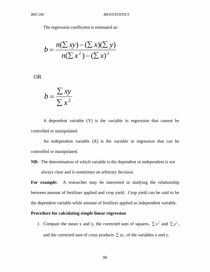
BIO 206 BIOSTATISTICS
86
The regression coefficient is estimated as:
22 )()(
))(()(
xxn
yxxynb
OR
2x
xyb
A dependent variable (Y) is the variable in regression that cannot be
controlled or manipulated.
An independent variable (X) is the variable in regression that can be
controlled or manipulated.
NB: The determination of which variable is the dependent or independent is not
always clear and is sometimes an arbitrary decision.
For example: A researcher may be interested in studying the relationship
between amount of fertilizer applied and crop yield. Crop yield can be said to be
the dependent variable while amount of fertilizer applied as independent variable.
Procedure for calculating simple linear regression
1. Compute the mean x and y, the corrected sum of squares, 2x and 2y ,
and the corrected sum of cross products xy , of the variables x and y.

BIO 206 BIOSTATISTICS
87
2. Compute the estimates of the regression parameters α and β as α = y - β x
(α and β are considered as the estimates of a and b rather than parameters).
Therefore β = 2/ xxy
3. Then substitute the value of β in the linear equation: α = y - β x. Thus the
estimated linear regression is y = α + β x
4. Plot the observed points and draw a graphical representation of the
estimated linear regression equation above.
Plot the scatter diagram and compute: yminimum = α + β xminimum and
ymaximum = α + β x maximum.
Plot the two points ( xmin, ymin) and (xmax, ymax) and draw the line
between the two points.
Note that:
o The drawn line must be within the range xmin. and xmax.
o The line must pass through the mean point (x, y).
o The slope of the is β
o The line, if extended, must intersect the y-axis at the y value of α
(intercept).
5. Test the significance of β. First you calculate the residual mean square as:
2
/)( 222
.2
n
xxyyS xy
and compute the tβ value as:

BIO 206 BIOSTATISTICS
88
2.
2 / xSt
xy
6. The Conclusion.
The regression coefficient β is said to be significantly different if the calculated
t-value above is greater than the tabular value at the 5% and 1% levels of
significance.
6.3.3 SCATTER DIAGRAM/PLOT
A scatter diagram is a graph of the ordered pairs (x,y) of numbers
consisting of the independent variable X and the dependent variable Y. It is a
visual way to describe the nature of the relationship between x and y. i.e. it enable
us to see whether there is any pattern among the points. The more distinct a
pattern is, the more closely the two variables are related in some way. For
example: Construct a scatter diagram for the data.
Subject Age Pressure
(x) (y)
A 43 128
B 48 120
C 56 135
D 61 143
E 67 141
F 70 154
G 32 96

BIO 206 BIOSTATISTICS
89
Figure 6.2 Scatter diagram
6.3.4 TYPES OF CORRELATION AND REGRESSION
Correlation can be Simple or Multiple. In simple relationships, there are
only two variables under study. For example, a researcher may wish to study the
relationship between height and weight in a population of rats.
In Multiple relationships more than two variables are under study for
example, a zoologist may wish to investigate the relationship between growth in
snails and factors such as different feed protein levels, quantity of feed given per
day and hours of lighting per day.
Regression can be linear or curvilinear regression. Linear could be either
simple linear regression or multiple linear regressions. Curvilinear – could be
exponential, quadratic, and logarithmic etc.
0
20
40
60
80
100
120
140
160
0 20 40 60 80
PRESSURE
AGE
SCATTER DIAGRAM

BIO 206 BIOSTATISTICS
90
Simple relationships can also be Positive or Negative. A positive
relationship exists when the two variables under study increase or decrease at the
same time. In a negative relationship as one variable increases the other variable
decreases, and vice versa.
Generally, simple correlation and simple linear regression may be:
1. Positive correlation – when an increase in one variable is associated to a
greater or lesser extent with an increase in the other.
2. Negative correlation – when an increase in one variable is associated to a
greater or lesser extent with a decrease in the other.
3. Perfect correlation – when a change in one variable is exactly matched by
a change in the other variable. If both increase together, it is perfect
positive correlation: if one decreases as the other increases, it is perfect
negative correlation.
4. High correlation – When a change in one variable is almost exactly
matched by a change in the other.
5. Low correlation – when a change in one variable is to a small extent
matched by a change in the other.
6. Zero correlation – when the two variables are not in matched at all, and
there is no relationship between changes in one variable and changes in the
other.

BIO 206 BIOSTATISTICS
91
Figure 6.3 A perfect positive correlation
Figure 6.4 A perfect negative correlation
0
5
10
15
20
25
30
35
40
0 5 10 15 20 25 30 35 40
Y-AXIS
X - AXIS
Perfect positive correlation (r=+1)
0
5
10
15
20
25
30
35
0 5 10 15 20 25 30 35
Y-Axis
X-Axis
Perfect negative correlation (r= -1)

BIO 206 BIOSTATISTICS
92
Figure 6.5 A zero correlation
Figure 6.6 A curvilinear graph
0
5
10
15
20
25
30
35
0 5 10 15 20 25 30
Y-Axis
X-Axis
Zero correlation (r=0)
0
5
10
15
20
25
30
35
0 5 10 15 20 25
Y-Axis
X-Axis
Curvilinear relationship

BIO 206 BIOSTATISTICS
93
6.3.5 SPURIOUS CORRELATION
When interpreting correlation, r, it is important to realize that, there may be
no direct connection at all between highly correlated variables. When this is so,
the correction is termed spurious or nonsense correlation. It can arise in two ways:
(a) There may be an indirect connection
(b) There may be a series of coincidences.
6.3.6 CONVARIANCE
When the association of two variables is assessed we can speak of the
resulting assessment as the covariance (‘Cov’) of the variables. The use of analysis
of covariance helps to eliminate variability. Covariance can be measured by
finding the average of the products of the deviations of each of the paired variables
from the overall mean of the relevant variable i.e.
nyyxxyyxCov ii /))((),(
WORKED EXAMPLE.
Assuming the following are given values of the length (X) and yield (Y) of five
Okro plants. Using the deviation method, estimate and interpret the linear
association between the length and yield of the Okro plants.
Length (X) 3 4 6 5 2
Yield (Y) 10 12 15 13 5
Compute the means for X and Y.

BIO 206 BIOSTATISTICS
94
Mean of X = 3 + 4 + 6 + 5 + 2 / 5 = 4
Mean of Y = 10 + 12 + 15 + 13 + 5 / 5 = 11
Compute the values of the deviates.
Deviation from mean Squares of deviates
Products
of deviates Length (X) Yield (Y) X Y x
2 y
2 xy
3 10 -1 -1 1 1 1
4 12 0 1 0 1 0
6 15 2 4 4 16 8
5 13 1 2 1 4 2
2 5 -2 -6 4 36 12
Total 10 58 23
Then we can compute the correlation (r) value.
))(( 22 yx
xyr
= . 23 = 23 = 0.954
√(10)(58) 24.1
The r value of 0.954 is high and positive. That means the longer the Okro plant the
more the yield.
The degrees of freedom (d.f) is given by:
d.f. = n – 2
where: n is the number of the bivariate data.
The d.f. = 5 – 2 =3
Then check the correlation table at d.f 3 and 95% level of significance = 0.878.
Since the absolute value of r (0.954) is greater than correlation table value (0.878)
at 5% probability level, the linear association between length and yield is
significant. That means that the longer the Okro plant, the more the yield in almost
95% of the population.

BIO 206 BIOSTATISTICS
95
6.4 TUTOR MARKED ASSIGNMENT
1. What is meant by the statement that two variables are related?
2. Give examples in nature of two variables that are positively correlation and
two that are negatively correlated.
3. The average normal daily temperature (oC) and the corresponding average
precipitate (inches) for the month of August for seven randomly selected
Local Government Areas in Plateau State are shown in the data below.
Av. daily temp. (x) 30 27 28 32 27 23 18
Av. mon. precip. (y) 3.4 1.8 3.5 3.6 3.7 1.5 0.2
(a). Draw a scatter plot for the variables.
(b). State the hypothesis.
(c). Compute the value of the correlation coefficient.
(d). Test the significance of the correlation coefficient at = 0.05.
(e). Give a brief explanation of the type of relationship.
4. The data of an experiment to apply sufficient quantities of fertilizer to optimize
vegetation growth (grass yield) and avoid excessive application that could lead to
runoff and nutrient enrichment of a nearby lake is shown in the table below.
Weight of fertilizer (g/
sq. m) (x).
25 50 75 100 125 150 175 200 225 250
Yield of grass (g/sq.
m) (y).
84 90 90 154 148 169 206 244 212 248
(a). Plot the scattergram for the data.
(b). determine the regression of y on x.

BIO 206 BIOSTATISTICS
96
6.5 REFERENCES
Bailey, N.T.J. (1994). Statistical Methods in Biology. Third Edition. Cambridge
University Press. United Kingdom.
Bluman, A.G. (2004). Elementary Statistics. A Step by Step Approach. Fifth
Edition. McGraw-Hill Companies Incorporated. London.
Clarke, G.M. (1971). Statistisc and Experimental Design. Edward Arnold
Publishers Limited. London.
Daniel, W.W. (1995). Biostatistics: a foundation for Analysis in Health sciences.
Sixth Edition. John Wiley and sons Incorporated. USA.
Fowler, J.A. and Cohen, L. Statistics for Ornithologist. British Trust for
Ornithology Guide 22.
Harper, W.M. (1991). Statistics. Sixth Edition. Pitman Publishing, Longman
Group, United Kingdom.
Hoel, P.G. (1976). Elementary Statistics. Four Edition. John Wiley and Sons
Incorporated, NewYork. Pp 151-204.
Mukhtar, F.B. (2003). An Introduction to Biostatistics. Samarib Publishers, Kano
Nigeria. Pp 1-112.
Sanders, D.H., Murph, A.F. and Eng, R.J. (1980). Statistics: A Fresh Approach.
McGraw-Hill Kogakusha, Limited. Kosaido Printing Company Limited,
Tokyo, Japan.
UNIT SEVEN: SIMPLE EXPERIMENTAL DESIGN AND ANALYSIS
OF VARIANCE (ANOVA)
7.1 INTRODUCTION
Over the years, an enormous range of experimental patterns has been
developed and designs are available to suit a wide variety of circumstances.
Experimental design may be considered under two main headings. The
first is the actual pattern of the experiment in which a correct of design depends

BIO 206 BIOSTATISTICS
97
partly on knowledge of the experimental material and partly on the kind of
question are wishes to ask. Secondly is the analysis of the data. As a rule, the
results of the kind of experimental can be summarized in an analysis of variance
(Anova) table. The design and analysis of an experiment obviously influence one
another very strongly. That is for a given design, there really one satisfactory way
of analyzing the data.
7.2 OBJECTIVES:
At the end of this unit, you should be able to:
1. Define experimental design.
2. Explain the principles of experimentation.
3. Mention and explain the different types of experimental design.
4. Define Anova and test statistical hypotheses using Anova.
7.3 MAIN CONTENT
7.3.1 EXPERIMENTAL DESIGN
Experimental design deals with the methods of constructing and analyzing
comparative experiments such as comparing the effect of different factors or
treatments. Planning experiments is made much more effective if you understand
the advantages and disadvantages of different experimental designs and how they
affect the “experimental error” against which we test our differences between
treatments. There is the need to understand how experimental design as well as

BIO 206 BIOSTATISTICS
98
treatment and replicate numbers impact on the “residual degrees of freedom” and
whether you should be looking at one-tailed or two-tailed statistical tables.
Experimental design ensures that maximum precision is achieved for the
amount of effort expended in an experiment. In every design, it is important that
the roles of the treatments should be well defined and the objectives of the
experiment properly understood.
An experiment is a systematic procedure for making observations under
controlled conditions in such a way that they can be used for arriving at general
conclusions regarding the population under study. An experimental unit is a plant
or animal or group of plants or animals making up a single replicate of a single
treatment. It is also called a plot.
7.3.2 PRINCIPLES INVOLVED IN EXPERIMENTATION
1. Randomization: This involves the allotting of treatments to the available
material at random.
2. Replication / Reproducibility: is the need for an experiment to be planned
in such a way that it can be replicated or reproduced. Replication is
important in reducing error and enhancing accuracy. (Note: An error is the
variation among varieties that cannot be accounted for by the variation due
to treatments, blocks and other factors controlled in the experiment).
Normally errors affecting any treatment tend to cancel out as the number of
replications is increased.

BIO 206 BIOSTATISTICS
99
3. Homogeneity/Sensitivity: A homogenous experimental setup is one that has
uniformity of materials and therefore does not require the control of local
variation. While sensitivity is to be able to estimate the effects of the
treatments so that valid conclusion can be drawn.
7.3.3 TYPES OF EXPERIMENTAL DESIGN
1. Completely Randomized Design (CRD): is the simplest type of
experimental design in which treatments are assigned at random to a set of
plots. It is applicable when homogenous (same) experimental material is
used on heterogeneous (different) experimental units or treatments, which
is replicated more than once. CRD ensures that treatments allotment is
completely random thereby avoiding biasness and minimizing inherent
differences in experimental units or treatment. For example, the CRD for
three replicates of six treatments is as follows.
A B A
A E B
D D E
C C C
F F E
F B D
A one-way analysis of variance is used in the analysis of CRD. Examples
of such simple experiment include: Effects of different fertilizers
(treatments) on yield of maize (experimental material), evaluating the
effects of a feed of different protein levels (treatments (experimental
material) on the growth of quails or fish of the same age, sex, size, etc.

BIO 206 BIOSTATISTICS
100
Advantages of CRD
a. The design is very flexible and can be used for any number of treatments.
b. The statistical analysis is comparatively easy and straightforward.
c. It is unaffected by missing observations for any treatment for some purely
random accidental reason.
Disadvantage of CRD
a. The design is inherently less informative than other more sophisticated
layouts.
2. Randomized Block Design (RBD): is an experimental design in which the
total area is divided into blocks and all of the treatments are arranged
within each block in a random order. It is the probably the most widely
used experimental design.
Block Plots
Fertility Trend
I A C B D
II B C A D
III D A C B
IV B D C A
There are two sources of variation (i.e Treatment and Blocks) in RBD and
therefore a two-way analysis of variance is used to analyze data obtained.
Examples include experiments to determine the response of quails of different age

BIO 206 BIOSTATISTICS
101
groups to different dietary protein levels, response of five variety of maize to three
levels Indole-Acetic-Acid (IAA), etc.
Advantages and Disadvantages of RBD
1. With heterogeneous material the residual variance can be reduced by
choosing blocks of plots such that the plots within the blocks are fairly
similar. i.e the design reduces the effect of heterogeneous material.
2. There is no restriction on the number of blocks or treatments, but in each
block there must be the same number of plots, one to each treatment.
3. If some yields are accidentally lost, the analysis is again without due
complications, although special modifications are required.
Procedure of a randomized block experiment
Phase 1
Total rows and columns, and check Grand total by adding both row and
column totals.
Calculate correction factor for experiment = Grand total2/number plots.
Calculate TOTAL sum of squares (added squares – correction factor!).
YOU HAVE NOW NO FURTHER USE FOR THE PLOT RESULT DATA
Phase 2
Construct the analysis of variance table with the headings: Source of
variation, d.f., Sum of squares, Mean square, F, and P.
Insert sources of variation as Treatments, Blocks, Residual, and Total.

BIO 206 BIOSTATISTICS
102
Allocate degrees of freedom as n − 1 for number of Treatments and
Replicates, and the product of these two d.f. for the Residual. Check that
the three d.f.’s add up to n−1 for the Total (i.e. one less than the number of
data in the experiment).
Square and add the TREATMENT totals to obtain the Treatments sum of
squares of deviations.
Square and add the REPLICATE totals to obtain the Replicates sum of
squares of deviations.
The “Residual” sum of squares of deviations is the remainder of the
“total” sum of squares of deviations.
YOU HAVE NOW USED ALL THE COLUMN AND ROW TOTALS
End Phase
Calculate mean square for “treatments,” “replicates,” and “residual” by
dividing each sum of squares of deviations by its own degrees of freedom.
3. Latin square: Is an experimental design in which the number of rows,
columns, and treatments are equal and each treatment occurs just once in
each row and column. As the name implies, a Latin square is a square
design in that it consists of the same number of plots (though these don’t
have to be square) in two dimensions, i.e. 4 × 4, 5 × 5, 6 × 6, etc. The
“dimension” of the square is the number of treatments in the experiment.
We’ll take as our example a Latin square with four treatments (A, B, C,and
D) – i.e. a 4×4 (16 plot) square.

BIO 206 BIOSTATISTICS
103
C B A D
D C B A
B A D C
A D C B
Simple Factorial Experiment
A factorial experiment is one where the treatments allocated to the
experimental plots are combinations of two or more factors (hence the term
“factorial”). For example, we might wish to test the effect on some measurement
of a NUMBER of different fertilizers on MORE THAN ONE plant variety. Each
plot would then be allocated the combination of one “level”of fertilizer (one of the
fertilizers) applied to one “level” of variety (one of the varieties).
7.3.4 ANALYSIS OF VARIANCE (ANOVA)
Analysis of variance (abbreviated as ANOVA) is a systematic procedure
for obtaining two or more estimate of variance and comparing them. Anova as a
technique enables the comparison of means and variances in an experiment that
involves more than two treatments. It estimates the value of the true variance of
the population (σ2) from which the sample is drawn.
Anova permits us to conclude whether or not all means of the population
under study are equal base upon the degree of variability in the sample data.
Therefore, it is extremely efficient and powerful technique for investigating
relationships between several groups of data.
ASSUMPTIONS IN ANOVA
In Anova, the following assumptions must be made or else its appropriateness
becomes questionable.

BIO 206 BIOSTATISTICS
104
1. Samples are drawn randomly and each sample is independent of the other
samples.
2. The populations under study have distribution which is approximately the
normal curve.
3. The populations from which the sample values are obtained, all have the
same population variance (σ2). That is (σ1
2 = σ2
2 = σ3
2 = ………….σk
2), the
variances of all the populations are equal.
HYPOTHESES IN ANOVA
1. The null hypothesis (Ho) in Anova is that the independent samples are
drawn from populations with the same means: Ho : µ1 = µ2 = µ3 =
…………….µk.
Where, k, is the number of populations under
study.
2. The alternative hypothesis (H1) in Anova is that, not all population means
are equal. That is, at least one mean is different from the others.
H1 : µ1 ≠ µ2 ≠ µ3 ≠ ……...µk.
THE CONCLUSIONS
Conclusions concerning Ho in Anova test are based on computed variance ratio,
sometimes called the F-ratio.
1. Accept the null hypothesis, Ho, if the F-ratio value is less than the table
value. That is, it is not significant.
2. Reject the null hypothesis, Ho, and accept the alternative hypothesis, H1, if
the F-ratio value is more than the table value. That is it is significant.
EXAMPLES:
1. The table below shows the number of seeds for five varieties of garden egg
to three level of Indo-acetic acid (IAA).

BIO 206 BIOSTATISTICS
105
IAA\varieties A B C D E
I 3 5 10 7 8
II 2 4 7 4 5
III 4 5 8 6 7
Solution:
State the null hypothesis: There is no significant difference between seed
number in five varieties of garden egg and levels of IAA.
Calculate the totals from the table as below:
IAA\varieties A B C D E Total
I 3 5 10 7 8 33
II 2 4 7 4 5 22
III 4 5 8 6 7 30
Total 9 14 25 17 20 GT=85
Then calculate the Correction Factor (CF) as:
CF = GT2/N = 85
2/15 = 481.7
Calculate the Mean Squares (SS)
BLOCKss = (332 + 22
2 + 30
2/5) – CF = 12.9
VARIETIESss = (92 + 14
2 +………..+ 20
2)/3 – CF = 48.6
TOTALss = (32 + 5
2 +………...+7
2) – CF = 65.3
ERRORss = TOTALss – (BLOCK + VARIETIESss) = 3.8
Then calculate:
BLOCKMS = BLOCKss/ BLOCKDF = 12.9/2 = 6.45
VARIETIESMS = VARIETIESss/VARIETIESDF = 48.6/4 = 12.15
Block F-value = BlockMS /ErrorMS = 6.45/0.475 = 13.58
Varieties F-value = VarietiesMS /ErrorMS = 12.15/0.475 = 25.58

BIO 206 BIOSTATISTICS
106
The calculated F-values are compared with the F-distribution table, using their
respective degrees of freedoms.
SOURCE DF SS MS F
Block 2 12.9 6.45 13.58**
Varieties 4 48.6 12.15 25.58**
Error 8 3.8 0.475
Total 14 65.3
** indicates that the values are highly significant.
Conclusion:
Since the F-values are highly significant, we reject the null hypothesis. It
means that the three levels of IAA have effect on the seed number of the five
varieties of garden egg.
2. Complete the Anova table below and draw your conclusions.
Source Sum of
squares (SS)
Degrees of
freedom
(DF)
Mean
squares (MS)
F-ratio
Varieties 123.44 * * *
Residual * 15 *
Total 210.21 18
RESIDUALss = 210.21 – 123.44 = 86.8
VARIETIESDF = 18 – 15 = 3
VARIETIESMS = 123.44/3 = 41.15
RESIDUALMS = 86.8/15 = 5.79
F- ratio = 41.15/5.79 = 7.11
The complete table is as shown below.
Source Sum of Degrees of Mean squares F-ratio

BIO 206 BIOSTATISTICS
107
squares (SS) freedom (DF) (MS)
Varieties 123.44 3 41.15 7.11
Residual 86.8 15 5.79
Total 210.21 18
Conclusion:
The observed variance ratio of 7.12 is greater than the table values at both
5% (3.29) and 1% (5.42). That means there is high significant difference
among the varieties. Therefore, we reject the null hypothesis that the varieties
are the same.
7.4 TUTOR MARKED ASSIGNMENT
1. What do you understand by ‘Experimental design’?
2. Which type of experimental design is most appropriate to use for the
following Anova. (a) One-way classification. (b) Two-way classification.
3. Outline and briefly discuss the principles involved in experimental.
4. What is the importance of using homogenous materials in an experiment?
5. From the Anova table below
Source of
variation
d.f. Sum of
Squares
Mean
Square
F
Block 2 16 8 11.94
Treatment 5 145.8 29.17 43.54
Residual/Error 10 6.67 0.67
Total 17 168.5
a. Name the type of design that was employed.
b. How many treatments were compared?
c. How many observations were analysed?
d. Draw your conclusions on the F-values.

BIO 206 BIOSTATISTICS
108
REFERENCES
Bailey, N.T.J. (1994). Statistical Methods in Biology. Third Edition. Cambridge
University Press. United Kingdom.
Bluman, A.G. (2004). Elementary Statistics. A Step by Step Approach. Fifth
Edition. McGraw-Hill Companies Incorporated. London.
Clarke, G.M. (1971). Statistisc and Experimental Design. Edward Arnold
Publishers Limited. London.
Daniel, W.W. (1995). Biostatistics: a foundation for Analysis in Health sciences.
Sixth Edition. John Wiley and sons Incorporated. USA.
Fowler, J.A. and Cohen, L. Statistics for Ornithologist. British Trust for
Ornithology Guide 22.
Harper, W.M. (1991). Statistics. Sixth Edition. Pitman Publishing, Longman
Group, United Kingdom.
Helmut F. van Emden.(2008). Statistics for Terrified Biologists. Blackwell
Publishing
Limited. USA.
Hoel, P.G. (1976). Elementary Statistics. Four Edition. John Wiley and Sons
Incorporated, NewYork. Pp 151-204.
Mukhtar, F.B. (2003). An Introduction to Biostatistics. Samarib Publishers, Kano
Nigeria. Pp 1-112.
Sanders, D.H., Murph, A.F. and Eng, R.J. (1980). Statistics: A Fresh Approach.
McGraw-Hill Kogakusha, Limited. Kosaido Printing Company Limited,
Tokyo, Japan.

BIO 206 BIOSTATISTICS
109
UNIT EIGHT: NON – PARAMETRIC TESTS
8.1 INTRODUCTION
Statistical test, such as mean, standard deviation, variance, Z, t and F- tests
are called parametric tests. This is because these assumptions are governed by the
distribution of the sampled population or populations that is/or are at least
approximately normal. But if the population in a particular hypothesis-testing
situation is not normally distributed, then the non-parametric or distribution – free
tests is used.
Non parametric test can also be used to test hypothesis that do not involve
specific population parameters such as μ, σ or P.
8.2 OBJECTIVES:
At the end of this unit, you should be able to
1. State the advantages and disadvantages of non parametric method.
2. Give the differences between non-parametric and parametric test.
3. Test hypotheses using non parametric tests such as Sign test and Kruskal-
Wallis test.
4. Compute the Spear rank correlation coefficient.
8.3 MAIN CONTENT
8.3.1 ADVANTAGES OF NON-PARAMETRIC TEST
There are five advantages that non parametric methods have over
parametric methods.

BIO 206 BIOSTATISTICS
110
1. They can be used to test population when the variable is not normally
distributed.
2. They can be used when the data are nominal or ordinal.
3. Can be used to test hypothesis that do not involve population parameters.
4. In most cases, computation is easier than in parametric.
5. They are easier to understand.
8.3.2 DISADVANTAGES OF NON-PARAMETRIC TEST
1. They are less sensitive than in parametric i.e larger differences are needed
before the null hypothesis can be rejected.
2. They tend to use less information than the parametric tests.
3. They are less efficient than their parametric counterparts when the
assumptions of the parametric are met.
NOTE:
The researcher should use caution in deciding whether to use non-
parametric or parametric methods. However, if the assumptions can be met, the
parametric methods are preferred.
DISTINCTION BETWEEN NON-PARAMETRIC AND PARAMETRIC
TESTS
NON – PARAMETRIC TESTS PARAMETRIC TEST
1 May be used with actual observations, or
with observations converted to ranks.
Are used only with actual
observations
2 May be used with observations on nominal,
ordinal and interval scales
Generally restricted to observations
on interval scales.
3 Compare medians Compare means and variances
4 Data are ‘distribute in free’ i.e must not be
normally distributed.
Data are required to be normally
distributed and to have similar
variances

BIO 206 BIOSTATISTICS
111
5 Are suitable for data which are counts Counts must be transformed
6 Are suitable for derived data e.g.
proportions, indices
Derived data may first have to be
transformed.
8.3.3 THE SIGN TEST
The simplest non-parametric test is the sign test for single samples. It is
used to test the value of a median for a specific sample. In using Sign test, you:
Hypothesize the specific value for the median of a population.
Select a sample of data and compare each value with the conjectured median.
Assign plus sign if the data value is above the conjectured median.
Assign minus sign if the data value is below the conjecture median.
And zero (0) if it is the same as the conjecture median.
Compare the number of plus and minus signs and ignore the zeros
If the null hypothesis (Ho) is true, the number of plus signs should be
approximately equal to the number of minus signs.
But if the Ho is not true, there will be disproportionate number of plus or
minus signs.
NB:
The test value is the smaller number of plus or minus signs obtained in a
sample. For example, if there are 12 plus signs and 5 minus signs, the test value is
5.

BIO 206 BIOSTATISTICS
112
For Example:
A chicken poultry owner hypothesizes that the median number of eggs he
gets per day is 40. A random sample of 20 days yields the following for the
number of eggs laid each day.
18 30 39 36 43
29 34 40 40 32
39 34 16 37 45
39 22 36 28 52
At α = 0.05, test the owner’s hypothesis
Solution:
State the hypotheses:
Ho: median = 40 – that is the claim
H1: median ≠ 40.
Find the critical value. Compare each value of data with the median
_ + 0 _ _
_ _ _ _ _
_ _ _ + _
_ 0 _ _ +
Then count the number of plus and minus signs, and ignore zero. This gives n =
18.

BIO 206 BIOSTATISTICS
113
Refer to Table of critical values for Sign test and α = 0.05 for a two-tailed test:
The critical value is 4.
Compute the test value.
Since there are 3 plus signs and 15 minutes sign, then the test value is 3. (Always
use the smaller value as the test value). The test value 3 is less than the critical
value 4 (3<4). Therefore, the null hypothesis is rejected.
In summary, there is enough evidence to reject the claim that the median number
of eggs layed per day is 40.
NB:
If the sample size is 25 or less, the table of critical values for Sign test is
used. But when the sample size is 26 or more, the standard normal distribution
table can be used to find the test value.
8.3.4 KRUSKAL – WALLIS TEST
The Kruskal – Wallis test, sometimes called the H - test is a non-
parametric test which can be used to compare three or more means, where the
assumptions for the ANOVA test: populations are normally distributed and the
population variances are equal, cannot be met. In Kruskal – Wallis test, each
sample size must be 5 or more with M-1 degrees of freedom, where m = number
of groups.
The distribution in kruskal – wallis can be approximated by the chi-square
distribution.

BIO 206 BIOSTATISTICS
114
Formula for Kruskal-Wallis Test
H = . 12 . ˟ (R12/n1+ R2
2/n2 + …….. + Rk
2/nk) – 3 (N + 1)
N(N+1)
Where:
R1 = Sum of ranks of sample 1
n1 = Size of sample 1
R2 = Sum of ranks of sample 2
n2 = Size of sample 2
Rk = Sum of ranks of sample K
nk = Size of sample k
N = n1 + n2 + ….. nk
k = number of samples
For Example:
A research was conducted to know the relationships of bill-length (mm) in three
bird species. The data below were obtained.
A B C
33.5 38.0 32.0
37.5 31.5 33.0
35.0 34.0 36.5
39.1 35.1 34.9
31.1 33.4 32.5
** At α = 0.05, is there enough evidence to reject the hypothesis that all the bird
species have the same bill length?

BIO 206 BIOSTATISTICS
115
Solution:
State the hypotheses
Ho: There is no difference in the bill length of the 3 bird species in the forest
reserve.
H1: There is a difference in the bill length of the 3 bird species in the forest
reserve.
Find the critical value using the chi-square distribution table at degrees of
freedom.
Df = m – 1 at α = 0.05, where m is the number of groups
df = 3 – 1 = 2: The critical value is 5.991
Arrange all the data from lowest to highest and rank each value
Bill - Length Species Rank
31.1 A 1
31.5 B 2
32.0 C 3
32.5 C 4
33.0 C 5
33.4 B 6
33.5 A 7
34.0 B 8
34.9 C 9
35.1 B 10
35.0 A 11
36.5 C 12
37.5 A 13
38.0 B 14
39.1 A 15

BIO 206 BIOSTATISTICS
116
Calculate the sum of the ranks of each bird species
Species A = 1 + 7 + 11 + 13 + 15 = 47
Species B = 2 + 6 + 8 + 10 + 14 = 40
Species C = 3 + 4 + 15 + 9 + 12 = 33
Substitute the Kruskal – Wallis Test formula
H = 12 (R2
1 + R2
2 + R2
3) – 3 (N + 1)
N(N+1) n1 n2 n3
Where:
N =15, R1 = 47, R2 = 40, R3 = 33 and n1 = n2 = n3 = 5
Therefore,
H = 12 (472 + 40
2 + 33
2) – 3 (15 + 1)
15(15+1) 5 5 5
= 0.05 (979.6) – 48
= 48.98 – 48
H = 0.98
Then deduce the decision.
Decision:
Since the test value 0.98 is less than the critical value 5.991, the decision is to
accept the null hypothesis. This simply means that there is no difference in the bill
length of the three bird species.
8.3.5 SPEARMAN RANK CORRELATION
The spearman rank correlation coefficient, denoted by rs, is the non-
parametric equivalent of the Pearson coefficient used for testing hypothesis when

BIO 206 BIOSTATISTICS
117
samples obtained are not normally distributed. It can be used when the data are
ranked. If the two sets of data have the same ranks, rs will be +1. If the ranks are
in exactly the opposite way, rs will be -1. If there is no relationship between the
rankings, then rs will be near 0.
The formula for spear rank correlation is given as:
)1(
)6(1
2
2
nn
drs
where: d = difference in ranks
n = number of data pairs
For Example:
The table below gives the number of horn bill nestlings ringed, and
juveniles captured in the same season, over a 6 year study period at a woodland
site. At α = 0.05, test the hypothesis that there is a linear correlation between the
nestlings ringed and juveniles captured.
Nestlings Ringed 16 9 1 7 13 5
Juveniles Captured 16 8 5 4 10 3
Solution:
State the hypothesis
Ho: ρ = 0 and H1: ρ ≠ 0

BIO 206 BIOSTATISTICS
118
Find the critical value using the table of critical values for the Rank correlation
coefficient.
And the value n = 6 and α = 0.05
The value is 0.886.
To find the test value, you first rank the data set.
Nestlings ringed Rank 1 Juveniles
captured
Rank 2
16 1 16 1
9 4 8 3
1 6 5 4
7 5 4 5
13 3 10 2
15 2 3 6
Then subtract the rankings for each season (R1 – R2) and square the differences.
R1 R2 d d2
1 1 0 0
4 3 -1 1
6 4 2 4
5 5 0 0
3 2 1 1
2 6 -4 16
222 d

BIO 206 BIOSTATISTICS
119
Substitute in the formula to find r.
)1(
)6(1
2
2
nn
drs
where n = the number of data pairs (n = 6)
rs = 1 – 6(22) = 0.371
6(62 – 1)
Make a decision.
Since the rs = 0.371, which is less than the critical value of 0.886, we accept
the null hypothesis. Therefore, there is no enough evidence to say that there is
a correlation between Nestlings ringed and Juveniles captured.
8.4 TUTOR MARKED ASSIGNMENT:
1. Why is the sign-test the simplest non-parametric test to use?
2. Ten patients suffering from severe muscle pains volunteered to try two new
analgesics and the time of relief were recorded in minutes for each patient
are as shown below.
Patient number 1 2 3 4 5 6 7 8 9 10
Analgesic A
(min.)
138 136 142 151 154 141 140 138 132 136
Analgesic B
(min.)
140 136 141 150 153 144 143 136 131 138
(a) State the hypotheses and identify the claim.
(b) Find the critical value and compute the test value.
(c) Make a decision based on your finding.

BIO 206 BIOSTATISTICS
120
3. A study was conducted on 10 adults to determine the effect of alcohol on
test scores. Each adult was given a test. Then for one week, each adult was
required to consume a certain amount of alcohol and then he or she was
retested. The results are shown below.
Adult Score before Score after
1 105 106
2 109 105
3 98 94
4 112 109
5 109 105
6 117 115
7 123 125
8 114 114
9 95 98
10 101 100
At α = 0.10, test the claim that alcohol does not affect a person’s test score.
8.5 REFERENCES
Bailey, N.T.J. (1994). Statistical Methods in Biology. Third Edition. Cambridge
University Press. United Kingdom.
Bluman, A.G. (2004). Elementary Statistics. A Step by Step Approach. Fifth
Edition. McGraw-Hill Companies Incorporated. London.
Daniel, W.W. (1995). Biostatistics: a foundation for Analysis in Health sciences.
Sixth Edition. John Wiley and sons Incorporated. USA.
Fowler, J.A. and Cohen, L. Statistics for Ornithologist. British Trust for
Ornithology Guide 22.
Harper, W.M. (1991). Statistics. Sixth Edition. Pitman Publishing, Longman
Group, United Kingdom.
Helmut F. van Emden.(2008). Statistics for Terrified Biologists. Blackwell
Publishing Limited. USA.

BIO 206 BIOSTATISTICS
121
Hoel, P.G. (1976). Elementary Statistics. Four Edition. John Wiley and Sons
Incorporated, NewYork. Pp 151-204.
Mukhtar, F.B. (2003). An Introduction to Biostatistics. Samarib Publishers, Kano
Nigeria. Pp 1-112.
Sanders, D.H., Murph, A.F. and Eng, R.J. (1980). Statistics: A Fresh Approach.
McGraw-Hill Kogakusha, Limited. Kosaido Printing Company Limited,
Tokyo, Japan.

BIO 206 BIOSTATISTICS
122
UNIT NINE: USE OF STATISTICAL PACKAGES
9.1 INTRODUCTION
In the past, statistical calculations were done with pencil and paper.
However, with the advent of calculators, numerical computations have become
much easier, especially where computers do all the numerical calculations. All
one does is to enter the data into the computer and use the appropriate command;
the computer will print the answer or display it on the screen. You should realize
that you are responsible for understanding and interpreting each statistical concept.
There are many statistical packages available. This unit discusses the SPSS
(Statistic al package for Social Sciences) and MINITAB.
9.2 OBJECTIVES:
At the end of this unit, you should be able to:
1. Describe the applications of SPSS and MINITAB in different statistical
procedures.
2. Mention examples of statistical tools in the statistical packages.
9.3 MAIN CONTENT
9.3.1 SPSS
This is a statistical package developed especially for the social sciences but
it has wide applicability in the areas of biology and agriculture. It can be used to
execute some statistical procedures such as summaries, custom tables, Anova
(Analysis of variance), correlation and regression analyses, non-parametric tests,

BIO 206 BIOSTATISTICS
123
time series, create charts (Bar, line, Pie, Area, Histogram, Scatter etc.) and lots
more.
The SPSS is a comprehensive package that is command based but
commands list can be generated from menus and interactive operations are
possible.
9.3.2 MINITAB
The MINITAB statistical software provides a wide range of statistical
analysis and graphical capabilities. Like the SPSS, it is also a comprehensive
command based statistical package. MINITAB can be used for various types of
statistical analysis ranging from editing and manipulating data, basic statistics,
arithmetic, regression, Anova, non parametric test, exploratory data analysis et.c.
9.4 REFERENCES
Bailey, N.T.J. (1994). Statistical Methods in Biology. Third Edition. Cambridge
University Press. United Kingdom.
Bluman, A.G. (2004). Elementary Statistics. A Step by Step Approach. Fifth
Edition. McGraw-Hill Companies Incorporated. London.
Mukhtar, F.B. (2003). An Introduction to Biostatistics. Samarib Publishers, Kano
Nigeria. Pp 1-112.
Copyright © 2022 FDOKUMEN