Introduction to Biostatistics with JMP - SAS Support
27
-
Upload
khangminh22 -
Category
Documents
-
view
0 -
download
0
Transcript of Introduction to Biostatistics with JMP - SAS Support

The correct bibliographic citation for this manual is as follows: Figard, Steve. 2019. Introduction to Biostatistics with JMP®. Cary, NC: SAS Institute Inc.
Introduction to Biostatistics with JMP®
Copyright © 2019, SAS Institute Inc., Cary, NC, USA ISBN 978-1-64295-456-2 (Hardcover) ISBN 978-1-62960-633-0 (Paperback) ISBN 978-1-63526-720-4 (Web PDF) ISBN 978-1-63526-718-1 (epub) ISBN 978-1-63526-719-8 (kindle)
All Rights Reserved. Produced in the United States of America.
For a hard copy book: No part of this publication may be reproduced, stored in a retrieval system, or transmitted, in any form or by any means, electronic, mechanical, photocopying, or otherwise, without the prior written permission of the publisher, SAS Institute Inc.
For a web download or e-book: Your use of this publication shall be governed by the terms established by the vendor at the time you acquire this publication.
The scanning, uploading, and distribution of this book via the Internet or any other means without the permission of the publisher is illegal and punishable by law. Please purchase only authorized electronic editions and do not participate in or encourage electronic piracy of copyrighted materials. Your support of others’ rights is appreciated.
U.S. Government License Rights; Restricted Rights: The Software and its documentation is commercial computer software developed at private expense and is provided with RESTRICTED RIGHTS to the United States Government. Use, duplication, or disclosure of the Software by the United States Government is subject to the license terms of this Agreement pursuant to, as applicable, FAR 12.212, DFAR 227.7202-1(a), DFAR 227.7202-3(a), and DFAR 227.7202-4, and, to the extent required under U.S. federal law, the minimum restricted rights as set out in FAR 52.227-19 (DEC 2007). If FAR 52.227-19 is applicable, this provision serves as notice under clause (c) thereof and no other notice is required to be affixed to the Software or documentation. The Government’s rights in Software and documentation shall be only those set forth in this Agreement.
SAS Institute Inc., SAS Campus Drive, Cary, NC 27513-2414
October 2019
SAS® and all other SAS Institute Inc. product or service names are registered trademarks or trademarks of SAS Institute Inc. in the USA and other countries. ® indicates USA registration.
Other brand and product names are trademarks of their respective companies.
SAS software may be provided with certain third-party software, including but not limited to open-source software, which is licensed under its applicable third-party software license agreement. For license information about third-party software distributed with SAS software, refer to http://support.sas.com/thirdpartylicenses.
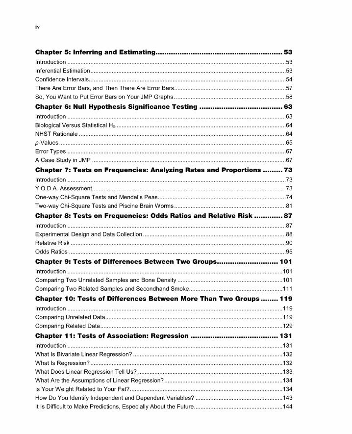
Contents
About This Book ........................................................................................ vii
About The Author ....................................................................................... ix
Chapter 1: Some JMP Basics ..................................................................... 1 Introduction ....................................................................................................................................... 1 JMP Help .......................................................................................................................................... 1 Manual Data Entry ............................................................................................................................ 6 Opening Excel Files ......................................................................................................................... 7 Column Information – Value Ordering .............................................................................................. 8 Formulas ........................................................................................................................................ 10 “Platforms” ...................................................................................................................................... 14 The Little Red Triangle is Your Friend! ........................................................................................... 14 Row States – Color and Markers .................................................................................................... 15 Row States – Hiding and Excluding ............................................................................................... 18 Saving Scripts ................................................................................................................................ 20 Saving Outputs – Journals & RTF Files.......................................................................................... 21 Graph Builder ................................................................................................................................. 22
Chapter 2: Thinking Statistically .............................................................. 23
Thinking Like a Statistician ............................................................................................................. 23 Summary ........................................................................................................................................ 26
Chapter 3: Statistical Topics in Experimental Design ............................... 29
Introduction ..................................................................................................................................... 29 Sample Size and Power ................................................................................................................. 29 Replication and Pseudoreplication ................................................................................................. 34 Randomization and Preventing Bias .............................................................................................. 36 Variation and Variables .................................................................................................................. 37
Chapter 4: Describing Populations ........................................................... 41 Introduction ..................................................................................................................................... 41 Population Description.................................................................................................................... 41 The Most Common Distribution – Normal or Gaussian .................................................................. 45 Two Other Biologically Relevant Distributions ................................................................................ 45 The JMP Distribution Platform ........................................................................................................ 46 An Example: Big Class.jmp ............................................................................................................ 48 Parametric versus Nonparametric and “Normal Enough” ............................................................... 51
iv
Chapter 5: Inferring and Estimating .......................................................... 53
Introduction ..................................................................................................................................... 53 Inferential Estimation ....................................................................................................................... 53 Confidence Intervals........................................................................................................................ 54 There Are Error Bars, and Then There Are Error Bars .................................................................... 57 So, You Want to Put Error Bars on Your JMP Graphs…................................................................. 58
Chapter 6: Null Hypothesis Significance Testing ...................................... 63 Introduction ..................................................................................................................................... 63 Biological Versus Statistical Ho........................................................................................................ 64 NHST Rationale .............................................................................................................................. 64 p-Values .......................................................................................................................................... 65 Error Types ..................................................................................................................................... 67 A Case Study in JMP ...................................................................................................................... 67
Chapter 7: Tests on Frequencies: Analyzing Rates and Proportions ......... 73 Introduction ..................................................................................................................................... 73 Y.O.D.A. Assessment ...................................................................................................................... 73 One-way Chi-Square Tests and Mendel’s Peas .............................................................................. 74 Two-way Chi-Square Tests and Piscine Brain Worms .................................................................... 81
Chapter 8: Tests on Frequencies: Odds Ratios and Relative Risk ............. 87
Introduction ..................................................................................................................................... 87 Experimental Design and Data Collection ....................................................................................... 88 Relative Risk ................................................................................................................................... 90 Odds Ratios .................................................................................................................................... 95
Chapter 9: Tests of Differences Between Two Groups ............................ 101 Introduction ................................................................................................................................... 101 Comparing Two Unrelated Samples and Bone Density ................................................................ 101 Comparing Two Related Samples and Secondhand Smoke ......................................................... 111
Chapter 10: Tests of Differences Between More Than Two Groups ........ 119 Introduction ................................................................................................................................... 119 Comparing Unrelated Data ............................................................................................................ 119 Comparing Related Data ............................................................................................................... 129
Chapter 11: Tests of Association: Regression ........................................ 131 Introduction ................................................................................................................................... 131 What Is Bivariate Linear Regression? ........................................................................................... 132 What Is Regression? ..................................................................................................................... 132 What Does Linear Regression Tell Us? ........................................................................................ 133 What Are the Assumptions of Linear Regression? ........................................................................ 134 Is Your Weight Related to Your Fat? ............................................................................................. 134 How Do You Identify Independent and Dependent Variables? ..................................................... 143 It Is Difficult to Make Predictions, Especially About the Future ...................................................... 144
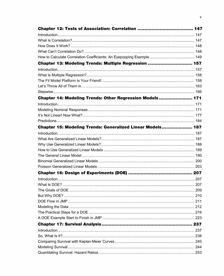
v
Chapter 12: Tests of Association: Correlation ........................................ 147 Introduction ................................................................................................................................... 147 What Is Correlation? ..................................................................................................................... 147 How Does It Work? ...................................................................................................................... 148 What Can’t Correlation Do? .......................................................................................................... 148 How to Calculate Correlation Coefficients: An Eyepopping Example ........................................... 149
Chapter 13: Modeling Trends: Multiple Regression ................................ 157
Introduction ................................................................................................................................... 157 What Is Multiple Regression? ....................................................................................................... 158 The Fit Model Platform Is Your Friend! ......................................................................................... 158 Let’s Throw All of Them in… ........................................................................................................ 163 Stepwise ....................................................................................................................................... 166
Chapter 14: Modeling Trends: Other Regression Models ........................ 171 Introduction ................................................................................................................................... 171 Modeling Nominal Responses ...................................................................................................... 171 It’s Not Linear! Now What? ........................................................................................................... 177 Predictions .................................................................................................................................... 184
Chapter 15: Modeling Trends: Generalized Linear Models ...................... 187
Introduction ................................................................................................................................... 187 What Are Generalized Linear Models? ......................................................................................... 187 Why Use Generalized Linear Models? ......................................................................................... 188 How to Use Generalized Linear Models ....................................................................................... 189 The General Linear Model ............................................................................................................ 190 Binomial Generalized Linear Models ............................................................................................ 200 Poisson Generalized Linear Models ............................................................................................. 203
Chapter 16: Design of Experiments (DOE) .............................................. 207
Introduction ................................................................................................................................... 207 What Is DOE? .............................................................................................................................. 207 The Goals of DOE ........................................................................................................................ 209 But Why DOE? ............................................................................................................................. 210 DOE Flow in JMP ......................................................................................................................... 211 Modeling the Data ........................................................................................................................ 212 The Practical Steps for a DOE ..................................................................................................... 216 A DOE Example Start to Finish in JMP ........................................................................................ 223
Chapter 17: Survival Analysis ................................................................. 237 Introduction ................................................................................................................................... 237 So, What Is It? .............................................................................................................................. 238 Comparing Survival with Kaplan-Meier Curves ............................................................................ 240 Modeling Survival ......................................................................................................................... 244 Quantitating Survival: Hazard Ratios ............................................................................................ 253
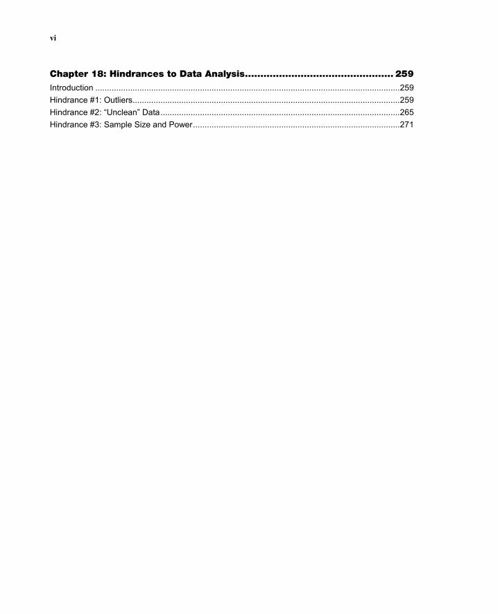
vi
Chapter 18: Hindrances to Data Analysis ................................................ 259
Introduction ................................................................................................................................... 259 Hindrance #1: Outliers ................................................................................................................... 259 Hindrance #2: “Unclean” Data ....................................................................................................... 265 Hindrance #3: Sample Size and Power ......................................................................................... 271
About This Book
This book is based on the need for a college-level textbook with examples derived from the biological sciences as an introduction to biostatistics using JMP software. The contents of this book follow that of an introductory course on biostatistics created for and taught at Bob Jones University and reflects an intended audience of undergraduates forced to take a course they really rather wished they could avoid. These undergraduates generally have enough biological and mathematical knowledge to be dangerous, coupled with an innate fear of “Statistics,” that renders them quite dangerous indeed. Although a basic knowledge of math up to and including algebra is generally desirable, this work studiously avoids the underlying formulas and mathematical gyrations found in many of the more “comprehensive” books on statistics. This is by design. Most practitioners of statistics are not mathematicians, don’t care about the underlying math, and are content to let their software deal with those details as long as they can get the answers that they need with some assurance that they are correct. To that end, the emphasis here will be on how to set up and execute the statistical tests in JMP and how to interpret the output.
Before getting into the details of the individual tests, however, it is necessary to cover some basics of how to think like a statistician, or a reasonable facsimile thereof, to ensure that the right analysis is being done in the first place. The reader will find most of these preliminaries in the first chapters, with their application to specific tests being covered in the remaining chapters. The ultimate goal is to create bioscientists who can competently incorporate biostatistics into their investigative toolkits to solve biological research questions as they arise.
Why Am I Reading This Book? Given the intended audience of this work – undergraduate biology and health science majors – the question asked in this section title is probably best answered by the opening paragraph of Dawn Hawkins’ excellent book when she writes:
Let us consider the likely scenario that you are a student of the biosciences. Whether you are a biomedic, a physiologist, a behaviourist, an ecologist, or whatever, you like learning about living things – you enjoy learning about the human body, bugs, and plants. Now, lo and behold, you have been forced to take a course that will make you do things with numbers and, dread-o-dread, even do something with numbers using a computer. You have probably decided that the people who are making you do this are mindless sadists.1
This captures many of the expressions I see on the first day of class on all too many of my students. Lest this seems to be an exaggeration, I have been asking those students to write down a one-word description of how they feel about taking this course and collecting those

viii Introduction to Biostatistics with JMP
responses. Using the text explorer feature in JMP to create a word cloud, I have acquired the following words to date:
Note that the majority of students are “nervous,” “unsure,” “afraid” or “anxious” as opposed to “excited” or “intrigued.” (Although it is intriguing that so many use that word to describe a biostatistics course at all!)
But I will argue here that we are neither mindless nor sadists in our demand that you, as a promising practitioner of the biological sciences, learn how to “do statistics.”
There are at least three reasons why this is so. First, if you are going to be a scientist of any kind, you should have some understanding of the philosophy and history of science. This is the “big picture” into which you will orient your own efforts at contributing to the body of knowledge. The twentieth century saw a paradigm shift in the basic philosophy underlying the scientific enterprise. The prior century, in part due to successful efforts in astronomy at understanding the movement of planets and other heavenly bodies, had developed a philosophical determinism in which mathematic formulas led to precise predictions. As David Salsburg notes,
Science entered the nineteenth century with a firm philosophical vision that has been called the clockwork universe. It was believed that there were a small number of mathematical formulas (like Newton’s laws of motion and Boyle’s laws for gases) that could be used to describe reality and to predict future events. All that was needed for such prediction was a complete set of these formulas and a group of associated measurements that were taken with sufficient precision.2
Alas and alack, the expected measurement precision never materialized. In fact, it proceeded to go from bad to worse. To account for this, scientists and mathematicians eventually developed and applied the ideas of randomness and probability to their observations, leading to a statistical model of reality that has revolutionized science. Salsburg points out, “Gradually, science began to work with a new paradigm, the statistical model of reality. By the end of the twentieth century, almost all of science had shifted to using statistical models.”3 If you are going to be a scientist professionally, you should understand something of this underlying foundation on which you will build your own construct with your research.
Given that data analysis will almost certainly be needed to interpret the results of your experiments, the second reason for learning how to do statistics is simply to do so correctly. There is a need for practitioners of the art, which is not the same as theoreticians, who can do so with competence. This is particularly true for the clinical and biomedical community where the use and interpretation of biostatistics often guides therapy, human health, and
About This Book ix
public policy, and is critical to understand published research. As one of the best standard textbooks on molecular biology points out:
Statistics – the mathematics of probabilistic processes and noisy data-sets – is an inescapable part of every biologist’s life.
This is true in two main ways. First, imperfect measurement devices and other errors generate experimental noise in our data. Second, all cell-biological processes depend on the stochastic behavior of individual molecules …and this results in biological noise in our results. How, in the face of all this noise, do we come to conclusions about the truth of hypotheses? The answer is statistical analysis, which shows how to move from one level of description to another: from a set of erratic individual data points to a simpler description of the key features of the data.4
And the demand for proficiency goes beyond the research laboratory. Clinical and medical testing laboratory professionals likewise need to be conversant with data analysis, as a recent article in Clinical Laboratory News observes:
Statistics! Just the mere mention of the word can strike fear, loathing, and dread in the hearts of some people. However, statistics is a key competency for laboratory professionals, both in normal clinical laboratory operations and in research. Not only does statistics provide the means to objectively evaluate data, it also summarizes data in a universal language that is meaningful to others.
But fear not! Computer software programs are available that can help you overcome your apprehensions about statistics.5
Yes, there is software to help, but using the software correctly means more than just plugging in the numbers, hitting a button, and out pops your answer! The process is much more involved, and even those who should know better by virtue of their training and experience don’t always get it right. Reviews of journals, even those servicing smaller specialty areas related to statistics, continue to put out a high frequency of statistical problems in published papers.6 And as Glantz rightly cautions,
The existence of errors in experimental design or biased samples in observational studies and misuse of elementary statistical techniques in a substantial fraction of published papers is especially important in clinical studies. These errors may lead investigators to report a treatment or diagnostic test to be of statistically demonstrated value when, in fact, the available data fail to support this conclusion. Health care professionals who believe that a treatment has been proved effective on the basis of publication in a reputable journal may use it for their patients. Because all medical procedures involve some risk, discomfort, or cost, people treated on the basis of erroneous research reports gain no benefit and may be harmed. On the other hand, errors could produce unnecessary delay in the use of helpful treatments. Scientific studies which document the effectiveness of medical procedures will become even more important as efforts grow to control medical costs without sacrificing quality. Such studies must be designed and interpreted correctly.7
x Introduction to Biostatistics with JMP
The third reason we are not mindless sadists in asking you to learn biostatistics is the benefits of doing so in terms of what such knowledge empowers you to do. (This is hinted at in the Clinical Laboratory News quote above.) This empowerment has at least three components.
First, the numbers that you need to analyze contain information that form a story about whatever it is you are investigating. As the analyst, it is your job to get the numbers to tell you their story. (You can view this as a counseling session or a torture situation, depending on your personal sense of humor.) In essence, you are the detective looking to reveal the information hidden in the data and interpreting it to determine “who done it.” To achieve this, you need to be able to actively explore your data, and it helps to be able to do so visually so that the capabilities of the human eye can be used in the process to make observations on your observations. JMP is particularly adept at facilitating this visual exploration. This outcome, which is indeed a skill, is foundational for the other two benefits.
Secondly, a knowledge of (bio)statistics allows for effective communication to others in the field in a language that is precise and concise.8 The third skill this knowledge imparts is the ability to understand and evaluate the work of others as you read the results of their investigations and analysis. This peer review is part of the scientific process as we now practice it, and thus to be able to participate as a scientist, biological or otherwise, you need some familiarity with the discipline to do so without being ignored, or laughed at.
This book seeks to start its readers off on the adventure of learning these skills and to do so in the context of JMP software. It will not make you an official Statistician, but at least if you talk to one to confirm your analysis, you will be able to speak his language intelligibly.
"Come, Watson, come!" he cried. "The game is afoot. Not a word! Into your clothes and come!"9
What Does This Book Cover? This book seeks to train students in the biological sciences in the most commonly used (and misused) statistical methods that they will need to analyze their experimental data. It covers many of the basic topics in statistics using biological examples for exercises so that the student biologists can see the relevance to future work in the problems addressed. One of the most critical aspects is how to select the right test to use to address a problem; a statistical strategy to accomplish this is covered.
The reader is then led through using that strategy with JMP addressing problems requiring analysis by chi-square tests, t tests, ANOVA analysis, various regression models, DOE, and survival analysis. Topics of particular interest to the biological or health science field include odds ratios, relative risk, and the survival analysis topics.
This book merely scratches the surface of biostatistics and JMP capabilities, but demonstrates the capabilities of JMP to do not just the “fancy” complex analyses of more advanced methodologies, but also the simpler basic analyses that make up the bulk of the analytics to be found in the biological literature.
About This Book xi
Is This Book for You? The intended audience for this book is undergraduate biology and health science majors minimally at the sophomore level. That is, beginning students who want to competently analyze their data (know how to drive the car correctly), but are not necessarily interested in the mechanics thereof (taking the engine apart and putting it back together again…with no extra parts at the end), just that they get it right (not crashing into anything in the process). Given this audience, the language seeks to be more conversational in tone. Despite this explicitly intended audience, the contents should also be of help for practicing biologists seeking guidelines for analysis of their research already underway.
What Should You Know about the Examples? This book includes tutorials for you to follow to gain hands-on experience with JMP.
Software Used to Develop the Book's Content JMP version 14.2
Example Code and Data and Chapter Exercises You can access the example code and data, along with chapter exercises, for this book by linking to its author page at https://support.sas.com/figard.
We Want to Hear from You SAS Press books are written by SAS Users for SAS Users. We welcome your participation in their development and your feedback on SAS Press books that you are using. Please visit sas.com/books to do the following:
● Sign up to review a book● Recommend a topic● Request information on how to become a SAS Press author● Provide feedback on a book
Do you have questions about a SAS Press book that you are reading? Contact the author through [email protected] or https://support.sas.com/author_feedback.
SAS has many resources to help you find answers and expand your knowledge. If you need additional help, see our list of resources: sas.com/books.
Learn more about this author by visiting his author page at https://support.sas.com/figard. There you can download free book excerpts, access example code and data, read the latest reviews, get updates, and more.
xii Introduction to Biostatistics with JMP
1 D. Hawkins, Biomeasurement: A Student’s Guide to Biostatistics, 3rd edition, Oxford University Press, Oxford, United Kingdom, 2014, page 1. And yes, I did steal her chapter title for use here. This text is a very good introduction that does not use JMP, but I am indebted to its guidance in the formulation of much of my own material.
2 D. Salsburg, The Lady Tasting Tea: How Statistics Revolutionized Science in the Twentieth Century, 1st Edition, Holt Paperbacks, New York, 2002, page vii. This is an excellent and very readable book on the development of statistics and its impact on creating a paradigm shift in the way science is done.
3 Salsburg, page viii. 4 B. Alberts, A. Johnson, J. Lewis, D. Morgan, M. Raff, K. Roberts, et al., Molecular Biology
of the Cell, 6th edition, Garland Science, New York, NY, 2014, pages 524-25. 5 J. Bornhorst, S. Post, “An Introduction to Practical Statistical Applications and Software
Tools,” Clinical Laboratory News. 39 (2013). https://www.aacc.org/publications/cln/articles/2013/march/sycl-snapshots (accessed May 19, 2016).
6 E.g., see R. Tsang, L. Colley, L.D. Lynd, “Inadequate statistical power to detect clinically significant differences in adverse event rates in randomized controlled trials,” Journal of Clinical Epidemiology. 62 (2009) 609–616. doi:10.1016/j.jclinepi.2008.08.005, and Boutron I, Dutton S, Ravaud P, Altman DG, “Reporting and interpretation of randomized controlled trials with statistically nonsignificant results for primary outcomes,” JAMA. 303 (2010) 2058–2064. doi:10.1001/jama.2010.651. Both are cited along with others in S. Glantz, Primer of Biostatistics, 7th edition, McGraw-Hill Education / Medical, New York, 2011, page 4.
7 Glantz, page 5. 8 This language should likewise be one held in common, but as already noted, all too many
are not truly competent in the language and this can lead to miscommunication. We are trying to prevent this miscommunication by promoting competence.
9 Sherlock Holmes in S.A.C. Doyle, The Adventure of the Abbey Grange, The Penguin Complete Sherlock Holmes, Viking, London, 1981, page 636.
Chapter 7: Tests on Frequencies: Analyzing Rates and Proportions
Pick up a sunflower and count the florets running into its center, or count the spiral scales of a pine cone or a pineapple, running from its bottom up its sides to the top, and you will find an extraordinary truth: recurring numbers, ratios and proportions.
Charles Jencks (1939– ), American landscape architect
Introduction ............................................................................................................73Y.O.D.A. Assessment ..............................................................................................73One-way Chi-Square Tests and Mendel’s Peas .......................................................74
Background and Data ......................................................................................................... 74Data Entry into JMP ............................................................................................................. 76Analysis................................................................................................................................. 78Interpretation and Statistical Conclusions ........................................................................ 81
Two-way Chi-Square Tests and Piscine Brain Worms .............................................81Background and Data ......................................................................................................... 81Data Entry into JMP ............................................................................................................. 82Analysis................................................................................................................................. 83Interpretation and Statistical Conclusions ........................................................................ 85
Introduction
Having equipped the reader with the basics of terminology and statistical strategy in the first six chapters, we now turn to pontificating upon the details of specific statistical tests and how to execute them in JMP. This will be our first instance of applying our Y.O.D.A. strategy up close and personal. Remember that to do so, we need to ask and answer the following questions: What is Your Objective? What type of Data do you have? And what are the Assumptions of the test chosen to analyze that type of data with that objective in mind?
Y.O.D.A. Assessment The first set of tests is used when the information needed by biological and medical scientists comes in the form of the number of subjects1 in different categories. In this case, the analyst is confronted with count Data that translates into rates or proportions, or, in other words, frequency data. The initial observations collected can be made using nominal, ordinal, discrete scale or continuous scale measurements. But these are then tabulated as frequencies (not percentages),2 and it is the frequency data that is evaluated. This type of analysis is done with a group of nonparametric inferential statistics tests known as chi-square tests.
74 Introduction to Biostatistics with JMP
Your Objective and the Data type integrate with one another to determine which of the two chi-square tests you will perform, and just to make things more fun, they are found in two different locations in the JMP menus due to the nature of the objectives.
The simplest situation is when you have collected data with only one category but two or more possible values within that category, and you have some hypothesis or theory that would predict a certain specific ratio of those subcategories if the hypothesis is correct. Your Objective in this case is inferential, that is, to compare the observed frequency distribution to the frequency distribution expected based on these theoretical considerations. This situation is evaluated with a one-way classification chi-square test, which is usually shortened to just a one-way chi-square test. Since this is a nonparametric test, the primary Assumption is that each item sampled can only fall into one subcategory, something that results from experimental design and not statistical evaluation.
A second frequently encountered situation is when the biologist has two variable categories with two or more subcategories in each and wants to know if the two categories are related to one another. Your Objective is to infer if there is an association between the two variables by comparing the observed frequencies with the expected frequencies calculated assuming no association between the two. This is a two-way classification chi-square test, or just two-way chi-square test. The primary Assumption for the two-way chi-square test is the same as that of the one-way. An additional concern that is not so much an assumption as it is a caution: chi-square tests become unreliable if some expected values are small. As a general rule, if 20% or more of the expected counts are less than 5, the reliability of the results is questionable enough to require extreme caution in using them as a basis for any critical conclusions or decision. JMP has a handy warning to that effect in the output of this test, so analysts do not have to worry about their eyeballs crossing from searching the resulting output table to check this out.
In the pattern that we will follow for the rest of the book, let’s now look at specific examples both to address additional associated issues and to see how to do the analysis in JMP and interpret the output.
One-way Chi-Square Tests and Mendel’s Peas
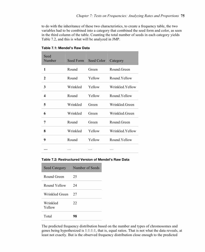
Background and Data Over 100 years before the genetically modified food controversy popped up into the public eye, an obscure (at the time) Austrian Augustinian monk by the name of Gregor Mendel was happily at work genetically modifying his pea crop in an effort to try to detect the principles of inheritance involved in the hybridization process of these plants. Following artificial fertilization, Mendel collected frequency data on the physical characteristics of the pea plants, such as seed color and seed form. We will look at one set of data from this experiment with its outcomes and refer the reader to the data source for more details should they be interested.3
Table 7.1 shows some of the “raw data” Mendel collected along with the category he created that combined the two characteristics in which he was interested (the seed form and seed color). As is obvious from this table, the raw data is nominal. Since Mendel’s hypothesis had
Chapter 7: Tests on Frequencies: Analyzing Rates and Proportions 75
to do with the inheritance of these two characteristics, to create a frequency table, the two variables had to be combined into a category that combined the seed form and color, as seen in the third column of the table. Counting the total number of seeds in each category yields Table 7.2, and this is what will be analyzed in JMP.
Table 7.1: Mendel’s Raw Data
Seed Number Seed Form Seed Color Category
1 Round Green Round.Green
2 Round Yellow Round.Yellow
3 Wrinkled Yellow Wrinkled.Yellow
4 Round Yellow Round.Yellow
5 Wrinkled Green Wrinkled.Green
6 Wrinkled Green Wrinkled.Green
7 Round Green Round.Green
8 Wrinkled Yellow Wrinkled.Yellow
9 Round Yellow Round.Yellow
… … … …
Table 7.2: Restructured Version of Mendel’s Raw Data
Seed Category Number of Seeds
Round Green 25
Round Yellow 24
Wrinkled Green 27
Wrinkled Yellow
22
Total 98
The predicted frequency distribution based on the number and types of chromosomes and genes being hypothesized is 1:1:1:1, that is, equal ratios. That is not what the data reveals, at least not exactly. But is the observed frequency distribution close enough to the predicted

76 Introduction to Biostatistics with JMP
distribution to be within the “noise cloud” of chance so that we can say the predicted and observed are not statistically different and that the observed differences are only due to biological variation and possible measurement error? The statistical null hypothesis is that of no difference between the observed and predicted frequency ratios, and this is one of the few instances that we would want to fail to reject the null hypothesis. The null hypothesis is, in this case, what we want to prove because the biological hypothesis that we are trying to support is the basis for the predicted frequency distribution. Therefore, showing no difference between the observed and predicted would provide evidence for the mechanism being proposed by the biological hypothesis under investigation.
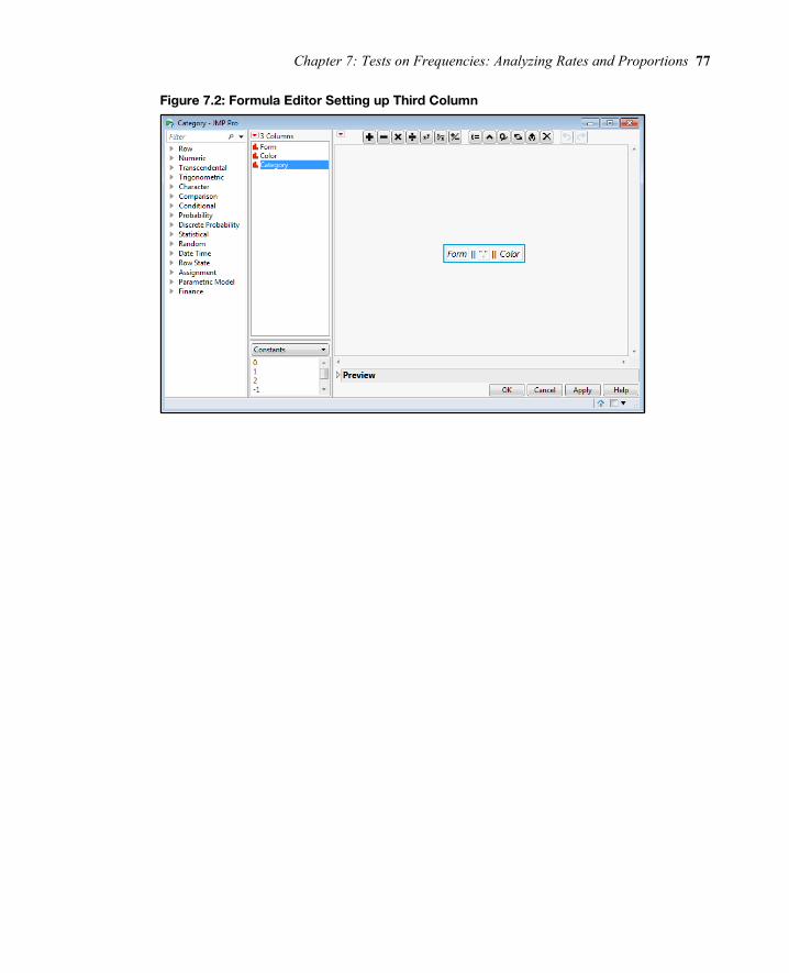
Data Entry into JMP There are two ways to handle data entry of this type, and they conform to the way the data is tabulated as shown in Tables 7.1 and 7.2. In other words, you can enter the data as in Table 7.1 and let JMP do the counting for you, or you can do the counting yourself and enter the data as in Table 7.2. If you opt for letting JMP do the counting for you, you will still have to enter the characteristics of each seed one at a time (Figure 7.1). However, you can use the JMP Formula function to create the combination designation by concatenating the Form and Color columns together (Figure 7.2).
Figure 7.1: Data Entry for Table 7.1
Chapter 7: Tests on Frequencies: Analyzing Rates and Proportions 77
Figure 7.2: Formula Editor Setting up Third Column

78 Introduction to Biostatistics with JMP
Figure 7.3 shows the data table modeled after Table 7.2 data entry. Note that the Count column has had the Frequency role pre-assigned (right-click the Count column and select Preselect Role ► Freq).
Figure 7.3: Data Entry for Table 7.2
Analysis We are comparing frequency distributions, but we have only one set of observations, so the Distribution platform is where we will find the one-way chi-square test. With either data entry method, select Analyze ► Distribution, and move the Category variable to the Y, Columns box, then click OK for the distribution (Figure 7.4).
Figure 7.4: Setting up the Analysis in the Distribution Platform
Chapter 7: Tests on Frequencies: Analyzing Rates and Proportions 79
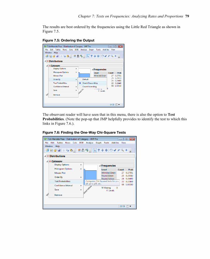
The results are best ordered by the frequencies using the Little Red Triangle as shown in Figure 7.5.
Figure 7.5: Ordering the Output
The observant reader will have seen that in this menu, there is also the option to Test Probabilities. (Note the pop-up that JMP helpfully provides to identify the test to which this links in Figure 7.6.).
Figure 7.6: Finding the One-Way Chi-Square Tests
80 Introduction to Biostatistics with JMP
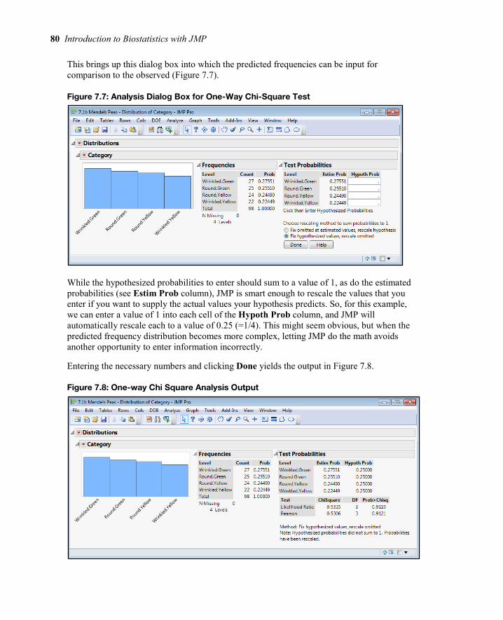
This brings up this dialog box into which the predicted frequencies can be input for comparison to the observed (Figure 7.7).
Figure 7.7: Analysis Dialog Box for One-Way Chi-Square Test
While the hypothesized probabilities to enter should sum to a value of 1, as do the estimated probabilities (see Estim Prob column), JMP is smart enough to rescale the values that you enter if you want to supply the actual values your hypothesis predicts. So, for this example, we can enter a value of 1 into each cell of the Hypoth Prob column, and JMP will automatically rescale each to a value of 0.25 (=1/4). This might seem obvious, but when the predicted frequency distribution becomes more complex, letting JMP do the math avoids another opportunity to enter information incorrectly.
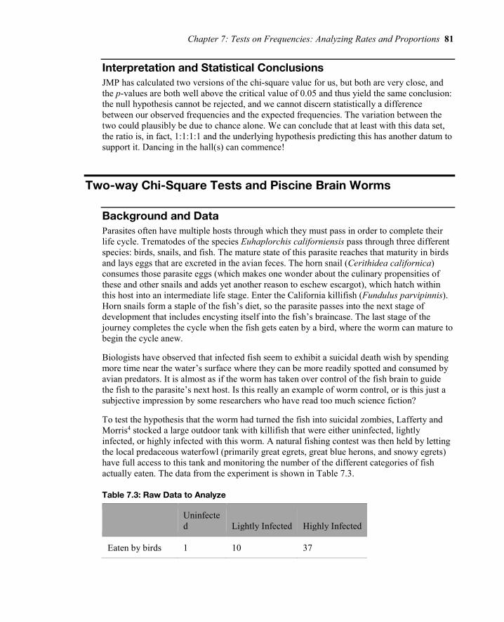
Entering the necessary numbers and clicking Done yields the output in Figure 7.8.
Figure 7.8: One-way Chi Square Analysis Output
Chapter 7: Tests on Frequencies: Analyzing Rates and Proportions 81
Interpretation and Statistical Conclusions JMP has calculated two versions of the chi-square value for us, but both are very close, and the p-values are both well above the critical value of 0.05 and thus yield the same conclusion: the null hypothesis cannot be rejected, and we cannot discern statistically a difference between our observed frequencies and the expected frequencies. The variation between the two could plausibly be due to chance alone. We can conclude that at least with this data set, the ratio is, in fact, 1:1:1:1 and the underlying hypothesis predicting this has another datum to support it. Dancing in the hall(s) can commence!
Two-way Chi-Square Tests and Piscine Brain Worms
Background and Data Parasites often have multiple hosts through which they must pass in order to complete their life cycle. Trematodes of the species Euhaplorchis californiensis pass through three different species: birds, snails, and fish. The mature state of this parasite reaches that maturity in birds and lays eggs that are excreted in the avian feces. The horn snail (Cerithidea californica) consumes those parasite eggs (which makes one wonder about the culinary propensities of these and other snails and adds yet another reason to eschew escargot), which hatch within this host into an intermediate life stage. Enter the California killifish (Fundulus parvipinnis). Horn snails form a staple of the fish’s diet, so the parasite passes into the next stage of development that includes encysting itself into the fish’s braincase. The last stage of the journey completes the cycle when the fish gets eaten by a bird, where the worm can mature to begin the cycle anew.
Biologists have observed that infected fish seem to exhibit a suicidal death wish by spending more time near the water’s surface where they can be more readily spotted and consumed by avian predators. It is almost as if the worm has taken over control of the fish brain to guide the fish to the parasite’s next host. Is this really an example of worm control, or is this just a subjective impression by some researchers who have read too much science fiction?
To test the hypothesis that the worm had turned the fish into suicidal zombies, Lafferty and Morris4 stocked a large outdoor tank with killifish that were either uninfected, lightly infected, or highly infected with this worm. A natural fishing contest was then held by letting the local predaceous waterfowl (primarily great egrets, great blue herons, and snowy egrets) have full access to this tank and monitoring the number of the different categories of fish actually eaten. The data from the experiment is shown in Table 7.3.
Table 7.3: Raw Data to Analyze
Uninfected Lightly Infected Highly Infected
Eaten by birds 1 10 37
82 Introduction to Biostatistics with JMP
Uninfected Lightly Infected Highly Infected
Not eaten by birds
49 35 9
Data Entry into JMP What we have in Table 7.3 is a classic contingency table in which two categorical variables, bird predation and infection level, are being shown together. The biological question is whether these two are associated, so the biological null and alternative hypotheses are as follows:
Ho: Bird predation and parasitic infection are not associated with one another.
HA: Bird predation and parasitic infection are associated with one another.
Notice that the biological hypotheses, the questions in which we are really interested, are formulated in terms of the specific biological question. Compare these now to the statistical null and alternative hypotheses, which are formulated in terms of the metric we are comparing, the frequency distributions:
Ho: There is no difference between the observed frequencies of bird predation versus parasitic infection and the frequencies predicted if the two are, indeed, not associated.
HA: There is a significant difference between the observed frequencies of bird predation versus parasitic infection and the frequencies predicted if the two are not associated. Therefore, there is an association between these two variables.
The alternative hypothesis is the one the investigators were really interested in, so in this case, disproving the null hypothesis would be the most interesting outcome. (Not disproving it might also have some interest, depending on your ultimate goal for the experiment.)
To enter this data into JMP, the contingency table in Table 7.3 will need to be rearranged a little so that the two categorical variables under consideration are each in their own column. The resulting rearrangement looks like Figure 7.9.
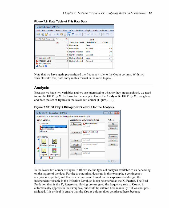
Chapter 7: Tests on Frequencies: Analyzing Rates and Proportions 83
Figure 7.9: Data Table of This Raw Data
Note that we have again pre-assigned the frequency role to the Count column. With two variables like this, data entry in this format is the most logical.
Analysis Because we have two variables and we are interested in whether they are associated, we need to use the Fit Y by X platform for the analysis. Go to the Analyze ► Fit Y by X dialog box and note the set of figures in the lower left corner (Figure 7.10).
Figure 7.10: Fit Y by X Dialog Box Filled Out for the Analysis
In the lower left corner of Figure 7.10, we see the types of analysis available to us depending on the nature of the data. For the two nominal data sets in this example, a contingency analysis is expected, and that is what we want. Based on the experimental design, the independent variable is the Infection Level, so it can be entered as the X, Factor. The Bird Predation then is the Y, Response. Having pre-assigned the frequency role to Count, it automatically appears in the Freq box, but could be entered here manually if it was not pre-assigned. It is critical to ensure that the Count column does get placed here, because
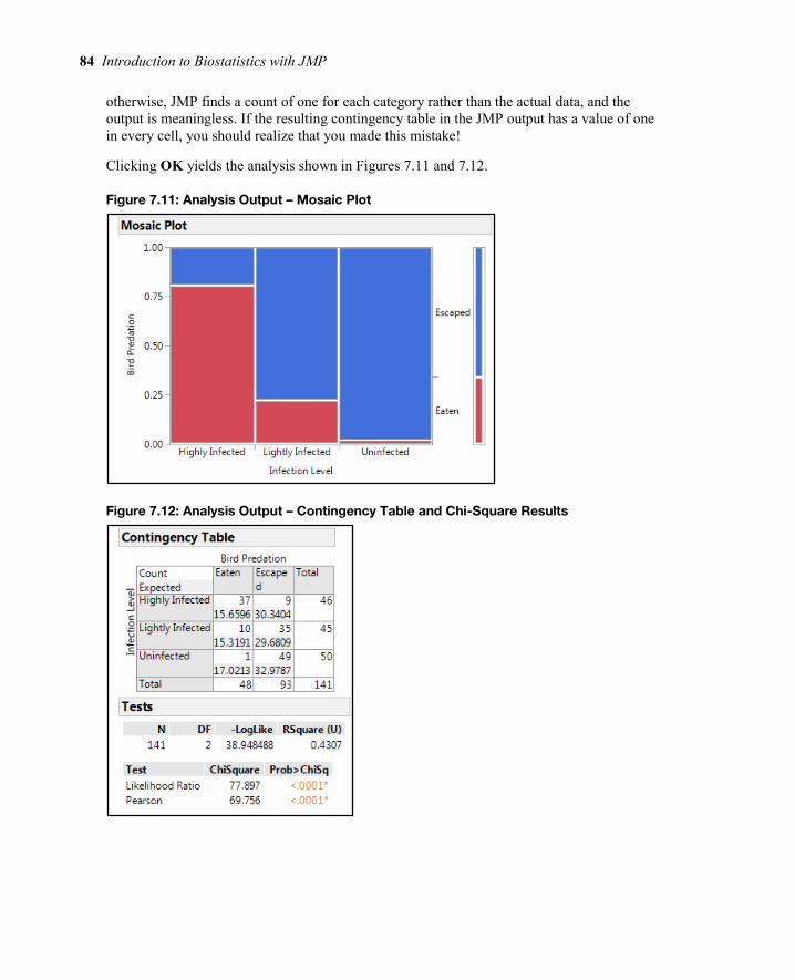
84 Introduction to Biostatistics with JMP
otherwise, JMP finds a count of one for each category rather than the actual data, and the output is meaningless. If the resulting contingency table in the JMP output has a value of one in every cell, you should realize that you made this mistake!
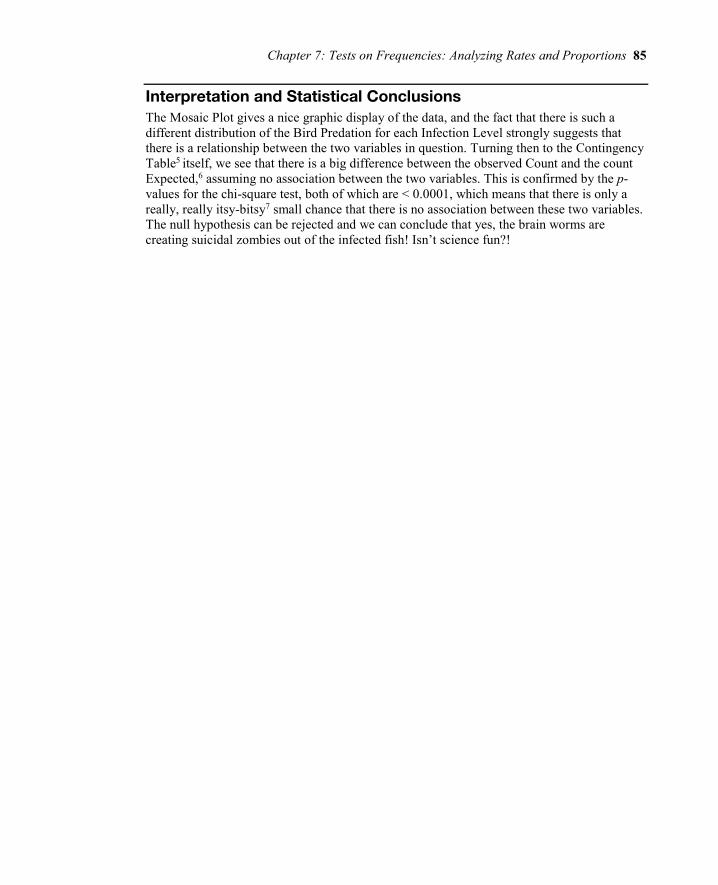
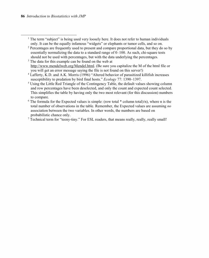
Clicking OK yields the analysis shown in Figures 7.11 and 7.12.
Figure 7.11: Analysis Output – Mosaic Plot
Figure 7.12: Analysis Output – Contingency Table and Chi-Square Results
Chapter 7: Tests on Frequencies: Analyzing Rates and Proportions 85
Interpretation and Statistical Conclusions The Mosaic Plot gives a nice graphic display of the data, and the fact that there is such a different distribution of the Bird Predation for each Infection Level strongly suggests that there is a relationship between the two variables in question. Turning then to the Contingency Table5 itself, we see that there is a big difference between the observed Count and the count Expected,6 assuming no association between the two variables. This is confirmed by the p-values for the chi-square test, both of which are < 0.0001, which means that there is only a really, really itsy-bitsy7 small chance that there is no association between these two variables. The null hypothesis can be rejected and we can conclude that yes, the brain worms are creating suicidal zombies out of the infected fish! Isn’t science fun?!
86 Introduction to Biostatistics with JMP
1 The term “subject” is being used very loosely here. It does not refer to human individuals only. It can be the equally infamous “widgets” or elephants or tumor cells, and so on.
2 Percentages are frequently used to present and compare proportional data, but they do so by essentially normalizing the data to a standard range of 0–100. As such, chi-square tests should not be used with percentages, but with the data underlying the percentages.
3 The data for this example can be found on the web at http://www.mendelweb.org/Mendel.html. (Be sure you capitalize the M of the html file or you will get an error message saying the file is not found on this server!)
4 Lafferty, K.D. and A.K. Morris (1996) “Altered behavior of parasitized killifish increases susceptibility to predation by bird final hosts.” Ecology 77: 1390–1397.
5 Using the Little Red Triangle of the Contingency Table, the default values showing column and row percentages have been deselected, and only the count and expected count selected. This simplifies the table by having only the two most relevant (for this discussion) numbers to compare.
6 The formula for the Expected values is simple: (row total * column total)/n), where n is the total number of observations in the table. Remember, the Expected values are assuming no association between the two variables. In other words, the numbers are based on probabilistic chance only.
7 Technical term for “teeny-tiny.” For ESL readers, that means really, really, really small!

SAS and all other SAS Institute Inc. product or service names are registered trademarks or trademarks of SAS Institute Inc. in the USA and other countries. ® indicates USA registration. Other brand and product names are trademarks of their respective companies. © 2017 SAS Institute Inc. All rights reserved. M1588358 US.0217
Be among the fi rst to know about new books, special events, and exclusive discounts.
support.sas.com/newbooks
Share your expertise. Write a book with SAS.support.sas.com/publish
sas.com/booksfor additional books and resources.
Ready to take your SAS® and JMP®skills up a notch?


![Course: Biostatistics Lecture No: [ 2 ] - Philadelphia University](https://static.fdokumen.com/doc/165x107/633a2618749bc7c55d0d5094/course-biostatistics-lecture-no-2-philadelphia-university.jpg)