Biostatistics of Cardiac Signals: Theory & Applications - IRIS
175
UNIVERSITÀ POLITECNICA DELLE MARCHE ENGINEERING FACULTY PhD Course in Information Engineering Curriculum “Biomedical, Electronics and Telecommunication Engineering” SSD: ING-INF/06 Biostatistics of Cardiac Signals: Theory & Applications Supervisor: Doctoral Dissertation of: Prof. Laura Burattini Agnese Sbrollini Co-Supervisor: Prof. Cees A. Swenne Academic Year 2017/2018
-
Upload
khangminh22 -
Category
Documents
-
view
0 -
download
0
Transcript of Biostatistics of Cardiac Signals: Theory & Applications - IRIS
UNIVERSITÀ POLITECNICA DELLE MARCHE
ENGINEERING FACULTY
PhD Course in Information Engineering
Curriculum “Biomedical, Electronics and Telecommunication Engineering”
SSD: ING-INF/06
Biostatistics of Cardiac Signals:
Theory & Applications
Supervisor: Doctoral Dissertation of:
Prof. Laura Burattini
Agnese Sbrollini
Co-Supervisor:
Prof. Cees A. Swenne
Academic Year 2017/2018

“Pure mathematics is, in its way,
the poetry of logical ideas.”
Albert Einstein
Abstract
Aims of bioengineering is to investigate phenomena of life sciences and to formalize their
physiological mechanisms. Considering that statistic is an excellent tool for modeling,
analyzing, characterizing and interpreting phenomena, aim of this doctoral thesis is to
merge the major biostatistical techniques and the bioengineering processing of cardiac
signals.
The major cardiac signals are the electrocardiogram, the vectorcardiogram, the
phonocardiogram and the tachogram. These signals are directly generated by heart and they
can be directly acquired placing electrodes on the body surface. The statistical
characterization of these signals passes by through some steps, that are statistical signal
modelling, signal preprocessing, feature extraction and classification analysis. Biomedical
signal modeling is the statistical theme that aims to propose mathematical models to
represent biomedical signals and their characteristics. For examples, electrocardiogram can
be modeled as a deterministic waveform, while the tachogram can be modeled as a point
process. The signal preprocessing is a step of signals processing that aims to remove noises
from signals, enhancing them. Some statistical methods can be used as cardiac preprocessing
techniques, and they are the averaging and the principal component analysis. Feature
extraction is a phase in which the selection and extraction of features are applied. A variable
is defined as feature if it is of interest. The selection, the extraction and the evaluation of
cardiac features is one of the essential phases in cardiologic diagnosis process. Classification
analysis is a procedure in which features of signals are divided in different categories,
according with their differences. Classification is the basis of clinical interpretation and
clinical decision.
The real importance of statistics in cardiac bioengineering can be deeply understand only
through its application; thus, four real applications were presented. The first application is
the Adaptive Thresholding Identification Algorithm (AThrIA), born to identify and to
segment electrocardiographic P waves. AThrIA is the perfect example of how much
preprocessing is important in cardiac clinical practice. Being standard preprocessing
insufficient, a specific statistical preprocessing based on the combination of standard
preprocessing and principal component analysis was design to remove noise and enhance
this low-amplitude wave. Specifically, it is the combination of standard preprocessing and
principal components analysis. The second application is CTG Analyzer, a graphical user
interface, born developed to support clinicians during the critical phases of delivery and
labor. After a specific evaluation of cardiotocographic signals, CTG Analyzer extracts all CTG
clinical features according with international guidelines. About CTG Analyzer feature
extraction, biostatistics is a fundamental instrument to evaluate the correctness of the
features and to compare the automated extracted features with the standard ones provided
by a clinician. The third application is eCTG, born to solve a practical clinical issue: the
digitalization of cardiotocographic signals. The basis of eCTG signal extraction is the Otsu’s
methods, a pixel clustering procedure that is the basis of the extraction procedure.
Combining the analysis of distributions and classification, eCTG is an important example of
statistics in image and signal processing. Finally, the fourth application is the creation of
deep-learning serial ECG classifiers, specific multilayer perceptron to detect cardiac
emerging pathology. Based on serial electrocardiography, these new and innovative
classifiers represent samples of the real importance of classification in cardiac clinical
practice.
In conclusion, this doctoral thesis underlines the importance of statistic in bioengineering,
specifically in cardiac signals processing. Considering the results of the presented
applications and their clinical meaning, the combination of cardiac bioengineering and
statistics is a valid point of view to support the scientific research. Linked by the same aim,
they are able to quantitative/qualitative characterize the phenomena of life sciences,
becoming a single science, biostatistics.

Contents
Introduction ........................................................................................................................... I
PART I BIOSTATISTICS OF CARDIAC SIGNALS: THEORY ........................................ 1
Chapter 1 Origin and Processing of Cardiac Signals .............................................................. 2
1.1 Heart Anatomy and Physiology ...................................................................................................... 2
1.2 Major Cardiac Signals.................................................................................................................... 14
1.3 Interference Affecting Cardiac Signals ........................................................................................ 31
1.4 Processing of Cardiac Signals ....................................................................................................... 35
Chapter 2 Statistical Signal Modelling and Sample Cardiac Applications ............................ 37
2.1 Statistical Modelling of Biological Signals ................................................................................... 37
2.2 Statistical Modelling of Cardiac Signals ...................................................................................... 43
Chapter 3 Signal Preprocessing and Sample Cardiac Applications ..................................... 46
3.1 Standard Preprocessing of Signals .............................................................................................. 46
3.2 Statistical Preprocessing of Signals ............................................................................................. 50
Chapter 4 Feature Extraction and Sample Cardiac Applications .......................................... 56
4.1 Feature Extraction ......................................................................................................................... 56
4.2 Statistical Feature Comparison ................................................................................................... 64
4.3 Statistical Feature Association ..................................................................................................... 68
Chapter 5Classification Analysis and Sample Cardiac Applications ..................................... 72
5.1 Statistics for Classification ............................................................................................................ 72
5.2 Classifier Construction ................................................................................................................. 78
5.3 Examples of Classifiers ................................................................................................................. 79
PART II BIOSTATISTICS OF CARDIAC SIGNALS: APPLICATIONS .......................... 89
Chapter 6 AThrIA: Adaptive Thresholding Identification Algorithm ................................... 91
6.1 Background..................................................................................................................................... 91
6.2 Methods .......................................................................................................................................... 95
6.3 Materials ....................................................................................................................................... 100
6.4 Statistics ........................................................................................................................................ 101

6.5 Results .......................................................................................................................................... 102
6.6 Discussion & Conclusion ............................................................................................................ 105
Chapter 7 CTG Analyzer Graphical User Interface ............................................................. 108
7.1 Clinical Background ..................................................................................................................... 108
7.2 CTG Analyzer Graphical User Interface ..................................................................................... 116
7.3 CTG Analyzer 2.0 Graphical User Interface .............................................................................. 119
7.4 Features Dependency from Sampling Frequency ..................................................................... 121
7.5 Discussion & Conclusion ............................................................................................................. 124
Chapter 8 eCTG Software ................................................................................................... 126
8.1 Technical Background ................................................................................................................. 126
8.2 Methods ........................................................................................................................................ 127
8.3 Materials ....................................................................................................................................... 130
8.4 Statistics ........................................................................................................................................ 131
8.5 Results ........................................................................................................................................... 131
8.6 Discussion & Conclusion ............................................................................................................ 132
Chapter 9 DLSEC: Deep-Learning Serial ECG Classifiers ................................................... 136
9.1 Clinical Background ..................................................................................................................... 136
9.2 Methods ........................................................................................................................................ 140
9.3 Materials ....................................................................................................................................... 145
9.4 Statistics ....................................................................................................................................... 146
9.5 Results .......................................................................................................................................... 146
9.6 Discussion & Conclusion ............................................................................................................ 149
Discussion & Conclusions ..................................................................................................... III
References .......................................................................................................................... 141
Abbreviations
• AC: cardiotocographic
Acceleration;
• ACC: Accuracy;
• AF: Atrial Fibrillation;
• ANCOVA: Analysis of
Covariances;
• ANOVA: Analysis of Variances;
• ANS: Autonomic Nervous
System;
• AT: Atrial Tachycardia;
• AThrIA: Adaptive Thresholding
Identification Algorithm;
• AUC: Area Under the Curve;
• AV node: Atrioventricular node;
• AVB: Atrioventricular Block;
• BC: cardiotocographic
Bradycardia;
• BL: cardiotocographic baseline;
• BL-ECG: Baseline
Electrocardiogram;
• BLV: cardiotocographic baseline
variability;
• CTG: Cardiotocography;
• DC: cardiotocographic
Deceleration;
• ECG: Electrocardiogram;
• EDC: Early cardiotocographic
Deceleration;
• EN: Effective Negatives;
• EP: Effective Positives;
• ERP: Effective Refractory Period;
• F1: F1 Score;
• FDR: False Discovery Rate;
• FHR: Fetal Heart Rate series;
• FN: False Negatives;
• FNR: False Negative Rate;
• FOR: False Omission Rate;
• FP: False Positives;
• FPR: False Positive Rate;
• FU-ECG: Follow-up
Electrocardiogram;
• HF: High Frequency;
• HR: Heart Rate;
• HRV: Heart Rate Variability;
• IQR: Interquartile Range;
• JT: Junctional Tachycardia;
• LDC: Late cardiotocographic
Deceleration;
• LF: Low Frequency;
• LR: Logistic Regression;
• LR-: Negative Likelihood Ratio;
• LR+: Positive Likelihood Ratio;
• MANOVA: Multivariate analysis
of variance;
• MdN: Median;
• MLP: Multilayer Perceptron;
• NN: Neural Networks;
• NPV: Negative Predicted Value;
• ODR: Diagnostic Odds Ratio;
• PCA: Principal Component
Analysis;
• PCG: Phonocardiogram;
• PDC: Prolonged
cardiotocographic Deceleration;
• PN: Predicted Negatives;
• PP: Predicted Positives;
• PPV: Positive Predictive Value;
• Pr: Prevalence;
• PVC: Premature Ventricular
Contraction;
• QTc: corrected QT interval;
• RMSSD: Root Mean Square of the
Square of Differences;
• ROC: Receiver Operating
Characteristic;
• RRP: Relative Refractory Period;
• RS&LP: Repeated Structuring &
Learning Procedure;
• S1: First Heart Sound;
• S2: Second Heart Sound;
• S3: Third Heart Sound;
• S4: Fourth Heart Sound;
• SA node: Sinus Atrial node;
• SDNN: Standard Deviation of NN
intervals;
• SE: Sensitivity;
• SNR: Signal-to-Noise Ratio;
• SP: Specificity (SP);
• SVT: Supraventricular
Tachycardia;
• TC: cardiotocographic
Tachycardia;
• TN: True Negatives;
• TP: True Positives;
• UC: Uterine Contractions signal;
• UCT: Uterine Contractions;
• VCG: Vectorcardiogram;
• VDC: Variable cardiotocographic
Deceleration;
• VLF: Very Low Frequency;
• VM: Vector Magnitude.
I
Introduction
Bioengineering is a discipline that applies engineering methods and technologies to
investigate issues related to life sciences. Aim of bioengineering is the study of the processes
that underline physiological systems. Compared to standard biological and medical sciences,
the main difference refers to tools and instruments that bioengineering uses. Indeed, its
application is linked to engineering techniques, such as mathematics, physics, mechanics,
fluid dynamics, computer science and, last but not least, statistics.
Mathematically, statistics has the purpose to quantitative and qualitative study a
particular phenomenon under conditions of uncertainty or non-determinism. It is an
instrument of the scientific method: it uses mathematics and experimental methodology to
study how a collective phenomenon can be synthesized and understood. Statistical
investigation starts from data collection, that will be statistically processed. Features will be
extracted and classified in order to investigate the proprieties of the considered dataset. All
this process is finalized to characterize unknown phenomena.
Considering the aims of bioengineering (to characterize the phenomena of life sciences)
and of statistics (to find a quantitative/qualitative method to characterize a phenomenon),
these two sciences are strongly linked. In fact, statistics is an excellent tool for modeling,
analyzing, characterizing and interpreting biological phenomena. Converted in a new term,
biostatistics, this science aims to quantitative and qualitative study of biological and medical
phenomena under conditions of uncertainty or non-determinism.
In this general consideration, biostatistics techniques can be used in every field of
medicine and biology. In particular, it is protagonist in medical and biological scientific
research, supporting epidemiological studies with its methods. In fact, its methods and
techniques are widely used to formalize a process (signal modeling), to test indices or
procedures (comparison) or to classify and/or discriminate individuals or observations
(classification).
One of the main filed in which bioengineering and biostatistics can be applied is the
cardiac signal investigation. This application studies all the signals generated by the heart,
specifically the electrocardiogram, the vectorcardiogram, the phonocardiogram and the
heart-rate series. These signals can be analyzed in order to investigate the major
cardiological disease: electrocardiogram/vectorcardiogram provides information about
II
cardiac electrical diseases (e.g. arrhythmias ), phonocardiogram provides information about
mechanical heart diseases (e.g. atrial valve stenosis) and the heart-rate series provides
information about the control of the autonomous nervous system on the heart.
Despite being one of the oldest themes of bioengineering, the study of cardiac signals is
still promising. Indeed, cardiological challenges are still unsolved. Examples of cardiac
signals research are the analysis of the cardiac electrical atrial activity, the analysis of the
fetal heart rate signal and the use of the serial electrocardiography for the diagnosis of
emerging pathologies. Application of biostatistical techniques could be a good solution to
investigate these unsolved issues.
Aim of this doctoral thesis is to merge the major biostatistical techniques and the analysis
of cardiac signals. Specifically, it is divided into two major part. The first is the theory
dissertation about the origins of cardiac signals and about the main biostatistical techniques
that can be applied in the study of cardiac signals. With a specific attention to the signals
processing steps, the theory part is divided into modelling, preprocessing, feature extraction
and classification. The second part presents four practical application of biostatistical
techniques in the cardiac signals research field, which are: the adaptive threshold
identification algorithm (AThrIA), CTG Analyzer graphical user interface, eCTG software,
and the innovative construction of deep-learning serial electrocardiography classifiers.
1
PART I
BIOSTATISTICS OF
CARDIAC SIGNALS:
THEORY
In order to understand the combination of biostatistics and cardiac signal processing, an
overview of all cardiac signals and statistical techniques is essential.
In the first part of this doctoral thesis, the basis of cardiac signals and statistical techniques
are introduced. Specifically, the cardiac signals considered here are electrocardiogram,
vectorcardiogram, phonocardiogram and tachogram. The real comprehension of these
signals can be understood only through the study of their genesis, acquisition and
interference. Moreover, the flow of the cardiac signal processing is presented.
After contextualizing the field of applications, an overview of all statistical techniques for
cardiac signal analysis is proposed. The main techniques are grouped in four main themes,
that are statistical signal modelling, signal preprocessing, feature extraction and
classification analysis. For clarity and to show the utility of biostatistics, sample applications
in cardiac bioengineering are presented for each of these themes.

Chapter 1. Origin and Processing of Cardiac Signals
2
Chapter 1
Origin and Processing of Cardiac Signals
1.1 Heart Anatomy and Physiology
1.1.1 Anatomy
The heart is the main organ of the circulatory system. It is located in the middle of the
thorax, specifically in the anterior mediastinum between the two lungs, behind the sternum
and the ribs, in front of the vertebral column, and over the diaphragm. It has a conical shape:
its elongated base is turned back and to the right, while its apex is facing forward and to the
left. In adults, it weighs about 250-300 g; it has a length of 13-15 cm, a width of 9-10 cm and
a thickness of 6 cm. Its weight and dimension can vary with age, sex and physical
constitution.
The organ (Fig.1.1) is divided into two sections, the right heart (Fig. 1.1-blue section) and
the left heart (Fig.1.1-red section). Each of these sections is composed of a superior cavity,
Figure 1.1. Anatomy of the heart. The blue section represents the right heart, while the red
section represents the left heart. The arrows show the flux direction inside the four chambers,
crossing the four valves (1. Tricuspid valve, 2. Pulmonary valve, 3. Mitral valve and 4. Aortic
valve).
Chapter 1. Origin and Processing of Cardiac Signals
3
the atrium, and an inferior cavity, the ventricle. The right heart is perfectly separated from
the left heart: an interatrial septum separates the atria, while an interventricular septum
separates the ventricles. Each atrium is connected to its ventricle through an atrioventricular
orifice, protected by a valve. Specifically, the tricuspid valve (Fig.1.1 (1)) and the mitral valve
(Fig.1.1 (3)) are located in the right and left atrioventricular orifices, respectively. Both
ventricles present semilunar valves that connected ventricles with arteries. In particular, the
pulmonary valve (Fig.1.1 (2)) connects the right ventricle with the pulmonary arteries, while
the aortic valve (Fig.1.1 (4)) connects the left ventricle with the aorta. The blood flow proceed
in a specific direction in both right and left hearts (Fig.1.1): atria receives blood from veins
(the venae cavae for the right atrium and the pulmonary veins for the left atrium); blood
passes atrioventricular valves (the tricuspid valve for the right heart and the mitral valve for
the left heart); and ventricles pump blood in arteries (pulmonary arteries for the right
ventricle and aorta for the left heart) , through semilunar valves (pulmonary valve for the
right heart and aortic valve for the left heart)1.
The right atrium is located in an anterior, inferior and right position relative to the left
atrium, and in the upper part of the right heart. It collects blood from the venae cavae. The
superior vena cava opens in the posterior/superior wall of the atrium without valve, while
the inferior vena cava opens in the posterior/inferior wall of the atrium through the
Eustachian valve. Additionally, the right atrium collects blood from the coronary sinus. The
right atrium hosts the sinus atrial node (SA node), the cardiac pacemaker, that
spontaneously activates cardiac depolarization. The left atrium, thinner than the right
atrium, is located in the upper part of the left heart. It collects blood from the four pulmonary
veins, in the posterior wall of the atrium.
The right ventricle, thinner than the left ventricle, is located in the lower part of the right
heart. It receives blood from the right atrium through the tricuspid valve and pumps it in
the pulmonary arteries through the pulmonary valve. The right ventricle is the center of the
pulmonary circuit, the small circulation that guides blood in the lungs. Due to the small
entity of this circuit, pressure in the right ventricle is smaller than pressure in the left one
(mean pressure of 2 mmHg and a maximal pressure of 25 mmHg). The left ventricle is
located in the lower part of the left heart. It receives blood from the left atrium through the
mitral valve and pumps it in the aorta through the pulmonary valve. It is longer and more
conical than the right ventricle and, in cross section, its concavity has an oval or almost
circular shape. Its walls are much thicker than right one (three to six times more), this
Chapter 1. Origin and Processing of Cardiac Signals
4
happens because it expresses a force five times higher, receiving blood at low pressure from
the atrium, about 5 mmHg, and moving it in the aorta at a pressure about 120 mmHg at each
heartbeat.
The blood flux in the heart is regulated by the action of the cardiac valves. The right
atrioventricular valve, the tricuspid valve, consists of three cusps, while the left valve, the
mitral valve, is composed of two cusps. Valves morphology avoids blood reflux from
ventricles to atria. Then, the heart contraction forces blood against the edges of the
atrioventricular valves, causing their closure and blood flux into arteries. Semilunar valves
consist of three cusps that protrude from the ventricle to the inner wall of the arteries. When
these valves are closed, blood fills the spaces between valve leaflets and the vessel wall. On
the contrary, when ventricles contract, the flow of blood proceeds into the arteries, releasing
blood in the cusps and causing the opening of the valves.
Heart valves are supported by the cardiac skeleton, consisting of strong connective
formations formed by collagen fibers. It is composed of four fibrous rings, which enclose the
four heart orifices. These rings are partly in contact and connected by two trigons of fibrous
connective tissue. In particular, the right fibrous trigone is a strong formation placed
between the aortic orifice and the two atrioventricular orifices, while the left fibrous trigone,
smaller than the right one, is located between the left atrioventricular orifice and the aortic
orifice. The cardiac skeleton aims to merge the muscular bundles of the atria and ventricles,
to provide a support for heart valves, and to electrically isolate atria from ventricles. It also
participates in the formation of the interatrial septum and of the interventricular septum.
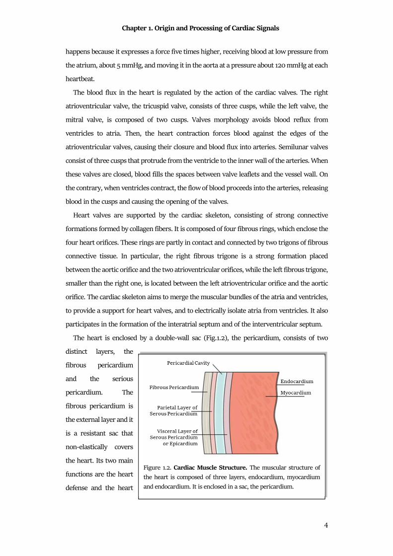
The heart is enclosed by a double-wall sac (Fig.1.2), the pericardium, consists of two
distinct layers, the
fibrous pericardium
and the serious
pericardium. The
fibrous pericardium is
the external layer and it
is a resistant sac that
non-elastically covers
the heart. Its two main
functions are the heart
defense and the heart
Figure 1.2. Cardiac Muscle Structure. The muscular structure of
the heart is composed of three layers, endocardium, myocardium
and endocardium. It is enclosed in a sac, the pericardium.
Chapter 1. Origin and Processing of Cardiac Signals
5
maintenance in situ. The serous pericardium is the internal layer and it perfectly adheres to
the cardiac muscle. It consists of two layers of mesothelium, the visceral pericardium and a
parietal pericardium which together delimit the pericardial cavity. The visceral layer of
serous pericardium (or epicardium) adheres to the heart, while the parietal layer of serous
pericardium is the external one. Between the two layers of the serous pericardium, of the
pericardial liquid, or liquor (20 ml and 50 ml), allows the heart movements, reducing its
frictional forces2. The cardiac muscular structure is composed of three layers, the
epicardium, the myocardium and the endocardium (Fig.1.2). The epicardium, formed as
described by the visceral layer of the serous pericardium, is a membrane that externally
covers the heart. The epicardium consists of a single layer of mesothelial cells and has a
lamina propria composed of elastic fibers. Myocardium, or cardiac muscle composed of
myocytes, is the muscular tissue of the heart. It is composed of 70% muscle fibers, while the
remaining 30% consists mainly of connective tissue and vessels. The myocardium is a hybrid
of skeletal muscle tissue, and partly of smooth muscle tissue. Finally, the endocardium is a
thin translucent membrane that internally covers all the cardiac cavities, adapting to all their
irregularities and covering also the valve leaflets.
Heart contraction is regulated by an electrical impulse, opportunely generated by a
specific group of cardiac cells, the cardiac conduction system. Cardiac conduction system
(Fig.1.3) is the intrinsic system that regulates the cardiac depolarization. The depolarization
is automatically generated by periodic electrical impulses that are born in the nodal cells.
These impulses rapidly propagate to adjacent contractile cells through the presence of
communicating junctions. The main four formations that composes the cardiac conduction
system are the SA node, the atrioventricular node (AV node), the His bundle and the Purkinje
fibers.
The SA node (Fig.1.3) is the part that autonomically regulates the occurrence of the
heartbeat, being the cardiac physiological pacemaker. It is located in the right atrium in the
junction between the cavity and the superior vena cava. It presents a crescent-shape, 15 mm
long and 5 mm large. It is composed of connective tissue that surrounds myocardial cells
with poor myofibrils. Its role is to generate the electrical stimulus that has to be transmitted
to atrial muscular tissue, provoking the atrial contraction. The SA node is innervated by
many fibers of the autonomic nervous system (ANS-both by the sympathetic nervous system
and the parasympathetic nervous system), in order to regulate the heart rhythm and the
atrial contraction force. The mean heart rate (HR) generated by the SA node is about 1 Hz
Chapter 1. Origin and Processing of Cardiac Signals
6
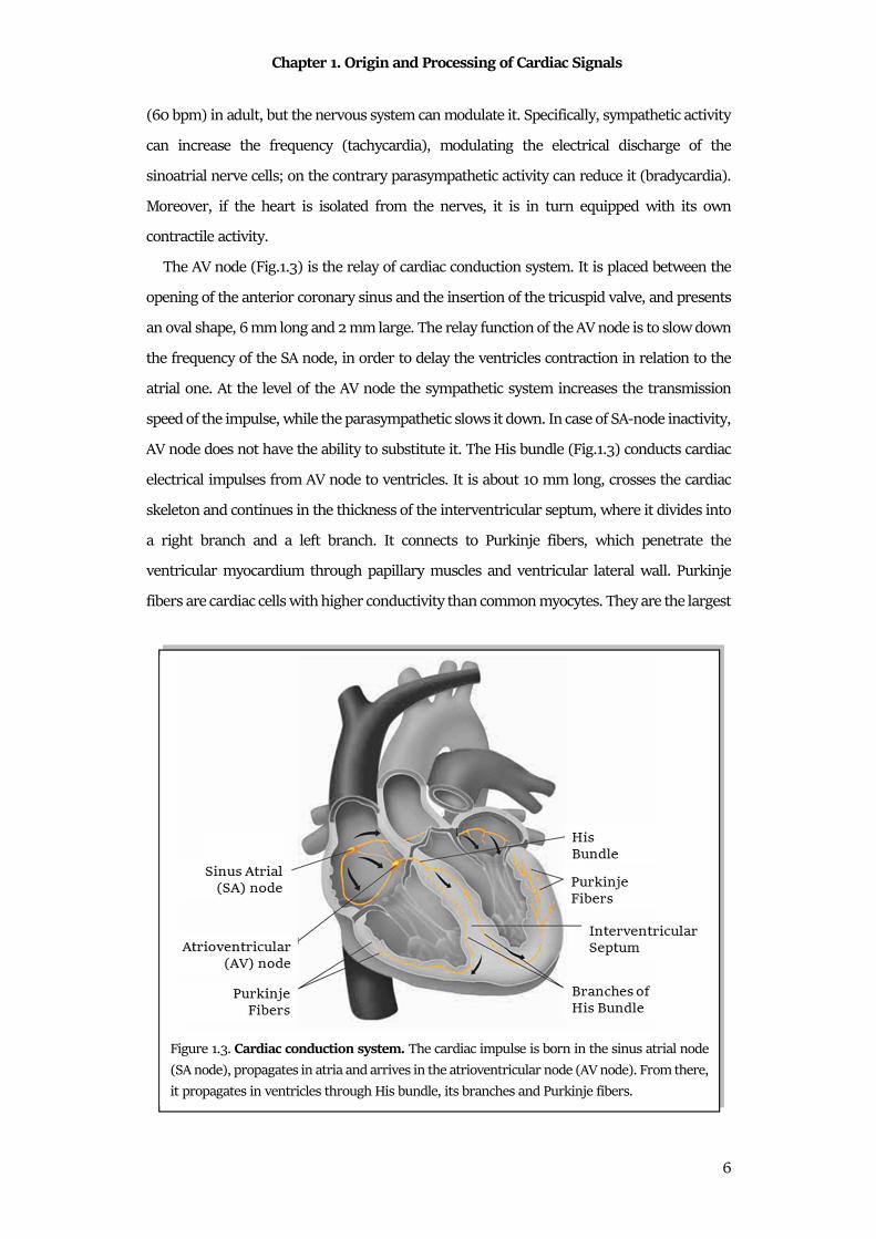
(60 bpm) in adult, but the nervous system can modulate it. Specifically, sympathetic activity
can increase the frequency (tachycardia), modulating the electrical discharge of the
sinoatrial nerve cells; on the contrary parasympathetic activity can reduce it (bradycardia).
Moreover, if the heart is isolated from the nerves, it is in turn equipped with its own
contractile activity.
The AV node (Fig.1.3) is the relay of cardiac conduction system. It is placed between the
opening of the anterior coronary sinus and the insertion of the tricuspid valve, and presents
an oval shape, 6 mm long and 2 mm large. The relay function of the AV node is to slow down
the frequency of the SA node, in order to delay the ventricles contraction in relation to the
atrial one. At the level of the AV node the sympathetic system increases the transmission
speed of the impulse, while the parasympathetic slows it down. In case of SA-node inactivity,
AV node does not have the ability to substitute it. The His bundle (Fig.1.3) conducts cardiac
electrical impulses from AV node to ventricles. It is about 10 mm long, crosses the cardiac
skeleton and continues in the thickness of the interventricular septum, where it divides into
a right branch and a left branch. It connects to Purkinje fibers, which penetrate the
ventricular myocardium through papillary muscles and ventricular lateral wall. Purkinje
fibers are cardiac cells with higher conductivity than common myocytes. They are the largest
Figure 1.3. Cardiac conduction system. The cardiac impulse is born in the sinus atrial node
(SA node), propagates in atria and arrives in the atrioventricular node (AV node). From there,
it propagates in ventricles through His bundle, its branches and Purkinje fibers.
Chapter 1. Origin and Processing of Cardiac Signals
7
cells found in the heart: they have a diameter of 70-80μm compared to 10-15μm of
myocardial cells. The large diameter is associated with a high conduction rate of about 1-4
V/s compared to 0.4-1 V/s of the other cells of the cardiac conduction system1.
The role to supply blood to the heart is guaranteed by coronary arteries. The right
coronary artery and the left coronary artery supply blood to the right heart and the left heart,
respectively, and are born in the initial part of the aorta. The course on the right coronary
artery follows the edge between the right atrium and the right ventricle. This artery sends
two branches down, the right marginal branch (or right marginal), and the posterior
descending artery (or posterior interventricular). The left coronary artery divides into a
circumflex artery, which gives rise to several branches for the obtuse margin, and anterior
descending artery, which marks the border between left ventricle and right ventricle. The
anterior descendant also originates other small arterial branches that go directly to irrigate
the interventricular septum, known as sepal branches.
1.1.2 Electrical Physiology
Cardiac Action Potential
Cardiac cells are able to be electrically activated, generating an action potential. The
cardiac action potential is a rapid voltage change between the walls of the cardiac cell
membrane, caused by crossing of ions. The main ions involved are sodium (Na+), chloride
(Cl−), calcium (Ca2+) and potassium (K+). At resting, Na+, Cl− and Ca2+ are highly present in
the outside the cell, while K+ is mainly present inside the cell. The balance between
concentrations of these ions makes negative the voltage of the cell membrane, that is around
-90 mV (resting membrane potential). When the action potential occurs, the membrane
became rapidly positive (depolarization) and, then, it slowly returns in its initial negative
condition (repolarization)3. The cardiac action potential duration ranges from 0.20 s to 0.40
s. Specifically, in the heart there are two types of cardiac action potentials: the non-
pacemaker action potential, addressed to the common cardiac cells, and pacemaker action
potential, addressed to the cells of the cardiac conduction system.
Non-pacemaker action potential is typically addressed to cardiac cells (atrial and
ventricular) and to Purkinje fibers. This action potential is defined as “non-pacemaker”
because its generation depends from the triggering of the adjacent cell depolarization. This
type of action potential is called “fast response” due to its reactivity to be released. Non-
pacemaker action potential is composed of 5 phases (Fig.1.4A)4:
Chapter 1. Origin and Processing of Cardiac Signals
8
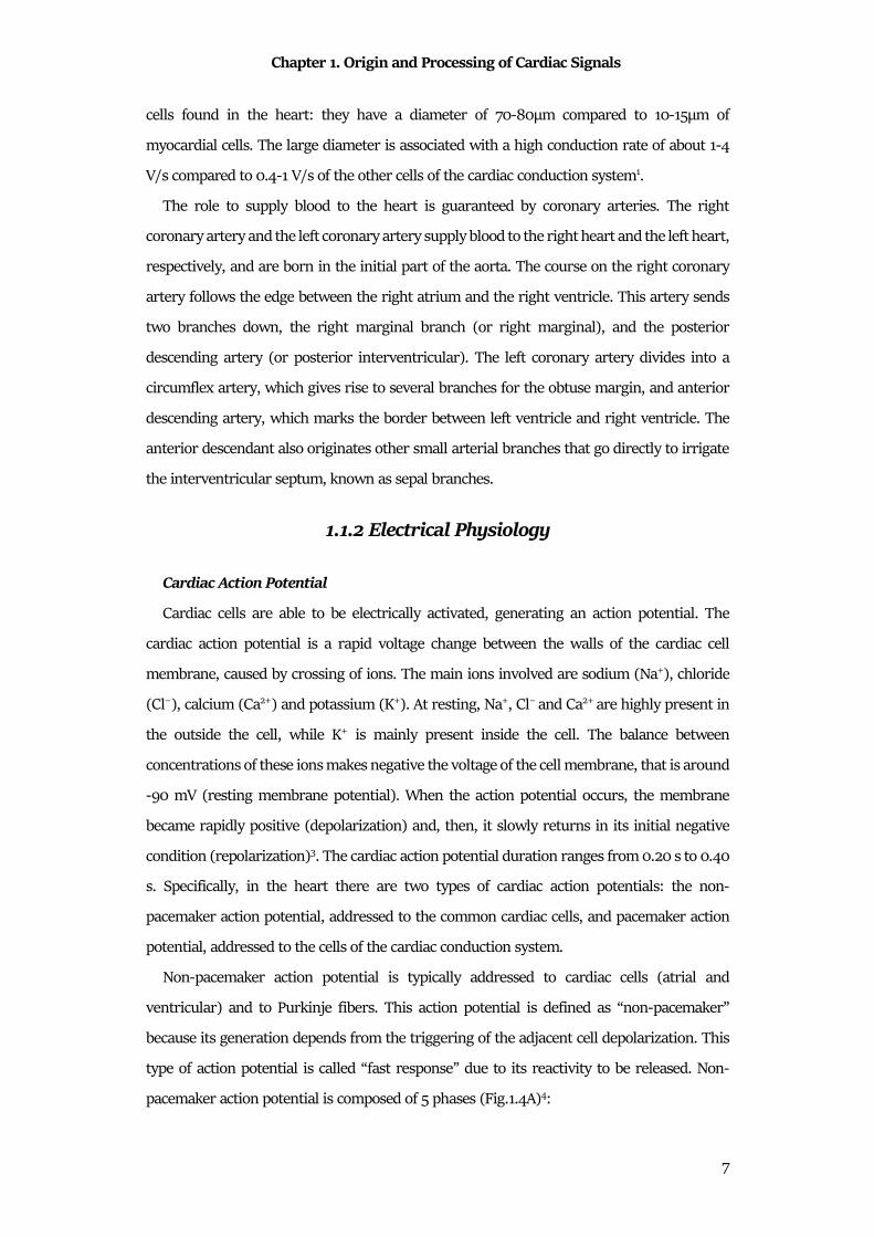
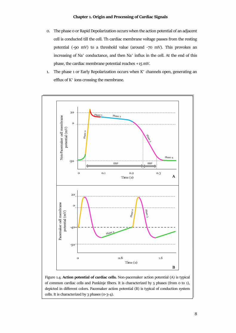
0. The phase 0 or Rapid Depolarization occurs when the action potential of an adjacent
cell is conducted till the cell. Th cardiac membrane voltage passes from the resting
potential (-90 mV) to a threshold value (around -70 mV). This provokes an
increasing of Na+ conductance, and then Na+ influx in the cell. At the end of this
phase, the cardiac membrane potential reaches +15 mV.
1. The phase 1 or Early Repolarization occurs when K+ channels open, generating an
efflux of K+ ions crossing the membrane.
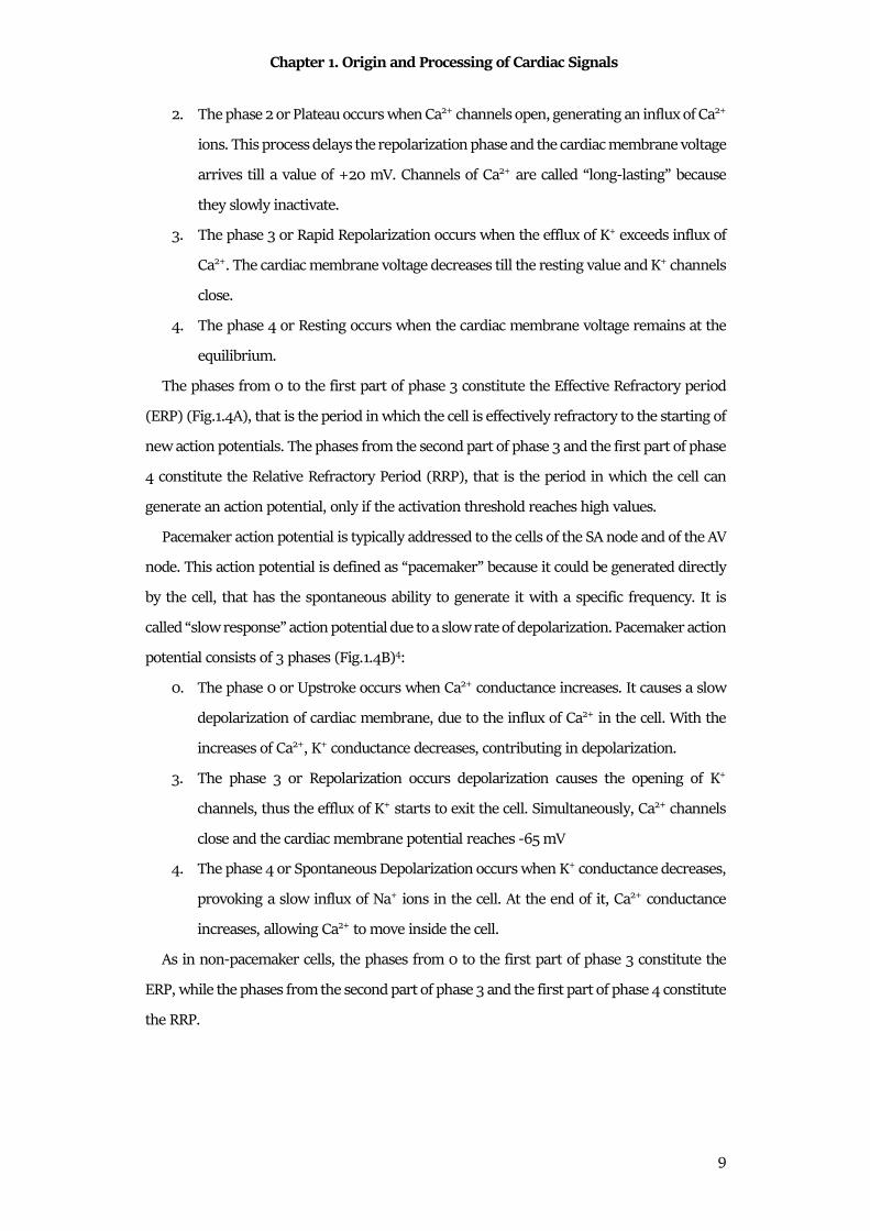
Figure 1.4. Action potential of cardiac cells. Non-pacemaker action potential (A) is typical
of common cardiac cells and Punkinje fibers. It is characterized by 5 phases (from 0 to 1),
depicted in different colors. Pacemaker action potential (B) is typical of conduction system
cells. It is characterized by 3 phases (0-3-4).
Chapter 1. Origin and Processing of Cardiac Signals
9
2. The phase 2 or Plateau occurs when Ca2+ channels open, generating an influx of Ca2+
ions. This process delays the repolarization phase and the cardiac membrane voltage
arrives till a value of +20 mV. Channels of Ca2+ are called “long-lasting” because
they slowly inactivate.
3. The phase 3 or Rapid Repolarization occurs when the efflux of K+ exceeds influx of
Ca2+. The cardiac membrane voltage decreases till the resting value and K+ channels
close.
4. The phase 4 or Resting occurs when the cardiac membrane voltage remains at the
equilibrium.
The phases from 0 to the first part of phase 3 constitute the Effective Refractory period
(ERP) (Fig.1.4A), that is the period in which the cell is effectively refractory to the starting of
new action potentials. The phases from the second part of phase 3 and the first part of phase
4 constitute the Relative Refractory Period (RRP), that is the period in which the cell can
generate an action potential, only if the activation threshold reaches high values.
Pacemaker action potential is typically addressed to the cells of the SA node and of the AV
node. This action potential is defined as “pacemaker” because it could be generated directly
by the cell, that has the spontaneous ability to generate it with a specific frequency. It is
called “slow response” action potential due to a slow rate of depolarization. Pacemaker action
potential consists of 3 phases (Fig.1.4B)4:
0. The phase 0 or Upstroke occurs when Ca2+ conductance increases. It causes a slow
depolarization of cardiac membrane, due to the influx of Ca2+ in the cell. With the
increases of Ca2+, K+ conductance decreases, contributing in depolarization.
3. The phase 3 or Repolarization occurs depolarization causes the opening of K+
channels, thus the efflux of K+ starts to exit the cell. Simultaneously, Ca2+ channels
close and the cardiac membrane potential reaches -65 mV
4. The phase 4 or Spontaneous Depolarization occurs when K+ conductance decreases,
provoking a slow influx of Na+ ions in the cell. At the end of it, Ca2+ conductance
increases, allowing Ca2+ to move inside the cell.
As in non-pacemaker cells, the phases from 0 to the first part of phase 3 constitute the
ERP, while the phases from the second part of phase 3 and the first part of phase 4 constitute
the RRP.
Chapter 1. Origin and Processing of Cardiac Signals
10
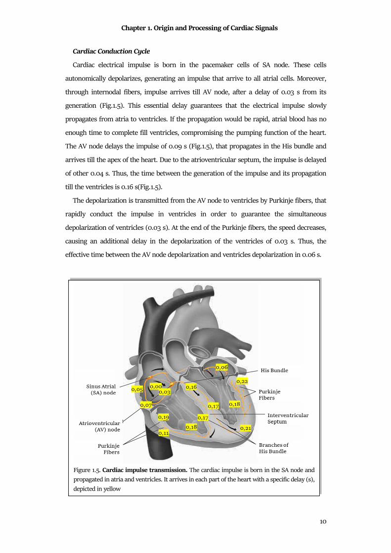
Cardiac Conduction Cycle
Cardiac electrical impulse is born in the pacemaker cells of SA node. These cells
autonomically depolarizes, generating an impulse that arrive to all atrial cells. Moreover,
through internodal fibers, impulse arrives till AV node, after a delay of 0.03 s from its
generation (Fig.1.5). This essential delay guarantees that the electrical impulse slowly
propagates from atria to ventricles. If the propagation would be rapid, atrial blood has no
enough time to complete fill ventricles, compromising the pumping function of the heart.
The AV node delays the impulse of 0.09 s (Fig.1.5), that propagates in the His bundle and
arrives till the apex of the heart. Due to the atrioventricular septum, the impulse is delayed
of other 0.04 s. Thus, the time between the generation of the impulse and its propagation
till the ventricles is 0.16 s(Fig.1.5).
The depolarization is transmitted from the AV node to ventricles by Purkinje fibers, that
rapidly conduct the impulse in ventricles in order to guarantee the simultaneous
depolarization of ventricles (0.03 s). At the end of the Purkinje fibers, the speed decreases,
causing an additional delay in the depolarization of the ventricles of 0.03 s. Thus, the
effective time between the AV node depolarization and ventricles depolarization in 0.06 s.
Figure 1.5. Cardiac impulse transmission. The cardiac impulse is born in the SA node and
propagated in atria and ventricles. It arrives in each part of the heart with a specific delay (s),
depicted in yellow
Chapter 1. Origin and Processing of Cardiac Signals
11
1.1.3 Mechanical Physiology
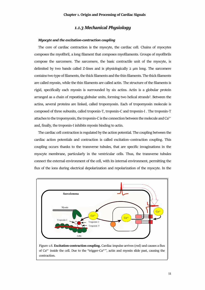
Myocyte and the excitation-contraction coupling
The core of cardiac contraction is the myocyte, the cardiac cell. Chains of myocytes
composes the myofibril, a long filament that composes myofilaments. Groups of myofibrils
compose the sarcomere. The sarcomere, the basic contractile unit of the myocyte, is
delimited by two bands called Z-lines and is physiologically 2 μm long. The sarcomere
contains two type of filaments, the thick filaments and the thin filaments. The thick filaments
are called myosin, while the thin filaments are called actin. The structure of the filaments is
rigid, specifically each myosin is surrounded by six actins. Actin is a globular protein
arranged as a chain of repeating globular units, forming two helical strands3. Between the
actins, several proteins are linked, called tropomyosin. Each of tropomyosin molecule is
composed of three subunits, called troponin-T, troponin-C and troponin-I . The troponin-T
attaches to the tropomyosin, the troponin-C is the connection between the molecule and Ca2+
and, finally, the troponin-I inhibits myosin binding to actin.
The cardiac cell contraction is regulated by the action potential. The coupling between the
cardiac action potentials and contraction is called excitation–contraction coupling. This
coupling occurs thanks to the transverse tubules, that are specific invaginations in the
myocyte membrane, particularly in the ventricular cells. Thus, the transverse tubules
connect the external environment of the cell, with its internal environment, permitting the
flux of the ions during electrical depolarization and repolarization of the myocyte. In the
Figure 1.6. Excitation-contraction coupling. Cardiac impulse arrives (red) and causes a flux
of Ca2+ inside the cell. Due to the “trigger-Ca2+”, actin and myosin slide past, causing the
contraction.
Chapter 1. Origin and Processing of Cardiac Signals
12
internal environment of the cell, the transverse tubules are strictly connected with a tubular
network called the sarcoplasmic reticulum, that surrounds the myofilaments (Fig.1.6). The
main role of the sarcoplasmic reticulum is to regulate intracellular Ca2+ concentrations,
which is involved with contraction and relaxation. At the terminal part of the reticulum,
there are several cisternae, near to the transverse tubules . This part of the cell is dense of
electron and are believed to sense Ca2+ between the Transverse tubules and the terminal
cisternae. Moreover, a large number of mitochondria are associated to the reticulum in order
to provide the energy necessary for the contraction. When the action potential arrives to the
myocyte, the excitation–contraction coupling process starts. the depolarization of the cell
causes the entering of Ca2+ ions in the cells, through Ca2+channels located on the external
membrane and Transverse tubules . This Ca2+ influx, relatively low in concentration, does
not increase the intracellular Ca2+ concentrations significantly, except in the regions inside
the sarcolemma. The Ca2+-release channels are sensitive to this low concentration; thus, this
quantity became a trigger for the subsequent release of large quantities of Ca2+ stored in the
terminal cisternae, provoking the increase of the Ca2+ quantity from 10−7 to 10−5 M.
Therefore, the Ca2+ that enters the cell during depolarization is sometimes referred to as
“trigger Ca2+”3. The Ca2+ ions bind to troponin-C and induce a conformational change in the
regulatory complex. Specifically, the tropomyosin complex moves and exposes a myosin-
binding site on the actin. The actin and myosin filaments slide past each other, thereby
shortening the sarcomere length. As intracellular Ca2+ concentration declines, Ca2+
dissociates from troponin-C, which causes the reverse conformational change in the
troponin–tropomyosin complex; this again leads to troponin–tropomyosin inhibition of the
actin-binding site.
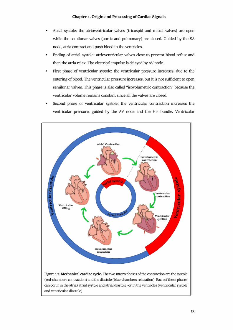
Cardiac Cycle
The period between a heart contraction and the next contraction is the cardiac cycle
(Fig.1.7). The heart periodically pumps blood towards the vessels, causing a rhythmic
contraction and relaxation of the four cardiac chambers. The cardiac cycle is divided in two
main phases: the systole and the diastole. The systole is the contraction period in which a
chamber pushes blood into the adjacent chamber or into an artery. The diastole is the
relaxation period in which a chamber fills with blood. Specifically, the phases of the cardiac
cycle are4:
Chapter 1. Origin and Processing of Cardiac Signals
13
• Atrial systole: the atrioventricular valves (tricuspid and mitral valves) are open
while the semilunar valves (aortic and pulmonary) are closed. Guided by the SA
node, atria contract and push blood in the ventricles.
• Ending of atrial systole: atrioventricular valves close to prevent blood reflux and
then the atria relax. The electrical impulse is delayed by AV node.
• First phase of ventricular systole: the ventricular pressure increases, due to the
entering of blood. The ventricular pressure increases, but it is not sufficient to open
semilunar valves. This phase is also called “isovolumetric contraction” because the
ventricular volume remains constant since all the valves are closed.
• Second phase of ventricular systole: the ventricular contraction increases the
ventricular pressure, guided by the AV node and the His bundle. Ventricular
Figure 1.7. Mechanical cardiac cycle. The two macro phases of the contraction are the systole
(red-chambers contraction) and the diastole (blue-chambers relaxation). Each of these phases
can occur in the atria (atrial systole and atrial diastole) or in the ventricles (ventricular systole
and ventricular diastole)
Chapter 1. Origin and Processing of Cardiac Signals
14
pressure exceeds the pressure in arteries and opens semilunar valves. Thus, blood
fluxes into artery is rapid in the first the ejection, while it became slower when the
pressure in the arteries decreases, due to the blood flux. Meanwhile, atrial pressure
starts to increase, due to blood that returns from veins.
• Early phase of ventricular diastole: ventricles relax and the ventricular pressure
decreases, causing the closure of the semilunar valves. When valves close,
ventricular volume remains constant. This is also called “isometric relaxation”.
• Late phase of ventricular diastole: blood enters in atria, causing an increase of the
atrial pressure, while ventricular pressure reaches its minimum value. Thus,
atrioventricular valves open and ventricles passive fills. At this point the heart is
ready to start the cycle again.
In normal condition, each ventricle expels from 70 ml to 90 ml during a single systole,
and about 5 l of blood per minute.
1.2 Major Cardiac Signals
1.2.1 Electrocardiogram
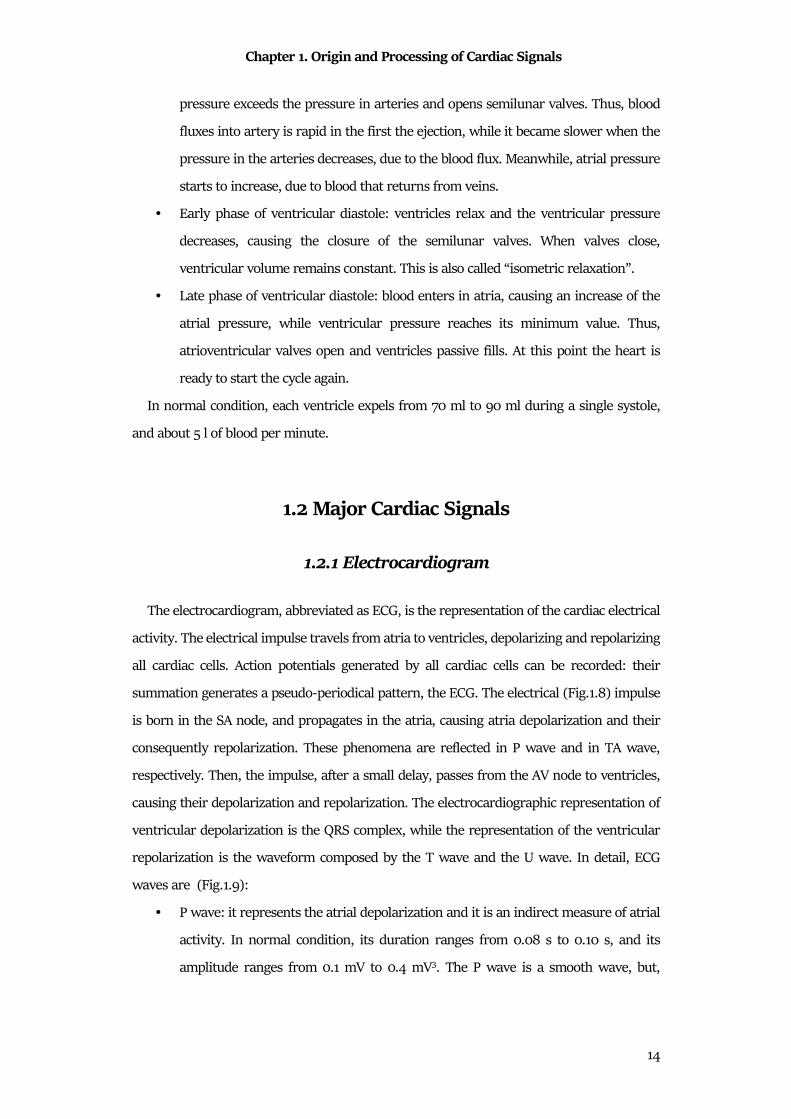
The electrocardiogram, abbreviated as ECG, is the representation of the cardiac electrical
activity. The electrical impulse travels from atria to ventricles, depolarizing and repolarizing
all cardiac cells. Action potentials generated by all cardiac cells can be recorded: their
summation generates a pseudo-periodical pattern, the ECG. The electrical (Fig.1.8) impulse
is born in the SA node, and propagates in the atria, causing atria depolarization and their
consequently repolarization. These phenomena are reflected in P wave and in TA wave,
respectively. Then, the impulse, after a small delay, passes from the AV node to ventricles,
causing their depolarization and repolarization. The electrocardiographic representation of
ventricular depolarization is the QRS complex, while the representation of the ventricular
repolarization is the waveform composed by the T wave and the U wave. In detail, ECG
waves are (Fig.1.9):
• P wave: it represents the atrial depolarization and it is an indirect measure of atrial
activity. In normal condition, its duration ranges from 0.08 s to 0.10 s, and its
amplitude ranges from 0.1 mV to 0.4 mV3. The P wave is a smooth wave, but,
Chapter 1. Origin and Processing of Cardiac Signals
15
occasionally, can present a small notch5. When a heart is affected by atrial diseases,
the P wave is altered. Specifically, abnormality in atrial structure can be
diagnosticate from the increasing of the P-wave area6 (increasing of its amplitude
or duration). For example, the atrial hypertrophy can be observed in P-wave
prolongation7. Moreover, P-wave absence is a fundamental diagnostic criterion,
associated to premature ventricular contraction (PVC), idioventricular rhythm,
junctional rhythm, but principally to atrial fibrillation (AF)8.
• TA wave: it represents the atrial repolarization. It is a shallow wave, that rarely can
be seen due to the overlapping with the ventricular depolarization wave.
Occasionally, it could be seen in patients with heart block, and it is opposite from
the P wave5.
• QRS complex: it represents the ventricular depolarization and it is the highest wave
of the ECG pattern. The main features of QRS complex are its morphology, its
amplitude and its duration. The morphology and the amplitude (usually ranged
from 1 mV to 4 mV) are lead-dependent, while the duration of the complex ranged
from 0.06 s to 0.10 s3. Usually, the normal pattern is composed by a small Q wave,
a large R wave and a small S wave in left-sided leads5. Enlargement of the QRS
complex can be symptom of ventricular hypertrophy9 and prolongation of this wave
can reflect heart failure10.
• T wave: it represents the phase 3 of repolarization of ventricular myocytes5 and its
duration ranges from 0.10 s to 0.25 s. Moreover, the T-wave duration is modulated
Figure 1.8. Genesis of electrocardiogram. The cardiac impulse generated the depolarization
of all cardiac cells, from SA node to ventricular muscle. The combination of the action
potentials of all the cells can be recorded, and it is called electrocardiogram (ECG).
Chapter 1. Origin and Processing of Cardiac Signals
16
by the duration of the entire cardiac cycle. The T-wave amplitude is not usually
quantified, but the polarity of this wave reflects important information related to
the clinical status of the patient. Examples are the myocardial ischemia and the
infarction11.
• U wave: it represents the late repolarization process of His-Purkinje cells and certain
left ventricular myocytes5. It is not always visible, but when present the normal U
wave has a low amplitude and the same polarity of the T wave.
The ECG waves are important in the monitoring of the cardiac electrical activity, but also
the interval between their occurrence can reflect important information. The main ECG
intervals in the clinical practice are:
• RR interval: it is defined as the interval between two consecutive cardiac cycles. It
could be expressed as a time interval (ms). From the RR intervals, the HR series can
be computed as their inverse. The HR is defined as the number of heartbeat present
in a minute and its unit is the heartbeat per minute (bpm). In normal condition the
RR interval ranges from 0.60 s to 1.00 s, corresponding to a HR between 60 bpm
and 100 bpm. The RR interval is essential for the diagnosis of arrhythmias, as
tachycardia or bradycardia. Tachycardia means a RR interval shorter than 0.60 s
(HR higher than 100 bpm), while bradycardia means a RR interval longer than 1.00
s (HR shorter than 60 bpm). Tachycardia and bradycardia can be physiological
events: for examples, the exercise induces tachycardia because the body needs more
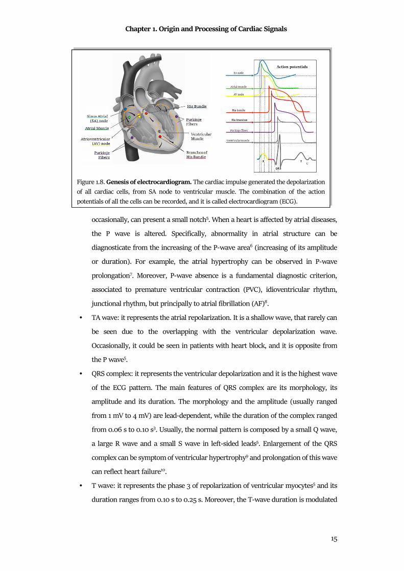
Figure 1.9. Electrocardiographic waves. ECG is composed of several waves: P wave, QRS
complex, T wave and, if present, U wave. Such important intervals (PR interval, ST interval,
RR interval and QT interval) and segments (PR segment, QRS duration and ST segment) can
be measures.
Chapter 1. Origin and Processing of Cardiac Signals
17
nutrients, while the sleep induces bradycardia. Anyway, such pathologies have
arrhythmic events as diagnostic clinical evidences12.
• PR interval: it is defined as the interval between the P-wave onset to the initial
deflection of ventricular activation. This interval includes several electrical events
because it represents the time that the cardiac electrical impulse employs to reach
the AV node. The normal PR interval is less than 0.16 s in young children or 0.18 s
in adults. A short PR interval (under 0.08 s) can reflects Wolff-Parkinson-White
syndrome5, while its prolongation reflects conduction system blocks3.
• ST segment: it is defined as the interval between the QRS-complex offset and the T-
wave offset. The QRS-complex offset is usually called J point, and it should not
deviate more than about 1 mm from baseline. Deviations in ST level may be caused
by ischemia, inflammation, severe hypertrophy, and some medications13.
• QT interval: it is defined as the interval between the QRS-complex onset and the T-
wave offset. This interval reflects the total action potential duration for ventricular
myocytes, comprising their depolarization and repolarization. As the T-wave
duration, the QT interval varies with the duration of the cardiac cycles, thus it is
usually adjusted in relation to the cardiac cycle, computing the corrected interval
(QTc) as:
��� = ��√�� (1.1)
In normal condition, the QTc is lower than 0.43 s in adults. Abnormality in QTc duration
means severe pathologies: the QTc prolongation reflects the long QT syndrome, while its
reduction reflects the short QT syndrome14.
The Standard 12 Leads
The ECG can be recorded with two different techniques, the surface ECG and the invasive
ECG. The surface ECG, usually called only ECG, records electrical fields generated by the
cardiac cycle. The signal is recorded by electrodes placed on the body surface. This technique
is low-cost, noninvasive and painless for patients. These features made ECG recording the
gold standard technique for the cardiological monitoring. On the other hand, the invasive
ECG, or endocardiogram, is recorded directly inside the heart chambers.
The basis of the ECG recording is to use at least two electrodes to record the cardiac
electrical activity. The placement of the ECG electrode was defined in the past, generating
Chapter 1. Origin and Processing of Cardiac Signals
18
different leads standardization. The mainly used in the clinical practice is the 12-lead
configuration. The 12-leads configuration is defined to have a complete visualization of
electrical heart activity from 12 different points of view. This configuration includes the
bipolar Einthoven leads, the augmented Goldberger leads and the unipolar precordial leads.
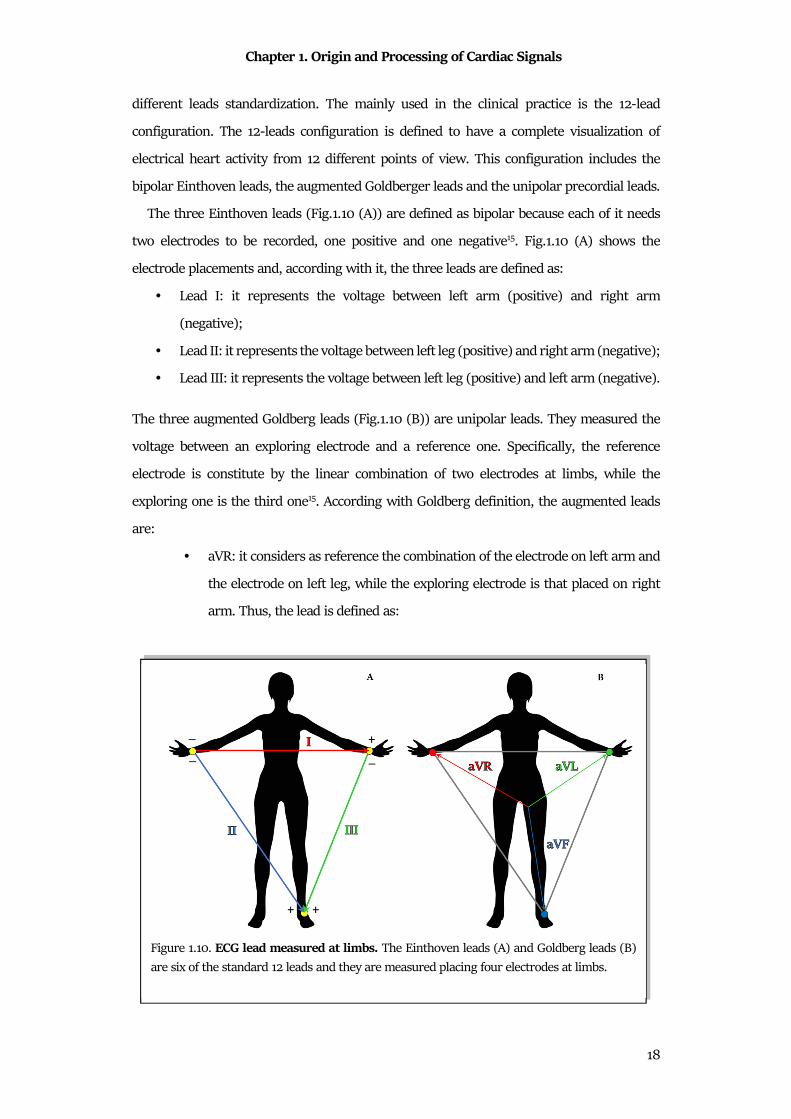
The three Einthoven leads (Fig.1.10 (A)) are defined as bipolar because each of it needs
two electrodes to be recorded, one positive and one negative15. Fig.1.10 (A) shows the
electrode placements and, according with it, the three leads are defined as:
• Lead I: it represents the voltage between left arm (positive) and right arm
(negative);
• Lead II: it represents the voltage between left leg (positive) and right arm (negative);
• Lead III: it represents the voltage between left leg (positive) and left arm (negative).
The three augmented Goldberg leads (Fig.1.10 (B)) are unipolar leads. They measured the
voltage between an exploring electrode and a reference one. Specifically, the reference
electrode is constitute by the linear combination of two electrodes at limbs, while the
exploring one is the third one15. According with Goldberg definition, the augmented leads
are:
• aVR: it considers as reference the combination of the electrode on left arm and
the electrode on left leg, while the exploring electrode is that placed on right
arm. Thus, the lead is defined as:
Figure 1.10. ECG lead measured at limbs. The Einthoven leads (A) and Goldberg leads (B)
are six of the standard 12 leads and they are measured placing four electrodes at limbs.
Chapter 1. Origin and Processing of Cardiac Signals
19
�� = 12 � � ��� (1.2)
• aVL: it considers as reference the combination of the electrode on right arm
and the electrode on left leg, while the exploring electrode is that placed on left
arm. Thus, the lead is defined as:
�� = 12 � ���� (1.3)
• aVF: it considers as reference the combination of the electrode on left arm and
the electrode on left one, while the exploring electrode is that placed on left leg.
Thus, the lead is defined as:
�� = 12 �� � ���� (1.4)
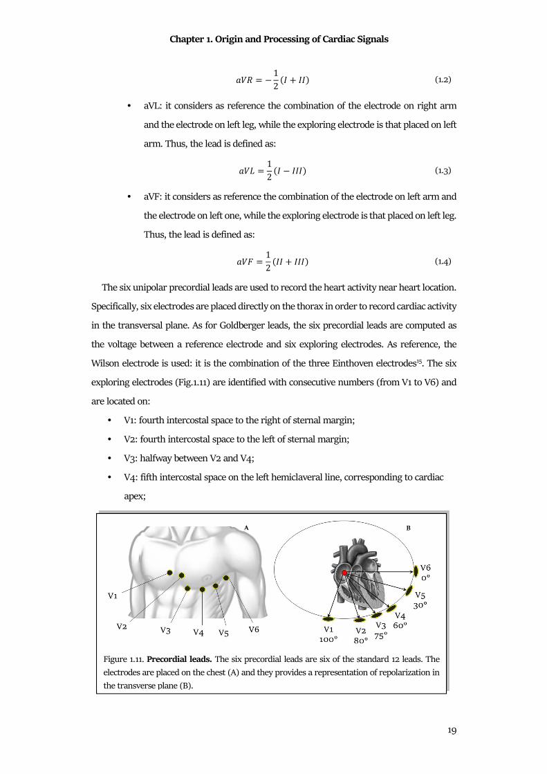
The six unipolar precordial leads are used to record the heart activity near heart location.
Specifically, six electrodes are placed directly on the thorax in order to record cardiac activity
in the transversal plane. As for Goldberger leads, the six precordial leads are computed as
the voltage between a reference electrode and six exploring electrodes. As reference, the
Wilson electrode is used: it is the combination of the three Einthoven electrodes15. The six
exploring electrodes (Fig.1.11) are identified with consecutive numbers (from V1 to V6) and
are located on:
• V1: fourth intercostal space to the right of sternal margin;
• V2: fourth intercostal space to the left of sternal margin;
• V3: halfway between V2 and V4;
• V4: fifth intercostal space on the left hemiclaveral line, corresponding to cardiac
apex;
Figure 1.11. Precordial leads. The six precordial leads are six of the standard 12 leads. The
electrodes are placed on the chest (A) and they provides a representation of repolarization in
the transverse plane (B).
Chapter 1. Origin and Processing of Cardiac Signals
20
• V5: fifth intercostal space on the left anterior axillary line, aligned with V4;
• V6: externally aligned with V4 and V5.
The 12-lead recording can be direct measured or indirect measured. The direct measure
provides a more realistic signals because electrodes are directly placed on anatomical sites.
Specifically, ten electrodes are placed on the body, and in particular six electrodes are placed
on the thorax (1. fourth intercostal space to the right of the sternal margin; 2. fourth
intercostal space to the left of the sternal margin; 3. halfway between V2 and V4; 4. fifth
intercostal space on the left hemiclaveral line, corresponding to the cardiac apex; 5. fifth
intercostal space on the left anterior axillary line, aligned with V4; 6. externally aligned with
V4 and V5), while other four are placed on the limbs (7. Left arm; 8. Left leg; 9. Right arm;
10. Right leg).
This is the standard electrodes placement, but the electrodes on limbs are uncomfortably
for portable devices, like long time monitoring (ECG Holter) or during the exercise. Thus, in
1966, Mason and Likar formulated an alternative location for electrodes on the limbs.
Specifically, they suggested to move arm electrodes on clavicles and legs electrodes on iliac
fossae16.
The indirect measure of the 12 leads is based on the recordings of the Frank leads. The
Frank leads are a set of three bipolar leads, orthogonal each other and orthogonal to the
reference system of human body. Specifically, the axis (X,Y,Z) are defined as the transversal
axis (left-right), the axis sagittal (or dorsoventral) and the longitudinal axis (or
craniocaudal). According with these axes, the Frank leads are recorded with seven
electrodes, five on the thorax, one on the left leg and one as reference. Through such
transformation matrices, three orthogonal leads can be mathematically transformed in the
12 standard leads. In particular, the most famous matrix for the 12 leads computation are
the Dower matrix17,18 and the Kors matrix19,20.
1.2.2 Vectorcardiogram
Heart Vector
An alternative line of the electrocardiography is the concept of the heart as a cardiac
dipole. Indeed, the heart generated an electrical field, that can be observed through its body
surface isopotential map. The cardiac electrical activity could be accurately described as an
equivalent dipole. The dipole is a system composed of two equal and opposite electric
Chapter 1. Origin and Processing of Cardiac Signals
21
charges, separated by a constant distance over time; it is usually represented in vector form
in which the vector amplitude indicates the electrical intensity while the arrow indicates its
orientation.
During cardiac depolarization, the extracellular fluid surrounding the heart and the
myocardium became two equal and opposite electric charges. Specifically, the extracellular
fluid becomes more negative, while the myocardium becomes more positive. This is caused
by the positive ions flux inside the cellular membrane. This phenomenon generates a dipole
between two charges, that changes its direction accordingly with the
depolarization/repolarization wave. This wave is not instantaneous; thus, the dipole changes
its direction in the space. Moreover, the heart tissue in not homogenous, thus the dipole
intensity (vector length) is not constant. According with these features, the cardiac dipole is
equivalent to a rotating vector with a positive and negative terminal spinning in three
dimensions, according with the depolarization/repolarization wave that spreads through
cardiac chambers. Moreover, the cardiac dipole spins around the heart, generating a current
that moves towards or away from skin electrodes. The upward or downward deflection of
cardiac vector depends on its direction, and in particular if it points the electrode or not.
Standard 12-lead ECG shows the dipole movement from different points of view, in order to
have a global overview of cardiac electrical activity. When the heart is completely depolarized
or repolarized, there is no dipole and ECG is flat (isoelectric).
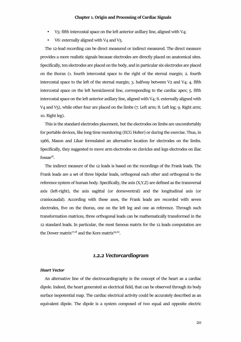
Figure 1.12. Cardiac vector. The depolarization wave follows a specific path that can be
modeled as a vector, which can be projected on the standard 12 leads.

Chapter 1. Origin and Processing of Cardiac Signals
22
A dipole is a vector (Fig.1.12); thus, it has a direction and a magnitude: specifically, it could
be represented as an arrow pointing from the most depolarized region of the heart to the
most polarized region. Where each end of the arrow is located depends on how the wave of
depolarization spreads through the heart, and how much mass of myocardium is
depolarized/repolarized. The dipole points from the biggest mass of depolarized
myocardium to the biggest mass of repolarized myocardium at any particular instant.
Vectorcardiogram
One of the electrocardiographic techniques to evaluate cardiac electrical activity is the
dynamic measurement of heart vector, the vectorcardiogram (VCG). The VCG is composed
by the three orthonormal leads X, Y and Z (Frank leads), with lead vectors in directions of
the main axes of the body. Usually, they are normalized lead strengths, thus measuring the
dynamic x, y and z components of the heart vector20. These three leads can be combined,
observing the heart vector movement in the three principal planes (longitudinal, sagittal or
transversal) of in the space. Additionally, the vector magnitude (VM) is also computed as:
� = ��� � �� � ��. (1.5)
The recordings of three orthogonal leads can be direct (using the Frank configuration) or
indirectly computed. In fact, as the three orthogonal leads can be computed from the
standard 12-lead, the inverse process is also possible. Specifically, it was demonstrated that
the Kors matrix20 allows to reliably approximate Frank leads from the eight independent
lead of the standard 12-lead configuration.
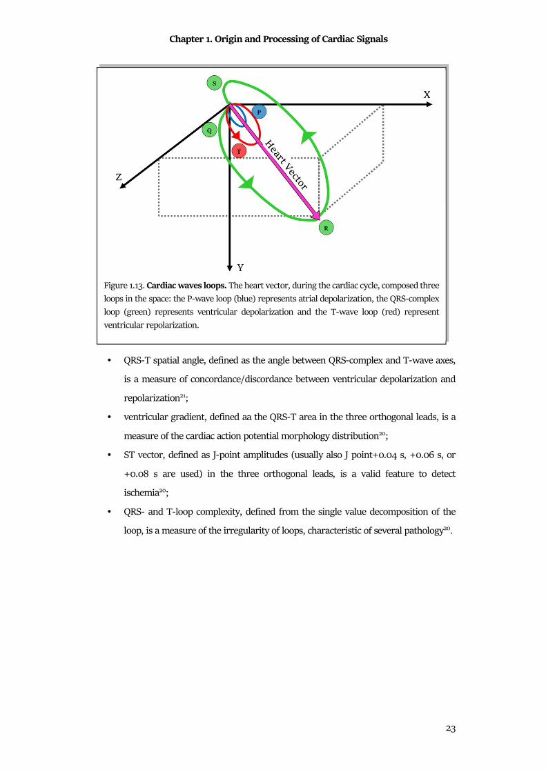
The main pattern that can be observed in VCG is composed of three wave loops, the P-
wave loop, the QRS-complex loop and the T-wave loop (Fig.1.13). Each of these loops
represents the movement of heart vector during a specific phase of the
depolarization/repolarization wave. Specifically, this pattern is repeated for each ECG
heartbeat, and the projection of each loop in one of the three principal planes can underline
proprieties of the cardiac electrical activity.
VCG contains less information than the ECG, but its nature to observe the heart vector in
space has additional value and gives access to information that remains unexplored in the
standard 12-lead ECG20. Examples of VCG features that could be useful in clinical practice
are:
Chapter 1. Origin and Processing of Cardiac Signals
23
• QRS-T spatial angle, defined as the angle between QRS-complex and T-wave axes,
is a measure of concordance/discordance between ventricular depolarization and
repolarization21;
• ventricular gradient, defined aa the QRS-T area in the three orthogonal leads, is a
measure of the cardiac action potential morphology distribution20;
• ST vector, defined as J-point amplitudes (usually also J point+0.04 s, +0.06 s, or
+0.08 s are used) in the three orthogonal leads, is a valid feature to detect
ischemia20;
• QRS- and T-loop complexity, defined from the single value decomposition of the
loop, is a measure of the irregularity of loops, characteristic of several pathology20.
Figure 1.13. Cardiac waves loops. The heart vector, during the cardiac cycle, composed three
loops in the space: the P-wave loop (blue) represents atrial depolarization, the QRS-complex
loop (green) represents ventricular depolarization and the T-wave loop (red) represent
ventricular repolarization.
Chapter 1. Origin and Processing of Cardiac Signals
24
1.2.3 Phonocardiogram
The phonocardiogram, or PCG, is the recording of the cardiac heart sounds. The
contraction and the relaxation of the four heart chambers periodically repeats in time:
ventricular contraction pushes blood in arteries and provokes closures of atrioventricular
valves; then, during the ventricular relaxation, atrioventricular valves open and semilunar
valves close in order to allow the blood to fill atria. The valve closures generate sounds, that
could be recorded. Cardiac heart sounds define the time of systole and diastole. Moreover,
abnormality in the heart sounds reflects valves dysfunction.
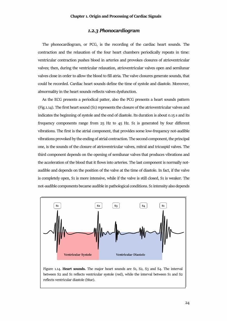
As the ECG presents a periodical patter, also the PCG presents a heart sounds pattern
(Fig.1.14). The first heart sound (S1) represents the closure of the atrioventricular valves and
indicates the beginning of systole and the end of diastole. Its duration is about 0.15 s and its
frequency components range from 25 Hz to 45 Hz. S1 is generated by four different
vibrations. The first is the atrial component, that provides some low-frequency not-audible
vibrations provoked by the ending of atrial contraction. The second component, the principal
one, is the sounds of the closure of atrioventricular valves, mitral and tricuspid valves. The
third component depends on the opening of semilunar valves that produces vibrations and
the acceleration of the blood that it flows into arteries. The last component is normally not-
audible and depends on the position of the valve at the time of diastole. In fact, if the valve
is completely open, S1 is more intensive, while if the valve is still closed, S1 is weaker. The
not-audible components became audible in pathological conditions. S1 intensity also depends
Figure 1.14. Heart sounds. The major heart sounds are S1, S2, S3 and S4. The interval
between S2 and S1 reflects ventricular systole (red), while the interval between S1 and S2
reflects ventricular diastole (blue).
Chapter 1. Origin and Processing of Cardiac Signals
25
on the rapidity of ventricular contraction and on the anatomical shape of valves. The
auscultation is better appreciated at the apex or in the left ventricular area.
The second heart sound (S2) represents the closure of semilunar valves and indicates the
beginning of diastole and the end of systole. Its duration is about 0.12 s and its frequency
components are around 50 Hz. S2 is more direct and acute than the first and is accompanied
by vibrations that are normally not audible. These vibrations are due to the reaction of the
ventricular wall at the beginning of diastole (not audible normally) to the closure of
semilunar valves, aortic and pulmonary valves, which represent the audible and
predominant part of S2. The vibrations of the vascular walls and the vibrations produced by
the opening of atrioventricular valves are added. Not-audible components become audible
in pathological conditions. Auscultation is better appreciated in aortic or pulmonary
auscultation sites.
The third heart sound (S3) is a dull, weak and serious sounds, perceivable after a physical
effort. Since S3 follows S2, it can be considered as a diastolic sound, or rather pre-diastolic.
S3 is present in a third of children/young people and corresponds to the rapid ventricular
filling. It is produced by the vibration of the mitral valve when blood rapidly passes in
ventricles. It must be monitored since S3 (physiological) is very similar to the pre-diastolic
gallop (pathological). The differences regard their population, in fact S3 is characteristic of
very young/young individuals, while the pre-diastolic gallop in adults with left ventricle
failure. In relation to the other sounds, S3 occurs after 0.10 s after S2. Auscultation is better
appreciated in the apical area with the subject prone on its left side.
The fourth heart sound (S4) precedes about 0.10 s S1 and is generated by atrial systole
(pre-systole), generally considered as an extra-localized sound near ventricles with a
frequency of 20-30 Hz. Although not confirmed, the literature believes that S4 is generated
due to the stiffening of ventricular walls, that causes a turbulent flow of blood as atria
contract to force blood into ventricles. If S4 becomes strong, it is a pathological state signal,
usually a collapse of the left ventricle. It is often referred to as atrial gallop.
With the four main cardiac sounds, additional tones and heart murmurs are added. The
cardiac tones are the "pericardial knock", which occurs in proto-diastole in case of
constrictive pericarditis; the ejection tones, which are intense and short, high-pitched
sounds that can be perceived in early diastole caused by opening pops of aortic (or
pulmonary) semilunar valves or sounds due to the distension of a dilated aorta; and finally
the "non-ejection systolic clicks", deriving from the tensioning of mitral cord tendons with
Chapter 1. Origin and Processing of Cardiac Signals
26
a length functionally not equal to that of the others. Heart murmurs are noises caused by a
rapid turbulent flow of blood, in case of low viscosity. The breaths are characterized by a
source point, duration and intensity defined in degrees (grade 1: very weak, almost not
perceptible, up to grade 6: very strong, perceptible even without a stethoscope). Another
kind of breath is the systolic and diastolic murmurs. The first start with the first tone and
last up to the second, the others start immediately after the beginning of the second tone.
These breaths are associated with pathological conditions or insufficiencies due to cardiac
stress.
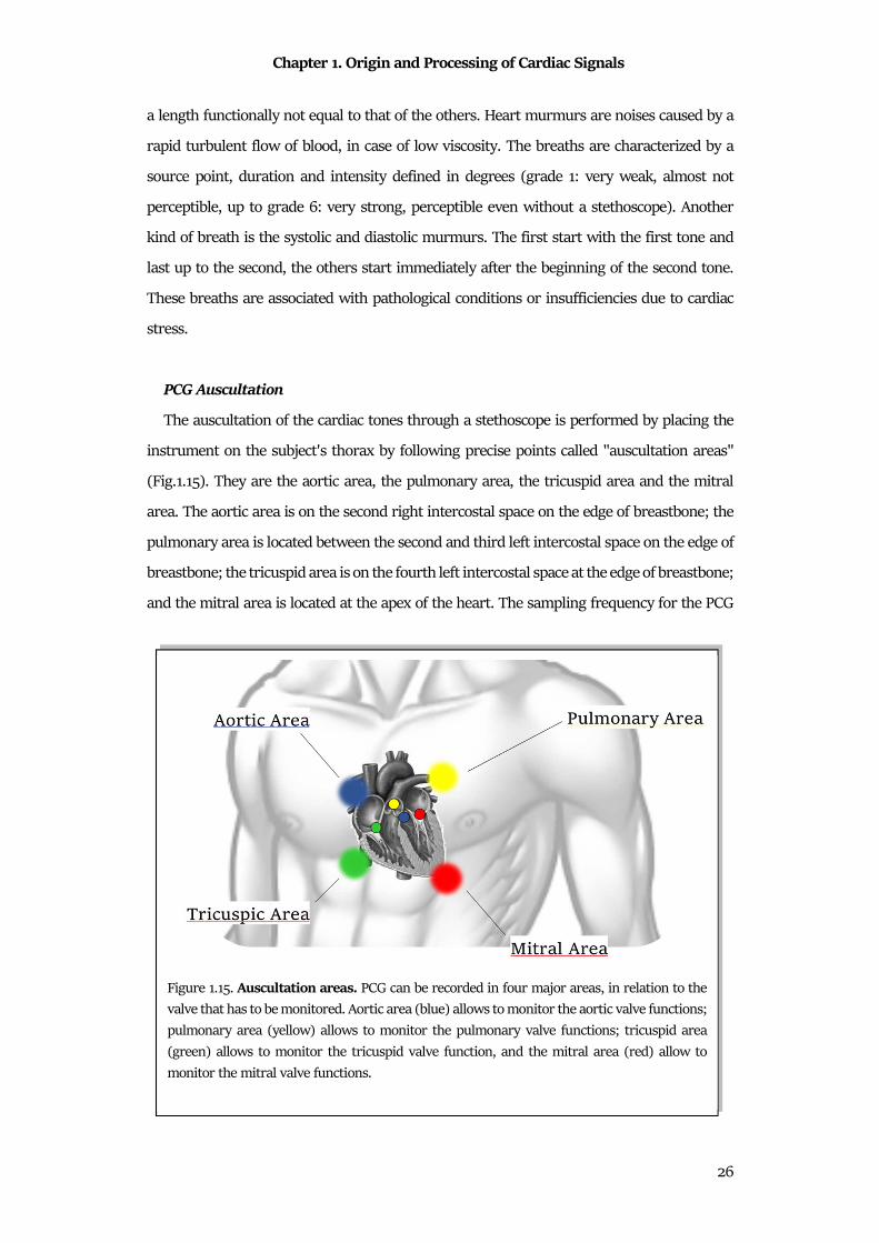
PCG Auscultation
The auscultation of the cardiac tones through a stethoscope is performed by placing the
instrument on the subject's thorax by following precise points called "auscultation areas"
(Fig.1.15). They are the aortic area, the pulmonary area, the tricuspid area and the mitral
area. The aortic area is on the second right intercostal space on the edge of breastbone; the
pulmonary area is located between the second and third left intercostal space on the edge of
breastbone; the tricuspid area is on the fourth left intercostal space at the edge of breastbone;
and the mitral area is located at the apex of the heart. The sampling frequency for the PCG
Figure 1.15. Auscultation areas. PCG can be recorded in four major areas, in relation to the
valve that has to be monitored. Aortic area (blue) allows to monitor the aortic valve functions;
pulmonary area (yellow) allows to monitor the pulmonary valve functions; tricuspid area
(green) allows to monitor the tricuspid valve function, and the mitral area (red) allow to
monitor the mitral valve functions.
Chapter 1. Origin and Processing of Cardiac Signals
27
signal is usually very high, ranged
from 4000 Hz to 16000 Hz. This
choice is related to the high frequency
components of heart sounds22.
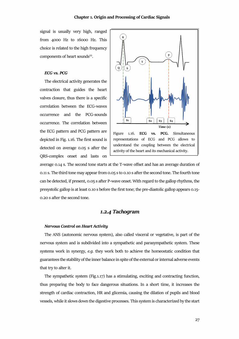
ECG vs. PCG
The electrical activity generates the
contraction that guides the heart
valves closure, thus there is a specific
correlation between the ECG-waves
occurrence and the PCG-sounds
occurrence. The correlation between
the ECG pattern and PCG pattern are
depicted in Fig. 1.16. The first sound is
detected on average 0.05 s after the
QRS-complex onset and lasts on
average 0.14 s. The second tone starts at the T-wave offset and has an average duration of
0.11 s. The third tone may appear from 0.05 s to 0.10 s after the second tone. The fourth tone
can be detected, if present, 0.05 s after P-wave onset. With regard to the gallop rhythms, the
presystolic gallop is at least 0.10 s before the first tone; the pre-diastolic gallop appears 0.15-
0.20 s after the second tone.
1.2.4 Tachogram
Nervous Control on Heart Activity
The ANS (autonomic nervous system), also called visceral or vegetative, is part of the
nervous system and is subdivided into a sympathetic and parasympathetic system. These
systems work in synergy, e.g. they work both to achieve the homeostatic condition that
guarantees the stability of the inner balance in spite of the external or internal adverse events
that try to alter it.
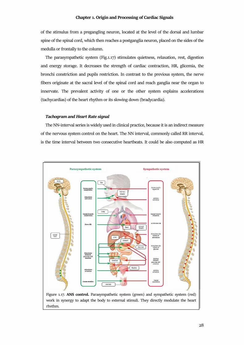
The sympathetic system (Fig.1.17) has a stimulating, exciting and contracting function,
thus preparing the body to face dangerous situations. In a short time, it increases the
strength of cardiac contraction, HR and glicemia, causing the dilation of pupils and blood
vessels, while it slows down the digestive processes. This system is characterized by the start
Figure 1.16. ECG vs. PCG. Simultaneous
representations of ECG and PCG allows to
understand the coupling between the electrical
activity of the heart and its mechanical activity.
Chapter 1. Origin and Processing of Cardiac Signals
28
of the stimulus from a pregangling neuron, located at the level of the dorsal and lumbar
spine of the spinal cord, which then reaches a postganglia neuron, placed on the sides of the
medulla or frontally to the column.
The parasympathetic system (Fig.1.17) stimulates quietness, relaxation, rest, digestion
and energy storage. It decreases the strength of cardiac contraction, HR, glicemia, the
bronchi constriction and pupils restriction. In contrast to the previous system, the nerve
fibers originate at the sacral level of the spinal cord and reach ganglia near the organ to
innervate. The prevalent activity of one or the other system explains accelerations
(tachycardias) of the heart rhythm or its slowing down (bradycardia).
Tachogram and Heart Rate signal
The NN-interval series is widely used in clinical practice, because it is an indirect measure
of the nervous system control on the heart. The NN interval, commonly called RR interval,
is the time interval between two consecutive heartbeats. It could be also computed as HR
Figure 1.17. ANS control. Parasympathetic system (green) and sympathetic system (red)
work in synergy to adapt the body to external stimuli. They directly modulate the heart
rhythm.
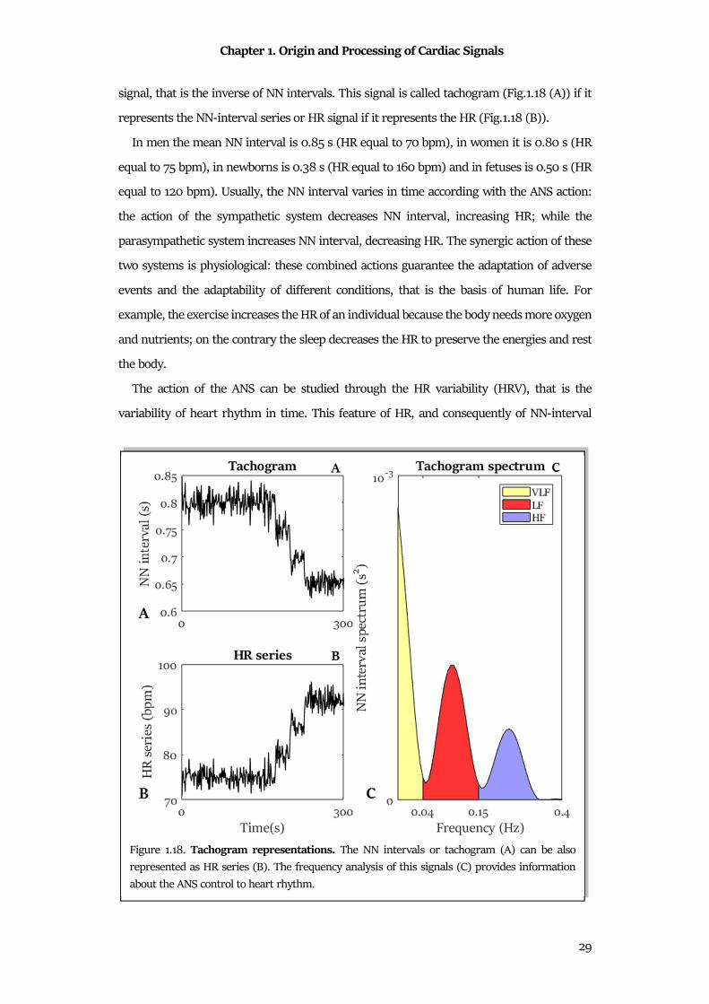
Chapter 1. Origin and Processing of Cardiac Signals
29
signal, that is the inverse of NN intervals. This signal is called tachogram (Fig.1.18 (A)) if it
represents the NN-interval series or HR signal if it represents the HR (Fig.1.18 (B)).
In men the mean NN interval is 0.85 s (HR equal to 70 bpm), in women it is 0.80 s (HR
equal to 75 bpm), in newborns is 0.38 s (HR equal to 160 bpm) and in fetuses is 0.50 s (HR
equal to 120 bpm). Usually, the NN interval varies in time according with the ANS action:
the action of the sympathetic system decreases NN interval, increasing HR; while the
parasympathetic system increases NN interval, decreasing HR. The synergic action of these
two systems is physiological: these combined actions guarantee the adaptation of adverse
events and the adaptability of different conditions, that is the basis of human life. For
example, the exercise increases the HR of an individual because the body needs more oxygen
and nutrients; on the contrary the sleep decreases the HR to preserve the energies and rest
the body.
The action of the ANS can be studied through the HR variability (HRV), that is the
variability of heart rhythm in time. This feature of HR, and consequently of NN-interval
Figure 1.18. Tachogram representations. The NN intervals or tachogram (A) can be also
represented as HR series (B). The frequency analysis of this signals (C) provides information
about the ANS control to heart rhythm.
Chapter 1. Origin and Processing of Cardiac Signals
30
series, is fundamental to investigate the ANS control in heart in several physiological
conditions, like exercise and sleep, or in critical condition, like the labor and the delivery.
The tachogram is a signal that could be extracted for a cardiac pseudo-periodical signal,
as the ECG and the PCG. Usually, the tachogram of an adult is computed from the R peak of
ECG, while the tachogram of a fetus, that is the gold standard of the fetal monitoring
(cardiotocography), is usually computed from fetal PCG.
From the signal processing point of view, the tachogram (Fig.1.18) is computed from the
difference between a normal heartbeat occurrence (R peak or S1) and the previous one,
according with the formula:
��� = �� ���� (1.5)
The series can be represented according to the number of heartbeats or in time. It is
represented in time, its time resolution, for definition of variability, have to be constant:
thus, the approximation is to consider the time resolution equal to the mean NN interval of
all the signal.
The tachogram is usually represented also in frequency domain. Assuming the mean NN
interval as the time resolution (constant) and the stationarity of the signal in few minutes
(usually 5 minutes), the spectrum can be computed.
The study of the HRV can be performed in two different manners, the time domain
analysis or the frequency domain analysis. The time domain analysis includes all the features
that could be computed from the tachogram considering its representation in time.
Specifically, the major features are:
• NNmax that is the maximum value of the NN series;
• NNmean that is the mean value of the NN series;
• NNmin that is the minimum value of the NN series;
• SDNN that is the standard deviation of the considered NN interval;
• NN triangular index that is the total number of NN intervals divided by the height
of the histogram of all NN intervals;
• RMSSD that is square root of the mean of the squares of the differences between
NN intervals.
On the other hand, the frequency domain analysis includes all the features that could be
computed from the tachogram spectrum (Fig.1.18 (C)). Specifically, the major features are:
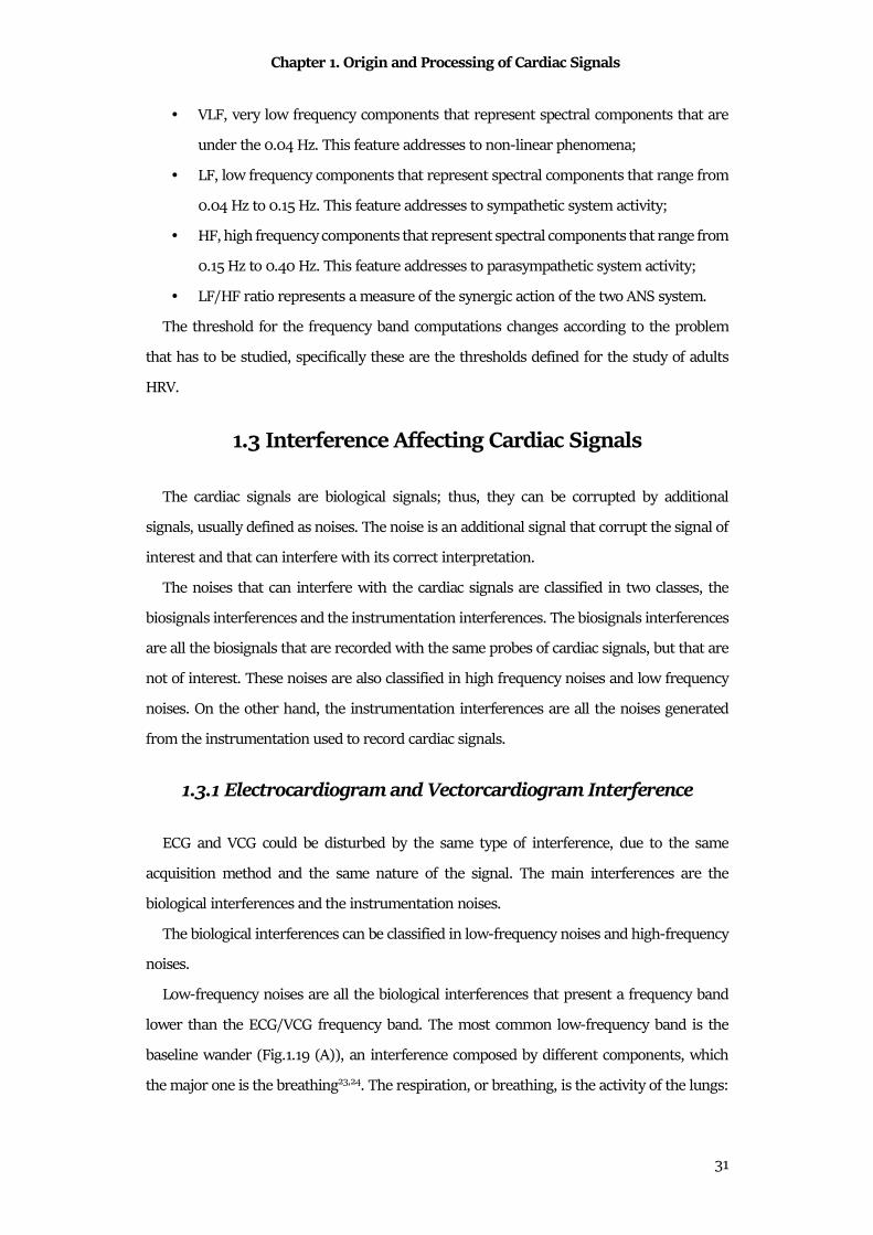
Chapter 1. Origin and Processing of Cardiac Signals
31
• VLF, very low frequency components that represent spectral components that are
under the 0.04 Hz. This feature addresses to non-linear phenomena;
• LF, low frequency components that represent spectral components that range from
0.04 Hz to 0.15 Hz. This feature addresses to sympathetic system activity;
• HF, high frequency components that represent spectral components that range from
0.15 Hz to 0.40 Hz. This feature addresses to parasympathetic system activity;
• LF/HF ratio represents a measure of the synergic action of the two ANS system.
The threshold for the frequency band computations changes according to the problem
that has to be studied, specifically these are the thresholds defined for the study of adults
HRV.
1.3 Interference Affecting Cardiac Signals
The cardiac signals are biological signals; thus, they can be corrupted by additional
signals, usually defined as noises. The noise is an additional signal that corrupt the signal of
interest and that can interfere with its correct interpretation.
The noises that can interfere with the cardiac signals are classified in two classes, the
biosignals interferences and the instrumentation interferences. The biosignals interferences
are all the biosignals that are recorded with the same probes of cardiac signals, but that are
not of interest. These noises are also classified in high frequency noises and low frequency
noises. On the other hand, the instrumentation interferences are all the noises generated
from the instrumentation used to record cardiac signals.
1.3.1 Electrocardiogram and Vectorcardiogram Interference
ECG and VCG could be disturbed by the same type of interference, due to the same
acquisition method and the same nature of the signal. The main interferences are the
biological interferences and the instrumentation noises.
The biological interferences can be classified in low-frequency noises and high-frequency
noises.
Low-frequency noises are all the biological interferences that present a frequency band
lower than the ECG/VCG frequency band. The most common low-frequency band is the
baseline wander (Fig.1.19 (A)), an interference composed by different components, which
the major one is the breathing23,24. The respiration, or breathing, is the activity of the lungs:
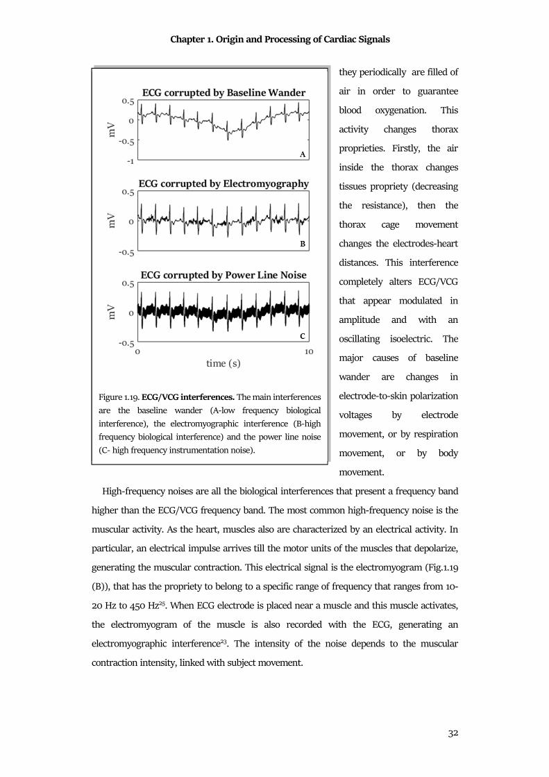
Chapter 1. Origin and Processing of Cardiac Signals
32
they periodically are filled of
air in order to guarantee
blood oxygenation. This
activity changes thorax
proprieties. Firstly, the air
inside the thorax changes
tissues propriety (decreasing
the resistance), then the
thorax cage movement
changes the electrodes-heart
distances. This interference
completely alters ECG/VCG
that appear modulated in
amplitude and with an
oscillating isoelectric. The
major causes of baseline
wander are changes in
electrode-to-skin polarization
voltages by electrode
movement, or by respiration
movement, or by body
movement.
High-frequency noises are all the biological interferences that present a frequency band
higher than the ECG/VCG frequency band. The most common high-frequency noise is the
muscular activity. As the heart, muscles also are characterized by an electrical activity. In
particular, an electrical impulse arrives till the motor units of the muscles that depolarize,
generating the muscular contraction. This electrical signal is the electromyogram (Fig.1.19
(B)), that has the propriety to belong to a specific range of frequency that ranges from 10-
20 Hz to 450 Hz25. When ECG electrode is placed near a muscle and this muscle activates,
the electromyogram of the muscle is also recorded with the ECG, generating an
electromyographic interference23. The intensity of the noise depends to the muscular
contraction intensity, linked with subject movement.
Figure 1.19. ECG/VCG interferences. The main interferences
are the baseline wander (A-low frequency biological
interference), the electromyographic interference (B-high
frequency biological interference) and the power line noise
(C- high frequency instrumentation noise).
Chapter 1. Origin and Processing of Cardiac Signals
33
Electromyographic interference is usually an interference for the recording of the ECG,
and indirectly for VCG and tachogram. The ECG has a frequency band lower than 100 Hz,
that means that the electromyographic signal can be considered as a high frequency
interference. Electromyogram is typically modeled by a Gaussian distribution function, with
a zero mean and a variance that depends on the environmental variables23,26.
Electromyogram is common in subjects with uncontrollable tremor, in disabled persons, in
kids and in that procedures that required the ECG recording during exercise.
The common instrumentation noises are the power line noise and the electrode noise.
Power line noise(Fig.1.19 (C)) is a signal that is generated by electrical equipment,
carrying the electromagnetic interference of frequency (50 Hz or 60 Hz). It is a dominant
source of noise during biosignals measurements: electromagnetic interference disturbs the
signal amplitude and coves the small features that could be essential for patients monitoring
and diagnosis. The power line interference is due to differences in the electrode impedance
and stray currents through the patient. Specifically, the current flowing through the cables
produces a magnetic flux that induces a current in adjacent circuits. The structure of
conductors and the separation between them decide the value of the mutual inductance, and
thus the degree of the inductive coupling. Typically, high frequency noise is contributed by
capacitive coupling and inductive coupling23. In order to reduce the power line interference,
the electrodes have to be properly applied and all components have adequate shielding. The
simplest model of the power line noise considers it as a finite bandwidth noise around its
nominal central frequency (50 Hz or 60 Hz), suggesting that the total noise is composed of
many sinusoids of similar frequency.
The electrode noise is the interference due to the movement of the electrode in relation to
the heart position. This noise provokes changes in the ECG amplitude, but also in baseline
(as in the respiration interference). It is caused by poor conductivity between electrodes and
skin that reduces the contact and can provokes electrode displacements. Larger ECG
electrode-skin impedances generated small relative impedance changes, which is required
to cause a major shift in ECG baseline23. Sudden changes in the skin-electrode impedance
induce sharp baseline transients which decay exponentially to the baseline value23, thus
easily recognizable.
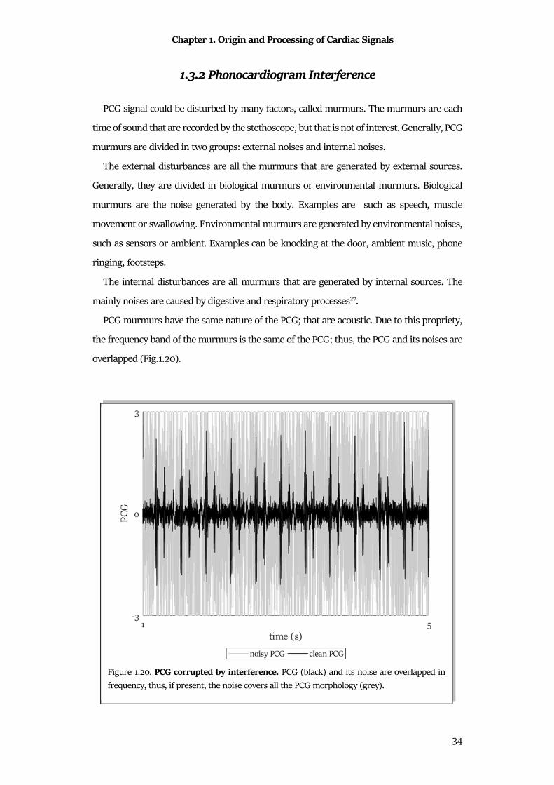
Chapter 1. Origin and Processing of Cardiac Signals
34
1.3.2 Phonocardiogram Interference
PCG signal could be disturbed by many factors, called murmurs. The murmurs are each
time of sound that are recorded by the stethoscope, but that is not of interest. Generally, PCG
murmurs are divided in two groups: external noises and internal noises.
The external disturbances are all the murmurs that are generated by external sources.
Generally, they are divided in biological murmurs or environmental murmurs. Biological
murmurs are the noise generated by the body. Examples are such as speech, muscle
movement or swallowing. Environmental murmurs are generated by environmental noises,
such as sensors or ambient. Examples can be knocking at the door, ambient music, phone
ringing, footsteps.
The internal disturbances are all murmurs that are generated by internal sources. The
mainly noises are caused by digestive and respiratory processes27.
PCG murmurs have the same nature of the PCG; that are acoustic. Due to this propriety,
the frequency band of the murmurs is the same of the PCG; thus, the PCG and its noises are
overlapped (Fig.1.20).
Figure 1.20. PCG corrupted by interference. PCG (black) and its noise are overlapped in
frequency, thus, if present, the noise covers all the PCG morphology (grey).
Chapter 1. Origin and Processing of Cardiac Signals
35
1.3.3 Tachogram Interference
Tachogram can presents abnormal heartbeats. The abnormal heartbeat is an occasional
NN interval that has a different value respect to the entire tachogram. The abnormal
heartbeats can be produced by arrythmias or instrumental interferences.
Arrythmias are pathological cardiac events that provokes a rapid reduction of the NN
interval, usually followed by one or multiple long NN intervals. The most common
arrythmias are the premature ventricular contraction (PVC) and the supraventricular
contraction (SVC). When these pathologies occur, the tachogram present a very short NN
heartbeat followed by long NN intervals, usually called ectopic heartbeats. These occasional
heartbeats interfere with the tachogram processing, and in particular with the spectral
analysis of the HRV.
The instrumental interference corrupts the recording of the tachogram. If the tachogram
is indirect measured (e.g. from ECG or PCG), the instrumental interference is represented
by an incorrect R peak/S1 detection. Moreover, some devices directly convert R-peak
sequences or S1 sequences in a tachogram and, then, resampled it with a specific sampling
frequency. In this automatic process, the sequences can be lost by the device, that replaced
the missing signal with a zero-line. These artifacts are called data-loss and are typical of the
fetal tachogram.
1.4 Processing of Cardiac Signals
Cardiac signals, as all other biosignals, are essential for the diagnosis, for patient
monitoring and biomedical research. In order to extract the information of interest, the
cardiac signal has to be processed: the cardiac signal represent data that have to be processed
in order to extract useful information.
The course to transform the cardiac signals in information is constituted of four steps28
(Fig.1.21):
1. Cardiac signal acquisition: this first step allows to measure and record the data of
interest. In relation to the cardiac signals, it could be performed according with the
standard procedure of each signal previously defined. In this stage, transducers
(electrical or mechanical) are used to convert the signal that are picked up by
electrode into electrical form that could be displayed or collected. Moreover, in this
stage there are the essential parts of sampling and quantization, that allow to obtain
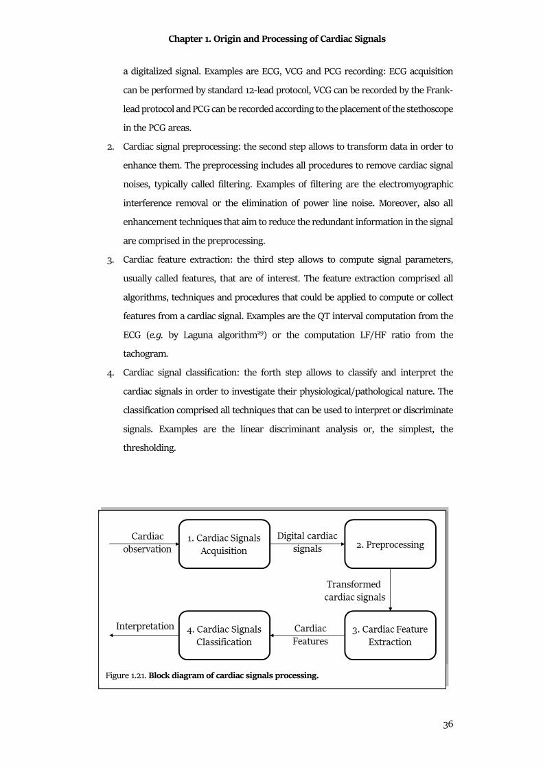
Chapter 1. Origin and Processing of Cardiac Signals
36
a digitalized signal. Examples are ECG, VCG and PCG recording: ECG acquisition
can be performed by standard 12-lead protocol, VCG can be recorded by the Frank-
lead protocol and PCG can be recorded according to the placement of the stethoscope
in the PCG areas.
2. Cardiac signal preprocessing: the second step allows to transform data in order to
enhance them. The preprocessing includes all procedures to remove cardiac signal
noises, typically called filtering. Examples of filtering are the electromyographic
interference removal or the elimination of power line noise. Moreover, also all
enhancement techniques that aim to reduce the redundant information in the signal
are comprised in the preprocessing.
3. Cardiac feature extraction: the third step allows to compute signal parameters,
usually called features, that are of interest. The feature extraction comprised all
algorithms, techniques and procedures that could be applied to compute or collect
features from a cardiac signal. Examples are the QT interval computation from the
ECG (e.g. by Laguna algorithm29) or the computation LF/HF ratio from the
tachogram.
4. Cardiac signal classification: the forth step allows to classify and interpret the
cardiac signals in order to investigate their physiological/pathological nature. The
classification comprised all techniques that can be used to interpret or discriminate
signals. Examples are the linear discriminant analysis or, the simplest, the
thresholding.
Figure 1.21. Block diagram of cardiac signals processing.
Chapter 2. Statistical Signal Modelling and Sample Cardiac Applications
37
Chapter 2
Statistical Signal Modelling and Sample
Cardiac Applications
Biomedical signal modeling aims to propose mathematical models to represent
biomedical signals and their characteristics. Mathematical modeling of biosignals allows to
explore the potential use of the model parameters in signal analysis and/or diagnostic
decision making30. With these aims, to find the correct instruments that allow to formalize
and to organize data is essential. The correct instrument is Biostatistics. This science applies
statistical techniques to biomedical data analysis, in order to correctly investigate their
properties. Specifically, biostatistical cardiac signal modeling aims to formalize models about
cardiac signals. Due to the different physiological aspects that generate these cardiac signals,
a very specific biostatistical model for each cardiac signal has to be found30.
2.1 Statistical Modelling of Biological Signals
Biosignals are signals derived from biological processes. Usually, they are highly complex
and dynamic. Usually (but not always), biosignals are in function of time: they represent a
variable that changes in time. Biosignals can be deterministic or stochastic (Fig.2.1). They
are deterministic waveforms if their pattern is fully determined by their parameters.
Sometimes, noise corrupts the deterministic waveform, or the nature of the signal is not
deterministic. These biosignals cannot be accurately predicted, thus they are called stochastic
biosignals28.
2.1.1 Deterministic Biological Signals
The deterministic waveforms are the signals that present a repetitive pattern.
Deterministic waveforms can be periodic, pseudo periodic, aperiodic or simply transient
(Fig.2.1). In biomedical fields, perfect periodical pattern is not visible, due to interference or
physiological variability. The terms pseudo periodic or periodic is more used28.
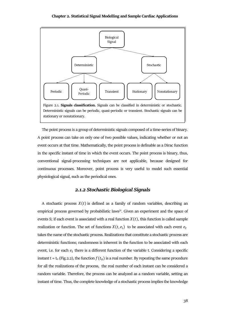
Chapter 2. Statistical Signal Modelling and Sample Cardiac Applications
38
The point process is a group of deterministic signals composed of a time-series of binary.
A point process can take on only one of two possible values, indicating whether or not an
event occurs at that time. Mathematically, the point process is definable as a Dirac function
in the specific instant of time in which the event occurs. The point process is binary, thus,
conventional signal-processing techniques are not applicable, because designed for
continuous processes. Moreover, point process is very useful to model such essential
physiological signal, such as the periodical ones.
2.1.2 Stochastic Biological Signals
A stochastic process � �� is defined as a family of random variables, describing an
empirical process governed by probabilistic laws31. Given an experiment and the space of
events S; if each event is associated with a real function � ��, this function is called sample
realization or function. The set of functions � �, �� to be associated with each event ! takes the name of the stochastic process. Realizations that constitute a stochastic process are
deterministic functions; randomness is inherent in the function to be associated with each
event, i.e. for each ! there is a different function of the variable t. Considering a specific
instant t = t0 (Fig.2.2), the function " �#� is a real number. By repeating the same procedure
for all the realizations of the process, the real number of each instant can be considered a
random variable. Therefore, the process can be analyzed as a random variable, setting an
instant of time. Thus, the complete knowledge of a stochastic process implies the knowledge
Figure 2.1. Signals classification. Signals can be classified in deterministic or stochastic.
Deterministic signals can be periodic, quasi-periodic or transient. Stochastic signals can be
stationary or nonstationary.
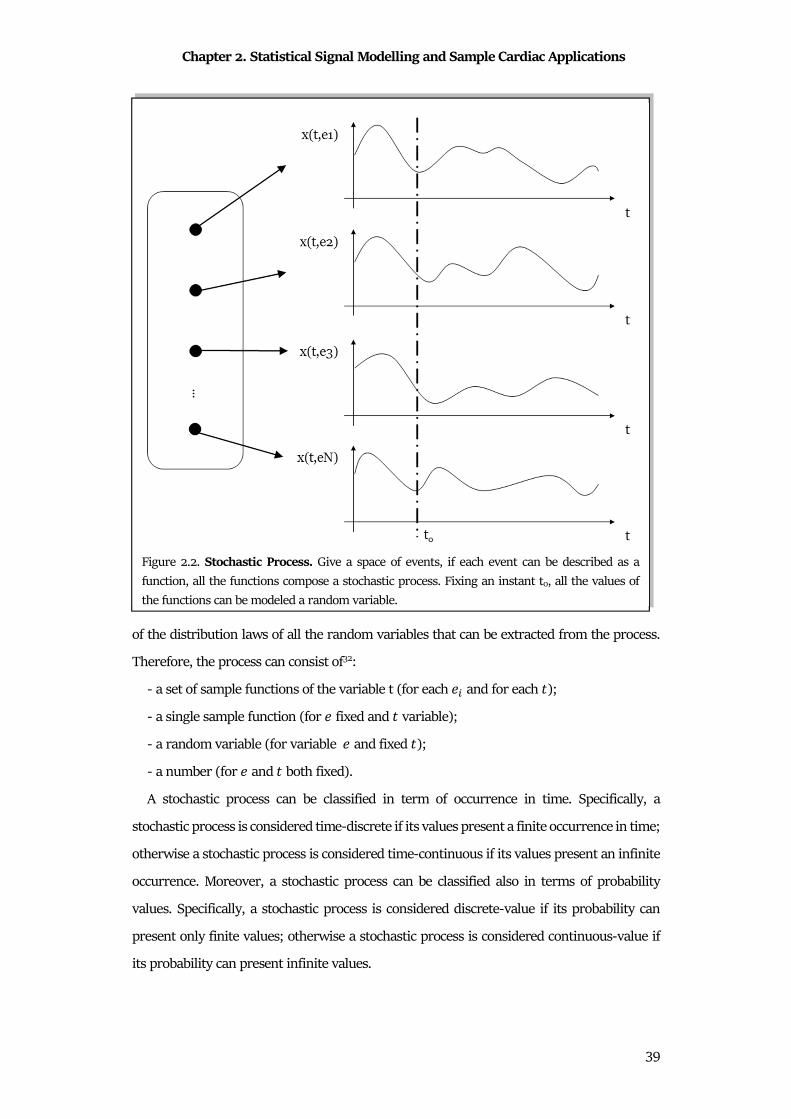
Chapter 2. Statistical Signal Modelling and Sample Cardiac Applications
39
of the distribution laws of all the random variables that can be extracted from the process.
Therefore, the process can consist of32:
- a set of sample functions of the variable t (for each � and for each �);
- a single sample function (for fixed and � variable);
- a random variable (for variable and fixed �);
- a number (for and � both fixed).
A stochastic process can be classified in term of occurrence in time. Specifically, a
stochastic process is considered time-discrete if its values present a finite occurrence in time;
otherwise a stochastic process is considered time-continuous if its values present an infinite
occurrence. Moreover, a stochastic process can be classified also in terms of probability
values. Specifically, a stochastic process is considered discrete-value if its probability can
present only finite values; otherwise a stochastic process is considered continuous-value if
its probability can present infinite values.
Figure 2.2. Stochastic Process. Give a space of events, if each event can be described as a
function, all the functions compose a stochastic process. Fixing an instant t0, all the values of
the functions can be modeled a random variable.
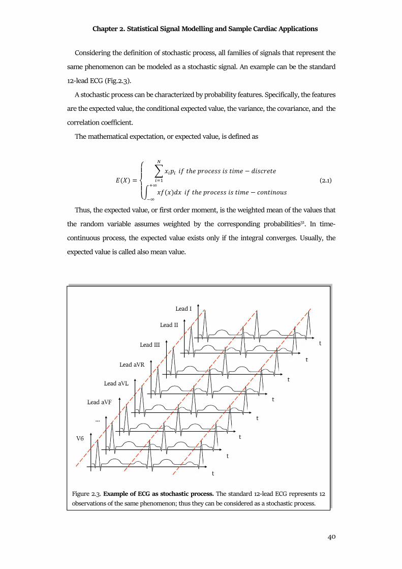
Chapter 2. Statistical Signal Modelling and Sample Cardiac Applications
40
Considering the definition of stochastic process, all families of signals that represent the
same phenomenon can be modeled as a stochastic signal. An example can be the standard
12-lead ECG (Fig.2.3).
A stochastic process can be characterized by probability features. Specifically, the features
are the expected value, the conditional expected value, the variance, the covariance, and the
correlation coefficient.
The mathematical expectation, or expected value, is defined as
$ �� =%&'&( ) *�+�
,�-� ." �/ +01� 22 .2 �.3 4.2�0 �
5 *" *�4*67�7 ." �/ +01� 22 .2 �.3 �18�.8192 (2.1)
Thus, the expected value, or first order moment, is the weighted mean of the values that
the random variable assumes weighted by the corresponding probabilities31. In time-
continuous process, the expected value exists only if the integral converges. Usually, the
expected value is called also mean value.
Figure 2.3. Example of ECG as stochastic process. The standard 12-lead ECG represents 12
observations of the same phenomenon; thus they can be considered as a stochastic process.
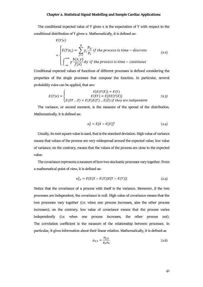
Chapter 2. Statistical Signal Modelling and Sample Cardiac Applications
41
The conditional expected value of Y given x is the expectation of Y with respect to the
conditional distribution of Y given x. Mathematically, it is defined as:
$ �|*�=
%&'&($ �|*.� = ) =. +.>+.
�>=1 ." �/ +01� 22 .2 �.3 4.2�0 �
5 = / *, =�" *� 4=�∞∞ ." �/ +01� 22 .2 �.3 �18�.8192
(2.2)
Conditional expected values of functions of different processes is defined considering the
properties of the single processes that compose the function. In particular, several
probability rules can be applied, that are:
$ �|*� = @ $[$ �|��] = $ ��$ ��� = $[�$ �|��]$ �� … �� = $ ��$ �� … $ �� ." �/ = �0 .84.+ 84 8� (2.3)
The variance, or second moment, is the measure of the spread of the distribution.
Mathematically, it is defined as:
DE� = $[� $[�]]� (2.4)
Usually, its root square value is used, that is the standard deviation. High value of variance
means that values of the process are very widespread around the expected value; low value
of variance, on the contrary, means that the values of the process are close to the expected
value.
The covariance represents a measure of how two stochastic processes vary together. From
a mathematical point of view, it is defined as:
DE,F� = ${$[� $ ��]$[� $ ��]} (2.5)
Notice that the covariance of a process with itself is the variance. Moreover, if the two
processes are independent, the covariance is null. High value of covariance means that the
two processes vary together (i.e. when one process increases, also the other process
increases); on the contrary, low value of covariance means that the process varies
independently (i.e. when one process increases, the other process not). The correlation coefficient is the measure of the relationship between processes. In
particular, it gives information about their linear relation. Mathematically, it is defined as
IE,F = DE,FDEDF (2.6)

Chapter 2. Statistical Signal Modelling and Sample Cardiac Applications
42
The values of the correlation coefficient can vary from -1 to �1. When it is �1, the processes
are perfectly correlated; when it is 0, the processes are uncorrelated; when it is -1, the
processes are inversely correlated.
The stochastic Gaussian process is a process composed of random variables distributed in
a Gaussian random vector. Assuming a defined expected value, the entire Gaussian process
is defined specified by the second moment, the variance. As linear transformations of
Gaussian random processes yield another Gaussian process, linear operations such as
differentiation, integration, linear filtering, sampling, and summation with other Gaussian
processes result in a Gaussian process33.
2.1.3 Stationarity and Ergodicity of Biological Signals
Stationarity and ergodicity are two fundamental assumptions of stochastic processes and
they are desirable in order to apply the conventional signal processing techniques.
A stochastic process is strictly stationary if its distribution is time-invariant, that is:
� � � L� = � L� (2.7)
when a process is strictly stationary, its probability does not vary over time.
Unfortunately, strict stationarity is often hard to verify and requires all moments to be
constant over time. To overcome this limitation, a process could be wide sense stationarity.
Under this condition, only the first two moments of the process have to be constant, the
expected value and the variance.
Thus, if all the moments of a process does not vary over time, the process is defined as strictly
stationary; if only the first two moments of a process do not vary over time, the process is
wide sense stationary.
If a stochastic process is wide sense stationary, the process is also wide sense ergodic if its
expected value and variance converge to their statistical quantities. It means that the process
can be studied with statistical techniques, having a single and sufficiently long sample path.
The ergodicity is essential in the estimation of the statistical quantities, where it ensures that
time series estimates serve as unbiased estimators of the considered statistical parameters31.
Stationary and ergodicity are essential, but not applicable in cardiac signal processing. In
fact, the nature of the cardiac signals is not stationary: the ANS applies continually its control
on the heart and, consequently, these signals are not constant in time. Moreover, intrinsic
variability and interferences can influence the cardiac signal, varying all their moments.
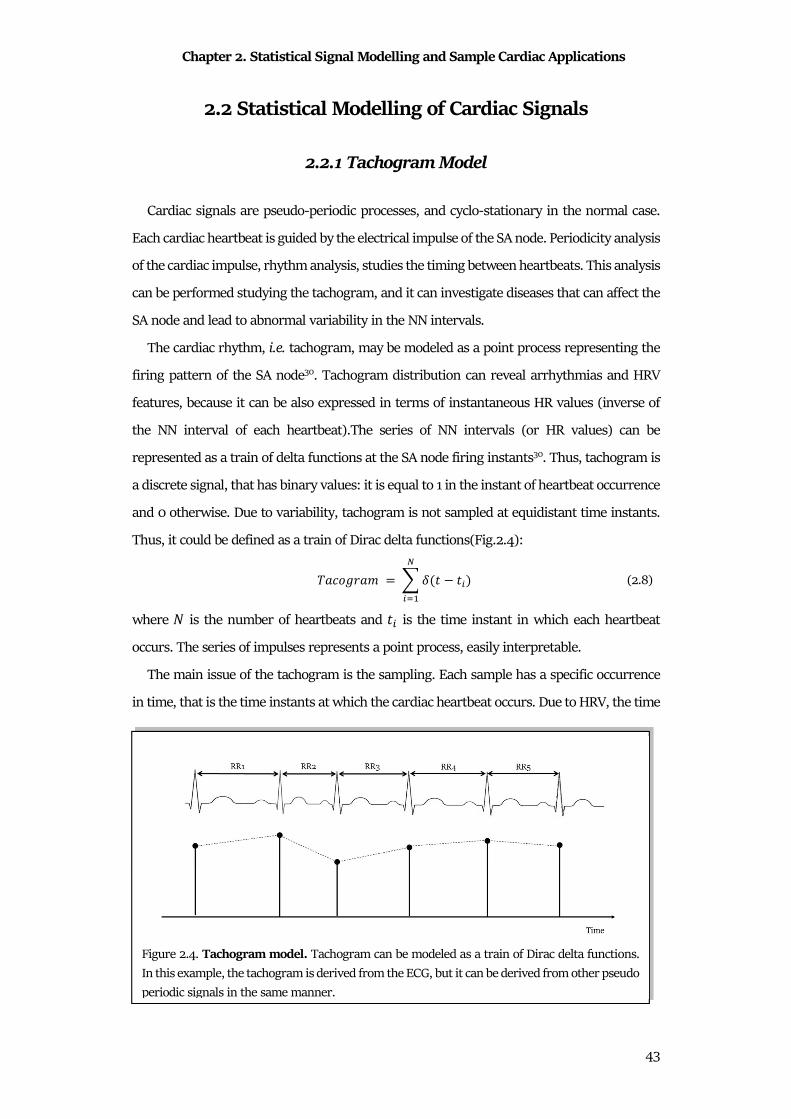
Chapter 2. Statistical Signal Modelling and Sample Cardiac Applications
43
2.2 Statistical Modelling of Cardiac Signals
2.2.1 Tachogram Model
Cardiac signals are pseudo-periodic processes, and cyclo-stationary in the normal case.
Each cardiac heartbeat is guided by the electrical impulse of the SA node. Periodicity analysis
of the cardiac impulse, rhythm analysis, studies the timing between heartbeats. This analysis
can be performed studying the tachogram, and it can investigate diseases that can affect the
SA node and lead to abnormal variability in the NN intervals.
The cardiac rhythm, i.e. tachogram, may be modeled as a point process representing the
firing pattern of the SA node30. Tachogram distribution can reveal arrhythmias and HRV
features, because it can be also expressed in terms of instantaneous HR values (inverse of
the NN interval of each heartbeat).The series of NN intervals (or HR values) can be
represented as a train of delta functions at the SA node firing instants30. Thus, tachogram is
a discrete signal, that has binary values: it is equal to 1 in the instant of heartbeat occurrence
and 0 otherwise. Due to variability, tachogram is not sampled at equidistant time instants.
Thus, it could be defined as a train of Dirac delta functions(Fig.2.4):
���1M0�3 = ) N � ���,�-� (2.8)
where � is the number of heartbeats and �� is the time instant in which each heartbeat
occurs. The series of impulses represents a point process, easily interpretable.
The main issue of the tachogram is the sampling. Each sample has a specific occurrence
in time, that is the time instants at which the cardiac heartbeat occurs. Due to HRV, the time
Figure 2.4. Tachogram model. Tachogram can be modeled as a train of Dirac delta functions.
In this example, the tachogram is derived from the ECG, but it can be derived from other pseudo
periodic signals in the same manner.
Chapter 2. Statistical Signal Modelling and Sample Cardiac Applications
44
interval between two consecutive samples is not constant; it means that the tachogram
presented a not-constant sampling in time. This issue represents a limitation in time domain
analysis, but it is a big issue in the frequency analysis. In order to solve it, generally a
correction is applied.
2.2.2 Electrocardiogram Model
ECG signal is the electrical activity of the heart. ECG waveform is quite constant for each
heartbeat of each leads and depends to the characteristics of the heart. ECG can be modeled
as the convolution of a point process (model of the heartbeat occurrence) with a
deterministic waveform, ECG standard pattern. The time interval between two consecutive
heartbeats is not constant and varies according with the ANS control. Thus, ECG is not
strictly stationary. In order to study it with the traditional techniques of signal processing, it
can be approximate as quasi-stationary process, limiting the observation in a small-time
window in which the same phenomenon is being produced. From a mathematical point of
view, ECG is modeled using a convolutional relationship:
$OP = 5 N � L� ∗ L� 4L (2.9)
where N is the point process representing the occurrence of the heartbeats (tachogram) and is the deterministic waveform of the ECG pattern. This is a simple model of the ECG: a
complex model should consider different patterns for each lead, for different age, for
different pathology, etc.
Being a deterministic signal, ECG is fully defined by its parameters. For example, ECG
amplitude can be defined as the maximum (usually R peak) minus the minimum of its
pattern. On the contrary, ECG interference can be model as stochastic process, specifically
gaussian. Thus, the amplitude of the interference is usually defined as four times standard
deviation of the noise34–38. these definitions are essential for soma biosignals application,
such as the signal-to-noise ratio (SNR) computation.
2.2.3 Phonocardiogram Model
PCG signal is an acoustic signal. The shape of the sound is varied according to the
phoneme to be produced; the system is therefore a time-variant system. PCG can be modeled
as the convolution of a point process (model of the heartbeat occurrence) with the random

Chapter 2. Statistical Signal Modelling and Sample Cardiac Applications
45
process that models heart sounds waveform. Clearly, as for the ECG signal, PCG cannot be
considered a stationary process, but it can be approximate as quasi-stationary if it is
observed in a short interval of time during which the same phoneme is being produced.
From a mathematical point of view, PCG is modeled using a convolutional relationship:
ROP = 5 N � L� ∗ 2 ��4L (2.10)
where N is the point process represented the occurrence of the heartbeats (tachogram) and 2 is the waveform of the heart sound. This is a simple model of the PCG, that presents
different waveforms (one for each heart sound).
As for the ECG, also PCG is a deterministic signal. Thus, its amplitude can be computed as
the maximum minus the minimum of the PCG pattern. Moreover, the PCG interference can
be modeled as a Gaussian distribution39,40.
Chapter 3. Signal Preprocessing and Sample Cardiac Applications
46
Chapter 3
Signal Preprocessing and Sample Cardiac
Applications
The second phase of biosignals processing is the preprocessing. Biomedical signals appear
usually covered by many other signals that are not of interest. Any signal that is different
from which of interest is considered as interference, artifact, or simply noise. The sources of
noise could be physiological, derived from instrumentation used, or the environment of the
experiment30.
Cardiac signals, such as other biomedical signals, are corrupted by noises. Considering
the physiology of these signals and the methods to record them, literature developed many
methods to filter them or to enhance their properties. Such of these techniques are signal
processing techniques (as digital filters), but other are statistical methods.
3.1 Standard Preprocessing of Signals
3.1.1 Linear Filtering
The most common filtering is the linear filtering. This preprocessing is usually
recommended when the frequency bands of the signal of interest and interference are
separated. The linear filters are defined in term of order and cutoff frequencies. The order
of a filter is the number of samples of delay that needs to obtain the output, while cutoff
frequencies are the frequency in which there an attenuation of -3dB. Standard linear filters
are the low-pass filter (to remove noise higher then cutoff frequency), high-pass filter (to
remove noise lower than cutoff frequency), band-pass filter (to remove noise out of a specific
frequency band) and stop-band filter (to remove noise in a specific band).
The perfect example of linear filtering is their application in ECG and VCG preprocessing.
ECG and VCG are usually corrupted by low-frequency noises (baseline wander), high-
frequency noises (electromyographic interference) and instrumentation noises (power-line).
Chapter 3. Signal Preprocessing and Sample Cardiac Applications
47
In order to remove the low-frequency noises, linear high-pass filters are usually used. The
American Heart Association defined two important recommendations in order to define the
optimal cut-off frequency of these filters. The first is the recommendations written in 1975:
AHA recommended a low cutoff frequency (3-dB down) of 0.05 Hz41. The definition of this
cut-off frequency was born from the consideration that this single-pole filter introduces no
distortion of ST segment and QT interval. The second is the recommendation written in
1990: American Heart Association recommended a lower-frequency cutoff (3-dB down) at
0.67 Hz that corresponds to a HR of 40 bpm, a 1 mV·s testing impulse for displacement and
slope evaluation and required less than 0.5 dB ripple over the range of 1 to 30 Hz. This
recommendation was born on the consideration that the longest RR interval corresponds to
the ECG lowest frequency components. Concerning the filters type, an analog high-pass filter
can introduce distortions of the ST segment if the cutoff frequency increases above 0.05 Hz.
This issue depends on the nonlinear phase41 of digital filters, such as Butterworth, that is an
infinite impulse response digital filter. On the other hand, a finite impulse response digital
filter (designed with a linear phase) introduces no ST-segment distortion, but it has longer
delay and needs special design considerations.
The high-frequency interference can be avoided applying linear low-pass filters.
Regarding the high cut-off frequency, the American Heart Association/American College of
Cardiology guidelines42 request a cut-off frequency of 150 Hz for adult and pediatric ECGs.
Moreover, literature suggested that the cutoff should be raised to 250 Hz or children41.
Finally, the power line noise can be removed during acquisition. Data acquisition analog
hardware at a very early stage is developed to reduce the line-frequency interference by
using common mode rejection circuitry design41. Some power line interference remains in
real ECG; thus, a line-frequency filter is applied constantly during ECG acquisitions. The
line-frequency filter is a band-rejection filter, which passes most frequencies unaltered, but
stops the specified band of frequencies from the −3 dB cutoffs fc1 to fc2. The stop bandwidth
(fc2-fc1) is typically narrow, as it is also called a notch filter41.
In ECG preprocessing, the standard preprocessing is performed applying a bidirectional
3rd-order Butterworth filter with cutoff frequencies of 0.5 Hz and 45 Hz. Sometimes, the
baseline removal is also applied. Baseline is usually computed as a cubic spline interpolation
of fiducial points, placed 0.08 s before R peaks. In paediatric/fetal application, the fiducial
points are placed 0.05 s before R peaks 35,36,43–48.
Chapter 3. Signal Preprocessing and Sample Cardiac Applications
48
3.1.2 Adaptive Filtering
When the signal of interest and the interference are not separated, but belong to same
frequency band, advanced methods have to be applied. One of it is the adaptive filtering, and
the perfect example of its application is the PCG preprocessing.
The PCG adaptive denoising usually are applied to remove external noise murmurs. The
main technique PCG is the adaptive noise canceller methods. These techniques need two
different acquisitions: the first record, called primary input, is the noisy PCG; while the
second record, the reference input, is the environmental noise correlated in some unknown
way with the primary noise. The reference input is filtered and subtracted from the primary
input to obtain the signal estimation49. Since both PCG and environmental noise vary in time,
the filter coefficients were adaptively adjusted in order to have a better approximation of the
PCG. The most used algorithms for these adjustments are least the mean square algorithm,
the normalized least mean square algorithm, the sub-band least mean square algorithm, the
sub-band normalized least mean square algorithm and the recursive least square
algorithm50.
3.1.3 Transformation Filtering
When adaptive filtering is not applicable (e.g. if there is no possibility to add a lead
recording for noise), signal transformation methods can be applied. The perfect example is
fetal PCG preprocessing: the signal of interest is the fetal PCG and it is surrounded by
internal mother murmurs. Thus, it is impossible to record only mother murmurs, without
fetal PCG.
Signal transform is the transformation of the signal from time domain to another, in order
to extract the information not observable in the original domain. The most popular
transformation technique is the Fourier transform, that transforms the time-domain signal
in the frequency-domain. The limit of Fourier transform applicability is the non-stationary
of the PCG: this transformation does not consider the variation in time. In order to overcome
this limitation, the short-time Fourier transform can be used51. The short-time Fourier
transform analyzes a small section of the signal at a time, which is known as windowing49.
The signal is decomposed in a time-frequency domain and the variations of the frequency
content of that signal within the time window function are revealed. The limitation of short-
time Fourier transform is the low resolution: a wide time window reflects a big resolution
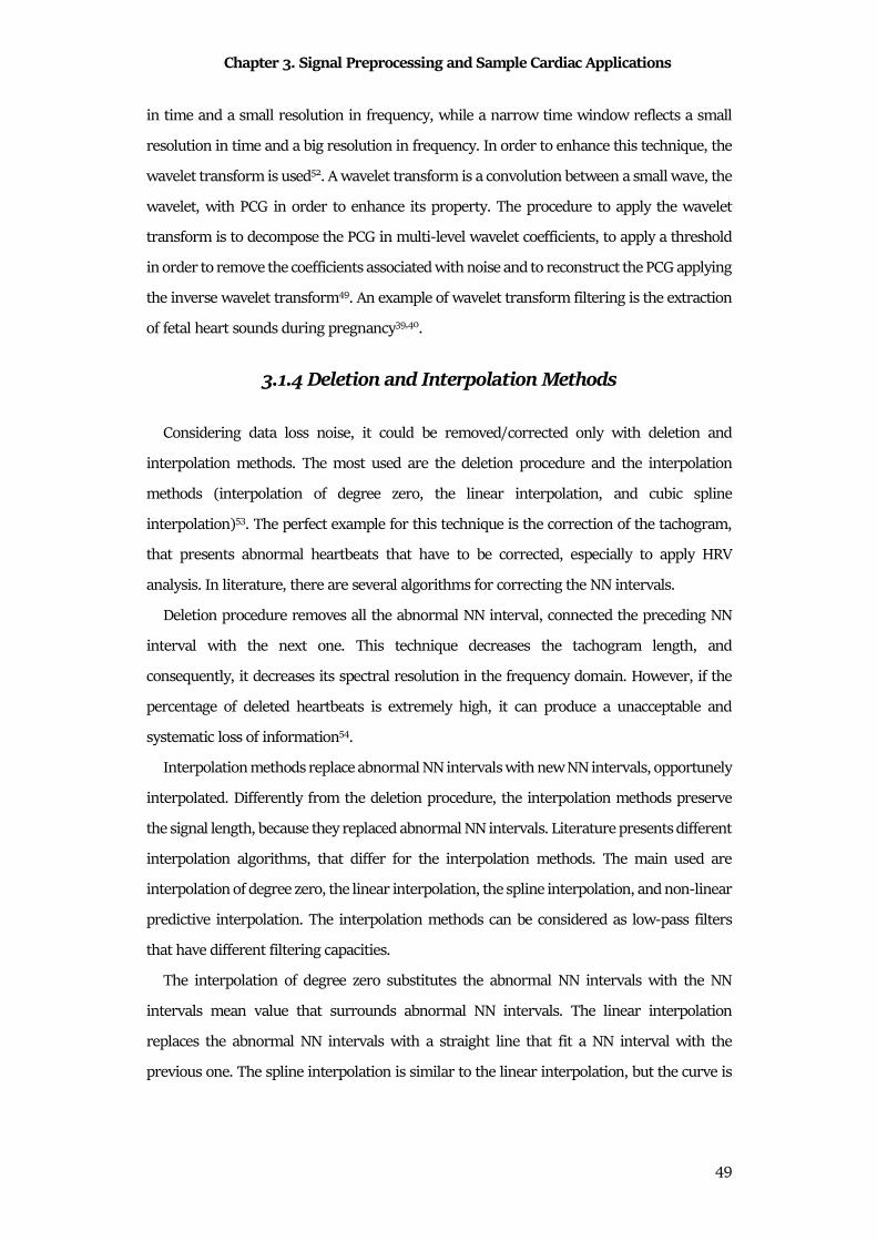
Chapter 3. Signal Preprocessing and Sample Cardiac Applications
49
in time and a small resolution in frequency, while a narrow time window reflects a small
resolution in time and a big resolution in frequency. In order to enhance this technique, the
wavelet transform is used52. A wavelet transform is a convolution between a small wave, the
wavelet, with PCG in order to enhance its property. The procedure to apply the wavelet
transform is to decompose the PCG in multi-level wavelet coefficients, to apply a threshold
in order to remove the coefficients associated with noise and to reconstruct the PCG applying
the inverse wavelet transform49. An example of wavelet transform filtering is the extraction
of fetal heart sounds during pregnancy39,40.
3.1.4 Deletion and Interpolation Methods
Considering data loss noise, it could be removed/corrected only with deletion and
interpolation methods. The most used are the deletion procedure and the interpolation
methods (interpolation of degree zero, the linear interpolation, and cubic spline
interpolation)53. The perfect example for this technique is the correction of the tachogram,
that presents abnormal heartbeats that have to be corrected, especially to apply HRV
analysis. In literature, there are several algorithms for correcting the NN intervals.
Deletion procedure removes all the abnormal NN interval, connected the preceding NN
interval with the next one. This technique decreases the tachogram length, and
consequently, it decreases its spectral resolution in the frequency domain. However, if the
percentage of deleted heartbeats is extremely high, it can produce a unacceptable and
systematic loss of information54.
Interpolation methods replace abnormal NN intervals with new NN intervals, opportunely
interpolated. Differently from the deletion procedure, the interpolation methods preserve
the signal length, because they replaced abnormal NN intervals. Literature presents different
interpolation algorithms, that differ for the interpolation methods. The main used are
interpolation of degree zero, the linear interpolation, the spline interpolation, and non-linear
predictive interpolation. The interpolation methods can be considered as low-pass filters
that have different filtering capacities.
The interpolation of degree zero substitutes the abnormal NN intervals with the NN
intervals mean value that surrounds abnormal NN intervals. The linear interpolation
replaces the abnormal NN intervals with a straight line that fit a NN interval with the
previous one. The spline interpolation is similar to the linear interpolation, but the curve is

Chapter 3. Signal Preprocessing and Sample Cardiac Applications
50
a third-degree polynomial, instead of a line. This technique is widely recommended when
NN interval contains ectopic heartbeats and artifacts53.
Finally, the non-linear predictive interpolation for NN interval artifact correction is based
on the fact that heartbeat-to-beat variations appear in a deterministic way. These advanced
methods use the chaos theory for locating ectopy-free portions of tachogram and
approximated a trajectory that most accurately can replace the tachogram segment referred
to the ectopic heartbeats55.
3.2 Statistical Preprocessing of Signals
Statistical methods for preprocessing fit well cardiac signals. In fact, the heart periodically
pumps blood into arteries provoking a pseudo periodic depolarization and repolarization
(ECG) and a pseudo periodic contraction and relaxation (PCG). These signals can be
decomposed in their heartbeats. Knowing landmarks (R peaks or S1), the heartbeats can be
separated and considered as single signals represented the same phenomenon. It means that
the statistical techniques can be used to extract the fundamental pattern, the clean heartbeat.
3.2.1 Averaging Methods
The averaging techniques are statistical methods that aims to extract the average patters
of a group of signals. Suppose to study a process composed by N signals. Each of this signal
is composed by P stochastic variables, and can be placed in a matrix X:
� = S*�,� ⋯ *�,U⋮ ⋱ ⋮*,,� ⋯ *,,UX (3.1)
If the N signals represents the same phenomenon, they are correlated and there is a
fundamental pattern common for all signals. It means that each column of the matrix X
represents the same variables: thus, each column of matrix can be considered as a random
distribution. This consideration allows to consider each variable as a distribution and,
consequently, allows to extract the expected value and the variance of each columns. The
expected values, or simply the averages, of all the variable distributions can be considered
as the average pattern of the process. The main content of the signal is the average pattern,
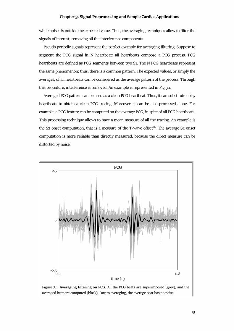
Chapter 3. Signal Preprocessing and Sample Cardiac Applications
51
while noises is outside the expected value. Thus, the averaging techniques allow to filter the
signals of interest, removing all the interference components.
Pseudo periodic signals represent the perfect example for averaging filtering. Suppose to
segment the PCG signal in N heartbeat: all heartbeats compose a PCG process. PCG
heartbeats are defined as PCG segments between two S1. The N PCG heartbeats represent
the same phenomenon; thus, there is a common pattern. The expected values, or simply the
averages, of all heartbeats can be considered as the average pattern of the process. Through
this procedure, interference is removed. An example is represented in Fig.3.1.
Averaged PCG pattern can be used as a clean PCG heartbeat. Thus, it can substitute noisy
heartbeats to obtain a clean PCG tracing. Moreover, it can be also processed alone. For
example, a PCG feature can be computed on the average PCG, in spite of all PCG heartbeats.
This processing technique allows to have a mean measure of all the tracing. An example is
the S2 onset computation, that is a measure of the T-wave offset56. The average S2 onset
computation is more reliable than directly measured, because the direct measure can be
distorted by noise.
Figure 3.1. Averaging filtering on PCG. All the PCG beats are superimposed (grey), and the
averaged beat are computed (black). Due to averaging, the average beat has no noise.
Chapter 3. Signal Preprocessing and Sample Cardiac Applications
52
3.2.2 Principal Components Analysis
The principal components analysis (PCA) is a way to identify patterns in different signals
and to express it in order to emphasize their similarities and differences. Usually, the dataset
is composed of many signals with different features: the PCA is able to reconstruct the
property of the signal without losing information. PCA is based on the idea to reduce the
dimensionality of a data set consisting of a large number of interrelated variables, while
retaining as much as possible of the variation present in the data set57. PCA transforms the
set of signals composed by correlated variables to a new set of variables, the principal
components (PCs), that are uncorrelated. Moreover, PCs are ordered according with their
intrinsic variation.
Suppose to have a process composed by N signals. Each of these signals is composed by P
stochastic variables. If these signals are the representation of the same phenomenon, they
are correlated. It means that there is a common pattern in all the signals, and that the
differences between them is due to interference. All these signals can be placed in a matrix:
� = S*�,� ⋯ *�,U⋮ ⋱ ⋮*,,� ⋯ *,,UX (3.2)
where the number of rows N represents the number of signals, while the number of columns
P represents the number of variables.
In order to study variances between signals and their common pattern, the covariance
matrix can be computed. Specifically, the covariance matrix between the rows emphasizes
the inter-signal pattern, while the covariance matrix between the columns emphasizes the
intervariable pattern. In this context, only the dissertation about the covariance matrix
between rows is presented, since the dissertation about the covariance matrix between
columns is perfectly specular.
The covariance matrix between the rows is:
OY �,� = Z DE[� ⋯ DE\E[ �⋮ ⋱ ⋮DE[E\ � ⋯ DE\� ] (3.3)
The covariance matrix could be decomposed in N principal components, PCs. Considering
the Rouché-Capelli theorem, this matrix is a homogeneous linear system that admits
solutions if:
4 �[OY �,� ^�] = 0. (3.4)
Chapter 3. Signal Preprocessing and Sample Cardiac Applications
53
The solutions are the eigenvalues (^_) and the eigenvectors (Lab ) of the covariance matrix.
The eigenvectors represent a basis: it is possible to obtain the original set of signals
projecting the data respect to all eigenvectors. Moreover, eigenvalues provide the order of
eigenvectors: the first eigenvector is associated with the highest eigenvalue and it is the
representation of the dataset considering the maxima percentage of variance. According
with that, the projection of the dataset considering only the first eigenvector provides the
first pattern that is in common among all signals. This first pattern is called first PC.
According to this, all components of signals can be computed using all eigenvectors.
The dimensionality reduction can be performed reducing the number of eigenvectors used
for the reconstruction of the dataset. Moreover, the dimensionality reduction is a good
method to remove the components of the signals that are not primary, that is the
interference or the noises. Considering that, the PCA is a good method for signal denoising.
PCA can be used as a denoising method for ECG signal. The starting point for the ECG
denoising by PCA is the segmentation of a noisy ECG in its heartbeats. Knowing the R peaks
position, a noisy heartbeat can be computed considering an ECG window around the R peak.
Accurate time alignment of the different noisy heartbeats is a key point in PCA, and special
care must be taken when performing this step58.
All the noisy heartbeat can be considered as observation and their samples as the measure
in time of the phenomenon. Thus, they can compose a matrix O, having N observations
(number of noisy heartbeats) and P variables (samples of noisy heartbeats):
Y = S$OP�. . .$OP,X. (3.5)
The noisy heartbeats can be considered as N observations of a random process; thus, they
can be analyzed with statistical techniques.
Considering that all the heartbeats of the same patient have similar morphology, their
common pattern can be considered as a clean heartbeat. The covariance matrix of the matrix
O can be computed are:
OY �,�= Z Dcde[ � ⋯ Dcde\cde[ �⋮ ⋱ ⋮Dcde[cde\ � ⋯ Dcde\ � ]. (3.6)
In order to extract the N principal components, the application of the Rouchè-Capelli
theorem allows to extract the eigenvalues (^_) and the eigenvectors (Lab ) of the covariance
matrix. The eigenvectors compose a transformation matrix, able to transform the N noisy
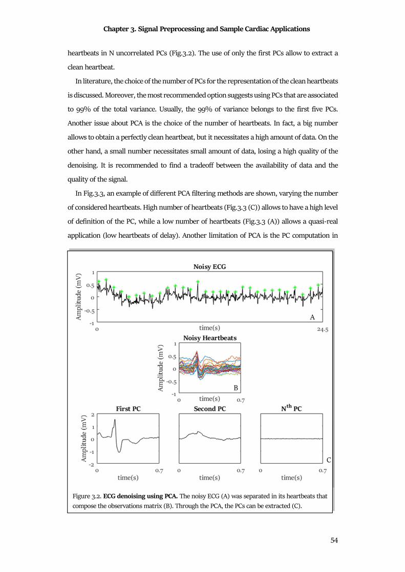
Chapter 3. Signal Preprocessing and Sample Cardiac Applications
54
heartbeats in N uncorrelated PCs (Fig.3.2). The use of only the first PCs allow to extract a
clean heartbeat.
In literature, the choice of the number of PCs for the representation of the clean heartbeats
is discussed. Moreover, the most recommended option suggests using PCs that are associated
to 99% of the total variance. Usually, the 99% of variance belongs to the first five PCs.
Another issue about PCA is the choice of the number of heartbeats. In fact, a big number
allows to obtain a perfectly clean heartbeat, but it necessitates a high amount of data. On the
other hand, a small number necessitates small amount of data, losing a high quality of the
denoising. It is recommended to find a tradeoff between the availability of data and the
quality of the signal.
In Fig.3.3, an example of different PCA filtering methods are shown, varying the number
of considered heartbeats. High number of heartbeats (Fig.3.3 (C)) allows to have a high level
of definition of the PC, while a low number of heartbeats (Fig.3.3 (A)) allows a quasi-real
application (low heartbeats of delay). Another limitation of PCA is the PC computation in
Figure 3.2. ECG denoising using PCA. The noisy ECG (A) was separated in its heartbeats that
compose the observations matrix (B). Through the PCA, the PCs can be extracted (C).

Chapter 3. Signal Preprocessing and Sample Cardiac Applications
55
presence of ectopic heartbeats. In these cases, PCs are distorted, thus an ectopic beat removal
algorithm is suggested.
The final step of the PCA could be the reconstruction of the original signal. In fact, the
clean heartbeat can be used as a template: the substitution of the original noisy heartbeats
with the template allows to obtain a clean ECG. Although the standard procedures required
to have a complete clean ECG tracing, such application of feature extraction require only a
clean heartbeat. In this application, the clean heartbeat can be used directly.
Figure 3.3. ECG denoising using PCA using different number of heartbeats.
Chapter 4. Feature Extraction and Sample Cardiac Applications
56
Chapter 4
Feature Extraction and Sample Cardiac
Applications
The third phase of signal processing is the feature extraction. Physiological and
pathological events are reflected in biosignals. Usually the evaluation about a single event is
reflected in the change of a characteristic of the signal, a variable. The variables that are of
interest for the specific problem are called features. Analysis of biosignals for monitoring or
diagnosis requires the features identification. Once an event has been identified, the
corresponding waveform may be segmented and analyzed in terms of its amplitude,
waveshape (morphology), time duration, intervals between events, energy distribution,
frequency content, and so on. Event detection is thus an important step in biomedical signal
analysis30.
As biomedical signals, the cardiac signals are intrinsic of features. The selection, the
extraction and the evaluation of cardiac features is one of the essential phases in cardiologic
diagnosis process. Specifically, the feature selection is the identification of the features that
are essential for the problem that has to be analyzed. Feature extraction is the practical
computation of them. Finally, the interpretation is based on the comparison of the value with
literature or on a statistical analysis.
This essential phase of the cardiac signal processing is full of biostatistics. The distribution
analysis, the relationships analysis and the statistical tests are maybe the most common
biostatistics techniques, and they represent the key for the evaluation of cardiac signals
features evaluation.
4.1 Feature Extraction
4.1.1 From Data to Distributions
In a clinical study, the population is the group of all data that represent the phenomenon
that has to be investigated. Generally, the collection of data of a population is difficult; thus,
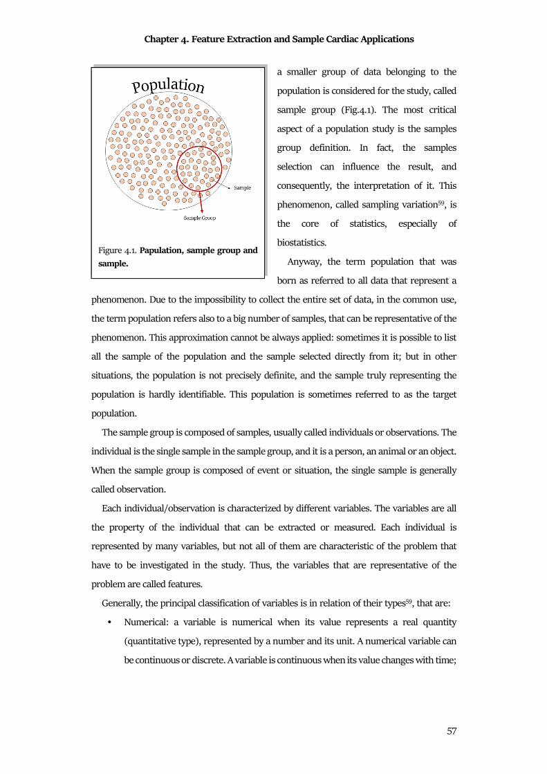
Chapter 4. Feature Extraction and Sample Cardiac Applications
57
a smaller group of data belonging to the
population is considered for the study, called
sample group (Fig.4.1). The most critical
aspect of a population study is the samples
group definition. In fact, the samples
selection can influence the result, and
consequently, the interpretation of it. This
phenomenon, called sampling variation59, is
the core of statistics, especially of
biostatistics.
Anyway, the term population that was
born as referred to all data that represent a
phenomenon. Due to the impossibility to collect the entire set of data, in the common use,
the term population refers also to a big number of samples, that can be representative of the
phenomenon. This approximation cannot be always applied: sometimes it is possible to list
all the sample of the population and the sample selected directly from it; but in other
situations, the population is not precisely definite, and the sample truly representing the
population is hardly identifiable. This population is sometimes referred to as the target
population.
The sample group is composed of samples, usually called individuals or observations. The
individual is the single sample in the sample group, and it is a person, an animal or an object.
When the sample group is composed of event or situation, the single sample is generally
called observation.
Each individual/observation is characterized by different variables. The variables are all
the property of the individual that can be extracted or measured. Each individual is
represented by many variables, but not all of them are characteristic of the problem that
have to be investigated in the study. Thus, the variables that are representative of the
problem are called features.
Generally, the principal classification of variables is in relation of their types59, that are:
• Numerical: a variable is numerical when its value represents a real quantity
(quantitative type), represented by a number and its unit. A numerical variable can
be continuous or discrete. A variable is continuous when its value changes with time;
Figure 4.1. Papulation, sample group and
sample.
Chapter 4. Feature Extraction and Sample Cardiac Applications
58
in contrast, a variable is discrete when it can be represented with only limited
numbers.
• Categorical: a variable is categorical when represents a nonquantifiable propriety
(qualitative type), represented by a label. Particular type of categorical variables is
the binary or dichotomic one, composed by the variables that have only two possible
values. Sometimes, the different categories of categorial variables have different
importance for the problem that have to be investigate, but they cannot be
represented as numbers. Thus, these variables are defined as ordered categorical
variables, whose categories can be considered to have a natural ordering.
A second variable classification refers to the collection of the variables. They could be
measured or derived. A variable is measured if it is directly recorded with an instrument or
with an observation. On the contrary, a variable is derived if it is computed as a combination
or categorization of measured variables. A variable can be derived in different ways. The
first is to calculate or to categorize a variable from recorded variables. In this case the new
variable can be a numerical value computed as the composition of other numerical variables;
or a categorical variable defined from a thresholding of numerical variable; or a categorical
variable defined from the combination of criteria on one or several categorical variables.
Another way is to define a categorical value in relation to a reference curve, based on
standard population values. Finally, it is possible to define a variable transforming it in order
to allow the application of relevant statistical methods. This process is applied when the
numerical values in the sample group cannot be modeled with the classical statistical
methods; thus, some transformation procedures allow to transform it in a standard way.
All variables computed for the sample group could be formally grouped using
distributions. The distribution is the formal representation of a variable that belongs to
sample group. The computation of the distributions depends of the type of the variable but
is based on the concept of frequency. In fact, the distribution is the representation of how
many times a variable of the sample group has a specific numerical value or belong to a
specific category. Distributions are more useful if the sample group size is large, because
these representations allow to underline the sample group properties, and indirectly
population properties. Thus, the first step in biostatistical modeling is to form a variable
distribution.
If the variables are categorical, the distribution is computed counting the number of
individuals that have the variable in each category; the number of individuals in a category
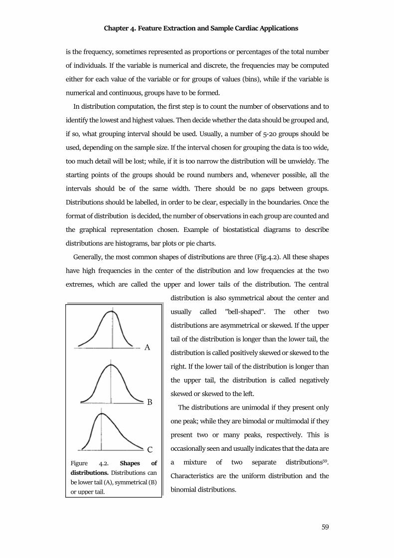
Chapter 4. Feature Extraction and Sample Cardiac Applications
59
is the frequency, sometimes represented as proportions or percentages of the total number
of individuals. If the variable is numerical and discrete, the frequencies may be computed
either for each value of the variable or for groups of values (bins), while if the variable is
numerical and continuous, groups have to be formed.
In distribution computation, the first step is to count the number of observations and to
identify the lowest and highest values. Then decide whether the data should be grouped and,
if so, what grouping interval should be used. Usually, a number of 5-20 groups should be
used, depending on the sample size. If the interval chosen for grouping the data is too wide,
too much detail will be lost; while, if it is too narrow the distribution will be unwieldy. The
starting points of the groups should be round numbers and, whenever possible, all the
intervals should be of the same width. There should be no gaps between groups.
Distributions should be labelled, in order to be clear, especially in the boundaries. Once the
format of distribution is decided, the number of observations in each group are counted and
the graphical representation chosen. Example of biostatistical diagrams to describe
distributions are histograms, bar plots or pie charts.
Generally, the most common shapes of distributions are three (Fig.4.2). All these shapes
have high frequencies in the center of the distribution and low frequencies at the two
extremes, which are called the upper and lower tails of the distribution. The central
distribution is also symmetrical about the center and
usually called "bell-shaped". The other two
distributions are asymmetrical or skewed. If the upper
tail of the distribution is longer than the lower tail, the
distribution is called positively skewed or skewed to the
right. If the lower tail of the distribution is longer than
the upper tail, the distribution is called negatively
skewed or skewed to the left.
The distributions are unimodal if they present only
one peak; while they are bimodal or multimodal if they
present two or many peaks, respectively. This is
occasionally seen and usually indicates that the data are
a mixture of two separate distributions59.
Characteristics are the uniform distribution and the
binomial distributions.
Figure 4.2. Shapes of
distributions. Distributions can
be lower tail (A), symmetrical (B)
or upper tail.
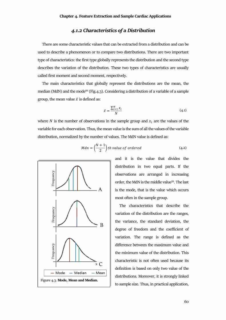
Chapter 4. Feature Extraction and Sample Cardiac Applications
60
4.1.2 Characteristics of a Distribution
There are some characteristic values that can be extracted from a distribution and can be
used to describe a phenomenon or to compare two distributions. There are two important
type of characteristics: the first type globally represents the distribution and the second type
describes the variation of the distribution. These two types of characteristics are usually
called first moment and second moment, respectively.
The main characteristics that globally represent the distributions are the mean, the
median (MdN) and the mode59 (Fig.4.3). Considering a distribution of a variable of a sample
group, the mean value * is defined as:
* = ∑ *�,�-�� (4.1)
where � is the number of observations in the sample group and *� are the values of the
variable for each observation. Thus, the mean value is the sum of all the values of the variable
distribution, normalized by the number of values. The MdN value is defined as:
�48 = h� � 12 i �/ j�k9 1" 104 0 4 (4.2)
and it is the value that divides the
distribution in two equal parts. If the
observations are arranged in increasing
order, the MdN is the middle value59. The last
is the mode, that is the value which occurs
most often in the sample group.
The characteristics that describe the
variation of the distribution are the ranges,
the variance, the standard deviation, the
degree of freedom and the coefficient of
variation. The range is defined as the
difference between the maximum value and
the minimum value of the distribution. This
characteristic is not often used because its
definition is based on only two value of the
distributions. Moreover, it is strongly linked
to sample size. Thus, in practical application,
Figure 4.3. Mode, Mean and Median.
Chapter 4. Feature Extraction and Sample Cardiac Applications
61
the interquartile range (IQR) is more used. IQR is defined as the difference between the 75th
percentiles (upper quartile) minus the 25th percentile (lower quartile) of the distribution. It
is also called midspread, middle 50%, or H-spread. This range is less dependent to the
sample group size and it is more stable than the range. The variance is defined in terms of
the deviations of the observations from the mean59. If the variance is small, the values of the
distribution are very close to the mean value; otherwise, if the variance is high, the values
are diffused around the mean value. Mathematically the variance is defined as:
D� = ∑ * *��,�-� � 1� (4.3)
the simple mean value of the deviations is not recommendable: the positive deviations
(above the mean value) balance the negative deviations (below the mean value), providing
a variance equal to zero. Thus, usually, the signed is ignored and the variance is computed
as the average of the squares of the deviations. Note that the denominator is � 1, that
corresponds to degrees of freedom of the variance59. It reflects the number of deviations that
are independent each other: the last one can be calculated indirectly from the others. The
limit of the variance is its unit: in fact, the unit of the variance is the square of the unit of the
distribution values. In order to avoid this formal limitation, it is more convenient to express
the variation in the original units by taking the square root of the variance, that is standard
deviation (D). Note that the standard deviation is essential also to interpret the distribution
value. In fact, mathematically, the 70% of the distribution value fall in one standard
deviation range; while the 90% fall in two standard deviation range59. Thus, the standard
deviation could be a useful measure of the distribution range.
From the standard deviation, the coefficient of variation could be computed as:
�j = D* × 100% (4.4)
This coefficient represents the standard deviation as the percentage of the mean value. It
could be used when the interest is the size of the variation, independently of sample size59.
4.1.3 The Normal Distribution
Distributions can be appeared in different forms, but the most used is the Gaussian
distribution or Normal distribution.
The normal frequency distribution (Fig.4.4) is a bell-shaped distribution, symmetrical
about the mean. It is univocally defined by two characteristics, its mean and its standard
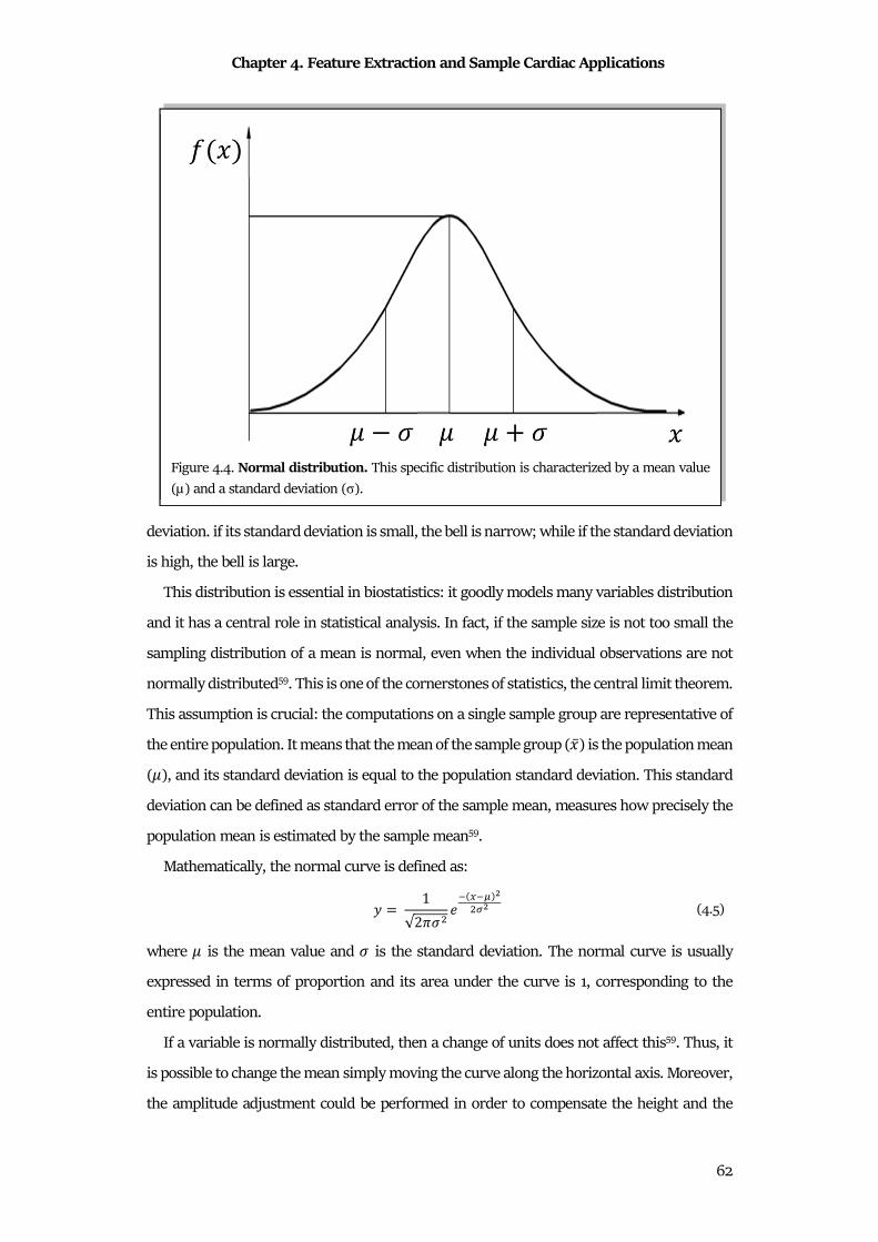
Chapter 4. Feature Extraction and Sample Cardiac Applications
62
deviation. if its standard deviation is small, the bell is narrow; while if the standard deviation
is high, the bell is large.
This distribution is essential in biostatistics: it goodly models many variables distribution
and it has a central role in statistical analysis. In fact, if the sample size is not too small the
sampling distribution of a mean is normal, even when the individual observations are not
normally distributed59. This is one of the cornerstones of statistics, the central limit theorem.
This assumption is crucial: the computations on a single sample group are representative of
the entire population. It means that the mean of the sample group (*) is the population mean
(n), and its standard deviation is equal to the population standard deviation. This standard
deviation can be defined as standard error of the sample mean, measures how precisely the
population mean is estimated by the sample mean59.
Mathematically, the normal curve is defined as:
= = 1√2oD� � p�q�r�sr (4.5)
where n is the mean value and D is the standard deviation. The normal curve is usually
expressed in terms of proportion and its area under the curve is 1, corresponding to the
entire population.
If a variable is normally distributed, then a change of units does not affect this59. Thus, it
is possible to change the mean simply moving the curve along the horizontal axis. Moreover,
the amplitude adjustment could be performed in order to compensate the height and the
Figure 4.4. Normal distribution. This specific distribution is characterized by a mean value
(µ) and a standard deviation (σ).
Chapter 4. Feature Extraction and Sample Cardiac Applications
63
width of the curve. Practically, the normal curve is usually change in order to have a zero
mean and a standard deviation equal to 1. Thus, characteristic distribution is the standard
normal distribution. Mathematically, it is:
= = 1√2o �pr� (4.6)
In order to compute the standard normal distribution for a normal distribution, the original
values * have to be subtracted by their mean value n and divided by their standard deviation D. The relation is:
t = * nD (4.7)
The value t is called standard normal deviate, or z-score.
Two important features of the normal distribution are the area under the curve and the
percentage points.
The area under the curve can be used to determine the proportion of the population that has
values in some specified range. Moreover, it could represent the probability that an
individual observation from the distribution will lie in the specified range. Being the total
area under the curve equal to 1, the probability that an observation lies somewhere could
be express in term of percentage.
The percentage points are specific points in the normal distribution that are
representative of distribution. Specifically, they can be defined from the z-score. As
explained, the z-score expresses the value of a variable in terms of the number of standard
deviations it is away from the mean59. Thus, it possible to compute the percentage of data
within a specific range considering the mean and the standard deviation of the distribution.
Specifically, these percentage points can be used to compute the confidence intervals, that
are the intervals in which the 95% of the values fall. Exactly 95% of the distribution lies
between -1.96 and 1.96 in a standard normal distribution. Moreover, the percentage points
are used in order to computer the P-values and compare different distributions (described
below) by the hypothesis tests. The values of the percentage points are usually reported in
tables and normalize for the standard normal distribution. Due to the symmetric nature of
the normal distribution, the values are usually provided for only one side59.
Chapter 4. Feature Extraction and Sample Cardiac Applications
64
4.1.4 The confidence intervals
The confidence intervals are defined as the intervals in which there is the 95% probability
that the population mean lies within. If the sample size is large enough, the distribution can
be modelled as normal (central limit theorem). Thus, considering the percentage points,
95% of samples means would lie within 1.96 standard errors above or below the population
mean, since 1.96 is the two-sided 5% point of the standard normal distribution.
If the sample size is small, the central limit theorem is not applicable, and two aspects
may alter. Firstly, the sample standard deviation is itself subject to sampling variation, thus
it cannot approximate the standard deviation; than the distribution in the population is not
normal and the distribution of the sample mean may also be non-normal. Thus, is not
possible to use the normal distribution in order to compute the confidence intervals. Instead,
a distribution called the T distribution is used.
Finally, in case of strong non-normality, it is recommendable to transform the distribution
in a T distribution or in a normal distribution. If it is not possible, an alternative is to calculate
a non-parametric confidence interval or to use bootstrap methods59.
4.2 Statistical Feature Comparison
The concept of statistical distribution is essential for comparison analysis. If there are two
group of features that have to be evaluated, statistical comparison can be useful to
understand if they represent the same measure or if they are completely different.
Suppose to have two sample groups, labelled A and B. Features of each group can be
represented as distributions and the two mean values are *u and *v. These two groups
could represent a lot of situations, in which could be of interest to discover if they represent
the same phenomenon or two different phenomena. Thus, specifically, a method to compare
distributions is needed an it has to answer to two important questions, that are59:
1. What does the difference between the two group means in our sample (*u and *v)
tell us about the difference between the two group means in the population?
2. Do the data provide evidence that the exposure actually affects the outcome, or
might the observed difference between the sample means have arisen by chance?
In order to answer to these questions, the statistical methods to compare the two groups
and to quantify their difference have to be explained. These methods are the hypothesis tests,
Chapter 4. Feature Extraction and Sample Cardiac Applications
65
or better, the statistical tests. Several tests are defined in literature in order to solve different
types of clinical situations. The criteria for statistical comparison could be different,
depending to the statistical test that is used, but the results can be interpreted in the same
manner.
Each statistical test computes an index, that is a measure of the similarity between the
groups and gives the name to the respective test. This index has to be compared with values
reported in literature (usually in forms of tables) in order to evaluate its statistical
significance. Thus, the results of a statistical test are the significance, associated with a
numerical value, the P-value. The significance indicates if the two distributions can be
considered similar or not (0 or 1 if the null hypothesis is accepted or not, respectively).
Specifically, if the hypothesis is null (0 or null hypothesis accepted), the groups can be
considered similar; if the hypothesis is not null (1 or null hypothesis rejected), the two groups
are considered different. Associated with this dichotomic value, the test provides the P value.
This numerical value, ranged from 0 to 1, reflects the probability to get difference between
the two groups. If the probability is high (high P value close to 1), the null hypothesis is
accepted, and the groups can be considered similar; while, if the probability is low (low P
value close to 0), the null hypothesis is rejected, and the two groups are considered different.
The statistical significance level (w) is defined as the threshold to decide if a P value is high
or low. Usually, in clinical setting, the statistical significance level is set to 0.05%.
Data can be continuous, discrete, binary, or categorical and distributed according to
different distribution shapes. Moreover, different kinds of problems can be investigated.
Each statistical investigation has to be approached using its point of view and the choice of
the specific test is essential. The choice of the correct statistical test is completely linked to
the nature of data and to the nature of the problem. In order to perform the correct statistical
test, it is important to consider the nature of the distribution (normal or not-normal), the
nature of data (categorical, numerical, etc.), the nature of the comparison (paired or
unpaired features; comparison considering one or two tails) and others. For these
evaluations, the choice of the correct statistical test is not easy.
The standard classification of the statistical test follows the nature of the distribution: a
statistical test is defined as parametric if the distributions that have to be compared are
normal; a statistical test is defined as nonparametric if both or one of the distributions are
not-normal. Several statistical tests, such as the Lilliefors test, can be used to evaluate the
normality of a distribution.
Chapter 4. Feature Extraction and Sample Cardiac Applications
66
4.2.1 Parametric Tests
Parametric tests are the statistical tests based on the assumptions that the distributions
of the groups are normal. These statistical tests are more robust and require less data than
nonparametric tests60.
To apply a parametric test, three parameters of the data distribution have to be assumed.
The first is that the data distributions in the two groups has to be normal. Secondly, the
groups variances and the standard deviations have to be the same. Finally, data distributions
have to be continuous. The most common parametric statistical tests are the student T-test
and the ANOVA test.
The most used parametric test is the student T-test. This common test is usually used to
determine if the mean value of a sample group (A) is different or not from a known mean
value (single sample T-test). Moreover, it is also used to establish if two groups (A and B)
have the same mean values (two sample T-test). The student T-test uses the mean values,
the standard deviation, the sample size of the considered groups and the statistical
significance level. The null hypothesis is accepted if the mean value of the distribution is
similar to the known mean value (single sample T-test) or if the two groups present similar
mean values (two sample T-test). On the contrary, the null hypothesis is rejected if the mean
value of the distribution is different from the known mean value (single sample T-test) or if
the two groups present different mean values (two sample T-test). The index to define the
significance and the P-value in the student T-test is the index t, computed as:
� = %&'&( *uxxx *2 .8 2.8Mk 2�3+k � � 2�
*uxxx *vxxx2 y �u�v�u � �v .8 �z1 2�3+k � � 2� (4.8)
where *uxxx and *vxxx are the mean values of the sample groups, �u and �v are the sample size
of groups and 2 is the mean standard deviation of the standard deviation (only the standard
deviation of the group A in the single sample T-test). If the t index is close to zero, the mean
values are the same and the distributions are similar (null hypothesis accepted); while if the
t index is high, the mean values, and consequently the distributions, are different (null
hypothesis rejected).
The ANOVA test is the acronym of analysis of variance60. This parametric test is widely
used to evaluate if two or more groups (��, … , �,) can be considered as similar or different.
It considers both means and variances to define the statistical significance. The null
Chapter 4. Feature Extraction and Sample Cardiac Applications
67
hypothesis is accepted if variances of groups can be considered similar; while the null
hypothesis rejected if the variances of groups are different. The index to define the
significance and the P-value in ANOVA is the index F, computed as:
� = �DEx�DE�xxx (4.9)
where � is the sample size in each group, DEx� is the variance of the mean values of the sample
groups and DE�xxxx is the mean value of variances of the sample groups. If the F index is close to
1, the variance of the mean values and the mean values of variances are similar, that means
that the variances in groups are similar (null hypothesis accepted); while if the F index is
high, the variances, and consequently the distributions, are different (null hypothesis
rejected). The ANOVA concept was enlarged also for the comparison between more features
between two groups (MANOVA-Multivariate analysis of variance) or to investigate also the
covariates between the groups (ANCOVA-Analysis of covariance), increasing the
mathematical complexity, although the concepts remain the same60.
4.2.2 Non-Parametric Tests
The nonparametric tests are applied if one of the parametric criteria are not
applicable47,56,61,62. Nonparametric tests are always the last choice in statistics, because their
robustness is not strong as parametric one and requires more data. Thus, is always
preferable trying to transform the nonparametric distribution in parametric distribution.
But if this transformation is not applicable, last choice is the nonparametric tests60. The most
common nonparametric statistical tests are the chi-squared test, the Mann-Whitney U test
and the Kruskal-Wallis test.
The chi-squared test is a nonparametric test for categorical data, specifically binary data.
It compares the percentages of data in each category. The null hypothesis is accepted if the
percentage of data in each category can be considered similar to the others; while the null
hypothesis rejected if the percentage of data in each category are different. The index to
define the significance and the P-value in the chi-squared test is the chi-squared, computed
as:
{� = Y $��$ (4.10)
where Y is the observed percentage, while $ is the expected percentage. Considering the
sample size in the category and their obtained percentages, the expected percentage is
Chapter 4. Feature Extraction and Sample Cardiac Applications
68
computed. If the {� index is close to zero, the obtained percentage is similar to the expected
percentage, and the two categories are similar (null hypothesis accepted); while if the {�
index is high, the percentages of the categories are different (null hypothesis rejected)60.
The Mann-Whitney U-test, sometimes called Wilcoxon ranksum test, is very similar to the
Student T-test. Due to the not-normal distributions of data, the U-test cannot consider the
mean value and the standard deviation. Thus, it is a rank-based method and considered the
MdN value. Equivalently to T-test, U-test could be used to investigate if the MdN value of a
sample group (A) is different or not from the MdN value of a second sample group (B). For
the applicability of this test, the ranks of the samples of groups and their sample sizes are
essential. The null hypothesis is accepted if the two groups present similar MdN values;
while the null hypothesis is rejected if MdN values of distributions are different. The index
to define the significance and the P-value in the U-test is the index U, computed for both
samples group as:
|u = ) ��u,}�-� �u �u � 1�2
|v = ) �~v,�~-� �v �v � 1�2
(4.11)
where �u and �v are the groups sample size, and �u and �v are the ranks of the samples
in the groups A and B, respectively. The considered ranks are computed considering all
samples as a unique distribution. If |u is close to |v, the MdN value of the group A is similar
to the MdN value of group B and the distributions are similar (null hypothesis accepted);
while if the intervals between |u and |v is large, the MdN values are different as the
distributions (null hypothesis rejected).
Finally, the Kruskal-Wallis test is the corresponding nonparametric test to ANOVA test60.
As for the U-test, the Kruskal-Wallis test computes the sum of the ranks of the samples for
each sample group and then compares the indices. As for the ANOVA, also the Kruskal-Wallis
test could be used to evaluate multivariate problems and covariate proprieties.
4.3 Statistical Feature Association
Sometimes, the simple consideration about the similarity/difference between two
distributions is not sufficient. Some studies necessities to evaluate the linkage between two
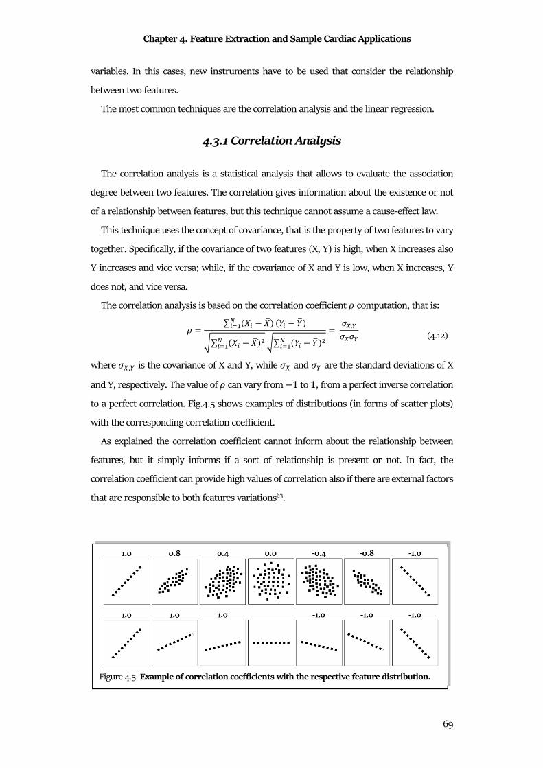
Chapter 4. Feature Extraction and Sample Cardiac Applications
69
variables. In this cases, new instruments have to be used that consider the relationship
between two features.
The most common techniques are the correlation analysis and the linear regression.
4.3.1 Correlation Analysis
The correlation analysis is a statistical analysis that allows to evaluate the association
degree between two features. The correlation gives information about the existence or not
of a relationship between features, but this technique cannot assume a cause-effect law.
This technique uses the concept of covariance, that is the property of two features to vary
together. Specifically, if the covariance of two features (X, Y) is high, when X increases also
Y increases and vice versa; while, if the covariance of X and Y is low, when X increases, Y
does not, and vice versa.
The correlation analysis is based on the correlation coefficient I computation, that is:
I = ∑ �� �x�,�-� �� �x�
�∑ �� �x��,�-� �∑ �� �x��,�-�= DE,FDEDF
(4.12)
where DE,F is the covariance of X and Y, while DE and DF are the standard deviations of X
and Y, respectively. The value of I can vary from 1 to 1, from a perfect inverse correlation
to a perfect correlation. Fig.4.5 shows examples of distributions (in forms of scatter plots)
with the corresponding correlation coefficient.
As explained the correlation coefficient cannot inform about the relationship between
features, but it simply informs if a sort of relationship is present or not. In fact, the
correlation coefficient can provide high values of correlation also if there are external factors
that are responsible to both features variations63.
Figure 4.5. Example of correlation coefficients with the respective feature distribution.

Chapter 4. Feature Extraction and Sample Cardiac Applications
70
Sometimes, the correlation coefficient can be used to evaluate if two variables represents
the same property. An example is the indirect measure of QT interval using the PCG S1S2
interval. In normal condition, the ratio between QT and S1S2 is equal to 1. It means that
their distributions in the same sample group correlate (ρ=0.60)56.
4.3.2 Linear Regression Analysis
Differently for the correlation analysis, the linear regression analysis can inform about
the cause-effect law between two features. The regression analysis is a statistical technique
that links two features using a specific curve; if the curve is a line, the regression analysis is
linear. In literature several type of regression analyses (in Chapter 5 logistic regression will
be presented) exist, varying the curve used to fit data. The procedure is the same for all the
methods: the curve that has to fit data is chosen; the two features become the input of the
model and its parameters that define the curve are estimated, minimizing the distances
between the features and the curve.
Suppose to investigate about the relationship of two features, � and �, and, specifically,
to define if a variation of the feature X linearly provokes a variation in the feature �. The
linear regression analysis tries to find the linear relationship between these two features.
Specifically, if this relation exists, there is an optimal line that describes the linkage between � and �. This optimal line will be:
�� = � � �� (4.13)
Once the relationship is set, the problem of the analysis is to estimate the parameters of the
curve, the values of � and �. Considering the definition of variance: it is the sum of the
differences between the feature values in the sample group and the mean value. Thus,
variances can be also considered as a measure of error. In fact, an error is the difference
between an obtained value (feature values in the sample group) and the expected value
(value of the curve). Thus, the variances (�) of the feature of samples group are the errors
between each feature value and the optimal line, as:
� = )��� �����,�-� = )[�� � � ����]�,
�-� (4.14)
Considering that, the line that better fit the data is the line that minimizes the error �. This
is a differential equation system describer by the formulas:
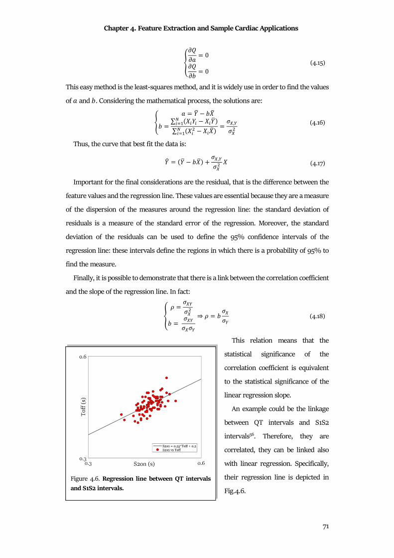
Chapter 4. Feature Extraction and Sample Cardiac Applications
71
����� = 0���� = 0 (4.15)
This easy method is the least-squares method, and it is widely use in order to find the values
of � and �. Considering the mathematical process, the solutions are:
@ � = �x ��x� = ∑ ���� ���x�,�-�∑ ��� ���x�,�-� = DE,FDE� (4.16)
Thus, the curve that best fit the data is:
�� = �x ��x� � DE,FDE� � (4.17)
Important for the final considerations are the residual, that is the difference between the
feature values and the regression line. These values are essential because they are a measure
of the dispersion of the measures around the regression line: the standard deviation of
residuals is a measure of the standard error of the regression. Moreover, the standard
deviation of the residuals can be used to define the 95% confidence intervals of the
regression line: these intervals define the regions in which there is a probability of 95% to
find the measure.
Finally, it is possible to demonstrate that there is a link between the correlation coefficient
and the slope of the regression line. In fact:
� I = DEFDE�� = DEFDEDF⇒ I = � DEDF (4.18)
This relation means that the
statistical significance of the
correlation coefficient is equivalent
to the statistical significance of the
linear regression slope.
An example could be the linkage
between QT intervals and S1S2
intervals56. Therefore, they are
correlated, they can be linked also
with linear regression. Specifically,
their regression line is depicted in
Fig.4.6.
Figure 4.6. Regression line between QT intervals
and S1S2 intervals.
Chapter 5. Classification Analysis and Sample Cardiac Applications
72
Chapter 5
Classification Analysis and Sample Cardiac
Applications
Once features extraction is complete, the last phase of the signal processing is the
classification. The objectives of classification are: to investigate different methods to classify
a signal/feature into a specific class; to explore the importance of a signal/feature and of the
classification method in arriving at a good diagnostic decision about the patient; to discover
the differences between the signals/features belonging to different classes in order to
discover new diagnostic criteria or validate the old ones. Thus, a classification method may
facilitate the labeling of a given signal/feature as being a member of a particular class. This
can help to arrive at a diagnosis, without consider other further clinical investigations to
obtain information. Although it is common to work with a pre-specified number of pattern
classes (classification problems), many problems do exist where the number of classes is not
a priori known (clustering problems). Statistical methods or algorithm that classify data are
called classifier.
5.1 Statistics for Classification
In order to evaluate if a method classifies data correctly or not, some statistical instrument
can measure its performances.
Formally, a classifier assigns class labels to each element (signal or feature) that it has to
classify. The performance of the classifier is evaluated for each class. It means that all
elements of the population can be labelled as belonged to the specific class (positive) or not
belonged to a specific class (negative). These labels are call predicted classes and they
represent the classification provided by the classifier. Usually, the correct classification is
known, and its labels are called targets. The targets are essential: in fact, the performances
of the classifier can be computed only if the correct classification is a priori known. In case
of no availability of targets, the standard methods of classification cannot be applied, and
clustering methods are used.
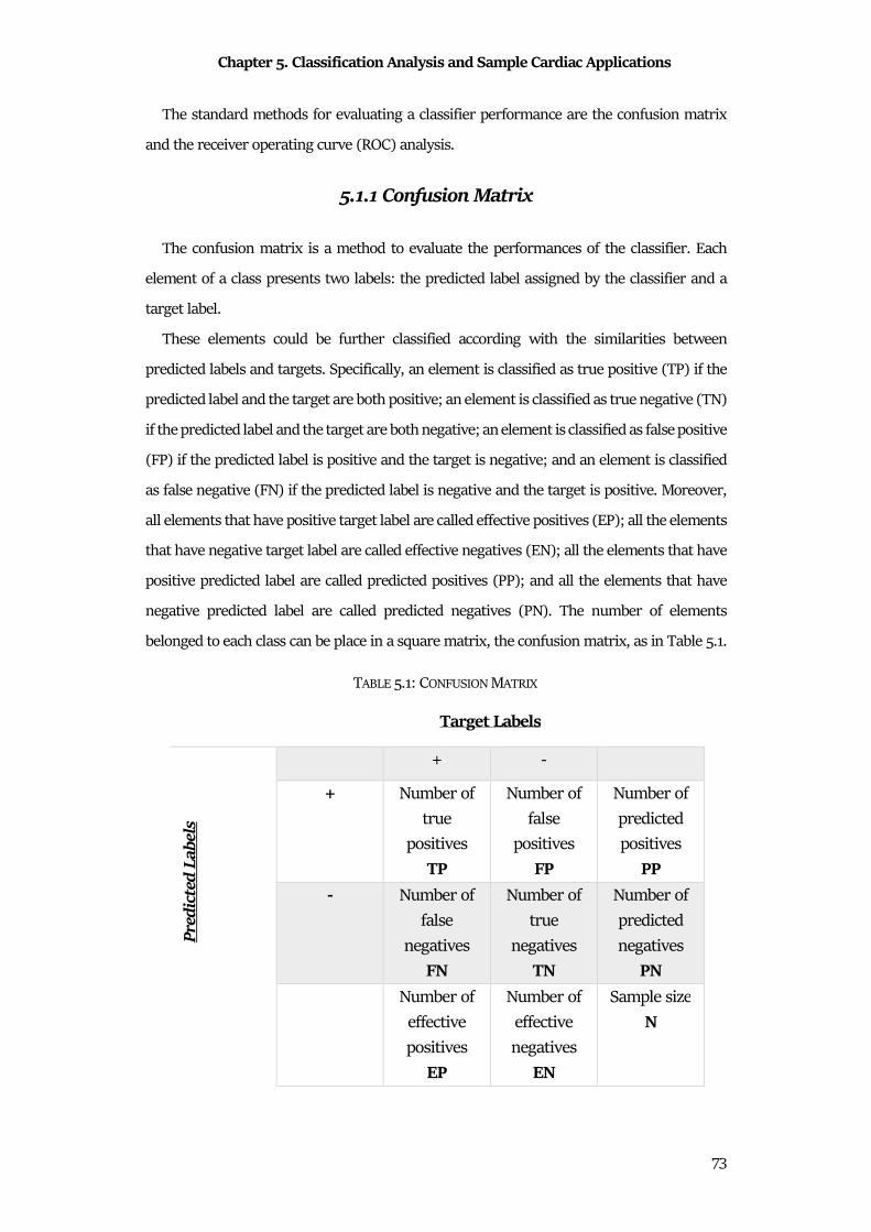
Chapter 5. Classification Analysis and Sample Cardiac Applications
73
The standard methods for evaluating a classifier performance are the confusion matrix
and the receiver operating curve (ROC) analysis.
5.1.1 Confusion Matrix
The confusion matrix is a method to evaluate the performances of the classifier. Each
element of a class presents two labels: the predicted label assigned by the classifier and a
target label.
These elements could be further classified according with the similarities between
predicted labels and targets. Specifically, an element is classified as true positive (TP) if the
predicted label and the target are both positive; an element is classified as true negative (TN)
if the predicted label and the target are both negative; an element is classified as false positive
(FP) if the predicted label is positive and the target is negative; and an element is classified
as false negative (FN) if the predicted label is negative and the target is positive. Moreover,
all elements that have positive target label are called effective positives (EP); all the elements
that have negative target label are called effective negatives (EN); all the elements that have
positive predicted label are called predicted positives (PP); and all the elements that have
negative predicted label are called predicted negatives (PN). The number of elements
belonged to each class can be place in a square matrix, the confusion matrix, as in Table 5.1.
TABLE 5.1: CONFUSION MATRIX
Target Labels
+ -
Pre
dic
ted
Lab
els
+ Number of
true
positives
TP
Number of
false
positives
FP
Number of
predicted
positives
PP
- Number of
false
negatives
FN
Number of
true
negatives
TN
Number of
predicted
negatives
PN
Number of
effective
positives
EP
Number of
effective
negatives
EN
Sample size
N

Chapter 5. Classification Analysis and Sample Cardiac Applications
74
The confusion matrix is based on six strength considerations:
(1) the number of true positive plus the number of false positives is the number of
predicted positives:
�R � �R = RR; (5.1)
(2) the number of the false negatives plus the number of true negatives is the number of
predicted negatives:
�� � �� = R�; (5.2)
(3) the number of true positives plus the number of false negatives is the number of
positives:
�R � �� = $R; (5.3)
(4) the number of false positives plus the number of true negatives is the number of
negatives:
�R � �� = $�; (5.4)
(5-6) the number of predicted positives plus the number of predicted negatives is equal
to the number of positives plus the number of negatives, that is the sample size:
RR � R� = $R � $�= �. (5.5)
From the confusion matrix, several indices can be computed. They are:
• Prevalence (Pr). The ratio between effective positives and sample size is the
percentage of the population that has a positive class:
R0 = $R� ; (5.6)
• Accuracy (ACC). The sum of true positives and true negatives over sample size is a
measure of how the classifier correctly identifies or excludes a condition:
�OO = �R � ��� ; (5.7)
• Positive Predictive Value (PPV) or Precision. The ratio between true positives and
predictive positives is the probability that a predictive positive is correctly positive:
RR = �RRR ; (5.8)
Chapter 5. Classification Analysis and Sample Cardiac Applications
75
• Negative Predicted Value (NPV). The ratio between true negatives and predictive
negatives is the probability that a predictive negative is correctly negative:
�R = ��R� ; (5.9)
• False Discovery Rate (FDR). The ratio between false positives and predictive
positives is the probability that a predictive positive is wrongly positive:
��� = �RRR ; (5.10)
• False Omission Rate (FOR). The ratio between false negatives and predicted
negatives is the probability that a predictive negative is wrongly negative:
�Y� = ��R� ; (5.11)
• True Positive Rate or Sensitivity (SE). The ratio between true positives and effective
positives is the ability of classifier to correctly recognize a positive:
�$ = �R$R ; (5.12)
• True Negative Rate or Specificity (SP). The ratio between true negatives and
effective negatives is the ability of classifier to correctly recognize a negative:
�R = ��$� ; (5.13)
• False Negative Rate(FNR) or Miss rate. The ratio between false negatives and
effective positives is the limit of classifier to correctly recognize a positive:
��� = ��$R ; (5.14)
• False Positive Rate (FPR) or Fall-out. The ratio between false positives and effective
negatives is the limit of classifier to correctly recognize a negative:
�R� = �R$� ; (5.15)
• Positive Likelihood Ratio (LR+). The ratio between the sensitivity and the false
positive rate is the probability that a positive result is not negative:
��� = �$�R� = �R ∙ $��R ∙ $R ; (5.16)
• Negative Likelihood Ratio (LR-). The ratio between the false negative ratio and the
specificity is the probability that a negative result is not positive:
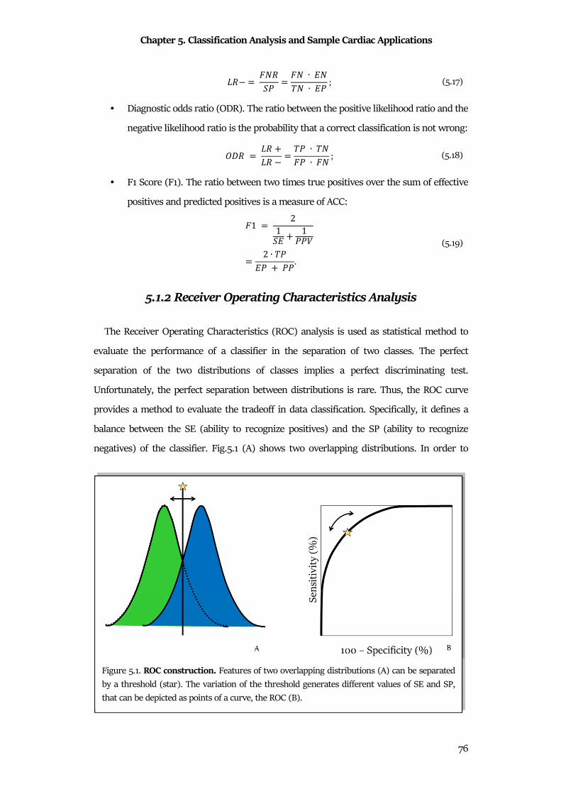
Chapter 5. Classification Analysis and Sample Cardiac Applications
76
�� = ����R = �� ∙ $��� ∙ $R ; (5.17)
• Diagnostic odds ratio (ODR). The ratio between the positive likelihood ratio and the
negative likelihood ratio is the probability that a correct classification is not wrong:
Y�� = �� ��� = �R ∙ ���R ∙ �� ; (5.18)
• F1 Score (F1). The ratio between two times true positives over the sum of effective
positives and predicted positives is a measure of ACC:
�1 = 21�$ � 1RR= 2 ∙ �R$R � RR. (5.19)
5.1.2 Receiver Operating Characteristics Analysis
The Receiver Operating Characteristics (ROC) analysis is used as statistical method to
evaluate the performance of a classifier in the separation of two classes. The perfect
separation of the two distributions of classes implies a perfect discriminating test.
Unfortunately, the perfect separation between distributions is rare. Thus, the ROC curve
provides a method to evaluate the tradeoff in data classification. Specifically, it defines a
balance between the SE (ability to recognize positives) and the SP (ability to recognize
negatives) of the classifier. Fig.5.1 (A) shows two overlapping distributions. In order to
Figure 5.1. ROC construction. Features of two overlapping distributions (A) can be separated
by a threshold (star). The variation of the threshold generates different values of SE and SP,
that can be depicted as points of a curve, the ROC (B).
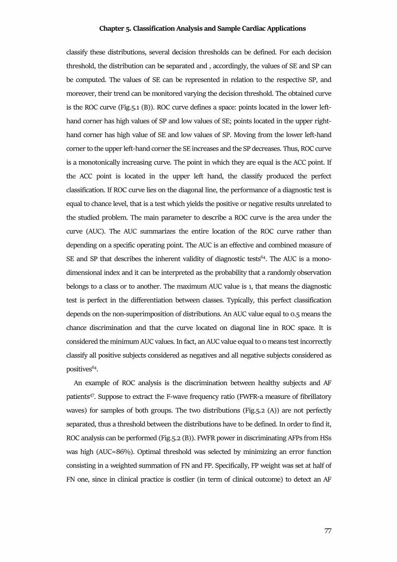
Chapter 5. Classification Analysis and Sample Cardiac Applications
77
classify these distributions, several decision thresholds can be defined. For each decision
threshold, the distribution can be separated and , accordingly, the values of SE and SP can
be computed. The values of SE can be represented in relation to the respective SP, and
moreover, their trend can be monitored varying the decision threshold. The obtained curve
is the ROC curve (Fig.5.1 (B)). ROC curve defines a space: points located in the lower left-
hand corner has high values of SP and low values of SE; points located in the upper right-
hand corner has high value of SE and low values of SP. Moving from the lower left-hand
corner to the upper left-hand corner the SE increases and the SP decreases. Thus, ROC curve
is a monotonically increasing curve. The point in which they are equal is the ACC point. If
the ACC point is located in the upper left hand, the classify produced the perfect
classification. If ROC curve lies on the diagonal line, the performance of a diagnostic test is
equal to chance level, that is a test which yields the positive or negative results unrelated to
the studied problem. The main parameter to describe a ROC curve is the area under the
curve (AUC). The AUC summarizes the entire location of the ROC curve rather than
depending on a specific operating point. The AUC is an effective and combined measure of
SE and SP that describes the inherent validity of diagnostic tests64. The AUC is a mono-
dimensional index and it can be interpreted as the probability that a randomly observation
belongs to a class or to another. The maximum AUC value is 1, that means the diagnostic
test is perfect in the differentiation between classes. Typically, this perfect classification
depends on the non-superimposition of distributions. An AUC value equal to 0.5 means the
chance discrimination and that the curve located on diagonal line in ROC space. It is
considered the minimum AUC values. In fact, an AUC value equal to 0 means test incorrectly
classify all positive subjects considered as negatives and all negative subjects considered as
positives64.
An example of ROC analysis is the discrimination between healthy subjects and AF
patients47. Suppose to extract the F-wave frequency ratio (FWFR-a measure of fibrillatory
waves) for samples of both groups. The two distributions (Fig.5.2 (A)) are not perfectly
separated, thus a threshold between the distributions have to be defined. In order to find it,
ROC analysis can be performed (Fig.5.2 (B)). FWFR power in discriminating AFPs from HSs
was high (AUC=86%). Optimal threshold was selected by minimizing an error function
consisting in a weighted summation of FN and FP. Specifically, FP weight was set at half of
FN one, since in clinical practice is costlier (in term of clinical outcome) to detect an AF
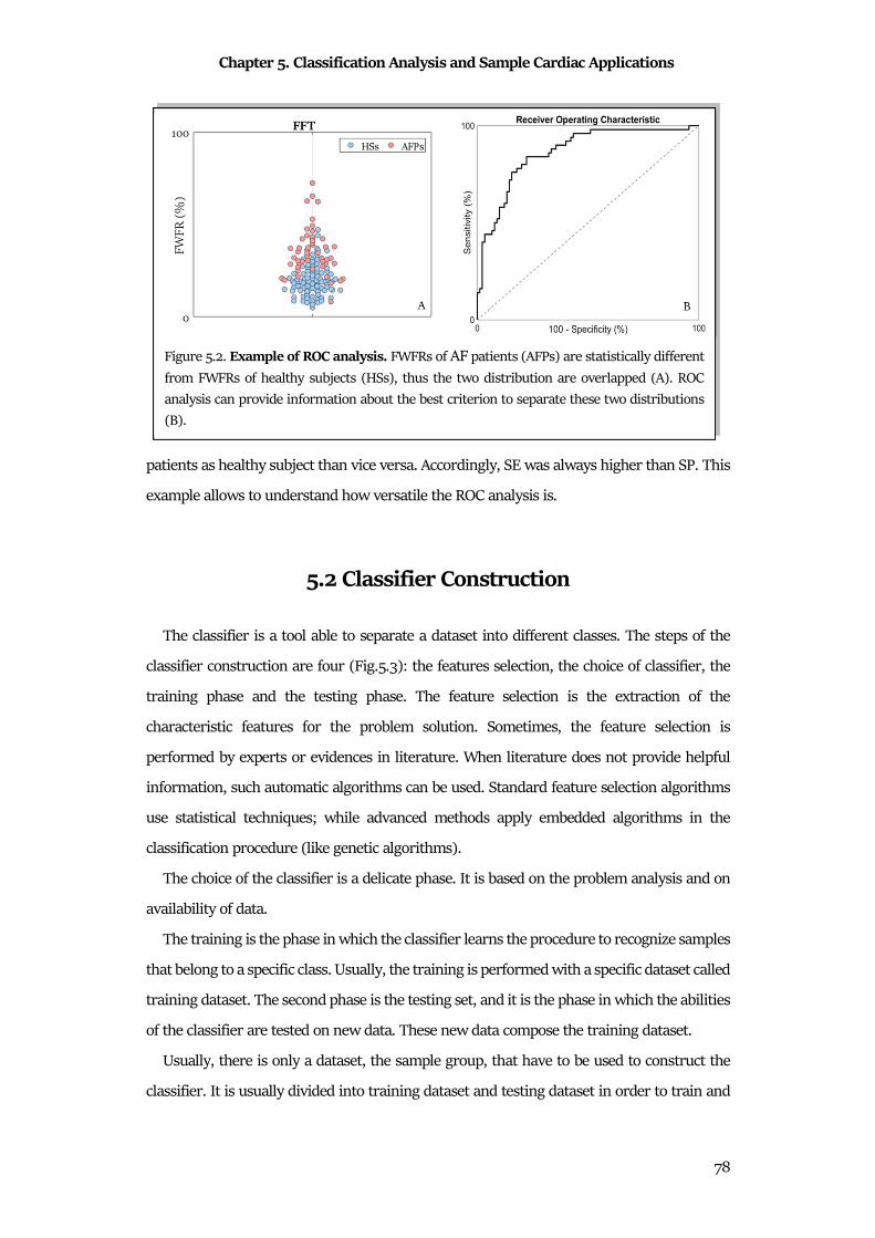
Chapter 5. Classification Analysis and Sample Cardiac Applications
78
patients as healthy subject than vice versa. Accordingly, SE was always higher than SP. This
example allows to understand how versatile the ROC analysis is.
5.2 Classifier Construction
The classifier is a tool able to separate a dataset into different classes. The steps of the
classifier construction are four (Fig.5.3): the features selection, the choice of classifier, the
training phase and the testing phase. The feature selection is the extraction of the
characteristic features for the problem solution. Sometimes, the feature selection is
performed by experts or evidences in literature. When literature does not provide helpful
information, such automatic algorithms can be used. Standard feature selection algorithms
use statistical techniques; while advanced methods apply embedded algorithms in the
classification procedure (like genetic algorithms).
The choice of the classifier is a delicate phase. It is based on the problem analysis and on
availability of data.
The training is the phase in which the classifier learns the procedure to recognize samples
that belong to a specific class. Usually, the training is performed with a specific dataset called
training dataset. The second phase is the testing set, and it is the phase in which the abilities
of the classifier are tested on new data. These new data compose the training dataset.
Usually, there is only a dataset, the sample group, that have to be used to construct the
classifier. It is usually divided into training dataset and testing dataset in order to train and
Figure 5.2. Example of ROC analysis. FWFRs of AF patients (AFPs) are statistically different
from FWFRs of healthy subjects (HSs), thus the two distribution are overlapped (A). ROC
analysis can provide information about the best criterion to separate these two distributions
(B).
Chapter 5. Classification Analysis and Sample Cardiac Applications
79
test the classifier. The common practice is to use the 70% of the sample group for the
training and the 30% for the testing. But, in cases of small amount of data, the entire sample
group is divided equally. Moreover, it is recommended to maintain the prevalence of classes
in the training and testing datasets, in order to have a balanced classification65.
Sometimes, such training procedure requires an iterative process. In these cases, it is
possible to lose the generalization propriety of the classifier. The generalization is the
propriety of the classifier to recognize new data. Thus, a new dataset is used, the validation
dataset. This dataset is used to test the performance of the classifier after each iteration in
order to evaluate its generalization. Usually, the validation dataset is extracted from the
training dataset. The thumb rule is applied: the validation dataset is the one fifth of the
training dataset66. In case of very small dataset, cross validation methods can be used66,67.
5.3 Examples of Classifiers
In statistics, there are different types of classifiers. The first division is between
continuous classifiers and discrete classifiers. The continuous classifiers are algorithms or
model whose output is continuous; while the discrete classifiers provide directly a categorical
output. Classifiers can also be divided in relation to their training. If the training is based on
the adjustment between the expected classification and the output, the classifier is
supervised. While, if the training is based on the similarity between data, without knowing
the expected classification, the classifier is unsupervised. The last classification is based on
the decision curve morphology. If the decision curve to discriminate classes is a line, the
classifier is linear. If the decision curve to discriminate classes is a generic curve, the
classifier is not linear. Non-linear classifiers are also called structural classifiers, because
they are usually composed by the combination of several linear classifiers.
Figure 5.3. Classifier construction step.
Chapter 5. Classification Analysis and Sample Cardiac Applications
80
5.3.1 Linear Classifier: Logistic Regression
Logistic regression (LR) is a statistical technique used to evaluate the association between
categorical dependent variables and sets of independent variables. Specifically, the
dependent variable (dichotomic or binary) has only two values, such as 0 and 1. LR is a
versatile technique and it can suite very well such modelling situations. This is because LR
is independent from the normal distributions of independent variables.
Logistic Function
Standard regression tries to predict the expected value of a dependent variable using the
mathematical model of a set of independent variables. On the contrary, LR tries to predict a
logit transformation of the dependent variables. Suppose that the dependent variable is
represented by two numerical values, 0 and 1, and that represent binary outputs
(positive/negative; male/female; healthy/diseased). P could be defined as the probability to
have an output equal to 1; while (1-P) is the probability to have an output equal to not 1, 0.
The ratio between these two probabilities is the odds and its logarithmic is the logit.
Mathematically, it is:
� = k1M.� R� = k8 h R1 Ri (5.20)
The logistic transformation, or logistic function, is the inverse of the logit, that is:
R = k1M.2.�� �� = �1 � � (5.21)
Logistic Model
In LR, a categorical dependent variable Y having N unique values is regressed on a set of
P independent variables *�, *�, . . . , *U. Since these classes are arbitrary, they are usually
labeled as consecutive numbers: Y can take on the values 1,2, . . . , �.
Suppose to have N inputs:
� = [*� *� . . . *,] (5.22)
And N parameters:
�� = S���. . .��UX (5.23)
the LR model is given by N equations
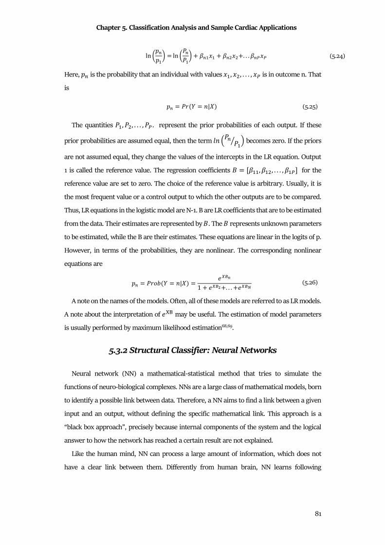
Chapter 5. Classification Analysis and Sample Cardiac Applications
81
ln h+�+�i = ln hR�R�i � ���*� � ���*��. . . ��U*U (5.24)
Here, +� is the probability that an individual with values *�, *�, . . . , *U is in outcome n. That
is
+� = R0 � = 8|�� (5.25)
The quantities R�, R�, . . . , RU. represent the prior probabilities of each output. If these
prior probabilities are assumed equal, then the term k8 �R� R�� � becomes zero. If the priors
are not assumed equal, they change the values of the intercepts in the LR equation. Output
1 is called the reference value. The regression coefficients � = [���, ���, . . . , ��U] for the
reference value are set to zero. The choice of the reference value is arbitrary. Usually, it is
the most frequent value or a control output to which the other outputs are to be compared.
Thus, LR equations in the logistic model are N-1. B are LR coefficients that are to be estimated
from the data. Their estimates are represented by �. The � represents unknown parameters
to be estimated, while the B are their estimates. These equations are linear in the logits of p.
However, in terms of the probabilities, they are nonlinear. The corresponding nonlinear
equations are
+� = R01� � = 8|�� = Ev�1 � Evr�. . . � Ev\ (5.26)
A note on the names of the models. Often, all of these models are referred to as LR models.
A note about the interpretation of �� may be useful. The estimation of model parameters
is usually performed by maximum likelihood estimation68,69.
5.3.2 Structural Classifier: Neural Networks
Neural network (NN) a mathematical-statistical method that tries to simulate the
functions of neuro-biological complexes. NNs are a large class of mathematical models, born
to identify a possible link between data. Therefore, a NN aims to find a link between a given
input and an output, without defining the specific mathematical link. This approach is a
“black box approach”, precisely because internal components of the system and the logical
answer to how the network has reached a certain result are not explained.
Like the human mind, NN can process a large amount of information, which does not
have a clear link between them. Differently from human brain, NN learns following

Chapter 5. Classification Analysis and Sample Cardiac Applications
82
mathematical-statistical laws by considering experimental data in order to determine, the
relationship that provides the solutions of a problem.
The pathway that the information follows defines the kind of the NN. The categories are:
• feedforward networks, in which the information travels in one direction, generally
from left to right;
• feedback networks, in which the information does not have a single direction in
which it can travel.
Another classification considers the connections between neurons. In this case, the
categories are:
• totally connected NN if all the neurons of a layer are connected to each neuron of
another layer;
• partially connected NN if the connection of each neuron of a layer is limited to a
particular subset of another layer.
The fundamental characteristic of NNs is their ability to be able to work in a high complex
environment. Nevertheless, every NN is able to face the same work in a totally different way
and in effectiveness. Depending on the task to be carried out, there will be a better
performing NN than others.
The NNs are composed of processing units called artificial neurons, which can be grouped
into several layers. The communication between one neuron and another occurs through
weighted connections (or weights) that recall the synapses concept. The artificial
neuron(Fig.5.4) is the unit of information processing that makes up the NN, developed by
McCullough and Pitts.
Considering the vector of inputs � = [*�, *�, . . . , *,], each element is associated with a
synapse, corresponding to a given synaptic weight z�,~ (indicating the weight between the
neuron ith and the neuron jth). Weights can take positive or negative values, reflecting the
synapse excitation and inhibition behavior. All this is described in the artificial model
through two blocks70:
• Summation (body of the neuron): represents the linear combination (as a sum
operator) between the associated synaptic inputs and weights:
j� = ) z�,~ ∙ *~� � ��,
~-# (5.27)

Chapter 5. Classification Analysis and Sample Cardiac Applications
83
The bias �� has the function of increasing or decreasing the input to the activation
function, so that it re-enters the interval [0,1] or [-1,1]. It is considered as an external
input of the fixed and positive value equal to 1. In addition, a synaptic weight is
associated with it.
• Activation function: limits the amplitude of the neuron output. The range of
normalized values is within the closed range [0,1] or in [-1,1]. Combinations f input,
weights and bias are the input of activation function:
=� = � �) z�,~ ∙ *~� � ��,
~-# � = � j�� (5.28)
The activation function depends on classification problem and the type of
architecture. The most common are the Heavside function, the linear saturation
function, the sigmoid or logistic function, and the normalized exponential function.
From the model of an artificial neuron, the first form of NN known is the perceptron
(Fig.5.5), developed by the mathematician and psychologist Frank Rosenblatt. Composed of
a row of neurons, it was born as a feedforward network for the recognition and classification
of patterns. In perceptron, all neurons have a step activation function (Heavside function)
with binary values output (0 or 1). Through a learning phase, weights associated with the
inputs are changed. Consequently, a movement of the hyperplane separating the entry space
is generated up to identify two very specific classes: the class 1 of the outputs high (1) and
class 0, for low outputs (0). In particular, the modification of the weights associated with
inputs generates a rotation of the hyperplane, while the presence of the bias serves to
Figure 5.4.The artificial neuron.
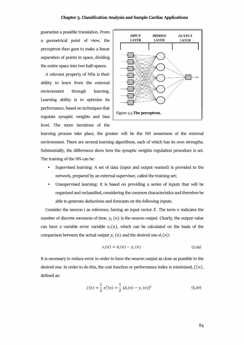
Chapter 5. Classification Analysis and Sample Cardiac Applications
84
guarantee a possible translation. From
a geometrical point of view, the
perceptron then goes to make a linear
separation of points in space, dividing
the entire space into two half-spaces.
A relevant property of NNs is their
ability to learn from the external
environment through learning.
Learning ability is to optimize its
performance, based on techniques that
regulate synaptic weights and bias
level. The more iterations of the
learning process take place, the greater will be the NN awareness of the external
environment. There are several learning algorithms, each of which has its own strengths.
Substantially, the differences show how the synaptic weights regulation procedure is set.
The training of the NN can be:
• Supervised learning: A set of data (input and output wanted) is provided to the
network, prepared by an external supervisor, called the training set;
• Unsupervised learning: It is based on providing a series of inputs that will be
organized and reclassified, considering the common characteristics and therefore be
able to generate deductions and forecasts on the following inputs.
Consider the neuron i as reference, having an input vector �. The term 8 indicates the
number of discrete moments of time. =� 8� is the neuron output. Clearly, the output value
can have a variable error variable � 8�, which can be calculated on the basis of the
comparison between the actual output =� 8� and the desired one 4� 8�:
� 8� = 4� 8� =� 8� (5.29)
It is necessary to reduce error in order to have the neuron output as close as possible to the
desired one. In order to do this, the cost function or performance index is minimized, � 8�,
defined as:
� 8� = 12 �� 8� = 12 [4� 8� =� 8�]� (5.30)
Figure 5.5.The perceptron.
Chapter 5. Classification Analysis and Sample Cardiac Applications
85
The purpose is to change the value of synaptic weights, for each instant n, going to modify
the output of the neuron and then making a reduction in the index � 8�. The delta rule states
that the variation of a generic weight w _, , associated with the jth entry *~ 8� is: ¡ z�~ = ¢ � 8�* ~ 8� (5.31)
The term η is called the learning rate, evaluating the speed of learning of the neuron. It
always has positive values between 0 and 1. The delta rule is based on the fact that the error
is directly measurable. Evaluated ¡ w_ we can go to define the new value of synaptic weight:
z�~ 8 � 1� = z�~ 8� �¡ z�~ 8� (5.32)
In order to compute it, the desired response has to be generated from an external source
directly accessible to the neuron ¤. Therefore, a supervised learning requires that both the * 8�and desired output values 4� 8� are a priori known.
To minimize the performance index (by varying the synaptic weights), the descent of the
gradient of the function can be applied. The gradient is described by a vector whose
components coincide with the partial derivatives of the performance index in relation to the
synaptic weights of the network:
¥$ z� = [ �$�z0 , … , �$
�z8 ] (5.33)
Applying the decreasing gradient, new weights are:
Δz~� = ¢ �$�z~� (5.34)
The perceptron, taken as a single unit, is able to solve problems of linear separation.
However, it presents problems when the problem to be treated is not linear. A first approach
may consist in using a different activation function (e.g. sigmoid), but this would make the
perceptron much more complex. On the other hand, multiple units interconnected can be
used: this leads to an increase in
the number of separation lines
that operate in the entry space.
The problem of non-linear
separation is split into several
sub-problems of linear nature
that can be solved with the Figure 5.6.The multilayer perceptron.

Chapter 5. Classification Analysis and Sample Cardiac Applications
86
perceptron, without corrupting its properties. Thus, a new model of NN is defined which
presents a stratification of the units, whose name is precisely a multilayer perceptron (MLP).
MLP is composed of 3 main layers (Fig.5.6): a first of input, one or more intermediate called
hidden layer and a last one of output.
The MLP has a feedforward structure, meaning that the units communicate in one
direction. In fact, except for the output one, the outputs of a layer are the input quantities of
the next. The bias is considered in each node, having a fixed value of -1. Precisely, MLP is
able to get where the perceptron is not able. Thanks to the hidden layers of the network, it
is possible to obtain an internal representation of the most articulated input, by identifying
arbitrary regions obtained by intersecting hyperplanes in the hyperspace of the input values.
The possibility, therefore, of breaking down the problem into simpler sub-problems allows
NN to be able to work even in larger cases.
The number of hidden layers can vary, depending on the complexity of the work to be
addressed, as well as the number of units per layer. This serves to increase the computing
power of NN, even if efficiency and processing time are quite lost. Above this it should be
noted that for the Kolmogorov theorem it is sufficient to have only one Hidden layer, to be
able to carry out any work, it is sufficient to increase the number of neurons of it (even if it
is still under debate).
The MLP networks are one of the types that is widely used, for the resolution of different
problems in various areas, through a supervised training called error back propagation
algorithm. The term indicates that the error evaluated on each layer, starting from the last,
is transmitted to the previous layer and so on. It is used in particular to calculate the error
of a unit of the Hidden layer, retro-propagating the error from the output layer, so that the
synaptic weights can be corrected. Consider an MLP network described by 3 layers: an input
layer �� (with i = 1,2, ..., N unit), a hidden �§ (with k = 1,2, ..., m unit) and one of output �~
(with j = 1, 2, ..., p unit). From the network performance index, applying the gradient rule
we obtain:
Δz~§ = ¢ �$�z~§ = ¢ �$�=~�=~�R~
�R~�z~§ = ¢�4~ =~�"¨ R~��§ (5.35)
The term =~, indicates the jth output of the network while R~ represents the activation
potential of the respective node. Thus:
©z~§ = ¢N~�§ (5.36)
Chapter 5. Classification Analysis and Sample Cardiac Applications
87
where
N~ = �4~ =~�"¨ R~� (5.37)
and the MLP weights of the output and hidden layers can be upgraded. Instead for the
connections between input and hidden layer:
Δz§� = ¢ �$�z§� = ¢ �$��§��§�R§
�R§�z§�= ¢ "′ R§� ) N~z~§�*�
«6�~-�
(5.38)
Consequently:
Δz§� = ¢N§*� (5.39)
with
N§ = "′ R§� ) N~z~§� «6�~-� (5.40)
Generalizing the mathematical formulation, it is:
Δz§� = ¢N§t� (5.41)
z§� 8 � 1� = z§� 8� �¡ z§� (5.42)
N§ = %'( 4§ =§�"¨ ¤� "10 19�+9� k�= 0 98.�
)�N~z~§�" R§�«6�~ "10 ¬.44 8 k�= 0 98.� (5.43)
Considering this process, the backpropagation algorithm follows a specific workflow. First
of all, a learning epoch is made, then to the input and output pairs of the training set, the
following steps are performed:
• Take a pair and calculate the network response for that input; the calculation
proceeds from the input level to the output level, with consequent forward
propagation of the error;
• The error E is calculated between the output of the network and the output of the
pair and determine the N§ of the output units;
• the error is propagated backwards towards the input level, and N§ are evaluated for
each Hidden unit;
• The synaptic weights are modified;
• The steps are repeated, starting from the first one until the couples are finished.
Chapter 5. Classification Analysis and Sample Cardiac Applications
88
Once all the steps have been completed for all the training set pairs, the global error is
calculated. If it turns out to be a still high value, a further learning period is repeated.
The back-propagation rule presents some relevant problems. As a very complex process
it requires great calculation skills. The presence of non-linear operations means that the
learning function can take a complex course. Another important problem is represented by
local minima, as it would cause a blockage of the algorithm. There are some improvements
applied to the back propagation, one of these is the coefficient (takes values between 0 and
1) α called momentum. In this case the learning formula becomes:
Δz~� 8 � 1� = ¢N~* � � w∆z~� 8� (5.44)
It is noted that this new formulation depends on the correction that was made in the
previous epoch. It is used to increase the learning speed when the corrections of two
consecutive epochs show unanimous signs. Likewise, the speed may decrease if the signs are
discordant, typically when the change in the index slope occurs that a local minimum has
been exceeded70.

89
PART II
BIOSTATISTICS OF
CARDIAC SIGNALS:
APPLICATIONS
The real importance of statistics in cardiac bioengineering can be deeply understood only
through its application. Statistical theory can appear general and difficult to understand in
practice. Instead, in reality, statistics is widely applicable and applied, but often hidden by
the scientific aspects of a research project. Moreover, it is widely known as the method for
supporting the epidemiological studies, without considering that it can be use also in other
aspects, such as signal processing.
In order to contextualize and to evaluate the real applicability of biostatistics in real
cardiac signal processing, the second part of this doctoral thesis is focused on the
presentation of four real applications. During the design and implementation of these
algorithms for cardiac signals analysis, biostatistics was essential. Indeed, biostatistics is
used in each of them to characterize a specific phase of statistical signal processing. Except
for cardiac signal acquisition, the considered phases were preprocessing, feature extraction,
comparison and association, and classification.
The first presented application is the adaptive thresholding identification algorithm
(AThrIA). It is an application specifically designed to identify and to segment the
electrocardiographic P wave, the occurrence of which is the major criterion for atrial diseases
diagnosis. AThrIA is presented at first because its preprocessing is a specifically-designed
90
combination of standard and statistical preprocessing. In particular, the standard ECG
denoising is combined with PCA .
The second presented application is CTG Analyzer, that is a graphical user interface for
the computation of the cardiotocographic features. These features are usually visually
evaluated, in spite of the clinical necessity to be objective. About CTG Analyzer feature
extraction, biostatistics is a fundamental instrument to evaluate the correctness of the
features. Moreover, it is essential to compare the automated extracted features with the
standard ones provided by a clinician.
The third presented application is eCTG, a software for the digitalization of
cardiotocographic signals from scanned images. Core of eCTG is the Otsu’s methods, a pixel
clustering procedure that is able to separate pixels in black and white. This statistical
technique is halfway between feature extraction methods and classification ones.
The fourth and last presented application implements the construction of deep-learning
serial ECG classifiers (DLSEC). Through a new constructive method, specific MLPs were
created in order to solve classification problems. The field of this new research is the serial
electrocardiography for the detection of new emerging pathology. In particular, this
application was tested in heart failure and ischemia detection. These DLSECs are the perfect
example of how statistics is essential in each problem of classification.
Chapter 6. AThrIA: Adaptive Thresholding Identification Algorithm
91
Chapter 6
AThrIA: Adaptive Thresholding Identification
Algorithm
AThrIA was born to identify and to segment electrocardiographic P waves. The P wave is
the lowest wave of the ECG pattern and it is difficult to identify. Its low amplitude can be
covered by interference. Moreover, its features are essential to investigate and to diagnose
atrial diseases. Differently from other algorithms71–79 that search P waves only in specific
windows before R peaks (normal P waves), AThrIA searches P waves in all RR interval
duration. This design choice was born from the necessity to identify not only physiological
P wave, but also pathological P waves.
AThrIA is the perfect example of how preprocessing is important in cardiac clinical
practice. Indeed, the P-wave amplitude is low and easily covered by interference. Standard
preprocessing is not enough; thus, a specific preprocessing has to be chosen, in order to
remove noises and to enhance this low-amplitude wave.
With this important purpose, AThrIA was designed with a specific preprocessing,
combining standard prefiltering and PCA. Specifically, a statistical preprocessing method can
substantially improve the performances of the algorithm, due to its property of extract
common statistical pattern.
6.1 Background
6.1.1 Clinical Background
Atrial activity is the representation of the depolarization and repolarization of atria. Atrial
activity can be monitored by P-wave observation. P wave reflects atrial depolarization. P-
wave abnormalities can reflect atrial arrythmias or atrioventricular blocks (AVB).
Atrial Arrythmias
Supraventricular tachycardias (SVT) are the main common atrial arrythmias. SVT is
generically a high-frequency heart rhythm due to improper electrical activity of the atria.
Chapter 6. AThrIA: Adaptive Thresholding Identification Algorithm
92
Episodes have a duration ranging from few minutes up to 1-2 days and sometimes persist
until the treatment. A very high HR (150-270 bpm) during the episode can reduce the heart
pump effectiveness, decreasing cardiac output and blood pressure. SVTs can be classified
into atrial tachycardias (AT) and junctional tachycardias (JT).
AT is a heart rhythm disorder caused by the generation of cardiac impulse from an ectopic
pacemaker in the upper chambers of the heart, rather than SA node. P-wave morphology
can indicate the ectopic myocardium site and the AT mechanism. The trigger mechanism
can be the rapid discharge from an abnormal focus, the presence of cardiac tissue ring that
causes a reentry mechanism, or an increase in rhythm due to other pathological conditions.
Characteristics of AT are sinus tachycardia (ST), AF (atrial fibrillation), atrial flutter and
focal AT.
ST is an arrhythmia characterized by an increase in frequency (HR> 100 bpm) and a rate
of sinus rhythm. Similar arrhythmic manifestations may be the normal consequence of
physiological events, followed by a heart rhythm that returns to normal condition.
Therefore, specific treatments are not necessary. As in a normal sinus rhythm, the P-wave
axis in frontal plane lies between 0° and + 90°.
The AF is a supraventricular arrhythmia characterized by atrial inability to depolarize
simultaneously: there is a chaotic and irregular activity that determines inability to guide
the atrial contraction. The AF can be presented in several cardiac and non-cardiac
pathological conditions, and also in apparently healthy subject. It is asymptomatic in over a
third of the population or it can occur with vague non-specific symptoms. It is often
diagnosed only when the patient has significant symptoms and signs of serious
complications. The initial clinical diagnosis of AF depends on the associated symptoms:
dyspnea, palpitations, vertigo / syncope or anginal chest pain80. A regular pulse detected in
symptom courses (breathlessness, dizziness, chest pain) is able to exclude an AF with high
ACC. Exceptions are the atrioventricular dissociation and the ventricles heartbeat regularly
stimulated by a pacemaker. The three diagnostic elements at the ECG are:
• The disappearance of P waves.
• The appearance of rapid oscillations of the isoelectric line, called fibrillation waves
(F waves). F waves are completely irregular, with continuous variations in shape,
voltage and F-F intervals; they have a very high frequency (400-600 bpm) and last
throughout the cardiac cycle.

Chapter 6. AThrIA: Adaptive Thresholding Identification Algorithm
93
• The irregularity of the R-R intervals. During AF, a large number of atrial-origin
pulses reach the AV junction, but only a part of them are actually transmitted to the
ventricles. Consequently, the duration of the R-R intervals constantly varies.
AF is the most frequent arrhythmia in clinical practice, with a prevalence in the general
population of 0.5-1.0%. Although it is relatively low among young people, it increases with
age: 4.8% between 70 and 79 years, 8.8% between 80 and 89 years. The AF is classified
according to its appearance and duration. Classes are the paroxysmal AF (AF that resolved
spontaneously within 7 days); the persistent AF (AF that lasts longer than 7 days or requires
pharmacological or electrical cardioversion to return to sinus rhythm); permanent or
chronic AF (AF in which no cardioversion attempts are made or, if performed, have been
unsuccessful); the new onset AF (diagnostic AF for the first time, regardless of the duration
of the arrhythmia or the presence or absence of symptoms related to it); and, finally, the
recurring AF (includes any form of recurrence of the AF).
Atrial flutter is an SVT with very rapid and well-organized atrium contraction, where the
atrial rate can reach 250/350 bpm. Conduction of atrial impulses to ventricles is slowed
down to blockage at the AV node whereby the ventricular activation rate is lower than the
atrial one (usually 120-130 bpm). The electrophysiological mechanism is a re-entry of the
electrical stimulus into atria (intra-atrial re-entry). Paroxysmal atrial flutter may develop
into a healthy heart or into hearts with abnormalities (atrial or changes in the conduction
system). Generally, atrial flutter patients experience irregularities in the rhythm or
accelerated frequency.
Focal AT is a form of arrhythmia characterized by an increase in heart rhythm due to the
presence of ectopic origin of the cardiac electrical impulse. It is defined by an HR of less than
200 bpm and an isoelectric interval between multiple P waves. It differs from chaotic AT in
which the source signal has variable localization. Focal AT can be classified into two groups,
unifocal AT (one ectopic site) and multifocal AT (multiple ectopic sites).
JT is a common type of SVT, characterized by the AV-node participation. It may be due to
increased automatism or triggered activity of AV node itself or His bundle. From the ECG
point of view, this arrhythmia shows negative P waves in II, III and aVF leads and positive
in V1 lead because atria are activated in a caudocranial direction. The retrograde P wave is
usually placed immediately after the QRS complex, sometimes it is covered by it and is rarely
located before the QRS complex.
Chapter 6. AThrIA: Adaptive Thresholding Identification Algorithm
94
Atrioventricular Blocks
The AVB (atrioventricular block) is an arrhythmia caused by the interruption of the
conduction between atria and ventricles. Specifically, the conduction can be blocked in the
AV node, in the His bundle or in its two branches. Depending on the degree of severity of
this conduction disorder, three types of AVB are distinguished that is the first degree AVB
conduction; the second degree AVB conduction and the third degree AVB conduction.
The first degree AVB consists in the slowing down of AV-node conduction. It is identified
by a prolongation of the PR interval over 0.20 s in adults (over 0.18 s in the child), remaining
however normally less than 0.4 s; a number of P waves equal to the number of QRS
complexes; and QRS complexes most often narrow.
The second degree AVB is characterized by the intermittent interruption of AV-node
conduction. It manifests itself with the intermittent appearance of P waves not followed by
a QRS complex. In this case depolarization wave is blocked and the number of P waves is
thus higher than the number of QRS complexes.
The third degree AVB is a disturbance of the cardiac impulse transmission.
Communication between the NAV and His bundle is regularly stopped; thus, the impulse is
completely blocked, and ventricles no longer contract. All the parts of the conduction system
have a specific automatism; thus, if there is a maintained period of latency, a zone of the
conduction system starts generating pulses acting as pacemakers. This process guarantees
ventricular contraction. In case of nodal blockage, there is a junctional escapement rhythm
with narrow QRS complexes (<0.12 s) and frequency between 40 and 50 bpm. The
pacemaker implantation is indicated for this type of block.
6.1.2 Algorithms for P-wave characterization
In literature, different algorithms were presented as methods for ECG waves
characterization. Specifically, they are not related only on P-wave identification and
segmentation, but on all the ECG waves. Bereza et al.81 compared the most important
methods that aim to characterizes ECG waves, in order to evaluate their performance. In
order to compare AThrIA performance with literature, the same algorithms were
considered.
Typically, ECG waves segmentation algorithms are composed by two steps: the first one
preprocessed the input signals in order to enhance it, while the second step identifies the
ECG waves landmarks with an adaptive threshold.
Chapter 6. AThrIA: Adaptive Thresholding Identification Algorithm
95
The most common algorithms are:
• Laguna71: The first step considered the use of a low-pass differentiation, giving a
filtered signal with information about the change in slope. The second step for
the identification of landmarks used an adaptive threshold. Wave limits (onset
and offset) of the original signal are found by searching the waves in windows
around the R peaks positions.
• Martinez72: The first step used the discrete wavelet transform are a preprocessing
technique, while an adaptive threshold is used for the second step.
• Singh74: The first step is the combination of a recursive low-pass filter and its first
derivative. The second step used auxiliary lines to identify the landmarks of the
waves.
• Di Marco76: This algorithm is an online algorithm that used the discrete wavelet
transform and an adaptive threshold to identify the ECG wave landmarks.
• Sun75: A multi-scale morphological derivative is used to identify the local maxima,
the local minima and the landmarks of the waves
• Martinez73: The algorithm transformed each instantaneous sample of ECG into a
simple phasor. The phase derivative is applied to find the limits of ECG waves.
• Vazquez78: The first step is composed by a combination of a band-pass
Butterworth filter and the first derivative. The second step is composed by a
geometric method in which a rectangular trapezium is continuously calculated
once the wave peak is detected, using three fixed vertices and one mobile or
variable vertex.
• Vítek79: The first step used the continuous wavelet transform, while the second
step considered ab adaptive threshold.
• Hughes77: The algorithm considered the discrete wavelet transform for the
preprocessing and a supervised algorithm for the identification of fiducial points.
6.2 Methods
AThrIA is an innovative algorithm specifically designed for P-waves identification and
characterization (Fig.6.1). Initially, input ECG is preprocessed to remove interference by
standard filtering application. Specifically, a band-pass bidirectional 6th-order Butterworth
filter (cut-off frequencies at 1Hz and 40Hz) and baseline subtraction are applied. The

Chapter 6. AThrIA: Adaptive Thresholding Identification Algorithm
96
standard preprocessed ECG (SPP_ECG) is recursively scanned to search for P waves in every
inter-RR heartbeat (IRRH). The IRRH is defined as the SPP_ECG segment between two
consecutive R peaks. If SPP_ECG contains N R peaks, number of IRRH is N-1.
Consider IRRHi the ith IRRH of SPP-ECG, its length in samples will be IRRHLi. In order to
search for P waves in IRRHi, the input of AThrIA will be a SPP-ECG window (SPP-ECGW).
SPP_ECGW is composed of NHB number of heartbeats (usually 857), in which IRRHi is the
last one. Thus, SPP_ECGW will be a segment of SPP-ECG comprised from the (i-NHB+1)th R
peak to the ith R peak. SPP-ECGW and its R peaks are the inputs of AThrIA
The three steps of AThrIA are the preprocessing, the P-wave identification and
segmentation and post-processing (Fig.6.1).
6.2.1 Preprocessing
The preprocessing step aims to enhance IRRHi, reducing its level of noise by PCA. SPP-
ECGW is segmented in its NHB, in which the last one is that of interest. Due to HRV, the
IRRHL of each heartbeat is different from the IRRHLi. Each IRRH is composed of six waves,
the first R peak, S wave, T wave, P wave, Q wave and the second R peak. Each IRRH can be
segmented in three segments (Fig.6.2), that are RS-complex segment, T-wave segment and
PQR-complex segment. RS-complex segment is defined as the segment of IRRH from the
Figure 6.1.Three steps of AThrIA. The three steps are the preprocessing (red), the P-wave
identification and segmentation (green) and the postprocessing (blue).
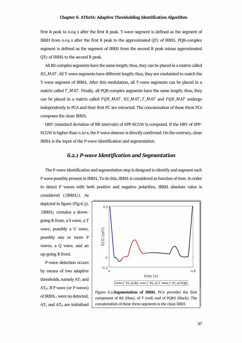
Chapter 6. AThrIA: Adaptive Thresholding Identification Algorithm
97
first R peak to 0.04 s after the first R peak. T-wave segment is defined as the segment of
IRRH from 0.04 s after the first R peak to the approximated QTc of IRRHi. PQR-complex
segment is defined as the segment of IRRH from the second R peak minus approximated
QTc of IRRHi to the second R peak.
All RS-complex segments have the same length; thus, they can be placed in a matrix called ��_���. All T-wave segments have different length; thus, they are modulated to match the
T-wave segment of IRRHi. After this modulation, all T-wave segments can be placed in a
matrix called �_���. Finally, all PQR-complex segments have the same length; thus, they
can be placed in a matrix called R��_���. ��_���, �_��� and R��_��� undergo
independently to PCA and their first PC are extracted. The concatenation of these three PCs
composes the clean IRRHi.
HRV (standard deviation of RR intervals) of SPP-ECGW is computed. If the HRV of SPP-
ECGW is higher than 0.20 s, the P-wave absence is directly confirmed. On the contrary, clean
IRRHi is the input of the P-wave identification and segmentation.
6.2.1 P-wave Identification and Segmentation
The P-wave identification and segmentation step is designed to identify and segment each
P wave possibly present in IRRHi. To do this, IRRHi is considered as function of time. In order
to detect P waves with both positive and negative polarities, IRRHi absolute value is
considered (|IRRHi|). As
depicted in figure (Fig.6.3),
|IRRHi| contains a down-
going R front, a S wave, a T
wave, possibly a U wave,
possibly one or more P
waves, a Q wave, and an
up-going R front.
P-wave detection occurs
by means of two adaptive
thresholds, namely ATL and
ATH. If P wave (or P waves)
of IRRHi-1 were no detected,
ATL and ATH are initialized
Figure 6.2.Segmentation of IRRH. PCA provides the first
component of RS (blue), of T (red) and of PQRS (black). The
concatenation of these three segments is the clean IRRH.
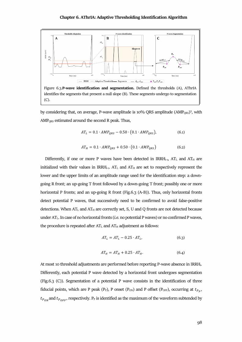
Chapter 6. AThrIA: Adaptive Thresholding Identification Algorithm
98
by considering that, on average, P-wave amplitude is 10% QRS amplitude (AMPQRS)3, with
AMPQRS estimated around the second R peak. Thus,
��� = 0.1 ∙ ��R °± 0.50 ∙ �0.1 ∙ ��R °±�, (6.1)
��³ = 0.1 ∙ ��R °± � 0.50 ∙ �0.1 ∙ ��R °±� (6.2)
Differently, if one or more P waves have been detected in IRRHi-1, ATL and ATH are
initialized with their values in IRRHi-1. ATL and ATH are set to respectively represent the
lower and the upper limits of an amplitude range used for the identification step: a down-
going R front; an up-going T front followed by a down-going T front; possibly one or more
horizontal P fronts; and an up-going R front (Fig.6.3 (A-B)). Thus, only horizontal fronts
detect potential P waves, that successively need to be confirmed to avoid false-positive
detections. When ATL and ATH are correctly set, S, U and Q fronts are not detected because
under ATL. In case of no horizontal fronts (i.e. no potential P waves) or no confirmed P waves,
the procedure is repeated after ATL and ATH adjustment as follows:
��� = ��� 0.25 ∙ ��� , (6.3)
��³ = ��³ � 0.25 ∙ ��³ . (6.4)
At most 10 threshold adjustments are performed before reporting P-wave absence in IRRHi.
Differently, each potential P wave detected by a horizontal front undergoes segmentation
(Fig.6.3 (C)). Segmentation of a potential P wave consists in the identification of three
fiducial points, which are P peak (PP), P onset (PON) and P offset (POFF), occurring at �U´, �Uµ\and �Uµ¶¶, respectively. PP is identified as the maximum of the waveform subtended by
Figure 6.3.P-wave identification and segmentation. Defined the thresholds (A), AThrIA
identifies the segments that present a null slope (B). These segments undergo to segmentation
(C).
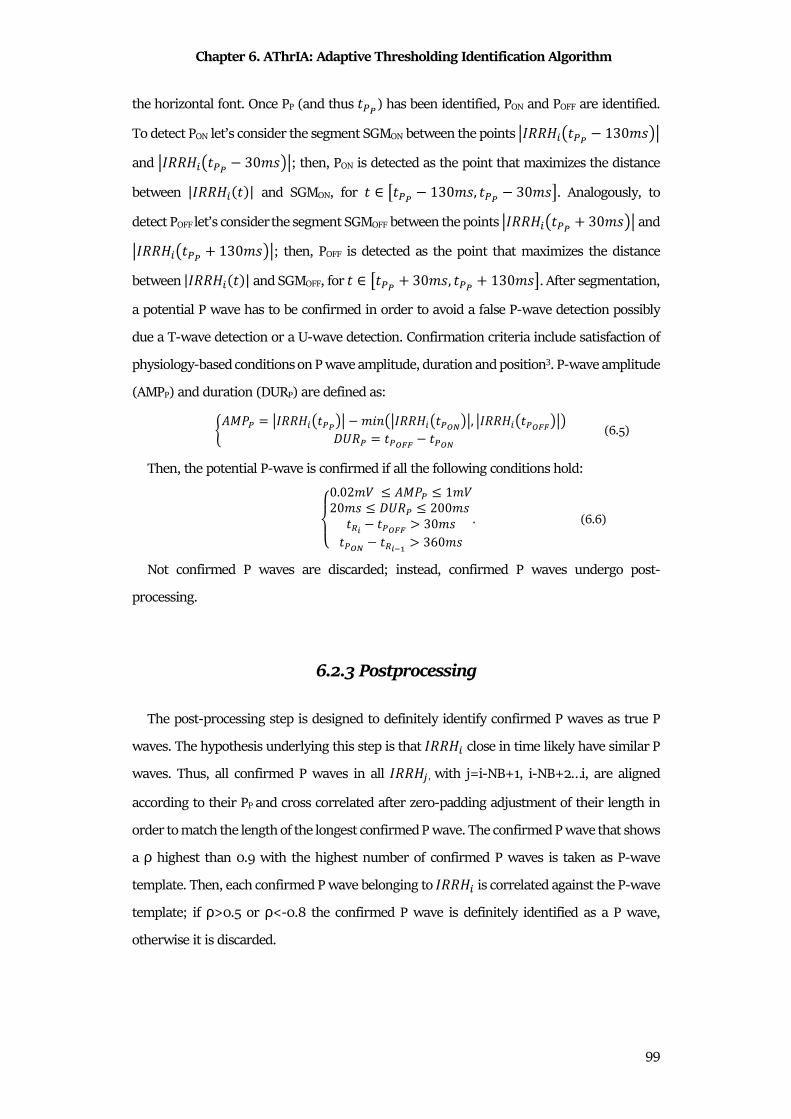
Chapter 6. AThrIA: Adaptive Thresholding Identification Algorithm
99
the horizontal font. Once PP (and thus �U´) has been identified, PON and POFF are identified.
To detect PON let’s consider the segment SGMON between the points ·���¬���U´ 13032�· and ·���¬���U´ 3032�·; then, PON is detected as the point that maximizes the distance
between |���¬� ��| and SGMON, for � ∈ º�U´ 13032, �U´ 3032». Analogously, to
detect POFF let’s consider the segment SGMOFF between the points ·���¬���U´ � 3032�· and ·���¬���U´ � 13032�·; then, POFF is detected as the point that maximizes the distance
between |���¬� ��| and SGMOFF, for � ∈ º�U´ � 3032, �U´ � 13032». After segmentation,
a potential P wave has to be confirmed in order to avoid a false P-wave detection possibly
due a T-wave detection or a U-wave detection. Confirmation criteria include satisfaction of
physiology-based conditions on P wave amplitude, duration and position3. P-wave amplitude
(AMPP) and duration (DURP) are defined as:
¼��RU = ·���¬���U´�· 3.8�·���¬���Uµ\�·, ·���¬���Uµ¶¶�·��|�U = �Uµ¶¶ �Uµ\ (6.5)
Then, the potential P-wave is confirmed if all the following conditions hold:
%'(0.023 ≤ ��RU ≤ 132032 ≤ �|�U ≤ 20032 �°¾ �Uµ¶¶ > 3032�Uµ\ �°¾À[ > 36032 . (6.6)
Not confirmed P waves are discarded; instead, confirmed P waves undergo post-
processing.
6.2.3 Postprocessing
The post-processing step is designed to definitely identify confirmed P waves as true P
waves. The hypothesis underlying this step is that ���¬� close in time likely have similar P
waves. Thus, all confirmed P waves in all ���¬~, with j=i-NB+1, i-NB+2…i, are aligned
according to their PP and cross correlated after zero-padding adjustment of their length in
order to match the length of the longest confirmed P wave. The confirmed P wave that shows
a ρ highest than 0.9 with the highest number of confirmed P waves is taken as P-wave
template. Then, each confirmed P wave belonging to ���¬� is correlated against the P-wave
template; if ρ>0.5 or ρ<-0.8 the confirmed P wave is definitely identified as a P wave,
otherwise it is discarded.
Chapter 6. AThrIA: Adaptive Thresholding Identification Algorithm
100
6.3 Materials
AThrIA was validated in both simulated and real conditions, in order to evaluate its
performance in both controlled and clinical situations.
Using Matlab ECG simulator82, six 0.80 s ECG patterns were simulated (sampling
frequency: 250Hz): the first ECG pattern reproduced the normal wave sequence (PQRST);
the second one also included the U wave (PQRSTU); the third one included double P waves
(PPQRST); the fourth one had no P wave (QRST); the fifth one had a negative P wave (-
PQRST) and the sixth one had a biphasic P wave (±PQRST). When present, simulated ECG
waveforms were characterized by the following amplitudes and durations: 0.16 mV and 0.09
s, respectively, for the P wave; -0.03 mV and 0.07 s, respectively, for the Q wave; 1.60 mV
and 0.08 s, respectively, for the R wave; -0.15mV and 0.07 s, respectively, for the S wave;
0.45 mV and 0.14 s, respectively, for the T-wave, and 0.04mV and 0.05 s, respectively, for
the U wave. Each pattern was repeated 30 times to obtain a simulated ECG. PQRST was
characterized by a mean HR of 75 bpm and HRV of 0.06 s; PQRSTU was characterized by a
mean HR of 75 bpm and HRV of 0.06 s; PPQRST was characterized by a mean HR of 50 bpm
and HRV of 0.05 s; QRST was characterized by a mean HR of 75 bpm and HRV of 0.20 s; -
PQRST was characterized by a mean HR of 75 bpm and HRV of 0.05 s; ±PQRST was
characterized by a mean HR of 75 bpm and HRV of 0.05 s. Specifically, PPQRST was
characterized by two P waves, with a PP distance of 0.08 s; -PQRST was characterized by a
P wave of -0.16 mV; and ±PQRST was characterized by a P wave of 0.16 mV with a positive
part 0f 0.12 mV and a negative part of -0.04 mV.
Simulated ECG were corrupted by adding tracings relative to four types of noise: power
line noise, baseline wander, motion artifact and electrode motion artifact. Power line noise
was simulated as a 50Hz sinusoidal signal; the other three noise tracings were real and taken
from the Physionet “MIT-BIH Noise Stress Test Database”83,84. The amplitude of the four
noise tracings was varied by amplification with four gain factors in order to have controlled
SNR values.
Overall, the simulated dataset was composed of 102 ECG tracings: 6 (one for each ECG
pattern) not affected by noise SNR=∞), and 72 obtained by combining six ECG pattern, four
noise type and three finite SNR .
Clinical data consisted of around 30-beat ECG segments of recordings belonging to the
“QT Database”71, the “AF Termination Challenge Database”85 and to the “MIT-BIH
Chapter 6. AThrIA: Adaptive Thresholding Identification Algorithm
101
Arrhythmia Database P-Wave Annotations”86 by Physionet 83. All data belonging to Physionet
have been fully anonymized and may be used without further approval of the institutional
review board.
The “QT Database”71 contains 105 fifteen-minute two-channel ECG recordings (sampling
frequency: 250 Hz) of all patterns but no PPQRST. Thirty heartbeats of all ECG recordings
but two (sel232 and sel36, respectively71) were previously chosen as representative and
manually annotated by cardiologists, who identified the beginning, peak and end of all ECG
waves, thus including PP, PON and POFF. Only annotated 30-beat ECG segments were used in
our study.
The “AF Termination Challenge Database”85 includes 80 recordings of AF events. Each
record is a one-minute segment of AF, containing two ECG signals (sampling frequency of
128 Hz) extracted from long-term (20-24 hour) ECG recordings. Each record includes a set
of QRS annotations produced by an automated detector. These signals are annotated as no
P-wave.
The “MIT-BIH Arrhythmia Database P-Wave Annotations”86 contains 12 signals with the
correspondence P-wave peak annotations. This database was included because it contains a
case of second order AVB. Four signals of this database were removed, because just present
in “QT Database”. An expert cardiologist was asked to identify and annotate the QRS and P
waves of 30-beat of these recordings, which was originally 30 minutes long (sampling
frequency: 250 Hz).
Overall, the clinical dataset was composed of 294 ECG tracings, 101 with the PQRST
pattern, 92 with the PQRSTU pattern, 1 with the PPQRST pattern, 92 with the QRST pattern,
7 with the -PQRST pattern and 1 with the ±PQRST pattern.
6.4 Statistics
All simulated and real ECG tracings were characterized in terms of HR, HRV and SNR.
Specifically, SNR was computed as:
��� = 20 ∙ log�# ��Rcde��R,Ä�ÅÆ (6.7)
where AMPECG was computed as the mean value of AMPQRS over all IRRHi for i=1,2, …N-
1, while AMPNoise was computed as four times standard deviation of all heartbeats (noisy
heartbeats) minus the related clean IRRHi. Additionally, ECG tracings were classified
according to their ECG pattern and SNR. Classification according to ECG pattern included
Chapter 6. AThrIA: Adaptive Thresholding Identification Algorithm
102
six classes: PQRST, PQRSTU, PPQRST, QRST, -PQRST and ±PQRST. Instead, classification
according to SNR included four classes: no noise (NNoise), for SNR=∞ (possible only in
simulated conditions); low noise (LNoise), for SNR>10dB; medium noise (MNoise), for
7.5dB≤SNR≤10dB; and high noise (HNoise), for SNR<7.5dB.
With the purpose to evaluate AThrIA performance in segmenting the P wave, the errors
(εX, with X=P, ON and OFF) between PP, PON and POFF identifications by AThrIA (REuÇÈÉÊu,
with X=P, ON and OFF) and by manual annotations (REËÌ�ÍÌÎ, with X=P, ON and OFF) were
computed; tolerance level was set at 5ms. Thus, ε was defined follows:
¼." ÏE = ·REuÇÈÉÊu REËÌ�ÍÌη > 532, �/ 8 ÏE = ·REuÇÈÉÊu REËÌ�ÍÌη 532; ." ÏE = ·REuÇÈÉÊu REËÌ�ÍÌη ≤ 532, �/ 8 ÏE = 0. (6.8)
An εP>120ms indicated a false (REuÇÈÉÊu < REËÌ�ÍÌÎ) or a missed (REuÇÈÉÊu > REËÌ�ÍÌÎ) P
wave detection by AThrIA 81. AThrIA performance were evaluated in terms of SE or SP.
Normality of SNR, HR, HRV and εX distributions were evaluated using the Lilliefors’ test.
Not normal distributions were described in terms of MdN and IQR
Finally, AThrIA performance was compared with the performance of the other algorithms
previously reported by Bereza81. Such comparison involved only the results related to the
“QT Database” in terms of εX (mean and standard deviation in ms), SE and the percentage
of P waves belonging in the acceptability group (G1)87, since all other statistics were not
available in Bereza et. Al.81. P-wave onsets, , P-wave peaks and P-wave offsets belong to G1
if their εON, εP, and εOFF are lower than 0.01 s, respectively.
6.5 Results
Results relative to the simulation study are reported in Table 6.1. Overall, 78 signals (2340
heartbeats) were analyzed; SNR was 10±9 dB, HR was 75±1 bpm, and HRV was 0.06±0.01
s. The SE and SP values were 87%, and 100%, respectively. The values of ε were null for all
the features.
Regarding the ECG pattern stratification, 13 signals (390 heartbeats) were classified in
each pattern. The lower value of SE is related to the identification of the PPQRST pattern
(71%), while the higher value of SE is related to the identification of biphasic P-wave patterns
(99%). All the ECG pattern present distributions of ε very close to zero.
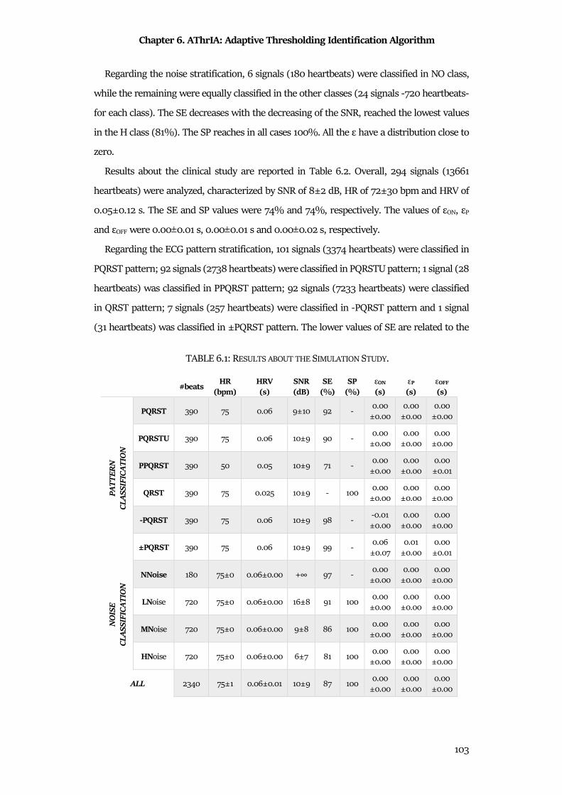
Chapter 6. AThrIA: Adaptive Thresholding Identification Algorithm
103
Regarding the noise stratification, 6 signals (180 heartbeats) were classified in NO class,
while the remaining were equally classified in the other classes (24 signals -720 heartbeats-
for each class). The SE decreases with the decreasing of the SNR, reached the lowest values
in the H class (81%). The SP reaches in all cases 100%. All the ε have a distribution close to
zero.
Results about the clinical study are reported in Table 6.2. Overall, 294 signals (13661
heartbeats) were analyzed, characterized by SNR of 8±2 dB, HR of 72±30 bpm and HRV of
0.05±0.12 s. The SE and SP values were 74% and 74%, respectively. The values of εON, εP
and εOFF were 0.00±0.01 s, 0.00±0.01 s and 0.00±0.02 s, respectively.
Regarding the ECG pattern stratification, 101 signals (3374 heartbeats) were classified in
PQRST pattern; 92 signals (2738 heartbeats) were classified in PQRSTU pattern; 1 signal (28
heartbeats) was classified in PPQRST pattern; 92 signals (7233 heartbeats) were classified
in QRST pattern; 7 signals (257 heartbeats) were classified in -PQRST pattern and 1 signal
(31 heartbeats) was classified in ±PQRST pattern. The lower values of SE are related to the
TABLE 6.1: RESULTS ABOUT THE SIMULATION STUDY.
#beats HR
(bpm) HRV
(s) SNR (dB)
SE (%)
SP
(%) εON
(s) εP
(s) εOFF
(s)
PA
TT
ER
N
CL
AS
SIF
ICA
TIO
N
PQRST 390 75 0.06 9±10 92 - 0.00
±0.00
0.00
±0.00
0.00
±0.00
PQRSTU 390 75 0.06 10±9 90 - 0.00
±0.00
0.00
±0.00
0.00
±0.00
PPQRST 390 50 0.05 10±9 71 - 0.00
±0.00
0.00
±0.00
0.00
±0.01
QRST 390 75 0.025 10±9 - 100 0.00
±0.00
0.00
±0.00
0.00
±0.00
-PQRST 390 75 0.06 10±9 98 - -0.01
±0.00
0.00
±0.00
0.00
±0.00
±PQRST 390 75 0.06 10±9 99 - 0.06
±0.07
0.01
±0.00
0.00
±0.01
NO
ISE
C
LA
SS
IFIC
AT
ION
NNoise 180 75±0 0.06±0.00 +∞ 97 - 0.00
±0.00
0.00
±0.00
0.00
±0.00
LNoise 720 75±0 0.06±0.00 16±8 91 100 0.00
±0.00
0.00
±0.00
0.00
±0.00
MNoise 720 75±0 0.06±0.00 9±8 86 100 0.00
±0.00
0.00
±0.00
0.00
±0.00
HNoise 720 75±0 0.06±0.00 6±7 81 100 0.00
±0.00
0.00
±0.00
0.00
±0.00
ALL 2340 75±1 0.06±0.01 10±9 87 100 0.00
±0.00
0.00
±0.00
0.00
±0.00
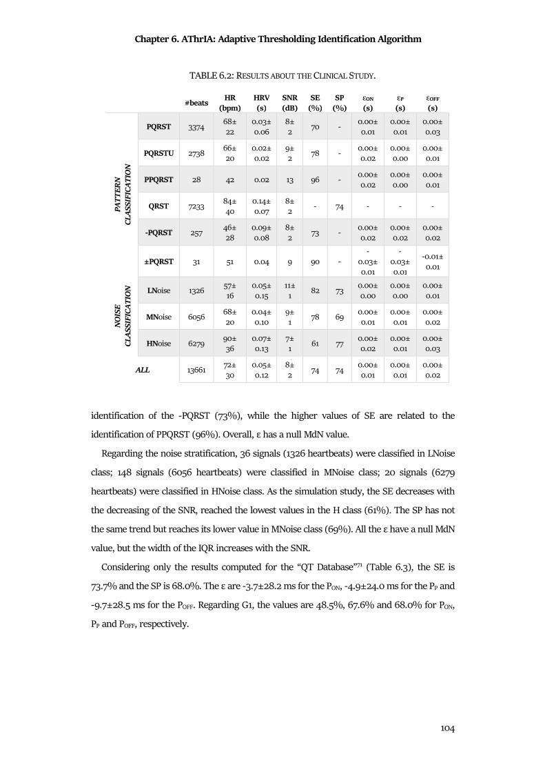
Chapter 6. AThrIA: Adaptive Thresholding Identification Algorithm
104
identification of the -PQRST (73%), while the higher values of SE are related to the
identification of PPQRST (96%). Overall, ε has a null MdN value.
Regarding the noise stratification, 36 signals (1326 heartbeats) were classified in LNoise
class; 148 signals (6056 heartbeats) were classified in MNoise class; 20 signals (6279
heartbeats) were classified in HNoise class. As the simulation study, the SE decreases with
the decreasing of the SNR, reached the lowest values in the H class (61%). The SP has not
the same trend but reaches its lower value in MNoise class (69%). All the ε have a null MdN
value, but the width of the IQR increases with the SNR.
Considering only the results computed for the “QT Database”71 (Table 6.3), the SE is
73.7% and the SP is 68.0%. The ε are -3.7±28.2 ms for the PON, -4.9±24.0 ms for the PP and
-9.7±28.5 ms for the POFF. Regarding G1, the values are 48.5%, 67.6% and 68.0% for PON,
PP and POFF, respectively.
TABLE 6.2: RESULTS ABOUT THE CLINICAL STUDY.
#beats HR
(bpm) HRV
(s) SNR (dB)
SE (%)
SP
(%) εON
(s) εP
(s) εOFF
(s) P
AT
TE
RN
C
LA
SS
IFIC
AT
ION
PQRST 3374
68±
22
0.03±
0.06
8±
2 70 -
0.00±
0.01
0.00±
0.01
0.00±
0.03
PQRSTU 2738 66±
20
0.02±
0.02
9±
2 78 -
0.00±
0.02
0.00±
0.00
0.00±
0.01
PPQRST 28 42 0.02 13 96 - 0.00±
0.02
0.00±
0.00
0.00±
0.01
QRST 7233 84±
40
0.14±
0.07
8±
2 - 74 - - -
-PQRST 257 46±
28
0.09±
0.08
8±
2 73 -
0.00±
0.02
0.00±
0.02
0.00±
0.02
±PQRST 31 51 0.04 9 90 -
-
0.03±
0.01
-
0.03±
0.01
-0.01±
0.01
NO
ISE
C
LA
SS
IFIC
AT
ION
LNoise 1326 57±
16
0.05±
0.15
11±
1 82 73
0.00±
0.00
0.00±
0.00
0.00±
0.01
MNoise 6056 68±
20
0.04±
0.10
9±
1 78 69
0.00±
0.01
0.00±
0.01
0.00±
0.02
HNoise 6279 90±
36
0.07±
0.13
7±
1 61 77
0.00±
0.02
0.00±
0.01
0.00±
0.03
ALL 13661 72±
30
0.05±
0.12
8±
2 74 74
0.00±
0.01
0.00±
0.01
0.00±
0.02
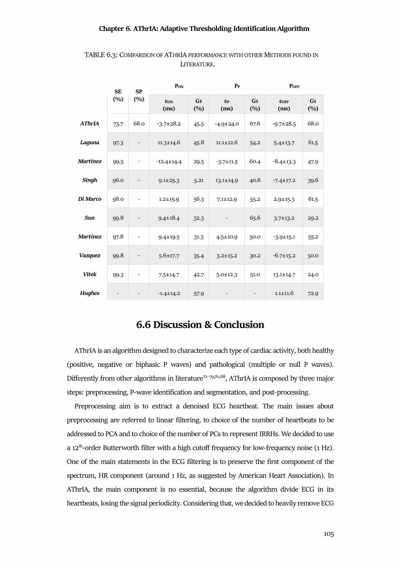
Chapter 6. AThrIA: Adaptive Thresholding Identification Algorithm
105
6.6 Discussion & Conclusion
AThrIA is an algorithm designed to characterize each type of cardiac activity, both healthy
(positive, negative or biphasic P waves) and pathological (multiple or null P waves).
Differently from other algorithms in literature72–79,81,88, AThrIA is composed by three major
steps: preprocessing, P-wave identification and segmentation, and post-processing.
Preprocessing aim is to extract a denoised ECG heartbeat. The main issues about
preprocessing are referred to linear filtering, to choice of the number of heartbeats to be
addressed to PCA and to choice of the number of PCs to represent IRRHs. We decided to use
a 12th-order Butterworth filter with a high cutoff frequency for low-frequency noise (1 Hz).
One of the main statements in the ECG filtering is to preserve the first component of the
spectrum, HR component (around 1 Hz, as suggested by American Heart Association). In
AThrIA, the main component is no essential, because the algorithm divide ECG in its
heartbeats, losing the signal periodicity. Considering that, we decided to heavily remove ECG
TABLE 6.3: COMPARISON OF ATHRIA PERFORMANCE WITH OTHER METHODS FOUND IN
LITERATURE.
SE
(%) SP
(%)
PON PP POFF
εON (ms)
G1 (%)
εP (ms)
G1 (%)
εOFF (ms)
G1 (%)
AThrIA 73.7 68.0 -3.7±28.2 45.5 -4.9±24.0 67.6 -9.7±28.5 68.0
Laguna 97.3 - 11.3±14.6 45.8 11.1±12.6 54.2 5.4±13.7 61.5
Martinez 99.5 - -12.4±14.4 29.5 -3.7±11.5 60.4 -8.4±13.3 47.9
Singh 96.0 - 9.1±25.3 5.21 13.1±14.9 40.6 -7.4±17.2 39.6
Di Marco 98.0 - 1.2±15.9 56.3 7.1±12.9 55.2 2.9±15.3 61.5
Sun 99.8 - 9.4±18.4 32.3 - 65.6 3.7±13.2 29.2
Martinez 97.8 - 9.4±19.5 31.3 4.5±10.9 50.0 -3.9±15.1 55.2
Vazquez 99.8 - 5.6±17.7 35.4 3.2±15.2 30.2 -6.7±15.2 50.0
Vitek 99.3 - 7.5±14.7 42.7 5.0±12.3 51.0 13.1±14.7 24.0
Hughes - - -1.4±14.2 57.9 - - 1.1±11.6 72.9
Chapter 6. AThrIA: Adaptive Thresholding Identification Algorithm
106
low-frequency components (baseline), that could be misinterpreted as P wave. Regarding
the number of heartbeats to be addressed to PCA, we decided to fix it to 8 (23) heartbeats. It
is an arbitrary choice in order to have a quite high number of heartbeats to erase noise, but
also a low number of heartbeats to be able to follow ECG modifications in time. Finally, the
number of PCs still remains an issue to be investigate. Literature58,89 proposed some criteria
to select the number of PCs, but they allow the possibility to maintain a small amount of
noise. In AThrIA, the preprocessing was designed to remove as much noise as possible, so
only the first PC is used to represent IRRHi.
Literature proposed studies about the comparison between PCA and others univariate
approach to filter the ECG signals. Examples are the empirical mode decomposition or the
single channel independent component analysis89. Considering the comparison between
these different statistical methods for filtering, future studies will evaluate if another
statistical method can be a better preprocessing method to enhance P waves.
The P-wave identification and segmentation is the core of AThrIA. Its major innovations
are the search of P waves in all along the IRRHi, allowing the multiple P-waves identifications
and the possibility to confirm a null P-wave. Thanks to two adaptive thresholds, AThrIA is
able to identify P waves, to segment them and to confirm their correctness through three
electrophysiological criteria, by construction defined very large in order to guarantee a high
SE, allowing the recognition of different P-wave morphologies.
The final step is the post-processing, a step added to be sure about the P-wave absence
identification. Several dangerous atrial diseases (e.g. AF) are linked to P-wave absence, thus
a good method to characterize the atrial activity must be able to identify it.
To evaluate AThrIA performance, two studies are applied: a simulation study in order to
test AThrIA under controlled conditions, and a clinical study in order to test AThrIA under
real conditions. For both studies, signals were classified with two different classifications.
First, data were classified according to their ECG pattern, considering six different waveform
configurations. The choice of these patterns is to evaluate the possibility to evaluate the
AThrIA performance in different leads (ECG pattern can contain the U waves or not, and the
P waves can be positive, negative or biphasic), or in pathological conditions (multiple P
waves or null P waves). Both simulation and clinical studies confirm the fact that AThrIA
correctly extracts P waves in all the morphologies and correctly confirms P-wave absence,
providing good values of SE (around 87% and 74% for simulation study and clinical study,
respectively) and SP (around 100% and 74% for simulation study and clinical study,

Chapter 6. AThrIA: Adaptive Thresholding Identification Algorithm
107
respectively). Regarding errors, the MdN values are zero, suggesting that, when AThrIA
identified a P wave, it is correctly segmented. Anyway, the major errors are related to the (-
P)QRST and (±P)QRST patterns, highlighting that AThrIA provides better performances
when it analyzes positive P waves. This issue can be addressed to the imperfect baseline
subtraction: when a small amount of baseline remains, the absolute value operation can
distort the heartbeat, causing difficulties in segmenting negative and biphasic P waves.
Future studies will investigate about adjustment of AThrIA in the identification and
segmentation of biphasic and negative P waves, specifically adding a more efficient baseline
removal.
Secondly, data were classified considering their SNR. SE tends to decrease with the SNR,
but its lowest value reached for the H class (SNR < 7.5 dB) is 61% that is still an acceptable
value. SP has not the same trend, due to the different number of signals in each class.
Anyway, its values are acceptable in each class. Thus, AThrIA is an algorithm robust to noise,
but it provides better results with good quality signals.
Finally, we compared AThrIA performances with the algorithms still present in
literature81. All these algorithms present values of SE very close to 100%, with no values of
SP. Despite the distributions of ε have non-normal distributions, the mean values and the
standard deviation of the ε are computed in order to compare algorithms performances.
Moreover, the G1 index is also computed. Considering AThrIA performances, our algorithm
provides the lowest SE (still acceptable) with good and acceptable values of SP. Nevertheless,
the G1 value are among the highest: it confirms again the fact that, when AThrIA identified
a P wave, it is correctly segmented (low ε).
These results are encouraging: the acceptable values of SE are compensated to
comparable and acceptable values of SP, and the percentage of acceptability are the highest
respect to all the other algorithms present in literature. It confirms that AThrIA correctly
characterizes atrial activity, both when it is normal and when it is pathological.
Chapter 7. CTG Analyzer Graphical User Interface
108
Chapter 7
CTG Analyzer Graphical User Interface
Cardiotocography (CTG) is the gold standard clinical practice for fetal monitoring. This
important test allows to monitor the fetal heart rhythm in relation to maternal uterine
contractions occurrences. The evaluation of the fetal tachogram in relation to maternal
uterine contractions allows to investigate about the fetal ANS control on heart rhythm. This
is essential in order to evaluate the fetal development and its general well-being. Due to these
important features, CTG remains the most important test to be performed at the end of the
pregnancy and during the labor/delivery.
In spite of its widely utility, CTG is still visually evaluated by clinicians. This practice is
common because the situation in which CTG is recorded (labor/delivery) is quite
“emergency”. Anyway, the features that clinicians visually extract are a lot. The high number
of features that have to be assessed and the emergency clinical decisions that have to be
quickly taken indicate that an automatic and objective tool could be essential.
Thus, CTG Analyzer90 is a graphical user interface, born to support clinicians during the
critical phases of delivery and labor. It evaluates the analyzability of CTG tracings and, if
possible, it extracts all the CTG features according with international guidelines.
Due to its characteristics, CTG Analyzer is the perfect example of automatic feature
extraction algorithm. Moreover, the reliability of this new automatic algorithm must be
always tested in clinical practice. The test could be done only by comparing CTG Analyzer
performance with the clinicians’ visual inspection. Moreover, some settings parameters (e.g.
sampling frequency) can be adjusted in order to improve the graphical user interface
performances. Thus, in order to investigate this important issue, biostatistics techniques are
essential.
7.1 Clinical Background
7.1.1 Pregnancy and Delivery
Pregnancy, or gestation, is a physiological state during which one or more fetuses develop
inside the woman. The pregnancy starts with the fertilization of the egg by the sperm and

Chapter 7. CTG Analyzer Graphical User Interface
109
concludes with the delivery. The gestational age is typically 40 weeks long (usually 9
months)(Fig.7.1), and it can be divided in three trimesters. Each trimester is characterized
by a particular aspect of the fetus growth and development. The first trimester starts at the
first week and persists for 12 weeks. During this period, the fertilized cell replicates by
mitosis and become an embryo. At the end of the trimester the fetus is 10 cm long and
weights at about 100 g91. The second trimester starts at the 13th weeks and persists for 15
weeks. During this period, the embryo is called fetus because of its “human” appearance.
The heart activity can be recorded, he/she develops the ability of hearing and also the gender
can be recognized. Moreover, movements can be felt by the mother-to be. At the end of the
second trimester, the fetus is 33 cm long and he/she reaches a weight of 1 kg91. The third
trimester starts at the 29th weeks and persists for 11 weeks, till the delivery. From the 24th
weeks, all the apparatuses are completely developed (except for the nervous and the
respiratory ones), thus, in case of emergency, the fetus has the 90% of possibilities to survive
outside the mother’s abdomen. At the end of the third trimester, the fetus is at about 39 cm
long and he/she weighs 1,7 kg91.
When the fetus is completely developed, the delivery occurs: it is defined as the process
through which the fetus passes from the uterus to the outside, becoming a baby. The uterus
starts to prepare to delivery, increasing its contractility91. Delivery is facilitated also by an
enlargement of the cervix canal and by the position change of the fetus. He/she moves to the
lowest part of the uterus (due also the weigh) and turns in a “headfirst” position. Delivery
starts with the rupture of the amniotic sac that surrounds the baby, causing the outflow of
the amniotic fluid. Thus, uterine contractions become stronger and closer in time, signing
the entrance of the mother-to-be in the labor phase. During the labor, the normal uterine
contractions can be assisted by mother’s voluntary contractions. These high forces,
Figure 7.1.Pregnancy and Gestational Age.

Chapter 7. CTG Analyzer Graphical User Interface
110
combined with a dilatation of the uterus cervix (10 cm), allow to expel the baby from the
mother’s abdomen91.
7.1.2 Maternal and fetal monitoring
All the treatments and examinations performed during the pregnancy are addressed to
monitor the maternal and fetal well-being. All these antenatal cares have to prevent
complications for both the mother and the baby, thus they are scheduled during all the
pregnancy. With the CTG (described below), the most frequent antenatal examinations are:
• Maternal anamnesis and parents’ medical history mother is essential to evaluate the
physical status of the mother (that have to sustain the effort of the labor) and the
fetal risks (like genetic pathologies);
• Blood pressure monitoring is essential to avoid risk for hypertension, risky for the
proceeding of the pregnancy;
• Glycemic curve measurements is performed in order to exclude the gestational
diabetes;
• Measures of the maternal and fetal heights and weights to supervise the changes of
the bodies;
• Pelvic examination and blood/urine tests;
• Periodic ultrasound checkups in order to evaluate the correct development of the
pregnancy (7th week), to investigate about the Down Syndrome (13th-14th weeks) and
to monitor fetal malformation, risks for the mother, the amniotic fluid and umbilical
cord (18th-20th weeks).
These examinations are regulated by different guidelines, with the aim to provide general
rules to ensure a normal and secure pregnancy. The National Institute for Health and Care
Excellence (NICE) published one of the most important guidelines in March 2008 and
updated in January 2017. The aim of this guideline is to offer the best advices to have a good
clinical check-up for all pregnancies and a full set of information to conduct the right
prenatal care for a “healthy woman with an uncomplicated singleton pregnancy”92.
7.1.2 Cardiotocography
Cardiotocography (CTG) is the most commonly used test performed by doctors during
pregnancy and labor in order to establish good health of the fetus93. This examination is
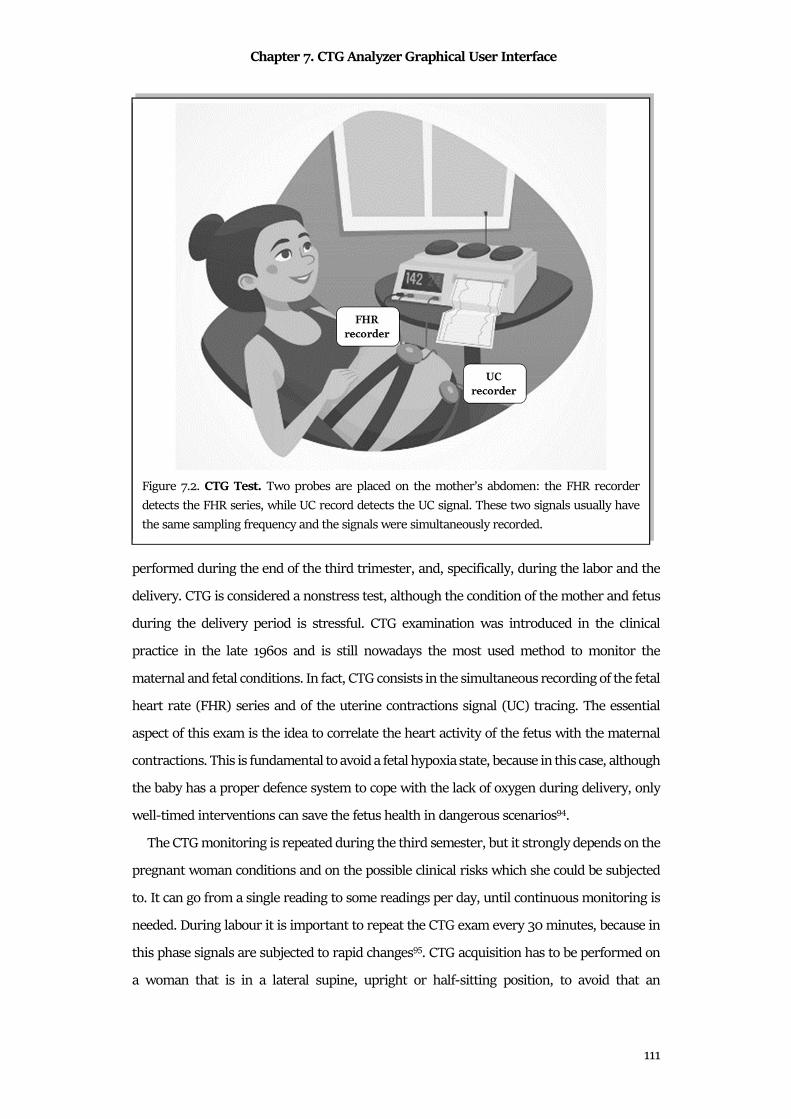
Chapter 7. CTG Analyzer Graphical User Interface
111
performed during the end of the third trimester, and, specifically, during the labor and the
delivery. CTG is considered a nonstress test, although the condition of the mother and fetus
during the delivery period is stressful. CTG examination was introduced in the clinical
practice in the late 1960s and is still nowadays the most used method to monitor the
maternal and fetal conditions. In fact, CTG consists in the simultaneous recording of the fetal
heart rate (FHR) series and of the uterine contractions signal (UC) tracing. The essential
aspect of this exam is the idea to correlate the heart activity of the fetus with the maternal
contractions. This is fundamental to avoid a fetal hypoxia state, because in this case, although
the baby has a proper defence system to cope with the lack of oxygen during delivery, only
well-timed interventions can save the fetus health in dangerous scenarios94.
The CTG monitoring is repeated during the third semester, but it strongly depends on the
pregnant woman conditions and on the possible clinical risks which she could be subjected
to. It can go from a single reading to some readings per day, until continuous monitoring is
needed. During labour it is important to repeat the CTG exam every 30 minutes, because in
this phase signals are subjected to rapid changes95. CTG acquisition has to be performed on
a woman that is in a lateral supine, upright or half-sitting position, to avoid that an
Figure 7.2. CTG Test. Two probes are placed on the mother’s abdomen: the FHR recorder
detects the FHR series, while UC record detects the UC signal. These two signals usually have
the same sampling frequency and the signals were simultaneously recorded.
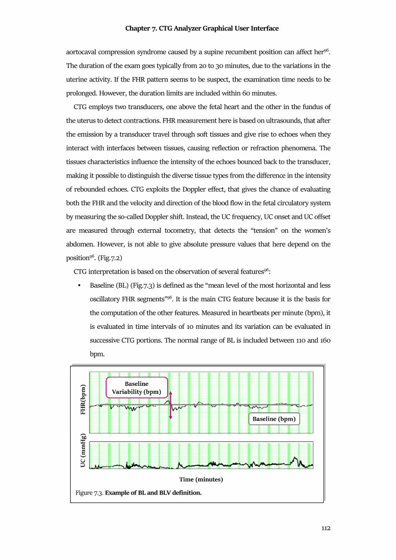
Chapter 7. CTG Analyzer Graphical User Interface
112
aortocaval compression syndrome caused by a supine recumbent position can affect her96.
The duration of the exam goes typically from 20 to 30 minutes, due to the variations in the
uterine activity. If the FHR pattern seems to be suspect, the examination time needs to be
prolonged. However, the duration limits are included within 60 minutes.
CTG employs two transducers, one above the fetal heart and the other in the fundus of
the uterus to detect contractions. FHR measurement here is based on ultrasounds, that after
the emission by a transducer travel through soft tissues and give rise to echoes when they
interact with interfaces between tissues, causing reflection or refraction phenomena. The
tissues characteristics influence the intensity of the echoes bounced back to the transducer,
making it possible to distinguish the diverse tissue types from the difference in the intensity
of rebounded echoes. CTG exploits the Doppler effect, that gives the chance of evaluating
both the FHR and the velocity and direction of the blood flow in the fetal circulatory system
by measuring the so-called Doppler shift. Instead, the UC frequency, UC onset and UC offset
are measured through external tocometry, that detects the “tension” on the women’s
abdomen. However, is not able to give absolute pressure values that here depend on the
position96. (Fig.7.2)
CTG interpretation is based on the observation of several features96:
• Baseline (BL) (Fig.7.3) is defined as the “mean level of the most horizontal and less
oscillatory FHR segments”96. It is the main CTG feature because it is the basis for
the computation of the other features. Measured in heartbeats per minute (bpm), it
is evaluated in time intervals of 10 minutes and its variation can be evaluated in
successive CTG portions. The normal range of BL is included between 110 and 160
bpm.
Figure 7.3. Example of BL and BLV definition.
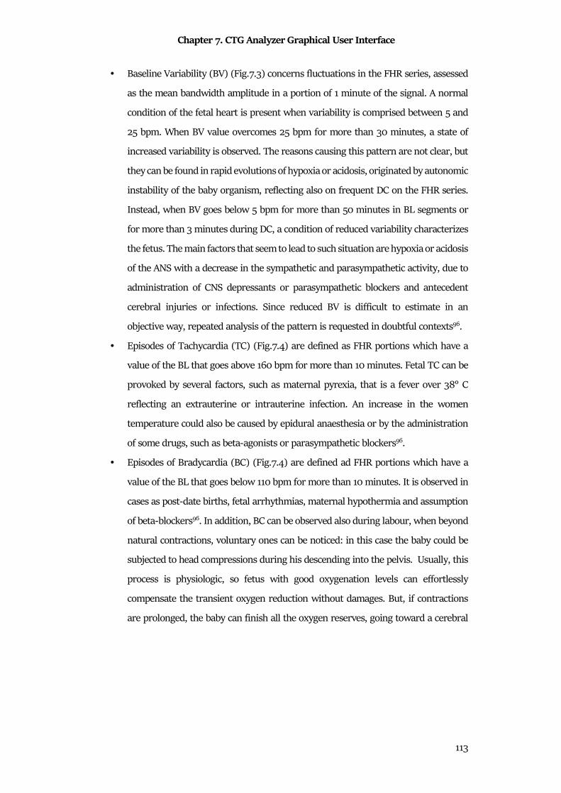
Chapter 7. CTG Analyzer Graphical User Interface
113
• Baseline Variability (BV) (Fig.7.3) concerns fluctuations in the FHR series, assessed
as the mean bandwidth amplitude in a portion of 1 minute of the signal. A normal
condition of the fetal heart is present when variability is comprised between 5 and
25 bpm. When BV value overcomes 25 bpm for more than 30 minutes, a state of
increased variability is observed. The reasons causing this pattern are not clear, but
they can be found in rapid evolutions of hypoxia or acidosis, originated by autonomic
instability of the baby organism, reflecting also on frequent DC on the FHR series.
Instead, when BV goes below 5 bpm for more than 50 minutes in BL segments or
for more than 3 minutes during DC, a condition of reduced variability characterizes
the fetus. The main factors that seem to lead to such situation are hypoxia or acidosis
of the ANS with a decrease in the sympathetic and parasympathetic activity, due to
administration of CNS depressants or parasympathetic blockers and antecedent
cerebral injuries or infections. Since reduced BV is difficult to estimate in an
objective way, repeated analysis of the pattern is requested in doubtful contexts96.
• Episodes of Tachycardia (TC) (Fig.7.4) are defined as FHR portions which have a
value of the BL that goes above 160 bpm for more than 10 minutes. Fetal TC can be
provoked by several factors, such as maternal pyrexia, that is a fever over 38° C
reflecting an extrauterine or intrauterine infection. An increase in the women
temperature could also be caused by epidural anaesthesia or by the administration
of some drugs, such as beta-agonists or parasympathetic blockers96.
• Episodes of Bradycardia (BC) (Fig.7.4) are defined ad FHR portions which have a
value of the BL that goes below 110 bpm for more than 10 minutes. It is observed in
cases as post-date births, fetal arrhythmias, maternal hypothermia and assumption
of beta-blockers96. In addition, BC can be observed also during labour, when beyond
natural contractions, voluntary ones can be noticed: in this case the baby could be
subjected to head compressions during his descending into the pelvis. Usually, this
process is physiologic, so fetus with good oxygenation levels can effortlessly
compensate the transient oxygen reduction without damages. But, if contractions
are prolonged, the baby can finish all the oxygen reserves, going toward a cerebral
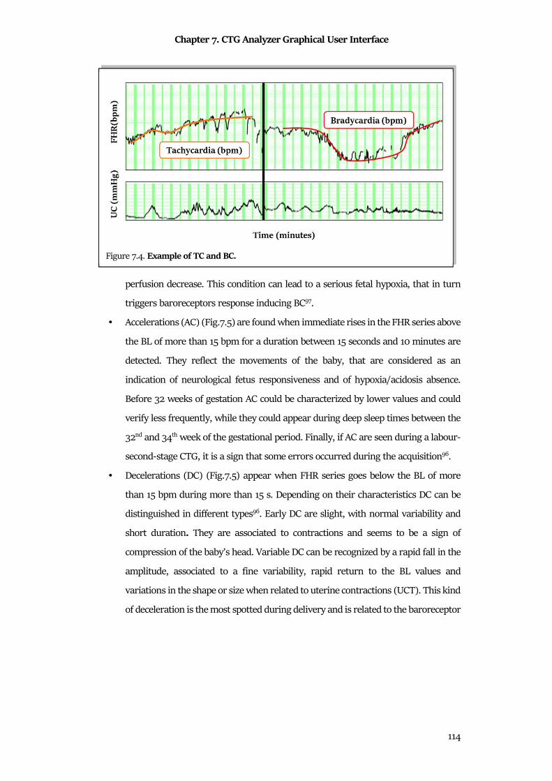
Chapter 7. CTG Analyzer Graphical User Interface
114
perfusion decrease. This condition can lead to a serious fetal hypoxia, that in turn
triggers baroreceptors response inducing BC97.
• Accelerations (AC) (Fig.7.5) are found when immediate rises in the FHR series above
the BL of more than 15 bpm for a duration between 15 seconds and 10 minutes are
detected. They reflect the movements of the baby, that are considered as an
indication of neurological fetus responsiveness and of hypoxia/acidosis absence.
Before 32 weeks of gestation AC could be characterized by lower values and could
verify less frequently, while they could appear during deep sleep times between the
32nd and 34th week of the gestational period. Finally, if AC are seen during a labour-
second-stage CTG, it is a sign that some errors occurred during the acquisition96.
• Decelerations (DC) (Fig.7.5) appear when FHR series goes below the BL of more
than 15 bpm during more than 15 s. Depending on their characteristics DC can be
distinguished in different types96. Early DC are slight, with normal variability and
short duration. They are associated to contractions and seems to be a sign of
compression of the baby’s head. Variable DC can be recognized by a rapid fall in the
amplitude, associated to a fine variability, rapid return to the BL values and
variations in the shape or size when related to uterine contractions (UCT). This kind
of deceleration is the most spotted during delivery and is related to the baroreceptor
Figure 7.4. Example of TC and BC.
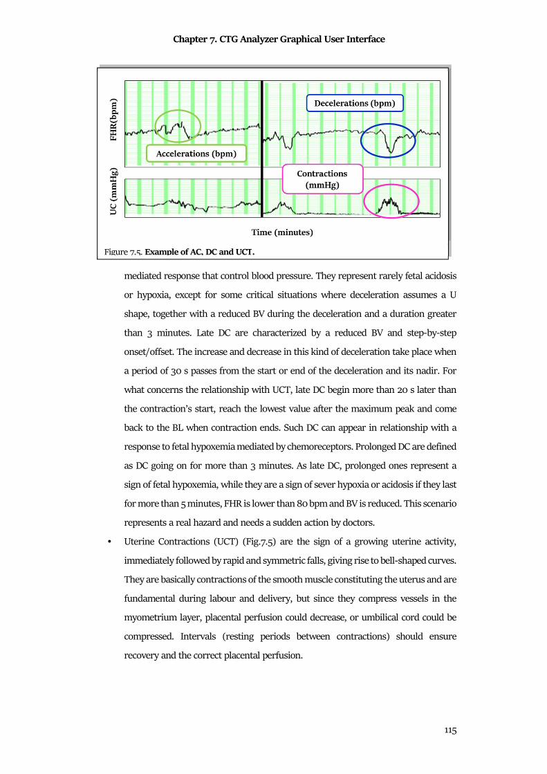
Chapter 7. CTG Analyzer Graphical User Interface
115
mediated response that control blood pressure. They represent rarely fetal acidosis
or hypoxia, except for some critical situations where deceleration assumes a U
shape, together with a reduced BV during the deceleration and a duration greater
than 3 minutes. Late DC are characterized by a reduced BV and step-by-step
onset/offset. The increase and decrease in this kind of deceleration take place when
a period of 30 s passes from the start or end of the deceleration and its nadir. For
what concerns the relationship with UCT, late DC begin more than 20 s later than
the contraction’s start, reach the lowest value after the maximum peak and come
back to the BL when contraction ends. Such DC can appear in relationship with a
response to fetal hypoxemia mediated by chemoreceptors. Prolonged DC are defined
as DC going on for more than 3 minutes. As late DC, prolonged ones represent a
sign of fetal hypoxemia, while they are a sign of sever hypoxia or acidosis if they last
for more than 5 minutes, FHR is lower than 80 bpm and BV is reduced. This scenario
represents a real hazard and needs a sudden action by doctors.
• Uterine Contractions (UCT) (Fig.7.5) are the sign of a growing uterine activity,
immediately followed by rapid and symmetric falls, giving rise to bell-shaped curves.
They are basically contractions of the smooth muscle constituting the uterus and are
fundamental during labour and delivery, but since they compress vessels in the
myometrium layer, placental perfusion could decrease, or umbilical cord could be
compressed. Intervals (resting periods between contractions) should ensure
recovery and the correct placental perfusion.
Figure 7.5. Example of AC, DC and UCT.
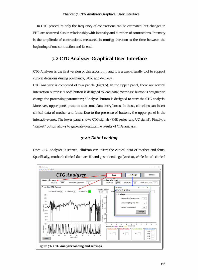
Chapter 7. CTG Analyzer Graphical User Interface
116
In CTG procedure only the frequency of contractions can be estimated, but changes in
FHR are observed also in relationship with intensity and duration of contractions. Intensity
is the amplitude of contractions, measured in mmHg; duration is the time between the
beginning of one contraction and its end.
7.2 CTG Analyzer Graphical User Interface
CTG Analyzer is the first version of this algorithm, and it is a user-friendly tool to support
clinical decisions during pregnancy, labor and delivery.
CTG Analyzer is composed of two panels (Fig.7.6). In the upper panel, there are several
interaction buttons: “Load” button is designed to load data; “Settings” button is designed to
change the processing parameters; “Analyze” button is designed to start the CTG analysis.
Moreover, upper panel presents also some data entry boxes. In these, clinicians can insert
clinical data of mother and fetus. Due to the presence of buttons, the upper panel is the
interactive ones. The lower panel shows CTG signals (FHR series and UC signal). Finally, a
“Report” button allows to generate quantitative results of CTG analysis.
7.2.1 Data Loading
Once CTG Analyzer is started, clinician can insert the clinical data of mother and fetus.
Specifically, mother’s clinical data are ID and gestational age (weeks), while fetus’s clinical
Figure 7.6. CTG Analyzer loading and settings.
Chapter 7. CTG Analyzer Graphical User Interface
117
data are the estimated weight (g), the estimated height (cm) and the gender (1 for male and
0 for female). Then, “Load” (Fig.7.6-red) button allows to lead CTG signals, choosing the
CTG files that clinician wants to analyze. Once selected, CTG signals were represented as
raw data in their entire length. Specifically, the standard CTG representation is maintained
(FHR series above UC signal) and CTG Analyzer provides the total length of CTG signals and
the number of windows in which they can be divided according to default setting. Moreover,
an analyzability criterion is provided. In fact, CTG Analyzer computed the number of
artifacts (data loss) that affect the FHR series. Data loss is defined as the percent of FHR
series that is null. A light indicates if the signals can be analyzed or not. Specifically, a green
light indicates that data loss is lower than 10% (analyzable), while a red light indicates that
data loss is higher than 10% (not analyzable).
7.2.2 Parameter settings
“Settings” button (Fig.7.6-blue) is optional: it could be used to fix CTG signals sampling
frequency and windows length. As default, a sampling frequency of 4 Hz98 and a window
length of 10 minnute96 are set. If FHR and UC sampling frequency or windows length are
changed from their default values, representation and characterization of raw data are
immediately updated accordingly.
7.2.3 Data Analysis
CTG Analyzer starts the signal processing when clinician select the "Analyze" button
(Fig.7.7-green). In order to remove artifacts (data loss), FHR series is pre-processed.
Specifically, data loss are replaced with linear interpolation99,100 between the FHR segments
that includes each artefact. Moreover, FHR series and UC signal are segmented in windows
that are which are then independently analyzed. According with FIGO guidelines96, windows
length of 10 minutes are recommended in order to reliably compute the BL. The last window
is not processed if it does not include the signal end. After the preprocessing, CTG Analyzer
compute the standard CTG features recommended by FIGO guidelines96. All features are
extracted from each CTG window and averaged over windows as a relative measure for a
measure relative to the entire CTG.
CTG features extracted by CTG Analyzer are:
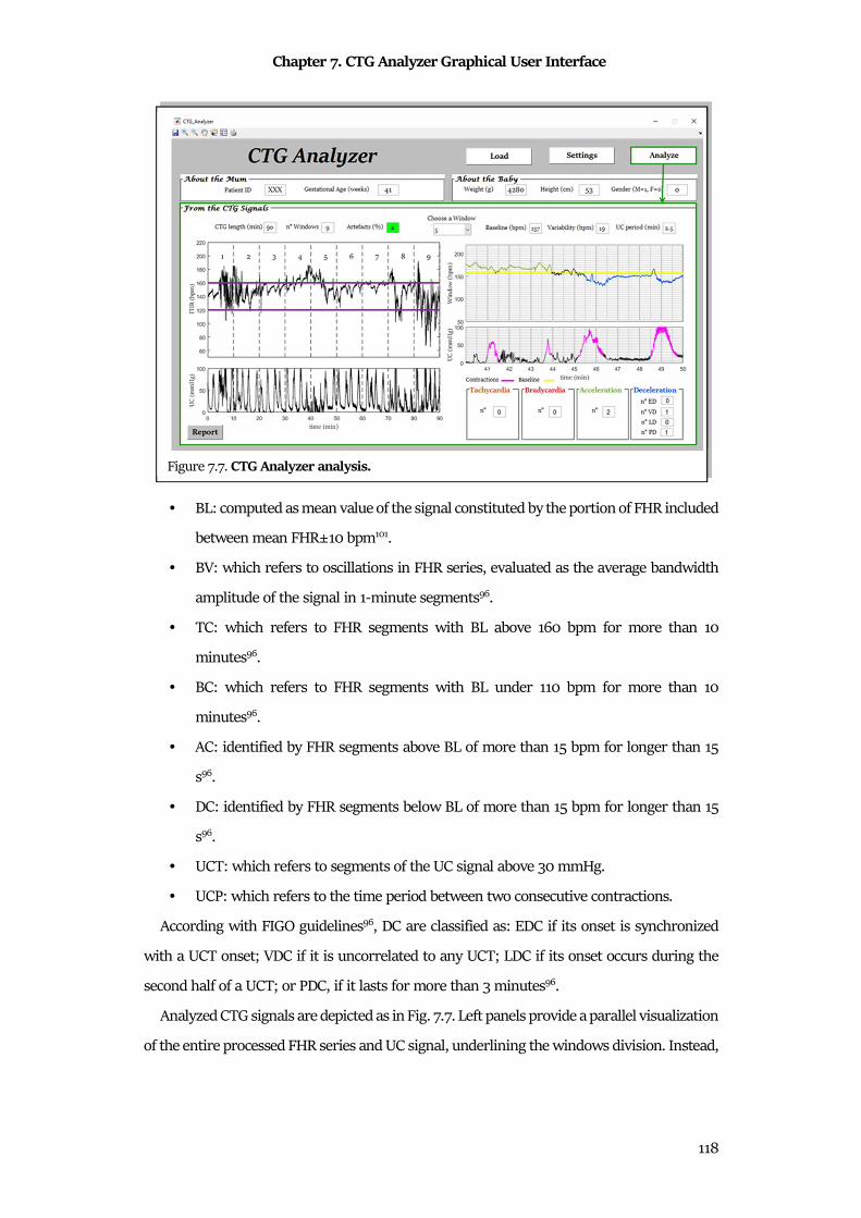
Chapter 7. CTG Analyzer Graphical User Interface
118
• BL: computed as mean value of the signal constituted by the portion of FHR included
between mean FHR±10 bpm101.
• BV: which refers to oscillations in FHR series, evaluated as the average bandwidth
amplitude of the signal in 1-minute segments96.
• TC: which refers to FHR segments with BL above 160 bpm for more than 10
minutes96.
• BC: which refers to FHR segments with BL under 110 bpm for more than 10
minutes96.
• AC: identified by FHR segments above BL of more than 15 bpm for longer than 15
s96.
• DC: identified by FHR segments below BL of more than 15 bpm for longer than 15
s96.
• UCT: which refers to segments of the UC signal above 30 mmHg.
• UCP: which refers to the time period between two consecutive contractions.
According with FIGO guidelines96, DC are classified as: EDC if its onset is synchronized
with a UCT onset; VDC if it is uncorrelated to any UCT; LDC if its onset occurs during the
second half of a UCT; or PDC, if it lasts for more than 3 minutes96.
Analyzed CTG signals are depicted as in Fig. 7.7. Left panels provide a parallel visualization
of the entire processed FHR series and UC signal, underlining the windows division. Instead,
Figure 7.7. CTG Analyzer analysis.
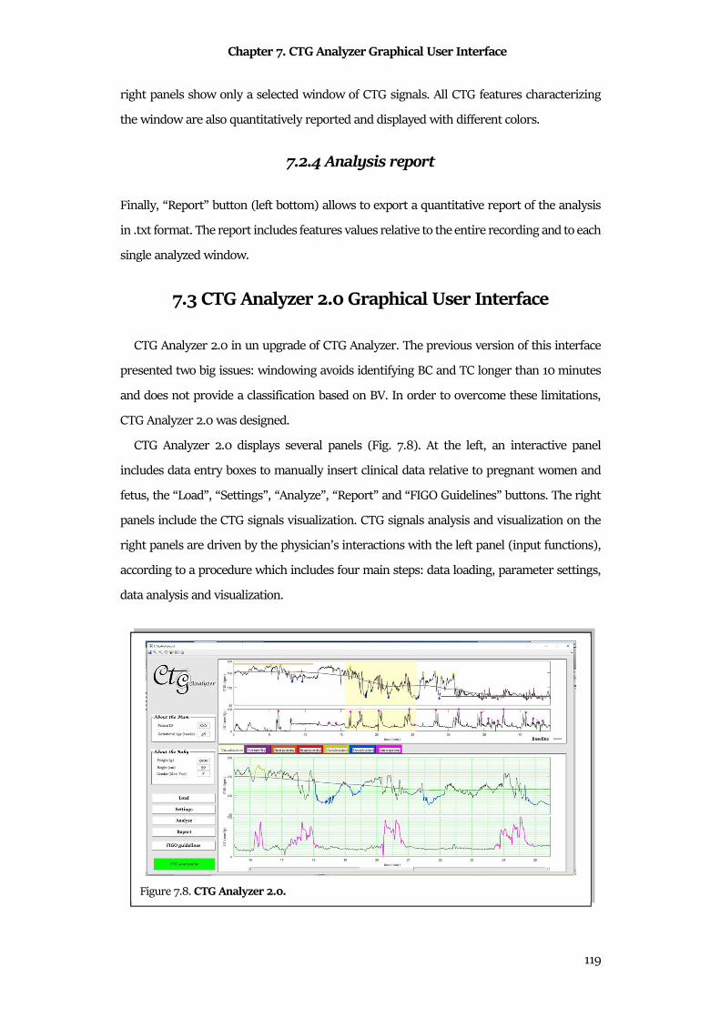
Chapter 7. CTG Analyzer Graphical User Interface
119
right panels show only a selected window of CTG signals. All CTG features characterizing
the window are also quantitatively reported and displayed with different colors.
7.2.4 Analysis report
Finally, “Report” button (left bottom) allows to export a quantitative report of the analysis
in .txt format. The report includes features values relative to the entire recording and to each
single analyzed window.
7.3 CTG Analyzer 2.0 Graphical User Interface
CTG Analyzer 2.0 in un upgrade of CTG Analyzer. The previous version of this interface
presented two big issues: windowing avoids identifying BC and TC longer than 10 minutes
and does not provide a classification based on BV. In order to overcome these limitations,
CTG Analyzer 2.0 was designed.
CTG Analyzer 2.0 displays several panels (Fig. 7.8). At the left, an interactive panel
includes data entry boxes to manually insert clinical data relative to pregnant women and
fetus, the “Load”, “Settings”, “Analyze”, “Report” and “FIGO Guidelines” buttons. The right
panels include the CTG signals visualization. CTG signals analysis and visualization on the
right panels are driven by the physician’s interactions with the left panel (input functions),
according to a procedure which includes four main steps: data loading, parameter settings,
data analysis and visualization.
Figure 7.8. CTG Analyzer 2.0.
Chapter 7. CTG Analyzer Graphical User Interface
120
7.3.1 Data Loading
Through the button “Load”, CTG Analyzer 2.0 loads CTG data (all file extension supported
by MATLAB® may be used). In CTG Analyzer, the clinician can optionally insert mother (ID
and gestational age) and fetus (estimated weight and height, and gender) clinical data. After
file selection, CTG Analyzer 2.0 evaluates the analyzability of the selected CTG signal. Indeed,
a green or red message appears if the acceptability criteria are respected or not, respectively.
Differently from CTG Analyzer90, two acceptability criteria are applied: the first criterion
establishes that the FHR data loss artefact has to be at most 10%90, while the second criterion
establishes that UC period has to be at least 0.003 Hz. CTG Analyzer 2.0 also provides the
CTG signal total length and the visualization of the entire raw traces on the right top panel.
Only acceptable CTG signals can be analyzed.
7.3.2 Parameter settings
Use of the “Settings” button is optional: it allows to change the CTG signals sampling
frequency (default: 4 Hz) and length of the window for the visualization of the signal
(default: 10 min).
7.3.3 Data Analysis
The button “Analyze” starts the CTG features extraction procedure. Firstly, CTG signals
are pre-processed: FHR is corrected to remove artefacts90 and the UC is filtered (low-pass
bidirectional 3rd-order Butterworth filter; cut-off frequency: 0.025 Hz). Then, CTG features
are extracted according to FIGO guidelines96: the BL is computed as mean value of FHR 10-
minutes portion included between mean FHR±10 bpm; the BV is computed as the average
bandwidth amplitude (implemented as standard deviation) of FHR in 1-minute segments;
TC and BC are computed as the FHR segments with BL above/under 160/110 bpm for more
than 10 minute, respectively; acceleration and deceleration are computed as the FHR
segments above/under BL±15 bpm for longer than 15 s, respectively; UCT are computed as
the UC segments above 30 mmHg; and the UCP is computed as the time between two
consecutive contractions. According with the uterine-contraction occurrence, DC are further
classified as: EDC, VDC, LDC, or PDC. Differently from CTG Analyzer90, CTG Analyzer 2.0 is
complete independent from a windowing process: features are computed using a mobile
Chapter 7. CTG Analyzer Graphical User Interface
121
window around each specific sample of the signal. The length of the window is dependent
on the computed feature; in particular, a window of 10 minute is used for the BL computation
(and for BL-dependent features) and a window of 1 minute is used for the BV computation.
Moreover, CTG Analyzer 2.0 provides a classification of the BV. According with FIGO
guidelines, the BV can be classified in reduced BV (below 5 bpm for more than 50 min) or
increased BV (above 25 bpm for more than 30 min).
7.3.4 Visualization
A completely new visualization of analyzed CTG signals (Fig. 7.8) is displayed on the right
panel. Right top panel provides a parallel visualization of entire processed FHR and UC
signals; additionally, all features are reported with different colors. In the right bottom panel,
user can choose what to plot among the seven CTG features, each identified by a specific
color for immediate recognition. All plots display CTG signals on the standard CTG green
grid, according with the FIGO Guidelines96. In particular, “Visualization” (light yellow)
shows a specific window of the signals (chosen by the user in the settings) that appears
yellow-shaded on the top panel; and “Variability” (Purple), “Tachycardia” (Orange),
“Bradycardia” (Red), “Acceleration” (Green), “Deceleration” (Blue) and “Contractions”
(Magenta) show and quantify (in terms of duration and amplitude) the episodes of
corresponding feature. As accessory functions, CTG Analyzer 2.0 can save the performed
analysis (“Report” button) and can open the PDF file relative to the used guidelines (“FIGO
Guidelines” button)96.
7.4 Features Dependency from Sampling Frequency
CTG Analyzer and CTG Analyzer 2.0 opens a big issue in CTG features computing, the
sampling frequency (Sf) choice. Indeed, all CTG features are susceptible to Sf: optimal Sf
should be a tradeoff between a sufficiently high to allow correct identification of CTG
features and a sufficiently low computational time to permit real-time CTG processing. In
absence formal recommendation in literature, the range of Sf values found in literature for
FHR series and UC signal is from 4 Hz to 0.2 Hz102–104.
In order to investigate which is the optimal Sf for CTG Analysis, CTG Analyzer was applied
to 552 CTG signals, sampled with different Sfs. Automatic CTG features were compared with
visual inspection features.
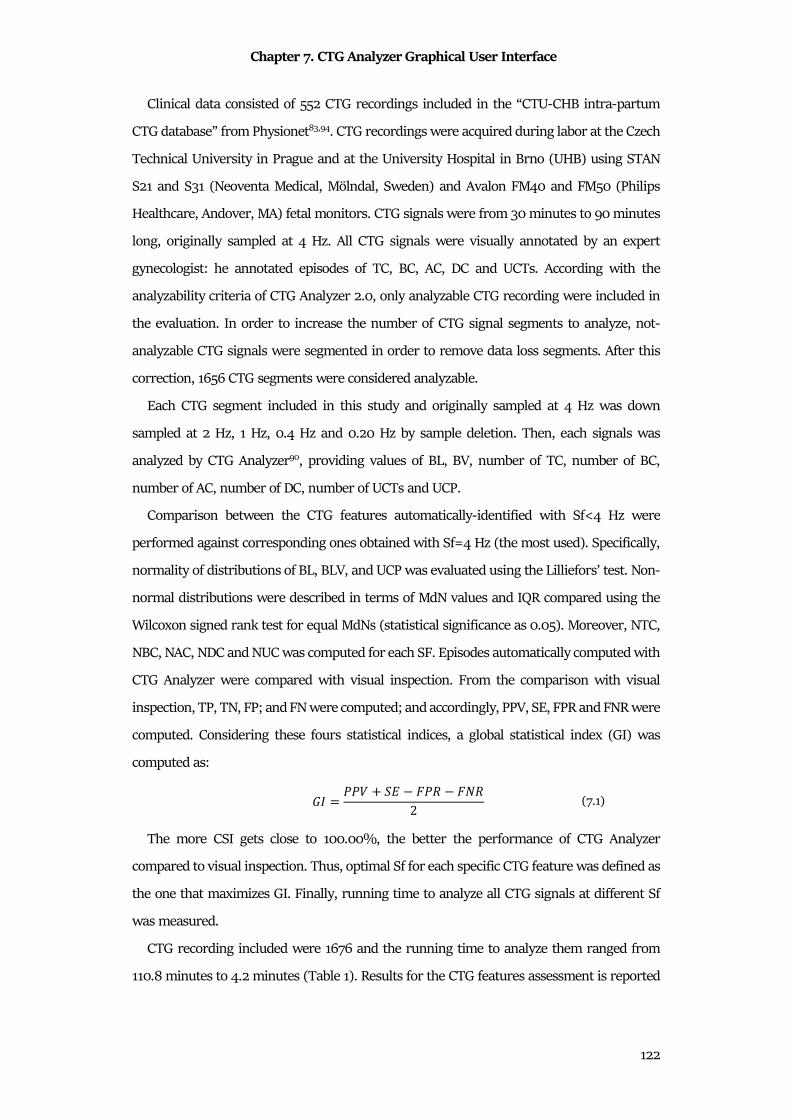
Chapter 7. CTG Analyzer Graphical User Interface
122
Clinical data consisted of 552 CTG recordings included in the “CTU-CHB intra-partum
CTG database” from Physionet83,94. CTG recordings were acquired during labor at the Czech
Technical University in Prague and at the University Hospital in Brno (UHB) using STAN
S21 and S31 (Neoventa Medical, Mölndal, Sweden) and Avalon FM40 and FM50 (Philips
Healthcare, Andover, MA) fetal monitors. CTG signals were from 30 minutes to 90 minutes
long, originally sampled at 4 Hz. All CTG signals were visually annotated by an expert
gynecologist: he annotated episodes of TC, BC, AC, DC and UCTs. According with the
analyzability criteria of CTG Analyzer 2.0, only analyzable CTG recording were included in
the evaluation. In order to increase the number of CTG signal segments to analyze, not-
analyzable CTG signals were segmented in order to remove data loss segments. After this
correction, 1656 CTG segments were considered analyzable.
Each CTG segment included in this study and originally sampled at 4 Hz was down
sampled at 2 Hz, 1 Hz, 0.4 Hz and 0.20 Hz by sample deletion. Then, each signals was
analyzed by CTG Analyzer90, providing values of BL, BV, number of TC, number of BC,
number of AC, number of DC, number of UCTs and UCP.
Comparison between the CTG features automatically-identified with Sf<4 Hz were
performed against corresponding ones obtained with Sf=4 Hz (the most used). Specifically,
normality of distributions of BL, BLV, and UCP was evaluated using the Lilliefors’ test. Non-
normal distributions were described in terms of MdN values and IQR compared using the
Wilcoxon signed rank test for equal MdNs (statistical significance as 0.05). Moreover, NTC,
NBC, NAC, NDC and NUC was computed for each SF. Episodes automatically computed with
CTG Analyzer were compared with visual inspection. From the comparison with visual
inspection, TP, TN, FP; and FN were computed; and accordingly, PPV, SE, FPR and FNR were
computed. Considering these fours statistical indices, a global statistical index (GI) was
computed as:
P� = RR � �$ �R� ���2 (7.1)
The more CSI gets close to 100.00%, the better the performance of CTG Analyzer
compared to visual inspection. Thus, optimal Sf for each specific CTG feature was defined as
the one that maximizes GI. Finally, running time to analyze all CTG signals at different Sf
was measured.
CTG recording included were 1676 and the running time to analyze them ranged from
110.8 minutes to 4.2 minutes (Table 1). Results for the CTG features assessment is reported
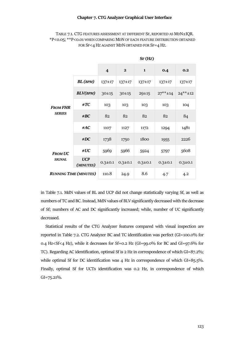
Chapter 7. CTG Analyzer Graphical User Interface
123
in Table 7.1. MdN values of BL and UCP did not change statistically varying Sf, as well as
numbers of TC and BC. Instead, MdN values of BLV significantly decreased with the decrease
of Sf; numbers of AC and DC significantly increased; while, number of UC significantly
decreased.
Statistical results of the CTG Analyzer features compared with visual inspection are
reported in Table 7.2. CTG Analyzer BC and TC identification was perfect (GI=100.0% for
0.4 Hz<Sf<4 Hz), while it decreases for Sf=0.2 Hz (GI=99.0% for BC and GI=97.6% for
TC). Regarding AC identification, optimal Sf is 2 Hz in correspondence of which GI=87.2%;
while optimal Sf for DC identification was 4 Hz in correspondence of which GI=85.5%.
Finally, optimal Sf for UCTs identification was 0.2 Hz, in correspondence of which
GI=75.21%.
TABLE 7.1. CTG FEATURES ASSESSMENT AT DIFFERENT SF, REPORTED AS MDN±IQR.
*P<0.05; **P<0.01 WHEN COMPARING MDN OF EACH FEATURE DISTRIBUTION OBTAINED
FOR SF<4 HZ AGAINST MDN OBTAINED FOR SF=4 HZ.
SF (HZ)
4 2 1 0.4 0.2
FROM FHR
SERIES
BL (BPM) 137±17 137±17 137±17 137±17 137±17
BLV(BPM) 30±15 30±15 29±15 27**±14 24**±12
#TC 103 103 103 103 104
#BC 82 82 82 82 84
#AC 1107 1127 1172 1294 1481
#DC 1738 1750 1800 1955 2226
FROM UC
SIGNAL
#UC 5969 5966 5924 5797 5608
UCP
(MINUTES) 0.3±0.1 0.3±0.1 0.3±0.1 0.3±0.1 0.3±0.1
RUNNING TIME (MINUTES) 110.8 24.9 8.6 4.7 4.2
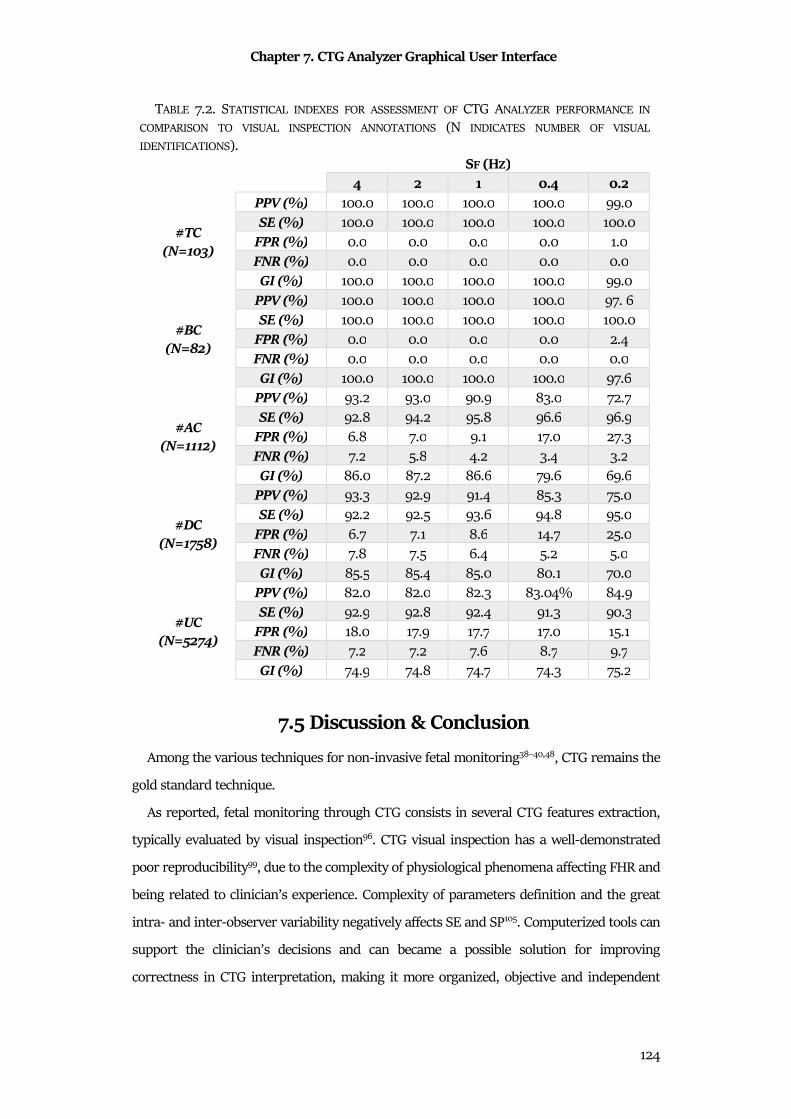
Chapter 7. CTG Analyzer Graphical User Interface
124
7.5 Discussion & Conclusion
Among the various techniques for non-invasive fetal monitoring38–40,48, CTG remains the
gold standard technique.
As reported, fetal monitoring through CTG consists in several CTG features extraction,
typically evaluated by visual inspection96. CTG visual inspection has a well-demonstrated
poor reproducibility99, due to the complexity of physiological phenomena affecting FHR and
being related to clinician’s experience. Complexity of parameters definition and the great
intra- and inter-observer variability negatively affects SE and SP105. Computerized tools can
support the clinician’s decisions and can became a possible solution for improving
correctness in CTG interpretation, making it more organized, objective and independent
TABLE 7.2. STATISTICAL INDEXES FOR ASSESSMENT OF CTG ANALYZER PERFORMANCE IN
COMPARISON TO VISUAL INSPECTION ANNOTATIONS (N INDICATES NUMBER OF VISUAL
IDENTIFICATIONS).
SF (HZ)
4 2 1 0.4 0.2
#TC (N=103)
PPV (%) 100.0 100.0 100.0 100.0 99.0
SE (%) 100.0 100.0 100.0 100.0 100.0
FPR (%) 0.0 0.0 0.0 0.0 1.0
FNR (%) 0.0 0.0 0.0 0.0 0.0
GI (%) 100.0 100.0 100.0 100.0 99.0
#BC (N=82)
PPV (%) 100.0 100.0 100.0 100.0 97. 6
SE (%) 100.0 100.0 100.0 100.0 100.0
FPR (%) 0.0 0.0 0.0 0.0 2.4
FNR (%) 0.0 0.0 0.0 0.0 0.0
GI (%) 100.0 100.0 100.0 100.0 97.6
#AC (N=1112)
PPV (%) 93.2 93.0 90.9 83.0 72.7
SE (%) 92.8 94.2 95.8 96.6 96.9
FPR (%) 6.8 7.0 9.1 17.0 27.3
FNR (%) 7.2 5.8 4.2 3.4 3.2
GI (%) 86.0 87.2 86.6 79.6 69.6
#DC (N=1758)
PPV (%) 93.3 92.9 91.4 85.3 75.0
SE (%) 92.2 92.5 93.6 94.8 95.0
FPR (%) 6.7 7.1 8.6 14.7 25.0
FNR (%) 7.8 7.5 6.4 5.2 5.0
GI (%) 85.5 85.4 85.0 80.1 70.0
#UC (N=5274)
PPV (%) 82.0 82.0 82.3 83.04% 84.9
SE (%) 92.9 92.8 92.4 91.3 90.3
FPR (%) 18.0 17.9 17.7 17.0 15.1
FNR (%) 7.2 7.2 7.6 8.7 9.7
GI (%) 74.9 74.8 74.7 74.3 75.2
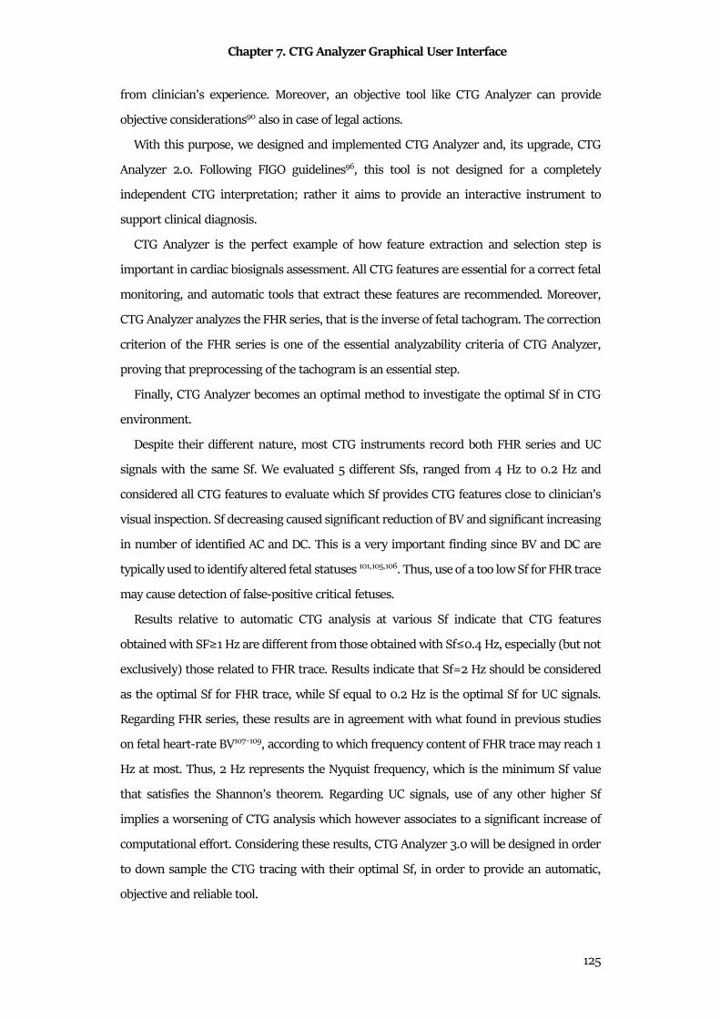
Chapter 7. CTG Analyzer Graphical User Interface
125
from clinician’s experience. Moreover, an objective tool like CTG Analyzer can provide
objective considerations90 also in case of legal actions.
With this purpose, we designed and implemented CTG Analyzer and, its upgrade, CTG
Analyzer 2.0. Following FIGO guidelines96, this tool is not designed for a completely
independent CTG interpretation; rather it aims to provide an interactive instrument to
support clinical diagnosis.
CTG Analyzer is the perfect example of how feature extraction and selection step is
important in cardiac biosignals assessment. All CTG features are essential for a correct fetal
monitoring, and automatic tools that extract these features are recommended. Moreover,
CTG Analyzer analyzes the FHR series, that is the inverse of fetal tachogram. The correction
criterion of the FHR series is one of the essential analyzability criteria of CTG Analyzer,
proving that preprocessing of the tachogram is an essential step.
Finally, CTG Analyzer becomes an optimal method to investigate the optimal Sf in CTG
environment.
Despite their different nature, most CTG instruments record both FHR series and UC
signals with the same Sf. We evaluated 5 different Sfs, ranged from 4 Hz to 0.2 Hz and
considered all CTG features to evaluate which Sf provides CTG features close to clinician’s
visual inspection. Sf decreasing caused significant reduction of BV and significant increasing
in number of identified AC and DC. This is a very important finding since BV and DC are
typically used to identify altered fetal statuses 101,105,106. Thus, use of a too low Sf for FHR trace
may cause detection of false-positive critical fetuses.
Results relative to automatic CTG analysis at various Sf indicate that CTG features
obtained with SF≥1 Hz are different from those obtained with Sf≤0.4 Hz, especially (but not
exclusively) those related to FHR trace. Results indicate that Sf=2 Hz should be considered
as the optimal Sf for FHR trace, while Sf equal to 0.2 Hz is the optimal Sf for UC signals.
Regarding FHR series, these results are in agreement with what found in previous studies
on fetal heart-rate BV107–109, according to which frequency content of FHR trace may reach 1
Hz at most. Thus, 2 Hz represents the Nyquist frequency, which is the minimum Sf value
that satisfies the Shannon’s theorem. Regarding UC signals, use of any other higher Sf
implies a worsening of CTG analysis which however associates to a significant increase of
computational effort. Considering these results, CTG Analyzer 3.0 will be designed in order
to down sample the CTG tracing with their optimal Sf, in order to provide an automatic,
objective and reliable tool.
Chapter 8. eCTG Software
126
Chapter 8
eCTG Software
As still discussed in the previous chapter, fetal monitoring by CTG is a consolidated
practice. One of the main issues of CTG clinical practice (with the visual inspection limitation
discussed in chapter 8) is that most CTG recorders still provide paper reports and no digital
outputs. This practice causes several difficulties, such as the difficulty in storing and
managing large volumes of CTG sheets that tend to get damaged over time; difficulty in
sharing CTG reports among clinicians for additional opinions; and, most importantly,
subjectivity in the clinical interpretation99,106 (printed CTG signals cannot be automatically
analyzed). Moreover, there are no possibility to have digital CTG databases. Law amount of
CTG databases influences the importance of retrospective studies finalized to set up
automatic procedures for CTG analysis90,99–101,105,106,110 and to investigate new criteria that can
be included in the clinical practice. However, CTG clinical practice is based on the use of CTG
paper report to evaluate the fetal well-being. Thus, new methods convert scanned images of
CTG paper report can be useful to obtain digital CTG signals. These obtained CTG signals,
opportunely collected in databases, can be the bases of new research on CTG monitoring.
Thus, this is the aim with which we designed and implemented eCTG, a new method for the
digitalization of CTG paper reports.
From a biostatistics point of view, the basis of eCTG signal extraction is the Otsu’s
methods and a specific correction algorithm based on statistical distributions.
8.1 Technical Background
Recorded CTG signals are typically included in a unique paper produced by the
cardiotocograph, the CTG paper report. This report usually presents the FHR series in the
upper part of the sheet and the simultaneous UC signal in the bottom part of the sheet. Upper
part is 2 times the bottom part, in order to facilitate the FHR series assessment.
Typically green96, CTG paper report presents a specific the paper scale. It is characterized
horizontally by the “paper speed”, for which usually chosen values are 1 cm/min. This time
axis is common for both FHR series and UC signal, and the minutes are separated by a
vertical line. An additional thinner vertical line is present with intervals of 30 s. FHR grid
Chapter 8. eCTG Software
127
ranges from FHR-minimum (minFHR, typically 50 bpm) to FHR-maximum (maxFHR,
typically 210÷250 bpm; horizontal-line distance=5 bpm); UC grid ranges from 0 mmHg to
UC maximum (maxUC, typically 100 mmHg; horizontal-line distance=10 mmHg).
8.2 Methods
eCTG procedure consists of four phases (Fig. 8.1): preprocessing, global thresholding, signal
extraction and signal calibration.
8.2.1 Preprocessing
Initially, a grayscale conversion of the scanned CTG paper is performed (28 gray levels)
maintaining the same resolution. Due to the same resolution, this grayscale image can be
represented with the same dimensions of the original scanned CTG paper, that is R×C
(R=number of rows; C=number of columns). Then, this grayscale image is resized into a
R×C’ matrix. C’ is defined according to desired sampling frequency (dSf), scanned CTG paper
and CTG-grid proprierties111:
O′ = O0.39 ⋅ 0 21k9�.18 ⋅ 60 ⋅ 4�". (8.1)
Finally, this resized grayscale image is divided into two parts: grayscale FHR image is a
2·R/3×C’ matrix, while grayscale UC image is a R/3×C’matrix.
8.2.2 Global thresholding
Global thresholding111 is a statistical techniques in image processing, used to transform a
grayscale image into a binary mask of the same size. The basis of the global thresholding is
the definition of an optimal threshold for classify pixels in black (background pixels, denoted
with the number 0) and white pixels (signal of interest, denoted with the number 1). The
method to select optimal threshold is the Otsu’s method112. It approximates the histogram
of a grayscale image to be bimodal and composed by summation of two Gaussian
distributions, one for each class of pixels (0 and 1). Optimal threshold minimizes the intra-
class variance. Otsu’s global thresholding was applied twice: firstly to discriminate pixels in
the grayscale FHR image and secondly to discriminate pixels in the grayscale UC image112.
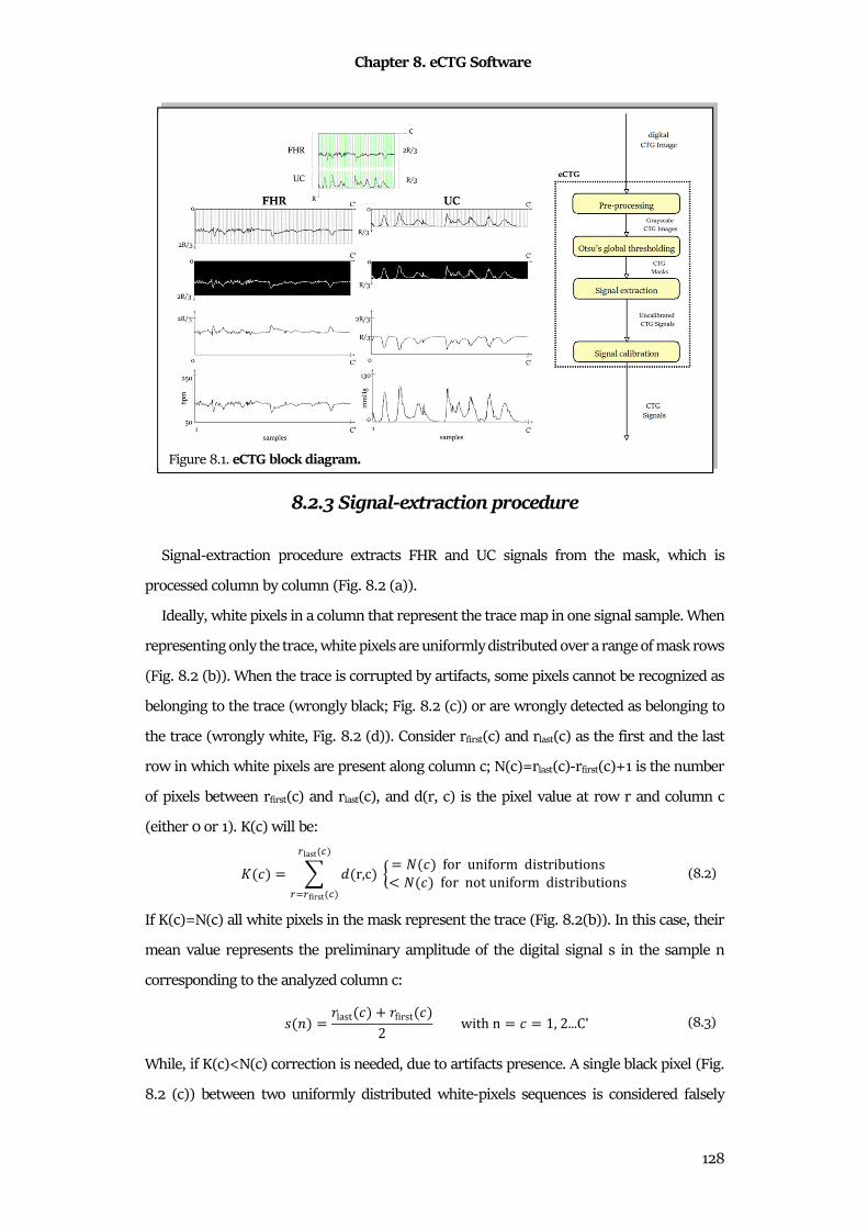
Chapter 8. eCTG Software
128
8.2.3 Signal-extraction procedure
Signal-extraction procedure extracts FHR and UC signals from the mask, which is
processed column by column (Fig. 8.2 (a)).
Ideally, white pixels in a column that represent the trace map in one signal sample. When
representing only the trace, white pixels are uniformly distributed over a range of mask rows
(Fig. 8.2 (b)). When the trace is corrupted by artifacts, some pixels cannot be recognized as
belonging to the trace (wrongly black; Fig. 8.2 (c)) or are wrongly detected as belonging to
the trace (wrongly white, Fig. 8.2 (d)). Consider rfirst(c) and rlast(c) as the first and the last
row in which white pixels are present along column c; N(c)=rlast(c)-rfirst(c)+1 is the number
of pixels between rfirst(c) and rlast(c), and d(r, c) is the pixel value at row r and column c
(either 0 or 1). K(c) will be:
Ó �� = ) 4 r,c� Ö = � �� for uniform distributions < � �� for not uniform distributionsÉlast à�
É-Éfirst à� (8.2)
If K(c)=N(c) all white pixels in the mask represent the trace (Fig. 8.2(b)). In this case, their
mean value represents the preliminary amplitude of the digital signal s in the sample n
corresponding to the analyzed column c:
2 8� = 0last �� � 0first ��2 with n = � = 1, 2...C' (8.3)
While, if K(c)<N(c) correction is needed, due to artifacts presence. A single black pixel (Fig.
8.2 (c)) between two uniformly distributed white-pixels sequences is considered falsely
Figure 8.1. eCTG block diagram.
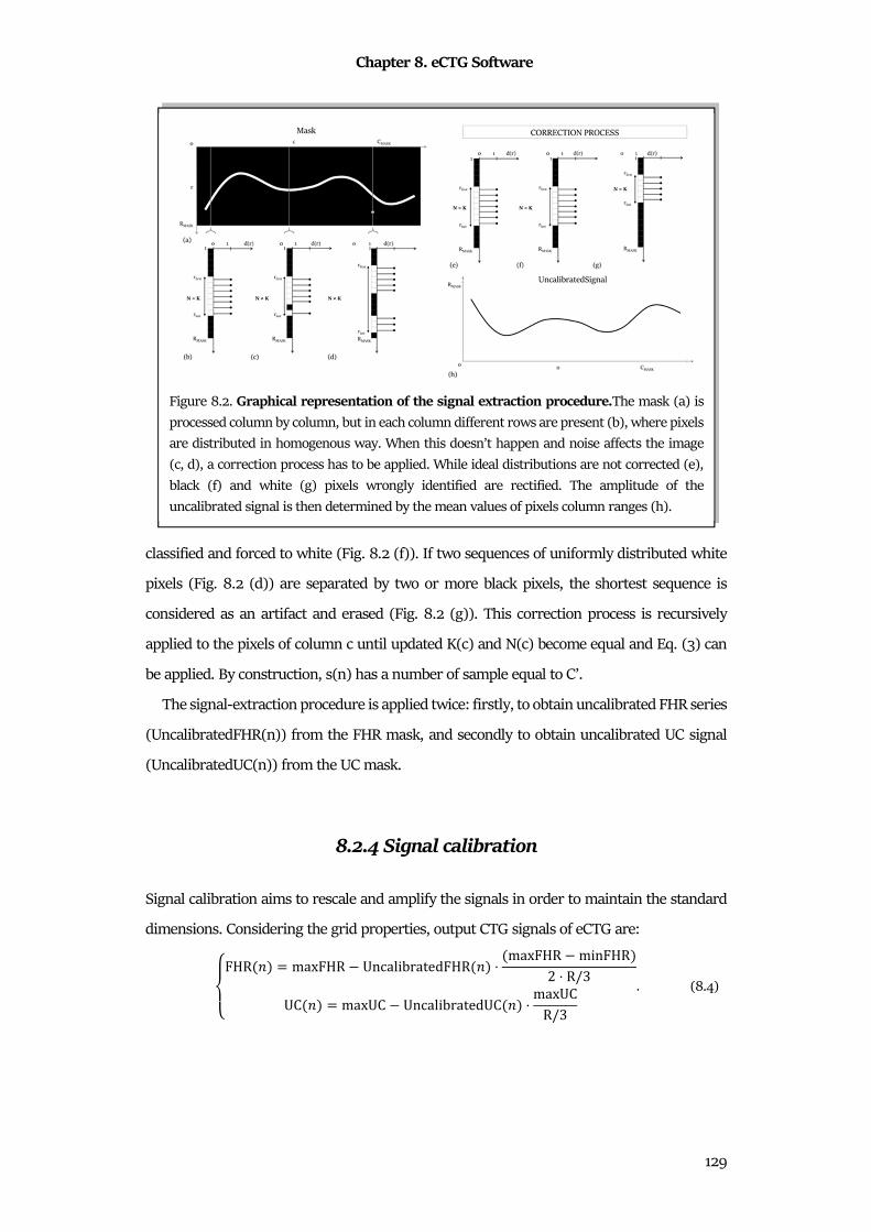
Chapter 8. eCTG Software
129
classified and forced to white (Fig. 8.2 (f)). If two sequences of uniformly distributed white
pixels (Fig. 8.2 (d)) are separated by two or more black pixels, the shortest sequence is
considered as an artifact and erased (Fig. 8.2 (g)). This correction process is recursively
applied to the pixels of column c until updated K(c) and N(c) become equal and Eq. (3) can
be applied. By construction, s(n) has a number of sample equal to C’.
The signal-extraction procedure is applied twice: firstly, to obtain uncalibrated FHR series
(UncalibratedFHR(n)) from the FHR mask, and secondly to obtain uncalibrated UC signal
(UncalibratedUC(n)) from the UC mask.
8.2.4 Signal calibration
Signal calibration aims to rescale and amplify the signals in order to maintain the standard
dimensions. Considering the grid properties, output CTG signals of eCTG are:
%'(FHR 8� = maxFHR UncalibratedFHR 8� ⋅ maxFHR minFHR�2 ⋅ R/3UC 8� = maxUC UncalibratedUC 8� ⋅ maxUCR/3 . (8.4)
Figure 8.2. Graphical representation of the signal extraction procedure.The mask (a) is
processed column by column, but in each column different rows are present (b), where pixels
are distributed in homogenous way. When this doesn’t happen and noise affects the image
(c, d), a correction process has to be applied. While ideal distributions are not corrected (e),
black (f) and white (g) pixels wrongly identified are rectified. The amplitude of the
uncalibrated signal is then determined by the mean values of pixels column ranges (h).
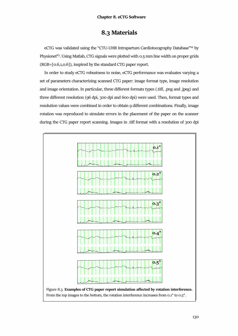
Chapter 8. eCTG Software
130
8.3 Materials
eCTG was validated using the “CTU-UHB Intrapartum Cardiotocography Database”94 by
Physionet83. Using Matlab, CTG signals were plotted with 0.5 mm line width on proper grids
(RGB=[0.6,1,0.6]), inspired by the standard CTG paper report.
In order to study eCTG robustness to noise, eCTG performance was evaluates varying a
set of parameters characterizing scanned CTG paper: image format type, image resolution
and image orientation. In particular, three different formats types (.tiff, .png and .jpeg) and
three different resolution (96 dpi, 300 dpi and 600 dpi) were used. Then, format types and
resolution values were combined in order to obtain 9 different combinations. Finally, image
rotation was reproduced to simulate errors in the placement of the paper on the scanner
during the CTG paper report scanning. Images in .tiff format with a resolution of 300 dpi
Figure 8.3. Examples of CTG paper report simulation affected by rotation interference.
From the top images to the bottom, the rotation interference increases from 0.1° to 0.5°.
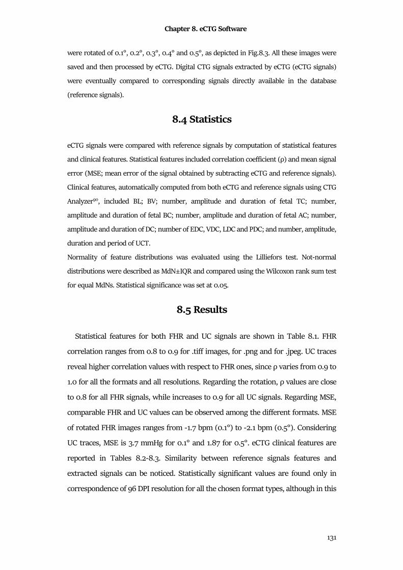
Chapter 8. eCTG Software
131
were rotated of 0.1°, 0.2°, 0.3°, 0.4° and 0.5°, as depicted in Fig.8.3. All these images were
saved and then processed by eCTG. Digital CTG signals extracted by eCTG (eCTG signals)
were eventually compared to corresponding signals directly available in the database
(reference signals).
8.4 Statistics
eCTG signals were compared with reference signals by computation of statistical features
and clinical features. Statistical features included correlation coefficient (ρ) and mean signal
error (MSE; mean error of the signal obtained by subtracting eCTG and reference signals).
Clinical features, automatically computed from both eCTG and reference signals using CTG
Analyzer90, included BL; BV; number, amplitude and duration of fetal TC; number,
amplitude and duration of fetal BC; number, amplitude and duration of fetal AC; number,
amplitude and duration of DC; number of EDC, VDC, LDC and PDC; and number, amplitude,
duration and period of UCT.
Normality of feature distributions was evaluated using the Lilliefors test. Not-normal
distributions were described as MdN±IQR and compared using the Wilcoxon rank sum test
for equal MdNs. Statistical significance was set at 0.05.
8.5 Results
Statistical features for both FHR and UC signals are shown in Table 8.1. FHR
correlation ranges from 0.8 to 0.9 for .tiff images, for .png and for .jpeg. UC traces
reveal higher correlation values with respect to FHR ones, since ρ varies from 0.9 to
1.0 for all the formats and all resolutions. Regarding the rotation, ρ values are close
to 0.8 for all FHR signals, while increases to 0.9 for all UC signals. Regarding MSE,
comparable FHR and UC values can be observed among the different formats. MSE
of rotated FHR images ranges from -1.7 bpm (0.1°) to -2.1 bpm (0.5°). Considering
UC traces, MSE is 3.7 mmHg for 0.1° and 1.87 for 0.5°. eCTG clinical features are
reported in Tables 8.2-8.3. Similarity between reference signals features and
extracted signals can be noticed. Statistically significant values are found only in
correspondence of 96 DPI resolution for all the chosen format types, although in this
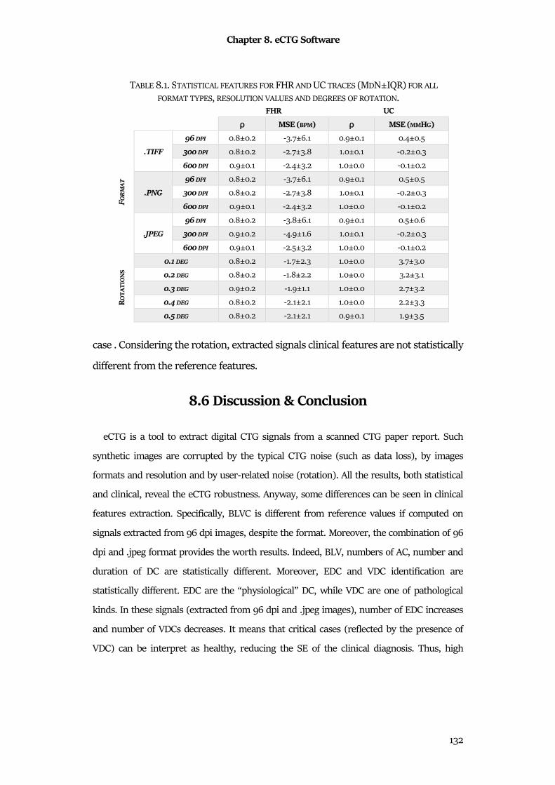
Chapter 8. eCTG Software
132
case . Considering the rotation, extracted signals clinical features are not statistically
different from the reference features.
8.6 Discussion & Conclusion
eCTG is a tool to extract digital CTG signals from a scanned CTG paper report. Such
synthetic images are corrupted by the typical CTG noise (such as data loss), by images
formats and resolution and by user-related noise (rotation). All the results, both statistical
and clinical, reveal the eCTG robustness. Anyway, some differences can be seen in clinical
features extraction. Specifically, BLVC is different from reference values if computed on
signals extracted from 96 dpi images, despite the format. Moreover, the combination of 96
dpi and .jpeg format provides the worth results. Indeed, BLV, numbers of AC, number and
duration of DC are statistically different. Moreover, EDC and VDC identification are
statistically different. EDC are the “physiological” DC, while VDC are one of pathological
kinds. In these signals (extracted from 96 dpi and .jpeg images), number of EDC increases
and number of VDCs decreases. It means that critical cases (reflected by the presence of
VDC) can be interpret as healthy, reducing the SE of the clinical diagnosis. Thus, high
TABLE 8.1. STATISTICAL FEATURES FOR FHR AND UC TRACES (MDN±IQR) FOR ALL
FORMAT TYPES, RESOLUTION VALUES AND DEGREES OF ROTATION.
FHR UC
ρ MSE (BPM) ρ MSE (MMHG) F
OR
MA
T
.TIFF
96 DPI 0.8±0.2 -3.7±6.1 0.9±0.1 0.4±0.5
300 DPI 0.8±0.2 -2.7±3.8 1.0±0.1 -0.2±0.3
600 DPI 0.9±0.1 -2.4±3.2 1.0±0.0 -0.1±0.2
.PNG
96 DPI 0.8±0.2 -3.7±6.1 0.9±0.1 0.5±0.5
300 DPI 0.8±0.2 -2.7±3.8 1.0±0.1 -0.2±0.3
600 DPI 0.9±0.1 -2.4±3.2 1.0±0.0 -0.1±0.2
.JPEG
96 DPI 0.8±0.2 -3.8±6.1 0.9±0.1 0.5±0.6
300 DPI 0.9±0.2 -4.9±1.6 1.0±0.1 -0.2±0.3
600 DPI 0.9±0.1 -2.5±3.2 1.0±0.0 -0.1±0.2
RO
TA
TIO
NS
0.1 DEG 0.8±0.2 -1.7±2.3 1.0±0.0 3.7±3.0
0.2 DEG 0.8±0.2 -1.8±2.2 1.0±0.0 3.2±3.1
0.3 DEG 0.9±0.2 -1.9±1.1 1.0±0.0 2.7±3.2
0.4 DEG 0.8±0.2 -2.1±2.1 1.0±0.0 2.2±3.3
0.5 DEG 0.8±0.2 -2.1±2.1 0.9±0.1 1.9±3.5
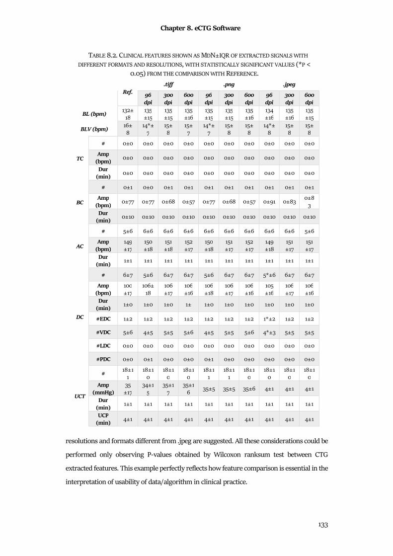
Chapter 8. eCTG Software
133
resolutions and formats different from .jpeg are suggested. All these considerations could be
performed only observing P-values obtained by Wilcoxon ranksum test between CTG
extracted features. This example perfectly reflects how feature comparison is essential in the
interpretation of usability of data/algorithm in clinical practice.
TABLE 8.2. CLINICAL FEATURES SHOWN AS MDN±IQR OF EXTRACTED SIGNALS WITH
DIFFERENT FORMATS AND RESOLUTIONS, WITH STATISTICALLY SIGNIFICANT VALUES (*P <
0.05) FROM THE COMPARISON WITH REFERENCE.
Ref. .tiff .png .jpeg
96 dpi
300 dpi
600 dpi
96 dpi
300 dpi
600 dpi
96 dpi
300 dpi
600 dpi
BL (bpm) 132±
18
135
±15
135
±15
135
±16
135
±15
135
±15
135
±16
134
±16
135
±16
135
±15
BLV (bpm) 16±
8
14*±
7
15±
8
15±
7
14*±
7
15±
8
15±
8
14*±
8
15±
8
15±
8
TC
# 0±0 0±0 0±0 0±0 0±0 0±0 0±0 0±0 0±0 0±0
Amp (bpm)
0±0 0±0 0±0 0±0 0±0 0±0 0±0 0±0 0±0 0±0
Dur (min)
0±0 0±0 0±0 0±0 0±0 0±0 0±0 0±0 0±0 0±0
BC
# 0±1 0±0 0±1 0±1 0±1 0±1 0±1 0±1 0±1 0±1
Amp (bpm)
0±77 0±77 0±68 0±57 0±77 0±68 0±57 0±91 0±83 0±8
3
Dur (min)
0±10 0±10 0±10 0±10 0±10 0±10 0±10 0±10 0±10 0±10
AC
# 5±6 6±6 6±6 6±6 6±6 6±6 6±6 6±6 6±6 5±6
Amp (bpm)
149
±17
150
±18
151
±18
152
±17
150
±18
151
±17
152
±17
149
±18
151
±17
151
±17
Dur (min)
1±1 1±1 1±1 1±1 1±1 1±1 1±1 1±1 1±1 1±1
DC
# 6±7 5±6 6±7 6±7 5±6 6±7 6±7 5*±6 6±7 6±7
Amp (bpm)
100
±17
106±
18
106
±17
106
±16
106
±18
106
±17
106
±16
105
±16
106
±17
106
±16
Dur (min)
1±0 1±0 1±0 1± 1±0 1±0 1±0 1±0 1±0 1±0
#EDC 1±2 1±2 1±2 1±2 1±2 1±2 1±2 1*±2 1±2 1±2
#VDC 5±6 4±5 5±5 5±6 4±5 5±5 5±6 4*±3 5±5 5±5
#LDC 0±0 0±0 0±0 0±0 0±0 0±0 0±0 0±0 0±0 0±0
#PDC 0±0 0±1 0±0 0±0 0±1 0±0 0±0 0±0 0±0 0±0
UCT
# 18±1
1
18±1
0
18±1
0
18±1
0
18±1
1
18±1
1
18±1
0
18±1
0
18±1
0
18±1
0
Amp (mmHg)
35
±17
34±1
5
35±1
7
35±1
6 35±5 35±5 35±6 4±1 4±1 4±1
Dur (min)
1±1 1±1 1±1 1±1 1±1 1±1 1±1 1±1 1±1 1±1
UCP (min)
4±1 4±1 4±1 4±1 4±1 4±1 4±1 4±1 4±1 4±1
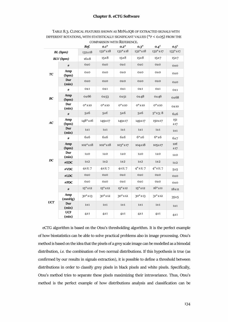
Chapter 8. eCTG Software
134
eCTG algorithm is based on the Otsu’s thresholding algorithm. It is the perfect example
of how biostatistics can be able to solve practical problems also in image processing. Otsu’s
method is based on the idea that the pixels of a grey scale image can be modelled as a bimodal
distribution, i.e. the combination of two normal distributions. If this hypothesis is true (as
confirmed by our results in signals extraction), it is possible to define a threshold between
distributions in order to classify grey pixels in black pixels and white pixels. Specifically,
Otsu’s method tries to separate these pixels maximizing their intravariance. Thus, Otsu’s
method is the perfect example of how distributions analysis and classification can be
TABLE 8.3. CLINICAL FEATURES SHOWN AS MDN±IQR OF EXTRACTED SIGNALS WITH
DIFFERENT ROTATIONS, WITH STATISTICALLY SIGNIFICANT VALUES (*P < 0.05) FROM THE
COMPARISON WITH REFERENCE. Ref. 0.1° 0.2° 0.3° 0.4° 0.5°
BL (bpm) 132±18 132*±18 132*±18 132*±18 132*±17 133*±17
BLV (bpm) 16±8 15±8 15±8 15±8 15±7 15±7
TC
# 0±0 0±0 0±0 0±0 0±0 0±0
Amp (bpm)
0±0 0±0 0±0 0±0 0±0 0±0
Dur (min)
0±0 0±0 0±0 0±0 0±0 0±0
BC
# 0±1 0±1 0±1 0±1 0±1 0±1
Amp (bpm)
0±66 0±53 0±51 0±48 0±46 0±68
Dur (min)
0*±10 0*±10 0*±10 0*±10 0*±10 0±10
AC
# 5±6 5±6 5±6 5±6 5*±3; 8 6±6
Amp (bpm)
148*±16 149±17 149±17 149±17 150±17 151
±17
Dur (min)
1±1 1±1 1±1 1±1 1±1 1±1
DC
# 6±6 6±6 6±6 6*±6 6*±6 6±7
Amp (bpm)
102*±18 102*±18 103*±17 104±18 105±17 106
±17
Dur (min)
1±0 1±0 1±0 1±0 1±0 1±0
#EDC 1±2 1±2 1±2 1±2 1±2 1±2
#VDC 4±2; 7 4±2; 7 4±2; 7 4*±2; 7 4*±2; 7 5±5
#LDC 0±0 0±0 0±0 0±0 0±0 0±0
#PDC 0±0 0±0 0±0 0±0 0±0 0±0
UCT
# 15*±12 15*±12 15*±12 15*±12 16*±11 18±11
Amp (mmHg)
30*±13 30*±12 30*±12 30*±13 31*±12 35±5
Dur (min)
1±1 1±1 1±1 1±1 1±1 1±1
UCP (min)
4±1 4±1 4±1 4±1 4±1 4±1

Chapter 8. eCTG Software
135
versatile and applicable in both signal and image processing. Thus, eCTG procedure is a
promising useful tool to accurately extract digital FHR and UC signals from digital CTG
images.
Chapter 9. DLSEC: Deep-Learning Serial ECG Classifiers
136
Chapter 9
DLSEC: Deep-Learning Serial ECG Classifiers
Deep-Learning Serial ECG Classifiers (DLSECs) are opportunely constructed MLPs,
finalized to detect emerging pathology using the theory of serial electrocardiography. Core
of these classifier design is the new Repeated Structuring & Learning Procedure (RS&LP).
This new method combines the NN structuring and leaning phases. It is a constructive
method and its main advantage is to be able to define a perfect NN structure that fit the
considered classification problem. Considering the multi-layer structure of these NN, these
DLSECs can be considered an example of deep learning. Its first use is the definition of
DLSECs to detect patients that developed heart failure after an experience of myocardial
infarction or to detect ischemia. Due to their classification abilities, DLSECs are the perfect
examples of classification.
9.1 Clinical Background
9.1.1 Serial Electrocardiography
Serial analysis of ECGs relies on the comparison of two or more successive recordings
from the same patient. Also defined as serial electrocardiography, the comparison of two
serial ECGs (SECG) in different moments in the same subject aims to contribute to the
diagnosis of newly emerging or aggravating pathology. Time period between the ECGs
depends on serial electrocardiography use. Some applications, such as clinical research or
experimentations, have a specific time period defined in a protocol. While, in clinical
practice, time period depends to data availability. This analysis allows cardiologist to obtain
a more reliable ECG interpretation. The interpreter takes advantage of the fact that even
small differences can be of pathological origin. Variation in ECG morphology from one
situation to another is usually much smaller than the variation in morphology between
different patients. Therefore, pathological changes in the ECG related to can be found more
easily by means of serial comparison113.
Anyway, this practice presents some confounders such as the intrasubject physiological
variability and the instrumentation interference. Indeed, the ECG of a person changes with
Chapter 9. DLSEC: Deep-Learning Serial ECG Classifiers
137
its body status, for example it changes in relation to blood pression, mental stress, body
position, respiration rate, age and weight. Moreover, it is impossible to perfectly reproduce
the electrode positioning, specifically of the six precordial electrodes114. Thus, the major
difficulty of serial electrocardiography is to discriminate between these confounders and real
changes in the patient status.
Some currently-available commercial programs for automated computerized ECG
analysis support serial electrocardiography interpretation (Glasgow program115). Actually,
automated SECGs analysis has not reached the level of sophistication and validated
performance that the algorithms for automated analysis of single ECG have achieved.
Additionally, current algorithms for SECGs analysis are rule-based and rigid.
9.1.2 Heart Failure
Heart failure is an abnormality of the cardiac structure or function. It leads to the inability
of the heart to supply enough oxygen to compensate for metabolic needs, despite the normal
vascular filling pressures. This disease is widespread, so that in the United States affects
about 5 million people a year (2% of the population), causing the death of about 300,000
people116.
Its etiopathogenesis is composed of both anatomopathological problems and functional
alterations (such as reduced contractility). During each ventricular systole, heart has to
pump no less than 60% of ventricular blood in arteries. In fact, if there is an increase in
preload (as happens in diseases such as mitral or aortic insufficiency and interatrial or
ventricular defects), the systolic range remains almost unchanged without increasing blood
pressure. However, if the increase in preload lasts over time, the prolonged stretching of
heart muscle fibers leads to eccentric ventricular hypertrophy. This abnormal distribution
of fibers leads to an inability to contract optimally and to an increase in the intracavitary
diameter (systolic decompensation). If instead the increase is afterload (as in the case of
aortic stenosis or arterial hypertension), in the long term the heart undergoes a structural
change called concentric hypertrophy, which results in a thickening of the parietal tissue and
a consequent decrease in the intracavitary diameter, causing difficulties in filling (diastolic
decompensation).
In heart failure, another major etiopathogenetic mechanism is represented by conduction
anomalies. These can be caused by the progression an existing pathology and for its onset:
relationships between heart failure and arrhythmic behaviors are very complicated. In fact,
Chapter 9. DLSEC: Deep-Learning Serial ECG Classifiers
138
heart failure involves modifications such as dilatation and hypertrophy, causing tissue
extension and ionic imbalances caused by neurohumoral compensatory mechanisms.
Moreover, bradycardia or tachycardia arrhythmias are characteristic of many cardiac
pathologies even in the absence of decompensation but may contribute to the inability to
maintain a hemodynamic equilibrium thus resulting in a situation of true heart failure.
Heart failure symptoms can be variable: they depend on the patient's age, etiology,
compensation mechanisms involved, and anamnesis. A correct diagnosis is based on specific
symptoms (major criteria) concurrent with other symptoms with less SP (minor criteria).
Among the major criteria we find: orthopnea (intense dyspnea that prevents the patient
from lying down, forcing him to stand upright), paroxysmal nocturnal dyspnea (difficulty
breathing or asthma that occurs during the nocturnal sleep phase, sometimes so intense as
to wake up the patient), turgor of the jugular veins, rales, cardiomegaly (a disproportionate
increase in the heart muscle), acute pulmonary edema (accumulation of blood fluids in the
lungs, due to the reduced pumping capacity of the heart), increase of central venous
pressure, slowing of the speed of circle, appearance of the third tone in a PCG (due to the
sudden release of the ventricle in the hypertrophic heart), hepatic reflux, a positive response
to drug therapy for decompensation. The minor criteria include nocturnal cough,
hepatomegaly (liver enlargement), tachycardia, pleural effusion, declining edema
(peripheral fluid accumulation). These minor criteria are common to other diseases, but if
present in combination with each other or with a symptom present among the major criteria
allow to perform the diagnosis (or a first attempt) with high clinical probability.
Clinical examinations for heart-failure diagnosis are ECG and echocardiogram. ECG
allows to have information about the correct carrying out of the electrical activity of the
heart, on the presence of any anomalies of conduction and arrhythmias. The echocardiogram
gives an anatomical and mechanical cardiac overview, allowing the detection of systolic or
diastolic dysfunctions. In addition to these tests, laboratory tests are suggested in order to
evaluate the compensatory functions of the body.
9.1.3 Myocardial Ischemia
Myocardial ischemia occurs when blood flow to heart is reduced, as the result of a partial
or complete blockage of cardiac arteries (coronary arteries). The factors involved in the
genesis of myocardial ischemia are the reduction of coronary flow and the increase in
myocardial oxygen consumption. An atherosclerotic lesion of an epicardial branch
Chapter 9. DLSEC: Deep-Learning Serial ECG Classifiers
139
determines downstream of the stenosis a pressure drop proportional to the reduction of the
vessel caliber. In order to maintain a flow congruent to the basal conditions, the pressure
gradient stimulates the expansion of the resistance vessels. However, when the diameter of
the epicardial branch is reduced by more than 80%, the flow is reduced even in basal
conditions. This causes the consumption of quantities of "reserve" by the coronary tree, in
order to maintain the necessary metabolic contribution. When the coronary blood flow
becomes inadequate, cells demands causing a myocardial suffering condition. It causes
biochemical, functional and electrocardiographic alterations as it derives from a deficit
related to the coronary flow117.
Acute myocardial ischemia is characterized by an ECG with ST-segment changes. The
depolarization phase is altered, with a reduction in the amplitude of the action potential and
a slowing of the ascent rate (phase 0). It causes a slowing of the depolarization of the
ischemic region. Simultaneously, there is a reduction in action-potential duration, translated
into the ECG with a shortening of phases 2 and 3. It generates, therefore, a current flow
determined by the potential difference between healthy and ischemic tissues. Repolarization
of ischemic myocardial cells may be incomplete, resulting in a resting membrane potential
of -70 mV instead of normal -90 mV. During diastole, then, a potential difference is
generated between healthy and ischemic tissue and a relative flow of current towards. An
altered ST segment is observed, which depends on ischemia location. From a VCG point of
view, the current flow from healthy tissue to pathological tissue modifies the VCG loops
pattern. Thus, the corresponding derivations will register a sub-segment of the ST segment
because the vector tends to move away118,119.
A further ECG abnormality in myocardial ischemic episode is the T-wave alteration. It
represents ventricular repolarization phase and constitutes a parameter that changes only
occasionally in cases of acute myocardial ischemia. In medical literature, T wave is often
associated with ischemic episodes, but its relevant alterations belong to ST. However, a
negative T wave remains an important parameter in the definition of episodes of previous
myocardial necrosis. These alterations are related to a prolongation of phase 3 of the action
potential in ischemic areas. In other cases, patients with acute ischemia appear in the ECG a
high, narrow and pointed T wave. It is present mainly in the early stages of an acute
myocardial infarction also called hyperacute ischemia. An ischemia that causes a delay in the
repolarization of the subendocardial region alone causes a flow of current that moves away
Chapter 9. DLSEC: Deep-Learning Serial ECG Classifiers
140
from it and goes towards the epicardium. It results in a raised and pointed T wave. However,
these alterations remain rare to monitor and record as they are often overhung by ST118,119.
Finally, the infarction causes the death of electrically active cells. This region therefore
becomes not electrically conductive, as in the ECG it determines the presence of a
pathological Q wave in the derivatives oriented towards the necrosis. Normally ventricular
walls depolarization proceeds in each myocardial region from the endocardium to the
epicardium. The depolarization vectors of the anterior wall are directed towards the front,
those of the lower wall towards the bottom and those of the rear wall towards the front. The
necrotic region causes the disappearance of vectors directed to that area, while the vectors
directed in the opposite direction will persist. Thus, if there is an exploratory electrode of a
lead above the necrosis, there is a negative wave in the initial part of QRS complex. This
wave Q is often present also in healthy patients and therefore turns out to be physiological.
In order to determine the presence of a myocardial pathology it must have a duration ≥ 0.04
s. Furthermore, the overall width must be ≥25% of the R wave and the presence of hooks.
The pathological Q wave is also a sign of generalized myocardial necrosis at the whole
thickness of the ventricular wall. In patients with myocardial infarction affecting only the
sub-endocardial layers, vice versa, there are usually exclusively more or less marked diffuse
changes of the ST and / or T-wave. If a sub-endocardial infarction affects more than half the
thickness of the myocardial wall, however, the electrocardiographic appearance is often
similar to that of a transmural infarction118,119.
9.2 Methods
9.2.1 Feature Selection
Input of the DLSEC is the serial database, contained couples of digital standard 10-second
12-lead ECGs from the same patient, recorded at different time instants, and called the
baseline ECG (BL-ECG) and the follow-up ECG (FU-ECG). In controls, the clinical status at
the time at which BL-ECG and FU-ECG were made remained unchanged. In cases, the
clinical status had changed in an unfavorable direction at the time at which the FU-ECG was
made; hence, their FU-ECG has to be associated with newly arisen pathology
All ECGs were analyzed by the Leiden ECG Analysis and Decomposition Software
(LEADS)120. This program converts the 12-lead ECG in a 3-lead VCG in which all heart beats
are detected, coherently averaged, after which onset QRS, J point and the end of the T wave

Chapter 9. DLSEC: Deep-Learning Serial ECG Classifiers
141
are determined. A multitude of variables is computed from the averaged heartbeat. For the
purpose of our study, we selected 13 major features to describe the average beat120–122: QRS
duration, QT interval, maximal QRS vector, maximal T vector, QRS integral vector, T integral
vector, QRS complexity, T-wave complexity, ventricular gradient (VG), QRS-T spatial angle
(SA), HR, J point amplitude vector and T-wave symmetry. Together, these 13 features
represent major physiological correlates of the electrical properties of the heart muscle.
To characterize the ECG changes within patients, the 13 BL-ECG features were subtracted
from the 13 FU-ECG features, thus obtaining 13 ECG difference descriptors; hence, a positive
value of a difference descriptor indicates an increase of the corresponding feature in time,
while a negative value indicates a decrease. The 13 difference descriptors are
defined/computed as follows:
1. ΔQRS: difference in QRS duration (ms);
2. ΔQT: difference in QT interval (ms);
3. ΔMQRS: difference in magnitude of the maximal QRS vectors (µV);
4. ΔMT: difference in magnitude of the maximal T vectors (µV);
5. ΔQRSIV: difference in magnitude of the QRS integral vectors (mV·ms);
6. ΔQTIV: difference in magnitude of the T integral vectors (mV·ms);
7. ΔCQRS: difference in QRS complexity (QRS complexity is derived from the singular
value decomposition – SVD – of the ECG during the QRS complex, considering only
the 8 independent leads I/II/V1/V2/V3/V4/V5/V6, by computing the ratio of the
sum of the 3rd-8th singular values to the sum of all 8 singular values);
8. ΔCT: difference in T-wave complexity (T-wave complexity is computed similarly as
QRS complexity, over the interval between the J point and the end of the T wave);
9. ΔVG: magnitude of the VG difference vector (mV·ms);
10. ΔSA: difference in SA (°; absolute value of the SA difference21);
11. ΔHR: difference in HR (bpm);
12. ΔJV: magnitude of the J-point difference vector (µV);
13. ΔTSYM: difference in T-wave symmetry (T-wave symmetry is computed as the ratio
of the integral of the VM signal between the T-wave apex and the end of the T wave
to the integral of the VM signal between the J point and the end of the T wave).
The 13 difference descriptors served as the input features for the classification procedure.
The original values of the BL- and FU-ECGs were not further used. The selection of difference
descriptors as features underscores the principle adopted in our approach that the patient
Chapter 9. DLSEC: Deep-Learning Serial ECG Classifiers
142
has to be taken as his/her own standard of reference. Irrespective the baseline ECG of a
patient (normal, or possibly even highly abnormal), if the ECG remains unchanged during
follow-up, the patient is to be classified as stable (not having developed new pathology).
9.2.2 Repeated Structuring & Learning Procedure
Our DLSEC consists of a MLP66 with 13 inputs for the 13 ECG difference descriptor values
and 1 output for the classification. The output values are >= 0 and <=1. The output value of
0 represents a certain classification as a control patient, and the output value of 1 represents
a certain classification as a case patient. Output values between 0 and 1 are associated with
a classification that is not completely certain and represent a classification as control or case
when they are smaller or larger than a threshold value, respectively. Our construction
decisions of MLP neurons are weight and bias values between ˗1 and +1 and sigmoid
activation functions. Moreover, learning dataset was divided in a training dataset (80% of
the data) and a validation dataset (20% of the data), maintaining the prevalence of cases
and controls in each dataset. During learning with a given neural-network architecture, the
weights and the biases of the neurons were adjusted according to the scaled-conjugate-
gradients algorithm123. This algorithm optimizes the classification for the training set by
minimizing a training error function computed as the normalized sum of the squared
differences between the estimated output values and the true classification values.
The architecture of MLP was built during the RS&LP124, thus alternating phases of learning
and of NN structuring. Each new structure contained the previous architecture plus one new
neuron.
In the first cycle, there is only the starting architecture to be initialized and learnt: it
consists of one hidden layer with one neuron (the minimal number of neurons per layer).
The maximal number of hidden layers is 3, there is no maximal number of neurons per layer.
In each structuring cycle, possible new alternative architectures are strategically built,
adding one neuron to the existing NN as follows:
• when the existing NN has one hidden layer, two new architectures are possible,
either by adding one extra neuron to the existing hidden layer or by adding a new
second hidden layer with one neuron;
• when the existing NN has two hidden layers, three new architectures are possible:
1) by adding one extra neuron to the first hidden layer, 2) by adding one extra
Chapter 9. DLSEC: Deep-Learning Serial ECG Classifiers
143
neuron to the second hidden layer, or 3) by adding a new third hidden layer with
one neuron;
• when the existing NN has three hidden layers, three new architectures are
possible, by adding one extra neuron to either the first, the second or the third
hidden layer;
• in case of multiple layers, the number of neurons in the second or third layer
cannot be larger than the number of neurons in the first or second layer,
respectively.
As an example, Fig. 9.1 illustrates the possibilities of adding neurons to the existing
architecture [4 4 2] (denoting three hidden layers consisting of 4, 4 and 2 neurons,
respectively).
All possible new architectures keep the weights and biases of the neurons in the existing
NN; only the new neuron is initialized with random weights and biases. A new possible
architecture is acceptable for further learning only if the new neuron helps the existing NN
to decrease in training error after one single initial learning iteration. Whether the validation
error decreases or increases with this single learning step is irrelevant for the acceptance of
the new architecture. If, after this single initial learning iteration, the training error is larger
than the training error of the existing NN, the initialization is unacceptable, and a next single
initial learning iteration with a different initialization is attempted. This process is repeated
till an initialization is found that renders the architecture acceptable, or till 500 attempts
have been done without success; in that case the possible new architecture is rejected. Might
all possible new architectures be rejected, the existing NN is kept as the final one and the
RS&LP is stopped (first stopping criterion). Possible new architectures that pass the
initialization step become new possible NNs and enter the learning procedure.
The possible new NNs enter the learning procedure. At the end of the learning process,
the validation error of each possible new NN is either larger than the validation error of the
existing NN (failure) or smaller/equal (success). In case of failure, the possible new NN is
rejected, and a next attempt is done by re-learning the same possible new architecture after
re-initialization according to the procedure described above. This is repeated until success
or till maximally 10 failures. When 10 failures occurred, the architecture is given up as a
possible new NN. When all possible new NNs fail in this way, the existing NN is kept as the
final one and the RS&LP is stopped (second stopping criterion).
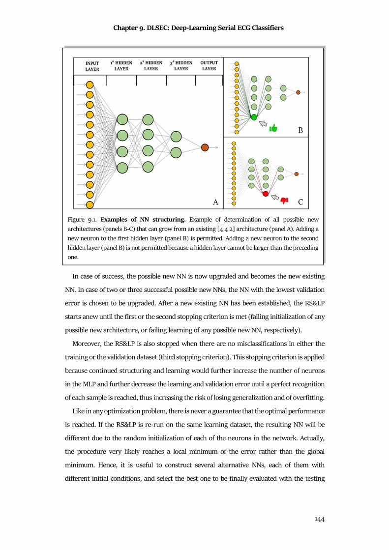
Chapter 9. DLSEC: Deep-Learning Serial ECG Classifiers
144
In case of success, the possible new NN is now upgraded and becomes the new existing
NN. In case of two or three successful possible new NNs, the NN with the lowest validation
error is chosen to be upgraded. After a new existing NN has been established, the RS&LP
starts anew until the first or the second stopping criterion is met (failing initialization of any
possible new architecture, or failing learning of any possible new NN, respectively).
Moreover, the RS&LP is also stopped when there are no misclassifications in either the
training or the validation dataset (third stopping criterion). This stopping criterion is applied
because continued structuring and learning would further increase the number of neurons
in the MLP and further decrease the learning and validation error until a perfect recognition
of each sample is reached, thus increasing the risk of losing generalization and of overfitting.
Like in any optimization problem, there is never a guarantee that the optimal performance
is reached. If the RS&LP is re-run on the same learning dataset, the resulting NN will be
different due to the random initialization of each of the neurons in the network. Actually,
the procedure very likely reaches a local minimum of the error rather than the global
minimum. Hence, it is useful to construct several alternative NNs, each of them with
different initial conditions, and select the best one to be finally evaluated with the testing
Figure 9.1. Examples of NN structuring. Example of determination of all possible new
architectures (panels B-C) that can grow from an existing [4 4 2] architecture (panel A). Adding a
new neuron to the first hidden layer (panel B) is permitted. Adding a new neuron to the second
hidden layer (panel B) is not permitted because a hidden layer cannot be larger than the preceding
one.
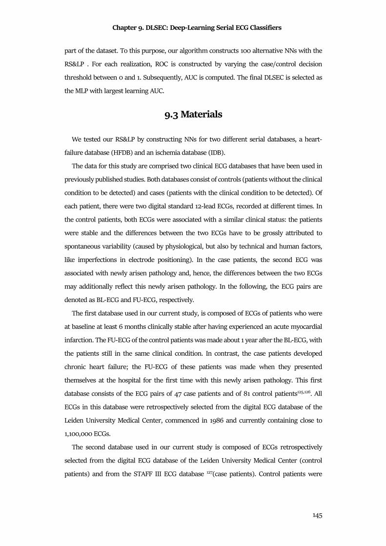
Chapter 9. DLSEC: Deep-Learning Serial ECG Classifiers
145
part of the dataset. To this purpose, our algorithm constructs 100 alternative NNs with the
RS&LP . For each realization, ROC is constructed by varying the case/control decision
threshold between 0 and 1. Subsequently, AUC is computed. The final DLSEC is selected as
the MLP with largest learning AUC.
9.3 Materials
We tested our RS&LP by constructing NNs for two different serial databases, a heart-
failure database (HFDB) and an ischemia database (IDB).
The data for this study are comprised two clinical ECG databases that have been used in
previously published studies. Both databases consist of controls (patients without the clinical
condition to be detected) and cases (patients with the clinical condition to be detected). Of
each patient, there were two digital standard 12-lead ECGs, recorded at different times. In
the control patients, both ECGs were associated with a similar clinical status: the patients
were stable and the differences between the two ECGs have to be grossly attributed to
spontaneous variability (caused by physiological, but also by technical and human factors,
like imperfections in electrode positioning). In the case patients, the second ECG was
associated with newly arisen pathology and, hence, the differences between the two ECGs
may additionally reflect this newly arisen pathology. In the following, the ECG pairs are
denoted as BL-ECG and FU-ECG, respectively.
The first database used in our current study, is composed of ECGs of patients who were
at baseline at least 6 months clinically stable after having experienced an acute myocardial
infarction. The FU-ECG of the control patients was made about 1 year after the BL-ECG, with
the patients still in the same clinical condition. In contrast, the case patients developed
chronic heart failure; the FU-ECG of these patients was made when they presented
themselves at the hospital for the first time with this newly arisen pathology. This first
database consists of the ECG pairs of 47 case patients and of 81 control patients125,126. All
ECGs in this database were retrospectively selected from the digital ECG database of the
Leiden University Medical Center, commenced in 1986 and currently containing close to
1,100,000 ECGs.
The second database used in our current study is composed of ECGs retrospectively
selected from the digital ECG database of the Leiden University Medical Center (control
patients) and from the STAFF III ECG database 127(case patients). Control patients were

Chapter 9. DLSEC: Deep-Learning Serial ECG Classifiers
146
outpatients of the cardiology department, selected on the availability of two digital ECG
recordings made about one year apart, while during this year the clinical condition of the
patients remained unchanged. As no other clinical criteria were applied to select these
patients, this patient group represents a general cardiology outpatient case mix. The STAFF
III ECG database, from which the case patients for our current study were taken, consists of
patients with exercise-inducible chest pain caused by a coronary artery stenosis. These
patients came to the hospital to undergo coronary angioplasty by positioning a catheter with
a deflated balloon at the tip at the site of the stenosis, after which the balloon was inflated to
widen the lumen of the artery. During balloon inflation, the coronary artery was completely
occluded, thus causing acute ischemia in the part of the heart muscle perfused by that artery.
The protocol of the study during which the STAFF III ECG database was collected was
designed to investigate the therapeutic benefits of prolonged balloon inflation times.
Throughout the procedure a 12-lead ECG was recorded. The BL-ECG of the case patients was
taken from the period immediately preceding the balloon inflation and the FU-ECG of the
case patients was taken after 3 minutes of balloon occlusion. In summary, the second
database used for our current study consists of the ECG pairs of 84 case patients and of 398
control patients125,127–129.
9.4 Statistics
The ECG and ROC feature distributions were described in terms of MdN±IQR and
compared using the Wilcoxon Ranksum and DeLong’s tests130. NN and LR performances
were quantified from the ROC curves of the testing databases in terms of AUC, 95% CI and
the diagnostic ACC. Statistical significance was set at 0.05.
In the absence of data from literature, in order to confirm superiority of flexible over rigid
algorithms with learning ability in SECGs analysis, performance of DLSECs were compared
with standard LR65,66,131–133.
9.5 Results
Distributions of 13 difference descriptors of both HFDB and IDB are reported in Table 9.1.
The number of difference features that were statistically different between cases and
controls was 9 in the HFDB (ΔQRS, ∆T, ∆QRSIV, ΔCQRS, ΔCT, ∆VG, ΔSA, ΔHR and ∆J), and
8 in the IDB (ΔQRS, ∆QRSM,
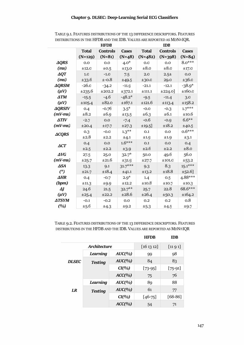
Chapter 9. DLSEC: Deep-Learning Serial ECG Classifiers
147
TABLE 9.1. FEATURES DISTRIBUTIONS OF THE 13 DIFFERENCE DESCRIPTORS. FEATURES
DISTRIBUTIONS IN THE HFDB AND THE IDB. VALUES ARE REPORTED AS MDN±IQR. HFDB IDB
Total
(N=129) Controls (N=81)
Cases (N=48)
Total (N=482)
Controls (N=398)
Cases (N=84)
ΔQRS (ms)
0.0
±12.0
0.0
±0.5
4.0*
±13.0
0.0
±8.0
0.0
±8.0
8.0***
±17.0
ΔQT (ms)
1.0
±33.6
-1.0
±-0.8
7.5
±49.5
2.0
±30.0
2.5±
29.0
0.0
±36.0
ΔQRSM (µV)
-26.0
±235.6
-34.2
±202.2
-11.9
±372.1
-21.1
±111.1
-12.1
±224.0]
-38.9*
±160.0
ΔTM (µV)
-15.5
±105.4
-4.6
±82.0
-48.2*
±167.1
-9.5
±121.6
-11.4
±113.4
3.0
±158.2
ΔQRSIV (mV·ms)
0.4
±8.2
-0.76
±6.9
3.5*
±13.5
-0.0
±6.3
-0.3
±6.1
1.7***
±10.6
ΔTIV (mV·ms)
-2.7
±20.4
0.0
±17.7
-7.4
±27.3
-0.6
±19.5]
-0.9
±18.2
6.6**
±40.5
ΔCQRS 0.3
±2.8
-0.0
±2.2
1.3**
±4.1
0.1
±1.9
0.0
±1.9
0.6***
±3.1
ΔCT 0.4
±2.5
0.0
±2.2
1.6***
±3.9
0.1
±2.6
0.0
±2.2
0.4
±8.0
ΔVG (mV·ms)
27.5
±25.7
25.0
±21.6
32.7*
±31.9
50.0
±27.7
49.6
±101.0
56.0
±53.2
ΔSA (°)
13.3
±21.7
9.1
±18.4
31.7***
±41.1
9.3
±13.2
8.3
±18.8
15.1***
±52.6]
ΔHR (bpm)
0.4
±11.3
-0.7
±9.9
2.9*
±12.2
1.4
±10.8
0.5
±10.7
4.88***
±10.3
ΔJ (µV)
24.6
±25.4
21.5
±22.2
32.7**
±28.6
25.7
±26.4
22.8
±50.3
68.6***
±164.2
ΔTSYM (%)
-0.1
±5.6
-0.2
±4.3
0.0
±9.2
0.2
±5.3
0.2
±4.5
0.8
±9.7
TABLE 9.2. FEATURES DISTRIBUTIONS OF THE 13 DIFFERENCE DESCRIPTORS. FEATURES
DISTRIBUTIONS IN THE HFDB AND THE IDB. VALUES ARE REPORTED AS MDN±IQR
HFDB IDB
Architecture [16 13 12] [11 9 1]
DLSEC
Learning AUC(%) 99 98
Testing
AUC(%) 84 83
CI(%) [73-95] [75-91]
ACC(%) 75 76
LR
Learning AUC(%) 89 88
Testing
AUC(%) 61 77
CI(%) [46-75] [68-86]
ACC(%) 54 71
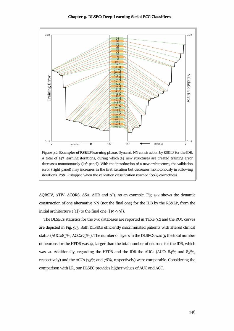
Chapter 9. DLSEC: Deep-Learning Serial ECG Classifiers
148
∆QRSIV, ∆TIV, ΔCQRS, ΔSA, ΔHR and ∆J). As an example, Fig. 9.2 shows the dynamic
construction of one alternative NN (not the final one) for the IDB by the RS&LP, from the
initial architecture ([1]) to the final one ([19 9 9]).
The DLSECs statistics for the two databases are reported in Table 9.2 and the ROC curves
are depicted in Fig. 9.3. Both DLSECs efficiently discriminated patients with altered clinical
status (AUC≥83%; ACC≥75%). The number of layers in the DLSECs was 3; the total number
of neurons for the HFDB was 41, larger than the total number of neurons for the IDB, which
was 21. Additionally, regarding the HFDB and the IDB the AUCs (AUC: 84% and 83%,
respectively) and the ACCs (75% and 76%, respectively) were comparable. Considering the
comparison with LR, our DLSEC provides higher values of AUC and ACC.
Figure 9.2. Examples of RS&LP learning phase. Dynamic NN construction by RS&LP for the IDB.
A total of 147 learning iterations, during which 34 new structures are created training error
decreases monotonously (left panel). With the introduction of a new architecture, the validation
error (right panel) may increases in the first iteration but decreases monotonously in following
iterations. RS&LP stopped when the validation classification reached 100% correctness.
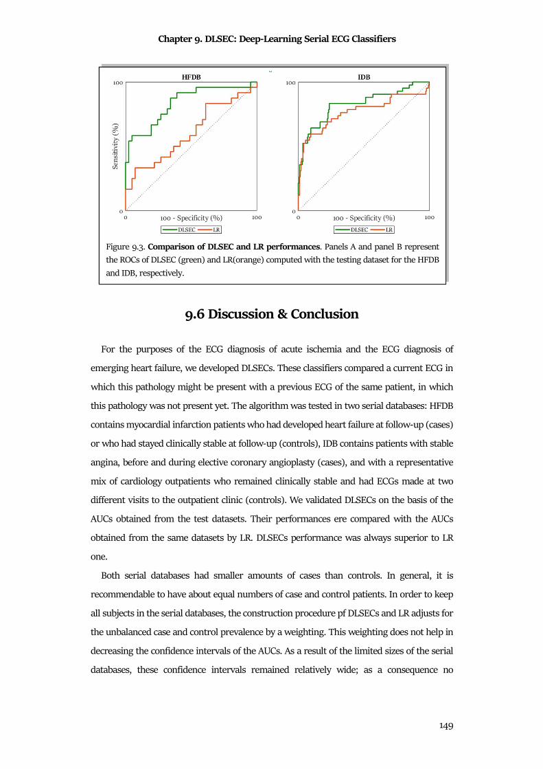
Chapter 9. DLSEC: Deep-Learning Serial ECG Classifiers
149
9.6 Discussion & Conclusion
For the purposes of the ECG diagnosis of acute ischemia and the ECG diagnosis of
emerging heart failure, we developed DLSECs. These classifiers compared a current ECG in
which this pathology might be present with a previous ECG of the same patient, in which
this pathology was not present yet. The algorithm was tested in two serial databases: HFDB
contains myocardial infarction patients who had developed heart failure at follow-up (cases)
or who had stayed clinically stable at follow-up (controls), IDB contains patients with stable
angina, before and during elective coronary angioplasty (cases), and with a representative
mix of cardiology outpatients who remained clinically stable and had ECGs made at two
different visits to the outpatient clinic (controls). We validated DLSECs on the basis of the
AUCs obtained from the test datasets. Their performances ere compared with the AUCs
obtained from the same datasets by LR. DLSECs performance was always superior to LR
one.
Both serial databases had smaller amounts of cases than controls. In general, it is
recommendable to have about equal numbers of case and control patients. In order to keep
all subjects in the serial databases, the construction procedure pf DLSECs and LR adjusts for
the unbalanced case and control prevalence by a weighting. This weighting does not help in
decreasing the confidence intervals of the AUCs. As a result of the limited sizes of the serial
databases, these confidence intervals remained relatively wide; as a consequence no
Figure 9.3. Comparison of DLSEC and LR performances. Panels A and panel B represent
the ROCs of DLSEC (green) and LR(orange) computed with the testing dataset for the HFDB
and IDB, respectively.
Chapter 9. DLSEC: Deep-Learning Serial ECG Classifiers
150
statistically significant difference between the performances of the DLSECs and the LR
models could be demonstrated. However, the consistent result in all modalities of our study
makes it likely that statistically significant differences can be obtained by larger serial
databases.
The investigation is based on intra-individual ECG changes only. This decision was taken
because absence of any ECG change would mean clinical stability which renders the patient
a control subject. Thus the problem of detecting ECG changes caused by emerging pathology,
which is the aim of our serial ECG analysis research, is the discrimination of pathology-
driven ECG changes from technical and biological ECG change114. Each ECG was
characterized by a set of variables which defines much of the ECG wave shape and that has
distinct physiological correlates. Specifically, QRS duration is linked to intraventricular
conduction; QT interval is linked to intraventricular conduction and action potential
duration; the maximal QRS vector is linked to ventricular mass; the maximal T vector is
increasing with ischemia; the QRS integral vector is a measure of dispersion of the
depolarization; the T integral vector is a measure of dispersion of the repolarization; the QRS
complexity and T-wave complexity are known to increase with pathology; the ventricular
gradient is a measure of the heterogeneity of action potential morphology distribution; the
QRS-T spatial angle in a measure of the concordance of the ECG; the HR partly expresses
ANS activity, and the J point amplitude vector and the T-wave symmetry change, amongst
others, with ischemia. Hence, it is unlikely that new pathology develops without affecting
one or more of these variables, thus causing one or more non-zero values in 13 difference
descriptors.
Our RS&LP, a form of incremental NN construction134, yielded efficiently a limited-size
DLSEC architecture with the high learning performance, while still having the necessary
generalization characteristics that are needed for high testing performance. Fig.9.2 shows
how fast the algorithm finds the final structure while efficiently decreasing the validation
error. Table 9.2 shows high learning performances of NNs, while the drop-in performances
for the testing datasets remains limited. Future studies will investigate the possibility to
optimize the DLSECs performance applying statistical methods of feature selection (e.g.
relief algorithm or PCA) before the DLSEC construction by RS&LP.
In order to evaluate the goodness of our DLSECs, their performance have to be compared
with other methods (LR) and with results obtained in earlier studies125,126. Fig.9.3 shows
consistently larger AUCs for the DLSECs. This consistency strongly suggests that NNs are
Chapter 9. DLSEC: Deep-Learning Serial ECG Classifiers
151
superior to the LR models, even if DLSEC-LR AUC differences do not reach statistical
significance. Larger databases, and especially larger proportions of cases would be needed
to reach statistical significance.
In an earlier study about heart failure database, De Jongh et al.126 compared two ROCs
constructed by applying a variable threshold to signed ΔSA and to |ΔSA|, respectively. This
was a crude analysis of the complete database; AUCs were 72% and 78%, respectively. In
another earlier study, in the ischemia database, Treskes et al.125, made a comparable analysis,
now of |ΔVG| and of |ΔST|, with AUCs of 88% and 91%, respectively. Both studies were
transversal analyses, without splitting the data into a learning and test set. Hence, no
predictions can be made on the basis of these data, and AUCs of these studies have to be
compared to the learning AUCs in our current study, rather than testing AUCs that represent
predictions by the trained DLSEC. Table 9.2 shows that the learning AUCs of the trained
DLSECs were all close to 1. Similarly, Table 9.2 shows that the testing AUCs in the ischemia
database for signed ΔSA and for |ΔSA| were 80% and 86%, of which the latter is very close
to the transversal results obtained by Treskes et al.125.
Our deep learning method has yielded high-performing DLSECs that can readily be
applied to serial ECGs to recognize emerging heart failure in post-infarction patients and to
recognize acute ischemia in patients with a sudden short-lasting complete coronary
occlusion. Before actual clinical application of these methods can be considered, additional
research is needed to answer some basic questions. A major question in ECG detection of
emerging heart failure is if ECG changes are already present in subclinical stage of heart
failure. If this was true, serial ECG analysis could be used as a screening method in post-
infarction patients. The major question to be answered in relation to the detection of
ischemia by serial ECG analysis would concern the representativeness for the real-world
situation: the method should be tested on ambulance ECGs of patients who are transported
because of chest pain possibly related to acute coronary ischemia. The ambulance patients
in this group mostly suffer from acute coronary syndrome, and this takes various forms.
This induces different ECG changes that will have an influence on the outcome. On the other
hand, the control patients in the ambulance may have other acute pathology that may also
affect the ECG. Another issue is that the BL-ECGs in the STAFF III study are made directly
preceding the FU-ECGs, while the BL-ECGs of the ambulance patients have to be found in
ECG databases in hospitals, these ECGs may be several years old. Overviewing this, it seems

Chapter 9. DLSEC: Deep-Learning Serial ECG Classifiers
152
recommendable to generate a new DLSEC with ECG data that are more representative for
the situation of spontaneous acute ischemia.
Finally, our RS&LP has been developed with the idea of serial ECG comparison in mind,
but it could well work in other classification problems. Many of such type of problems exist
in medicine, but also in other fields. Thus our method is generally applicable, not necessarily
restricted to serial ECG analysis.
III
Discussion & Conclusions
The purpose of this doctoral thesis was to investigate how the major biostatistical
techniques can be applied on cardiac signals analysis.
The cardiac signals considered here were standard clinical cardiac signals, namely
electrocardiogram, vectorcardiogram, phonocardiogram and tachogram. Other signals can
be used to investigate the status of the heart, such as echocardiography, magnetic resonance
imaging of the heart or computed tomography. All these signals (images) can be important
in the diagnosis of heart disease, but they are not real signals provided by heart. They are
acquired by general techniques, applicable also to study other organs of the body and not
closely link to cardiac physiology. Thus, this thesis was focused only on the pure cardiac
signals, in order to further investigate the link between the signal manifestation and the
electrophysiological meaning of what is observed.
The process of cardiac signal analysis starts with the acquisition phase, which is widely
standard. In fact, each cardiac signal presents its acquisition protocol that can be difficultly
changed. There are anyway some exceptions: for example some applications on wearable
sensors43,135,136 present their acquisition protocol. To be used in clinics, these sensors and
protocols have to be tested in order to be used in clinical settings.
The second step is the preprocessing, that depends on signals noises. Each cardiac signal
presents its interferences, that has to be specifically treated. This is the first step of cardiac
signals processing in which biostatistics can be fundamental: statistical preprocessing
techniques (as averaging or PCA) can be easily adapted to several situations. Specifically,
these techniques are applicable in cardiac signals, because pseudo periodic. Due to their
intrinsic periodicity, these signals can be decomposed in segments, heartbeats, knowing
their periods. Thus, each cardiac signal can be considered as a stochastic process and
analyzed with the versatile and advanced statistical techniques. Sample of the strength of
these preprocessing procedures is AThrIA. Its combination of standard and statistical
preprocessing is essential to have a clean and reliable heartbeat, allowing the identification
and segmentation of low amplitude waves, such as the electrocardiographic P wave.
The third steps is the feature extraction. This step is one of the most discussed because
the selection and the extraction of features is widely problem dependent. Sometimes feature
selection is essential for the investigation of a specific problem, but absolutely negligible for
another one. Thus, this is the step in which the attention of the researcher has to be high
IV
and in which the experience could be essential. Subjectivity is always not recommendable in
sciences; thus, objective techniques are needed. Due to this necessity, biostatistics is decisive
in this phase. It is a method to organize and to interpret features, consequently a
mathematical and objective instrument to formalize feature extraction. Features distribution
analysis, with comparison tests and association methods, can be the basis of feature selection
and can validate researchers' decisions. Moreover, statistical techniques for feature
extraction and selection are essential to evaluate and to define algorithm settings or results,
as widely demonstrated in CTG Analyzer and eCTG applications.
The final step of cardiac signals processing is classification. This step is likely the most
classical step of biostatistics. The discrimination between diseased and healthy subjects is a
standard sample of statistical analysis. Anyway, this step is not so easily applicable and
requires to be deeply designed. A little change in classification procedure can completely
change the clinical interpretations. Moreover, the advanced classification methods bring the
research in a new concept of classification, in which the thresholding method is overcome.
The idea to create a “black block” classifier able to learn how to detect a diseased patient can
be compelling or alarming. To achieve this issue, the best tradeoff is the consideration of
these new classifiers as a supporting method for the clinical investigations, created not to
substitute the clinician, but to support him/her. With this idea, the deep-learning serial ECG
classifiers aims to be introduced in clinical practice.
In conclusion, this doctoral thesis underlines the importance of statistic in bioengineering,
specifically in cardiac signals processing. Considering the results of the presented
applications and their clinical meaning, the combination of cardiac bioengineering and
statistics is a valid point of view to support the scientific research. Linked by a same aim,
they are able to quantitative/qualitative characterize the phenomena of life sciences,
becoming a single science, biostatistics.

141
References
1. Barrett, K. E. & Raybould, H. E. Berne & Levy Physiology. Berne & Levy Physiology
(2010). doi:10.1016/B978-0-323-07362-2.50044-9
2. Moore, K. L., Dalley, A. F. & Agur, A. M. R. Introduction to Clinically Oriented
Anatomy. Clin. Oriented Anat. (2010).
3. Klabunde, R. E. Cardiovascular Physiology Concepts. Lippincott Williams & Wilkins
256 (2004). doi:citeulike-article-id:2086320
4. Conti, F. Fisiologia medica. Edi Ermes (2010).
5. Walsh, E. P., Alexander, M. E. & Cecchin, F. Electrocardiography and Introduction to
Electrophysiologic Techniques. Nadas’ Pediatr. Cardiol. (2006). doi:10.1016/B978-1-
4160-2390-6.50017-9
6. German, D. M., Kabir, M. M., Dewland, T. A., Henrikson, C. A. & Tereshchenko, L. G.
Atrial Fibrillation Predictors: Importance of the Electrocardiogram. Annals of
Noninvasive Electrocardiology 21, 20–29 (2016).
7. Francia, P. et al. P-wave Duration in Lead aVR and the Risk of Atrial Fibrillation in
Hypertension. Ann Noninvasive Electrocardiol 20, 167–174 (2015).
8. Kirchhof, P. et al. 2016 ESC Guidelines for the Management of Atrial Fibrillation
Developed in Collaboration with EACTS. Eur. J. Cardio-Thoracic Surg. 50, e1–e88
(2016).
9. Malmivuo, J. Bioelectromagnetism. Disputatio (2014).
doi:10.1109/IEMBS.2004.1404457
10. Kashani, A. & Barold, S. S. Significance of QRS Complex Duration in Patients with
Heart Failure. J. Am. Coll. Cardiol. (2005). doi:10.1016/j.jacc.2005.01.071
11. Lobdell, K. W., Haden, D. W. & Mistry, K. P. Cardiothoracic Critical Care. Surg. Clin.
North Am. (2017). doi:10.1016/j.suc.2017.03.001
12. Savalia, S., Acosta, E. & Emamian, V. Classification of Cardiovascular Disease Using
Feature Extraction and Artificial Neural Networks. J. Biosci. Med. 05, 64–79 (2017).
13. Kaplan, J. Essentials of Cardiac Anesthesia. Essentials of Cardiac Anesthesia (2008).
doi:10.1016/B978-1-4160-3786-6.X0035-6
14. Couderc, J. P. & Lopes, C. M. Short and Long QT Syndromes: Does QT Length Really
Matter. J. Electrocardiol. (2010). doi:10.1007/s10681-015-1562-5
15. Branca, F. Fondamenti di ingegneria clinica. (2000).

142
16. Mason, R. E. & Likar, I. A New System of Multiple-Lead Exercise Electrocardiography.
Am. Heart J. 71, 196–205 (1966).
17. Dower, G. E., Machado, H. B. & Osborne, J. A. On Deriving the Electrocardiogram
from Vectorcardiographic Leads. Clin. Cardiol. 3, 87–95 (1980).
18. Dower, G. E., Yakush, A., Nazzal, S. B., Jutzy, R. V. & Ruiz, C. E. Deriving the 12-lead
Electrocardiogram from Four (EASI) Electrodes. J. Electrocardiol. 21, (1988).
19. Burattini, L., Zareba, W. & Burattini, R. Is T-wave Alternans T-wave Amplitude
Dependent? Biomed. Signal Process. Control 7, 358–364 (2012).
20. Man, S., Maan, A. C., Schalij, M. J. & Swenne, C. A. Vectorcardiographic diagnostic &
prognostic information derived from the 12-lead electrocardiogram: Historical
review and clinical perspective. J. Electrocardiol. 48, 463–475 (2015).
21. Sbrollini, A. et al. Serial ECG Analysis : Absolute Rather than Signed Changes in the
Spatial QRS-T Angle Should Be Used to Detect Emerging Cardiac Pathology Deep-
Learning Serial ECG Classifier. in Computing in Cardiology 1–4 (2018).
22. Liu, C. et al. An open access database for the evaluation of heart sound algorithms.
Physiol. Meas. (2016). doi:10.1088/0967-3334/37/12/2181
23. Mr. Hrishikesh Limaye, M. V. V. D. ECG Noise Sources and Various Noise Removal
Techniques: A Survey. Int. J. Appl. or Innov. Eng. Manag. (2016).
24. Pambianco, B. et al. Electrocardiogram Derived Respiratory Signal through the
Segmented-Beat Modulation Method. in 2018 40th Annual International Conference
of the IEEE Engineering in Medicine and Biology Society (EMBC) 5681–5684 (IEEE,
2018). doi:10.1109/EMBC.2018.8513493
25. Winter, D., Rau, G., Kadefors, R., Broman, H. & De Luca, C. J. Summary for
Policymakers. in Climate Change 2013 - The Physical Science Basis (ed.
Intergovernmental Panel on Climate Change) 1–30 (Cambridge University Press,
1980). doi:10.1017/CBO9781107415324.004
26. Burattini, L. et al. Cleaning the electrocardiographic signal from muscular noise. in
12th International Workshop on Intelligent Solutions in Embedded Systems (WISES)
57–61 (2015).
27. Kumar, D., Carvalho, P., Antunes, M., Paiva, R. P. & Henriques, J. Noise detection
during heart sound recording using periodicity signatures. Physiol. Meas. (2011).
doi:10.1088/0967-3334/32/5/008
28. Bemmel, J. & van Musen, M. Handbook of Medical Informatics. Statistics in Medicine

143
(1997). doi:10.1002/(SICI)1097-0258(19980630)17:12<1416::AID-
SIM883>3.0.CO;2-M
29. Laguna, P. et al. New algorithm for QT interval analysis in 24-hour Holter ECG:
performance and applications. Med. Biol. Eng. Comput. (1990).
doi:10.1007/BF02441680
30. Rangayyan, R. M. Biomedical Signal Analysis - A Case-Study Approach. Signals
(2002). doi:10.1002/9780470544204
31. Ching Long, C. Introduction to Stochastic Processes in Biostatistics. Wiley (1968).
doi:10.1080/00401706.1969.10490745
32. Landini, L. Fondamenti di analisi di segnali biomedici. (2005).
33. Johonson, D. H. Statistical signal processing. (2013).
34. Sbrollini, A. et al. Surface electromyography low-frequency content: Assessment in
isometric conditions after electrocardiogram cancellation by the Segmented-Beat
Modulation Method. Informatics Med. Unlocked 13, 71–80 (2018).
35. Sbrollini, A. et al. Separation of Superimposed Electrocardiographic and
Electromyographic Signals. in IFMBE Proceedings 65, 518–521 (2018).
36. Sbrollini, A. et al. Evaluation of the Low-Frequency Components in Surface
Electromyography. in 2016 38th Annual International Conference of the IEEE
Engineering in Medicine and Biology Society (EMBC) 3622–3625 (IEEE, 2016).
doi:10.1109/EMBC.2016.7591512
37. Nasim, A. et al. GPU-Based Segmented-Beat Modulation Method for Denoising
Athlete Electrocardiograms During Training. in Computing in Cardiology 2–5 (2018).
doi:10.22489/CinC.2018.038
38. Agostinelli, A. et al. Noninvasive Fetal Electrocardiography Part II: Segmented-Beat
Modulation Method for Signal Denoising. Open Biomed. Eng. J. 11, 25–35 (2017).
39. Strazza, A. et al. PCG-Delineator: an Efficient Algorithm for Automatic Heart Sounds
Detection in Fetal Phonocardiography. in Computing in Cardiology 1–4 (2018).
doi:10.22489/CinC.2018.045
40. Sbrollini, A. et al. Fetal Phonocardiogram Denoising by Wavelet Transformation:
Robustness to Noise. in Computing in Cardiology 1–4 (2017).
doi:10.22489/CinC.2017.331-075
41. Luo, S. & Johnston, P. A review of electrocardiogram filtering. in Journal of
Electrocardiology (2010). doi:10.1016/j.jelectrocard.2010.07.007
144
42. C.E. Kossman, D.A. Brody, G.E. Burch, H.H. Hecht, F.D. Johnston, C. Kay, E.
Lepeschkin, H.V. Pipberger, G. Baule, A.S. Berson, S.A. Briller, D.B. Geselowitz, L.G.
Horan, O.H. Schmitt. Recommendations for Standardization of Leads and of
Specifications for Instruments in Electrocardiography and Vectorcardiography.
Circulation 35, 583–602 (1967).
43. Agostinelli, A. et al. CaRiSMA 1.0: Cardiac Risk Self-Monitoring Assessment. Open
Sports Sci. J. 10, 179–190 (2017).
44. Agostinelli, A. et al. Segmented Beat Modulation Method for Electrocardiogram
Estimation from Noisy Recordings. Med. Eng. Phys. 38, 560–568 (2016).
45. Marcantoni, I. et al. T-Wave Alternans in Partial Epileptic Patients. in Computing in
Cardiology 1–4 (2018). doi:10.22489/CinC.2018.043
46. Sbrollini, A. et al. AThrIA: a New Adaptive Threshold Identification Algorithm for
Electrocardiographic P Waves. in Computing in Cardiology 1–4 (2017).
doi:10.22489/CinC.2017.237-179
47. Sbrollini, A. et al. Automatic Identification of Atrial Fibrillation by Spectral Analysis
of Fibrillatory Waves. in Computing in Cardiology 1–4 (2018).
doi:10.22489/CinC.2018.066
48. Agostinelli, A. et al. Noninvasive Fetal Electrocardiography Part I: Pan-Tompkins’
Algorithm Adaptation to Fetal R-peak Identification. Open Biomed. Eng. J. 11, 17–24
(2017).
49. Leng, S. et al. The electronic stethoscope. BioMedical Engineering Online (2015).
doi:10.1186/s12938-015-0056-y
50. Jatupaiboon, N., Pan-Ngum, S. & Israsena, P. Electronic stethoscope prototype with
adaptive noise cancellation. in Proceedings - 2010 8th International Conference on
ICT and Knowledge Engineering, ICT and KE 2010 (2010).
doi:10.1109/ICTKE.2010.5692909
51. Gabor, D. Theory of communication. J. Inst. Electr. Eng. - Part I Gen. (1947).
doi:10.1049/ji-1.1947.0015
52. Graps, A. An Introduction to Wavelets. IEEE Comput. Sci. Eng. (1995).
doi:10.1109/99.388960
53. Peltola, M. A. Role of editing of R-R intervals in the analysis of heart rate variability.
Frontiers in Physiology (2012). doi:10.3389/fphys.2012.00148
54. Salo, M. A., Huikuri, H. V. & Seppanen, T. Ectopic beats in heart rate variability

145
analysis: Effects of editing on time and frequency domain measures. Ann.
Noninvasive Electrocardiol. (2001). doi:10.1111/j.1542-474X.2001.tb00080.x
55. Lippman, N., Stein, K. M. & Lerman, B. B. Comparison of methods for removal of
ectopy in measurement of heart rate variability. Am. J. Physiol. Circ. Physiol. (1994).
doi:10.1152/ajpheart.1994.267.1.H411
56. Sbrollini, A. et al. Second Heart Sound Onset to Identify T-Wave Offset. in Computing
in Cardiology (2017). doi:10.22489/CinC.2017.085-076
57. Jolliffe, I. T. Principal Component Analysis(BookFi.org).pdf. (2002).
doi:10.2307/1270093
58. Castells, F., Laguna, P., S??rnmo, L., Bollmann, A. & Roig, J. M. Principal component
analysis in ECG signal processing. EURASIP J. Adv. Signal Process. (2007).
doi:10.1155/2007/74580
59. Kirkwood, B. R. & Sterne, J. A. C. Essential Medical Statistics. Medical statistics
(2003). doi:10.1017/CBO9781107415324.004
60. Neideen, T. & Brasel, K. Understanding Statistical Tests. J. Surg. Educ. (2007).
doi:10.1016/j.jsurg.2007.02.001
61. Marcantoni, I. et al. T-Wave Alternans Identification in Direct Fetal
Electrocardiography. in Computing in Cardiology 1–4 (2017).
doi:10.22489/CinC.2017.219-085
62. Marcantoni, I. et al. Automatic T-Wave Alternans Identification in Indirect and Direct
Fetal Electrocardiography. in 2018 40th Annual International Conference of the IEEE
Engineering in Medicine and Biology Society (EMBC) 4852–4855 (IEEE, 2018).
doi:10.1109/EMBC.2018.8513109
63. Asuero, A. G., Sayago, A. & González, A. G. The correlation coefficient: An overview.
Critical Reviews in Analytical Chemistry (2006). doi:10.1080/10408340500526766
64. Hajian-Tilaki, K. Receiver Operating Characteristic (ROC) Curve Analysis for Medical
Diagnostic Test Evaluation. Casp. J Intern Med (2013).
doi:10.1017/CBO9781107415324.004
65. King, G. & Zeng, L. Logistic Regression in Rare Events Data. Polit. Anal. 9, 137–163
(2001).
66. Goodfellow, Ian, Bengio, Yoshua, Courville, A. Deep learning. MIT Press (2016).
67. Morettini, M. et al. Assessment of glucose effectiveness from short IVGTT in
individuals with different degrees of glucose tolerance. Acta Diabetol. (2018).
146
doi:10.1007/s00592-018-1182-3
68. Czepiel, S. A. Maximum Likelihood Estimation of Logistic Regression Models: Theory
and Implementation. Cl. Notes (2002). doi:10.1016/j.molbrainres.2004.09.017
69. Pace, R. K. Maximum likelihood estimation. in Handbook of Regional Science (2014).
doi:10.1007/978-3-642-23430-9_88
70. Haykin, S. Neural networks - a comprehensive foundation. The Knowledge
Engineering Review (1999). doi:10.1017/S0269888998214044
71. Laguna, P., Mark, R. G., Goldberg, A. & Moody, G. B. A Database for Evaluation of
Algorithms for Measurement of QT and Other Waveform Intervals in the ECG. in
Computers in Cardiology 673–676 (IEEE, 1997). doi:10.1109/CIC.1997.648140
72. Martínez, J. P., Almeida, R., Olmos, S., Rocha, A. P. & Laguna, P. A Wavelet-Based
ECG Delineator Evaluation on Standard Databases. IEEE Trans. Biomed. Eng. 51,
570–581 (2004).
73. Martinez, A., Alcaraz, R. & Rieta, J. J. A New Method for Automatic Delineation of
ECG Fiducial Points Based on the Phasor Transform. in 2010 Annual International
Conference of the IEEE Engineering in Medicine and Biology 4586–4589 (IEEE, 2010).
doi:10.1109/IEMBS.2010.5626498
74. Singh, Y. N. & Gupta, P. ECG to Individual Identification. in 2008 IEEE Second
International Conference on Biometrics: Theory, Applications and Systems 1–8 (IEEE,
2008). doi:10.1109/BTAS.2008.4699343
75. Sun, Y., Chan, K. L. & Krishnan, S. M. Characteristic Wave Detection in ECG Signal
using Morphological Transform. BMC Cardiovasc. Disord. 5, 28 (2005).
76. Di Marco, L. Y. & Chiari, L. A Wavelet-based ECG Delineation Algorithm for 32-bit
Integer Online Processing. Biomed. Eng. Online 10, 23 (2011).
77. Hughes, N. P., Tarassenko, L. & Roberts, S. J. Markov Models for Automated ECG
Interval Analysis. Adv. Neural Inf. Process. Syst. 16, 611–618 (2004).
78. Vázquez-Seisdedos, C. R., Neto, J., Marañón Reyes, E. J., Klautau, A. & Limão de
Oliveira, R. C. New Approach for T-wave End Detection on Electrocardiogram:
Performance in Noisy Conditions. Biomed. Eng. Online 10, 77 (2011).
79. Vitek, M., Hrubes, J. & Kozumplik, J. A Wavelet-Based ECG Delineation with
Improved P Wave Offset Detection Accuracy. Anal. Biomed. Signals Images 20, 1–6
(2010).
80. Battigelli, D., Brignoli, O., Ermini, G., Filippi, A. & Guillaro, B. Fibrillazione Atriale in
147
Medicina Generale. Dis. Manag. Soc. Ital. Di Med. Gen. (2013).
doi:10.1509/jmr.12.0335
81. Beraza, I. & Romero, I. Comparative Study of Algorithms for ECG Segmentation.
Biomed. Signal Process. Control 34, 166–173 (2017).
82. Karthik Raviprakash. ECG Simulation using MATLAB. (2006). Available at:
https://www.mathworks.com/matlabcentral/fileexchange/10858-ecg-simulation-
using-matlab.
83. Goldberger, A. L. et al. PhysioBank, PhysioToolkit, and PhysioNet : Components of a
New Research Resource for Complex Physiologic Signals. Circulation 101, e215–e220
(2000).
84. Moody GB, Muldrow WE & Mark RG. The MIT-BIH Noise Stress Test Database. in
Computers in Cardiology 381–384 (1984). doi:10.13026/C2HS3T
85. Moody, G. E. Spontaneous Termination of Atrial Fibrillation: a Challenge from
Physionet and Computers in Cardiology 2004. in Computers in Cardiology 101–104
(IEEE, 2004). doi:10.1109/CIC.2004.1442881
86. Maršánová, L. et al. Automatic detection of P wave in ECG during ventricular
extrasystoles. in IFMBE Proceedings (2018). doi:10.1007/978-981-10-9038-7_72
87. Jane, R., Blasi, A., Garcìa, J. & Laguna, P. Evaluation of an Automatic Threshold based
Detector of Waveform Limits in Holter ECG with the QT Database. in Computers in
Cardiology 295–298 (1997).
88. Laguna, P., Jané, R. & Caminal, P. Automatic Detection of Wave Boundaries in
Multilead ECG Signals: Validation with the CSE Database. Comput. Biomed. Res. 27,
45–60 (1994).
89. Chawla, M. P. S. PCA and ICA Processing Methods for Removal of Artifacts and Noise
in Electrocardiograms: A Survey and Comparison. Appl. Soft Comput. 11, 2216–2226
(2011).
90. Sbrollini, A. et al. CTG Analyzer: A Graphical User Interface for Cardiotocography. in
39th Annual International Conference of the IEEE Engineering in Medicine and
Biology Society (EMBC) 2606–2609 (IEEE, 2017). doi:10.1109/EMBC.2017.8037391
91. Stanfield, C. L. Principles of Human Physiology. Postgraduate medical journal (1962).
doi:10.1136/pgmj.38.446.713
92. NICE. Antenatal Care for Uncomplicated Pregnancies CG62. Clinical Guideline
(2008). doi:10.1017/CBO9781107415324.004
148
93. Agostinelli, A. et al. Relationship between Deceleration Areas in the Second Stage of
Labor and Neonatal Acidemia. in Computing in Cardiology 1–4 (2016).
doi:10.22489/CinC.2016.260-352
94. Chudáček, V. et al. Open Access Intrapartum CTG Database. BMC Pregnancy
Childbirth 14, 16 (2014).
95. Schneider, K. T. M., Beckmann, M. W., German Society of Gynecology, German
Society of Prenatal Medicine & German Society of Perinatal Medicine (DGPM). S1-
guideline on the use of CTG during pregnancy and labor. Geburtshilfe Frauenheilkd.
(2014). doi:10.1055/s-0034-1382874
96. Ayres-de-Campos, D., Spong, C. Y. & Chandraharan, E. FIGO Consensus Guidelines
on Intrapartum Fetal Monitoring: Cardiotocography. Int. J. Gynecol. Obstet. 131, 13–
24 (2015).
97. Biagini, A., Landi, B. & Tranquilli, A. L. The clinical significance of bradycardia in the
second stage of labor. G. Ital. di Ostet. e Ginecol. (2013).
doi:10.11138/giog/2013.35.6.717
98. Gonçalves, H., Rocha, A. P., Ayres-de-Campos, D. & Bernardes, J. Internal Versus
External Intrapartum Foetal Heart Rate Monitoring: the Effect on Linear and
Nonlinear Parameters. Physiol. Meas. 27, 307–319 (2006).
99. Ovhed, I., Johansson, E., Odeberg, H. & Råstam, L. A Comparison of Two Different
Team Models for Treatment of Diabetes Mellitus in Primary Care. Scand. J. Caring
Sci. 14, 253–258 (2000).
100. Ayres-De-Campos, D. & Bernardes, J. Comparison of Fetal Heart Rate Baseline
Estimation by SisPorto® 2.01 and a Consensus of Clinicians. in European Journal of
Obstetrics Gynecology and Reproductive Biology (2004).
doi:10.1016/j.ejogrb.2004.03.013
101. Agostinelli, A. et al. Statistical Baseline Assessment in Cardiotocography. in 39th
Annual International Conference of the IEEE Engineering in Medicine and Biology
Society (EMBC) 3166–3169 (IEEE, 2017). doi:10.1109/EMBC.2017.8037529
102. Ayres-De-Campos, D. & Nogueira-Reis, Z. Technical characteristics of current
cardiotocographic monitors. Best Pract. Res. Clin. Obstet. Gynaecol. 30, 22–32
(2016).
103. Chandraharan, E. & Arulkumaran, S. Prevention of birth asphyxia: responding
appropriately to cardiotocograph (CTG) traces. Best Practice and Research: Clinical
149
Obstetrics and Gynaecology (2007). doi:10.1016/j.bpobgyn.2007.02.008
104. Sbrollini, A. et al. eCTG: an automatic procedure to extract digital cardiotocographic
signals from digital images. Comput. Methods Programs Biomed. 156, 133–139
(2018).
105. Todros, T., Preve, C. U., Plazzotta, C., Biolcati, M. & Lombardo, P. Fetal heart rate
tracings: observers versus computer assessment. Eur. J. Obstet. Gynecol. Reprod.
Biol. 68, 83–86 (1996).
106. Mantel, R., Van Geijn, H. P., Ververs, I. A. P., Colenbrander, G. J. & Kostense, P. J.
Automated analysis of antepartum fetal heart rate in relation to fetal rest-activity
states: A longitudinal study of uncomplicated pregnancies using the Sonicaid System
8000. Eur. J. Obstet. Gynecol. Reprod. Biol. 71, 41–51 (1997).
107. Signorini, M. G., Magenes, G., Cerutti, S. & Arduini, D. Linear and nonlinear
parameters for the analysis of fetal heart rate signal from cardiotocographic
recordings. IEEE Trans. Biomed. Eng. (2003). doi:10.1109/TBME.2003.808824
108. Cesarelli, M. et al. PSD modifications of FHRV due to interpolation and CTG storage
rate. in Biomedical Signal Processing and Control (2011).
doi:10.1016/j.bspc.2010.10.002
109. Gonçalves, H. et al. Comparison of real beat-to-beat signals with commercially
available 4 Hz sampling on the evaluation of foetal heart rate variability. Med. Biol.
Eng. Comput. (2013). doi:10.1007/s11517-013-1036-7
110. Al-yousif, S. N. & Ali, M. A. M. Cardiotocography Trace Pattern Evaluation Using
MATLAB Program. Int. Conf. Biomed. Eng. Technol. (2011).
111. Gonzalez, R. & Woods, R. Digital image processing. Prentice Hall (2002).
doi:10.1016/0734-189X(90)90171-Q
112. Otsu, N. A Threshold Selection Method from Gray-Level Histograms. IEEE Trans.
Syst. Man. Cybern. (1979). doi:10.1109/TSMC.1979.4310076
113. Sunemark, M., Edenbrandt, L., Holst, H. & Sörnmo, L. Serial VCG/ECG analysis using
neural networks. Comput. Biomed. Res. 31, 59–69 (1998).
114. Schijvenaars, B. J. A., van Herpen, G. & Kors, J. A. Intraindividual variability in
electrocardiograms. Journal of Electrocardiology 41, 190–196 (2008).
115. Macfarlane, P. W. et al. Methodology of ECG interpretation in the Glasgow Program.
Methods of Information in Medicine 29, 354–361 (1990).
116. Robbins & Cotran. Le basi patologiche delle malattie. Volume II (2010). doi:DOI
150
10.1016/j.scienta.2011.03.011
117. Braunwald, E. Control of myocardial oxygen consumption. Physiologic and clinical
considerations. The American Journal of Cardiology (1971). doi:10.1016/0002-
9149(71)90439-5
118. Crea, F. & Gaspardone, A. New look to an old symptom: Angina pectoris. Circulation
(1997). doi:10.1161/01.CIR.96.10.3766
119. Camici, P. G. & Crea, F. Coronary Microvascular Dysfunction. N. Engl. J. Med. (2007).
doi:10.1056/NEJMra061889
120. Draisma, H. H. M. et al. LEADS: an interactive research oriented ECG/VCG analysis
system. in Computers in Cardiology 515–518 (IEEE, 2005).
doi:10.1109/CIC.2005.1588151
121. Draisma, H. H. M., Schalij, M. J., van der Wall, E. E. & Swenne, C. A. Elucidation of
the spatial ventricular gradient and its link with dispersion of repolarization. Heart
Rhythm 3, 1092–1099 (2006).
122. Man, S. et al. Influence of the vectorcardiogram synthesis matrix on the power of the
electrocardiogram-derived spatial QRS-T angle to predict arrhythmias in patients
with ischemic heart disease and systolic left ventricular dysfunction. Journal of
Electrocardiology 44, 410–415 (2011).
123. Møller, M. F. A scaled conjugate gradient algorithm for fast supervised learning.
Neural Networks 6, 525–533 (1993).
124. Sbrollini, A. et al. Serial Electrocardiography to Detect Newly Emerging or
Aggravating Cardiac Pathology : a Deep-Learning Approach. Biomed. Eng. Online
125. Treskes, R. W. et al. Performance of ST and ventricular gradient difference vectors
in electrocardiographic detection of acute myocardial ischemia. J. Electrocardiol. 48,
498–504 (2015).
126. De Jongh, M. C. et al. Progression towards Heart failure after myocardial infarction
is accompanied by a change in the spatial QRS-T angle. in Computing in Cardiology
1–4 (2017). doi:10.22489/CinC.2017.292-342
127. Warren, S. G. & Wagner, G. S. The STAFF studies of the first 5 minutes of
percutaneous coronary angioplasty balloon occlusion in man. in Journal of
Electrocardiology 47, 402–407 (2014).
128. Ter Haar, C. C., Maan, A. C., Schalij, M. J. & Swenne, C. A. Directionality and
proportionality of the ST and ventricular gradient difference vectors during acute
151
ischemia. in Journal of Electrocardiology 47, 500–504 (2014).
129. Ter Haar, C. C. et al. Difference vectors to describe dynamics of the ST segment and
the ventricular gradient in acute ischemia. in Journal of Electrocardiology 46, 302–
311 (2013).
130. DeLong, E. R., DeLong, D. M. & Clarke-Pearson, D. L. Comparing the areas under two
or more correlated receiver operating characteristic curves: a nonparametric
approach. Biometrics 44, 837 (1988).
131. Jahandideh, S., Abdolmaleki, P. & Movahedi, M. M. Comparing performances of
logistic regression and neural networks for predicting melatonin excretion patterns
in the rat exposed to ELF magnetic fields. Bioelectromagnetics 31, 164–171 (2010).
132. Eftekhar, B., Mohammad, K., Ardebili, H. E., Ghodsi, M. & Ketabchi, E. Comparison
of artificial neural network and logistic regression models for prediction of mortality
in head trauma based on initial clinical data. BMC Med. Inform. Decis. Mak. (2005).
doi:10.1186/1472-6947-5-3
133. Green, M. et al. Comparison between neural networks and multiple logistic
regression to predict acute coronary syndrome in the emergency room. Artif Intell
Med (2006). doi:10.1016/j.artmed.2006.07.006
134. Parekh, R., Yang, J. & Honavar, V. Constructive Neural Network Learning Algorithms
for Pattern Classiication. Comput. Sci. Tech. Reports 49 (1998).
135. Nepi, D. et al. Validation of the Heart:Rate Signal Provided by the Zephyr BioHarness
3.0. in Computing in Cardiology 361–364 (2016). doi:10.22489/CinC.2016.106-358
136. Gambi, E. et al. Heart rate detection using microsoft kinect: Validation and
comparison to wearable devices. Sensors (Switzerland) 17, (2017).