Biostatistics - KSUMSC

Chapter 2 l Biostatistics

19

4The Genetic Code, Mutations and Translations

Learning Objectives

Demonstrate understanding of key probability rules

Summarize data

Solve problems using inferential statistics

Use knowledge of nominal, ordinal, interval, and ratio scales

Answer questions about statistical tests

KEY PROBABILITY RULES

Independence: across Multiple Events

a. Combine probabilities for independent events by multiplication i. Events are independent if the occurrence of one tells

you nothing about the occurrence of another. The issue here is the intersection of two sets.

ii. E.g., if the chance of having blond hair is 0.3 and the chance of having a cold is 0.2, the chance of meeting a blond-haired person with a cold is: 0.3 × 0.2 = 0.06 (or 6%)

b. If events are nonindependent i. Multiply the probability of one event by the probability

of the second, assuming that the first has occurred.

ii. E.g., if a box has 5 white balls and 5 black balls, the chance of picking 2 black balls is: (5/10) × (4/9) = 0.5 × 0.44 = 0.22 (or 22%)

Mutually Exclusive: within a Single Event

a. Combine probabilities for mutually exclusive events by addition i. Mutually exclusive means that the occurrence of one

event precludes the occurrence of the other. The issue here is the union of two sets.

ii. E.g., if a coin lands on heads, it cannot be tails; the two are mutually exclusive. If a coin is flipped, the chance that it will be either heads or tails is: 0.5 + 0.5 = 1.0 (or 100%)

Biostatistics 2

20

USMLE Step 1 l Behavioral Science and Social Sciences

b. If two events are not mutually exclusive i. The combination of probabilities is accomplished by

adding the two together and subtracting out the multi-plied probabilities.

ii. E.g., if the chance of having diabetes is 10% and the chance of being obese is 30%, the chance of meeting someone who is obese or has diabetes or both is: 0.1 + 0.3 – (0.1 × 0.3) = 0.37 (or 37%)

A B B

Mutually Exclusive Nonmutually Exclusive

Figure 2-1. Venn Diagram Representations of Mutually Exclusive andNonmutually Exclusive Events

A

Practice Questions

1. If the prevalence of diabetes is 10%, what is the chance that 3 people selected at random from the population will all have diabetes? (0.1 × 0.1 × 0.1 = 0.001)

2. Chicago has a population of 10,000,000. If 25% of the population is Latino, 30% is African American, 5% is Arab American, and 40% is of European extraction, how many people in Chicago are classified as other than of Euro-pean extraction? (25% + 30% + 5% = 60%. 60% × 10,000,000 = 6,000,000)

3. At age 65, the probability of surviving for the next 5 years is 0.8 for a white man and 0.9 for a white woman. For a married couple who are both white and age 65, the probability that the wife will be a living widow 5 years later is:

(A) 90% (B) 72% (C) 18% (D) 10% (E) 8%

Answer: C. This question asks for the joint probability of independent events; therefore, the probabilities are multiplied. Chance of the wife being alive: 90%. Chance of the husband being dead: 100% – 80% = 20%. Therefore, 0.9 × 0.2 = 18%.


21

4. If the chance of surviving for 1 year after being diagnosed with prostate cancer is 80% and the chance of surviving for 2 years after diagnosis is 60%, what is the chance of surviving for 2 years after diagnosis, given that the patient is alive at the end of the first year?

(A) 20% (B) 48% (C) 60% (D) 75% (E) 80%

Answer: D. The question tests knowledge of “conditional probability.” Out of 100 pa-tients, 80 are alive at the end of 1 year and 60 at the end of 2 years. The 60 patients alive after 2 years are a subset of those that make it to the first year. Therefore, 60/80 = 75%.

DESCRIPTIVE STATISTICS: SUMMARIZING THE DATA

Distributions

Statistics deals with the world as distributions. These distributions are sum-marized by a central tendency and variation around that center. The most important distribution is the normal or Gaussian curve. This “bell-shaped” curve is symmetric, with one side the mirror image of the other.

Symmetric

MdX

Figure 2-2. Measures of Central Tendency

Central tendencya. Central tendency is a general term for several characteristics of the

distribution of a set of values or measurements around a value at or near the middle of the set.

l Mean (X!) (a synonym for average): the sum of the values of the observations divided by the numbers of observations

l Median (Md): the simplest division of a set of measurements is into two parts — the upper half and lower half. The point on the scale that divides the group in this way is the median. The measurement below which half the observations fall: the 50th percentile

l Mode: the most frequently occurring value in a set of observations

22


Given the distribution of numbers: 3, 6, 7, 7, 9, 10, 12, 15, 16

The mode is 7, the median is 9, the mean is 9.4

l Skewed curves: not all curves are normal. Sometimes the curve is skewed either positively or negatively. A positive skew has the tail to the right and the mean greater than the median. A negative skew has the tail to the left and the median greater than the mean. For skewed distributions, the median is a better representation of central tendency than is the mean.

Negatively s e ed

Md Md

ositively s e ed

Figure 2- . e ed Distri ution urves

Measures of variability

The simplest measure of variability is the range, the difference between the highest and the lowest score. But the range is unstable and changes eas-ily. A more stable and more useful measure of dispersion is the standard deviation.

a. To calculate the standard deviation, we first subtract the mean from each score to obtain deviations from the mean. This will give us both positive and negative values. But squaring the devia-tions, the next step, makes them all positive. The squared devia-tions are added together and divided by the number of cases. The square root is taken of this average, and the result is the standard deviation (S or SD).

"(X!X)2""

n ! 1s = #$

The square of the standard deviation (s2) equals the variance.


23

Figure 2-4. Comparison of 2 Normal Curves with the Same Means,but Different Standard Deviations

X XX1 2 3

Figure 2-5. Comparison of 3 Normal Curves with the SameStandard Deviations, but Different Means

b. You will not be asked to calculate a standard deviation or variance on the exam, but you do need to know what they are and how they relate to the normal curve. In ANY normal curve, a constant proportion of the cases fall within one, two, and three standard deviations of the mean. i. Within one standard deviation: 68%

ii. Within two standard deviations: 95.5%

iii. Within three standard deviations: 99.7%

24


s ss: s : s : s

Figure 2- . ercentage of ases it in and tandard Deviations of t e Mean in a Normal Distri ution

Know the constants presented in Figure 2-6 and be able to combine the given constants to answer simple questions.

Practice Questions

1. In a normal distribution curve, what percent of the cases are below 2s below the mean? (2.5%)

2. In a normal distribution curve, what percent of the cases are above 1s below the mean? (84%)

3. A student who scores at the 97.5 percentile falls where on the curve? (2s above the mean)

4. A student took two tests:

Score Mean Standard Deviation

Test A 45% 30% 5%

Test B 60% 40% 10%

On which test did the student do better, relative to his classmates? (On Test A, she scored 3s above the mean versus only 2s above the mean for Test B.)


25

INFERENTIAL STATISTICS: GENERALIZATIONS FROM A SAMPLE TO THE POPULATION AS A WHOLEThe purpose of inferential statistics is to designate how likely it is that a given finding is simply the result of chance. Inferential statistics would not be neces-sary if investigators studied all members of a population. However, because we can rarely observe and study entire populations, we try to select samples that are representative of the entire population so that we can generalize the results from the sample to the population.

Confidence Intervals Confidence intervals are a way of admitting that any measurement from a

sample is only an estimate of the population. Although the estimate given from the sample is likely to be close, the true values for the population may be above or below the sample values. A confidence interval speci-fies how far above or below a sample-based value the population value lies within a given range, from a possible high to a possible low. Reality, therefore, is most likely to be somewhere within the specified range.

Practice Questions

1. Assuming the graph (Figure 2-7) presents 95% confidence intervals, which groups, if any, are statistically different from each other?

Drug A

o

ig

Bloodressure

Drug B Drug

Figure 2- . Blood ressures at End of linical rial for Drugs

Answer: When comparing two groups, any overlap of confidence inter-vals means the groups are not significantly different. Therefore, if the graph represents 95% confidence intervals, Drugs B and C are no dif-ferent in their effects; Drug B is no different from Drug A; Drug A has a better effect than Drug C.

26


Confidence intervals for relative risk and odds ratios

If the given confidence interval contains 1.0, then there is no statisti-cally significant effect of exposure.

Example:

Relative Risk Confidence Interval Interpretation

1.77 (1.22 − 2.45) Statistically significant (increased risk)

1.63 (0.85 − 2.46) NOT statistically significant (risk is the same)

0.78 (0.56 − 0.94) Statistically significant (decreased risk)

l If RR > 1.0, then subtract 1.0 and read as percent increase. So 1.77 means one group has 77% more cases than the other.

l If RR < 1.0, then subtract from 1.0 and read as reduction in risk. So 0.78 means one group has a 22% reduction in risk.

Understanding Statistical InferenceThe goal of science is to define reality. Think about statistics as the referee in the game of science. We have all agreed to play the game according to the judgment calls of the referee, even though we know the referee can and will be wrong sometimes.

Basic steps of statistical inference

a. Define the research question: what are you trying to show?b. Define the null hypothesis, generally the opposite of what you hope

to show i. Null hypothesis says that the findings are the result of

chance or random factors. If you want to show that a drug works, the null hypothesis will be that the drug does NOT work.

ii. Alternative hypothesis says what is left after defining the null hypothesis. In this example, that the drug does actu-ally work.

c. Two types of null hypotheses i. One-tailed, i.e., directional or “one-sided,” such that one

group is either greater than, or less than, the other. E.g., Group A is not < than Group B, or Group A is not > Group B

ii. Two-tailed, i.e., nondirectional or “two-sided,” such that two groups are not the same. E.g., Group A = Group B

Hypothesis testing

At this point, data are collected and analyzed by the appropriate statistical test. How to run these tests is not tested on USMLE, but you may need to be able to interpret results of statistical tests with which you are presented.

a. p-value: to interpret output from a statistical test, focus on the p-value. The term p-value refers to two things. In its first sense, the p-value is a standard against which we compare our results. In the second sense, the p-value is a result of computation.


27

i. The computed p-value is compared with the p-value criterion to test statistical significance. If the computed value is less than the criterion, we have achieved statistical significance. In general, the smaller the p the better.

ii. The p-value criterion is traditionally set at p ≤ 0.05. (Assume that these are the criteria if no other value is explicitly specified.) Using this standard:

l If p ≤ 0.05, reject the null hypothesis (reached statistical significance)

l If p > 0.05, do not reject the null hypothesis (has not reached statistical significance).

Figure 2-8. Making Decisions Using p-Values

p = 0.13 (computed p value)Do NOT Reject Null Hypothesis Risk of type II, β error

p = 0.02 (computed p value)Reject Null Hypothesis Risk of type I, α error

p ≤ 0.05(α-criterion)

PossibleOutcome

#2

PossibleOutcome

#1

l If p = 0.02, reject the null hypothesis, i.e., decide that the drug works

l If p = 0.13, fail to reject the null hypothesis, i.e., decide that the drug does not work

Types of errors Just because we reject the null hypothesis, we are not certain that

we are correct. For some reason, the results given by the sample may be inconsistent with the full population. If this is true, any decision we make on the basis of the sample could be in error. There are two possible types of errors that we could make: i. Type I error (# error): rejecting the null hypothesis

when it is really true, i.e., assuming a statistically sig-nificant effect on the basis of the sample when there is none in the population, e.g., asserting that the drug works when it doesn’t. The chance of type I error is given by the p-value. If p = 0.05, then the chance of a type I error is 5 in 100, or 1 in 20.

ii. Type II error ($ error): failing to reject the null hypothesis when it is really false, i.e., declaring no significant effect on the basis of the sample when there really is one in the population, e.g., asserting the drug does not work when it really does. The chance of a type II error cannot be directly estimated from the p-value.

NoteWe never accept the null hypothesis. We either reject it or fail to reject it. Saying we do not have sufficient evidence to reject it is not the same as being able to affirm that it is true.

Notel If the null hypothesis is rejected,

there is no chance of a type II error. If the null hypothesis is not rejected, there is no chance of a type I error.

l Type I error (error of commission) is generally considered worse than type II error (error of omission).

28


Meaning of the p-value i. Provides criterion for making decisions about the null

hypothesis

ii. Quantifies the chances that a decision to reject the null hypothesis will be wrong

iii. Tells statistical significance, not clinical significance or likelihood of benefit

iv. Limits to the p-value: the p-value does NOT tell us

– The chance that an individual patient will benefit

– The percentage of patients who will benefit

– The degree of benefit expected for a given patient

Statistical power i. In statistics, power is the capacity to detect a difference if

there is one.

ii. Just as increasing the power of a microscope makes it easier to see what is going on in histology, increasing statistical power allows us to detect what is happening in the data.

iii. Power is directly related to type II error: 1 – β = Power

iv. There are a number of ways to increase statistical power. The most common is to increase the sample size.

Reality

Drug WorksDrug Does Not Work

ResearchReject Power Type I Error

Not Reject Type II Error

NOMINAL, ORDINAL, INTERVAL, AND RATIO SCALES To convert the world into numbers, we use 4 types of scales. Focus on nominal

and interval scales for the exam.

Table 2-1. Types of Scales in Statistics

Type of Scale Description Key Words Examples

Nominal (Categorical) Different groups This or that or that Gender, comparing among treatment interventions

Ordinal Groups in sequence Comparative quality, rank order

Olympic medals, class rank in medical school

Interval Exact differences among groups

Quantity, mean, and standard deviation

Height, weight, blood pressure, drug dosage

Ratio Interval + true zero point Zero means zero Temperature measured in degrees Kelvin


29

Nominal or Categorical Scale A nominal scale puts people into boxes, without specifying the relation-

ship between the boxes. Gender is a common example of a nominal scale with two groups, male and female. Anytime you can say, “It’s either this or that,” you are dealing with a nominal scale. Other examples: cit-ies, drug versus control group.

Ordinal Scale Numbers can also be used to express ordinal or rank order relations. For

example, we say Ben is taller than Fred. Now we know more than just the category in which to place someone. We know something about the rela-tionship between the categories (quality). What we do not know is how different the two categories are (quantity). Class rank in medical school and medals at the Olympics are examples of ordinal scales.

Interval Scale Uses a scale graded in equal increments. In the scale of length, we know

that one inch is equal to any other inch. Interval scales allow us to say not only that two things are different, but also by how much. If a mea-surement has a mean and a standard deviation, treat it as an interval scale. It is sometimes called a “numeric scale.”

Ratio Scale The best measure is the ratio scale. This scale orders things and contains

equal intervals, like the previous two scales. But it also has one addi-tional quality: a true zero point. In a ratio scale, zero is a floor, you can’t go any lower. Measuring temperature using the Kelvin scale yields ratio scale measurement.

STATISTICAL TESTS

Table 2-2. Types of Scales and Basic Statistical Tests

Variables

Name of Statistical Test Interval Nominal Comment

Pearson Correlation 2 0 Is there a linear relationship?

Chi-square 0 2 Any # of groups

t-test 1 1 2 groups only

One-way ANOVA 1 1 2 or more groups

Matched pairs t-test 1 1 2 groups, linked data pairs, before and after

Repeated measures ANOVA 1 1 More than 2 groups, linked data

ANOVA = Analysis of Variance

NoteThe scales are hierarchically arranged from least information provided (nominal) to most information provided (ratio). Any scale can be degraded to a lower scale, e.g., interval data can be treated as ordinal.

For the USMLE, concentrate on identifying nominal and interval scales.

30


Correlation Analysis (r, ranges from –1.0 to +1.0)a. A positive value means that two variables go together in the

same direction, e.g., MCAT scores have a positive correlation with medical school grades.

b. A negative value means that the presence of one variable is asso-ciated with the absence of another variable, e.g., there is a nega-tive correlation between age and quickness of reflexes.

c. The further from 0, the stronger the relationship (r = 0) d. A zero correlation means that two variables have no linear rela-

tion to one another, e.g., height and success in medical school.e. Graphing correlations using scatterplots

i. Scatterplot will show points that approximate a line.

ii. Be able to interpret scatterplots of data: positive slope, negative slope, and which of a set of scatterplots indi-cates a stronger correlation.

Figure 2- . catterplots and orrelations

trong ositiveorrelation

ea ositiveorrelation

trong Negativeorrelation

ea Negativeorrelation

eroorrelation r

f. NOTE: Correlation, by itself, does not mean causation. A correlation coefficient indicates the degree to which two mea-

sures are related, not why they are related. It does not mean that one variable necessarily causes the other. There are 2 types of cor-relations.

a. Pearson correlation: compares 2 interval level variables b. Spearman correlation: compares 2 ordinal level variables

t-testsa. Output of a t-test is a “t” statisticb. Comparing the means of 2 groups from a single nominal vari-

able, using means from an interval variable to see whether the groups are different

c. Used for two groups only, i.e., compares 2 means. E.g., do patients with MI who are in psychotherapy have a reduced length of con-valescence compared with those who are not in therapy?

d. “Pooled t-test” is regular t-test, assuming the variances of the 2 groups are the same

NoteRemember, your default choices are:

l Correlation for interval data

l Chi-square for nominal data

l t-test for a combination of nominal and interval data

NoteYou will not be asked to compute any of these statistical tests. Only recognize what they are and when they should be used.


31

e. Matched pairs t-test: each person in one group is matched with a person in the second. Applies to before and after measures and linked data

Figure 2-1 . omparison of t e Distri utions of o roups

re uency

orter eig t aller

omen Men

Analysis of Variance (ANOVA)a. Output from an ANOVA is one or more “F” statisticsb. One-way: compares means of many groups (two or more) of a

single nominal variable using an interval variable. Significant p-value means that at least two of the tested groups are different.

c. Two-way: compares means of groups generated by two nomi-nal variables using an interval variable. Can test effects of several variables at the same time.

d. Repeated measures ANOVA: multiple measurements of same people over time

Chi-squarea. Nominal data onlyb. Any number of groups (2%2, 2%3, 3%3, etc.)c. Tests to see whether two nominal variables are independent, e.g.,

testing the efficacy of a new drug by comparing the number of recovered patients given the drug with those who are not

Table 2-3. Chi-Square Analysis for Nominal Data

New Drug Placebo Totals

Recovered 45 35 80

Not Recovered 15 25 40

Totals 60 60 120

32


Review Questions 1. A recent study found a higher incidence of SIDS for children of mothers

who smoke. If the rate for smoking mothers is 230/100,000 and the rate for nonsmoking mothers is 71/100,000, what is the relative risk for children of mothers who smoke?

(A) 159

(B) 32

(C) 230

(D) 3.2

(E) 8.4

2. A researcher wishing to demonstrate the efficacy of a new treatment for hypertension compares the effects of the new treatment versus a placebo. This study provides a test of the null hypothesis that the new treatment has no effect on hypertension. In this case, the null hypothesis should be considered as

(A) positive proof that the stated premise is correct

(B) the assertion of a statistically significant relationship

(C) the assumption that the study design is adequate

(D) the probability that the relationship being studied is the result of ran-dom factors

(E) the result the experimenter hopes to achieve

3. A standardized test was used to assess the level of depression in a group of patients on a cardiac care unit. The results yielded a mean of 14.60 with confidence limits of 14.55 and 14.65. This presented confidence limit is

(A) less precise, but has a higher confidence than 14.20 and 15.00

(B) more precise, but has a lower confidence than 14.20 and 15.00

(C) less precise, but has a lower confidence than 14.20 and 15.00

(D) more precise, but has a higher confidence than 14.20 and 15.00

(E) indeterminate, because the degree of confidence is not specified

4. A recently published report explored the relationship between height and subjects’ self-reported cholesterol levels in a sample of 44- to 65-year-old males. The report included a correlation of +0.02, computed for the rela-tionship between height and cholesterol level. One of the possible interpre-tations of this correlation is:

(A) The statistic proves that there is no definable relationship between the two specified variables.

(B) There is a limited causal relationship between the two specified variables.

(C) A real-life relationship may exist, but the measurement error is too large.

(D) A scatterplot of the data will show a clear linear slope.

(E) The correlation is significant at the 0.02 level.


33

Items 5 through 7

The Collaborative Depression study examined several factors impacting the de-tection and treatment of depression. One primary focus was to develop a bio-chemical test for diagnosing depression. For this research, a subpopulation of 300 persons was selected and subjected to the Dexamethasone Suppression Test (DST). The results of the study are as follows:

Actual Depression

NO YES

DST Results

Depressed 87 102

Nondepressed 63 48

Using this table, the following ratios were computed:

(A) 102:150

(B) 102:189

(C) 63:150

(D) 87:150

(E) 63:111

5. Which of these ratios measures specificity?

6. Which of these ratios measures positive predictive value?

7. Which of these ratios measures sensitivity?

8. Initial research supported a conclusion that a positive relationship exists between coffee consumption and heart disease. However, subsequent, more extensive research suggests that this initial conclusion was the result of a Type I error. In this context, a Type I error

(A) means there is no real-life significance, but statistical significance is found

(B) suggests that the researcher has probably selected the wrong statistical test

(C) results from a nonexclusionary clause in the null hypothesis

(D) indicates that the study failed to detect an effect statistically, when one is present in the population

(E) has a probability in direct proportion to the size of the test statistic

9. A survey of a popular seaside community (population =1,225) found the local inhabitants to have unusually elevated blood pressures. In this sur-vey, just over 95% of the population had systolics between 110 and 190. Assuming a normal distribution for these assessed blood pressures, the standard deviation for systolic blood pressure in this seaside community is most likely

(A) 10

(B) 20

(C) 30

(D) 40

(E) 50

34


10. A report of a clinical trial of a new drug for herpes simplex II versus a pla-cebo noted that the new drug gave a higher proportion of success than the placebo. The report ended with the statement: chi-sq = 4.72, p <0.05. In light of this information, we may conclude that

(A) fewer than one in 20 will fail to benefit from the drug

(B) the chance that an individual patient will fail to benefit is less than 0.05

(C) if the drug were effective, the probability of the reported finding is less than one in 20

(D) if the drug were ineffective, the probability of the reported finding is less than 0.05

(E) the null hypothesis is false

11. A recent study was conducted to assess the intelligence of students enrolled in an alternative high school program. The results showed the IQs of the students distributed according to the normal curve, with a mean of 115 and a standard deviation of 10. Based on this information it is most reasonable to conclude that

(A) 50% of the students will have an IQ below the standard mean of 100

(B) 5% of the students will have IQs below 105

(C) students with IQs of 125 are at the 84th percentile

(D) 2.5% of the students will have IQs greater than 125

(E) all of the students’ scores fall between 85 and 135

12. A correlation of +0.56 is found between alcohol consumption and systolic blood pressure in men. This correlation is significant at the 0.001 level. From this information we may conclude that:

(A) There is no association between alcohol consumption and systolic pressure.

(B) Men who consume less alcohol are at lower risk for increased systolic pressure.

(C) Men who consume less alcohol are at higher risk for increased systolic pressure.

(D) High alcohol consumption can cause increased systolic pressure in men.

(E) High systolic pressure can cause increased alcohol consumption in men.


35

Questions 13-15

To assess the effects of air pollution on health, a random sample of 250 residents of Denver, Colorado, were given thorough checkups every 2 years. This same proce-dure was followed on a matched sample of persons living in Fort Collins, Colorado, a smaller town located about 60 miles north. Some of the results, presented as per-cent mortality, are displayed in the table below.

Table 1. Cumulative Mortality in Two Communities Over 10 Years

1975 1977 1979 1981 1983 1985

Denver 4% 6% 10% 15% 22% 28%

Fort Collins 2% 3% 7% 10% 12% 14%

13. This type of study can be best characterized as a

(A) cross-sectional study

(B) clinical case trial design

(C) cross-over study

(D) cohort study

(E) case-control study

14. According to the data presented in the table, the cumulative relative risk for living in Denver by the year 1981 was

(A) 0.67

(B) 5%

(C) 1.5

(D) 2.0

(E) 1.33

15. What statistical test would you run to test whether there was a difference between the cumulative mortality rate for Denver and Fort Collins in 1985?

(A) t-test

(B) ANOVA

(C) Regression

(D) Correlation coefficient

(E) Chi-square

36


16. A study is conducted to examine the relationship between myocardial infarctions and time spent driving when commuting to and from work. One hundred married males who had suffered infarcts were selected and their average commuting time ascertained from either the subject, or if the infarct had been fatal, their spouse. A comparison group of 100 married males who had not suffered infarcts was also selected and their average commuting time recorded. When examining this data for a possibly causal relationship between commuting time and the occurrence of myocardial infarcts, the most likely measure of association is

(A) odds ratio(B) relative risk(C) incidence rate(D) attributable risk(E) correlation coefficient

17. A particular association determines membership based on members’ IQ scores. Only those people who have documented IQ scores at least two standard deviations above the mean on the Wechsler Adult Intelligence Scale, Revised (WAIS-R), are eligible for admission. Out of a group of 400 people randomly selected from the population at large, how many would be eligible for membership in this society?

(A) 2(B) 4(C) 6(D) 8(E) 10

18. A physician wishes to study whether moderate alcohol consumption is associated with heart disease. If, in reality, moderate alcohol consumption leads to a relative risk of heart disease of 0.60, the physician wants to have a 95% chance of detecting an effect this large in the planned study. This statement is an illustration of specifying

(A) alpha error(B) beta error(C) a null hypothesis(D) criterion odds

(E) statistical power

19. Public health officials were examining a suspicious outbreak of diarrhea in an inner city community child-care center. Center workers identified children with diarrhea and all children at the center were studied. Officials discovered that children who drank liquids from a bottle were more likely to have diarrhea than children who drank from a glass. They concluded that drinking from unclean bottles was the cause of the outbreak. The use of bottles was subsequently banned from the center. The outbreak subsided. Which of the following is the most likely source of bias in this study?

(A) Recall bias(B) Lead-time bias

(C) Measurement bias

(D) Confounding

(E) Random differences as to the identification of diarrhea


37

20. Suicides in teenagers in a small Wisconsin town had been a rare event before 11 cases were recorded in 1994. This unusual occurrence led to the initia-tion of an investigation to try to determine the reason for this upsurge. The researchers suspect that the suicides are linked to the increasing numbers of new families who have recently moved to the town. The best type of study to explore this possibility would likely be a

(A) cohort study

(B) case-control study

(C) cross-over study

(D) cross-sectional study

(E) community trial study

Items 21-30

Which statistical test will most likely be used to analyze the data suggested by the following statements?

(A) t-test

(B) Chi-square test

(C) One-way ANOVA

(D) Two-way ANOVA

(E) Pearson correlation

(F) Matched pairs t-test

21. Comparing the blood sugar levels of husbands and wives.

22. Comparing the number of staff who do or do not call in sick for each of three different nursing shifts.

23. Is there a relationship between time spent on studying and test score?

24. A researcher believes that boys with same-sex siblings are more likely to have higher testosterone levels.

25. A doctor believes that drawing blood is faster with a vacutainer for some-one once that person is trained, but faster with a standard syringe for some-one with no training.

26. Twenty rats are coated with margarine and 20 with butter as part of a study to explore the carcinogenic effects of oleo.

27. To assess the efficacy of surgical interventions for breast cancer, the quality of life, measured on a ten-point scale, of 30 women who underwent radical mastectomies was compared with 30 women who received radiation treat-ments and 15 women who refused any medical intervention.

28. Comparison of passing and failure rates at each of three test sites.

29. Comparison of actual measured test scores for students at each of three test sites.

30. Assessing changes in blood pressure for a group of 30 hypertensives 1 week before and 3 months after beginning a course of antihypertensive medication.

38


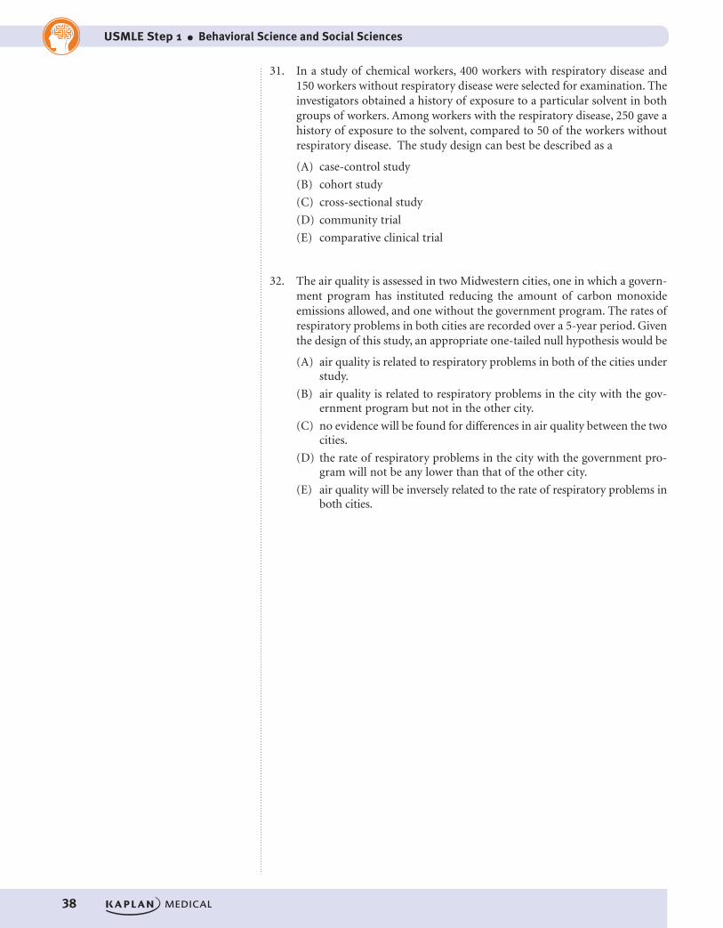
31. In a study of chemical workers, 400 workers with respiratory disease and 150 workers without respiratory disease were selected for examination. The investigators obtained a history of exposure to a particular solvent in both groups of workers. Among workers with the respiratory disease, 250 gave a history of exposure to the solvent, compared to 50 of the workers without respiratory disease. The study design can best be described as a

(A) case-control study

(B) cohort study

(C) cross-sectional study

(D) community trial

(E) comparative clinical trial

32. The air quality is assessed in two Midwestern cities, one in which a govern-ment program has instituted reducing the amount of carbon monoxide emissions allowed, and one without the government program. The rates of respiratory problems in both cities are recorded over a 5-year period. Given the design of this study, an appropriate one-tailed null hypothesis would be

(A) air quality is related to respiratory problems in both of the cities under study.

(B) air quality is related to respiratory problems in the city with the gov-ernment program but not in the other city.

(C) no evidence will be found for differences in air quality between the two cities.

(D) the rate of respiratory problems in the city with the government pro-gram will not be any lower than that of the other city.

(E) air quality will be inversely related to the rate of respiratory problems in both cities.


39

Answers1. Answer: D. Relative risk means divide, compute the ratio between the two

groups. [230/71 = 3.2]

2. Answer: D. Definition question. Null hypothesis is a statement of chance, the opposite of what the researcher hopes to find.

3. Answer: B. Smaller interval is more precise, but less confident. Precise means narrower interval. 95% confidence yields a smaller interval than 99% confidence.

4. Answer: C. One reason for a near-zero correlation is that the error of mea-surement is so large that it obscures an underlying relationship. Shows no linear relationship. Does not mean cause. Number given is coefficient, not p-value.

5. Answer: C. True negatives, out of all nondiseased. [TN/(TN+FP)] = [63/(87+63)]. Note, divided by number ending in “0”.

6. Answer: B. True positives, out of all positives. [TP/(TP+FP)] = [102/(102+87)]. Note, divided by number ending in “9”.

7. Answer: A. True positives, out of all diseased. [TP/(TP+FN)] = [102/(102+48)]. Note, divided by number ending in “0”.

8. Answer: A. Type I error means the researcher rejected the null hypothesis, but should not have. This means that although statistical significance is found, there is no real-world significance. By reversing the clauses in the answer, the correct answer becomes more apparent. Answer D is a good defi-nition of a Type II error.

9. Answer: B. If 95% of cases fall between 110 and 190 and the distribution is symmetrical, then the mean must be 150, and the numbers given are two standard deviations above and below the mean. This means that two stan-dard deviations must equal 40 and that one standard deviation equals 20.

10. Answer: D. Key here is the “p-value.” Ignore the chi-square value. If less than 0.05, this gives the chance of a Type I error. Therefore, the probability of the finding if the drug was ineffective.

11. Answer: C. This is one standard deviation above the mean. [115 + 10]. Below this point are 84% of the cases using the normal curve.

12. Answer: B. The given correlation is statistically significant at the 0.001 level and can therefore be interpreted. It is a positive correlation, suggesting that high goes with high and low goes with low. Avoid answers that suggest a causal relationship.

13. Answer: D. People in the two communities are followed forward in time and incidence (mortality) is the outcome.

14. Answer: C. Key is to focus only on 1981. Relative risk means divide. [15%/10% = 1.5] or 1.5 times the risk.

15. Answer: E. Denver versus Fort Collins is one nominal variable with two groups. Dead versus alive is the second nominal variable. Two nominal vari-ables with n >25 = chi-square.

40


16. Answer: A. This is a case-control study (infarcts versus no infarcts). Therefore, use an odds ratio. The data is not incidence data, so relative risk does not apply.

17. Answer: E. The IQ is scaled to have a mean of 100 and a standard devia-tion of 15. What percent of the cases are above two standard deviations above the mean? (2.5%) Therefore, what is 2.5% of 400? (10)

18. Answer: E. Power is the chance of detecting a difference in the study if there really is a difference in the real world. The question tells us what chance the researcher will have of finding a difference.

19. Answer: D. Bottle versus glass is confounded with age or maturity. The other options, while possible, are unlikely.

20. Answer: B. Select suicide cases and compare with nonsuicides (controls).

21. Answer: F. Blood sugar levels are ratio data, treated as interval data. Husbands and wives are nominal, but are nonindependent, matched pairs; therefore, matched pairs t-test.

22. Answer: B. Staff either call in sick or do not (nominal variable) over three shifts (nominal variable). Two nominal variables with a 2 × 3 design, chi-square.

23. Answer: E. “Is there a relationship?” between two interval level variables. Pearson correlation.

24. Answer: A. Same sex versus no same sex (nominal variable). Testosterone level is assessed as ratio and treated as interval. Therefore, simple t-test.

25. Answer: D. Vacutainer versus standard syringe (nominal), training versus no training (nominal), and time (interval). Two nominal and one interval = two-way ANOVA.

26. Answer: B. Margarine versus butter (nominal), cancer versus no cancer (nominal). Therefore, chi-square.

27. Answer: C. Three types of treatment: surgery, radiation, and none (nomi-nal variable, three groups), quality of life on the given scale (interval). Therefore, one-way ANOVA.

28. Answer: B. Passing versus failure (nominal), three sites (nominal). Therefore, chi-square.

29. Answer: C. Three sites (nominal) with actual test scores (interval). Therefore, one-way ANOVA.

30. Answer: F. Before and after (nominal, two-groups, matched pairs), and blood pressure (interval). Therefore, matched pairs t-test.

31. Answer: A. Respiratory (cases) versus nonrespiratory disease (controls), look-ing at history.

32. Answer: D. The correct statement needs to be a one-directional statement of no effect. “Not any lower than” satisfies this criterion.

Biostatistics - KSUMSC

Documents

Transcript of Biostatistics - KSUMSC