Modern Issues and Methods in Biostatistics (Statistics for ...
322
-
Upload
khangminh22 -
Category
Documents
-
view
3 -
download
0
Transcript of Modern Issues and Methods in Biostatistics (Statistics for ...


Statistics for Biology and HealthSeries Editors:M. GailK. KrickebergJ. SametA. TsiatisW. Wong
For other titles published in this series, go tohttp://www.springer.com/series/2848


Mark Chang
Modern Issues and Methodsin Biostatistics
123

Mark ChangAMAG Pharmaceuticals, Inc.BiometricsHayden Ave. 10002421 Lexington MassachusettsUSA
Statistics for Biology and Health Series EditorsM. GailNational Cancer InstituteBethesda, MD 20892USA
Klaus KrickebergLe ChateletF-63270 ManglieuFrance
Jonathan M. SametDepartment of Preventive MedicineKeck School of MedicineUniversity of Southern California1441 Eastlake Ave. Room 4436, MC 9175Los Angles, CA 90089
A. TsiatisDepartment of StatisticsNorth Carolina State UniversityRaleigh, NC 27695USA
W. WongDepartment of StatisticsStanford UniversityStanford, CA 94305-4065USA
ISSN 1431-8776ISBN 978-1-4419-9841-5 e-ISBN 978-1-4419-9842-2DOI 10.1007/978-1-4419-9842-2Springer New York Dordrecht Heidelberg London
Library of Congress Control Number: 2011931898
c� Springer Science+Business Media, LLC 2011All rights reserved. This work may not be translated or copied in whole or in part without the writtenpermission of the publisher (Springer Science+Business Media, LLC, 233 Spring Street, New York,NY 10013, USA), except for brief excerpts in connection with reviews or scholarly analysis. Use inconnection with any form of information storage and retrieval, electronic adaptation, computer software,or by similar or dissimilar methodology now known or hereafter developed is forbidden.The use in this publication of trade names, trademarks, service marks, and similar terms, even if they arenot identified as such, is not to be taken as an expression of opinion as to whether or not they are subjectto proprietary rights.
Printed on acid-free paper
Springer is part of Springer Science+Business Media (www.springer.com)

Preface
Classic biostatistics, a branch of statistical science, has as its main focus the applica-tions of statistics in public health, the life sciences, and the pharmaceutical industry.Modern biostatistics, beyond just a simple application of statistics, is a confluence ofstatistics and knowledge of multiple intertwined fields. Biostatistics often requiresinnovations across disciplines. Over the years, biostatistics has gradually shaped itsown unique characteristics and approaches. Indeed, the application demands, theadvancements in computer technology, and the rapid growth of life science data(e.g., genomics data) have promoted the formation of modern biostatistics.
There are at least three characteristics of modern biostatistics: (1) in-depthengagement in the application fields that require penetration of knowledge acrossseveral fields, (2) high-level complexity of data because they are longitudinal,incomplete, or latent because they are heterogeneous due to a mixture of data orexperiment types, because of high-dimensionality, which may make meaningfulreduction impossible, or because of extremely small or large size; and (3) dynamics,the speed of development in methodology and analyses, has to match the fast growthof data with a constantly changing face.
This book is written for researchers, biostatisticians/statisticians, and scientistswho are interested in quantitative analyses. The goal is to introduce modern issuesand methods in biostatistics and help researchers and students quickly grasp keyconcepts and methods. Bear in mind that many methods can solve the same problemand many problems can be solved by the same method, which becomes apparentwhen those topics are discussed in a single volume. Modern biostatistics requiresresearchers to possess diverse knowledge. However, given the vast number ofpublications in the research area, it requires a huge investment of time to gaininsight into modern biostatistics. Therefore, I hope this book can serve as a vehicleto achieve this objective, though by no means do I want or am I able to cover thisfast-growing field completely. I would also like to warn readers that, inevitably, thebook will often reflect the author’s opinions, especially in discussing controversialmatters. Nevertheless, it displays broad coverage and can be used as a textbook oras a reference text.
v

vi Preface
The book consists of ten chapters: Multiple-Hypothesis Testing Strategy, Phar-maceutical Decision and Game Theory, Noninferiority Trial Design, AdaptiveTrial Design, Missing Data Imputation and Analysis, Multivariate and MultistageSurvival Data Modeling, Meta-analysis, Data Mining and Signal Detection, MonteCarlo Simulation, and Bayesian Methods and Applications. Some of these titlesare new; others are not that new but include novel ingredients or developments inmethodology, computation algorithms, or applications. These areas have a commonreason for their popularity in that they are in high demand by the real world andespecially from the pharmaceutical industry.
Each chapter includes an introduction to the concepts, discussions of methodol-ogy, and examples of applications. Controversies and challenges are also included.Each chapter is limited to about 30 pages. Given the limit in length, materials areselected to focus on the key concepts and methods that have been used in practice;lengthy mathematical derivations are generally omitted, but references to them areprovided. At the end of each chapter, exercises are provided as well as a list ofreferences for further reading.
I point out that, due to the nature of each of the ten topics, the mathematicalcomplexity varies from chapter to chapter. Some are more theoretical, whereasothers are more scientifically involved and require thinking rather beyond straightmathematics. I have fully realized the importance of consistency in presentationacross chapters but will not over-emphasize it. The book is organized as follows.
Chapter 1, Multiple – Hypothesis Testing Strategy, introduces commonly usedmethods for multiplicity adjustment in the frequentist paradigm, including com-monly used single-step and stepwise procedures such as gatekeeping and tree-structured test procedures. Discussions of applications will focus on clinical trials.The controversies surrounding multiplicity issues particularly are addressed.
Chapter 2, Pharmaceutical Decision and Game Theory, addresses decision andgame theory, which has a long history in economics. However, recently the need formore cost-effective R & D programs has demanded a shift in the pharmaceuticaldecision-making process from the qualitative decision paradigm to the quantitativedecision approaches that are based on formal decision and game theory. For thisreason, this chapter first introduces decision and game theory in general andthen discusses how to apply it to the pharmaceutical decision process by usingmodels, such as the Markov decision process and implementations using computersimulations. Applications presented include clinical development program and R &D portfolio optimizations, and prescription drug commercialization among others.
Chapter 3, Noninferiority Trial Design, discusses the needs of noninferiority(NI) trials and summarizes three common methods for NI trial designs, includingthe fixed-margin, lamda, and synthetic methods. Comparisons are made amongthe different methods, and the controversies surrounding such trials are discussed.The materials covered in this chapter should meet the basic needs for designing anNI trial.
Chapter 4, Adaptive Trial Design, deals with adaptive trials, a coming stormin the pharmaceutical industry thanks to the leadership of biostatistics. Thischapter introduces the adaptive design concept and provides a uniform formulation
Preface vii
for hypothesis-based adaptive trial designs. The evaluation matrix and variousapplications are studied. Controversies and challenges are considered.
Chapter 5, Missing Data Imputation and Analysis, discusses the problem ofimperfect or incomplete information. Traditional methods such as the general linearmodel, which ignore subjects with incomplete observations, often cause bias andoften are not applicable in practice. Statistical models that effectively deal withmissing observations are becoming increasingly important, and research in thisarea is developing rapidly. This chapter discusses different types of missing dataand various models for analyses with ignorable and nonignorable missing patterns.Implementations using software such as SAS are presented as well.
Chapter 6, Multivariate and Multistage Survival Data Modeling, addresses thefact that the survival data model we are dealing with today in the life sciences ismore complicated than ever, involving multivariates and many covariates. Multi-stage models provide powerful tools for solving various problems with survivaldata such as competing risks, adaptive treatment switching, informative dropouts,progressive disease, and longitudinal data modeling. This chapter starts with areview of various survival models, including Cox’s proportional hazard model, thefrailty model, the copula model, the first-hitting-time model, and nonparametricapproaches. The frailty, copula, and first-hitting-time models are discussed in detailand expanded to multivariate and multistage models. We discuss step-by-step modelbuilding using various examples.
Chapter 7, Meta-analysis, discusses what is in a sense an art, with manycontroversies, especially for post hoc meta-analysis. Meta-analysis methods areclassified into three categories based on data type: subject-based data, study-based data, and mixed-data models. Fixed-effect and random-effect models andsequential methods are at the center of the discussion. Graphical presentations andinterpretations of the results are also made.
Chapter 8, Data Mining and Signal Detection, introduces supervised, unsuper-vised, and reinforcement learning mechanics in data mining methods, including linkanalysis, the nearest-neighbor method, kernel and tree methods, the support vectormachine, artificial neural networks, the k-means algorithm, genetic programming,cellular automata, and agent-based methods. Applications in the life sciences anddrug development are discussed. Signal detection with various sequential likelihoodratio tests and other data mining methods is studied.
Chapter 9, Monte Carlo Simulation, notes that computer simulations havebecome a very powerful and cost-effective approach in the life sciences and in thepharmaceutical industry. This chapter discusses several random sampling methods,clinical trial simulations, molecular designs, biological pathway simulations, andpharmacokinetic and pharmacodynamic simulations.
Chapter 10, Bayesian Methods and Applications, introduces Bayesian infer-ences, hierarchical models, decision models, model selection, Bayesian multiplicity,and computational methods. It also provides application examples for clinical trials,signal detection, missing data-imputation, meta-analysis, disease mapping, andother areas.

viii Preface
The draft manuscripts were reviewed by nine statisticians. Their constructivecomments have greatly improved the manuscript. In the big picture, they consis-tently suggested reducing the mathematical complexity and adding more motivatingexamples. As a result, I have added about 20 examples and 40 pages. I have alsoremoved some mathematical content; but I found it difficult to cut math too muchand at the same time cover a reasonable scope in depth of topic within 30 pages – Iwanted it to be concise.
My little daughter, Monica, a middle school student, reviewed an early draftmanuscript of all ten chapters and corrected many of my grammatical errors (shevery much enjoyed doing that for me!). I want to thank her a lot! Dr. Robert Piercecarefully reviewed parts of the manuscript before I submitted it to the publisher.Without his review, the quality of the book would not be as good as you haveright now. Finally, I would like to thank Mr. John Kimmel and Mr. Marc Straussat Springer for providing me with the opportunity to work on this project.
Mark Chang ( )

Contents
1 Multiple-Hypothesis Testing Strategy . . . . . . . . . . . . . . . . . . . . . . . . . . . . . . . . . . . . 11.1 Multiple-Testing Problems. . . . . . . . . . . . . . . . . . . . . . . . . . . . . . . . . . . . . . . . . . . 1
1.1.1 Statistical Hypothesis Testing . . . . . . . . . . . . . . . . . . . . . . . . . . . . . . 11.1.2 Sources of Multiplicity . . . . . . . . . . . . . . . . . . . . . . . . . . . . . . . . . . . . . 11.1.3 Multiple-Testing Taxonomy.. . . . . . . . . . . . . . . . . . . . . . . . . . . . . . . 3
1.2 Multiple-Testing Approaches .. . . . . . . . . . . . . . . . . . . . . . . . . . . . . . . . . . . . . . . 71.2.1 Single-Step Procedures . . . . . . . . . . . . . . . . . . . . . . . . . . . . . . . . . . . . . 71.2.2 Stepwise Procedures . . . . . . . . . . . . . . . . . . . . . . . . . . . . . . . . . . . . . . . . 101.2.3 Common Gatekeeper Procedure . . . . . . . . . . . . . . . . . . . . . . . . . . . 151.2.4 Tree Gatekeeping Procedure . . . . . . . . . . . . . . . . . . . . . . . . . . . . . . . 171.2.5 Generalized FWER and Partitioning Testing . . . . . . . . . . . . . . 181.2.6 Procedures Controlling False Discovery Rate. . . . . . . . . . . . . 21
1.3 Controversies and Challenges . . . . . . . . . . . . . . . . . . . . . . . . . . . . . . . . . . . . . . . 241.3.1 Family of Errors . . . . . . . . . . . . . . . . . . . . . . . . . . . . . . . . . . . . . . . . . . . . 241.3.2 Interpretation of Multiple-Testing Results . . . . . . . . . . . . . . . . 251.3.3 The Spring Water Paradox . . . . . . . . . . . . . . . . . . . . . . . . . . . . . . . . . 251.3.4 A Patient’s Dilemma with Multiple-Testing.. . . . . . . . . . . . . . 26
1.4 Exercises . . . . . . . . . . . . . . . . . . . . . . . . . . . . . . . . . . . . . . . . . . . . . . . . . . . . . . . . . . . . . . 27Further Readings and References . . . . . . . . . . . . . . . . . . . . . . . . . . . . . . . . . . . . . . . . . . . 28
2 Pharmaceutical Decision and Game Theory . . . . . . . . . . . . . . . . . . . . . . . . . . . . 312.1 Pharmaceutical Decisions . . . . . . . . . . . . . . . . . . . . . . . . . . . . . . . . . . . . . . . . . . . . 31
2.1.1 Markov Decision Process . . . . . . . . . . . . . . . . . . . . . . . . . . . . . . . . . . 312.1.2 Dynamic Programming.. . . . . . . . . . . . . . . . . . . . . . . . . . . . . . . . . . . . 332.1.3 Clinical Development Program . . . . . . . . . . . . . . . . . . . . . . . . . . . . 342.1.4 R & D Portfolio Optimization . . . . . . . . . . . . . . . . . . . . . . . . . . . . . 382.1.5 Prescription Drug Marketing .. . . . . . . . . . . . . . . . . . . . . . . . . . . . . . 40
2.2 Pharmaceutical Games . . . . . . . . . . . . . . . . . . . . . . . . . . . . . . . . . . . . . . . . . . . . . . . 422.2.1 The Game Concept . . . . . . . . . . . . . . . . . . . . . . . . . . . . . . . . . . . . . . . . . 422.2.2 Multiple-Player Game . . . . . . . . . . . . . . . . . . . . . . . . . . . . . . . . . . . . . . 462.2.3 Queuing Game . . . . . . . . . . . . . . . . . . . . . . . . . . . . . . . . . . . . . . . . . . . . . . 47
ix

x Contents
2.2.4 Cooperative Games . . . . . . . . . . . . . . . . . . . . . . . . . . . . . . . . . . . . . . . . . 492.2.5 Sequential Game . . . . . . . . . . . . . . . . . . . . . . . . . . . . . . . . . . . . . . . . . . . . 50
2.3 Implementation Challenges . . . . . . . . . . . . . . . . . . . . . . . . . . . . . . . . . . . . . . . . . . 532.4 Exercises . . . . . . . . . . . . . . . . . . . . . . . . . . . . . . . . . . . . . . . . . . . . . . . . . . . . . . . . . . . . . . 55Further Readings and References . . . . . . . . . . . . . . . . . . . . . . . . . . . . . . . . . . . . . . . . . . . 56
3 Noninferiority Trial Design . . . . . . . . . . . . . . . . . . . . . . . . . . . . . . . . . . . . . . . . . . . . . . . . 593.1 Concept of Noninferiority Trial . . . . . . . . . . . . . . . . . . . . . . . . . . . . . . . . . . . . . 59
3.1.1 Needs for Noninferiority Design. . . . . . . . . . . . . . . . . . . . . . . . . . . 593.1.2 Noninferiority Lingo . . . . . . . . . . . . . . . . . . . . . . . . . . . . . . . . . . . . . . . 613.1.3 Noninferiority Design Methods . . . . . . . . . . . . . . . . . . . . . . . . . . . . 613.1.4 Analysis of Noninferiority Trials . . . . . . . . . . . . . . . . . . . . . . . . . . 65
3.2 Two-Arm Design . . . . . . . . . . . . . . . . . . . . . . . . . . . . . . . . . . . . . . . . . . . . . . . . . . . . . 663.2.1 Fixed-Margin Method . . . . . . . . . . . . . . . . . . . . . . . . . . . . . . . . . . . . . . 663.2.2 �-Portion Method.. . . . . . . . . . . . . . . . . . . . . . . . . . . . . . . . . . . . . . . . . . 693.2.3 Synthesis Method .. . . . . . . . . . . . . . . . . . . . . . . . . . . . . . . . . . . . . . . . . . 703.2.4 Paired Data . . . . . . . . . . . . . . . . . . . . . . . . . . . . . . . . . . . . . . . . . . . . . . . . . . 74
3.3 Three-Arm Design . . . . . . . . . . . . . . . . . . . . . . . . . . . . . . . . . . . . . . . . . . . . . . . . . . . 753.4 The Noninferiority Margin and Regulatory Guidance.. . . . . . . . . . . . . 77
3.4.1 ICH Guidance. . . . . . . . . . . . . . . . . . . . . . . . . . . . . . . . . . . . . . . . . . . . . . . 773.4.2 FDA Guidance .. . . . . . . . . . . . . . . . . . . . . . . . . . . . . . . . . . . . . . . . . . . . . 773.4.3 CHMP Guidance.. . . . . . . . . . . . . . . . . . . . . . . . . . . . . . . . . . . . . . . . . . . 79
3.5 Controversies and Challenges . . . . . . . . . . . . . . . . . . . . . . . . . . . . . . . . . . . . . . . 813.5.1 Assay Sensitivity, Constancy and Biocreep . . . . . . . . . . . . . . . 813.5.2 Conflicting Noninferiority-Superiority Claims. . . . . . . . . . . . 813.5.3 Dilemma of Totality Evidence . . . . . . . . . . . . . . . . . . . . . . . . . . . . . 823.5.4 Superiority-Noninferiority Testing . . . . . . . . . . . . . . . . . . . . . . . . 833.5.5 Summary .. . . . . . . . . . . . . . . . . . . . . . . . . . . . . . . . . . . . . . . . . . . . . . . . . . . 83
3.6 Exercises . . . . . . . . . . . . . . . . . . . . . . . . . . . . . . . . . . . . . . . . . . . . . . . . . . . . . . . . . . . . . . 84Further Readings and References . . . . . . . . . . . . . . . . . . . . . . . . . . . . . . . . . . . . . . . . . . . 85
4 Adaptive Trial Design . . . . . . . . . . . . . . . . . . . . . . . . . . . . . . . . . . . . . . . . . . . . . . . . . . . . . . 874.1 Concept of Adaptive Trial Design . . . . . . . . . . . . . . . . . . . . . . . . . . . . . . . . . . . 87
4.1.1 Reasons for Adaptive Design . . . . . . . . . . . . . . . . . . . . . . . . . . . . . . 874.1.2 Hypothesis-Based Adaptive Design . . . . . . . . . . . . . . . . . . . . . . . 88
4.2 Adaptive Design Methods . . . . . . . . . . . . . . . . . . . . . . . . . . . . . . . . . . . . . . . . . . . 924.2.1 p-value Weighting Approach . . . . . . . . . . . . . . . . . . . . . . . . . . . . . . 924.2.2 Fisher Combination Approach . . . . . . . . . . . . . . . . . . . . . . . . . . . . . 944.2.3 p-value Inversion Approach . . . . . . . . . . . . . . . . . . . . . . . . . . . . . . . 954.2.4 Error-Spending Approach .. . . . . . . . . . . . . . . . . . . . . . . . . . . . . . . . . 96
4.3 Evaluation and Analysis of Adaptive Design . . . . . . . . . . . . . . . . . . . . . . . 974.3.1 Evaluation Matrix . . . . . . . . . . . . . . . . . . . . . . . . . . . . . . . . . . . . . . . . . . 974.3.2 Analysis of Adaptive Trial Data . . . . . . . . . . . . . . . . . . . . . . . . . . . 994.3.3 Comparison of Adaptive Design Methods . . . . . . . . . . . . . . . . 102
4.4 Adaptive Designs in Action . . . . . . . . . . . . . . . . . . . . . . . . . . . . . . . . . . . . . . . . . . 1054.4.1 Sample Size Reestimation. . . . . . . . . . . . . . . . . . . . . . . . . . . . . . . . . . 105

Contents xi
4.4.2 Adaptive Seamless Design . . . . . . . . . . . . . . . . . . . . . . . . . . . . . . . . . 1074.4.3 Noninferiority-Superiority Adaptive Design . . . . . . . . . . . . . . 108
4.5 Adaptive Design Debates . . . . . . . . . . . . . . . . . . . . . . . . . . . . . . . . . . . . . . . . . . . . 1094.5.1 Sufficiency Principle . . . . . . . . . . . . . . . . . . . . . . . . . . . . . . . . . . . . . . . 1094.5.2 Minimum Sufficiency Principle and Efficiency . . . . . . . . . . . 1104.5.3 Conditionality and Exchangeability Principles. . . . . . . . . . . . 1104.5.4 Equal Weight Principle . . . . . . . . . . . . . . . . . . . . . . . . . . . . . . . . . . . . . 1114.5.5 Consistency of Stagewise Results . . . . . . . . . . . . . . . . . . . . . . . . . 1114.5.6 Adjusted p-value . . . . . . . . . . . . . . . . . . . . . . . . . . . . . . . . . . . . . . . . . . . 1124.5.7 Summary .. . . . . . . . . . . . . . . . . . . . . . . . . . . . . . . . . . . . . . . . . . . . . . . . . . . 112
4.6 Exercises . . . . . . . . . . . . . . . . . . . . . . . . . . . . . . . . . . . . . . . . . . . . . . . . . . . . . . . . . . . . . . 113Further Readings and References . . . . . . . . . . . . . . . . . . . . . . . . . . . . . . . . . . . . . . . . . . . 114
5 Missing Data Imputation and Analysis . . . . . . . . . . . . . . . . . . . . . . . . . . . . . . . . . . 1175.1 Missing Data Problems . . . . . . . . . . . . . . . . . . . . . . . . . . . . . . . . . . . . . . . . . . . . . . 117
5.1.1 Missing Data Issue and Its Impact . . . . . . . . . . . . . . . . . . . . . . . . . 1175.1.2 Missing Data Taxonomy . . . . . . . . . . . . . . . . . . . . . . . . . . . . . . . . . . . 118
5.2 Analysis Methods for Missing at Random . . . . . . . . . . . . . . . . . . . . . . . . . . 1205.2.1 Single Imputation Methods . . . . . . . . . . . . . . . . . . . . . . . . . . . . . . . . 1205.2.2 Generalized Linear Mixed Models . . . . . . . . . . . . . . . . . . . . . . . . 1205.2.3 Expectation-Maximization Algorithm .. . . . . . . . . . . . . . . . . . . . 1225.2.4 Inverse-Probability Weighting Method .. . . . . . . . . . . . . . . . . . . 1235.2.5 Multiple-Imputation Method .. . . . . . . . . . . . . . . . . . . . . . . . . . . . . . 1255.2.6 Weighted Generalized Estimating Equations.. . . . . . . . . . . . . 126
5.3 Analysis Methods for Missing Not at Random .. . . . . . . . . . . . . . . . . . . . 1285.3.1 Missing Data Frameworks . . . . . . . . . . . . . . . . . . . . . . . . . . . . . . . . . 1285.3.2 Selection Model . . . . . . . . . . . . . . . . . . . . . . . . . . . . . . . . . . . . . . . . . . . . 1305.3.3 Pattern-Mixture Model . . . . . . . . . . . . . . . . . . . . . . . . . . . . . . . . . . . . . 1315.3.4 Shared-Parameter Models . . . . . . . . . . . . . . . . . . . . . . . . . . . . . . . . . . 131
5.4 Analysis Examples Using SAS and SOLAS . . . . . . . . . . . . . . . . . . . . . . . . 1335.4.1 Likelihood Ignorable Analysis . . . . . . . . . . . . . . . . . . . . . . . . . . . . . 1345.4.2 Multiple-Imputation Method .. . . . . . . . . . . . . . . . . . . . . . . . . . . . . . 1345.4.3 EM Algorithm Using SAS . . . . . . . . . . . . . . . . . . . . . . . . . . . . . . . . . 1365.4.4 SOLAS for Missing Data Analysis . . . . . . . . . . . . . . . . . . . . . . . . 136
5.5 Controversies, Challenges, and Recommendations .. . . . . . . . . . . . . . . . 1375.5.1 Comparisons of Different Methods . . . . . . . . . . . . . . . . . . . . . . . . 1375.5.2 How to Implement Missingness . . . . . . . . . . . . . . . . . . . . . . . . . . . 1385.5.3 Regulatory Perspective . . . . . . . . . . . . . . . . . . . . . . . . . . . . . . . . . . . . . 1395.5.4 Recommendations for Clinical Trials . . . . . . . . . . . . . . . . . . . . . . 140
5.6 Exercises . . . . . . . . . . . . . . . . . . . . . . . . . . . . . . . . . . . . . . . . . . . . . . . . . . . . . . . . . . . . . . 142Further Readings and References . . . . . . . . . . . . . . . . . . . . . . . . . . . . . . . . . . . . . . . . . . . 142
6 Multivariate and Multistage Survival Data Modeling . . . . . . . . . . . . . . . . . . 1456.1 Introduction to Survival Data Modeling . . . . . . . . . . . . . . . . . . . . . . . . . . . . 145
6.1.1 Basic Terms in Survival Analysis . . . . . . . . . . . . . . . . . . . . . . . . . . 1456.1.2 Maximum Likelihood Method . . . . . . . . . . . . . . . . . . . . . . . . . . . . . 1466.1.3 Overview of Survival Model . . . . . . . . . . . . . . . . . . . . . . . . . . . . . . . 147

xii Contents
6.2 Frailty Model . . . . . . . . . . . . . . . . . . . . . . . . . . . . . . . . . . . . . . . . . . . . . . . . . . . . . . . . . 1516.2.1 Univariate Frailty Models . . . . . . . . . . . . . . . . . . . . . . . . . . . . . . . . . . 1516.2.2 Multivariate Frailty Models . . . . . . . . . . . . . . . . . . . . . . . . . . . . . . . . 1526.2.3 The Shared Frailty Copula . . . . . . . . . . . . . . . . . . . . . . . . . . . . . . . . . 1526.2.4 The Correlated Frailty Copula . . . . . . . . . . . . . . . . . . . . . . . . . . . . . 153
6.3 First-Hitting-Time Model . . . . . . . . . . . . . . . . . . . . . . . . . . . . . . . . . . . . . . . . . . . . 1536.3.1 Wiener Process and First Hitting Time . . . . . . . . . . . . . . . . . . . . 1536.3.2 Covariates and Link Function . . . . . . . . . . . . . . . . . . . . . . . . . . . . . . 1546.3.3 Parameter Estimation and Inference .. . . . . . . . . . . . . . . . . . . . . . 1556.3.4 Applications of First-Hitting-Time Model . . . . . . . . . . . . . . . . 1566.3.5 Multivariate Model with Biomarkers . . . . . . . . . . . . . . . . . . . . . . 157
6.4 Multistage Model. . . . . . . . . . . . . . . . . . . . . . . . . . . . . . . . . . . . . . . . . . . . . . . . . . . . . 1596.4.1 General Framework of Multistage Model . . . . . . . . . . . . . . . . . 1596.4.2 Covariates and Treatment Switching . . . . . . . . . . . . . . . . . . . . . . 1616.4.3 Latent Process and Competing Risks . . . . . . . . . . . . . . . . . . . . . . 1636.4.4 Competing Risks in Progressive Disease . . . . . . . . . . . . . . . . . . 1676.4.5 Longitudinal Multivariate Model . . . . . . . . . . . . . . . . . . . . . . . . . . 169
6.5 Challenges and Controversies . . . . . . . . . . . . . . . . . . . . . . . . . . . . . . . . . . . . . . . 1706.6 Exercises . . . . . . . . . . . . . . . . . . . . . . . . . . . . . . . . . . . . . . . . . . . . . . . . . . . . . . . . . . . . . . 172Further Readings and References . . . . . . . . . . . . . . . . . . . . . . . . . . . . . . . . . . . . . . . . . . . 172
7 Meta-Analysis . . . . . . . . . . . . . . . . . . . . . . . . . . . . . . . . . . . . . . . . . . . . . . . . . . . . . . . . . . . . . . . 1757.1 Concept of Meta-Analysis . . . . . . . . . . . . . . . . . . . . . . . . . . . . . . . . . . . . . . . . . . . 175
7.1.1 The Art and Science of Meta-Analysis . . . . . . . . . . . . . . . . . . . . 1757.1.2 Study Endpoints . . . . . . . . . . . . . . . . . . . . . . . . . . . . . . . . . . . . . . . . . . . . 1767.1.3 Basic Methods . . . . . . . . . . . . . . . . . . . . . . . . . . . . . . . . . . . . . . . . . . . . . . 179
7.2 Subject-Based Meta-Analysis . . . . . . . . . . . . . . . . . . . . . . . . . . . . . . . . . . . . . . . 1807.3 Study-Based Meta-Analysis . . . . . . . . . . . . . . . . . . . . . . . . . . . . . . . . . . . . . . . . . 180
7.3.1 The Fixed-Effect Model . . . . . . . . . . . . . . . . . . . . . . . . . . . . . . . . . . . . 1807.3.2 Assessing Heterogeneity . . . . . . . . . . . . . . . . . . . . . . . . . . . . . . . . . . . 1847.3.3 Random-Effect Model . . . . . . . . . . . . . . . . . . . . . . . . . . . . . . . . . . . . . . 1847.3.4 Mixture Model for Relative Risk . . . . . . . . . . . . . . . . . . . . . . . . . . 186
7.4 Meta-Analysis in Complex Settings . . . . . . . . . . . . . . . . . . . . . . . . . . . . . . . . . 1907.4.1 Individual and Aggregate Data Mixtures . . . . . . . . . . . . . . . . . . 1907.4.2 Mixture of Matched and Unmatched Pairs . . . . . . . . . . . . . . . . 1937.4.3 p-value Combination Approaches .. . . . . . . . . . . . . . . . . . . . . . . . 1947.4.4 Cumulative Meta-Analysis . . . . . . . . . . . . . . . . . . . . . . . . . . . . . . . . . 195
7.5 Graphical Presentations . . . . . . . . . . . . . . . . . . . . . . . . . . . . . . . . . . . . . . . . . . . . . . 1977.5.1 Funnel Plots . . . . . . . . . . . . . . . . . . . . . . . . . . . . . . . . . . . . . . . . . . . . . . . . . 197
7.6 Controversies and Challenges . . . . . . . . . . . . . . . . . . . . . . . . . . . . . . . . . . . . . . . 1987.6.1 Inclusion of Studies . . . . . . . . . . . . . . . . . . . . . . . . . . . . . . . . . . . . . . . . 1987.6.2 Inclusion, Analysis, and Reporting Bias. . . . . . . . . . . . . . . . . . . 1997.6.3 Inconsistency in Weight Selection . . . . . . . . . . . . . . . . . . . . . . . . . 200
7.7 Exercises . . . . . . . . . . . . . . . . . . . . . . . . . . . . . . . . . . . . . . . . . . . . . . . . . . . . . . . . . . . . . . 201Further Readings and References . . . . . . . . . . . . . . . . . . . . . . . . . . . . . . . . . . . . . . . . . . . 202
Contents xiii
8 Data Mining and Signal Detection . . . . . . . . . . . . . . . . . . . . . . . . . . . . . . . . . . . . . . . . 2058.1 Common Data Mining Methods . . . . . . . . . . . . . . . . . . . . . . . . . . . . . . . . . . . . . 205
8.1.1 Supervised, Unsupervised, and Reinforcement Learning. 2058.1.2 Link Analysis . . . . . . . . . . . . . . . . . . . . . . . . . . . . . . . . . . . . . . . . . . . . . . . 2068.1.3 Nearest-Neighbors Method . . . . . . . . . . . . . . . . . . . . . . . . . . . . . . . . 2088.1.4 Kernel Method . . . . . . . . . . . . . . . . . . . . . . . . . . . . . . . . . . . . . . . . . . . . . . 2098.1.5 Support Vector Machine. . . . . . . . . . . . . . . . . . . . . . . . . . . . . . . . . . . . 2098.1.6 Tree Methods . . . . . . . . . . . . . . . . . . . . . . . . . . . . . . . . . . . . . . . . . . . . . . . 2108.1.7 Artificial Neural Network . . . . . . . . . . . . . . . . . . . . . . . . . . . . . . . . . . 2138.1.8 Unsupervised to Supervised Learning .. . . . . . . . . . . . . . . . . . . . 2158.1.9 K-Means Algorithm . . . . . . . . . . . . . . . . . . . . . . . . . . . . . . . . . . . . . . . . 2168.1.10 Genetic Programming . . . . . . . . . . . . . . . . . . . . . . . . . . . . . . . . . . . . . . 2178.1.11 Cellular Automata Method . . . . . . . . . . . . . . . . . . . . . . . . . . . . . . . . . 2178.1.12 Agent-Based Models . . . . . . . . . . . . . . . . . . . . . . . . . . . . . . . . . . . . . . . 218
8.2 Signal Detection and Analysis . . . . . . . . . . . . . . . . . . . . . . . . . . . . . . . . . . . . . . . 2198.2.1 Pharmacovigilance . . . . . . . . . . . . . . . . . . . . . . . . . . . . . . . . . . . . . . . . . 2198.2.2 Traditional Hypothesis Test . . . . . . . . . . . . . . . . . . . . . . . . . . . . . . . . 2208.2.3 Sequential Probability Ratio Test . . . . . . . . . . . . . . . . . . . . . . . . . . 2218.2.4 Disproportional Analysis . . . . . . . . . . . . . . . . . . . . . . . . . . . . . . . . . . . 2238.2.5 Group Sequential Method .. . . . . . . . . . . . . . . . . . . . . . . . . . . . . . . . . 2268.2.6 Data Mining Approach . . . . . . . . . . . . . . . . . . . . . . . . . . . . . . . . . . . . . 226
8.3 Challenges . . . . . . . . . . . . . . . . . . . . . . . . . . . . . . . . . . . . . . . . . . . . . . . . . . . . . . . . . . . . 2278.4 Exercises . . . . . . . . . . . . . . . . . . . . . . . . . . . . . . . . . . . . . . . . . . . . . . . . . . . . . . . . . . . . . . 229Further Readings and References . . . . . . . . . . . . . . . . . . . . . . . . . . . . . . . . . . . . . . . . . . . 229
9 Monte Carlo Simulation . . . . . . . . . . . . . . . . . . . . . . . . . . . . . . . . . . . . . . . . . . . . . . . . . . . 2339.1 Random Number Generation . . . . . . . . . . . . . . . . . . . . . . . . . . . . . . . . . . . . . . . . 233
9.1.1 Inverse c.d.f Method .. . . . . . . . . . . . . . . . . . . . . . . . . . . . . . . . . . . . . . . 2339.1.2 Acceptance-Rejection Methods .. . . . . . . . . . . . . . . . . . . . . . . . . . . 2349.1.3 Markov Chain Monte Carlo . . . . . . . . . . . . . . . . . . . . . . . . . . . . . . . . 235
9.2 Clinical Trial Simulation . . . . . . . . . . . . . . . . . . . . . . . . . . . . . . . . . . . . . . . . . . . . . 2369.2.1 Adaptive Trial Simulation .. . . . . . . . . . . . . . . . . . . . . . . . . . . . . . . . . 2369.2.2 Dynamic Drug Supply. . . . . . . . . . . . . . . . . . . . . . . . . . . . . . . . . . . . . . 2389.2.3 Bootstrapping Methods. . . . . . . . . . . . . . . . . . . . . . . . . . . . . . . . . . . . . 240
9.3 Molecular Design and Simulation .. . . . . . . . . . . . . . . . . . . . . . . . . . . . . . . . . . 2429.3.1 The Landscape of Molecular Design . . . . . . . . . . . . . . . . . . . . . . 2429.3.2 The Drug-Likeness Concept . . . . . . . . . . . . . . . . . . . . . . . . . . . . . . . 2439.3.3 Molecular Docking . . . . . . . . . . . . . . . . . . . . . . . . . . . . . . . . . . . . . . . . . 245
9.4 Biological Pathway Simulation . . . . . . . . . . . . . . . . . . . . . . . . . . . . . . . . . . . . . . 2489.4.1 Biology Pathways . . . . . . . . . . . . . . . . . . . . . . . . . . . . . . . . . . . . . . . . . . 2489.4.2 Petri Nets . . . . . . . . . . . . . . . . . . . . . . . . . . . . . . . . . . . . . . . . . . . . . . . . . . . . 2499.4.3 Biological Pathway Simulations . . . . . . . . . . . . . . . . . . . . . . . . . . . 251
9.5 PK and PD Modeling and Simulation . . . . . . . . . . . . . . . . . . . . . . . . . . . . . . . 2529.5.1 Pharmacokinetic Simulation . . . . . . . . . . . . . . . . . . . . . . . . . . . . . . . 2529.5.2 Pharmacodynamic Simulation . . . . . . . . . . . . . . . . . . . . . . . . . . . . . 255

xiv Contents
9.6 Implementation Challenges . . . . . . . . . . . . . . . . . . . . . . . . . . . . . . . . . . . . . . . . . . 2579.7 Exercises . . . . . . . . . . . . . . . . . . . . . . . . . . . . . . . . . . . . . . . . . . . . . . . . . . . . . . . . . . . . . . 258Further Readings and References . . . . . . . . . . . . . . . . . . . . . . . . . . . . . . . . . . . . . . . . . . . 259
10 Bayesian Methods and Applications . . . . . . . . . . . . . . . . . . . . . . . . . . . . . . . . . . . . . . 26110.1 Bayesian Paradigm .. . . . . . . . . . . . . . . . . . . . . . . . . . . . . . . . . . . . . . . . . . . . . . . . . . 261
10.1.1 Bayesian Inference . . . . . . . . . . . . . . . . . . . . . . . . . . . . . . . . . . . . . . . . . 26110.1.2 Model Selection . . . . . . . . . . . . . . . . . . . . . . . . . . . . . . . . . . . . . . . . . . . . 26610.1.3 Hierarchical Model . . . . . . . . . . . . . . . . . . . . . . . . . . . . . . . . . . . . . . . . . 26710.1.4 Bayesian Decision-Making . . . . . . . . . . . . . . . . . . . . . . . . . . . . . . . . 26810.1.5 Bayesian Approach to Multiplicity . . . . . . . . . . . . . . . . . . . . . . . . 26910.1.6 Bayesian Computation . . . . . . . . . . . . . . . . . . . . . . . . . . . . . . . . . . . . . 272
10.2 Applications of Bayesian Methods . . . . . . . . . . . . . . . . . . . . . . . . . . . . . . . . . . 27510.2.1 Clinical Trial Design . . . . . . . . . . . . . . . . . . . . . . . . . . . . . . . . . . . . . . . 27510.2.2 Bayesian Adaptive Trial . . . . . . . . . . . . . . . . . . . . . . . . . . . . . . . . . . . . 27610.2.3 Safety Signal Detection . . . . . . . . . . . . . . . . . . . . . . . . . . . . . . . . . . . . 27910.2.4 Missing-Data Handling. . . . . . . . . . . . . . . . . . . . . . . . . . . . . . . . . . . . . 28110.2.5 Meta-Analysis . . . . . . . . . . . . . . . . . . . . . . . . . . . . . . . . . . . . . . . . . . . . . . 28110.2.6 Noninferiority Design . . . . . . . . . . . . . . . . . . . . . . . . . . . . . . . . . . . . . . 28210.2.7 Disease Mapping . . . . . . . . . . . . . . . . . . . . . . . . . . . . . . . . . . . . . . . . . . . 284
10.3 Controversies and Debates . . . . . . . . . . . . . . . . . . . . . . . . . . . . . . . . . . . . . . . . . . . 28410.3.1 Internal Consistency .. . . . . . . . . . . . . . . . . . . . . . . . . . . . . . . . . . . . . . . 28510.3.2 Subjectivity . . . . . . . . . . . . . . . . . . . . . . . . . . . . . . . . . . . . . . . . . . . . . . . . . 287
10.4 Exercises . . . . . . . . . . . . . . . . . . . . . . . . . . . . . . . . . . . . . . . . . . . . . . . . . . . . . . . . . . . . . . 287Further Readings and References . . . . . . . . . . . . . . . . . . . . . . . . . . . . . . . . . . . . . . . . . . . 288
Index . . . . . . . . . . . . . . . . . . . . . . . . . . . . . . . . . . . . . . . . . . . . . . . . . . . . . . . . . . . . . . . . . . . . . . . . . . . . . . . 291
Chapter 1Multiple-Hypothesis Testing Strategy
1.1 Multiple-Testing Problems
1.1.1 Statistical Hypothesis Testing
In this chapter, we will discuss multiple hypothesis-testing issues from a frequentistperspective. The Bayesian approaches for multiple-testing problems will be dis-cussed briefly in Chap. 10. As we all know, a typical hypothesis test in the frequentistparadigm can be written as
Ho W ı 2 �0 or Ha W ı 2 �1; (1.1)
where ı is a parameter such as treatment effect, the domain�0 can be, for example,a set of nonpositive values, and the domain �1 can be the negation of �0. In thiscase, (1.1) becomes
Ho W ı � 0 or Ha W ı > 0: (1.2)
The probability of erroneously rejectingHo when it is true is called the type-I errorrate, ˛. Similarly, the probability of erroneously rejecting Ha when it is true iscalled the type-II error rate, ˇ. The probability of rejecting Ho is the power ofthe hypothesis test, which is dependent on the particular value of ı. The poweris numerically equal to 1 � ˇ when Ha is true. When Ho is true, the power isnumerically equal to the type-I error rate, ˛.
1.1.2 Sources of Multiplicity
It is well known that multiple-hypothesis testing (multiple-testing) can inflatethe type-I error dramatically without proper adjustments for the p-values orsignificance level. This is referred to as a multiplicity issue. The multiplicity
M. Chang, Modern Issues and Methods in Biostatistics, Statistics for Biology and Health,DOI 10.1007/978-1-4419-9842-2 1, © Springer Science+Business Media, LLC 2011
1

2 1 Multiple-Hypothesis Testing Strategy
can come from different sources, for example, in clinical trials, it can comefrom (1) multiple-treatment comparisons, (2) multiple tests performed at differenttimes, (3) multiple tests for several endpoints, (4) multiple tests conducted formultiple populations using the same treatment within a single experiment, and (5) acombination of some or all of the sources above.
Multiple-treatment comparisons are often conducted in dose-finding studies.Multiple time-point analyses are often conducted in longitudinal studies withrepeated measures, or in trials with group sequential or adaptive designs.
Why are multiple-endpoint analyses required? Lemuel Moye points out (2003,p. 76) that there are three primary reasons why we conduct a multiple-endpointstudy: (1) a disease has an unknown aetiology or no clinical consensus on thesingle most important clinical efficacy endpoint exists; (2) a disease manifestsitself in multidimensional ways; and (3) a therapeutic area for which the prevailingmethods for assessment of treatment efficacy dictate a multifaceted approach bothfor selection of the efficacy endpoints and for their evaluation.
The statistical analyses of multiple-endpoint problems can be categorized as(1) a single primary efficacy endpoint with one or more secondary endpoints,(2) coprimary endpoints (more than one primary endpoint) with secondary end-points, (3) composite primary efficacy endpoints with interest in each individualendpoint, or (4) a surrogate primary endpoint with supportive secondary endpoints.A surrogate endpoint is a biological or clinical marker that can replace a goldstandard endpoint such as survival.
In the case of diseases of unknown etiology, where no clinical consensus hasbeen reached on the single most important clinical efficacy endpoint, coprimaryendpoints may be used. When diseases manifest themselves in multidimensionalways, drug effectiveness is often characterized by the use of composite endpoints,global disease scores, or the disease activity index (DAI). When a compositeprimary efficacy endpoint is used, we are often interested in the particular aspector endpoint where the drug has demonstrated benefits. An ICH guideline (EuropeanMedicines Agency 1998) suggests: “If a single primary variable cannot be selectedfrom multiple measurements associated with the primary objective, another usefulstrategy is to integrate or combine the multiple measurements into a single or‘composite’ variable, using a predefined algorithm. . . This approach addresses themultiplicity problem without requiring adjustment to the type-I error.” For someindications, such as oncology, it is difficult to use a gold standard endpoint, such assurvival, as the primary endpoint because it requires a longer follow-up time andbecause patients switch treatments after disease progression. Instead, a surrogateendpoint, such as time-to-progression, might be chosen as the primary endpointwith other supporting efficacy evidence, such as infection rate. Huque and Rohmel(2010) provide an excellent overview of multiplicity problems in clinical trials fromthe regulatory perspective. Following are some motivating examples.
(1) A trial compares two doses of a new treatment to a control with respect tothe primary efficacy endpoint. (2) In a clinical trial, there are two endpoints; at leastone needs to be statistically significant or all need to be statistically significant.(3) Given three specified primary endpoints E1, E2 and E3, either E1 needs to

1.1 Multiple-Testing Problems 3
be statistically significant or both E2, and E3 need to be statistically significant.(4) One of the two specified endpoints must be statistically significant and the otherone needs to show noninferiority. (5) A trial tests for treatment effects for multipleprimary and secondary endpoints at low, medium and high doses of a new treatmentcompared with a placebo with the restriction that tests for the secondary endpointsfor a specific dose can be carried out only when certain primary endpoints showmeaningful treatment efficacy for that dose. (6) A clinical trial uses a surrogateendpoint S for an accelerated approval and a clinically important endpoint T for afull approval. (7) In a multiple-group oncology trial, each treatment group representsa single drug or combination of drugs. The goal is to identify the most effective drugor combination of drugs, if any. (8) In pharmacovigilance or sequential drug safetymonitoring in postmarketing, how can we effectively control the false signals? (9) Inadaptive sequential design, multiple tests are performed at different time points.How can we control the type-I error rate?
In this chapter, we will discuss various multiplicity issues and methods. However,multiplicity due to sequential analyses or adaptive designs will be discussed inChap. 4. The multiplicity in data mining and pharmacovigilance will be discussedin Chap. 8.
1.1.3 Multiple-Testing Taxonomy
Let Hoi .i D 1; : : : ; K/ be the null hypotheses of interest in an experiment. Thereare at least three different types of global multiple-hypothesis testing that can beperformed.
1.1.3.1 Union-Intersection Testing
Ho W \KiD1Hoi versusHa W NHo: (1.3)
In this setting, if any H0i is rejected, the global null hypothesis Ho is rejected.For union-intersection testing, if the global testing has a size of ˛, then this hasto be adjusted to a smaller value for testing each individual Hio, called the localsignificance level.
Example 1.1. In a typical dose-finding trial, patients are randomly assigned to oneof several (K) parallel dose levels or a placebo. The goal is to find out if there isa drug effect and which dose(s) has the effect. In such a trial, Hoi will representthe null hypothesis that the i th dose level has no effect in comparison with theplacebo. The goal of the dose-finding trial can be formulated in terms of hypothesistesting (1.3).

4 1 Multiple-Hypothesis Testing Strategy
1.1.3.2 Intersection-Union Testing
Ho W [KiD1Hoi versusHa W NHo: (1.4)
In this setting, if and only if all H0i (i D 1; : : : ; K) are rejected is the globalnull hypothesis Ho rejected. For intersection-union testing, the global ˛ will applyto each individualHio testing.
Example 1.2. Alzheimer’s trials in mild to moderate disease generally includeADAS Cog and CIBIC (Clinician’s Interview Based Impression of Change) end-points as coprimaries. The ADAS Cog endpoint measures patients’ cognitivefunctions, while the CIBIC endpoint measures patients’ deficit in activities of dailyliving. For proving a claim of a clinically meaningful treatment benefit for thisdisease, it is generally required to demonstrate statistically significant treatmentbenefit on each of these two primary endpoints (called coprimary endpoints). If wedenote Ho1 as the null hypothesis of no effect in terms of the ADAS Cog and Ho2
as the null hypothesis of no effect in terms of CIBIC, then the hypothesis testing forthe efficacy claim in the clinical trial can be expressed as (1.4).
1.1.3.3 Union-Intersection Mixture Testing
This is a mixture of (1) and (2), for example,
Ho W \KiD1H�
oi versusHa W NHo; (1.5)
whereH�oi D [Ki
jD1Hoij.
Example 1.3. This example is a combination of Examples 1.1 and 1.2, Supposethis dose-finding trial has K D 2 dose levels and a placebo. For each dose level,the efficacy claim is based on the coprimary endpoints, ADAS Cog and CIBIC. LetHoi1 and Hoi2 be the null hypotheses for the two primary endpoints for the i th doselevel. Rejection of H �
oi will lead to an efficacy claim for the i th dose in terms of thetwo coprimary endpoints. Then, the efficacy claim in this trial can be postulated interms of hypothesis test (1.5).
Familywise Error Rate
Familywise Error Rate (FWER) is the maximum (sup) probability of falselyrejectingHo under all possible null hypothesis configurations:
FWER D supHo
P .rejectingHo/ : (1.6)
In intersection-union testing, a null hypothesis configuration can be just acombination of some Hoi (i D 1; : : : ; K).
1.1 Multiple-Testing Problems 5
Table 1.1 Error inflation dueto correlations betweenendpoints
CorrelationLevel ˛A Level ˛B RAB FWER
0 0.0980.25 0.097
0.05 0.05 0.50 0.0930.75 0.0831.00 0.050
Note: ˛A D ˛ for endpoint A, ˛A D ˛ for endpoint B
Table 1.2 Error inflation dueto different numbers ofendpoints
Level ˛A Level ˛BNumber ofanalyses FWER
1 0.0502 0.098
0.05 0.05 3 0.1435 0.226
10 0.401
The strong FWER ˛ control requires that
FWER D supHo
P .rejectingHo/ � ˛: (1.7)
On the other hand, the weak FWER control requires only ˛ control under theglobal null hypothesis. We will focus on the strong FWER control for the rest ofthis chapter.
Local alpha: A local alpha is the type-I error rate allowed (often called the size ofa local test) for individualHoi testing. In most hypothesis test procedures, the local˛ is numerically different from (smaller than) the global (familywise) ˛ to avoidFWER inflation. Without the adjusted local ˛, FWER inflation usually increases asthe number of tests in the family increases.
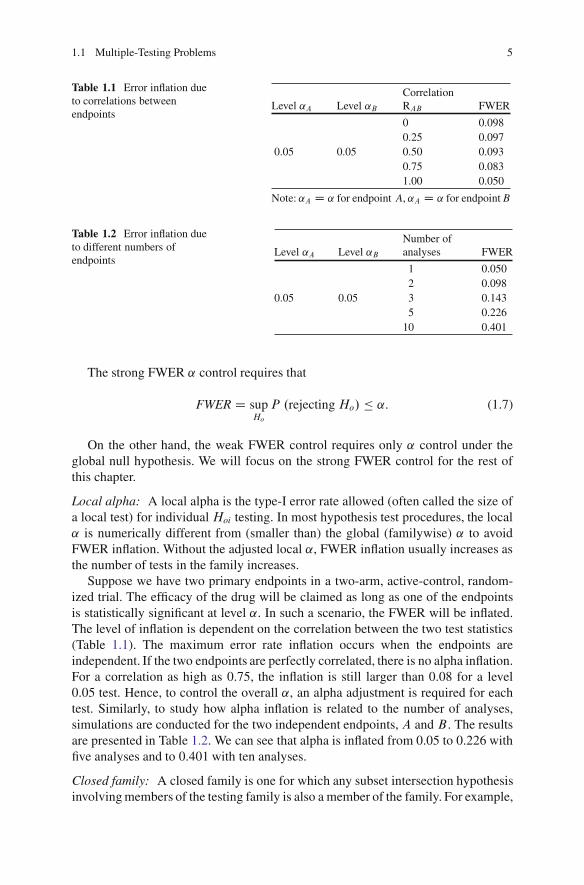
Suppose we have two primary endpoints in a two-arm, active-control, random-ized trial. The efficacy of the drug will be claimed as long as one of the endpointsis statistically significant at level ˛. In such a scenario, the FWER will be inflated.The level of inflation is dependent on the correlation between the two test statistics(Table 1.1). The maximum error rate inflation occurs when the endpoints areindependent. If the two endpoints are perfectly correlated, there is no alpha inflation.For a correlation as high as 0.75, the inflation is still larger than 0.08 for a level0.05 test. Hence, to control the overall ˛, an alpha adjustment is required for eachtest. Similarly, to study how alpha inflation is related to the number of analyses,simulations are conducted for the two independent endpoints, A and B . The resultsare presented in Table 1.2. We can see that alpha is inflated from 0.05 to 0.226 withfive analyses and to 0.401 with ten analyses.
Closed family: A closed family is one for which any subset intersection hypothesisinvolving members of the testing family is also a member of the family. For example,

6 1 Multiple-Hypothesis Testing Strategy
a closed family of three hypothesesH1; H2; H3 has a total of seven members, listedas follows: H1; H2; H3, H1\ H2, H2\H3, H1\ H3, H1 \H2\ H3.
Closure principle: This was developed by Marcus et al. (1976). This principleasserts that one can ensure strong control of FWER and coherence (see below) atthe same time by conducting the following procedure. Test every member of theclosed family using a local ˛-level test (here, ˛ refers to the comparison-wise errorrate, not the FWER). A hypothesis can be rejected provided (1) its correspondingtest was significant at the ˛-level, and (2) every other hypothesis in the family thatimplies it has also been rejected by its corresponding ˛-level test.
Closed testing procedure: A test procedure is said to be closed if and only if therejection of a particular univariate null hypothesis at an ˛-level of significanceimplies the rejection of all higher-level (multivariate) null hypotheses containingthe univariate null hypothesis at the same ˛-level. The procedure can be describedas follows (Bretz et al. 2006):
1. Define a set of elementary hypotheses,H1I : : : IHK , of interest.2. Construct all possible m>K intersection hypotheses, HI D \ Hi; I �
f1; : : : ; Kg.3. For each of the m hypotheses find a suitable local ˛-level test.4. Reject Hi at FWER ˛ if all hypotheses HI with i 2 I are rejected, each at the
(local) ˛-level.
This procedure is not often used directly in practice. However, the closureprinciple has been used to derive many useful test procedures, such as those ofHolm (1979), Hochberg (1988), Hommel (1988), and gatekeeping procedures.
˛-exhaustive procedure: If P .Reject HI/ D ˛ for every intersection hypothesisHI ; I � f1; : : : ; Kg, the test procedure is ˛-exhaustive.
Partition principle: This is similar to the closed testing procedure with strongcontrol over the familywise ˛-level for the null hypotheses. The partition principleallows for test procedures that are formed by partitioning the parameter spaceinto disjointed partitions with some logical ordering. Tests of the hypotheses arecarried out sequentially at different partition steps. The process of testing stops uponfailure to reject a given null hypothesis for predetermined partition steps (Hsu 1996;Dmitrienko et al. 2010, pp. 45–46). We will discuss this more later in this chapter.
Coherence and consonance are two interesting concepts in closed testing pro-cedures.Coherence means that if hypothesis H implies H �, then whenever H isretained, so must beH �. Consonance mean that wheneverH is rejected, at least oneof its components is rejected, too. Coherence is a necessary property of closed testprocedures; consonance is desirable but not necessary. A procedure can be coherentbut not consonant because of asymmetry in the hypothesis testing paradigm. WhenH is rejected we conclude that it is false. However, when H is retained, we do notconclude that it is true; rather, we say that there is not sufficient evidence to rejectit. Multiple comparison procedures that satisfy the closure principle are alwayscoherent but not necessarily consonant (Westfall et al. 1999).

1.2 Multiple-Testing Approaches 7
Adjusted p-value
The adjusted p-value for a hypothesis test is defined as the smallest significancelevel at which one would reject the hypothesis using the multiple-testing procedure(Westfall and Young 1993). If pI denotes the p-value for testing intersectionhypothesisHI , the adjusted p-value for Hoi is given by
padji D max
I Wi2I pI : (1.8)
If padji � ˛, Hoi is rejected.
Simultaneous confidence interval
It is well known that a two-sided .1 � ˛/% confidence interval for parameter �consists of all parameter values for which the hypothesis Ho W � D 0 is retainedat level ˛. This concept can be applied to multiple-parameter problems to form aconfidence set or a simultaneous confidence interval.
1.2 Multiple-Testing Approaches
1.2.1 Single-Step Procedures
The commonly used single-stage procedures include the Sidak method (Sidak1967), the simple Bonferroni method, the Simes-Bonferroni method (Global test:Simes 1986), and Dunnett’s test for all active arms against the control arm (Dunnett1955). In the single-step procedure, to control the FWER, the unadjusted p-valuesare compared against the adjusted alpha to make the decision to reject or not rejectthe corresponding null hypothesis. Alternatively, we can use the adjusted p-valuesto compare against the original ˛ for decision-making.
1.2.1.1 Sidak Method
The Sidak method is derived from the simple fact that the probability of rejectingat least one null hypothesis is equal to 1� Pr (all null hypotheses are correct). Tocontrol the FWER, the adjusted alpha ˛k for the null hypothesisHok (k D 1; : : : ; K)can be found by solving the following equation:
˛ D 1 � .1 � ˛k/K . (1.9)

8 1 Multiple-Hypothesis Testing Strategy
Therefore, the adjusted alpha is given by
˛k D 1 � .1 � ˛/1=K . (1.10)
If the p-value is less than or equal to ˛k , reject Hok . Alternatively we can calculatethe adjusted p-value:
Qpk D 1 � .1 � pk/K . (1.11)
If the adjusted p-value Qpk is less than or equal to ˛; then reject Hok:
1.2.1.2 Bonferroni Method
The simple Bonferroni method is a simplification of the Sidak method that uses theBonferroni inequality:
P.[KkD1Hk/ �
KX
kD1P.Hk/: (1.12)
Based on (1.12), we can conservatively use the adjusted alpha,
˛k D ˛
K, (1.13)
and the adjusted p-value,Qpk D Kpk.
This is a very conservative approach without consideration of any correlationsamong p-values.
The alpha doesn’t have to be split equally among all tests. We can use theso-called weighted Bonferroni tests, for which the adjusted alpha and p-value aregiven by
˛k D wk˛ and Qpk D pk
wk, (1.14)
where the weight wk � 0 andPK
kD1 wk D 1. The weight wk can be determinedbased on the clinical importance of the kth hypothesis or the power of the kthhypothesis test.
1.2.1.3 Simes Global Testing Method
The Simes-Bonferroni method is a global test in which the type-I error rate iscontrolled for the global null hypothesis (1.3). We reject the null hypothesisHo if
p.k/ � k˛
Kfor at least one i D 1; : : : ; K , (1.15)
where p.1/ < : : : < p.K/ are the ordered p-values.

1.2 Multiple-Testing Approaches 9
The adjusted p-value is given by
Qp D maxk2f1;:::;Kg
�K
kp.k/
�. (1.16)
If Qp � ˛, the global null hypothesis (1.3) is rejected.
1.2.1.4 Dunnett’s Method
Dunnett’s method can be used for multiple comparisons of active groups against acommon control group, which is often done in clinical trials with multiple parallelgroups. Let n0 and ni .i D 1; : : : ; K/ be the sample sizes for the control and the i thdose group; the test statistic (one-sided) is given by Westfall et al. (1999, p. 77)
T D maxi
Nyi � Ny0�p1=ni C 1=n0
, (1.17)
The multivariate t-distribution of T in (1.17) is called one-sided Dunnettdistribution with v D PKC1
iD1 .ni � 1/ degrees of freedom. The cdf is defined by
F .xjK; v/ D P .T � x/ : (1.18)
The calculation of (1.18) requires numerical integrations (Hochberg andTamhane 1987, p. 141). Tabulation of the critical values is available from thebook by Kanji (2006), and in software such as SAS.
The adjusted p-value corresponding to ti is given by
Qpi D 1 � F .ti jK; v/ . (1.19)
If Qpi < ˛, Hi is rejected, i D 1; : : : ; K .
1.2.1.5 Fisher-Combination Test
To test the global null hypothesis Ho D \KiD1Hoi, we can use the so-called Fisher
combination statistic,
�2 D �2KX
iD1ln .pi/ , (1.20)
where pi is the p-value for testingHoi. WhenHoi is true, pi is uniformly distributedover [0,1]. Furthermore, if the pi .i D 1; : : : ; K/ are independent, the test statistic�2 is distributed as a chi-square statistic with 2K degrees of freedom. Thus Ho isrejected if �2 � �22K;1�˛ . Note that if the pi are not independent or Ho is not true(e.g., one of the Hoi is not true), then �2 is not necessarily a chi-square distribution.

10 1 Multiple-Hypothesis Testing Strategy
1.2.2 Stepwise Procedures
Stepwise procedures are different from single-step procedures in the sense thata stepwise procedure must follow a specific order to test each hypothesis. In general,stepwise procedures are more powerful than single-step procedures. There arethree categories of stepwise procedures which are dependent on how the stepwisetests proceed: stepup, stepdown, and fixed-sequence procedures. The commonlyused stepwise procedures include the Bonferroni-Holm stepdown method (Holm1979), the Sidak-Holm stepdown method (Westfall et al. 1999, p. 31), Hommel’sprocedure (Hommel 1988), Hochberg’s stepup method (Hochberg and Benjamini1990), Rom’s method (Rom 1990), and the sequential test with fixed sequences(Westfall et al. 1999).
1.2.2.1 Stepdown Procedure
A stepdown procedure starts with the most significant p-value and ends with theleast significant. In this procedure, the p-values are arranged in ascending order,
p.1/ � p.2/ � : : : � p.K/, (1.21)
with the corresponding hypotheses
H.1/;H.2/; : : : ;H.K/.
The test proceeds from H.1/ to H.K/: If p.k/ > Ck˛ .k D 1; : : : ; K/, retain allH.i/ .i � k/; otherwise, reject H.k/ and continue to test H.kC1/: The critical valuesCk are different for different procedures.
The adjusted p-values are
� Qp1 D C1p.1/,Qpk D max
� Qpk�1; Ckp.k/�
, k D 2; : : : ; n.(1.22)
Therefore an alternative test procedure is to compare the adjusted p-valuesagainst the unadjusted ˛. After adjusting p-values, one can test the hypotheses inany order.
1.2.2.2 Stepup Procedure
A stepup procedure starts with the least significant p-value and ends with themost significant p-value. The procedure proceeds from H.K/ to H.1/: If, P.k/ �Ck˛ .k D 1; : : : ; K/, reject all H.i/ .i � k/; otherwise, retain H.k/ and continueto test H.k�1/: The critical values Ck for the Hochberg stepup procedure areCk D K � k C 1 .k D 1; ::; K/.

1.2 Multiple-Testing Approaches 11
The adjusted p-values are� QpK D CKp.K/;
Qpk D min� QpkC1; Ckp.k/
�; k D K � 1; : : : ; 1: (1.23)
Therefore, an alternative test procedure is to compare the adjusted p-valuesagainst the unadjusted ˛.
The Hochberg stepup method does not control the FWER for all correlations,but it is a little conservative when p-values are independent (Westfall et al. 1999,p. 33). The Rom method (Rom 1990) controls ˛ exactly for independent p-values.However, the calculation of Ck is complicated.
1.2.2.3 Fixed-Sequence Test
This procedure is a stepdown procedure with the order of hypotheses predetermined:
H1;H2; : : : ;HK:
The test proceeds from H1 to HK: If pk > ˛ .k D 1; : : : ; K/, retain all Hi
.i � k/. Otherwise, reject Hk and continue to test HkC1:The adjusted p-values are given by
Qpk D max .p1; : : : ; pk/ ; k D 1; ::; K: (1.24)
The sequence of the tests can be based on the importance of hypotheses or thepower of the tests. Note that if the previous test is not significant, the next test willnot proceed even if its p-value is extremely small.
1.2.2.4 Dunnett Stepdown Procedure
A commonly used stepdown procedure is the Dunnett stepdown procedure. Theadjusted p-values are formulated as follows. First, p-values are arranged in adescending order,
t.1/ � t.2/ � : : : � t.K/,
with the corresponding hypotheses
H.1/;H.2/; : : : ;H.K/.
Based on (1.18), we calculate p�k D 1 � F
�t.k/jK � k C 1; v
�, where the second
argument in F .�/ is K � k C 1 instead of K as in the single-step Dunnett test. Theadjusted p-values are then calculated as follows:
Qpk D�p�1
max� Qpk�1; p�
k
�if k D 2; : : : ; K:
(1.25)
The decision rule can be specified as: if Qpk < ˛, reject H.k/.
12 1 Multiple-Hypothesis Testing Strategy
1.2.2.5 Holm Stepdown Procedure
Suppose there are K hypothesis tests Hi (i D 1; : : : ; K). The Holm stepdownprocedure (Holm 1979; Dmitrienko et al. 2010) can be outlined as follows:
Step 1. If p.1/ � ˛=K , reject H.1/ and go to the next step; otherwise retain allhypotheses and stop.
Step i (i D 2; : : : ; K � 1). If p.i/ � ˛= .K � i C 1/, reject H.i/ and go to the nextstep; otherwise retainH.i/; : : : ;H.K/ and stop.
Step K . If p.K/ � ˛, reject H.K/; otherwise retain H.K/.
The adjusted p-values are given by
Qpk D�p.K/ if k D K
min . QpkC1; .K � k C 1/pkC1/ if k D K � 1; : : : ; 1: (1.26)
1.2.2.6 Shaffer Procedure
Shaffer (1986) and Dmitrienko et al. (2010) uses logical dependencies between thehypotheses to improve the Holm procedure. The dependency means that the truth ofcertain hypotheses implies the truth of other hypotheses. To illustrate, suppose a trialwith four dose levels and a placebo group has a treatment mean �i for the i th group(i D 0 for the placebo). If the null hypotheses under consideration areHij:�i D �j ,thenH12 andH13 implyH23. The steps of the Shaffer procedure are similar to thosefor the Holm procedure, but replace the divisors .K � i C 1/ by ki . Here ki is themaximum number of hypotheses H.i/; : : : ;H.K/ that can be simultaneously true,given that H.1/; : : : ;H.i�1/ are false. Thus, at the i th step, reject H.i/ if
p.j / � ˛
kj; j D 1; : : : ; i: (1.27)
As an example, for the five-group dose-response study, there can be k1 D�52
� D 10 pairwise comparisons (the same as for the Holm procedure). After H.1/
is rejected, there are k2 D �42
� D 6 possible pairwise comparisons (compared toK � i C 1 D 9 in the Holm procedure).
1.2.2.7 Fallback Procedure
The Holm procedure is based on a data-driven order of testing, while the fixed-sequence procedure is based on a prefixed order of testing. A compromise betweenthem is the so-called fallback procedure. The fallback procedure was introduced byWiens (2003) and was further studied by Wiens and Dmitrienko (2005) and Hommeland Bretz (2008). The test procedure can be outlined as follows:
Suppose hypotheses Hi (i D 1; : : : ; K) are ordered according to (1.22). Weallocate the overall error rate ˛ among the hypotheses according to their weights

1.2 Multiple-Testing Approaches 13
wi , where wi � 0 andP
i wi D 1. For Fixed-Sequence test, w1 D 1 and w2 D: : : D wK D 0.
1. Test H1 at ˛1 D ˛w1. If p1 � ˛1, reject this hypothesis; otherwise retain it. Goto the next step.
2. Test Hi at ˛i D ˛i�1 C ˛wi (i D 2; : : : ; K � 1) if Hi�1 is rejected and at˛i D ˛wi if Hi�1 is retained. If pi � ˛i , rejectHi ; otherwise retain it. Go to thenext step.
3. Test HK at ˛K D ˛K�1 C˛wK if HK�1 is rejected and at ˛K D ˛wK ifHK�1 isretained. If pK � ˛K , reject HK ; otherwise retain it.
Example 1.4. Suppose that a dose-finding trial has been conducted to compare low(L), medium (M ), and high (H ) doses of a new antihypertension drug. The primaryefficacy variable is diastolic blood pressure (DBP). The mean reduction in DBP isdenoted by �P , �L, �M , and �H for the placebo, and low, medium, and high doses,respectively. The global null hypothesis of equality, �P D �L D �M D �H , canbe tested using an F-test from a model such as analysis of covariance (ANCOVA).However, for strong FWER control, this F -test is not sufficient. We illustrate howto apply various multiple-testing procedures to this problem. One is interested inthree pairwise comparisons (one for each dose) against a placebo (P ) with nullhypotheses: H1 W �P D �L, H2 W �P D �M , and H3 W �P D �H . Denote thep-values for these tests by p1; p2, and p3, respectively. A one-sided significancelevel ˛ of 2.5% is used for the trial.
In the following methods or procedures (1)–(8), we assume p1 D 0:009, p2 D0:0085, and p3 D 0:008.
Weighted Bonferroni Procedure
Suppose we suspect the high dose may be more toxic than the low dose. Unlessthe high dose is more efficacious than the low dose, we will choose the low doseas the target dose. For this reason, we want to spend more alpha in the low-dosecomparison than in the high-dose comparison. Specifically, we choose one-sidedsignificance levels ˛1 D 0:01, ˛2 D 0:008, and ˛3 D 0:007 (˛1 C ˛2 C ˛3 D ˛),which will be used to comparep1,p2, andp3, respectively, for rejecting or acceptingthe corresponding hypotheses. Since p1 D 0:009 < ˛1, p2 D 0:0085 > ˛2, andp3 D 0:008 > ˛3, we will reject H1 but accept H2 and H3.
Simes-Bonferroni Method
We first order the p-values: p.1/ D p3 < p.2/ D p2 < p.3/ D p1; the adjustedp-values calculated from (1.16) are Qp D maxf 3
1p.1/ D 0:024; 3
2p.2/ D 0:01275;
33p.3/ D 0:009g D 0:024 < ˛. Therefore the global hypotheses (�P D �L D�M D �H ) are rejected and we conclude that one or more dose levels are effective,but the testing procedure has not indicated which one.

14 1 Multiple-Hypothesis Testing Strategy
Fisher Combination Method
This method usually requires independent p-values; otherwise, the test may be onthe conservative or liberal side. However, for illustrating the calculation procedure,let’s pretend the p-values are independent. From (1.20), we can calculate the Chi-square value: �2 D �2 ln..0:009/.0:0085/.0:008// D 28:62 with six degrees offreedom. The correspondingp-value is 0:0001 < ˛. Thus the global null hypothesisis rejected.
Fixed-Sequence Procedure
Suppose we have fixed the test sequence asH3;H2;H1 before we see the data. Sincep3 < ˛, we reject H3 and continue to test H2. Because p2 < ˛, we reject H2 andcontinue to test H1. Since p1 < ˛, we reject H1.
Holm Procedure
Since p.1/ D p3 D 0:008 < ˛=K D 0:025=3, reject H3 and continue to test H2.Because p.2/ D p2 D 0:0085 < ˛= .K � 2C 1/ D 0:025=2 D 0:0125, rejectH2 and continue to test H1. Since p1 D 0:009 < ˛= .K � 3C 1/ D 0:025, H1 isrejected.
Shaffer Procedure
Since p.1/ D p3 D 0:008 < ˛=k1 D 0:025=3, reject H3. After H3 is rejected,H1 and H2 can be simultaneously true, but k2 D 2 and p.2/ D p2 D 0:0085 <
˛=k2 D 0:025=2 D 0:0125, so reject H2. We have only H1 left, and thus k3 D 1
and p1 D 0:009 < ˛= .K � 3C 1/ D 0:025; H1 is rejected. We can see that inthis case the Holm and Shaffer procedures are equivalent. This is because we arenot interested in the other possible comparisons: �1 versus �2, �2 versus �3, and�3 versus �1.
Fallback Procedure
Choose equal weights wi D 1=K D 1=3. ˛1 D ˛=3 D 0:00833, ˛2 D ˛1 C ˛=3 D0:0167, and ˛3 D ˛2 C˛=3 D ˛ D 0:025. Since p1 D 0:009 > ˛1, p2 D 0:0085 <
˛2, and p3 D 0:008 < ˛3, H1 is retained but H2 andH3 are rejected.
Hochberg Stepup Procedure
Since p.3/ D 0:009 < ˛ D 0:025, we reject all three hypotheses, H1, H2, and H3.The adjusted p-values Qp1, Qp2, and Qp3 can be calculated using (1.23).

1.2 Multiple-Testing Approaches 15
Dunnett’s Procedure
Suppose the adjusted p-values calculated from (1.19) (requiring a software package)are Qp1 D 0:027 > ˛, Qp2 D 0:021 < ˛, and Qp3 D 0:019 < ˛. Then, we reject H2
andH3 but retain H1.
Dunnett’s Stepdown Procedure
Suppose the test statistics t.1/ D t3 > t.2/ D t2 > t.3/ D t1 for the three hypothesesH3;H2, andH1. Assume that the p-values are p�
1 D 0:019, p�2 D 0:018, and p�
3 D0:0245 for the hypotheses H.1/ D H3;H.2/ D H2, and H.3/ D H1, respectively.The adjusted p-values can be calculated from (1.25): Qp1 D p�
1 D 0:019 < ˛,Qp2 D max
� Qp1; p�2
� D 0:019 < ˛, Qp3 D max� Qp2; p�
1
� D 0:0245 < ˛. Then, wereject H3;H2, andH1.
1.2.3 Common Gatekeeper Procedure
The gatekeeper procedure (Dmitrienko et al. 2005, pp. 106–127) is an extension ofthe fixed-sequence method. The method is motivated by the following hypothesis-testing problems in clinical trials. (1) Benefit of secondary endpoints can be claimedin the drug label only if the primary endpoint is statistically significant. (2) If thereare coprimary endpoints (multiple primary endpoints), secondary endpoints canbe claimed only if one of the primary endpoints is statistically significant. (3) Inmultiple-endpoint problems, the endpoints can be grouped based on their clinicalimportance.
Suppose there areK null hypotheses to test. We group them intom families. Eachfamily is a composite of hypotheses. The null hypotheses in the i th.i D 1; : : : ; mi /
family are denoted by either a serial gatekeeper
Fi D Hi1 [Hi2 [ : : : [Himi (1.28)
or a parallel gatekeeper
Fi D Hi1 \Hi2 \ : : : \Himi : (1.29)
The hypothesis test proceeds from the first family, F1, to the last family, Fm. Totest Fi .i D 2; : : : ; m/ ; the test procedure has to pass i � 1 previous gatekeepers,i.e., reject all Fk .k D 1; : : : ; i � 1/ at the predetermined level of significance ˛.
For a parallel gatekeeper we can either weakly or strongly control the familywisetype-I error. For a serial gatekeeper, we always strongly control the familywiseerror. The serial gatekeeping procedure is straightforward: test each family of nullhypotheses sequentially at a level ˛ with any strong ˛-control method.
16 1 Multiple-Hypothesis Testing Strategy
The stepwise procedure of parallel gatekeeping proposed by Dmitrienko andTamhane (2007) can be described as follows. The procedure is built around theconcept of a rejection gain factor. At the kth stage, the significance test is performedat the �k˛ level, k D 1; 2; : : : ; m, where ˛ is the FWER, and the rejection gainfactor, 0 � �k � 1 (with �1 D 1/, depends on the number and importance of thehypotheses rejected at the earlier stages.
The stepwise parallel gatekeeping procedure for testing the null hypotheses inF1; : : : ; Fm can be performed as follows:
1. Family Fk , k D 1; : : : ; m� 1: Test the null hypotheses using the Bonferroni testat the �k˛ level.
2. Family Fm: Test the null hypotheses using the weighted Holm test at the �m˛level.
The rejection gain factors �i are given by
�1 D 1, �k Dk�1Y
iD1
0
@miX
jD1rijwij
1
A , k D 2; : : : ; m; (1.30)
where the weights wij � 0 withPni
jD1 wij D 1 represent the importance of the nullhypotheses in Fi , and rij D 1 ifHij is rejected and 0 otherwise. For equally weightedhypotheses (wij D 1=mi), the formula for �k reduces to
�k Dk�1Y
iD1
�ri
mi
�; k D 2; : : : ; m; (1.31)
where ri D Pj rij is the number of rejected hypotheses in Fi . Thus, �k is the
product of the proportions of previously rejected hypotheses in F1 through Fk�1.The modified adjusted p-value for Hij, i D 2; : : : ; m, is given by p�
ij D Qpij=�i ,where Qpij is the usual adjusted p-value produced by the multiple tests within Fi .Inferences in F2; : : : ; Fm can be performed by p�
ij to the prespecified FWER, ˛.
Example 1.5. This example was given by Dmitrienko and Tamhane (2007). Thetrial was designed to compare a single dose of an experimental drug with aplacebo. Two families of endpoints were considered in this trial. F1 consisted of twohypotheses related to the primary endpoints, P1 (lung function) and P2 (mortality),and F2 consisted of two hypotheses related to the secondary endpoints, S1 (ICU-free days) and S2 (quality of life). The raw p-values pij for the endpoints P1, P2, S1,and S2 are 0.048, 0.003, 0.026, and 0.002, respectively. F1 was chosen as a parallelgatekeeper. P1 was deemed more important than P2 in F1 with weights w11 D 0:9
and w12 D 0:1, respectively; S1 and S2 were considered equally important withweight w21 D w22 D 0:5. The FWER is to be controlled at ˛ D 0:05.
To apply the stepwise parallel gatekeeping procedure, one first considers theadjusted p-values produced by the weighted Bonferroni test and the Holm test for

1.2 Multiple-Testing Approaches 17
the null hypotheses in F1 and F2, respectively. The adjusted p-values Qpij for theendpoints P1, P2, S1, and S2 are 0:048=0:9 D 0:053 (the weighted Bonferronitest), 0:003=0:1 D 0:03 (the weighted Bonferroni test), 0.026 (the Holm test), and0:002 � 2 D 0:004, respectively. Next, since �1 D 1, the primary hypothesesare tested at the full ˛ D 0:05 level. The P2 comparison is significant at thislevel, whereas the P1 comparison is not. Therefore, the rejection gain factor forthe secondary family based on (1.31) is �2 D w12 D 0:1, and the adjusted p-valuesfor S1 and S2 are 0:026=�2 D 0:260 and 0:004=�2 D 0:040, respectively. It is clearthat only the hypothesis concerning S2 is rejected.
1.2.4 Tree Gatekeeping Procedure
The tree gatekeeping procedure (TGP) is a stepwise procedure that combines thecharacteristics of both the parallel and series gatekeeping methods. For each individ-ual hypothesisHij in family Fi , where i D 2; : : : ; m, j D 1; : : : ; ni , we define twoassociated hypothesis sets: the serial rejection set, RSij , and the parallel rejection set,RPij . These sets consist of some hypotheses from F1; : : : ; Fi�1; at least one of themis non-empty. Without loss of generality, we assume RSij and RPij do not overlap.
Dmitrienko et al. (2007) developed Bonferroni-based and resampling-basedtree gatekeeping procedures. The Bonferroni-based tree-gatekeeping procedure isdescribed as follows.
Let H be any non-empty intersection of the hypotheses Hij and let wij.H/ bethe weight assigned to the hypothesis Hij 2H . From (1.14), we know that theBonferroni (adjusted) p-value for testing H is given by p.H/ D min
i;jf pij
wij.H/g.
Because there can be more than one H that includes each Hij, we need tofurther adjust the p-value p .H/. The multiplicity-adjusted p-value for the nullhypothesis Hij is defined as Qpij D max
Hfp.H/g, where the maximum is taken over
all intersection hypothesesH such that Hij � H . The rejection rules are: rejectHij
if Qpij � ˛; and retainHij otherwise.The testing procedure above for the adjusted p-value is based on the closure
principle, which requires us to construct the weight wij .H/ appropriately. Forconvenience, we define two indicator variables: let ıij.H/ D 0 if Hij 2 H and1 otherwise, and let �ij.H/ D 0 if H contains any hypothesis from RSij or allhypotheses from RPij and 1 otherwise. The following three conditions together forthe weights will constitute a sufficient condition for using the closure principle, andthus for the TGP, also.
Condition 1: For any intersection hypothesis H , wij.H/ � 0,Pmi
jD1 wij.H/ � 1
and wij.H/ D 0 if ıij.H/ D 0 or �ij.H/ D 0.Condition 2: wi .H/ D .wi1.H/; : : : ;wimi .H// is a vector function of the weights
w1.H/, . . . , wi�1.H/ (i D 2; : : : ; m) and does not depend on wiC1.H/, . . . ,wm.H/ (i D 1; : : : ; m � 1).

18 1 Multiple-Hypothesis Testing Strategy
Condition 3: The weights for F1; : : : ; Fm�1 meet the monotonicity condition, i.e.wij.H/ � wij.H
�/, i D 1; : : : ; m � 1, if Hij 2 H , Hij 2 H�, and H� � H .
1.2.4.1 Implementation of a Tree Gatekeeping Procedure
The authors developed the following algorithm for the weight assignments thatmeets conditions 1–3. Here we define 0=0 D 0.
Step 0: Choose Bonferroni weights Qwij > 0 satisfyingPmi
jD1 Qwij D 1 and theserial rejection set RSij and the parallel rejection set RPij for i D 2; : : : ; m,j D 1; : : : ; mi .
Step 1: Family F1. Let w1j .H/ D w�1 .H/ Qw1j ı1j .H/, j D 1; : : : ; m1, where
w�1 .H/ D 1 and w�
2 .H/ D w�1 .H/ �Pm1
jD1 w1j .H/.Step i D 2; : : : ; m � 1: Family Fi . Let wij.H/ D w�
i .H/ Qwijıij.H/�ij.H/, j D1; : : : ; mi , and w�
iC1.H/ D w�i .H/�Pmi
jD1 wij.H/.Step m: Family Fm. Let
wmj .H/ D w�m.H/ Qwmj ımj .H/�mj .H/PmmkD1 Qwmkımk .H/ �mk .H/ ; j D 1; : : : ; mm: (1.32)
After each wij is determined, we can calculate the adjusted p-value
Qpij D maxH
mini;j
�pij
wij .H/
�. (1.33)
If Qpij � ˛, reject Hij; otherwise, accept Hij.
1.2.5 Generalized FWER and Partitioning Testing
LetHoi W � 2‚oi; i D 1; : : : ; K , be a family of null hypotheses, where the parametersubspace‚oi constitutes the null parameter subspace‚o D [‚oi. The complemen-tary set of ‚oi, denoted by ‚ai , constitutes of the alternative parameter subspace‚a D [‚ai . The parameter space is therefore ‚ D ‚o [ ‚a. The generalizedFWER (gFWER) is defined as the probability of making strictly more than � 0
false rejections in multiple-hypothesis testing. We define gFWER by
# ./ D sup�2‚0
P . > j�/ , (1.34)
where is the number of different null hypotheses rejected. FWER is the specialcase of gFWER when D 0.

1.2 Multiple-Testing Approaches 19
1.2.5.1 Single-Step Test
Let pi be the raw p-value associated with the null hypothesis Hoi; i D 1; : : : ; K .Define the adjusted p-value as
Qpi DkX
jDC1
k
j
!pji .1 � pi/
k�j . (1.35)
The procedure, which rejects Hoi if Qpi � ˛ and retains it otherwise, will controlgFWER./ at level ˛ in the strong sense for the single hypothesisHoi, i D 1; : : : ; K ,if the pi are independently distributed. See the Ph.D. dissertation by Xu (2005).
Lehmann and Romano (2005) proposed the following generalized Bonferroniprocedure.
Reject Hoi if the adjusted p-value Qpi � ˛, where
Qpi D min
�K
C 1pi ; 1
�; i D 1; : : : ; K:
When D 0, the Lehmann-Romano procedure degenerates to the commonBonferroni test.
1.2.5.2 Partitioning Testing Principle
1. Let I D f1; : : : ; Kg. Partition ‚ into disjoint ‚�J , J � I , based on different
combinations of the null parameter subspace ‚oi and the alternative parameter
subspace ‚ai , i.e., for each J � I , let ‚�J D \
i2J ‚oi \�
\j…J
‚aj
�. Then
˚‚�J ; J � I
�and ‚; D \
j2I‚aj partition the parameter space ‚.
2. Test each null hypothesis HPoJ :� 2 ‚�
J at level ˛. There are no multiplicityadjustments needed because the HP
oJ ; J � I are disjoint.3. For all J � I , infer � … ‚�
J if all HPoJ 0 such that J � J 0 are rejected. That is,
reject the intersection null hypothesis H0J if all null hypotheses HPoJ 0 implying
it are rejected, particularly rejecting Hoi; i 2 I , if all HPoJ such that i 2 J are
rejected.
As discussed earlier, the closed testing principle can be stated as:
1. Let I D f1; : : : ; Kg. For every J � I; J ¤ ;, define ‚J D \i2J‚i and the
intersection null hypothesisHoJ W � 2 ‚J .2. Test each HoJ W � 2 ‚J at level ˛.3. For all J � I , infer � … ‚J if allHP
oJ 0 such that J � J 0, are rejected, i.e., rejectthe intersection null hypothesisHoJ if all hypotheses implying it are rejected.

20 1 Multiple-Hypothesis Testing Strategy
Comparing the partitioning testing principle with the closed testing principle, wecan see that in the partitioning testing principle ‚�
J consists of all null parametersubspaces ‚oi for which i 2 J and all alternative parameter subspaces ‚aj forwhich j … J (There are
PKjDC1
�Kj
� D 2K � 2 such ‚�J s.) In the closed testing
procedure,‚J is the parameter subspace, for which Hoi; i 2 J , are true. This is theessential difference between the two principles.
1.2.5.3 Generalized Partitioning Testing Principle for Controlling gFWER
Xu (2005) proposed the following procedure for the gFWER:
1. Partition ‚ into disjoint ‚�J , J � I D f1; : : : ; Kg, such that, for each J � I ,
‚�J D \
i2J‚oi \�
\j…J‚aj
�.
2. In each ‚�J , reject all Hoi; i … J , and test HP
oJ D fHoi W �i 2 ‚i ; i 2 J g at levelgFWER ˛, controlling sup
�2‚�
J
P . > j�/ � ˛.
3. For i 2 J � I , defineHoi to be J -rejected to meanHoi is rejected in‚�J . Reject
Hoi if Hoi is J -rejected for any J � I .
1.2.5.4 Stepdown Partitioning Testing
As we stated earlier there are 2K � 2 tests with the partitioning principle. Xu(2005) proposed a stepdown procedure that reduces the maximum number of testsrequired to no more than K � . This reduction is significant for larger K , such asin microarray analysis. A set of sufficient conditions for such a reduction to be validis specified as:
S1 All tests are based on a set of statistics fTi ; i D 1; : : : ; Kg whose values do notdepend on which‚�
J is being tested.S2 The tests are performed in each of the disjoint‚�
J s, defined previously.S3 For jJ j > , where jJ j denotes the cardinality of J , the critical values CJ have
the property that if J � J 0, then CJ � CJ 0 , and CJ D CJ 0 if jJ j D jJ 0j.As an example, consider the test statistics Ti D 1 � pi , i D 1; : : : ; k, where pi
is a suitably defined p-value for testing Hoi. Define the critical values as
CJ D 1 � .C 1/ ˛
jJ j : (1.36)
Since CJ is dependent on jJ j, it can be denoted by CjJ j . Let T.1/ � : : : � T.K/be the test statistics that associate the hypotheses H.1/; : : : ;H.K/. The stepdownprocedure is specified as follows:
1. Reject H.K/; : : : ;H.K�C1/.
1.2 Multiple-Testing Approaches 21
2. For i D ; : : : ; K � 1, if T.K�i / � CK�i , reject H.K�i / and continue; otherwiseretain H.K�i / and stop.
Xu’s stepdown procedure includes Lehmann and Romano’s (2005) procedure asa special case.
1.2.5.5 General Stopping Boundary
Suppose the stepdown testing condition S1 holds and the distribution of Ti when thenull hypothesisH0i is true is the same for all i . Denote by F the common marginalnull distribution and by P0 the probability computed based on the assumptionof the null hypotheses involved. Let ˛c D F
�CjJ j�
�. If the test statistics are
independent, then
P0 . > / D 1 �X
jD0
jJ jj
!˛jc .1 � ˛c/
jJ j�j : (1.37)
In general, Markov’s inequality holds
P0 . > / � jJ j˛cC 1
: (1.38)
Keep in mind that neither (1.37) nor (1.38) is necessarily the upper bound ofthe gFWER or FWER when the dependence of Ti is not specified. The rejectionboundary Ci can be determined using either simulation or numerical methods.
1.2.6 Procedures Controlling False Discovery Rate
1.2.6.1 Type-I Error Rate Versus False Discovery Rate
The false discovery rate (FDR) is the expected proportion of false rejections amongall rejections. The FDR is defined to be zero when the total number of rejectionsequals zero (Benjamini and Hochberg 1995; Westfall et al. 1999, p. 21)
FDR D E
�
max .R; 1/
�; (1.39)
where R denotes the number of rejected hypotheses and is the number of falselyrejected hypotheses.
FDR-controlling procedures may lead to more type-I errors and fewer type-IIerrors than FWER-controlling procedures. However, increasing the number of truepositive drugs in the market is as important as reducing the number of false drugs,

22 1 Multiple-Hypothesis Testing Strategy
because a reduction in FDR will increase the probability of treating patients withthe right drugs. FDR is more relevant than the type-I error rate for increasing theprobability of patients getting the right drugs. Therefore, controlling the proportionof false drugs in the market may be more meaningful than type-I error rates.However, be cautious. In the FDR procedure, one can purposely include somehypotheses that are known to be rejected in the set of hypotheses to be tested, andthis will increase the test level for the hypothesis of main interest (Finner and Roter2001).
It is informative to investigate the relationship between FDR and the type-I rate˛. If we denote by Pe the proportion of effective test compounds and by Pw thepower for the pivotal trials, then the expected proportion of ineffective drugs in themarket is (neglecting other factors such as drug disapproval due to safety issues)
FDR D .1 � Pe/ ˛
.1 � Pe/ ˛ C PePw: (1.40)
The FDR is a monotonic function of ˛.From (1.40) we know that when Pe D 0 the FDR is 100% and so is the type-I
error rate. In other words, if all test drugs in the pivotal trials are ineffective, thenregardless of the ˛ value, 100% of the approved drugs are no more effective than thecontrol. On the other hand, if all drugs in the pivotal trials are effective (Pe D 1),then regardless of ˛, 100% of the approved drugs are effective (FDR D 0).
1.2.6.2 Benjamini-Hochberg Procedure
Let p.i/ be the p-value associated with the hypothesis H.i/, where p.1/ � : : : �p.K/. The Benjamini and Hochberg (1995) linear stepup (LSU) procedure can bedescribed as: reject all H.i/, i D 1; : : : ; K�, where K� is the largest i for whichP.i/ � i
K˛. This procedure will control the FDR strongly at level ˛ when the p-
values are independent or positively dependent (Benjamini and Yekutieli 2001). Infact, the FDR of the LSU is bounded by �0˛, where �0 is the proportion of truenull hypotheses. Moreover, if the p-values associated with the true null hypothesesare exactly distributed as a uniform distribution, the linear stepup procedure has anFDR exactly equal to �0˛ (Blanchard and Roquain 2009).
1.2.6.3 Blanchard-Roquain Procedure
Under an unspecified dependence of the family of p-values pi forHi (i D 1; : : : K),and ˇ being a shape function of the form
ˇ .r/ DZ r
0
udv .u/ , (1.41)

1.2 Multiple-Testing Approaches 23
where v is some fixed prior probability distribution on (0;1) and r > 0, Blanchardand Roquain (2009) proved that the procedure that rejectsHi ifpi <Ci D˛ˇ .i/ =K
has an FDR bounded above by ˛�0.This general result can be used to develop different testing procedures depending
on different estimations of O�0. Such a procedure that includes an estimating �0 iscalled an adaptive procedure. As an example, if the p-values are independent and� 2 .0; 1/ is fixed, then the following procedure will control the FDR at level ˛:reject Hi if the p-value pi � Ci , where Ci D min
�.1 � �/ ˛i
K�iC1 ; ��.
Theorem 1.1. (Blanchard and Roquain 2009) Let ˇ be a fixed shape function givenby (1.41), and 0 < ˛0 < ˛1 < 1. Denote by R0 the stepup procedure with criticalvalues C0i D ˛0ˇ.i/
K. Then the adaptive stepup procedure R with data-dependent
critical values C1i D ˛1ˇ.i/
KF
jR0jK
has an FDR bounded above by ˛1 C ˛0,
where � 2 and
F .x/ D(1 if x � 1= ,
2=
1�p1�4.1�x/= otherwise. (1.42)
1.2.6.4 Storey-Taylor-Siegmund Procedure
If the rejection rule for Hi is pi � � , then a conservative FDR is given by
FDR D K O�0�max .R .�/ ; 1/
; (1.43)
where O�0 D .# fpi � �g C 1/ = Œ.1 � �/K� is an estimator of �0 and R .�/ is thenumber of rejected hypotheses. Here #fpi � �g denotes the number of p-valuesexceeding � 2 Œ0; 1/: The larger � is, the smaller the bias of O�0 will be (at the costof a larger variance). The critical value is chosen as the maximal � � � such thatthe estimated FDR .�/ � ˛. This procedure controls the FDR at the nominal level˛ if the p-values corresponding to the true null hypotheses are independent and areobtained from conservative tests (Storey et al. 2004).
1.2.6.5 Sequential Testing Method
Suppose an experiment has K hypotheses and up to N stages. Denote the p-valueof hypothesis i at stage t by pit, which is computed from the data accumulated forhypothesis i up to stage t . Let � denote the random variable determining the stagewhere the trial is stopped. The stopping time � may be a function of the collecteddata (e.g., pit) but may also depend on external information. Posch et al. (2009)proved that the following procedure asymptotically (K ! 1) controlled the FDRat level ˛.
For the stopping stage � , define the critical value �� to be the maximal �� � �
such that F ODR� .�� / � ˛, where F ODR� is defined as in (1.43) with pi replaced

24 1 Multiple-Hypothesis Testing Strategy
by pit. Here � is assumed to be a fixed prior. All null hypotheses with pi�� �� are rejected. Furthermore, sampling is stopped for all hypotheses at thesame interim analysis, and the test in the final analysis solely determines whichhypotheses are rejected; we restrict early stopping to interim analyses where at leasta certain fraction of null hypotheses can be rejected. No stopping rule needs to beprespecified, but one can flexibly decide at every interim analysis to stop the trial orchange the sample size.
1.3 Controversies and Challenges
1.3.1 Family of Errors
We want to control the familywise type-I error rate in a multiple-testing problem.However, how should we determine the “family” of errors? Should the familychosen be an experiment (e.g., a clinical trial) even when two completely differenthypotheses (a single drug treating two different diseases, two drugs treating thesame disease, or two drugs treating two different diseases) are included in the sameexperiment? Why should we adjust multiplicity when hypotheses are addressed inthe same experiment but not when they are addressed in two different experiments?Does this discourage people who use a more efficient way (one experiment) to doscientific research? Keep in mind that the concept of “an experiment” is subjective.We can define two experiments as a super-experiment. We can even consider thewhole life of an individual an experiment and all the errors one has made in his lifethe family of errors. The difference in the definition of the family of errors couldlead to completely different adjustments of p-values and conclusions. On the otherhand, controlling alpha beyond the scope of the (commonly defined) experiment isdifficult because we don’t know what types of studies and how many of them weare going to conduct.
We should be aware that the same term, type-I error, does not necessarily meanthe same thing at different times. As a result, ˛ D 2.5% may not imply the samecriterion at different times. The first drug for an indication may be tested againsta placebo. Newer compounds are being tested each year against better and betterdrugs in the market. It appears that ˛ D 2.5% doesn’t change, but in fact the bar isset higher and higher because different competitors are used.
As we mentioned earlier, a reduction in FDR will increase the chance of treatingpatients with the right drugs. Thus, it seems reasonable to consider FDR controlin place of the type-I error control ˛. However, one can purposely include somehypotheses known to be rejected in the set of hypotheses to be tested and thereforeincrease the test level for the hypothesis of main interest.
Furthermore, not all type-I errors have the same impact. Why do we control theerror rate, and not the impact of the errors (Chap. 2)?

1.3 Controversies and Challenges 25
1.3.2 Interpretation of Multiple-Testing Results
Remember that all stepwise testing procedures can be expressed in a single-stepfashion using adjusted p-values (Chang 2009). In general, for any given dataand any stepwise test procedure, the rejection criterion associated with the nullhypothesisHok at the kth step can be written as
pk � ˛k.˛; p1; p2; : : : ; pk�1/; k D 1; 2; : : : K; (1.44)
where the critical point ˛k.˛; p1; p2; : : : ; pk�1/ is a function of the overall alphaand the previous p-values in the procedure. By solving for ˛, (1.44) is equivalent(leads to the same decision) to
Qk.p1; p2; : : : ; pk/ � ˛; k D 1; 2; : : :K; (1.45)
where the functionQk.p1; p2; : : : ; pk/ usually is not continuous in the pi . Note thatthe right-hand side of (1.45) is the constant ˛ for all ks and can be used in any orderof k, just as in a single-step test procedure.
Formulation (1.45) suggests that all stepwise procedures in fact implicitly usesome form of “composite endpoint” – rejection of Hok is dependent on a certaincombination of p1; p2; : : : ; pk for the k “endpoints.” This type of “compositeendpoint,” unlike a common endpoint (e.g., ACR50 for rheumatoid arthritis),often makes little sense scientifically or clinically, so interpretations of “compositeendpoints” are difficult. In light of this, why shouldn’t we use direct p-value com-binations with clear clinical meanings for the test statistics (e.g., Tk D PK
i wkipi ,where wki � 0 and
PKiD1 wki D 1)?
1.3.3 The Spring Water Paradox
If controlling the type-I error rate is a critical goal for an experiment, the followingis a paradox. An experiment is to be conducted to test the hypothesis that springwater is effective compared with a placebo in a certain disease population. To carryout the trial at a minimal cost, we will need a coin and two patients with the disease.To control type-I error, the coin is used; i.e., zero patients are needed. To havean unbiased point estimate, a sample size of two patients is required (for a higherprecision, more patients are needed). The trial is carried out as follows:
1. Randomize two patients: one takes the placebo and the other drinks spring water.The unbiased estimate of the treatment difference is given by y�x, where x andy are the clinical responses from the placebo and the spring water, respectively.

26 1 Multiple-Hypothesis Testing Strategy
2. If y � x > 0, we will proceed with the hypothesis test Ho W �y � �x � 0 at alevel of one-sided ˛ D 0:05. To perform the hypothesis test, we flip the coin 100times. If the number of heads (n) appears at least 95 times, the efficacy of springwater will be claimed.
Suppose the spring water is presumably very safe. This is a cost-effectiveapproach (two patients C a coin), even though there is only approximately a 5%power and approximately a 2.5% probability of making the efficacy claim.
What if all pharmaceutical companies test such water-like compounds, over andover again, in their drug development? There will be many ineffective drugs onthe market. In fact, this scenario could happen for two reasons: (1) A small ˛makes it difficult to show statistical significance for compounds that have smallto moderate effects, so testing water-like compounds is more cost-effective. (2)Many companies screen the same compound libraries without multiple-testingadjustments. Therefore, a smaller ˛ (more stringent type-I error control) could leadto more ineffective compounds flowing into the drug development pipeline and tothe market.
1.3.4 A Patient’s Dilemma with Multiple-Testing
Andy is a biochemists and Mike is a statistician working for a pharmaceuticalcompany. They both had cancer and were hospitalized in the same room on the sameday. Their doctor was discussing their treatment options: drug A or drug B . Bothhave been tested on 500 patients, drug A prolongs survival by 6 months and drugB prolongs survival by 2 years. Andy preferred drug B without a second thought.Mike proceeded cautiously, asking: “Was there any interim analysis and multiplicityadjustment?” The doctor told him that the raw p-value was 0.04 for A and 0.01for B . However after the multiplicity adjustment, the p-value for B was close tosignificance .p D 0:055/; no adjustment was needed for drug A. After listening tothe details, Mike chose drug A. He thought B was not even statistically significant.Andy asked Mike: “Why did you pick A? Do you believe the statistical testingprocedure will damage the chemical structure of the compound?” Mike replied:“The false positive rate will be very high if you choose drugs this way!” Andy waswondering: “Everyone only has one life; we don’t have many chances to repeat this!Also, the selection of the type-I error rate 5% is a somewhat arbitrary value; whydid Mike take this literally?” Later, however, Mike learned that there was an interimanalysis showing thatB was better than the control in the trial. Mike informed Andyabout this, and asked him if he wanted to switch the treatment to drugA. What wouldbe your answer if you were Andy (Fig. 1.1)?

1.4 Exercises 27
Fig. 1.1 A personal dilemmaI don’t think the p-value should beadjusted for multiplicity since thehypothesis test procedure will notdamage the drug. However, if the p-value is not adjusted, the falsepositive rate could be very high.Adjust or not adjust?
1.4 Exercises
1.1. Suppose there are six hypotheses in an experiment with the associated p-values(one-sided): 0.0001, 0.0018, 0.009, 0.021, 0.034, and 0.052. Use the single-steptesting procedures in Sect. 1.2.1 to test the six hypotheses with a familywise type-Ierror rate of ˛ D 0:05 (one-sided).
1.2. Given the same p-values as in Exercise 1.1, perform the hypothesis test usingthe Holm, Shaffer, and fallback procedures (one-sided ˛ D 0:05).
1.3. (Dmitrienko and Tamhane 2007) Suppose a parallel-group trial is conductedto compare a new formulation of an insulin therapy (formulationA) with a standardformulation (formulation B) in patients with Type 2 diabetes. Patients are allocatedto three treatment groups (A, B , and A C B), and the efficacy analysis is basedon the mean change in hemoglobin A1c from baseline to a 6-month endpoint. Thethree pairwise comparisons among the treatment groups are ordered according totheir clinical relevance. The primary objective of the study is to compare the newformulation with the standard one (A versus B). After that, the combination iscompared with the standard formulation (ACB versus B) and the new formulation(AC B versus A). Each comparison begins with a noninferiority test, followed bya superiority test if noninferiority is established. According to this strategy, the sixnull hypotheses are grouped into four families:
Family F1 D fH1g, where H1 states that A is inferior to B .Family F2 D fH2;H3g, where H2 states that A is not superior to B and H3
states that AC B is inferior to B .Family F3 D fH4;H5g, whereH4 states thatACB is not superior to B andH5
states that AC B is inferior to A.Family F 4 D fH6g, whereH6 states that ACB is not superior to A.The raw p-values are presented in Table 1.3. Please draw the decision tree
(diagram) for the testing procedure and complete the table by filling in the adjustedp-values. The adjusted p-values are then compared with ˛ D 0:05 for rejecting oraccepting the corresponding hypothesis.
1.4. Do you believe the FDR, the type-I error rate, or another efficacy criterionshould be used in the regulatory approval of a drug? Why?

28 1 Multiple-Hypothesis Testing Strategy
Table 1.3 Tree gatekeeping procedure based on the Bonferroni test
Family HypothesisSerialrejection set Raw p-value
Adjustedp-value
F1 H1 NA 0.011F2 H2 H1 0.023F2 H3 H1 0.006F3 H4 H3 0.018F3 H5 H3 0.042F4 H6 H5 0.088
Note: The parallel rejection sets are empty
1.5. In Sect. 1.3.2, we stated that any stagewise testing procedure implies anadoption of a “composite endpoint.” Do you agree? Why? How do you interpretthe results from a stepwise testing procedure?
1.6. If you faced the dilemma presented in Sect. 1.3.4, which drug would you take?Why?
Further Readings and References
Bauer, P., Rohmel, J., Maurer, W., Hothorn, L.: Testing strategies in multi-dose experimentsincluding active control. Stat. Med. 17, 2133–2146 (1998)
Benjamini, Y., Hochberg, Y.: Controlling the false discovery rate: A practical and powerfulapproach to multiple testing. J. R. Stat. Soc. B 57(2), 289–300 (1995)
Benjamini, Y., Liu, W.: A step-down multiple hypotheses testing procedure that controls the falsediscovery rate under independence. J. Stat. Plan. Inference 82, 163–170 (1999)
Benjamini, Y., Yekutieli, D.: The control of the false discovery rate in multiple testing underdependency. Ann. Stat. 29(4), 1165–1188 (2001)
Berger, R.L.: Multiparameter hypothesis testing and acceptance sampling. Technometrics 24,295–300 (1982)
Birnbaum, A.: On the foundations of statistical inference (with discussion). J. Am. Stat. Assoc. 57,269–326 (1962)
Blanchard, G., Roquain, E.: Adaptive false discovery rate control under independence anddependence. J. Mach. Learn. Res. 10, 2837–2871 (2009)
Bretz, F., Schmidli1, H., Konig, F., Racine1, A., Maurer, W.: Confirmatory seamless phase II/IIIclinical trials with hypotheses selection at interim: General concepts. Biom. J. 48:4.48, 623–634(2006)
Bretz, F., Hothorn, T., Westfall, P.: Multiple Comparison Using R. CRC Press, Boca Raton (2010)Chang, M.: Adaptive Design Theory and Implementation Using SAS and R. Chapman and
Hall/CRC, Boca Raton (2007)Chang, M.: Limitations of hypothesis testing in clinical trials: Discussion of “Some Controversial
Multiple Testing Problems in Regulatory Applications.” J. Biopharm. Stat. 19, 35–41 (2009)Chang, M., Chow, S.C.: Analysis strategy of multiple-endpoint adaptive design. J. Biopharm. Stat.
17, 1189–1200 (2007)Chen, X., Luo, X., Capizzi, T.: The application of enhanced parallel gatekeeping strategies. Stat.
Med. 24, 1385–1397 (2005)Dmitrienko, A., Offen, W.W., Westfall, P.H.: Gatekeeping strategies for clinical trials that do not
require all primary effects to be significant. Stat. Med. 22, 2387–2400 (2003)

Further Readings and References 29
Dmitrienko, A., Molenberghs, G., Chuang-Stein, C., Offen, W.: Analysis of Clinical Trials UsingSAS: A Practical Guide. SAS, Cary (2005)
Dmitrienko, A., Offen, W., Wang, O., Xiao, D.: Gatekeeping procedures in dose–response clinicaltrials based on the Dunnett test. Pharm. Stat. 5, 19–28 (2006a)
Dmitrienko, A., Tamhane, A.C., Wang, X., Chen, X.: Stepwise gatekeeping procedures in clinicaltrial applications. Biom. J. 48, 984–991 (2006b)
Dmitrienko, A., Wiens, B.L., Westfall, P.H.: Fallback tests in dose–response clinical trials. J.Biopharm. Stat. 16, 745–755 (2006c)
Dmitrienko, A., Tamhane, A.C.: Gatekeeping procedures with clinical trial applications. Pharma.Stat. 6, 171–180 (2007)
Dmitrienko, A., Wiens, B.L., Tamhane, A.C., Wang, X.: Tree-structured gatekeeping tests inclinical trials with hierarchically ordered multiple objectives. Stat. Med. 26, 2465–2478 (2007)
Dmitrienko, A., Tamhane, A.C., Bretz, F.: Multiple Testing Problems in Pharmaceutical Statistics.Chapman and Hall/CRC, Boca Raton (2010)
Dunnett, C.W.: A multiple comparison procedure for comparing several treatments with a control.J. Am. Stat. Assoc. 50, 1096–1121 (1955)
European Medicines Agency: ICH Topic E 9 Statistical Principles for Clinical Trials. Step 5. http://www.ema.europa.eu (1998). Accessed 8 Jan 2011
Finner, H., Roter, M.: On the false discovery rate and expected type I errors. Biom. J. 43, 985–1005(2001)
Ghosh, J.K., Delampady, M., Samanta, T.: An Introduction to Bayesian Analysis. Springer, NewYork (2006)
Grechanovsky, E., Hochberg, Y.: Closed procedures are better and often admit a shortcut. J. Stat.Plan. Inference 76, 79–91 (1999)
Hochberg, Y.: A sharper Bonferroni procedure for multiple tests of significance. Biometrika 75,800–802 (1988)
Hochberg, Y., Benjamini, Y.: More powerful procedures for multiple significance testing. Stat.Med. 9, 811–818 (1990)
Hochberg, Y., Tamhane, A.C.: Multiple Comparison Procedures. Wiley, New York (1987)Holm, S.: A simple sequentially rejective multiple test procedure. Scand. J. Stat. 6, 65–70 (1979)Hommel, G.: A stagewise rejective multiple test procedure based on a modified Bonferroni test.
Biometrika 75, 383–386 (1988)Hommel, G., Bretz, F.: Aesthetics and power considerations in multiple testing – a contradiction?
Biom. J. 50, 657–666 (2008)Hommel, G., Bretz, F., Maurer, W.: Powerful shortcuts for multiple testing procedures with special
reference to gatekeeping strategies. Stat. Med. 99, 25–41 (2007)Hsu, J.C.: Multiple Comparisons: Theory and Methods. Chapman and Hall, London (1996)Hung, H.M.J.: Some controversival multiple testing problems in regulatory applications. J.
Biopharm. Stat. 4, 1–25 (2008)Huque, M., Rohmel, J.: Multiplicity problems in clinical trials: A regulatory perspective. In:
Dmitrienko, A., Tamhane, A.C., Bretz, F. (eds.) Multiple Testing Problems in PharmaceuticalStatistics. Chapman and Hall/CRC, Boca Raton (2010)
Kanji, G.K.: 100 Statistical Tests, 3rd edn. Sage Publications, London (2006)Lehmacher, W., Wassmer, G., Reimeir, P.: Procedure for two-sample comparisons with multiple
endpoints controlling the experimentwise error rate. Biometrics 47, 511–521 (1991)Lehmann, E.L., Romano, J.P.: Generalizations of the familywise error rate. Ann. Stat. 33,
1138–1154 (2005)Marcus, R., Peritz, E., Gabriel, K.R.: On closed testing procedures with special reference to ordered
analysis of variance. Biometrika 63, 655–660 (1976)Lemuel, A.M.: Multiple analysis in clinical trials. Springer-Verlag, New York (2003)Pocock, S., Geller, N., Tsiatis, A.: Analysis of multiple endpoints in clinical trials. Biometrics 43,
487–498 (1987)Posch, M., Zehetmayer, S., Bauer, P.: Hunting for significance with the false discovery rate. J. Am.
Stat. Assoc. 104(486), 832–840 (2009)

30 1 Multiple-Hypothesis Testing Strategy
Quan, H., Luo, X., Capizzi, T.: Multiplicity adjustment for multiple endpoints in clinical trials withmultiple doses of an active control. Stat. Med. 24, 2151–2170 (2005)
Rom, D.M.: A sequentially rejective test procedure based on a modified Bonferroni inequality.Biometrika 77, 663–665 (1990)
Roy, S.N.: On a heuristic method for test construction and its use in multivariate analysis. Ann.Stat. 24, 220–238 (1953)
Sarkar, S.K., Chang, C.K.: Simes’ method for multiple hypothesis testing with positively depen-dent test statistics. J. Am. Stat. Assoc. 92, 1601–1608 (1997)
Shaffer, J.P.: Modified sequentially rejective multiple test procedures. J. Am. Stat. Assoc. 81,826–831 (1986)
Sidak, Z.: Rectangular confidence regions for the means of multivariate normal distributions.J. Am. Stat. Assoc. 62, 626–633 (1967)
Simes, R.J.: An improved Bonferroni procedure for multiple tests of significance. Biometrika 63,655–660 (1986)
Storey, J., Taylor, J., Siegmund, D.: Strong control, conservative point estimation and simultaneousconservative consistency of false discovery rates: A unified approach. J. R. Stat. Soc. Ser. B,66(1), 187–205 (2004)
Tsong, Y., Wang, S.J., Hung, H.M.J., Cui, L.: Statistical issues on objective, design, and analysisof noninferiority active-controlled clinical trial. J. Biopharm. Stat. 13, 29–41 (2003)
Wang, X.: Gatekeeping procedures for multiple endpoints. Ph.D. Dissertation, Department ofStatistics, Northwestern University, Evanston (2006)
Westfall, P.H., Krishen, A.: Optimally weighted, fixed-sequence and gatekeeper multiple testingprocedures. J. Stat. Plan. Inference 99, 25–41 (2001)
Westfall, P.H., Tobias, R.D., Rom, D., Wolfinger, R.D., Hochberg, Y.: Multiple Comparisons andMultiple Tests Using the SAS System. SAS Institute, Cary (1999)
Westfall, P.H., Young, S.S.: Resampling-Based Multiple Testing: Examples and Methods for p-value Adjustment. Wiley, New York (1993)
Wiens, B.L.: A fixed-sequence Bonferroni procedure for testing multiple endpoints. Pharm. Stat.2, 211–215 (2003)
Wiens, B., Dmitrienko, A.: The fallback procedure for evaluating a single family of hypotheses. J.Biopharm. Stat. 15, 929–942 (2005)
Xu, H.: Using the partitioning principle to control generalized familywise error rate. Ph.D.Dissertation, The Ohio State University, Columbus (2005)

Chapter 2Pharmaceutical Decision and Game Theory
2.1 Pharmaceutical Decisions
A pharmaceutical or biopharmaceutical company is a commercial business licensedto research, develop, market, and/or distribute drugs, most commonly in the contextof healthcare. It is subject to a variety of laws and regulations regarding thepatenting, testing, and marketing of drugs, particularly prescription drugs.
Drug development involves large, lengthy collaborations among people fromdozens of disciplines. The entire development process includes multiple stages orphases from discovery, preclinical, and clinical trials, to phase IV commitment ormarketing. It is estimated that, on average, a drug takes 10–12 years from initialresearch to the commercialization stage. The cost of this process is estimated to bemore than US$500 million. At each stage of research and development, decisionshave to be made. A correct decision will lead to successful of drug development,the mitigation of risks, or a cost reduction. A wrong decision can have a significantnegative impact. Thus, drug development can be viewed as a sequence of decisionprocesses, which can be modeled statistically by Markov decision processes. Wewill give many examples later, after we introduce the concept of a Markov decisionprocess.
2.1.1 Markov Decision Process
A Markov decision process (MPP) is similar to a Markov chain, but there are alsoactions and utilities (rewards or gains, see Fig. 2.1). MDPs provide a powerfulmathematical framework for modeling the decision-making process in situationswhere outcomes are partly random and partly under the control of the decision-maker. They are useful in studying a wide range of optimization problems solvedvia dynamic programming and reinforced learning. Since the 1950s, when MDP firstbecame known (Bellman, 1957a), it has been widely used in robotics, automated
M. Chang, Modern Issues and Methods in Biostatistics, Statistics for Biology and Health,DOI 10.1007/978-1-4419-9842-2 2, © Springer Science+Business Media, LLC 2011
31

32 2 Pharmaceutical Decision and Game Theory
Fig. 2.1 Markov sequentialdecision-making
Action: a1 a2 a3
State: S1 S2 S3
Gain: g1 g2 g3
S4
g4
control, economics, business management, nursing system, and manufacturing(Gosavi 2003; Bertsekas 1995).
There are two types of MDPs: finite and infinite horizon problems. In a finitehorizon problem, the transition probabilities (from state s at time t to state s0 at timet C 1) vary over time,
T�s; a; s0� D Pr
�stC1 D s0jst D s; at D a
�, (2.1)
whereas in the infinite horizon MDP problem, the system reaches a steady state andthe transition probability is only dependent on the two states (s and s0) and theaction taken, a, but is independent of the time when the transition occurs. Thus, thetransition probability can be simplified as
T�s; a; s0� D Pr
�s0js; a� : (2.2)
We will focus our discussions on infinite horizon MDPs.Suppose a dynamic system (Fig. 2.1) moves over states si 2S; i D 1; 2; : : : ; N
and the motion is controlled by choosing a sequence of actions ai 2 A; i D;1; 2; : : : N . There is a net numerical gain (immediate reward or cost) gi .˛i /associated with each action ai . The goal is to find a policy (strategy) that maximizesthe total expected gain. This problem can be formalized as a Markov decisionprocess.
An infinite horizon Markov decision process is a 4-tuple of four elementsfS;A;Pr .S;A/, g .S;A/g with the following properties:
1. Finite (N ) set of states, S .2. Set of actions, A (can be conditioned on the state s).3. Policy/strategy/action rule – action mapping to state s.4. Discount rate for future rewards 0 < � < 1.5. Immediate reward (utility or gain function) g W S�A ! <; g .s; a/ D immediate
reward by reaching the state s and taking action a.6. Transition model (dynamics) T W S � A � S ! Œ0; 1� T .s; a; s0/ D probability
of going from s to s0 under action a.
T�s; a; s0� D Pr
�s0js; ai D a
�. (2.3)
7. The goal is to find a policy �� D fa�i ; i D 1; : : : ; N g that maximizes the total
expected reward over the course of motion, which is subject to some initialconditions and possible constraints. Note that action a often associates withstate s. We may write as for action at state s.

2.1 Pharmaceutical Decisions 33
Here are examples of Markov decision processes in drug development(Fig. 2.1):
1. s1 D drug discovery phase, s2 D preclinical phase, s3 D clinical developmentphase, and s4 D regulatory approval and marketing. The ai represents the generaldecision rules or action rules for moving from the i th phase to the next phase inthe drug development process.
2. s1 D Preclinical phase, si D the i th phase clinical trial (i D 1; 2; 3), and ai hasa similar meaning as in (1).
3. s1 D initiation of a clinical trial, si D interim and final analyses for the .i � 1/thphase trial (i D 2; 3; 4); the actions, ai , are the stopping and adaptive rules (seethe details in Chap. 4).
2.1.2 Dynamic Programming
2.1.2.1 Bellman’s Optimality Principle
An optimal policy has the property that, whatever the initial state and initialdecision, the remaining decisions must constitute an optimal policy with regard tothe state resulting from the first decision (Bellman 1957a).
This principle can be applied to the stochastic decision problems here, but theoptimal policy is regarded as the expected gain (loss) as opposed to loss in adeterministic sense.
Computationally, stochastic decision problems are usually solved using the so-called Bellman equations in terms of value V.s/:
V.s/ D maxas2A
g .s; a/C �
X
s02SPr�s0js; as
� � V �s0�!: (2.4)
The optimal policy, �� D fa�1 ; a
�2 ; : : : ; a
�N g, for the MDP is a vector whose com-
ponents are defined by
a�s D arg max
as
(g .s; as/C �
X
s02SPr�s0js; as
� � V �s0�): (2.5)
Equation 2.4 can be written in matrix form:
V � D g� C �P�V � : (2.6)
The solution to (2.6) can be written in matrix form:
V � D .I � �P�/�1
g� : (2.7)

34 2 Pharmaceutical Decision and Game Theory
Fig. 2.2 Markov decisionprocess for CDP
P11
P12 P23 P34
P22P33
a1 a2 a3
g1 g2 g3 g4
Phase 1 Phase 2 Phase 3 Approval
We can optimize policy � among all possible policy options to maximize V� in(2.7). However, a more efficient way is to use the Bellman equations (2.4) as thedynamic programming algorithm (a backward induction algorithm) to obtain theoptimal policy. The iterations will go from the last state to the first state (Chang2010).
2.1.3 Clinical Development Program
The success of a pharmaceutical company depends on integrating scientific, clinical,regulatory, and marketing approaches into the development and commercializationof therapies. The MDP-based clinical development program design can eliminateunnecessary or redundant clinical trials that are used for internal decision-making,identify and address critical path issues that could delay development timelines, andensure that clinical programs focus quickly and unambiguously on key attributes ofthe compound.
A stochastic decision process can provide a rational basis for decision-makingand help optimize the compound’s regulatory strategy and determine its commercialposition and value. Simulation of the clinical development program (CDP) canincrease confidence in decision-making and help to define and track critical successfactors and their uncertainties.
Let’s study how to model a clinical development program using a Markovdecision process.
A typical drug development program includes phases I–IV clinical trials that areconducted in a sequence. At the end of each phase the decision is made regardingwhether to stop the program (the “No-Go” decision) or to carry on to the next phase(the “Go” decision). Each action is associated with an estimated net gain (Fig. 2.2).Formally, it can be modeled by the following MDP:
1. A finite set of states, S . For the case in Fig. 2.2, the state space is given by S Dfphase I, phase II, phase III, NDA approvalg.
2. A set of actions, As (state-dependent action space). The choice of the action setcan be As D fGo, No-Gog and/or sample size ni for the i th phase.
3. Action rules. The action rule or decision rule is typically a set of values, Ai D˚aij ; j D 1; 2; : : : m; i D 1; 2; 3
�, where aij can be a set of sample size options

2.1 Pharmaceutical Decisions 35
(j D 1; : : : ; m) for the i th phase trial or Ai D Œamin; amax� as the range of thecutpoint for “Go or No-Go” decision-making. The action space can also be avector, e.g., corresponding to efficacy and safety requirements or to the pointestimate and confidence interval of a parameter (or a p-value). The goal is tofind the optimal policy A�
i D fa1�; a2�; a3�g that maximizes the expected gain.4. A discount factor for future rewards, 0 < � � 1:
5. Immediate reward. In the simplest case, the immediate reward gi .ai D a/, orgi .a/ for simplicity, at the i th state (phase) can be a cost ciC1 and a reward fromNDA approval or the value of out-licensing of the new molecular entity (NME).
6. Transition dynamics T W S �A � S ! Œ0; 1�.
The transition probability of going from the i th phase to the .i C 1/th phase is afunction of the action rule Ai , written as
T .si ; a; siC1/ D Pr .siC1jsi ; Ai / : (2.8)
We now use a numerical example to illustrate the process.
Example 2.1. Optimal Sample Size for Trials in a Clinical Development Plan:Suppose the CDP team wants to develop a clinical development program for adisease indication that includes phases I–III trials (Fig. 2.2). Phase I is a single-armtoxicity study; the phases II and III trials are two-group efficacy studies with twoparallel groups. A common and important question is how to determine the optimalsample size for each trial so that the success or the expected overall gain for the CDPis maximized. Let’s build, step by step, a Markov decision process for this problem.
1. State space
S D fphase I, phase II, phase III, NDA approvalg2. Action space
In practice, there are limits for the sample size. For simplicity, assume thelimits (i.e., the action space) are independent of state (the phase):
A D f10; : : : ; 1; 000g:3. Discount rate
Based on typical trial durations, assume that the discount rate is
� D 0:95:
4. Immediate reward and costIn calculating immediate gains in phases I–III trials, the costs are ap-
proximately proportional to the corresponding sample size. After approval formarketing, there is a commercial/advertising cost. The net gains (cost) for phasesI–III can be written as functions of sample size or simply the sample sizesthemselves:
gi .ni / D ni ; i D 1; 2; 3; (2.9)
and the net gain for marketing the drug (less commercial cost) is assumed to beg4 D 10;000:

36 2 Pharmaceutical Decision and Game Theory
5. Decision rules and transition probabilitiesAssume the decision rule for the phase I trial is that if the toxicity rate r1 �
�1 D 0:2, the study will continue to phase II; otherwise stop. The decision rulesfor phase II are based on a hypothesis test for treatment differences in efficacy.Specifically, if the one-sided p-value for the test is p2 � �2 D 0:1, the study willcontinue and a phase III trial will be launched; otherwise, the clinical programwill stop after phase II. Similar to phase II, phase III is a parallel two-groupactive-controlled trial. The decision rule is that if the one-sided p-value for theefficacy test is p3 < �3 D 0:025, the drug will be approved for marketing,otherwise, the NDA will fail.
From these decision rules, we can determine the transition probabilities. Thetransition probability from phases I to II can be calculated using the binomialdistribution
p12 .n1/ Db�1n1cX
iD0B .i Ip0; n1/ D
b�1n1cX
iD0
n1
i
!pi0.1 � p0/n1�i ; (2.10)
where p0 is the toxicity rate of the NME, B .i Ip0; n1/ is the binomial probabilitymass function (p.m.f.). and the floor function bxc gives the integer part of x.
The transition probability p23 from phases II to III is the power of thehypothesis test in the phase II trial at the one-sided alpha level of �2 D 0:1,
p23 .n2/ D ˚
�pn2
2ı � z1��2
�, (2.11)
where ı is the standardized treatment difference and ˚ is the standard normalc.d.f.
Similarly, the transition probability from phase III to NDA approval isgiven by
p34 .n3/ D ˚
�pn3
2ı � z1��3
�. (2.12)
Note that there is no repeated trial, even though pii in Fig. 2.2 seems to representa transition loop. Keep in mind that in this simple case each state has onlyone immediately proceeding state. The rest of the transition probabilities canbe easily calculated as follows:
8<
:
p11 D 1 � p12;p22 D 1 � p23;p33 D 1 � p34:
(2.13)

2.1 Pharmaceutical Decisions 37
6. Dynamic programmingWe are now ready to use dynamic programming to solve this problem. Start
with Bellman’s equation:
(V4 D g4;
Vi D maxni2A
fgi .ni /C �pi;iC1 .ni / ViC1g , i D 3; 2; 1: (2.14)
Example 2.2. In Example 2.1, we are only concerned with the optimization ofsample size, but in practice it is also important to optimize the cutpoints f�1; �2; �3gsimultaneously. Let’s build the MDP for the decision problem:
1. State space
S D fphase I, phase II, phase III, NDA approvalg.
2. Action spaceAi D ui � vi ; (2.15)
where the sample size space and cutpoint space are given, respectively, by
ui D fni;min; : : : ; ni;maxg and vi D Œ�i;min; �i;max�; i D 1; 2; 3:
3. Discount rateLet � D 1 for simplicity.
4. Immediate reward and costAssume the rewards have the form
gi .ai / D c0i C ni ; i D 1; 2; 3; (2.16)
where c0i is a constant.The net gain for marketing the drug (less commercial cost) is assumed to be a
linear function of the estimated treatment effect Oı,g4 D g0 C b Oı; (2.17)
where g0 and b are constants.5. Decision rules and transition probabilities
Assume the decision rules are similar to those in Example 2.1, specified asfollows:
phase I: If the observed toxicity rate is r1 � �1, the study will continue to phaseII; otherwise stop.
phase II: If the one-sided p-value for the efficacy test is p2 � �2, launch a phaseIII trial; otherwise, stop.
phase III: If the one-sided p-value for the efficacy test is p3 < 0:025 (0.025is a regulatory requirement for approval and therefore is not considered avariable), the drug will be approved for marketing; otherwise, the NDA willfail.

38 2 Pharmaceutical Decision and Game Theory
The expressions for the transition probabilities are the same as in Example 2.1.For clarity, we rewrite pij as a function of both the sample size ni and thecutpoint �i ,
p12 .n1; �1/ Db�1n1cX
iD0B .i Ip0; n1/ , (2.18)
where p0 is the toxicity rate of the NME.The transition probability p23 from phases II to III is the power of the
hypothesis test in the phase II trial (Chang 2008; Chang and Chow 2006),
p23 .n2; �2/ D ˚
�pn2
2ı � z1��2
�. (2.19)
Similarly, the transition probability from phase III to approval is given by
p34 .n3/ D ˚
�pn3
2ı � z1�0:025
�. (2.20)
The rest of the transition probabilities can be calculated using (2.13).6. Dynamic programming
We are now ready to use dynamic programming to solve this problem. Startwith Bellman’s equation:
(V4 D g4,Vi D max
ni2ui ;�i2vifgi .ni /C pi;iC1 .ni / ViC1g ; i D 3; 2; 1: (2.21)
So far, we have not considered the action rules (policy) that concern efficacyand safety jointly. In most realistic settings, they have to be considered simulta-neously at some point (e.g., in phases II and III trials). The key is to constructthe transition probabilities using the policy with efficacy and safety components.We may consider another common situation, multiple optional paths in clinicaldevelopment plans. This will be illustrated in the next section.
2.1.4 R & D Portfolio Optimization
Most pharmaceutical research efforts have focused on four major disease areas:central nervous system, cancer, cardiovascular, and infectious disease. Increasingly,researchers will have to search for products in poorly understood and more com-plex therapeutic areas such as autoimmune diseases and genitourinary conditions(Bernard 2002; Hu et al. 2007). The increasing failure rate and cost in pharma R & D(5,000 patients per NDA based on data from 1999 to 2003) alert pharmaceuticalcompanies to be extremely cautious in their decision-making. They have to carefully

2.1 Pharmaceutical Decisions 39
SAD P12
P15
P56
P55
SAD = single ascending, DFS = Dose finding study, OL = out-licensing, JV = Joint venture, PPS = Pivotal phase 3 study
P66 P77
P67 P78
P25
P39 P45
P23 P34
g1(a1)
SADg5(a5)
DFSg6(a6)
PPSg7(a7)
MarketingNME-2
DFSg2(a2)
OLNME-2
g9
PPSg3(a3)
MarketingNME-1
g4
g8
NME-1:
NME-2:
Fig. 2.3 Decision modeling for two new molecular entities
evaluate their core competencies, technological advantages, competitive barriers,and financial resources before committing to develop a drug to fulfill the unmetneed. They have to weigh their options carefully from the perspectives of marketpotential, patent, intellectual property portfolio, competitive forces and regulatorystatus, and core competencies, and build their R & D portfolio accordingly.
In this regard, many new technologies can be used in conjunction with traditionalmethods to accelerate the R & D process and reduce the cost. The following exampleillustrates how to use MDPs in the product development program.
Example 2.3. Suppose a biotech company has identified two leading compounds(NME-1 and NME-2) from drug discovery and preclinical studies. Due to financialconstraints, the management team proposed the following strategy for evaluations:If the NME-1 phases I or II trial fails, we will consider launching the NME-2 trials.If the phases I and II trials are successful but the NME-1 phase III fails, the sponsordoesn’t have enough cash to invest in the NME-1 clinical trials and NME-2 will beconsidered for out-licensing. However, if phase III is successful for drug marketing,the company will consider investigating NME-2 in clinical trials. Other options suchas joint ventures are, for simplicity, not considered. This strategy is plotted as anMDP in Fig. 2.3.
What the working team needs to do is to develop an MDP with specific actionrules that optimize the MDP and evaluate the maximum expected net gain.
Example 2.4. Risk Aversion and Pick-Winner Strategy: Risk aversion is a conceptin economics, finance, and psychology related to the behavior of consumers andinvestors in the face of uncertainty. Risk aversion is the reluctance of a person toaccept a bargain with an uncertain payoff rather than another bargain with morecertainty but possibly a lower expected payoff. This concept is also applicable tothe pharmaceutical industry. Risk aversion is measured as the additional marginalreward required for an investor to accept additional risk, which is measured as thestandard deviation of the return on investment.
40 2 Pharmaceutical Decision and Game Theory
Risk aversion is reflected in the diversity of the pharmaceutical portfolio. Withmultiple leading NMEs in the drug discovery and preclinical pipeline, an optimalstrategy to pick the winners and carry them forward to clinical developmentbecomes critically important. We can do this by means of an MDP. Suppose thereare n leading NMEs identified. If n is relatively small, we can launch all n NMEsat the same time. In the development process (preclinical to phase III trials), anMDP can be used to tune the decision rule for picking the winner so that the gainis optimized. If n is large, a subset of the NMEs can be tested first and losers (badNMEs) are dropped over time in the development process. Then, more NMEs canbe tested later in development.
There are many criteria (i.e., decision rules) that can be used for picking thewinners. For example, pick the safest m0 out of n NMEs, based on the observedtoxicity rate (aggregated toxicity rate from multiple components) in the preclinicalphase, for further testing in the phase I; pick m1 best responses out of m0 NMEsin the phase I trial and carry on to the phase II trial. The criteria for the bestresponse can be measured by some utility index that consists of safety and efficacybiomarkers. After a set of decision rules is formed, the corresponding transitionprobabilities can be constructed as well as gain/reward functions. Finally, theoptimal policy can be found using the dynamic programming algorithm to maximizethe gain or success.
2.1.5 Prescription Drug Marketing
A pharmaceutical company usually starts its marketing strategy research beforethe drug gets approval for marketing. There are several key factors to consider inmaking the strategy: (1) company marketing positioning; (2) characteristics of theprescription drug and its competitors, including efficacy, safety, convenience, andcost; (3) target patient segmentation and mapping to the drug characteristics in (2);(4) physician prescription behavior of the drug class; (5) behavior characteristics ofthe competitors; (6) financial condition of the company and its competitors; and (7)availability of the marketing force.
Example 2.5. Suppose we do marketing consulting for the company and need todecide marketing strategies, and there are three patient segments (inferior, mixed,and prime) that are determined for the overall patient population. For each of thepatient segments, we have to decide on x dollars for advertising. If x D 0, it meansno direct advertising at all for that segment; if x D Dmax, it reaches the financialconstraint.
It is important to fully realize that the outcomes of the advertisement are not onlydependent on the company’s advertising strategy but are also influenced by thebehavior of other game players (competitors).
Let’s build the Markov decision process. For the current problem (Fig. 2.4), thereare three states, S D fs1; s2; s3g, for each patient segment: (1) the inferior, patients

2.1 Pharmaceutical Decisions 41
Fig. 2.4 Markov decisionprocess for marketing
Primec(a)
g = g3
P31(a)
P13(a)
Mixed
c(a)
g = g 2P21(a)
P12(a)
Inferiorc(a)g = g1
P32(a)
P23(a)
Table 2.1 Probabilitiesof strategy matching
Competitor
SC LA DN
Sponsor SC Qpss Qpsl Qpsd
LA Qpls Qpll Qpld
DN Qpds Qpdl Qpdd
who will mostly use the competitor’s drug (the gain at this state is g D g1 D 0); (2)the mixed, patients who will use both our client’s and the competitor’s drugs (thegain at this state is g D g2.�/, which is dependent on the patient segment �); and(3) the prime, patients who will virtually use only our client’s drug.
At each stage, we have to make a decision on whether to launch a strongcampaign (SC), do limited advertising (LA), or do nothing (DN); i.e., the actionspace is AD fSC, LA, DNg : A cost is associated with each action taken, specifi-cally C D fc1; c2; c3g corresponding to AD fSC, LA, DNg. No discount � will beconsidered.
The transition probabilities pij .a/ can be estimated using the informationabout the competitor’s possible strategies. We can use Table 2.1 to illustrate thisconceptually. The probability that both the sponsor and the competitor have a strongmarketing campaign is Qpss , and the conditional transition probability from statei to state j under this campaign condition is Opij .ss/. Therefore, the transitionprobability is given by
pij DX
a2A�AQpa Opij .a/ . (2.22)
Bellman’s equation can be written as
V.s/ D maxa2A
g�s0� � c .a/C �
X
s02SPr�s0js; a� � V �s0�
!. (2.23)

42 2 Pharmaceutical Decision and Game Theory
The optimal policy �� D ˚a�1 ; a
�2 ; : : : ; a
�N
�for the MDP is a vector whose i th
component is the optimal action taken at state s and is defined by
a�s D arg max
as
(g�s0� � c .a/C �
X
s02SPr�s0js; as
� � V �s0�)
. (2.24)
The implementation algorithms of (2.23) and (2.24) can be found elsewhere(Chang 2010).
2.2 Pharmaceutical Games
2.2.1 The Game Concept
A game is a formal description of a strategic situation. Game theory is theformal study of decision-making wherein several players must make choices thatpotentially affect the interests of the other players. A player is an agent who makesdecisions in a game.
Tucker’s Prisoners’ Dilemma is one of the most influential examples in eco-nomics and the social sciences. It is stated like this: Two criminals, Bob and John,are captured at the scene of their crime. Each has to choose whether or not to confessand implicate the other. If neither man confesses, then both will serve 2 years. Ifboth confess, they will go to prison for 10 years each. However, if one of themconfesses and implicates the other, and the other does not confess, the one who hascollaborated with the police will go free while the other will go to prison for 20years on the maximum charge.
The strategies offered in this case are confess or don’t confess. The payoffs orpenalties are the sentences served. We can express all this in a standard payoff tablein game theory (Table 2.2).
Let’s discuss how to solve this game. Assume both prisoners are rational andtry to minimize the time they spend in jail. Bob might reason as follows: If Johnconfesses, I will get 20 years if I don’t confess and 10 years if I do, so in thatcase it’s best to confess. On the other hand, if John doesn’t confess, I will go freeif I confess and get 2 years if I don’t confess. Therefore, either way, it’s better(best) if I confess. John reasons in the same way. Therefore, they both confessand get 10 years. This is the solution or equilibrium for the game. This solution
Table 2.2 The Prisoners’Dilemma
John (Player B)
Confess Don’t
Bob(PlayerA)
Confess .10; 10/ .0; 20/
Don’t .20; 0/ .2; 2/

2.2 Pharmaceutical Games 43
Fig. 2.5 Braess’s Paradox
is a noncooperative solution; it is a solution to a noncooperative game in whichno communication is allowed and thus no collaboration exists between the players.However, we can see in this example that it is better for both players if they bothdon’t confess, which is a solution of a cooperative game and will be discussed later.
We now introduce an important concept in game theory: Nash equilibrium.Nash equilibrium, named after John Forbes Nash, is a solution concept of a gameinvolving two or more players in which no player can benefit by changing hisstrategy unilaterally. If each player has chosen a strategy and no player can benefitby changing his or her strategy while the other players keep theirs unchanged,then the current set of strategy choices and the corresponding payoffs constitute aNash equilibrium (see Nash 1951). The Nash equilibrium is a pretty simple idea:we have a Nash equilibrium if each participant chooses the best strategy, giventhe strategies chosen by other participants. In the Prisoners’ Dilemma, the pair ofstrategies fconfess, confessg constitutes the equilibrium of the game.
Another well-known example is the so-called Braess’s Paradox: eliminating aroad, rather than building a road, will sometimes improve traffic conditions.
When 42nd Street in New York City was temporarily closed to traffic, ratherthan the expected gridlock resulting, traffic flowed more easily. In fact, it wasreported in the September 2, 2002, edition of The New Yorker that in the 23American cities that added the most new roads per person during the 1990s, trafficcongestion rose by more than 70% (Havil 2008). Braess’s Paradox was named afterthe German mathematician Dietrich Braess, who published a paper (Braess 1969) inwhich he showed that, under the appropriate conditions, building new roads to easecongestion actually makes the problem worse.
Suppose there are initially two alternative roads to E from S : S ! A ! E andS ! B ! E. The one-way relief road A ! B was added with the intention ofeasing congestion. The time taken on each route is shown in Fig. 2.5, where xi isthe number of vehicles on that road. Assume that each driver is completely awareof the traffic situation at all times and selfishly chooses the route that minimizes histime of driving.
Suppose there are six cars. Let’s look into the process consisting of six cars withand without the relief road.
1. Without the relief road A ! B , there will be three cars on route S ! A ! E
and three cars on route S ! B ! E. The average driving time is 10.3/C 3C50 D 83.

44 2 Pharmaceutical Decision and Game Theory
2. With road A ! B , we assume all six cars line up at the starting point (S ) one byone. Because each driver takes the shortest route available at the moment, the firsttwo cars will be on S ! A ! B ! E with the drivers’ perceived driving time60 min, shorter than the alternative routes. The third and fourth cars will be onS ! A ! E and S ! B ! E, with the drivers’ perceived driving time 81 min,one on each route; the fifth and sixth cars will also be on S ! A ! E andS ! B ! E, with the drivers’ perceived driving time 92 (minutes). However,the drivers’ perceived time is not the actual time because they didn’t consider thedrivers behind them. The actual drive time should be based on the actual numberof cars on the routes: x1 D 4 cars on S ! A, x2 D 2 cars on S ! B , x3 D 2
cars on A ! E, x4 D 4 cars on B ! E, and x1 D 2 cars on A ! B . Thedriving time on route S ! A ! E or S ! B ! E is 10.4/C 2 C 50 D 92.The driving time on route S ! A ! B ! E is 10.4/C 10.2/C 10.4/ D 100.It is interesting that the first two drivers, who think they are getting the best dealfor being the first two making the choice, are actually getting the worst result, orthe longest driving time.
Braess’s Paradox can be found in any network, such as water flow, computer datatransfer, electrical and electronic networks, and telephone exchanges. In 1990, theBritish Telecom network suffered in such a way when its “intelligent” exchangesreacted to blocked routes by rerouting calls along “better” paths. This in turn causedlater calls to be rerouted with a cascade effect, leading to a catastrophic change in thenetwork’s behavior (Havil 2008). Can you identify examples of Braess’s Paradox inthe pharmaceutical and health industries?
Game theory is a distinct and interdisciplinary approach to the study of humanbehavior. Game theory addresses interactions using the metaphor of a game: inthese serious interactions, the individual’s choice is essentially a choice of strategy,and the outcome of the interaction depends on the strategies chosen by each of theparticipants. The significance of game theory is dignified by the three Nobel Prizesto researchers whose work is largely game theory: in 1994 to Nash, Selten, andHarsanyi, in 2005 to Aumann and Schelling, and in 2007 to Maskin and Myerson.
Most game theories assume three conditions: common knowledge, perfectinformation, and rationality. A fact is common knowledge if all players know it, andknow that they all know it, and so on. The structure of the game is often assumed tobe common knowledge among the players. A game has perfect information when atany point in time only one player makes a move and knows all the actions that havebeen made until then. A player is said to be rational if he seeks to play in a mannerthat maximizes his own payoff. It is often assumed that the rationality of all playersis common knowledge. A payoff is a number, also called the utility, that reflects thedesirability of an outcome to a player, for whatever reason. When the outcome israndom, payoffs are usually weighted with their associated probabilities. Note thatthe expected payoff incorporates the player’s attitude toward risk.
There are games that have more than one Nash equilibrium point. The followingexample contains multiple equilibria.
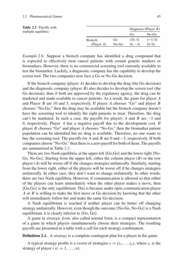
2.2 Pharmaceutical Games 45
Table 2.3 Payoffs withmultiple equilibria
Diagnosis (Player B)
Go No-Go
Biotech(Player A)
Go .10; 5/ .�5; 0/No-Go .0;�3/ .0; 0/
Example 2.6. Suppose a biotech company has identified a drug compound thatis expected to effectively treat cancer patients with certain genetic markers orbiomarkers. However, there is no commercial screening tool currently available totest the biomarker. Luckily, a diagnostic company has the capability to develop thescreen tool. The two companies now face a Go or No-Go decision.
If the biotech company (player A) decides to develop the drug (the Go decision)and the diagnostic company (player B) also decides to develop the screen tool (theGo decision), then if both are approved by the regulatory agency, the drug can bemarketed and made available to cancer patients. As a result, the gains for player Aand Player B are 10 and 5, respectively. If player A chooses “Go” and player Bchooses “No-Go,” then the drug may be available but the biotech company doesn’thave the screening tool to identify the right patients to treat. Therefore, the drugcan’t be marketed. In such a case, the payoffs for players A and B are �5 and0, respectively. Player A has a negative payoff due to the development cost. Ifplayer B chooses “Go” and player A chooses “No-Go,” then the biomarker patientpopulation can be identified but no drug is available. Therefore, no one wants tobuy the screening tool. The payoffs for A and B are 0 and �3, respectively. If bothcompanies choose “No-Go,” then there is a zero payoff for both of them. The payoffsare summarized in Table 2.3.
There are two Nash equilibria, at the upper left fGo,Gog and the lower right fNo-Go, No-Gog. Starting from the upper left, either the column player (B) or the rowplayer (A) will be worse off if she changes strategies unilaterally. Similarly, startingfrom the lower right, either of the players will be worse off if he changes strategiesunilaterally. In either case, they don’t want to change unilaterally. In other words,there are two Nash equilibria. However, if communication is allowed so that eitherof the players can learn immediately when the other player makes a move, thenfGo,Gog is the only equilibrium. This is because under open communication playerA or B is willing to make the first move or Go decision by knowing that the otherwill immediately follow her and make the same Go decision.
A Nash equilibrium is reached if neither player can be better off changingstrategy unilaterally. However, even though the outcome fNo-Go, No-Gog is a Nashequilibrium, it is clearly inferior to fGo, Gog.
A game in strategic form, also called normal form, is a compact representationof a game in which players simultaneously choose their strategies. The resultingpayoffs are presented in a table with a cell for each strategy combination.
Definition 2.1. A strategy is a complete contingent plan for a player in the game.
A typical strategy profile is a vector of strategies s D .s1; : : : sn/, where si is thestrategy of player i .i D 1; : : : ; n/.

46 2 Pharmaceutical Decision and Game Theory
A two-person win-lose game can be played on a so-called graph, G D .X; F /,by stipulating a starting position x0 2 X and using the following rules:
1. Player 1 moves first, starting at x0.2. Players alternate moves.3. At position x, the player whose turn it is to move chooses a position y 2 F.x/.4. The player who is confronted with a terminal position at his turn, and thus cannot
move, loses.
A game is often solved efficiently using so-called backward induction. Backwardinduction is a technique to solve a game of perfect information. It first considers themoves that are the last in the game and determines the best move for the player ineach case. Then, taking these as given future actions, it proceeds backward in time,again determining the best move for the respective player, until the beginning of thegame is reached.
Among various types of games, a simple and well-studied type of game is thezero-sum game. A zero-sum game is a game in which one player’s winnings areequal to the other player’s losses.
We have discussed the pure game, where there is no probability involved regard-ing strategy selection. However, in reality we more often encounter mixed strategygames, where each player’s strategy selection involves a probability distribution.
Definition 2.2. If a player in a game chooses among two or more strategiesrandomly according to specific probabilities, this choice is called a mixed strategy.
The game of matching pennies has a solution in mixed strategies. The game rulesare: The two players involved show their pennies at the same time; if both are headsor tails, player A wins, and if one is a head and one is a tail, player B wins. In sucha game, neither player wants his opponent to know what to show. In other words,they both should randomly choose heads or tails with a probability of 0.5.
We may be curious about the existence of an equilibrium in a game. Thefollowing well-known theorem by John Nash answers the question.
Theorem 2.1. (Nash 1951). Every finite pure or mixed game with a finite numberof players and a finite strategy space has at least one Nash equilibrium.
2.2.2 Multiple-Player Game
In the prisoner’s game, there are two players and each has only two options. Thesolution of the game can be found intuitively. However, in practice there are usuallymore than two options for each player. To solve such games, the following theoremis a very powerful tool.
Theorem 2.2. (Dresher 1961, p. 43). Suppose all pure strategies for each player ina two-person zero-sum matrix game are active (i.e., no dominance or saddle point

2.2 Pharmaceutical Games 47
Fig. 2.6 Mechanismof competition Oncology
drug
Prof
it
N, number of investors
Inflammationdrug
Nc
exists in the game) and the matrix of the game is square and nonsingular. Then aunique optimal mixed strategy for each player can be computed using
q� D�A
0
��11
10
A�11and p� D A�11
10
A�11, (2.25)
where A D ˚aij�n�n is a nonsingular payoff matrix of the game, 1 D .1; 1; : : : ; 1/
0
is an n � 1 column vector, and the column vectors q� and p� are the optimalmixed strategies for the players with row and column strategies in the matrix game,respectively. The value of the game to the row player using q� is u D 1
0
A�11.
One way of phrasing this theorem is that player A searches for a strategy thatmakes playerB indifferent as to which of the (good) pure strategies to use. Similarly,playerB should play in such a way as to make playerA indifferent among his (good)strategies. This is called the Principle of Indifference.
2.2.3 Queuing Game
Queuing theory deals with providing a service on a waiting line (queue). In aqueuing game, the order of a player benefiting more is based on his order in thequeue. Economic competition and highway congestion are two common examples.When the number of players, N , is larger, we traditionally simplify with someassumptions such as the representative agent model, in which we assume that allplayers are identical, have the same strategy options, and get symmetrical payoffs.We also assume that the payoff to each player depends only on the number of otherplayers who choose each strategy and not on which agent chooses which strategy.
Example 2.7. An example of the representative agent model is shown in Fig. 2.6,where each investor has to decide whether to invest in inflammation or oncologydrug development but the return on investment (ROI) is dependent on the numberof investors in the product. In this hypothetical example, at the beginning the ROI is

48 2 Pharmaceutical Decision and Game Theory
Table 2.4 Payoff structuresin a queuing game
Order Gross Cost of Expected netserved payoff standing payoff
1 20 3 172 17 3 143 14 3 114 11 3 85 8 3 5
higher for oncology than for inflammation drugs. When the number of oncologydrug investors increases, development becomes expensive and at the same timedevelopment of inflammation drugs becomes less expensive in comparison. Notethat when more drugs become available for treating one disease, the chance ofhaving or dying from other diseases increases.
Suppose the objective is to maximum the ROI. The equilibrium is reached at theintersection of the two profit lines in Fig. 2.6. From the figure, it is obvious that thefirstNc investors will be interested in investing in oncology drugs but investors whocome after will be interested in investing in inflammation drugs. This is a queuinggame in which multiple players are involved and payoffs are dependent on the orderof the player’s engagement.
The following is another example of a queuing game.
Example 2.8. Suppose there are five customers trying to receive a service. They allwant to get the service as early as possible, but at the same time they don’t like tostand in line. To quantify, we make the following assumptions that apply to all fiveplayers: The gross payoffs and cost of standing depend on the order served as listedin Table 2.4. Net payoffs are the difference between the gross payoff and the cost ofstanding (Table 2.4).
Those who do not stand in line are chosen randomly for service, after thosestanding in line have been served. Therefore, the expected payoff for anyone notstanding in the line is their average gross payoff. The player’s decision on whetherto stand in line or not is driven by the maximization of his net payoff. The game canbe analyzed as follows:
1. If no one stands in line, then each person will have an equal probability of beingserved first, second, . . . , and fifth. The expected payoff is .20 C 17 C 14 C11C 8/=5 D 14. However, such a case can be improved since an individual canimprove his payoff by standing first in line. The net payoff to the person first inline is .20� 3/ D 17 > 14, so someone will get up and stand in line.
2. If no more persons stand in line, the expected payoff is .17C 14C 11C 8/=4 D12:5 for the four remaining. Since the second person in line gets a net payoff of14 > 12:5, someone will get up and stand in the second place in line.
3. This leaves the average payoff at 11 for the three remaining. Since the thirdperson in line gets a net payoff of 11, there may or may not be someone standingin the third place in line. When either two or three persons stand in the line, theNash equilibrium is reached, i.e., there are two equilibria.

2.2 Pharmaceutical Games 49
4. If no one stands in the third place, the game is over; if there is a third personin line, then the remaining two have the expected payoff of 9:5 for not standingin line and 8 for standing in line. Therefore, no one wants to stand in the fourthplace. The game is definitely over.
With two or three people standing in the line, a Nash equilibrium is reached. Thetotal net payoff for queuing is 17C 14C 11C 9:5C 9:5 D 61, which is less than70 for not queuing at all. We call such a case inefficient queuing. To prevent thisfrom happening, the authority (e.g., an airline) can simply ignore the queue and,let’s say, pass out lots for order of service at the time of each customer’s arrival, andno standing in line will be necessary.
2.2.4 Cooperative Games
Games in which the participants cannot make commitments to coordinate theirstrategies are noncooperative games. In a noncooperative game, the rational per-son’s problem is to answer the question “What is the rational choice of strategywhen other players will try to choose their best responses to my strategy?” Incontrast, games in which the participants can make commitments to coordinate theirstrategies are cooperative games.
In noncooperative games, the solution from an individual perspective often leadsto inferior outcomes, as in the Prisoners’ Dilemma. It is preferable, in many cases,to define a criterion to rank outcomes for the group of players as a whole. The Paretocriterion is one of this kind: an outcome is better than another if at least one personis better off and no one is worse off. If an outcome cannot be improved upon (i.e.,if no one can be made better off without making somebody else worse off), then wesay that the outcome is Pareto optimal. A Pareto optimization for the drug price, ifit exists, would be the price value such that any change to this price will either makethe pharmaceutical company less profitable or provide less benefit to patients.
Example 2.9. Suppose two companies are in a position to decide whether todevelop competitive drugs for anemia – a decrease in the normal number of redblood cells (RBCs) or less than the normal quantity of hemoglobin in the blood.Since hemoglobin (found inside RBCs) normally carries oxygen from the lungsto the tissues, anemia’s leading symptoms are nonspecific symptoms: a feeling ofweakness or fatigue, general malaise and sometimes poor concentration.
The cost (including opportunity loss) for developing such a drug is presumablyCa for company A and Cb for company B . The probability of success of such anindication for marketing is denoted by p; if the drug gets regulatory approval, grossprofit for the successful company is dependent on the success of the other companyfor the same indication. Assume that the total profit for the two companies is fixedand equals G billion dollars if at least one is successful in developing the drug;if both companies are successful in developing drugs for anemia, they get G=2

50 2 Pharmaceutical Decision and Game Theory
Table 2.5 Expected netprofits
Company B
Go No-Go
Company A Go .0; 0/ .0:5; 0/
No-Go .0; 0:5/ .0; 0/
Note: GD $10B, Ca DCb D 0:5, pD 0:1
billion dollars each. If both companies make the Go decision (develop the drug),the expected net profits will be pG=2 � Ca and pG=2 � Cb for companies A andB , respectively. If only one company, say company A, made the Go decision andcompanyB made the No-Go decision, the net profit for companyA is pG�Ca andthat for company B is zero. Similarly, we can calculate the net profits for the twoother scenarios as summarized in Table 2.5.
fGo, Gog is a Nash equilibrium (can you explain why?) with an expected netprofit of $0 for each company. Remember that the values for the parameters in thisexample more or less reflect the realities in the pharmaceutical industry.
Other than by internal development, a firm can acquire necessary resourcesthrough partnerships with other stakeholders in the pharmaceutical industry such aspharmas, biotechs, CROs, academicians, policy-makers, and government. Commonforms of partnerships include (1) spot market exchanges, (2) contractual agreementsand alliances, and (3) mergers and acquisitions.
In Example 2.9, companiesA and B can make a joint venture to develop the twodrug candidates sequentially; i.e., if one fails, then the second will be invested in theclinical trials. This will reduce the risk and increase the success of development.
2.2.5 Sequential Game
2.2.5.1 Compulsory Licensing and Parallel Importation
Compulsory licenses are licenses that are granted by a government to regulatethe use of patents, copyrighted works, and other types of intellectual property.Compulsory licenses are an essential government instrument to intervene in themarket and limit patent and other intellectual property rights, in order to correctmarket failures. As concerns public health and compulsory licensing, the restrictionsimposed by the intellectual property rights (IPRs) system on access to (patented)drugs must be reasonable, not creating situations where entire populations aredenied access to known therapies. Therefore, the 1994 WTO TRIPs agreementcontains provisions on safeguards, exceptions, and mechanisms to protect essentialpublic health interests. The TRIP provides for compulsory licenses of patents butalso provides a number of restrictions on the use of compulsory licenses.
The propriety of parallel trade is a matter of intense policy debate in a number ofcountries and in the World Trade Organization (WTO). Presently, WTO provisionsallow member countries to establish their own rules for the “exhaustion” of
2.2 Pharmaceutical Games 51
intellectual property rights (IPRs). If a country opts for national exhaustion of IPRs,a rights holder there may exclude parallel imports because intellectual propertyrights continue until such time as a protected product is first sold in that market. Ifa country instead chooses international exhaustion of IPR, parallel imports cannotbe blocked because the rights of the patent, copyright, or trademark holder expirewhen a protected product is sold anywhere in the world. The United States practicesnational exhaustion for patents and copyrights, but permits parallel imports oftrademarked goods except when the trademark owner can show that the imports areof different quality from goods sold locally or otherwise might cause confusion forconsumers. The European Union provides for regional exhaustion of IPR, wherebygoods circulate freely within the trading bloc but parallel imports from nonmembercountries are banned. Japanese commercial law permits parallel imports exceptwhen such trade is explicitly excluded by contract provisions or when the originalsale is made subject to foreign price controls (Grossman and Lai 2008).
When parallel trade comes into play, the regulated price cap becomes a strategicvariable in an international setting. Parallel trade is an arbitrage mechanism throughwhich the drugs produced in a low-price market flow into a high-price market,reestablishing nearly uniform prices in the presence of a large number of paralleltraders. The price difference mainly results from the transportation and transactioncosts for the reimportation.
Opponents of parallel trade are concerned that such trade undermines manufac-turers’ intellectual property rights. The prevailing wisdom, expressed for exampleby Barfield and Groombridge (1998), Chard and Mellor (1989), and Danzon andTowse (2003), is that parallel trade impedes the ability of research-intensive firmssuch as those in the pharmaceutical industry to reap an adequate return on theirinvestments in new technologies. Grossman and Lai (2008) challenge the prevailingwisdom that parallel trade is induced by different national price controls. They arguethat the existing policy discussions and formal modeling overlook an importanteffect of national policy regarding the exhaustion of IPRs. First, the admissibilityof parallel trade introduces the possibility that a manufacturer will eschew low-price sales in the foreign market in order to mitigate or avoid reimportation.When arbitrage is impossible, the manufacturer is willing to export at any priceabove the marginal production cost. But when the potential for arbitrage exists, themanufacturer may earn higher profits by selling only in the unregulated (or high-price) market than by serving both markets at the lower, foreign-controlled price.Accordingly, a switch from a regime of national exhaustion to one of internationalexhaustion can induce an increase in the controlled price as the foreign governmentseeks to ensure that its consumers are adequately served. Second, the admissibilityof parallel trade mitigates the opportunity for one government to free-ride on theprotection of IPRs granted by another.
Example 2.10. In this example, we will discuss how to model drug marketing usinga sequential game. Suppose a sequential game consists of three stages specified asfollows, where we use North and South to represent two countries with and withoutan intellectual property, respectively.

52 2 Pharmaceutical Decision and Game Theory
Fig. 2.7 Extensive formof drug marketing game
North
SouthUnnp(pn, ps), Usnp(ps, ps)
Unnc(pn, ps), Usnc(ps, ps)
Unip(pn, ps), Usip(ps, ps)
Unic(pn, ps), Usic(ps, ps)South
South utility, North utility
Stage 1: North decides to go for national exhaustion (ne) or international exhaus-tion (ie).
Stage 2: South decides to exercise a price control (pc), i.e., set up a price cap pc ora compulsory license (cl).
Stage 3: North decides the price for North and South, pn and ps .
The extensive form of the sequential game is shown in Fig. 2.7.A non-cooperative solution is the solution to the game when the players take
actions to maximize each individual gain. LetUnij .�; �/ be North’s utility when Northtakes strategy i and South takes strategy j ; letUsij .�; �/ be South’s utility when Northtakes strategy i and South takes strategy j , as illustrated in Fig. 2.7.
Using backward induction, South will take the action Ask (price controlor compulsory license) to maximize its utility Usk such that Usk D max.Uskp.pn; ps/; Uskc.ps; ps//, where kDn for national exhaustion or kD i forinternational exhaustion. After knowing South will take action Ask, North willtake action Ank to maximize its utility.
If maxUnnp.pn; ps/> maxUnnc.pn; ps/> maxUnip.pn; ps/> maxUnic.pn; ps/;
maxUsnp.pn; ps/< maxUsnc.pn; ps/, and max Usip.pn; ps/> maxUsic.pn; ps/,then South will decide to exercise the compulsory license if North opts for nationalexhaustion of IPRs. On the other hand, South will exercise price control if North optsfor international exhaustion, which implies North either has utility maxUnnc .pn; ps/
under national exhaustion or maxUnip .pn; ps/ under international exhaustion.Knowing this fact and that maxUnnc .pn; ps/ > maxUnip .pn; ps/, North willexercise national exhaustion.
The noncooperative solution can often be improved. We use an example toillustrate how to find a Pareto optimum for the cooperative game in Fig. 2.5. Supposemax Unip .pn; ps/ D 10 > maxUnnp .pn; ps/ D 8 > maxUnnc .pn; ps/ D 5 > maxUnic .pn; ps/ D 1 and maxUsnp .pn; ps/ D 2 < maxUsnc .pn; ps/ D 3 < maxUsip .pn; ps/ D 7 < max Usic .pn; ps/ D 10. In such a case, South will exercisethe compulsory license regardless of North’s action (national or internationalexhaustion), which implies North either has utility maxUnnc .pn; ps/ D 4 undernational exhaustion or maxUnic .pn; ps/ D 1 under international exhaustion. It is

2.3 Implementation Challenges 53
obvious that North will exercise national exhaustion with a utility of 5 and Southwill have a utility of 3. However, the result can be improved through an agreementthat North will use international exhaustion and South will use the price control.This is the only Pareto optimum for the game, which gives North 10 and South 7 forthe utility.
2.3 Implementation Challenges
The most fundamental step in pharmaceutical decision-making and game modelingis to quantify a utility function based on the objective and to understand theprocess of the problem to be modeled. For different objectives, the assumptionsmade about the process are different because an assumption may be quite suitablefor one purpose but not suitable at all for another. Model building is an abstractthinking process in which the model builder tries to capture the most importantfactors and simplify or convert the problem into a decision or game model. Theselection of factors to be included in the model is a dimension-reduction processusing knowledge beyond statistics, which is different from and not replaceable bystatistical modeling approaches such as stepwise elimination in a linear regression.Pharmaceutical decision modeling here is beyond traditional modeling. It is large-scale, cross-discipline modeling directed by decision and game theory.
Decision modeling requires strong collaborations among people from differentdisciplines, in which the statistician plays the critical role of the “project coordi-nator.” He or she has to know what information is needed, and where and how toacquire it. Furthermore, the statistician should have a good sense about the precisionor variability of the information. For example, to determine the utility of developinga drug, we have to determine the value proposition and project the short-term andlong-term market values, which can usually be obtained by working with the com-mercial/marketing group of the company. The statistician may be asked to designclinical development programs, which involve multiple phases in clinical trials.
The success of decision-process modeling will also include the campaign ofthe proposed model, which requires diverse skills, including presentation andinterpersonal skills. Such soft skills are critical but unfortunately often neglectedby statisticians. Statistics alone can, in this case, only make things look good onpaper. Note that the campaign for the project is itself a game.
The utility in the Markov decision process will direct the choice of the optimaldesign. Years ago, a colleague of mine told me that he had tried different pharma-ceutical decision models in a certain clinical trial but the maximization of utilityalways led to an infinitely large sample size or a Go decision. I suspect that thereason behind this is an overly optimistic model. This overly optimistic attitude is ageneral trend in the pharmaceutical industry. I am going to elaborate upon this anddiscuss how pharmaceutical decision modeling can be made realistic and successful.
A study (Pearlman, 2007) shows that big pharma has consistently been the singlemost profitable industry of all 47 represented in the Fortune 500. However, this

54 2 Pharmaceutical Decision and Game Theory
kind of comparison may not be very informative, as we know that investment inpharmaceutical R & D has a high risk. The success rate in the pharmaceutical indus-try is very low: there are many failures and bankruptcies; only a small proportionof the NMEs can make it all the way to market. The profitability for successfulbig pharma is naturally higher. Just like playing lotteries, if the profitability iscalculated based only on the winners, it will be much higher than that for the real-life pharmaceutical industry. However, the expected profit of playing any lotterygame is negative. Because “the winner talks all,” we often overestimate the value ofa new drug. This optimism may sometimes be used as a strategy of a team to get thefinancial support they need. Not only is the drug’s value over-projected, but also theprobability of success (I will provide an example soon). Optimism adversely inflatesthe probability of moving the project forward but eventually fails with high costs.
The most obvious example, but surprisingly not well recognized, concernsthe power calculation in clinical trial designs. We know that the phase III trialapproval rate has been about 40% in the past 10 years, including the reason offailing to demonstrate efficacy. However, phase III trials are commonly designed atapproximately a 90% power, which means that about 90% (81% if two independenttrials are required) will demonstrate statistical significance. Why is there such abig difference, 90 versus 40%? There are several reasons: (1) overestimating thetreatment effect or using the minimal clinical difference inappropriately to calculatethe power, (2) underestimating the variance, and (3) the commonly used methods forpower calculation do not consider variability of the treatment effect (see Chap. 10).
The Markov decision processes we have discussed so far have known transitionprobabilities, so that calculation can be carried out. What if the probability isunknown, or is too complicated and becomes intractable? In our previous examplesof clinical development, both the transition probabilities and the expected overallgain are heavily dependent on the toxicity rate p0 and the treatment effect ı, twounknown parameters. If the assumptions about the two parameters change, theoverall expected gain will change. In other words, the optimal action rules willdepend on the assumptions around the parameters. To solve this dilemma, severalmethods are proposed, includingQ-learning and the one-step-forward approach.Q-Learning (Gosavi 2003) is a form of model-free reinforcement learning. It
is a forward induction and an asynchronous dynamic programming. The powerof reinforcement learning lies in its ability to solve the Markov decision processwithout computing the transition probabilities that are needed in value and policyiteration.
One of the popular approaches in robotics is to let the agent randomly choosean action with the selection probability proportional to the potential gain from eachaction. The idea behind this approach is to modify the randomization probabilitygradually in such a way that when our initial judgment about expected gains iswrong, the action will be corrected over time. This has motivated the one-step-forward approach, which has the transition probability
pij D gjPk gk
;

2.4 Exercises 55
where the summation is performed over all nodes that can be reached by one stepforward from node i . We will use this concept in designing adaptive trials, i.e., theresponse-randomization trials in Chap. 4.
However, both the Q-learning and one-step-forward approaches are effectiveonly when the same experiments can be repeated many times, which does nothappen for any single drug candidate.
Most game theories are developed under the assumption of common knowledge.However, such an assumption generally does not hold because each pharmaceuticalcompany is very protective of its intellectual properties. In such a scenario, thecomplexity of the game increases, and we have to distinguish between what ouropponent actually knows and what we think they know.
In collaborative games, many details about partnerships between the two ormultiple players cannot be specified in the contract; the actions and associatedconsequences have great uncertainties. Therefore, probability theory, includingBayesian approaches (Chap. 10), plays an important role here. Pharmaceuticaldecision and game modeling often require simulation for support (see Chap. 9).
2.4 Exercises
2.1. Braess illustrated his paradox using an example in Fig. 2.5, but the time takenon the relief road A ! B was 10 C x5 instead of 10x5. Solve this game (BraessParadox). If there are generally a total of n cars, solve the game. Hint: At Nashequilibrium, the times taken on each road of the three routes (S ! A ! E, S !A ! B ! E, and S ! B ! E) will be the same; furthermore, x1 D x3 C x5 andx2 C x5 D x4.
2.2. Table 2.6 represents the actual success rates of different phases of clinicaltrials. Success is defined as the launch of the next phase, with the exception ofphase III. Success for a phase III trial means NDA approval. Please discuss howto use this prior to your clinical development program (CDP) modeling using thestochastic decision process.
2.3. Explain the terms: game, strategy, player, zero-sum game, mixed strategygame, matrix game, queuing game, cooperative and non-cooperative games, equi-librium in a game, Nash equilibrium, Pareto optimum, and strategic and extensiveforms.
Table 2.6 Success rates of various phases of trials
Year
1990 1992 1994 1996 1998 2000
Preclinical 0.24 0.24 0.19 0.21 0.18 0.21Phase I 0.55 0.60 0.52 0.55 0.55 0.50Phase II 0.47 0.44 0.42 0.47 0.39 0.28Phase III 0.78 0.79 0.73 0.60 0.65 0.43
Source: Chang (2010)

56 2 Pharmaceutical Decision and Game Theory
2.4. Find the Pareto optimal solution set for the following cooperative game(McCain, 2009).
Suppose that Joey has a bicycle. Joey would rather have a game machine than abicycle, and he could buy a game machine for $80 but doesn’t have any money.We express this by saying that Joey values his bicycle at $80. Mikey has $100 andno bicycle, and would rather have a bicycle than anything else he can buy for $100.We express this by saying that Mikey values a bicycle at $100. Analyze the game,construct a 2 � 2 payoff table, and solve the game. You can make assumptions asnecessary.
2.5. Elaborate how Bellman’s backward induction algorithm can improve theefficiency of simulations in the CDP.
2.6. Discuss different forms of alliances, their advantages, and their disadvantages.
2.7. Elaborate on the three common assumptions in game theory, and discuss thefitness of those assumptions in situations of interest.
2.8. For the two-player pharmaceutical game (Table 2.3), discuss the followingcooperative game: The two companies make strategic alliances in which they agreeto jointly develop a drug for an indication using one of the NMEs. If it is successful,the second NME will not be studied; if it fails, they will bring the second one to thedevelopment pipeline.
Further Readings and References
Barfield, C.E., Groombridge, M.A.: The economic case for copyright and owner control overparallel imports. J. World Intellect. Prop. 1, 903–939 (1998)
Bellman, R.: A Markovian decision process. J. Math. Mech. 6, 23–35 (1957a)Bellman, R.: Dynamic Programming. Princeton University Press, Princeton (1957b)Berger, J.: Statistical Decision Theory and Bayesian Analysis. Springer, New York (1985)Bernard, S.: The drug drought, Pharmaceutical Executive, November 1 (2002). www.design-and-
determination.com. Accessed 15 June 2010Bertsekas, D.: Dynamic Programming and Optimal Control, vol. 2. Athena, Belmont (1995)Braess, D.: Uber ein Paradoxon aus der Verkehrsplanung. Unternehmensforschung 12, 258–268
(1969)Cambridge Pharma Consultancy: Pricing and Reimbursement Review 2003. IMS Health-
Management Consulting, Cambridge (2004)Chang, M.: Biomarker development. In: Statistics for Translational Medicine. Taylor and Francis,
New York (2008)Chang, M., Chow, S.C.: Power and sample size for dose response studies. In: Ting, N. (ed.) Dose
Finding in Drug Development. Springer, New York (2006)Chang, M.: Monte Carlo Simulation for the Pharmaceutical Industry. Chapman and Hall/CRC,
Boca Raton (2010)Chard, J.S., Mellor, C.J.: Intellectual property rights and parallel imports. World Econ. 12, 69–83
(1989)Danzon, P., Towse, A.: Differential pricing for pharmaceuticals: Reconciling access, R&D and
patents. Int. J. Health Care Finance Econ. 3, 183–205 (2003)

Further Readings and References 57
Gosavi, A.: Simulation-based Optimization: Parametric Optimization Techniques and Reinforce-ment Learning. Springer, Boston (2003)
Dresher, M.: Games of Strategy. Prentice-Hall, Englewood Cliffs (1961)Grossman, G., Lai, E.: Parallel imports and price controls. RAND J Econ. 39(2), 378–402 (2008)Havil, J.: Impossible? Surprising Solutions to Counterintuitive Conundrums. Princeton University
Press, Priceton (2008)Hu, M., Schultz, K., Sheu, J., Tschopp, D.: The Innovation Gap in Pharmaceutical Drug
Discovery & New Models for R&D Success. www.kellogg.northwestern.edu/academic/biotech/faculty/articles/NewRDModel.pdf (2007). Accessed 2 Mar 2009
McCain, R.: Strategy and Conflict: An Introductory Sketch of Game Theory. http://william-king.www.drexel.edu (2009). Accessed 20 June 2009
Nash, J.: Non-coorperative games. Ann. Math. 5, 286–295 (1951)Parmigiani, G., Inoue, L.: Decision Theory: Principles and Approaches. Wiley, Hokoken (2009)Pearlman, J.B.: The commercialization of medicine. http://www.google.com (2007). Accessed
10 Sep 2009Powell, W.B.: Approximate Dynamic Programming: Solving the Curses of Dimensionality. Wiley-
Interscience, New York (2007)Watson, J.: Strategy. W.W. Norton and Company, New York (2008)


Chapter 3Noninferiority Trial Design
3.1 Concept of Noninferiority Trial
3.1.1 Needs for Noninferiority Design
Superiority and noninferiority (NI) trials are two common types of clinical trials.Superiority means, in layman’s language, that the test drug is better than thecomparative drug (active comparator or active-control), whereas noninferioritysuggests that the test drug may not be as good as the comparative drug, but thedifference is not clinically significant. If a test drug is noninferior to an active-control, it must be at least superior to a placebo (Fig. 3.1).
Statistically, the hypothesis tests for superiority and noninferiority are expressed,respectively, as
Ho W �T � �C � 0 versusHa W NHo
andHo W �T � �C � �ıNI versusHa W NHo,
where �T and �C are treatment effects for the test and control groups, respectively.Here the so-called noninferiority margin ıNI is usually defined based on clinical andstatistical considerations (see details later in this chapter).
As the European regulatory agency, Committee for Medicinal Products for Hu-man Use (CHMP 2005) stated, “Many clinical trials comparing a test product withan active comparator are designed as noninferiority trials. The term ‘noninferiority’is now well established, but if taken literally could be misleading. The objective of anoninferiority trial is sometimes stated as being to demonstrate that the test productis not inferior to the comparator. However, only a superiority trial can demonstratethis. In fact a noninferiority trial aims to demonstrate that the test product is notworse than the comparator by more than a pre-specified, small amount. This amountis known as the noninferiority margin, or delta.”
Until recent years, the majority of clinical trials were designed for superiority toa comparative drug (the control group). A statistic shows that only 23% of all NDAs
M. Chang, Modern Issues and Methods in Biostatistics, Statistics for Biology and Health,DOI 10.1007/978-1-4419-9842-2 3, © Springer Science+Business Media, LLC 2011
59

60 3 Noninferiority Trial Design
Fig. 3.1 Superiority versusnoninferiority
Treatment Effect θ
Placebo effect Noninferior
test drug
Control effect
NI Margin δNI
Superiortest drug
Inferiortest drug
from 1998 to 2002 were innovative drugs, and the rest were accounted for as “me-too” drugs (Chang, 2010). Those me-too drugs are based on noninferiority criteria.The increasing popularity of noninferiority trials is a reflection of the regulatory andindustry adjustments in response to the increasing challenges in drug development.
The emerging trend of more noninferiority trials than superiority trials can beattributed to the following causes:
1. When many efficacious treatments are available, the use of placebo-controltrials for the evaluation of new medical treatments in clinical trials is ethicallyproblematic.
2. Test and control drugs are expected to have a similar magnitude of efficacy, butthey may have different mechanics of action and hence will work for different (atleast partially) populations.
3. A new test drug may be safer, cheaper, more convenient or easy to administrate,or have a better taste, different interactions with other drugs, or other kinds ofbenefits to patients.
4. There is growing interest among third-party payers and some regulatory au-thorities, on both cost-effectiveness and medical grounds, in the comparativeeffectiveness of treatments.
5. The “low-hanging fruits” in drug development are much less available than inprior years. When we continue to make more effective and/or safer drugs, thechance of finding a compound better than the “best” in the market is smaller andthe efforts required to find such a compound are bigger.
6. There are great attractions to develop generic drugs after patent expiration ofinnovative drugs.
CHMP (2005) pointed out the situations in which NI trials may be used, whichinclude:
1. Applications based upon essential similarity in areas where bioequivalencestudies are not possible, e.g., modified release products or topical preparations;
2. Products with a potential safety advantage over the standard might require anefficacy comparison to the standard to allow a risk-benefit assessment to be made;
3. Cases where a direct comparison against the active comparator is needed to helpassess risk/benefit;
4. Cases where no important loss of efficacy compared to the active comparatorwould be acceptable;
5. Disease areas where the use of a placebo arm is not possible and an active-controltrial is used to demonstrate the efficacy of the test product.

3.1 Concept of Noninferiority Trial 61
However, there are concerns and challenges in design, conduct, and analysisand interpretation of a noninferiority trial, such as active-control selection, thenoninferiority margin determination, and inclusion of a placebo arm. We willdiscuss these issues in later sections.
3.1.2 Noninferiority Lingo
1. Noninferiority margin: The noninferiority active-control trial should demonstratethat the new treatment T is within the noninferiority margin ıNI of the active-control C . This margin should have clinical relevance. The determination of theNI margin is a major challenge in designing an NI trial.
2. Assay sensitivity: Assay sensitivity, a property of a clinical trial, refers to theability of the trial to distinguish effective drugs from ineffective ones. Assaysensitivity depends on the effect size one needs to detect. A trial may haveassay sensitivity for an effect of ten but not an effect of five. One thereforeneeds to know the effect of the control drug (Temple 2002). Assay sensitivityis the assurance that the active-control would have been superior to a placeboif a placebo had been employed in the noninferiority trial. Establishing assaysensitivity is a basic requirement in an NI trial, which is usually accomplishedusing an adequate NI margin that is based on past placebo-control trials.
3. Constancy: The constancy assumption means that the historical differencebetween the active-control and placebo is assumed to hold in the setting of thenew trial if a placebo control was used. The populations in the historical trial andthe current NI trial are similar (D’Agostino et al. 2003).
4. Putative placebo: The term “putative placebo” is often used in a situation whereno placebo has actually been used. Since an NI trial often does not include aplacebo group, to establish the assay sensitivity it is then necessary to use Cversus T data in conjunction with C versus P , the historical placebo-controlledtrial data, to demonstrate that T is superior to P . This process is called theputative placebo comparison.
5. Biocreep: Biocreep refers to the phenomenon that can occur when a slightly infe-rior treatment becomes the active-control for the next generation of noninferioritytrials, and so on. Eventually the active controls become no better than a placebo.
6. Noninferiority design methods include the fixed-effect method, �-method, syn-thesis method, NI95-H95 method, and others.
3.1.3 Noninferiority Design Methods
There are three major sources of uncertainty about the conclusions from an NI study:(1) the uncertainty of the active-control effect over a placebo, which is estimatedfrom historical data, (2) the control effect may change over time, violating the

62 3 Noninferiority Trial Design
“constancy assumption,” and (3) that the risk of making a wrong decision from thetest of the noninferiority hypothesis in the NI study, i.e., the type-I error. These threeuncertainties have to be considered in developing a noninferiority design method.
Most commonly used noninferiority trials are based on parallel, two-groupdesigns. Three-group designs with a placebo may sometimes be used, but they arenot very cost-effective and often face ethical challenges by including a placebogroup, especially in the United States.
We now discuss five commonly used hypothesis-testing methods for noninfe-riority trials: the fixed-margin method, the �-portion method, and three synthesismethods (one in original scale and two in log scale). In the rest of the chapter, we willdenote the test and the active-control groups by subscripts T and C , respectively.Where there is no confusion, T will also be used for test statistics. We will usethe hat “ˆ” to represent an estimate of the corresponding parameter, e.g., O� is anestimate of � .
3.1.3.1 Fixed-Margin Method
The null hypothesis for the fixed-margin method is given by
Ho W �T � �C C ıNI � 0, (3.1)
where � can be the mean, hazard rate, adverse event rate, recurrent events rate, orthe mean number of events. The constant noninferiority margin ıNI � 0 is usuallydetermined based on a historical placebo-control study (see more discussions later).When �NI D 0, (3.1) becomes a null hypothesis test for superiority.
The rejection of (3.1) can be interpreted in layman’s terms: The test drug T isnot inferior to C by ıNI or more.
3.1.3.2 �-Portion Method
The null hypothesis for the �-portion method is given by
Ho W �T � �NI �C � 0, (3.2)
where 0 < �NI < 1. For the superiority test, �NI D 1.The rejection of (3.2) can be interpreted in layman’s terms: Drug T is at least
100�NI% as effective as drug C .
3.1.3.3 Synthesis Method
The null hypothesis for the synthesis method is given by
Ho W �T � �P
�C � �P� �NI � 0. (3.3)

3.1 Concept of Noninferiority Trial 63
Assuming we have proved �C � �P > 0,(3.3) is then equivalent to
Ho W �T � �C C .1 � �NI / .�C � �P / � 0; (3.4)
where 0 < �NI < 1. For the superiority test, �NI D 1.The rejection of (3.3) can be interpreted in layman’s terms: The test drug T
is at least 100�NI% as effective as C after subtracting the placebo effect. When�NI D 0, (3.3) represents a null hypothesis for a putative placebo-control trial.
3.1.3.4 Synthesis Method in Log Form
Drug effect is often measured by the hazard ratio (relative risk) or odds ratio, i.e.,�T�C
and �C�P
. These ratios are often expressed in log scale, so that their distributionsare close to normal distributions. In such cases, we can use the NI null hypothesis
Ho W �T =�C�C =�P
� �NI � 0, (3.5)
where 0 < �NI < 1 if a larger value of �i indicates a better result and �NI > 1 if asmaller �i indicates a better result.
Taking the logarithm, (3.5) becomes
Ho W ln
��T
�C
�� ln
��C
�P
�� ��
NI � 0; (3.6)
where ��NI D ln�NI . Thus ��
NI < 0 if a larger value of �i indicates a better resultand ��
NI > 0 if a smaller �i indicates a better result.The rejection of (3.5) can be interpreted in layman’s terms: The incremental
effect of test drug T over the active-control is at least 100�NI% of the effect . �C�P/
of the active versus placebo. Note that �T =�C is addressed in the current NI trial,whereas �C =�P is addressed in the historical trial.
3.1.3.5 Synthesis Method for Time-to-Event Endpoint
Rothmann et al. (2003) proposed the noninferiority test method for the time-to-eventanalysis with the null hypothesis being
Ho W ln�T
�CC ��
NI ln�C
�P� 0, (3.7)
where 0 < ��NI � 1 if a smaller �i indicates a better result and ��
NI < 0 if a larger�i indicates a better result. Hypothesis (3.7) can also be used for a hazard ratio testfor a binary (not time-to-event) endpoint. The advantage of (3.7) is small varianceand higher power in comparison with (3.6), but interpretation is not intuitive.

64 3 Noninferiority Trial Design
We can rewrite the hypothesis tests (3.1)–(3.7) above in a general form,
Ho W L.„ .�// � 0 versusHa W NHo; (3.8)
where NHo is the negation of Ho, L.�/ is a linear function, function „.�/ can be, forexample, the natural logarithm function, and vector � can be, for example, means,proportions, or hazard rates.
For hypothesis (3.8), we can define the test statistic as
T DL�„� O���
v; (3.9)
where O� can be an estimate of � with variance
v2 D var�L�„. O�/
��: (3.10)
The asymptotic distribution of the test statistic T given by (3.9) usually has anormal distribution,
T � N�"
v; 1�; (3.11)
where " D L.„.�// D E�L�„. O�/
��.
Under the null hypothesis boundary "D0, the test statistic has the standard normaldistribution T � N .0; 1/. Therefore, the power can be expressed as
1 � ˇ D ˚�"
v� z1�˛
�, (3.12)
where ˇ is the type-II error rate, ˚ .�/ is the standard normal c.d.f., and z1�˛ D˚�1 .1� ˛/.
Solving (3.12) for 1=v, we have
1
vD .z1�a C z1�ˇ/
". (3.13)
Where, under a large-sample assumption, v can usually be expressed as v D �pn
,where � is independent of the total sample size n. Therefore, the sample size can beobtained from (3.13),
n D .z1�a C z1�ˇ/2�2
"2; (3.14)
where the “equivalent variance,” �2; will be discussed later for each particular case.
Remark. The rejection of the null hypothesis Ho W � � 0 implies concluding thegeneral condition � > 0 (the negation ofHo) but not concluding any particular valueof � D " even if we have written the alternative hypothesis asHa W � D ". Therefore,

3.1 Concept of Noninferiority Trial 65
in this chapter, we always use the negation of Ho as the alternative hypothesis inhypothesis-testing. However we have to assume a particular value for � D " for thepurpose of power or sample size calculation.
3.1.4 Analysis of Noninferiority Trials
In superiority trials, the intent-to-treat (ITT) population is the primary analysispopulation because of the ITT principle and is also a conservative approach.However, for the NI trial, both ITT and per protocol analyses are equally important,according to CPMP (2000), partially because ITT analysis does not necessarilyprovide conservative results.P -values for the NI hypothesis-test and confidence interval are usually presented.
The two methods are equivalent in terms of making the positive or negative claimabout the test drug. The confidence interval consists of all the possible values of theparameter (e.g., �T � �C , �T =�C , etc.) that will not lead to the rejection of the nullhypothesis. Theorem 3.1 and its converse, Proposition 3.1, assert the equivalence.In practice, the confidence interval (CI) method is used more often because it is acommon view that it is more informative than the p-value. In fact, CHMP (2005)suggests applicants provide CIs both for each treatment group separately, and forthe difference between the groups.
Theorem 3.1. (Shao, 2003, p. 477) For each �0 2 � (parameter space), let T�0 bea test for Ho W � � �0 D 0 versus Ha W NH with significance level ˛ and acceptanceregion A .�0/. For each x in the range of X , define
C .x/ D f� W x 2 A .�/g :
Then C .x/ is a level 1 � ˛ confidence set for � .
Proof. Under the given condition,
sup�D�0
P .X … A .�0// D sup�D�0
P .T�0 D 1/ � ˛
is the same as
1 � ˛ � inf�D�0
P .X 2 A .�0// D inf�D�0
P .�0 2 C .X// .
Since this holds for all �0, the result follows from
infP2} P .X 2 C .X// D inf
�02�inf�D�0
P .�0 2 C .X// � 1 � ˛.

66 3 Noninferiority Trial Design
Scenario 1
Scenario 2
Scenario 3
-δNI 0 Treatment difference δ T-C
Fig. 3.2 Determination of superiority and noninferiority with CI
The converse of Theorem 3.1 is the following proposition.
Proposition 3.1. Let C .X/ be a confidence set for � with significance level 1� ˛.For any �0 2 �, define a region A .�0/ D fx W �0 2 C .x/g. Then the test T .X/ D1 � IA.�0/ .X/ has a significance level ˛ for testing Ho W � D �0 versus NHa.
However, the equivalence between the CI method and hypothesis-testing may nothold for sequential or multiple-testing; e.g., in a multiple-endpoint NI trial. In sucha case, we may use the methods discussed in Chap. 1.
We have illustrated the concepts of noninferiority and superiority in terms ofthe true treatment effect (parameter). However, because the true effect can’t beknown exactly, the confidence method is illustrated in Fig. 3.2. In scenario 1, thelower 95% confidence bound is larger than the NI margin (�ıNI ), indicating thetest drug is effective (NI demonstrated). In scenario 2, the point estimate favorsthe test drug but the lower 95% confidence bound is smaller than the NI margin(�ıNI ), indicating unacceptable loss of the control effect (assume a larger treatmentdifference is better). In scenario 3, the test drug is superior to the active-controlbecause the lower 95% confidence bound is larger than 0.
3.2 Two-Arm Design
3.2.1 Fixed-Margin Method
Based on the fixed-margin method, a hypothesis test for a noninferiority test for twoindependent parallel-group designs can be specified as
Ho W �T � �C C ıNI � 0 versusHa W NHo: (3.15)

3.2 Two-Arm Design 67
The test statistic is defined as
T D O"pnO� , (3.16)
where8<
:
O" D O�T � O�C C ıNI ;
O� Ds
O�2TfT
C O�2CfC;
(3.17)
with O�2i being the sample variance (i D T;C ), n being the total sample size, andsample size fractions fi D ni =n (i D T;C ).
For a large sample size, T has the standard normal distribution ofN .0; 1/ on theboundary of the null hypothesis domain (�T � �C C ıNI D 0) and has the normal
distribution N."pn
�; 1/ under the condition �T � �C C ıNI D ".
For the mean endpoint�i , O�T and O�C are the sample standard deviations. For theproportion endpoint pi , the standard deviations are
O�2i D Opi .1 � Opi /; i D T;C . (3.18)
For the survival endpoint, O�i D O�i ; i D T;C , where �i is the population hazard ratefor group i . The standard deviation for O�i , under exponential distribution, is givenby (e.g., Chang 2007b):
�2i D �2i
�1C e��iTs .1 � e�i T0 /
T0�i
��1, (3.19)
where T0 and Ts are the accrual time period and the total trial duration, respectively.Under an exponential survival model, the relationship between hazard .�/,
median .Tmedian/, and mean .Tmean/ survival time is very simple:
TMedian D ln 2
�D .ln 2/Tmean.
The rejection rule is specified as follows (assume larger � is preferred):
�Reject Ho if T � z1�˛ ,Accept Ho otherwise.
(3.20)
Equivalently, we can use the confidence interval of ":
(Reject Ho if O" � z1�˛ O�p
n� 0,
AcceptHo otherwise.(3.21)

68 3 Noninferiority Trial Design
The power of the test statistic T under a particularHa can be expressed as
1 � ˇ D ˚
�"pn
�� z1�˛
�; (3.22)
where " and � are estimated by (3.17).Solving (3.22) for the sample size, we obtain
n Dz1�˛ C z1�ˇ
2�2
"2: (3.23)
Equation 3.23 is a general sample size formulation for the two-group designswith a normal, binary, or survival endpoint (Chang 2007a).
For the test statistic given by (3.16), the p-value is given by
p D 1 � ˚
� O"pnO��
. (3.24)
Remark. A common misconception is that for an NI trial the sample size calculationmust assume �T � �C D 0, which is not true at all. One could choose an NI designbecause the difference �T � �C > 0 is too small for superiority testing withreasonable power. The treatment difference can be positive or negative dependingon the particular situation. The power and sample size calculation should be basedon the best knowledge about the value of �T � �C , and this knowledge should notchange because of the different choice of hypothesis test. Therefore, for a givenvalue of �T � �C and power, superiority testing always requires a smaller samplesize than noninferiority testing.
Example 3.1. Arteriosclerotic Vascular Disease Trial: Cholesterol is the main lipidassociated with arteriosclerotic vascular disease. The purpose of cholesterol testingis to identify patients at risk for arteriosclerotic heart disease. The liver metabolizescholesterol to its free form and transports it to the bloodstream via lipoproteins.Nearly 75% of the cholesterol is bound to low-density lipoproteins (LDLs) – “badcholesterol” and 25% is bound to high-density lipoproteins (HDLs) (“good choles-terol”). Therefore, cholesterol is the main component of LDLs and only a minimalcomponent of HDLs and very-low-density lipoproteins. LDL is the substance mostdirectly associated with increased risk of coronary heart disease (CHD).
Suppose we are interested in a phase III trial for evaluating the effect of a testdrug on cholesterol in patients with CHD. A two-group (test versus control) paralleldesign is chosen for the trial, with LDL as the primary endpoint. The treatmentdifference in LDL is estimated from the previous phase II trial to be �T � �C D 5%(LDL reduction O�TD25% and O�CD20%) with a standard deviation of O� D 2 O�T D2 O�C D 0:3 (sample size fraction fT D fC D 0:5 for the balance design, O�C D0:15). For power = 90% and one-sided ˛ D 0:025, the total sample required forsuperiority can be calculated:

3.2 Two-Arm Design 69
n D4.1:96C 1:28/20:32
0:052D 1;512:
For a noninferiority test with a margin ıNI D �0:01, the total sample size isgiven by (2.23):
n D4.1:96C 1:28/20:32
.0:05C 0:01/2D 1;050:
We can see that the required sample size is smaller for the noninferiority testthan for a superiority test under the same assumption of treatment effect �T � �C .However, if we assume the treatment difference is �T � �C D 0 instead of 5%, thesample size for the noninferiority trial will be
n D4.1:96C 1:28/20:32
0:012D 27;791;
which means that if the test drug has the same effect as the control, �T D �C , it isnot feasible for a superiority trial (n D 1) or noninferiority trial (n D 27;791). Inpractice, if the estimate �T � �C D 5% is reliable, we may design the noninferioritytrial with 90% power (n D 1;050). The trial will be tested both for noninferiorityand superiority claims at one-sided ˛ D 0:025. With the same size of n D 1;050,the power for the superiority test is 77%.
3.2.2 �-Portion Method
For the �-portion method, the hypothesis is given by
Ho W �T � �NI �C � 0 ; (3.25)
where 0 < �NI < 1 (assume that a larger � is better).The test statistic is defined in the same way as in (3.16), where
8<
:
O" D O�T � �NI O�C ;O�2 D O�2T
fTC �2NI
O�2CfC:
(3.26)
With O" and O� given by (3.25), the calculations for the p-value (3.24), the rejectionrule (3.21), power formulation (3.22), and the sample size formulation (3.23) are stillvalid.
The �-portion method is usually more powerful than the fixed-margin methodbecause the variance given by (3.26) is usually smaller than the correspondingvariance (3.17) for the fixed-margin method.

70 3 Noninferiority Trial Design
Example 3.2. For the LDL trial in Example 3.1, the estimated O" D O�T � O�C CıNI D 0:06. For the purpose of comparison with the fixed-margin method, assume�NI D 0:95 such that the estimated
O" D O�T � �NI O�C D 25% � 0:95.20%/ D 0:06:
From (3.26), we can obtain
O�2 Dp0:152=0:5C 0:952.0:152=0:5/ D 0:293:
Therefore, the total sample size required can be obtained from (3.14),
n D4.1:96C 1:28/20:2932
0:062� 1;000;
which is smaller than the sample size (n D 1;050) required for the fixed-marginmethod.
For the survival endpoint, the logarithm of the hazard ratio (ln�/ is often used inthe hypothesis test. The standard error of ln� is conveniently expressed as a functionof events (deaths),
SEln O� DZ 1
0
�nT � nC
nC C nT ��.��1/=�
�1=2d� �
�1
dTC 1
dC
�1=2,
where dT and dC are the number of deaths for the test and control groups,respectively. The approximate upper limit of the confidence interval of � is given by
UL D exp�
ln O� C z1�˛SEln O��
.
If the UL � ��NI (the cut point for NI, e.g., ��NI D 1:25), noninferiority will beclaimed.
3.2.3 Synthesis Method
1. With the synthesis method, the hypothesis test for noninferiority with two-groupdesigns can be specified as
Ho W �T � �C C .1 � �NI / .�C � �P / � 0 versusHa W NHo. (3.27)
The test statistic is again defined as in (3.16), where8<
:
O" D O�T � O�C C .1 � �NI / OıC�P ,
O�2 D� O�2TfT
PC O�2CfC
C .1� �NI / s2en
�,
(3.28)

3.2 Two-Arm Design 71
and �i (i D T;C ) is the same as given earlier for the fixed-margin approach fordifferent endpoints, mean proportion, and hazard rate. Both OıC�P D O�C� O�P and thestandard error se of OıC�P are obtained from the historical placebo-control trial(s).The standard error se can be estimated by
se Dr
O�C�1 � O�C
�=nC C O�P
�1 � O�P
�=nP ;
where ni (i D C;P ) are the sample sizes in the treatment groups C and P of thehistorical trial, respectively.
For a large sample size, T � N."pn
�; 1/, where
" D �T � �C C .1 � �NI / ıC�P : (3.29)
Therefore, using (3.28) and (3.29), the calculations for the p-value (3.24) andrejection rules (3.21) are still valid; so are the power (3.22) and sample size (3.23).However, because � involves n, the sample size needs to be reformulated for easycalculation.
The sample size can be obtained through iterations based on the followingformulation:
n Dz1�˛ C z1�ˇ
2 � �2TfT
C �2CfC
C .1 � �NI/ s2e n�
"2: (3.30)
Alternatively, we can solve (3.30) for n. We can obtain
n D�0
��2TfT
C �2CfC
�
1 � .1� �NI / s2e �0; (3.31)
where
�0 Dz1�˛ C z1�ˇ
2
"2: (3.32)
Because the synthesis method considers the variability of the historical trial, thereis a bigger variance in the denominator of the test statistic in comparison with thefixed-margin method. As a result, the synthesis method is less powerful.
Example 3.3. Suppose we are going to design a two-arm phase III cardiovascular(CV) disease trial comparing the effect of the test treatment T to an active-controlCwith 1:1 randomization. The primary endpoint is the rate of the composite endpoint,i.e., death or MI (myocardial infarction) within 30 days. The proportion of the com-posite endpoint in the historical randomized trial was O�C D 0:14 and O�P D 0:16 forthe treatment C (nC D 5;000) and the standard care P (nP D 5;000), respectively.Thus ıC�P D 0:14 � 0:16 D �0:02. The standard error is estimated to be
se Dp.0:14.1� 0:14/=5;000/C 0:16.1� 0:16/=5;000 D 0:00714:

72 3 Noninferiority Trial Design
The death rate with treatment T is estimated to be O�T D 0:115. The target power is90%, and the one-sided significance level is ˛ D 0:025. Assume we want to retain80% of the historical active-control effect, i.e., �NI D 0:8 (or about 0:4% morecomposite events in terms of the fixed NI margin). To calculate the total sample sizerequired for a balanced design (f1 D f2 D 0:5), we estimate " from (3.29):
" D 0:12� 0:14C .1 � 0:8/ .�0:02/ D �0:024.
From (3.32), we obtain
�0 D .1:96C 1:28/2 =.�0:024/2 D 18; 225.
Finally, from (3.31), we obtain the total sample size
n D18; 225
�0:12.1�0:12/
0:5C 0:14.1�0:14/
0:5
�
1 � .1 � 0:8/ 0:007142.18; 225/ D 10; 118.
For the superiority design, the total same size would be
n D�0:115.1� 0:115/
0:5C 0:14.1� 0:14/
0:5
�.1:96C 1:28/2
.0:12� 0:14/2D 11;662.
2. We now study the hypothesis
Ho W ln�T
�C� ln
�C
�P� ��
NI � 0, (3.33)
where ��NI D ln�NI as given in (3.6). Hypothesis (3.33) is often used for survival
problems, where �T�C
represents the hazard rate. The test statistic can again be definedby (3.16), where
O" D lnO�TO�C
� lnO�CO�P
� ��NI . (3.34)
The estimated log hazard ratio, lnO�CO�P , is usually obtained from a historical placebo-
control trial(s), whereas lnO�TO�C is obtained from the current NI trial, and
O�2 D n
"var
ln
O�TO�C
!C var
ln
O�CO�P
!#, (3.35)
where the first and second terms on the right-hand side of the equation are obtainedfrom the current NI and historical trials, respectively. The variance of the log relativerisk can be calculated using

3.2 Two-Arm Design 73
�2TC D var
ln
O�TO�C
!D 1
n
�1
rT� 1
fTC 1
rC� 1
fC
�, (3.36)
where ri and fi are the response (death) rate and the sample size fraction in group i(i D T;C ), respectively.
Therefore, with (3.34) and (3.36), the formulations for the p-value (3.24),rejection rules (3.21), power (3.22), and sample size (3.23) are still valid.
Example 3.4. Suppose we are conducting a two-group oncology trial with a 1 yeardeath rate as the primary endpoint (more often it is survival time). Assume that in
the historical trial we know O�C D 0:4 and O�P D 0:52, and var�
lnO�CO�P
�D 0.0065.
Because a smaller �i indicates a better result, ��NI should be positive. Assume
��NI D 0:4 or, equivalently, �NI D e0:4 D 1:5. Given the true rates �C D 0:4 and�P D 0:52, we know from (3.5) that it can be that �T
�CD �NI
�C�P
D 1:5 0:40:52
� 0:85.This means that the use of ��
NI D 0:4 will retain about 85% of the control effect.
From (3.34), we obtain
O" D ln0:3
0:4� ln
0:4
0:52� 0:4 D �0:425,
from (3.36), we obtain
O�2TC D 1
n
�1
0:3.0:5/� 1
.0:5/C 1
0:4.0:5/� 1
.0:5/
�D 7:667
n,
and from (3.35) we can obtain �2 D n .7:667=nC 0:0065/ D 7:667 C 0:0065n.The sample size can be calculated from (3.23):
n D .1:96C 1:28/2 .7:667C 0:0065n/
.�0:425/2 D 445:6C 0:3778n.
Solving for n, we obtain nD716 for the noninferiority design. For the superioritydesign, the sample size would be
n D .1:96C 1:28/2.7:667/.�
ln0:3
0:4
� 2
� 972.
We can see that the savings on sample size for the NI trial using (3.33) aredramatic when the event rate is low. When the event rate is high (e.g., 0.3),the savings in sample size are much smaller using (3.33). For high event rates,the method based on (3.27) can be better than the method based on (3.33) in termsof sample size.

74 3 Noninferiority Trial Design
3. We now study the hypothesis
Ho W ln�T
�CC ��
NI ln�C
�P� 0. (3.37)
The test statistic is given by (3.16), where
O" D lnO�TO�C
C ��NI ln
O�CO�P
. (3.38)
Here lnO�CO�P and ln
O�TO�C are the same as previously stated, but the variance is different
and is given by
O�2 D n
"var
ln
O�TO�C
!C ��2
NIvar
ln
O�CO�P
!#.
Using (3.36), we can obtain
O�2 D 1
rT� 1
fTC 1
rC� 1
fCC ��2
NI
�1
rC� 1
fCC 1
rP� 1
fP
�. (3.39)
With (3.38) and (3.39), the calculations of p-value (3.24), rejection rules (3.21),power (3.22), and sample size (2.23) are still valid. The can also be formulated interms of the number of events under, for example, exponential distribution.
As pointed out in the draft FDA guidance (FDA 2010), because of the waythe variance of the historical data and the NI data are combined for the synthesistest, the synthesis test is more efficient (it uses a smaller sample size or achievesgreater power for the same sample size) than the fixed-margin approach but requiresassumptions that may not be appropriate.
3.2.4 Paired Data
Let Y1 and Y2 be, respectively, binary response variables of treatments 1and 2 with the joint distribution P.Y1 D i IY2 D j /Dpij for i D 0; 1I j D 0; 1.P1
iD0P1
jD0 pij D 1. This kind of data is usually displayed in a 2 2 contingencytable as in Table 3.1.
Nam and Tango’s asymptotic test (Nam 1997; Tango 1998) is given by
Ho W p01 � p10 � ıNI vs. Ha: NHo. (3.40)

3.3 Three-Arm Design 75
Table 3.1 Matched-pair data Test Total
Control 1 0
1 x11 x100 x01 x00Total n
Define the test statistic in (3.16), where
8<
:
O" D Op01 � Op10 � ıNI ,
Opij D xij =n,
O�2 D 2 Qp10 C ıNI � ı2NI ,
(3.41)
and Qp10 is the restricted MLE of p10,
8ˆ<
ˆ:
Qp10 D �b C pb2 � 8c4
,
b D .2C Op10 � Op01/ ıNI � Op01 � Op10,c D � Op10ıNI .1 � ıNI / .
(3.42)
Nam (1997) proved that under the constraint p01 � p10 D ıNI , T in (3.16) followsthe normal distribution for large n,
T � N
�pn"
�; 1
�, (3.43)
where " D E .O"/ and � D E . O�/ can be obtained by replacing Opij with pij (i D0; 1I j D 0; 1) in the corresponding expressions.
Using (3.41) and (3.42), the calculations of the p-value (3.24), the rejectionrules (3.21), and power (3.22) are the same, but the sample size calculation requiresnumerical iterations.
3.3 Three-Arm Design
CHMP (2005) suggested: “A three-armed trial with test, reference and placeboallows some within-trial validation of the choice of noninferiority margin and istherefore associated with fewer difficulties. This is the recommended design andshould be used wherever possible.”
76 3 Noninferiority Trial Design
In the United States, a noninferiority trial with a placebo arm is often consideredethically problematic. However, there are situations when the use of a placebois permissible. According to Ellenberg and Temple (2000), placebo controls areethical when delaying or omitting available treatment has no permanent adverseconsequences for the patient and as long as patients are fully informed aboutthe alternatives and settings where the available “effective treatment” may not beuniformly accepted as standard treatment and so placebo-control trials are justified.The escape clauses are suggested to be included in the study protocol.
In a three-arm NI trial, we can use the synthesis method and then rewrite thehypothesis test as
Ho W �T � �NI �C � .1 � �NI / �P � 0, and
Ha W �T � �NI �C � .1 � �NI / �P > 0: (3.44)
Let the test statistic be
T D O"pnO� , (3.45)
where n is the total sample size,
8ˆ<
ˆ:
O" D O�T � �NI O�C � .1 � �NI / O�P
O� Ds
O�2TfT
C �2NI O�2CfC
C .1 � �NI /2 O�2PfP
;(3.46)
and fi is the sample size fraction for the i th group.T in (3.45) follows a t-distribution with � D nT C nC C nP � 3 degrees of
freedom under H0. Thus, noninferiority can be claimed if T � t1�˛;� . Since mostNI trials have a large sample size, we can use a normal approximation; therefore,using (3.46), the calculations for the p-value (3.24), the rejection rule (3.21), andpower formulation (3.22) are still valid.
However, unlike in the two-arm trial, we now have to reject the hypothesisH00 W�C � �P � 0 first before we test (3.44), as suggested by Pigeot et al. (2003) andKieser and Friede (2007). Therefore, the sample size and overall power calculationscan be obtained using simulations.
There are some dilemmas in three-arm NI trials. For example, what if we failedto reject H0 W �C � �P � 0 but rejected H0 W �T � �P � 0, and failed to rejectH0 W �T � �C C ıNI � 0? Should we claim T superiority to C , or not evenclaim T is noninferior to C ? CHMP’s guidance (CHMP 2005) states that when�C � �P is smaller than what was previously estimated, the appropriateness of thepredetermined margin is in doubt and modifications may be needed. This inevitablyfurther undermines the validity of the statistical method for the NI design. We willdiscuss controversies and challenges further in Sect. 3.5.

3.4 The Noninferiority Margin and Regulatory Guidance 77
3.4 The Noninferiority Margin and Regulatory Guidance
3.4.1 ICH Guidance
Different regulatory authorities may have different requirements and recommen-dations regarding the NI trial in general and the determination of the NI margin.Therefore, it is important to carefully review their guidance documents beforedesigning an NI trial.
According to the ICH E10 guidance, the design and conduct of a noninferioritytrial thus involves four critical steps:
1. Determining that historical evidence of sensitivity to drug effects exists. Withoutthis determination, demonstration of efficacy from a showing of noninferiority isnot possible and should not be attempted.
2. Designing a trial. Important details of the trial design, e.g., study population,concomitant therapy, endpoints, run-in periods, should adhere closely to thedesign of the trials used to determine that historical evidence of sensitivity todrug effects exists.
3. Setting a margin. An acceptable noninferiority margin should be defined, takinginto account the historical data and relevant clinical and statistical considerations.
4. Conducting the trial. The trial conduct should also adhere closely to that of thehistorical trials and should be of high quality.
The determination of the noninferiority margin “. . . should reflect uncertaintiesin the evidence on which the choice is based, and should be suitably conservative.”The guidance states: “In practice, the noninferiority margin chosen usually will besmaller than that suggested by the smallest expected effect size of the active-controlbecause of interest in ensuring some clinically acceptable effect size (or fraction ofthe control drug effect) was maintained.”
3.4.2 FDA Guidance
Conceptually, the NI study design provides two comparisons: (1) a direct compari-son of the test drug with the active comparator drug, and (2) an indirect comparisonof the test drug with a placebo, based on what is known about how the effect of theactive comparator compares with the placebo. For this reason, the determination ofthe NI margin requires two quantities: (1) ı1D the entire effect of the active-controlassumed to be present in the NI study and (2) the minimal clinically meaningfuldifference ı2. The NI margin ıNID min .ı1 ı2/ is interpreted as the largest clinicallyacceptable difference (degree of inferiority) of the test drug compared with theactive-control, which implies (1) ıNI � ı1, a condition to rule out “the testdrug is worse than the placebo” when the inferiority hypothesis is rejected, and(2) ıNI � ı2, a condition to rule out “the test drug is inferior to the control by morethan a clinically meaningful difference” when the inferiority hypothesis is rejected.

78 3 Noninferiority Trial Design
The commonly used method is NI95-H95, in which NI95 means the NI marginis determined by a 95% confidence interval bound (ı1 D either lower or upper 95%confidence bound of the treatment difference between the active-control and placebofrom a historical study), and the NI hypothesis test is also based on a 95% CI.According to the draft FDA guidance (FDA 2010), in this traditional method, therecan be flexibility in the CI choice, such as a 90% or even narrower confidenceinterval, when the circumstances are appropriate to do so (e.g., strong evidence ofa class effect, strong biomarker data). It is recognized that use of a fixed marginto define the control response is conservative, as it picks the “worst case” out ofa confidence interval that consists of values of effect that are all larger. Whenthe qualities of the historical trials are good and constancy holds well, a narrowconfidence interval can be used in determining the NI margin.
The determination of ı2 is a matter of clinical judgment, which may take intoaccount the actual disease incidence or prevalence and its impact on the practicalityof sample sizes that would have to be accrued for a study. According to the draftguidance, there can be flexibility in the ı2 margin; for example, when:
1. The difference between the active comparator response rate and the spontaneousresponse rate is large.
2. The primary endpoint does not involve an irreversible outcome such as death.3. The test product is associated with fewer serious adverse effects than other
therapies already available.4. The test product is in a new pharmacological category and has been shown to be
tolerated by patients who do not tolerate therapies that are already available.
The draft guidance indicates that choosing ıNI as 50% of ı1 has become theusual practice for cardiovascular (CV) outcome studies, whereas in antibiotic trialseffect sizes are relatively large, ıNI D 10–15% is common. In large cardiovascularstudies, it is unusual to seek retention of more than 50% of ı1, even if this might beclinically reasonable, because doing so will usually make the study size infeasible.
The guidance allows the NI margin to be determined based on a historical single-arm trial (the active-control arm for the disease being assessed) under circumstancessimilar to those in which a historically controlled trial can be persuasive (see ICHE10). First, there should be a good estimate of the historical spontaneous cure rateor outcome without treatment. Examination of medical literature and other sourcesof information may provide data upon which to base these estimates (e.g., historicalinformation on natural history or the results of ineffective therapy). Second, the curerate of the active-control should be estimated from historical experience, preferablyfrom multiple experiences in various settings, and should be substantially differentfrom the untreated rate.
Since the NI margin is determined (partially) based on clinical judgment, asindicated by the draft guidance, prior information could be characterized in astatistical model or in a Bayesian framework by taking into account such factors asevidence of effects in multiple related indications or on many endpoints. Examplesare provided in the appendix of the draft guidance.

3.4 The Noninferiority Margin and Regulatory Guidance 79
Remark. The draft guidance states: “Seeking an NI conclusion in the event of afailed superiority test would almost never be acceptable. It would be very difficultto make a persuasive case for an NI margin based on data analyzed with studyresults in hand. If it is clear that an NI conclusion is a possibility, the study shouldbe designed as an NI study.” If you didn’t read this carefully, you may conclude thatwe can perform the NI test first, followed by a superiority test, without a multiplicityadjustment, but we can’t do it the other way around. In fact, the testing sequence isirrelevant as far as the type-I error control is concerned, as long as the NI margin isprespecified before seeing the NI trial data.
Regarding the analysis population, the draft guidance requires performing bothITT and as-treated analyses in NI studies.
The FDA usually requires at least two pivotal studies. However, one NI trialmay be sufficient, as the draft guidance states it is common in NI trials forthe test drug to be pharmacologically similar to the active-control. (If they werenot pharmacologically similar, an add-on study would usually have been morepersuasive and more practical.) In that case, the expectation of similar performance(but still requiring confirmation in a trial) might make it possible to accept asingle trial and perhaps could also allow less conservative choices in choosing thenoninferiority margin. A similar conclusion might be reached when other typesof data are available, for example: (1) if there were a very persuasive biomarkerconfirming similar activity of the test drug and active-control (e.g., tumor response,ACE inhibition, or extent of beta blockage), (2) if the drug has been shown to beeffective in closely related clinical settings (e.g., effective as adjunctive therapy withan NI study of monotherapy), and (3) if the drug has been shown to be effective indistinct but related populations (e.g., pediatric versus adult).
3.4.3 CHMP Guidance
CHMP (2005) provides general guidelines on the choice of the noninferioritymargin, which include:
1. The selection of the noninferiority margin is based upon a combination ofstatistical reasoning and clinical judgement.
2. There are many conditions where established effective agents do not consistentlydemonstrate superiority in placebo controlled trials (e.g. depression or allergicrhinitis). In areas where this lack of sensitivity exists, a noninferiority trial whichdoes not also include a placebo arm is not appropriate. See ICH E10 for a fullerdiscussion of assay sensitivity.
3. If the performance of the reference product in a trial is very different from whatwas assumed when defining the noninferiority margin then the chosen marginmay no longer be appropriate. The implications of this should be considered atthe planning stage.
80 3 Noninferiority Trial Design
4. It may be possible to justify a wider noninferiority margin for efficacy if theproduct has an advantage in some other aspect of its profile. This margin shouldnot, however, be so wide that superiority to placebo is left in doubt.
5. In some extreme situations it may be acceptable to run a superiority trialspecifying a significance level greater than 0.05 as an alternative to defining anoninferiority margin (a 15% level of significance has been used as example inthe document for demonstrating superiority. This increased alpha must be clearlystated in the protocol and should be discussed with CHMP beforehand regardingthe appropriateness for the particular situation).
CHMP (2005) states: “It is not appropriate to define the noninferiority margin asa proportion of the difference between active comparator and placebo. Such ideaswere formulated with the aim of ensuring that the test product was superior to(a putative) placebo; however they may not achieve this purpose. If the referenceproduct has a large advantage over placebo this does not mean that large differencesare unimportant, it just means that the reference product is very efficacious.”However, this is not necessarily the view of the U.S. regulatory authority. A counterargument might be: a patient may consider the two drugs similar in terms of benefitif one prolongs his life for 10 years and the other 9 years and 11 months; however,he will definitely say the two drugs are different in life saving if they prolong lifefor 3 and 2 months, even though there is a 1 month difference in both situations.
CHMP (2005) also allows a larger NI margin when the test drug can demonstrateadvantages on coprimary endpoints. When historical control-placebo trial data arenot available and conducting a placebo-control trial is not ethical, such as inoncology settings and some orphan indications, a putative placebo may not benecessary since the treatment benefit over the placebo is generally acceptable. Inother cases, it is possible to survey practitioners on the range of differences thatthey consider to be unimportant and choose the NI margin based upon a summarystatistic of the responses.
CHMP (2005) emphasizes: “A judgement must be made regarding whether thedifference seen is clinically useful. This judgement is usually made in the context ofthe safety profile via an assessment of benefit/risk.” As we can see, this will be verychallenging because it includes a large portion of subjectivity, and sometimes posthoc analyses. While it is necessary, the NI margin also faces challenges in interpre-tation. For continuous variables, if ıNI D ımin (the minimum clinical difference orthe minimum assay detectable level), it can be challenged because it could be thathalf of the patients showed ı D 0 and the other half showed ı D 2ımin, which isimportant because half of the patients had good responses, even though the averagechange was ımin. For binary responses, any percentage always seems meaningful.
During the literature search for determining the NI margin, we should avoidselection bias. Publication bias also should be noted. Constancy is important. Weshould consider the constancy of trial design and clinical practice over time; payattention to the changes in standard care, medical practice, the criteria or methodsfor measuring, entry criteria, the method of diagnosis, concomitant treatmentsallowed, dosing regime of reference products, endpoints measured, and timing ofassessments.
3.5 Controversies and Challenges 81
CHMP (2005) states: “It is not appropriate to use effect size (treatment differencedivided by standard deviation) as justification for the choice of noninferioritymargin. This statistic provides information on how difficult a difference would be todetect, but does not help justify the clinical relevance of the difference, and does notensure that the test product is superior to placebo.” However, it is arguable that weuse �
pn=� instead of�
pn for the test statistic for superiority. Fleming (2008) and
Koch (2008) provide several case studies and insightful discussions on this issue.
3.5 Controversies and Challenges
3.5.1 Assay Sensitivity, Constancy and Biocreep
There are often no or a few historical placebo-control trials available, and thereforethe NI margin is difficult to assess precisely. When there are many such historicalplacebo-control trials available, the variability is often large. Moreover, the con-stancy does not usually hold exactly due to medical practice change, differencein study populations, and others. The impact due to violating the constancyrequirement is difficult to assess.
Biocreep can occur when a test drug is slightly inferior to the comparator fromgeneration to generation. However, the current NI testing method is conservative(see Sect. 3.5.3), and biocreep may not actually happen. Of course, under an extremesituation where all test drugs are inferior or even worse than the placebo, regardlessof what hypothesis (superiority or noninferiority) test is used, all the approved drugswill be inferior or worse than placebo (Chang 2007b). We should not be confused bythe two different concepts, the type-I error rate and the false discovery rate (FDR).The former is the probability of rejecting the null hypothesis Ho (negative drug)when it is true. The latter (FDR) is the expected proportion of false positive drugsamong all the drugs approved (rejectingHo). Ideally, we want to control FDR belowa certain value (e.g., ˛); however, this is difficult because it depends on both thelevel of significance of the hypothesis test and the prior distribution of the treatmentparameter �s for all test drugs (i.e., the effectiveness of the test drugs).
3.5.2 Conflicting Noninferiority-Superiority Claims
Recall that the noninferiority null hypothesis for T versus C is defined as
Ho W �T � �C C ıNI � 0. (3.47)
The superiority null hypothesis for C versus T is defined as
Ho W �C � �T � 0 (3.48)

82 3 Noninferiority Trial Design
instead of
Ho W �C � �T � ıNI � 0. (3.49)
It is obvious that (3.47) and (3.49) are symmetric in the sense that rejecting (3.47)implies acceptance of (3.49). In other words, if we conclude T is noninferior to C ,then C is not superior to T ; if T is inferior to C , then C is superior to T . However,(3.47) and (3.48), which are currently used in practice and for drug approval, areconsistent. This inconsistency will lead to some contradictory conclusions whenthe confidence interval for the treatment difference .T � C/ lies completely within.�ıNI ; 0/. When this happens, we conclude T is not inferior to C based on (3.47)but at the same time have to concludeC is superior to T based on (3.48) because theconfidence interval for the difference .C � T / lies completely with .0; ıNI /. Notethat medical significance has already been considered in NI margin ıNI , as stated inthe regulatory guidance.
To give T and C an equal “right” to claim superiority and noninferiority, if thereshould be a test for superiority/noninferiority for T versus C , then there should beanother test for superiority/noninferiority for C versus T and vice versa.
Ideally, to make the superiority testing and noninferiority test symmetric, the nullhypothesis for the superiority test should be defined by (3.47) with a larger level ofsignificance. The problem with that is that we will encounter the same challengesfor determining ıNI .
3.5.3 Dilemma of Totality Evidence
Suppose we have data from two trials conducted sequentially: a superiority trialfor P versus C was conducted first, followed by an NI trial with T versus C . Thehypothetical efficacy data are presented in Table 3.2. In the P versus C trial, thep-value D 0:0227 < ˛ D 0:025; therefore we claim C is superior to P . In thesecond NI T versus C trial, the p-value = 0:0286 > ˛; hence we failed to show T
is noninferior to C . However, if we consider the totality of the evidence under theconstancy assumption (i.e., considering the data from the two trials together), wecan find the following:
1. The standard deviation �i is the same for all the groups in the two trials.2. The treatment effect �i for the control group is consistent between the two trials.3. The total sample sizes in the two trials are the same (200) for the control and test
groups.4. The treatment effect is 2 for the control group and 2:8 for the test group.
How can we conclude C is significantly better than P , and T is not evennoninferior to C ? Don’t data show clearly that T is better than, or at least as goodas, C ? Is there something fundamentally wrong with NI testing?
Furthermore, when ıNI > �C � �T > 0 and the sample size is large enough, wecan reject bothHos W �C � �T � 0 and H0NI W �T � �C < �ıNI . The first rejection

3.5 Controversies and Challenges 83
Table 3.2 Dilemma of totality evidence
Trial Drug Effect �i Std dev. Sample size P -value
1 Control 2 3.5 100 0.0227Placebo 1 3.5 100
2 Test 2.8 3.5 200 0.0286 (NI)Control 2 3.5 100
Note: One-sided ˛ D 0:025, ıNI D 0:015 D 50% of the 95% CIlower limit for the treatment difference in trial one
leads to the conclusion that the control is superior to the test drug. On the otherhand, the second rejection leads to the conclusion that the test drug is noninferior tothe control. These two conclusions are contradictory to each other.
3.5.4 Superiority-Noninferiority Testing
CPMP (2000) states that, in a noninferiority trial, if the null hypothesis is rejected,we can proceed to test the null hypothesis for superiority. No ˛-adjustment is neededbecause of the closed test procedure. This argument is supported by, for example,two papers (Dunnett and Gent 1976; Morikawa and Yoshida 1995).
However, Tie-Hua Ng (2007) argues that allowing simultaneous testing ofsuperiority and noninferiority will increase the FDR (false discovery rate or theprobability of claiming false superiority) in comparison with the scenario wherejust one test (either superiority or noninferiority) is allowed. He argues that thecompounds that would have been tested for noninferiority will now be tested forsuperiority and noninferiority simultaneously, and this will increase the probabilityof false superiority claims. However, he didn’t mention the positive side, thatthe simultaneous testing tends to increase the positive discovery rate (PDR),too.A simple solution to make T and C even is to simultaneously test Ho W T < C
and H0 W C > T so that the chance of a positive claim and the chance of a negativeclaim increase simultaneously. Readers may refer to Chaps. 10 and 1 for in-depthdiscussions on type-I error and FDR.
3.5.5 Summary
The NI margin is the most challenging issue in NI design. Especially when theconstancy requirements have not been met well, the NI margin is inevitably largelysubjective. In some or most cases, a judgment must be made regarding whether thedifference seen is clinically useful. This judgment is usually made in the context ofthe safety profile via an assessment of benefit/risk (CHMP 2005).
There are other methods, such as the modeling approach and the nonparametricapproaches, that we have not yet covered. Readers can find the relevant materials in

84 3 Noninferiority Trial Design
the papers by Siqueira et al. (2008) (with Comments by Brittain and Hu 2009). Wangand her colleagues (2001) discuss group sequential test strategies for superiority andnoninferiority hypotheses. However, we will not discuss this issue here. Instead, wewill discuss this topic in Chap. 4.
The following questions suggested by D’Agostino (2003) are very helpful inplanning an NI trial:
1. Is the disease condition being studied now the same as in the historical studies?Have there been changes in the diagnosis of the disease or curse of the disease?
2. Have there been changes in the standard of care or treatment of the diseasecondition?
3. Is the same population being studied? Are the new study subjects from similarsettings, same age, same gender, etc.?
4. Are the dose and route of administration of the active-control in the historicaltrials the same as in the current study?
5. Are the outcomes and modes of data collection consistent across studies? Will weallow a retrospective collection of outcomes in the historical controlled studies?If so, what is the effect on our estimate of assay sensitivity?
6. Which historical placebo-control studies do we use? If not all, how do we selectthose of interest? If some studies showed no significant effect of active-controlversus placebo (due to lack of efficacy of the active drug or due to a high placeboeffect), then do we include these studies? What are the implications of theirinclusion or exclusion?
Wang and her colleagues (2001) discuss group sequential test strategies forsuperiority and noninferiority hypotheses. However, we will not discuss this issuehere. Instead, we will discuss this topic in Chap. 4.
3.6 Exercises
3.1. Suppose we are interested in a trial for evaluating the effect of a test drugon cholesterol in patients with CHD. A two-group parallel design is chosen forthe trial with LDL as the primary endpoint. The treatment difference in LDL isestimated to be 5%, with a standard deviation of 0.3. Use at least three differentmethods to design noninferiority trials and provide justifications for the design yourecommended. You can make any assumptions necessary.
3.2. Discuss the Dilemma of Totality Evidence presented in Table 3.2.
3.3. In a noninferiority design, biocreep theoretically can occur. Can biocreepoccur with superiority trials, too? If test compounds are randomly drawn from achemical compound pool with an effective size ı=� that has the standard normaldistribution, study the probability of biocreep using noninferiority trials (ıNID0:02)and superiority trials (ıNI D 0), respectively. All trials are assumed to have 90%power. What are the probabilities that the first, fifth, and tenth drugs, respectively,are worse than a placebo?

Further Readings and References 85
Further Readings and References
Brittain, E., Hu, Z.: Noninferiority trial design and analysis with an ordered three-level categoricalendpoint. J. Biopharm. Stat. 19, 685–699 (2009)
Chan, I.S.F.: Power and sample size determination for noninferiority trials using an exact method.J. Biopharm. Stat. 12(4), 457–469 (2002)
Chang, M.: Multiple-arm superiority and noninferiority designs with various endpoints. Pharm.Stat. 6, 43–52 (2007a)
Chang, M.: Adaptive Design Theory and Implementation Using SAS and R. Chapman &Hall/CRC, Boca Raton (2007b)
Chang, M.: Monte Carlo Simulation for the Pharmaceutical Industry. Chapman and Hall/CRC,Raton (2010)
CHMP: Points to consider on switching between superiority and noninferiority. Br. J. Clin. Pharm.52, 223–228 (2001)
CHMP: Guideline on the choice of the noninferiority margin, EMEA/EWP/2158/99. London, July27, 2005 (2005)
Chow, S.C., Shao, J.: On noninferiority margin and statistical tests in active control trials. Stat.Med. 25, 1101–1113 (2005)
Cook, R.J., Lee, K.A., Li, H.: Noninferiority trial design for recurrent events. Stat. Med. 26,4563–4577 (2007)
CPMP: Points to consider on switching between superiority and non-inferiority. www.ema.europa.eu (2000). Accessed 18 May 2010
D’Agostino, R.B.: Editoral, noninferiority trials: Advances in concepts and methodology. Stat.Med. 22, 165–167 (2003)
D’Agostino, R.B., Massaro, J.M., Sullivan, L.M.: Noninferiority trials: Design concepts andissues-the encounters of academic consultants in statistics. Stat. Med. 22, 169–186 (2003)
Dunnett, C.W., Gent, M.: An alternative to the use of two-sided tests in clinical trials. Stat. Med.15, 1729–1738 (1976)
Dunnett, C.W., Gent, M.: Significant testing to establish equivalence between treatments withspecial reference to data in the form of 2�2 tables. Biometrics 33, 593–602 (1977)
Ellenberg, S.S., Temple, R.: Placebo-controlled trials and active controlled trials in the evaluationof new treatment. Part 2: Practical issues and specific cases. Ann. Intern. Med. 133, 464–470(2000)
Farrington, C.P., Manning, G.: Test statistics and sample size formulae for comparative binomialtrials with null hypothesis of non-zero risk difference or non-unity relative risk. Stat. Med. 9,1447–1454 (1990)
FDA: International Conference on Harmonisation. Statistical Principles for Clinical Trials (ICH E9). Food and Drug Administration, Department of Health and Human Services, Washingtom(1998)
FDA: Guidance for Industry Non-Inferiority Clinical Trials (draft). Food and Drug Administration,Department of Health and Human Services, Washingtom (2010)
Fleming, T.R.: Current issues in noninferiority trials. Stat. Med. 27, 317–332 (2008)Hung, H.M., Wang, S.J., O’Neill, R.T.: Issues with statistical risks for testing methods in
noninferiority trial without a placebo arm. J. Biopharm. Stat. 17(2), 201–213 (2007)Ioannidis, J.P.A.: Why most published research findings are false. PLoS Med. 2(8), e124 (2005)Kieser, M., Friede, T.: Planning and analysis of three-arm non-inferiority trials with binary
endpoints. Stat. Med. 26, 253–273 (2007)Liu, J.P., Hsueh, H.M., Hsieh, E., Chen, J.J.: Tests for equivalence or noninferiority for paired
binary data. Stat. Med. 21, 231–245 (2002)Koch, G.G.: Commentory, comments on ‘Current issues in noninferiority trials’. Stat. Med. 27,
333–342 (2008)

86 3 Noninferiority Trial Design
Kong, L., Kohberger, R.C., Koch, G.G.: Type I error and power in noninferiority/equivalence trialswith correlated multiple endpoints: An example from vaccine development trials. J. Biopharm.Stat. 14, 893–907 (2004)
Koyama, T., Westfall, P.H.: Decision-theoretic views on simultaneous testing of superiority andnoninferiority. J. Biopharm. Stat. 15, 943–955 (2005)
Lu, Y., Jin, H., Genant, H.K.: On the noninferiority of a diagnostic test based on pairedobservations. Stat. Med. 22, 3029–3044 (2003)
Morikawa, T., Yoshida, M.: A useful testing strategy in phase III trials: Combined test of superiorityand test of equivalence. J. Biopharm. Stat. 5, 297–306 (1995)
Nam, J.: Establishing equivalence of two treatments and sample size requirements in matched-pairsdesign. Biometrics 53, 1422–1430 (1997)
Nam, J., Kwon, D.: Noninferiority tests for clustered matched-pair data. Stat. Med. 28, 1668–1679(2009)
Ng, T.H.: Issues of simultaneous tests for noninferiority and superiority, with discussions. J.Biopharm. Stat. 13, 629–639 (2003)
Ng, T.H.: Simultaneous testing of noninferiority and superiority increases the false discovery rate.J. Biopharm. Stat. 17, 259–264 (2007)
PAREXEL: Parexel’s Bio/Pharmaceutical R&D Statistical Sourcebook 2007/2008. PAREXEL,Waltham (2008)
Pearlman, J.B.: The commercialization of medicine. http://www.google.com (2007). Accessed 10Sep 2009
Pigeot, I., Schafer, J., Rohmel, J., Hauschke, D.: Assessing noninferiority of a new treatment in athree-arm clinical trial including a placebo. Stat. Med. 22, 883–899 (2003)
Rothmann, M., Li, N., Chen, G., Chi1, G.Y.H., Temple, R., Tsou, H.H.: Design and analysis ofnoninferiority mortality trials in oncology. Stat. Med. 22, 239–264 (2003)
Shao, J.: Mathematical Statistics. Springer, New York, NY (2003)Sidik, K.: Exact unconditional tests for testing noninferiority in matched-pairs design. Stat. Med.
22, 265–278 (2003)Siqueira, A.L., Whitehead, A., Todd, S.: Active-control trials with binary data: A comparison of
methods for testing superiority or noninferiority using the odds ratio, with comments. Stat.Med. 27, 353–370 (2008)
Snapinn, S., Jiang, Q.: Correction. Stat. Med. 27, 4855–4856 (2008)Tang, M.L., Tang, N.S.: Tests of noninferiority via rate difference for three-arm clinical trials with
placebo. J. Biopharm. Stat. 14, 337–347 (2004)Tango, T.: Equivalence test and confidence interval for the difference in proportions for the paired-
sample design. Stat. Med. 17, 891–908 (1998)Temple, R.: Active control noninferiority studies: Theory, assay sensitivity, choice of margin. FDA
presentation. www.FDA.gov (2002). Accessed 19 Feb 2002Temple, R., Ellenberg, S.S.: Placebo-controlled trials and active-controlled trials in the evaluation
of new treatments. Part 1: Ethical and scientific issues. Ann. Intern. Med. 133, 455–463 (2000)Tsong, Y., Chen, W.J.: Noninferiority testing beyond simple two-sample comparison. J. Biopharm.
Stat. 17, 289–308 (2007)Wang, Y.C., Chen, G., Chi, G.Y.H.: A ratio test in active control non-inferiority trials with time-to-
event endpoint. J. Biopharm. Stat. 16, 151–164 (2006)Wang, S.J., Hung, H.M., Tsong, Y., Cui, L.: Group sequential test strategies for superiority and
noninferiority hypotheses in active controlled clinical trials. Stat. Med. 20, 1903–1912 (2001)Wiens, B.L., Heyes, J.F.: Testing for interactions in studies of noninferiority. J. Biopharm. Stat. 13,
103–115 (2003)

Chapter 4Adaptive Trial Design
4.1 Concept of Adaptive Trial Design
4.1.1 Reasons for Adaptive Design
The utilization of adaptive trial designs can increase the probability of success,reduce the cost, reduce the time to market, and deliver the right drug to the rightpatient. Two popular definitions of adaptive design are: (1) Chow and Chang’sdefinition that an adaptive design is a clinical trial design that allows adaptationsor modification to aspects of the trial after its initiation without undermining thevalidity and integrity of the trial (Chow and Chang 2005), and (2) The PhRMAWorking Group’s definition that adaptive design refers to a clinical trial designthat uses accumulating data to decide on how to modify aspects of the study asit continues, without undermining the validity and integrity of the trial (Gallo et al.2006). Most recently, the FDA released the draft guidance on Adaptive Design forClinical Drugs and Biologics, where the definition of adaptive trial design is statedas “a study that includes a prospectively planned opportunity for modification of oneor more specified aspects of the study design and hypotheses based on analysis ofdata (usually interim data) from subjects in the study. Analyses of the accumulatingstudy data are performed at prospectively planned timepoints within the study, canbe performed in a fully blinded manner or in an unblinded manner, and can occurwith or without formal statistical hypothesis-testing.”
Commonly used types of adaptive trials include standard group sequentialdesign, sample size reestimation, drop-loser design, adaptive dose-finding study,and response-adaptive randomization (Chang 2007b).
In this chapter, our discussions will focus on the hypothesis-based adaptive de-signs. There are many different methods for hypothesis-based adaptive designs, forwhich we are going to present a unified approach using combinations of stagewisep-values. There are four major components of adaptive designs in the frequentistparadigm: (1) type-I error rate or ˛-control: determination of stopping boundaries,(2) type-II error rate ˇ: calculation of power or sample size, (3) trial monitoring and
M. Chang, Modern Issues and Methods in Biostatistics, Statistics for Biology and Health,DOI 10.1007/978-1-4419-9842-2 4, © Springer Science+Business Media, LLC 2011
87

88 4 Adaptive Trial Design
adaptations: calculation of conditional power and making adaptations (e.g., samplesize reestimation, stopping a trial, dropping an inferior arm); and (4) analysis afterthe completion of a trial: calculations of adjusted p-values, unbiased point estimates,and confidence intervals. The mathematical formulations for these components willbe discussed.
4.1.2 Hypothesis-Based Adaptive Design
4.1.2.1 Stopping Boundary
Consider a clinical trial with K stages where at each stage a hypothesis test is per-formed, followed by some actions that are dependent on the analysis results. Suchactions can be early futility or efficacy stopping, sample size reestimation, modifi-cation of randomization, or other adaptations. The objective of the trial (e.g., testingthe efficacy of the experimental drug) can be formulated using a hypothesis test,
Ho versus NHo; (4.1)
where Ho is the null hypothesis (e.g., Ho :ı � ı0) with ı being the treatmentdifference and ı0 a constant; the alternative hypothesis NHo is negation of Ho.
Generally, the test statistic Tk at the kth stage can be a function �.p1; p2; : : : ; pk/where pi is the one-sided p-value calculated based on the i th stage subsample and�.p1; p2; : : : ; pk/ is a strictly increasing function of all pi (i D 1; 2; : : : k).
The stopping rules are given by
8<
:
stop for efficacy if Tk � ˛k;
stop for futility if Tk > ˇk;
continue with adaptations if ˛k < Tk � ˇk;
(4.2)
where ˛k < ˇk (k D 1; : : : ; K � 1) and ˛K D ˇK . For convenience, ˛k and ˇk arecalled the efficacy and futility boundaries, respectively.
To reach the kth stage, a trial has to pass through the first to the .k � 1/th stages.Therefore, the conditional c.d.f. of Tk is given by
k.t/ D Pr.˛1 < T1 < ˇ1; : : : ; ˛k�1 < Tk�1 < ˇk�1; Tk < t/
DZ ˇ1
˛1
: : :
Z ˇk�1
˛k�1
Z t
�1fT1:::Tk dtk dtk�1 : : : dt1; (4.3)
where fT1:::Tk is the joint p.d.f. of T1; : : : ; and Tk .

4.1 Concept of Adaptive Trial Design 89
4.1.2.2 Type-I Error Control, p-value, and Power
When H0 is true, k.t/ is the stagewise p-value pc if the trial stopped at the kthstage,
pc.t I k/ D k.t jH0/: (4.4)
The stagewise error rate (˛ spent) �k at the kth stage is given by
�k D k.˛k jH0/: (4.5)
The stagewise power of rejectingHo at the kth stage is given by
$k D k.˛k jHa/: (4.6)
When efficacy is claimed at a certain stage, the trial is stopped. Therefore, thetype-I errors at different stages are mutually exclusive. Hence the experiment-wisetype-I error rate can be written as
˛ DKX
kD1�k: (4.7)
Similarly, the power can be written as
power DKX
kD1$k: (4.8)
Equation 4.5 is the key to determining the stopping boundaries for adaptivedesigns.
There are several possible definitions of (adjusted) p-values. Here we are mostinterested in the so-called stagewise-ordering p-values, defined as
p.t I k/ Dk�1X
iD1�i C pc.t I k/: (4.9)
The adjusted p-value is a measure of overall statistical strength against Ho.The later the Ho is rejected, the larger the adjusted p-value is and the weaker thestatistical evidence (against Ho) is. A late rejection leading to a larger p-valueis reasonable because the alpha at earlier stages has been spent. An importantcharacteristic of the adjusted p-value is that when the test statistic t is on stoppingboundary ak; pk must be equal to the alpha spent so far.
90 4 Adaptive Trial Design
4.1.2.3 Selection of Test Statistics
There are many possible forms to choose for the test statistic � .p1; p2; : : : ; pk/,such as:
1. linear combination (Chang 2007b),
Tk D ˙kiD1wkipi ; k D 1; : : : ; K , where constants wki > 0; (4.10)
2. product of stagewise p-values (Fisher combination, Bauer and Kohne 1994),
Tk DkY
iD1pi ; k D 1; : : : ; K; (4.11)
and3. linear combination of inverse-normal stagewise p-values (Lehmacher and
Wassmer 1999; Cui et al. 1999; Lan and DeMets 1987)
Tk D ˙kiD1wki˚
�1 .1 � pi / ; k D 1; : : : ; K; (4.12)
where weight, wki > 0, satisfyingPk
iD1 w2ki D 1, can be a constant or function ofdata from previous stages and K is the number of analyses planned in the trial.Note that pk is the naive p-value from the subsample at the kth stage, whilepc.t I k/ and p.t I k/ are stagewise and stagewise-orderingp-values, respectively.
4.1.2.4 Method for Determining Stopping Boundary
After selection of the test statistic, we can determine the stopping boundaries ˛kand ˇk by using (4.3) and (4.7) under the null hypothesis (4.1). Once the stoppingboundaries are determined, the power and sample size under a particular Ha canbe obtained using (4.3) and (4.8) in conjunction with the Monte Carlo method.We can choose one of the following approaches to fully determine the stoppingboundaries:
1. Classical method: Choose certain types of functions for the boundaries ˛k andˇk . The advantage of using a stopping boundary function is that there areonly limited parameters in the function to be determined. After the parametersare determined, the stopping boundaries are then fully determined, regardlessof the number of stages. The commonly used boundaries are O’Brien andFleming (1979), Pocock (1977), and Wang and Tsiatis (1987). The Wang-Tsiatis’boundary was originally defined on the standardized z-scale but can equivalentlybe defined as ˛k D 1�˚.ct�k �0:5/ on the p-scale, where tk D k=K or the samplesize fraction (information time); c is a constant determined by the significancelevel ˛. When the parameter � D 0 and 0:5, the Wang-Tsiatis boundary willdegenerate to the O’Brien-Fleming and Pocock boundaries, respectively (Chang2008).

4.1 Concept of Adaptive Trial Design 91
2. Error-spending method: Choose certain forms of functions for �k such that˙KkD1�k D ˛: Traditionally, the cumulative quantity ��
k D ˙kiD1 �i is called
the error-spending function, which can be either a function of stage k or theso-called information time based on the sample size fraction. After the function�k or equivalently ��
k is determined, the stopping boundaries ˛k and ˇk .k D1; : : : ; K/ can be determined using (4.3), (4.5), and (4.7).
3. Nonparametric method: Choose non-parametric stopping boundaries, i.e., nofunction is assumed. Instead, use computer simulations to determine the stoppingboundaries via a trial and error method. The non-parametric method does notallow for changes to the number and timing of the interim analyses.
4. Conditional error function method: One can rewrite the stagewise error rate fora two-stage design as
�2 D 2.˛2jHo/ DZ ˇ1
˛1
A.p1/ dp1; (4.13)
where A.p1/ is called the conditional error function. For a given ˛1 and ˇ1;by carefully selecting A.p1/, the overall ˛ control can be met (Proschan andHunsberger 1995). However, A.p1/ cannot be an arbitrary monotonic functionof p1. In fact, when the test statistic (e.g., sum of p-values, Fisher’s combinationof p-values, or inverse-normal p-values) and constant stopping boundaries aredetermined, the conditional error function A .p1/ is determined. For example,for the three commonly used adaptive methods, MSP, MPP, and MINP, A.p1/ isgiven by
8<
:
A .p1/ D ˛2 � p1 for MSP,A .p1/ D ˛2=p1 for MPP,A .p1/ D �
˛2 � pn1p1
�=pn2 for MINP,
(4.14)
where ni is the subsample size for the i th stage.On the other hand, if an arbitrary (monotonic) A .p1/ is chosen for a
test statistic (e.g., sum of p-values or inverse-normal p-values), the stoppingboundaries ˛2 and ˇ2 may not be constants anymore. Instead, they are usuallyfunctions of p1.
5. Conditional error method: In this method, for a given ˛1 and ˇ1; A.p1/ iscalculated on the fly or in real time, and only for the observed p1. Adaptationscan be made under the condition that A.p1jHo/ is kept unchanged.
Note that ˛k and ˇk are usually only functions of stage k or informationtime, but they can be functions of response data from previous stages, i.e.,˛k D˛k .t1; : : : ; tk�1/ and ˇk Dˇk .t1; : : : ; tk�1/ : In fact using variable trans-formation of one test statistic to another, the stopping boundaries often changefrom response-independent to response-dependent. For example, in MSP, we usestopping boundary p1 C p2 � ˛2, which implies that p1p2 � ˛2p2 � p22 . Inother words, the MSP stopping boundary at the second stage, p1 C p2 � ˛2,is equivalent to the MPP boundary at the second stage, p1p2 � ˛2p2 � p22 , aresponse-dependent stopping boundary.

92 4 Adaptive Trial Design
6. Recursive design method: Based on Muller and Shafer’s conditional errorprinciple, this method recursively constructs two-stage designs at the time ofinterim analysis, making the method a simple but very flexible approach to ageneral K-stage design (Muller and Shafer 2004; Chang 2007a).
4.2 Adaptive Design Methods
4.2.1 p-value Weighting Approach
Chang (2007b) proposed an adaptive design method in which the test statistic isdefined as the sum of the stagewise p-values (MSP),
Tk D ˙kiD1pi ; k D 1; : : : ; K; (4.15)
where pi is a stagewise p-value that is calculated based on a subsample (not acumulative sample) from the i th stage. The type-I error rate at stage k can beexpressed as (assume ˇi � ˛iC1; i D 1 : : :/
�k DZ ˇ1
˛1
Z ˇ2
˛2�p1� � �Z ˇk�1
˛k�1�Pk�2iD1 pi
Z ˛k�Pk�1iD1 pi
0
dpkdpk�1 � � � dp2dp1, (4.16)
where for the nonfutility binding rule, let ˇi D ˛k; i D 1 : : : ; i.e.,
�k DZ ˛k
˛1
Z ˛k
max.0;˛2�p1/� � �Z ˛K
max.0;˛k�1�Pk�2iD1 pi /
Z max.0;˛k�Pk�1iD1 pi /
0
dpkdpk�1 � � � dp2dp1 (4.17)
We set up ˛k > ˛k�1, and if pi > ˛k , then analysis is necessary for stages i C 1
to k because there is no chance to reject Ho at these stages.To control the overall type-I error, it is required that
˙KiD1�i D ˛: (4.18)
Theoretically, (4.17) can be carried out for any k. Here, we provide the analyticalforms for k D 1–3, which should satisfy most practical needs.
8ˆ<
ˆ:
�1 D ˛1,
�2 D 1
2.˛2 � ˛1/2 ,
�3 D ˛1˛2˛3 C 1
3˛32 C 1
6˛33 � 1
2˛1˛
22 � 1
2˛1˛
23 � 1
2˛22˛3.
(4.19)

4.2 Adaptive Design Methods 93
Table 4.1 Stoppingboundaries with MMP
˛1 0.0010 0.0025 0.005 0.010 0.015 0.020˛2 0.1100 0.1073 0.1025 0.0916 0.0782 0.0600
Note: One-sided ˛ D 0:025, ˛2 D ˇ1 D ˇ2
It might be convenient to define the test statistic as (we refer to this as MMP)
Tk D 1
k˙kiD1pi ; k D 1; : : : ; K; (4.20)
so that Tk will be bounded by Œ0; 1�. The stopping boundary corresponding to (4.20)can be obtained by modifying (4.19), where ˛k is replaced by k˛k (question forreaders: why?); that is,
8ˆ<
ˆ:
�1 D ˛1,
�2 D 1
2.2˛2 � ˛1/2 ,
�3 D 6˛1˛2˛3 C 8
3˛32 C 9
2˛33 � 2˛1˛22 � 9
2˛1˛
23 � 6˛22˛3.
(4.21)
�i can be viewed as the error spent at the i th stage, which can be predeterminedindividually or specified as the error-spending function �k D f .k/. The stoppingboundary can be solved recursively. Specifically, determine �i .i D 1; 2; : : : ; K/;from �1 D ˛1, solve for ˛1; from �2 D 1
2.2˛2 � ˛1/
2, obtain ˛2; : : :; and from�K D �K .˛1; : : : ; ˛K�1/, obtain ˛K .
See Table 4.1 for numerical examples of the stopping boundaries definedby (4.21).
The stagewise-ordering p-value is given by
p.t I k/ D8<
:t; k D 1;
˛1 C 1
2.2t � ˛1/2; k D 2 ;
(4.22)
where t D p1 if the trial stops at stage 1 and t D 12.p1 C p2/ if it stops at stage 2.
It is interesting to know that when p1 > ˛2, there is no point in continuingthe trial because p1 C p2 > p1 > ˛2; and futility should be claimed. Therefore,statistically it is always a good idea to choose ˇ1 � ˛2. However, because thenonbinding futility rule is adopted currently by the regulatory bodies, it is betterto use the stopping boundaries with ˇ1 D ˛2.
The conditional power is the conditional probability of rejecting the nullhypothesis during the rest of the trial based on the observed interim data. Theconditional power for a two-stage design with MMP is given by
cP D 1 � ˚
z1�2˛2Cp1 �
OıO�rn2
2
!, ˛1 < p1 � ˇ1; (4.23)
where n2 D sample size per group at stage 2; Oı and O� are observed treatmentdifference and standard deviation, respectively.

94 4 Adaptive Trial Design
To obtain power and conditional power for a generalK-stage design using MMP,Monte Carlo simulation can be used (Chang 2007b, 2010).
4.2.2 Fisher Combination Approach
This method is referred to as MPP. The test statistic in this method is based onthe product (Fisher’s combination) of the stagewise p-values from the subsamples(Bauer and Kohne 1994; Bauer and Rohmel 1995), defined as
Tk D ˘kiD1pi ; k D 1; : : : ; K , (4.24)
�k DZ ˇ1
˛1
Z ˇ2
˛2=p1
Z ˇ3
˛3=.p1p2/
� � �Z ˇk�1
˛k�1=.p1 ���pk�2/
Z ˛k=.p1���pk�1/
0
dpk � � � dp1. (4.25)
For a design without a futility boundary, we choose ˇ1 D 1: It is interesting toknow that when p1 < ˛2, there is no point in continuing the trial because p1p2 <p1 < ˛2 and efficacy should be claimed. Therefore it is suggested that we shouldchoose ˇ1 > ˛2 and ˛1 > ˛2. In general, if pk � max .ak; : : : ˛n/, stop the trial.In other words, ˛k should monotonically decrease in k. The relationships betweenerror spent �i and stopping boundary ˛i at the i th stage are given up to three stages:
8ˆ<
ˆ:
�1 D ˛1,
�2 D ˛2 ln1
˛1,
�3 D ˛3
�ln ˛2 � 1
2ln˛1
�ln ˛1.
(4.26)
The closed form of �k for any K-stage design with Fisher’s combination isprovided by Wassmer (1999). Numerical examples of stopping boundaries for two-stage adaptive designs with MPP are presented in Table 4.2.
The stagewise-ordering p-value for a two-stage design can be obtained using
p.t I k/ D(t; k D 1;
˛1 � t ln˛1; k D 2 ;(4.27)
where t D p1 if the trial stops at stage 1 .k D 1/ and t D p1p2 if the trial stops atstage 2 .k D 2/.
The conditional power is given by Chang (2007b)
cP D 1 �˚0
@z1�˛2
p1
�OıO�rn2
2
1
A , ˛1 < p1 � ˇ1: (4.28)
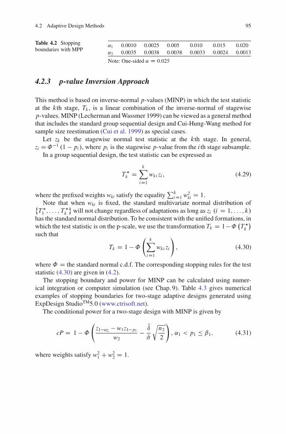
4.2 Adaptive Design Methods 95
Table 4.2 Stoppingboundaries with MPP
˛1 0.0010 0.0025 0.005 0.010 0.015 0.020˛2 0.0035 0.0038 0.0038 0.0033 0.0024 0.0013
Note: One-sided ˛ D 0:025
4.2.3 p-value Inversion Approach
This method is based on inverse-normal p-values (MINP) in which the test statisticat the kth stage, Tk , is a linear combination of the inverse-normal of stagewisep-values. MINP (Lecherman and Wassmer 1999) can be viewed as a general methodthat includes the standard group sequential design and Cui-Hung-Wang method forsample size reestimation (Cui et al. 1999) as special cases.
Let zk be the stagewise normal test statistic at the kth stage. In general,zi D˚�1 .1 � pi/, where pi is the stagewise p-value from the i th stage subsample.
In a group sequential design, the test statistic can be expressed as
T �k D
kX
iD1wki zi , (4.29)
where the prefixed weights wki satisfy the equalityPk
iD1 w2ki D 1.Note that when wki is fixed, the standard multivariate normal distribution of˚
T �1 ; : : : ; T
�k
�will not change regardless of adaptations as long as zi .i D 1; : : : ; k/
has the standard normal distribution. To be consistent with the unified formations, inwhich the test statistic is on the p-scale, we use the transformation Tk D 1�˚ �T �
k
�
such that
Tk D 1 �˚
kX
iD1wki zi
!, (4.30)
where ˚ D the standard normal c.d.f. The corresponding stopping rules for the teststatistic (4.30) are given in (4.2).
The stopping boundary and power for MINP can be calculated using numer-ical integration or computer simulation (see Chap. 9). Table 4.3 gives numericalexamples of stopping boundaries for two-stage adaptive designs generated usingExpDesign StudioTM5.0 (www.ctrisoft.net).
The conditional power for a two-stage design with MINP is given by
cP D 1 � ˚
z1�˛2 � w1z1�p1
w2�
OıO�rn2
2
!, ˛1 < p1 � ˇ1; (4.31)
where weights satisfy w21 C w22 D 1.

96 4 Adaptive Trial Design
Table 4.3 Stoppingboundaries with MINP
˛1 0.0010 0.0025 0.0050 0.0100 0.0150 0.0200˛2 0.0247 0.0240 0.0226 0.0189 0.0143 0.0087
Note: One-sided ˛ D :025; w1 D w2
4.2.4 Error-Spending Approach
MINPs have fixed weights wki regardless of the changes in the timing of the interimanalyses. For example, if the equal weights for all stages were initially decided,then whether the interim analysis was performed on 10 or 80% of the patients, theweights will not change. Theoretically we can change the weights without peekingat the data, which is exactly the notion of the so-called error-spending method (Lanand DeMets 1987).
If we define the error function as
˛�.k/ DkX
iD1�i ; (4.32)
then the familywise type-I error is controlled because ˛� .K/ D ˛.Because �k > 0 is arbitrary as long as
PKkD1 �k D ˛ (or smaller than ˛), ˛�.k/
can be any nondecreasing scale function with ˛�.K/ D 1. This is why MSP, MMP,MPP are flexible regarding �k or ˛�.k/ selection. These methods are valid if thetotal number of analysesK is modified but not based on the interim trial results, pk .
Similarly, an error-spending function can also be used for MINP as long as thetiming and the total number of analyses are not dependent on interim results. TheMINP can be expanded (i.e., allow the weights wki to be modified as long as they are
not dependent on the interim results from the trial, e.g., wki Dq
niNK
, where ni is the
subsample size per group from stage i and Nk is the cumulative sample size up to(including) stage k). Historically, the error-spending approach based on MINP with
weight wki Dq
niNK
was first developed by Lan and DeMets (1987) using a property
of a Brownian motion (Wiener process) with the error-spending function
˛�.Ik/ D8<
:2
�1 � ˚
�z1�˛=2pIk
��; for 0 < Ik � 1,
0; for Ik D 0.: (4.33)
This error-spending function ˛�.t/ is an increasing function in information timeIk D Nk=Nmax (Nmax D the maximum sample size) and satisfies the conditions˛�.0/ D 0 and ˛�.1/ D ˛; the one-sided significance level. Note that
KX
iD1�i D
KX
kD1
˛� .Ik/� ˛� .Ik�1/
D ˛� .1/ � ˛� .0/ D ˛; (4.34)
and thus familywise error is controlled.

4.3 Evaluation and Analysis of Adaptive Design 97
Table 4.4 OF-like error-spending stopping boundaries
Ik 0.3 0.4 0.5 0.6 0.7 0.8˛1 0.00004 0.00039 0.00153 0.00381 0.00738 0.01221˛2 0.22347 0.02490 0.02454 0.02380 0.02271 0.02142
Note: One-sided ˛ D :025. Computed by ExpDesign StudioTM5.0
When ˛� .Ik/ D ˛� .Ik�1/, the kth stage interim analysis is used either forfutility stopping or modifying the design (such as its randomization) but notfor efficacy stopping. Note that (4.33) is an error-spending function very similarto the O’Brien-Fleming stopping boundaries (called OF-like stopping boundary).Other commonly used error-spending functions include the Pocock-like function˛�.t/D˛ lnŒ1 C .e � 1/t� (Kim and DeMets 1992) and power family ˛�.t/ D˛t� ; � > 0.
For the two-stage design with OF-like error-spending function (4.33), thestopping boundaries are given in Table 4.4. Please keep in mind that OF-like andO’Brien-Fleming stopping boundaries are two types of stopping boundaries that arevery similar but not identical (Proschan et al. 2006; Chang 2008).
We should emphasize that the error-spending method is valid only when thetime and the number of interim analyses as well as the weight wki change areindependent of interim analysis results. It is also important to keep in mind that theerror-spending function has to be predetermined before the first interim analysis. Inother words, the error-spending function should also be independent of interim data.For example, the stopping boundaries in Tables 4.3 and 4.4 are both valid, but wehave to predetermine which one to use before we review the interim results.
4.3 Evaluation and Analysis of Adaptive Design
4.3.1 Evaluation Matrix
4.3.1.1 Stopping Probabilities
The stopping probability at each stage is an important property of an adaptive designbecause it provides the information about time-to-market. The stopping probabilitiesare also used to calculate the expected samples that measure the average cost orefficiency of the trial design.
There are two types of stopping probabilities: unconditional probability ofstopping to claim efficacy (reject Ho) and unconditional probability of stoppingto claim futility (accept Ho). The former is called the efficacy stopping probability(ESP), and the latter is called the futility stopping probability (FSP). From (4.3), itis obvious that the ESP at the kth stage is given by
ESPk D k.˛k/ (4.35)

98 4 Adaptive Trial Design
and the FSP at the kth stage is given by
FSPk D 1 � k.ˇk/: (4.36)
4.3.1.2 Expected Duration of an Adaptive Trial
The expected trial duration is definitely an important feature of an adaptive design.The conditionally (on the efficacy claim) expected trial duration is given by
Nte DKX
kD1ESPk tk; (4.37)
where tk is the time from the first patient in until the kth interim analysis.The conditionally (on the futility claim) expected trial duration is given by
Ntf DKX
kD1FSPk tk : (4.38)
The unconditionally expected trial duration is given by
Nt DKX
kD1.ESPk C FSPk/ tk: (4.39)
4.3.1.3 Expected Sample Sizes
The expected sample size is a function of the treatment difference and its variability,which are unknowns. Therefore, the expected sample size is really based onhypothetical values of the parameters. For this reason, it is important to calculatethe expected sample size under various values of the parameters. The total expectedsample size can be expressed as
Nexp DKX
kD1nk .ESPk C FSPk/ D
KX
kD1nk .1C k.˛k/� k.ˇk// , (4.40)
where nk is the sample size at stage k. Equation 4.40 can also be written as
Nexp D Nmax �KX
kD1nk . k.ˇk/� k.˛k// , (4.41)
where Nmax D PKkD1 nk is the maximum sample size.

4.3 Evaluation and Analysis of Adaptive Design 99
4.3.1.4 Conditional Power and Futility Index
The conditional power is the conditional probability of rejecting the null hypothesisduring the rest of the trial based on the observed interim data so far. The conditionalpower is commonly used for monitoring an ongoing trial. Similar to the ESP andFSP, conditional power is dependent on the population parameters or treatmenteffect and its variability. The conditional power at the kth stage is the sum of theprobability of rejecting the null hypothesis at stage k C 1 through K (K does nothave to be predetermined), given the observed data from stages 1 through k,
cPk DKX
jDkC1Pr�\j�1iDkC1 .ai < Ti < ˇi/\ Tj � ˛j j \k
iD1 Ti D ti
�, (4.42)
where ti is the observed test statistic Ti at the i th stage. For a two-stage design, theconditional power can be expressed as
cP1 D Pr .T2 � ˛2jt1/ . (4.43)
Specific formulations of conditional power for two-stage designs with MSP,MPP, and MINP were provided in earlier sections.
The futility index is defined as the conditional probability of accepting the nullhypothesis:
FIk D 1 � cPk: (4.44)
Computer algorithms and programs for calculating the operating characteristicsof an adaptive design can be found elsewhere (Chang 2007b, 2010).
4.3.2 Analysis of Adaptive Trial Data
4.3.2.1 Parameter Estimation
Unbiased estimation of parameters is challenging adaptive design. Let’s start witha two-stage standard group sequential design. Consider the hypothesis test formean �:
Ho W � � 0 versusHa W � > 0:Let xij be the independent observations from the j th patient at the kth stage
(k D 1; 2 and j D 1; : : : ; ni ). Assume xij has the normal distribution N��; �2
�
with known � . Denote by Nxk the stagewise sample mean at the kth stage (not basedon cumulative data), thus Nx1 and Nx2 are independent. The test statistic at the firststage of the standard group sequential design can be written as T1 D Nx1pn1=� ,where n1 is the sample size at the first stage. The stopping rule at the first stageis: stop the trial if T1 � c1 (p1 � ˛1 on the p-scale) and continue otherwise. It isobvious that T1 D Nx1pn1=� � c1 implies x1 � �c1=
pn1.

100 4 Adaptive Trial Design
The expectation of the conditional mean at the first stage is
�1 DR1�c1=
pn1
Nx1f NX1 . Nx1/ d Nx1R1�c1=
pn1f NX1 . Nx1/ d Nx1
. (4.45)
The expectation of the conditional mean at the second stage is
�2 DR �c1=pn1
�1R1
�1Nx1n1C Nx2n2n1Cn2 f NX1 . Nx1/ f NX2 . Nx2/ d Nx1d Nx2
R �c1=pn1�1 f NX1 . Nx1/ d Nx1
DR �c1=pn1
�1n1 Nx1Cn2�n1Cn2 f NX1 . Nx1/ d Nx1
R �c1=pn1�1 f NX1 . Nx1/ d Nx1
. (4.46)
For normal distribution f NXk . Nx1/ D N� NXk I�; �2=ni
�, we have
�1 D 1
1 �˚0 .c�/
Z 1
�c1=pn1
Nx1 1p2��2=n1
e�.Nx1��/2n1
2�2 d Nx1
D �C� exp
�� c2
�
2
�
Œ1 � ˚0 .c�/�p2�n1
, (4.47)
where c� D c1 � �pn1=�:
If n2 is independent of x1 (i.e., there is no sample size adjustment), then
�2 D 1
˚0 .c�/
Z �c1=pn1
�1n1 Nx1 C n2�
n1 C n2
1p2�=n1
e�.Nx1��/2n1
2�2 d Nx1
D n1
n1 C n2
�� � �
˚0 .c�/p2�n1
exp
��c
2�2
��C n2
n1 C n2�
D � �n1� exp
�� c2
�
2
�
.n1 C n2/˚0 .c�/p2�n1
: (4.48)
From (4.47) to (4.48), the expectation of the conditional mean can beexpressed as
�naive D Œ1 � ˚0 .c�/� �1 C˚0 .c�/ �2 D �C n2
n1 C n2
�p2�n1
exp
��c
2�2
�.
(4.49)
The bias can be calculated as
�bias D �naive � � D n2
n1 C n2
�p2�n1
exp
��c
2�2
�<
�p2�n1
: (4.50)

4.3 Evaluation and Analysis of Adaptive Design 101
To calculate the bias, the standard normal c.d.f. can be approximated by
˚0 .c/ D 1 � .c2 C 5:575192695cC 12:77436324/ exp��c2=2�p
2�c3 C 14:38718147c2 C 31:53531977cC 2.12:77436324/.
(4.51)
The error of approximation (4.51) is less than 1:9 � 10�5 over 0 � c < 1. Thelargest error occurs when c ranges from 1.03 to 1.04 (Yun 2009).
In my view, the conditional estimate is more important than the unconditionalestimate. The reason is simple: We know from (4.47) to (4.48) that Nx1 is biasedupward and Nx2 is biased downward. If the trial stops at stage 1, we should reportNx1 with the adjustment given by (4.47). On the other hand, if the trial stops atstage 2, we should report Nx2 with the adjustment given by (4.48). It doesn’t makesense to report xk with the overall adjustment given by (4.49), especially whenthe trial stops at stage 2, and adjust x2 downward using (4.49), knowing that x2is already biased downward. Although both the conditional and overall adjustmentscan provide unbiased estimates, the conditional adjustment makes much more sense.
Equations 4.45–4.50 are valid for MINP, MSP, and MPP because the naive meanis determined by the c1 (or ˛1) and n1 independent of the definition of the teststatistic for the two-stage designs. In other words, for two-stage designs, there arealways equivalent stopping boundaries for any two adaptive design methods (MSP,MPP, MINP). However, this conclusion is applicable to a design with more than twostages because such equivalent boundaries don’t exist in general.
In general K-stage design, the expectation of the unconditional mean at the nthstage is
�n DR˝1
� � � R˝n�1
R1�1
Nx1n1C���C Nxnnnn1C���Cnn f NX1 : : : NXn . Nx1; : : : ; Nxn/ d Nx1 : : : d Nxn
R˝1
� � � R˝n�1
R1�1 f NX1 : : : NXn . Nx1; : : : ; Nxn/ d Nx1 : : : d Nxn
, (4.52)
where if xi 2 ˝i , the trial will continue to the .i C 1/th stage.For an adaptive design with a sample size adjustment, the calculation of bias is
more complicated because sample size at the second stage, n2, is a function of x1.Several sample size reestimation rules have been proposed such as the conditionalpower approach. These rules will lead to different functions of n2 .x1/, and integral(4.46) can only be carried out using numerical methods or simulations.
For a K-stage design, the integral (4.52) may sometimes be easier in p-scale,which may involve the p-value distribution under the alternative hypothesis. Thep-value distribution can be easily derived.
Denote by f o .t/ > 0 and f a .t/ the distributions of the test statistic T underthe null hypothesisHo and the alternative hypothesisHa, respectively. The p-valuefor a one-sided test is defined as p .t/ D R1
t f o ./ d . To derive the distributionof p-value p .t/ under Ha , we start with the c.d.f. identity: FT .t/ D FP .p .t//.
102 4 Adaptive Trial Design
Taking the derivative with respect to p (Kokoska and Zwillinger 2000, p. 40), weobtain the p.d.f. of the p-value:
P � fP .p/ D f a .t/1
jdp.t/=dt j D f a .t/
f o .t/; (4.53)
where t is function of p.When the null hypothesis Ho is true, f a .t/ D f o .t/, p-value P has a uniform
distribution in Œ0; 1�.
4.3.2.2 Confidence Interval
The confidence interval calculation is usually complicated for adaptive designs.There are even several different versions of confidence intervals. The so-calledrepeated confidence interval at the k, RCIk , consists of all possible values for theparameter for which the null hypothesis will not be rejected given the observedvalue. When xij is normally distributed and MINP, the RCIk can be expressed as
. Nx � ck� Nx; Nx C ck� Nx/;
in ck is the stopping boundary at the kth stage and � Nx is the standard deviation of Nx.A general approach to obtain RCIk numerically is through Monte Carlo
simulations, but we are not going to discuss the simulation details here.
4.3.3 Comparison of Adaptive Design Methods
Different adaptive methods have different stopping boundaries, as shown in Fig. 4.1for MSP, MPP, and MINP for two-stage adaptive designs. Because of the differencesin the stopping boundaries, the same data can lead to different conclusions withdifferent methods. For example, for data point A with p1 D 0:025 and p2 D 0:008,the null hypothesis is rejected by all three methods. However, for data point B withp1 D 0:01 and p2 D 0:25, the null hypothesis is rejected by MPP and MINP but notby MSP. Yet for data point C with p1 D 0:07 and p2 D 0:12, the null hypothesis isrejected by MSP but not by MPP or MINP.
Conditional power is an important feature of an adaptive design. The conditionalpower curves for different methods (MSP, MPP, and MINP) are constructed basedon (4.23), (4.28), and (4.31) with ˛1 D 0:005 (Fig. 4.2). We know that when atrial is appropriately powered (�90%), the interim p-value is mostly near the targetvalue ˛ D 0:023 (one-sided) or smaller. When a trial is underpowered, the interimp-value would be mostly near 0.1. Since an important goal of sample sizereestimation is to save the trial when it is underpowered, we should focus on theconditional power when the interim p-value is near 0.1. As we can see from Fig. 4.2,MSP (or equivalently MMP) has higher power near one-sided p1 D 0:1 than MPP
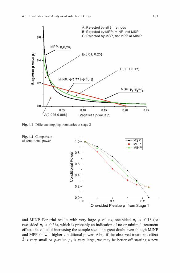
4.3 Evaluation and Analysis of Adaptive Design 103
Fig. 4.1 Different stopping boundaries at stage 2
Fig. 4.2 Comparisonof conditional power
0.0 0.1 0.20.0
0.2
0.4
0.6
0.8
1.0
Con
ditio
nal P
ower
One-sided P-value p1 from Stage 1
MSPMPPMINP
and MINP. For trial results with very large p-values, one-sided p1 > 0:18 (ortwo-sided p1 > 0:36), which is probably an indication of no or minimal treatmenteffect, the value of increasing the sample size is in great doubt even though MINPand MPP show a higher conditional power. Also, if the observed treatment effectOı is very small or p-value p1 is very large, we may be better off starting a new

104 4 Adaptive Trial Design
trial than continuing the current trial. Having said that, we may be curious aboutthe reality of underpowered trials. In fact, the recent approval rate for NDAs (newdrug applications) submitted to the FDA is about 40%. In contrast, the power formost phase-III trials is about 90%. Considering there are phase-III trials withdrawnby sponsors before they are rejected by the FDA, the failure rate of phase-IIIclinical trials is realistically more than 60%, which clearly indicates there are plentyof trials that are underpowered due to overestimating the treatment difference orunderestimating its variance. The challenge is that we don’t know which trials areunderpowered, and thus uniformly increasing the sample size across all trials is nota wise practice. This is exactly the reason for introducing an adaptive design withsample size reestimation.
In additional to the conditional power, another commonly used method tocompare different adaptive design methods is based on the power of the hypothesistest or equivalently the sample size (maximum or expected sample sizes). Thesetypes of criteria are often not very informative for adaptive design because they havenot considered the magnitude of treatment difference and reduction in trial durationor time-to-market as well as the flexibility of adaptive designs that allow mitigationof the risks later. A better approach is to use the decision theory discussed in Chap. 2.To illustrate this, let’s construct a utility function. We know that the magnitude of adrug effect (e.g., years of survival prolongation) often plays a critical role in termsof the benefit to patients and the profit of the drug maker. Because the true treatmenteffect (parameter ı for treatment difference) is not known, we use the observedtreatment difference Oı for the purpose of constructing utility,
U D Oır � C; (4.54)
where r > 0 is a constant and C is the associated cost, which is often a function ofsample size. The expected utility is given by
NU DZI�˛ � p
� Oı�� Oı df
� Oı�
, (4.55)
where I.x/ is an indication function with value 1 if x � 0 and 0 otherwise, thep-value p. Oı/ is a function of the observed treatment difference Oı, ˛ is the levelof significance, and f . Oı/ is the p.d.f. of Oı. I.˛ � p. Oı// � 0 implies achievementof statistical significance or rejection of the null hypothesis. The constant r shouldbe constructed at least based on the clinical and commercial values. The expectedutility (4.51) can be easily calculated using simulations after the cost and r aredetermined.
In Tables 4.5 and 4.6, we present some typical simulation results, both power andthe utility U , respectively, for SSR trials. In the utility comparison, we use r D 1
and remove the cost factor by making the expected sample size (cost) the same.From the tables, we can see that when the trial is underpowered, MSP is better
than MPP and MINP in terms of power. MINP always has slightly higher powerthan MPP. When the power reaches around 70% or higher, MINP is better than

4.4 Adaptive Designs in Action 105
Table 4.5 Comparison of power from MSP (MMP), MPP, and MINP
ı=� 0.1 0.15 0.2 0.25 0.3 0.35Nn 173 180 180 175 166 153MSP(MMP) 0.182 0.334 0.514 0.686 0.824 0.915MPP 0.161 0.308 0.496 0.685 0.835 0.928MINP 0.161 0.315 0.507 0.696 0.843 0.933
Note: Nn D expected sample size , � D 1. Best values are highlighted
Table 4.6 Expected utilities from MSP(MMP), MPP, and MINP
ı=� 0.1 0.15 0.2 0.25 0.3 0.35Nn 173 180 180 175 166 153MSP(MMP) 9.62 17.9 27.8 37.6 46.0 51.7MPP 7.69 15.2 25.3 36.0 45.3 51.6MINP 7.90 15.5 25.7 36.5 45.6 51.8
Note: Nn D expected sample size, � D 1. Best values are highlighted
MSP or MMP (MSP) (Table 4.5). In terms of utility defined by (4.50) with r D 1,MMP (MSP) is better until the power reaches about 90% or higher (Table 4.6). Thenotion of the adaptive design with SSR reminds us to focus on situations wherethe trial is underpowered. As we discussed earlier, a majority of phase-III trials areunderpowered. For this reason, among others, MMP or MSP is recommended forSSR. Keep in mind that the uniformly most powerful test for the classic design maynot be applicable in the context of adaptive designs (see Sect. 4.5.2).
4.4 Adaptive Designs in Action
4.4.1 Sample Size Reestimation
Sample size determination is critical in clinical trial designs. It is estimated at about5,000 patients per NDA on average (Mathieu 2008). The average cost per patientranges from $20,000 USD to $50,000 USD. A small but adequate sample sizewill allow sponsors to use their resources efficiently, shorten the trial duration, anddeliver the drug to the patients earlier.
From the efficacy point of view, sample size is often determined by the power forthe hypothesis test of the primary endpoint. However, the challenge is to estimateprecisely the treatment effect and its variability at the time of protocol design. Ifthe effect size of the NME is overestimated or its variability is underestimated, thesample size will be underestimated and consequently the power will be too low tohave a reasonable probability of detecting a clinically meaningful difference. Onthe other hand, if the effect size of the NME is underestimated or its variabilityis overestimated, the sample size will be overestimated and consequently the

106 4 Adaptive Trial Design
power will be unnecessarily higher, which could lead to unnecessary exposure ofmany patients to a potentially harmful compound when the drug in fact is noteffective. The commonly used adaptive design, called sample size reestimation(SSR), emerged to provide a remedy for this problem.
An SSR design refers to an adaptive trial that allows for sample size adjustmentor reestimation based on the review of interim analysis results. There are two typesof sample size reestimation procedures, based on blinded and unblinded data. In thefirst scenario, the sample size adjustment is based on the (observed) pooled varianceat the interim analysis to recalculate the required sample size, which does notrequire unblinding the data. In this scenario, the type-I error adjustment is usuallynegligible. In the second scenario, the effect size and its variability are re-assessed,and the sample size is adjusted based on the unblinded treatment information. Thestatistical method for the adjustment can be based on the observed effect size or theconditional power.
For a two-stage trial with two parallel groups, the sample size per group for thesecond stage, n2, can be calculated based on the target conditional power
8ˆˆ<
ˆˆ:
n2 D 2 O�2Oı2�z1�˛2Cp1 � z1�cP
�2, for MSP,
n2 D 2 O�2Oı2�z1�˛2=p1 � z1�cP
�2, for MPP,
n2 D 2 O�2Oı2�
z1�˛2w2
� w1w2
z1�p1 � z1�cP�2
, for MINP,
(4.56)
where, for the purpose of calculation, Oı and O� are taken to be the observed treatmenteffect and standard deviation at stage 1, and cP is the target conditional power.
For a general K-stage design, the sample size rule at the kth stage can be basedon the observed treatment effect in comparison with the initial assessment:
nj D�ı
Nı�2n0j ; j D k; k C 1; : : : ; K; (4.57)
where n0j is the original sample size for the j th stage, ı is the initial assessment for
the treatment effect, Nı is the updated assessment after interim analyses, given by
Nı DPk
iD1 ni OıiPkiD1 ni
for MMP and MPP, (4.58)
Nı DkX
iD1w2ki
Oıi for MINP. (4.59)
The stagewise p-value pc given by (4.4) can be calculated using the Monte Carlomethod. Specifically, if the trial is stopped at the Qkth stage with T Qk D t Qk , then the
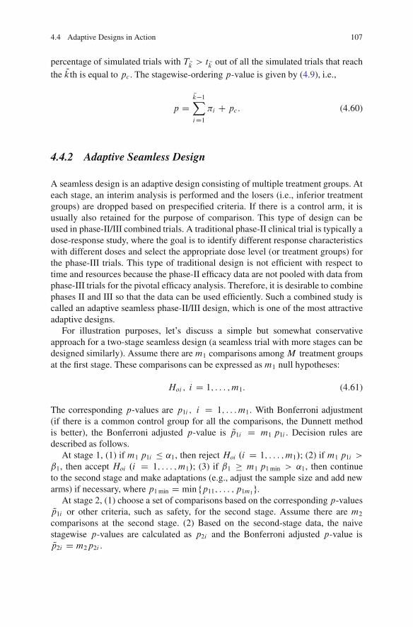
4.4 Adaptive Designs in Action 107
percentage of simulated trials with T Qk > t Qk out of all the simulated trials that reachthe Qkth is equal to pc . The stagewise-ordering p-value is given by (4.9), i.e.,
p DQk�1X
iD1�i C pc: (4.60)
4.4.2 Adaptive Seamless Design
A seamless design is an adaptive design consisting of multiple treatment groups. Ateach stage, an interim analysis is performed and the losers (i.e., inferior treatmentgroups) are dropped based on prespecified criteria. If there is a control arm, it isusually also retained for the purpose of comparison. This type of design can beused in phase-II/III combined trials. A traditional phase-II clinical trial is typically adose-response study, where the goal is to identify different response characteristicswith different doses and select the appropriate dose level (or treatment groups) forthe phase-III trials. This type of traditional design is not efficient with respect totime and resources because the phase-II efficacy data are not pooled with data fromphase-III trials for the pivotal efficacy analysis. Therefore, it is desirable to combinephases II and III so that the data can be used efficiently. Such a combined study iscalled an adaptive seamless phase-II/III design, which is one of the most attractiveadaptive designs.
For illustration purposes, let’s discuss a simple but somewhat conservativeapproach for a two-stage seamless design (a seamless trial with more stages can bedesigned similarly). Assume there are m1 comparisons among M treatment groupsat the first stage. These comparisons can be expressed as m1 null hypotheses:
Hoi ; i D 1; : : : ; m1: (4.61)
The corresponding p-values are p1i ; i D 1; : : :m1: With Bonferroni adjustment(if there is a common control group for all the comparisons, the Dunnett methodis better), the Bonferroni adjusted p-value is Qp1i D m1 p1i . Decision rules aredescribed as follows.
At stage 1, (1) if m1 p1i � ˛1, then reject Hoi .i D 1; : : : ; m1/; (2) if m1 p1i >
ˇ1, then accept Hoi .i D 1; : : : ; m1/; (3) if ˇ1 � m1 p1min > ˛1, then continueto the second stage and make adaptations (e.g., adjust the sample size and add newarms) if necessary, where p1min D min fp11; : : : ; p1m1g.
At stage 2, (1) choose a set of comparisons based on the corresponding p-valuesQp1i or other criteria, such as safety, for the second stage. Assume there are m2
comparisons at the second stage. (2) Based on the second-stage data, the naivestagewise p-values are calculated as p2i and the Bonferroni adjusted p-value isQp2i D m2p2i .

108 4 Adaptive Trial Design
If MSP is used, the decision rules at stage 2 are: if Qp1i C Qp2i D m1p1i Cm2p2i �˛2, then rejectHoi .i D 1; : : : ; m2/; otherwise, don’t reject the null. The global nullhypothesis can be rejected as long as m1p1min C m2p2min � ˛2, where p2min Dfp21; : : : ; p2m2g.
Bauer and Kieser (1999) provided a two-stage method for this purpose, whereinvestigators can terminate the trial entirely or drop a subset of treatment groups forlack of efficacy after the first stage. Shun et al. (2008) developed a simple methodusing normal approximation.
Let’s consider a drop-loser design with three arms: A, B; and C (control). Atthe first stage, we perform two pairwise comparisons: A versus C and B versus C .The corresponding p-values are denoted by p1A and p1B . If p1A < p1B , arm B isdropped; otherwise, arm A is dropped. If we don’t drop any arm, the p-values forthe two comparisons at the final stage are denoted by pA and pB . It is obvious thatp1A, p1B , pA, and pB are uniformly distributed under the global null that impliesall three arms are equally effective. For the drop-loser design, we are interested inthe statistic
Zw D IABZA C .1 � IAB/Z
B; (4.62)
where IAB D 1 if arm B is dropped; otherwise, IAB D 0, ZA D ˚.1 � pA/, andZB D ˚.1 � pB/.
Shun et al. (2008) found that, under the global null hypothesis, Zw is approxi-mately normally distributed with mean E .Zw/ D p
2�
and var.Zw/ D 1 � 2�
,where the information time for the interim analysis D n1
n(the sample size fraction
at the interim analysis). Therefore they proposed as a test statistic
Zws D Zw �p2�p
1 � 2�
, (4.63)
which has approximately the standard normal distribution under the global nullhypothesis that treatments A, B , and C have the same treatment effect.
The approximate p-value hence can be easily obtained: pA D 1�˚ .Zws/ : Theexact p-value is given by
p D pA C 0:0003130571 .4:444461/� 0:00033. (4.64)
Note that we have used the inverse-normal transformation to generalize the Shen-Lan-Soo method to binary and survival endpoints.
4.4.3 Noninferiority-Superiority Adaptive Design
For a standard K-stage group sequential trial, usually either a superiority ornoninferiority test is performed at each stage. However, it is often of interest topharmaceutical companies to perform both superiority (HS ) and noninferiority(HNI) tests in a single trial. Wang et al. (2001) proposed a procedure to test

4.5 Adaptive Design Debates 109
superiority and noninferiority simultaneously in a single adaptive design, where anoninferiority test procedure with a fixed margin was used. Recall that the standardgroup sequential design is a special case of MINP. The authors proposed twoclosed test procedures, referred to as GSC S-NI and GSC NI-S, as illustrated inFig. 4.1. Both procedures control the maximum total type-I error probability forboth noninferiority and superiority at the ˛ level. Furthermore, the GSC procedureachieves the power for superiority at the planned level ˛ (i.e., not a reduced power)because of testing superiority and noninferiority simultaneously. The proceduresare established on the usual lower limit of the confidence interval, LLi , for thetreatment difference from the i th interim analysis. The fixed noninferiority marginis denoted by ıNI (see Chap. 3, Sect. 3.1.3.1).
The procedure GSC S-NI is described as follows:
1. At stage i , if LLi > 0, then claim superiority and stop the trial; otherwise,continue to step 2.
2. If LLi > �ıNI , then claim noninferiority; otherwise, the trial continues to stagei C 1 (if i C 1 > K , conclude noninferiority).
The procedure GSC NI–S is described as follows:
1. At stage i , if LLi > �ıNI , then claim noninferiority and continue examining forsuperiority:
a. If LLi > 0, then claim superiority and stop.b. If LLi � 0, continue on step 2.
2. If LLi > 0, then claim superiority and stop; otherwise continue to stage iC1 andrepeat steps 1 and 2 until loop over all the stages.
These two procedures imply that we can test superiority and noninferiorityseparately in the sequential trial. Superiority can be claimed regardless of thenoninferiority claim as long as the superiority hypothesis HS is rejected at a stage.Similarly, noninferiority can be claimed regardless of the superiority claim as longas the noninferiority hypothesisHNI is rejected at a stage.
Wang et al. (2001) proved that the previous closed procedures are also validfor a two-stage adaptive design with SSR at the interim analysis using a methodequivalent to MINP.
4.5 Adaptive Design Debates
4.5.1 Sufficiency Principle
Jennison and Turnbull (2003), Posch et al. (2003), and Burman and Sonesson (2006)pointed out that the adaptive design using a weighted statistic violates the sufficiencyprinciple because it weighs the same amount of information from different stages

110 4 Adaptive Trial Design
differently. Michael A. Proschan (Burman and Sonesson 2006, discussion) provedthat no test based on the sufficient statistic can maintain a level ˛ irrespective ofwhether the prespecified sample size rule is followed.
The “unweighted test” utilizes the distribution of sample size N to choose acritical level with the desired probability of rejecting the null hypothesis uncon-ditional on N but disregards the observed value of N . Because N is part of theminimal sufficient statistic, it is not in accordance with the sufficiency principle andis inefficient (Marianne Frisen, in Burman and Sonesson 2006, discussion).
The key question is: should information (or sufficiency of a statistic) regarding� be based on data or data + procedure? The conclusion that each observationcontains the same amount of information is valid in a classic design but not inan adaptive design because a later observation contains some information fromprevious observations due to the dependent sampling procedure. Therefore, aninsufficient statistic in a classic design can become sufficient under an adaptivedesign. For example, suppose we want to assess the quantity # D 1�RB
1�RA , whereRA and RB are the true response rates in groups A and B , respectively. In aclassic design with balanced randomization, NA
NBis asymptotically approaching 1.
However, in the randomized play-the-winner design, NANB
asymptotically converges
to #: Therefore, the same data NANB
could contain different amounts of information indifferent designs.
4.5.2 Minimum Sufficiency Principle and Efficiency
Jennison and Turnbull (2006) raised the question as to when an adaptive designusing nonsufficient statistics can be improved upon by a nonadaptive groupsequential design. Tsiatis and Mehta (2003) have proved that for any SSR adaptivedesign there exists a more powerful group sequential design. On the other hand, theweighted method (or MINP) provides great flexibility, and when the sample sizedoes not change, it has the same power as the classic group sequential design.
It is really analogous with a two-player game. Player A says to player B: if youtell me the sample size rule, I can find a group sequential design (with as manyanalyses as I want to have) that is more efficient than the adaptive design. Player Bsays to playerA: if you tell me how many and when you plan the interim analyses, Ican produce an adaptive trial with the same number and timing of the analyses thatis more flexible, and if the sample size does not change, it is identical to the groupsequential design.
4.5.3 Conditionality and Exchangeability Principles
Burman and Sonesson (2006) pointed out that SSR also violates the invarianceand conditionality principles because the weighted test depends on the orderof exchangeable observations. Marianne Frisen (Burman and Sonesson 2006,

4.5 Adaptive Design Debates 111
discussion) stated similarly: “The ‘weighted’ test avoids this by forcing a certainerror spending. This is done at the cost of violating the conditionality principle.The ordering of the observations is an ancillary statistic for a conclusion aboutthe hypothesis. Thus, by the conditionality principle the test statistic should notdepend on the ordering of the realized observations.” For a general distribution, notbelonging to the exponential family, the weighted test will violate the conditionalityprinciple but not the sufficiency principle (Burman and Sonesson 2006).
If sufficiency and conditionality are important, then the combination of the two isthe likelihood principle, which also faces challenges (Robert 1997; Chang 2007a).
4.5.4 Equal Weight Principle
Exchangeable observations should be weighted equally in the test statistic. Theequal weight principle views exchangeability from the weight perspective. However,the measurement of the information level is not unique. For example observation xi ,1=xi , or pi can be counted as the unit of information. The adaptive design methodMSP equally weights the evidence (pi ) againstHo from the two stages.
It has been misunderstood that the classic group sequential design equallyweights information, but actually it does not because the observations from thefirst stage have the potential of being used more than once in decision-making(hypothesis-testing); e.g., if ˇ2 > p1 > ˛1, the trial continues and the data fromthe first stage will be combined with data from the second stage to calculate the teststatistic for rejecting or accepting the null hypothesis. The patients from the firststage have the chance of “voting twice or more” in the decision process.
4.5.5 Consistency of Stagewise Results
Compared with the classic design, adaptive designs naturally allow for an interimlook to check the consistency of results from different stages. If p1 and p2 are verydifferent, we may have to look at the reasons, such as baseline difference, genedifference, and others. The question is should we check this consistency for a classicdesign, too, by splitting the data in different ways?
It is also controversial in adaptive designs (including group sequential designs)that we often reject the null hypothesis with weaker evidence but don’t rejectthe null hypothesis with stronger evidence. For example, in a two-stage groupsequential design with the O’Brien-Fleming spending function (˛1 D 0:0025 and˛2 D 0:0238/, we will not reject the null when the p-value D 0:003 > ˛1 at theinterim look but we do reject the null when the p-value D 0:022 < ˛2. Why don’twe reject the null hypothesis when the evidence against the null is stronger (p-valueD 0.003) and rejectHo when the evidence is much weaker (p-value D 0.022)? Let’selaborate on the controversy using the following patient-statistician dilemma.

112 4 Adaptive Trial Design
Suppose you are a patient and a statistician. As a patient, you have to be treatedwith some drug. As a statistician, you have designed two trials for two NMEs (newmolecular entities) for a therapeutic indication with classical and adaptive features,respectively. As a patient, you have specified the criteria for selecting the treatment:rank the two p-values for the efficacy tests from the two NME trials and pick theNME with a smaller associated p-value.
Suppose now that NME 1 with a classical design has tested with 30% improve-ment (p D 0:04 < ˛ D 0:05), statistically significant, whereas NME 2 with anadaptive design has been tested with 50% improvement and the final p D 0:026,which is not statistically significant due to the multiple looks at the data. You furtherexamine the sample size and variability of the efficacy data; they are similar betweenthe two groups. The safety, tolerability, cost, and convenience of drug administrationare all similar between the two NMEs. As a statistician for the trials, you shouldrecommend NME 1 for treating the disease; as a patient with that disease, you willtake NME 2. Since you are the statistician with the disease, what do you do?
4.5.6 Adjusted p-value
Controversies surrounding p-values have been discussed in Chap. 1. Ourdiscussions here focus on the p-value issues that are particular to adaptive design.The type-I error control is not very challenging, and most adaptive designs controlthe familywise error. However, because hypothesis-testing is primarily based onthe concept of repeated experiments, the scope in which the experiment willpotentially be repeated is critical. In clinical trials, we virtually never test thesame compound for the same indication in a phase-III study repeatedly. For thisreason, the implication of control of the experimental error rate ˛ may be totallydifferent from what we initially intended.
The definition, not the calculation, of the p-value is challenging because thereare so many options for an adaptive design. Remember that the p-value is theprobability of the test statistic under the null hypothesis being more extreme thanthe critical point. The key lies in how the extreme should be defined. Unlike in aclassic design, definitions of extremeness of a test statistic can be defined in manydifferent ways in adaptive designs (e.g., stagewise ordering, sample mean ordering,and likelihood ratio ordering). None of these definitions simultaneously satisfiesthe concerns raised from statistical, scientific, and ethical perspectives. Similarly,an agreeable definition and calculations of the unbiased point estimate and theconfidence interval remain challenging for adaptive designs.
4.5.7 Summary
Adaptive designs violate several commonly accepted statistical principles. Theviolations on the one hand remind us to adopt the new approaches with extreme
4.6 Exercises 113
caution. On the other hand, the new approaches may suggest that principles ofinference only go so far and that new principles may be desirable. Indeed, adaptivedesigns present great challenges to frequentist statistics and conventional thinkingin development. Group sequential designs have been widely used in clinical trials;however, there are many controversial issues with these designs that are only fullyrealized when we widen the concept to a more general category of adaptive designs.
It is obvious that efficiency in clinical trials is not identical to the power ofhypothesis-testing. In clinical trials, the concept of efficiency often includes thepower, the time-to-market, and the operational flexibility. Overemphasizing thepower can be very misleading when evaluating adaptive designs. This simple fact isoften overlooked.
Despite the challenges, adaptive designs have been proved useful in practice andmore and more clinical trials have adopted.
4.6 Exercises
4.1. In a two-arm comparative oncology trial, the primary efficacy endpoint is timeto progression (TTP). The median of TTP is estimated to be 8 months (hazard rateD 0.08664) for the control group and 10.5 months (hazard rate D 0.06601) for thetest group. Assume the trial has a uniform enrollment with an accrual period of 9months and a total study duration of 24 months. The log-rank test will be used forthe analysis. An exponential survival distribution is assumed for the purpose of thesample size calculation. The classic design requires a sample size of 323 subjectsper group. Design a group sequential trial using MMP, MPP, and MINP.
4.2. Use each of the adaptive methods (MMP, MPP, and MINP) to design a two-stage trial with a sample size reestimation. Assume the stopping boundary for thefirst stage ˛1 D 0:01, the effect size ı=� D 0:2, and power D 40%. The sample sizeadjustment at the interim analysis is based on (4.52) or (4.53). Compare the sixexpected sample sizes NN under the condition ı=� D 0:2 between the two methods.(Hint: Computer simulation programs can be downloaded from www.statisticians.org.)
4.3. In Exercise 4.1, assume the sample size adjustment is based on the followingformulation. The sample size per group for the second stage is determined by
n2 D p1 .
Determine the constant to minimize the expected sample size NN under thecondition ı=� D 0:2 and ˛ D 0:01. (Hint: For a given , adjust the maximumsample size Nmax such that power D 40%.)
4.4. Compare the nine expected sample sizes obtained from Exercises 4.2 and 4.3.Summarize your findings.
114 4 Adaptive Trial Design
4.5. Assume a classic three-arm trial including placebo, low-dose, and high-dosegroups. The objective is to prove either the low dose or high dose is effectivecompared with the placebo at the level ˛ D 5% using the Dunnett method (seeChap. 1). Calculate the total sample size required for the trial design. Then take anadaptive seamless design using the Shun-Lan-Soo method and compare the samplesize against that from the classic design.
4.6. Suppose that in a classicm-group dose-finding trial with a continuous response(variance �2 D 1) the test statistics for pairwise comparisons are defined as
Zi D Nxi � Nx0pn
;
where Nxi is the mean of the i th group, i D 0 for the control group, and n is thesample size per group. Study (analytically or numerically using simulation) thedistributions of the following order statistics:
Z.1/ <; : : : ; < Z.m/:
4.7. Do you believe the exchangeability holds between an observation from the firststage and an observation from the second stage of the adaptive design? Why?
Further Readings and References
Bauer, P., Kieser, M.: Combining different phases in development of medical treatments within asingle trial. Stat. Med. 18, 1833–1848 (1999)
Bauer, P., Kohne, K.: Evaluation of experiments with adaptive interim analysis. Biometrics 50,1029–1041 (1994)
Bauer, P., Rohmel, J.: An adaptive method for establishing a dose-response relationship. Stat. Med.14, 1595–1607 (1995)
Burman, C.F., Sonesson, C.: Are flexible designs sound? (with discussion). Biometrics 62,664–683 (2006)
Chang, M.: Adaptive Design Theory and Implementation Using SAS and R. Chapman andHall/CRC, Boca Raton (2007a)
Chang, M.: Adaptive design method based on sum of p-values. Stat. Med. 26, 2772–2784 (2007b)Chang, M., et al.: BIO White Paper: Innovative approaches in drug development. J. Biopharm.
Stat. 17, 775–789 (2007c)Chang, M.: Classical and Adaptive Designs Using ExpDesign Studio. Wiley, New York (2008)Chang, M.: Monte Carlo Simulations for the Pharmaceutical Industry: Concepts, Algorithms, and
Case Studies. Chapman and Hall/CRC, Boca Raton (2010)Chang, M., Chow, S.C., Pong, A.: Adaptive design in clinical research – Issues, opportunities, and
recommendations. J. Biopharm. Stat. 16, 299–309 (2006)Chow, S.C., Chang, M.: Statistical consideration of adaptive methods in clinical development.
J. Biopharm. Stat. 15, 575–591 (2005)Chow, S.C., Chang, M.: Adaptive Design Methods in Clinical Trials. Chapman and Hall/CRC,
Boca Raton (2006)

Further Readings and References 115
Cui, L., Hung, H.M.J., Wang, S.J.: Modification of sample-size in group sequential trials.Biometrics 55, 853–857 (1999)
FDA: Guidance for Industry: Adaptive Design Clinical Trials for Drugs and Biologics (draft).www.fda.org (2010). Accessed 12 Mar 2010
Gallo, P., Chuang-Stein, C., Dragalin, V., Gaydos, B., Krams, M., Pinheiro, J.: Adaptive designsin clinical drug development – an executive summary of the PhRMA Working Group. J.Biopharm. Stat. 16, 275–283 (2006)
Hu, F., Rosenberger, W.: The Theory of Response-Adaptive Randomization in Clinical Trials.Wiley, Hoboken (2006)
Jennison, C., Turnbull, B.W.: Mid-course sample size modification in clinical trials. Stat. Med. 22,971–993 (2003)
Jennison, C., Turnbull, B.W.: Adaptive and non-adaptive group sequential tests. Biometrika 93,1–21 (2006)
Kim, K., DeMets, D.L.: Sample size determination for group sequential clinical trials withimmediate response. Stat. Med. 11, 1391–1399 (1992)
Kokoska, S., Zwillinger, D.: Standard Probability and Statistical tables and Formula. Chapman &Hall/CRC, Boca Raton (2000)
Lan, K.K.G., DeMets, D.L.: Group sequential procedures: Calendar versus information time. Stat.Med. 8, 1191–1198 (1987)
Lehmacher, W., Wassmer, G.: Adaptive sample size calculations in group sequential trials.Biometrics 55, 1286–1290 (1999)
Ling, X., Hsu, J.: Using the partitioning principle to adaptively design dose-response studies. J.Biopharm. Stat. 16, 733–743 (2006)
Mathieu, M.P. (ed.): PAREXEL’s Bio/Pharma R&D Statistical Sourcebook 2007/2008. PAREXEL.PH (2008)
Muller, H.H., Shafer, H.: A general ststistical principle of changing a design any time during thecourse of a trial. Stat. Med. 23, 2497–2508 (2004)
O’Brien, P.C., Fleming, T.R.: A multiple testing procedure for clinical trials. Biometrika 35,549–556 (1979)
Pocock, S.J.: Group sequential methods in the design and analysis of clinical trials. Biometrika 64,191–199 (1977)
Posch, M., Bauer, P., Brannath, W.: Issues on flexible designs. Stat. Med. 22, 953–969 (2003)Proschan, M.A., Hunsberger, S.A.: Designed extension of studies based on conditional power.
Biometrics 51, 1315–1324 (1995)Proschan, M.A., Lan, K.K.G., Wittes, J.T.: Statistical Monitoring of Clinical Trials, A Uniform
Approach. Springer, New York (2006)Robert, C.P.: The Bayesian Choice. Springer, New York (1997)Shun, Z., Lan, K.K.G., Soo, Y.: Interim treatment selection using the normal approximation
approach in clinical trials. Stat. Med. 27, 597–618 (2008)Tsiatis, A.A., Mehta, C.: On the inefficiency of the adaptive design for monitoring clinical trials.
Biometrika 90, 367–378 (2003)Wang, S.J., Hung, J., Tsong, Y., Cui, L.: Group sequential test strategies for superiority and
noninferiority hypotheses in active controlled clinical trials. Stat. Med. 20, 1903–1912 (2001)Wang, S.K., Tsiatis, A.A.: Approximately optimal one-parameter boundaries for a sequential trials.
Biometrics 43, 193–200 (1987)Wassmer, G.: Multistage adaptive test procedures based on Fisher’s product criterion. Biom. J. 41,
279–293 (1999)Yun, B.I.: Approximation to the cumulative normal distribution using hyperbolic tangent based
functions. J. Korean Math. Soc. 46, 1267–1276 (2009)


Chapter 5Missing Data Imputation and Analysis
5.1 Missing Data Problems
5.1.1 Missing Data Issue and Its Impact
Missing data are a common occurrence in scientific research and in our daily lives.In a survey, a lack of response constitutes missing data. In clinical trials, missingdata can be caused by a patient’s refusal to continue in a study, treatment failures,adverse events, or patient relocations.
Missing data will complicate data analysis. In many medical settings, missingdata can cause difficulties in estimation, precision, and inference. In clinicaltrials, missing data can undermine randomization (Little 2010). CHMP’s guideline(CHMP 2009) provides advice on how the presence of missing data in a confir-matory clinical trial should be addressed in a regulatory submission. It is statedthat the pattern of missing data (including reasons for and timing of the missingdata) observed in previous related clinical trials should be taken into account whenplanning a confirmatory clinical trial.
An analysis that ignores subjects with missing data is called a completer analysis.Completer analyses, on the one hand, can reduce the power of hypothesis-testingdue to a reduction in sample size; on the other hand, noncompleters might bemore likely to have extreme values (e.g., treatment failure leading to dropout,or extremely good response leading to loss of follow-up). Therefore, the lossof noncompleters could lead to an underestimate of variability, hence artificiallynarrowing the confidence interval for the treatment effect and artificially increasingthe power of the study. Therefore, the overall effect of missing data depends on thesituation.
A completer analysis can potentially cause bias if missingness is not at random(i.e., it relates to observed, unobserved or both measurements). Generally, missingdata will not be expected to lead to bias in the completer analysis if they are notrelated to the observed or unobserved measurements (e.g., poor outcomes are nomore likely to be missing than good outcomes). However, it is virtually impossible
M. Chang, Modern Issues and Methods in Biostatistics, Statistics for Biology and Health,DOI 10.1007/978-1-4419-9842-2 5, © Springer Science+Business Media, LLC 2011
117

118 5 Missing Data Imputation and Analysis
to elucidate whether the relationship between missing values and the unobservedoutcome variable is completely absent. Consequently, unbiasedness cannot be firmlyasserted in reality.
If subjects with missing data are excluded from the analysis in a clinical trial,it may affect the comparability of the treatment groups and the representativenessof the study sample in relation to the target population (external validity) isquestionable.
In this chapter, we study different types of missing data, except censoring survivaldata, which will be studied in Chap. 6.
5.1.2 Missing Data Taxonomy
5.1.2.1 Syntax Conventions
Let Yij denote the random variable measured at the j th time point on the i th subject,where i D 1; : : : ; n and j D 1; : : : ; ni . We use vector Y i D .Yi1; : : : ; Yini /
0 to de-note the measurements on subject i , where the prime represents the matrix transport.We use an uppercase letter to denote a random variable and a lowercase letter for acorresponding observation. We use superscripts or subscripts, “obs” and “mis”, toindicate observed and missing quantities, respectively. Therefore,yij consists of yobs
ij
and ymisij . The indicatorRij D 1 if the value of Yij is observed; otherwise,Rij D 0. Let
Ri D .Ri1; : : : ; Rini /0. The mechanism of missingness will be denoted by $i , and
the matrix of covariates for the i th subject is denoted by Xi D .Xi1 : : : ; Xini /.
5.1.2.2 Classification of Missing Mechanisms
According to Rubin (1976) and Little and Rubin (2002), the missing value processcan be characterized by way of three different categories in terms of its marginalprobability distribution.
1. If the probability of an observation being missing does not depend on observedor unobserved measurements, then the observation is classified as missingcompletely at random (MCAR). The marginal density for missingness is given by
f .r i jy i ;$i ; / D f .r i j$i; / , (5.1)
where is the parameter vector characterizing the mechanism of missingness.MCAR is difficult to find in reality. One may consider a patient moving to anothercity for nonhealth reasons as MCAR. However, we can reason that if a newoncology drug works well, the patient is more unlikely to move out of the citythan otherwise. A car accident may be considered as MCAR, but it could also becaused by one’s health condition.

5.1 Missing Data Problems 119
2. If the probability of an observation being missing depends only on observedmeasurements, then the observation is classified as missing at random (MAR).This assumption implies that the behavior (i.e., distribution) of the post-dropoutobservations can be predicted from the observed values, and therefore thatresponse can be estimated without bias using exclusively the observed data.Mathematically, the density of MAR is given by
f .r i jy i ;$i ; / D f�r i jyobsi ;$i ;
�. (5.2)
3. When observations are neither MCAR nor MAR, they are classified as missingnot at random (MNAR), i.e., the probability of an observation being missingdepends on both observed and unobserved measurements. The density of miss-ingness, f .r i jy i ;$i ; /, cannot be simplified.
Mathematically, there is no way to know whether missing is MACR, MAR, orMNAR. However, we often believe MCAR/MAR can be a good approximation incertain situations.
Ignorability is a property of missingness. Ignorability ensures that ignoring theunobserved data in the analysis will not lead to biased results.
Monotonic missingness is a common and simple pattern of missingness. Ifthe missing data pattern is monotone, then all observations after time point tare missing, where t is the time point when the first missing observation occurs.Sufficient conditions for ignorability are the following two requirements.
1. The joint prior distribution for � and can factor into independent priors
P.�; / D P.�/P. /; (5.3)
i.e., the joint distribution is ’distinct.’ In this case, the change in one parameterwill not cause a change in the other parameter.
2. MAR holds. In other words, the distribution of missingness depends only on theobserved data, and all the information about missing data is contained in theobserved part of the data. Mathematically, it is characterized as
P.RijjY ; / D P.RijjY obs; /: (5.4)
A commonly used parametric model for missingness is the logistic model thatmodels the continuation probability for subject i , at time j , using
pij. / D P.Rij D 1jYi1; : : : ; Yij; / D exp. 0 C 1Yi1 C � � � C jYij/
1C exp. 0 C 1Yi1 C � � � C jYij/:
(5.5)
For MCAR, 1 D � � � D j D 0, and for MAR, j D 0.

120 5 Missing Data Imputation and Analysis
5.2 Analysis Methods for Missing at Random
5.2.1 Single Imputation Methods
As mentioned earlier, completer analysis often is not preferred. There are severalcommonly used simple methods that deal with missing data. An example would bethe last-observation carry forward (LOCF), which can be used if the outcome for aparticipant would not change after his dropping out. The LOCF is not unbiased evenunder the MCAR assumption (Little 2010) and can give the two groups better orworse results. If the timing of two withdrawals is different (e.g., some may withdrawwhen the drug effect starts to decline, others may withdraw when the efficacy isstill at its trough, and others may withdraw from the study due to side-effects) orthe baseline covariates differ between the treatment groups, bias can occur. Otherkinds of simple implementations, as mentioned in the CHMP guidance (CHMP2009) are, for e.g., to replace the unobserved measurements by values derivedfrom other sources such as information from the same subject collected beforewithdrawal, from other subjects with similar baseline characteristics, a predictedvalue from an empirically developed model, or historical data. Examples ofempirically developed models such as unconditional/conditional mean imputationand best/worst case imputation (assigning the worst possible value of the outcometo some dropouts and the best possible value to others) are also mentioned in theguidance.
5.2.2 Generalized Linear Mixed Models
Some statistical approaches to handling missing data do not employ any explicitmissing imputation. Generalized estimating equations (GEEs), random-effects ap-proaches, and general linear mixed models (GLMMs) are examples of such models.They are usually valid under MAR assumptions. GLMMs can be used for data withrepeated measures. Unlike a general linear model (GLM), in which subjects withmissing values are removed from the analysis (i.e., completer analysis), GLMMsutilize all the observed data. GLMs are only valid under MCAR, but GLMMs arevalid under MAR.
The general linear mixed model family is given by
Y i D Xiˇ CZi� i C "i , (5.6)
where Y i is the response vector, Xi is fixed effects with the associated un-known parameter vector ˇ, Zi is random effects with the associated parameters� i �N .0; G/ ; and the random error term "i � N .0; ˙i /. It is assumed that � i and"i are independent.

5.2 Analysis Methods for Missing at Random 121
The fitting of a linear model is usually based on the marginal model that,for subject i , is multivariate normal with mean Xiˇ and covariance Vi .˛/ DZiGZ
0
i C ˙i . The parameters in ˛ are usually called “variance components.” Acommon approach to estimation and inference is based on maximum likelihood(ML) or likelihood. Assuming independence across subjects, the likelihood takesthe form
L.�/ DnY
iD1
exp�� 1
2.Y i � Xiˇ/
0 V �1i .˛/ .Y i �Xiˇ/
�
.2�/ni=2pjVi .˛/ j . (5.7)
After ignoring a constant term, the log-likelihood is given by
LL D �n2
ln jVi .˛/ j �nX
iD1
��12.Y i �Xiˇ/0 V �1
i .˛/ .Y i � Xiˇ/
�. (5.8)
For the linear mixed model case, inference is conventionally based on themarginal model for Y i , which is obtained from integrating out the random effects.The likelihood contribution for subject i then becomes
fi .y i jˇ; G; �/ DZ njY
jD1fij�yijj� i ;ˇ; �
�f .� i jG/ d� i . (5.9)
Based on (5.9), the likelihood for ˇ; G, and � can be derived as
L.ˇ; G; �/ DnY
iD1fi .y i jˇ; G; �/
DnY
iD1
Z njY
jD1fij�yijj� i ;ˇ; �
�f .� i jG/ d� i . (5.10)
The exponential-family distributions are often used in conditional form,
fi�yijj� i ;ˇ; �
� D exp
yij�ij � ��ij
�
�� c �yij; �
�!
, (5.11)
with a link function g��ij� D g
�E�Yijj� i
�� D x0ijˇ C z0
ij� i , where xij and zij arep-dimensional and q-dimensional vectors of known covariate values, vectorˇ D un-known fixed regression coefficients, � D scale parameter, and �ij are the canonicalparameters. Furthermore, let f .� i jG/ be the density of the N .0; G/ distributionfor the random effects � i . Various covariance structures, such as the compound-symmetric, first-order autoregressive, and unstructured, can be used for G.

122 5 Missing Data Imputation and Analysis
The maximization of likelihood (5.10) is challenging because of the presenceof n integrals over the high-dimensional random effects. Monte Carlo simulationmay be used since the efficiency of Monte Carlo for integrals is independentof dimensionality. Other numerical approximations and quasi-likelihood estimateshave also been proposed.
A trial example and SAS program using the mixed model will be illustrated inSect. 5.4, Example 5.2 and SAS Program 5.4.
5.2.3 Expectation-Maximization Algorithm
The term “expectation-maximization (EM) algorithm” was coined in 1977(Dempster et al. 1977). The EM algorithm is an iterative algorithm used to calculatemaximum likelihood estimates in parametric models in the presence of missing data.After the initial values are chosen, the iteration involves two steps: the expectationor E-step and the maximization or M-step. The condition for the EM algorithm tobe valid, in its basic form, is ignorability, and hence MAR.
In the implementation of the EM algorithm, before the E-step and M-step begin,the choice of an initial value of the parameter, �.0/, is important since this valuewill affect the speed of convergence. A commonly used value for � .0/ is thesolution from the complete-case (completer) analysis or from some simple methodof imputation.
1. The E-stepGiven the parameter values �.k/ at the kth iteration, the E-step computes theobjective function:
Q�� j�.k/
DZL.� jy/ f
�ymisjyobs;�
.k/
dymis
D EhL.� jy/ jyobs;�
.k/i: (5.12)
2. The M-step� .kC1/ is calculated to maximize the log-likelihood of the imputed data (or theimputed log-likelihood). Formally, � .kC1/ satisfies
� .kC1/ D arg max�2� Q
�� j�.k/
. (5.13)
The EM algorithm is guaranteed to be convergent, but the solution can be alocal maximum, and the speed of convergence can be slow.
A trial example and SAS program using the mixed model will be illustratedin Sect. 5.4, Example 5.2 and SAS Program 5.5.

5.2 Analysis Methods for Missing at Random 123
5.2.4 Inverse-Probability Weighting Method
5.2.4.1 Univariate Outcome
When data are MAR but not MCAR, a modification of complete-case analysis is toassign a missingness weight to the complete cases so that bias may be reduced.Suppose that in the complete dataset there are ten counts for yD 1 but onlyseven of them are actually observed (70% observed, 30% missing). We weightthese observations by the inverse of the proportion of observed (70%), makingit equivalent to ten observations for the estimation of the mean. However theproportion being observed is a random variable, so in practice we use the probabilityof being observed. That is the basic idea behind the inverse-probability weighting(IPW) method.
Consider the simple case in which the intended outcome is Y and the designvariables are X (they can also include an auxiliary variable). Define a responseindicator, RD 1 when Y is observed and RD 0 when it is missing. An IPWestimator for the mean of Y can be computed as follows:
1. Specify an appropriate model (e.g., the logistic model) for the missingness�.X; �/ D P� .R D 1jX/.
2. Estimate the mean of Y using the weighted average
O� D 1
n
nX
iD1
RiYi
��Xi ; O�
; (5.14)
whereRi D 1 when Yi is observed andRi D 0 when Yi is missing. The estimator(5.14) is obtained by inflating the average of the observed Y by the inverseprobability of being observed.
As pointed out by Little (2010) for large samples, this method properly adjusts forbias when the data are MAR, provided the model for �.X; �/ is correctly specified.In finite samples, the method can yield mean estimates that have a high variancewhen some individual-specific weights are high and � is close to zero. To avoid thehigh variance, we can lower the limit for the weights, making a trade off betweenbias and variance.
In addition to the MAR assumption, the IPW method requires that the possiblevalues of the missing responses be the same as those of the observed responses.The IPW method, and generally any method that relies on MAR, is estimating themean under the condition that everyone remained in treatment in the clinical trial.This is why it is important to collect outcome data after individuals withdraw fromtreatment.

124 5 Missing Data Imputation and Analysis
5.2.4.2 Augmented IPW Estimation Under MAR
IPW can be combined with the GEE method. Hogan et al. (2004) conducted ananalysis of repeated binary data from a smoking cessation study. The investigatorsused IPW to estimate the effect of a behavioral intervention involving supervisedexercise on the rate of smoking cessation in women. The publication includes SAScode for fitting the model.
However, IPW with GEE does not make full use of the information in incompletecases. The augmented IPW GEE procedure remedies this weakness. The procedureis best understood in the simple case in which only the values (Yit) at the last timepoint, t DK , are missing for some subject i , and they are MAR. Suppose one wishesto estimate � D E.YK/, the mean outcome in a particular treatment group in aclinical trial. Let ZiK� D fZi1; : : : ZiK�1g, and let RiK D 1 if the i th subject hasthe observation YiK at the time point t D K , and RiK D 0 otherwise. Fit a model�i .�/ D P� .RiK D 1jZiK�/ as described earlier for the univariate outcome.
The augmented IPW (AIPW) estimator of � is given by
O� D 1
n
nX
iD1
RiKYiK
�i
� O� C 1
n
nX
iD1
8<
:RiK
�i
� O� � 1
9=
;g .ZiK�; Xi / , (5.15)
where g .ZiK�; Xi/ is some function of the observed-data history up to K � 1.The first term is just the IPW estimator of �. The second (augmentation) term
has mean zero, so that O� is still a consistent estimator. However, the variance of O�will depend on the choice of g, where the optimal choice isE.YiKjZiK�; Xi /, whichin practice can be approximated by the regression prediction OYiK .
5.2.4.3 Imputing Nonmissing Responses
Relevant to the IPW method, Muller et al. (2006) proposed a better estimator(smaller variance) by imputing responses that are not missing.
Let h.X; Y / be a square-integrable function of a random vector .X; Y /.We want to estimate its expectation EŒh.X; Y /� using the empirical estimator1n
PniD1 h .xi ; yi /. If nothing is known about the distribution of .X; Y /, this
estimator is efficient. We are interested in the situation whereX is always observablebut Y is observable only if some indicatorR equals one. We assume thatR and Y areconditionally independent given X , i.e., Y is MAR. In this case, the empirical esti-mator is not available unless all Ri are one. Let �.X/ D E.RjX/ D P.R D 1jX/.If � .�/ is known and positive, we could use the estimator 1
n
PniD1
Ri�.Xi /
h .Xi ; Yi /.If � .�/ is unknown, one could replace � by an estimator O� , resulting in
1
n
nX
iD1
Ri
O� .Xi/h .Xi ; Yi / . (5.16)
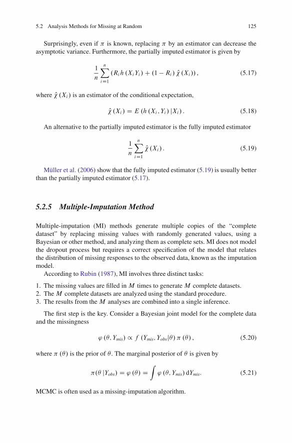
5.2 Analysis Methods for Missing at Random 125
Surprisingly, even if � is known, replacing � by an estimator can decrease theasymptotic variance. Furthermore, the partially imputed estimator is given by
1
n
nX
iD1.Rih .XiYi /C .1 �Ri/ O� .Xi// , (5.17)
where O� .Xi/ is an estimator of the conditional expectation,
O� .Xi / D E .h .Xi ; Yi / jXi/ . (5.18)
An alternative to the partially imputed estimator is the fully imputed estimator
1
n
nX
iD1O� .Xi/ . (5.19)
Muller et al. (2006) show that the fully imputed estimator (5.19) is usually betterthan the partially imputed estimator (5.17).
5.2.5 Multiple-Imputation Method
Multiple-imputation (MI) methods generate multiple copies of the “completedataset” by replacing missing values with randomly generated values, using aBayesian or other method, and analyzing them as complete sets. MI does not modelthe dropout process but requires a correct specification of the model that relatesthe distribution of missing responses to the observed data, known as the imputationmodel.
According to Rubin (1987), MI involves three distinct tasks:
1. The missing values are filled in M times to generateM complete datasets.2. The M complete datasets are analyzed using the standard procedure.3. The results from the M analyses are combined into a single inference.
The first step is the key. Consider a Bayesian joint model for the complete dataand the missingness
' .�; Ymis/ / f .Ymis; Yobsj�/ � .�/ , (5.20)
where � .�/ is the prior of � . The marginal posterior of � is given by
�.� jYobs/ D ' .�/ DZ' .�; Ymis/ dYmis. (5.21)
MCMC is often used as a missing-imputation algorithm.

126 5 Missing Data Imputation and Analysis
Ignorability is the weakest general condition under which the distribution ofmissingness does not need to be taken into account when making likelihood-basedor Bayesian inferences (Rubin 1987). Without ignorability, MIs would have to bedrawn from (5.21).
Because MI uses a Bayesian method to generate missing values, how to have avalid frequentist inference is an interesting topic. Rubin (1976) describes conditionsunder which the following asymptotic result holds in a frequentist sense, i.e., thetest statistic has a t-distribution.
To estimate ˇ, we can use the weighted average of the M estimates,
O DMX
mD1wm O.m/, (5.22)
with varianceOV D W C
M C 1
M
�B , (5.23)
where (W D PM
mD1 wm OV .m/B D PM
mD1 wm� O.m/ � O � O.m/ � O0
.(5.24)
Under MAR, wm D 1=M . Under MNAR, weight wm can be calculated usingsensitivity methods (Carpenter et al. 2007).
A trial example and SAS program using the multiple-imputation method will beillustrated in Sect. 5.4, Example 5.2 and SAS Program 5.2.
5.2.6 Weighted Generalized Estimating Equations
The GEE model is described as a marginal model for the response Yij (j D1; : : : ; ni ; i D 1; : : : ; n, and ˙n
iD1ni DN ). The parameter vector ˇ is obtained bysolving the system of equations,
S .ˇ/ DnX
iD1
@�i
@ˇ0ŒVi .˛/�
�1 .y i ��i / D 0, (5.25)
where the mean �i D E .Y i / and the marginal covariance matrix
Vi .˛/ D �A1=2i W
�1=2i Ci .˛/W
�1=2i A
1=2i ; (5.26)
in which the variance matrix for repeated measures on subject i is �Ai D��diagŒv .�i1/ ; : : : ; v .�iT/�, with � being the unknown dispersion parameter andCi .˛/ the so-called ni � ni working matrix for the i th subject. If Ci .˛/ is the truecorrelation matrix of Yi , then Vi .˛/ is the true covariance matrix of Yi .

5.2 Analysis Methods for Missing at Random 127
With the logistic dropout model (5.5), the weight is given by (e.g., SAS InstituteInc. 2008, p. 1681)
1
wiD .1 � im/
I .m�T /m�1Y
jD2ij; (5.27)
where ij D P�rij D 1jri;j�1 D 1;Xi ; Yi;j�1
�, m is the time of dropout for the i th
subject (2 � m < T � 1), and the indicator I .m � T / D 1 if m � T ; otherwiseI .m � T / D 0. When the weight matrixWi is the identity matrix, (5.25) and (5.26)reduce to the estimate for the unweighted GEE.
The dispersion parameter � has to be estimated through iterations, and usuallyby means of the following Pearson residuals:
eij D yij � �ijqv��ij�=wij
: (5.28)
Specifically, the dispersion parameter � can be estimated by
O� D 1
N � p
nX
iD1
niX
jD1e2ij; (5.29)
where p is the size of parameter vector ˇ.The correlation matrix Ci .˛/ is dependent on the correlation structure. The
following commonly used structures, as well as others, are available in the SASGENMOD procedure.
1. For the m-independent structure,
Corr�Yij; Yi;jCt
� D
8<
:
1 for t D 0,
˛t for t D 1; 2; : : : ; m,
0 for t > m,
(5.30)
O t D 1
.N � nt � p/ �nX
iD1
X
j�ni�teijei;jCt . (5.31)
2. For the exchangeable structure,
Corr�Yij; Yik
� D(1 for j D k,
˛ for j ¤ k,(5.32)
O D 1�12
PniD1 ni .ni � 1/� p� �
nX
iD1
X
j<k
eijeik. (5.33)

128 5 Missing Data Imputation and Analysis
3. For an unstructured covariance,
Corr�Yij; Yik
� D�1 for j D k,˛jk for j ¤ k,
(5.34)
O jk D 1
.n � p/ �
nX
iD1eijeik. (5.35)
4. For the first-order autoregressive AR(1) structure,
Corr�Yij; Yi;jCt
� D ˛t for t D 0; 1; : : : ; ni � j , (5.36)
O D 1
.N � n � p/ �
nX
iD1
X
j�ni�teijei;jCt . (5.37)
The link function g, defined by
g .�i / D X iˇ, (5.38)
can be chosen from various categories. Thus the derivatives are
@�i
@ˇ0
D
266664
xi11
g0 .�i1/� � � xini 1
g0 .�ini /:::
:::xi1p
g0 .�i1/� � � xinip
g0 .�ini /
377775
. (5.39)
Unlike the classic GLM, GEE uses all data available in pairwise fashion asdefined in the estimates for O and O:
5.3 Analysis Methods for Missing Not at Random
In many cases, there are a variety of settings for each method, which can leadto different conclusions. Therefore, approaches that investigate different MNARscenarios, such as pattern-mixture, selection, and shared parameter models, shouldbe explored.
5.3.1 Missing Data Frameworks
The common model-based methods for MNAR are likelihood-based approaches,which can be classified into selection model, pattern-mixture model, and

5.3 Analysis Methods for Missing Not at Random 129
shared-parameter model frameworks by factorization of the full data model(conditional probability density)
f .y i ; r i jXi;$i ;� ; / , (5.40)
where Xi and $i denote design matrices for the measurement and missing-ness mechanisms, respectively. The corresponding parameter vectors are � and , respectively. For simplicity, we omit Xi and $i in (5.40), giving simplyf .y i ; r i j�; /.1. The selection model combines a model for the distribution of the complete data
with a conditional model for the missingness given the data, i.e., it factorizes themarginal density as
f .y i ; r i j�; / D f .y i j�/ f .r i jy i ; / , (5.41)
where the first factor is the marginal density of the measurement process andthe second one is the density of the missingness process, conditional on theoutcomes.
In the selection model approach (Diggle and Kenward 1994), the missing-data mechanism was modelled to depend on the missing outcome variable aswell as covariates. Gao and Hui (2000) extended the selection model approachfrom continuous outcomes to binary outcomes. The results from these modelstend to be highly sensitive to departures from the assumptions about the shape ofthe complete-data population.
2. The pattern-mixture model (Little 1993, 1995) factorizes the marginal density as
f .y i ; r i j�; / D f .y i jr i ;�/ f .r i j / . (5.42)
The pattern-mixture model approach models the probability of the missingdata and appends it to the joint likelihood for the outcome models conditionalon the missing-data status. The pattern-mixture model allows for a differentresponse model (e.g., Bernoulli distribution or logistic regression) for eachpattern of missingness. The population of the complete data becomes a mixtureof distributions, weighted by the probabilities of the missingness pattern.
3. The shared-parameter model factorizes the marginal density as
f .y i ; r i j�; ; bi / D f .y i jr i ;�; bi / f .r i j ; bi / , (5.43)
where parameters bi for subject-specific latent (or random) effects are includedto model certain common latent mechanisms shared by both the measurementand missingness processes.
The notion behind the shared random-effect parameter approach is that theremay be some latent quantity underlying a person’s susceptibility to two processes

130 5 Missing Data Imputation and Analysis
(e.g., disease and death). This latent quantity may represent genetic/genomic orenvironmental risk factors yet to be identified (Lancaster and Intrator 1998; TenHave et al. 1998).
5.3.2 Selection Model
Let Yij be measured at time points for the i th subject at time tij, i D 1; : : : ; n, j D1; : : : ; ni , and Y i D .Yi1; : : : ; Yini /
0. We consider a special type of missingness, thedropout; i.e., once missingness occurs at the j th measuring time, all measurementsafter that are missing. Suppose a dropout occurs at the occasion j D Di (1 <Di � ni ) for the i th subject, so that the first measurement is always available. Wedecompose vector Y i into the observed and missing parts, Y i D .Y obs
i ;Y misni/0. The
likelihood contribution of the i th subject based on the observed data (yobsi ; di ) is
proportional to the marginal density function
f .yi ; di j�; / DZf .yi ; di j�; / dymis
i DZf .yi j�/ f .di jyi ; / dymis
i ,
(5.44)where we have utilized the selection factorization (5.37).Let vector y ij� D .yi1; : : : ; yij�1/. The Diggle-Kenward model (Diggle and
Kenward 1994) for the dropout process allows the conditional probability density tobe specified at occasionDi :
fij . / D
8ˆˆ<
ˆˆ:
P�Di D j jDi � j;y ij�; yij;
�, j D 2,
P�Di D j jDi � j;y ij�; yij;
��Qj�1kD2
�1 � P
�Di D kjDi � k;y ij�; yij;
��, 2 < j � ni ,
QnikD2
�1 � P
�Di D kjDi � k;y ij�; yij;
��, j > ni .
(5.45)
A multivariate normal model,
Yi � f .Yi j�/ D N .Xiˇ; ˙i / ; i D 1; : : : ; n, (5.46)
is used for the measurement process, where various forms can be chosen for thecovariance matrix ˙ . Meanwhile, a simplified logistic model from (5.5) for themissing mechanism is,
P�Di D j jDi � j;y ij�; yij;
� D exp. 0 C 1yij C 2yij�1/1C exp. 0 C 1yij C 2yij�1/
: (5.47)
The likelihood involves marginalization over the unobserved outcomes Y misi ,
which are computationally intensive. Molenberghs and Kenward (2008) providedillustrative examples.

5.3 Analysis Methods for Missing Not at Random 131
5.3.3 Pattern-Mixture Model
The high sensitivity of the selection model to the misspecification of the mea-surement process and dropout mechanism has led to growing interest in thepattern-mixture model with the factorization of marginal density for pattern-mixedmodels (PMMs) given by (5.42). To illustrate the method, let ti be the index(measurement time, clinic visit) indicating the late measurement for the i th subject.After time ti , the subject dropped out of the experiment. Here we use f .y i jti ;�/instead of f .y i jr i ;�/ and f .ti j / instead of f .r i j /. We assume
f .y i jti ;�/ D N .� .ti / ; ˙ .ti // . (5.48)
A pattern-mixture model is usually overparameterized if there are no restrictions.Different restrictions can be used, such as.,
fi�yj jyj�;�
� DniX
kDj!jkfk
�yj jyj�;�
�; j D i C 1; : : : ; ni , (5.49)
where the weights !jk satisfyPni
kDj !jk D 1.The full density function can be expressed as
fi .yj�/ D fi�yobsj�� D
ni�i�1Y
jD1
2
4niX
kDni�j!ni�j;kfk
�yni�j jy.ni�j /�;�
�3
5 .
(5.50)
Different weights in (5.49) and (5.50) will lead to different models (Yanget al. 2008; Little 1993, 1995; DeGruttola and Tu 1994; Hogan and Laird 1997;Henderson et al. 2000; Vonesh et al. 2006).
There are also various f .ti j / to choose; an example would be f .ti j / Du C vti , where u and v are constants. The likelihood function and MLEs can beconstructed using the standard procedures.
5.3.4 Shared-Parameter Models
Recently there have been many discussions of shared-parameter modeling, wherethe factorization of the marginal density is given as in (5.43).
Gao (2004) proposed a method that models both the probability of diseaseand the probability of death using shared random-effect parameters. Gao used theLaplace approximation to obtain an approximate likelihood function to avoid high-dimensional integration over the distributions of the random-effect parameters.

132 5 Missing Data Imputation and Analysis
Let Yij be a binary variable denoting disease status (yij D 0 for non-disease,yij D 1 for disease) for the i th subject at the j th assessment, i D 1; : : : ; nI j D1; : : : ; ni . Let Dij be the variable for survival status, with Dij D 1 indicating the i thsubject died before the j th assessment. Let Xij be the covariates associated with yij
and Zij the covariates associated with Dij. Let i be an m � 1 vector of unobservedrandom effects contributing to the probabilities of disease. Let Uij and Vij be the setsof covariates associated with the random effects in the disease model and the deathmodel, respectively.
Gao (2004) starts with a general disease model for the disease outcome bydefining the conditional probability of new disease to relate linearly to fixed andrandom effects by a link function, � .�/,
pij D Pr .yij D 1jyij�1 D 0IXij; Uij/ D �.Xijˇ C Uij˙1=2� i /; j � 2, (5.51)
where ˇ is the fixed-effect parameter and � i in the disease model is the componentof � � N.�I 0; I /, with I being an identity and ˙ 0˙ a positive definite covariancematrix.
The mortality model is defined through another link function, � .�/,
�ij D Pr�Dij D 1jDij�1 D 0;Zij; Vij
� D ��Zij˛C Vij
1=2� i�; j � 2, (5.52)
where ˛ is the fixed-effect parameter and 0 is a positive definite variance-covariance matrix.
Assuming that yij and Dij are independent given normally distributed i , thelikelihood function of y andD is
L DZf .y j�/g.Dj�/ dN.�I 0; I /
D 1p2�
Zexp
�ln Œf .y j�/g.Dj�/� � 1
2� 0�
d� . (5.53)
The derivation of maximum likelihood estimates from the joint likelihoodfunction above usually requires high dimensional integration over the distributionsof the random effect parameters. A Monte Carlo method may be used since itsefficiency is independent of the dimensionality. Alternatively, Gao (2004) expandsln Œf .y j�/g.Dj�/� � 1
2� 0� at O�0 as a second-order Taylor series, where O�0
maximizes ln Œf .y j�/g.Dj�/� � 12� 0� . The approximate log-likelihood function
leads to
lnL � ln Œf .yj�0/ g .Dj�0/� �O� 00 O�02
�12
ln
ˇˇI � @2 ln Œf .y j�/ g .Dj�/�
@�2
ˇˇ�D�0
: (5.54)
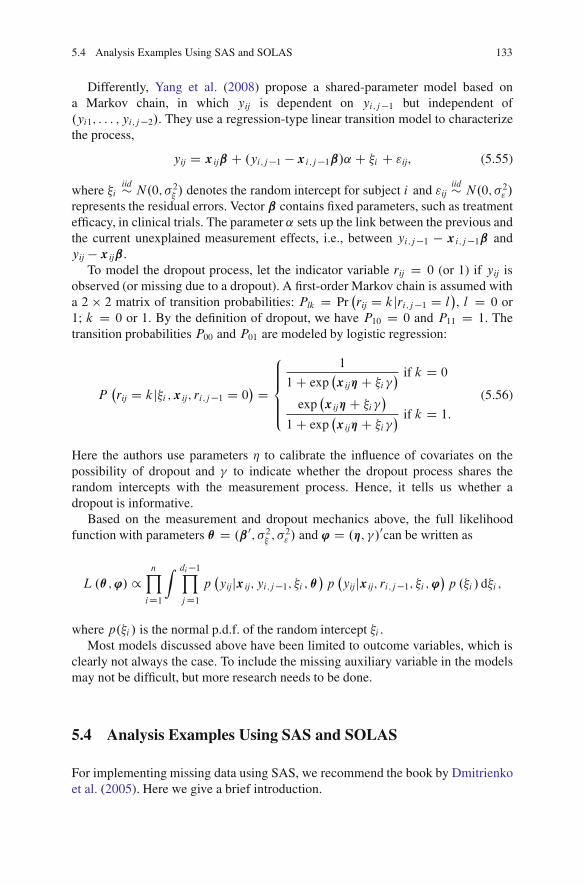
5.4 Analysis Examples Using SAS and SOLAS 133
Differently, Yang et al. (2008) propose a shared-parameter model based ona Markov chain, in which yij is dependent on yi;j�1 but independent of.yi1; : : : ; yi;j�2/. They use a regression-type linear transition model to characterizethe process,
yij D xijˇ C .yi;j�1 � xi;j�1ˇ/˛ C �i C "ij, (5.55)
where �iiid� N.0; �2� / denotes the random intercept for subject i and "ij
iid� N.0; �2" /
represents the residual errors. Vector ˇ contains fixed parameters, such as treatmentefficacy, in clinical trials. The parameter ˛ sets up the link between the previous andthe current unexplained measurement effects, i.e., between yi;j�1 � xi;j�1ˇ andyij � xijˇ.
To model the dropout process, let the indicator variable rij D 0 (or 1) if yij isobserved (or missing due to a dropout). A first-order Markov chain is assumed witha 2 � 2 matrix of transition probabilities: Plk D Pr
�rij D kjri;j�1 D l
�, l D 0 or
1; k D 0 or 1. By the definition of dropout, we have P10 D 0 and P11 D 1. Thetransition probabilities P00 and P01 are modeled by logistic regression:
P�rij D kj�i ;xij; ri;j�1 D 0
� D
8ˆ<
ˆ:
1
1C exp�xij�C �i
� if k D 0
exp�xij�C �i
�
1C exp�xij�C �i
� if k D 1:
(5.56)
Here the authors use parameters � to calibrate the influence of covariates on thepossibility of dropout and to indicate whether the dropout process shares therandom intercepts with the measurement process. Hence, it tells us whether adropout is informative.
Based on the measurement and dropout mechanics above, the full likelihoodfunction with parameters � D .ˇ0; �2� ; �2" / and ' D .�; /0can be written as
L.�;'/ /nY
iD1
Z di�1Y
jD1p�yijjxij; yi;j�1; �i ;�
�p�yijjxij; ri;j�1; �i ;'
�p .�i / d�i ;
where p.�i / is the normal p.d.f. of the random intercept �i .Most models discussed above have been limited to outcome variables, which is
clearly not always the case. To include the missing auxiliary variable in the modelsmay not be difficult, but more research needs to be done.
5.4 Analysis Examples Using SAS and SOLAS
For implementing missing data using SAS, we recommend the book by Dmitrienkoet al. (2005). Here we give a brief introduction.

134 5 Missing Data Imputation and Analysis
Table 5.1 Depression datastructure
Patient Visit Basval Change Y Trt Ctr
1001 4 25 �7 2 103
1001 5 25 �14 2 103
1001 6 25 �19 2 103
1001 7 25 � 2 103
1002 4 17 �4 1 105
1002 5 17 �8 1 105
1002 6 17 � 1 105
1002 7 17 � 1 105:::
:::
:::
:::
:::
5.4.1 Likelihood Ignorable Analysis
A likelihood ignorable analysis for MAR uses all available information withoutdirectly implementing any missing data. The analysis using SAS PROC MIXEDis straightforward. The order of the measurements should be correctly specified,which can be done by supplying records with missing data in the input dataset.
Example 5.1. A multicenter depression trial was conducted with the HamiltonDepression Rating Scale as the primary efficacy endpoint. For each patient, abaseline assessment is available and the change from baseline (Basval) is denotedby Y . Y is missing when the assessment at postbaseline visit is not available. Thereare four treatment options (Trt). The clinic center is denoted by variable Ctr. Thedata structure is presented in Table 5.1, where a dot represents a missing value.
SAS Program 5.1: MAR Analysis of the Depression Trial
Proc mixed data = depression method = ml noitprint ic;class Patient Visit Ctr Trt;model Y = Trt Ctr Visit Trt*Visit Basval Basval*Visit/solution ddfm = satterth;repeated visit / subject = patient type = un;
Run;
Details about options in Proc Mixed can be found in the SAS User’s Guide (SASInstitute 2004).
5.4.2 Multiple-Imputation Method
A multiple-imputation method using SAS involves two steps: implementation andanalysis. We illustrate the process with the growth data in Table 5.2.
Example 5.2. The growth data contain growth measurements for girls and boys. Foreach subject, the distance from the center of the pituitary to the maxillary fissure

5.4 Analysis Examples Using SAS and SOLAS 135
Table 5.2 Growth datastructure
ID Sex Meas8 Meas12 Meas14 Meas10
1 1 26 29.0 31.0 272 1 21.5 23.0 26.5 �3 2 23 24.0 27.5 23.54 1 20 26.5 27.0 �� � �
was recorded at ages 8, 10, 12, and 14 years and denoted by variables Meas8,Meas10, Meas12, and Meas14 (Table 5.2). Note that the measurement times areordered as age D 8, 12, 14, and 10 years because the data at age 10 are incomplete.In this way, a monotone ordering is achieved, which is required for the monotoneregression method. The implementation step with SAS PROC MI is presented inSAS Program 5.2.
SAS Program 5.2: Imputation Step
Proc mi data = Growth seed = 213 simple Nimpute = 10round = 0.1 out = outmi;by sex;monotone method = reg;var Meas8 Meas12 Meas14 Meas10;
Run;
To prepare for a standard linear mixed model analysis, we convert the outputoutmi from SAS Program 5.2 to vertical structure using SAS Program 5.3.
SAS Program 5.3: Data Manipulation
Proc sort data = outmi;by imputation idnr;
Run;Data outmi2;
set outmi;array y (4) meas8 meas10 meas12 meas14;do j = 1 to 4;measmi = y(j) ;age = 6 + 2*j;output;end;
Run;
The analysis step using the SAS MIXED procedure requires four sets of inputsfor the inference task: (1) parameter estimates of the fixed effects (mixbetap), (2) pa-rameter estimates of the variance components (mixalfap), (3) the covariance matrixof the fixed effects (mixbetav), and (4) the covariance matrix of the variance compo-nents (mixalfav). An example of a SAS program is presented in SAS Program 5.4.

136 5 Missing Data Imputation and Analysis
SAS Program 5.4: Analysis Step Using PROC MIXED
Proc mixed data = outmi2 asycov;class idnr age sex;model measmi = age*sex / noint solution covb;repeated age / subject = idnr type = cs;by Imputation ;ods output solutionF = mixbetap covb = mixbetav
covparms = mixalfap asycov = mixalfav;Run;
However, to use PROC MIANALYZE, further data manipulation is required; seeSAS Programs 5.17 and 5.18 in the book by Dmitrienko et al. (2005), or the SASUser’s Guide for details.
When missingness is nonmonotone, Dmitrienko et al. (2005) suggest generatingmultiple imputations that render the datasets monotonically missing by includingthe statement in PROC MI: mcmc impute D monotone and then applying a methodof choice to the multiple sets of data that are thus completed.
5.4.3 EM Algorithm Using SAS
The MI procedure in SAS provides an EM algorithm for both multivariate normaland categorical data by means of an MCMC imputation method (for generalnonmonotone settings). The EM algorithm for the growth data is presented in SASProgram 5.5. PROC MI uses the means and standard deviations from the availablecases as the initial estimates for the EM algorithm. The correlations are set equalto zero.
SAS Program 5.5: The EM Algorithm Using PROC MI
Proc mi data = Growth seed = 213 simple nimpute = 0;em itprint outem = growthem;var Meas8 Meas12 Meas14 Meas10;by sex;
Run;
5.4.4 SOLAS for Missing Data Analysis
SOLAS, developed in conjunction with Prof. Donald Rubin, is a software applica-tion that has a user-friendly graphical interface and provides a range of missing-dataimputation techniques. The single-imputation techniques include the hot deckimputation, in which missing values are replaced with values taken from matchingrespondents, the last value carried forward, the group means, or the predicted meanfrom the models. The predictive-model-based multiple-imputation methods include
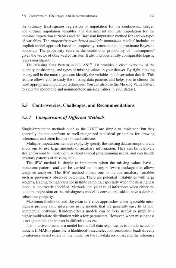
5.5 Controversies, Challenges, and Recommendations 137
the ordinary least-squares regression of imputation for the continuous, integer,and ordinal imputation variables, the discriminant multiple imputation for thenominal imputation variables and the Bayesian imputation method for various typesof variables. The propensity-score-based multiple imputation method includes animplicit model approach based on propensity scores and an approximate Bayesianbootstrap. The propensity score is the conditional probability of “missingness”given the vector of observed covariates. It also includes a fully configurable logisticregression algorithm.
The Missing Data Pattern in SOLASTM 3.0 provides a clear overview of thequantity, positioning, and types of missing values in your dataset. By right-clickingon any cell in the matrix, you can identify the variable and observation details. Thisfeature allows you to study the missing-data patterns and helps you to choose themost appropriate imputation techniques. You can also use the Missing Value Patternto view the monotone and nonmonotone missing values in your dataset.
5.5 Controversies, Challenges, and Recommendations
5.5.1 Comparisons of Different Methods
Single-imputation methods such as the LOCF are simple to implement but theygenerally do not conform to well-recognized statistical principles for drawinginferences, and often lead to a biased estimate.
Multiple-imputation methods explicitly specify the missing data assumptions andallow one to use large amounts of auxiliary information. They can be relativelystraightforward to implement, without special programming needs, and can handlearbitrary patterns of missing data.
The IPW method is simple to implement when the missing values have amonotone pattern, and can be carried out in any software package that allowsweighted analyses. The IPW method allows one to include auxiliary variablessuch as previously observed outcomes. There are potential instabilities with largeweights, leading to high variance in finite samples, especially when the missingnessmodel is incorrectly specified. Methods that yield valid inferences when either theoutcome regression or the missingness model is correct are said to have a double-robustness property.
Maximum likelihood and Bayesian inference approaches under ignorable miss-ingness provide valid inferences using models that are generally easy to fit withcommercial software. Random-effects models can be very useful to simplify ahighly multivariate distribution with a few parameters. However, when missingnessis not ignorable, the impact is difficult to assess.
It is intuitive to assume a model for the full-data response, as is done in selectionmodels. If MAR is plausible, a likelihood-based selection formulation leads directlyto inference based solely on the model for the full-data response, and the inference

138 5 Missing Data Imputation and Analysis
can be carried out using MLE. However, it may not be intuitive to specify therelationship between nonresponse probability and the outcome of interest, whichtypically has to be done in the logit or probit scale. Selection models are highlysensitive to parametric assumptions about the full-data distribution. This concerncan be alleviated by using semiparametric selection models (Little 2010).
In pattern-mixture models, respondents and nonrespondents have differentoutcome distributions. The models are explicit in specifying how missingobservations are being imputed because the within-pattern models specify thepredictive distribution directly. However, pattern-mixture models can presentcomputational difficulties for estimating treatment effects because of the needto average over missing-data patterns; this is particularly true of pattern-mixturespecifications involving regression models within each pattern.
5.5.2 How to Implement Missingness
Practically speaking, missing data usually refers to any data points that wereintended for collection but were not obtained. Theoretically, any unobservedvariable at any time point can be considered a missing value in an analysis, evenif the measurement was not intended to be collected at all. In the most generaland abstract form, “missing data” can refer to any augmented component of theprobabilistic system under consideration, and the inclusion of this component oftenresults in a simpler structure and easier computation (Liu 2003). On the other hand,people may argue that if missing imputation is allowed, one can “make up” anyvalue at any point in time and space, and as many as one wants, in the name ofcomputational convenience.
Regarding the pattern of missingness, in clinical trials missingness is often amixture of MCAR, MAR, and MNAR because, for example, missingness shouldnot just relate to how one collects and measures the data but also to the behaviorof the subject from whom the data are collected. The choice of MAR or MCAR isoften simply motivated by mathematical convenience. However, the question is: ifwe know the missingness is MAR in a practical problem, why do we try to collectit in the first place? The answer may be to increase data points and thus the powerfor the hypothesis-test. Another argument would be that although MAR is a non-testable assumption, we can get very close to justifying the MAR hypothesis if weinclude enough variables in the imputation models (Harel and Zhou 2007).
A simple example of MNAR is when the values to be measured are out ofthe range of the measurement instrument. Another example would be a patientwithdrawal due to lack of efficacy or side effects. If the drug is not very effective,causing a large number of dropouts due to ineffectiveness, models based on MARwould not be appropriate.
We may say the true value should be imputed for a missing value; however, thetruth is missing and how to impute it is a matter of belief. To elaborate on this, letme share a story with you. When I appeared in court for my first traffic citation,

5.5 Controversies, Challenges, and Recommendations 139
I argued: “I don’t think this is my fault. . . . I’ve never gotten any citation for a trafficviolation in my 13 years driving history.” Of course, the judge didn’t observe theaccident; it is a missing value to her. She replied nicely: “Yes, I know; but everyonehas his first time.” In this case, who is at fault is unknown or missing. I tried toimpute the missingness “longitudinally” by looking back at my own driving historyand concluding the missing value should be 0: not my fault. However, the judgeimputed the missing value “cross-sectionally” by looking at all the drivers whohad 13 years of driving experience and concluded that most of them had trafficviolations; therefore it was likely my fault, and the missing value should be 1. Doyou think it is fair to make a judgment of me based on other people’s behavior?
In clinical trials, the missing imputation faces the same dilemma: should we lookfor a data pattern within the trial or across different trials, or even in everythinghappening in the whole world?
Regarding who should perform the data implementation, Harel and Zhou (2007)offer their opinion: Many public-data users differ in their statistical proficiency,computing power, and objectives. Most users only have access to complete-datamethodology and software. Database constructors have additional information aboutthe data that can help in modeling the missing values. Therefore, it would bepreferable if the missing data modeling was done by the data constructors and notby the users. However, in many cases, that is not possible.
5.5.3 Regulatory Perspective
For clinical trials, the health authority (CHMP 2009) states: “Missing data are apotential source of bias when analyzing clinical trials. . . A critical discussion of thenumber, timing, pattern, reason for and possible implications of missing values inefficacy and safety assessments should be included in the clinical report as a matterof routine. . . It should be noted that just ignoring missing data is not an acceptableoption when planning, conducting or interpreting the analysis of a confirmatoryclinical trial. . . The justification for selecting a particular method should not be basedprimarily on the properties of the method under particular assumptions (for exampleMAR or MCAR) but on whether it will provide an appropriately conservativeestimate for the comparison of primary regulatory interest in the circumstancesof the trial under consideration.” They believe missing data (completer analyses)violate the strict ITT principle, which requires measurement of all patient outcomesregardless of the protocol adherence. This principle is of critical importance, as con-firmatory clinical trials should estimate the effect of the experimental interventionin the population of patients with the greatest external validity.
There are many factors that can affect missingness: (1) the complexity of themeasurements, (2) the frequency of measurements, (3) self-reported versus in-clinic measures by clinicians, (4) the nature of the outcome variable, such asmodality versus morbidity, (5) the treatment modalities, such as surgical versusmedical treatment, (6) frequency of the treatment, (7) the benefit-risk profile of the

140 5 Missing Data Imputation and Analysis
treatment, (8) duration of the clinical trial (since a longer trial will likely have alarger proportion missing than a shorter trial), (9) the therapeutic indication (missingvalues are more frequent in those diseases where the adherence of patients to thestudy protocol is usually low, such as psychiatric disorders, (10) data entry error(some numbers may be easier to missight than others), and (11) the design andconduct of the experiment.
A reduction in missing data can be achieved by favoring clinical trial designs,strengthening data collection, and whenever possible, collecting outcome data afterwithdrawals. To minimize potential bias, CHMP (2009) recommends that a detaileddescription of the preplanned methods used for handling missing data and anyamendments of that plan and a justification for each amendment should be includedin the clinical study report. A critical discussion of the number, timing, pattern,and reasons for and possible implications of missing values in efficacy and safetyassessments should be included in the clinical report as a matter of routine. Becauseof the unpredictability of some problems, the study protocol sometimes allows thepossibility of updating the strategy for dealing with missing values in the statisticalanalysis plan or during the blind review of the data at the end of the trial.
5.5.4 Recommendations for Clinical Trials
At the request of the FDA, the National Research Council convened the Panelon the Handling of Missing Data in Clinical Trials, under the Committee onNational Statistics, to prepare “a report with recommendations that would beuseful for FDA’s development of a guidance for clinical trials on appropriate studydesigns and follow-up methods to reduce missing data and appropriate statisticalmethods to address missing data for analysis of results.” The panel, chaired byProf. Rod Little, developed an excellent report, “The prevention and treatmentof missing data in clinical trials” (Little 2010). The panel consisted of a groupof academic statisticians, but I believe there was some interaction with industrystatisticians, as indicated in the acknowledgments. Among many useful suggestions,they recommend the following.
5.5.4.1 Clinical Trial Design
Investigators, sponsors, and regulators should design clinical trials consistent withthe goal of maximizing the number of participants who are maintained on theprotocol-specified intervention until the outcome data are collected.
The techniques to reduce the occurrence of missingness include (1) adding run-in periods before randomization to identify who can tolerate or respond to the studytreatment, (2) using flexible doses (titration), (3) restricting the trial to the targetpopulation for whom treatment is indicated, (4) adding the study treatment to astandard treatment, (5) reducing the length of the follow-up period, (6) allowing

5.5 Controversies, Challenges, and Recommendations 141
rescue medication in the event of poor response, and (7) defining outcomes thatcan be ascertained in a high proportion of participants. Of course, benefits of theseoptions need to be weighed against costs.
5.5.4.2 Clinical Trial Conduct
Trial sponsors should continue to collect information on key outcomes in partic-ipants who discontinue their protocol-specified intervention in the course of thestudy, except in those cases for which a compelling cost-benefit analysis arguesotherwise, and this information should be recorded and used in the analysis.
The techniques to limit the amount of missing data include (1) choices of studysites, investigators, participants, study outcomes, time in study and times of mea-surement, and the nature and frequency of follow-up to limit the amount of missingdata, (2) limiting participant burden in other ways, such as making follow-up visitseasy in terms of travel and childcare, (3) providing frequent reminders of studyvisits, (4) training of investigators on the importance of avoiding missing data,(5) providing incentives to investigators and participants to limit dropouts, and(6) monitoring of adherence and in other ways dealing with participants who cannottolerate or do not adequately respond to treatment.
The panel recommends that study sponsors should explicitly anticipate potentialproblems of missing data. In particular, the trial protocol should contain a sectionthat addresses missing-data issues, including the anticipated amount of missing dataand steps taken in trial design and trial conduct to monitor and limit the impact ofmissing data.
5.5.4.3 Trial Data Analysis
There is no universal method for handling incomplete data in a clinical trial. Despitedifferences among the trials, there are common principles that can be applied in awide variety of settings as suggested by the panel:
1. A basic assumption is that missingness of a particular value hides a trueunderlying value that is meaningful for analysis.
2. The analysis must be formulated to draw inferences about an appropriate andwell-defined causal estimand.
3. Reasons for missing data must be documented as much as possible.4. The trial designers should decide on a primary set of assumptions about the
missing-data mechanism. Those primary assumptions then serve as an anchorpoint for the sensitivity analyses.
5. The trial sponsors should conduct a statistically valid analysis under the primarymissing-data assumptions.
6. The analysts should assess the robustness of the treatment effect inferences byconducting a sensitivity analysis.

142 5 Missing Data Imputation and Analysis
Despite efforts to minimize missing data in the design and conduct of clinicaltrials, the statistical analysis often has to deal with a nontrivial amount of missingdata. There is no single correct method for handling missing data. As such, the panelrecommends that statistical methods for handling missing data should be specifiedby clinical trial sponsors in study protocols, and their associated assumptions statedin a way that can be understood by clinicians. Single-imputation methods like lastobservation carried forward and baseline observation carried forward should not beused as the primary approach to the treatment of missing data unless the assumptionsthat underlie them are scientifically justified. Sensitivity analyses should be part ofthe primary reporting of findings from clinical trials. Examining sensitivity to theassumptions about the missing-data mechanism should be a mandatory componentof reporting.
5.6 Exercises
5.1. Suppose there are data available from two clinical trials. Trial A is a 2 � 2
crossover design (one treatment sequence is drugs C and T ; the other sequenceis drugs T and C ) and trial B is a design with two parallel treatment groups (Cand T ). The statistician wants to combine data from these two clinical trials usingthe technique for the missing data. He treats trial B as an imaginary 2� 2 crossovertrial with one group missing the first period and the other group missing the secondperiod. Furthermore, he assumes that the missing data are completely at random(MCAR) because it was not planned to collect the missing data. Discuss his strategy.
5.2. Compare different methods for the missing data analysis under differentscenarios, such as percentage of missing data and missing patterns.
Further Readings and References
Carpenter J.R., Kenward, M.G., White, I.R.: Sensitivity analysis after multiple imputation undermissing at random: A weighting approach. Stat. Methods Med. Res. 16, 259–275 (2007)
CHMP: Guideline on missing data in confirmatory clinical trials/1776/99 Rev. 1. www.ema.europa.eu (2009). Accessed 8 Aug 2010
DeGruttola, V., Tu, X.M.: Modeling progression of CD4C lymphocyte count and its relationshipto survival time. Biometrics 50, 1003–1014 (1994)
Dempster, A.P., Laird, N.M., Rubin, D.B.: Maximum likelihood estimation from incomplete datavia the EM algorithm. J. R. Stat. Soc. Ser. B 39, 1–38 (1977)
Dmitrienko, A., Molenberghs, G., Chuang-Stein, C., Often, W.: Analysis of Clinical Trials UsingSAS. SAS Institute, Cary (2005)
Diggle P., Kenward, M.G.: Informative drop-out in longitudinal data analysis. Appl. Stat. 43, 49–93(1994)
Gao, S.: A shared random effect parameter approach for longitudinal dementia data with non-ignorable missing data. Stat. Med. 23, 211–219 (2004)

Further Readings and References 143
Gao, S., Hui, S.L.: Estimating the incidence of dementia from two-phase sampling with non-ignorable missing data. Stat. Med. 19, 1545–554 (2000)
Harel, O., Zhou, X.H.: Multiple imputation: Review of theory, implementation and software. Stat.Med. 26, 3057–3077 (2007)
Henderson, R., Diggle, P., Dobson, A.: Joint modeling of longitudinal measurements and eventtime data. Biostatistics 1, 465–480 (2000)
Hogan, J.W., Laird, N.M.: Model-based approaches to analysing incomplete longitudinal andfailure time data. Stat. Med. 16, 259–272 (1997)
Hogan, J.W., Roy, J., Korkontzelou C.: Biostatistics tutorial: Handling dropout in longitudinal data.Stat. Med. 23, 1455–1497 (2004)
Horvitz, D.G., Thompson, D.J.: A Generalization of sampling without replacement from a finiteuniverse, J. Am. Stat. Assoc. 47, 663–685 (1952)
Lancaster, T., Intrator, O.: Panel data with survival: Hospitalization of HIV-positive patients. J.Am. Stat. Assoc. 93, 46–53 (1998)
Little, R.J.A.: Pattern-mixture models for multivariate incomplete data. J. Am. Stat. Assoc. 88,125–134 (1993)
Little, R.J.A.: Modeling the drop-out mechanism in repeated-measure studies. J. Am. Stat. Assoc.90, 1112–1121 (1995)
Little, R.J.: Panel on Handling Missing Data in Clinical Trial: The Prevention and Treatment ofMissing Data in Clinical Trials. The National Academies Press, Washington (2010)
Little, R.J., Rubin, D.B.: Statistical Analysis with Missing Data, 2nd edn. Wiley, New York (2002)Liu, J.: Monte Carlo Strategies in Scientific Computing. Springer, New York (2003)Molenberghs, G., Kenward, M.G.: Missing Data in Clinical Studies. Wiley, Chichester (2008)Muller, U.U., Schick, A., Wefelmeyer, W.: Imputing responses that are not missing. In: Nikulin, M.,
Commengs, D., Huber, C. (eds.) Probability, Statistics and Modeling in Public Health. Springer,New York (2006)
Rubin D.B.: Inference and missing data. Biometrika 63, 581–592 (1976)Rubin D.B.: Multiple Imputation for Nonresponse in Surveys. Wiley, New York (1987)SAS Institute: SAS/STAT 9.1 User’s Guide, vol. 1–7. SAS Institute, Gary (2004)SAS Institute Inc.: SAS/STAT 9.2 User’s Guide. Cary, NC: SAS Institute Inc. (2008)Ten Have, T.R., Kunselman, A.R., Pulkstenis, E.P., Landis, J.R. Mixed effect logistic regression
models for longitudinal binary response data with informative drop out. Biometrics 54,367–383 (1998)
Tsiatis, A.A.: Semiparametric Theory and Missing Data. Springer, New York (2009)Van Der Laan, M.J., Robins, J.M.: Unified Methods for Censored Longitudinal Data and Causality.
Springer, New York (2003)Vonesh, E.F., Greene, T., Schluchter, M.D.: Shared parameter models for the joint analysis of
longitudinal data and event times. Stat. Med. 25, 143–163 (2006)Yang, X., Li, J., Shoptaw, S.: Imputation-based strategies for clinical trial longitudinal data with
nonignorable missing values. Stat. Med. 27, 2826–2849 (2008)


Chapter 6Multivariate and Multistage SurvivalData Modeling
6.1 Introduction to Survival Data Modeling
6.1.1 Basic Terms in Survival Analysis
Survival analysis or time-to-event analysis is a branch of statistics dealing withdeath (failure) or degradation in biological organisms, mechanical or electronicsystems, or other areas. This topic is called reliability theory or reliability analysis inengineering, and duration analysis or duration modeling in economics or sociology.
The term lifetime distribution function F .t/ is defined as the probability ofthe event (e.g., death) occurring on or before time t , i.e., F .t/ DP .T � t/. Thesurvival function S .t/ is the probability of an individual surviving longer than t ,i.e., S .t/ D 1 � F .t/. Thus the event density is f .t/ D dF .t/ =dt . The hazardfunction or rate � .t/, is defined as the event rate at time t , conditional on survivaluntil time t or later,
� .t/ dt D P .t < T � t C dt jT > t/ D f .t/ dt
S .t/D �S
0 .t/S .t/
dt . (6.1)
Integrating (6.1) with respect to t , we obtain S .t/ D exp .��.t//, where�.t/ D R t
0� .u/ du is called the cumulative hazard function. From (6.1), we can
obtainf .t/ D � .t/ S .t/ . (6.2)
The expected future (residual) lifetime at a given time t0 is defined as 1S.t0/
R10
t f .t C t0/ dt D 1S.t0/
R1t0S .t/ dt .
In Chap. 5, we discussed missing-data issues in general. In survival analysis, weusually have a special type of missing data; i.e., censoring. In practice, survival datainvolve different types of censoring: (1) left-censoring if a data point (time value)is equal to or below a certain value but it is unknown by how much (e.g., missingadverse event start date), (2) right-censoring if a data point is above a certain value
M. Chang, Modern Issues and Methods in Biostatistics, Statistics for Biology and Health,DOI 10.1007/978-1-4419-9842-2 6, © Springer Science+Business Media, LLC 2011
145
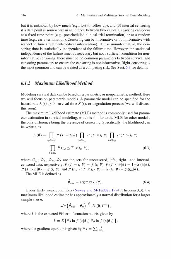
146 6 Multivariate and Multistage Survival Data Modeling
but it is unknown by how much (e.g., lost to follow up), and (3) interval censoringif a data point is somewhere in an interval between two values. Censoring can occurat a fixed time point (e.g., prescheduled clinical trial termination) or at a randomtime (e.g., early termination). Censoring can be informative or noninformative withrespect to time (treatment/medical intervention). If it is noninformative, the cen-soring time is statistically independent of the failure time. However, the statisticalindependence of the failure time is a necessary but not a sufficient condition for non-informative censoring; there must be no common parameters between survival andcensoring parameters to ensure the censoring is noninformative. Right-censoring isthe most common and can be treated as a competing risk. See Sect. 6.3 for details.
6.1.2 Maximum Likelihood Method
Modeling survival data can be based on a parametric or nonparametric method. Herewe will focus on parametric models. A parametric model can be specified for thehazard rate � .t/ � 0, survival time S .t/, or degradation process (we will discussthis soon).
The maximum likelihood estimate (MLE) method is commonly used for param-eter estimation in survival modeling, which is similar to the MLE for other models,the only difference being the presence of censoring. Specifically, the likelihood canbe written as
L.�/ DY
ti2˝UP .T D ti j�/
Y
tj2˝LP .T � ti j�/
Y
ti2˝RP .T > ti j�/
�Y
ti2˝IP .tia � T < tibj�/ , (6.3)
where ˝U , ˝L, ˝R, ˝I are the sets for uncensored, left-, right-, and interval-censored data, respectively;P .T D ti j�/ D f .ti j�/, P .T � ti j�/ D 1�S .ti j�/,P .T > ti j�/ D S .ti j�/, and P .ti;a < T � ti;bj�/ D S .tiaj�/� S .tibj�/.
The MLE is defined as
O�mle D arg maxL.�/ . (6.4)
Under fairly weak conditions (Newey and McFadden 1994, Theorem 3.3), themaximum likelihood estimator has approximately a normal distribution for a largersample size n, p
n� O�mle � �0
�d! N
�0; I�1� ,
where I is the expected Fisher information matrix given by
I D E�O� ln f .xj�0/O� lnf .xj�0/0
�,
where the gradient operator is given by O� D Pi@@�i
.

6.1 Introduction to Survival Data Modeling 147
Hougaard (2000) provided two reasons not to use the expected information forsurvival analysis. He argued that first, for the evaluation, it is necessary to makeassumptions on the general censoring pattern, whereas the observed information isbased only on the actual observed censoring times. Consequently, the evaluationis only valid under precisely that censoring pattern. Second, for censored data, theexpected information is more complicated to evaluate than the observed informationbecause integration is necessary. This is in contrast to many other models, such asnonlinear regression and exponential families, where taking the expectation makessome terms vanish.
6.1.3 Overview of Survival Model
6.1.3.1 Proportion Hazard Model
Proportional hazard models are widely used in practice. Just as the name suggests, aproportional hazard model assumes the hazard is proportional (i.e., independent oftime) between any two different groups with covariatesX 0 D x0
1 andX 0 D x02,
h .t/ D h0 .t/ exp�X 0ˇ
�, (6.5)
where X is the vector of observed covariates and ˇ are the correspondingparameters. If the baseline hazard function is specified (e.g., h0 .t/ D ��t��1),(6.5) represents a parametric proportional hazard model; otherwise, (6.5) is the well-known Cox semiparametric proportional hazard model (Cox 1972).
6.1.3.2 Accelerated Failure Time Model
When the proportional hazard assumption does not hold, we may use the acceleratedfailure time model with a hazard function:
h .t/ D exp�X 0ˇ
�h0�exp
�X 0ˇ
�t�
. (6.6)
Different baseline functions h0 .�/ will lead to different parametric models. Forthe exponential model, h0 .t/ D � and S0 .t/ D exp .��t/, where � > 0; for theWeibull model, h0 .t/ D ��t��1 and S0 .t/ D exp .��t�/, where �; � > 0; for theGompertz model, h0 .t/ D � exp .� t/ and S0 .t/ D exp
�����1 .exp .� t/� 1/�,
where �; � > 0; and for the loglogistic model, h0 .t/ D exp.˛/ktk�1
1Cexp.˛/tkand S0 .t/ D
1
1Cexp.˛/tk, where ˛ 2 R; k > 0.

148 6 Multivariate and Multistage Survival Data Modeling
6.1.3.3 Frailty Model
The notion of frailty provides a convenient way to introduce random effects,association and unobserved heterogeneity into models for survival data. In itssimplest form, a frailty is an unobserved random factor that modifies the hazardfunction of an individual or related individuals. The term frailty was coined byVaupel et al. (1979) in univariate survival models, and the model was substantiallypromoted for its application to multivariate survival data in a seminal paper byClayton (1978) on chronic disease incidence in families. The simplest form offrailty model with a (unobserved) scale frailty variable Z can be written as
h .t; Z;X/ D Zh0 .t/ exp�X 0ˇ
�.
We will discuss this approach further later.
6.1.3.4 Copula Model
Copula modeling is a general approach to formulating different multivariate distri-butions. The idea is that a simple transformation can be made of each marginalvariable in such a way that each transformed marginal variable has a uniformdistribution. Once this is done, the dependence structure can be expressed as amultivariate distribution on the obtained uniforms, and a copula is precisely amultivariate distribution on marginally uniform random variables.
In the context of survival analysis, a copula model is often constructed frommarginal survival functions instead of marginal distribution functions. If the argu-ments of the copula function are univariate survival functions S1.t1/DP.X1 > t1/
and S2.t2/DP.X2 > t2/, the copula function C.S1; S2/ is a legitimate joint(bivariate) survival function S.t1; t2/ D P.X1 > t1; X2 > t2/ with marginals S1and S2.
Archimedean copulas are commonly used copulas in survival analysis. Supposethat W Œ0;1� ! Œ0; 1� is a strictly decreasing convex function such that .0/ D 1.Then an Archimedean copula can be written as
C .S1; S2I �/ D � �1 .S1/C �1 .S2/
�, S1; S1 2 Œ0; 1� ; (6.7)
where � is the parameter of association. For example, the stable (Gumbel-Hougaard)copula, generated by �1 .s/ D .� ln s/� , � � 1, can be expressed as
S .t1; t2I �/ D exp
��h.� lnS1/
� C .� lnS2/�i1=�
:
Archimedean copulas can be conveniently used for modeling a bivariate survivalfunction with such marginal distributions as Gompertz, Weibull, or even in thesemiparametric setup in combination with Kaplan-Meier estimates for the marginalsurvival functions (Genest and Rivest 1993). All information concerning depen-dence between the marginals is contained in the association parameter.

6.1 Introduction to Survival Data Modeling 149
6.1.3.5 First-Hitting-Time Model
Many practical problems, such as biomarker or clinical responses, survival time andrandom vibrations of a bridge, can be modeled using stochastic processes X .t/.When the stochastic process reaches a certain level (i.e., X .t/ D ß) for the firsttime, it is called first hitting time (FHT). FHT usually indicates a critical state suchas a biological inhibition, death, or bridge collapse. The critical value ß, called theboundary or threshold, can be a constant or function of time t . Threshold regressionrefers to the first-hitting-time models with regression structures that accommodatecovariate data (Lee and Whitmore 2006).
A very commonly used stochastic process is a Wiener process or Brownianmotion, which describes, for example, a particle random motion on the microscope.The macro-behavior (i.e., the average properties for Brownian motion) of the massis governed by the so-called diffusion equation, which is widely used in science andengineering, the social sciences, and other areas. We will discuss this approach inSect. 6.3.
6.1.3.6 Multistage Model
A multistage model consists of several stages across a time axis. At each stage, atime-to-event model is applied. In principle, all models mentioned above can be usedin multistage models. However, most common multistage models are semi-Markovprocesses (continuous time, discrete states).
The rationale for using multistage models is that it may not be easy to specify asingle model across the entire time course. This is because, for example, the naturalcourse of disease may consist of stages and the time-to-event model is relativelyeasy to specify for each stage separately. The model within each stage can bethe proportional hazard model, frailty model, exponential model, or a combinationof them. In principle, a time-dependent hazard model can be approximated by amultistage model with a time-independent hazard rate at each stage, but the numberof stages required may be large in order to have the desired precision. The time-independent hazard rate � does not have to be a constant; it can include covariates�i:e:;� D �
�X 0ˇ
��. The examples to illustrate the method in this chapter will focus
on Markov or semi-Markov models because their calculations don’t require specificsoftware. However, for more complicated multistage models, a software package isrequired. The transitional probability matrix for a semi-Markov chain is given by
P .t/ D eAt D I C1X
kD1
Aktk
kŠ,
where A D limh!0
.P .h/ � I/ =h with I being the identity matrix. We will discuss
the multistage approach in Sect. 6.4.

150 6 Multivariate and Multistage Survival Data Modeling
6.1.3.7 Nonparametric Approach
Nelson-Aalen Estimator
Let Y .t/ be the number of individuals at risk at (just before) time t and �i theoccurrence of the i th event. The Nelson-Aalen estimator for the cumulative hazardis given by
O�.t/ DX
�i�t
1
Y .�i /,
with variance estimator
O2� .t/ DX
�i�t
1
Y .�i /2
.
The cumulative hazard O�.t/ approaches to a normal distribution as the samplesize approaches infinity. To improve precision, log-transformation can be used.
Kaplan-Meier Estimator
The Kaplan-Meier estimator is given by
OS .t/ DY
�k�tS .�kj�k�1/ D
Y
�i�t
�1 � 1
Y .�i /
,
with variance
O2S .t/ D OS .t/2X
�i�t
1
Y .�i /2
.
Alternatively, the variance can be estimated using Greenwood’s formulation:
O2S .t/ D OS .t/2X
�i�t
1
Y .�i /2 � Y .�i/
.
For a large sample size, OS .t/ has approximately a normal distribution. Toimprove precision, log-transformation can be used.
Many software packages, such as SAS, R, and STATA, have the built-incapability of performing survival analyses with various models.
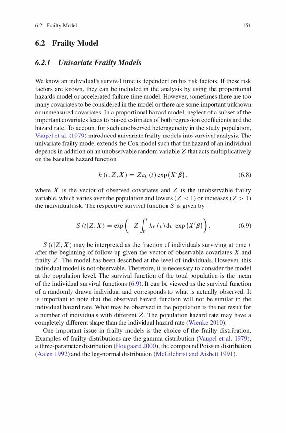
6.2 Frailty Model 151
6.2 Frailty Model
6.2.1 Univariate Frailty Models
We know an individual’s survival time is dependent on his risk factors. If these riskfactors are known, they can be included in the analysis by using the proportionalhazards model or accelerated failure time model. However, sometimes there are toomany covariates to be considered in the model or there are some important unknownor unmeasured covariates. In a proportional hazard model, neglect of a subset of theimportant covariates leads to biased estimates of both regression coefficients and thehazard rate. To account for such unobserved heterogeneity in the study population,Vaupel et al. (1979) introduced univariate frailty models into survival analysis. Theunivariate frailty model extends the Cox model such that the hazard of an individualdepends in addition on an unobservable random variableZ that acts multiplicativelyon the baseline hazard function
h .t; Z;X/ D Zh0 .t/ exp�X 0ˇ
�, (6.8)
where X is the vector of observed covariates and Z is the unobservable frailtyvariable, which varies over the population and lowers (Z < 1) or increases (Z > 1)the individual risk. The respective survival function S is given by
S .t jZ;X / D exp
�Z
Z t
0
h0 .�/ d� exp�X 0ˇ
��. (6.9)
S .t jZ;X / may be interpreted as the fraction of individuals surviving at time tafter the beginning of follow-up given the vector of observable covariates X andfrailty Z. The model has been described at the level of individuals. However, thisindividual model is not observable. Therefore, it is necessary to consider the modelat the population level. The survival function of the total population is the meanof the individual survival functions (6.9). It can be viewed as the survival functionof a randomly drawn individual and corresponds to what is actually observed. Itis important to note that the observed hazard function will not be similar to theindividual hazard rate. What may be observed in the population is the net result fora number of individuals with different Z. The population hazard rate may have acompletely different shape than the individual hazard rate (Wienke 2010).
One important issue in frailty models is the choice of the frailty distribution.Examples of frailty distributions are the gamma distribution (Vaupel et al. 1979),a three-parameter distribution (Hougaard 2000), the compound Poisson distribution(Aalen 1992) and the log-normal distribution (McGilchrist and Aisbett 1991).

152 6 Multivariate and Multistage Survival Data Modeling
6.2.2 Multivariate Frailty Models
Multivariate frailty models can be useful when lifetimes in a cluster or recurrentevents like infections are considered because in such cases independence betweenthe clustered survival times cannot be assumed. Multivariate models are able toaccount for dependence between these event times. A general approach is to assumeindependence among observed data items conditional on a set of unobserved orlatent variables (Hougaard 2000); for example, let S.t1jZ;X1/ and S.t2jZ;X 2/ bethe conditional survival functions of two related individuals with different vectorsof observed covariates X 1 and X 2, respectively, in (6.9). Integrating out the noisevariable Z, the two-dimensional survival function can be written as
S .t1; t2/ DZ 1
0
S .t1jz;X 1/ S .t2jz;X 2/ g .z/ d z; (6.10)
where g.Z/ denotes the density of the frailty Z. In the case of twins, S.t1; t2/denotes the fraction of twins pairs with twin 1 surviving t1 and twin 2 surviving t2.
6.2.3 The Shared Frailty Copula
The shared frailty model is relevant to event times of related subjects (similar organsand repeated measurements). Subjects in a cluster are assumed to share the samefrailty Z (Clayton 1978; Hougaard 2000). The survival times are assumed to beconditionally independent with respect to the shared (common) frailty. Conditionalon the frailty Z, the hazard function of an individual in a pair is of the formZh0.t/ exp.X 0ˇ/, where the value of Z is common to both individuals in the pairand thus is the cause for dependence between survival times within pairs.
S .t1; t2jZ/ D S1 .t1/Z S2 .t2/
Z .
In most applications it is assumed that the frailty distribution is a gamma dis-tribution with mean 1 and variance 2. Averaging the conditional survival functionsunder this assumption, the survival functions can be written as (Wienke 2010)
S .t1; t2/ D�S1 .t1/
�2 C S2 .t2/�2 � 1
� 1
2 .
where 2 > 0 indicates a dependent model and 2 > 0 with Z D 1 indicates anindependent model.
Shared frailty explains correlations between subjects within clusters. There area few issues with the model: When covariates are present in a proportional hazardmodel with gamma-distributed frailty, the dependence parameter and the populationheterogeneity are confounded, which implies that the joint distribution can be

6.3 First-Hitting-Time Model 153
identified from the marginal distributions (Hougaard 1986). In most cases, a one-dimensional frailty can only induce positive association within the cluster. However,there are some situations in which the survival times for subjects within the samecluster are negatively associated. For example, in the Stanford Heart TransplantationStudy, generally the longer an individual must wait for an available heart, theshorter he or she is likely to survive after the transplantation. Therefore, the waitingtime and the survival time afterward may be negatively associated. To avoid theabove-mentioned limitations of shared frailty models, correlated frailty models weredeveloped (Wienke 2010).
6.2.4 The Correlated Frailty Copula
Correlated frailty models were initially developed for the analysis of bivariate failuretime data, in which two associated random variables are used to characterize thefrailty effect for each pair. For example, processes of biomarkers 1 and 2 areassociated with a joint distribution but don’t have a common frailty distribution.These two variables can also be negatively associated, which would induce anegative association between survival times. Assuming gamma-distributed frailties,Yashin and Iachine (1995) used the correlated gamma frailty model, resulting in abivariate survival distribution of the form:
S .t1; t2/ D S1 .t1/1�� S2 .t2/1��
�S1 .t1/
�2 C S2 .t2/�2 � 1
� �
2
.
Research on applications of correlated frailty models has been done, including ashared log-normal frailty model for the catheter infection (McGilchrist and Aisbett1991), a shared frailty model with gamma and log-normally distributed frailty forthe recurrence of breast cancer (dos Santos et al. 1995), a shared positive stablefrailty model for a diabetic retinopathy study (Manatunga and Oakes 1999), and acorrelated gamma frailty model to analyze genetic factors involved in mortality dueto coronary heart disease in twins (Wienke et al. 2001; Zdravkovic et al. 2002).
6.3 First-Hitting-Time Model
6.3.1 Wiener Process and First Hitting Time
Definition 6.1. A stochastic process fX.t/; t � 0g is said to be a Brownian motionwith a drift if (1) X .0/ D 0; (2) fX.t/; t � 0g has stationary and independent

154 6 Multivariate and Multistage Survival Data Modeling
increments; and (3) for every t > 0;X .t/ is normally distributed with mean t andvariance 2t ,
X .t/ � 1p2�2t
exp
� .x � t/2
22t
!. (6.11)
The covariance of the Brownian motion is covŒX.t/; X .s/� D 2 min fs; tg.The standard Brownian motion B .t/ is the Brownian motion with drift D 0
and diffusion 2 D 1. The relationship between the standard Brownian motion andBrownian motion with drift and diffusion parameter 2 can be expressed as
X .t/ D t C B .t/ . (6.12)
The c.d.f. is given by
Pr fX .t/ � yjX .0/ D xg D ˚
y � x � t
pt
�, (6.13)
where ˚ .�/ is the c.d.f. of the standard normal distribution.The first hitting time T is a random variable when X .t/ starts from the initial
position X .0/ D 0 2 ˝nß and reaches a given constant boundary ß D b ofthe domain ˝ (non-negative values). The FHT for Brownian motion is the inversenormal distribution:
T � f�t j; 2; b� D bp
2�2t3e
� .bCt/2
22t : (6.14)
The c.d.f. corresponding to (6.14) is given by
F�t j; 2; b� D ˚
�� .t C b/p
2t
C e
� 2b
2 ˚
�t � bp2t
: (6.15)
Note that if > 0, then the FHT is not certain to occur and the p.d.f. is improper.Specifically, in this case, P.t D 1/ D 1�exp.�2b=2/.Definition 6.2. In general, an FHT model < X.t/; ß> has two essential com-ponents: (1) a parent stochastic process fX.t/; t 2 T , x 2 Rg with initial valueX.0/ D 0, where T is the time space and R is the state space of the process, and(2) a boundary set or threshold ß, where ß � R. Note that ß can be a constant orfunction vector of time t or a stochastic process.
6.3.2 Covariates and Link Function
In an FHT model, both the parent process fX.t/g and boundary ß can haveparameters that depend on covariates. As a simple sample, the Wiener process hasmean parameter and variance parameter 2. The boundary ß has parameter x0,

6.3 First-Hitting-Time Model 155
the initial position. In FHT regression models, these parameters will be connectedto linear combinations of covariates using a suitable regression link function,
g .�/ D Zˇ0, (6.16)
where g .�/ is the link function that has the inverse function g�1 .�/, � is theparameter vector in the FHT model, Z D .1;Z1; : : : ; Zk/ is the covariate vector(with a leading unit to include an intercept term), and fi D .ˇ0; ˇ1; : : : ; ˇk/ is theassociated vector of regression coefficients. The commonly used link functionsinclude the identity and logistic functions.
There are two different covariates: time-independent (e.g., DNA markers) andtime-dependent covariates (e.g., RNA markers). The use of time-dependent covari-ates should be taken cautiously since it could be very controversial (see Sect. 6.4).
We can solve (6.16) for � :
� D g�1 �Zˇ0� . (6.17)
6.3.3 Parameter Estimation and Inference
The parameter estimations for FHT models have been dominated by the maximumlikelihood method. Consider a latent health status process characterized by aWiener diffusion process. The FHT for such a process follows an inverse Gaussiandistribution. The inverse Gaussian distribution depends on the mean and varianceparameters of the underlying Wiener process ( and 2) and the initial health statuslevel (x0), i.e., � D .; ; x0/. Let f .t j�/ and F.t j�/ be the p.d.f. and c.d.f. of theFHT distribution, respectively. Using (6.17), we can obtain
(f .t j�/ D f
�t jg�1 �Zˇ0�� ,
F.t j�/ D F�t jg�1 �Zˇ0�� .
(6.18)
To form a likelihood function, denote by Z i (i D 1; : : : ne) the realization ofcovariate vector Z on the i th subject who had an event at time ti , and by Z j
(j D ne C 1; : : : ne C ns) the realization of covariate vector Z on the j th subject,who is right-censored at time tj . Then the likelihood function is given by
L.ˇ/ DneY
iD1f�ti jg�1 �Z iˇ
0
�� neCnsY
jDneC1S�tj jg�1 �Z jˇ
0�� : (6.19)
To estimate parameters ˇ, the likelihood or the log-likelihood function can beused. Numerical gradient methods can be used to find the maximum likelihoodestimates for ˇ. Then the parameter vector � can be found using (6.17), and thedistribution function f .t j�/ and F.t j�/ can be obtained from (6.18).

156 6 Multivariate and Multistage Survival Data Modeling
6.3.4 Applications of First-Hitting-Time Model
Example 6.1. A death can be viewed as the final result of the degradation of anindividual’s health. If we model an individual’s health state using a Wiener process,then death can be viewed as the Wiener process reaching a certain threshold ß. Thesurvival analysis becomes the study of the FHT of the process, which has an inversenormal distribution.
Alternatively, if a gamma process is chosen to model the health state, the survival(FHT) will have an inverse gamma distribution. Singpurwalla (1995) and Lawlessand Crowder (2004) consider the gamma process as a model for degradation. TheOrnstein-Uhlenbeck process can also be used for modeling the biological process.The FHT for the Ornstein-Uhlenbeck process has the Ricciardi-Sato distribution(Ricciardi and Sato 1988).
Example 6.2. Survival analysis in a clinical trial with treatment switching is achallenge. In randomized oncology trials, a patient’s treatment may be switchedin the middle of the study because of a progressive disease (PD), which indicatesa failure of the initial treatment regimen. In such cases, the total survival time isthe sum of two event times: randomization to switching and switching to death.If the test drug is more effective than the control, then the majority of patients inthe control group will switch to the test drug and the survival difference betweenthe two treatment groups will be significantly reduced in comparison with the casewithout treatment switching. This marker-based treatment switch is not randomswitching but rather response-adaptive switching. Branson and Whitehead (2002)and Shao et al. (2005) proposed different approaches to the problem. Lee et al.(2008) proposed a mixture of Wiener processes for clinical trials with adaptiveswitching and applied it to an oncology study. It is outlined as follows.
Since the actual or censored survival time can be composed of two intervals,representing the time on the primary therapy and the time on the alternative therapy,the disease may progress at different rates in these two intervals (irrespective of thetreatment). We transform survival times from calendar time to the so-called runningtime, which has the form
r D a1�1 C �2, (6.20)
where �1 and �2 correspond to time to progression and progression to death,respectively, and a1 is a scale parameter to be estimated.
The mixture of Wiener processes with FHT used for the modeling is given by
Pr .S > r/ D p .1 � F1 .r//C .1 � p/ .1 � F2 .r// . (6.21)
The respective lifetime functions Fj .r/ (j D 1; 2) are the same as (6.15) butexpressed in terms of running time r . The parameter p is to be estimated.

6.3 First-Hitting-Time Model 157
6.3.5 Multivariate Model with Biomarkers
There are different biomarkers: a pharmacodynamic biomarker informs if a drug hasreached its target; a functional response biomarker informs if a drug has affecteda target pathway; a pharmacogenomic biomarker (PGx) measures variations ina target; a disease biomarker monitors or predicts disease risk, progression, andimprovement; and a surrogate endpoint reflects how a patient feels or physical ormental functions.
Biomarkers, compared with a clinical endpoint such as survival, can often bemeasured earlier, easier, and more frequently. They are less subject to competingrisks and are less confounded by changes in treatment modalities. Among differentbiomarkers, some are static, such as DNA markers, while others are time-dependent,such as RNA markers. A time-independent biomarker can be treated as a covariate,whereas a time-dependent marker can be treated in multivariate survival models.There are also models that treat a time-dependent variable as a covariate. However,we will show you that the results from such models can be very misleading. Theutility of biomarkers in clinical trial designs, especially in adaptive designs, hasbeen discussed in Chang (2007). Here we discuss how to use the biomarker processto assist in tracking the progress of the parent process if the parent process is latentor only infrequently observed. In this way, the marker process forms a basis for apredictive inference about the status of the parent process and its progress toward anFHT. As markers of the parent process, they offer potential insights into the causalforces that are generating the movements of the parent process (Whitmore et al.1998).
We now introduce the Whitmore-Crowder-Lawless method (Whitmore et al.1998). Suppose there are the parent survival process, X .t/, and a correlatedbiomarker process, Y .t/. They form a two-dimensional Wiener diffusion processfX .r/ , Y .r/g for r � 0 and the initial condition fX .0/ , Y .0/g D f0; 0g. VectorfX .r/ , Y .r/g has a bivariate normal distribution with a mean vector r�, where
� D �x , y
�0, x � 0, and covariance matrix r˙ with ˙ D
xx xy
yx yy
�. The
correlation coefficient is � D xy=pxxyy .
The key is to formulate the probability or p.d.f. for the survival and failingsubjects. For a survivor at time t , an observed value Y .t/ D y .t/ for the biomarkerconstitutes a censored observation of failure time because we know S > t . Thep.d.f. for survival subjects is given by
ps .y/ D ˚ .c1/ � .c2/� e2xxx ˚
0
@c1 � 2
s.1 � �2/xxt
1
A�c2 � 2xy
xxpyyt
�,
(6.22)

158 6 Multivariate and Multistage Survival Data Modeling
where � and ˚ are, respectively, the standard normal p.d.f. and c.d.f., and
8ˆ<
ˆ:
c1 D 1 � xt � xy�y � yt
�
yypxx .1 � �2/ t
,
c2 D y � ytpyyt
.
(6.23)
For a subject that died at time S D s with an observed value Y .S/ D y .s/ forthe biomarker, the joint p.d.f. is
pf .y; s/ D exp�� 1
2W T˙�1W
�
2�pj˙ js2 , (6.24)
where
W T Dy � ysp
s;1 � xsp
s
�. (6.25)
The probability of surviving longer than time t is
P .S > t/ DZ 1
�1ps .y/ dy. (6.26)
Numerical methods can be used to calculate P .S > t/.To carry out maximum likelihood estimation of the parameters, we denote the
independent sample observations on failing items by . Oyi ; Osi /, i D 1; : : : ; , andthose on surviving items by Oyi , i D C 1; : : : ; n. The log-likelihood can then bewritten as
lnL.;˙/ D X
iD1lnpf . Oyi ; Osi /C
nX
iD C1lnps . Oyi / . (6.27)
The maximum likelihood estimates of the parameters and ˙ can be foundbased on (6.27).
From (6.22) through (6.27), we have assumed the threshold for failure is x D 1. Iffailure is defined as x D a, then the estimates Ox , Oxx , and Oxy from (6.20) shouldbe multiplied by a constant a. Other estimates and probabilities are independentof a. Thus no changes are needed.
So far, we have considered a single-marker case. In practice, there is usuallymore than one relevant marker, while each marker will have a certain degree ofcorrelation with the underlying parent process. We wish to find that the linearcombination of the available markers will have the largest possible correlation withthe degradation component. Whitmore et al. (1998) extended their method to includea composite marker or a combination of several markers.
Suppose there are k candidate markers available, denoted by Z .t/ D .Z1.t/ ; : : : ; Zk .t//, with the initial condition Z .0/ D 0. Assume that vector Z .t/,

6.4 Multistage Model 159
together with the degradation componentX .t/, forms a k C 1 dimensional Wienerprocess. We define the composite marker denoted by Y .t/ as
Y .t/ D Z .t/ˇ0 DkX
jD1Zj .t/ ˇj ; (6.28)
where ˇ D .1; ˇ2; : : : ; ˇk/ is a k � 1 vector of coefficients that we wish to estimate.The linear structure of (6.28) assures that the joint process for Y .t/ andX .t/ retainsits bivariate Wiener form. The parameterization is defined by
y D Zˇ0; yy D ˇ˙ZZ ˇ
0; yy D ˙XZ ˇ0; (6.29)
where Z and ˙ZZ denote the k � 1 mean vector and k � k covariance matrix ofmarkersZ .t/ and ˙XZ denotes the 1 � k covariate vector of X .t/ with Z .t/.
The MLEs presented earlier for a single marker can be extended to estimate theoptimal composite marker in (6.28). This extension requires rewriting the likelihoodfunction in (6.27) in terms of the new parameterization in (6.29).
6.4 Multistage Model
6.4.1 General Framework of Multistage Model
Multistage models are not only used for longitudinal data but can also be usedfor multivariate survival analysis if we partition all the possible event scenariosinto stages (or states) and build a progressive model. According to Hougaard(2000), a progressive model is a stochastic model in which all states except theinitial state have only one possible transition into the state. We consider the time-dependent Markov progressive model in which the probability (density) of transitionis usually dependent on the time relative to the previous state but independent ofany earlier states. For example, a healthy individual can become a disabled personand then die, as shown in Fig. 6.1. The progressive Markov model says that thetransition probability from the state “Disabled” to “Death” is a function of time from“Disabled” but is independent of how healthy he was and how quickly he became adisabled person.
Suppose we have a simple multistage model, as shown in Fig. 6.1, that has threestates of an individual: health, disabled, and death. Possible transition directions areindicated by arrows, with a corresponding transition probability Fi .t/ and densityfi .t/ (i D 1; 2), which are the lifetime and event density functions.
After a multistage model is constructed, we need to formulate the likelihood forthe MLE of parameters. Similar to the single stage model discussed in Sect. 6.1, the
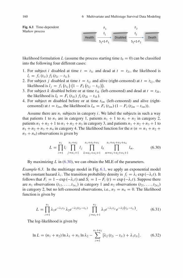
160 6 Multivariate and Multistage Survival Data Modeling
Fig. 6.1 Time-dependentMarkov process
F1
Health Disabled DeathS1=1-F1 S2=1-F2
f1
F2
f2
likelihood formulationL (assume the process starting time t0 D 0) can be classifiedinto the following four different cases:
1. For subject i disabled at time t D t1i and dead at t D t2i , the likelihood isli D f1 .t1i / f2 .t2i � t1i /.
2. For subject j disabled at time t D t1j and alive (right-censored) at t D t2j , thelikelihood is lj D f1
�t1j� �1 � F2
�t2j � t1j
��.
3. For subject k disabled before or at time t1k (left-censored) and dead at t D t2k ,the likelihood is lk D F1 .t1k/ f2 .t2k � t1k/.
4. For subject m disabled before or at time t1m (left-censored) and alive (right-censored) at t D t2m, the likelihood is lm D F1 .t1m/ .1 � F2 .t2m � t1m//.Assume there are ni subjects in category i . We label the subjects in such a way
that patients 1 to n1 are in category 1, patients n1 C 1 to n1 C n2 in category 2,patients n1 Cn2 C 1 to n1 Cn2 Cn3 in category 3, and patients n1 Cn2 Cn3 C 1 ton1 C n2 C n3 C n4 in category 4. The likelihood function for the n (n D n1 C n2 Cn3 C n4) observations is given by
L Dn1Y
iD1li
n1Cn2Y
jDn1C1lj
n1Cn2Cn3Y
kDn1Cn2C1lk
n1Cn2Cn3Cn4Y
mDn1Cn2Cn3C1lm: (6.30)
By maximizing L in (6.30), we can obtain the MLE of the parameters.
Example 6.3. In the multistage model in Fig. 6.1, we apply an exponential modelwith constant hazard �i . The transition probability density is fi D �i exp .��i t/. Itfollows that Fi D 1� exp .��i t/ and Si D 1�Fi .t/ D exp .��i t/. Suppose thereare n1 observations .t11; : : : ; t1n1/ in category 1 and n2 observations .t21; : : : ; t2n2 /in category 2, but no left-censored observations, i.e., n3 D n4 D 0. The likelihoodfunction is given by
L Dn1Y
iD1�1e
��1t1i �2e��2.t2i�t1i /n2Y
jDn1C1�1e
��1t1j e��2.t2j�t1j /. (6.31)
The log-likelihood is given by
lnL D .n1 C n2/ ln�1 C n1 ln�2 �n1Cn2X
iD1Œ�2 .t2i � t1i /C �1t1i � . (6.32)

6.4 Multistage Model 161
Fig. 6.2 Effect of treatmentswitching
Treatmentrandomization
A PD B
DeathB PD A
The maximization of lnL gives
�1 D n1 C n2Pn1Cn2iD1 t1i
I�2 D n1Pn1Cn2iD1 .t2i � t1i /
. (6.33)
6.4.2 Covariates and Treatment Switching
Covariates such as medical treatment, age, race, and disease status may or may notbe time-dependent. In Example 6.4, a progressive disease (PD) is an indication oftreatment failure and the patient usually has to switch from the initial treatment toan alternative. Thus, treatment for a patient is a time-dependent variable: before PDwith one treatment, after PD with another treatment (Fig. 6.2).
To consider covariates in a multistage model, we can use a link function asdefined in (6.16). Then substitute (6.17) into (6.30) and maximize it to obtain MLEsof the parameters ˇ.
Example 6.4. Suppose patients in a two-group oncology clinical trial are random-ized to receive either treatmentA orB . If a progressive disease is observed, meaningthe patient has developed a resistance to the drug, then the patient will switch thetreatment from A to B or B to A (in practice, there are more options, i.e., differentcombinations of drugs). Let Zi.t/ be a random process for the i th patient. If patienti is on treatment A at time t , then Zi.t/D 1; otherwise, Zi.t/D 0. We use theidentity link function
�i .t/ D ˇi .t/ Zi .t/ . (6.34)
Recognizing the different hazard rates before and after PD, we use the piecewiseconstant hazard
�i .t/ D ˇi1Z .t/C ˇi2 .1�Z .t// ; i D 1; 2;
where i D 1 before PD and i D 2 after PD. In other words, the hazard rates are ˇ11for treatmentA before PD, ˇ21 for treatmentA after PD, ˇ12 for treatment B beforePD, and ˇ22 for treatment B after PD.
For simplicity we assume PD is always observed immediately (i.e., no censoringon PD). Thus, a typical patient i initially treated with drugAwill have the followingtwo possible likelihood functions:
1. PD at time t D t1i and death at t D t2i , li D ˇ11e�ˇ11t1i ˇ21e�ˇ21.t2i�t1i /, where
i D 1; : : : ; n1.

162 6 Multivariate and Multistage Survival Data Modeling
2. PD at time t D t1i and alive (right-censored) at t D t2i , li D ˇ11e�ˇ11t1i
e�ˇ21.t2i�t1i /, where i D n1 C 1; : : : ; n1 C n2.
Similarly, a typical patient i initially treated with drug B will have the followingtwo possible likelihood functions:
1. PD at time t D t1i and death at t D t2i , li D ˇ12e�ˇ12t1i ˇ22e�ˇ22.t2i�t1i /, where
i D n1 C n2 C 1; : : : ; n1 C n2 C n3.2. PD at time t D t1i and alive (right-censored) at t D t2i , li D ˇ12e
�ˇ12t1ie�ˇ22.t2i�t1i /, where i D n1 C n2 C n3 C 1; : : : ; n1 C n2 C n3 C n4.
The likelihood function based on the total n1 C n2 C n3 C n4 observations is thesame as (6.30). The log-likelihood function can be given explicitly by
lnL D .n1 C n2/ lnˇ11 C .n3 C n4/ lnˇ12 C n1 lnˇ21 C n3 lnˇ22
�n1Cn2X
iD1Œˇ21 .t2i � t1i /C ˇ11t1i �
�n1Cn2Cn3Cn4X
iD1Cn1Cn2Œˇ22 .t2i � t1i /C ˇ12t1i � . (6.35)
Letting @ lnL@ˇjk
D 0, we can obtain
8ˆˆˆˆ<
ˆˆˆˆ:
ˇ11 D n1 C n2Pn1Cn2iD1 t1i
,
ˇ12 D n3 C n4Pn1Cn2Cn3Cn4iD1Cn1Cn2 t1i
,
ˇ21 D n1Pn1Cn2iD1 .t2i � t1i /
,
ˇ22 D n3Pn1Cn2Cn3Cn4iD1Cn1Cn2
.t2i�t1i /.
(6.36)
The relative treatment efficacy between the treatment groups can be measured bythe hazard ratio:
8ˆ<
ˆ:
HR1 D ˇ11
ˇ12, before PD,
HR2 D ˇ21
ˇ22, after PD.
(6.37)
In practice, cancer drugs are categorized by the number of PDs: newly diagnosedpatients usually use first-line drugs, after one PD they use second-line drugs, andso on.

6.4 Multistage Model 163
Fig. 6.3 Competing risks
InitialState
Death ofcause k
Death ofcause M
Death ofcause 1
The efficacy should be compared in terms of life saving between the twoconditions with and without the new drugB . (1) Without drugB , the patients wouldbe treated withA initially and then treated with some other available drugs. (2) Withdrug B , the patients will eventually have PD and will be treated with drug B orother drugs. If there are other drugs available (as good as drugB) after the PD, thenHR1 D ˇ11
ˇ12should be used to measure the survival benefit, which implies that PD
is a good surrogate marker for survival.
6.4.3 Latent Process and Competing Risks
Most survival data are gathered under conditions of competing risks, in which twoor more causes are competing to determine the observed duration (Fig. 6.3). In aclinical trial, an early withdrawal can be considered as either a censor or a competingrisk. Because of the censoring or competing risks, the FHT may not be observableor latent. Latent FHT models are theoretically not necessary, but in practice it isconvenient to the concept of latent FHT. An engineer may be interested in howmuch repair work can be reduced if one or more old machines are replaced withnew ones in the production line. Health authorities may be interested in an optimalresource allocation and predicting the survival prolongation by investing resourcesin different therapeutic areas. Simply investing all government health resources onthe treatments of leading causes of death may not be a good idea. Such problems canbe dealt with by using the difference in FHT (survival time) between the two models,with and without a certain competing risk. Lee and Whitmore (2006) providedapplications of such models in the health and medical field. It is obvious that ifthe underlying multidimensional Wiener process is correlated, the latent survivaltimes for different causes of death will be dependent. Competing-risk problems arealso viewed as cluster survival problems because of the correlation between therisks. A mixed distribution may be required in this case. In what follows, we willdiscuss independent competing risks. The competing-risks analysis of correlatedfailure time data or clustered data can be found elsewhere (e.g., Chen et al., 2008).

164 6 Multivariate and Multistage Survival Data Modeling
General steps in building a multistage model with independent competing riskscan be outlined as follows:
1. Identify competing risks.2. Propose a local failure density model fk .�; t/.3. Formulate the lifetime function F .�; t/=
PMkD1 fk .� ; t/ and the survival func-
tion S .�; t/ D 1 � F .�; t/, where M is the number of competing risks.4. Determine the link function g .�/ D Xˇ
0
if any, where X represents covariates;
� D g�1�Xˇ
0
�.
5. Formulate the likelihood function
L DY
i2�S�g�1 �Xˇ0
�, ti� Y
j…�fkj
��; tj
�, (6.38)
where � is the set of indices for right-censoring observations. Here we haveassumed that there is only right-censoring.
6. Obtain the MLE of ˇ0
by maximizing L. Other parameters of interest can beobtained consequently.
Before we discuss more complicated models, let’s study a degenerated case:single-stage competing risks. Denote by fk the hazard function of the kth cause(k D 1; : : : ;M ). Then the total hazard function for the parallel competing-risksmodel in Fig. 6.3 is f .u/ D PM
kD1 fk .u/. In light of (6.2), we assume the hazarddensity has the form
fk.t/ D �k .t/ .1 � F .t// D �kS .t/ , (6.39)
where S .t/ D 1 � F .t/ is the survival function with the lifetime function F .t/ DR t0f .u/ du.Given a subject alive at time t , the probability of dying within the time interval
dt due to cause k is given by
�k .t/ dt D fk .t/
1 � F .t/dt . (6.40)
Summing up (6.40) over all causes and letting � .t/ D PMkD1 �k .t/, we obtain
�dt D f .t/
1 � F .t/dt D dF .t/
1 � F .t/. (6.41)
As shown in Sect. 6.1, the overall survival function derived from (6.41) is
S .t/ D exp .��.t// D exp
�Z t
0
� .u/ du
�. (6.42)

6.4 Multistage Model 165
From (6.34), we know that fkj�tj� D �kj S
�tj�. Substituting this into (6.38) we
can obtain the likelihood
L DY
i2˝S .ti /
Y
j…˝�kj
�tj�S�tj�: (6.43)
The transitional probability from the initial state to the death state due to cause kis given by
Fk .t/ DZ t
0
�k .u/ S .u/ du DZ t
0
�k .u/ exp
�Z u
0
MX
iD1�i .v/ dv
!du. (6.44)
We can see that for each death there is a hazard term, depending only on theactual cause, and an exponential term depending on the integrated hazard for allcauses together. It is obvious that F .t/ D P
k Fk .t/ D 1 � S .t/.When all �k .t/ D �k; k D 1; : : :M , are independent of time, S .t/ D
exp .��t/, � D PMkD1 �k . Thus, the system acts just like a single risk system with a
big hazard (the sum of all individual hazard rates). The transition probability densityis given by fk .t/ D �k exp .��t/.
To consider the covariates, we can use the identity link function
�k D X k .t/ˇ0
.t/ , (6.45)
whereX k represents covariates with corresponding parameters ˇ. Both of them canbe time-dependent or time-independent.
Substituting (6.45) into (6.43), we obtain the likelihood function in terms ofparameters ˇ:
L DY
i2˝exp
�Z ti
0
MX
kD1Xk .u/ˇ
T .u/ du
!Y
j…˝�kj
�tj�
exp
�Z tj
0
� .u/ du
�.
(6.46)Note that the term S .t/ in model (6.39) implies that an individual having a higher
risk of dying from one cause will have a higher risk of dying from other causes too.Alternatively, we can remove this constraint and propose as a local model for cause-specific death,
fk .t/ D ak�k .t/ Sk .t/ D ak�k .t/ exp
�Z t
0
�k .u/ du
�, (6.47)
where ˛k is independent of time andPM
kD1 ak D 1 (see explanation later). Thus akcan be viewed as a weight.
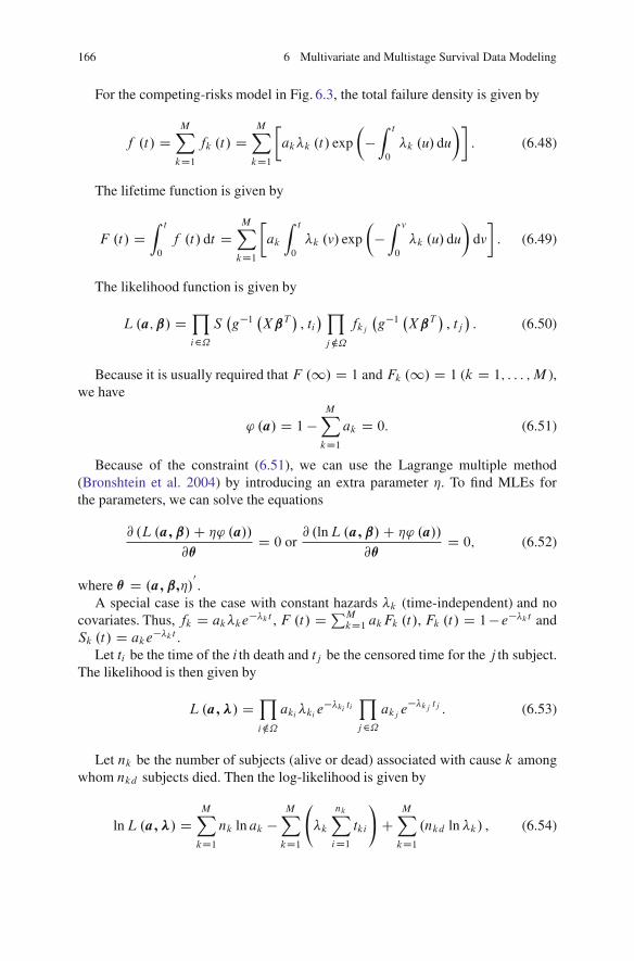
166 6 Multivariate and Multistage Survival Data Modeling
For the competing-risks model in Fig. 6.3, the total failure density is given by
f .t/ DMX
kD1fk .t/ D
MX
kD1
�ak�k .t/ exp
�Z t
0
�k .u/ du
� . (6.48)
The lifetime function is given by
F .t/ DZ t
0
f .t/ dt DMX
kD1
�ak
Z t
0
�k .v/ exp
�Z v
0
�k .u/ du
�dv
. (6.49)
The likelihood function is given by
L.a;ˇ/ DY
i2˝S�g�1 �XˇT
�, ti� Y
j…˝fkj
�g�1 �XˇT
�, tj�
. (6.50)
Because it is usually required that F .1/ D 1 and Fk .1/ D 1 (k D 1; : : : ;M ),we have
' .a/ D 1 �MX
kD1ak D 0. (6.51)
Because of the constraint (6.51), we can use the Lagrange multiple method(Bronshtein et al. 2004) by introducing an extra parameter �. To find MLEs forthe parameters, we can solve the equations
@ .L .a; ˇ/C �' .a//
@�D 0 or
@ .lnL.a; ˇ/C �' .a//
@�D 0; (6.52)
where � D .a; ˇ;�/0
.A special case is the case with constant hazards �k (time-independent) and no
covariates. Thus, fk D ak�ke��kt , F .t/ D PM
kD1 akFk .t/, Fk .t/ D 1� e��kt andSk .t/ D ake
��kt .Let ti be the time of the i th death and tj be the censored time for the j th subject.
The likelihood is then given by
L.a; �/ DY
i…˝aki �ki e
��ki tiY
j2˝akj e
��kj tj . (6.53)
Let nk be the number of subjects (alive or dead) associated with cause k amongwhom nkd subjects died. Then the log-likelihood is given by
lnL.a; �/ DMX
kD1nk ln ak �
MX
kD1
�k
nkX
iD1tki
!C
MX
kD1.nkd ln�k/ , (6.54)

6.4 Multistage Model 167
Entering
Progressivedisease
Dropout dueto lack ofefficacy
Death incancer
Dropout due toadverse events
Censorings including non-cancer deaths
f31
f12
f22
f41
f 11(f 21
)
Clinical Trial
Fig. 6.4 Progressive disease with competing risks
where tki is the observed time (death or censoring) associated with cause k.Substituting (6.54) into (6.52), we obtain the MLE of �:
8ˆ<
ˆ:
ak D nkPMkD1 nk
,
�k D nkdPnkiD1 tki
.(6.55)
It can be seen that ak D nkPMkD1 nk
holds true for general model (6.47), which is
consistent with our intuition.There are many other research studies on competing risks. Among them, Shen
and Thall (1998) applied a mixed distribution for multiple nonfatal and fatalcompeting risks. Chen et al. (2008) studied the competing risks of correlated failuretime data.
6.4.4 Competing Risks in Progressive Disease
Suppose that in an oncology clinical trial the patients in the study can be ap-proximately grouped into four categories (Fig. 6.4): (1) progressive disease (PD),then death (D) due to cancer; (2) PD, then dropout due to lack of efficacy (LE);(3) dropout due to adverse events (AE); and (4) dropout due to other reasons.For simplicity, we group other scenarios such as death for other reasons andearly withdrawals for other reasons in scenario (4). Scenarios (1), (2), and (3) areconsidered competing risks because they are likely treatment-related. Scenario (4)

168 6 Multivariate and Multistage Survival Data Modeling
is considered non-informative censoring. Here we have generalized the concept ofcompeting risks; i.e., the risks can be a mixture of different events. The reason wecan do this is because the likelihood function (joint probability) does not requirethat all the events be of the same type. In practice, if there are enough patients, wecan have more than these four categories.
The complexity of the model is not substantial, even though the steps involvedin solving the problem are more tedious. The key is to formulate likelihoodfunctions:
1. A patient with PD at t1i and who died of cancer at t2i has l1 D f11 .t1i / f12 .t2i /.There are n1 patients in this category.
2. A patient with PD at t1i and dropout after PD at t2i due to LE has l2 Df11 .t1i / f22 .t2i � t1i /. There are n2 patients in this category.
3. A patient dropout at t1i due to AE has l3 D f31 .ti /. There are n3 patients in thiscategory.
4. A patient censored at t1i after PD, not because of LE or AE, has l4 D.1 � F41.t1i //, where F41 .t/ D R t
0f41 .u/ du. There are n4 patients in this
category.
The likelihood for the patients can be expressed as
L Dn1Y
iD1l1
n2Y
iD1l2
n3Y
iD1l3
n4Y
iD1l4 (6.56)
or
L Dn1Y
iD1f11 .t1i / f12 .t2i /
n2Y
iD1f11 .t1i / f22 .t2i � t1i /
n3Y
iD1f31 .ti /
n4Y
iD1.1 � F41 .t1i // .
(6.57)Since we have used multiple stages, we can choose relatively simple transition
probability densities fjk . For example, assume constant �jk for transition proba-bility densities fjk :
fjk .t/ D ajk�jk exp���jkt
�, (6.58)
Again, because of the condition of the transition probabilities at t D 1 (i.e.,R10fjk .t/ dt D 1), constants ak satisfy (through derivations similar to the previous
MLE derivations)
aj1 D nj
n1 C n2 C n3 C n4; j D 1; 2; 3; 4. (6.59)
Therefore, we have
Fjk .t/ DZ t
0
fjk .u/ du D ajk�1 � exp
���jkt��
. (6.60)

6.4 Multistage Model 169
Using the identity link function, �jk D Xˇ0
jk , where X represents covariates.We assume ajk is covariate-independent such that
fjk�t I ajk;ˇjk
� D ajkXˇ0
jk exp��Xˇ0
jkt�
, (6.61)
Fjk�t I ajk;ˇjk
� D ajk
�1 � exp
��Xˇ0
jkt��
. (6.62)
Substituting (6.61) and (6.62) into (6.57) and then taking derivatives with respectto vector ˇ
0
jk , the MLEs of the parameters can be found using numerical methods.Other transition probability densities can also be used, such as the Weibull
distribution with S.t/ D exp.��t� / or f .t/ D ��t��1 exp.��t� /; Gompertzdistribution with hazard �.t/ D �wt , S.t/ D exp.� R t0 �wudu/ D exp. �
1Ct wtC1/ �
exp.�w/, and f .t/ D � dS.t/dt , where the positive constant w can be <1;D 1, and
>1. We can also construct the transition probability using the FHT distributiongiven by (6.14) or (6.15). The simplest case is probably the model with constanttransition probability density (rate), which leads to a homogeneous Markov processor finite-state continuous time Markov chains. However, such an oversimplifiedmodel is not very practical in survival analysis, though it is useful elsewhere.
6.4.5 Longitudinal Multivariate Model
Unlike in Sect. 6.3.5, where we modeled the correlation between parent and markerprocesses, we are going to model the correlation of the hitting times between parentand marker processes directly, which will greatly simplify the problem.
For the problem presented in Fig. 6.5, with one primary disease process X1 .t/,a disease marker process X2 .t/, and a (composite) PGx marker process X3 .t/, wecan specify the joint transition probability densities
fij .t1; t2; t3/ , (6.63)
or more explicitlyfij .t11; t12; t21; t22; t31; t32/ . (6.64)
We then can obtain the conditional “survival” probability
Scij DZfij .ujtkm/ du; i D 1; 2; 3I j D 1; 2, (6.65)
where the integration is carried out with respect to all censored variables. Forexample, if X1 .t/ is right-censored at t D t12, X2 .t/ is left-censored at t D t21,

170 6 Multivariate and Multistage Survival Data Modeling
Primary DiseaseProcess X1(t): State S11
State S21 State S22 State S33
State S12 State S13
f11
t11
f21
t21
f22
t22
State S31 State S32 State S33
f31
t31
f32
t32
f12
t12
Disease MarkerProcess X2(t):
Time
PGx MarkerProcess X3(t):
Fig. 6.5 Longitudinal multivariate model
and X3 .t/ has no censoring, the conditional “survival” probability is given by
Scij DZ t21
0
Z 1
t12
fij .t11; u12; u21; t22; t31; t32/ du12du21; i D 1; 2; 3I j D 1; 2;
(6.66)
where we have assumed that t21 imposes no constraint on the upper limit of t12;otherwise, the upper limit 1 should change to the upper limit imposed by t21.
The contribution of this individual likelihood to the overall likelihood func-tion is Scij , whereas for an individual without censoring, the contribution isfij .t11; t12; t21; t22; t31; t32/. Therefore the likelihood function is
L DY
˝
Scij
Y
Nfij ; (6.67)
where˝ is the censoring set and N is the noncensoring set.The consideration of covariates using the link function and MLE of parameters
is similar to what we discussed earlier. If there are a larger number of markers, itis difficult to construct valid joint transition probability densities. Therefore we canuse composite markers, as suggested by Whitmore et al. (1998) in Sect. 6.3.5.
6.5 Challenges and Controversies
One of the main challenges in multivariate models is the construction of thetransition probabilities. Alternatively, we may use time-dependent covariates if weare only interested in the primary or parent process. However, regression with time-dependent covariates has controversies, as discussed below.
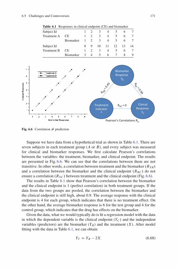
6.5 Challenges and Controversies 171
Table 6.1 Responses in clinical endpoint (CE) and biomarker
Subject Id 1 2 3 4 5 6 7Treatment A CE 1 2 3 4 5 6 7
Biomarker 1 2 3 4 5 6 7
Subject Id 8 9 10 11 12 13 14Treatment B CE 1 2 3 4 5 6 7
Biomarker 3 4 5 6 7 8 9
BiomarkerResponse
YB
Treatmentindicator
X
ClinicalResponse
YC
RXC = 0
RBC = 0.90R XB
= 0.
45
Pearson’s Correlations Rij
Fig. 6.6 Correlation ¤ prediction
Suppose we have data from a hypothetical trial as shown in Table 6.1. There areseven subjects in each treatment group (A or B), and every subject was measuredfor clinical and biomarker responses. We first calculate Pearson’s correlationsbetween the variables: the treatment, biomarker, and clinical endpoint. The resultsare presented in Fig. 6.6. We can see that the correlations between them are nottransitive. In other words, a correlation between treatment and the biomarker .RXB/and a correlation between the biomarker and the clinical endpoint .RBC / do notensure a correlation .RXC / between treatment and the clinical endpoint (Fig. 6.6).
The results in Table 6.1 show that Pearson’s correlation between the biomarkerand the clinical endpoint is 1 (perfect correlation) in both treatment groups. If thedata from the two groups are pooled, the correlation between the biomarker andthe clinical endpoint is still high, about 0.9. The average response with the clinicalendpoint is 4 for each group, which indicates that there is no treatment effect. Onthe other hand, the average biomarker response is 6 for the test group and 4 for thecontrol group, which indicates that the drug has effects on the biomarker.
Given the data, what we would typically do is fit a regression model with the datain which the dependent variable is the clinical endpoint (YC / and the independentvariables (predictors) are the biomarker (YB ) and the treatment (X ). After modelfitting with the data in Table 6.1, we can obtain
YT D YB � 2X: (6.68)
172 6 Multivariate and Multistage Survival Data Modeling
This model fits the data well based on the model-fitting p-value and R2.Specifically, R2 is equal to 1. The p-values for the model and all parameters areequal to 0. The coefficient 2 in model (6.68) is the separation between the two lines.Based on (6.68), we would conclude that both the biomarker and the treatment affectthe clinical endpoint. However, if the population is well represented by the data, thetreatment has no effect on the clinical endpoint at all. In fact, the biomarker predictsthe response in the clinical endpoint, but it does not predict the treatment effect onthe clinical endpoint, i.e., it is a prognostic marker.
6.6 Exercises
6.1. Prove the FHT for Brownian motion is the inverse normal distribution givenby (6.14) and (6.15).
6.2. Suppose in Example 6.3 there are four (instead of two) categories of patients,as specified in Sect. 6.3.1. Derive the MLEs of �1, �2, �3, and �4.
6.3. Suppose in Example 6.3 �1 D a1t and �2 D a2t . Derive the MLEs of a1and a2.
6.4. Suppose in Example 6.3 �1 D �01!t1 and �2 D �02!
t2. Derive the MLEs of the
parameters.
6.5. Study the bias of the estimators �1and �2 given by (6.33).
6.6. Study the bias of the estimators defined by (6.36).
6.7. Study the competing risk problem presented in Fig. 6.3, assuming the death foreach cause follows the Gompertz model with a hazard rate of � .t/ D �!t .
6.8. Discuss the challenges presented in Table 6.1 and Fig. 6.6.
Further Readings and References
Aalen, O.O.: Modeling heterogeneity in survival analysis by the compound Poisson distribution.Ann. Appl. Probab. 4(2), 951–972 (1992)
Aalen, O.O., Gjessing, H.K.: Survival models based on the Ornstein–Uhlenbeck process. LifetimeData Anal. 10, 407–423 (2004)
Aalen, O., Borgan, O., Gjessing, H.: Survival and Event History Analysis. Springer, New York(2010)
Alonso, A., Molenberghs, G., Geys, H., Buyse, M., Vangeneugden, T.: A unifying approach forsurrogate marker validation based on Prentice’s criteria. Stat. Med. 25, 205–221 (2006)
Branson, M., Whitehead, W.: Estimating a treatment effect in survival studies in which patientsswitch treatment. Stat. Med. 21, 2449–2463 (2002)
Bronshtein, I.N., Semendyayev, K.A, Musiol, G., Muehlig, H., Muhlig, H.: Handbook of Mathe-matics. Springer, New Nork (2004)

Further Readings and References 173
Chang, M.: Adaptive Design Theory and Implementation Using SAS and R. Chapman &Hall/CRC, Boca Raton (2007)
Chen, B.E., Kramer, J.L., Greene, M.H., Rosenberg, P.S.: Competing risks analysis of correlatedfailure time data. Biometrics 64, 172–179 (2008)
Clayton, D.G.: A model for association in bivariate life tables and its application in epidemiologicalstudies of familial tendency in chronic disease incidence. Biometrika 65, 141–151 (1978)
Cox, D.R.: Regression models and life-tables. J. R. Stat. Soc. B 34, 187–220 (1972)Crowder, M.J.: Classical Competing Risks. Chapman & Hall/CRC, Boca Raton (2001)Genest, C., Rivest, L.P.: Statistical inference procedures for bivariate Archimedean copulas. J. Am.
Stat. Assoc. 88, 1034–1043 (1993)De Gruttola, V.G., Clax, P., DeMets, D.L., Downing, G.J., Ellenberg, S.S., Friedman, L., Gail,
M.H., Prentice, R., Wittes, J., Zeger, S.L.: Considerations in the evaluation of surrogateendpoints in clinical trials: Summary of a National Institutes of Health workshop. Control.Clin. Trials 22, 485–502 (2001)
dos Santos, D.M., Davies, R.B., Francis, B.: Nonparametric hazard versus nonparametric frailtydistribution in modelling recurrence of breast cancer. J. Stat. Plan. Infer. 47, 111–127 (1995)
Duchateau, L., Janssen, P.: The Frailty Model. Springer, New York (2008)Hosmer, D.W., Lemeshow, S., May, S.: Applied Survival Analysis: Regression Modeling of Time
to Event Data. Wiley, Hoboken (2008)Hougaard, P.: Survival models for heterogeneous populations derived from stable distributions.
Biometrika 73, 671–678 (1986)Hougaard, P.: Analysis of multivariate survival data. Springer, New York (2000)Lawless, J., Crowder, M.: Covariates and random effects in a gamma process model with
application to degradation and failure. Lifetime Data Anal. 10, 213–227 (2004)Lee, M.L.T., DeGruttola, V., Schoenfeld, D.: A model for markers and latent health status.
J. R. Stat. Soc. Ser. B 62, 747–762 (2000)Lee, M.L.T., Chang, M., Whitmore, G.A.: A Threshold regression mixture model for assessing
treatment efficacy in a multiple myeloma clinical trial. J. Biopharm. Stat. 18, 1136–1149 (2008)Lee, M.L.T., Whitmore, G.A.: Threshold regression for survival analysis: Modeling event times by
a stochastic process reaching a boundary. Stat. Sci. 21(4), 501–513 (2006)Manatunga, A.K., Oakes, D.: Parametric analysis of matched pair survival data. Lifetime Data
Anal. 5, 371–387 (1999)Marubini, E., Valsecchi, M.G.: Analysing Survival Data from Clinical Trials and Observational
Studies. Wiley-Interscience, New York (2004)McGilchrist, C.A., Aisbett, C.W.: Regression with frailty in survival analysis. Biometrics 47,
461–466 (1991)Molenberghs, G., Buyse, M., Burzykowski, T.: The history of surrogate endpoint validation. In:
Burzykowski, T., Molenberghs, G., Buyse M. (eds.) The Evaluation of Surrogate Endpoint.Springer, New York (2005)
Newey, W.K., McFadden, D.: Large sample estimation and hypothesis testing. In: Engle, R.,McFadden, D. (eds.) Handbook of Econometrics, vol. IV, Chap. 36, pp. 2111–2245. ElsevierScience, Amsterdam (1994)
Peace, K.E. (ed.): Design and Analysis of Clinical Trials with Time-to-Event Endpoints. Chapmanand Hall/CRC, Boca Raton (2009)
Ricciardi, M., Sato, S.: First-passage-time density and moments of the Ornstein–Uhlenbeckprocess. J. Appl. Probab. 25, 43–57 (1988)
Shao, J., Chang, M., Chow, S.C.: Statistical inference for cancer trials with treatment switching.Stat. Med. 24, 1783–1790 (2005)
Shen, Y., Thall, P.: Parametric likelihoods for multiple non-fatal competing risks and death. Stat.Med. 17 999–1015 (1998)
Singpurwalla, N.D.: Survival in dynamic environments. Stat. Sci. 10, 86–103 (1995)Singpurwalla, N.D.: Reliability and Risk, a Bayesian Perspective. Wiley, West Sussex (2006)

174 6 Multivariate and Multistage Survival Data Modeling
Tsiatis, A.A., Degruttola, V., Wulfsohn, M.S.: Modeling the relationship of survival to longitudinaldata measured with error. Applications to survival and CD4 counts in patients with AIDS.J. Am. Stat. Assoc. 90, 27–41 (1995)
Van Der Laan, M.J., Robins, J.M.: Unified Methods for Censored Longitudinal Data and Causality.Springer, New York (2003)
Vaupel, J.W., Manton, K.G., Stallard, E.: The impact of heterogeneity in individual frailty on thedynamics of mortality. Demography 16, 439–454 (1979)
Weir, C.J., Walley, R.J.: Statistical evaluation of biomarkers as surrogate endpoints: A literaturereview. Stat. Med. 25, 183–203 (2006)
Whitmore, G.A.: First-passage-time models for duration data: Regression structures and competingrisks. The Statistician 35, 207–219 (1986)
Whitmore, G.A., Crowder, M.J., Lawkess, J.F.: Failure inference from a marker process based ona bivariate Wiener model. Lifetime Data Anal. 4, 229–251 (1998)
Wienke, A.: Frailty Models in Survival Analysis. Chapman and Hall/CRC, Boca Raton (2010)Wienke, A., Holm, N., Skytthe, A., Yashin, A.I.: The heritability of mortality due to heart diseases:
A correlated frailty model applied to Danish twins. Twin Res. 4, 266–274 (2001)Williamson, P.R., Kolamunnage-Dona, R., Philipson, P., Marson, A.G.: Joint modeling of longitu-
dinal and competing risks data. Stat. Med. 27, 6426–6438 (2008)Yashin, A.I., Iachine, I.A.: Genetic analysis of durations: Correlated frailty model applied to
survival of Danish twins. Genet. Epidemiol. 12, 529–538 (1995)Zdravkovic, S., Wienke, A., Pedersen, N.L., Marenberg, M.E., Yashin, A.I., de Faire, U.:
Heritability of death from coronary heart disease: A 36-year follow-up of 20,966 Swedishtwins. J. Intern. Med. 252, 247–254 (2002)

Chapter 7Meta-Analysis
7.1 Concept of Meta-Analysis
7.1.1 The Art and Science of Meta-Analysis
Meta-analysis is a statistical technique of performing integrated analyses bycombining results of several independent studies to answer specific questions.In fact, any time we make a decision we have actually performed, often implicitly,a meta-analysis in our mind. This kind of meta-analysis varies from individualto individual. The analyses we are going to discuss are formal, explicit, andretrospective analyses, but may be more subjective than prospective analyses thatare planned before the experiment data are available.
Meta-analyses are undertaken for a variety of reasons. A large number of themare undertaken with the broad aim of summarizing existing evidence. On the otherhand, many meta-analyses are undertaken to inform specific decisions and may beextended to incorporate economic considerations in a decision analysis framework(Sutton and Higgins 2008). Well-conducted meta-analyses allow a more objectiveappraisal of the evidence than traditional narrative reviews, provide a more preciseestimate of a treatment effect, and may explain heterogeneity between the resultsof individual studies. Poorly conducted meta-analyses, on the other hand, may bebiased due to exclusion of relevant studies, inclusion of inadequate studies, or theuse of inappropriate models.
Meta-analysis is not only a science but also an art because of the great hetero-geneity among studies: differences in interventions, place and time of the exper-iments, study design, evaluation method, and endpoint. Sometimes very differentresults or conclusions can be reached with different methods. For this reason, weshould conduct meta-analysis in a cohesive way and avoid ad hoc approaches asmuch as we can. The QUOROM statement (Moher et al. 1999) offers guidelines forreporting meta-analyses of randomized controlled trials.
Since the development of the QUOROM statement, there have been several con-ceptual, methodological, and practical advances regarding the conduct and reporting
M. Chang, Modern Issues and Methods in Biostatistics, Statistics for Biology and Health,DOI 10.1007/978-1-4419-9842-2 7, © Springer Science+Business Media, LLC 2011
175

176 7 Meta-Analysis
Table 7.1 2� 2 contingencytable
Failure/death Success/survival
Drug A a b
Drug B c d
of systematic reviews and meta-analyses. Also, reviews of published systematicreviews have found that key information about these studies is often poorly reported.Realizing these issues, an international group that included experienced authorsand methodologists developed PRISMA (Preferred Reporting Items for Systematicreviews and Meta-Analyses) as an evolution of the original QUOROM guidelinefor systematic reviews and meta-analyses of evaluations of health care interventions(Liberati et al. 2009).
The PRISMA Statement consists of a 27-item checklist and a four-phase flowdiagram. The checklist includes items deemed essential for transparent reporting ofa systematic review. In the Explanation and Elaboration document, the meaningand rationale for each checklist item are explained, including an example ofgood reporting and, where possible, references to relevant empirical studies andmethodological literature (www.prisma-statement.org).
There are a large number of recent publications on meta-analysis. For anintroduction to meta-analysis of controlled clinical trials, see the book by Whitehead(2002). For the step-by-step practical guidance to meta-analysis, see the introduc-tory book by Borenstein et al. (2009), which has minimal statistical background.
In this chapter, we will review many different methods for meta-analysis. Thecore methods are based on the normality assumption. The methods are equallyapplicable to several different types of data such as the mean for continuousvariables or the risk ratio or hazard ratio for binary variables under the large-sampleassumption. Therefore, it is helpful to review different study endpoints and see howthey can form (approximately) a normal distribution.
7.1.2 Study Endpoints
There are three common endpoints: binary/categorical/ordinal, continuous, andsurvival. For binary data, we often present them in a 2 � 2 table as shown inTable 7.1.
7.1.2.1 Odds Ratio
The term odds ratio is defined as
OR D ad
bc: (7.1)

7.1 Concept of Meta-Analysis 177
When the cell frequencies a, b, c, and d are the expected values, OR is apopulation parameter. When a, b, c, and d are observed values, (7.1) is an estimationof the parameter. The same interpretations are applicable to (7.2)–(7.8).
The log odds ratio is given by
ln OR D ln aC ln d � ln b � ln c: (7.2)
For a large sample size, ln OR is approximately a normal distribution with avariance of (Fleiss 1993)
var .ln OR/ D 1
aC 1
bC 1
cC 1
d: (7.3)
When there is a zero cell, we usually add 0:5 to each cell as an approximation.
7.1.2.2 Relative – Risk
The risk ratio or relative risk (RR) is defined as the ratio between the probability(a=.aC b/) of an event in the treatment group and the probability (c=.cCd/) of anevent in the control group,
RR D a.c C d/
c.a C b/. (7.4)
The variance of ln RR is given by
var .ln RR/ D 1
a� 1
a C bC 1
c� 1
c C d: (7.5)
7.1.2.3 Risk Difference
The risk difference (RD) or rate (proportion) difference is defined by
RD D a
a C b� c
c C d: (7.6)
For a large sample size, RD has approximately a normal distribution withvariance
var .RD/ D a .b � a/
.aC b/3C c .d � c/.c C d/3
: (7.7)

178 7 Meta-Analysis
7.1.2.4 Number Needed to Treat (NNT)
Another commonly used measure in clinical trials is the number needed to treat(NNT), which is the reciprocal of the risk difference,
NNT D�
a
a C b� c
c C d
��1: (7.8)
The interpretation of NNT can be the number of patients that need to be treatedusing the new treatment rather than placebo to prevent one additional adverseoutcome.
7.1.2.5 Ordinal Endpoint
For an endpoint with more than two categories, we can collapse them into twocategories and use the methods for the binary endpoint for the meta-analysis. Thisapproach is also applied when there is a mixture of a different number of categoriesamong the trials.
7.1.2.6 Continuous Endpoint
For continuous variables xiiid� N
��x; �
2�, yi
iid� N��y; �
2�, .i D 1; : : : ; n/, the
mean difference, defined by
Nx � Ny D 1
n1
n1X
iD1xi � 1
n2
n2X
iD1yi , (7.9)
has approximately a normal distribution for a large sample with mean � and variance�2. 1
n1C 1
n2/.
Since different measurement scales or instruments may be used in differentexperiments under meta-analysis (e.g., some may range from 0 to 100, others mayrange from 0 to 1), to make them comparable a standard index may be created suchas the standard mean, which is defined as mean divided by the standard deviation.We may also rescale them to, for example, 0–1. However, if they measure differentthings, scaling could be more problematic and could invalidate the meta-analysis.
7.1.2.7 Survival Endpoint
Denote the hazard rate by �i for group i ; the hazard ratio (HR) is defined as
HR D �1
�2. (7.10)

7.1 Concept of Meta-Analysis 179
For a larger sample size, the observed lnHR has approximately a normaldistribution.
7.1.3 Basic Methods
The basic, widely applicable, meta-analysis method is a weighted average ofpoint estimates (one from each study), with weights wi based on the within-studyand/or between-study variances of the parameter estimates O�i (e.g., the treatmentdifference). The commonly used models are fixed-effect and random-effect models.A fixed-effect meta-analysis usually takes the inverse variances of the estimates asweights, and interpretation relies on an assumption of a common effect underlyingevery study. A random-effect meta-analysis incorporates the underlying among-study variation of effects into the weights. Both methods can be extended toincorporate study-level covariates. The fixed-effect methods are classic or relativelystandardized, don’t have much recent development, and are criticized for not beingable to take the between-study variation or covariates into consideration.
For both the fixed-effect and the mixed-effect models, the parameter estimate isgiven by
O� D 1PK
iD1 wi
KX
iD1wi O�i , (7.11)
and
var� O��
D 1�PK
iD1 wi�2
KX
iD1w2i �
2�i
. (7.12)
The difference between the fixed-effect and random-effect models is in weightwi . For the fixed-effect model, we have wi D 1=�2�i , where �2�i is within studyvariance. For the random-effect model, we have wi D 1=.�2�i C �2/, where �2 isbetween-study variance. The parameter can be mean, ln OR, ln RR, or ln RD.
The test statistic for testing Ho W � � 0 is defined as
T DO�r
var� O�� , (7.13)
which usually has approximately the standard normal distribution under the condi-tion � D 0.
The two-sided 100.1� ˛/% confidence interval can be constructed as
CI D
O� � z1�˛=2r
var� O��; O� C z1�˛=2
rvar
� O��!
. (7.14)
180 7 Meta-Analysis
7.2 Subject-Based Meta-Analysis
Meta-analyses can be based on individual patient data (IPD) or subject-based.Collecting individual patient data from original study investigators is widelyregarded as the ideal approach to meta-analysis. However, IPD is usually availableonly for some of the patients. A systematic review with individual patient datameta-analysis to evaluate diagnostic tests is provided by Khan et al. (2003).Tobias et al. (2004) investigated meta-analysis based on individual patient datain epidemiological studies. IPD random-effect models have been developed forcontinuous, binary, survival, and ordinal outcome variables (Higgins et al. 2001;Turner et al. 2000; Tudor et al. 2005). The majority of meta-analyses use simplefixed-effect pooling after obtaining an effect size from each study dataset, with onlya small proportion considering among-study heterogeneity and adopting a random-effect approach (Sutton and Higgins 2008).
If IPD are available, the model for meta-analysis can be similar to the modelfor each individual study but includes the additional factor, study, in the model(Whitehead 1997).
7.3 Study-Based Meta-Analysis
The study-based model is based on summary data from each individual study. Thesimplest study-based model is a fixed-effect model, which assumes the true effectis the same for all studies. In other words, a fixed-effect model concerns the truetreatment effect for the overall population, whose characteristics are shared bysubpopulations in the meta-analysis. A random-effect model, however, allows thetrue effect to vary across studies, with the mean true effect as the parameter ofinterest. The introduction of parameters for the subpopulation allows a distributionallink between parameters for the subpopulations and the parameter for the overallpopulation.
7.3.1 The Fixed-Effect Model
O�i D � C "i : (7.15)
The most intuitive way to combine individual studies into a meta-analysis is theweighting method. Let O�i .i D 1; : : : K/ be the mean of the i th independent studywith variance �2�i and sample size ni per group (two-group design). The populationparameter � can be estimated by (7.11) and the variance estimated by (7.12).
In principle, weight wi can be, for example, 1=ni (ethically justified), 1/��i , or1/�2�i . Under a homogeneous variance, �i D � (standard deviation for the individual

7.3 Study-Based Meta-Analysis 181
patient; note O��i D O�p2=ni ). The three weights will not lead to identical results.We will discuss weights further in Sect. 7.6. We will also examine the meaning of � .
The most commonly used method for estimating the weight is probably MLE.Under the normality assumption with a fixed-effect model, we have
O�i ind� N��; �2�i
�, (7.16)
where ��i D O��i is assumed known.The log-likelihood is given by
LL D �KX
iD1
�� � O�i
�2
2�2�i
C ln ��i C constant. (7.17)
To maximize LL, take @LL@�
D 0, which leads to the MLE (7.11) of � with
wi D 1
�2�i
: (7.18)
Substituting (7.18) into (7.12), we obtain
var� O��
D 1PK
iD1 wi: (7.19)
Therefore, we have
O� � N
�;
1PK
iD1 wi
!. (7.20)
Using (7.20), constructing the CI of � and performing the hypothesis test arestraightforward tasks.
The result (7.20) is robust even when the normality does not hold well. In such acase, (7.17) becomes an approximation.
When the normality does not hold, (7.17) can be viewed as a Taylor second-orderexpansion,
LL D �KX
iD1
�� � O�i
�2
2�2�i
C Ci CO
� � O�i��i
!3;
where Ci is not dependent on �i .As we have discussed in Sect. 7.1, � can be the mean, ln OR, ln RD, ln RR, or
ln HR. Under the large-sample assumption, they all have normal distributions. Withthe given variances, the application of the inverse-variance weighting method isstraightforward.

182 7 Meta-Analysis
Table 7.2 Outcomes from two studies of Alzheimer’s disease
Selegiline Placebo
Rating No. of Std. Std. No. of Std. Std.Trial scale patients mean dev. patients mean dev.
1 GBS 9 �:0203 .1733 9 .0172 .17832 BDS 15 .0016 .0076 15 .0027 .0129
Deeks (2002) empirically investigated four summary statistics: odds ratios (OR),risk differences (RD) and risk ratio of beneficial outcomes (RR(B)), and risk ratioof harmful outcomes (RR(H)). Based on a sample of 551 systematic reviews,he concluded that the RR and OR models are on average more consistent thanRD. From a second sample of 114 meta-analyses, evidence indicates that forinterventions aimed at preventing an undesirable event, the greatest absolute benefitsare observed in trials with the highest baseline event rates, corresponding to themodel of constant RR(H). Deeks concludes that selection of a summary statisticsolely based on identification of the best-fitting model by comparing tests ofheterogeneity is problematic, principally due to low numbers of trials, and suggeststhat the choice of a summary statistic should be guided by both empirical evidenceand a clinically informed debate as to which model is likely to be closest to theexpected pattern of treatment benefit across baseline risks.
Example 7.1. The outcomes from two studies of Alzheimer’s disease are presentedin Table 7.5 of Exercise 7.1. For illustration purposes, we perform a meta-analysisthat just includes the first two trials. The Gottfries-Brane-Steen (GBS) score rangesfrom 0 to 36. The Blessed Dementia Scale (BDS) ranges from 0 to 84. A lower valuemeans good. Because of the different scales, we rescale them into a range of 0–1.To do that, we divide the GBS scores by 36 and BDS scores by 84. The resultingoutcomes are presented in Table 7.2.
The mean difference is O�1 D �0:0375, with variance �2�1 D 0:17332C0:178322.9�1/ D
0:0039 for trial 1. Similarly, O�2 D �0:0011 and �2�2 D 0:00762C0:012922.15�1/ D 0:00000
8 for trial 2.PK
iD1 wi D 125; 260. The estimated mean of the Selegiline effect onthe standard rating scale is calculated from (7.11): O� D .�0:0375
0:0039C �0:0011
0:000008/ 1125260
D�0:00117. From (7.12) or (7.19), we have var. O�/ D 1
125260D 0:00000798: The test
statistic from (7.13) is T D �0:00117=p0:00000798 D �0:41418. The p-valueobtained from the standard c.d.f. is p D 0:3394. The two-sided 95% confidenceinterval is given by �0:00117˙ 196
p0:0798.
To interpret the difference O� in a particular rating scale, we can multiply O� by thescale factor. For example, O� D �0:00117 on the standardized scale is equivalent toO� D �0:00117.84/ D �0:098 28 on the Blessed Dementia Scale. Of course, theinterpretation of meta-analysis results can be controversial.

7.3 Study-Based Meta-Analysis 183
Table 7.3 Cases of pre-eclampsia in nine diuretics trials
Cases/total Odds VarianceTrail Treated Control Ratio ln OR (ln OR)
1 14/131 14/136 1.04 0.04 0.162 21/385 17/134 0.40 �0:92 0.12
Example 7.2. The outcomes of nine clinical trials that examine the effect of takingdiuretics during pregnancy on the risk of pre-eclampsia are summarized in Table 7.6in Exercise 7.2. For illustration purposes, we perform a meta-analysis that justincludes the first two trials. The OR, ln OR, and var(ln OR) in Table 7.3 arecalculated using (7.1)–(7.3).
The variance can be obtained from (7.19), var. O�/ D . 10:16
C 10:12/�1 D 0:06857.
The log odds ratio can be obtained from (7.11), O� D 0:06857.0:040:16
C �0:920:12
/ D�0:5086. The test statistic T D �0:5086p
0:06857D �1: 9423, and p-value p D 0:026. The
95% confidence interval is 0:06857˙ 1:96p0:06857.
7.3.1.1 Mantel-Haenszel Method
In addition to the weighting method, the Mantel and Haenszel (1959) method forcombining odds ratios from different strata can be used directly for meta-analyses.
The pooled estimate for the OR is given by
ORMH DPK
iD1ai diniPK
iD1bi cini
. (7.21)
The ln ORMH has approximately a normal distribution with a variance (Robins etal. 1986) of
var .ln ORMH/ DPK
iD1 PiRi
2�PK
iD1 Ri�2 C
PKiD1 .PiSi CQiRi /
2PK
iD1 RiPK
iD1 SiC
PKiD1 QiSi
2�PK
iD1 Si�2 ,
(7.22)
where Pi D .ai C di/ =ni , Qi D .bi C ci / =ni , Ri D aidi=ni , and Si D bici =ni .Engels et al. (2000) summarized methods for pooling risk differences and odds
ratios. For ordinal endpoints, when individual patient data are available, we canuse the proportional odds model for ordinal data; when only study-level data areavailable, we can collapse the ordinal data into binary data. This approach isalso applicable when the studies in the meta-analysis have different numbers ofcategories.

184 7 Meta-Analysis
7.3.2 Assessing Heterogeneity
The termed “heterogeneity” here refers to the differences across studies inpopulations, exposures/interventions, outcomes, design, and/or conduct. A forestplot can be useful for a visual assessment of consistency of results across studies.
Traditionally, a chi-square test is undertaken to determine whether there is statis-tically significant evidence against a null hypothesis of no heterogeneity. Cochran’sheterogeneity statistic, Q, is calculated using the inverse variance weights wi as
Q DKX
iD1wi� O�i � O�
�2; (7.23)
where O�i is the ln OR, ln RR, or RD in each trial and O� is the common ln OR, ln RR,or RD estimated from the meta-analysis.
7.3.3 Random-Effect Model
The random-effect model can be specified as
O�i D � C �i C "i , (7.24)
O�i j�i ; ��i ind� N��i ; �
2�i
�, (7.25)
and�i D N
��; �2
�. (7.26)
But for now we use the restricted maximum likelihood (REML). This is a methodfor estimating variance components in GLM using the marginal distribution for � Df�1; : : : ; �Kg. The log-likelihood to be maximized is
LL��; �2j�1; : : : �K; �2�1 ; : : : ; �2�K
�
/KX
iD1
2
64ln��2 C �2�i
�C� O� � O�i
�2
�2 C �2�i
3
75C lnKX
iD1
1
�2 C �2�i
. (7.27)
The REML of �2 is the solution to (Normand 1999)
O�2 DPK
iD1�
w2i . O�/�
KK�1
� O�i � O��2 � �2�i
�
PKiD1 w2i . O�/
. (7.28)

7.3 Study-Based Meta-Analysis 185
The estimator for the population mean is then calculated as
O� DPK
iD1 wi . O�/ O�iPKiD1 wi . O�/
, (7.29)
where
wi . O�/ D 1
O�2 C �2�i
. (7.30)
The inferences are made using
O� � N
�;
1PK
iD1 wi . O�/
!. (7.31)
This method is available in the SAS Mixed procedure (Normand 1999; White-head 1997).
The iteration procedure (7.28)–(7.29) is not convenient. A noniterative procedurefor O�2 can be obtained by using the method of moments and equating Qw to itsexpected value (DerSimonian and Laird 1986; Borenstein et al. 2009),
O�2 D Q � .K � 1/PK
iD1 1
�2�i
��PK
iD1 1
�2�i
�1PKiD1 1
�4�i
, (7.32)
whereQ is given by (7.23).
Example 7.3. In Example 7.2, we have used a fixed-effect model. We now usethe random-effect model for the same problem. Since O� D �0:5086 from Exam-ple 7.2, we can obtain Q from (7.23): QD .0:04 � .�0:5086//2=0:16C .�0:92 �.�0:5086//2=0:12 D 3:29 and O�2 from (7.31): O�2 D 3:29�.2�1/
14:583�.108:51/=14:583 D 0:321.From (7.30), we obtain w1 . O�/ D 1=.0:321C0:16/D 2:08 and w2 . O�/ D 1=.0:321C0:12/ D 2:27. From (7.29), O� D .2:08.0:04/C .2:27/.�0:92//=.2:08C 2:27/ D�0:461. The test statistic T D O�=
qPKiD1 wi . O�/D � 0:461=
p2:08C 2:27D �
0:221, and p-value p D 0:4125. This p-value is much bigger than the p-valuefrom the fixed-effect model (p D 0:026) because of the among-study variabilityincluded in the random-effect model. The 95% confidence interval is �0:461 ˙1:96
p2:08C 2:27 D �0:461˙ 4:0879.
The parameter estimation in the random-effect model is sensitive to the estimationof among-study variance, which is poor when there are only a few studies.Brockwell and Gordon (2001) show that the DerSimonian and Laird method doesnot adequately reflect the error associated with parameter estimation, especiallywhen the number of studies is small. Several different methods have been proposedincluding the profile likelihood method, the nonparametric maximum likelihood,and Bayesian models (Chap. 10 of this book; Smith et al. 1995).

186 7 Meta-Analysis
7.3.3.1 Profile Likelihood Method
When an estimate problem usually involves more than one parameter, we can usethe profile likelihood method (PLM). In PLM, the maximization proceeds in astepwise fashion based on the number of parameters. A profile likelihood functioncan be used to find the global maximum and to construct a confidence interval for aparameter. For the moment, the profile likelihood function is defined as
L�.�0/ D L.�0I O�2.�0//, (7.33)
where O�2.�0/ satisfies
O�2 .�0/ DX
i
2
64.yi � �0/2 � O�2i�O�2�i C O�2 .�0/
�2
3
75
2
64X
i
1�
O�2�i C O�2 .�0/�2
3
75
�1
. (7.34)
Clearly O�2 .�0/ is not assumed fixed for all �0.An approximate .1 � ˛/100% confidence interval for � is then given by values
of �0 that satisfy
ln.L� .�0// > ln.L. O�ML; O�2ML// � 1
2C1�˛.�21/, (7.35)
where C�.�21/ is the � -quantile of the �21-distribution and O�ML is the maximum
likelihood estimate; i.e., the solution of L. O�ML/ D L. O�ML; O�2ML/ D 0 (Brockwelland Gordon 2001). After O�ML is found, the minimum and maximum values of �0can be found through iterations based on (7.35) and (7.33).
Brockwell and Gordon (2001) compared several fixed-effect and random-effectmodels as well as the profile likelihood method using simulations. They found thatthe random-effect methods generally perform better than the fixed-effect methods,with respect to coverage probabilities. However, particularly when the number ofstudies is modest (fewer than 20), the commonly used DerSimonian and Lairdmethod has a coverage probability considerably below 0.95. This suggests that theerror associated with the estimation of �2 is not adequate. The profile likelihoodmethod usually produces the highest coverage probabilities. The coverage probabili-ties for small k were considerably closer to 0.95 than for the two other random-effectmethods.
7.3.4 Mixture Model for Relative Risk
Kuhnert and Bohning (2007) compare three statistical models (approximate likeli-hood, multilevel, and profile likelihood) used to estimate the relative risk. The threemodels can be derived through the general mixture model as described below.

7.3 Study-Based Meta-Analysis 187
We express the treatment effect in a two-group (T D treatment, C D Control)
study as the relative risk �i D pTipCi
, which can be estimated as xTi nCi
xCi nTi
. Here xTi and xCiare the number of events in the treatment and control groups, respectively; nCi andnTi are the number of subjects in the treatment and control groups, respectively.To model the cluster (study) structure, we can use the nonparametric mixturedistribution:
f .xi j�; q/ DmX
jD1f .xi j�j /qj ; (7.36)
where f .xi j�j / is a parametric density, called the mixture kernel, xi contains thedata for trial i , � D .�1; : : : ; �m/, q D .q1; ::; qm/, qj > 0, and
PmjD1 qj D 1,
with m being the number of components or clusters. For the homogeneous model,m D 1; usually m < K (the number of studies).
The three different models can be derived from the mixture model using threedifferent kernels.
Let ıij be the latent indicator variable ıij, defined as 1 if trial i belongs tocomponent j and 0 otherwise. The unconditional joint density of (xi ; ıij) is given by
mY
jD1
qj f
�xi j�j
��ıij , (7.37)
where the product in (7.37) is taken over all components. The full-sample log-likelihood becomes
KX
iD1
mX
jD1ıij ln
qj f
�xi j�j
�� DKX
iD1
mX
jD1ıij ln
qj�C
KX
iD1
mX
jD1ıij ln
f�xi j�j
��:
(7.38)
An advantage is that in (7.38) the qs and �s can be maximized separately. Inthe EM algorithm, the unobserved indicator ıij is replaced by its expected value,conditional on current values of �j and qj (j D 1; : : : ; m), leading to the E-step(DerSimonian and Laird 1986; Kuhnert and Bohning 2007):
eij D qj f�xi j�j
�
˙mtD1qtf .xi j�t /
: (7.39)
Replace eij for ıij in (7.38) and maximize the expected log-likelihood in qi ,leading to the M-step that is specified for the three different models as follows.
7.3.4.1 Approximate Likelihood Model
The logarithmic relative risk, i D ln.�i /, can be estimated as
Oi D ln
�xTi
nTi
�� ln
�xCi
nCi
�.

188 7 Meta-Analysis
Assume Oi has approximately a normal distribution with unknown mean �i andknown standard deviation �i .
Therefore, the associated kernel f .xi j�j / in the mixture model is the normaldensity, written as
f .xi j�j / D f� Oi j�j
�� 1p
2 O�iexp
0B@�
� Oi � ln��j��2
2 O�2i
1CA . (7.40)
The log-likelihood can be written as
KX
iD1
mX
jD1eij ln
f�xi j�j
�� DKX
iD1
mX
jD1
�eij .xi � ln .�i //
2 O�2i. (7.41)
Thus the MLE in the M-step is given by
O�j D exp
PKiD1 eijxi = O�2iPKiD1 eij= O�2i
!. (7.42)
7.3.4.2 The Multilevel Model
The ML model captures the hierarchical structure of the data used in the meta-analysis. The first level (within study) can be modeled by means of the log-linearregression:
�pCi D e˛i ,pTi D e˛iCˇi , (7.43)
where ˛i is in this case the baseline parameter and ˇi D i D ln.pTi =pCi /. Let
xi D �xTi ; n
Ti ; x
Ci ; n
Ci
�. Under the assumption that the observations have a Poisson
distribution, the likelihood for trial i is given as
f�xi jpCi ; pTi
� D2
4e�nTi pTi�nTi p
Ti
�xTi
xTi Š
3
5 �2
4e�nCi pCi�nCi p
Ci
�xCi
xCi Š
3
5 . (7.44)
Substituting (7.43) into (7.44), we obtain the likelihood for the i th trial:
f .xi j˛i ; ˇi / D e�nTi e˛iCˇi
�nTi e
˛iCˇi �xTi
xTi Š� e�nCi e˛i
�nCi e
˛i�xCi
xCi Š. (7.45)
The log-likelihood function is given by (omitting the terms not involving theparameters ˛j ,ˇj , and �i )

7.3 Study-Based Meta-Analysis 189
KX
iD1
mX
jD1eij ln
f�xi j˛j ; ˇj
�� DKX
iD1
mX
jD1eij�xCi ˛j � nCi exp .˛i /
CxTi�˛j C ˇj
�� nTi exp .˛i C ˇi/�: (7.46)
The MLEs in the M-step are given by
8ˆ<
ˆ:
Oj D ln�PK
iD1 eijxCiPK
iD1 eijnCi
�,
Oj D ln
�PKiD1 eijx
Ti
PKiD1 eij0n
CiPK
iD1 eijnTi
PKiD1 eijx
Ci
�,
O�j DPKiD1 eijx
Ti
PKiD1 eijn
CiPK
iD1 eijnTi
PKiD1 eijx
Ci
.
(7.47)
The effect parameter Oj is the log relative risk.
7.3.4.3 Profile Likelihood Model
The profile likelihood (PL) model is usually complex and sometimes only exists inan iterative form. Fortunately, in our case, a simple PL model will do the job. Thejoint density function f
�xi jpCi ; pTi
�is the same as (7.44). Substituting pTi with
�ipCi in (7.44), we obtain
f�xi jpCi ; �i
� D2
4e�nTi �i pCi�nTi �ip
Ci
�xTi
xTi Š
3
5
2
4e�nCi pCi�nCi p
Ci
�xCi
xCi Š
3
5 . (7.48)
To follow the PL approach, we replace pCi with its profile maximum likelihoodestimator (PMLE). The PMLE, denoted by QpCi , can be obtained by taking thederivative of f
�xi jpCi ; �i
�with respect to pCi and setting the result to 0, which
leads to
QpCi D xTi C xCi
nTi �i C nCi. (7.49)
The PMLE QpCi replaces pCi in (7.48), and the resulting outcome is denoted byf .xi jpCi D QpCi ; �i /.
Thus in the M-step, we obtain the MLE of �i by maximizing the following log-likelihood using numerical methods and Monte Carlo simulations:
O�i D arg max�i
KX
iD1
mX
jD1eij ln
f�xi jpCi D QpCi ; �i
��. (7.50)

190 7 Meta-Analysis
Kuhnert and Bohning (2007) develop the implementation algorithms and analyze22 trials to prevent respiratory tract infections and show that by using the multilevelapproach in the case of baseline heterogeneity, the number of clusters or componentsis considerably overestimated. They conclude that the profile likelihood can beconsidered a clear alternative to the approximate likelihood model. In the case ofstrong baseline heterogeneity, the profile likelihood method shows superior behaviorwhen compared with the multilevel model.
7.4 Meta-Analysis in Complex Settings
7.4.1 Individual and Aggregate Data Mixtures
A simple way to deal with the mixture of IPD and AD is to reduce IPD to ADand then apply standard AD meta-analysis techniques. However, a better and morecomplex approach is to include both patient-level and study-level parameters. Themodel can use a dummy variable to distinguish IPD trials from AD trials and toconstrain which parameters the AD trials estimate. Riley and colleagues (2008a)show that this is important when assessing how patient-level covariates modifythe treatment effect, as aggregate-level relationships across trials are subject toecological bias and confounding. Thus they develop models to separate within-trialand across-trial treatment-covariate interactions; this ensures that only IPD trialsestimate the former, while both IPD and AD trials estimate the latter in addition tothe pooled treatment effect and any between-study heterogeneities.
For each IPD trial, there are patient responses, yij, and their residual variances,�2i . However, for each AD trial, there is only one “patient” with the response O�i andvariance V. O�i/. A dummy variable,Di , is defined to distinguish between responsesfrom IPD trials (Di D 1) and responses from AD trials (Di D 0). This ensures thatonly the IPD trials estimate their trial effect, �i , and their residual variance, �2i , butallows both the IPD trials and the AD trials to estimate the pooled treatment effect,� , and the between-study variance, �2. The model can be expressed as follows:
8ˆ<
ˆ:
y�ij D Dii C �ixij C "�
ij ,�i D � C ui ,ui � N.0; �2/,"�
ij � N.0; V �i /.
(7.51)
For each IPD trial, y�ij D yij and V �
i D �2i ; for each AD trial, there is only one
response (j D 1), and we set xi1 D 1, y�i1 D O�i , and V �
i D V. O�i /, with the latterassumed to be known. The necessary SAS code is available from the authors onrequest. This model can also have covariates included.

7.4 Meta-Analysis in Complex Settings 191
Fig. 7.1 Data mixture inmeta-analysis
IndividuallyAllocated IPD
Random-EffectMeta-Analysis
IndividuallyAllocated AD
Cluster-Allocated IPD
Cluster-Allocated AD
Sutton et al. (2008) propose a (random-effect) meta-analysis model that synthe-sizes individual-level and aggregate-level binary outcome data while exploring theeffects of binary covariates also available in a combination of individual participantand aggregate-level data. Their model also involves a mixture of cluster andindividual participant allocated designs. The Bayesian model uses Markov chainMonte Carlo (MCMC) to estimate parameters. Both models, with and withoutcovariates, are studied.
Here are four different categories of two-arm studies that are included in themodel: (1) IPD individually allocated studies; (2) IPD cluster-allocated studies;(3) AD individually allocated studies; and (4) AD cluster-allocated studies (oftenanalyzed by ignoring clustering). Each of these study/datatype combinations ismodeled separately in the analysis, but each contributes to one overall meta-analysis, as outlined schematically in Fig. 7.1. The model includes four submodelsand one parent model.
The model includes four submodels and one parent model.
Submodel One: The model for individually allocated IPD studies is
8<
:
Yij � Ber.pij/,logit.pij/ D �j C �j t rtij,�j � N.0; 106/,
(7.52)
where Yij D binary response of the i th subject in the j th noncluster-allocated IPDstudy, pij D probability of response, Ber D Bernoulli, and t rt D treatment.
Submodel Two: The model for cluster-allocated IPD studies is given by
8ˆˆ<
ˆˆ:
Yikj � Ber.pikj/,logit.pikj/ D �kj C �j trtikj,�kj � N. j ; �
2cj/,
j � N.0; 106/,�cj � U.0; 0:1/,
(7.53)

192 7 Meta-Analysis
where Yikj D response of the i th subject in the kth cluster of the j th cluster-allocatedIPD study, �2cj D variance within the j th cluster, �j D ln OR, and U .�; �/ D uniformdistribution.
Submodel Three: The model for individually allocated AD studies is
8ˆˆ<
ˆˆ:
rCj � Bin.pCj; nCj/,rTj � Bin.pTj; nTj/,logit.pCj/ D �j ,logit.pTj/ D �j C �j ,�j � N.0; 106/,
(7.54)
where rij D the number of events in the i th arm (the subscripts i D C D control,i D T D test) out of nij subjects.
Submodel Four: The model for cluster-allocated AD studies is8<
:
ıj D 1C .mj � 1/�j ,Q�2j D �2j ıj ,Tj � N.�j ; Q�2j /,
(7.55)
where ıj is called the design effect, mj D the average cluster size, �j is theintraclass correlation coefficient in the j th study, and Q�2j D adjusted variance inthe j th study.
This submodel combines AD cluster-allocated studies assuming the reportedanalysis (data source) ignored the effect of clustering. Since this will result in thesestudies being given more weight in the analysis than they should, an attempt hasbeen made to adjust this by inflating the variances of the treatment effects. Theproposed adjustment is simply multiplying a factor of ıj , as defined in (7.55).
Parent Model: The model for combining all estimates of the intervention effectfrom the four data sources is
8<
:
�j � N.�; �2/,� � N.0; 106/,� � U.0; 0:1/.
(7.56)
This part of the model specifies a random effect to be placed across all ln.OR/estimates, the �j s, from submodels 1–4 (i.e., they are specified as exchangeable).These intervention effects are assumed to be normally distributed with mean �and variance �2. Both parameters are given vague prior distributions. This is thestandard random-effect model for combining treatment effects commonly used inmeta-analysis.
The WinBug software package can be used for the simulation. The posterior� and �2 are the outcomes for the overall treatment effect ln OR and its variance,respectively.

7.4 Meta-Analysis in Complex Settings 193
7.4.2 Mixture of Matched and Unmatched Pairs
It is not uncommon that a meta-analysis involves a mixture of clustered andunclustered measures. Chang (2011) developed a simple method to analyze themixture of matched and unmatched pairs, which is outlined as follows.
Let xts be the response of the sth subject in treatment group t , s D 1; : : : ; n1 forpaired data, and s D 1; : : : ; nt2 for unpaired data.
For paired data, let the treatment difference Oıp D 1n1
Pn1iD1.x2i � x1i /; for un-
paired data, the treatment difference is estimated by Oıu D 1n12
Pn12iD1 x2i � 1
n22Pn22iD1 x1i :We now propose the estimator for the treatment difference using a linear
combination of ıp and ıu,
Oı D wp Oıp C wuOıu.
where the prefixed weight wp C wu D 1. Therefore, given the unbiased estimatorsOıp and Oıu of the treatment difference ı, Oı will also be an unbiased estimator of ı:
E Oı D wpE Oıp C wuE Oıu D ı.
The variance of Oı is given by
�2ı D w2p�2ıp
C �1 � wp
�2�2ıu
.
The variance can also be expressed as a function of the common variance��2x�
of xij,
�2ı D 2w2p .1 � �/�2xn1
C �1 � wp
�2�1
n12C 1
n22
��2x ,
where � is the correlation coefficient between the matched observations.The weights wp and wu can be chosen such that the variance is minimized. This
can be accomplished by letting
@�2ı@wp
D 0,
which leads to
wp D 1
1C 2 .1 � �/ n12n22n1.n12Cn22/
.
When n12 D n22 D n2, the weight becomes
wp D 1
1C .1 � �/ n2n1
.

194 7 Meta-Analysis
It is helpful to look into some special cases: (1) for paired data only, n2 D 0, andthus wp D 1 and wu D 0; (2) for independent data, n1 D 0, and thus wp D 0 andwu D 1; (3) when � > 0, wp > n1= .n1 C n2/, when � < 0, wp < n1= .n1 C n2/,and as � ! 0, wp ! n1= .n1 C n2/.
Usually, � is determined independent of the current data. However, if � is(approximately) independent of Oıu and Oıp , it can be estimated from the data.
For hypothesis test
Ho W ı � 0 versusHa W ı > 0,
we can define the test statistic as
T DOıO�ı � N .ı; 1/ .
When ı D 0, T has the standard normal distribution: T �N .0; 1/. The two-sided .1 � ˛/100% confidence interval for treatment difference ı is given by
wpıp C �1 � wp
�ıu ˙ z1�˛=2
hw2p�
2ıp
C �1 � wp
�2�2ıu
i.
7.4.3 p-value Combination Approaches
To deal with a situation such as a mixture of endpoints (continuous, binary, categor-ical), study populations, interventions, assessment methods, and even differences instudy design and conduct, we can use methods of p-value combinations.
Let Tk D PkiD1 pi , where pk are independent variables with uniform distribu-
tions on [0,1]. We can prove (Sadooghi-Alvandi et al. 2009) that the p.d.f. of Tk isgiven by
fk.x/ D(
1.k�1/Š
PkiD0.�1/i
�ki
�.x � i/k�1 I .x > i/ for 0 � x � k,
0; otherwise,(7.57)
where the indicator function I .x > i/ is defined as 1 if x > i and 0 otherwise. Ask ! 1, Tk approaches the normal distribution N .k=2; k=12/.
The overall “treatment effect” can be estimated byP
wi O�i , where the wi s arepredetermined weights.
Theorem 7.1. Let Tn be the product of n independent, uniform [0,1] randomvariables pi (i D 1; : : : ; n):
Tn DnY
iD1pi : (7.58)

7.4 Meta-Analysis in Complex Settings 195
Then the c.d.f. of Tn is given by
Fn .x/ D x
n�1X
iD0
.� ln x/i
i Š; (7.59)
where 0 < x � 1 and Fn .0/ D 0.
Proof. (Feller 1957) Let Yi D � lnpi for 1 � i � n such that Yi are mutuallyindependent and exponentially distributed because
Pr .Yi � t/ D Pr�pi � e�t� D e�t :
Therefore, Z D Y1 C : : : ;CYn is the sum of independent, exponential randomvariables and has an Erlang distribution with the p.d.f. given by (Kokoska andZwillinger 2000),
f .z/ D zn�1e�z
.n � 1/Š,
and the c.d.f. given by
Gn .z/ D 1 � e�zn�1X
iD0
zi
i Š; z > 0. (7.60)
Since Tn D e�Z and e�Z < x if and only if Z > � ln x, the c.d.f. of Tn is givenby 1 �Gn .� lnx/. Substituting � ln x for z in (7.60) proves the theorem.
7.4.4 Cumulative Meta-Analysis
7.4.4.1 Sequential Approaches and Statistical Power
Cumulative meta-analysis typically refers to the retrospective undertaking of a seriesof meta-analyses, each one repeated upon the inclusion of an additional study. Forinstance, an infinitely updated cumulative meta-analysis with a constant rejectionboundary would eventually yield a statistically significant finding even under thenull hypothesis (Sutton and Higgins 2008). Researchers who use sequential methodsfor cumulative meta-analyses include Pogue and Yusuf (1997), and Whitehead(1997), among others. Since the studies are often conducted at different times withdifferent protocols, the heterogeneity among studies is generally not ignorable. Theestimation of the between-study variation is particularly problematic in the earlierstage of the cumulative meta-analyses when the number of studies is small. Lan etal. (2003) proposed a method based on the Law of the Iterated Logarithm and byusing a penalty factor for the test statistic to account for multiple tests. Their methodcan account for estimation of heterogeneity in the treatment effects across studies.

196 7 Meta-Analysis
Definition 7.1. The Law of Iterated Logarithm: If fXng are independent, identicallydistributed random variables with mean zeros and unit variances, let Zn D .X1 C: : :CXn/=
pn. Then
P
lim supn!1
Znpln.ln n/
D p2
!D 1: (7.61)
The asymptotically bounded property of statistic Znpln.ln n/
can be used to constructthe sequential tests for the meta-analysis. For the fixed-effect model, Lan et al.simply pooled the data from different studies and proposed the following teststatistic for the hypothesis-testingHo W � � 0 for two independent two-arm trials atthe kth meta-analysis,
Z�k D Zkr
& ln�
lnPk
iD1 wi� , (7.62)
whereZk is the classical test statistic based on cumulative data from all first k trials,wi D 1
�2�i
is the inverse variance of O�i , and & can be determined through simulation.
For one-sided ˛-level testing, the rejection rule is to reject Ho if Z�k � z1�˛ and
otherwise retainHo. For ˛ D 0:025, the simulation results of Lan et al. suggest that& D 1:5 is a good choice for practical use with sample size ni � 20 for the i thtrial and number of analyses K � 25. For ni � 300, & D 1 is sufficient to controlthe familywise type-I error. In general, whenK increases or ni is reduced, & shouldincrease.
The penalty factorq& ln.ln
PkiD1 wi / is used in the test statistic due to multiple-
testing. Alternatively, we can keep Zk unchanged and adjust the critical value z1�˛by multiplying the same factor, which becomes a sort of error-spending approach inadaptive designs.
For the mixed-effect model, (7.62) still holds but the weight wi is modified to
w�i D 1
�2�i C �2; (7.63)
where �2 can be the DerSimonian-Larid estimate (7.32).The precision of estimating the between-study availability �2 is largely depen-
dent on the number of studies in the meta-analysis; therefore, in the first severalanalyses in the sequential meta-analysis, �2 cannot be precisely estimated andcauses some unstable conditions. Equation (7.62) is stable because the wi or the�2 is within the ln function and the square root, which makes the dominator muchless sensitive to the change of the between-study variability �2. An alternative is touse the Bayesian prior for �2 as proposed in Chap. 10.

7.5 Graphical Presentations 197
7.5 Graphical Presentations
In a traditional forest plot (Fig. 7.2), a collection of confidence intervals fromstudies can be visually misleading: the eye is drawn to the longer CI bars, and thusless informative studies will draw more attention. Therefore, it is helpful to useproportional symbols for point estimates to reduce this distortion. Sometimes colorcan also be added.
7.5.1 Funnel Plots
Funnel plots (Fig. 7.3) are another way to visualize the results from meta-analyses.A funnel plot is a scatterplot of treatment effects against a precision measure or“study size.” A funnel plot can be used visually to “detect” bias or systematicheterogeneity. Light and Pillemer (1984) state: “If all studies come from a singleunderlying population, this graph should look like a funnel, with the effect sizeshoming in on the true underlying value as n increases. If there is publication biasthere should be a bite out of the funnel.” A symmetric funnel shape indicates that
Fig. 7.2 Forest plot with proportional symbols (Sutton et al. 2007)

198 7 Meta-Analysis
Fig. 7.3 Funnel plot of precision by effect size
publication bias is unlikely. An asymmetric funnel plot indicates a relationshipbetween effect and sample size. Such a relationship leads to doubts over theappropriateness of a simple meta-analysis and suggests that there needs to beinvestigation of possible causes.
A variety of choices of measures of “study size” or “precision” are available,including total sample size, standard error of the treatment effect, and inversevariance of the treatment effect (weight).
Caution should be taken with the funnel plot: the visual effect of the funnel plotcan be dramatically affected by the scales used on the axis; if high-precision studiesreally are different from low-precision studies with respect to effect size (e.g., dueto different populations examined), a funnel plot may give the wrong impression ofpublication bias.
7.6 Controversies and Challenges
7.6.1 Inclusion of Studies
There are several challenges when selecting the individual studies to be included inthe meta-analyses. This is because meta-analyses have different objectives, and in-dividual studies differ in many ways: different study populations, drug competitors,

7.6 Controversies and Challenges 199
efficacy endpoint definition, measuring method and timepoint, experiment design(e.g., parallel or crossover), information included in the publication (e.g., mean,standard deviation, CI, standard error, sample size, p-value), and general qualityin trial conduct, analysis, and reporting. Thus, determining the set of studies tobe included in the meta-analysis study is an art and a science. There is littleconsensus on the best practice, but the proposed alternatives include (1) restrictingthose studies meta-analyzed to only those of the best quality, either as a primaryor sensitivity analysis, but this approach may be result in too few studies to allowmeta-analysis to draw sensible conclusions; (2) down-weighting studies based on aquantitative assessment of quality, but the weight selection is subjective (Tritchler1999); (3) exploring the effect of components of quality via meta-regression (Juniet al. 1999); and (4) using “assay sensitivity” as an inclusion criterion for meta-analysis (Gelfand et al. 2006).
7.6.2 Inclusion, Analysis, and Reporting Bias
The issue of publication and related biases is always a concern in the scientificcommunity, especially with meta-analysis, since if statistically significant or “posi-tive” results are more likely to be published, a meta-analysis based on the resultingliterature will be biased. In other words, if individual studies have a global “positive-bias” trend, meta-analyses have a global “positive-bias” on top of the “positive-bias”trend; i.e., more bias. On the other hand, if all studies have a “positive-bias” withthe exception of this one, then this study will have a relatively “negative bias.” Thefunnel plot is used to explore the potential bias. However, a symmetric funnel plotdoesn’t ensure nonbias, especially when the size is small. Similarly, an asymmetricfunnel plot does not guarantee bias is present.
It is controversial as to whether adjustment for publication bias should beencouraged. Despite some disagreement, many authors have considered their ad-justment methods as a form of sensitivity analysis. Jackson (2006) investigates howpublication bias affects the estimation of the among-study heterogeneity parameterin a random-effect meta-analysis model, Sutton et al. (2002) allow different levelsof publication bias across studies of different designs, and Bennett et al. (2004)uses capture–recapture methods across electronic databases in order to estimate thenumber of missing studies (Sutton and Higgins 2008).
One relevant and interesting controversy is that if we repeatedly investigate thereporting bias, what is the false positive discovery (false bias) rate (see Chap. 1)?Remember the studies that have “identified” reporting bias are much easier topublish and draw more attention than research studies that have no bias findings.This recursive nature of reporting bias makes the issue very complicated.
One practical limitation of carrying out an IPD regression analysis is that it relieson datasets for all studies in the meta-analysis that are available. Study designs ofteninvolve many aspects. Even if the data are available, simply performing the analysis

200 7 Meta-Analysis
Table 7.4 Meta analysis versus mega-analysis
Control Test
Trail Deaths/patients Risk Deaths/groups Risk Risk ratio
A 20/100 0.20 40/100 0.40 0:2=0:4 D 0:50
B 40/400 0.10 20/100 0.20 0:1=0:2 D 0:50
Total 60/500 0.12 60/200 0.30 0:12=0:3 D 0:40
on the final dataset without fully understanding the design aspects is problematic forthe validity and interpretation of meta-analysis results.
There are recent research studies that are not well covered in this chapter.Examples would be meta-analysis using a binary surrogate endpoint to predictthe effect of intervention on the true endpoint (Baker 2006), meta-analysis for acrossover design (Curtin et al. 2002), meta-analysis for matched-pair and unmatcheddata (Sutton et al. 2000), and meta-analyses for survival endpoint (Parmar et al.1998; Moodie et al. 2004; Fiocco et al. 2009).
7.6.3 Inconsistency in Weight Selection
The controversies in weight selection in meta-parameter estimation can be illus-trated as follows. Suppose we split the data from a trial into two parts as if theywere from two smaller “trials.” We then perform a meta-analysis based on these twosmaller “trials” and estimate the parameter � by O�meta D 1p
w1Cw2.w1�1 C w2�2/,
where wi D 1=�2�i D ni�2i
. However, the data are actually a single trial, and thus the
parameter is usually estimated by O� D 1pw1Cw2
.w1�1 C w2�2/, where wi D ni , the
sample size of the i th artificially divided trial. The two estimates O�meta and O� forthe same parameter � are usually different. Furthermore, using the inverse varianceweight wi D 1=�2�i , the outcomes from different patients weigh differently if thevariance �2i is different among the trials. This creates an ethical controversy; i.e.,violating the principle of “one person one vote.”
Here we actually discuss the controversies between the meta-analysis and the so-called mega-analysis. In a mega-analysis, all data from different trials are lumpedtogether to obtain one estimate, treating patients from different trials as if they werefrom the same trial and ignoring the treatment difference between the trials. Thiscontroversy can also be illustrated in the following example for the binary endpoint(Table 7.4). The trials (A and B) both have two parallel treatment groups (controland test). In both trials, the risk ratio is 50%. However, the sample size is differentin the two trials, which leads to different risk ratios for the meta-analysis (50%) andmega-analysis (40%).

7.7 Exercises 201
7.7 Exercises
7.1. The outcomes of seven studies of Alzheimer’s Disease are presented inTable 7.5. Different scales were used for these studies (Whitehead 1997, p. 221).The ranges of the different rating scales are GBS (0–36), BDS (0–84), NOSIE (0–320), DS (1–7), and PIADL (0–24). Perform meta-analyses using the fixed-effectand random-effect models, and generate the forest plot.
7.2. The outcomes of nine clinical trials that examine the effect of taking diureticsduring pregnancy on the risk of pre-eclampsia are summarized in Table 7.6(Thompson and Pocock 1991). Fill in the numbers in the empty cells, perform ameta-analysis, and generate the forest and funnel plots.
7.3. Suppose there are six cancer studies. Their outcomes are presented in Table 7.7(Whitehead 1997, p. 239). Perform a meta-analysis using a p-value combinationmethod.
7.4. Develop a model for meta-analysis when the outcomes are the mixture ofcontinuous and binary variables.
Table 7.5 Results from seven studies of Alzheimer’s disease
Selegiline Placebo
Rating No. of No. ofTrial scale patients Mean Std. dev. patients Mean Std. dev.
1 GBS 9 �0.73 6.24 9 0.62 6.422 BDS 15 0.13 0.64 15 0.23 1.083 NOSIE 79 �0.84 6.28 77 0.43 6.644 BDS 59 �1.90 3.47 49 1.04 3.525 BDS 62 �2.02 2.44 46 0.63 2.596 DS 172 �0.02 0.89 169 0.01 0.897 PIADL 25 0.88 2.82 24 0.08 2.83
Table 7.6 Cases ofpre-eclampsia in ninediuretics trials
Cases/total Odds VarianceTrail Treated Control ratio ln OR (ln OR)
1 14/131 14/136 1.04 0.04 0.162 21/385 17/134 0.40 �0.92 0.123 14/57 24/48 0.33 �1.12 0.184 6/38 18/405 12/1011 35/7606 138/1370 175/13367 15/506 20/5248 6/108 2/1039 65/153 40/102

202 7 Meta-Analysis
Table 7.7 Outcomes from six cancer studies
Study 1 2 3 4 5 6
ln OR �0.329 �0.385 �0.216 �0.220 �0.225 0.125p-value 0.048 0.029 0.216 0.063 0.115 0.898
7.5. Repeated measures are often present in clinical trials, e.g., the primary efficacyendpoint is measured twice at different timepoints. Develop a model for meta-analysis with repeated-measures data.
7.6. Conduct three sets of sequential/cumulative meta-analyses using the data inTables 7.3–7.5.
Further Readings and References
Baker, S.G.: A simple meta-analytic approach for using a binary surrogate endpoint to predict theeffect of intervention on true endpoint. Biostatistics 7, 58–70 (2006)
Baujat, B., Mahe, C., Pignon, J.P., Hill, C.: A graphical method for exploring heterogeneity inmeta-analyses: Application to a meta-analysis of 65 trials. Stat. Med. 21, 2641–2652 (2002)
Bennett, D.A., Latham, N.K., Stretton, C., Anderson, C.S.: Capture–recapture is a potentiallyuseful method for assessing publication bias. J. Clin. Epidemiol. 57, 349–357 (2004)
Borenstein, M., Hedges, L.V., Higgins, J.P.T., Rothstein, H.R.: Introduction to Meta-Analysis.Wiley, Hobken (2009)
Brockwell, S.E., Gordon, I.R.: A comparison of statistical methods for meta-analysis. Stat. Med.20, 825–840 (2001)
Chang, M.: Meta-analysis with mixture of matched and unmatched paris. A paper manuscript inpreparation (2011)
Curtin, F., Altman, D.G., Elbourne, D.: Meta-analysis combining parallel and cross-over clinicaltrials. I: Continuous outcomes. Stat. Med. 21, 2131–2144 (2002)
Deeks, J.J.: Issues in the selection of a summary statistic for meta-analysis of clinical trials withbinary outcomes. Stat. Med. 21, 1575–1600 (2002)
DerSimonian, R., Laird, N.: Meta-Analysis in clinical trials. Control. Clin. Trials 7, 177–188(1986)
Engels, E.A., Schmid, C.H., Terrin, N., Olkin, I., Lau, J.: Heterogeneity and statistical significancein meta-analysis: An empirical study of 125 meta-analyses. Stat. Med. 19, 1707–1728 (2000)
Feller, R.A.: An Introduction to Probability Theory and Its Applications, vol. 2, 2nd edn. Wiley,New York (1957)
Fiocco, M. Putter, H., van Houwelingen, J.C.: Meta-analysis of pairs of survival curves underheterogeneity: A Poisson correlated gamma-frailty approach. Stat. Med. 28, 3782–3797 (2009)
Fleiss, J.L.: Statistical Methods for Rates and Proportions, 2nd edn. Wiley-Interscience, New York(1993)
Gelfand, L.A., Strunk, D.R., Tu, X.M., Noble, R.E.S., DeRubeis, R.J.: Bias resulting from the useof ‘assay sensitivity’ as an inclusion criterion for meta-analysis. Stat. Med. 25, 943–955 (2006)
Higgins, J.P.T., Whitehead, A., Turner, R.M., Omar, R.Z., Thompson, S.G.: Meta-analysis ofcontinuous outcome data from individual patients. Stat. Med. 20, 2219–2241 (2001)
Jackson, D.: The implication of publication bias for meta-analysis’ other parameter. Stat. Med. 25,2911–2921 (2006)
Juni, P., Witschi, A., Bloch, R., Egger, M.: The hazards of scoring the quality of clinical trials formeta-analysis. J. Am. Med. Assoc. 282, 1054–1060 (1999)

Further Readings and References 203
Khan, K.S., Bachmann, L.M., ter Riet, G.: Systematic reviews with individual patient datameta-analysis to evaluate diagnostic tests. Eur. J. Obstet. Gynecol. Reprod. Biol. 108, 121–125(2003)
Kokoska, S., Zwillinger, D.: Standard Probability and Statistical Tables and Formula. Chapman &Hall/CRC, Boca Raton (2000)
Kuhnert, R., Bohning, D.: A comparison of three different models for estimating relative riskin meta-analysis of clinical trials under unobserved heterogeneity. Stat. Med. 26, 2277–2296(2007)
Lan K.K.G, Hu, M., Cappelleri, J.C.: Applying the law of the iterated logarithm to cumulativemeta-analysis of a continuous endpoint. Stat. Sin. 13, 1135–1145 (2003)
Liberati, A., Altman, D.G., Tetzlaff, J., Mulrow, C., Gøtzsche, P.C., Ioannidis, J.P., et al.: ThePRISMA statement for reporting systematic reviews and meta-analyses of studies that evaluatehealth care interventions: Explanation and elaboration. PLoS Med. 6(7), e1000100 (2009).doi:10.1371/journal.pmed.1000100
Light, R.J., Pillemer, D.B.: Summing Up: The Science of Reviewing Research. Harvard UniversityPress, Boston (1984)
Mantel, N., Haenszel, W.: Statistical aspects of the analysis of data from retrospective studies ofdisease. J. Nat. Cancer Inst. 22, 719–748 (1959)
Moher, D., Cook, D.J., Eastwood, S., Olkin, I., Rennie, D., Stroup, D., for the QUORUM group:Improving the quality of reporting of meta-analysis of randomised controlled trials: TheQUORUM statement. Lancet 354, 1896–1900 (1999)
Moodie, P.F., Nelson, N.A., Koch, G.G.: A non-parametric procedure for evaluating treatmenteffect in the meta-analysis of survival data. Stat. Med. 23, 1075–1093 (2004)
Motoda, H., Ohara, K.: Apriori. In: Wu, X., Kumar, V. (eds.) The Top Ten Algorithms in DataMining. CRC/Chapman & Hall, Boca Raton (2009)
Normand, S.L.T.: Tutorial in biostatistics, meta-analysis: Formulating, evaluating, combining, andreporting. Stat. Med. 18, 321–359 (1999)
Pagliaro, L., D’Amico, G., Sorensen, T.I., Lebrec, D., Burroughs, A.K., Morabito, A., Tine, F.,Politi, F., Traina, M.: Prevention of rst bleeding in cirrhosis – a meta-analysis of randomizedtrials of nonsurgical treatment. Ann. Intern. Med. 117, 59–70 (1992)
Parmar, M.K.B., Torri, V., Stewart, L.: Extracting summary statistics to perform meta-analysis ofthe published literature for survival endpoints. Stat. Med. 17, 2815–2834 (1998)
Pogue, J.M., Yusuf, S.: Cumulating evidence from randomized trials: Utilizing sequential moni-toring boundaries for cumulative meta-analysis. Control. Clin. Trials 18, 580–593 (1997)
Poli, R., Langdon, W.R., McPhee, N.F.: (2008). A field guide to genetic programming, CreativeCommons Attribution. England & Wales License, UK.
Riley, R.D., Dodd, S.R., Craig, J.V., Thompson, J.R., Williamson, P.R.: Meta-analysis of diagnostictest studies using individual patient data and aggregate data. Stat. Med. 27, 6111–6136 (2008a)
Riley, R.D., Lambert, P.C., Staessen, J.A., Wang, J., Gueyffier, F., Thijs, L., Boutitie, F.: Meta-analysis of continuous outcomes combining individual patient data and aggregate data. Stat.Med. 27, 1870–1893 (2008b)
Robins, J., Breslow, N., Greenland, S.: Estimators of the Mantel-Haenszel variance consistent inboth sparse data and large-strata limiting models. Biometrics 42, 311–323 (1986)
Sadooghi-Alvandi, S.M., Nematollahi. A.R., Habibi, R.: On the distribution of the sum ofindependent uniform random variables. Stat. Pap. 50, 171–175 (2009)
Smith, T.C., Spiegelhalter, D.J., Thomas, A.: Bayesian approaches to random-effects meta-analysis: A comparative study. Stat. Med. 14, 2685–2699 (1995)
Sutton, A.J., Abrams, K.R., Jones, D.R., Sheldon, T.A., Song, F.: Methods for Meta-Analysis inMedical Research. Wiley, Ontario (2000)
Sutton, A.J., Abrams, K.R., Jones, D.R.: Generalized synthesis of evidence and the threat ofdissemination bias: The example of electronic fetal heart rate monitoring (EFM). J. Clin.Epidemiol. 55, 1013–1024 (2002)

204 7 Meta-Analysis
Sutton, A.J., Cooper, N.J., Jones, D.R., Lambert, P.C., Thompson, J.R., Abrams, K.R.: Evidence-based sample size calculations based upon updated meta-analysis. Stat. Med. 26, 2479–2500(2007)
Sutton, A.J., Higgins, J.P.T.: Recent developments in meta-analysis. Stat. Med. 27, 625–650 (2008)Sutton, A.J., Kenrick, D., Coupland, C.A.C.: Meta-analysis of individual- and aggregate-level data.
Stat. Med. 27, 651–669 (2008)Thompson, S.G., Pocock, S.J.: Can meta-analyses be trusted? Lancet 338, 1127–1130 (1991)Tobias, A., Saez, M., Kogevinas, M.: Meta-analysis of results and individual patient data in
epidemiological studies. J. Mod. Appl. Stat. Methods, 3, 176–185 (2004)Tritchler, D.: Modeling study quality in meta-analysis. Stat. Med. 18, 2135–2145 (1999)Tudor, S.C., Williamson, P.R., Marson, A.G.: Investigating heterogeneity in an individual patient
data meta-analysis of time to event outcomes. Stat. Med. 24, 1307–319 (2005)Turner, R.M., Omar, R.Z., Yang, M., Goldstein, H., Thompson, S.G.: A multilevel model
framework for meta-analysis of clinical trials with binary outcomes. Stat. Med. 19, 3417–3432(2000)
Whitehead, A.: A prospectively planned cumulative meta-analysis applied to a series of concurrentclinical trials. Stat. Med. 16, 2901–2913 (1997)
Whitehead, A.: Meta-Analysis of Controlled Clinical Trials. Wiley, Chichester (2002)

Chapter 8Data Mining and Signal Detection
8.1 Common Data Mining Methods
8.1.1 Supervised, Unsupervised, and Reinforcement Learning
Data mining, a the confluence of multiple intertwined disciplines such as statistics,machine learning, pattern recognition, database systems, information retrieval, theWorld Wide Web, visualization, and many application domains, has made greatprogress in the past decade. Statistics plays a vital role in successful machinelearning or data mining in which we are constantly dealing with streamed data,which are usually of vast volume, changing dynamically, possibly infinite, andcontaining multidimensional features. The contents and methods to be discussedin this chapter often appear under bioinformatics, data mining, signal detection, orpharmacovigilance.
Learning algorithms in data mining fall into three categories (supervised,unsupervised, and reinforcement learning) based on the type of feedback that thelearner can get. In supervised learning, the learner will give a response Oy basedon input x and will be able to compare his response Oy to the target (correct)response y. In other words, the “student” presents an answer Oyi for each xi in thetraining sample, and the supervisor provides either the correct answer and/or an errorassociated with the student’s answer. If .X; Y / are random variables representedby some joint probability density P.X; Y /, then supervised learning can beformally characterized as a density estimation problem where one is concerned withdetermining properties of the conditional density P.Y jX/. Usually the properties ofinterest are the “location” parameters � that minimize the expected error at each x(Hastie et al. 2001),
�.x/ D arg min�
EY jXL.Y; �/;
where L.Y; �/ is the loss function.In unsupervised learning, the learner receives no feedback from the supervisor at
all. Instead, the learner’s task is to re-represent the inputs in a more efficient way,
M. Chang, Modern Issues and Methods in Biostatistics, Statistics for Biology and Health,DOI 10.1007/978-1-4419-9842-2 8, © Springer Science+Business Media, LLC 2011
205

206 8 Data Mining and Signal Detection
as clusters or a reduced set of dimensions. Unsupervised learning is based on thesimilarities and differences among the input patterns. In this case, one has a set of nobservations .x1; : : : ; xn/ of a random p-vector X having joint density P.X/. Thegoal is to directly infer the properties of this probability density without the helpof a supervisor or teacher providing a correct answer or degree of error for eachobservation (Hastie et al. 2001).
Reinforcement learning is an active area in artificial intelligence study ormachine learning that concerns how a learner should take actions in an environmentso as to maximize some notion of long-term reward. Reinforcement learningalgorithms attempt to find a policy (or a set of action rules) that maps states ofthe world to the actions the learner should take in those states. In economics andgame theory, reinforcement learning is considered a rational interpretation of howequilibrium may arise. A Markov decision process is considered a reinforcementlearning model.
Unlike supervised learning, in reinforcement learning, the correct input-outputpairs are never presented. Furthermore, there is a focus on on-line performance,which involves finding a balance between exploration (of uncharted territory) andexploitation (of current knowledge).
8.1.2 Link Analysis
In many situations, finding causality relationships is the goal. When there are alarger number of variables, the task is not trivial. However, association is a necessarycondition for a causal relationship. Finding the set of events that correlate with manyothers is often the focus and a subject for further research. Link analysis provides away to find the event set with high density. Finding sale items that are highly related(or frequently purchased together) can be very helpful for stocking shelves, cross-marketing in sales promotions, catalog design, and consumer segmentation basedon buying patterns. A commonly used algorithm for such density problems is theso-called Apriori (Motoda and Ohara, 2009, in Wu and Kumar 2009, p. 61).
Link analysis explores the associations between large numbers of objects ofdifferent types. Link analysis can be used to examine the adverse effects ofmedications during postmarketing surveillance (Fig. 8.1), determining whether aparticular adverse event can be linked to just one medication or a combination ofmedications. Link analysis can examine specific patient characteristics to determinewhether they might correlate with both the adverse event and the medication (Cerrito2003). Link analysis has also been used in page ranking of webpages.
8.1.2.1 PageRank Algorithm
The name “PageRank” is a trademark of Google, and the PageRank process hasbeen patented (U.S. Patent 6,285,999). However, the patent is assigned to Stanford

8.1 Common Data Mining Methods 207
Fig. 8.1 Link analysis indrug AE (adverse event)relationship
DrugB
DrugA
DrugC
AE1
AE3
AE4
AE5
AE2
University and not to Google. Google has exclusive licensing rights on the patentfrom Stanford University. The university received 1.8 million shares of Google stockin exchange for use of the patent according to wikipedia.org.
The PageRank algorithm (Brin and Page 1998) first forms the so-called adja-cency matrix A, whose element is 1 if page links to page and 0 otherwise. Then aprobability transition matrix W is constructed by renormalizing each row of A tosum to 1. Imagine a random web surfer who randomly clicks a hyperlink on thepage with a probability of .1 � p"/ to jump to another page or enter randomly aurl to a new page with a probability of p". The process continues until the websurfer stops. This process defines a Markov chain on the webpages with transitionmatrix p"U C .1 � p"/W , where U is the transition matrix of uniform transitionprobabilities (Uij D 1=n for all i; j ). The vector of PageRank scores s is thendefined to be the stationary distribution of this Markov chain. Equivalently, s is theprincipal right eigenvector of the transition matrix ."U C .1 � "/W /0. Here againthe apostrophe represents the transpose of the matrix (Golub and Van Loan 1996;Langville and Meyer 2005)
."U C .1 � "/M/0 s D s. (8.1)
8.1.2.2 HITS Algorithm
Another popular algorithm is the Kleinberg HITS algorithm (Kleinberg 1999),which is also an eigenvector-based method; it essentially computes principaleigenvectors of particular matrices related to the adjacency graph to determine“authority,” a. The HITS algorithm posits that an article has high “authority” weightif it is linked by many pages with high “hub” weight and that a page has high

208 8 Data Mining and Signal Detection
hub weight if it links to many authoritative pages. The HITS algorithm iterates thefollowing equations:
(a.tC1/ D .A0A/a.t/,h.tC1/ D .AA0/h.t/.
(8.2)
When the iterations are initialized with the vector of ones .1; : : : ; 1/0, this is thepower method of obtaining the principal eigenvector of a matrix (Golub and VanLoan 1996). From (8.2) we know that a� D a.1/ and h� D h.1/ are the principaleigenvectors of A0A and AA0, respectively. The authoritativeness of page i is thentaken to be a� and likewise for hubs h�.
The properties of .AA0/ determine the stability of the ranks generated by theHITS algorithm under small perturbations. The HITS, the PageRank, and otherlink-analysis algorithms can be used for identifying “authoritative” or “influential”articles, given hyperlink or citation information. The questions are: will suchalgorithms be reliable and will they give consistent answers? Ng et al. (2001)analyzed such algorithms when they can be expected to give stable ranks undersmall perturbations to the linkage patterns.
8.1.3 Nearest-Neighbors Method
Probably the simplest of all machine learning algorithms is the k nearest neighbors(kNN) method, in which an object is classified by a majority vote of its neighbors,with the object being assigned to the class most common among its k nearestneighbors. The kNN is a type of instance-based learning, or lazy learning, wherethe function is only approximated locally and all computation is deferred until clas-sification. Despite its simplicity, kNN has been used in many classification problemssuch as handwritten digits, satellite imaging scenes, and electrocardiograms (EKGsor ECGs).
The kNN can be used for regression by simply assigning the property value forthe object to be the average of the values of its k nearest neighbors.
Oy D Ave .yi jxi 2 Nk .x// , (8.3)
whereNk .x/ is the set of k points nearest to x. We may weigh neighbors differentlyaccording to the distances. e.g.; to choose weight to be the reciprocal of the distanceto the neighbor.
The neighbors are taken from a set of objects for which the correct classification(or, in the case of regression, the value of the property) is known. This can be thoughtof as the training set for the algorithm, though no explicit training step is required.The kNN can be effective when the decision boundary is very irregular (Hastie et al.2001, 2009).
8.1 Common Data Mining Methods 209
8.1.4 Kernel Method
The kernel method is a natural extension of the kNN method. The localizationis achieved via two steps: (1) fitting a local model (e.g., a polynomial model)and (2) using a weighting function or kernel K� .x0; xi /, which assigns a weightto xi based on its distance from x0. The index parameter � in the kernel K� isused to determine the width of the neighborhood. These memory-based methods inprinciple require little or no training. In general, larger � implies lower variance buthigher bias.
For a local linear regression, if the squared error is used, the kernel methodbecomes the following minimization problem at each target point x0:
mina.x0/;ˇ.x0/
NX
iD1K� .x0; xi / Œyi � ˛ .x0/ � ˇ .x0/ xi �2 . (8.4)
The estimate is then Oy D Of .x0/ D O .x0/C O.x0/x0.The kernel function can be an Epanechnikov quadratic kernel,
8<
:
K� .x0; x/ D D
� jjx � x0jj�
�,
D .t/ D 3
4
�1 � t2� I .jt j � 1/ .
(8.5)
Kernel density estimation (or the Parzen window method) is an unsupervisedlearning method. If a random sample x1; : : : ; xn is independently drawn from aprobability density fX .x/, we can estimate fX .x/ using
OfX .xI�/ D 1
n
nX
iD1
1
�iK
�x � xi
�i
�, (8.6)
where K.�/ is some kernel and �i is a smoothing parameter called the bandwidth.A commonly used kernel is the standard Gaussian function with a constant band-width �i D �. Thus the variance is controlled indirectly through the parameter �.
Binary kernel discrimination has thus far mostly been used for distinguishingbetween active and inactive compounds in the context of virtual screening (Wiltonet al. 2006; Harper et al. 2001).
8.1.5 Support Vector Machine
Linear discriminant analysis is based on the construction of the hyperplane thatminimizes the misclassification error. Similarly, a support vector machine (SVM)is used to construct a hypersurface (multiple hyperplanes) that minimizes themisclassification or regression error.

210 8 Data Mining and Signal Detection
The classifier is defined as
G .x/ � sgn�xTi ˇ C ˇ0
�. (8.7)
The parameters ˇ and ˇ0 that determine the hypersurface are obtained by solvingthe following optimization:
min jjˇjj, (8.8)
subject to
�yi�xTi ˇ C ˇ0
� � 1 � �i 8i ,�i � 0.
(8.9)
The interpretation of ˇ is that jjˇjj is the distance or margin that separates thetwo classes. When the slack variable �i D � (constant), (8.8) defines a hyperplane.The computational details of (8.8) can be found elsewhere (e.g., Hastie et al. 2001,2009).
8.1.6 Tree Methods
Tree methods are simple and popular methods in data mining and machine learning.The goal is to predict an outcome variable y based on input variables x D.x1; : : : ; xn/. There are so-called classification and regression trees (CARTs). In aregression tree, y is treated as continuous variable, and in a classification tree, it istreated as a discrete variable.
In the tree method, each input variable xi .i D 1; : : : ; p/ is divided into categoriesin terms of value (e.g., age divided into age groups) sequentially (Fig. 8.2). A binarytree is a simple one in which xi is divided into two categories. At the end of the treeare the leaves, denoted by Rj (i D 1; 2; : : : ; m). Rj represents a classification of x.A value cj is attached to each leaf. The prediction with the tree method is
Oy DmX
iD1ci I .x 2 Ri/ , (8.10)
where ci is a constant and I.x 2 Ri/ is an indicator function, which is equal to 1 ifx 2 Ri and 0 otherwise. Here are two questions that the tree methods try to answer:(1) For a given tree structure, how should the constant ci be determined so that theerror can be minimized? (2) How should the tree be constructed so that the error canbe minimized?
Suppose we have observations .x1j ; : : : ; xpj; yj /, where j D 1; : : : n. We take asubset .x1j ; : : : ; xpj; yj /, where j D 1; : : : nt Int < n. To determine the constant ci ,we minimize the error or impurity measure,
Err D 1
nt
ntX
jD1.yj � Oyj /2; (8.11)

8.1 Common Data Mining Methods 211
Fig. 8.2 Tree structureX1
X2 X1
R1 R2 R3
R4 R5
x2
C1<
C2< C3<
C4<
C2<
C1<
C3<
C4<
which leads to
ci D ave�yj jxj 2 Ri
�: (8.12)
Here we have assumed there are no missing data.Knowing how to determine ci in the minimization, we now can determine the
tree structure to further minimize the error. The process is recursive. We split one xieach time into categories from i D 1 to p and calculate the error Erri from (8.11).Then we find the index i with minimum error,
i.1/ D arg mini
.Erri / . (8.13)
After we find the first index i.1/, we further split the second variable and thesecond-best index i.2/ and search among the rest of the p � 1 variables using thesame criterion of minimizing the error given by (8.13). However, this time there aretwo variables that are split in the search process. This recursive process continuesuntil all variables xi have been split.
In a classification tree, if the classification problem has K categories (i.e.,y1; : : : ; yK ), the proportion of the kth class observations in a node can be written as
Opjk D 1
nt
X
xi2RjI .yi D k/ , (8.14)
where I .A/ D 1 if A D True and 0 otherwise.The common impurity measures are misclassification error,
1
nt
X
xi2RjI .yi ¤ k/ D 1 � Opjk; (8.15)

212 8 Data Mining and Signal Detection
Gini index,KX
kD1Opjk�1 � Opjk
�; (8.16)
and gross entropy or deviance,
KX
kD1Opjk ln Opjk. (8.17)
Note that the number of leaves in the binary tree is much less than the number ofunique categories (2p) formulated by the n input variables.
There are, for example, several obvious questions in the tree methods: How manyclasses should the tree have? How do we determine the tree depth? How do wesplit the data for training and validation? A large training set will usually make themodel better. The question is: Do you want a better model without knowing howgood it is (if all the data available are used for training only) or a worse model withinformation on the quality of the model?
A single big tree is not stable because a single error in classification canpropagate to the leaves. Therefore, different methods have been proposed asremedies, such as bagging, boosting, and random forests. The boosted trees canbe used for regression-type and classification-type problems.
8.1.6.1 Bagging
Bagging (bootstrap aggregating) is a variance reduction method that averagespredictions from multiple tree models. The tree models are generated by multiplesampling from training sets with replacement,
Oybag D 1
Nb
NbX
iD1Oyi : (8.18)
Bagging is also known as bootstrap aggregating.
8.1.6.2 Boosting
A week classifier Gi.x/, with value either �1 or 1, is one whose misclassificationerror rate is only slightly better than random guessing. A boost sequentially appliesthe weak classification algorithm to repeatedly reweigh the data, thereby producinga sequence of weak classifiers Gi.x/; i D 1; 2; : : : ; nt . The predictions from allof them are then combined through a weighted majority vote to produce the finalprediction,
G .x/ D sgn
ntX
iD1˛iGi .x/
!, (8.19)

8.1 Common Data Mining Methods 213
where ˛1; ˛2; : : : ; ˛nt are computed by the boosting algorithm in such a way thatmore accurate classifiers in the sequence will get larger weights.
The data modifications at each boosting step consist of applying weightsw1; : : : ;wnt to each of the training observations .xi ; yi /, i D 1; 2; : : : ; nt , such thatthe weight shifts more to misclassified observations. Initially all of the weightsare set to wi D 1=nt , so that the first step simply trains the classifier on the datain the usual manner. At step i , those observations that were misclassified bythe classifier Gi�1.x/ induced at the previous step have their weights increased,whereas the weights are decreased for those that were classified correctly. Thus,as iterations proceed, observations that are difficult to correctly classify receiveever-increasing influence. Each successive classifier is thereby forced to concentrateon those training observations that are missed by previous ones in the sequence(Hastie et al. 2001).
8.1.6.3 Random Forests
A random forest is an ensemble classifier that consists of many decision trees andoutputs the class that is the mode of the class’s output by individual trees. Themethod was introduced by Ho (1998) and Breiman (2001). The method combinesBreiman’s “bagging” idea and the random selection of features. There are manyversions of random forest algorithms. Here is the basic one.
Each tree is constructed using the following algorithm:
1. Choose p for the number of variables in the classifier and nt for the number oftraining cases.
2. Choosem � p input variables for determining the decision at a node of the tree.3. Choose a training set for this tree by choosing n times with replacement from all
available training cases.4. For each node of the tree, randomly choosem variables, from which the decision
at that node is made. Calculate the best split based on these m variables in thetraining set.
8.1.7 Artificial Neural Network
An artificial neural network (ANN), or simply neural network (NN), is an artificialintelligence method for system modeling. An ANN mimics the mechanism of ahuman neural network using adaptive weights between the layers in the network tomodel very complicated systems. It can be used in supervised learning (classifica-tion) and predictions, and can be locally linear (having a relationship between twoadjacent layers), but collectively it shows global nonlinear behavior.
An ANN is configured for a specific application, such as pattern recognitionor data classification, through a learning process. Learning in biological systems

214 8 Data Mining and Signal Detection
Fig. 8.3 A multilayerfeedforward ANN x1
y1
y2
z1
z2
z3
x2
x3
Input Layer Hidden Layer Output Layer
involves adjustments to the synaptic connections that exist between the neurons;the same is true for ANNs. An ANN features adaptive learning (an ability to learnhow to do tasks based on the data given for training or initial experience) and self-organization (creating its own organization or representation of the information itreceives at the learning phase).
What we know about how the brain trains itself to process information is verylimited. In the human brain, a typical neuron collects signals from others througha host of fine structures called dendrites. The neuron sends out spikes of electricalactivity through a long, thin strand known as an axon, which splits into thousandsof branches. At the end of each branch, a structure called a synapse converts theactivity from the axon into electrical effects that inhibit or excite activity from theaxon into electrical effects that inhibit or excite activity in the connected neurons.When a neuron receives an excitatory input that is sufficiently large compared withits inhibitory input, it sends a spike of electrical activity down its axon. Learningoccurs by changing the effectiveness of the synapses so that the influence of oneneuron on another changes (Chang 2010).
The multiple-layer ANN model in Fig. 8.3 is an example of a perceptron with ahidden layer where data are not measurable or observable.
The local models (link functions) for the hidden layer and the output layer are
yk D Ga .˙iaikxi / , (8.20)
and
zm D Gb�˙jbjmyj
�, (8.21)
respectively. The squared error loss is expressed as
E D 1
2
X
m
.Ozm � zm/2 , (8.22)
where Ozm and zm are the observed and model outputs at themth node, respectively.

8.1 Common Data Mining Methods 215
Therefore we have
8ˆ<
ˆ:
@E
@bikD �G0
b .Ozk � zk/ yi ,
@E
@aikD �G0
b G0axi
Pm Œ.Ozm � zm/ bkm� .
(8.23)
Given these derivatives, a gradient descent update at the .r C 1/th iteration canbe formed,
8<
:b.rC1/ik D b
.r/
ik C ˇ.r/G0b .Ozk � zk/ yi ,
a.rC1/ik D a
.r/ik C ˛.r/G0
b G0axi
Pm Œ.Ozm � zm/ bkm� ,
(8.24)
where ˛.r/ is the learning rate at the r th iteration.Equations 8.23 and 8.24 formulate a back-propagation training algorithm for
updating coefficients aik and bik. The computer pseudocode is available elsewhere(Chang 2010).
The performance of an ANN depends on the weights and the link function.A commonly used link function is the additive logit function, given by
G .x/ D 1
1C exp .�f .x// I G0 .x/ D G .x/ .1 �G .x//
df .x/
dx, (8.25)
where f .�/ is a real function.
8.1.8 Unsupervised to Supervised Learning
We are going to discuss a very interesting method that converts the unsupervisedproblem into a supervised problem.
The density estimation problem can be stated as finding a subset sj of data (orsupport Sj ), j D 1; : : : ; p, such that
Ph\pjD1
�Xj 2 sj
�i(8.26)
is high.To solve this unsupervised density problem, we can convert it to the supervised
problem (Hastie et al. 2001).Let x1; x2; : : : ; xn be the i.i.d. random sample from an unknown p.d.f. g .x/. Let
xnC1; xnC2; : : : ; xnCn0 be the i.i.d. random sample from a reference (e.g., uniform)p.d.f., g0.x/. Assign weight w D n0=.n0 C n/ to each observation from g.x/ andw0 D n/.n0 C n/ to each observation from g0.x/. Then the resulting pooled data

216 8 Data Mining and Signal Detection
with nCn0 observations can be viewed as a sample drawn from the mixture density.g.x/ C g0.x//=2. Let Y D 1 to each sample point from g.x/ and Y D 0 to eachsample point from g0.x/. Then
� .x/ D E .Y jx/ D g .x/
g .x/C g0 .x/(8.27)
can be estimated by supervised learning using the combined sample
.y1; x1/ ; .y2; x2/ ; : : : .ynCn0;xnCn0/ , (8.28)
as the training dataset. The resulting estimate O� .x/ can be inverted to provide anestimate for g .x/:
Og .x/ D g0 .x/O� .x/
1 � O� .x/ . (8.29)
Similarly, for logistic regression, since the log odds ratio is given by
f .x/ D lng .x/
g0 .x/, (8.30)
g .x/ can be estimated by
Og .x/ D g0 .x/ eOf .x/: (8.31)
8.1.9 K-Means Algorithm
The k-means algorithm is one of the simplest and most popular clustering methods.Let data beX D fxi I i D 1; : : : ; ng and clusterC D ˚
cj I j D 1; : : : ; k�. For a given
k, the goal of clustering is to find C such that
mincj Ij
nX
iD1jjxi � cj jj
!. (8.32)
The k-means algorithm is described as follows:
1. Randomly choose k data points from X as the initial cluster C .2. Reassign all xi 2 X to the closest cluster mean cj .3. Update all cj 2 C with the means of their corresponding clusters.4. Repeat steps 2 and 3 until the cluster assignments don’t change.
The convergence of the algorithm is guaranteed in a finite number of iterations.However, when the distance
PniD1 jjxi � cj jj is a nonconvex function, the con-
vergence can lead to a local optimum. The algorithm is also sensitive to outliersand could lead to some empty clusters. Here we have assumed that k is fixed. Theclustering problem with variable k is very challenging computationwise.

8.1 Common Data Mining Methods 217
8.1.10 Genetic Programming
Genetic programming (GP), inspired by biological evolution, is an evolutionarycomputation (EC) technique that automatically solves problems without requiringthe user to know or specify the form or structure of the solution in advance. Atthe most abstract level GP is a systematic, domain-independent method for gettingcomputers to solve problems automatically starting from a high-level statement ofwhat needs to be done (Poli et al. 2008). The idea of GP is to evolve a populationof computer programs such that, generation by generation, GP stochasticallytransforms populations of programs into new populations of programs that willeffectively solve the problem under consideration. Like evolution in nature, It hasbeen very successful at developing novel and unexpected ways of solving problems(Chang 2010). GP is considered a reinforced learning approach.
8.1.11 Cellular Automata Method
Cellular automata (CAs) are a class of simple computer simulation methods used tomodel both temporal and spatiotemporal processes. They normally consist of largenumbers of identical cells that form a lattice or drift (like a chessboard) with definedinteraction rules.
Cellular automata were invented in the late 1940s by von Neumann and Ulam(von Neumann 1966) and have been used to model a wide range of artificialintelligence, image processing, virtual music creation, and physical science appli-cations (Wolfram 2002). Cellular automata also have a long history in biologicalmodeling. Indeed, one of the first and most interesting CA simulations in biologywas Conway’s Game of Life (Berlekamp et al. 1982). CAs are simple but can dovirtually everything that any computer can do. For example, there is a finite initialstate such that any paragraph of English prose, when properly coded as a sequenceof gliders, will result in a “spell-checked” paragraph of English prose (again codedas a sequence of gliders).
The rule of CAs can be defined in many ways. Here is a simple example.
Example 8.1. An occupant of a cell with less than two neighbors will, sadly, die ofloneliness; with two or three neighbors she will continue into the next generation;and with four or more neighbors she will die of overexcitement.
The objects (cells, proteins, or reagents) in a CA simulation usually do not move:they only appear, change properties, or disappear. Object properties, attributes,or information are the only things that “move” in CA simulations. Variationson the CA model, known as dynamic cellular automata (DCAs), actually enableobjects to exhibit motions (Wishart et al. 2005). We can apply random-walk orother stochastic processes to DCA. Depending on the implementation of the DCAalgorithm, molecules can move one or more cells in a single time step. DCA modelspermit considerably more flexibility in simulating biological processes (Materi andWishart 2007).

218 8 Data Mining and Signal Detection
There are CA applications in the pharmaceutical industry, such as drug releasein bio-erodible microspheres (Zygourakis and Markenscoff 1996), lipophilic drugdiffusion (Kier et al. 1997; Wishart et al. 2005), drug-carrying micelle formation(Kier et al. 1996), the progression of HIV/AIDS and HIV treatment strategies (Peeret al. 2004), and simulation of different drug therapies or combination therapies.The CA model has the capacity to model the extreme timescales (days to decades)efficiently and to simulate the spatial heterogeneity of viral infections.
8.1.12 Agent-Based Models
In an agent-based model (ABM) of a biological system, agents represent biologicalentities (molecule or drug, gene, cell, metabolites, proteins, tissue, organ, body,humanecosystem, etc.). The term “agent” is used to indicate a “conscious” computerprogram entity with potential learning capabilities that is characterized by somedegree of autonomy and synchrony with regard to its interactions with other agentsand its environment. An agent must be distinguishable from its environment by somekind of spatial, temporal, or functional attribute.
The first step in devising an agent-based model is to identify the entities tobe modeled. There are many possible levels of entities, from molecule, to cell, tohumanecosystem, that can be chosen for modeling and simulation. An appropriateselection of the entity level is important to the success of the simulation.
A quite interesting observation on agent-based simulation is that by using simpleagents who interact locally with simple rules of behavior and actions limited tomerely responding befittingly to environmental cues without necessarily striving foran overall goal, we have as a result a synergy that leads to a higher-level whole withmuch more intricate behavior than that of each component agent. Agents, though,as discrete, diverse, and heterogeneous entities, besides having their own goals andbehavior, share the ability to adapt and modify their behavior to their environment,placing their autonomy characteristic at a more sophisticated level (Politopoulos2007). This is again the general phenomenon called “micro-motivated and macro-consequence.”
In the medical field, ABMs have been used for real-time signaling inducedin osteocytic networks by mechanical stimuli (Ausk et al. 2005), studying socialbehavior of cells and understanding important clinical problems (Walker et al.2006), investigating the patterns in tumor systems and the dynamics of cell motilityand aggregation, studying the theory and approaches for stem cell organizationin the adult human body (d’Inverno and Prophet 2005), modeling the effect ofexogenous calcium on keratinocyte and HaCat cell proliferation and differentiation(Walker et al. 2006), simulating bacterial chemotaxis (Emonet et al. 2005), modelingthe calcium-dependent cell migration events in wound healing (Walker et al. 2006),developing optimal breast cancer vaccination protocols (Lollini et al. 2006), andpredicting clinical trial outcomes of different anticytokine treatments for sepsis

8.2 Signal Detection and Analysis 219
(An 2004). In An’s study, an ABM model of the innate immune response wasconstructed using extensive literature data and information about all the relevantcell types, cell functions, and cell mediators (cytokines).
8.2 Signal Detection and Analysis
8.2.1 Pharmacovigilance
There is no unified definition of the term “signal” in pharmacovigilance. Onecommonly cited definition is from the WHO (World Health Organization), whichdefines a safety signal as reported information on a possible causal relationship be-tween an adverse event and a drug, the relationship being unknown or incompletelydocumented previously. Another popular definition, given by the PhRMA workinggroup (Almenoff et al. 2005), is that a signal is a relationship between a drug andevent that is strong enough, using a predefined threshold or criteria set by an analyst,to warrant further evaluation.
When a safety signal is identified, further investigation is generally warrantedto determine whether an actual connection exists. Data contained in spontaneousadverse event reports are collected from patients, health care providers, lawyers,health authorities, the medical literature, and other sources. This information isentered by pharmaceutical companies into their safety databases so that, first,serious events meeting certain reporting criteria can be reported to regulators inan expedited manner, and, second, so that the adverse event data can be analyzedcumulatively for potential safety signals. Where a spontaneously reported seriousadverse event meets expedited reporting criteria, it must be reported to regulatoryagencies within 15 days, depending on the nature of the event. All spontaneousreports received by the FDA are entered into the Adverse Event Reporting System(AERS), a database designed to support the FDA’s postapproval safety monitoring.The AERS contains data for all approved medicines and therapeutic biologicproducts, with a goal of providing a vehicle for signal detection by the agency(www.pfizer.com/medicinesafety, August 2008). The most recent FDA SentinelInitiative, the Observational Medical Outcomes Partnership (OMOP), has the goalof developing a nationwide electronic safety monitoring system to strengthen theFDA’s ability to monitor postmarket performance of a product. The system willenable the FDA to partner with existing data owners (e.g., insurance companieswith large claims databases, owners of electronic health records). The data sourcesremain with the original owners behind existing firewalls. Owners would run queriesper clients’ requests and convey summary results of their queries to the networkaccording to strict privacy and security safeguards. This initiative was a response tothe U.S. Congress’s request. In 2007, Congress (FDA Amendments Act) asked theFDA to develop postmarket safety surveillance and analysis (25 million patients by2010; 100 million by 2012) guidance and do it in collaboration with others.

220 8 Data Mining and Signal Detection
The postapproval spontaneous safety reporting systems maintained by pharma-ceutical companies and regulatory agencies contain substantially larger volumesof data than preapproval databases, which are mainly based on clinical studydata. Although useful, spontaneous reports have some limitations, such as no“denominators” for calculating the AE rate. Patients can take more than onemedication. In such instances, one bad medicine can make others look good.
According to Pfizer (www.pfizer.com/medicinesafety, August 2008), safety sig-nals that warrant further investigation include, but are not limited to:
• new adverse events, not currently documented in the product label, especially ifserious and in rare untreated populations;
• an apparent increase in the severity of an adverse event that is already includedin the product label;
• occurrence of serious adverse events known to be extremely rare in the generalpopulation;
• previously unrecognized interactions with other medicines, dietary supplements,foods, or medical devices;
• identification of a previously unrecognized at-risk population, such as pop-ulations with specific genetic or racial predisposition or coexisting medicalconditions;
• confusion about a product’s name, labeling, packaging, or use;• concerns arising from the way a product is used (e.g., adverse events seen at
doses higher than normally prescribed, or in populations not recommended, inthe label);
• concerns arising from a failure to achieve a risk management goal.
8.2.2 Traditional Hypothesis Test
Hypothesis-testing for drug safety can be confusing. For example, the ICH E9Guideline (EMEA 1998) states that for safety data “statistical adjustments formultiplicity to quantify the type-I error are appropriate, but the type-II error isusually of more concern,” whereas the CPMP Points to Consider on Multiplicity(CPMP 2002), on the other hand, states that “an adjustment for multiplicity iscounterproductive for considerations of safety.”
The confusion can come from the way the hypothesis test is formulated in aclinical trial. Suppose we are investigating the safety issue in a two-arm paralleltrial using hypothesis testing. We may use hypothesis
Ho W RT � RC � ı versus RT � RC > ı (8.33a)
or
Ho W RT �RC > ı versus RT � RC � ı; (8.33b)

8.2 Signal Detection and Analysis 221
where ı is usually a positive value and RT and RC are adverse event rates in thetest and control groups, respectively. In clinical trials, due to low event rates in tier1 AE (see Chap. 10), the power for (8.33a) is usually low and it is often unable todetect safety problems. However, if (8.33b) is used, an insufficient sample size willlead to potential false safety warnings (i.e., acceptance of Ho W RT � RC > ı) anda conclusion that the AE rate is higher in the treatment group than in the control.
8.2.3 Sequential Probability Ratio Test
A commonly used method for pharmacovigilance is the sequential likelihood ratiotest or the sequential probability ratio test (SPRT).
Wald’s SPRT tests a null hypothesis Ho W f D f0 versus a simple alternativehypothesisHaWf Df1, based on independent observations x1; : : : ; xi ; : : : that havea common density function f . As the i th observation arrives, the log-likelihoodratio statistic �i is calculated as
�i D lnL.xjHa/
L .xjHo/D ln
QijD1 f1 .xi /QijD1 f0 .xi /
: (8.34)
The stopping rule is as follows:
1. If �i � A, stop monitoring and acceptHo.2. If A < �i < B , continue monitoring.3. If �i � B , stop monitoring and acceptHa .
Here A and B are constants and 0 < A < B .A and B are chosen to maintain the prespecified type-I and type-II error rates.
Exact values of A and B are difficult to calculate analytically, but Wald showed an
approximation to the thresholds, A � ln�
ˇ
1�˛
, B � ln�1�ˇ˛
, where ˛ and ˇ are
the type-I and type-II error rates, respectively. This approximation is based on theassumption of negligible excess of the likelihood ratio over the threshold when thetest ends, which is often true in practice.
Suppose the random variable Ct , the number of adverse events up until andincluding time t , follows a Poisson distribution with its mean being �t and r�tfor some r > 1 under the null and the alternative hypotheses, respectively, where�t is a known function reflecting the baseline risk of adverse events adjusted forthe time a person exposed and some confounders like age or sex. The relative risk(RR) of the drug equals 1 under the null hypothesis (Ho) and equals r > 1 underthe alternative hypothesis (Ha). The test statistic �t for the sequential probabilityratio test becomes
�t � lnP .Ct D ct jHa/
P .Ct D ct jHo/D ln
exp .�r�t / .r�t/ct =ct Šexp .��t/ .�t /ct =ct Š D .1 � r/ �t C ct ln r;
(8.35)where ct is a realization of Ct .

222 8 Data Mining and Signal Detection
8.2.3.1 Maximum SPRT
Because the performance of Wald’s SPRT depends heavily on the prespecifiedvalue r for the alternative hypothesis (Abt 1998), an inappropriate specificationof r for the alternative hypothesis may fail to detect the excess risk or delaythe detection. To overcome the difficulty of correctly specifying a single-pointalternative hypothesis, Kulldorff (2006) generalized Wald’s SPRT by proposing themaximum SPRT (MaxSPRT) for a null hypothesisHo W f D f0 versus a compositealternative hypothesisHa W f D f1 using the likelihood ratio:
�i D ln
sup�2�o[�a
L .x1; : : : ; xi j�/sup�2�o
L .x1; : : : ; xi j�/ D ln
QijD1 f1
�Xi j O�
QijD1 f0
�Xi j O�0
, (8.36)
where O� D arg sup�2�o[�a
L .x1; : : : ; xi j�/ and O�0 D arg sup�2�o
L .x1; : : : ; xi j�/.Under the Poisson distribution, the test statistic for the MaxSPRT is given by
�t D ln
0
@maxr>1
P .Ct D ct jRR D r/
P .Ct D ct jRR D 1/
1
A
D ln maxr>1
exp .�r�t / .r�t/ct =ct Šexp .��t/ .�t /ct =ct Š : (8.37)
Because the MLE of r is ct=�t , we can write the log-likelihood ratio for theMaxSPRT as
�t D �t � ct C ct lnct
�t; (8.38)
where the indicator function I .�/ was defined previously. The critical values for thestopping rules are provided by Li and Kulldorff (2010).
8.2.3.2 Conditional MaxSPRT
It is known that for a homogeneous Poisson process with rate � > 0, Pk , thecumulative person time from the beginning of the surveillance until the kth event,is a sum of k i.i.d. random variables from the exponential distribution with rate�v and thus follows an Erlang distribution, which is a special case of the gammadistribution with shape k and scale 1=�v. According to Li and Kulldorff (2010), V ,the total person time in the historical data, is in general greater than the cumulativeperson time for the observed events c, as it is extremely rare that the historical dataends right after the last observed event. However, for simplicity, we assume they do.Thus, as a sum of the i.i.d. random variables c from the exponential distribution with

8.2 Signal Detection and Analysis 223
rate �h, V is also gamma-distributed with shape c and scale 1=�h. Right after thekth adverse event in the surveillance population, the joint likelihood of the historicaldata and the current data Lk is
Lk D �ch exp .��hV / �kv exp .��vPk/ , (8.39)
and the test statistic is defined as
�k D lnmax�v��h
P .Lk j�h; �v/
max�0P .Lkj�h D �v D �0/
D lnmax�v��h
e��hV��vPk�ch�kv
max�vD�hD�0
e��0.VCPk/�c0�k0
D I
�k
c>Pk
V
�c ln
c .1C Pk=V /
c C kC k ln
k .1C Pk=V /
.Pk=V / .c C k/
�. (8.40)
Conditioning on the number of adverse events, the only random part in �k isthe ratio of the person-times Pk=V . Furthermore, under the null hypothesis, thedistribution of the ratio Pk=V does not depend on the value of �0 simply becausePk=V D �0Pk=�0V and the distributions of �0Pk and �0V depend on c andk only. Therefore, under H0, the distribution of �k and the joint distribution of(�1;�2; : : : ; �k) for any k � 1 depend on c and k only. The critical values fordecision-making are provided by the authors (Li and Kulldorff 2010).
8.2.4 Disproportional Analysis
Pharmacovigilance spontaneous reporting systems are primarily devoted to early de-tection of the adverse reactions of marketed drugs. They maintain large spontaneousreporting databases (SRDs) for which several automatic signaling methods havebeen developed (Ahmed et al. 2010). The commonly used public safety databasesinclude FDA Spontaneous Report System (SRS) (postmarketing surveillance ofall drugs since 1969), FDA Adverse Event Reporting System (AERS), FDA/CDCVaccine Adverse Events (VAERS), World Health Organization Collects SimilarData across Countries, and others.
The methods for disproportional analysis of drug safety are often considered asdata mining approaches since they are applied to these larger databases. The mostcommonly used methods are the proportional reporting ratio (PRR), the reportingodds ratio (ROR), the Bayesian confidence propagation neural network (BCPNN)and the multi-gamma Poisson shrinker (MGPS or GPS). Currently, none of thesemethods is defined as a reference method. The BCPNN method is used for the WHOsafety database, the MGPS method for the AERS, and the ROR and PRR methodsfor the European Medicines Agency EudraVigilance database (Ahmed et al. 2010).

224 8 Data Mining and Signal Detection
Table 8.1 Drug-event pairs Target event Other events All events
Target drug a b ntd
Other drugs c d nod
All drugs nte noe n
8.2.4.1 Nonparametric Method
A basic disproportional analysis method is a nonparametric one based on a two-way table for any particular drug and event, as shown in Table 8.1, where the countnumbers of drug-event pairs are generated by the reports in a spontaneous reportingdatabase. This is not the same as the number of reports because each report couldgenerate multiple drug-event pairs.
The degree of reporting association is measured by the statistic
� D a
E .a/; (8.41)
where the reporting ratio,E.a/, denotes the expected number of reports mentioningthe target drug and target event. A value of � larger than 1 indicates a drug-event reporting association. If the value of � is large, the drug will be “flaggedfor follow-up.”
Different definitions of E.a/ lead to different estimators of �, e.g.,
reporting ratio: E.a/ D ntdnten
,proportional reporting ratio: E.a/ D ntdc
nod,
odds ratio: E.a/ D bcd
.
8.2.4.2 GPS Method
The parameter � can also come from the model. Two commonly used methods arethe empirical Bayes method (DuMouchel 1999), employed by the FDA, and thefully Bayesian method (Bate et al. 1998), used by the World Health Organization(WHO). In the empirical Bayes approach models, parameters for the posteriordistributions are determined by the MLE. The empirical Bayes (FDA) and Bayes(WHO) approaches flag a drug-event pair for follow-up if the lower 5% quantile of� (the posterior distribution of �) exceeds a critical value of �0. The choice of valuesfor �0 is somewhat arbitrary and there is no consensus in the pharmacovigilancecommunity as to the appropriate critical value to use (Gould 2007).
Both empirical Bayes and Bayes methods utilize a mixture of gamma distribu-tions accounting for multiplicity (see Sect. 10.1.5). The method can be described asfollows.
Assume mij, the number of spontaneous reports mentioning the drug-event pairassociated with the i th drug and the j th event, is a realization from a Poissondistribution with parameter �ij D �ijEij and p.d.f.
8.2 Signal Detection and Analysis 225
f�mijI�ij
� D �mij
ij e��ij
ni Š, (8.42)
where Eij, assumed known, denotes the number of reports that would be expectedto mention the i th drug-j th event pair.
The mixture model has p.d.f.
gmix��ijI!
� D !g��ijI a0; b0
�C .1 � !/g ��ijI a1; b1�
, (8.43)
where 0 � ! � 1 is the weight; g��ijI a0; b0
�and g
��ijI a1; b1
�. Here g .�I �I �/ is
the gamma distribution given by
g .�I a; b/ D b .b�/a�1 exp .�b�/ = .a/ . (8.44)
Integrating (8.43) out with respect to �ij and using (8.42), we obtain
f�mij� D !f0
�mij�C .1 � !/ f
1
�mij�
, (8.45)
where
fk�mij� D 1
mijB�ak;mij
��
bk
bk C Eij
�ak � Eij
bk C Eij
�mij
; k D 0; 1. (8.46)
Estimates of !, a0, b0, a1, and b1 are obtained by maximizing the likelihood,
max!;a0;b0;a1;b1
Y
i;j
f�mij�
. (8.47)
The empirical Bayes approach given by the following posterior density of �ij isstill a mixture of the gamma density:
f�mij� D !�
ijg��ijI a0 Cmij; b0 C Eij
�C �1 � !�
ij
�g��ijI a1 Cmij; b1 C Eij
�,
(8.48)
where
!�ij D
1C 1 � !
!
f1 .ni /
f0 .ni /
��1. (8.49)
The initial strategy of DuMouchel was to rank the cells according to the posteriorexpectation of log2(�ij); later he ranked them according to the 5% quantile Q0:05
of the posterior distribution of �ij, and a threshold of 2 for this quantile wasrecommended by Szarfman et al. (2002) on the basis of several retrospective studies.The GPS software is available online at ftp://ftp.research.att.com/dist/gps/.
Gould (2007) discussed the posterior based on the Bayes approach. The resultturns out to be the same formulation as (8.49) but with a different weight !�.

226 8 Data Mining and Signal Detection
8.2.4.3 FPR and FNR
Ahmed et al. (2010) proposed the Bayesian false positive rate and false negativerate, respectively denoted by FDR and FNR. The quantity dij 2 f0; 1g represents thedecision to generate a signal (dij D 1) or not (dij D 0). Define by vij the posteriorprobability for the alternative hypothesis to be true,
FDR DP
ij
�1 � vij
�dijP
ij dijand FNR D
Pij
�1 � dij
�vij
ncell �Pij dij
;
where ncell is the number of cells and vij is the posterior probability for the alternativehypothesis to be true, which can be calculated based on GPS or BNPNN.
8.2.5 Group Sequential Method
In Chap. 7, we discussed the cumulative meta-analysis using (7.62), which is derivedfrom the Law of the Iterated Logarithm. This method can be used directly forsequential safety monitoring. Here we discuss a group sequential method basedon a combination of stagewise p-values. From Chap. 4, we know that when pi U .0; 1/, the sum of stagewisep-values Tk D Pk
iD1 pi has p.d.f. (Sadooghi-Alvandiand Nematollahi 2009)
fk.x/ D
8<
:
1
.k � 1/Š
PkiD0.�1/i
�ki
�.x � i/k�1 I .x � i/ for 0 � x � k,
0; otherwise,
(8.50)
where the indicator function I .x � i/ is defined as 1 if x � i > 0 and 0 otherwise.As k ! 1, Tk approaches the normal distribution N .k=2; k=12/.
Therefore, for the statistic, the average of stagewise p-values (with large k) is
Tk D 1
k
kX
iD1pi N
�0:5;
1
12k
�underHo. (8.51)
Using the error spending function ˛� .k/ D 12kc for the stopping rules, the
constant c can be easily determined for large k.Note that this method is valid as long as pi (i D 1; : : : ; k) is stochastically larger
than uniform pi . Therefore, it is valid even when the variability of the interstudy is large.
8.2.6 Data Mining Approach
In postmarketing pharmacovigilance, a primary task is to assign an adverse eventto its treatment cause or treatments in the case of interaction or to classify

8.3 Challenges 227
subjects into treatments based on their adverse events. To this end, Southworth andO’Connell (2009) quantify the ability of all the adverse events to classify subjectsby treatment. In this setting, the response variable is the treatment classificationand the explanatory variables are the adverse events experienced by each subject.The authors a variety of tree ensemble methods, including bagging (Breiman 1996),boosting (Friedman 2001), random forests (Breiman 2001), and boosted randomizedtrees, to the model formulation. These methods fit a sequence of trees throughbootstrapping and give all adverse events a chance to classify subjects into treatmentgroups. In contrast, a single tree produced by a greedy algorithm may get stuck in alocal optimum as mentioned earlier. Southworth and O’Connell use observationsleft out of the bootstrap sample for each tree (out-of-bag patients/observations)to estimate the prediction accuracy of the model and relative importance of theadverse events in classifying the treatment. They use both the permutation and splitimprovement measures of variable importance in the analysis. In the random forests,the number of variables considered at each split is set to be log2.nae/C1, where nae
is the number of adverse event terms in the analysis. The bagging method allows allinteractions between adverse events available within individual trees in the forest.Examples are provided by the authors (Southworth and O’Connell 2009).
8.3 Challenges
The challenges of data mining in the biological and medical fields come frommultiple sources. Large-scale databases from genetic mapping, microarray studies,functional genomics, protein-protein and protein-ligand interactions, structural biol-ogy, and open source journal articles are growing at rapid rates. The challenge in sys-tems biology is to connect all the dots from the diverse molecular, cellular, organism,and environmental data sources to deduce how subsystems and whole organismswork using dimension reduction technologies. We need to decipher the language oflife – the language of the genome, protein folding, and biology pathways.
Establishment of the structure activity relationship (SAR) in drug developmentis a challenging task. Over ten million nonredundant chemical structures cover theactual chemical space, out of which only about 1,000 are currently approved asdrugs. The complexity of the 3D structures of proteins and ligands, and their relativelocations that determine the interactions, raise numerous computational challengesin collecting, indexing, searching, and mining these vast data sources. Mining thediverse data sources from private and public sectors is a crucial component inpiecing together the bigger picture.
Proteomics, the large-scale study of proteins, particularly their structures andfunctions, becomes very attractive to biological scientists and bioinformaticians.The proteome is the complete set of proteins in the cell under a set of conditions.It is a dynamic and complex system that is characterized in terms of structure,protein expression level, localization (subcellular location), post-translational mod-ifications, and protein interactions.
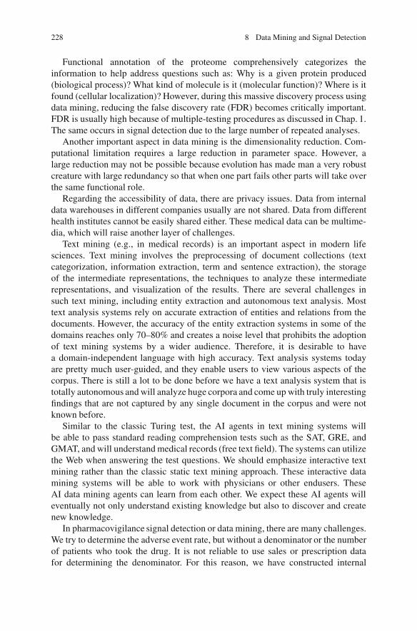
228 8 Data Mining and Signal Detection
Functional annotation of the proteome comprehensively categorizes theinformation to help address questions such as: Why is a given protein produced(biological process)? What kind of molecule is it (molecular function)? Where is itfound (cellular localization)? However, during this massive discovery process usingdata mining, reducing the false discovery rate (FDR) becomes critically important.FDR is usually high because of multiple-testing procedures as discussed in Chap. 1.The same occurs in signal detection due to the large number of repeated analyses.
Another important aspect in data mining is the dimensionality reduction. Com-putational limitation requires a large reduction in parameter space. However, alarge reduction may not be possible because evolution has made man a very robustcreature with large redundancy so that when one part fails other parts will take overthe same functional role.
Regarding the accessibility of data, there are privacy issues. Data from internaldata warehouses in different companies usually are not shared. Data from differenthealth institutes cannot be easily shared either. These medical data can be multime-dia, which will raise another layer of challenges.
Text mining (e.g., in medical records) is an important aspect in modern lifesciences. Text mining involves the preprocessing of document collections (textcategorization, information extraction, term and sentence extraction), the storageof the intermediate representations, the techniques to analyze these intermediaterepresentations, and visualization of the results. There are several challenges insuch text mining, including entity extraction and autonomous text analysis. Mosttext analysis systems rely on accurate extraction of entities and relations from thedocuments. However, the accuracy of the entity extraction systems in some of thedomains reaches only 70–80% and creates a noise level that prohibits the adoptionof text mining systems by a wider audience. Therefore, it is desirable to havea domain-independent language with high accuracy. Text analysis systems todayare pretty much user-guided, and they enable users to view various aspects of thecorpus. There is still a lot to be done before we have a text analysis system that istotally autonomous and will analyze huge corpora and come up with truly interestingfindings that are not captured by any single document in the corpus and were notknown before.
Similar to the classic Turing test, the AI agents in text mining systems willbe able to pass standard reading comprehension tests such as the SAT, GRE, andGMAT, and will understand medical records (free text field). The systems can utilizethe Web when answering the test questions. We should emphasize interactive textmining rather than the classic static text mining approach. These interactive datamining systems will be able to work with physicians or other endusers. TheseAI data mining agents can learn from each other. We expect these AI agents willeventually not only understand existing knowledge but also to discover and createnew knowledge.
In pharmacovigilance signal detection or data mining, there are many challenges.We try to determine the adverse event rate, but without a denominator or the numberof patients who took the drug. It is not reliable to use sales or prescription datafor determining the denominator. For this reason, we have constructed internal

Further Readings and References 229
denominators from an independence model. However, this approach also faceschallenges; i.e., data reliability because of substantial under-reporting to the FDA,uncertainty about the cause of a reported reaction, and different reporting rates ofadverse events by drug.
8.4 Exercises
8.1. Construct a link-analysis model for a practical problem in a biological ormedical field, and perform the analysis.
8.2. Assume y D xCexp.2 sin.x//C", where the random error " has the standardnormal distribution. Perform a comparative analysis between the nearest-neighborsmethod, kernel method, and support vector machine.
8.3. Prove the constants ci given by (8.12) will minimize the error given by (8.11).
8.4. Following the idea of Southworth and O’Connell (2009), perform data miningto identify the treatment code for blinded data from a clinical trial.
8.5. In Sect. 8.1.8, for general weights !0 and !, what is the correspondingexpression �.x/ in (8.27)? Study the effect of !0 and ! on the variance of O� .x/.
Further Readings and References
Abt, K.: Poisson sequential sampling modified towards maximal safety in adverse event monitor-ing. Biomed J. 40, 21–41 (1998)
Ahmed, C., Dalmasso, F., Haramburu, F., Thiessard, F., Broet, P., Tubert-Bitter, P.: False discoveryrate estimation for frequentist pharmacovigilance signal detection methods. Biometrics 66,301–309 (2010)
Ahmed, I., Haramburu, F., Fourrier-Reglat, A., Thiessard, F., Kreft-Jais, C., Miremont-Salame, G.et al.: Bayesian pharmacovigilance signal detection methods revisited in a multiple comparisonsetting. Stat. Med. 28, 1774–1792 (2009)
Almenoff, J., Tonning, J.M., Gould, A.L., et al.: Perspectives on the use of data mining inpharmacovigilance. Drug Saf. 28(11), 981–1007 (2005)
An, G.: In-silico experiments of existing and hypothetical cytokine-directed clinical trials usingagent based modeling. Crit. Care Med. 32(10), 2050–2060 (2004)
Ausk, B.J, Gross, T.S., Srinivasan, S.: An agent based model for real-time signaling induced inosteocytic networks by mechanical stimuli. J. Biomech. 39, 2638–2646 (2005)
Balakin, K.V. (ed.): Pharmaceutical Data Mining: Approaches and Applications for Drug Discov-ery. Wiley, Hoboken (2010)
Bate, A., Lindquist, M., Edwards, I.R., Olsson, S., Orre, R., Lansner, A., De Freitas, R.M.ABayesian neural network method for adverse drug reaction signal generation. Eur. J. Clin.Pharmacol. 54, 315–321 (1998)
Berlekamp, E.R., Conway, J.H., Guy, R.K.: Winning Ways for Your Mathematical Plays. AcademicPress, London (1982)
Breiman, L.: Bagging predictors. Mach. Learn. 24, 123–140 (1996)Breiman, L.: Random forests. Mach. Learn. 45, 5–32 (2001)

230 8 Data Mining and Signal Detection
Brin, S., Page, L.: The anatomy of a large-scale hypertextual (Web) search engine, in the seventhinternational World Wide Web conference. Comput. Netw. ISDN Syst. 30, 1–767 (1998)
Carroll, K.: Analysis of progression-free survival in oncology trials: Some common statisticalissues. Pharm. Stat. 6, 99–113 (2007)
Cerrito, P.B.: Data mining and biopharmaceutical research. In: Chow, S.C. (ed.) Encyclopedia ofBiopharmaceutical Statistics. Marcel Dekker, Boca Raton (2003)
Chang, M.: Monte Carlo Simulation for the Pharmaceutical Industry. CRC, Boca Raton (2010)Committee for Proprietary Medicinal Products (CPMP): Points to Consider on Switching between
Superiority and Non-inferiority. London (2000)Committee for Proprietary Medicinal Products (CPMP): Points to Consider on Multiplicity Issues
in Clinical Trials. London (2002)Crowe, B.J., Xia, H.A., Berlin, J.A., Watson, D.J., Shi, H., et al.: Recommendations for safety plan-
ning, data collection, evaluation and reporting during drug, biologic and vaccine development:A report of the safety planning, evaluation, and reporting team. Clin. Trials 6, 430–440 (2009)
d’Inverno, M., Prophet, J.: Multidisciplinary investigation into adult stem cell behaviour. In:Priami, C., Merelli, E., Gonzalez, P., Omicini, A. (eds.) Transactions on Computational SystemsBiology III. Lecture Notes in Computer Science, vol. 3737, pp. 49–64. Springer, Berlin (2005)
DuMouchel, W.: Bayesian data mining in large frequency tables, with an application to the FDAspontaneous reporting system (Discussion pp. 190–202). Am. Stat. 53, 177–190 (1999)
EMEA: ICH Topic E9: Statistical principles for clinical trials. http://www.ema.europa.eu/pdfs/human/ich/036396en.pdf (1998). Accessed 10 Oct 2010
Emonet, T., Macal, C.M., North, M.J., Wickersham, C.E., Cluzel, P.: AgentCell: A digital single-cell assay for bacterial chemotaxis. Bioinformatics 21, 2714–2721 (2005)
Friedman, J.H.: Greedy function approximation: A gradient boosting machine. Ann. Stat. 29(5),1189–1232 (2001)
Golub, G.H., Van Loan, C.F.: Matrix Computations. Johns Hopkins University Press, Baltimore(1996)
Gould, A.L.: Accounting for multiplicity in the evaluation of signals obtained by data mining fromspontaneous report adverse event databases. Biom. J. 49, 151–165 (2007)
Hand, D., Mannila, H., Smyth, P.: Principles of Data Mining. MIT Press, Cambridge (2001)Harper, G., Bradshaw, J., Gittins, J.C., Green, D.V.S., Leach, A.R.: Prediction of biological activity
for high-throughput screening using binary kernel discrimination. J. Chem. Info. Comput. Sci.41, 1295–1300 (2001)
Hastie, T., Tibshirani, R., Friedman, J.: The Elements of Statistical Learning. Springer, London(2001, 2nd edn., 2009)
Ho, T.: The random subspace method for constructing decision forests. IEEE Trans. Pattern Anal.Mach. Intell. 20(8), 832–844 (1998)
June, A., Joseph, T.M., Gouid, L.A., Ana, S. Manfred, H., Rita, O.H., et al.: Perspectives on theuse of data mining in pharmacovigilance. Drug Saf. 28(11), 981–1007 (2005)
Kier, L.B., Cheng, C.K., Testa, B., Carrupt, P.A.: A cellular automata model of micelle formation.Pharm. Res. 13, 1419–1422 (1996)
Kier, L.B., Cheng, C.K., Testa, B., Carrupt, P.A.: A cellular automata model of diffusion in aqueoussystems. J. Pharm. Sci. 86, 774–778 (1997)
Kleinberg, J.: Authoritative sources in a hyperlinked environment. J. ACM 46(5), 577–603 (1999)Kulldorff, M.: A maximized sequential probability ratio test for drug and vaccine adverse event
surveillance. Presented at the Vaccine Safety Datalink Annual Meeting, Berkeley, 11 May 2006Langville, A.N., Meyer, C.D.: Deeper inside PageRank. Internet Math. 1(3), 335–380 (2005)Li, L.: A conditional sequential sampling procedure for drug safety surveillance. Stat. Med. 28,
3124–3138 (2009)Li, L., Kulldorff, M.: A conditional maximized sequential probability ratio test for pharmacovigi-
lance. Stat. Med. 29, 284–295 (2010)Lollini, P.L., Motta, S., Pappalardo, F.: Discovery of cancer vaccination protocols with a genetic
algorithm driving an agent-based simulator. BMC Bioinfom. 7, 352–352 (2006)

Further Readings and References 231
Materi, W., Wishart, D.S.: Computational systems biology in drug discovery and development:Methods and applications. Drug Discov. Today 12(7/8) (2007)
Mehrotra, D.V., Heyse, J.F.: Multiplicity considerations in clinical safety analysis. Stat. Meth. Med.Res. 13, 227–238 (2004)
Ng, A.Y., Zheng, A.X., Jordan, M.I.: Link analysis, eigenvectors and stability. In: Proceedings ofthe Seventeenth International Joint Conference on Artificial Intelligence, pp. 903–910. MorganKaufmann Publishers, San Francisco (2001)
Peer, M.A., Shah, N.A., Khan, K.A.: Cellular automata and its advances to drug therapy for HIVinfection. Indian J. Exp. Biol. 42, 131–137 (2004)
Poli, R., Langdon, W.R., McPhee, N.F.: A field guide to genetic programming, Creative CommonsAttribution. England & Wales License, UK (2008)
Politopoulos, I.: Review and Analysis of Agent-Based Models in Biology. University of Liverpool,Liverpool (2007)
Posch, M., Zehetmayer, S., Bauer, P.: Hunting for significance with the false discovery rate. J. Am.Stat. Assoc. 104, 832–840 (2009).
Sadooghi-Alvandi, S.M., Nematollahi, A.R.: On the distribution of sum of independent uniformrandom variables. Stat. Pap. 50, 171–175 (2009)
Spiegelhalter, D.J., Best, N.G., Carlin, B.P., van der Linde, A.: Bayesian measures of modelcomplexity and fit (with discussion). J. R. Stat. Soc. B Ser. 64, 583–640 (2002)
Southworth, H., O’Connell, M.: Data mining and statistically guided clinical review of adverseevent data in clinical trials. J. Biopharm. Stat. 19, 803–817 (2009)
Szarfman, A., Machado, S., O’Neill, R.: Use of screening algorithms and computer systems toefficiently signal higher-than-expected combinations of drugs and events in the US FDA’sspontaneous reports database. Drug Saf. 25(6), 381–392 (2002)
von Neumann, J.: Elementary cellular automata. In: Burks, A. (ed.) The Theory of Self-Reproducing Automata. University of Illinois Press, Urbana-Champaign (1966)
Walker, D.C., Hill, G., Wood, S.M., Smallwood, R.H., Southgate, J.: Agent-based computationalmodeling of wounded epithelial cell monolayers. IEEE Trans. Nanobiosci. 3, 153–163 (2006)
Wilton, D.J., Harrison, R.F., Willett, P.: Virtual screening using binary kernel discrimination:analysis of pesticide data. J. Chem. Info. Model. 46, 471–477 (2006)
Wishart, D.S., Yang, R., Arndt, D., Tang, P., Cruz, J.: Dynamic cellular automata: an alternativeapproach to cellular simulation. In Silico Biol. 5, 139–161 (2005).
Wolfram, S.: A new kind of science. Wolfram Media. http://www.wolframscience.com (2002).Accessed 15 Oct 2010
Wu, X., Kumar, V.: The Top Ten Algorithms in Data Mining. Chapman and Hall/CRC, Boca Raton(2009)
Zygourakis, K., Markenscoff, P.A.: Computer-aided design of bioerodible devices with optimalrelease characteristics: A cellular automata approach. Biomaterials 17, 125–135 (1996)


Chapter 9Monte Carlo Simulation
9.1 Random Number Generation
Monte Carlo simulation is the technique to mimic a dynamic system or processusing a computer program. Computer simulations, as an efficient and effectiveresearch tool, have been used virtually everywhere, including in biostatistics,engineering, finance, and other areas. To perform simulations, we often need todraw random samples from a certain probability distribution. Typically, the simplestand most important random sampling procedure is sampling from the uniformdistribution over .0; 1/, denoted by U .0; 1/. The computer-generated “random”number is not truly random because the sequence of numbers is determined bythe so-called seed, an initial number. Random variates from other distributionscan often be obtained by applying a transformation to uniform variates. There areusually several algorithms available to generate random numbers from a particulardistribution. The algorithms differ in speed, accuracy, and the computer memoryrequired. Many software packages have implemented various algorithms to generaterandom numbers with different probability distributions. Here we introduce a fewcommonly used algorithms.
9.1.1 Inverse c.d.f Method
The inverse c.d.f. (cumulative distribution function) method, if available, is a directmethod of generating a sample with a given distribution.
Theorem 9.1. LetfF .z/ ; a � z � bg denote a distribution with inverse distribution
F �1 .u/ D inf fz 2 Œa; b� W F .z/ � u; 0 � u � 1g . (9.1)
Let U denote a random variable from the uniform distribution U .0; 1/. ThenZ D F �1 .U / has the c.d.f. F .
M. Chang, Modern Issues and Methods in Biostatistics, Statistics for Biology and Health,DOI 10.1007/978-1-4419-9842-2 9, © Springer Science+Business Media, LLC 2011
233

234 9 Monte Carlo Simulation
Algorithm 9.1 Inverse c.d.f. Method
Objective: generate Z from fF .z/ ; a � z � bg using the inverse c.d.f. method.Generate U from U .0; 1/
Z WD F�1 .U /
Return Z�
The proof is straightforward because Pr .Z � z/D Pr�F�1 .U / � z
�D PrŒU � F .z/� D F .z/. The algorithm for implementing the inverse c.d.f. method issimple (Algorithm 9.1).
The inverse c.d.f. relationship exists between any two continuous (nonsingular)random variables. If X is a continuous random variable with c.d.f. F and Y is acontinuous random variable with c.d.f. G, then X D F �1.G.Y // over the rangesof positive support. To use this relationship is actually to match percentile points ofone distribution, F , with those of another distribution, G.
Although the inverse method is simple, the closed form of F�1 is not alwaysavailable. When F does not exist in a closed form, the inverse c.d.f. method can beapplied by solving equation F.x/ � u D 0 numerically.
The inverse c.d.f. method also applies to discrete distributions. Suppose thediscrete random variable X has mass points of m1 < m2 < m3 < : : :withassociated probabilities of p1; p2; p3; : : : ; and the distribution function
F.x/ DX
mi�xpi . (9.2)
To use the inverse c.d.f. method, we generate a realization u of the uniformrandom variableU , then deliver the realization of the target distribution as x, wherex satisfies the relationship
F.x ��x/ < u � F.x/, (9.3)
where�x > 0 is a small increment of x determining the precision of the histogram.
9.1.2 Acceptance-Rejection Methods
The acceptance-rejection method is an elegant method for random number gen-eration. For generating realizations of a random variable X with p.d.f. f .x/, theacceptance-rejection method generates random numbers by using realizations ofanother random variable, Y , with a simpler distribution, g. The method is based onthe following theorem (Fishman 1996, p. 171).
Theorem 9.2. (Von Neuman 1951) Let ff .z/ ; a � z � bg denote a p.d.f. withfactorization
f .z/ D cg .z/ h .z/ , (9.4)
where h .z/ � 0;R bah .z/ d z D 1; c D sup
zŒf .z/ =h .z/�, and 0 � g .z/ � 1.

9.1 Random Number Generation 235
Algorithm 9.2 Acceptance-Rejection Method
Objective: Generate a random number from distribution g.rejection WDTrueWhile rejection:
Generate y from p.d.f. gGenerate u from U.0; 1/
If u < f.y/=cg.y/; Then rejection WD FalseEndwhileReturn y�
Let Z denote a random variable with p.d.f. fh .z/g and let U be the standarduniform distribution U .0; 1/. If U � g .Z/, then Z has the p.d.f. ff .z/g.
The algorithm with acceptance-rejection method is presented in Algorithm 9.2.
9.1.3 Markov Chain Monte Carlo
A Markov chain fXng with a countable state space S and transition probabilitymatrixP � �
pij�
is said to be irreducible if for any two states i and j the probabilityof the Markov chain visiting j starting from i is positive, i.e., for some n � 1,p.n/ij � P .Xn D j jX0 D i/ > 0.
Theorem 9.3. (Law of Large Numbers for Markov chains) Let fXngn�0 be anirreducible Markov chain with countable states, a transition probability matrix P ,and a stationary probability distribution � � .�i W i 2 S/. Then, for any boundedfunction h: S ! R and for any initial distribution of X0
1
n
n�1X
iD0h .Xi / !
X
j
h .j / �j (9.5)
in probability as n ! 1.
A similar Law of Large Numbers holds when the state space S is not countable.Monte Carlo simulations based on this theorem are called MCMC. For example,
to calculateP
j h .j / �j , we can use an irreducible Markov chain fXi g with statespace S and stationary distribution � . Let the stochastic process run sufficientlylong. Then the integral of h with respect to � reduces to:
X
j
h .j / �j D 1
n
n�1X
iD0h .Xi/ . (9.6)

236 9 Monte Carlo Simulation
A discrete-time Markov chain is the basis for several schemes for generatingrandom numbers, either continuous or discrete, multivariate or univariate. Thedifferences in the various methods using Markov processes come from differencesin the transition kernel. To generate variate from an arbitrary distribution � D.�i > 0; i 2 L / on a finite state space L D f0; 1; : : : ; v � 1g, we use theMetropolis-Hastings method (Chang 2010).
9.2 Clinical Trial Simulation
9.2.1 Adaptive Trial Simulation
Clinical trial simulation (CTS) is a powerful tool for supporting strategic decision-making in clinical trials. CTS is very intuitive, easy to implement with minimalcost, and can be done in a short time. The utilities of CTS include (1) sensitivityanalysis and risk assessment, (2) estimation of the probability of success (power),(3) design evaluation and optimization, (4) cost, time, and risk reduction, (5) clinicaldevelopment program evaluation and prioritization, (6) prediction of long-termbenefits using short-term outcomes, (7) validation of trial design and statisticalmethods, and (8) streamlining communication among different parties. Withinregulatory bodies, CTS has been frequently used for assessing the robustness ofresults, validating statistical methodology, and predicting long-term benefits ofaccelerated approvals.
In classical designs, CTS not only can be used to simulate the power of ahypothesis test for a complex trial, but also allows us to calculate the probabilityof success. CTS plays an important role in adaptive design for the followingreasons: First, statistical theory for adaptive designs is often complicated undersome relatively strong assumptions, and CTS is useful in modeling very complicatedsituations not only to control the type-I error but also to calculate the powerand generate many other important operating characteristics such as the expectedsample size, conditional power, and unbiased estimates. Second, CTS can be used toevaluate the robustness of the adaptive design against protocol deviations. Moreover,CTS can be used as a tool to monitor trials, predict outcomes, identify potentialproblems, and provide early remedies.
As discussed in Chap. 4, there are four major components of adaptive designsin the frequentist paradigm: (1) type-I error rate or ˛-control, determination ofstopping boundaries, (2) calculation of power or sample size and probability ofsuccess, (3) in trial monitoring: calculation of the conditional power or futility index,and (4) in analysis after the completion of the trial, calculation of adjusted p-values,unbiased point estimates, and confidence intervals.

9.2 Clinical Trial Simulation 237
9.2.1.1 Sample Size Reestimation
A sample size reestimation (SSR) design refers to an adaptive design that allows forsample size reestimation based on the review of interim analysis results.
For a two-stage SSR of a two-group trial, the sample size per group for the secondstage can be calculated based on the target conditional power cP (Chap. 4),
8ˆ<
ˆ:
n2 D 2 O�2Oı2�z1�˛2Cp1 � z1�cP
�2; for MSP,
n2 D 2 O�2Oı2�z1�˛2=p1 � z1�cP
�2; for MPP,
n2 D 2 O�2Oı2�
z1�˛2w2
� w1w2
z1�p1 � z1�cP�2; for MINP,
(9.7)
where, for the purpose of calculation, Oı and O� are taken to be the observed treatmenteffect and standard deviation at stage 1.
An algorithm for a two-stage design with SSR based on MSP (see Chap. 4) ispresented in Algorithm 9.3.
Algorithm 9.3 Two-Stage Sample Size Reestimation with MSP
Objective: Return power and PE for two-stage adaptive design.Input treatment difference ı and common � , stopping boundaries ˛1; ˛2; ˇ1, n1; n2, targetconditional power for SSR, the maximum sample size nmax, clinical meaningful and commercialviable ımin, target conditional power cP , and the number of simulation runs nRuns.power WD 0
PE WD 0
For iRun WD 1 To nRunsT WD 0
Generate u from N .0; 1/
z1 D ıpn1=2=� C u
p1 D 1� ˚ .z1/If p1 > ˇ1 Then ExitforIf p1 � ˛1 Then power WD power+1/nRunsIf p1 � ˛1 And Oı1 � ımin Then PE WD PE+1/nRunsIf ˛1 < p1 � ˇ1 Then
n2 WD 2�2
Oı21
�z1�˛2Cp1 � z1�cP
�2
Generate u from N .0; 1/
z2 D ıpn2=2=� C u
p2 D 1� ˚ .z2/T WD p1 C p2If T � ˛2 Then power WD power+1/nRunsOı D .Oı1n1 C Oı1n2/=.n1 C n2/
If T � ˛2 And Oı � ımin Then PE WD PE+1/nRunsEndif
EndforReturn fpower, PEg�

238 9 Monte Carlo Simulation
9.2.2 Dynamic Drug Supply
The conventional way for drug supply in a clinical trial separates the supply chainsfor each stratum or treatment group. In this approach, an initial drug shipmentwould be made for each stratum. Resupply shipments would then follow, based onfixed trigger levels for each stratum. However, keeping the supply chains separaterequires a high initial outlay and can result in a lot of waste if a site does not enrollas anticipated. This conventional drug supply can be particularly problematic foradaptive trials.
Hamilton and Ho (2004) described a dynamic drug supply method as follows:To randomize a patient, a site would call the IVRS and enter some basic patientidentifiers such as ID number and date of birth, along with the stratum to which thepatient belonged. The system would then access the randomization and treatmentkit lists and read back to site personnel the blinded kit number assigned to thatpatient. A fax confirming patient information and the assigned kit number wouldthen be automatically generated by the system and sent to the site.
Their logistic steps for the dynamic supply are:
1. At site initiation, ship enough drug to cover the first y patients enrolling into thestudy, regardless of strata.
2. After each patient is randomized, recalculate the patient coverage based on therandomization list and current levels of drug supply at the site.
3. If the patient coverage falls below a lower resupply threshold x, ship enough drugto replenish supply to an upper resupply threshold y. That is, ship enough drugso that the next y patients can be enrolled into the study, regardless of strata.
The implementation aspect of the dynamic supply can be further elaborated asfollows: In the original study, the dynamic drug supply scheme was implementedutilizing a telephone-based interactive voice response system. The system wasdesigned in such a way that when a site completed regulatory and contractualrequirements, sponsor personnel could go to a secure administrative Web page andactivate that site. Upon activation, the system would examine the randomizationlist for that site and calculate the amount of drug needed to cover the first ypatients, regardless of strata. Notifications via email and fax would then be sentto the central drug repository indicating which drug kits to ship and the shipmentnumber to appear on the waybill. When the site received the drug shipment, theywere instructed to register the shipment number with the IVRS, making those drugkits available to be used to randomize patients at the site.
The steps to randomize a patient via IVRS are similar to the conversional ap-proach. After each patient was successfully randomized, the IVRS would recalculatepatient coverage at the site. If patient coverage dropped below x patients, anothercalculation was made by the IVRS to determine which kit types were necessary tobring the coverage back up to cover the next y patients. An automatic notificationwould then be sent to the central drug repository, indicating which drug kits to beshipped to the site.
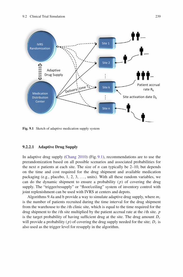
9.2 Clinical Trial Simulation 239
IVRSRandomization
Site 1
Site 2
Site k
Site n
MedicationDistribution
Center
AdaptiveDrug Supply
Patient accrualrate Rk
Site activation date Dk
Delivery time Tk
Fig. 9.1 Sketch of adaptive medication supply system
9.2.2.1 Adaptive Drug Supply
In adaptive drug supply (Chang 2010) (Fig. 9.1), recommendations are to use theprerandomization based on all possible scenarios and associated probabilities forthe next n patients at each site. The size of n can typically be 2–10, but dependson the time and cost required for the drug shipment and available medicationpackaging (e.g., placebo, 1, 2, 3, . . . , units). With all these random variables, wecan do the dynamic shipment to ensure a probability (p) of covering the drugsupply. The “trigger/resupply” or “floor/ceiling” system of inventory control withjoint replenishment can be used with IVRS at centers and depots.
Algorithms 9.4a and b provide a way to simulate adaptive drug supply, wheremi
is the number of patients recruited during the time interval for the drug shipmentfrom the warehouse to the i th clinic site, which is equal to the time required for thedrug shipment to the i th site multiplied by the patient accrual rate at the i th site. pis the target probability of having sufficient drug at the site. The drug amount Dc
will provide a probability (p) of covering the drug supply needed for the site; Dc isalso used as the trigger level for resupply in the algorithm.

240 9 Monte Carlo Simulation
Algorithm 9.4a Adaptive Drug Supply
Objective: Return the amount of drug required for a trial.Input p and fmig for sites.mDrug WD P
i ni0fdig WD fni0gWhen each patient is enrolled at site i
Dc WD DrugCoverage(p)Calculate the drug inventory di at the siteIf di < Dc Then mDrugWD mDrug + Dc
Return mDrugEndwhen
Algorithm 9.4b Function DrugCoverage (p)
Objective: Function used in Algorithm 9.4a.For i WD 1 To 10000
Di WD 0
For j WD 1 Tomi
Randomize patient j based on randomization rule.Determine the drug package x required for patient j .Di WD Di C x
EndforEndforSort Di in ascending order
Return D10000�pro
9.2.3 Bootstrapping Methods
Bootstrapping is a resampling method that estimates the distribution of an estimatorby sampling with replacement from the original sample. Bootstrapping is usefulwhen the analytical form of distribution is not available or unknown. Bootstrappingis often used for deriving robust estimates of standard errors and confidence intervalsof a population parameter like a mean, median, proportion, odds ratio, correlationcoefficient, or regression coefficient.
Suppose x1; x2; : : : ; xn is i.i.d. from probability distribution F . The empiricaldistribution function OF is defined to be the discrete distribution that put 1=n oneach value xi .i D 1; : : : ; n/,
OPr fAg D # fxi 2 Agn
. (9.8)
9.2.3.1 The Plug-in Principle
The plug-in principle is a simple method of estimating parameters from samples.The plug-in estimate of a parameter � D t .F / is defined as (Efron and Tibshirani1994; Chernick 2007)
O� D t� OF�
. (9.9)
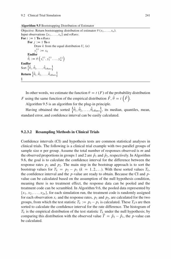
9.2 Clinical Trial Simulation 241
Algorithm 9.5 Bootstrapping Distribution of Estimator
Objective: Return bootstrapping distribution of estimator � .x1; : : : ; xn/.Input observations fx1; : : : ; xng and nRuns.For i WD 1 To nRuns
For j WD 1 To nDraw k from the equal distribution Uc .n/
y.i/j WD xk
EndforO�i WD �
�y.i/1 ; y
.i/2 : : : ; y.i/m
�
EndforSort
n O�1; O�2; : : : ; O�nRuns
o
Returnn O�1; O�2; : : : ; O�nRuns
o
�
In other words, we estimate the function � D t .F / of the probability distribution
F using the same function of the empirical distribution OF , O� D t� OF�
.
Algorithm 9.5 is an algorithm for the plug-in principle.
Having obtained the sortedn O�1; O�2; : : : ; O�nRuns
o, its median, quantiles, mean,
standard error, and confidence interval can be easily calculated.
9.2.3.2 Resampling Methods in Clinical Trials
Confidence intervals (CI) and hypothesis tests are common statistical analyses inclinical trials. The following is a clinical trial example with two parallel groups ofsample size n per group. Assume the total number of responses observed is m andthe observed proportions in groups 1 and 2 are Op1 and Op2, respectively. In Algorithm9.6, the goal is to calculate the confidence interval for the difference between theresponse rates p1 and p2. The main step in the bootstrap approach is to sort thebootstrap values for Tk D p2 � p1 (k D 1; 2;. . . ). With these sorted values Tk ,the confidence interval and the p-value are ready to obtain. Because the CI and p-value can be calculated based on the assumption of the null hypothesis condition,meaning there is no treatment effect, the response data can be pooled and thetreatment code can be scrambled. In Algorithm 9.6, the pooled data represented byfx1; x2; : : : ; x2ng, for each simulation run, the treatment code is randomly assignedfor each observation xi and the response rates, p1 and p2, are calculated for the twogroups, from which the test statistic Tk WD p2 �p1 is calculated. These Tks are thensorted to calculate the confidence interval for the rate difference. The histogram ofTk is the empirical distribution of the test statistic Tk under the null hypothesis; bycomparing this distribution with the observed value OT D Op2 � Op1, the p-value canbe calculated.

242 9 Monte Carlo Simulation
Algorithm 9.6 Bootstrapping CI for Rate Difference
Objective: Return a bootstrap 100.1� ˛/% CI for Op2� Op1.Input n, m, Op1, Op2, and binary responses fx1; x2; : : : ; x2ng.For k WD 1 To nRuns
p1 WD 0
p2 WD 0
For i WD 1 To 2nGenerate a random sample u from Uc .n/
If u D 1 Then p1 WD p1 C xi=n
If u D 2 Then p2 WD p2 C xi=n
EndforTk WD p2 � p1
EndforSort fT1; T2; : : : ; TnRunsg in ascending orderCI WD ˚
Tb˛�nRunsc; Td.1�˛/�nRunse
�
Return CI and fT1; T2; : : : ; TnRunsg�
9.3 Molecular Design and Simulation
9.3.1 The Landscape of Molecular Design
As mentioned earlier, Pharmaceutical R & D expense has increased dramaticallyover the past 15 years, while the number of NDAs approved has been relativelyflat. Innovative and cost-effective drug discovery approaches become inevitable forany pharmaceutical company to stay competive. Molecular design and modeling isa promising new field, in which computer simulations and a chemical compounddatabase are used to screen, model, and design NMEs in order to reduce thediscovery cost and accelerate the discovery process. The reasons why this in-silico method can help in this aspect are because (1) the number of compoundsthat can be examined by a human mind is limited compared with the capacitythroughput of virtual, computer-based storage, modeling, and virtual screeningsystems, and (2) compound supply is also limited. Many different companies useblind screening for the same compound libraries even after many of the compoundshave been proven structurally unfavorable, which often turns out to be a waste oftime and resources. Computer-based design of activity enriched screening librariescan be of great value here, and (3) the traditional biochemical screening assayscan be very expensive, especially for cell-based systems or when elaborate proteinpurification schemes are required. Costs have been estimated to fall somewherebetween $0.02 and $10 per well. When considering a screening library containingone million compounds with multiple measurements, the sum adds up (Schneiderand Baringhaus 2008).
There are approximately 8,000 drug targets, of which 5,000 could be “hit”by small druglike molecules. Only about 3,000 targets out of the 5,000 arepharmacological interest, and only 200–500 targets are addressed by marketed

9.3 Molecular Design and Simulation 243
drugs – there are many more targets to be explored in the future. It is estimatedthat out of the 20,000–25,000 human genes supposed to code for about 3,000druggable targets, only a subset of the pharmacological space (about 800 proteins)has currently been investigated by the pharmaceutical industry (Paolini et al. 2006).Over ten million nonredundant chemical structures cover the actual chemical space,out of which only about 1,000 are currently approved as drugs. Chemogenomics isthe new interdisciplinary field that attempts to fully match target and ligand space,and ultimately identify all ligands of all targets. The 8,000 drug targets can befurther categorized into seven different classes: proteases (19%), kinases (12%),other enzymes (17%), G-protein coupled receptors (GPCRs, 16%), ion channel(13%), nuclear receptor (4%), and other targets (19%).
The steps in the standard drug lead approach include (1) identifying the target(e.g., enzyme, receptor, ion channel, transporter), (2) determining the DNA and/orprotein sequence, (3) elucidating the structures and functions of proteins, (4)proving the therapeutic concept in animals (“knock-outs”), (5) developing an assayfor HTS, (6) mass screening, and (7) selecting lead structures.
A goal of Monte Carlo molecular design is to identify novel substances thatexhibit desired properties. An example would be a particular biological activityprofile including a selective binding to a single target or desired activity modulationof multiple targets simultaneously. This design certainly must include properphysicochemical and ADMET (absorption, distribution, metabolism, excretion, andtoxicity) properties of the novel compounds (Schneider and Baringhaus 2008).
9.3.2 The Drug-Likeness Concept
The term “druglike” describes various empirically found structural characteristicsof molecular agents that are associated with pharmacological activities. It is notstrictly defined but provides a general concept of what makes a drug a drug. Drug-likeness may be considered as the overall likelihood that a molecular agent canbe turned into a drug. Therefore, it is a measure of complex physicochemical andstructural features of the compound that can be used to guide the rational design oflead structures that can be further optimized to become a drug.
The well-known QSAR (quantitative structure-activity relationship) Lipinski’srule-of-five is often used in rational drug design to reduce the risk of costly late-stagepreclinical and clinical failures. The guidelines predict that poor passive absorptionor permeation of an orally administered compound is more likely if the compoundmeets at least two of the following criteria (Lipinski et al. 1997):
1. molecular weight greater than 500 Da;2. high lipophilicity (expressed as clogP > 5);3. more than five hydrogen-bond donors, expressed as the sum of OHs and NHs;4. more than ten hydrogen-bond acceptors, expressed as the sum of Os and Ns;5. containing more than five rotatable bonds to limit its conformational freedom.

244 9 Monte Carlo Simulation
Fig. 9.2 Weight distribution of druglike molecules
These guidelines were developed based on an empirical pharmaceutical database.For example, Fig. 9.2 is the distribution of molecular weights of 4,500 selecteddruglike molecules containing marketed drugs and drug candidates. We can see thatmost druglike molecules weight between 300 and 600 Da.
9.3.2.1 Tanimoto Similarity Index
The rationale behind a similarity search is the so-called similar property principle:structurally similar molecules are likely to have similar chemical or physiologicalproperties. A variety of methods are used in these searches, including 2D and 3Dshape similarity, graph theory, vector space models based on 2D fingerprints, andmachine learning methods.
Similarity searching can be achieved by comparing representations of moleculeswith respect to the substructure elements they contain. A popular similarity index isthe Tanimoto (Jaccard) index defined by
TAB D nAB
nA C nB � nAB; (9.10)
where nA is the number of bits set to 1 (indicating a certain substructure) in moleculeA, nB is the number of bits set to 1 in molecule B , and nAB is the number of set bitscommon to both A and B . The possible value of TAB ranges between 0 (maximaldissimilarity) and 1 (identical bitstrings). However, TAB D 1 implies A and B haveidentical fingerprint but does not necessarily mean that the two molecules A and Bare identical.

9.3 Molecular Design and Simulation 245
Ligands A and B can be viewed as fingerprint vectors, and the quantity
DAB D 1� TAB (9.11)
is called the distance in vector space. For the distance, the following triangularinequality holds (Lipkus 1999):
jDAB �DAC � DBC � DAC CDAB: (9.12)
From (9.12) we can obtain the following bound on the Tanimoto similarity index:
TBC � 1 � jTAB � TAC j: (9.13)
This bound (9.13) has been improved by Baldi and Hirschberg (2009).
9.3.2.2 Bayesian Network for Similarity Search
In a similarity search, a Bayesian network (BN) is a simple and popular way ofdoing probabilistic inference that formalizes the way to synchronize the evidenceusing the Bayes rule:
P.H jE/ D P.EjH/P.H/=P.E/:A Bayesian network is a directed acyclic graph and has the following properties:
• Nodes of the BN represent random variables and the parents of a node are thosejudged to be direct causes of it.
• The roots of the network are the nodes without parents.• The arcs represent causal relationships between these variables, and the strengths
of these casual influences are expressed by conditional probabilities.• Let X D fx1; : : : ; xng be a set of parents of y (child node), where xi \ xj D� .empty/ for i ¤ j and xi is a direct cause of y. The influence of X on y canbe quantified with the conditional probability P .yjX/.
9.3.3 Molecular Docking
A ligand (drug candidate) has to bind the protein closely enough in order to have adrug effect. This requires the ligand to have the right shape and orientation to fit the“pocket” of the protein target. Molecular docking is a computer-based technologyto find the binding orientation of a ligand (small molecule) to the protein targetin order to predict the affinity and activity of the small molecule. Hence dockingplays an important role in the rational design of drugs. The docking methodscan be geometry or energy-based. Here we only discuss the energy minimizationapproach.

246 9 Monte Carlo Simulation
9.3.3.1 Energy Minimization Approach
The design of ligands that interact with a target receptor always yields a low energyligand-receptor complex. The free energy (Gibbs energy) change�G for a receptor-ligand interaction was defined by Gibbs in 1873 as
�G D �H � T�S; (9.14)
where�H and T�S are enthalpic and entropic terms, respectively, contributing tothe change in the free energy of binding�G.
This ligand conformation is not necessarily the global minimum-energy con-formation. However, typical bioactive ligand conformations are close to globalminimum conformations in water, which might differ substantially from confor-mations in a vacuum.
Free-energy differences between two states are almost independent of high-energy contributions. This allows an approximation of each state by its meanpartition function, taking into account only relevant low-energy conformationsweighted by their Boltzmann probability. The energy differences between the twostates can be quantified from Monte Carlo or molecular dynamics (MD) simulations(Schneider and Baringhaus 2008).
9.3.3.2 Monte Carlo Simulated Annealing
In solid physics, annealing is known as a thermal process for obtaining the lowest-energy states of a solid. The processes are governed by molecular dynamics in whichthe system starts at a high-temperature state with its particles being relatively free tomove around. The temperature then slowly deceases and the particles are forced toline up to achieve the local energy minimization. In this process, the system is cooleddown slowly; otherwise, if it cools too fast, the particles will not have enough timeto line up (Liu 2001). In Monte Carlo simulated annealing, during each constanttemperature cycle, random perturbations are made to the ligand’s current orientationand conformation. The new state is accepted if its energy is lower than the energy ofthe preceding state. Otherwise, the configuration is accepted probabilistically basedupon a Boltzmann equation (Holtje et al. 2008). The probability of acceptance isgiven by
Pa D exp
� �E
kBT
, (9.15)
where �E is the difference in energy from the previous step, T is the absolutetemperature in Kelvin, and kB is the Boltzmann constant.
From (9.15), we can see that the higher the temperature of the cycle, the higherthe probability that the new state is accepted. When the energy change �E isnegative,Pa will be larger than 1. Therefore, regardless of the direction of the energychange in Monte Carlo simulated annealing, the acceptance probability for a statecan be written as

9.3 Molecular Design and Simulation 247
Algorithm 9.7 Simulated Annealing
Objective: Docking with simulated annealingSet up initial ligand’s coordinates.Input temperature sequence fTi g, kB; and a small " > 0.For i WD 1 To K
Make random perturbations to the ligand’s current orientation andconformation.Calculate the incremental energy �EGenerate random number u from U .0; 1/
If u < Pa D min�1; e
��EkBTi
�Then accept new state
If �E < " Then ExitforEndforReturn current state of the ligand
�
Pa D min�1; e
� �EkBT
�. (9.16)
Keep in mind that the final state in Monte Carlo simulated annealing usuallydepends on the initial placement of the ligand because the algorithm does notexplore the solution space exhaustively. The algorithm for the simulated annealingis presented in Algorithm 9.7.
9.3.3.3 Scoring Functions
A scoring function is a measure of interaction between a ligand and a receptor; itis a measure of the drug-likeness of a ligand. The scoring function can be the freeenergy of binding given by the Gibbs-Helmholtz equation (9.14), where�G relatesto the binding constantKi through the equation
�G D �RT lnKi , (9.17)
where R is the gas constant.The binding free-energy difference between a ligand and a reference
molecule can be accurately calculated using energy perturbation Miyamoto andKollman (1993). However, such a time-consuming approach is not practical forvirtual screening to compute energies for thousands of protein-ligand complexes. Afast method is desirable. A scoring function, monotonic in �G, can be calculatedquickly and the resulting conformation rankings based on a score function will bethe same as those by the �G.
Holtje and colleagues (2008) categorize scoring functions into three groups:empirical scoring functions, force-field-based functions, and knowledge-basedpotential of mean force. Scoring functions can be used in two ways (1) during thedocking process, they serve as fitness functions in the optimal placement of theligand; and (2) when the docking is completed, they are used to rank each ligand ofthe database for which a docking solution has been found.
248 9 Monte Carlo Simulation
9.4 Biological Pathway Simulation
9.4.1 Biology Pathways
A biological pathway is a molecular interaction network in biological processes.The pathways can be classified into the fundamental categories: metabolic, regula-tory, and signal transduction. There are about 10,000 pathways, nearly 160 pathwaysinvolving 800 reactions.
A metabolic pathway is a series of chemical reactions occurring within a cell,catalyzed by enzymes, resulting in either the formulation of a metabolic productto be used or stored by the cell, or the inhibition of another metabolic pathway.Pathways are important to the maintenance of homeostasis within an organism.
A gene regulatory pathway or genetic regulatory pathway is a collection of DNAsegments in a cell that interact with each other and with other substances in thecell, thereby governing the rates at which genes in the network are transcribed intomRNA. In general, each mRNA molecule goes on to make a specific protein orits particular structural properties. The protein can be an enzyme for breakdownof a food source or toxin. By binding to the promoter region at the start of othergenes, some proteins can turn the genes on, initiating or inhibiting the production ofanother protein.
A signal transduction pathway is a series of processes involving a group ofmolecules in a cell that work together to control one or more cell functions, suchas cell division or cell death. Molecular signals are transmitted between cells bythe secretion of hormones and other chemical factors, which are then picked up bydifferent cells. After the first molecule in a pathway receives a signal, it activatesanother molecule, and then another, until the last molecule in the signal chain isactivated. Abnormal activation of signaling pathways can lead to a disease such ascancer. Drugs are being developed to block these disease pathways.
Systems biology is a newly emerging, multidisciplinary field that studies themechanisms underlying complex biological processes by treating these processesas integrated systems of many interacting components (Materi and Wishart 2007).Quantitative studies in systems biology require the utilization of computer modelingand simulation, which has given rise to a new discipline called computationalsystems biology (CSB).
The modeling and simulation can be carried out on different temporal and spatialscales, ranging from nanometers to meters and milliseconds to days. Conventionally,“fine grain” models simulate the events that concern short times (ms) or small (nm)dimensions, and coarse “grain models” simulate the events that concern longer times(s) or larger (mm or cm) dimensions.

9.4 Biological Pathway Simulation 249
9.4.2 Petri Nets
A Petri net (PN) is a mathematical network model for simulating a dynamic systemsuch as an electronic process, traffic system, or biological pathway. Petri nets wereproposed by Carl Adam Petri in 1962 in his PhD thesis in computer science. PN hasgained an increasing attention in the biological sciences and drug development in thepast 10 years. PN research papers dominate the field in simulations of life sciencesand PNs have been adopted more and more by the pharmaceutical industry.
The basic elements in PNs include places (or stelle) to symbolize the states orconditions of the system, transitions to symbolize the actions in the system, tokensto symbolize the resources responsible for the changes of the system, directed arcsto indicate the directions of token (resource) travel, and weights for the directed arcsrepresenting the minimum required tokens for firing (executing action). Graphically,a place is often denoted by a circle; a transition is denoted by a rectangle; tokens areallocated in places; places and transitions are connected by directed lines (arcs); andweights are values next to the corresponding arcs. When the number of tokens in aplace meets the minimum requirement for firing (execution), some of the tokens aremoving from one place to another – the firing rules. Figure 9.3 is a PN representationof the chemical reaction of water.
The mathematical definition of a PN can be described as follows.
Definition 9.1. A Petri net is a 5-tuple PN D .P; T; F;W;M0/ where
• P D fp1; : : : pKg is the set ofK places,• T D ft1; : : : tN g is the set of N transitions, with P \ T D ; and P [ T ¤ ;,• F D I � .P � T / [ O � .T � P/ is the flow relation defining the set of
directed arcs,• W W F ! .Nn f0g/ (N D f0; 1 : : :g) is the arc weight function, and• M0 D fm01; : : : ; m0Kg 2 N
K is the initial marking, i.e., an integer number oftokens associated to each place initially.
p1
p2
p3
2
t
2
H2
O2
H2O
2
Chemicalreaction
2
Fig. 9.3 PN representing chemical reaction of water

250 9 Monte Carlo Simulation
Note that the preset I corresponds to all the directed arcs from places totransitions, whereas postset O corresponds to all the directed arcs from transitionsto places. M .p/ often denotes the number of tokens in place p in markingM .
The state of a Petri system is characterized by the distribution of tokens in theplaces. The dynamics of PN is characterized by the firing mechanism. A place maycontain zero or several tokens, which may be interpreted as resources. There may beseveral input and output arcs between a place and a transition. The number of thesearcs is represented as the weight of a single arc. A transition is enabled if each of itsinput places contains at least as many tokens as the corresponding input arc weightindicates. When an enabled transition is fired, its input arc weights are subtractedfrom the input place markings and its output arc weights are added to the outputplace markings. Formally, we have the following definition.
Petri nets can be of different types: (1) place/transition PNs (colored or non-colored) or (2) time-dependent PNs (discrete PN, continuous PN, hybrid PN formixtures of continuous and discrete systems, and stochastic PN).
9.4.2.1 Why Petri Nets
Biological networks or pathways are extremely complicated, and their mechanismsare difficult to understand using the traditional 2D representation. Using a Petrinet, we can have a coherent presentation of the very diverse forms of informationand solve the problem by means of computer simulation. Petri nets offer a generalframework for analyzing the dynamic properties of large systems, either from aqualitative or a quantitative point of view. The mathematical properties of standardPetri nets are well studied and can be used for model validation. PNs can beused on an abstract level with specification of limited resources possible andallow for combining all these different abstract levels within one model. PNsallow for integration of qualitative and quantitative analyses. Petri nets have anexecutable graphical representation, supporting the intuitive understanding of thesystem modeled and the communication between experimentally and theoreticallyworking scientists. There are movable objects, the animation of which visualizespossible flows through the network. Model animation helps us experience thenetwork behavior and allows us to test whether the model actually does behave inthe desired manner (Koch and Heiner 2008). Petri nets can be used as both analysisand prediction tools. There exist many public-domain software tools such as editors,animators, and analyzers. One of the nice features with a PN is its scalability to fitthe constantly updated knowledge of systems biology. Any update to the currentknowledge can be easily implemented in the previous PN by simply modifying therelevant substructure of the PN without recreating a completely new PN.
There are biological interpretations for most properties of a PN. For example, thereachability of a marking from some other marking in the PN model of a metabolicpathway determines the possibility of forming a specified set of product metabolitesfrom another set of reactant metabolites, using some sequence of reactions that isdictated by the PN’s firing sequence(s).

9.4 Biological Pathway Simulation 251
9.4.2.2 Petri Net Dynamics
PN dynamics include reachability, liveness, and boundedness. They all relateto the initial marking. A reachability study concerns whether a marking underconsideration can be reached from the initial marking; liveness study addresseswhether any transition will eventually be fired for the given initial marking; anda boundedness study investigates whether the number of tokens at each place isbounded for any initial marking of the Petri net.
There are three commonly used abstract levels in the simulation, (1) molecularlevel (biochemical network), (2) gene cross-regulation level (genetic network), and(3) tissue level (intercellular network), in which the biological cells are believed tooperate with a steady state of the internal metabolites. Note that the same compoundcan be presented using multiple places in the same network if they play differentbiological roles.
9.4.3 Biological Pathway Simulations
9.4.3.1 Petri Net for Metabolic Pathways
A metabolic pathway is a series of enzymatic reactions consuming certain metabo-lites and producing others. These metabolites usually participate in more than onemetabolic pathway, forming a complex network of reactions.
The S-transformation of biochemical reactions can be modeled using PNsin which (1) places can be metabolites, reactants, products, genes, cells, andenzymes, (2) transitions can be reactions, catalysis, activation, and inhibition, and(3) weighted arcs can be stoichiometries (Chang 2010).
9.4.3.2 Stochastic PN for Regulatory Pathways
Regulation of gene expression (or gene regulation) includes the processes (amountand timing) turning the information in genes into gene products (RNA or protein).The majority of known mechanisms regulate protein coding genes. Any step ofthe gene’s expression may be modulated, from DNA-RNA transcription to thepost-translational modification of a protein. The stages where gene expression isregulated are chromatin domains, transcription, post-transcriptional modification,RNA transport, translation, mRNA degradation, and post-translational modification.Gene regulation is essential for viruses, prokaryotes, and eukaryotes, as it increasesthe versatility and adaptability of an organism by allowing the cell to express proteinwhen needed. The first discovered (by Jacques Monod) example of a gene regulationsystem was the lac operon, in which proteins involved in lactose metabolism areexpressed by E. coli only in the presence of lactose and absence of glucose (Chang2010).

252 9 Monte Carlo Simulation
9.4.3.3 Hybrid PN for Regulatory Pathways
In many cases, molecular concentration is considered continuous rather thandiscrete. How do we deal with actual molecule numbers? If we represent eachmolecule by one token, it is not feasible for simulations; if one token stands for,for example, 1 mol of a substance, it might not be accurate enough. The solution isto allow continuous values for certain places, which leads to the so-called hybridPetri nets (HPNs) (Chang 2010).
An HPN can have continuous and discrete tokens in places. Discrete places havetokens, whereas continuous places contain real variables. Discrete transitions fireafter a certain delay. Continuous transitions fire continuously at a given rate.
Chen and Hofestadt (2003) conducted a case study on the urea cycle disorder,a genetic disease caused by a deficiency of one enzyme in the urea cycle that isresponsible for removing ammonia from the bloodstream. In urea cycle disorders,the nitrogen, a waste product of the metabolite, is not removed from the body.Ammonia then reaches the brain through the blood, where it causes irreversiblebrain damage, coma, and/or death.
The metabolic behavior is modeled using continuous places and transitions,whereas gene regulations are modeled by discrete net elements. The regulationboth on genomic and metabolic levels can be simulated. A generalization of hybridPetri nets (hybrid function Petri nets) was developed by Matsuno et al. (2003).The typical examples they studied included a metabolic pathway (the glycolysis)and a signaling pathway (the Fas legand induced apoptosis). The effectivenessof PN-based biopathway modeling was demonstrated in the circadian rhythm inDrosophila and the apoptosis induced by the Fas ligand. The simulations of thesemodels were performed with the software tool Genomic Object Net.
9.5 PK and PD Modeling and Simulation
9.5.1 Pharmacokinetic Simulation
For a drug to interact with a target, it is necessary for the drug to present sufficientconcentration in the fluid medium surrounding the cells with receptors. Pharma-cokinetics is the study of the kinetics of absorption, distribution, metabolism, andexcretion (ADME) of a drug. It analyzes the way the human body works with a drugafter it has been administered, and the transportation of the drug to the specific sitefor drug-receptor interactions.
In what follows, we will discuss the ADME mechanisms to guide our PK model-ing and simulation. There are two schools of modeling and simulation approaches.One is to model the complex ADME directly, treating the whole body as one entity –the macro-approach. The mixed-effect population PK model is an example of thistype of statistical modeling. There are nearly 100 commercial software products

9.5 PK and PD Modeling and Simulation 253
BrainQBR
QLU
QHT
QMUS
QKID
QLIV
QBO
QAD
QSK
Lung
Heart
Muscle
Veno
us b
lood
Arte
rial b
loodKidney
Liver
Bone
Adipose
Skin
Urine
Fig. 9.4 Physiology-based pharmacokinetic model
available (see, e.g., www.boomer.org/pkin/soft.html for such a list) for this type ofmodeling and most PK specialists are familiar with the approach and software. I amnot going to discuss this approach. Alternatively, we can use low-level modeling,which either models the four components of ADME separately or models themechanisms at the organ level as for the physiologically based pharmacokinetic(PBPK) model (Fig. 9.4) and then integrate the low-level components into a higher-level model. The integration is accomplished through simulation.
The law governing the drug concentration C .t/ over time t is the diffusionequation:
dC .t/
dtD kC .t/ . (9.18)
It is interesting that the model is mathematically equivalent to the survival model(6.1). Therefore, the same method can deal with two complete problems in twocompletely different disciplines.
PBPK model structures are based on the actual physiological and biochemicalstructure of the species being described, allowing the physiological and biochemicalparameters in the model to be changed from those for the test species to thoseappropriate for humans to perform animal to human extrapolations and predict drug

254 9 Monte Carlo Simulation
Algorithm 9.8 Physiologically Based Pharmacokinetics
1. Construct a typical compartment model using object-oriented programming (any OOP com-puter language or visual simulation tool).
2. Make copies of the typical compartment model (TCM) and that customized based on the PBPKmodel
3. Connect the TCMs based on the PBPK diagram.4. Input parameters for each TCM:
The model parameters can be assumed to be fixed values, from data, or validated by data. Themodel parameters can also be chosen as random variables. In such cases, one can generateparameter distributions for each compartment using the technique in Sect. 9.1.
5. Determining output parameters:Many different PK outputs can be easily obtained for the model for each compartment (organ)or the body as a single entity. The PBPK simulation model can also output the traditional PKparameters such as Cmax, AUC, t1=2, and others.
effects over a wide range of conditions. The improved dose metric can then be usedin place of traditional dose metrics (e.g., administered dose) or can be generated asa time-dependent input for a more biologically based response model to simulatethe time course of the drug. Figure 9.4 is an illustration of a PBPK model.
In general, a PBPK model can be determined by the permeability matrix�kij�,
where the element kij is the permeability between the i th and j th compartments. Ifkij are constants, the network is a Markovian process; if kij � 0 are time-dependent,the model is a time-dependent Markovian chain.
Implementation of PBPK models can follow the steps outlined in Algorithm 9.8.If you know any object-oriented programming and visual simulation tools such asExtentSim, building a PBPK model is a straightforward job programming-wise.However, determining the parameters and validating the model are still challenging.
9.5.1.1 Markov Chain with Constant Permeability
It is possible to include fixed and known covariates in the time-independentpermeability kij from state (compartment) i to state (compartment) j . The totalpermeability for state m is defined as km D ˙i¤j kij . In this model, the transitionprobabilities can be evaluated by means of exponential functions:
dPkl .t/=dt D ˙mPkm.t/Gml , (9.19)
where Gml D �kml .m ¤ l/ and Gmm D km.In general, we can show that
Pkl .v; t/ D Pkl .0; t � v/ . (9.20)
The solution can be described by means of the matrix exponential function,where the matrix of transition probabilities satisfies (Hougaard 2001)
P .v; t/ D exp fG .t � v/g D1X
rD0
Gr .t � v/r
rŠ. (9.21)
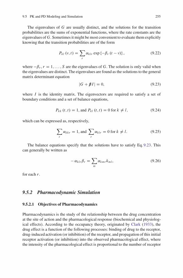
9.5 PK and PD Modeling and Simulation 255
The eigenvalues of G are usually distinct, and the solutions for the transitionprobabilities are the sums of exponential functions, where the rate constants are theeigenvalues ofG. Sometimes it might be most convenient to evaluate them explicitlyknowing that the transition probabilities are of the form
Pkl .v; t/ DX
r
˛klr exp f�ˇr .t � v/g , (9.22)
where �ˇr , r D 1; : : : ; S are the eigenvalues of G. The solution is only valid whenthe eigenvalues are distinct. The eigenvalues are found as the solutions to the generalmatrix determinant equation
jG C ˇI j D 0, (9.23)
where I is the identity matrix. The eigenvectors are required to satisfy a set ofboundary conditions and a set of balance equations,
Pkk .t; t/ D 1, and Pkl .t; t/ D 0 for k ¤ l; (9.24)
which can be expressed as, respectively,
X
r
˛kkr D 1, andX
r
˛klr D 0 for k ¤ l: (9.25)
The balance equations specify that the solutions have to satisfy Eq. 9.23. Thiscan generally be written as
� ˛klrˇr DX
m
˛kmrkml , (9.26)
for each r .
9.5.2 Pharmacodynamic Simulation
9.5.2.1 Objectives of Pharmacodynamics
Pharmacodynamics is the study of the relationship between the drug concentrationat the site of action and the pharmacological response (biochemical and physiolog-ical effects). According to the occupancy theory, originated by Clark (1933), thedrug effect is a function of the following processes: binding of drug to the receptor,drug-induced activation (or inhibition) of the receptor, and propagation of this initialreceptor activation (or inhibition) into the observed pharmacological effect, wherethe intensity of the pharmacological effect is proportional to the number of receptor

256 9 Monte Carlo Simulation
0
6
1
4
2 3
5
Drug Dose
PK CompartmentLayer
Receptor Layer
Pharmacological Output Layer
W0,3W0,1
W0,2
W2,4 W2,5W3,4
W3,5
W5,6
W1,5
W1,4
W4,6
Fig. 9.5 Artificial neural network for PD
sites occupied by drug. The interaction of a drug molecule with a receptor causes achain of reactions (events) that could lead to a desirable pharmacological effect orundesirable side effect. Therefore, the relationship between pharmacokinetic andpharmacodynamic properties is a focus of pharmacodynamics. In PK, we study therelationship between dose regimen and plasma drug concentration (PK); in PD,we study the time course of the concentration in relation to the pharmacological(positive or negative) responses using modeling and simulation. The goal is to usepharmacokinetics to develop dosing regimens that will result in plasma concentra-tions in the therapeutic window and yield the desired therapeutic or pharmacologicalresponse.
In general, a typical PK-PD curve for an ideal drug can be divided into threestages: (1) low dose level, where no biological effect will be seen; (2) moderate doselevel, where pharmacological or clinical effects are expected to be seen, but someinfrequent adverse events will also be observed; and (3) pharmacological responsehas no significant changes but toxicity increases dramatically. We should choose adose regimen to avoid situations (1) and (3) and target situation (2).
The commonly used models are logistic and Emax models (Chang 2010). Herewe consider the artificial neural network (ANN). There are many possible ANNsfor pharmacodynamic analyses. Figure 9.5 presents an ANN with four layers: input,PK compartment, receptor, and pharmacological output layers.
The layer structure such as the one in ANNs is very common in our lives. Thenodes in each layer perform similar roles but differ in magnitude or efficiency(weights differ). Once some nodes fail, other nodes in the same layer will takemore “responsibilities” or weights to accomplish the mission. There are plenty ofexamples where several units in a system have the same functionality but differ inefficiency or time (it seems that redundant equals robust). For example, many people

9.6 Implementation Challenges 257
can accomplish the same task, but their speed and quality of outcomes differ. Thereare many cells that carry out similar functions or several biological pathways thatcould cause the same disease. For this reason, we can consider them the nodes inthe same layer in an ANN and use a linear combination for the outcome.
Keep in mind that, in the regression method, less significant parameters areremoved from the final model to avoid overfitting. In an ANN, no parameters areremoved from the model, but the weights are adjusted gradually based on observed(training) data using algorithms such as the back-propagation method discussed inChap. 8.
9.6 Implementation Challenges
The precision of simulation results will depend on the model assumptions, machinememory, and quality of the random number generation. Let’s illustrate the precisionof simulation using a trivial example for which the exact answer is known. Supposewe want to know the probability of x < 0:000001, where random variable x hasa uniform distribution in Œ0; 1�. We draw a sample xi (i D 1 to 10; 000; 000) andinspect the number of observations within Œ0; 0:000001/. Ideally, we should find 10such observations. However, we can’t always expect 10; otherwise, x is not randomat all. If it is one off from 10 (i.e., 11 or 9), it will be 11% off in precision. In addition,pseudorandom numbers are not completely random: x may not be truly uniformover an arbitrary small interval of [0,1], and x will repeat the whole sequence aftera certain point. The largest size of nonrepeated sequence is called the period of arandom number sequence.
The second problem is computer power. The currently available power froma single computer or a small-scale parallel computing network is good enoughfor clinical trial simulations but not sufficient for complex biological simulationand molecular modeling. The large number of pathways (10,000) and reactionsinvolved (800 identified) demand more computing power. The same is true formolecular modeling: 3D molecular docking itself requires a large amount of CPUtime, and, on top of that, finding the structure-activity relationship adds another layerof complexity. The emerging IT platform cloud-computing technology, could be abetter solution. Cloud computing is an IT platform that aims at global informationand computer resource exchanges. It is predicted that computing will 1 day be thefifth utility (after water, electricity, gas, and telephony). This computing utility, likeall four other existing utilities, will provide computing services that are consideredessential to meet the everyday needs of individuals and communities.
Sensitivity analyses, often used in simulation, can be used to answer “What if”questions and serve as a supporting tool in optimization. These sensitivity analysesprovide insights about how the model behaves and thus can be used as a modelvalidation tool. The analyses allow us to make earlier preparations if the actualcourse deviates from our initial predictions. However, to determine a small set of

258 9 Monte Carlo Simulation
“what if” scenarios that are just enough to cover what is likely to happen is notalways easy. Many other challenges in simulation are the same as those in modelingusing pharmaceutical decision and game theory (Chap. 2), and will not be repeatedhere.
Keep in mind that computer simulations require the ability to rapidly integrateknowledge and experiences from different disciplines into the decision-makingprocess and hence require a shift to a more collaborative working environmentamong disciplines.
9.7 Exercises
9.1. The log-normal distribution LN�; �2
�p.d.f. is given by
f .x/ D 1p2��x
exp
� .lnx � /2
2�2
!.
Devise a computer algorithm for generating samples from this distribution.
9.2. Use Monte Carlo to evaluate the value of � from the formula � D 4p2R 1
01Cx21Cx4 dx.
9.3. Use Monte Carlo to evaluate the constant e D �2=R10
cosx1Cx2 dx.
9.4. Implement Algorithm 9.3 using a computer language, and design an adaptivetrial (see Chap. 4).
9.5. Implement Algorithm 9.4 and run simulations.
9.6. Implement Algorithm 9.6 and run simulations.
9.7. Carry out a comparative study on software products available for moleculardesign and docking.
9.8. Conduct research and give the mathematical definitions and biological inter-pretations of the following terms in a Petri net: reachability, coverability, liveness,boundedness, P -invariance, and T -invariance. Hint: See Chang (2010).
9.9. Develop a computer algorithm using the pseudocode for the PBPK modelpresented in Fig. 9.4.
9.10. Develop a back-propagation algorithm for the ANN defined in Fig. 9.5.

Further Readings and References 259
Further Readings and References
Baldi, P., Hirschberg, D.S.: An intersection inequality sharper than the Tanimoto triangle inequalityfor efficiently searching large databases. J. Chem. Inf. Model. 49(8), 1866–1870 (2009)
Chang, M.: Clinical trial simulations in early development phases. In: Chow, S.C. (ed.) Encyclo-pedia of Biopharmaceutical Statistics. Taylor and Francis, New York (2007)
Chang, M.: Monte Carlo Simulation for the Pharmaceutical Industry. Chapman and Hall/CRC,Boca Raton (2010)
Chen, M., Hofestadt, R.: Quantitative Petri net model of gene regulated metabolic networks in thecell. In Silico Biol. 3(3), 347–365 (2003)
Chernick, M.: Bootstrap Methods: A Guide for Practitioners and Researchers, 2nd edn. Wiley-Interscience, New York (2007)
Clark, A.: Applied Pharmacology, 5th edn. Churchill, London (1933)Efron, B., Tibshirani, R.: An Introduction to the Bootstrap. Chapman and Hall/CRC, Boca Raton
(1994)Fishman, G.: Monte Carlo, Concepts, Algorithms and Applications. Springer, New York (1996)Hamilton, S., Ho, K.F.: Efficient drug supply algorithms for stratified clinical trials by focusing on
patient coverage-not just site supplies-this dynamic approach significantly reduces drug waste.Appl. Clin. Trials Feb 1 (2004)
Holtje, H., Sippl, W., et al.: Molecular Modeling: Basic Principles and Applications, 3rd edn.Wiley-VCH, Frankfurt (2008)
Hougaard, P.: Analysis of Multivariate Survival Data. Springer-Verlag, New York (2001)Koch, I., Heiner, M.: Petri net. In: Junker, B.H. (eds.) Analysis of Biological Netwarks. Wiley,
Hoboken (2008)Lipinski, C.A., Lombardo, F., Dominy, B.W., Feeney, P.J.: Experimental and computational
approaches to estimate solubility and permeability in drug discovery and development settings.Adv. Drug Deliv. Rev. 23, 3–25 (1997)
Lipkus, A.: A proof of the triangle inequality for the Tanimoto distance. J. Math. Chem. 26, 263–265 (1999)
Liu, J.S.: Monte Carlo Strategies in Scientific Computing. Springer, New York (2001)Materi, W., Wishart, D.S.: Computational systems biology in drug discovery and development:
Methods and applications. Drug Discov. Today 12(7/8), 295–303 (2007)Matsuno, H., et al.: Biopathways representation and simulation on hybrid functional Petri net. In
Silico Biol. 3, 389–404 (2003)Miyamoto, S., Kollman, P.A.: Absolute and relative binding free energy calculations of the
interaction of biotin and its analogs with streptavidin using molecular dynamics/free energyperturbation approaches. Proteins 16, 226–245 (1993)
Paolini, G.V., Shapland, R.H.B., van Hoorn, W.P., Mason, J.S., Hopkins, A.L.: Global mapping ofpharmacological space. Nat. Biotechnol. 24, 805–815 (2006)
Schneider, G., Baringhaus, K.H.: Molecular Design: Concepts and Applications. Wiley-VCHVerlag, Frankfurt (2008)
Szarfman, A., Machado, S.G., O’Neill, R.T.: Use of screening algorithms and computer systemsto efficiently signal higher-than-expected combinations of drugs and events in the US FDA’sspontaneous reports database. Drug Saf. 25(6), 381–392 (2002)
Taylor, H.M., Karlin, S.: An Introduction to Stochastic Modeling, 3rd edn. Academic, San Diego(1998)
Von Neuman, J.: Various technigues used in connection with random digits. National Bureau ofStandards Applied Math Series 3, 36–38 (1951)


Chapter 10Bayesian Methods and Applications
10.1 Bayesian Paradigm
This introductory section will provide some key elements in the Bayesian paradigmand a quick review of basic Bayesian methods. It is intended mainly for those whoare new to Bayesianism or Bayesian applications in biostatistics.
10.1.1 Bayesian Inference
There are different statistical paradigms or theoretical frameworks that reflectdifferent philosophies or beliefs. These differences have provoked quite a fewcontroversies. However, within each paradigm or axiom system, consistency andcompleteness are expected. Our discussions in this chapter will focus on theBayesian paradigm.
Definition 10.1. A Bayesian statistical model is made of a parametric statisticalmodel, f .xj�/, and a prior distribution of the parameters, �.�/.
The Bayes Theorem places causes (observations) and effects (parameters) on thesame conceptual level since both have probability distributions. It is considered amajor step from the notion of an unknown parameter to the notion of a randomparameter (Robert 1997). However, it is important to distinguish x and � : x isusually observable, but � is usually latent.
Denote the prior distribution by �.�/ and the sample distribution by f .xj�/. Thefollowing are four basic elements of the Bayesian approach:
1. the joint distribution of .�; x/, given by
' .�; x/ D f .xj�/ � .�/ , (10.1)
M. Chang, Modern Issues and Methods in Biostatistics, Statistics for Biology and Health,DOI 10.1007/978-1-4419-9842-2 10, © Springer Science+Business Media, LLC 2011
261

262 10 Bayesian Methods and Applications
2. the marginal distribution of x, given by
m.x/ DZ' .�; x/ d� D
Zf .xj�/ � .�/ d� , (10.2)
3. the posterior distribution of � , given by the Bayes formula
� .� jx/ D f .xj�/ � .�/m .x/
; and (10.3)
4. the predictive probability distribution, given by
P .yjx/ DZP .xjy; �/ � .� jx/ d� . (10.4)
Example 10.1. Beta Posterior Distribution: Assume that X � Bin.n; p/ and p �Beta.˛; ˇ/. The sample distribution is given by
f .xjp/ D n
x
!px .1 � p/n�x , x D 0; 1; : : : ; n. (10.5)
The prior about the parameter p is given by
� .p/ D 1
B .˛; ˇ/p˛�1 .1 � p/ˇ�1 ; 0 � p � 1, (10.6)
for the beta function B.˛; ˇ/ D � .˛/� .ˇ/
� .˛Cˇ/ :The joint distribution then is given by
' .p; x/ D�nx
�
B .˛; ˇ/p˛Cx�1 .1 � p/n�xCˇ�1 , (10.7)
and the marginal distribution is
m.x/ D�nx
�
B .˛; ˇ/B .˛ C x; n � x C ˇ/ . (10.8)
Therefore the posterior distribution is given by
� .pjx/ D p˛Cx�1 .1 � p/n�xCˇ�1
B .˛ C x; ˇ C n � x/D Beta .˛ C x; ˇ C n � x/ . (10.9)
Example 10.2. Normal Posterior Distribution: Assume that X has a normal dis-tribution: X �N.�; �2=n/ and � �N.�; �2=n0/. The posterior distribution can bewritten as
� .� jX/ _ f .X j�/ � .�/ (10.10)

10.1 Bayesian Paradigm 263
or
� .� jX/ D Ce� .X��/2n
2�2 e� .���/2n0
2�2 , (10.11)
where C is a constant. We immediately recognize that (10.11) is the normaldistribution of N.n0�CnX
n0Cn ; �2
n0Cn/.We now wish to make predictions concerning future values of X , taking into
account our uncertainty about its mean � . We may write X D .X � �/C � , so thatwe can consider X the sum of two independent quantities: .X � �/ � N.0; �2=n/
and � � N.�; �2=n0/. The predictive probability distribution is given by
X � N
��; �2
�1
nC 1
n0
��. (10.12)
If we have already observed the mean of the first n1 observations Nxn1 , thepredictive distribution is given by
X jxn1 � N
�n0�C n1 Nxn1n0 C n1
; �2�
1
n0 C n1C 1
n
��: (10.13)
10.1.1.1 Conjugate Family
We have noticed that, in Examples 10.1 and 10.2, the posterior distributions are thesame as the priors. In general, a family ± of probability distributions on � is saidto be conjugate if, for every � 2 ± , the posterior distribution �.� jx/ also belongsto ± . Commonly used conjugate families are presented in Table 10.1.
10.1.1.2 Point Estimate
The Bayesian point estimate is the posterior expectation of the parameter, given by
E .�/ DZ� .� jx/ �d�: (10.14)
Parallel to the frequentist confidence interval, the Bayesian credible interval(BCI) describes the variability of the parameter � .
Table 10.1 Commonly usedconjugate families
Model f .xj�/ Prior � .�/ Posterior � .� jx/Normal N
��; �2
�N��; �2
�N��2�C�2x
�2C�2; �2�2
�2C�2;�
Poisson P .�/ G .˛; ˇ/ G .˛ C x; ˇC 1/
Gamma G .; �/ G .˛; ˇ/ G .˛ C ; ˇ C x/
Binomial Bin .n; �/ Beta .˛; ˇ/ Beta .˛ C x; ˇ C n�x/Neg. Bin NB .m; �/ Beta .˛; ˇ/ Beta .˛ Cm; ˇ C x/

264 10 Bayesian Methods and Applications
Definition 10.2. For 0 < ˛ < 1, a 100.1�˛/% credible set for � is a subset C 2 �such that
P fC jX D xg D 1 � ˛. (10.15)
The BCI usually is not unique. The commonly used equal-tailed credible intervaldoes not necessarily have the smallest size. The smallest-sized credible interval isdefined by the highest posterior density (HPD).
Definition 10.3. Suppose the posterior density for � is unimodal. Then the HPDinterval for � is the interval
C D f� W � .� jX D x/ � kg , (10.16)
where k is chosen such that
P .C jX D x/ D 1 � ˛. (10.17)
10.1.1.3 Hypothesis Testing
For the hypothesis test,
Ho W � 2 �0 versusHa W � 2 �a; (10.18)
we would use the posterior odds ratio (POR) P.�0jx/P.�ajx/ ; a small value of POR is strong
“evidence” against the null hypothesisHo.We can separate the POR into the prior component and current evidence from the
current dataP .�0jx/P .�ajx/ D P .� 2 �0/
P .� 2 �a/BF; (10.19)
where the Bayes factor (BF) is defined as
BF DR�0f .xj�/ �0 .�/ d�
R�af .xj�/ �a .�/ d�
: (10.20)
The BF is independent of the prior and equal to the POR when P.� 2 �0/ DP.� 2 �a/. The BF may be more useful in practice than the POR because the prioris subjective and varies from individual to individual, and it is difficult to convinceeveryone to use a particular individual prior. In general, we reject Ho if the BF �k0, where k0 is a small value, e.g., 0.1. A small value of the BF implies strongevidence in favor of Ha or againstHo.

10.1 Bayesian Paradigm 265
10.1.1.4 Bayesian p-value
Suppose we want to test the null hypothesis that Ho W � � 0 against an alternativehypothesis that Ha W � > 0.
The frequentist p-value is the probability of having the observed treatmentdifference or larger under the condition � D 0; i.e., Pr.more extreme dataj� D 0/.The Bayesian p-value, calculated from the posterior distribution, is the probabilityof � � 0 (no treatment effect) given the observed data, i.e., Pr.� � 0jdata/.
Bayesian significance is claimed when the Bayesian p-value is less than or equalto the so-called Bayesian significance level ˛, a predetermined constant that does nothave to be the same as the frequentist significance level. Spiegelhalter et al. (2004)provided examples in clinical trials using the concept of the Bayesian p-value.
10.1.1.5 Asymptotic Property
Using Taylor’s expansion near Q�n, we have
ln� .�jXn/ D ln�� Q�njXn
�C�� � Q�n
� @
@�ln .�jXn/ j Q�n
�12
�� � Q�n
�0 QIn�� � Q�n
�C o
�jj� � Q�njj3
�, (10.21)
where the generalized observed Fisher information matrix is given by
QIn�� � Q�n
�D � @2
@� i @�jln .� jXn/ j�D Q�n . (10.22)
Here we have assumed that ln .�jXn/ is sufficiently differentiable and has finitederivatives at Q�n with respect to � .
Theorem 10.1. If ln .�jXn/ is sufficiently differentiable and has finite derivativesat �0 with respect to � , then for any prior �0.�/,
P
0
BBBB@lim
n ! 1Q�n ! �0
Z�n .t jX1; : : : ; Xn/ �
qQI .�0/p2�
exp
��12t2 QI .�0/
�dt D 0
1
CCCCAD 1;
(10.23)
where �n.t jX1; : : : ; Xn/ is the posterior density of t D pn.� � Q�n/ given
X1; : : : ; Xn.

266 10 Bayesian Methods and Applications
10.1.2 Model Selection
Suppose i.i.d. samples x are drawn from a density f .xj�/ with an unknownparameter � . Then we face a model selection problem:
�M0 W X � f .xj�/ where � 2 �0,M1 W X � f .xj�/ where � 2 �1. (10.24)
Let �i .�/ be the prior density conditional on Mi being the true model. We canuse the Bayes factor BF01 for model selection:
BF01 DR�0f .xj�/ �0 .�/ d�
R�1f .xj�/ �1 .�/ d�
. (10.25)
We know that the Bayes factor is the ratio of the posterior odds ratio of thehypotheses to the corresponding prior odds ratio. Thus, if the prior probabilityP.M0/ D P.�0/ and P.M1/ D P.�1/ D 1 � P.�0/, then
P .M0jx/ D�1C 1 � P .�0/
P .�0/
1
BF01 .x/
�1. (10.26)
Therefore, if conditional prior densities �0 and �1 can be specified, we shouldsimply use the Bayes factor BF01 for model selection. If P.�0/ is also specified,the posterior odds ratio of M0 to M1 can be used.
However, the computation of the BF may not always be easy. In such cases, wecan use the Bayesian information criterion (BIC). Using the Taylor series expansion,we have the approximation (Ghosh et al. 2006)
2 ln .BF01/ D 2 ln
0
@f�xj O�0
�
f�xj O�1
�
1
A � .›0 � ›1/ ln nCO .1/ , (10.27)
where ›0 and ›1 are the number of parameters in models M0 and M1, respectively,and n is the number of data points in x. Here the term .p0 � p1/ ln n can be viewedas a penalty for using a more complex model. Alternatively, the Akaike informationcriterion (AIC),
AIC D 2 lnf�xj O�
�� 2›, (10.28)
is often used, where › is the number of parameters in the model. The AIC has asmaller penalty for more complex models than the BIC does.

10.1 Bayesian Paradigm 267
10.1.3 Hierarchical Model
For modeling, it is often convenient and appropriate to use Bayesian statisticalmodels hierarchically with several levels of conditional prior distributions.
Definition 10.4. A hierarchical Bayes model is a Bayesian statistical model,.f .xj�/; �.�//, where the prior distribution �.�/ is decomposed into conditionaldistributions
�1 .� j�1/ ; �2 .�1j�2/ ; � � � ; �n .�n�1j�n/ (10.29)
and a marginal distribution �nC1.�n/ such that
� .�/ DZ
�1������n�1 .� j�1/ �2 .�1j�2/ � � ��n .�n�1j�n/ �nC1 .�n/ d�1 � � � d�n.
(10.30)
The parameters �i are called hyperparameters of level i .
Note that hierarchical structures do exist in frequentist models. See the followingexample.
Example 10.3. The following random-effect model can be viewed as a hierarchicalmodel:
y j� � N .�; ˙1/
� jˇ � N .Xˇ; ˙2/ : (10.31)
The mean of y, �; is decomposed into fixed effects,Xˇ, and random effects, andZ� is normal with mean 0 (the covariance˙2 can be singular).
10.1.3.1 Exchangeability
The parameters (�1; : : : ; �n) are exchangeable in their joint distribution if the densityf .�1; : : : ; �n/ is invariant with respect to permutations of the indexes .1; : : : ; n/.
The simplest form of exchangeable distribution has each of the parameters �j asan independent sample from a prior (or population) distribution governed by someunknown parameter vector ; thus,
f .� j/ DnY
jD1f��j j� . (10.32)
In general, is unknown, so our distribution for � must average over our uncertaintyin :
f .�/ DZ nY
jD1f��j j�� ./ d. (10.33)

268 10 Bayesian Methods and Applications
10.1.3.2 Elimination of Nuisance Parameters
In a multivariate or hierarchical model, our interest may not be in the full parametervector � D .�1; : : : ; �n/ but only certain components of � . In the frequentistparadigm, there are three methods that can be used (Ghosh et al. 2006, p. 51): (1)constructing a conditional test, (2) using an invariance argument, and (3) using theprofile likelihood defined as
Lp .�1/ D sup�2
f .xj�1;�1C/ D f�xj�1; O�1C .�1/
�, (10.34)
where �1 is the parameter of interest, �1C D .�2; �3; : : : ; �n/, and O�1C.�1/ is theMLE of �1C given the value of �1.
In the Bayesian paradigm, to eliminate the nuisance parameters we just integratethem out in the joint posterior. This “integrate out” approach can also be used onother quantities; e.g., analogous to profile likelihood,
L.�1/ DZf .xj�1;�1C/ � .�1Cj�1/ d�1C: (10.35)
10.1.4 Bayesian Decision-Making
Statistical analyses and predictions are motivated by objectives. When we choosebetween models, we evaluate their consequences or impacts. The impact is char-acterized by a loss function in decision theory. The challenge is that differentpeople have different perspectives on the loss and hence different loss functions.Loss functions are often vague and not explicitly defined, especially when we makedecisions in our daily lives. Decision theory makes this loss explicit and deals withit with mathematical rigor.
In decision theory, statistical models involve three spaces: the observation spaceX , the parameter space�, and the action space A. Actions are guided by a decisionrule ı.x/. An action ˛ 2 A always has an associated consequence characterized bythe loss function L.�; a/. In hypothesis-testing, the action space is A D faccept,rejectg.
Because it is usually impossible to uniformly minimize the loss L.�; a/, in thefrequentist paradigm, the decision rule ı is determined to minimize the followingaverage loss:
R .�; ı/ D EX j� .L .�; ı .x///
DZ
X
L .�; ı .x// f .xj�/ dx: (10.36)

10.1 Bayesian Paradigm 269
The rule a D ı.x/ is often called an estimator in estimation problems. Commonlyused loss functions are squared error loss (SEL), L.�; a/ D .� �a/2, absolute loss,L.�; a/ D j� � ˛j; and 0-1 loss, L.�; a/ D I (j˛ � � j), for example.
Definition 10.5. Bayesian expected loss is the expectation of the loss function withrespect to the posterior measure,
� .ı .x/ ; �/ D E� jXL .ı .x/ ; �/ DZ
�
L .�; ı .x// � .� jx/ d� . (10.37)
An action a� D ı�.x/ that minimizes the posterior expected loss is called a Bayesaction.
By averaging (10.36) over a range of � for a given prior �.�/, we can obtain
r .�; ı/ D E� .R .�; ı//
DZ
�
Z
X
L .�; ı .x// f .xj�/ � .�/ dx d�: (10.38)
The two notions in (10.37) and (10.38) are equivalent in the sense that they leadto the same decision.
Theorem 10.2. An estimator minimizing the integrated risk r.�; ı/ can be obtainedby selecting, for every x 2 X , the value ı.x/ that minimizes the posterior expectedloss, �.a; �/, because
r .�; ı/ DZ
X
� .a; ı .x/ jx/m .x/ dx: (10.39)
The Bayes estimators use uniform representations of loss functions.
10.1.5 Bayesian Approach to Multiplicity
In Chap. 1, we provided many multiplicity examples. Here are three more examples:(1) In analyses of gene expression microarrays, we are interested in the meandifferential expression, �i , of genes i D 1; : : : ;10,000, using hypothesis tests H0 :�i D 0 versusH1 : �i ¤ 0. The multiplicity problem is that even if all �i D 0, onewould find that roughly 500 tests reject at, say, level ˛ D 0:05, so a correctionfor this effect is needed. (2) In pharmacovigilance for monitoring drug safety,we conduct a sequence of analyses on a cumulative adverse drug event database(Chap. 8). Without multiplicity control, all drugs will eventually be flagged unsafe.(3) In syndromic surveillance of the national defense and homeland security, manycounties in the USA perform daily tests on the “excess” of some symptoms, wishingto have early detection of the outbreak of epidemics or bioterrorist attacks (Berger2009).

270 10 Bayesian Methods and Applications
We should be aware that Bayesian views on multiplicity are different from thoseof frequentists. Therefore, the Bayesian approach to multiplicity is different from thefrequentist approaches. We also must not confuse the penalty on a more complexmodel (Occam’s Razor principle) with the multiplicity penalty. When competinghypotheses are equal in other respects, the principle recommends selection of thehypothesis that introduces the fewest assumptions and postulates the fewest entitieswhile still sufficiently answering the question.
Multiple tests in exchangeable settings are handled by a mixed model yi Dwf0 C .1 � w/f1, where f0 and f1 are distributions under signal and noise,respectively. The primary goal is to flag which yi s are signals and which are noise.We have seen an application of this approach to drug safety signal detections inChap. 8.
The general empirical Bayes approach to such a problem can be outlined asfollows:
1. Represent the hypothesis-testing problem, Hi W �i D 0, as a model uncertaintyproblem: model Mi , with densities fi .xj�i / for data x, given unknown parame-ters �i .
2. Specify prior distributions �i .�i /, and calculate the marginal likelihoods mi.x/
D Rfi .xj�i /�id�i .
3. Specify the forms of prior probabilities, P.Mi/, of models to reflect themultiplicity issues.
4. Implement Bayesian model averaging based on
P .Mi jx/ D P .Mi/mi .x/Pj P
�Mj
�mj .x/
. (10.40)
The quantities of interest are P.Mi jx/, the probabilities of inclusion of �i(equivalent to �i ¤ 0) in the model and the distributions of the “signals” if thecorresponding null is not true.
Example 10.4. Suppose data X arise from a normal linear regression model, withK possible regressors having associated unknown regression coefficients ˇi ; i D1; : : :K , and unknown variance �2. Consider selection from among the submodelsMi; i D 1; : : : ; 2K , having only ki regressors with coefficients ˇi (a subset of.ˇ1; : : : ; ˇK/) and resulting density fi .xjˇi ; �2/. We consider Zellner-Siow priors�i .ˇi ; �
2/ for the prior density underMi . The marginal likelihood ofMi is given by
mi.x/ DZfi .xjˇi ; �2/�i .ˇi ; �2/dˇid�2. (10.41)
Define Bernoulli variables �i D 1 if ˇi ¤ 0 and �i D 0 if ˇi D 0. The standardmodern practice in Bayesian variable-selection problems is to treat variable inclu-sions as exchangeable Bernoulli trials with common success probabilityp.�i D 1/

10.1 Bayesian Paradigm 271
(called the inclusion probability), which implies that the prior probability of a modelis given by
P.Mi/ D pki .1 � p/K�ki . (10.42)
We discuss the empirical and full Bayes choice of the prior inclusionprobability p.
1. Empirical Bayes exchangeable variable inclusion
Find the MLE Op by maximizing the marginal likelihood of p (often called type-IImaximum likelihood),
Op D arg maxp2Œ0;1
X
j
pkj .1 � p/K�kj mj .x/ , (10.43)
and use P.Mi/ D Opki .1 � Op/K�ki as the prior model probabilities. Thus, from(10.40), the posterior probability of Mi becomes
P .Mi jx/ / Opki .1 � Op/K�ki mi .x/ . (10.44)
From (10.43), we can see that the empirical Bayes model does control formultiplicity in that Op will be small if K is large due to many ˇi s that are zero. Ifpi;max D max
�iD1;j2.1;:::;K/P.Mj jx/ > pc , ˇi will be included. In other words, if model
Mj includes ˇi ¤ 0 and a posterior P.Mj jx/ > pc , then ˇi will be included. Withthat approach, the false positive (inclusion of ˇi D 0 in any submodelMj ) rate canbe controlled. Numerical examples can be found elsewhere (Scott and Berger 2010).
It is interesting to know (Scott and Berger 2010) that in the variable-selectionproblem, if the null model M0 (including no ˇi ) has the (strictly) largest marginallikelihood among all models, then the type-II MLE of p is OpD 0. Similarly, if thefull model MF (including all ˇis) has the (strictly) largest marginal likelihood,then the type-II MLE of p is OpD 1. As a consequence, the empirical Bayesapproach here would assign final probability 1 to M0 whenever it has the largestmarginal likelihood and final probability 1 to MF whenever it has the largestmarginal likelihood. These are clearly very unsatisfactory answers. My suggestionfor handling this problem is to add an artificial variable x0 known to have thecorresponding parameter ˇ0 ¤ 0 and another variable xKC1 known to have thecorresponding parameter ˇKC1 D 0. With these two artificial variables, we canignore the posterior null model and full model because we know they are false.Of course, we can add more variables that have known ˇi to improve modelperformance.
A good model should have higher probabilities to include any ˇis that are nottruly zero and lower probabilities to include any ˇis that are truly 0. The separationof these two types of probabilities (the true and false inclusion probabilities) isdetermined by the curvature of mi.x/, which is instructive in selecting the densityfi .xj�i / for modelMi .

272 10 Bayesian Methods and Applications
2. Bayes exchangeable variable inclusion
Each variable, ˇi , is independently in the model with unknown inclusionprobability p. A commonly used prior is p � Beta.pja; b/. Thus
P .Mi/ DZ 1
0
pki .1 � p/K�ki Beta .pja; b/ dp D Beta .aC ki ; b CK � ki /Beta .a; b/
:
(10.45)For a uniform prior on p, a D b D 1, (10.45) reduces to
P .Mi/ D ki Š .K � ki /Š.K C 1/KŠ
D 1
K C 1
K
ki
!�1. (10.46)
Therefore the posterior model is
P .Mi jx/ / 1
K C 1
K
ki
!�1mi .x/ . (10.47)
Similar to the situation for the empirical Bayes model, it is clear thatP.Mi/ ! 0
asK ! 1, and the separation of true and false inclusion probabilities is determinedby the curvature of mi.x/.
Scott and Berger (2010) show that the prior odds ratio (smaller/larger) is reducedas the number of variables K increases, and if one uses the posterior inclusioncriterion � pc D 0:5 to include ˇi , the false positive (inclusion of noise variable)rate will be controlled – multiplicity control.
It should be pointed out that the equal prior probabilities P.Mi/ D 2�K donot control for the multiplicity; it corresponds to a fixed prior inclusion probabilityp D 1=2 for each variable.
Note that the control of multiplicity by Bayesian variable inclusion usuallyreduces model complexity but is different from the usual Bayesian Occam’s Razoreffect that reduces model complexity. The latter operates through the effect of modelpriors �i .ˇi ; �2/ on mi.x/, penalizing models with more parameters, whereasmultiplicity correction occurs through the choice of the P.Mi/.
The multiple associations that arise in fitting structured low-dimensional modelsin order to describe high-dimensional joint distributions (dimension reduction), suchas Gaussian graphical models, can be found elsewhere (Carvalho and Scott 2009).
10.1.6 Bayesian Computation
A Markov chain is a sequence of random variables �.1/, �.2/; : : : ; such that forany t the distribution of �.t/ depends only on �.t�1/. Markov chain Monte Carlo

10.1 Bayesian Paradigm 273
(MCMC) is a general method based on drawing values of � from approximateMarkov chain distributions and then correcting those draws over time to betterapproximate the target posterior, p.� jy/. MCMC is an effective means of samplingfrom the posterior distribution of interest even when the form of that posterior hasno known algebraic form.
The idea behind the simulation of a posterior distribution is that if we can easilysimulate a sequence of �i (i D 1; 2; : : :) from an unnormalized conditional densityq.� jy/, given observations y, we can construct an empirical distribution of � usingthe normalization
O�i D �iP�j: (10.48)
In other words, the histogram of O�i forms the desired empirical distribution.Using this empirical distribution, an inference (estimate, hypothesis test, CI) isa straightforward task. Once simulations have been obtained from the posteriordistribution, p.� j Qy/, sampling from the predictive distribution of future data, Qy,can be simple. For each draw of � from the posterior distribution, we just draw onevalue Qy from the predictive distribution, p. Qyj�/. The set of simulated Qys from allthe �s characterizes the posterior predictive distribution.
The key to Markov chain simulation is to create a Markov process whosestationary distribution is the target posterior distribution. If such an MC is found,then we can run the simulation long enough so that the distribution reachesapproximately its stationary state. The number of simulation runs needed to reachthe stationary state is called the “burning period.”
There are two popular MCMC algorithms, Gibbs and Metropolis-Hastings (see,e.g., Chang 2010), described below.
10.1.6.1 Gibbs Algorithm
The Gibbs method is an iteration algorithm in which during each iteration cyclethrough the parameter �1, �2, . . . , �n, a typical O�i is drawn conditional on the valueof all the others, ��i D f�1; : : : ; �i�1; �iC1; : : : �ng. Let’s illustrate this with a simplebivariate normal distribution (Gelman et al. 2004).
Consider a single observation .y1; y2/ from a bivariate normally distributedpopulation with an unknown mean �D .�1; �2/ and a known covariance matrix
�1 �� 1
�.
With a uniform prior distribution on � , the posterior distribution is��1�2
�jy � N
��y1y2
�;
�1 �
� 1
��. (10.49)

274 10 Bayesian Methods and Applications
At step t , draw a sample from each of the following marginal posteriordistributions in turn:
8<
:
draw O�.t/1 from �1j�2;y � N�y1 C �
��.t�1/2 � y2
�; 1 � �2
�,
draw O�.t/2 from �2j�1;y � N�y2 C �
��.t/1 � y1
�; 1 � �2
�.
(10.50)
The initial value �.0/ can affect the convergence of the algorithm.
10.1.6.2 Metropolis Algorithms
The Metropolis algorithm is a general term for a family of Markov chain simulationmethods for drawing samples from Bayesian posterior distributions. The methodis an extension of the usual rejection-acceptance sampling method (Chap. 9). Thealgorithm proceeds as follows:
1. Draw a starting point �.0/ at timestep t D 0, for which p.�.0/jy/ > 0, from astarting distribution p0.�/.
2. Sample a proposal �� from a proposal distribution at timestep t , Jt .��j�.t�1//,where Jt is symmetric; i.e., Jt .� j�/ D Jt .�j�/.
3. Draw a sample u from the uniform distribution U.0; 1/.4. If u < Qr , then �.t/ D ��, otherwise, �.t/ D �.t�1/, where Qr D p.��jy/
p.�.t�1/jy/ .5. Increase the timestep t by 1 and go back to step 2.
The symmetry requirement for Ji .�j�/ can be removed if we define the quantityr as
Qr D p .��jy/ Jt��.t�1/j���
p��.t�1/jy�Jt
���j�.t�1/� : (10.51)
The Metropolis algorithm with Qr defined by (10.43) is called the Metropolis-Hastings algorithm.
To illustrate the algorithm, Gelman et al. (2004, p. 290) provided the followingexample. The target density is the bivariate unit normal, p.� jy/DN.0j0; I /, whereI is the 2 � 2 identity matrix. The jumping distribution is also bivariate normal,centered at the current iteration, Jt .��j�t�1/ D N.��j�t�1; 0:22I /. At each step,the density ratio r D N.��j0; I /=N.�t�1j0; I / can be calculated. In general, theproposal distribution should be chosen such that (1) for any � it is easy to samplefrom Jt .�
�j�.t�1//; (2) the value r is larger (otherwise samples will be rejectedtoo often, causing inefficiency) and is easy to compute; and (3) each step goes areasonable distance in the parameter space.

10.2 Applications of Bayesian Methods 275
10.1.6.3 Convergence
MCMC is convergent to the target posterior over time. To determine the timeof convergence or the burning period, we can use multiple sequences with m
overdispersed starting points. The convergence can be determined using the quantity
G D n � 1n
W C 1
nB; (10.52)
where B and W are between- and within-sequence variances, i.e., the burning endsas soon as G < " (a small positive value).
10.2 Applications of Bayesian Methods
10.2.1 Clinical Trial Design
We are going to use an example to illustrate some differences between Bayesian andfrequentist approaches in trial designs.
Example 10.5. Effect of Prior on Power: Consider a two-arm parallel design com-paring a test treatment with a control. Suppose three historical trials show that theeffect sizes are 0.1, 0.25, and 0.4. The three trials have approximately the samesample size and variance of the effect size.
For the two-arm trial, the power of the hypothesis test from the frequentist approachis a function of effect size ",
power ."/ D ˚
�pn"
2� z1�˛
�, (10.53)
where ˚ is the c.d.f. of the standard normal distribution and z1�˛ D ˚�1 .1 � ˛/.With the Bayesian approach we consider the uncertainty of ", with prior � ."/ D
1=3 for " D 0:1, 0.25, and 0.4. The expected power can be calculated as
Pexp=Z˚
�pn"
2� z1�˛
�� ."/ d": (10.54)
Numerical integration is usually required for evaluation (10.46).To illustrate the implication of (10.54), let’s assume a one-sided ˛ D 0:025;
z1�˛ D 1:96, and the prior
� ."/ D�
1/3, " D 0:1; 0:25; 0:4,0, otherwise.
(10.55)

276 10 Bayesian Methods and Applications
Conventionally, we use the average of the effect size, N" D 0:25, to design the trialand calculate the sample size. For the two-arm balanced design with type-II errorrate ˇ D 0:2 or power D 80%; the total sample from (10.45) is given by
n D4.z1�a C z1�ˇ/2
"2D 4 .1:96C 0:842/2
0:252D 502: (10.56)
With the Bayesian approach, the expected power from (10.54) with a sample sizeof 252 is the average of the three powers calculated using the three different effectsizes (0.1, 0.25, and 0.4), which turns out to be 66%, much lower than the 80% fromthe frequentist approach.
This is an example of a Bayesian-frequentist hybrid approach, i.e., the Bayesianapproach is used for the trial design to increase the probability of success given thefinal statistical criterion, p-value � ˛ D 0:025.
10.2.2 Bayesian Adaptive Trial
How the response is related to the dose for a new investigational product is aquestion that is usually answered in a dose-finding or dose-response study. Dose-response trials may serve a number of objectives, among which the following twoare particularly important: the investigation of the shape and location of the dose-response curve and the determination of a maximal dose beyond which additionalbenefit would be unlikely to occur. These objectives should be addressed usingthe data collected at a number of doses under investigation, including a placebo(zero dose) wherever appropriate. There are various sample size calculation methodsavailable for dose-response trials with different endpoints (Chang and Chow 2006;Chang 2007b).
The continual reassessment method (CRM) is a model approach in which theparameters for the response model are continually updated based on the observedresponse data using a Bayesian approach. Actions taken (assigning the next patientan appropriate dose, modifying or dropping doses, and/or adjusting sample size) arebased on the updated dose-response relationship. In principle, this method can beapplied to many different problems, but here we use an oncology dose-escalationtrial as an example.
10.2.2.1 Probability Model for Dose-Response
Let x be the dose or dose level, and p .x/ be the probability of response or responserate. The commonly used model for dose-response is the logistic model
p.x/ D Œ1C b exp.�ax/ �1 , (10.57)
where b can be a predetermined constant and a is a parameter to be updated basedon observed data.

10.2 Applications of Bayesian Methods 277
10.2.2.2 Prior Distribution of Parameter
The Bayesian approach requires the specification of the prior probability distributionof the unknown parameter a,
a � g0.a/; (10.58)
where g0.a/ is the prior probability. A beta distribution is often used.When there is very limited knowledge about the prior, a noninformative prior can
be used.
10.2.2.3 Likelihood Function
The next step is to construct the likelihood function. Given n observations with yi.i D 1; : : : ; n/ associated with dose xmi , the likelihood function can be written as
fn.r ja/ DnY
iD1Œp.xmi /
ri Œ1 � p.xmi / 1�ri , (10.59)
where
ri D�1, if a response is observed for xmi ,0, otherwise.
(10.60)
10.2.2.4 Reassessment of Parameter: Posterior Distribution
The response model (10.57) is continually updated through the posterior distributionbased on the cumulative response data observed from the trial thus far. In otherwords, the posterior probability of parameter a can be obtained as follows:
gn.ajr/ D fn.rja/g0 .a/Rfn.rja/g0.a/ da
. (10.61)
After obtaining gn.ajr/, we can update the predictive probability using
p.x/ DZŒ1C b exp.�ax/ �1 gn.ajr/ da: (10.62)
10.2.2.5 Assignment for the Next Patient
The updated dose-toxicity model is usually used to choose the dose level for thenext patient. In other words, the next patient enrolled in the trial is assigned thecurrently estimated MTD (maximum tolerated dose) based on the dose-response

278 10 Bayesian Methods and Applications
model (10.57). In practice, this assignment is subject to safety constraints such as alimited dose jump. Assignment to a patient of the most updated MTD is intuitive.This way, the majority of the patients will be assigned to the dose levels near theMTD, which allows for a more precise estimation of the MTD.
10.2.2.6 Stopping Rule
There are many possible rules for stopping a trial. For example, when a fixed totalnumber of subjects is reached, the trial will stop. However, this simple method oftendoes not work well. An alternative is to fix the number of subjects at a dose level andwhenever the number is reached at any dose level, the trial will stop. Simulationshave shown that this is more efficient than fixing the total number of subjects (Chang2008).
10.2.2.7 Extension of CRM
Extensive studies have been done along the lines of CRM and dose-finding studies:CRM for bivariate competing outcomes (Braun 2002), dose-finding based ontoxicity-efficacy trade-offs (Thall and Cook 2004), dose-finding with two agentsin phase-I oncology trials (Thall et al. 2003), a hybrid Bayesian adaptive designfor dose-response trials (Chang and Chow 2005), a logistic regression for drugcombination trials (Wang and Ivanova 2005), a dose-finding model using toxicity-efficacy odds-ratio contour (Yin et al. 2006), a quasi-likelihood approach toaccommodating multiple toxicity grades (Yuan et al. 2007), the Bayesian modelaveraging approach, safety-efficacy modeling to time-to-event outcomes, copularegression for drug-combination trials (Yin and Yuan 2009a,b), and others.
For a combination of drugs, a single model may not fit the data well. In suchcases, the average CRM can be used, in which multiple models are specified and thefinal average toxicity rate is the weighted average of the models,
Np .x/ D O�k .x/ Pr .Mk jD/ ,
where D denotes the observed data and Mk is the kth model with toxicity ratepk .xI ak/ (e.g., a logistic model (10.57)). The weight O�k .x/ is the posterior meanof the toxicity probability,
O�k .x/ DRpk .xI ak/L .DjMk .ak// f .ak jMk/ d˛kR
L.DjMk .ak// f .ak jMk/dak,
where f .akjMk/ is the prior distribution of ak under modelMk and L.DjMk.ak//
is the likelihood function under modelMk.ak/.For a bivariate model that models the toxicity and efficacy data of a compound,
the joint distribution function can be constructed using a copula (see Chap. 6) that

10.2 Applications of Bayesian Methods 279
combines the two marginal distributions pe.x/ for efficacy and pt.x/ for toxicity(Nelsen 1999),
pet .x/ D 1 � ˚.1 � pae .x//
�c C .1� pbt .x//�c � 1
�1=c,
where the association parameter c > 0 characterizes the correlation between efficacyand toxicity, and a and b are constants.
Copulas can also be used for studying drug combinations. In such cases, theassociation parameter c >0 characterizes the drug-drug interactions.
Alternative to the multivariate approach, we can combine the response variablesto form a composite response variable (e.g., in the efficacy-toxicity model, we canconstruct a univariate model based on the efficacy-toxicity trade-off). However,because the response pattern of the composite variables may not be a simplefunction, a Bayesian averaging model may be very helpful in this regard.
10.2.3 Safety Signal Detection
For the purpose of analysis, it is helpful to classify adverse drug events (AEs) intotiers. According to Mehrotra and Heyse (2004), Tier 1 AEs are those thought to becaused by the drug or AEs of special interest (AESI). Tier 1 AEs are predefinedin the clinical trial protocol, and, if the rate is not very low, this hypothesis may bepredefined and tested using the trial data. Tier 2 AEs are any AEs other than Tier 1that are routinely collected in clinical trials. The analysis of those AEs is descriptivein nature; confidence intervals and p-values for comparison between treatment armsmay be reported, but no criteria for rejecting hypotheses are prespecified. Tier 3 AEsare those from postmarketing or are spontaneous. Here we focus on Tier 2 AEs. Asstated by Chi et al. (2002), from a regulatory perspective, “Safety assessment isone area where frequentist strategies have been less applicable. Perhaps Bayesianapproaches in this area have more promise.” Berry and Berry (2004) proposed athree-level hierarchical Bayesian model for analyzing the Tier 2 AEs accordingto the hierarchical structure of MedDRA (the Medical Dictionary for RegulatoryActivities Terminology). MedDRA is a controlled vocabulary widely used as amedical coding scheme. It is a clinically validated international medical terminologyused by regulatory authorities and the pharmaceutical industry. The terminology isused throughout the entire regulatory process, from premarketing to postmarketing,and for data entry, retrieval, evaluation, and presentation.
The MedDRA hierarchical structure includes about 25 System Organ Classes(SOCs), 350 high-level group terms, 1,700 high-level terms, 11,000 preferredterms (PTs), and 46,000 lowest-level terms. The hierarchical model will be ableto synergize the information within and across SOCs and will allow early detectionof safety signals and alert medical reviewers to focus on the right safety issues.
Let Abj be the j th AEs in the SOC, which are assumed exchangeable withinthe SOC in the following three-level hierarchical mixed model. The probabilities

280 10 Bayesian Methods and Applications
of experiencing Abj are cbj and tbj for subjects in the control and treatment groups,respectively. A commonly used risk measure is the log odds ratio �bj, which is alogistic transformation of the AE probabilities:
8ˆ<
ˆ:
�bj D ln
�cbj
1 � cbj
�,
�bj D ln
�tbj
1 � tbj
�� �bj.
(10.63)
When �bj D 0, the probability that a patient experiences Abj is the same for thecontrol and treatment; that is, cbj D tbj.
For a level 1 model,
8<
:�bj � N
���b; �
2�
�,
�bj � �bI��bj D 0
�C .1� �b/N���b; �
2�b
�,
(10.64)
where function I Œx D 1 if x is true and 0 otherwise.For a level 2 model,
8ˆ<
ˆ:
��b � N���0; �
2�0
�; �2� � IG
�˛�� ; ˇ��
�,
�b � Beta .˛� ; ˇ�/ ,
��b � N���0; �
2�0
�; �2�b � IG .˛� ; ˇ� / ,
(10.65)
where IG.�; �/ is the inverse-Gaussian distribution, and ˛˛� and ˇ�� are fixedconstants.
For a level 3 model,
8ˆ<
ˆ:
��0 � N���00; �
2�00
�; �2�0 � IG
�˛�� ; ˇ��
�,
˛� � �˛ exp .�˛�˛/exp .��˛/ I .˛ > 1/ ; ˇ� � �ˇ exp
��˛�ˇ�
exp���ˇ
� I .ˇ > 1/ ,
��0 � N���00; �
2�00
�; ��0 � IG .˛�0; ˇ�0/ .
(10.66)
The hyperparameters ��00, �2�00, ˛�� , and ˇ�� are fixed constants. Here, thefunction I Œx is used to restrict both parameters in the beta-distribution to be greaterthan 1 so that the posterior density of � will not become too heavily concentrated atone of its edges.
Berry and Berry (2004) use the parameter values ��00 D 0, �2�00 D 10, ˛� D 3,ˇ� D 1, ˛�0 D 3, ˇ�0 D 1, ˛�� D 3, ˇ�� D 1, ˛�� D 3, ˇ�� D 1, and �˛D �ˇ D 1 in their simulations, with 10,000 observations from the posterior aftera burn-in of 1,000 observations. The posterior distributions and the details of theMCMC methods are available in their paper.

10.2 Applications of Bayesian Methods 281
10.2.4 Missing-Data Handling
Missing data are common in practice. Missing data can reduce the power of analysisand cause bias and imprecise estimation. We use Bayesian bootstrapping to illustratethe Bayesian method in handling missing-data issues.
From the Bayes Theorem, the joint posterior distribution of ymis and � is
' .�;ymis/ _ f .ymis;yobsj�/ � .�/ , (10.67)
where � .�/ is the prior. The marginal posterior of � is given by
� .�jyobs/ DZ' .�;ymis/ dymis: (10.68)
We can draw random samples .�.1/;y.1/mis/; : : : ; .�.m/;y
.m/mis / from '.�;ymis/ to
form an empirical distribution to approximate�.�jyobs/. This empirical distributioncan be used for estimation and inference. For example, given the function h.�/, wecan have
E fh .� jyobs/g ' 1
m
hh��.1/
�C : : :C h
��.m/
�i. (10.69)
In the case that there is no analytical form available, we can easily obtainthe marginal distributions p.ymisj�.t/;yobs/ and p.� jy .tC1/mis ;yobs/ from the jointdistribution '.�;ymis/. The computer algorithms to obtain the posterior distributionof � are available elsewhere (Chang 2010).
10.2.5 Meta-Analysis
As we discussed in Chap. 7, meta-analysis is a statistical technique for performingintegrated analyses by combining results of several independent studies to answerspecific questions. Let �i and �2�i be the treatment effect and its variance for the i thclinical trial, (i D 1; 2; : : : ; K).
We can propose a Bayesian hierarchical model,8ˆ<
ˆ:
O�i j�i ; ��i ind� N��i ; �
2�i
�;
�i D N��; �2i
�;
�2i � ���2�:
(10.70)
A frequentist estimate for the overall parameter is given by (see Chap. 7)
O� DPK
iD1 w2i .�/ O�iPKiD1 w2i .�/
; (10.71)

282 10 Bayesian Methods and Applications
where � can be estimated using a frequentist approach. However, the frequentistestimate O� is inaccurate when the number of meta-analyses is small and O� is sensitiveto O� . This sensitivity issue can be overcome by using a Bayesian prior for �2.Accordingly, wi in (10.71) is replaced by
wi .�/ DZ
���2�
�2�i C �2d�2: (10.72)
Particularly, for the flat prior �� O�2� D 1
�2max��2min;
wi D 1
�2max � �2min
Z1
�2�i
C �2d�2 D 1
�2max � �2min
ln�2�i C �2max
�2�i
C �2min
: (10.73)
10.2.6 Noninferiority Design
Noninferiority trials are intended to show that the effect of a new medical treatmentis not worse than that of an active-control by more than a specified margin, calledthe noninferiority margin.
The hypothesis test for noninferiority is given by
Ho W �T � �C � �ıNI versusHa W NHo, (10.74)
where �T and �C are treatment effects for the test and control groups, respectively.Here ıNI > 0 is the noninferiority margin, which is determined based on clinicaland statistical considerations.
NI trials are also utilized in the so-called bridging studies. A bridging study (de-fined by The International Conference on Harmonization E5) is usually conductedin the new region only after the test product has been approved for commercialmarketing in the original region due to its proven efficacy and safety. If the foreignclinical data contained in the complete clinical data package (CCDP) cannot providesufficient bridging evidence, ICH E5 suggests that a bridging study should beconducted in the new region to generate additional information to bridge the foreignclinical data. The ICH E5 therefore defines a bridging study as a supplementarystudy conducted in the new region to provide pharmacodynamic or clinical dataon efficacy, safety, dosage, and dose regimen to allow extrapolation of the foreignclinical data to the population of the new region.
Following Simon (1999), Liu et al. (2004) proposed the model
Y D �P .1 �X/C f�NTZ C �OT .1 �Z/gX C "; (10.75)

10.2 Applications of Bayesian Methods 283
where �P is the common placebo effect for both new and original regions, �NT
(�OT) is the treatment mean for the new (original) region, the dummy variableX D 1
for the test group and 0 for the placebo group, Z D 1 for the new region and 0 for
the original region, and "iid� N.0; �2/.
Given the data from the bridging study and prior information (�P , �NT , �OT )formulated from the CCDP, the efficacy observed in the bridging study of thenew region is similar if the posterior probability of similarity using the conceptof noninferiority is at least 1 � ˛; that is,
PSI D P f�NT � �OT C ıNI � 0jbridging data, priorg � 1 � ˛: (10.76)
For the proportional margin ıNI D �.�OT ��P /, where 0 < � < 1, (10.76) becomes
PSI D P f�NT � .1 � �/�OT � ��P � 0jbridging data, priorg � 1 � ˛: (10.77)
Based on the n clinical responses from the bridging study, the least-squares meanestimators for �NT and �P are given as (Liu et al. 2004)
�YNT
YNP
�D
0
B@
P XY
NNTP 1 � X
NNP
1
CA � N
0
BB@
��NT
�P
�;
0
BB@
�2
NNT0
0�2
NNP
1
CCA
1
CCA , (10.78)
where NNT and NNP are the sample sizes for the test and placebo groups, respec-tively, in the bridging study.
Assume the prior distribution of the parameter vector .�P ; �OT ; �NT/0 with mean
.�P ; �OT ; �NT/0 and diagonal covariance matrix with diagonal elements �2P , �2OT , and
�2NT , respectively. Using the normal prior distribution, the posterior distribution isnormal with mean .�P ; �OT ; �NT/
0 and a diagonal covariance matrix with diagonalelements �2P , �2OT , and �2NT , where
8ˆˆˆˆˆˆ<
ˆˆˆˆˆˆ:
�P D��P
�2PC YNP
v2P
��2P ,
�2P D�1
�2PC 1
v2P
��1,
�OT D �OT ,
�2OT D �2OT ,
�NT D��NT
�2NT
C YNT
v2NT
��2NT ,
�2NT D�1
�2NT
C 1
v2NT
��1.
(10.79)

284 10 Bayesian Methods and Applications
It follows that the posterior distribution of the quantity �NT � .1��/�OT ���Pis normal with mean � and variance !2, where
8<
:� D �NT � .1 � �/ �OT � ��P ;
!2 D �2NT � .1� �/2 �2OT � �2�2P :(10.80)
With posterior (10.80) and similarity criterion (10.77), it is straightforward todetermine the efficacy of the drug in the new region.
10.2.7 Disease Mapping
Hierarchical models can be used in epidemiological studies such as disease map-ping. The goal of disease mapping is to provide a geographical distribution of adisease displaying some index such as the relative risk of the disease. LetOi andEi(i D 1; : : : ; N ) be the observed and expected number of cases of a disease in the i thregion. Ghosh et al. (2006) used a multivariate normal distribution for log-relativerisks ln �i in their hierarchical model:
�Oi j�i � Poisson .Ei�i / ,where link function ln �i D x0
iˇ C i :(10.81)
Let � D f1; : : : ; N g. Assuming the conditional autoregressive model for thecorrelation among the i s, we can obtain the prior
� � N .0;˙/ , (10.82)
where ˙ D � .Dw � ˛W /�1. Here 0 < ˛ < 1, which ensures the prior spatialcorrelation, and the proximity matrix W satisfies ˙N
iD1wij D 1. The element wij
spatially connects regions i and j in a certain manner.Dw DDiag.�21 ; : : : ; �2N /.
Ghosh et al. (2006) used a constant ˛ and a vague prior for ˇ in their examplefor modeling cancer rates in 56 countries. There are many other applications of theBayesian approach in the medical and life sciences. More examples can be found inGelman et al. (2004), Simon (1999), and Spiegelhalter et al. (2004).
10.3 Controversies and Debates
There is a long history of debate between frequentists and Bayesians. Since thenineteenth century, frequentists have dominated the field of statistics. However,there is an apparent trend that Bayesianism is starting to gain momentum. One of thedistinctions between frequentist and Bayesianism is that a parameter is considereda fixed unknown in frequentism but an unknown quantity with a distribution inBayesianism. However, with the development of random-effect modeling in the

10.3 Controversies and Debates 285
frequentist approach, this distinction is not that clear anymore. The purpose ofstatistical modeling and analysis is to guide our decisions. We make our decisions(or take actions) based on our knowledge or perceptions about the truth and not thetruth itself. Knowledge virtually always involves uncertainty. This justifies why weconsider the distributions of parameters even though the true parameters are fixed.
10.3.1 Internal Consistency
As we mentioned in the beginning of the chapter, Bayesianism and frequentismreflect different beliefs. It is usually acceptable for two controversial mathematicalaxiom systems to coexist as long as each of them is internally consistent andcomplete. We are going to discuss consistency within frequentist and Bayesianstatistics.
Two fundamental principles are the sufficiency and conditionality principles.
Definition 10.6. When x � f .xj�/, a function T of x (also called a statistic) issaid to be sufficient if the distribution of x conditionally on T .x/ does not dependon � .
A sufficient statistic T .x/ contains the whole information brought by x about thedistribution of � .
When the model allows for a minimal sufficient statistic (i.e., for a sufficientstatistic that a function of all the other sufficient statistics), we only have to considerthe procedures depending on this statistic.
10.3.1.1 Sufficiency Principle
Two observations, x and y, factorizing through the same value of a sufficient statisticT (i.e., such that T .x/ D T .y/) must lead to the same inference on � .
10.3.1.2 Conditionality Principle
If m experiments . ME1; : : : ; MEm/ on the parameter � are available with equalprobability of being selected, the resulting inference on � should only depend onthe selected experiment.
The sufficiency and conditionality principles are so intuitively appealing that noproofs are required, i.e., they are considered axioms.
We now examine the same hypothesis test based on two different experiments.
Example 10.6. Paradox: Binomial or Negative Binomial? Suppose we are inter-ested in the hypothesis test of a binary endpoint
Ho W p D 0:5 vs: Ha W p > 0:5: (10.83)

286 10 Bayesian Methods and Applications
The experiment is finished with 3 responses out of 12 patients. However, thisinformation is not sufficient for rejecting or accepting the null hypothesis.
Scenario 1: If the total number of patients,N D 12, is predetermined, the numberof responsesX follows the binomial distributionB.nIp/ and the frequentistp-valueof the test is given by
Pr .X � 9jHo/ D12X
xD9
12
x
!0:5x0:512�x D 0:073.
The null cannot be rejected at a one-sided level ˛ D 0:05. The likelihood in thiscase is given by
l1 .xjp/ D 12
9
!p9 .1� p/3 D 220p9 .1 � p/3 .
Scenario 2: If the number of responses, nD 3; is predetermined and the exper-iment continues until three responses are observed, then X follows the negativebinomialNB.3I 1� p/, and the frequentist p-value of the test is given by
Pr .X � 9jHo/ D1X
xD9
3C x � 1
2
!0:5x0:53 D 0:0327.
Therefore, the null is rejected at a one-sided level, ˛ D 0:05. The likelihood in thiscase is given by
l2 .xjp/ D 3C 9 � 1
2
!p9 .1 � p/3 D 55p9 .1 � p/3 .
These two different conclusions are not surprising to any frequentist statisticianbecause it is a routine hypothesis that is based on the control of the type-I error rate˛. However, we want to look at the problem a little more closely.
We can show that the conjunction of the sufficiency and conditionality principlesleads to the likelihood principle (Robert 1997), which says that the two scenariosabove should lead to the same conclusion.
10.3.1.3 Likelihood Principle
The information contained in an observation x about � is entirely contained in thelikelihood function l.� jx/. Moreover, if x1 and x2 are two observations dependingon the same parameter � , such that there exists a constant c satisfying
l1 .� jx/ D cl2 .� jx2/ , (10.84)

10.4 Exercises 287
for every � , then l1 and l2 contain the same information about � and must lead toidentical inferences.
In fact, the likelihood principle is intuitively appealing, too. Since l1.xjp/ D22055l2.xjp/ in Example 10.5, we can, according to the likelihood principle, conclude
that all information is included in l.p/ D p9.1� p/3, and the two scenarios shouldnot lead to different conclusions (rejection or nonrejection).
Note that the likelihood principle is only valid when (1) the inference is aboutthe same parameter � and (2) � includes every unknown factor of the model.The likelihood and sufficiency principles are naturally followed by the Bayesianparadigm. On the other hand, the Bayesian approach rejects other principles, suchas the notion of unbiasedness. This notion was once a cornerstone of classicalstatistics and restricted the choice of estimators to those that are, on average, correct(Lehmann 1983).
10.3.2 Subjectivity
Subjectivity is nothing but a pretext for all kinds of abductions, including theparticular choice of research subjects, experiment designs, and model selectionprocesses. Subjectivity exists in every scientific discipline. On the other hand,subjectivity is a reflection of individual experiences; some of those experiences areclosely related to the current study, and many others are remotely related. Becausethese relationships to the current study are unclear or difficult to specify, we call thisaggregation of knowledge (evidence) a “subjective prior.” However, without thissubjective prior, everyone would act no more mature than a newborn baby.
Subjectivity does raise concerns in practice when a decision is required to bemade jointly by stockholders who have different priors and when the decision madewill have different impacts on them. The statistical criterion for NDA (new drugapplication) approval is an example. The current regulatory criterion is p-value �˛D 5%, which we all know is not a good scientific criterion. However, if we usea Bayesian criterion, which prior should be used? Should the prior be differentfor different drug candidates? Does it sound practical and scientific to get mutualagreement on the prior before we obtain the clinical trial results? If not, poststudydisputes could lead to a disaster.
10.4 Exercises
10.1. Divide the class into teams and perform debates between Bayesian andfrequentist paradigms.
10.2. What are the differences in utilization of prior knowledge between Bayesianand frequentist approaches?

288 10 Bayesian Methods and Applications
10.3. In Example 10.2, suppose X � N.�; �2=n/ and � � N.�; �20 =n0/. Derivethe posterior distribution.
10.4. Suppose that in Example 10.2 the prior has just a single observation x0 froma normal distribution. Derive the posterior distribution.
10.5. If in Example 10.5 we lose the information about how the design wasconducted (i.e., we don’t know whether the distribution is binomial or negativebinomial, but we do know 3 responses out of 12 subjects), how do you use theinformation to make a conclusion for the hypothesis test?
10.6. Study the relationship between the frequentist p-value and the Bayesian p-value under a normal distribution.
10.7. Discuss the differences between Bayesian hierarchical modeling and frequen-tist random-effect modeling.
10.8. Discuss the importance of the exchangeability in Bayesian and frequentistparadigms, and study the exchangeability of observations from sequential trialdesigns.
10.9. Justify the Bayesian decision approach in general.
Further Readings and References
Berger, J.: Statistical Decision Theory and Bayesian Analysis. Springer, New York (1985)Berger, J.: Bayesian Adjustment for Multiplicity. Subjective Bayes 2009. Duke University
Statistical and Applied Mathematical Sciences Institute. December 14–16 (2009)Berry, S.M., Berry, D.A.: Accounting for multiplicities in assessing drug safety: A three-level
hierarchical mixture model. Biometrics 60, 418–426 (2004)Braun, T.M.: The bivariate continual reassessment method: Extending the CRM to phase I trials of
two competing outcomes. Control. Clin. Trials 23, 240–256 (2002)Braun, T.M., Thall, P.F., Nguyen, H., de Lima, M.: Simultaneously optimizing dose and schedule
of a new cytotoxic agent. Clin. Trials 4, 113–124 (2007)Chang, M.: Adaptive Design Theory and Implementation Using SAS and R. Chapman and
Hall/CRC, Boca Raton (2007a)Chang, M.: Multiple-arm superiority and noninferiority designs with various endpoints. Pharm.
Stat. 6, 43–52 (2007b)Chang, M.: Classical and Adaptive Designs Using ExpDesign Studio. Wiley, New York (2008)Chang, M.: Monte Carlo Simulation for the Pharmaceutical Industry. Chapman and Hall/CRC,
Boca Raton (2010)Chang, M., Boral, A.: Current opinion: ABC of Bayesian approach for clinical trials. J. Pharm.
Med. 22(3), 141–150 (2008)Chang, M., Chow, S.C.: A hybrid Bayesian adaptive design for dose response trials. J. Biopharm.
Stat. 15, 667–691 (2005)Chang, M., Chow, S.C.: Power and sample size for dose response studies. In: Ting, N. (ed.) Dose
Finding in Drug Development. Springer, New York (2006)Chen, M.H., Shao, Q.M., Ibrahim, J.G.: Monte Carlo Methods in Bayesian Computation. Springer,
New York (2000)

Further Readings and References 289
Chi, G., Hung, H.M.J., O’Neill, R.: Some comments on “Adaptive Trials and Bayesian Statisticsin Drug Development” by Don Berry. Pharm. Rep. 9, 1–11 (2002)
Carvalho, C.M., Scott, J.G.: Objective Bayesian model selection in Gaussian graphical models.Biometrika 96(3), 497–512 (2009)
Gelman, A., Carlin, B.J., Stern, H.S., Rubin, D.B.: Bayesain Data Analysis, 2nd edn. Chapmanand Hall/CRC, Boca Raton (2004)
Ghosh, G.K., Delampady, M., Samanta, T.: An Introduction to Bayesian Analysis: Theory andMethods. Springer, New York (2006)
Lehmann, E.L.: The Theory of Point Estimation. Wiley, New York (1983)Liu, J.P., Hsueh, H., Hsiao, C.F.: A Bayesian noninferiority approach to evaluation of bridging
studies. J. Biopharm. Stat. 14, 291–300 (2004)Mehrotra, D.V., Heyse, J.F.: Multiplicity considerations in clinical safety analyses. Stat. Meth.
Med. Res. 13, 227–238 (2004)Nelsen, R.B.: An Introduction to Copulas. Springer, New York (1999)Robert, C.P.: The Bayesian Choice. Springer, New York (1997)Scott, J.G., Berger, J.O.: Bayes and Empirical-Bayes multiplicity adjustment in the variable-
selection problem. Ann. Stat. 38, 2587–2619 (2010)Simon, R.: Bayesian design and analysis of active control trials. Biometrics 55, 484–487 (1999)Spiegelhalter, D.J., Abrams, K.R., Myles, K.J.: Bayesian Approaches to Clinical Trials and Health-
Care Evaluation. Wiley, Southern Chichester (2004)Thall, P.F., Cook, J.: Dose-finding based on toxicity-efficacy trade-offs. Biometrics 60, 684–693
(2004)Thall, P.F., Millikan, R.E., MAuller, P., Lee, S.-J.: Dose-finding with two agents in phase I oncology
trials. Biometrics 59, 487–496 (2003)Wang, K., Ivanova, A.: Two-dimensional dose-finding in discrete dose space. Biometrics 61,
217–222 (2005)Yuan, Z., Chappell, R., Bailey, H.: The continual reassessment method for multiple toxicity grades:
A Bayesian quasi-likelihood approach. Biometrics 63, 173–179 (2007)Yin, G., Li, Y., Ji, Y.: Bayesian dose-finding in phase I/II clinical trials using toxicity and efficacy
odds ratios. Biometrics 62, 777–784 (2006)Yin, G., Yuan, Y.: Bayesian model averaging continual reassessment method in phase I clinical
trials. J. Am. Stat. Assoc. 104, 954–968 (2009a)Yin, G., Yuan, Y.: Bayesian dose–finding in oncology for drug combinations by copula regression.
J. R. Stat. Soc. C 58, 211–224 (2009b)


Index
AAbductions, 287Absorption, 243, 252Absorption, distribution, metabolism,
excretion, and toxicity (ADMET), 243Accelerated failure time model, 147, 151Acceptance-rejection method, 234–235ACE inhibition, 79Acquisitions, 50Action, 31–35, 39–42, 52, 60, 105–109, 249,
255, 269rule, 32–35, 38, 39, 54, 206space, 34, 35, 37, 41, 268
Activation, 238, 248, 251, 255Active comparator drug, 59, 60, 77Active-controlled trial, 5, 9, 36, 59–61AD, 190–192Adaptability, 251Adaptation(s), 87, 88, 91, 95, 107Adaptive
designs, 2, 3, 87–113, 157, 196, 236, 237,278
drug supply, 239–240rules, 33sequential design, 3, 87trial design, 55, 87–114
ADAS Cog, 4AD individually allocated studies, 191, 192Adjunctive, 79Adjusted, 3, 5, 7, 8, 106, 221, 257p-values, 7–19, 25, 27, 88, 89, 107, 112,
236ADMET. See Absorption, distribution,
metabolism, excretion, and toxicityAdmissibility, 51Adverse, 54, 76, 78, 178, 206, 223
Adverse event reporting system (AERS), 219,223
Adverse events (AE), 62, 117, 145, 167, 168,206, 207, 219–221, 223, 226–229, 256,279, 280
Advertising strategy, 40AEs of special interest (AESI), 279Aetiologies, 2Agency, 2, 45, 59, 219, 223Agent-based models (ABM), 218–219Agents, 42, 47, 54, 79, 218, 228, 243, 278Aggregation of knowledge, 287Ahmed, C., 223, 226AIPW. See Augmented inverse-probability
weightingAkaike, 266Allergic, 79Alliances, 50, 56Alpha, 5, 7, 8, 13, 24, 25, 36, 80, 89Alternative
hypothesis, 7, 64, 65, 88, 101, 221, 222,226, 265
test procedure, 10, 11Alzheimer’s disease, 4, 182, 201Among p-values, 8Among-study variation, 179, 180,
185Analogue, 110, 268Analysis of covariance (ANCOVA), 13ANCOVA. See Analysis of covarianceAnemia, 49Animators, 250Annealing, 246–247Annotation, 228Antibiotic, 78Anticipated, 141, 238
M. Chang, Modern Issues and Methods in Biostatistics, Statistics for Biology and Health,DOI 10.1007/978-1-4419-9842-2, © Springer Science+Business Media, LLC 2011
291

292 Index
Antihypertensive, 13Apoptosis, 252Approximate likelihood model, 187–188, 190Apriori, 206Arbitrage, 51Area under the curve (AUC), 254Arteriosclerotic, 68Artificial, 117, 200, 206, 213–215, 256, 271Artificial intelligence (AI) agents, 228Artificial neural network (ANN), 213–215,
256–258Ascending, 10, 240, 242Ascertained, 141Assay(s), 61, 79–81, 84, 199, 242, 243Associated kernel, 188Asymmetric, 197–199Asymptotic, 23, 64, 74, 110, 125, 126, 196,
265variance, 125
Augmented, 124, 138Augmented inverse-probability weighting
(AIPW) estimator, 124Authority, 49, 50, 139, 207Autoimmune diseases, 38Automata, 217–218Automated control, 30–31Automatic signaling methods, 223Autonomous, 228Autoregressive (AR), 121, 128, 284Auxiliary variable, 123, 133, 137Aversion, 39–40Axioms, 261, 283, 285
BBack propagation, 215, 257, 258Backward(s), 46
induction, 34, 46, 52, 56Bacterial, 218Bagging, 212, 213, 227Baseline, 27, 111, 120, 134, 142, 151, 182,
188, 190, 221functions, 147
Bate, A., 224Bayes
action, 269exchangeable variable inclusion, 271, 272formula, 262
Bayesianapproach to multiplicity, 1, 261, 269–272computation, 272–275decision-making, 268–269false positive rate (FPR), 225inference, 126, 137, 261–265
method, 126, 224, 261–288multiplicity, 269–272Occam’s Razor effect, 272paradigm, 261–275, 287, 288significance, 265
Bayesian confidence propagation (BCPNN),223
Bayesianism, 261, 284, 285Bayesian network (BN), 245BC, 171, 176, 224, 245BCPNN. See Bayesian confidence propagationBDS. See Blessed dementia scaleBellman equations, 33, 34, 37, 38, 41–42, 56Bellman’s optimality principle, 33–34Bernoulli, 129, 191, 270–271Best/worst case imputation, 120Beta, 79, 262, 263, 272, 275, 280Between-study variation, 179, 190, 195Bias, 23, 80, 100, 101, 117, 119, 120, 123,
137, 139, 140, 151, 172, 175, 190,197–100, 209, 281
Bin, 192, 262, 263Binding, 92, 243, 245–248, 255
free, 247Binomial, 36, 263, 285, 286, 288Bioactive, 246Biochemical screening assays, 242Biocreep, 61, 81, 84Bioerodible, 218Bioinformaticians, 227Bioinformatics, 205Biologic, 219Biological, 2, 149, 213, 218, 227, 229, 243,
249–251, 256, 258organisms, 145pathway simulation, 248–252processes, 156, 217, 228, 248
Biology, 145, 217, 227, 248, 250Biomarker, 40, 45, 78, 79, 149, 153, 157–159,
171, 172Biopharmaceutical, 31Biostatistics, 233, 261Biotech, 39, 45, 50Bit(s), 244Bivariate, 157, 159, 273, 274
model, 278survival function, 148, 153
Blanchard-Roquain procedure, 22–23Blessed dementia scale (BDS), 182, 201Blind, 87, 106, 140, 229, 238, 242Bloodstream, 68, 252BN. See Bayesian networkBoltzmann probability, 246Bonds, 243

Index 293
Bonferroni adjustment, 17, 107Boosted trees, 212Boosting, 212–213, 227Bootstrap, 137, 212, 227, 240–242, 281Boundaries, 21, 64, 67, 87–97, 101–103, 113,
149, 154, 195, 208, 236, 237, 255Bounded, 21–23, 66, 68, 78, 93, 235, 245Boundness, 251, 258Bradshaw, J., 209Braess’s paradox, 43, 44, 55Breast, 153, 218Bridging, 149, 282, 283British Telecom network, 44Brownian motion, 96, 149, 153, 154, 172
CCA. See Cellular automataCalibrate, 133Cancer, 26, 38, 45, 153, 162, 167, 168, 201,
202, 218, 248, 284Candidate, 50, 55, 158, 244, 245, 287Canonical, 121Capacity, 218, 242Cardiovascular (CV), 38, 71, 78CART. See Classification and regression treesCascade, 44Catastrophic change, 44Catheter, 153Causality, 206CCDP. See Complete clinical data packageCDC. See Centers for disease control and
preventioncdf. See Cumulative distribution functionCDP. See Clinical development programCeiling, 239Cell-based systems, 242Cells, 49, 201, 217, 218, 225, 226, 248, 251,
252, 257Cellular, 227, 228Cellular automata (CA), 217–218Censored, 146, 147, 155, 156, 160, 162, 166,
168, 169observation, 157, 160
Censoring, 118, 145–147, 161, 163, 164, 167,168, 170
pattern, 147Centers for disease control and prevention
(CDC), 223Central nervous system, 38Chain(s), 238, 248, 256Chemical, 26, 84, 227, 242–244, 248, 249Chemotaxis, 218Chi-square statistic, 9, 14, 184
Cholesterol, 68, 84Chromatin, 251CIBIC. See Clinician’s interview based
impression of changeCIs. See Confidence intervalsClasses, 40, 78, 208, 210–213, 217, 243, 287Classic biostatistics, 110, 112, 114, 196, 228,
287Classic GLM, 128Classification, 118–119, 208–213, 227
tree, 210, 211Classification and regression trees (CART),
210Classifier, 210, 212, 213Clinic, 2, 131, 134, 139, 239Clinical development phase, 33Clinical development program (CDP), 31–38,
55, 56, 282Clinical meaningful difference, 77, 105Clinical trial simulation (CTS), 2, 236–242Clinician’s interview based impression of
change (CIBIC), 4Closed testing principle, 19, 20Closure principle, 6, 17Cluster(s), 152, 153, 163, 187, 190–193, 206,
216Clustered data, 163Coarse, 248Code, 124, 190, 217, 229, 241, 243, 251, 279Coefficients, 157, 159, 172, 192, 193, 215, 240Coexisting, 220Coherence, 6Cohesive, 175Collaborations, 31, 43, 53, 219Combined drugs, 3, 161, 278, 279Commercial position, 34Committee for medicinal products for human
use (CHMP), 13, 59, 60, 65, 75, 76,79–81, 83, 117, 120
Common control group, 9, 107Common variance, 193Comparator, 59, 60, 77, 80, 81Compared, 3, 7, 12, 25, 27, 60, 104, 111, 114,
157, 163, 186, 190, 214, 242Comparison-wise error rate, 6Compartment, 254, 256Competing, 278
hypotheses, 270risks, 157, 163–169
Competition, 47Competitor(s), 24, 40, 41, 198Complete clinical data package (CCDP), 282,
283Completeness, 261
294 Index
Completer analysis, 117, 120, 122Composite
alternative hypothesis, 222marker, 158, 159, 170primary efficacy endpoints, 2
Compound Poisson distribution, 151Compounds, 22, 24, 26, 34, 39, 45, 60, 83, 84,
106, 112, 121, 209, 242, 243, 251, 278Compulsory, 50–53Computation methods, 217, 248Computer
based design, 242pseudocode, 215, 258simulations, 91, 95, 113, 217, 233, 242,
250, 258Concentrations, 49, 252, 253, 255, 256Concomitant therapy, 77Conditional c.d.f., 88Conditional error method, 91, 92Conditional expectation, 92, 100, 125Conditionality, 110–111, 222–223, 245, 266,
267, 273, 284–286Conditional mean, 100, 241Conditional power, 88, 93–95, 99, 101–104,
106, 236, 237Conditional prior densities, 266Conditioning, 17, 18, 20, 21, 32, 38, 40, 41,
43, 44, 64, 65, 67, 77, 79, 84, 91, 96,113, 118, 119, 121–123, 126, 146, 157,158, 163, 168, 179, 196, 206, 223, 227,249, 254, 255, 265
Confidence, 7, 34, 35, 65, 66, 78set, 7, 65, 66
Confidence intervals (CIs), 7, 35, 65, 67, 70,78, 82, 88, 102, 109, 112, 117, 179,181–183, 185, 186, 194, 197, 199, 236,240–242, 263, 279
Configuration, 4, 246Confirmatory, 117, 139Conflicting, 81–82Conform, 137, 243, 246, 247Confounding, 190Conjugate, 263Conjunction, 39, 61, 90, 136, 286Conservative approach, 8, 65, 107Conservative tests, 23Consistency, 111–112, 184, 261, 285Consonance, 6Constancy, 61, 62, 78, 80–83Constraint, 32, 39, 40, 75, 165, 166, 278Containing, 6, 17, 44, 50, 110, 119, 133, 134,
141, 148, 187, 205, 219, 220, 242–244,250, 252, 282, 285, 286
Contingency, 74, 176
Continual reassessment method (CRM), 276,278–279
Contrast, 49, 104, 147, 227Controversies, 112, 137–142, 170, 200, 261,
284–287and challenges, 24–27, 76, 81–84, 112,
137–142, 170–172, 198–199Convergence, 122, 216, 274, 275Convergent, 122, 275Cooperative, 43, 55, 56Cooperative games, 43, 49–50, 52, 55, 56Coprimary, 15, 80
endpoints, 2, 4, 15, 80Copula(s), 148, 152–153, 278, 279
model, 148Corpora, 44, 228Correlated failure time data, 163, 167Correlation(s), 5, 8, 11, 127, 136, 152, 157,
158, 163, 169, 171, 192, 193, 240, 279,284
Correlation matrix, 126, 127Cost-effective, 26, 62, 242Covariance, 13, 121, 128, 154, 267
matrix of markers, 126, 130, 132, 135, 157,159, 273, 283
Covariates, 118, 120, 121, 129, 132, 133, 137,147, 149, 151, 152, 154–155, 157, 159,161–166, 169, 170, 179, 190, 191, 254
Cox’s proportional hazard model, 147, 151CPMP, 65, 83, 220Critically, 9, 10, 20, 23, 25, 34, 40, 53, 77, 104,
105, 110, 112, 139, 140, 149, 196,222–224, 228
Critical path, 34CRM. See Continual reassessment methodCrossover, 142, 199, 200CTS. See Clinical trial simulationCui-Hung-Wang method, 95Cumulative distribution function (cdf), 9, 36,
64, 95, 101, 154, 155, 158, 182, 195,233–234, 275
Cumulative hazard, 145, 150Cumulative meta-analyses, 195–196, 202Curvature, 271, 272Cutpoint, 35, 37, 38, 70CV. See CardiovascularCytokines, 219
DDAI. See Disease activity indexDatabase systems, 205Data mining, 3
and single detection, 205–229

Index 295
Dataset, 123, 125, 134, 136, 137, 180, 199,200, 216
DBP. See Diastolic blood pressureDCA. See Dynamic cellular automataDecision
maker, 31models, 39, 53rule, 11, 33, 34, 36–38, 40, 107, 108, 268
Deficiency, 252Degradation, 145, 146, 156, 158–159, 251Degree, 77, 158, 206, 218, 224Degrees of freedom, 9, 14, 76Dendrites, 214Denominator, 71, 220, 228–229Densities, 68, 118, 119, 121, 128–131, 145,
152, 159, 160, 164–166, 168–170,187–189, 205–206, 209, 215–216, 221,225, 264–267, 266, 270–274, 280
Deoxyribonucleic acid (DNA), 155, 157, 243,248, 251
Depression, 79, 134Derivation, 132, 168Derivatives, 101–102, 128, 169, 189,
215, 265DerSimonian and Laird method, 185, 186Descending, 11, 215Description, 42, 140Design, 2, 3, 16, 34, 53–55, 59–84, 87–114,
123, 129, 140–142, 157, 175, 180, 184,191, 192, 194, 196, 198–200, 206, 219,236–238, 242–247, 275–276, 278,282–284, 287
matrices, 129Determinant, 255Deviance, 212Deviation, 39, 67, 68, 81–84, 93, 102, 106,
136, 178, 180–182, 188, 199, 201, 236,237
df, 104, 215Diabetic, 153Diagnosis, 45, 80, 84, 180Diastolic blood pressure (DBP), 13Diffusion, 149, 155, 157, 218, 253
parameter, 154Dilemmas, 26–28, 42, 43, 49, 54, 76, 82–84,
111, 139Dimensionality, 122, 131, 132, 228Disciplinary, 44, 243, 248Disciplines, 31, 53, 205, 248, 253,
258, 287Discount factor, 35Discourage, 24Discrete-time Markov, 236Discrimination, 137, 209
Disease activity index (DAI), 2Diseases
biomarker, 157manifest, 2mapping, 284
Disjoint, 6, 19, 20Disorder, 140, 252Dispersion, 126, 127, 275Disproportional, 223–226Disputes, 287Dissimilarity, 244Distinction, 44, 79, 119, 125, 255,
284–285Distortions, 197Distribution, 9, 36, 63, 95, 118, 145, 176, 207,
233, 261Divisors, 12DNA, 155, 157, 243, 248DNA-RNA transcription, 251Domain, 1, 67, 154, 205, 217, 228, 250,
251Dose
escalation trial, 276finding studies, 2, 39, 87, 278response curve, 276response study, 12, 107, 276
Drop-loser design, 87, 108Dropout
mechanics, 131, 133process, 125, 130, 133
Dropped, 40, 107, 108, 120, 131, 238, 276Dropping an inferior arms, 88Drug
combination trials, 278development process, 33event, 224, 269, 279induced activation, 255likeness, 243–245, 247safety, 3, 220, 223, 269, 270
Druggable targets, 243DS, 201Dunnett, C.W., 7, 83Dunnett method, 9, 107, 114Dynamic(s), 32, 35, 157, 205, 218, 227, 233,
246, 249–251drug supply, 238–240programming, 31, 33–34, 37–38, 40, 54
Dynamic cellular automata (DCA), 217
EEarly termination, 146EC. See Evolutionary computationECG. See Electrocardiograph

296 Index
Ecological bias, 190Economics/sociology, 31–32, 39, 42, 47, 145,
206Efficacy, 2–5, 13, 26, 27, 35–38, 40, 54, 60,
77, 80, 82, 88, 89, 97, 105, 107, 108,113, 133, 134, 138–140, 162, 163,278–279, 282–284
Efficacy stopping probability (ESP), 97–99Efficiency, 56, 97, 110, 113, 122, 132, 256Eigenvalues, 255Eigenvector(s), 207, 208, 255Electrocardiogram, 208Electrocardiograph (ECG), 208Electronic systems, 145Elementary, 6Elements, 32, 207, 244, 249, 252, 254, 261,
283, 284Elucidate, 117–118EM algorithm. See Expectation-maximization
algorithmEMEA. See European Medicines AgencyEmpirical, 120, 124, 176, 182, 240, 241, 243,
244, 247, 271, 273, 281Bayes method, 224, 225, 270–272
Endpoint(s), 2–5, 15–17, 25, 28, 63–65, 67,68, 70, 71, 73, 78, 80, 84, 105, 108,113, 134, 175–179, 194, 200, 276,285
Energy, 245–247Enthalpic and entropic terms, 246Entities, 218, 228, 252, 254, 270Entropic, 246Enzymatic, 251Enzyme, 243, 248, 251, 252Epanechnikov quadratic kernel, 209Epidemiology, 180, 284Equilibrium, 42–46, 48–50, 55, 206Equivalence, 65, 66Erlang distribution, 195, 222Error-spending
function, 91, 93, 96, 97, 226method, 91, 96, 97
Escalation, 276ESP. See Efficacy stopping probabilityEstimation, 23, 99–102, 117, 122–124, 146,
155, 158, 177, 185, 186, 195, 199, 200,205, 209, 215, 236, 278, 281
Estimator, 23, 123–125, 146, 150, 185, 193,224, 240, 241, 269, 283, 287
Ethic, 62, 76, 80, 112, 180–181, 200Etiologies, 2European Medicines Agency (EMEA), 2, 220,
223European regulatory agency, 59
Evaluation, 2, 39, 60, 97–105, 147, 175, 176,219, 236, 275, 279
matrix, 97–98Event, 62, 70, 79, 140–141, 145, 150, 152,
155, 156, 159, 168, 177, 182, 189, 206,218–219, 222, 224, 248
rate, 62, 73, 145, 182, 221Evolution, 176, 217, 228Evolutionary computation (EC), 217Exact p-value, 108Exceptions, 50, 55, 199Exchangeability principles, 110–111, 114,
267, 288Exchangeable, 110, 111, 127, 192, 267,
270–272, 279Exchangeable Bernoulli trials, 270–271Excitatory, 214˛-Exhaustive, 6Exogenous, 218ExpDesign studio, 95Expectation, 79, 100, 101, 122, 124, 125, 147,
225, 263, 269gain, 32, 33, 35, 54sample sizes, 98, 104, 105, 113, 236trial duration, 98
Expectation-maximization (EM) algorithm,122, 136, 187
Expirations, 60Exploration, 206Exponential
distribution, 67, 74, 222–223family distributions, 111, 121survival model, 67
ExtentSim, 254External information, 23Extrapolations, 253–254, 282
FFactorization, 128–131, 234–235, 285Fallback, 12–15, 27False discovery rate (FDR), 21–24, 27, 81, 83,
226, 228False negative rate (FNR), 226False positive rate (FPR), 226False signals, 3Familywise
error, 15, 24, 27, 96, 112, 196inflation, 5
Familywise error rate (FWER), 4–7, 11, 13,16, 18, 21
Fatigue, 49FDR. See False discovery rateFeedback, 205

Index 297
FHT. See First-hitting-timeFine grain, 248Fingerprint, 244, 245Finite horizon problem, 32Firing (executing action), 249First-hitting-time (FHT), 149, 154–157, 163,
169, 172model, 149, 153–159, 163
First-order autoregressive, 121, 128Fisher combination method, 14, 94–95Fisher information matrix, 146, 265Fitness, 56, 247Fixed effect, 61, 120, 132, 135, 179–183, 185,
186, 196, 201, 267Fixed margin, 62, 66–71, 74, 78, 108–109Fixed prior, 23, 24, 272FNR. See False negative rateFood and drug administration (FDA) guidance,
74, 77–79FPR. See False positive rateFractions, 24, 67, 68, 73, 76, 77, 90, 91, 108,
151, 152Frailty
distribution, 151–153model, 148, 149, 151–153
Framework(s), 31, 78, 128–130, 159–161, 175,250, 261
Freedoms, 9, 14, 76, 243Frequentism, 284, 285Frequentist(s), 113, 126, 265, 267, 270, 275,
276, 279, 281–282, 284–286confidence interval, 263paradigm, 1, 87, 236, 268, 287, 288
F-test, 13Ftp, 225Funnel plot, 197–199, 201Futility, 88, 93, 97, 98
boundaries, 88, 94index, 99, 236
Future rewards, 32, 35FWER. See Familywise error rate
GGame, 42–56, 110, 217
players, 40, 46, 48, 49, 52, 55theory, 31–56, 206, 258
Gamma distribution, 151–153, 156, 222–225Gamma Poisson shrinker (GPS), 223–226Gatekeeper, 15–17Gatekeeping procedures, 6, 15–17Gaussian, 155, 209, 272, 280GBS. See Gottfries-Brane-SteenGEEs. See Generalized estimating equations
Gene cross-regulation level, 251Generalized estimating equations (GEEs), 120,
124, 126–128General linear mixed models (GLMM), 120General linear model (GLM), 120, 128, 184General mixture model, 186Gene regulation, 251, 252Genes, 111, 218, 243, 248, 251, 252, 269Genetic, 45, 130, 153, 220, 227, 248, 251,
252Genetic programming (GP), 217Genitourinary conditions, 38Genome, 227Genomic, 130, 227, 252Geographical, 284Geometry, 245Gibbs, 246, 247, 273–274
method, 273GLM. See General linear modelGLMM. See General linear mixed modelsGlobal maximum, 186Global null hypothesis, 3–5, 8, 9, 13, 14, 108Glucose, 251GMAT. See Graduate management admission
testGold standard, 2Gompertz, 147, 148, 169, 172Gottfries-Brane-Steen (GBS), 182, 201GP. See Genetic programmingGPCRs. See G-protein coupled receptorsG-protein coupled receptors (GPCRs), 243GPS. See Gamma Poisson shrinkerGradient descent, 215Graduate management admission test
(GMAT), 228Graduate record examinations (GRE), 228Grain models, 248Graphical presentations, 197–198, 250GRE. See Graduate record examinationsGreenwood’s formulation, 150Group sequential, 2, 84, 87, 95, 99, 108–111,
113, 226Guidance, 76–82, 87, 120, 140, 176, 219Guidelines, 79, 117, 175, 176, 220, 243, 244
HH95, 61, 78Hazard, 67, 147, 150–153, 160, 165, 166, 169
density, 164function/rate, 145, 147–149, 151, 152,
164rates, 62, 64, 67, 70–72, 113, 146, 149,
151, 161, 165, 172, 178

298 Index
Hazard ratio (HR), 63, 70, 72, 162, 176, 178,179, 181
HDLs. See High-density lipoproteinsHeart transplantation, 153Heterogeneity, 148, 151–153, 175, 180, 182,
184, 190, 195, 197, 199, 218Heterogeneous, 218Hidden layer, 214Hierarchical, 188, 267, 279
Bayes model, 267, 279, 281models, 267–268, 279, 284structure of MedDRA, 279
Hierarchically, 267High-density lipoproteins (HDLs), 68High-dimensional random effects, 122Highest posterior density (HPD), 264High throughput screening (HTS), 243Histogram, 234, 241, 273Historical placebo-control trial, 61, 71, 72, 80,
81HITS, 207–208Hitting, 169, 242Hochberg’s stepup metHod, 10, 11Hommel’s procedure, 10Homogeneous model, 187HPD. See Highest posterior densityHPNs. See Hybrid Petri netsHR. See Hazard ratioHTS. See High throughput screeningHuman, 44, 213, 214, 218, 242, 243, 252–254Humanecosystem, 218Hybrid, 252, 276, 278Hybrid Petri nets (HPNs), 250, 252Hyperlink, 207, 208Hyperparameters, 267, 280Hyperplane, 209, 210Hypersurface, 209, 210Hypothesis-based adaptive designs, 87–92
IICH, 77–79
E5, 282guideline, 2, 220
Identity, 101–102, 155, 161, 165, 169matrix, 127, 132, 149, 255, 274
IG, 280Ignorability, 119, 122, 126Ignorable, 134, 137, 195Immune, 218–219Improper, 154Impurity measure, 210, 211Imputation, 117–142Imputed estimator, 125
Incomplete, 124, 135, 141, 219Independent endpoints, 5, 171Indication function, 104Indicator variable, 17, 133, 187Individual patient data (IPD), 180, 183,
190–192, 199Induction, 34, 46, 52, 54, 56Infarction, 71Infection, 119, 152, 153, 218
rate, 2Infectious disease, 38Inferences, 16, 113, 117, 121, 125, 126, 135,
137–138, 141, 155, 157, 185, 245,261–265, 273, 281, 285–287
Inferior, 27, 40–41, 45, 49, 59, 61, 62, 77, 81,82, 88, 107
Infinite horizon MDP problem, 32Inflammation, 47–48Inflation, 1, 5, 54, 123, 192Information time, 90, 91, 96, 97, 108Informative dropouts, 133Inhibiting, 248Inhibition, 79, 149, 214, 248, 251, 255Initial position, 154–155Innovative, 59–60, 242In-silico, 242Insulin, 27Integrity, 87Intellectual property, 39, 50, 51, 55Intellectual property rights (IPRs), 50–52Intelligence, 206, 213, 217Intelligent, 44Interactive voice response system (IVRS), 238,
239Inter-cellular network, 251Interim analyses, 24, 26, 33, 87, 91, 92, 96–98,
106–110, 113, 237Internal consistency, 285–287Internal metabolites, 251International exhaustion of IPR, 51Interval censoring, 145–146Interventions, 124, 139–141, 146, 175, 176,
182, 184, 192, 194, 200Intractable, 54Invariance, 110, 258, 268Invariant, 267Inverse Gaussian distribution, 155, 280Inverse-normal stagewise p-values, 90, 95Inverse-probability weighting (IPW) method,
123–125, 137Inversion, 95–96IPD. See Individual patient dataIPD individually allocated studies, 191IPRs. See Intellectual property rights

Index 299
IPW method. See Inverse-probabilityweighting method
Irreducible Markov chain, 235Iterative, 34, 54, 71, 75, 122, 127, 185, 189,
195, 196, 208, 213, 215, 216, 226, 273,274
form, 189, 215IVRS. See Interactive voice response system
JJoint density function, 189Joint prior distribution, 119Joint ventures, 39, 50
KKaplan–Meier Estimator, 148, 150Kernels, 187, 188, 209, 229, 236
density, 188, 209Kinases, 243k-means algorithm, 216k nearest neighbors (kNN) method, 208, 209kNN method. See k nearest neighbors method
LLA. See Limited advertisingLack of efficacy (LE), 84, 108, 138,
167, 168Lagrange, 166Lamda(�/-method, 61Large sample assumption, 64, 176, 181Last-observation-carry-forward (LOCF), 120,
137Latent, 129–130, 152, 155, 157, 163–167, 187,
261FHT, 163quantity, 129–130
Lattice, 217LDL. See Low-density lipoproteinLE. See Lack of efficacyLeading compounds, 39Least significant p-value, 10Left censoring, 145, 160, 169–170Lehmann and Romano’s procedure, 19Life science, 228, 249, 284Lifetime distribution function, 145Ligand space, 243Likelihood, 111, 112, 121, 122, 126, 128–134,
137–138, 146–147, 155, 158–162,164–166, 168, 170, 181, 184–190,221–223, 225, 243, 268, 270, 271, 277,278, 286–287
based approaches, 128–129ignorable analysis, 134principle, 111, 286–287
Limitation, 153, 199, 220, 228Limited advertising (LA), 41Linear discriminant analysis, 209Linear stepup (LSU) procedure, 22Linkage, 208Link-analysis, 206–208, 229Link-function, 121, 128, 132, 154–155, 161,
164, 165, 169, 170, 214, 215, 284Lipid, 68Lipinski’s rule-of-five, 243Lipophilic, 218, 243Lipoproteins, 68Liveness, 251, 258Local alpha (type-I error rate allowed), 5Localization, 209, 227, 228LOCF. See Last-observation-carry-forwardLogarithm, 63, 64, 70, 187, 195, 196, 226Logistic, 119, 123, 127, 129, 130, 133, 137,
155, 216, 238, 256, 276, 278, 280Logit, 138, 191, 192, 215Lognormal, 151, 153, 258Log odd-ratio, 177, 183, 216, 280Log-transformation, 150Longitudinal, 2, 139, 159, 169–170
data modeling, 159studies, 2
Low-density lipoprotein (LDL), 68, 70, 84Low energy ligand-receptor complex, 246Lowest-energy, 246LSU procedure. See Linear stepup procedure
MMachine, 56, 163, 209, 229, 257Machine learning, 205, 206, 208, 210, 244MACR, 119Macro behavior, 149Majority, 59, 105, 156, 180, 208, 212,
251, 278Manifest, 2MAR. See Missing at randomMargin, 76–79, 210, 282, 283Marginal
covariance matrix, 126density, 118, 129–131distribution, 148, 152–153, 184, 262, 267,
278–279, 281posterior, 125, 274, 281survival functions, 148
Marginalization, 130Market failures, 50

300 Index
Marketing, 21–22, 24, 26, 31, 33–37, 39–42,45, 49–54, 60, 87, 97, 104, 113, 206,223, 242–244, 282
Markings, 249–251Markov chain, 31, 133, 149, 169, 207, 235,
236, 254–255, 274Markov chain Monte Carlo (MCMC), 125,
136, 191, 235–236, 272–273,275, 280
Markov decision process (MDPs), 31–35, 37,39–42, 53, 54, 206
Markov’s inequality, 21Matched, 75, 193–194, 200Mathematical framework, 31Matrix game, 46–47, 55Mature, 287Maximal, 23–24, 244, 276Maximization, 48, 53, 122, 161, 186Maximum, 4, 12, 17, 20, 39, 42, 48, 109, 121,
122, 132, 137, 146–147, 155, 158,184–186, 189, 222, 271, 277–278
error rate inflation, 5sample size, 96, 98, 104, 113, 237
Maximum likelihood estimates (MLEs), 75,122, 131, 132, 137–138, 146, 155,158–161, 164, 166–170, 172, 181, 186,188, 189, 222, 224, 268, 271
Maximum tolerated dose (MTD), 277–278Maxmin, 18, 282May, 2, 13, 14, 21–24, 32, 38, 45, 46, 48, 51,
53–54, 59–62, 66, 69, 74, 76–81, 83,91, 101, 103–105, 111–113, 118, 120,122, 123, 129–130, 132, 133, 138, 140,147, 149, 151, 153, 156, 161, 163, 170,175, 178, 198, 199, 206, 208, 220, 222,227, 228, 243, 250, 251, 257, 263, 264,266, 268, 276, 278, 279
MC, 273MCMC. See Markov chain Monte CarloMDPs. See Markov decision processMDs. See Molecular dynamicsMean, 6, 12, 13, 20, 27, 61, 66, 70, 79,
99–101, 108, 112, 119, 121, 123, 124,126, 136, 151–155, 157, 176, 178–182,185, 189, 192, 196, 198, 199, 201, 216,221, 240, 241, 244, 246, 247, 263, 267,269, 273, 278, 283, 284
Mechanics, 60, 133, 145, 218Mechanism, 47, 50, 51, 118–119, 129–131,
141, 142, 213, 248, 250–253MedDRA. See Medical dictionary for
regulatory activitiesMedian, 67, 113, 240, 241Mediators, 219
Medical dictionary for regulatory activities(MedDRA), 279
Mega-analysis, 200Mergers, 50Meta-analysis, 175–202, 226, 281–282
model, 191, 199Metabolic, 248, 250–252Metabolism, 243, 251, 252Metabolites, 218, 250–252Metaphor, 44Meta-regression, 199Meters, 248Metric, 254Metropolis, 236, 273, 274Metropolis-Hastings algorithm, 274MGPS. See Multi-gamma Poisson
shrinkerMI. See Multiple imputationMicro, 218Microarray, 20, 227, 269Microscope, 149Microspheres, 218Minimization, 209, 211, 245, 246Minimum, 80, 186, 211, 246, 249
sufficiency principle, 110Mining methods, 205–219MINP, 91, 95, 96, 99, 101–106, 109, 110, 113,
237Misclassification, 209, 211–213Misclassifier, 213Missing at random (MAR), 119–128, 134,
137–139Missing data, 145, 211, 281
imputation, 117–142Missingness, 117–119, 123, 125, 126, 130,
136–141mechanisms, 118, 129process, 129
Missing not at random (MNAR), 117, 119,126, 128–133, 138
Missing patterns, 117, 119, 129, 138, 142Mitigation, 31, 51, 104MIXED, 134–136Mixed strategy, 46–47, 55Mixture
of data, 190–192kernel, 187, 188of matched and unmatched pairs, 193–194
MLEs. See Maximum likelihood estimatesMNAR. See Missing not at randomModality, 139, 157Model-building, 53Model selection, 128–131, 137, 138, 266, 287Modern, 228, 270–271

Index 301
Modification, 76, 87, 88, 123, 213, 227,251
Molecular, 227, 228, 243–248, 252design and modeling, 39, 242–247, 257,
258designs, 242–247, 258dynamics, 246level, 251
Molecular dynamics (MDs), 246Moments, 44, 185, 186, 284Monitors, 3, 87–88, 99, 141, 157, 219, 221,
226, 236, 269Monotherapy, 79Monotone, 119, 135–137Monotonic, 22, 91, 94, 119, 136, 247Monotonicity, 17–18Monte Carlo molecular design, 243Monte Carlo simulations, 93–94, 102, 122,
189, 233–258Mortality model, 132Motivating examples, 2MPPs, 31, 91, 94–96, 99, 101–106, 113, 237mRNA degradation, 251MSP, 91, 92, 96, 99, 101, 102, 104–106, 108,
111, 237M-step, 18, 122, 187–189MTD. See Maximum tolerated doseMuller–Shafer’s conditional error princ, 92Multi-faceted approach, 2Multi-gamma Poisson shrinker (MGPS), 223Multilayer, 214Multi-level
approach, 190model, 188–190
Multiplecomparisons, 2, 6, 9endpoint NI trial, 66equilibria, 44, 45measurements, 2, 242testing, 1–26, 66, 195, 196, 228, 270time-point analyses, 2treatment comparisons, 2
Multiple imputation (MI), 125–126, 134–137Multiplicity, 1–3, 17, 24, 220, 224, 269–272
adjustment, 19, 26, 79issue, 1, 3, 270
Multistage, 145–172approach, 149models, 149, 159–170
Multivariate, 6, 9, 95, 121, 130, 136, 137,145–172, 236, 268, 279, 284
frailty models, 152normal model, 130survival data, 148
Mutually independent, 195Myocardial, 71
NNash equilibrium, 43–46, 48–50, 55National exhaustion of IPR, 51, 52NDA. See New drug applicationNearest-neighbors method, 208, 229Negative binomial, 285, 286, 288Net gain, 34, 35, 37, 39Networks, 44, 213, 218, 219, 248–251, 254Neural network, 213–215, 256Neurons, 214New drug application (NDA), 34–38, 55, 59,
104, 105, 242, 287New molecular entities (NMEs), 35, 36, 38,
40, 54, 56, 105, 112, 242NI. See NoninferiorityNI95-H95, 61, 78NI trial, 59–61, 63, 65, 66, 68, 72, 73, 76, 77,
79, 82, 84, 282NMEs. See New molecular entitiesNNT. See Number needed to treatNodes, 55, 213, 214, 245, 256, 257Nominal, 23, 137Nonconvex, 216Noncooperative game, 42–43, 49, 55Noncooperative solution, 42–43, 52Nonignorable, 137, 195Noninferior, 59, 76, 82, 83Noninferiority (NI), 3, 27, 59–84, 108–109,
282–284margin, 59, 61, 62, 75, 77–81, 109, 282trial, 58–84, 282
Non-iterative procedure, 185Nonlinear regression, 147Nonparametric, 83, 91, 146, 150, 185, 187,
224Non-parametric maximum likelihood, 146,
185Nonsingular, 46–47, 234Normal approximation, 76, 108Normality, 176, 181, 273Nuclear receptor, 243Nuisance parameters, 268Null hypothesis, 3–9, 12–19, 21–25, 27,
62–65, 67, 81–83, 88, 90, 93, 99, 101,102, 104, 107, 108, 110–112, 184, 195,221–223, 241, 264, 265, 286
configurations, 4Number needed to treat (NNT), 178Numerical gradient methods, 155Numerical integrations, 9, 95, 275

302 Index
Numerically, 1, 5, 9, 21, 32, 35, 75, 93–95,101, 102, 114, 122, 155, 158, 169, 189,234, 271, 275
Numerical methods, 21, 101, 158, 169, 189
OObservational medical outcomes partners
(OMOP), 219Occurrence, 117, 140, 150, 220Odds ratios (OR), 63, 176–177, 179, 181–184,
192, 201, 202, 216, 224, 240, 278, 280OF-like error-spending function, 97OMOP. See Observational medical outcomes
partnersOncology, 2, 3, 47–48, 73, 80, 113, 118, 156,
161, 167, 276, 278trial, 3, 73, 113, 156, 278
One-sided significance level, 13, 72, 96One-step-forward approach, 54, 55Online, 206, 225OOP, 254Optimal, 33–35, 40, 42, 47, 49, 53, 54, 56,
124, 159, 163, 218, 247composite marker, 159
Optimality, 33–34Optimal policy, 33–35, 40, 42Optimism, 54Optimization, 31, 37–40, 49, 210, 236, 257
of sample-size, 37OR. See Odds ratiosOrder, 6, 8, 10–13, 25, 27, 47–51, 89, 90, 93,
94, 107, 110–112, 114, 121, 128,132–135, 149, 181, 199, 240, 242, 245,272
Ordered p-values, 8Ordinal, 136–137, 176, 178, 180, 183
endpoint, 178, 183Osteocytic, 218Out-licensing, 35, 39Overall error rate, 12Overdispersed, 275Overestimated, 54, 104–106, 190Overfitting, 257Overparameterized, 131
PPageRank, 206–208Paired data, 74–75, 193, 194Pairwise comparisons, 12, 13, 27, 108, 114Paradox, 25, 285–286Parallel imports, 50–53Parameterization, 159
Parametric model, 119, 122, 146, 147Parent process, 154, 157, 158, 170Pareto optimal, 49, 56Partition, 6, 19, 20, 159, 246
principle, 6Partitioning, 6, 18–21
testing principle, 19–20Partner, 219Passive, 243Patenting, 31Patents, 39, 50, 51, 60, 206–207Pathways, 157, 248, 251, 252, 257Patient segment, 40–41Pattern-mixed models (PMMs), 131Pattern-mixture models, 128–129,
131, 138Pattern recognition, 205, 213Payoffs, 39, 42–45, 47–49, 56PBPK. See Physiologically based
pharmacokineticPD. See Progressive diseasePDs. See PharmacodynamicsPearson residuals, 127Pediatric, 79Penalties, 42, 266, 270Penalty factor, 195, 196Percentile, 234Perceptron, 214Perfect information, 44, 46Permeability, 254–255Permissible, 76Permutations, 227, 267Perturbations, 208, 246, 247Petri, C.A., 249Petri net (PN) dynamics, 251PG. See PharmacogenomicPharmaceutical decision-making Process, 53Pharmacodynamics (PDs), 157, 162, 252–257,
255–257, 282simulation, 255–257
Pharmacogenomic (PG), 157, 169Pharmacokinetic (PK), 252–257Pharmacological, 78, 79, 255–256
activities, 243interest, 242–243
Pharmacovigilance, 3, 205, 219–221, 224,226–229, 269
spontaneous reporting, 223Phase-III trials, 36, 37, 40, 54, 55, 68, 104,
105, 107PhRMA, 87, 219Physiologically based pharmacokinetic
(PBPK), 253–254, 258PIADL, 201

Index 303
Piecewise, 161Pillemer, D.B., 197Pipeline, 26, 40, 56PK. See PharmacokineticPL. See Profile-likelihoodPlacebo, 3, 4, 12, 13, 16, 24, 25, 59–63,
75–81, 83, 84, 114, 178, 182, 201, 276,283
Places, 24, 249–252, 254, 261Plasma, 256PLM. See Profile likelihood methodPlug-in principle, 240–241PMMs. See Pattern-mixed modelsPN dynamics. See Petri net dynamicsPocock-like function, 97Poisson, 151, 188, 221, 222, 224Policy, 32, 34, 38, 50, 51, 54, 206Polynomial, 209Portfolio, 39, 40
optimization, 38–40Posterior distribution, 224, 225, 262–263,
265, 273, 274, 277, 280, 281, 283,284
Posterior expectation, 225, 263Posterior predictive distribution, 273Postmarketing, 3, 206, 223, 226–227, 279
spontaneous AEs, 279Potential, 39, 42, 51, 54, 60, 105–106, 111,
112, 117, 137, 139–141, 157, 199, 218,219, 221, 236, 247
Power family, 97Preclinical, 31, 39, 40, 55, 243
phase, 33, 40Predictive probability distribution, 262, 263Preferred reporting items for systematic
reviews and meta-analyses (PRISMA),176
Preset, 250Price controls, 51–53Primary objective, 2, 27Principal, 207, 208Principle, 6, 20, 33, 47, 65, 92, 109–113, 137,
139, 141, 149, 180–181, 200, 209, 270,276, 285–287
Prioritization, 236PRISMA. See Preferred reporting items for
systematic reviews and meta-analysesPrisoners’ dilemma, 42, 43, 49Probability of success, 49, 54, 87, 236, 276PROC MIANALYZE, 136Profile, 45, 80, 83, 139–140, 243Profile-likelihood (PL), 186, 189–190, 268Profile likelihood method (PLM), 185, 186,
190
Progressive disease (PD), 156, 161–163,167–169
Proliferation, 218Propagation, 215, 255–257Proportional hazard models, 147, 149,
151–153Proportional reporting ratio (PRR), 223, 224Propriety, 50–51Proteases, 243Proteins, 217, 218, 227, 228, 242, 243, 245,
247, 248, 251purification schemes, 242
Proteomics, 227Protocol deviations, 236PRR. See Proportional reporting ratioPseudo, 215, 257, 258Pseudorandom, 257Purification, 242Putative, 61, 63, 80
QQ-learning, 54, 55QSAR. See Quantitative structure-activity
relationshipQualitative, 250Quantiles, 186, 224, 225, 241Quantitative, 199, 243, 248, 250Quantitative structure-activity relationship
(QSAR), 243Quantity, 49, 91, 110, 129–130, 137, 226, 245,
274, 275, 284Quasi-likelihood estimates, 122Queuing game, 47–49, 55QUOROM, 175, 176
RRandom effect, 120–122, 129, 131, 132, 137,
148, 179, 180, 184–186, 190–192, 191,192, 199, 201, 267, 284–285
meta-analysis, 179, 180, 191, 199model, 179, 180, 184–186, 192, 267,
284–285Random forests, 212, 213, 227Randomization, 54, 55, 71, 87, 88, 97, 110,
117, 140, 156, 161, 238–240Random number generation, 233–236,
257Random sampling methods, 233Random variable, 23, 118, 123, 148, 151, 153,
154, 194–196, 205, 221, 222, 233–235,239, 245, 254, 257, 272–273
Random-walk, 217

304 Index
Ranking, 206, 247Ranks, 49, 112, 113, 206–208, 225, 247Rate, 1–6, 8, 12–3, 21–27, 32, 35–38, 40, 54,
62, 64, 67, 71–73, 78, 81, 83, 87, 89, 91,92, 104, 112, 113, 124, 145, 146, 149,151, 169, 172, 177, 178, 199, 212, 215,220–223, 226, 228, 236, 239, 241, 242,252, 255, 271, 272, 276, 278, 279, 286
Rational, 34, 42, 44, 49, 149, 176, 206,243–245
Rationality, 44RBCs. See Red blood cellsRCI. See Repeated confidence intervalRD. See Risk differenceReachability, 250, 251, 258Reactants, 250, 251Reassessment, 277Recapture, 199Receptor-ligand interaction, 246Reciprocal, 178, 208Recurrent, 62, 152Recursive, 93, 199, 211
design method, 92Red blood cells (RBCs), 49Reduction in missing data, 140Reestimation, 87, 88, 95, 101, 102, 104–107,
237Regime, 51, 80Regimens, 156, 256, 282Regression, 53, 124, 129, 133, 135–138, 147,
149, 154–155, 170, 171, 188, 199,208–210, 212, 216, 257, 278
coefficients, 121, 151, 155, 240,270
error, 209Regressors, 270Regulators, 140, 219Regulatory
approval, 27, 33, 49bodies, 93, 236perspective, 2, 139–140, 279requirement, 37
Reimportation, 51Reinforcement learning, 54, 205–206Rejection criterion, 25Relative risk (RR), 63, 72, 177, 186–190, 221,
284Relevance, 27, 61, 81Reliability, 145, 229
analysis, 145REML. See Restricted maximum likelihoodRepeated confidence interval (RCI), 102Replenishment, 239Reporting-bias, 199–200
Representations, 45, 214, 228, 244, 249, 250,269
Resampling, 17, 240–242Rescale, 178, 182Residuals, 127, 133, 145, 190
errors, 133Respiratory, 190Response-adaptive randomization, 87Response-model, 129, 254, 276, 277Restricted maximum likelihood (REML), 184Retrospective, 84, 175, 195, 225Rewards, 31, 32, 35, 37, 39, 40, 206Rheumatoid arthritis, 25Rhythm, 252Right censoring, 145–146, 155, 160, 162, 164,
169Risk
aversion, 39–40ratio, 176, 177, 182, 200reduction, 236
Risk difference (RD), 177–179, 181–184Robotics, 31–32, 54Robust, 181, 228, 236, 240, 256Robustness, 137, 141, 236Rom’s method, 10Row player, 45, 47
SSafety signals, 219, 220, 270, 279–280Sample-size, 9, 24, 25, 34–35, 37, 38, 53, 64,
65, 67–76, 78, 82, 83, 87, 90, 91, 93,96, 98–100, 103, 104, 107, 110, 114,117, 146, 150, 177, 179, 180, 196,198–200, 221, 236, 241, 275, 276, 283
adjustment, 100, 101, 106, 113fractions, 67, 68, 73, 76, 90, 91, 108
Sample-size re-estimation (SSR), 87, 88, 95,101, 102, 104–107, 109, 110, 113, 237
Sample variance, 67, 275SAS, 9, 122, 124, 126, 127, 133–137, 150,
185, 190mixed procedure, 135, 185PROC MIXED, 134
Scalability, 250Scales, 53, 62, 63, 90, 95, 96, 99, 101, 121,
134, 138, 148, 156, 178, 182, 198, 201,222–223, 227, 248, 257
Scatterplot, 197Scheme, 236, 238, 242, 279Scores, 2, 137, 182, 207, 247Scoring function, 247Seamless design, 107–108, 114Secondary endpoints, 2, 3, 15, 16

Index 305
Secretion, 248Selection model, 128–131, 137, 138, 266, 287Semi-Markov process, 149Sensitivity, 61, 77, 79, 81, 84, 126, 131, 141,
142, 199, 236, 257, 282analysis, 141, 199, 236
Sequential, 2, 3, 6, 10, 15, 23–24, 32, 50–53,66, 82, 84, 87, 95, 99, 108–111, 113,202, 210, 212, 221–223, 226–227
approaches, 195–196likelihood ratio test, 221meta-analysis, 196methods, 195, 226
Sequential probability ratio test (SPRT),221–223
Shaffer procedure, 12, 14Shared frailty, 152–153Shared-parameter, 128–129, 131–133Sidak-Holm stepdown method, 10Signal
detection, 205–229, 270, 279–280transduction pathway, 248
Signaling pathways, 248, 252Significance level, 1, 3, 7, 13, 65, 66, 72, 80,
90, 96, 265Simes–Bonferroni method, 7, 8, 13Simes, R.J., 7–9, 13Simply neural network (NN), 213Simulations, 21, 34, 55, 94, 95, 102, 104, 113,
114, 122, 192, 196, 217, 218, 233–258,273, 274
Simultaneous confidence interval, 7Single-imputation methods, 120, 137, 142Single-step procedure, 7–10Small druglike molecules, 242So-called weighted Bonferroni tests, 8SOCs. See System organ classesSOLAS, 133–137Spatiotemporal, 217Spontaneous report system (SRS), 223Spring water paradox, 25–26SPRT. See Sequential probability ratio testSquared error lossSRS. See Spontaneous report systemSSR. See Sample-size re-estimationStability, 208Stagewise, 28, 87, 89–95, 99, 106, 107,
111–112, 226ordering p-values, 89, 90, 93, 94, 107
StandardBrownian motion, 154deviation, 39group sequential design, 87, 95, 99, 109
STATA, 150
Stationaryand independent increments, 153–154probability distribution, 235
Statistical models, 53, 78, 186, 252, 261, 267,268, 285
Statistical power, 195–196Stepdown
procedure, 10–12, 15, 20, 21Stepup, 10, 11, 22, 23Stepwise, 10, 16, 25, 186
elimination, 53procedures, 9–17, 25
Stimuli, 218Stochastic, 33, 159, 226, 250, 251
decision process, 34, 55processes, 149, 153, 154, 217, 235
Stockholders, 287Stoichiometries, 251Stopping
boundaries, 21, 87–97, 101–103, 113, 236,237
rule, 24, 88, 95, 99, 221, 222, 226, 278time, 23
Straightforward, 15, 134, 137, 181, 234, 254,273, 284
Strategic decision-making, 236Stratum, 238Strictly increasing function, 88Strong familywise error rate (FWER) control,
5, 13Study-level covariates, 179Study sites, 141Subjectivity, 80, 287Subject-specific latent, 129Submodels, 191–192, 270, 271Subpopulation, 180Subsample, 88, 90–92, 94–96Subspaces, 18–20Substances, 68, 243, 248, 252Superiority, 27, 59–60, 62, 63, 65, 66, 68, 69,
72, 73, 76, 79–84, 108–109Supervised learning, 205, 206, 213, 215–216Supportive secondary endpoints, 2Support vector machine (SVM), 209–210Surrogate endpoint, 2, 3, 157, 200Survival
data model, 145–172endpoint, 67, 68, 70, 108, 178–179, 200function, 145, 148, 151, 152, 164modeling, 67, 146–150, 157, 253
SVM. See Support vector machineSymbolize, 249Symmetric funnel shape, 197Symmetry, 47, 82, 121, 197, 199, 274

306 Index
Synapse, 214Synaptic, 214Synchrony, 54, 218, 245Synergy, 218, 279Synthesis methods, 61–65, 70–74, 76System organ classes (SOCs), 279
TTanimoto similarity index, 244–245Target
dose, 13event, 224power, 72
Taxonomy, 3–7, 118–119TCM. See Typical compartment modelT-distribution, 9, 76, 126Terminal, 46Text mining, 228Therapeutic concept, 243Therapeutic window, 256Three-parameter distribution, 151Time-dependent covariates, 155, 157, 170Time-dependent Markovian chain, 254Time-to-market, 87, 97, 104, 113Time to progression (TTP), 113Tokens, 249–252Tolerability, 112Totality, 6, 21, 32, 49, 55, 64, 67–70, 72, 75,
76, 82–84, 96, 99, 109, 112–114, 151,156, 162, 164, 166, 183, 198, 200, 201,222, 228, 241, 254, 276, 278, 286
Toxicity rate, 36–38, 40, 54, 278Trade mark (TM), 51, 206–207Transformation, 91, 95, 108, 148, 150, 233,
259, 280Transition, 32, 35–38, 40, 41, 54, 133, 149,
159, 160, 165, 168–170, 207, 235, 236,249–252, 254, 255
model, 32, 133probability, 32, 35–38, 40, 41, 133, 159,
160, 165, 168–170, 207, 235, 254,255
Transitive, 171Translation, 227, 251Transplantation, 153Transporter, 51, 68, 118, 243, 251, 252Treatment modalities, 139–140, 157Trees, 17–18, 27, 28, 227
depth, 212methods, 210–213
TRIPs, 50TTP. See Time to progression
Two-player game, 46, 56, 110Two-stage designs, 91–95, 97, 99, 101, 102,
107, 109, 111, 113, 237Type-I errors, 1–3, 5, 8, 15, 21–22, 24–27, 62,
79, 81, 83, 87, 89, 92, 96, 106, 109,112, 196, 220, 221, 236, 276, 286
control, 24–26, 79, 89, 112Type-II errors, 1, 21, 64, 87–88, 220,
221, 276Typical compartment model (TCM), 254
UUnbiased estimates, 25, 101, 236Unbiased estimator, 193Unbiasedness, 117–118, 287Unconditional joint density, 187Unconditional probability of stopping, 97Underestimate, 54, 104–106, 117Underpowered trials, 102–105Unified, 87, 95, 219Uniform distribution, 22, 102, 148, 192, 194,
233, 235, 257, 274Unilaterally, 43, 45Unimodal, 264Union, 3–7, 51Univariate frailty models, 151Univariate survival functions, 148Unmatched, 193–194, 200Unobservable frailty variable, 151Unobserved heterogeneity, 148, 151Unpaired, 193Unstructured, 121, 128
structures, 121Unsupervised, 205–206, 209, 215–216Unweighted test, 110Utilities, 31, 105, 236, 257
VVaccine adverse events (VAERS), 223VAERS. See Vaccine adverse eventsValidity, 20, 76, 87, 96, 110, 118, 137, 139,
199–200Variable-selection problem, 270, 271Variance
components, 121, 135, 184of ln risk ratio/relative risk (RR), 177
WWald’s sequential probability ratio test (SPRT)
tests, 221

Index 307
Weak familywise error rate (FWER) control, 5,15
Weighted average, 123, 126, 179, 278Weight matrix, 127Whitmore–Crowder–Lawless method, 157Wiener process, 96, 149, 153–156, 158–159,
163
World Health Organization (WHO), 219, 223,224
World Trade Organization (WTO), 50–51
ZZero-sum game, 46–47, 55