Biostatistics: A Foundation for Analysis in the Health Sciences ...

3GFFIRS 11/28/2012 15:43:56

3GFFIRS 11/28/2012 15:43:56 Page 1

T EN T H ED I T I O N

BIOSTATISTICSA Foundation for Analysisin the Health Sciences

3GFFIRS 11/28/2012 15:43:56 Page 2

3GFFIRS 11/28/2012 15:43:56 Page 3

T EN T H ED I T I O N

BIOSTATISTICSA Foundation for Analysisin the Health Sciences

WAYNE W. DANIEL, PH.D.Professor EmeritusGeorgia State University

CHAD L. CROSS, PH.D., PSTAT R�StatisticianOffice of Informatics and AnalyticsVeterans Health Administration

Associate Graduate FacultyUniversity of Nevada, Las Vegas

3GFFIRS 11/28/2012 15:43:56 Page 4

This book was set in 10/12pt, Times Roman by Thomson Digital and printed and bound by Edwards Brothers Malloy.The cover was printed by Edwards Brothers Malloy.

This book is printed on acid free paper. �1

Founded in 1807, John Wiley & Sons, Inc. has been a valued source of knowledge and understanding for morethan 200 years, helping people around the world meet their needs and fulfill their aspirations. Our company isbuilt on a foundation of principles that include responsibility to the communities we serve and where we live andwork. In 2008, we launched a Corporate Citizenship Initiative, a global effort to address the environmental,social, economic, and ethical challenges we face in our business. Among the issues we are addressing are carbonimpact, paper specifications and procurement, ethical conduct within our business and among our vendors, andcommunity and charitable support. For more information, please visit our website: www.wiley.com/go/citizenship.

Copyright # 2013, 2009, 2005, 1999 John Wiley & Sons, Inc. All rights reserved. No part of this publicationmay be reproduced, stored in a retrieval system or transmitted in any form or by any means, electronic,mechanical, photocopying, recording, scanning or otherwise, except as permitted under Sections 107 or 108 ofthe 1976 United States Copyright Act, without either the prior written permission of the Publisher, orauthorization through payment of the appropriate per-copy fee to the Copyright Clearance Center, Inc. 222Rosewood Drive, Danvers, MA 01923, website www.copyright.com. Requests to the Publisher for permissionshould be addressed to the Permissions Department, John Wiley & Sons, Inc., 111 River Street, Hoboken, NJ07030-5774, (201)748-6011, fax (201)748-6008, website http://www.wiley.com/go/permissions.

Evaluation copies are provided to qualified academics and professionals for review purposes only, for use in theircourses during the next academic year. These copies are licensed and may not be sold or transferred to a thirdparty. Upon completion of the review period, please return the evaluation copy to Wiley. Return instructions anda free of charge return mailing label are available at www.wiley.com/go/returnlabel. If you have chosen to adoptthis textbook for use in your course, please accept this book as your complimentary desk copy. Outside of theUnited States, please contact your local sales representative.

Library of Congress Cataloging-in-Publication DataDaniel, Wayne W., 1929-

Biostatistics : a foundation for analysis in the health sciences / Wayne W.Daniel, Chad Lee Cross. — Tenth edition.

pages cmIncludes index.ISBN 978-1-118-30279-8 (cloth)

1. Medical statistics. 2. Biometry. I. Cross, Chad Lee, 1971- II. Title.RA409.D35 2013610.72 07—dc23 2012038459

Printed in the United States of America

10 9 8 7 6 5 4 3 2 1

VP & EXECUTIVE PUBLISHER:ACQUISITIONS EDITOR:PROJECT EDITOR:MARKETING MANAGER:MARKETING ASSISTANT:PHOTO EDITOR:DESIGNER:PRODUCTION MANAGEMENT SERVICES:ASSOCIATE PRODUCTION MANAGER:PRODUCTION EDITOR:COVER PHOTO CREDIT:

Laurie RosatoneShannon CorlissEllen KeohaneMelanie KurkjianPatrick FlatleySheena GoldsteinKenji NgiengThomson DigitalJoyce PohJolene Ling# ktsimage/iStockphoto

http://www.wiley.com/go/citizenship

http://www.wiley.com/go/citizenship

http://www.copyright.com

http://www.wiley.com/go/permissions

http://www.wiley.com/go/returnlabel

3GFFIRS 11/28/2012 15:43:56 Page 5

Dr. DanielTo my children, Jean, Carolyn,and John, and to the memory oftheir mother, my wife, Mary.

Dr. CrossTo my wife Pamela

and to my children, Annabella Graceand Breanna Faith.

3GFFIRS 11/28/2012 15:43:56 Page 6

3GFPREF 11/08/2012 1:59:19 Page 7

PREFACE

This 10th edition of Biostatistics: A Foundation for Analysis in the Health Sciences wasprepared with the objective of appealing to a wide audience. Previous editions of the bookhave been used by the authors and their colleagues in a variety of contexts. For under-graduates, this edition should provide an introduction to statistical concepts for students inthe biosciences, health sciences, and for mathematics majors desiring exposure to appliedstatistical concepts. Like its predecessors, this edition is designed to meet the needs ofbeginning graduate students in various fields such as nursing, applied sciences, and publichealth who are seeking a strong foundation in quantitative methods. For professionalsalready working in the health field, this edition can serve as a useful desk reference.

The breadth of coverage provided in this text, along with the hundreds of practicalexercises, allow instructors extensive flexibility in designing courses at many levels. Tothat end, we offer below some ideas on topical coverage that we have found to be useful inthe classroom setting.

Like the previous editions of this book, this edition requires few mathematical pre-requisites beyond a solid proficiency in college algebra. We have maintained an emphasison practical and intuitive understanding of principles rather than on abstract concepts thatunderlie some methods, and that require greater mathematical sophistication. With that inmind, we have maintained a reliance on problem sets and examples taken directly from thehealth sciences literature instead of contrived examples. We believe that this makes the textmore interesting for students, and more practical for practicing health professionals whoreference the text while performing their work duties.

For most of the examples and statistical techniques covered in this edition, wediscuss the use of computer software for calculations. Experience has informed ourdecision to include example printouts from a variety of statistical software in this edition(e.g., MINITAB, SAS, SPSS, and R). We feel that the inclusion of examples from theseparticular packages, which are generally the most commonly utilized by practitioners,provides a rich presentation of the material and allows the student the opportunity toappreciate the various technologies used by practicing statisticians.

CHANGES ANDUPDATES TO THIS EDITION

The majority of the chapters include corrections and clarifications that enhance the materialthat is presented and make it more readable and accessible to the audience. We did,however, make several specific changes and improvements that we believe are valuablecontributions to this edition, and we thank the reviewers of the previous edition for theircomments and suggestions in that regard.

vii

3GFPREF 11/08/2012 1:59:19 Page 8

Specific changes to this edition include additional text concerning measures ofdispersion in Chapter 2, additional text and examples using program R in Chapter 6, a newintroduction to linear models in Chapter 8 that ties together the regression and ANOVAconcepts in Chapters 8–11, the addition of two-factor repeated measures ANOVA inChapter 8, a discussion of the similarities of ANOVA and regression in Chapter 11,and extensive new text and examples on testing the fit of logistic regression models inChapter 11.

Most important to this new edition is a new Chapter 14 on Survival Analysis. Thisnew chapter was borne out of requests from reviewers of the text and from the experienceof the authors in terms of the growing use of these methods in applied research. In thisnew chapter, we included some of the material found in Chapter 12 in previous editions,and added extensive material and examples. We provide introductory coverage ofcensoring, Kaplan–Meier estimates, methods for comparing survival curves, and theCox Regression Proportional Hazards model. Owing to this new material, we electedto move the contents of the vital statistics chapter to a new Chapter 15 and make itavai labl e o nl ine (w ww. wi ley. com/colleg e/ daniel).

COURSE COVERAGE IDEAS

In the table below we provide some suggestions for topical coverage in a variety ofcontexts, with “X” indicating those chapters we believe are most relevant for a variety ofcourses for which this text is appropriate. The text has been designed to be flexible in orderto accommodate various teaching styles and various course presentations. Although thetext is designed with progressive presentation of concepts in mind, certain of the topics maybe skipped or covered briefly so that focus can be placed on concepts important toinstructors.

Course Chapters

1 2 3 4 5 6 7 8 9 10 11 12 13 14 15

Undergraduate course for healthsciences students

X X X X X X X X X O O X O O O

Undergraduate course inapplied statistics formathematics majors

X O O O X X X X X X O X X X O

First biostatistics course forbeginning graduate students

X X X X X X X X X X O X X X O

Biostatistics course for graduatehealth sciences students whohave completed an introductorystatistics course

X O O O O X X X X X X X X X X

X: Suggested coverage; O: Optional coverage.

viii PREFACE

http://www.wiley.com/college/daniel

3GFPREF 11/08/2012 1:59:19 Page 9

SUPPLEMENTS

Instructor’s Solutions Manual. Prepared by Dr. Chad Cross, this manual includessolutions to all problems found in the text. This manual is available only to instructorswho have adopted the text.

Student Solutions Manual. Prepared by Dr. Chad Cross, this manual includes solutionsto all odd-numbered exercises. This manual may be packaged with the text at a discountedprice.

Data Sets. More than 250 data sets are available online to accompany the text. These datasets include those data presented in examples, exercises, review exercises, and the largedata sets found in some chapters. These are available in SAS, SPSS, and Minitab formatsas well as CSV format for importing into other programs. Data are available for down-loading at

www.wiley.com /college/daniel

Those without Internet access may contact Wiley directly at 111 River Street, Hoboken, NJ07030-5774; telephone: 1-877-762-2974.

ACKNOWLEDGMENTS

Many reviewers, students, and faculty have made contributions to this text through theircareful review, inquisitive questions, and professional discussion of topics. In particular,we would like to thank Dr. Sheniz Moonie of the University of Nevada, Las Vegas; Dr. RoyT. Sabo of Virginia Commonwealth University; and Dr. Derek Webb, Bemidji StateUniversity for their useful comments on the ninth edition of this text.

There are three additional important acknowledgments that must be made toimportant contributors of the text. Dr. John. P. Holcomb of Cleveland State Universityupdated many of the examples and exercises found in the text. Dr. Edward Danial ofMorgan State University provided an extensive accuracy review of the ninth edition of thetext, and his valuable comments added greatly to the book. Dr. Jodi B. A. McKibben of theUniformed Services University of the Health Sciences provided an extensive accuracyreview of the current edition of the book.

We wish to acknowledge the cooperation of Minitab, Inc. for making availableto the authors over many years and editions of the book the latest versions of theirsoftware.

Thanks are due to Professors Geoffrey Churchill and Brian Schott of Georgia StateUniversity who wrote computer programs for generating some of the Appendix tables,and to Professor Lillian Lin, who read and commented on the logistic regression materialin earlier editions of the book. Additionally, Dr. James T. Wassell provided useful

PREFACE ix


3GFPREF 11/08/2012 1:59:19 Page 10

assistance with some of the survival analysis methods presented in earlier editions ofthe text.

We are grateful to the many researchers in the health sciences field who publish theirresults and hence make available data that provide valuable practice to the students ofbiostatistics.

Wayne W. DanielChad L. Cross�

�The views presented in this book are those of the author and do not necessarily represent the views of the U.S.Department of Veterans Affairs.

x PREFACE

3GFTOC 11/08/2012 2:16:14 Page 11

BRIEF CONTENTS

1 INTRODUCTION TO BIOSTATISTICS 1

2 DESCRIPTIVE STATISTICS 19

3 SOME BASIC PROBABILITY

CONCEPTS 65

4 PROBABILITY DISTRIBUTIONS 92

5 SOME IMPORTANT SAMPLING

DISTRIBUTIONS 134

6 ESTIMATION 161

7 HYPOTHESIS TESTING 214

8 ANALYSIS OF VARIANCE 304

9 SIMPLE LINEAR REGRESSION AND

CORRELATION 413

10 MULTIPLE REGRESSION AND

CORRELATION 489

11 REGRESSION ANALYSIS: SOME

ADDITIONAL TECHNIQUES 539

12 THE CHI-SQUARE DISTRIBUTION

AND THE ANALYSIS OF

FREQUENCIES 600

13 NONPARAMETRIC AND

DISTRIBUTION-FREE STATISTICS 670

14 SURVIVAL ANALYSIS 750

15 VITAL STATISTICS (ONLINE)

APPENDIX: STATISTICAL TABLES A-1

ANSWERS TO ODD-NUMBERED

EXERCISES A-107

INDEX I-1

xi

3GFTOC 11/08/2012 2:16:14 Page 12

3GFTOC 11/08/2012 2:16:14 Page 13

CONTENTS

1 INTRODUCTION TO BIOSTATISTICS 1

1.1 Introduction 2

1.2 Some Basic Concepts 2

1.3 Measurement and Measurement Scales 5

1.4 Sampling and Statistical Inference 7

1.5 The Scientific Method and the Design ofExperiments 13

1.6 Computers and Biostatistical Analysis 15

1.7 Summary 16

Review Questions and Exercises 17

References 18

2 DESCRIPTIVE STATISTICS 19

2.1 Introduction 20

2.2 The Ordered Array 20

2.3 Grouped Data: The Frequency Distribution 22

2.4 Descriptive Statistics: Measures of CentralTendency 38

2.5 Descriptive Statistics: Measures of Dispersion 43

2.6 Summary 55


References 63

3 SOME BASIC PROBABILITY

CONCEPTS 65

3.1 Introduction 65

3.2 Two Views of Probability: Objective andSubjective 66

3.3 Elementary Properties of Probability 68

3.4 Calculating the Probability of an Event 69

3.5 Bayes’ Theorem, Screening Tests, Sensitivity,Specificity, and Predictive Value Positive andNegative 78

3.6 Summary 84


References 90

4 PROBABILITY DISTRIBUTIONS 92

4.1 Introduction 93

4.2 Probability Distributions of DiscreteVariables 93

4.3 The Binomial Distribution 99

4.4 The Poisson Distribution 108

4.5 Continuous Probability Distributions 113

4.6 The Normal Distribution 116

4.7 Normal Distribution Applications 122

4.8 Summary 128


References 133

5 SOME IMPORTANT SAMPLING

DISTRIBUTIONS 134

5.1 Introduction 134

5.2 Sampling Distributions 135

5.3 Distribution of the Sample Mean 136

5.4 Distribution of the Difference Between TwoSample Means 145

5.5 Distribution of the Sample Proportion 150

5.6 Distribution of the Difference Between TwoSample Proportions 154

5.7 Summary 157


References 160

6 ESTIMATION 161


6.2 Confidence Interval for a Population Mean 165

xiii

3GFTOC 11/08/2012 2:16:15 Page 14

6.3 The t Distribution 171

6.4 Confidence Interval for the Difference BetweenTwo Population Means 177

6.5 Confidence Interval for a PopulationProportion 185

6.6 Confidence Interval for the DifferenceBetween Two PopulationProportions 187

6.7 Determination of Sample Size for EstimatingMeans 189

6.8 Determination of Sample Size for EstimatingProportions 191

6.9 Confidence Interval for the Varianceof a Normally DistributedPopulation 193

6.10 Confidence Interval for the Ratio of theVariances of Two Normally DistributedPopulations 198

6.11 Summary 203


References 210

7 HYPOTHESIS TESTING 214


7.2 Hypothesis Testing: A Single PopulationMean 222

7.3 Hypothesis Testing: The Difference Between TwoPopulation Means 236

7.4 Paired Comparisons 249

7.5 Hypothesis Testing: A Single PopulationProportion 257

7.6 Hypothesis Testing: The Difference Between TwoPopulation Proportions 261

7.7 Hypothesis Testing: A Single PopulationVariance 264

7.8 Hypothesis Testing: The Ratio of Two PopulationVariances 267

7.9 The Type II Error and the Power ofa Test 272

7.10 Determining Sample Size to Control Type IIErrors 277

7.11 Summary 280


References 300

8 ANALYSIS OF VARIANCE 304


8.2 The Completely Randomized Design 308

8.3 The Randomized Complete BlockDesign 334

8.4 The Repeated Measures Design 346

8.5 The Factorial Experiment 358

8.6 Summary 373


References 408

9 SIMPLE LINEAR REGRESSION AND

CORRELATION 413


9.2 The Regression Model 414

9.3 The Sample Regression Equation 417

9.4 Evaluating the Regression Equation 427

9.5 Using the Regression Equation 441

9.6 The Correlation Model 445

9.7 The Correlation Coefficient 446

9.8 Some Precautions 459

9.9 Summary 460


References 486

10 MULTIPLE REGRESSION AND

CORRELATION 489


10.2 The Multiple Linear RegressionModel 490

10.3 Obtaining the Multiple RegressionEquation 492

10.4 Evaluating the Multiple RegressionEquation 501

10.5 Using the Multiple RegressionEquation 507

10.6 The Multiple Correlation Model 510

10.7 Summary 523


References 537

xiv CONTENTS

3GFTOC 11/08/2012 2:16:15 Page 15

11 REGRESSION ANALYSIS: SOME

ADDITIONAL TECHNIQUES 539


11.2 Qualitative Independent Variables 543

11.3 Variable Selection Procedures 560

11.4 Logistic Regression 569

11.5 Summary 582


References 597

12 THE CHI-SQUARE DISTRIBUTION AND

THE ANALYSIS OF FREQUENCIES 600


12.2 The Mathematical Properties of the Chi-SquareDistribution 601

12.3 Tests of Goodness-of-Fit 604

12.4 Tests of Independence 619

12.5 Tests of Homogeneity 630

12.6 The Fisher Exact Test 636

12.7 Relative Risk, Odds Ratio, and theMantel–Haenszel Statistic 641

12.8 Summary 655


References 666

13 NONPARAMETRIC AND

DISTRIBUTION-FREE STATISTICS 670


13.2 Measurement Scales 672

13.3 The Sign Test 673

13.4 The Wilcoxon Signed-Rank Test forLocation 681

13.5 The Median Test 686

13.6 The Mann–Whitney Test 690

13.7 The Kolmogorov–Smirnov Goodness-of-FitTest 698

13.8 The Kruskal–Wallis One-Way Analysis of Varianceby Ranks 704

13.9 The Friedman Two-Way Analysis of Variance byRanks 712

13.10 The Spearman Rank CorrelationCoefficient 718

13.11 Nonparametric Regression Analysis 727

13.12 Summary 730


References 747

14 SURVIVAL ANALYSIS 750


14.2 Time-to-Event Data and Censoring 751

14.3 The Kaplan–Meier Procedure 756

14.4 Comparing Survival Curves 763

14.5 Cox Regression: The Proportional HazardsModel 768

14.6 Summary 773


References 777

15 VITAL STATISTICS (ONLINE)

www.wiley.com/college/daniel

15.1 Introduction

15.2 Death Rates and Ratios

15.3 Measures of Fertility

15.4 Measures of Morbidity

15.5 Summary

Review Questions and Exercises

References

APPENDIX: STATISTICAL TABLES A-1

ANSWERS TO ODD-NUMBERED

EXERCISES A-107

INDEX I-1

CONTENTS xv

3GFTOC 11/08/2012 2:16:15 Page 16

3GC01 11/07/2012 21:50:37 Page 1

CHAPTER1INTRODUCTION TOBIOSTATISTICS

CHAPTER OVERVIEW

This chapter is intended to provide an overview of the basic statisticalconcepts used throughout the textbook. A course in statistics requires thestudent to learn many new terms and concepts. This chapter lays the founda-tion necessary for understanding basic statistical terms and concepts and therole that statisticians play in promoting scientific discovery and wisdom.

TOPICS

1.1 INTRODUCTION

1.2 SOME BASIC CONCEPTS

1.3 MEASUREMENT AND MEASUREMENT SCALES

1.4 SAMPLING AND STATISTICAL INFERENCE

1.5 THE SCIENTIFIC METHOD AND THE DESIGN OF EXPERIMENTS

1.6 COMPUTERS AND BIOSTATISTICAL ANALYSIS

1.7 SUMMARY

LEARNING OUTCOMES

After studying this chapter, the student will

1. understand the basic concepts and terminology of biostatistics, including thevarious kinds of variables, measurement, and measurement scales.

2. be able to select a simple random sample and other scientific samples from apopulation of subjects.

3. understand the processes involved in the scientific method and the design ofexperiments.

4. appreciate the advantages of using computers in the statistical analysis of datagenerated by studies and experiments conducted by researchers in the healthsciences.

1

3GC01 11/07/2012 21:50:37 Page 2

1.1 INTRODUCTION

We are frequently reminded of the fact that we are living in the information age.Appropriately, then, this book is about information—how it is obtained, how it is analyzed,and how it is interpreted. The information about which we are concerned we call data, andthe data are available to us in the form of numbers.

The objectives of this book are twofold: (1) to teach the student to organize andsummarize data, and (2) to teach the student how to reach decisions about a large body ofdata by examining only a small part of it. The concepts and methods necessary forachieving the first objective are presented under the heading of descriptive statistics, andthe second objective is reached through the study of what is called inferential statistics.This chapter discusses descriptive statistics. Chapters 2 through 5 discuss topics that formthe foundation of statistical inference, and most of the remainder of the book deals withinferential statistics.

Because this volume is designed for persons preparing for or already pursuing acareer in the health field, the illustrative material and exercises reflect the problems andactivities that these persons are likely to encounter in the performance of their duties.

1.2 SOME BASIC CONCEPTS

Like all fields of learning, statistics has its own vocabulary. Some of the words and phrasesencountered in the study of statistics will be new to those not previously exposed to thesubject. Other terms, though appearing to be familiar, may have specialized meanings thatare different from the meanings that we are accustomed to associating with these terms.The following are some terms that we will use extensively in this book.

Data The raw material of statistics is data. For our purposes we may define data asnumbers. The two kinds of numbers that we use in statistics are numbers that result fromthe taking—in the usual sense of the term—of a measurement, and those that resultfrom the process of counting. For example, when a nurse weighs a patient or takesa patient’s temperature, a measurement, consisting of a number such as 150 pounds or100 degrees Fahrenheit, is obtained. Quite a different type of number is obtained when ahospital administrator counts the number of patients—perhaps 20—discharged from thehospital on a given day. Each of the three numbers is a datum, and the three takentogether are data.

Statistics The meaning of statistics is implicit in the previous section. Moreconcretely, however, we may say that statistics is a field of study concerned with (1)the collection, organization, summarization, and analysis of data; and (2) the drawing ofinferences about a body of data when only a part of the data is observed.

The person who performs these statistical activities must be prepared to interpret andto communicate the results to someone else as the situation demands. Simply put, we maysay that data are numbers, numbers contain information, and the purpose of statistics is toinvestigate and evaluate the nature and meaning of this information.

2 CHAPTER 1 INTRODUCTION TO BIOSTATISTICS

3GC01 11/07/2012 21:50:37 Page 3

Sources of Data The performance of statistical activities is motivated by theneed to answer a question. For example, clinicians may want answers to questionsregarding the relative merits of competing treatment procedures. Administrators maywant answers to questions regarding such areas of concern as employee morale orfacility utilization. When we determine that the appropriate approach to seeking ananswer to a question will require the use of statistics, we begin to search for suitable datato serve as the raw material for our investigation. Such data are usually available fromone or more of the following sources:

1. Routinely kept records. It is difficult to imagine any type of organization thatdoes not keep records of day-to-day transactions of its activities. Hospital medicalrecords, for example, contain immense amounts of information on patients, whilehospital accounting records contain a wealth of data on the facility’s businessactivities. When the need for data arises, we should look for them first amongroutinely kept records.

2. Surveys. If the data needed to answer a question are not available from routinelykept records, the logical source may be a survey. Suppose, for example, that theadministrator of a clinic wishes to obtain information regarding the mode oftransportation used by patients to visit the clinic. If admission forms do not containa question on mode of transportation, we may conduct a survey among patients toobtain this information.

3. Experiments. Frequently the data needed to answer a question are available only asthe result of an experiment. A nurse may wish to know which of several strategies isbest for maximizing patient compliance. The nurse might conduct an experiment inwhich the different strategies of motivating compliance are tried with differentpatients. Subsequent evaluation of the responses to the different strategies mightenable the nurse to decide which is most effective.

4. External sources. The data needed to answer a question may already exist in theform of published reports, commercially available data banks, or the researchliterature. In other words, we may find that someone else has already asked thesame question, and the answer obtained may be applicable to our presentsituation.

Biostatistics The tools of statistics are employed in many fields—business,education, psychology, agriculture, and economics, to mention only a few. When thedata analyzed are derived from the biological sciences and medicine, we use the termbiostatistics to distinguish this particular application of statistical tools and concepts. Thisarea of application is the concern of this book.

Variable If, as we observe a characteristic, we find that it takes on different valuesin different persons, places, or things, we label the characteristic a variable. We do thisfor the simple reason that the characteristic is not the same when observed in differentpossessors of it. Some examples of variables include diastolic blood pressure, heart rate,the heights of adult males, the weights of preschool children, and the ages of patientsseen in a dental clinic.

1.2 SOME BASIC CONCEPTS 3

3GC01 11/07/2012 21:50:37 Page 4

Quantitative Variables A quantitative variable is one that can be measured inthe usual sense. We can, for example, obtain measurements on the heights of adult males,the weights of preschool children, and the ages of patients seen in a dental clinic. These areexamples of quantitative variables. Measurements made on quantitative variables conveyinformation regarding amount.

QualitativeVariables Some characteristics are not capable of being measuredin the sense that height, weight, and age are measured. Many characteristics can becategorized only, as, for example, when an ill person is given a medical diagnosis, aperson is designated as belonging to an ethnic group, or a person, place, or object issaid to possess or not to possess some characteristic of interest. In such casesmeasuring consists of categorizing. We refer to variables of this kind as qualitativevariables. Measurements made on qualitative variables convey information regardingattribute.

Although, in the case of qualitative variables, measurement in the usual sense of theword is not achieved, we can count the number of persons, places, or things belonging tovarious categories. A hospital administrator, for example, can count the number of patientsadmitted during a day under each of the various admitting diagnoses. These counts, orfrequencies as they are called, are the numbers that we manipulate when our analysisinvolves qualitative variables.

Random Variable Whenever we determine the height, weight, or age of anindividual, the result is frequently referred to as a value of the respective variable.When the values obtained arise as a result of chance factors, so that they cannot beexactly predicted in advance, the variable is called a random variable. An example of arandom variable is adult height. When a child is born, we cannot predict exactly his or herheight at maturity. Attained adult height is the result of numerous genetic and environ-mental factors. Values resulting from measurement procedures are often referred to asobservations or measurements.

Discrete Random Variable Variables may be characterized further as towhether they are discrete or continuous. Since mathematically rigorous definitions ofdiscrete and continuous variables are beyond the level of this book, we offer, instead,nonrigorous definitions and give an example of each.

A discrete variable is characterized by gaps or interruptions in the values that it canassume. These gaps or interruptions indicate the absence of values between particularvalues that the variable can assume. Some examples illustrate the point. The number ofdaily admissions to a general hospital is a discrete random variable since the number ofadmissions each day must be represented by a whole number, such as 0, 1, 2, or 3. Thenumber of admissions on a given day cannot be a number such as 1.5, 2.997, or 3.333. Thenumber of decayed, missing, or filled teeth per child in an elementary school is anotherexample of a discrete variable.

Continuous Random Variable A continuous random variable does notpossess the gaps or interruptions characteristic of a discrete random variable. Acontinuous random variable can assume any value within a specified relevant interval


3GC01 11/07/2012 21:50:37 Page 5

of values assumed by the variable. Examples of continuous variables include the variousmeasurements that can be made on individuals such as height, weight, and skullcircumference. No matter how close together the observed heights of two people, forexample, we can, theoretically, find another person whose height falls somewhere inbetween.

Because of the limitations of available measuring instruments, however, observa-tions on variables that are inherently continuous are recorded as if they were discrete.Height, for example, is usually recorded to the nearest one-quarter, one-half, or wholeinch, whereas, with a perfect measuring device, such a measurement could be made asprecise as desired.

Population The average person thinks of a population as a collection of entities,usually people. A population or collection of entities may, however, consist of animals,machines, places, or cells. For our purposes, we define a population of entities as thelargest collection of entities for which we have an interest at a particular time. If we take ameasurement of some variable on each of the entities in a population, we generate apopulation of values of that variable. We may, therefore, define a population of values asthe largest collection of values of a random variable for which we have an interest at aparticular time. If, for example, we are interested in the weights of all the children enrolledin a certain county elementary school system, our population consists of all these weights.If our interest lies only in the weights of first-grade students in the system, we have adifferent population—weights of first-grade students enrolled in the school system. Hence,populations are determined or defined by our sphere of interest. Populations may be finiteor infinite. If a population of values consists of a fixed number of these values, thepopulation is said to be finite. If, on the other hand, a population consists of an endlesssuccession of values, the population is an infinite one.

Sample A sample may be defined simply as a part of a population. Suppose ourpopulation consists of the weights of all the elementary school children enrolled in a certaincounty school system. If we collect for analysis the weights of only a fraction of thesechildren, we have only a part of our population of weights, that is, we have a sample.

1.3 MEASUREMENT ANDMEASUREMENT SCALES

In the preceding discussion we used the word measurement several times in its usual sense,and presumably the reader clearly understood the intended meaning. The word measure-ment, however, may be given a more scientific definition. In fact, there is a whole body ofscientific literature devoted to the subject of measurement. Part of this literature isconcerned also with the nature of the numbers that result from measurements. Authoritieson the subject of measurement speak of measurement scales that result in the categoriza-tion of measurements according to their nature. In this section we define measurement andthe four resulting measurement scales. A more detailed discussion of the subject is to befound in the writings of Stevens (1,2).

1.3 MEASUREMENT ANDMEASUREMENT SCALES 5

3GC01 11/07/2012 21:50:37 Page 6

Measurement This may be defined as the assignment of numbers to objects orevents according to a set of rules. The various measurement scales result from the fact thatmeasurement may be carried out under different sets of rules.

The Nominal Scale The lowest measurement scale is the nominal scale. As thename implies it consists of “naming” observations or classifying them into variousmutually exclusive and collectively exhaustive categories. The practice of using numbersto distinguish among the various medical diagnoses constitutes measurement on a nominalscale. Other examples include such dichotomies as male–female, well–sick, under 65 yearsof age–65 and over, child–adult, and married–not married.

The Ordinal Scale Whenever observations are not only different from category tocategory but can be ranked according to some criterion, they are said to be measured on anordinal scale. Convalescing patients may be characterized as unimproved, improved, andmuch improved. Individuals may be classified according to socioeconomic status as low,medium, or high. The intelligence of children may be above average, average, or belowaverage. In each of these examples the members of any one category are all consideredequal, but the members of one category are considered lower, worse, or smaller than thosein another category, which in turn bears a similar relationship to another category. Forexample, a much improved patient is in better health than one classified as improved, whilea patient who has improved is in better condition than one who has not improved. It isusually impossible to infer that the difference between members of one category and thenext adjacent category is equal to the difference between members of that category and themembers of the next category adjacent to it. The degree of improvement betweenunimproved and improved is probably not the same as that between improved andmuch improved. The implication is that if a finer breakdown were made resulting inmore categories, these, too, could be ordered in a similar manner. The function of numbersassigned to ordinal data is to order (or rank) the observations from lowest to highest and,hence, the term ordinal.

The Interval Scale The interval scale is a more sophisticated scale than the nominalor ordinal in that with this scale not only is it possible to order measurements, but also thedistance between any two measurements is known. We know, say, that the difference betweena measurement of 20 and a measurement of 30 is equal to the difference betweenmeasurements of 30 and 40. The ability to do this implies the use of a unit distance anda zero point, both of which are arbitrary. The selected zero point is not necessarily a true zeroin that it does not have to indicate a total absence of the quantity being measured. Perhaps thebest example of an interval scale is provided by the way in which temperature is usuallymeasured (degrees Fahrenheit or Celsius). The unit of measurement is the degree, and thepoint of comparison is the arbitrarily chosen “zero degrees,” which does not indicate a lack ofheat. The interval scale unlike the nominal and ordinal scales is a truly quantitative scale.

The Ratio Scale The highest level of measurement is the ratio scale. This scale ischaracterized by the fact that equality of ratios as well as equality of intervals may bedetermined. Fundamental to the ratio scale is a true zero point. The measurement of suchfamiliar traits as height, weight, and length makes use of the ratio scale.


3GC01 11/07/2012 21:50:37 Page 7

1.4 SAMPLING ANDSTATISTICAL INFERENCE

As noted earlier, one of the purposes of this book is to teach the concepts of statisticalinference, which we may define as follows:

DEFINITION

Statistical inference is the procedure by which we reach a conclusionabout a population on the basis of the information contained in a samplethat has been drawn from that population.

There are many kinds of samples that may be drawn from a population. Not everykind of sample, however, can be used as a basis for making valid inferences about apopulation. In general, in order to make a valid inference about a population, we need ascientific sample from the population. There are also many kinds of scientific samples thatmay be drawn from a population. The simplest of these is the simple random sample. In thissection we define a simple random sample and show you how to draw one from apopulation.

If we use the letter N to designate the size of a finite population and the letter n todesignate the size of a sample, we may define a simple random sample as follows:

DEFINITION

If a sample of size n is drawn from a population of size N in such a waythat every possible sample of size n has the same chance of being selected,the sample is called a simple random sample.

The mechanics of drawing a sample to satisfy the definition of a simple randomsample is called simple random sampling.

We will demonstrate the procedure of simple random sampling shortly, but first let usconsider the problem of whether to samplewith replacement orwithout replacement. Whensampling with replacement is employed, every member of the population is available ateach draw. For example, suppose that we are drawing a sample from a population of formerhospital patients as part of a study of length of stay. Let us assume that the samplinginvolves selecting from the shelves in the medical records department a sample of charts ofdischarged patients. In sampling with replacement we would proceed as follows: select achart to be in the sample, record the length of stay, and return the chart to the shelf. Thechart is back in the “population” and may be drawn again on some subsequent draw, inwhich case the length of stay will again be recorded. In sampling without replacement, wewould not return a drawn chart to the shelf after recording the length of stay, but would layit aside until the entire sample is drawn. Following this procedure, a given chart couldappear in the sample only once. As a rule, in practice, sampling is always done withoutreplacement. The significance and consequences of this will be explained later, but first letus see how one goes about selecting a simple random sample. To ensure true randomness ofselection, we will need to follow some objective procedure. We certainly will want to avoid

1.4 SAMPLING AND STATISTICAL INFERENCE 7

3GC01 11/07/2012 21:50:39 Page 8

using our own judgment to decide which members of the population constitute a randomsample. The following example illustrates one method of selecting a simple random samplefrom a population.

EXAMPLE 1.4.1

Gold et al. (A-1) studied the effectiveness on smoking cessation of bupropion SR, anicotine patch, or both, when co-administered with cognitive-behavioral therapy. Consec-utive consenting patients assigned themselves to one of the three treatments. For illustrativepurposes, let us consider all these subjects to be a population of size N¼ 189. We wish toselect a simple random sample of size 10 from this population whose ages are shown inTable 1.4.1.

TABLE 1.4.1 Ages of 189 Subjects Who Participated in a Study on Smoking

Cessation

Subject No. Age Subject No. Age Subject No. Age Subject No. Age

1 48 49 38 97 51 145 52

2 35 50 44 98 50 146 53

3 46 51 43 99 50 147 61

4 44 52 47 100 55 148 60

5 43 53 46 101 63 149 53

6 42 54 57 102 50 150 53

7 39 55 52 103 59 151 50

8 44 56 54 104 54 152 53

9 49 57 56 105 60 153 54

10 49 58 53 106 50 154 61

11 44 59 64 107 56 155 61

12 39 60 53 108 68 156 61

13 38 61 58 109 66 157 64

14 49 62 54 110 71 158 53

15 49 63 59 111 82 159 53

16 53 64 56 112 68 160 54

17 56 65 62 113 78 161 61

18 57 66 50 114 66 162 60

19 51 67 64 115 70 163 51

20 61 68 53 116 66 164 50

21 53 69 61 117 78 165 53

22 66 70 53 118 69 166 64

23 71 71 62 119 71 167 64

24 75 72 57 120 69 168 53

25 72 73 52 121 78 169 60

26 65 74 54 122 66 170 54

27 67 75 61 123 68 171 55

28 38 76 59 124 71 172 58

(Continued )


3GC01 11/07/2012 21:50:39 Page 9

Solution: One way of selecting a simple random sample is to use a table of randomnumbers like that shown in the Appendix, Table A. As the first step, we locatea random starting point in the table. This can be done in a number of ways,one of which is to look away from the page while touching it with the point ofa pencil. The random starting point is the digit closest to where the penciltouched the page. Let us assume that following this procedure led to a randomstarting point in Table A at the intersection of row 21 and column 28. Thedigit at this point is 5. Since we have 189 values to choose from, we can useonly the random numbers 1 through 189. It will be convenient to pick three-digit numbers so that the numbers 001 through 189 will be the only eligiblenumbers. The first three-digit number, beginning at our random starting pointis 532, a number we cannot use. The next number (going down) is 196, whichagain we cannot use. Let us move down past 196, 372, 654, and 928 until wecome to 137, a number we can use. The age of the 137th subject from Table1.4.1 is 43, the first value in our sample. We record the random number andthe corresponding age in Table 1.4.2. We record the random number to keeptrack of the random numbers selected. Since we want to sample withoutreplacement, we do not want to include the same individual’s age twice.Proceeding in the manner just described leads us to the remaining ninerandom numbers and their corresponding ages shown in Table 1.4.2. Noticethat when we get to the end of the column, we simply move over three digits

29 37 77 57 125 69 173 62

30 46 78 52 126 77 174 62

31 44 79 54 127 76 175 54

32 44 80 53 128 71 176 53

33 48 81 62 129 43 177 61

34 49 82 52 130 47 178 54

35 30 83 62 131 48 179 51

36 45 84 57 132 37 180 62

37 47 85 59 133 40 181 57

38 45 86 59 134 42 182 50

39 48 87 56 135 38 183 64

40 47 88 57 136 49 184 63

41 47 89 53 137 43 185 65

42 44 90 59 138 46 186 71

43 48 91 61 139 34 187 71

44 43 92 55 140 46 188 73

45 45 93 61 141 46 189 66

46 40 94 56 142 48

47 48 95 52 143 47

48 49 96 54 144 43

Source: Data provided courtesy of Paul B. Gold, Ph.D.

Subject No. Age Subject No. Age Subject No. Age Subject No. Age


3GC01 11/07/2012 21:50:40 Page 10

to 028 and proceed up the column. We could have started at the top with thenumber 369.

Thus we have drawn a simple random sample of size 10 from apopulation of size 189. In future discussions, whenever the term simplerandom sample is used, it will be understood that the sample has been drawnin this or an equivalent manner. &

The preceding discussion of random sampling is presented because of the importantrole that the sampling process plays in designing research studies and experiments. Themethodology and concepts employed in sampling processes will be described in moredetail in Section 1.5.

DEFINITION

A research study is a scientific study of a phenomenon of interest.Research studies involve designing sampling protocols, collecting andanalyzing data, and providing valid conclusions based on the results ofthe analyses.

DEFINITION

Experiments are a special type of research study in which observationsare made after specific manipulations of conditions have been carriedout; they provide the foundation for scientific research.

Despite the tremendous importance of random sampling in the design of researchstudies and experiments, there are some occasions when random sampling may not be themost appropriate method to use. Consequently, other sampling methods must be consid-ered. The intention here is not to provide a comprehensive review of sampling methods, but

TABLE 1.4.2 Sample of

10 Ages Drawn from the

Ages in Table 1.4.1

RandomNumber

SampleSubject Number Age

137 1 43

114 2 66

155 3 61

183 4 64

185 5 65

028 6 38

085 7 59

181 8 57

018 9 57

164 10 50


3GC01 11/07/2012 21:50:40 Page 11

rather to acquaint the student with two additional sampling methods that are employed inthe health sciences, systematic sampling and stratified random sampling. Interested readersare referred to the books by Thompson (3) and Levy and Lemeshow (4) for detailedoverviews of various sampling methods and explanations of how sample statistics arecalculated when these methods are applied in research studies and experiments.

Systematic Sampling A sampling method that is widely used in healthcareresearch is the systematic sample. Medical records, which contain raw data used inhealthcare research, are generally stored in a file system or on a computer and hence areeasy to select in a systematic way. Using systematic sampling methodology, a researchercalculates the total number of records needed for the study or experiment at hand. Arandom numbers table is then employed to select a starting point in the file system. Therecord located at this starting point is called record x. A second number, determined by thenumber of records desired, is selected to define the sampling interval (call this interval k).Consequently, the data set would consist of records x, xþ k, xþ 2k, xþ 3k, and so on, untilthe necessary number of records are obtained.

EXAMPLE 1.4.2

Continuing with the study of Gold et al. (A-1) illustrated in the previous example, imaginethat we wanted a systematic sample of 10 subjects from those listed in Table 1.4.1.

Solution: To obtain a starting point, we will again use Appendix Table A. For purposesof illustration, let us assume that the random starting point in Table Awas theintersection of row 10 and column 30. The digit is a 4 and will serve as ourstarting point, x. Since we are starting at subject 4, this leaves 185 remainingsubjects (i.e., 189–4) from which to choose. Since we wish to select 10subjects, one method to define the sample interval, k, would be to take185/10¼ 18.5. To ensure that there will be enough subjects, it is customary toround this quotient down, and hence we will round the result to 18. Theresulting sample is shown in Table 1.4.3.

&

TABLE 1.4.3 Sample of 10 Ages Selected Using aSystematic Sample from the Ages in Table 1.4.1

Systematically Selected Subject Number Age

4 44

22 66

40 47

58 53

76 59

94 56

112 68

130 47

148 60

166 64


3GC01 11/07/2012 21:50:40 Page 12

Stratified Random Sampling A common situation that may be encounteredin a population under study is one in which the sample units occur together in a groupedfashion. On occasion, when the sample units are not inherently grouped, it may be possibleand desirable to group them for sampling purposes. In other words, it may be desirable topartition a population of interest into groups, or strata, in which the sample units within aparticular stratum are more similar to each other than they are to the sample units thatcompose the other strata. After the population is stratified, it is customary to take a randomsample independently from each stratum. This technique is called stratified randomsampling. The resulting sample is called a stratified random sample. Although the benefitsof stratified random sampling may not be readily observable, it is most often the case thatrandom samples taken within a stratum will have much less variability than a randomsample taken across all strata. This is true because sample units within each stratum tend tohave characteristics that are similar.

EXAMPLE 1.4.3

Hospital trauma centers are given ratings depending on their capabilities to treat varioustraumas. In this system, a level 1 trauma center is the highest level of available trauma careand a level 4 trauma center is the lowest level of available trauma care. Imagine that we areinterested in estimating the survival rate of trauma victims treated at hospitals within alarge metropolitan area. Suppose that the metropolitan area has a level 1, a level 2, and alevel 3 trauma center. We wish to take samples of patients from these trauma centers in sucha way that the total sample size is 30.

Solution: We assume that the survival rates of patients may depend quite significantlyon the trauma that they experienced and therefore on the level of care thatthey receive. As a result, a simple random sample of all trauma patients,without regard to the center at which they were treated, may not representtrue survival rates, since patients receive different care at the various traumacenters. One way to better estimate the survival rate is to treat each traumacenter as a stratum and then randomly select 10 patient files from each of thethree centers. This procedure is based on the fact that we suspect that thesurvival rates within the trauma centers are less variable than the survivalrates across trauma centers. Therefore, we believe that the stratified randomsample provides a better representation of survival than would a sample takenwithout regard to differences within strata. &

It should be noted that two slight modifications of the stratified sampling techniqueare frequently employed. To illustrate, consider again the trauma center example. In thefirst place, a systematic sample of patient files could have been selected from each traumacenter (stratum). Such a sample is called a stratified systematic sample.

The second modification of stratified sampling involves selecting the sample from agiven stratum in such a way that the number of sample units selected from that stratum isproportional to the size of the population of that stratum. Suppose, in our trauma centerexample that the level 1 trauma center treated 100 patients and the level 2 and level 3trauma centers treated only 10 each. In that case, selecting a random sample of 10 from


3GC01 11/07/2012 21:50:40 Page 13

each trauma center overrepresents the trauma centers with smaller patient loads. To avoidthis problem, we adjust the size of the sample taken from a stratum so that it is proportionalto the size of the stratum’s population. This type of sampling is called stratified samplingproportional to size. The within-stratum samples can be either random or systematic asdescribed above.

EXERCISES

1.4.1 Using the table of random numbers, select a new random starting point, and draw another simplerandom sample of size 10 from the data in Table 1.4.1. Record the ages of the subjects in this newsample. Save your data for future use. What is the variable of interest in this exercise? Whatmeasurement scale was used to obtain the measurements?

1.4.2 Select another simple random sample of size 10 from the population represented in Table 1.4.1.Compare the subjects in this sample with those in the sample drawn in Exercise 1.4.1. Are there anysubjects who showed up in both samples? How many? Compare the ages of the subjects in the twosamples. How many ages in the first sample were duplicated in the second sample?

1.4.3 Using the table of random numbers, select a random sample and a systematic sample, each of size 15,from the data in Table 1.4.1. Visually compare the distributions of the two samples. Do they appearsimilar? Which appears to be the best representation of the data?

1.4.4 Construct an example where it would be appropriate to use stratified sampling. Discuss how youwould use stratified random sampling and stratified sampling proportional to size with this example.Which do you think would best represent the population that you described in your example? Why?

1.5 THE SCIENTIFICMETHODAND THE DESIGN OF EXPERIMENTS

Data analyses using a broad range of statistical methods play a significant role in scientificstudies. The previous section highlighted the importance of obtaining samples in ascientific manner. Appropriate sampling techniques enhance the likelihood that the resultsof statistical analyses of a data set will provide valid and scientifically defensible results.Because of the importance of the proper collection of data to support scientific discovery, itis necessary to consider the foundation of such discovery—the scientific method—and toexplore the role of statistics in the context of this method.

DEFINITION

The scientific method is a process by which scientific information iscollected, analyzed, and reported in order to produce unbiased andreplicable results in an effort to provide an accurate representation ofobservable phenomena.

The scientific method is recognized universally as the only truly acceptable way toproduce new scientific understanding of the world around us. It is based on an empiricalapproach, in that decisions and outcomes are based on data. There are several key elements

1.5 THE SCIENTIFIC METHOD AND THE DESIGN OF EXPERIMENTS 13

3GC01 11/07/2012 21:50:40 Page 14

associated with the scientific method, and the concepts and techniques of statistics play aprominent role in all these elements.

Making an Observation First, an observation is made of a phenomenon or agroup of phenomena. This observation leads to the formulation of questions or uncer-tainties that can be answered in a scientifically rigorous way. For example, it is readilyobservable that regular exercise reduces body weight in many people. It is also readilyobservable that changing diet may have a similar effect. In this case there are twoobservable phenomena, regular exercise and diet change, that have the same endpoint.The nature of this endpoint can be determined by use of the scientific method.

Formulating a Hypothesis In the second step of the scientific method ahypothesis is formulated to explain the observation and to make quantitative predictionsof new observations. Often hypotheses are generated as a result of extensive backgroundresearch and literature reviews. The objective is to produce hypotheses that are scientifi-cally sound. Hypotheses may be stated as either research hypotheses or statisticalhypotheses. Explicit definitions of these terms are given in Chapter 7, which discussesthe science of testing hypotheses. Suffice it to say for now that a research hypothesis fromthe weight-loss example would be a statement such as, “Exercise appears to reduce bodyweight.” There is certainly nothing incorrect about this conjecture, but it lacks a trulyquantitative basis for testing. A statistical hypothesis may be stated using quantitativeterminology as follows: “The average (mean) loss of body weight of people who exercise isgreater than the average (mean) loss of body weight of people who do not exercise.” In thisstatement a quantitative measure, the “average” or “mean” value, is hypothesized to begreater in the sample of patients who exercise. The role of the statistician in this step of thescientific method is to state the hypothesis in a way that valid conclusions may be drawnand to interpret correctly the results of such conclusions.

Designing an Experiment The third step of the scientific method involvesdesigning an experiment that will yield the data necessary to validly test an appropriatestatistical hypothesis. This step of the scientific method, like that of data analysis, requiresthe expertise of a statistician. Improperly designed experiments are the leading cause ofinvalid results and unjustified conclusions. Further, most studies that are challenged byexperts are challenged on the basis of the appropriateness or inappropriateness of thestudy’s research design.

Those who properly design research experiments make every effort to ensure that themeasurement of the phenomenon of interest is both accurate and precise. Accuracy refersto the correctness of a measurement. Precision, on the other hand, refers to the consistencyof a measurement. It should be noted that in the social sciences, the term validity issometimes used to mean accuracy and that reliability is sometimes used to mean precision.In the context of the weight-loss example given earlier, the scale used to measure the weightof study participants would be accurate if the measurement is validated using a scale that isproperly calibrated. If, however, the scale is off by þ3 pounds, then each participant’sweight would be 3 pounds heavier; the measurements would be precise in that each wouldbe wrong by þ3 pounds, but the measurements would not be accurate. Measurements thatare inaccurate or imprecise may invalidate research findings.


3GC01 11/07/2012 21:50:40 Page 15

The design of an experiment depends on the type of data that need to be collected totest a specific hypothesis. As discussed in Section 1.2, data may be collected or madeavailable through a variety of means. For much scientific research, however, the standardfor data collection is experimentation. A true experimental design is one in which studysubjects are randomly assigned to an experimental group (or treatment group) and a controlgroup that is not directly exposed to a treatment. Continuing the weight-loss example, asample of 100 participants could be randomly assigned to two conditions using themethods of Section 1.4. A sample of 50 of the participants would be assigned to a specificexercise program and the remaining 50 would be monitored, but asked not to exercise for aspecific period of time. At the end of this experiment the average (mean) weight losses ofthe two groups could be compared. The reason that experimental designs are desirableis that if all other potential factors are controlled, a cause–effect relationship may be tested;that is, all else being equal, we would be able to conclude or fail to conclude that theexperimental group lost weight as a result of exercising.

The potential complexity of research designs requires statistical expertise, andChapter 8 highlights some commonly used experimental designs. For a more in-depthdiscussion of research designs, the interested reader may wish to refer to texts by Kuehl (5),Keppel and Wickens (6), and Tabachnick and Fidell (7).

Conclusion In the execution of a research study or experiment, one would hope tohave collected the data necessary to draw conclusions, with some degree of confidence,about the hypotheses that were posed as part of the design. It is often the case thathypotheses need to be modified and retested with new data and a different design.Whatever the conclusions of the scientific process, however, results are rarely consideredto be conclusive. That is, results need to be replicated, often a large number of times, beforescientific credence is granted them.

EXERCISES

1.5.1 Using the example of weight loss as an endpoint, discuss how you would use the scientific method totest the observation that change in diet is related to weight loss. Include all of the steps, including thehypothesis to be tested and the design of your experiment.

1.5.2 Continuing with Exercise 1.5.1, consider how you would use the scientific method to test theobservation that both exercise and change in diet are related to weight loss. Include all of the steps,paying particular attention to how you might design the experiment and which hypotheses would betestable given your design.

1.6 COMPUTERS ANDBIOSTATISTICAL ANALYSIS

The widespread use of computers has had a tremendous impact on health sciences researchin general and biostatistical analysis in particular. The necessity to perform long andtedious arithmetic computations as part of the statistical analysis of data lives only in the

1.6 COMPUTERS AND BIOSTATISTICAL ANALYSIS 15

3GC01 11/07/2012 21:50:40 Page 16

memory of those researchers and practitioners whose careers antedate the so-calledcomputer revolution. Computers can perform more calculations faster and far moreaccurately than can human technicians. The use of computers makes it possible forinvestigators to devote more time to the improvement of the quality of raw data and theinterpretation of the results.

The current prevalence of microcomputers and the abundance of available statisticalsoftware programs have further revolutionized statistical computing. The reader in searchof a statistical software package may wish to consult The American Statistician, a quarterlypublication of the American Statistical Association. Statistical software packages areregularly reviewed and advertised in the periodical.

Computers currently on the market are equipped with random number generatingcapabilities. As an alternative to using printed tables of random numbers, investigators mayuse computers to generate the random numbers they need. Actually, the “random” numbersgenerated by most computers are in reality pseudorandom numbers because they are theresult of a deterministic formula. However, as Fishman (8) points out, the numbers appearto serve satisfactorily for many practical purposes.

The usefulness of the computer in the health sciences is not limited to statisticalanalysis. The reader interested in learning more about the use of computers in the healthsciences will find the books by Hersh (4), Johns (5), Miller et al. (6), and Saba andMcCormick (7) helpful. Those who wish to derive maximum benefit from the Internet maywish to consult the books Physicians’ Guide to the Internet (13) and Computers inNursing’s Nurses’ Guide to the Internet (14). Current developments in the use of computersin biology, medicine, and related fields are reported in several periodicals devoted tothe subject. A few such periodicals are Computers in Biology and Medicine, Computersand Biomedical Research, International Journal of Bio-Medical Computing, ComputerMethods and Programs in Biomedicine, Computer Applications in the Biosciences, andComputers in Nursing.

Computer printouts are used throughout this book to illustrate the use of computers inbiostatistical analysis. The MINITAB, SPSS, R, and SAS® statistical software packages forthe personal computer have been used for this purpose.

1.7 SUMMARY

In this chapter we introduced the reader to the basic concepts of statistics. We definedstatistics as an area of study concerned with collecting and describing data and with makingstatistical inferences. We defined statistical inference as the procedure by which we reach aconclusion about a population on the basis of information contained in a sample drawnfrom that population. We learned that a basic type of sample that will allow us to make validinferences is the simple random sample. We learned how to use a table of random numbersto draw a simple random sample from a population.

The reader is provided with the definitions of some basic terms, such as variableand sample, that are used in the study of statistics. We also discussed measurement anddefined four measurement scales—nominal, ordinal, interval, and ratio. The reader is


3GC01 11/07/2012 21:50:40 Page 17

also introduced to the scientific method and the role of statistics and the statistician inthis process.

Finally, we discussed the importance of computers in the performance of theactivities involved in statistics.

REVIEW QUESTIONS AND EXERCISES

1. Explain what is meant by descriptive statistics.

2. Explain what is meant by inferential statistics.

3. Define:(a) Statistics (b) Biostatistics(c) Variable (d) Quantitative variable(e) Qualitative variable (f) Random variable(g) Population (h) Finite population(i) Infinite population (j) Sample(k) Discrete variable (l) Continuous variable(m) Simple random sample (n) Sampling with replacement(o) Sampling without replacement

4. Define the word measurement.

5. List, describe, and compare the four measurement scales.

6. For each of the following variables, indicate whether it is quantitative or qualitative and specify themeasurement scale that is employed when taking measurements on each:

(a) Class standing of the members of this class relative to each other

(b) Admitting diagnosis of patients admitted to a mental health clinic

(c) Weights of babies born in a hospital during a year

(d) Gender of babies born in a hospital during a year

(e) Range of motion of elbow joint of students enrolled in a university health sciences curriculum

(f) Under-arm temperature of day-old infants born in a hospital

7. For each of the following situations, answer questions a through e:

(a) What is the sample in the study?

(b) What is the population?

(c) What is the variable of interest?

(d) How many measurements were used in calculating the reported results?

(e) What measurement scale was used?

Situation A. A study of 300 households in a small southern town revealed that 20 percent had at leastone school-age child present.Situation B. A study of 250 patients admitted to a hospital during the past year revealed that, on theaverage, the patients lived 15 miles from the hospital.

8. Consider the two situations given in Exercise 7. For Situation A describe how you would use astratified random sample to collect the data. For Situation B describe how you would use systematicsampling of patient records to collect the data.

REVIEW QUESTIONS AND EXERCISES 17

3GC01 11/07/2012 21:50:40 Page 18

REFERENCES

Methodology References

1. S. S. STEVENS, “On the Theory of Scales of Measurement,” Science, 103 (1946), 677–680.2. S. S. STEVENS, “Mathematics, Measurement and Psychophysics,” in S. S. Stevens (ed.), Handbook of Experimental

Psychology, Wiley, New York, 1951.3. STEVEN K. THOMPSON, Sampling (2nd ed.), Wiley, New York, 2002.4. PAUL S. LEVY and STANLEY LEMESHOW, Sampling of Populations: Methods and Applications (3rd ed.), Wiley,

New York, 1999.5. ROBERT O. KUEHL, Statistical Principles of Research Design and Analysis (2nd ed.), Duxbury Press, Belmont, CA,

1999.6. GEOFFREY KEPPEL and THOMAS D. WICKENS, Design and Analysis: A Researcher’s Handbook (4th ed.), Prentice

Hall, Upper Saddle River, NJ, 2004.7. BARBARA G. TABACHNICK and LINDA S. FIDELL, Experimental Designs using ANOVA, Thomson, Belmont, CA, 2007.8. GEORGE S. FISHMAN, Concepts and Methods in Discrete Event Digital Simulation, Wiley, New York, 1973.9. WILLIAM R. HERSH, Information Retrieval: A Health Care Perspective, Springer, New York, 1996.

10. MERIDA L. JOHNS, Information Management for Health Professions, Delmar Publishers, Albany, NY, 1997.11. MARVIN J. MILLER, KENRIC W. HAMMOND, and MATTHEW G. HILE (eds.), Mental Health Computing, Springer,

New York, 1996.12. VIRGINIA K. SABA and KATHLEEN A. MCCORMICK, Essentials of Computers for Nurses, McGraw-Hill, New York,

1996.13. LEE HANCOCK, Physicians’ Guide to the Internet, Lippincott Williams & Wilkins Publishers, Philadelphia, 1996.14. LESLIE H. NICOLL and TEENA H. OUELLETTE, Computers in Nursing’s Nurses’ Guide to the Internet, 3rd ed.,

Lippincott Williams & Wilkins Publishers, Philadelphia, 2001.

Applications References

A-1. PAUL B. GOLD, ROBERT N. RUBEY, and RICHARD T. HARVEY, “Naturalistic, Self-Assignment Comparative Trialof Bupropion SR, a Nicotine Patch, or Both for Smoking Cessation Treatment in Primary Care,” American Journalon Addictions, 11 (2002), 315–331.


3GC02 11/07/2012 21:58:58 Page 19

CHAPTER2DESCRIPTIVE STATISTICS

CHAPTER OVERVIEW

This chapter introduces a set of basic procedures and statistical measures fordescribing data. Data generally consist of an extensive number of measure-ments or observations that are too numerous or complicated to be understoodthrough simple observation. Therefore, this chapter introduces several tech-niques including the construction of tables, graphical displays, and basicstatistical computations that provide ways to condense and organize infor-mation into a set of descriptive measures and visual devices that enhance theunderstanding of complex data.

TOPICS

2.1 INTRODUCTION

2.2 THE ORDERED ARRAY

2.3 GROUPED DATA: THE FREQUENCY DISTRIBUTION

2.4 DESCRIPTIVE STATISTICS: MEASURES OF CENTRAL TENDENCY

2.5 DESCRIPTIVE STATISTICS: MEASURES OF DISPERSION

2.6 SUMMARY

LEARNING OUTCOMES


1. understand how data can be appropriately organized and displayed.

2. understand how to reduce data sets into a few useful, descriptive measures.

3. be able to calculate and interpret measures of central tendency, such as the mean,median, and mode.

4. be able to calculate and interpret measures of dispersion, such as the range,variance, and standard deviation.

19

3GC02 11/07/2012 21:58:58 Page 20

2.1 INTRODUCTION

In Chapter 1 we stated that the taking of a measurement and the process of counting yieldnumbers that contain information. The objective of the person applying the tools ofstatistics to these numbers is to determine the nature of this information. This task is mademuch easier if the numbers are organized and summarized. When measurements of arandom variable are taken on the entities of a population or sample, the resulting values aremade available to the researcher or statistician as a mass of unordered data. Measurementsthat have not been organized, summarized, or otherwise manipulated are called raw data.Unless the number of observations is extremely small, it will be unlikely that these raw datawill impart much information until they have been put into some kind of order.

In this chapter we learn several techniques for organizing and summarizing data sothat we may more easily determine what information they contain. The ultimate insummarization of data is the calculation of a single number that in some way conveysimportant information about the data from which it was calculated. Such single numbersthat are used to describe data are called descriptive measures. After studying this chapteryou will be able to compute several descriptive measures for both populations and samplesof data.

The purpose of this chapter is to equip you with skills that will enable you tomanipulate the information—in the form of numbers—that you encounter as a healthsciences professional. The better able you are to manipulate such information, the betterunderstanding you will have of the environment and forces that generate the information.

2.2 THE ORDERED ARRAY

A first step in organizing data is the preparation of an ordered array. An ordered array is alisting of the values of a collection (either population or sample) in order of magnitude fromthe smallest value to the largest value. If the number of measurements to be ordered is ofany appreciable size, the use of a computer to prepare the ordered array is highly desirable.

An ordered array enables one to determine quickly the value of the smallestmeasurement, the value of the largest measurement, and other facts about the arrayeddata that might be needed in a hurry. We illustrate the construction of an ordered array withthe data discussed in Example 1.4.1.

EXAMPLE 2.2.1

Table 1.4.1 contains a list of the ages of subjects who participated in the study on smokingcessation discussed in Example 1.4.1. As can be seen, this unordered table requiresconsiderable searching for us to ascertain such elementary information as the age of theyoungest and oldest subjects.

Solution: Table 2.2.1 presents the data of Table 1.4.1 in the form of an ordered array. Byreferring to Table 2.2.1 we are able to determine quickly the age of theyoungest subject (30) and the age of the oldest subject (82). We also readilynote that about one-third of the subjects are 50 years of age or younger.

20 CHAPTER 2 DESCRIPTIVE STATISTICS

3GC02 11/07/2012 21:58:59 Page 21

&

Computer Analysis If additional computations and organization of a data sethave to be done by hand, the work may be facilitated by working from an ordered array. Ifthe data are to be analyzed by a computer, it may be undesirable to prepare an ordered array,unless one is needed for reference purposes or for some other use. A computer does notneed for its user to first construct an ordered array before entering data for the constructionof frequency distributions and the performance of other analyses. However, almost allcomputer statistical packages and spreadsheet programs contain a routine for sorting datain either an ascending or descending order. See Figure 2.2.1, for example.

TABLE 2.2.1 Ordered Array of Ages of Subjects from Table 1.4.1

30 34 35 37 37 38 38 38 38 39 39 40 40 42 42

43 43 43 43 43 43 44 44 44 44 44 44 44 45 45

45 46 46 46 46 46 46 47 47 47 47 47 47 48 48

48 48 48 48 48 49 49 49 49 49 49 49 50 50 50

50 50 50 50 50 51 51 51 51 52 52 52 52 52 52

53 53 53 53 53 53 53 53 53 53 53 53 53 53 53

53 53 54 54 54 54 54 54 54 54 54 54 54 55 55

55 56 56 56 56 56 56 57 57 57 57 57 57 57 58

58 59 59 59 59 59 59 60 60 60 60 61 61 61 61

61 61 61 61 61 61 61 62 62 62 62 62 62 62 63

63 64 64 64 64 64 64 65 65 66 66 66 66 66 66

67 68 68 68 69 69 69 70 71 71 71 71 71 71 71

72 73 75 76 77 78 78 78 82

Dialog box:

Data

Session command:

Sort MTB > Sort C1 C2;SUBC> By C1.

FIGURE 2.2.1 MINITAB dialog box for Example 2.2.1.

2.2 THE ORDERED ARRAY 21

3GC02 11/07/2012 21:58:59 Page 22

2.3 GROUPEDDATA: THEFREQUENCYDISTRIBUTION

Although a set of observations can be made more comprehensible and meaningful bymeans of an ordered array, further useful summarization may be achieved by grouping thedata. Before the days of computers one of the main objectives in grouping large data setswas to facilitate the calculation of various descriptive measures such as percentages andaverages. Because computers can perform these calculations on large data sets without firstgrouping the data, the main purpose in grouping data now is summarization. One must bearin mind that data contain information and that summarization is a way of making it easier todetermine the nature of this information. One must also be aware that reducing a largequantity of information in order to summarize the data succinctly carries with it thepotential to inadvertently lose some amount of specificity with regard to the underlyingdata set. Therefore, it is important to group the data sufficiently such that the vast amountsof information are reduced into understandable summaries. At the same time data shouldbe summarized to the extent that useful intricacies in the data are not readily obvious.

To group a set of observations we select a set of contiguous, nonoverlapping intervalssuch that each value in the set of observations can be placed in one, and only one, of theintervals. These intervals are usually referred to as class intervals.

One of the first considerations when data are to be grouped is how many intervals toinclude. Too few intervals are undesirable because of the resulting loss of information. Onthe other hand, if too many intervals are used, the objective of summarization will not bemet. The best guide to this, as well as to other decisions to be made in grouping data, is yourknowledge of the data. It may be that class intervals have been determined by precedent, asin the case of annual tabulations, when the class intervals of previous years are maintainedfor comparative purposes. A commonly followed rule of thumb states that there should beno fewer than five intervals and no more than 15. If there are fewer than five intervals, thedata have been summarized too much and the information they contain has been lost. Ifthere are more than 15 intervals, the data have not been summarized enough.

Those who need more specific guidance in the matter of deciding how many classintervals to employ may use a formula given by Sturges (1). This formula givesk ¼ 1 þ 3:322 log10 nð Þ, where k stands for the number of class intervals and n is thenumber of values in the data set under consideration. The answer obtained by applyingSturges’s rule should not be regarded as final, but should be considered as a guide only. Thenumber of class intervals specified by the rule should be increased or decreased forconvenience and clear presentation.

Suppose, for example, that we have a sample of 275 observations that we want togroup. The logarithm to the base 10 of 275 is 2.4393. Applying Sturges’s formula givesk ¼ 1 þ 3:322 2:4393ð Þ ’ 9. In practice, other considerations might cause us to use eightor fewer or perhaps 10 or more class intervals.

Another question that must be decided regards the width of the class intervals. Classintervals generally should be of the same width, although this is sometimes impossible toaccomplish. This width may be determined by dividing the range by k, the number of classintervals. Symbolically, the class interval width is given by

w ¼ R

k(2.3.1)


3GC02 11/07/2012 21:58:59 Page 23

where R (the range) is the difference between the smallest and the largest observation in thedata set, and k is defined as above. As a rule this procedure yields a width that isinconvenient for use. Again, we may exercise our good judgment and select a width(usually close to one given by Equation 2.3.1) that is more convenient.

There are other rules of thumb that are helpful in setting up useful class intervals.When the nature of the data makes them appropriate, class interval widths of 5 units, 10units, and widths that are multiples of 10 tend to make the summarization morecomprehensible. When these widths are employed it is generally good practice to havethe lower limit of each interval end in a zero or 5. Usually class intervals are ordered fromsmallest to largest; that is, the first class interval contains the smaller measurements and thelast class interval contains the larger measurements. When this is the case, the lower limitof the first class interval should be equal to or smaller than the smallest measurement in thedata set, and the upper limit of the last class interval should be equal to or greater than thelargest measurement.

Most statistical packages allow users to interactively change the number of classintervals and/or the class widths, so that several visualizations of the data can be obtainedquickly. This feature allows users to exercise their judgment in deciding which data displayis most appropriate for a given purpose. Let us use the 189 ages shown in Table 1.4.1 andarrayed in Table 2.2.1 to illustrate the construction of a frequency distribution.

EXAMPLE 2.3.1

We wish to know how many class intervals to have in the frequency distribution of the data.We also want to know how wide the intervals should be.

Solution: To get an idea as to the number of class intervals to use, we can applySturges’s rule to obtain

k ¼ 1 þ 3:322 log 189ð Þ¼ 1 þ 3:322 2:2764618ð Þ� 9

Now let us divide the range by 9 to get some idea about the classinterval width. We have

R

k¼ 82 � 30

9¼ 52

9¼ 5:778

It is apparent that a class interval width of 5 or 10 will be moreconvenient to use, as well as more meaningful to the reader. Suppose wedecide on 10. We may now construct our intervals. Since the smallest value inTable 2.2.1 is 30 and the largest value is 82, we may begin our intervals with30 and end with 89. This gives the following intervals:

30–3940–4950–5960–69

2.3 GROUPED DATA: THE FREQUENCY DISTRIBUTION 23

3GC02 11/07/2012 21:58:59 Page 24

70–7980–89

We see that there are six of these intervals, three fewer than the numbersuggested by Sturges’s rule.

It is sometimes useful to refer to the center, called the midpoint, of aclass interval. The midpoint of a class interval is determined by obtaining thesum of the upper and lower limits of the class interval and dividing by 2.Thus, for example, the midpoint of the class interval 30–39 is found to be30 þ 39ð Þ=2 ¼ 34:5. &

When we group data manually, determining the number of values falling into eachclass interval is merely a matter of looking at the ordered array and counting the numberof observations falling in the various intervals. When we do this for our example, wehave Table 2.3.1.

A table such as Table 2.3.1 is called a frequency distribution. This table shows theway in which the values of the variable are distributed among the specified class intervals.By consulting it, we can determine the frequency of occurrence of values within any one ofthe class intervals shown.

Relative Frequencies It may be useful at times to know the proportion, ratherthan the number, of values falling within a particular class interval. We obtain thisinformation by dividing the number of values in the particular class interval by the totalnumber of values. If, in our example, we wish to know the proportion of values between 50and 59, inclusive, we divide 70 by 189, obtaining .3704. Thus we say that 70 out of 189, or70/189ths, or .3704, of the values are between 50 and 59. Multiplying .3704 by 100 gives usthe percentage of values between 50 and 59. We can say, then, that 37.04 percent of thesubjects are between 50 and 59 years of age. We may refer to the proportion of valuesfalling within a class interval as the relative frequency of occurrence of values in thatinterval. In Section 3.2 we shall see that a relative frequency may be interpreted also as theprobability of occurrence within the given interval. This probability of occurrence is alsocalled the experimental probability or the empirical probability.

TABLE 2.3.1 Frequency Distribution ofAges of 189 Subjects Shown in Tables 1.4.1

and 2.2.1

Class Interval Frequency

30–39 11

40–49 46

50–59 70

60–69 45

70–79 16

80–89 1

Total 189


3GC02 11/07/2012 21:59:0 Page 25

In determining the frequency of values falling within two or more class intervals, weobtain the sum of the number of values falling within the class intervals of interest.Similarly, if we want to know the relative frequency of occurrence of values falling withintwo or more class intervals, we add the respective relative frequencies. We may sum, orcumulate, the frequencies and relative frequencies to facilitate obtaining informationregarding the frequency or relative frequency of values within two or more contiguousclass intervals. Table 2.3.2 shows the data of Table 2.3.1 along with the cumulativefrequencies, the relative frequencies, and cumulative relative frequencies.

Suppose that we are interested in the relative frequency of values between 50 and 79.We use the cumulative relative frequency column of Table 2.3.2 and subtract .3016 from.9948, obtaining .6932.

We may use a statistical package to obtain a table similar to that shown in Table 2.3.2.Tables obtained from both MINITAB and SPSS software are shown in Figure 2.3.1.

The Histogram We may display a frequency distribution (or a relative frequencydistribution) graphically in the form of a histogram, which is a special type of bar graph.

When we construct a histogram the values of the variable under consideration arerepresented by the horizontal axis, while the vertical axis has as its scale the frequency (orrelative frequency if desired) of occurrence. Above each class interval on the horizontalaxis a rectangular bar, or cell, as it is sometimes called, is erected so that the heightcorresponds to the respective frequency when the class intervals are of equal width. Thecells of a histogram must be joined and, to accomplish this, we must take into account thetrue boundaries of the class intervals to prevent gaps from occurring between the cells ofour graph.

The level of precision observed in reported data that are measured on a continuousscale indicates some order of rounding. The order of rounding reflects either the reporter’spersonal preference or the limitations of the measuring instrument employed. When afrequency distribution is constructed from the data, the class interval limits usually reflectthe degree of precision of the raw data. This has been done in our illustrative example.

TABLE 2.3.2 Frequency, Cumulative Frequency, Relative Frequency,

and Cumulative Relative Frequency Distributions of the Ages of Subjects

Described in Example 1.4.1

ClassInterval Frequency

CumulativeFrequency

RelativeFrequency

CumulativeRelative

Frequency

30–39 11 11 .0582 .0582

40–49 46 57 .2434 .3016

50–59 70 127 .3704 .6720

60–69 45 172 .2381 .9101

70–79 16 188 .0847 .9948

80–89 1 189 .0053 1.0001

Total 189 1.0001

Note: Frequencies do not add to 1.0000 exactly because of rounding.


3GC02 11/07/2012 21:59:0 Page 26

We know, however, that some of the values falling in the second class interval, for example,when measured precisely, would probably be a little less than 40 and some would be a littlegreater than 49. Considering the underlying continuity of our variable, and assuming thatthe data were rounded to the nearest whole number, we find it convenient to think of 39.5and 49.5 as the true limits of this second interval. The true limits for each of the classintervals, then, we take to be as shown in Table 2.3.3.

If we construct a graph using these class limits as the base of our rectangles, no gapswill result, and we will have the histogram shown in Figure 2.3.2. We used MINITAB toconstruct this histogram, as shown in Figure 2.3.3.

We refer to the space enclosed by the boundaries of the histogram as the area of thehistogram. Each observation is allotted one unit of this area. Since we have 189observations, the histogram consists of a total of 189 units. Each cell contains a certainproportion of the total area, depending on the frequency. The second cell, for example,contains 46/189 of the area. This, as we have learned, is the relative frequency ofoccurrence of values between 39.5 and 49.5. From this we see that subareas of thehistogram defined by the cells correspond to the frequencies of occurrence of valuesbetween the horizontal scale boundaries of the areas. The ratio of a particular subarea to thetotal area of the histogram is equal to the relative frequency of occurrence of valuesbetween the corresponding points on the horizontal axis.

:dnammoc noisseS:xob golaiD

Stat Tables Tally Individual Variables MTB > Tally C2;SUBC> Counts;

Type C2 in Variables. Check Counts, Percents, SUBC> CumCounts;Cumulative counts, and Cumulative percents in SUBC> Percents;Display. Click OK. SUBC> CumPercents;

Output:

Tally for Discrete Variables: C2

tuptuO SSPStuptuO BATINIM

C2 Count CumCnt Percent CumPct0 11 11 5.82 5.821 46 57 24.34 30.162 70 127 37.04 67.203 45 172 23.81 91.014 16 188 8.47 99.475 1 189 0.53 100.00

N= 189

Valid CumulativeFrequency Percent Percent Percent

Valid 30-39 11 5.8 5.8 5.840-49 46 24.3 24.3 30.250-59 70 37.0 37.0 67.260-69 45 23.8 23.8 91.070-79 16 8.5 8.5 99.580-89 1 .5 .5 100.0Total 189 100.0 100.0

FIGURE 2.3.1 Frequency, cumulative frequencies, percent, and cumulative percent

distribution of the ages of subjects described in Example 1.4.1 as constructed by MINITAB and

SPSS.


3GC02 11/07/2012 21:59:0 Page 27

The Frequency Polygon A frequency distribution can be portrayed graphicallyin yet another way by means of a frequency polygon, which is a special kind of line graph.To draw a frequency polygon we first place a dot above the midpoint of each class intervalrepresented on the horizontal axis of a graph like the one shown in Figure 2.3.2. The heightof a given dot above the horizontal axis corresponds to the frequency of the relevant classinterval. Connecting the dots by straight lines produces the frequency polygon. Figure 2.3.4is the frequency polygon for the age data in Table 2.2.1.

Note that the polygon is brought down to the horizontal axis at the ends at points thatwould be the midpoints if there were an additional cell at each end of the correspondinghistogram. This allows for the total area to be enclosed. The total area under the frequencypolygon is equal to the area under the histogram. Figure 2.3.5 shows the frequency polygonof Figure 2.3.4 superimposed on the histogram of Figure 2.3.2. This figure allows you tosee, for the same set of data, the relationship between the two graphic forms.

TABLE 2.3.3 The Data of

Table 2.3.1 Showing True Class

Limits

True Class Limits Frequency

29.5–39.5 11

39.5–49.5 46

49.5–59.5 70

59.5–69.5 45

69.5–79.5 16

79.5–89.5 1

Total 18934.5 44.5 54.5 64.5 74.5 84.5

Age

0

10

20

30

40

50

60

70

Freq

uenc

y

FIGURE 2.3.2 Histogram of ages of

189 subjects from Table 2.3.1.


Graph Histogram Simple OK MTB > Histogram 'Age';SUBC> MidPoint 34.5:84.5/10;

Type Age in Graph Variables: Click OK. SUBC> Bar.

Now double click the histogram and click Binning Tab.Type 34.5:84.5/10 in MidPoint/CutPoint positions:Click OK.

FIGURE 2.3.3 MINITAB dialog box and session command for constructing histogram from

data on ages in Example 1.4.1.


3GC02 11/07/2012 21:59:0 Page 28

Stem-and-Leaf Displays Another graphical device that is useful for represent-ing quantitative data sets is the stem-and-leaf display. A stem-and-leaf display bears astrong resemblance to a histogram and serves the same purpose. A properly constructedstem-and-leaf display, like a histogram, provides information regarding the range of thedata set, shows the location of the highest concentration of measurements, and reveals thepresence or absence of symmetry. An advantage of the stem-and-leaf display over thehistogram is the fact that it preserves the information contained in the individualmeasurements. Such information is lost when measurements are assigned to the classintervals of a histogram. As will become apparent, another advantage of stem-and-leafdisplays is the fact that they can be constructed during the tallying process, so theintermediate step of preparing an ordered array is eliminated.

To construct a stem-and-leaf display we partition each measurement into two parts.The first part is called the stem, and the second part is called the leaf. The stem consists ofone or more of the initial digits of the measurement, and the leaf is composed of one ormore of the remaining digits. All partitioned numbers are shown together in a singledisplay; the stems form an ordered column with the smallest stem at the top and the largestat the bottom. We include in the stem column all stems within the range of the data evenwhen a measurement with that stem is not in the data set. The rows of the display containthe leaves, ordered and listed to the right of their respective stems. When leaves consist ofmore than one digit, all digits after the first may be deleted. Decimals when present in theoriginal data are omitted in the stem-and-leaf display. The stems are separated from theirleaves by a vertical line. Thus we see that a stem-and-leaf display is also an ordered array ofthe data.

Stem-and-leaf displays are most effective with relatively small data sets. As a rulethey are not suitable for use in annual reports or other communications aimed at the generalpublic. They are primarily of value in helping researchers and decision makers understandthe nature of their data. Histograms are more appropriate for externally circulatedpublications. The following example illustrates the construction of a stem-and-leaf display.

0

10

20

30

40

50

60

70Fr

eque

ncy

74.5 84.5 94.524.5 34.5 44.5 54.5 64.5

Age

FIGURE 2.3.4 Frequency polygon for the ages of

189 subjects shown in Table 2.2.1.

0

10

20

30

40

50

60

70

Freq

uenc

y

74.5 84.5 94.524.5 34.5 44.5 54.5 64.5

Age

FIGURE 2.3.5 Histogram and frequency polygon

for the ages of 189 subjects shown in Table 2.2.1.


3GC02 11/07/2012 21:59:0 Page 29

EXAMPLE 2.3.2

Let us use the age data shown in Table 2.2.1 to construct a stem-and-leaf display.

Solution: Since the measurements are all two-digit numbers, we will have one-digitstems and one-digit leaves. For example, the measurement 30 has a stem of 3and a leaf of 0. Figure 2.3.6 shows the stem-and-leaf display for the data.

The MINITAB statistical software package may be used to constructstem-and-leaf displays. The MINITAB procedure and output are as shown inFigure 2.3.7. The increment subcommand specifies the distance from onestem to the next. The numbers in the leftmost output column of Figure 2.3.7

Stem Leaf

3 045778888994 00223333334444444555666666777777888888899999995 00000000111122222233333333333333333444444444445556666667777777889999996 0000111111111112222222334444445566666678889997 01111111235678888 2

FIGURE 2.3.6 Stem-and-leaf display of ages of 189 subjects shown in Table 2.2.1 (stem

unit ¼ 10, leaf unit ¼ 1).


Graph Stem-and-Leaf MTB > Stem-and-Leaf 'Age';SUBC> Increment 10.

Type Age in Graph Variables. Type 10 in Increment.Click OK.

Output:

Stem-and-Leaf Display: Age

Stem-and-leaf of Age N = 189Leaf Unit = 1.0

11 3 04577888899

57 4 0022333333444444455566666677777788888889999999

(70) 5 00000000111122222233333333333333333444444444445556666667777777889+

62 6 000011111111111222222233444444556666667888999

17 7 0111111123567888

1 8 2

FIGURE 2.3.7 Stem-and-leaf display prepared by MINITAB from the data on subjects’ ages

shown in Table 2.2.1.


3GC02 11/07/2012 21:59:0 Page 30

provide information regarding the number of observations (leaves) on a givenline and above or the number of observations on a given line and below. Forexample, the number 57 on the second line shows that there are 57observations (or leaves) on that line and the one above it. The number 62on the fourth line from the top tells us that there are 62 observations on thatline and all the ones below. The number in parentheses tells us that there are70 observations on that line. The parentheses mark the line containing themiddle observation if the total number of observations is odd or the twomiddle observations if the total number of observations is even.

The þ at the end of the third line in Figure 2.3.7 indicates that thefrequency for that line (age group 50 through 59) exceeds the line capacity,and that there is at least one additional leaf that is not shown. In this case, thefrequency for the 50–59 age group was 70. The line contains only 65 leaves,so the þ indicates that there are five more leaves, the number 9, that are notshown. &

One way to avoid exceeding the capacity of a line is to have more lines. This isaccomplished by making the distance between lines shorter, that is, by decreasing thewidths of the class intervals. For the present example, we may use class interval widths of 5,so that the distance between lines is 5. Figure 2.3.8 shows the result when MINITAB is usedto produce the stem-and-leaf display.

EXERCISES

2.3.1 In a study of the oral home care practice and reasons for seeking dental care among individuals onrenal dialysis, Atassi (A-1) studied 90 subjects on renal dialysis. The oral hygiene status of allsubjects was examined using a plaque index with a range of 0 to 3 (0 ¼ no soft plaque deposits,

Stem-and-leaf of Age N = 189Leaf Unit = 1.0

2 3 0411 3 57788889928 4 0022333333444444457 4 55566666677777788888889999999

(46) 5 000000001111222222333333333333333334444444444486 5 55566666677777778899999962 6 00001111111111122222223344444432 6 55666666788899917 7 01111111237 7 5678881 8 2

FIGURE 2.3.8 Stem-and-leaf display prepared by MINITAB from the data on subjects’ ages

shown in Table 2.2.1; class interval width ¼ 5.


3GC02 11/07/2012 21:59:1 Page 31

3 ¼ an abundance of soft plaque deposits). The following table shows the plaque index scores for all90 subjects.

1.17 2.50 2.00 2.33 1.67 1.331.17 2.17 2.17 1.33 2.17 2.002.17 1.17 2.50 2.00 1.50 1.501.00 2.17 2.17 1.67 2.00 2.001.33 2.17 2.83 1.50 2.50 2.330.33 2.17 1.83 2.00 2.17 2.001.00 2.17 2.17 1.33 2.17 2.500.83 1.17 2.17 2.50 2.00 2.500.50 1.50 2.00 2.00 2.00 2.001.17 1.33 1.67 2.17 1.50 2.001.67 0.33 1.50 2.17 2.33 2.331.17 0.00 1.50 2.33 1.83 2.670.83 1.17 1.50 2.17 2.67 1.502.00 2.17 1.33 2.00 2.33 2.002.17 2.17 2.00 2.17 2.00 2.17

Source: Data provided courtesy of FarhadAtassi, DDS, MSc, FICOI.

(a) Use these data to prepare:

A frequency distributionA relative frequency distributionA cumulative frequency distributionA cumulative relative frequency distributionA histogramA frequency polygon

(b) What percentage of the measurements are less than 2.00?

(c) What proportion of the subjects have measurements greater than or equal to 1.50?

(d) What percentage of the measurements are between 1.50 and 1.99 inclusive?

(e) How many of the measurements are greater than 2.49?

(f) What proportion of the measurements are either less than 1.0 or greater than 2.49?

(g) Someone picks a measurement at random from this data set and asks you to guess the value.What would be your answer? Why?

(h) Frequency distributions and their histograms may be described in a number of ways dependingon their shape. For example, they may be symmetric (the left half is at least approximately a mirrorimage of the right half), skewed to the left (the frequencies tend to increase as the measurementsincrease in size), skewed to the right (the frequencies tend to decrease as the measurements increasein size), or U-shaped (the frequencies are high at each end of the distribution and small in the center).How would you describe the present distribution?

2.3.2 Janardhan et al. (A-2) conducted a study in which they measured incidental intracranial aneurysms(IIAs) in 125 patients. The researchers examined postprocedural complications and concluded thatIIAs can be safely treated without causing mortality and with a lower complications rate thanpreviously reported. The following are the sizes (in millimeters) of the 159 IIAs in the sample.

8.1 10.0 5.0 7.0 10.0 3.020.0 4.0 4.0 6.0 6.0 7.0

(Continued )

EXERCISES 31

3GC02 11/07/2012 21:59:2 Page 32

10.0 4.0 3.0 5.0 6.0 6.06.0 6.0 6.0 5.0 4.0 5.06.0 25.0 10.0 14.0 6.0 6.04.0 15.0 5.0 5.0 8.0 19.0

21.0 8.3 7.0 8.0 5.0 8.05.0 7.5 7.0 10.0 15.0 8.0

10.0 3.0 15.0 6.0 10.0 8.07.0 5.0 10.0 3.0 7.0 3.3

15.0 5.0 5.0 3.0 7.0 8.03.0 6.0 6.0 10.0 15.0 6.03.0 3.0 7.0 5.0 4.0 9.2

16.0 7.0 8.0 5.0 10.0 10.09.0 5.0 5.0 4.0 8.0 4.03.0 4.0 5.0 8.0 30.0 14.0

15.0 2.0 8.0 7.0 12.0 4.03.8 10.0 25.0 8.0 9.0 14.0

30.0 2.0 10.0 5.0 5.0 10.022.0 5.0 5.0 3.0 4.0 8.0

7.5 5.0 8.0 3.0 5.0 7.08.0 5.0 9.0 11.0 2.0 10.06.0 5.0 5.0 12.0 9.0 8.0

15.0 18.0 10.0 9.0 5.0 6.06.0 8.0 12.0 10.0 5.05.0 16.0 8.0 5.0 8.04.0 16.0 3.0 7.0 13.0

Source: Data provided courtesy ofVallabh Janardhan, M.D.

(a) Use these data to prepare:


(b) What percentage of the measurements are between 10 and 14.9 inclusive?

(c) How many observations are less than 20?

(d) What proportion of the measurements are greater than or equal to 25?

(e) What percentage of the measurements are either less than 10.0 or greater than 19.95?

(f) Refer to Exercise 2.3.1, part h. Describe the distribution of the size of the aneurysms in this sample.

2.3.3 Hoekema et al. (A-3) studied the craniofacial morphology of patients diagnosed with obstructivesleep apnea syndrome (OSAS) in healthy male subjects. One of the demographic variables theresearchers collected for all subjects was the Body Mass Index (calculated by dividing weight in kgby the square of the patient’s height in cm). The following are the BMI values of 29 OSAS subjects.

33.57 27.78 40.8138.34 29.01 47.7826.86 54.33 28.99

(Continued )


3GC02 11/07/2012 21:59:2 Page 33

25.21 30.49 27.3836.42 41.50 29.3924.54 41.75 44.6824.49 33.23 47.0929.07 28.21 42.1026.54 27.74 33.4831.44 30.08

Source: Data provided courtesyof A. Hoekema, D.D.S.

(a) Use these data to construct:


(b) What percentage of the measurements are less than 30?

(c) What percentage of the measurements are between 40.0 and 49.99 inclusive?

(d) What percentage of the measurements are greater than 34.99?

(e) Describe these data with respect to symmetry and skewness as discussed in Exercise 2.3.1, part h.

(f) How many of the measurements are less than 40?

2.3.4 David Holben (A-4) studied selenium levels in beef raised in a low selenium region of the UnitedStates. The goal of the study was to compare selenium levels in the region-raised beef to seleniumlevels in cooked venison, squirrel, and beef from other regions of the United States. The data beloware the selenium levels calculated on a dry weight basis inmg=100 g for a sample of 53 region-raisedcattle.

11.23 15.8229.63 27.7420.42 22.3510.12 34.7839.91 35.0932.66 32.6038.38 37.0336.21 27.0016.39 44.2027.44 13.0917.29 33.0356.20 9.6928.94 32.4520.11 37.3825.35 34.9121.77 27.9931.62 22.3632.63 22.6830.31 26.5246.16 46.01

(Continued )

EXERCISES 33

3GC02 11/07/2012 21:59:3 Page 34

56.61 38.0424.47 30.8829.39 30.0440.71 25.9118.52 18.5427.80 25.5119.49

Source: Data provided courtesyof David Holben, Ph.D.

(a) Use these data to construct:


(b) Describe these data with respect to symmetry and skewness as discussed in Exercise 2.3.1, part h.

(c) How many of the measurements are greater than 40?

(d) What percentage of the measurements are less than 25?

2.3.5 The following table shows the number of hours 45 hospital patients slept following the administrationof a certain anesthetic.

7 10 12 4 8 7 3 8 512 11 3 8 1 1 13 10 4

4 5 5 8 7 7 3 2 38 13 1 7 17 3 4 5 53 1 17 10 4 7 7 11 8

(a) From these data construct:

A frequency distributionA relative frequency distributionA histogramA frequency polygon

(b) Describe these data relative to symmetry and skewness as discussed in Exercise 2.3.1, part h.

2.3.6 The following are the number of babies born during a year in 60 community hospitals.

30 55 27 45 56 48 45 49 32 57 47 5637 55 52 34 54 42 32 59 35 46 24 5732 26 40 28 53 54 29 42 42 54 53 5939 56 59 58 49 53 30 53 21 34 28 5052 57 43 46 54 31 22 31 24 24 57 29


A frequency distributionA relative frequency distributionA histogramA frequency polygon



3GC02 11/07/2012 21:59:4 Page 35

2.3.7 In a study of physical endurance levels of male college freshman, the following composite endurancescores based on several exercise routines were collected.

254 281 192 260 212 179 225 179 181 149182 210 235 239 258 166 159 223 186 190180 188 135 233 220 204 219 211 245 151198 190 151 157 204 238 205 229 191 200222 187 134 193 264 312 214 227 190 212165 194 206 193 218 198 241 149 164 225265 222 264 249 175 205 252 210 178 159220 201 203 172 234 198 173 187 189 237272 195 227 230 168 232 217 249 196 223232 191 175 236 152 258 155 215 197 210214 278 252 283 205 184 172 228 193 130218 213 172 159 203 212 117 197 206 198169 187 204 180 261 236 217 205 212 218191 124 199 235 139 231 116 182 243 217251 206 173 236 215 228 183 204 186 134188 195 240 163 208


A frequency distributionA relative frequency distributionA frequency polygonA histogram


2.3.8 The following are the ages of 30 patients seen in the emergency room of a hospital on a Friday night.Construct a stem-and-leaf display from these data. Describe these data relative to symmetry andskewness as discussed in Exercise 2.3.1, part h.

35 32 21 43 39 6036 12 54 45 37 5345 23 64 10 34 2236 45 55 44 55 4622 38 35 56 45 57

2.3.9 The following are the emergency room charges made to a sample of 25 patients at two city hospitals.Construct a stem-and-leaf display for each set of data. What does a comparison of the two displayssuggest regarding the two hospitals? Describe the two sets of data with respect to symmetry andskewness as discussed in Exercise 2.3.1, part h.

Hospital A

249.10 202.50 222.20 214.40 205.90214.30 195.10 213.30 225.50 191.40201.20 239.80 245.70 213.00 238.80171.10 222.00 212.50 201.70 184.90248.30 209.70 233.90 229.80 217.90

EXERCISES 35

3GC02 11/07/2012 21:59:5 Page 36

Hospital B

199.50 184.00 173.20 186.00 214.10125.50 143.50 190.40 152.00 165.70154.70 145.30 154.60 190.30 135.40167.70 203.40 186.70 155.30 195.90168.90 166.70 178.60 150.20 212.40

2.3.10 Refer to the ages of patients discussed in Example 1.4.1 and displayed in Table 1.4.1.

(a) Use class interval widths of 5 and construct:



2.3.11 The objectives of a study by Skjelbo et al. (A-5) were to examine (a) the relationship betweenchloroguanide metabolism and efficacy in malaria prophylaxis and (b) the mephenytoin metabolismand its relationship to chloroguanide metabolism among Tanzanians. From information providedby urine specimens from the 216 subjects, the investigators computed the ratio of unchangedS-mephenytoin to R-mephenytoin (S/R ratio). The results were as follows:

0.0269 0.0400 0.0550 0.0550 0.0650 0.0670 0.0700 0.07200.0760 0.0850 0.0870 0.0870 0.0880 0.0900 0.0900 0.09900.0990 0.0990 0.0990 0.0990 0.0990 0.0990 0.0990 0.09900.0990 0.0990 0.0990 0.0990 0.0990 0.0990 0.0990 0.09900.0990 0.0990 0.0990 0.0990 0.0990 0.0990 0.0990 0.09900.0990 0.0990 0.0990 0.0990 0.0990 0.1000 0.1020 0.10400.1050 0.1050 0.1080 0.1080 0.1090 0.1090 0.1090 0.11600.1190 0.1200 0.1230 0.1240 0.1340 0.1340 0.1370 0.13900.1460 0.1480 0.1490 0.1490 0.1500 0.1500 0.1500 0.15400.1550 0.1570 0.1600 0.1650 0.1650 0.1670 0.1670 0.16770.1690 0.1710 0.1720 0.1740 0.1780 0.1780 0.1790 0.17900.1810 0.1880 0.1890 0.1890 0.1920 0.1950 0.1970 0.20100.2070 0.2100 0.2100 0.2140 0.2150 0.2160 0.2260 0.22900.2390 0.2400 0.2420 0.2430 0.2450 0.2450 0.2460 0.24600.2470 0.2540 0.2570 0.2600 0.2620 0.2650 0.2650 0.26800.2710 0.2800 0.2800 0.2870 0.2880 0.2940 0.2970 0.29800.2990 0.3000 0.3070 0.3100 0.3110 0.3140 0.3190 0.32100.3400 0.3440 0.3480 0.3490 0.3520 0.3530 0.3570 0.36300.3630 0.3660 0.3830 0.3900 0.3960 0.3990 0.4080 0.40800.4090 0.4090 0.4100 0.4160 0.4210 0.4260 0.4290 0.42900.4300 0.4360 0.4370 0.4390 0.4410 0.4410 0.4430 0.45400.4680 0.4810 0.4870 0.4910 0.4980 0.5030 0.5060 0.52200.5340 0.5340 0.5460 0.5480 0.5480 0.5490 0.5550 0.59200.5930 0.6010 0.6240 0.6280 0.6380 0.6600 0.6720 0.6820

(Continued )


3GC02 11/07/2012 21:59:6 Page 37

0.6870 0.6900 0.6910 0.6940 0.7040 0.7120 0.7200 0.72800.7860 0.7950 0.8040 0.8200 0.8350 0.8770 0.9090 0.95200.9530 0.9830 0.9890 1.0120 1.0260 1.0320 1.0620 1.1600

Source: Data provided courtesy of Erik Skjelbo, M.D.

(a) From these data construct the following distributions: frequency, relative frequency, cumulativefrequency, and cumulative relative frequency; and the following graphs: histogram, frequencypolygon, and stem-and-leaf plot.


(c) The investigators defined as poor metabolizers of mephenytoin any subject with an S/Rmephenytoin ratio greater than .9. How many and what percentage of the subjects were poormetabolizers?

(d) How many and what percentage of the subjects had ratios less than .7? Between .3 and .6999inclusive? Greater than .4999?

2.3.12 Schmidt et al. (A-6) conducted a study to investigate whether autotransfusion of shed mediastinalblood could reduce the number of patients needing homologous blood transfusion and reduce theamount of transfused homologous blood if fixed transfusion criteria were used. The following tableshows the heights in centimeters of the 109 subjects of whom 97 were males.

1.720 1.710 1.700 1.655 1.800 1.7001.730 1.700 1.820 1.810 1.720 1.8001.800 1.800 1.790 1.820 1.800 1.6501.680 1.730 1.820 1.720 1.710 1.8501.760 1.780 1.760 1.820 1.840 1.6901.770 1.920 1.690 1.690 1.780 1.7201.750 1.710 1.690 1.520 1.805 1.7801.820 1.790 1.760 1.830 1.760 1.8001.700 1.760 1.750 1.630 1.760 1.7701.840 1.690 1.640 1.760 1.850 1.8201.760 1.700 1.720 1.780 1.630 1.6501.660 1.880 1.740 1.900 1.8301.600 1.800 1.670 1.780 1.8001.750 1.610 1.840 1.740 1.7501.960 1.760 1.730 1.730 1.8101.810 1.775 1.710 1.730 1.7401.790 1.880 1.730 1.560 1.8201.780 1.630 1.640 1.600 1.8001.800 1.780 1.840 1.8301.770 1.690 1.800 1.620

Source: Data provided courtesy of Erik Skjelbo, M.D.

(a) For these data construct the following distributions: frequency, relative frequency, cumulativefrequency, and cumulative relative frequency; and the following graphs: histogram, frequencypolygon, and stem-and-leaf plot.


(c) How do you account for the shape of the distribution of these data?

(d) How tall were the tallest 6.42 percent of the subjects?

(e) How tall were the shortest 10.09 percent of the subjects?

EXERCISES 37

3GC02 11/07/2012 21:59:6 Page 38

2.4 DESCRIPTIVE STATISTICS:MEASURES OF CENTRAL TENDENCY

Although frequency distributions serve useful purposes, there are many situations thatrequire other types of data summarization. What we need in many instances is the ability tosummarize the data by means of a single number called a descriptive measure. Descriptivemeasures may be computed from the data of a sample or the data of a population. Todistinguish between them we have the following definitions:

DEFINITIONS

1. A descriptivemeasure computed from the data of a sample is called astatistic.

2. A descriptive measure computed from the data of a population iscalled a parameter.

Several types of descriptive measures can be computed from a set of data. In thischapter, however, we limit discussion to measures of central tendency and measures ofdispersion. We consider measures of central tendency in this section and measures ofdispersion in the following one.

In each of the measures of central tendency, of which we discuss three, we have asingle value that is considered to be typical of the set of data as a whole. Measures of centraltendency convey information regarding the average value of a set of values. As we will see,the word average can be defined in different ways.

The three most commonly used measures of central tendency are the mean, themedian, and the mode.

ArithmeticMean The most familiar measure of central tendency is the arithmeticmean. It is the descriptive measure most people have in mind when they speak of the“average.” The adjective arithmetic distinguishes this mean from other means that can becomputed. Since we are not covering these other means in this book, we shall refer to thearithmetic mean simply as the mean. The mean is obtained by adding all the values in apopulation or sample and dividing by the number of values that are added.

EXAMPLE 2.4.1

We wish to obtain the mean age of the population of 189 subjects represented in Table 1.4.1.

Solution: We proceed as follows:

mean age ¼ 48 þ 35 þ 46 þ � � � þ 73 þ 66

189¼ 55:032

&

The three dots in the numerator represent the values we did not show in order to savespace.


3GC02 11/07/2012 21:59:6 Page 39

General Formula for theMean It will be convenient if we can generalize theprocedure for obtaining the mean and, also, represent the procedure in a more compactnotational form. Let us begin by designating the random variable of interest by the capitalletter X. In our present illustration we let X represent the random variable, age. Specificvalues of a random variable will be designated by the lowercase letter x. To distinguish onevalue from another, we attach a subscript to the x and let the subscript refer to the first, thesecond, the third value, and so on. For example, from Table 1.4.1 we have

x1 ¼ 48; x2 ¼ 35; . . . ; x189 ¼ 66

In general, a typical value of a random variable will be designated by xi and the final value,in a finite population of values, by xN, where N is the number of values in the population.Finally, we will use the Greek letter m to stand for the population mean. We may now writethe general formula for a finite population mean as follows:

m ¼PNi¼1

xi

N(2.4.1)

The symbolPN

i¼1 instructs us to add all values of the variable from the first to the last. Thissymbol S, called the summation sign, will be used extensively in this book. When from thecontext it is obvious which values are to be added, the symbols above and below S will beomitted.

The Sample Mean When we compute the mean for a sample of values, theprocedure just outlined is followed with some modifications in notation. We use �x todesignate the sample mean and n to indicate the number of values in the sample. Thesample mean then is expressed as

�x ¼Pni¼1

xi

n(2.4.2)

EXAMPLE 2.4.2

In Chapter 1 we selected a simple random sample of 10 subjects from the population ofsubjects represented in Table 1.4.1. Let us now compute the mean age of the 10 subjects inour sample.

Solution: We recall (see Table 1.4.2) that the ages of the 10 subjects in our sample werex1 ¼ 43; x2 ¼ 66; x3 ¼ 61; x4 ¼ 64; x5 ¼ 65; x6 ¼ 38; x7 ¼ 59; x8 ¼ 57;x9 ¼ 57; x10 ¼ 50. Substitution of our sample data into Equation 2.4.2 gives

�x ¼Pni¼1

xi

n¼ 43 þ 66 þ � � � þ 50

10¼ 56

&

2.4 DESCRIPTIVE STATISTICS: MEASURES OF CENTRAL TENDENCY 39

3GC02 11/07/2012 21:59:7 Page 40

Properties of theMean The arithmetic mean possesses certain properties, somedesirable and some not so desirable. These properties include the following:

1. Uniqueness. For a given set of data there is one and only one arithmetic mean.

2. Simplicity. The arithmetic mean is easily understood and easy to compute.

3. Since each and every value in a set of data enters into the computation of the mean, itis affected by each value. Extreme values, therefore, have an influence on the meanand, in some cases, can so distort it that it becomes undesirable as a measure ofcentral tendency.

As an example of how extreme values may affect the mean, consider the followingsituation. Suppose the five physicians who practice in an area are surveyed to determinetheir charges for a certain procedure. Assume that they report these charges: $75, $75, $80,$80, and $280. The mean charge for the five physicians is found to be $118, a value that isnot very representative of the set of data as a whole. The single atypical value had the effectof inflating the mean.

Median The median of a finite set of values is that value which divides the set intotwo equal parts such that the number of values equal to or greater than the median isequal to the number of values equal to or less than the median. If the number of values isodd, the median will be the middle value when all values have been arranged in order ofmagnitude. When the number of values is even, there is no single middle value. Insteadthere are two middle values. In this case the median is taken to be the mean of these twomiddle values, when all values have been arranged in the order of their magnitudes. Inother words, the median observation of a data set is the nþ 1ð Þ=2th one when theobservation have been ordered. If, for example, we have 11 observations, the median isthe 11 þ 1ð Þ=2 ¼ 6th ordered observation. If we have 12 observations the median is the12 þ 1ð Þ=2 ¼ 6:5th ordered observation and is a value halfway between the 6th and 7th

ordered observations.

EXAMPLE 2.4.3

Let us illustrate by finding the median of the data in Table 2.2.1.

Solution: The values are already ordered so we need only to find the two middle values.The middle value is the nþ 1ð Þ=2 ¼ 189 þ 1ð Þ=2 ¼ 190=2 ¼ 95th one.Counting from the smallest up to the 95th value we see that it is 54.Thus the median age of the 189 subjects is 54 years. &

EXAMPLE 2.4.4

We wish to find the median age of the subjects represented in the sample described inExample 2.4.2.

Solution: Arraying the 10 ages in order of magnitude from smallest to largest gives 38,43, 50, 57, 57, 59, 61, 64, 65, 66. Since we have an even number of ages, there


3GC02 11/07/2012 21:59:7 Page 41

is no middle value. The two middle values, however, are 57 and 59. Themedian, then, is 57 þ 59ð Þ=2 ¼ 58. &

Properties of the Median Properties of the median include the following:

1. Uniqueness. As is true with the mean, there is only one median for a given set ofdata.

2. Simplicity. The median is easy to calculate.

3. It is not as drastically affected by extreme values as is the mean.

The Mode The mode of a set of values is that value which occurs most frequently. Ifall the values are different there is no mode; on the other hand, a set of values may havemore than one mode.

EXAMPLE 2.4.5

Find the modal age of the subjects whose ages are given in Table 2.2.1.

Solution: A count of the ages in Table 2.2.1 reveals that the age 53 occurs mostfrequently (17 times). The mode for this population of ages is 53. &

For an example of a set of values that has more than one mode, let us considera laboratory with 10 employees whose ages are 20, 21, 20, 20, 34, 22, 24, 27, 27,and 27. We could say that these data have two modes, 20 and 27. The sampleconsisting of the values 10, 21, 33, 53, and 54 has no mode since all the values aredifferent.

The mode may be used also for describing qualitative data. For example, suppose thepatients seen in a mental health clinic during a given year received one of the followingdiagnoses: mental retardation, organic brain syndrome, psychosis, neurosis, and personal-ity disorder. The diagnosis occurring most frequently in the group of patients would becalled the modal diagnosis.

An attractive property of a data distribution occurs when the mean, median, andmode are all equal. The well-known “bell-shaped curve” is a graphical representation ofa distribution for which the mean, median, and mode are all equal. Much statisticalinference is based on this distribution, the most common of which is the normaldistribution. The normal distribution is introduced in Section 4.6 and discussed furtherin subsequent chapters. Another common distribution of this type is the t-distribution,which is introduced in Section 6.3.

Skewness Data distributions may be classified on the basis of whether they aresymmetric or asymmetric. If a distribution is symmetric, the left half of its graph(histogram or frequency polygon) will be a mirror image of its right half. When theleft half and right half of the graph of a distribution are not mirror images of each other, thedistribution is asymmetric.

2.4 DESCRIPTIVE STATISTICS: MEASURES OF CENTRAL TENDENCY 41

3GC02 11/07/2012 21:59:7 Page 42

DEFINITION

If the graph (histogram or frequency polygon) of a distribution isasymmetric, the distribution is said to be skewed . If a distribution isnot symmetric because its graph extends further to the right than tothe left, that is, if it has a long tail to the right, we say that the distributionis skewed to the right or is positively skewed. If a distribution is notsymmetric because its graph extends further to the left than to the right,that is, if it has a long tail to the left, we say that the distribution isskewed to the left or is negatively skewed.

A distribution will be skewed to the right, or positively skewed, if its mean is greaterthan its mode. A distribution will be skewed to the left, or negatively skewed, if its mean isless than its mode. Skewness can be expressed as follows:

Skewness ¼ffiffiffin

p Pni¼1

xi � �xð Þ3

Pni¼1

xi � �xð Þ2

� �3=2¼

ffiffiffin

p Pni¼1

xi � �xð Þ3

n� 1ð Þ ffiffiffiffiffiffiffiffiffiffiffin� 1

ps3

(2.4.3)

In Equation 2.4.3, s is the standard deviation of a sample as defined in Equation 2.5.4. Mostcomputer statistical packages include this statistic as part of a standard printout. A value ofskewness > 0 indicates positive skewness and a value of skewness < 0 indicates negativeskewness. An illustration of skewness is shown in Figure 2.4.1.

EXAMPLE 2.4.6

Consider the three distributions shown in Figure 2.4.1. Given that the histograms representfrequency counts, the data can be easily re-created and entered into a statistical package.For example, observation of the “No Skew” distribution would yield the following data:5, 5, 6, 6, 6, 7, 7, 7, 7, 8, 8, 8, 8, 8, 9, 9, 9, 9, 10, 10, 10, 11, 11. Values can be obtained from

FIGURE 2.4.1 Three histograms illustrating skewness.


3GC02 11/07/2012 21:59:7 Page 43

the skewed distributions in a similar fashion. Using SPSS software, the followingdescriptive statistics were obtained for these three distributions

No Skew Right Skew Left Skew

Mean 8.0000 6.6667 8.3333Median 8.0000 6.0000 9.0000Mode 8.00 5.00 10.00Skewness .000 .627 �.627

&

2.5 DESCRIPTIVE STATISTICS:MEASURES OF DISPERSION

The dispersion of a set of observations refers to the variety that they exhibit. A measure ofdispersion conveys information regarding the amount of variability present in a set of data.If all the values are the same, there is no dispersion; if they are not all the same, dispersion ispresent in the data. The amount of dispersion may be small when the values, thoughdifferent, are close together. Figure 2.5.1 shows the frequency polygons for two popula-tions that have equal means but different amounts of variability. Population B, which ismore variable than population A, is more spread out. If the values are widely scattered, thedispersion is greater. Other terms used synonymously with dispersion include variation,spread, and scatter.

The Range One way to measure the variation in a set of values is to compute therange. The range is the difference between the largest and smallest value in a set ofobservations. If we denote the range by R, the largest value by xL, and the smallest valueby xS, we compute the range as follows:

R ¼ xL � xS (2.5.1)

Population A

Population B

m

FIGURE 2.5.1 Two frequency distributions with equal means but different amounts

of dispersion.

2.5 DESCRIPTIVE STATISTICS: MEASURES OF DISPERSION 43

3GC02 11/07/2012 21:59:8 Page 44

EXAMPLE 2.5.1

We wish to compute the range of the ages of the sample subjects discussed in Table 2.2.1.

Solution: Since the youngest subject in the sample is 30 years old and the oldest is 82,we compute the range to be

R ¼ 82 � 30 ¼ 52 &

The usefulness of the range is limited. The fact that it takes into account only two valuescauses it to be a poor measure of dispersion. The main advantage in using the range is thesimplicity of its computation. Since the range, expressed as a single measure, impartsminimal information about a data set and therefore is of limited use, it is often preferable toexpress the range as a number pair, xS; xL½ �, in which xS and xL are the smallest and largestvalues in the data set, respectively. For the data in Example 2.5.1, we may express the rangeas the number pair [30, 82]. Although this is not the traditional expression for the range, it isintuitive to imagine that knowledge of the minimum and maximum values in this data setwould convey more information than knowing only that the range is equal to 52. An infinitenumber of distributions, each with quite different minimum and maximum values, mayhave a range of 52.

The Variance When the values of a set of observations lie close to their mean, thedispersion is less than when they are scattered over a wide range. Since this is true, it wouldbe intuitively appealing if we could measure dispersion relative to the scatter of the valuesabout their mean. Such a measure is realized in what is known as the variance. Incomputing the variance of a sample of values, for example, we subtract the mean from eachof the values, square the resulting differences, and then add up the squared differences. Thissum of the squared deviations of the values from their mean is divided by the sample size,minus 1, to obtain the sample variance. Letting s2 stand for the sample variance, theprocedure may be written in notational form as follows:

s2 ¼Pni¼1

xi � �xð Þ2

n� 1(2.5.2)

It is therefore easy to see that the variance can be described as the average squareddeviation of individual values from the mean of that set. It may seem nonintuitive at thisstage that the differences in the numerator be squared. However, consider a symmetricdistribution. It is easy to imagine that if we compute the difference of each data point in thedistribution from the mean value, half of the differences would be positive and half wouldbe negative, resulting in a sum that would be zero. A variance of zero would be anoninformative measure for any distribution of numbers except one in which all of thevalues are the same. Therefore, the square of each difference is used to ensure a positivenumerator and hence a much more valuable measure of dispersion.

EXAMPLE 2.5.2

Let us illustrate by computing the variance of the ages of the subjects discussed inExample 2.4.2.


3GC02 11/07/2012 21:59:8 Page 45

Solution:s2 ¼ 43 � 56ð Þ2 þ 66 � 56ð Þ2 þ � � � þ 50 � 56ð Þ2

9

¼ 810

9¼ 90

&

Degrees of Freedom The reason for dividing by n� 1 rather than n, as we mighthave expected, is the theoretical consideration referred to as degrees of freedom. Incomputing the variance, we say that we have n� 1 degrees of freedom. We reason asfollows. The sum of the deviations of the values from their mean is equal to zero, as can beshown. If, then, we know the values of n� 1 of the deviations from the mean, we know thenth one, since it is automatically determined because of the necessity for all n values to addto zero. From a practical point of view, dividing the squared differences by n� 1 rather thann is necessary in order to use the sample variance in the inference procedures discussedlater. The concept of degrees of freedom will be revisited in a later chapter. Studentsinterested in pursuing the matter further at this time should refer to the article by Walker (2).

When we compute the variance from a finite population of N values, the proceduresoutlined above are followed except that we subtract m from each x and divide by N ratherthan N � 1. If we let s2 stand for the finite population variance, the formula is as follows:

s2 ¼PNi¼1

xi � mð Þ2

N(2.5.3)

Standard Deviation The variance represents squared units and, therefore, is notan appropriate measure of dispersion when we wish to express this concept in terms of theoriginal units. To obtain a measure of dispersion in original units, we merely take the squareroot of the variance. The result is called the standard deviation. In general, the standarddeviation of a sample is given by

s ¼ffiffiffiffis2

p¼

ffiffiffiffiffiffiffiffiffiffiffiffiffiffiffiffiffiffiffiffiffiffiffiPni¼1

xi � �xð Þ2

n� 1

vuuut(2.5.4)

The standard deviation of a finite population is obtained by taking the square root of thequantity obtained by Equation 2.5.3, and is represented by s.

The Coefficient of Variation The standard deviation is useful as a measure ofvariation within a given set of data. When one desires to compare the dispersion in two setsof data, however, comparing the two standard deviations may lead to fallacious results. Itmay be that the two variables involved are measured in different units. For example, wemay wish to know, for a certain population, whether serum cholesterol levels, measured inmilligrams per 100 ml, are more variable than body weight, measured in pounds.

Furthermore, although the same unit of measurement is used, the two means may bequite different. If we compare the standard deviation of weights of first-grade children withthe standard deviation of weights of high school freshmen, we may find that the latterstandard deviation is numerically larger than the former, because the weights themselvesare larger, not because the dispersion is greater.


3GC02 11/07/2012 21:59:8 Page 46

What is needed in situations like these is a measure of relative variation rather thanabsolute variation. Such a measure is found in the coefficient of variation, which expressesthe standard deviation as a percentage of the mean. The formula is given by

C:V: ¼ s

�x100ð Þ% (2.5.5)

We see that, since the mean and standard deviations are expressed in the same unit ofmeasurement, the unit of measurement cancels out in computing the coefficient ofvariation. What we have, then, is a measure that is independent of the unit of measurement.

EXAMPLE 2.5.3

Suppose two samples of human males yield the following results:

Sample 1 Sample 2

Age 25 years 11 yearsMean weight 145 pounds 80 poundsStandard deviation 10 pounds 10 pounds

We wish to know which is more variable, the weights of the 25-year-olds or the weights ofthe 11-year-olds.

Solution: A comparison of the standard deviations might lead one to conclude that thetwo samples possess equal variability. If we compute the coefficients ofvariation, however, we have for the 25-year-olds

C:V: ¼ 10

145100ð Þ ¼ 6:9%

and for the 11-year-olds

C:V: ¼ 10

80100ð Þ ¼ 12:5%

If we compare these results, we get quite a different impression. It is clearfrom this example that variation is much higher in the sample of 11-year-oldsthan in the sample of 25-year-olds. &

The coefficient of variation is also useful in comparing the results obtained bydifferent persons who are conducting investigations involving the same variable. Since thecoefficient of variation is independent of the scale of measurement, it is a useful statistic forcomparing the variability of two or more variables measured on different scales. We could,for example, use the coefficient of variation to compare the variability in weights of onesample of subjects whose weights are expressed in pounds with the variability in weights ofanother sample of subjects whose weights are expressed in kilograms.


3GC02 11/07/2012 21:59:8 Page 47

Computer Analysis Computer software packages provide a variety of possibilit-ies in the calculation of descriptive measures. Figure 2.5.2 shows a printout of thedescriptive measures available from the MINITAB package. The data consist of theages from Example 2.4.2.

In the printout Q1 and Q3 are the first and third quartiles, respectively. Thesemeasures are described later in this chapter. N stands for the number of data observations,and N� stands for the number of missing values. The term SEMEAN stands for standarderror of the mean. This measure will be discussed in detail in a later chapter. Figure 2.5.3shows, for the same data, the SAS® printout obtained by using the PROC MEANSstatement.

Percentiles and Quartiles The mean and median are special cases of a familyof parameters known as location parameters. These descriptive measures are calledlocation parameters because they can be used to designate certain positions on thehorizontal axis when the distribution of a variable is graphed. In that sense the so-calledlocation parameters “locate” the distribution on the horizontal axis. For example, adistribution with a median of 100 is located to the right of a distribution with a medianof 50 when the two distributions are graphed. Other location parameters include percentilesand quartiles. We may define a percentile as follows:

DEFINITION

Given a set of n observations x1; x2; . . . xn, the pth percentile P is thevalue of X such that p percent or less of the observations are less than Pand 100� pð Þ percent or less of the observations are greater than P.

Variable N N* Mean SE Mean StDev Minimum Q1 Median Q3 MaximumC1 10 0 56.00 3.00 9.49 38.00 48.25 58.00 64.25 66.00

FIGURE 2.5.2 Printout of descriptive measures computed from the sample of ages in

Example 2.4.2, MINITAB software package.

The MEANS Procedure

Analysis Variable: Age

N Mean Std Dev Minimum Maximum10 56.0000000 9.4868330 38.0000000 66.0000000

Coeff ofStd Error Sum Variance Variation3.0000000 560.0000000 90.0000000 16.9407732

FIGURE 2.5.3 Printout of descriptive measures computed from the sample of ages in

Example 2.4.2, SAS® software package.


3GC02 11/07/2012 21:59:8 Page 48

Subscripts on P serve to distinguish one percentile from another. The 10th percentile,for example, is designated P10, the 70th is designated P70, and so on. The 50th percentile isthe median and is designated P50. The 25th percentile is often referred to as the first quartileand denoted Q1. The 50th percentile (the median) is referred to as the second or middlequartile and written Q2, and the 75th percentile is referred to as the third quartile, Q3.

When we wish to find the quartiles for a set of data, the following formulas are used:

Q1 ¼ nþ 1

4th ordered observation

Q2 ¼ 2 nþ 1ð Þ4

¼ nþ 1

2th ordered observation

Q3 ¼ 3 nþ 1ð Þ4

th ordered observation

(2.5.6)

It should be noted that the equations shown in 2.5.6 determine the positions of the quartilesin a data set, not the values of the quartiles. It should also be noted that though there is auniversal way to calculate the median (Q2), there are a variety of ways to calculate Q1, andQ2 values. For example, SAS provides for a total of five different ways to calculate thequartile values, and other programs implement even different methods. For a discussion ofthe various methods for calculating quartiles, interested readers are referred to the articleby Hyndman and Fan (3). To illustrate, note that the printout in MINITAB in Figure 2.5.2shows Q1¼ 48.25 and Q3¼ 64.25, whereas program R yields the values Q1¼ 52.75 andQ3¼ 63.25.

Interquartile Range As we have seen, the range provides a crude measure ofthe variability present in a set of data. A disadvantage of the range is the fact that it iscomputed from only two values, the largest and the smallest. A similar measure thatreflects the variability among the middle 50 percent of the observations in a data set isthe interquartile range.

DEFINITION

The interquartile range (IQR) is the difference between the third and firstquartiles: that is,

IQR ¼ Q3 �Q1 (2.5.7)

A large IQR indicates a large amount of variability among the middle 50 percent of therelevant observations, and a small IQR indicates a small amount of variability among therelevant observations. Since such statements are rather vague, it is more informative tocompare the interquartile range with the range for the entire data set. A comparison maybe made by forming the ratio of the IQR to the range (R) and multiplying by 100. That is,100 (IQR/R) tells us what percent the IQR is of the overall range.

Kurtosis Just as we may describe a distribution in terms of skewness, we maydescribe a distribution in terms of kurtosis.

9>>>>>>>=>>>>>>>;


3GC02 11/07/2012 21:59:8 Page 49

DEFINITION

Kurtosis is a measure of the degree to which a distribution is “peaked” orflat in comparison to a normal distribution whose graph is characterizedby a bell-shaped appearance.

A distribution, in comparison to a normal distribution, may possesses an excessiveproportion of observations in its tails, so that its graph exhibits a flattened appearance.Such a distribution is said to be platykurtic. Conversely, a distribution, in comparison to anormal distribution, may possess a smaller proportion of observations in its tails, so that itsgraph exhibits a more peaked appearance. Such a distribution is said to be leptokurtic. Anormal, or bell-shaped distribution, is said to be mesokurtic.

Kurtosis can be expressed as

Kurtosis ¼nPni¼1

xi � �xð Þ4

Pni¼1

xi � �xð Þ2

� �2 � 3 ¼nPni¼1

xi � �xð Þ4

n� 1ð Þ2s4� 3 (2.5.8)

Manual calculation using Equation 2.5.8 is usually not necessary, since most statisticalpackages calculate and report information regarding kurtosis as part of the descriptivestatistics for a data set. Note that each of the two parts of Equation 2.5.8 has been reducedby 3. A perfectly mesokurtic distribution has a kurtosis measure of 3 based on the equation.Most computer algorithms reduce the measure by 3, as is done in Equation 2.5.8, so that thekurtosis measure of a mesokurtic distribution will be equal to 0. A leptokurtic distribution,then, will have a kurtosis measure > 0, and a platykurtic distribution will have a kurtosismeasure < 0. Be aware that not all computer packages make this adjustment. In such cases,comparisons with a mesokurtic distribution are made against 3 instead of against 0. Graphsof distributions representing the three types of kurtosis are shown in Figure 2.5.4.

EXAMPLE 2.5.4

Consider the three distributions shown in Figure 2.5.4. Given that the histograms representfrequency counts, the data can be easily re-created and entered into a statistical package.For example, observation of the “mesokurtic” distribution would yield the following data:1, 2, 2, 3, 3, 3, 3, 3, . . . , 9, 9, 9, 9, 9, 10, 10, 11. Values can be obtained from the otherdistributions in a similar fashion. Using SPSS software, the following descriptive statisticswere obtained for these three distributions:

Mesokurtic Leptokurtic Platykurtic

Mean 6.0000 6.0000 6.0000Median 6.0000 6.0000 6.0000Mode 6.00 6.00 6.00Kurtosis .000 .608 �1.158

&


3GC02 11/07/2012 21:59:9 Page 50

Box-and-Whisker Plots A useful visual device for communicating the infor-mation contained in a data set is the box-and-whisker plot. The construction of a box-and-whisker plot (sometimes called, simply, a boxplot) makes use of the quartiles of a data setand may be accomplished by following these five steps:

1. Represent the variable of interest on the horizontal axis.

2. Draw a box in the space above the horizontal axis in such a way that the left end of thebox aligns with the first quartile Q1 and the right end of the box aligns with the thirdquartile Q3.

3. Divide the box into two parts by a vertical line that aligns with the median Q2.

4. Draw a horizontal line called a whisker from the left end of the box to a point thataligns with the smallest measurement in the data set.

5. Draw another horizontal line, or whisker, from the right end of the box to a point thataligns with the largest measurement in the data set.

Examination of a box-and-whisker plot for a set of data reveals informationregarding the amount of spread, location of concentration, and symmetry of the data.

The following example illustrates the construction of a box-and-whisker plot.

EXAMPLE 2.5.5

Evans et al. (A-7) examined the effect of velocity on ground reaction forces (GRF) indogs with lameness from a torn cranial cruciate ligament. The dogs were walked andtrotted over a force platform, and the GRF was recorded during a certain phase of theirperformance. Table 2.5.1 contains 20 measurements of force where each value shown isthe mean of five force measurements per dog when trotting.

FIGURE 2.5.4 Three histograms representing kurtosis.

TABLE 2.5.1 GRF Measurements When Trotting of 20 Dogs with a Lame

Ligament

14.6 24.3 24.9 27.0 27.2 27.4 28.2 28.8 29.9 30.7

31.5 31.6 32.3 32.8 33.3 33.6 34.3 36.9 38.3 44.0

Source: Data provided courtesy of Richard Evans, Ph.D.


3GC02 11/07/2012 21:59:9 Page 51

Solution: The smallest and largest measurements are 14.6 and 44, respectively. Thefirst quartile is the Q1 ¼ 20 þ 1ð Þ=4 ¼ 5:25th measurement, which is27:2 þ :25ð Þ 27:4 � 27:2ð Þ ¼ 27:25. The median is the Q2 þ 20 þ 1ð Þ=2 ¼10:5 th measurement or 30:7 þ :5ð Þ 31:5 � 30:7ð Þ ¼ 31:1; and the thirdquartile is the Q3 þ 3 20 þ 1ð Þ=4 ¼ 15:75th measurement, which is equalto 33:3 þ :75ð Þ 33:6 � 33:3ð Þ ¼ 33:525. The interquartile range isIQR ¼ 33:525 � 27:25 ¼ 6:275. The range is 29.4, and the IQR is100 6:275=29:4ð Þ ¼ 21 percent of the range. The resulting box-and-whiskerplot is shown in Figure 2.5.5. &

Examination of Figure 2.5.5 reveals that 50 percent of the measurements are betweenabout 27 and 33, the approximate values of the first and third quartiles, respectively. Thevertical bar inside the box shows that the median is about 31.

Many statistical software packages have the capability of constructing box-and-whisker plots. Figure 2.5.6 shows one constructed by MINITAB and one constructed byNCSS from the data of Table 2.5.1. The procedure to produce the MINTAB plot is shown inFigure 2.5.7. The asterisks in Figure 2.5.6 alert us to the fact that the data set contains oneunusually large and one unusually small value, called outliers. The outliers are the dogsthat generated forces of 14.6 and 44. Figure 2.5.6 illustrates the fact that box-and-whiskerplots may be displayed vertically as well as horizontally.

An outlier, or a typical observation, may be defined as follows.

14 16 18 20 22 24 26 28 30 32 34 36 38 40 42 4644

GRF Measurements

FIGURE 2.5.5 Box-and-whisker plot for Example 2.5.5.

*

*

For

ce

45 45

40

35

30

25

20

15

35

25

15

FIGURE 2.5.6 Box-and-whisker plot constructed by MINITAB (left) and by R (right) from the

data of Table 2.5.1.


3GC02 11/07/2012 21:59:9 Page 52

DEFINITION

An outlier is an observation whose value, x, either exceeds the valueof the third quartile by a magnitude greater than 1.5(IQR) or is less thanthe value of the first quartile by a magnitude greater than 1.5(IQR).That is, an observation of x > Q3 þ 1:5 IQRð Þ or an observation ofx < Q1 � 1:5 IQRð Þ is called an outlier.

For the data in Table 2.5.1 we may use the previously computed values of Q1; Q3,and IQR to determine how large or how small a value would have to be in order to beconsidered an outlier. The calculations are as follows:

x < 27:25 � 1:5 6:275ð Þ ¼ 17:8375 and x > 33:525 þ 1:5 6:275ð Þ ¼ 42:9375

For the data in Table 2.5.1, then, an observed value smaller than 17.8375 or larger than42.9375 would be considered an outlier.

The SAS® statement PROC UNIVARIATE may be used to obtain a box-and-whiskerplot. The statement also produces other descriptive measures and displays, including stem-and-leaf plots, means, variances, and quartiles.

ExploratoryDataAnalysis Box-and-whisker plots and stem-and-leaf displaysare examples of what are known as exploratory data analysis techniques. These tech-niques, made popular as a result of the work of Tukey (4), allow the investigator to examinedata in ways that reveal trends and relationships, identify unique features of data sets, andfacilitate their description and summarization.

EXERCISES

For each of the data sets in the following exercises compute (a) the mean, (b) the median, (c) themode, (d) the range, (e) the variance, (f) the standard deviation, (g) the coefficient of variation, and (h)the interquartile range. Treat each data set as a sample. For those exercises for which you think itwould be appropriate, construct a box-and-whisker plot and discuss the usefulness in understandingthe nature of the data that this device provides. For each exercise select the measure of centraltendency that you think would be most appropriate for describing the data. Give reasons to justifyyour choice.


Stat EDA Boxplot Simple MTB > Boxplot ‘Force’;Click OK. SUBC> IQRbox;

SUBC> Outlier.Type Force Graph Variables.Click OK.

FIGURE 2.5.7 MINITAB procedure to produce Figure 2.5.6.


3GC02 11/07/2012 21:59:10 Page 53

2.5.1 Porcellini et al. (A-8) studied 13 HIV-positive patients who were treated with highly activeantiretroviral therapy (HAART) for at least 6 months. The CD4 T cell counts �106=L

� �at baseline

for the 13 subjects are listed below.

230 205 313 207 227 245 17358 103 181 105 301 169

Source: Simona Porcellini, Guiliana Vallanti, Silvia Nozza,Guido Poli, Adriano Lazzarin, Guiseppe Tambussi,Antonio Grassia, “Improved Thymopoietic Potential inAviremic HIV Infected Individuals with HAART byIntermittent IL-2 Administration,” AIDS, 17 (2003),1621–1630.

2.5.2 Shair and Jasper (A-9) investigated whether decreasing the venous return in young rats would affectultrasonic vocalizations (USVs). Their research showed no significant change in the number ofultrasonic vocalizations when blood was removed from either the superior vena cava or the carotidartery. Another important variable measured was the heart rate (bmp) during the withdrawal of blood.The table below presents the heart rate of seven rat pups from the experiment involving the carotidartery.

500 570 560 570 450 560 570Source: Harry N. Shair and Anna Jasper, “DecreasedVenous Return Is Neither Sufficient nor Necessary to ElicitUltrasonic Vocalization of Infant Rat Pups,” BehavioralNeuroscience, 117 (2003), 840–853.

2.5.3 Butz et al. (A-10) evaluated the duration of benefit derived from the use of noninvasive positive-pressure ventilation by patients with amyotrophic lateral sclerosis on symptoms, quality of life, andsurvival. One of the variables of interest is partial pressure of arterial carbon dioxide (PaCO2). Thevalues below (mm Hg) reflect the result of baseline testing on 30 subjects as established by arterialblood gas analyses.

40.0 47.0 34.0 42.0 54.0 48.0 53.6 56.9 58.0 45.054.5 54.0 43.0 44.3 53.9 41.8 33.0 43.1 52.4 37.934.5 40.1 33.0 59.9 62.6 54.1 45.7 40.6 56.6 59.0Source: M. Butz, K. H. Wollinsky, U. Widemuth-Catrinescu, A. Sperfeld,S. Winter, H. H. Mehrkens, A. C. Ludolph, and H. Schreiber, “Longitudinal Effectsof Noninvasive Positive-Pressure Ventilation in Patients with Amyotrophic LateralSclerosis,” American Journal of Medical Rehabilitation, 82 (2003), 597–604.

2.5.4 According to Starch et al. (A-11), hamstring tendon grafts have been the “weak link” in anteriorcruciate ligament reconstruction. In a controlled laboratory study, they compared two techniques forreconstruction: either an interference screw or a central sleeve and screw on the tibial side. For eightcadaveric knees, the measurements below represent the required force (in newtons) at which initialfailure of graft strands occurred for the central sleeve and screw technique.

172.5 216.63 212.62 98.97 66.95 239.76 19.57 195.72Source: David W. Starch, Jerry W. Alexander, Philip C. Noble, Suraj Reddy, and David M.Lintner, “Multistranded Hamstring Tendon Graft Fixation with a Central Four-Quadrant ora Standard Tibial Interference Screw for Anterior Cruciate Ligament Reconstruction,” TheAmerican Journal of Sports Medicine, 31 (2003), 338–344.

EXERCISES 53

3GC02 11/07/2012 21:59:10 Page 54

2.5.5 Cardosi et al. (A-12) performed a 4-year retrospective review of 102 women undergoing radicalhysterectomy for cervical or endometrial cancer. Catheter-associated urinary tract infection wasobserved in 12 of the subjects. Below are the numbers of postoperative days until diagnosis of theinfection for each subject experiencing an infection.

16 10 49 15 6 158 19 11 22 13 17

Source: Richard J. Cardosi, Rosemary Cardosi, EdwardC. Grendys Jr., James V. Fiorica, and Mitchel S. Hoffman,“Infectious Urinary Tract Morbidity with ProlongedBladder Catheterization After Radical Hysterectomy,” AmericanJournal of Obstetrics and Gynecology,189 (2003), 380–384.

2.5.6 The purpose of a study by Nozawa et al. (A-13) was to evaluate the outcome of surgical repair of parsinterarticularis defect by segmental wire fixation in young adults with lumbar spondylolysis. Theauthors found that segmental wire fixation historically has been successful in the treatment ofnonathletes with spondylolysis, but no information existed on the results of this type of surgery inathletes. In a retrospective study, the authors found 20 subjects who had the surgery between 1993 and2000. For these subjects, the data below represent the duration in months of follow-up care after theoperation.

103 68 62 60 60 54 49 44 42 4138 36 34 30 19 19 19 19 17 16

Source: Satoshi Nozawa, Katsuji Shimizu, Kei Miyamoto, andMizuo Tanaka, “Repair of Pars Interarticularis Defectby Segmental Wire Fixation in Young Athletes withSpondylolysis,” American Journal of Sports Medicine, 31 (2003),359–364.

2.5.7 See Exercise 2.3.1.







2.5.14 In a pilot study, Huizinga et al. (A-14) wanted to gain more insight into the psychosocialconsequences for children of a parent with cancer. For the study, 14 families participated insemistructured interviews and completed standardized questionnaires. Below is the age of thesick parent with cancer (in years) for the 14 families.

37 48 53 46 42 49 4438 32 32 51 51 48 41

Source: Gea A. Huizinga, Winette T.A. van der Graaf, AnnemikeVisser, Jos S. Dijkstra, and Josette E. H. M. Hoekstra-Weebers, “PsychosocialConsequences for Children of a Parent with Cancer,” Cancer Nursing, 26(2003), 195–202.


3GC02 11/07/2012 21:59:11 Page 55

2.6 SUMMARY

In this chapter various descriptive statistical procedures are explained. These include theorganization of data by means of the ordered array, the frequency distribution, the relativefrequency distribution, the histogram, and the frequency polygon. The concepts ofcentral tendency and variation are described, along with methods for computing theirmore common measures: the mean, median, mode, range, variance, and standarddeviation. The reader is also introduced to the concepts of skewness and kurtosis,and to exploratory data analysis through a description of stem-and-leaf displays and box-and-whisker plots.

We emphasize the use of the computer as a tool for calculating descriptive measuresand constructing various distributions from large data sets.

SUMMARY OF FORMULAS FOR CHAPTER 2

FormulaNumber Name Formula

2.3.1 Class interval widthusing Sturges’s Rule

w ¼ R

k

2.4.1 Mean of a population

m ¼PNi¼1

xi

N

2.4.2 Skewness

Skewness ¼ffiffiffin

p Pni¼1

xi � �xð Þ3

Pni¼1

xi � �xð Þ2

� �32

¼ffiffiffin

p Pni¼1

xi � �xð Þ3

n� 1ð Þ ffiffiffiffiffiffiffiffiffiffiffin� 1

ps3

2.4.2 Mean of a sample

�x ¼Pni¼1

xi

n

2.5.1 Range R ¼ xL � xs

2.5.2 Sample variance

s2 ¼Pni¼1

xi � �xð Þ2

n� 1

2.5.3 Population variance

s2 ¼PNi¼1

xi � mð Þ2

N

(Continued )

SUMMARY OF FORMULAS FOR CHAPTER 2 55

3GC02 11/07/2012 21:59:11 Page 56

2.5.4 Standard deviation

s ¼ffiffiffiffis2

p¼

ffiffiffiffiffiffiffiffiffiffiffiffiffiffiffiffiffiffiffiffiffiffiffiffiPni¼1

xi � �xð Þ2

n� 1

vuuut

2.5.5 Coefficient of variation C:V : ¼ s

�x100ð Þ%

2.5.6 Quartile location inordered array

Q1 ¼ 1

4nþ 1ð Þ

Q2 ¼ 1

2nþ 1ð Þ

Q3 ¼ 3

4nþ 1ð Þ

2.5.7 Interquartile range IQR ¼ Q3 � Q1

2.5.8 Kurtosis

Kurtosis ¼Pni¼1

xi � �xð Þ4

Pni¼1

xi � �xð Þ2

� �2 � 3 ¼nPni¼1

xi � �xð Þ4

n� 1ð Þ2s4� 3

Symbol Key � C:V: ¼ coefficient of variation

� IQR ¼ Interquartile range

� k ¼ number of class intervals

� m ¼ population mean

� N ¼ population size

� n ¼ sample size

� n� 1ð Þ ¼ degrees of freedom

� Q1 ¼ first quartile

� Q2 ¼ second quartile ¼ median

� Q3 ¼ third quartile

� R ¼ range

� s ¼ standard deviation� s2 ¼ sample variance

� s2 ¼ population variance

� xi ¼ ith data observation

� xL ¼ largest data point

� xS ¼ smallest data point

� �x ¼ sample mean

� w ¼ class width


3GC02 11/07/2012 21:59:11 Page 57


1. Define:

(a) Stem-and-leaf display (b) Box-and-whisker plot(c) Percentile (d) Quartile(e) Location parameter (f) Exploratory data analysis(g) Ordered array (h) Frequency distribution(i) Relative frequency distribution (j) Statistic(k) Parameter (l) Frequency polygon(m) True class limits (n) Histogram

2. Define and compare the characteristics of the mean, the median, and the mode.

3. What are the advantages and limitations of the range as a measure of dispersion?

4. Explain the rationale for using n� 1 to compute the sample variance.

5. What is the purpose of the coefficient of variation?

6. What is the purpose of Sturges’s rule?

7. What is another name for the 50th percentile (second or middle quartile)?

8. Describe from your field of study a population of data where knowledge of the central tendency anddispersion would be useful. Obtain real or realistic synthetic values from this population and computethe mean, median, mode, variance, and standard deviation.

9. Collect a set of real, or realistic, data from your field of study and construct a frequency distribution, arelative frequency distribution, a histogram, and a frequency polygon.

10. Compute the mean, median, mode, variance, and standard deviation for the data in Exercise 9.

11. Find an article in a journal from your field of study in which some measure of central tendency anddispersion have been computed.

12. The purpose of a study by Tam et al. (A-15) was to investigate the wheelchair maneuvering inindividuals with lower-level spinal cord injury (SCI) and healthy controls. Subjects used a modifiedwheelchair to incorporate a rigid seat surface to facilitate the specified experimental measurements.Interface pressure measurement was recorded by using a high-resolution pressure-sensitive mat witha spatial resolution of 4 sensors per square centimeter taped on the rigid seat support. During staticsitting conditions, average pressures were recorded under the ischial tuberosities. The data formeasurements of the left ischial tuberosity (in mm Hg) for the SCI and control groups are shownbelow.

Control 131 115 124 131 122 117 88 114 150 169

SCI 60 150 130 180 163 130 121 119 130 148

Source: Eric W. Tam, Arthur F. Mak, Wai Nga Lam, John H. Evans, and York Y.Chow, “Pelvic Movement and Interface Pressure Distribution During Manual Wheel-chair Propulsion,” Archives of Physical Medicine and Rehabilitation, 84 (2003),1466–1472.

(a) Find the mean, median, variance, and standard deviation for the controls.

(b) Find the mean, median variance, and standard deviation for the SCI group.


3GC02 11/07/2012 21:59:12 Page 58

(c) Construct a box-and-whisker plot for the controls.

(d) Construct a box-and-whisker plot for the SCI group.

(e) Do you believe there is a difference in pressure readings for controls and SCI subjects in thisstudy?

13. Johnson et al. (A-16) performed a retrospective review of 50 fetuses that underwent open fetalmyelomeningocele closure. The data below show the gestational age in weeks of the 50 fetusesundergoing the procedure.

25 25 26 27 29 29 29 30 30 3132 32 32 33 33 33 33 34 34 3435 35 35 35 35 35 35 35 35 3636 36 36 36 36 36 36 36 36 3636 36 36 36 36 36 36 36 37 37

Source: Mark P. Johnson, Leslie N. Sutton, Natalie Rintoul, Timothy M. Crom-bleholme, Alan W. Flake, Lori J. Howell, Holly L. Hedrick, R. Douglas Wilson, andN. Scott Adzick, “Fetal Myelomeningocele Repair: Short-Term Clinical Outcomes,”American Journal of Obstetrics and Gynecology, 189 (2003), 482–487.

(a) Construct a stem-and-leaf plot for these gestational ages.

(b) Based on the stem-and-leaf plot, what one word would you use to describe the nature of the data?

(c) Why do you think the stem-and-leaf plot looks the way it does?

(d) Compute the mean, median, variance, and standard deviation.

14. The following table gives the age distribution for the number of deaths in New York State due toaccidents for residents age 25 and older.

Age (Years)Number of DeathsDue to Accidents

25–34 39335–44 51445–54 46055–64 34165–74 36575–84 61685–94� 618

Source: New York State Department of Health, VitalStatistics of New York State, 2000, Table 32: DeathSummary Information by Age.�May include deaths due to accident for adults overage 94.

For these data construct a cumulative frequency distribution, a relative frequency distribution, and acumulative relative frequency distribution.

15. Krieser et al. (A-17) examined glomerular filtration rate (GFR) in pediatric renal transplantrecipients. GFR is an important parameter of renal function assessed in renal transplant recipients.The following are measurements from 19 subjects of GFR measured with diethylenetriamine penta-acetic acid. (Note: some subjects were measured more than once.)


3GC02 11/07/2012 21:59:12 Page 59

18 4221 4321 4323 4827 4827 5130 5532 5832 6032 6236 6737 6841 8842 63

Source: Data provided courtesy of D. M. Z. Krieser, M.D.

(a) Compute mean, median, variance, standard deviation, and coefficient of variation.

(b) Construct a stem-and-leaf display.

(c) Construct a box-and-whisker plot.

(d) What percentage of the measurements is within one standard deviation of the mean? Twostandard deviations? Three standard deviations?

16. The following are the cystatin C levels (mg/L) for the patients described in Exercise 15 (A-17).Cystatin C is a cationic basic protein that was investigated for its relationship to GFR levels. Inaddition, creatinine levels are also given. (Note: Some subjects were measured more than once.)

Cystatin C (mg/L) Creatinine (mmol/L)

1.78 4.69 0.35 0.142.16 3.78 0.30 0.111.82 2.24 0.20 0.091.86 4.93 0.17 0.121.75 2.71 0.15 0.071.83 1.76 0.13 0.122.49 2.62 0.14 0.111.69 2.61 0.12 0.071.85 3.65 0.24 0.101.76 2.36 0.16 0.131.25 3.25 0.17 0.091.50 2.01 0.11 0.122.06 2.51 0.12 0.062.34

Source: Data provided courtesy of D. M. Z. Krieser, M.D.

(a) For each variable, compute the mean, median, variance, standard deviation, and coefficient ofvariation.

(b) For each variable, construct a stem-and-leaf display and a box-and-whisker plot.

(c) Which set of measurements is more variable, cystatin C or creatinine? On what do you base youranswer?


3GC02 11/07/2012 21:59:12 Page 60

17. Give three synonyms for variation (variability).

18. The following table shows the age distribution of live births in Albany County, New York, for2000.

Mother’s Age Number of Live Births

10–14 715–19 25820–24 58525–29 84130–34 98135–39 52640–44 9945–49� 4

Source: New York State Department of Health, AnnualVital Statistics 2000, Table 7, Live Births by ResidentCounty and Mother’s Age.�May include live births to mothers over age 49.

For these data construct a cumulative frequency distribution, a relative frequency distribution, and acumulative relative frequency distribution.

19. Spivack (A-18) investigated the severity of disease associated with C. difficilie in pediatric inpatients.One of the variables they examined was number of days patients experienced diarrhea. The data forthe 22 subjects in the study appear below. Compute the mean, median, variance, and standarddeviation.

3 11 3 4 14 2 4 5 3 11 22 3 2 1 1 7 2 1 1 3 2

Source: Jordan G. Spivack, Stephen C. Eppes, and Joel D. Klien,“Clostridium Difficile–Associated Diarrhea in a PediatricHospital,” Clinical Pediatrics, 42 (2003), 347–352.

20. Express in words the following properties of the sample mean:

(a) S x� �xð Þ2 ¼ a minimum

(b) n�x ¼ Sx

(c) S x� �xð Þ ¼ 0

21. Your statistics instructor tells you on the first day of class that there will be five tests during the term.From the scores on these tests for each student, the instructor will compute a measure of centraltendency that will serve as the student’s final course grade. Before taking the first test, you mustchoose whether you want your final grade to be the mean or the median of the five test scores. Whichwould you choose? Why?

22. Consider the following possible class intervals for use in constructing a frequency distribution ofserum cholesterol levels of subjects who participated in a mass screening:

(a) 50–74 (b) 50–74 (c) 50–7575–99 75–99 75–100100–149 100–124 100–125150–174 125–149 125–150


3GC02 11/07/2012 21:59:13 Page 61

175–199 150–174 150–175200–249 175–199 175–200250–274 200–224 200–225etc. 225–249 225–250

etc. etc.

Which set of class intervals do you think is most appropriate for the purpose? Why? State specificallyfor each one why you think the other two are less desirable.

23. On a statistics test students were asked to construct a frequency distribution of the blood creatinelevels (units/liter) for a sample of 300 healthy subjects. The mean was 95, and the standard deviationwas 40. The following class interval widths were used by the students:

(a) 1 (d) 15(b) 5 (e) 20(c) 10 (f) 25

Comment on the appropriateness of these choices of widths.

24. Give a health sciences-related example of a population of measurements for which the mean wouldbe a better measure of central tendency than the median.

25. Give a health sciences-related example of a population of measurements for which the median wouldbe a better measure of central tendency than the mean.

26. Indicate for the following variables which you think would be a better measure of central tendency,the mean, the median, or mode, and justify your choice:

(a) Annual incomes of licensed practical nurses in the Southeast.

(b) Diagnoses of patients seen in the emergency department of a large city hospital.

(c) Weights of high-school male basketball players.

27. Refer to Exercise 2.3.11. Compute the mean, median, variance, standard deviation, first quartile, thirdquartile, and interquartile range. Construct a boxplot of the data. Are the mode, median, and meanequal? If not, explain why. Discuss the data in terms of variability. Compare the IQR with the range.What does the comparison tell you about the variability of the observations?

28. Refer to Exercise 2.3.12. Compute the mean, median, variance, standard deviation, first quartile, thirdquartile, and interquartile range. Construct a boxplot of the data. Are the mode, median, and meanequal? If not, explain why. Discuss the data in terms of variability. Compare the IQR with the range.What does the comparison tell you about the variability of the observations?

29. Thilothammal et al. (A-19) designed a study to determine the efficacy of BCG (bacillusCalmette-Gu�erin) vaccine in preventing tuberculous meningitis. Among the data collected oneach subject was a measure of nutritional status (actual weight expressed as a percentage ofexpected weight for actual height). The following table shows the nutritional status values of the107 cases studied.

73.3 54.6 82.4 76.5 72.2 73.6 74.080.5 71.0 56.8 80.6 100.0 79.6 67.350.4 66.0 83.0 72.3 55.7 64.1 66.350.9 71.0 76.5 99.6 79.3 76.9 96.064.8 74.0 72.6 80.7 109.0 68.6 73.874.0 72.7 65.9 73.3 84.4 73.2 70.072.8 73.6 70.0 77.4 76.4 66.3 50.5


3GC02 11/07/2012 21:59:14 Page 62

72.0 97.5 130.0 68.1 86.4 70.0 73.059.7 89.6 76.9 74.6 67.7 91.9 55.090.9 70.5 88.2 70.5 74.0 55.5 80.076.9 78.1 63.4 58.8 92.3 100.0 84.071.4 84.6 123.7 93.7 76.9 79.645.6 92.5 65.6 61.3 64.5 72.777.5 76.9 80.2 76.9 88.7 78.160.6 59.0 84.7 78.2 72.4 68.367.5 76.9 82.6 85.4 65.7 65.9

Source: Data provided courtesy of Dr. N. Thilothammal.

(a) For these data compute the following descriptive measures: mean, median, mode, variance,standard deviation, range, first quartile, third quartile, and IQR.

(b) Construct the following graphs for the data: histogram, frequency polygon, stem-and-leaf plot,and boxplot.

(c) Discuss the data in terms of variability. Compare the IQR with the range. What does thecomparison tell you about the variability of the observations?

(d) What proportion of the measurements are within one standard deviation of the mean? Twostandard deviations of the mean? Three standard deviations of the mean?

(e) What proportion of the measurements are less than 100?

(f) What proportion of the measurements are less than 50?

Exer cises for Use wit h Large Data Set s Availabl e on th e Foll owing Websit e: www .wiley.com /c ollege/da niel

1. Refer to the dataset NCBIRTH800. The North Carolina State Center for Health Statistics andHoward W. Odum Institute for Research in Social Science at the University of North Carolina atChapel Hill (A-20) make publicly available birth and infant death data for all children born in thestate of North Carolina. These data can be accessed at www.irss.unc.edu/ncvital/bfd1down.html.Records on birth data go back to 1968. This comprehensive data set for the births in 2001 contains120,300 records. The data represents a random sample of 800 of those births and selected variables.The variables are as follows:

Variable Label Description

PLURALITY Number of children born of the pregnancySEX Sex of child 1 ¼ male; 2 ¼ femaleð ÞMAGE Age of mother (years)WEEKS Completed weeks of gestation (weeks)MARITAL Marital status 1 ¼ married; 2 ¼ not marriedð ÞRACEMOM Race of mother (0 ¼ other non-White, 1 ¼ White; 2 ¼ Black; 3 ¼ American

Indian, 4 ¼ Chinese; 5 ¼ Japanese; 6 ¼ Hawaiian; 7 ¼ Filipino; 8 ¼ OtherAsian or Pacific Islander)

HISPMOM Mother of Hispanic origin (C ¼ Cuban; M ¼ Mexican; N ¼ Non-Hispanic,O ¼ other and unknown Hispanic, P ¼ Puerto Rican, S ¼ Central=SouthAmerican, U ¼ not classifiable)

GAINED Weight gained during pregnancy (pounds)SMOKE 0 ¼ mother did not smoke during pregnancy

1 ¼ mother did smoke during pregnancy




http://www.irss.unc.edu/ncvital/bfd1down.html

3GC02 11/07/2012 21:59:14 Page 63

DRINK 0 ¼ mother did not consume alcohol during pregnancy1 ¼ mother did consume alcohol during pregnancy

TOUNCES Weight of child (ounces)TGRAMS Weight of child (grams)LOW 0 ¼ infant was not low birth weight

1 ¼ infant was low birth weightPREMIE 0 ¼ infant was not premature

1 ¼ infant was prematurePremature defined at 36 weeks or sooner

For the variables of MAGE, WEEKS, GAINED, TOUNCES, and TGRAMS:0

1. Calculate the mean, median, standard deviation, IQR, and range.

2. For each, construct a histogram and comment on the shape of the distribution.

3. Do the histograms for TOUNCES and TGRAMS look strikingly similar? Why?

4. Construct box-and-whisker plots for all four variables.

5. Construct side-by-side box-and-whisker plots for the variable of TOUNCES for women whoadmitted to smoking and women who did not admit to smoking. Do you see a difference in birthweight in the two groups? Which group has more variability?

6. Construct side-by-side box-and-whisker plots for the variable of MAGE for women who are and arenot married. Do you see a difference in ages in the two groups? Which group has more variability?Are the results surprising?

7. Calculate the skewness and kurtosis of the data set. What do they indicate?

REFERENCES


1. H. A. STURGES, “The Choice of a Class Interval,” Journal of the American Statistical Association, 21 (1926),65–66.

2. HELEN M. WALKER, “Degrees of Freedom,” Journal of Educational Psychology, 31 (1940), 253–269.3. ROB J. HYNDMAN and YANAN FAN, “Sample Quantiles in Statistical Packages,” The American Statistician, 50

(1996), 361–365.4. JOHN W. TUKEY, Exploratory Data Analysis, Addison-Wesley, Reading, MA, 1977.


A-1. FARHAD ATASSI, “Oral Home Care and the Reasons for Seeking Dental Care by Individuals on Renal Dialysis,”Journal of Contemporary Dental Practice, 3 (2002), 031–041.

A-2. VALLABH JANARDHAN, ROBERT FRIEDLANDER, HOWARD RIINA, and PHILIP EDWIN STIEG, “Identifying Patients at Risk forPostprocedural Morbidity after Treatment of Incidental Intracranial Aneurysms: The Role of Aneurysm Size andLocation,” Neurosurgical Focus, 13 (2002), 1–8.

A-3. A. HOEKEMA, B. HOVINGA, B. STEGENGA, and L. G. M. De BONT, “Craniofacial Morphology and Obstructive SleepApnoea: A Cephalometric Analysis,” Journal of Oral Rehabilitation, 30 (2003), 690–696.

REFERENCES 63

3GC02 11/07/2012 21:59:14 Page 64

A-4. DAVID H. HOLBEN, “Selenium Content of Venison, Squirrel, and Beef Purchased or Produced in Ohio, a LowSelenium Region of the United States,” Journal of Food Science, 67 (2002), 431–433.

A-5. ERIK SKJELBO, THEONEST K. MUTABINGWA, IB BYGBJERG, KARIN K. NIELSEN, LARS F. GRAM, and KIM BRØSEN,“Chloroguanide Metabolism in Relation to the Efficacy in Malaria Prophylaxis and the S-Mephenytoin Oxidationin Tanzanians,” Clinical Pharmacology & Therapeutics, 59 (1996), 304–311.

A-6. HENRIK SCHMIDT, POUL ERIK MORTENSEN, S�AREN LARS F�ALSGAARD, and ESTHER A. JENSEN, “Autotransfusion afterCoronary Artery Bypass Grafting Halves the Number of Patients Needing Blood Transfusion,” Annals of ThoracicSurgery, 61 (1996), 1178–1181.

A-7. RICHARD EVANS, WANDA GORDON, and MIKE CONZEMIUS, “Effect of Velocity on Ground Reaction Forces in Dogswith Lameness Attributable to Tearing of the Cranial Cruciate Ligament,” American Journal of VeterinaryResearch, 64 (2003), 1479–1481.

A-8. SIMONA PORCELLINI, GUILIANA VALLANTI, SILVIA NOZZA, GUIDO POLI, ADRIANO LAZZARIN, GUISEPPE TAMBUSSI, andANTONIO GRASSIA, “Improved Thymopoietic Potential in Aviremic HIV Infected Individuals with HAART byIntermittent IL-2 Administration,” AIDS, 17 (2003) 1621–1630.

A-9. HARRY N. SHAIR and ANNA JASPER, “Decreased Venous Return is Neither Sufficient nor Necessary to ElicitUltrasonic Vocalization of Infant Rat Pups,” Behavioral Neuroscience, 117 (2003), 840–853.

A-10. M. BUTZ, K. H. WOLLINSKY, U. WIDEMUTH-CATRINESCU, A. SPERFELD, S. WINTER, H. H. MEHRKENS, A. C.LUDOLPH, and H. SCHREIBER, “Longitudinal Effects of Noninvasive Positive-Pressure Ventilation inPatients with Amyotophic Lateral Sclerosis,” American Journal of Medical Rehabilitation, 82 (2003),597–604.

A-11. DAVID W. STARCH, JERRY W. ALEXANDER, PHILIP C. NOBLE, SURAJ REDDY, and DAVID M. LINTNER, “MultistrandedHamstring Tendon Graft Fixation with a Central Four-Quadrant or a Standard Tibial Interference Screw forAnterior Cruciate Ligament Reconstruction,” American Journal of Sports Medicine, 31 (2003), 338–344.

A-12. RICHARD J. CARDOSI, ROSEMARY CARDOSI, EDWARD C. GRENDYS Jr., JAMES V. FIORICA, and MITCHEL S. HOFFMAN,“Infectious Urinary Tract Morbidity with Prolonged Bladder Catheterization after Radical Hysterectomy,”American Journal of Obstetrics and Gynecology, 189 (2003), 380–384.

A-13. SATOSHI NOZAWA, KATSUJI SHIMIZU, KEI MIYAMOTO, and MIZUO TANAKA, “Repair of Pars Interarticularis Defect bySegmental Wire Fixation in Young Athletes with Spondylolysis,” American Journal of Sports Medicine, 31(2003), 359–364.

A-14. GEA A. HUIZINGA, WINETTE T. A. van der GRAAF, ANNEMIKE VISSER, JOS S. DIJKSTRA, and JOSETTE E. H. M.HOEKSTRA-WEEBERS, “Psychosocial Consequences for Children of a Parent with Cancer,” Cancer Nursing, 26(2003), 195–202.

A-15. ERIC W. TAM, ARTHUR F. MAK, WAI NGA LAM, JOHN H. EVANS, and YORK Y. CHOW, “Pelvic Movement and InterfacePressure Distribution During Manual Wheelchair Propulsion,” Archives of Physical Medicine and Rehabilita-tion, 84 (2003), 1466–1472.

A-16. MARK P. JOHNSON, LESLIE N. SUTTON, NATALIE RINTOUL, TIMOTHY M. CROMBLEHOLME, ALAN W. FLAKE, LORI

J. HOWELL, HOLLY L. HEDRICK, R. DOUGLAS WILSON, and N. SCOTT ADZICK, “Fetal MyelomeningoceleRepair: Short-term Clinical Outcomes,” American Journal of Obstetrics and Gynecology, 189 (2003),482–487.

A-17. D. M. Z. KRIESER, A. R. ROSENBERG, G. KAINER, and D. NAIDOO, “The Relationship between Serum Creatinine,Serum Cystatin C, and Glomerular Filtration Rate in Pediatric Renal Transplant Recipients: A Pilot Study,”Pediatric Transplantation, 6 (2002), 392–395.

A-18. JORDAN G. SPIVACK, STEPHEN C. EPPES, and JOEL D. KLIEN, “Clostridium Difficile—Associated Diarrhea in aPediatric Hospital,” Clinical Pediatrics, 42 (2003), 347–352.

A-19. N. THILOTHAMMAL, P. V. KRISHNAMURTHY, DESMOND K. RUNYAN, and K. BANU, “Does BCG Vaccine PreventTuberculous Meningitis?” Archives of Disease in Childhood, 74 (1996), 144–147.

A-20. North Carolina State Center for Health Statistics and Howard W. Odum Institute for Research in Social Scienceat the University of North Carolina at Chapel Hill. Birth data set for 2001 found at www.irss.unc.edu/ncvital/bfd1down.html. All calculations were performed by John Holcomb and do not represent the findings of theCenter or Institute.




3GC03 11/07/2012 22:6:32 Page 65

CHAPTER3SOME BASIC PROBABILITYCONCEPTS

CHAPTER OVERVIEW

Probability lays the foundation for statistical inference. This chapter provides abrief overview of the probability concepts necessary for understanding topicscovered in the chapters that follow. It also provides a context for under-standing the probability distributions used in statistical inference, and intro-duces the student to several measures commonly found in the medicalliterature (e.g., the sensitivity and specificity of a test).

TOPICS

3.1 INTRODUCTION

3.2 TWO VIEWS OF PROBABILITY: OBJECTIVE AND SUBJECTIVE

3.3 ELEMENTARY PROPERTIES OF PROBABILITY

3.4 CALCULATING THE PROBABILITY OF AN EVENT

3.5 BAYES’ THEOREM, SCREENING TESTS, SENSITIVITY, SPECIFICITY,AND PREDICTIVE VALUE POSITIVE AND NEGATIVE

3.6 SUMMARY

LEARNING OUTCOMES


1. understand classical, relative frequency, and subjective probability.

2. understand the properties of probability and selected probability rules.

3. be able to calculate the probability of an event.

4. be able to apply Bayes’ theorem when calculating screening test results.

3.1 INTRODUCTION

The theory of probability provides the foundation for statistical inference. However, thistheory, which is a branch of mathematics, is not the main concern of this book, and,consequently, only its fundamental concepts are discussed here. Students who desire to

65

3GC03 11/07/2012 22:6:32 Page 66

pursue this subject should refer to the many books on probability available in most collegeand university libraries. The books by Gut (1), Isaac (2), and Larson (3) are recommended.The objectives of this chapter are to help students gain some mathematical ability in thearea of probability and to assist them in developing an understanding of the more importantconcepts. Progress along these lines will contribute immensely to their success in under-standing the statistical inference procedures presented later in this book.

The concept of probability is not foreign to health workers and is frequentlyencountered in everyday communication. For example, we may hear a physician saythat a patient has a 50–50 chance of surviving a certain operation. Another physician maysay that she is 95 percent certain that a patient has a particular disease. A public healthnurse may say that nine times out of ten a certain client will break an appointment. As theseexamples suggest, most people express probabilities in terms of percentages. In dealingwith probabilities mathematically, it is more convenient to express probabilities asfractions. (Percentages result from multiplying the fractions by 100.) Thus, we measurethe probability of the occurrence of some event by a number between zero and one. Themore likely the event, the closer the number is to one; and the more unlikely the event, thecloser the number is to zero. An event that cannot occur has a probability of zero, and anevent that is certain to occur has a probability of one.

Health sciences researchers continually ask themselves if the results of their effortscould have occurred by chance alone or if some other force was operating to produce theobserved effects. For example, suppose six out of ten patients suffering from some diseaseare cured after receiving a certain treatment. Is such a cure rate likely to have occurred ifthe patients had not received the treatment, or is it evidence of a true curative effect on thepart of the treatment? We shall see that questions such as these can be answered through theapplication of the concepts and laws of probability.

3.2 TWO VIEWS OF PROBABILITY:OBJECTIVE AND SUBJECTIVE

Until fairly recently, probability was thought of by statisticians and mathematicians only asan objective phenomenon derived from objective processes.

The concept of objective probability may be categorized further under the headingsof (1) classical, or a priori, probability, and (2) the relative frequency, or a posteriori,concept of probability.

Classical Probability The classical treatment of probability dates back to the17th century and the work of two mathematicians, Pascal and Fermat. Much of this theorydeveloped out of attempts to solve problems related to games of chance, such as thoseinvolving the rolling of dice. Examples from games of chance illustrate very well theprinciples involved in classical probability. For example, if a fair six-sided die is rolled, theprobability that a 1 will be observed is equal to 1=6 and is the same for the other five faces.If a card is picked at random from a well-shuffled deck of ordinary playing cards, theprobability of picking a heart is 13=52. Probabilities such as these are calculated by theprocesses of abstract reasoning. It is not necessary to roll a die or draw a card to compute

66 CHAPTER 3 SOME BASIC PROBABILITY CONCEPTS

3GC03 11/07/2012 22:6:32 Page 67

these probabilities. In the rolling of the die, we say that each of the six sides is equally likelyto be observed if there is no reason to favor any one of the six sides. Similarly, if there is noreason to favor the drawing of a particular card from a deck of cards, we say that each of the52 cards is equally likely to be drawn. We may define probability in the classical senseas follows:

DEFINITION

If an event can occur in Nmutually exclusive and equally likely ways,and if m of these possess a trait E, the probability of the occurrence of Eis equal to m=N.

If we read P Eð Þ as “the probability of E,” we may express this definition as

P Eð Þ ¼ m

N(3.2.1)

Relative Frequency Probability The relative frequency approach to prob-ability depends on the repeatability of some process and the ability to count the numberof repetitions, as well as the number of times that some event of interest occurs. In thiscontext we may define the probability of observing some characteristic, E, of an eventas follows:

DEFINITION

If some process is repeated a large number of times, n, and if someresulting event with the characteristic E occurs m times, the relativefrequency of occurrence of E, m=n, will be approximately equal to theprobability of E.

To express this definition in compact form, we write

P Eð Þ ¼ m

n(3.2.2)

We must keep in mind, however, that, strictly speaking, m=n is only an estimate of P Eð Þ.

Subjective Probability In the early 1950s, L. J. Savage (4) gave considerableimpetus to what is called the “personalistic” or subjective concept of probability. This viewholds that probability measures the confidence that a particular individual has in the truth ofa particular proposition. This concept does not rely on the repeatability of any process. Infact, by applying this concept of probability, one may evaluate the probability of an eventthat can only happen once, for example, the probability that a cure for cancer will bediscovered within the next 10 years.

Although the subjective view of probability has enjoyed increased attention over theyears, it has not been fully accepted by statisticians who have traditional orientations.

3.2 TWO VIEWS OF PROBABILITY: OBJECTIVE AND SUBJECTIVE 67

3GC03 11/07/2012 22:6:32 Page 68

Bayesian Methods Bayesian methods are named in honor of the ReverendThomas Bayes (1702–1761), an English clergyman who had an interest in mathematics.Bayesian methods are an example of subjective probability, since it takes into considera-tion the degree of belief that one has in the chance that an event will occur. Whileprobabilities based on classical or relative frequency concepts are designed to allow fordecisions to be made solely on the basis of collected data, Bayesian methods make use ofwhat are known as prior probabilities and posterior probabilities.

DEFINITION

The prior probability of an event is a probability based on priorknowledge, prior experience, or results derived from priordata collection activity.

DEFINITION

The posterior probability of an event is a probability obtained by usingnew information to update or revise a prior probability.

As more data are gathered, the more is likely to be known about the “true” probability of theevent under consideration. Although the idea of updating probabilities based on newinformation is in direct contrast to the philosophy behind frequency-of-occurrence proba-bility, Bayesian concepts are widely used. For example, Bayesian techniques have foundrecent application in the construction of e-mail spam filters. Typically, the application ofBayesian concepts makes use of a mathematical formula called Bayes’ theorem. In Section3.5 we employ Bayes’ theorem in the evaluation of diagnostic screening test data.

3.3 ELEMENTARY PROPERTIESOF PROBABILITY

In 1933 the axiomatic approach to probability was formalized by the Russian mathemati-cian A. N. Kolmogorov (5). The basis of this approach is embodied in three properties fromwhich a whole system of probability theory is constructed through the use of mathematicallogic. The three properties are as follows.

1. Given some process (or experiment) with n mutually exclusive outcomes (calledevents), E1;E2; . . . ;En, the probability of any event Ei is assigned a nonnegativenumber. That is,

P Eið Þ � 0 (3.3.1)

In other words, all events must have a probability greater than or equal to zero,a reasonable requirement in view of the difficulty of conceiving of negative prob-ability. A key concept in the statement of this property is the concept of mutuallyexclusive outcomes. Two events are said to be mutually exclusive if they cannot occursimultaneously.


3GC03 11/07/2012 22:6:32 Page 69

2. The sum of the probabilities of the mutually exclusive outcomes is equal to 1.

P E1ð Þ þ P E2ð Þ þ � � � þ P Enð Þ ¼ 1 (3.3.2)

This is the property of exhaustiveness and refers to the fact that the observer ofa probabilistic process must allow for all possible events, and when all are takentogether, their total probability is 1. The requirement that the events be mutuallyexclusive is specifying that the events E1;E2; . . . ;En do not overlap; that is, no two ofthem can occur at the same time.

3. Consider any two mutually exclusive events, Ei and Ej. The probability of theoccurrence of either Ei or Ej is equal to the sum of their individual probabilities.

P Ei þ Ej

� � ¼ P Eið Þ þ P Ej

� �(3.3.3)

Suppose the two events were not mutually exclusive; that is, suppose they couldoccur at the same time. In attempting to compute the probability of the occurrence of eitherEi or Ej the problem of overlapping would be discovered, and the procedure could becomequite complicated. This concept will be discusses further in the next section.

3.4 CALCULATING THE PROBABILITYOF AN EVENT

We now make use of the concepts and techniques of the previous sections in calculating theprobabilities of specific events. Additional ideas will be introduced as needed.

EXAMPLE 3.4.1

The primary aim of a study by Carter et al. (A-1) was to investigate the effect of the age atonset of bipolar disorder on the course of the illness. One of the variables investigated wasfamily history of mood disorders. Table 3.4.1 shows the frequency of a family history of

TABLE 3.4.1 Frequency of Family History of Mood Disorder by

Age Group among Bipolar Subjects

Family History of Mood Disorders Early ¼ 18(E) Later > 18(L) Total

Negative (A) 28 35 63

Bipolar disorder (B) 19 38 57

Unipolar (C) 41 44 85

Unipolar and bipolar (D) 53 60 113

Total 141 177 318

Source: Tasha D. Carter, Emanuela Mundo, Sagar V. Parkh, and James L. Kennedy,

“Early Age at Onset as a Risk Factor for Poor Outcome of Bipolar Disorder,” Journal ofPsychiatric Research, 37 (2003), 297–303.

3.4 CALCULATING THE PROBABILITY OF AN EVENT 69

3GC03 11/07/2012 22:6:32 Page 70

mood disorders in the two groups of interest (Early age at onset defined to be 18 years oryounger and Later age at onset defined to be later than 18 years). Suppose we pick a personat random from this sample. What is the probability that this person will be 18 years oldor younger?

Solution: For purposes of illustrating the calculation of probabilities we consider thisgroup of 318 subjects to be the largest group for which we have an interest. Inother words, for this example, we consider the 318 subjects as a population.We assume that Early and Later are mutually exclusive categories and that thelikelihood of selecting any one person is equal to the likelihood of selectingany other person. We define the desired probability as the number of subjectswith the characteristic of interest (Early) divided by the total number ofsubjects. We may write the result in probability notation as follows:

PðEÞ ¼ number of Early subjects=total number of subjects¼ 141=318 ¼ :4434 &

Conditional Probability On occasion, the set of “all possible outcomes” mayconstitute a subset of the total group. In other words, the size of the group of interest may bereduced by conditions not applicable to the total group. When probabilities are calculatedwith a subset of the total group as the denominator, the result is a conditional probability.

The probability computed in Example 3.4.1, for example, may be thought of as anunconditional probability, since the size of the total group served as the denominator. Noconditions were imposed to restrict the size of the denominator. We may also think of thisprobability as a marginal probability since one of the marginal totals was used as thenumerator.

We may illustrate the concept of conditional probability by referring again toTable 3.4.1.

EXAMPLE 3.4.2

Suppose we pick a subject at random from the 318 subjects and find that he is 18 years oryounger (E). What is the probability that this subject will be one who has no family historyof mood disorders (A)?

Solution: The total number of subjects is no longer of interest, since, with the selectionof an Early subject, the Later subjects are eliminated. We may define thedesired probability, then, as follows: What is the probability that a subject hasno family history of mood disorders (A), given that the selected subject isEarly (E)? This is a conditional probability and is written as PðA jEÞ in whichthe vertical line is read “given.” The 141 Early subjects become thedenominator of this conditional probability, and 28, the number of Earlysubjects with no family history of mood disorders, becomes the numerator.Our desired probability, then, is

PðA jEÞ ¼ 28=141 ¼ :1986 &


3GC03 11/07/2012 22:6:33 Page 71

Joint Probability Sometimes we want to find the probability that a subject pickedat random from a group of subjects possesses two characteristics at the same time. Such aprobability is referred to as a joint probability. We illustrate the calculation of a jointprobability with the following example.

EXAMPLE 3.4.3

Let us refer again to Table 3.4.1. What is the probability that a person picked at randomfrom the 318 subjects will be Early (E) and will be a person who has no family history ofmood disorders (A)?

Solution: The probability we are seeking may be written in symbolic notation asPðE \ AÞ in which the symbol \ is read either as “intersection” or “and.” Thestatement E \ A indicates the joint occurrence of conditions E and A. Thenumber of subjects satisfying both of the desired conditions is found inTable 3.4.1 at the intersection of the column labeled E and the row labeled Aand is seen to be 28. Since the selection will be made from the total set ofsubjects, the denominator is 318. Thus, we may write the joint probability as

PðE \ AÞ ¼ 28=318 ¼ :0881 &

The Multiplication Rule A probability may be computed from other probabili-ties. For example, a joint probability may be computed as the product of an appropriatemarginal probability and an appropriate conditional probability. This relationship is knownas the multiplication rule of probability. We illustrate with the following example.

EXAMPLE 3.4.4

We wish to compute the joint probability of Early age at onset (E) and a negative familyhistory of mood disorders (A) from a knowledge of an appropriate marginal probability andan appropriate conditional probability.

Solution: The probability we seek is PðE \ AÞ. We have already computed a marginalprobability, PðEÞ ¼ 141=318 ¼ :4434, and a conditional probability,PðAjEÞ ¼ 28=141 ¼ :1986. It so happens that these are appropriate marginaland conditional probabilities for computing the desired joint probability. Wemay now compute PðE \ AÞ ¼ PðEÞPðA jEÞ ¼ ð:4434Þð:1986Þ ¼ :0881.This,wenote, is, asexpected, thesameresultweobtainedearlier forPðE \ AÞ.&

We may state the multiplication rule in general terms as follows: For any two eventsA and B,

P A \ Bð Þ ¼ P Bð ÞP A jBð Þ; if P Bð Þ 6¼ 0 (3.4.1)

For the same two events A and B, the multiplication rule may also be written asP A \ Bð Þ ¼ P Að ÞP B jAð Þ; if P Að Þ 6¼ 0.

We see that through algebraic manipulation the multiplication rule as stated inEquation 3.4.1 may be used to find any one of the three probabilities in its statement if theother two are known. We may, for example, find the conditional probability P A jBð Þ by


3GC03 11/07/2012 22:6:33 Page 72

dividing P A \ Bð Þ by P Bð Þ. This relationship allows us to formally define conditionalprobability as follows.

DEFINITION

The conditional probability of A given B is equal to the probability ofA \ B divided by the probability of B, provided the probability of Bis not zero.

That is,

P A jBð Þ ¼ P A \ Bð ÞP Bð Þ ; P Bð Þ 6¼ 0 (3.4.2)

We illustrate the use of the multiplication rule to compute a conditional probability with thefollowing example.

EXAMPLE 3.4.5

We wish to use Equation 3.4.2 and the data in Table 3.4.1 to find the conditional probability,PðA jEÞ

Solution: According to Equation 3.4.2,

PðA jEÞ ¼ PðA \ EÞ=PðEÞ &

Earlier we found P E \ Að Þ ¼ P A \ Eð Þ ¼ 28=318 ¼ :0881. We have also determined thatP Eð Þ ¼ 141=318 ¼ :4434. Using these results we are able to compute P A jEð Þ ¼:0881=:4434 ¼ :1987, which, as expected, is the same result we obtained by using thefrequencies directly from Table 3.4.1. (The slight discrepancy is due to rounding.)

The Addition Rule The third property of probability given previously states thatthe probability of the occurrence of either one or the other of two mutually exclusive eventsis equal to the sum of their individual probabilities. Suppose, for example, that we pick aperson at random from the 318 represented in Table 3.4.1. What is the probability that thisperson will be Early age at onset Eð Þ or Later age at onset Lð Þ? We state this probabilityin symbols as P E [ Lð Þ, where the symbol [ is read either as “union” or “or.” Since thetwo age conditions are mutually exclusive, P E \ Lð Þ ¼ 141=318ð Þ þ 177=318ð Þ ¼:4434 þ :5566 ¼ 1.

What if two events are not mutually exclusive? This case is covered by what is knownas the addition rule, which may be stated as follows:

DEFINITION

Given two events A and B, the probability that event A, or event B, orboth occur is equal to the probability that event A occurs, plus theprobability that event B occurs, minus the probability that the eventsoccur simultaneously.


3GC03 11/07/2012 22:6:34 Page 73

The addition rule may be written

P A [ Bð Þ ¼ P Að Þ þ P Bð Þ � P A \ Bð Þ (3.4.3)

When events A and B cannot occur simultaneously, P A \ Bð Þ is sometimes called“exclusive or,” and P A [ Bð Þ ¼ 0. When events A and B can occur simultaneously,P A [ Bð Þ is sometimes called “inclusive or,” and we use the addition rule to calculateP A [ Bð Þ. Let us illustrate the use of the addition rule by means of an example.

EXAMPLE 3.4.6

If we select a person at random from the 318 subjects represented in Table 3.4.1, what is theprobability that this person will be an Early age of onset subject (E) or will have no familyhistory of mood disorders (A) or both?

Solution: The probability we seek is PðE [ AÞ. By the addition rule as expressedby Equation 3.4.3, this probability may be written as PðE [ AÞ ¼PðEÞ þ PðAÞ � PðE \ AÞ. We have already found that PðEÞ ¼ 141=318 ¼:4434 and PðE \ AÞ ¼ 28=318 ¼ :0881. From the information in Table 3.4.1we calculate PðAÞ ¼ 63=318 ¼ :1981. Substituting these results into theequation for PðE [ AÞ we have PðE [ AÞ ¼ :4434 þ :1981 � :0881 ¼:5534. &

Note that the 28 subjects who are both Early and have no family history of mood disordersare included in the 141 who are Early as well as in the 63 who have no family history ofmood disorders. Since, in computing the probability, these 28 have been added into thenumerator twice, they have to be subtracted out once to overcome the effect of duplication,or overlapping.

Independent Events Suppose that, in Equation 3.4.2, we are told that event B hasoccurred, but that this fact has no effect on the probability of A. That is, suppose that theprobability of event A is the same regardless of whether or not B occurs. In this situation,P A jBð Þ ¼ P Að Þ. In such cases we say that A and B are independent events. Themultiplication rule for two independent events, then, may be written as

P A \ Bð Þ ¼ P Að ÞP Bð Þ; P Að Þ 6¼ 0; P Bð Þ 6¼ 0 (3.4.4)

Thus, we see that if two events are independent, the probability of their jointoccurrence is equal to the product of the probabilities of their individual occurrences.

Note that when two events with nonzero probabilities are independent, each of thefollowing statements is true:

P A jBð Þ ¼ P Að Þ; P BjAð Þ ¼ P Bð Þ; P A \ Bð Þ ¼ P Að ÞP Bð Þ

Two events are not independent unless all these statements are true. It is important to beaware that the terms independent and mutually exclusive do not mean the same thing.

Let us illustrate the concept of independence by means of the following example.


3GC03 11/07/2012 22:6:34 Page 74

EXAMPLE 3.4.7

In a certain high school class, consisting of 60 girls and 40 boys, it is observed that 24 girlsand 16 boys wear eyeglasses. If a student is picked at random from this class, theprobability that the student wears eyeglasses, P(E), is 40=100, or .4.

(a) What is the probability that a student picked at random wears eyeglasses, given thatthe student is a boy?

Solution: By using the formula for computing a conditional probability, we find thisto be

PðE jBÞ ¼ PðE \ BÞPðBÞ ¼ 16=100

40=100¼ :4

Thus the additional information that a student is a boy does not alter theprobability that the student wears eyeglasses, and PðEÞ ¼ PðE jBÞ. We saythat the events being a boy and wearing eyeglasses for this group areindependent. We may also show that the event of wearing eyeglasses, E,and not being a boy, �B are also independent as follows:

PðE j �BÞ ¼ PðE \ �BÞPð�BÞ ¼ 24=100

60=100¼ 24

60¼ :4

(b) What is the probability of the joint occurrence of the events of wearing eyeglassesand being a boy?

Solution: Using the rule given in Equation 3.4.1, we have

PðE \ BÞ ¼ PðBÞPðE jBÞ

but, since we have shown that events E and B are independent we may replacePðE jBÞ by P(E) to obtain, by Equation 3.4.4,

PðE \ BÞ ¼ PðBÞPðEÞ

¼ 40

100

� �40

100

� �

¼ :16 &

Complementary Events Earlier, using the data in Table 3.4.1, we computed theprobability that a person picked at random from the 318 subjects will be an Early age ofonset subject as P Eð Þ ¼ 141=318 ¼ :4434. We found the probability of a Later age at onsetto be P Lð Þ ¼ 177=318 ¼ :5566. The sum of these two probabilities we found to be equalto 1. This is true because the events being Early age at onset and being Later age at onset arecomplementary events. In general, we may make the following statement about comple-mentary events. The probability of an event A is equal to 1 minus the probability of its


3GC03 11/07/2012 22:6:34 Page 75

complement, which is written �A and

P �Að Þ ¼ 1 � P Að Þ (3.4.5)

This follows from the third property of probability since the event, A, and itscomplement, �A are mutually exclusive.

EXAMPLE 3.4.8

Suppose that of 1200 admissions to a general hospital during a certain period of time, 750are private admissions. If we designate these as set A, then �A is equal to 1200 minus 750, or450. We may compute

PðAÞ ¼ 750=1200 ¼ :625

and

Pð�AÞ ¼ 450=1200 ¼ :375

and see that

Pð�AÞ ¼ 1 � PðAÞ:375 ¼ 1 � :625

:375 ¼ :375&

Marginal Probability Earlier we used the term marginal probability to referto a probability in which the numerator of the probability is a marginal total from a tablesuch as Table 3.4.1. For example, when we compute the probability that a person pickedat random from the 318 persons represented in Table 3.4.1 is an Early age of onsetsubject, the numerator of the probability is the total number of Early subjects, 141. Thus,P Eð Þ ¼ 141=318 ¼ :4434. We may define marginal probability more generally as follows:

DEFINITION

Given some variable that can be broken down into m categoriesdesignated by A1;A2; . . . ;Ai; . . . ;Am and another jointly occurringvariable that is broken down into n categories designated by B1;B2; . . . ;Bj; . . . ;Bn, the marginal probability of Ai;P Aið Þ, is equal to thesum of the joint probabilities of Ai with all the categories of B. That is,

P Aið Þ ¼ SP Ai \ Bj

� �; for all values of j (3.4.6)

The following example illustrates the use of Equation 3.4.6 in the calculation of a marginalprobability.

EXAMPLE 3.4.9

We wish to use Equation 3.4.6 and the data in Table 3.4.1 to compute the marginalprobability P(E).


3GC03 11/07/2012 22:6:35 Page 76

Solution: The variable age at onset is broken down into two categories, Early for onset18 years or younger (E) and Later for onset occurring at an age over 18 years(L). The variable family history of mood disorders is broken down into fourcategories: negative family history (A), bipolar disorder only (B), unipolardisorder only (C), and subjects with a history of both unipolar and bipolardisorder (D). The category Early occurs jointly with all four categories of thevariable family history of mood disorders. The four joint probabilities thatmay be computed are

P E \ Að Þ ¼ 28=318 ¼ :0881

P E \ Bð Þ ¼ 19=318 ¼ :0597

P E \ Cð Þ ¼ 41=318 ¼ :1289

P E \ Dð Þ ¼ 53=318 ¼ :1667

We obtain the marginal probability P(E) by adding these four joint probabili-ties as follows:

P Eð Þ ¼ P E \ Að Þ þ P E \ Bð Þ þ P E \ Cð Þ þ P E \ Dð Þ¼ :0881 þ :0597 þ :1289 þ :1667

¼ :4434 &

The result, as expected, is the same as the one obtained by using the marginal total forEarly as the numerator and the total number of subjects as the denominator.

EXERCISES

3.4.1 In a study of violent victimization of women and men, Porcerelli et al. (A-2) collected informationfrom 679 women and 345 men aged 18 to 64 years at several family practice centers in themetropolitan Detroit area. Patients filled out a health history questionnaire that included a questionabout victimization. The following table shows the sample subjects cross-classified by sex and thetype of violent victimization reported. The victimization categories are defined as no victimization,partner victimization (and not by others), victimization by persons other than partners (friends,family members, or strangers), and those who reported multiple victimization.

No Victimization Partners Nonpartners Multiple Victimization Total

Women 611 34 16 18 679Men 308 10 17 10 345

Total 919 44 33 28 1024

Source: Data provided courtesy of John H. Porcerelli, Ph.D., Rosemary Cogan, Ph.D.

(a) Suppose we pick a subject at random from this group. What is the probability that this subjectwill be a woman?

(b) What do we call the probability calculated in part a?

(c) Show how to calculate the probability asked for in part a by two additional methods.


3GC03 11/07/2012 22:6:35 Page 77

(d) If we pick a subject at random, what is the probability that the subject will be a woman and haveexperienced partner abuse?

(e) What do we call the probability calculated in part d?

(f) Suppose we picked a man at random. Knowing this information, what is the probability that heexperienced abuse from nonpartners?

(g) What do we call the probability calculated in part f?

(h) Suppose we pick a subject at random. What is the probability that it is a man or someone whoexperienced abuse from a partner?

(i) What do we call the method by which you obtained the probability in part h?

3.4.2 Fernando et al. (A-3) studied drug-sharing among injection drug users in the South Bronx in NewYork City. Drug users in New York City use the term “split a bag” or “get down on a bag” to refer tothe practice of dividing a bag of heroin or other injectable substances. A common practice includessplitting drugs after they are dissolved in a common cooker, a procedure with considerable HIV risk.Although this practice is common, little is known about the prevalence of such practices. Theresearchers asked injection drug users in four neighborhoods in the South Bronx if they ever“got down on” drugs in bags or shots. The results classified by gender and splitting practice aregiven below:

Gender Split Drugs Never Split Drugs Total

Male 349 324 673Female 220 128 348

Total 569 452 1021

Source: Daniel Fernando, Robert F. Schilling, Jorge Fontdevila,and Nabila El-Bassel, “Predictors of Sharing Drugs amongInjection Drug Users in the South Bronx: Implications for HIVTransmission,” Journal of Psychoactive Drugs, 35 (2003), 227–236.

(a) How many marginal probabilities can be calculated from these data? State each in probabilitynotation and do the calculations.

(b) How many joint probabilities can be calculated? State each in probability notation and do thecalculations.

(c) How many conditional probabilities can be calculated? State each in probability notation and dothe calculations.

(d) Use the multiplication rule to find the probability that a person picked at random never splitdrugs and is female.

(e) What do we call the probability calculated in part d?

(f) Use the multiplication rule to find the probability that a person picked at random is male, giventhat he admits to splitting drugs.

(g) What do we call the probability calculated in part f?

3.4.3 Refer to the data in Exercise 3.4.2. State the following probabilities in words and calculate:

(a) P Male \ Split Drugsð Þ(b) P Male [ Split Drugsð Þ(c) P Male j Split Drugsð Þ(d) P(Male)

EXERCISES 77

3GC03 11/07/2012 22:6:35 Page 78

3.4.4 Laveist and Nuru-Jeter (A-4) conducted a study to determine if doctor–patient race concordance wasassociated with greater satisfaction with care. Toward that end, they collected a national sample ofAfrican-American, Caucasian, Hispanic, and Asian-American respondents. The following tableclassifies the race of the subjects as well as the race of their physician:

Patient’s Race

Physician’s Race CaucasianAfrican-American Hispanic

Asian-American Total

White 779 436 406 175 1796African-American 14 162 15 5 196Hispanic 19 17 128 2 166Asian=Pacific-Islander 68 75 71 203 417Other 30 55 56 4 145

Total 910 745 676 389 2720

Source: Thomas A. Laveist and Amani Nuru-Jeter, “Is Doctor–Patient Race Concordance Associated with GreaterSatisfaction with Care?” Journal of Health and Social Behavior, 43 (2002), 296–306.

(a) What is the probability that a randomly selected subject will have an Asian=Pacific-Islanderphysician?

(b) What is the probability that an African-American subject will have an African-Americanphysician?

(c) What is the probability that a randomly selected subject in the study will be Asian-American andhave an Asian=Pacific-Islander physician?

(d) What is the probability that a subject chosen at random will be Hispanic or have a Hispanicphysician?

(e) Use the concept of complementary events to find the probability that a subject chosen at randomin the study does not have a white physician.

3.4.5 If the probability of left-handedness in a certain group of people is .05, what is the probability ofright-handedness (assuming no ambidexterity)?

3.4.6 The probability is .6 that a patient selected at random from the current residents of a certain hospitalwill be a male. The probability that the patient will be a male who is in for surgery is .2. A patientrandomly selected from current residents is found to be a male; what is the probability that the patientis in the hospital for surgery?

3.4.7 In a certain population of hospital patients the probability is .35 that a randomly selected patient willhave heart disease. The probability is .86 that a patient with heart disease is a smoker. What is the prob-ability that a patient randomly selected from the population will be a smoker and have heart disease?

3.5 BAYES’ THEOREM, SCREENING TESTS,SENSITIVITY, SPECIFICITY, AND PREDICTIVEVALUE POSITIVE ANDNEGATIVE

In the health sciences field a widely used application of probability laws and concepts isfound in the evaluation of screening tests and diagnostic criteria. Of interest to clinicians isan enhanced ability to correctly predict the presence or absence of a particular disease from


3GC03 11/07/2012 22:6:35 Page 79

knowledge of test results (positive or negative) and=or the status of presenting symptoms(present or absent). Also of interest is information regarding the likelihood of positive andnegative test results and the likelihood of the presence or absence of a particular symptomin patients with and without a particular disease.

In our consideration of screening tests, we must be aware of the fact that they are notalways infallible. That is, a testing procedure may yield a false positive or a false negative.

DEFINITION1. A false positive results when a test indicates a positive status when

the true status is negative.2. A false negative results when a test indicates a negative status when

the true status is positive.

In summary, the following questions must be answered in order to evaluate theusefulness of test results and symptom status in determining whether or not a subject hassome disease:

1. Given that a subject has the disease, what is the probability of a positive test result (orthe presence of a symptom)?

2. Given that a subject does not have the disease, what is the probability of a negativetest result (or the absence of a symptom)?

3. Given a positive screening test (or the presence of a symptom), what is the probabilitythat the subject has the disease?

4. Given a negative screening test result (or the absence of a symptom), what is theprobability that the subject does not have the disease?

Suppose we have for a sample of n subjects (where n is a large number) theinformation shown in Table 3.5.1. The table shows for these n subjects their status withregard to a disease and results from a screening test designed to identify subjects with thedisease. The cell entries represent the number of subjects falling into the categories definedby the row and column headings. For example, a is the number of subjects who have thedisease and whose screening test result was positive.

As we have learned, a variety of probability estimates may be computed from theinformation displayed in a two-way table such as Table 3.5.1. For example, we may

TABLE 3.5.1 Sample of n Subjects (Where n Is

Large) Cross-Classified According to Disease Statusand Screening Test Result

Disease

Test Result Present (D) Absent (�D) Total

Positive (T ) a b a þ b

Negative (�T ) c d c þ d

Total a þ c b þ d n

3.5 BAYES’ THEOREM, SCREENING TESTS, SENSITIVITY, SPECIFICITY 79

3GC03 11/07/2012 22:6:36 Page 80

compute the conditional probability estimate P T jDð Þ ¼ a= aþ cð Þ. This ratio is anestimate of the sensitivity of the screening test.

DEFINITION

The sensitivity of a test (or symptom) is the probability of a positive testresult (or presence of the symptom) given the presence of the disease.

We may also compute the conditional probability estimate P �T j �Dð Þ ¼ d= bþ dð Þ.This ratio is an estimate of the specificity of the screening test.

DEFINITION

The specificity of a test (or symptom) is the probability of a negative testresult (or absence of the symptom) given the absence of the disease.

From the data in Table 3.5.1 we answer Question 3 by computing the conditionalprobability estimate P D j Tð Þ. This ratio is an estimate of a probability called the predictivevalue positive of a screening test (or symptom).

DEFINITION

The predictive value positive of a screening test (or symptom) is theprobability that a subject has the disease given that the subject has apositive screening test result (or has the symptom).

Similarly, the ratio P �D j �Tð Þ is an estimate of the conditional probability that a subjectdoes not have the disease given that the subject has a negative screening test result (or doesnot have the symptom). The probability estimated by this ratio is called the predictive valuenegative of the screening test or symptom.

DEFINITION

The predictive value negative of a screening test (or symptom) is theprobability that a subject does not have the disease, given that the subjecthas a negative screening test result (or does not have the symptom).

Estimates of the predictive value positive and predictive value negative of a test (orsymptom) may be obtained from knowledge of a test’s (or symptom’s) sensitivity andspecificity and the probability of the relevant disease in the general population. To obtainthese predictive value estimates, we make use of Bayes’s theorem. The following statementof Bayes’s theorem, employing the notation established in Table 3.5.1, gives the predictivevalue positive of a screening test (or symptom):

P D j Tð Þ ¼ P T jDð ÞP Dð ÞP T jDð ÞP Dð Þ þ P T j �Dð ÞP �Dð Þ (3.5.1)


3GC03 11/07/2012 22:6:36 Page 81

It is instructive to examine the composition of Equation 3.5.1. We recall fromEquation 3.4.2 that the conditional probability P D j Tð Þ is equal to P D \ Tð Þ=P Tð Þ. Tounderstand the logic of Bayes’s theorem, we must recognize that the numerator of Equation3.5.1 represents P D \ Tð Þ and that the denominator represents P Tð Þ. We know from themultiplication rule of probability given in Equation 3.4.1 that the numerator of Equation3.5.1, P T jDð ÞP Dð Þ, is equal to P D \ Tð Þ.

Now let us show that the denominator of Equation 3.5.1 is equal to P Tð Þ. We knowthat event T is the result of a subject’s being classified as positive with respect to ascreening test (or classified as having the symptom). A subject classified as positive mayhave the disease or may not have the disease. Therefore, the occurrence of T is the resultof a subject having the disease and being positive P D \ Tð Þ½ � or not having the diseaseand being positive P �D \ Tð Þ½ �. These two events are mutually exclusive (their intersec-tion is zero), and consequently, by the addition rule given by Equation 3.4.3, wemay write

P Tð Þ ¼ P D \ Tð Þ þ P �D \ Tð Þ (3.5.2)

Since, by the multiplication rule, P D \ Tð Þ ¼ P T jDð Þ P Dð Þ and P �D \ Tð Þ ¼P T j �Dð Þ P �Dð Þ, we may rewrite Equation 3.5.2 as

P Tð Þ ¼ P T jDð ÞP Dð Þ þ P T j �Dð ÞP �Dð Þ (3.5.3)

which is the denominator of Equation 3.5.1.Note, also, that the numerator of Equation 3.5.1 is equal to the sensitivity times the

rate (prevalence) of the disease and the denominator is equal to the sensitivity times the rateof the disease plus the term 1 minus the sensitivity times the term 1 minus the rate of thedisease. Thus, we see that the predictive value positive can be calculated from knowledgeof the sensitivity, specificity, and the rate of the disease.

Evaluation of Equation 3.5.1 answers Question 3. To answer Question 4 wefollow a now familiar line of reasoning to arrive at the following statement of Bayes’stheorem:

P �D j �Tð Þ ¼ P �T j �Dð ÞP �Dð ÞP �T j �Dð ÞP �Dð Þ þ P �T jDð ÞP Dð Þ (3.5.4)

Equation 3.5.4 allows us to compute an estimate of the probability that a subject who isnegative on the test (or has no symptom) does not have the disease, which is the predictivevalue negative of a screening test or symptom.

We illustrate the use of Bayes’ theorem for calculating a predictive value positivewith the following example.

EXAMPLE 3.5.1

A medical research team wished to evaluate a proposed screening test for Alzheimer’sdisease. The test was given to a random sample of 450 patients with Alzheimer’s diseaseand an independent random sample of 500 patients without symptoms of the disease.

3.5 BAYES’ THEOREM, SCREENING TESTS, SENSITIVITY, SPECIFICITY 81

3GC03 11/07/2012 22:6:36 Page 82

The two samples were drawn from populations of subjects who were 65 years of age orolder. The results are as follows:

Alzheimer’s Diagnosis?

Test Result Yes (D) No (�D) Total

Positive (T) 436 5 441Negative (�T) 14 495 509

Total 450 500 950

Using these data we estimate the sensitivity of the test to be PðT jDÞ ¼ 436=450 ¼ :97. Thespecificity of the test is estimated to bePð�T j �DÞ ¼ 495=500 ¼ :99. We now use the results ofthe study to compute the predictive value positive of the test. That is, we wish to estimate theprobability that a subject who is positive on the test has Alzheimer’s disease. From thetabulated data we compute PðT jDÞ ¼ 436=450 ¼ :9689 and PðT j �DÞ ¼ 5=500 ¼ :01.Substitution of these results into Equation 3.5.1 gives

PðD j TÞ ¼ ð:9689ÞPðDÞð:9689ÞPðDÞ þ ð:01ÞPð�DÞ (3.5.5)

We see that the predictive value positive of the test depends on the rate of the disease in therelevant population in general. In this case the relevant population consists of subjects whoare 65 years of age or older. We emphasize that the rate of disease in the relevant generalpopulation,P(D), cannot be computed from the sample data, since two independent sampleswere drawn from two different populations. We must look elsewhere for an estimate ofP(D).Evans et al. (A-5) estimated that 11.3 percent of the U.S. population aged 65 and over haveAlzheimer’s disease. When we substitute this estimate of P(D) into Equation 3.5.5 weobtain

PðD jTÞ ¼ ð:9689Þð:113Þð:9689Þð:113Þ þ ð:01Þð1 � :113Þ ¼ :93

As we see, in this case, the predictive value of the test is very high.Similarly, let us now consider the predictive value negative of the test. We have

already calculated all entries necessary except for Pð�T jDÞ ¼ 14=450 ¼ :0311. Using thevalues previously obtained and our new value, we find

Pð�D j TÞ ¼ ð:99Þð1 � :113Þð:99Þð1 � :113Þ þ ð:0311Þð:113Þ ¼ :996

As we see, the predictive value negative is also quite high. &


3GC03 11/07/2012 22:6:37 Page 83

EXERCISES

3.5.1 A medical research team wishes to assess the usefulness of a certain symptom (call it S) in thediagnosis of a particular disease. In a random sample of 775 patients with the disease, 744 reportedhaving the symptom. In an independent random sample of 1380 subjects without the disease, 21reported that they had the symptom.

(a) In the context of this exercise, what is a false positive?

(b) What is a false negative?

(c) Compute the sensitivity of the symptom.

(d) Compute the specificity of the symptom.

(e) Suppose it is known that the rate of the disease in the general population is. 001. What is thepredictive value positive of the symptom?

(f) What is the predictive value negative of the symptom?

(g) Find the predictive value positive and the predictive value negative for the symptom for thefollowing hypothetical disease rates: .0001, .01, and .10.

(h) What do you conclude about the predictive value of the symptom on the basis of the resultsobtained in part g?

3.5.2 In an article entitled “Bucket-Handle Meniscal Tears of the Knee: Sensitivity and Specificity of MRIsigns,” Dorsay and Helms (A-6) performed a retrospective study of 71 knees scanned by MRI. One ofthe indicators they examined was the absence of the “bow-tie sign” in the MRI as evidence of abucket-handle or “bucket-handle type” tear of the meniscus. In the study, surgery confirmed that 43 ofthe 71 cases were bucket-handle tears. The cases may be cross-classified by “bow-tie sign” status andsurgical results as follows:

Tear SurgicallyConfirmed (D)

Tear Surgically Confirmed AsNot Present �Dð Þ Total

Positive Test(absent bow-tie sign) (T)

38 10 48

Negative Test(bow-tie sign present) �Tð Þ

5 18 23

Total 43 28 71

Source: Theodore A. Dorsay and Clyde A. Helms, “Bucket-handle Meniscal Tears of the Knee: Sensitivityand Specificity of MRI Signs,” Skeletal Radiology, 32 (2003), 266–272.

(a) What is the sensitivity of testing to see if the absent bow tie sign indicates a meniscal tear?

(b) What is the specificity of testing to see if the absent bow tie sign indicates a meniscal tear?

(c) What additional information would you need to determine the predictive value of the test?

3.5.3 Oexle et al. (A-7) calculated the negative predictive value of a test for carriers of X-linked ornithinetranscarbamylase deficiency (OTCD—a disorder of the urea cycle). A test known as the “allopurinoltest” is often used as a screening device of potential carriers whose relatives are OTCD patients. Theycited a study by Brusilow and Horwich (A-8) that estimated the sensitivity of the allopurinol test as.927. Oexle et al. themselves estimated the specificity of the allopurinol test as .997. Also theyestimated the prevalence in the population of individuals with OTCD as 1=32000. Use thisinformation and Bayes’s theorem to calculate the predictive value negative of the allopurinolscreening test.

EXERCISES 83

3GC03 11/07/2012 22:6:37 Page 84

3.6 SUMMARY

In this chapter some of the basic ideas and concepts of probability were presented. Theobjective has been to provide enough of a “feel” for the subject so that the probabilisticaspects of statistical inference can be more readily understood and appreciated when thistopic is presented later.

We defined probability as a number between 0 and 1 that measures the likelihood ofthe occurrence of some event. We distinguished between subjective probability andobjective probability. Objective probability can be categorized further as classical orrelative frequency probability. After stating the three properties of probability, we definedand illustrated the calculation of the following kinds of probabilities: marginal, joint, andconditional. We also learned how to apply the addition and multiplication rules to findcertain probabilities. We learned the meaning of independent, mutually exclusive, andcomplementary events. We learned the meaning of specificity, sensitivity, predictive valuepositive, and predictive value negative as applied to a screening test or disease symptom.Finally, we learned how to use Bayes’s theorem to calculate the probability that a subjecthas a disease, given that the subject has a positive screening test result (or has the symptomof interest).

SUMMARYOF FORMULAS FOR CHAPTER 3

Formula number Name Formula

3.2.1 Classical probability P Eð Þ ¼ m

N

3.2.2 Relative frequencyprobability

P Eð Þ ¼ m

n

3.3.1–3.3.3 Properties of probability P Eið Þ � 0

P E1ð Þ þ P E2ð Þ þ � � � þ P Enð Þ ¼ 1

P Ei þ Ej

� � ¼ P Eið Þ þ P Ej

� �3.4.1 Multiplication rule PðA \ BÞ ¼ PðBÞPðA jBÞ ¼ PðAÞPðB jAÞ3.4.2 Conditional probability

PðA jBÞ ¼ PðA \ BÞPðBÞ

3.4.3 Addition rule PðA [ BÞ ¼ PðAÞ þ PðBÞ � PðA \ BÞ3.4.4 Independent events PðA \ BÞ ¼ PðAÞPðBÞ3.4.5 Complementary events Pð�AÞ ¼ 1 � PðAÞ3.4.6 Marginal probability PðAiÞ ¼

PPðAi \ BjÞ

Sensitivity of a screening test PðT jDÞ ¼ a

ðaþ cÞSpecificity of a screening test

Pð�T j �DÞ ¼ d

ðbþ dÞ


3GC03 11/07/2012 22:6:38 Page 85

3.5.1 Predictive value positive of ascreening test

P D j Tð Þ ¼ P T jDð ÞP Dð ÞP T jDð ÞP Dð Þ þ P T j �Dð ÞP �Dð Þ

3.5.2 Predictive value negative of ascreening test P �D j �Tð Þ ¼ P �T j �Dð ÞP �Dð Þ

P �T j �Dð ÞP �Dð Þ þ P �T jDð ÞP Dð ÞSymbol Key � D ¼ disease

� E ¼ Event� m ¼ the number of times an event Ei occurs� n ¼ sample size or the total number of times a process occurs� N ¼ Population size or the total number of mutually exclusive and

equally likely events� Pð�AÞ ¼ a complementary event; the probability of an event A, not

occurring� PðEiÞ ¼ probability of some event Ei occurring� PðA \ BÞ ¼ an “intersection” or “and” statement; the probability of

an event A and an event B occurring� PðA [ BÞ ¼ an “union” or “or” statement; the probability of an eventA or an event B or both occurring

� PðA jBÞ ¼ a conditional statement; the probability of an event Aoccurring given that an event B has already occurred

� T ¼ test results


1. Define the following:

(a) Probability (b) Objective probability(c) Subjective probability (d) Classical probability(e) The relative frequency concept of probability (f) Mutually exclusive events(g) Independence (h) Marginal probability(i) Joint probability (j) Conditional probability(k) The addition rule (l) The multiplication rule(m) Complementary events (n) False positive(o) False negative (p) Sensitivity(q) Specificity (r) Predictive value positive(s) Predictive value negative (t) Bayes’s theorem

2. Name and explain the three properties of probability.

3. Coughlin et al. (A-9) examined the breast and cervical screening practices of Hispanic and non-Hispanic women in counties that approximate the U.S. southern border region. The study used datafrom the Behavioral Risk Factor Surveillance System surveys of adults age 18 years or olderconducted in 1999 and 2000. The table below reports the number of observations of Hispanic andnon-Hispanic women who had received a mammogram in the past 2 years cross-classified withmarital status.


3GC03 11/07/2012 22:6:38 Page 86

Marital Status Hispanic Non-Hispanic Total

Currently Married 319 738 1057Divorced or Separated 130 329 459Widowed 88 402 490Never Married or Living Asan Unmarried Couple

41 95 136

Total 578 1564 2142

Source: Steven S. Coughlin, Robert J. Uhler, Thomas Richards, and KatherineM. Wilson, “Breast and Cervical Cancer Screening Practices Among Hispanicand Non-Hispanic Women Residing Near the United States–Mexico Border,1999–2000,” Family and Community Health, 26 (2003), 130–139.

(a) We select at random a subject who had a mammogram. What is the probability that she isdivorced or separated?

(b) We select at random a subject who had a mammogram and learn that she is Hispanic. With thatinformation, what is the probability that she is married?

(c) We select at random a subject who had a mammogram. What is the probability that she is non-Hispanic and divorced or separated?

(d) We select at random a subject who had a mammogram. What is the probability that she isHispanic or she is widowed?

(e) We select at random a subject who had a mammogram. What is the probability that she is notmarried?

4. Swor et al. (A-10) looked at the effectiveness of cardiopulmonary resuscitation (CPR) training inpeople over 55 years old. They compared the skill retention rates of subjects in this age group whocompleted a course in traditional CPR instruction with those who received chest-compression onlycardiopulmonary resuscitation (CC-CPR). Independent groups were tested 3 months after training.The table below shows the skill retention numbers in regard to overall competence as assessed byvideo ratings done by two video evaluators.

Rated OverallCompetent CPR CC-CPR Total

Yes 12 15 27No 15 14 29

Total 27 29 56

Source: Robert Swor, Scott Compton, Fern Vining, Lynn OsoskyFarr, Sue Kokko, Rebecca Pascual, and Raymond E. Jackson,“A Randomized Controlled Trial of Chest Compression OnlyCPR for Older Adults—a Pilot Study,” Resuscitation, 58 (2003),177–185.

(a) Find the following probabilities and explain their meaning:

1. A randomly selected subject was enrolled in the CC-CPR class.2. A randomly selected subject was rated competent.3. A randomly selected subject was rated competent and was enrolled in the CPR course.4. A randomly selected subject was rated competent or was enrolled in CC-CPR.5. A Randomly selected subject was rated competent given that they enrolled in the CC-CPR

course.


3GC03 11/07/2012 22:6:38 Page 87

(b) We define the following events to be

A ¼ a subject enrolled in the CPR courseB ¼ a subject enrolled in the CC-CPR courseC ¼ a subject was evaluated as competentD ¼ a subject was evaluated as not competent

Then explain why each of the following equations is or is not a true statement:1. P A \ Cð Þ ¼ P C \ Að Þ 2. P A [ Bð Þ ¼ P B [ Að Þ3. P Að Þ ¼ P A [ Cð Þ þ P A [ Dð Þ 4. P B [ Cð Þ ¼ P Bð Þ þ P Cð Þ5. P D jAð Þ ¼ P Dð Þ 6. P C \ Bð Þ ¼ P Cð ÞP Bð Þ7. P A \ Bð Þ ¼ 0 8. P C \ Bð Þ ¼ P Bð ÞP C jBð Þ9. P A \ Dð Þ ¼ P Að ÞP AjDð Þ

5. Pillman et al. (A-11) studied patients with acute brief episodes of psychoses. The researchersclassified subjects into four personality types: obsessiod, asthenic=low self-confident, asthenic=highself-confident, nervous=tense, and undeterminable. The table below cross-classifies these personalitytypes with three groups of subjects—those with acute and transient psychotic disorders (ATPD),those with “positive” schizophrenia (PS), and those with bipolar schizo-affective disorder (BSAD):

Personality Type ATPD (1) PS (2) BSAD (3) Total

Obsessoid (O) 9 2 6 17Asthenic=low Self-confident (A) 20 17 15 52Asthenic=high Self-confident (S) 5 3 8 16Nervous=tense (N) 4 7 4 15Undeterminable (U) 4 13 9 26

Total 42 42 42 126

Source: Frank Pillmann, Raffaela Bloink, Sabine Balzuweit, Annette Haring, andAndreas Marneros, “Personality and Social Interactions in Patients with Acute BriefPsychoses,” Journal of Nervous and Mental Disease, 191 (2003), 503–508.

Find the following probabilities if a subject in this study is chosen at random:

(a) P(O) (b) P A [ 2ð Þ (c) P(1) (d) P �Að Þ(e) P A j 3ð Þ (f) P �3Þð (g) P 2 \ 3ð Þ (h) P 2 jAð Þ

6. A certain county health department has received 25 applications for an opening that exists for a publichealth nurse. Of these applicants 10 are over 30 and 15 are under 30. Seventeen hold bachelor’sdegrees only, and eight have master’s degrees. Of those under 30, six have master’s degrees. If aselection from among these 25 applicants is made at random, what is the probability that a personover 30 or a person with a master’s degree will be selected?

7. The following table shows 1000 nursing school applicants classified according to scores made on acollege entrance examination and the quality of the high school from which they graduated, as ratedby a group of educators:

Quality of High Schools

Score Poor (P) Average (A) Superior (S) Total

Low (L) 105 60 55 220Medium (M) 70 175 145 390High (H) 25 65 300 390

Total 200 300 500 1000


3GC03 11/07/2012 22:6:39 Page 88

(a) Calculate the probability that an applicant picked at random from this group:

1. Made a low score on the examination.2. Graduated from a superior high school.3. Made a low score on the examination and graduated from a superior high school.4. Made a low score on the examination given that he or she graduated from a superior high

school.5. Made a high score or graduated from a superior high school.

(b) Calculate the following probabilities:

1. P(A) 2. P(H) 3. P(M)4. PðA jHÞ 5. PðM \ PÞ 6. ðH j SÞ

8. If the probability that a public health nurse will find a client at home is .7, what is the probability(assuming independence) that on two home visits made in a day both clients will be home?

9. For a variety of reasons, self-reported disease outcomes are frequently used without verification inepidemiologic research. In a study by Parikh-Patel et al. (A-12), researchers looked at the relationshipbetween self-reported cancer cases and actual cases. They used the self-reported cancer data from aCalifornia Teachers Study and validated the cancer cases by using the California Cancer Registrydata. The following table reports their findings for breast cancer:

Cancer Reported (A) Cancer in Registry (B) Cancer Not in Registry Total

Yes 2991 2244 5235No 112 115849 115961

Total 3103 118093 121196

Source: Arti Parikh-Patel, Mark Allen, William E. Wright, and the California Teachers Study Steering Committee,“Validation of Self-reported Cancers in the California Teachers Study,” American Journal of Epidemiology,157 (2003), 539–545.

(a) Let A be the event of reporting breast cancer in the California Teachers Study. Find theprobability of A in this study.

(b) Let B be the event of having breast cancer confirmed in the California Cancer Registry. Find theprobability of B in this study.

(c) Find PðA \ BÞ(d) Find A jBð Þ(e) Find PðB jAÞ(f) Find the sensitivity of using self-reported breast cancer as a predictor of actual breast cancer inthe California registry.

(g) Find the specificity of using self-reported breast cancer as a predictor of actual breast cancer inthe California registry.

10. In a certain population the probability that a randomly selected subject will have been exposed toa certain allergen and experience a reaction to the allergen is .60. The probability is .8 that asubject exposed to the allergen will experience an allergic reaction. If a subject is selected atrandom from this population, what is the probability that he or she will have been exposed to theallergen?

11. Suppose that 3 percent of the people in a population of adults have attempted suicide. It is also knownthat 20 percent of the population are living below the poverty level. If these two events are


3GC03 11/07/2012 22:6:39 Page 89

independent, what is the probability that a person selected at random from the population will haveattempted suicide and be living below the poverty level?

12. In a certain population of women 4 percent have had breast cancer, 20 percent are smokers, and 3percent are smokers and have had breast cancer. Awoman is selected at random from the population.What is the probability that she has had breast cancer or smokes or both?

13. The probability that a person selected at random from a population will exhibit the classic symptomof a certain disease is .2, and the probability that a person selected at random has the disease is .23.The probability that a person who has the symptom also has the disease is .18. A person selected atrandom from the population does not have the symptom. What is the probability that the person hasthe disease?

14. For a certain population we define the following events for mother’s age at time of giving birth: A ¼under 20 years; B ¼ 20–24 years; C ¼ 25–29 years; D ¼ 30–44 years. Are the events A, B, C, and Dpairwise mutually exclusive?

15. Refer to Exercise 14. State in words the event E ¼ ðA [ BÞ.16. Refer to Exercise 14. State in words the event F ¼ ðB [ CÞ.17. Refer to Exercise 14. Comment on the event G ¼ ðA \ BÞ.18. For a certain population we define the following events with respect to plasma lipoprotein levels

(mg=dl): A ¼ (10–15); B ¼ ð� 30Þ; C ¼ ð� 20Þ. Are the events A and B mutually exclusive? A andC? B and C? Explain your answer to each question.

19. Refer to Exercise 18. State in words the meaning of the following events:

(a) A [ B (b) A \ B (c) A \ C (d) A [ C

20. Refer to Exercise 18. State in words the meaning of the following events:

(a) �A (b) �B (c) �C

21. Rothenberg et al. (A-13) investigated the effectiveness of using the Hologic Sahara Sonometer, aportable device that measures bone mineral density (BMD) in the ankle, in predicting a fracture. Theyused a Hologic estimated bone mineral density value of .57 as a cutoff. The results of theinvestigation yielded the following data:

Confirmed Fracture

Present (D) Not Present �Dð Þ Total

BMD ¼ :57ðTÞ 214 670 884BMD > :57ð�TÞ 73 330 403

Total 287 1000 1287

Source: Data provided courtesy of Ralph J. Rothenberg, M.D., JoanL. Boyd, Ph.D., and John P. Holcomb, Ph.D.

(a) Calculate the sensitivity of using a BMD value of .57 as a cutoff value for predicting fracture andinterpret your results.

(b) Calculate the specificity of using a BMD value of .57 as a cutoff value for predicting fracture andinterpret your results.


3GC03 11/07/2012 22:6:39 Page 90

22. Verma et al. (A-14) examined the use of heparin-PF4 ELISA screening for heparin-inducedthrombocytopenia (HIT) in critically ill patients. Using C-serotonin release assay (SRA) as theway of validating HIT, the authors found that in 31 patients tested negative by SRA, 22 also testednegative by heparin-PF4 ELISA.

(a) Calculate the specificity of the heparin-PF4 ELISA testing for HIT.

(b) Using a “literature derived sensitivity” of 95 percent and a prior probability of HIToccurrence as3.1 percent, find the positive predictive value.

(c) Using the same information as part (b), find the negative predictive value.

23. The sensitivity of a screening test is .95, and its specificity is .85. The rate of the disease for which thetest is used is .002. What is the predictive value positive of the test?

Exercises for Use with Large Data Sets Available on the Following Website:www.wiley.com /college/ daniel

Refer to the random sample of 800 subjects from the North Carolina birth registry we investigated inthe Chapter 2 review exercises.

1. Create a table that cross-tabulates the counts of mothers in the classifications of whether the babywas premature or not (PREMIE) and whether the mother admitted to smoking during pregnancy(SMOKE) or not.

(a) Find the probability that a mother in this sample admitted to smoking.(b) Find the probability that a mother in this sample had a premature baby.(c) Find the probability that a mother in the sample had a premature baby given that the mother

admitted to smoking.(d) Find the probability that a mother in the sample had a premature baby given that the mother

did not admit to smoking.(e) Find the probability that a mother in the sample had a premature baby or that the mother did

not admit to smoking.

2. Create a table that cross-tabulates the counts of each mother’s marital status (MARITAL) andwhether she had a low birth weight baby (LOW).

(a) Find the probability a mother selected at random in this sample had a low birth weight baby.(b) Find the probability a mother selected at random in this sample was married.(c) Find the probability a mother selected at random in this sample had a low birth weight child

given that she was married.(d) Find the probability a mother selected at random in this sample had a low birth weight child

given that she was not married.(e) Find the probability a mother selected at random in this sample had a low birth weight child

and the mother was married.

REFERENCES


1. ALLAN GUT, An Intermediate Course in Probability, Springer-Verlag, New York, 1995.2. RICHARD ISAAC, The Pleasures of Probability, Springer-Verlag, New York, 1995.3. HAROLD J. LARSON, Introduction to Probability, Addison-Wesley, Reading, MA, 1995.4. L. J. SAVAGE, Foundations of Statistics, Second Revised Edition, Dover, New York, 1972.5. A. N. KOLMOGOROV, Foundations of the Theory of Probability, Chelsea, New York, 1964 (Original German edition

published in 1933).



3GC03 11/07/2012 22:6:39 Page 91


A-1. TASHA D. CARTER, EMANUELA MUNDO, SAGAR V. PARKH, and JAMES L. KENNEDY, “Early Age at Onset as a Risk Factorfor Poor Outcome of Bipolar Disorder,” Journal of Psychiatric Research, 37 (2003), 297–303.

A-2. JOHN H. PORCERELLI, ROSEMARY COGAN, PATRICIA P. WEST, EDWARD A. ROSE, DAWN LAMBRECHT, KAREN E. WILSON,RICHARD K. SEVERSON, and DUNIA KARANA, “Violent Victimization of Women and Men: Physical and PsychiatricSymptoms,” Journal of the American Board of Family Practice, 16 (2003), 32–39.

A-3. DANIEL FERNANDO, ROBERT F. SCHILLING, JORGE FONTDEVILA, and NABILA EL-BASSEL, “Predictors of Sharing Drugsamong Injection Drug Users in the South Bronx: Implications for HIV Transmission,” Journal of PsychoactiveDrugs, 35 (2003), 227–236.

A-4. THOMAS A. LAVEIST and AMANI NURU-JETER, “Is Doctor-patient Race Concordance Associated with GreaterSatisfaction with Care?” Journal of Health and Social Behavior, 43 (2002), 296–306.

A-5. D. A. EVANS, P. A. SCHERR, N. R. COOK, M. S. ALBERT, H. H. FUNKENSTEIN, L. A. SMITH, L. E. HEBERT, T. T. WETLE,L. G. BRANCH, M. CHOWN, C. H. HENNEKENS, and J. O. TAYLOR, “Estimated Prevalence of Alzheimer’s Disease inthe United States,” Milbank Quarterly, 68 (1990), 267–289.

A-6. THEODORE A. DORSAY and CLYDE A. HELMS, “Bucket-handle Meniscal Tears of the Knee: Sensitivity andSpecificity of MRI Signs,” Skeletal Radiology, 32 (2003), 266–272.

A-7. KONRAD OEXLE, LUISA BONAFE, and BEAT STENMANN, “Remark on Utility and Error Rates of the Allopurinol Testin Detecting Mild Ornithine Transcarbamylase Deficiency,” Molecular Genetics and Metabolism, 76 (2002),71–75.

A-8. S. W. BRUSILOW, A.L. HORWICH, “Urea Cycle Enzymes,” in: C. R. SCRIVER, A. L. BEAUDET, W. S. SLY, D. VALLE

(Eds.), The Metabolic and Molecular Bases of Inherited Disease, 8th ed., McGraw-Hill, New York, 2001,pp. 1909–1963.

A-9. STEVEN S. COUGHLIN, ROBERT J. UHLER, THOMAS RICHARDS, and KATHERINE M. WILSON, “Breast and Cervical CancerScreening Practices Among Hispanic and Non-Hispanic Women Residing Near the United States-MexicoBorder, 1999–2000,” Family and Community Health, 26 (2003), 130–139.

A-10. ROBERT SWOR, SCOTT COMPTON, FERN VINING, LYNN OSOSKY FARR, SUE KOKKO, REBECCA PASCUAL, and RAYMOND E.JACKSON, “A Randomized Controlled Trial of Chest Compression Only CPR for Older Adults—a Pilot Study,”Resuscitation, 58 (2003), 177–185.

A-11. FRANK PILLMANN, RAFFAELA BL~oINK, SABINE BALZUWEIT, ANNETTE HARING, and ANDREAS MARNEROS, “Personalityand Social Interactions in Patients with Acute Brief Psychoses,” The Journal of Nervous andMental Disease, 191(2003), 503–508.

A-12. ARTI PARIKH-PATEL, MARK ALLEN, WILLIAM E. WRIGHT, and the California Teachers Study Steering Committee,“Validation of Self-reported Cancers in the California Teachers Study,” American Journal of Epidemiology, 157(2003), 539–545.

A-13. RALPH J. ROTHENBERG, JOAN L. BOYD, and JOHN P. HOLCOMB, “Quantitative Ultrasound of the Calcaneus as aScreening Tool to Detect Osteoporosis: Different Reference Ranges for Caucasian Women, African-AmericanWomen, and Caucasian Men,” Journal of Clinical Densitometry, 7 (2004), 101–110.

A-14. ARUN K. VERMA, MARC LEVINE, STEPHEN J. CARTER, and JOHN G. KELTON, “Frequency of Herparin-InducedThrombocytopenia in Critical Care Patients,” Pharmacotheray, 23 (2003), 645–753.

REFERENCES 91

3GC04 11/24/2012 13:51:41 Page 92

CHAPTER4PROBABILITY DISTRIBUTIONS

CHAPTER OVERVIEW

Probability distributions of random variables assume powerful roles in statis-tical analyses. Since they show all possible values of a random variable and theprobabilities associated with these values, probability distributions may besummarized in ways that enable researchers to easily make objective deci-sions based on samples drawn from the populations that the distributionsrepresent. This chapter introduces frequently used discrete and continuousprobability distributions that are used in later chapters to make statisticalinferences.

TOPICS

4.1 INTRODUCTION

4.2 PROBABILITY DISTRIBUTIONS OF DISCRETE VARIABLES

4.3 THE BINOMIAL DISTRIBUTION

4.4 THE POISSON DISTRIBUTION

4.5 CONTINUOUS PROBABILITY DISTRIBUTIONS

4.6 THE NORMAL DISTRIBUTION

4.7 NORMAL DISTRIBUTION APPLICATIONS

4.8 SUMMARY

LEARNING OUTCOMES


1. understand selected discrete distributions and how to use them to calculateprobabilities in real-world problems.

2. understand selected continuous distributions and how to use them to calculateprobabilities in real-world problems.

3. be able to explain the similarities and differences between distributions of thediscrete type and the continuous type and when the use of each is appropriate.

92

3GC04 11/24/2012 13:51:41 Page 93

4.1 INTRODUCTION

In the preceding chapter we introduced the basic concepts of probability as well as methodsfor calculating the probability of an event. We build on these concepts in the present chapterand explore ways of calculating the probability of an event under somewhat more complexconditions. In this chapter we shall see that the relationship between the values of a randomvariable and the probabilities of their occurrence may be summarized by means of a devicecalled a probability distribution. A probability distribution may be expressed in the form ofa table, graph, or formula. Knowledge of the probability distribution of a random variableprovides the clinician and researcher with a powerful tool for summarizing and describinga set of data and for reaching conclusions about a population of data on the basis of asample of data drawn from the population.

4.2 PROBABILITY DISTRIBUTIONSOF DISCRETE VARIABLES

Let us begin our discussion of probability distributions by considering the probabilitydistribution of a discrete variable, which we shall define as follows:

DEFINITION

The probability distribution of a discrete random variable is a table,graph, formula, or other device used to specify all possible values of adiscrete random variable along with their respective probabilities.

If we let the discrete probability distribution be represented by p xð Þ, then p xð Þ ¼P X ¼ xð Þ is the probability of the discrete random variable X to assume a value x.

EXAMPLE 4.2.1

In an article appearing in the Journal of the American Dietetic Association, Holben et al.(A-1) looked at food security status in families in the Appalachian region of southern Ohio.The purpose of the study was to examine hunger rates of families with children in a localHead Start program in Athens, Ohio. The survey instrument included the 18-question U.S.Household Food Security Survey Module for measuring hunger and food security. Inaddition, participants were asked how many food assistance programs they had used in thelast 12 months. Table 4.2.1 shows the number of food assistance programs used by subjectsin this sample.

We wish to construct the probability distribution of the discrete variable X, whereX ¼ number of food assistance programs used by the study subjects.

Solution: The values of X are x1 ¼ 1; x2 ¼ 2; . . . ; x7 ¼ 7, and x8 ¼ 8. We compute theprobabilities for these values by dividing their respective frequencies bythe total, 297. Thus, for example, p x1ð Þ ¼ P X ¼ x1ð Þ ¼ 62=297 ¼ :2088.

4.2 PROBABILITY DISTRIBUTIONS OF DISCRETE VARIABLES 93

3GC04 11/24/2012 13:51:42 Page 94

We display the results in Table 4.2.2, which is the desired probabilitydistribution. &

Alternatively, we can present this probability distribution in the form of a graph, as inFigure 4.2.1. In Figure 4.2.1 the length of each vertical bar indicates the probability for thecorresponding value of x.

It will be observed in Table 4.2.2 that the values of p xð Þ ¼ P X ¼ xð Þ are allpositive, they are all less than 1, and their sum is equal to 1. These are not phenomenapeculiar to this particular example, but are characteristics of all probability distributionsof discrete variables. If x1; x2; x3; . . . ; xk are all possible values of the discrete random

TABLE 4.2.1 Number of Assistance

Programs Utilized by Families with

Children in Head Start Programs inSouthern Ohio

Number of Programs Frequency

1 62

2 47

3 39

4 39

5 58

6 37

7 4

8 11

Total 297

Source: Data provided courtesy of David H. Holben,Ph.D. and John P. Holcomb, Ph.D.

TABLE 4.2.2 Probability Distribution

of Programs Utilized by FamiliesAmong the Subjects Described in

Example 4.2.1

Number of Programs (x) P X ¼ xð Þ

1 .2088

2 .1582

3 .1313

4 .1313

5 .1953

6 .1246

7 .0135

8 .0370

Total 1.0000

94 CHAPTER 4 PROBABILITY DISTRIBUTIONS

3GC04 11/24/2012 13:51:42 Page 95

variable X, then we may then give the following two essential properties of a probabilitydistribution of a discrete variable:

ð1Þ 0 � P X ¼ xð Þ � 1ð2Þ P

P X ¼ xð Þ ¼ 1; for all x

The reader will also note that each of the probabilities in Table 4.2.2 is the relativefrequency of occurrence of the corresponding value of X.

With its probability distribution available to us, we can make probability statementsregarding the random variable X. We illustrate with some examples.

EXAMPLE 4.2.2

What is the probability that a randomly selected family used three assistance programs?

Solution: We may write the desired probability as p 3ð Þ ¼ P X ¼ 3ð Þ. We see inTable 4.2.2 that the answer is .1313. &

EXAMPLE 4.2.3

What is the probability that a randomly selected family used either one or two programs?

Solution: To answer this question, we use the addition rule for mutually exclusiveevents. Using probability notation and the results in Table 4.2.2, we write theanswer as P 1 [ 2ð Þ ¼ P 1ð Þ þ P 2ð Þ ¼ :2088 þ :1582 ¼ :3670: &

0.00

0.05

0.10

0.15

0.20

0.25

Pro

bab

ility

x (number of assistance programs)

1 2 3 4 5 6 7 8

FIGURE 4.2.1 Graphical representation of the probability

distribution shown in Table 4.2.1.


3GC04 11/24/2012 13:51:42 Page 96

Cumulative Distributions Sometimes it will be more convenient to work withthe cumulative probability distribution of a random variable. The cumulative probabilitydistribution for the discrete variable whose probability distribution is given in Table 4.2.2may be obtained by successively adding the probabilities, P X ¼ xið Þ, given in the lastcolumn. The cumulative probability for xi is written as F xið Þ ¼ P X � xið Þ. It gives theprobability that X is less than or equal to a specified value, xi.

The resulting cumulative probability distribution is shown in Table 4.2.3. The graphof the cumulative probability distribution is shown in Figure 4.2.2. The graph of acumulative probability distribution is called an ogive. In Figure 4.2.2 the graph of F(x)consists solely of the horizontal lines. The vertical lines only give the graph a connectedappearance. The length of each vertical line represents the same probability as that of thecorresponding line in Figure 4.2.1. For example, the length of the vertical line at X ¼ 3in Figure 4.2.2 represents the same probability as the length of the line erected at X ¼ 3 inFigure 4.2.1, or .1313 on the vertical scale.

TABLE 4.2.3 Cumulative Probability Distribution of

Number of Programs Utilized by Families Among the

Subjects Described in Example 4.2.1

Number of Programs (x) Cumulative Frequency P X � xð Þ

1 .2088

2 .3670

3 .4983

4 .6296

5 .8249

6 .9495

7 .9630

8 1.0000

0.0

0.1

0.2

0.3

0.4

0.5

0.6

0.7

0.8

0.9

1.0

1 2 3 54 6 7 8

x (number of programs)

f (x)

FIGURE 4.2.2 Cumulative probability distribution of number of assistance programs

among the subjects described in Example 4.2.1.


3GC04 11/24/2012 13:51:42 Page 97

By consulting the cumulative probability distribution we may answer quicklyquestions like those in the following examples.

EXAMPLE 4.2.4

What is the probability that a family picked at random used two or fewer assistanceprograms?

Solution: The probability we seek may be found directly in Table 4.2.3 by reading thecumulative probability opposite x ¼ 2, and we see that it is .3670. That is,P X � 2ð Þ ¼ :3670. We also may find the answer by inspecting Figure 4.2.2and determining the height of the graph (as measured on the vertical axis)above the value X ¼ 2. &

EXAMPLE 4.2.5

What is the probability that a randomly selected family used fewer than four programs?

Solution: Since a family that used fewer than four programs used either one, two, orthree programs, the answer is the cumulative probability for 3. That is,P X < 4ð Þ ¼ P X � 3ð Þ ¼ :4983. &

EXAMPLE 4.2.6

What is the probability that a randomly selected family used five or more programs?

Solution: To find the answer we make use of the concept of complementary probabili-ties. The set of families that used five or more programs is the complement ofthe set of families that used fewer than five (that is, four or fewer) programs.The sum of the two probabilities associated with these sets is equal to 1. Wewrite this relationship in probability notation as P X � 5ð Þ þ P X � 4ð Þ ¼ 1:Therefore, P X � 5ð Þ ¼ 1 � P X � 4ð Þ ¼ 1 � :6296 ¼ :3704. &

EXAMPLE 4.2.7

What is the probability that a randomly selected family used between three and fiveprograms, inclusive?

Solution: P X � 5ð Þ ¼ :8249 is the probability that a family used between one and fiveprograms, inclusive. To get the probability of between three and fiveprograms, we subtract, from .8249, the probability of two or fewer. Usingprobability notation we write the answer as P 3 � X � 5ð Þ ¼ P X � 5ð Þ�P X � 2ð Þ ¼ :8249 � :3670 ¼ :4579. &

The probability distribution given in Table 4.2.1 was developed out of actual experience, soto find another variable following this distribution would be coincidental. The probability


3GC04 11/24/2012 13:51:42 Page 98

distributions of many variables of interest, however, can be determined or assumed on thebasis of theoretical considerations. In later sections, we study in detail three of thesetheoretical probability distributions: the binomial, the Poisson, and the normal.

Mean and Variance of Discrete Probability Distributions Themean and variance of a discrete probability distribution can easily be found using theformulae below.

m ¼X

xpðxÞ (4.2.1)

s2 ¼X

ðx� mÞ2pðxÞ ¼X

x2pðxÞ � m2 (4.2.2)

where p(x) is the relative frequency of a given random variable X. The standard deviation issimply the positive square root of the variance.

EXAMPLE 4.2.8

What are the mean, variance, and standard deviation of the distribution from Example 4.2.1?

Solution:

m ¼ ð1Þð:2088Þ þ ð2Þð:1582Þ þ ð3Þð:1313Þ þ � � � þ ð8Þð:0370Þ ¼ 3:5589

s2 ¼ ð1 � 3:5589Þ2ð:2088Þ þ ð2 � 3:5589Þ2ð:1582Þ þ ð3 � 3:5589Þ2ð:1313Þþ � � � þ ð8 � 3:5589Þ2ð:0370Þ ¼ 3:8559

We therefore can conclude that the mean number of programs utilized was 3.5589 with avariance of 3.8559. The standard deviation is therefore

ffiffiffiffiffiffiffiffiffiffiffiffiffiffi3:8559

p ¼ 1:9637 programs. &

EXERCISES

4.2.1. In a study by Cross et al. (A-2), patients who were involved in problem gambling treatment wereasked about co-occurring drug and alcohol addictions. Let the discrete random variable X representthe number of co-occurring addictive substances used by the subjects. Table 4.2.4 summarizes thefrequency distribution for this random variable.

(a) Construct a table of the relative frequency and the cumulative frequency for this discretedistribution.

(b) Construct a graph of the probability distribution and a graph representing the cumulativeprobability distribution for these data.

4.2.2. Refer to Exercise 4.2.1.

(a) What is probability that an individual selected at random used five addictive substances?

(b) What is the probability that an individual selected at random used fewer than three addictivesubstances?

(c) What is the probability that an individual selected at random used more than six addictivesubstances?

(d) What is the probability that an individual selected at random used between two and five addictivesubstances, inclusive?

4.2.3. Refer to Exercise 4.2.1. Find the mean, variance, and standard deviation of this frequency distribution.


3GC04 11/24/2012 13:51:43 Page 99

4.3 THE BINOMIAL DISTRIBUTION

The binomial distribution is one of the most widely encountered probability distributions inapplied statistics. The distribution is derived from a process known as a Bernoulli trial,named in honor of the Swiss mathematician James Bernoulli (1654–1705), who madesignificant contributions in the field of probability, including, in particular, the binomialdistribution. When a random process or experiment, called a trial, can result in only one oftwo mutually exclusive outcomes, such as dead or alive, sick or well, full-term orpremature, the trial is called a Bernoulli trial.

The Bernoulli Process A sequence of Bernoulli trials forms a Bernoulli processunder the following conditions.

1. Each trial results in one of two possible, mutually exclusive, outcomes. One of thepossible outcomes is denoted (arbitrarily) as a success, and the other is denoted a failure.

2. The probability of a success, denoted by p, remains constant from trial to trial. Theprobability of a failure, 1 � p, is denoted by q.

3. The trials are independent; that is, the outcome of any particular trial is not affectedby the outcome of any other trial.

EXAMPLE 4.3.1

We are interested in being able to compute the probability of x successes in n Bernoullitrials. For example, if we examine all birth records from the North Carolina State Center forHealth Statistics (A-3) for the calendar year 2001, we find that 85.8 percent of thepregnancies had delivery in week 37 or later. We will refer to this as a full-term birth. Withthat percentage, we can interpret the probability of a recorded birth in week 37 or later as.858. If we randomly select five birth records from this population, what is the probabilitythat exactly three of the records will be for full-term births?

TABLE 4.2.4 Number of Co-occurring Addictive Substances

Used by Patients in Selected Gambling Treatment Programs

Number of Substances Used Frequency

0 144

1 342

2 142

3 72

4 39

5 20

6 6

7 9

8 2

9 1

Total 777

4.3 THE BINOMIAL DISTRIBUTION 99

3GC04 11/24/2012 13:51:43 Page 100

Solution: Let us designate the occurrence of a record for a full-term birth (F) as a“success,” and hasten to add that a premature birth (P) is not a failure, butmedical research indicates that children born in week 36 or sooner are at riskfor medical complications. If we are looking for birth records of prematuredeliveries, these would be designated successes, and birth records of full-termwould be designated failures.

It will also be convenient to assign the number 1 to a success (record fora full-term birth) and the number 0 to a failure (record of a premature birth).

The process that eventually results in a birth record we consider to be aBernoulli process.

Suppose the five birth records selected resulted in this sequence of full-term births:

FPFFP

In coded form we would write this as

10110

Since the probability of a success is denoted by p and the probability ofa failure is denoted by q, the probability of the above sequence of outcomes isfound by means of the multiplication rule to be

Pð1; 0; 1; 1; 0Þ ¼ pqppq ¼ q2p3

The multiplication rule is appropriate for computing this probability since weare seeking the probability of a full-term, and a premature, and a full-term,and a full-term, and a premature, in that order or, in other words, the jointprobability of the five events. For simplicity, commas, rather than intersectionnotation, have been used to separate the outcomes of the events in theprobability statement.

The resulting probability is that of obtaining the specific sequence ofoutcomes in the order shown. We are not, however, interested in the order ofoccurrence of records for full-term and premature births but, instead, as hasbeen stated already, the probability of the occurrence of exactly three records offull-term births out of five randomly selected records. Instead of occurring inthe sequence shown above (call it sequence number 1), three successes and twofailures could occur in any one of the following additional sequences as well:

Number Sequence

2 111003 100114 110105 110016 101017 011108 001119 01011

10 01101


3GC04 11/24/2012 13:51:43 Page 101

Each of these sequences has the same probability of occurring, and thisprobability is equal to q2p3, the probability computed for the first sequencementioned.

When we draw a single sample of size five from the populationspecified, we obtain only one sequence of successes and failures. Thequestion now becomes, What is the probability of getting sequence number1 or sequence number 2 . . . or sequence number 10? From the addition rulewe know that this probability is equal to the sum of the individual probabili-ties. In the present example we need to sum the 10q2p3’s or, equivalently,multiply q2p3 by 10. We may now answer our original question: What is theprobability, in a random sample of size 5, drawn from the specified popula-tion, of observing three successes (record of a full-term birth) and two failures(record of a premature birth)? Since in the population, p ¼ :858; q ¼1 � pð Þ ¼ 1 � :858ð Þ ¼ :142 the answer to the question is

10 :142ð Þ2 :858ð Þ3 ¼ 10 :0202ð Þ :6316ð Þ ¼ :1276&

Large Sample Procedure: Use of Combinations We can easilyanticipate that, as the size of the sample increases, listing the number of sequencesbecomes more and more difficult and tedious. What is needed is an easy method ofcounting the number of sequences. Such a method is provided by means of a countingformula that allows us to determine quickly how many subsets of objects can be formedwhen we use in the subsets different numbers of the objects that make up the set from whichthe objects are selected. When the order of the objects in a subset is immaterial, the subsetis called a combination of objects. When the order of objects in a subset does matter, werefer to the subset as a permutation of objects. Though permutations of objects are oftenused in probability theory, they will not be used in our current discussion. If a set consists ofn objects, and we wish to form a subset of x objects from these n objects, without regard tothe order of the objects in the subset, the result is called a combination. For examples, wedefine a combination as follows when the combination is formed by taking x objects from aset of n objects.

DEFINITION

A combination of n objects taken x at a time is an unordered subset of xof the n objects.

The number of combinations of n objects that can be formed by taking x of them at atime is given by

nCx ¼ n!

x!ðn� xÞ! (4.3.1)

where x!, read x factorial, is the product of all the whole numbers from x down to 1. That is,x! ¼ x x� 1ð Þ x� 2ð Þ . . . 1ð Þ. We note that, by definition, 0! ¼ 1:

Let us return to our example in which we have a sample of n ¼ 5 birth records and weare interested in finding the probability that three of them will be for full-term births.


3GC04 11/24/2012 13:51:44 Page 102

The number of sequences in our example is found by Equation 4.3.1 to be

nC3 ¼ 5!

3!ð5 � 3Þ! ¼5 � 4 � 3 � 2 � 1

ð3 � 2 � 1Þð2 � 1Þ ¼120

12¼ 10

In our example we let x ¼ 3, the number of successes, so that n� x ¼ 2, the numberof failures. We then may write the probability of obtaining exactly x successes in n trials as

f ðxÞ ¼ nCxqn�xpx ¼ nCxp

xqn�x for x ¼ 0; 1; 2; . . . ; n

¼ 0; elsewhere

(4.3.2)

This expression is called the binomial distribution. In Equation 4.3.2 f ðxÞ ¼PðX ¼ xÞ,where X is the random variable, the number of successes in n trials. We use f ðxÞ ratherthan PðX ¼ xÞ because of its compactness and because of its almost universal use.

We may present the binomial distribution in tabular form as in Table 4.3.1.We establish the fact that Equation 4.3.2 is a probability distribution by showing the

following:

1. f ðxÞ � 0 for all real values of x. This follows from the fact that n and p are bothnonnegative and, hence, nCx; p

x, and ð1 � pÞn�x are all nonnegative and, therefore,their product is greater than or equal to zero.

2.P

f xð Þ ¼ 1. This is seen to be true if we recognize thatP

nCxqn�xpx is equal to

1 � pð Þ þ p½ �n ¼ 1n ¼ 1, the familiar binomial expansion. If the binomial qþ pð Þn isexpanded, we have

qþ pð Þn ¼ qn þ nqn�1p1 þ n n� 1ð Þ2

qn�2p2 þ � � � þ nq1pn�1 þ pn

If we compare the terms in the expansion, term for term, with the f ðxÞ in Table 4.3.1we see that they are, term for term, equivalent, since

f 0ð Þ ¼ nC0qn�0p0 ¼ qn

f 1ð Þ ¼ nC1qn�1p1 ¼ nqn�1p

TABLE 4.3.1 The Binomial Distribution

Number of Successes, x Probability, f ðxÞ

0 nC0qn�0p0

1 nC1qn�1p1

2 nC2qn�2p2

..

. ...

x nCxqn�xpx

..

. ...

n nCnqn�npn

Total 1


3GC04 11/24/2012 13:51:44 Page 103

f 2ð Þ ¼ nC2qn�2p2 ¼ n n� 1ð Þ

2qn�2p2

..

. ... ..

.

f nð Þ ¼ nCnqn�npn ¼ pn

EXAMPLE 4.3.2

As another example of the use of the binomial distribution, the data from the NorthCarolina State Center for Health Statistics (A-3) show that 14 percent of mothers admittedto smoking one or more cigarettes per day during pregnancy. If a random sample of size 10is selected from this population, what is the probability that it will contain exactly fourmothers who admitted to smoking during pregnancy?

Solution: We take the probability of a mother admitting to smoking to be .14. UsingEquation 4.3.2 we find

f 4ð Þ ¼ 10C4 :86ð Þ6 :14ð Þ4

¼ 10!

4!6!:4045672ð Þ :0003842ð Þ

¼ :0326 &

Binomial Table The calculation of a probability using Equation 4.3.2 can be atedious undertaking if the sample size is large. Fortunately, probabilities for differentvalues of n, p, and x have been tabulated, so that we need only to consult an appropriatetable to obtain the desired probability. Table B of the Appendix is one of many such tablesavailable. It gives the probability that X is less than or equal to some specified value. Thatis, the table gives the cumulative probabilities from x ¼ 0 up through some specifiedpositive number of successes.

Let us illustrate the use of the table by using Example 4.3.2, where it was desired tofind the probability that x ¼ 4 when n ¼ 10 and p ¼ :14. Drawing on our knowledge ofcumulative probability distributions from the previous section, we know that P x ¼ 4ð Þ maybe found by subtracting P X � 3ð Þ from P X � 4ð Þ. If in Table B we locate p ¼ :14 forn ¼ 10, we find that P X � 4ð Þ ¼ :9927 and P X � 3ð Þ ¼ :9600. Subtracting the latter fromthe former gives :9927 � :9600 ¼ :0327, which nearly agrees with our hand calculation(discrepancy due to rounding).

Frequently we are interested in determining probabilities, not for specific values ofX, but for intervals such as the probability that X is between, say, 5 and 10. Let us illustratewith an example.

EXAMPLE 4.3.3

Suppose it is known that 10 percent of a certain population is color blind. If a randomsample of 25 people is drawn from this population, use Table B in the Appendix to find theprobability that:

(a) Five or fewer will be color blind.


3GC04 11/24/2012 13:51:45 Page 104

Solution: This probability is an entry in the table. No addition or subtraction isnecessary, P X � 5ð Þ ¼ :9666.

(b) Six or more will be color blind.

Solution: We cannot find this probability directly in the table. To find the answer, weuse the concept of complementary probabilities. The probability that six ormore are color blind is the complement of the probability that five or fewerare color blind. That is, this set is the complement of the set specified in parta; therefore,

P X � 6ð Þ ¼ 1 � P X � 5ð Þ ¼ 1 � :9666 ¼ :0334

(c) Between six and nine inclusive will be color blind.

Solution: We find this by subtracting the probability that X is less than or equal to 5from the probability that X is less than or equal to 9. That is,

P 6 � X � 9ð Þ ¼ P X � 9ð Þ � P X � 5ð Þ ¼ :9999 � :9666 ¼ :0333

(d) Two, three, or four will be color blind.

Solution: This is the probability that X is between 2 and 4 inclusive.

P 2 � X � 4ð Þ ¼ P X � 4ð Þ � P X � 1ð Þ ¼ :9020 � :2712 ¼ :6308&

Using Table B When p > :5 Table B does not give probabilities for values of pgreater than .5. We may obtain probabilities from Table B, however, by restating theproblem in terms of the probability of a failure, 1 � p, rather than in terms of the probabilityof a success, p. As part of the restatement, we must also think in terms of the number offailures, n� x, rather than the number of successes, x. We may summarize this ideaas follows:

P X ¼ xjn; p > :50ð Þ ¼ P X ¼ n� xjn; 1 � pð Þ (4.3.3)

In words, Equation 4.3.3 says, “The probability that X is equal to some specified valuegiven the sample size and a probability of success greater than .5 is equal to the probabilitythat X is equal to n� x given the sample size and the probability of a failure of 1 � p:” Forpurposes of using the binomial table we treat the probability of a failure as though it werethe probability of a success. When p is greater than .5, we may obtain cumulativeprobabilities from Table B by using the following relationship:

P X � xjn; p > :50ð Þ ¼ P X � n� xjn; 1 � pð Þ (4.3.4)

Finally, to use Table B to find the probability that X is greater than or equal to some x whenP > :5, we use the following relationship:

P X � xjn; p > :50ð Þ ¼ P X � n� xjn; 1 � pð Þ (4.3.5)


3GC04 11/24/2012 13:51:45 Page 105

EXAMPLE 4.3.4

According to a June 2003 poll conducted by the Massachusetts Health Benchmarks project(A-4), approximately 55 percent of residents answered “serious problem” to the question,“Some people think that childhood obesity is a national health problem. What do youthink? Is it a very serious problem, somewhat of a problem, not much of a problem, or not aproblem at all?” Assuming that the probability of giving this answer to the question is .55for any Massachusetts resident, use Table B to find the probability that if 12 residents arechosen at random:

(a) Exactly seven will answer “serious problem.”

Solution: We restate the problem as follows: What is the probability that a randomlyselected resident gives an answer other than “serious problem” from exactlyfive residents out of 12, if 45 percent of residents give an answer other than“serious problem.” We find the answer as follows:

P X ¼ 5jn ¼ 12; p ¼ :45ð Þ ¼ P X � 5ð Þ � P X � 4ð Þ¼ :5269 � :3044 ¼ :2225

(b) Five or fewer households will answer “serious problem.”

Solution: The probability we want is

P X � 5jn ¼ 12; p ¼ :55ð Þ ¼ P X � 12 � 5jn ¼ 12; p ¼ :45ð Þ¼ P X � 7jn ¼ 12; p ¼ :45ð Þ¼ 1 � P X � 6jn ¼ 12; p ¼ :45ð Þ¼ 1 � :7393 ¼ :2607

(c) Eight or more households will answer “serious problem.”

Solution: The probability we want is

P X � 8jn ¼ 12; p ¼ :55ð Þ ¼ P X � 4jn ¼ 12; p ¼ :45ð Þ ¼ :3044 &

Figure 4.3.1 provides a visual representation of the solution to the three parts ofExample 4.3.4.

TheBinomial Parameters The binomial distribution has two parameters, n andp. They are parameters in the sense that they are sufficient to specify a binomialdistribution. The binomial distribution is really a family of distributions with each possiblevalue of n and p designating a different member of the family. The mean and variance of thebinomial distribution are m ¼ np and s2 ¼ np 1 � pð Þ, respectively.

Strictly speaking, the binomial distribution is applicable in situations where sam-pling is from an infinite population or from a finite population with replacement. Sincein actual practice samples are usually drawn without replacement from finite populations,the question arises as to the appropriateness of the binomial distribution under thesecircumstances. Whether or not the binomial is appropriate depends on how drastic theeffect of these conditions is on the constancy of p from trial to trial. It is generally agreed


3GC04 11/24/2012 13:51:45 Page 106

that when n is small relative to N, the binomial model is appropriate. Some writers say thatn is small relative to N if N is at least 10 times as large as n.

Most statistical software programs allow for the calculation of binomial probabilitieswith a personal computer. EXCEL, for example, can be used to calculate individual orcumulative probabilities for specified values of x, n, and p. Suppose we wish to find theindividual probabilities for x ¼ 0 through x ¼ 6 when n ¼ 6 and p ¼ :3. We enter thenumbers 0 through 6 in Column 1 and proceed as shown in Figure 4.3.2. We may follow asimilar procedure to find the cumulative probabilities. For this illustration, we use MINITABand place the numbers 1 through 6 in Column 1. We proceed as shown in Figure 4.3.3.

FIGURE 4.3.1 Schematic representation of solutions to Example 4.3.4 (the relevant numbers

of successes and failures in each case are circled).

0 0.117649

1 0.302526

2 0.324135

3 0.185220

4 0.059535

5 0.010206

6 0.000729

Using the following cell command:

BINOMDIST(A*, 6, .3, false), where A* is the appropriate cell reference

We obtain the following output:

FIGURE 4.3.2 Excel calculation of individual binomial probabilities for x ¼ 0 through x ¼ 6

when n ¼ 6 and p ¼ :3:


3GC04 11/24/2012 13:51:46 Page 107

EXERCISES

In each of the following exercises, assume that N is sufficiently large relative to n that thebinomial distribution may be used to find the desired probabilities.

4.3.1 Based on data collected by the National Center for Health Statistics and made available to the publicin the Sample Adult database (A-5), an estimate of the percentage of adults who have at some point intheir life been told they have hypertension is 23.53 percent. If we select a simple random sample of 20U.S. adults and assume that the probability that each has been told that he or she has hypertension is.24, find the probability that the number of people in the sample who have been told that they havehypertension will be:

(a) Exactly three (b) Three or more(c) Fewer than three (d) Between three and seven, inclusive

Data:

C1: 0 1 2 3 4 5 6


Calc Probability Distributions MTB > CDF C1;Binomial SUBC> BINOMIAL 6 0.3.

Choose Cumulative probability. Type 6 in Number oftrials. Type 0.3 in Probability of success. ChooseInput column and type C1. Click OK.

Output:

Cumulative Distribution Function

Binomial with n 6 and p 0.300000

x P( X < x)0.00 0.11761.00 0.42022.00 0.74433.00 0.92954.00 0.98915.00 0.99936.00 1.0000

FIGURE 4.3.3 MINITAB calculation of cumulative binomial probabilities for x ¼ 0 through x ¼6 when n ¼ 6 and p ¼ :3.

EXERCISES 107

3GC04 11/24/2012 13:51:46 Page 108

4.3.2 Refer to Exercise 4.3.1. How many adults who have been told that they have hypertension would youexpect to find in a sample of 20?

4.3.3 Refer to Exercise 4.3.1. Suppose we select a simple random sample of five adults. Use Equation 4.3.2to find the probability that, in the sample, the number of people who have been told that they havehypertension will be:

(a) Zero (b) More than one(c) Between one and three, inclusive (d) Two or fewer(e) Five

4.3.4 The same survey database cited in exercise 4.3.1 (A-5) shows that 32 percent of U.S. adults indicatedthat they have been tested for HIVat some point in their life. Consider a simple random sample of 15adults selected at that time. Find the probability that the number of adults who have been tested forHIV in the sample would be:

(a) Three (b) Less than five(c) Between five and nine, inclusive (d) More than five, but less than 10(e) Six or more

4.3.5 Refer to Exercise 4.3.4. Find the mean and variance of the number of people tested for HIV in samplesof size 15.

4.3.6 Refer to Exercise 4.3.4. Suppose we were to take a simple random sample of 25 adults today and findthat two have been tested for HIVat some point in their life. Would these results be surprising? Whyor why not?

4.3.7 Coughlin et al. (A-6) estimated the percentage of women living in border counties along the southernUnited States with Mexico (designated counties in California, Arizona, New Mexico, and Texas) whohave less than a high school education to be 18.7. Assume the corresponding probability is .19.Suppose we select three women at random. Find the probability that the number with less than a high-school education is:

(a) Exactly zero (b) Exactly one(c) More than one (d) Two or fewer(e) Two or three (f) Exactly three

4.3.8 In a survey of nursing students pursuing a master’s degree, 75 percent stated that they expect to bepromoted to a higher position within one month after receiving the degree. If this percentage holds forthe entire population, find, for a sample of 15, the probability that the number expecting a promotionwithin a month after receiving their degree is:

(a) Six (b) At least seven(c) No more than five (d) Between six and nine, inclusive

4.3.9 Given the binomial parameters p ¼ :8 and n ¼ 3, show by means of the binomial expansion given inTable 4.3.1 that

Pf xð Þ ¼ 1.

4.4 THE POISSON DISTRIBUTION

The next discrete distribution that we consider is the Poisson distribution, named for theFrench mathematician Simeon Denis Poisson (1781–1840), who is generally credited forpublishing its derivation in 1837. This distribution has been used extensively as a


3GC04 11/24/2012 13:51:46 Page 109

probability model in biology and medicine. Haight (1) presents a fairly extensive catalog ofsuch applications in Chapter 7 of his book.

If x is the number of occurrences of some random event in an interval of time or space(or some volume of matter), the probability that x will occur is given by

f xð Þ ¼ e�llx

x!; x ¼ 0; 1; 2; . . . (4.4.1)

The Greek letter l (lambda) is called the parameter of the distribution and is theaverage number of occurrences of the random event in the interval (or volume). The symbole is the constant (to four decimals) 2.7183.

It can be shown that f xð Þ � 0 for every x and thatP

xf xð Þ ¼ 1 so that the distributionsatisfies the requirements for a probability distribution.

The Poisson Process We have seen that the binomial distribution results from aset of assumptions about an underlying process yielding a set of numerical observations.Such, also, is the case with the Poisson distribution. The following statements describewhat is known as the Poisson process.

1. The occurrences of the events are independent. The occurrence of an event in aninterval1 of space or time has no effect on the probability of a second occurrence ofthe event in the same, or any other, interval.

2. Theoretically, an infinite number of occurrences of the event must be possible in theinterval.

3. The probability of the single occurrence of the event in a given interval isproportional to the length of the interval.

4. In any infinitesimally small portion of the interval, the probability of more than oneoccurrence of the event is negligible.

An interesting feature of the Poisson distribution is the fact that the mean andvariance are equal. Both are represented by the symbol l.

When to Use the Poisson Model The Poisson distribution is employedas a model when counts are made of events or entities that are distributed at randomin space or time. One may suspect that a certain process obeys the Poisson law, andunder this assumption probabilities of the occurrence of events or entities within someunit of space or time may be calculated. For example, under the assumptions that thedistribution of some parasite among individual host members follows the Poissonlaw, one may, with knowledge of the parameter l, calculate the probability that arandomly selected individual host will yield x number of parasites. In a later chapter wewill learn how to decide whether the assumption that a specified process obeys thePoisson law is plausible. An additional use of the Poisson distribution in practice occurswhen n is large and p is small. In this case, the Poisson distribution can be used to

1 For simplicity, the Poisson distribution is discussed in terms of intervals, but other units, such as a volume ofmatter, are implied.

4.4 THE POISSON DISTRIBUTION 109

3GC04 11/24/2012 13:51:46 Page 110

approximate the binomial distribution. In other words,

nCxpxqn�x � e�llx

x!; x ¼ 0; 1; 2; . . .

where l ¼ np:To illustrate the use of the Poisson distribution for computing probabilities, let us

consider the following examples.

EXAMPLE 4.4.1

In a study of drug-induced anaphylaxis among patients taking rocuronium bromide as partof their anesthesia, Laake and Røttingen (A-7) found that the occurrence of anaphylaxisfollowed a Poisson model with l ¼ 12 incidents per year in Norway. Find the probabilitythat in the next year, among patients receiving rocuronium, exactly three will experienceanaphylaxis.

Solution: By Equation 4.4.1, we find the answer to be

P X ¼ 3ð Þ ¼ e�12123

3!¼ :00177

&

EXAMPLE 4.4.2

Refer to Example 4.4.1. What is the probability that at least three patients in the next yearwill experience anaphylaxis if rocuronium is administered with anesthesia?

Solution: We can use the concept of complementary events in this case. Since P X � 2ð Þis the complement of P X � 3ð Þ, we have

P X � 3ð Þ ¼ 1 � P X � 2ð Þ ¼ 1 � P X ¼ 0ð Þ þ P X ¼ 1ð Þ þ P X ¼ 2ð Þ½ �

¼ 1 � e�12120

0!þ e�12121

1!þ e�12122

2!

� �

¼ 1 � :00000614 þ :00007373 þ :00044238½ �¼ 1 � :00052225

¼ :99947775&

In the foregoing examples the probabilities were evaluated directly from the equation.We may, however, use Appendix Table C, which gives cumulative probabilities for variousvalues of l and X.

EXAMPLE 4.4.3

In the study of a certain aquatic organism, a large number of samples were taken from apond, and the number of organisms in each sample was counted. The average number of


3GC04 11/24/2012 13:51:46 Page 111

organisms per sample was found to be two. Assuming that the number of organisms followsa Poisson distribution, find the probability that the next sample taken will contain one orfewer organisms.

Solution: In Table C we see that when l ¼ 2, the probability that X � 1 is .406. That is,P X � 1j2ð Þ ¼ :406. &

EXAMPLE 4.4.4

Refer to Example 4.4.3. Find the probability that the next sample taken will contain exactlythree organisms.

Solution:

P X ¼ 3j2ð Þ ¼ P X � 3ð Þ � P X � 2ð Þ ¼ :857 � :677 ¼ :180&

Data:

C1: 0 1 2 3 4 5 6


Calc Probability Distributions Poisson MTB > PDF C1;SUBC> Poisson .70.

Choose Probability. Type .70 in Mean. Choose Input column andtype C1. Click OK.

Output:

Probability Density Function

Poisson with mu 0.700000

x P( X x)0.00 0.49661.00 0.34762.00 0.12173.00 0.02844.00 0.00505.00 0.00076.00 0.0001

FIGURE 4.4.1 MINITAB calculation of individual Poisson probabilities for x ¼ 0 through x ¼ 6

and l¼ :7.

4.4 THE POISSON DISTRIBUTION 111

3GC04 11/24/2012 13:51:46 Page 112

EXAMPLE 4.4.5

Refer to Example 4.4.3. Find the probability that the next sample taken will contain morethan five organisms.

Solution: Since the set of more than five organisms does not include five, we are askingfor the probability that six or more organisms will be observed. This isobtained by subtracting the probability of observing five or fewer from one.That is,

P X > 5j2ð Þ ¼ 1 � P X � 5ð Þ ¼ 1 � :983 ¼ :017&

Poisson probabilities are obtainable from most statistical software packages. To illustratethe use of MINITAB for this purpose, suppose we wish to find the individual probabilitiesfor x ¼ 0 through x ¼ 6 when l ¼ :7. We enter the values of x in Column 1 and proceed asshown in Figure 4.4.1. We obtain the cumulative probabilities for the same values of x and las shown in Figure 4.4.2 .

EXERCISES

4.4.1 Singh et al. (A-8) looked at the occurrence of retinal capillary hemangioma (RCH) in patients withvon Hippel–Lindau (VHL) disease. RCH is a benign vascular tumor of the retina. Using aretrospective consecutive case series review, the researchers found that the number of RCH tumor

Using commands found in:

Analysis Other Probability Calculator


0 <= X Prob(x <= X)

0 0.4966

1 0.8442

2 0.9659

3 0.9942

4 0.9992

5 0.9999

6 1.0000

FIGURE 4.4.2 MINITAB calculation of cumulative Poisson probabilities for x ¼ 0

through x ¼ 6 and l ¼ :7.


3GC04 11/24/2012 13:51:47 Page 113

incidents followed a Poisson distribution with l ¼ 4 tumors per eye for patients with VHL. Using thismodel, find the probability that in a randomly selected patient with VHL:

(a) There are exactly five occurrences of tumors per eye.

(b) There are more than five occurrences of tumors per eye.

(c) There are fewer than five occurrences of tumors per eye.

(d) There are between five and seven occurrences of tumors per eye, inclusive.

4.4.2 Tubert-Bitter et al. (A-9) found that the number of serious gastrointestinal reactions reported tothe British Committee on Safety of Medicine was 538 for 9,160,000 prescriptions of the anti-inflammatory drug piroxicam. This corresponds to a rate of .058 gastrointestinal reactions per 1000prescriptions written. Using a Poisson model for probability, with l ¼ :06, find the probability of

(a) Exactly one gastrointestinal reaction in 1000 prescriptions

(b) Exactly two gastrointestinal reactions in 1000 prescriptions

(c) No gastrointestinal reactions in 1000 prescriptions

(d) At least one gastrointestinal reaction in 1000 prescriptions

4.4.3 If the mean number of serious accidents per year in a large factory (where the number of employeesremains constant) is five, find the probability that in the current year there will be:

(a) Exactly seven accidents (b) Ten or more accidents(c) No accidents (d) Fewer than five accidents

4.4.4 In a study of the effectiveness of an insecticide against a certain insect, a large area of land wassprayed. Later the area was examined for live insects by randomly selecting squares and counting thenumber of live insects per square. Past experience has shown the average number of live insects persquare after spraying to be .5. If the number of live insects per square follows a Poisson distribution,find the probability that a selected square will contain:

(a) Exactly one live insect (b) No live insects(c) Exactly four live insects (d) One or more live insects

4.4.5 In a certain population an average of 13 new cases of esophageal cancer are diagnosed each year. Ifthe annual incidence of esophageal cancer follows a Poisson distribution, find the probability that in agiven year the number of newly diagnosed cases of esophageal cancer will be:

(a) Exactly 10 (b) At least eight(c) No more than 12 (d) Between nine and 15, inclusive(e) Fewer than seven

4.5 CONTINUOUS PROBABILITYDISTRIBUTIONS

The probability distributions considered thus far, the binomial and the Poisson, are dis-tributions of discrete variables. Let us now consider distributions of continuous randomvariables. In Chapter 1 we stated that a continuous variable is one that can assume anyvalue within a specified interval of values assumed by the variable. Consequently,between any two values assumed by a continuous variable, there exist an infinite numberof values.

4.5 CONTINUOUS PROBABILITY DISTRIBUTIONS 113

3GC04 11/24/2012 13:51:47 Page 114

To help us understand the nature of the distribution of a continuous random variable,let us consider the data presented in Table 1.4.1 and Figure 2.3.2. In the table we have 189values of the random variable, age. The histogram of Figure 2.3.2 was constructed bylocating specified points on a line representing the measurement of interest and erecting aseries of rectangles, whose widths were the distances between two specified points on theline, and whose heights represented the number of values of the variable falling betweenthe two specified points. The intervals defined by any two consecutive specified points wecalled class intervals. As was noted in Chapter 2, subareas of the histogram correspond tothe frequencies of occurrence of values of the variable between the horizontal scaleboundaries of these subareas. This provides a way whereby the relative frequency ofoccurrence of values between any two specified points can be calculated: merely determinethe proportion of the histogram’s total area falling between the specified points. This can bedone more conveniently by consulting the relative frequency or cumulative relativefrequency columns of Table 2.3.2.

Imagine now the situation where the number of values of our random variable is verylarge and the width of our class intervals is made very small. The resulting histogram couldlook like that shown in Figure 4.5.1.

If we were to connect the midpoints of the cells of the histogram in Figure 4.5.1 toform a frequency polygon, clearly we would have a much smoother figure than thefrequency polygon of Figure 2.3.4.

In general, as the number of observations, n, approaches infinity, and the width of theclass intervals approaches zero, the frequency polygon approaches a smooth curve such asis shown in Figure 4.5.2. Such smooth curves are used to represent graphically thedistributions of continuous random variables. This has some important consequences whenwe deal with probability distributions. First, the total area under the curve is equal to one, aswas true with the histogram, and the relative frequency of occurrence of values betweenany two points on the x-axis is equal to the total area bounded by the curve, the x-axis,and perpendicular lines erected at the two points on the x-axis. See Figure 4.5.3. The

x

f (x)

FIGURE 4.5.1 A histogram resulting from a large number of values

and small class intervals.


3GC04 11/24/2012 13:51:47 Page 115

probability of any specific value of the random variable is zero. This seems logical, since aspecific value is represented by a point on the x-axis and the area above a point is zero.

Finding Area Under a Smooth Curve With a histogram, as we have seen,subareas of interest can be found by adding areas represented by the cells. We have no cellsin the case of a smooth curve, so we must seek an alternate method of finding subareas.Such a method is provided by the integral calculus. To find the area under a smooth curvebetween any two points a and b, the density function is integrated from a to b. A densityfunction is a formula used to represent the distribution of a continuous random variable.Integration is the limiting case of summation, but we will not perform any integrations,since the level of mathematics involved is beyond the scope of this book. As we will seelater, for all the continuous distributions we will consider, there will be an easier way to findareas under their curves.

Although the definition of a probability distribution for a continuous random variablehas been implied in the foregoing discussion, by way of summary, we present it in a morecompact form as follows.

DEFINITION

A nonnegative function f (x) is called a probability distribution(sometimes called a probability density function) of the continuousrandom variable X if the total area bounded by its curve and the x -axis isequal to 1 and if the subarea under the curve bounded by the curve, thex -axis, and perpendiculars erected at any two points a and b give theprobability that X is between the points a and b.

x

f (x)

FIGURE 4.5.2 Graphical representation of a continuous

distribution.

xa b

f (x)

FIGURE 4.5.3 Graph of a continuous distribution

showing area between a and b.

4.5 CONTINUOUS PROBABILITY DISTRIBUTIONS 115

3GC04 11/24/2012 13:51:47 Page 116

Thus, the probability of a continuous random variable to assume values between aand b is denoted by P a < X < bð Þ.

4.6 THE NORMAL DISTRIBUTION

We come now to the most important distribution in all of statistics—the normal dis-tribution. The formula for this distribution was first published by Abraham De Moivre(1667–1754) on November 12, 1733. Many other mathematicians figure prominently inthe history of the normal distribution, including Carl Friedrich Gauss (1777–1855). Thedistribution is frequently called the Gaussian distribution in recognition of hiscontributions.

The normal density is given by

f xð Þ ¼ 1ffiffiffiffiffiffi2p

pse� x�mð Þ2=2s2

; �1 < x < 1 (4.6.1)

In Equation 4.6.1, p and e are the familiar constants, 3.14159 . . . and 2.71828. . . , respectively, which are frequently encountered in mathematics. The two parametersof the distribution are m, the mean, and s, the standard deviation. For our purposes we maythink of m and s of a normal distribution, respectively, as measures of central tendency anddispersion as discussed in Chapter 2. Since, however, a normally distributed randomvariable is continuous and takes on values between �1 and þ1, its mean and standarddeviation may be more rigorously defined; but such definitions cannot be given withoutusing calculus. The graph of the normal distribution produces the familiar bell-shapedcurve shown in Figure 4.6.1.

Characteristics of the Normal Distribution The following are someimportant characteristics of the normal distribution.

1. It is symmetrical about its mean, m. As is shown in Figure 4.6.1, the curve on eitherside of m is a mirror image of the other side.

2. The mean, the median, and the mode are all equal.

3. The total area under the curve above the x-axis is one square unit. This characteristicfollows from the fact that the normal distribution is a probability distribution.Because of the symmetry already mentioned, 50 percent of the area is to the rightof a perpendicular erected at the mean, and 50 percent is to the left.

μ x

FIGURE 4.6.1 Graph of a normal distribution.


3GC04 11/24/2012 13:51:47 Page 117

4. If we erect perpendiculars a distance of 1 standard deviation from the mean in bothdirections, the area enclosed by these perpendiculars, the x-axis, and the curve will beapproximately 68 percent of the total area. If we extend these lateral boundaries adistance of two standard deviations on either side of the mean, approximately95 percent of the area will be enclosed, and extending them a distance of threestandard deviations will cause approximately 99.7 percent of the total area to beenclosed. These approximate areas are illustrated in Figure 4.6.2.

5. The normal distribution is completely determined by the parameters m and s. In otherwords, a different normal distribution is specified for each different value of m and s.Different values of m shift the graph of the distribution along the x-axis as is shown inFigure 4.6.3. Different values of s determine the degree of flatness or peakedness ofthe graph of the distribution as is shown in Figure 4.6.4. Because of the character-istics of these two parameters, m is often referred to as a location parameter and s isoften referred to as a shape parameter.

μ _ 1σ μ μ + 1σ x

.68

1σ 1σ

(a)

μ _ 2σ μ μ + 2σ x

.95

2σ 2σ

(b)

μ _ 3σ μ μ + 3σ x

.997

3σ 3σ

(c)

.025.025

.16 .16

.0015 .0015

FIGURE 4.6.2 Subdivision of the area under the normal curve

(areas are approximate).

4.6 THE NORMAL DISTRIBUTION 117

3GC04 11/24/2012 13:51:47 Page 118

The Standard Normal Distribution The last-mentioned characteristicof the normal distribution implies that the normal distribution is really a family ofdistributions in which one member is distinguished from another on the basis of thevalues of m and s. The most important member of this family is the standard normaldistribution or unit normal distribution, as it is sometimes called, because it has a mean of0 and a standard deviation of 1. It may be obtained from Equation 4.6.1 by creating arandom variable.

z ¼ x� mð Þ=s (4.6.2)

The equation for the standard normal distribution is written

f zð Þ ¼ 1ffiffiffiffiffiffi2p

p e�z2=2; �1 < z < 1 (4.6.3)

The graph of the standard normal distribution is shown in Figure 4.6.5.The z-transformation will prove to be useful in the examples and applications that

follow. This value of z denotes, for a value of a random variable, the number of standarddeviations that value falls above ðþzÞ or below ð�zÞ the mean, which in this case is 0. Forexample, a z-transformation that yields a value of z ¼ 1 indicates that the value of x used inthe transformation is 1 standard deviation above 0. A value of z ¼ �1 indicates that thevalue of x used in the transformation is 1 standard deviation below 0. This property isillustrated in the examples of Section 4.7.

μ1 μ2μ1 < μ2 < μ3

μ3 x

FIGURE 4.6.3 Three normal distributions with different means but the same amount of

variability.

σ1 < σ2 < σ3

σ1

σ2

σ3

x

FIGURE 4.6.4 Three normal distributions with different standard deviations but the

same mean.


3GC04 11/24/2012 13:51:47 Page 119

To find the probability that z takes on a value between any two points on the z-axis,say, z0 and z1, we must find the area bounded by perpendiculars erected at these points, thecurve, and the horizontal axis. As we mentioned previously, areas under the curve of acontinuous distribution are found by integrating the function between two values of thevariable. In the case of the standard normal, then, to find the area between z0 and z1 directly,we would need to evaluate the following integral:

Z z1

z0

1ffiffiffiffiffiffi2p

p e�z2=2 dz

Although a closed-form solution for the integral does not exist, we can use numericalmethods of calculus to approximate the desired areas beneath the curve to a desiredaccuracy. Fortunately, we do not have to concern ourselves with such matters, since thereare tables available that provide the results of any integration in which we might beinterested. Table D in the Appendix is an example of these tables. In the body of Table D arefound the areas under the curve between �1 and the values of z shown in the leftmostcolumn of the table. The shaded area of Figure 4.6.6 represents the area listed in the table asbeing between �1 and z0, where z0 is the specified value of z.

We now illustrate the use of Table D by several examples.

EXAMPLE 4.6.1

Given the standard normal distribution, find the area under the curve, above the z-axisbetween z ¼ �1 and z ¼ 2.

μ = 0

σ = 1

z

FIGURE 4.6.5 The standard normal distribution.

0 zz0

FIGURE 4.6.6 Area given by Appendix Table D.


3GC04 11/24/2012 13:51:47 Page 120

Solution: It will be helpful to draw a picture of the standard normal distribution andshade the desired area, as in Figure 4.6.7. If we locate z ¼ 2 in Table D andread the corresponding entry in the body of the table, we find the desired areato be .9772. We may interpret this area in several ways. We may interpret it asthe probability that a z picked at random from the population of z’s will have avalue between�1 and 2. We may also interpret it as the relative frequency ofoccurrence (or proportion) of values of z between �1 and 2, or we may saythat 97.72 percent of the z’s have a value between �1 and 2. &

EXAMPLE 4.6.2

What is the probability that a z picked at random from the population of z’s will have avalue between �2:55 and þ2:55?

Solution: Figure 4.6.8 shows the area desired. Table D gives us the area between �1and 2.55, which is found by locating 2.5 in the leftmost column of the tableand then moving across until we come to the entry in the column headed by0.05. We find this area to be .9946. If we look at the picture we draw, we seethat this is more area than is desired. We need to subtract from .9946 the areato the left of �2:55. Reference to Table D shows that the area to the left of�2:55 is .0054. Thus the desired probability is

P �2:55 < z < 2:55ð Þ ¼ :9946 � :0054 ¼ :9892

&

0 2 z

FIGURE 4.6.7 The standard normal distribution showing

area between z ¼ �1 and z ¼ 2.

0_2.55 2.55 x

FIGURE 4.6.8 Standard normal curve showing

P �2:55 < z < 2:55ð Þ.


3GC04 11/24/2012 13:51:48 Page 121

Suppose we had been asked to find the probability that z is between �2:55 and 2.55inclusive. The desired probability is expressed as P �2:55 � z � 2:55ð Þ. Since, as we notedin Section 4.5, P z ¼ z0ð Þ ¼ 0;P �2:55 � z � 2:55ð Þ ¼ P �2:55 < z < 2:55ð Þ ¼ :9892.

EXAMPLE 4.6.3

What proportion of z values are between �2:74 and 1.53?

Solution: Figure 4.6.9 shows the area desired. We find in Table D that the area between�1 and 1.53 is .9370, and the area between �1 and �2:74 is .0031. Toobtain the desired probability we subtract .0031 from .9370. That is,

P �2:74 � z � 1:53ð Þ ¼ :9370 � :0031 ¼ :9339 &

EXAMPLE 4.6.4

Given the standard normal distribution, find P z � 2:71ð Þ.

Solution: The area desired is shown in Figure 4.6.10. We obtain the area to the right ofz ¼ 2:71 by subtracting the area between �1 and 2.71 from 1. Thus,

P z � 2:71ð Þ ¼ 1 � P z � 2:71ð Þ¼ 1 � :9966

¼ :0034

&

0_2.74 1.53 z

FIGURE4.6.9 Standard normal curve showing proportion of

z values between z ¼ �2:74 and z ¼ 1:53.

0 2.71 z

FIGURE 4.6.10 Standard normal distribution showing

P z � 2:71ð Þ.


3GC04 11/24/2012 13:51:48 Page 122

EXAMPLE 4.6.5

Given the standard normal distribution, find P :84 � z � 2:45ð Þ.

Solution: The area we are looking for is shown in Figure 4.6.11. We first obtain the areabetween �1 and 2.45 and from that subtract the area between �1 and .84.In other words,

P :84 � z � 2:45ð Þ ¼ P z � 2:45ð Þ � P z � :84ð Þ¼ :9929 � :7995

¼ :1934

&

EXERCISES

Given the standard normal distribution find:4.6.1 The area under the curve between z ¼ 0 and z ¼ 1:43

4.6.2 The probability that a z picked at random will have a value between z ¼ �2:87 and z ¼ 2:64

4.6.3 P z � :55ð Þ 4.6.4 P z � �:55ð Þ4.6.5 P z < �2:33ð Þ 4.6.6 P z < 2:33ð Þ4.6.7 P �1:96 � z � 1:96ð Þ 4.6.8 P �2:58 � z � 2:58ð Þ4.6.9 P �1:65 � z � 1:65ð Þ 4.6.10 P z ¼ :74ð Þ

Given the following probabilities, find z1:

4.6.11 P z � z1ð Þ ¼ :0055 4.6.12 P �2:67 � z � z1ð Þ ¼ :9718

4.6.13 P z > z1ð Þ ¼ :0384 4.6.14 P z1 � z � 2:98ð Þ ¼ :1117

4.6.15 P �z1 � z � z1ð Þ ¼ :8132

4.7 NORMAL DISTRIBUTION APPLICATIONS

Although its importance in the field of statistics is indisputable, one should realize that thenormal distribution is not a law that is adhered to by all measurable characteristicsoccurring in nature. It is true, however, that many of these characteristics are approximately

0 2.45.84 z

FIGURE 4.6.11 Standard normal curve showing

P :84 � z � 2:45ð Þ.


3GC04 11/24/2012 13:51:48 Page 123

normally distributed. Consequently, even though no variable encountered in practice isprecisely normally distributed, the normal distribution can be used to model the distribu-tion of many variables that are of interest. Using the normal distribution as a model allowsus to make useful probability statements about some variables much more convenientlythan would be the case if some more complicated model had to be used.

Human stature and human intelligence are frequently cited as examples of variablesthat are approximately normally distributed. On the other hand, many distributions relevantto the health field cannot be described adequately by a normal distribution. Whenever it isknown that a random variable is approximately normally distributed, or when, in theabsence of complete knowledge, it is considered reasonable to make this assumption, thestatistician is aided tremendously in his or her efforts to solve practical problems relative tothis variable. Bear in mind, however, that “normal” in this context refers to the statisticalproperties of a set of data and in no way connotes normality in the sense of health ormedical condition.

There are several other reasons why the normal distribution is so important instatistics, and these will be considered in due time. For now, let us see how we may answersimple probability questions about random variables when we know, or are willing toassume, that they are, at least, approximately normally distributed.

EXAMPLE 4.7.1

The Uptimer is a custom-made lightweight battery-operated activity monitor that recordsthe amount of time an individual spends in the upright position. In a study of children ages8 to 15 years, Eldridge et al. (A-10) studied 529 normally developing children who eachwore the Uptimer continuously for a 24-hour period that included a typical school day. Theresearchers found that the amount of time children spent in the upright position followed anormal distribution with a mean of 5.4 hours and standard deviation of 1.3 hours. Assumethat this finding applies to all children 8 to 15 years of age. Find the probability that a childselected at random spends less than 3 hours in the upright position in a 24-hour period.

Solution: First let us draw a picture of the distribution and shade the area correspondingto the probability of interest. This has been done in Figure 4.7.1.

3.0 μ = 5.4

σ = 1.3

x

FIGURE 4.7.1 Normal distribution to approximate

distribution of amount of time children spent in upright

position (mean and standard deviation estimated).

4.7 NORMAL DISTRIBUTION APPLICATIONS 123

3GC04 11/24/2012 13:51:48 Page 124

If our distribution were the standard normal distribution with amean of 0 and a standard deviation of 1, we could make use of Table Dand find the probability with little effort. Fortunately, it is possible forany normal distribution to be transformed easily to the standard normal.What we do is transform all values of X to corresponding values of z. Thismeans that the mean of X must become 0, the mean of z. In Figure 4.7.2both distributions are shown. We must determine what value of z, say, z0,corresponds to an x of 3.0. This is done using formula 4.6.2, z ¼ x� mð Þ=s,which transforms any value of x in any normal distribution to the corre-sponding value of z in the standard normal distribution. For the presentexample we have

z ¼ 3:0 � 5:4

1:3¼ �1:85

The value of z0 we seek, then, is �1:85. &

Let us examine these relationships more closely. It is seen that the distance from themean, 5.4, to the x-value of interest, 3.0, is 3:0 � 5:4 ¼ �2:4, which is a distance of 1.85standard deviations. When we transform x values to z values, the distance of the z valueof interest from its mean, 0, is equal to the distance of the corresponding x value from itsmean, 5.4, in standard deviation units. We have seen that this latter distance is 1.85standard deviations. In the z distribution a standard deviation is equal to 1, andconsequently the point on the z scale located a distance of 1.85 standard deviationsbelow 0 is z ¼ �1:85, the result obtained by employing the formula. By consulting

3.0 5.4

σ = 1.3

σ = 1

_1.85 0

x

z

FIGURE 4.7.2 Normal distribution of time spent upright

(x) and the standard normal distribution (z).


3GC04 11/24/2012 13:51:48 Page 125

Table D, we find that the area to the left of z ¼ �1:85 is .0322. We may summarize thisdiscussion as follows:

P x < 3:0ð Þ ¼ P z <3:0 � 5:4

1:3

� �¼ P z < �1:85ð Þ ¼ :0322

To answer the original question, we say that the probability is .0322 that a randomlyselected child will have uptime of less than 3.0 hours.

EXAMPLE 4.7.2

Diskin et al. (A-11) studied common breath metabolites such as ammonia, acetone,isoprene, ethanol, and acetaldehyde in five subjects over a period of 30 days. Each day,breath samples were taken and analyzed in the early morning on arrival at the laboratory.For subject A, a 27-year-old female, the ammonia concentration in parts per billion (ppb)followed a normal distribution over 30 days with mean 491 and standard deviation 119.What is the probability that on a random day, the subject’s ammonia concentration isbetween 292 and 649 ppb?

Solution: In Figure 4.7.3 are shown the distribution of ammonia concentrations and thez distribution to which we transform the original values to determine thedesired probabilities. We find the z value corresponding to an x of 292 by

z ¼ 292 � 491

119¼ �1:67

491292 649 x

0_1.67 1.33 z

σ = 119

σ = 1

FIGURE4.7.3 Distribution of ammonia concentration (x) and

the corresponding standard normal distribution (z).

4.7 NORMAL DISTRIBUTION APPLICATIONS 125

3GC04 11/24/2012 13:51:48 Page 126

Similarly, for x ¼ 649 we have

z ¼ 649 � 491

119¼ 1:33

From Table D we find the area between �1 and �1:67 to be .0475 and thearea between �1 and 1.33 to be .9082. The area desired is the differencebetween these, :9082 � :0475 ¼ :8607. To summarize,

P 292 � x � 649ð Þ ¼ P292 � 491

119� z � 649 � 491

119

� �

¼ P �1:67 � z � 1:33ð Þ¼ P �1 � z � 1:33ð Þ � P �1 � z � �1:67ð Þ¼ :9082 � :0475

¼ :8607

The probability asked for in our original question, then, is .8607. &

EXAMPLE 4.7.3

In a population of 10,000 of the children described in Example 4.7.1, how many would youexpect to be upright more than 8.5 hours?

Solution: We first find the probability that one child selected at random from thepopulation would be upright more than 8.5 hours. That is,

P x � 8:5ð Þ ¼ P z � 8:5 � 5:4

1:3

� �¼ P z � 2:38ð Þ ¼ 1 � :9913 ¼ :0087

Out of 10,000 people we would expect 10; 000 :0087ð Þ ¼ 87 to spend morethan 8.5 hours upright. &

We may use MINITAB to calculate cumulative standard normal probabilities. Supposewe wish to find the cumulative probabilities for the following values of z :�3;�2;�1; 0; 1; 2; and 3. We enter the values of z into Column 1 and proceed asshown in Figure 4.7.4.

The preceding two sections focused extensively on the normal distribution, the mostimportant and most frequently used continuous probability distribution. Though much ofwhat will be covered in the next several chapters uses this distribution, it is not the onlyimportant continuous probability distribution. We will be introducing several othercontinuous distributions later in the text, namely the t-distribution, the chi-squaredistribution, and the F-distribution. The details of these distributions will be discussedin the chapters in which we need them for inferential tests.


3GC04 11/24/2012 13:51:49 Page 127

EXERCISES

4.7.1 For another subject (a 29-year-old male) in the study by Diskin et al. (A-11), acetone levels werenormally distributed with a mean of 870 and a standard deviation of 211 ppb. Find the probability thaton a given day the subject’s acetone level is:

(a) Between 600 and 1000 ppb

(b) Over 900 ppb

(c) Under 500 ppb

(d) Between 900 and 1100 ppb

4.7.2 In the study of fingerprints, an important quantitative characteristic is the total ridge count for the10 fingers of an individual. Suppose that the total ridge counts of individuals in a certain populationare approximately normally distributed with a mean of 140 and a standard deviation of 50. Find theprobability that an individual picked at random from this population will have a ridge count of:

(a) 200 or more

(b) Less than 100

Data:

C1: -3 -2 -1 0 1 2 3


Calc Probability Distributions Normal MTB > CDF C1;SUBC> Normal 0 1.

Choose Cumulative probability. Choose Input columnand type C1. Click OK.

Output:

Cumulative Distribution Function

Normal with mean 0 and standarddeviation 1.00000

x P( X < x)3.0000 0.00132.0000 0.02281.0000 0.15870.0000 0.50001.0000 0.84132.0000 0.97723.0000 0.9987

FIGURE 4.7.4 MINITAB calculation of cumulative standard normal probabilities.

EXERCISES 127

3GC04 11/24/2012 13:51:49 Page 128

(c) Between 100 and 200

(d) Between 200 and 250

(e) In a population of 10,000 people how many would you expect to have a ridge count of 200 ormore?

4.7.3 One of the variables collected in the North Carolina Birth Registry data (A-3) is pounds gained duringpregnancy. According to data from the entire registry for 2001, the number of pounds gained duringpregnancy was approximately normally distributed with a mean of 30.23 pounds and a standarddeviation of 13.84 pounds. Calculate the probability that a randomly selected mother in NorthCarolina in 2001 gained:

(a) Less than 15 pounds during pregnancy (b) More than 40 pounds(c) Between 14 and 40 pounds (d) Less than 10 pounds(e) Between 10 and 20 pounds

4.7.4 Suppose the average length of stay in a chronic disease hospital of a certain type of patient is 60 days witha standard deviation of 15. If it is reasonable to assume an approximately normal distribution of lengths ofstay, find the probability that a randomly selected patient from this group will have a length of stay:

(a) Greater than 50 days (b) Less than 30 days(c) Between 30 and 60 days (d) Greater than 90 days

4.7.5 If the total cholesterol values for a certain population are approximately normally distributed with amean of 200 mg=100 ml and a standard deviation of 20 mg=100 ml, find the probability that anindividual picked at random from this population will have a cholesterol value:

(a) Between 180 and 200 mg=100 ml (b) Greater than 225 mg=100 ml(c) Less than 150 mg=100 ml (d) Between 190 and 210 mg=100 ml

4.7.6 Given a normally distributed population with a mean of 75 and a variance of 625, find:

(a) P 50 � x � 100ð Þ (b) P x > 90ð Þ(c) P x < 60ð Þ (d) P x � 85ð Þ(e) P 30 � x � 110ð Þ

4.7.7 The weights of a certain population of young adult females are approximately normally distributedwith a mean of 132 pounds and a standard deviation of 15. Find the probability that a subject selectedat random from this population will weigh:

(a) More than 155 pounds (b) 100 pounds or less(c) Between 105 and 145 pounds

4.8 SUMMARY

In this chapter the concepts of probability described in the preceding chapter are furtherdeveloped. The concepts of discrete and continuous random variables and their probabilitydistributions are discussed. In particular, two discrete probability distributions, thebinomial and the Poisson, and one continuous probability distribution, the normal, areexamined in considerable detail. We have seen how these theoretical distributions allow usto make probability statements about certain random variables that are of interest to thehealth professional.


3GC04 11/24/2012 13:51:50 Page 129



4.2.1 Mean of a frequencydistribution

m ¼ PxpðxÞ

4.2.2 Variance of a frequencydistribution

s2 ¼ P ðx� mÞ2pðxÞors2 ¼ P

x2p xð Þ � m2

4.3.1 Combination of objectsnCx ¼ n!

x!ðn� 1Þ!4.3.2 Binomial distribution function f ðxÞ ¼ n Cxp

xqn�x; x ¼ 0; 1; 2; . . .

4.3.3–4.3.5 Tabled binomial probabilityequalities

PðX ¼ xjn; p � :50Þ ¼ PðX ¼ n� xjn; 1 � pÞPðX � xjn; p > :50Þ ¼ PðX � n� xjn; 1 � pÞPðX � xjn; p > :50Þ ¼ PðX � n� xjn; 1 � pÞ

4.4.1 Poisson distribution functionf ðxÞ ¼ e�llx

x!; x ¼ 0; 1; 2; . . .

4.6.1 Normal distribution functionf ðxÞ ¼ 1ffiffiffiffiffiffiffiffiffi

2psp e�ðx�mÞ2=2s2

;�1 < x < 1�1 < m < 1s > 0

4.6.2 z-transformationz ¼ X � m

s

4.6.3 Standard normal distributionfunction

f ðzÞ ¼ 1ffiffiffiffiffiffi2p

p e�z2=2; �1 < z < 1

Symbol Key � nCx ¼ a combination of n events taken x at a time� e ¼ Euler’s constant ¼ 2:71828 . . .� f ðxÞ ¼ function of x� l ¼ the parameter of the Poisson distribution� n ¼ sample size or the total number of time a process occurs� p ¼ binomial “success” probability� pðxÞ ¼ discrete probability of random variableX� q ¼ 1 � p ¼ binomial “failure” probability� p ¼ pi ¼ constant ¼ 3:14159 . . .� s ¼ population standard deviation� s2 ¼ population variance� m ¼ population mean� x ¼ a quantity of individual value of X� X ¼ random variable� z ¼ standard normal transformation


3GC04 11/24/2012 13:51:50 Page 130

REVIEWQUESTIONS AND EXERCISES

1. What is a discrete random variable? Give three examples that are of interest to the healthprofessional.

2. What is a continuous random variable? Give three examples of interest to the health professional.

3. Define the probability distribution of a discrete random variable.

4. Define the probability distribution of a continuous random variable.

5. What is a cumulative probability distribution?

6. What is a Bernoulli trial?

7. Describe the binomial distribution.

8. Give an example of a random variable that you think follows a binomial distribution.

9. Describe the Poisson distribution.

10. Give an example of a random variable that you think is distributed according to the Poisson law.

11. Describe the normal distribution.

12. Describe the standard normal distribution and tell how it is used in statistics.

13. Give an example of a random variable that you think is, at least approximately, normally distributed.

14. Using the data of your answer to Question 13, demonstrate the use of the standard normal distributionin answering probability questions related to the variable selected.

15. Kanjanarat et al. (A-12) estimate the rate of preventable adverse drug events (ADEs) in hospitals tobe 35.2 percent. Preventable ADEs typically result from inappropriate care or medication errors,which include errors of commission and errors of omission. Suppose that 10 hospital patientsexperiencing an ADE are chosen at random. Let p ¼ :35, and calculate the probability that:

(a) Exactly seven of those drug events were preventable

(b) More than half of those drug events were preventable

(c) None of those drug events were preventable

(d) Between three and six inclusive were preventable

16. In a poll conducted by the Pew Research Center in 2003 (A-13), a national sample of adults answeredthe following question, “All in all, do you strongly favor, favor, oppose, or strongly oppose . . .making it legal for doctors to give terminally ill patients the means to end their lives?” The resultsshowed that 43 percent of the sample subjects answered “strongly favor” or “favor” to this question.If 12 subjects represented by this sample are chosen at random, calculate the probability that:

(a) Exactly two of the respondents answer “strongly favor” or “favor”

(b) No more than two of the respondents answer “strongly favor” or “favor”

(c) Between five and nine inclusive answer “strongly favor” or “favor”

17. In a study by Thomas et al. (A-14) the Poisson distribution was used to model the number of patientsper month referred to an oncologist. The researchers use a rate of 15.8 patients per month that arereferred to the oncologist. Use Table C in the Appendix and a rate of 16 patients per month tocalculate the probability that in a month:

(a) Exactly 10 patients are referred to an oncologist

(b) Between five and 15 inclusive are referred to an oncologist

(c) More than 10 are referred to an oncologist


3GC04 11/24/2012 13:51:50 Page 131

(d) Less than eight are referred to an oncologist

(e) Less than 12, but more than eight are referred to an oncologist

18. On the average, two students per hour report for treatment to the first-aid room of a large elementaryschool.

(a) What is the probability that during a given hour three students come to the first-aid room fortreatment?

(b) Whatis theprobability thatduringagivenhour twoorfewerstudentswill report to the first-aidroom?

(c) What is the probability that during a given hour between three and five students, inclusive, willreport to the first-aid room?

19. A Harris Interactive poll conducted in Fall, 2002 (A-15) via a national telephone survey of adultsasked, “Do you think adults should be allowed to legally use marijuana for medical purposes if theirdoctor prescribes it, or do you think that marijuana should remain illegal even for medical purposes?”The results showed that 80 percent of respondents answered “Yes” to the above question. Assuming80 percent of Americans would say “Yes” to the above question, find the probability when eightAmericans are chosen at random that:

(a) Six or fewer said “Yes” (b) Seven or more said “Yes”(c) All eight said “Yes” (d) Fewer than four said “Yes”(e) Between four and seven inclusive said “Yes”

20. In a study of the relationship between measles vaccination and Guillain-Barr�e syndrome (GBS),Silveira et al. (A-16) used a Poisson model in the examination of the occurrence of GBS during latentperiods after vaccinations. They conducted their study in Argentina, Brazil, Chile, and Colombia.They found that during the latent period, the rate of GBS was 1.28 cases per day. Using this estimaterounded to 1.3, find the probability on a given day of:

(a) No cases of GBS (b) At least one case of GBS(c) Fewer than five cases of GBS

21. The IQs of individuals admitted to a state school for the mentally retarded are approximatelynormally distributed with a mean of 60 and a standard deviation of 10.

(a) Find the proportion of individuals with IQs greater than 75.

(b) What is the probability that an individual picked at random will have an IQ between 55 and 75?

(c) Find P 50 � X � 70ð Þ:22. A nurse supervisor has found that staff nurses, on the average, complete a certain task in 10 minutes.

If the times required to complete the task are approximately normally distributed with a standarddeviation of 3 minutes, find:

(a) The proportion of nurses completing the task in less than 4 minutes

(b) The proportion of nurses requiring more than 5 minutes to complete the task

(c) The probability that a nurse who has just been assigned the task will complete it within 3 minutes

23. Scores made on a certain aptitude test by nursing students are approximately normally distributedwith a mean of 500 and a variance of 10,000.

(a) What proportion of those taking the test score below 200?

(b) A person is about to take the test. What is the probability that he or she will make a score of650 or more?

(c) What proportion of scores fall between 350 and 675?

24. Given a binomial variable with a mean of 20 and a variance of 16, find n and p.


3GC04 11/24/2012 13:51:50 Page 132

25. Suppose a variable X is normally distributed with a standard deviation of 10. Given that .0985 of thevalues of X are greater than 70, what is the mean value of X?

26. Given the normally distributed random variable X, find the numerical value of k such thatP m� ks � X � mþ ksð Þ ¼ :754.

27. Given the normally distributed random variable X with mean 100 and standard deviation 15, find thenumerical value of k such that:

(a) P X � kð Þ ¼ :0094

(b) P X � kð Þ ¼ :1093

(c) P 100 � X � kð Þ ¼ :4778

(d) P k0 � X � kð Þ ¼ :9660, where k0 and k are equidistant from m

28. Given the normally distributed random variable X with s ¼ 10 and P X � 40ð Þ ¼ :0080, find m.



31. Given the normally distributed random variable X with m ¼ 25 and P X � 10ð Þ ¼ :0778, find s.

32. Given the normally distributed random variable X with m ¼ 30 and P X � 50ð Þ ¼ :9772, find s.

33. Explain why each of the following measurements is or is not the result of a Bernoulli trial:

(a) The gender of a newborn child

(b) The classification of a hospital patient’s condition as stable, critical, fair, good, or poor

(c) The weight in grams of a newborn child

34. Explain why each of the following measurements is or is not the result of a Bernoulli trial:

(a) The number of surgical procedures performed in a hospital in a week

(b) A hospital patient’s temperature in degrees Celsius

(c) A hospital patient’s vital signs recorded as normal or not normal

35. Explain why each of the following distributions is or is not a probability distribution:

(a)x P X ¼ xð Þ0 0.151 0.252 0.103 0.254 0.30

(b)x P X ¼ xð Þ0 0.151 0.202 0.303 0.10

(c)x P X ¼ xð Þ0 0.151 �0:202 0.303 0.204 0.15

(d)x P X ¼ xð Þ

�1 0.150 0.301 0.202 0.153 0.104 0.10


3GC04 11/24/2012 13:51:51 Page 133

REFERENCES


1. FRANK A. HAIGHT, Handbook of the Poisson Distribution, Wiley, New York, 1967.


A-1. DAVID H. HOLBEN, MEGAN C. MCCLINCY, and JOHN P. HOLCOMB, “Food Security Status of Households inAppalachian Ohio with Children in Head Start,” Journal of American Dietetic Association, 104 (2004),238–241.

A-2. CHAD L. CROSS, BO BERNHARD, ANNE ROTHWEILER, MELANIE MULLIN, and ANNABELLE JANAIRO,“Research andEvaluation of Problem Gambling: Nevada Annual Report, April 2006–April 2007,” Final Grant Report to theNevada Division of Health and Human Services.

A-3. North Carolina State Center for Health Statistics and Howard W. Odum Institute for Research in Social Science atthe University of North Carolina at Chapel Hill. Birth Data set for 2001 found at www.irss.unc.edu/ncvital/bfd1down.html. All calculations were performed by John Holcomb and do not represent the findings of theCenter or Institute.

A-4. The University of Massachusetts Poll, Conducted May 29–June 2, 2003. Data provided by Massachusetts HealthBenchmarks. http://www.healthbenchmarks.org/Poll/June2003Survey.cfm.

A-5. National Center for Health Statistics (2001) Data File Documentation, National Health Interview Survey, CDSeries 10, No. 16A, National Center for Health Statistics, Hyattsville, Maryland. All calculations are theresponsibility of John Holcomb and do not reflect efforts by NCHS.

A-6. STEVEN S. COUGHLIN, ROBERT J. UHLER, THOMAS RICHARDS, and KATHERINE M. WILSON, “Breast and Cervical CancerScreening Practices Among Hispanic and Non-Hispanic Women Residing Near the United States–MexicoBorder, 1999–2000,” Family Community Health, 26 (2003), 130–139.

A-7. J. H. LAAKE and J. A. RøTTINGEN, “Rocuronium and Anaphylaxis—a Statistical Challenge,” Acta Anasthesio-logica Scandinavica, 45 (2001), 1196–1203.

A-8. ARUN D. SINGH, MAHNAZ NOURI, CAROL L. SHIELDS, JERRY A. SHIELDS, and ANDREW F. SMITH, “Retinal CapillaryHemangioma,” Ophthalmology, 10 (2001), 1907–1911.

A-9. PASCALE TUBERT-BITTER, BERNARD BEGAUD, YOLA MORIDE, ANICET CHASLERIE, and FRANCOISE HARAMBURU,“Comparing the Toxicity of Two Drugs in the Framework of Spontaneous Reporting: A Confidence IntervalApproach,” Journal of Clinical Epidemiology, 49 (1996), 121–123.

A-10. B. ELDRIDGE, M. GALEA, A. MCCOY, R. WOLFE, H., and K. GRAHAM, “Uptime Normative Values in Children Aged 8to 15 Years,” Developmental Medicine and Child Neurology, 45 (2003), 189–193.

A-11. ANN M. DISKIN, PATRIK 9SPANEL, and DAVID SMITH, “Time Variation of Ammonia, Acetone, Isoprene, and Ethanol inBreath: A Quantitative SIFT-MS study over 30 days,” Physiological Measurement, 24 (2003), 107–119.

A-12. PENKARN KANJANARAT, ALMUT G. WINTERSTEIN, THOMAS E. JOHNS, RANDY C. HATTON, RICARDO GONZALEZ-ROTHI,and RICHARD SEGAL, “Nature of Preventable Adverse Drug Events in Hospitals: A Literature Review,” AmericanJournal of Health-System Pharmacy, 60 (2003), 1750–1759.

A-13. Pew Research Center survey conducted by Princeton Survey Research Associates, June 24–July 8, 2003. Dataprovided by the Roper Center for Public Opinion Research. www.kaisernetwork.org/health_poll/hpoll_index.cfm.

A-14. S. J. THOMAS, M. V. WILLIAMS, N. G. BURNET, and C. R. BAKER, “How Much Surplus Capacity Is Required toMaintain Low Waiting Times?,” Clinical Oncology, 13 (2001), 24–28.

A-15. Time, Cable News Network survey conducted by Harris Associates, October 22–23, 2002. Data provided by theRoper Center for Public Opinion Research. www.kaisernetwork.org/health_poll/hpoll_index.cfm.

A-16. CLAUDIO M. DA SILVEIRA, DAVID M. SALISBURY, and CIRO A DE QUADROS, “Measles Vaccination and Guillain-Barr�eSyndrome,” The Lancet, 349 (1997), 14–16.

REFERENCES 133



http://www.healthbenchmarks.org/Poll/June2003Survey.cfm

http://www.kaisernetwork.org/health_poll/hpoll_index.cfm



3GC05 11/07/2012 22:24:23 Page 134

CHAPTER5SOME IMPORTANT SAMPLINGDISTRIBUTIONS

CHAPTER OVERVIEW

This chapter ties together the foundations of applied statistics: descriptivemeasures, basic probability, and inferential procedures. This chapter alsoincludes a discussion of one of the most important theorems in statistics, thecentral limit theorem. Students may find it helpful to revisit this chapter fromtime to time as they study the remaining chapters of the book.

TOPICS

5.1 INTRODUCTION

5.2 SAMPLING DISTRIBUTIONS

5.3 DISTRIBUTION OF THE SAMPLE MEAN

5.4 DISTRIBUTION OF THE DIFFERENCE BETWEEN TWO SAMPLE MEANS

5.5 DISTRIBUTION OF THE SAMPLE PROPORTION

5.6 DISTRIBUTION OF THE DIFFERENCE BETWEEN TWO SAMPLE PROPORTIONS

5.7 SUMMARY

LEARNING OUTCOMES


1. be able to construct a sampling distribution of a statistic.

2. understand how to use a sampling distribution to calculate basic probabilities.

3. understand the central limit theorem and when to apply it.

4. understand the basic concepts of sampling with replacement and withoutreplacement.

5.1 INTRODUCTION

Before we examine the subject matter of this chapter, let us review the high points ofwhat we have covered thus far. Chapter 1 introduces some basic and useful statistical

134

3GC05 11/07/2012 22:24:23 Page 135

vocabulary and discusses the basic concepts of data collection. In Chapter 2, theorganization and summarization of data are emphasized. It is here that we encounterthe concepts of central tendency and dispersion and learn how to compute theirdescriptive measures. In Chapter 3, we are introduced to the fundamental ideas ofprobability, and in Chapter 4 we consider the concept of a probability distribution. Theseconcepts are fundamental to an understanding of statistical inference, the topic thatcomprises the major portion of this book.

This chapter serves as a bridge between the preceding material, which is essentiallydescriptive in nature, and most of the remaining topics, which have been selected from thearea of statistical inference.

5.2 SAMPLING DISTRIBUTIONS

The topic of this chapter is sampling distributions. The importance of a clear understandingof sampling distributions cannot be overemphasized, as this concept is the very key tounderstanding statistical inference. Sampling distributions serve two purposes: (1) theyallow us to answer probability questions about sample statistics, and (2) they provide thenecessary theory for making statistical inference procedures valid. In this chapter we usesampling distributions to answer probability questions about sample statistics. We recallfrom Chapter 2 that a sample statistic is a descriptive measure, such as the mean, median,variance, or standard deviation, that is computed from the data of a sample. In the chaptersthat follow, we will see how sampling distributions make statistical inferences valid.

We begin with the following definition.

DEFINITION

The distribution of all possible values that can be assumed by somestatistic, computed from samples of the same size randomly drawn fromthe same population, is called the sampling distribution of that statistic.

Sampling Distributions: Construction Sampling distributions may beconstructed empirically when sampling from a discrete, finite population. To construct asampling distribution we proceed as follows:

1. From a finite population of size N, randomly draw all possible samples of size n.

2. Compute the statistic of interest for each sample.

3. List in one column the different distinct observed values of the statistic, and inanother column list the corresponding frequency of occurrence of each distinctobserved value of the statistic.

The actual construction of a sampling distribution is a formidable undertaking if thepopulation is of any appreciable size and is an impossible task if the population is infinite.In such cases, sampling distributions may be approximated by taking a large number ofsamples of a given size.

5.2 SAMPLING DISTRIBUTIONS 135

3GC05 11/07/2012 22:24:23 Page 136

Sampling Distributions: Important Characteristics We usually areinterested in knowing three things about a given sampling distribution: its mean, itsvariance, and its functional form (how it looks when graphed).

We can recognize the difficulty of constructing a sampling distribution according tothe steps given above when the population is large. We also run into a problem whenconsidering the construction of a sampling distribution when the population is infinite. Thebest we can do experimentally in this case is to approximate the sampling distribution of astatistic.

Both of these problems may be obviated by means of mathematics. Although theprocedures involved are not compatible with the mathematical level of this text,sampling distributions can be derived mathematically. The interested reader can consultone of many mathematical statistics textbooks, for example, Larsen and Marx (1) orRice (2).

In the sections that follow, some of the more frequently encountered samplingdistributions are discussed.

5.3 DISTRIBUTION OF THE SAMPLEMEAN

An important sampling distribution is the distribution of the sample mean. Let us see howwe might construct the sampling distribution by following the steps outlined in the previoussection.

EXAMPLE 5.3.1

Suppose we have a population of size N ¼ 5, consisting of the ages of five children who areoutpatients in a community mental health center. The ages are as follows:x1 ¼ 6; x2 ¼ 8; x3 ¼ 10; x4 ¼ 12, and x5 ¼ 14. The mean, m, of this population is equalto

Pxi=N ¼ 10 and the variance is

s2 ¼P

xi � mð Þ2

N¼ 40

5¼ 8

Let us compute another measure of dispersion and designate it by capital S asfollows:

S2 ¼P

xi � mð Þ2

N � 1¼ 40

4¼ 10

We will refer to this quantity again in the next chapter. We wish to construct the samplingdistribution of the sample mean, �x, based on samples of size n ¼ 2 drawn from thispopulation.

Solution: Let us draw all possible samples of size n ¼ 2 from this population. Thesesamples, along with their means, are shown in Table 5.3.1.

136 CHAPTER 5 SOME IMPORTANT SAMPLING DISTRIBUTIONS

3GC05 11/07/2012 22:24:24 Page 137

We see in this example that, when sampling is with replacement, thereare 25 possible samples. In general, when sampling is with replacement, thenumber of possible samples is equal to Nn.

We may construct the sampling distribution of �x by listing the differentvalues of �x in one column and their frequency of occurrence in another, as inTable 5.3.2. &

We see that the data of Table 5.3.2 satisfy the requirements for a probabilitydistribution. The individual probabilities are all greater than 0, and their sum is equalto 1.

TABLE 5.3.1 All Possible Samples of Size n ¼ 2 from a Population of Size

N ¼ 5. Samples Above or Below the Principal Diagonal Result When Sampling Is

Without Replacement. Sample Means Are in Parentheses

Second Draw

6 8 10 12 14

6 6, 6 6, 8 6, 10 6, 12 6, 14

(6) (7) (8) (9) (10)

8 8, 6 8, 8 8, 10 8, 12 8, 14

(7) (8) (9) (10) (11)

First Draw 10 10, 6 10, 8 10, 10 10, 12 10, 14

(8) (9) (10) (11) (12)

12 12, 6 12, 8 12, 10 12, 12 12, 14

(9) (10) (11) (12) (13)

14 14, 6 14, 8 14, 10 14, 12 14, 14

(10) (11) (12) (13) (14)

TABLE 5.3.2 Sampling

Distribution of �x Computedfrom Samples in Table 5.3.1

�x FrequencyRelative

Frequency

6 1 1/25

7 2 2/25

8 3 3/25

9 4 4/25

10 5 5/25

11 4 4/25

12 3 3/25

13 2 2/25

14 1 1/25

Total 25 25/25

5.3 DISTRIBUTION OF THE SAMPLE MEAN 137

3GC05 11/07/2012 22:24:24 Page 138

It was stated earlier that we are usually interested in the functional form of a samplingdistribution, its mean, and its variance. We now consider these characteristics for thesampling distribution of the sample mean, �x.

Sampling Distribution of �x: Functional Form Let us look at thedistribution of �x plotted as a histogram, along with the distribution of the population,both of which are shown in Figure 5.3.1. We note the radical difference in appearancebetween the histogram of the population and the histogram of the sampling distribution of�x. Whereas the former is uniformly distributed, the latter gradually rises to a peak and thendrops off with perfect symmetry.

SamplingDistribution of �x: Mean Now let us compute the mean, which wewill call m�x, of our sampling distribution. To do this we add the 25 sample means and divideby 25. Thus,

m�x ¼P

�xiNn ¼ 6 þ 7 þ 7 þ 8 þ � � � þ 14

25¼ 250

25¼ 10

We note with interest that the mean of the sampling distribution of �x has the samevalue as the mean of the original population.

FIGURE 5.3.1 Distribution of population and sampling distribution of �x .


3GC05 11/07/2012 22:24:25 Page 139

Sampling Distribution of �x: Variance Finally, we may compute thevariance of �x, which we call s2

�x as follows:

s�x2 ¼

P�xi � m�xð Þ2

Nn

¼ 6 � 10ð Þ2 þ 7 � 10ð Þ2 þ 7 � 10ð Þ2 þ � � � þ 14 � 10ð Þ2

25

¼ 100

25¼ 4

We note that the variance of the sampling distribution is not equal to the populationvariance. It is of interest to observe, however, that the variance of the sampling distributionis equal to the population variance divided by the size of the sample used to obtain thesampling distribution. That is,

s2�x ¼

s2

n¼ 8

2¼ 4

The square root of the variance of the sampling distribution,ffiffiffis

p 2�x ¼ s=

ffiffiffin

pis called the

standard error of the mean or, simply, the standard error.These results are not coincidences but are examples of the characteristics of sampling

distributions in general, when sampling is with replacement or when sampling is from aninfinite population. To generalize, we distinguish between two situations: sampling from anormally distributed population and sampling from a nonnormally distributed population.

Sampling Distribution of �x: Sampling from Normally Distrib-uted Populations When sampling is from a normally distributed population, thedistribution of the sample mean will possess the following properties:

1. The distribution of �x will be normal.

2. The mean,m�x, of the distribution of �xwill be equal to the mean of the population fromwhich the samples were drawn.

3. The variance, s2�x of the distribution of �x will be equal to the variance of the population

divided by the sample size.

Sampling fromNonnormallyDistributedPopulations For the casewhere sampling is from a nonnormally distributed population, we refer to an importantmathematical theorem known as the central limit theorem. The importance of this theoremin statistical inference may be summarized in the following statement.

The Central Limit Theorem

Given a population of any nonnormal functional form with a meanm and finite variances2, the sampling distribution of �x, computed from samples of size n from this population,will have mean m and variance s2=n and will be approximately normally distributedwhen the sample size is large.


3GC05 11/07/2012 22:24:25 Page 140

A mathematical formulation of the central limit theorem is that the distribution of

�x� m

s=ffiffiffin

p

approaches a normal distribution with mean 0 and variance 1 as n ! 1. Note that thecentral limit theorem allows us to sample from nonnormally distributed populations with aguarantee of approximately the same results as would be obtained if the populations werenormally distributed provided that we take a large sample.

The importance of this will become evident later when we learn that a normallydistributed sampling distribution is a powerful tool in statistical inference. In the case of thesample mean, we are assured of at least an approximately normally distributed samplingdistribution under three conditions: (1) when sampling is from a normally distributedpopulation; (2) when sampling is from a nonnormally distributed population and oursample is large; and (3) when sampling is from a population whose functional form isunknown to us as long as our sample size is large.

The logical question that arises at this point is, How large does the sample have to bein order for the central limit theorem to apply? There is no one answer, since the size of thesample needed depends on the extent of nonnormality present in the population. One ruleof thumb states that, in most practical situations, a sample of size 30 is satisfactory. Ingeneral, the approximation to normality of the sampling distribution of �x becomes betterand better as the sample size increases.

Sampling Without Replacement The foregoing results have been given onthe assumption that sampling is either with replacement or that the samples are drawn frominfinite populations. In general, we do not sample with replacement, and in most practicalsituations it is necessary to sample from a finite population; hence, we need to becomefamiliar with the behavior of the sampling distribution of the sample mean underthese conditions. Before making any general statements, let us again look at the datain Table 5.3.1. The sample means that result when sampling is without replacement arethose above the principal diagonal, which are the same as those below the principaldiagonal, if we ignore the order in which the observations were drawn. We see that there are10 possible samples. In general, when drawing samples of size n from a finite population ofsize N without replacement, and ignoring the order in which the sample values are drawn,the number of possible samples is given by the combination of N things taken n at a time. Inour present example we have

NCn ¼ N!

n! N � nð Þ! ¼5!

2!3!¼ 5 � 4 � 3!

2!3!¼ 10 possible samples:

The mean of the 10 sample means is

m�x ¼P

�xi

NCn¼ 7 þ 8 þ 9 þ � � � þ 13

10¼ 100

10¼ 10

We see that once again the mean of the sampling distribution is equal to the populationmean.


3GC05 11/07/2012 22:24:25 Page 141

The variance of this sampling distribution is found to be

s2�x ¼

P�xi � m�xð Þ2

NCn¼ 30

10¼ 3

and we note that this time the variance of the sampling distribution is not equal to thepopulation variance divided by the sample size, since s2

�x ¼ 3 6¼ 8=2 ¼ 4. There is,however, an interesting relationship that we discover by multiplying s2=n byN � nð Þ= N � 1ð Þ. That is,

s2

n� N � n

N � 1¼ 8

2� 5 � 2

4¼ 3

This result tells us that if we multiply the variance of the sampling distribution that wouldbe obtained if sampling were with replacement, by the factor N � nð Þ= N � 1ð Þ, we obtainthe value of the variance of the sampling distribution that results when sampling is withoutreplacement. We may generalize these results with the following statement.

When sampling is without replacement from a finite population, the sampling distribu-tion of �x will have mean m and variance

s2�x ¼

s2

n� N � n

N � 1

If the sample size is large, the central limit theorem applies and the samplingdistribution of �x will be approximately normally distributed.

The Finite Population Correction The factor N � nð Þ= N � 1ð Þ is called thefinite population correction and can be ignored when the sample size is small incomparison with the population size. When the population is much larger than the sample,the difference between s2=n and s2=nð Þ N � nð Þ= N � 1ð Þ½ � will be negligible. Imagine apopulation of size 10,000 and a sample from this population of size 25; the finite populationcorrection would be equal to 10; 000 � 25ð Þ= 9999ð Þ ¼ :9976. To multiply s2=n by .9976 isalmost equivalent to multiplying it by 1. Most practicing statisticians do not use the finitepopulation correction unless the sample is more than 5 percent of the size of the population.That is, the finite population correction is usually ignored when n=N � :05.

The Sampling Distribution of �x: A Summary Let us summarize thecharacteristics of the sampling distribution of �x under two conditions.

1. Sampling is from a normally distributed population with a known populationvariance:

(a) m�x ¼ m

(b) s�x ¼ s=ffiffiffin

p(c) The sampling distribution of �x is normal.


3GC05 11/07/2012 22:24:25 Page 142

2. Sampling is from a nonnormally distributed population with a known populationvariance:

(a) m�x ¼ m

(b) s�x ¼ s=ffiffiffin

p; when n=N � :05

s�x ¼ s=ffiffiffin

pð ÞffiffiffiffiffiffiffiffiffiffiffiffiN � n

N � 1

r; otherwise

(c) The sampling distribution of �x is approximately normal.

Applications As we will see in succeeding chapters, knowledge and understandingof sampling distributions will be necessary for understanding the concepts of statisticalinference. The simplest application of our knowledge of the sampling distribution of thesample mean is in computing the probability of obtaining a sample with a mean of somespecified magnitude. Let us illustrate with some examples.

EXAMPLE 5.3.2

Suppose it is known that in a certain large human population cranial length is approxi-mately normally distributed with a mean of 185.6 mm and a standard deviation of 12.7 mm.What is the probability that a random sample of size 10 from this population will have amean greater than 190?

Solution: We know that the single sample under consideration is one of all possiblesamples of size 10 that can be drawn from the population, so that the meanthat it yields is one of the �x’s constituting the sampling distribution of �x that,theoretically, could be derived from this population.

When we say that the population is approximately normally distrib-uted, we assume that the sampling distribution of �x will be, for all practicalpurposes, normally distributed. We also know that the mean and standarddeviation of the sampling distribution are equal to 185.6 andffiffiffiffiffiffiffiffiffiffiffiffiffiffiffiffiffiffiffiffiffiffi

12:7ð Þ2=10q

¼ 12:7=ffiffiffiffiffi10

p ¼ 4:0161, respectively. We assume that the pop-

ulation is large relative to the sample so that the finite population correctioncan be ignored.

We learn in Chapter 4 that whenever we have a random variable that isnormally distributed, we may very easily transform it to the standard normaldistribution. Our random variable now is �x, the mean of its distribution is m�x,and its standard deviation is s�x ¼ s=

ffiffiffin

p. By appropriately modifying the

formula given previously, we arrive at the following formula for transformingthe normal distribution of �x to the standard normal distribution:

z ¼ �x� m�x

s=ffiffiffin

p (5.3.1)&

The probability that answers our question is represented by the area to the right of �x ¼ 190under the curve of the sampling distribution. This area is equal to the area to the right of

z ¼ 190 � 185:6

4:0161¼ 4:4

4:0161¼ 1:10


3GC05 11/07/2012 22:24:25 Page 143

By consulting the standard normal table, we find that the area to the right of 1.10 is .1357;hence, we say that the probability is .1357 that a sample of size 10 will have a mean greaterthan 190.

Figure 5.3.2 shows the relationship between the original population, the samplingdistribution of �x and the standard normal distribution.

EXAMPLE 5.3.3

If the mean and standard deviation of serum iron values for healthy men are 120 and15 micrograms per 100 ml, respectively, what is the probability that a random sample of50 normal men will yield a mean between 115 and 125 micrograms per 100 ml?

Solution: The functional form of the population of serum iron values is not specified,but since we have a sample size greater than 30, we make use of the central

FIGURE 5.3.2 Population distribution, sampling distribution, and standard normal

distribution, Example 5.3.2: (a) population distribution; (b) sampling distribution of �x for

samples of size 10; (c) standard normal distribution.


3GC05 11/07/2012 22:24:26 Page 144

limit theorem and transform the resulting approximately normal samplingdistribution of �x (which has a mean of 120 and a standard deviation of15=

ffiffiffiffiffi50

p ¼ 2:1213) to the standard normal. The probability we seek is

P 115 � �x � 125ð Þ ¼ P115 � 120

2:12� z � 125 � 120

2:12

� �

¼ P �2:36 � z � 2:36ð Þ¼ :9909 � :0091¼ :9818 &

EXERCISES

5.3.1 The National Health and Nutrition Examination Survey of 1988–1994 (NHANES III, A-1) estimatedthe mean serum cholesterol level for U.S. females aged 20–74 years to be 204 mg/dl. The estimate ofthe standard deviation was approximately 44. Using these estimates as the mean m and standarddeviation s for the U.S. population, consider the sampling distribution of the sample mean based onsamples of size 50 drawn from women in this age group. What is the mean of the samplingdistribution? The standard error?

5.3.2 The study cited in Exercise 5.3.1 reported an estimated mean serum cholesterol level of 183 forwomen aged 20–29 years. The estimated standard deviation was approximately 37. Use theseestimates as the mean m and standard deviation s for the U.S. population. If a simple random sampleof size 60 is drawn from this population, find the probability that the sample mean serum cholesterollevel will be:

(a) Between 170 and 195 (b) Below 175(c) Greater than 190

5.3.3 If the uric acid values in normal adult males are approximately normally distributed with a mean andstandard deviation of 5.7 and 1 mg percent, respectively, find the probability that a sample of size 9will yield a mean:

(a) Greater than 6 (b) Between 5 and 6(c) Less than 5.2

5.3.4 Wright et al. [A-2] used the 1999–2000 National Health and Nutrition Examination Survey(NHANES) to estimate dietary intake of 10 key nutrients. One of those nutrients was calcium(mg). They found in all adults 60 years or older a mean daily calcium intake of 721 mg with astandard deviation of 454. Using these values for the mean and standard deviation for the U.S.population, find the probability that a random sample of size 50 will have a mean:

(a) Greater than 800 mg (b) Less than 700 mg(c) Between 700 and 850 mg

5.3.5 In the study cited in Exercise 5.3.4, researchers found the mean sodium intake in men and women60 years or older to be 2940 mg with a standard deviation of 1476 mg. Use these values for themean and standard deviation of the U.S. population and find the probability that a random sample of75 people from the population will have a mean:

(a) Less than 2450 mg (b) Over 3100 mg(c) Between 2500 and 3300 mg (d) Between 2500 and 2900 mg


3GC05 11/07/2012 22:24:26 Page 145

5.3.6 Given a normally distributed population with a mean of 100 and a standard deviation of 20, find thefollowing probabilities based on a sample of size 16:

(a) P �x � 100ð Þ (b) P �x � 110ð Þ(c) P 96 � �x � 108ð Þ

5.3.7 Given m ¼ 50; s ¼ 16, and n ¼ 64, find:

(a) P 45 � �x � 55ð Þ (b) P �x > 53ð Þ(c) P �x < 47ð Þ (d) P 49 � �x � 56ð Þ

5.3.8 Suppose a population consists of the following values: 1, 3, 5, 7, 9. Construct the samplingdistribution of �x based on samples of size 2 selected without replacement. Find the mean andvariance of the sampling distribution.

5.3.9 Use the data of Example 5.3.1 to construct the sampling distribution of �x based on samples of size 3selected without replacement. Find the mean and variance of the sampling distribution.

5.3.10 Use the data cited in Exercise 5.3.1. Imagine we take samples of size 5, 25, 50, 100, and 500 from thewomen in this age group.

(a) Calculate the standard error for each of these sampling scenarios.

(b) Discuss how sample size affects the standard error estimates calculated in part (a) and thepotential implications this may have in statistical practice.

5.4 DISTRIBUTION OF THE DIFFERENCEBETWEEN TWO SAMPLEMEANS

Frequently the interest in an investigation is focused on two populations. Specifically, aninvestigator may wish to know something about the difference between two populationmeans. In one investigation, for example, a researcher may wish to know if it is reasonableto conclude that two population means are different. In another situation, the researchermay desire knowledge about the magnitude of the difference between two populationmeans. A medical research team, for example, may want to know whether or not the meanserum cholesterol level is higher in a population of sedentary office workers than in apopulation of laborers. If the researchers are able to conclude that the population means aredifferent, they may wish to know by how much they differ. A knowledge of the samplingdistribution of the difference between two means is useful in investigations of this type.

Sampling from Normally Distributed Populations The followingexample illustrates the construction of and the characteristics of the sampling distributionof the difference between sample means when sampling is from two normally distributedpopulations.

EXAMPLE 5.4.1

Suppose we have two populations of individuals—one population (population 1) hasexperienced some condition thought to be associated with mental retardation, and the otherpopulation (population 2) has not experienced the condition. The distribution of

5.4 DISTRIBUTION OF THE DIFFERENCE BETWEEN TWO SAMPLE MEANS 145

3GC05 11/07/2012 22:24:27 Page 146

intelligence scores in each of the two populations is believed to be approximately normallydistributed with a standard deviation of 20.

Suppose, further, that we take a sample of 15 individuals from each population andcompute for each sample the mean intelligence score with the following results: �x1 ¼ 92and �x2 ¼ 105. If there is no difference between the two populations, with respect to theirtrue mean intelligence scores, what is the probability of observing a difference this large orlarger �x1 � �x2ð Þ between sample means?

Solution: To answer this question we need to know the nature of the samplingdistribution of the relevant statistic, the difference between two samplemeans, �x1 � �x2. Notice that we seek a probability associated with thedifference between two sample means rather than a single mean. &

Sampling Distribution of �x1 � �x2: Construction Although, in prac-tice, we would not attempt to construct the desired sampling distribution, we canconceptualize the manner in which it could be done when sampling is from finitepopulations. We would begin by selecting from population 1 all possible samples ofsize 15 and computing the mean for each sample. We know that there would be N1Cn1 suchsamples where N1 is the population size and n1 ¼ 15. Similarly, we would select allpossible samples of size 15 from population 2 and compute the mean for each of thesesamples. We would then take all possible pairs of sample means, one from population 1 andone from population 2, and take the difference. Table 5.4.1 shows the results of followingthis procedure. Note that the 1’s and 2’s in the last line of this table are not exponents, butindicators of population 1 and 2, respectively.

Sampling Distribution of �x1 � �x2: Characteristics It is the distribu-tion of the differences between sample means that we seek. If we plotted the sampledifferences against their frequency of occurrence, we would obtain a normal distributionwith a mean equal to m1 � m2, the difference between the two population means, and avariance equal to s2

1=n1

� �þ s22=n2

� �. That is, the standard error of the difference between

TABLE 5.4.1 Working Table for Constructing the Distribution of the Difference

Between Two Sample Means

SamplesfromPopulation 1

Samplesfrom

Population 2

SampleMeans

Population 1

SampleMeans

Population 2

All PossibleDifferences

Between Means

n11 n12 �x11 �x12 �x11 � �x12

n21 n22 �x21 �x22 �x11 � �x22

n31 n32 �x31 �x32 �x11 � �x32

� � � � �� nN1

Cn1 1 nN2Cn2 2 �xN1

Cn1 1 �xN2Cn2 2 �xN1

Cn1 1 � �xN2Cn2 2


3GC05 11/07/2012 22:24:27 Page 147

sample means would be equal toffiffiffiffiffiffiffiffiffiffiffiffiffiffiffiffiffiffiffiffiffiffiffiffiffiffiffiffiffiffiffiffiffiffiffiffiffiffis2

1=n1

� �þ s22=n2

� �q. It should be noted that these

properties convey two important points. First, the means of two distributions can besubtracted from one another, or summed together, using standard arithmetic operations.Second, since the overall variance of the sampling distribution will be affected by bothcontributing distributions, the variances will always be summed even if we are interested inthe difference of the means. This last fact assumes that the two distributions areindependent of one another.

For our present example we would have a normal distribution with a mean of 0(if there is no difference between the two population means) and a variance of

½ 20ð Þ2=15� þ ½ 20ð Þ2=15� ¼ 53:3333. The graph of the sampling distribution is shown inFigure 5.4.1.

Converting to z We know that the normal distribution described in Example 5.4.1can be transformed to the standard normal distribution by means of a modification of apreviously learned formula. The new formula is as follows:

z ¼ �x1 � �x2ð Þ � m1 � m2ð Þffiffiffiffiffiffiffiffiffiffiffiffiffiffiffiffis2

1

n1þ s2

2

n2

s (5.4.1)

The area under the curve of �x1 � �x2 corresponding to the probability we seek is thearea to the left of �x1 � �x2 ¼ 92 � 105 ¼ �13. The z value corresponding to �13, assumingthat there is no difference between population means, is

z ¼ �13 � 0ffiffiffiffiffiffiffiffiffiffiffiffiffiffiffiffiffiffiffiffiffiffiffiffiffiffiffi20ð Þ2

15þ 20ð Þ2

15

s ¼ �13ffiffiffiffiffiffiffiffiffi53:3

p ¼ �13

7:3¼ �1:78

By consulting Table D, we find that the area under the standard normal curve to the left of�1:78 is equal to .0375. In answer to our original question, we say that if there is no

FIGURE 5.4.1 Graph of the sampling distribution of �x1 � �x2 when there is no difference

between population means, Example 5.4.1.

5.4 DISTRIBUTION OF THE DIFFERENCE BETWEEN TWO SAMPLE MEANS 147

3GC05 11/07/2012 22:24:27 Page 148

difference between population means, the probability of obtaining a difference betweensample means as large as or larger than 13 is .0375.

Sampling fromNormal Populations The procedure we have just followedis valid even when the sample sizes, n1 and n2, are different and when the populationvariances, s2

1 and s22 have different values. The theoretical results on which this procedure

is based may be summarized as follows.

Given two normally distributed populations with means m1 and m2 and variances s21

and s22, respectively, the sampling distribution of the difference, �x1 � �x2, between the

means of independent samples of size n1 and n2 drawn from these populations is

normally distributed with mean m1 � m2 and varianceffiffiffiffiffiffiffiffiffiffiffiffiffiffiffiffiffiffiffiffiffiffiffiffiffiffiffiffiffiffiffiffiffiffiffiffiffiffis2

1=n1

� �þ s22=n2

� �q.

Sampling from Nonnormal Populations Many times a researcher isfaced with one or the other of the following problems: the necessity of (1) sampling fromnonnormally distributed populations, or (2) sampling from populations whose functionalforms are not known. A solution to these problems is to take large samples, since when thesample sizes are large the central limit theorem applies and the distribution of thedifference between two sample means is at least approximately normally distributedwith a mean equal to m1 � m2 and a variance of s2

1=n1

� �þ s22=n2

� �. To find probabilities

associated with specific values of the statistic, then, our procedure would be the same asthat given when sampling is from normally distributed populations.

EXAMPLE 5.4.2

Suppose it has been established that for a certain type of client the average length of a homevisit by a public health nurse is 45 minutes with a standard deviation of 15 minutes, and thatfor a second type of client the average home visit is 30 minutes long with a standarddeviation of 20 minutes. If a nurse randomly visits 35 clients from the first and 40 from thesecond population, what is the probability that the average length of home visit will differbetween the two groups by 20 or more minutes?

Solution: No mention is made of the functional form of the two populations, so let usassume that this characteristic is unknown, or that the populations are notnormally distributed. Since the sample sizes are large (greater than 30) inboth cases, we draw on the results of the central limit theorem to answer thequestion posed. We know that the difference between sample means is atleast approximately normally distributed with the following mean andvariance:

m�x1��x2¼ m1 � m2 ¼ 45 � 30 ¼ 15

s2�x1��x2

¼ s21

n1þ s2

2

n2¼ 15ð Þ2

35þ 20ð Þ2

40¼ 16:4286


3GC05 11/07/2012 22:24:28 Page 149

The area under the curve of �x1 � �x2 that we seek is that area to the right of 20.The corresponding value of z in the standard normal is

z ¼ �x1 � �x2ð Þ � m1 � m2ð Þffiffiffiffiffiffiffiffiffiffiffiffiffiffiffiffis2

1

n1þ s2

2

n2

s ¼ 20 � 15ffiffiffiffiffiffiffiffiffiffiffiffiffiffiffiffi16:4286

p ¼ 5

4:0532¼ 1:23

In Table D we find that the area to the right of z ¼ 1:23 is1 � :8907 ¼ :1093. We say, then, that the probability of the nurse’s randomvisits resulting in a difference between the two means as great as or greaterthan 20 minutes is .1093. The curve of �x1 � �x2 and the correspondingstandard normal curve are shown in Figure 5.4.2. &

EXERCISES

5.4.1 The study cited in Exercises 5.3.1 and 5.3.2 gives the following data on serum cholesterol levels inU.S. females:

Population Age Mean Standard Deviation

A 20–29 183 37.2B 30–39 189 34.7

FIGURE 5.4.2 Sampling distribution of �x1 � �x2 and the corresponding standard normal

distribution, home visit example.

EXERCISES 149

3GC05 11/07/2012 22:24:28 Page 150

Use these estimates as the mean m and standard deviation s for the respective U.S. populations.Suppose we select a simple random sample of size 50 independently from each population. What isthe probability that the difference between sample means �xB � �xA will be more than 8?

5.4.2 In the study cited in Exercises 5.3.4 and 5.3.5, the calcium levels in men and women ages 60 years orolder are summarized in the following table:

Mean Standard Deviation

Men 797 482Women 660 414

Use these estimates as the mean m and standard deviation s for the U.S. populations for these agegroups. If we take a random sample of 40 men and 35 women, what is the probability of obtaining adifference between sample means of 100 mg or more?

5.4.3 Given two normally distributed populations with equal means and variances of s21 ¼ 100 and

s22 ¼ 80, what is the probability that samples of size n1 ¼ 25 and n2 ¼ 16 will yield a value of �x1 � �x2

greater than or equal to 8?

5.4.4 Given two normally distributed populations with equal means and variances of s21 ¼ 240 and

s22 ¼ 350, what is the probability that samples of size n1 ¼ 40 and n2 ¼ 35 will yield a value of

�x1 � �x2 as large as or larger than 12?

5.4.5 For a population of 17-year-old boys and 17-year-old girls, the means and standard deviations,respectively, of their subscapular skinfold thickness values are as follows: boys, 9.7 and 6.0; girls,15.6 and 9.5. Simple random samples of 40 boys and 35 girls are selected from the populations. Whatis the probability that the difference between sample means �xgirls � �xboys will be greater than 10?

5.5 DISTRIBUTION OF THESAMPLE PROPORTION

In the previous sections we have dealt with the sampling distributions of statisticscomputed from measured variables. We are frequently interested, however, in the samplingdistribution of a statistic, such as a sample proportion, that results from counts or frequencydata.

EXAMPLE 5.5.1

Results [A-3] from the 2009–2010 National Health and Nutrition Examination Survey(NHANES), show that 35.7 percent of U.S. adults aged 20 and over are obese (obese asdefined with body mass index greater than or equal to 30.0). We designate this populationproportion as p ¼ :357. If we randomly select 150 individuals from this population, what isthe probability that the proportion in the sample who are obese will be as great as .40?

Solution: To answer this question, we need to know the properties of the samplingdistribution of the sample proportion. We will designate the sample propor-tion by the symbol p.


3GC05 11/07/2012 22:24:28 Page 151

You will recognize the similarity between this example and thosepresented in Section 4.3, which dealt with the binomial distribution. Thevariable obesity is a dichotomous variable, since an individual can be classi-fied into one or the other of two mutually exclusive categories: obese or notobese. In Section 4.3, we were given similar information and were asked tofind the number with the characteristic of interest, whereas here we areseeking the proportion in the sample possessing the characteristic of interest.We could with a sufficiently large table of binomial probabilities, such asTable B, determine the probability associated with the number correspondingto the proportion of interest. As we will see, this will not be necessary, sincethere is available an alternative procedure, when sample sizes are large, that isgenerally more convenient. &

SamplingDistribution of p: Construction The sampling distribution ofa sample proportion would be constructed experimentally in exactly the same manner aswas suggested in the case of the arithmetic mean and the difference between two means.From the population, which we assume to be finite, we would take all possible samplesof a given size and for each sample compute the sample proportion, p. We would thenprepare a frequency distribution of p by listing the different distinct values of p alongwith their frequencies of occurrence. This frequency distribution (as well as thecorresponding relative frequency distribution) would constitute the sampling distribu-tion of p.

Sampling Distribution of p: Characteristics When the sample sizeis large, the distribution of sample proportions is approximately normally distributedby virtue of the central limit theorem. The mean of the distribution, mp, that is, theaverage of all the possible sample proportions, will be equal to the true populationproportion, p, and the variance of the distribution, s2

p, will be equal to p 1 � pð Þ=n orpq=n, where q ¼ 1 � p. To answer probability questions about p, then, we use thefollowing formula:

z ¼ p� pffiffiffiffiffiffiffiffiffiffiffiffiffiffiffiffiffip 1 � pð Þ

n

r (5.5.1)

The question that now arises is, How large does the sample size have to be for the useof the normal approximation to be valid? A widely used criterion is that both np andn 1 � pð Þ must be greater than 5, and we will abide by that rule in this text.

We are now in a position to answer the question regarding obesity in the sample of150 individuals from a population in which 35.7 percent are obese. Since both np andn 1 � pð Þ are greater than 5 150 � :357 ¼ 53:6 and 150 � :643 ¼ 96:5ð Þ, we can say that, inthis case, p is approximately normally distributed with a mean mp;¼ p ¼ :357 ands2p ¼ p 1 � pð Þ=n ¼ :357ð Þ :643ð Þ=150 ¼ :00153. The probability we seek is the area under

the curve of p that is to the right of .40. This area is equal to the area under the standard

5.5 DISTRIBUTION OF THE SAMPLE PROPORTION 151

3GC05 11/07/2012 22:24:29 Page 152

normal curve to the right of

z ¼ p� pffiffiffiffiffiffiffiffiffiffiffiffiffiffiffiffiffip 1 � pð Þ

n

r ¼ :40 � :357ffiffiffiffiffiffiffiffiffiffiffiffiffiffi:00153

p ¼ 1:10

The transformation to the standard normal distribution has been accomplished inthe usual manner. The value of z is found by dividing the difference between a value of astatistic and its mean by the standard error of the statistic. Using Table D we find that thearea to the right of z ¼ 1:10 is 1 � :8643 ¼ :1357. We may say, then, that the probabilityof observing p � :40 in a random sample of size n ¼ 150 from a population in whichp ¼ :357 is .1357.

Correction for Continuity The normal approximation may be improved byusing the correction for continuity, a device that makes an adjustment for the fact that adiscrete distribution is being approximated by a continuous distribution. Suppose we letx ¼ np, the number in the sample with the characteristic of interest when the proportion isp. To apply the correction for continuity, we compute

zc ¼xþ :5

n� pffiffiffiffiffiffiffiffiffiffi

pq=np ; for x < np (5.5.2)

or

zc ¼x� :5


pq=np ; for x > np (5.5.3)

where q ¼ 1 � p. The correction for continuity will not make a great deal of differencewhen n is large. In the above example np ¼ 150 :4ð Þ ¼ 60, and

zc ¼60 � :5

150� :357ffiffiffiffiffiffiffiffiffiffiffiffiffiffiffiffiffiffiffiffiffiffiffiffiffiffiffiffiffiffiffiffiffiffiffi

:357ð Þ :643ð Þ=150p ¼ 1:01

and P p � :40ð Þ ¼ 1 � :8461 ¼ :1539, a result not greatly different from that obtainedwithout the correction for continuity. This adjustment is not often done by hand, since moststatistical computer programs automatically apply the appropriate continuity correctionwhen necessary.

EXAMPLE 5.5.2

Blanche Mikhail [A-4] studied the use of prenatal care among low-income African-American women. She found that only 51 percent of these women had adequate prenatalcare. Let us assume that for a population of similar low-income African-American women,


3GC05 11/07/2012 22:24:29 Page 153

51 percent had adequate prenatal care. If 200 women from this population are drawn atrandom, what is the probability that less than 45 percent will have received adequateprenatal care?

Solution: We can assume that the sampling distribution of p is approximately normallydistributed with mp ¼ :51 and s2

p ¼ :51ð Þ :49ð Þ=200 ¼ :00125. We compute

z ¼ :45 � :51ffiffiffiffiffiffiffiffiffiffiffiffiffiffi:00125

p ¼ �:06

:0353¼ �1:70

The area to the left of �1:70 under the standard normal curve is .0446.Therefore, P p � :45ð Þ ¼ P z � �1:70ð Þ ¼ :0446. &

EXERCISES

5.5.1 Smith et al. [A-5] performed a retrospective analysis of data on 782 eligible patients admitted withmyocardial infarction to a 46-bed cardiac service facility. Of these patients, 248 (32 percent) reporteda past myocardial infarction. Use .32 as the population proportion. Suppose 50 subjects are chosen atrandom from the population. What is the probability that over 40 percent would report previousmyocardial infarctions?

5.5.2 In the study cited in Exercise 5.5.1, 13 percent of the patients in the study reported previous episodesof stroke or transient ischemic attack. Use 13 percent as the estimate of the prevalence of stroke ortransient ischemic attack within the population. If 70 subjects are chosen at random from thepopulation, what is the probability that 10 percent or less would report an incidence of stroke ortransient ischemic attack?

5.5.3 In the 1999-2000 NHANES report, researchers estimated that 64 percent of U.S. adults ages 20–74were overweight or obese (overweight: BMI 25–29, obese: BMI 30 or greater). Use this estimateas the population proportion for U.S. adults ages 20–74. If 125 subjects are selected at randomfrom the population, what is the probability that 70 percent or more would be found to beoverweight or obese?

5.5.4 Gallagher et al. [A-6] reported on a study to identify factors that influence women’s attendanceat cardiac rehabilitation programs. They found that by 12 weeks post-discharge, only 64percent of eligible women attended such programs. Using 64 percent as an estimate of theattendance percentage of all eligible women, find the probability that in a sample of 45 womenselected at random from the population of eligible women less than 50 percent would attendprograms.

5.5.5 Given a population in which p ¼ :6 and a random sample from this population of size 100, find:

(a) P p � :65ð Þ (b) P p � :58ð Þ(c) P :56 � p � :63ð Þ

5.5.6 It is known that 35 percent of the members of a certain population suffer from one or more chronicdiseases. What is the probability that in a sample of 200 subjects drawn at random from thispopulation 80 or more will have at least one chronic disease?

EXERCISES 153

3GC05 11/07/2012 22:24:29 Page 154

5.6 DISTRIBUTION OF THE DIFFERENCEBETWEEN TWO SAMPLE PROPORTIONS

Often there are two population proportions in which we are interested and we desire toassess the probability associated with a difference in proportions computed from samplesdrawn from each of these populations. The relevant sampling distribution is the distributionof the difference between the two sample proportions.

Sampling Distribution of p1 � p2: Characteristics The character-istics of this sampling distribution may be summarized as follows:

If independent random samples of size n1 and n2 are drawn from two populationsof dichotomous variables where the proportions of observations with the character-istic of interest in the two populations are p1 and p2, respectively, the distributionof the difference between sample proportions, p1 � p2, is approximately normalwith mean

mp1�p2¼ p1 � p2

and variance

s2p1�p2

¼ p1 1 � p1ð Þn1

þ p2 1 � p2ð Þn2

when n1 and n2 are large.

We consider n1 and n2 sufficiently large when n1p1; n2p2; n1 1 � p1ð Þ, and n2 1 � p2ð Þare all greater than 5.

Sampling Distribution of p1 � p2: Construction To physically con-struct the sampling distribution of the difference between two sample proportions, wewould proceed in the manner described in Section 5.4 for constructing the samplingdistribution of the difference between two means.

Given two sufficiently small populations, one would draw, from population 1, allpossible simple random samples of size n1 and compute, from each set of sample data, thesample proportion p1. From population 2, one would draw independently all possiblesimple random samples of size n2 and compute, for each set of sample data, the sampleproportion p2. One would compute the differences between all possible pairs of sampleproportions, where one number of each pair was a value of p1 and the other a value of p2.The sampling distribution of the difference between sample proportions, then, wouldconsist of all such distinct differences, accompanied by their frequencies (or relativefrequencies) of occurrence. For large finite or infinite populations, one could approximatethe sampling distribution of the difference between sample proportions by drawing a largenumber of independent simple random samples and proceeding in the manner justdescribed.


3GC05 11/07/2012 22:24:29 Page 155

To answer probability questions about the difference between two sample propor-tions, then, we use the following formula:

z ¼ p1 � p2ð Þ � p1 � p2ð Þffiffiffiffiffiffiffiffiffiffiffiffiffiffiffiffiffiffiffiffiffiffiffiffiffiffiffiffiffiffiffiffiffiffiffiffiffiffiffiffiffiffiffiffiffiffiffip1 1 � p1ð Þ

n1þ p2 1 � p2ð Þ

n2

r (5.6.1)

EXAMPLE 5.6.1

The 1999 National Health Interview Survey, released in 2003 [A-7], reported that28 percent of the subjects self-identifying as white said they had experienced lowerback pain during the three months prior to the survey. Among subjects of Hispanic origin,21 percent reported lower back pain. Let us assume that .28 and .21 are the proportions forthe respective races reporting lower back pain in the United States. What is the probabilitythat independent random samples of size 100 drawn from each of the populations will yielda value of p1 � p2 as large as .10?

Solution: We assume that the sampling distribution of p1 � p2 is approximately normalwith mean

mp1�p2¼ :28 � :21 ¼ :07

and variance

s2p1�p2

¼ :28ð Þ :72ð Þ100

þ :21ð Þ :79ð Þ100

¼ :003675

The area corresponding to the probability we seek is the area under the curveof p1 � p2 to the right of .10. Transforming to the standard normal distribu-tion gives

z ¼ p1 � p2ð Þ � p1 � p2ð Þffiffiffiffiffiffiffiffiffiffiffiffiffiffiffiffiffiffiffiffiffiffiffiffiffiffiffiffiffiffiffiffiffiffiffiffiffiffiffiffiffiffiffiffiffiffiffip1 1 � p1ð Þ

n1þ p2 1 � p2ð Þ

n2

r ¼ :10 � :07ffiffiffiffiffiffiffiffiffiffiffiffiffiffiffiffi:003675

p ¼ :49

Consulting Table D, we find that the area under the standard normal curvethat lies to the right of z ¼ :49 is 1 � :6879 ¼ :3121. The probability ofobserving a difference as large as .10 is, then, .3121. &

EXAMPLE 5.6.2

In the 1999 National Health Interview Survey [A-7], researchers found that among U.S.adults ages 75 or older, 34 percent had lost all their natural teeth and for U.S. adults ages65–74, 26 percent had lost all their natural teeth. Assume that these proportions are theparameters for the United States in those age groups. If a random sample of 200 adults ages65–74 and an independent random sample of 250 adults ages 75 or older are drawn from

5.6 DISTRIBUTION OF THE DIFFERENCE BETWEEN TWO SAMPLE PROPORTIONS 155

3GC05 11/07/2012 22:24:29 Page 156

these populations, find the probability that the difference in percent of total natural teethloss is less than 5 percent between the two populations.

Solution: We assume that the sampling distribution p1 � p2 is approximately normal.The mean difference in proportions of those losing all their teeth is

mp1�p2¼ :34 � :26 ¼ :08

and the variance is

s2p1�p2

¼ p1 1 � p1ð Þn1

þ p2 1 � p2ð Þn2

¼ :34ð Þ :66ð Þ250

þ :26ð Þ :74ð Þ200

¼ :00186

The area of interest under the curve of p1 � p2 is that to the left of .05. Thecorresponding z value is

z ¼ :05 � :08ð Þffiffiffiffiffiffiffiffiffiffiffiffiffiffi:00186

p ¼ �:70

Consulting Table D, we find that the area to the left of z ¼ �:70 is .2420.&

EXERCISES

5.6.1 According to the 2000 U.S. Census Bureau [A-8], in 2000, 9.5 percent of children in the state ofOhio were not covered by private or government health insurance. In the neighboring state ofPennsylvania, 4.9 percent of children were not covered by health insurance. Assume that theseproportions are parameters for the child populations of the respective states. If a random sampleof size 100 children is drawn from the Ohio population, and an independent random sample of size120 is drawn from the Pennsylvania population, what is the probability that the samples would yield adifference, p1 � p2 of .09 or more?

5.6.2 In the report cited in Exercise 5.6.1 [A-8], the Census Bureau stated that for Americans in the agegroup 18–24 years, 64.8 percent had private health insurance. In the age group 25–34 years, thepercentage was 72.1. Assume that these percentages are the population parameters in those agegroups for the United States. Suppose we select a random sample of 250 Americans from the 18–24age group and an independent random sample of 200 Americans from the age group 25–34; find theprobability that p2 � p1 is less than 6 percent.

5.6.3 From the results of a survey conducted by the U.S. Bureau of Labor Statistics [A-9], it was estimatedthat 21 percent of workers employed in the Northeast participated in health care benefits programsthat included vision care. The percentage in the South was 13 percent. Assume these percentages arepopulation parameters for the respective U.S. regions. Suppose we select a simple random sample ofsize 120 northeastern workers and an independent simple random sample of 130 southern workers.What is the probability that the difference between sample proportions, p1 � p2, will be between .04and .20?


3GC05 11/07/2012 22:24:30 Page 157

5.7 SUMMARY

This chapter is concerned with sampling distributions. The concept of a samplingdistribution is introduced, and the following important sampling distributions are covered:

1. The distribution of a single sample mean.

2. The distribution of the difference between two sample means.

3. The distribution of a sample proportion.

4. The distribution of the difference between two sample proportions.

We emphasize the importance of this material and urge readers to make sure that theyunderstand it before proceeding to the next chapter.


Formula Number Name Formula

5.3.1 z-transformation for sample meanZ ¼

�X � m�x

s=ffiffiffin

p

5.4.1 z-transformation for differencebetween two means Z ¼

�X1 � �X2ð Þ � m1 � m2ð Þffiffiffiffiffiffiffiffiffiffiffiffiffiffiffiffis2

1

n1þ s2

2

n2

s

5.5.1 z-transformation for sampleproportion

Z ¼ p� pffiffiffiffiffiffiffiffiffiffiffiffiffiffiffiffiffip 1 � pð Þ

n

r

5.5.2 Continuity correction when x < np

Zc ¼xþ :5


pq=np

5.5.3 Continuity correction when x > np

Zc ¼X þ :5

nþ pffiffiffiffiffiffiffiffiffiffi

pq=np

5.6.1 z-transformation for differencebetween two proportions

Zc ¼ p1 � p2ð Þ � p1 � p2ð Þffiffiffiffiffiffiffiffiffiffiffiffiffiffiffiffiffiffiffiffiffiffiffiffiffiffiffiffiffiffiffiffiffiffiffiffiffiffiffiffiffiffiffiffiffiffiffiffip1 1 � p1ð Þ

n1þ p2 1 � p2ð Þ

n2

r

Symbol Key � mi ¼ mean of population i

� m�x ¼ mean of sampling distribution if �x� ni ¼ sample size for sample i from population i

� pi ¼ proportion for population i

� pi ¼ proportion for sample i from population i

� s2i ¼ variance for population i

� �Xi ¼ mean of sample i from population i

� z ¼ standard normal random variable


3GC05 11/07/2012 22:24:30 Page 158


1. What is a sampling distribution?

2. Explain how a sampling distribution may be constructed from a finite population.

3. Describe the sampling distribution of the sample mean when sampling is with replacement from anormally distributed population.

4. Explain the central limit theorem.

5. How does the sampling distribution of the sample mean, when sampling is without replacement,differ from the sampling distribution obtained when sampling is with replacement?

6. Describe the sampling distribution of the difference between two sample means.

7. Describe the sampling distribution of the sample proportion when large samples are drawn.

8. Describe the sampling distribution of the difference between two sample means when large samplesare drawn.

9. Explain the procedure you would follow in constructing the sampling distribution of the differencebetween sample proportions based on large samples from finite populations.

10. Suppose it is known that the response time of healthy subjects to a particular stimulus is a normallydistributed random variable with a mean of 15 seconds and a variance of 16. What is theprobability that a random sample of 16 subjects will have a mean response time of 12 seconds ormore?

11. Janssen et al. [A-10] studied Americans ages 60 and over. They estimated the mean body mass indexof women over age 60 with normal skeletal muscle to be 23.1 with a standard deviation of 3.7. Usingthese values as the population mean and standard deviation for women over age 60 with normalskeletal muscle index, find the probability that 45 randomly selected women in this age range withnormal skeletal muscle index will have a mean BMI greater than 25.

12. In the study cited in Review Exercise 11, the researchers reported the mean BMI for men ages 60and older with normal skeletal muscle index to be 24.7 with a standard deviation of 3.3. Usingthese values as the population mean and standard deviation, find the probability that 50randomly selected men in this age range with normal skeletal muscle index will have a meanBMI less than 24.

13. Using the information in Review Exercises 11 and 12, find the probability that the difference in meanBMI for 45 women and 50 men selected independently and at random from the respectivepopulations will exceed 3.

14. In the results published by Wright et al. [A-2] based on data from the 1999–2000 NHANES studyreferred to in Exercises 5.4.1 and 5.4.2, investigators reported on their examination of iron levels. Themean iron level for women ages 20–39 years was 13.7 mg with an estimated standard deviation of8.9 mg. Using these as population values for women ages 20–39, find the probability that a randomsample of 100 women will have a mean iron level less than 12 mg.

15. Refer to Review Exercise 14. The mean iron level for men between the ages of 20 and 39 years is17.9 mg with an estimated standard deviation of 10.9 mg. Using 17.9 and 10.9 as populationparameters, find the probability that a random sample of 120 men will have a mean iron level higherthan 19 mg.


3GC05 11/07/2012 22:24:30 Page 159

16. Using the information in Review Exercises 14 and 15, and assuming independent random samples ofsize 100 and 120 for women and men, respectively, find the probability that the difference in samplemean iron levels is greater than 5 mg.

17. The results of the 1999 National Health Interview Survey released in 2003 [A-7] showed that amongU.S. adults ages 60 and older, 19 percent had been told by a doctor or other health care provider thatthey had some form of cancer. If we use this as the percentage for all adults 65 years old and olderliving in the United States, what is the probability that among 65 adults chosen at random more than25 percent will have been told by their doctor or some other health care provider that they havecancer?

18. Refer to Review Exercise 17. The reported cancer rate for women subjects ages 65 and older is 17percent. Using this estimate as the true percentage of all females ages 65 and over who have been toldby a health care provider that they have cancer, find the probability that if 220 women are selected atrandom from the population, more than 20 percent will have been told they have cancer.

19. Refer to Review Exercise 17. The cancer rate for men ages 65 and older is 23 percent. Use thisestimate as the percentage of all men ages 65 and older who have been told by a health care providerthat they have cancer. Find the probability that among 250 men selected at random that fewer than20 percent will have been told they have cancer.

20. Use the information in Review Exercises 18 and 19 to find the probability that the difference in thecancer percentages between men and women will be less than 5 percent when 220 women and250 men aged 65 and older are selected at random.

21. How many simple random samples (without replacement) of size 5 can be selected from a populationof size 10?

22. It is estimated by the 1999–2000 NHANES [A-7] that among adults 18 years old or older 53 percenthave never smoked. Assume the proportion of U.S. adults who have never smoked to be .53. Considerthe sampling distribution of the sample proportion based on simple random samples of size 110drawn from this population. What is the functional form of the sampling distribution?

23. Refer to Exercise 22. Compute the mean and variance of the sampling distribution.

24. Refer to Exercise 22. What is the probability that a single simple random sample of size 110 drawnfrom this population will yield a sample proportion smaller than .50?

25. In a population of subjects who died from lung cancer following exposure to asbestos, it was foundthat the mean number of years elapsing between exposure and death was 25. The standard deviationwas 7 years. Consider the sampling distribution of sample means based on samples of size 35 drawnfrom this population. What will be the shape of the sampling distribution?

26. Refer to Exercise 25. What will be the mean and variance of the sampling distribution?

27. Refer to Exercise 25. What is the probability that a single simple random sample of size 35 drawnfrom this population will yield a mean between 22 and 29?

28. For each of the following populations of measurements, state whether the sampling distribution of thesample mean is normally distributed, approximately normally distributed, or not approximatelynormally distributed when computed from samples of size (A) 10, (B) 50, and (C) 200.

(a) The logarithm of metabolic ratios. The population is normally distributed.

(b) Resting vagal tone in healthy adults. The population is normally distributed.

(c) Insulin action in obese subjects. The population is not normally distributed.


3GC05 11/07/2012 22:24:30 Page 160

29. For each of the following sampling situations indicate whether the sampling distribution of thesample proportion can be approximated by a normal distribution and explain why or why not.

(a) p ¼ :50; n ¼ 8 (b) p ¼ :40; n ¼ 30(c) p ¼ :10; n ¼ 30 (d) p ¼ :01; n ¼ 1000(e) p ¼ :90; n ¼ 100 (f) p ¼ :05; n ¼ 150

REFERENCES


1. RICHARD J. LARSEN and MORRIS L. MARX, An Introduction to Mathematical Statistics and Its Applications, 2nd ed.,Prentice-Hall, Englewood Cliffs, NJ, 1986.

2. JOHN A. RICE, Mathematical Statistics and Data Analysis, 2nd ed., Duxbury, Belmont, CA, 1995.


A-1. The Third National Health and Nutrition Examination Survey, NHANES III (1988–94), Table 2. National Centerfor Health Statistics, Division of Data Services, Hyattsville, MD. Available at http://www.cdc.gov/nchs/about/major/nhanes/datatblelink.htm.

A-2. JACQUELINE D. WRIGHT, CHIA-YIH WANG, JOCELYN KENNEDY-STEPHENSON, and R. BETHENE ERVIN,“Dietary Intake ofTen Key Nutrients for Public Health, United States: 1999–2000,” National Center for Health Statistics. AdvanceData from Vital and Health Statistics, No. 334 (2003).

A-3. CYNTHIA L. OGDEN, MARGARET D. CARROLL, BRIAN K. KIT, and KATHERINE M. FLEGAL,“Prevalence of Obesity in theUnited States, 2009–2010,” National Center for Health Statistics, Data Brief No. 82, http://www.cdc.gov/nchs/data/databriefs/db82.pdf.

A-4. BLANCHE MIKHAIL, “Prenatal Care Utilization among Low-Income African American Women,” Journal ofCommunity Health Nursing, 17 (2000), 235–246.

A-5. JAMES P. SMITH, RAJENDRA H. MEHTA, SUGATA K. DAS, THOMAS TSAI, DEAN J. KARAVITE, PAMELA L. RUSMAN, DAVID

BRUCKMAN, and KIM A. EAGLE, “Effects of End-of-Month Admission on Length of Stay and Quality of Care AmongInpatients with Myocardial Infarction,” American Journal of Medicine, 113 (2002), 288–293.

A-6. ROBYN GALLAGHER, SHARON MCKINLEY, and KATHLEEN DRACUP, “Predictor’s of Women’s Attendance at CardiacRehabilitation Programs,” Progress in Cardiovascular Nursing, 18 (2003), 121–126.

A-7. J. R. PLEIS, and R. COLES, “Summary Health Statistics for U.S. Adults: National Health Interview Survey, 1999,”National Center for Health Statistics. Vital and Health Statistics, 10 (212), (2003).

A-8. U.S. Census Bureau, Current Population Reports, P60–215, as reported in Statistical Abstract of the United States:2002 (118th edition), U.S. Bureau of the Census, Washington, DC, 2002, Table Nos. 137–138.

A-9. U.S. Bureau of Labor Statistics, News, USDL 01–473, as reported in Statistical Abstract of the United States: 2002(118th edition), U.S. Bureau of the Census, Washington, DC, 2002, Table No. 139.

A-10. IAN JANSSEN, STEVEN B. HEYMSFIELD, and ROBERT ROSS, “Low Relative Skeletal Muscle Mass (Sacopenia) in OlderPersons Is Associated with Functional Impairment and Physical Disability,” Journal of the American GeriatricsSociety, 50 (2002), 889–896.


http://www.cdc.gov/nchs/about/major/nhanes/datatblelink.htm

http://www.cdc.gov/nchs/about/major/nhanes/datatblelink.htm

http://www.cdc.gov/nchs/data/databriefs/db82.pdf

http://www.cdc.gov/nchs/data/databriefs/db82.pdf

3GC06 11/26/2012 14:0:0 Page 161

CHAPTER6ESTIMATION

CHAPTER OVERVIEW

This chapter covers estimation, one of the two types of statistical inference. Asdiscussed in earlier chapters, statistics, such as means and variances, can becalculated from samples drawn from populations. These statistics serve asestimates of the corresponding population parameters. We expect theseestimates to differ by some amount from the parameters they estimate.This chapter introduces estimation procedures that take these differencesinto account, thereby providing a foundation for statistical inference proce-dures discussed in the remaining chapters of the book.

TOPICS

6.1 INTRODUCTION

6.2 CONFIDENCE INTERVAL FOR A POPULATION MEAN

6.3 THE t DISTRIBUTION

6.4 CONFIDENCE INTERVAL FOR THE DIFFERENCE BETWEEN TWO POPULATIONMEANS

6.5 CONFIDENCE INTERVAL FOR A POPULATION PROPORTION

6.6 CONFIDENCE INTERVAL FOR THE DIFFERENCE BETWEEN TWO POPULATIONPROPORTIONS

6.7 DETERMINATION OF SAMPLE SIZE FOR ESTIMATING MEANS

6.8 DETERMINATION OF SAMPLE SIZE FOR ESTIMATING PROPORTIONS

6.9 CONFIDENCE INTERVAL FOR THE VARIANCE OF A NORMALLY DISTRIBUTEDPOPULATION

6.10 CONFIDENCE INTERVAL FOR THE RATIO OF THE VARIANCES OF TWONORMALLY DISTRIBUTED POPULATIONS

6.11 SUMMARY

161

3GC06 11/26/2012 14:0:0 Page 162

LEARNING OUTCOMES


1. understand the importance and basic principles of estimation.

2. be able to calculate interval estimates for a variety of parameters.

3. be able to interpret a confidence interval from both a practical and a probabilisticviewpoint.

4. understand the basic properties and uses of the t distribution, chi-square distri-bution, and F distribution.

6.1 INTRODUCTION

We come now to a consideration of estimation, the first of the two general areas of statisticalinference. The second general area, hypothesis testing, is examined in the next chapter.

We learned in Chapter 1 that inferential statistics is defined as follows.

DEFINITION

Statistical inference is the procedure by which we reach a conclusionabout a population on the basis of the information contained in a sampledrawn from that population.

The process of estimation entails calculating, from the data of a sample, somestatistic that is offered as an approximation of the corresponding parameter of thepopulation from which the sample was drawn.

The rationale behind estimation in the health sciences field rests on the assumptionthat workers in this field have an interest in the parameters, such as means and proportions,of various populations. If this is the case, there is a good reason why one must rely onestimating procedures to obtain information regarding these parameters. Many populationsof interest, although finite, are so large that a 100 percent examination would be prohibitivefrom the standpoint of cost.

Suppose the administrator of a large hospital is interested in the mean age of patientsadmitted to his hospital during a given year. He may consider it too expensive to go throughthe records of all patients admitted during that particular year and, consequently, elect toexamine a sample of the records from which he can compute an estimate of the mean age ofpatients admitted that year.

A physician in general practice may be interested in knowing what proportion of acertain type of individual, treated with a particular drug, suffers undesirable side effects.No doubt, her concept of the population consists of all those persons who ever have been orever will be treated with this drug. Deferring a conclusion until the entire population hasbeen observed could have an adverse effect on her practice.

These two examples have implied an interest in estimating, respectively, a populationmean and a population proportion. Other parameters, the estimation of which we will coverin this chapter, are the difference between two means, the difference between twoproportions, the population variance, and the ratio of two variances.

162 CHAPTER 6 ESTIMATION

3GC06 11/26/2012 14:0:0 Page 163

We will find that for each of the parameters we discuss, we can compute two types ofestimate: a point estimate and an interval estimate.

DEFINITION

A point estimate is a single numerical value used to estimate thecorresponding population parameter.

DEFINITION

An interval estimate consists of two numerical values defining a rangeof values that, with a specified degree of confidence, most likelyincludes the parameter being estimated.

These concepts will be elaborated on in the succeeding sections.

Choosing anAppropriate Estimator Note that a single computed value hasbeen referred to as an estimate. The rule that tells us how to compute this value, or estimate, isreferred to as an estimator. Estimators are usually presented as formulas. For example,

�x ¼P

xin

is an estimator of the population mean, m. The single numerical value that results fromevaluating this formula is called an estimate of the parameter m.

In many cases, a parameter may be estimated by more than one estimator. Forexample, we could use the sample median to estimate the population mean. How then dowe decide which estimator to use for estimating a given parameter? The decision is basedon an objective measure or set of criteria that reflect some desired property of a particularestimator. When measured against these criteria, some estimators are better than others.One of these criteria is the property of unbiasedness.

DEFINITION

An estimator, say, T, of the parameter u is said to be an unbiased estimatorof u if E(T) = u.

E(T) is read, “the expected value of T.” For a finite population, E(T) is obtained bytaking the average value of T computed from all possible samples of a given size that maybe drawn from the population. That is, E Tð Þ ¼ mT . For an infinite population, E(T) isdefined in terms of calculus.

In the previous chapter we have seen that the sample mean, the sample proportion,the difference between two sample means, and the difference between two sampleproportions are each unbiased estimates of their corresponding parameters. This propertywas implied when the parameters were said to be the means of the respective samplingdistributions. For example, since the mean of the sampling distribution of �x is equal to m,we know that �x is an unbiased estimator of m. The other criteria of good estimators will not

6.1 INTRODUCTION 163

3GC06 11/26/2012 14:0:0 Page 164

be discussed in this book. The interested reader will find them covered in detail in mostmathematical statistics texts.

Sampled Populations and Target Populations The health researcherwho uses statistical inference procedures must be aware of the difference between twokinds of population—the sampled population and the target population.

DEFINITION

The sampled population is the population from which one actually drawsa sample.

DEFINITION

The target population is the population about which one wishes to makean inference.

These two populations may or may not be the same. Statistical inference proceduresallow one to make inferences about sampled populations (provided proper samplingmethods have been employed). Only when the target population and the sampledpopulation are the same is it possible for one to use statistical inference procedures toreach conclusions about the target population. If the sampled population and the targetpopulation are different, the researcher can reach conclusions about the target populationonly on the basis of nonstatistical considerations.

Suppose, for example, that a researcher wishes to assess the effectiveness of somemethod for treating rheumatoid arthritis. The target population consists of all patients sufferingfrom the disease. It is not practical to draw a sample from this population. The researcher may,however, select a sample from all rheumatoid arthritis patients seen in some specific clinic.These patients constitute the sampled population, and, if proper sampling methods are used,inferences about this sampled population may be drawn on the basis of the information in thesample. If the researcher wishes to make inferences about all rheumatoid arthritis sufferers, heor she must rely on nonstatistical means to do so. Perhaps the researcher knows that the sampledpopulation is similar, with respect to all important characteristics, to the target population. Thatis, the researcher may know that the age, sex, severity of illness, duration of illness, and so on aresimilar in both populations. And on the strength of this knowledge, the researcher may bewilling to extrapolate his or her findings to the target population.

In many situations the sampled population and the target population are identical; whenthis is the case, inferences about the target population are straightforward. The researcher,however, should be aware that this is not always the case and not fall into the trap of drawingunwarranted inferences about a population that is different from the one that is sampled.

Random and Nonrandom Samples In the examples and exercises of thisbook, we assume that the data available for analysis have come from random samples. Thestrict validity of the statistical procedures discussed depends on this assumption. In manyinstances in real-world applications it is impossible or impractical to use truly randomsamples. In animal experiments, for example, researchers usually use whatever animals areavailable from suppliers or their own breeding stock. If the researchers had to depend on


3GC06 11/26/2012 14:0:0 Page 165

randomly selected material, very little research of this type would be conducted. Again,nonstatistical considerations must play a part in the generalization process. Researchersmay contend that the samples actually used are equivalent to simple random samples, sincethere is no reason to believe that the material actually used is not representative of thepopulation about which inferences are desired.

In many health research projects, samples of convenience, rather than randomsamples, are employed. Researchers may have to rely on volunteer subjects or on readilyavailable subjects such as students in their classes. Samples obtained from such sources areexamples of convenience samples. Again, generalizations must be made on the basis ofnonstatistical considerations. The consequences of such generalizations, however, may beuseful or they may range from misleading to disastrous.

In some situations it is possible to introduce randomization into an experiment eventhough available subjects are not randomly selected from some well-defined population. Incomparing two treatments, for example, each subject may be randomly assigned to one orthe other of the treatments. Inferences in such cases apply to the treatments and not thesubjects, and hence the inferences are valid.

6.2 CONFIDENCE INTERVALFOR A POPULATIONMEAN

Suppose researchers wish to estimate the mean of some normally distributed population.They draw a random sample of size n from the population and compute �x, which they use asa point estimate of m. Although this estimator of m possesses all the qualities of a goodestimator, we know that because random sampling inherently involves chance, �x cannot beexpected to be equal to m.

It would be much more meaningful, therefore, to estimate m by an interval thatsomehow communicates information regarding the probable magnitude of m.

Sampling Distributions and Estimation To obtain an interval estimate,we must draw on our knowledge of sampling distributions. In the present case, because weare concerned with the sample mean as an estimator of a population mean, we must recallwhat we know about the sampling distribution of the sample mean.

In the previous chapter we learned that if sampling is from a normally distributedpopulation, the sampling distribution of the sample mean will be normally distributed witha mean m�x equal to the population mean m, and a variance s2

�x equal to s2=n. We could plotthe sampling distribution if we only knew where to locate it on the �x-axis. From ourknowledge of normal distributions, in general, we know even more about the distribution of�x in this case. We know, for example, that regardless of where the distribution of �x islocated, approximately 95 percent of the possible values of �x constituting the distributionare within two standard deviations of the mean. The two points that are two standarddeviations from the mean are m� 2s�x and mþ 2s�x, so that the interval m� 2s�x willcontain approximately 95 percent of the possible values of �x. We know that m and, hencem�x, are unknown, but we may arbitrarily place the sampling distribution of �x on the �x-axis.

Since we do not know the value of m, not a great deal is accomplished by theexpression m� 2s�x. We do, however, have a point estimate of m, which is �x. Would it be

6.2 CONFIDENCE INTERVAL FOR A POPULATIONMEAN 165

3GC06 11/26/2012 14:0:1 Page 166

useful to construct an interval about this point estimate of m? The answer is yes. Supposewe constructed intervals about every possible value of �x computed from all possiblesamples of size n from the population of interest. We would have a large number ofintervals of the form �x� 2s�x with widths all equal to the width of the interval about theunknown m. Approximately 95 percent of these intervals would have centers falling withinthe �2s�x interval about m. Each of the intervals whose centers fall within 2s�x of m wouldcontain m. These concepts are illustrated in Figure 6.2.1, in which we see that �x;�x3, and �x4

all fall within the interval about m, and, consequently, the 2s�x intervals about these samplemeans include the value of m. The sample means �x2 and �x5 do not fall within the 2s�xinterval about m, and the 2s�x intervals about them do not include m.

EXAMPLE 6.2.1

Suppose a researcher, interested in obtaining an estimate of the average level of someenzyme in a certain human population, takes a sample of 10 individuals, determines thelevel of the enzyme in each, and computes a sample mean of �x ¼ 22. Suppose further it isknown that the variable of interest is approximately normally distributed with a variance of45. We wish to estimate m.

Solution: An approximate 95 percent confidence interval for m is given by

�x� 2s�x

22 � 2

ffiffiffiffiffi45

10

r

22 � 2ð2:1213Þ17:76; 26:24 &

μ

α/2 α/2

x2

x1

x3

x4

x5

(1 _ α) = .95

x

2σ x 2σ

x

FIGURE 6.2.1 The 95 percent confidence interval for m.


3GC06 11/26/2012 14:0:1 Page 167

Interval Estimate Components Let us examine the composition of theinterval estimate constructed in Example 6.2.1. It contains in its center the point estimateof m. The 2 we recognize as a value from the standard normal distribution that tells uswithin how many standard errors lie approximately 95 percent of the possible values of �x.This value of z is referred to as the reliability coefficient. The last component, s�x, is thestandard error, or standard deviation of the sampling distribution of �x. In general, then, aninterval estimate may be expressed as follows:

estimator � reliability coefficientð Þ � standard errorð Þ (6.2.1)

In particular, when sampling is from a normal distribution with known variance, aninterval estimate for m may be expressed as

�x� z 1�a=2ð Þs�x (6.2.2)

where z 1�a=2ð Þ is the value of z to the left of which lies 1 � a=2 and to the right of which liesa=2 of the area under its curve.

Interpreting Confidence Intervals How do we interpret the interval givenby Expression 6.2.2? In the present example, where the reliability coefficient is equal to 2,we say that in repeated sampling approximately 95 percent of the intervals constructed byExpression 6.2.2 will include the population mean. This interpretation is based on theprobability of occurrence of different values of �x. We may generalize this interpretation ifwe designate the total area under the curve of �x that is outside the interval m� 2s�x as a andthe area within the interval as 1 � a and give the following probabilistic interpretation ofExpression 6.2.2.

Probabilistic Interpretation

In repeated sampling, from a normally distributed population with a known standarddeviation, 100 1 � að Þ percent of all intervals of the form �x� z 1�a=2ð Þs�x will in the longrun include the population mean m.

The quantity 1 � a, in this case .95, is called the confidence coefficient (or confidencelevel), and the interval �x� z 1�a=2ð Þs�x is called a confidence interval for m. When1 � að Þ ¼ :95, the interval is called the 95 percent confidence interval for m. In the

present example we say that we are 95 percent confident that the population mean isbetween 17.76 and 26.24. This is called the practical interpretation of Expression 6.2.2. Ingeneral, it may be expressed as follows.

Practical Interpretation

When sampling is from a normally distributed population with known standarddeviation, we are 100 1 � að Þ percent confident that the single computed interval,�x� z 1�a=2ð Þs�x, contains the population mean m.

In the example given here we might prefer, rather than 2, the more exact value of z,1.96, corresponding to a confidence coefficient of .95. Researchers may use any confidencecoefficient they wish; the most frequently used values are .90, .95, and .99, which haveassociated reliability factors, respectively, of 1.645, 1.96, and 2.58.


3GC06 11/26/2012 14:0:2 Page 168

Precision The quantity obtained by multiplying the reliability factor by the standarderror of the mean is called the precision of the estimate. This quantity is also called themargin of error.

EXAMPLE 6.2.2

A physical therapist wished to estimate, with 99 percent confidence, the mean maximalstrength of a particular muscle in a certain group of individuals. He is willing to assume thatstrength scores are approximately normally distributed with a variance of 144. A sample of15 subjects who participated in the experiment yielded a mean of 84.3.

Solution: The zvalue corresponding to a confidence coefficient of .99 is found in AppendixTable D to be 2.58. This is our reliability coefficient. The standard error iss�x ¼ 12=

ffiffiffiffiffi15

p ¼ 3:0984. Our 99 percent confidence interval for m, then, is

84:3 � 2:58ð3:0984Þ84:3 � 8:0

76:3; 92:3

We say we are 99 percent confident that the population mean is between76.3 and 92.3 since, in repeated sampling, 99 percent of all intervalsthat could be constructed in the manner just described would include thepopulation mean. &

Situations in which the variable of interest is approximately normally distributed with aknown variance are quite rare. The purpose of the preceding examples, which assumed thatthese ideal conditions existed, was to establish the theoretical background for constructingconfidence intervals for population means. In most practical situations either the variablesare not approximately normally distributed or the population variances are not known orboth. Example 6.2.3 and Section 6.3 explain the procedures that are available for use in theless than ideal, but more common, situations.

Sampling from Nonnormal Populations As noted, it will not always bepossible or prudent to assume that the population of interest is normally distributed. Thanksto the central limit theorem, this will not deter us if we are able to select a large enoughsample. We have learned that for large samples, the sampling distribution of �x isapproximately normally distributed regardless of how the parent population is distributed.

EXAMPLE 6.2.3

Punctuality of patients in keeping appointments is of interest to a research team. In a studyof patient flow through the offices of general practitioners, it was found that a sample of 35patients was 17.2 minutes late for appointments, on the average. Previous research hadshown the standard deviation to be about 8 minutes. The population distribution was felt tobe nonnormal. What is the 90 percent confidence interval for m, the true mean amount oftime late for appointments?


3GC06 11/26/2012 14:0:2 Page 169

Solution: Since the sample size is fairly large (greater than 30), and since the populationstandard deviation is known, we draw on the central limit theorem andassume the sampling distribution of �x to be approximately normally distrib-uted. From Appendix Table D we find the reliability coefficient correspond-ing to a confidence coefficient of .90 to be about 1.645, if we interpolate. Thestandard error is s�x ¼ 8=

ffiffiffiffiffi35

p ¼ 1:3522, so that our 90 percent confidenceinterval for m is

17:2 � 1:645 1:3522ð Þ17:2 � 2:2

15:0; 19:4 &

Frequently, when the sample is large enough for the application of the central limittheorem, the population variance is unknown. In that case we use the sample variance as areplacement for the unknown population variance in the formula for constructing aconfidence interval for the population mean.

Computer Analysis When confidence intervals are desired, a great deal of timecan be saved if one uses a computer, which can be programmed to construct intervals fromraw data.

EXAMPLE 6.2.4

The following are the activity values (micromoles per minute per gram of tissue) of acertain enzyme measured in normal gastric tissue of 35 patients with gastric carcinoma.

.360 1.189 .614 .788 .273 2.464 .5711.827 .537 .374 .449 .262 .448 .971

.372 .898 .411 .348 1.925 .550 .622

.610 .319 .406 .413 .767 .385 .674

.521 .603 .533 .662 1.177 .307 1.499

We wish to use the MINITAB computer software package to construct a 95 percent confi-dence interval for the population mean. Suppose we know that the population variance is .36.It is not necessary to assume that the sampled population of values is normally distributedsince the sample size is sufficiently large for application of the central limit theorem.

Solution: We enter the data into Column 1 and proceed as shown in Figure 6.2.2 . Theseinstructions tell the computer that the reliability factor is z, that a 95 percentconfidence interval is desired, that the population standard deviation is .6, andthat the data are in Column 1. The output tells us that the sample mean is .718,the sample standard deviation is .511, and the standard error of the mean,s=

ffiffiffin

pis :6=

ffiffiffiffiffi35

p ¼ :101. &

We are 95 percent confident that the population mean is somewhere between .519and .917. Confidence intervals may be obtained through the use of many other softwarepackages. Users of SAS®, for example, may wish to use the output from PROC MEANS orPROC UNIVARIATE to construct confidence intervals.


3GC06 11/26/2012 14:0:2 Page 170

Alternative Estimates of Central Tendency As noted previously, themean is sensitive to extreme values—those values that deviate appreciably from most of themeasurements in a data set. They are sometimes referred to as outliers. We also noted earlierthat the median, because it is not so sensitive to extreme measurements, is sometimespreferred over the mean as a measure of central tendency when outliers are present. For thesame reason, we may prefer to use the sample median as an estimator of the populationmedian when we wish to make an inference about the central tendency of a population. Notonly may we use the sample median as a point estimate of the population median, we also mayconstruct a confidence interval for the population median. The formula is not given here butmay be found in the book by Rice (1).

Trimmed Mean Estimators that are insensitive to outliers are called robustestimators. Another robust measure and estimator of central tendency is the trimmedmean. For a set of sample data containing n measurements we calculate the 100a percenttrimmed mean as follows:

1. Order the measurements.

2. Discard the smallest 100a percent and the largest 100a percent of the measurements.The recommended value of a is something between .1 and .2.

3. Compute the arithmetic mean of the remaining measurements.

Note that the median may be regarded as a 50 percent trimmed mean.

EXERCISES

For each of the following exercises construct 90, 95, and 99 percent confidence intervals for thepopulation mean, and state the practical and probabilistic interpretations of each. Indicate whichinterpretation you think would be more appropriate to use when discussing confidence intervals with

Session command:Dialog box:

Stat Basic Statistics 1-Sample z MTB > ZINTERVAL 95 .6 C1

Type C1 in Samples in Columns.Type .6 in Standard deviation. Click OK.

Output:

One-Sample Z: C1

The assumed standard deviation 0.600

Variable N Mean StDev SE Mean 95.0 % C.I.MicMoles 35 0.718 0.511 0.101 ( 0.519, 0.917)

FIGURE 6.2.2 MINITAB procedure for constructing 95 percent confidence interval for a

population mean, Example 6.2.4.


3GC06 11/26/2012 14:0:3 Page 171

someone who has not had a course in statistics, and state the reason for your choice. Explain why thethree intervals that you construct are not of equal width. Indicate which of the three intervals youwould prefer to use as an estimate of the population mean, and state the reason for your choice.

6.2.1. We wish to estimate the average number of heartbeats per minute for a certain population. Theaverage number of heartbeats per minute for a sample of 49 subjects was found to be 90. Assume thatthese 49 patients constitute a random sample, and that the population is normally distributed with astandard deviation of 10.

6.2.2. We wish to estimate the mean serum indirect bilirubin level of 4-day-old infants. The mean for asample of 16 infants was found to be 5.98 mg/100 cc. Assume that bilirubin levels in 4-day-old infantsare approximately normally distributed with a standard deviation of 3.5 mg/100 cc.

6.2.3. In a length of hospitalization study conducted by several cooperating hospitals, a random sample of64 peptic ulcer patients was drawn from a list of all peptic ulcer patients ever admitted to theparticipating hospitals and the length of hospitalization per admission was determined for each. Themean length of hospitalization was found to be 8.25 days. The population standard deviation is knownto be 3 days.

6.2.4. A sample of 100 apparently normal adult males, 25 years old, had a mean systolic blood pressure of125. It is believed that the population standard deviation is 15.

6.2.5. Some studies of Alzheimer’s disease (AD) have shown an increase in 14CO2 production in patientswith the disease. In one such study the following 14CO2 values were obtained from 16 neocorticalbiopsy samples from AD patients.

1009 1280 1180 1255 1547 2352 1956 10801776 1767 1680 2050 1452 2857 3100 1621

Assume that the population of such values is normally distributed with a standard deviation of 350.

6.3 THE tDISTRIBUTION

In Section 6.2, a procedure was outlined for constructing a confidence interval for apopulation mean. The procedure requires knowledge of the variance of the population fromwhich the sample is drawn. It may seem somewhat strange that one can have knowledge ofthe population variance and not know the value of the population mean. Indeed, it is theusual case, in situations such as have been presented, that the population variance, as wellas the population mean, is unknown. This condition presents a problem with respect toconstructing confidence intervals. Although, for example, the statistic

z ¼ �x� m

s=ffiffiffin

p

is normally distributed when the population is normally distributed and is at leastapproximately normally distributed when n is large, regardless of the functional formof the population, we cannot make use of this fact because s is unknown. However, all isnot lost, and the most logical solution to the problem is the one followed. We use the samplestandard deviation

s ¼ffiffiffiffiffiffiffiffiffiffiffiffiffiffiffiffiffiffiffiffiffiffiffiffiffiffiffiffiffiffiffiffiffiffiffiffiffiffiffiffiffiffiX

xi � �xð Þ2= n� 1ð Þq

6.3 THE t DISTRIBUTION 171

3GC06 11/26/2012 14:0:3 Page 172

to replace s. When the sample size is large, say, greater than 30, our faith in s as anapproximation of s is usually substantial, and we may be appropriately justified in usingnormal distribution theory to construct a confidence interval for the population mean. Inthat event, we proceed as instructed in Section 6.2.

It is when we have small samples that it becomes mandatory for us to find analternative procedure for constructing confidence intervals.

As a result of the work of Gosset (2), writing under the pseudonym of “Student,” analternative, known as Student’s t distribution, usually shortened to t distribution, isavailable to us.

The quantity

t ¼ �x� m

s=ffiffiffin

p (6.3.1)

follows this distribution.

Properties of the t Distribution The t distribution has the followingproperties.

1. It has a mean of 0.

2. It is symmetrical about the mean.

3. In general, it has a variance greater than 1, but the variance approaches 1 as thesample size becomes large. For df > 2, the variance of the t distribution isdf= df � 2ð Þ, where df is the degrees of freedom. Alternatively, since here df ¼n� 1 for n > 3, we may write the variance of the t distribution as n� 1ð Þ= n� 3ð Þ.

4. The variable t ranges from �1 to þ1.

5. The t distribution is really a family of distributions, since there is a differentdistribution for each sample value of n� 1, the divisor used in computing s2. Werecall that n� 1 is referred to as degrees of freedom. Figure 6.3.1 shows tdistributions corresponding to several degrees-of-freedom values.

Degrees of freedom = 30



t

FIGURE 6.3.1 The t distribution for different degrees-of-freedom values.


3GC06 11/26/2012 14:0:4 Page 173

6. Compared to the normal distribution, the t distribution is less peaked in the center andhas thicker tails. Figure 6.3.2 compares the t distribution with the normal.

7. The t distribution approaches the normal distribution as n� 1 approaches infinity.

The t distribution, like the standard normal, has been extensively tabulated. One suchtable is given as Table E in the Appendix. As we will see, we must take both the confidencecoefficient and degrees of freedom into account when using the table of the t distribution.

You may use MINITAB to graph the t distribution (for specified degrees-of-freedomvalues) and other distributions. After designating the horizontal axis by following direc-tions in the Set Patterned Data box, choose menu path Calc and then ProbabilityDistributions. Finally, click on the distribution desired and follow the instructions. Usethe Plot dialog box to plot the graph.

Confidence Intervals Using t The general procedure for constructing confi-dence intervals is not affected by our having to use the t distribution rather than the standardnormal distribution. We still make use of the relationship expressed by

estimator � reliability coefficientð Þ � standard error of the estimatorð ÞWhat is different is the source of the reliability coefficient. It is now obtained from the table ofthe t distribution rather than from the table of the standard normal distribution. To be morespecific, when sampling is from a normal distribution whose standard deviation, s, isunknown, the 100 1 � að Þ percent confidence interval for the population mean,m, is given by

�x� t 1�a=2ð Þsffiffiffin

p (6.3.2)

We emphasize that a requirement for the strictly valid use of the t distribution is that thesample must be drawn from a normal distribution. Experience has shown, however, thatmoderate departures from this requirement can be tolerated. As a consequence, the tdistribution is used even when it is known that the parent population deviates somewhatfrom normality. Most researchers require that an assumption of, at least, a mound-shapedpopulation distribution be tenable.

EXAMPLE 6.3.1

Maffulli et al. (A-1) studied the effectiveness of early weightbearing and ankle mobiliza-tion therapies following acute repair of a ruptured Achilles tendon. One of the variables

x

Normal distributiont distribution

FIGURE 6.3.2 Comparison of normal distribution and t distribution.

6.3 THE t DISTRIBUTION 173

3GC06 11/26/2012 14:0:4 Page 174

they measured following treatment was the isometric gastrocsoleus muscle strength. In19 subjects, the mean isometric strength for the operated limb (in newtons) was 250.8 witha standard deviation of 130.9. We assume that these 19 patients constitute a random samplefrom a population of similar subjects. We wish to use these sample data to estimate for thepopulation the mean isometric strength after surgery.

Solution: We may use the sample mean, 250.8, as a point estimate of the populationmean but, because the population standard deviation is unknown, we mustassume the population of values to be at least approximately normallydistributed before constructing a confidence interval for m. Let us assumethat such an assumption is reasonable and that a 95 percent confidenceinterval is desired. We have our estimator, �x, and our standard error iss=

ffiffiffin

p ¼ 130:9=ffiffiffiffiffi19

p ¼ 30:0305. We need now to find the reliabilitycoefficient, the value of t associated with a confidence coefficient of .95and n� 1 ¼ 18 degrees of freedom. Since a 95 percent confidence intervalleaves .05 of the area under the curve of t to be equally divided between thetwo tails, we need the value of t to the right of which lies .025 of the area. Welocate in Appendix Table E the column headed t:975. This is the value of t tothe left of which lies .975 of the area under the curve. The area to the right ofthis value is equal to the desired .025. We now locate the number 18 in thedegrees-of-freedom column. The value at the intersection of the row labeled18 and the column labeled t:975 is the t we seek. This value of t, which is ourreliability coefficient, is found to be 2.1009. We now construct our 95 percentconfidence interval as follows:

250:8 � 2:1009 30:0305ð Þ250:8 � 63:1

187:7; 313:9&

This interval may be interpreted from both the probabilistic and practical points of view.We are 95 percent confident that the true population mean, m, is somewhere between 187.7and 313.9 because, in repeated sampling, 95 percent of intervals constructed in like mannerwill include m.

Deciding Between z and t When we construct a confidence interval for apopulation mean, we must decide whether to use a value of z or a value of t as the reliabilityfactor. To make an appropriate choice we must consider sample size, whether the sampledpopulation is normally distributed, and whether the population variance is known. Figure6.3.3 provides a flowchart that one can use to decide quickly whether the reliability factorshould be z or t.

Computer Analysis If you wish to have MINITAB construct a confidenceinterval for a population mean when the t statistic is the appropriate reliability factor,the command is TINTERVAL. In Windows choose 1-Sample t from the Basic Statisticsmenu.


3GC06 11/26/2012 14:0:4 Page 175

EXERCISES

6.3.1. Use the t distribution to find the reliability factor for a confidence interval based on the followingconfidence coefficients and sample sizes:

a b c d

Confidence coefficient .95 .99 .90 .95Sample size 15 24 8 30

6.3.2. In a study of the effects of early Alzheimer’s disease on nondeclarative memory, Reber et al. (A-2)used the Category Fluency Test to establish baseline persistence and semantic memory and languageabilities. The eight subjects in the sample had Category Fluency Test scores of 11, 10, 6, 3, 11, 10, 9,11. Assume that the eight subjects constitute a simple random sample from a normally distributedpopulation of similar subjects with early Alzheimer’s disease.

(a) What is the point estimate of the population mean?

(b) What is the standard deviation of the sample?

(c) What is the estimated standard error of the sample mean?

(d) Construct a 95 percent confidence interval for the population mean category fluency test score.

(e) What is the precision of the estimate?

(f) State the probabilistic interpretation of the confidence interval you constructed.

(g) State the practical interpretation of the confidence interval you constructed.

6.3.3. Pedroletti et al. (A-3) reported the maximal nitric oxide diffusion rate in a sample of 15 asthmaticschoolchildren and 15 controls as mean � standard error of the mean. For asthmatic children, they

Populationnormallydistributed

Populationvarianceknown?



Populationnormally

distributed?

Yes

Yes

No Yes No

No Yes No

or

Yes

Yes

No

*

Yes No

No

Samplesize

large?

Samplesize

large?


z

z

t z ztz

Central limit theorem applies

*

FIGURE 6.3.3 Flowchart for use in deciding between z and t when making inferences about

population means. (�Use a nonparametric procedure. See Chapter 13.)

EXERCISES 175

3GC06 11/26/2012 14:0:5 Page 176

reported 3:5 � 0:4 nL=s (nanoliters per second) and for control subjects they reported 0:7 � :1 nL=s.For each group, determine the following:

(a) What was the sample standard deviation?

(b) What is the 95 percent confidence interval for the mean maximal nitric oxide diffusion rate of thepopulation?

(c) What assumptions are necessary for the validity of the confidence interval you constructed?

(d) What are the practical and probabilistic interpretations of the interval you constructed?

(e) Which interpretation would be more appropriate to use when discussing confidence intervalswith someone who has not had a course in statistics? State the reasons for your choice.

(f) If you were to construct a 90 percent confidence interval for the population mean from theinformation given here, would the interval be wider or narrower than the 95 percent confidenceinterval? Explain your answer without actually constructing the interval.

(g) If you were to construct a 99 percent confidence interval for the population mean from theinformation given here, would the interval be wider or narrower than the 95 percent confidenceinterval? Explain your answer without actually constructing the interval.

6.3.4. The concern of a study by Beynnon et al. (A-4) were nine subjects with chronic anteriorcruciate ligament (ACL) tears. One of the variables of interest was the laxity of the anteroposterior,where higher values indicate more knee instability. The researchers found that among subjectswith ACL-deficient knees, the mean laxity value was 17.4 mm with a standard deviation of4.3 mm.

(a) What is the estimated standard error of the mean?

(b) Construct the 99 percent confidence interval for the mean of the population from which the ninesubjects may be presumed to be a random sample.

(c) What is the precision of the estimate?

(d) What assumptions are necessary for the validity of the confidence interval you constructed?

6.3.5. A sample of 16 ten-year-old girls had a mean weight of 71.5 and a standard deviation of 12 pounds,respectively. Assuming normality, find the 90, 95, and 99 percent confidence intervals for m.

6.3.6. The subjects of a study by Dugoff et al. (A-5) were 10 obstetrics and gynecology interns at theUniversity of Colorado Health Sciences Center. The researchers wanted to assess competence inperforming clinical breast examinations. One of the baseline measurements was the number of suchexaminations performed. The following data give the number of breast examinations performed forthis sample of 10 interns.

Intern Number No. of Breast Exams Performed

1 302 403 84 205 266 357 358 209 25

10 20

Source: Lorraine Dugoff, Mauritha R.Everett, Louis Vontver, and Gwyn E.Barley, “Evaluation of Pelvic and BreastExamination Skills of Interns inObstetrics and Gynecology and InternalMedicine,” American Journal ofObstetrics and Gynecology, 189 (2003),655–658.


3GC06 11/26/2012 14:0:5 Page 177

Construct a 95 percent confidence interval for the mean of the population from which the studysubjects may be presumed to have been drawn.

6.4 CONFIDENCE INTERVAL FORTHE DIFFERENCE BETWEEN TWOPOPULATIONMEANS

Sometimes there arise cases in which we are interested in estimating the differencebetween two population means. From each of the populations an independent randomsample is drawn and, from the data of each, the sample means �x1 and �x2, respectively, arecomputed. We learned in the previous chapter that the estimator �x1 � �x2 yields an unbiasedestimate of m1 � m2, the difference between the population means. The variance of theestimator is s2

1=n1

� �þ s22=n2

� �. We also know from Chapter 5 that, depending on the

conditions, the sampling distribution of �x1 � �x2 may be, at least, approximately normallydistributed, so that in many cases we make use of the theory relevant to normal distributionsto compute a confidence interval for m1 � m2. When the population variances are known,the 100 1 � að Þ percent confidence interval for m1 � m2 is given by

�x1 � �x2ð Þ � z1�a=2

ffiffiffiffiffiffiffiffiffiffiffiffiffiffiffiffis2

1

n1þ s2

2

n2

s(6.4.1)

An examination of a confidence interval for the difference between population meansprovides information that is helpful in deciding whether or not it is likely that the twopopulation means are equal. When the constructed interval does not include zero, we saythat the interval provides evidence that the two population means are not equal. When theinterval includes zero, we say that the population means may be equal.

Let us illustrate a case where sampling is from the normal distributions.

EXAMPLE 6.4.1

A research team is interested in the difference between serum uric acid levels in patientswith and without Down’s syndrome. In a large hospital for the treatment of the mentallychallenged, a sample of 12 individuals with Down’s syndrome yielded a mean of�x1 ¼ 4:5 mg=100 ml. In a general hospital a sample of 15 normal individuals of thesame age and sex were found to have a mean value of �x2 ¼ 3:4. If it is reasonable to assumethat the two populations of values are normally distributed with variances equal to 1 and1.5, find the 95 percent confidence interval for m1 � m2.

Solution: For a point estimate of m1 � m2, we use �x1 � �x2 ¼ 4:5 � 3:4 ¼ 1:1. Thereliability coefficient corresponding to .95 is found in Appendix Table D to be1.96. The standard error is

s�x1��x2 ¼ffiffiffiffiffiffiffiffiffiffiffiffiffiffiffiffis2

1

n1þ s2

2

n2

s¼

ffiffiffiffiffiffiffiffiffiffiffiffiffiffiffiffiffi1

12þ 1:5

15

r¼ :4282

6.4 CONFIDENCE INTERVAL FOR THE DIFFERENCE BETWEEN TWO POPULATIONMEANS 177

3GC06 11/26/2012 14:0:5 Page 178

The 95 percent confidence interval, then, is

1:1 � 1:96 :4282ð Þ1:1 � :84ð:26; 1:94Þ

We say that we are 95 percent confident that the true difference,m1 � m2, is somewhere between .26 and 1.94 because, in repeated sampling,95 percent of the intervals constructed in this manner would include thedifference between the true means.

Since the interval does not include zero, we conclude that the twopopulation means are not equal. &

Sampling from Non-normal Populations The construction of a confi-dence interval for the difference between two population means when sampling is fromnon-normal populations proceeds in the same manner as in Example 6.4.1 if the samplesizes n1 and n2 are large. Again, this is a result of the central limit theorem. If the populationvariances are unknown, we use the sample variances to estimate them.

EXAMPLE 6.4.2

Despite common knowledge of the adverse effects of doing so, many women continue tosmoke while pregnant. Mayhew et al. (A-6) examined the effectiveness of a smokingcessation program for pregnant women. The mean number of cigarettes smoked daily at theclose of the program by the 328 women who completed the program was 4.3 with astandard deviation of 5.22. Among 64 women who did not complete the program, the meannumber of cigarettes smoked per day at the close of the program was 13 with a standarddeviation of 8.97. We wish to construct a 99 percent confidence interval for the differencebetween the means of the populations from which the samples may be presumed to havebeen selected.

Solution: No information is given regarding the shape of the distribution of cigarettessmoked per day. Since our sample sizes are large, however, the central limittheorem assures us that the sampling distribution of the difference betweensample means will be approximately normally distributed even if thedistribution of the variable in the populations is not normally distributed.We may use this fact as justification for using the z statistic as the reliabilityfactor in the construction of our confidence interval. Also, since the popula-tion standard deviations are not given, we will use the sample standarddeviations to estimate them. The point estimate for the difference betweenpopulation means is the difference between sample means, 4:3 � 13:0 ¼�8:7. In Appendix Table D we find the reliability factor to be 2.58. Theestimated standard error is

s�x1��x2 ¼ffiffiffiffiffiffiffiffiffiffiffiffiffiffiffiffiffiffiffiffiffiffiffiffiffiffiffi5:222

328þ 8:972

64

s¼ 1:1577


3GC06 11/26/2012 14:0:6 Page 179

By Equation 6.4.1, our 99 percent confidence interval for the differencebetween population means is

�8:7 � 2:58 1:1577ð Þð�11:7;�5:7Þ

We are 99 percent confident that the mean number of cigarettes smoked perday for women who complete the program is between 5.7 and 11.7 lower thanthe mean for women who do not complete the program. &

The t Distribution and the Difference Between Means Whenpopulation variances are unknown, and we wish to estimate the difference between twopopulation means with a confidence interval, we can use the t distribution as a source of thereliability factor if certain assumptions are met. We must know, or be willing to assume,that the two sampled populations are normally distributed. With regard to the populationvariances, we distinguish between two situations: (1) the situation in which the populationvariances are equal, and (2) the situation in which they are not equal. Let us consider eachsituation separately.

Population Variances Equal If the assumption of equal population variancesis justified, the two sample variances that we compute from our two independent samplesmay be considered as estimates of the same quantity, the common variance. It seemslogical, then, that we should somehow capitalize on this in our analysis. We do just that andobtain a pooled estimate of the common variance. This pooled estimate is obtained bycomputing the weighted average of the two sample variances. Each sample variance isweighted by its degrees of freedom. If the sample sizes are equal, this weighted average isthe arithmetic mean of the two sample variances. If the two sample sizes are unequal, theweighted average takes advantage of the additional information provided by the largersample. The pooled estimate is given by the formula

s2p ¼

n1 � 1ð Þs21 þ n2 � 1ð Þs2

2

n1 þ n2 � 2(6.4.2)

The standard error of the estimate, then, is given by

s�x1��x2 ¼ffiffiffiffiffiffiffiffiffiffiffiffiffiffiffis2p

n1þ s2

p

n2

s(6.4.3)

and the 100 1 � að Þ percent confidence interval for m1 � m2 is given by

�x1 � �x2ð Þ � t 1�a=2ð Þ

ffiffiffiffiffiffiffiffiffiffiffiffiffiffiffis2p

n1þ s2

p

n2

s(6.4.4)

The number of degrees of freedom used in determining the value of t to use in constructingthe interval is n1 þ n2 � 2, the denominator of Equation 6.4.2. We interpret this intervalin the usual manner.

Methods that may be used in reaching a decision about the equality of populationvariances are discussed in Sections 6.10 and 7.8.


3GC06 11/26/2012 14:0:6 Page 180

EXAMPLE 6.4.3

The purpose of a study by Granholm et al. (A-7) was to determine the effectiveness of anintegrated outpatient dual-diagnosis treatment program for mentally ill subjects. Theauthors were addressing the problem of substance abuse issues among people with severemental disorders. A retrospective chart review was performed on 50 consecutive patientreferrals to the Substance Abuse/Mental Illness program at the VA San Diego HealthcareSystem. One of the outcome variables examined was the number of inpatient treatmentdays for psychiatric disorder during the year following the end of the program. Among 18subjects with schizophrenia, the mean number of treatment days was 4.7 with a standarddeviation of 9.3. For 10 subjects with bipolar disorder, the mean number of psychiatricdisorder treatment days was 8.8 with a standard deviation of 11.5. We wish to construct a 95percent confidence interval for the difference between the means of the populationsrepresented by these two samples.

Solution: First we use Equation 6.4.2 to compute the pooled estimate of the commonpopulation variance.

s2p ¼

18 � 1ð Þ 9:32� �þ 10 � 1ð Þ 11:5ð Þ2

18 þ 10 � 2¼ 102:33

When we enter Appendix Table E with 18 þ 10 � 2 ¼ 26 degrees of freedomand a desired confidence level of .95, we find that the reliability factor is2.0555. By Expression 6.4.4 we compute the 95 percent confidence intervalfor the difference between population means as follows:

4:7 � 8:8ð Þ � 2:0555

ffiffiffiffiffiffiffiffiffiffiffiffiffiffiffiffiffiffiffiffiffiffiffiffiffiffiffiffiffiffiffiffiffi102:33

18þ 102:33

10

r

�4:1 � 8:20

ð�12.3, 4.1Þ

We are 95 percent confident that the difference between population means issomewhere between �12:3 and 4.10. We can say this because we know that ifwe were to repeat the study many, many times, and compute confidenceintervals in the same way, about 95 percent of the intervals would include thedifference between the population means.

Since the interval includes zero, we conclude that the population meansmay be equal. &

Population Variances Not Equal When one is unable to conclude that thevariances of two populations of interest are equal, even though the two populations may beassumed to be normally distributed, it is not proper to use the t distribution as just outlinedin constructing confidence intervals.

As a practical rule in applied problems, one may wish to assume the inequality ofvariances if the ratio of the larger to the smaller variance exceeds 2; however, a more formaltest is described in Section 6.10.


3GC06 11/26/2012 14:0:6 Page 181

A solution to the problem of unequal variances was proposed by Behrens (3) andlater was verified and generalized by Fisher (4,5). Solutions have also been proposed byNeyman (6), Scheff�e (7,8), and Welch (9,10). The problem is discussed in detail byCochran (11).

The problem revolves around the fact that the quantity

�x1 � �x2ð Þ � m1 � m2ð Þffiffiffiffiffiffiffiffiffiffiffiffiffiffiffis2p

n1þ s2

p

n2

s

does not follow a t distribution with n1 þ n2 � 2 degrees of freedom when the populationvariances are not equal. Consequently, the t distribution cannot be used in the usual way toobtain the reliability factor for the confidence interval for the difference between the meansof two populations that have unequal variances. The solution proposed by Cochran consistsof computing the reliability factor, t 01�a=2, by the following formula:

t01�a=2 ¼ w1t1 þ w2t2w1 þ w2

(6.4.5)

where w1 ¼ s21=n1;w2 ¼ s2

2=n2; t1 ¼ t1�a=2 for n1 � 1 degrees of freedom, and t2 ¼ t1�a=2

for n2 � 1 degrees of freedom. An approximate 100 1 � að Þ percent confidence interval form1 � m2 is given by

�x1 � �x2ð Þ � t01�a=2ð Þ

ffiffiffiffiffiffiffiffiffiffiffiffiffiffiffis2

1

n1þ s2

2

n2

s(6.4.6)

Adjustments to the reliability coefficient may also be made by reducing the number ofdegrees of freedom instead of modifying t in the manner just demonstrated. Manycomputer programs calculate an adjusted reliability coefficient in this way.

EXAMPLE 6.4.4

Let us reexamine the data presented in Example 6.4.3 from the study by Granholm et al.(A-7). Recall that among the 18 subjects with schizophrenia, the mean number of treatmentdays was 4.7 with a standard deviation of 9.3. In the bipolar disorder treatment group of 10subjects, the mean number of psychiatric disorder treatment days was 8.8 with a standarddeviation of 11.5. We assume that the two populations of number of psychiatric disorderdays are approximately normally distributed. Now let us assume, however, that the twopopulation variances are not equal. We wish to construct a 95 percent confidence intervalfor the difference between the means of the two populations represented by the samples.

Solution: We will use t0 as found in Equation 6.4.5 for the reliability factor. Referenceto Appendix Table E shows that with 17 degrees of freedom and1 � :05=2 ¼ :975; t1 ¼ 2:1098. Similarly, with 9 degrees of freedom and


3GC06 11/26/2012 14:0:6 Page 182

1 � :05=2 ¼ :975; t2 ¼ 2:2622. We now compute

t0 ¼ 9:32=18� �

2:1098ð Þ þ 11:52=10� �

2:2622ð Þ9:32=18� �þ 11:52=10

� � ¼ 2:2216

By Expression 6.4.6 we now construct the 95 percent confidence interval forthe difference between the two population means.

4:7 � 8:8ð Þ � 2:2216

ffiffiffiffiffiffiffiffiffiffiffiffiffiffiffiffiffiffiffiffiffiffiffiffiffi9:32

18þ 11:52

10

r

4:7 � 8:8ð Þ � 2:2216 4:246175ð Þ�13:5; 5:3

Since the interval does include zero, we conclude that the two populationmeans may be equal.

An example of this type of calculation using program R, which usesWelch’s approximation to the problem of unequal variances, is provided inFigure 6.4.2. Notice that there is a slight difference in the endpoints of theinterval. &

When constructing a confidence interval for the difference between two populationmeans one may use Figure 6.4.1 to decide quickly whether the reliability factor should bez, t, or t0.

Populationnormally

distributed?

Yes

Yes

Yes = ?

Yes

Samplesizes

large?

Populationvariancesknown?

z


No Yes No

No Yes = ? No Yes = ? No Yes = ? No

z

z z

t t' z z t t'

YesNo

Yes

Yes = ?

No

Samplesizes

large?


z


No Yes No

No Yes = ? No Yes = ? No Yes = ? No

z z t'

Central limit theorem appliesor or

No

* * * *

FIGURE 6.4.1 Flowchart for use in deciding whether the reliability factor should be z, t, or t 0

when making inferences about the difference between two population means. (�Use a

nonparametric procedure. See Chapter 13.)


3GC06 11/26/2012 14:0:7 Page 183

EXERCISES

For each of the following exercises construct 90, 95, and 99 percent confidence intervals for thedifference between population means. Where appropriate, state the assumptions that make yourmethod valid. State the practical and probabilistic interpretations of each interval that you construct.Consider the variables under consideration in each exercise, and state what use you think researchersmight make of your results.

6.4.1. Iannelo et al. (A-8) performed a study that examined free fatty acid concentrations in 18 lean subjectsand 11 obese subjects. The lean subjects had a mean level of 299 mEq/L with a standard error of themean of 30, while the obese subjects had a mean of 744 mEq/L with a standard error of the mean of 62.

6.4.2. Chan et al. (A-9) developed a questionnaire to assess knowledge of prostate cancer. There was a total of36 questions to which respondents could answer “agree,” “disagree,” or “don’t know.” Scores couldrange from 0 to 36. The mean scores for Caucasian study participants was 20.6 with a standard deviationof 5.8, while the mean scores for African-American men was 17.4 with a standard deviation of 5.8. Thenumber of Caucasian study participants was 185, and the number of African-Americans was 86.

6.4.3. The objectives of a study by van Vollenhoven et al. (A-10) were to examine the effectiveness ofetanercept alone and etanercept in combination with methotrexate in the treatment of rheumatoidarthritis. The researchers conducted a retrospective study using data from the STURE database,which collects efficacy and safety data for all patients starting biological treatments at the majorhospitals in Stockholm, Sweden. The researchers identified 40 subjects who were prescribedetanercept only and 57 subjects who were given etanercept with methotrexate. Using a 100-mmvisual analogue scale (the higher the value, the greater the pain), researchers found that after 3 monthsof treatment, the mean pain score was 36.4 with a standard error of the mean of 5.5 for subjects takingetanercept only. In the sample receiving etanercept plus methotrexate, the mean score was 30.5 with astandard error of the mean of 4.6.

6.4.4. The purpose of a study by Nozawa et al. (A-11) was to determine the effectiveness of segmental wirefixation in athletes with spondylolysis. Between 1993 and 2000, 20 athletes (6 women and 14 men)

R Code:> tsum.test(mean.x¼ 4.7, s.x¼ 9.3, n.x¼ 18, mean.y¼ 8.8, s.y¼ 11.5, n.y¼ 10, alternative ¼“two.sided”, mu¼ 0, var.equal¼ FALSE, conf.level¼ 0.95)

ROutput:

Welch Modified Two-Sample t-Test

data: Summarized x and y

t¼�0.9656, df¼ 15.635, p-value¼ 0.349

alternative hypothesis: true difference in means is not equal to 0

95 percent confidence interval:�13.118585 4.918585

sample estimates:mean of x mean of y

4.7 8.8

FIGURE 6.4.2 Program R example calculation for the confidence interval between two means

assuming unequal variances using the data in Example 6.4.4.

EXERCISES 183

3GC06 11/26/2012 14:0:7 Page 184

with lumbar spondylolysis were treated surgically with the technique. The following table gives theJapanese Orthopaedic Association (JOA) evaluation score for lower back pain syndrome for men andwomen prior to the surgery. The lower score indicates less pain.

Gender JOA scores

Female 14, 13, 24, 21, 20, 21Male 21, 26, 24, 24, 22, 23, 18, 24, 13, 22, 25, 23, 21, 25

Source: Satoshi Nozawa, Katsuji Shimizu, Kei Miyamoto, and MizuoTanaka, “Repair of Pars Interarticularis Defect by Segmental WireFixation in Young Athletes with Spondylolysis,” American Journal ofSports Medicine, 31 (2003), 359–364.

6.4.5. Krantz et al. (A-12) investigated dose-related effects of methadone in subjects with torsadede pointes, a polymorphic ventricular tachycardia. In the study of 17 subjects, nine were beingtreated with methadone for opiate dependency and eight for chronic pain. The mean dailydose of methadone in the opiate dependency group was 541 mg/day with a standard deviation of156, while the chronic pain group received a mean dose of 269 mg/day with a standard deviationof 316.

6.4.6. Transverse diameter measurements on the hearts of adult males and females gave the followingresults:

Group Sample Size �x (cm) s (cm)

Males 12 13.21 1.05Females 9 11.00 1.01

Assume normally distributed populations with equal variances.

6.4.7. Twenty-four experimental animals with vitamin D deficiency were divided equally into two groups.Group 1 received treatment consisting of a diet that provided vitamin D. The second group was nottreated. At the end of the experimental period, serum calcium determinations were made with thefollowing results:

Treated group : �x ¼ 11:1 mg=100 ml; s ¼ 1:5Untreated group : �x ¼ 7:8 mg=100 ml; s ¼ 2:0

Assume normally distributed populations with equal variances.

6.4.8. Two groups of children were given visual acuity tests. Group 1 was composed of 11 children whoreceive their health care from private physicians. The mean score for this group was 26 with astandard deviation of 5. Group 2 was composed of 14 children who receive their health care from thehealth department, and had an average score of 21 with a standard deviation of 6. Assume normallydistributed populations with equal variances.

6.4.9. The average length of stay of a sample of 20 patients discharged from a general hospital was 7 dayswith a standard deviation of 2 days. A sample of 24 patients discharged from a chronic diseasehospital had an average length of stay of 36 days with a standard deviation of 10 days. Assumenormally distributed populations with unequal variances.

6.4.10. In a study of factors thought to be responsible for the adverse effects of smoking on humanreproduction, cadmium level determinations (nanograms per gram) were made on placenta tissue of a


3GC06 11/26/2012 14:0:8 Page 185

sample of 14 mothers who were smokers and an independent random sample of 18 nonsmokingmothers. The results were as follows:

Nonsmokers: 10.0, 8.4, 12.8, 25.0, 11.8, 9.8, 12.5, 15.4, 23.5,9.4, 25.1, 19.5, 25.5, 9.8, 7.5, 11.8, 12.2, 15.0

Smokers: 30.0, 30.1, 15.0, 24.1, 30.5, 17.8, 16.8, 14.8,13.4, 28.5, 17.5, 14.4, 12.5, 20.4

Does it appear likely that the mean cadmium level is higher among smokers than nonsmokers? Whydo you reach this conclusion?

6.5 CONFIDENCE INTERVAL FORA POPULATION PROPORTION

Many questions of interest to the health worker relate to population proportions. Whatproportion of patients who receive a particular type of treatment recover? What proportionof some population has a certain disease? What proportion of a population is immune to acertain disease?

To estimate a population proportion we proceed in the same manner as whenestimating a population mean. A sample is drawn from the population of interest, and thesample proportion, p, is computed. This sample proportion is used as the point estimator ofthe population proportion. A confidence interval is obtained by the general formula

estimator � reliability coefficientð Þ � standard error of the estimatorð Þ

In the previous chapter we saw that when both np and n 1 � pð Þ are greater than 5, wemay consider the sampling distribution of p to be quite close to the normal distribution.When this condition is met, our reliability coefficient is some value of z from the standard

normal distribution. The standard error, we have seen, is equal to sp ¼ffiffiffiffiffiffiffiffiffiffiffiffiffiffiffiffiffiffiffiffiffiffip 1 � pð Þ=np

.Since p, the parameter we are trying to estimate, is unknown, we must use p as an estimate.

Thus, we estimate sp byffiffiffiffiffiffiffiffiffiffiffiffiffiffiffiffiffiffiffiffiffiffip 1 � pð Þ=np

, and our 100 1 � að Þ percent confidence intervalfor p is given by

p� z1�a=2

ffiffiffiffiffiffiffiffiffiffiffiffiffiffiffiffiffiffiffiffiffiffip 1 � pð Þ=n

p(6.5.1)

We give this interval both the probabilistic and practical interpretations.

EXAMPLE 6.5.1

The Pew Internet and American Life Project (A-13) reported in 2003 that 18 percent ofInternet users have used it to search for information regarding experimental treatments ormedicines. The sample consisted of 1220 adult Internet users, and information wascollected from telephone interviews. We wish to construct a 95 percent confidence intervalfor the proportion of Internet users in the sampled population who have searched forinformation on experimental treatments or medicines.

6.5 CONFIDENCE INTERVAL FOR A POPULATION PROPORTION 185

3GC06 11/26/2012 14:0:8 Page 186

Solution: We shall assume that the 1220 subjects were sampled in randomfashion. The best point estimate of the population proportion is p ¼ :18.The size of the sample and our estimate of p are of sufficient magnitudeto justify use of the standard normal distribution in constructing aconfidence interval. The reliability coefficient corresponding to a confi-dence level of .95 is 1.96, and our estimate of the standard error sp isffiffiffiffiffiffiffiffiffiffiffiffiffiffiffiffiffiffiffiffiffiffi

p 1 � pð Þ=np ¼ ffiffiffiffiffiffiffiffiffiffiffiffiffiffiffiffiffiffiffiffiffiffiffiffiffiffiffiffiffiffiffiffi:18ð Þ :82ð Þ=1220

p ¼ :0110. The 95 percent confidenceinterval for p, based on these data, is

:18 � 1:96 :0110ð Þ:18 � :022

:158; :202

We are 95 percent confident that the population proportion p is between .158and .202 because, in repeated sampling, about 95 percent of the intervalsconstructed in the manner of the present single interval would include the truep. On the basis of these results we would expect, with 95 percent confidence, tofind somewhere between 15.8 percent and 20.2 percent of adult Internet users tohave used it for information on medicine or experimental treatments. &

EXERCISES

For each of the following exercises state the practical and probabilistic interpretations of the intervalthat you construct. Identify each component of the interval: point estimate, reliability coefficient, andstandard error. Explain why the reliability coefficients are not the same for all exercises.

6.5.1. Luna et al. (A-14) studied patients who were mechanically ventilated in the intensive care unit of sixhospitals in Buenos Aires, Argentina. The researchers found that of 472 mechanically ventilatedpatients, 63 had clinical evidence of ventilator-associated pneumonia (VAP). Construct a 95 percentconfidence interval for the proportion of all mechanically ventilated patients at these hospitals whomay be expected to develop VAP.

6.5.2. Q waves on the electrocardiogram, according to Schinkel et al. (A-15), are often considered to bereflective of irreversibly scarred myocardium. These researchers assert, however, that there are someindications that residual viable tissue may be present in Q-wave-infarcted regions. Their study of 150patients with chronic electrocardiographic Q-wave infarction found 202 dysfunctional Q-wave regions.With dobutamine stress echocardiography (DSE), they noted that 118 of these 202 regions were viablewith information from the DSE testing. Construct a 90 percent confidence interval for the proportion ofviable regions that one might expect to find a population of dysfunctional Q-wave regions.

6.5.3. In a study by von zur Muhlen et al. (A-16), 136 subjects with syncope or near syncope were studied.Syncope is the temporary loss of consciousness due to a sudden decline in blood flow to the brain. Ofthese subjects, 75 also reported having cardiovascular disease. Construct a 99 percent confidenceinterval for the population proportion of subjects with syncope or near syncope who also havecardiovascular disease.

6.5.4. In a simple random sample of 125 unemployed male high-school dropouts between the ages of 16and 21, inclusive, 88 stated that they were regular consumers of alcoholic beverages. Construct a95 percent confidence interval for the population proportion.


3GC06 11/26/2012 14:0:8 Page 187

6.6 CONFIDENCE INTERVAL FORTHE DIFFERENCE BETWEEN TWOPOPULATION PROPORTIONS

The magnitude of the difference between two population proportions is often of interest. Wemay want to compare, for example, men and women, two age groups, two socioeconomicgroups, or two diagnostic groups with respect to the proportion possessing some characteris-tic of interest. An unbiased point estimator of the difference between two populationproportions is provided by the difference between sample proportions, p1 � p2. As wehave seen, when n1 and n2 are large and the population proportions are not too close to 0 or 1,the central limit theorem applies and normal distribution theory may be employed to obtainconfidence intervals. The standard error of the estimate usually must be estimated by

sp1�p2¼

ffiffiffiffiffiffiffiffiffiffiffiffiffiffiffiffiffiffiffiffiffiffiffiffiffiffiffiffiffiffiffiffiffiffiffiffiffiffiffiffiffiffiffiffiffiffiffip1 1 � p1ð Þ

n1þ p2 1 � p2ð Þ

n2

s

because, as a rule, the population proportions are unknown. A 100 1 � að Þ percentconfidence interval for p1 � p2 is given by

p1 � p2ð Þ � z1�a=2

ffiffiffiffiffiffiffiffiffiffiffiffiffiffiffiffiffiffiffiffiffiffiffiffiffiffiffiffiffiffiffiffiffiffiffiffiffiffiffiffiffiffiffiffiffiffiffip1 1 � p1ð Þ

n1þ p2 1 � p2ð Þ

n2

s(6.6.1)

We may interpret this interval from both the probabilistic and practical points of view.

EXAMPLE 6.6.1

Connor et al. (A-17) investigated gender differences in proactive and reactive aggression ina sample of 323 children and adolescents (68 females and 255 males). The subjects werefrom unsolicited consecutive referrals to a residential treatment center and a pediatricpsychopharmacology clinic serving a tertiary hospital and medical school. In the sample,31 of the females and 53 of the males reported sexual abuse. We wish to construct a 99percent confidence interval for the difference between the proportions of sexual abuse inthe two sampled populations.

Solution: The sample proportions for the females and males are, respectively, pF ¼31=68 ¼ :4559 and pM ¼ 53=255 ¼ :2078. The difference between sampleproportions is pF � pM ¼ :4559 � :2078 ¼ :2481. The estimated standarderror of the difference between sample proportions is

spF�pM ¼ffiffiffiffiffiffiffiffiffiffiffiffiffiffiffiffiffiffiffiffiffiffiffiffiffiffiffiffiffiffiffiffiffiffiffiffiffiffiffiffiffiffiffiffiffiffiffiffiffiffiffiffiffiffiffiffiffiffiffiffiffiffiffiffiffi:4559ð Þ :5441ð Þ

68þ :2078ð Þ :7922ð Þ

255

r

¼ :0655

The reliability factor from Appendix Table D is 2.58, so that our confidenceinterval, by Expression 6.6.1, is

:2481 � 2:58 :0655ð Þ:0791; :4171

6.6 CONFIDENCE INTERVAL FOR THE DIFFERENCE BETWEEN TWO POPULATION PROPORTIONS 187

3GC06 11/26/2012 14:0:8 Page 188

We are 99 percent confident that for the sampled populations, the proportionof cases of reported sexual abuse among females exceeds the proportion ofcases of reported sexual abuse among males by somewhere between .0791and .4171.

Since the interval does not include zero, we conclude that the twopopulation proportions are not equal. &

EXERCISES

For each of the following exercises state the practical and probabilistic interpretations of the interval

that you construct. Identify each component of the interval: point estimate, reliability coefficient, and

standard error. Explain why the reliability coefficients are not the same for all exercises.

6.6.1. Horwitz et al. (A-18) studied 637 persons who were identified by court records from 1967 to 1971 ashaving experienced abuse or neglect. For a control group, they located 510 subjects who as childrenattended the same elementary school and lived within a five-block radius of those in theabused/neglected group. In the abused/neglected group, and control group, 114 and 57 subjects,respectively, had developed antisocial personality disorders over their lifetimes. Construct a 95percent confidence interval for the difference between the proportions of subjects developingantisocial personality disorders one might expect to find in the populations of subjects from whichthe subjects of this study may be presumed to have been drawn.

6.6.2. The objective of a randomized controlled trial by Adab et al. (A-19) was to determine whether providingwomen with additional information on the pros and cons of screening for cervical cancer would increasethe willingness to be screened. A treatment group of 138 women received a leaflet on screening thatcontained more information (average individual risk for cervical cancer, likelihood of positive finding,the possibility of false positive/negative results, etc.) than the standard leaflet developed by the BritishNational Health Service that 136 women in a control group received. In the treatment group, 109 womenindicated they wanted to have the screening test for cervical cancer while in the control group, 120indicated they wanted the screening test. Construct a 95 percent confidence interval for the difference inproportions for the two populations represented by these samples.

6.6.3. Spertus et al. (A-20) performed a randomized single blind study for subjects with stable coronaryartery disease. They randomized subjects into two treatment groups. The first group had currentangina medications optimized, and the second group was tapered off existing medications and thenstarted on long-acting diltiazem at 180 mg/day. The researchers performed several tests to determineif there were significant differences in the two treatment groups at baseline. One of the characteristicsof interest was the difference in the percentages of subjects who had reported a history of congestiveheart failure. In the group where current medications were optimized, 16 of 49 subjects reported ahistory of congestive heart failure. In the subjects placed on the diltiazem, 12 of the 51 subjectsreported a history of congestive heart failure. State the assumptions that you think are necessary andconstruct a 95 percent confidence interval for the difference between the proportions of thosereporting congestive heart failure within the two populations from which we presume these treatmentgroups to have been selected.

6.6.4. To study the difference in drug therapy adherence among subjects with depression who received usualcare and those who received care in a collaborative care model was the goal of a study conducted byFinley et al. (A-21). The collaborative care model emphasized the role of clinical pharmacists inproviding drug therapy management and treatment follow-up. Of the 50 subjects receiving usual care,24 adhered to the prescribed drug regimen, while 50 out of 75 subjects in the collaborative care model


3GC06 11/26/2012 14:0:8 Page 189

adhered to the drug regimen. Construct a 90 percent confidence interval for the difference inadherence proportions for the populations of subjects represented by these two samples.

6.7 DETERMINATION OF SAMPLE SIZEFOR ESTIMATINGMEANS

The question of how large a sample to take arises early in the planning of any survey orexperiment. This is an important question that should not be treated lightly. To take a largersample than is needed to achieve the desired results is wasteful of resources, whereas verysmall samples often lead to results that are of no practical use. Let us consider, then, howone may go about determining the sample size that is needed in a given situation. In thissection, we present a method for determining the sample size required for estimating apopulation mean, and in the next section we apply this method to the case of sample sizedetermination when the parameter to be estimated is a population proportion. Bystraightforward extensions of these methods, sample sizes required for more complicatedsituations can be determined.

Objectives The objectives in interval estimation are to obtain narrow intervals withhigh reliability. If we look at the components of a confidence interval, we see that the widthof the interval is determined by the magnitude of the quantity

reliability coefficientð Þ � standard error of the estimatorð Þsince the total width of the interval is twice this amount. We have learned that this quantityis usually called the precision of the estimate or the margin of error. For a given standarderror, increasing reliability means a larger reliability coefficient. But a larger reliabilitycoefficient for a fixed standard error makes for a wider interval.

On the other hand, if we fix the reliability coefficient, the only way to reduce thewidth of the interval is to reduce the standard error. Since the standard error is equal tos=

ffiffiffin

p; and since s is a constant, the only way to obtain a small standard error is to take a

large sample. How large a sample? That depends on the size of s, the population standarddeviation, the desired degree of reliability, and the desired interval width.

Let us suppose we want an interval that extends d units on either side of the estimator.We can write

d ¼ reliability coefficientð Þ � standard error of the estimatorð Þ (6.7.1)

If sampling is to be with replacement, from an infinite population, or from apopulation that is sufficiently large to warrant our ignoring the finite population correction,Equation 6.7.1 becomes

d ¼ zsffiffiffin

p (6.7.2)

which, when solved for n, gives

n ¼ z2s2

d2 (6.7.3)

6.7 DETERMINATION OF SAMPLE SIZE FOR ESTIMATING MEANS 189

3GC06 11/26/2012 14:0:8 Page 190

When sampling is without replacement from a small finite population, the finite populationcorrection is required and Equation 6.7.1 becomes

d ¼ zsffiffiffin

pffiffiffiffiffiffiffiffiffiffiffiffiN � n

N � 1

r(6.7.4)

which, when solved for n, gives

n ¼ Nz2s2

d2 N � 1ð Þ þ z2s2(6.7.5)

If the finite population correction can be ignored, Equation 6.7.5 reduces toEquation 6.7.3.

Estimating s2 The formulas for sample size require knowledge of s2 but, as hasbeen pointed out, the population variance is, as a rule, unknown. As a result, s2 has to beestimated. The most frequently used sources of estimates for s2 are the following:

1. A pilot or preliminary sample may be drawn from the population, and the variancecomputed from this sample may be used as an estimate of s2. Observations used inthe pilot sample may be counted as part of the final sample, so that n (the computedsample size) �n1 (the pilot sample size) ¼ n2 (the number of observations needed tosatisfy the total sample size requirement).

2. Estimates of s2 may be available from previous or similar studies.

3. If it is thought that the population from which the sample is to be drawn isapproximately normally distributed, one may use the fact that the range is approxi-mately equal to six standard deviations and compute s � R=6. This method requiressome knowledge of the smallest and largest value of the variable in the population.

EXAMPLE 6.7.1

A health department nutritionist, wishing to conduct a survey among a population ofteenage girls to determine their average daily protein intake (measured in grams), isseeking the advice of a biostatistician relative to the sample size that should be taken.

What procedure does the biostatistician follow in providing assistance to thenutritionist? Before the statistician can be of help to the nutritionist, the latter mustprovide three items of information: (1) the desired width of the confidence interval, (2) thelevel of confidence desired, and (3) the magnitude of the population variance.

Solution: Let us assume that the nutritionist would like an interval about 10 gramswide; that is, the estimate should be within about 5 grams of the populationmean in either direction. In other words, a margin of error of 5 grams isdesired. Let us also assume that a confidence coefficient of .95 is decidedon and that, from past experience, the nutritionist feels that the populationstandard deviation is probably about 20 grams. The statistician now has


3GC06 11/26/2012 14:0:8 Page 191

the necessary information to compute the sample size: z ¼ 1:96; s ¼ 20and d ¼ 5. Let us assume that the population of interest is large so thatthe statistician may ignore the finite population correction and useEquation 6.7.3. On making proper substitutions, the value of n is foundto be

n ¼ 1:96ð Þ2 20ð Þ2

ð5Þ2

¼ 61:47

The nutritionist is advised to take a sample of size 62. When calculatinga sample size by Equation 6.7.3 or Equation 6.7.5, we round up to the next-largest whole number if the calculations yield a number that is not itself aninteger. &

EXERCISES

6.7.1. A hospital administrator wishes to estimate the mean weight of babies born in her hospital. How largea sample of birth records should be taken if she wants a 99 percent confidence interval that is 1 poundwide? Assume that a reasonable estimate of s is 1 pound. What sample size is required if theconfidence coefficient is lowered to .95?

6.7.2. The director of the rabies control section in a city health department wishes to draw a sample from thedepartment’s records of dog bites reported during the past year in order to estimate the mean age ofpersons bitten. He wants a 95 percent confidence interval, he will be satisfied to let d ¼ 2:5, and fromprevious studies he estimates the population standard deviation to be about 15 years. How large asample should be drawn?

6.7.3. A physician would like to know the mean fasting blood glucose value (milligrams per 100 ml) ofpatients seen in a diabetes clinic over the past 10 years. Determine the number of records thephysician should examine in order to obtain a 90 percent confidence interval for m if the desired widthof the interval is 6 units and a pilot sample yields a variance of 60.

6.7.4. For multiple sclerosis patients we wish to estimate the mean age at which the disease was firstdiagnosed. We want a 95 percent confidence interval that is 10 years wide. If the population varianceis 90, how large should our sample be?

6.8 DETERMINATION OF SAMPLE SIZEFOR ESTIMATING PROPORTIONS

The method of sample size determination when a population proportion is to be estimatedis essentially the same as that described for estimating a population mean. We make use ofthe fact that one-half the desired interval, d, may be set equal to the product of the reliabilitycoefficient and the standard error.

Assuming that random sampling and conditions warranting approximate normalityof the distribution of p leads to the following formula for n when sampling is with

6.8 DETERMINATION OF SAMPLE SIZE FOR ESTIMATING PROPORTIONS 191

3GC06 11/26/2012 14:0:9 Page 192

replacement, when sampling is from an infinite population, or when the sampled popula-tion is large enough to make use of the finite population correction unnecessary,

n ¼ z2pq

d2 (6.8.1)

where q ¼ 1 � p:If the finite population correction cannot be disregarded, the proper formula for n is

n ¼ Nz2pq

d2 N � 1ð Þ þ z2pq(6.8.2)

When N is large in comparison to n (that is, n=N � :05 the finite populationcorrection may be ignored, and Equation 6.8.2 reduces to Equation 6.8.1.

Estimating p As we see, both formulas require knowledge of p, the proportion inthe population possessing the characteristic of interest. Since this is the parameter we aretrying to estimate, it, obviously, will be unknown. One solution to this problem is to takea pilot sample and compute an estimate to be used in place of p in the formula for n.Sometimes an investigator will have some notion of an upper bound for p that can beused in the formula. For example, if it is desired to estimate the proportion ofsome population who have a certain disability, we may feel that the true proportioncannot be greater than, say, .30. We then substitute .30 for p in the formula for n. If it isimpossible to come up with a better estimate, one may set p equal to .5 and solve for n.Since p ¼ :5 in the formula yields the maximum value of n, this procedure will give alarge enough sample for the desired reliability and interval width. It may, however, belarger than needed and result in a more expensive sample than if a better estimate of phad been available. This procedure should be used only if one is unable to arrive at abetter estimate of p.

EXAMPLE 6.8.1

A survey is being planned to determine what proportion of families in a certain area aremedically indigent. It is believed that the proportion cannot be greater than .35. A 95percent confidence interval is desired with d ¼ :05. What size sample of families should beselected?

Solution: If the finite population correction can be ignored, we have

n ¼ 1:96ð Þ2 :35ð Þ :65ð Þ:05ð Þ2 ¼ 349:59

The necessary sample size, then, is 350. &


3GC06 11/26/2012 14:0:9 Page 193

EXERCISES

6.8.1. An epidemiologist wishes to know what proportion of adults living in a large metropolitan areahave subtype ayr hepatitis B virus. Determine the sample size that would be required to estimatethe true proportion to within .03 with 95 percent confidence. In a similar metropolitan area theproportion of adults with the characteristic is reported to be .20. If data from another metropolitanarea were not available and a pilot sample could not be drawn, what sample size would berequired?

6.8.2. A survey is planned to determine what proportion of the high-school students in a metropolitanschool system have regularly smoked marijuana. If no estimate of p is available from previousstudies, a pilot sample cannot be drawn, a confidence coefficient of .95 is desired, and d ¼ :04 is tobe used, determine the appropriate sample size. What sample size would be required if 99 percentconfidence were desired?

6.8.3. A hospital administrator wishes to know what proportion of discharged patients is unhappy withthe care received during hospitalization. How large a sample should be drawn if we let d ¼ :05, theconfidence coefficient is .95, and no other information is available? How large should the samplebe if p is approximated by .25?

6.8.4. A health planning agency wishes to know, for a certain geographic region, what proportion ofpatients admitted to hospitals for the treatment of trauma die in the hospital. A 95 percentconfidence interval is desired, the width of the interval must be .06, and the population proportion,from other evidence, is estimated to be .20. How large a sample is needed?

6.9 CONFIDENCE INTERVAL FORTHE VARIANCE OF A NORMALLYDISTRIBUTED POPULATION

Point Estimation of the Population Variance In previous sections ithas been suggested that when a population variance is unknown, the sample variancemay be used as an estimator. You may have wondered about the quality of this estimator.We have discussed only one criterion of quality—unbiasedness—so let us see if thesample variance is an unbiased estimator of the population variance. To be unbiased,the average value of the sample variance over all possible samples must be equal tothe population variance. That is, the expression E s2ð Þ ¼ s2 must hold. To see if thiscondition holds for a particular situation, let us refer to the example of constructinga sampling distribution given in Section 5.3. In Table 5.3.1 we have all possiblesamples of size 2 from the population consisting of the values 6, 8, 10, 12, and 14.It will be recalled that two measures of dispersion for this population were computedas follows:

s2 ¼P

xi � mð Þ2

N¼ 8 and S2 ¼

Pxi � mð Þ2

N � 1¼ 10

If we compute the sample variance s2 ¼ Pxi � �xð Þ2= n� 1ð Þ for each of the possible

samples shown in Table 5.3.1, we obtain the sample variances shown in Table 6.9.1.

6.9 CONFIDENCE INTERVAL FOR THE VARIANCE OF A NORMALLY DISTRIBUTED POPULATION 193

3GC06 11/26/2012 14:0:9 Page 194

Sampling with Replacement If sampling is with replacement, the expectedvalue of s2 is obtained by taking the mean of all sample variances in Table 6.9.1. When wedo this, we have

E s2� � ¼

Ps2i

Nn ¼ 0 þ 2 þ � � � þ 2 þ 0

25¼ 200

25¼ 8

and we see, for example, that when sampling is with replacement E s2ð Þ ¼ s2, where s2 ¼Pxi � �xð Þ2= n� 1ð Þ and s2 ¼ P

xi � mð Þ2=N.

SamplingWithout Replacement If we consider the case where sampling iswithout replacement, the expected value of s2 is obtained by taking the mean of allvariances above (or below) the principal diagonal. That is,

E s2� � ¼

Ps2i

NCn¼ 2 þ 8 þ � � � þ 2

10¼ 100

10¼ 10

which, we see, is not equal to s2, but is equal to S2 ¼ Pxi � mð Þ2= N � 1ð Þ.

These results are examples of general principles, as it can be shown that, in general,

E s2ð Þ ¼ s2 when sampling is with replacementE s2ð Þ ¼ S2 when sampling is without replacement

When N is large, N � 1 and N will be approximately equal and, consequently, s2

and S2 will be approximately equal.These results justify our use of s2 ¼ P

xi � �xð Þ2= n� 1ð Þ when computing thesample variance. In passing, let us note that although s2 is an unbiased estimator ofs2; s is not an unbiased estimator of s. The bias, however, diminishes rapidly as nincreases.

Interval Estimation of a Population Variance With a point estimateavailable, it is logical to inquire about the construction of a confidence interval for apopulation variance. Whether we are successful in constructing a confidence interval for s2

will depend on our ability to find an appropriate sampling distribution.

TABLE 6.9.1 Variances Computed from Samples

Shown in Table 5.3.1

Second Draw

6 8 10 12 14

6 0 2 8 18 32

8 2 0 2 8 18

First Draw 10 8 2 0 2 8

12 18 8 2 0 2

14 32 18 8 2 0


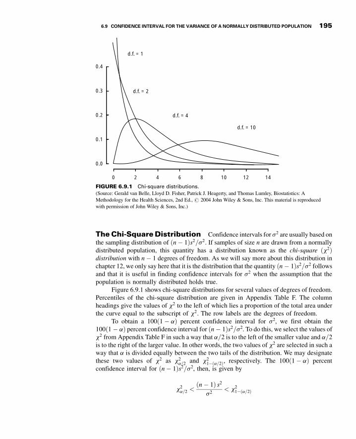
3GC06 11/26/2012 14:0:10 Page 195

TheChi-SquareDistribution Confidence intervals for s2 are usually based onthe sampling distribution of n� 1ð Þs2=s2. If samples of size n are drawn from a normallydistributed population, this quantity has a distribution known as the chi-square x2ð Þdistribution with n� 1 degrees of freedom. As we will say more about this distribution inchapter 12, we only say here that it is the distribution that the quantity n� 1ð Þs2=s2 followsand that it is useful in finding confidence intervals for s2 when the assumption that thepopulation is normally distributed holds true.

Figure 6.9.1 shows chi-square distributions for several values of degrees of freedom.Percentiles of the chi-square distribution are given in Appendix Table F. The columnheadings give the values of x2 to the left of which lies a proportion of the total area underthe curve equal to the subscript of x2. The row labels are the degrees of freedom.

To obtain a 100 1 � að Þ percent confidence interval for s2, we first obtain the100 1 � að Þ percent confidence interval for n� 1ð Þs2=s2. To do this, we select the values ofx2 from Appendix Table F in such a way that a=2 is to the left of the smaller value and a=2is to the right of the larger value. In other words, the two values of x2 are selected in such away that a is divided equally between the two tails of the distribution. We may designatethese two values of x2 as x2

a=2 and x21� a=2ð Þ, respectively. The 100 1 � að Þ percent

confidence interval for n� 1ð Þs2=s2, then, is given by

x2a=2 <

n� 1ð Þ s2

s2< x2

1� a=2ð Þ

0.4

d.f. = 1

d.f. = 2

d.f. = 4

d.f. = 10

0.3

0.2

0.1

0.0

0 2 4 6 8 10 12 14

FIGURE 6.9.1 Chi-square distributions.(Source: Gerald van Belle, Lloyd D. Fisher, Patrick J. Heagerty, and Thomas Lumley, Biostatistics: AMethodology for the Health Sciences, 2nd Ed., # 2004 John Wiley & Sons, Inc. This material is reproducedwith permission of John Wiley & Sons, Inc.)

6.9 CONFIDENCE INTERVAL FOR THE VARIANCE OF A NORMALLY DISTRIBUTED POPULATION 195

3GC06 11/26/2012 14:0:10 Page 196

We now manipulate this expression in such a way that we obtain an expression withs2 alone as the middle term. First, let us divide each term by n� 1ð Þ s2 to get

x2a=2

n� 1ð Þs2<

1

s2<

x21� a=2ð Þ

n� 1ð Þs2

If we take the reciprocal of this expression, we have

n� 1ð Þs2

x2a=2

> s2 >n� 1ð Þs2

x21� a=2ð Þ

Note that the direction of the inequalities changed when we took the reciprocals. If wereverse the order of the terms, we have

n� 1ð Þs2

x21� a=2ð Þ

< s2 <n� 1ð Þs2

x2a=2

(6.9.1)

which is the 100 1 � að Þ percent confidence interval for s2. If we take the square root ofeach term in Expression 6.9.1, we have the following 100 1 � að Þ percent confidenceinterval for s, the population standard deviation:

ffiffiffiffiffiffiffiffiffiffiffiffiffiffiffiffiffiffiffin� 1ð Þs2

x21� a=2ð Þ

s< s <


x2a=2

s(6.9.2)

EXAMPLE 6.9.1

In a study of the effectiveness of a gluten-free diet in first-degree relatives of patientswith type I diabetics, Hummel et al. (A-22) placed seven subjects on a gluten-free dietfor 12 months. Prior to the diet, they took baseline measurements of several antibodiesand autoantibodies, one of which was the diabetes related insulin autoantibody (IAA).The IAA levels were measured by radiobinding assay. The seven subjects had IAAunits of

9:7; 12:3; 11:2; 5:1; 24:8; 14:8; 17:7

We wish to estimate from the data in this sample the variance of the IAA units in thepopulation from which the sample was drawn and construct a 95 percent confidenceinterval for this estimate.

Solution: The sample yielded a value of s2 ¼ 39:763. The degrees of freedom are

n� 1 ¼ 6: The appropriate values of x2 from Appendix Table F are


3GC06 11/26/2012 14:0:10 Page 197

x21� a=2ð Þ ¼ 14:449 and x2

a=2 ¼ 1:237. Our 95 percent confidence interval for

s2 is

6 39:763ð Þ14:449

< s2 <6 39:763ð Þ

1:237

16:512 < s2 < 192:868

The 95 percent confidence interval for s is

4:063 < s < 13:888

We are 95 percent confident that the parameters being estimated are withinthe specified limits, because we know that in the long run, in repeatedsampling, 95 percent of intervals constructed as illustrated would include therespective parameters. &

SomePrecautions Although this method of constructing confidence intervals fors2 is widely used, it is not without its drawbacks. First, the assumption of the normality ofthe population from which the sample is drawn is crucial, and results may be misleading ifthe assumption is ignored.

Another difficulty with these intervals results from the fact that the estimator is not inthe center of the confidence interval, as is the case with the confidence interval for m. Thisis because the chi-square distribution, unlike the normal, is not symmetric. The practicalimplication of this is that the method for the construction of confidence intervals for s2,which has just been described, does not yield the shortest possible confidence intervals.Tate and Klett (12) give tables that may be used to overcome this difficulty.

EXERCISES

6.9.1. A study by Aizenberg et al. (A-23) examined the efficacy of sildenafil, a potent phosphodiesteraseinhibitor, in the treatment of elderly men with erectile dysfunction induced by antidepressanttreatment for major depressive disorder. The ages of the 10 enrollees in the study were

74; 81; 70; 70; 74; 77; 76; 70; 71; 72

Assume that the subjects in this sample constitute a simple random sample drawn from a populationof similar subjects. Construct a 95 percent confidence interval for the variance of the ages of subjectsin the population.

6.9.2. Borden et al. (A-24) performed experiments on cadaveric knees to test the effectiveness of severalmeniscal repair techniques. Specimens were loaded into a servohydraulic device and tension-loadedto failure. The biomechanical testing was performed by using a slow loading rate to simulate thestresses that the medial meniscus might be subjected to during early rehabilitation exercises andactivities of daily living. One of the measures is the amount of displacement that occurs. Of the 12specimens receiving the vertical mattress suture and the FasT-FIX method, the displacement values

EXERCISES 197

3GC06 11/26/2012 14:0:11 Page 198

measured in millimeters are 16.9, 20.2, 20.1, 15.7, 13.9, 14.9, 18.0, 18.5, 9.2, 18.8, 22.8, 17.5.Construct a 90 percent confidence interval for the variance of the displacement in millimeters for apopulation of subjects receiving these repair techniques.

6.9.3. Forced vital capacity determinations were made on 20 healthy adult males. The sample variance was1,000,000. Construct 90 percent confidence intervals for s2 and s.

6.9.4. In a study of myocardial transit times, appearance transit times were obtained on a sample of30 patients with coronary artery disease. The sample variance was found to be 1.03. Construct99 percent confidence intervals for s2 and s.

6.9.5. A sample of 25 physically and mentally healthy males participated in a sleep experiment in which thepercentage of each participant’s total sleeping time spent in a certain stage of sleep was recorded. Thevariance computed from the sample data was 2.25. Construct 95 percent confidence intervals for s2

and s.

6.9.6. Hemoglobin determinations were made on 16 animals exposed to a harmful chemical. The followingobservations were recorded: 15.6, 14.8, 14.4, 16.6, 13.8, 14.0, 17.3, 17.4, 18.6, 16.2, 14.7, 15.7, 16.4,13.9, 14.8, 17.5. Construct 95 percent confidence intervals for s2 and s.

6.9.7. Twenty air samples taken at the same site over a period of 6 months showed the following amounts ofsuspended particulate matter (micrograms per cubic meter of air):

68 22 36 3242 24 28 3830 44 28 2728 43 45 5079 74 57 21

Consider these measurements to be a random sample from a population of normally distributedmeasurements, and construct a 95 percent confidence interval for the population variance.

6.10 CONFIDENCE INTERVALFOR THE RATIO OF THE VARIANCESOF TWONORMALLY DISTRIBUTEDPOPULATIONS

It is frequently of interest to compare two variances, and one way to do this is to form theirratio, s2

1=s22. If two variances are equal, their ratio will be equal to 1. We usually will not

know the variances of populations of interest, and, consequently, any comparisons we makewill be based on sample variances. In other words, we may wish to estimate the ratio of twopopulation variances. We learned in Section 6.4 that the valid use of the t distribution toconstruct a confidence interval for the difference between two population means requiresthat the population variances be equal. The use of the ratio of two population variances fordetermining equality of variances has been formalized into a statistical test. The distribu-tion of this test provides test values for determining if the ratio exceeds the value 1 to a largeenough extent that we may conclude that the variances are not equal. The test is referred toas the F-max Test by Hartley (13) or the Variance Ratio Test by Zar (14). Many computerprograms provide some formalized test of the equality of variances so that the assumptionof equality of variances associated with many of the tests in the following chapters can be


3GC06 11/26/2012 14:0:11 Page 199

examined. If the confidence interval for the ratio of two population variances includes 1, weconclude that the two population variances may, in fact, be equal. Again, since this is a formof inference, we must rely on some sampling distribution, and this time the distribution ofs2

1=s21

� �= s2

2=s22

� �is utilized provided certain assumptions are met. The assumptions are

that s21 and s2

2 are computed from independent samples of size n1 and n2 respectively, drawnfrom two normally distributed populations. We use s2

1 to designate the larger of the twosample variances.

The F Distribution If the assumptions are met, s21=s

21

� �= s2

2=s22

� �follows a

distribution known as the F distribution. We defer a more complete discussion of thisdistribution until chapter 8, but note that this distribution depends on two-degrees-of-freedom values, one corresponding to the value of n1 � 1 used in computing s2

1 and theother corresponding to the value of n2 � 1 used in computing s2

2. These are usually referredto as the numerator degrees of freedom and the denominator degrees of freedom.Figure 6.10.1 shows some F distributions for several numerator and denominatordegrees-of-freedom combinations. Appendix Table G contains, for specified combinationsof degrees of freedom and values of a;F values to the right of which lies a=2 of the areaunder the curve of F.

A Confidence Interval for s21=s

22 To find the 100 1 � að Þ percent confidence

interval for s21=s

22, we begin with the expression

Fa=2 <s2

1=s21

s22=s

22

< F1� a=2ð Þ

where Fa=2 and F1� a=2ð Þ are the values from the F table to the left and right of which,respectively, lies a=2 of the area under the curve. The middle term of this expression maybe rewritten so that the entire expression is

Fa=2 <s2

1

s22

� s22

s21

< F1� a=2ð Þ

(10; ∞)

(10; 50)

(10; 10)

(10; 4)

0 0.5 1.0 1.5 2.0 2.5 3.0 3.5 4.0

F

f (x)

0.0

0.2

0.4

0.6

0.8

1.0

FIGURE 6.10.1 The F distribution for various degrees of freedom.(From Documenta Geigy, Scientific Tables, Seventh Edition, 1970. Courtesy of Ciba-Geigy Limited, Basel,Switzerland.)

6.10 CONFIDENCE INTERVAL FOR THE RATIO OF THE VARIANCES OF TWO NORMALLY DISTRIBUTED POPULATIONS 199

3GC06 11/26/2012 14:0:12 Page 200

If we divide through by s21=s

22, we have

Fa=2

s21=s

22

<s2

2

s21

<F1� a=2ð Þs2

1=s22

Taking the reciprocals of the three terms gives

s21=s

22

Fa=2>

s21

s22

>s2

1=s22

F1� a=2ð Þ

and if we reverse the order, we have the following 100 1 � að Þ percent confidence intervalfor s2

1=s22:

s21=s

22

F1� a=2ð Þ<

s21

s22

<s2

1=s22

Fa=2(6.10.1)

EXAMPLE 6.10.1

Allen and Gross (A-25) examine toe flexors strength in subjects with plantar fasciitis (painfrom heel spurs, or general heel pain), a common condition in patients with musculo-skeletal problems. Inflammation of the plantar fascia is often costly to treat and frustratingfor both the patient and the clinician. One of the baseline measurements was the body massindex (BMI). For the 16 women in the study, the standard deviation for BMI was 8.1 and forfour men in the study, the standard deviation was 5.9. We wish to construct a 95 percentconfidence interval for the ratio of the variances of the two populations from which wepresume these samples were drawn.

Solution: We have the following information:

n1 ¼ 16 n2 ¼ 4

s21 ¼ 8:1ð Þ2 ¼ 65:61 s2

2 ¼ 5:9ð Þ2 ¼ 34:81

df 1 ¼ numerator degrees of freedom ¼ n1 � 1 ¼ 15

df 2 ¼ denominator degrees of freedom ¼ n2 � 1 ¼ 3

a ¼ :05

F:025 ¼ :24096 F:975 ¼ 14:25

We are now ready to obtain our 95 percent confidence interval fors2

1=s22 by substituting appropriate values into Expression 6.10.1:

65:61=34:81

14:25<

s21

s22

<65:61=34:81

:24096

:1323 <s2

1

s22

< 7:8221


3GC06 11/26/2012 14:0:12 Page 201

We give this interval the appropriate probabilistic and practicalinterpretations.

Since the interval .1323 to 7.8221 includes 1, we are able to concludethat the two population variances may be equal. &

Finding F 1� a=2ð Þ and F a=2 At this point we must make a cumbersome, butunavoidable, digression and explain how the values F:975 ¼ 14:25 and F:025 ¼ :24096 wereobtained. The value of F:975 at the intersection of the column headed df 1 ¼ 15 and the rowlabeled df 2 ¼ 3 is 14.25. If we had a more extensive table of the F distribution, findingF:025 would be no trouble; we would simply find F:025 as we found F:975. We would take thevalue at the intersection of the column headed 15 and the row headed 3. To include everypossible percentile of F would make for a very lengthy table. Fortunately, however, thereexists a relationship that enables us to compute the lower percentile values from our limitedtable. The relationship is as follows:

Fa;df 1;df 2¼ 1

F1�a;df 2;df 1

(6.10.2)

We proceed as follows.Interchange the numerator and denominator degrees of freedom and locate the

appropriate value of F. For the problem at hand we locate 4.15, which is at the intersectionof the column headed 3 and the row labeled 15. We now take the reciprocal of this value,1=4:15 ¼ :24096. In summary, the lower confidence limit (LCL) and upper confidencelimit (UCL) s2

1=s22 are as follows:

LCL ¼ s21

s22

1

F 1�a=2ð Þ;df 1;df 2

UCL ¼ s21

s22

F1� a=2ð Þ;df 2;df 1

Alternative procedures for making inferences about the equality of two varianceswhen the sampled populations are not normally distributed may be found in the book byDaniel (15).

Some Precautions Similar to the discussion in the previous section of construct-ing confidence intervals for s2, the assumption of normality of the populations from whichthe samples are drawn is crucial to obtaining correct intervals for the ratio of variancesdiscussed in this section. Fortunately, most statistical computer programs provide alter-natives to the F-ratio, such as Levene’s test, when the underlying distributions cannot beassumed to be normally distributed. Computationally, Levene’s test uses a measure ofdistance from a sample median instead of a sample mean, hence removing the assumptionof normality.

6.10 CONFIDENCE INTERVAL FOR THE RATIO OF THE VARIANCES OF TWO NORMALLY DISTRIBUTED POPULATIONS 201

3GC06 11/26/2012 14:0:12 Page 202

EXERCISES

6.10.1. The purpose of a study by Moneim et al. (A-26) was to examine thumb amputations from team ropingat rodeos. The researchers reviewed 16 cases of thumb amputations. Of these, 11 were completeamputations while five were incomplete. The ischemia time is the length of time that insufficientoxygen is supplied to the amputated thumb. The ischemia times (hours) for 11 subjects experiencingcomplete amputations were

4:67; 10:5; 2:0; 3:18; 4:00; 3:5; 3:33; 5:32; 2:0; 4:25; 6:0

For five victims of incomplete thumb amputation, the ischemia times were

3:0; 10:25; 1:5; 5:22; 5:0

Treat the two reported sets of data as sample data from the two populations as described.Construct a 95 percent confidence interval for the ratio of the two unknown populationvariances.

6.10.2. The objective of a study by Horesh et al. (A-27) was to explore the hypothesis that some forms ofsuicidal behavior among adolescents are related to anger and impulsivity. The sample consisted of65 adolescents admitted to a university-affiliated adolescent psychiatric unit. The researchers usedthe Impulsiveness-Control Scale (ICS, A-28) where higher numbers indicate higher degrees ofimpulsiveness and scores can range from 0 to 45. The 33 subjects classified as suicidal had an ICSscore standard deviation of 8.4 while the 32 nonsuicidal subjects had a standard deviation of 6.0.Assume that these two groups constitute independent simple random samples from two populationsof similar subjects. Assume also that the ICS scores in these two populations are normally distributed.Find the 99 percent confidence interval for the ratio of the two population variances of scores onthe ICS.

6.10.3. Stroke index values were statistically analyzed for two samples of patients suffering frommyocardial infarction. The sample variances were 12 and 10. There were 21 patients in eachsample. Construct the 95 percent confidence interval for the ratio of the two populationvariances.

6.10.4. Thirty-two adult asphasics seeking speech therapy were divided equally into two groups. Group 1received treatment 1, and group 2 received treatment 2. Statistical analysis of the treatmenteffectiveness scores yielded the following variances: s2

1 ¼ 8; s22 ¼ 15. Construct the 90 percent

confidence interval for s22=s

21.

6.10.5. Sample variances were computed for the tidal volumes (milliliters) of two groups of patients sufferingfrom atrial septal defect. The results and sample sizes were as follows:

n1 ¼ 31; s21 ¼ 35; 000

n2 ¼ 41; s22 ¼ 20; 000

Construct the 95 percent confidence interval for the ratio of the two population variances.

6.10.6. Glucose responses to oral glucose were recorded for 11 patients with Huntington’s disease (group 1)and 13 control subjects (group 2). Statistical analysis of the results yielded the following samplevariances: s2

1 ¼ 105; s22 ¼ 148. Construct the 95 percent confidence interval for the ratio of the two

population variances.


3GC06 11/26/2012 14:0:13 Page 203

6.10.7. Measurements of gastric secretion of hydrochloric acid (milliequivalents per hour) in 16 normalsubjects and 10 subjects with duodenal ulcer yielded the following results:

Normal subjects: 6.3, 2.0, 2.3, 0.5, 1.9, 3.2, 4.1, 4.0, 6.2, 6.1, 3.5, 1.3, 1.7, 4.5, 6.3, 6.2Ulcer subjects: 13.7, 20.6, 15.9, 28.4, 29.4, 18.4, 21.1, 3.0, 26.2, 13.0

Construct a 95 percent confidence interval for the ratio of the two population variances. Whatassumptions must be met for this procedure to be valid?

6.11 SUMMARY

This chapter is concerned with one of the major areas of statistical inference—estimation.Both point estimation and interval estimation are covered. The concepts and methodsinvolved in the construction of confidence intervals are illustrated for the followingparameters: means, the difference between two means, proportions, the difference betweentwo proportions, variances, and the ratio of two variances. In addition, we learned in thischapter how to determine the sample size needed to estimate a population mean and apopulation proportion at specified levels of precision.

We learned, also, in this chapter that interval estimates of population parameters aremore desirable than point estimates because statements of confidence can be attached tointerval estimates.



6.2.1 Expression of an intervalestimate

estimator � reliability coefficientð Þ �standard error of the estimatorð Þ

6.2.2 Interval estimate for mwhen s is known

�x� z 1�a=2ð Þs�x

6.3.1 t-transformationt ¼ �x� m

s=ffiffiffin

p

6.3.2 Interval estimate for mwhen s is unknown

�x� t 1�a=2ð Þ ¼ sffiffiffin

p

6.4.1 Interval estimate for thedifference between twopopulation means whens1 and s2 are known

�x1 � �x2ð Þ � z 1�a=2ð Þ

ffiffiffiffiffiffiffiffiffiffiffiffiffiffiffiffis2

1

n1þ s2

2

n2

s

6.4.2 Pooled variance estimates2p ¼

n1 � 1ð Þs21 þ n2 � 1ð Þs2

2

n1 þ n2 � 2

6.4.3 Standard error of estimates �x1��x2ð Þ ¼


n1þ s2

p

n2

s

(Continued )


3GC06 11/26/2012 14:0:13 Page 204

6.4.4 Interval estimate for thedifference between twopopulation means whens1 is unknown

�x1 � �x2ð Þ � t 1�a=2ð Þ


n1þ s2

p

n2

s

6.4.5 Cochran’s correction forreliability coefficientwhen variances are notequal

t01�a=2ð Þ ¼w1t1 þ w2t2w1 þ w2

6.4.6 Interval estimate usingCochran’s correction for t �x1 � �x2ð Þ � t01�a=2ð Þ

ffiffiffiffiffiffiffiffiffiffiffiffiffiffiffis2

1

n1þ s2

2

n2

s

6.5.1 Interval estimate for apopulation proportion

p� z 1�a=2ð Þffiffiffiffiffiffiffiffiffiffiffiffiffiffiffiffiffiffiffiffiffiffip 1 � pð Þ=n

p

6.6.1 Interval estimate for thedifference between twopopulation proportions

p1 � p2ð Þ � z 1�a=2ð Þ

ffiffiffiffiffiffiffiffiffiffiffiffiffiffiffiffiffiffiffiffiffiffiffiffiffiffiffiffiffiffiffiffiffiffiffiffiffiffiffiffiffiffiffiffiffiffiffiffip1 1 � p1ð Þ

n1þ p2 1 � p2ð Þ

n2

s

6.7.1–6.7.3 Sample size determinationwhen sampling withreplacement

d ¼ reliability coefficientð Þ � standard errorð Þd ¼ z

sffiffiffin

p

;

n ¼ z2s2

d2

6.7.4–6.7.5 Sample size determinationwhen sampling withoutreplacement

d ¼ zsffiffiffin

pffiffiffiffiffiffiffiffiffiffiffiffiN � n

N � 1

r

;

n ¼ Nz2s2

d2 N � 1ð Þ þ z2s2

6.8.1 Sample size determinationfor proportions whensampling withreplacement

n ¼ z2pq

d2

6.8.2 Sample size determinationfor proportions whensampling withoutreplacement

n ¼ Nz2s2

d2 N � 1ð Þ þ z2s2

6.9.1 Interval estimate for s2 n� 1ð Þs2

x21� a=2ð Þ

< s2 <n� 1ð Þs2

x2a=2ð Þ

6.9.2 Interval estimate for sffiffiffiffiffiffiffiffiffiffiffiffiffiffiffiffiffiffiffin� 1ð Þs2

x21� a=2ð Þ

s< s <


x2a=2ð Þ

s

6.10.1 Interval estimate for theratio of two variances

s21=s

22

F1� a=2ð Þ<

s21

s22

<s2

1=s22

Fa=2


3GC06 11/26/2012 14:0:14 Page 205

6.10.2 Relationship among Fratios

Fa;df 1 ;df 2¼ 1

F1�a;df 2;df 1

SymbolKey

a ¼ Type 1 error rate x2 ¼ Chi-square distribution d ¼ error component of interval estimate df ¼ degrees of freedom F ¼ F-distribution m ¼ mean of population n ¼ sample size p ¼ proportion for population q ¼ 1 � pð Þ p ¼ estimated proportion for sample s2 ¼ population variance s ¼ population standard deviation s�x ¼ standard error s ¼ standard deviation of sample sp ¼ pooled standard deviation t ¼ Student’s t-transformation t0 ¼Cochran’s correction to t �x ¼ mean of sample z ¼ standard normal distribution


1. What is statistical inference?

2. Why is estimation an important type of inference?

3. What is a point estimate?

4. Explain the meaning of unbiasedness.


(a) Reliability coefficient (b) Confidence coefficient (c) Precision(d) Standard error (e) Estimator (f) Margin of error

6. Give the general formula for a confidence interval.

7. State the probabilistic and practical interpretations of a confidence interval.

8. Of what use is the central limit theorem in estimation?

9. Describe the t distribution.

10. What are the assumptions underlying the use of the t distribution in estimating a single populationmean?

11. What is the finite population correction? When can it be ignored?

12. What are the assumptions underlying the use of the t distribution in estimating the difference betweentwo population means?


3GC06 11/26/2012 14:0:14 Page 206

13. Arterial blood gas analyses performed on a sample of 15 physically active adult males yielded thefollowing resting PaO2 values:

75; 80; 80; 74; 84; 78; 89; 72; 83; 76; 75; 87; 78; 79; 88

Compute the 95 percent confidence interval for the mean of the population.

14. What proportion of asthma patients are allergic to house dust? In a sample of 140, 35 percent hadpositive skin reactions. Construct the 95 percent confidence interval for the population proportion.

15. An industrial hygiene survey was conducted in a large metropolitan area. Of 70 manufacturing plantsof a certain type visited, 21 received a “poor” rating with respect to absence of safety hazards.Construct a 95 percent confidence interval for the population proportion deserving a “poor” rating.

16. Refer to the previous problem. How large a sample would be required to estimate the populationproportion to within .05 with 95 percent confidence (.30 is the best available estimate of p):

(a) If the finite population correction can be ignored?

(b) If the finite population correction is not ignored and N ¼ 1500?

17. In a dental survey conducted by a county dental health team, 500 adults were asked to give the reasonfor their last visit to a dentist. Of the 220 who had less than a high-school education, 44 said they wentfor preventative reasons. Of the remaining 280, who had a high-school education or better, 150 statedthat they went for preventative reasons. Construct a 95 percent confidence interval for the differencebetween the two population proportions.

18. A breast cancer research team collected the following data on tumor size:

Type of Tumor n �x s

A 21 3.85 cm 1.95 cmB 16 2.80 cm 1.70 cm

Construct a 95 percent confidence interval for the difference between population means.

19. A certain drug was found to be effective in the treatment of pulmonary disease in 180 of 200 casestreated. Construct the 90 percent confidence interval for the population proportion.

20. Seventy patients with stasis ulcers of the leg were randomly divided into two equal groups. Eachgroup received a different treatment for edema. At the end of the experiment, treatment effectivenesswas measured in terms of reduction in leg volume as determined by water displacement. The meansand standard deviations for the two groups were as follows:

Group (Treatment) �x s

A 95 cc 25B 125 cc 30

Construct a 95 percent confidence interval for the difference in population means.

21. What is the average serum bilirubin level of patients admitted to a hospital for treatment of hepatitis?A sample of 10 patients yielded the following results:

20:5; 14:8; 21:3; 12:7; 15:2; 26:6; 23:4; 22:9; 15:7; 19:2

Construct a 95 percent confidence interval for the population mean.


3GC06 11/26/2012 14:0:14 Page 207

22. Determinations of saliva pH levels were made in two independent random samples of seventh-gradeschoolchildren. Sample A children were caries-free while sample B children had a high incidence ofcaries. The results were as follows:

A: 7.14, 7.11, 7.61, 7.98, 7.21, 7.16, 7.897.24, 7.86, 7.47, 7.82, 7.37, 7.66, 7.62, 7.65

B: 7.36, 7.04, 7.19, 7.41, 7.10, 7.15, 7.36,7.57, 7.64, 7.00, 7.25, 7.19

Construct a 90 percent confidence interval for the difference between the population means. Assumethat the population variances are equal.

23. Drug Awas prescribed for a random sample of 12 patients complaining of insomnia. An independentrandom sample of 16 patients with the same complaint received drug B. The number of hours of sleepexperienced during the second night after treatment began were as follows:

A: 3.5, 5.7, 3.4, 6.9, 17.8, 3.8, 3.0, 6.4, 6.8, 3.6, 6.9, 5.7B: 4.5, 11.7, 10.8, 4.5, 6.3, 3.8, 6.2, 6.6, 7.1, 6.4, 4.5, 5.1,

3.2, 4.7, 4.5, 3.0

Construct a 95 percent confidence interval for the difference between the population means. Assumethat the population variances are equal.

24. The objective of a study by Crane et al. (A-29) was to examine the efficacy, safety, and maternalsatisfaction of (a) oral misoprostol and (b) intravenous oxytocin for labor induction in women withpremature rupture of membranes at term. Researchers randomly assigned women to the twotreatments. For the 52 women who received oral misoprostol, the mean time in minutes to activelabor was 358 minutes with a standard deviation of 308 minutes. For the 53 women taking oxytocin,the mean time was 483 minutes with a standard deviation of 144 minutes. Construct a 99 percentconfidence interval for the difference in mean time to active labor for these two different medications.What assumptions must be made about the reported data? Describe the population about which aninference can be made.

25. Over a 2-year period, 34 European women with previous gestational diabetes were retrospectivelyrecruited from West London antenatal databases for a study conducted by Kousta et al. (A-30). One ofthe measurements for these women was the fasting nonesterified fatty acids concentration (NEFA)measured in mmol=L. In the sample of 34 women, the mean NEFA level was 435 with a samplestandard deviation of 215.0. Construct a 95 percent confidence interval for the mean fasting NEFAlevel for a population of women with gestational diabetes. State all necessary assumptions about thereported data and subjects.

26. Scheid et al. (A-31) questioned 387 women receiving free bone mineral density screening. Thequestions focused on past smoking history. Subjects undergoing hormone replacement therapy(HRT), and subjects not undergoing HRT, were asked if they had ever been a regular smoker. In theHRT group, 29.3 percent of 220 women stated that they were at some point in their life a regularsmoker. In the non–HRT group, 17.3 percent of 106 women responded positively to being at somepoint in their life a regular smoker. (Sixty-one women chose not to answer the question.) Construct a95 percent confidence interval for the difference in smoking percentages for the two populations ofwomen represented by the subjects in the study. What assumptions about the data are necessary?

27. The purpose of a study by Elliott et al. (A-32) was to assess the prevalence of vitamin D deficiency inwomen living in nursing homes. The sample consisted of 39 women in a 120-bed skilled nursingfacility. Women older than 65 years of age who were long-term residents were invited to participate ifthey had no diagnosis of terminal cancer or metastatic disease. In the sample, 23 women had 25-hydroxyvitamin D levels of 20 ng/ml or less. Construct a 95 percent confidence interval for thepercent of women with vitamin D deficiency in the population presumed to be represented by thissample.


3GC06 11/26/2012 14:0:15 Page 208

28. In a study of the role of dietary fats in the etiology of ischemic heart disease the subjects were60 males between 40 and 60 years of age who had recently had a myocardial infarction and50 apparently healthy males from the same age group and social class. One variable of interest in thestudy was the proportion of linoleic acid (L.A.) in the subjects’ plasma triglyceride fatty acids. Thedata on this variable were as follows:

Subjects with Myocardial Infarction

Subject L.A. Subject L.A. Subject L.A. Subject L.A.

1 18.0 2 17.6 3 9.6 4 5.55 16.8 6 12.9 7 14.0 8 8.09 8.9 10 15.0 11 9.3 12 5.8

13 8.3 14 4.8 15 6.9 16 18.317 24.0 18 16.8 19 12.1 20 12.921 16.9 22 15.1 23 6.1 24 16.625 8.7 26 15.6 27 12.3 28 14.929 16.9 30 5.7 31 14.3 32 14.133 14.1 34 15.1 35 10.6 36 13.637 16.4 38 10.7 39 18.1 40 14.341 6.9 42 6.5 43 17.7 44 13.445 15.6 46 10.9 47 13.0 48 10.649 7.9 50 2.8 51 15.2 52 22.353 9.7 54 15.2 55 10.1 56 11.557 15.4 58 17.8 59 12.6 60 7.2

Healthy Subjects

Subject L.A. Subject L.A. Subject L.A. Subject L.A.

1 17.1 2 22.9 3 10.4 4 30.95 32.7 6 9.1 7 20.1 8 19.29 18.9 10 20.3 11 35.6 12 17.2

13 5.8 14 15.2 15 22.2 16 21.217 19.3 18 25.6 19 42.4 20 5.921 29.6 22 18.2 23 21.7 24 29.725 12.4 26 15.4 27 21.7 28 19.329 16.4 30 23.1 31 19.0 32 12.933 18.5 34 27.6 35 25.0 36 20.037 51.7 38 20.5 39 25.9 40 24.641 22.4 42 27.1 43 11.1 44 32.745 13.2 46 22.1 47 13.5 48 5.349 29.0 50 20.2

Construct the 95 percent confidence interval for the difference between population means. What dothese data suggest about the levels of linoleic acid in the two sampled populations?

29. The purpose of a study by Tahmassebi and Curzon (A-33) was to compare the mean salivary flow rateamong subjects with cerebral palsy and among subjects in a control group. Each group had10 subjects. The following table gives the mean flow rate in ml/minute as well as the standard error.


3GC06 11/26/2012 14:0:16 Page 209

Group Sample Size Mean ml/minute Standard Error

Cerebral palsy 10 0.220 0.0582Control 10 0.334 0.1641

Source: J. F. Tahmassebi and M. E. J. Curzon, “The Cause of Drooling in Children withCerebral Palsy—Hypersalivation or Swallowing Defect?” International Journal of PaediatricDentistry, 13 (2003), 106–111.

Construct the 90 percent confidence interval for the difference in mean salivary flow rate for the twopopulations of subjects represented by the sample data. State the assumptions necessary for this to bea valid confidence interval.

30. Culligan et al. (A-34) compared the long-term results of two treatments: (a) a modified Burchprocedure, and (b) a sling procedure for stress incontinence with a low-pressure urethra. Thirty-sixwomen took part in the study with 19 in the Burch treatment group and 17 in the sling proceduretreatment group. One of the outcome measures at three months post-surgery was maximum urethralclosure pressure (cm H2O). In the Burch group the mean and standard deviation were 16.4 and 8.2 cm,respectively. In the sling group, the mean and standard deviation were 39.8 and 23.0, respectively.Construct the 99 percent confidence interval for the difference in mean maximum urethral closurepressure for the two populations represented by these subjects. State all necessary assumptions.

31. In general, narrow confidence intervals are preferred over wide ones. We can make an interval narrowby using a small confidence coefficient. For a given set of other conditions, what happens to the levelof confidence when we use a small confidence coefficient? What would happen to the interval widthand the level of confidence if we were to use a confidence coefficient of zero?

32. In general, a high level of confidence is preferred over a low level of confidence. For a given set ofother conditions, suppose we set our level of confidence at 100 percent. What would be the effect ofsuch a choice on the width of the interval?

33. The subjects of a study by Borland et al. (A-35) were children in acute pain. Thirty-two children whopresented at an emergency room were enrolled in the study. Each child used the visual analogue scaleto rate pain on a scale from 0 to 100 mm. The mean pain score was 61.3 mm with a 95 percentconfidence interval of 53.2 mm–69.4 mm. Which would be the appropriate reliability factor for theinterval, z or t? Justify your choice. What is the precision of the estimate? The margin of error?

34. Does delirium increase hospital stay? That was the research question investigated by McCusker et al.(A-36). The researchers sampled 204 patients with prevalent delirium and 118 without delirium. Theconclusion of the study was that patients with prevalent delirium did not have a higher mean length ofstay compared to those without delirium. What was the target population? The sampled population?

35. Assessing driving self-restriction in relation to vision performance was the objective of a study by Westet al. (A-37). The researchers studied 629 current drivers ages 55 and older for 2 years. The variables ofinterest were driving behavior, health, physical function, and vision function. The subjects were part of alarger vision study at the Smith-Kettlewell Eye Research Institute. A conclusion of the study was thatolder adults with early changes in spatial vision function and depth perception appear to recognize theirlimitations and restrict their driving. What was the target population? The sampled population?

36. In a pilot study conducted by Ayouba et al. (A-38), researchers studied 123 children born of HIV-1-infected mothers in Yaound�e, Cameroon. Counseled and consenting pregnant women were given asingle dose of nevirapine at the onset of labor. Babies were given a syrup containing nevirapine withinthe first 72 hours of life. The researchers found that 87 percent of the children were considered notinfected at 6–8 weeks of age. What is the target population? What is the sampled population?


3GC06 11/26/2012 14:0:16 Page 210

37. Refer to Exercise 2.3.11. Construct a 95 percent confidence interval for the population mean S/Rratio. Should you use t or z as the reliability coefficient? Why? Describe the population about whichinferences based on this study may be made.

38. Refer to Exercise 2.3.12. Construct a 90 percent confidence interval for the population mean height.Should you use t or z as the reliability coefficient? Why? Describe the population about whichinferences based on this study may be made.

Exercises for Use with Large Data Sets Available on the Following Website:www.wiley.com /college/ daniel

1. Refer to North Carolina Birth Registry Data NCBIRTH800 with 800 observations (see LargeData Exercise 1 in Chapter 2). Calculate 95 percent confidence intervals for the following:

(a) the percentage of male children(b) the mean age of a mother giving birth(c) the mean weight gained during pregnancy(d) the percentage of mothers admitting to smoking during pregnancy(e) the difference in the average weight gained between smoking and nonsmoking mothers(f) the difference in the average birth weight in grams between married and nonmarried mothers(g) the difference in the percentage of low birth weight babies between married and nonmarried

mothers

2. Refer to the serum cholesterol levels for 1000 subjects (CHOLEST). Select a simple randomsample of size 15 from this population and construct a 95 percent confidence interval for thepopulation mean. Compare your results with those of your classmates. What assumptions arenecessary for your estimation procedure to be valid?

3. Refer to the serum cholesterol levels for 1000 subjects (CHOLEST). Select a simple randomsample of size 50 from the population and construct a 95 percent confidence interval for theproportion of subjects in the population who have readings greater than 225. Compare yourresults with those of your classmates.

4. Refer to the weights of 1200 babies born in a community hospital (BABY WGTS). Draw a simplerandom sample of size 20 from this population and construct a 95 percent confidence interval forthe population mean. Compare your results with those of your classmates. What assumptions arenecessary for your estimation procedure to be valid?

5. Refer to the weights of 1200 babies born in a community hospital (BABY WGTS). Draw a simplerandom sample of size 35 from the population and construct a 95 percent confidence interval forthe population mean. Compare this interval with the one constructed in Exercise 4.

6. Refer to the heights of 1000 twelve-year-old boys (BOY HGTS). Select a simple random sampleof size 15 from this population and construct a 99 percent confidence interval for the populationmean. What assumptions are necessary for this procedure to be valid?

7. Refer to the heights of 1000 twelve-year-old boys (BOY HGTS). Select a simple random sampleof size 35 from the population and construct a 99 percent confidence interval for the populationmean. Compare this interval with the one constructed in Exercise 5.

REFERENCES


1. JOHN A. RICE, Mathematical Statistics and Data Analysis, 2nd ed., Duxbury, Belmont, CA, 1988.2. W. S. GOSSET (“Student”), “The Probable Error of a Mean,” Biometrika, 6 (1908), 1–25.



3GC06 11/26/2012 14:0:16 Page 211

3. W. V. BEHRENS, “Ein Beitrag zu Fehlerberechnung bei wenige Beobachtungen,” LandwirtsschaftlicheJahrb€ucher, 68 (1929), 807–837.

4. R. A. FISHER, “The Comparison of Samples with Possibly Unequal Variances,” Annals of Eugenics, 9 (1939),174–180.

5. R. A. FISHER, “The Asymptotic Approach to Behrens’ Integral with Further Tables for the d Test of Significance,”Annals of Eugenics, 11 (1941), 141–172.

6. J. NEYMAN, “Fiducial Argument and the Theory of Confidence Intervals,” Biometrika, 32 (1941), 128–150.7. H. SCHEFF�E, “On Solutions of the Behrens-Fisher Problem Based on the t-Distribution,” Annals of Mathematical

Statistics, 14 (1943), 35–44.8. H. SCHEFF�E, “A Note on the Behrens-Fisher Problem,” Annals of Mathematical Statistics, 15 (1944), 430–432.9. B. L. WELCH, “The Significance of the Difference Between Two Means When the Population Variances Are

Unequal,” Biometrika, 29 (1937), 350–361.10. B. L. WELCH, “The Generalization of ‘Student’s Problem When Several Different Population Variances Are

Involved,” Biometrika, 34 (1947), 28–35.11. WILLIAM G. COCHRAN, “Approximate Significance Levels of the Behrens-Fisher Test,” Biometrics, 20 (1964),

191–195.12. R. F. TATE and G. W. KLETT, “Optimal Confidence Intervals for the Variance of a Normal Distribution,” Journal of

the American Statistical Association, 54 (1959), 674–682.13. H. O. HARTLEY, “The Maximum F-Ratio as a Short Cut Test for Heterogeneity of Variances,” Biometrika,

37 (1950), 308–312.14. J. H. ZAR, Biostatistical Analysis, 4th ed., Prentice-Hall, Upper Saddle River, NJ, 1999.15. WAYNE W. DANIEL, Applied Nonparametric Statistics, 2nd ed., PWS-KENT, Boston, 1989.


A-1. NICOLA MAFFULLI, CHERLY TALLON, JASON WONG, KIM PENG, and ROBERT BLEAKNEY, “Early Weightbearing andAnkle Mobilization after Open Repair of Acute Midsubstance Tears of the Achilles Tendon,” American Journalof Sports Medicine, 31 (2003), 692–700.

A-2. PAUL J. REBER, LUCY A. MARTINEZ, and SANDRA WEINTRAUB, “Artificial Grammar Learning in Alzheimer’sDisease,” Cognitive, Affective, and Behavioral Neuroscience, 3 (2003), 145–153.

A-3. CHRISTOPHE PEDROLETTI, MARIEANN H€oGMAN, PEKKA MERIL€AINEN, LENNART S. NORDVALL, GUNILLA HEDLIN, andKJELL ALVING, “Nitric Oxide Airway Diffusing Capacity and Mucosal Concentration in Asthmatic School-children,” Pediatric Research, 54 (2003), 496–501.

A-4. BRUCE D. BEYNNON, BRADEN C. FLEMING, DAVID L. CHURCHILL, and DANIEL BROWN, “The Effect of AnteriorCruciate Ligament Deficiency and Functional Bracing on Translation of the Tibia Relative to the Femur duringNonweightbearing and Weightbearing,” American Journal of Sports Medicine, 31 (2003), 99–105.

A-5. LORRAINE DUGOFF, MAURITHA R. EVERETT, LOUIS VONTVER, and GWYN E. BARLEY, “Evaluation of Pelvic and BreastExamination Skills of Interns in Obstetrics and Gynecology and Internal Medicine,” American Journal ofObstetrics and Gynecology, 189 (2003), 655–658.

A-6. DIONNE MAYHEW, KAREN M. PERRIN, and WENDY STRUCHEN, “An Analysis of a Healthy Start Smoking CessationProgram,” American Journal of Health Studies, 17 (2002), 186–190.

A-7. ERIC GRANHOLM, ROBERT ANTHENELLI, RITA MONTEIRO, JOHN SEVCIK, and MARILYN STOLER, “Brief IntegratedOutpatient Dual-Diagnosis Treatment Reduces Psychiatric Hospitalizations,” American Journal on Addictions,12 (2003), 306–313.

A-8. SILVIA IANNELO, ANTONINA CAVALERI, PAOLINA MILAZZO, SANTI CANTARELLA, and FRANCESCO BELFIORE, “Low FastingSerum Triglyceride Level as a Precocious Marker of Autoimmune Disorders,” Medscape General Medicine,5 (3) (2003).

A-9. EVELYN C. Y. CHAN, SALLY W. VERNON, FREDERICK T. O’DONNELL, CHUL AHN, ANTHONY GRESINGER, and DONNIE W.AGA, “Informed Consent for Cancer Screening with Prostate-Specific Antigen: How Well Are Men Getting theMessage?” American Journal of Public Health, 93 (2003), 779–785.

A-10. RONALD F. VAN VOLLENHOVEN, SOFIA ERNESTAM, ANDERS HARJU, JOHAN BRATT, and LARS KLARESKOG, “EtanerceptVersus Etanercept Plus Methotrexate: A Registry-Based Study Suggesting that the Combination Is ClinicallyMore Effacious,” Arthritis Research and Therapy, 5 (2003), R347–R351.

REFERENCES 211

3GC06 11/26/2012 14:0:16 Page 212

A-11. SATOSHI NOZAWA, KATSUJI SHIMIZU, KEI MIYAMOTO, and MIZUO TANAKA, “Repair of Pars Interarticularis Defectby Segmental Wire Fixation in Young Athletes with Spondylolysis,” American Journal of Sports Medicine,31 (2003), 359–364.

A-12. MORI J. KRANTZ, ILANA B. KUTINSKY, ALASTAIR D. ROBERTSON, and PHILIP S. MEHLER, “Dose-Related Effects ofMethadone on QT Prolongation in a Series of Patients with Torsade de Pointes,” Pharmacotherapy, 23 (2003),802–805.

A-13. SUSANNAH FOX and DEBORAH FELLOWS, “Health Searches and Email Have Become More Commonplace, But ThereIs Room for Improvement in Searches and Overall Internet Access,” Pew Internet and American Life Project,www.pewinternet.org/PPF/r/95/report_display.asp.

A-14. CARLOS M. LUNA, DANIEL BLANZACO, MICHAEL S. NIDERMAN, WALTER MATARUCCO, NATALIO C. BAREDES, PABLO

DESMERY, FERNANDO PALIZAS, GUILLERMO MENGA, FERNANDO RIOS, and CARLOS APEZTEGUIA, “Resolution ofVentilator-Associated Pneumonia: Prospective Evaluation of the Clinical Pulmonary Infection Score as anEarly Clinical Predictor of Outcome,” Critical Care Medicine, 31 (3) (2003), 676–682.

A-15. AREND F. L. SCHINKEL, JEROEN J. BAX, ERIC BOERSMA, ABDOU ELHENDY, ELENI C. VOURVOURI, JOS R. T. C. ROELANDT,and DON POLDERMANS, “Assessment of Residual Myocardial Viability in Regions with Chronic Electrocardio-graphic Q-Wave Infarction,” American Heart Journal, 144 (2002), 865–869.

A-16. FRIEDERIKE VON ZUR MUHLEN, WEILUM QUAN, DAVID J. D’AGATE, and TODD J. COHEN, “A Study of Carotid SinusMassage and Head-Up Tilt Table Testing in Patients with Syncope and Near-Syncope,” Journal of InvasiveCardiology, 14 (2002), 477–482.

A-17. DANIEL F. CONNOR, RONALD J. STEINGARD, JENNIFER J. ANDERSON, and RICHARD H. MELLONI, Jr., “Gender Differencesin Reactive and Proactive Aggression,” Child Psychiatry and Human Development, 33 (2003), 279–294.

A-18. ALLAN V. HORWITZ, CATHY SPATZ WIDOM, JULIE MCLAUGHLIN, and HELENE RASKIN WHITE, “The Impact ofChildhood Abuse and Neglect on Adult Mental Health: A Prospective Study,” Journal of Health and SocialBehavior, 42 (2001), 184–201.

A-19. P. ADAB, T. MARSHALL, A. ROUSE, B. RANDHAWA, H. SANGHA, and N. BHANGOO, “Randomised Controlled Trial ofthe Effect of Evidence Based Information on Women’s Willingness to Participate in Cervical Cancer Screening,”Journal of Epidemiology and Community Health, 57 (2003), 589–593.

A-20. JOHN A. SPERTUS, TIM KEWHURST, CYNTHIA M. DOUGHERTY, and PAUL NICHOL, “Testing the Effectiveness ofConverting Patients to Long-Acting Antianginal Medications: The Quality of Life in Angina Research,”American Heart Journal, 141 (2001), 550–558.

A-21. PATRICK R. FINLEY, HEIDI R. RENS, JOAN T. PONT, SUSAN L. GESS, CLIFTON LOUIE, SCOTT A. BULL, JANELLE Y. LEE, andLISA A. BERO, “Impact of a Collaborative Care Model on Depression in a Primary Care Setting: A Randomized,Controlled Trial,” Pharmacotherapy, 23 (9) (2003), 1175–1185.

A-22. MICHAEL HUMMEL, EZIO BONIFACIO, HEIKE E. NASERKE, and ANETTE G. ZIEGLER, “Elimination of Dietary GlutenDoes Not Reduce Titers of Type 1 Diabetes-Associated Autoantibodies in High-Risk Subjects,” Diabetes Care,25 (2002), 1111–1116.

A-23. DOV AIZENBERG, ABRAHAM WEIZMAN, and YORAM BARAK, “Sildenafil for Selective Serotonin Reuptake Inhibitor-Induced Erectile Dysfunction in Elderly Male Depressed Patients,” Journal of Sex and Marital Therapy, 29(2003), 297–303.

A-24. PETER BORDEN, JOHN NYLAND, DAVID N. M. CABORN, and DAVID PIENKOWSKI, “Biomechanical Comparison of theFasT-Fix Meniscal Repair Suture System with Vertical Mattress Sutures and Meniscus Arrows,” AmericanJournal of Sports Medicine, 31 (2003), 374–378.

A-25. RACHEL H. ALLEN and MICHAEL T. GROSS, “Toe Flexors Strength and Passive Extension Range of Motion of theFirst Metatarsophalangeal Joint in Individuals with Plantar Fasciitis,” Journal of Orthopaedic and SportsPhysical Therapy, 33 (2003), 468–477.

A-26. MOHEB S. MONEIM, KEIKHOSROW FIROOZBAKHSH, DOMINIC GROSS, STEVEN D. YOUNG, and GEORGE OMER, “ThumbAmputations from Team Roping,” American Journal of Sports Medicine, 31 (2003), 728–735.

A-27. NETTA HORESH, ISRAEL ORBACH, DORON GOTHELF, MEIR EFRATI, and ALAN APTER, “Comparison of the SuicidalBehavior of Adolescent Inpatients with Borderline Personality Disorder and Major Depression,” Journal ofNervous and Mental Disease, 191 (2003), 582–588.

A-28. R. PLUTCHIK, and H. VAN PRAAG, “The Measurement of Suicidality, Aggressivity and Impulsivity,” ClinicalNeuropharmacology, 9(suppl) (1989), 380–382.

A-29. JOAN M. G. CRANE, TINA DELANEY, and DONNA HUTCHENS, “Oral Misoprostol for Premature Rupture of Membranesat Term,” American Journal of Obstetrics and Gynecology, 189 (2003), 720–724.


http://www.pewinternet.org/PPF/r/95/report_display.asp

3GC06 11/26/2012 14:0:16 Page 213

A-30. ELENI KOUSTA, NATASHA J. LAWRENCE, IAN F. GODSLAND, ANNA PENNY, VICTOR ANYAOKU, BARBARA A. MILLAUER,ESTER CELA, DESMOND G. JOHNSTON, STEPHEN ROBINSON, and MARK I. MCCARTHY, “Insulin Resistance and Beta-Cell Dysfunction in Normoglycaemic European Women with a History of Gestational Diabetes,” ClinicalEndocrinology, 59 (2003), 289–297.

A-31. DEWEY C. SCHEID, MARIO T. COLEMAN, and ROBERT M. HAMM, “Do Perceptions of Risk and Quality of Life AffectUse of Hormone Replacement Therapy by Postmenopausal Women?” Journal of the American Board of FamilyPractice, 16 (2003), 270–277.

A-32. MARY E. ELLIOTT, NEIL C. BINKLEY, MOLLY CARNES, DAVID R. ZIMMERMAN, KIM PETERSEN, KATHY KNAPP, JESSICA J.BEHLKE, NANCY AHMANN, and MARY A. KIESER, “Fracture Risks for Women in Long-Term Care: High Prevalenceof Calcaneal Osteoporosis and Hypovitaminosis D,” Pharmacotherapy, 23 (2003), 702–710.

A-33. J. F. TAHMASSEBI and M. E. J. CURZON, “The Cause of Drooling in Children with Cerebral Palsy—Hypersalivationor Swallowing Defect?” International Journal of Paediatric Dentistry, 13 (2003), 106–111.

A-34. PATRICK J. CULLIGAN, ROGER P. GOLDBERG, and PETER K. SAND, “A Randomized Controlled Trial Comparing aModified Burch Procedure and a Suburethral Sling: Long-Term Follow-Up,” International UrogynecologyJournal, 14 (2003), 229–233.

A-35. MEREDITH L. BORLAND, IAN JACOBS, and GARY GEELHOE, “Intranasal Fentanyl Reduces Acute Pain in Children inthe Emergency Department: A Safety and Efficacy Study,” Emergency Medicine, 14 (2002), 275–280.

A-36. JANE MCCUSKER, MARTIN G. COLE, NANDINI DENDUKURI, and ERIC BELZILE, “Does Delirium Increase HospitalStay?” Journal of the American Geriatrics Society, 51 (2003), 1539–1546.

A-37. CATHERINE G. WEST, GINNY GILDENGORIN, GUNILLA HAEGERSTROM PORTNOY, LORI A. LOTT, MARILYN E. SCHNECK, andJOHN A. BRABYN, “Vision and Driving Self-Restriction in Older Adults,” Journal of the American GeriatricsSociety, 51 (2003), 1348–1355.

A-38. AHIDJO AYOUBA, GILBERT TENE, PATRICK CUNIN, YACOUBA FOUPOUAPOUOGNIGNI, ELISABETH MENU, ANFUMBOM

KFUTWAH, JOCELYN THONNON, GABRIELLA SCARLATTI, MARCEL MONNY-LOB�E, NICOLE ETEKI, CHARLES KOUANFACK,MICH�ELE TARDY, ROBERT LEKE, MAURICE NKAM, ANNE E. NLEND, FRAN SCOISE BARR�E-SINOUSSI, PAUL M. V. MARTIN,and ERIC NERRIENET, “Low Rate of Mother-to-Child Transmission of HIV-1 After Nevirapine Intervention in aPilot Public Health Program in Yaound�e, Cameroon,” Journal of Acquired Immune Deficiency Syndrome,34 (2003), 274–280.

REFERENCES 213

3GC07 11/24/2012 14:19:24 Page 214

CHAPTER7HYPOTHESIS TESTING

CHAPTER OVERVIEW

This chapter covers hypothesis testing, the second of two general areas ofstatistical inference.Hypothesis testing isa topicwithwhich youasa studentarelikely to have some familiarity. Interval estimation, discussed in the precedingchapter, and hypothesis testing are based on similar concepts. In fact, confi-dence intervals may be used to arrive at the same conclusions that are reachedthrough the use of hypothesis tests. This chapter provides a format, followedthroughout the remainder of this book, for conducting a hypothesis test.

TOPICS

7.1 INTRODUCTION

7.2 HYPOTHESIS TESTING: A SINGLE POPULATION MEAN

7.3 HYPOTHESIS TESTING: THE DIFFERENCE BETWEEN TWO POPULATIONMEANS

7.4 PAIRED COMPARISONS

7.5 HYPOTHESIS TESTING: A SINGLE POPULATION PROPORTION

7.6 HYPOTHESIS TESTING: THE DIFFERENCE BETWEEN TWO POPULATIONPROPORTIONS

7.7 HYPOTHESIS TESTING: A SINGLE POPULATION VARIANCE

7.8 HYPOTHESIS TESTING: THE RATIO OF TWO POPULATION VARIANCES

7.9 THE TYPE II ERROR AND THE POWER OF A TEST

7.10 DETERMINING SAMPLE SIZE TO CONTROL TYPE II ERRORS

7.11 SUMMARY

LEARNING OUTCOMES


1. understand how to correctly state a null and alternative hypothesis and carry out astructured hypothesis test.

2. understand the concepts of type I error, type II error, and the power of a test.

3. be able to calculate and interpret z, t, F, and chi-square test statistics for makingstatistical inferences.

4. understand how to calculate and interpret p values.

214

3GC07 11/24/2012 14:19:25 Page 215

7.1 INTRODUCTION

One type of statistical inference, estimation, is discussed in the preceding chapter. Theother type, hypothesis testing, is the subject of this chapter. As is true with estimation,the purpose of hypothesis testing is to aid the clinician, researcher, or administrator inreaching a conclusion concerning a population by examining a sample from thatpopulation. Estimation and hypothesis testing are not as different as they are made toappear by the fact that most textbooks devote a separate chapter to each. As we will explainlater, one may use confidence intervals to arrive at the same conclusions that are reached byusing the hypothesis testing procedures discussed in this chapter.

Basic Concepts In this section some of the basic concepts essential to an under-standing of hypothesis testing are presented. The specific details of particular tests will begiven in succeeding sections.

DEFINITION

A hypothesismay be defined simply as a statement about one or morepopulations.

The hypothesis is frequently concerned with the parameters of the populationsabout which the statement is made. A hospital administrator may hypothesize that theaverage length of stay of patients admitted to the hospital is 5 days; a public health nursemay hypothesize that a particular educational program will result in improved com-munication between nurse and patient; a physician may hypothesize that a certain drugwill be effective in 90 percent of the cases for which it is used. By means of hypothesistesting one determines whether or not such statements are compatible with the availabledata.

Types of Hypotheses Researchers are concerned with two types of hypotheses—research hypotheses and statistical hypotheses.

DEFINITION

The research hypothesis is the conjecture or supposition that motivatesthe research.

It may be the result of years of observation on the part of the researcher. A publichealth nurse, for example, may have noted that certain clients responded more readily to aparticular type of health education program. A physician may recall numerous instances inwhich certain combinations of therapeutic measures were more effective than any one ofthem alone. Research projects often result from the desire of such health practitioners todetermine whether or not their theories or suspicions can be supported when subjected tothe rigors of scientific investigation.


3GC07 11/24/2012 14:19:25 Page 216

Research hypotheses lead directly to statistical hypotheses.

DEFINITION

Statistical hypotheses are hypotheses that are stated in such a way thatthey may be evaluated by appropriate statistical techniques.

In this book the hypotheses that we will focus on are statistical hypotheses. We willassume that the research hypotheses for the examples and exercises have already beenconsidered.

Hypothesis Testing Steps For convenience, hypothesis testing will be pre-sented as a ten-step procedure. There is nothing magical or sacred about this particularformat. It merely breaks the process down into a logical sequence of actions and decisions.

1. Data. The nature of the data that form the basis of the testing procedures must beunderstood, since this determines the particular test to be employed. Whether thedata consist of counts or measurements, for example, must be determined.

2. Assumptions. As we learned in the chapter on estimation, different assumptionslead to modifications of confidence intervals. The same is true in hypothesistesting: A general procedure is modified depending on the assumptions. In fact,the same assumptions that are of importance in estimation are important inhypothesis testing. We have seen that these include assumptions about thenormality of the population distribution, equality of variances, and independenceof samples.

3. Hypotheses. There are two statistical hypotheses involved in hypothesis testing, andthese should be stated explicitly. The null hypothesis is the hypothesis to be tested. Itis designated by the symbol H0. The null hypothesis is sometimes referred to as ahypothesis of no difference, since it is a statement of agreement with (or no differencefrom) conditions presumed to be true in the population of interest. In general, the nullhypothesis is set up for the express purpose of being discredited. Consequently, thecomplement of the conclusion that the researcher is seeking to reach becomes thestatement of the null hypothesis. In the testing process the null hypothesis either isrejected or is not rejected. If the null hypothesis is not rejected, we will say that thedata on which the test is based do not provide sufficient evidence to cause rejection. Ifthe testing procedure leads to rejection, we will say that the data at hand are notcompatible with the null hypothesis, but are supportive of some other hypothesis. Thealternative hypothesis is a statement of what we will believe is true if our sample datacause us to reject the null hypothesis. Usually the alternative hypothesis and theresearch hypothesis are the same, and in fact the two terms are used interchangeably.We shall designate the alternative hypothesis by the symbol HA.

Rules for Stating Statistical Hypotheses When hypotheses are of thetype considered in this chapter an indication of equality ðeither ¼;�; or �Þ mustappear in the null hypothesis. Suppose, for example, that we want to answer the

216 CHAPTER 7 HYPOTHESIS TESTING

3GC07 11/24/2012 14:19:25 Page 217

question: Can we conclude that a certain population mean is not 50? The nullhypothesis is

H0: m ¼ 50

and the alternative is

HA: m 6¼ 50

Suppose we want to know if we can conclude that the population mean is greater than50. Our hypotheses are

H0: m � 50 HA: m > 50

If we want to know if we can conclude that the population mean is less than 50, thehypotheses are

H0: m � 50 HA: m < 50

In summary, we may state the following rules of thumb for deciding whatstatement goes in the null hypothesis and what statement goes in the alternativehypothesis:

(a) What you hope or expect to be able to conclude as a result of the test usually shouldbe placed in the alternative hypothesis.

(b) The null hypothesis should contain a statement of equality, either ¼;�; or �.

(c) The null hypothesis is the hypothesis that is tested.

(d) The null and alternative hypotheses are complementary. That is, the two togetherexhaust all possibilities regarding the value that the hypothesized parameter canassume.

A Precaution It should be pointed out that neither hypothesis testing nor statisticalinference, in general, leads to the proof of a hypothesis; it merely indicates whether thehypothesis is supported or is not supported by the available data. When we fail to reject anull hypothesis, therefore, we do not say that it is true, but that it may be true. When wespeak of accepting a null hypothesis, we have this limitation in mind and do not wish toconvey the idea that accepting implies proof.

4. Test statistic. The test statistic is some statistic that may be computed from the dataof the sample. As a rule, there are many possible values that the test statistic mayassume, the particular value observed depending on the particular sample drawn. Aswe will see, the test statistic serves as a decision maker, since the decision to reject ornot to reject the null hypothesis depends on the magnitude of the test statistic.An example of a test statistic is the quantity

z ¼ �x� m0

s=ffiffiffin

p (7.1.1)


3GC07 11/24/2012 14:19:25 Page 218

where m0 is a hypothesized value of a population mean. This test statistic is related tothe statistic

z ¼ �x� m

s=ffiffiffin

p (7.1.2)

with which we are already familiar.

General Formula for Test Statistic The following is a general formula fora test statistic that will be applicable in many of the hypothesis tests discussed in thisbook:

test statistic ¼ relevant statistic � hypothesized parameter

standard error of the relevant statistic

In Equation 7.1.1, �x is the relevant statistic, m0 is the hypothesized parameter, and s=ffiffiffin

pis

the standard error of �x, the relevant statistic.

5. Distribution of test statistic. It has been pointed out that the key to statisticalinference is the sampling distribution. We are reminded of this again when it becomesnecessary to specify the probability distribution of the test statistic. The distributionof the test statistic

z ¼ �x� m0

s=ffiffiffin

p

for example, follows the standard normal distribution if the null hypothesis is trueand the assumptions are met.

6. Decision rule. All possible values that the test statistic can assume are points on thehorizontal axis of the graph of the distribution of the test statistic and are divided intotwo groups; one group constitutes what is known as the rejection region and the othergroup makes up the nonrejection region. The values of the test statistic forming therejection region are those values that are less likely to occur if the null hypothesis istrue, while the values making up the acceptance region are more likely to occur ifthe null hypothesis is true. The decision rule tells us to reject the null hypothesis if thevalue of the test statistic that we compute from our sample is one of the values in therejection region and to not reject the null hypothesis if the computed value of the teststatistic is one of the values in the nonrejection region.

Significance Level The decision as to which values go into the rejection regionand which ones go into the nonrejection region is made on the basis of the desired level ofsignificance, designated by a. The term level of significance reflects the fact that hypothesistests are sometimes called significance tests, and a computed value of the test statistic thatfalls in the rejection region is said to be significant. The level of significance, a, specifiesthe area under the curve of the distribution of the test statistic that is above the values on thehorizontal axis constituting the rejection region.


3GC07 11/24/2012 14:19:26 Page 219

DEFINITION

The level of significance a is a probability and, in fact, is the probabilityof rejecting a true null hypothesis.

Since to reject a true null hypothesis would constitute an error, it seems onlyreasonable that we should make the probability of rejecting a true null hypothesis smalland, in fact, that is what is done. We select a small value of a in order to make theprobability of rejecting a true null hypothesis small. The more frequently encounteredvalues of a are .01, .05, and .10.

Types of Errors The error committed when a true null hypothesis is rejected iscalled the type I error. The type II error is the error committed when a false null hypothesisis not rejected. The probability of committing a type II error is designated by b.

Whenever we reject a null hypothesis there is always the concomitant risk ofcommitting a type I error, rejecting a true null hypothesis. Whenever we fail to reject a nullhypothesis the risk of failing to reject a false null hypothesis is always present. We make asmall, but we generally exercise no control over b, although we know that in most practicalsituations it is larger than a.

We never know whether we have committed one of these errors when we reject or failto reject a null hypothesis, since the true state of affairs is unknown. If the testing procedureleads to rejection of the null hypothesis, we can take comfort from the fact that we made asmall and, therefore, the probability of committing a type I error was small. If we fail toreject the null hypothesis, we do not know the concurrent risk of committing a type II error,since b is usually unknown but, as has been pointed out, we do know that, in most practicalsituations, it is larger than a.

Figure 7.1.1 shows for various conditions of a hypothesis test the possible actionsthat an investigator may take and the conditions under which each of the two types of errorwill be made. The table shown in this figure is an example of what is generally referred to asa confusion matrix.

7. Calculation of test statistic. From the data contained in the sample we compute avalue of the test statistic and compare it with the rejection and nonrejection regionsthat have already been specified.

8. Statistical decision. The statistical decision consists of rejecting or of not rejectingthe null hypothesis. It is rejected if the computed value of the test statistic falls in the

Condition of Null Hypothesis

FalseTrue

Type II errorCorrect actionFail to

Possible reject H0

Action Reject H0 Correct actionType I error

FIGURE 7.1.1 Conditions under which type I and type II errors may be committed.


3GC07 11/24/2012 14:19:26 Page 220

rejection region, and it is not rejected if the computed value of the test statistic falls inthe nonrejection region.

9. Conclusion. If H0 is rejected, we conclude that HA is true. If H0 is not rejected, weconclude that H0 may be true.

10. p values. The p value is a number that tells us how unusual our sample results are,given that the null hypothesis is true. A p value indicating that the sample results arenot likely to have occurred, if the null hypothesis is true, provides justification fordoubting the truth of the null hypothesis.

DEFINITION

A p value is the probability that the computed value of a test statistic isat least as extreme as a specified value of the test statistic when the nullhypothesis is true. Thus, the p value is the smallest value of a for which wecan reject a null hypothesis.

We emphasize that when the null hypothesis is not rejected one should not say thatthe null hypothesis is accepted. We should say that the null hypothesis is “not rejected.” Weavoid using the word “accept” in this case because we may have committed a type II error.Since, frequently, the probability of committing a type II error can be quite high, we do notwish to commit ourselves to accepting the null hypothesis.

Figure 7.1.2 is a flowchart of the steps that we follow when we perform a hypothesistest.

Purpose of Hypothesis Testing The purpose of hypothesis testing is to assistadministrators and clinicians in making decisions. The administrative or clinical decisionusually depends on the statistical decision. If the null hypothesis is rejected, the adminis-trative or clinical decision usually reflects this, in that the decision is compatible with thealternative hypothesis. The reverse is usually true if the null hypothesis is not rejected. Theadministrative or clinical decision, however, may take other forms, such as a decision togather more data.

We also emphasize that the hypothesis testing procedures highlighted in theremainder of this chapter generally examine the case of normally distributed data orcases where the procedures are appropriate because the central limit theorem applies. Inpractice, it is not uncommon for samples to be small relative to the size of the population,or to have samples that are highly skewed, and hence the assumption of normality isviolated. Methods to handle this situation, that is distribution-free or nonparametricmethods, are examined in detail in Chapter 13. Most computer packages include ananalytical procedure (for example, the Shapiro-Wilk or Anderson-Darling test) fortesting normality. It is important that such tests are carried out prior to analysis ofdata. Further, when testing two samples, there is an implicit assumption that thevariances are equal. Tests for this assumption are provided in Section 7.8. Finally, itshould be noted that hypothesis tests, just like confidence intervals, are relatively


3GC07 11/24/2012 14:19:26 Page 221

sensitive to the size of the samples being tested, and caution should be taken wheninterpreting results involving very small sample sizes.

We must emphasize at this point, however, that the outcome of the statistical test isonly one piece of evidence that influences the administrative or clinical decision. Thestatistical decision should not be interpreted as definitive but should be considered alongwith all the other relevant information available to the experimenter.

With these general comments as background, we now discuss specific hypothesistests.

Do notreject H0

Makestatisticaldecision

Evaluatedata

Reviewassumptions

Statehypotheses

Selecttest

statistics

State decision

rule

Calculatetest

statistics

Determinedistribution

of teststatistics

Reject H0

Conclude H0may be true

Conclude HAis true

FIGURE 7.1.2 Steps in the hypothesis testing procedure.


3GC07 11/24/2012 14:19:26 Page 222

7.2 HYPOTHESIS TESTING:A SINGLE POPULATIONMEAN

In this section we consider the testing of a hypothesis about a population mean underthree different conditions: (1) when sampling is from a normally distributed populationof values with known variance; (2) when sampling is from a normally distributedpopulation with unknown variance, and (3) when sampling is from a population that isnot normally distributed. Although the theory for conditions 1 and 2 depends onnormally distributed populations, it is common practice to make use of the theorywhen relevant populations are only approximately normally distributed. This is satis-factory as long as the departure from normality is not drastic. When sampling is from anormally distributed population and the population variance is known, the test statisticfor testing H0: m ¼ m0 is

z ¼ �x� m

s=ffiffiffin

p (7.2.1)

which, when H0 is true, is distributed as the standard normal. Examples 7.2.1 and 7.2.2illustrate hypothesis testing under these conditions.

Sampling from Normally Distributed Populations: PopulationVariances Known As we did in Chapter 6, we again emphasize that situations inwhich the variable of interest is normally distributed with a known variance are rare. Thefollowing example, however, will serve to illustrate the procedure.

EXAMPLE 7.2.1

Researchers are interested in the mean age of a certain population. Let us say that they areasking the following question: Can we conclude that the mean age of this population isdifferent from 30 years?

Solution: Based on our knowledge of hypothesis testing, we reply that they canconclude that the mean age is different from 30 if they can reject the nullhypothesis that the mean is equal to 30. Let us use the ten-step hypothesistesting procedure given in the previous section to help the researchers reach aconclusion.

1. Data. The data available to the researchers are the ages of a simplerandom sample of 10 individuals drawn from the population of interest.From this sample a mean of �x ¼ 27 has been computed.

2. Assumptions. It is assumed that the sample comes from a populationwhose ages are approximately normally distributed. Let us also assumethat the population has a known variance of s2 ¼ 20.

3. Hypotheses. The hypothesis to be tested, or null hypothesis, is that themean age of the population is equal to 30. The alternative hypothesis is


3GC07 11/24/2012 14:19:27 Page 223

that the mean age of the population is not equal to 30. Note that we areidentifying with the alternative hypothesis the conclusion the researcherswish to reach, so that if the data permit rejection of the null hypothesis, theresearchers’ conclusion will carry more weight, since the accompanyingprobability of rejecting a true null hypothesis will be small. We will makesure of this by assigning a small value to a, the probability of committinga type I error. We may present the relevant hypotheses in compact form asfollows:

H0: m ¼ 30HA: m 6¼ 30

4. Test statistic. Since we are testing a hypothesis about a populationmean, since we assume that the population is normally distributed, andsince the population variance is known, our test statistic is given byEquation 7.2.1.

5. Distribution of test statistic. Based on our knowledge of samplingdistributions and the normal distribution, we know that the test statisticis normally distributed with a mean of 0 and a variance of 1, if H0 istrue. There are many possible values of the test statistic that thepresent situation can generate; one for every possible sample of size 10that can be drawn from the population. Since we draw only onesample, we have only one of these possible values on which to base adecision.

6. Decision rule. The decision rule tells us to reject H0 if the computedvalue of the test statistic falls in the rejection region and to fail to reject H0

if it falls in the nonrejection region. We must now specify the rejection andnonrejection regions. We can begin by asking ourselves what magnitudeof values of the test statistic will cause rejection of H0. If the nullhypothesis is false, it may be so either because the population mean isless than 30 or because the population mean is greater than 30. Therefore,either sufficiently small values or sufficiently large values of the teststatistic will cause rejection of the null hypothesis. We want these extremevalues to constitute the rejection region. How extreme must a possiblevalue of the test statistic be to qualify for the rejection region? The answerdepends on the significance level we choose, that is, the size of theprobability of committing a type I error. Let us say that we want theprobability of rejecting a true null hypothesis to be a ¼ :05. Since ourrejection region is to consist of two parts, sufficiently small values andsufficiently large values of the test statistic, part of a will have to beassociated with the large values and part with the small values. It seemsreasonable that we should divide a equally and let a=2 ¼ :025 beassociated with small values and a=2 ¼ :025 be associated with largevalues.

7.2 HYPOTHESIS TESTING: A SINGLE POPULATIONMEAN 223

3GC07 11/24/2012 14:19:27 Page 224

Critical Value of Test Statistic

What value of the test statistic is so large that, when the null hypothesis is true, theprobability of obtaining a value this large or larger is .025? In other words, what is the valueof z to the right of which lies .025 of the area under the standard normal distribution? Thevalue of z to the right of which lies .025 of the area is the same value that has .975 of the areabetween it and �1. We look in the body of Appendix Table D until we find .975 or itsclosest value and read the corresponding marginal entries to obtain our z value. In thepresent example thevalue of z is 1.96. Similar reasoning will lead us to find�1:96 as thevalueof the test statistic so small that when the null hypothesis is true, the probability of obtaininga value this small or smaller is .025. Our rejection region, then, consists of all values ofthe test statistic equal to or greater than 1.96 and less than or equal to �1:96. Thenonrejection region consists of all values in between. We may state the decision rule forthis test as follows: reject H0 if the computed value of the test statistic is either � 1:96 or� �1:96. Otherwise, do not reject H0. The rejection and nonrejection regions are shownin Figure 7.2.1. The values of the test statistic that separate the rejection and nonrejectionregions are called critical values of the test statistic, and the rejection region issometimes referred to as the critical region.

The decision rule tells us to compute a value of the test statistic from the data ofour sample and to reject H0 if we get a value that is either equal to or greater than 1.96or equal to or less than �1:96 and to fail to reject H0 if we get any other value. Thevalue of a and, hence, the decision rule should be decided on before gathering the data.This prevents our being accused of allowing the sample results to influence our choiceof a. This condition of objectivity is highly desirable and should be preserved inall tests.

7. Calculation of test statistic. From our sample we compute

z ¼ 27 � 30ffiffiffiffiffiffiffiffiffiffiffiffiffi20=10

p ¼ �3

1:4142¼ �2:12

8. Statistical decision. Abiding by the decision rule, we are able toreject the null hypothesis since �2:12 is in the rejection region. We

s = 1

0_ 69.169.1

a/2 = .025a/2= .025

.95

z

Nonrejectionregion

Rejection regionRejection region

FIGURE 7.2.1 Rejection and nonrejection regions for Example 7.2.1.


3GC07 11/24/2012 14:19:27 Page 225

can say that the computed value of the test statistic is significant atthe .05 level.

9. Conclusion. We conclude that m is not equal to 30 and let ouradministrative or clinical actions be in accordance with this conclu-sion.

10. p values. Instead of saying that an observed value of the test statisticis significant or is not significant, most writers in the researchliterature prefer to report the exact probability of getting a value asextreme as or more extreme than that observed if the null hypothesis istrue. In the present instance these writers would give the computedvalue of the test statistic along with the statement p ¼ :0340. Thestatement p ¼ :0340 means that the probability of getting a value asextreme as 2.12 in either direction, when the null hypothesis is true, is.0340. The value .0340 is obtained from Appendix Table D and is theprobability of observing a z � 2:12 or a z � �2:12 when the nullhypothesis is true. That is, when H0 is true, the probability ofobtaining a value of z as large as or larger than 2.12 is .0170, andthe probability of observing a value of z as small as or smaller than�2:12 is .0170. The probability of one or the other of these eventsoccurring, when H0 is true, is equal to the sum of the two individualprobabilities, and hence, in the present example, we say thatp ¼ :0170 þ :0170 ¼ :0340.

Recall that the p value for a test may be defined also as thesmallest value of a for which the null hypothesis can be rejected. Since,in Example 7.2.1, our p value is .0340, we know that we could havechosen an a value as small as .0340 and still have rejected the nullhypothesis. If we had chosen an a smaller than .0340, we would not havebeen able to reject the null hypothesis. A general rule worthremembering, then, is this: if the p value is less than or equal to a,we reject the null hypothesis; if the p value is greater than a, we do notreject the null hypothesis.

The reporting of p values as part of the results of an investigation ismore informative to the reader than such statements as “the null hypothesis isrejected at the .05 level of significance” or “the results were not significant atthe .05 level.” Reporting the p value associated with a test lets the readerknow just how common or how rare is the computed value of the test statisticgiven that H0 is true. &

Testing H0 by Means of a Confidence Interval Earlier, we stated thatone can use confidence intervals to test hypotheses. In Example 7.2.1 we used ahypothesis testing procedure to test H0: m ¼ 30 against the alternative, HA: m 6¼ 30.We were able to reject H0 because the computed value of the test statistic fell in therejection region.


3GC07 11/24/2012 14:19:27 Page 226

Let us see how we might have arrived at this same conclusion by using a 100 1 � að Þpercent confidence interval. The 95 percent confidence interval for m is

27 � 1:96ffiffiffiffiffiffiffiffiffiffiffiffiffi20=10

p27 � 1:96 1:414ð Þ27 � 2:7714

ð24:2286; 29:7714Þ

Since this interval does not include 30, we say 30 is not a candidate for the mean we areestimating and, therefore, m is not equal to 30 and H0 is rejected. This is the sameconclusion reached by means of the hypothesis testing procedure.

If the hypothesized parameter, 30, had been within the 95 percent confidenceinterval, we would have said that H0 is not rejected at the .05 level of significance. Ingeneral, when testing a null hypothesis by means of a two-sided confidence interval, wereject H0 at the a level of significance if the hypothesized parameter is not contained withinthe 100 1 � að Þ percent confidence interval. If the hypothesized parameter is containedwithin the interval, H0 cannot be rejected at the a level of significance.

One-Sided Hypothesis Tests The hypothesis test illustrated by Example7.2.1 is an example of a two-sided test, so called because the rejection region is splitbetween the two sides or tails of the distribution of the test statistic. A hypothesis test maybe one-sided, in which case all the rejection region is in one or the other tail of thedistribution. Whether a one-sided or a two-sided test is used depends on the nature of thequestion being asked by the researcher.

If both large and small values will cause rejection of the null hypothesis, a two-sidedtest is indicated. When either sufficiently “small” values only or sufficiently “large” valuesonly will cause rejection of the null hypothesis, a one-sided test is indicated.

EXAMPLE 7.2.2

Refer to Example 7.2.1. Suppose, instead of asking if they could conclude that m 6¼ 30, theresearchers had asked: Can we conclude that m < 30? To this question we would reply thatthey can so conclude if they can reject the null hypothesis that m � 30.

Solution: Let us go through the ten-step procedure to reach a decision based on aone-sided test.

1. Data. See the previous example.

2. Assumptions. See the previous example.

3. Hypotheses.

H0: m � 30HA: m < 30

The inequality in the null hypothesis implies that the null hypothesisconsists of an infinite number of hypotheses. The test will be made only


3GC07 11/24/2012 14:19:27 Page 227

at the point of equality, since it can be shown that if H0 is rejected whenthe test is made at the point of equality it would be rejected if the testwere done for any other value of m indicated in the null hypothesis.

4. Test statistic.

z ¼ �x� m0

s=ffiffiffin

p

5. Distribution of test statistic. See the previous example.

6. Decision rule. Let us again use a ¼ :05. To determine where to place therejection region, let us ask ourselves what magnitude of values wouldcause rejection of the null hypothesis. If we look at the hypotheses, wesee that sufficiently small values would cause rejection and that largevalues would tend to reinforce the null hypothesis. We will want ourrejection region to be where the small values are—at the lower tail of thedistribution. This time, since we have a one-sided test, all of a will go inthe one tail of the distribution. By consulting Appendix Table D, we findthat the value of z to the left of which lies .05 of the area under thestandard normal curve is �1:645 after interpolating. Our rejection andnonrejection regions are now specified and are shown in Figure 7.2.2.

Our decision rule tells us to reject H0 if the computed value of thetest statistic is less than or equal to �1:645.

7. Calculation of test statistic. From our data we compute

z ¼ 27 � 30ffiffiffiffiffiffiffiffiffiffiffiffiffi20=10

p ¼ �2:12

8. Statistical decision. We are able to reject the null hypothesis since�2:12 < �1:645.

9. Conclusion. We conclude that the population mean is smaller than 30and act accordingly.

10. p value. The p value for this test is .0170, since Pðz � �2:12Þ, when H0

is true, is .0170 as given by Appendix Table D when we determine the

s = 1

0_1.645

.05

.95

z

Rejection region Nonrejection region



3GC07 11/24/2012 14:19:28 Page 228

magnitude of the area to the left of �2:12 under the standard normalcurve. One can test a one-sided null hypothesis by means of a one-sidedconfidence interval. However, we will not cover the construction andinterpretation of this type of confidence interval in this book.

If the researcher’s question had been, “Can we conclude that the mean isgreater than 30?”, following the above ten-step procedure would have led to aone-sided test with all the rejection region at the upper tail of the distributionof the test statistic and a critical value of þ1:645. &

Sampling from a Normally Distributed Population: PopulationVarianceUnknown As we have already noted, the population variance is usuallyunknown in actual situations involving statistical inference about a population mean. Whensampling is from an approximately normal population with an unknown variance, the teststatistic for testing H0: m ¼ m0 is

t ¼ �x� m0

s=ffiffiffin

p (7.2.2)

which, when H0 is true, is distributed as Student’s t with n� 1 degrees of freedom. Thefollowing example illustrates the hypothesis testing procedure when the population isassumed to be normally distributed and its variance is unknown. This is the usual situationencountered in practice.

EXAMPLE 7.2.3

Nakamura et al. (A-1) studied subjects with medial collateral ligament (MCL) and anteriorcruciate ligament (ACL) tears. Between February 1995 and December 1997, 17 consecu-tive patients with combined acute ACL and grade III MCL injuries were treated by thesame physician at the research center. One of the variables of interest was the length of timein days between the occurrence of the injury and the first magnetic resonance imaging(MRI). The data are shown in Table 7.2.1. We wish to know if we can conclude that themean number of days between injury and initial MRI is not 15 days in a populationpresumed to be represented by these sample data.

TABLE 7.2.1 Number of Days Until MRI for Subjects with MCL and ACL Tears

Subject Days Subject Days Subject Days Subject Days

1 14 6 0 11 28 16 14

2 9 7 10 12 24 17 9

3 18 8 4 13 24

4 26 9 8 14 2

5 12 10 21 15 3

Source: Norimasa Nakamura, Shuji Horibe, Yukyoshi Toritsuka, Tomoki Mitsuoka, Hideki Yoshikawa, andKonsei Shino, “Acute Grade III Medial Collateral Ligament Injury of the Knee Associated with Anterior CruciateLigament Tear,” American Journal of Sports Medicine, 31 (2003), 261–267.


3GC07 11/24/2012 14:19:28 Page 229

Solution: We will be able to conclude that the mean number of days for the populationis not 15 if we can reject the null hypothesis that the population mean isequal to 15.

1. Data. The data consist of number of days until MRI on 17 subjects aspreviously described.

2. Assumptions. The 17 subjects constitute a simple random sample froma population of similar subjects. We assume that the number of daysuntil MRI in this population is approximately normally distributed.

3. Hypotheses.

H0: m ¼ 15HA: m 6¼ 15

4. Test statistic. Since the population variance is unknown, our teststatistic is given by Equation 7.2.2.

5. Distribution of test statistic. Our test statistic is distributed asStudent’s t with n� 1 ¼ 17 � 1 ¼ 16 degrees of freedom if H0 is true.

6. Decision rule. Let a ¼ :05. Since we have a two-sided test, we puta=2 ¼ :025 in each tail of the distribution of our test statistic. The tvalues to the right and left of which .025 of the area lies are 2.1199 and�2:1199. These values are obtained from Appendix Table E. Therejection and nonrejection regions are shown in Figure 7.2.3.

The decision rule tells us to compute a value of the test statistic andreject H0 if the computed t is either greater than or equal to 2.1199 or lessthan or equal to �2:1199.

7. Calculation of test statistic. From our sample data we compute asample mean of 13.2941 and a sample standard deviation of 8.88654.Substituting these statistics into Equation 7.2.2 gives

t ¼ 13:2941 � 15

8:88654=ffiffiffiffiffi17

p ¼ �1:7059

2:1553¼ �:791

0 2.1199–2.1199

.025.025

.95

t

Nonrejectionregion

Rejection regionRejection region



3GC07 11/24/2012 14:19:29 Page 230

8. Statistical decision. Do not reject H0, since �.791 falls in the non-rejection region.

9. Conclusion. Our conclusion, based on these data, is that the mean of thepopulation from which the sample came may be 15.

10. p value. The exact p value for this test cannot be obtained fromAppendix Table E since it gives t values only for selected percentiles.The p value can be stated as an interval, however. We find that �:791 isless than �1:337, the value of t to the left of which lies .10 of the areaunder the t with 16 degrees of freedom. Consequently, when H0 is true,the probability of obtaining a value of t as small as or smaller than �:791is greater than .10. That is P t � �:791ð Þ > :10. Since the test was two-sided, we must allow for the possibility of a computed value of the teststatistic as large in the opposite direction as that observed. AppendixTable E reveals that P t � :791ð Þ > :10 also. The p value, then, isp > :20. In fact, Excel calculates the p value to be .4403. Figure7.2.4 shows the p value for this example.

If in the previous example the hypotheses had been

H0: m � 15HA: m < 15

the testing procedure would have led to a one-sided test with all the rejectionregion at the lower tail of the distribution, and if the hypotheses had been

H0: m � 15HA: m > 15

we would have had a one-sided test with all the rejection region at the uppertail of the distribution. &

Sampling from a Population That Is Not Normally DistributedIf, as is frequently the case, the sample on which we base our hypothesis test about apopulation mean comes from a population that is not normally distributed, we may, if oursample is large (greater than or equal to 30), take advantage of the central limit theorem anduse z ¼ �x� m0ð Þ= s=

ffiffiffin

pð Þ as the test statistic. If the population standard deviation is not

.791 1.337p > .20

–1.337 –.791

p/2 > .10p/2 > .10

0

.10.10

t

FIGURE 7.2.4 Determination of p value for Example 7.2.3.


3GC07 11/24/2012 14:19:29 Page 231

known, the usual practice is to use the sample standard deviation as an estimate. The teststatistic for testing H0: m ¼ m0, then, is

z ¼ �x� m0

s=ffiffiffin

p (7.2.3)

which, when H0 is true, is distributed approximately as the standard normal distribution if nis large. The rationale for using s to replace s is that the large sample, necessary for thecentral limit theorem to apply, will yield a sample standard deviation that closelyapproximates s.

EXAMPLE 7.2.4

The goal of a study by Klingler et al. (A-2) was to determine how symptom recognition andperception influence clinical presentation as a function of race. They characterizedsymptoms and care-seeking behavior in African-American patients with chest painseen in the emergency department. One of the presenting vital signs was systolic bloodpressure. Among 157 African-American men, the mean systolic blood pressure was146 mm Hg with a standard deviation of 27. We wish to know if, on the basis of thesedata, we may conclude that the mean systolic blood pressure for a population of African-American men is greater than 140.

Solution: We will say that the data do provide sufficient evidence to conclude that thepopulation mean is greater than 140 if we can reject the null hypothesis thatthe mean is less than or equal to 140. The following test may be carried out:

1. Data. The data consist of systolic blood pressure scores for 157 African-American men with �x ¼ 146 and s ¼ 27.

2. Assumptions. The data constitute a simple random sample from apopulation of African-American men who report to an emergencydepartment with symptoms similar to those in the sample. We areunwilling to assume that systolic blood pressure values are normallydistributed in such a population.

3. Hypotheses.

H0: m � 140HA: m > 140

4. Test statistic. The test statistic is given by Equation 7.2.3, since s isunknown.

5. Distribution of test statistic. Because of the central limit theorem, thetest statistic is at worst approximately normally distributed with m ¼ 0 ifH0 is true.

6. Decision rule. Let a ¼ :05. The critical value of the test statistic is1.645. The rejection and nonrejection regions are shown in Figure 7.2.5.Reject H0 if computed z � 1:645.


3GC07 11/24/2012 14:19:29 Page 232

7. Calculation of test statistic.

z ¼ 146 � 140

27=ffiffiffiffiffiffiffiffi157

p ¼ 6

2:1548¼ 2:78

8. Statistical decision. Reject H0 since 2:78 > 1:645.

9. Conclusion. Conclude that the mean systolic blood pressure for thesampled population is greater than 140.

10. p value. The p value for this test is 1 � :9973 ¼ :0027, since as shown inAppendix Table D, the area (.0027) to the right of 2.78 is less than .05,the area to the right of 1.645. &

Procedures for Other Conditions If the population variance had beenknown, the procedure would have been identical to the above except that the knownvalue of s, instead of the sample value s, would have been used in the denominator of thecomputed test statistic.

Depending on what the investigators wished to conclude, either a two-sided test or aone-sided test, with the rejection region at the lower tail of the distribution, could have beenmade using the above data.

When testing a hypothesis about a single population mean, we may use Figure 6.3.3to decide quickly whether the test statistic is z or t.

Computer Analysis To illustrate the use of computers in testing hypotheses, weconsider the following example.

EXAMPLE 7.2.5

The following are the head circumferences (centimeters) at birth of 15 infants:

33.38 32.15 33.99 34.10 33.9734.34 33.95 33.85 34.23 32.7333.46 34.13 34.45 34.19 34.05

We wish to test H0: m ¼ 34:5 against HA: m 6¼ 34:5.

1.6450 z

Rejection regionNonrejection region

.05



3GC07 11/24/2012 14:19:29 Page 233

Solution: We assume that the assumptions for use of the t statistic are met. We enter thedata into Column 1 and proceed as shown in Figure 7.2.6.

To indicate that a test is one-sided when in Windows, click on theOptions button and then choose “less than” or “greater than” as appropriatein the Alternative box. If z is the appropriate test statistic, we choose1-Sample z from the Basic Statistics menu. The remainder of the commandsare the same as for the t test.

We learn from the printout that the computed value of the test statistic is�4:31 and the p value for the test is .0007. SAS® users may use the outputfrom PROC MEANS or PROC UNIVARIATE to perform hypothesis tests.

When both the z statistic and the t statistic are inappropriate teststatistics for use with the available data, one may wish to use a non-parametric technique to test a hypothesis about a single population measureof central tendency. One such procedure, the sign test, is discussed inChapter 13. &

EXERCISES

For each of the following exercises carry out the ten-step hypothesis testing procedure for the givensignificance level. For each exercise, as appropriate, explain why you chose a one-sided test or a two-sided test. Discuss how you think researchers and/or clinicians might use the results of yourhypothesis test. What clinical and/or research decisions and/or actions do you think would beappropriate in light of the results of your test?

7.2.1 Escobar et al. (A-3) performed a study to validate a translated version of the Western Ontario andMcMaster Universities Osteoarthritis Index (WOMAC) questionnaire used with Spanish-speakingpatients with hip or knee osteoarthritis. For the 76 women classified with severe hip pain, the


Stat Basic Statistics 1-Sample t MTB > TTEST 34.5 C1

Type C1 in Samples in columns. Type 34.5in the Test mean box. Click OK .

Output:

One-Sample T: C1

TEST OF MU 34.5 VS NOT 34.5VARIABLE N MEAN STDEV SE MEAN 95% CI T PC1 15 33.7980 0.6303 0.1627 (33.4490, 34.1470) 4.31 0.001

FIGURE 7.2.6 MINITAB procedure and output for Example 7.2.5.

EXERCISES 233

3GC07 11/24/2012 14:19:29 Page 234

WOMAC mean function score (on a scale from 0 to 100 with a higher number indicating lessfunction) was 70.7 with a standard deviation of 14.6. We wish to know if we may conclude that themean function score for a population of similar women subjects with severe hip pain is less than 75.Let a ¼ :01.

7.2.2 A study by Thienprasiddhi et al. (A-4) examined a sample of 16 subjects with open-angle glaucomaand unilateral hemifield defects. The ages (years) of the subjects were:

62 62 68 48 51 60 51 5757 41 62 50 53 34 62 61Source: Phamornsak Thienprasiddhi, Vivienne C. Greenstein,Candice S. Chen, Jeffrey M. Liebmann, Robert Ritch, andDonald C. Hood, “Multifocal Visual Evoked PotentialResponses in Glaucoma Patients with Unilateral HemifieldDefects,” American Journal of Ophthalmology, 136 (2003),34–40.

Can we conclude that the mean age of the population from which the sample may be presumed tohave been drawn is less than 60 years? Let a ¼ :05.

7.2.3 The purpose of a study by Lugli�e et al. (A-5) was to investigate the oral status of a group of patientsdiagnosed with thalassemia major (TM). One of the outcome measures was the decayed, missing, andfilled teeth index (DMFT). In a sample of 18 patients the mean DMFT index value was 10.3 with astandard deviation of 7.3. Is this sufficient evidence to allow us to conclude that the mean DMFTindex is greater than 9.0 in a population of similar subjects? Let a ¼ :10.

7.2.4 A study was made of a sample of 25 records of patients seen at a chronic disease hospital on anoutpatient basis. The mean number of outpatient visits per patient was 4.8, and the sample standarddeviation was 2. Can it be concluded from these data that the population mean is greater than fourvisits per patient? Let the probability of committing a type I error be .05. What assumptions arenecessary?

7.2.5 In a sample of 49 adolescents who served as the subjects in an immunologic study, one variable ofinterest was the diameter of skin test reaction to an antigen. The sample mean and standard deviationwere 21 and 11 mm erythema, respectively. Can it be concluded from these data that the populationmean is less than 30? Let a ¼ :05.

7.2.6 Nine laboratory animals were infected with a certain bacterium and then immunosuppressed. Themean number of organisms later recovered from tissue specimens was 6.5 (coded data) with astandard deviation of .6. Can one conclude from these data that the population mean is greater than 6?Let a ¼ :05. What assumptions are necessary?

7.2.7 A sample of 25 freshman nursing students made a mean score of 77 on a test designed to measureattitude toward the dying patient. The sample standard deviation was 10. Do these data providesufficient evidence to indicate, at the .05 level of significance, that the population mean is less than80? What assumptions are necessary?

7.2.8 We wish to know if we can conclude that the mean daily caloric intake in the adult rural population ofa developing country is less than 2000. A sample of 500 had a mean of 1985 and a standard deviationof 210. Let a ¼ :05.

7.2.9 A survey of 100 similar-sized hospitals revealed a mean daily census in the pediatrics service of 27with a standard deviation of 6.5. Do these data provide sufficient evidence to indicate that thepopulation mean is greater than 25? Let a ¼ :05.


3GC07 11/24/2012 14:19:30 Page 235

7.2.10 Following a week-long hospital supervisory training program, 16 assistant hospital administratorsmade a mean score of 74 on a test administered as part of the evaluation of the training program. Thesample standard deviation was 12. Can it be concluded from these data that the population mean isgreater than 70? Let a ¼ :05. What assumptions are necessary?

7.2.11 A random sample of 16 emergency reports was selected from the files of an ambulance service.The mean time (computed from the sample data) required for ambulances to reach theirdestinations was 13 minutes. Assume that the population of times is normally distributed witha variance of 9. Can we conclude at the .05 level of significance that the population mean is greaterthan 10 minutes?

7.2.12 The following data are the oxygen uptakes (milliliters) during incubation of a random sample of15 cell suspensions:

14.0, 14.1, 14.5, 13.2, 11.2, 14.0, 14.1, 12.2,11.1, 13.7, 13.2, 16.0, 12.8, 14.4, 12.9

Do these data provide sufficient evidence at the .05 level of significance that the population mean isnot 12 ml? What assumptions are necessary?

7.2.13 Can we conclude that the mean maximum voluntary ventilation value for apparently healthy collegeseniors is not 110 liters per minute? A sample of 20 yielded the following values:

132, 33, 91, 108, 67, 169, 54, 203, 190, 133,96, 30, 187, 21, 63, 166, 84, 110, 157, 138

Let a ¼ :01. What assumptions are necessary?

7.2.14 The following are the systolic blood pressures (mm Hg) of 12 patients undergoing drug therapy forhypertension:

183, 152, 178, 157, 194, 163, 144, 114, 178, 152, 118, 158

Can we conclude on the basis of these data that the population mean is less than 165? Let a ¼ :05.What assumptions are necessary?

7.2.15 Can we conclude that the mean age at death of patients with homozygous sickle-cell disease is lessthan 30 years? A sample of 50 patients yielded the following ages in years:

15.5 2.0 45.1 1.7 .8 1.1 18.2 9.7 28.1 18.227.6 45.0 1.0 66.4 2.0 67.4 2.5 61.7 16.2 31.7

6.9 13.5 1.9 31.2 9.0 2.6 29.7 13.5 2.6 14.420.7 30.9 36.6 1.1 23.6 .9 7.6 23.5 6.3 40.223.7 4.8 33.2 27.1 36.7 3.2 38.0 3.5 21.8 2.4

Let a ¼ :05. What assumptions are necessary?

7.2.16 The following are intraocular pressure (mm Hg) values recorded for a sample of 21 elderlysubjects:

14.5 12.9 14.0 16.1 12.0 17.5 14.1 12.9 17.9 12.016.4 24.2 12.2 14.4 17.0 10.0 18.5 20.8 16.2 14.919.6

Can we conclude from these data that the mean of the population from which the sample was drawn isgreater than 14? Let a ¼ :05. What assumptions are necessary?

EXERCISES 235

3GC07 11/24/2012 14:19:30 Page 236

7.2.17 Suppose it is known that the IQ scores of a certain population of adults are approximatelynormally distributed with a standard deviation of 15. A simple random sample of 25 adults drawnfrom this population had a mean IQ score of 105. On the basis of these data can we conclude thatthe mean IQ score for the population is not 100? Let the probability of committing a type I errorbe .05.

7.2.18 A research team is willing to assume that systolic blood pressures in a certain population of males areapproximately normally distributed with a standard deviation of 16. A simple random sample of 64males from the population had a mean systolic blood pressure reading of 133. At the .05 level ofsignificance, do these data provide sufficient evidence for us to conclude that the population mean isgreater than 130?

7.2.19 A simple random sample of 16 adults drawn from a certain population of adults yielded a meanweight of 63 kg. Assume that weights in the population are approximately normally distributed with avariance of 49. Do the sample data provide sufficient evidence for us to conclude that the meanweight for the population is less than 70 kg? Let the probability of committing a type I error be .01.

7.3 HYPOTHESIS TESTING:THE DIFFERENCE BETWEEN TWOPOPULATIONMEANS

Hypothesis testing involving the difference between two population means is mostfrequently employed to determine whether or not it is reasonable to conclude that thetwo population means are unequal. In such cases, one or the other of the followinghypotheses may be formulated:

1. H0: m1 � m2 ¼ 0; HA: m1 � m2 6¼ 0

2. H0: m1 � m2 � 0; HA: m1 � m2 < 0

3. H0: m1 � m2 � 0; HA: m1 � m2 > 0

It is possible, however, to test the hypothesis that the difference is equal to, greaterthan or equal to, or less than or equal to some value other than zero.

As was done in the previous section, hypothesis testing involving the differencebetween two population means will be discussed in three different contexts: (1) whensampling is from normally distributed populations with known population variances, (2)when sampling is from normally distributed populations with unknown populationvariances, and (3) when sampling is from populations that are not normally distributed.

Sampling from Normally Distributed Populations: PopulationVariances Known When each of two independent simple random samples hasbeen drawn from a normally distributed population with a known variance, the test statisticfor testing the null hypothesis of equal population means is

z ¼ �x1 � �x2ð Þ � m1 � m2ð Þ0ffiffiffiffiffiffiffiffiffiffiffiffiffiffiffiffis2

1

n1þ s2

2

n2

s (7.3.1)


3GC07 11/24/2012 14:19:30 Page 237

where the subscript 0 indicates that the difference is a hypothesized parameter. When H0

is true the test statistic of Equation 7.3.1 is distributed as the standard normal.

EXAMPLE 7.3.1

Researchers wish to know if the data they have collected provide sufficient evidence toindicate a difference in mean serum uric acid levels between normal individuals andindividuals with Down’s syndrome. The data consist of serum uric acid readingson 12 individuals with Down’s syndrome and 15 normal individuals. The means are �x1 ¼4:5 mg/100 ml and �x2 ¼ 3:4 mg/100 ml.

Solution: We will say that the sample data do provide evidence that the populationmeans are not equal if we can reject the null hypothesis that the populationmeans are equal. Let us reach a conclusion by means of the ten-stephypothesis testing procedure.

1. Data. See problem statement.

2. Assumptions. The data constitute two independent simple randomsamples each drawn from a normally distributed population with avariance equal to 1 for the Down’s syndrome population and 1.5 for thenormal population.

3. Hypotheses.H0: m1 � m2 ¼ 0HA: m1 � m2 6¼ 0

An alternative way of stating the hypotheses is as follows:

H0: m1 ¼ m2

HA: m1 6¼ m2

4. Test statistic. The test statistic is given by Equation 7.3.1.

5. Distribution of test statistic. When the null hypothesis is true, the teststatistic follows the standard normal distribution.

6. Decision rule. Let a ¼ :05. The critical values of z are �1:96. RejectH0

unless �1:96 < zcomputed < 1:96. The rejection and nonrejection regionsare shown in Figure 7.3.1.


z ¼ 4:5 � 3:4ð Þ � 0ffiffiffiffiffiffiffiffiffiffiffiffiffiffiffiffiffiffiffiffiffiffiffiffiffiffiffiffiffi1=12 þ 1:5=15

p ¼ 1:1

:4282¼ 2:57

8. Statistical decision. Reject H0, since 2:57 > 1:96.

9. Conclusion. Conclude that, on the basis of these data, there is anindication that the two population means are not equal.

10. p value. For this test, p ¼ :0102.

7.3 HYPOTHESIS TESTING: THE DIFFERENCE BETWEEN TWO POPULATIONMEANS 237

3GC07 11/24/2012 14:19:31 Page 238

&

A 95 Percent Confidence Interval for m1 � m2 In the previous chapterthe 95 percent confidence interval for m1 � m2, computed from the same data, wasfound to be .26 to 1.94. Since this interval does not include 0, we say that 0 is not acandidate for the difference between population means, and we conclude that thedifference is not zero. Thus we arrive at the same conclusion by means of a confidenceinterval.

Sampling from Normally Distributed Populations: PopulationVariances Unknown As we have learned, when the population variances areunknown, two possibilities exist. The two population variances may be equal or they maybe unequal. We consider first the case where it is known, or it is reasonable to assume, thatthey are equal. A test of the hypothesis that two population variances are equal is describedin Section 7.8.

Population Variances Equal When the population variances are unknown,but assumed to be equal, we recall from Chapter 6 that it is appropriate to pool the samplevariances by means of the following formula:

s2p ¼

n1 � 1ð Þs21 þ n2 � 1ð Þs2

2

n1 þ n2 � 2

When each of two independent simple random samples has been drawn from a normallydistributed population and the two populations have equal but unknown variances, the teststatistic for testing H0: m1 ¼ m2 is given by

t ¼ �x1 � �x2ð Þ � m1 � m2ð Þ0ffiffiffiffiffiffiffiffiffiffiffiffiffiffiffis2p

n1þ s2

p

n2

s (7.3.2)

which, when H0 is true, is distributed as Student’s t with n1 þ n2 � 2 degrees of freedom.

0_ 1.961.96 z

Rejection regionNonrejection regionRejection region

s = 1

FIGURE 7.3.1 Rejection and nonrejection regions for Example 7.3.1


3GC07 11/24/2012 14:19:31 Page 239

EXAMPLE 7.3.2

The purpose of a study by Tam et al. (A-6) was to investigate wheelchair maneuvering inindividuals with lower-level spinal cord injury (SCI) and healthy controls (C). Subjectsused a modified wheelchair to incorporate a rigid seat surface to facilitate the specifiedexperimental measurements. Interface pressure measurement was recorded by using ahigh-resolution pressure-sensitive mat with a spatial resolution of four sensors per squarecentimeter taped on the rigid seat support. During static sitting conditions, averagepressures were recorded under the ischial tuberosities (the bottom part of the pelvicbones). The data for measurements of the left ischial tuberosity (in mm Hg) for the SCI andcontrol groups are shown in Table 7.3.1. We wish to know if we may conclude, on the basisof these data, that, in general, healthy subjects exhibit lower pressure than SCI subjects.

Solution:

1. Data. See statement of problem.

2. Assumptions. The data constitute two independent simple randomsamples of pressure measurements, one sample from a population ofcontrol subjects and the other sample from a population with lower-levelspinal cord injury. We shall assume that the pressure measurements inboth populations are approximately normally distributed. The popula-tion variances are unknown but are assumed to be equal.

3. Hypotheses. H0: mC � mSCI;HA: mC < mSCI.


5. Distribution of test statistic. When the null hypothesis is true, the teststatistic follows Student’s t distribution with n1 þ n2 � 2 degrees offreedom.

6. Decision rule. Let a ¼ :05. The critical value of t is �1:7341. Reject H0

unless tcomputed > �1:7341.

7. Calculation of test statistic. From the sample data we compute

�xC ¼ 126:1; sC ¼ 21:8; �xSCI ¼ 133:1; sSCI ¼ 32:2

Next, we pool the sample variances to obtain

s2p ¼

9 21:8ð Þ2 þ 9 32:2ð Þ2

9 þ 9¼ 756:04

TABLE 7.3.1 Pressures (mm Hg) Under the Pelvis during Static Conditions for

Example 7.3.2

Control 131 115 124 131 122 117 88 114 150 169

SCI 60 150 130 180 163 130 121 119 130 148

Source: Eric W. Tam, Arthur F. Mak, Wai Nga Lam, John H. Evans, and York Y. Chow, “Pelvic Movement andInterface Pressure Distribution During Manual Wheelchair Propulsion,” Archives of Physical Medicine andRehabilitation, 84 (2003), 1466–1472.


3GC07 11/24/2012 14:19:32 Page 240

We now compute

t ¼ 126:1 � 133:1ð Þ � 0ffiffiffiffiffiffiffiffiffiffiffiffiffiffiffiffiffiffiffiffiffiffiffiffiffiffiffiffiffiffiffiffiffi756:04

10þ 756:04

10

r ¼ �:569

8. Statistical decision. We fail to reject H0, since �1:7341 < �:569; thatis, �:569 falls in the nonrejection region.

9. Conclusion. On the basis of these data, we cannot conclude that thepopulation mean pressure is less for healthy subjects than for SCIsubjects.

10. p value. For this test, p > :10 using Table E, or .5764 using a computersince �1:330 < �:569. &

Population Variances Unequal When two independent simple randomsamples have been drawn from normally distributed populations with unknown andunequal variances, the test statistic for testing H0: m1 ¼ m2 is

t0 ¼ �x1 � �x2ð Þ � m1 � m2ð Þ0ffiffiffiffiffiffiffiffiffiffiffiffiffiffiffis2

1

n1þ s2

2

n2

s (7.3.3)

The critical value of t0 for an a level of significance and a two-sided test is approximately

t01� a=2ð Þ ¼ w1t1 þ w2t2w1 þ w2

(7.3.4)

where w1 ¼ s21=n1;w2 ¼ s2

2=n2; t1 ¼ t1� a=2ð Þ for n1 � 1 degrees of freedom, and t2 ¼t1� a=2ð Þ for n2 � 1 degrees of freedom. The critical value of t0 for a one-sided test isfound by computing t01�a by Equation 7.3.4, using t1 ¼ t1�a for n1 � 1 degrees of freedomand t2 ¼ t1�a for n2 � 1 degrees of freedom.

For a two-sided test, reject H0 if the computed value of t0 is either greater than orequal to the critical value given by Equation 7.3.4 or less than or equal to the negative ofthat value.

For a one-sided test with the rejection region in the right tail of the sampling distribution,rejectH0 if the computed t0 is equal to or greater than the critical t0. For a one-sided test with aleft-tail rejection region, reject H0 if the computed value of t0 is equal to or smaller than thenegative of the critical t0 computed by the indicated adaptation of Equation 7.3.4.

EXAMPLE 7.3.3

Dernellis and Panaretou (A-7) examined subjects with hypertension and healthy controlsubjects. One of the variables of interest was the aortic stiffness index. Measures of thisvariable were calculated from the aortic diameter evaluated by M-mode echocardiographyand blood pressure measured by a sphygmomanometer. Generally, physicians wish to


3GC07 11/24/2012 14:19:32 Page 241

reduce aortic stiffness. In the 15 patients with hypertension (group 1), the mean aorticstiffness index was 19.16 with a standard deviation of 5.29. In the 30 control subjects(group 2), the mean aortic stiffness index was 9.53 with a standard deviation of 2.69. Wewish to determine if the two populations represented by these samples differ with respect tomean aortic stiffness index.

Solution:

1. Data. The sample sizes, means, and sample standard deviations are:

n1 ¼ 15; �x1 ¼ 19:16; s1 ¼ 5:29n2 ¼ 30; �x2 ¼ 9:53; s2 ¼ 2:69

2. Assumptions. The data constitute two independent random samples,one from a population of subjects with hypertension and the other from acontrol population. We assume that aortic stiffness values are approxi-mately normally distributed in both populations. The population vari-ances are unknown and unequal.

3. Hypotheses.

H0: m1 � m2 ¼ 0HA: m1 � m2 6¼ 0


5. Distribution of test statistic. The statistic given by Equation 7.3.3 doesnot follow Student’s t distribution. We, therefore, obtain its criticalvalues by Equation 7.3.4.

6. Decision rule. Let a ¼ :05. Before computing t0 we calculate w1 ¼5:29ð Þ2=15 ¼ 1:8656 and w2 ¼ 2:69ð Þ2=30 ¼ :2412. In Appendix Table

E we find that t1 ¼ 2:1448 and t2 ¼ 2:0452. By Equation 7.3.4 wecompute

t0 ¼ 1:8656 2:1448ð Þ þ :2412 2:0452ð Þ1:8656 þ :2412

¼ 2:133

Our decision rule, then, is reject H0 if the computed t is either � 2:133or � �2:133.

7. Calculation of test statistic. By Equation 7.3.3 we compute

t0 ¼ 19:16 � 9:53ð Þ � 0ffiffiffiffiffiffiffiffiffiffiffiffiffiffiffiffiffiffiffiffiffiffiffiffiffiffiffiffiffiffiffiffiffiffiffi5:29ð Þ2

15þ 2:69ð Þ2

30

s ¼ 9:63

1:4515¼ 6:63


3GC07 11/24/2012 14:19:33 Page 242

8. Statistical decision. Since 6:63 > 2:133, we reject H0.

9. Conclusion. On the basis of these results we conclude that the twopopulation means are different.

10. p value. For this test p < :05; program R calculates this value to be< .00001. &

Sampling from Populations That Are Not Normally DistributedWhen sampling is from populations that are not normally distributed, the results of thecentral limit theorem may be employed if sample sizes are large (say, �30). This willallow the use of normal theory since the distribution of the difference between samplemeans will be approximately normal. When each of two large independent simplerandom samples has been drawn from a population that is not normally distributed,the test statistic for testing H0: m1 ¼ m2 is


1

n1þ s2

2

n2

s (7.3.5)

which, when H0 is true, follows the standard normal distribution. If the populationvariances are known, they are used; but if they are unknown, as is the usual case, thesample variances, which are necessarily based on large samples, are used as estimates.Sample variances are not pooled, since equality of population variances is not a necessaryassumption when the z statistic is used.

EXAMPLE 7.3.4

The objective of a study by Sairam et al. (A-8) was to identify the role of various diseasestates and additional risk factors in the development of thrombosis. One focus of thestudy was to determine if there were differing levels of the anticardiolipin antibody IgGin subjects with and without thrombosis. Table 7.3.2 summarizes the researchers’findings:

TABLE 7.3.2 IgG Levels for Subjects With and Without Thrombosisfor Example 7.3.4

GroupMean IgG Level

(ml/unit) Sample Size Standard Deviation

Thrombosis 59.01 53 44.89

No thrombosis 46.61 54 34.85

Source: S. Sairam, B. A. Baethge and T. McNearney, “Analysis of Risk Factors and ComorbidDiseases in the Development of Thrombosis in Patients with Anticardiolipin Antibodies,”

Clinical Rheumatology, 22 (2003), 24–29.


3GC07 11/24/2012 14:19:33 Page 243

We wish to know if we may conclude, on the basis of these results, that, in general,persons with thrombosis have, on the average, higher IgG levels than persons withoutthrombosis.

Solution:

1. Data. See statement of example.

2. Assumptions. The statistics were computed from two independentsamples that behave as simple random samples from a population ofpersons with thrombosis and a population of persons who do not havethrombosis. Since the population variances are unknown, we will use thesample variances in the calculation of the test statistic.

3. Hypotheses.

H0: mT � mNT � 0HA: mT � mNT > 0

or, alternatively,

H0: mT � mNT

HA: mT > mNT

4. Test statistic. Since we have large samples, the central limit theoremallows us to use Equation 7.3.5 as the test statistic.

5. Distribution of test statistic. When the null hypothesis is true, the teststatistic is distributed approximately as the standard normal.

6. Decision rule. Let a ¼ :01. This is a one-sided test with a critical valueof z equal to 2.33. Reject H0 if zcomputed � 2:33.


z ¼ 59:01 � 46:61ffiffiffiffiffiffiffiffiffiffiffiffiffiffiffiffiffiffiffiffiffiffiffiffiffiffiffiffiffiffiffiffi44:892

53þ 34:852

54

r ¼ 1:59

8. Statistical decision. Fail to reject H0, since z ¼ 1:59 is in the non-rejection region.

9. Conclusion. These data indicate that on the average, persons withthrombosis and persons without thrombosis may not have differing IgGlevels.

10. p value. For this test, p ¼ :0559. When testing a hypothesis about thedifference between two populations means, we may use Figure 6.4.1 todecide quickly whether the test statistic should be z or t. &

We may use MINITAB to perform two-sample t tests. To illustrate, let us referto the data in Table 7.3.1. We put the data for control subjects and spinal cord


3GC07 11/24/2012 14:19:33 Page 244

injury subjects in Column 1 and Column 2, respectively, and proceed as shown inFigure 7.3.2.

The SAS® statistical package performs the t test for equality of population meansunder both assumptions regarding population variances: that they are equal and that theyare not equal. Note that SAS® designates the p value as Pr > jtj. The default output is ap value for a two-sided test. The researcher using SAS® must divide this quantity in halfwhen the hypothesis test is one-sided. The SAS® package also tests for equality ofpopulation variances as described in Section 7.8. Figure 7.3.3 shows the SAS® outputfor Example 7.3.2.

Alternatives to z and t Sometimes neither the z statistic nor the t statistic isan appropriate test statistic for use with the available data. When such is the case, onemay wish to use a nonparametric technique for testing a hypothesis about the differencebetween two population measures of central tendency. The Mann-Whitney test statisticand the median test, discussed in Chapter 13, are frequently used alternatives to the z andt statistics.

Session command:Dialog box:

Stat Basic Statistics 2-Sample t C2C1 95.0 TwoSample > MTBAlternative SUBC> 1,

Choose Samples in different columns. Type C1 Pooled.SUBC> in First and C2 in Second. Click the Options boxand select “less than” in the Alternatives box. Check Assume equal variances. Click OK.

Output:

SCIC, CI: and T-Test Two-Sample

SCIvs C for T Two-sample MeanSE StDevMeanN6.921.8126.110C1032.2133.110SCI

Difference C mu SCImu difference: for Estimate 7.0

14.3difference: for bound upper 95% differenceof T-Test T-Value<): (vs 0 P-Value0.57 0.288

DF 18StDevPooled use Both 27.5

FIGURE 7.3.2 MINITAB procedure and output for two-sample t test, Example 7.3.2

(data in Table 7.3.1).


3GC07 11/24/2012 14:19:33 Page 245

EXERCISES

In each of the following exercises, complete the ten-step hypothesis testing procedure. State theassumptions that are necessary for your procedure to be valid. For each exercise, asappropriate, explain why you chose a one-sided test or a two-sided test. Discuss how youthink researchers or clinicians might use the results of your hypothesis test. What clinical orresearch decisions or actions do you think would be appropriate in light of the results of yourtest?

7.3.1 Subjects in a study by Dabonneville et al. (A-9) included a sample of 40 men who claimed to engagein a variety of sports activities (multisport). The mean body mass index (BMI) for these menwas 22.41 with a standard deviation of 1.27. A sample of 24 male rugby players had a mean BMI of27.75 with a standard deviation of 2.64. Is there sufficient evidence for one to claim that, in general,rugby players have a higher BMI than the multisport men? Let a ¼ :01.

7.3.2 The purpose of a study by Ingle and Eastell (A-10) was to examine the bone mineral density(BMD) and ultrasound properties of women with ankle fractures. The investigators recruited 31postmenopausal women with ankle fractures and 31 healthy postmenopausal women to serve ascontrols. One of the baseline measurements was the stiffness index of the lunar Achilles. The meanstiffness index for the ankle fracture group was 76.9 with a standard deviation of 12.6. In thecontrol group, the mean was 90.9 with a standard deviation of 12.5. Do these data providesufficient evidence to allow you to conclude that, in general, the mean stiffness index is higher in

SystemSAS The ProcedureTTEST The

Statistics CLUpper CLLower StdStdStdStdCLUpper CLLower ErrDevDevDevMeanMeanMeanNgroupVariable

--------------------------------------------------------------------------- 6.939.83421.8215.008141.71126.1110.4910Cpressure

10.17658.74532.17822.133156.12133.1110.0810SCIpressure(1–2)Diff pressure 32.83 12.29440.65527.49120.77318.837

T-Tests---------------------------------------------------------------------------

|t|> Pr Valuet DFVariancesMethodVariable

18EqualPooledpressure 0.57610.5715.8UnequalSatterthwaitepressure 0.57710.57

Variancesof Equality ---------------------------------------------------------------------------

F> Pr ValueF DFDen DFNum MethodVariable0.26262.1799FFolded pressure

FIGURE 7.3.3 SAS® output for Example 7.3.2 (data in Table 7.3.1).

EXERCISES 245

3GC07 11/24/2012 14:19:34 Page 246

healthy postmenopausal women than in postmenopausal women with ankle fractures? Leta ¼ :05.

7.3.3 Hoekema et al. (A-11) studied the craniofacial morphology of 26 male patients with obstructive sleepapnea syndrome (OSAS) and 37 healthy male subjects (non–OSAS). One of the variables of interestwas the length from the most superoanterior point of the body of the hyoid bone to the Frankforthorizontal (measured in millimeters).

Length (mm) Non–OSAS Length (mm) OSAS

96.80 97.00 101.00 88.95 105.95 114.90 113.70100.70 97.70 88.25 101.05 114.90 114.35 116.30

94.55 97.00 92.60 92.60 110.35 112.25 108.7599.65 94.55 98.25 97.00 123.10 106.15 113.30

109.15 106.45 90.85 91.95 119.30 102.60 106.00102.75 94.55 95.25 88.95 110.00 102.40 101.75

97.70 94.05 88.80 95.75 98.95 105.0592.10 89.45 101.40 114.20 112.6591.90 89.85 90.55 108.95 128.9589.50 98.20 109.80 105.05 117.70

Source: Data provided courtesy of A. Hoekema, D.D.S.

Do these data provide sufficient evidence to allow us to conclude that the two sampledpopulations differ with respect to length from the hyoid bone to the Frankfort horizontal? Leta ¼ :01.

7.3.4 Can we conclude that patients with primary hypertension (PH), on the average, have higher totalcholesterol levels than normotensive (NT) patients? This was one of the inquiries of interest for Rossiet al. (A-12). In the following table are total cholesterol measurements (mg/dl) for 133 PH patientsand 41 NT patients. Can we conclude that PH patients have, on average, higher total cholesterollevels than NT patients? Let a ¼ :05.

Total Cholesterol (mg/dl)

Primary Hypertensive Patients Normotensive Patients

207 221 212 220 190 286 189172 223 260 214 245 226 196191 181 210 215 171 187 142221 217 265 206 261 204 179203 208 206 247 182 203 212241 202 198 221 162 206 163208 218 210 199 182 196 196199 216 211 196 225 168 189185 168 274 239 203 229 142235 168 223 199 195 184 168214 214 175 244 178 186 121134 203 203 214 240 281226 280 168 236 222 203

(Continued)


3GC07 11/24/2012 14:19:35 Page 247

222 203 178 249 117 177 135213 225 217 212 252 179 161272 227 200 259 203 194185 239 226 189 245 206181 265 207 235 218 219238 228 232 239 152 173141 226 182 239 231 189203 236 215 210 237 194222 195 239 203 196221 284 210 188 212180 183 207 237 168276 266 224 231 188226 258 251 222 232224 214 212 174 242206 260 201 219 200

Source: Data provided courtesy of Gian Paolo Rossi, M.D., F.A.C.C., F.A.H.A.

7.3.5 GarSc~ao and Cabrita (A-13) wanted to evaluate the community pharmacist’s capacity topositively influence the results of antihypertensive drug therapy through a pharmaceuticalcare program in Portugal. Eighty-two subjects with essential hypertension were randomlyassigned to an intervention or a control group. The intervention group received monthlymonitoring by a research pharmacist to monitor blood pressure, assess adherence totreatment, prevent, detect, and resolve drug-related problems, and encourage nonpharmaco-logic measures for blood pressure control. The changes after 6 months in diastolic bloodpressure (pre � post, mm Hg) are given in the following table for patients in each of thetwo groups.

Intervention Group Control Group

20 4 12 16 0 4 12 02 24 6 10 12 2 2 8

36 6 24 16 18 2 0 1026 �2 42 10 0 8 0 142 8 20 6 8 10 �4 8

20 8 14 6 10 0 12 02 16 �2 2 8 6 4 2

14 14 10 8 14 10 28 �830 8 2 16 4 �2 �18 1618 20 18 �12 �2 2 12 12

6 �6

Source: Data provided courtesy of Jos�e GarSc~ao, M.S., Pharm.D.

On the basis of these data, what should the researcher conclude? Let a ¼ :05.

7.3.6 A test designed to measure mothers’ attitudes toward their labor and delivery experiences was givento two groups of new mothers. Sample 1 (attenders) had attended prenatal classes held at the local

Total Cholesterol (mg/dl)

Primary Hypertensive Patients Normotensive Patients

EXERCISES 247

3GC07 11/24/2012 14:19:35 Page 248

health department. Sample 2 (nonattenders) did not attend the classes. The sample sizes and meansand standard deviations of the test scores were as follows:

Sample n �x s

1 15 4.75 1.02 22 3.00 1.5

Do these data provide sufficient evidence to indicate that attenders, on the average, score higher thannonattenders? Let a ¼ :05.

7.3.7 Cortisol level determinations were made on two samples of women at childbirth. Group 1 subjectsunderwent emergency cesarean section following induced labor. Group 2 subjects delivered by eithercesarean section or the vaginal route following spontaneous labor. The sample sizes, mean cortisollevels, and standard deviations were as follows:

Sample n �x s

1 10 435 652 12 645 80

Do these data provide sufficient evidence to indicate a difference in the mean cortisol levels in thepopulations represented? Let a ¼ :05.

7.3.8 Protoporphyrin levels were measured in two samples of subjects. Sample 1 consisted of 50 adult malealcoholics with ring sideroblasts in the bone marrow. Sample 2 consisted of 40 apparently healthyadult nonalcoholic males. The mean protoporphyrin levels and standard deviations for the twosamples were as follows:

Sample �x s

1 340 2502 45 25

Can one conclude on the basis of these data that protoporphyrin levels are higher in the representedalcoholic population than in the nonalcoholic population? Let a ¼ :01.

7.3.9 A researcher was interested in knowing if preterm infants with late metabolic acidosis andpreterm infants without the condition differ with respect to urine levels of a certain chemical.The mean levels, standard deviations, and sample sizes for the two samples studied were asfollows:

Sample n �x s

With condition 35 8.5 5.5Without condition 40 4.8 3.6

What should the researcher conclude on the basis of these results? Let a ¼ :05.


3GC07 11/24/2012 14:19:36 Page 249

7.3.10 Researchers wished to know if they could conclude that two populations of infants differ with respectto mean age at which they walked alone. The following data (ages in months) were collected:

Sample from population A: 9.5, 10.5, 9.0, 9.75, 10.0, 13.0,10.0, 13.5, 10.0, 9.5, 10.0, 9.75

Sample from population B: 12.5, 9.5, 13.5, 13.75, 12.0, 13.75,12.5, 9.5, 12.0, 13.5, 12.0, 12.0

What should the researchers conclude? Let a ¼ :05.

7.3.11 Does sensory deprivation have an effect on a person’s alpha-wave frequency? Twenty volunteersubjects were randomly divided into two groups. Subjects in group A were subjected to a 10-dayperiod of sensory deprivation, while subjects in group B served as controls. At the end of theexperimental period, the alpha-wave frequency component of subjects’ electroencephalograms wasmeasured. The results were as follows:

Group A: 10.2, 9.5, 10.1, 10.0, 9.8, 10.9, 11.4, 10.8, 9.7, 10.4Group B: 11.0, 11.2, 10.1, 11.4, 11.7, 11.2, 10.8, 11.6, 10.9, 10.9

Let a ¼ :05.

7.3.12 Can we conclude that, on the average, lymphocytes and tumor cells differ in size? The following arethe cell diameters mmð Þ of 40 lymphocytes and 50 tumor cells obtained from biopsies of tissue frompatients with melanoma:

Lymphocytes

9.0 9.4 4.7 4.8 8.9 4.9 8.4 5.96.3 5.7 5.0 3.5 7.8 10.4 8.0 8.08.6 7.0 6.8 7.1 5.7 7.6 6.2 7.17.4 8.7 4.9 7.4 6.4 7.1 6.3 8.88.8 5.2 7.1 5.3 4.7 8.4 6.4 8.3

Tumor Cells

12.6 14.6 16.2 23.9 23.3 17.1 20.0 21.0 19.1 19.416.7 15.9 15.8 16.0 17.9 13.4 19.1 16.6 18.9 18.720.0 17.8 13.9 22.1 13.9 18.3 22.8 13.0 17.9 15.217.7 15.1 16.9 16.4 22.8 19.4 19.6 18.4 18.2 20.716.3 17.7 18.1 24.3 11.2 19.5 18.6 16.4 16.1 21.5

Let a ¼ :05.

7.4 PAIRED COMPARISONS

In our previous discussion involving the difference between two population means, it wasassumed that the samples were independent. A method frequently employed for assessingthe effectiveness of a treatment or experimental procedure is one that makes use of related

7.4 PAIRED COMPARISONS 249

3GC07 11/24/2012 14:19:36 Page 250

observations resulting from nonindependent samples. A hypothesis test based on this typeof data is known as a paired comparisons test.

Reasons for Pairing It frequently happens that true differences do not existbetween two populations with respect to the variable of interest, but the presence ofextraneous sources of variation may cause rejection of the null hypothesis of no difference.On the other hand, true differences also may be masked by the presence of extraneous factors.

Suppose, for example, that we wish to compare two sunscreens. There are at least twoways in which the experiment may be carried out. One method would be to select a simplerandom sample of subjects to receive sunscreen A and an independent simple randomsample of subjects to receive sunscreen B. We send the subjects out into the sunshine for aspecified length of time, after which we will measure the amount of damage from the raysof the sun. Suppose we employ this method, but inadvertently, most of the subjectsreceiving sunscreen A have darker complexions that are naturally less sensitive to sunlight.Let us say that after the experiment has been completed we find that subjects receivingsunscreen A had less sun damage. We would not know if they had less sun damage becausesunscreen A was more protective than sunscreen B or because the subjects were naturallyless sensitive to the sun.

A better way to design the experiment would be to select just one simple randomsample of subjects and let each member of the sample receive both sunscreens. We could,for example, randomly assign the sunscreens to the left or the right side of each subject’sback with each subject receiving both sunscreens. After a specified length of exposure tothe sun, we would measure the amount of sun damage to each half of the back. If the half ofthe back receiving sunscreen A tended to be less damaged, we could more confidentlyattribute the result to the sunscreen, since in each instance both sunscreens were applied toequally pigmented skin.

The objective in paired comparisons tests is to eliminate a maximum number ofsources of extraneous variation by making the pairs similar with respect to as manyvariables as possible.

Related or paired observations may be obtained in a number of ways. The samesubjects may be measured before and after receiving some treatment. Litter mates of the samesex may be assigned randomly to receive either a treatment or a placebo. Pairs of twins orsiblings may be assigned randomly to two treatments in such a way that members of a singlepair receive different treatments. In comparing two methods of analysis, the material to beanalyzed may be divided equally so that one-half is analyzed by one method and one-half isanalyzed by the other. Or pairs may be formed by matching individuals on some characteris-tic, for example, digital dexterity, which is closely related to the measurement of interest, say,posttreatment scores on some test requiring digital manipulation.

Instead of performing the analysis with individual observations, we use di, thedifference between pairs of observations, as the variable of interest.

When the n sample differences computed from the n pairs of measurementsconstitute a simple random sample from a normally distributed population of differences,the test statistic for testing hypotheses about the population mean difference md is

t ¼�d � md0

s�d(7.4.1)


3GC07 11/24/2012 14:19:37 Page 251

where �d is the sample mean difference, md0is the hypothesized population mean

difference, s�d ¼ sd=ffiffiffin

p, n is the number of sample differences, and sd is the standard

deviation of the sample differences. When H0 is true, the test statistic is distributed asStudent’s t with n� 1 degrees of freedom.

Although to begin with we have two samples—say, before levels and after levels—we do not have to worry about equality of variances, as with independent samples, since ourvariable is the difference between readings in the same individual, or matched individuals,and, hence, only one variable is involved. The arithmetic involved in performing a pairedcomparisons test, therefore, is the same as for performing a test involving a single sampleas described in Section 7.2.

The following example illustrates the procedures involved in a paired comparisonstest.

EXAMPLE 7.4.1

John M. Morton et al. (A-14) examined gallbladder function before and after fundopli-cation—a surgery used to stop stomach contents from flowing back into the esophagus(reflux)—in patients with gastroesophageal reflux disease. The authors measuredgallbladder functionality by calculating the gallbladder ejection fraction (GBEF) beforeand after fundoplication. The goal of fundoplication is to increase GBEF, which ismeasured as a percent. The data are shown in Table 7.4.1. We wish to know if thesedata provide sufficient evidence to allow us to conclude that fundoplication increasesGBEF functioning.

Solution: We will say that sufficient evidence is provided for us to conclude that thefundoplication is effective if we can reject the null hypothesis that thepopulation mean change md is different from zero in the appropriate direc-tion. We may reach a conclusion by means of the ten-step hypothesis testingprocedure.

1. Data. The data consist of the GBEF for 12 individuals, before and afterfundoplication. We shall perform the statistical analysis on the differ-ences in preop and postop GBEF. We may obtain the differences in oneof two ways: by subtracting the preop percents from the postop percentsor by subtracting the postop percents from the preop percents. Let us

TABLE 7.4.1 Gallbladder Function in Patients with Presentations ofGastroesophageal Reflux Disease Before and After Treatment

Preop (%) 22 63.3 96 9.2 3.1 50 33 69 64 18.8 0 34

Postop (%) 63.5 91.5 59 37.8 10.1 19.6 41 87.8 86 55 88 40

Source: John M. Morton, Steven P. Bowers, Tananchai A. Lucktong, Samer Mattar, W. Alan Bradshaw, Kevin E.

Behrns, Mark J. Koruda, Charles A. Herbst, William McCartney, Raghuveer K. Halkar, C. Daniel Smith, andTimothy M. Farrell, “Gallbladder Function Before and After Fundoplication,” Journal of GastrointestinalSurgery, 6 (2002), 806–811.


3GC07 11/24/2012 14:19:37 Page 252

obtain the differences by subtracting the preop percents from the postoppercents. The di ¼ postop � preop differences are:

41.5, 28.2, �37:0, 28.6, 7.0, �30:4, 8.0, 18.8, 22.0, 36.2, 88.0, 6.0

2. Assumptions. The observed differences constitute a simple randomsample from a normally distributed population of differences that couldbe generated under the same circumstances.

3. Hypotheses. The way we state our null and alternative hypothesesmust be consistent with the way in which we subtract measurements toobtain the differences. In the present example, we want to know if wecan conclude that the fundoplication is useful in increasing GBEFpercentage. If it is effective in improving GBEF, we would expect thepostop percents to tend to be higher than the preop percents. If,therefore, we subtract the preop percents from the postop percentsðpostop � preopÞ, we would expect the differences to tend to bepositive. Furthermore, we would expect the mean of a populationof such differences to be positive. So, under these conditions, asking ifwe can conclude that the fundoplication is effective is the same asasking if we can conclude that the population mean difference ispositive (greater than zero).

The null and alternative hypotheses are as follows:

H0: md � 0HA: md > 0

If we had obtained the differences by subtracting the postop percents fromthe preop weights ðpreop � postopÞ, our hypotheses would have been

H0: md � 0HA: md < 0

If the question had been such that a two-sided test was indicated, thehypotheses would have been

H0: md ¼ 0HA: md 6¼ 0

regardless of the way we subtracted to obtain the differences.

4. Test statistic. The appropriate test statistic is given by Equation 7.4.1.

5. Distribution of test statistic. If the null hypothesis is true, the teststatistic is distributed as Student’s t with n� 1 degrees of freedom.

6. Decision rule. Let a ¼ :05. The critical value of t is 1.7959. Reject H0 ifcomputed t is greater than or equal to the critical value. The rejection andnonrejection regions are shown in Figure 7.4.1.


3GC07 11/24/2012 14:19:37 Page 253

7. Calculation of test statistic. From the n ¼ 12 differences di, wecompute the following descriptive measures:

�d ¼P

din

¼ 41:5ð Þ þ 28:2ð Þ þ �37:0ð Þ þ � � � þ 6:0ð Þ12

¼ 216:9

12¼ 18:075

s2d ¼

Pdi � �dð Þ2

n� 1¼ n

Pd2i �

Pdið Þ2

n n� 1ð Þ ¼ 12 15669:49ð Þ � 216:9ð Þ2

12ð Þ 11ð Þ ¼ 1068:0930

t ¼ 18:075 � 0ffiffiffiffiffiffiffiffiffiffiffiffiffiffiffiffiffiffiffiffiffiffiffiffiffiffiffiffi1068:0930=12

p ¼ 18:075

9:4344¼ 1:9159

8. Statistical decision. Reject H0, since 1.9159 is in the rejection region.

1.79590 t

a = .05


FIGURE 7.4.1 Rejection and nonrejection regions for

Example 7.4.1.

Paired T-Test and CI: C2, C1

Paired T for C2 - C1

N Mean StDev SE MeanC2 12 56.6083 27.8001 8.0252C1 12 38.5333 30.0587 8.6772Difference 12 18.0750 32.6817 9.4344

95% lower bound for mean difference: 1.1319T-Test of mean difference 0 (vs 0): T-Value 1.92 P-Value 0.041

FIGURE 7.4.2 MINITAB procedure and output for paired comparisons test, Example 7.4.1

(data in Table 7.4.1).


3GC07 11/24/2012 14:19:37 Page 254

9. Conclusion. We may conclude that the fundoplication procedure incre-ases GBEF functioning.

10. p value. For this test, :025 < p < :05, since 1:7959 < 1:9159 < 2:2010.MINITAB provides the exact p value as .041 (Figure 7.4.2). &

AConfidence Interval for md A 95 percent confidence interval for md may beobtained as follows:

�d � t1� a=2ð Þs�d18:075 � 2:2010

ffiffiffiffiffiffiffiffiffiffiffiffiffiffiffiffiffiffiffiffiffiffiffiffiffiffiffiffi1068:0930=12

p18:075 � 20:765

ð�2:690; 38:840ÞThe Use of z If, in the analysis of paired data, the population variance of thedifferences is known, the appropriate test statistic is

z ¼�d � md

sd=ffiffiffin

p (7.4.2)

It is unlikely that sd will be known in practice.If the assumption of normally distributed di’s cannot be made, the central limit

theorem may be employed if n is large. In such cases, the test statistic is Equation 7.4.2,with sd used to estimate sd when, as is generally the case, the latter is unknown.

Disadvantages The use of the paired comparisons test is not without its problems.If different subjects are used and randomly assigned to two treatments, considerable timeand expense may be involved in our trying to match individuals on one or more relevantvariables. A further price we pay for using paired comparisons is a loss of degrees offreedom. If we do not use paired observations, we have 2n� 2 degrees of freedomavailable as compared to n� 1 when we use the paired comparisons procedure.

In general, in deciding whether or not to use the paired comparisons procedure, oneshould be guided by the economics involved as well as by a consideration of the gains to berealized in terms of controlling extraneous variation.

Alternatives If neither z nor t is an appropriate test statistic for use with availabledata, one may wish to consider using some nonparametric technique to test a hypothesisabout a median difference. The sign test, discussed in Chapter 13, is a candidate for use insuch cases.

EXERCISES

In the following exercises, carry out the ten-step hypothesis testing procedure at the specifiedsignificance level. For each exercise, as appropriate, explain why you chose a one-sided test or a two-sided test. Discuss how you think researchers or clinicians might use the results of your hypothesistest. What clinical or research decisions or actions do you think would be appropriate in light of theresults of your test?


3GC07 11/24/2012 14:19:39 Page 255

7.4.1 Ellen Davis Jones (A-15) studied the effects of reminiscence therapy for older women withdepression. She studied 15 women 60 years or older residing for 3 months or longer in an assistedliving long-term care facility. For this study, depression was measured by the Geriatric DepressionScale (GDS). Higher scores indicate more severe depression symptoms. The participants receivedreminiscence therapy for long-term care, which uses family photographs, scrapbooks, and personalmemorabilia to stimulate memory and conversation among group members. Pre-treatment and post-treatment depression scores are given in the following table. Can we conclude, based on these data,that subjects who participate in reminiscence therapy experience, on average, a decline in GDSdepression scores? Let a ¼ :01.

Pre–GDS: 12 10 16 2 12 18 11 16 16 10 14 21 9 19 20Post–GDS: 11 10 11 3 9 13 8 14 16 10 12 22 9 16 18Source: Data provided courtesy of Ellen Davis Jones, N.D., R.N., FNP-C.

7.4.2 Beney et al. (A-16) evaluated the effect of telephone follow-up on the physical well-being dimensionof health-related quality of life in patients with cancer. One of the main outcome variables wasmeasured by the physical well-being subscale of the Functional Assessment of Cancer TherapyScale-General (FACT-G). A higher score indicates higher physical well-being. The following tableshows the baseline FACT-G score and the follow-up score to evaluate the physical well-being duringthe 7 days after discharge from hospital to home for 66 patients who received a phone call 48–72hours after discharge that gave patients the opportunity to discuss medications, problems, and advice.Is there sufficient evidence to indicate that quality of physical well-being significantly decreases inthe first week of discharge among patients who receive a phone call? Let a ¼ :05.

SubjectBaselineFACT-G

Follow-upFACT-G Subject

BaselineFACT-G

Follow-upFACT-G

1 16 19 34 25 142 26 19 35 21 173 13 9 36 14 224 20 23 37 23 225 22 25 38 19 166 21 20 39 19 157 20 10 40 18 238 15 20 41 20 219 25 22 42 18 11

10 20 18 43 22 2211 11 6 44 7 1712 22 21 45 23 913 18 17 46 19 1614 21 13 47 17 1615 25 25 48 22 2016 17 21 49 19 2317 26 22 50 5 1718 18 22 51 22 1719 7 9 52 12 620 25 24 53 19 1921 22 15 54 17 2022 15 9 55 7 6

(Continued )

EXERCISES 255

3GC07 11/24/2012 14:19:39 Page 256

SubjectBaselineFACT-G

Follow-upFACT-G Subject

BaselineFACT-G

Follow-upFACT-G

23 19 7 56 27 1024 23 20 57 22 1625 19 19 58 16 1426 21 24 59 26 2427 24 23 60 17 1928 21 15 61 23 2229 28 27 62 23 2330 18 26 63 13 331 25 26 64 24 2232 25 26 65 17 2133 28 28 66 22 21

Source: Data provided courtesy of Johnny Beney, Ph.D. and E. Beth Devine, Pharm.D.,M.B.A. et al.

7.4.3 The purpose of an investigation by Morley et al. (A-17) was to evaluate the analgesic effectivenessof a daily dose of oral methadone in patients with chronic neuropathic pain syndromes. Theresearchers used a visual analogue scale (0–100 mm, higher number indicates higher pain) ratingsfor maximum pain intensity over the course of the day. Each subject took either 20 mg ofmethadone or a placebo each day for 5 days. Subjects did not know which treatment they weretaking. The following table gives the mean maximum pain intensity scores for the 5 days onmethadone and the 5 days on placebo. Do these data provide sufficient evidence, at the .05 level ofsignificance, to indicate that in general the maximum pain intensity is lower on days whenmethadone is taken?

Subject Methadone Placebo

1 29.8 57.22 73.0 69.83 98.6 98.24 58.8 62.45 60.6 67.26 57.2 70.67 57.2 67.88 89.2 95.69 97.0 98.4

10 49.8 63.211 37.0 63.6

Source: John S. Morley, John Bridson, Tim P. Nash, John B.Miles, Sarah White, and Matthew K. Makin, “Low-DoseMethadone Has an Analgesic Effect in Neuropathic Pain:A Double-Blind Randomized Controlled Crossover Trial,”Palliative Medicine, 17 (2003), 576–587.

7.4.4 Woo and McKenna (A-18) investigated the effect of broadband ultraviolet B (UVB) therapy andtopical calcipotriol cream used together on areas of psoriasis. One of the outcome variables is thePsoriasis Area and Severity Index (PASI). The following table gives the PASI scores for 20subjects measured at baseline and after eight treatments. Do these data provide sufficientevidence, at the .01 level of significance, to indicate that the combination therapy reducesPASI scores?


3GC07 11/24/2012 14:19:40 Page 257

Subject BaselineAfter 8

Treatments

1 5.9 5.22 7.6 12.23 12.8 4.64 16.5 4.05 6.1 0.46 14.4 3.87 6.6 1.28 5.4 3.19 9.6 3.5

10 11.6 4.911 11.1 11.112 15.6 8.413 6.9 5.814 15.2 5.015 21.0 6.416 5.9 0.017 10.0 2.718 12.2 5.119 20.2 4.820 6.2 4.2

Source: Data provided courtesy of W. K. Woo, M.D.

7.4.5 One of the purposes of an investigation by Porcellini et al. (A-19) was to investigate the effect on CD4T cell count of administration of intermittent interleukin (IL-2) in addition to highly activeantiretroviral therapy (HAART). The following table shows the CD4 T cell count at baseline andthen again after 12 months of HAART therapy with IL-2. Do the data show, at the .05 level, asignificant change in CD4 T cell count?

Subject 1 2 3 4 5 6 7

CD4 T cell count at entry ð� 106=LÞ 173 58 103 181 105 301 169CD4 T cell count at end lof follow-upð� 106=LÞ

257 108 315 362 141 549 369

Source: Simona Procellini, Giuliana Vallanti, Silvia Nozza, Guido Poli, Adraino Lazzarin, Guiseppe Tabussi, andAntonio Grassia, “Improved Thymopoietic Potential in Aviremic HIV-Infected Individuals with HAART byIntermittent IL-2 Administration,” AIDS, 17 (2003), 1621–1630.

7.5 HYPOTHESIS TESTING: A SINGLEPOPULATION PROPORTION

Testing hypotheses about population proportions is carried out in much the same way as formeans when the conditions necessary for using the normal curve are met. One-sided ortwo-sided tests may be made, depending on the question being asked. When a sample

7.5 HYPOTHESIS TESTING: A SINGLE POPULATION PROPORTION 257

3GC07 11/24/2012 14:19:40 Page 258

sufficiently large for application of the central limit theorem as discussed in Section 5.5 isavailable for analysis, the test statistic is

z ¼ p� p0ffiffiffiffiffiffiffiffiffip0q0

n

r (7.5.1)

which, when H0 is true, is distributed approximately as the standard normal.

EXAMPLE 7.5.1

Wagenknecht et al. (A-20) collected data on a sample of 301 Hispanic women living in SanAntonio, Texas. One variable of interest was the percentage of subjects with impairedfasting glucose (IFG). IFG refers to a metabolic stage intermediate between normal glucosehomeostasis and diabetes. In the study, 24 women were classified in the IFG stage. Thearticle cites population estimates for IFG among Hispanic women in Texas as 6.3 percent.Is there sufficient evidence to indicate that the population of Hispanic women in SanAntonio has a prevalence of IFG higher than 6.3 percent?

Solution:

1. Data. The data are obtained from the responses of 301 individuals ofwhich 24 possessed the characteristic of interest; that is, p ¼ 24=301¼ :080.

2. Assumptions. The study subjects may be treated as a simple randomsample from a population of similar subjects, and the sampling distri-bution of p is approximately normally distributed in accordance with thecentral limit theorem.

3. Hypotheses.

H0: p � :063

HA: p > :063

We conduct the test at the point of equality. The conclusion we reachwill be the same as we would reach if we conducted the test using anyother hypothesized value of p greater than .063. If H0 is true, p ¼ :063

and the standard error sp ¼ffiffiffiffiffiffiffiffiffiffiffiffiffiffiffiffiffiffiffiffiffiffiffiffiffiffiffiffiffiffiffiffiffiffiffi:063ð Þ :937ð Þ=301

p. Note that we use the

hypothesized value of p in computing sp. We do this because the entiretest is based on the assumption that the null hypothesis is true. Touse the sample proportion, p, in computing sp would not be consistentwith this concept.


5. Distribution of test statistic. If the null hypothesis is true, the teststatistic is approximately normally distributed with a mean of zero.

6. Decision rule. Let a ¼ :05. The critical value of z is 1.645. Reject H0 ifthe computed z is � 1:645.


3GC07 11/24/2012 14:19:40 Page 259


z ¼ :080 � :063ffiffiffiffiffiffiffiffiffiffiffiffiffiffiffiffiffiffiffiffiffiffiffiffiffi:063ð Þ :937ð Þ

301

r ¼ 1:21

8. Statistical decision. Do not reject H0 since 1:21 < 1:645.

9. Conclusion. We cannot conclude that in the sampled population theproportion who are IFG is higher than 6.3 percent.

10. p value. p ¼ :1131. &

Tests involving a single proportion can be carried out using a variety of computerprograms. Outputs from MINITAB and NCSS, using the data from Example 7.5.1, areshown in Figure 7.5.1. It should be noted that the results will vary slightly, because ofrounding errors, if calculations are done by hand. It should also be noted that someprograms, such as NCSS, use a continuity correction in calculating the z-value, andtherefore the test statistic values and corresponding p values differ slightly from theMINITAB output.

MINITAB Output

Test and CI for One Proportion

Test of p 0.063 vs p 0.063

95% LowerSample X N Sample p Bound Z-Value P-Value1 24 301 0.079734 0.054053 1.19 0.116

Using the normal approximation.

NCSS Output

Normal Approximation using (P0)

Alternative Z-Value Prob Decision )%5(leveLsisehtopyH

P P0 1.0763 0.281780 Accept H0P P0 1.0763 0.859110 Accept H0P P0 1.0763 0.140890 Accept H0

FIGURE 7.5.1 MINITAB and partial NCSS output for the data in Example 7.5.1.

7.5 HYPOTHESIS TESTING: A SINGLE POPULATION PROPORTION 259

3GC07 11/24/2012 14:19:40 Page 260

EXERCISES

For each of the following exercises, carry out the ten-step hypothesis testing procedure at thedesignated level of significance. For each exercise, as appropriate, explain why you chose a one-sidedtest or a two-sided test. Discuss how you think researchers or clinicians might use the results of yourhypothesis test. What clinical or research decisions or actions do you think would be appropriate inlight of the results of your test?

7.5.1 Jacquemyn et al. (A-21) conducted a survey among gynecologists-obstetricians in theFlanders region and obtained 295 responses. Of those responding, 90 indicated that they hadperformed at least one cesarean section on demand every year. Does this study provide sufficientevidence for us to conclude that less than 35 percent of the gynecologists-obstetricians in the Flandersregion perform at least one cesarean section on demand each year? Let a ¼ :05.

7.5.2 In an article in the journal Health and Place, Hui and Bell (A-22) found that among 2428 boys ages7 to 12 years, 461 were overweight or obese. On the basis of this study, can we conclude that morethan 15 percent of the boys ages 7 to 12 in the sampled population are obese or overweight? Leta ¼ :05.

7.5.3 Becker et al. (A-23) conducted a study using a sample of 50 ethnic Fijian women. The womencompleted a self-report questionnaire on dieting and attitudes toward body shape and change.The researchers found that five of the respondents reported at least weekly episodes of bingeeating during the previous 6 months. Is this sufficient evidence to conclude that less than 20percent of the population of Fijian women engage in at least weekly episodes of binge eating?Let a ¼ :05.

7.5.4 The following questionnaire was completed by a simple random sample of 250 gynecologists. Thenumber checking each response is shown in the appropriate box.

1. When you have a choice, which procedure do you prefer for obtaining samples of endometrium?

(a) Dilation and curettage 175(b) Vobra aspiration 75

2. Have you seen one or more pregnant women during the past year whom you knew to haveelevated blood lead levels?

(a) Yes 25(b) No 225

3. Do you routinely acquaint your pregnant patients who smoke with the suspected hazards ofsmoking to the fetus?

(a) Yes 238(b) No 12

Can we conclude from these data that in the sampled population more than 60 percent prefer dilationand curettage for obtaining samples of endometrium? Let a ¼ :01.

7.5.5 Refer to Exercise 7.5.4. Can we conclude from these data that in the sampled population fewer than15 percent have seen (during the past year) one or more pregnant women with elevated blood leadlevels? Let a ¼ :05.

7.5.6 Refer to Exercise 7.5.4. Can we conclude from these data that more than 90 percent acquainttheir pregnant patients who smoke with the suspected hazards of smoking to the fetus? Leta ¼ :05.


3GC07 11/24/2012 14:19:41 Page 261

7.6 HYPOTHESIS TESTING:THE DIFFERENCE BETWEEN TWOPOPULATION PROPORTIONS

The most frequent test employed relative to the difference between two populationproportions is that their difference is zero. It is possible, however, to test that thedifference is equal to some other value. Both one-sided and two-sided tests may bemade.

When the null hypothesis to be tested is p1 � p2 ¼ 0, we are hypothesizing that thetwo population proportions are equal. We use this as justification for combining the resultsof the two samples to come up with a pooled estimate of the hypothesized commonproportion. If this procedure is adopted, one computes

�p ¼ x1 þ x2

n1 þ n2; and �q ¼ 1 � �p

where x1 and x2 are the numbers in the first and second samples, respectively, possessingthe characteristic of interest. This pooled estimate of p ¼ p1 ¼ p2 is used in computingsp1�p2

, the estimated standard error of the estimator, as follows:

sp1�p2¼

ffiffiffiffiffiffiffiffiffiffiffiffiffiffiffiffiffiffiffiffiffiffiffiffiffiffiffiffiffiffiffiffiffiffiffiffiffiffiffiffi�p 1 � �pð Þ

n1þ �p 1 � �pð Þ

n2

s(7.6.1)

The test statistic becomes

z ¼ p1 � p2ð Þ � p1 � p2ð Þ0

sp1�p2

(7.6.2)

which is distributed approximately as the standard normal if the null hypothesis istrue.

EXAMPLE 7.6.1

Noonan syndrome is a genetic condition that can affect the heart, growth, blood clotting,and mental and physical development. Noonan et al. (A-24) examined the stature of menand women with Noonan syndrome. The study contained 29 male and 44 female adults.One of the cut-off values used to assess stature was the third percentile of adult height.Eleven of the males fell below the third percentile of adult male height, while 24 of thefemales fell below the third percentile of female adult height. Does this study providesufficient evidence for us to conclude that among subjects with Noonan syndrome, femalesare more likely than males to fall below the respective third percentile of adult height? Leta ¼ :05.

7.6 HYPOTHESIS TESTING: THE DIFFERENCE BETWEEN TWO POPULATION PROPORTIONS 261

3GC07 11/24/2012 14:19:41 Page 262

Solution:

1. Data. The data consist of information regarding the height status ofNoonan syndrome males and females as described in the statement ofthe example.

2. Assumptions. We assume that the patients in the study constituteindependent simple random samples from populations of males andfemales with Noonan syndrome.

3. Hypotheses.

H0: pF � pM or pF � pM � 0

HA: pF > pM or pF � pM > 0

where pF is the proportion of females below the third percentile offemale adult height and pM is the proportion of males below the thirdpercentile of male adult height.


5. Distribution of test statistic. If the null hypothesis is true, the teststatistic is distributed approximately as the standard normal.

6. Decision rule. Let a ¼ :05. The critical value of z is 1.645. Reject H0 ifcomputed z is greater than 1.645.

7. Calculation of test statistic. From the sample data we computepF ¼ 24=44 ¼ :545; pM ¼ 11=29 ¼ :379, and �p ¼ 24 þ 11ð Þ= 44 þ 29ð Þ ¼:479. The computed value of the test statistic, then, is

z ¼ :545 � :379ð Þffiffiffiffiffiffiffiffiffiffiffiffiffiffiffiffiffiffiffiffiffiffiffiffiffiffiffiffiffiffiffiffiffiffiffiffiffiffiffiffiffiffiffiffiffiffiffiffiffiffiffiffiffiffiffið:479Þð:521Þ

44þ ð:479Þð:521Þ

29

r ¼ 1:39

8. Statistical decision. Fail to reject H0 since 1:39 < 1:645.

9. Conclusion. In the general population of adults with Noonan syndromethere may be no difference in the proportion of males and females whohave heights below the third percentile of adult height.

10. p value. For this test p ¼ :0823. &

Tests involving two proportions, using the data from Example 7.6.1, can be carriedout with a variety of computer programs. Outputs from MINITAB and NCSS are shown inFigure 7.6.1. Again, it should be noted that, because of rounding errors, the results will varyslightly if calculations are done by hand.


3GC07 11/24/2012 14:19:41 Page 263

EXERCISES

In each of the following exercises use the ten-step hypothesis testing procedure. For eachexercise, as appropriate, explain why you chose a one-sided test or a two-sided test. Discusshow you think researchers or clinicians might use the results of your hypothesis test. What clinicalor research decisions or actions do you think would be appropriate in light of the results of yourtest?

7.6.1 Ho et al. (A-25) used telephone interviews of randomly selected respondents in Hong Kong to obtaininformation regarding individuals’ perceptions of health and smoking history. Among 1222 currentmale smokers, 72 reported that they had “poor” or “very poor” health, while 30 among 282 formermale smokers reported that they had “poor” or “very poor” health. Is this sufficient evidence to allowone to conclude that among Hong Kong men there is a difference between current and formersmokers with respect to the proportion who perceive themselves as having “poor” and “very poor”health? Let a ¼ :01.

7.6.2 Landolt et al. (A-26) examined rates of posttraumatic stress disorder (PTSD) in mothers and fathers.Parents were interviewed 5 to 6 weeks after an accident or a new diagnosis of cancer or diabetesmellitus type I for their child. Twenty-eight of the 175 fathers interviewed and 43 of the 180 mothers

MINITAB Output

Test and CI for Two Proportions

Sample X N Sample p

1 24 44 0.545455

2 11 29 0.379310

Difference p (1) p (2)

Estimate for difference: 0.166144

95% lower bound for difference: 0.0267550

Test for difference 0 (vs > 0): Z 1.39 P-Value 0.082

NCSS Output

Test Test Test Prob Conclude H1Name Statistic’s Statistic Level at 5%

?ecnacfiingiSeulaVnoitubirtsiDZ-Test Normal 1.390 0.0822 No

FIGURE 7.6.1 MINITAB and partial NCSS output for the data in Example 7.6.1.

EXERCISES 263

3GC07 11/24/2012 14:19:41 Page 264

interviewed met the criteria for current PTSD. Is there sufficient evidence for us to conclude thatfathers are less likely to develop PTSD than mothers when a child is traumatized by an accident,cancer diagnosis, or diabetes diagnosis? Let a ¼ :05.

7.6.3 In a Kidney International article, Avram et al. (A-27) reported on a study involving 529 hemodialysispatients and 326 peritoneal dialysis patients. They found that at baseline 249 subjects in thehemodialysis treatment group were diabetic, while at baseline 134 of the subjects in the peritonealdialysis group were diabetic. Is there a significant difference in diabetes prevalence at baselinebetween the two groups of this study? Let a ¼ :05. What does your finding regarding samplesignificance imply about the populations of subjects?

7.6.4 In a study of obesity the following results were obtained from samples of males and females betweenthe ages of 20 and 75:

n Number Overweight

Males 150 21Females 200 48

Can we conclude from these data that in the sampled populations there is a difference in theproportions who are overweight? Let a ¼ :05.

7.7 HYPOTHESIS TESTING: A SINGLEPOPULATION VARIANCE

In Section 6.9 we examined how it is possible to construct a confidence interval for thevariance of a normally distributed population. The general principles presented in thatsection may be employed to test a hypothesis about a population variance. When the dataavailable for analysis consist of a simple random sample drawn from a normallydistributed population, the test statistic for testing hypotheses about a populationvariance is

x2 ¼ n� 1ð Þs2=s2 (7.7.1)

which, when H0 is true, is distributed as x2 with n� 1 degrees of freedom.

EXAMPLE 7.7.1

The purpose of a study by Wilkins et al. (A-28) was to measure the effectiveness ofrecombinant human growth hormone (rhGH) on children with total body surface area burns> 40 percent. In this study, 16 subjects received daily injections at home of rhGH. Atbaseline, the researchers wanted to know the current levels of insulin-like growth factor(IGF-I) prior to administration of rhGH. The sample variance of IGF-I levels (in ng/ml) was670.81. We wish to know if we may conclude from these data that the population varianceis not 600.


3GC07 11/24/2012 14:19:41 Page 265

Solution:

1. Data. See statement in the example.

2. Assumptions. The study sample constitutes a simple random samplefrom a population of similar children. The IGF-I levels are normallydistributed.

3. Hypotheses.

H0: s2 ¼ 600

HA: s2 6¼ 600


5. Distribution of test statistic. When the null hypothesis is true, the teststatistic is distributed as x2 with n� 1 degrees of freedom.

6. Decision rule. Let a ¼ :05. Critical values of x2 are 6.262 and 27.488.Reject H0 unless the computed value of the test statistic is between6.262 and 27.488. The rejection and nonrejection regions are shown inFigure 7.7.1.


x2 ¼ 15ð670:81Þ600

¼ 16:77

8. Statistical decision. Do not reject H0 since 6:262 < 16:77 < 27:488.

9. Conclusion. Based on these data we are unable to conclude that thepopulation variance is not 600.

10. p value. The determination of the p value for this test is complicated bythe fact that we have a two-sided test and an asymmetric samplingdistribution. When we have a two-sided test and a symmetric samplingdistribution such as the standard normal or t, we may, as we haveseen, double the one-sided p value. Problems arise when we attempt to

27.4886.2620

Rejection regionNonrejection regionRejection region

.025.025

x215


7.7 HYPOTHESIS TESTING: A SINGLE POPULATION VARIANCE 265

3GC07 11/24/2012 14:19:42 Page 266

do this with an asymmetric sampling distribution such as the chi-squaredistribution. In this situation the one-sided p value is reported along withthe direction of the observed departure from the null hypothesis. In fact,this procedure may be followed in the case of symmetric samplingdistributions. Precedent, however, seems to favor doubling the one-sidedp value when the test is two-sided and involves a symmetric samplingdistribution.

For the present example, then, we may report the p value as follows:p > :05 (two-sided test). A population variance greater than 600 issuggested by the sample data, but this hypothesis is not stronglysupported by the test.

If the problem is stated in terms of the population standard deviation,one may square the sample standard deviation and perform the test asindicated above. &

One-Sided Tests Although this was an example of a two-sided test, one-sided testsmay also be made by logical modification of the procedure given here.

ForHA: s2 > s2

0; rejectH0 if computedx2 � x21�a

ForHA: s2 < s2

0; rejectH0 if computedx2 � x2a

Tests involving a single population variance can be carried out using MINITABsoftware. Most other statistical computer programs lack procedures for carrying out thesetests directly. The output from MINITAB, using the data from Example 7.7.1, is shown inFigure 7.7.2.

Test and CI for One Variance

Statistics

N StDev Variance16 25.9 671

95% Confidence Intervals

CI for CI forMethod StDev VarianceStandard (19.1, 40.1) (366, 1607)

Tests

Method Chi-Square DF P-ValueStandard 16.77 15 0.666

FIGURE 7.7.2 MINITAB output for the data in Example 7.7.1.


3GC07 11/24/2012 14:19:42 Page 267

EXERCISES

In each of the following exercises, carry out the ten-step testing procedure. For each exercise, asappropriate, explain why you chose a one-sided test or a two-sided test. Discuss how you thinkresearchers or clinicians might use the results of your hypothesis test. What clinical or researchdecisions or actions do you think would be appropriate in light of the results of your test?

7.7.1 Recall Example 7.2.3, where Nakamura et al. (A-1) studied subjects with acute medial collateralligament injury (MCL) with anterior cruciate ligament tear (ACL). The ages of the 17 subjects were:

31; 26; 21; 15; 26; 16; 19; 21; 28; 27; 22; 20; 25; 31; 20; 25; 15

Use these data to determine if there is sufficient evidence for us to conclude that in a population ofsimilar subjects, the variance of the ages of the subjects is not 20 years. Let a ¼ :01.

7.7.2 Robinson et al. (A-29) studied nine subjects who underwent baffle procedure for transposition of thegreat arteries (TGA). At baseline, the systemic vascular resistance (SVR) (measured in WU � m2)values at rest yielded a standard deviation of 28. Can we conclude from these data that the SVRvariance of a population of similar subjects with TGA is not 700? Let a ¼ :10.

7.7.3 Vital capacity values were recorded for a sample of 10 patients with severe chronic airwayobstruction. The variance of the 10 observations was .75. Test the null hypothesis that the populationvariance is 1.00. Let a ¼ :05.

7.7.4 Hemoglobin (g percent) values were recorded for a sample of 20 children who were part of a study ofacute leukemia. The variance of the observations was 5. Do these data provide sufficient evidence toindicate that the population variance is greater than 4? Let a ¼ :05.

7.7.5 A sample of 25 administrators of large hospitals participated in a study to investigate the nature andextent of frustration and emotional tension associated with the job. Each participant was given a testdesigned to measure the extent of emotional tension he or she experienced as a result of the duties andresponsibilities associated with the job. The variance of the scores was 30. Can it be concluded fromthese data that the population variance is greater than 25? Let a ¼ :05.

7.7.6 In a study in which the subjects were 15 patients suffering from pulmonary sarcoid disease, blood gasdeterminations were made. The variance of the Pao2 (mm Hg) values was 450. Test the nullhypothesis that the population variance is greater than 250. Let a ¼ :05.

7.7.7 Analysis of the amniotic fluid from a simple random sample of 15 pregnant women yielded thefollowing measurements on total protein (grams per 100 ml) present:

:69; 1:04; :39; :37; :64; :73; :69; 1:04;:83; 1:00; :19; :61; :42; :20; :79

Do these data provide sufficient evidence to indicate that the population variance is greater than .05?Let a ¼ :05. What assumptions are necessary?

7.8 HYPOTHESIS TESTING: THE RATIOOF TWO POPULATION VARIANCES

As we have seen, the use of the t distribution in constructing confidence intervals and intesting hypotheses for the difference between two population means assumes that thepopulation variances are equal. As a rule, the only hints available about the magnitudes of

7.8 HYPOTHESIS TESTING: THE RATIO OF TWO POPULATION VARIANCES 267

3GC07 11/24/2012 14:19:42 Page 268

the respective variances are the variances computed from samples taken from thepopulations. We would like to know if the difference that, undoubtedly, will exist betweenthe sample variances is indicative of a real difference in population variances, or if thedifference is of such magnitude that it could have come about as a result of chance alonewhen the population variances are equal.

Two methods of chemical analysis may give the same results on the average. It maybe, however, that the results produced by one method are more variable than the results ofthe other. We would like some method of determining whether this is likely to be true.

Variance Ratio Test Decisions regarding the comparability of two populationvariances are usually based on the variance ratio test, which is a test of the null hypothesisthat two population variances are equal. When we test the hypothesis that two populationvariances are equal, we are, in effect, testing the hypothesis that their ratio is equal to 1.

We learned in the preceding chapter that, when certain assumptions are met, thequantity s2

1=s21

� �= s2

2=s22

� �is distributed as F with n1 � 1 numerator degrees of freedom and

n2 � 1 denominator degrees of freedom. If we are hypothesizing that s21 ¼ s2

2, we assumethat the hypothesis is true, and the two variances cancel out in the above expression leavings2

1=s22, which follows the same F distribution. The ratio s2

1=s22 will be designated V.R. for

variance ratio.For a two-sided test, we follow the convention of placing the larger sample variance

in the numerator and obtaining the critical value of F for a=2 and the appropriate degrees offreedom. However, for a one-sided test, which of the two sample variances is to be placed inthe numerator is predetermined by the statement of the null hypothesis. For example, forthe null hypothesis that s2

1=s22, the appropriate test statistic is V:R: ¼ s2

1=s22. The critical

value of F is obtained for a (not a=2) and the appropriate degrees of freedom. In likemanner, if the null hypothesis is that s2

1 � s22, the appropriate test statistic is V:R: ¼ s2

2=s21.

In all cases, the decision rule is to reject the null hypothesis if the computed V.R. is equal toor greater than the critical value of F.

EXAMPLE 7.8.1

Borden et al. (A-30) compared meniscal repair techniques using cadaveric knee specimens.One of the variables of interest was the load at failure (in newtons) for knees fixed with theFasT-FIX technique (group 1) and the vertical suture method (group 2). Each techniquewas applied to six specimens. The standard deviation for the FasT-FIX method was 30.62,and the standard deviation for the vertical suture method was 11.37. Can we conclude that,in general, the variance of load at failure is higher for the FasT-FIX technique than thevertical suture method?

Solution:

1. Data. See the statement of the example.

2. Assumptions. Each sample constitutes a simple random sample of apopulation of similar subjects. The samples are independent. We assumethe loads at failure in both populations are approximately normallydistributed.


3GC07 11/24/2012 14:19:42 Page 269

3. Hypotheses.

H0: s21 � s2

2

HA: s21 > s2

2

4. Test statistic.

V:R: ¼ s21

s22

(7.8.1)

5. Distribution of test statistic. When the null hypothesis is true, the teststatistic is distributed as F with n1 � 1 numerator and n2 � 1 denomi-nator degrees of freedom.

6. Decision rule. Let a ¼ :05. The critical value of F, from AppendixTable G, is 5.05. Note that if Table G does not contain an entry for thegiven numerator degrees of freedom, we use the column closest in valueto the given numerator degrees of freedom. Reject H0 if V:R: � 5:05.The rejection and nonrejection regions are shown in Figure 7.8.1.


V:R: ¼ 30:62ð Þ2

11:37ð Þ2 ¼ 7:25

8. Statistical decision. We reject H0, since 7:25 > 5:05; that is, thecomputed ratio falls in the rejection region.

9. Conclusion. The failure load variability is higher when using the FasT-FIX method than the vertical suture method.

10. p value. Because the computed V.R. of 7.25 is greater than 5.05, the pvalue for this test is less than 0.05. Excel calculates this p value to be.0243.

&

Several computer programs can be used to test the equality of two variances. Outputsfrom these programs will differ depending on the test that is used. We saw in Figure 7.3.3,

5.050 F(5, 5)


.05

FIGURE 7.8.1 Rejection and nonrejection regions,

Example 7.8.1.

7.8 HYPOTHESIS TESTING: THE RATIO OF TWO POPULATION VARIANCES 269

3GC07 11/24/2012 14:19:42 Page 270

for example, that the SAS system uses a folded F-test procedure. MINITAB uses twodifferent tests. The first is an F-test under the assumption of normality, and the other is amodified Levene’s test (1) that is used when normality cannot be assumed. SPSS uses anunmodified Levene’s test (2). Regardless of the options, these tests are generallyconsidered superior to the variance ratio test that is presented in Example 7.8.1. Discussionof the mathematics behind these tests is beyond the scope of this book, but an example isgiven to illustrate these procedures, since results from these tests are often providedautomatically as outputs when a computer program is used to carry out a t-test.

EXAMPLE 7.8.2

Using the data from Example 7.3.2, we are interested in testing whether the assumption ofthe equality of variances can be assumed prior to performing a t-test. For ease of discussion,the data are reproduced below (Table 7.8.1):

Partial outputs for MINITAB, SAS, and SPSS are shown in Figure 7.8.2. Regardless ofthe test or program that is used, we fail to reject the null hypothesis of equal variancesH0: s

21 ¼ s2

2

� �because all p values > 0:05. We may now proceed with a t-test under the

assumption of equal variances. &

TABLE 7.8.1 Pressures (mm Hg) Under the Pelvis During Static Conditions for

Example 7.3.2

Control 131 115 124 131 122 117 88 114 150 169

SCI 60 150 130 180 163 130 121 119 130 148

MINITAB Output SPSS Output

SAS Output

Equality of Variances

Variable Method Num DF Den DF F Value Pr Fpressure Folded F 9 9 2.17 0.2626

F-Test

Test Statistic 0.46P-Value 0.263

Levene’s Test

Test Statistic 0.49P-Value 0.495

Levene’s Test forEquality of Variances

F Sig.

.664 .482

FIGURE 7.8.2 Partial MINITAB, SPSS, and SAS outputs for testing the equality of two

population variances.


3GC07 11/24/2012 14:19:43 Page 271

EXERCISES

In the following exercises perform the ten-step test. For each exercise, as appropriate, explain whyyou chose a one-sided test or a two-sided test. Discuss how you think researchers or clinicians mightuse the results of your hypothesis test. What clinical or research decisions or actions do you thinkwould be appropriate in light of the results of your test?

7.8.1 Dora et al. (A-31) investigated spinal canal dimensions in 30 subjects symptomatic with discherniation selected for a discectomy and 45 asymptomatic individuals. The researchers wanted toknow if spinal canal dimensions are a significant risk factor for the development of sciatica. Towardthat end, they measured the spinal canal dimension between vertebrae L3 and L4 and obtained amean of 17.8 mm in the discectomy group with a standard deviation of 3.1. In the control group, themean was 18.5 mm with a standard deviation of 2.8 mm. Is there sufficient evidence to indicate that inrelevant populations the variance for subjects symptomatic with disc herniation is larger than thevariance for control subjects? Let a ¼ :05.

7.8.2 Nagy et al. (A-32) studied 50 stable patients who were admitted for a gunshot wound that traversedthe mediastinum. Of these, eight were deemed to have a mediastinal injury and 42 did not. Thestandard deviation for the ages of the eight subjects with mediastinal injury was 4.7 years, and thestandard deviation of ages for the 42 without injury was 11.6 years. Can we conclude from these datathat the variance of age is larger for a population of similar subjects without injury compared to apopulation with mediastinal injury? Let a ¼ :05.

7.8.3 A test designed to measure level of anxiety was administered to a sample of male and a sample offemale patients just prior to undergoing the same surgical procedure. The sample sizes and thevariances computed from the scores were as follows:

Males: n ¼ 16; s2 ¼ 150

Females: n ¼ 21; s2 ¼ 275

Do these data provide sufficient evidence to indicate that in the represented populations the scoresmade by females are more variable than those made by males? Let a ¼ :05.

7.8.4 In an experiment to assess the effects on rats of exposure to cigarette smoke, 11 animals wereexposed and 11 control animals were not exposed to smoke from unfiltered cigarettes. At the endof the experiment, measurements were made of the frequency of the ciliary beat (beats/min at20�C) in each animal. The variance for the exposed group was 3400 and 1200 for the unexposedgroup. Do these data indicate that in the populations represented the variances are different?Let a ¼ :05.

7.8.5 Two pain-relieving drugs were compared for effectiveness on the basis of length of time elapsingbetween administration of the drug and cessation of pain. Thirteen patients received drug 1, and 13received drug 2. The sample variances were s2

1 ¼ 64 and s22 ¼ 16. Test the null hypothesis that the two

populations variances are equal. Let a ¼ :05.

7.8.6 Packed cell volume determinations were made on two groups of children with cyanotic congenitalheart disease. The sample sizes and variances were as follows:

Group n s2

1 10 402 16 84

EXERCISES 271

3GC07 11/24/2012 14:19:43 Page 272

Do these data provide sufficient evidence to indicate that the variance of population 2 is larger thanthe variance of population 1? Let a ¼ :05.

7.8.7 Independent simple random samples from two strains of mice used in an experiment yielded thefollowing measurements on plasma glucose levels following a traumatic experience:

Strain A: 54; 99; 105; 46; 70; 87; 55; 58; 139; 91

Strain B: 93; 91; 93; 150; 80; 104; 128; 83; 88; 95; 94; 97

Do these data provide sufficient evidence to indicate that the variance is larger in the population ofstrain A mice than in the population of strain B mice? Let a ¼ :05. What assumptions are necessary?

7.9 THE TYPE II ERROR ANDTHE POWER OF A TEST

In our discussion of hypothesis testing our focus has been on a, the probability ofcommitting a type I error (rejecting a true null hypothesis). We have paid scant attentionto b, the probability of committing a type II error (failing to reject a false null hypothesis).There is a reason for this difference in emphasis. For a given test, a is a single numberassigned by the investigator in advance of performing the test. It is a measure of theacceptable risk of rejecting a true null hypothesis. On the other hand, b may assume one ofmany values. Suppose we wish to test the null hypothesis that some population parameter isequal to some specified value. If H0 is false and we fail to reject it, we commit a type IIerror. If the hypothesized value of the parameter is not the true value, the value of b (theprobability of committing a type II error) depends on several factors: (1) the true value ofthe parameter of interest, (2) the hypothesized value of the parameter, (3) the value of a,and (4) the sample size, n. For fixed a and n, then, we may, before performing a hypothesistest, compute many values of b by postulating many values for the parameter of interestgiven that the hypothesized value is false.

For a given hypothesis test it is of interest to know how well the test controls type IIerrors. If H0 is in fact false, we would like to know the probability that we will reject it. Thepower of a test, designated 1 � b, provides this desired information. The quantity 1 � b isthe probability that we will reject a false null hypothesis; it may be computed for anyalternative value of the parameter about which we are testing a hypothesis. Therefore,1 � b is the probability that we will take the correct action when H0 is false because the trueparameter value is equal to the one for which we computed 1 � b. For a given test we mayspecify any number of possible values of the parameter of interest and for each compute thevalue of 1 � b. The result is called a power function. The graph of a power function, calleda power curve, is a helpful device for quickly assessing the nature of the power of a giventest. The following example illustrates the procedures we use to analyze the power of a test.

EXAMPLE 7.9.1

Suppose we have a variable whose values yield a population standard deviation of 3.6.From the population we select a simple random sample of size n ¼ 100. We select a valueof a ¼ :05 for the following hypotheses:

H0: m ¼ 17:5; HA: m 6¼ 17:5


3GC07 11/24/2012 14:19:44 Page 273

Solution: When we study the power of a test, we locate the rejection and nonrejectionregions on the �x scale rather than the z scale. We find the critical values of �xfor a two-sided test using the following formulas:

�xU ¼ m0 þ zsffiffiffin

p (7.9.1)

and

�xL ¼ m0 � zsffiffiffin

p (7.9.2)

where �xU and �xL are the upper and lower critical values, respectively, of �x;þz and �z are the critical values of z; and m0 is the hypothesized value of m.For our example, we have

�xU ¼ 17:50 þ 1:96ð3:6Þð10Þ ¼ 17:50 þ 1:96ð:36Þ

¼ 17:50 þ :7056 ¼ 18:21

and

�xL ¼ 17:50 � 1:96ð:36Þ ¼ 17:50 � :7056 ¼ 16:79

Suppose that H0 is false, that is, that m is not equal to 17.5. In that case,m is equal to some value other than 17.5. We do not know the actual value ofm. But if H0 is false, m is one of the many values that are greater than orsmaller than 17.5. Suppose that the true population mean is m1 ¼ 16:5. Thenthe sampling distribution of �x1 is also approximately normal, withm�x ¼ m ¼ 16:5. We call this sampling distribution f �x1ð Þ, and we call thesampling distribution under the null hypothesis f �x0ð Þ.

b, the probability of the type II error of failing to reject a false nullhypothesis, is the area under the curve of f �x1ð Þ that overlaps the non-rejection region specified under H0. To determine the value of b, we find thearea under f �x1ð Þ, above the �x axis, and between �x ¼ 16:79 and �x ¼ 18:21.The value of b is equal to P 16:79 � �x � 18:21ð Þ when m ¼ 16:5. This is thesame as

P16:79 � 16:5

:36� z � 18:21 � 16:5

:36

� �¼ P

:29

:36� z � 1:71

:36

� �

¼ P :81 � z � 4:75ð Þ 1 � :7910 ¼ :2090

Thus, the probability of taking an appropriate action (that is, rejectingH0) when the null hypothesis states that m ¼ 17:5, but in fact m ¼ 16:5, is

7.9 THE TYPE II ERROR AND THE POWER OF A TEST 273

3GC07 11/24/2012 14:19:44 Page 274

1 � :2090 ¼ :7910. As we noted, m may be one of a large number of possiblevalues when H0 is false. Figure 7.9.1 shows a graph of several suchpossibilities. Table 7.9.1 shows the corresponding values of b and 1 � b

(which are approximate), along with the values of b for some additionalalternatives.

Note that in Figure 7.9.1 and Table 7.9.1 those values of m under thealternative hypothesis that are closer to the value of m specified by H0 havelarger associated b values. For example, when m ¼ 18 under the alternativehypothesis, b ¼ :7190; and when m ¼ 19:0 under HA, b ¼ :0143. The powerof the test for these two alternatives, then, is 1 � :7190 ¼ :2810 and1 � :0143 ¼ :9857, respectively. We show the power of the test graphically

FIGURE 7.9.1 Size of b for selected values for H1 for Example 7.9.1.


3GC07 11/24/2012 14:19:45 Page 275

in a power curve, as in Figure 7.9.2. Note that the higher the curve, the greaterthe power. &

Although only one value of a is associated with a given hypothesis test, there are manyvalues of b, one for each possible value of m if m0 is not the true value of m as hypothesized.Unless alternative values of m are much larger or smaller than m0, b is relatively largecompared with a. Typically, we use hypothesis-testing procedures more often in thosecases in which, when H0 is false, the true value of the parameter is fairly close tothe hypothesized value. In most cases, b, the computed probability of failing to reject afalse null hypothesis, is larger than a, the probability of rejecting a true null hypothesis.These facts are compatible with our statement that a decision based on a rejected nullhypothesis is more conclusive than a decision based on a null hypothesis that is notrejected. The probability of being wrong in the latter case is generally larger than theprobability of being wrong in the former case.

Figure 7.9.2 shows the V-shaped appearance of a power curve for a two-sided test. Ingeneral, a two-sided test that discriminates well between the value of the parameter in H0

and values in H1 results in a narrow V-shaped power curve. A wide V-shaped curve

1.000.900.800.700.600.500.400.300.200.10

016.0 17.0 18.0 19.0

Alternative values of m

1 – b

FIGURE 7.9.2 Power curve for Example 7.9.1.

TABLE 7.9.1 Values of b and 1� b for

Selected Alternative Values of m1,

Example 7.9.1

Possible Values of m UnderHA When H0 is False b 1� b

16.0 0.0143 0.9857

16.5 0.2090 0.7910

17.0 0.7190 0.2810

18.0 0.7190 0.2810

18.5 0.2090 0.7910

19.0 0.0143 0.9857

7.9 THE TYPE II ERROR AND THE POWER OF A TEST 275

3GC07 11/24/2012 14:19:45 Page 276

indicates that the test discriminates poorly over a relatively wide interval of alternativevalues of the parameter.

Power Curves for One-Sided Tests The shape of a power curve for a one-sided test with the rejection region in the upper tail is an elongated S. If the rejection regionof a one-sided test is located in the lower tail of the distribution, the power curve takes theform of a reverse elongated S. The following example shows the nature of the power curvefor a one-sided test.

EXAMPLE 7.9.2

The mean time laboratory employees now take to do a certain task on a machine is 65seconds, with a standard deviation of 15 seconds. The times are approximately normallydistributed. The manufacturers of a new machine claim that their machine will reduce themean time required to perform the task. The quality-control supervisor designs a test todetermine whether or not she should believe the claim of the makers of the new machine.She chooses a significance level of a ¼ 0:01 and randomly selects 20 employees toperform the task on the new machine. The hypotheses are

H0: m � 65; HA: m < 65

The quality-control supervisor also wishes to construct a power curve for the test.

Solution: The quality-control supervisor computes, for example, the followingvalue of 1 � b for the alternative m ¼ 55. The critical value of 1 � b

for the test is

65 � 2:3315ffiffiffiffiffi20

p� �

¼ 57

We find b as follows:

b ¼ P �x > 57 jm ¼ 55ð Þ ¼ P z >57 � 55

15=ffiffiffiffiffi20

p� �

¼ P z > :60ð Þ¼ 1 � :7257 ¼ :2743

Consequently, 1 � b ¼ 1 � :2743 ¼ :7257. Figure 7.9.3 shows the calcu-lation of b. Similar calculations for other alternative values of m

a = 0.01 b = 0.2743

55 57 65x–

FIGURE 7.9.3 b calculated for m ¼ 55.


3GC07 11/24/2012 14:19:45 Page 277

also yield values of 1 � b. When plotted against the values of m, these givethe power curve shown in Figure 7.9.4. &

Operating Characteristic Curves Another way of evaluating a test is tolook at its operating characteristic (OC) curve. To construct an OC curve, we plot values ofb, rather than 1 � b, along the vertical axis. Thus, an OC curve is the complement of thecorresponding power curve.

EXERCISES

Construct and graph the power function for each of the following situations.

7.9.1 H0: m � 516; HA: m > 516; n ¼ 16; s ¼ 32; a ¼ 0:05:

7.9.2 H0: m ¼ 3; HA: m 6¼ 3; n ¼ 100; s ¼ 1; a ¼ 0:05:

7.9.3 H0: m � 4:25; HA: m > 4:25; n ¼ 81; s ¼ 1:8; a ¼ 0:01:

7.10 DETERMINING SAMPLE SIZETO CONTROL TYPE II ERRORS

You learned in Chapter 6 how to find the sample sizes needed to construct confidenceintervals for population means and proportions for specified levels of confidence. Youlearned in Chapter 7 that confidence intervals may be used to test hypotheses. The methodof determining sample size presented in Chapter 6 takes into account the probability of atype I error, but not a type II error since the level of confidence is determined by theconfidence coefficient, 1 � a.

1.00

0.90

0.80

0.70

0.60

0.50

0.40

0.30

0.20

0.10

1 – b

51 53 55 57 59 61 63 65Alternative values of m

FIGURE 7.9.4 Power curve for Example 7.9.2.

7.10 DETERMINING SAMPLE SIZE TO CONTROL TYPE II ERRORS 277

3GC07 11/24/2012 14:19:45 Page 278

In many statistical inference procedures, the investigator wishes to consider the typeII error as well as the type I error when determining the sample size. To illustrate theprocedure, we refer again to Example 7.9.2.

EXAMPLE 7.10.1

In Example 7.9.2, the hypotheses are

H0: m � 65; HA: m < 65

The population standard deviation is 15, and the probability of a type I error is set at .01.Suppose that we want the probability of failing to reject H0 bð Þ to be .05 if H0 is falsebecause the true mean is 55 rather than the hypothesized 65. How large a sample do weneed in order to realize, simultaneously, the desired levels of a and b?

Solution: For a ¼ :01 and n ¼ 20; b is equal to .2743. The critical value is 57. Under thenew conditions, the critical value is unknown. Let us call this new critical valueC. Let m0 be the hypothesized mean and m1 the mean under the alternativehypothesis. We can transform each of the relevant sampling distributions of �x,the one with a mean of m0 and the one with a mean of m1 to a z distribution.Therefore, we can convert C to a z value on the horizontal scale of each of thetwo standard normal distributions. When we transform the sampling distribu-tion of �x that has a mean ofm0 to the standard normal distribution, we call the zthat results z0. When we transform the sampling distribution �x that has amean of m1 to the standard normal distribution, we call the z that results z1.Figure 7.10.1 represents the situation described so far.

We can express the critical valueC as a function of z0 andm0 and also asa function of z1 and m1. This gives the following equations:

C ¼ m0 � z0sffiffiffin

p (7.10.1)

C ¼ m1 þ z1sffiffiffin

p (7.10.2)

a b

m1 C m0

x–

z

z

0

z0

z1

0

FIGURE7.10.1 Graphic representation of relationships in determination

of sample size to control both type I and type II errors.


3GC07 11/24/2012 14:19:46 Page 279

We set the right-hand sides of these equations equal to each other and solvefor n, to obtain

n ¼ z0 þ z1ð Þsm0 � m1ð Þ

� �2

(7.10.3)

To find n for our illustrative example, we substitute appropriate quanti-ties into Equation 7.10.3. We have m0 ¼ 65, m1 ¼ 55, and s ¼ 15. FromAppendix Table D, the value of z that has .01 of the area to its left is�2:33. Thevalue of z that has .05 of the area to its right is 1.645. Both z0 and z1 are taken aspositive. We determine whetherC lies above or below eitherm0 orm1 when wesubstitute into Equations 7.10.1 and 7.10.2. Thus, we compute

n ¼ 2:33 þ 1:645ð Þ 15ð Þ65 � 55ð Þ

� �2

¼ 35:55

We would need a sample of size 36 to achieve the desired levels of a and b

when we choose m1 ¼ 55 as the alternative value of m.We now computeC, the critical value for the test, and state an appropriate

decision rule. To find C, we may substitute known numerical values into eitherEquation 7.10.1 or Equation 7.10.2. For illustrative purposes, we solve bothequations for C. First we have

C ¼ 65 � 2:3315ffiffiffiffiffi36

p� �

¼ 59:175

From Equation 7.10.2, we have

C ¼ 55 � 1:64515ffiffiffiffiffi36

p� �

¼ 59:1125

The difference between the two results is due to rounding error.The decision rule, when we use the first value of C, is as follows:

Select a sample of size 36 and compute �x, if �x � 59:175, reject H0. If�x > 59:175, do not reject H0.

We have limited our discussion of the type II error and the power of atest to the case involving a population mean. The concepts extend to casesinvolving other parameters. &

EXERCISES

7.10.1 Given H0: m ¼ 516; HA: m > 516; n ¼ 16; s ¼ 32; a ¼ :05: Let b ¼ :10 and m1 ¼ 520, andfind n and C. State the appropriate decision rule.

7.10.2 Given H0: m � 4:500; HA: m > 4:500; n ¼ 16; s ¼ :020; a ¼ :01: Let b ¼ :05 andm1 ¼ 4:52,and find n and C. State the appropriate decision rule.

7.10.3 Given H0: m � 4:25; HA: m > 4:25; n ¼ 81; s ¼ 1:8; a ¼ :01: Let b ¼ :03 and m1 ¼ 5:00,and find n and C. State the appropriate decision rule.

EXERCISES 279

3GC07 11/24/2012 14:19:47 Page 280

7.11 SUMMARY

In this chapter the general concepts of hypothesis testing are discussed. A generalprocedure for carrying out a hypothesis test consisting of the following ten steps issuggested.

1. Description of data.

2. Statement of necessary assumptions.

3. Statement of null and alternative hypotheses.

4. Specification of the test statistic.

5. Specification of the distribution of the test statistic.

6. Statement of the decision rule.

7. Calculation of test statistic from sample data.

8. The statistical decision based on sample results.

9. Conclusion.

10. Determination of p value.

A number of specific hypothesis tests are described in detail and illustrated withappropriate examples. These include tests concerning population means, the differencebetween two population means, paired comparisons, population proportions, the differencebetween two population proportions, a population variance, and the ratio of two populationvariances. In addition we discuss the power of a test and the determination of sample sizefor controlling both type I and type II errors.


Formula Number Name Formula

7.1.1, 7.1.2, 7.2.1 z-transformation(using either m or m0)

z ¼ �x� m0

s=ffiffiffin

p

7.2.2 t-transformationt ¼ �x� m0

s=ffiffiffin

p

7.2.3 Test statistic whensampling from apopulation that is notnormally distributed

z ¼ �x� m0

s=ffiffiffin

p

7.3.1 Test statistic whensampling from normallydistributed populations:population variancesknown


1

n1þ s2

2

n2

s


3GC07 11/24/2012 14:19:47 Page 281

7.3.2 Test statistic whensampling from normallydistributed populations:population variancesunknown and equal

t ¼ �x1 � �x2ð Þ � m1 � m2ð Þ0ffiffiffiffiffiffiffiffiffiffiffiffiffiffiffis2p

n1þ s2

p

n2

s , where

s2p ¼

n1 � 1ð Þs21 þ n2 � 1ð Þs2

2

n1 þ n2 � 2

7.3.3, 7.3.4 Test statistic whensampling from normallydistributed populations:population variancesunknown and unequal

t0 ¼ �x1 � �x2ð Þ � m1 � m2ð Þ0ffiffiffiffiffiffiffiffiffiffiffiffiffiffiffis2

1

n1þ s2

2

n2

s , where

t01� a=2ð Þ ¼ w1t1 þ w2t2w1 þ w2

7.3.5 Sampling frompopulations that are notnormally distributed


1

n1þ s2

2

n2

s

7.4.1 Test statistic for paireddifferences when thepopulation variance isunknown

t ¼�d � md0

s�d

7.4.2 Test statistic for paireddifferences when thepopulation variance isknown

z ¼�d � md

sd=ffiffiffin

p

7.5.1 Test statistic for a singlepopulation proportion

z ¼ p� p0ffiffiffiffiffiffiffiffiffip0q0

n

r

7.6.1, 7.6.2 Test statistic for thedifference between twopopulation proportions

z ¼ p1 � p2ð Þ � p1 � p2ð Þ0

sp1�p2

, where

�p ¼ x1 þ x2

n1 þ n2, and

sp1�p2¼

ffiffiffiffiffiffiffiffiffiffiffiffiffiffiffiffiffiffiffiffiffiffiffiffiffiffiffiffiffiffiffiffiffiffiffiffiffiffiffiffi�p 1 � �pð Þ

n1þ �p 1 � �pð Þ

n2

r

7.7.1 Test statistic for a singlepopulation variance x2 ¼ n� 1ð Þs2

s2

7.8.1 Variance ratioV:R: ¼ s2

1

s22

(Continued)


3GC07 11/24/2012 14:19:47 Page 282

7.9.1, 7.9.2 Upper and lower criticalvalues for �x

�xU ¼ m0 þ zsffiffiffin

p

�xL ¼ m0 � zsffiffiffin

p

7.10.1, 7.10.2 Critical value fordetermining samplesize to controltype II errors

C ¼ m0 � z0sffiffiffin

p ¼ m1 þ z1sffiffiffin

p

7.10.3 Sample size to controltype II errors n ¼ z0 þ z1ð Þs

m0 � m1ð Þ� �2

Symbol Key a ¼ type 1 error rate C ¼ critical value x2 ¼ chi-square distribution �d ¼ average difference m ¼ mean of population m0 ¼ hypothesized mean n ¼ sample size p ¼ proportion for population �p ¼ average proportion q ¼ 1 � pð Þ p ¼ estimated proportion for sample s2 ¼ population variance s ¼ population standard deviation s�d ¼ standard error of difference s�x ¼ standard error s ¼ standard deviation of sample s�d ¼ standard deviation of the difference sp ¼ pooled standard deviation t ¼ Student’s t-transformation t0 ¼ Cochran’s correction to t �x ¼ mean of sample �xL ¼ lower limit of critical value for�x �xU ¼ upper limit of critical value for�x z ¼ standard normal transformation


1. What is the purpose of hypothesis testing?

2. What is a hypothesis?

3. List and explain each step in the ten-step hypothesis testing procedure.


3GC07 11/24/2012 14:19:48 Page 283

4. Define:

(a) Type I error (b) Type II error

(c) The power of a test (d) Power function

(e) Power curve (f) Operating characteristic curve

5. Explain the difference between the power curves for one-sided tests and two-sided tests.

6. Explain how one decides what statement goes into the null hypothesis and what statement goes intothe alternative hypothesis.

7. What are the assumptions underlying the use of the t statistic in testing hypotheses about a singlemean? The difference between two means?

8. When may the z statistic be used in testing hypotheses about

(a) a single population mean?

(b) the difference between two population means?

(c) a single population proportion?

(d) the difference between two population proportions?

9. In testing a hypothesis about the difference between two population means, what is the rationalebehind pooling the sample variances?

10. Explain the rationale behind the use of the paired comparisons test.

11. Give an example from your field of interest where a paired comparisons test would be appropriate.Use real or realistic data and perform an appropriate hypothesis test.

12. Give an example from your field of interest where it would be appropriate to test a hypothesis aboutthe difference between two population means. Use real or realistic data and carry out the ten-stephypothesis testing procedure.

13. Do Exercise 12 for a single population mean.

14. Do Exercise 12 for a single population proportion.

15. Do Exercise 12 for the difference between two population proportions.

16. Do Exercise 12 for a population variance.

17. Do Exercise 12 for the ratio of two population variances.

18. Ochsenk€uhn et al. (A-33) studied birth as a result of in vitro fertilization (IVF) and birth fromspontaneous conception. In the sample, there were 163 singleton births resulting from IVF witha mean birth weight of 3071 g and sample standard deviation of 761 g. Among the 321singleton births resulting from spontaneous conception, the mean birth weight was 3172 g witha standard deviation of 702 g. Determine if these data provide sufficient evidence for us toconclude that the mean birth weight in grams of singleton births resulting from IVF is lower, ingeneral, than the mean birth weight of singleton births resulting from spontaneous conception.Let a ¼ :10.

19. William Tindall (A-34) performed a retrospective study of the records of patients receiving care forhypercholesterolemia. The following table gives measurements of total cholesterol for patientsbefore and 6 weeks after taking a statin drug. Is there sufficient evidence at the a ¼ :01 level ofsignificance for us to conclude that the drug would result in reduction in total cholesterol in apopulation of similar hypercholesterolemia patients?


3GC07 11/24/2012 14:19:50 Page 284

Id. No. Before After Id. No. Before After Id. No. Before After

1 195 125 37 221 191 73 205 1512 208 164 38 245 164 74 298 1633 254 152 39 250 162 75 305 1714 226 144 40 266 180 76 262 1295 290 212 41 240 161 77 320 1916 239 171 42 218 168 78 271 1677 216 164 43 278 200 79 195 1588 286 200 44 185 139 80 345 1929 243 190 45 280 207 81 223 117

10 217 130 46 278 200 82 220 11411 245 170 47 223 134 83 279 18112 257 182 48 205 133 84 252 16713 199 153 49 285 161 85 246 15814 277 204 50 314 203 86 304 19015 249 174 51 235 152 87 292 17716 197 160 52 248 198 88 276 14817 279 205 53 291 193 89 250 16918 226 159 54 231 158 90 236 18519 262 170 55 208 148 91 256 17220 231 180 56 263 203 92 269 18821 234 161 57 205 156 93 235 17222 170 139 58 230 161 94 184 15123 242 159 59 250 150 95 253 15624 186 114 60 209 181 96 352 21925 223 134 61 269 186 97 266 18626 220 166 62 261 164 98 321 20627 277 170 63 255 164 99 233 17328 235 136 64 275 195 100 224 10929 216 134 65 239 169 101 274 10930 197 138 66 298 177 102 222 13631 253 181 67 265 217 103 194 13132 209 147 68 220 191 104 293 22833 245 164 69 196 129 105 262 21134 217 159 70 177 142 106 306 19235 187 139 71 211 138 107 239 17436 265 171 72 244 166

Source: Data provided courtesy of William Tindall, Ph.D. and the Wright State UniversityConsulting Center.

20. The objective of a study by van Vollenhoven et al. (A-35) was to examine the effectiveness ofEtanercept alone and Etanercept in combination with methotrexate in the treatment of rheumatoidarthritis. They performed a retrospective study using data from the STURE database, whichcollects efficacy and safety data for all patients starting biological treatments at the majorhospitals in Stockholm, Sweden. The researchers identified 40 subjects who were prescribedEtanercept only and 57 who were given Etanercept with methotrexate. One of the outcomemeasures was the number of swollen joints. The following table gives the mean number of swollenjoints in the two groups as well as the standard error of the mean. Is there sufficient evidence at the


3GC07 11/24/2012 14:19:51 Page 285

a ¼ :05 level of significance for us to conclude that there is a difference in mean swollen jointcounts in the relevant populations?

Treatment Mean Standard Error of Mean

Etanercept 5.56 0.84Etanercept plus methotrexate 4.40 0.57

21. Miyazaki et al. (A-36) examined the recurrence-free rates of stripping with varicectomy and strippingwith sclerotherapy for the treatment of primary varicose veins. The varicectomy group consisted of122 limbs for which the procedure was done, and the sclerotherapy group consisted of 98 limbs forwhich that procedure was done. After 3 years, 115 limbs of the varicectomy group and 87 limbs of thesclerotherapy group were recurrence-free. Is this sufficient evidence for us to conclude there is nodifference, in general, in the recurrence-free rate between the two procedures for treating varicoseveins? Let a ¼ :05.

22. Recall the study, reported in Exercise 7.8.1, in which Dora et al. (A-37) investigated spinalcanal dimensions in 30 subjects symptomatic with disc herniation selected for a discectomyand 45 asymptomatic individuals (control group). One of the areas of interest was determiningif there is a difference between the two groups in the spinal canal cross-sectional area (cm2)between vertebrae L5/S1. The data in the following table are simulated to be consistent withthe results reported in the paper. Do these simulated data provide evidence for us to concludethat a difference in the spinal canal cross-sectional area exists between a population ofsubjects with disc herniations and a population of those who do not have disc herniations? Leta ¼ :05.

Herniated Disc Group Control Group

2.62 2.57 1.98 3.21 3.59 3.72 4.30 2.87 3.87 2.73 5.281.60 1.80 3.91 2.56 1.53 1.33 2.36 3.67 1.64 3.54 3.632.39 2.67 3.53 2.26 2.82 4.26 3.08 3.32 4.00 2.76 3.582.05 1.19 3.01 2.39 3.61 3.11 3.94 4.39 3.73 2.22 2.732.09 3.79 2.45 2.55 2.10 5.02 3.62 3.02 3.15 3.57 2.372.28 2.33 2.81 3.70 2.61 5.42 3.35 2.62 3.72 4.37 5.28

4.97 2.58 2.25 3.12 3.433.95 2.98 4.11 3.08 2.22

Source: Simulated data.

23. Iannelo et al. (A-38) investigated differences between triglyceride levels in healthy obese (control)subjects and obese subjects with chronic active B or C hepatitis. Triglyceride levels of 208 obesecontrols had a mean value of 1.81 with a standard error of the mean of .07 mmol/L. The 19 obesehepatitis subjects had a mean of .71 with a standard error of the mean of .05. Is this sufficient evidencefor us to conclude that, in general, a difference exists in average triglyceride levels between obesehealthy subjects and obese subjects with hepatitis B or C? Let a ¼ :01.

24. Kindergarten students were the participants in a study conducted by Susan Bazyk et al. (A-39). Theresearchers studied the fine motor skills of 37 children receiving occupational therapy. They used anindex of fine motor skills that measured hand use, eye–hand coordination, and manual dexterity


3GC07 11/24/2012 14:19:52 Page 286

before and after 7 months of occupational therapy. Higher values indicate stronger fine motor skills.The scores appear in the following table.

Subject Pre Post Subject Pre Post

1 91 94 20 76 1122 61 94 21 79 913 85 103 22 97 1004 88 112 23 109 1125 94 91 24 70 706 112 112 25 58 767 109 112 26 97 978 79 97 27 112 1129 109 100 28 97 112

10 115 106 29 112 10611 46 46 30 85 11212 45 41 31 112 11213 106 112 32 103 10614 112 112 33 100 10015 91 94 34 88 8816 115 112 35 109 11217 59 94 36 85 11218 85 109 37 88 9719 112 112

Source: Data provided courtesy of Susan Bazyk, M.H.S.

Can one conclude on the basis of these data that after 7 months, the fine motor skills in a population ofsimilar subjects would be stronger? Let a ¼ :05. Determine the p value.

25. A survey of 90 recently delivered women on the rolls of a county welfare department revealed that27 had a history of intrapartum or postpartum infection. Test the null hypothesis that the populationproportion with a history of intrapartum or postpartum infection is less than or equal to .25. Leta ¼ :05. Determine the p value.

26. In a sample of 150 hospital emergency admissions with a certain diagnosis, 128 listed vomiting as apresenting symptom. Do these data provide sufficient evidence to indicate, at the .01 level ofsignificance, that the population proportion is less than .92? Determine the p value.

27. A research team measured tidal volume in 15 experimental animals. The mean and standard deviationwere 45 and 5 cc, respectively. Do these data provide sufficient evidence to indicate that thepopulation mean is greater than 40 cc? Let a ¼ :05.

28. A sample of eight patients admitted to a hospital with a diagnosis of biliary cirrhosis had a mean IgMlevel of 160.55 units per milliliter. The sample standard deviation was 50. Do these data providesufficient evidence to indicate that the population mean is greater than 150? Let a ¼ :05. Determinethe p value.

29. Some researchers have observed a greater airway resistance in smokers than in nonsmokers. Supposea study, conducted to compare the percent of tracheobronchial retention of particles in smoking-discordant monozygotic twins, yielded the following results:


3GC07 11/24/2012 14:19:52 Page 287

Percent Retention Percent Retention

Smoking Twin Nonsmoking Twin Smoking Twin Nonsmoking Twin

60.6 47.5 57.2 54.312.0 13.3 62.7 13.956.0 33.0 28.7 8.975.2 55.2 66.0 46.112.5 21.9 25.2 29.829.7 27.9 40.1 36.2

Do these data support the hypothesis that tracheobronchial clearance is slower in smokers? Leta ¼ :05. Determine the p value for this test.

30. Circulating levels of estrone were measured in a sample of 25 postmenopausal women followingestrogen treatment. The sample mean and standard deviation were 73 and 16, respectively. At the .05significance level can one conclude on the basis of these data that the population mean is higher than70?

31. Systemic vascular resistance determinations were made on a sample of 16 patients with chronic,congestive heart failure while receiving a particular treatment. The sample mean and standarddeviation were 1600 and 700, respectively. At the .05 level of significance do these data providesufficient evidence to indicate that the population mean is less than 2000?

32. The mean length at birth of 14 male infants was 53 cm with a standard deviation of 9 cm. Can oneconclude on the basis of these data that the population mean is not 50 cm? Let the probability ofcommitting a type I error be .10.

For each of the studies described in Exercises 33 through 38, answer as many of the followingquestions as possible: (a) What is the variable of interest? (b) Is the parameter of interest a mean, thedifference between two means (independent samples), a mean difference (paired data), a proportion,or the difference between two proportions (independent samples)? (c) What is the sampledpopulation? (d) What is the target population? (e) What are the null and alternative hypotheses?(f) Is the alternative one-sided (left tail), one-sided (right tail), or two-sided? (g) What type I and type IIerrors are possible? (h) Do you think the null hypothesis was rejected? Explain why or why not.

33. During a one-year period, Hong et al. (A-40) studied all patients who presented to the surgicalservice with possible appendicitis. One hundred eighty-two patients with possible appendicitiswere randomized to either clinical assessment (CA) alone or clinical evaluation and abdominal/pelvic CT. A true-positive case resulted in a laparotomy that revealed a lesion requiring operation.A true-negative case did not require an operation at one-week follow-up evaluation. At the close ofthe study, they found no significant difference in the hospital length of stay for the two treatmentgroups.

34. Recall the study reported in Exercise 7.8.2 in which Nagy et al. (A-32) studied 50 stable patientsadmitted for a gunshot wound that traversed the mediastinum. They found that eight of the subjectshad a mediastinal injury, while 42 did not have such an injury. They performed a student’s t test todetermine if there was a difference in mean age (years) between the two groups. The reported p valuewas .59.

35. Dykstra et al. (A-41) studied 15 female patients with urinary frequency with or withoutincontinence. The women were treated with botulinum toxin type B (BTX-B). A t test of the


3GC07 11/24/2012 14:19:52 Page 288

pre/post-difference in frequency indicated that these 15 patients experienced an average of 5.27fewer frequency episodes per day after treatment with BTX-B. The p value for the test was lessthan 0.001.

36. Recall the study reported in Exercise 6.10.2 in which Horesh et al. (A-42) investigated suicidalbehavior among adolescents. In addition to impulsivity, the researchers studied hopelessness amongthe 33 subjects in the suicidal group and the 32 subjects in the nonsuicidal group. The means for thetwo groups on the Beck Hopelessness Scale were 11.6 and 5.2, respectively, and the t value for the testwas 5.13.

37. Mauksch et al. (A-43) surveyed 500 consecutive patients (ages 18 to 64 years) in a primary care clinicserving only uninsured, low-income patients. They used self-report questions about why patientswere coming to the clinic, and other tools to classify subjects as either having or not having majormental illness. Compared with patients without current major mental illness, patients with a currentmajor mental illness reported significantly p < :001ð Þ more concerns, chronic illnesses, stressors,forms of maltreatment, and physical symptoms.

38. A study by Hosking et al. (A-44) was designed to compare the effects of alendronate and risedronateon bone mineral density (BMD). One of the outcome measures was the percent increase in BMD at12 months. Alendronate produced a significantly higher percent change (4.8 percent) in BMD thanrisedronate (2.8 percent) with a p value < :001.

39. For each of the following situations, identify the type I and type II errors and the correct actions.

(a) H0: A new treatment is not more effective than the traditional one.

(1) Adopt the new treatment when the new one is more effective.(2) Continue with the traditional treatment when the new one is more effective.(3) Continue with the traditional treatment when the new one is not more effective.(4) Adopt the new treatment when the new one is not more effective.

(b) H0: A new physical therapy procedure is satisfactory.

(1) Employ a new procedure when it is unsatisfactory.(2) Do not employ a new procedure when it is unsatisfactory.(3) Do not employ a new procedure when it is satisfactory.(4) Employ a new procedure when it is satisfactory.

(c) H0: A production run of a drug is of satisfactory quality.

(1) Reject a run of satisfactory quality.(2) Accept a run of satisfactory quality.(3) Reject a run of unsatisfactory quality.(4) Accept a run of unsatisfactory quality.

For each of the studies described in Exercises 40 through 55, do the following:

(a) Perform a statistical analysis of the data (including hypothesis testing and confidence intervalconstruction) that you think would yield useful information for the researchers.

(b) State all assumptions that are necessary to validate your analysis.

(c) Find p values for all computed test statistics.

(d) Describe the population(s) about which you think inferences based on your analysis would beapplicable.

40. A study by Bell (A-45) investigated the hypothesis that alteration of the vitamin D–endocrine systemin blacks results from reduction in serum 25-hydroxyvitamin D and that the alteration is reversed byoral treatment with 25-hydroxyvitamin D3. The eight subjects (three men and five women) werestudied while on no treatment (control) and after having been given 25-hydroxyvitamin D3 for 7 days


3GC07 11/24/2012 14:19:52 Page 289

(25-OHD3). The following are the urinary calcium (mg/d) determinations for the eight subjects underthe two conditions.

Subject Control 25-OHD3

A 66 98B 115 142C 54 78D 88 101E 82 134F 115 158G 176 219H 46 60 Source: Data provided courtesy of

Dr. Norman H. Bell.

41. Montner et al. (A-46) conducted studies to test the effects of glycerol-enhanced hyperhydration(GEH) on endurance in cycling performance. The 11 subjects, ages 22–40 years, regularly cycled atleast 75 miles per week. The following are the pre-exercise urine output volumes (ml) followingingestion of glycerol and water:

Subject #Experimental, ml

(Glycerol)Control, ml(Placebo)

1 1410 23752 610 16103 1170 16084 1140 14905 515 14756 580 14457 430 8858 1140 11879 720 1445

10 275 89011 875 1785 Source: Data provided courtesy

of Dr. Paul Montner.

42. D’Alessandro et al. (A-47) wished to know if preexisting airway hyperresponsiveness (HR)predisposes subjects to a more severe outcome following exposure to chlorine. Subjects werehealthy volunteers between the ages of 18 and 50 years who were classified as with and without HR.The following are the FEV1 and specific airway resistance (Sraw) measurements taken on thesubjects before and after exposure to appropriately diluted chlorine gas:

Hyperreactive Subjects

Pre-Exposure Post-ExposureSubject FEV1 Sraw FEV1 Sraw

1 3.0 5.80 1.8 21.42 4.1 9.56 3.7 12.53 3.4 7.84 3.0 14.34 3.3 6.41 3.0 10.95 3.3 9.12 3.0 17.1


3GC07 11/24/2012 14:19:55 Page 290

Normal Subjects

Pre-Exposure Post-ExposureSubject FEV1 Sraw FEV1 Sraw

1 4.3 5.52 4.2 8.702 3.9 6.43 3.7 6.943 3.6 5.67 3.3 10.004 3.6 3.77 3.5 4.545 5.1 5.53 4.9 7.37 Source: Data provided courtesy

of Dr. Paul Blanc.

43. Noting the paucity of information on the effect of estrogen on platelet membrane fatty acid composition,Ranganath et al. (A-48) conducted a study to examine the possibility that changes may be present inpostmenopausal women and that these may be reversible with estrogen treatment. The 31 womenrecruited for the study had not menstruated for at least 3 months or had symptoms of the menopause. Nowoman was on any form of hormone replacement therapy (HRT) at the time she was recruited. Thefollowing are the platelet membrane linoleic acid values before and after a period of HRT:

Subject Before After Subject Before After Subject Before After

1 6.06 5.34 12 7.65 5.55 23 5.04 4.742 6.68 6.11 13 4.57 4.25 24 7.89 7.483 5.22 5.79 14 5.97 5.66 25 7.98 6.244 5.79 5.97 15 6.07 5.66 26 6.35 5.665 6.26 5.93 16 6.32 5.97 27 4.85 4.266 6.41 6.73 17 6.12 6.52 28 6.94 5.157 4.23 4.39 18 6.05 5.70 29 6.54 5.308 4.61 4.20 19 6.31 3.58 30 4.83 5.589 6.79 5.97 20 4.44 4.52 31 4.71 4.10

10 6.16 6.00 21 5.51 4.9311 6.41 5.35 22 8.48 8.80

Source: Data provided courtesy of Dr. L. Ranganath.

44. The purpose of a study by Goran et al. (A-49) was to examine the accuracy of some widely used body-composition techniques for children through the use of the dual-energy X-ray absorptiometry (DXA)technique. Subjects were children between the ages of 4 and 10 years. The following are fat massmeasurements taken on the children by three techniques—DXA, skinfold thickness (ST), andbioelectrical resistance (BR):

DXA ST BRSex

(1 ¼ Male; 0 ¼ Female)

3.6483 4.5525 4.2636 12.9174 2.8234 6.0888 07.5302 3.8888 5.1175 06.2417 5.4915 8.0412 0

10.5891 10.4554 14.1576 09.5756 11.1779 12.4004 0

(Continued )


3GC07 11/24/2012 14:19:55 Page 291

DXA ST BRSex


2.4424 3.5168 3.7389 13.5639 5.8266 4.3359 11.2270 2.2467 2.7144 12.2632 2.4499 2.4912 12.4607 3.1578 1.2400 14.0867 5.5272 6.8943 04.1850 4.0018 3.0936 12.7739 5.1745 � 14.4748 3.6897 4.2761 04.2329 4.6807 5.2242 02.9496 4.4187 4.9795 02.9027 3.8341 4.9630 05.4831 4.8781 5.4468 03.6152 4.1334 4.1018 15.3343 3.6211 4.3097 03.2341 2.0924 2.5711 15.4779 5.3890 5.8418 04.6087 4.1792 3.9818 02.8191 2.1216 1.5406 14.1659 4.5373 5.1724 13.7384 2.5182 4.6520 14.8984 4.8076 6.5432 13.9136 3.0082 3.2363 1

12.1196 13.9266 16.3243 115.4519 15.9078 18.0300 020.0434 19.5560 21.7365 09.5300 8.5864 4.7322 12.7244 2.8653 2.7251 13.8981 5.1352 5.2420 04.9271 8.0535 6.0338 03.5753 4.6209 5.6038 16.7783 6.5755 6.6942 13.2663 4.0034 3.2876 01.5457 2.4742 3.6931 02.1423 2.1845 2.4433 14.1894 3.0594 3.0203 11.9863 2.5045 3.2229 13.3916 3.1226 3.3839 12.3143 2.7677 3.7693 11.9062 3.1355 12.4938 13.7744 4.0693 5.9229 12.3502 2.7872 4.3192 04.6797 4.4804 6.2469 04.7260 5.4851 7.2809 04.2749 4.4954 6.6952 02.6462 3.2102 3.8791 0

(Continued )


3GC07 11/24/2012 14:19:56 Page 292

DXA ST BRSex


2.7043 3.0178 5.6841 04.6148 4.0118 5.1399 03.0896 3.2852 4.4280 05.0533 5.6011 4.3556 06.8461 7.4328 8.6565 1

11.0554 13.0693 11.7701 14.4630 4.0056 7.0398 02.4846 3.5805 3.6149 07.4703 5.5016 9.5402 08.5020 6.3584 9.6492 06.6542 6.8948 9.3396 14.3528 4.1296 6.9323 03.6312 3.8990 4.2405 14.5863 5.1113 4.0359 12.2948 2.6349 3.8080 13.6204 3.7307 4.1255 12.3042 3.5027 3.4347 14.3425 3.7523 4.3001 14.0726 3.0877 5.2256 01.7928 2.8417 3.8734 14.1428 3.6814 2.9502 15.5146 5.2222 6.0072 03.2124 2.7632 3.4809 15.1687 5.0174 3.7219 13.9615 4.5117 2.7698 13.6698 4.9751 1.8274 14.3493 7.3525 4.8862 02.9417 3.6390 3.4951 15.0380 4.9351 5.6038 07.9095 9.5907 8.5024 01.7822 3.0487 3.0028 13.4623 3.3281 2.8628 1

11.4204 14.9164 10.7378 11.2216 2.2942 2.6263 12.9375 3.3124 3.3728 14.6931 5.4706 5.1432 08.1227 7.7552 7.7401 0

10.0142 8.9838 11.2360 02.5598 2.8520 4.5943 03.7669 3.7342 4.7384 04.2059 2.6356 4.0405 06.7340 6.6878 8.1053 03.5071 3.4947 4.4126 12.2483 2.8100 3.6705 07.1891 5.4414 6.6332 06.4390 3.9532 5.1693 0

Source: Data provided courtesy ofDr. Michael I. Goran.

� Missing data.


3GC07 11/24/2012 14:19:57 Page 293

45. Hartard et al. (A-50) conducted a study to determine whether a certain training regimen cancounteract bone density loss in women with postmenopausal osteopenia. The following are strengthmeasurements for five muscle groups taken on 15 subjects before (B) and after (A) 6 months oftraining:

Leg Press Hip Flexor Hip Extensor

Subject (B) (A) (B) (A) (B) (A)

1 100 180 8 15 10 202 l55 195 10 20 12 253 115 150 8 13 12 194 130 170 10 14 12 205 120 150 7 12 12 156 60 140 5 12 8 167 60 100 4 6 6 98 140 215 12 18 14 249 110 150 10 13 12 19

10 95 120 6 8 8 1411 110 130 10 12 10 1412 150 220 10 13 15 2913 120 140 9 20 14 2514 100 150 9 10 15 2915 110 130 6 9 8 12

Arm Abductor Arm Adductor

Subject (B) (A) (B) (A)

1 10 12 12 192 7 20 10 203 8 14 8 144 8 15 6 165 8 13 9 136 5 13 6 137 4 8 4 88 12 15 14 199 10 14 8 14

10 6 9 6 1011 8 11 8 1212 8 14 13 1513 8 19 11 1814 4 7 10 2215 4 8 8 12

Source: Data provided courtesy of Dr. Manfred Hartard.

46. Vitacca et al. (A-51) conducted a study to determine whether the supine position or sitting positionworsens static, forced expiratory flows and measurements of lung mechanics. Subjects were aged


3GC07 11/24/2012 14:19:58 Page 294

persons living in a nursing home who were clinically stable and without clinical evidence ofcardiorespiratory diseases. Among the data collected were the following FEV1 percent values forsubjects in sitting and supine postures:

Sitting Supine Sitting Supine

64 56 103 9444 37 109 9244 39 �99 �9940 43 169 16532 32 73 6670 61 95 9482 58 �99 �9974 48 73 5891 63

Source: Data provided courtesy of Dr. M. Vitacca.

47. The purpose of an investigation by Young et al. (A-52) was to examine the efficacy and safety of aparticular suburethral sling. Subjects were women experiencing stress incontinence who also metother criteria. Among the data collected were the following pre- and postoperative cystometriccapacity (ml) values:

Pre Post Pre Post Pre Post Pre Post

350 321 340 320 595 557 475 344700 483 310 336 315 221 427 277356 336 361 333 363 291 405 514362 447 339 280 305 310 312 402361 214 527 492 200 220 385 282304 285 245 330 270 315 274 317675 480 313 310 300 230 340 323367 330 241 230 792 575 524 383387 325 313 298 275 140 301 279535 325 323 349 307 192 411 383328 250 438 345 312 217 250 285557 410 497 300 375 462 600 618569 603 302 335 440 414 393 355260 178 471 630 300 250 232 252320 362 540 400 379 335 332 331405 235 275 278 682 339 451 400351 310 557 381

Source: Data provided courtesy of Dr. Stephen B. Young.

48. Diamond et al. (A-53) wished to know if cognitive screening should be used to help select appropriatecandidates for comprehensive inpatient rehabilitation. They studied a sample of geriatric rehabilita-tion patients using standardized measurement strategies. Among the data collected were thefollowing admission and discharge scores made by the subjects on the Mini Mental StateExamination (MMSE):


3GC07 11/24/2012 14:19:59 Page 295

Admission Discharge Admission Discharge

9 10 24 2611 11 24 3014 19 24 2815 15 25 2616 17 25 2216 15 26 2616 17 26 2816 17 26 2617 14 27 2817 18 27 2817 21 27 2718 21 27 2718 21 27 2719 21 28 2819 25 28 2919 21 28 2919 22 28 2919 19 29 2820 22 29 2821 23 29 3022 22 29 3022 19 29 3022 26 29 3023 21 29 3024 21 30 3024 20

Source: Data provided courtesy of Dr. Stephen N. Macciocchi.

49. In a study to explore the possibility of hormonal alteration in asthma, Weinstein et al. (A-54)collected data on 22 postmenopausal women with asthma and 22 age-matched, postmenopausal,women without asthma. The following are the dehydroepiandrosterone sulfate (DHEAS) valuescollected by the investigators:

Without Asthma With Asthma Without Asthma With Asthma

20.59 87.50 15.90 166.0237.81 111.52 49.77 129.0176.95 143.75 25.86 31.0277.54 25.16 55.27 47.6619.30 68.16 33.83 171.8835.00 136.13 56.45 241.88

146.09 89.26 19.91 235.16166.02 96.88 24.92 25.16

96.58 144.34 76.37 78.7124.57 97.46 6.64 111.5253.52 82.81 115.04 54.69

Source: Data provided courtesy of Dr. Robert E. Weinstein.


3GC07 11/24/2012 14:20:0 Page 296

50. The motivation for a study by Gruber et al. (A-55) was a desire to find a potentially useful serummarker in rheumatoid arthritis (RA) that reflects underlying pathogenic mechanisms. They meas-ured, among other variables, the circulating levels of gelatinase B in the serum and synovial fluid(SF) of patients with RA and of control subjects. The results were as follows:

Serum Synovial Fluid Serum Synovial Fluid

RA Control RA Control RA Control RA Control

26.8 23.4 71.8 3.0 36.719.1 30.5 29.4 4.0 57.2

249.6 10.3 185.0 3.9 71.353.6 8.0 114.0 6.9 25.266.1 7.3 69.6 9.6 46.752.6 10.1 52.3 22.1 30.914.5 17.3 113.1 13.4 27.522.7 24.4 104.7 13.3 17.243.5 19.7 60.7 10.325.4 8.4 116.8 7.529.8 20.4 84.9 31.627.6 16.3 215.4 30.0

106.1 16.5 33.6 42.076.5 22.2 158.3 20.3

Source: Data provided courtesy of Dr. Darius Sorbi.

51. Benini et al. (A-56) conducted a study to evaluate the severity of esophageal acidification in achalasiafollowing successful dilatation of the cardias and to determine which factors are associated withpathological esophageal acidification in such patients. Twenty-two subjects, of whom seven weremales; ranged in ages from 28 to 78 years. On the basis of established criteria they were classifiedas refluxers or nonrefluxers. The followingare theacid clearancevalues (min/reflux) for the22 subjects:

Refluxers Nonrefluxers

8.9 2.330.0 0.223.0 0.9

6.2 8.311.5 0.0

0.90.42.00.73.60.51.40.20.7

17.92.10.0

Source: Data provided courtesyof Dr. Luigi Benini.


3GC07 11/24/2012 14:20:1 Page 297

52. The objective of a study by Baker et al. (A-57) was to determine whether medical deformation altersin vitro effects of plasma from patients with preeclampsia on endothelial cell function to produce aparadigm similar to the in vivo disease state. Subjects were 24 nulliparous pregnant women beforedelivery, of whom 12 had preeclampsia and 12 were normal pregnant patients. Among the datacollected were the following gestational ages (weeks) at delivery:

Preeclampsia Normal Pregnant

38 4032 4142 3830 4038 4035 3932 3938 4139 4129 4029 4032 40

Source: Data provided courtesyof Dr. James M. Roberts.

53. Zisselman et al. (A-58) conducted a study to assess benzodiazepine use and the treatment ofdepression before admission to an inpatient geriatric psychiatry unit in a sample of elderly patients.Among the data collected were the following behavior disorder scores on 27 patients treated withbenzodiazepines (W) and 28 who were not (WO).

W WO

.00 1.00 .00 .00

.00 1.00 .00 10.00

.00 .00 .00 .00

.00 .00 .00 18.00

.00 10.00 .00 .00

.00 2.00 .00 2.00

.00 .00 5.00

.00 .00

.00 4.00

.00 1.004.00 2.003.00 .002.00 6.00

.00 .0010.00 .00

2.00 1.00.00 2.00

9.00 1.00.00 22.00

1.00 .0016.00 .00

Source: Data provided courtesyof Dr. Yochi Shmuely.


3GC07 11/24/2012 14:20:1 Page 298

54. The objective of a study by Reinecke et al. (A-59) was to investigate the functional activity andexpression of the sarcolemmal Naþ=Ca2þ exchange in the failing human heart. The researchersobtained left ventricular samples from failing human hearts of 11 male patients (mean age 51 years)undergoing cardiac transplantation. Nonfailing control hearts were obtained from organ donors (fourfemales, two males, mean age 41 years) whose hearts could not be transplanted for noncardiacreasons. The following are the Naþ=Ca2þ exchanger activity measurements for the patients with end-stage heart failure (CHF) and nonfailing controls (NF).

NF CHF

0.075 0.2210.073 0.2310.167 0.1450.085 0.1120.110 0.1700.083 0.207

0.1120.2910.1640.1950.185

Source: Data provided courtesy of Dr. Hans Reinecke.

55. Reichman et al. (A-60) conducted a study with the purpose of demonstrating that negative symptomsare prominent in patients with Alzheimer’s disease and are distinct from depression. The followingare scores made on the Scale for the Assessment of Negative Symptoms in Alzheimer’s Disease bypatients with Alzheimer’s disease (PT) and normal elderly, cognitively intact, comparisonsubjects (C).

PT C

19 65 5

36 1022 1

1 118 024 517 5

7 419 6

5 62 7

14 59 3

34 513 12(Continued )


3GC07 11/24/2012 14:20:1 Page 299

PT C

0 021 530 143 219 331 1921 341 5

243 Source: Data provided courtesy

of Dr. Andrew C. Coyne.

Exercises for Use with Large Data Sets Available on the Following Website:www.wile y.com/co llege/dan iel

1. Refer to the creatine phosphokinase data on 1005 subjects (PCKDATA). Researchers would like toknow if psychologically stressful situations cause an increase in serum creatine phosphokinase(CPK) levels among apparently healthy individuals. To help the researchers reach a decision, select asimple random sample from this population, perform an appropriate analysis of the sample data, andgive a narrative report of your findings and conclusions. Compare your results with those of yourclassmates.

2. Refer to the prothrombin time data on 1000 infants (PROTHROM). Select a simple random sample ofsize 16 from each of these populations and conduct an appropriate hypothesis test to determinewhether one should conclude that the two populations differ with respect to mean prothrombin time.Let a ¼ :05. Compare your results with those of your classmates. What assumptions are necessary forthe validity of the test?

3. Refer to the head circumference data of 1000 matched subjects (HEADCIRC). Select a simplerandom sample of size 20 from the population and perform an appropriate hypothesis test todetermine if one can conclude that subjects with the sex chromosome abnormality tend to havesmaller heads than normal subjects. Let a ¼ :05. Construct a 95 percent confidence interval for thepopulation mean difference. What assumptions are necessary? Compare your results with those ofyour classmates.

4. Refer to the hemoglobin data on 500 children with iron deficiency anemia and 500 apparently healthychildren (HEMOGLOB). Select a simple random sample of size 16 from population A and anindependent simple random sample of size 16 from population B. Does your sample data providesufficient evidence to indicate that the two populations differ with respect to mean Hb value? Leta ¼ :05. What assumptions are necessary for your procedure to be valid? Compare your results withthose of your classmates.

5. Refer to the manual dexterity scores of 500 children with learning disabilities and 500 children withno known learning disabilities (MANDEXT). Select a simple random sample of size 10 frompopulation A and an independent simple random sample of size 15 from population B. Do yoursamples provide sufficient evidence for you to conclude that learning-disabled children, on theaverage, have lower manual dexterity scores than children without a learning disability? Let a ¼ :05.What assumptions are necessary in order for your procedure to be valid? Compare your results withthose of your classmates.



3GC07 11/24/2012 14:20:1 Page 300

REFERENCES


1. M. B. BROWN and A. B. FORSYTHE, “Robust Tests for the Equality of Variances,” Journal of the American StatisticalAssociation, 69 (1974), 364–367.

2. H. LEVENE, “Robust Tests for Equality of Variances,” in I. Olkin, ed., Contributions to Probability and Statistics,Stanford University Press, Palo Alto, CA, 1960, 278–292.


A-1. NORIMASA NAKAMURA, SHUJI HORIBE, YUKYOSHI TORITSUKA, TOMOKI MITSUOKA, HIDEKI YOSHIKAWA, and KONSEI

SHINO, “Acute Grade III Medial Collateral Ligament Injury of the Knee Associated with Anterior CruciateLigament Tear,” American Journal of Sports Medicine, 31 (2003), 261–267.

A-2. DIANE KLINGLER, ROBBYA GREEN-WEIR, DAVID NERENZ, SUZANNE HAVSTAD, HOWARD S. ROSMAN, LEONARD CETNER,SAMIR SHAH, FRANCES WIMBUSH, and STEVEN BORZAK, “Perceptions of Chest Pain Differ by Race,”AmericanHeartJournal, 144 (2002), 51–59.

A-3. A. ESCOBAR, J. M. QUINTANA, A. BILBAO, J. AZK�ARATE, and J. I. G€UENAGA, “Validation of the Spanish Version of theWOMAC Questionnaire for Patients with Hip or Knee Osteoarthritis,”Clinical Rheumatology, 21 (2002), 466–471.

A-4. PHAMORNSAK THIENPRASIDDHI, VIVIENNE C. GREENSTEIN, CANDICE S. CHEN, JEFFREY M. LIEBMANN, ROBERT RITCH, andDONALD C. HOOD, “Multifocal Visual Evoked Potential Responses in Glaucoma Patients with UnilateralHemifield Defects,” American Journal of Opthalmology, 136 (2003), 34–40.

A-5. P. F. LUGLI�E, GUGLIELMO CAMPUS, C. DEIOLA, M. G. MELA, and D. GALLISAI, “Oral Condition, Chemistry of Saliva,and Salivary Levels of Streptococcus Mutans in Thalassemic Patients,” Clinical Oral Investigations, 6 (2002),223–226.

A-6. ERIC W. TAM, ARTHUR F. MAK, WAI NGA LAM, JOHN H. EVANS, and YORK Y. CHOW, “Pelvic Movement and InterfacePressure Distribution During Manual Wheelchair Propulsion,” Archives of Physical Medicine and Rehabilita-tion, 84 (2003), 1466–1472.

A-7. JOHN DERNELLIS and MARIA PANARETOU, “Effects of Thyroid Replacement Therapy on Arterial Blood Pressure inPatients with Hypertension and Hypothyroidism,” American Heart Journal, 143 (2002), 718–724.

A-8. S. SAIRAM, B. A. BAETHGE, and T. MCNEARNEY, “Analysis of Risk Factors and Comorbid Diseases in the Developmentof Thrombosis in Patients with Anticardiolipin Antibodies,” Clinical Rheumatology, 22 (2003), 24–29.

A-9. MICHEL DABONNEVILLE, PAUL BERTHON, PHILIPPE VASLIN, and NICOLE FELLMANN, “The 5 M in Running Field Test:Test and Retest Reliability on Trained Men and Women,” European Journal of Applied Physiology, 88 (2003),353–360.

A-10. B. M. INGLE and R. EASTELL, “Site-Specific Bone Measurements in Patients with Ankle Fracture,” OsteoporosisInternational, 13 (2002), 342–347.

A-11. A. HOEKEMA, B. HOVINGA, B. STEGENGA, and L. G. M. DE BONT, “Craniofacial Morphology and Obstructive SteepApnoea: A Cephalometric Analysis,” Journal of Oral Rehabilitation, 30 (2003), 690–696.

A-12. GIAN PAOLO ROSSI, STEFANO TADDEI, AGOSTINO VIRDIS, MARTINA CAVALLIN, LORENZO GHIADONI, STEFANIA FAVILLA,DANIELE VERSARI, ISABELLA SUDANO, ACHILLE C. PESSINA, and ANTONIO SALVETTI, “The T786C and Glu298AspPolymorphisms of the Endothelial Nitric Oxide Gene Affect the Forearm Blood Flow Responses of CaucasianHypertensive Patients,” Journal of the American College of Cardiology, 41 (2003), 938–945.

A-13. JOS�E GAR SC ~AO and JOS�E CABRITA, “Evaluation of a Pharmaceutical Care Program for Hypertensive Patients in RuralPortugal,” Journal of the American Pharmaceutical Association, 42 (2002), 858–864.

A-14. JOHN M. MORTON, STEVEN P. BOWERS, TANANCHAI A. LUCKTONG, SAMER MATTAR, W. ALAN BRADSHAW, KEVIN E.BEHRNS, MARK J. KORUDA, CHARLES A. HERBST, WILLIAMMCCARTNEY, RAGHUVEER K. HALKAR, C. DANIEL SMITH, andTIMOTHY M. FARRELL, “Gallbladder Function Before and After Fundoplication,” Journal of GastrointestinalSurgery, 6 (2002), 806–811.

A-15. ELLEN DAVIS JONES, “Reminiscence Therapy for Older Women with Depression: Effects of Nursing InterventionClassification in Assisted-Living Long-Term Care,” Journal of Gerontological Nursing, 29 (2003), 26–33.

A-16. JOHNNY BENEY, E. BETH DEVINE, VALBY CHOW, ROBERT J. IGNOFFO, LISA MITSUNAGA, MINA SHAHKARAMI, ALEX

MCMILLAN, and LISA A. BERO. “Effect of Telephone Follow-Up on the Physical Well-Being Dimension of Qualityof Life in Patients with Cancer,” Pharmacotherapy, 22 (2002), 1301–1311.


3GC07 11/24/2012 14:20:1 Page 301

A-17. JOHN S. MORLEY, JOHN BRIDSON, TIM P. NASH, JOHN B. MILES, SARAH WHITE, and MATTHEW K. MAKIN, “Low-DoseMethadone Has an Analgesic Effect in Neuropathic Pain: A Double-Blind Randomized Controlled CrossoverTrial,” Palliative Medicine, 17 (2003), 576–587.

A-18. W. K. WOO and K. E. MCKENNA, “Combination TL01 Ultraviolet B Phototherapy and Topical Calcipotriol forPsoriasis: A Prospective Randomized Placebo-Controlled Clinical Trial,” British Journal of Dermatology, 149(2003), 146–150.

A-19. SIMONA PORCELLINI, GIULIANA VALLANTI, SILVIA NOZZA, GUIDO POLI, ADRAINO LAZZARIN, GUISEPPE TABUSSI, andANTONIO GRASSIA, “Improved Thymopoietic Potential in Aviremic HIV-Infected Individuals with HAART byIntermittent IL-2 Administration,” AIDS, 17 (2003), 1621–1630.

A-20. LYNNE E. WAGENKNECHT, CARL D. LANGEFELD, ANN L. SCHERZINGER, JILL M. NORRIS, STEVEN M. HAFFNER,MOHAMMED F. SAAD, and RICHARD N. BERGMAN, “Insulin Sensitivity, Insulin Secretion, and Abdominal Fat,”Diabetes, 52 (2003), 2490–2496.

A-21. YVES JACQUEMYN, FATIMA AHANKOUR, and GUY MARTENS, “Flemish Obstetricians’ Personal Preference RegardingMode of Delivery and Attitude Towards Caesarean Section on Demand,” European Journal of Obstetrics andGynecology and Reproductive Biology, 111 (2003), 164–166.

A-22. LI HUI and A. COLIN BELL, “Overweight and Obesity in Children from Shenzhen, People’s Republic of China,”Health and Place, 9 (2003), 371–376.

A-23. ANNE E. BECKER, REBECCA A. BURWELL, KESAIA NAVARA, and STEPHEN E. GILMAN, “Binge Eating and Binge EatingDisorder in a Small-Scale, Indigenous Society: The View from Fiji,” International Journal of Eating Disorders,34 (2003), 423–431.

A-24. JACQUELINE A. NOONAN, RENSKE RAAIJMAKERS, and BRYAN D. HALL, “Adult Height in Noonan Syndrome,”American Journal of Medical Genetics, 123A (2003), 68–71.

A-25. SAI YIN HO, TAI HING LAM, RICHARD FIELDING, and EDWARD DENIS JANUS, “Smoking and Perceived Health in HongKong Chinese,” Social Science and Medicine, 57 (2003), 1761–1770.

A-26. MARKUS A. LANDOLT, MARGARETE VOLLRATH, KARIN RIBI, HANSPETER E. GNEHM, and FELIX H. SENNHAUSER,“Incidence and Associations of Parental and Child Posttraumatic Stress Symptoms in Pediatric Patients,” Journalof Child Psychology and Psychiatry, 44 (2003), 1199–1207.

A-27. MORELL MICHAEL AVRAM, DANIEL BLAUSTEIN, PAUL A. FEIN, NAVEEN GOEL, JYOTIPRAKAS CHATTOPADYAY, and NEAL

MITTMAN, “Hemoglobin Predicts Long-Term Survival in Dialysis Patients: A 15-Year Single-Center LongitudinalStudy and a Correlation Trend Between Prealbumin and Hemoglobin,” Kidney International, 64 (2003), 6–11.

A-28. JUDY P. WILKINS, OSCAR E. SUMAN, DEB A. BENJAMIN, and DAVID N. HEMDON, “Comparison of Self-Reported andMonitored Compliance of Daily Injection of Human Growth Hormone in Burned Children,” Burns, 29 (2003),697–701.

A-29. B. ROBINSON, C. T. HEISE, J. W. MOORE, J. ANELLA, M. SOKOLOSKI, and E. ESHAGHPOUR, “Afterload ReductionTherapy in Patients Following Intraatrial Baffle Operation for Transposition of the Great Arteries,” PediatricCardiology, 23 (2003), 618–623.

A-30. PETER BORDEN, JOHN NYLAND, DAVID N. M. CABORN, and DAVID PIENOWSKI, “Biomechanical Comparison of theFasT-FIX Meniscal Repair Suture System with Vertical Mattress and Meniscus Arrows,” American Journal ofSports Medicine, 31 (2003), 374–378.

A-31. CLAUDIO DORA, BEAT WA€LCHLI, ACHIM ELFERING, IMRE GAL, DOMINIK WEISHAUPT, and NORBERT BOOS, “TheSignificance of Spinal Canal Dimensions in Discriminating Symptomatic from Asymptomatic DiscHerniations,” European Spine Journal, 11 (2002), 575–581.

A-32. KIMBERLY K. NAGY, ROXANNE R. ROBERTS, ROBERT F. SMITH, KIMBERLY T. JOSEPH, GARY, C. AN, FARAN BOKHARI, andJOHN BARRETT, “Trans-Mediastinal Gunshot Wounds: Are ‘Stable’ Patients Really Stable?” World Journal ofSurgery, 26 (2002), 1247–1250.

A-33. ROBERT OCHSENK€UHN, THOMAS STROWITZKI, MONIKA GURTNER, ALEXANDER STRAUSS, ANDREAS SCHULZE, HERMANN

HEPP, and PETER HILLEMANNS, “Pregnancy Complications, Obstetric Risks, and Neonatal Outcome in Singletonand Twin Pregnancies after GIFT and IVF,” Archives of Gynecology and Obstetrics, 268 (2003), 256–261.

A-34. William Tindall and the Wright State University Consulting Center (2003).A-35. RONALD F. VAN VOLLENHOVEN, SOFIA ERNESTAM, ANDERS HARJU, JOHAN BRATT, and LARS KLARESKOG, “Etanercept

Versus Etanercept Plus Methotrexate: A Registry-Based Study Suggesting that the Combination Is ClinicallyMore Effacious,” Arthritis Research & Therapy, 5 (2003), R347–R351.

A-36. KICKO MIYAZAKI, TOSHIYA NISHIBE, FUMIHIRO SATA, TAKAHIRO IMAI, FAVIO A. KUDO, JORGE FLORES, YASUMASA J.MIYAZAKI, and KEISHU YASUDA, “Stripping Operation with Sclerotherapy for Primary Varicose Veins Due toGreater Saphenous Vein Reflux: Three Year Results,” World Journal of Surgery, 27 (2003), 551–553.

REFERENCES 301

3GC07 11/24/2012 14:20:2 Page 302

A-37. CLAUDIO DORA, BEAT WA€LCHLI, ACHIM ELFERING, IMRE GAL, DOMINIK WEISHAUPT, and NORBERT BOOS, “TheSignificance of Spinal Canal Dimensions in Discriminating Symptomatic from Asymptomatic DiscHerniations,” European Spine Journal, 11 (2002), 575–581.

A-38. SILVIA IANNELO, ANTONINA CAVALERI, PAOLINA MILAZZO, SANTI CANTARELLA, and FRANCESCO BELFIORE, “Low FastingSerum Triglyceride Level as a Precocious Marker of Autoimmune Disorders,”Medscape GeneralMedicine, 5 (3)(2003).

A-39. SUSAN BAZYK, PAULA MICHAUD, GLENN GOODMAN, and PAULA PAPP, “Integrating Occupational Therapy Services in aKindergarten Curriculum: A Look at the Outcomes.” Submitted to American Journal of Occupational Therapy,June 30, 2004.

A-40. JOHN J. HONG, STEPHEN M. COHN, A. PETER EKEH, MARTIN NEWMAN, MOISES SALAMA, and SUZANNE D. LEBLANG, “AProspective Randomized Study of Clinical Assessment Versus Computed Tomography for the Diagnosis ofAcute Appendicitis,” Surgical Infections, 4 (2003), 231–239.

A-41. DENNIS DYKSTRA, AL ENRIQUEZ, and MICHAEL VALLEY, “Treatment of Overactive Bladder with Botulinum ToxinType B: A Pilot Study,” International Urogynecological Journal, 14 (2003), 424–426.

A-42. NETTA HORESH, ISRAEL ORBACH, DORON GOTHELF, MEIR EFRATI, and ALAN APTER, “Comparison of the SuicidalBehavior of Adolescent Inpatients with Borderline Personality Disorder and Major Depression,” Journal ofNervous and Mental Disease, 191 (2003), 582–588.

A-43. LARRY B. MAUKSCH, WAYNE J. KATON, JOAN RUSSO, SUZANNE M. TUCKER, EDWARD WALKER, and JANET CAMERON,“The Content of a Low-Income, Uninsured Primary Care Population: Including the Patient Agenda,” Journal ofthe American Board of Family Practice, 16 (2003), 278–289.

A-44. DAVID HOSKING, SILVANO ADAMI, DIETER FELSENBERG, JORGE CANNATA ANDIA, MATTI VA€LIMA€KI, LAURENT BENBAMOU,JEAN-YVES REGINSTER, CAROL YACIK, ANDREA RYBAK-FEGLIN, RICHARD A. PETRUSCHKE, LUNA ZARU, and ARTHUR C.SANTORA, “Comparison of Change in Bone Resorption and Bone Mineral Density with Once-Weekly Alendronateand Daily Risedronate: A Randomised, Placebo-Controlled Study,” Current Medical Research Opinion, 19(2003), 383–394.

A-45. NORMAN H. BELL, “25-Hydroxyvitamin D3[r] Reverses Alteration of the Vitamin D–Endocrine System inBlacks,” The American Journal of Medicine, 99 (December 1995), 597–599.

A-46. P. MONTNER, D. M. STARK, M. L. RIEDESEL, G. MURATA, R. ROBERGS, M. TIMMS, and T. W. CHICK, “Pre-exercise Gly-cerol Hydration Improves Cycling Endurance Time,” International Journal of Sports Medicine, 17 (1996), 27–33.

A-47. ALESSANDRA D’ALESSANDRO, WARE KUSHNER, HOFER WONG, HOMER A. BOUSHEY, and PAUL D. BLANC, “ExaggeratedResponses to Chlorine Inhalation Among Persons with Nonspecific Airway Hyperreactivity,” Chest, 109 (1996),331–337.

A-48. L. R. RANGANATH, J. A. CHRISTOFIDES, J. W. WRIGHT, and V. MARKS, “Effect of Hormone Replacement Therapy onPlatelet Membrane Fatty Acid Composition,” Journal of Endocrinology, 148 (1996), 207–212.

A-49. MICHAEL I. GORAN, PATRICIA DRISCOLL, RACHEL JOHNSON, TIM R. NAGY, and GARY HUNTER, “Cross-Calibration ofBody-Composition Techniques Against Dual-Energy X-Ray Absorptiometry in Young Children,” AmericanJournal of Clinical Nutrition, 63 (1996), 299–305.

A-50. MANFRED HARTARD, PAUL HABER, DIANA ILIEVA, ELISABETH PREISINGER, GEORG SEIDL, and JOHANNES HUBER,“Systematic Strength Training as a Model of Therapeutic Intervention,” American Journal of Physical Medicine& Rehabilitation, 75 (1996), 21–28.

A-51. M. VITACCA, E. CLINI, W. SPASSINI, L. SCAGLIA, P. NEGRINI, and A. QUADRI, “Does the Supine Position WorsenRespiratoy Function in Elderly Subjects?” Gerontology, 42 (1996), 46–53.

A-52. STEPHEN B. YOUNG, PETER L. ROSENBLATT, DIANE M. PINGETON, ALLISON E. HOWARD, and STEPHEN P. BAKER, “TheMersilene Mesh Suburethral Sling: A Clinical and Urodynamic Evaluation,” American Journal of Obstetrics andGynecology, 173 (1995), 1719–1726.

A-53. PAUL T. DIAMOND, GERALD FELSENTHAL, STEPHEN N. MACCIOCCHI, DONNA H. BUTLER, and DENISE LALLY-CASSADY,“Effect of Cognitive Impairment on Rehabilitation Outcome,” American Journal of Physical Medicine &Rehabilitation, 75 (1996), 40–43.

A-54. ROBERT E. WEINSTEIN, CATHERINE A. LOBOCKI, SHARON GRAVETT, HILLMAN HUM, RONALD NEGRICH, JONATHAN

HERBST, DANA GREENBERG, and DAVID R. PIEPER, “Decreased Adrenal Sex Steroid Levels in the Absence ofGlucocorticoid Suppression in Postmenopausal Asthmatic Women,” Journal of Allergy and Clinical Immunol-ogy, 97 (1996), 1–8.

A-55. BARRY L. GRUBER, DARIUS SORBI, DEBORAH L. FRENCH, MARY J. MARCHESE, GERARD J. NUOVO, RICHARD R. KEW, andLEONARD A. ARBEIT, “Markedly Elevated Serum MMP-9 (Gelatinase B) Levels in Rheumatoid Arthritis: APotentially Useful Laboratory Marker,” Clinical Immunology and Immunopathology, 78 (1996), 161–171.


3GC07 11/24/2012 14:20:2 Page 303

A-56. LUIGI BENINI, CARLO SEMBENINI, GRETA CASTELLANI, ENRICO BARDELLI, MARIA TERESA BRENTEGANI, PIERGIORGIO

GIORGETTI, and ITALO VANTINI, “Pathological Esophageal Acidification and Pneumatic Dilatation in AchalasicPatients: Too Much or Not Enough?” Digestive Diseases and Sciences, 41 (1996), 365–371.

A-57. PHILIP N. BAKER, CHRISTOPHER P. STRANKO, SANDRA T. DAVIDGE, PAUL S. DAVIES, and JAMES M. ROBERTS,“Mechanical Stress Eliminates the Effects of Plasma from Patients with Preeclampsia on Endothelial Cells,”American Journal of Obstetrics and Gynecology, 174 (1996), 703–706.

A-58. MARC H. ZISSELMAN, BARRY W. ROVNER, and YOCHI SHMUELY, “Benzodiazepine Use in the Elderly Prior toPsychiatric Hospitalization,” Psychosomatics, 37 (1996), 38–42.

A-59. HANS REINECKE, ROLAND STRUDER, ROLAND VETTER, JURGEN HOLTZ, and HELMUT DREXLER, “Cardiac Na+/Ca2+

Exchange Activity in Patients with End-Stage Heart Failure,” Cardiovascular Research, 31 (1996), 48–54.A-60. WILLIAM E. REICHMAN, ANDREW C. COYNE, SATISH AMIRNENI, BRUNO MOLINO, and SANDRA EGAN, “Negative

Symptoms in Alzheimer’s Disease,” American Journal of Psychiatry, 153 (1996), 424–426.

REFERENCES 303

3GC08 12/04/2012 14:43:1 Page 304

CHAPTER8ANALYSIS OF VARIANCE

CHAPTER OVERVIEW

This chapter introduces the first in a series of chapters devoted to linearmodels. The topic of this chapter, analysis of variance, provides a metho-dology for partitioning the total variance computed from a data set intocomponents, each of which represents the amount of the total variancethat can be attributed to a specific source of variation. The results of thispartitioning can then be used to estimate and test hypotheses about popula-tion variances and means. In this chapter we focus our attention on hypothesistesting of means. Specifically, we discuss the testing of differences amongmeans when there is interest in more than two populations or two or morevariables. The techniques discussed in this chapter are widely used in thehealth sciences.

TOPICS

8.1 INTRODUCTION

8.2 THE COMPLETELY RANDOMIZED DESIGN

8.3 THE RANDOMIZED COMPLETE BLOCK DESIGN

8.4 THE REPEATED MEASURES DESIGN

8.5 THE FACTORIAL EXPERIMENT

8.6 SUMMARY

LEARNING OUTCOMES


1. understand the basic statistical concepts related to linear models.

2. understand how the total variation in a data set can be partitioned into differentcomponents.

3. be able to compare the means of more than two samples simultaneously.

4. understand multiple comparison tests and when their use is appropriate.

5. understand commonly used experimental designs.

304

3GC08 12/04/2012 14:43:1 Page 305

8.1 INTRODUCTION

In the preceding chapters the basic concepts of statistics have been examined, and theyprovide a foundation for this and the next several chapters. In this chapter and the three thatfollow, we provide an overview of two of the most commonly employed analytical toolsused by applied statisticians, analysis of variance and linear regression. The conceptualfoundations of these analytical tools are statistical models that provide useful representa-tions of the relationships among several variables simultaneously.

Linear Models A statistical model is a mathematical representation of the relation-ships among variables. More specifically for the purposes of this book, a statistical model ismost often used to describe how random variables are related to one another in a context inwhich the value of one outcome variable, often referred to with the letter “y,” can bemodeled as a function of one or more explanatory variables, often referred to with the letter“x.” In this way, we are interested in determining how much variability in outcomes can beexplained by random variables that were measured or controlled as part of an experiment.The linear model can be expanded easily to the more generalized form, in which we includemultiple outcome variables simultaneously. These models are referred to as General LinearModels, and can be found in more advanced statistics books.

DEFINITION

An outcome variable is represented by the set of measured values thatresult from an experiment or some other statistical process. Anexplanatory variable, on the other hand, is a variable that is useful forpredicting the value of the outcome variable.

A linear model is any model that is linear in the parameters that define the model. Wecan represent such models generically in the form:

Yj ¼ b0 þ b1X1j þ b2X2j þ . . .þ bkXkj þ ej (8.1.1)

In this equation, bj represents the coefficients in the model and ej represents random error.Therefore, any model that can be represented in this form, where the coefficients areconstants and the algebraic order of the model is one, is considered a linear model. Thoughat first glance this equation may seem daunting, it actually is generally easy to find valuesfor the parameters using basic algebra or calculus, as we shall see as the chapter progresses.

We will see many representations of linear models in this and other forms in the nextseveral chapters. In particular, we will focus on the use of linear models for analyzing datausing the analysis of variance for testing differences among means, regression for makingpredictions, and correlation for understanding associations among variables. In the contextof analysis of variance, the predictor variables are classification variables used to definefactors of interest (e.g., differentiating between a control group and a treatment group), andin the context of correlation and linear regression the predictor variables are most oftencontinuous variables, or at least variables at a higher level than nominal classes. Though theunderlying purposes of these tasks may seem quite different, studying these techniques and


3GC08 12/04/2012 14:43:1 Page 306

the structure of the models used to represent them will prove to be valuable for under-standing some of the most commonly used inferential statistics.

Analysis of Variance This chapter is concerned with analysis of variance, whichmay be defined as a technique whereby the total variation present in a set of data ispartitioned into two or more components. Associated with each of these components is aspecific source of variation, so that in the analysis it is possible to ascertain the magnitudeof the contributions of each of these sources to the total variation.

The development of analysis of variance (ANOVA) is due mainly to the work ofR. A. Fisher (1), whose contributions to statistics, spanning the years 1912 to 1962, havehad a tremendous influence on modern statistical thought (2,3).

Applications Analysis of variance finds its widest application in the analysis ofdata derived from experiments. The principles of the design of experiments are wellcovered in many books, including those by Hinkelmann and Kempthorne (4),Montgomery (5), and Myers and Well (6). We do not study this topic in detail, sinceto do it justice would require a minimum of an additional chapter. Some of the importantconcepts in experimental design, however, will become apparent as we discuss analysisof variance.

Analysis of variance is used for two different purposes: (1) to estimate and testhypotheses about population variances, and (2) to estimate and test hypotheses aboutpopulation means. We are concerned here with the latter use. However, as we will see,our conclusions regarding the means will depend on the magnitudes of the observedvariances.

The concepts and techniques that we cover under the heading of analysis of varianceare extensions of the concepts and techniques covered in Chapter 7. In Chapter 7 welearned to test the null hypothesis that two means are equal. In this chapter we learn to testthe null hypothesis that three or more means are equal. Whereas, for example, what welearned in Chapter 7 enables us to determine if we can conclude that two treatments differin effectiveness, what we learn in this chapter enables us to determine if we can concludethat three or more treatments differ in effectiveness. The following example illustratessome basic ideas involved in the application of analysis of variance. These will be extendedand elaborated on later in this chapter.

EXAMPLE 8.1.1

Suppose we wish to know if three drugs differ in their effectiveness in lowering serumcholesterol in human subjects. Some subjects receive drug A, some drug B, and some drugC. After a specified period of time, measurements are taken to determine the extent towhich serum cholesterol was reduced in each subject. We find that the amount by whichserum cholesterol was lowered is not the same in all subjects. In other words, there isvariability among the measurements. Why, we ask ourselves, are the measurements not allthe same? Presumably, one reason they are not the same is that the subjects receiveddifferent drugs. We now look at the measurements of those subjects who received drug A.We find that the amount by which serum cholesterol was lowered is not the same amongthese subjects. We find this to be the case when we look at the measurements for subjects

306 CHAPTER 8 ANALYSIS OF VARIANCE

3GC08 12/04/2012 14:43:1 Page 307

who received drug B and those subjects who received drug C. We see that there isvariability among the measurements within the treatment groups. Why, we ask ourselvesagain, are these measurements not the same? Among the reasons that come to mind aredifferences in the genetic makeup of the subjects and differences in their diets. Through ananalysis of the variability that we have observed, we will be able to reach a conclusionregarding the equivalence of the effectiveness of the three drugs. To do this we employ thetechniques and concepts of analysis of variance. &

Variables In our example we allude to three kinds of variables. We find thesevariables to be present in all situations in which the use of analysis of variance isappropriate. First, we have the treatment variable, which in our example was “drug.”We had three “values” of this variable, drug A, drug B, and drug C. The second kind ofvariable we refer to is the response variable. In the example it is change in serumcholesterol. The response variable is the variable that we expect to exhibit different valueswhen different “values” of the treatment variable are employed. Finally, we have the othervariables that we mention—genetic composition and diet. These are called extraneousvariables. These variables may have an effect on the response variable, but they are not thefocus of our attention in the experiment. The treatment variable is the variable of primaryconcern, and the question to be answered is: Do the different “values” of the treatmentvariable result in differences, on the average, in the response variable?

Assumptions Underlying the valid use of analysis of variance as a tool of statisticalinference is a set of fundamental assumptions. Although an experimenter must not expectto find all the assumptions met to perfection, it is important that the user of analysis ofvariance techniques be aware of the underlying assumptions and be able to recognize whenthey are substantially unsatisfied. Because experiments in which all the assumptions areperfectly met are rare, analysis of variance results should be considered as approximaterather than exact. These assumptions are pointed out at appropriate points in thefollowing sections.

We discuss analysis of variance as it is used to analyze the results of two differentexperimental designs, the completely randomized and the randomized complete blockdesigns. In addition to these, the concept of a factorial experiment is given through its use ina completely randomized design. These do not exhaust the possibilities. A discussion ofadditional designs may be found in the references (4–6).

The ANOVA Procedure In our presentation of the analysis of variance for thedifferent designs, we follow the ten-step procedure presented in Chapter 7. The following isa restatement of the steps of the procedure, including some new concepts necessary for itsadaptation to analysis of variance.

1. Description of data. In addition to describing the data in the usual way, we displaythe sample data in tabular form.

2. Assumptions. Along with the assumptions underlying the analysis, we present themodel for each design we discuss. The model consists of a symbolic representationof a typical value from the data being analyzed.

3. Hypotheses.


3GC08 12/04/2012 14:43:2 Page 308

4. Test statistic.

5. Distribution of test statistic.

6. Decision rule.

7. Calculation of test statistic. The results of the arithmetic calculations will besummarized in a table called the analysis of variance (ANOVA) table. The entries inthe table make it easy to evaluate the results of the analysis.

8. Statistical decision.

9. Conclusion.


We discuss these steps in greater detail in Section 8.2.

The Use of Computers The calculations required by analysis of variance arelengthier and more complicated than those we have encountered in preceding chapters.For this reason the computer assumes an important role in analysis of variance. All theexercises appearing in this chapter are suitable for computer analysis and may be solvedwith the statistical packages mentioned in Chapter 1. The output of the statisticalpackages may vary slightly from that presented in this chapter, but this should pose nomajor problem to those who use a computer to analyze the data of the exercises. Thebasic concepts of analysis of variance that we present here should provide the necessarybackground for understanding the description of the programs and their output in any ofthe statistical packages.

8.2 THE COMPLETELY RANDOMIZED DESIGN

We saw in Chapter 7 how it is possible to test the null hypothesis of no difference betweentwo population means. It is not unusual for the investigator to be interested in testing thenull hypothesis of no difference among several population means. The student firstencountering this problem might be inclined to suggest that all possible pairs of samplemeans be tested separately by means of the Student t test. Suppose there are fivepopulations involved. The number of possible pairs of sample means is 5C2 ¼ 10. Asthe amount of work involved in carrying out this many t tests is substantial, it would beworthwhile if a more efficient alternative for analysis were available. A more importantconsequence of performing all possible t tests, however, is that it is very likely to lead to afalse conclusion.

Suppose we draw five samples from populations having equal means. As we haveseen, there would be 10 tests if we were to do each of the possible tests separately. If weselect a significance level of a ¼ :05 for each test, the probability of failing to reject ahypothesis of no difference in each case would be :95. By the multiplication rule ofprobability, if the tests were independent of one another, the probability of failing to reject ahypothesis of no difference in all 10 cases would be :95ð Þ10 ¼ :5987. The probability ofrejecting at least one hypothesis of no difference, then, would be 1 � :5987 ¼ :4013. Sincewe know that the null hypothesis is true in every case in this illustrative example, rejectingthe null hypothesis constitutes the committing of a type I error. In the long run, then, in


3GC08 12/04/2012 14:43:2 Page 309

testing all possible pairs of means from five samples, we would commit a type I error40 percent of the time. The problem becomes even more complicated in practice, sincethree or more t tests based on the same data would not be independent of one another.

It becomes clear, then, that some other method for testing for a significant differenceamong several means is needed. Analysis of variance provides such a method.

One-Way ANOVA The simplest type of analysis of variance is that known asone-way analysis of variance, in which only one source of variation, or factor, isinvestigated. It is an extension to three or more samples of the t test procedure (discussedin Chapter 7) for use with two independent samples. Stated another way, we can say thatthe t test for use with two independent samples is a special case of one-way analysisof variance.

In a typical situation we want to use one-way analysis of variance to test the nullhypothesis that three or more treatments are equally effective. The necessary experimentis designed in such a way that the treatments of interest are assigned completely atrandom to the subjects or objects on which the measurements to determine treatmenteffectiveness are to be made. For this reason the design is called the completely randomizedexperimental design.

We may randomly allocate subjects to treatments as follows. Suppose we have 16subjects available to participate in an experiment in which we wish to compare four drugs.We number the subjects from 01 through 16. We then go to a table of random numbers andselect 16 consecutive, unduplicated numbers between 01 and 16. To illustrate, let us useAppendix Table A and a random starting point that, say, is at the intersection of Row 4 andColumns 11 and 12. The two-digit number at this intersection is 98. The succeeding(moving downward) 16 consecutive two-digit numbers between 01 and 16 are 16, 09, 06,15, 14, 11, 02, 04, 10, 07, 05, 13, 03, 12, 01, and 08. We allocate subjects 16, 09, 06, and 15to drug A; subjects 14, 11, 02, and 04 to drug B; subjects 10, 07, 05, and 13 to drug C; andsubjects 03, 12, 01, and 08 to drug D. We emphasize that the number of subjects ineach treatment group does not have to be the same. Figure 8.2.1 illustrates the scheme ofrandom allocation.

Availablesubjects 16151413121110090807060504030201

08011203130507100402111415060916

0609 021516 11 050414 07 011310 12 0803

Randomnumbers

DCBATreatment

FIGURE 8.2.1 Allocation of subjects to treatments, completely randomized design.

8.2 THE COMPLETELY RANDOMIZED DESIGN 309

3GC08 12/04/2012 14:43:2 Page 310

Hypothesis Testing Steps Once we decide that the completely randomizeddesign is the appropriate design, we may proceed with the hypothesis testing steps. Wediscuss these in detail first, and follow with an example.

1. Description of data. The measurements (or observations) resulting from acompletely randomized experimental design, along with the means and totals thatcan be computed from them, may be displayed for convenience as in Table 8.2.1. Thesymbols used in Table 8.2.1 are defined as follows:

xij ¼ the ith observation resulting from the jth treatmentthere are a total of k treatmentsð Þ

i ¼ 1; 2; . . . ; nj; j ¼ 1; 2; . . . ; k

T: j ¼Xnji¼1

xij ¼ total of the jth treatment

�x:j ¼ T :j

nj¼ mean of the jth treatment

T :: ¼Xkj¼1

T :j ¼Xkj¼1

Xnji¼1

xij ¼ total of all observations

�x�� ¼ T ::

N; N ¼

Xkj¼1

nj

2. Assumptions. Before stating the assumptions, let us specify the model for theexperiment described here.

TheModel As already noted, a model is a symbolic representation of a typical value ofa data set. To write down the model for the completely randomized experimental design, letus begin by identifying a typical value from the set of data represented by the sampledisplayed in Table 8.2.1. We use the symbol xij to represent this typical value.

TABLE 8.2.1 Table of Sample Values for the

Completely Randomized Design

Treatment

1 2 3 . . . k

x11 x12 x13 . . . x1k

x21 x22 x23 . . . x2k

x31 x32 x33 . . . x3k

..

. ... ..

. ... ..

.

xn11 xn22 xn33 . . . xnkk

Total T :1 T :2 T :3 . . . T �k T ::

Mean �x :1 �x :2 �x ::3 . . . �x �k �x ::


3GC08 12/04/2012 14:43:3 Page 311

The one-way analysis of variance model may be written as follows:

xij ¼ mþ tj þ eij; i ¼ 1; 2; . . . ; nj; j ¼ 1; 2; . . . ; k (8.2.1)

The terms in this model are defined as follows:

1. m represents the mean of all k population means and is called the grand mean.

2. tj represents the difference between the mean of the jth population and the grandmean and is called the treatment effect.

3. eij represents the amount by which an individual measurement differs from the meanof the population to which it belongs and is called the error term.

Components of the Model By looking at our model we can see that a typicalobservation from the total set of data under study is composed of (1) the grand mean, (2) atreatment effect, and (3) an error term representing the deviation of the observation from itsgroup mean.

In most situations we are interested only in the k treatments represented in ourexperiment. Any inferences that we make apply only to these treatments. We do not wish toextend our inference to any larger collection of treatments. When we place such arestriction on our inference goals, we refer to our model as the fixed-effects model, ormodel 1. The discussion in this book is limited to this model.

Assumptions of the Model The assumptions for the fixed-effects model are asfollows:

(a) The k sets of observed data constitute k independent random samples from therespective populations.

(b) Each of the populations from which the samples come is normally distributed withmean mj and variance s2

j .

(c) Each of the populations has the same variance. That is, s21 ¼ s2

2 ¼ . . . s2k ¼ s2 the

common variance.

(d) The tj are unknown constants andP

tj ¼ 0 since the sum of all deviations of the mj

from their mean, m, is zero.

(e) The eij have a mean of 0, since the mean of xij is mj.

(f) The eij have a variance equal to the variance of the xij, since the eij and xij differ onlyby a constant; that is, the error variance is equal to s2, the common variance specifiedin assumption c.

(g) The eij are normally (and independently) distributed.

3. Hypotheses. We test the null hypothesis that all population or treatment meansare equal against the alternative that the members of at least one pair are not equal.We may state the hypotheses formally as follows:

H0 : m1 ¼ m2 ¼ � � � ¼ mk

HA : not allmj are equal


3GC08 12/04/2012 14:43:3 Page 312

If the population means are equal, each treatment effect is equal to zero, so that,alternatively, the hypotheses may be stated as

H0 : tj ¼ 0; j ¼ 1; 2; . . . ; kHA : not all tj ¼ 0

If H0 is true and the assumptions of equal variances and normally distributedpopulations are met, a picture of the populations will look like Figure 8.2.2. When H0

is true the population means are all equal, and the populations are centered at thesame point (the common mean) on the horizontal axis. If the populations are allnormally distributed with equal variances the distributions will be identical, so that indrawing their pictures each is superimposed on each of the others, and a singlepicture sufficiently represents them all.

When H0 is false it may be false because one of the population means is differentfrom the others, which are all equal. Or, perhaps, all the population means are different.These are only two of the possibilities when H0 is false. There are many other possiblecombinations of equal and unequal means. Figure 8.2.3 shows a picture of thepopulations when the assumptions are met, but H0 is false because no two populationmeans are equal.

4. Test statistic. The test statistic for one-way analysis of variance is a computedvariance ratio, which we designate by V.R. as we did in Chapter 7. The two

m1 = m2 = ... = mk

s 2 =

1 2 s 2ks 2

= ... =

FIGURE 8.2.2 Picture of the populations represented in

a completely randomized design when H0 is true and the

assumptions are met.

m1 m2 mk

FIGURE 8.2.3 Picture of the populations represented in a

completely randomized design when the assumptions of equal

variances and normally distributed populations are met, but H0 is

false because none of the population means are equal.


3GC08 12/04/2012 14:43:3 Page 313

variances from which V.R. is calculated are themselves computed from the sampledata. The methods by which they are calculated will be given in the discussion thatfollows.

5. Distribution of test statistic. As discussed in Section 7.8, V.R. is distributed as theF distribution when H0 is true and the assumptions are met.

6. Decision rule. In general, the decision rule is: reject the null hypothesis if thecomputed value of V.R. is equal to or greater than the critical value of F for thechosen a level.

7. Calculation of test statistic. We have defined analysis of variance as a processwhereby the total variation present in a set of data is partitioned into components thatare attributable to different sources. The term variation used in this context refersto the sum of squared deviations of observations from their mean, or sum of squaresfor short.

The initial computations performed in one-way ANOVA consist of the partitioning ofthe total variation present in the observed data into its basic components, each of which isattributable to an identifiable source.

Those who use a computer for calculations may wish to skip the following discussionof the computations involved in obtaining the test statistic.

The Total Sum of Squares Before we can do any partitioning, we must firstobtain the total sum of squares. The total sum of squares is the sum of the squares of thedeviations of individual observations from the mean of all the observations taken together.This total sum of squares is defined as

SST ¼Xkj¼1

Xnji¼1

xij � �x::� �2

(8.2.2)

whereSnji¼1 tells us to sum the squared deviations for each treatment group, and S

kj¼1 tells us

to add the k group totals obtained by applying Snji¼1. The reader will recognize Equation

8.2.2 as the numerator of the variance that may be computed from the complete set ofobservations taken together.

The Within Groups Sum of Squares Now let us show how to compute thefirst of the two components of the total sum of squares.

The first step in the computation calls for performing certain calculations within eachgroup. These calculations involve computing within each group the sum of the squareddeviations of the individual observations from their mean. When these calculations havebeen performed within each group, we obtain the sum of the individual group results. Thiscomponent of variation is called the within groups sum of squares and may be designatedSSW. This quantity is sometimes referred to as the residual or error sum of squares. Theexpression for these calculations is written as follows:

SSW ¼Xkj¼1

Xnji¼1

xij � �x:j� �2

(8.2.3)


3GC08 12/04/2012 14:43:3 Page 314

The Among Groups Sum of Squares To obtain the second component ofthe total sum of squares, we compute for each group the squared deviation of the groupmean from the grand mean and multiply the result by the size of the group. Finally, we addthese results over all groups. This quantity is a measure of the variation among groups andis referred to as the sum of squares among groups or SSA. The formula for calculating thisquantity is as follows:

SSA ¼Xkj¼1

nj �x:j � �x::� �2

(8.2.4)

In summary, then, we have found that the total sum of squares is equal to the sum ofthe among and the within sum of squares. We express this relationship as follows:

SST ¼ SSAþ SSW

From the sums of squares that we have now learned to compute, it is possible to obtain twoestimates of the common population variance, s2. It can be shown that when theassumptions are met and the population means are all equal, both the among sum ofsquares and the within sum of squares, when divided by their respective degrees offreedom, yield independent and unbiased estimates of s2.

The First Estimate of s2 Within any sample,

Xnji¼1

xij � �x:j� �2

nj � 1

provides an unbiased estimate of the true variance of the population from which the samplecame. Under the assumption that the population variances are all equal, we may pool the kestimates to obtain

MSW ¼

Xkj¼1

Xnji¼1

xij � �x:j� �2

Xkj¼1

nj � 1� � (8.2.5)

This is our first estimate of s2 and may be called the within groups variance, since it isthe within groups sum of squares of Equation 8.2.3 divided by the appropriate degrees offreedom. The student will recognize this as an extension to k samples of the pooling ofvariances procedure encountered in Chapters 6 and 7 when the variances from twosamples were pooled in order to use the t distribution. The quantity in Equation 8.2.5is customarily referred to as the within groups mean square rather than the withingroups variance.


3GC08 12/04/2012 14:43:3 Page 315

The within groups mean square is a valid estimate of s2 only if the populationvariances are equal. It is not necessary, however, for H0 to be true in order for the withingroups mean square to be a valid estimate of s2; that is, the within groups mean squareestimates s2 regardless of whether H0 is true or false, as long as the population variancesare equal.

The Second Estimate of s2 The second estimate of s2 may be obtained fromthe familiar formula for the variance of sample means, s2

�x ¼ s2=n. If we solve thisequation for s2, the variance of the population from which the samples were drawn, wehave

s2 ¼ ns2�x (8.2.6)

An unbiased estimate of s2�x computed from sample data is provided by

Pkj¼1

�x:j � �x::� �2

k � 1

If we substitute this quantity into Equation 8.2.6, we obtain the desired estimateof s2,

MSA ¼nPkj¼1

�x:j � �x::� �2

k � 1(8.2.7)

The reader will recognize the numerator of Equation 8.2.7 as the among groupssum of squares for the special case when all sample sizes are equal. This sum of squareswhen divided by the associated degrees of freedom k � 1 is referred to as the among groupsmean square.

When the sample sizes are not all equal, an estimate of s2 based on the variabilityamong sample means is provided by

MSA ¼

Pkj¼1

nj �x:j � �x::� �2

k � 1(8.2.8)

If, indeed, the null hypothesis is true we would expect these two estimates of s2 to befairly close in magnitude. If the null hypothesis is false, that is, if all population means arenot equal, we would expect the among groups mean square, which is computed by using thesquared deviations of the sample means from the overall mean, to be larger than the withingroups mean square.

In order to understand analysis of variance we must realize that the among groupsmean square provides a valid estimate of s2 when the assumption of equal population


3GC08 12/04/2012 14:43:4 Page 316

variances is met and when H0 is true. Both conditions, a true null hypothesis and equalpopulation variances, must be met in order for the among groups mean square to be a validestimate of s2.

TheVariance Ratio What we need to do now is to compare these two estimates ofs2, and we do this by computing the following variance ratio, which is the desiredtest statistic:

V:R: ¼ among groups mean square

within groups mean square¼ MSA

MSW

If the two estimates are about equal, V.R. will be close to 1. A ratio close to 1 tends tosupport the hypothesis of equal population means. If, on the other hand, the among groupsmean square is considerably larger than the within groups mean square, V.R. will beconsiderably greater than 1. Avalue of V.R. sufficiently greater than 1 will cast doubt on thehypothesis of equal population means.

We know that because of the vagaries of sampling, even when the null hypothesis istrue, it is unlikely that the among and within groups mean squares will be equal. We mustdecide, then, how big the observed difference must be before we can conclude that thedifference is due to something other than sampling fluctuation. In other words, how large avalue of V.R. is required for us to be willing to conclude that the observed differencebetween our two estimates of s2 is not the result of chance alone?

The F Test To answer the question just posed, we must consider the samplingdistribution of the ratio of two sample variances. In Chapter 6 we learned that the quantitys2

1=s21

� �= s2

2=s22

� �follows a distribution known as the F distribution when the sample

variances are computed from random and independently drawn samples from normalpopulations. The F distribution, introduced by R. A. Fisher in the early 1920s, has becomeone of the most widely used distributions in modern statistics. We have already becomeacquainted with its use in constructing confidence intervals for, and testing hypothesesabout, population variances. In this chapter, we will see that it is the distributionfundamental to analysis of variance. For this reason the ratio that we designate V.R. isfrequently referred to as F, and the testing procedure is frequently called the F test. It is ofinterest to note that the F distribution is the ratio of two Chi-square distributions.

In Chapter 7 we learned that when the population variances are the same, they cancelin the expression s2

1=s21

� �= s2

2=s22

� �, leaving s2

1=s22, which is itself distributed as F. The F

distribution is really a family of distributions, and the particular F distribution we use in agiven situation depends on the number of degrees of freedom associated with the samplevariance in the numerator (numerator degrees of freedom) and the number of degreesof freedom associated with the sample variance in the denominator (denominator degreesof freedom).

Once the appropriate F distribution has been determined, the size of theobserved V.R. that will cause rejection of the hypothesis of equal population variancesdepends on the significance level chosen. The significance level chosen determinesthe critical value of F, the value that separates the nonrejection region from therejection region.


3GC08 12/04/2012 14:43:4 Page 317

As we have seen, we compute V.R. in situations of this type by placing the amonggroups mean square in the numerator and the within groups mean square in the denominator,so that the numerator degrees of freedom is equal to k � 1ð Þ, the number of groups minus 1,and the denominator degrees of freedom value is equal to

Xkj¼1

nj � 1� � ¼ Xk

j¼1

nj

!� k ¼ N � k

The ANOVA Table The calculations that we perform may be summarized anddisplayed in a table such as Table 8.2.2 , which is called the ANOVA table.

8. Statistical decision. To reach a decision we must compare our computed V.R.with the critical value of F, which we obtain by entering Appendix Table Gwith k � 1 numerator degrees of freedom and N � k denominator degrees offreedom.

If the computed V.R. is equal to or greater than the critical value of F, we reject the nullhypothesis. If the computed value of V.R. is smaller than the critical value of F, we do notreject the null hypothesis.

Explaining a Rejected Null Hypothesis There are two possible explan-ations for a rejected null hypothesis. If the null hypothesis is true, that is, if the two samplevariances are estimates of a common variance, we know that the probability of getting avalue of V.R. as large as or larger than the critical F is equal to our chosen level ofsignificance. When we reject H0 we may, if we wish, conclude that the null hypothesis istrue and assume that because of chance we got a set of data that gave rise to a rare event. Onthe other hand, we may prefer to take the position that our large computed V.R. value doesnot represent a rare event brought about by chance but, instead, reflects the fact thatsomething other than chance is operative. We then conclude that we have a false nullhypothesis.

It is this latter explanation that we usually give for computed values of V.R. thatexceed the critical value of F. In other words, if the computed value of V.R. is greater thanthe critical value of F, we reject the null hypothesis.

TABLE 8.2.2 Analysis of Variance Table for the Completely Randomized Design

Source ofVariation Sum of Squares

Degrees ofFreedom Mean Square

VarianceRatio

Among samples SSA ¼ Pkj¼1

nj �x �j � �x ::

� �2k � 1 MSA ¼ SSA= k � 1ð Þ V:R� ¼ MSA

MSW

Within samples SSW ¼ Pkj¼1

Pnj

i¼1

xij � �x �j� �2

N � k MSW ¼ SSW = N � kð Þ

Total SST ¼ Pkj¼1

Pnj

i¼1

xij � �x ::

� �2N � 1


3GC08 12/04/2012 14:43:5 Page 318

It will be recalled that the original hypothesis we set out to test was

H0 : m1 ¼ m2 ¼ � � � ¼ mk

Does rejection of the hypothesis about variances imply a rejection of the hypothesis ofequal population means? The answer is yes. A large value of V.R. resulted from the fact thatthe among groups mean square was considerably larger than the within groups meansquare. Since the among groups mean square is based on the dispersion of the samplemeans about their mean (called the grand mean), this quantity will be large when there is alarge discrepancy among the sizes of the sample means. Because of this, then, a significantvalue of V.R. tells us to reject the null hypothesis that all population means are equal.

9. Conclusion. When we reject H0, we conclude that not all population means areequal. When we fail to reject H0, we conclude that the population means are notsignificantly different from each other.


EXAMPLE 8.2.1

Game meats, including those from white-tailed deer and eastern gray squirrels, are used asfood by families, hunters, and other individuals for health, cultural, or personal reasons. Astudy by David Holben (A-1) assessed the selenium content of meat from free-roamingwhite-tailed deer (venison) and gray squirrel (squirrel) obtained from a low seleniumregion of the United States. These selenium content values were also compared to those ofbeef produced within and outside the same region. We want to know if the selenium levelsare different among the four meat groups.

Solution:

1. Description of data. Selenium content of raw venison (VEN), squirrelmeat (SQU), region-raised beef (RRB), and nonregion-raised beef(NRB), in mg=100 g of dry weight, are shown in Table 8.2.3. A graphof the data in the form of a dotplot is shown in Figure 8.2.4. Such a graphhighlights the main features of the data and brings into clear focusdifferences in selenium levels among the different meats.

TABLE 8.2.3 Selenium Content, in mg=100g, of Four Different Meat Types

Meat Type

VEN SQU RRB NRB

26.72 14.86 37.42 37.57 11.23 15.82 44. 33

28.58 16.47 56.46 25.71 29.63 27.74 76.86

29.71 25.19 51.91 23.97 20.42 22.35 4.45

26.95 37.45 62.73 13.82 10.12 34.78 55.01

10.97 45.08 4.55 42.21 39.91 35.09 58.21

21.97 25.22 39.17 35.88 32.66 32.60 74.72

(Continued)


3GC08 12/04/2012 14:43:6 Page 319

2. Assumptions. We assume that the four sets of data constitute indepen-dent simple random samples from the four indicated populations. Weassume that the four populations of measurements are normally distrib-uted with equal variances.

Meat Type

VEN SQU RRB NRB

14.35 22.11 38.44 10.54 38.38 37.03 11.84

32.21 33.01 40.92 27.97 36.21 27.00 139.09

19.19 31.20 58.93 41.89 16.39 44.20 69.01

30.92 26.50 61.88 23.94 27.44 13.09 94.61

10.42 32.77 49.54 49.81 17.29 33.03 48.35

35.49 8.70 64.35 30.71 56.20 9.69 37.65

36.84 25.90 82.49 50.00 28.94 32.45 66.36

25.03 29.80 38.54 87.50 20.11 37.38 72.48

33.59 37.63 39.53 68.99 25.35 34.91 87.09

33.74 21.69 21.77 27.99 26.34

18.02 21.49 31.62 22.36 71.24

22.27 18.11 32.63 22.68 90.38

26.10 31.50 30.31 26.52 50.86

20.89 27.36 46.16 46.01

29.44 21.33 56.61 38.04

24.47 30.88

29.39 30.04

40.71 25.91

18.52 18.54

27.80 25.51

19.49

Source: Data provided courtesy of David H. Holben, Ph.D.

Mea

t ty

pe

VEN

SQU

RRB

Selenium content (mg/100 g of dry weight)

NRB0 20 40 60 80 100 120 140

FIGURE 8.2.4 Selenium content of four meat types. VEN ¼ venison, SQU ¼ squirrel, RRB ¼region-raised beef, and NRB ¼ nonregion-raised beef.


3GC08 12/04/2012 14:43:6 Page 320

3. Hypotheses.H0 : m1 ¼ m2 ¼ m3 ¼ m4 (On average the four meats havethe same selenium content.)

HA: Not all m’s are equal (At least one meat yields an average seleniumcontent different from the average selenium content of at least oneother meat.)

4. Test statistic. The test statistic is V:R: ¼ MSA=MSW .

5. Distribution of test statistic. If H0 is true and the assumptions are met,the V.R. follows the F distribution with 4 � 1 ¼ 3 numerator degrees offreedom and 144 � 4 ¼ 140 denominator degrees of freedom.

6. Decision rule. Suppose we let a ¼ :01. The critical value of F fromAppendix Table G is < 3:95. The decision rule, then, is reject H0 if thecomputed V.R. statistic is equal to or greater than 3.95.


SST ¼ 58009:05560

By Equation 8.2.4 we compute

SSA ¼ 21261:82886

SSW ¼ 58009:05560 � 21261:82886 ¼ 36747:22674

The results of our calculations are displayed in Table 8.2.4.

8. Statistical decision. Since our computed F of 27.00 is greater than 3.95we reject H0.

9. Conclusion. Since we reject H0, we conclude that the alternativehypothesis is true. That is, we conclude that the four meat types donot all have the same average selenium content.

10. p value. Since 27:00 > 3:95; p < :01 for this test. &

A Word of Caution The completely randomized design is simple and, therefore,widely used. It should be used, however, only when the units receiving the treatments arehomogeneous. If the experimental units are not homogeneous, the researcher shouldconsider an alternative design such as one of those to be discussed later in this chapter.

In our illustrative example the treatments are treatments in the usual sense of theword. This is not always the case, however, as the term “treatment” as used in experimentaldesign is quite general. We might, for example, wish to study the response to the same

TABLE 8.2.4 ANOVA Table for Example 8.2.1

Source SS df MS F

Among samples 21261.82886 3 7087.27629 27.00

Within samples 36747.22674 140 262.48019

Total 58009.05560 143


3GC08 12/04/2012 14:43:6 Page 321

treatment (in the usual sense of the word) of several breeds of animals. We would, however,refer to the breed of animal as the “treatment.”

We must also point out that, although the techniques of analysis of variance are moreoften applied to data resulting from controlled experiments, the techniques also may beused to analyze data collected by a survey, provided that the underlying assumptions arereasonably well met.

Computer Analysis Figure 8.2.5 shows the computer procedure and output forExample 8.2.1 provided by a one-way analysis of variance program found in the MINITABpackage. The data were entered into Columns 1 through 4. When you compare the ANOVAtable on this printout with the one given in Table 8.2.4, you see that the printout uses thelabel “factor” instead of “among samples.” The different treatments are referred to on theprintout as levels. Thus level 1 ¼ treatment 1, level 2 ¼ treatment 2, and so on. Theprintout gives the four sample means and standard deviations as well as the pooled


Stat ANOVA Oneway (Unstacked) MTB>AOVONEWAY C1-C4

Type C1-C4 in responses (in separate columns)Click OK.

Output:

One-way ANOVA: NRB, RRB, SQU, VEN

Analysis of Variance for Selenium

Source DF SS MS F PMeat Typ 3 21262 7087 27.00 0.000Error 140 36747 262Total 143 58009

Individual 95% CIs For Mean

Based on Pooled StDevLevel N Mean StDev -------+---------+--------+----------

)----*----(51.1350.2691BRNRRB 53 29.08 10.38 (--*--)SQU 30 43.25 19.51 (---*---)VEN 42 25.88 8.03 (--*---)

-------+---------+--------+----------Pooled StDeV = 16.20 30 45 60



3GC08 12/04/2012 14:43:6 Page 322

standard deviation. This last quantity is equal to the square root of the error mean squareshown in the ANOVA table. Finally, the computer output gives graphic representations ofthe 95% confidence intervals for the mean of each of the four populations represented bythe sample data.

Figure 8.2.6 contains a partial SAS® printout resulting from analysis of the data ofExample 8.2.1 through use of the SAS® statement PROC ANOVA. SAS® computes someadditional quantities as shown in the output. R-Square ¼ SSA=SST. This quantity tells uswhat proportion of the total variability present in the observations is accounted for bydifferences in response to the treatments. C:V: ¼ 100 (root MSE/selen mean). Root MSE isthe square root of MSW, and selen mean is the mean of all observations.

Note that the test statistic V.R. is labeled differently by different statisticalsoftware programs. MINITAB, for example, uses F rather than V.R. SAS® uses thelabel F Value.

A useful device for displaying important characteristics of a set of data analyzed byone-way analysis of variance is a graph consisting of side-by-side boxplots. For eachsample a boxplot is constructed using the method described in Chapter 2. Figure 8.2.7shows the side-by-side boxplots for Example 8.2.1. Note that in Figure 8.2.7 the variable ofinterest is represented by the vertical axis rather than the horizontal axis.

Alternatives If the data available for analysis do not meet the assumptions for one-way analysis of variance as discussed here, one may wish to consider the use of theKruskal-Wallis procedure, a nonparametric technique discussed in Chapter 13.

Testing for Significant Differences Between Individual Pairs ofMeans When the analysis of variance leads to a rejection of the null hypothesisof no difference among population means, the question naturally arises regarding justwhich pairs of means are different. In fact, the desire, more often than not, is to carryout a significance test on each and every pair of treatment means. For instance, in

The SAS System

Analysis of Variance Procedure

Dependent Variable: selen

Sum of Source DF Squares Mean Square F Value Pr > FModel 3 21261.82886 7087.27629 27.00 <.0001Error 140 36747.22674 262.48019Corrected Total 143 58009.05560

R-Square Coeff Var Root MSE selen Mean0.366526 45.70507 16.20124 35.44736

FIGURE 8.2.6 Partial SAS® printout for Example 8.2.1.


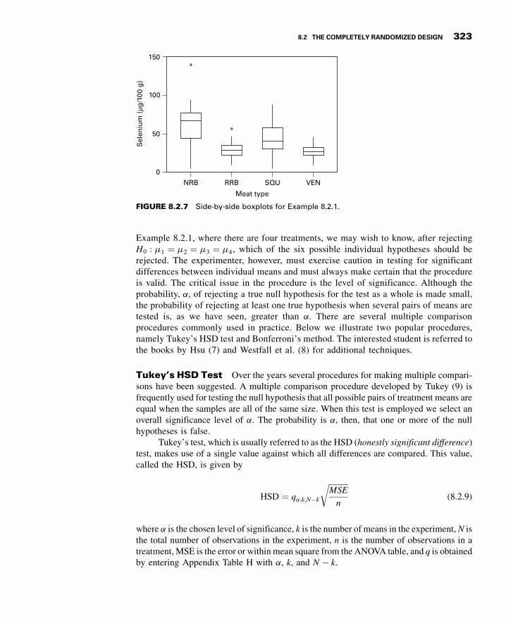
3GC08 12/04/2012 14:43:6 Page 323

Example 8.2.1, where there are four treatments, we may wish to know, after rejectingH0 : m1 ¼ m2 ¼ m3 ¼ m4, which of the six possible individual hypotheses should berejected. The experimenter, however, must exercise caution in testing for significantdifferences between individual means and must always make certain that the procedureis valid. The critical issue in the procedure is the level of significance. Although theprobability, a, of rejecting a true null hypothesis for the test as a whole is made small,the probability of rejecting at least one true hypothesis when several pairs of means aretested is, as we have seen, greater than a. There are several multiple comparisonprocedures commonly used in practice. Below we illustrate two popular procedures,namely Tukey’s HSD test and Bonferroni’s method. The interested student is referred tothe books by Hsu (7) and Westfall et al. (8) for additional techniques.

Tukey’s HSD Test Over the years several procedures for making multiple compari-sons have been suggested. A multiple comparison procedure developed by Tukey (9) isfrequently used for testing the null hypothesis that all possible pairs of treatment means areequal when the samples are all of the same size. When this test is employed we select anoverall significance level of a. The probability is a, then, that one or more of the nullhypotheses is false.

Tukey’s test, which is usually referred to as the HSD (honestly significant difference)test, makes use of a single value against which all differences are compared. This value,called the HSD, is given by

HSD ¼ qa;k;N�k

ffiffiffiffiffiffiffiffiffiffiMSE

n

r(8.2.9)

where a is the chosen level of significance, k is the number of means in the experiment, N isthe total number of observations in the experiment, n is the number of observations in atreatment, MSE is the error or within mean square from the ANOVA table, and q is obtainedby entering Appendix Table H with a, k, and N � k.

NRB

Meat type

Sel

eniu

m (

mg/1

00 g

)

RRB SQU VEN

150

*

*

100

50

0

FIGURE 8.2.7 Side-by-side boxplots for Example 8.2.1.


3GC08 12/04/2012 14:43:7 Page 324

The statistic q, tabulated in Appendix Table H, is known as the studentized rangestatistic. It is defined as the difference between the largest and smallest treatment meansfrom an ANOVA (that is, it is the range of the treatment means) divided by the error meansquare over n, the number of observations in a treatment. The studentized range isdiscussed in detail by Winer (10).

All possible differences between pairs of means are computed, and any differencethat yields an absolute value that exceeds HSD is declared significant.

Tukey’s Test for Unequal Sample Sizes When the samples are not all thesame size, as is the case in Example 8.2.1, Tukey’s HSD test given by Equation 8.2.9 isnot applicable. Tukey himself (9) and Kramer (11), however, have extended the Tukeyprocedure to the case where the sample sizes are different. Their procedure, which issometimes called the Tukey-Kramer method, consists of replacing MSE/n in Equation8.2.9 with MSE=2ð Þ 1=ni þ 1=nj

� �, where ni and nj are the sample sizes of the two groups

to be compared. If we designate the new quantity by HSD�, we have as the newtest criterion

HSD� ¼ qa;k;N�k

ffiffiffiffiffiffiffiffiffiffiffiffiffiffiffiffiffiffiffiffiffiffiffiffiffiffiffiffiffiffiffiMSE

2

1

niþ 1

nj

� �s(8.2.10)

Any absolute value of the difference between two sample means that exceeds HSD�

is declared significant.

Bonferroni’sMethod Another very commonly used multiple comparison testis based on a method developed by C. E. Bonferroni. As with Tukey’s method, wedesire to maintain an overall significance level of a for the total of all pair-wise tests.In the Bonferroni method, we simply divide the desired significance level by thenumber of individual pairs that we are testing. That is, instead of testing at asignificance level of a, we test at a significance level of a=k, where k is the numberof paired comparisons. The sum of all a=k terms cannot, then, possibly exceed ourstated level of a. For example, if one has three samples, A, B, and C, then there arek ¼ 3 pair-wise comparisons. These are mA ¼ mB;mA ¼ mC, and mB ¼ mC. If wechoose a significance level of a ¼ :05, then we would proceed with the comparisonsand use a Bonferroni-corrected significance level of a=3 ¼ :017. Therefore, ourp value must be no greater then :017 in order to reject the null hypothesis andconclude that two means differ.

Most computer packages compute values using the Bonferroni method andproduce an output similar to the Tukey’s HSD or other multiple comparisonprocedures. In general, these outputs report the actual corrected p value using theBonferroni method. Given the basic relationship that p ¼ a=k, then algebraically wecan multiply both sides of the equation by k to obtain a ¼ pk. In other words,the total a is simply the sum of all of the pk values, and the actual corrected p valueis simply the calculated p value multiplied by the number of tests that wereperformed.


3GC08 12/04/2012 14:43:8 Page 325

EXAMPLE 8.2.2

Let us illustrate the use of the HSD test with the data from Example 8.2.1.

Solution: The first step is to prepare a table of all possible (ordered) differencesbetween means. The results of this step for the present example are displayedin Table 8.2.5.

Suppose we let a ¼ :05. Entering Table H with a ¼ :05, k ¼ 4, and N � k ¼ 140, wefind that q < 3:68. The actual value is q ¼ 3:667, which can be obtained from SAS®.In Table 8.2.4 we have MSE ¼ 262:4802.

The hypotheses that can be tested, the value of HSD�, and the statistical decision foreach test are shown in Table 8.2.6.

SAS® uses Tukey’s procedure to test the hypothesis of no difference betweenpopulation means for all possible pair s of sample means. The output also contains

TABLE 8.2.5 Differences Between Sample

Means (Absolute Value) for Example 8.2.2

VEN RRB SQR NRB

VEN – 3.208 17.37 36.171

RRB – 14.163 32.963

SOU – 18.801

NRB –

TABLE 8.2.6 Multiple Comparison Tests Using Data of Example 8.2.1 and HSD�

Hypotheses HSO� Statistical Decision

H0: mVEN ¼ mRRB HSD� ¼ 3:677

ffiffiffiffiffiffiffiffiffiffiffiffiffiffiffiffiffiffiffiffiffiffiffiffiffiffiffiffiffiffiffiffiffiffiffiffiffiffiffiffiffiffiffiffiffi262:4802

2

1

42þ 1

53

� �s¼ 8:68 Do not reject H0

since 3:208 < 8:68

H0: mVEN ¼ mSQU HSD� ¼ 3:677


2

1

42þ 1

30

� �s¼ 10:04 Reject H0 since

17:37 > 10:04

H0: mVEN ¼ mNRB HSD� ¼ 3:677


2

1

42þ 1

19


36:171 > 11:61

H0: mRRB ¼ mSQU HSD� ¼ 3:677


2

1

53þ 1

30


14:163 > 9:60

H0: mRRB ¼ mNRB HSD� ¼ 3:677


2

1

53þ 1

19


32:963 > 11:23

H0: mSQU ¼ mNRB HSD� ¼ 3:677


2

1

30þ 1

19


18:801 > 12:32


3GC08 12/04/2012 14:43:8 Page 326

confidence intervals for the difference between all possible pairs of population means. ThisSAS output for Example 8.2.1 is displayed in Figure 8.2.8.

One may also use SPSS to perform multiple comparisons by a variety of methods,including Tukey’s. The SPSS outputs for Tukey’s HSD and Bonferroni’s method for thedata for Example 8.2.1 are shown in Figures 8.2.9 and 8.2.10, respectively. The outputscontain an exhaustive comparison of sample means, along with the associated standarderrors, p values, and 95% confidence intervals. &

The SAS System


Tukey’s Studentized Range (HSD) Test for selen

NOTE: This test controls the Type I experimentwise error rate.

50.0ahplA041modeerF fo seergeD rorrE2084.262erauqS naeM rorrE

Critical Value of Studentized Range 3.67719

Comparisons significant at the 0.05 level are indicated by ***.

Difference type Between Simultaneous 95%

Comparison Means Confidence Limits

NRB - SQU 18.801 6.449 31.152 ***NRB - RRB 32.963 21.699 44.228 ***NRB - VEN 36.171 24.524 47.818 ***SQU - NRB -18.801 -31.152 -6.449 ***SQU - RRB 14.163 4.538 23.787 ***SQU - VEN 17.370 7.300 27.440 ***RRB - NRB -32.963 -44.228 -21.699 ***RRB - SQU -14.163 -23.787 -4.538 ***RRB - VEN 3.208 -5.495 11.910VEN - NRB -36.171 -47.818 -24.524 ***VEN - SQU -17.370 -27.440 -7.300 ***VEN - RRB -3.208 -11.910 5.495

FIGURE 8.2.8 SAS® multiple comparisons for Example 8.2.1.


3GC08 12/04/2012 14:43:8 Page 327

Multiple Comparisons

Dependent Variable: SeleniumTukey HSD

95% Confidence Interval MeanDifference

Upper BoundLower BoundSig.Std. Error(I–J)(J) Meat_type(I) Meat_type

SQUVEN .0003.87283721017.370190* 7.30020793RRB .7733.3469366283.2075427 5.49501609NRB .0004.47931638236.170840*

27.4401730211.9101014547.81776286 24.52391634

27.440173027.30020793.0003.87283721017.370190*VENSQU23.787370514.53792509.0013.70159372914.162648*RRB

NRB .0014.75016700718.800649* 31.15182638 6.44947187

.7733.3469366283.2075427VENRRB 11.910101455.49501609SQU .0013.70159372914.162648* 23.78737051 4.53792509NRB .0004.33211303332.963297* 44.22746845 21.69912540

47.8177628624.52391634.0004.47931638236.170840*VENNRB31.151826386.44947187.0014.75016700718.800649*SQU44.2274684521.69912540.0004.33211303332.963297*RRB

* The mean difference is significant at the .05 level.

FIGURE 8.2.9 SPSS output for Tukey’s HSD using data from Example 8.2.1.

Multiple Comparisons

Dependent Variable: SeleniumBonferroni

95% Confidence IntervalMeanDifference

Upper BoundLower BoundSig.Std. Error(I–J)(J) Meat_type(I) Meat_type

RRBVEN 1.0003.346943.20754 5.749712.1648SQU .0003.8728417.37019* 27.7349 7.0055NRB .0004.4793236.17084* 48.1587 24.1830

1.0003.346943.20754VENRRB 12.16485.7497SQU .0013.7015914.16265* 24.0691 4.2562NRB .0004.3321132.96330* 44.5572 21.3694

27.73497.0055.0003.8728417.37019*VENSQU24.06914.2562.0013.7015914.16265*RRB

NRB .0014.7501718.80065* 31.5134 6.0879

48.158724.1830.0004.4793236.17084*VENNRB44.557221.3694.0004.3321132.96330*RRB31.51346.0879.0014.7501718.80065*SQU

* The mean difference is significant at the .05 level.

FIGURE 8.2.10 SPSS output for Bonferroni’s method using data from Example 8.2.1.

327

3GC08 12/04/2012 14:43:10 Page 328

EXERCISES

In Exercise 8.2.1 to 8.2.7, go through the ten steps of analysis of variance hypothesis testing to see ifyou can conclude that there is a difference among population means. Let a ¼ :05 for each test. UseTukey’s HSD procedure to test for significant differences among individual pairs of means(if appropriate). Use the same a value for the F test. Construct a dot plot and side-by-side boxplotsof the data.

8.2.1. Researchers at Case Western Reserve University (A-2) wanted to develop and implement atransducer, manageable in a clinical setting, for quantifying isometric moments produced at theelbow joint by individuals with tetraplegia (paralysis or paresis of all four limbs). The apparatus,called an elbow moment transducer (EMT), measures the force the elbow can exert when flexing. Theoutput variable is voltage. The machine was tested at four different elbow extension angles, 30, 60,90, and 120 degrees, on a mock elbow consisting of two hinged aluminum beams. The data are shownin the following table.

Elbow Angle (Degrees)

30 60 90 120

�0.003 1.094 0.000 –0.001 0.000 �0.007 0.558 0.0030.050 1.061 0.053 0.010 0.006 0.012 0.529 0.0620.272 1.040 0.269 0.028 0.026 �0.039 0.524 0.2870.552 1.097 0.555 0.055 0.053 �0.080 0.555 0.5551.116 1.080 1.103 0.105 0.108 �0.118 0.539 1.1182.733 1.051 2.727 0.272 0.278 �0.291 0.536 2.7630.000 1.094 �0.002 0.553 0.555 �0.602 0.557 0.0060.056 1.075 0.052 0.840 0.834 �0.884 0.544 0.0500.275 1.035 0.271 1.100 1.106 �1.176 0.539 0.2770.556 1.096 0.550 1.647 1.650 �1.725 1.109 0.5571.100 1.100 1.097 2.728 2.729 0.003 1.085 1.1132.723 1.096 2.725 �0.001 0.005 0.003 1.070 2.759

�0.003 1.108 0.003 0.014 �0.023 �0.011 1.110 0.0100.055 1.099 0.052 0.027 �0.037 �0.060 1.069 0.0600.273 1.089 0.270 0.057 �0.046 �0.097 1.045 0.2860.553 1.107 0.553 0.111 �0.134 �0.320 1.110 0.5641.100 1.094 1.100 0.276 �0.297 �0.593 1.066 1.1042.713 1.092 2.727 0.555 �0.589 �0.840 1.037 2.7600.007 1.092 0.022 0.832 �0.876 �1.168 2.728 �0.003

�0.066 1.104 �0.075 1.099 �1.157 �1.760 2.694 �0.060�0.258 1.121 �0.298 1.651 �1.755 0.004 2.663 �0.289�0.581 1.106 �0.585 2.736 �2.862 0.566 2.724 �0.585�1.162 1.135 �1.168 0.564 0.000 1.116 2.693 �1.180

0.008 1.143 0.017 0.556 0.245 2.762 2.670 0.000�0.045 1.106 �0.052 0.555 0.497 0.563 2.720 �0.034�0.274 1.135 �0.258 0.567 0.001 0.551 2.688 �0.295�0.604 1.156 �0.548 0.559 0.248 0.551 2.660 �0.579�1.143 1.112 �1.187 0.551 0.498 0.561 0.556 �1.165�0.004 1.104 0.019 1.107 0.001 0.555 0.560 �0.019

(Continued)


3GC08 12/04/2012 14:43:11 Page 329

Elbow Angle (Degrees)

30 60 90 120

�0.050 1.107 �0.044 1.104 0.246 0.558 0.557 �0.056�0.290 1.107 �0.292 1.102 0.491 0.551 0.551 �0.270�0.607 1.104 �0.542 1.112 0.001 0.566 0.564 �0.579�1.164 1.117 �1.189 1.103 0.262 0.560 0.555 �1.162

1.105 1.101 1.104 0.527 1.107 0.5511.103 1.114 0.001 1.104 0.563

1.095 0.260 1.109 0.5591.100 0.523 1.108 1.1132.739 �0.005 1.106 1.1142.721 0.261 1.102 1.1012.687 0.523 1.111 1.1132.732 2.696 1.102 1.1132.702 2.664 1.107 1.0972.660 2.722 2.735 1.1162.743 2.686 2.733 1.1122.687 2.661 2.659 1.0982.656 0.548 2.727 2.7322.733 2.739 0.542 2.7222.731 2.742 0.556 2.734

2.728 2.747

Source: Data provided courtesy of S. A. Snyder, M.S.

8.2.2. Patients suffering from rheumatic diseases or osteoporosis often suffer critical losses in bone mineraldensity (BMD). Alendronate is one medication prescribed to build or prevent further loss of BMD.Holcomb and Rothenberg (A-3) looked at 96 women taking alendronate to determine if a differenceexisted in the mean percent change in BMD among five different primary diagnosis classifications.Group 1 patients were diagnosed with rheumatoid arthritis (RA). Group 2 patients were a mixedcollection of patients with diseases including lupus, Wegener’s granulomatosis and polyarteritis, andother vasculitic diseases (LUPUS). Group 3 patients had polymyalgia rheumatica or temporalarthritis (PMRTA). Group 4 patients had osteoarthritis (OA) and group 5 patients had osteoporosis(O) with no other rheumatic diseases identified in the medical record. Changes in BMD are shown inthe following table.

Diagnosis

RA LUPUS PMRTA OA O

11.091 7.412 2.961 �3.669 11.146 2.93724.414 5.559 0.293 �7.816 �0.838 15.96810.025 4.761 8.394 4.563 4.082 5.349�3.156 �3.527 2.832 �0.093 6.645 1.719

6.835 4.839 �1.369 �0.185 4.329 6.4453.321 1.850 11.288 1.302 1.234 20.2431.493 �3.933 3.997 5.299 �2.817 3.290

(Continued)

EXERCISES 329

3GC08 12/04/2012 14:43:12 Page 330

Diagnosis

RA LUPUS PMRTA OA O

�1.864 9.669 7.260 10.734 3.544 8.9925.386 4.659 5.546 1.399 4.160 6.1203.868 1.137 0.497 1.160 25.6556.209 7.521 0.592 �0.247

�5.640 0.073 3.950 5.3723.514 �8.684 0.674 6.721

�2.308 �0.372 9.354 9.95015.981 21.311 2.610 10.820�9.646 10.831 5.682 7.280

5.188 3.351 6.605�1.892 9.557 7.50716.553 5.075

0.16312.767

3.4810.917

15.853

Source: Data provided courtesy of John P. Holcomb, Ph.D. and Ralph J. Rothenberg, M.D.

8.2.3. Ilich-Ernst et al. (A-4) investigated dietary intake of calcium among a cross section of 113 healthywomen ages 20–88. The researchers formed four age groupings as follows: Group A, 20.0–45.9years; group B, 46.0–55.9 years; group C, 56.0–65.9 years; and group D, over 66 years. Calcium fromfood intake was measured in mg/day. The data below are consistent with summary statistics given inthe paper.

Age Groups (Years) Age Groups (Years)

A B C D A B C D

1820 191 724 1652 1020 7752588 1098 613 1309 805 13932670 644 918 1002 631 5331022 136 949 966 641 7341555 1605 877 788 760 485

222 1247 1368 472 4491197 1529 1692 471 2361249 1422 697 771 8311520 445 849 869 698

489 990 1199 513 1672575 489 429 731 8241426 2408 798 1130 4481846 1064 631 1034 9911088 629 1016 1261 590

912 1025 42 9941383 948 767 1781

(Continued)


3GC08 12/04/2012 14:43:14 Page 331

Age Groups (Years) Age Groups (Years)

A B C D A B C D

1483 1085 752 9371723 775 804 1022

727 1307 1182 10731463 344 1243 9481777 961 985 2221129 239 1295 721

944 1676 3751096 754 1187

8.2.4. Gold et al. (A-5) investigated the effectiveness on smoking cessation of a nicotine patch, bupropionSR, or both, when co-administered with cognitive-behavioral therapy. Consecutive consentingpatients n ¼ 164ð Þ assigned themselves to one of three treatments according to personal preference:nicotine patch NTP; n ¼ 13ð Þ, bupropion SR B; n ¼ 92ð Þ, and bupropion SR plus nicotine patchBNTP; n ¼ 59ð Þ. At their first smoking cessation class, patients estimated the number of packs of

cigarettes they currently smoked per day and the numbers of years they smoked. The “pack years” isthe average number of packs the subject smoked per day multiplied by the number of years the subjecthad smoked. The results are shown in the following table.

Pack Years

NTP B BNTP

15 8 60 90 8 8017 10 60 90 15 8018 15 60 90 25 8220 20 60 95 25 8620 22 60 96 25 8720 24 60 98 26 9030 25 60 98 30 9037 26 66 99 34 9043 27 66 100 35 9048 29 67 100 36 9060 30 68 100 40 95

100 30 68 100 45 99100 35 70 100 45 100

35 70 100 45 10239 70 105 45 10540 75 110 48 10540 75 110 48 10540 75 120 49 11140 75 120 52 11340 76 123 60 12040 80 125 60 12045 80 125 60 12545 80 126 64 125

(Continued)

EXERCISES 331

3GC08 12/04/2012 14:43:14 Page 332

Pack Years

NTP B BNTP

45 80 130 64 12950 80 130 70 13051 80 132 70 13352 80 132 70 13555 84 142 75 14058 84 157 75 15460 84 180 7660 90

Source: Data provided courtesy of Paul B. Gold, Ph.D.

8.2.5. In a study by Wang et al. (A-6), researchers examined bone strength. They collected 10 cadavericfemurs from subjects in three age groups: young (19–49 years), middle-aged (50–69 years), andelderly (70 years or older) [Note: one value was missing in the middle-aged group]. One of theoutcome measures (W) was the force in Newtons required to fracture the bone. The following tableshows the data for the three age groups.

Young (Y) Middle-aged (MA) Elderly (E)

193.6 125.4 59.0137.5 126.5 87.2122.0 115.9 84.4145.4 98.8 78.1117.0 94.3 51.9105.4 99.9 57.1

99.9 83.3 54.774.0 72.8 78.674.4 83.5 53.7

112.8 96.0

Source: Data provided courtesy of Xiaodu Wang, Ph.D.

8.2.6. In a study of 90 patients on renal dialysis, Farhad Atassi (A-7) assessed oral home care practices. Hecollected data from 30 subjects who were in (1) dialysis for less than 1 year, (2) dialysis for 1 to 3years, and (3) dialysis for more than 3 years. The following table shows plaque index scores for thesesubjects. A higher score indicates a greater amount of plaque.

Group 1 Group 2 Group 3

2.00 2.67 2.83 2.83 1.83 1.831.00 2.17 2.00 1.83 2.00 2.672.00 1.00 2.67 2.00 1.83 1.331.50 2.00 2.00 1.83 1.83 2.172.00 2.00 2.83 2.00 2.83 3.001.00 2.00 2.17 2.17 2.17 2.33

(Continued)


3GC08 12/04/2012 14:43:16 Page 333

Group 1 Group 2 Group 3

1.00 2.33 2.17 1.67 2.83 2.501.00 1.50 2.00 2.33 2.50 2.831.00 1.00 2.00 2.00 2.17 2.831.67 2.00 1.67 2.00 1.67 2.331.83 .83 2.33 2.17 2.17 2.332.17 .50 2.00 3.00 1.83 2.671.00 2.17 1.83 2.50 2.83 2.002.17 2.33 1.67 2.17 2.33 2.002.83 2.83 2.17 2.00 2.00 2.00

Source: Data provided courtesy of Farhad Atassi, DDS, MSC, FICOI.

8.2.7. Thrombocytopaenia is a condition of abnormally low platelets that often occurs during necrotizingenterocolitis (NEC)—a serious illness in infants that can cause tissue damage to the intestines.Ragazzi et al. (A-8) investigated differences in the log10 of platelet counts in 178 infants with NEC.Patients were grouped into four categories of NEC status. Group 0 referred to infants with nogangrene, group 1 referred to subjects in whom gangrene was limited to a single intestinal segment,group 2 referred to patients with two or more intestinal segments of gangrene, and group 3 referred topatients with the majority of small and large bowel involved. The following table gives the log10

platelet counts for these subjects.

Gangrene Grouping

0 1 2 3

1.97 2.33 2.48 1.38 2.45 1.87 2.37 1.770.85 2.60 2.23 1.86 2.60 1.90 1.75 1.681.79 1.88 2.51 2.26 1.83 2.43 2.57 1.462.30 2.33 2.38 1.99 2.47 1.32 1.51 1.531.71 2.48 2.31 1.32 1.92 2.06 1.08 1.362.66 2.15 2.08 2.11 2.51 1.04 2.36 1.652.49 1.41 2.49 2.54 1.79 1.99 1.58 2.122.37 2.03 2.21 2.06 2.17 1.52 1.83 1.731.81 2.59 2.45 2.41 2.18 1.99 2.55 1.912.51 2.23 1.96 2.23 2.53 2.52 1.80 1.572.38 1.61 2.29 2.00 1.98 1.93 2.44 2.272.58 1.86 2.54 2.74 1.93 2.29 2.81 1.002.58 2.33 2.23 2.00 2.42 1.75 2.17 1.812.84 2.34 2.78 2.51 0.79 2.16 2.72 2.272.55 1.38 2.36 2.08 1.38 1.81 2.44 2.431.90 2.52 1.89 2.46 1.98 1.742.28 2.35 2.26 1.66 1.57 1.602.33 2.63 1.79 2.51 2.05 2.081.77 2.03 1.87 1.76 2.30 2.341.83 1.08 2.51 1.72 1.36 1.891.67 2.40 2.29 2.57 2.48 1.752.67 1.77 2.38 2.30 1.40 1.69

(Continued)

EXERCISES 333

3GC08 12/04/2012 14:43:16 Page 334

Gangrene Grouping

0 1 2 3

1.80 0.70 1.75 2.492.16 2.67 1.752.17 2.37 1.862.12 1.46 1.262.27 1.91 2.36

Source: Data provided courtesy of Simon Eaton, M.D.

8.2.8. The objective of a study by Romita et al. (A-9) was to determine whether there is a different responseto different calcium channel blockers. Two hundred and fifty patients with mild-to-moderate hypertension were randomly assigned to 4 weeks of treatment with once-daily dosesof (1) lercanidipine, (2) felodipine, or (3) nifedipine. Prior to treatment and at the end of 4 weeks, eachof the subjects had his or her systolic blood pressure measured. Researchers then calculated thechange in systolic blood pressure. What is the treatment variable in this study? The response variable?What extraneous variables can you think of whose effects would be included in the error term? Whatare the “values” of the treatment variable? Construct an analysis of variance table in which youspecify for this study the sources of variation and the degrees of freedom.

8.2.9. Kosmiski et al. (A-10) conducted a study to examine body fat distributions of men infected and notinfected with HIV, taking and not taking protease inhibitors (PI), and having been diagnosed and notdiagnosed with lipodystrophy. Lipodystrophy is a syndrome associated with HIV/PI treatment thatremains controversial. Generally, it refers to fat accumulation in the abdomen or viscera accompaniedby insulin resistance, glucose intolerance, and dyslipidemia. In the study, 14 subjects were takingprotease inhibitors and were diagnosed with lipodystrophy, 12 were taking protease inhibitors, butwere not diagnosed with lipodystrophy, five were HIV positive, not taking protease inhibitors, norhad diagnosed lypodystrophy, and 43 subjects were HIV negative and not diagnosed with lipodys-trophy. Each of the subjects underwent body composition and fat distribution analyses by dual-energyX-ray absorptiometry and computed tomography. Researchers were able to then examine the percentof body fat in the trunk. What is the treatment variable? The response variable? What are the “values”of the treatment variable? Who are the subjects? What extraneous variables can you think of whoseeffects would be included in the error term? What was the purpose of including HIV-negative men inthe study? Construct an ANOVA table in which you specify the sources of variation and the degrees offreedom for each. The authors reported a computed V.R. of 11.79. What is the p value for the test?

8.3 THE RANDOMIZED COMPLETEBLOCKDESIGN

The randomized complete block design was developed about 1925 by R. A. Fisher, who wasseeking methods of improving agricultural field experiments. The randomized completeblock design is a design in which the units (called experimental units) to which thetreatments are applied are subdivided into homogeneous groups called blocks, so thatthe number of experimental units in a block is equal to the number (or some multiple of thenumber) of treatments being studied. The treatments are then assigned at random to theexperimental units within each block. It should be emphasized that each treatment appearsin every block, and each block receives every treatment.


3GC08 12/04/2012 14:43:16 Page 335

Objective The objective in using the randomized complete block design is to isolateand remove from the error term the variation attributable to the blocks, while assuring thattreatment means will be free of block effects. The effectiveness of the design depends on theability to achieve homogeneous blocks of experimental units. The ability to form homoge-neous blocks depends on the researcher’s knowledge of the experimental material. Whenblocking is used effectively, the error mean square in the ANOVA table will be reduced, theV.R. will be increased, and the chance of rejecting the null hypothesis will be improved.

In animal experiments, the breed of animal may be used as a blocking factor. Littersmay also be used as blocks, in which case an animal from each litter receives a treatment. Inexperiments involving human beings, if it is desired that differences resulting from age beeliminated, then subjects may be grouped according to age so that one person of each agereceives each treatment. The randomized complete block design also may be employedeffectively when an experiment must be carried out in more than one laboratory (block) orwhen several days (blocks) are required for completion.

The random allocation of treatments to subjects is restricted in the randomizedcomplete block design. That is, each treatment must be represented an equal number oftimes (one or more times) within each blocking unit. In practice this is generallyaccomplished by assigning a random permutation of the order of treatments to subjectswithin each block. For example, if there are four treatments representing three drugs and aplacebo (drug A, drug B, drug C, and placebo [P]), then there are 4! ¼ 24 possiblepermutations of the four treatments: (A, B, C, P) or (A, C, B, P) or (C, A, P, B), and so on.One permutation is then randomly assigned to each block.

Advantages One of the advantages of the randomized complete block design is thatit is easily understood. Furthermore, certain complications that may arise in the course ofan experiment are easily handled when this design is employed.

It is instructive here to point out that the paired comparisons analysis presented inChapter 7 is a special case of the randomized complete block design. Example 7.4.1, forexample, may be treated as a randomized complete block design in which the two points intime (Pre-op and Post-op) are the treatments and the individuals on whom the measure-ments were taken are the blocks.

Data Display In general, the data from an experiment utilizing the randomizedcomplete block design may be displayed in a table such as Table 8.3.1. The following newnotation in this table should be observed:

total of the ith block ¼ Ti: ¼Xkj¼1

xij

mean of the ith block ¼ �xi: ¼

Xkj¼1

xij

k¼ Ti:

k

grand total ¼ T :: ¼Xkj¼1

T �j ¼Xni¼1

Ti�

8.3 THE RANDOMIZED COMPLETE BLOCK DESIGN 335

3GC08 12/04/2012 14:43:17 Page 336

indicating that the grand total may be obtained either by adding row totals or by addingcolumn totals.

Two-Way ANOVA The technique for analyzing the data from a randomizedcomplete block design is called two-way analysis of variance since an observation iscategorized on the basis of two criteria—the block to which it belongs as well as thetreatment group to which it belongs.

The steps for hypothesis testing when the randomized complete block design is usedare as follows:

1. Data. After identifying the treatments, the blocks, and the experimental units, thedata, for convenience, may be displayed as in Table 8.3.1.

2. Assumptions. The model for the randomized complete block design and itsunderlying assumptions are as follows:

The Model

xij ¼ mþ bi þ tj þ eij

i ¼ 1; 2; . . . ; n; j ¼ 1; 2; . . . ; k(8.3.1)

In this model

xij is a typical value from the overall population.

m is an unknown constant.

bi represents a block effect reflecting the fact that the experimental unit fell in the ithblock.

tj represents a treatment effect, reflecting the fact that the experimental unit receivedthe jth treatment.

eij is a residual component representing all sources of variation other than treatmentsand blocks.

TABLE 8.3.1 Table of Sample Values for the Randomized

Complete Block Design

Treatments

Blocks 1 2 3 . . . k Total Mean

1 x11 x12 x13 . . . x1k T 1: �x1:

2 x21 x22 x23 . . . x2k T 2: �x2:

3 x31 x32 x33 . . . x3k T 3: �x3:

..

. ... ..

. ...

..

. ... ..

. ...

n xn1 xn2 xn3 . . . xnk Tn� �xn�

Total T :1 T :2 T :3 . . . T �k T ::

Mean �x :1 �x :2 �x :3 . . . �x �k �x ::


3GC08 12/04/2012 14:43:17 Page 337

Assumptions of the Model

(a) Each xij that is observed constitutes a random independent sample of size 1 from oneof the kn populations represented.

(b) Each of these kn populations is normally distributed with mean mij and the samevariance s2. This implies that the eij are independently and normally distributed withmean 0 and variance s2.

(c) The block and treatment effects are additive. This assumption may be interpreted tomean that there is no interaction between treatments and blocks. In other words, aparticular block-treatment combination does not produce an effect that is greater orless than the sum of their individual effects. It can be shown that when thisassumption is met,

Xkj¼1

tj ¼Xni¼1

bi ¼ 0

The consequences of a violation of this assumption are misleading results. One neednot become concerned with the violation of the additivity assumption unless thelargest mean is more than 50 percent greater than the smallest.

When these assumptions hold true, the tj and bi are a set of fixed constants, and we have asituation that fits the fixed-effects model.

3. Hypotheses. We may test

H0 : tj ¼ 0; j ¼ 1; 2; . . . ; k

against the alternative

HA : not all tj ¼ 0

A hypothesis test regarding block effects is not usually carried out under theassumptions of the fixed-effects model for two reasons. First, the primary interest is intreatment effects, the usual purpose of the blocks being to provide a means of eliminatingan extraneous source of variation. Second, although the experimental units are randomlyassigned to the treatments, the blocks are obtained in a nonrandom manner.

4. Test statistic. The test statistic is V.R.

5. Distribution of test statistic. When H0 is true and the assumptions are met, V.R.follows an F distribution.

6. Decision rule. Reject the null hypothesis if the computed value of the test statisticV.R. is equal to or greater than the critical value of F.

7. Calculation of test statistic. It can be shown that the total sum of squares for therandomized complete block design can be partitioned into three components, oneeach attributable to blocks (SSBl), treatments (SSTr), and error (SSE). That is,

SST ¼ SSBlþ SSTr þ SSE (8.3.2)


3GC08 12/04/2012 14:43:18 Page 338

The formulas for the quantities in Equation 8.3.2 are as follows:

SST ¼Xkj¼1

Xni¼1

xij � �x::� �2

(8.3.3)

SSBl ¼Xkj¼1

Xni¼1

�xi� � �x::ð Þ2 (8.3.4)

SSTr ¼Xkj¼1

Xni¼1

�x�j � �x::� �2

(8.3.5)

SSE ¼ SST � SSBl� SSTr (8.3.6)

The appropriate degrees of freedom for each component of Equation 8.3.2 are

total blocks treatments residual errorð Þkn� 1 ¼ n� 1ð Þ þ k � 1ð Þ þ n� 1ð Þ k � 1ð Þ

The residual degrees of freedom, like the residual sum of squares, may be obtainedby subtraction as follows:

kn� 1ð Þ � n� 1ð Þ � k � 1ð Þ ¼ kn� 1 � nþ 1 � k þ 1¼ n k � 1ð Þ � 1 k � 1ð Þ ¼ n� 1ð Þ k � 1ð Þ

The ANOVA Table The results of the calculations for the randomized completeblock design may be displayed in an ANOVA table such as Table 8.3.2.

8. Statistical decision. It can be shown that when the fixed-effects model applies andthe null hypothesis of no treatment effects all ti ¼ 0ð Þ is true, both the error, orresidual, mean square and the treatments mean square are estimates of the commonvariance s2. When the null hypothesis is true, therefore, the quantity

MSTr=MSE

is distributed as F with k � 1 numerator degrees of freedom and n� 1ð Þ � k � 1ð Þdenominator degrees of freedom. The computed variance ratio, therefore, is com-pared with the critical value of F.

TABLE 8.3.2 ANOVA Table for the Randomized Complete Block Design

Source SS d.f. MS V.R.

Treatments SSTr k � 1ð Þ MSTr ¼ SSTr= k � 1ð Þ MSTr/MSE

Blocks SSBl n � 1ð Þ MSBl ¼ SSBl= n � 1ð ÞResidual SSE n � 1ð Þ k � 1ð Þ MSE ¼ SSE= n � 1ð Þ k � 1ð Þ

Total SST kn � 1


3GC08 12/04/2012 14:43:19 Page 339

9. Conclusion. If we reject H0, we conclude that the alternative hypothesis is true. Ifwe fail to reject H0, we conclude that H0 may be true.

10. p value.

The following example illustrates the use of the randomized complete blockdesign.

EXAMPLE 8.3.1

A physical therapist wished to compare three methods for teaching patients to use a certainprosthetic device. He felt that the rate of learning would be different for patients of differentages and wished to design an experiment in which the influence of age could be taken intoaccount.

Solution: The randomized complete block design is the appropriate design for thisphysical therapist.

1. Data. Three patients in each of five age groups were selected toparticipate in the experiment, and one patient in each age group wasrandomly assigned to each of the teaching methods. The methods ofinstruction constitute our three treatments, and the five age groups arethe blocks. The data shown in Table 8.3.3 were obtained.

2. Assumptions. We assume that each of the 15 observations constitutes asimple random sample of size 1 from one of the 15 populations definedby a block-treatment combination. For example, we assume that thenumber 7 in the table constitute s a randomly selected response from apopulation of responses that would result if a population of subjectsunder the age of 20 received teaching method A. We assume that theresponses in the 15 represented populations are normally distributedwith equal variances.

TABLE 8.3.3 Time (in Days) Required to Learn the Use

of a Certain Prosthetic Device

Teaching Method

Age Group A B C Total Mean

Under 20 7 9 10 26 8.67

20 to 29 8 9 10 27 9.00

30 to 39 9 9 12 30 10.00

40 to 49 10 9 12 31 10.33

50 and over 11 12 14 37 12.33

Total 45 48 58 151

Mean 9.0 9.6 11.6 10.07


3GC08 12/04/2012 14:43:19 Page 340

3. Hypotheses.

H0 : tj ¼ 0 j ¼ 1; 2; 3HA : not all tj ¼ 0

4. Test statistic. The test statistic is V:R: ¼ MSTr=MSE.

5. Distribution of test statistic. When H0 is true and the assumptions aremet, V.R. follows an F distribution with 2 and 8 degrees of freedom.

6. Decision rule. Let a ¼ :05. Reject the null hypothesis if the computedV.R. is equal to or greater than the critical F, which we find in AppendixTable G to be 4.46.

7. Calculation of test statistic. We compute the following sums ofsquares:

SST ¼ ð7 � 10:07Þ2 þ ð8 � 10:07Þ2 þ � � � þ ð14 � 10:07Þ2 ¼ 46:9335

SSBI ¼ 3½ð8:67 � 10:07Þ2 þ ð9:00 � 10:07Þ2 þ � � � þ ð12:33 � 10:07Þ2� ¼ 24:855

SSTr ¼ 5½ð9 � 10:07Þ2 þ ð9:6 � 10:07Þ2 þ ð11:6 � 10:07Þ2� ¼ 18:5335

SSE ¼ 46:9335 � 24:855 � 18:5335 ¼ 3:545

The degrees of freedom are total ¼ ð3Þð5Þ � 1 ¼ 14, blocks ¼5 � 1 ¼ 4, treatments ¼ 3 � 1 ¼ 2, and residual ¼ ð5 � 1Þð3 � 1Þ ¼8. The results of the calculations may be displayed in an ANOVA tableas in Table 8.3.4

8. Statistical decision. Since our computed variance ratio, 20.91, isgreater than 4.46, we reject the null hypothesis of no treatment effectson the assumption that such a large V.R. reflects the fact that the twosample mean squares are not estimating the same quantity. The onlyother explanation for this large V.R. would be that the null hypothesis isreally true, and we have just observed an unusual set of results. We ruleout the second explanation in favor of the first.

TABLE 8.3.4 ANOVA Table for Example 8.3.1


Treatments 18.5335 2 9.26675 20.91

Blocks 24.855 4 6.21375

Residual 3.545 8 .443125

Total 46.9335 14


3GC08 12/04/2012 14:43:19 Page 341

9. Conclusion. We conclude that not all treatment effects are equal to zero,or equivalently, that not all treatment means are equal.

10. p value. For this test p < :005. &

Computer Analysis Most statistical software packages will analyze data from arandomized complete block design. We illustrate the input and output for MINITAB. Weuse the data from the experiment to set up a MINITAB worksheet consisting of threecolumns. Column 1 contains the observations, Column 2 contains numbers that identify theblock to which each observation belongs, and Column 3 contains numbers that identify thetreatment to which each observation belongs. Figure 8.3.1 shows the MINITAB worksheetfor Example 8.3.1. Figure 8.3.2 contains the MINITAB dialog box that initiates the analysisand the resulting ANOVA table.

The ANOVA table from the SAS® output for the analysis of Example 8.3.1 isshown in Figure 8.3.3 . Note that in this output the model SS is equal to the sum of SSBland SSTr.

Alternatives When the data available for analysis do not meet the assumptions ofthe randomized complete block design as discussed here, the Friedman procedurediscussed in Chapter 13 may prove to be a suitable nonparametric alternative.

ROW C1 C2 C3

1171

2192

3 10 1 3

1284

2295

6 10 2 3

1397

2398

9 12 3 3

10 10 4 1

24911

12 12 4 3

13 11 5 1

14 12 5 2

15 14 5 3

FIGURE 8.3.1 MINITAB worksheet for the data in Figure 8.3.2.


3GC08 12/04/2012 14:43:19 Page 342

EXERCISES

For Exercise 8.3.1 to 8.3.5 perform the ten-step hypothesis testing procedure for analysis of variance.

8.3.1. The objective of a study by Brooks et al. (A-11) was to evaluate the efficacy of using a virtualkitchen for vocational training of people with learning disabilities. Twenty-four students participated


Stat ANOVA Twoway MTB > TWOWAY C1 C2 C3;SUBC > MEANS C2 C3.

Type C1 in Response. Type C2 in Row factor andcheck Display means. Type C3 in Column factor andcheck Display means. Click OK.

Output:

Two-Way ANOVA: C1 versus C2, C3

Analysis of Variance for C1Source DF SS MS F PC2 4 24.933 6.233 14.38 0.001C3 2 18.533 9.267 21.38 0.001Error 8 3.467 0.433Total 14 46.933

Individual 95% CIC2 Mean ---+---------+----------+---------+--1 8.67 (-----*-----)2 9.00 (-----*-----)

-----(00.013 *-----)-----(33.014 *-----)

-----(33.215 *-----)---+---------+----------+---------+--9.00 10.50 12.00 13.50

Individual 95% CIC3 Mean ---+---------+----------+---------+--1 9.00 (-----*-----)2 9.60 (-----*-----)

----(06.113 *----)---+---------+----------+---------+--9.00 10.00 11.00 12.00

FIGURE8.3.2 MINITAB dialog box and output for two-way analysis of variance, Example 8.3.1.


3GC08 12/04/2012 14:43:20 Page 343

in the study. Each participant performed four food preparation tasks and they were scored on thequality of the preparation. Then each participant received regular vocational training in foodpreparation (real training), virtual training using a TV and computer screen of a typical kitchen,workbook training with specialized reading materials, and no training (to serve as a control). Aftereach of these trainings, the subjects were tested on food preparation. Improvement scores for each ofthe four training methods are shown in the following table.

SubjectNo.

RealTraining

VirtualTraining

WorkbookTraining

NoTraining

1 2 10 2 �42 4 3 2 13 4 13 0 14 6 11 2 15 5 13 5 16 2 0 1 47 10 17 2 68 5 5 2 29 10 4 5 2

10 3 6 9 311 11 9 8 712 10 9 6 1013 5 8 4 1

The SAS System


Dependent Variable: DAYS

Source DF Sum of Squares Mean Square F Value Pr > F

4000.027.6144444442.776666664.346ledoM

33333334.076666664.38rorrE

Corrected Total 14 46.93333333

R-Square C.V. Root MSE DAYS Mean

0.926136 6.539211 0.65828059 10.06666667

Source DF Anova SS Mean Square F Value Pr > F

6000.083.1276666662.933333335.812PUORG0100.083.4133333332.633333339.424EGA

FIGURE 8.3.3 Partial SAS® output for analysis of Example 8.3.1.

(Continued)

EXERCISES 343

3GC08 12/04/2012 14:43:20 Page 344

SubjectNo.

RealTraining

VirtualTraining

WorkbookTraining

NoTraining

14 8 11 1 115 4 8 5 216 11 8 10 217 6 11 1 318 2 5 1 219 3 1 0 �320 7 5 0 �621 7 10 4 422 8 7 �2 823 4 9 3 024 9 6 3 5

Source: Data provided courtesy of B. M. Brooks, Ph.D.

After eliminating subject effects, can we conclude that the improvement scores differ among methodsof training? Let a ¼ :05.

8.3.2. McConville et al. (A-12) report the effects of chewing one piece of nicotine gum (containing 2 mgnicotine) on tic frequency in patients whose Tourette’s disorder was inadequately controlled byhaloperidol. The following are the tic frequencies under four conditions:

Number of Tics During 30-Minute Period

After End of Chewing

Patient BaselineGum

Chewing0–30

Minutes30–60

Minutes

1 249 108 93 592 1095 593 600 8613 83 27 32 614 569 363 342 3125 368 141 167 1806 326 134 144 1587 324 126 312 2608 95 41 63 719 413 365 282 321

10 332 293 525 455

Source: Data provided courtesy of Brian J. McConville, M. Harold Fogelson,Andrew B. Norman, William M. Klykylo, Pat Z. Manderscheid, Karen W.Parker, and Paul R. Sanberg. “Nicotine Potentiation of Haloperidol inReducing Tic Frequency in Tourette’s Disorder,” American Journal ofPsychiatry, 148 (1991), 793–794. Copyright # 1991, American PsychiatricAssociation.

After eliminating patient effects, can we conclude that the mean number of tics differs among the fourconditions? Let a ¼ :01.

8.3.3. A remotivation team in a psychiatric hospital conducted an experiment to compare five methods forremotivating patients. Patients were grouped according to level of initial motivation. Patients in each


3GC08 12/04/2012 14:43:21 Page 345

group were randomly assigned to the five methods. At the end of the experimental period the patientswere evaluated by a team composed of a psychiatrist, a psychologist, a nurse, and a social worker,none of whom was aware of the method to which patients had been assigned. The team assigned eachpatient a composite score as a measure of his or her level of motivation. The results were as follows:

Level of InitialMotivation

Remotivation Method

A B C D E

Nil 58 68 60 68 64Very low 62 70 65 80 69Low 67 78 68 81 70Average 70 81 70 89 74

Do these data provide sufficient evidence to indicate a difference in mean scores among methods? Leta ¼ :05.

8.3.4. The nursing supervisor in a local health department wished to study the influence of time of day onlength of home visits by the nursing staff. It was thought that individual differences among nursesmight be large, so the nurse was used as a blocking factor. The nursing supervisor collected thefollowing data:

Length of Home Visit by Time of Day

NurseEarly

MorningLate

MorningEarly

AfternoonLate

Afternoon

A 27 28 30 23B 31 30 27 20C 35 38 34 30D 20 18 20 14

Do these data provide sufficient evidence to indicate a difference in length of home visit among thedifferent times of day? Let a ¼ :05.

8.3.5. Four subjects participated in an experiment to compare three methods of relieving stress. Eachsubject was placed in a stressful situation on three different occasions. Each time a different methodfor reducing stress was used with the subject. The response variable is the amount of decrease in stresslevel as measured before and after treatment application. The results were as follows:

Treatment

Subject A B C

1 16 26 222 16 20 233 17 21 224 28 29 36

Can we conclude from these data that the three methods differ in effectiveness? Let a ¼ :05.

EXERCISES 345

3GC08 12/04/2012 14:43:21 Page 346

8.3.6. In a study by Valencia et al. (A-13), the effects of environmental temperature and humidity on24-hour energy expenditure were measured using whole-body indirect calorimetry in eight normal-weight young men who wore standardized light clothing and followed a controlled activity regimen.Temperature effects were assessed by measurements at 20, 23, 26, and 30 degrees Celsius at ambienthumidity and at 20 and 30 degrees Celsius with high humidity. What is the blocking variable? Thetreatment variable? How many blocks are there? How many treatments? Construct an ANOVA tablein which you specify the sources of variability and the degrees of freedom for each. What are theexperimental units? What extraneous variables can you think of whose effects would be included inthe error term?

8.3.7. Hodgson et al. (A-14) conducted a study in which they induced gastric dilatation in sixanesthetized dogs maintained with constant-dose isoflurane in oxygen. Cardiopulmonary mea-surements prior to stomach distension (baseline) were compared with measurements takenduring .1, .5, 1.0, 1.5, 2.5, and 3.5 hours of stomach distension by analyzing the change frombaseline. After distending the stomach, cardiac index increased from 1.5 to 3.5 hours. Strokevolume did not change. During inflation, increases were observed in systemic arterial, pulmonaryarterial, and right atrial pressure. Respiratory frequency was unchanged. PaO2 tended to decreaseduring gastric dilatation. What are the experimental units? The blocks? Treatment variable?Response variable(s)? Can you think of any extraneous variable whose effect would contribute tothe error term? Construct an ANOVA table for this study in which you identify the sources ofvariability and specify the degrees of freedom.

8.4 THE REPEATEDMEASURES DESIGN

One of the most frequently used experimental designs in the health sciences field is therepeated measures design.

DEFINITION

A repeated measures design is one in which measurements of the samevariable are made on each subject on two or more different occasions.

The different occasions during which measurements are taken may be either points intime or different conditions such as different treatments.

When to Use Repeated Measures The usual motivation for using arepeated measures design is a desire to control for variability among subjects. Insuch a design each subject serves as its own control. When measurements are takenon only two occasions, we have the paired comparisons design that we discussed inChapter 7. One of the most frequently encountered situations in which the repeatedmeasures design is used is the situation in which the investigator is concerned withresponses over time.

Advantages The major advantage of the repeated measures design is, as previouslymentioned, its ability to control for extraneous variation among subjects. An additionaladvantage is the fact that fewer subjects are needed for the repeated measures design than


3GC08 12/04/2012 14:43:21 Page 347

for a design in which different subjects are used for each occasion on which measurementsare made. Suppose, for example, that we have four treatments (in the usual sense) or fourpoints in time on each of which we would like to have 10 measurements. If a differentsample of subjects is used for each of the four treatments or points in time, 40 subjectswould be required. If we are able to take measurements on the same subject for eachtreatment or point in time—that is, if we can use a repeated measures design—only 10subjects would be required. This can be a very attractive advantage if subjects are scarce orexpensive to recruit.

Disadvantages A major potential problem to be on the alert for is what is known asthe carry-over effect. When two or more treatments are being evaluated, the investigatorshould make sure that a subject’s response to one treatment does not reflect a residual effectfrom previous treatments. This problem can frequently be solved by allowing a sufficientlength of time between treatments.

Another possible problem is the position effect. A subject’s response to a treatmentexperienced last in a sequence may be different from the response that would have occurredif the treatment had been first in the sequence. In certain studies, such as those involvingphysical participation on the part of the subjects, enthusiasm that is high at the beginning ofthe study may give way to boredom toward the end. A way around this problem is torandomize the sequence of treatments independently for each subject.

Single-Factor Repeated Measures Design The simplest repeated mea-sures design is the one in which, in addition to the treatment variable, one additionalvariable is considered. The reason for introducing this additional variable is to measure andisolate its contribution to the total variability among the observations. We refer to thisadditional variable as a factor.

DEFINITION

The repeated measures design in which one additional factor is introducedinto the experiment is called a single-factor repeated measures design.

We refer to the additional factor as subjects. In the single-factor repeated measuresdesign, each subject receives each of the treatments. The order in which the subjects areexposed to the treatments, when possible, is random, and the randomization is carried outindependently for each subject.

Assumptions The following are the assumptions of the single-factor repeatedmeasures design that we consider in this text. A design in which these assumptions are metis called a fixed-effects additive design.

1. The subjects under study constitute a simple random sample from a population ofsimilar subjects.

2. Each observation is an independent simple random sample of size 1 from each of knpopulations, where n is the number of subjects and k is the number of treatments towhich each subject is exposed.

8.4 THE REPEATED MEASURES DESIGN 347

3GC08 12/04/2012 14:43:22 Page 348

3. The kn populations have potentially different means, but they all have the samevariance.

4. The k treatments are fixed; that is, they are the only treatments about which we havean interest in the current situation. We do not wish to make inferences to some largercollection of treatments.

5. There is no interaction between treatments and subjects; that is, the treatment andsubject effects are additive.

Experimenters may find frequently that their data do not conform to the assumptionsof fixed treatments and/or additive treatment and subject effects. For such cases thereferences at the end of this chapter may be consulted for guidance.

In addition to the assumptions just listed, it should be noted that in a repeated-measures experiment there is a presumption that correlations should exist among therepeated measures. That is, measurements at time 1 and 2 are likely correlated, asare measurements at time 1 and 3, 2 and 3, and so on. This is expected because themeasurements are taken on the same individuals through time.

An underlying assumption of the repeated-measures ANOVA design is that all ofthese correlations are the same, a condition referred to as compound symmetry. Thisassumption, coupled with assumption 3 concerning equal variances, is referred to assphericity. Violations of the sphericity assumption can result in an inflated type I error.Most computer programs provide a formal test for the sphericity assumption along withalternative estimation methods if the sphericity assumption is violated.

The Model The model for the fixed-effects additive single-factor repeated measuresdesign is


i ¼ 1; 2; . . . ; n; j ¼ 1; 2; . . . ; k(8.4.1)

The reader will recognize this model as the model for the randomized complete blockdesign discussed in Section 8.3. The subjects are the blocks. Consequently, the notation,data display, and hypothesis testing procedure are the same as for the randomized completeblock design as presented earlier. The following is an example of a repeated measuresdesign.

EXAMPLE 8.4.1

Licciardone et al. (A-15) examined subjects with chronic, nonspecific low back pain. Inthis study, 18 of the subjects completed a survey questionnaire assessing physicalfunctioning at baseline, and after 1, 3, and 6 months. Table 8.4.1 shows the data forthese subjects who received a sham treatment that appeared to be genuine osteopathicmanipulation. Higher values indicate better physical functioning. The goal of the experi-ment was to determine if subjects would report improvement over time even though thetreatment they received would provide minimal improvement. We wish to know if there is adifference in the mean survey values among the four points in time.


3GC08 12/04/2012 14:43:22 Page 349

Solution:

1. Data. See Table 8.4.1.

2. Assumptions. We assume that the assumptions for the fixed-effects,additive single-factor repeated measures design are met.

3. Hypotheses.

H0: mB ¼ mM1 ¼ mM3 ¼ mM6

HA: not allm’s are equal

4. Test statistic. V:R: ¼ treatment MS=error MS.

5. Distribution of test statistic. F with 4 � 1 ¼ 3 numerator degrees offreedom and 71 � 3 � 17 ¼ 51 denominator degrees of freedom.

6. Decision rule. Let a ¼ :05. The critical value of F is 2.80 (obtainedby interpolation). Reject H0 if computed V.R. is equal to or greaterthan 2.80.

7. Calculation of test statistic. We use MINITAB to perform thecalculations. We first enter the measurements in Column 1, the row(subject) codes in Column 2, the treatment (time period) codes inColumn 3, and proceed as shown in Figure 8.4.1.

TABLE 8.4.1 SF-36 Health Scores at Four Different

Points in Time

Subject Baseline Month 1 Month 3 Month 6

1 80 60 95 100

2 95 90 95 95

3 65 55 50 45

4 50 45 70 70

5 60 75 80 85

6 70 70 75 70

7 80 80 85 80

8 70 60 75 65

9 80 80 70 65

10 65 30 45 60

11 60 70 95 80

12 50 50 70 60

13 50 65 80 65

14 85 45 85 80

15 50 65 90 70

16 15 30 20 25

17 10 15 55 75

18 80 85 90 70

Source: Data provided courtesy of John C. Licciardone.


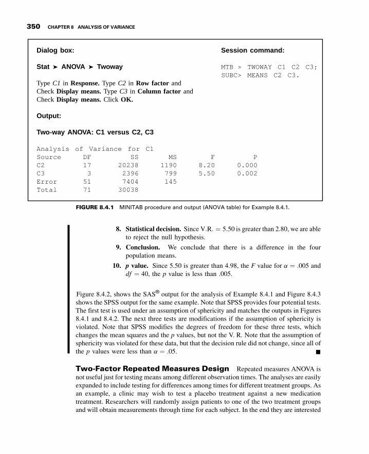
3GC08 12/04/2012 14:43:23 Page 350

8. Statistical decision. Since V:R: ¼ 5:50 is greater than 2.80, we are ableto reject the null hypothesis.

9. Conclusion. We conclude that there is a difference in the fourpopulation means.

10. p value. Since 5.50 is greater than 4.98, the F value for a ¼ :005 anddf ¼ 40, the p value is less than .005.

Figure 8.4.2, shows the SAS® output for the analysis of Example 8.4.1 and Figure 8.4.3shows the SPSS output for the same example. Note that SPSS provides four potential tests.The first test is used under an assumption of sphericity and matches the outputs in Figures8.4.1 and 8.4.2. The next three tests are modifications if the assumption of sphericity isviolated. Note that SPSS modifies the degrees of freedom for these three tests, whichchanges the mean squares and the p values, but not the V. R. Note that the assumption ofsphericity was violated for these data, but that the decision rule did not change, since all ofthe p values were less than a ¼ :05. &

Two-Factor Repeated Measures Design Repeated measures ANOVA isnot useful just for testing means among different observation times. The analyses are easilyexpanded to include testing for differences among times for different treatment groups. Asan example, a clinic may wish to test a placebo treatment against a new medicationtreatment. Researchers will randomly assign patients to one of the two treatment groupsand will obtain measurements through time for each subject. In the end they are interested


Stat ANOVA Twoway MTB > TWOWAY C1 C2 C3;SUBC> MEANS C2 C3.

Type C1 in Response. Type C2 in Row factor andCheck Display means. Type C3 in Column factor andCheck Display means. Click OK.

Output:

Two-way ANOVA: C1 versus C2, C3

Analysis of Variance for C1Source DF SS MS F PC2 17 20238 1190 8.20 0.000C3 3 2396 799 5.50 0.002Error 51 7404 145Total 71 30038

FIGURE 8.4.1 MINITAB procedure and output (ANOVA table) for Example 8.4.1.


3GC08 12/04/2012 14:43:23 Page 351

Tests of Within-Subjects Effects

Measure: MEASURE_1

Type III Sum Mean.giSFerauqSfdserauqS foecruoS

factor 1 Sphericity Assumed 2395.833 3 798.611 5.501 .002Greenhouse-Geisser 2395.833 2.216 1080.998 5.501 .006Huynh-Feldt 2395.833 2.563 934.701 5.501 .004Lower-bound 2395.833 1.000 2395.833 5.501 .031

Error (factor 1) Sphericity Assumed 7404.167 51 145.180Greenhouse-Geisser 7404.167 37.677 196.515Huynh-Feldt 7404.167 43.575 169.919Lower-bound 7404.167 17.000 435.539

FIGURE 8.4.3 SPSS output for the analysis of Example 8.4.1.

The ANOVA Procedure

Dependent Variable: sf36

Source DF Sum of Squares Mean Square F Value Pr > F

1000.<97.776666.131133333.3362202ledoM

47971.54176661.404715rorrE


R-Square Coeff Var Root MSE sf36 Mean

0.753503 18.18725 12.04906 66.25000

Source DF Anova SS Mean Square F Value Pr > F

1000.<02.881144.091100005.7320271 jbus

4200.005.511116.89733338.59323emit

FIGURE 8.4.2 SAS® output for analysis of Example 8.4.1.


3GC08 12/04/2012 14:43:23 Page 352

in knowing if there were differences between the two treatments on subjects that weremeasured multiple times.

Assumptions The assumptions of the two-factor repeated measures design are the sameas the single-factor repeated measures design. However, it is not uncommon for there to beinteractions among the treatments in this design, a potential violation of Assumption 5,above. Interaction effects can be interesting to examine, but are complex to calculate. Forthis reason, and at the level of the intended audience using this text, we will assume thatinteraction effects, when present, are mathematically handled using a statistical softwarepackage that provides correct calculations for this issue.

The Model The model for the two-factor repeated measures design must represent thefact that there are two factors, A and B, and they have a potential interaction. Thesefeatures, along with the block effect and error, must be accounted for in the model, which isgiven by

xijk ¼ mþ rij þ ai þ bj þ ðabÞij þ eijk

i ¼ 1; 2; . . . ; a; j ¼ 1; 2; . . . ; b; k ¼ 1; 2; . . . ; n(8.4.2)

In this model

xijk is a typical individual from the overall population

m an unknown constant

rij represents a block effect

aj represents the main effect of factor A

bk represents the main effect of factor B

ðabÞjk represents the interaction effect of factor A and factor B

eijk is a residual component representing all sources of variation other than treatmentsand blocks.

This model is very similar to the two-factor ANOVA model presented in Section 8.5.

EXAMPLE 8.4.2

The Mid-Michigan Medical Center (A-16) examined 25 subjects with neck cancer andmeasured as one of the outcome variables an oral health condition score. Patients wererandomly divided into two treatment groups. These were a placebo treatment (treatment 1)and an aloe juice group (treatment 2). Cancer health was measured at baseline and at theend of 2, 4, and 6 weeks of treatment. The goal was to discern if there was any change inoral health condition over the course of the experiment and to see if there were anydifferences between the two treatment conditions.

Solution:


2. Assumptions. We assume that the assumptions for the two-factorrepeated measures experiment are met.


3GC08 12/04/2012 14:43:24 Page 353

3. Hypotheses.

a. H0: ai ¼ 0 i ¼ 1; 2; . . . ; a

Ha: not allai ¼ 0

b. H0: bj ¼ 0 j ¼ 1; 2; . . . ; b

Ha: not all bj ¼ 0

c. H0: ðabÞij ¼ 0 i ¼ 1; 2; . . . ; a; j ¼ 1; 2; . . . ; b

Ha: not all ðabÞij ¼ 0

TABLE 8.4.2 Oral Health Condition Scores at Four Different Points in Time

Under Two Treatment Conditions

Treatment

Subject1 ¼ placebo

TotalC1 TotalC2 TotalC3 TotalC42 ¼ aloe juice

1 1 6 6 6 7

2 1 9 6 10 9

3 1 7 9 17 19

4 1 6 7 9 3

5 1 6 7 16 13

6 1 6 6 6 11

7 1 6 11 11 10

8 1 6 11 15 15

9 1 6 9 6 8

10 1 6 4 8 7

11 1 7 8 11 11

12 1 6 6 9 6

13 1 8 8 9 10

14 1 7 16 9 10

15 2 6 10 11 9

16 2 4 6 8 7

17 2 6 11 11 14

18 2 6 7 6 6

19 2 12 11 12 9

20 2 5 7 13 12

21 2 6 7 7 7

22 2 8 11 16 16

23 2 5 7 7 7

24 2 6 8 16 16

25 2 7 8 10 8

Source: Mid-Michigan Medical Center, Midland, Michigan, 1999: A study of oral condition of cancer patients.Availab le in the public domain at: http:// calcnet.mth.c mich.edu/org/ spss/Prj_can cer_data.h tm.


http://www.calcnet.mth.cmich.edu/org/spss/Prj_cancer_data.htm

3GC08 12/04/2012 14:43:25 Page 354

4. Test statistic. The test statistic for each hypothesis set is V.R.

5. Distribution of test statistics. When H0 is true and the assumptions aremet, each of the test statistics is distributed as F. If all assumptions aremet for the within-subjects effects, we will have F with 4 � 1 ¼ 3numerator degrees of freedom for the time factor, ð4 � 1Þð2 � 1Þ ¼ 3numerator degrees of freedom for the interaction factor, andð4 � 1Þð25 � 2Þ ¼ 69 denominator degrees of freedom for both tests;interpolation from Table G provides a critical F value of 2.74. Further, forthe between-subjects factor, we will have ð2 � 1Þ ¼ 1 numerator degreesof freedom and 25 � 2 ¼ 23 denominator degrees of freedom; Table Ggives the critical F value to be 4.28. If we do not meet the assumptions,specifically of sphericity, then the computer program will alter the degreesof freedom and hence the critical value for comparisons.

6. Decision rule. Let a ¼ :05. Reject H0 if the computed p value is lessthan a.

7. Calculation of test statistic. We use SPSS to perform the calculations.We enter the data just as it is shown in Table 8.4.2, though we do notneed to enter the “Subject” number. The SPSS code and pertinent outputare shown in Figure 8.4.4.

8. Statistical decision. SPSS provides a formal test for sphericity called“Mauchley’s Test of Sphericity”. Since we reject the null for this testaccording to the output in Figure 8.4.2, we will use the “Greenhouse-Geisser” test statistic. Since V.R. is greater than the critical value forTotalC, we reject the null hypothesis for this variable. However, both thecritical values for the interaction effect and the between-subjects factorare quite small and less than the necessary critical value, and wetherefore fail to reject these two null hypotheses.

9. Conclusion. We conclude that there is no statistical difference betweentreatments, but that subjects did have a change in oral condition throughtime regardless of the treatment they received.

10. p value. As seen in Figure 8.4.4, all p values are provided for each test.To summarize: since p < :001, we reject the null hypothesis concerningchanges through time. Since p ¼ :931, we fail to reject the nullhypothesis concerning the interaction of time and treatment. Sincep ¼ :815, we fail to reject the null hypothesis concerning differencesbetween treatments.

Though the output provided in Figure 8.4.2 can be valuable for statistical interpretation, itis often useful to examine plots to obtain a visual interpretation of the results. Figure 8.4.5shows a plot of marginal means against time, with lines representing each of the treatments.It is evident that changes in oral condition did occur through time, but that the twotreatments were very similar, as can be seen by the close proximity of the two curves.Further, it is evident that interaction between time and treatment occurred, as evidenced bythe crossing of the plotted lines. &


3GC08 12/04/2012 14:43:25 Page 355

SPSS CodeGLM TOTALCIN T0TALCW2 TOTALCW4 T0TALCW6 BY TRT

/WSFACTOR¼TotatC 4 Polynomial

/METHOD¼SSTYPE(3)

/PLOT¼PROFILE(TRT�TotalCTot3lC�TRT)

/EMMEANS¼TABLES(TRT)

/EMMEANS¼TABLES(TotalC)

/EMMEANS¼TABLES(TRT�TotalC)

/PR!NT¼DESCRIPTIVE

/CRITERIA¼ALPHA(.O5)

/WSDESIGN¼TotalC

/DESIGN¼TRT.

Partial SPSS Outout

Mauchly’s Test of Sphericityb

Within Subjects Effect Mauchly’s W Approx. Chi-Square df Sig.

TotalC .487 15.620 5 .008

Tests of Within-Subjects Effects

SourceType 111 Sum

of Squares df Mean Square F Sig.

TotalC Sphericity Assumed 233.391 3 77.797 13.926 .000

Greenhouse-Geisser 233.391 2.025 115.261 13.926 .000

Huynh-Feldt 233.391 2.318 100.682 13.926 .000

Lower-bound 233.391 1.000 233.391 13.926 .001

TotalC � TRT Sphericity Assumed 1.231 3 .410 .073 .974

Greenhouse-Geisser 1.231 2.025 .608 .073 .931

Huynh-Feldt 1.231 2.318 .531 .073 .949

Lower-bound 1.231 1.000 1.231 .073 .789

Error(TotalC) Sphericity Assumed 385.469 69 5.587

Greenhouse-Geisser 385.469 46.572 8.277

Huynh-Feldt 385.469 53.316 7.230

Lower-bound 385.469 23.000 16.760

Tests of Between-Subjects Effects

SourceType III Sum

of Squares df Mean Square F Sig.

Intercept 7637.274 1 7637.274 382.508 .000

TRT 1.114 1 1.114 .056 .815

Error 459.226 23 19.966

FIGURE 8.4.4 SPSS code and partial output for Example 8.4.2.


3GC08 12/04/2012 14:43:26 Page 356

EXERCISES

For Exercises 8.4.1 to 8.4.3 perform the ten-step hypothesis testing procedure. Let a ¼ :05.

8.4.1. One of the purposes of a study by Liu et al. (A-17) was to determine the effects of MRZ 2/579 onneurological deficit in Sprague-Dawley rats. In this study, 10 rats were measured at four time periodsfollowing occlusion of the middle carotid artery and subsequent treatment with the uncompetitive N-methly-D-aspartate antagonist MRZ 2/579, which previous studies had suggested provides neuro-protective activity. The outcome variable was a neurological function variable measured on a scale of0–12. A higher number indicates a higher degree of neurological impairment.

Rat 60 Minutes 24 Hours 48 Hours 72 Hours

1 11 9 8 42 11 7 5 33 11 10 8 64 11 4 3 25 11 10 9 96 11 6 5 57 11 6 6 68 11 7 6 59 11 7 5 5

10 11 9 7 7

Source: Data provided courtesy of Ludmila Belayev, M.D.

8.4.2. Starch et al. (A-18) wanted to show the effectiveness of a central four-quadrant sleeve and screw inanterior cruciate ligament reconstruction. The researchers performed a series of reconstructions oneight cadaveric knees. The following table shows the loads (in newtons) required to achieve differentgraft laxities (mm) for seven specimens (data not available for one specimen) using five different loadweights. Graft laxity is the separation (in mm) of the femur and the tibia at the points of graft fixation.

11

10

9

8Placebo

7

6Time 2Time 1 Time 3 Time 4

Total C

Marg

inal M

ean

Aloe Juice

FIGURE 8.4.5 Excel plot of marginal means against total oral health score for the data of

Example 8.4.2.


3GC08 12/04/2012 14:43:27 Page 357

Is there sufficient evidence to conclude that different loads are required to produce different levels ofgraft laxity? Let a ¼ :05.

Graft Laxity (mm)

Specimen 1 2 3 4 5

1 297.1 297.1 297.1 297.1 297.12 264.4 304.6 336.4 358.2 379.33 188.8 188.8 188.8 188.8 188.84 159.3 194.7 211.4 222.4 228.15 228.2 282.1 282.1 334.8 334.86 100.3 105.0 106.3 107.7 108.77 116.9 140.6 182.4 209.7 215.4

Source: David W. Starch, Jerry W. Alexander, Philip C. Noble, Suraj Reddy, and David M.Lintner, “Multistranded Hamstring Tendon Graft Fixation with a Central Four-Quadrantor a Standard Tibial Interference Screw for Anterior Cruciate Ligament Reconstruction,”American Journal of Sports Medicine, 31 (2003), 338–344.

8.4.3. Holben et al. (A-19) designed a study to evaluate selenium intake in young women in the years ofpuberty. The researchers studied a cohort of 16 women for three consecutive summers. One of theoutcome variables was the selenium intake per day. The researchers examined dietary journals ofthe subjects over the course of 2 weeks and then computed the average daily selenium intake. Thefollowing table shows the average daily selenium intake values inmg=dð Þ for the 16 women in years1, 2, and 3 of the study.

Subject Year 1 Year 2 Year 3 Subject Year 1 Year 2 Year 3

1 112.51 121.28 94.99 9 95.05 93.89 73.262 106.20 121.14 145.69 10 112.65 100.47 145.693 102.00 121.14 130.37 11 103.74 121.14 123.974 103.74 90.21 135.91 12 103.74 121.14 135.915 103.17 121.14 145.69 13 112.67 104.66 136.876 112.65 98.11 145.69 14 106.20 121.14 126.427 106.20 121.14 136.43 15 103.74 121.14 136.438 83.57 102.87 144.35 16 106.20 100.47 135.91

Source: Data provided courtesy of David H. Holben, Ph.D. and John P. Holcomb, Ph.D.

8.4.4. Linke et al. (A-20) studied seven male mongrel dogs. They induced diabetes by injecting the animalswith alloxan monohydrate. The researchers measured the arterial glucose (mg/gl), arterial lactate(mmol/L), arterial free fatty acid concentration, and arterial b-hydroxybutyric acid concentrationprior to the alloxan injection, and again in weeks 1, 2, 3, and 4 post-injection. What is the responsevariable(s)? Comment on carryover effect and position effect as they may or may not be of concern inthis study. Construct an ANOVA table for this study in which you identify the sources of variabilityand specify the degrees of freedom for each.

8.4.5. Werther et al. (A-21) examined the vascular endothelial growth factor (VEGF) concentration in bloodfrom colon cancer patients. Research suggests that inhibiting VEGF may disrupt tumor growth. Theresearchers measured VEGF concentration (ng/L) for 10 subjects and found an upward trend inVEGF concentrations during the clotting time measured at baseline, and hours 1 and 2. What is theresponse variable? What is the treatment variable? Construct an ANOVA table for this study in whichyou identify the sources of variability and specify the degrees of freedom for each.

EXERCISES 357

3GC08 12/04/2012 14:43:27 Page 358

8.4.6. Yucha et al. (A-22) conducted a study to determine if nursing students who were assigned to a homehospital (HH) experience differed from those traditionally placed (TP) in hospitals throughout theirnursing training. A small subset of data is provided in the table below. In this data set, hospitalplacement is the between-subjects variable. Anxiety, as measured by Spielberger’s State AnxietyScale (where higher scores suggest higher levels of anxiety), is the within-subjects variable and isprovided at four points in time during nursing training. Is there evidence that anxiety level changedthrough time for these nursing students? Is there a difference in anxiety between those in a homehospital placement versus traditional placement? Is there significant interaction between placementtype and anxiety? Let a ¼ :05.

Subject Hospital Placement Anxiety 1 Anxiety 2 Anxiety 3 Anxiety 4

1 HH 51 33 12 312 HH 50 51 50 443 HH 65 58 45 374 HH 43 40 31 515 HH 67 56 50 426 HH 46 69 62 467 HH 29 28 28 438 HH 76 69 62 609 HH 66 39 47 38

10 HH 56 46 34 3111 TP 44 48 51 5912 TP 44 50 54 4013 TP 54 49 35 4614 TP 38 38 32 3715 TP 25 27 25 2416 TP 61 60 55 6617 TP 42 51 42 3418 TP 36 49 49 5119 TP 52 63 50 6420 TP 41 55 56 34

Source: Data provided Courtesy of Carolyn B. Yucha, RN, PhD, FAAN.

8.5 THE FACTORIAL EXPERIMENT

In the experimental designs that we have considered up to this point, we have beeninterested in the effects of only one variable—the treatments. Frequently, however, we maybe interested in studying, simultaneously, the effects of two or more variables. We refer tothe variables in which we are interested as factors. The experiment in which two or morefactors are investigated simultaneously is called a factorial experiment.

The different designated categories of the factors are called levels. Suppose, forexample, that we are studying the effect on reaction time of three dosages of some drug.The drug factor, then, is said to occur at three levels. Suppose the second factor of interest inthe study is age, and it is thought that two age groups, under 65 years and 65 years andolder, should be included. We then have two levels of the age factor. In general, we say thatfactor A occurs at a levels and factor B occurs at b levels.


3GC08 12/04/2012 14:43:28 Page 359

In a factorial experiment we may study not only the effects of individual factors butalso, if the experiment is properly conducted, the interaction between factors. To illustratethe concept of interaction let us consider the following example.

EXAMPLE 8.5.1

Suppose, in terms of effect on reaction time, that the true relationship between three dosagelevels of some drug and the age of human subjects taking the drug is known. Supposefurther that age occurs at two levels—“young” (under 65) and “old” (65 and older). If thetrue relationship between the two factors is known, we will know, for the three dosagelevels, the mean effect on reaction time of subjects in the two age groups. Let us assumethat effect is measured in terms of reduction in reaction time to some stimulus. Supposethese means are as shown in Table 8.5.1.

The following important features of the data in Table 8.5.1 should be noted.

1. For both levels of factor A the difference between the means for any two levels offactor B is the same. That is, for both levels of factor A, the difference between meansfor levels 1 and 2 is 5, for levels 2 and 3 the difference is 10, and for levels 1 and 3 thedifference is 15.

2. For all levels of factor B the difference between means for the two levels of factor A isthe same. In the present case the difference is 5 at all three levels of factor B.

3. A third characteristic is revealed when the data are plotted as in Figure 8.5.1. We notethat the curves corresponding to the different levels of a factor are all parallel.

When population data possess the three characteristics listed above, we say that there is nointeraction present.

TABLE 8.5.1 Mean Reduction in Reaction Time

(milliseconds) of Subjects in Two Age Groups atThree Drug Dosage Levels

Factor B—Drug Dosage

Factor A—Age j ¼ 1 j ¼ 2 j ¼ 3

Young ði ¼ 1Þ m11 ¼ 5 m12 ¼ 10 m13 ¼ 20

Old ði ¼ 2Þ m21 ¼ 10 m22 ¼ 15 m23 ¼ 25

30

25

20

15

10

5

0Red

uct

ion

in r

eact

ion

tim

e

30

25

20

15

10

5

0

Red

uct

ion

in r

eact

ion

tim

e

b1 b2 b3

a1

a2

Drug dosage

a1 a2

Age

Age

b3

b2

b1

Drug dosage

FIGURE 8.5.1 Age and drug effects, no interaction present.

8.5 THE FACTORIAL EXPERIMENT 359

3GC08 12/04/2012 14:43:28 Page 360

The presence of interaction between two factors can affect the characteristics of thedata in a variety of ways depending on the nature of the interaction. We illustrate the effectof one type of interaction by altering the data of Table 8.5.1 as shown in Table 8.5.2.

The important characteristics of the data in Table 8.5.2 are as follows.

1. The difference between means for any two levels of factor B is not the same for bothlevels of factor A. We note in Table 8.5.2. for example, that the difference betweenlevels 1 and 2 of factor B is �5 for the young age group and þ5 for the old age group.

2. The difference between means for both levels of factor A is not the same at all levelsof factor B. The differences between factor A means are �10, 0, and 15 for levels 1, 2,and 3, respectively, of factor B.

3. The factor level curves are not parallel, as shown in Figure 8.5.2.

When population data exhibit the characteristics illustrated in Table 8.5.2 andFigure 8.5.2, we say that there is interaction between the two factors. We emphasizethat the kind of interaction illustrated by the present example is only one of many types ofinteraction that may occur between two factors. &

In summary, then, we can say that there is interaction between two factors if a changein one of the factors produces a change in response at one level of the other factor differentfrom that produced at other levels of this factor.

Advantages The advantages of the factorial experiment include the following.

1. The interaction of the factors may be studied.

2. There is a saving of time and effort.

TABLE 8.5.2 Data of Table 8.5.1 Altered to Show

the Effect of One Type of Interaction

Factor B—Drug Dosage

Factor A—Age j ¼ 1 j ¼ 2 j ¼ 3

Young ði ¼ 1Þ m11 ¼ 5 m12 ¼ 10 m13 ¼ 20

Old ði ¼ 2Þ m21 ¼ 15 m22 ¼ 10 m23 ¼ 5

30

25

20

15

10

5

0

Red

uct

ion

in r

eact

ion

tim

e

30

25

20

15

10

5

0

Red

uct

ion

in r

eact

ion

tim

e

b1 b2 b3

a1

a2

Drug dosage

Age

a1 a2

Age

b1

b2

b3

Drug dosage

FIGURE 8.5.2 Age and drug effects, interaction present.


3GC08 12/04/2012 14:43:29 Page 361

In the factorial experiment all the observations may be used to study the effects ofeach of the factors under investigation. The alternative, when two factors are beinginvestigated, would be to conduct two different experiments, one to study each of the twofactors. If this were done, some of the observations would yield information only on one ofthe factors, and the remainder would yield information only on the other factor. To achievethe level of accuracy of the factorial experiment, more experimental units would be neededif the factors were studied through two experiments. It is seen, then, that 1 two-factorexperiment is more economical than 2 one-factor experiments.

3. Because the various factors are combined in one experiment, the results have a widerrange of application.

The Two-Factor Completely Randomized Design A factorialarrangement may be studied with either of the designs that have been discussed. Weillustrate the analysis of a factorial experiment by means of a two-factor completelyrandomized design.

1. Data. The results from a two-factor completely randomized design may be presentedin tabular form as shown in Table 8.5.3.

Here we have a levels of factor A, b levels of factor B, and n observations foreach combination of levels. Each of the ab combinations of levels of factor A withlevels of factor B is a treatment. In addition to the totals and means shown in Table8.5.3, we note that the total and mean of the ijth cell are

Tij� ¼Xnk¼1

xijk and �xij� ¼ Tij�=n

TABLE 8.5.3 Table of Sample Data from a Two-FactorCompletely Randomized Experiment

Factor B

Factor A 1 2 . . . b Totals Means

1 x111 x121 . . . x1b1

..

. ... ..

. ...

T 1:: �x1::

x11n x12n . . . x1bn

2 x211 x221 . . . x2b1

..

. ... ..

. ...

T 2:: �x2::

x21n x22n . . . x2bn

..

. ... ..

. ... ..

. ... ..

.

a xa11 xa21 . . . xab1

..

. ... ..

. ...

Ta:: �xa::

xa1n xa2n . . . xabn

Totals T :1: T :2: . . . T :b: T ...

Means �x :1: �x :2: . . . �x :b: �x ...


3GC08 12/04/2012 14:43:29 Page 362

respectively. The subscript i runs from 1 to a and j runs from 1 to b. The total numberof observations is nab.

To show that Table 8.5.3 represents data from a completely randomized design,we consider that each combination of factor levels is a treatment and that we have nobservations for each treatment. An alternative arrangement of the data would beobtained by listing the observations of each treatment in a separate column. Table8.5.3 may also be used to display data from a two-factor randomized block design ifwe consider the first observation in each cell as belonging to block 1, the secondobservation in each cell as belonging to block 2, and so on to the nth observation ineach cell, which may be considered as belonging to block n.

Note the similarity of the data display for the factorial experiment as shown inTable 8.5.3 to the randomized complete block data display of Table 8.3.1. Thefactorial experiment, in order that the experimenter may test for interaction, requiresat least two observations per cell, whereas the randomized complete block designrequires only one observation per cell. We use two-way analysis of variance toanalyze the data from a factorial experiment of the type presented here.

2. Assumptions. We assume a fixed-effects model and a two-factor completelyrandomized design. For a discussion of other designs, consult the references atthe end of this chapter.

The Model The fixed-effects model for the two-factor completely randomizeddesign may be written as

xijk ¼ mþ ai þ bj þ abð Þij þ eijk

i ¼ 1; 2; . . . ; a; j ¼ 1; 2; . . . ; b; k ¼ 1; 2; . . . ; n(8.5.1)

where xijk is a typical observation, m is a constant, ai represents an effect due to factor A, bj

represents an effect due to factor B, abð Þij represents an effect due to the interaction offactors A and B, and eijk represents the experimental error.

Assumptions of the Model

a. The observations in each of the ab cells constitute a random independent sample ofsize n drawn from the population defined by the particular combination of the levelsof the two factors.

b. Each of the ab populations is normally distributed.

c. The populations all have the same variance.

3. Hypotheses. The following hypotheses may be tested:

a. H0: ai ¼ 0 i ¼ 1; 2; . . . ; aHA: notall ai ¼ 0

b. H0: bj ¼ 0 j ¼ 1; 2; . . . ; bHA: not all bj ¼ 0

c. H0: abð Þij ¼ 0 i ¼ 1; 2; . . . ; a; j ¼ 1; 2; . . . ; bHA: not all abð Þij ¼ 0


3GC08 12/04/2012 14:43:30 Page 363

Before collecting data, the researchers may decide to test only one of the possiblehypotheses. In this case they select the hypothesis they wish to test, choose a significancelevel a, and proceed in the familiar, straightforward fashion. This procedure is free of thecomplications that arise if the researchers wish to test all three hypotheses.

When all three hypotheses are tested, the situation is complicated by the fact that thethree tests are not independent in the probabilistic sense. If we let a be the significance levelassociated with the test as a whole, and a0;a00; and a000 the significance levels associatedwith hypotheses 1, 2, and 3, respectively, we find

a < 1 � 1 � a0ð Þ 1 � a00ð Þ 1 � a000ð Þ (8.5.2)

If a0 ¼ a00 ¼ a000¼ :05, then a < 1 � :95ð Þ3, or a < :143. This means that theprobability of rejecting one or more of the three hypotheses is less than .143 when asignificance level of .05 has been chosen for the hypotheses and all are true. To demonstratethe hypothesis testing procedure for each case, we perform all three tests. The reader,however, should be aware of the problem involved in interpreting the results.


5. Distribution of test statistic. When H0 is true and the assumptions are met, each ofthe test statistics is distributed as F.

6. Decision rule. Reject H0 if the computed value of the test statistic is equal to orgreater than the critical value of F.

7. Calculation of test statistic. By an adaptation of the procedure used in partitioningthe total sum of squares for the completely randomized design, it can be shown thatthe total sum of squares under the present model can be partitioned into two parts asfollows:

Xai¼1

Xbj¼1

Xnk¼1

ðxijk � �x...Þ2 ¼Xai¼1

Xbj¼1

Xnk¼1

�xij� � �x...� �2 þ

Xai¼1

Xbj¼1

Xnk¼1

xijk � �xij�� 2

(8.5.3)

or

SST ¼ SSTr þ SSE (8.5.4)

The sum of squares for treatments can be partitioned into three parts as follows:

Xai¼1

Xbj¼1

Xnk¼1

�xij � �x...� �2 ¼

Xai¼1

Xbj¼1

Xnk¼1

�xi:: � �x...ð Þ2

þXai¼1

Xbj¼1

Xnk¼1

�x:j: � �x...� �2

þXai¼1

Xbj¼1

Xnk¼1

�xij� � �xi:: � �x:j: þ �x...� �2

(8.5.5)


3GC08 12/04/2012 14:43:31 Page 364

or

SSTr ¼ SSAþ SSBþ SSAB

TheANOVATable The results of the calculations for the fixed-effects model for atwo-factor completely randomized experiment may, in general, be displayed as shown inTable 8.5.4.

8. Statistical decision. If the assumptions stated earlier hold true, and if eachhypothesis is true, it can be shown that each of the variance ratios shown inTable 8.5.4 follows an F distribution with the indicated degrees of freedom. Wereject H0 if the computed V.R. values are equal to or greater than thecorresponding critical values as determined by the degrees of freedom andthe chosen significance levels.

9. Conclusion. If we reject H0, we conclude that HA is true. If we fail to reject H0, weconclude that H0 may be true.

10. p value.

EXAMPLE 8.5.2

In a study of length of time spent on individual home visits by public health nurses, datawere reported on length of home visit, in minutes, by a sample of 80 nurses. A record wasmade also of each nurse’s age and the type of illness of each patient visited. The researcherswished to obtain from their investigation answers to the following questions:

1. Does the mean length of home visit differ among different age groups of nurses?

2. Does the type of patient affect the mean length of home visit?

3. Is there interaction between nurse’s age and type of patient?

Solution:

1. Data. The data on length of home visit that were obtained during thestudy are shown in Table 8.5.5.

TABLE 8.5.4 Analysis of Variance Table for a Two-Factor Completely

Randomized Experiment (Fixed-Effects Model)


A SSA a � 1 MSA ¼ SSA= a � 1ð Þ MSA=MSE

B SSB b � 1 MSB ¼ SSB= b � 1ð Þ MSB=MSE

AB SSAB a � 1ð Þ b � 1ð Þ MSAB ¼ SSAB= a � 1ð Þ b � 1ð Þ MSAB=MSE

Treatments SSTr ab � 1

Residual SSE ab n � 1ð Þ MSE ¼ SSE=ab n � 1ð Þ

Total SST abn � 1


3GC08 12/04/2012 14:43:31 Page 365

2. Assumptions. To analyze these data, we assume a fixed-effects modeland a two-factor completely randomized design.

3. Hypotheses. For our illustrative example we may test the followinghypotheses subject to the conditions mentioned above.

a. H0: a1 ¼ a2 ¼ a3 ¼ a4 ¼ 0 HA: not all ai ¼ 0b. H0: b1 ¼ b2 ¼ b3 ¼ b4 ¼ 0 HA: not all bj ¼ 0c. H0: all ðabÞij ¼ 0 HA: not all ðabÞij ¼ 0

Let a ¼ :05


5. Distribution of test statistic. When H0 is true and the assumptions aremet, each of the test statistics is distributed as F.

TABLE 8.5.5 Length of Home Visit in Minutes by Public Health Nurses by

Nurse’s Age Group and Type of Patient

Factor B (Nurse’s Age Group) Levels

Factor A(Type of Patient)Levels

1(20 to 29)

2(30 to 39)

3(40 to 49)

4(50 and Over)

1 (Cardiac) 20 25 24 28

25 30 28 31

22 29 24 26

27 28 25 29

21 30 30 32

2 (Cancer) 30 30 39 40

45 29 42 45

30 31 36 50

35 30 42 45

36 30 40 60

3 (C.V.A.) 31 32 41 42

30 35 45 50

40 30 40 40

35 40 40 55

30 30 35 45

4 (Tuberculosis) 20 23 24 29

21 25 25 30

20 28 30 28

20 30 26 27

19 31 23 30


3GC08 12/04/2012 14:43:33 Page 366

6. Decision rule. Reject H0 if the computed value of the test statistic isequal to or greater than the critical value of F. The critical values of F fortesting the three hypotheses of our illustrative example are 2.76, 2.76,and 2.04, respectively. Since denominator degrees of freedom equal to64 are not shown in Appendix Table G, 60 was used as the denominatordegrees of freedom.

7. Calculation of test statistic. We use MINITAB to perform thecalculations. We put the measurements in Column 1, the row (factorA) codes in Column 2, and the column (factor B) codes in Column 3. Theresulting column contents are shown in Table 8.5.6 . The MINITABoutput is shown in Figure 8.5.3.

TABLE 8.5.6 Column Contents for MINITAB Calculations,Example 8.5.2

Row C1 C2 C3 Row C1 C2 C3

1 20 1 1 41 31 3 1

2 25 1 1 42 30 3 1

3 22 1 1 43 40 3 1

4 27 1 1 44 35 3 1

5 21 1 1 45 30 3 1

6 25 1 2 46 32 3 2

7 30 1 2 47 35 3 2

8 29 1 2 48 30 3 2

9 28 1 2 49 40 3 2

10 30 1 2 50 30 3 2

11 24 1 3 51 41 3 3

12 28 1 3 52 45 3 3

13 24 1 3 53 40 3 3

14 25 1 3 54 40 3 3

15 30 1 3 55 35 3 3

16 28 1 4 56 42 3 4

17 31 1 4 57 50 3 4

18 26 1 4 58 40 3 4

19 29 1 4 59 55 3 4

20 32 1 4 60 45 3 4

21 30 2 1 61 20 4 1

22 45 2 1 62 21 4 1

23 30 2 1 63 20 4 1

24 35 2 1 64 20 4 1

25 36 2 1 65 19 4 1

26 30 2 2 66 23 4 2

27 29 2 2 67 25 4 2

28 31 2 2 68 28 4 2

(Continued)


3GC08 12/04/2012 14:43:34 Page 367

8. Statistical decision. The variance ratios are V:R: ðAÞ ¼ 997:5=14:7 ¼ 67:86, V:R: ðBÞ ¼ 400:4=14:7 ¼ 27:24, and V:R: ðABÞ ¼67:6= 14:7 ¼ 4:60. Since the three computed values of VR. are allgreater than the corresponding critical values, we reject all three nullhypotheses.

9. Conclusion. When H0: a1 ¼ a2 ¼ a3 ¼ a4 is rejected, we concludethat there are differences among the levels of A, that is, differences in theaverage amount of time spent in home visits with different types ofpatients. Similarly, when H0: b1 ¼ b2 ¼ b3 ¼ b4 is rejected, we con-clude that there are differences among the levels of B, or differences inthe average amount of time spent on home visits among the differentnurses when grouped by age. When H0: ðabÞij ¼ 0 is rejected, weconclude that factors A and B interact; that is, different combinationsof levels of the two factors produce different effects.

10. p value. Since 67.86, 27.24, and 4.60 are all greater than the criticalvalues of F:995 for the appropriate degrees of freedom, the p value foreach of the tests is less than .005. When the hypothesis of no interactionis rejected, interest in the levels of factors A and B usually becomesubordinate to interest in the interaction effects. In other words, we aremore interested in learning what combinations of levels are significantlydifferent.

Figure 8.5.4 shows the SAS® output for the analysis of Example 8.5.2. &

We have treated only the case where the number of observations in each cell is the same.When the number of observations per cell is not the same for every cell, the analysisbecomes more complex.

In such cases the design is said to be unbalanced. To analyze these designs withMINITAB we use the general linear (GLM) procedure. Other software packages such asSAS® also will accommodate unequal cell sizes.

Row C1 C2 C3 Row C1 C2 C3

29 30 2 2 69 30 4 2

30 30 2 2 70 31 4 2

31 39 2 3 71 24 4 3

32 42 2 3 72 25 4 3

33 36 2 3 73 30 4 3

34 42 2 3 74 26 4 3

35 40 2 3 75 23 4 3

36 40 2 4 76 29 4 4

37 45 2 4 77 30 4 4

38 50 2 4 78 28 4 4

39 45 2 4 79 27 4 4

40 60 2 4 80 30 4 4


3GC08 12/04/2012 14:43:34 Page 368


Stat ANOVA Twoway MTB > TWOWAY C1 C2 C3;SUBC > MEANS C2 C3.

Type C1 in Response. Type C2 in Row factor andcheck Display means. Type C3 in Column factor andcheck Display means. Click OK.

Output:

Two-Way ANOVA: C1 versus C2, C3

Analysis of Variance for C1Source DF SS MS F PC2 3 2992.4 997.483 67.94 0.000C3 3 1201.1 400.350 27.27 0.000Interaction 9 608.5 67.606 4.60 0.000Error 64 939.6 14.681Total 79 5741.5

Individual 95% CIC2 Mean -+---------+---------+---------+---------+1 26.70 (----*---)

----(52.832 *---)----(03.833 *---)

4 25.45 (----*---)-+---------+---------+---------+---------+

24.00 28.00 32.00 36.00 40.00

Individual 95% CIC3 Mean ------+---------+---------+---------+-----1 27.85 (----*---)2 29.80 (----*---)

----(59.233 *---)----(01.834 *---)

------+---------+---------+---------+-----28.00 31.50 35.00 38.50

FIGURE 8.5.3 MINITAB procedure and ANOVA table for Example 8.5.2.


3GC08 12/04/2012 14:43:34 Page 369

EXERCISES

For Exercises 8.5.1 to 8.5.4, perform the analysis of variance, test appropriate hypotheses at the.05 level of significance, and determine the p value associated with each test.

8.5.1. Uryu et al. (A-23) studied the effect of three different doses of troglitazone mMð Þ on neuro cell death.Cell death caused by stroke partially results from the accumulation of high concentrations ofglutamate. The researchers wanted to determine if different doses of troglitazone (1.3, 4.5, and13:5mM) and different ion forms � and þð Þ of LY294002, a PI3-kinase inhibitor, would givedifferent levels of neuroprotection. Four rats were studied at each dose and ion level, and the mea-sured variable is the percent of cell death as compared to glutamate. Therefore, a higher value impliesless neuroprotection. The results are displayed in the table below.

Percent Comparedto Glutamate �LY294002 vsþ LY294002

TroglitazoneDose (mM)

73.61 Negative 1.3130.69 Negative 1.3118.01 Negative 1.3140.20 Negative 1.3

The SAS System


Dependent Variable: TIME

rPeulaV FerauqS naeMserauqS fo muSFD ecruoS F

1000.018.1200000031.02300000059.108451 ledoM

00052186.4100000006.93946rorrE


R-Square C.V. Root MSE TIME Mean

0.836351 11.90866 3.83161193 32.17500000

rPeulaV FerauqS naeMSS avonAFDecruoS F

1000.072.7200000053.00400000050.10213BROTCAF1000.049.7633333384.79900000054.29923AROTCAF

FACTORB*FACTORA 9 608.450000000 67.60555556 4.60 0.0001

FIGURE 8.5.4 SAS® output for analysis of Example 8.5.2.

(Continued)

EXERCISES 369

3GC08 12/04/2012 14:43:35 Page 370

Percent Comparedto Glutamate �LY294002 vsþ LY294002

TroglitazoneDose mMð Þ

97.11 Positive 1.3114.26 Positive 1.3120.26 Positive 1.3

92.39 Positive 1.326.95 Negative 4.553.23 Negative 4.559.57 Negative 4.553.23 Negative 4.528.51 Positive 4.530.65 Positive 4.544.37 Positive 4.536.23 Positive 4.5�8:83 Negative 13.525.14 Negative 13.520.16 Negative 13.534.65 Negative 13.5

�35:80 Positive 13.5�7:93 Positive 13.5�19:08 Positive 13.5

5.36 Positive 13.5

Source: Data provided courtesy of Shigeko Uryu.

8.5.2. Researchers at a trauma center wished to develop a program to help brain-damaged trauma victimsregain an acceptable level of independence. An experiment involving 72 subjects with the samedegree of brain damage was conducted. The objective was to compare different combinations ofpsychiatric treatment and physical therapy. Each subject was assigned to one of 24 differentcombinations of four types of psychiatric treatment and six physical therapy programs. Therewere three subjects in each combination. The response variable is the number of months elapsingbetween initiation of therapy and time at which the patient was able to function independently. Theresults were as follows:

Psychiatric TreatmentPhysicalTherapy Program A B C D

11.0 9.4 12.5 13.2I 9.6 9.6 11.5 13.2

10.8 9.6 10.5 13.5

10.5 10.8 10.5 15.0II 11.5 10.5 11.8 14.6

12.0 10.5 11.5 14.0

12.0 11.5 11.8 12.8III 11.5 11.5 11.8 13.7

11.8 12.3 12.3 13.1

(Continued)


3GC08 12/04/2012 14:43:36 Page 371

Psychiatric TreatmentPhysicalTherapy Program A B C D

11.5 9.4 13.7 14.0IV 11.8 9.1 13.5 15.0

10.5 10.8 12.5 14.0

11.0 11.2 14.4 13.0V 11.2 11.8 14.2 14.2

10.0 10.2 13.5 13.7

11.2 10.8 11.5 11.8VI 10.8 11.5 10.2 12.8

11.8 10.2 11.5 12.0

Can one conclude on the basis of these data that the different psychiatric treatment programs havedifferent effects? Can one conclude that the physical therapy programs differ in effectiveness? Canone conclude that there is interaction between psychiatric treatment programs and physical therapyprograms? Let a ¼ :05 for each test.

Exercises 8.5.3 and 8.5.4 are optional since they have unequal cell sizes. It is recommended thatthe data for these be analyzed using SAS® or some other software package that will accept unequalcell sizes.

8.5.3. Main et al. (A-24) state, “Primary headache is a very common condition and one that nursesencounter in many different care settings. Yet, there is a lack of evidence as to whether advicegiven to sufferers is effective and what improvements may be expected in the conditions.” Theresearchers assessed frequency of headaches at the beginning and end of the study for 19subjects in an intervention group (treatment 1) and 25 subjects in a control group (treatment 2).Subjects in the intervention group received health education from a nurse, while the controlgroup did not receive education. In the 6 months between pre- and post-evaluation, the subjectskept a headache diary. The following table gives as the response variable the difference (pre –post) in frequency of headaches over the 6 months for two factors: (1) treatment with two levels(intervention and control), and (2) migraine status with two levels (migraine sufferer andnonmigraine sufferer).

Change inFrequency ofHeadaches

Migraine Sufferer(1 = No, 2 = Yes) Treatment



�2 1 1 �3 2 2

2 2 1 �6 2 2

33 1 1 11 1 2

�6 2 1 64 1 2

6 2 1 65 1 2

98 1 1 14 1 2

2 2 1 8 1 2

6 2 1 6 2 2

(Continued)

EXERCISES 371

3GC08 12/04/2012 14:43:37 Page 372

Can one conclude on the basis of these data that there is a difference in the reduction ofheadache frequency between the control and treatment groups? Can one conclude that there is adifference in the reduction of headache frequency between migraine and non-migraine sufferers?Can one conclude that there is interaction between treatments and migraine status? Let a ¼ :05for each test.

8.5.4. The purpose of a study by Porcellini et al. (A-25) was to study the difference in CD4 cell response inpatients taking highly active antiretroviral therapy (HAART, treatment 1) and patients takingHAART plus intermittent interleukin (IL-2, treatment 2). Another factor of interest was the HIV-RNA plasma count at baseline of study. Subjects were classified as having fewer than 50 copies/ml(plasma 1) or having 50 or more copies/ml (plasma 2). The outcome variable is the percent change inCD4 T cell count from baseline to 12 months of treatment. Can one conclude that there is a differencein the percent change in CD4 T cell count between the two treatments? The results are shown in thefollowing table. Can one conclude that there is a difference in the percent change in CD4 T cell countbetween those who have fewer than 50/ml plasma copies of HIV-RNA and those who do not? Can oneconclude that there is interaction between treatments and plasma levels? Let a ¼ :05 for each test.

Percent Change in CD4 T Cell Treatment Plasma

�12:60 1 1�14:60 2 1

28.10 2 1(Continued)

33 1 1 14 1 2

�7 2 1 �11 2 2

�1 2 1 53 1 2

�12 2 1 26 2 2

12 1 1 3 1 2

64 1 1 15 1 2

36 2 1 3 1 2

6 2 1 41 1 2

4 2 1 16 1 2

11 2 1 �4 2 2

0 2 1 �6 2 2

9 1 2

9 2 2

�3 2 2

9 2 2

3 1 2

4 2 2

Source: Data provided courtesy of A. Main, H. Abu-Saad, R. Salt, l. Vlachonikolis, and A. Dowson, “Management by Nurses of PrimaryHeadache: A Pilot Study,” Current Medical Research Opinion, 18 (2002), 471–478.






3GC08 12/04/2012 14:43:37 Page 373

Percent Change in CD4 T Cell Treatment Plasma

77.30 1 1�0:44 1 150.20 1 148.60 2 286.20 2 2

205.80 1 2100.00 1 2

34.30 1 282.40 1 2

118.30 1 2

Source: Data provided courtesy of Simona Porcellini, Guiliana Vallanti,Silvia Nozza, Guido Poli, Adriano Lazzarin, Guiseppe Tabussi,and Antonio Grassia, “Improved Thymopoietic Potential in AviremicHIV Infected Individuals with HAART by Intermittent IL-2Administration,” AIDS, 17 (2003), 1621–1630.

8.5.5. A study by G�orecka et al. (A-26) assessed the manner in which among middle-aged smokers thediagnosis of airflow limitation (AL) combined with advice to stop smoking influences the smokingcessation rate. Their concerns were whether having AL, whether the subject successfully quitsmoking, and whether interaction between AL and smoking status were significant factors in regardto baseline variables and lung capacity variables at the end of the study. Some of the variables ofinterest were previous years of smoking (pack years), age at which subject first began smoking,forced expiratory volume in one second ðFEV1Þ, and forced vital capacity (FVC). There were 368subjects in the study. What are the factors in this study? At how many levels does each occur? Whoare the subjects? What is (are) the response variable(s)? Can you think of any extraneous variableswhose effects are included in the error term?

8.5.6. A study by Meltzer et al. (A-27) examined the response to 5 mg desloratadine, an H1-receptorantagonist, in patients with seasonal allergies. During the fall allergy season, 172 subjects wererandomly assigned to receive treatments of desloratadine and 172 were randomly assigned to receivea placebo. Subjects took the medication for 2 weeks after which changes in the nasal symptom scorewere calculated. A significant reduction was noticed in the treatment group compared to the placebogroup, but gender was not a significant factor. What are the factors in the study? At how many levelsdoes each occur? What is the response variable?

8.6 SUMMARY

The purpose of this chapter is to introduce the student to the basic ideas and techniques ofanalysis of variance. Two experimental designs, the completely randomized and therandomized complete block, are discussed in considerable detail. In addition, the conceptof repeated measures designs and a factorial experiment as used with the completelyrandomized design are introduced. Individuals who wish to pursue further any aspect ofanalysis of variance will find the methodology references at the end of the chapter mosthelpful.

8.6 SUMMARY 373

3GC08 12/04/2012 14:43:38 Page 374



8.2.1 One-way ANOVAmodel

xij ¼ mþ tj þ eij

8.2.2 Total sum-of-squaresSST ¼

Xkj¼1

Xnji¼1

xij � �x::� �2

8.2.3 Within-groupsum-of-squares SSW ¼

Xkj¼1

Xnji¼1

xij � �x:j� �2

8.2.4 Among-groupsum-of-squares SSA ¼

Xkj¼1

nj �x�j � �x::� �2

8.2.5 Within-group variance

MSW ¼

Xkj¼1

Xnji¼1

xij � �x�j� �2

Xkj¼1

nj � 1� �

8.2.6 Among-groupvariance I

s2 ¼ ns2�x

8.2.7 Among-groupvariance II(equal sample sizes) MSA ¼

nXkj¼1

�x�j � �x::� �2

k � 1

8.2.8 Among-groupvariance III(unequal sample sizes) MSA ¼

Xkj¼1

nj �x�j � �x::� �2

k � 1

8.2.9 Tukey’s HSD(equal sample sizes) HSD ¼ qa;k;N�k


n

r

8.2.10 Tukey’s HSD(unequal sample sizes) HSD� ¼ qa;k;N�k

ffiffiffiffiffiffiffiffiffiffiffiffiffiffiffiffiffiffiffiffiffiffiffiffiffiffiffiffiffiffiffiMSE

2

1

niþ 1

nj

� �s

8.3.1 Two-way ANOVAmodel


8.3.2 Sum-of-squaresrepresentation

SST ¼ SSBlþ SSTr þ SSE

(Continued)


3GC08 12/04/2012 14:43:39 Page 375

8.3.3 Sum-of-squares totalSST ¼

Xkj¼1

Xni¼1

xij � �x: :� �2

8.3.4 Sum-of-squares blockSSBl ¼

Xkj¼1

Xni¼1

�xi� � �x: :ð Þ2

8.3.5 Sum-of-squarestreatments SSTr ¼

Xkj¼1

Xni¼1

�x�j � �x: :� �2

8.3.6 Sum-of-squares error SSE ¼ SST � SSBl� SSTr

8.4.1 Fixed-effects, additivesingle-factor, repeated-measures ANOVAmodel


8.4.2 Two-factor repeatedmeasures model

xijk ¼ mþ rij þ ai þ bj þ ðabÞij þ eijk

8.5.1 Two-factor completelyrandomized fixed-effects factorial model

xijk ¼ mþ ai þ bj þ abð Þij þ eijk

8.5.2 Probabilisticrepresentation of a

a < 1 � 1 � a0ð Þ 1 � a00ð Þ 1 � a000ð Þ

8.5.3 Sum-of-squares total I Xai¼1

Xbj¼1

Xnk¼1

xijk � �x: : :� �2 ¼

Xai¼1

Xbj¼1

Xnk¼1

�xij� � �x: : :� �2

þXai¼1

Xbj¼1

Xnk¼1

xijk � �xij�� 2

8.5.4 Sum-of-squares total II SST ¼ SSTr þ SSE

8.5.5 Sum-of-squarestreatment partition

Xai¼1

Xbj¼1

Xnk¼1

�xij� � �x:::� �2 ¼

Xai¼1

Xbj¼1

Xnk¼1

�xi:: � �x:::ð Þ2

þXai¼1

Xbj¼1

Xnk¼1

�x�j� � �x:::� �2

þXai¼1

Xbj¼1

Xnk¼1

�xij� � �xi:: � �x�j� þ �x:::� �2

Symbol Key � a ¼ Probability of Type I error� ai ¼ treatment A effect� bj ¼ treatment B effect� bi ¼ block effect� abð Þij ¼ interaction effect� eij ¼ error term� HSD ¼ honestly significant difference� k ¼ number of treatments


3GC08 12/04/2012 14:43:40 Page 376

� m ¼ mean of population or the grand meanð Þ� n ¼ number or blocks� nx ¼ sample size� rij ¼ block effect for two-factor repeated measures around� s2 ¼ variance� SSX ¼ sum � of � squares where X : A ¼ among;ð

Bl ¼ block;T ¼ total; Tr ¼ treatment; W ¼ withinÞ� ti ¼ treatment effect� xxxx ¼ measurement


1. Define analysis of variance.

2. Describe the completely randomized design.

3. Describe the randomized block design.

4. Describe the repeated measures design.

5. Describe the factorial experiment as used in the completely randomized design.

6. What is the purpose of Tukey’s HSD test?

7. What is an experimental unit?

8. What is the objective of the randomized complete block design?

9. What is interaction?

10. What is a mean square?

11. What is an ANOVA table?

12. For each of the following designs describe a situation in your particular field of interest where thedesign would be an appropriate experimental design. Use real or realistic data and do the appropriateanalysis of variance for each one:

(a) Completely randomized design

(b) Randomized complete block design

(c) Completely randomized design with a factorial experiment

(d) Repeated measures designs

13. Werther et al. (A-28) examined the b-leucocyte count �109=L� �

in 51 subjects with colorectal cancerand 19 healthy controls. The cancer patients were also classified into Dukes’s classification (A, B, C)for colorectal cancer that gives doctors a guide to the risk, following surgery, of the cancer comingback or spreading to other parts of the body. An additional category (D) identified patients withdisease that had not been completely resected. The results are displayed in the following table.Perform an analysis of these data in which you identify the sources of variability and specify thedegrees of freedom for each. Do these data provide sufficient evidence to indicate that, on theaverage, leucocyte counts differ among the five categories? Let a ¼ :01 and find the p value. UseTukey’s procedure to test for significant differences between individual pairs of sample means.


3GC08 12/04/2012 14:43:41 Page 377

Healthy A B C D

6.0 7.7 10.4 8.0 9.56.3 7.8 5.6 6.7 7.85.1 6.1 7.0 9.3 5.76.2 9.6 8.2 6.6 8.0

10.4 5.5 9.0 9.3 9.64.4 5.8 8.4 7.2 13.77.4 4.0 8.1 5.2 6.37.0 5.4 8.0 9.8 7.35.6 6.5 6.2 6.25.3 9.1 10.12.6 11.0 9.36.3 10.9 9.46.1 10.6 6.55.3 5.2 5.45.4 7.9 7.65.2 7.6 9.24.3 5.84.9 7.07.34.96.94.35.65.1

Source: Data provided courtesy of Kim Werther, M.D., Ph.D.

14. In Example 8.4.1, we examined data from a study by Licciardone et al. (A-15) on osteopathicmanipulation as a treatment for chronic back pain. At the beginning of that study, there were actually91 subjects randomly assigned to one of three treatments: osteopathic manipulative treatment(OMT), sham manipulation (SHAM), or non-intervention (CONTROL). One important outcomevariable was the rating of back pain at the beginning of the study. The researchers wanted to know ifthe treatment had essentially the same mean pain level at the start of the trial. The results aredisplayed in the following table. The researchers used a visual analog scale from 0 to 10 cm where 10indicated “worst pain possible.” Can we conclude, on the basis of these data, that, on the average,pain levels differ in the three treatment groups? Let a ¼ :05 and find the p value. If warranted, useTukey’s procedure to test for differences between individual pairs of sample means.

CONTROL SHAM OMT

2.6 5.8 7.8 3.55.6 1.3 4.1 3.43.3 2.4 1.7 1.14.6 1.0 3.3 0.58.4 3.2 4.3 5.10.0 0.4 6.5 1.92.5 5.4 5.4 2.0

(Continued)


3GC08 12/04/2012 14:43:41 Page 378

CONTROL SHAM OMT

5.0 4.5 4.0 2.81.7 1.5 4.1 3.73.8 0.0 2.6 1.62.4 0.6 3.2 0.01.1 0.0 2.8 0.20.7 7.6 3.4 7.32.4 3.5 6.7 1.73.3 3.9 7.3 7.56.6 7.0 2.1 1.60.4 7.4 3.7 3.00.4 6.5 2.3 6.50.9 1.6 4.4 3.06.0 1.3 2.8 3.3

6.6 0.4 7.36.3 0.7 4.67.0 7.9 4.8

1.3 4.9

Source: Data provided courtesy of J. C. Licciardone, D.O.

15. The goal of a study conducted by Meshack and Norman (A-29) was to evaluate the effects of weightson postural hand tremor related to self-feeding in subjects with Parkinson’s disease (PD). Each of the16 subjects had the tremor amplitude measured (in mm) under three conditions: holding a built-upspoon (108 grams), holding a weighted spoon (248 grams), and holding the built-up spoon whilewearing a weighted wrist cuff (470 grams). The data are displayed in the following table.

Tremor Amplitude (mm)

Subject Built-Up Spoon Weighted Spoon Built-Up Spoon þWrist Cuff

1 .77 1.63 1.022 .78 .88 1.113 .17 .14 .144 .30 .27 .265 .29 .27 .286 1.60 1.49 1.737 .38 .39 .378 .24 .24 .249 .17 .17 .16

10 .38 .29 .2711 .93 1.21 .9012 .63 .52 .6613 .49 .73 .7614 .42 .60 .2915 .19 .21 .2116 .19 .20 .16

Source: Rubia P. Meshack and Kathleen E. Norman, “A Randomized Controlled Trial of the Effects ofWeights on Amplitude and Frequency of Postural Hand Tremor in People with Parkinson’s Disease,”Clinical Rehabilitation, 16 (2003), 481–492.


3GC08 12/04/2012 14:43:42 Page 379

Can one conclude on the basis of these data that the three experimental conditions, on the average,have different effects on tremor amplitude? Let a ¼ :05. Determine the p value.

16. In a study of pulmonary effects on guinea pigs, Lacroix et al. (A-30) exposed 18 ovalbumin-sensitized guinea pigs and 18 nonsensitized guinea pigs to regular air, benzaldehyde, andacetaldehyde. At the end of exposure, the guinea pigs were anesthetized and allergicresponses were assessed in bronchoalveolar lavage (BAL). The following table shows thealveolar cell count �106

� �by treatment group for the ovalbumin-sensitized and nonsensitized

guinea pigs.

Ovalbumin-Sensitized Treatment Alveolar Count �106

no acetaldehyde 49.90no acetaldehyde 50.60no acetaldehyde 50.35no acetaldehyde 44.10no acetaldehyde 36.30no acetaldehyde 39.15no air 24.15no air 24.60no air 22.55no air 25.10no air 22.65no air 26.85no benzaldehyde 31.10no benzaldehyde 18.30no benzaldehyde 19.35no benzaldehyde 15.40no benzaldehyde 27.10no benzaldehyde 21.90yes acetaldehyde 90.30yes acetaldehyde 72.95yes acetaldehyde 138.60yes acetaldehyde 80.05yes acetaldehyde 69.25yes acetaldehyde 31.70yes air 40.20yes air 63.20yes air 59.10yes air 79.60yes air 102.45yes air 64.60yes benzaldehyde 22.15yes benzaldehyde 22.75yes benzaldehyde 22.15yes benzaldehyde 37.85yes benzaldehyde 19.35yes benzaldehyde 66.70

Source: Data provided courtesy of G. Lacroix, Docteur en Toxicologie.


3GC08 12/04/2012 14:43:43 Page 380

Test for differences (a) between ovalbumin-sensitized and nonsensitized outcomes, (b) among thethree different exposures, and (c) interaction. Let a ¼ :05 for all tests.

17. Watanabe et al. (A-31) studied 52 healthy middle-aged male workers. The researchers used theMasstricht Vital Exhaustion Questionnaire to assess vital exhaustion. Based on the resultant scores,they assigned subjects into three groups: VE1, VE2, and VE3. VE1 indicates the fewest signs ofexhaustion, and VE3 indicates the most signs of exhaustion. The researchers also asked subjectsabout their smoking habits. Smoking status was categorized as follows: SMOKE1 are nonsmokers,SMOKE2 are light smokers (20 cigarettes or fewer per day), SMOKE3 are heavy smokers (more than20 cigarettes per day). One of the outcome variables of interest was the amplitude of the high-frequency spectral analysis of heart rate variability observed during an annual health checkup. Thisvariable, HF-amplitude, was used as an index of parasympathetic nervous function. The data aresummarized in the following table:

HF-Amplitude

Smoking Status

Vital ExhaustionGroup SMOKE1 SMOKE2 SMOKE3

VE1 23.33 13.37 16.14 16.8331.82 9.76 20.80 29.4010.61 22.24 15.44 6.5042.59 8.77 13.73 10.1823.15 20.28 13.8617.29

VE2 20.69 11.67 44.92 27.9116.21 30.17 36.8928.49 29.20 16.8025.67 8.73 17.0815.29 9.08 18.77

7.51 22.53 18.3322.03 17.1910.27

VE3 9.44 17.59 5.5719.16 18.90 13.5114.46 17.37

10.6313.83

Source: Data provided courtesy of Takemasa Watanabe, M.D., Ph.D.

Perform an analysis of variance on these data and test the three possible hypotheses. Leta0 ¼ a00 ¼ a000 ¼ :05. Determine the p values.


3GC08 12/04/2012 14:43:45 Page 381

18. The effects of thermal pollution on Corbicula fluminea (Asiatic clams) at three different geographi-cal locations were analyzed by John Brooker (A-32). Sample data on clam shell length, width, andheight are displayed in the following table. Determine if there is a significant difference in meanlength, height, or width (measured in mm) of the clam shell at the three different locations byperforming three analyses. What inferences can be made from your results? What are theassumptions underlying your inferences? What are the target populations?

Location 1 Location 2 Location 3

Length Width Height Length Width Height Length Width Height

7.20 6.10 4.45 7.25 6.25 4.65 5.95 4.75 3.207.50 5.90 4.65 7.23 5.99 4.20 7.60 6.45 4.566.89 5.45 4.00 6.85 5.61 4.01 6.15 5.05 3.506.95 5.76 4.02 7.07 5.91 4.31 7.00 5.80 4.306.73 5.36 3.90 6.55 5.30 3.95 6.81 5.61 4.227.25 5.84 4.40 7.43 6.10 4.60 7.10 5.75 4.107.20 5.83 4.19 7.30 5.95 4.29 6.85 5.55 3.896.85 5.75 3.95 6.90 5.80 4.33 6.68 5.50 3.907.52 6.27 4.60 7.10 5.81 4.26 5.51 4.52 2.707.01 5.65 4.20 6.95 5.65 4.31 6.85 5.53 4.006.65 5.55 4.10 7.39 6.04 4.50 7.10 5.80 4.457.55 6.25 4.72 6.54 5.89 3.65 6.81 5.45 3.517.14 5.65 4.26 6.39 5.00 3.72 7.30 6.00 4.317.45 6.05 4.85 6.08 4.80 3.51 7.05 6.25 4.717.24 5.73 4.29 6.30 5.05 3.69 6.75 5.65 4.007.75 6.35 4.85 6.35 5.10 3.73 6.75 5.57 4.066.85 6.05 4.50 7.34 6.45 4.55 7.35 6.21 4.296.50 5.30 3.73 6.70 5.51 3.89 6.22 5.11 3.356.64 5.36 3.99 7.08 5.81 4.34 6.80 5.81 4.507.19 5.85 4.05 7.09 5.95 4.39 6.29 4.95 3.697.15 6.30 4.55 7.40 6.25 4.85 7.55 5.93 4.557.21 6.12 4.37 6.00 4.75 3.37 7.45 6.19 4.707.15 6.20 4.36 6.94 5.63 4.09 6.70 5.55 4.007.30 6.15 4.65 7.51 6.20 4.746.35 5.25 3.75 6.95 5.69 4.29

7.50 6.20 4.65

Source: Data provided courtesy of John Brooker, M.S. and the Wright State University StatisticalConsulting Center.

19. Eleftherios Kellis (A-33) conducted an experiment on 18 pubertal males. He recorded theelectromyographic (EMG) activity at nine different angular positions of the biceps femorismuscle. The EMG values are expressed as a percent (0–100 percent) of the maximal effort exertedwith the muscle and represent an average in a range of flexion angles. The nine positionscorrespond to testing knee flexion angles of 1–10�, 11–20�, 21–30�, 31–40�, 41–50�, 51–60�,61–70�, 71–80�, and 81–90�. The results are displayed in the following table. For subject 1, forexample, the value of 30.96 percent represents the average maximal percent of effort in angularpositions from 1 to 10 degrees.


3GC08 12/04/2012 14:43:46 Page 382

Subject 1–10� 11–20� 21–30� 31–40� 41–50� 51–60� 61–70� 71–80� 81–90�

1 30.96 11.32 4.34 5.99 8.43 10.50 4.49 10.93 33.262 3.61 1.47 3.50 10.25 3.30 3.62 10.14 11.05 8.783 8.46 2.94 1.83 5.80 11.59 15.17 13.04 10.57 8.224 0.69 1.06 1.39 1.08 0.96 2.52 2.90 3.27 5.525 4.40 3.02 3.74 3.83 3.73 10.16 9.31 12.70 11.456 4.59 9.80 10.71 11.64 9.78 6.91 8.53 8.30 11.757 3.31 3.31 4.12 12.56 4.60 1.88 2.42 2.46 2.198 1.98 6.49 2.61 3.28 10.29 7.56 16.68 14.52 13.499 10.43 4.96 12.37 24.32 17.16 34.71 35.30 37.03 45.65

10 20.91 20.72 12.70 15.06 12.03 11.31 28.47 26.81 25.0811 5.59 3.13 2.83 4.31 6.37 13.95 13.48 11.15 30.9712 8.67 4.32 2.29 6.20 13.01 19.30 9.33 12.30 12.2013 2.11 1.59 2.40 2.56 2.83 2.55 5.84 5.23 8.8414 3.82 5.04 6.81 10.74 10.10 13.14 19.39 13.31 12.0215 39.51 62.34 70.46 20.48 17.38 54.04 25.76 50.32 46.8416 3.31 4.95 12.49 9.18 14.00 16.17 25.75 11.82 13.1717 11.42 7.53 4.65 4.70 7.57 9.86 5.30 4.47 3.9918 2.97 2.18 2.36 4.61 7.83 17.49 42.55 61.84 39.70

Source: Data provided courtesy of Eleftherios Kellis, Ph.D.

Can we conclude on the basis of these data that the average EMG values differ among the nineangular locations? Let a ¼ :05.

20. In a study of Marfan syndrome, Pyeritz et al.(A-34) reported the following severity scores of patientswith no, mild, and marked dural ectasia. May we conclude, on the basis of these data, that mean severityscores differ among the three populations represented in the study? Leta ¼ :05 and find thepvalue. UseTukey’s procedure to test for significant differences among individual pairs of sample means.

No dural ectasia: 18, 18, 20, 21, 23, 23, 24, 26, 26, 27, 28, 29, 29, 29, 30, 30, 30,30, 32, 34, 34, 38

Mild dural ectasia: 10, 16, 22, 22, 23, 26, 28, 28, 28, 29, 29, 30, 31, 32, 32, 33, 33,38, 39, 40, 47

Marked dural ectasia: 17, 24, 26, 27, 29, 30, 30, 33, 34, 35, 35, 36, 39

Source: Data provided courtesy of Reed E. Pyeritz, M.D., Ph.D.

21. The following table shows the arterial plasma epinephrine concentrations (nanograms per milliliter)found in 10 laboratory animals during three types of anesthesia:

Animal

Anesthesia 1 2 3 4 5 6 7 8 9 10

A .28 .50 .68 .27 .31 .99 .26 .35 .38 .34B .20 .38 .50 .29 .38 .62 .42 .87 .37 .43C 1.23 1.34 .55 1.06 .48 .68 1.12 1.52 .27 .35

Can we conclude from these data that the three types of anesthesia, on the average, have differenteffects? Let a ¼ :05.


3GC08 12/04/2012 14:43:47 Page 383

22. The aim of a study by Hartman-Maeir et al. (A-35) was to evaluate the awareness of deficit profilesamong stroke patients undergoing rehabilitation. She studied 35 patients with a stroke lesion in theright hemisphere and 19 patients with a lesion on the left hemisphere. She also grouped lesion size as

2 ¼ “1-3 cm”; 3 ¼ “3-5 cm”; and 4 ¼ “5 cm or greater”

One of the outcome variables was a measure of each patient’s total unawareness of their ownlimitations. Scores ranged from 8 to 24, with higher scores indicating more unawareness.

Unawareness Score

Lesion SizeGroup

LeftHemisphere

RightHemisphere

2 11 10 813 11 1010 13 911 10 9

9 13 910 10

9 108 9

10 8

3 13 11 108 10 11

10 10 1210 14 1110 8

4 11 10 1113 13 914 10 1913 10 1014 15 9

8 10Source: Data provided courtesy ofAdina Hartman-Maeir, Ph.D., O.T.R.

Test for a difference in lesion size, hemisphere, and interaction. Let a ¼ :05 for all tests.

23. A random sample of the records of single births was selected from each of four populations. Theweights (grams) of the babies at birth were as follows:

Sample

A B C D

2946 3186 2300 22862913 2857 2903 29382280 3099 2572 29523685 2761 2584 2348

(Continued)


3GC08 12/04/2012 14:43:48 Page 384

Sample

A B C D

2310 3290 2675 26912582 2937 2571 28583002 3347 24142408 2008

28502762

Do these data provide sufficient evidence to indicate, at the .05 level of significance, that the fourpopulations differ with respect to mean birth weight? Test for a significant difference between allpossible pairs of means.

24. The following table shows the aggression scores of 30 laboratory animals reared under three differentconditions. One animal from each of 10 litters was randomly assigned to each of the three rearingconditions.

Rearing Condition

LitterExtremelyCrowded

ModeratelyCrowded

NotCrowded

1 30 20 102 30 10 203 30 20 104 25 15 105 35 25 206 30 20 107 20 20 108 30 30 109 25 25 10

10 30 20 20

Do these data provide sufficient evidence to indicate that level of crowding has an effect onaggression? Let a ¼ :05.

25. The following table shows the vital capacity measurements of 60 adult males classified by occupationand age group:

Occupation

Age Group A B C D

1 4.31 4.68 4.17 5.754.89 6.18 3.77 5.704.05 4.48 5.20 5.534.44 4.23 5.28 5.974.59 5.92 4.44 5.52

(Continued)


3GC08 12/04/2012 14:43:49 Page 385

Occupation

Age Group A B C D

2 4.13 3.41 3.89 4.584.61 3.64 3.64 5.213.91 3.32 4.18 5.504.52 3.51 4.48 5.184.43 3.75 4.27 4.15

3 3.79 4.63 5.81 6.894.17 4.59 5.20 6.184.47 4.90 5.34 6.214.35 5.31 5.94 7.563.59 4.81 5.56 6.73

Test for differences among occupations, for differences among age groups, and for interaction.Let a ¼ :05 for all tests.

26. Complete the following ANOVA table and state which design was used.

Source SS d.f. MS V.R. p

Treatments 154.9199 4Error

Total 200.4773 39

27. Complete the following ANOVA table and state which design was used.


Treatments 3Blocks 183.5 3Error 26.0

Total 709.0 15

28. Consider the following ANOVA table.


A 12.3152 2 6.15759 29.4021 <.005B 19.7844 3 6.59481 31.4898 <.005AB 8.94165 6 1.49027 7.11596 <.005Treatments 41.0413 11Error 10.0525 48 0.209427

Total 51.0938 59


3GC08 12/04/2012 14:43:49 Page 386

(a) What sort of analysis was employed?

(b) What can one conclude from the analysis? Let a ¼ :05.



Treatments 5.05835 2 2.52917 1.0438Error 65.42090 27 2.4230

(a) What design was employed?

(b) How many treatments were compared?

(c) How many observations were analyzed?

(d) At the .05 level of significance, can one conclude that there is a difference among treatments?Why?



Treatments 231.5054 2 115.7527 2.824Blocks 98.5000 7 14.0714Error 573.7500 14 40.9821

(a) What design was employed?

(b) How many treatments were compared?

(c) How many observations were analyzed?

(d) At the .05 level of significance, can one conclude that the treatments have different effects? Why?

31. In a study of the relationship between smoking and serum concentrations of high-density lipoproteincholesterol (HDL-C), the following data (coded for ease of calculation) were collected from samplesof adult males who were nonsmokers, light smokers, moderate smokers, and heavy smokers. We wishto know if these data provide sufficient evidence to indicate that the four populations differ withrespect to mean serum concentration of HDL-C. Let the probability of committing a type I error be.05. If an overall significant difference is found, determine which pairs of individual sample meansare significantly different.

Smoking Status

Nonsmokers Light Moderate Heavy

12 9 5 310 8 4 211 5 7 113 9 9 5

9 9 5 49 10 7 6

12 8 6 2


3GC08 12/04/2012 14:43:50 Page 387

32. Polyzogopoulou et al. (A-36) report the effects of bariatric surgery on fasting glucose levels (mmol/L)on 12 obese subjects with type 2 diabetes at four points in time: pre-operation, at 3 months, 6 months,and 12 months. Can we conclude, after eliminating subject effects, that fasting glucose levels differ overtime after surgery? Let a ¼ :05.

Subject No. Pre-op 3 Months 6 Months 12 Months

1 108.0 200.0 94.3 92.02 96.7 119.0 84.0 93.03 77.0 130.0 76.0 74.04 92.0 181.0 82.5 80.55 97.0 134.0 81.0 76.06 94.0 163.0 96.0 71.07 76.0 125.0 74.0 75.58 100.0 189.0 97.0 88.59 82.0 282.0 91.0 93.0

10 103.5 226.0 86.0 80.511 85.5 145.0 83.5 83.012 74.5 156.0 71.0 87.0

Source: Data provided courtesy of Theodore K. Alexandrides, M.D.

33. Refer to Review Exercise 32. In addition to studying the 12 type 2 diabetes subjects (group 1),Polyzogopoulou et al. (A-36) studied five subjects with impaired glucose tolerance (group 2), andeight subjects with normal glucose tolerance (group 3). The following data are the 12-month post-surgery fasting glucose levels for the three groups.

Group

1.0 92.01.0 93.01.0 74.01.0 80.51.0 76.01.0 71.01.0 75.51.0 88.51.0 93.01.0 80.51.0 83.01.0 87.02.0 79.02.0 78.02.0 100.02.0 76.52.0 68.03.0 81.53.0 75.03.0 76.5

(Continued)


3GC08 12/04/2012 14:43:50 Page 388

Group

3.0 70.53.0 69.03.0 73.83.0 74.03.0 80.0

Source: Data provided courtesy ofTheodore K. Alexandrides, M.D.

Can we conclude that there is a difference among the means of the three groups? If so, which pairs ofmeans differ? Let a ¼ :05 for all tests.

For exercises 34 to 38 do the following:

(a) Indicate which technique studied in this chapter (the completely randomized design, therandomized block design, the repeated measures design, or the factorial experiment) is appropriate.

(b) Identify the response variable and treatment variables.

(c) As appropriate, identify the factors and the number of levels of each, the blocking variables, andthe subjects.

(d) List any extraneous variables whose effects you think might be included in the error term.

(e) As appropriate, comment on carry-over and position effects.

(f) Construct an ANOVA table in which you indicate the sources of variability and the number ofdegrees of freedom for each.

34. Johnston and Bowling (A-37) studied the ascorbic acid content (vitamin C) in several orange juiceproducts. One of the products examined was ready-to-drink juice packaged in a re-sealable, screw-top container. One analysis analyzed the juice for reduced and oxidized vitamin C content at time ofpurchase and reanalyzed three times weekly for 4 to 5 weeks.

35. A study by Pittini et al. (A-38) assessed the effectiveness of a simulator-based curriculum on 30trainees learning the basic practice of amniocentesis. Pre- and post-training performance wereevaluated with the same instrument. The outcome variable was the post-training score—pretrainingscore. Trainees were grouped by years of postgraduate experience: PGY 0–2, PGY 3–5, Fellows, andFaculty.

36. Anim-Nyame et al. (A-39) studied three sets of women in an effort to understand factors related topre-eclampsia. Enrolled in the study were 18 women with pre-eclampsia, 18 normal pregnantwomen, and 18 nonpregnant female matched controls. Blood samples were obtained to measureplasma levels of vascular endothelial growth factor, leptin, TNF-a plasma protein concentrations, andfull blood count.

37. In a study by lwamoto et al. (A-40) 26 women were randomly assigned to the medication alfacalcidolfor treatment of lumbar bone mineral density (BMD). BMD of the lumbar spine was measured atbaseline and every year for 5 years.

38. Inoue et al. (A-41) studied donor cell type and genotype on the efficiency of mouse somatic cellcloning. They performed a factorial experiment with two donor cell types (Sertoli cells or cumulus)and six genotypes. Outcome variables were the cleavage rate and the birth rate of pups in eachtreatment combination.


3GC08 12/04/2012 14:43:51 Page 389

For the studies described in Exercises 39 through 66, do the following:


(b) Determine p values for each computed test statistic.

(c) State all assumptions that are necessary to validate your analysis.

(d) Describe the population(s) about which you think inferences based on your analysis would beapplicable.

39. Shirakami et al. (A-42) investigated the clinical significance of endothelin (ET), natriuretic peptides,and the renin-angiotensin-aldosterone system in pediatric liver transplantation. Subjects werechildren ages 6 months to 12 years undergoing living-related liver transplantation due to congenitalbiliary atresia and severe liver cirrhosis. Among the data collected were the following serum totalbilirubin (mg/dl) levels after transplantation (h–hours, d–days):

Time After Reperfusion of Donor Liver

Preoperative Liver Transection Anhepatic Phase 1 h 2 h 4 h 8 h 1 d 2 d 3 d

6.2 1.2 0.9 0.8 1.1 1.5 2 1.4 1.6 1.317.6 11.9 9.3 3.5 3 6.1 9 6.3 6.4 6.213.2 10.2 7.9 5.3 4.9 3.3 3.6 2.8 1.9 1.9

3.9 3.3 3 2.9 2.3 1.4 1.2 0.8 0.8 0.920.8 19.4 � 9.4 8.4 6.8 7.1 3.7 3.8 3.21.8 1.8 1.6 1.4 1.4 1.1 1.9 0.7 0.8 0.78.6 6.5 4.8 3.1 2.1 1 1.3 1.5 1.6 3.2

13.4 12 10.1 5.8 5.6 4.5 4.1 3 3.1 3.616.8 13.9 8.3 3.7 3.7 2.2 2.1 1.9 3.1 4.120.4 17.8 17 10.8 9.3 8.9 7 2.8 3.8 4.825 21.5 13.8 7.6 7 5 11.5 12.3 10.1 11.4

9.2 6.3 6.8 5.3 4.8 0.2 4 4.2 3.7 3.58 6.5 6.4 4.1 3.8 3.8 3.5 3.1 2.9 2.82.9 3 4.1 3.4 3.4 3.7 4.2 3.3 2 1.9

21.3 17.3 13.6 9.2 7.9 7.9 9.8 8.6 4.7 5.525 25 24 20.1 19.3 18.6 23.6 25 14.4 20.623.3 23.7 15.7 13.2 11 9.6 9.3 7.2 6.3 6.317.5 16.2 14.4 12.6 12.7 11.5 10 7.8 5.5 4.9

� Missing observation.Source: Data provided courtesy of Dr. Gotaro Shirakami.

Note that there is a missing observation in the data set. You may handle this problem in at least threeways.

(a) Omit the subject whose datum is missing, and analyze the data of the remaining 17 subjects.

(b) Use a computer package that automatically deals with missing data.

(c) Analyze the data using a missing data procedure. For such a procedure, see Jerome L. Myers andArnold D. Well, Research Design and Statistical Analysis, Erlbaum Associates, Hillsdale, NJ, 1995,pp. 256–258.


3GC08 12/04/2012 14:43:52 Page 390

40. The purpose of a study by Sakakibara and Hayano (A-43) was to examine the effect of voluntarilyslowed respiration on the cardiac parasympathetic response to a threat (the anticipation of anelectric shock). Subjects were 30 healthy college students whose mean age was 23 years with astandard deviation of 1.5 years. An equal number of subjects were randomly assigned to slow (sixmales, four females), fast (seven males, three females), and nonpaced (five males, five females)breathing groups. Subjects in the slow- and fast-paced breathing groups regulated their breathingrate to 8 and 30 cpm, respectively. The nonpaced group breathed spontaneously. The following arethe subjects’ scores on the State Anxiety Score of State-Trait Anxiety Inventory after baseline andperiod of threat:

Slow paced Fast paced Nonpaced

Baseline Threat Baseline Threat Baseline Threat

39 59 37 49 36 5144 47 40 42 34 7148 51 39 48 50 3750 61 47 57 49 5334 48 45 49 38 5254 69 43 44 39 5634 43 32 45 66 6738 52 27 54 39 4944 48 44 44 45 6539 65 41 61 42 57

Source: Data provided courtesyof Dr. Masahito Sakakibara.

41. Takahashi et al. (A-44) investigated the correlation of magnetic resonance signal intensity with spinalcord evoked potentials and spinal cord morphology after 5 hours of spinal cord compression in cats.Twenty-four adult cats were divided into four groups on the basis of a measure of spinal cord functionplus a control group that did not undergo spinal compression. Among the data collected were thefollowing compression ratio [(sagittal diameter/transverse diameter) �100] values after 5 hours ofcompression:

Control 80.54298679.11111170.53571487.32394480.00000082.222222

Group I 83.92857184.18367348.18181898.461538

Group II 30.26315834.86590043.77510082.439024

Group III 36.92307731.30434853.33333355.27638240.725806

Group IV 66.66666729.56521712.09677434.27419424.000000

Source: Data providedcourtesy of Dr. ToshiakiTakahashi.


3GC08 12/04/2012 14:43:53 Page 391

42. The objective of a study by Yamashita et al. (A-45) was to investigate whether pentoxifyllineadministered in the flush solution or during reperfusion would reduce ischemia-reperfusion lunginjury in preserved canine lung allografts. Three groups of animals were studied. Pentoxifylline wasnot administered to animals in group 1 (C), was administered only during the reperfusion period (P)to animals in group 2, and was administered only in the flush solution to animals in group 3 (F). Atotal of 14 left lung allotransplantations were performed. The following are the aortic pressurereadings for each animal during the 6-hour assessment period:

Group0

min60min

120min

180min

240min

300min

360min

C 85.0 100.0 120.0 80.0 72.0 75.0 �

C 85.0 82.0 80.0 80.0 85.0 80.0 80.0C 100.0 75.0 85.0 98.0 85.0 80.0 82.0C 57.0 57.0 57.0 30.0 � � �

C 57.0 75.0 52.0 56.0 65.0 95.0 75.0P 112.0 67.0 73.0 90.0 71.0 70.0 66.0P 92.0 70.0 90.0 80.0 75.0 80.0 2�P 105.0 62.0 73.0 75.0 70.0 55.0 50.0P 80.0 73.0 50.0 35.0 � � �

F 70.0 95.0 105.0 115.0 110.0 105.0 100.0F 60.0 63.0 140.0 135.0 125.0 130.0 120.0F 67.0 65.0 75.0 75.0 80.0 80.0 80.0F 115.0 107.0 90.0 103.0 110.0 112.0 95.0F 90.0 99.0 102.0 110.0 117.0 118.0 103.0

� Missing observation.Source: Data provided courtesy of Dr. Motohiro Yamashita.

43. In a study investigating the relative bioavailability of beta-carotene (BC) and alpha-carotene(AC) from different sources of carrots, Zhou et al. (A-46) used ferrets as experimental animals.Among the data collected were the following concentrations of BC, AC, and AC/BC molar ratiosin the sera of 24 ferrets provided with different sources of carotenoids for 3 days in their drinkingwater:

BC(mmol/g)

AC(mmol/g)

AC/BC(mol/mol)

Unheated Juice

0.637 0.506 0.7950.354 0.297 0.8400.287 0.249 0.8690.533 0.433 0.8130.228 0.190 0.8330.632 0.484 0.767

Heated Juice

0.303 0.266 0.8780.194 0.180 0.927

(Continued)


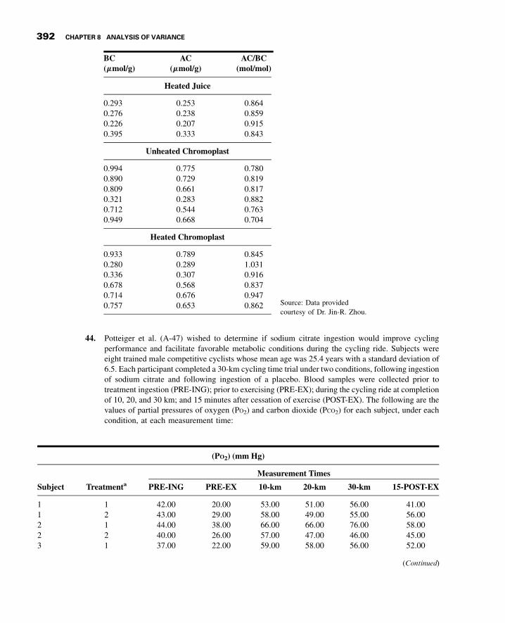
3GC08 12/04/2012 14:43:54 Page 392

BC(mmol/g)

AC(mmol/g)

AC/BC(mol/mol)

Heated Juice

0.293 0.253 0.8640.276 0.238 0.8590.226 0.207 0.9150.395 0.333 0.843

Unheated Chromoplast

0.994 0.775 0.7800.890 0.729 0.8190.809 0.661 0.8170.321 0.283 0.8820.712 0.544 0.7630.949 0.668 0.704

Heated Chromoplast

0.933 0.789 0.8450.280 0.289 1.0310.336 0.307 0.9160.678 0.568 0.8370.714 0.676 0.9470.757 0.653 0.862 Source: Data provided

courtesy of Dr. Jin-R. Zhou.

44. Potteiger et al. (A-47) wished to determine if sodium citrate ingestion would improve cyclingperformance and facilitate favorable metabolic conditions during the cycling ride. Subjects wereeight trained male competitive cyclists whose mean age was 25.4 years with a standard deviation of6.5. Each participant completed a 30-km cycling time trial under two conditions, following ingestionof sodium citrate and following ingestion of a placebo. Blood samples were collected prior totreatment ingestion (PRE-ING); prior to exercising (PRE-EX); during the cycling ride at completionof 10, 20, and 30 km; and 15 minutes after cessation of exercise (POST-EX). The following are thevalues of partial pressures of oxygen (PO2) and carbon dioxide (PCO2) for each subject, under eachcondition, at each measurement time:

(PO2) (mm Hg)

Measurement Times

Subject Treatmenta PRE-ING PRE-EX 10-km 20-km 30-km 15-POST-EX

1 1 42.00 20.00 53.00 51.00 56.00 41.001 2 43.00 29.00 58.00 49.00 55.00 56.002 1 44.00 38.00 66.00 66.00 76.00 58.002 2 40.00 26.00 57.00 47.00 46.00 45.003 1 37.00 22.00 59.00 58.00 56.00 52.00

(Continued)


3GC08 12/04/2012 14:43:55 Page 393

(PO2) (mm Hg)

Measurement Times


3 2 36.00 30.00 52.00 65.00 65.00 36.004 1 34.00 21.00 65.00 62.00 62.00 59.004 2 46.00 36.00 65.00 72.00 72.00 66.005 1 36.00 24.00 41.00 43.00 50.00 46.005 2 41.00 25.00 52.00 60.00 67.00 54.006 1 28.00 31.00 52.00 60.00 53.00 46.006 2 34.00 21.00 57.00 58.00 57.00 41.007 1 39.00 28.00 72.00 69.00 65.00 72.007 2 40.00 27.00 64.00 61.00 57.00 60.008 1 49.00 27.00 67.00 61.00 51.00 49.008 2 27.00 22.00 56.00 64.00 49.00 34.00

(PCO2) (mm Hg)

Measurement Times


1 1 31.70 30.20 28.20 29.80 28.20 30.101 2 24.60 24.40 34.40 35.20 30.90 34.002 1 27.10 35.90 31.30 35.40 34.10 42.002 2 21.70 37.90 31.90 39.90 45.10 48.003 1 37.40 49.60 39.90 39.70 39.80 42.803 2 38.40 42.10 40.90 37.70 37.70 45.604 1 36.60 45.50 34.80 33.90 34.00 40.504 2 39.20 40.20 31.90 32.30 33.70 45.905 1 33.70 39.50 32.90 30.50 28.50 37.205 2 31.50 37.30 32.40 31.90 30.20 31.706 1 35.00 41.00 38.70 37.10 35.80 40.006 2 27.20 36.10 34.70 36.30 34.10 40.607 1 28.00 36.50 30.70 34.60 34.30 38.607 2 28.40 31.30 48.10 43.70 35.10 34.708 1 22.90 28.40 25.70 28.20 32.30 34.808 2 41.40 41.80 29.50 29.90 31.30 39.00

a 1 ¼ Sodium citrate; 2 ¼ placebo.Source: Data provided courtesy of Dr. Jeffrey A. Potteiger.

45. Teitge et al. (A-48) describe a radiographic method to demonstrate patellar instability. The 90subjects ranged in age from 13 to 52 years and were divided into the following four groups onthe basis of clinical findings regarding the nature of instability of the knee: normal (nosymptoms or signs related to the knee), lateral, medial, and multidirectional instability. Amongthe data collected were the following radiographic measurements of the congruence angle(degrees):


3GC08 12/04/2012 14:43:57 Page 394

Normal Lateral Medial Multidirectional

�8 4 12 �16 10 15�16 18 �8 �25 �5 �26�22 5 �8 20 �10 �8�26 �6 �20 �8 �12 �12�8 32 �5 8 �14 �4012 30 �10 �14 �20�8 �10 �18 �1612 28 �4 �34

�20 6 �20 �14�20 9 �20 �6�5 10 �20 �3510 20 �22 �24�4 �9 �15 �25�2 �10 �10 10�6 12 �5 �16�7 0 �5 �30

0 35 �6 �30�2 �1 �15�15 5 �25�5 22 �10

22 �20

Source: Data provided courtesy of Dr. Robert A. Teitge.

46. A study by Ikeda et al. (A-49) was designed to determine the dose of ipratropium bromide aerosolthat improves exercise performance using progressive cycle ergometry in patients with stable chronicobstructive pulmonary disease. The mean age of the 20 male subjects was 69.2 years with a standarddeviation of 4.6 years. Among the data collected were the following maximum ventilationVEmax;L=min� �

values at maximum achieved exercise for different ipratropium bromide dosagelevels mgð Þ:

Placebo 40 80 160 240

26 24 23 25 2838 39 43 43 3749 46 54 57 5237 39 39 38 3834 33 37 37 4142 38 44 44 4223 26 28 27 2238 41 44 37 4037 37 36 38 3933 35 34 38 3640 37 40 46 4052 58 48 58 6345 48 47 51 38

(Continued)


3GC08 12/04/2012 14:43:57 Page 395

Placebo 40 80 160 240

24 30 23 27 3041 37 39 46 4256 54 51 58 5835 51 49 51 4628 41 37 33 3828 34 34 35 3538 40 43 39 45

Source: Data provided courtesy of Dr. Akihiko Ikeda.

47. Pertovaara et al. (A-50) compared the effect of skin temperature on the critical threshold temperatureeliciting heat pain with the effect of skin temperature on the response latency to the first heat painsensation. Subjects were healthy adults between the ages of 23 and 54 years. Among the datacollected were the following latencies (seconds) to the first pain response induced by radiant heatstimulation at three different skin temperatures:

Subject 25�C 30�C 35�C

1 6.4 4.5 3.62 8.1 5.7 6.33 9.4 6.8 3.24 6.75 4.6 3.95 10 6.2 6.26 4.5 4.2 3.4

Source: Data provided courtesy of Dr. Antti Pertovaara.

48. A study for the development and validation of a sensitive and specific method for quantifying totalactivin-A concentrations has been reported on by Knight et al. (A-51). As part of the study theycollected the following peripheral serum concentrations of activin-A in human subjects ofdiffering reproductive status: normal follicular phase (FP), normal luteal phase (LP), pregnant(PREG), ovarian hyperstimulated for in vivo fertilization (HYP), postmenopausal (PM), andnormal adult males. Hint: Convert responses to logarithms before performing analysis.

FP LP PREG HYP PM Male

134.5 78.0 2674.0 253.1 793.1 196.7159.2 130.4 945.6 294.3 385.1 190.6133.2 128.3 5507.6 170.2 270.9 185.3225.0 166.4 7796.5 219.8 640.3 335.4146.4 115.2 5077.5 165.8 459.8 214.6180.5 148.9 4541.9 159.0

Source: Data provided courtesy of Dr. Philip G. Knight.

49. The purpose of a study by Maheux et al. (A-52) was to evaluate the effect of labor on glucoseproduction and glucose utilization. Subjects were six normal pregnant women. Among the data


3GC08 12/04/2012 14:43:58 Page 396

collected were the following glucose concentrations during four stages of labor: latent (A1) andactive (A2) phases of cervical dilatation, fetal expulsion (B), and placental expulsion (C).

A1 A2 B C

3.60 4.40 5.30 6.203.53 3.70 4.10 3.804.02 4.80 5.40 5.274.90 5.33 6.30 6.204.06 4.65 6.10 6.903.97 5.20 4.90 4.60

Source: Data provided courtesy of Dr. Pierre C. Maheux.

50. Trachtman et al. (A-53) conducted studies (1) to assess the effect of recombinant human (rh) IGF-I onchronic puromycin aminonucleoside (PAN) nephropathy and (2) to compare the results of rhIGF-Iversus rhGH treatment in a model of focal segmental glomerulosclerosis. As part of the studies, maleSprague-Dawley rats were divided into four groups: PAN (IA), PAN þ rhIGF-I (IB), normal (IIA),and normal þ rhIGF-I (IIB). The animals yielded the following data on creatinine levels before (pre)and after 4, 8, and 12 weeks of treatment:

Group

IA IB IIA IIB

Pre

44 44 44 3544 44 44 4444 44 44 4453 44 44 3544 4444 53

4 Weeks

97 44 53 4488 35 44 5362 44 44 5353 35 53 4462 6253 53

8 Weeks

53 53 62 4453 53 53 6244 53 62 4453 44 53 4462 5370 62

(Continued)


3GC08 12/04/2012 14:44:0 Page 397

Group

IA IB IIA IIB

12 Weeks

88 79 53 5370 79 62 6253 79 53 5370 62 62 5388 7988 70

Source: Data provided courtesy of Dr. Howard Trachtman.

51. Twelve healthy men, ages 22 through 35 years, yielded the following serum T3ðnmol=LÞ levels at0800 hours after 8 (day 1), 32 (day 2), and 56 (day 3) hours of fasting, respectively. Subjects wereparticipants in a study of fasting-induced alterations in pulsatile glycoprotein secretion conducted bySamuels and Kramer (A-54).

Subject T3 Day Subject T3 Day Subject T3 Day Subject T3 Day

1 88 1 2 115 1 3 119 1 4 164 11 73 2 2 77 2 3 93 2 4 120 21 59 3 2 75 3 3 65 3 4 86 3


5 93 1 6 119 1 7 152 1 8 121 15 91 2 6 57 2 7 70 2 8 107 25 113 3 6 44 3 7 74 3 8 133 3


9 108 1 10 124 1 11 102 1 12 131 19 93 2 10 97 2 11 56 2 12 83 29 75 3 10 74 3 11 58 3 12 66 3

Source: Data provided courtesy of Dr. Mary H. Samuels.

52. To determine the nature and extent to which neurobehavioral changes occur in association with thetoxicity resulting from exposure to excess dietary iron (Fe), Sobotka et al. (A-55) used weanling maleSprague-Dawley rats as experimental subjects. The researchers randomly assigned the animals,according to ranked body weights, to one of five diet groups differentiated on the basis of amountof Fe present: Control—35 (1), 350 (2), 3500 (3), 4 (iron deficient) (4), and 20,000 (5) ppm,respectively. The following are the body weights of the animals (grams) at the end of 10 weeks.

Diet Weight Diet Weight Diet Weight

1 396 1 335 1 3732 368 2 349 4 2923 319 3 302 5 116

(Continued)


3GC08 12/04/2012 14:44:1 Page 398

Diet Weight Diet Weight Diet Weight

4 241 4 220 4 2915 138 5 118 5 1541 331 1 394 4 2812 325 2 300 5 1183 331 3 285 4 2504 232 4 237 5 1195 116 5 113 4 2421 349 1 377 5 1182 364 2 366 4 2773 392 3 269 5 1044 310 4 344 5 1205 131 5 Dead 5 1021 341 1 3362 399 2 3793 274 3 1954 319 4 2775 131 5 1481 419 1 3012 373 2 3683 Dead 3 3084 220 4 2995 146 5 Dead

Source: Data provided courtesy of Dr. Thomas J. Sobotka.

53. Hansen (A-56) notes that brain bilirubin concentrations are increased by hyperosmolality andhypercarbia, and that previous studies have not addressed the question of whether increased brainbilirubin under different conditions is due to effects on the entry into or clearance of bilirubin frombrain. In a study, he hypothesized that the kinetics of increased brain bilirubin concentration woulddiffer in respiratory acidosis (hypercarbia) and hyperosmolality. Forty-four young adult maleSprague-Dawley rats were sacrificed at various time periods following infusion with bilirubin.The following are the blood bilirubin levels mmol=Lð Þ of 11 animals just prior to sacrifice 60 minutesafter the start of bilirubin infusion:

Controls Hypercarbia Hyperosmolality

30 48 10294 20 11878 58 7452 74

Source: Data provided courtesy of Dr. Thor Willy Ruud Hansen.

54. Johansson et al. (A-57) compared the effects of short-term treatments with growth hormone (GH) andinsulin-like growth factor I (IGF-I) on biochemical markers of bone metabolism in men withidiopathic osteoporosis. Subjects ranged in age from 32 to 57 years. Among the data collected werethe following serum concentrations of IGF binding protein-3 at 0 and 7 days after first injection and 1,4, 8, and 12 weeks after last injection with GH and IGF-I.


3GC08 12/04/2012 14:44:2 Page 399

Patient No. Treatment 0 Day 7 Days 1 Week 4 Weeks 8 Weeks 12 Weeks

1 GH 4507 4072 3036 2484 3540 34801 IGF-I 3480 3515 4003 3667 4263 47972 GH 2055 4095 2315 1840 2483 23542 IGF-I 2354 3570 3630 3666 2700 27823 GH 3178 3574 3196 2365 4136 30883 IGF-I 3088 3405 3309 3444 2357 38314 GH 3464 5874 2929 3903 3367 29384 IGF-I 2905 2888 2797 3083 3376 34645 GH 4142 4465 3967 4213 4321 49905 IGF-I 4990 4590 2989 4081 4806 44356 GH 3622 6800 6185 4247 4450 41996 IGF-I 3504 3529 4093 4114 4445 36227 GH 5390 5188 4788 4602 4926 57937 IGF-I 5130 4784 4093 4852 4943 53908 GH 3161 4942 3222 2699 3514 29638 IGF-I 3074 2691 2614 3003 3145 31619 GH 3228 5995 3315 2919 3235 43799 IGF-I 4379 3548 3339 2379 2783 3000

10 GH 5628 6152 4415 5251 3334 391010 IGF-I 5838 5025 4137 5777 5659 562811 GH 2304 4721 3700 3228 2440 269811 IGF-I 2698 2621 3072 2383 3075 2822

Source: Data provided courtesy of Dr. Anna G. Johansson.

55. The objective of a study by Strijbos et al. (A-58) was to compare the results of a 12-week hospital-based outpatient rehabilitation program (group 1) with those of a 12-week home-care rehabilitationprogram (group 2) in chronic obstructive pulmonary disease with moderate to severe airflowlimitation. A control group (group 3) did not receive rehabilitation therapy. Among the data collectedwere the following breathing frequency scores of subjects 18 months after rehabilitation:

Group Group

1 2 3 1 2 3

12 16 24 12 16 2416 14 16 12 12 1416 12 18 14 12 1514 12 18 16 12 1612 18 24 12 12 1612 12 24 12 15 1812 10 18 20 16

Source: Data provided courtesy of Dr. Jaap H. Strijbos.

56. Seven healthy males (mean age 27.4 years with a standard deviation of 4.4) participated in a study byLambert et al. (A-59), who measured intestinal absorption following oral ingestion and intestinalperfusion of a fluid. As part of the study the researchers recorded the following percent changes in


3GC08 12/04/2012 14:44:4 Page 400

plasma volume at six points during 85 minutes of cycle exercise in the drinking and infusionexperiments:

Subject 1 2 3

Drinking

1 �8.4151514 �7.4902674 �8.022773302 �12.1966790 �5.1496679 �10.464863003 �9.7418719 �5.9062747 �7.065169504 �15.0291920 �14.4165470 �16.612682005 �5.8845683 �5.8845683 �3.577817506 �9.7100000 �7.5700000 �3.529955607 �6.9787024 �6.5752716 �5.07020210

Infusion

1 �13.5391010 �11.7186910 �10.773129002 �8.8259516 �8.9029745 �6.381600303 �4.2410016 �1.3448910 �2.497403904 �10.7192870 �9.7651132 �11.121409005 �6.9487760 �2.9830660 1.778281576 �7.1160660 �5.4111706 �7.070863407 �7.0497788 �5.7725485 �5.18045500

Subject 4 5 6

Drinking

1 �7.35202650 �7.89172340 �7.847267002 �8.40517240 �9.02789810 5.133339853 �4.19974130 �3.33795970 �5.653807004 �15.36239700 �17.63314100 �14.439820005 �5.50433470 �5.12242600 �6.263137906 �4.22938570 �7.86923080 �7.511682207 �5.94416340 �5.21535350 �6.34285620

Infusion

1 �11.64145400 �12.40814000 �8.264113202 �5.69396590 �6.38160030 �7.373509203 �1.01234570 �5.58572150 �2.818110904 �12.13053100 �15.98360700 �12.646675005 2.28844839 2.59034233 1.566220586 �8.35430040 �10.60663700 �9.456895807 �7.92841880 �8.38462720 �8.44542770

Source: Data provided courtesy of Dr. C. V. Gisolfi.

57. Roemer et al. (A-60) developed a self-report measure of generalized anxiety disorder(GAD) for use with undergraduate populations. In reliability studies the undergraduatesubjects completed the GAD questionnaire (GAD-Q) as well as the Penn State WorryQuestionnaire (PSWQ). The following are the PSWQ scores made by four groups ofsubjects determined by their GAD status: GAD by questionnaire, Study II (group 1); non-GAD by questionnaire, Study II (group 2); GAD by questionnaire, Study I (group 3); andclinical GAD (group 4).


3GC08 12/04/2012 14:44:5 Page 401

Group

1 2 3 4

59.0 50.0 46.0 65.0 65.051.0 28.0 77.0 62.0 66.058.0 43.0 80.0 76.0 69.061.0 36.0 60.0 66.0 73.064.0 36.0 59.0 78.0 67.068.0 30.0 56.0 76.0 78.064.0 24.0 44.0 74.0 76.067.0 39.0 71.0 73.0 66.056.0 29.0 54.0 61.0 55.078.0 48.0 64.0 63.0 59.048.0 36.0 66.0 75.0 44.062.0 38.0 59.0 63.0 68.077.0 42.0 68.0 55.0 64.072.0 26.0 59.0 67.5 41.059.0 35.0 61.0 70.0 54.0

32.0 78.0 70.0 72.043.0 70.0 55.0 74.055.0 74.0 73.0 59.042.0 73.0 80.0 63.037.0 79.0 51.036.0 79.0 72.041.0 61.0 63.036.0 61.0 58.034.0 72.0 71.042.0 67.035.0 74.051.0 65.037.0 68.050.0 72.039.0 75.0

56.0

Source: Data provided courtesy of Dr. T. D. Borkovec.

58. Noting that non-Hodgkin’s lymphomas (NHL) represent a heterogeneous group of diseases in whichprognosis is difficult to predict, Christiansen et al. (A-61) report on the prognostic aspects of solubleintercellular adhesion molecule-1 (sICAM-1) in NHL. Among the data collected were the followingserum sICAM-1 (ng/ml) levels in four groups of subjects: healthy controls (C), high-grade NHL(hNHL), low-grade NHL (1NHL), and patients with hairy cell leukemia (HCL).

C hNHL lNHL HCL

309 460 844 824 961 581 382329 222 503 496 1097 601 975314 663 764 656 1099 572 663

(Continued)


3GC08 12/04/2012 14:44:7 Page 402

C hNHL lNHL HCL

254 1235 1088 1038 625 439 429304 500 470 1050 473 1135 1902335 739 806 446 654 590 1842381 1847 482 1218 508 404 314456 477 734 511 454 382 430294 818 616 317 889 692 645450 585 836 334 805 484 637422 1837 1187 1026 541 438 712528 362 581 534 655 787 581461 671 381 292 654 77 860286 375 699 782 1859 478 448309 543 1854 1136 619 602 735226 352 769 476 1837 802388 443 510 534 568377 359 571 424 665310 383 1248 571261 587 784 420350 648 514 408405 782 678 391319 472 1264 493289 506 618 1162310 663 1123 460227 873 912 1113206 987 520 572226 859 1867 653309 1193 485 1340382 1836 287 656325 691 455

522

Source: Data provided courtesy of Dr. Ilse Christiansen.

59. Cossette et al. (A-62) examined gender and kinship with regard to caregivers’ use of informal andformal support and to two models of support. Among the data collected were the following ages ofthree groups of caregivers of a demented relative living at home: husbands, wives, and adultdaughters.

Husband Wife Daughter

64 66 73 59 67 40 5070 58 71 66 67 47 5855 81 70 80 57 46 4667 77 71 76 53 45 4779 76 56 68 50 69 5067 64 68 53 70 48 5377 82 76 78 70 53 5768 85 67 75 50 6572 63 66 74 47 50

(Continued)


3GC08 12/04/2012 14:44:8 Page 403

Husband Wife Daughter

67 72 67 86 62 4377 77 72 63 55 5970 79 72 52 49 4465 63 70 55 43 4565 80 66 71 44 4174 70 73 67 47 5086 85 78 78 57 5872 76 64 70 49 3571 67 78 68 5078 72 59 78 5971 60 71 59 4588 74 70 72 5077 65 67 73 4875 53 78 75 5166 70 67 54 4680 72 55 65 6276 74 64 67 5567 79 69 83 5065 63 59 70 4362 77 55 72 3982 78 75 71 5075 69 68 76 5080 65 74 4374 81 68 2870 79 69

75 72

Source: Data provided courtesy of Sylvie Cossette, M.Sc., R.N.

60. Tasaka et al. (A-63) note that Corynebacterium parvum (CP) increases susceptibility to endotoxin,which is associated with increased production of tumor necrosis factor (TNF). They investigated theeffect of CP-priming on the pathogenesis of acute lung injury caused by intratracheal Escherichiacoli endotoxin (lipopolysaccharide [LPS]). Experimental animals consisted of female guinea pigsdivided into four groups. Animals in two groups received a 4-mg/kg treatment of CP 7 days before thestudy. Subsequently, nonpretreated animals received either saline alone (Control) or endotoxin (LPS-alone). The pretreated groups received either saline (CP-alone) or LPS CP þ LPSð Þ. Among thedata collected were the following values of lung tissue-to-plasma ratio of radio-iodized serumalbumin assay:

Control CP-alone LPS-alone CPþ LPS

0.12503532 0.18191647 0.17669093 0.36511660.10862729 0.30887462 0.25344761 0.640629640.10552931 0.25011885 0.17372285 0.392087340.15587316 0.23858085 0.1786867 0.499420590.13672624 0.26558231 0.22209666 0.857184750.11290446 0.32298454 0.27064831 0.93030465

Source: Data provided courtesy of Dr. Sadatomo Tasaka.


3GC08 12/04/2012 14:44:9 Page 404

61. According to Takahashi et al. (A-64) research indicates that there is an association betweenalterations in calcium metabolism and various bone diseases in patients with other disabilities.Using subjects with severe mental retardation (mean age 16 years) who had been living in institutionsfor most of their lives, Takahashi et al. examined the relationship between bone change and othervariables. Subjects were divided into groups on the basis of severity of bone change. Among the datacollected were the following serum alkaline phosphatase (IU/L) values:

Grade I: 109, 86, 79, 103, 47, 105, 188, 96, 249

Grade II: 86, 106, 164, 146, 111, 263, 162, 111

Grade III: 283, 201, 208, 301, 135, 192, 135, 83, 193, 175, 174, 193, 224,192, 233

Source: Data provided courtesy of Dr. Mitsugi Takahashi.

62. Research indicates that dietary copper deficiency reduces growth rate in rats. In a related study, Allen(A-65) assigned weanling male Sprague-Dawley rats to one of three food groups: copper-deficient(CuD), copper-adequate (CuA), and pair-fed (PF). Rats in the PF group were initially weight-matched to rats of the CuD group and then fed the same weight of the CuA diet as that consumed bytheir CuD counterparts. After 20 weeks, the rats were anesthetized, blood samples were drawn, andorgans were harvested. As part of the study the following data were collected:

Rat Diet

Bodyweight(BW)(g)

Heartweight(HW)(g)

Liverweight(LW)(g)

Kidneyweight(KW)(g)

Spleenweight(SW)(g)

1 253.66 0.89 2.82 1.49 0.412 400.93 1.41 3.98 2.15 0.763 CuD 355.89 1.24 5.15 2.27 0.694 404.70 2.18 4.77 2.99 0.76

6 397.28 0.99 2.34 1.84 0.507 421.88 1.20 3.26 2.32 0.798 PF 386.87 0.88 3.05 1.86 0.849 401.74 1.02 2.80 2.06 0.76

10 437.56 1.22 3.94 2.25 0.75

11 490.56 1.21 4.51 2.30 0.7812 528.51 1.34 4.38 2.75 0.7613 CuA 485.51 1.36 4.40 2.46 0.8214 509.50 1.27 4.67 2.50 0.7915 489.62 1.31 5.83 2.74 0.81

Rat DietHW/BW(g/100 g)

LW/BW(g/100 g)

KW/BW(g/100 g)

SW/BW(g/100 g)

Ceruloplasmin(mg/dl)

1 0.00351 0.01112 0.00587 0.00162 nd2 0.00352 0.00993 0.00536 0.00190 5.273 CuD 0.00348 0.01447 0.00638 0.00194 4.804 0.00539 0.01179 0.00739 0.00188 4.97

(Continued)


3GC08 12/04/2012 14:44:10 Page 405

Rat DietHW/BW(g/100 g)

LW/BW(g/100 g)

KW/BW(g/100 g)

SW/BW(g/100 g)

Ceruloplasmin(mg/dl)

6 0.00249 0.00589 0.00463 0.00126 35.307 0.00284 0.00773 0.00550 0.00187 39.008 PF 0.00227 0.00788 0.00481 0.00217 28.009 0.00254 0.00697 0.00513 0.00189 34.20

10 0.00279 0.00900 0.00514 0.00171 45.20

11 0.00247 0.00919 0.00469 0.00159 34.6012 0.00254 0.00829 0.00520 0.00144 39.0013 CuA 0.00280 0.00906 0.00507 0.00169 37.1014 0.00249 0.00917 0.00491 0.00155 33.4015 0.00268 0.01191 0.00560 0.00165 37.30

nd, no data.Source: Data provided courtesy of Corrie B. Allen.

63. Hughes et al. (A-66) point out that systemic complications in acute pancreatitis are largely responsiblefor mortality associated with the disease. They note further that proinflammatory cytokines, particularlyTNFa, may play a central role in acute pancreatitis by mediating the systemic sequelae. In their researchthey used a bile-infusion model of acute pancreatitis to show amelioration of disease severity as well asan improvement in overall survival by TNFa inhibition. Experimental material consisted of adult maleSprague-Dawley rats weighing between 250 and 300 grams divided into three groups: untreated (bilesolution infused without treatment); treated (bile solution infused preceded by treatment withpolyclonal anti � TNFa antibody); and sham (saline infused). Among the data collected were thefollowing hematocrit (%) values for animals surviving more than 48 hours:

Sham Untreated Treated

38 56 4040 60 4232 50 3836 50 4640 50 3640 3538 4040 4038 5540 35

3640403545

Source: Data provided courtesy ofDr. A. Osama Gaber.

64. A study by Sm�arason et al. (A-67) was motivated by the observations of other researchers that serafrom pre-eclamptic women damaged cultured human endothelial cells. Subjects for the present studywere women with pre-eclampsia, matched control women with normal pregnancies, and nonpregnant


3GC08 12/04/2012 14:44:10 Page 406

women of childbearing age. Among the data collected were the following observations on a relevantvariable measured on subjects in the three groups.

Pre-Eclampsia Pregnant Controls Nonpregnant Controls

113.5 91.4 94.5106.6 95.6 115.9

39.1 113.1 107.295.5 100.8 103.243.5 88.2 104.749.2 92.2 94.999.5 78.6 93.0

102.9 96.9 100.4101.2 91.6 107.1104.9 108.6 105.5

75.4 77.3 119.371.1 100.0 88.273.9 61.7 82.276.0 83.3 125.081.3 103.6 126.172.7 92.3 129.175.3 98.6 106.955.2 85.0 110.090.5 128.2 127.355.8 88.3 128.6

Source: Data provided courtesy of Dr. Alexander Sm�arason.

65. The objective of a study by LeRoith et al. (A-68) was to evaluate the effect of a 7-week administrationof recombinant human GH (rhGH) and recombinant human insulin-like growth factor (rhIGF-I)separately and in combination on immune function in elderly female rhesus monkeys. The assay forthe in vivo function of the immune system relied on the response to an immunization with tetanustoxoid. The following are the responses for the three treatment groups and a control group:

Saline rhIGF-I rhGH rhIGF-I þ rhGH

11.2 12.2 12.15 11.59.0 9.4 11.20 12.4

10.8 10.7 10.60 10.810.0 10.8 11.30 11.9

9.1 11.00 11.012.6

Source: Data provided courtesy of Dr. Jack A. Yanowski.

66. Hampl et al. (A-69) note that inhaled nitric oxide (NO) is a selective pulmonary vasodilator. Theyhypothesized that a nebulized diethylenetriamine/NO (DETA/NO) would stay in the lower airwaysand continuously supply sufficient NO to achieve sustained vasodilation in chronic pulmonaryhypertension. Experimental material consisted of adult, male, specific pathogen-free Sprague-Dawley rats randomly divided into four groups: untreated, pulmonary normotensive controls;


3GC08 12/04/2012 14:44:10 Page 407

monocrotaline-injected (to induce hypertension) with no treatment (MCT); monocrotaline-injectedtreated with either a 5 � mmol dose or a 50 � mmol dose of DETA/NO. Nineteen days after inducingpulmonary hypertension in the two groups of rats, the researchers began the treatment procedure,which lasted for 4 days. They collected, among other data, the following measurements on cardiacoutput for the animals in the four groups:

MCT þ DETA/NO

Control MCT 5mmol 50mmol

71.8 42.8 72.5 47.166.1 53.2 62.9 86.667.6 56.1 58.9 56.066.4 56.5 69.3

Source: Data provided courtesy of Dr. Stephen L. Archer.


1. In Kreiter et al. (A-70) medical school exams were delivered via computer format. Because therewere not enough computer stations to test the entire class simultaneously, the exams wereadministered over 2 days. Both students and faculty wondered if students testing on day 2 mighthave an advantage due to extra study time or a breach in test security. Thus, the researchersexamined a large medical class n ¼ 193ð Þ tested over 2 days with three 2-hour 80-item multiple-choice exams. Students were assigned testing days via pseudorandom assignment. Of interest waswhether taking a particular exam on day 1 or day 2 had a significant impact on scores. Use thedata set MEDSCORES to determine if test, day, or interaction has significant impact on testscores. Let a ¼ :05.

2. Refer to the serum lipid-bound sialic acid data on 1400 subjects (LSADATA). We wish to conducta study to determine if the measurement of serum lipid-bound sialic acid (LSA) might be of use inthe detection of breast cancer. The LSA measurements (mg/dl) are for four populations ofsubjects: normal controls, A; patients with benign breast disease, B; patients with primary breastcancer, C; and patients with recurrent metastatic breast cancer, D. Select a simple random sampleof size 10 from each population and perform an appropriate analysis to determine if we mayconclude that the four population means are different. Let a ¼ :05 and determine the p value. Testall possible pairs of sample means for significance. What conclusions can one draw from theanalysis? Prepare a verbal report of the findings. Compare your results with those of yourclassmates.

3. Refer to the serum angiotensin-converting enzyme data on 1600 subjects (SACEDATA).Sarcoidosis, found throughout the world, is a systemic granulomatous disease of unknowncause. The assay of serum angiotensin-converting enzyme (SACE) is helpful in the diagnosis ofactive sarcoidosis. The activity of SACE is usually increased in patients with the disease, whilenormal levels occur in subjects who have not had the disease, those who have recovered, andpatients with other granulomatous disorders. The data are the SACE values for four populationsof subjects classified according to status regarding sarcoidosis: never had, A; active, B; stable, C;recovered, D. Select a simple random sample of 15 subjects from each population and perform ananalysis to determine if you can conclude that the population means are different. Let a ¼ :05.Use Tukey’s test to test for significant differences among individual pairs of means. Prepare awritten report on your findings. Compare your results with those of your classmates.



3GC08 12/04/2012 14:44:10 Page 408

4. Refer to the urinary colony-stimulating factor data on 1500 subjects (CSFDATA). The data are theurinary colony-stimulating factor (CSF) levels in five populations: normal subjects and subjectswith four different diseases. Each observation represents the mean colony count of four plates from asingle urine specimen from a given subject. Select a simple random sample of size 15 from each ofthe five populations and perform an analysis of variance to determine if one may conclude that thepopulation means are different. Let a ¼ :05. Use Tukey’s HSD statistic to test for significantdifferences among all possible pairs of sample means. Prepare a narrative report on the results ofyour analysis. Compare your results with those of your classmates.

5. Refer to the red blood cell data on 1050 subjects (RBCDATA). Suppose that you are astatistical consultant to a medical researcher who is interested in learning something about therelationship between blood folate concentrations in adult females and the quality of their diet.The researcher has available three populations of subjects: those whose diet quality is rated asgood, those whose diets are fair, and those with poor diets. For each subject there is alsoavailable her red blood cell (RBC) folate value (in mg=liter of red cells). Draw a simple randomsample of size 10 from each population and determine whether the researcher can concludethat the three populations differ with respect to mean RBC folate value. Use Tukey’s test tomake all possible comparisons. Let a ¼ :05 and find the p value for each test. Compare yourresults with those of your classmates.

6. Refer to the serum cholesterol data on 350 subjects under three diet regimens (SERUMCHO).A total of 347 adult males between the ages of 30 and 65 participated in a study to investigatethe relationship between the consumption of meat and serum cholesterol levels. Each subjectate beef as his only meat for a period of 20 weeks, pork as his only meat for another period of20 weeks, and chicken or fish as his only meat for another 20-week period. At the end of eachperiod serum cholesterol determinations mg=100mlð Þ were made on each subject. Select asimple random sample of 10 subjects from the population of 350. Use two-way analysis ofvariance to determine whether one should conclude that there is a difference in populationmean serum cholesterol levels among the three diets. Let a ¼ :05. Compare your results withthose of your classmates.

REFERENCES


1. R. A. FISHER, The Design of Experiments, Eighth Edition, Oliver and Boyd, Edinburgh, 1966.2. R. A. FISHER, Contributions to Mathematical Statistics, Wiley, New York, 1950.3. R. A. FISHER, Statistical Methods for Research Workers, Fourteenth Edition, Hafner, New York, 1973.4. KLAUS HINKELMANN and OSCAR KEMPTHORNE, Design and Analysis of Experiments, Revised Edition, Wiley, New

York, 1994.5. DOUGLAS C. MONTGOMERY, Design and Analysis of Experiments, Fourth Edition, Wiley, New York, 1997.6. JEROME L. MYERS and ARNOLD D. WELL, Research Design and Statistical Analysis, Earlbaum Associates,

Hillsdale, NJ, 1995.7. JASON C. HSU, Multiple Comparisons: Theory and Methods, Chapman & Hall, New York, 1996.8. PETER H. WESTFALL, RANDALL D. TOBIAS, DROR ROM, RUSSELL D. WOLFINGER, and YOSEF HOCHBERG, Multiple

Comparisons and Multiple Tests, SAS Publishing, Cary, NC, 2001.9. J. W. TUKEY, “The Problem of Multiple Comparisons,” Mimeographed Monograph, Princeton University, 1953;

cited in Yosef Hochberg and Ajit C. Tamhane, Multiple Comparison Procedures, John Wiley and Sons, NewYork, 1987.

10. B. J. WINER, Statistical Principles in Experimental Design, Second Edition, McGraw-Hill, New York, 1971.11. C. Y. KRAMER, “Extension of Multiple Range Tests to Group Means with Unequal Sample Sizes,” Biometrics, 63

(1956), 307–310.


3GC08 12/04/2012 14:44:11 Page 409


A-1 DAVID H. HOLBEN, “Selenium Content of Venison, Squirrel, and Beef Purchased or Produced in Ohio, a LowSelenium Region of the United States,” Journal of Food Science, 67 (2002), 431–433.

A-2 W. D. MEMBER, W. M. MURRY, S. I. RINGLEB, K. L. KILGORE, and S. A. SNYDER, “ATransducer to Measure IsometricElbow Moments,” Clinical Biomechanics, 16 (2001), 918–920.

A-3 JOHN P. HOLCOMB and RALPH J. ROTHENBERG,“The Effectiveness of Alendronate and Etidronate in ClinicalPractice,” (unpublished manuscript).

A-4 JASMINKA ILICH-ERNST, RHONDA A. BROWNBILL, MARTHA A. LUDEMANN, and RONGWEI FU, “Critical Factors for BoneHealth in Women across the Age Span: How Important Is Muscle Mass?” MedscapeWomen’s Health eJournal, 7(2002).

A-5 PAUL B. GOLD, ROBERT N. RUBEY, and RICHARD T. HARVEY, “Naturalistic, Self-Assignment Comparative Trial ofBupropion SR, a Nicotine Patch, or Both for Smoking Cessation Treatment in Primary Care,” American Journalon Addictions, 11 (2002), 315–331.

A-6 X. WANG, X. SHEN, X. LI, and C. MAULI AGRAWAL, “Age-Related Changes in the Collagen Network and Toughnessof Bone,” Bone, 31 (2002), 1–7.

A-7 FARHAD ATASSI, “Oral Home Care and the Reasons for Seeking Dental Care by Individuals on Renal Dialysis,”Journal of Contemporary Dental Practice, 3 (2002), 031–041.

A-8 SIMONE RAGAZZI, AGOSTINO PIERRO, MARK PETERS, LORELLA FASOLI, and SIMON EATON, “Early Full Blood Count andSeverity of Disease in Neonates with Necrotizing Enterocolitis,” Pediatric Surgery International, 19 (2003),376–379.

A-9 ROBERTA ROMITO, MARIA IDA PANSINI, FRANCESCO PERTICONE, GIANFRANCO ANTONELLI, MARIAVITTORIA PITZALIS, andPAOLO RIZZON, “Comparative Effect of Lercanidipine, Felodipine, and Nifedipine FITS on Blood Pressure andHeart Rate in Patients with Mild to Moderate Arterial Hypertension: The Lercanidipine in Adults (LEAD)Study,” Journal of Clinical Hypertension, 5 (2003), 249–253.

A-10 L. KOSMISKI, D. KURITZKES, J. HAMILTON, T. SHARP, K. LICHTENSTIEN, J. HILL, and R. ECKEL, “Fat Distribution IsAltered in HIV-Infected Men Without Clinical Evidence of the HIV Lipodystrophy Syndrome,” HIVMedicine, 4(2003), 235–240.

A-11 B. M. BROOKS, F. D. ROSE, E. A. ATTREE, and A. ELLIOT-SQUARE, “An Evaluation of the Efficacy of Training Peoplewith Learning Disabilities in a Virtual Environment,” Disability and Rehabilitation, 24 (2002), 622–626.

A-12 BRIAN J. MCCONVILLE, M. HAROLD FOGELSON, ANDREW B. NORMAN, WILLIAM M. KLYKYLO, PAT Z. MANDERSCHEID,KAREN W. PARKER, and PAUL R. SANBERG, “Nicotine Potentiation of Haloperidol in Reducing Tic Frequency inTourette’s Disorder,” American Journal of Psychiatry, 148 (1991), 793–794.

A-13 M. E. VALENCIA, G. MCNEILL, J. M. BROCKWAY, and J. S. SMITH, “The Effect of Environmental Temperature andHumidity on 24h Energy Expenditure in Men,” British Journal of Nutrition, 68 (September 1992), 319–327.

A-14 D. S. HODGSON, C. I. DUNLOP, P. L. CHAPMAN, and J. L. GRANDY, “Cardiopulmonary Responses to ExperimentallyInduced Gastric Dilatation in Isoflurane-Anesthetized Dogs,” American Journal of Veterinary Research, 53 (June1992), 938–943.

A-15 JOHN C. LICCIARDONE, SCOTT T. STOLL, KIMBERLY G. FULDA, DAVID P. RUSSO, JEFF SIU, WILLIAM WINN, and JOHN

SWIFT, Jr., “Osteopathic Manipulative Treatment for Chronic Low Back Pain: A Randomized Controlled Trial,”Spine, 28 (2003), 1355–1362.

A-16 Mid-Michigan Medical Center, Midland, Michigan, 1999; A study of oral condition of cancer patients. Availableonline at: http://calcnet.mth.cmich.edu/org/spss/Prj_cancer_data.htm.

A-17 YITAO LIU, LUDMILA BELAYEV, WEIZHAO ZHAO, RAUL BUSTO, and MYRON D. GINSBURG, “MRZ 2/579, a NovelUncompetitive N-Methyl-D-Aspartate Antagonist, Reduces Infarct Volume and Brain Swelling and ImprovesNeurological Deficit After Focal Cerebral Ischemia in Rats,” Brain Research, 862 (2000), 111–119.

A-18 DAVID W. STARCH, JERRY W. ALEXANDER, PHILIP C. NOBLE, SURAJ REDDY, and DAVID M. LINTNER, “MultistrandedHamstring Tendon Graft Fixation with a Central Four-Quadrant or a Standard Tibial Interference Screw forAnterior Cruciate Ligament Reconstruction,” American Journal of Sports Medicine, 31 (2003), 338–344.

A-19 D. HOLBEN, A. SMITH, J. ILICH, J. LANDOLL, J. HOLCOMB, and V. MATKOVIK, “Puberty Does Not Negatively AffectSelenium Status in Young Females,” Journal of the American Dietetic Association, 102 (2002), 1082–1087.

A-20 AXEL LINKE, GONG ZHAO, FABIO A. RECCHIA, JEFFREY WILLIAMS, XIAOBIN XU, and THOMAS H. HINTZE, “Shift inMetabolic Substrate Uptake by the Heart During Development of Alloxan-Induced Diabetes,” American Journalof Physiology—Heart and Circulatory Physiology, 285 (2003), H1007–H1014.

REFERENCES 409

http://www.calcnet.mth.cmich.edu/org/spss/Prj_cancer_data.htm

3GC08 12/04/2012 14:44:11 Page 410

A-21 K. WERTHER, I. J. CHRISTENSEN, and H. J. NIELSEN, “Determination of Vascular Endothelial Growth Factor (VEGF)in Circulating Blood: Significance of VEGF in Various Leucocytes and Platelets,” Scandinavian Journal ofClinical and Laboratory Investigation, 62 (2002), 343–350.

A-22 CAROLYN B. YUCHA, SUSAN KOWALSKI, and CHAD L. CROSS. “Student Stress and Academic Performance: HomeHospital Program,” Journal of Nursing Education, 48 (2009), 631–637.

A-23 SHIGEKO URYU, JUN HARADA, MARIE HISAMOTO, and TOMIICHIRO ODA, “Troglitazone Inhibits Both PostglutamateNeurotoxicity and Low-Potassium-Induced Apoptosis in Cerebellar Granule Neurons,” Brain Research, 924(2002), 229–236.

A-24 A. MAIN, H. ABU-SAAD, R. SALT, I. VLACHONIKOLIS, and A. DOWSON, “Management by Nurses of PrimaryHeadache: A Pilot Study,” Current Medical Research Opinion, 18 (2002), 471–478.

A-25 SIMONA PORCELLINI, GUILIANA VALLANTI, SILVIA NOZZA, GUIDO POLI, ADRIANO LAZZARIN, GUISEPPE TABUSSI, andANTONIO GRASSIA, “Improved Thymopoietic Potential in Aviremic HIV Infected Individuals with HAART byIntermittent IL-2 Administration,” AIDS, 17 (2003), 1621–1630.

A-26 DOROTA G�oRECKA, MICHAL BENAREK, ADAM NOWINSKI, ELZBIETA PUSCINSKA, ANNA GOLJAN-GEREMEK, and JAN

ZIELINSKI, “Diagnosis of Airflow Limitation Combined with Smoking Cessation Advice Increases Stop-SmokingRate,” Chest, 123 (2003), 1916–1923.

A-27 ELI MELTZER, BRUCE M. PRENNER, and ANJULI NAYAK, “Efficacy and Tolerability of Once-Daily 5 mg ofDesloratadine, an H1-Receptor Antagonist, in Patients with Seasonal Allergic Rhinitis Assessment Duringthe Spring and Fall Allergy Seasons,” Clinical Drug Investigations, 21 (2001), 25–32.

A-28 K. WERTHER, I. J. CHRISTENSEN, and H. J. NIELSEN, “Determination of Vascular Endothelial Growth Factor (VEGF)in Circulating Blood: Significance of VEGF in Various Leucocytes and Platelets,” Scandinavian Journal ofClinical and Laboratory Investigation, 62 (2002), 343–350.

A-29 RUBIA P. MESHACK and KATHLEEN E. NORMAN, “A Randomized Controlled Trial of the Effects of Weights onAmplitude and Frequency of Postural Hand Tremor in People with Parkinson’s Disease,”Clinical Rehabilitation,16 (2003), 481–492.

A-30 G. LACROIX, S. TISSOT, F. ROGERIEUX, R. BEAULIEU, L. CORNU, C. GILLET, F. R. OBIDEL, J. P. LEFEVRE, and F. Y.BOIS, “Decrease in Ovalbumin-Induced Pulmonary Allergic Response by Benzaldehyde but Not Acetalde-hyde Exposure in a Guinea Pig Model,” Journal of Toxicology and Environmental Health, Part A (2002), 995–1012.

A-31 TAKEMASA WATANABE, YOSHIKI SUGIYAMA, YOSHIKO SUMI, MISUZU WATANABE, KIYOMI TAKEUCHI, FUMIO KOBAYASHI,and KOICHI KONO, “Effects of Vital Exhaustion on Cardiac Autonomic Nervous Functions Assessed by HeartRate Variability at Rest in Middle-Aged Male Workers,” International Journal of Behavioral Medicine, 9 (2002),68–75.

A-32 JOHN BROOKER, Data analyzed by the Wright State University Statistical Consulting Center, Wright StateUniversity, Dayton, OH (1997).

A-33 ELEFTHERIOS KELLIS, Ph.D., “Pubertal Children Are Unable to Relax During the Passive Gravity CorrectionProcedure on the Iskinetic Dynamometer,” Isokinetics and Exercise Science, 10 (2002), 97–105.

A-34 REED E. PYERITZ, ELLIOT K. FISHMAN, BARBARA A.BERNHARDT, and STANLEY S. SIEGELMAN, “Dural Ectasia Is aCommon Feature of the Marfan Syndrome,” American Journal of Human Genetics, 43 (1988), 726–732.

A-35 ADINA HARTMAN-MAEIR, NACHUM SOROKER, HAIM RING, and NOOMI KATZ, “Awareness of Deficits in StrokeRehabilitation,” Journal of Rehabilitation Medicine, 34 (2002), 158–164.

A-36 EFTIHIA V. POLYZOGOPOULOU, FOTIOS KALFARENTZOS, APOSTOLOS G. VAGENAKIS, and THEODORE K. ALEXANDRIDES,“Restoration of Euglycemia and Normal Acute Insulin Response to Glucose in Obese Subjects with Type 2Diabetes Following Bariatric Surgery,” Diabetes, 53 (2003), 1098–1103.

A-37 CAROL S. JOHNSTON and D. L. BOWLING, “Stability of Ascorbic Acid in Commercially Available Orange Juices,”Journal of the American Dietetic Association, 102 (2002), 525–529.

A-38 R. PITTINI, D. OEPKESS, K. MACRURY, R. REZNICK, J. BEYENE, and R. WINDRIM, “Teaching Invasive PerinatalProcedures: Assessment of a High Fidelity Simulator-Based Curriculum,” Ultrasound Obstetrics and Gynecol-ogy, 19 (2002), 478–483.

A-39 NICK ANIM-NYAME, JOHN GAMBLE, SUREN R. SOORANNA, MARK R. JOHNSON, and PHILIP J. STEER, “MicrovascularPermeability Is Related to Circulating Levels of Tumour Necrosis Factor-a in Pre-Eclampsia,” CardiovascularResearch, 58 (2003), 162–169.

A-40 JUN IWAMOTO, TSUYOSHI TAKEDA, SHOICHI ICHIMURA, and MITSUYOSHI UZAWA, “Effects of 5-Year Treatment withElcatonin and Alfacalcidol on Lumbar Bone Mineral Density and the Incidence of Vertebral Fractures in


3GC08 12/04/2012 14:44:11 Page 411

Postmenopausal Women with Osteoporosis: A Retrospective Study,” Journal of Orthopaedic Science, 7 (2002),637–643.

A-41 KIMIKO INOUE, NARUMI OGONUKI, KEIJI MOCHIDA, YOSHIE YAMAMOTO, KAORU TAKANO, FUMITOSHI ISHINO, and ATSUO

OGURA, “Effects of Donor Cell Type and Genotype on the Efficiency of Mouse Somatic Cell Cloning,” Biology ofReproduction, 69 (2003), 1394–1400.

A-42 GOTARO SHIRAKAMI, MASAHIRO MURAKAWA, KOH SHINGU, SUSUMU MASHIMA, SHIN-ICHI SUGA, TATSUO MAGARIBUCHI,TOYOHIKO O’HIGASHI, TSUTOMU SHICHINO, KAZUWA NAKAO, and KENJIRO MORI, “Perioperative Plasma Concentra-tions of Endothelin and Natriuretic Peptides in Children Undergoing Living-Related Liver Transplantation,”Anesthesia and Analgesia, 82 (1996), 235–240.

A-43 MASAHITO SAKAKIBARA and JUNICHIRO HAYANO, “Effect of Slowed Respiration on Cardiac ParasympatheticResponse to Threat,” Psychosomatic Medicine, 58 (1996), 32–37.

A-44 TOSHIAKI TAKAHASHI, YUJI SUTO, SHINSUKE KATO, and EISAKU OHAMA, “Experimental Acute Dorsal Compression ofCat Spinal Cord,” Spine, 21 (1996), 166–173.

A-45 MOTOHIRO YAMASHITA, RALPH A. SCHMID, KAN OKABAYASHI, KOEI ANDO, JUN KOBAYASHI, JOEL D. COOPER, and G.ALEXANDER PATTERSON, “Pentoxifylline in Flush Solution Improves Early Lung Allograft Function,” Annals ofThoracic Surgery, 61 (1996), 1055–1061.

A-46 JIN-R. ZHOU, ERIC T. GUGGER, and JOHN W. ERDMAN, JR., “The Crystalline Form of Carotenes and the Food Matrixin Carrot Root Decrease the Relative Bioavailability of Beta- and Alpha-Carotene in the Ferret Model,” Journalof the American College of Nutrition, 15 (1996), 84–91.

A-47 J. A. POTTEIGER, G. L. NICKEL, M. J. WEBSTER, M. D. HAUB, and R. J. PALMER, “Sodium Citrate Ingestion Enhances30 km Cycling Performance,” International Journal of Sports Medicine, 17 (1996), 7–11.

A-48 ROBERT A. TEITGE, WADE FAERBER, PATRICIA DES MADRYL, and THOMAS M. MATELIC, “Stress Radiographs of thePatellofemoral Joint,” Journal of Bone and Joint Surgery, 78-A (February 1996), 193–203.

A-49 AKIHIKO IKEDA, KOICHI NISHIMURA, HIROSHI KOYAMA, MITSUHIRO TSUKINO, MICHIAKI MISHIMA, and TAKATERU IZUMI,“Dose Response Study of Ipratropium Bromide Aerosol on Maximum Exercise Performance in Stable Patientswith Chronic Obstructive Pulmonary Disease,” Thorax, 51 (1996), 48–53.

A-50 ANTTI PERTOVAARA, TIMO KAUPPILA, and MINNA M. HA€M€AL€AINEN, “Influence of Skin Temperature on Heat PainThreshold in Humans,” Experimental Brain Research, 107 (1996), 497–503.

A-51 P. G. KNIGHT, S. MUTTUKRISHNA, and N. P. GROOME, “Development and Application of a Two-Site EnzymeImmunoassay for the Determination of ‘Total’ Activin-A Concentrations in Serum and Follicular Fluid,” Journalof Endocrinology, 148 (1996), 267–279.

A-52 PIERRE C. MAHEUX, BRIGITTE BONIN, ANNE DIZAZO, PIERRE GUIMOND, DANIELLE MONIER, JOS�EE BOURQUE, and JEAN-LOUIS CHIASSON, “Glucose Homeostasis During Spontaneous Labor in Normal Human Pregnancy,” Journal ofClinical Endocrinology and Metabolism, 81 (1996), 209–215.

A-53 HOWARD TRACHTMAN, JOHN MAESAKA, STEPHEN FUTTERWEIT, CHAN MA, ELSA VALDERRAMA, JAMES C. M. CHAN, andWINNIE CHAN, “The Effect of Recombinant Human Insulin-Like Growth Factor-I on Chronic PuromycinAminonucleoside Nephropathy in Rats,” Pediatric Research, 39 (1996), 13–19.

A-54 M. H. SAMUELS and P. KRAMER, “Differential Effects of Short-Term Fasting on Pulsatile Thyrotropin, Gonado-tropin, and a-Subunit Secretion in Healthy Men—A Clinical Research Center Study,” Journal of ClinicalEndocrinology and Metabolism, 81 (1996), 32–36.

A-55 T. J. SOBOTKA, P. WHITTAKER, J. M. SOBOTKA, R. E. BRODIE, D. Y. QUANDER, M. ROBL, M. BRYANT, and C. N. BARTON,“Neurobehavioral Dysfunctions Associated with Dietary Iron Overload,” Physiology and Behavior, 58 (1996),213–219.

A-56 THOR WILLY RUUD HANSEN, “Bilirubin Entry into and Clearance from Rat Brain During Hypercarbia andHyperosmolality,” Pediatric Research, 39 (1996), 72–76.

A-57 ANNA G. JOHANSSON, ERIK LINDH, WERNER F. BLUM, GINA KOLLERUP, OLE H. SøRENSEN, and SVERKER LJUNGHALL,“Effects of Growth Hormone and Insulin-Like Growth Factor I in Men with Idiopathic Osteoporosis,” Journal ofClinical Endocrinology and Metabolism, 81 (1996), 44–48.

A-58 JAAP H. STRIJBOS, DIRKJE S. POSTMA, RICHARD ALTENA, FERNANDO GIMENO, and GERARD H. KO€ETER, “A ComparisonBetween an Outpatient Hospital-Based Pulmonary Rehabilitation Program and a Home-Care PulmonaryRehabilitation Program in Patients with COPD,” Chest, 109 (1996), 366–372.

A-59 G. P. LAMBERT, R. T. CHANG, D. JOENSEN, X. SHI, R. W. SUMMERS, H. P. SCHEDL, and C. V. GISOLFI, “SimultaneousDetermination of Gastric ing and Intestinal Absorption During Cycle Exercise in Humans,” International Journalof Sports Medicine, 17 (1996), 48–55.

REFERENCES 411

3GC08 12/04/2012 14:44:11 Page 412

A-60 LIZABETH ROEMER, MARY BORKOVEC, SHARON POSA, and T. D. BORKOVEC, “A Self-Diagnostic Measure ofGeneralized Anxiety Disorder,” Journal of Behavior Therapy & Experimental Psychiatry, 26 (1995), 345–350.

A-61 ILSE CHRISTIANSEN, CECILIA GIDL€OF, KARL-MICHAEL KA€LKNER, HANS HAGBERG, HELGE BENNMARKER, and THOMAS

T€oTTERMAN, “Elevated Serum Levels of Soluble ICAM-1 in Non-Hodgkin’s Lymphomas Correlate with TumourBurden, Disease Activity and Other Prognostic Markers,” British Journal of Haematology, 92 (1996), 639–646.

A-62 SYLVIE COSSETTE, LOUISE LE�VESQUE, and LIANE LAURIN, “Informal and Formal Support for Caregivers of a Demen-ted Relative: Do Gender and Kinship Make a Difference?” Research in Nursing & Health, 18 (1995), 437–451.

A-63 SADATOMO TASAKA, AKITOSHI ISHIZAKA, KOICHI SAYAMA, FUMIO SAKAMAKI, HIDETOSHI NAKAMURA, TAKESHI TERA-

SHIMA, YASUHIRO WAKI, KENZO SOEJIMA, MORIO NAKAMURA, HIROAKI MATSUBARA, SEITARO FUJISHIMA, and MINORU

KANAZAWA, “Heat-Killed Corynebacterium parvum Enhances Endotoxin Lung Injury with Increased TNFProduction in Guinea Pigs,” American Journal of Respiratory and Critical Care Medicine, 153 (1996),1047–1055.

A-64 MITSUGI TAKAHASHI, HIDEO NAGAO, and HIROSI MATSUDA, “Estimating Bone Change in Patients with SevereDisability,” Development Medicine and Child Neurology, 37 (1995), 1085–1093.

A-65 CORRIE B. ALLEN, “Effects of Dietary Copper Deficiency on Relative Food Intake and Growth Efficiency in Rats,”Physiology & Behavior, 59 (1996), 247–253.

A-66 CHRISTOPHER B. HUGHES, LILLIAN W. GABER, ABOU BAKR MOHEY EL-DIN, HANI P. GREWAL, MALAK KOTB, LINDA

MANN, and A. OSAMA GABER, “Inhibition of TNFa Improves Survival in an Experimental Model of AcutePancreatitis,” American Surgeon, 62 (1996), 8–13.

A-67 ALEXANDER K. SM�ARASON, IAN L. SARGENT, and CHRISTOPHER W. G. REDMAN, “Endothelial Cell Proliferation IsSuppressed by Plasma but Not Serum from Women with Preeclampsia,” American Journal of Obstetrics andGynecology, 174 (1996), 787–793.

A-68 DEREK LEROITH, JACK YANOWSKI, ERIC P. KALDJIAN, ELAINE S. JAFFE, TANYA LeROITH, KATHY PURDUE, BARBARA

D. COOPER, ROBERT PYLE, and WILLIAM ADLER, “The Effects of Growth Hormone and Insulin-Like Growth Factor Ion the Immune System of Aged Female Monkeys,” Endocrinology, 137 (1996), 1071–1079.

A-69 VA�CLAV HAMPL, MARTIN TRISTANI-FIROUZI, THOMAS C. HUTSELL, and STEPHEN L. ARCHER, “Nebulized Nitric Oxide/Nucleophile Adduct Reduces Chronic Pulmonary Hypertension,” Cardiovascular Research, 31 (1996), 55–62.

A-70 C. KREITER, M. W. PETERSON, K. FERGUSON, and S. ELLIOTT, “The Effects of Testing in Shifts on a Clinical In-Course Computerized Exam,” Medical Education, 37 (2003), 202–204.


3GC09 12/04/2012 15:4:23 Page 413

CHAPTER9SIMPLE LINEAR REGRESSIONAND CORRELATION

CHAPTER OVERVIEW

This chapter provides an introduction and overview of two common techniquesfor exploring the strength of the relationship between two variables. The firsttechnique, linear regression, will help us find an objective way to predict orestimate the value of one variable given a value of another variable. The secondtechnique, correlation, will help us find an objective measure of the strength ofthe relationship between two variables.

TOPICS

9.1 INTRODUCTION

9.2 THE REGRESSION MODEL

9.3 THE SAMPLE REGRESSION EQUATION

9.4 EVALUATING THE REGRESSION EQUATION

9.5 USING THE REGRESSION EQUATION

9.6 THE CORRELATION MODEL

9.7 THE CORRELATION COEFFICIENT

9.8 SOME PRECAUTIONS

9.9 SUMMARY

LEARNING OUTCOMES


1. be able to obtain a simple linear regression model and use it to make predictions.

2. be able to calculate the coefficient of determination and to interpret tests ofregression coefficients.

3. be able to calculate correlations among variables.

4. understand how regression and correlation differ and when the use of each isappropriate.

413

3GC09 12/04/2012 15:4:23 Page 414

9.1 INTRODUCTION

In analyzing data for the health sciences disciplines, we find that it is frequently desirable tolearn something about the relationship between two numeric variables. We may, for example,be interested in studying the relationship between blood pressure and age, height and weight,the concentration of an injected drug and heart rate, the consumption level of some nutrientand weight gain, the intensity of a stimulus and reaction time, or total family income andmedical care expenditures. The nature and strength of the relationships between variablessuch as these may be examined using linear models such as regression and correlationanalysis, two statistical techniques that, although related, serve different purposes.

Regression Regression analysis is helpful in assessing specific forms of the relation-ship between variables, and the ultimate objective when this method of analysis is employedusually is to predict or estimate the value of one variable corresponding to a given value ofanother variable. The ideas of regression were first elucidated by the English scientist SirFrancis Galton (1822–1911) in reports of his research on heredity—first in sweet peas andlater in human stature. He described a tendency of adult offspring, having either short or tallparents, to revert back toward the average height of the general population. He first used theword reversion, and later regression, to refer to this phenomenon.

Correlation Correlation analysis, on the other hand, is concerned with measuringthe strength of the relationship between variables. When we compute measures ofcorrelation from a set of data, we are interested in the degree of the correlation betweenvariables. Again, the concepts and terminology of correlation analysis originated withGalton, who first used the word correlation in 1888.

In this chapter our discussion is limited to the exploration of the linear relationshipbetween two variables. The concepts and methods of regression are covered first,beginning in the next section. In Section 9.6 the ideas and techniques of correlationare introduced. In the next chapter we consider the case where there is an interest in therelationships among three or more variables.

Regression and correlation analysis are areas in which the speed and accuracy of acomputer are most appreciated. The data for the exercises of this chapter, therefore, arepresented in a way that makes them suitable for computer processing. As is always the case,the input requirements and output features of the particular programs and softwarepackages to be used should be studied carefully.

9.2 THE REGRESSIONMODEL

In the typical regression problem, as in most problems in applied statistics, researchers haveavailable for analysis a sample of observations from some real or hypothetical population.Based on the results of their analysis of the sample data, they are interested in reachingdecisions about the population from which the sample is presumed to have been drawn. It isimportant, therefore, that the researchers understand the nature of the population in whichthey are interested. They should know enough about the population to be able either toconstruct a mathematical model for its representation or to determine if it reasonably fits

414 CHAPTER 9 SIMPLE LINEAR REGRESSION AND CORRELATION

3GC09 12/04/2012 15:4:23 Page 415

some established model. A researcher about to analyze a set of data by the methods of simplelinear regression, for example, should be secure in the knowledge that the simple linearregression model is, at least, an approximate representation of the population. It is unlikelythat the model will be a perfect portrait of the real situation, since this characteristic is seldomfound in models of practical value. A model constructed so that it corresponds precisely withthe details of the situation is usually too complex to yield any information of value. On theother hand, the results obtained from the analysis of data that have been forced into a modelthat does not fit are also worthless. Fortunately, however, a perfectly fitting model is not arequirement for obtaining useful results. Researchers, then, should be able to distinguishbetween the occasion when their chosen models and the data are sufficiently compatible forthem to proceed and the case where their chosen model must be abandoned.

Assumptions Underlying Simple Linear Regression In the simplelinear regression model two variables, usually labeled X and Y, are of interest. The letter X isusually used to designate a variable referred to as the independent variable, sincefrequently it is controlled by the investigator; that is, values of X may be selected bythe investigator and, corresponding to each preselected value of X, one or more values ofanother variable, labeled Y, are obtained. The variable, Y, accordingly, is called thedependent variable, and we speak of the regression of Y on X. The following are theassumptions underlying the simple linear regression model.

1. Values of the independent variable X are said to be “fixed.” This means that thevalues of X are preselected by the investigator so that in the collection of the data theyare not allowed to vary from these preselected values. In this model, X is referred toby some writers as a nonrandom variable and by others as a mathematical variable. Itshould be pointed out at this time that the statement of this assumption classifies ourmodel as the classical regression model. Regression analysis also can be carried outon data in which X is a random variable.

2. The variable X is measured without error. Since no measuring procedure is perfect,this means that the magnitude of the measurement error in X is negligible.

3. For each value of X there is a subpopulation of Y values. For the usual inferentialprocedures of estimation and hypothesis testing to be valid, these subpopulationsmust be normally distributed. In order that these procedures may be presented it willbe assumed that the Y values are normally distributed in the examples and exercisesthat follow.

4. The variances of the subpopulations of Y are all equal and denoted by s2.

5. The means of the subpopulations of Y all lie on the same straight line. This is knownas the assumption of linearity. This assumption may be expressed symbolically as

myjx ¼ b0 þ b1x (9.2.1)

where myjx is the mean of the subpopulation of Y values for a particular value of X,and b0 and b1 are called the population regression coefficients. Geometrically, b0 andb1 represent the y-intercept and slope, respectively, of the line on which all of themeans are assumed to lie.

9.2 THE REGRESSIONMODEL 415

3GC09 12/04/2012 15:4:23 Page 416

6. The Y values are statistically independent. In other words, in drawing the sample, it isassumed that the values of Y chosen at one value of X in no way depend on the valuesof Y chosen at another value of X.

These assumptions may be summarized by means of the following equation, which iscalled the simple linear regression model:

y ¼ b0 þ b1xþ e (9.2.2)

where y is a typical value from one of the subpopulations of Y, b0 and b1 are as defined forEquation 9.2.1, and e is called the error term. If we solve 9.2.2 for e, we have

e ¼ y� b0 þ b1xð Þ¼ y� myjx

(9.2.3)

and we see that e shows the amount by which y deviates from the mean of the subpopulationof Y values from which it is drawn. As a consequence of the assumption that thesubpopulations of Y values are normally distributed with equal variances, the e’s foreach subpopulation are normally distributed with a variance equal to the common varianceof the subpopulations of Y values.

The following acronym will help the reader remember most of the assumptionsnecessary for inference in linear regression analysis:

LINE [Linear (assumption 5), Independent (assumption 6), Normal (assumption 3), Equalvariances (assumption 4)]

A graphical representation of the regression model is given in Figure 9.2.1.

μy|x = β0

+β1x

μy |x1

μy |x2

μy |x3

μy |x4

f(X, Y)

x1

x2

x3

x4

X

Y

FIGURE 9.2.1 Representation of the simple linear regression model.


3GC09 12/04/2012 15:4:24 Page 417

9.3 THE SAMPLE REGRESSION EQUATION

In simple linear regression the object of the researcher’s interest is the populationregression equation—the equation that describes the true relationship between thedependent variable Y and the independent variable X. The variable designated by Y issometimes called the response variable and X is sometimes called the predictor variable.

In an effort to reach a decision regarding the likely form of this relationship, theresearcher draws a sample from the population of interest and using the resulting data,computes a sample regression equation that forms the basis for reaching conclusionsregarding the unknown population regression equation.

Steps in Regression Analysis In the absence of extensive informationregarding the nature of the variables of interest, a frequently employed strategy is toassume initially that they are linearly related. Subsequent analysis, then, involves thefollowing steps.

1. Determine whether or not the assumptions underlying a linear relationship are met inthe data available for analysis.

2. Obtain the equation for the line that best fits the sample data.

3. Evaluate the equation to obtain some idea of the strength of the relationship and theusefulness of the equation for predicting and estimating.

4. If the data appear to conform satisfactorily to the linear model, use the equationobtained from the sample data to predict and to estimate.

When we use the regression equation to predict, we will be predicting the value Y islikely to have when X has a given value. When we use the equation to estimate, we will beestimating the mean of the subpopulation of Y values assumed to exist at a given value of X.Note that the sample data used to obtain the regression equation consist of known values ofboth X and Y. When the equation is used to predict and to estimate Y, only the correspondingvalues of X will be known. We illustrate the steps involved in simple linear regressionanalysis by means of the following example.

EXAMPLE 9.3.1

Despr�es et al. (A-1) point out that the topography of adipose tissue (AT) is associated withmetabolic complications considered as risk factors for cardiovascular disease. It isimportant, they state, to measure the amount of intraabdominal AT as part of the evaluationof the cardiovascular-disease risk of an individual. Computed tomography (CT), the onlyavailable technique that precisely and reliably measures the amount of deep abdominal AT,however, is costly and requires irradiation of the subject. In addition, the technique is notavailable to many physicians. Despr�es and his colleagues conducted a study to developequations to predict the amount of deep abdominal AT from simple anthropometricmeasurements. Their subjects were men between the ages of 18 and 42 years whowere free from metabolic disease that would require treatment. Among the measurementstaken on each subject were deep abdominal AT obtained by CT and waist circumference as

9.3 THE SAMPLE REGRESSION EQUATION 417

3GC09 12/04/2012 15:4:26 Page 418

shown in Table 9.3.1. A question of interest is how well one can predict and estimate deepabdominal AT from knowledge of the waist circumference. This question is typical of thosethat can be answered by means of regression analysis. Since deep abdominal AT is thevariable about which we wish to make predictions and estimations, it is the dependentvariable. The variable waist measurement, knowledge of which will be used to make thepredictions and estimations, is the independent variable.

TABLE 9.3.1 Waist Circumference (cm), X, and Deep Abdominal AT, Y, of 109 Men

Subject X Y Subject X Y Subject X Y

1 74.75 25.72 38 103.00 129.00 75 108.00 217.00

2 72.60 25.89 39 80.00 74.02 76 100.00 140.00

3 81.80 42.60 40 79.00 55.48 77 103.00 109.00

4 83.95 42.80 41 83.50 73.13 78 104.00 127.00

5 74.65 29.84 42 76.00 50.50 79 106.00 112.00

6 71.85 21.68 43 80.50 50.88 80 109.00 192.00

7 80.90 29.08 44 86.50 140.00 81 103.50 132.00

8 83.40 32.98 45 83.00 96.54 82 110.00 126.00

9 63.50 11.44 46 107.10 118.00 83 110.00 153.00

10 73.20 32.22 47 94.30 107.00 84 112.00 158.00

11 71.90 28.32 48 94.50 123.00 85 108.50 183.00

12 75.00 43.86 49 79.70 65.92 86 104.00 184.00

13 73.10 38.21 50 79.30 81.29 87 111.00 121.00

14 79.00 42.48 51 89.80 111.00 88 108.50 159.00

15 77.00 30.96 52 83.80 90.73 89 121.00 245.00

16 68.85 55.78 53 85.20 133.00 90 109.00 137.00

17 75.95 43.78 54 75.50 41.90 91 97.50 165.00

18 74.15 33.41 55 78.40 41.71 92 105.50 152.00

19 73.80 43.35 56 78.60 58.16 93 98.00 181.00

20 75.90 29.31 57 87.80 88.85 94 94.50 80.95

21 76.85 36.60 58 86.30 155.00 95 97.00 137.00

22 80.90 40.25 59 85.50 70.77 96 105.00 125.00

23 79.90 35.43 60 83.70 75.08 97 106.00 241.00

24 89.20 60.09 61 77.60 57.05 98 99.00 134.00

25 82.00 45.84 62 84.90 99.73 99 91.00 150.00

26 92.00 70.40 63 79.80 27.96 100 102.50 198.00

27 86.60 83.45 64 108.30 123.00 101 106.00 151.00

28 80.50 84.30 65 119.60 90.41 102 109.10 229.00

29 86.00 78.89 66 119.90 106.00 103 115.00 253.00

30 82.50 64.75 67 96.50 144.00 104 101.00 188.00

31 83.50 72.56 68 105.50 121.00 105 100.10 124.00

32 88.10 89.31 69 105.00 97.13 106 93.30 62.20

33 90.80 78.94 70 107.00 166.00 107 101.80 133.00

34 89.40 83.55 71 107.00 87.99 108 107.90 208.00

35 102.00 127.00 72 101.00 154.00 109 108.50 208.00

36 94.50 121.00 73 97.00 100.00

37 91.00 107.00 74 100.00 123.00

Source: Data provided courtesy of Jean-Pierre Despr�es, Ph.D.


3GC09 12/04/2012 15:4:26 Page 419

The Scatter Diagram

A first step that is usually useful in studying the relationship between two variables is toprepare a scatter diagram of the data such as is shown in Figure 9.3.1. The points areplotted by assigning values of the independent variable X to the horizontal axis and valuesof the dependent variable Y to the vertical axis.

The pattern made by the points plotted on the scatter diagram usually suggests thebasic nature and strength of the relationship between two variables. As we look atFigure 9.3.1, for example, the points seem to be scattered around an invisible straightline. The scatter diagram also shows that, in general, subjects with large waist circumfer-ences also have larger amounts of deep abdominal AT. These impressions suggest that therelationship between the two variables may be described by a straight line crossing the Y-axis below the origin and making approximately a 45-degree angle with the X-axis. It looksas if it would be simple to draw, freehand, through the data points the line that describes therelationship between X and Y. It is highly unlikely, however, that the lines drawn by any twopeople would be exactly the same. In other words, for every person drawing such a line byeye, or freehand, we would expect a slightly different line. The question then arises as towhich line best describes the relationship between the two variables. We cannot obtain ananswer to this question by inspecting the lines. In fact, it is not likely that any freehand line

0

Dee

p a

bd

om

inal

AT

are

a (c

m2 )

, Y

Waist circumference (cm), X

0

20

40

60

80

100

120

140

160

180

200

220

240

260

60 65 70 75 80 85 90 95 100 105 110 115 120 125

FIGURE 9.3.1 Scatter diagram of data shown in Table 9.3.1.


3GC09 12/04/2012 15:4:26 Page 420

drawn through the data will be the line that best describes the relationship between X and Y,since freehand lines will reflect any defects of vision or judgment of the person drawing theline. Similarly, when judging which of two lines best describes the relationship, subjectiveevaluation is liable to the same deficiencies.

What is needed for obtaining the desired line is some method that is not fraught withthese difficulties.

The Least-Squares Line

The method commonly employed for obtaining the desired line is known as the method ofleast squares, and the resulting line is called the least-squares line. The reason for callingthe method by this name will be explained in the discussion that follows.

We recall from algebra that the general equation for a straight line may be written as

y ¼ aþ bx (9.3.1)

where y is a value on the vertical axis, x is a value on the horizontal axis, a is the point wherethe line crosses the vertical axis, and b shows the amount by which y changes for each unitchange in x. We refer to a as the y-intercept and b as the slope of the line. To draw a linebased on Equation 9.3.1, we need the numerical values of the constants a and b. Given theseconstants, we may substitute various values of x into the equation to obtain correspondingvalues of y. The resulting points may be plotted. Since any two such coordinates determinea straight line, we may select any two, locate them on a graph, and connect them to obtainthe line corresponding to the equation.

Obtaining the Least-Square Line

The least-squares regression line equation may be obtained from sample data by simplearithmetic calculations that may be carried out by hand using the following equations

b1 ¼Pni¼1

xi � �xð Þ yi � �yð ÞPni¼1

xi � �xð Þ2(9.3.2)

b0 ¼ �y� b1�x (9.3.3)

where xi and yi are the corresponding values of each data point (X, Y), �x and �y are themeans of the X and Y sample data values, respectively, and b0 and b1 are the estimates ofthe intercept b0 and slope b1, respectively, of the population regression line. Since thenecessary hand calculations are time consuming, tedious, and subject to error, theregression line equation is best obtained through the use of a computer software package.Although the typical researcher need not be concerned with the arithmetic involved, theinterested reader will find them discussed in references listed at the end of this chapter.

For the data in Table 9.3.1 we obtain the least-squares regression equation by meansof MINITAB. After entering the X values in Column 1 and the Y values in Column 2 weproceed as shown in Figure 9.3.2.

For now, the only information from the output in Figure 9.3.2 that we are interested inis the regression equation. Other information in the output will be discussed later.


3GC09 12/04/2012 15:4:26 Page 421


Stat Regression Regression MTB > Name C3 = ‘FITS1’ C4 = ‘RESI1’Type y in Response and x in Predictors. MTB > Regress ‘y’ 1 ‘x’;Click Storage. Check Residuals and Fits. SUBC> Fits ‘FITS1’;Click OK. SUBC> Constant;

SUBC> Residuals ‘RESI1’.

Output:

Regression Analysis: y versus xThe regression equation isy = -216 + 3.46 x

Predictor Coef Stdev t-ratio pConstant -215.98 21.80 -9.91 0.000x 3.4589 0.2347 14.74 0.000

s = 33.06 R-sq = 67.0% R-sq(adj) = 66.7%

Analysis of Variance

SOURCE DF SS MS F pRegression 1 237549 237549 217.28 0.000Error 107 116982 1093Total 108 354531

Unusual ObservationsObs. x y Fit Stdev.Fit Residual St.Resid58 86 155.00 82.52 3.43 72.48 2.20R65 120 90.41 197.70 7.23 -107.29 -3.33R66 120 106.00 198.74 7.29 -92.74 -2.88R71 107 87.99 154.12 4.75 -66.13 -2.02R97 106 241.00 150.66 4.58 90.34 2.76R102 109 229.00 161.38 5.13 67.62 2.07R103 115 253.00 181.79 6.28 71.21 2.19R

R denotes an obs. with a large st. resid.

FIGURE 9.3.2 MINITAB procedure and output for obtaining the least-squares regression

equation from the data in Table 9.3.1.


3GC09 12/04/2012 15:4:26 Page 422

From Figure 9.3.2 we see that the linear equation for the least-squares line thatdescribes the relationship between waist circumference and deep abdominal AT may bewritten, then, as

y ¼ �216 þ 3:46x

This equation tells us that since b0 is negative, the line crosses the Y-axis below theorigin, and that since b1 the slope, is positive, the line extends from the lower left-handcorner of the graph to the upper right-hand corner. We see further that for each unit increasein x, y increases by an amount equal to 3.46. The symbol y denotes a value of y computedfrom the equation, rather than an observed value of Y.

By substituting two convenient values of X into Equation 9.3.2, we may obtain thenecessary coordinates for drawing the line. Suppose, first, we let X ¼ 70 and obtain

y ¼ �216 þ 3:46 70ð Þ ¼ 26:2

If we let X ¼ 110 we obtain

y ¼ �216 þ 3:46 110ð Þ ¼ 164

The line, along with the original data, is shown in Figure 9.3.3.

&

0

Dee

p a

bd

om

inal

AT

are

a (c

m2 )

, Y


0

20

40

60

80

100

120

140

160

180

200

220

240

260

60 65 70 75 80 85 90 95 100 105 110 115 120 125

y = _216 + 3.46x

FIGURE 9.3.3 Original data and least-squares line for Example 9.3.1.


3GC09 12/04/2012 15:4:26 Page 423

The Least-Squares Criterion Now that we have obtained what we call the“best fit” line for describing the relationship between our two variables, we need todetermine by what criterion it is considered best. Before the criterion is stated, let usexamine Figure 9.3.3. We note that generally the least-squares line does not pass throughthe observed points that are plotted on the scatter diagram. In other words, most of theobserved points deviate from the line by varying amounts.

The line that we have drawn through the points is best in this sense:

The sum of the squared vertical deviations of the observed data points (yi) from the least-squares line is smaller than the sum of the squared vertical deviations of the data pointsfrom any other line.

In other words, if we square the vertical distance from each observed point (yi) tothe least-squares line and add these squared values for all points, the resulting total willbe smaller than the similarly computed total for any other line that can be drawnthrough the points. For this reason the line we have drawn is called the least-squaresline.

EXERCISES

9.3.1 Plot each of the following regression equations on graph paper and state whether X and Yare directlyor inversely related.

(a) y ¼ �3 þ 2x

(b) y ¼ 3 þ 0:5x

(c) y ¼ 10 � 0:75x

9.3.2 The following scores represent a nurse’s assessment (X) and a physician’s assessment (Y) of thecondition of 10 patients at time of admission to a trauma center.

X: 18 13 18 15 10 12 8 4 7 3Y: 23 20 18 16 14 11 10 7 6 4

(a) Construct a scatter diagram for these data.

(b) Plot the following regression equations on the scatter diagram and indicate which one you thinkbest fits the data. State the reason for your choice.

(1) y ¼ 8 þ 0:5x(2) y ¼ �10 þ 2x(3) y ¼ 1 þ 1x

For each of the following exercises (a) draw a scatter diagram and (b) obtain the regression equationand plot it on the scatter diagram.

9.3.3 Methadone is often prescribed in the treatment of opioid addiction and chronic pain. Krantz et al.(A-2) studied the relationship between dose of methadone and the corrected QT (QTc) interval for17 subjects who developed torsade de pointes (ventricular tachycardia nearly always due tomedications). QTc is calculated from an electrocardiogram and is measured in mm/sec. A higherQTc value indicates a higher risk of cardiovascular mortality. A question of interest is how wellone can predict and estimate the QTc value from a knowledge of methadone dose. This question istypical of those that can be answered by means of regression analysis. Since QTc is the variable

EXERCISES 423

3GC09 12/04/2012 15:4:28 Page 424

about which we wish to make predictions and estimations, it is the dependent variable. Thevariable methadone dose, knowledge of which will be used to make the predictions andestimations, is the independent variable.

Methadone Dose Methadone Dose(mg/day) QTc (mm/sec) (mg/day) QTc (mm/sec)

1000 600 650 785550 625 600 765

97 560 660 61190 585 270 60085 590 680 625

126 500 540 650300 700 600 635110 570 330 522

65 540

Source: Mori J. Krantz, Ilana B. Kutinsky, Alastair D. Roberston, and Philip S. Mehler,“Dose-Related Effects of Methadone on QT Prolongation in a Series of Patients withTorsade de Pointes,” Pharmacotherapy, 23 (2003), 802–805.

9.3.4 Reiss et al. (A-3) compared point-of-care and standard hospital laboratory assays for monitoringpatients receiving a single anticoagulant or a regimen consisting of a combination of anticoagulants.It is quite common when comparing two measuring techniques, to use regression analysis in whichone variable is used to predict another. In the present study, the researchers obtained measures ofinternational normalized ratio (INR) by assay of capillary and venous blood samples collected from90 subjects taking warfarin. INR, used especially when patients are receiving warfarin, measures theclotting ability of the blood. Point-of-care testing for INR was conducted with the CoaguChek assayproduct. Hospital testing was done with standard hospital laboratory assays. The authors used thehospital assay INR level to predict the CoaguChek INR level. The measurements are given in thefollowing table.

CoaguChek Hospital CoaguChek Hospital CoaguChek Hospital(Y) (X) (Y) (X) (Y) (X)

1.8 1.6 2.4 1.2 3.1 2.41.6 1.9 2.3 2.3 1.7 1.82.5 2.8 2.0 1.6 1.8 1.61.9 2.4 3.3 3.8 1.9 1.71.3 1.5 1.9 1.6 5.3 4.22.3 1.8 1.8 1.5 1.6 1.61.2 1.3 2.8 1.8 1.6 1.42.3 2.4 2.5 1.5 3.3 3.32.0 2.1 0.8 1.0 1.5 1.51.5 1.5 1.3 1.2 2.2 2.82.1 2.4 3.7 1.4 1.1 1.61.5 1.5 2.4 1.6 2.6 2.6

(Continued )


3GC09 12/04/2012 15:4:29 Page 425

1.5 1.7 4.1 3.2 6.4 5.01.8 2.1 2.4 1.2 1.5 1.41.0 1.2 2.3 2.3 3.0 2.82.1 1.9 3.1 1.6 2.6 2.31.6 1.6 1.5 1.4 1.2 1.21.7 1.6 3.6 2.1 2.1 1.92.0 1.9 2.5 1.7 1.1 1.11.8 1.6 2.1 1.7 1.0 1.01.3 4.1 1.8 1.2 1.4 1.51.5 1.9 1.5 1.3 1.7 1.33.6 2.1 2.5 1.1 1.2 1.12.4 2.2 1.5 1.2 2.5 2.42.2 2.3 1.5 1.1 1.2 1.32.7 2.2 1.6 1.2 2.5 2.92.9 3.1 1.4 1.4 1.9 1.72.0 2.2 4.0 2.3 1.8 1.71.0 1.2 2.0 1.2 1.2 1.12.4 2.6 2.5 1.5 1.3 1.1

Source: Data provided courtesy of Curtis E. Haas, Pharm.D.

9.3.5 Digoxin is a drug often prescribed to treat heart ailments. The purpose of a study by Parker et al. (A-4)was to examine the interactions of digoxin with common grapefruit juice. In one experiment, subjectstook digoxin with water for 2 weeks, followed by a 2-week period during which digoxin waswithheld. During the next 2 weeks subjects took digoxin with grapefruit juice. For seven subjects, theaverage peak plasma digoxin concentration (Cmax) when taking water is given in the first column ofthe following table. The second column contains the percent change in Cmax concentration whensubjects were taking the digoxin with grapefruit juice [GFJ (%) change]. Use the Cmax level whentaking digoxin with water to predict the percent change in Cmax concentration when taking digoxinwith grapefruit juice.

Cmax (ngl/ml) with Water Change in Cmax with GFJ (%)

2.34 29.52.46 40.71.87 5.33.09 23.35.59 �45:14.05 �35:36.21 �44:62.34 29.5

Source: Data provided courtesy of Robert B. Parker, Pharm.D.

9.3.6 Evans et al. (A-5) examined the effect of velocity on ground reaction forces (GRF) in dogs withlameness from a torn cranial cruciate ligament. The dogs were walked and trotted over a force

CoaguChek Hospital CoaguChek Hospital CoaguChek Hospital(Y) (X) (Y) (X) (Y) (X)

EXERCISES 425

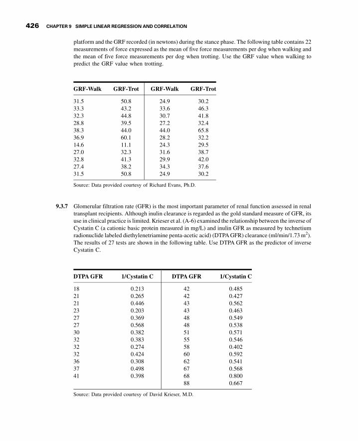
3GC09 12/04/2012 15:4:29 Page 426

platform and the GRF recorded (in newtons) during the stance phase. The following table contains 22measurements of force expressed as the mean of five force measurements per dog when walking andthe mean of five force measurements per dog when trotting. Use the GRF value when walking topredict the GRF value when trotting.

GRF-Walk GRF-Trot GRF-Walk GRF-Trot

31.5 50.8 24.9 30.233.3 43.2 33.6 46.332.3 44.8 30.7 41.828.8 39.5 27.2 32.438.3 44.0 44.0 65.836.9 60.1 28.2 32.214.6 11.1 24.3 29.527.0 32.3 31.6 38.732.8 41.3 29.9 42.027.4 38.2 34.3 37.631.5 50.8 24.9 30.2

Source: Data provided courtesy of Richard Evans, Ph.D.

9.3.7 Glomerular filtration rate (GFR) is the most important parameter of renal function assessed in renaltransplant recipients. Although inulin clearance is regarded as the gold standard measure of GFR, itsuse in clinical practice is limited. Krieser et al. (A-6) examined the relationship between the inverse ofCystatin C (a cationic basic protein measured in mg/L) and inulin GFR as measured by technetiumradionuclide labeled diethylenetriamine penta-acetic acid) (DTPA GFR) clearance (ml/min/1.73 m2).The results of 27 tests are shown in the following table. Use DTPA GFR as the predictor of inverseCystatin C.

DTPAGFR 1/Cystatin C DTPAGFR 1/Cystatin C

18 0.213 42 0.48521 0.265 42 0.42721 0.446 43 0.56223 0.203 43 0.46327 0.369 48 0.54927 0.568 48 0.53830 0.382 51 0.57132 0.383 55 0.54632 0.274 58 0.40232 0.424 60 0.59236 0.308 62 0.54137 0.498 67 0.56841 0.398 68 0.800

88 0.667

Source: Data provided courtesy of David Krieser, M.D.


3GC09 12/04/2012 15:4:30 Page 427

9.4 EVALUATINGTHEREGRESSIONEQUATION

Once the regression equation has been obtained it must be evaluated to determine whetherit adequately describes the relationship between the two variables and whether it can beused effectively for prediction and estimation purposes.

When H0 : b1 ¼ 0 Is Not Rejected If in the population the relationshipbetween X and Y is linear, b1, the slope of the line that describes this relationship, willbe either positive, negative, or zero. If b1 is zero, sample data drawn from thepopulation will, in the long run, yield regression equations that are of little or novalue for prediction and estimation purposes. Furthermore, even though we assume thatthe relationship between X and Y is linear, it may be that the relationship could bedescribed better by some nonlinear model. When this is the case, sample data whenfitted to a linear model will tend to yield results compatible with a population slope ofzero. Thus, following a test in which the null hypothesis that b1 equals zero is notrejected, we may conclude (assuming that we have not made a type II error byaccepting a false null hypothesis) either (1) that although the relationship between Xand Y may be linear it is not strong enough for X to be of much value in predicting andestimating Y, or (2) that the relationship between X and Y is not linear; that is, somecurvilinear model provides a better fit to the data. Figure 9.4.1 shows the kinds ofrelationships between X and Y in a population that may prevent rejection of the nullhypothesis that b1 ¼ 0.

When H0 : b1 ¼ 0 Is Rejected Now let us consider the situations in apopulation that may lead to rejection of the null hypothesis that b1 ¼ 0. Assumingthat we do not commit a type I error, rejection of the null hypothesis that b1 ¼ 0 maybe attributed to one of the following conditions in the population: (1) the relationshipis linear and of sufficient strength to justify the use of sample regression equations topredict and estimate Y for given values of X; and (2) there is a good fit of the data toa linear model, but some curvilinear model might provide an even better fit.Figure 9.4.2 illustrates the two population conditions that may lead to rejection ofH0 : b1 ¼ 0.

Thus, we see that before using a sample regression equation to predict andestimate, it is desirable to test H0 : b1 ¼ 0. We may do this either by using analysisof variance and the F statistic or by using the t statistic. We will illustrate both methods.Before we do this, however, let us see how we may investigate the strength of therelationship between X and Y.

The Coefficient of Determination One way to evaluate the strength of theregression equation is to compare the scatter of the points about the regression line with thescatter about �y, the mean of the sample values of Y. If we take the scatter diagram forExample 9.3.1 and draw through the points a line that intersects the Y-axis at �y and isparallel to the X-axis, we may obtain a visual impression of the relative magnitudes of thescatter of the points about this line and the regression line. This has been done inFigure 9.4.3.

9.4 EVALUATING THE REGRESSIONEQUATION 427

3GC09 12/04/2012 15:4:30 Page 428

It appears rather obvious from Figure 9.4.3 that the scatter of the points about theregression line is much less than the scatter about the �y line. We would not wish,however, to decide on this basis alone that the equation is a useful one. The situation maynot be always this clear-cut, so that an objective measure of some sort would be muchmore desirable. Such an objective measure, called the coefficient of determination, isavailable.

The Total Deviation Before defining the coefficient of determination, let usjustify its use by examining the logic behind its computation. We begin by considering thepoint corresponding to any observed value, yi, and by measuring its vertical distance fromthe �y line. We call this the total deviation and designate it yi � �yð Þ.

The Explained Deviation If we measure the vertical distance from theregression line to the �y line, we obtain yi � �yð Þ, which is called the explained deviation,since it shows by how much the total deviation is reduced when the regression line isfitted to the points.

X

Y

Y

X

(a)

(b)

FIGURE 9.4.1 Conditions in a population that may prevent rejection of the null hypothesis

that b1 ¼ 0. (a) The relationship between X and Y is linear, but b1 is so close to zero that sample

data are not likely to yield equations that are useful for predicting Y when X is given. (b) The

relationship between X and Y is not linear; a curvilinear model provides a better fit to the data;

sample data are not likely to yield equations that are useful for predicting Y when X is given.


3GC09 12/04/2012 15:4:30 Page 429

Unexplained Deviation Finally, we measure the vertical distance of theobserved point from the regression line to obtain yi � yið Þ, which is called theunexplained deviation, since it represents the portion of the total deviation not“explained” or accounted for by the introduction of the regression line. These threequantities are shown for a typical value of Y in Figure 9.4.4. The difference between theobserved value of Yand the predicted value of Y, yi � yið Þ, is also referred to as a residual.The set of residuals can be used to test the underlying linearity and equal-variancesassumptions of the regression model described in Section 9.2. This procedure isillustrated at the end of this section.

It is seen, then, that the total deviation for a particular yi is equal to the sum of theexplained and unexplained deviations. We may write this symbolically as

yi � �yð Þtotal

deviation

¼ yi � �yð Þexplaineddeviation

þ yi � yið Þunexplained

deviation

(9.4.1)

X

Y

Y

X

(a)

(b)

FIGURE 9.4.2 Population conditions relative to X and Y that may cause rejection of the

null hypothesis that b1 ¼ 0. (a) The relationship between X and Y is linear and of sufficient

strength to justify the use of a sample regression equation to predict and estimate Y for

given values of X. (b) A linear model provides a good fit to the data, but some curvilinear

model would provide an even better fit.


3GC09 12/04/2012 15:4:30 Page 430

If we measure these deviations for each value of yi and yi, square each deviation, andadd up the squared deviations, we haveX

yi � �yð Þ2

totalsum

of squares

¼X

yi � �yð Þ2

explainedsum

of squares

þX

yi � yið Þ2

unexplainedsum

of squares

(9.4.2)

These quantities may be considered measures of dispersion or variability.

Total Sumof Squares The total sum of squares (SST), for example, is a measureof the dispersion of the observed values of Y about their mean �y; that is, this term is ameasure of the total variation in the observed values of Y. The reader will recognize thisterm as the numerator of the familiar formula for the sample variance.

Explained Sum of Squares The explained sum of squares measures theamount of the total variability in the observed values of Y that is accounted for by thelinear relationship between the observed values of X and Y. This quantity is referred to alsoas the sum of squares due to linear regression (SSR).

0

Dee

p a

bd

om

inal

AT

are

a (c

m2 )

, Y


0

20

40

60

80

100

120

140

160

180

200

220

240

260

60 65 70 75 80 85 90 95 100 105 110 115 120 125

y– = 101.89

y = _216 + 3.46x

FIGURE 9.4.3 Scatter diagram, sample regression line, and �y line for Example 9.3.1.


3GC09 12/04/2012 15:4:30 Page 431

Unexplained Sum of Squares The unexplained sum of squares is a measureof the dispersion of the observed Y values about the regression line and is sometimes calledthe error sum of squares, or the residual sum of squares (SSE). It is this quantity that isminimized when the least-squares line is obtained.

We may express the relationship among the three sums of squares values as

SST ¼ SSRþ SSE

The numerical values of these sums of squares for our illustrative example appear in theanalysis of variance table in Figure 9.3.2. Thus, we see that SST ¼ 354531, SSR ¼ 237549,SSE ¼ 116982, and

354531 ¼ 237549 þ 116982354531 ¼ 354531

Calculating r2 It is intuitively appealing to speculate that if a regression equationdoes a good job of describing the relationship between two variables, the explained orregression sum of squares should constitute a large proportion of the total sum of

0

Dee

p a

bd

om

inal

AT

are

a (c

m2 )

, Y


0

20

40

60

80

100

120

140

160

180

200

220

240

260

60 65 70 75 80 85 90 95 100 105 110 115 120 125

y– = 101.89

y = _216 + 3.46x

Total deviation(yi – y–)

Explaineddeviation

(yi – y_)

Unexplaineddeviation

(yi – yi)

FIGURE 9.4.4 Scatter diagram showing the total, explained, and unexplained deviations

for a selected value of Y, Example 9.3.1.


3GC09 12/04/2012 15:4:30 Page 432

squares. It would be of interest, then, to determine the magnitude of this proportion bycomputing the ratio of the explained sum of squares to the total sum of squares. This isexactly what is done in evaluating a regression equation based on sample data, and theresult is called the sample coefficient of determination, r2. That is,

r2 ¼P

yi � �yð Þ2

Pyi � �yð Þ2 ¼ SSR

SST

In our present example we have, using the sums of squares values from Figure 9.3.2,

r2 ¼ 237549

354531¼ :67

The sample coefficient of determination measures the closeness of fit of the sampleregression equation to the observed values of Y. When the quantities yi � yið Þ, the verticaldistances of the observed values of Y from the equations, are small, the unexplained sum ofsquares is small. This leads to a large explained sum of squares that leads, in turn, to a largevalue of r2. This is illustrated in Figure 9.4.5.

In Figure 9.4.5(a) we see that the observations all lie close to the regression line, andwe would expect r2 to be large. In fact, the computed r2 for these data is .986, indicating thatabout 99 percent of the total variation in the yi is explained by the regression.

In Figure 9.4.5(b) we illustrate a case in which the yi are widely scattered aboutthe regression line, and there we suspect that r2 is small. The computed r2 for the datais .403; that is, less than 50 percent of the total variation in the yi is explained by theregression.

The largest value that r2 can assume is 1, a result that occurs when all the variation inthe yi is explained by the regression. When r2 ¼ 1 all the observations fall on the regressionline. This situation is shown in Figure 9.4.5(c).

The lower limit of r2 is 0. This result is obtained when the regression line andthe line drawn through �y coincide. In this situation none of the variation in the yi isexplained by the regression. Figure 9.4.5(d) illustrates a situation in which r2 is closeto zero.

When r2 is large, then, the regression has accounted for a large proportion of the totalvariability in the observed values of Y, and we look with favor on the regression equation.On the other hand, a small r2 which indicates a failure of the regression to account for alarge proportion of the total variation in the observed values of Y, tends to cast doubt on theusefulness of the regression equation for predicting and estimating purposes. We do not,however, pass final judgment on the equation until it has been subjected to an objectivestatistical test.

Testing H0 : b1 ¼ 0with the F Statistic The following example illustratesone method for reaching a conclusion regarding the relationship between X and Y.

EXAMPLE 9.4.1

Refer to Example 9.3.1. We wish to know if we can conclude that, in the population fromwhich our sample was drawn, X and Y are linearly related.


3GC09 12/04/2012 15:4:31 Page 433

Solution: The steps in the hypothesis testing procedure are as follows:

1. Data. The data were described in the opening statement of Example9.3.1.

2. Assumptions. We presume that the simple linear regression model andits underlying assumptions as given in Section 9.2 are applicable.

3. Hypotheses.

H0 : b1 ¼ 0

HA : b1 6¼ 0

a ¼ :05

(a)

Close fit, large r2

(c)

r2 = 1

(d)

r2 0

(b)

Poor fit, small r2

←

FIGURE 9.4.5 r2 as a measure of closeness-of-fit of the sample regression line to the sample

observations.


3GC09 12/04/2012 15:4:31 Page 434

4. Test statistic. The test statistic is V.R. as explained in the discussion thatfollows.

From the three sums-of-squares terms and their associated degreesof freedom the analysis of variance table of Table 9.4.1 may be constructed.

In general, the degrees of freedom associated with the sum of squaresdue to regression is equal to the number of constants in the regressionequation minus 1. In the simple linear case we have two estimates, b0 andb1; hence the degrees of freedom for regression are 2 � 1 ¼ 1.

5. Distribution of test statistic. It can be shown that when the hypothesisof no linear relationship between X and Y is true, and when theassumptions underlying regression are met, the ratio obtained bydividing the regression mean square by the residual mean square isdistributed as F with 1 and n� 2 degrees of freedom.

6. Decision rule. Reject H0 if the computed value of V.R. is equal to orgreater than the critical value of F.

7. Calculation of test statistic. As shown in Figure 9.3.2, the computedvalue of F is 217.28.

8. Statistical decision. Since 217.28 is greater than 3.94, the critical valueof F (obtained by interpolation) for 1 and 107 degrees of freedom, thenull hypothesis is rejected.

9. Conclusion. We conclude that the linear model provides a good fit tothe data.

10. p value. For this test, since 217:28 > 8:25, we have p < :005.Examing Figure 9.3.2, we see that, in fact, p< .001.

&

Estimating the Population Coefficient of Determination Thesample coefficient of determination provides a point estimate of r2 the populationcoefficient of determination. The population coefficient of determination, r2 has thesame function relative to the population as r2 has to the sample. It shows what proportionof the total population variation in Y is explained by the regression of Y on X. When thenumber of degrees of freedom is small, r2 is positively biased. That is, r2 tends to be large.An unbiased estimator of r2 is provided by

~r2 ¼ 1 �P

yi � yið Þ2= n� 2ð ÞPyi � �yð Þ2= n� 1ð Þ (9.4.3)

TABLE 9.4.1 ANOVA Table for Simple Linear Regression

Source of Variation SS d.f. MS V.R.

Linear regression SSR 1 MSR ¼ SSR=1 MSR/MSE

Residual SSE n � 2 MSE ¼ SSE= n � 2ð Þ

Total SST n � 1


3GC09 12/04/2012 15:4:31 Page 435

Observe that the numerator of the fraction in Equation 9.4.3 is the unexplained meansquare and the denominator is the total mean square. These quantities appear in theanalysis of variance table. For our illustrative example we have, using the data fromFigure 9.3.2,

~r2 ¼ 1 � 116982=107

354531=108¼ :66695

This quantity is labeled R-sq(adj) in Figure 9.3.2 and is reported as 66.7 percent. We seethat this value is less than

r2 ¼ 1 � 116982

354531¼ :67004

We see that the difference in r2 and ~r2 is due to the factor n� 1ð Þ= n� 2ð Þ. When n is large,this factor will approach 1 and the difference between r2 and ~r2 will approach zero.

Testing H0 : b1 ¼ 0 with the t Statistic When the assumptions stated inSection 9.2 are met, b0 and b1 are unbiased point estimators of the correspondingparameters b0 and b1. Since, under these assumptions, the subpopulations of Y valuesare normally distributed, we may construct confidence intervals for and test hypothesesabout b0 and b1. When the assumptions of Section 9.2 hold true, the sampling distributionsof b0 and b1 are each normally distributed with means and variances as follows:

mb0¼ b0 (9.4.4)

s2b0

¼s2y=x

Px2i

nP

xi � �xð Þ2 (9.4.5)

mb1¼ b1 (9.4.6)

and

s2b1

¼s2yjxP

xi � �xð Þ2 (9.4.7)

In Equations 9.4.5 and 9.4.7s2y=x is the unexplained variance of the subpopulations of Y

values.With knowledge of the sampling distributions of b0 and b1 we may construct

confidence intervals and test hypotheses relative to b0 and b1 in the usual manner.Inferences regarding a are usually not of interest. On the other hand, as we have seen, agreat deal of interest centers on inferential procedures with respect to b1. The reason forthis is the fact that b1 tells us so much about the form of the relationship between X and Y.When X and Yare linearly related a positive b1 indicates that, in general, Y increases as Xincreases, and we say that there is a direct linear relationship between X and Y. Anegative b1 indicates that values of Y tend to decrease as values of X increase, and we say


3GC09 12/04/2012 15:4:32 Page 436

that there is an inverse linear relationship between X and Y. When there is no linearrelationship between X and Y, b1 is equal to zero. These three situations are illustrated inFigure 9.4.6.

The Test Statistic For testing hypotheses about b1 the test statistic when s2yjx is

known is

z ¼ b1 � b1ð Þ0

sb1

(9.4.8)

where b1ð Þ0 is the hypothesized value of b1. The hypothesized value of b1 does not haveto be zero, but in practice, more often than not, the null hypothesis of interest is thatb1 ¼ 0.

As a rule s2yjx is unknown. When this is the case, the test statistic is

t ¼ b1 � b1ð Þ0

sb1

(9.4.9)

where sb1is an estimate of sb1

and t is distributed as Student’s t with n� 2 degrees offreedom.

If the probability of observing a value as extreme as the value of the test statisticcomputed by Equation 9.4.9 when the null hypothesis is true is less than a=2 (since we havea two-sided test), the null hypothesis is rejected.

EXAMPLE 9.4.2

Refer to Example 9.3.1. We wish to know if we can conclude that the slope of thepopulation regression line describing the relationship between X and Y is zero.

Solution:

1. Data. See Example 9.3.1.

2. Assumptions. We presume that the simple linear regression model andits underlying assumptions are applicable.

X

Y

X

Y

X

Y

)c()b()a(

FIGURE 9.4.6 Scatter diagrams showing (a) direct linear relationship, (b) inverse linear

relationship, and (c) no linear relationship between X and Y.


3GC09 12/04/2012 15:4:32 Page 437

3. Hypotheses.

H0 : b1 ¼ 0

HA : b1 6¼ 0

a ¼ :05


5. Distribution of test statistic. When the assumptions are met and H0 istrue, the test statistic is distributed as Student’s t with n� 2 degrees offreedom.

6. Decision rule. Reject H0 if the computed value of t is either greater thanor equal to 1.9826 or less than or equal to �1:9826.

7. Calculation of statistic. The output in Figure 9.3.2 shows thatb1 ¼ 3:4589, sb1

¼ :2347, and

t ¼ 3:4589 � 0

:2347¼ 14:74

8. Statistical decision. Reject H0 because 14:74 > 1:9826.

9. Conclusion. We conclude that the slope of the true regression line is notzero.

10. p value. The p value for this test is less than .01, since, when H0 is true,the probability of getting a value of t as large as or larger than 2.6230(obtained by interpolation) is .005, and the probability of getting a valueof t as small as or smaller than �2:6230 is also .005. Since 14.74 isgreater than 2.6230, the probability of observing a value of t as large asor larger than 14.74 (when the null hypothesis is true) is less than .005.We double this value to obtain 2 :005ð Þ ¼ :01.

Either the F statistic or the t statistic may be used for testingH0 : b1 ¼ 0. The value of the variance ratio is equal to the square ofthe value of the t statistic (i.e., t2 ¼ F) and, therefore, both statisticslead to the same conclusion. For the current example, we see that14:74ð Þ2 ¼ 217:27, the value obtained by using the F statistic in

Example 9.4.1. Hence, the corresponding p value will be the samefor with the f statistic and the t statistic.

The practical implication of our results is that we can expect to getbetter predictions and estimates of Y if we use the sample regressionequation than we would get if we ignore the relationship betweenX and Y.The fact that b is positive leads us to believe that b1 is positive and thatthe relationship between X and Y is a direct linear relationship. &

As has already been pointed out, Equation 9.4.9 may be used to test the null hypothesis thatb1 is equal to some value other than 0. The hypothesized value for b1, b1ð Þ0 is substitutedinto Equation 9.4.9. All other quantities, as well as the computations, are the same as in theillustrative example. The degrees of freedom and the method of determining significanceare also the same.


3GC09 12/04/2012 15:4:32 Page 438

AConfidence Interval for b1 Once we determine that it is unlikely, in light ofsample evidence, that b1 is zero, we may be interested in obtaining an interval estimateof b1. The general formula for a confidence interval,

estimator � reliability factorð Þ standard error of the estimateð Þmay be used. When obtaining a confidence interval for b1, the estimator is b1, thereliability factor is some value of z or t (depending on whether or not s2

y xj is known), andthe standard error of the estimator is

sb1¼

ffiffiffiffiffiffiffiffiffiffiffiffiffiffiffiffiffiffiffiffiffiffiffis2yjxP

xi � �xð Þ2

s

When s2yjx is unknown, sb is estimated by

sb1¼

ffiffiffiffiffiffiffiffiffiffiffiffiffiffiffiffiffiffiffiffiffiffiffis2yjxP

xi � �xð Þ2

s

where s2yjx ¼ MSE

In most practical situations our 100 1 � að Þ percent confidence interval for b is

b1 � t 1�a=2ð Þsb1(9.4.10)

For our illustrative example we construct the following 95 percent confidenceinterval for b:

3:4589 � 1:9826 :2347ð Þð2:99; 3:92Þ

We interpret this interval in the usual manner. From the probabilistic point of view we saythat in repeated sampling 95 percent of the intervals constructed in this way will include b1.The practical interpretation is that we are 95 percent confident that the single intervalconstructed includes b1.

Using the Confidence Interval to Test H0 : b1 ¼ 0 It is instructive tonote that the confidence interval we constructed does not include zero, so that zero is not acandidate for the parameter being estimated. We feel, then, that it is unlikely that b1 ¼ 0.This is compatible with the results of our hypothesis test in which we rejected the nullhypothesis that b1 ¼ 0. Actually, we can always test H0 : b1 ¼ 0 at the a significance levelby constructing the 100 1 � að Þ percent confidence interval for b1, and we can reject or failto reject the hypothesis on the basis of whether or not the interval includes zero. If theinterval contains zero, the null hypothesis is not rejected; and if zero is not contained in theinterval, we reject the null hypothesis.

Interpreting the Results It must be emphasized that failure to reject the nullhypothesis that b1 ¼ 0 does not mean that X and Y are not related. Not only is it possiblethat a type II error may have been committed but it may be true that X and Y are related insome nonlinear manner. On the other hand, when we reject the null hypothesis that b1 ¼ 0,we cannot conclude that the true relationship between X and Y is linear. Again, it may be


3GC09 12/04/2012 15:4:32 Page 439

that although the data fit the linear regression model fairly well (as evidenced by the factthat the null hypothesis that b1 ¼ 0 is rejected), some nonlinear model would provide aneven better fit. Consequently, when we reject H0 that b1 ¼ 0, the best we can say is thatmore useful results (discussed below) may be obtained by taking into account theregression of Y on X than in ignoring it.

Testing the Regression Assumptions The values of the set of residuals,yi � yið Þ, for a data set are often used to test the linearity and equal-variances

assumptions (assumptions 4 and 5 of Section 9.2) underlying the regression model.This is done by plotting the values of the residuals on the y-axis and the predicted valuesof y on the x-axis. If these plots show a relatively random scatter of points above andbelow a horizontal line at yi � yið Þ ¼ 0, these assumptions are assumed to have been metfor a given set of data. A non-random pattern of points can indicate violation of thelinearity assumption, and a funnel-shaped pattern of the points can indicate violation ofthe equal-variances assumption. Examples of these patterns are shown in Figure 9.4.7.

FIGURE 9.4.7 Residual plots useful for testing the linearity and equal-variances assumptions

of the regression model. (a) A random pattern of points illustrating non-violation of the

assumptions. (b) A non-random pattern illustrating a likely violation of the linearity assumption.

(c) A funneling pattern illustrating a likely violation of the equal-variances assumption.


3GC09 12/04/2012 15:4:33 Page 440

Many computer packages will provide residual plots automatically. These plots often usestandardized values (i.e., ei=


p) of the residuals and predicted values, but are

interpreted in the same way as are plots of unstandardized values.

EXAMPLE 9.4.3

Refer to Example 9.3.1. We wish to use residual plots to test the assumptions of linearityand equal variances in the data.

Solution: A residual plot is shown in Figure 9.4.8.Since there is a relatively equal and random scatter of points above and

below the residual yi � yið Þ ¼ 0 line, the linearity assumption is presumed tobe valid. However, the funneling tendency of the plot suggests that as thepredicted value of deep abdominal AT area increases, so does the amount oferror. This indicates that the assumption of equal variances may not be validfor these data. &

EXERCISES

9.4.1 to 9.4.5 Refer to Exercises 9.3.3 to 9.3.7, and for each one do the following:

(a) Compute the coefficient of determination.

(b) Prepare an ANOVA table and use the F statistic to test the null hypothesis that b1 ¼ 0. Leta ¼ :05.

(c) Use the t statistic to test the null hypothesis that b1 ¼ 0 at the .05 level of significance.

(d) Determine the p value for each hypothesis test.

(e) State your conclusions in terms of the problem.

(f) Construct the 95 percent confidence interval for b1.

FIGURE 9.4.8 Residual plot of data from Example 9.3.1.


3GC09 12/04/2012 15:4:33 Page 441

9.5 USING THE REGRESSION EQUATION

If the results of the evaluation of the sample regression equation indicate that there is arelationship between the two variables of interest, we can put the regression equation topractical use. There are two ways in which the equation can be used. It can be used topredict what value Y is likely to assume given a particular value of X. When the normalityassumption of Section 9.2 is met, a prediction interval for this predicted value of Y may beconstructed.

We may also use the regression equation to estimate the mean of the sub-population of Y values assumed to exist at any particular value of X. Again, if theassumption of normally distributed populations holds, a confidence interval for thisparameter may be constructed. The predicted value of Y and the point estimate of themean of the subpopulation of Y will be numerically equivalent for any particular valueof X but, as we will see, the prediction interval will be wider than the confidenceinterval.

Predicting Y for a Given X If it is known, or if we are willing to assumethat the assumptions of Section 9.2 are met, and when s2

yjx is unknown, then the 100 1 � að Þpercent prediction interval for Y is given by

y� t 1�a=2ð Þsyjx

ffiffiffiffiffiffiffiffiffiffiffiffiffiffiffiffiffiffiffiffiffiffiffiffiffiffiffiffiffiffiffiffiffiffiffiffiffiffiffiffi1 þ 1

nþ xp � �x

� �2

Pxi � �xð Þ2

vuut (9.5.1)

where xp is the particular value of x at which we wish to obtain a prediction interval for Yand the degrees of freedom used in selecting t are n� 2.

Estimating the Mean of Y for a Given X The 100 1 � að Þ percentconfidence interval for myjx, when s2

yjx is unknown, is given by


ffiffiffiffiffiffiffiffiffiffiffiffiffiffiffiffiffiffiffiffiffiffiffiffiffiffiffiffiffiffiffiffi1

nþ xp � �x

� �2

Pxi � �xð Þ2

vuut (9.5.2)

We use MINITAB to illustrate, for a specified value of X, the calculation of a 95 percentconfidence interval for the mean of Yand a 95 percent prediction interval for an individual Ymeasurement.

Suppose, for our present example, we wish to make predictions and estimates aboutAT for a waist circumference of 100 cm. In the regression dialog box click on “Options.”Enter 100 in the “Prediction interval for new observations” box. Click on “Confidencelimits,” and click on “Prediction limits.”


Fit Stdev.Fit 95.0% C.I. 95.0% P.I.129.90 3.69 (122.58, 137.23) (63.93, 195.87)

9.5 USING THE REGRESSION EQUATION 441

3GC09 12/04/2012 15:4:33 Page 442

We interpret the 95 percent confidence interval (C.I.) as follows.If we repeatedly drew samples from our population of men, performed a regression

analysis, and estimated myjx¼100 with a similarly constructed confidence interval, about95 percent of such intervals would include the mean amount of deep abdominal AT forthe population. For this reason we are 95 percent confident that the single intervalconstructed contains the population mean and that it is somewhere between 122.58and 137.23.

Our interpretation of a prediction interval (P.I.) is similar to the interpretation of aconfidence interval. If we repeatedly draw samples, do a regression analysis, and constructprediction intervals for men who have a waist circumference of 100 cm, about 95 percent ofthem will include the man’s deep abdominal AT value. This is the probabilistic interpre-tation. The practical interpretation is that we are 95 percent confident that a man who has awaist circumference of 100 cm will have a deep abdominal AT area of somewhere between63.93 and 195.87 square centimeters.

Simultaneous confidence intervals and prediction intervals can be calculated for allpossible points along a fitted regression line. Plotting lines through these points will thenprovide a graphical representation of these intervals. Since the mean data point �X; �Yð Þ isalways included in the regression equation, as illustrated by equations 9.3.2 and 9.3.3, plotsof the simultaneous intervals will always provide the best estimates at the middle of the lineand the error will increase toward the ends of the line. This illustrates the fact thatestimation within the bounds of the data set, called interpolation, is acceptable, but thatestimation outside of the bounds of the data set, called extrapolation, is not advisable sincethe pridiction error can be quite large. See Figure 9.5.1.

Figure 9.5.2 contains a partial printout of the SAS® simple linear regression analysisof the data of Example 9.3.1.

Resistant Line Frequently, data sets available for analysis by linear regressiontechniques contain one or more “unusual” observations; that is, values of x or y, or both,may be either considerably larger or considerably smaller than most of the othermeasurements. In the output of Figure 9.3.2, we see that the computer detected seven

FIGURE 9.5.1 Simultaneous confidence intervals (a) and prediction intervals (b) for the data in

Example 9.3.1.


3GC09 12/04/2012 15:4:33 Page 443

unusual observations in the waist circumference and deep abdominal AT data shown inTable 9.3.1.

The least-squares method of fitting a straight line to data is sensitive to unusualobservations, and the location of the fitted line can be affected substantially by them.Because of this characteristic of the least-squares method, the resulting least-squares line issaid to lack resistance to the influence of unusual observations. Several methods have beendevised for dealing with this problem, including one developed by John W. Tukey. Theresulting line is variously referred to as Tukey’s line and the resistant line.

Based on medians, which, as we have seen, are descriptive measures that arethemselves resistant to extreme values, the resistant line methodology is an exploratorydata analysis tool that enables the researcher to quickly fit a straight line to a set of dataconsisting of paired x, y measurements. The technique involves partitioning, on the basis ofthe independent variable, the sample measurements into three groups of as near equal sizeas possible: the smallest measurements, the largest measurements, and those in between.The resistant line is the line fitted in such a way that there are an equal number of values

The SAS System

Model: MODEL1Dependent Variable: Y


Sum of MeanSource DF Squares Square F Value Prob>F

Model 1 237548.51620 237548.51620 217.279 0.0001Error 107 116981.98602 1093.28959C Total 108 354530.50222

Root MSE 33.06493 R-square 0.6700Dep Mean 101.89404 Adj R-sq 0.6670C.V. 32.45031

Parameter Estimates

Parameter Standard T for H0:Variable DF Estimate Error Parameter =0 Prob > |T|

INTERCEP 1 -215.981488 21.79627076 -9.909 0.0001X 1 3.458859 0.23465205 14.740 0.0001

FIGURE 9.5.2 Partial printout of the computer analysis of the data given in Example 9.3.1,

using the SAS® software package.

9.5 USING THE REGRESSION EQUATION 443

3GC09 12/04/2012 15:4:33 Page 444

above and below it in both the smaller group and the larger group. The resulting slope andy-intercept estimates are resistant to the effects of either extreme y values, extreme x values,or both. To illustrate the fitting of a resistant line, we use the data of Table 9.3.1 andMINITAB. The procedure and output are shown in Figure 9.5.3.

We see from the output in Figure 9.5.3 that the resistant line has a slope of 3.2869 anda y-intercept of �203:7868. The half-slope ratio, shown in the output as equal to .690, is anindicator of the degree of linearity between x and y. A slope, called a half-slope, iscomputed for each half of the sample data. The ratio of the right half-slope, bR, and the lefthalf-slope, bL, is equal to bR=bL. If the relationship between x and y is straight, the half-slopes will be equal, and their ratio will be 1. A half-slope ratio that is not close to 1indicates a lack of linearity between x and y.

The resistant line methodology is discussed in more detail by Hartwig and Dearing(1), Johnstone and Velleman (2), McNeil (3), and Velleman and Hoaglin (4).

EXERCISES

In each exercise refer to the appropriate previous exercise and, for the value of X indicated,(a) construct the 95 percent confidence interval for myjx and (b) construct the 95 percentprediction interval for Y.

9.5.1 Refer to Exercise 9.3.3 and let X ¼ 400.

9.5.2 Refer to Exercise 9.3.4 and let X ¼ 1:6.



9.5.5 Refer to Exercise 9.3.7 and let X ¼ 35.


Stat EDA Resistant Line MTB > Name C3 ’RESI1’ C4 ’FITS1’MTB > RLine C2 C1 ’RESI1’ ’FITS1’;SUBC> MaxIterations 10.

Type C2 in Response and C1 in Predictors.Check Residuals and Fits. Click OK.

Output:

Resistant Line Fit: C2 versus C1

Slope = 3.2869 Level = -203.7868 Half-slope ratio = 0.690

FIGURE 9.5.3 MINITAB resistant line procedure and output for the data of Table 9.3.1.


3GC09 12/04/2012 15:4:33 Page 445

9.6 THE CORRELATIONMODEL

In the classic regression model, which has been the underlying model in our discussion upto this point, only Y, which has been called the dependent variable, is required to be random.The variable X is defined as a fixed (nonrandom or mathematical) variable and is referred toas the independent variable. Recall, also, that under this model observations are frequentlyobtained by preselecting values of X and determining corresponding values of Y.

When both Y and X are random variables, we have what is called the correlationmodel. Typically, under the correlation model, sample observations are obtained byselecting a random sample of the units of association (which may be persons, places,animals, points in time, or any other element on which the two measurements are taken)and taking on each a measurement of X and a measurement of Y. In this procedure, values ofX are not preselected but occur at random, depending on the unit of association selected inthe sample.

Although correlation analysis cannot be carried out meaningfully under the classicregression model, regression analysis can be carried out under the correlation model.Correlation involving two variables implies a co-relationship between variables that putsthem on an equal footing and does not distinguish between them by referring to one as thedependent and the other as the independent variable. In fact, in the basic computationalprocedures, which are the same as for the regression model, we may fit a straight line to thedata either by minimizing

Pyi � yið Þ2 or by minimizing

Pxi � xið Þ2. In other words, we

may do a regression of X on Y as well as a regression of Y on X. The fitted line in the twocases in general will be different, and a logical question arises as to which line to fit.

If the objective is solely to obtain a measure of the strength of the relationshipbetween the two variables, it does not matter which line is fitted, since the measure usuallycomputed will be the same in either case. If, however, it is desired to use the equationdescribing the relationship between the two variables for the purposes discussed in thepreceding sections, it does matter which line is fitted. The variable for which we wish toestimate means or to make predictions should be treated as the dependent variable; that is,this variable should be regressed on the other variable.

The Bivariate Normal Distribution Under the correlation model, X and Yare assumed to vary together in what is called a joint distribution. If this joint distribution isa normal distribution, it is referred to as a bivariate normal distribution. Inferencesregarding this population may be made based on the results of samples properly drawnfrom it. If, on the other hand, the form of the joint distribution is known to be nonnormal, orif the form is unknown and there is no justification for assuming normality, inferentialprocedures are invalid, although descriptive measures may be computed.

Correlation Assumptions The following assumptions must hold for infer-ences about the population to be valid when sampling is from a bivariate distribution.

1. For each value of X there is a normally distributed subpopulation of Y values.

2. For each value of Y there is a normally distributed subpopulation of X values.

3. The joint distribution of X and Y is a normal distribution called the bivariate normaldistribution.

9.6 THE CORRELATION MODEL 445

3GC09 12/04/2012 15:4:33 Page 446

4. The subpopulations of Y values all have the same variance.

5. The subpopulations of X values all have the same variance.

The bivariate normal distribution is represented graphically in Figure 9.6.1. In thisillustration we see that if we slice the mound parallel to Y at some value of X, the cutawayreveals the corresponding normal distribution of Y. Similarly, a slice through the moundparallel to X at some value of Y reveals the corresponding normally distributed sub-population of X.

9.7 THE CORRELATION COEFFICIENT

The bivariate normal distribution discussed in Section 9.6 has five parameters, sx, sy, mx,my, and r. The first four are, respectively, the standard deviations and means associatedwith the individual distributions. The other parameter, r, is called the population

)Y ,X(f)Y ,X(f

f(X, Y)

Y X

XY

Y X

)b()a(

(c)

FIGURE 9.6.1 A bivariate normal distribution. (a) A bivariate normal distribution. (b) A

cutaway showing normally distributed subpopulation of Y for given X. (c) A cutaway showing

normally distributed subpopulation of X for given Y.


3GC09 12/04/2012 15:4:34 Page 447

correlation coefficient and measures the strength of the linear relationship between Xand Y.

The population correlation coefficient is the positive or negative square root of r2,the population coefficient of determination previously discussed, and since the coefficientof determination takes on values between 0 and 1 inclusive, r may assume any valuebetween �1 and þ1. If r ¼ 1 there is a perfect direct linear correlation between the twovariables, while r ¼ �1 indicates perfect inverse linear correlation. If r ¼ 0 the twovariables are not linearly correlated. The sign of r will always be the same as the sign of b1,the slope of the population regression line for X and Y.

The sample correlation coefficient, r, describes the linear relationship between thesample observations on two variables in the same way that r describes the relationship in apopulation. The sample correlation coefficient is the square root of the sample coefficientof determination that was defined earlier.

Figures 9.4.5(d) and 9.4.5(c), respectively, show typical scatter diagrams wherer ! 0 r2 ! 0ð Þ and r ¼ þ1 r2 ¼ 1ð Þ. Figure 9.7.1 shows a typical scatter diagram wherer ¼ �1.

We are usually interested in knowing if we may conclude that r 6¼ 0, that is, that Xand Y are linearly correlated. Since r is usually unknown, we draw a random sample fromthe population of interest, compute r, the estimate of r, and test H0 : r ¼ 0 against thealternative r 6¼ 0. The procedure will be illustrated in the following example.

EXAMPLE 9.7.1

The purpose of a study by Kwast-Rabben et al. (A-7) was to analyze somatosensory evokedpotentials (SEPs) and their interrelations following stimulation of digits I, III, and V in thehand. The researchers wanted to establish reference criteria in a control population. Thus,healthy volunteers were recruited for the study. In the future this information could be quitevaluable as SEPs may provide a method to demonstrate functional disturbances in patientswith suspected cervical root lesion who have pain and sensory symptoms. In the study,stimulation below-pain-level intensity was applied to the fingers. Recordings of spinal

Y

X

FIGURE 9.7.1 Scatter diagram for r ¼ �1.

9.7 THE CORRELATION COEFFICIENT 447

3GC09 12/04/2012 15:4:36 Page 448

responses were made with electrodes fixed by adhesive electrode cream to the subject’sskin. One of the relationships of interest was the correlation between a subject’s height(cm) and the peak spinal latency (Cv) of the SEP. The data for 155 measurements are shownin Table 9.7.1.

TABLE 9.7.1 Height and Spine SEP Measurements (Cv)

from Stimulation of Digit I for 155 Subjects Describedin Example 9.7.1

Height Cv Height Cv Height Cv

149 14.4 168 16.3 181 15.8

149 13.4 168 15.3 181 18.8

155 13.5 168 16.0 181 18.6

155 13.5 168 16.6 182 18.0

156 13.0 168 15.7 182 17.9

156 13.6 168 16.3 182 17.5

157 14.3 168 16.6 182 17.4

157 14.9 168 15.4 182 17.0

158 14.0 170 16.6 182 17.5

158 14.0 170 16.0 182 17.8

160 15.4 170 17.0 184 18.4

160 14.7 170 16.4 184 18.5

161 15.5 171 16.5 184 17.7

161 15.7 171 16.3 184 17.7

161 15.8 171 16.4 184 17.4

161 16.0 171 16.5 184 18.4

161 14.6 172 17.6 185 19.0

161 15.2 172 16.8 185 19.6

162 15.2 172 17.0 187 19.1

162 16.5 172 17.6 187 19.2

162 17.0 173 17.3 187 17.8

162 14.7 173 16.8 187 19.3

163 16.0 174 15.5 188 17.5

163 15.8 174 15.5 188 18.0

163 17.0 175 17.0 189 18.0

163 15.1 175 15.6 189 18.8

163 14.6 175 16.8 190 18.3

163 15.6 175 17.4 190 18.6

163 14.6 175 17.6 190 18.8

164 17.0 175 16.5 190 19.2

164 16.3 175 16.6 191 18.5

164 16.0 175 17.0 191 18.5

164 16.0 176 18.0 191 19.0

165 15.7 176 17.0 191 18.5

165 16.3 176 17.4 194 19.8

(Continued )


3GC09 12/04/2012 15:4:37 Page 449

Solution: The scatter diagram and least-squares regression line are shown in Figure 9.7.2.Let us assume that the investigator wishes to obtain a regression

equation to use for estimating and predicting purposes. In that case thesample correlation coefficient will be obtained by the methods discussedunder the regression model.

Height Cv Height Cv Height Cv

13

14

15

16

17

18

19

20

21

150 160 170 180 190 200

Height (cm)

Cv

(un

its)

FIGURE 9.7.2 Height and cervical (spine) potentials in digit I

stimulation for the data described in Example 9.7.1.

165 17.4 176 18.2 194 18.8

165 17.0 176 17.3 194 18.4

165 16.3 177 17.2 194 19.0

166 14.1 177 18.3 195 18.0

166 14.2 179 16.4 195 18.2

166 14.7 179 16.1 196 17.6

166 13.9 179 17.6 196 18.3

166 17.2 179 17.8 197 18.9

167 16.7 179 16.1 197 19.2

167 16.5 179 16.0 200 21.0

167 14.7 179 16.0 200 19.2

167 14.3 179 17.5 202 18.6

167 14.8 179 17.5 202 18.6

167 15.0 180 18.0 182 20.0

167 15.5 180 17.9 190 20.0

167 15.4 181 18.4 190 19.5

168 17.3 181 16.4

Source: Data provided courtesy of Olga Kwast-Rabben, Ph.D.


3GC09 12/04/2012 15:4:37 Page 450

The Regression Equation

Let us assume that we wish to predict Cv levels from knowledge of heights. In that case wetreat height as the independent variable and Cv level as the dependent variable and obtainthe regression equation and correlation coefficient with MINITAB as shown in Figure 9.7.3.For this example r ¼ ffiffiffiffiffiffiffiffiffi

:719p ¼ :848. We know that r is positive because the slope of the

regression line is positive. We may also use the MINITAB correlation procedure to obtain ras shown in Figure 9.7.4.

The printout from the SAS® correlation procedure is shown in Figure 9.7.5. Note thatthe SAS® procedure gives descriptive measures for each variable as well as the p value forthe correlation coefficient.

When a computer is not available for performing the calculations, r may be obtainedby means of the following formulas:

r ¼

ffiffiffiffiffiffiffiffiffiffiffiffiffiffiffiffiffiffiffiffiffiffiffiffiffiffiffiffiffiffiffiffiffiffiffiffiffiffiffiffiffiffiffiffiffib

2

1

Px2i �

Pxið Þ2=n

h iP

y2i �

Pyið Þ2=n

vuut(9.7.1)

The regression equation isCv = -3.20 + 0.115 Height

Predictor Coef SE Coef T PConstant -3.198 1.016 -3.15 0.002Height 0.114567 0.005792 19.78 0.000

S = 0.8573 R-Sq = 71.9% R-Sq(adj) = 71.7%


Source DF SS MS F PRegression 1 287.56 287.56 391.30 0.000Residual Error 153 112.44 0.73Total 154 400.00

Unusual ObservationsObs Height Cv Fit SE Fit Residual St Resid39 166 14.1000 15.8199 0.0865 -1.7199 -2.02R42 166 13.9000 15.8199 0.0865 -1.9199 -2.25R105 181 15.8000 17.5384 0.0770 -1.7384 -2.04R151 202 18.6000 19.9443 0.1706 -1.3443 -1.60 X152 202 18.6000 19.9443 0.1706 -1.3443 -1.60 X153 182 20.0000 17.6529 0.0798 2.3471 2.75R

R denotes an observation with a large standardized residualX denotes an observation whose X value gives it large influence.

FIGURE 9.7.3 MINITAB output for Example 9.7.1 using the simple regression procedure.


3GC09 12/04/2012 15:4:37 Page 451

The CORR Procedure2 Variables: HEIGHT CV

Simple Statistics

Variable N Mean Std Dev Sum Minimum MaximumHEIGHT 155 175.04516 11.92745 27132 149.00000 202.00000CV 155 16.85613 1.61165 2613 13.00000 21.00000

Pearson Correlation Coefficients, N = 155Prob > |r| under H0: Rho=0

HEIGHT CVHEIGHT 1.00000 0.84788

<.0001CV 0.84788 1.00000

<.0001

FIGURE 9.7.5 SAS® printout for Example 9.7.1.

Data:

C1: HeightC2: Cv

:dnammoc noisseS:xoB golaiD

Stat Basic Statistics Correlation MTB > Correlation C1 C2.

Type C1 C2 in Variables. Click OK.

OUTPUT:

Correlations: Height, Cv

Pearson correlation of Height and Cv = 0.848P-Value = 0.000

FIGURE 9.7.4 MINITAB procedure for Example 9.7.1 using the correlation command.


3GC09 12/04/2012 15:4:37 Page 452

EXAMPLE 9.7.2

Refer to Example 9.7.1. We wish to see if the sample value of r ¼ :848 is of sufficientmagnitude to indicate that, in the population, height and Cv SEP levels are correlated.

Solution: We conduct a hypothesis test as follows.

1. Data. See the initial discussion of Example 9.7.1.

2. Assumptions. We presume that the assumptions given in Section 9.6are applicable.

3. Hypotheses.

H0 : r ¼ 0

HA : r 6¼ 0

4. Test statistic. When r ¼ 0, it can be shown that the appropriate teststatistic is

t ¼ r

ffiffiffiffiffiffiffiffiffiffiffiffiffin� 2

1 � r2

r(9.7.3)

5. Distribution of test statistic. When H0 is true and the assumptions aremet, the test statistic is distributed as Student’s t distribution with n� 2degrees of freedom.

6. Decision rule. If we let a ¼ :05, the critical values of t in the presentexample are �1:9754 (by interpolation). If, from our data, we compute avalue of t that is either greater than or equal to þ1:9754 or less than orequal to �1:9754, we will reject the null hypothesis.

7. Calculation of test statistic. Our calculated value of t is

t ¼ :848

ffiffiffiffiffiffiffiffiffiffiffiffiffiffiffiffiffi153

1 � :719

r¼ 19:787

8. Statistical decision. Since the computed value of the test statistic doesexceed the critical value of t, we reject the null hypothesis.

An alternative formula for computing r is given by

r ¼ nP

xiyi �P

xið Þ Pyið Þffiffiffiffiffiffiffiffiffiffiffiffiffiffiffiffiffiffiffiffiffiffiffiffiffiffiffiffiffiffiffiffiffiffi

nP

x2i �

Pxið Þ2

q ffiffiffiffiffiffiffiffiffiffiffiffiffiffiffiffiffiffiffiffiffiffiffiffiffiffiffiffiffiffiffiffiffiffinP

y2i �

Pyið Þ2

q (9.7.2)

An advantage of this formula is that r may be computed without first computing b.This is the desirable procedure when it is not anticipated that the regression equation willbe used.

Remember that the sample correlation coefficient, r, will always have the same signas the sample slope, b. &


3GC09 12/04/2012 15:4:38 Page 453

9. Conclusion. We conclude that, in the population, height and SEP levelsin the spine are linearly correlated.

10. p value. Since t ¼ 19:787 > 2:6085 (interpolated value of t for 153,.995), we have for this test, p < :005. &

One may also notice that the test statistic for the correlation coefficient is equivalentto the test statistic for the slope of the regression line. Hence, squaring the t statistic insolution step 7 results in the F statistic provided in Figure 9.7.3. This may be useful whenusing a computer package that does not routinely provide the t statistic for the correlationcoefficient (e.g., SPSS) and one does not wish to calculate the test statistic by hand.

ATest for UseWhen the Hypothesized r Is a Nonzero Value Theuse of the t statistic computed in the above test is appropriate only for testing H0 : r ¼ 0. Ifit is desired to test H0 : r ¼ r0, where r0 is some value other than zero, we must useanother approach. Fisher (5) suggests that r be transformed to zr as follows:

zr ¼ 1

2ln

1 þ r

1 � r(9.7.4)

where ln is a natural logarithm. It can be shown that zr is approximately normally distributedwith a mean of zr ¼ 1

2 ln 1 þ rð Þ= 1 � rð Þf g and estimated standard deviation of

szr ¼1ffiffiffiffiffiffiffiffiffiffiffin� 3

p (9.7.5)

To test the null hypothesis that r is equal to some value other than zero, the teststatistic is

Z ¼ zr � zr

1=ffiffiffiffiffiffiffiffiffiffiffin� 3

p (9.7.6)

which follows approximately the standard normal distribution.To determine zr for an observed r and zr for a hypothesized r, we consult Table I,

thereby avoiding the direct use of natural logarithms.Suppose in our present example we wish to test

H0 : r ¼ :80

against the alternativeHA : r 6¼ :80

at the .05 level of significance. By consulting Table I (and interpolating), we find that for

r ¼ :848; zr ¼ 1:24726

and for

r ¼ :80; zr ¼ 1:09861

Our test statistic, then, is

Z ¼ 1:24726 � 1:09861

1=ffiffiffiffiffiffiffiffiffiffiffiffiffiffiffiffi155 � 3

p ¼ 1:83


3GC09 12/04/2012 15:4:38 Page 454

Since 1.83 is less than the critical value of z ¼ 1:96, we are unable to reject H0. Weconclude that the population correlation coefficient may be .80.

For sample sizes less than 25, Fisher’s Z transformation should be used with caution,if at all. An alternative procedure from Hotelling (6) may be used for sample sizes equal toor greater than 10. In this procedure the following transformation of r is employed:

z� ¼ zr � 3zr þ r

4n(9.7.7)

The standard deviation of z� is

sz� ¼ 1ffiffiffiffiffiffiffiffiffiffiffin� 1

p (9.7.8)

The test statistic is

Z� ¼ z� � z�


p ¼ z� � z�ð Þffiffiffiffiffiffiffiffiffiffiffin� 1

p(9.7.9)

where

z� pronounced zetað Þ ¼ zr �3zr þ r� �

4n

Critical values for comparison purposes are obtained from the standard normaldistribution.

In our present example, to test H0 : r ¼ :80 against HA : r 6¼ :80 using the Hotel-ling transformation and a ¼ :05, we have

z� ¼ 1:24726 � 3 1:24726ð Þ þ :848

4 155ð Þ ¼ 1:2339

z� ¼ 1:09861 � 3 1:09861ð Þ þ :8

4 155ð Þ ¼ 1:0920

Z� ¼ 1:2339 � 1:0920ð Þ ffiffiffiffiffiffiffiffiffiffiffiffiffiffiffiffi155 � 1

p ¼ 1:7609

Since 1.7609 is less than 1.96, the null hypothesis is not rejected, and the same conclusionis reached as when the Fisher transformation is used.

Alternatives In some situations the data available for analysis do not meet theassumptions necessary for the valid use of the procedures discussed here for testinghypotheses about a population correlation coefficient. In such cases it may be moreappropriate to use the Spearman rank correlation technique discussed in Chapter 13.

Confidence Interval for r Fisher’s transformation may be used to construct100 1 � að Þ percent confidence intervals for r. The general formula for a confidenceinterval

estimator � reliability factorð Þ standard errorð Þ


3GC09 12/04/2012 15:4:38 Page 455

is employed. We first convert our estimator, r, to zr, construct a confidence interval about zr,and then reconvert the limits to obtain a 100 1 � að Þ percent confidence interval about r.The general formula then becomes

zr � z 1=ffiffiffiffiffiffiffiffiffiffiffin� 3

p� �(9.7.10)

For our present example the 95 percent confidence interval for zr is given by

1:24726 � 1:96 1=ffiffiffiffiffiffiffiffiffiffiffiffiffiffiffiffi155 � 3

p� �ð1:08828; 1:40624Þ

Converting these limits (by interpolation in Appendix Table I), which are values of zr,into values of r gives

zr r

1.08828 .79621.40624 .8866

We are 95 percent confident, then, that r is contained in the interval .7962 to .88866. Becauseof the limited entries in the table, these limits must be considered as only approximate.

EXERCISES

In each of the following exercises:

(a) Prepare a scatter diagram.

(b) Compute the sample correlation coefficient.

(c) Test H0 : r ¼ 0 at the .05 level of significance and state your conclusions.

(d) Determine the p value for the test.

(e) Construct the 95 percent confidence interval for r.

9.7.1 The purpose of a study by Brown and Persley (A-8) was to characterize acute hepatitis A in patientsmore than 40 years old. They performed a retrospective chart review of 20 subjects who werediagnosed with acute hepatitis A, but were not hospitalized. Of interest was the use of age (years) topredict bilirubin levels (mg/dl). The following data were collected.

Age (Years) Bilirubin (mg/dl) Age (Years) Bilirubin (mg/dl)

78 7.5 44 7.072 12.9 42 1.881 14.3 45 .859 8.0 78 3.864 14.1 47 3.548 10.9 50 5.146 12.3 57 16.5

(Continued )

EXERCISES 455

3GC09 12/04/2012 15:4:40 Page 456

42 1.0 52 3.558 5.2 58 5.652 5.1 45 1.9

Source: Data provided courtesy of Geri R. Brown, M.D.

9.7.2 Another variable of interest in the study by Reiss et al. (A-3) (see Exercise 9.3.4) was partialthromboplastin (aPTT), the standard test used to monitor heparin anticoagulation. Use the data in thefollowing table to examine the correlation between aPTT levels as measured by the CoaguCheckpoint-of-care assay and standard laboratory hospital assay in 90 subjects receiving heparin alone,heparin with warfarin, and warfarin and exoenoxaparin.

Heparin WarfarinWarfarin andExoenoxaparin

CoaguCheck Hospital CoaguCheck Hospital CoaguCheck HospitalaPTT aPTT aPTT aPTT aPTT aPTT

49.3 71.4 18.0 77.0 56.5 46.557.9 86.4 31.2 62.2 50.7 34.959.0 75.6 58.7 53.2 37.3 28.077.3 54.5 75.2 53.0 64.8 52.342.3 57.7 18.0 45.7 41.2 37.544.3 59.5 82.6 81.1 90.1 47.190.0 77.2 29.6 40.9 23.1 27.155.4 63.3 82.9 75.4 53.2 40.620.3 27.6 58.7 55.7 27.3 37.828.7 52.6 64.8 54.0 67.5 50.464.3 101.6 37.9 79.4 33.6 34.290.4 89.4 81.2 62.5 45.1 34.864.3 66.2 18.0 36.5 56.2 44.289.8 69.8 38.8 32.8 26.0 28.274.7 91.3 95.4 68.9 67.8 46.3

150.0 118.8 53.7 71.3 40.7 41.032.4 30.9 128.3 111.1 36.2 35.720.9 65.2 60.5 80.5 60.8 47.289.5 77.9 150.0 150.0 30.2 39.744.7 91.5 38.5 46.5 18.0 31.361.0 90.5 58.9 89.1 55.6 53.036.4 33.6 112.8 66.7 18.0 27.452.9 88.0 26.7 29.5 18.0 35.757.5 69.9 49.7 47.8 78.3 62.039.1 41.0 85.6 63.3 75.3 36.774.8 81.7 68.8 43.5 73.2 85.332.5 33.3 18.0 54.0 42.0 38.3

125.7 142.9 92.6 100.5 49.3 39.877.1 98.2 46.2 52.4 22.8 42.3

143.8 108.3 60.5 93.7 35.8 36.0


Age (Years) Bilirubin (mg/dl) Age (Years) Bilirubin (mg/dl)


3GC09 12/04/2012 15:4:40 Page 457

9.7.3 In the study by Parker et al. (A-4) (see Exercise 9.3.5), the authors also looked at the change in AUC(area under the curve of plasma concentration of digoxin) when comparing digoxin levels taken withand without grapefruit juice. The following table gives the AUC when digoxin was consumed withwater ng�hr=mlð Þ and the change in AUC compared to the change in AUC when digoxin is taken withgrapefruit juice (GFJ, %).

Water AUC Levelng � hr=mlð Þ

Change in AUCwith GFJ (%)

6.96 17.45.59 24.55.31 8.58.22 20.8

11.91 �26.79.50 �29.3

11.28 �16.8

Source: Data provided courtesy of Robert B. Parker,Pharm.D.

9.7.4 An article by Tuzson et al. (A-9) in Archives of Physical Medicine and Rehabilitation reported thefollowing data on peak knee velocity in walking (measured in degrees per second) at flexion andextension for 18 subjects with cerebral palsy.

Flexion �=sð Þ Extension �=sð Þ100 100150 150210 180255 165200 210185 155440 440110 180400 400160 140150 250425 275375 340400 400400 450300 300300 300320 275

Source: Ann E. Tuzson, Kevin P. Granata,and Mark F. Abel, “Spastic Velocity ThresholdConstrains Functional Performance inCerebral Palsy,” Archives of Physical Medicineand Rehabilitation, 84 (2003), 1363–1368.

EXERCISES 457

3GC09 12/04/2012 15:4:41 Page 458

9.7.5 Amyotrophic lateral sclerosis (ALS) is characterized by a progressive decline of motor function. Thedegenerative process affects the respiratory system. Butz et al. (A-10) investigated the longitudinalimpact of nocturnal noninvasive positive-pressure ventilation on patients with ALS. Prior totreatment, they measured partial pressure of arterial oxygen (Pao2) and partial pressure of arterialcarbon dioxide (Paco2) in patients with the disease. The results were as follows:

Paco2 Pao2

40.0 101.047.0 69.034.0 132.042.0 65.054.0 72.048.0 76.053.6 67.256.9 70.958.0 73.045.0 66.054.5 80.054.0 72.043.0 105.044.3 113.053.9 69.241.8 66.733.0 67.043.1 77.552.4 65.137.9 71.034.5 86.540.1 74.733.0 94.059.9 60.462.6 52.554.1 76.945.7 65.340.6 80.356.6 53.259.0 71.9

Source: M. Butz, K. H. Wollinsky, U. Widemuth-Catrinescu,A. Sperfeld, S. Winter, H. H. Mehrkens, A. C. Ludolph, andH. Schreiber, “Longitudinal Effects of Noninvasive Positive-Pressure Ventilation in Patients with Amyotrophic LateralSclerosis,” American Journal of Medical Rehabilitation, 82(2003) 597–604.

9.7.6 A simple random sample of 15 apparently healthy children between the ages of 6 months and 15 yearsyielded the following data on age, X, and liver volume per unit of body weight (ml/kg), Y:

X Y X Y

.5 41 10.0 26

.7 55 10.1 352.5 41 10.9 254.1 39 11.5 31

(Continued )


3GC09 12/04/2012 15:4:41 Page 459

5.9 50 12.1 316.1 32 14.1 297.0 41 15.0 238.2 42

9.8 SOME PRECAUTIONS

Regression and correlation analysis are powerful statistical tools when properly employed.Their inappropriate use, however, can lead only to meaningless results. To aid in the properuse of these techniques, we make the following suggestions:

1. The assumptions underlying regression and correlation analysis should be reviewedcarefully before the data are collected. Although it is rare to find that assumptions aremet to perfection, practitioners should have some idea about the magnitude of the gapthat exists between the data to be analyzed and the assumptions of the proposedmodel, so that they may decide whether they should choose another model; proceedwith the analysis, but use caution in the interpretation of the results; or use the chosenmodel with confidence.

2. In simple linear regression and correlation analysis, the two variables of interest aremeasured on the same entity, called the unit of association. If we are interested in therelationship between height and weight, for example, these two measurements aretaken on the same individual. It usually does not make sense to speak of thecorrelation, say, between the heights of one group of individuals and the weights ofanother group.

3. No matter how strong is the indication of a relationship between two variables, itshould not be interpreted as one of cause and effect. If, for example, a significantsample correlation coefficient between two variables X and Y is observed, it can meanone of several things:

(a) X causes Y.(b) Y causes X.(c) Some third factor, either directly or indirectly, causes both X and Y.(d) An unlikely event has occurred and a large sample correlation coefficient has

been generated by chance from a population in which X and Y are, in fact, notcorrelated.

(e) The correlation is purely nonsensical, a situation that may arise when measure-ments of X and Y are not taken on a common unit of association.

4. The sample regression equation should not be used to predict or estimate outside therange of values of the independent variable represented in the sample. As illustratedin Section 9.5, this practice, called extrapolation, is risky. The true relationshipbetween two variables, although linear over an interval of the independent variable,sometimes may be described at best as a curve outside this interval. If our sample bychance is drawn only from the interval where the relationship is linear, we have only a

X Y X Y

9.8 SOME PRECAUTIONS 459

3GC09 12/04/2012 15:4:41 Page 460

limited representation of the population, and to project the sample results beyond theinterval represented by the sample may lead to false conclusions. Figure 9.8.1illustrates the possible pitfalls of extrapolation.

9.9 SUMMARY

In this chapter, two important tools of statistical analysis, simple linear regression andcorrelation, are examined. The following outline for the application of these techniques hasbeen suggested.

1. Identify the model. Practitioners must know whether the regression model or thecorrelation model is the appropriate one for answering their questions.

2. Review assumptions. It has been pointed out several times that the validity of theconclusions depends on how well the analyzed data fit the chosen model.

3. Obtain the regression equation. We have seen how the regression equation isobtained by the method of least squares. Although the computations, when done byhand, are rather lengthy, involved, and subject to error, this is not the problem todaythat it has been in the past. Computers are now in such widespread use that theresearcher or statistician without access to one is the exception rather than the rule.No apology for lengthy computations is necessary to the researcher who has acomputer available.

4. Evaluate the equation. We have seen that the usefulness of the regression equationfor estimating and predicting purposes is determined by means of the analysis of

Y

X

Sampled Interval

Extrapolation

Extrapolation

FIGURE 9.8.1 Example of extrapolation.


3GC09 12/04/2012 15:4:42 Page 461

variance, which tests the significance of the regression mean square. The strength ofthe relationship between two variables under the correlation model is assessed bytesting the null hypothesis that there is no correlation in the population. If thishypothesis can be rejected we may conclude, at the chosen level of significance, thatthe two variables are correlated.

5. Use the equation. Once it has been determined that it is likely that the regressionequation provides a good description of the relationship between two variables, X andY, it may be used for one of two purposes:

(a) To predict what value Y is likely to assume, given a particular value of X, or(b) To estimate the mean of the subpopulation of Y values for a particular value

of X.

This necessarily abridged treatment of simple linear regression and correlation mayhave raised more questions than it has answered. It may have occurred to the reader, forexample, that a dependent variable can be more precisely predicted using two or moreindependent variables rather than one. Or, perhaps, he or she may feel that knowledge ofthe strength of the relationship among several variables might be of more interest thanknowledge of the relationship between only two variables. The exploration of thesepossibilities is the subject of the next chapter, and the reader’s curiosity along these linesshould be at least partially relieved.

For those who would like to pursue further the topic of regression analysis a numberof excellent references are available, including those by Dielman (7), Hocking (8),Mendenhall and Sincich (9), and Neter et al. (10).



9.2.1 Assumption oflinearity

myjx ¼ b0 þ b1x

9.2.2 Simple linearregression model

y ¼ b0 þ b1xþ e

9.2.3 Error (residual) term e ¼ y� b0 þ b1xð Þ ¼ y� myjx

9.3.1 Algebraicrepresentationof a straight line

y ¼ aþ bx

9.3.2 Least squareestimate of theslope of aregression line

b1 ¼Pni¼1

xi � �xð Þ yi � �yð ÞPni¼1

xi � �xð Þ2

(Continued )

9.9 SUMMARY 461

3GC09 12/04/2012 15:4:42 Page 462

9.3.3 Least square estimateof the intercept of aregression line

b0 ¼ �y� b1�x

9.4.1 Deviation equation yi � �yð Þ ¼ yi � �yð Þ þ yi � yið Þ9.4.2 Sum-of-squares

equation

Pyi � �yð Þ2 ¼ P

yi � �yð Þ2 þPyi � yið Þ2

9.4.3 Estimatedpopulationcoefficient ofdetermination

~r2 ¼ 1 �P

yi � yið Þ2= n� 2ð ÞPyi � �yð Þ2= n� 1ð Þ

9.4.4–9.4.7 Means andvariances ofpoint estimatorsa and b

mb0 ¼ b0

s2b0

¼s2yjx

Px2i

nXni¼1

xi � �xð Þ2

mb1¼ b1

s2b1

¼s2yjxXn

i¼1

xi � �xð Þ2

9.4.8 z statistic for testinghypothesesabout b

z ¼ b1 � b1ð Þ0

sb0

9.4.9 t statistic for testinghypothesesabout b

t ¼ b1 � b1ð Þ0

sb0

9.5.1

9.5.2

Predictioninterval for Yfor a given X

Confidenceinterval forthe mean of Yfor a given X

y� t 1�a=2ð Þsy=x

ffiffiffiffiffiffiffiffiffiffiffiffiffiffiffiffiffiffiffiffiffiffiffiffiffiffiffiffiffiffiffiffiffiffiffiffiffiffiffiffi1 þ 1

nþ xp � �x

� �2

Pxi � �xð Þ2

vuut


ffiffiffiffiffiffiffiffiffiffiffiffiffiffiffiffiffiffiffiffiffiffiffiffiffiffiffiffiffiffi1

nþ xp � �x

� �P

xi � �xð Þ

s

9.7.1–9.7.2 Correlation coefficient

r ¼

ffiffiffiffiffiffiffiffiffiffiffiffiffiffiffiffiffiffiffiffiffiffiffiffiffiffiffiffiffiffiffiffiffiffiffiffiffiffiffiffiffiffiffiffiffib

2

1

Px2i �

Pxið Þ2=n

h iP

y2i �

Pyið Þ2=n

vuut

¼ nP

xiyi �P

xið Þ Pyið Þffiffiffiffiffiffiffiffiffiffiffiffiffiffiffiffiffiffiffiffiffiffiffiffiffiffiffiffiffiffiffiffiffiffi

nP

x2i �

Pxið Þ2

q ffiffiffiffiffiffiffiffiffiffiffiffiffiffiffiffiffiffiffiffiffiffiffiffiffiffiffiffiffiffiffiffiffiffinP

y2i �

Pyið Þ2

q


3GC09 12/04/2012 15:4:43 Page 463

9.7.3 t statistic forcorrelation coefficient t ¼ r

ffiffiffiffiffiffiffiffiffiffiffiffiffin� 2

1 � r2

r

9.7.4 z statistic forcorrelation coefficient

zr ¼ 1

2ln

1 þ r

1 � r

9.7.5 Estimated standarddeviation for z statistic

szp ¼1ffiffiffiffiffiffiffiffiffiffiffin� 3

p

9.7.6 Z statistic forcorrelation coefficient

Z ¼ zr � zp


p

9.7.7 Z statistic forcorrelation coefficientwhen n < 25

z� ¼ zr � 3zr þ r

4n

9.7.8 Standard deviation forz�

sz� ¼ 1ffiffiffiffiffiffiffiffiffiffiffin� 3

p

9.7.9 Z� statistic forcorrelation coefficient

Z� ¼ z� � j�


p ¼ z� � j�ð Þffiffiffiffiffiffiffiffiffiffiffin� 1

p, where

j� ¼ Zp �3zp þ r� �

4n

9.7.10 Confidence intervalfor r

Zr ¼ Z 1=ffiffiffiffiffiffiffiffiffiffiffin� 3

p� �

Symbol Key � b0 ¼ regression intercept term� b0 ¼ estimated regression intercept� a ¼ probability of type I error or regression intercept� b1 ¼ estimated regression slope� b1 ¼ regression slope� e ¼ error term� mx ¼ population mean of statistic=variable x� n ¼ sample size� s2

x ¼ population variance of statistic=variable x� r ¼ population correlation coefficient� r ¼ sample correlation coefficient� r2 ¼ sample coefficient of determination� t ¼ t statistic� xi ¼ value of independent variable at i� �x ¼ sample mean of independent variable� yi ¼ value of dependent variable at i� �y ¼ sample mean of dependent variable� y ¼ estimated y� z ¼ z statistic

9.9 SUMMARY 463

3GC09 12/04/2012 15:4:43 Page 464


1. What are the assumptions underlying simple linear regression analysis when one of the objectives isto make inferences about the population from which the sample data were drawn?

2. Why is the regression equation called the least-squares equation?

3. Explain the meaning of b0 in the sample regression equation.

4. Explain the meaning of b1 in the sample regression equation.

5. Explain the following terms:

(a) Total sum of squares

(b) Explained sum of squares

(c) Unexplained sum of squares

6. Explain the meaning of and the method of computing the coefficient of determination.

7. What is the function of the analysis of variance in regression analysis?

8. Describe three ways in which one may test the null hypothesis that b1 ¼ 0.

9. For what two purposes can a regression equation be used?

10. What are the assumptions underlying simple correlation analysis when inference is an objective?

11. What is meant by the unit of association in regression and correlation analysis?

12. What are the possible explanations for a significant sample correlation coefficient?

13. Explain why it is risky to use a sample regression equation to predict or to estimate outside the rangeof values of the independent variable represented in the sample.

14. Describe a situation in your particular area of interest where simple regression analysis would beuseful. Use real or realistic data and do a complete regression analysis.

15. Describe a situation in your particular area of interest where simple correlation analysis would beuseful. Use real or realistic data and do a complete correlation analysis.

In each of the following exercises, carry out the required analysis and test hypotheses at the indicatedsignificance levels. Compute the p value for each test.

16. A study by Scrogin et al. (A-11) was designed to assess the effects of concurrent manipulations ofdietary NaCl and calcium on blood pressure as well as blood pressure and catecholamine responses tostress. Subjects were salt-sensitive, spontaneously hypertensive male rats. Among the analysesperformed by the investigators was a correlation between baseline blood pressure and plasmaepinephrine concentration (E). The following data on these two variables were collected.Let a ¼ :01.

BP PlasmaE BP PlasmaE

163.90 248.00 143.20 179.00195.15 339.20 166.00 160.40170.20 193.20 160.40 263.50171.10 307.20 170.90 184.70

(Continued )


3GC09 12/04/2012 15:4:44 Page 465

148.60 80.80 150.90 227.50195.70 550.00 159.60 92.35151.00 70.00 141.60 139.35166.20 66.00 160.10 173.80177.80 120.00 166.40 224.80165.10 281.60 162.00 183.60174.70 296.70 214.20 441.60164.30 217.30 179.70 612.80152.50 88.00 178.10 401.60202.30 268.00 198.30 132.00171.70 265.50

Source: Data provided courtesy of Karie E. Scrogin.

17. Dean Parmalee (A-12) wished to know if the year-end grades assigned to Wright State UniversityMedical School students are predictive of their second-year board scores. The following table shows,for 89 students, the year-end score (AVG, in percent of 100) and the score on the second-year medicalboard examination (BOARD).

AVG BOARD AVG BOARD AVG BOARD

95.73 257 85.91 208 82.01 19694.03 256 85.81 210 81.86 17991.51 242 85.35 212 81.70 20791.49 223 85.30 225 81.65 20291.13 241 85.27 203 81.51 23090.88 234 85.05 214 81.07 20090.83 226 84.58 176 80.95 20090.60 236 84.51 196 80.92 16090.30 250 84.51 207 80.84 20590.29 226 84.42 207 80.77 19489.93 233 84.34 211 80.72 19689.83 241 84.34 202 80.69 17189.65 234 84.13 229 80.58 20189.47 231 84.13 202 80.57 17788.87 228 84.09 184 80.10 19288.80 229 83.98 206 79.38 18788.66 235 83.93 202 78.75 16188.55 216 83.92 176 78.32 17288.43 207 83.73 204 78.17 16388.34 224 83.47 208 77.39 16687.95 237 83.27 211 76.30 17087.79 213 83.13 196 75.85 15987.01 215 83.05 203 75.60 15486.86 187 83.02 188 75.16 16986.85 204 82.82 169 74.85 15986.84 219 82.78 205 74.66 167

BP PlasmaE BP PlasmaE

(Continued )


3GC09 12/04/2012 15:4:46 Page 466

86.30 228 82.57 183 74.58 15486.13 210 82.56 181 74.16 14886.10 216 82.45 173 70.34 15985.92 212 82.24 185

Source: Data provided courtesy of Dean Parmalee, M.D. and the Wright State UniversityStatistical Consulting Center.

Perform a complete regression analysis with AVG as the independent variable. Let a ¼ :05 forall tests.

18. Maria Mathias (A-13) conducted a study of hyperactive children. She measured the children’sattitude, hyperactivity, and social behavior before and after treatment. The following table shows for31 subjects the age and improvement scores from pre-treatment to post-treatment for attitude (ATT),social behavior (SOC), and hyperactivity (HYP). A negative score for HYP indicates an improve-ment in hyperactivity; a positive score in ATTor SOC indicates improvement. Perform an analysis todetermine if there is evidence to indicate that age (years) is correlated with any of the three outcomevariables. Let a ¼ :05 for all tests.

Subject No. AGE ATT HYP SOC

1 9 �1:2 �1:2 0.02 9 0.0 0.0 1.03 13 �0:4 0.0 0.24 6 �0:4 �0:2 1.25 9 1.0 �0:8 0.26 8 0.8 0.2 0.47 8 �0:6 �0:2 0.68 9 �1:2 �0:8 �0:69 7 0.0 0.2 0.8

10 12 0.4 �0:8 0.411 9 �0:8 0.8 �0:212 10 1.0 �0:8 1.213 12 1.4 �1:6 0.614 9 1.0 �0:2 �0:215 12 0.8 �0:8 1.016 9 1.0 0.4 0.417 10 0.4 �0:2 0.618 7 0.0 �0:4 0.619 12 1.1 �0:6 0.820 9 0.2 �0:4 0.221 7 0.4 �0:2 0.622 6 0.0 �3:2 1.023 11 0.6 �0:4 0.024 11 0.4 �0:4 0.025 11 1.0 �0:7 �0:626 11 0.8 �0:8 0.0

AVG BOARD AVG BOARD AVG BOARD

(Continued )


3GC09 12/04/2012 15:4:48 Page 467

27 11 1.2 0.6 1.028 11 0.2 0.0 �0:229 11 0.8 �1:2 0.330 8 0.0 0.0 �0:431 9 0.4 �0:2 0.2

Source: Data provided courtesyof Maria Mathias, M.D. andthe Wright State UniversityStatistical Consulting Center.

19. A study by Triller et al. (A-14) examined the length of time required for home health-care nurses torepackage a patient’s medications into various medication organizers (i.e., pill boxes). For the 19patients in the study, researchers recorded the time required for repackaging of medications. Theyalso recorded the number of problems encountered in the repackaging session.

Patient No. No. of ProblemsRepackaging

Time (Minutes) Patient No. No. of ProblemsRepackaging

Time (Minutes)

1 9 38 11 1 102 2 25 12 2 153 0 5 13 1 174 6 18 14 0 185 5 15 15 0 236 3 25 16 10 297 3 10 17 0 58 1 5 18 1 229 2 10 19 1 20

10 0 15

Source: Data provided courtesy of Darren M. Triller, Pharm.D.

Perform a complete regression analysis of these data using the number of problems to predict the timeit took to complete a repackaging session. Let a ¼ :05 for all tests. What conclusions can be drawnfrom your analysis? How might your results be used by health-care providers?

20. The following are the pulmonary blood flow (PBF) and pulmonary blood volume (PBV) valuesrecorded for 16 infants and children with congenital heart disease:

Y XPBV (ml/sqM) PBF (L/min/sqM)

168 4.31280 3.40391 6.20420 17.30303 12.30429 13.99605 8.73522 8.90224 5.87291 5.00

Subject No. AGE ATT HYP SOC

(Continued )


3GC09 12/04/2012 15:4:48 Page 468

233 3.51370 4.24531 19.41516 16.61211 7.21439 11.60

Find the regression equation describing the linear relationship between the two variables, compute r2,and test H0 : b1 ¼ 0 by both the F test and the t test. Let a ¼ :05.

21. Fifteen specimens of human sera were tested comparatively for tuberculin antibody by two methods.The logarithms of the titers obtained by the two methods were as follows:

Method

A (X) B (Y)

3.31 4.092.41 3.842.72 3.652.41 3.202.11 2.972.11 3.223.01 3.962.13 2.762.41 3.422.10 3.382.41 3.282.09 2.933.00 3.542.08 3.142.11 2.76

Find the regression equation describing the relationship between the two variables, compute r2, andtest H0 : b1 ¼ 0 by both the F test and the t test.

22. The following table shows the methyl mercury intake and whole blood mercury values in 12 subjectsexposed to methyl mercury through consumption of contaminated fish:

X YMethylMercury IntakemgHg=dayð Þ

Mercury inwhole blood(ng/g)

180 90200 120230 125410 290

YPBV (ml/sqM)

XPBF (L/min/sqM)

(Continued )


3GC09 12/04/2012 15:4:49 Page 469

600 310550 290275 170580 375105 70250 105460 205650 480

Find the regression equation describing the linear relationship between the two variables, compute r2,and test H0 : b1 ¼ 0 by both the F and t tests.

23. The following are the weights (kg) and blood glucose levels (mg/100 ml) of 16 apparently healthyadult males:

Weight (X) Glucose (Y)

64.0 10875.3 10973.0 10482.1 10276.2 10595.7 12159.4 7993.4 10782.1 10178.9 8576.7 9982.1 10083.9 10873.0 10464.4 10277.6 87

Find the simple linear regression equation and testH0 : b1 ¼ 0 using both ANOVA and the t test. TestH0 : r ¼ 0 and construct a 95 percent confidence interval for r. What is the predicted glucose levelfor a man who weighs 95 kg? Construct the 95 percent prediction interval for his weight. Let a ¼ :05for all tests.

24. The following are the ages (years) and systolic blood pressures of 20 apparently healthy adults:

Age (X) BP (Y) Age (X) BP (Y)

20 120 46 12843 128 53 13663 141 70 146

XMethylMercury IntakemgHg=dayð Þ

YMercury inWhole Blood

(ng/g)

(Continued )


3GC09 12/04/2012 15:4:50 Page 470

26 126 20 12453 134 63 14331 128 43 13058 136 26 12446 132 19 12158 140 31 12670 144 23 123

Find the simple linear regression equation and test H0 : b1 ¼ 0 using both ANOVA and the t test.Test H0 : r ¼ 0 and construct a 95 percent confidence interval for r. Find the 95 percentprediction interval for the systolic blood pressure of a person who is 25 years old. Let a ¼ :05for all tests.

25. The following data were collected during an experiment in which laboratory animals wereinoculated with a pathogen. The variables are time in hours after inoculation and temperature indegrees Celsius.

Time Temperature Time Temperature

24 38.8 44 41.128 39.5 48 41.432 40.3 52 41.636 40.7 56 41.840 41.0 60 41.9

Find the simple linear regression equation and test H0 : b1 ¼ 0 using both ANOVA and the t test. TestH0 : r ¼ 0 and construct a 95 percent confidence interval for r. Construct the 95 percent predictioninterval for the temperature at 50 hours after inoculation. Let a ¼ :05 for all tests.

For each of the studies described in Exercises 26 through 28, answer as many of the followingquestions as possible.

(a) Which is more relevant, regression analysis or correlation analysis, or are both techniquesequally relevant?

(b) Which is the independent variable?

(c) Which is the dependent variable?

(d) What are the appropriate null and alternative hypotheses?

(e) Do you think the null hypothesis was rejected? Explain why or why not.

(f) Which is the more relevant objective, prediction or estimation, or are the two equallyrelevant?

(g) What is the sampled population?

(h) What is the target population?

(i) Are the variables directly or inversely related?

26. Lamarre-Cliche et al. (A-15) state, “The QT interval corrected for heart rate (QTc) is believed toreflect sympathovagal balance. It has also been established that b-blockers influence the autonomicnervous system.” The researchers performed correlation analysis to measure the association betweenQTc interval, heart rate, heart rate change, and therapeutic blood pressure response for 73

Age (X) BP (Y) Age (X) BP (Y)


3GC09 12/04/2012 15:4:50 Page 471

hypertensive subjects taking b-blockers. The researchers found that QTc interval length, pretreat-ment heart rate, and heart rate change with therapy were not good predictors of blood pressureresponse to b1-selective b-blockers in hypertensive subjects.

27. Skinner et al. (A-16) conducted a cross-sectional telephone survey to obtain 24-hour dietary recall ofinfants’ and toddlers’ food intakes, as reported by mothers or other primary caregivers. One findingof interest was that among 561 toddlers ages 15–24 months, the age in weeks of the child wasnegatively related to vitamin C density b1 ¼ �:43, p ¼ :01. When predicting calcium density, age inweeks of the child produced a slope coefficient of �1:47 with a p of .09.

28. Park et al. (A-17) studied 29 male subjects with clinically confirmed cirrhosis. Among othervariables, they measured whole blood manganese levels (MnB), plasma manganese (MnP), urinarymanganese (MnU), and pallidal index (PI), a measure of signal intensity in T1 weighted magneticresonance imaging (MRI). They found a correlation coefficient of .559, p < :01, between MnB andPI. However, there were no significant correlations between MnP and Pi or MnU and Pi (r ¼ :353,p > :05, r ¼ :252, p > :05, respectively).

For the studies described in Exercises 29 through 46, do the following:


(b) Construct graphs that you think would be helpful in illustrating the relationships amongvariables.

(c) Where you think appropriate, use techniques learned in other chapters, such as analysis ofvariance and hypothesis testing and interval estimation regarding means and proportions.

(d) Determine p values for each computed test statistic.

(e) State all assumptions that are necessary to validate your analysis.

(f) Describe the population(s) about which you think inferences based on your analysis would beapplicable.

(g) If available, consult the cited reference and compare your analyses and results with those of theauthors.

29. Moerloose et al. (A-18) conducted a study to evaluate the clinical usefulness of a new laboratorytechnique (method A) for use in the diagnosis of pulmonary embolism (PE). The performance ofthe new technique was compared with that of a standard technique (method B). Subjectsconsisted of patients with clinically suspected PE who were admitted to the emergency ward of aEuropean university hospital. The following are the measurements obtained by the twotechniques for 85 patients. The researchers performed two analyses: (1) on all 85 pairs ofmeasurements and (2) on those pairs of measurements for which the value for method B was lessthan 1000.

B A B A B A

9 119 703 599 2526 183084 115 725 610 2600 188086 108 727 3900 2770 2100

190 182 745 4050 3100 1780208 294 752 785 3270 1870218 226 884 914 3280 2480251 311 920 1520 3410 1440

(Continued )


3GC09 12/04/2012 15:4:52 Page 472

252 250 966 972 3530 2190256 312 985 913 3900 2340264 403 994 556 4260 3490282 296 1050 1330 4300 4960294 296 1110 1410 4560 7180296 303 1170 484 4610 1390311 336 1190 867 4810 1600344 333 1250 1350 5070 3770371 257 1280 1560 5470 2780407 424 1330 1290 5576 2730418 265 1340 1540 6230 1260422 347 1400 1710 6260 2870459 412 1530 1333 6370 2210468 389 1560 1250 6430 2210481 414 1840 764 6500 2380529 667 1870 1680 7120 5220540 486 2070 1310 7430 2650562 720 2120 1360 7800 4910574 343 2170 1770 8890 4080646 518 2270 2240 9930 3840664 801 2490 1910670 760 2520 2110

Source: Data provided courtesy of Dr. Philippe de Moerloose.

30. Research by Huhtaniemi et al. (A-19) focused on the quality of serum luteinizing hormone (LH) duringpubertal maturation in boys. Subjects, consisting of healthy boys entering puberty (ages 11 years5 months to 12 years), were studied over a period of 18 months. The following are the concentrations(IU/L) of bioactive LH (B-LH) and immunoreactive LH (I-LH) in serum samples taken from thesubjects. Only observations in which the subjects’ B/I ratio was greater than 3.5 are reported here.

I-LH B-LH I-LH B-LH

.104 .37 .97 3.63

.041 .28 .49 2.26

.124 .64 1 4.55

.808 2.32 1.17 5.06

.403 1.28 1.46 4.81

.27 .9 1.97 8.18

.49 2.45 .88 2.48

.66 2.8 1.24 4.8

.82 2.6 1.54 3.121.09 4.5 1.71 8.41.05 3.2 1.11 6.83 3.65 1.35 7.2.89 5.25 1.59 7.6.75 2.9

Source: Data provided courtesy of Dr. Ilpo T. Huhtaniemi.

B A B A B A


3GC09 12/04/2012 15:4:52 Page 473

31. Tsau et al. (A-20) studied urinary epidermal growth factor (EGF) excretion in normal children andthose with acute renal failure (ARF). Random urine samples followed by 24-hour urine collectionwere obtained from 25 children. Subjects ranged in age from 1 month to 15 years. Urinary EGFexcretion was expressed as a ratio of urinary EGF to urinary creatinine concentration (EGF/Cr). Theauthors conclude from their research results that it is reasonable to use random urine tests formonitoring EGF excretion. Following are the random (spot) and 24-hour urinary EGF/Cr concen-trations (pmol/mmol) for the 25 subjects:

24-h Urine Spot Urine 24-h Urine Spot UrineSubject EGF/Cr (x) EGF/Cr (y) Subject EGF/Cr (x) EGF/Cr (y)

1 772 720 14 254 3332 223 271 15a 93 843 494 314 16 303 5124 432 350 17 408 2775a 79 79 18 711 4436a 155 118 19 209 3097 305 387 20 131 2808 318 432 21 165 1899a 174 97 22 151 101

10 1318 1309 23 165 22111 482 406 24 125 22812 436 426 25 232 15713 527 595

a Subjects with ARF.Source: Data provided courtesy of Dr. Yong-Kwei Tsau.

32. One of the reasons for a study by Usaj and Starc (A-21) was an interest in the behavior of pH kineticsduring conditions of long-term endurance and short-term endurance among healthy runners. The ninesubjects participating in the study were marathon runners aged 26 � 5 years. The authors report thatthey obtained a good correlation between pH kinetics and both short-term and long-term endurance.The following are the short- (VSE) and long-term (VLE) speeds and blood pH measurements for theparticipating subjects.

VLE VSE pH Range

5.4 5.6 .0834.75 5.1 .14.6 4.6 .0214.6 5 .0654.55 4.9 .0564.4 4.6 .014.4 4.9 .0584.2 4.4 .0134.2 4.5 .03

Source: Data provided courtesyof Anton Usaj, Ph.D.

33. Bean et al. (A-22) conducted a study to assess the performance of the isoelectric focusing/immunoblotting/laser densitometry (IEF/IB/LD) procedure to evaluate carbohydrate-deficient trans-ferrin (CDT) derived from dry blood spots. The investigators evaluated paired serum (S) and dry


3GC09 12/04/2012 15:4:54 Page 474

blood spot (DBS) specimens simultaneously for CDT. Assessment of CDT serves as a marker foralcohol abuse. The use of dry blood spots as a source of CDT for analysis by IEF/IB/LD results insimplified sampling, storage, and transportation of specimens. The following are the IEF/IB/LDvalues in densitometry units (DU) of CDT from 25 serum and dry blood spot specimens:

Specimen No. S DBS Specimen No. S DBS

1 64 23 14 9 132 74 38 15 10 83 75 37 16 17 74 103 53 17 38 145 10 9 18 9 96 22 18 19 15 97 33 20 20 70 318 10 5 21 61 269 31 14 22 42 14

10 30 15 23 20 1011 28 12 24 58 2612 16 9 25 31 1213 13 7

Source: Data provided courtesyof Dr. Pamela Bean.

34. Kato et al. (A-23) measured the plasma concentration of adrenomedullin (AM) in patients withchronic congestive heart failure due to various cardiac diseases. AM is a hypotensive peptide, which,on the basis of other studies, the authors say, has an implied role as a circulating hormone inregulation of the cardiovascular system. Other data collected from the subjects included plasmaconcentrations of hormones known to affect the cardiovascular system. Following are the plasma AM(fmol/ml) and plasma renin activity (PRA) ng=L � � � sð Þ values for 19 heart failure patients:

Patient Sex Age AM PRANo. 1 ¼ M; 2 ¼ Fð Þ (Years) (fmol/ml) ng=L � � � sð Þ

1 1 70 12.11 .4805942 1 44 7.306 .638943 1 72 6.906 1.2195424 1 62 7.056 .4500365 2 52 9.026 .194466 2 65 10.864 1.9668247 2 64 7.324 .291698 1 71 9.316 1.7751429 2 61 17.144 9.33408

10 1 68 6.954 .3194711 1 63 7.488 1.59457212 2 59 10.366 .96396613 2 55 10.334 2.19184214 2 57 13 3.9725415 2 68 6.66 .5278216 2 51 8.906 .35002817 1 69 8.952 1.7362518 1 71 8.034 .10278619 1 46 13.41 1.13898

Source: Data providedcourtesy of Dr. Johji Kato.


3GC09 12/04/2012 15:4:55 Page 475

35. In a study reported on in Archives of Disease in Childhood, Golden et al. (A-24) tested the hypothesisthat plasma calprotectin (PCal) (a neutrophil cytosolic protein released during neutrophil activationor death) concentration is an early and sensitive indicator of inflammation associated with bacterialinfection in cystic fibrosis (CF). Subjects were children with confirmed CF and a control group ofage- and sex-matched children without the disease. Among the data collected were the followingplasma calprotectin mg=Lð Þ and plasma copper (PCu) mmol=Lð Þ measurements. Plasma copper is anindex of acute phase response in cystic fibrosis. The authors reported a correlation coefficient of .48between plasma calprotectin (log10) and plasma copper.

CF CF CFSubject Subject SubjectNo. PCal PCu No. PCal PCu No. PCal PCu

1 452 17.46 12 1548 15.31 22 674 18.112 590 14.84 13 708 17.00 23 3529 17.423 1958 27.42 14 8050 20.00 24 1467 17.424 2015 18.51 15 9942 25.00 25 1116 16.735 417 15.89 16 791 13.10 26 611 18.116 2884 17.99 17 6227 23.00 27 1083 21.567 1862 21.66 18 1473 16.70 28 1432 21.568 10471 19.03 19 8697 18.11 29 4422 22.609 25850 16.41 20 621 18.80 30 3198 18.91

10 5011 18.51 21 1832 17.08 31 544 14.3711 5128 22.70

Control ControlSubject SubjectNo. PCal PCu No. PCal PCu

1 674 16.73 17 368 16.732 368 16.73 18 674 16.733 321 16.39 19 815 19.824 1592 14.32 20 598 16.15 518 16.39 21 684 13.636 815 19.82 22 684 13.637 684 17.96 23 674 16.738 870 19.82 24 368 16.739 781 18.11 25 1148 24.15

10 727 18.11 26 1077 22.3011 727 18.11 27 518 9.4912 781 18.11 28 1657 16.1013 674 16.73 29 815 19.8214 1173 20.53 30 368 16.7315 815 19.82 31 1077 22.3016 727 18.11

Source: Data provided courtesy of Dr. Barbara E. Golden.


3GC09 12/04/2012 15:4:56 Page 476

36. Gelb et al. (A-25) conducted a study in which they explored the relationship between moderate tosevere expiratory airflow limitation and the presence and extent of morphologic and CT scoredemphysema in consecutively seen outpatients with chronic obstructive pulmonary disease. Amongthe data collected were the following measures of lung CT and pathology (PATH) for emphysemascoring:

CT Score PATH CT Score PATH

5 15 45 5090 70 45 4050 20 85 7510 25 7 012 25 80 8535 10 15 540 35 45 4045 30 37 35

5 5 75 4525 50 5 560 60 5 2070 60

Source: Data provided courtesy of Dr. Arthur F. Gelb.

37. The objective of a study by Witteman et al. (A-26) was to investigate skin reactivity with purifiedmajor allergens and to assess the relation with serum levels of immunoglobulin E (IgE) antibodiesand to determine which additional factors contribute to the skin test result. Subjects consisted ofpatients with allergic rhinitis, allergic asthma, or both, who were seen in a European medicalcenter. As part of their study, the researchers collected, from 23 subjects, the followingmeasurements on specific IgE (IU/ml) and skin test (ng/ml) in the presence of Lol p 5, a purifiedallergen from grass pollen. We wish to know the nature and strength of the relationship betweenthe two variables. (Note: The authors converted the measurements to natural logarithms beforeinvestigating this relationship.)

IgE Skin Test

24.87 .05512.90 .041034

9.87 .0509098.74 .0466.88 .0390325.90 .0509094.85 .0421423.53 .0552.25 4.3333332.14 .551.94 .0509091.29 .446153

.94 .4

.91 .475

(Continued )


3GC09 12/04/2012 15:4:56 Page 477

.55 4.461538

.30 4.103448

.14 7.428571

.11 4.461538

.10 6.625

.10 49.13043

.10 36.47058

.10 52.85714

.10 47.5

Source: Data provided courtesyof Dr. Jaring S. van der Zee.

38. Garland et al. (A-27) conducted a series of experiments to delineate the complex maternal-fetalpharmacokinetics and the effects of zidovudine (AZT) in the chronically instrumented maternal andfetal baboon (Papio species) during both steady-state intravenous infusion and oral bolus dosageregimens. Among the data collected were the following measurements on dosage (mg/kg/h) andsteady-state maternal plasma AZT concentration (ng/ml):

AZT AZTDosage Concentration Dosage Concentration

2.5 832 2.0 7712.5 672 1.8 7572.5 904 0.9 2132.5 554 0.6 3942.5 996 0.9 3911.9 878 1.3 4302.1 815 1.1 4401.9 805 1.4 3521.9 592 1.1 3370.9 391 0.8 1811.5 710 0.7 1741.4 591 1.0 4701.4 660 1.1 4261.5 694 0.8 1701.8 668 1.0 3601.8 601 0.9 320

Source: Data provided courtesy of Dr. Marianne Garland.

39. The purpose of a study by Halligan et al. (A-28) was to evaluate diurnal variation in bloodpressure (BP) in women who were normotensive and those with pre-eclampsia. The subjectswere similar in age, weight, and mean duration of gestation (35 weeks). The researcherscollected the following BP readings. As part of their analysis they studied the relationshipbetween mean day and night measurements and day/night differences for both diastolic andsystolic BP in each group.

IgE Skin Test


3GC09 12/04/2012 15:4:58 Page 478

C1 C2 C3 C4 C5 C1 C2 C3 C4 C5

0 75 56 127 101 1 94 78 137 1190 68 57 113 104 1 90 86 139 1380 72 58 115 105 1 85 69 138 1170 71 51 111 94 1 80 75 133 1260 81 61 130 110 1 81 60 127 1120 68 56 111 101 1 89 79 137 1260 78 60 113 102 1 107 110 161 1610 71 55 120 99 1 98 88 152 1410 65 51 106 96 1 78 74 134 1320 78 61 120 109 1 80 80 121 1210 74 60 121 104 1 96 83 143 1290 75 52 121 102 1 85 76 137 1310 68 50 109 91 1 79 74 135 1200 63 49 108 99 1 91 95 139 1350 77 47 132 115 1 87 67 137 1150 73 51 112 90 1 83 64 143 1190 73 52 118 97 1 94 85 127 1230 64 62 122 114 1 85 70 142 1240 64 54 108 94 1 78 61 119 1100 66 54 106 88 1 80 59 129 1140 72 49 116 101 1 98 102 156 1630 83 60 127 103 1 100 100 149 1490 69 50 121 104 1 89 84 141 1350 72 52 108 95 1 98 91 148 139

C1 ¼ group 0 ¼ normotensive; 1 ¼ pre-eclampticð Þ; C2 ¼ day diastolic; C3 ¼ night diastolic;C4 ¼ day systolic; C5 ¼ night systolic.Source: Data provided courtesy of Dr. Aidan Halligan.

40. Marks et al. (A-29) conducted a study to determine the effects of rapid weight loss on contraction ofthe gallbladder and to evaluate the effects of ursodiol and ibuprofen on saturation, nucleation andgrowth, and contraction. Subjects were obese patients randomly assigned to receive ursodiol,ibuprofen, or placebo. Among the data collected were the following cholesterol saturation indexvalues (CSI) and nucleation times (NT) in days of 13 (six male, seven female) placebo-treatedsubjects at the end of 6 weeks:

CSI NT

1.20 4.001.42 6.001.18 14.00

.88 21.001.05 21.001.00 18.001.39 6.001.31 10.001.17 9.00

(Continued )


3GC09 12/04/2012 15:4:59 Page 479

1.36 14.001.06 21.001.30 8.001.71 2.00

Source: Data provided courtesyof Dr. Jay W. Marks.

41. The objective of a study by Peacock et al. (A-30) was to investigate whether spinal osteoarthritis isresponsible for the fact that lumbar spine bone mineral density (BMD) is greater when measured inthe anteroposterior plane than when measured in the lateral plane. Lateral spine radiographs werestudied from women (age range 34 to 87 years) who attended a hospital outpatient department forbone density measurement and underwent lumbar spine radiography. Among the data collected werethe following measurements on anteroposterior (A) and lateral (L) BMD (g/cm2):

ABMD LBMD ABMD LBMD ABMD LBMD

.879 .577 1.098 .534 1.091 .836

.824 .622 .882 .570 .746 .433

.974 .643 .816 .558 1.127 .732

.909 .664 1.017 .675 1.411 .766

.872 .559 .669 .590 .751 .397

.930 .663 .857 .666 .786 .515

.912 .710 .571 .474 1.031 .574

.758 .592 1.134 .711 .622 .5061.072 .702 .705 .492 .848 .657

.847 .655 .775 .348 .778 .5371.000 .518 .968 .579 .784 .419

.565 .354 .963 .665 .659 .4291.036 .839 .933 .626 .948 .485

.811 .572 .704 .194 .634 .544

.901 .612 .624 .429 .946 .5501.052 .663 1.119 .707 1.107 .458

.731 .376 .686 .508 1.583 .975

.637 .488 .741 .484 1.026 .550

.951 .747 1.028 .787

.822 .610 .649 .469

.951 .710 1.166 .7961.026 .694 .954 .5481.022 .580 .666 .545

1.047 .706.737 .526

Source: Data provided courtesy of Dr. Cyrus Cooper.

42. Sloan et al. (A-31) note that cardiac sympathetic activation and parasympathetic withdrawal result inheart rate increases during psychological stress. As indicators of cardiac adrenergic activity, plasmaepinephrine (E) and norepinephrine (NE) generally increase in response to psychological challenge.Power spectral analysis of heart period variability also provides estimates of cardiac autonomic

CSI NT


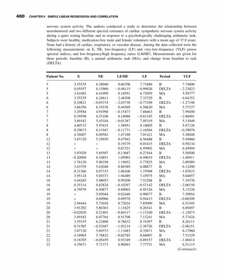
3GC09 12/04/2012 15:5:2 Page 480

nervous system activity. The authors conducted a study to determine the relationship betweenneurohumoral and two different spectral estimates of cardiac sympathetic nervous system activityduring a quiet resting baseline and in response to a psychologically challenging arithmetic task.Subjects were healthy, medication-free male and female volunteers with a mean age of 37.8 years.None had a history of cardiac, respiratory, or vascular disease. Among the data collected were thefollowing measurements on E, NE, low-frequency (LF) and very-low-frequency (VLF) powerspectral indices, and low-frequency/high frequency ratios (LH/HF). Measurements are given forthree periods: baseline (B), a mental arithmetic task (MA), and change from baseline to task(DELTA).

Patient No. E NE LF/HF LF Period VLF

5 3.55535 6.28040 0.66706 7.71886 B 7.746005 0.05557 0.13960 �0.48115 �0.99826 DELTA �2.238235 3.61092 6.41999 0.18591 6.72059 MA 5.507776 3.55535 6.24611 2.48308 7.33729 B 6.643536 0.10821 �0.05374 �2.03738 �0.77109 DELTA �1.271966 3.66356 6.19236 0.44569 6.56620 MA 5.371577 3.29584 4.91998 �0.15473 7.86663 B 7.994507 0.59598 0.53106 0.14086 �0.81345 DELTA �2.864017 3.89182 5.45104 �0.01387 7.05319 MA 5.130498 4.00733 5.97635 1.58951 8.18005 B 5.971268 0.29673 0.11947 �0.11771 �1.16584 DELTA �0.390788 4.30407 6.09582 1.47180 7.01421 MA 5.5804812 3.87120 5.35659 0.47942 6.56488 B 5.9496012 � � 0.19379 0.03415 DELTA 0.5013412 � � 0.67321 6.59903 MA 6.4509413 3.97029 5.85507 0.13687 6.27444 B 5.5850013 �0.20909 0.10851 1.05965 �0.49619 DELTA �1.6891113 3.76120 5.96358 1.19652 5.77825 MA 3.8958914 3.63759 5.62040 0.88389 6.08877 B 6.1249014 0.31366 0.07333 1.06100 1.37098 DELTA �1.0763314 3.95124 5.69373 1.94489 7.45975 MA 5.0485718 4.44265 5.88053 0.99200 7.52268 B 7.1937618 0.35314 0.62824 �0.10297 �0.57142 DELTA �2.0615018 4.79579 6.50877 0.88903 6.95126 MA 5.1322619 � 5.03044 0.62446 6.90677 B 7.3985419 � 0.69966 0.09578 0.94413 DELTA �0.8830919 2.94444 5.73010 0.72024 7.85090 MA 6.5154520 3.91202 5.86363 1.11825 8.26341 B 6.8949720 �0.02020 0.21401 �0.60117 �1.13100 DELTA �1.1207320 3.89182 6.07764 0.51708 7.13241 MA 5.7742421 3.55535 6.21860 0.78632 8.74397 B 8.2611121 0.31585 �0.52487 �1.92114 �2.38726 DELTA �2.0815121 3.87120 5.69373 �1.13483 6.35671 MA 6.1796022 4.18965 5.76832 �0.02785 8.66907 B 7.5152922 0.16705 �0.05459 0.93349 �0.89157 DELTA �1.0041422 4.35671 5.71373 0.90563 7.77751 MA 6.51115

(Continued )


3GC09 12/04/2012 15:5:3 Page 481


23 3.95124 5.52545 �0.24196 6.75330 B 6.9302023 0.26826 0.16491 �0.00661 0.18354 DELTA �1.1891223 4.21951 5.69036 �0.24856 6.93684 MA 5.7410824 3.78419 5.59842 �0.67478 6.26453 B 6.4526824 0.32668 �0.17347 1.44970 0.52169 DELTA 0.3927724 4.11087 5.42495 0.77493 6.78622 MA 6.845451 3.36730 6.13123 0.19077 6.75395 B 6.137081 0.54473 0.08538 0.79284 0.34637 DELTA �0.565691 3.91202 6.21661 0.98361 7.10031 MA 5.571393 2.83321 5.92158 1.89472 7.92524 B 6.306643 1.15577 0.64930 �0.75686 �1.58481 DELTA �1.956363 3.98898 6.57088 1.13786 6.34042 MA 4.350284 4.29046 5.73657 1.81816 7.02734 B 7.028824 0.14036 0.47000 �0.26089 �1.08028 DELTA �1.438584 4.43082 6.20658 1.55727 5.94705 MA 5.590245 3.93183 5.62762 1.70262 6.76859 B 6.111025 0.80437 0.67865 �0.26531 �0.29394 DELTA �0.949105 4.73620 6.30628 1.43731 6.47465 MA 5.161926 3.29584 5.47227 0.18852 6.49054 B 6.842796 �0.16034 0.27073 �0.16485 �1.12558 DELTA �1.842886 3.13549 5.74300 0.02367 5.36496 MA 4.999918 3.25810 5.37064 �0.09631 7.23131 B 7.163718 0.40547 �0.13953 0.97906 �0.62894 DELTA �2.151088 3.66356 5.23111 0.88274 6.60237 MA 5.012639 3.78419 5.94542 0.77839 5.86126 B 6.229109 0.64663 0.05847 �0.42774 �0.53530 DELTA �2.184309 4.43082 6.00389 0.35066 5.32595 MA 4.0448010 4.07754 5.87493 2.32137 6.71736 B 6.5976910 0.23995 �0.00563 �0.25309 �0.00873 DELTA �0.7535710 4.31749 5.86930 2.06827 6.70863 MA 5.8441211 4.33073 5.84064 2.89058 7.22570 B 5.7607911 �3.63759 �0.01464 �1.22533 �1.33514 DELTA �0.5524011 0.69315 5.82600 1.66525 5.89056 MA 5.2083912 3.55535 6.04501 1.92977 8.50684 B 7.1579712 0.13353 0.12041 �0.15464 �0.84735 DELTA 0.1352512 3.68888 6.16542 1.77513 7.65949 MA 7.2932213 3.33220 4.63473 �0.11940 6.35464 B 6.7628513 1.16761 1.05563 0.85621 0.63251 DELTA �0.5212113 4.49981 5.69036 0.73681 6.98716 MA 6.2416414 3.25810 5.96358 1.10456 7.01270 B 7.4942614 � � 0.26353 �1.20066 DELTA �3.1504614 � � 1.36809 5.81204 MA 4.3438115 5.42935 6.34564 2.76361 9.48594 B 7.0573015 � � �1.14662 �1.58468 DELTA �0.0890115 � � 1.61699 7.90126 MA 6.9682916 4.11087 6.59441 �0.23319 6.68269 B 6.7687216 �0.06782 �0.54941 0.34755 �0.29398 DELTA �1.80868

(Continued )


3GC09 12/04/2012 15:5:4 Page 482


16 4.04305 6.04501 0.11437 6.38871 MA 4.9600417 � 6.28040 1.40992 6.09671 B 4.8267117 � �0.12766 �0.17490 �0.05945 DELTA 0.6999317 � 6.15273 1.23501 6.03726 MA 5.5266518 2.39790 6.03548 0.23183 6.39707 B 6.6042118 1.06784 0.11299 0.27977 �0.38297 DELTA �1.9267218 3.46574 6.14847 0.51160 6.01410 MA 4.6774919 4.21951 6.35784 1.08183 5.54214 B 5.6907019 0.21131 �0.00347 0.12485 �0.54440 DELTA �1.4980219 4.43082 6.35437 1.20669 4.99774 MA 4.1926820 4.14313 5.73334 0.89483 7.35045 B 6.9397420 �0.11778 0.00000 0.17129 �0.58013 DELTA �1.7291620 4.02535 5.73334 1.06612 6.77032 MA 5.2105821 3.66356 6.06843 �0.87315 5.09848 B 6.0297221 0.20764 �0.10485 0.41178 �0.33378 DELTA �2.0097421 3.87120 5.96358 �0.46137 4.76470 MA 4.0199822 3.29584 5.95324 2.38399 7.62877 B 7.5435922 0.36772 0.68139 �0.75014 �0.89992 DELTA �1.2555522 3.66356 6.63463 1.63384 6.72884 MA 6.28804

� ¼ missing data.Source: Data provided courtesy of Dr. Richard P. Sloan.

43. The purpose of a study by Chati et al. (A-32) was to ascertain the role of physical deconditioning inskeletal muscle metabolic abnormalities in patients with chronic heart failure (CHF). Subjectsincluded ambulatory CHF patients (12 males, two females) ages 35 to 74 years. Among the datacollected were the following measurements, during exercise, of workload (WL) under controlledconditions, peak oxygen consumption (Vo2), anaerobic ventilatory threshold (AT), both measured inml/kg/min, and exercise total time (ET) in seconds.

WL Vo2 AT ET WL Vo2 AT ET

7.557 32.800 13.280 933.000 3.930 22.500 18.500 720.0003.973 8.170 6.770 255.000 3.195 17.020 8.520 375.0005.311 16.530 11.200 480.000 2.418 15.040 12.250 480.0005.355 15.500 10.000 420.000 0.864 7.800 4.200 240.0006.909 24.470 11.550 960.000 2.703 12.170 8.900 513.0001.382 7.390 5.240 346.000 1.727 15.110 6.300 540.0008.636 19.000 10.400 600.000 7.773 21.100 12.500 1200.000

Source: Data provided courtesy of Dr. Zuka€ı Chati.

44. Czader et al. (A-33) investigated certain prognostic factors in patients with centroblastic-centrocytic non-Hodgkin’s lymphomas (CB/CC NHL). Subjects consisted of men and womenbetween the ages of 20 and 84 years at time of diagnosis. Among the data collected were thefollowing measurements on two relevant factors, A and B. The authors reported a significantcorrelation between the two.


3GC09 12/04/2012 15:5:6 Page 483

A B A B A B

20.00 .154 22.34 .147 48.66 .56936.00 .221 18.00 .132 20.00 .227

6.97 .129 18.00 .085 17.66 .12513.67 .064 22.66 .577 14.34 .08936.34 .402 45.34 .134 16.33 .05139.66 .256 20.33 .246 18.34 .10014.66 .188 16.00 .175 26.49 .20227.00 .138 15.66 .105 13.33 .077

2.66 .078 23.00 .145 6.00 .20622.00 .142 27.33 .129 15.67 .15311.00 .086 6.27 .062 32.33 .54920.00 .170 24.34 .14722.66 .198 22.33 .769

7.34 .092 11.33 .13029.67 .227 6.67 .09911.66 .159

8.05 .22322.66 .065

Source: Data provided courtesy of Dr. Magdalena Czader and Dr. Anna Porwit-MacDonald.

45. Fleroxacin, a fluoroquinolone derivative with a broad antibacterial spectrum and potent activity invitro against gram-negative and many gram-positive bacteria, was the subject of a study by Reignerand Welker (A-34). The objectives of their study were to estimate the typical values of clearance oversystemic availability (CL/F) and the volume of distribution over systemic availability (V/F) after theadministration of therapeutic doses of fleroxacin and to identify factors that influence the dispositionof fleroxacin and to quantify the degree to which they do so. Subjects were 172 healthy male andfemale volunteers and uninfected patients representing a wide age range. Among the data analyzedwere the following measurements (ml/min) of CL/F and creatinine clearance (CLcr). According tothe authors, previous studies have shown that there is a correlation between the two variables.

CL/F CLer CL/F CLer CL/F CLer CL/F CLer

137.000 96.000 77.000 67.700 152.000 109.000 132.000 111.000106.000 83.000 57.000 51.500 100.000 82.000 94.000 118.000165.000 100.000 69.000 52.400 86.000 88.000 90.000 111.000127.000 101.000 69.000 65.900 69.000 67.000 87.000 124.000139.000 116.000 76.000 60.900 108.000 68.700 48.000 10.600102.000 78.000 77.000 93.800 77.000 83.200 26.000 9.280

72.000 84.000 66.000 73.800 85.000 72.800 54.000 12.50086.000 81.000 53.000 99.100 89.000 82.300 36.000 9.86085.000 77.000 26.000 110.000 105.000 71.100 26.000 4.740

122.000 102.000 89.000 99.900 66.000 56.000 39.000 7.02076.000 80.000 44.000 73.800 73.000 61.000 27.000 6.57057.000 67.000 27.000 65.800 64.000 79.500 36.000 13.60062.000 41.000 96.000 109.000 26.000 9.120 15.000 7.60090.000 93.000 102.000 76.800 29.000 8.540 138.000 100.000

(Continued )


3GC09 12/04/2012 15:5:9 Page 484

165.000 88.000 159.000 125.000 39.100 93.700 127.000 108.000132.000 64.000 115.000 112.000 75.500 65.600 203.000 121.000159.000 92.000 82.000 91.600 86.000 102.000 198.000 143.000148.000 114.000 96.000 83.100 106.000 105.000 151.000 126.000116.000 59.000 121.000 88.800 77.500 67.300 113.000 111.000124.000 67.000 99.000 94.000 87.800 96.200 139.000 109.000

76.000 56.000 120.000 91.500 25.700 6.830 135.000 102.00040.000 61.000 101.000 83.800 89.700 74.800 116.000 110.00023.000 35.000 118.000 97.800 108.000 84.000 148.000 94.00027.000 38.000 116.000 100.000 58.600 79.000 221.000 110.00064.000 79.000 116.000 67.500 91.700 68.500 115.000 101.00044.000 64.000 87.000 97.500 48.900 20.600 150.000 110.00059.000 94.000 59.000 45.000 53.500 10.300 135.000 143.00047.000 96.000 96.000 53.500 41.400 11.800 201.000 115.00017.000 25.000 163.000 84.800 24.400 7.940 164.000 103.00067.000 122.000 39.000 73.700 42.300 3.960 130.000 103.00025.000 43.000 73.000 87.300 34.100 12.700 162.000 169.00024.000 22.000 45.000 74.800 28.300 7.170 107.000 140.00065.000 55.000 94.000 100.000 47.000 6.180 78.000 87.10069.000 42.500 74.000 73.700 30.500 9.470 87.500 134.00055.000 71.000 70.000 64.800 38.700 13.700 108.000 108.00039.000 34.800 129.000 119.000 60.900 17.000 126.000 118.00058.000 50.300 34.000 30.000 51.300 6.810 131.000 109.00037.000 38.000 42.000 65.900 46.100 24.800 94.400 60.00032.000 32.000 48.000 34.900 25.000 7.200 87.700 82.90066.000 53.500 58.000 55.900 29.000 7.900 94.000 99.60049.000 60.700 30.000 40.100 25.000 6.600 157.000 123.00040.000 66.500 47.000 48.200 40.000 8.60034.000 22.600 35.000 14.800 28.000 5.50087.000 61.800 20.000 14.400

Source: Data provided courtesy of Dr. Bruno Reigner.

46. Yasu et al. (A-35) used noninvasive magnetic resonance spectroscopy to determine the short- andlong-term effects of percutaneous transvenous mitral commissurotomy (PTMC) on exercisecapacity and metabolic responses of skeletal muscles during exercise. Data were collected on11 patients (2 males, 9 females) with symptomatic mitral stenosis. Their mean age was 52 yearswith a standard deviation of 11. Among the data collected were the following measurements onchanges in mitral valve area (d-MVA) and peak oxygen consumption (d-Vo2) 3, 30, and 90 dayspost-PTMC:

Days d-Vo2Subject Post-PTMC d-MVA (cm2) (ml/kg/min)

1 3 0.64 0.32 3 0.76 �0:93 3 0.3 1.94 3 0.6 �3:1

CL/F CLer CL/F CLer CL/F CLer CL/F CLer


3GC09 12/04/2012 15:5:10 Page 485

5 3 0.3 �0:56 3 0.4 �2:77 3 0.7 1.58 3 0.9 1.19 3 0.6 �7:4

10 3 0.4 �0:411 3 0.65 3.8

1 30 0.53 1.62 30 0.6 3.33 30 0.4 2.64 30 0.5 �5 30 0.3 3.66 30 0.3 0.27 30 0.67 4.28 30 0.75 39 30 0.7 2

10 30 0.4 0.811 30 0.55 4.2

1 90 0.6 1.92 90 0.6 5.93 90 0.4 3.34 90 0.6 55 90 0.25 0.66 90 0.3 2.57 90 0.7 4.68 90 0.8 49 90 0.7 1

10 90 0.38 1.111 90 0.53 �� ¼ Missing data.Source: Data provided courtesy of Dr. Takanori Yasu.


1. Refer to the data for 1050 subjects with cerebral edema (CEREBRAL). Cerebral edema withconsequent increased intracranial pressure frequently accompanies lesions resulting from headinjury and other conditions that adversely affect the integrity of the brain. Available treatments forcerebral edema vary in effectiveness and undesirable side effects. One such treatment is glycerol,administered either orally or intravenously. Of interest to clinicians is the relationship betweenintracranial pressure and glycerol plasma concentration. Suppose you are a statistical consultantwith a research team investigating the relationship between these two variables. Select a simplerandom sample from the population and perform the analysis that you think would be useful to theresearchers. Present your findings and conclusions in narrative form and illustrate with graphswhere appropriate. Compare your results with those of your classmates.

Days d-Vo2Subject Post-PTMC d-MVA (cm2) (ml/kg/min)



3GC09 12/04/2012 15:5:10 Page 486

2. Refer to the data for 1050 subjects with essential hypertension (HYPERTEN). Suppose you are astatistical consultant to a medical research team interested in essential hypertension. Select asimple random sample from the population and perform the analyses that you think would beuseful to the researchers. Present your findings and conclusions in narrative form and illustratewith graphs where appropriate. Compare your results with those of your classmates. Consult withyour instructor regarding the size of sample you should select.

3. Refer to the data for 1200 patients with rheumatoid arthritis (CALCIUM). One hundred patientsreceived the medicine at each dose level. Suppose you are a medical researchers wishing to gaininsight into the nature of the relationship between dose level of prednisolone and total bodycalcium. Select a simple random sample of three patients from each dose level group and do thefollowing.

(a) Use the total number of pairs of observations to obtain the least-squares equation describingthe relationship between dose level (the independent variable) and total body calcium.

(b) Draw a scatter diagram of the data and plot the equation.(c) Compute r and test for significance at the .05 level. Find the p value.(d) Compare your results with those of your classmates.

REFERENCES


1. FREDERICK HARTWIG with BRAIN E. DEARING, Exploratory Data Analysis, Sage Publications, Beverly Hills, 1979.2. IAIN M. JOHNSTONE and PAUL F. VELLEMAN, “The Resistant Line and Related Regression Methods,” Journal of the

American Statistical Association, 80 (1985), 1041–1054.3. DONALD R. MCNEIL, Interactive Data Analysis: A Practical Primer, Wiley, New York, 1977.4. PAUL F. VELLEMAN and DAVID C. HOAGLIN, Applications, Basics, and Computing of Exploratory Data Analysis,

Duxbury, Belmont, CA, 1981.5. R. A. FISHER, “On the Probable Error of a Coefficient of Correlation Deduced from a Small Sample,” Metron, 1

(1921), 3–21.6. H. HOTELLING, “New Light on the Correlation Coefficient and Its Transforms,” Journal of the Royal Statistical

Society, Series B, 15 (1953), 193–232.7. TERRY E. DIELMAN,Applied Regression Analysis for Business and Economics, Second Edition, Duxbury, Belmont,

CA, 1996.8. RONALD R. HOCKING, Methods and Applications of Linear Models: Regression and the Analysis of Variance,

Wiley, New York, 1996.9. WILLIAM MENDENHALL and TERRY SINCICH, A Second Course in Statistics: Regression Analysis, Fifth Edition,

Prentice Hall, Upper Saddle River, NJ, 1996.10. JOHN NETER, MICHAEL H. KUTNER, CHRISTOPHER J. NACHTSHEIM, and WILLIAM WASSERMAN, Applied Linear

Regression Models, Third Edition, Irwin, Chicago, 1996.


A-1. JEAN-PIERRE DESPR�ES, DENIS PRUD’HOMME, MARIE-CHRISTINE POULIOT, ANGELO TREMBLAY, and CLAUDE BOUCHARD,“Estimation of Deep Abdominal Adipose-Tissue Accumulation from Simple Anthropometric Measurements inMen,” American Journal of Clinical Nutrition, 54 (1991), 471–477.

A-2. MORI J. KRANTZ, ILANA B. KUTINSKY, ALASTAIR D. ROBERSTON, and PHILIP S. MEHLER, “Dose-Related Effects ofMethadone on QT Prolongation in a Series of Patients with Torsade de Pointes,” Pharmacotherapy, 23 (2003),802–805.

A-3. ROBERT A. REISS, CURTIS E. HAAS, DEBORAH L. GRIFFIS, BERNADETTE PORTER, and MARY ANN TARA, “Point-of-CareVersus Laboratory Monitoring of Patients Receiving Different Anticoagulant Therapies,” Pharmacotherapy, 22(2002), 677–685.


3GC09 12/04/2012 15:5:10 Page 487

A-4. ROBERT B. PARKER, RYAN YATES, JUDITH E. SOBERMAN, and CASEY LAIZURE, “Effects of Grapefruit Juice on IntestialP-glycoprotein: Evaluation Using Digoxin in Humans,” Pharmacotherapy, 23 (2003), 979–987.

A-5. R. B. EVANS, W. GORDON, and M. CONZEMIUS, “Effect of Velocity on Ground Reaction Forces in Dogs withLameness Attributable to Tearing of the Cranial Cruciate Ligament,” American Journal of Veterinary Research,64 (2003), 1479–1481.

A-6. DAVID KRIESER, ANDREW ROSENBERG, and GAD KAINER, “The Relationship Between Serum Creatinine, SerumCystatin C and Glomerular Filtration Rate in Pediatric Renal Transplant Recipients: A Pilot Study,” PediatricTransplantation, 6 (2002), 392–395.

A-7. OLGA KWAST-RABBEN, ROLF LIBELIUS, and HANNU HEIKKIL€A, “Somatosensory Evoked Potentials FollowingStimulation of Digital Nerves,” Muscle and Nerve, 26 (2002), 533–538.

A-8. GERI R. BROWN and KIM PERSLEY, “Hepatitis A Epidemic in the Elderly,” Southern Medical Journal, 95 (2002),826–833.

A-9. ANN E. TUZSON, KEVIN P. GRANATA, and MARK F. ABEL, “Spastic Velocity Threshold Constrains FunctionalPerformance in Cerebral Palsy,” Archives of Physical Medicine and Rehabilitation, 84 (2003), 1363–1368.

A-10. M. BUTZ, K. H. WOLLINSKY, U. WIDEMUTH-CATRINESCU, A. SPERFELD, S. WINTER, H. H. MEHRKENS, A. C. LUDOLPH,and H. SCHREIBER, “Longitudinal Effects of Noninvasive Positive-Pressure Ventilation in Patients with Amyo-trophic Lateral Sclerosis,” American Journal of Medical Rehabilitation, 82 (2003), 597–604.

A-11. KARIE E. SCROGIN, DANIEL C. HATTON, and DAVID A. MCCARRON, “The Interactive Effects of Dietary SodiumChloride and Calcium on Cardiovascular Stress Responses,” American Journal of Physiology (RegulatoryIntegrative Comp. Physiol. 30) 261 (1991), R945–R949.

A-12. DEAN PARMALEE, Data analyzed by the Wright State University Statistical Consulting Center, Wright StateUniversity, Dayton, OH (2003).

A-13. MARIA MATHIAS, Data analyzed by the Wright State University Statistical Consulting Center, Wright StateUniversity, Dayton, OH (2001).

A-14. DARREN M. TRILLER, STEVEN L. CLAUSE, and CHRISTOPHER DOMAREW, “Analysis of Medication ManagementActivities for Home-Dwelling Patients,” American Journal of Health-System Pharmacy, 59 (2002), 2356–2359.

A-15. MAXIME LAMARRE-CLICHE, YVES LACOURCI�ERE, JACQUES DE CHAMPLAIN, LUC POIRIER, and PIERRE LAROCHELLE, “DoesQTc Interval Predict the Response to Beta-Blockers and Calcium Channel Blockers in Hypertensives?” Heartand Disease, 5 (2003), 244–252.

A-16. JEAN D. SKINNER, PAULA ZIEGLER, and MICHAEL PONZA, “Transitions in Infants’ and Toddlers’ Beverage Patterns,”Journal of the American Dietetic Association, Supplement, 104 (2004), 45–50.

A-17. NEUNG HWA PARK, JI KANG PARK, YOUNGHEE CHOI, CHEOL-IN YOO, CHOONG RYEOL LEE, HUN LEE, HYO KYUNG KIM,SUNG-RYUL KIM, TAE-HEUM JEONG, JUNGSUN PARK, CHUNG SIK YOON, and YANGHO KIM, “Whole Blood ManganeseCorrelates with High Signal Intensities on T-Weighted MRI in Patients with Liver Cirrhosis,” NeuroToxicology,24 (2003), 909–915.

A-18. PHILIPPE DE MOERLOOSE, SYLVIE DESMARAIS, HENRI BOUNAMEAUX, GUIDO REBER, ARNAUD PERRIER, GEORGES DUPUY,and JEAN-LOUIS PITTET, “Contribution of a New, Rapid, Individual and Quantitative Automated D-Dimer ELISAto Exclude Pulmonary Embolism,” Thrombosis and Haemostasis, 75 (1996), 11–13.

A-19. ILPO T. HUHTANIEMI, ANNE-MAARIT HAAVISTO, RAIJA ANTTILA, MARTTI A. SIIMES, and LEO DUNKEL, “SensitiveImmunoassay and In Vitro Bioassay Demonstrate Constant Bioactive/Immunoreactive Ratio of LuteinizingHormone in Healthy Boys During the Pubertal Maturation,” Pediatric Research, 39 (1996), 180–184.

A-20. YONG-KWEI TSAU, JI-NAN SHEU, CHIUNG-HUI CHEN, RU-JENG TENG, and HUI-CHI CHEN, “Decreased UrinaryEpidermal Growth Factor in Children with Acute Renal Failure: Epidermal Growth Factor/Creatinine Ratio Not aReliable Parameter for Urinary Epidermal Growth Factor Excretion,” Pediatric Research, 39 (1996), 20–24.

A-21. A. USAJ and V. STARC, “Blood pH and Lactate Kinetics in the Assessment of Running Endurance,” InternationalJournal of Sports Medicine, 17 (1996), 34–40.

A-22. PAMELA BEAN, MARY SUSAN SUTPHIN, PATRICIA NECESSARY, MELKON S. AGOPIAN, KARSTEN LIEGMANN, CARL

LUDVIGSEN, and JAMES B. PETER, “Carbohydrate-Deficient Transferrin Evaluation in Dry Blood Spots,” Alcohol-ism: Clinical and Experimental Research, 20 (1996), 56–60.

A-23. JOHJI KATO, KOHJI KOBAYASHI, TAKUMA ETOH, MIHO TANAKA, KAZUO KITAMURA, TAKUROH IMAMURA, YASUSHI

KOIWAYA, KENJI KANGAWA, and TANENAO ETO, “Plasma Adrenomedullin Concentration in Patients with HeartFailure,” Journal of Clinical Endocrinology and Metabolism, 81 (1996), 180–183.

A-24. B. E. GOLDEN, P. A. CLOHESSY, G. RUSSELL, and M. K. FAGERHOL, “Calprotectin as a Marker of Inflammation inCystic Fibrosis,” Archives of Disease in Childhood, 74 (1996), 136–139.

REFERENCES 487

3GC09 12/04/2012 15:5:10 Page 488

A-25. ARTHUR F. GELB, JAMES C. HOGG, NESTOR L. MU€ LLER, MARK J. SCHEIN, JOSEPH KUEI, DONALD P. TASHKIN, JOEL D.EPSTEIN, JOZEF KOLLIN, ROBERT H. GREEN, NOE ZAMEL, W. MARK ELLIOTT, and LIDA HADJIAGHAI, “Contribution ofEmphysema and Small Airways in COPD,” Chest, 109 (1996), 353–359.

A-26. AGNES M. WITTEMAN, STEVEN O. STAPEL, GERRARD J. PERDOK, DEMAN H. S. SJAMSOEDIN, HENK M. JANSEN, ROB C.AALBERSE, and JARING S. VAN DER ZEE, “The Relationship Between RAST and Skin Test Results in Patients withAsthma or Rhinitis: A Quantitative Study with Purified Major Allergens,” Journal of Allergy and ClinicalImmunology, 97 (1996), 16–25.

A-27. MARIANNE GARLAND, HAZEL H. SZETO, SALHA S. DANIEL, PAMELA J. TROPPER, MICHAEL M. MYERS, and RAYMOND I.STARK, “Zidovudine Kinetics in the Pregnant Baboon,” Journal of Acquired Immune Deficiency Syndromes andHuman Retrovirology, 11 (1996), 117–127.

A-28. A. HALLIGAN, A. SHENNAN, P. C. LAMBERT, M. DE SWIET, and D. J. TAYLOR, “Diurnal Blood Pressure Difference inthe Assessment of Preeclampsia,” Obstetrics & Gynecology, 87 (1996), 205–208.

A-29. JAY W. MARKS, GEORGE G. BONORRIS, and LESLIE J. SCHOENFIELD, “Effects of Ursodiol or Ibuprofen on Contractionof Gallbladder and Bile Among Obese Patients During Weight Loss,” Digestive Diseases and Sciences, 41(1996), 242–249.

A-30. D. J. PEACOCK, P. EGGER, P. TAYLOR, M. I. D. CAWLEY, and C. COOPER, “Lateral Bone Density Measurements inOsteoarthritis of the Lumbar Spine,” Annals of the Rheumatic Diseases, 55 (1996), 196–198.

A-31. R. P. SLOAN, P. A. SHAPIRE, E. BAGIELLA, J. T. BIGGER, E. S. LO, and J. M. GORMAN, “Relationships BetweenCirculating Catecholamines and Low Frequency Heart Period Variability as Indices of Cardiac SympatheticActivity During Mental Stress,” Psychosomatic Medicine, 58 (1996) 25–31.

A-32. ZUKA€I CHATI, FA€IEZ ZANNAD, CLAUDE JEANDEL, BRIGITTE LHERBIER, JEAN-MARIE ESCANYE, JACQUES ROBERT, andETIENNE ALIOT, “Physical Deconditioning May Be a Mechanism for the Skeletal Muscle Energy PhosphateMetabolism Abnormalities in Chronic Heart Failure,” American Heart Journal, 131 (1996), 560–566.

A-33. MAGDALENA CZADER, JOANNA MAZUR, MIKAEL PETTERSSON, JAN LILIEMARK, MATS STR€OMBERG, BIRGER CHRISTENSSON,BERNARD TRIBUKAIT, GERT AUER, A

�KE €OST, and ANNA PORWIT, “Prognostic Significance of Proliferative and

Apoptotic Fractions in Low Grade Follicle Center Cell-Derived Non-Hodgkin’s Lymphomas,” Cancer, 77(1996), 1180–1188.

A-34. B. G. REIGNER and H. A. WELKER, “Factors Influencing Elimination and Distribution of Fleroxacin: Metaanalysisof Individual Data from 10 Pharmacokinetic Studies,” Antimicrobial Agents and Chemotherapy, 40 (1996),575–580.

A-35. TAKANORI YASU, TAKA’AKI KATSUKI, NOBUHIRO OHMURA, IKUKO NAKADA, MAFUMI OWA, MIKIHISA FUJII, AKIRA

SAKAGUCHI, and MUNEYASU SAITO, “Delayed Improvement in Skeletal Muscle Metabolism and Exercise Capacityin Patients with Mitral Stenosis Following Immediate Hemodynamic Amelioration by Percutaneous TransvenousMitral Commissurotomy,” American Journal of Cardiology, 77 (1996), 492–497.


3GC10 12/04/2012 15:18:1 Page 489

CHAPTER10MULTIPLE REGRESSIONAND CORRELATION

CHAPTER OVERVIEW

This chapter provides extensions of the simple linear regression and bivariatecorrelation models discussed in Chapter 9. The concepts and techniquesdiscussed here are useful when the researcher wishes to consider simulta-neously the relationships among more than two variables. Although theconcepts, computations, and interpretations associated with analysis ofmultiple-variable data may seem complex, they are natural extensions ofmaterial explored in previous chapters.

TOPICS

10.1 INTRODUCTION

10.2 THE MULTIPLE LINEAR REGRESSION MODEL

10.3 OBTAINING THE MULTIPLE REGRESSION EQUATION

10.4 EVALUATING THE MULTIPLE REGRESSION EQUATION

10.5 USING THE MULTIPLE REGRESSION EQUATION

10.6 THE MULTIPLE CORRELATION MODEL

10.7 SUMMARY

LEARNING OUTCOMES


1. understand how to include more than one independent variable in a regressionequation.

2. be able to obtain a multiple regression model and use it to make predictions.

3. be able to evaluate the multiple regression coefficients and the suitability of theregression model.

4. understand how to calculate and interpret multiple, bivariate, and partialcorrelation coefficients.

489

3GC10 12/04/2012 15:18:2 Page 490

10.1 INTRODUCTION

In Chapter 9 we explored the concepts and techniques for analyzing and making use of thelinear relationship between two variables. We saw that this analysis may lead to a linearequation that can be used to predict the value of some dependent variable given the value ofan associated independent variable.

Intuition tells us that, in general, we ought to be able to improve our predicting abilityby including more independent variables in such an equation. For example, a researchermay find that intelligence scores of individuals may be predicted from physical factors suchas birth order, birth weight, and length of gestation along with certain hereditary andexternal environmental factors. Length of stay in a chronic disease hospital may be relatedto the patient’s age, marital status, sex, and income, not to mention the obvious factor ofdiagnosis. The response of an experimental animal to some drug may depend on the size ofthe dose and the age and weight of the animal. A nursing supervisor may be interested inthe strength of the relationship between a nurse’s performance on the job, score on the stateboard examination, scholastic record, and score on some achievement or aptitude test. Or ahospital administrator studying admissions from various communities served by thehospital may be interested in determining what factors seem to be responsible fordifferences in admission rates.

The concepts and techniques for analyzing the associations among severalvariables are natural extensions of those explored in the previous chapters. Thecomputations, as one would expect, are more complex and tedious. However, as ispointed out in Chapter 9, this presents no real problem when a computer is available. It isnot unusual to find researchers investigating the relationships among a dozen or morevariables. For those who have access to a computer, the decision as to how manyvariables to include in an analysis is based not on the complexity and length of thecomputations but on such considerations as their meaningfulness, the cost of theirinclusion, and the importance of their contribution.

In this chapter we follow closely the sequence of the previous chapter. The regressionmodel is considered first, followed by a discussion of the correlation model. In consideringthe regression model, the following points are covered: a description of the model, methodsfor obtaining the regression equation, evaluation of the equation, and the uses that may bemade of the equation. In both models the possible inferential procedures and theirunderlying assumptions are discussed.

10.2 THEMULTIPLE LINEARREGRESSIONMODEL

In the multiple regression model we assume that a linear relationship exists between somevariable Y, which we call the dependent variable, and k independent variables,X1;X2; . . . ;Xk. The independent variables are sometimes referred to as explanatoryvariables, because of their use in explaining the variation in Y. They are also calledpredictor variables, because of their use in predicting Y.

490 CHAPTER 10 MULTIPLE REGRESSION AND CORRELATION

3GC10 12/04/2012 15:18:2 Page 491

Assumptions The assumptions underlying multiple regression analysis are asfollows.

1. The Xi are nonrandom (fixed) variables. This assumption distinguishes the multipleregression model from the multiple correlation model, which will be presented inSection 10.6. This condition indicates that any inferences that are drawn from sampledata apply only to the set ofX values observed and not to some larger collection ofX’s.Under the regression model, correlation analysis is not meaningful. Under the correla-tion model to be presented later, the regression techniques that follow may be applied.

2. For each set of Xi values there is a subpopulation of Y values. To construct certainconfidence intervals and test hypotheses, it must be known, or the researcher must bewilling to assume, that these subpopulations of Y values are normally distributed.Since we will want to demonstrate these inferential procedures, the assumption ofnormality will be made in the examples and exercises in this chapter.

3. The variances of the subpopulations of Y are all equal.

4. The Y values are independent. That is, the values of Y selected for one set of X valuesdo not depend on the values of Y selected at another set of X values.

The Model Equation The assumptions for multiple regression analysis may bestated in more compact fashion as

yj ¼ b0 þ b1x1j þ b2x2j þ � � � þ bkxkj þ ej (10.2.1)

where yj is a typical value from one of the subpopulations of Y values; the bi are called theregression coefficients; x1j; x2j; . . . ; xkj are, respectively, particular values of the indepen-dent variables X1;X2; . . .Xk; and ej is a random variable with mean 0 and variance s2; thecommon variance of the subpopulations of Y values. To construct confidence intervals forand test hypotheses about the regression coefficients, we assume that the ej are normallyand independently distributed. The statements regarding ej are a consequence of theassumptions regarding the distributions of Y values. We will refer to Equation 10.2.1 as themultiple linear regression model.

When Equation 10.2.1 consists of one dependent variable and two independentvariables, that is, when the model is written

yj ¼ b0 þ b1x1j þ b2x2j þ ej (10.2.2)

a plane in three-dimensional space may be fitted to the data points as illustrated in Figure10.2.1. When the model contains more than two independent variables, it is describedgeometrically as a hyperplane.

In Figure 10.2.1 the observer should visualize some of the points as being locatedabove the plane and some as being located below the plane. The deviation of a point fromthe plane is represented by

ej ¼ yj � b0 � b1x1j � b2x2j (10.2.3)

In Equation 10.2.2, b0 represents the point where the plane cuts the Y-axis; that is, itrepresents the Y-intercept of the plane. b1 measures the average change in Y for a unit

10.2 THE MULTIPLE LINEAR REGRESSIONMODEL 491

3GC10 12/04/2012 15:18:2 Page 492

change in X1 when X2 remains unchanged, and b2 measures the average change in Y for aunit change in X2 when X1 remains unchanged. For this reason b1 and b2 are referred to aspartial regression coefficients.

10.3 OBTAINING THEMULTIPLEREGRESSION EQUATION

Unbiased estimates of the parameters b0; b1; . . . ;bk of the model specified in Equation10.2.1 are obtained by the method of least squares. This means that the sum of the squareddeviations of the observed values of Y from the resulting regression surface is minimized.In the three-variable case, as illustrated in Figure 10.2.1, the sum of the squared deviationsof the observations from the plane are a minimum when b0; b1; and b2 are estimated by themethod of least squares. In other words, by the method of least squares, sample estimates ofb0; b1; . . . ;bk are selected in such a way that the quantity

Xe2j ¼

Xyj � b0 � b1x1j � b2x2j � � � � � bkxkj� �2

is minimized. This quantity, referred to as the sum of squares of the residuals, may also bewritten as X

e2j ¼

Xyj � yj� �2

(10.3.1)

indicating the fact that the sum of squares of deviations of the observed values of Y from thevalues of Y calculated from the estimated equation is minimized.

Y

X2 X1

Dev

iati

on

s fr

om

th

ep

lan

e

Regression plane

FIGURE 10.2.1 Multiple regression plane and scatter of points.


3GC10 12/04/2012 15:18:3 Page 493

Estimates of the multiple regression parameters may be obtained by means ofarithmetic calculations performed on a handheld calculator. This method of obtaining theestimates is tedious, time-consuming, subject to errors, and a waste of time when acomputer is available. Those interested in examining or using the arithmetic approach mayconsult earlier editions of this text or those by Snedecor and Cochran (1) and Steel andTorrie (2), who give numerical examples for four variables, and Anderson and Bancroft (3),who illustrate the calculations involved when there are five variables. In the followingexample we use SPSS software to illustrate an interesting graphical summary of sampledata collected on three variables. We then use MINITAB and SAS to illustrate theapplication of multiple regression analysis.

EXAMPLE 10.3.1

Researchers Jansen and Keller (A-1) used age and education level to predict the capacity todirect attention (CDA) in elderly subjects. CDA refers to neural inhibitory mechanisms thatfocus the mind on what is meaningful while blocking out distractions. The study collectedinformation on 71 community-dwelling older women with normal mental status. The CDAmeasurement was calculated from results on standard visual and auditory measures requiringthe inhibition of competing and distracting stimuli. In this study, CDA scores ranged from�7:65 to 9.61 with higher scores corresponding with better attentional functioning. Themeasurements on CDA, age in years, and education level (years of schooling) for 71 subjectsare shown in Table 10.3.1. We wish to obtain the sample multiple regression equation.

TABLE 10.3.1 CDA Scores, Age, and Education Level

for 71 Subjects Described in Example 10.3.1

Age Ed-Level CDA Age Ed-Level CDA

72 20 4.57 79 12 3.17

68 12 �3.04 87 12 �1.19

65 13 1.39 71 14 0.99

85 14 �3.55 81 16 �2.94

84 13 �2.56 66 16 �2.21

90 15 �4.66 81 16 �0.75

79 12 �2.70 80 13 5.07

74 10 0.30 82 12 �5.86

69 12 �4.46 65 13 5.00

87 15 �6.29 73 16 0.63

84 12 �4.43 85 16 2.62

79 12 0.18 83 17 1.77

71 12 �1.37 83 8 �3.79

76 14 3.26 76 20 1.44

73 14 �1.12 77 12 �5.77

86 12 �0.77 83 12 �5.77

69 17 3.73 79 14 �4.62

66 11 �5.92 69 12 �2.03

(Continued )

10.3 OBTAINING THE MULTIPLE REGRESSION EQUATION 493

3GC10 12/04/2012 15:18:4 Page 494

Prior to analyzing the data using multiple regression techniques, it is useful toconstruct plots of the relationships among the variables. This is accomplished by makingseparate plots of each pair of variables, (X1, X2), (X1, Y ), and (X2, Y ). A software packagesuch as SPSS displays each combination simultaneously in a matrix format as shown inFigure 10.3.1. From this figure it is apparent that we should expect a negative relationship

Age Ed-Level CDA Age Ed-Level CDA

FIGURE 10.3.1 SPSS matrix scatter plot of the data in Table 10.3.1.

65 16 5.74 66 14 �2.22

71 14 2.83 75 12 0.80

80 18 �2.40 77 16 �0.75

81 11 �0.29 78 12 �4.60

66 14 4.44 83 20 2.68

76 17 3.35 85 10 �3.69

70 12 �3.13 76 18 4.85

76 12 �2.14 75 14 �0.08

67 12 9.61 70 16 0.63

72 20 7.57 79 16 5.92

68 18 2.21 75 18 3.63

102 12 �2.30 94 8 �7.07

67 12 1.73 76 18 6.39

66 14 6.03 84 18 �0.08

75 18 �0.02 79 17 1.07

91 13 �7.65 78 16 5.31

74 15 4.17 79 12 0.30

90 15 �0.68

Source: Data provided courtesy of Debra A. Jansen, Ph.D., R.N.


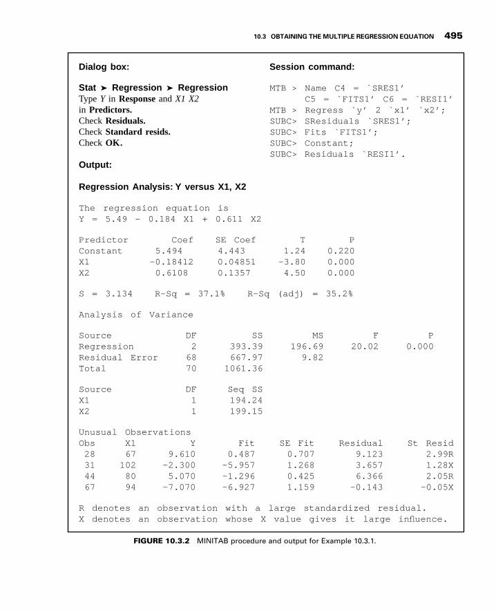
3GC10 12/04/2012 15:18:4 Page 495


Stat Regression Regression MTB > Name C4 = `SRES1’Type Y in Response and X1 X2 C5 = `FITS1’ C6 = `RESI1’in Predictors. MTB > Regress `y’ 2 `x1’ `x2’;Check Residuals. SUBC> SResiduals `SRES1’;Check Standard resids. SUBC> Fits `FITS1’;Check OK. SUBC> Constant;

SUBC> Residuals `RESI1’.Output:

Regression Analysis: Y versus X1, X2

The regression equation isY = 5.49 - 0.184 X1 + 0.611 X2

Predictor Coef SE Coef T PConstant 5.494 4.443 1.24 0.220X1 -0.18412 0.04851 -3.80 0.000X2 0.6108 0.1357 4.50 0.000

S = 3.134 R-Sq = 37.1% R-Sq (adj) = 35.2%



Source DF Seq SS42.49111X51.99112X

Unusual ObservationsObs X1 Y Fit SE Fit Residual St Resid28 67 9.610 0.487 0.707 9.123 2.99R31 102 -2.300 -5.957 1.268 3.657 1.28X44 80 5.070 -1.296 0.425 6.366 2.05R67 94 -7.070 -6.927 1.159 -0.143 -0.05X

R denotes an observation with a large standardized residual.X denotes an observation whose X value gives it large influence.


10.3 OBTAINING THE MULTIPLE REGRESSION EQUATION 495

3GC10 12/04/2012 15:18:4 Page 496

between CDA and Age and a positive relationship between CDA and Ed-Level. We shallsee that this is indeed the case when we use MINITAB to analyze the data.

Solution: We enter the observations on age, education level, and CDA in c1 through c3and name them X1, X2, and Y, respectively. The MINITAB dialog box andsession command, as well as the output, are shown in Figure 10.3.2. We seefrom the output that the sample multiple regression equation, in the notationof Section 10.2, is

yj ¼ 5:49 � :184x1j þ :611x2j

Other output entries will be discussed in the sections that follow.The SAS output for Example 10.3.1 is shown in Figure 10.3.3. &

After the multiple regression equation has been obtained, the next step involves itsevaluation and interpretation. We cover this facet of the analysis in the next section.

The REG Procedure

Model: MODEL1Dependent Variable: CDA


Sum of MeanSource DF Squares Square F Value Pr > F

Model 2 393.38832 196.69416 20.02 <.0001Error 68 667.97084 9.82310Corrected Total 70 1061.35915

Root MSE 3.13418 R-Square 0.3706Dependent Mean 0.00676 Adj R-Sq 0.3521Coeff Var 46360

Parameter Estimates

Parameter StandardVariable DF Estimate Error t Value Pr > |t|

Intercept 1 5.49407 4.44297 1.24 0.2205AGE 1 -0.18412 0.04851 -3.80 0.0003EDUC 1 0.61078 0.13565 4.50 <.0001

FIGURE 10.3.3 SAS® output for Example 10.3.1.


3GC10 12/04/2012 15:18:6 Page 497

EXERCISES

Obtain the regression equation for each of the following data sets.10.3.1 Machiel Naeije (A-2) studied the relationship between maximum mouth opening and measurements

of the lower jaw (mandible). He measured the dependent variable, maximum mouth opening (MMO,measured in mm), as well as predictor variables, mandibular length (ML, measured in mm) and angleof rotation of the mandible (RA, measured in degrees) of 35 subjects.

MMO (Y) ML (X1) RA (X2) MMO (Y) ML (X1) RA (X2)

52.34 100.85 32.08 50.82 90.65 38.3351.90 93.08 39.21 40.48 92.99 25.9352.80 98.43 33.74 59.68 108.97 36.7850.29 102.95 34.19 54.35 91.85 42.0257.79 108.24 35.13 47.00 104.30 27.2049.41 98.34 30.92 47.23 93.16 31.3753.28 95.57 37.71 41.19 94.18 27.8759.71 98.85 44.71 42.76 89.56 28.6953.32 98.32 33.17 51.88 105.85 31.0448.53 92.70 31.74 42.77 89.29 32.7851.59 88.89 37.07 52.34 92.58 37.8258.52 104.06 38.71 50.45 98.64 33.3662.93 98.18 43.89 43.18 83.70 31.9357.62 91.01 41.06 41.99 88.46 28.3265.64 96.98 41.92 39.45 94.93 24.8252.85 97.85 35.25 38.91 96.81 23.8864.43 96.89 45.11 49.10 93.13 36.1757.25 98.35 39.44

Source: Data provided courtesy of M. Naeije, D.D.S.

10.3.2 Family caregiving of older adults is more common in Korea than in the United States. Son et al. (A-3)studied 100 caregivers of older adults with dementia in Seoul, South Korea. The dependent variablewas caregiver burden as measured by the Korean Burden Inventory (KBI). Scores ranged from 28 to140, with higher scores indicating higher burden. Explanatory variables were indexes that measuredthe following:

ADL: total activities of daily living (low scores indicate that the elderly perform activitiesindependently).

MEM: memory and behavioral problems (higher scores indicate more problems).

COG: cognitive impairment (lower scores indicate a greater degree of cognitive impairment).

The reported data are as follows:

KBI (Y ) ADL (X1) MEM (X2) COG (X3) KBI (Y ) ADL (X1) MEM (X2) COG (X3)

28 39 4 18 88 76 50 568 52 33 9 54 79 44 1159 89 17 3 73 48 57 991 57 31 7 87 90 33 6

(Continued )

EXERCISES 497

3GC10 12/04/2012 15:18:8 Page 498

70 28 35 19 47 55 11 2038 34 3 25 60 83 24 1146 42 16 17 65 50 21 2557 52 6 26 57 44 31 1889 88 41 13 85 79 30 2048 90 24 3 28 24 5 2274 38 22 13 40 40 20 1778 83 41 11 87 35 15 2743 30 9 24 80 55 9 2176 45 33 14 49 45 28 1772 47 36 18 57 46 19 1761 90 17 0 32 37 4 2163 63 14 16 52 47 29 377 34 35 22 42 28 23 2185 76 33 23 49 61 8 731 26 13 18 63 35 31 2679 68 34 26 89 68 65 692 85 28 10 67 80 29 1076 22 12 16 43 43 8 1391 82 57 3 47 53 14 1878 80 51 3 70 60 30 16

103 80 20 18 99 63 22 1899 81 20 1 53 28 9 2773 30 7 17 78 35 18 1488 27 27 27 112 37 33 1764 72 9 0 52 82 25 1352 46 15 22 68 88 16 071 63 52 13 63 52 15 041 45 26 18 49 30 16 1885 77 57 0 42 69 49 1252 42 10 19 56 52 17 2068 60 34 11 46 59 38 1757 33 14 14 72 53 22 2184 49 30 15 95 65 56 291 89 64 0 57 90 12 083 72 31 3 88 88 42 673 45 24 19 81 66 12 2357 73 13 3 104 60 21 769 58 16 15 88 48 14 1381 33 17 21 115 82 41 1371 34 13 18 66 88 24 1491 90 42 6 92 63 49 548 48 7 23 97 79 34 394 47 17 18 69 71 38 1757 32 13 15 112 66 48 1349 63 32 15 88 81 66 1

Source: Data provided courtesy of Gwi-Ryung Son, R.N., Ph.D.

KBI (Y ) ADL (X1) MEM (X2) COG (X3) KBI (Y ) ADL (X1) MEM (X2) COG (X3)


3GC10 12/04/2012 15:18:9 Page 499

10.3.3 In a study of factors thought to be related to patterns of admission to a large general hospital, anadministrator obtained these data on 10 communities in the hospital’s catchment area:

Community

Persons per 1000Population AdmittedDuring Study Period

(Y)

Index ofAvailability ofOther Health

Services(X1)

Index ofIndigency

(X2)

1 61.6 6.0 6.32 53.2 4.4 5.53 65.5 9.1 3.64 64.9 8.1 5.85 72.7 9.7 6.86 52.2 4.8 7.97 50.2 7.6 4.28 44.0 4.4 6.09 53.8 9.1 2.8

10 53.5 6.7 6.7

Total 571.6 69.9 55.6

10.3.4 The administrator of a general hospital obtained the following data on 20 surgery patients duringa study to determine what factors appear to be related to length of stay:

PostoperativeLength ofStay in Days(Y)

Number of CurrentMedical Problems

(X1)

PreoperativeLength of

Stay in Days(X2)

6 1 16 2 1

11 2 29 1 3

16 3 316 1 5

4 1 18 3 1

11 2 213 3 213 1 4

9 1 217 3 317 2 412 4 1

6 1 15 1 1

(Continued )

EXERCISES 499

3GC10 12/04/2012 15:18:9 Page 500

12 3 28 1 29 2 2

Total 208 38 43

10.3.5 A random sample of 25 nurses selected from a state registry yielded the following information oneach nurse’s score on the state board examination and his or her final score in school. Both scoresrelate to the nurse’s area of affiliation. Additional information on the score made by each nurse on anaptitude test, taken at the time of entering nursing school, was made available to the researcher. Thecomplete data are as follows:

State Board Score(Y)

Final Score(X1)

Aptitude Test Score(X2)

440 87 92480 87 79535 87 99460 88 91525 88 84480 89 71510 89 78530 89 78545 89 71600 89 76495 90 89545 90 90575 90 73525 91 71575 91 81600 91 84490 92 70510 92 85575 92 71540 93 76595 93 90525 94 94545 94 94600 94 93625 94 73

Total 13,425 2263 2053

PostoperativeLength ofStay in Days(Y)

Number of CurrentMedical Problems

(X1)

PreoperativeLength of

Stay in Days(X2)


3GC10 12/04/2012 15:18:11 Page 501

10.3.6 The following data were collected on a simple random sample of 20 patients with hypertension. Thevariables are

Y ¼ mean arterial blood pressure mm Hgð ÞX1 ¼ age yearsð ÞX2 ¼ weight kgð ÞX3 ¼ body surface area sq mð ÞX4 ¼ duration of hypertension yearsð ÞX5 ¼ basal pulse beatsthn=minð ÞX6 ¼ measure of stress

Patient Y X1 X2 X3 X4 X5 X6

1 105 47 85.4 1.75 5.1 63 332 115 49 94.2 2.10 3.8 70 143 116 49 95.3 1.98 8.2 72 104 117 50 94.7 2.01 5.8 73 995 112 51 89.4 1.89 7.0 72 956 121 48 99.5 2.25 9.3 71 107 121 49 99.8 2.25 2.5 69 428 110 47 90.9 1.90 6.2 66 89 110 49 89.2 1.83 7.1 69 62

10 114 48 92.7 2.07 5.6 64 3511 114 47 94.4 2.07 5.3 74 9012 115 49 94.1 1.98 5.6 71 2113 114 50 91.6 2.05 10.2 68 4714 106 45 87.1 1.92 5.6 67 8015 125 52 101.3 2.19 10.0 76 9816 114 46 94.5 1.98 7.4 69 9517 106 46 87.0 1.87 3.6 62 1818 113 46 94.5 1.90 4.3 70 1219 110 48 90.5 1.88 9.0 71 9920 122 56 95.7 2.09 7.0 75 99

10.4 EVALUATING THEMULTIPLEREGRESSION EQUATION

Before one uses a multiple regression equation to predict and estimate, it is desirable todetermine first whether it is, in fact, worth using. In our study of simple linear regression wehave learned that the usefulness of a regression equation may be evaluated by aconsideration of the sample coefficient of determination and estimated slope. In evaluatinga multiple regression equation we focus our attention on the coefficient of multipledetermination and the partial regression coefficients.

The Coefficient of Multiple Determination In Chapter 9 the coeffi-cient of determination is discussed in considerable detail. The concept extends logically

10.4 EVALUATING THE MULTIPLE REGRESSION EQUATION 501

3GC10 12/04/2012 15:18:11 Page 502

to the multiple regression case. The total variation present in the Y values may bepartitioned into two components—the explained variation, which measures the amountof the total variation that is explained by the fitted regression surface, and theunexplained variation, which is that part of the total variation not explained by fittingthe regression surface. The measure of variation in each case is a sum of squareddeviations. The total variation is the sum of squared deviations of each observation of Yfrom the mean of the observations and is designated by

Pyj � �y� �2

or SST. Theexplained variation, designated

Pyj � �y� �2

or SST, is the sum of squared deviationsof the calculated values from the mean of the observed Y values. This sum of squareddeviations is called the sum of squares due to regression (SSR). The unexplainedvariation, written as

Pyj � yj� �2

, is the sum of squared deviations of the originalobservations from the calculated values. This quantity is referred to as the sum of squaresabout regression or the error sum of squares (SSE). We may summarize the relationshipamong the three sums of squares with the following equation:

Pyj � �y� �2 ¼ P

yj � �y� �2 þP

yj � yj� �2

SST ¼ SSRþ SSE

total sum of squares ¼ explained regressionð Þsum of squares

þ unexplained errorð Þsum of squares

(10.4.1)

The coefficient of multiple determination, R2y:12...k is obtained by dividing the

explained sum of squares by the total sum of squares. That is,

R2y:12...k ¼

Pyj � �y� �2

Pyj � �y� �2 ¼ SSR

SST(10.4.2)

The subscript y:12 . . . k indicates that in the analysis Y is treated as the dependent variableand the X variables from X1 through Xk are treated as the independent variables. The valueof R2

y:12...k indicates what proportion of the total variation in the observed Y values isexplained by the regression of Yon X1;X2; . . . ;Xk. In other words, we may say that R2

y:12...k

is a measure of the goodness of fit of the regression surface. This quantity is analogous tor2, which was computed in Chapter 9.

EXAMPLE 10.4.1

Refer to Example 10.3.1. Compute R2y:12.

Solution: For our illustrative example we have in Figure 10.3.1

SST ¼ 1061:36

SSR ¼ 393:39

SSE ¼ 667:97

R2y:12 ¼ 393:39

1061:36¼ :3706 � :371


3GC10 12/04/2012 15:18:11 Page 503

We say that about 37.1 percent of the total variation in the Y values isexplained by the fitted regression plane, that is, by the linear relationshipwith age and education level. &

Testing the Regression Hypothesis To determine whether the overallregression is significant (that is, to determine whether R2

y:12 is significant), we mayperform a hypothesis test as follows.

1. Data. The research situation and the data generated by the research are examined todetermine if multiple regression is an appropriate technique for analysis.

2. Assumptions. We assume that the multiple regression model and its underlyingassumptions as presented in Section 10.2 are applicable.

3. Hypotheses. In general, the null hypothesis is H0: b1 ¼ b2 ¼ b3 ¼ � � � ¼ bk ¼ 0and the alternative is HA: not all bi ¼ 0. In words, the null hypothesis states thatall the independent variables are of no value in explaining the variation in theY values.

4. Test statistic. The appropriate test statistic is V.R., which is computed as part ofan analysis of variance. The general ANOVA table is shown as Table 10.4.1. InTable 10.4.1, MSR stands for mean square due to regression and MSE stands formean square about regression or, as it is sometimes called, the error meansquare.

5. Distribution of test statistic. When H0 is true and the assumptions are met, V.R. isdistributed as F with k and n� k � 1 degrees of freedom.

6. Decision rule. Reject H0 if the computed value of V.R. is equal to or greater than thecritical value of F.

7. Calculation of test statistic. See Table 10.4.1.

8. Statistical decision. Reject or fail to reject H0 in accordance with the decision rule.

9. Conclusion. If we reject H0 we conclude that, in the population from which thesample was drawn, the dependent variable is linearly related to the independentvariables as a group. If we fail to reject H0, we conclude that, in the population fromwhich our sample was drawn, there may be no linear relationship between thedependent variable and the independent variables as a group.

10. p value. We obtain the p value from the table of the F distribution.

We illustrate the hypothesis testing procedure by means of the following example.

TABLE 10.4.1 ANOVA Table for Multiple Regression


Due to regression SSR k MSR ¼ SSR=k MSR=MSE

About regression SSE n � k � 1 MSE ¼ SSE= n � k � 1ð Þ

Total SST n � 1


3GC10 12/04/2012 15:18:12 Page 504

EXAMPLE 10.4.2

We wish to test the null hypothesis of no linear relationship among the three variablesdiscussed in Example 10.3.1: CDA score, age, and education level.

Solution:

1. Data. See the description of the data given in Example 10.3.1.

2. Assumptions. We assume that the assumptions discussed in Section10.2 are met.

3. Hypotheses.H0: ¼ b1 ¼ b2 ¼ 0HA: ¼ not all bi ¼ 0

4. Test statistic. The test statistic is V.R.

5. Distribution of test statistic. If H0 is true and the assumptions are met,the test statistic is distributed as F with 2 numerator and 68 denominatordegrees of freedom.

6. Decision rule. Let us use a significance level of a ¼ :01. The decisionrule, then, is reject H0 if the computed value of V.R. is equal to or greaterthan 4.95 (obtained by interpolation).

7. Calculation of test statistic. The ANOVA for the example is shown inFigure 10.3.1, where we see that the computed value of V.R. is 20.02.

8. Statistical decision. Since 20.02 is greater than 4.95, we reject H0.

9. Conclusion. We conclude that, in the population from which the samplecame, there is a linear relationship among the three variables.

10. p value. Since 20.02 is greater than 5.76, the p value for the test is lessthan .005. &

Inferences Regarding Individual b0s Frequently, we wish to evaluate thestrength of the linear relationship between Y and the independent variables individually.That is, we may want to test the null hypothesis that bi ¼ 0 against the alternativebi 6¼ 0 i ¼ 1; 2; . . . ; kð Þ. The validity of this procedure rests on the assumptions statedearlier: that for each combination of Xi values there is a normally distributed subpopulationof Y values with variance s2.

Hypothesis Tests for the bi To test the null hypothesis that bi is equal to someparticular value, say, bi0, the following t statistic may be computed:

t ¼ bi � bi0

sbi(10.4.3)

where the degrees of freedom are equal to n� k � 1, and sbi is the standard deviation ofthe bi.

The standard deviations of the bi are given as part of the output from most computersoftware packages that do regression analysis.


3GC10 12/04/2012 15:18:12 Page 505

EXAMPLE 10.4.3

Let us refer to Example 10.3.1 and test the null hypothesis that age (years) is irrelevant inpredicting the capacity to direct attention (CDA).

Solution:

1. Data. See Example 10.3.1.

2. Assumptions. See Section 10.2.

3. Hypotheses.

H0: b1 ¼ 0

HA: b1 6¼ 0

Let a ¼ :05

4. Test statistic. See Equation 10.4.3.

5. Distribution of test statistic. When H0 is true and the assumptions aremet, the test statistic is distributed as Student’s t with 68 degrees offreedom.

6. Decision rule. Reject H0 if the computed t is either greater than orequal to 1.9957 (obtained by interpolation) or less than or equal to�1:9957.

7. Calculation of test statistic. By Equation 10.4.3 and data from Figure10.3.2 we compute

t ¼ b1 � 0

sb1

¼ �:18412

:04851¼ �3:80

8. Statistical decision. The null hypothesis is rejected since the computedvalue of t, �3:80, is less than �1:9957.

9. Conclusion. We conclude, then, that there is a linear relationshipbetween age and CDA in the presence of education level.

10. p value. For this test, p < 2 :005ð Þ ¼ :01 because �3:80 < �2:6505(obtained by interpolation). As shown in Figure 10.3.2, the p-value is<.001 for this test.

&

Now, let us perform a similar test for the second partial regression coefficient, b2:

H0: b2 ¼ 0

HA: b2 6¼ 0

a ¼ :05

t ¼ b2 � 0

sb2

¼ :6108

:1357¼ 4:50


3GC10 12/04/2012 15:18:12 Page 506

In this case also the null hypothesis is rejected, since 4.50 is greater than 1.9957. Weconclude that there is a linear relationship between education level and CDA in thepresence age, and that education level, used in this manner, is a useful variable forpredicting CDA. [For this test, p < 2 :005ð Þ ¼ :01.

Confidence Intervals for the bi When the researcher has been led toconclude that a partial regression coefficient is not 0, he or she may be interested inobtaining a confidence interval for this bi. Confidence intervals for the bi may beconstructed in the usual way by using a value from the t distribution for the reliabilityfactor and standard errors given above.

A 100 1 � að Þ percent confidence interval for bi is given by

bi � t1� a=2ð Þ; n�k�1sbi

For our illustrative example we may compute the following 95 percent confidenceintervals for b1 and b2.

The 95 percent confidence interval for b1 is

�:18412 � 1:9957 :04851ð Þ�:18412 � :0968

ð�:28092;� :08732Þ

The 95 percent confidence interval for b2 is

:6108 � 1:9957ð Þ :1357ð Þ:6108 � :2708

ð:3400; :8816Þ

We may give these intervals the usual probabilistic and practical interpretations. We are95 percent confident, for example, that b2 is contained in the interval from .3400 to .8816since, in repeated sampling, 95 percent of the intervals that may be constructed in thismanner will include the true parameter.

SomePrecautions One should be aware of the problems involved in carrying outmultiple hypothesis tests and constructing multiple confidence intervals from the samesample data. The effect on a of performing multiple hypothesis tests from the same data isdiscussed in Section 8.2. A similar problem arises when one wishes to construct confidenceintervals for two or more partial regression coefficients. The intervals will not beindependent, so that the tabulated confidence coefficient does not, in general, apply. Inother words, all such intervals would not be 100 1 � að Þ percent confidence intervals.

In order to maintain approximate 100 1 � að Þ confidence intervals for partialregression coefficients, adjustments must be made to the calculation of errors in theprevious equations. These adjustments are sometimes called family-wise error rates, andcan be found in many computer software packages. The topic is discussed in detail byKutner, et al. (4).


3GC10 12/04/2012 15:18:12 Page 507

Another problem sometimes encountered in the application of multiple regression isan apparent incompatibility in the results of the various tests of significance that one mayperform. In a given problem for a given level of significance, one or the other of thefollowing situations may be observed.

1. R2 and all bi significant

2. R2 and some but not all bi significant

3. R2 significant but none of the bi significant

4. All bi significant but not R2

5. Some bi significant, but not all nor R2

6. Neither R2 nor any bi significant

Notice that situation 1 exists in our illustrative example, where we have a significantR2 and two significant regression coefficients. This situation does not occur in all cases. Infact, situation 2 is very common, especially when a large number of independent variableshave been included in the regression equation.

EXERCISES

10.4.1 Refer to Exercise 10.3.1. (a) Calculate the coefficient of multiple determination; (b) perform ananalysis of variance; (c) test the significance of each bi i > 0ð Þ. Let a ¼ :05 for all tests ofsignificance and determine the p value for all tests; (d) construct a 95 percent confidence intervalfor each significant sample slope.

10.4.2 Refer to Exercise 10.3.2. Do the analysis suggested in Exercise 10.4.1.





10.5 USING THEMULTIPLEREGRESSION EQUATION

As we learned in the previous chapter, a regression equation may be used to obtain acomputed value of Y, y, when a particular value of X is given. Similarly, we may use ourmultiple regression equation to obtain a y value when we are given particular values of thetwo or more X variables present in the equation.

Just as was the case in simple linear regression, we may, in multiple regression,interpret a y value in one of two ways. First we may interpret y as an estimate of the meanof the subpopulation of Y values assumed to exist for particular combinations of Xi

values. Under this interpretation y is called an estimate, and when it is used for thispurpose, the equation is thought of as an estimating equation. The second interpretationof y is that it is the value Y is most likely to assume for given values of the Xi. In this case y

10.5 USING THE MULTIPLE REGRESSION EQUATION 507

3GC10 12/04/2012 15:18:13 Page 508

is called the predicted value of Y, and the equation is called a prediction equation. In bothcases, intervals may be constructed about the y value when the normality assumption ofSection 10.2 holds true. When y is interpreted as an estimate of a population mean, theinterval is called a confidence interval, and when y is interpreted as a predicted value ofY, the interval is called a prediction interval. Now let us see how each of these intervals isconstructed.

The Confidence Interval for the Mean of a Subpopulation ofY Values Given Particular Values of the Xi We have seen that a100 1 � að Þ percent confidence interval for a parameter may be constructed by the generalprocedure of adding to and subtracting from the estimator a quantity equal to the reliabilityfactor corresponding to 1 � a multiplied by the standard error of the estimator. We havealso seen that in multiple regression the estimator is

yj ¼ b0 þ b1x1j þ b2x2j þ � � � þ bkxkj (10.5.1)

If we designate the standard error of this estimator by sy, the 100 1 � að Þ percent confidenceinterval for the mean of Y, given specified Xi is as follows:

yj � t 1�a=2ð Þ;n�k�1syj (10.5.2)

The Prediction Interval for a Particular Value of Y GivenParticular Values of the Xi When we interpret y as the value Y is most likelyto assume when particular values of the Xi are observed, we may construct a predictioninterval in the same way in which the confidence interval was constructed. The onlydifference in the two is the standard error. The standard error of the prediction is slightlylarger than the standard error of the estimate, which causes the prediction interval to bewider than the confidence interval.

If we designate the standard error of the prediction by s0y; the 100 1 � að Þ percentprediction interval is

yj � t 1�a=2ð Þ;n�k�1s0yj (10.5.3)

The calculations of syj and s0yj in the multiple regression case are complicated and will notbe covered in this text. The reader who wishes to see how these statistics are calculated mayconsult the book by Anderson and Bancroft (3), other references listed at the end of thischapter and Chapter 9, and previous editions of this text. The following example illustrateshow MINITAB may be used to obtain confidence intervals for the mean of Yand predictionintervals for a particular value of Y.

EXAMPLE 10.5.1

We refer to Example 10.3.1. First, we wish to construct a 95 percent confidence intervalfor the mean CDA score (Y) in a population of 68-year-old subjects (X1) who completed12 years of education (X2). Second, suppose we have a subject who is 68 years of age


3GC10 12/04/2012 15:18:13 Page 509

and has an education level of 12 years. What do we predict to be this subject’s CDAscore?

Solution: The point estimate of the mean CDA score is

y ¼ 5:494 � :18412 68ð Þ þ :6108 12ð Þ ¼ :3034

The point prediction, which is the same as the point estimate obtainedpreviously, also is

y ¼ 5:494 � :18412 68ð Þ þ :6108 12ð Þ ¼ :3034

To obtain the confidence interval and the prediction interval for theparameters for which we have just computed a point estimate and a pointprediction, we use MINITAB as follows. After entering the information for aregression analysis of our data as shown in Figure 10.3.2, we click on Optionsin the dialog box. In the box labeled “Prediction intervals for new obser-vations,” we type 68 and 12 and click OK twice. In addition to the regressionanalysis, we obtain the following output:

New Obs Fit SE Fit 95.0% CI 95.0% PI

1 0.303 0.672 (�1.038, 1.644) (�6.093, 6.699)

We interpret these intervals in the usual ways. We look first at theconfidence interval. We are 95 percent confident that the interval from�1:038to 1.644 includes the mean of the subpopulation of Y values for the specifiedcombination of Xi values, since this parameter would be included in about 95percent of the intervals that can be constructed in the manner shown.

Now consider the subject who is 68 years old and has 12 years ofeducation. We are 95 percent confident that this subject would have a CDAscore somewhere between �6:093 and 6.699. The fact that the P.I. is widerthan the C.I. should not be surprising. After all, it is easier to estimate themean response than it is estimate an individual observation. &

EXERCISES

For each of the following exercises compute the y value and construct (a) 95 percentconfidence and (b) 95 percent prediction intervals for the specified values of Xi.

10.5.1 Refer to Exercise 10.3.1 and let x1j ¼ 95 and x2j ¼ 35:

10.5.2 Refer to Exercise 10.3.2 and let x1j ¼ 50; x2j ¼ 20, and x3j ¼ 22:



EXERCISES 509

3GC10 12/04/2012 15:18:13 Page 510


10.5.6 Refer to Exercise 10.3.6 and let x1j ¼ 50; x2j ¼ 95:0; x3j ¼ 2:00; x4j ¼ 6:00; x5j ¼ 75, andx6j ¼ 70:

10.6 THEMULTIPLE CORRELATIONMODEL

We pointed out in the preceding chapter that while regression analysis is concerned withthe form of the relationship between variables, the objective of correlation analysis is togain insight into the strength of the relationship. This is also true in the multivariable case,and in this section we investigate methods for measuring the strength of the relationshipamong several variables. First, however, let us define the model and assumptions on whichour analysis rests.

The Model Equation We may write the correlation model as

yj ¼ b0 þ b1x1j þ b2x2j þ � � � þ bkxkj þ ej (10.6.1)

where yj is a typical value from the population of values of the variable Y, the b’s are theregression coefficients defined in Section 10.2, and the xij are particular (known) values ofthe random variables Xi. This model is similar to the multiple regression model, but there isone important distinction. In the multiple regression model, given in Equation 10.2.1, the Xi

are nonrandom variables, but in the multiple correlation model the Xi are random variables.In other words, in the correlation model there is a joint distribution of Y and the Xi that wecall a multivariate distribution. Under this model, the variables are no longer thought of asbeing dependent or independent, since logically they are interchangeable and either of theXi may play the role of Y.

Typically, random samples of units of association are drawn from a population ofinterest, and measurements of Y and the Xi are made.

A least-squares plane or hyperplane is fitted to the sample data by methods describedin Section 10.3, and the same uses may be made of the resulting equation. Inferences maybe made about the population from which the sample was drawn if it can be assumed thatthe underlying distribution is normal, that is, if it can be assumed that the joint distributionof Yand Xi is a multivariate normal distribution. In addition, sample measures of the degreeof the relationship among the variables may be computed and, under the assumption thatsampling is from a multivariate normal distribution, the corresponding parameters may beestimated by means of confidence intervals, and hypothesis tests may be carried out.Specifically, we may compute an estimate of the multiple correlation coefficient thatmeasures the dependence between Y and the Xi. This is a straightforward extension of theconcept of correlation between two variables that we discuss in Chapter 9. We may alsocompute partial correlation coefficients that measure the intensity of the relationshipbetween any two variables when the influence of all other variables has been removed.

The Multiple Correlation Coefficient As a first step in analyzing therelationships among the variables, we look at the multiple correlation coefficient.


3GC10 12/04/2012 15:18:14 Page 511

The multiple correlation coefficient is the square root of the coefficient of multipledetermination and, consequently, the sample value may be computed by taking the squareroot of Equation 10.4.2. That is,

Ry:12...k ¼ffiffiffiffiffiffiffiffiffiffiffiffiffiffiR2y:12...k

q¼

ffiffiffiffiffiffiffiffiffiffiffiffiffiffiffiffiffiffiffiffiffiffiffiffiPyj � �y� �2

Pyj � �y� �2

vuut ¼ffiffiffiffiffiffiffiffiSSR

SST

r(10.6.2)

To illustrate the concepts and techniques of multiple correlation analysis, let usconsider an example.

EXAMPLE 10.6.1

Wang et al. (A-4), using cadaveric human femurs from subjects ages 16 to 19 years,investigated toughness properties of the bone and measures of the collagen network withinthe bone. Two variables measuring the collagen network are porosity (P, expressed as apercent) and a measure of collagen network tensile strength (S). The measure of toughness(W, Newtons), is the force required for bone fracture. The 29 cadaveric femurs used in thestudy were free from bone-related pathologies. We wish to analyze the nature and strengthof the relationship among the three variables. The measurements are shown in thefollowing table.

TABLE 10.6.1 Bone Toughness and

Collagen Network Properties for

29 Femurs

W P S

193.6 6.24 30.1

137.5 8.03 22.2

145.4 11.62 25.7

117.0 7.68 28.9

105.4 10.72 27.3

99.9 9.28 33.4

74.0 6.23 26.4

74.4 8.67 17.2

112.8 6.91 15.9

125.4 7.51 12.2

126.5 10.01 30.0

115.9 8.70 24.0

98.8 5.87 22.6

94.3 7.96 18.2

99.9 12.27 11.5

83.3 7.33 23.9

72.8 11.17 11.2

83.5 6.03 15.6

59.0 7.90 10.6

(Continued )

10.6 THE MULTIPLE CORRELATION MODEL 511

3GC10 12/04/2012 15:18:15 Page 512

Solution: We use MINITAB to perform the analysis of our data. Readers interested inthe derivation of the underlying formulas and the arithmetic proceduresinvolved may consult the texts listed at the end of this chapter and Chapter 9,as well as previous editions of this text. If a least-squares prediction equationand multiple correlation coefficient are desired as part of the analysis, wemay obtain them by using the previously described MINITAB multipleregression procedure. When we do this with the sample values of Y, X1, andX2, stored in Columns 1 through 3, respectively, we obtain the output shownin Figure 10.6.1.

The least-squares equation, then, is

yj ¼ 35:61 þ 1:451x1j þ 2:3960x2j

87.2 8.27 24.7

84.4 11.05 25.6

78.1 7.61 18.4

51.9 6.21 13.5

57.1 7.24 12.2

54.7 8.11 14.8

78.6 10.05 8.9

53.7 8.79 14.9

96.0 10.40 10.3

89.0 11.72 15.4Source: Data provided courtesyof Xiaodu Wang, Ph.D.

The regression equation isY = 35.6 + 1.45 X1 + 2.40 X2

Predictor Coef SE Coef T PConstant 35.61 29.13 1.22 0.232X1 1.451 2.763 0.53 0.604X2 2.3960 0.7301 3.28 0.003

S = 27.42 R-Sq = 29.4% R-Sq(adj) = 24.0%



FIGURE 10.6.1 Output from MINITAB multiple regression procedure for the data in

Table 10.6.1.

W P S


3GC10 12/04/2012 15:18:15 Page 513

Partial Correlation The researcher may wish to have a measure of the strengthof the linear relationship between two variables when the effect of the remaining variableshas been removed. Such a measure is provided by the partial correlation coefficient.

This equation may be used for estimation and prediction purposes and maybe evaluated by the methods discussed in Section 10.4.

As we see in Figure 10.6.1, the multiple regression output also gives usthe coefficient of multiple determination, which, in our present example, is

R2y:12 ¼ :294

The multiple correlation coefficient, therefore, is

Ry:12 ¼ffiffiffiffiffiffiffiffiffi:294

p¼ :542

Interpretation of Ry:12

We interpret Ry:12 as a measure of the correlation among the variables force required tofracture, porosity, and collagen network strength in the sample of 29 femur bones fromsubjects ages 16 to 19. If our data constitute a random sample from the population of suchpersons, we may use Ry:12 as an estimate of ry:12, the true population multiple correlationcoefficient. We may also interpret Ry:12 as the simple correlation coefficient between yj andy, the observed and calculated values, respectively, of the “dependent” variable. Perfectcorrespondence between the observed and calculated values of Y will result in a correlationcoefficient of 1, while a complete lack of a linear relationship between observed andcalculated values yields a correlation coefficient of 0. The multiple correlation coefficientis always given a positive sign.

We may test the null hypothesis that ry:12...k ¼ 0 by computing

F ¼ R2y:12...k

1 � R2y:12...k

� n� k � 1

k(10.6.3)

The numerical value obtained from Equation 10.6.3 is compared with the tabulated valueof F with k and n� k � 1 degrees of freedom. The reader will recall that this is identical tothe test of H0: b1 ¼ b2 ¼ � � � ¼ bk ¼ 0 described in Section 10.4.

For our present example let us test the null hypothesis that ry:12 ¼ 0 against thealternative that ry:12 6¼ 0. We compute

F ¼ :294

1 � :294� 29 � 2 � 1

2¼ 5:41

Since 5.41 is greater than 4.27, p < :025, so that we may reject the null hypothesis at the.025 level of significance and conclude that the force required for fracture is correlated withporosity and the measure of collagen network strength in the sampled population.

The computed value of F for testing H0 that the population multiple correlationcoefficient is equal to zero is given in the analysis of variance table in Figure 10.6.1 and is5.42. The two computed values of F differ as a result of differences in rounding in theintermediate calculations. &


3GC10 12/04/2012 15:18:15 Page 514

For example, the partial sample correlation coefficient ry:12 is a measure of the correlationbetween Y and X1 after controlling for the effect of X2.

The partial correlation coefficients may be computed from the simple correlationcoefficients. The simple correlation coefficients measure the correlation between twovariables when no effort has been made to control other variables. In other words, they arethe coefficients for any pair of variables that would be obtained by the methods of simplecorrelation discussed in Chapter 9.

Suppose we have three variables, Y, X1, and X2. The sample partial correlationcoefficient measuring the correlation between Y and X1 after controlling for X2, forexample, is written ry1:2. In the subscript, the symbol to the right of the decimal pointindicates the variable whose effect is being controlled, while the two symbols to the left ofthe decimal point indicate which variables are being correlated. For the three-variable case,there are two other sample partial correlation coefficients that we may compute. They arery2:1 and r12:y.

The Coefficient of Partial Determination The square of the partialcorrelation coefficient is called the coefficient of partial determination. It provides usefulinformation about the interrelationships among variables. Consider ry1:2, for example. Itssquare, r2

y1:2 tells us what proportion of the remaining variability in Y is explained by X1

after X2 has explained as much of the total variability in Y as it can.

Calculating the Partial Correlation Coefficients For three variablesthe following simple correlation coefficients may be calculated:

ry1, the simple correlation between Y and X1

ry2, the simple correlation between Y and X2

r12, the simple correlation between X1 and X2

The MINITAB correlation procedure may be used to compute these simple correla-tion coefficients as shown in Figure 10.6.2. As noted earlier, the sample observations arestored in Columns 1 through 3. From the output in Figure 10.6.2 we see thatr12 ¼ �:08; ry1 ¼ :043, and ry2 ¼ :535.

The sample partial correlation coefficients that may be computed from the simplecorrelation coefficients in the three-variable case are:

1. The partial correlation between Y and X1 after controlling for the effect of X2:

ry1:2 ¼ ry1 � ry2r12

� �=

ffiffiffiffiffiffiffiffiffiffiffiffiffiffiffiffiffiffiffiffiffiffiffiffi1�r2

y2ð Þ 1�r212ð Þ

q(10.6.4)

2. The partial correlation between Y and X2 after controlling for the effect of X1:

ry2:1 ¼ ry2 � ry1r12

� �=


y1ð Þ 1�r212ð Þ

q(10.6.5)

3. The partial correlation between X1 and X2 after controlling for the effect of Y:

r12:y ¼ r12 � ry1ry2

� �=


y1ð Þ 1�r2y2ð Þ

q(10.6.6)


3GC10 12/04/2012 15:18:16 Page 515

EXAMPLE 10.6.2

To illustrate the calculation of sample partial correlation coefficients, let us refer toExample 10.6.1, and calculate the partial correlation coefficients among the variables forceto fracture (Y ), porosity (X1), and collagen network strength (X2).

Solution: Instead of computing the partial correlation coefficients from the simplecorrelation coefficients by Equations 10.6.4 through 10.6.6, we use MINITABto obtain them.

The MINITAB procedure for computing partial correlation coefficientsis based on the fact that a given partial correlation coefficient is itself thesimple correlation between two sets of residuals. A set of residuals isobtained as follows. Suppose we have measurements on two variables, X(independent) and Y (dependent). We obtain the least-squares predictionequation, y ¼ b0 þ bx. For each value of X we compute a residual, which isequal to yi � yið Þ, the difference between the observed value of Y and thepredicted value of Y associated with the X.

Now, suppose we have three variables, X1;X2, and Y. We want tocompute the partial correlation coefficient between X1 and Y while holdingX2 constant. We regressX1 onX2 and compute the residuals, which we may callresidual set A. We regress Y on X2 and compute the residuals, which we maycall residual setB. The simple correlation coefficient measuring the strength ofthe relationship between residual set A and residual set B is the partialcorrelation coefficient between X1 and Y after controlling for the effect of X2.

:dnammoC noisseS:xob golaiD

Stat Basic Statistics Correlation MTB> CORRELATION C1-C3

Type C1-C3 in Variables. Click OK.

Output:

Y X1X1 0.043

0.823

X2 0.535 -0.0800.003 0.679

Cell Contents: Pearson correlationP-Value

FIGURE 10.6.2 MINITAB procedure for calculating the simple correlation coefficients for the

data in Table 10.6.1.


3GC10 12/04/2012 15:18:16 Page 516

When using MINITAB we store each set of residuals in a differentcolumn for future use in calculating the simple correlation coefficientsbetween them.

We use session commands rather than a dialog box to calculate thepartial correlation coefficients when we use MINITAB. With the observa-tions on X1;X2, and Y stored in Columns 1 through 3, respectively, theprocedure for the data of Table 10.6.1 is shown in Figure 10.6.3. The outputshows that ry1:2 ¼ :102; r12:y ¼ �:122, and ry2:1 ¼ :541.

Partial correlations can be calculated directly using SPSS software asseen in Figure 10.6.5. This software displays, in a succinct table, both thepartial correlation coefficient and the p value associated with each partialcorrelation. &

Testing Hypotheses About Partial Correlation Coefficients Wemay test the null hypothesis that any one of the population partial correlation coefficients is0 by means of the t test. For example, to test H0: ry1:2...k ¼ 0, we compute

t ¼ ry1:2...k

ffiffiffiffiffiffiffiffiffiffiffiffiffiffiffiffiffiffiffiffiffin� k � 1

1 � r2y1:2...k

s(10.6.7)

which is distributed as Student’s t with n� k � 1 degrees of freedom.Let us illustrate the procedure for our current example by testing H0: ry1:2 ¼ 0

against the alternative, HA: ry1:2 6¼ 0. The computed t is

t ¼ :102

ffiffiffiffiffiffiffiffiffiffiffiffiffiffiffiffiffiffiffiffiffiffiffi29 � 2 � 1

1 � :102ð Þ2

s¼ :523

Since the computed t of .523 is smaller than the tabulated t of 2.0555 for 26 degrees offreedom and a ¼ :05 (two-sided test), we fail to reject H0 at the .05 level of significanceand conclude that there may be no correlation between force required for fracture andporosity after controlling for the effect of collagen network strength. Significance tests forthe other two partial correlation coefficients will be left as an exercise for the reader. Notethat p values for these tests are calculated by MINITAB as shown in Figure 10.6.3.

The SPSS statistical software package for the PC provides a convenient procedure forobtaining partial correlation coefficients. To use this feature choose “Analyze” from themenu bar, then “Correlate,” and, finally, “Partial.” Following this sequence of choices thePartial Correlations dialog box appears on the screen. In the box labeled “Variables:,” enterthe names of the variables for which partial correlations are desired. In the box labeled“Controlling for:” enter the names of the variable(s) for which you wish to control. Selecteither a two-tailed or one-tailed level of significance. Unless the option is deselected, actualsignificance levels will be displayed. For Example 10.6.2, Figure 10.6.4 shows the SPSScomputed partial correlation coefficients between the other two variables when controlling,successively, for X1 (porosity), X2 (collagen network strength), and Y (force required forfracture).


3GC10 12/04/2012 15:18:16 Page 517

MTB > regress C1 1 C2;SUBC> residuals C4.






MTB > corr C4 C5

Correlations: C4, C5

Pearson correlation of C4 and C5 = 0.102P-Value = 0.597

MTB > corr C6 C7


Pearson correlation of C6 and C7 = -0.122P-Value = 0.527

MTB > corr C8 C9


Pearson correlation of C8 and C9 = 0.541P-Value = 0.002

FIGURE 10.6.3 MINITAB procedure for computing partial correlation coefficients from the

data of Table 10.6.1.


3GC10 12/04/2012 15:18:16 Page 518

Controlling for: X1

X2 Y

X2 1.0000 .5412( 0) ( 26)P= . P= .003

Y .5412 1.0000( 26) ( 0)P= .003 P= .

Controlling for: X2

Y X1

Y 1.0000 .1024( 0) ( 26)P= . P= .604

X1 .1024 1.0000( 26) ( 0)P= .604 P= .

Controlling for: Y

X1 X2

X1 1.0000 -.1225( 0) ( 26)P= . P= .535

X2 -.1225 1.0000( 26) ( 0)P= .535 P= .

(Coefficient / (D.F.) / 2-tailed Significance)“.” is printed if a coefficient cannot be computed

FIGURE 10.6.4 Partial coefficients obtained with SPSS for Windows, Example 10.6.2.


3GC10 12/04/2012 15:18:16 Page 519

Although our illustration of correlation analysis is limited to the three-variablecase, the concepts and techniques extend logically to the case of four or more variables.The number and complexity of the calculations increase rapidly as the number ofvariables increases.

(a)

Correlations

Porosity Tensile)2X(htgnertS)1X(selbairaV lortnoC

Force to Fracture (Y) Porocity (X1) Correlation 1.000 .122Significance (2-tailed) . .535

620fd

Tensile Strength (X2) Correlation .122 1.000Significance (2-tailed) .535 .

062fd

(b)

Correlations

Tensile Force to)Y( erutcarF)2X( htgnertSselbairaV lortnoC

Porosity (X1) Tensile Strength (X2) Correlation 1.000 .541Significance (2-tailed) . .003

620fd

Force to Fracture (Y) Correlation .541 1.000Significance (2-tailed) .003 .

062fd

(c)

Correlations

Force to)1X( ytisoroP)Y( erutcarFselbairaV lortnoC

Tensile Strength (X2) Force to Fracture (Y) Correlation 1.000 .102Significance (2-tailed) . .604

620fd

Porosity (X1) Correlation .102 1.000Significance (2-tailed) .604 .

062fd

FIGURE 10.6.5 Partial correlation coefficients for the data in Example 10.6.1. (a) ry1.2, (b) r12.y,

and (c) ry2.1.


3GC10 12/04/2012 15:18:17 Page 520

EXERCISES

10.6.1 The objective of a study by Anton et al. (A-5) was to investigate the correlation structure of multiplemeasures of HIV burden in blood and tissue samples. They measured HIV burden four ways. Twomeasurements were derived from blood samples, and two measurements were made on rectal tissue.The two blood measures were based on HIV DNA assays and a second co-culture assay that was amodification of the first measure. The third and fourth measurements were quantitations of HIV-1DNA and RNA from rectal biopsy tissue. The table below gives data on HIV levels from thesemeasurements for 34 subjects.

HIV DNABlood (Y)

HIV Co-CultureBlood (X1)

HIV DNA RectalTissue (X2)

HIV RNA RectalTissue (X3)

115 .38 899 5686 1.65 167 15819 .16 73 152

6 .08 146 3523 .02 82 60

147 1.98 2483 199327 .15 404 30

140 .25 2438 72345 .55 780 12

92 .22 517 585 .09 346 524 .17 82 12

109 .41 1285 55 .02 380 5

95 .84 628 3246 .02 451 525 .64 159 5

187 .20 1335 1215 .04 30 5

47 .02 13 30118 .24 5 5112 .72 625 83

79 .45 719 7052 .23 309 16752 .06 27 29

7 .37 199 513 .13 510 4280 .24 271 1586 .96 273 4526 .29 534 7153 .25 473 264

185 .28 2932 10830 .19 658 33

9 .03 103 576 .21 2339 5

(Continued )


3GC10 12/04/2012 15:18:18 Page 521

51 .09 31 3673 .06 158 547 .08 773 548 .12 545 6716 .03 5 5

Source: Data provided courtesy of Peter A. Anton, M.D.

(a) Compute the simple correlation coefficients between all possible pairs of variables.

(b) Compute the multiple correlation coefficient among the four variables. Test the overallcorrelation for significance.

(c) Calculate the partial correlations between HIV DNA blood and each one of the othervariables while controlling for the other two. (These are called second-order partial correlationcoefficients.)

(d) Calculate the partial correlation between HIV co-culture blood and HIV DNA, controlling for theother two variables.

(e) Calculate the partial correlation between HIV co-culture blood and HIV RNA, controlling for theother two variables.

(f) Calculate the partial correlations between HIV DNA and HIV RNA, controlling for the other twovariables.

10.6.2 The following data were obtained on 12 males between the ages of 12 and 18 years (all measurementsare in centimeters):

Height(Y)

Radius Length(X1)

Femur Length(X2)

149.0 21.00 42.50152.0 21.79 43.70155.7 22.40 44.75159.0 23.00 46.00163.3 23.70 47.00166.0 24.30 47.90169.0 24.92 48.95172.0 25.50 49.90174.5 25.80 50.30176.1 26.01 50.90176.5 26.15 50.85179.0 26.30 51.10

Total 1992.1 290.87 573.85

(a) Find the sample multiple correlation coefficient and test the null hypothesis that ry:12 ¼ 0.

(b) Find each of the partial correlation coefficients and test each for significance. Let a ¼ :05 for alltests.

(c) Determine the p value for each test.

(d) State your conclusions.

HIV DNABlood (Y)

HIV Co-CultureBlood (X1)

HIV DNA RectalTissue (X2)

HIV RNA RectalTissue (X3)

EXERCISES 521

3GC10 12/04/2012 15:18:18 Page 522

10.6.3 The following data were collected on 15 obese girls:

Weight inKilograms(Y)

Lean BodyWeight(X1)

Mean DailyCaloric Intake

(X2)

79.2 54.3 267064.0 44.3 82067.0 47.8 121078.4 53.9 267866.0 47.5 120563.0 43.0 81565.9 47.1 120063.1 44.0 118073.2 44.1 185066.5 48.3 126061.9 43.5 117072.5 43.3 1852

101.1 66.4 179066.2 47.5 125099.9 66.1 1789

Total 1087.9 741.1 22739

(a) Find the multiple correlation coefficient and test it for significance.

(b) Find each of the partial correlation coefficients and test each for significance. Let a ¼ :05 for alltests.

(c) Determine the p value for each test.

(d) State your conclusions.

10.6.4 A research project was conducted to study the relationships among intelligence, aphasia, and apraxia.The subjects were patients with focal left hemisphere damage. Scores on the following variables wereobtained through the application of standard tests.

Y ¼ intelligence

X1 ¼ ideomotor apraxia

X2 ¼ constructive apraxia

X3 ¼ lesion volume pixelsð ÞX4 ¼ severity of aphasia

The results are shown in the following table. Find the multiple correlation coefficient and testfor significance. Let a ¼ :05 and find the p value.

Subject Y X1 X2 X3 X4

1 66 7.6 7.4 2296.87 22 78 13.2 11.9 2975.82 83 79 13.0 12.4 2839.38 114 84 14.2 13.3 3136.58 15

(Continued )


3GC10 12/04/2012 15:18:20 Page 523

5 77 11.4 11.2 2470.50 56 82 14.4 13.1 3136.58 97 82 13.3 12.8 2799.55 88 75 12.4 11.9 2565.50 69 81 10.7 11.5 2429.49 11

10 71 7.6 7.8 2369.37 611 77 11.2 10.8 2644.62 712 74 9.7 9.7 2647.45 913 77 10.2 10.0 2672.92 714 74 10.1 9.7 2640.25 815 68 6.1 7.2 1926.60 5

10.7 SUMMARY

In this chapter we examine how the concepts and techniques of simple linear regression andcorrelation analysis are extended to the multiple-variable case. The least-squares method ofobtaining the regression equation is presented and illustrated. This chapter also isconcerned with the calculation of descriptive measures, tests of significance, and theuses to be made of the multiple regression equation. In addition, the methods and conceptsof correlation analysis, including partial correlation, are discussed.

When the assumptions underlying the methods of regression and correlationpresented in this and the previous chapter are not met, the researcher must resort toalternative techniques such as those discussed in Chapter 13.



10.2.1 Representation ofthe multiplelinear regressionequation

yj ¼ b0 þ b1x1j þ b2x2j þ � � � þ bkxkj þ ej

10.2.2 Representationof the multiplelinear regressionequation withtwo independentvariables

yj ¼ b0 þ b1x1j þ b2x2j þ ej

(Continued )

Subject Y X1 X2 X3 X4


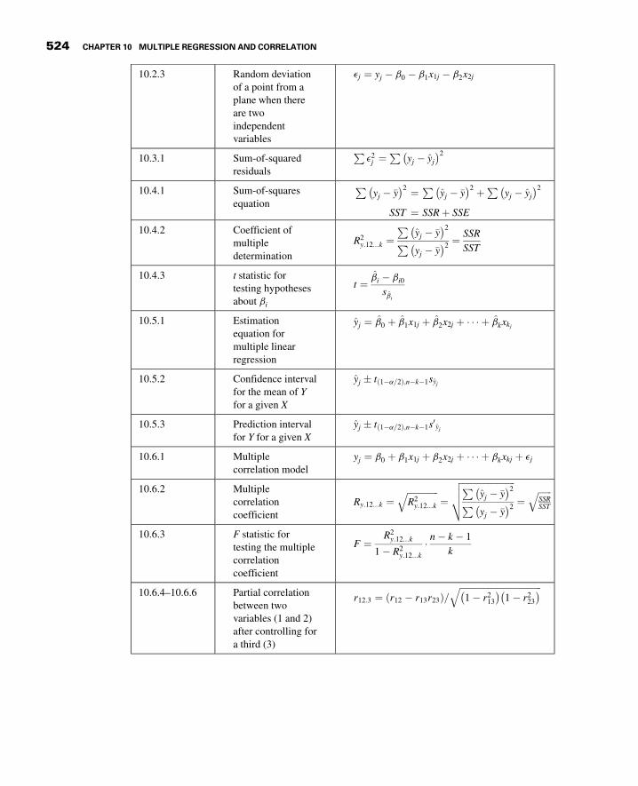
3GC10 12/04/2012 15:18:20 Page 524

10.2.3 Random deviationof a point from aplane when thereare twoindependentvariables

ej ¼ yj � b0 � b1x1j � b2x2j

10.3.1 Sum-of-squaredresiduals

Pe2j ¼

Pyj � yj� �2

10.4.1 Sum-of-squaresequation

Pyj � �y� �2 ¼ P

yj � �y� �2 þP

yj � yj� �2

SST ¼ SSRþ SSE

10.4.2 Coefficient ofmultipledetermination

R2y:12...k ¼

Pyj � �y� �2

Pyj � �y� �2 ¼ SSR

SST

10.4.3 t statistic fortesting hypothesesabout bi

t ¼ bi � bi0sbi

10.5.1 Estimationequation formultiple linearregression

yj ¼ b0 þ b1x1j þ b2x2j þ � � � þ bkxkj

10.5.2 Confidence intervalfor the mean of Yfor a given X

yj � t 1�a=2ð Þ;n�k�1syj

10.5.3 Prediction intervalfor Y for a given X

yj � t 1�a=2ð Þ;n�k�1s0yj

10.6.1 Multiplecorrelation model

yj ¼ b0 þ b1x1j þ b2x2j þ � � � þ bkxkj þ ej

10.6.2 Multiplecorrelationcoefficient

Ry:12...k ¼ffiffiffiffiffiffiffiffiffiffiffiffiffiffiR2y:12...k

q¼

ffiffiffiffiffiffiffiffiffiffiffiffiffiffiffiffiffiffiffiffiffiffiffiffiPyj � �y� �2

Pyj � �y� �2

vuut ¼ffiffiffiffiffiffiSSRSST

q

10.6.3 F statistic fortesting the multiplecorrelationcoefficient

F ¼ R2y:12...k

1 � R2y:12...k

� n� k � 1

k

10.6.4–10.6.6 Partial correlationbetween twovariables (1 and 2)after controlling fora third (3)

r12:3 ¼ r12 � r13r23ð Þ=ffiffiffiffiffiffiffiffiffiffiffiffiffiffiffiffiffiffiffiffiffiffiffiffiffiffiffiffiffiffiffiffiffiffiffiffiffi1 � r2

13

� �1 � r2

23

� �q


3GC10 12/04/2012 15:18:20 Page 525

10.6.7 t statistic for testinghypotheses aboutpartial correlationcoefficients

t ¼ ry1:2...k

ffiffiffiffiffiffiffiffiffiffiffiffiffiffiffiffiffiffiffiffiffin� k � 1

1 � r2y1:2...k

s

Symbol Key � bx ¼ estimated regression=correlation coefficient x� bx ¼ regression=correlation coefficient� e ¼ model error term� k¼ number of independent variables� n¼ sample size� r12.3 ¼ sample partial correlation coefficient between 1 and 2

after controlling for 3� R¼ sample correlation coefficient� R2¼multiple coefficient of determination� t ¼ t statistic� xi¼value of independent variable at i� �x ¼ sample mean of independent variable� yi¼value of dependent variable at i� �y ¼ sample mean of dependent variable� y ¼ estimated y� z ¼ z statistic


1. What are the assumptions underlying multiple regression analysis when one wishes to infer about thepopulation from which the sample data have been drawn?

2. What are the assumptions underlying the correlation model when inference is an objective?

3. Explain fully the following terms:

(a) Coefficient of multiple determination (b) Multiple correlation coefficient(c) Simple correlation coefficient (d) Partial correlation coefficient

4. Describe a situation in your particular area of interest where multiple regression analysis would beuseful. Use real or realistic data and do a complete regression analysis.

5. Describe a situation in your particular area of interest where multiple correlation analysis would beuseful. Use real or realistic data and do a complete correlation analysis.

In Exercises 6 through 11 carry out the indicated analysis and test hypotheses at the indicatedsignificance levels. Compute the p value for each test.

6. We learned in Example 9.7.1 that the purpose of a study by Kwast-Rabben et al. (A-6) was to analyzesomatosensory evoked potentials (SEPs) and their interrelations following stimulation of digits I, III,and V in the hand. Healthy volunteers were recruited for the study. Researchers applied stimulationbelow-pain-level intensity to the fingers. Recordings of spinal responses were made with electrodesfixed by adhesive electrode cream to the subject’s skin. Results are shown in the following table for


3GC10 12/04/2012 15:18:23 Page 526

114 subjects. Use multiple regression to see how well you can predict the peak spinal latency (Cv) ofthe SEP for digit I when age (years) and arm length (cm) are the predictor variables. Evaluate theusefulness of your prediction equation.

Age Arm Length Cv Dig.I Age Arm Length Cv Dig.I Age Arm Length Cv Dig.I

35.07 76.5 13.50 32.00 82.0 16.30 42.08 94.0 17.7035.07 76.5 13.50 32.00 82.0 15.40 40.09 94.0 17.7021.01 77.0 13.00 38.09 86.5 16.60 40.09 94.0 17.4021.01 77.0 13.60 38.09 86.5 16.00 42.09 92.5 18.4047.06 75.5 14.30 58.07 85.0 17.00 20.08 95.0 19.0047.06 75.5 14.90 58.07 85.0 16.40 50.08 94.5 19.1026.00 80.0 15.40 54.02 88.0 17.60 50.08 94.5 19.2026.00 80.0 14.70 48.10 92.0 16.80 47.11 97.5 17.8053.04 82.0 15.70 48.10 92.0 17.00 47.11 97.5 19.3053.04 82.0 15.80 54.02 88.0 17.60 26.05 96.0 17.5043.07 79.0 15.20 45.03 91.5 17.30 26.05 96.0 18.0039.08 83.5 16.50 45.03 91.5 16.80 43.02 98.0 18.0039.08 83.5 17.00 35.11 94.0 17.00 43.02 98.0 18.8043.07 79.0 14.70 26.04 88.0 15.60 32.06 98.5 18.3029.06 81.0 16.00 51.07 87.0 16.80 32.06 98.5 18.6029.06 81.0 15.80 51.07 87.0 17.40 33.09 97.0 18.8050.02 86.0 15.10 26.04 88.0 16.50 33.09 97.0 19.2025.07 81.5 14.60 35.11 94.0 16.60 35.02 100.0 18.5025.07 81.5 15.60 52.00 88.5 18.00 35.02 100.0 18.5025.10 82.5 14.60 44.02 90.0 17.40 26.05 96.0 19.0047.04 86.0 17.00 44.02 90.0 17.30 26.05 96.0 18.5047.04 86.0 16.30 24.05 91.0 16.40 25.08 100.5 19.8037.00 83.0 16.00 24.00 87.0 16.10 25.06 100.0 18.8037.00 83.0 16.00 24.00 87.0 16.10 25.06 100.0 18.4034.10 84.0 16.30 24.00 87.0 16.00 25.08 100.5 19.0047.01 87.5 17.40 24.00 87.0 16.00 30.05 101.0 18.0047.01 87.5 17.00 53.05 90.0 17.50 30.05 101.0 18.2030.04 81.0 14.10 53.05 90.0 17.50 36.07 104.5 18.9023.06 81.5 14.20 52.06 90.0 18.00 36.07 104.5 19.2023.06 81.5 14.70 52.06 90.0 17.90 35.09 102.0 21.0030.04 81.0 13.90 53.04 93.0 18.40 35.09 102.0 19.2078.00 81.0 17.20 22.04 90.0 16.40 21.01 101.5 18.6041.02 83.5 16.70 22.04 90.0 15.80 21.01 101.5 18.6041.02 83.5 16.50 46.07 95.5 18.80 40.00 95.5 20.0028.07 78.0 14.80 46.07 95.5 18.60 42.09 92.5 18.4028.07 78.0 15.00 47.00 93.5 18.00 42.08 94.0 18.5036.05 88.0 17.30 47.00 93.5 17.90 35.04 86.0 16.0035.04 86.0 15.30 39.05 94.5 17.40 36.05 88.0 16.60

Source: Data provided courtesy of Olga Kwast-Rabben, Ph.D.

7. The following table shows the weight and total cholesterol and triglyceride levels in 15 patients withprimary type II hyperlipoproteinemia just prior to initiation of treatment:


3GC10 12/04/2012 15:18:23 Page 527

YWeight (kg)

X1

Total Cholesterol(mg/100 ml)

X2

Triglyceride(mg/100 ml)

76 302 13997 336 10183 220 5752 300 5670 382 11367 379 4275 331 8478 332 18670 426 16499 399 20575 279 23078 332 18670 410 16077 389 15376 302 139

Compute the multiple correlation coefficient and test for significance at the .05 level.

8. In a study of the relationship between creatinine excretion, height, and weight, the data shown in thefollowing table were collected on 20 infant males:

Infant

CreatinineExcretion(mg/day)

YWeight (kg)

X1

Height (cm)X2

1 100 9 722 115 10 763 52 6 594 85 8 685 135 10 606 58 5 587 90 8 708 60 7 659 45 4 54

10 125 11 8311 86 7 6412 80 7 6613 65 6 6114 95 8 6615 25 5 5716 125 11 8117 40 5 59

(Continued )


3GC10 12/04/2012 15:18:24 Page 528

18 95 9 7119 70 6 6220 120 10 75

(a) Find the multiple regression equation describing the relationship among these variables.

(b) Compute R2 and do an analysis of variance.

(c) Let X1 ¼ 10 and X2 ¼ 60 and find the predicted value of Y.

9. A study was conducted to examine those variables thought to be related to the job satisfaction ofnonprofessional hospital employees. A random sample of 15 employees gave the followingresults:

Score on JobSatisfactionTest (Y)

CodedIntelligence

Score(X1)

Index ofPersonal

Adjustment(X2)

54 15 837 13 130 15 148 15 737 10 437 14 231 8 349 12 743 1 912 3 130 15 137 14 261 14 1031 9 131 4 5

(a) Find the multiple regression equation describing the relationship among these variables.

(b) Compute the coefficient of multiple determination and do an analysis of variance.

(c) Let X1 ¼ 10 and X2 ¼ 5 and find the predicted value of Y.

10. A medical research team obtained the index of adiposity, basal insulin, and basal glucose values on 21normal subjects. The results are shown in the following table. The researchers wished to investigatethe strength of the association among these variables.

Infant

CreatinineExcretion(mg/day)

YWeight (kg)

X1

Height (cm)X2


3GC10 12/04/2012 15:18:25 Page 529

Index ofAdiposityY

Basal Insulin(mU/ml)

X1

Basal Glucose(mg/100 ml)

X2

90 12 98112 10 103127 14 101137 11 102103 10 90140 38 108105 9 100

92 6 10192 8 9296 6 91

114 9 95108 9 95160 41 117

91 7 101115 9 86167 40 106108 9 84156 43 117167 17 99165 40 104168 22 85

Compute the multiple correlation coefficient and test for significance at the .05 level.

11. As part of a study to investigate the relationship between stress and certain other variables, thefollowing data were collected on a simple random sample of 15 corporate executives.

(a) Find the least-squares regression equation for these data.

(b) Construct the analysis of variance table and test the null hypothesis of no relationship among thefive variables.

(c) Test the null hypothesis that each slope in the regression model is equal to zero.

(d) Find the multiple coefficient of determination and the multiple correlation coefficient. Leta ¼ :05 and find the p value for each test.

Measure ofStress (Y)

Measure ofFirm Size

(X1)

Number of Yearsin Present

Position (X2)

AnnualSalary(�1000)(X3) Age (X4)

101 812 15 $30 3860 334 8 20 5210 377 5 20 2727 303 10 54 36

(Continued )


3GC10 12/04/2012 15:18:25 Page 530

89 505 13 52 3460 401 4 27 4516 177 6 26 50

184 598 9 52 6034 412 16 34 4417 127 2 28 3978 601 8 42 41

141 297 11 84 5811 205 4 31 51

104 603 5 38 6376 484 8 41 30

For each of the studies described in Exercises 12 through 16, answer as many of the followingquestions as possible:

(a) Which is more relevant, regression analysis or correlation analysis, or are both techniquesequally relevant?

(b) Which is the dependent variable?

(c) What are the independent variables?

(d) What are the appropriate null and alternative hypotheses?

(e) Which null hypotheses do you think were rejected? Why?

(f) Which is the more relevant objective, prediction or estimation, or are the two equally relevant?Explain your answer.

(g) What is the sampled population?

(h) What is the target population?

(i) Which variables are related to which other variables? Are the relationships direct orinverse?

(j) Write out the regression equation using appropriate numbers for parameter estimates.

(k) What is the numerical value of the coefficient of multiple determination?

(l) Give numerical values for any correlation coefficients that you can.

12. Hashimoto et al. (A-7) developed a multiple regression model to predict the number of visits toemergency rooms at Jikei University hospitals in Tokyo for children having an asthma attack. Theresearchers found that the number of visits per night increased significantly when climate conditionsshowed a rapid decrease from higher barometric pressure, from higher air temperature, and fromhigher humidity, as well as lower wind speed. The final model demonstrated that 22 percent of thevariation in the number of visits was explained by variation in the predictor variables mentionedabove with eight other significant climate variables.

13. Correlation was one of many procedures discussed in a study reported by Stenvinkel et al. (A-8). In acohort of 204 subjects with end-stage renal disease, they found no significant correlations betweenlog plasma adiponectin levels and age and no significant correlation between log plasma adiponectinand glomerular filtration rate.

Measure ofStress (Y)

Measure ofFirm Size

(X1)

Number of Yearsin Present

Position (X2)

AnnualSalary(�1000)(X3) Age (X4)


3GC10 12/04/2012 15:18:27 Page 531

14. Van Schuylenbergh et al. (A-9) used physiological and anthropometric measurements as independentvariables to predict triathlon performance (expressed in minutes). Ten triathletes underwentextensive physiological testing in swimming, cycling, and running. Within 2 weeks after the lastlaboratory test, all subjects competed in the National University Triathlon Championship. The finalregression model was

TP ¼ 130 � 9:2MLSSR� 25:9MLSSSþ 1:4BLCR

in which TP¼ triathlon performance in minutes, MLSSR¼ the running speed at MLSS (m/s),MLSSS¼ the swimming speed at MLSS, and BLCR¼ blood lactate concentration at running MLSS(mmol/L). MLSS refers to maximal lactate steady state and is generally acknowledged to be a goodmarker of functional aerobic power during prolonged exercise. It also differs for each physicalactivity. For the above model R2 ¼ :98.

15. Maximal static inspiratory (PImax) mouth pressure is a simple measurement of respiratory musclestrength. A study by Tomalak et al. (A-10) examined correlations among the variables with PImax

(measured sitting), forced expiratory volume (FEV), peak expiratory flow (PEF), and maximalinspiratory flow (PIF) in 144 boys and 152 girls ages 7–14. The researchers found PImax wascorrelated with FEV, PEF, and PIF in boys (p ¼ :001; p ¼ :0055, and p ¼ :002; respectively) and forgirls the correlations were also significant (p < :001; p < :001, and p < :001, respectively).

16. Di Monaco et al. (A-11) used multiple regression to predict bone mineral density of the femoral neck(among other locations). Among 124 Caucasian, healthy postmenopausal women, they found thatweight p < :001ð Þ, age p < :01ð Þ, and total lymphocyte count p < :001ð Þ were each useful inpredicting bone mineral density. In addition, R2 ¼ :40.

For each of the data sets given in Exercises 17 through 19, do as many of the following as you thinkappropriate:

(a) Obtain the least-squares multiple regression equation.

(b) Compute the sample coefficient of multiple determination.

(c) Compute the sample coefficient of multiple correlation.

(d) Compute simple coefficients of determination and correlation.

(e) Compute partial correlation coefficients.

(f) Construct graphs.

(g) Formulate relevant hypotheses, perform the appropriate tests, and find p values.

(h) State the statistical decisions and clinical conclusions that the results of your hypothesis testsjustify.

(i) Use your regression equations to make predictions and estimates about the dependent variablefor your selected values of the independent variables.

(j) Construct confidence intervals for relevant population parameters.

(k) Describe the population(s) to which you think your inferences are applicable.

17. Pellegrino et al. (A-12) hypothesized that maximal bronchoconstriction can be predicted from thebronchomotor effect of deep inhalation and the degree of airway sensitivity to methacholine(MCh). One group of participants consisted of 26 healthy or mildly asthmatic subjects (22 males,4 females) who had limited bronchoconstriction to inhaled MCh. The mean age of the patients was31 years with a standard deviation of 8. There was one smoker in the group. Among the datacollected on each subject were the following observations on various lung function measurementvariables:


3GC10 12/04/2012 15:18:30 Page 532

(X1)FEV1

(X2)FEV1,% Pred

X3ð ÞFEV1=

FVC;%X4ð Þ_Vm50

X5ð Þ_Vp50

X6ð ÞM=PRatio

(X7)MPSlope

(X8)PD15FEV1

(In mg)

X9ð ÞPD40

_Vm50

Inmgð Þ

X10ð ÞPD40

_Vp50Inmgð Þ

(X11) FEV1

Max decr(%)

X12ð Þ_Vm50 Maxdecr %ð Þ

X13ð Þ_Vp50 Maxdecr %ð Þ

5.22 108.75 83.92 5.30 3.90 1.36 0.75 8.44 8.24 6.34 21.40 55.40 74.405.38 123.96 78.54 6.00 3.70 1.62 0.56 7.76 7.00 6.18 15.80 50.80 85.143.62 111.04 86.19 3.10 2.85 1.10 0.69 6.92 6.61 5.56 30.40 54.36 83.073.94 94.26 85.28 4.10 2.70 1.52 0.44 6.79 8.52 6.38 16.40 29.10 58.504.48 104.43 76.58 3.21 3.00 1.07 0.63 8.79 9.74 6.68 27.80 46.30 76.705.28 117.33 81.99 5.65 5.55 1.02 0.83 8.98 8.97 8.19 32.60 70.80 90.003.80 93.37 76.61 3.75 4.70 0.80 0.50 10.52 10.60 10.04 15.80 35.30 64.903.14 104.67 82.63 3.20 3.20 1.00 0.70 6.18 6.58 6.02 37.60 64.10 87.505.26 120.09 84.84 6.30 7.40 0.89 0.55 11.85 11.85 11.85 11.70 29.10 41.204.87 121.14 89.69 5.50 5.50 1.00 0.56 11.85 11.85 11.85 10.30 16.40 29.705.35 124.71 84.65 5.60 7.00 0.80 0.40 11.98 11.98 11.29 0.00 18.00 47.204.30 95.98 80.37 5.78 4.90 1.18 0.59 6.48 6.19 5.11 17.00 48.20 79.603.75 87.82 65.79 2.26 1.65 1.37 0.53 6.25 7.02 5.03 27.10 39.53 81.804.41 112.21 69.78 3.19 2.95 1.08 0.57 7.66 8.08 5.51 24.70 48.80 85.904.66 108.37 78.72 5.00 5.90 0.85 0.49 7.79 9.77 6.10 15.00 35.00 70.305.19 99.05 73.62 4.20 1.50 2.80 0.63 5.15 5.78 4.72 31.40 61.90 86.704.32 122.38 75.13 4.39 3.30 1.33 0.74 6.20 6.34 5.10 28.25 60.30 78.004.05 95.97 84.38 3.40 2.50 1.30 0.59 5.64 8.52 5.61 18.20 29.50 46.003.23 88.25 87.30 4.00 4.00 1.00 0.71 3.47 3.43 2.77 21.60 64.50 86.003.99 105.56 86.74 5.30 2.70 1.96 0.76 6.40 5.20 6.17 22.50 63.00 77.804.37 102.34 80.18 3.20 1.80 1.77 0.85 5.05 4.97 5.42 35.30 57.00 78.002.67 68.11 65.12 1.70 1.30 1.38 0.91 3.97 3.95 4.11 32.40 58.80 82.404.75 103.71 73.08 4.60 3.60 1.21 0.71 6.34 5.29 6.04 18.85 47.50 72.203.19 88.12 85.07 3.20 1.80 1.77 0.76 5.08 4.85 5.16 36.20 83.40 93.003.29 102.17 92.68 3.80 2.40 1.58 0.50 8.21 6.90 10.60 21.60 28.10 66.702.87 95.03 95.67 3.00 3.00 1.00 0.75 6.24 5.99 7.50 27.00 46.70 68.30

_Vm50 and _Vp50 ¼ maximal and partial forced expiratory flows at 50 percent of control FVC; M=P ratio ¼ ratio of _Vm50 to _Vp50 atcontrol; MP slope = slope of the regression of percent decrements of _Vm50 and _Vp50 recorded during the MCh inhalation challenge;PD15FEV1 ¼ dose of MCh that decreased FEV1 by 15 percent of control; PD40 Vm50 and PD40

_Vp50 ¼ doses of MCh that decreased_Vm50 and Vp50 by 40 percent of control respectively; % max decr = percent maximal decrement at plateau.Source: Data providedcourtesy of Dr. Riccardo Pellegrino.

18. The purpose of a study by O’Brien et al. (A-13) was to assess hypothalamic-pituitary-adrenal(HPA) axis function (known to be altered in depression) in patients with Alzheimer’s disease (AD)by means of the adrenocorticotrophic hormone (ACTH) test, which assesses adrenal function bymeasuring cortisol production by the adrenal gland in response to an injection of ACTH. ADsubjects (mean age 69.9 years with standard deviation of 9.8) were recruited from referrals to ahospital memory clinic. Normal control subjects consisted of spouses of patients and residents of aretirement hostel (mean age 73.8 with standard deviation of 11.6). There were eight males andeight females in the AD group and 10 males and eight females in the control group. Among thedata collected were the following observations on age (C1), age at onset for AD subjects (C2),length of history of disease in months (C3), cognitive examination score (C4), peak cortisol level(C5), and total hormone response (C6):


3GC10 12/04/2012 15:18:34 Page 533

Alzheimer’s Disease Subjects Controls

C1 C2 C3 C4 C5 C6 C1 C2 C3 C4 C5 C6

73 69 48 75 400.00 44610 70 � � 97 419.00 5317587 83 48 39 565.00 63855 81 � � 93 470.00 5428560 54 72 67 307.00 31110 82 � � 93 417.00 4716062 57 60 64 335.00 36000 57 � � 101 215.00 2712075 70 48 51 352.00 44760 87 � � 91 244.00 2389563 60 24 79 426.00 47250 88 � � 88 355.00 3356581 77 48 51 413.00 51825 87 � � 91 392.00 4281066 64 24 61 402.00 41745 70 � � 100 354.00 4510578 73 60 32 518.00 66030 63 � � 103 457.00 4876572 64 72 61 505.00 49905 87 � � 81 323.00 3936069 65 48 73 427.00 55350 73 � � 94 386.00 4815076 73 36 63 409.00 51960 87 � � 91 244.00 2583046 41 60 73 333.00 33030 58 � � 103 353.00 4206077 75 18 63 591.00 73125 85 � � 93 335.00 3742564 61 36 59 559.00 60750 58 � � 99 470.00 5514072 69 30 47 511.00 54945 67 � � 100 346.00 50745

68 � � 100 262.00 2844062 � � 93 271.00 23595

� ¼Not applicable.Source: Data provided courtesy of Dr. John T. O’Brien.

19. Johnson et al. (A-14) note that the ability to identify the source of remembered information is afundamental cognitive function. They conducted an experiment to explore the relative contribution ofperceptual cues and cognitive operations information to age-related deficits in discriminatingmemories from different external sources (external source monitoring). Subjects for the experimentincluded 96 graduate and undergraduate students (41 males and 55 females) ranging in ages from 18to 27 years. Among the data collected were the following performance recognition scores on sourcemonitoring conditions (C1, C2, C3) and scores on the Benton Facial Recognition Test (C4), theWechsler Adult Intelligence Scale—Revised (WAIS-R), WAIS-R Block Design subscale (C5),WAIS-R Vocabulary subscale (C6), the Benton Verbal Fluency Test (C7), and the Wisconsin CardSorting Test (C8):

C1 C2 C3 C4 C5 C6 C7 C8

0.783 2.63 0.808 25 38 62 67 60.909 3.36 0.846 � � 50 � �

0.920 2.14 0.616 23 25 53 47 60.727 3.36 0.846 25 40 49 58 60.737 2.93 0.731 � � 59 � �

0.600 4.07 0.962 19 50 51 35 60.840 3.15 0.885 � � 57 � �

0.850 3.06 0.769 � � 55 � �

0.875 3.72 0.923 24 23 52 35 6

(Continued )


3GC10 12/04/2012 15:18:36 Page 534

0.792 3.15 0.884 � � 50 � �

0.680 4.07 0.962 � � 56 � �

0.731 4.64 1.000 23 30 59 47 30.826 1.84 0.616 � � 52 � �

0.609 2.98 0.846 � � 56 � �

0.923 4.64 1.000 � � 53 � �

0.773 3.36 0.846 � � 60 � �

0.714 1.62 0.577 23 43 53 42 60.667 3.72 0.923 20 32 59 28 60.769 1.40 0.423 � � 51 � �

0.565 3.55 0.885 � � 45 � �

0.824 1.78 0.577 � � 45 � �

0.458 1.90 0.615 21 46 50 47 60.840 4.07 0.962 � � 59 � �

0.720 4.07 0.962 � � 53 � �

0.917 3.72 0.923 24 31 43 37 60.560 4.07 0.926 � � 62 � �

0.840 4.07 0.962 26 22 50 40 60.720 4.07 0.962 � � 52 � �

0.783 1.74 0.577 � � 54 � �

0.696 1.62 0.539 � � 57 � �

0.625 3.72 0.923 22 37 55 40 60.737 1.12 0.423 � � 47 � �

0.900 1.92 0.654 22 40 46 42 60.565 3.55 0.885 22 43 56 64 60.680 4.07 0.962 � � 54 � �

0.760 4.07 0.962 � � 58 � �

0.958 1.90 0.615 24 36 46 43 60.652 2.98 0.846 � � 54 � �

0.560 4.07 0.962 � � 56 � �

0.500 1.92 0.654 24 42 45 46 60.826 2.63 0.808 � � 60 � �

0.783 2.58 0.808 � � 60 � �

0.783 2.63 0.808 � � 49 � �

0.750 2.14 0.692 22 37 62 58 60.913 2.11 0.693 � � 46 � �

0.952 1.49 0.539 26 32 48 36 60.800 4.07 0.962 � � 59 � �

0.870 3.55 0.885 � � 48 � �

0.652 1.97 0.654 � � 59 � �

0.640 4.07 0.962 25 36 56 54 60.692 4.64 1.000 23 23 58 25 60.917 3.72 0.923 � � 55 � �

0.760 4.07 0.962 22 35 52 33 60.739 3.55 0.885 24 43 58 43 6

(Continued )

C1 C2 C3 C4 C5 C6 C7 C8


3GC10 12/04/2012 15:18:39 Page 535

0.857 3.20 0.808 � � 59 � �

0.727 3.36 0.846 � � 61 � �

0.833 2.80 0.846 � � 56 � �

0.840 4.07 0.962 21 11 49 58 30.478 2.27 0.731 � � 60 � �

0.920 4.07 0.962 24 40 64 50 60.731 4.64 1.000 20 40 51 50 60.920 4.07 0.962 23 50 61 53 60.720 4.07 0.962 � � 57 � �

1.000 2.79 0.807 25 47 56 30 60.708 3.72 0.923 24 16 57 42 61.000 4.64 1.000 25 48 55 54 60.739 3.55 0.885 23 27 57 38 60.600 4.20 0.962 22 38 57 33 60.962 4.64 1.000 25 37 63 31 60.772 2.22 0.731 24 48 51 41 60.800 2.92 0.847 24 28 47 45 60.923 4.64 1.000 25 45 54 48 60.870 3.50 0.885 24 44 54 48 50.808 4.64 1.000 24 43 57 58 61.000 4.07 0.962 25 30 59 49 60.870 3.55 0.885 26 44 61 35 60.923 4.64 1.000 � � 52 � �

0.958 2.58 0.808 27 32 52 33 60.826 3.50 0.885 21 31 61 44 60.962 3.72 0.923 23 31 57 38 60.783 3.50 0.885 23 46 60 36 60.905 3.20 0.808 23 34 55 37 41.000 4.64 1.000 23 33 57 33 60.875 3.72 0.923 21 34 55 29 60.885 4.07 0.962 � � 52 � �

0.913 2.92 0.846 23 44 57 47 60.962 4.07 0.961 24 36 54 43 60.682 3.36 0.846 20 41 61 34 10.810 2.63 0.769 20 40 57 43 60.720 2.79 0.808 25 23 64 43 30.875 2.80 0.846 24 43 59 43 20.923 3.72 0.924 25 40 58 33 60.909 3.36 0.846 24 43 56 41 60.920 4.07 0.962 24 50 52 28 61.000 3.72 0.923 21 45 64 46 60.609 3.50 0.885 22 25 49 35 6

�¼Missing data.Source: Data provided courtesy of Dr. Doreen M. De Leonardis.

C1 C2 C3 C4 C5 C6 C7 C8


3GC10 12/04/2012 15:18:39 Page 536

Exercises for Use with the Large Data Sets Available on the Following Website:www.wiley.com/college/daniel

1. Winters et al. (A-15) conducted a study involving 248 high-school students enrolled inintroductory physical education courses. The researchers wanted to know if social cognitivetheory constructs were correlated with discretionary, “leisure-time” physical exercise. The mainoutcome variable is STREN, which is the number of days in a week that a high-school studentengaged in strenuous physical activity (operationally defined as exercise that results in sweating,labored breathing, and rapid heart rate). Students in the study filled out lengthy questionnairesfrom which the following variables were derived:

SELFR100—measures personal regulation of goal-directed behavior (higher values indicatemore goal oriented).

SS100—measures social support, social encouragement, and social expectation that areprovided by friends and family for physical exercise (higher values indicate more support).

SSE100—measures perceived ability to overcome barriers to exercise (higher values indicatehigher ability).

OEVNORM—measures outcome expectations and their associated expectancies for physicalexercise (higher values indicate stronger perceived links to desired outcomes from exercise).

With these data (LTEXER),

(a) Calculate the bivariate correlation for each pair of variables and interpret the meaning ofeach.(b) Using STREN as the dependent variable, compute the multiple correlation coefficient.(c) Using STREN as the dependent variable, calculate the partial correlation coefficient forSTREN and SELFR100 after controlling for SS100.(d) Using STREN as the dependent variable, calculate the partial correlation coefficient forSTREN and SSE100 after controlling for OEVNORM.

Note that there many missing values in this data set.

2. With data obtained from a national database on childbirth, Matulavich et al. (A-16) examined thenumber of courses of prescribed steroids a mother took during pregnancy (STEROIDS). The sizeof the baby was measured by length (cm), weight (grams), and head circumference (cm).Calculate the correlation of the number of courses of steroids with each of the three outcomevariables. What are the hypotheses for your tests? What are the p-values? What are yourconclusions? (The name of the data set is STERLENGTH.)

3. Refer to the data on cardiovascular risk factors (RISKFACT). The subjects are 1000 malesengaged in sedentary occupations. You wish to study the relationships among risk factors in thispopulation. The variables are

Y ¼ oxygen consumptionX1 ¼ systolic blood pressure mm Hgð ÞX2 ¼ total cholesterol mg=dlð ÞX3 ¼ HDL cholesterol mg=dlð ÞX4 ¼ triglycerides mg=dlð Þ

Select a simple random sample from this population and carry out an appropriate statisticalanalysis. Prepare a narrative report of your findings and compare them with those of yourclassmates. Consult with your instructor regarding the size of the sample.



3GC10 12/04/2012 15:18:39 Page 537

4. Refer to the data on 500 patients who have sought treatment for the relief of respiratory diseasesymptoms (RESPDIS). A medical research team is conducting a study to determine what factorsmay be related to respiratory disease. The dependent variable Y is a measure of the severity of thedisease. A larger value indicates a more serious condition. The independent variables are asfollows:

X1¼ education (highest grade completed)

X2¼measure of crowding of living quarters

X3¼measure of air quality at place of residence (a larger number indicates poorer quality)

X4¼ nutritional status (a large number indicates a higher level of nutrition)

X5 ¼ smoking status 0 ¼ smoker; 1 ¼ nonsmokerð ÞSelect a simple random sample of subjects from this population and conduct a statistical analysisthat you think would be of value to the research team. Prepare a narrative report of your resultsand conclusions. Use graphic illustrations where appropriate. Compare your results with those ofyour classmates. Consult your instructor regarding the size of sample you should select.

REFERENCES


1. GEORGE W. SNEDECOR and WILLIAM G. COCHRAN, Statistical Methods, Sixth Edition, Iowa State University Press,Ames, 1967.

2. ROBERT G. D. STEEL and JAMES H. TORRIE, Principles and Procedures of Statistics, McGraw-Hill, New York, 1960.3. R. L. ANDERSON and T. A. BANCROFT, Statistical Theory in Research, McGraw-Hill, New York, 1952.4. M. H. KUTNER, C. J. NACHTSHEIM, J. NETER, and W. LI, Applied Linear Statistical Models, Fifth Edition, McGraw-

Hill/Irwin, New York, 2005.


A-1. DEBRA A. JANSEN and MARY L. KELLER, “Cognitive Function in Community-Dwelling Elderly Women,” Journalof Gerontological Nursing, 29 (2003), 34–43.

A-2. M. NAEIJE, “Local Kinematic and Anthropometric Factors Related to the Maximum Mouth Opening in HealthyIndividuals,” Journal of Oral Rehabilitation, 29 (2002), 534–539.

A-3. GWI-RYUNG SON, MAY L. WYKLE, and JACLENE A. ZAUSZNIEWSKI, “Korean Adult Child Caregivers of Older Adultswith Dementia,” Journal of Gerontological Nursing, 29 (2003), 19–28.

A-4. X. WANG, X. SHEN, X. LI, and C. MAULI AGRAWAL, “Age-Related Changes in the Collagen Network and Toughnessof Bone,” Bone, 31 (2002), 1–7.

A-5. PETER A. ANTON, RONALD T. MITSUYASU, STEVEN G. DEEKS, DAVID T. SCADDEN, BRIDGET WAGNER, CHRISTINE HUANG,CATHERINE MACKEN, DOUGLAS D. RICHMAN, CINDY CHRISTOPHERSON, FLAVIA BORELLINI, RICHARD LAZAR, and KRISTEN

M. HEGE, “Multiple Measures of HIV Burden in Blood and Tissue Are Correlated with Each Other but Not withClinical Parameter in Aviremic Subjects,” AIDS, 17 (2003), 53–63.

A-6. OLGA KWAST-RABBEN, ROLF LIBELIUS, and HANNU HEIKKIL€A, “Somatosensory Evoked Potentials FollowingStimulation of Digital Nerves,” Muscle and Nerve, 26 (2002), 533–538.

A-7. MITSUO HASHIMOTO, TAIKI FUKUDA, TETSUYA SHIMIZU, SHOU WATANABE, SATOSHI WATANUKI, YOSHIKATSU ETO, andMITSUYOSHI URASHIMA, “Influence of Climate Factors on Emergency Visits for Childhood Asthma Attack,”Pediatrics International, 46 (2004), 48–52.

A-8. PETER STENVINKEL, ALICIA MARCHELEWSKA, ROBERTO PECOITS-FILHO, OLOF HEIMB€URGER, ZHENGZHONG ZHANG,CATHERINE HOFF, CLIFF HOLMES, JOANAS AXELSSON, SIVONNE ARVIDSSON, MARTIN SCHALLING, PETER BARANY, BENGT

LINKHOLM, and LOUISE NORDFORS, “Adiponectin in Renal Disease: Relationship to Phenotype and GeneticVariation in the Genetic Encoding Adiponectin,” Kidney International, 65 (2004), 274–281.

REFERENCES 537

3GC10 12/04/2012 15:18:39 Page 538

A-9. R. VAN SCHUYLENBERGH, B. VANDEN EYNDE, and P. HESPEL, “Prediction of Sprint Triathlon Performance fromLaboratory Tests,” European Journal of Applied Physiology, 91 (2004), 94–99.

A-10. WALDEMAR TOMALAK, ANDRZEJ POGORZELSKI, and JAROSLAW PRUSAK, “Normal Values for Maximal StaticInspiratory and Expiratory Pressures in Healthy Children,” Pediatric Pulmonology, 34 (2002), 42–46.

A-11. MARCO DI MONACO, FULVIA VALLERO, ROBERTO DI MONACO, FULVIO MAUTINO, and ALBERTO CAVANNA, “TotalLymphocyte Count and Femoral Bone Mineral Density in Postmenopausal Women,” Journal of Bone MineralMetabolism, 22 (2004), 58–63.

A-12. RICCARDO PELLEGRINO, BENEDETTO VIOLANTE, and VITO BRUSASCO, “Maximal Bronchoconstriction in Humans:Relationship to Deep Inhalation and Airway Sensitivity,” American Journal of Respiratory and Critical CareMedicine, 153 (1996), 115–121.

A-13. J. T. O’BRIEN, D. AMES, I. SCHWEITZER, M. MASTWYK, and P. COLMAN, “Enhanced Adrenal Sensitivity toAdrenocorticotrophic Hormone (ACTH) Is Evidence of HPA Axis Hyperactivity in Alzheimer’s Disease,”Psychological Medicine, 26 (1996), 7–14.

A-14. MARCIA K. JOHNSON, DOREEN M. DE LEONARDIS, SHAHIN HARSHTROUDI, and SUSAN A. FERGUSON, “Aging and SingleVersus Multiple Cues in Source Monitoring,” Psychology and Aging, 10 (1995), 507–517.

A-15. ERIC R. WINTERS, RICK L. PETOSA, and THOMAS E. CHARLETON, “Using Social Cognitive Theory to ExplainDiscretionary, ‘Leisure-Time’ Physical Exercise Among High School Students,” Journal of Adolescent Health,32 (2003), 436–442.

A-16. ANGELA MATULAVICH, DONNA MILES-CURRY, BARBARA WARNER, BOBBE GRAY, and the National Institute of Child andHealth Development. Data analyzed at the Wright State University Statistical Consulting Center.


3GC11 12/04/2012 15:47:23 Page 539

CHAPTER11REGRESSION ANALYSIS:SOME ADDITIONAL TECHNIQUES

CHAPTER OVERVIEW

This chapter provides an introduction to some additional tools and conceptsthat are useful in regression analysis. The presentation includes expansions ofthe basic ideas and techniques of regression analysis that were introduced inChapters 9 and 10.

TOPICS

11.1 INTRODUCTION

11.2 QUALITATIVE INDEPENDENT VARIABLES

11.3 VARIABLE SELECTION PROCEDURES

11.4 LOGISTIC REGRESSION

11.5 SUMMARY

LEARNING OUTCOMES


1. understand how to include qualitative variables in a regression analysis.

2. understand how to use automated variable selection procedures to developregression models.

3. be able to perform logistic regression for dichotomous and polytomous depen-dent variables.

539

3GC11 12/04/2012 15:47:23 Page 540

11.1 INTRODUCTION

The basic concepts and methodology of linear regression analysis are covered inChapters 9 and 10. In Chapter 9 we discuss the situation in which the objective is toobtain an equation that can be used to make predictions and estimates about somedependent variable from knowledge of some other single variable that we call theindependent, predictor, or explanatory variable. In Chapter 10 the ideas and techniqueslearned in Chapter 9 are expanded to cover the situation in which it is believed that theinclusion of information on two or more independent variables will yield a better equationfor use in making predictions and estimations. Regression analysis is a complex andpowerful statistical tool that is widely employed in health sciences research. To do thesubject justice requires more space than is available in an introductory statistics textbook.However, for the benefit of those who wish additional coverage of regression analysis, wepresent in this chapter some additional topics that should prove helpful to the student andpractitioner of statistics.

Regression Assumptions Revisited As we learned in Chapters 9 and 10,there are several assumptions underlying the appropriate use of regression procedures.Often there are certain measurements that strongly influence the shape of a distributionor impact the magnitude of the variance of a measured variable. Other times, certainindependent variables that are being used to develop a model are highly correlated, leadingto the development of a model that may not be unique or correct.

Non-Normal Data Many times the data that are used to build a regression modelare not normally distributed. One may wish to explore the possibility that some of theobserved data points are outliers or that they disproportionately affect the distribution ofthe data. Such an investigation may be accomplished informally by constructing a scatterplot and looking for observations that do not seem to fit with the others. Alternatively,many computer packages produce formal tests to evaluate potential outlying observa-tions in either the dependent variable or the independent variables. It is always up to theresearcher, however, to justify which observations are to be removed from the data setprior to analysis.

Often one may wish to attempt a transformation of the data. Mathematical transfor-mations are useful because they do not affect the underlying relationships among variables.Since hypothesis tests for the regression coefficients are based on normal distributionstatistics, data transformations can sometimes normalize the data to the extent necessary toperform such tests. Simple transformations, such as taking the square root of measurementsor taking the logarithm of measurements, are quite common.

EXAMPLE 11.1.1

Researchers were interested in blood concentrations of delta-9-tetrahydrocannabinol(D-9-THC), the active psychotropic component in marijuana, from 25 research subjects.These data are presented in Table 11.1.1, as are these same data after using a log10

transformation.

540 CHAPTER 11 REGRESSION ANALYSIS: SOME ADDITIONAL TECHNIQUES

3GC11 12/04/2012 15:47:23 Page 541

Box-and-whisker plots from SPSS software for these data are shown in Figure 11.1.1. Theraw data are clearly skewed, and an outlier is identified (observation 25). A log10 transfor-mation, which is often useful for such skewed data, removes the magnitude of the outlier andresults in a distribution that is much more nearly symmetric about the median. Therefore, thetransformed data could be used in lieu of the raw data for constructing the regression model.Though symmetric data do not, necessarily, imply that the data are normal, they do result in amore appropriate model. Formal tests of normality, as previously mentioned, should alwaysbe carried out prior to analysis. &

Unequal Error Variances When the variances of the error terms are not equal, wemay obtain a satisfactory equation for the model, but, because the assumption that the errorvariances are equal is violated, we will not be able to perform appropriate hypothesis tests onthe model coefficients. Just as was the case in overcoming the non-normality problem,transformations of the regressionvariables may reduce the impact of unequal error variances.

TABLE 11.1.1 Data from a Random Sample of 25 Research

Subjects Tested for D-9-THC, Example 11.1.1

Case No. Concentration (mg/ml) Log10 Concentration (mg/ml)

1 .30 �.52

2 2.75 .44

3 2.27 .36

4 2.37 .37

5 1.12 .05

6 .60 �.22

7 .61 �.21

8 .89 �.05

9 .33 �.48

10 .85 �.07

11 2.18 .34

12 3.59 .56

13 .28 �.55

14 1.90 .28

15 1.71 .23

16 .85 �.07

17 1.53 .18

18 2.25 .35

19 .88 �.05

20 .49 �.31

21 4.35 .64

22 .67 �.17

23 2.74 .44

24 .79 �.10

25 6.94 .84


3GC11 12/04/2012 15:47:23 Page 542

Correlated Independent Variables Multicollinearity is a common problem thatarises when one attempts to build a model using many independent variables. Multicolli-nearityoccurswhenthere isahighdegreeofcorrelationamongthe independentvariables.Forexample, imagine that we want to find an equation relating height and weight to bloodpressure. A common variable that is derived from height and weight is called the body massindex (BMI). If we attempt to find an equation relating height, weight, and BMI to bloodpressure, we can expect to run into analytical problems because BMI, by definition, is highlycorrelated with both height and weight.

The problem arises mathematically when the solutions for the regression coefficientsare derived. Since the data are correlated, solutions may not be found that are unique to agiven model. The least complex solution to multicollinearity is to calculate correlationsamong all of the independent variables and to retain only those variables that are not highlycorrelated. A conservative rule of thumb to remove redundancy in the data set is toeliminate variables that are related to others with a significant correlation coefficientabove 0.7.

EXAMPLE 11.1.2

A study of obesity and metabolic syndrome used data collected from 15 students, andincluded systolic blood pressure (SBP), weight, and BMI. These data are presented inTable 11.1.2.

Correlations for the three variables are shown in Figure 11.1.2. The very large andsignificant correlation between the variables weight and BMI suggests that including bothof these variables in the model is inappropriate because of the high level of redundancy inthe information provided by these variables. This makes logical sense since BMI is afunction of weight. The researcher is now faced with the task of deciding which of thevariables to retain for constructing the regression model.

FIGURE 11.1.1 Box-and-whisker plots of data from Example 11.1.1.


3GC11 12/04/2012 15:47:24 Page 543

&

11.2 QUALITATIVE INDEPENDENTVARIABLES

The independent variables considered in the discussion in Chapter 10 were all quantitative;that is, they yielded numerical values that were either counts or measurements in the usualsense of the word. For example, some of the independent variables used in our examplesand exercises were age, education level, collagen porosity, and collagen tensile strength.Frequently, however, it is desirable to use one or more qualitative variables as independentvariables in the regression model. Qualitative variables, it will be recalled, are thosevariables whose “values” are categories and that convey the concept of attribute rather thanamount or quantity. The variable marital status, for example, is a qualitative variable whosecategories are “single,” “married,” “widowed,” and “divorced.” Other examples ofqualitative variables include sex (male or female), diagnosis, race, occupation, and

TABLE 11.1.2 Data from 8 Random Sample of 15

Students

Case No. SBP Weight (lbs.) BMI

1 126 125 24.41

2 129 130 23.77

3 126 132 20.07

4 123 200 27.12

5 124 321 39.07

6 125 100 20.90

7 127 138 22.96

8 125 138 24.44

9 123 149 23.33

10 119 180 25.82

11 127 184 26.40

12 126 251 31.37

13 122 197 26.72

14 126 107 20.22

15 125 125 23.62

Correlations: SBP, Weight, BMI

SBP Weight

Weight 0.289p-value 0.296

BMI 0.213 0.962p-value 0.447 0.000

FIGURE 11.1.2 Correlations calculated in MINITAB software for the data in Example 11.1.2.

11.2 QUALITATIVE INDEPENDENT VARIABLES 543

3GC11 12/04/2012 15:47:24 Page 544

immunity status to some disease. In certain situations an investigator may suspect thatincluding one or more variables such as these in the regression equation would contributesignificantly to the reduction of the error sum of squares and thereby provide more preciseestimates of the parameters of interest.

Suppose, for example, that we are studying the relationship between the dependentvariable systolic blood pressure and the independent variables weight and age. We mightalso want to include the qualitative variable sex as one of the independent variables. Orsuppose we wish to gain insight into the nature of the relationship between lung capacityand other relevant variables. Candidates for inclusion in the model might consist of suchquantitative variables as height, weight, and age, as well as qualitative variables suchas sex, area of residence (urban, suburban, rural), and smoking status (current smoker,ex-smoker, never smoked).

Dummy Variables In order to incorporate a qualitative independent variablein the multiple regression model, it must be quantified in some manner. This may beaccomplished through the use of what are known as dummy variables.

DEFINITION

A dummy variable is a variable that assumes only a finite number ofvalues (such as 0 or 1) for the purpose of identifying the differentcategories of a qualitative variable.

The term “dummy” is used to indicate the fact that the numerical values (such as0 and 1) assumed by the variable have no quantitative meaning but are used merely toidentify different categories of the qualitative variable under consideration. Qualitativevariables are sometimes called indicator variables, and when there are only two categories,they are sometimes called dichotomous variables.

The following are some examples of qualitative variables and the dummy variablesused to quantify them:

Qualitative Variable Dummy Variable

Sex (male, female):x1 ¼ 1 for male

0 for female

�:

Place of residence (urban, rural, suburban):x1 ¼ 1 for urban

0 for rural and suburban

�:

x2 ¼ 1 for rural0 for urban and suburban

�:

Smoking status [current smoker, ex-smoker(has not smoked for 5 years or less), ex-smoker(has not smoked for more than 5 years), never smoked]:

x1 ¼ 1 for current smoker0 for otherwise

�:

x2 ¼ 1 for ex-smoker � 5 yearsð Þ0 otherwise

�:

x3 ¼ 1 for ex-smoker > 5 yearsð Þ0 otherwise

�:


3GC11 12/04/2012 15:47:26 Page 545

Note in these examples that when the qualitative variable has k categories, k � 1dummy variables must be defined for all the categories to be properly coded. This rule isapplicable for any multiple regression containing an intercept constant. The variable sex,with two categories, can be quantified by the use of only one dummy variable, while threedummy variables are required to quantify the variable smoking status, which has fourcategories.

The following examples illustrate some of the uses of qualitative variables inmultiple regression. In the first example we assume that there is no interaction betweenthe independent variables. Since the assumption of no interaction is not realistic in manyinstances, we illustrate, in the second example, the analysis that is appropriate wheninteraction between variables is accounted for.

EXAMPLE 11.2.1

In a study of factors thought to be associated with birth weight, a simple random sample of100 birth records was selected from the North Carolina 2001 Birth Registry (A-1).Table 11.2.1 shows, for three variables, the data extracted from each record. There aretwo independent variables: length of gestation (weeks), which is quantitative, andsmoking status of mother (smoke), a qualitative variable. The dependent variable is birthweight (grams).

TABLE 11.2.1 Data from a Simple Random Sample of 100 Births from theNorth Carolina Birth Registry, Example 11.2.1

Case No. Grams Weeks Smoke Case No. Grams Weeks Smoke

1 3147 40 0 51 3232 38 0

2 2977 41 0 52 3317 40 0

3 3119 38 0 53 2863 37 0

4 3487 38 0 54 3175 37 0

5 4111 39 0 55 3317 40 0

6 3572 41 0 56 3714 34 0

7 3487 40 0 57 2240 36 0

8 3147 41 0 58 3345 39 0

9 3345 38 1 59 3119 39 0

10 2665 34 0 60 2920 37 0

11 1559 34 0 61 3430 41 0

12 3799 38 0 62 3232 35 0

13 2750 38 0 63 3430 38 0

14 3487 40 0 64 4139 39 0

15 3317 38 0 65 3714 39 0

16 3544 43 1 66 1446 28 1

17 3459 45 0 67 3147 39 1

18 2807 37 0 68 2580 31 0

19 3856 40 0 69 3374 37 0

20 3260 40 0 70 3941 40 0

(Continued )


3GC11 12/04/2012 15:47:28 Page 546

Solution: For the analysi s, we quant ify smoking status by means of a dummy variablethat is coded 1 if the mother is a smoker and 0 if she is a nonsmoker. The datain Table 11.2.1 are plotted as a scatter diagram in Figure 11.2.1. The scatterdiagram suggests that, in general, longer periods of gestation are associatedwith larger birth weights.

To obtain additional insight into the nature of these data, we may enterthem into a computer and employ an appropriate program to perform furtheranalyses. For example, we enter the observations y1¼ 3147, x11¼ 40, x21¼ 0,for the first case; Y2¼ 2977, x12¼ 41, x22¼ 0 for the second case; and so on.Figure 11.2.2 shows the computer output obtained with the use of theMINITAB multiple regression program.

21 2183 42 1 71 2070 37 0

22 3204 38 0 72 3345 40 0

23 3005 36 0 73 3600 40 0

24 3090 40 1 74 3232 41 0

25 3430 39 0 75 3657 38 1

26 3119 40 0 76 3487 39 0

27 3912 39 0 77 2948 38 0

28 3572 40 0 78 2722 40 0

29 3884 41 0 79 3771 40 0

30 3090 38 0 80 3799 45 0

31 2977 42 0 81 1871 33 0

32 3799 37 0 82 3260 39 0

33 4054 40 0 83 3969 38 0

34 3430 38 1 84 3771 40 0

35 3459 41 0 85 3600 40 0

36 3827 39 0 86 2693 35 1

37 3147 44 1 87 3062 45 0

38 3289 38 0 88 2693 36 0

39 3629 36 0 89 3033 41 0

40 3657 36 0 90 3856 42 0

41 3175 41 1 91 4111 40 0

42 3232 43 1 92 3799 39 0

43 3175 36 0 93 3147 38 0

44 3657 40 1 94 2920 36 0

45 3600 39 0 95 4054 40 0

46 3572 40 0 96 2296 36 0

47 709 25 0 97 3402 38 0

48 624 25 0 98 1871 33 1

49 2778 36 0 99 4167 41 0

50 3572 35 0 100 3402 37 1

Source: John P. Holcomb, sampled and coded from North Ca rolina Birth Registry data found at www.irss.un c.edu/ ncvit al/ bfd1down.html .

Case No. Grams Weeks Smoke Case No. Grams Weeks Smoke



3GC11 12/04/2012 15:47:28 Page 547

The regression equation is

grams 1724 130 x1 294 x2

Predictor Coef SE Coef T PConstant 1724.4 558.8 3.09 0.003weeks (x1) 130.05 14.52 8.96 0.000smoke (x2) 294.4 135.8 2.17 0.033

S 484.6 R-Sq 46.4% R-Sq(adj) 45.3%


SOURCE DF SS MS F PRegression 2 19689185 9844593 41.92 0.000Residual Error 97 22781681 234863Total 99 42470867

SOURCE DF Seq SSx1 1 18585166x2 1 1104020

FIGURE 11.2.2 Partial computer printout, MINITAB multiple regression analysis.

Example 11.2.1.

25 30 35 40 45 500

1000

2000

3000

4000

5000

Length of gestation (weeks)

Bir

th w

eig

ht

(gra

ms)

FIGURE 11.2.1 Birth weights and lengths of gestation for 100 births: (~) smoking and (�)

nonsmoking mothers.


3GC11 12/04/2012 15:47:28 Page 548

We see in the printout that the multiple regression equation is

yj ¼ b0 þb1x1j þb2x2j

yj ¼ �1724:4 þ 130:05x1j � 294:4x2j

(11.2.1)

To observe the effect on this equation when we wish to consider onlythe births to smoking mothers, we let x2j ¼ 1. The equation then becomes

yj ¼ �1724:4 þ 130:05x1j � 294:4ð1Þ¼ �2018:8 þ 130:05x1j

(11.2.2)

which has a y-intercept of�2018.8 and a slope of 130. Note that the y-interceptfor the new equation is equal to (b0 þ b1)¼ [�1724.4þ (�294.4)]¼�2018.

Now let us consider only births to nonsmoking mothers. When we letx2¼ 0, our regression equation reduces to

yj ¼ �1724:4 þ 130:05x1j � 294ð0Þ¼ �1724:4 þ 130:05x1j

(11.2.3)

The slope of this equation is the same as the slope of the equation forsmoking mothers, but the y-intercepts are different. The y-intercept for theequation associated with nonsmoking mothers is larger than the one for thesmoking mothers. These results show that for this sample, babies born to

25 30 35 40 45 500

1000

2000

3000

4000

5000

Length of gestation (weeks)

Nonsmokingmothers

Bir

th w

eig

ht

(gra

ms)

Smokingmothers

FIGURE 11.2.3 Birth weights and lengths of gestation for 100 births and the fitted regression

lines: (~) smoking and (�) nonsmoking mothers.


3GC11 12/04/2012 15:47:28 Page 549

mothers who do not smoke weighed, on the average, more than babies born tomothers who do smoke, when length of gestation is taken into account. Theamount of the difference, on the average, is 294 grams. Stated another way,we can say that for this sample, babies born to mothers who smoke weighed,on the average, 294 grams less than the babies born to mothers who do notsmoke, when length of gestation is taken into account. Figure 11.2.3 showsthe scatter diagram of the original data along with a plot of the two regressionlines (Equations 11.2.2 and 11.2.3). &

EXAMPLE 11.2.2

At this point a question arises regarding what inferences we can make about the sampledpopulation on the basis of the sample results obtained in Example 11.2.1. First of all, wewish to know if the sample difference of 294 grams is significant. In other words, doessmoking have an effect on birth weight? We may answer this question through thefollowing hypothesis testing procedure.

Solution:

1. Data. The data are as given in Example 11.2.1.

2. Assumptions. We presume that the assumptions underlying multipleregression analysis are met.

3. Hypotheses. H0: b2¼ 0; HA: b2 6¼ 0. Suppose we let a¼ .05.

4. Test statistic. The test statistic is t¼ (b2 � 0)/sb2.

5. Distribution of test statistic. When the assumptions are met and H0 istrue the test statistic is distributed as Student’s t with 97 degrees offreedom.

6. Decision rule. We reject H0 if the computed t is either greater than orequal to 1.9848 or less than or equal to �1.9848 (obtained byinterpolation).

7. Calculation of test statistic. The calculated value of the test statisticappears in Figure 11.2.2 as the t ratio for the coefficient associated withthe variable appearing in Column 4 of Table 11.2.1. This coefficient, ofcourse, is b2. We see that the computed t is �2.17.

8. Statistical decision. Since �2.17<�1.9848, we reject H0.

9. Conclusion. We conclude that, in the sampled population, whether themothers smoke is associated with a reduction in the birth weights of theirbabies.

10. p value. For this test we have p¼ .033 from Figure 11.2.2. &

A Confidence Interval for b2 Given that we are able to conclude that in thesampled population the smoking status of the mothers does have an effect on the birthweights of their babies, we may now inquire as to the magnitude of the effect. Our best


3GC11 12/04/2012 15:47:29 Page 550

point estimate of the average difference in birth weights, when length of gestation is takeninto account, is 294 grams in favor of babies born to mothers who do not smoke. We mayobtain an interval estimate of the mean amount of the difference by using information fromthe computer printout by means of the following expression:

b2 � tsb2

For a 95% confidence interval, we have

�294:4 � 1:9848 135:8ð Þ�563:9;�24:9ð Þ

Thus, we are 95% confident that the difference is somewhere between about 564 grams and25 grams.

Advantages of DummyVariables The reader may have correctly surmisedthat an alternative analysis of the data of Example 11.2.1 would consist of fitting twoseparate regression equations: one to the subsample of mothers who smoke and another tothe subsample of those who do not. Such an approach, however, lacks some of theadvantages of the dummy variable technique and is a less desirable procedure when thelatter procedure is valid. If we can justify the assumption that the two separate regressionlines have the same slope, we can get a better estimate of this common slope through theuse of dummy variables, which entails pooling the data from the two subsamples. InExample 11.2.1 the estimate using a dummy variable is based on a total sample size of 100observations, whereas separate estimates would be based on a sample of 85 smokers andonly 15 nonsmokers. The dummy variables approach also yields more precise inferencesregarding other parameters since more degrees of freedom are available for the calculationof the error mean square.

UseofDummyVariables: InteractionPresent Now let us consider thesituation in which interaction between the variables is assumed to be present. Suppose, forexample, that we have two independent variables: one quantitative variable X1 and onequalitative variable with three response levels yielding the two dummy variables X2 and X3.The model, then, would be

yj ¼ b0 þ b1X1j þ b2X2j þ b3X3j þ b4X1jX2j þ b5X1jX3j þ ej (11.2.4)

in which b4X1jX2j and b5X1jX3j are called interaction terms and represent the interactionbetween the quantitative and the qualitative independent variables. Note that there is noneed to include in the model the term containing X2jX3j; it will always be zero becausewhen X2 ¼ 1; X3 ¼ 0, and when X3 ¼ 1; X2 ¼ 0. The model of Equation 11.2.4 allows fora different slope and Y-intercept for each level of the qualitative variable.

Suppose we use dummy variable coding to quantify the qualitative variable as follows:

X2 ¼ 1 for level 10 otherwise

�

X3 ¼ 1 for level 20 otherwise

�


3GC11 12/04/2012 15:47:29 Page 551

The three sample regression equations for the three levels of the qualitative variable,then, are as follows:

Level 1 X 2 ¼ 1;X 3 ¼ 0ð Þyj ¼ b0 þb1x1j þb2 1ð Þ þb3 0ð Þ þb4x1j 1ð Þ þb5x1j 0ð Þ

¼ b0 þb1x1j þb2 þb4x1j

¼ b0 þb2

� �þ b1 þb4

� �x1j

(11.2.5)

Level 2 X 2 ¼ 0; X 3 ¼ 1ð Þyj ¼ b0 þb1x1j þb2 0ð Þ þb3 1ð Þ þb4x1j 0ð Þ þb5x1j 1ð Þ

¼ b0 þb1x1j þb3 þb5x1j

¼ b0 þb3

� �þ b1 þb5

� �x1j

(11.2.6)

Level 3 X 2 ¼ 0; X 3 ¼ 0ð Þyj ¼ b0 þb1x1j þb2 0ð Þ þb3 0ð Þ þb4x1j 0ð Þ þb5x1j 0ð Þ

¼ b0 þb1x1j

(11.2.7)

Let us illustrate these results by means of an example.

EXAMPLE 11.2.3

A team of mental health researchers wishes to compare three methods (A, B, and C) oftreating severe depression. They would also like to study the relationship between ageand treatment effectiveness as well as the interaction (if any) between age and treatment.Each member of a simple random sample of 36 patients, comparable with respect todiagnosis and severity of depression, was randomly assigned to receive treatment A, B,or C. The results are shown in Table 11.2.2. The dependent variable Y is treatmenteffectiveness, the quantitative independent variable X1 is patient’s age at nearest birthday,and the independent variable type of treatment is a qualitative variable that occurs at threelevels. The following dummy variable coding is used to quantify the qualitative variable:

X2 ¼ 1 for treatment A0 otherwise

�

X3 ¼ 1 for treatment B0 otherwise

�

The scatter diagram for these data is shown in Figure 11.2.4. Table 11.2.3 shows thedata as they were entered into a computer for analysis. Figure 11.2.5 contains the printoutof the analysis using the MINITAB multiple regression program.

Solution: Now let us examine the printout to see what it provides in the way of insightinto the nature of the relationships among the variables. The least-squaresequation is

yj ¼ 6:21 þ 1:03x1j þ 41:3x2j þ 22:7x3j � :703x1jx2j � :510x1jx3j


3GC11 12/04/2012 15:47:30 Page 552

The three regression equations for the three treatments are as follows:

Treatment A (Equation 11.2.5)

yj ¼ ð6:21 þ 41:3Þ þ ð1:03 � :703Þx1j

¼ 47:51 þ :327x1j

TABLE 11.2.2 Data for Example 11.2.3

Measure of Effectiveness Age Method of Treatment

56 21 A

41 23 B

40 30 B

28 19 C

55 28 A

25 23 C

46 33 B

71 67 C

48 42 B

63 33 A

52 33 A

62 56 C

50 45 C

45 43 B

58 38 A

46 37 C

58 43 B

34 27 C

65 43 A

55 45 B

57 48 B

59 47 C

64 48 A

61 53 A

62 58 B

36 29 C

69 53 A

47 29 B

73 58 A

64 66 B

60 67 B

62 63 A

71 59 C

62 51 C

70 67 A

71 63 C


3GC11 12/04/2012 15:47:30 Page 553

Treatment B (Equation 11.2.6)

yj ¼ ð6:21 þ 22:7Þ þ ð1:03 � :510Þx1j

¼ 28:91 þ :520x1j

Treatment C (Equation 11.2.7)

yj ¼ 6:21 þ 1:03x1j

Figure 11.2.6 contains the scatter diagram of the original dataalong with the regression lines for the three treatments. Visual inspectionof Figure 11.2.6 suggests that treatments A and B do not differ greatly withrespect to their slopes, but their y-intercepts are considerably different. Thegraph suggests that treatment A is better than treatment B for youngerpatients, but the difference is less dramatic with older patients. Treatment Cappears to be decidedly less desirable than both treatments A and B foryounger patients but is about as effective as treatment B for older patients.These subjective impressions are compatible with the contention that there isinteraction between treatments and age.

Inference Procedures

The relationships we see in Figure 11.2.6, however, are sample results. What can weconclude about the population from which the sample was drawn?

For an answer let us look at the t ratios on the computer printout in Figure 11.2.5.Each of these is the test statistic

t ¼ bi � 0

sbi

15

80

75

70

65

60

55

50

45

40

35

30

25

20 25 30 35 40 45 50 55 60 65 70 75 80

Age

Trea

tmen

t ef

fect

iven

ess

FIGURE 11.2.4 Scatter diagram of data for Example 11.2.3: (�) treatment A, (~) treatment B,

(&) treatment C.


3GC11 12/04/2012 15:47:31 Page 554

for testingH0: bi¼ 0. We see by Equation 11.2.5 that the y-intercept of the regression line fortreatment A is equal tob0 þb2. Since the t ratio of 8.12 for testing H0: b2¼ 0 is greater thanthe critical t of 2.0423 (for a¼ .05), we can reject H0 that b2¼ 0 and conclude that the y-intercept of the population regression line for treatment A is different from the y-intercept ofthe population regression line for treatment C, which has a y-intercept of b0. Similarly,

TABLE 11.2.3 Data for Example 11.2.3 Coded for Computer Analysis

Y X1 X2 X3 X1X2 X1X3

56 21 1 0 21 0

55 28 1 0 28 0

63 33 1 0 33 0

52 33 1 0 33 0

58 38 1 0 38 0

65 43 1 0 43 0

64 48 1 0 48 0

61 53 1 0 53 0

69 53 1 0 53 0

73 58 1 0 58 0

62 63 1 0 63 0

70 67 1 0 67 0

41 23 0 1 0 23

40 30 0 1 0 30

46 33 0 1 0 33

48 42 0 1 0 42

45 43 0 1 0 43

58 43 0 1 0 43

55 45 0 1 0 45

57 48 0 1 0 48

62 58 0 1 0 58

47 29 0 1 0 29

64 66 0 1 0 66

60 67 0 1 0 67

28 19 0 0 0 0

25 23 0 0 0 0

71 67 0 0 0 0

62 56 0 0 0 0

50 45 0 0 0 0

46 37 0 0 0 0

34 27 0 0 0 0

59 47 0 0 0 0

36 29 0 0 0 0

71 59 0 0 0 0

62 51 0 0 0 0

71 63 0 0 0 0


3GC11 12/04/2012 15:47:31 Page 555


Predictor Coef Stdev t-ratio pConstant 6.211 3.350 1.85 0.074x1 1.03339 0.07233 14.29 0.000x2 41.304 5.085 8.12 0.000x3 22.707 5.091 4.46 0.000

000.00901.04x000.04011.05x


SOURCE DF SS MS F pRegression 5 4932.85 986.57 64.04 0.000Error 30 462.15 15.40Total 35 5395.00

SOURCE DF SEQ SSx1 1 3424.43x2 1 803.80x3 1 1.19x4 1 375.00x5 1 328.42

R-sq1adj2 = 90.0%R-sq = 91.4%s = 3.925

-4.62-0.5097-6.45-0.7029

y = 6.21 + 1.03 x1 + 41.3 x2 + 22.7 x3 - 0.703 x4 - 0.510 x5

FIGURE 11.2.5 Computer printout, MINITAB multiple regression analysis, Example 11.2.3.

15

80

75

70

65

60

55

50

45

40

35

30

25

20 25 30 35 40 45 50 55 60 65 70 75 80

Age

Treatment C

Treatment A

Treatment B

Trea

tmen

t ef

fect

iven

ess

FIGURE 11.2.6 Scatter diagram of data for Example 11.2.3 with the fitted regression lines: (�)

treatment A, (~) treatment B, (&) treatment C.


3GC11 12/04/2012 15:47:31 Page 556

Another question of interest is this: Is the slope of the population regression line fortreatment A different from the slope of the population regression line for treatment B? Toanswer this question requires computational techniques beyond the scope of this text. Theinterested reader is referred to books devoted specifically to regression analysis.

In Section 10.4 the reader was warned that there are problems involved in makingmultiple inferences from the same sample data. Again, books on regression analysis areavailable that may be consulted for procedures to be followed when multiple inferences,such as those discussed in this section, are desired.

We have discussed only two situations in which the use of dummy variables isappropriate. More complex models involving the use of one or more qualitative indepen-dent variables in the presence of two or more quantitative variables may be appropriate incertain circumstances. More complex models are discussed in the many books devoted tothe subject of multiple regression analysis.

At this point it may be evident that there are many similarities between the use of a linearregression model using dummy variables and the basic ANOVA approach. In both cases, one isattempting to model the relationship between predictor variables and an outcome variable.In the case of linear regression, we are generally most interested in prediction, and in ANOVA,we are generally most interested in comparing means. If the desire is to compare meansusing regression, one could develop a model to predict mean response, say mi, instead of anoutcome,yi. Modeling the mean response using regression with dummy variables is equivalentto ANOVA. For the interested student, we suggest the book by Bowerman and O’Connell (1),who provide an example of using both approaches for the same data.

EXERCISES

For each exercise do the following:

(a) Draw a scatter diagram of the data using different symbols for the different categorical variables.

(b) Use dummy variable coding and regression to analyze the data.

(c) Perform appropriate hypothesis tests and construct appropriate confidence intervals using yourchoice of significance and confidence levels.

(d) Find the p value for each test that you perform.

since the t ratio of 4.46 for testingH0:b3¼ 0 is also greater than the critical t of 2.0423, we canconclude (at the .05 level of significance) that they-intercept of the population regression linefor treatment B is also different from the y-intercept of the population regression line fortreatment C. (See the y-intercept of Equation 1l.2.6.)

Now let us consider the slopes. We see by Equation 11.2.5 that the slope of theregression line for treatment A is equal to b1 (the slope of the line for treatment C) þb4.Since the t ratio of �6.45 for testing H0: b4¼ 0 is less than the critical t of �2.0423, we canconclude (for a¼ .05) that the slopes of the population regression lines for treatments Aand C are different. Similarly, since the computed t ratio for testing H0: b5¼ 0 is also lessthan �2.0423, we conclude (for a¼ .05) that the population regression lines for treatmentsB and C have different slopes (see the slope of Equation 11.2.6). Thus, we conclude thatthere is interaction between age and type of treatment. This is reflected by a lack ofparallelism among the regression lines in Figure 11.2.6. &


3GC11 12/04/2012 15:47:33 Page 557

11.2.1 For subjects undergoing stem cell transplants, dendritic cells (DCs) are antigen-presenting cells thatare critical to the generation of immunologic tumor responses. Bolwell et al. (A-2) studied lymphoidDCs in 44 subjects who underwent autologous stem cell transplantation. The outcome variable is theconcentration of DC2 cells as measured by flow cytometry. One of the independent variables is theage of the subject (years), and the second independent variable is the mobilization method. Duringchemotherapy, 11 subjects received granulocyte colony-stimulating factor (G-CSF) mobilizer(mg/kg/day) and 33 received etoposide (2 g=m2). The mobilizer is a kind of blood progenitorcell that triggers the formation of the DC cells. The results were as follows:

G-CSF Etoposide

DC Age DC Age DC Age DC Age

6.16 65 3.18 70 4.24 60 4.09 366.14 55 2.58 64 4.86 40 2.86 515.66 57 1.69 65 4.05 48 2.25 548.28 47 2.16 55 5.07 50 0.70 502.99 66 3.26 51 4.26 23 0.23 628.99 24 1.61 53 11.95 26 1.31 564.04 59 6.34 24 1.88 59 1.06 316.02 60 2.43 53 6.10 24 3.14 48

10.14 66 2.86 37 0.64 52 1.87 6927.25 63 7.74 65 2.21 54 8.21 62

8.86 69 11.33 19 6.26 43 1.44 60

Source: Data provided courtesy of Lisa Rybicki, M.S.

11.2.2 According to Pandey et al. (A-3) carcinoma of the gallbladder is not infrequent. One of the primaryrisk factors for gallbladder cancer is cholelithiasis, the asymptomatic presence of stones in thegallbladder. The researchers performed a case-control study of 50 subjects with gallbladder cancerand 50 subjects with cholelithiasis. Of interest was the concentration of lipid peroxidation products ingallbladder bile, a condition that may give rise to gallbladder cancer. The lipid peroxidation productmelonaldehyde (MDA, mg=mg) was used to measure lipid peroxidation. One of the independentvariables considered was the cytochrome P-450 concentration (CYTO, nmol/mg). Researchers useddisease status (gallbladder cancer vs. cholelithiasis) and cytochrome P-450 concentration to predictMDA. The following data were collected.

Cholelithiasis Gallbladder Cancer

MDA CYTO MDA CYTO MDA CYTO MDA CYTO

0.68 12.60 11.62 4.83 1.60 22.74 9.20 8.990.16 4.72 2.71 3.25 4.00 4.63 0.69 5.860.34 3.08 3.39 7.03 4.50 9.83 10.20 28.323.86 5.23 6.10 9.64 0.77 8.03 3.80 4.760.98 4.29 1.95 9.02 2.79 9.11 1.90 8.093.31 21.46 3.80 7.76 8.78 7.50 2.00 21.051.11 10.07 1.72 3.68 2.69 18.05 7.80 20.224.46 5.03 9.31 11.56 0.80 3.92 16.10 9.061.16 11.60 3.25 10.33 3.43 22.20 0.98 35.07

(Continued )

EXERCISES 557

3GC11 12/04/2012 15:47:34 Page 558

1.27 9.00 0.62 5.72 2.73 11.68 2.85 29.501.38 6.13 2.46 4.01 1.41 19.10 3.50 45.063.83 6.06 7.63 6.09 6.08 36.70 4.80 8.990.16 6.45 4.60 4.53 5.44 48.30 1.89 48.150.56 4.78 12.21 19.01 4.25 4.47 2.90 10.121.95 34.76 1.03 9.62 1.76 8.83 0.87 17.980.08 15.53 1.25 7.59 8.39 5.49 4.25 37.182.17 12.23 2.13 12.33 2.82 3.48 1.43 19.090.00 0.93 0.98 5.26 5.03 7.98 6.75 6.051.35 3.81 1.53 5.69 7.30 27.04 4.30 17.053.22 6.39 3.91 7.72 4.97 16.02 0.59 7.791.69 14.15 2.25 7.61 1.11 6.14 5.30 6.784.90 5.67 1.67 4.32 13.27 13.31 1.80 16.031.33 8.49 5.23 17.79 7.73 10.03 3.50 5.070.64 2.27 2.79 15.51 3.69 17.23 4.98 16.605.21 12.35 1.43 12.43 9.26 9.29 6.98 19.89

Source: Data provided courtesy of Manoj Pandey, M.D.

11.2.3 The purpose of a study by Krantz et al. (A-4) was to investigate dose-related effects of methadonein subjects with torsades de pointes, a polymorphic ventricular tachycardia. In the study of17 subjects, 10 were men (sex ¼ 0) and seven were women (sex ¼ 1). The outcome variable, isthe QTc interval, a measure of arrhythmia risk. The other independent variable, in addition to sex,was methadone dose (mg/day). Measurements on these variables for the 17 subjects were asfollows.

Sex Dose (mg/day) QTc (msec)

0 1000 6000 550 6250 97 5601 90 5851 85 5901 126 5000 300 7000 110 5701 65 5401 650 7851 600 7651 660 6111 270 6001 680 6250 540 6500 600 6351 330 522

Source: Data provided courtesy of Mori J. Krantz, M.D.

Cholelithiasis Gallbladder Cancer

MDA CYTO MDA CYTO MDA CYTO MDA CYTO


3GC11 12/04/2012 15:47:35 Page 559

11.2.4 Refer to Exercise 9.7.2, which describes research by Reiss et al. (A-5), who collected samples from90 patients and measured partial thromboplastin time (aPTT) using two different methods: theCoaguChek point-of-care assay and standard laboratory hospital assay. The subjects were alsoclassified by their medication status: 30 receiving heparin alone, 30 receiving heparin with warfarin,and 30 receiving warfarin and enoxaparin. The data are as follows.

Heparin Heparin and Warfarin Warfarin and Enoxaparin

CoaguChekaPTT

HospitalaPTT

CoaguChekaPTT

HospitalaPTT

CoaguChekaPTT

HospitalaPTT

49.3 71.4 18.0 77.0 56.5 46.557.9 86.4 31.2 62.2 50.7 34.959.0 75.6 58.7 53.2 37.3 28.077.3 54.5 75.2 53.0 64.8 52.342.3 57.7 18.0 45.7 41.2 37.544.3 59.5 82.6 81.1 90.1 47.190.0 77.2 29.6 40.9 23.1 27.155.4 63.3 82.9 75.4 53.2 40.620.3 27.6 58.7 55.7 27.3 37.828.7 52.6 64.8 54.0 67.5 50.464.3 101.6 37.9 79.4 33.6 34.290.4 89.4 81.2 62.5 45.1 34.864.3 66.2 18.0 36.5 56.2 44.289.8 69.8 38.8 32.8 26.0 28.274.7 91.3 95.4 68.9 67.8 46.3

150.0 118.8 53.7 71.3 40.7 41.032.4 30.9 128.3 111.1 36.2 35.720.9 65.2 60.5 80.5 60.8 47.289.5 77.9 150.0 150.0 30.2 39.744.7 91.5 38.5 46.5 18.0 31.361.0 90.5 58.9 89.1 55.6 53.036.4 33.6 112.8 66.7 18.0 27.452.9 88.0 26.7 29.5 18.0 35.757.5 69.9 49.7 47.8 78.3 62.039.1 41.0 85.6 63.3 75.3 36.774.8 81.7 68.8 43.5 73.2 85.332.5 33.3 18.0 54.0 42.0 38.3

125.7 142.9 92.6 100.5 49.3 39.877.1 98.2 46.2 52.4 22.8 42.3

143.8 108.3 60.5 93.7 35.8 36.0


Use the multiple regression to predict the hospital aPTT from the CoaguCheck aPTT level as well asthe medication received. Is knowledge of medication useful in the prediction? Let a ¼ :05 for alltests.

EXERCISES 559

3GC11 12/04/2012 15:47:35 Page 560

11.3 VARIABLE SELECTION PROCEDURES

Health sciences researchers contemplating the use of multiple regression analysis toinvestigate a question usually find that they have a large number of variables from which toselect the independent variables to be employed as predictors of the dependent variable.Such investigators will want to include in their model as many variables as possible in orderto maximize the model’s predictive ability. The investigator must realize, however, thatadding another independent variable to a set of independent variables always increases thecoefficient of determination R2. Therefore, independent variables should not be added tothe model indiscriminately, but only for good reason. In most situations, for example, somepotential predictor variables are more expensive than others in terms of data-collectioncosts. The cost-conscious investigator, therefore, will not want to include an expensivevariable in a model unless there is evidence that it makes a worthwhile contribution to thepredictive ability of the model.

The investigator who wishes to use multiple regression analysis most effectivelymust be able to employ some strategy for making intelligent selections from among thosepotential predictor variables that are available. Many such strategies are in current use, andeach has its proponents. The strategies vary in terms of complexity and the tedium involvedin their employment. Unfortunately, the strategies do not always lead to the same solutionwhen applied to the same problem.

Stepwise Regression Perhaps the most widely used strategy for selecting inde-pendent variables for a multiple regression model is the stepwise procedure. The procedureconsists of a series of steps. At each step of the procedure each variable then in the model isevaluated to see if, according to specified criteria, it should remain in the model.

Suppose, for example, that we wish to perform stepwise regression for a modelcontaining k predictor variables. The criterion measure is computed for each variable.Of all the variables that do not satisfy the criterion for inclusion in the model, the one thatleast satisfies the criterion is removed from the model. If a variable is removed in this step,the regression equation for the smaller model is calculated and the criterion measure iscomputed for each variable now in the model. If any of these variables fail to satisfy thecriterion for inclusion in the model, the one that least satisfies the criterion is removed. If avariable is removed at this step, the variable that was removed in the first step is reenteredinto the model, and the evaluation procedure is continued. This process continues until nomore variables can be entered or removed.

The nature of the stepwise procedure is such that, although a variable may be deletedfrom the model in one step, it is evaluated for possible reentry into the model in subsequentsteps.

MINITAB’s STEPWISE procedure, for example, uses the associated F statistic asthe evaluative criterion for deciding whether a variable should be deleted or added tothe model. Unless otherwise specified, the cutoff value is F ¼ 4. The printout of theSTEPWISE results contains t statistics (the square root of F) rather than F statistics. Ateach step MINITAB calculates an F statistic for each variable then in the model. If the Fstatistic for any of these variables is less than the specified cutoff value (4 if some othervalue is not specified), the variable with the smallest F is removed from the model. Theregression equation is refitted for the reduced model, the results are printed, and the


3GC11 12/04/2012 15:47:36 Page 561

procedure goes to the next step. If no variable can be removed, the procedure tries to add avariable. An F statistic is calculated for each variable not then in the model. Of thesevariables, the one with the largest associated F statistic is added, provided its F statistic islarger than the specified cutoff value (4 if some other value is not specified). The regressionequation is refitted for the new model, the results are printed, and the procedure goes on tothe next step. The procedure stops when no variable can be added or deleted.

The following example illustrates the use of the stepwise procedure for selectingvariables for a multiple regression model.

EXAMPLE. 11.3.1

A nursing director would like to use nurses’ personal characteristics to develop a regressionmodel for predicting the job performance (JOBPER). The following variables are availablefrom which to choose the independent variables to include in the model:

X1 ¼ assertiveness ðASRVÞX2 ¼ enthusiasm ðENTHÞX3 ¼ ambition ðAMBÞX4 ¼ communication skills ðCOMMÞX5 ¼ problem-solving skills ðPROBÞX6 ¼ initiative ðINITÞ

We wish to use the stepwise procedure for selecting independent variables from thoseavailable in the table to construct a multiple regression model for predicting jobperformance.

Solution: Table 11.3.1 shows the measurements taken on the dependent variable,JOBPER, and each of the six independent variables for a sample of30 nurses.

TABLE 11.3.1 Measurements on Seven Variables

for Examples 11.3.1

Y X1 X2 X3 X4 X5 X6

45 74 29 40 66 93 47

65 65 50 64 68 74 49

73 71 67 79 81 87 33

63 64 44 57 59 85 37

83 79 55 76 76 84 33

45 56 48 54 59 50 42

60 68 41 66 71 69 37

73 76 49 65 75 67 43

74 83 71 77 76 84 33

(Continued )

11.3 VARIABLE SELECTION PROCEDURES 561

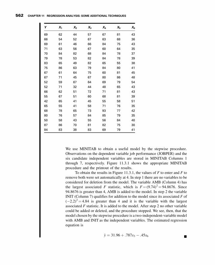
3GC11 12/04/2012 15:47:37 Page 562

We use MINITAB to obtain a useful model by the stepwise procedure.Observations on the dependent variable job performance (JOBPER) and thesix candidate independent variables are stored in MINITAB Columns 1through 7, respectively. Figure 11.3.1 shows the appropriate MINITABprocedure and the printout of the results.

To obtain the results in Figure 11.3.1, the values of F to enter and F toremove both were set automatically at 4. In step 1 there are no variables to beconsidered for deletion from the model. The variable AMB (Column 4) hasthe largest associated F statistic, which is F¼ (9.74)2¼ 94.8676. Since94.8676 is greater than 4, AMB is added to the model. In step 2 the variableINIT (Column 7) qualifies for addition to the model since its associated F of(�2.2)2¼ 4.84 is greater than 4 and it is the variable with the largestassociated F statistic. It is added to the model. After step 2 no other variablecould be added or deleted, and the procedure stopped. We see, then, that themodel chosen by the stepwise procedure is a two-independent-variable modelwith AMB and INIT as the independent variables. The estimated regressionequation is

y ¼ 31:96 þ :787x3 � :45x6 &

69 62 44 57 67 81 43

66 54 52 67 63 68 36

69 61 46 66 84 75 43

71 63 56 67 60 64 35

70 84 82 68 84 78 37

79 78 53 82 84 78 39

83 65 49 82 65 55 38

75 86 63 79 84 80 41

67 61 64 75 60 81 45

67 71 45 67 80 86 48

52 59 67 64 69 79 54

52 71 32 44 48 65 43

66 62 51 72 71 81 43

55 67 51 60 68 81 39

42 65 41 45 55 58 51

65 55 41 58 71 76 35

68 78 65 73 93 77 42

80 76 57 84 85 79 35

50 58 43 55 56 84 40

87 86 70 81 82 75 30

84 83 38 83 69 79 41

Y X1 X2 X3 X4 X5 X6


3GC11 12/04/2012 15:47:37 Page 563

To change the criterion for allowing a variable to enter the model from 4 to someother value K, click on Options, then type the desired value of K in the Enter box. The newcriterion F statistic, then, is K rather than 4. To change the criterion for deleting a variablefrom the model from 4 to some other value K, click on Options, then type the desired valueof K in the Remove box. We must choose K to enter to be greater than or equal to K toremove.

Though the stepwise selection procedure is a common technique employed byresearchers, other methods are available. Following is a brief discussion of two such tools.The final model obtained by each of these procedures is the same model that was found byusing the stepwise procedure in Example 11.3.1.

Forward Selection This strategy is closely related to the stepwise regressionprocedure. This method builds a model using correlations. Variables are retained that meetthe criteria for inclusion, as in stepwise selection. The first variable entered into the modelis the one with the highest correlation with the dependent variable. If this variable meets theinclusion criterion, it is retained. The next variable to be considered for inclusion is the onewith the highest partial correlation with the dependent variable. If it meets the inclusioncriteria, it is retained. This procedure continues until all of the independent variables have


Stat Regression Stepwise MTB > Stepwise C1 C2–C7;SUBC> FEnter 4.0;

Type C1 in Response and C2–C7 in Predictors. SUBC> FRemove 4.0.

Stepwise Regression

F-to-Enter: 4.00 F-to-Remove: 4.00

Response is C1 on 6 predictors, with N = 30

Step 1 2Constant 7.226 31.955

C4 0.888 0.787T-Ratio 9.74 8.13

54.0-7CT-Ratio -2.20

S 5.90 5.53R-Sq 77.21 80.68

FIGURE 11.3.1 MINITAB stepwise procedure and output for the data of Table 11.3.1.

11.3 VARIABLE SELECTION PROCEDURES 563

3GC11 12/04/2012 15:47:40 Page 564

been considered. The final model contains all of the independent variables that meet theinclusion criteria.

Backward Elimination This model-building procedure begins with all of thevariables in the model. This strategy also builds a model using correlations and apredetermined inclusion criterion based on the F statistic. The first variable consideredfor removal from the model is the one with the smallest partial correlation coefficient. Ifthis variable does not meet the criterion for inclusion, it is eliminated from the model. Thenext variable to be considered for elimination is the one with the next lowest partialcorrelation. It will be eliminated if it fails to meet the criterion for inclusion. This procedurecontinues until all variables have been considered for elimination. The final model containsall of the independent variables that meet the inclusion criteria.

EXERCISES

11.3.1 Refer to the data of Exercise 10.3.2 reported by Son et al. (A-6), who studied family caregiving inKorea of older adults with dementia. The outcome variable, caregiver burden (BURDEN), wasmeasured by the Korean Burden Inventory (KBI) where scores ranged from 28 to 140 with higherscores indicating higher burden. Perform a stepwise regression analysis on the following independentvariables reported by the researchers:

CGAGE: caregiver age (years)

CGINCOME: caregiver income (Won-Korean currency)

CGDUR: caregiver-duration of caregiving (month)

ADL: total activities of daily living where low scores indicate the elderly perform activitiesindependently.

MEM: memory and behavioral problems with higher scores indicating more problems.

COG: cognitive impairment with lower scores indicating a greater degree of cognitive impairment.

SOCIALSU: total score of perceived social support (25–175, higher values indicating moresupport). The reported data are as follows.

CGAGE CGINCOME CGDUR ADL MEM COG SOCIALSU BURDEN

41 200 12 39 4 18 119 2830 120 36 52 33 9 131 6841 300 60 89 17 3 141 5935 350 2 57 31 7 150 9137 600 48 28 35 19 142 7042 90 4 34 3 25 148 3849 300 26 42 16 17 172 4639 500 16 52 6 26 147 5749 309 30 88 41 13 98 8940 250 60 90 24 3 147 48

(Continued )


3GC11 12/04/2012 15:47:43 Page 565

40 300 36 38 22 13 146 7470 60 10 83 41 11 97 7849 450 24 30 9 24 139 4355 300 18 45 33 14 127 7627 309 30 47 36 18 132 7239 250 10 90 17 0 142 6139 260 12 63 14 16 131 6344 250 32 34 35 22 141 7733 200 48 76 33 23 106 8542 200 12 26 13 18 144 3152 200 24 68 34 26 119 7948 300 36 85 28 10 122 9253 300 12 22 12 16 110 7640 300 11 82 57 3 121 9135 200 8 80 51 3 142 7847 150 60 80 20 18 101 10333 180 19 81 20 1 117 9941 200 48 30 7 17 129 7343 300 36 27 27 27 142 8825 309 24 72 9 0 137 6435 250 12 46 15 22 148 5235 200 6 63 52 13 135 7145 200 7 45 26 18 144 4136 300 24 77 57 0 128 8552 600 60 42 10 19 148 5241 230 6 60 34 11 141 6840 200 36 33 14 14 151 5745 400 96 49 30 15 124 8448 75 6 89 64 0 105 9150 200 30 72 31 3 117 8331 250 30 45 24 19 111 7333 300 2 73 13 3 146 5730 200 30 58 16 15 99 6936 250 6 33 17 21 115 8145 500 12 34 13 18 119 7132 300 60 90 42 6 134 9155 200 24 48 7 23 165 4850 309 20 47 17 18 101 9437 250 30 32 13 15 148 5740 1000 21 63 32 15 132 4940 300 12 76 50 5 120 8849 300 18 79 44 11 129 5437 309 18 48 57 9 133 7347 250 38 90 33 6 121 8741 200 60 55 11 20 117 4733 1000 18 83 24 11 140 6028 309 12 50 21 25 117 65


(Continued )

EXERCISES 565

3GC11 12/04/2012 15:47:46 Page 566

33 400 120 44 31 18 138 5734 330 18 79 30 20 163 8540 200 18 24 5 22 157 2854 200 12 40 20 17 143 4032 300 32 35 15 27 125 8744 280 66 55 9 21 161 8044 350 40 45 28 17 142 4942 280 24 46 19 17 135 5744 500 14 37 4 21 137 3225 600 24 47 29 3 133 5241 250 84 28 23 21 131 4228 1000 30 61 8 7 144 4924 200 12 35 31 26 136 6365 450 120 68 65 6 169 8950 200 12 80 29 10 127 6740 309 12 43 8 13 110 4347 1000 12 53 14 18 120 4744 300 24 60 30 16 115 7037 309 54 63 22 18 101 9936 300 12 28 9 27 139 5355 200 12 35 18 14 153 7845 2000 12 37 33 17 111 11245 400 14 82 25 13 131 5223 200 36 88 16 0 139 6842 1000 12 52 15 0 132 6338 200 36 30 16 18 147 4941 230 36 69 49 12 171 4225 200 30 52 17 20 145 5647 200 12 59 38 17 140 4635 100 12 53 22 21 139 7259 150 60 65 56 2 133 9549 300 60 90 12 0 145 5751 200 48 88 42 6 122 8854 250 6 66 12 23 133 8153 30 24 60 21 7 107 10449 100 36 48 14 13 118 8844 300 48 82 41 13 95 11536 200 18 88 24 14 100 6664 200 48 63 49 5 125 9251 120 2 79 34 3 116 9743 200 66 71 38 17 124 6954 150 96 66 48 13 132 11229 309 19 81 66 1 152 88

Source: Data provided courtesy of Gwi-Ryung Son, R.N., Ph.D.



3GC11 12/04/2012 15:47:48 Page 567

11.3.2 Machiel Naeije (A-7) identifies variables useful in predicting maximum mouth opening (MMO,millimeters) for 35 healthy volunteers. The variables examined were:

AGE: yearsDOWN_CON: downward condylar translation, mmFORW_CON: forward condylar translation, mmGender: 0¼ Female, 1¼MaleMAN_LENG: mandibular length, mmMAN_WIDT: mandibular width, mm

Use the following reported measurements to perform a stepwise regression.

AGE DOWN_CON FORW_CON GENDER MAN_LENG MAN_WIDT MMO

21.00 4.39 14.18 1 100.86 121.00 52.3426.00 1.39 20.23 0 93.08 118.29 51.9030.00 2.42 13.45 1 98.43 130.56 52.8028.00 �.18 19.66 1 102.95 125.34 50.2921.00 4.10 22.71 1 108.24 125.19 57.7920.00 4.49 13.94 0 98.34 113.84 49.4121.00 2.07 19.35 0 95.57 115.41 53.2819.00 �.77 25.65 1 98.86 118.30 59.7124.00 7.88 18.51 1 98.32 119.20 53.3218.00 6.06 21.72 0 92.70 111.21 48.5322.00 9.37 23.21 0 88.89 119.07 51.5921.00 3.77 23.02 1 104.06 127.34 58.5220.00 1.10 19.59 0 98.18 111.24 62.9322.00 2.52 16.64 0 91.01 113.81 57.6224.00 5.99 17.38 1 96.98 114.94 65.6422.00 5.28 22.57 0 97.86 111.58 52.8522.00 1.25 20.89 0 96.89 115.16 64.4322.00 6.02 20.38 1 98.35 122.52 57.2519.00 1.59 21.63 0 90.65 118.71 50.8226.00 6.05 10.59 0 92.99 119.10 40.4822.00 �1.51 20.03 1 108.97 129.00 59.6824.00 �.41 24.55 0 91.85 100.77 54.3521.00 6.75 14.67 1 104.30 127.15 47.0022.00 4.87 17.91 1 93.16 123.10 47.2322.00 .64 17.60 1 94.18 113.86 41.1929.00 7.18 15.19 0 89.56 110.56 42.7625.00 6.57 17.25 1 105.85 140.03 51.8820.00 1.51 18.01 0 89.29 121.70 42.7727.00 4.64 19.36 0 92.58 128.01 52.3426.00 3.58 16.57 1 98.64 129.00 50.4523.00 6.64 12.47 0 83.70 130.98 43.1825.00 7.61 18.52 0 88.46 124.97 41.9922.00 5.39 11.66 1 94.93 129.99 39.4531.00 5.47 12.85 1 96.81 132.97 38.9123.00 2.60 19.29 0 93.13 121.03 49.10

Source: Data provided courtesy of Machiel Naeije, D.D.S.

EXERCISES 567

3GC11 12/04/2012 15:47:50 Page 568

11.3.3 One purpose of a study by Connor et al. (A-8) was to examine reactive aggression amongchildren and adolescents referred to a residential treatment center. The researchers used theProactive/Reactive Rating Scale, obtained by presenting three statements to clinicians whoexamined the subjects. The respondents answered, using a scale from 1 to 5, with 5 indicatingthat the statement almost always applied to the child. An example of a reactive aggressionstatement is, “When this child has been teased or threatened, he or she gets angry easily and strikesback.” The reactive score was the average response to three statements of this type. With thisvariable as the outcome variable, researchers also examined the following: AGE (years),VERBALIQ (verbal IQ), STIM (stimulant use), AGEABUSE (age when first abused), CTQ(a measure of hyperactivity in which higher scores indicate higher hyperactivity), TOTALHOS(total hostility as measured by an evaluator, with higher numbers indicating higher hostility).Perform stepwise regression to find the variables most useful in predicting reactive aggression inthe following sample of 68 subjects.

REACTIVE AGE VERBALIQ STIM AGEABUSE CTQ TOTALHOS

4.0 17 91 0 0 0 83.7 12 94 0 1 29 102.3 14 105 0 1 12 105.0 16 97 0 1 9 112.0 15 97 0 2 17 102.7 8 91 0 0 6 42.0 10 111 0 0 6 63.3 12 105 0 0 28 72.0 17 101 1 0 12 94.3 13 102 1 1 8 114.7 15 83 0 0 9 94.3 15 66 0 1 5 82.0 15 90 0 2 3 84.0 13 88 0 1 28 82.7 13 98 0 1 17 102.7 9 135 0 0 30 112.7 18 72 0 0 10 92.0 13 93 0 2 20 83.0 14 94 0 2 10 112.7 13 93 0 1 4 83.7 16 73 0 0 11 112.7 12 74 0 1 10 72.3 14 97 0 2 3 114.0 13 91 1 1 21 114.0 12 88 0 1 14 94.3 13 90 0 0 15 23.7 14 104 1 1 10 103.0 18 82 0 0 1 74.3 14 79 1 3 6 71.0 16 93 0 0 5 84.3 16 99 0 1 21 11

(Continued )


3GC11 12/04/2012 15:47:52 Page 569

2.3 14 73 0 2 8 93.0 12 112 0 0 15 91.3 15 102 0 1 1 53.0 16 78 1 1 26 82.3 9 95 1 0 23 101.0 15 124 0 3 0 113.0 17 73 0 1 1 103.3 11 105 0 0 23 54.0 11 89 0 0 27 81.7 9 88 0 1 2 82.3 16 96 0 1 5 74.7 15 76 1 1 17 91.7 16 87 0 2 0 41.7 15 90 0 1 10 124.0 12 76 0 0 22 105.0 12 83 1 1 19 74.3 10 88 1 0 10 55.0 9 98 1 0 8 93.7 12 100 0 0 6 43.3 14 80 0 1 3 102.3 16 84 0 1 3 91.0 17 117 0 2 1 91.7 12 145 1 0 0 53.7 12 123 0 0 1 32.0 16 94 0 2 6 63.7 17 70 0 1 11 134.3 14 113 0 0 8 82.0 12 123 1 0 2 83.0 7 107 0 0 11 93.7 12 78 1 0 15 114.3 14 73 0 1 2 82.3 18 91 0 3 8 104.7 12 91 0 0 6 93.7 15 111 0 0 2 91.3 15 71 0 1 20 103.7 7 102 0 0 14 91.7 9 89 0 0 24 6

Source: Data provided courtesy of Daniel F. Connor, M.D. and Lang Lin.

11.4 LOGISTIC REGRESSION

Up to now our discussion of regression analysis has been limited to those situations inwhich the dependent variable is a continuous variable such as weight, blood pressure,or plasma levels of some hormone. Much research in the health sciences field is

REACTIVE AGE VERBALIQ STIM AGEABUSE CTQ TOTALHOS

11.4 LOGISTIC REGRESSION 569

3GC11 12/04/2012 15:47:52 Page 570

motivated by a desire to describe, understand, and make use of the relationshipbetween independent variables and a dependent (or outcome) variable that is discrete.Particularly plentiful are circumstances in which the outcome variable is dichotomous.A dichotomous variable, we recall, is a variable that can assume only one of twomutually exclusive values. These values are usually coded Y ¼ 1 for a success and Y ¼ 0for a nonsuccess, or failure. Dichotomous variables include those whose two possiblevalues are such categories as died–did not die; cured–not cured; disease occurred–disease did not occur; and smoker–nonsmoker. The health sciences professional whoeither engages in research or needs to understand the results of research conducted byothers will find it advantageous to have, at least, a basic understanding of logisticregression, the type of regression analysis that is usually employed when the dependentvariable is dichotomous. The purpose of the present discussion is to provide thereader with this level of understanding. We shall limit our presentation to the case inwhich there is only one independent variable that may be either continuous ordichotomous.

The Logistic Regression Model Recall that in Chapter 9 we referred toregression analysis involving only two variables as simple linear regression analysis. Thesimple linear regression model was expressed by the equation

y ¼ b0 þ b1xþ e (11.4.1)

in which y is an arbitrary observed value of the continuous dependent variable. When theobserved value of Y is myjx, the mean of a subpopulation of Y values for a given value of X,the quantity e, the difference between the observed Y and the regression line (seeFigure 9.2.1) is zero, and we may write Equation 11.4.1 as

myjx ¼ b0 þ b1x (11.4.2)

which may also be written as

E yjxð Þ ¼ b0 þ b1x (11.4.3)

Generally, the right-hand side of Equations (11.4.1) through (11.4.3) may assume any valuebetween minus infinity and plus infinity.

Even though only two variables are involved, the simple linear regression model isnot appropriate when Y is a dichotomous variable because the expected value (or mean)of Y is the probability that Y ¼ 1 and, therefore, is limited to the range 0 through 1,inclusive. Equations (11.4.1) through (11.4.3), then, are incompatible with the reality ofthe situation.

If we let p ¼ P Y ¼ 1ð Þ, then the ratio p= 1 � pð Þ can take on values between 0 andplus infinity. Furthermore, the natural logarithm (ln) of p= 1 � pð Þ can take on values


3GC11 12/04/2012 15:47:52 Page 571

between minus infinity and plus infinity just as can the right-hand side of Equations 11.4.1through (11.4.3). Therefore, we may write

lnp

1 � p

� �¼ b0 þ b1x (11.4.4)

Equation 11.4.4 is called the logistic regression model and the transformation of myjx(that is, p) to ln p= 1 � pð Þ½ � is called the logit transformation. Equation 11.4.4 may also bewritten as

p ¼ exp b0 þ b1xð Þ1 þ exp b0 þ b1xð Þ (11.4.5)

in which exp is the inverse of the natural logarithm.The logistic regression model is widely used in health sciences research. For

example, the model is frequently used by epidemiologists as a model for the probability(interpreted as the risk) that an individual will acquire a disease during some specified timeperiod during which he or she is exposed to a condition (called a risk factor) known to be orsuspected of being associated with the disease.

Logistic Regression: Dichotomous Independent Variable Thesimplest situation in which logistic regression is applicable is one in which both thedependent and the independent variables are dichotomous. The values of the dependent(or outcome) variable usually indicate whether or not a subject acquired a disease orwhether or not the subject died. The values of the independent variable indicate thestatus of the subject relative to the presence or absence of some risk factor. In thediscussion that follows we assume that the dichotomies of the two variables are coded0 and 1. When this is the case the variables may be cross-classified in a table, such asTable 11.4.1, that contains two rows and two columns. The cells of the table containthe frequencies of occurrence of all possible pairs of values of the two variables: (1, 1),(1, 0), (0, 1), and (0, 0).

An objective of the analysis of data that meet these criteria is a statistic known as theodds ratio. To understand the concept of the odds ratio, we must understand the term odds,

TABLE 11.4.1 Two Cross-ClassifiedDichotomous Variables Whose Values

Are Coded 1 and 0

IndependentVariable (X)

DependentVariable (Y ) 1 0

1 n1;1 n1;0

2 n0;1 n0;0


3GC11 12/04/2012 15:47:52 Page 572

which is frequently used by those who place bets on the outcomes of sporting events orparticipate in other types of gambling activities. Using probability terminology, we maydefine odds as follows.

DEFINITION

The odds for success is the ratio of the probability of success to theprobability of failure.

The odds ratio is a measure of how much greater (or less) the odds are for subjectspossessing the risk factor to experience a particular outcome. This conclusion assumes thatthe outcome is a rare event. For example, when the outcome is the contracting of a disease,the interpretation of the odds ratio assumes that the disease is rare.

Suppose, for example, that the outcome variable is the acquisition or nonacquisitionof skin cancer and the independent variable (or risk factor) is high levels of exposure to thesun. Analysis of such data collected on a sample of subjects might yield an odds ratio of 2,indicating that the odds of skin cancer are two times higher among subjects with high levelsof exposure to the sun than among subjects without high levels of exposure.

Computer software packages that perform logistic regression frequently provide aspart of their output estimates of b0 and b1 and the numerical value of the odds ratio. As itturns out the odds ratio is equal to exp(b1).

EXAMPLE 11.4.1

LaMont et al. (A-9) tested for obstructive coronary artery disease (OCAD) among 113 menand 35 women who complained of chest pain or possible equivalent to their primary carephysician. Table 11.4.2 shows the cross-classification of OCAD with gender. We wish touse logistic regression analysis to determine how much greater the odds are of findingOCAD among men than among women.

Solution: We may use the SAS® software package to analyze these data. Theindependent variable is gender and the dependent variable is status withrespect to having obstructive coronary artery disease (OCAD). Use of theSAS® command PROC LOGIST yields. as part of the resulting output, thestatistics shown in Figure 11.4.1.

TABLE 11.4.2 Cases of Obstructive Coronary

Artery Disease (OCAD) Classified by Sex

Disease Males Females Total

OCAD present 92 15 107

OCAD not present 21 20 41

Total 113 35 148

Source: Data provided courtesy of Matthew J. Budoff, M.D.


3GC11 12/04/2012 15:47:53 Page 573

We see that the estimate of a is �0.2877 and the estimate of b1 is1.7649. The estimated odds ratio, then, is cOR ¼ expð1:7649Þ ¼ 5:84. Thus,we estimate that the odds of finding a case of obstructive coronary arterydisease to be almost six times higher among men than women. &

Logistic Regression: Continuous Independent Variable Now letus consider the situation in which we have a dichotomous dependent variable and acontinuous independent variable. We shall assume that a computer is available to performthe calculations. Our discussion, consequently, will focus on an evaluation of the adequacyof the model as a representation of the data at hand, interpretation of key elements of thecomputer printout, and the use of the results to answer relevant questions about therelationship between the two variables.

ProcedureLOGISTIC The

EstimatesLikelihood Maximum of Analysis

WaldStandardEstimateDFParameterChiSq>PrChi-SquareError

0.39970.70900.3416-0.28771Intercept<.000117.78440.41851.76491sex

FIGURE 11.4.1 Partial output from use of SAS® command PROC LOGISTIC with the data of

Table 11.4.2.

EXAMPLE 11.4.2

According to Gallagher et al. (A-10), cardiac rehabilitation programs offer “information,support, and monitoring for return to activities, symptom management, and risk factormodification.” The researchers conducted a study to identify among women factors that areassociated with participation in such programs. The data in Table 11.4.3 are the ages of 185women discharged from a hospital in Australia who met eligibility criteria involvingdischarge for myocardial infarction, artery bypass surgery, angioplasty, or stent. We wish touse these data to obtain information regarding the relationship between age (years) andparticipation in a cardiac rehabilitation program (ATT¼ 1, if participated, and ATT¼ 0,if not). We wish also to know if we may use the results of our analysis to predict thelikelihood of participation by a woman if we know her age.

Solution: The independent variable is the continuous variable age (AGE), and thedependent or response variable is status with respect to attendance in acardiac rehabilitation program. The dependent variable is a dichotomousvariable that can assume one of two values: 0¼ did not attend, and 1¼ did


3GC11 12/04/2012 15:47:54 Page 574

attend. We use the SAS® software package to analyze the data. The SAS®

command is PROC LOGISTIC, but if we wish to predict attendance in thecardiac program, we need to use the “descending” option with PROCLOGISTIC. (When you wish to predict the outcome labeled “1” of thedependent variable, use the “descending option” in SAS®. Consult

TABLE 11.4.3 Ages of Women Participating and Not

Participating in a Cardiac Rehabilitation Program

Nonparticipating(ATT¼ 0)

Participating(ATT¼1)

50 73 46 74 74 62

59 75 57 59 50 74

42 71 53 81 55 61

50 69 40 74 66 69

34 78 73 77 49 76

49 69 68 59 55 71

67 74 72 75 73 61

44 86 59 68 41 46

53 49 64 81 64 69

45 63 78 74 46 66

79 63 68 65 65 57

46 72 67 81 50 60

62 64 55 62 61 63

58 72 71 85 64 63

70 79 80 84 59 56

60 75 75 39 73 70

67 70 69 52 73 70

64 73 80 67 65 63

62 66 79 82 67 63

50 75 71 84 60 65

61 73 69 79 69 67

69 71 78 81 61 68

74 72 75 74 79 84

65 69 71 85 66 69

80 76 69 92 68 78

69 60 77 69 61 69

77 79 81 83 63 79

61 78 78 82 70 83

72 62 76 85 68 67

67 73 84 82 59 47

80 64 57

66

Source: Data provided courtesy of Robyn Gallagher, R.N., Ph.D.


3GC11 12/04/2012 15:47:54 Page 575

SAS®documentation for further details.) A partial printout of the analysis isshown in Figure 11.4.2.

The slope of our regression is �.0379, and the intercept is 1.8744. Theregression equation, then, is

yi ¼ 1:8744 � :0379xi

where yi ¼ ln½pið1 � piÞ� and pi is the predicted probability of attendingcardiac rehabilitation for a woman aged xi.

Test of H0 that b1 ¼ 0

We reach a conclusion about the adequacy of the logistic model by testing the nullhypothesis that the slope of the regression line is zero. The test statistic is z ¼ b1=sb1

wherez is the standard normal statistic, b1 is the sample slope (�.0379), and sb1

is its standarderror (.0146) as shown in Figure 11.4.2. From these numbers we compute z¼�.0379/.0146¼�2.5959, which has an associated two-sided p value of .0094. Weconclude, therefore, that the logistic model is adequate. The square of z is chi-squarewith 1 degree of freedom, a statistic that is shown in Figure 11.4.2.

Using the Logistic Regression to Estimate p

We may use Equation 11.4.5 and the results of our analysis to estimate p, the probabilitythat a woman of a given age (within the range of ages represented by the data) willattend a cardiac rehabilitation program. Suppose, for example, that we wish to estimatethe probability that a woman who is 50 years of age will participate in a rehabilitationprogram. Substituting 50 and the results shown in Figure 11.4.2 into Equation 11.4.5gives

p ¼ exp½1:8744 � ð:0379Þð50Þ�1 þ exp½1:8744 � ð:0379Þð50Þ� ¼ :49485

SAS® calculates the estimated probabilities for the given values of X. We can see theestimated probabilities of attending cardiac rehabilitation programs for the age rangeof the subjects enrolled in the study in Figure 11.4.3. Since the slope was negative,we see a decreasing probability of attending a cardiac rehabilitation program for olderwomen.

Standard WaldParameter DF Estimate Error Chi-Square Pr > ChiSq

Intercept 1 1.8744 0.9809 3.6518 0.0560age 1 0.0379 0.0146 6.7083 0.0096

FIGURE 11.4.2 Partial SAS® printout of the logistic regression analysis of the data in Table 11.4.3.


3GC11 12/04/2012 15:47:54 Page 576

Multiple Logistic Regression Practitioners often are interested in the rela-tionships of several independent variables to a response variable. These independentvariables may be either continuous or discrete or a combination of the two.

Multiple logistic models are constructed by expanding Equations (11.4.1) to (11.4.4).If we begin with Equation 11.4.4, multiple logistic regression can be represented as

lnp

1 � p

� �¼ b0 þ b1x1j þ b2x2j þ � � � þ bkxkj (11.4.6)

Using the logit transformation, we now have

p ¼ exp b0 þ b1x1j þ b2x2j þ � � � þ bkxkj� �

1 þ exp b0 þ b1x1j þ b2x2j þ � � � þ bkxkj� � (11.4.7)

&

0503 00109080706040.15

0.20

0.25

0.30

0.35

0.40

0.45

0.50

0.55

0.60

0.65

Est

imat

ed p

rob

abili

ty

FIGURE 11.4.3 Estimated probabilities of attendance for ages within the study for

Example 11.4.2.

EXAMPLE 11.4.3

Consider the data presented in Review Exercise 24. In this study by Fils-Aime et al. (A-21),data were gathered and classified with regard to alcohol use. Subjects were classifiedas having either early (< 25 years) or late (> 25 years) onset of excessive alcohol use.


3GC11 12/04/2012 15:47:54 Page 577

Assessing Goodness of Fit A natural question that arises when doing logisticregression is: “How good is my model?” In classical linear regression we discussedmeasures such as R2 for determining how much variation is explained by the model, withvalues of R2 approaching 1 as a good indicator of model adequacy based on the predictorschosen to model the outcome. Given the nature of the response variable in logisticregression, a coefficient of determination does not provide the same information as it doesin linear regression. This is because in logistic regression values of the parameters are notderived to minimize sums of squares, but rather are iterative estimates; hence, there is noequivalent measure of R2 in logistic regression. Below, we provide an explanation of somecommonly used approaches to evaluate logistic regression models, and follow theseexplanations with two illustrative examples.

Many authors have attempted to develop what are known as “pseudo-R2” values thatrange from 0 to 1, with higher values indicating better fit. In general, these measures are

Levels of cerebrospinal fluid (CSF) tryptophan (TRYPT) and 5-hydroxyindoleacetic acid(5-HIAA) concentrations were also obtained.

Solution: The independent variables are the concentrations of TRYPTand 5-HIAA, andthe dependent variable is the dichotomous response for onset of excessivealcohol use. We use SPSS software to analyze the data. The output ispresented in Figure 11.4.4.

The equation can be written as

yi ¼ 2:076 � :013x1j þ 0x2j

Note that the coefficient for TRYPT is 0, and therefore it is not playing a role in themodel.

Test of H0 that b1 ¼ 0

Tests for significance of the regression coefficients can be obtained directly fromFigure 11.4.4. Note that both the constant (intercept) and the 5-HIAA variables aresignificant in the model (both have p values, noted as “Sig.” in the table, <.05); however,TRYPT is not significant and therefore need not be in the model, suggesting that it is notuseful for identifying those study participants with early or late alcoholism onset.

As above, probabilities can be easily obtained by using Equation 11.4.7 andsubstituting the values obtained from the analysis. &

Parameter B S.E. Wald Df Sig. Exp(B)

5-HIAA .013 .006 5.878 1 .015 .987

TRYPT .000 .000 .000 1 .983 1.000

Constant 2.076 1.049 3.918 1 .048 7.970

FIGURE 11.4.4 SPSS output for the data in Example 11.4.3.


3GC11 12/04/2012 15:47:54 Page 578

based on comparisons of a derived model with a model that contains only an intercept. Inother words, they are comparative measures designed to indicate “how much better” amodel with predictor variables is when compared to a model with no predictors. Twocommonly used pseudo-R2 statistics were developed by Cox and Snell (4) and Nagelkerke(5). These are often provided in standard outputs of statistical software. The value of thesemeasures is the fact that they may be useful for comparing models with different predictorvariables, but provide little relative use for examining a single model. Both of theseapproaches are based on the idea of using a measure of fit known as the log-likelihoodstatistic. The log-likelihood for the intercept-only model is used to represent the total sumof squares, while the log-likelihood for the model with predictor variables is used torepresent the error sum of squares. Interested readers may find an explanation of the log-likelihood statistic in Hosmer and Lemeshow (2).

Another intuitive approach is to consider a classification table. Using this method,one develops a contingency table that provides frequency counts of the number of datapoints that were observed to be either 0 or 1 in the raw data, along with whether the raw datawere classified as 0 or 1 based on the predictive equation. One can then estimate how manyof the data points were correctly classified. As a general rule-of-thumb, correctlyclassifying 70 percent or greater is considered evidence of a satisfactory model from astatistical viewpoint. However, the model may not provide great enough predictive abilityto be useful in a practice sense. A problem does arise, however, in that reclassifying thesame data used to build a model with the model itself may bias the results. There are twopractical ways to deal with this issue. First, one may use part of the data set to construct themodel and the other part of the data set to develop a classification table. This strategy, ofcourse, requires a sample large enough to accommodate adequately the needs of bothprocedures. A second approach is to construct a model using the data in hand and thencollect additional data to test the adequacy of the model using a classification table. Thisstrategy, too, has its shortcomings, as the collection of additional data can be both time-consuming and expensive.

A third approach that also has intuitive visual appeal is to develop a plot that showsthe frequency of observations against their predicted probability. In this type of plot, onewould hope to see a complete separation of 0 and 1 values. When there is misclassificationof the outcome variable, this type of plot provides a means of determining where themisclassification occurred, and how frequently observations were misclassified.

Finally, in a commonly used approach known as the Hosmer and Lemeshow test, onedevelops a table of observed and expected frequencies and uses a chi-square test todetermine if there is a significant deviation between the observed and expected frequen-cies. For the interested reader, we suggest the text by Hosmer and Lemeshow (2).

EXAMPLE 11.4.4

Consider the logistic regression model that was constructed from the cardiac rehabilitationprogram data in Example 11.4.2.

Figure 11.4.5 shows standard SPSS output for this logistic regression model. In thisfigure, we see that both the Cox and Snell and the Nagelkerke pseudo-R2 values areprovided. Since they are both > 0, the model with the predictor provides more informationthan the intercept-only model. One can readily see that only 63% of the data were correctly


3GC11 12/04/2012 15:47:54 Page 579

reclassified, with those participating in the rehabilitation program much more poorly classi-fied than those who did not attend the program. The frequency distribution shows the largenumber of ATT¼ 1 subjects who were misclassified as ATT¼ 0 based on the model. &

EXAMPLE 11.4.5

Consider the logistic regression model that was constructed from the cardiac rehabilitationprogram data in Example 11.4.3.

Figure 11.4.6 shows standard SPSS output for this logistic regression model. In thisfigure, we see that both the Cox and Snell and the Nagelkerke pseudo-R2 values are provided,and since they are both > 0, the model with the predictors provides more information thanthe intercept-only model. One can readily see that only 69% of the data were correctlyreclassified, with the model reclassifying those with onset of excessive alcohol use at a much

Model Summary

Classification Tablea

Cox & Snell R

Square

.037 .051

Nagelkerke R

Square

Predicted

Percentage

Correct0 1Observed

att

att 0 111

58

10

5

91.7

7.9

63.01

Overall Percentage

FIGURE 11.4.5 Partial SPSS output for the logistic regression analysis of the data in Example

11.4.2.


3GC11 12/04/2012 15:47:54 Page 580

higher rate than those without such onset. The frequency distribution shows the large numberof those without onset of excessive alcohol use predicted by the model to develop early onset

of alcoholism. &

Polytomous Logistic Regression Thus far we have limited our discussionto situations in which there is a dichotomous response variable (e.g., successful orunsuccessful). Often, we have a situation in which multiple categories make up theresponse. We may, for example, have subjects that are classified as positive, negative, andundetermined for a given disease (a standard polytomous response). There may also betimes when we have a response variable that is ordered. We may, for example, classify oursubjects by BMI as underweight, ideal weight, overweight, or obese (an ordinal poly-tomous response). The modeling process is slightly more complex and requires the use of acomputer program. For those interested in exploring these valuable methods further, werecommend the book by Hosmer and Lemeshow (2).

Model Summary

Classification Tablea

Cox & Snell R

Square

0.49 .069

Nagelkerke R

Square

Predicted

Percentage

Correct0 1Observed

Onset

onset 0 2

3

37

87

5.1

96.7

69.01

Overall Percentage

a. The cut value is. 500

FIGURE 11.4.6 Partial SPSS output for the logistic regression analysis of the data in Example 11.4.3.


3GC11 12/04/2012 15:47:55 Page 581

Further Reading We have discussed only the basic concepts and applications oflogistic regression. The technique has much wider application. Stepwise regression analysismay be used with logistic regression. There are also techniques available for constructingconfidence intervals for odds ratios. The reader who wishes to learn more about logisticregression may consult the books by Hosmer and Lemeshow (2) and Kleinbaum (3).

EXERCISES

11.4.1 In a study of violent victimization of women and men, Porcerelli et al. (A-11) collected informationfrom 679 women and 345 men ages 18 to 64 years at several family-practice centers in themetropolitan Detroit area. Patients filled out a health history questionnaire that included a questionabout victimization. The following table shows the sample subjects cross-classified by gender andwhether the subject self-identified as being “hit, kicked, punched, or otherwise hurt by someonewithin the past year.” Subjects answering yes to that question are classified “violently victimized.”Use logistic regression analysis to find the regression coefficients and the estimate of the odds ratio.Write an interpretation of your results.

Victimization Women Men Total

No victimization 611 308 919Violently victimized 68 37 105Total 679 345 1024

Source: John H. Porcerelli, Rosemary Cogan, Patricia P. West, Edward A. Rose, DawnLambrecht, Karen E. Wilson, Richard K. Severson, and Dunia Karana, “Violent Victimizationof Women and Men: Physical and Psychiatric Symptoms,” Journal of the American Board ofFamily Practice, 16 (2003), 32–39.

11.4.2 Refer to the research of Gallagher et al. (A-10) discussed in Example 11.4.2. Another covariate ofinterest was a score using the Hospital Anxiety and Depression Index. A higher value for this scoreindicates a higher level of anxiety and depression. Use the following data to predict whether a womanin the study participated in a cardiac rehabilitation program.

Hospital Anxiety and Depression IndexScores for Nonparticipating Women

Hospital Anxietyand DepressionIndex Scores forParticipating

Women

17 14 19 16 23 257 21 6 9 3 6

19 13 8 22 24 2916 15 13 17 13 2223 21 4 14 26 1127 12 15 14 19 1223 9 23 5 25 2018 29 19 5 15 1821 4 14 14 22 2427 18 19 20 13 18

(Continued )

EXERCISES 581

3GC11 12/04/2012 15:47:56 Page 582

14 22 17 21 21 825 5 13 17 15 1019 27 14 17 12 1723 16 14 10 25 14

6 11 17 13 29 218 19 26 10 17 25

15 23 15 20 21 2530 22 19 3 8 1618 25 16 18 19 2310 11 10 9 16 1929 20 15 10 24 24

8 11 22 5 17 1112 28 8 15 26 1727 12 15 13 12 1912 19 20 16 19 20

9 18 12 13 1716 13 2 23 31

6 12 6 11 022 7 14 17 1810 12 19 29 18

9 14 14 6 1511 13 19 20

Source: Data provided courtesy of Robyn Gallagher, R.N., Ph.D.

11.5 SUMMARY

This chapter is included for the benefit of those who wish to extend their understanding ofregression analysis and their ability to apply techniques to models that are more complexthan those covered in Chapters 9 and 10. In this chapter we present some additional topicsfrom regression analysis. We discuss the analysis that is appropriate when one or more ofthe independent variables is dichotomous. In this discussion the concept of dummyvariable coding is presented. A second topic that we discuss is how to select the mostuseful independent variables when we have a long list of potential candidates. Thetechnique we illustrate for the purpose is stepwise regression analysis. Finally, we presentthe basic concepts and procedures that are involved in logistic regression analysis. Wecover two situations: the case in which the independent variable is dichotomous, and thecase in which the independent variable is continuous.

Since the calculations involved in obtaining useful results from data that areappropriate for analysis by means of the techniques presented in this chapter arecomplicated and time-consuming when attempted by hand, it is recommended that acomputer be used to work the exercises.

Hospital Anxiety and Depression IndexScores for Nonparticipating Women

Hospital Anxietyand DepressionIndex Scores forParticipating

Women


3GC11 12/04/2012 15:47:57 Page 583



11.4.1–11.4.3

Representations of the simplelinear regression model

y ¼ b0 þ b1xþ e

myjx ¼ b0 þ b1xE yjxð Þ ¼ b0 þ b1x

11.4.4 Simple logistic regression model ln p1�p

h i¼ b0 þ b1x

11.4.5 Alternative representation of thesimple logistic regression model

p ¼ exp b0 þ b1xð Þ1 þ exp b0 þ b1xð Þ

11.4.6 Alternative representation of themultiple logistic regression model

ln p1�p

h i¼ b0 þ b1x1j þ b2x2j þ � � � þ bkxkj

11.4.7 Alternative representation of themultiple logistic regression model p ¼ exp b0 þ b1x1j þ b2x2j þ � � � þ bkxkj

� �1 þ exp b0 þ b1x1j þ b2x2j þ � � � þ bkxkj

� �SymbolKey

� b0 ¼ regression intercept� bi ¼ regression coefficient� e ¼ regression model error term� E yjxð Þ ¼ expected value of y at x

� ln p1�p

h i¼ log it transformation

� myjx ¼ mean of y at x� xi ¼ value of independent variable at i


1. What is a qualitative variable?

2. What is a dummy variable?

3. Explain and illustrate the technique of dummy variable coding.

4. Why is a knowledge of variable selection techniques important to the health sciences researcher?

5. What is stepwise regression?

6. Explain the basic concept involved in stepwise regression.

7. When is logistic regression used?

8. Write out and explain the components of the logistic regression model.

9. Define the word odds.

10. What is an odds ratio?

11. Give an example in your field in which logistic regression analysis would be appropriate when theindependent variable is dichotomous.


3GC11 12/04/2012 15:47:59 Page 584

12. Give an example in your field in which logistic regression analysis would be appropriate when theindependent variable is continuous.

13. Find a published article in the health sciences field in which each of the following techniques is employed:

(a) Dummy variable coding

(b) Stepwise regression

(c) Logistic regression

Write a report on the article in which you identify the variables involved, the reason for the choice ofthe technique, and the conclusions that the authors reach on the basis of their analysis.

14. In Example 10.3.1, we saw that the purpose of a study by Jansen and Keller (A-12) was to predict thecapacity to direct attention (CDA) in elderly subjects. The study collected information on 71community-dwelling older women with normal mental status. Higher CDA scores indicate betterattentional functioning. In addition to the variables age and education level, the researchersperformed stepwise regression with two additional variables: IADL, a measure of activities ofdaily living (higher values indicate greater number of daily activities), and ADS, a measure ofattentional demands (higher values indicate more attentional demands). Perform stepwise regressionwith the data in the following table and report your final model, p values, and conclusions.

CDA Age Edyrs IADL ADS CDA Age Edyrs IADL ADS

4.57 72 20 28 27 3.17 79 12 28 18�3:04 68 12 27 96 �1:19 87 12 21 61

1.39 65 13 24 97 0.99 71 14 28 55�3:55 85 14 27 48 �2:94 81 16 27 124�2:56 84 13 28 50 �2:21 66 16 28 42�4:66 90 15 27 47 �0:75 81 16 28 64�2:70 79 12 28 71 5.07 80 13 28 26

0.30 74 10 24 48 �5:86 82 12 28 84�4:46 69 12 28 67 5.00 65 13 28 43�6:29 87 15 21 81 0.63 73 16 26 70�4:43 84 12 27 44 2.62 85 16 28 20

0.18 79 12 28 39 1.77 83 17 23 80�1:37 71 12 28 124 �3:79 83 8 27 21

3.26 76 14 29 43 1.44 76 20 28 26�1:12 73 14 29 30 �5:77 77 12 28 53�0:77 86 12 26 44 �5:77 83 12 22 69

3.73 69 17 28 47 �4:62 79 14 27 82�5:92 66 11 28 49 �2:03 69 12 28 77

5.74 65 16 28 48 �2:22 66 14 28 382.83 71 14 28 46 0.80 75 12 28 28

�2:40 80 18 28 25 �0:75 77 16 27 85�0:29 81 11 28 27 �4:60 78 12 22 82

4.44 66 14 29 54 2.68 83 20 28 343.35 76 17 29 26 �3:69 85 10 20 72

�3:13 70 12 25 100 4.85 76 18 28 24�2:14 76 12 27 38 �0:08 75 14 29 49

9.61 67 12 26 84 0.63 70 16 28 297.57 72 20 29 44 5.92 79 16 27 83

(Continued )


3GC11 12/04/2012 15:48:1 Page 585

2.21 68 18 28 52 3.63 75 18 28 32�2:30 102 12 26 18 �7:07 94 8 24 80

1.73 67 12 27 80 6.39 76 18 28 416.03 66 14 28 54 �0:08 84 18 27 75

�0:02 75 18 26 67 1.07 79 17 27 21�7:65 91 13 21 101 5.31 78 16 28 18

4.17 74 15 28 90 0.30 79 12 28 38

Source: Data provided courtesy of Debra Jansen, Ph.D., R.N.

15. In the following table are the cardiac output (L/min) and oxygen consumption (VO2 ) values for asample of adults (A) and children (C), who participated in a study designed to investigate therelationship among these variables. Measurements were taken both at rest and during exercise. Treatcardiac output as the dependent variable and use dummy variable coding and analyze the data byregression techniques. Explain the results. Plot the original data and the fitted regression equations.

CardiacOutput (L/min)

VO2

(L/min)Age

GroupCardiac

Output (L/min)VO2

(L/min) Age Group

4.0 .21 A 4.0 .25 C7.5 .91 C 6.1 .22 A3.0 .22 C 6.2 .61 C8.9 .60 A 4.9 .45 C5.1 .59 C 14.0 1.55 A5.8 .50 A 12.9 1.11 A9.1 .99 A 11.3 1.45 A3.5 .23 C 5.7 .50 C7.2 .51 A 15.0 1.61 A5.1 .48 C 7.1 .83 C6.0 .74 C 8.0 .61 A5.7 .70 C 8.1 .82 A

14.2 1.60 A 9.0 1.15 C4.1 .30 C 6.1 .39 A

16. A simple random sample of normal subjects between the ages of 6 and 18 yielded the data on totalbody potassium (mEq) and total body water (liters) shown in the following table. Let total potassiumbe the dependent variable and use dummy variable coding to quantify the qualitative variable.Analyze the data using regression techniques. Explain the results. Plot the original data and the fittedregression equations.

Total BodyPotassium

Total BodyWater Sex

Total BodyPotassium

Total BodyWater Sex

795 13 M 950 12 F1590 16 F 2400 26 M1250 15 M 1600 24 F1680 21 M 2400 30 M

CDA Age Edyrs IADL ADS CDA Age Edyrs IADL ADS

(Continued )


3GC11 12/04/2012 15:48:2 Page 586

800 10 F 1695 26 F2100 26 M 1510 21 F1700 15 F 2000 27 F1260 16 M 3200 33 M1370 18 F 1050 14 F1000 11 F 2600 31 M1100 14 M 3000 37 M1500 20 F 1900 25 F1450 19 M 2200 30 F1100 14 M

17. The data shown in the following table were collected as part of a study in which the subjects werepreterm infants with low birth weights born in three different hospitals. Use dummy variable codingand multiple regression techniques to analyze these data. May we conclude that the three samplehospital populations differ with respect to mean birth weight when gestational age is taken intoaccount? May we conclude that there is interaction between hospital of birth and gestational age?Plot the original data and the fitted regression equations.

BirthWeight (kg)

GestationAge (weeks)

Hospitalof Birth

BirthWeight (kg)

GestationAge (weeks)

Hospitalof Birth

1.4 30 A 1.0 29 C.9 27 B 1.4 33 C

1.2 33 A .9 28 A1.1 29 C 1.0 28 C1.3 35 A 1.9 36 B.8 27 B 1.3 29 B

1.0 32 A 1.7 35 C.7 26 A 1.0 30 A

1.2 30 C .9 28 A.8 28 A 1.0 31 A

1.5 32 B 1.6 31 B1.3 31 A 1.6 33 B1.4 32 C 1.7 34 B1.5 33 B 1.6 35 C1.0 27 A 1.2 28 A1.8 35 B 1.5 30 B1.4 36 C 1.8 34 B1.2 34 A 1.5 34 C1.1 28 B 1.2 30 A1.2 30 B 1.2 32 C

18. Refer to Chapter 9, Review Exercise 18. In the study cited in that exercise, Maria Mathias (A-13)investigated the relationship between ages (AGE) of boys and improvement in measures ofhyperactivity, attitude, and social behavior. In the study, subjects were randomly assigned to twodifferent treatments. The control group (TREAT ¼ 0) received standard therapy for hyperactivity,and the treatment group (TREAT ¼ 1) received standard therapy plus pet therapy. The results are

Total BodyPotassium

Total BodyWater Sex

Total BodyPotassium

Total BodyWater Sex


3GC11 12/04/2012 15:48:3 Page 587

shown in the following table. Create a scatter plot with age as the independent variable and ATT(change in attitude with positive numbers indicating positive change in attitude) as the dependentvariable. Use different symbols for the two different treatment groups. Use multiple regressiontechniques to determine whether age, treatment, or the interaction are useful in predicting ATT.Report your results.

Subject TREAT AGE ATT Subject TREAT AGE ATT

1 1 9 �1:2 17 0 10 0.42 1 9 0.0 18 0 7 0.03 1 13 �0:4 19 0 12 1.14 1 6 �0:4 20 0 9 0.25 1 9 1.0 21 0 7 0.46 1 8 0.8 22 0 6 0.07 1 8 �0:6 23 1 11 0.68 1 9 �1:2 24 1 11 0.49 0 7 0.0 25 1 11 1.0

10 0 12 0.4 26 1 11 0.811 0 9 �0:8 27 1 11 1.212 0 10 1.0 28 1 11 0.213 0 12 1.4 29 1 11 0.814 0 9 1.0 30 1 8 0.015 0 12 0.8 31 1 9 0.416 0 9 1.0

Source: Data provided courtesy of Maria Mathias, M.D. and the Wright State University Statistical ConsultingCenter.

For each study described in Exercises 19 through 21, answer as many of the following questions aspossible:

(a) Which is the dependent variable?

(b) What are the independent variables?

(c) What are the appropriate null and alternative hypotheses?

(d) Which null hypotheses do you think were rejected? Why?

(e) Which is the more relevant objective, prediction or estimation, or are the two equally relevant?Explain your answer.

(f) What is the sampled population?

(g) What is the target population?

(h) Which variables are related to which other variables? Are the relationships direct orinverse?

(i) Write out the regression equation using appropriate numbers for parameter estimates.

(j) Give numerical values for any other statistics that you can.

(k) Identify each variable as to whether it is quantitative or qualitative.

(l) Explain the meaning of any statistics for which numerical values are given.

19. Golfinopoulos and Arhonditsis (A-14) used a multiple regression model in a study of trihalomethanes(THMs) in drinking water in Athens, Greece. THMs are of concern since they have been related tocancer and reproductive outcomes. The researchers found the following regression model useful in


3GC11 12/04/2012 15:48:3 Page 588

predicting THM:

THM ¼ �:26chlaþ 1:57 pH þ 28:74Br � 66:72Br2

�43:63Sþ 1:13Spþ 2:62T � S� :72T � CL

The variables were as follows: chla ¼ chlorophyll concentration, pH ¼ acid=base scale,Br ¼ bromide concentration, S ¼ dummy variable for summer, Sp ¼ dummy variable for spring,T ¼ Temperature, and CL ¼ chlorine concentration. The researchers reported R ¼ :52, p < :001.

20. In a study by Takata et al. (A-15), investigators evaluated the relationship between chewing abilityand teeth number and measures of physical fitness in a sample of subjects ages 80 or higher in Japan.One of the outcome variables that measured physical fitness was leg extensor strength. To measurethe ability to chew foods, subjects were asked about their ability to chew 15 foods (peanuts, vinegaredoctopus, and French bread, among others). Consideration of such variables as height, body weight,gender, systolic blood pressure, serum albumin, fasting glucose concentration, back pain, smoking,alcohol consumption, marital status, regular medical treatment, and regular exercise revealed that thenumber of chewable foods was significant in predicting leg extensor strength (b1 ¼ :075; p ¼ :0366).However, in the presence of the other variables, number of teeth was not a significant predictor(b1 ¼ :003; p ¼ :9373).

21. Varela et al. (A-16) examined 515 patients who underwent lung resection for bronchogeniccarcinoma. The outcome variable was the occurrence of cardiorespiratory morbidity after surgery.Any of the following postoperative events indicated morbidity: pulmonary atelectasis or pneu-monia, respiratory or ventilatory insufficiency at discharge, need for mechanical ventilation at anytime after extubation in the operating room, pulmonary thromboembolism, arrhythmia, myocar-dial ischemia or infarct, and clinical cardiac insufficiency. Performing a stepwise logisticregression, the researchers found that age (p < :001) and postoperative forced expiratory volume(p ¼ :003) were statistically significant in predicting the occurrence of cardiorespiratorymorbidity.

For each of the data sets given in Exercises 22 through 29, do as many of the following as you thinkappropriate:

(a) Apply one or more of the techniques discussed in this chapter.

(b) Apply one or more of the techniques discussed in previous chapters.

(c) Construct graphs.

(d) Formulate relevant hypotheses, perform the appropriate tests, and find p values.

(e) State the statistical decisions and clinical conclusions that the results of your hypothesis testsjustify.

(f) Describe the population(s) to which you think your inferences are applicable.

22. A study by Davies et al. (A-17) was motivated by the fact that, in previous studies of contractileresponses to b-adrenoceptor agonists in single myocytes from failing and nonfailing humanhearts, they had observed an age-related decline in maximum response to isoproterenol, atfrequencies where the maximum response to high Ca2þ in the same cell was unchanged. For thepresent study, the investigators computed the isoproterenol/Ca2þ ratio (ISO/CA) from measure-ments taken on myocytes from patients ranging in age from 7 to 70 years. Subjects wereclassified as older (> 50 years) and younger. The following are the (ISO/CA) values, age,and myocyte source of subjects in the study. Myocyte sources were reported as donor andbiopsy.


3GC11 12/04/2012 15:48:4 Page 589

Age ISO/CA Myocyte Source

7 1.37 Donor21 1.39 Donor28 1.17 Donor35 0.71 Donor38 1.14 Donor50 0.95 Donor51 0.86 Biopsy52 0.72 Biopsy55 0.53 Biopsy56 0.81 Biopsy61 0.86 Biopsy70 0.77 Biopsy

Source: Data provided courtesy of Dr. Sian E. Harding.

23. Hayton et al. (A-18) investigated the pharmacokinetics and bioavailability of cefetamet andcefetamet pivoxil in infants between the ages of 3.5 and 17.3 months who had received the antibioticduring and after urological surgery. Among the pharmacokinetic data collected were the followingmeasurements of the steady-state apparent volume of distribution (V). Also shown are previouslycollected data on children ages 3 to 12 years (A-19) and adults (A-20). Weights (W) of subjects arealso shown.

Infants Children Adults

W (kg) V (liters) W (kg) V (liters) W (kg) V (liters)

6.2 2.936 13 4.72 61 19.77.5 3.616 14 5.23 80 23.77.0 1.735 14 5.85 96 20.07.1 2.557 15 4.17 75 19.57.8 2.883 16 5.01 60 19.68.2 2.318 17 5.81 68 21.58.3 3.689 17 7.03 72.2 21.98.5 4.133 17.5 6.62 87 30.98.6 2.989 17 4.98 66.5 20.48.8 3.500 17.5 6.45

10.0 4.235 20 7.7310.0 4.804 23 7.6710.2 2.833 25 9.8210.3 4.068 37 14.4010.6 3.640 28 10.9010.7 4.067 47 15.4010.8 8.366 29 9.8611.0 4.614 37 14.4012.5 3.16813.1 4.158

Source: Data provided courtesy of Dr. Klaus Stoeckel.


3GC11 12/04/2012 15:48:6 Page 590

24. According to Fils-Aime et al. (A-21), epidemiologic surveys have found that alcoholism is the mostcommon mental or substance abuse disorder among men in the United States. Fils-Aime andassociates investigated the interrelationships of age at onset of excessive alcohol consumption, familyhistory of alcoholism, psychiatric comorbidity, and cerebrospinal fluid (CSF) monoamine metaboliteconcentrations in abstinent, treatment-seeking alcoholics. Subjects were mostly white malesclassified as experiencing early (25 years or younger) or late (older than 25 years) onset of excessivealcohol consumption. Among the data collected were the following measurements on CSF trypto-phan (TRYPT) and 5-hydroxyindoleacetic acid (5-HIAA) concentrations (pmol/ml).

5-HIAA TRYPT

Onset1 ¼ Early0 ¼ Late 5-HIAA TRYPT

Onset1 ¼ Early0 ¼ Late

57 3315 1 102 3181 1116 2599 0 51 2513 1

81 3334 1 92 2764 178 2505 0 104 3098 1

206 3269 0 50 2900 164 3543 1 93 4125 1

123 3374 0 146 6081 1147 2345 1 96 2972 1102 2855 1 112 3962 0

93 2972 1 23 4894 1128 3904 0 109 3543 1

69 2564 1 80 2622 120 8832 1 111 3012 166 4894 0 85 2685 190 6017 1 131 3059 0

103 3143 0 58 3946 168 3729 0 110 3356 081 3150 1 80 3671 1

143 3955 1 42 4155 1121 4288 1 80 1923 1149 3404 0 91 3589 1

82 2547 1 102 3839 0100 3633 1 93 2627 0117 3309 1 98 3181 0

41 3315 1 78 4428 0223 3418 0 152 3303 0

96 2295 1 108 5386 187 3232 0 102 3282 196 3496 1 122 2754 134 2656 1 81 4321 198 4318 1 81 3386 186 3510 0 99 3344 1

118 3613 1 73 3789 184 3117 1 163 2131 199 3496 1 109 3030 0

114 4612 1 90 4731 1

(Continued )


3GC11 12/04/2012 15:48:8 Page 591

140 3051 1 110 4581 174 3067 1 48 3292 045 2782 1 77 4494 051 5034 1 67 3453 199 2564 1 92 3373 154 4335 1 86 3787 093 2596 1 101 3842 150 2960 1 88 2882 1

118 3916 0 38 2949 196 2797 0 75 2248 049 3699 1 35 3203 0

133 2394 0 53 3248 1105 2495 0 77 3455 0

61 2496 1 179 4521 1197 2123 1 151 3240 1

87 3320 0 57 3905 150 3117 1 45 3642 1

109 3308 0 76 5233 059 3280 1 46 4150 1

107 3151 1 98 2579 185 3955 0 84 3249 1

156 3126 0 119 3381 0110 2913 0 41 4020 1

81 3786 1 40 4569 153 3616 1 149 3781 164 3277 1 116 2346 157 2656 1 76 3901 129 4953 0 96 3822 134 4340 1

Source: Data provided courtesy of Dr. Markku Linnoila.

25. The objective of a study by Abrahamsson et al. (A-22) was to investigate the anti-thrombotic effectsof an inhibitor of the plasminogen activator inhibitor-1 (PAI-1) in rats given endotoxin. Experimentalsubjects were male Sprague–Dawley rats weighing between 300 and 400 grams. Among the datacollected were the following measurements on PAI-1 activity and the lung 125I-concentration inanesthetized rats given three drugs:

DrugsPlasma PAI-1Activity (U/ml)

125I-Fibrin in the Lungs(% of Ref. Sample)

Endotoxin 127 158175 154161 118137 77219 172

5-HIAA TRYPT

Onset1 ¼ Early0 ¼ Late 5-HIAA TRYPT

Onset1 ¼ Early0 ¼ Late

(Continued )


3GC11 12/04/2012 15:48:9 Page 592

260 277203 216195 169414 272244 192

Endotoxin þ PRAP ¼ 1 low dose 107 49103 28248 187164 109176 96230 126184 148276 17201 97158 86

Endotoxin þ PRAP ¼ 1 high dose 132 86130 24

75 17140 41166 114194 110121 26111 53208 71211 90

Source: Data provided courtesy of Dr. Tommy Abrahamsson.

26. Pearse and Sylvester (A-23) conducted a study to determine the separate contributions of ischemiaand extracorporeal perfusion to vascular injury occurring in isolated sheep lungs and to determine theoxygen dependence of this injury. Lungs were subjected to ischemia alone, extracorporeal perfusionalone, and both ischemia and extracorporeal perfusion. Among the data collected were the followingobservations on change in pulmonary arterial pressure (mm Hg) and pulmonary vascular perme-ability assessed by estimation of the reflection coefficient for albumin in perfused lungs with andwithout preceding ischemia:

Ischemic–Perfused Lungs Perfused Lungs

Change inPulmonaryPressure

ReflectionCoefficient



8.0 0.220 34.0 0.6933.0 0.560 31.0 0.470

10.0 0.550 4.0 0.65123.0 0.806 48.0 0.999

DrugsPlasma PAI-1Activity (U/ml)

125I-Fibrin in the Lungs(% of Ref. Sample)


3GC11 12/04/2012 15:48:10 Page 593

15.0 0.472 32.0 0.71943.0 0.759 27.0 0.90218.0 0.489 25.0 0.73627.0 0.546 25.0 0.71813.0 0.5480.0 0.467

Source: Data provided courtesy of Dr. David B. Pearse.

27. The purpose of a study by Balzamo et al. (A-24) was to investigate, in anesthetized rabbits, the effectsof mechanical ventilation on the concentration of substance P (SP) measured by radioimmunoassayin nerves and muscles associated with ventilation and participating in the sensory innervation of therespiratory apparatus and heart. SP is a neurotransmitter located in primary sensory neurons in thecentral and autonomic nervous systems. Among the data collected were the following measures of SPconcentration in cervical vagus nerves (X) and corresponding nodose ganglia (NG), right and leftsides:

SPXright SPNGright SPXleft SPNGleft

0.6500 9.6300 3.3000 1.93002.5600 3.7800 0.6200 2.87001.1300 7.3900 0.9600 1.31001.5500 3.2800 2.7000 5.6400

35.9000 22.0000 4.5000 9.100019.0000 22.8000 8.6000 8.000013.6000 2.3000 7.0000 8.3000

8.0000 15.8000 4.1000 4.70007.4000 1.6000 5.5000 2.50003.3000 11.6000 9.7000 8.0000

19.8000 18.0000 13.8000 8.00008.5000 6.2000 11.0000 17.20005.4000 7.8000 11.9000 5.3000

11.9000 16.9000 8.2000 10.600047.7000 35.9000 3.9000 3.300014.2000 10.2000 3.2000 1.9000

2.9000 1.6000 2.7000 3.50006.6000 3.7000 2.8000 2.50003.7000 1.3000

Source: Data provided courtesy of Dr. Yves Jammes.

28. Scheeringa and Zeanah (A-25) examined the presence of posttraumatic stress disorder (PTSD), theseverity of posttraumatic symptomatology, and the pattern of expression of symptom clusters inrelation to six independent variables that may be salient to the development of a posttraumaticdisorder in children under 48 months of age. The following data were collected during the course ofthe study.

Ischemic–Perfused Lungs Perfused Lungs






3GC11 12/04/2012 15:48:13 Page 594

Predictor Variables Response Variables

Gender Age Acute/Rept. InjuryWit./Exper.

Threat toCaregiver Reexp Numb Arous FrAgg

0 1 0 1 1 1 3 0 0 10 1 0 0 0 1 2 2 1 11 1 0 0 0 1 3 1 1 10 1 0 0 0 1 3 1 0 41 0 1 1 1 0 1 3 1 11 1 0 1 1 0 3 1 0 10 1 0 1 1 0 4 2 0 10 1 0 0 1 0 5 2 0 41 1 0 0 0 1 2 1 3 21 1 1 1 1 0 4 1 0 00 0 1 1 1 0 1 3 0 11 0 1 0 1 0 1 3 0 21 0 1 1 1 0 0 3 0 01 1 0 1 1 0 4 1 2 11 0 0 1 1 1 3 2 1 31 0 0 1 1 1 3 1 2 10 1 0 1 1 1 3 1 2 20 1 0 0 0 1 5 2 1 10 1 0 0 0 1 1 2 2 20 1 0 1 1 0 4 4 0 31 0 1 1 1 0 2 1 2 31 0 0 1 1 1 1 1 2 11 1 0 0 0 1 4 1 1 10 1 0 0 0 1 3 2 1 00 1 0 0 0 1 3 1 2 40 1 0 0 0 1 3 1 2 40 1 0 0 1 0 2 2 0 01 1 0 0 0 1 2 0 3 01 1 0 0 0 1 2 0 1 20 1 0 1 0 1 2 3 1 31 1 1 0 1 0 1 2 1 11 1 0 1 1 1 3 2 0 41 1 0 0 0 0 2 4 2 00 1 0 0 0 1 1 1 0 20 0 1 0 0 1 2 3 2 30 0 1 0 0 1 3 1 4 30 0 1 0 0 1 3 1 2 30 0 0 0 1 0 1 1 0 01 0 0 0 0 1 4 3 2 31 0 0 1 1 0 4 2 3 20 0 1 1 1 0 1 2 2 1


3GC11 12/04/2012 15:48:15 Page 595

Key: Gender 0¼male1¼ female

Age 0¼ younger than 18 months at time of trauma1¼ older than 18 months

Acute/Rept. 0¼ trauma was acute, single blow1¼ trauma was repealed or chronic

Injury 0¼ subject was not injured in the trauma1¼ subject was physically injured in the trauma

Wit./Exper. 0¼ subject witnessed but did not directly experience trauma1¼ subject directly experienced the trauma

Threat to Caregiver 0¼ caregiver was not threatened in the trauma1¼ caregiver was threatened in the trauma

Reexp ¼ Reexperiencing cluster symptom countNumb ¼ Numbing of responsiveness/avoidance cluster symptom countArous ¼ Hyperarousal cluster symptom countFrAgg ¼ New fears/aggression cluster symptom count

Source: Data provided courtesy of Dr. Michael S. Scheeringa.

29. One of the objectives of a study by Mulloy and McNicholas (A-26) was to compare ventilation andgas exchange during sleep and exercise in chronic obstructive pulmonary disease (COPD). Theinvestigators wished also to determine whether exercise studies could aid in the prediction ofnocturnal desaturation in COPD. Subjects (13 male, 6 female) were ambulatory patients attending anoutpatient respiratory clinic. The mean age of the patients, all of whom had severe, stable COPD, was64.8 years with a standard deviation of 5.2. Among the data collected were measurements on thefollowing variables:

Age(years) BMI

PaO2

(mm Hg)PaCO2

(mm Hg)FEV1

(% Predicted)

LowestEx.Sao2

a

MeanSleepSao2

a

LowestSleepSao2

a

FallSleepSao2

a

67 23.46 52.5 54 22 74 70.6 56 29.662 25.31 57.75 49.575 19 82 85.49 76 11.6668 23.11 72 43.8 41 95 88.72 82 11.161 25.15 72 47.4 38 88 91.11 76 18.4570 24.54 78 40.05 40 88 92.86 92 0.871 25.47 63.75 45.375 31 85 88.95 80 1360 19.49 80.25 42.15 28 91 94.78 90 457 21.37 84.75 40.2 20 91 93.72 89 5.869 25.78 68.25 43.8 32 85 90.91 79 1357 22.13 83.25 43.725 20 88 94.39 86 9.574 26.74 57.75 51 33 75 89.89 80 14.1163 19.07 78 44.175 36 81 93.95 82 1364 19.61 90.75 40.35 27 90 95.07 92 473 30.30 69.75 38.85 53 87 90 76 18

(Continued )

Predictor Variables Response Variables

Gender Age Acute/Rept. InjuryWit./Exper.

Threat toCaregiver Reexp Numb Arous FrAgg


3GC11 12/04/2012 15:48:16 Page 596

63 26.12 51.75 46.8 39 67 69.31 46 34.962 21.71 72 41.1 27 88 87.95 72 2267 24.75 84.75 40.575 45 87 92.95 90 2.1757 25.98 84.75 40.05 35 94 93.4 86 8.4566 32.00 51.75 53.175 30 83 80.17 71 16

a Treated as dependent variable in the authors’ analyses. BMI¼ body mass index; Pao2¼ arterial oxygentension: Paco2¼ arterial carbon dioxide pressure; FEV1¼ forced expiratory volume in 1 second; Sao2¼ arterialoxygen saturation.Source: Data provided courtesy of Dr. Eithne Mulloy.

Exercises for Use with the Large Data Sets Available on the Following Website:www.wi ley.com/ college/dan iel

1. The goal of a study by Gyurcsik et al. (A-27) was to examine the usefulness of aquatic exercise-related goals, task self-efficacy, and scheduling self-efficacy for predicting aquatic exercise attend-ance by individuals with arthritis. The researchers collected data on 142 subjects participating inArthritis Foundation Aquatics Programs. The outcome variable was the percentage of sessionsattended over an 8-week period (ATTEND). The following predictor variables are all centered values.Thus, for each participant, the mean for all participants is subtracted from the individual score. Thevariables are:

GOALDIFF—higher values indicate setting goals of higher participation.

GOALSPEC—higher values indicate higher specificity of goals related to aquatic exercise.

INTER—interaction of GOALDIFF and GOALSPEC.

TSE—higher values indicate participants’ confidence in their abilities to attend aquatic classes.

SSE—higher values indicate participants’ confidence in their abilities to perform eight tasks relatedto scheduling exercise into their daily routine for 8 weeks.

MONTHS—months of participation in aquatic exercise prior to start of study.

With the data set AQUATICS, perform a multiple regression to predict ATTEND with each of theabove variables. What is the multiple correlation coefficient? What variables are significant inpredicting ATTEND? What are your conclusions?

2. Rodehorst (A-28) conducted a prospective study of 212 rural elementary school teachers. Themain outcome variable was the teachers’ intent to manage children demonstrating symptoms ofasthma in their classrooms. This variable was measured with a single-item question that used aseven-point Likert scale (INTENT, with possible responses of 1 ¼ extremely probable to 7 ¼extremely improbable). Rodehorst used the following variables as independent variables to predictINTENT:

SS ¼ Social Support. Scores range from 7 to 49, with higher scores indicating higher perceivedsocial support for managing children with asthma in a school setting.

ATT ¼ Attitude. Scores range from 15 to 90, with higher scores indicating more favorable attitudestoward asthma.

Age(years) BMI

PaO2

(mm Hg)PaCO2

(mm Hg)FEV1

(% Predicted)

LowestEx.Sao2

a

MeanSleepSao2

a

LowestSleepSao2

a

FallSleepSao2

a



3GC11 12/04/2012 15:48:16 Page 597

KNOW ¼ Knowledge. Scores range from 0 to 24, with higher scores indicating higher generalknowledge about asthma.

CHILD ¼Number of children with asthma the teacher has had in his or her class during his or herentire teaching career.

SE ¼ Self-efficacy. Scores range from 12 to 60, with higher scores indicating higher self-efficacyfor managing children with asthma in the school setting.

YRS ¼Years of teaching experience.

With the data TEACHERS, use stepwise regression analysis to select the most useful variables toinclude in a model for predicting INTENT.

3. Refer to the weight loss data on 588 cancer patients and 600 healthy controls (WGTLOSS). Weightloss among cancer patients is a well-known phenomenon. Of interest to clinicians is the role played inthe process by metabolic abnormalities. One investigation into the relationships among thesevariables yielded data on whole-body protein turnover (Y) and percentage of ideal body weightfor height (X). Subjects were lung cancer patients and healthy controls of the same age. Select asimple random sample of size 15 from each group and do the following:

(a) Draw a scatter diagram of the sample data using different symbols for each of the two groups.

(b) Use dummy variable coding to analyze these data.

(c) Plot the two regression lines on the scatter diagram. May one conclude that the two sampledpopulations differ with respect to mean protein turnover when percentage of ideal weight is takeninto account?

May one conclude that there is interaction between health status and percentage of ideal body weight?Prepare a verbal interpretation of the results of your analysis and compare your results with those ofyour classmates.

REFERENCES


1. BRUCE L. BOWERMAN and RICHARD T. O’CONNELL, Linear Statistical Models: An Applied Approach, 2nd ed. PWS-Kent Publishing, Boston, 1990.

2. DAVID W. HOSMER and STANLEY LEMESHOW, Applied Logistic Regression, 2nd Ed. Wiley, New York, 2000.3. DAVID G. KLEINBAUM, Logistic Regression: A Self-Learning Text, New York, Springer, 1994.4. D. R. COX and E. J. SNELL, Analysis of Binary Data, 2nd ed. Chapman and Hall/CRC, New York, 1989.5. N. J. D. NAGELKERKE, “A Note on a General Definition of the Coefficient of Determination”,Biometrika, 78 (1991),

691–692.


A-1. North Carolina State Center for Health Statistics and Howard W. Odum Institute for Research in Social Scienceat the University of North Carolina at Chapel Hill, Birth Data set for 2001 found at www.irss.unc.edu/ncvi-tal/bfd1down.html. All sampling and coding performed by John Holcomb and do not represent the findings of theCenter or Institute.

A-2. B. BOLWELL, R. SOBECKS, B. POHLMAN, S. ANDRESEN, K. THEIL, S. SERAFINO, L. RYBICKI, and M. KALAYCIO,“Etoposide (VP-16) Plus G-CSF Mobilizes Different Dendritic Cell Subsets than Does G-CSF Alone,” BoneMarrow Transplantation, 31 (2003), 95–98.

A-3. MANOJ PANDEY, LAL B. SHARMA, and VIJAY K. SHUKLA, “Cytochrome P-450 Expression and Lipid Peroxidation inGallbladder Cancer,” Journal of Surgical Oncology, 82 (2003), 180–183.

REFERENCES 597



3GC11 12/04/2012 15:48:16 Page 598

A-4. MORI J. KRANTZ, ILANA B. KUTINSKY, ALASTAIR D. ROBERTSON, and PHILIP S. MEHLER, “Dose-Related Effects ofMethadone on QT Prolongation in a Series of Patients with Torsade de Pointes,” Pharmacotherapy, 23 (2003),802–805.

A-5. ROBERT A. REISS, CURTIS E. HAAS, DEBORAH L. GRIFFIS, BERNADETTE PORTER, and MARY ANN TARA, “Point-of-Careversus Laboratory Monitoring of Patients Receiving Different Anticoagulant Therapies,” Pharmacotherapy 22,(2002), 677–685.

A-6. GWI-RYUNG SON, MAY L. WYKLE, and JACLENE A. ZAUSZNIEWSKI, “Korean Adult Child Caregivers of Older Adultswith Dementia,” Journal of Gerontological Nursing, 29 (2003), 19–28.

A-7. M. NAEIJE, “Local Kinematic and Anthropometric Factors Related to the Maximum Mouth Opening in HealthyIndividuals,” Journal of Oral Rehabilitation, 29 (2002), 534–539.

A-8. DANIEL F. CONNOR, RONALD J. STEINGARD, JENNIFER J. ANDERSON, and RICHARD H. MELLONI, “Gender Differences inReactive and Proactive Aggression,” Child Psychiatry and Human Development, 33 (2003), 279–294.

A-9. DANIEL H. LAMONT, MATTHEW J. BUDOFF, DAVID M. SHAVELLE, ROBERT SHAVELLE, BRUCE H. BRUNDAGE, and JAMES

M. HAGAR, “Coronary Calcium Scanning Adds Incremental Value to Patients with Positive Stress Tests,”American Heart Journal, 143 (2002), 861–867.

A-10. ROBYN GALLAGHER, SHARON MCKINLEY, and KATHLEEN DRACUP, “Predictors of Women’s Attendance at CardiacRehabilitation Programs,” Progress in Cardiovascular Nursing, 18 (2003), 121–126.


A-12. DEBRA A. JANSEN, and MARY L. KELLER, “Cognitive Function in Community-Dwelling Elderly Women,” Journalof Gerontological Nursing, 29 (2003), 34–43.

A-13. MARIA MATHIAS and the Wright State University Statistical Consulting Center.A-14. SPYROS K. GOLFINOPOULOS and GEORGE B. ARHONDITSIS, “Multiple Regression Models: A Methodology for

Evaluating Trihalomethane Concentrations in Drinking Water from Raw Water Characteristics,” Chemosphere,47 (2002), 1007–1018.

A-15. Y. TAKATA, T. ANSAI, S. AWANO, T. HAMASAKI, Y. YOSHITAKE, Y. KIMURA, K. SONOKI, M. WAKISAKA, M. FUKUHARA,and T. TAKEHARA, “Relationship of Physical Fitness to Chewing in an 80-Year-Old Population,”Oral Diseases, 10(2004), 44–49.

A-16. G. VARELA, N. NOVOA, M. F. JIM�ENEZ, and G. SANTOS, “Applicability of Logistic Regression (LR) RiskModeling to Decision Making in Lung Cancer Resection,” Interactive Cardiovascular and Thoracic Surgery,2 (2003), 12–15.

A-17. C. H. DAVIES, N. FERRARA, and S. E. HARDING, “b-Adrenoceptor Function Changes with Age of Subject inMyocytes from Non-Failing Human Ventricle,” Cardiovascular Research, 31 (1996), 152–156.

A-18. WILLIAM L. HAYTON, JOHANNES KNEER, RONALD GROOT, and KLAUS STOECKEL, “Influence of Maturation and Growthon Cefetamet Pivoxil Pharmacokinetics: Rational Dosing for Infants,” Antimicrobial Agents and Chemotherapy,40 (1996), 567–574.

A-19. W. L. HAYTON, R. A. WALSTAD, E. THURMANN-NIELSEN, T. KUFAAS, J. KNEER, R. J. AMBROS, H. E. RUGSTAD, E. MONN,E. BODD, and K. STOECKEL, “Pharmacokinetics of Intravenous Cefetamet and Oral Cefetamet Pivoxil inChildren,” Antimicrobial Agents and Chemotherapy, 35 (1991), 720–725. Erratum, 36 (1992), 2575.

A-20. M. P. DUCHARME, D. J. EDWARDS, P. J. MCNAMARA, and K. STOECKEL, “Bioavailability of Syrup and TabletFormulations of Cefetamet Pivoxil,” Antimicrobial Agents and Chemotherapy, 37 (1993), 2706–2709.

A-21. MARIE-LOURDES FILS-AIME, MICHAEL J. ECKARDT, DAVID T. GEORGE, GERALD L. BROWN, IVAN MEFFORD, and MARKKU

LINNOILA, “Early-Onset Alcoholics Have Lower Cerebrospinal Fluid 5-Hydroxyindoleacetic Acid Levels thanLate-Onset Alcoholics,” Archives of General Psychiatry, 53 (1996), 211–216.

A-22. T. ABRAHAMSSON, V. NERME, M. STR€OMQVIST, B. A

KERBLOM, A. LEGNEHED, K. PETTERSSON, and A. WESTIN ERIKSSON,“Anti-thrombotic Effect of PAI-1 Inhibitor in Rats Given Endotoxin,” Thrombosis and Haemostasis, 75 (1996),118–126.

A-23. DAVID B. PEARSE and J. T. SYLVESTER, “Vascular Injury in Isolated Sheep Lungs: Role of Ischemia, ExtracorporealPerfusion, and Oxygen,” American Journal of Respiratory and Critical Care Medicine, 153 (1996), 196–202.

A-24. EMMANUEL BALZAMO, PIERRE JOANNY, JEAN GUILLAUME STEINBERG, CHARLES OLIVER, and YVES JAMMES, “MechanicalVentilation Increases Substance P Concentration in the Vagus, Sympathetic, and Phrenic Nerves,” AmericanJournal of Respiratory and Critical Care Medicine, 153 (1996), 153–157.

A-25. MICHAEL S. SCHEERINGA and CHARLES H. ZEANAH, “Symptom Expression and Trauma Variables in Children Under48 Months of Age,” Infant Mental Health Journal, 16 (1995), 259–270.


3GC11 12/04/2012 15:48:16 Page 599

A-26. EITHNE MULLOYand WALTER T. MCNICHOLAS, “Ventilation and Gas Exchange During Sleep and Exercise in SevereCOPD,” Chest, 109 (1996), 387–394.

A-27. NANCY C. GYURCSIK, PAUL A. ESTABROOKS, and MELISSA J. FRAHM-TEMPLAR, “Exercise-Related Goals and Self-Efficacy as Correlates of Aquatic Exercise in Individuals with Arthritis,” Arthritis Care and Research, 49 (2003),306–313.

A-28. T. KIM RODEHURST, “Rural Elementary School Teachers’ Intent to Manage Children with Asthma Symptoms,”Pediatric Nursing, 29 (2003), 184–194.

REFERENCES 599

3GC12 12/04/2012 15:57:56 Page 600

CHAPTER12THE CHI-SQUAREDISTRIBUTION AND THE ANALYSISOF FREQUENCIES

CHAPTER OVERVIEW

This chapter explores techniques that are commonly used in the analysis ofcount or frequency data. Uses of the chi-square distribution, which wasmentioned briefly in Chapter 6, are discussed and illustrated in greater detail.Additionally, statistical techniques often used in epidemiological studies areintroduced and demonstrated by means of examples.

TOPICS

12.1 INTRODUCTION

12.2 THE MATHEMATICAL PROPERTIES OF THE CHI-SQUARE DISTRIBUTION

12.3 TESTS OF GOODNESS-OF-FIT

12.4 TESTS OF INDEPENDENCE

12.5 TESTS OF HOMOGENEITY

12.6 THE FISHER EXACT TEST

12.7 RELATIVE RISK, ODDS RATIO, AND THE MANTEL–HAENSZEL STATISTIC

12.8 SUMMARY

LEARNING OUTCOMES


1. understand the mathematical properties of the chi-square distribution.

2. be able to use the chi-square distribution for goodness-of-fit tests.

3. be able to construct and use contingency tables to test independenceand homogeneity.

4. be able to apply Fisher’s exact test for 2 � 2 tables.

5. understand how to calculate and interpret the epidemiological concepts of relativerisk, odds ratios, and the Mantel-Haenszel statistic.

600

3GC12 12/04/2012 15:57:56 Page 601

12.1 INTRODUCTION

In the chapters on estimation and hypothesis testing, brief mention is made of the chi-square distribution in the construction of confidence intervals for, and the testing of,hypotheses concerning a population variance. This distribution, which is one of the mostwidely used distributions in statistical applications, has many other uses. Some of the morecommon ones are presented in this chapter along with a more complete description of thedistribution itself, which follows in the next section.

The chi-square distribution is the most frequently employed statistical technique forthe analysis of count or frequency data. For example, we may know for a sample ofhospitalized patients how many are male and how many are female. For the same samplewe may also know how many have private insurance coverage, how many have Medicareinsurance, and how many are on Medicaid assistance. We may wish to know, for thepopulation from which the sample was drawn, if the type of insurance coverage differsaccording to gender. For another sample of patients, we may have frequencies for eachdiagnostic category represented and for each geographic area represented. We might wantto know if, in the population from which the same was drawn, there is a relationshipbetween area of residence and diagnosis. We will learn how to use chi-square analysis toanswer these types of questions.

There are other statistical techniques that may be used to analyze frequency data inan effort to answer other types of questions. In this chapter we will also learn about thesetechniques.

12.2 THEMATHEMATICAL PROPERTIESOF THE CHI-SQUARE DISTRIBUTION

The chi-square distribution may be derived from normal distributions. Suppose that from anormally distributed random variable Y with mean m and variance s2 we randomly andindependently select samples of size n ¼ 1. Each value selected may be transformed to thestandard normal variable z by the familiar formula

zi ¼ yi � m

s(12.2.1)

Each value of z may be squared to obtain z2. When we investigate the sampling distri-bution of z2, we find that it follows a chi-square distribution with 1 degree of freedom.That is,

x2ð1Þ ¼

y� m

s

� �2¼ z2

Now suppose that we randomly and independently select samples of size n ¼ 2 from thenormally distributed population of Y values. Within each sample we may transform each

12.2 THE MATHEMATICAL PROPERTIES OF THE CHI-SQUARE DISTRIBUTION 601

3GC12 12/04/2012 15:57:56 Page 602

value of y to the standard normal variable z and square as before. If the resulting values of z2

for each sample are added, we may designate this sum by

x2ð2Þ ¼

y1 � m

s

� �2þ y2 � m

s

� �2¼ z2

1 þ z22

since it follows the chi-square distribution with 2 degrees of freedom, the number ofindependent squared terms that are added together.

The procedure may be repeated for any sample size n. The sum of the resulting z2

values in each case will be distributed as chi-square with n degrees of freedom. In general,then,

x2ðnÞ ¼ z2

1 þ z22 þ � � � þ z2

n (12.2.2)

follows the chi-square distribution with n degrees of freedom. The mathematical form ofthe chi-square distribution is as follows:

f ðuÞ ¼ 1

k

2� 1

� �!

1

2k=2uðk=2Þ�1e�ðu=2Þ; u > 0

(12.2.3)

where e is the irrational number 2.71828 . . . and k is the number of degrees of freedom.The variate u is usually designated by the Greek letter chi (x) and, hence, the distribution iscalled the chi-square distribution. As we pointed out in Chapter 6, the chi-squaredistribution has been tabulated in Appendix Table F. Further use of the table is demon-strated as the need arises in succeeding sections.

The mean and variance of the chi-square distribution are k and 2k, respectively. Themodal value of the distribution is k � 2 for values of k greater than or equal to 2 and is zerofor k ¼ 1.

The shapes of the chi-square distributions for several values of k are shown in Figure6.9.1. We observe in this figure that the shapes for k ¼ 1 and k ¼ 2 are quite different fromthe general shape of the distribution for k > 2. We also see from this figure that chi-squareassumes values between 0 and infinity. It cannot take on negative values, since it is the sumof values that have been squared. A final characteristic of the chi-square distribution worthnoting is that the sum of two or more independent chi-square variables also follows achi-square distribution.

Types of Chi-Square Tests As already noted, we make use of the chi-squaredistribution in this chapter in testing hypotheses where the data available for analysis arein the form of frequencies. These hypothesis testing procedures are discussed under thetopics of tests of goodness-of-fit, tests of independence, and tests of homogeneity. We willdiscover that, in a sense, all of the chi-square tests that we employ may be thought of asgoodness-of-fit tests, in that they test the goodness-of-fit of observed frequencies tofrequencies that one would expect if the data were generated under some particular theoryor hypothesis. We, however, reserve the phrase “goodness-of-fit” for use in a more

602 CHAPTER 12 THE CHI-SQUARE DISTRIBUTION AND THE ANALYSIS OF FREQUENCIES

3GC12 12/04/2012 15:57:56 Page 603

restricted sense. We use it to refer to a comparison of a sample distribution to some theoreticaldistribution that it is assumed describes the population from which the sample came. Thejustification of our use of the distribution in these situations is due to Karl Pearson (1), whoshowed that the chi-square distribution may be used as a test of the agreement betweenobservation and hypothesis whenever the data are in the form of frequencies. An extensivetreatment of the chi-square distribution is to be found in the book by Lancaster (2). Nikulinand Greenwood (3) offer practical advice for conducting chi-square tests.

Observed Versus Expected Frequencies The chi-square statistic is mostappropriate for use with categorical variables, such as marital status, whose values arethe categories married, single, widowed, and divorced. The quantitative data used inthe computation of the test statistic are the frequencies associated with each category of theone or more variables under study. There are two sets of frequencies with which we areconcerned, observed frequencies and expected frequencies. The observed frequenciesare the number of subjects or objects in our sample that fall into the various categories ofthe variable of interest. For example, if we have a sample of 100 hospital patients, we mayobserve that 50 are married, 30 are single, 15 are widowed, and 5 are divorced. Expectedfrequencies are the number of subjects or objects in our sample that we would expect toobserve if some null hypothesis about the variable is true. For example, our null hypothesismight be that the four categories of marital status are equally represented in the populationfrom which we drew our sample. In that case we would expect our sample to contain 25married, 25 single, 25 widowed, and 25 divorced patients.

The Chi-Square Test Statistic The test statistic for the chi-square tests wediscuss in this chapter is

X2 ¼X Oi � Eið Þ2

Ei

" #(12.2.4)

When the null hypothesis is true, X2 is distributed approximately as x2 with k � rdegrees of freedom. In determining the degrees of freedom, k is equal to the number ofgroups for which observed and expected frequencies are available, and r is the number ofrestrictions or constraints imposed on the given comparison. A restriction is imposed whenwe force the sum of the expected frequencies to equal the sum of the observed frequencies,and an additional restriction is imposed for each parameter that is estimated from thesample.

In Equation 12.2.4, Oi is the observed frequency for the ith category of the variable ofinterest, and Ei is the expected frequency (given that H0 is true) for the ith category.

The quantity X2 is a measure of the extent to which, in a given situation, pairs ofobserved and expected frequencies agree. As we will see, the nature of X2 is such that whenthere is close agreement between observed and expected frequencies it is small, and whenthe agreement is poor it is large. Consequently, only a sufficiently large value of X2 willcause rejection of the null hypothesis.

If there is perfect agreement between the observed frequencies and the frequenciesthat one would expect, given that H0 is true, the term Oi � Ei in Equation 12.2.4 will be

12.2 THE MATHEMATICAL PROPERTIES OF THE CHI-SQUARE DISTRIBUTION 603

3GC12 12/04/2012 15:57:56 Page 604

equal to zero for each pair of observed and expected frequencies. Such a result would yielda value of X2 equal to zero, and we would be unable to reject H0.

When there is disagreement between observed frequencies and the frequencies onewould expect given that H0 is true, at least one of the Oi � Ei terms in Equation 12.2.4 willbe a nonzero number. In general, the poorer the agreement between the Oi and the Ei, thegreater or the more frequent will be these nonzero values. As noted previously, if theagreement between the Oi and the Ei is sufficiently poor (resulting in a sufficiently large X2

value,) we will be able to reject H0.When there is disagreement between a pair of observed and expected frequencies, the

difference may be either positive or negative, depending on which of the two frequencies isthe larger. Since the measure of agreement, X2, is a sum of component quantities whosemagnitudes depend on the difference Oi � Ei, positive and negative differences must begiven equal weight. This is achieved by squaring each Oi � Ei difference. Dividing thesquared differences by the appropriate expected frequency converts the quantity to a termthat is measured in original units. Adding these individual Oi � Eið Þ2=Ei terms yields X2, asummary statistic that reflects the extent of the overall agreement between observed andexpected frequencies.

The Decision Rule The quantityP½ Oi � Eið Þ2=Ei� will be small if the observed

and expected frequencies are close together and will be large if the differences are large.The computed value of X2 is compared with the tabulated value of x2 with k � r

degrees of freedom. The decision rule, then, is: Reject H0 if X2 is greater than or equal to thetabulated x2 for the chosen value of a.

Small Expected Frequencies Frequently in applications of the chi-square testthe expected frequency for one or more categories will be small, perhaps much less than 1.In the literature the point is frequently made that the approximation of X2 to x2 is notstrictly valid when some of the expected frequencies are small. There is disagreementamong writers, however, over what size expected frequencies are allowable before makingsome adjustment or abandoning x2 in favor of some alternative test. Some writers,especially the earlier ones, suggest lower limits of 10, whereas others suggest that allexpected frequencies should be no less than 5. Cochran (4,5), suggests that for goodness-of-fit tests of unimodal distributions (such as the normal), the minimum expectedfrequency can be as low as 1. If, in practice, one encounters one or more expectedfrequencies less than 1, adjacent categories may be combined to achieve the suggestedminimum. Combining reduces the number of categories and, therefore, the number ofdegrees of freedom. Cochran’s suggestions appear to have been followed extensively bypractitioners in recent years.

12.3 TESTS OF GOODNESS-OF-FIT

As we have pointed out, a goodness-of-fit test is appropriate when one wishes to decide ifan observed distribution of frequencies is incompatible with some preconceived orhypothesized distribution.


3GC12 12/04/2012 15:57:57 Page 605

We may, for example, wish to determine whether or not a sample of observed valuesof some random variable is compatible with the hypothesis that it was drawn from apopulation of values that is normally distributed. The procedure for reaching a decisionconsists of placing the values into mutually exclusive categories or class intervals andnoting the frequency of occurrence of values in each category. We then make use of ourknowledge of normal distributions to determine the frequencies for each category that onecould expect if the sample had come from a normal distribution. If the discrepancy is ofsuch magnitude that it could have come about due to chance, we conclude that the samplemay have come from a normal distribution. In a similar manner, tests of goodness-of-fitmay be carried out in cases where the hypothesized distribution is the binomial, thePoisson, or any other distribution. Let us illustrate in more detail with some examples oftests of hypotheses of goodness-of-fit.

EXAMPLE 12.3.1 The Normal Distribution

Cranor and Christensen (A-1) conducted a study to assess short-term clinical, economic,and humanistic outcomes of pharmaceutical care services for patients with diabetes incommunity pharmacies. For 47 of the subjects in the study, cholesterol levels aresummarized in Table 12.3.1.

We wish to know whether these data provide sufficient evidence to indicate that thesample did not come from a normally distributed population. Let a ¼ .05

Solution:


2. Assumptions. We assume that the sample available for analysis is asimple random sample.

TABLE 12.3.1 Cholesterol Levels as

Described in Example 12.3.1

CholesterolLevel (mg/dl) Number of Subjects

100.0–124.9 1

125.0–149.9 3

150.0–174.9 8

175.0–199.9 18

200.0–224.9 6

225.0–249.9 4

250.0–274.9 4

275.0–299.9 3

Source: Data provided courtesy of Carole W. Cranor, andDale B. Christensen, “The Asheville Project: Short-TermOutcomes of a Community Pharmacy Diabetes CareProgram,” Journal of the American PharmaceuticalAssociation, 43 (2003), 149–159.

12.3 TESTS OF GOODNESS-OF-FIT 605

3GC12 12/04/2012 15:57:57 Page 606

3. Hypotheses.H0: In the population from which the sample was drawn, cholesterol

levels are normally distributed.HA: The sampled population is not normally distributed.

4. Test statistic. The test statistic is

X2 ¼Xki¼1

Oi � Eið Þ2

Ei

" #

5. Distribution of test statistic. If H0 is true, the test statistic is distributedapproximately as chi-square with k � r degrees of freedom. The valuesof k and r will be determined later.

6. Decision rule. We will reject H0 if the computed value of X2 is equal toor greater than the critical value of chi-square.

7. Calculation of test statistic. Since the mean and variance of thehypothesized distribution are not specified, the sample data must beused to estimate them. These parameters, or their estimates, will beneeded to compute the frequency that would be expected in each classinterval when the null hypothesis is true. The mean and standarddeviation computed from the grouped data of Table 12.3.1 are

�x ¼ 198:67s ¼ 41:31

As the next step in the analysis, we must obtain for each classinterval the frequency of occurrence of values that we would expect whenthe null hypothesis is true, that is, if the sample were, in fact, drawn froma normally distributed population of values. To do this, we first determinethe expected relative frequency of occurrence of values for each classinterval and then multiply these expected relative frequencies by the totalnumber of values to obtain the expected number of values for eachinterval.

The Expected Relative Frequencies

It will be recalled from our study of the normal distribution that the relative frequency ofoccurrence of values equal to or less than some specified value, say, x0, of the normallydistributed random variable X is equivalent to the area under the curve and to the left of x0

as represented by the shaded area in Figure 12.3.1. We obtain the numerical value of thisarea by converting x0 to a standard normal deviation by the formula z0 ¼ ðx0 � mÞ=s andfinding the appropriate value in Appendix Table D. We use this procedure to obtain theexpected relative frequencies corresponding to each of the class intervals in Table 12.3.1.We estimate m and s with �x and s as computed from the grouped sample data. The first stepconsists of obtaining z values corresponding to the lower limit of each class interval. Thearea between two successive z values will give the expected relative frequency ofoccurrence of values for the corresponding class interval.


3GC12 12/04/2012 15:57:57 Page 607

For example, to obtain the expected relative frequency of occurrence of values in theinterval 100.0 to 124.9 we proceed as follows:

The z value corresponding toX ¼ 100:0 is z ¼ 100:0 � 198:67

41:31¼ �2:39

The z value corresponding toX ¼ 125:0 is z ¼ 125:0 � 198:67

41:31¼ �1:78

In Appendix Table D we find that the area to the left of �2:39 is .0084, and the area tothe left of �1:78 is .0375. The area between �1:78 and �2:39 is equal to.0375 � .0084 ¼ .0291, which is equal to the expected relative frequency of occurrenceof cholesterol levels within the interval 100.0 to 124.9. This tells us that if the nullhypothesis is true, that is, if the cholesterol levels are normally distributed, we shouldexpect 2.91 percent of the values in our sample to be between 100.0 and 124.9. When wemultiply our total sample size, 47, by .0291 we find the expected frequency for the intervalto be 1.4. Similar calculations will give the expected frequencies for the other intervals asshown in Table 12.3.2.

x0 X

FIGURE 12.3.1 A normal distribution showing the relative frequency of occurrence of values

less than or equal to x0. The shaded area represents the relative frequency of occurrence of values

equal to or less than x0.

TABLE 12.3.2 Class Intervals and Expected Frequencies forExample 12.3.1

Class Interval

z x i � �xð Þ=sAt Lower Limit

of IntervalExpected Relative

FrequencyExpectedFrequency

< 100 .0084 .4

1.4

�1.8

100.0–124.9 �2.39 .0291

125.0–149.9 �1.78 .0815 3.8

150.0–174.9 �1.18 .1653 7.8

175.0–199.9 �.57 .2277 10.7

200.0–224.9 .03 .2269 10.7

225.0–249.9 .64 .1536 7.2

250.0–274.9 1.24 .0753 3.5

275.0–299.9 1.85 .0251 1.2

.3

�1.5

300.0 and greater 2.45 .0071


3GC12 12/04/2012 15:57:58 Page 608

Comparing Observed and Expected Frequencies

We are now interested in examining the magnitudes of the discrepancies between theobserved frequencies and the expected frequencies, since we note that the two sets offrequencies do not agree. We know that even if our sample were drawn from a normaldistribution of values, sampling variability alone would make it highly unlikely that theobserved and expected frequencies would agree perfectly. We wonder, then, if thediscrepancies between the observed and expected frequencies are small enough that wefeel it reasonable that they could have occurred by chance alone, when the null hypothesisis true. If they are of this magnitude, we will be unwilling to reject the null hypothesis thatthe sample came from a normally distributed population.

If the discrepancies are so large that it does not seem reasonable that they could haveoccurred by chance alone when the null hypothesis is true, we will want to reject the nullhypothesis. The criterion against which we judge whether the discrepancies are “large” or“small” is provided by the chi-square distribution.

The observed and expected frequencies along with each value of ðOi � EiÞ2=Ei areshown in Table 12.3.3. The first entry in the last column, for example, is computed fromð1 � 1:8Þ2=1:8 ¼ .356. The other values of ðOi � EiÞ2=Ei are computed in a similarmanner.

From Table 12.3.3 we see that X2 ¼ P½ðOi � EiÞ2=Ei� ¼ 10:566. The appropriatedegrees of freedom are 8 (the number of groups or class intervals) �3 (for the threerestrictions: making

PEi ¼

POi, and estimating m and s from the sample data) ¼ 5.

8. Statistical decision. When we compare X2 ¼ 10:566 with values of x2 inAppendix Table F, we see that it is less than x2

.95 ¼ 11:070, so that, at the.05 level of significance, we cannot reject the null hypothesis that thesample came from a normally distributed population.

TABLE 12.3.3 Observed and Expected Frequencies andOi � Eið Þ2=Ei for Example 12.3.1

Class Interval

ObservedFrequency

(Oi)

ExpectedFrequency

(Ei) Oi � Eið Þ2=Ei

< 100 0 .4

1.4

�1.8 .356

100.0–124.9 1

125.0–149.9 3 3.8 .168

150.0–174.9 8 7.8 .005

175.0–199.9 18 10.7 4.980

200.0–224.9 6 10.7 2.064

225.0–249.9 4 7.2 1.422

250.0–274.9 4 3.5 .071

275.0–299.9 3 1.2

.3

�1.5 1.500

300.0 andgreater

0

Total 47 47 10.566


3GC12 12/04/2012 15:57:59 Page 609

Sometimes the parameters are specified in the null hypothesis. It should be notedthat had the mean and variance of the population been specified as part of the nullhypothesis in Example 12.3.1, we would not have had to estimate them from the sampleand our degrees of freedom would have been 8 � 1 ¼ 7.

Alternatives Although one frequently encounters in the literature the use of chi-square to test for normality, it is not the most appropriate test to use when the hypothesizeddistribution is continuous. The Kolmogorov–Smirnov test, described in Chapter 13, wasespecially designed for goodness-of-fit tests involving continuous distributions.

9. Conclusion. We conclude that in the sampled population, cholesterollevels may follow a normal distribution.

10. p value. Since 11:070 > 10:566 > 9:236, .05 < p < .10. In other words,the probability of obtaining a value of X2 as large as 10.566, when the nullhypothesis is true, is between .05 and .10. Thus we conclude that such anevent is not sufficiently rare to reject the null hypothesis that the data comefrom a normal distribution. &

EXAMPLE 12.3.2 The Binomial Distribution

In a study designed to determine patient acceptance of a new pain reliever, 100 physicianseach selected a sample of 25 patients to participate in the study. Each patient, after tryingthe new pain reliever for a specified period of time, was asked whether it was preferable tothe pain reliever used regularly in the past.

The results of the study are shown in Table 12.3.4.

TABLE 12.3.4 Results of Study Described in Example 12.3.2

Number of PatientsOut of 25 PreferringNew Pain Reliever

Number ofDoctors

Reporting thisNumber

Total Number of PatientsPreferring New PainReliever by Doctor

0 5 0

1 6 6

2 8 16

3 10 30

4 10 40

5 15 75

6 17 102

7 10 70

8 10 80

9 9 81

10 or more 0 0

Total 100 500


3GC12 12/04/2012 15:57:59 Page 610

We are interested in determining whether or not these data are compatible with thehypothesis that they were drawn from a population that follows a binomial distribution.Again, we employ a chi-square goodness-of-fit test.

Solution: Since the binomial parameter, p, is not specified, it must be estimated fromthe sample data. A total of 500 patients out of the 2500 patients participatingin the study said they preferred the new pain reliever, so that our pointestimate of p is p ¼ 500=2500 ¼ .20. The expected relative frequencies canbe obtained by evaluating the binomial function

f ðxÞ ¼ 25Cxð.2Þxð.8Þ25�x

for x ¼ 0; 1; . . . ; 25. For example, to find the probability that out of a sampleof 25 patients none would prefer the new pain reliever, when in the totalpopulation the true proportion preferring the new pain reliever is .2, we wouldevaluate

f ð0Þ ¼ 25Coð:2Þoð:8Þ25�o

This can be done most easily by consulting Appendix Table B, where we seethat PðX ¼ 0Þ ¼ .0038. The relative frequency of occurrence of samples ofsize 25 in which no patients prefer the new pain reliever is .0038. To obtainthe corresponding expected frequency, we multiply .0038 by 100 to get .38.Similar calculations yield the remaining expected frequencies, which, alongwith the observed frequencies, are shown in Table 12.3.5. We see in this table

TABLE 12.3.5 Calculations for Example 12.3.2

Number ofPatients Out of 25Preferring New PainReliever

Number ofDoctors Reporting

This Number(Observed

Frequency, Oi)

ExpectedRelative

FrequencyExpected

Frequency Ei

0 5

6

�11

.0038 .38

2.36

�2.74

1 .0236

2 8 .0708 7.08

3 10 .1358 13.58

4 10 .1867 18.67

5 15 .1960 19.60

6 17 .1633 16.33

7 10 .1109 11.09

8 10 .0623 6.23

9 9 .0295 2.95

10 or more 0 .0173 1.73

Total 100 1.0000 100.00


3GC12 12/04/2012 15:58:0 Page 611

that the first expected frequency is less than 1, so that we follow Cochran’ssuggestion and combine this group with the second group. When we do this,all the expected frequencies are greater than 1.

From the data, we compute

X2 ¼ 11 � 2:74ð Þ2

2:74þ 8 � 7:08ð Þ2

7:08þ � � � þ 0 � 1:73ð Þ2

1:73¼ 47:624

The appropriate degrees of freedom are 10 (the number of groups leftafter combining the first two) less 2, or 8. One degree of freedom is lostbecause we force the total of the expected frequencies to equal the totalobserved frequencies, and one degree of freedom is sacrificed because weestimated p from the sample data.

We compare our computed X2 with the tabulated x2 with 8 degrees offreedom and find that it is significant at the .005 level of significance; that is,p < .005. We reject the null hypothesis that the data came from a binomialdistribution. &

EXAMPLE 12.3.3 The Poisson Distribution

A hospital administrator wishes to test the null hypothesis that emergency admissionsfollow a Poisson distribution with l ¼ 3. Suppose that over a period of 90 days the numbersof emergency admissions were as shown in Table 12.3.6.

TABLE 12.3.6 Number of Emergency Admissions to a Hospital During a90-Day Period

DayEmergencyAdmissions Day

EmergencyAdmissions Day


EmergencyAdmissions

1 2 24 5 47 4 70 3

2 3 25 3 48 2 71 5

3 4 26 2 49 2 72 4

4 5 27 4 50 3 73 1

5 3 28 4 51 4 74 1

6 2 29 3 52 2 75 6

7 3 30 5 53 3 76 3

8 0 31 1 54 1 77 3

9 1 32 3 55 2 78 5

10 0 33 2 56 3 79 2

11 1 34 4 57 2 80 1

12 0 35 2 58 5 81 7

13 6 36 5 59 2 82 7

14 4 37 0 60 7 83 1

15 4 38 6 61 8 84 5

16 4 39 4 62 3 85 1(Continued )


3GC12 12/04/2012 15:58:1 Page 612

The data of Table 12.3.6 are summarized in Table 12.3.7.

Solution: To obtain the expected frequencies we first obtain the expected relativefrequencies by evaluating the Poisson function given by Equation 4.4.1 foreach entry in the left-hand column of Table 12.3.7. For example, the firstexpected relative frequency is obtained by evaluating

f ð0Þ ¼ e�330

0!

We may use Appendix Table C to find this and all the other expected rel-ative frequencies that we need. Each of the expected relative frequencies

17 3 40 4 63 1 86 4

18 4 41 5 64 3 87 4

19 3 42 1 65 1 88 9

20 3 43 3 66 0 89 2

21 3 44 1 67 3 90 3

22 4 45 2 68 2

23 3 46 3 69 1

DayEmergencyAdmissions Day



EmergencyAdmissions

TABLE 12.3.7 Summary of Data Presentedin Table 12.3.6

Number ofEmergency Admissionsin a Day

Number ofDays This Number

of EmergencyAdmissions Occurred

0 5

1 14

2 15

3 23

4 16

5 9

6 3

7 3

8 1

9 1

10 or more 0

Total 90


3GC12 12/04/2012 15:58:1 Page 613

is multiplied by 90 to obtain the corresponding expected frequencies.These values along with the observed and expected frequencies and thecomponents of X2, ðOi � EiÞ2=Ei, are displayed in Table 12.3.8, in which wesee that


Ei

" #¼ 5 � 4:50ð Þ2

4:50þ � � � þ 2 � 1:08ð Þ2

1:08¼ 3:664

We also note that the last three expected frequencies are less than 1, so thatthey must be combined to avoid having any expected frequencies less than 1.This means that we have only nine effective categories for computing degreesof freedom. Since the parameter, l, was specified in the null hypothesis, wedo not lose a degree of freedom for reasons of estimation, so that theappropriate degrees of freedom are 9 � 1 ¼ 8. By consulting AppendixTable F, we find that the critical value of x2 for 8 degrees of freedom anda ¼ .05 is 15.507, so that we cannot reject the null hypothesis at the .05 level,or for that matter any reasonable level, of significance (p > .10). Weconclude, therefore, that emergency admissions at this hospital may followa Poisson distribution with l ¼ 3. At least the observed data do not cast anydoubt on that hypothesis.

If the parameter l has to be estimated from sample data, the estimate isobtained by multiplying each value x by its frequency, summing theseproducts, and dividing the total by the sum of the frequencies. &

TABLE 12.3.8 Observed and Expected Frequencies and Componentsof X2 for Example 12.3.3

Number ofEmergencyAdmissions

Number ofDays thisNumber

Occurred,Oi

ExpectedRelative

FrequencyExpectedFrequency

Oi � Eið Þ2Ei

0 5 .050 4.50 .056

1 14 .149 13.41 .026

2 15 .224 20.16 1.321

3 23 .224 20.16 .400

4 16 .168 15.12 .051

5 9 .101 9.09 .001

6 3 .050 4.50 .500

7 3 .022 1.98 .525

8 1

1

0

9>=>;2

.008 .72

.27

.09

9>=>;1.089 .003 .784

10 or more .001

Total 90 1.000 90.00 3.664


3GC12 12/04/2012 15:58:2 Page 614

EXAMPLE 12.3.4 The Uniform Distribution

The flu season in southern Nevada for 2005–2006 ran from December to April, thecoldest months of the year. The Southern Nevada Health District reported the numbersof vaccine-preventable influenza cases shown in Table 12.3.9. We are interested inknowing whether the numbers of flu cases in the district are equally distributed amongthe five flu season months. That is, we wish to know if flu cases follow a uniformdistribution.

Solution:


2. Assumptions. We assume that the reported cases of flu constitute asimple random sample of cases of flu that occurred in the district.

3. Hypotheses.H0: Flu cases in southern Nevada are uniformly distributed over the five

flu season months.HA: Flu cases in southern Nevada are not uniformly distributed over the

five flu season months.Let a ¼ .01.


X2 ¼X ðOi � EiÞ2

Ei

5. Distribution of test statistic. If H0 is true, X2 is distributed approxi-mately as x2 with ð5 � 1Þ ¼ 4 degrees of freedom.

6. Decision rule. Reject H0 if the computed value of X2 is equal to orgreater than 13.277.

TABLE 12.3.9 Reported Vaccine-PreventableInfluenza Cases from Southern Nevada,

December 2005–April 2006

Month

Number ofReported Casesof Influenza

December 2005 62

January 2006 84

February 2006 17

March 2006 16

April 2006 21

Total 200

Source: http://www.southernnevadahealthdistrict.org/epidemiology/disease_statistics.htm.


http://www.southernnevadahealthdistrict.org/epidemiology/disease_statistics.htm

http://www.southernnevadahealthdistrict.org/epidemiology/disease_statistics.htm

3GC12 12/04/2012 15:58:2 Page 615

7. Calculation of test statistic. If the null hypothesis is true, we wouldexpect to observe 200=5 ¼ 40 cases per month. Figure 12.3.2 shows thecomputer printout obtained from MINITAB. The bar graph shows theobserved and expected frequencies per month. The chi-square tableprovides the observed frequencies, the expected frequencies based on auniform distribution, and the individual chi-square contribution for eachtest value.

8. Statistical decision. Since 97.15, the computed value of X2, is greaterthan 13.277, we reject, based on these data, the null hypothesis of a

Chi-Square Goodness-of-Fit Test for Observed Counts in Variable: C1

Test Contribution

Category Observed Proportion Expected to Chi-Sq001.21042.0261

004.84042.0482

522.31042.0713

004.41042.0614

520.9042.0125

N DF Chi-Sq P-Value

200 4 97.15 0.000

Category 54321

90

80

70

60

50

40

30

20

10

0

Valu

e

ExpectedObserved

Chart of Observed and Expected Values

FIGURE 12.3.2 MINITAB output for Example 12.3.4.


3GC12 12/04/2012 15:58:2 Page 616

EXAMPLE 12.3.5

A certain human trait is thought to be inherited according to the ratio 1:2:1 for homozygousdominant, heterozygous, and homozygous recessive. An examination of a simple randomsample of 200 individuals yielded the following distribution of the trait: dominant, 43;heterozygous, 125; and recessive, 32. We wish to know if these data provide sufficientevidence to cast doubt on the belief about the distribution of the trait.

Solution:

1. Data. See statement of the example.

2. Assumptions. We assume that the data meet the requirements for theapplication of the chi-square goodness-of-fit test.

3. Hypotheses.

H0: The trait is distributed according to the ratio 1:2:1 for homozygousdominant, heterozygous, and homozygous recessive.

HA: The trait is not distributed according to the ratio 1:2:1.


X2 ¼X O� Eð Þ2

E

" #

5. Distribution of test statistic. If H0 is true, X2 is distributed as chi-squarewith 2 degrees of freedom.

6. Decision rule. Suppose we let the probability of committing a type Ierror be .05. Reject H0 if the computed value of X2 is equal to or greaterthan 5.991.

7. Calculation of test statistic. If H0 is true, the expected frequencies forthe three manifestations of the trait are 50, 100, and 50 for dominant,heterozygous, and recessive, respectively. Consequently,

X2 ¼ ð43 � 50Þ2=50 þ ð125 � 100Þ2=100 þ ð32 � 50Þ2=50 ¼ 13:71

8. Statistical decision. Since 13:71 > 5:991, we reject H0.

9. Conclusion. We conclude that the trait is not distributed according to theratio 1:2:1.

10. p value. Since 13:71 > 10:597, the p value for the test is p < .005. &

uniform distribution of flu cases during the flu season in southernNevada.

9. Conclusion. We conclude that the occurrence of flu cases does notfollow a uniform distribution.

10. p value. From the MINITAB output we see that p ¼ .000 (i.e., < .001).&


3GC12 12/04/2012 15:58:3 Page 617

EXERCISES

12.3.1 The following table shows the distribution of uric acid determinations taken on 250 patients. Test thegoodness-of-fit of these data to a normal distribution with m ¼ 5:74 and s ¼ 2:01. Let a ¼ .01.

Uric AcidDetermination

ObservedFrequency

Uric AcidDetermination

ObservedFrequency

< 1 1 6 to 6.99 451 to 1.99 5 7 to 7.99 302 to 2.99 15 8 to 8.99 223 to 3.99 24 9 to 9.99 104 to 4.99 43 10 or higher 55 to 5.99 50

Total 250

12.3.2 The following data were collected on 300 eight-year-old girls. Test, at the .05 level of significance,the null hypothesis that the data are drawn from a normally distributed population. The samplemean and standard deviation computed from grouped data are 127.02 and 5.08.

Height inCentimeters

ObservedFrequency

Height inCentimeters

ObservedFrequency

114 to 115.9 5 128 to 129.9 43116 to 117.9 10 130 to 131.9 42118 to 119.9 14 132 to 133.9 30120 to 121.9 21 134 to 135.9 11122 to 123.9 30 136 to 137.9 5124 to 125.9 40 138 to 139.9 4126 to 127.9 45

Total 300

12.3.3 The face sheet of patients’ records maintained in a local health department contains 10 entries.A sample of 100 records revealed the following distribution of erroneous entries:

Number of ErroneousEntries Out of 10 Number of Records

0 81 252 323 244 105 or more 1

Total 100

EXERCISES 617

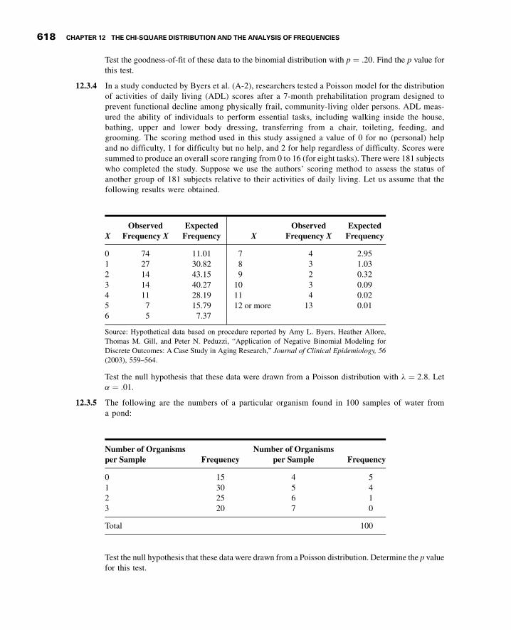
3GC12 12/04/2012 15:58:3 Page 618

Test the goodness-of-fit of these data to the binomial distribution with p ¼ .20. Find the p value forthis test.

12.3.4 In a study conducted by Byers et al. (A-2), researchers tested a Poisson model for the distributionof activities of daily living (ADL) scores after a 7-month prehabilitation program designed toprevent functional decline among physically frail, community-living older persons. ADL meas-ured the ability of individuals to perform essential tasks, including walking inside the house,bathing, upper and lower body dressing, transferring from a chair, toileting, feeding, andgrooming. The scoring method used in this study assigned a value of 0 for no (personal) helpand no difficulty, 1 for difficulty but no help, and 2 for help regardless of difficulty. Scores weresummed to produce an overall score ranging from 0 to 16 (for eight tasks). There were 181 subjectswho completed the study. Suppose we use the authors’ scoring method to assess the status ofanother group of 181 subjects relative to their activities of daily living. Let us assume that thefollowing results were obtained.

XObserved

Frequency XExpectedFrequency X

ObservedFrequency X

ExpectedFrequency

0 74 11.01 7 4 2.951 27 30.82 8 3 1.032 14 43.15 9 2 0.323 14 40.27 10 3 0.094 11 28.19 11 4 0.025 7 15.79 12 or more 13 0.016 5 7.37

Source: Hypothetical data based on procedure reported by Amy L. Byers, Heather Allore,Thomas M. Gill, and Peter N. Peduzzi, “Application of Negative Binomial Modeling forDiscrete Outcomes: A Case Study in Aging Research,” Journal of Clinical Epidemiology, 56(2003), 559–564.

Test the null hypothesis that these data were drawn from a Poisson distribution with l ¼ 2:8. Leta ¼ .01.

12.3.5 The following are the numbers of a particular organism found in 100 samples of water froma pond:

Number of Organismsper Sample Frequency

Number of Organismsper Sample Frequency

0 15 4 51 30 5 42 25 6 13 20 7 0

Total 100

Test the null hypothesis that these data were drawn from a Poisson distribution. Determine the p valuefor this test.


3GC12 12/04/2012 15:58:4 Page 619

12.3.6 A research team conducted a survey in which the subjects were adult smokers. Each subject in asample of 200 was asked to indicate the extent to which he or she agreed with the statement: “I wouldlike to quit smoking.” The results were as follows:

Response: Strongly agree Agree Disagree Strongly DisagreeNumberResponding: 102 30 60 8

Can one conclude on the basis of these data that, in the sampled population, opinions are not equallydistributed over the four levels of agreement? Let the probability of committing a type I error be .05and find the p value.

12.4 TESTS OF INDEPENDENCE

Another, and perhaps the most frequent, use of the chi-square distribution is to test the nullhypothesis that two criteria of classification, when applied to the same set of entities, areindependent. We say that two criteria of classification are independent if the distribution ofone criterion is the same no matter what the distribution of the other criterion. For example,if socioeconomic status and area of residence of the inhabitants of a certain city areindependent, we would expect to find the same proportion of families in the low, medium,and high socioeconomic groups in all areas of the city.

The Contingency Table The classification, according to two criteria, of a set ofentities, say, people, can be shown by a table in which the r rows represent the variouslevels of one criterion of classification and the c columns represent the various levels of thesecond criterion. Such a table is generally called a contingency table, with dimension r�c.The classification according to two criteria of a finite population of entities is shown inTable 12.4.1.

We will be interested in testing the null hypothesis that in the population the twocriteria of classification are independent. If the hypothesis is rejected, we will conclude that

TABLE 12.4.1 Two-Way Classification of a FinitePopulation of Entities

First Criterion of Classification Level

SecondCriterion ofClassificationLevel 1 2 3 . . . c Total

1 N11 N12 N13 . . . N1c N1.

2 N21 N22 N23 . . . N2c N2.

3 N31 N32 N33 . . . N3c N3.... ..

. ... ..

. ... ..

. ...

r Nr1 Nr2 Nr3 . . . Nrc Nr :

Total N.1 N.2 N.3 . . . N.c N

12.4 TESTS OF INDEPENDENCE 619

3GC12 12/04/2012 15:58:4 Page 620

the two criteria of classification are not independent. A sample of size n will be drawn fromthe population of entities, and the frequency of occurrence of entities in the samplecorresponding to the cells formed by the intersections of the rows and columns of Table12.4.1 along with the marginal totals will be displayed in a table such as Table 12.4.2.

Calculating the Expected Frequencies The expected frequency, underthe null hypothesis that the two criteria of classification are independent, is calculated foreach cell.

We learned in Chapter 3 (see Equation 3.4.4) that if two events are independent, theprobability of their joint occurrence is equal to the product of their individual probabilities.Under the assumption of independence, for example, we compute the probability that oneof the n subjects represented in Table 12.4.2 will be counted in Row 1 and Column 1 of thetable (that is, in Cell 11) by multiplying the probability that the subject will be counted inRow 1 by the probability that the subject will be counted in Column 1. In the notation of thetable, the desired calculation is

n1:

n

� � n.1n

� �

To obtain the expected frequency for Cell 11, we multiply this probability by the totalnumber of subjects, n. That is, the expected frequency for Cell 11 is given by

n1:

n

� � n.1n

� �ðnÞ

Since the n in one of the denominators cancels into numerator n, this expression reduces to

ðn1:Þðn.1Þn

In general, then, we see that to obtain the expected frequency for a given cell, we multiplythe total of the row in which the cell is located by the total of the column in which the cell islocated and divide the product by the grand total.

TABLE 12.4.2 Two-Way Classification of a Sampleof Entities

First Criterion of Classification Level

SecondCriterion ofClassificationLevel 1 2 3 . . . c Total

1 n11 n12 n13 . . . n1c n1.

2 n21 n22 n23 . . . n2c n2.

3 n31 n32 n33 . . . n3c n3.... ..

. ... ..

. ... ..

.

r nr1 nr2 nr3 . . . nrc nr.

Total n.1 n.2 n.3 . . . n.c n


3GC12 12/04/2012 15:58:5 Page 621

Observed Versus Expected Frequencies The expected frequencies andobserved frequencies are compared. If the discrepancy is sufficiently small, the nullhypothesis is tenable. If the discrepancy is sufficiently large, the null hypothesis is rejected,and we conclude that the two criteria of classification are not independent. The decision asto whether the discrepancy between observed and expected frequencies is sufficiently largeto cause rejection of H0 will be made on the basis of the size of the quantity computed whenwe use Equation 12.2.4, where Oi and Ei refer, respectively, to the observed and expectedfrequencies in the cells of Table 12.4.2. It would be more logical to designate the observedand expected frequencies in these cells by Oij and Eij, but to keep the notation simple and toavoid the introduction of another formula, we have elected to use the simpler notation. Itwill be helpful to think of the cells as being numbered from 1 to k, where 1 refers to Cell 11and k refers to Cell rc. It can be shown that X2 as defined in this manner is distributedapproximately as x2 with ðr � 1Þðc� 1Þ degrees of freedom when the null hypothesis istrue. If the computed value of X2 is equal to or larger than the tabulated value of x2 for somea, the null hypothesis is rejected at the a level of significance. The hypothesis testingprocedure is illustrated with the following example.

EXAMPLE 12.4.1

In 1992, the U.S. Public Health Service and the Centers for Disease Control and Preventionrecommended that all women of childbearing age consume 400mg of folic acid daily toreduce the risk of having a pregnancy that is affected by a neural tube defect such as spinabifida or anencephaly. In a study by Stepanuk et al. (A-3), 693 pregnant women called ateratology information service about their use of folic acid supplementation. The research-ers wished to determine if preconceptional use of folic acid and race are independent. Thedata appear in Table 12.4.3.

Solution:


2. Assumptions. We assume that the sample available for analysis is equiv-alent to a simple random sample drawn from the population of interest.

TABLE 12.4.3 Race of Pregnant Caller and Use ofFolic Acid

Preconceptional Use of Folic Acid

Yes No Total

White 260 299 559

Black 15 41 56

Other 7 14 21

Total 282 354 636

Source: Kathleen M. Stepanuk, Jorge E. Tolosa, Dawneete Lewis, Victoria

Meyers, Cynthia Royds, Juan Carlos Saogal, and Ron Librizzi, “Folic AcidSupplementation Use Among Women Who Contact a Teratology InformationService,” American Journal of Obstetrics and Gynecology, 187 (2002), 964–967.


3GC12 12/04/2012 15:58:5 Page 622

3. Hypotheses.

H0: Race and preconceptional use of folic acid are independent.HA: The two variables are not independent.Let a ¼ .05.


X2 ¼Xki¼1

ðOi � EiÞ2

Ei

" #

5. Distribution of test statistic. When H0 is true, X2 is distributedapproximately as x2 with ðr � 1Þðc� 1Þ ¼ ð3 � 1Þð2 � 1Þ ¼ ð2Þð1Þ ¼2 degrees of freedom.


7. Calculation of test statistic. The expected frequency for the first cell isð559 � 282Þ=636 ¼ 247:86. The other expected frequencies are calcu-lated in a similar manner. Observed and expected frequencies aredisplayed in Table 12.4.4. From the observed and expected frequencieswe may compute

X2 ¼ P ðOi � EiÞ2

Ei

" #

¼ 260 � 247:86ð Þ2

247:86þ 299 � 311:14ð Þ2

311:14þ . . .þ 14 � 11:69ð Þ2

11:69

¼ .59461 þ .47368 þ . . .þ .45647 ¼ 9:08960

8. Statistical decision. We reject H0 since 9:08960 > 5:991.

9. Conclusion. We conclude that H0 is false, and that there is a relationshipbetween race and preconceptional use of folic acid.

10. p value. Since 7:378 < 9:08960 < 9:210, .01 < p < .025.

&

TABLE 12.4.4 Observed and Expected Frequenciesfor Example 12.4.1

Preconceptional Use of Folic Acid

Yes No Total

White 260 (247.86) 299 (311.14) 559

Black 15 (24.83) 41 (31.17) 56

Other 7 (9.31) 14 (11.69) 21

Total 282 354 636


3GC12 12/04/2012 15:58:5 Page 623

ComputerAnalysis The computer may be used to advantage in calculating X2 fortests of independence and tests of homogeneity. Figure 12.4.1 shows the procedure andprintout for Example 12.4.1 when the MINITAB program for computing X2 fromcontingency tables is used. The data were entered into MINITAB Columns 1 and 2,corresponding to the columns of Table 12.4.3.

We may use SAS® to obtain an analysis and printout of contingency table data byusing the PROC FREQ statement. Figure 12.4.2 shows a partial SAS® printout reflectingthe analysis of the data of Example 12.4.1.

Data:

C1: 260 15 7C2: 299 41 14

:dnammoc noisseS:xoB golaiD

Stat Tables Chi-square Test MTB > CHISQUARE C1-C3

Type C1-C2 in Columns containing the table.Click OK.

Output:

Chi-Square Test: C1, C2

Expected counts are printed below observed counts

C1 C2 Total1 260 299 559

247.86 311.14

2 15 41 5624.83 31.17

3 7 14 219.31 11.69

Total 282 354 636

Chi-Sq = 0.595 + 0.474 +3.892 + 3.100 +0.574 + 0.457 = 9.091

DF = 2, P-Value = 0.011

FIGURE 12.4.1 MINITAB procedure and output for chi-square analysis of data in Table 12.4.3.


3GC12 12/04/2012 15:58:5 Page 624

The SAS System

The FREQ Procedure

Table of race by folic

race folicFrequencyPercentRow PctCol Pct No Yes Total-----------------------------Black 41 15 56

6.45 2.36 8.8173.21 26.7911.58 5.32

-----------------------------Other 14 7 21

2.20 1.10 3.3066.67 33.333.95 2.48

-----------------------------White 299 260 559

47.01 40.88 87.8953.49 46.5184.46 92.20

-----------------------------Total 354 282 636

55.66 44.34 100.00

Statistics for Table of race by folic

borPeulaVFDcitsitatS----------------------------------------------------------

6010.03190.92erauqS-ihCLikelihood Ratio Chi-Square 2 9.4808 0.0087Mantel—Haenszel Chi-Square 1 8.9923 0.0027

6911.0tneicfifeoC ihPContingency Coefficient 0.1187

6911.0V s’remarC

Sample Size = 636

FIGURE 12.4.2 Partial SAS® printout for the chi-square analysis of the data from

Example 12.4.1.


3GC12 12/04/2012 15:58:6 Page 625

Note that the SAS® printout shows, in each cell, the percentage that cell frequency isof its row total, its column total, and the grand total. Also shown, for each row and columntotal, is the percentage that the total is of the grand total. In addition to the X2 statistic,SAS® gives the value of several other statistics that may be computed from contingencytable data. One of these, the Mantel–Haenszel chi-square statistic, will be discussed in alater section of this chapter.

Small Expected Frequencies The problem of small expected frequenciesdiscussed in the previous section may be encountered when analyzing the data ofcontingency tables. Although there is a lack of consensus on how to handle this problem,many authors currently follow the rule given by Cochran (5). He suggests that forcontingency tables with more than 1 degree of freedom a minimum expectation of 1 isallowable if no more than 20 percent of the cells have expected frequencies of less than 5.To meet this rule, adjacent rows and/or adjacent columns may be combined when todo so is logical in light of other considerations. If X2 is based on less than 30 degrees offreedom, expected frequencies as small as 2 can be tolerated. We did not experience theproblem of small expected frequencies in Example 12.4.1, since they were all greaterthan 5.

The 2� 2 Contingency Table Sometimes each of two criteria of classifica-tion may be broken down into only two categories, or levels. When data are cross-classified in this manner, the result is a contingency table consisting of two rows and twocolumns. Such a table is commonly referred to as a 2 � 2 table. The value of X2 may becomputed by first calculating the expected cell frequencies in the manner discussedabove. In the case of a 2 � 2 contingency table, however, X2 may be calculated by thefollowing shortcut formula:

X2 ¼ nðad � bcÞ2

ðaþ cÞðbþ dÞðaþ bÞðcþ dÞ (12.4.1)

where a, b, c, and d are the observed cell frequencies as shown in Table 12.4.5. When weapply the ðr � 1Þðc� 1Þ rule for finding degrees of freedom to a 2 � 2 table, the result is1 degree of freedom. Let us illustrate this with an example.

TABLE 12.4.5 A 2� 2 Contingency Table

First Criterion of ClassificationSecond Criterionof Classification 1 2 Total

1 a b a þ b

2 c d c þ d



3GC12 12/04/2012 15:58:6 Page 626

EXAMPLE 12.4.2

According to Silver and Aiello (A-4), falls are of major concern among polio survivors.Researchers wanted to determine the impact of a fall on lifestyle changes. Table 12.4.6shows the results of a study of 233 polio survivors on whether fear of falling resulted inlifestyle changes.

Solution:

1. Data. From the information given we may construct the 2 � 2 contin-gency table displayed as Table 12.5.6.

2. Assumptions. We assume that the sample is equivalent to a simplerandom sample.

3. Hypotheses.

H0: Fall status and lifestyle change because of fear of falling areindependent.

H1: The two variables are not independent.

Let a ¼ .05.


X2 ¼Xki¼1

Oi � Eið Þ2

Ei

" #

5. Distribution of test statistic. When H0 is true, X2 is distributedapproximately as x2 with ðr � 1Þðc� 1Þ ¼ ð2 � 1Þð2 � 1Þ ¼ ð1Þð1Þ ¼1 degree of freedom.



X2 ¼ 233 ð131Þð36Þ � ð52Þð14Þ½ �2ð145Þð88Þð183Þð50Þ ¼ 31:7391

8. Statistical decision. We reject H0 since 31:7391 > 3:841.

TABLE 12.4.6 Contingency Table for the Data of Example 12.4.2

Made Lifestyle Changes Because of Fear of Falling

Yes No Total

Fallers 131 52 183

Nonfallers 14 36 50

Total 145 88 233

Source: J. K. Silver and D. D. Aiello, “Polio Survivors: Falls and Subsequent Injuries,”American Journal of Physical Medicine and Rehabilitation, 81 (2002), 567–570.


3GC12 12/04/2012 15:58:6 Page 627

9. Conclusion. We conclude thatH0 is false, and that there is a relationshipbetween experiencing a fall and changing one’s lifestyle because of fearof falling.

10. p value. Since 31:7391 > 7:879, p < .005. &

Small Expected Frequencies The problems of how to handle small expectedfrequencies and small total sample sizes may arise in the analysis of 2 � 2 contingencytables. Cochran (5) suggests that the x2 test should not be used if n < 20 or if 20 < n < 40and any expected frequency is less than 5. When n ¼ 40, an expected cell frequency assmall as 1 can be tolerated.

Yates’s Correction The observed frequencies in a contingency table are discreteand thereby give rise to a discrete statistic, X2, which is approximated by the x2

distribution, which is continuous. Yates (6) in 1934 proposed a procedure for correctingfor this in the case of 2 � 2 tables. The correction, as shown in Equation 12.4.2, consists ofsubtracting half the total number of observations from the absolute value of the quantityad � bc before squaring. That is,

X2corrected ¼ n jad � bcj � .5nð Þ2

ðaþ cÞðbþ dÞðaþ bÞðcþ dÞ (12.4.2)

It is generally agreed that no correction is necessary for larger contingency tables.Although Yates’s correction for 2 � 2 tables has been used extensively in the past,more recent investigators have questioned its use. As a result, some practitioners recom-mend against its use.

We may, as a matter of interest, apply the correction to our current example. UsingEquation 12.4.2 and the data from Table 12.4.6, we may compute

X2 ¼ 233 jð131Þð36Þ � ð52Þð14Þj � .5ð233Þ½ �2ð145Þð88Þð183Þð50Þ ¼ 29:9118

As might be expected, with a sample this large, the difference in the two results is notdramatic.

Tests of Independence: Characteristics The characteristics of a chi-square test of independence that distinguish it from other chi-square tests are as follows:

1. A single sample is selected from a population of interest, and the subjects or objectsare cross-classified on the basis of the two variables of interest.

2. The rationale for calculating expected cell frequencies is based on the probabilitylaw, which states that if two events (here the two criteria of classification) areindependent, the probability of their joint occurrence is equal to the product of theirindividual probabilities.

3. The hypotheses and conclusions are stated in terms of the independence (or lack ofindependence) of two variables.


3GC12 12/04/2012 15:58:7 Page 628

EXERCISES

In the exercises that follow perform the test at the indicated level of significance and determine the pvalue.

12.4.1 In the study by Silver and Aiello (A-4) cited in Example 12.4.2, a secondary objective was todetermine if the frequency of falls was independent of wheelchair use. The following table gives thedata for falls and wheelchair use among the subjects of the study.

Wheelchair Use

Yes No

Fallers 62 121Nonfallers 18 32

Source: J. K. Silver and D. D. Aiello, “Polio Survivors: Falls andSubsequent Injuries,” American Journal of Physical Medicine andRehabilitation, 81 (2002), 567–570.

Do these data provide sufficient evidence to warrant the conclusion that wheelchair use and falling arerelated? Let a ¼ .05.

12.4.2 Sternal surgical site infection (SSI) after coronary artery bypass graft surgery is a complication thatincreases patient morbidity and costs for patients, payers, and the health care system. Segal andAnderson (A-5) performed a study that examined two types of preoperative skin preparation beforeperforming open heart surgery. These two preparations used aqueous iodine and insoluble iodine withthe following results.

Comparison of Aqueousand Insoluble Preps

Prep Group Infected Not Infected

Aqueous iodine 14 94Insoluble iodine 4 97

Source: Cynthia G. Segal and Jacqueline J. Anderson, “Preoperative SkinPreparation of Cardiac Patients,” AORN Journal, 76 (2002), 821–827.

Do these data provide sufficient evidence at the a ¼ .05 level to justify the conclusion that the type ofskin preparation and infection are related?

12.4.3 The side effects of nonsteroidal antiinflammatory drugs (NSAIDs) include problems involving pepticulceration, renal function, and liver disease. In 1996, the American College of Rheumatology issuedand disseminated guidelines recommending baseline tests (CBC, hepatic panel, and renal tests) whenprescribing NSAIDs. A study was conducted by Rothenberg and Holcomb (A-6) to determine ifphysicians taking part in a national database of computerized medical records performed therecommended baseline tests when prescribing NSAIDs. The researchers classified physicians inthe study into four categories—those practicing in internal medicine, family practice, academicfamily practice, and multispeciality groups. The data appear in the following table.


3GC12 12/04/2012 15:58:7 Page 629

Performed Baseline Tests

Practice Type Yes No

Internal medicine 294 921Family practice 98 2862Academic family practice 50 3064Multispecialty groups 203 2652

Source: Ralph Tothenberg and John P. Holcomb, “Guidelines for Monitoring of NSAIDs: WhoListened?,” Journal of Clinical Rheumatology, 6 (2000), 258–265.

Do the data above provide sufficient evidence for us to conclude that type of practice andperformance of baseline tests are related? Use a ¼ .01.

12.4.4 Boles and Johnson (A-7) examined the beliefs held by adolescents regarding smoking and weight.Respondents characterized their weight into three categories: underweight, overweight, or appropri-ate. Smoking status was categorized according to the answer to the question, “Do you currentlysmoke, meaning one or more cigarettes per day?” The following table shows the results of a telephonestudy of adolescents in the age group 12–17.

Smoking

Yes No

Underweight 17 97Overweight 25 142Appropriate 96 816

Source: Sharon M. Boles and Patrick B. Johnson, “Gender, Weight Concerns, and AdolescentSmoking,” Journal of Addictive Diseases, 20 (2001), 5–14.

Do the data provide sufficient evidence to suggest that weight perception and smoking status arerelated in adolescents? a ¼ .05.

12.4.5 A sample of 500 college students participated in a study designed to evaluate the level of collegestudents’ knowledge of a certain group of common diseases. The following table shows the studentsclassified by major field of study and level of knowledge of the group of diseases:

Knowledge of Diseases

Major Good Poor Total

Premedical 31 91 122Other 19 359 378

Total 50 450 500

Do these data suggest that there is a relationship between knowledge of the group of diseasesand major field of study of the college students from which the present sample was drawn?Let a ¼ .05.

12.4.6 The following table shows the results of a survey in which the subjects were a sample of 300 adultsresiding in a certain metropolitan area. Each subject was asked to indicate which of three policies theyfavored with respect to smoking in public places.

EXERCISES 629

3GC12 12/04/2012 15:58:7 Page 630

Policy Favored

Highest EducationLevel

NoRestrictionson Smoking

Smoking Allowedin DesignatedAreas Only

NoSmokingat All

NoOpinion Total

College graduate 5 44 23 3 75High-school graduate 15 100 30 5 150Grade-school graduate 15 40 10 10 75

Total 35 184 63 18 300

Can one conclude from these data that, in the sampled population, there is a relationship betweenlevel of education and attitude toward smoking in public places? Let a ¼ .05.

12.5 TESTS OF HOMOGENEITY

A characteristic of the examples and exercises presented in the last section is that, in eachcase, the total sample was assumed to have been drawn before the entities were classifiedaccording to the two criteria of classification. That is, the observed number of entities fallinginto each cell was determined after the sample was drawn. As a result, the row and columntotals are chance quantities not under the control of the investigator. We think of the sampledrawn under these conditions as a single sample drawn from a single population. Onoccasion, however, either row or column totals may be under the control of the investigator;that is, the investigator may specify that independent samples be drawn from each of severalpopulations. In this case, one set of marginal totals is said to be fixed, while the other set,corresponding to the criterion of classification applied to the samples, is random. The formerprocedure, as we have seen, leads to a chi-square test of independence. The latter situationleads to a chi-square test of homogeneity. The two situations not only involve differentsampling procedures; they lead to different questions and null hypotheses. The test ofindependence is concerned with the question: Are the two criteria of classification indepen-dent? The homogeneity test is concerned with the question: Are the samples drawn frompopulations that are homogeneous with respect to some criterion of classification? In thelatter case the null hypothesis states that the samples are drawn from the same population.Despite these differences in concept and sampling procedure, the two tests are mathemati-cally identical, as we see when we consider the following example.

Calculating Expected Frequencies Either the row categories or the col-umn categories may represent the different populations from which the samples are drawn.If, for example, three populations are sampled, they may be designated as populations 1, 2,and 3, in which case these labels may serve as either row or column headings. If the variableof interest has three categories, say,A, B, andC, these labels may serve as headings for rowsor columns, whichever is not used for the populations. If we use notation similar to thatadopted for Table 12.4.2, the contingency table for this situation, with columns used torepresent the populations, is shown as Table 12.5.1. Before computing our test statistic weneed expected frequencies for each of the cells in Table 12.5.1. If the populations are indeed


3GC12 12/04/2012 15:58:8 Page 631

homogeneous, or, equivalently, if the samples are all drawn from the same population, withrespect to the categories A, B, and C, our best estimate of the proportion in the combinedpopulation who belong to category A is nA:=n. By the same token, if the three populationsare homogeneous, we interpret this probability as applying to each of the populationsindividually. For example, under the null hypothesis, nA. is our best estimate of theprobability that a subject picked at random from the combined population will belong tocategory A. We would expect, then, to find n.1ðnA:=nÞ of those in the sample from population1 to belong to category A, n.2ðnA:=nÞ of those in the sample from population 2 to belong tocategory A, and n.3ðnA:=nÞ of those in the sample from population 3 to belong to category A.These calculations yield the expected frequencies for the first row of Table 12.5.1. Similarreasoning and calculations yield the expected frequencies for the other two rows.

We see again that the shortcut procedure of multiplying appropriate marginal totalsand dividing by the grand total yields the expected frequencies for the cells.

From the data in Table 12.5.1 we compute the following test statistic:

X2 ¼Xki¼1

Oi � Eið Þ2

Ei

" #

EXAMPLE 12.5.1

Narcolepsy is a disease involving disturbances of the sleep–wake cycle. Members of theGerman Migraine and Headache Society (A-8) studied the relationship between migraineheadaches in 96 subjects diagnosed with narcolepsy and 96 healthy controls. The resultsare shown in Table 12.5.2. We wish to know if we may conclude, on the basis of these data,

TABLE 12.5.1 A Contingency Table for Data for aChi-Square Test of Homogeneity

Population

Variable Category 1 2 3 Total

A nA1 nA2 nA3 nA:

B nB1 nB2 nB3 nB:

C nC1 nC2 nC3 nC :

Total n.1 n.2 n.3 n

TABLE 12.5.2 Frequency of Migraine Headaches by Narcolepsy Status

Reported Migraine Headaches

Yes No Total

Narcoleptic subjects 21 75 96

Healthy controls 19 77 96

Total 40 152 192

Source: The DMG Study Group, “Migraine and Idiopathic Narcolepsy—A Case-Control Study,”Cephalagia, 23 (2003), 786–789.

12.5 TESTS OF HOMOGENEITY 631

3GC12 12/04/2012 15:58:8 Page 632

that the narcolepsy population and healthy populations represented by the samples are nothomogeneous with respect to migraine frequency.

Solution:


2. Assumptions. We assume that we have a simple random sample fromeach of the two populations of interest.

3. Hypotheses.

H0: The two populations are homogeneous with respect to migrainefrequency.

HA: The two populations are not homogeneous with respect to migrainefrequency.

Let a ¼ .05.


X2 ¼X

Oi � Eið Þ2=Ei

h i

5. Distribution of test statistic. If H0 is true, X2 is distributed approxi-mately as x2 with ð2 � 1Þð2 � 1Þ ¼ ð1Þð1Þ ¼ 1 degree of freedom.


7. Calculation of test statistic. The MINITAB output is shown in Figure12.5.1.

Chi-Square Test

Expected counts are printed below observed counts

Rows: Narcolepsy Columns: Migraine

No Yes All

No 77 19 9676.00 20.00 96.00

Yes 75 21 9676.00 20.00 96.00

All 152 40 192152.00 40.00 192.00

Chi-Square = 0.126, DF = 1, P-Value = 0.722

FIGURE 12.5.1 MINITAB output for Example 12.5.1.


3GC12 12/04/2012 15:58:8 Page 633

8. Statistical decision. Since .126 is less than the critical value of 3.841,we are unable to reject the null hypothesis.

9. Conclusion. We conclude that the two populations may be homoge-neous with respect to migraine frequency.

10. p value. From the MINITAB output we see that p ¼ .722. &

Small Expected Frequencies The rules for small expected frequencies givenin the previous section are applicable when carrying out a test of homogeneity.

In summary, the chi-square test of homogeneity has the following characteristics:

1. Two or more populations are identified in advance, and an independent sample isdrawn from each.

2. Sample subjects or objects are placed in appropriate categories of the variable ofinterest.

3. The calculation of expected cell frequencies is based on the rationale that if thepopulations are homogeneous as stated in the null hypothesis, the best estimate of theprobability that a subject or object will fall into a particular category of the variable ofinterest can be obtained by pooling the sample data.

4. The hypotheses and conclusions are stated in terms of homogeneity (with respect tothe variable of interest) of populations.

Test of Homogeneity and H0:p1 ¼ p2 The chi-square test of homogeneityfor the two-sample case provides an alternative method for testing the null hypothesis thattwo population proportions are equal. In Section 7.6, it will be recalled, we learned to testH0 :p1 ¼ p2 against HA :p1 6¼ p2 by means of the statistic

z ¼ p1 � p2ð Þ � p1 � p2ð Þ0ffiffiffiffiffiffiffiffiffiffiffiffiffiffiffiffiffiffiffiffiffiffiffiffiffiffiffiffiffiffiffiffiffiffiffiffiffiffiffiffi�p 1 � �pð Þ

n1þ �p 1 � �pð Þ

n2

r

where �p is obtained by pooling the data of the two independent samples available foranalysis.

Suppose, for example, that in a test of H0 :p1 ¼ p2 against HA :p1 6¼ p2, the sampledata were as follows: n1 ¼ 100; p1 ¼ .60; n2 ¼ 120; p2 ¼ .40. When we pool the sampledata we have

�p ¼ .60 100ð Þ þ .40 120ð Þ100 þ 120

¼ 108

220¼ .4909

and

z ¼ .60 � .40ffiffiffiffiffiffiffiffiffiffiffiffiffiffiffiffiffiffiffiffiffiffiffiffiffiffiffiffiffiffiffiffiffiffiffiffiffiffiffiffiffiffiffiffiffiffiffiffiffiffiffiffiffiffiffiffiffiffiffiffiffiffiffiffi.4909ð Þ .5091ð Þ

100þ .4909ð Þ .5091ð Þ

120

r ¼ 2:95469

which is significant at the .05 level since it is greater than the critical value of 1.96.

12.5 TESTS OF HOMOGENEITY 633

3GC12 12/04/2012 15:58:9 Page 634

If we wish to test the same hypothesis using the chi-square approach, our contin-gency table will be

Characteristic Present

Sample Yes No Total

1 60 40 1002 48 72 120

Total 108 112 220


X2 ¼ 220 60ð Þ 72ð Þ � 40ð Þ 48ð Þ½ �2108ð Þ 112ð Þ 100ð Þ 120ð Þ ¼ 8:7302

which is significant at the .05 level because it is greater than the critical value of 3.841. Wesee, therefore, that we reach the same conclusion by both methods. This is not surprisingbecause, as explained in Section 12.2, x2

1ð Þ ¼ z2. We note that 8:7302 ¼ 2:95469ð Þ2 andthat 3:841 ¼ 1:96ð Þ2.

EXERCISES

In the exercises that follow perform the test at the indicated level of significance and determine the pvalue.

12.5.1 Refer to the study by Carter et al. [A-9], who investigated the effect of age at onset of bipolar disorderon the course of the illness. One of the variables studied was subjects’ family history. Table 3.4.1shows the frequency of a family history of mood disorders in the two groups of interest: early age atonset (18 years or younger) and later age at onset (later than 18 years).

Family History of MoodDisorders Early � 18ðEÞ Later > 18ðLÞ Total

Negative (A) 28 35 63Bipolar disorder (B) 19 38 57Unipolar (C) 41 44 85Unipolar and bipolar (D) 53 60 113

Total 141 177 318

Source: Tasha D. Carter, Emanuela Mundo, Sagar V. Parkh, and James L. Kennedy,“Early Age at Onset as a Risk Factor for Poor Outcome of Bipolar Disorder,” Journal ofPsychiatric Research, 37 (2003), 297–303.

Can we conclude on the basis of these data that subjects 18 or younger differ from subjects older than18 with respect to family histories of mood disorders? Let a ¼ .05.


3GC12 12/04/2012 15:58:9 Page 635

12.5.2 Coughlin et al. (A-10) examined breast and cervical screening practices of Hispanic and non-Hispanic women in counties that approximate the U.S. southern border region. The study used datafrom the Behavioral Risk Factor Surveillance System surveys of adults ages 18 years or olderconducted in 1999 and 2000. The following table shows the number of observations of Hispanicand non-Hispanic women who had received a mammogram in the past 2 years cross-classified bymarital status.

Marital Status Hispanic Non-Hispanic Total

Currently married 319 738 1057Divorced or separated 130 329 459Widowed 88 402 490Never married or living asan unmarried couple

41 95 136

Total 578 1564 2142

Source: Steven S. Coughlin, Robert J. Uhler, Thomas Richards, and KatherineM. Wilson, “Breast and Cervical Cancer Screening Practices Among Hispanicand Non-Hispanic Women Residing Near the United States–Mexico Border,1999–2000,” Family and Community Health, 26, (2003), 130–139.

We wish to know if we may conclude on the basis of these data that marital status and ethnicity(Hispanic and non-Hispanic) in border counties of the southern United States are not homogeneous.Let a ¼ .05.

12.5.3 Swor et al. (A-11) examined the effectiveness of cardiopulmonary resuscitation (CPR) training inpeople over 55 years of age. They compared the skill retention rates of subjects in this age group whocompleted a course in traditional CPR instruction with those who received chest-compression–onlycardiopulmonary resuscitation (CC-CPR). Independent groups were tested 3 months after training.Among the 27 subjects receiving traditional CPR, 12 were rated as competent. In the CC-CPR group,15 out of 29 were rated competent. Do these data provide sufficient evidence for us to conclude thatthe two populations are not homogeneous with respect to competency rating 3 months after training?Let a ¼ .05.

12.5.4 In an air pollution study, a random sample of 200 households was selected from each of twocommunities. A respondent in each household was asked whether or not anyone in the household wasbothered by air pollution. The responses were as follows:

Any Member of HouseholdBothered by Air Pollution?

Community Yes No Total

I 43 157 200II 81 119 200

Total 124 276 400

Can the researchers conclude that the two communities differ with respect to the variable of interest?Let a ¼ .05.

EXERCISES 635

3GC12 12/04/2012 15:58:9 Page 636

12.5.5 In a simple random sample of 250 industrial workers with cancer, researchers found that 102 hadworked at jobs classified as “high exposure” with respect to suspected cancer-causing agents. Of theremainder, 84 had worked at “moderate exposure” jobs, and 64 had experienced no known exposurebecause of their jobs. In an independent simple random sample of 250 industrial workers fromthe same area who had no history of cancer, 31 worked in “high exposure” jobs, 60 worked in“moderate exposure” jobs, and 159 worked in jobs involving no known exposure to suspected cancer-causing agents. Does it appear from these data that persons working in jobs that expose them tosuspected cancer-causing agents have an increased risk of contracting cancer? Let a ¼ .05.

12.6 THE FISHER EXACT TEST

Sometimes we have data that can be summarized in a 2 � 2 contingency table, but thesedata are derived from very small samples. The chi-square test is not an appropriate methodof analysis if minimum expected frequency requirements are not met. If, for example, n isless than 20 or if n is between 20 and 40 and one of the expected frequencies is less than 5,the chi-square test should be avoided.

A test that may be used when the size requirements of the chi-square test are not metwas proposed in the mid-1930s almost simultaneously by Fisher (7,8), Irwin (9), and Yates(10). The test has come to be known as the Fisher exact test. It is called exact because, ifdesired, it permits us to calculate the exact probability of obtaining the observed results orresults that are more extreme.

Data Arrangement When we use the Fisher exact test, we arrange the data in theform of a 2 � 2 contingency table like Table 12.6.1. We arrange the frequencies in such away that A > B and choose the characteristic of interest so that a=A > b=B.

Some theorists believe that Fisher’s exact test is appropriate only when both marginaltotals of Table 12.6.1 are fixed by the experiment. This specific model does not appear toarise very frequently in practice. Many experimenters, therefore, use the test when bothmarginal totals are not fixed.

Assumptions The following are the assumptions for the Fisher exact test.

1. The data consist of A sample observations from population 1 and B sampleobservations from population 2.

2. The samples are random and independent.

3. Each observation can be categorized as one of two mutually exclusive types.

TABLE 12.6.1 A 2� 2 Contingency Table for the Fisher Exact Test

SampleWith

CharacteristicWithout

Characteristic Total

1 a A� a A

2 b B � b B

Total a þ b Aþ B � a � b Aþ B


3GC12 12/04/2012 15:58:9 Page 637

Hypotheses The following are the null hypotheses that may be tested and theiralternatives.

1. (Two-sided)

H0: The proportion with the characteristic of interest is the same in both populations;that is, p1 ¼ p2.

HA: The proportion with the characteristic of interest is not the same in bothpopulations; p1 6¼ p2.

2. (One-sided)

H0: The proportion with the characteristic of interest in population 1 is less than orthe same as the proportion in population 2; p1 � p2.

HA: The proportion with the characteristic of interest is greater in population 1 thanin population 2; p1 > p2.

Test Statistic The test statistic is b, the number in sample 2 with the characteristicof interest.

Decision Rule Finney (11) has prepared critical values of b for A � 15. Latscha(12) has extended Finney’s tables to accommodate values of A up to 20. Appendix Table Jgives these critical values of b for A between 3 and 20, inclusive. Significance levels of .05,.025, .01, and .005 are included. The specific decision rules are as follows:

1. Two-sided test. Enter Table J with A, B, and a. If the observed value of b is equal toor less than the integer in a given column, reject H0 at a level of significance equal totwice the significance level shown at the top of that column. For example, supposeA ¼ 8, B ¼ 7, a ¼ 7, and the observed value of b is 1. We can reject the nullhypothesis at the 2 .05ð Þ ¼ .10, the 2 .025ð Þ ¼ .05, and the 2 .01ð Þ ¼ .02 levels ofsignificance, but not at the 2 .005ð Þ ¼ .01 level.

2. One-sided test. Enter Table J with A, B, and a. If the observed value of b is less thanor equal to the integer in a given column, reject H0 at the level of significance shownat the top of that column. For example, suppose that A ¼ 16, B ¼ 8, a ¼ 4, and theobserved value of b is 3. We can reject the null hypothesis at the .05 and .025 levels ofsignificance, but not at the .01 or .005 levels.

Large-Sample Approximation For sufficiently large samples we can test thenull hypothesis of the equality of two population proportions by using the normalapproximation. Compute

z ¼ a=Að Þ � b=Bð Þffiffiffiffiffiffiffiffiffiffiffiffiffiffiffiffiffiffiffiffiffiffiffiffiffiffiffiffiffiffiffiffiffiffiffiffiffiffiffiffiffiffip 1 � pð Þ 1=Aþ 1=Bð Þp (12.6.1)

where

p ¼ aþ bð Þ= Aþ Bð Þ (12.6.2)

and compare it for significance with appropriate critical values of the standard normaldistribution. The use of the normal approximation is generally considered satisfactory if a,

12.6 THE FISHER EXACT TEST 637

3GC12 12/04/2012 15:58:10 Page 638

b, A� a, and B� b are all greater than or equal to 5. Alternatively, when sample sizes aresufficiently large, we may test the null hypothesis by means of the chi-square test.

Further Reading The Fisher exact test has been the subject of some controversyamong statisticians. Some feel that the assumption of fixed marginal totals is unrealistic inmost practical applications. The controversy then centers around whether the test isappropriate when both marginal totals are not fixed. For further discussion of this and otherpoints, see the articles by Barnard (13–15), Fisher (16), and Pearson (17).

Sweetland (18) compared the results of using the chi-square test with those obtainedusing the Fisher exact test for samples of size Aþ B ¼ 3 to Aþ B ¼ 69. He found closeagreement when A and B were close in size and the test was one-sided.

Carr (19) presents an extension of the Fisher exact test to more than two samples ofequal size and gives an example to demonstrate the calculations. Neave (20) presents theFisher exact test in a new format; the test is treated as one of independence rather than ofhomogeneity. He has prepared extensive tables for use with his approach.

The sensitivity of Fisher’s exact test to minor perturbations in 2 � 2 contingencytables is discussed by Dupont (21).

EXAMPLE 12.6.1

The purpose of a study by Justesen et al. (A-12) was to evaluate the long-term efficacy oftaking indinavir/ritonavir twice a day in combination with two nucleoside reversetranscriptase inhibitors among HIV-positive subjects who were divided into two groups.Group 1 consisted of patients who had no history of taking protease inhibitors (PI Na€ıve).Group 2 consisted of patients who had a previous history taking a protease inhibitor (PIExperienced). Table 12.6.2 shows whether these subjects remained on the regimen for the120 weeks of follow-up. We wish to know if we may conclude that patients classified asgroup 1 have a lower probability than subjects in group 2 of remaining on the regimen for120 weeks.

TABLE 12.6.2 Regimen Status at 120 Weeks for

PI Na€ıve and PI Experienced Subjects TakingIndinavir/Ritonavir as Described in Example 12.6.1

Remained inthe Regimenfor 120 Weeks

Total Yes No

1 (PI Na€ıve) 9 2 7

2 (PA Experienced) 12 8 4

Total 21 10 11

Source: U.S. Justesen, A. M. Lervfing, A. Thomsen, J. A. Lindberg,

C. Pedersen, and P. Tauris, “Low-Dose Indinavir in Combination withLow-Dose Ritonavir: Steady-State Pharmacokinetics and Long-TermClinical Outcome Follow-Up,” HIV Medicine, 4 (2003), 250–254.


3GC12 12/04/2012 15:58:10 Page 639

Solution:

1. Data. The data as reported are shown in Table 12.6.2. Table 12.6.3shows the data rearranged to conform to the layout of Table 12.6.1.Remaining on the regimen is the characteristic of interest.

2. Assumptions. We presume that the assumptions for application of theFisher exact test are met.

3. Hypotheses.

H0: The proportion of subjects remaining 120 weeks on the regimen in apopulation of patients classified as group 2 is the same as or lessthan the proportion of subjects remaining on the regimen 120 weeksin a population classified as group 1.

HA: Group 2 patients have a higher rate than group 1 patients ofremaining on the regimen for 120 weeks.

4. Test statistic. The test statistic is the observed value of b as shown inTable 12.6.3.

5. Distribution of test statistic. We determine the significance of b byconsulting Appendix Table J.

6. Decision rule. Suppose we let a ¼ .05. The decision rule, then, is toreject H0 if the observed value of b is equal to or less than 1, the value ofb in Table J for A ¼ 12, B ¼ 9, a ¼ 8, and a ¼ .05.

7. Calculation of test statistic. The observed value of b, as shown inTable 12.6.3, is 2.

8. Statistical decision. Since 2 > 1, we fail to reject H0.

9. Conclusion. Since we fail to reject H0, we conclude that the nullhypothesis may be true. That is, it may be true that the rate of remainingon the regimen for 120 weeks is the same or less for the PI experiencedgroup compared to the PI na€ıve group.

10. p value. We see in Table J that when A ¼ 12, B ¼ 9, a ¼ 8, the value ofb ¼ 2 has an exact probability of occurring by chance alone, when H0 istrue, greater than .05. &

TABLE 12.6.3 Data of Table 12.6.2 Rearranged to Conform to theLayout of Table 12.6.1

Remained in Regimen for 120Weeks

Yes No Total

2 (PI Experienced) 8 ¼ a 4 ¼ A� a 12 ¼ A

1 (PI Na€ıve) 2 ¼ b 7 ¼ B � b 9 ¼ B

Total 10 ¼ a þ b 11 ¼ Aþ B � a � b 21 ¼ Aþ B

12.6 THE FISHER EXACT TEST 639

3GC12 12/04/2012 15:58:10 Page 640

Various statistical software programs perform the calculations for the Fisher exacttest. Figure 12.6.1 shows the results of Example 12.6.1 as computed by SPSS. The exact pvalue is provided for both a one-sided and a two-sided test. Based on these results, we fail toreject H0 (p value >.05), just as we did using the statistical tables in the Appendix. Notethat in addition to the Fisher exact test several alternative tests are provided. The readershould be aware that these alternative tests are not appropriate if the assumptions under-lying them have been violated.

EXERCISES

12.6.1 The goal of a study by Tahmassebi and Curzon (A-13) was to determine if drooling in childrenwith cerebral palsy is due to hypersalivation. One of the procedures toward that end was to examinethe salivary buffering capacity of cerebral palsied children and controls. The following table givesthe results.

Pl * Remained Cross-Tabulation

Count

Remained

Yes No Total

Pl Experienced 8 4 12Naive 2 7 9

121101latoT

Chi-Square Tests

Asymp. Sig. Exact Sig. Exact Sig.Value df (2-sided) (2-sided) (1-sided)

Pearson Chi-Square 4.073b 1 .044Continuity Correctiona 2.486 1 .115Likelihood Ratio 4.253 1 .039

650.080.tseT tcaxE s’rehsiFLinear-by-Linear 3.879 1 .049AssociationN of Valid Cases 21

a. Computed only for a 2 2 table

b. 2 cells (50.0%) have expected count less than 5. The minimum expected count is 4.29.

FIGURE 12.6.1 SPSS output for Example 12.6.1.


3GC12 12/04/2012 15:58:10 Page 641

Buffering Capacity

Group Medium High

Cerebral palsy 2 8Control 3 7

Source: J. F. Tahmassebi and M. E. J. Curzon, “The Cause of Drooling inChildren with Cerebral Palsy—Hypersalivation or Swallowing Defect?”International Journal of Paediatric Dentistry, 13 (2003), 106–111.

Test for a significant difference between cerebral palsied children and controls with respect to high orlow buffering capacity. Let a ¼ .05 and find the p value.

12.6.2 In a study by Xiao and Shi (A-14), researchers studied the effect of cranberry juice in the treatmentand prevention of Helicobacter pylori infection in mice. The eradication of Helicobacter pyloriresults in the healing of peptic ulcers. Researchers compared treatment with cranberry juice to “tripletherapy (amoxicillin, bismuth subcitrate, and metronidazole) in mice infected with Helicobacterpylori. After 4 weeks, they examined the mice to determine the frequency of eradication of thebacterium in the two treatment groups. The following table shows the results.

No. of Mice with Helicobacter pylori Eradicated

Yes No

Triple therapy 8 2Cranberry juice 2 8

Source: Shu Dong Xiao and Tong Shi, “Is Cranberry Juice Effective in the Treatment andPrevention of Helicobacter Pylori Infection of Mice,” Chinese Journal of Digestive Diseases,4 (2003), 136–139.

May we conclude, on the basis of these data, that triple therapy is more effective than cranberry juiceat eradication of the bacterium? Let a ¼ .05 and find the p value.

12.6.3 In a study by Shaked et al. (A-15), researchers studied 26 children with blunt pancreatic injuries.These injuries occurred from a direct blow to the abdomen, bicycle handlebars, fall from height, orcar accident. Nineteen of the patients were classified as having minor injuries, and seven wereclassified as having major injuries. Pseudocyst formation was suspected when signs of clinicaldeterioration developed, such as increased abdominal pain, epigastric fullness, fever, and increasedpancreatic enzyme levels. In the major injury group, six of the seven children developed pseudocystswhile in the minor injury group, three of the 19 children developed pseudocysts. Is this sufficientevidence to allow us to conclude that the proportion of children developing pseudocysts is higher inthe major injury group than in the minor injury group? Let a ¼ .01.

12.7 RELATIVE RISK, ODDS RATIO, ANDTHEMANTEL–HAENSZEL STATISTIC

In Chapter 8 we learned to use analysis of variance techniques to analyze data that arisefrom designed experiments, investigations in which at least one variable is manipulatedin some way. Designed experiments, of course, are not the only sources of data that are

12.7 RELATIVE RISK, ODDS RATIO, AND THE MANTEL–HAENSZEL STATISTIC 641

3GC12 12/04/2012 15:58:11 Page 642

of interest to clinicians and other health sciences professionals. Another important class ofscientific investigation that is widely used is the observational study.

DEFINITION

An observational study is a scientific investigation in which neither thesubjects under study nor any of the variables of interest are manipulatedin any way.

An observational study, in other words, may be defined simply as an investigationthat is not an experiment. The simplest form of observational study is one in which there areonly two variables of interest. One of the variables is called the risk factor, or independentvariable, and the other variable is referred to as the outcome, or dependent variable.

DEFINITION

The term risk factor is used to designate a variable that is thought to berelated to some outcome variable. The risk factor may be a suspectedcause of some specific state of the outcome variable.

In a particular investigation, for example, the outcome variable might be subjects’status relative to cancer and the risk factor might be their status with respect to cigarettesmoking. The model is further simplified if the variables are categorical with only twocategories per variable. For the outcome variable the categories might be cancer presentand cancer absent. With respect to the risk factor subjects might be categorized as smokersand nonsmokers.

When the variables in observational studies are categorical, the data pertaining tothem may be displayed in a contingency table, and hence the inclusion of the topic in thepresent chapter. We shall limit our discussion to the situation in which the outcome variableand the risk factor are both dichotomous variables.

Types of Observational Studies There are two basic types of observationalstudies, prospective studies and retrospective studies.

DEFINITION

A prospective study is an observational study in which two randomsamples of subjects are selected. One sample consists of subjects whopossess the risk factor, and the other sample consists of subjects who donot possess the risk factor. The subjects are followed into the future (thatis, they are followed prospectively), and a record is kept on the number ofsubjects in each sample who, at some point in time, are classifiable intoeach of the categories of the outcome variable.

The data resulting from a prospective study involving two dichotomous variables canbe displayed in a 2 � 2 contingency table that usually provides information regarding thenumber of subjects with and without the risk factor and the number who did and did not


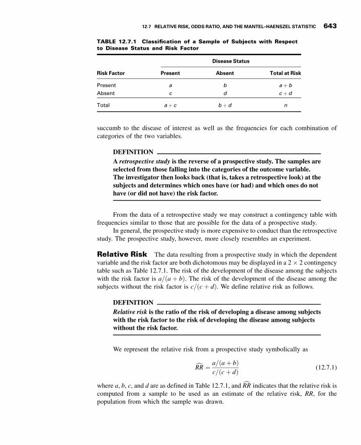
3GC12 12/04/2012 15:58:11 Page 643

succumb to the disease of interest as well as the frequencies for each combination ofcategories of the two variables.

DEFINITION

A retrospective study is the reverse of a prospective study. The samples areselected from those falling into the categories of the outcome variable.The investigator then looks back (that is, takes a retrospective look) at thesubjects and determines which ones have (or had) and which ones do nothave (or did not have) the risk factor.

From the data of a retrospective study we may construct a contingency table withfrequencies similar to those that are possible for the data of a prospective study.

In general, the prospective study is more expensive to conduct than the retrospectivestudy. The prospective study, however, more closely resembles an experiment.

Relative Risk The data resulting from a prospective study in which the dependentvariable and the risk factor are both dichotomous may be displayed in a 2 � 2 contingencytable such as Table 12.7.1. The risk of the development of the disease among the subjectswith the risk factor is a= aþ bð Þ. The risk of the development of the disease among thesubjects without the risk factor is c= cþ dð Þ. We define relative risk as follows.

DEFINITION

Relative risk is the ratio of the risk of developing a disease among subjectswith the risk factor to the risk of developing the disease among subjectswithout the risk factor.

We represent the relative risk from a prospective study symbolically as

cRR ¼ a= aþ bð Þc= cþ dð Þ (12.7.1)

where a, b, c, and d are as defined in Table 12.7.1, and cRR indicates that the relative risk iscomputed from a sample to be used as an estimate of the relative risk, RR, for thepopulation from which the sample was drawn.

TABLE 12.7.1 Classification of a Sample of Subjects with Respectto Disease Status and Risk Factor

Disease Status

Risk Factor Present Absent Total at Risk

Present a b a þ b

Absent c d c þ d



3GC12 12/04/2012 15:58:11 Page 644

We may construct a confidence interval for RR

100 1 � að Þ%CI ¼ cRR1� za=ffiffiffiffiX2

pð Þ (12.7.2)

where za is the two-sided z value corresponding to the chosen confidence coefficient and X2

is computed by Equation 12.4.1.

Interpretation of RR The value of RR may range anywhere between zero andinfinity. A value of 1 indicates that there is no association between the status of the riskfactor and the status of the dependent variable. In most cases the two possible states ofthe dependent variable are disease present and disease absent. We interpret an RR of 1 tomean that the risk of acquiring the disease is the same for those subjects with the riskfactor and those without the risk factor. A value of RR greater than 1 indicates that therisk of acquiring the disease is greater among subjects with the risk factor than amongsubjects without the risk factor. An RR value that is less than 1 indicates less risk ofacquiring the disease among subjects with the risk factor than among subjects withoutthe risk factor. For example, a risk factor of 2 is taken to mean that those subjects with therisk factor are twice as likely to acquire the disease as compared to subjects without therisk factor.

We illustrate the calculation of relative risk by means of the following example.

EXAMPLE 12.7.1

In a prospective study of pregnant women, Magann et al. (A-16) collected extensiveinformation on exercise level of low-risk pregnant working women. A group of 217 womendid no voluntary or mandatory exercise during the pregnancy, while a group of 238 womenexercised extensively. One outcome variable of interest was experiencing preterm labor.The results are summarized in Table 12.7.2.

We wish to estimate the relative risk of preterm labor when pregnant women exerciseextensively.

Solution: By Equation 12.7.1 we compute

cRR ¼ 22=238

18=217¼ .0924

.0829¼ 1:1

TABLE 12.7.2 Subjects with and without the Risk Factor Who Became Casesof Preterm Labor

Risk Factor Cases of Preterm Labor Noncases of Preterm Labor Total

Extreme exercising 22 216 238

Not exercising 18 199 217

Total 40 415 455

Source: Everett F. Magann, Sharon F. Evans, Beth Weitz, and John Newnham, “Antepartum, Intrapartum,and Neonatal Significance of Exercise on Healthy Low-Risk Pregnant Working Women,” Obstetrics andGynecology, 99 (2002), 466–472.


3GC12 12/04/2012 15:58:11 Page 645

These data indicate that the risk of experiencing preterm labor when a womanexercises heavily is 1.1 times as great as it is among women who do notexercise at all.

We compute the 95 percent confidence interval for RR as follows. ByEquation 12.4.1, we compute from the data in Table 12.7.2:

X2 ¼ 455 22ð Þ 199ð Þ � 216ð Þ 18ð Þ½ �240ð Þ 415ð Þ 238ð Þ 217ð Þ ¼ .1274

By Equation 12.7.2, the lower and upper confidence limits are, respectively,

1:11�1:96=ffiffiffiffiffiffiffiffi:1274

p¼ :65 and 1:11þ1:96=

ffiffiffiffiffiffiffiffi:1274

p¼ 1:86. Since the interval includes

1, we conclude, at the .05 level of significance, that the population risk maybe 1. In other words, we conclude that, in the population, there may not bean increased risk of experiencing preterm labor when a pregnant womanexercises extensively.

The data were processed by NCSS. The results are shown in Figure12.7.1. The relative risk calculation is shown in the column at the far right ofthe output, along with the 95% confidence limits. Because of rounding errors,these values differ slightly from those given in the example. &

Odds Ratio When the data to be analyzed come from a retrospective study, relativerisk is not a meaningful measure for comparing two groups. As we have seen, aretrospective study is based on a sample of subjects with the disease (cases) and a separatesample of subjects without the disease (controls or noncases). We then retrospectivelydetermine the distribution of the risk factor among the cases and controls. Given the resultsof a retrospective study involving two samples of subjects, cases, and controls, we maydisplay the data in a 2 � 2 table such as Table 12.7.3, in which subjects are dichotomizedwith respect to the presence and absence of the risk factor. Note that the column headings inTable 12.7.3 differ from those in Table 12.7.1 to emphasize the fact that the data are from aretrospective study and that the subjects were selected because they were either cases orcontrols. When the data from a retrospective study are displayed as in Table 12.7.3,the ratio a=ðaþ bÞ, for example, is not an estimate of the risk of disease for subjects withthe risk factor. The appropriate measure for comparing cases and controls in a retrospectivestudy is the odds ratio. As noted in Chapter 11, in order to understand the concept of

Odds Ratio and Relative Risk Section

Common Original Iterated Log Odds Relative

Parameter Odds Ratio Odds Ratio Odds Ratio Ratio Risk

2911.25857.03862.20531.2.L.C %59 reppU

Estimate 1.1260 1.1207 1.1207 0.1140 1.1144

6065.03885.0.L.C %59 rewoL 0.5305 0.5896

FIGURE 12.7.1 NCSS output for the data in Example 12.7.1.


3GC12 12/04/2012 15:58:12 Page 646

the odds ratio, we must understand the term odds, which is frequently used by those whoplace bets on the outcomes of sporting events or participate in other types of gamblingactivities.

DEFINITION

The odds for success are the ratio of the probability of success to theprobability of failure.

We use this definition of odds to define two odds that we can calculate from datadisplayed as in Table 12.7.3:

1. The odds of being a case (having the disease) to being a control (not having thedisease) among subjects with the risk factor is a= aþ bð Þ½ �= b= aþ bð Þ½ � ¼ a=b.

2. The odds of being a case (having the disease) to being a control (not having thedisease) among subjects without the risk factor is c= cþ dð Þ½ �= d= cþ dð Þ½ � ¼ c=d.

We now define the odds ratio that we may compute from the data of a retrospectivestudy. We use the symbol cOR to indicate that the measure is computed from sample dataand used as an estimate of the population odds ratio, OR.

DEFINITION

The estimate of the population odds ratio is

cOR ¼ a=b

c=d¼ ad

bc(12.7.3)

where a, b, c, and d are as defined in Table 12.7.3.

We may construct a confidence interval for OR by the following method:

100 1 � að Þ%CI ¼ cOR1� za=ffiffiffiffiX2

pð Þ (12.7.4)

where za is the two-sided z value corresponding to the chosen confidence coefficient andX2 is computed by Equation 12.4.1.

TABLE 12.7.3 Subjects of a Retrospective StudyClassified According to Status Relativeto a Risk Factor

and Whether They Are Cases or Controls

Sample

Risk Factor Cases Controls Total

Present a b a þ b

Absent c d c þ d



3GC12 12/04/2012 15:58:12 Page 647

Interpretation of the Odds Ratio In the case of a rare disease, the popula-tion odds ratio provides a good approximation to the population relative risk. Conse-quently, the sample odds ratio, being an estimate of the population odds ratio, provides anindirect estimate of the population relative risk in the case of a rare disease.

The odds ratio can assume values between zero and 1. A value of 1 indicates noassociation between the risk factor and disease status. A value less than 1 indicates reducedodds of the disease among subjects with the risk factor. A value greater than 1 indicatesincreased odds of having the disease among subjects in whom the risk factor is present.

EXAMPLE 12.7.2

Toschke et al. (A-17) collected data on obesity status of children ages 5–6 years and thesmoking status of the mother during the pregnancy. Table 12.7.4 shows 3970 subjectsclassified as cases or noncases of obesity and also classified according to smoking status ofthe mother during pregnancy (the risk factor). We wish to compare the odds of obesity atages 5–6 among those whose mother smoked throughout the pregnancy with the odds ofobesity at age 5–6 among those whose mother did not smoke during pregnancy.

Solution: The odds ratio is the appropriate measure for answering the question posed.By Equation 12.7.3 we compute

cOR ¼ 64ð Þ 3496ð Þ342ð Þ 68ð Þ ¼ 9:62

We see that obese children (cases) are 9.62 times as likely as nonobesechildren (noncases) to have had a mother who smoked throughout thepregnancy.

We compute the 95 percent confidence interval for OR as follows. ByEquation 12.4.1 we compute from the data in Table 12.7.4


TABLE 12.7.4 Subjects Classified According to ObesityStatus and Mother’s Smoking Status during Pregnancy

Obesity Status

Smoking StatusDuring Pregnancy

Cases Noncases Total

Smoked throughout 64 342 406

Never smoked 68 3496 3564

Total 132 3838 3970

Source: A. M. Toschke, S. M. Montgomery, U. Pfeiffer, and R. von Kries, “EarlyIntrauterine Exposure to Tobacco-Inhaled Products and Obesity,” American Jour-nal of Epidemiology, 158 (2003), 1068–1074.


3GC12 12/04/2012 15:58:12 Page 648

The lower and upper confidence limits for the population OR, respectively, are

9:621�1:96=ffiffiffiffiffiffiffiffiffiffiffiffiffi217:6831

p¼ 7:12 and 9:621þ1:96=

ffiffiffiffiffiffiffiffiffiffiffiffiffi217:6831

p¼ 13:00. We conclude

with 95 percent confidence that the population OR is somewhere between7.12 and 13.00. Because the interval does not include 1, we conclude that, in thepopulation, obese children (cases) are more likely than nonobese children(noncases) to have had a mother who smoked throughout the pregnancy.

The data from Example 12.7.2 were processed using SPSS. Theresults are shown in Figure 12.7.2. The odds ratio calculation, along withthe 95% confidence limits, are shown in the top line of the Risk Estimatebox. These values differ slightly from those in the example because ofrounding error. &

The Mantel–Haenszel Statistic Frequently when we are studying the rela-tionship between the status of some disease and the status of some risk factor, we are

Smoking_status * Obsesity_status Cross-Tabulation

Count

Obesity status

Cases Noncases Total

Smoking_status Smoked throughout 64 342 406Never smoked 68 3496 3564

07938383231latoT

Risk Estimate

95% Confidence Interval

Value Lower Upper

Odds Ratio forSmoking_status(Smoked throughout 9.621 6.719 13.775/Never smoked)For cohort Obesity_ 8.262 5.966 11.441status CasesFor cohort Obesity_ .859 .823 .896status NoncasesN of Valid Cases 3970



3GC12 12/04/2012 15:58:12 Page 649

aware of another variable that may be associated with the disease, with the risk factor,or with both in such a way that the true relationship between the disease status and therisk factor is masked. Such a variable is called a confounding variable. For example,experience might indicate the possibility that the relationship between some diseaseand a suspected risk factor differs among different ethnic groups. We would then treatethnic membership as a confounding variable. When they can be identified, it isdesirable to control for confounding variables so that an unambiguous measure of therelationship between disease status and risk factor may be calculated. A technique foraccomplishing this objective is the Mantel–Haenszel (22) procedure, so called inrecognition of the two men who developed it. The procedure allows us to test the nullhypothesis that there is no association between status with respect to disease and riskfactor status. Initially used only with data from retrospective studies, the Mantel–Haenszel procedure is also appropriate for use with data from prospective studies, asdiscussed by Mantel (23).

In the application of the Mantel–Haenszel procedure, case and control subjects areassigned to strata corresponding to different values of the confounding variable. The dataare then analyzed within individual strata as well as across all strata. The discussion thatfollows assumes that the data under analysis are from a retrospective or a prospective studywith case and noncase subjects classified according to whether they have or do not have thesuspected risk factor. The confounding variable is categorical, with the different categoriesdefining the strata. If the confounding variable is continuous it must be categorized. Forexample, if the suspected confounding variable is age, we might group subjects intomutually exclusive age categories. The data before stratification may be displayed asshown in Table 12.7.3.

Application of the Mantel–Haenszel procedure consists of the following steps.

1. Form k strata corresponding to the k categories of the confounding variable. Table12.7.5 shows the data display for the ith stratum.

2. For each stratum compute the expected frequency ei of the upper left-hand cell ofTable 12.7.5 as follows:

ei ¼ ai þ bið Þ ai þ cið Þni

(12.7.5)

TABLE 12.7.5 Subjects in the ith Stratum of a ConfoundingVariable Classified According to Status Relative to a Risk

Factor and Whether They Are Cases or Controls

Sample

Risk Factor Cases Controls Total

Present ai bi ai þ bi

Absent ci di ci þ di

Total ai þ ci bi þ di ni


3GC12 12/04/2012 15:58:13 Page 650

3. For each stratum compute

vi ¼ ai þ bið Þ ci þ dið Þ ai þ cið Þ bi þ dið Þn2i ni � 1ð Þ (12.7.6)

4. Compute the Mantel–Haenszel test statistic, x2MH as follows:

x2MH ¼

Pki¼1

ai �Pki¼1

ei

� �2

Pki¼1

vi

(12.7.7)

5. Reject the null hypothesis of no association between disease status and suspected riskfactor status in the population if the computed value of x2

MH is equal to or greater thanthe critical value of the test statistic, which is the tabulated chi-square value for 1degree of freedom and the chosen level of significance.

Mantel–Haenszel Estimator of theCommonOddsRatio When wehave k strata of data, each of which may be displayed in a table like Table 12.7.5, we maycompute the Mantel–Haenszel estimator of the common odds ratio, cORMH as follows:

cORMH ¼Pki¼1

aidi=nið ÞPki¼1

bici=nið Þ(12.7.8)

When we use the Mantel–Haenszel estimator given by Equation 12.7.4, we assume that, inthe population, the odds ratio is the same for each stratum.

We illustrate the use of the Mantel–Haenszel statistics with the followingexamples.

EXAMPLE 12.7.3

In a study by LaMont et al. (A-18), researchers collected data on obstructive coronaryartery disease (OCAD), hypertension, and age among subjects identified by a treadmillstress test as being at risk. In Table 12.7.6, counts on subjects in two age strata are presentedwith hypertension as the risk factor and the presence of OCAD as the case/noncasevariable.

Solution:


2. Assumptions. We assume that the assumptions discussed earlier for thevalid use of the Mantel–Haenszel statistic are met.


3GC12 12/04/2012 15:58:13 Page 651

3. Hypotheses.

H0: There is no association between the presence of hypertensionand occurrence of OCAD in subjects 55 and under and subjectsover 55.

HA: There is a relationship between the two variables.

4. Test statistic.

x2MH ¼

Pki¼1

ai �Pki¼1

ei

� �2

Pki¼1

vi

as given in Equation 12.7.7.

5. Distribution of test statistic. Chi-square with 1 degree of freedom.

6. Decision rule. Suppose we let a ¼ .05. Reject H0 if the computed valueof the test statistic is greater than or equal to 3.841.

7. Calculation of test statistic. By Equation 12.7.5 we compute thefollowing expected frequencies:

e1 ¼ 21 þ 11ð Þ 21 þ 16ð Þ=54 ¼ 32ð Þ 37ð Þ=54 ¼ 21:93e2 ¼ 50 þ 14ð Þ 50 þ 18ð Þ=88 ¼ 64ð Þ 68ð Þ=88 ¼ 49:45

TABLE 12.7.6 Patients Stratified by Age and Classified by StatusRelative to Hypertension (the Risk Factor) and OCAD (Case/Noncase

Variable)

Stratum 1 (55 and under)

Risk Factor(Hypertension) Cases (OCAD) Noncases Total

Present 21 11 32

Absent 16 6 22

Total 37 17 54

Stratum 2 (over 55)

Risk Factor(Hypertension) Cases (OCAD) Noncases Total

Present 50 14 64

Absent 18 6 24

Total 68 20 88

Source: Data provided courtesy of Matthew J. Budoff, MD.


3GC12 12/04/2012 15:58:13 Page 652


v1 ¼ 32ð Þ 22ð Þ 37ð Þ 17ð Þ= 2916ð Þ 54 � 1ð Þ ¼ 2:87v2 ¼ 64ð Þ 24ð Þ 68ð Þ 20ð Þ= 7744ð Þ 88 � 1ð Þ ¼ 3:10

Finally, by Equation 12.7.7 we compute

x2MH ¼ 21 þ 50ð Þ � 21:93 þ 49:45ð Þ½ �2

2:87 þ 3:10¼ .0242

8. Statistical decision. Since .0242 < 3:841, we fail to reject H0.

9. Conclusion. We conclude that there may not be an association betweenhypertension and the occurrence of OCAD.

10. p value. Since .0242 < 2:706, the p value for this test is p > .10.

We now illustrate the calculation of the Mantel–Haenszel estimator of thecommon odds ratio. &

EXAMPLE 12.7.4

Let us refer to the data in Table 12.7.6 and compute the common odds ratio.

Solution: From the stratified data in Table 12.7.6 we compute the numerator of the ratioas follows:

a1d1=n1ð Þ þ a2d2=n2ð Þ ¼ 21ð Þ 6ð Þ=54½ � þ 50ð Þ 6ð Þ=88½ �¼ 5:7424

The denominator of the ratio is

b1c1=n1ð Þ þ b2c2=n2ð Þ ¼ 11ð Þ 16ð Þ=54½ � þ 14ð Þ 18ð Þ=88½ �¼ 6:1229

Now, by Equation 12.7.7, we compute the common odds ratio:

cORMH ¼ 5:7424

6:1229¼ .94

From these results we estimate that, regardless of age, patients whohave hypertension are less likely to have OCAD than patients who do nothave hypertension. &

Hand calculation of the Mantel–Haenszel test statistics can prove to be a cumber-some task. Fortunately, the researcher can find relief in one of several statistical softwarepackages that are available. To illustrate, results from the use of SPSS to process the data ofExample 12.7.3 are shown in Figure 12.7.3. These results differ from those given in theexample because of rounding error.


3GC12 12/04/2012 15:58:13 Page 653

EXERCISES

12.7.1 Davy et al. (A-19) reported the results of a study involving survival from cervical cancer. Theresearchers found that among subjects younger than age 50, 16 of 371 subjects had not survived for1 year after diagnosis. In subjects age 50 or older, 219 of 376 had not survived for 1 year afterdiagnosis. Compute the relative risk of death among subjects age 50 or older. Does it appear fromthese data that older subjects diagnosed as having cervical cancer are prone to higher mortalityrates?

Smoking_status * Obsesity_status * Stratum Cross-Tabulation

Count

Obesity status

latoTsesacnoNsesaCmutartS

55 and under Smoking_status Smoked throughout 21 11 32Never smoked 16 6 22

457173latoT

Over 55 Smoking_status Smoked throughout 50 14 64Never smoked 18 6 24

880286latoT

Tests of Conditional Independence

Asymp. Sig.Chi-Squared df (2-sided)

Cochran's .025 1 .875Mantel-Haenszel .002 1 .961

Mantel–Haenszel Common Odds Ratio Estimate

839.etamitsEIn(Estimate) .064

214.)etamitsE(nI fo rorrE .dtS678.)dedis-2( .giS .pmysA

Asymp. 95% confidence Common Odds Lower Bound .418Interval Ratio Upper Bound 2.102

In(Common) Lower Bound .871Odds Ratio) Upper Bound .743


EXERCISES 653

3GC12 12/04/2012 15:58:14 Page 654

12.7.2 The objective of a prospective study by Stenestrand et al. (A-20) was to compare the mortality ratefollowing an acute myocardial infarction (AMI) among subjects receiving early revascularization tothe mortality rate among subjects receiving conservative treatments. Among 2554 patients receivingrevascularization within 14 days of AMI, 84 died in the year following the AMI. In the conservativetreatment group (risk factor present), 1751 of 19,358 patients died within a year of AMI. Compute therelative risk of mortality in the conservative treatment group as compared to the revascularizationgroup in patients experiencing AMI.

12.7.3 Refer to Example 12.7.2. Toschke et al. (A-17), who collected data on obesity status of children ages5–6 years and the smoking status of the mother during the pregnancy, also reported on anotheroutcome variable: whether the child was born premature (37 weeks or fewer of gestation). Thefollowing table summarizes the results of this aspect of the study. The same risk factor (smokingduring pregnancy) is considered, but a case is now defined as a mother who gave birth prematurely.

Premature Birth Status

Smoking StatusDuring Pregnancy Cases Noncases Total

Smoked throughout 36 370 406Never smoked 168 3396 3564

Total 204 3766 3970

Source: A. M. Toschke, S. M. Montgomery, U. Pfeiffer, and R. von Kries, “Early IntrauterineExposure to Tobacco-Inhaled Products and Obesity,” American Journal of Epidemiology, 158(2003), 1068–1074.

Compute the odds ratio to determine if smoking throughout pregnancy is related to premature birth.Use the chi-square test of independence to determine if one may conclude that there is an associationbetween smoking throughout pregnancy and premature birth. Let a ¼ .05.

12.7.4 Sugiyama et al. (A-21) examined risk factors for allergic diseases among 13- and 14-year-oldschoolchildren in Japan. One risk factor of interest was a family history of eating an unbalanced diet.The following table shows the cases and noncases of children exhibiting symptoms of rhinitis in thepresence and absence of the risk factor.

Rhinitis

Family History Cases Noncases Total

Unbalanced diet 656 1451 2107Balanced diet 677 1662 2339

Total 1333 3113 4446

Source: Takako Sugiyama, Kumiya Sugiyama, Masao Toda, Tastuo Yukawa, Sohei Makino,and Takeshi Fukuda, “Risk Factors for Asthma and Allergic Diseases Among 13–14-Year-OldSchoolchildren in Japan,” Allergology International, 51 (2002), 139–150.

What is the estimated odds ratio of having rhinitis among subjects with a family history of anunbalanced diet compared to those eating a balanced diet? Compute the 95 percent confidenceinterval for the odds ratio.

12.7.5 According to Holben et al. (A-22), “Food insecurity implies a limited access to or availability of foodor a limited/uncertain ability to acquire food in socially acceptable ways.” These researchers


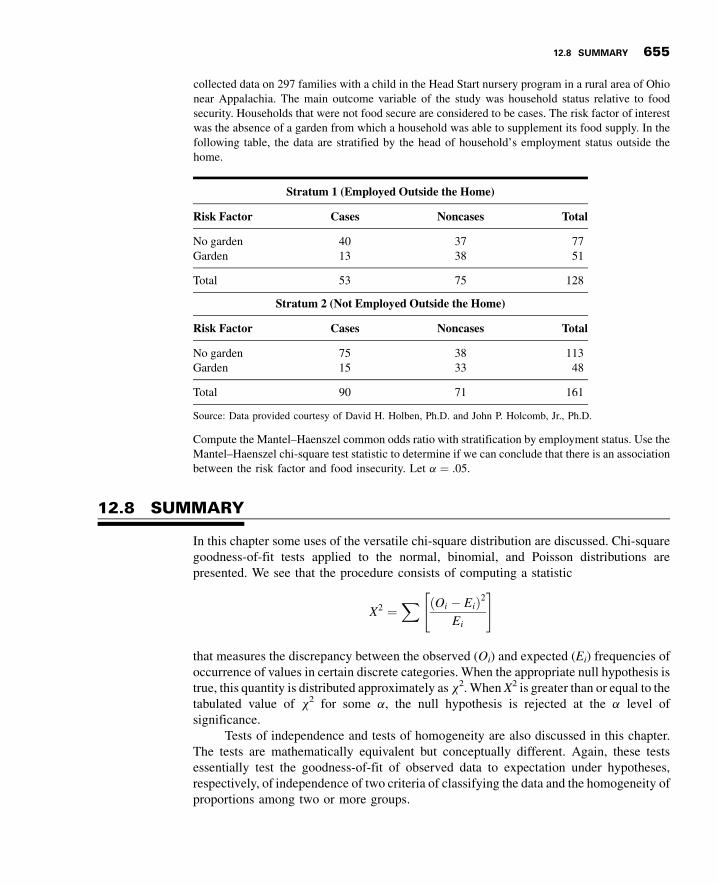
3GC12 12/04/2012 15:58:14 Page 655

collected data on 297 families with a child in the Head Start nursery program in a rural area of Ohionear Appalachia. The main outcome variable of the study was household status relative to foodsecurity. Households that were not food secure are considered to be cases. The risk factor of interestwas the absence of a garden from which a household was able to supplement its food supply. In thefollowing table, the data are stratified by the head of household’s employment status outside thehome.

Stratum 1 (Employed Outside the Home)

Risk Factor Cases Noncases Total

No garden 40 37 77Garden 13 38 51

Total 53 75 128

Stratum 2 (Not Employed Outside the Home)

Risk Factor Cases Noncases Total

No garden 75 38 113Garden 15 33 48

Total 90 71 161

Source: Data provided courtesy of David H. Holben, Ph.D. and John P. Holcomb, Jr., Ph.D.

Compute the Mantel–Haenszel common odds ratio with stratification by employment status. Use theMantel–Haenszel chi-square test statistic to determine if we can conclude that there is an associationbetween the risk factor and food insecurity. Let a ¼ .05.

12.8 SUMMARY

In this chapter some uses of the versatile chi-square distribution are discussed. Chi-squaregoodness-of-fit tests applied to the normal, binomial, and Poisson distributions arepresented. We see that the procedure consists of computing a statistic


Ei

" #

that measures the discrepancy between the observed (Oi) and expected (Ei) frequencies ofoccurrence of values in certain discrete categories. When the appropriate null hypothesis istrue, this quantity is distributed approximately as x2. When X2 is greater than or equal to thetabulated value of x2 for some a, the null hypothesis is rejected at the a level ofsignificance.

Tests of independence and tests of homogeneity are also discussed in this chapter.The tests are mathematically equivalent but conceptually different. Again, these testsessentially test the goodness-of-fit of observed data to expectation under hypotheses,respectively, of independence of two criteria of classifying the data and the homogeneity ofproportions among two or more groups.

12.8 SUMMARY 655

3GC12 12/04/2012 15:58:15 Page 656

In addition, we discussed and illustrated in this chapter four other techniques foranalyzing frequency data that can be presented in the form of a 2 � 2 contingency table: theFisher exact test, the odds ratio, relative risk, and the Mantel–Haenszel procedure. Finally,we discussed the basic concepts of survival analysis and illustrated the computationalprocedures by means of two examples.



12.2.1 Standard normal randomvariable

zi ¼ yi � m

s

12.2.2 Chi-square distribution withn degrees of freedom

x2nð Þ ¼ z2

1 þ z22 þ � � � þ z2

n

12.2.3 Chi-square probabilitydensity function

f uð Þ ¼ 1

k

2� 1

� �!

1

2k=2u k=2ð Þ�1e� u=2ð Þ

12.2.4 Chi-square test statisticx2 ¼ P Oi � Eið Þ2

Ei

" #

12.4.1 Chi-square calculationformula for a 2 � 2contingency table

x2 ¼ n ad � bcð Þ2

aþ cð Þ bþ dð Þ aþ bð Þ cþ dð Þ

12.4.2 Yates’s corrected chi-squarecalculation for a 2 � 2contingency table

x2corrected ¼ n ad � bcj j � .5nð Þ2

aþ cð Þ bþ dð Þ aþ bð Þ cþ dð Þ

12.6.1–12.6.2 Large-sample approximationto the chi-square

z ¼ a=Að Þ � b=Bð Þffiffiffiffiffiffiffiffiffiffiffiffiffiffiffiffiffiffiffiffiffiffiffiffiffiffiffiffiffiffiffiffiffiffiffiffiffiffiffiffiffiffip 1 � pð Þ 1=Aþ 1=Bð Þp

where

p ¼ aþ bð Þ= Aþ Bð Þ12.7.1 Relative risk estimate cRR ¼ a= aþ bð Þ

c= cþ dð Þ12.7.2 Confidence interval for the

relative risk estimate100 1 � að Þ%CI ¼ cRR1� za=

ffiffiffix2

pð Þ

12.7.3 Odds ratio estimate cOR ¼ a=b

c=d¼ ad

bc

12.7.4 Confidence interval for theodds ratio estimate

100 1 � að Þ%CI ¼ cOR1� za=ffiffiffix2

pð Þ

(Continued )


3GC12 12/04/2012 15:58:15 Page 657

12.7.5 Expected frequency in theMantel–Haenszel statistic

ei ¼ ai þ bið Þ ai þ cið Þni

12.7.6 Stratum expected frequencyin the Mantel–Haenszelstatistic

vi ¼ ai þ bið Þ ci þ dið Þ ai þ cið Þ bi þ dið Þn2i ni � 1ð Þ

12.7.7 Mantel–Haenszel test statistic

x2MH ¼

Pki¼1

ai �Pki¼1

ei

� �

Pki¼1

vi

12.7.8 Mantel–Haenszel estimatorof the common odds ratio cORMH ¼

Pki¼1

aidi=nið ÞPki¼1

bici=nið Þ

Symbol Key � a; b; c; d ¼ cell frequencies in a 2 � 2 contingency table� A; B ¼ row totals in the 2 � 2 contingency table� b ¼ regression coefficient� x2 orX2

� ¼ chi-square� ei ¼ expected frequency in the Mantel–Haenszel statistic� Ei ¼ expected frequency� E yjxð Þ ¼ expected value of y at x� k ¼ degrees of freedom in the chi-square distribution� m ¼ mean� Oi ¼ observed frequency� cOR ¼ odds ratio estimate� s ¼ standard deviation� cRR ¼ relative risk estimate� vi ¼ stratum expected frequency in the Mantel–Haenszel statistic� yi ¼ data value at point i� z ¼ normal variate


1. Explain how the chi-square distribution may be derived.

2. What are the mean and variance of the chi-square distribution?

3. Explain how the degrees of freedom are computed for the chi-square goodness-of-fit tests.

4. State Cochran’s rule for small expected frequencies in goodness-of-fit tests.

5. How does one adjust for small expected frequencies?

6. What is a contingency table?

7. How are the degrees of freedom computed when an X2 value is computed from a contingencytable?


3GC12 12/04/2012 15:58:15 Page 658

8. Explain the rationale behind the method of computing the expected frequencies in a test ofindependence.

9. Explain the difference between a test of independence and a test of homogeneity.

10. Explain the rationale behind the method of computing the expected frequencies in a test ofhomogeneity.

11. When do researchers use the Fisher exact test rather than the chi-square test?


(a) Observational study (b) Risk factor(c) Outcome (d) Retrospective study(e) Prospective study (f) Relative risk(g) Odds (h) Odds ratio(i) Confounding variable

13. Under what conditions is the Mantel–Haenszel test appropriate?

14. Explain how researchers interpret the following measures:

(a) Relative risk

(b) Odds ratio

(c) Mantel–Haenszel common odds ratio

15. In a study of violent victimization of women and men, Porcerelli et al. (A-23) collected infor-mation from 679 women and 345 men ages 18 to 64 years at several family practice centersin the metropolitan Detroit area. Patients filled out a health history questionnaire that includeda question about victimization. The following table shows the sample subjects cross-classifiedby gender and the type of violent victimization reported. The victimization categories aredefined as no victimization, partner victimization (and not by others), victimization by a personother than a partner (friend, family member, or stranger), and those who reported multiplevictimization.

Gender No Victimization Partner Nonpartner Multiple Total

Women 611 34 16 18 679Men 308 10 17 10 345

Total 919 44 33 28 1024

Source: John H. Porcerelli, Rosemary Cogan, Patricia P. West, Edward A. Rose, DawnLambrecht, Karen E. Wilson, Richard K. Severson, and Dunia Karana, “Violent Victimizationof Women and Men: Physical and Psychiatric Symptoms,” Journal of the American Board ofFamily Practice, 16 (2003), 32–39.

Can we conclude on the basis of these data that victimization status and gender are not independent?Let a ¼ .05.

16. Refer to Exercise 15. The following table shows data reported by Porcerelli et al. for 644 African-American and Caucasian women. May we conclude on the basis of these data that for women, raceand victimization status are not independent? Let a ¼ .05.


3GC12 12/04/2012 15:58:16 Page 659

No Victimization Partner Nonpartner Multiple Total

Caucasian 356 20 3 9 388African-American 226 11 10 9 256

Total 582 31 13 18 644

Source: John H. Porcerelli, Rosemary Cogan, Patricia P. West, Edward A. Rose, Dawn Lambrecht,Karen E. Wilson, Richard K. Severson, and Dunia Karana, “Violent Victimization of Women andMen: Physical and Psychiatric Symptoms,” Journal of the American Board of Family Practice, 16(2003), 32–39.

17. A sample of 150 chronic carriers of a certain antigen and a sample of 500 noncarriers revealed thefollowing blood group distributions:

Blood Group Carriers Noncarriers Total

0 72 230 302A 54 192 246B 16 63 79AB 8 15 23

Total 150 500 650

Can one conclude from these data that the two populations from which the samples were drawn differwith respect to blood group distribution? Let a ¼ .05. What is the p value for the test?

18. The following table shows 200 males classified according to social class and headache status:

Social Class

Headache Group A B C Total

No headache (in previous year) 6 30 22 58Simple headache 11 35 17 63Unilateral headache (nonmigraine) 4 19 14 37Migraine 5 25 12 42

Total 26 109 65 200

Do these data provide sufficient evidence to indicate that headache status and social class are related?Let a ¼ .05. What is the p value for this test?

19. The following is the frequency distribution of scores made on an aptitude test by 175 applicants to aphysical therapy training facility �x ¼ 39:71; s ¼ 12:92ð Þ.

Score Number of Applicants Score Number of Applicants

10–14 3 40–44 2815–19 8 45–49 2020–24 13 50–54 1825–29 17 55–59 12

(Continued )


3GC12 12/04/2012 15:58:16 Page 660

Score Number of Applicants Score Number of Applicants

30–34 19 60–64 835–39 25 65–69 4

Total 175

Do these data provide sufficient evidence to indicate that the population of scores is not normallydistributed? Let a ¼ .05. What is the p value for this test?

20. A local health department sponsored a venereal disease (VD) information program that was open tohigh-school juniors and seniors who ranged in age from 16 to 19 years. The program director believedthat each age level was equally interested in knowing more about VD. Since each age level was aboutequally represented in the area served, she felt that equal interest in VD would be reflected by equalage-level attendance at the program. The age breakdown of those attending was as follows:

Age Number Attending

16 2617 5018 4419 40

Are these data incompatible with the program director’s belief that students in the four age levels areequally interested in VD? Let a ¼ .05. What is the p value for this test?

21. A survey of children under 15 years of age residing in the inner-city area of a large city were classifiedaccording to ethnic group and hemoglobin level. The results were as follows:

Hemoglobin Level (g/100 ml)

Ethnic Group 10.0 or Greater 9.0–9.9 < 9:0 Total

A 80 100 20 200B 99 190 96 385C 70 30 10 110

Total 249 320 126 695

Do these data provide sufficient evidence to indicate, at the .05 level of significance, that the twovariables are related? What is the p value for this test?

22. A sample of reported cases of mumps in preschool children showed the following distribution by age:

Age (Years) Number of Cases

Under 1 61 202 353 414 48

Total 150


3GC12 12/04/2012 15:58:17 Page 661

Test the hypothesis that cases occur with equal frequency in the five age categories. Let a ¼ .05.What is the p value for this test?

23. Each of a sample of 250 men drawn from a population of suspected joint disease victims was askedwhich of three symptoms bother him most. The same question was asked of a sample of 300suspected women joint disease victims. The results were as follows:

Most Bothersome Symptom Men Women

Morning stiffness 111 102Nocturnal pain 59 73Joint swelling 80 125

Total 250 300

Do these data provide sufficient evidence to indicate that the two populations are not homogeneouswith respect to major symptoms? Let a ¼ .05. What is the p value for this test?

For each of the Exercises 24 through 34, indicate whether a null hypothesis of homogeneity or a nullhypothesis of independence is appropriate.

24. A researcher wishes to compare the status of three communities with respect to immunity against polioin preschool children. A sample of preschool children was drawn from each of the three communities.

25. In a study of the relationship between smoking and respiratory illness, a random sample of adultswere classified according to consumption of tobacco and extent of respiratory symptoms.

26. A physician who wished to know more about the relationship between smoking and birth defectsstudies the health records of a sample of mothers and their children, including stillbirths andspontaneously aborted fetuses where possible.

27. A health research team believes that the incidence of depression is higher among people withhypoglycemia than among people who do not suffer from this condition.

28. In a simple random sample of 200 patients undergoing therapy at a drug abuse treatment center,60 percent belonged to ethnic group I. The remainder belonged to ethnic group II. In ethnic group I,60 were being treated for alcohol abuse (A), 25 for marijuana abuse (B), and 20 for abuse of heroin,illegal methadone, or some other opioid (C). The remainder had abused barbiturates, cocaine,amphetamines, hallucinogens, or some other nonopioid besides marijuana (D). In ethnic group II theabused drug category and the numbers involved were as follows:

Að28Þ Bð32Þ Cð13Þ D ðthe remainderÞCan one conclude from these data that there is a relationship between ethnic group and choice of drugto abuse? Let a ¼ .05 and find the p value.

29. Solar keratoses are skin lesions commonly found on the scalp, face, backs of hands, forearms, ears,scalp, and neck. They are caused by long-term sun exposure, but they are not skin cancers. Chen et al.(A-24) studied 39 subjects randomly assigned (with a 3 to 1 ratio) to imiquimod cream and a controlcream. The criterion for effectiveness was having 75 percent or more of the lesion area cleared after14 weeks of treatment. There were 21 successes among 29 imiquimod-treated subjects and threesuccesses among 10 subjects using the control cream. The researchers used Fisher’s exact test andobtained a p value of .027. What are the variables involved? Are the variables quantitative orqualitative? What null and alternative hypotheses are appropriate? What are your conclusions?


3GC12 12/04/2012 15:58:17 Page 662

30. Janardhan et al. (A-25) examined 125 patients who underwent surgical or endovascular treatment forintracranial aneurysms. At 30 days postprocedure, 17 subjects experienced transient/persistentneurological deficits. The researchers performed logistic regression and found that the 95 percentconfidence interval for the odds ratio for aneurysm size was .09–.96. Aneurysm size was dichoto-mized as less than 13 mm and greater than or equal to 13 mm. The larger tumors indicated higher oddsof deficits. Describe the variables as to whether they are continuous, discrete, quantitative, orqualitative. What conclusions may be drawn from the given information?

31. In a study of smoking cessation by Gold et al. (A-26), 189 subjects self-selected into three treatments:nicotine patch only (NTP), Bupropion SR only (B), and nicotine patch with Bupropion SRNTP þ Bð Þ. Subjects were grouped by age into younger than 50 years old, between 50 and 64,

and 65 and older. There were 15 subjects younger than 50 years old who chose NTP, 26 who chose B,and 16 who chose NTP þ B. In the 50–64 years category, six chose NTP, 54 chose B, and 40 choseNTP þ B. In the oldest age category, six chose NTP, 21 chose B, and five chose NTP þ B. Whatstatistical technique studied in this chapter would be appropriate for analyzing these data? Describethe variables involved as to whether they are continuous, discrete, quantitative, or qualitative. Whatnull and alternative hypotheses are appropriate? If you think you have sufficient information, conducta complete hypothesis test. What are your conclusions?

32. Kozinszky and B�artai (A-27) examined contraceptive use by teenage girls requesting abortion inSzeged, Hungary. Subjects were classified as younger than 20 years old or 20 years old or older. Ofthe younger than 20-year-old women, 146 requested an abortion. Of the older group, 1054 requestedan abortion. A control group consisted of visitors to the family planning center who did not request anabortion or persons accompanying women who requested an abortion. In the control group, therewere 147 women under 20 years of age and 1053 who were 20 years or older. One of the outcomevariables of interest was knowledge of emergency contraception. The researchers report that,“Emergency contraception was significantly [(Mantel–Haenszel) p < .001] less well known amongthe would-be aborter teenagers as compared to the older women requesting artificial abortionOR ¼ .07ð Þ than the relevant knowledge of the teenage controls OR ¼ .10ð Þ.” Explain the meaning

of the reported statistics. What are your conclusions based on the given information?

33. The goal of a study by Crosignani et al. (A-28) was to assess the effect of road traffic exhaust on therisk of childhood leukemia. They studied 120 children in Northern Italy identified through apopulation-based cancer registry (cases). Four controls per case, matched by age and gender, weresampled from population files. The researchers used a diffusion model of benzene to estimateexposure to traffic exhaust. Compared to children whose homes were not exposed to road trafficemissions, the rate of childhood leukemia was significantly higher for heavily exposed children.Characterize this study as to whether it is observational, prospective, or retrospective. Describe thevariables as to whether they are continuous, discrete, quantitative, qualitative, a risk factor, or aconfounding variable. Explain the meaning of the reported results. What are your conclusions basedon the given information?

34. Gallagher et al. (A-29) conducted a descriptive study to identify factors that influence women’sattendance at cardiac rehabilitation programs following a cardiac event. One outcome variable ofinterest was actual attendance at such a program. The researchers enrolled women discharged fromfour metropolitan hospitals in Sydney, Australia. Of 183 women, only 57 women actually attendedprograms. The authors reported odds ratios and confidence intervals on the following variables thatsignificantly affected outcome: age-squared (1.72; 1.10–2.70). Women over the age of 70 had thelowest odds, while women ages 55–70 years had the highest odds.), perceived control (.92; .85–1.00),employment (.20; .07–.58), diagnosis (6.82, 1.84–25.21, odds ratio was higher for women whoexperienced coronary artery bypass grafting vs. myocardial infarction), and stressful event (.21, .06–.73).Characterize this study as to whether it is observational, prospective, or retrospective. Describe the


3GC12 12/04/2012 15:58:17 Page 663

variables as to whether they are continuous, discrete, quantitative, qualitative, a risk factor, or aconfounding variable. Explain the meaning of the reported odds ratios.

For each of the Exercises 35 through 51, do as many of the following as you think appropriate:



(c) Construct graphs.

(d) Construct confidence intervals for population parameters.

(e) Formulate relevant hypotheses, perform the appropriate tests, and find p values.

(f) State the statistical decisions and clinical conclusions that the results of your hypothesis tests justify.

(g) Describe the population(s) to which you think your inferences are applicable.

(h) State the assumptions necessary for the validity of your analyses.

35. In a prospective, randomized, double-blind study, Stanley et al. (A-30) examined the relative efficacyand side effects of morphine and pethidine, drugs commonly used for patient-controlled analgesia(PCA). Subjects were 40 women, between the ages of 20 and 65 years, undergoing total abdominalhysterectomy. Patients were allocated randomly to receive morphine or pethidine by PCA. At the endof the study, subjects described their appreciation of nausea and vomiting, pain, and satisfaction bymeans of a three-point verbal scale. The results were as follows:

Satisfaction

DrugUnhappy/Miserable

ModeratelyHappy

Happy/Delighted Total

Pethidine 5 9 6 20Morphine 9 9 2 20

Total 14 18 8 40

Pain

DrugUnbearable/

Severe ModerateSlight/None Total


Total 4 18 18 40

Nausea

DrugUnbearable/

Severe ModerateSlight/None Total


Total 12 17 11 40

Source: Data provided courtesy of Dr. Balraj L. Appadu.


3GC12 12/04/2012 15:58:17 Page 664

36. Screening data from a statewide lead poisoning prevention program between April 1990 and March1991 were examined by Sargent et al. (A-31) in an effort to learn more about community risk factorsfor iron deficiency in young children. Study subjects ranged in age between 6 and 59 months.Among 1860 children with Hispanic surnames, 338 had iron deficiency. Four-hundred-fifty-sevenof 1139 with Southeast Asian surnames and 1034 of 8814 children with other surnames had irondeficiency.

37. To increase understanding of HIV-infection risk among patients with severe mental illness, Horwathet al. (A-32) conducted a study to identify predictors of injection drug use among patients who did nothave a primary substance use disorder. Of 192 patients recruited from inpatient and outpatient publicpsychiatric facilities, 123 were males. Twenty-nine of the males and nine of the females were foundto have a history of illicit-drug injection.

38. Skinner et al. (A-33) conducted a clinical trial to determine whether treatment with melphalan,prednisone, and colchicine (MPC) is superior to colchicine (C) alone. Subjects consisted of 100patients with primary amyloidosis. Fifty were treated with C and 50 with MPC. Eighteen monthsafter the last person was admitted and 6 years after the trial began, 44 of those receiving C and 36 ofthose receiving MPC had died.

39. The purpose of a study by Miyajima et al. (A-34) was to evaluate the changes of tumor cellcontamination in bone marrow (BM) and peripheral blood (PB) during the clinical course of patientswith advanced neuroblastoma. Their procedure involved detecting tyrosine hydroxylase (TH) mRNAto clarify the appropriate source and time for harvesting hematopoietic stem cells for transplantation.The authors used Fisher’s exact test in the analysis of their data. If available, read their article anddecide if you agree that Fisher’s exact text was the appropriate technique to use. If you agree,duplicate their procedure and see if you get the same results. If you disagree, explain why.

40. Cohen et al. (A-35) investigated the relationship between HIV seropositivity and bacterial vaginosisin a population at high risk for sexual acquisition of HIV. Subjects were 144 female commercial sexworkers in Thailand of whom 62 were HIV-positive and 109 had a history of sexually transmitteddiseases (STD). In the HIV-negative group, 51 had a history of STD.

41. The purpose of a study by Lipschitz et al. (A-36) was to examine, using a questionnaire, the rates andcharacteristics of childhood abuse and adult assaults in a large general outpatient population.Subjects consisted of 120 psychiatric outpatients (86 females, 34 males) in treatment at a largehospital-based clinic in an inner-city area. Forty-seven females and six males reported incidents ofchildhood sexual abuse.

42. Subjects of a study by O’Brien et al. (A-37) consisted of 100 low-risk patients having well-datedpregnancies. The investigators wished to evaluate the efficacy of a more gradual method forpromoting cervical change and delivery. Half of the patients were randomly assigned to receivea placebo, and the remainder received 2 mg of intravaginal prostaglandin E2 (PGE2) for 5 consecutivedays. One of the infants born to mothers in the experimental group and four born to those in thecontrol group had macrosomia.

43. The purposes of a study by Adra et al. (A-38) were to assess the influence of route of delivery onneonatal outcome in fetuses with gastroschisis and to correlate ultrasonographic appearance of thefetal bowel with immediate postnatal outcome. Among 27 cases of prenatally diagnosed gastro-schisis the ultrasonograph appearance of the fetal bowel was normal in 15. Postoperative complica-tions were observed in two of the 15 and in seven of the cases in which the ultrasonographicappearance was not normal.

44. Liu et al. (A-39) conducted household surveys in areas of Alabama under tornado warnings. In one ofthe surveys (survey 2) the mean age of the 193 interviewees was 54 years. Of these 56.0 percent were


3GC12 12/04/2012 15:58:17 Page 665

women, 88.6 percent were white, and 83.4 percent had a high-school education or higher. Amongthe information collected were data on shelter-seeking activity and understanding of the term“tornado warning.” One-hundred-twenty-eight respondents indicated that they usually seekshelter when made aware of a tornado warning. Of these, 118 understood the meaning of tornadowarning. Forty-six of those who said they didn’t usually seek shelter understood the meaningof the term.

45. The purposes of a study by Patel et al. (A-40) were to investigate the incidence of acute angle-closureglaucoma secondary to pupillary dilation and to identify screening methods for detecting angles atrisk of occlusion. Of 5308 subjects studied, 1287 were 70 years of age or older. Seventeen of the oldersubjects and 21 of the younger subjects (40 through 69 years of age) were identified as havingpotentially occludable angles.

46. Voskuyl et al. (A-41) investigated those characteristics (including male gender) of patients withrheumatoid arthritis (RA) that are associated with the development of rheumatoid vasculitis (RV).Subjects consisted of 69 patients who had been diagnosed as having RV and 138 patients with RAwho were not suspected to have vasculitis. There were 32 males in the RV group and 38 among theRA patients.

47. Harris et al. (A-42) conducted a study to compare the efficacy of anterior colporrhaphy andretropubic urethropexy performed for genuine stress urinary incontinence. The subjects were 76women who had undergone one or the other surgery. Subjects in each group were comparable in age,social status, race, parity, and weight. In 22 of the 41 cases reported as cured the surgery had beenperformed by attending staff. In 10 of the failures, surgery had been performed by attending staff. Allother surgeries had been performed by resident surgeons.

48. Kohashi et al. (A-43) conducted a study in which the subjects were patients with scoliosis. As part ofthe study, 21 patients treated with braces were divided into two groups, group A nA ¼ 12ð Þ and groupB nB ¼ 9ð Þ, on the basis of certain scoliosis progression factors. Two patients in group A and eight ingroup B exhibited evidence of progressive deformity, while the others did not.

49. In a study of patients with cervical intraepithelial neoplasia, Burger et al. (A-44) compared those whowere human papillomavirus (HPV)-positive and those who were HPV-negative with respect to riskfactors for HPV infection. Among their findings were 60 out of 91 nonsmokers with HPV infectionand 44 HPV-positive patients out of 50 who smoked 21 or more cigarettes per day.

50. Thomas et al. (A-45) conducted a study to determine the correlates of compliance with follow-upappointments and prescription filling after an emergency department visit. Among 235 respondents,158 kept their appointments. Of these, 98 were females. Of those who missed their appointments, 31were males.

51. The subjects of a study conducted by O’Keefe and Lavan (A-46) were 60 patients with cognitiveimpairment who required parenteral fluids for at least 48 hours. The patients were randomly assignedto receive either intravenous (IV) or subcutaneous (SC) fluids. The mean age of the 30 patients in theSC group was 81 years with a standard deviation of 6. Fifty-seven percent were females. The meanage of the IV group was 84 years with a standard deviation of 7. Agitation related to the cannula ordrip was observed in 11 of the SC patients and 24 of the IV patients.

Exercises for Use with the Large Data Sets Available on the Following Website:www.wile y.com/ college / daniel

1. Refer to the data on smoking, alcohol consumption, blood pressure, and respiratory disease among1200 adults (SMOKING). The variables are as follows:



3GC12 12/04/2012 15:58:18 Page 666

Sex Að Þ :Smoking status Bð Þ :Drinking level Cð Þ :

Symptoms of respiratory disease Dð Þ :High blood pressure status Eð Þ :

1 ¼ male; 0 ¼ female0 ¼ nonsmoker; 1 ¼ smoker0 ¼ nondrinker1 ¼ light to moderate drinker2 ¼ heavy drinker1 ¼ present; 0 ¼ absent1 ¼ present; 0 ¼ absent

Select a simple random sample of size 100 from this population and carry out an analysis to see if youcan conclude that there is a relationship between smoking status and symptoms of respiratory disease.Let a ¼ .05 and determine the p value for your test. Compare your results with those of yourclassmates.

2. Refer to Exercise 1. Select a simple random sample of size 100 from the population and carry out atest to see if you can conclude that there is a relationship between drinking status and high bloodpressure status in the population. Let a ¼ .05 and determine the p value. Compare your results withthose of your classmates.

3. Refer to Exercise 1. Select a simple random sample of size 100 from the population and carry out atest to see if you can conclude that there is a relationship between gender and smoking status in thepopulation. Let a ¼ .05 and determine the p value. Compare your results with those of yourclassmates.

4. Refer to Exercise 1. Select a simple random sample of size 100 from the population and carry out atest to see if you can conclude that there is a relationship between gender and drinking level in thepopulation. Let a ¼ .05 and find the p value. Compare your results with those of your classmates.

REFERENCES


1. KARL PEARSON, “On the Criterion that a Given System of Deviations from the Probable in the Case of a CorrelatedSystem of Variables Is Such that It Can Be Reasonably Supposed to Have Arisen from Random Sampling,” TheLondon, Edinburgh and Dublin Philosophical Magazine and Journal of Science, Fifth Series, 50 (1900), 157–175. Reprinted in Karl Pearson’s Early Statistical Papers, Cambridge University Press, 1948.

2. H. O. LANCASTER, The Chi-Squared Distribution, Wiley, New York, 1969.3. MIKHAIL S. NIKULIN and PRISCILLA E. GREENWOOD, A Guide to Chi-Squared Testing, Wiley, New York, 1996.4. WILLIAM G. COCHRAN, “The x2 Test of Goodness of Fit,” Annals of Mathematical Statistics, 23 (1952), 315–345.5. WILLIAM G. COCHRAN, “Some Methods for Strengthening the Common x2 Tests,” Biometrics, 10 (1954),

417–451.6. F. YATES, “Contingency Tables Involving Small Numbers and the x2 Tests,” Journal of the Royal Statistical

Society, Supplement, 1, 1934 (Series B), 217–235.7. R. A. FISHER, Statistical Methods for Research Workers, Fifth Edition, Oliver and Boyd, Edinburgh, 1934.8. R. A. FISHER, “The Logic of Inductive Inference,” Journal of the Royal Statistical Society Series A, 98 (1935),

39–54.9. J. O. IRWIN, “Tests of Significance for Differences Between Percentages Based on Small Numbers,” Metron, 12

(1935), 83–94.10. F. YATES, “Contingency Tables Involving Small Numbers and the x2 Test,” Journal of the Royal Statistical

Society, Supplement, 1, (1934), 217–235.11. D. J. FINNEY, “The Fisher-Yates Test of Significance in 2 � 2 Contingency Tables,” Biometrika, 35 (1948),

145–156.


3GC12 12/04/2012 15:58:18 Page 667

12. R. LATSCHA, “Tests of Significance in a 2 � 2 Contingency Table: Extension of Finney’s Table,” Biometrika,40 (1955), 74–86.

13. G. A. BARNARD, “A New Test for 2 � 2 Tables,” Nature, 156 (1945), 117.14. G. A. BARNARD, “A New Test for 2 � 2 Tables,” Nature, 156 (1945), 783–784.15. G. A. BARNARD, “Significance Tests for 2 � 2 Tables,” Biometrika, 34 (1947), 123–138.16. R. A. FISHER, “A New Test for 2 � 2 Tables,” Nature, 156 (1945), 388.17. E. S. PEARSON, “The Choice of Statistical Tests Illustrated on the Interpretation of Data Classed in a 2 � 2 Table,”

Biometrika, 34 (1947), 139–167.18. A. SWEETLAND, “A Comparison of the Chi-Square Test for 1 df and the Fisher Exact Test,” Rand Corporation,

Santa Monica, CA, 1972.19. WENDELL E. CARR, “Fisher’s Exact Text Extended to More than Two Samples of Equal Size,” Technometrics, 22

(1980), 269–270.20. HENRY R. NEAVE, “A New Look at an Old Test,” Bulletin of Applied Statistics, 9 (1982), 165–178.21. WILLIAM D. DUPONT, “Sensitivity of Fisher’s Exact Text to Minor Perturbations in 2 � 2 Contingency Tables,”

Statistics in Medicine, 5 (1986), 629–635.22. N. MANTEL and W. HAENSZEL, “Statistical Aspects of the Analysis of Data from Retrospective Studies of Disease,”

Journal of the National Cancer Institute, 22 (1959), 719–748.23. N. MANTEL, “Chi-Square Tests with One Degree of Freedom: Extensions of the Mantel-Haenszel Procedure,”

Journal of the American Statistical Association, 58 (1963), 690–700.


A-1. CAROLE W. CRANOR and DALE B. CHRISTENSEN, “The Asheville Project: Short-Term Outcomes of a CommunityPharmacy Diabetes Care Program,” Journal of the American Pharmaceutical Association, 43 (2003), 149–159.

A-2. AMY L. BYERS, HEATHER ALLORE, THOMAS M. GILL, and PETER N. PEDUZZI, “Application of Negative BinomialModeling for Discrete Outcomes: A Case Study in Aging Research,” Journal of Clinical Epidemiology, 56(2003), 559–564.

A-3. KATHLEEN M. STEPANUK, JORGE E. TOLOSA, DAWNEETE LEWIS, VICTORIA MEYERS, CYNTHIA ROYDS, JUAN CARLOS

SAOGAL, and RON LIBRIZZI, “Folic Acid Supplementation Use Among Women Who Contact a TeratologyInformation Service,” American Journal of Obstetrics and Gynecology, 187 (2002), 964–967.

A-4. J. K. SILVER and D. D. AIELLO, “Polio Survivors: Falls and Subsequent Injuries,” American Journal of PhysicalMedicine and Rehabilitation, 81 (2002), 567–570.

A-5. CYNTHIA G. SEGAL and JACQUELINE J. ANDERSON, “Preoperative Skin Preparation of Cardiac Patients,” AORNJournal, 76 (2002), 821–827.

A-6. RALPH ROTHENBERG and JOHN P. HOLCOMB, “Guidelines for Monitoring of NSAIDs: Who Listened?,” Journal ofClinical Rheumatology, 6 (2000), 258–265.

A-7. SHARON M. BOLES and PATRICK B. JOHNSON, “Gender, Weight Concerns, and Adolescent Smoking,” Journal ofAddictive Diseases, 20 (2001), 5–14.

A-8. The DMG Study Group, “Migraine and Idiopathic Narcolepsy—A Case-Control Study,” Cephalagia, 23 (2003),786–789.

A-9. TASHA D. CARTER, EMANUELA MUNDO, SAGAR V. PARKH, and JAMES L. KENNEDY, “Early Age at Onset as a Risk Factorfor Poor Outcome of Bipolar Disorder,” Journal of Psychiatric Research, 37 (2003), 297–303.

A-10. STEVEN S. COUGHLIN, ROBERT J. UHLER, THOMAS RICHARDS, and KATHERINE M. WILSON, “Breast and Cervical CancerScreening Practices Among Hispanic and Non-Hispanic Women Residing Near the United States–MexicoBorder, 1999-2000,” Family and Community Health, 26 (2003), 130–139.

A-11. ROBERT SWOR, SCOTT COMPTON, FERN VINING, LYNN OSOSKY FARR, SUE KOKKO, REBECCA PASCUAL, and RAYMOND E.JACKSON, “A Randomized Controlled Trial of Chest Compression Only CPR for Older Adults: A Pilot Study,”Resuscitation, 58 (2003), 177–185.

A-12. U. S. JUSTESEN, A. M. LERVFING, A. THOMSEN, J. A. LINDBERG, C. PEDERSEN, and P. TAURIS, “Low-Dose Indinavir inCombination with Low-Dose Ritonavir: Steady-State Pharmacokinetics and Long-Term Clinical OutcomeFollow-Up,” HIV Medicine, 4 (2003), 250–254.

A-13. J. F. TAHMASSEBI and M. E. J. CURZON, “The Cause of Drooling in Children with Cerebral Palsy—Hypersalivationor Swallowing Defect?” International Journal of Paediatric Dentistry, 13 (2003), 106–111.

A-14. SHU DONG XIAO and TONG SHI, “Is Cranberry Juice Effective in the Treatment and Prevention of HelicobacterPylori Infection of Mice?,” Chinese Journal of Digestive Diseases, 4 (2003), 136–139.

REFERENCES 667

3GC12 12/04/2012 15:58:18 Page 668

A-15. GAD SHAKED, OLEG KLEINER, ROBERT FINALLY, JACOB MORDECHAI, NITZA NEWMAN, and ZAHAVI COHEN,“Management of Blunt Pancreatic Injuries in Children,” European Journal of Trauma, 29 (2003), 151–155.

A-16. EVERETT F. MAGANN, SHARON F. EVANS, BETH WEITZ, and JOHN NEWNHAM, “Antepartum, Intrapartum, and NeonatalSignificance of Exercise on Healthy Low-Risk Pregnant Working Women,” Obstetrics and Gynecology, 99(2002), 466–472.

A-17. A. M. TOSCHKE, S. M. MONTGOMERY, U. PFEIFFER, and R.von KRIES, “Early Intrauterine Exposure to Tobacco-Inhaled Products and Obesity,” American Journal of Epidemiology, 158 (2003), 1068–1074.

A-18. DANIEL H. LAMONT, MATTHEW J. BUDOFF, DAVID M. SHAVELLE, ROBERT SHAVELLE, BRUCE H. BRUNDAGE, and JAMES

M. HAGAR, “Coronary Calcium Scanning Adds Incremental Value to Patients with Positive Stress Tests,”American Heart Journal, 143 (2002), 861–867.

A-19. MARGARET L. J. DAVY, TOM J. DODD, COLIN G. LUKE, and DAVID M. RODER, “Cervical Cancer: Effect of GlandularCell Type on Prognosis, Treatment, and Survival,” Obstetrics and Gynecology, 101 (2003), 38–45.

A-20. U. STENESTRAND and L. WALLENTIN, “Early Revascularization and 1-Year Survival in 14-Day Survivors of AcuteMyocardial Infarction,” Lancet, 359 (2002), 1805–1811.

A-21. TAKAKO SUGIYAMA, KUMIYA SUGIYAMA, MASAO TODA, TASTUO YUKAWA, SOHEI MAKINO, and TAKESHI FUKUDA, “RiskFactors for Asthma and Allergic Diseases Among 13-14-Year-Old Schoolchildren in Japan,” AllergologyInternational, 51 (2002), 139–150.

A-22. D. HOLBEN, M. C. MCCLINCY, J. P. HOLCOMB, and K. L. DEAN, “Food Security Status of Households in AppalachianOhio with Children in Head Start,” Journal of American Dietetic Association, 104 (2004), 238–241.


A-24. KENG CHEN, LEE MEI YAP, ROBIN MARKS, and STEPHEN SHUMACK, “Short-Course Therapy with Imiquimod 5%Cream for Solar Keratoses: A Randomized Controlled Trial,” Australasian Journal of Dermatology, 44 (2003),250–255.

A-25. VALLABH JANARDHAN, ROBERT FRIEDLANDER, HOWARD RIINA, and PHILIP EDWIN STIEG, “Identifying Patients at Riskfor Postprocedural Morbidity After Treatment of Incidental Intracranial Aneurysms: The Role of Aneurysm Sizeand Location,” Neurosurgical Focus, 13 (2002), 1–8.

A-26. PAUL B. GOLD, ROBERT N. RUBEY, and RICHARD T. HARVEY, “Naturalistic, Self-Assignment Comparative Trial ofBupropion SR, a Nicotine Patch, or Both for Smoking Cessation Treatment in Primary Care,” American Journalon Addictions, 11 (2002), 315–331.

A-27. ZOLT�AN KOZINSZKY and GY€ORGY B�ARTAI, “Contraceptive Behavior of Teenagers Requesting Abortion,” EuropeanJournal of Obstetrics and Gynecology and Reproductive Biology, 112 (2004), 80–83.

A-28. PAOLO CROSIGNANI, ANDREA TITTARELLI, ALESSANDRO BORGINI, TIZIANA CODAZZI, ADRIANO ROVELLI, EMMA PORRO,PAOLO CONTIERO, NADIA BIANCHI, GIOVANNA TAGLIABUE, ROSARIA FISSI, FRANCESCO ROSSITTO, and FRANCO BERRINO,“Childhood Leukemia and Road Traffic: A Population-Based Case-Control Study,” International Journal ofCancer, 108 (2004), 596–599.

A-29. ROBYN GALLAGHER, SHARON MCKINLEY, and KATHLEEN DRACUP, “Predictors of Women’s Attendance at CardiacRehabilitation Programs,” Progress in Cardiovascular Nursing, 18 (2003), 121–126.

A-30. G. STANLEY, B. APPADU, M. MEAD, and D. J. ROWBOTHAM, “Dose Requirements, Efficacy and Side Effects ofMorphine and Pethidine Delivered by Patient-Controlled Analgesia After Gynaecological Surgery,” BritishJournal of Anaesthesia, 76 (1996), 484–486.

A-31. JAMES D. SARGENT, THERESE A. STUKEL, MADELINE A. DALTON, JEAN L. FREEMAN, and MARY JEAN BROWN, “IronDeficiency in Massachusetts Communities: Socioeconomic and Demographic Risk Factors Among Children,”American Journal of Public Health, 86 (1996), 544–550.

A-32. EWALD HORWATH, FRANCINE COURNOS, KAREN MCKINNON, JEANNINE R. GUIDO, and RICHARD HERMAN, “Illicit-DrugInjection Among Psychiatric Patients Without a Primary Substance Use Disorder,” Psychiatric Services, 47(1996), 181–185.

A-33. MARTHA SKINNER, JENNIFER J. ANDERSON, ROBERT SIMMS, RODNEY FALK, MING WANG, CARYN A. LIBBEY, LEE ANNA JONES,and ALAN S. COHEN, “Treatment of 100 Patients with Primary Amyloidosis: A Randomized Trial of Melphalan,Prednisone, and Colchicine Versus Colchicine Only,” American Journal of Medicine, 100 (1996), 290–298.

A-34. YUJI MIYAJIMA, KEIZO HORIBE, MINORU FUKUDA, KIMIKAZU MATSUMOTO, SHIN-ICHIRO NUMATA, HIROSHI MORI, andKOJI KATO, “Sequential Detection of Tumor Cells in the Peripheral Blood and Bone Marrow of Patients with StageIV Neuroblastoma by the Reverse Transcription-Polymerase Chain Reaction for Tyrosine Hydroxylase mRNA,”Cancer, 77 (1996), 1214–1219.


3GC12 12/04/2012 15:58:18 Page 669

A-35. CRAIG R. COHEN, ANN DUERR, NIWAT PRUITHITHADA, SUNGWAL RUGPAO, SHARON HILLIER, PATRICIA GARCIA, andKENRAD NELSON, “Bacterial Vaginosis and HIV Seroprevalence Among Female Commercial Sex Workers inChiang Mai, Thailand,” AIDS, 9 (1995), 1093–1097.

A-36. DEBORAH S. LIPSCHITZ, MARGARET L. KAPLAN, JODIE B. SORKENN, GIANNI L. FAEDDA, PETER CHORNEY, and GREGORY

M. ASNIS, “Prevalence and Characteristics of Physical and Sexual Abuse Among Psychiatric Outpatients,”Psychiatric Services, 47 (1996), 189–191.

A-37. JOHN M. O’BRIEN, BRIAN M. MERCER, NANCY T. CLEARY, and BAHA M. SIBAI, “Efficacy of Outpatient Induction withLow-Dose Intravaginal Prostaglandin E2: A Randomized, Double-Blind, Placebo-Controlled Trial,” AmericanJournal of Obstetrics and Gynecology, 173 (1995), 1855–1859.

A-38. ABDALLAH M. ADRA, HELAIN J. LANDY, JAIME NAHMIAS, and ORLANDO G�OMEZ-MAR�ıN, “The Fetus with Gastro-schisis: Impact of Route of Delivery and Prenatal Ultrasonography,” American Journal of Obstetrics andGynecology, 174 (1996), 540–546.

A-39. SIMIN LIU, LYNN E. QUENEMOEN, JOSEPHINE MALILAY, ERIC NOJI, THOMAS SINKS, and JAMES MENDLEIN, “Assessmentof a Severe-Weather Warning System and Disaster Preparedness, Calhoun Country, Alabama, 1994,” AmericanJournal of Public Health, 86 (1996), 87–89.

A-40. KETAN H. PATEL, JONATHAN C. JAVITT, JAMES M. TIELSCH, DEBRA A. STREET, JOANNE KATZ, HARRY A. QUIGLEY, andALFRED SOMMER, “Incidence of Acute Angle-Closure Glaucoma After Pharmacologic Mydriasis,” AmericanJournal of Ophthalmology, 120 (1995), 709–717.

A-41. ALEXANDRE E. VOSKUYL, AEILKO H. ZWINDERMAN, MARIE LOUISE WESTEDT, JAN P. VANDENBROUCKE, FERDINAND C.BREEDVELD, and JOHANNA M. W. HAZES, “Factors Associated with the Development of Vasculitis in RheumatoidArthritis: Results of a Case-Control Study,” Annals of the Rheumatic Diseases, 55 (1996), 190–192.

A-42. ROBERT L. HARRIS, CHRISTOPHER A. YANCEY, WINFRED L. WISER, JOHN C. MORRISON, and G. RODNEY MEEKS,“Comparison of Anterior Colporrhaphy and Retropubic Urethropexy for Patients with Genuine Stress UrinaryIncontinence,” American Journal of Obstetrics and Gynecology, 173 (1995), 1671–1675.

A-43. YOSHIHIRO KOHASHI, MASAYOSHI OGA, and YOICHI SUGIOKA, “A New Method Using Top Views of the Spine toPredict the Progression of Curves in Idiopathic Scoliosis During Growth,” Spine, 21 (1996), 212–217.

A-44. M. P. M. BURGER, H. HOLLEMA, W. J. L. M. PIETERS, F. P. SCHR€oDER, and W. G. V. QUINT, “EpidemiologicalEvidence of Cervical Intraepithelial Neoplasia Without the Presence of Human Papillomavirus,” British Journalof Cancer, 73 (1996), 831–836.

A-45. ERIC J. THOMAS, HELEN R. BURSTIN, ANNE C. O’NEIL, E. JOHN ORAV, and TROYEN A. BRENNAN, “PatientNoncompliance with Medical Advice After the Emergency Department Visit,” Annals of Emergency Medicine,27 (1996), 49–55.

A-46. S. T. O’KEEFE and J. N. LAVAN, “Subcutaneous Fluids in Elderly Hospital Patients with Cognitive Impairment,”Gerontology, 42 (1996), 36–39.

REFERENCES 669

3GC13 11/24/2012 15:46:10 Page 670

CHAPTER13NONPARAMETRIC ANDDISTRIBUTION-FREESTATISTICS

CHAPTER OVERVIEW

This chapter explores a wide variety of techniques that are useful when theunderlying assumptions of traditional hypothesis tests are violated or onewishes to perform a test without making assumptions about the sampledpopulation.

TOPICS

13.1 INTRODUCTION

13.2 MEASUREMENT SCALES

13.3 THE SIGN TEST

13.4 THE WILCOXON SIGNED-RANK TEST FOR LOCATION

13.5 THE MEDIAN TEST

13.6 THE MANN–WHITNEY TEST

13.7 THE KOLMOGOROV–SMIRNOV GOODNESS-OF-FIT TEST

13.8 THE KRUSKAL–WALLIS ONE-WAY ANALYSIS OF VARIANCE BY RANKS

13.9 THE FRIEDMAN TWO-WAY ANALYSIS OF VARIANCE BY RANKS

13.10 THE SPEARMAN RANK CORRELATION COEFFICIENT

13.11 NONPARAMETRIC REGRESSION ANALYSIS

13.12 SUMMARY

LEARNING OUTCOMES


1. understand the rank transformation and how nonparametric procedures can beused for weak measurement scales.

670

3GC13 11/24/2012 15:46:10 Page 671

2. be able to calculate and interpret a wide variety of nonparametric tests commonlyused in practice.

3. understand which nonparametric tests may be used in place of traditional para-metric statistical tests when various test assumptions are violated.

13.1 INTRODUCTION

Most of the statistical inference procedures we have discussed up to this point are classifiedas parametric statistics. One exception is our use of chi-square—as a test of goodness-of-fitand as a test of independence. These uses of chi-square come under the heading ofnonparametric statistics.

The obvious question now is, “What is the difference?” In answer, let us recall thenature of the inferential procedures that we have categorized as parametric. In each case, ourinterest was focused on estimating or testing a hypothesis about one or more populationparameters. Furthermore, central to these procedures was a knowledge of the functional formof the population from which were drawn the samples providing the basis for the inference.

An example of a parametric statistical test is the widely used t test. The most commonuses of this test are for testing a hypothesis about a single population mean or the differencebetween two population means. One of the assumptions underlying the valid use of this testis that the sampled population or populations are at least approximately normallydistributed.

As we will learn, the procedures that we discuss in this chapter either are notconcerned with population parameters or do not depend on knowledge of the sampledpopulation. Strictly speaking, only those procedures that test hypotheses that are notstatements about population parameters are classified as nonparametric, while those thatmake no assumption about the sampled population are called distribution-free procedures.Despite this distinction, it is customary to use the terms nonparametric and distribution-free interchangeably and to discuss the various procedures of both types under the headingnonparametric statistics. We will follow this convention.

The above discussion implies the following four advantages of nonparametricstatistics.

1. They allow for the testing of hypotheses that are not statements about populationparameter values. Some of the chi-square tests of goodness-of-fit and the tests ofindependence are examples of tests possessing this advantage.

2. Nonparametric tests may be used when the form of the sampled population isunknown.

3. Nonparametric procedures tend to be computationally easier and consequently morequickly applied than parametric procedures. This can be a desirable feature in certaincases, but when time is not at a premium, it merits a low priority as a criterion forchoosing a nonparametric test. Indeed, most statistical software packages nowinclude a wide variety of nonparametric analysis options, making considerationsabout computation speed unnecessary.

4. Nonparametric procedures may be applied when the data being analyzed consistmerely of rankings or classifications. That is, the data may not be based on a


3GC13 11/24/2012 15:46:10 Page 672

measurement scale strong enough to allow the arithmetic operations necessary forcarrying out parametric procedures. The subject of measurement scales is discussedin more detail in the next section.

Although nonparametric statistics enjoy a number of advantages, their disadvantagesmust also be recognized.

1. The use of nonparametric procedures with data that can be handled with a parametricprocedure results in a waste of data.

2. The application of some of the nonparametric tests may be laborious for largesamples.

13.2 MEASUREMENT SCALES

As was pointed out in the previous section, one of the advantages of nonparametric sta-tistical procedures is that they can be used with data that are based on a weak measurementscale. To understand fully the meaning of this statement, it is necessary to know andunderstand the meaning of measurement and the various measurement scales mostfrequently used. At this point the reader may wish to refer to the discussion of measurementscales in Chapter 1.

Many authorities are of the opinion that different statistical tests require differentmeasurement scales. Although this idea appears to be followed in practice, there arealternative points of view.

Data based on ranks, as will be discussed in this chapter, are commonly encounteredin statistics. We may, for example, simply note the order in which a sample of subjectscomplete an event instead of the actual time taken to complete it. More often, however, weuse a rank transformation on the data by replacing, prior to analysis, the original data bytheir ranks. Although we usually lose some information by employing this procedure (forexample, the ability to calculate the mean and variance), the transformed measurementscale allows the computation of most nonparametric statistical procedures. In fact, most ofthe commonly used nonparametric procedures, including most of those presented in thischapter, can be obtained by first applying the rank transformation and then using thestandard parametric procedure on the transformed data instead of on the original data. Forexample, if we wish to determine whether two independent samples differ, we may employthe independent samples t test if the data are approximately normally distributed. If wecannot make the assumption of normal distributions, we may, as we shall see in the sectionsthat follow, employ an appropriate nonparametric test. In lieu of these procedures, we couldfirst apply the rank transformation on the data and then use the independent samples t teston the ranks. This will provide an equivalent test to the nonparametric test, and is a usefultool to employ if a desired nonparametric test is not available in your available statisticalsoftware package.

Readers should also keep in mind that other transformations (e.g., taking thelogarithm of the original data) may sufficiently normalize the data such that standardparametric procedures can be used on the transformed data in lieu of using nonparametricmethods.

672 CHAPTER 13 NONPARAMETRIC AND DISTRIBUTION-FREE STATISTICS

3GC13 11/24/2012 15:46:11 Page 673

13.3 THE SIGN TEST

The familiar t test is not strictly valid for testing (1) the null hypothesis that a populationmean is equal to some particular value, or (2) the null hypothesis that the mean of apopulation of differences between pairs of measurements is equal to zero unless the relevantpopulations are at least approximately normally distributed. Case 2 will be recognized as asituation that was analyzed by the paired comparisons test in Chapter 7. When the normalityassumptions cannot be made or when the data at hand are ranks rather than measurementson an interval or ratio scale, the investigator may wish for an optional procedure. Althoughthe t test is known to be rather insensitive to violations of the normality assumption, thereare times when an alternative test is desirable.

A frequently used nonparametric test that does not depend on the assumptions of the ttest is the sign test. This test focuses on the median rather than the mean as a measure ofcentral tendency or location. The median and mean will be equal in symmetric distribu-tions. The only assumption underlying the test is that the distribution of the variable ofinterest is continuous. This assumption rules out the use of nominal data.

The sign test gets its name from the fact that pluses and minuses, rather thannumerical values, provide the raw data used in the calculations. We illustrate the use of thesign test, first in the case of a single sample, and then by an example involving pairedsamples.

EXAMPLE 13.3.1

Researchers wished to know if instruction in personal care and grooming would improve theappearance of mentally retarded girls. In a school for the mentally retarded, 10 girls selectedat random received special instruction in personal care and grooming. Two weeks aftercompletion of the course of instruction the girls were interviewed by a nurse and a socialworker who assigned each girl a score based on her general appearance. The investigatorsbelieved that the scores achieved the level of an ordinal scale. They felt that although a scoreof, say, 8 represented a better appearance than a score of 6, they were unwilling to say that thedifference between scores of 6 and 8 was equal to the difference between, say, scores of 8 and10; or that the difference between scores of 6 and 8 represented twice as much improvementas the difference between scores of 5 and 6. The scores are shown in Table 13.3.1. We wish toknow if we can conclude that the median score of the population from which we assume thissample to have been drawn is different from 5.

TABLE 13.3.1 General AppearanceScores of 10 Mentally Retarded Girls

Girl Score Girl Score

1 4 6 6

2 5 7 10

3 8 8 7

4 8 9 6

5 9 10 6

13.3 THE SIGN TEST 673

3GC13 11/24/2012 15:46:11 Page 674

Solution:


2. Assumptions. We assume that the measurements are taken on acontinuous variable.

3. Hypotheses.

H0 : The population median is 5:HA : The population median is not 5:

Let a ¼ :05.

4. Test statistic. The test statistic for the sign test is either the observednumber of plus signs or the observed number of minus signs. The natureof the alternative hypothesis determines which of these test statisticsis appropriate. In a given test, any one of the following alternativehypotheses is possible:

HA : P þð Þ > �ð Þ one-sided alternativeHA : P þð Þ < �ð Þ one-sided alternativeHA : P þð Þ 6¼ 1 �ð Þ two-sided alternative

If the alternative hypothesis is

HA : P þð Þ > P �ð Þ

a sufficiently small number of minus signs causes rejection of H0. Thetest statistic is the number of minus signs. Similarly, if the alternativehypothesis is

HA : P þð Þ < P �ð Þ

a sufficiently small number of plus signs causes rejection of H0. The teststatistic is the number of plus signs. If the alternative hypothesis is

HA : P þð Þ 6¼ P �ð Þ

either a sufficiently small number of plus signs or a sufficiently smallnumber of minus signs causes rejection of the null hypothesis. We maytake as the test statistic the less frequently occurring sign.

5. Distribution of test statistic. As a first step in determining the nature ofthe test statistic, let us examine the data in Table 13.3.1 to determinewhich scores lie above and which ones lie below the hypothesizedmedian of 5. If we assign a plus sign to those scores that lie above thehypothesized median and a minus to those that fall below, we have theresults shown in Table 13.3.2.

If the null hypothesis were true, that is, if the median were, in fact,5, we would expect the numbers of scores falling above and below 5 to be


3GC13 11/24/2012 15:46:12 Page 675

approximately equal. This line of reasoning suggests an alternative way inwhich we could have stated the null hypothesis, namely, that the prob-ability of a plus is equal to the probability of a minus, and theseprobabilities are equal to .5. Stated symbolically, the hypothesis would be

H0 : P þð Þ ¼ P �ð Þ ¼ :5

In other words, we would expect about the same number of plus signs asminus signs in Table 13.3.2 when H0 is true. A look at Table 13.3.2 revealsa preponderance of pluses; specifically, we observe eight pluses, oneminus, and one zero, which was assigned to the score that fell exactly onthe median. The usual procedure for handling zeros is to eliminate themfrom the analysis and reduce n, the sample size, accordingly. If we followthis procedure, our problem reduces to one consisting of nine observa-tions of which eight are plus and one is minus.

Since the number of pluses and minuses is not the same, wewonder if the distribution of signs is sufficiently disproportionate to castdoubt on our hypothesis. Stated another way, we wonder if this small anumber of minuses could have come about by chance alone when thenull hypothesis is true, or if the number is so small that something otherthan chance (that is, a false null hypothesis) is responsible for theresults.

Based on what we learned in Chapter 4, it seems reasonable toconclude that the observations in Table 13.3.2 constitute a set of nindependent random variables from the Bernoulli population with param-eter p. If we let k ¼ the test statistic, the sampling distribution of k is thebinomial probability distribution with parameter p ¼ :5 if the nullhypothesis is true.

6. Decision rule. The decision rule depends on the alternative hypothesis.For HA : P þð Þ > P �ð Þ, reject H0 if, when H0 is true, the probability of

observing k or fewer minus signs is less than or equal to a.For HA : P þð Þ < P �ð Þ, reject H0 if the probability of observing, when

H0 is true, k or fewer plus signs is equal to or less than a.For HA : P þð Þ 6¼ P �ð Þ, reject H0 if (given that H0 is true) the

probability of obtaining a value of k as extreme as or more extremethan was actually computed is equal to or less than a=2.

For this example the decision rule is: Reject H0 if the p value for thecomputed test statistic is less than or equal to .05.

TABLE 13.3.2 Scores Above þð Þ and Below �ð Þ the Hypothesized Median Based

on Data of Example 13.3.1

Girl 1 2 3 4 5 6 7 8 9 10

Score relative tohypothesizedmedian

� 0 þ þ þ þ þ þ þ þ


3GC13 11/24/2012 15:46:12 Page 676

7. Calculation of test statistic. We may determine the probability ofobserving x or fewer minus signs when given a sample of size n andparameter p by evaluating the following expression:

P k � x j n; pð Þ ¼Xxk¼0

nCkpkqn�k (13.3.1)

For our example we would compute

9C0 :5ð Þ0 :5ð Þ9�0 þ 9C1 :5ð Þ1 :5ð Þ9�1 ¼ :00195 þ :01758 ¼ :0195

8. Statistical decision. In Appendix Table B we find

P k � 1j9; :5ð Þ ¼ :0195

With a two-sided test either a sufficiently small number of minusesor a sufficiently small number of pluses would cause rejection of the nullhypothesis. Since, in our example, there are fewer minuses, we focus ourattention on minuses rather than pluses. By setting a equal to .05, we aresaying that if the number of minuses is so small that the probability ofobserving this few or fewer is less than .025 (half of a), we will reject thenull hypothesis. The probability we have computed, .0195, is less than.025. We, therefore, reject the null hypothesis.

9. Conclusion. We conclude that the median score is not 5.

10. p value. The p value for this test is 2 :0195ð Þ ¼ :0390. &

Sign Test: Paired Data When the data to be analyzed consist of observations inmatched pairs and the assumptions underlying the t test are not met, or the measurementscale is weak, the sign test may be employed to test the null hypothesis that the mediandifference is 0. An alternative way of stating the null hypothesis is

P Xi > Yið Þ ¼ P Xi < Yið Þ ¼ :5

One of the matched scores, say, Yi, is subtracted from the other score, Xi. If Yi is lessthan Xi, the sign of the difference is þ, and if Yi is greater than Xi, the sign of the differenceis �. If the median difference is 0, we would expect a pair picked at random to be just aslikely to yield a þ as a � when the subtraction is performed. We may state the nullhypothesis, then, as

H0 : P þð Þ ¼ P �ð Þ ¼ :5

In a random sample of matched pairs, we would expect the number of þ’s and �’s to beabout equal. If there are more þ’s or more �’s than can be accounted for by chance alonewhen the null hypothesis is true, we will entertain some doubt about the truth of our nullhypothesis. By means of the sign test, we can decide how many of one sign constitutesmore than can be accounted for by chance alone.


3GC13 11/24/2012 15:46:13 Page 677

EXAMPLE 13.3.2

A dental research team wished to know if teaching people how to brush their teeth wouldbe beneficial. Twelve pairs of patients seen in a dental clinic were obtained by carefullymatching on such factors as age, sex, intelligence, and initial oral hygiene scores. Onemember of each pair received instruction on how to brush his or her teeth and on otheroral hygiene matters. Six months later all 24 subjects were examined and assigned anoral hygiene score by a dental hygienist unaware of which subjects had received theinstruction. A low score indicates a high level of oral hygiene. The results are shown inTable 13.3.3.

Solution:


2. Assumptions. We assume that the population of differences betweenpairs of scores is a continuous variable.

3. Hypotheses. If the instruction produces a beneficial effect, this factwould be reflected in the scores assigned to the members of each pair. Ifwe take the differences Xi � Yi, we would expect to observe more �’sthan þ’s if instruction had been beneficial, since a low score indicates ahigher level of oral hygiene. If, in fact, instruction is beneficial, themedian of the hypothetical population of all such differences would beless than 0, that is, negative. If, on the other hand, instruction has noeffect, the median of this population would be zero. The null andalternate hypotheses, then, are:

TABLE 13.3.3 Oral Hygiene Scores of 12

Subjects Receiving Oral Hygiene Instruction (Xi)and 12 Subjects Not Receiving Instruction (Yi)

Score

Pair Number Instructed (Xi) Not Instructed (Yi)

1 1.5 2.0

2 2.0 2.0

3 3.5 4.0

4 3.0 2.5

5 3.5 4.0

6 2.5 3.0

7 2.0 3.5

8 1.5 3.0

9 1.5 2.5

10 2.0 2.5

11 3.0 2.5

12 2.0 2.5


3GC13 11/24/2012 15:46:13 Page 678

H0: The median of the differences is zero P þð Þ ¼ P �ð Þ½ �.HA: The median of the differences is negative P þð Þ < P �ð Þ½ �.

Let a be .05.

4. Test statistic. The test statistic is the number of plus signs.

5. Distribution of test statistic. The sampling distribution of k is thebinomial distribution with parameters n and .5 if H0 is true.

6. Decision rule. Reject H0 if P k � 2 11; :5jð Þ � :05.

7. Calculation of test statistic. As will be seen, the procedure here isidentical to the single sample procedure once the score differences havebeen obtained for each pair. Performing the subtractions and observingsigns yields the results shown in Table 13.3.4.

The nature of the hypothesis indicates a one-sided test so that all ofa ¼ :05 is associated with the rejection region, which consists of all valuesof k (where k is equal to the number ofþ signs) for which the probability ofobtaining that many or fewer pluses due to chance alone whenH0 is true isequal to or less than .05. We see in Table 13.3.4 that the experiment yieldedone zero, two pluses, and nine minuses. When we eliminate the zero, theeffective sample size is n ¼ 11 with two pluses and nine minuses. In otherwords, since a “small” number of plus signs will cause rejection of the nullhypothesis, the value of our test statistic is k ¼ 2.

8. Statistical decision. We want to know the probability of obtaining nomore than two pluses out of 11 tries when the null hypothesis is true. Aswe have seen, the answer is obtained by evaluating the appropriatebinomial expression. In this example we find

P k � 2 j11; :5ð Þ ¼X2

k¼011Ck :5ð Þk :5ð Þ11�k

By consulting Appendix Table B, we find this probability to be .0327.Since .0327 is less than .05, we must reject H0.

9. Conclusion. We conclude that the median difference is negative. Thatis, we conclude that the instruction was beneficial.

10. p value. For this test, p ¼ :0327. &

Sign Test with “Greater Than” Tables As has been demonstrated, thesign test may be used with a single sample or with two samples in which each member of

TABLE 13.3.4 Signs of Differences ðXi � Y iÞ in Oral Hygiene Scores of 12

Subjects Instructed Xið Þ and 12 Matched Subjects Not Instructed Y ið Þ

Pair 1 2 3 4 5 6 7 8 9 10 11 12

Sign of scoredifferences

� 0 � þ � � � � � � þ �


3GC13 11/24/2012 15:46:13 Page 679

one sample is matched with a member of the other sample to form a sample of matchedpairs. We have also seen that the alternative hypothesis may lead to either a one-sided or atwo-sided test. In either case we concentrate on the less frequently occurring sign andcalculate the probability of obtaining that few or fewer of that sign.

We use the least frequently occurring sign as our test statistic because the binomialprobabilities in Appendix Table B are “less than or equal to” probabilities. By using the leastfrequently occurring sign, we can obtain the probability we need directly from Table Bwithout having to do any subtracting. If the probabilities in Table B were “greater than orequal to” probabilities, which are often found in tables of the binomial distribution, we woulduse the more frequently occurring sign as our test statistic in order to take advantage of theconvenience of obtaining the desired probability directly from the table without having to doany subtracting. In fact, we could, in our present examples, use the more frequently occurringsign as our test statistic, but because Table B contains “less than or equal to” probabilities wewould have to perform a subtraction operation to obtain the desired probability. As anillustration, consider the last example. If we use as our test statistic the most frequentlyoccurring sign, it is 9, the number of minuses. The desired probability, then, is the probabilityof nine or more minuses, when n ¼ 11 and p ¼ :5. That is, we want

P k ¼ 9 j 11; :5ð Þ

However, since Table B contains “less than or equal to” probabilities, we must obtain thisprobability by subtraction. That is,

P k � 9 j 11; :5ð Þ ¼ 1 � P k � 8 j 11; :5ð Þ¼ 1 � :9673¼ :0327

which is the result obtained previously.

Sample Size We saw in Chapter 5 that when the sample size is large and when p isclose to .5, the binomial distribution may be approximated by the normal distribution. Therule of thumb used was that the normal approximation is appropriate when both np and nqare greater than 5. When p ¼ :5, as was hypothesized in our two examples, a sample of size12 would satisfy the rule of thumb. Following this guideline, one could use the normalapproximation when the sign test is used to test the null hypothesis that the median ormedian difference is 0 and n is equal to or greater than 12. Since the procedure involvesapproximating a continuous distribution by a discrete distribution, the continuity correc-tion of .5 is generally used. The test statistic then is

z ¼ k � :5ð Þ � :5n

:5ffiffiffin

p (13.3.2)

which is compared with the value of z from the standard normal distribution correspondingto the chosen level of significance. In Equation 13.3.2, k þ :5 is used when k < n=2 andk � :5 is used when k � n=2.


3GC13 11/24/2012 15:46:13 Page 680

Computer Analysis Many statistics software packages will perform the sign test.For example, if we use MINITAB to perform the test for Example 13.3.1 in which the dataare stored in Column 1, the procedure and output would be as shown in Figure 13.3.1.

EXERCISES

13.3.1 A random sample of 15 student nurses was given a test to measure their level of authoritarianism withthe following results:

StudentNumber

AuthoritarianismScore

StudentNumber

AuthoritarianismScore

1 75 9 822 90 10 1043 85 11 884 110 12 1245 115 13 1106 95 14 767 132 15 988 74

Test at the .05 level of significance, the null hypothesis that the median score for the sampledpopulation is 100. Determine the p value.

Data:

C1: 4 5 8 8 9 6 10 7 6 6


Stat Nonparametrics 1-Sample Sign MTB > STest 5 C1;SUBC> Alternative 0.

Type C1 in Variables. Choose Test median and type 5 inthe text box. Click OK.

Output:

Sign Test for Median: C1

Sign test of median 5.00 versus N.E. 5.000N BELOW EQUAL ABOVE P-VALUE MEDIAN

C1 10 1 1 8 0.0391 6.500



3GC13 11/24/2012 15:46:14 Page 681

13.3.2 Determining the effects of grapefruit juice on pharmacokinetics of oral digoxin (a drug oftenprescribed for heart ailments) was the goal of a study by Parker et al. (A-1). Seven healthynonsmoking volunteers participated in the study. Subjects took digoxin with water for 2 weeks,no digoxin for 2 weeks, and digoxin with grapefruit juice for 2 weeks. The average peak plasmadigoxin concentration (Cmax) when subjects took digoxin with water is given in the first column ofthe following table. The second column gives the Cmax concentration when subjects took digoxinwith grapefruit juice. May we conclude on the basis of these data that the Cmax concentration ishigher when digoxin is taken with grapefruit juice? Let a ¼ :5.

Cmax

Subject H2O GFJ

1 2.34 3.032 2.46 3.463 1.87 1.974 3.09 3.815 5.59 3.076 4.05 2.627 6.21 3.44

Source: Data provided courtesy ofRobert B. Parker, Pharm.D.

13.3.3 A sample of 15 patients suffering from asthma participated in an experiment to study the effect of anew treatment on pulmonary function. Among the various measurements recorded were those offorced expiratory volume (liters) in 1 second (FEV1) before and after application of the treatment.The results were as follows:

Subject Before After Subject Before After

1 1.69 1.69 9 2.58 2.442 2.77 2.22 10 1.84 4.173 1.00 3.07 11 1.89 2.424 1.66 3.35 12 1.91 2.945 3.00 3.00 13 1.75 3.046 .85 2.74 14 2.46 4.627 1.42 3.61 15 2.35 4.428 2.82 5.14

On the basis of these data, can one conclude that the treatment is effective in increasing the FEV1

level? Let a ¼ :05 and find the p value.

13.4 THEWILCOXON SIGNED-RANKTEST FOR LOCATION

Sometimes we wish to test a null hypothesis about a population mean, but for some reasonneither z nor t is an appropriate test statistic. If we have a small sample n < 30ð Þ from apopulation that is known to be grossly nonnormally distributed, and the central limittheorem is not applicable, the z statistic is ruled out. The t statistic is not appropriate

13.4 THE WILCOXON SIGNED-RANK TEST FOR LOCATION 681

3GC13 11/24/2012 15:46:14 Page 682

because the sampled population does not sufficiently approximate a normal distribution.When confronted with such a situation we usually look for an appropriate nonparametricstatistical procedure. As we have seen, the sign test may be used when our data consist of asingle sample or when we have paired data. If, however, the data for analysis are measuredon at least an interval scale, the sign test may be undesirable because it would not make fulluse of the information contained in the data. A more appropriate procedure might be theWilcoxon (1) signed-rank test, which makes use of the magnitudes of the differencesbetween measurements and a hypothesized location parameter rather than just the signs ofthe differences.

Assumptions The Wilcoxon test for location is based on the following assumptionsabout the data.

1. The sample is random.

2. The variable is continuous.

3. The population is symmetrically distributed about its mean m.

4. The measurement scale is at least interval.

Hypotheses The following are the null hypotheses (along with their alternatives)that may be tested about some unknown population mean m0.

(a) H0 : m ¼ m0

HA : m 6¼ m0

(b) H0 : m � m0

HA : m < m0

(c) H0 : m � m0

HA : m > m0

When we use the Wilcoxon procedure, we perform the following calculations.

1. Subtract the hypothesized mean m0 from each observation xi, to obtain

di ¼ xi � m0

If any xi is equal to the mean, so that di ¼ 0, eliminate that di from the calculationsand reduce n accordingly.

2. Rank the usable di from the smallest to the largest without regard to the sign of di.That is, consider only the absolute value of the di, designated dij j, when rankingthem. If two or more of the dij j are equal, assign each tied value the mean of therank positions the tied values occupy. If, for example, the three smallest dij j are allequal, place them in rank positions 1, 2, and 3, but assign each a rank of1 þ 2 þ 3ð Þ=3 ¼ 2.

3. Assign each rank the sign of the di that yields that rank.

4. Find Tþ, the sum of the ranks with positive signs, and T�, the sum of the ranks withnegative signs.

The Test Statistic The Wilcoxon test statistic is either Tþ or T�, depending onthe nature of the alternative hypothesis. If the null hypothesis is true, that is, if the truepopulation mean is equal to the hypothesized mean, and if the assumptions are met, theprobability of observing a positive difference di ¼ xi � m0 of a given magnitude is equal to


3GC13 11/24/2012 15:46:15 Page 683

the probability of observing a negative difference of the same magnitude. Then, in repeatedsampling, when the null hypothesis is true and the assumptions are met, the expected valueof Tþ is equal to the expected value of T�. We do not expect Tþ and T� computed from agiven sample to be equal. However, when H0 is true, we do not expect a large difference intheir values. Consequently, a sufficiently small value of Tþ or a sufficiently small valueof T� will cause rejection of H0.

When the alternative hypothesis is two-sided m 6¼ m0ð Þ, either a sufficiently smallvalue of Tþ or a sufficiently small value of T� will cause us to reject H0 : m ¼ m0. The teststatistic, then, is Tþ or T�, whichever is smaller. To simplify notation, we call the smaller ofthe two T.

When H0 : m � m0 is true, we expect our sample to yield a large value of Tþ.Therefore, when the one-sided alternative hypothesis states that the true population mean isless than the hypothesized mean m < m0ð Þ, a sufficiently small value of Tþ will causerejection of H0, and Tþ is the test statistic.

When H0 : m � m0 is true, we expect our sample to yield a large value of T�.Therefore, for the one-sided alternative HA : m > m0, a sufficiently small value of T� willcause rejection of H0 and T� is the test statistic.

Critical Values Critical values of the Wilcoxon test statistic are given inAppendix Table K. Exact probability levels (P) are given to four decimal places forall possible rank totals (T) that yield a different probability level at the fourth decimalplace from .0001 up through .5000. The rank totals (T) are tabulated for all sample sizesfrom n ¼ 5 through n ¼ 30. The following are the decision rules for the three possiblealternative hypotheses:

(a) HA : m 6¼ m0. Reject H0 at the a level of significance if the calculated T is smallerthan or equal to the tabulated T for n and preselected a=2. Alternatively, we may enterTable K with n and our calculated value of T to see whether the tabulated P associatedwith the calculated T is less than or equal to our stated level of significance. If so, wemay reject H0.

(b) HA : m < m0. Reject H0 at the a level of significance if Tþ is less than or equal to thetabulated T for n and preselected a.

(c) HA : m > m0. Reject H0 at the a level of significance if T� is less than or equal to thetabulated T for n and preselected a.

EXAMPLE 13.4.1

Cardiac output (liters/minute) was measured by thermodilution in a simple randomsample of 15 postcardiac surgical patients in the left lateral position. The results were asfollows:

4.91 4.10 6.74 7.27 7.42 7.50 6.56 4.645.98 3.14 3.23 5.80 6.17 5.39 5.77

We wish to know if we can conclude on the basis of these data that the population mean isdifferent from 5.05.

13.4 THE WILCOXON SIGNED-RANK TEST FOR LOCATION 683

3GC13 11/24/2012 15:46:15 Page 684

Solution:

1. Data. See statement of example.

2. Assumptions. We assume that the requirements for the application ofthe Wilcoxon signed-ranks test are met.

3. Hypotheses.

H0 : m ¼ 5:05HA : m 6¼ 5:05

Let a ¼ 0:05.

4. Test statistic. The test statistic will be Tþ or T�, whichever is smaller.We will call the test statistic T.

5. Distribution of test statistic. Critical values of the test statistic aregiven in Table K of the Appendix.

6. Decision rule. We will reject H0 if the computed value of T is less thanor equal to 25, the critical value for n ¼ 15, and a=2 ¼ :0240, the closestvalue to .0250 in Table K.

7. Calculation of test statistic. The calculation of the test statistic isshown in Table 13.4.1.

8. Statistical decision. Since 34 is greater than 25, we are unable toreject H0.

9. Conclusion. We conclude that the population mean may be 5.05.

10. p value. From Table K we see that p ¼ 2 :0757ð Þ ¼ :1514.

&

TABLE 13.4.1 Calculation of the Test Statistic for Example 13.4.1

CardiacOutput d i ¼ x i � 5:05 Rank of d ij j Signed Rank of d ij j

4.91 �:14 1 �1

4.10 �:95 7 �7

6.74 þ1:69 10 þ10

7.27 þ2:22 13 þ13

7.42 þ2:37 14 þ14

7.50 þ2:45 15 þ15

6.56 þ1:51 9 þ9

4.64 �:41 3 �3

5.98 þ:93 6 þ6

3.14 �1:91 12 �12

3.23 �1:82 11 �11

5.80 þ:75 5 þ5

6.17 þ1:12 8 þ8

5.39 þ:34 2 þ2

5.77 þ:72 4 þ4

Tþ ¼ 86; T� ¼ 34; T ¼ 34


3GC13 11/24/2012 15:46:16 Page 685

Wilcoxon Matched-Pairs Signed-Ranks Test The Wilcoxon test maybe used with paired data under circumstances in which it is not appropriate to usethe paired-comparisons t test described in Chapter 7. In such cases obtain each of then di values, the difference between each of the n pairs of measurements. If we letmD ¼ the mean of a population of such differences, we may follow the proceduredescribed above to test any one of the following null hypotheses: H0 : mD ¼ 0,H0 : mD � 0, and H0 : mD � 0.

Computer Analysis Many statistics software packages will perform the Wil-coxon signed-rank test. If, for example, the data of Example 13.4.1 are stored in Column 1,we could use MINITAB to perform the test as shown in Figure 13.4.1.

EXERCISES

13.4.1 Sixteen laboratory animals were fed a special diet from birth through age 12 weeks. Their weightgains (in grams) were as follows:

63 68 79 65 64 63 65 64 76 74 66 66 67 73 69 76

Can we conclude from these data that the diet results in a mean weight gain of less than 70 grams? Leta ¼ :05, and find the p value.

13.4.2 Amateur and professional singers were the subjects of a study by Grape et al. (A-2). The researchersinvestigated the possible beneficial effects of singing on well-being during a single singing lesson.One of the variables of interest was the change in cortisol as a result of the signing lesson. Use the datain the following table to determine if, in general, cortisol (nmol/L) increases after a singing lesson.Let a ¼ :05. Find the p value.


Stat Nonparametrics 1-Sample Wilcoxon MTB > WTEST 5.05 C1;SUBC> Alternative 0.

Type C1 in Variables. Choose Test median. Type 5.05 inthe text box. Click OK .

Output:

Wilcoxon Signed Rank Test: C1

TEST OF MEDIAN 5.050 VERSUS MEDIAN N.E. 5.050

N FOR WILCOXON ESTIMATEDN TEST STATISTIC P-VALUE MEDIAN

C1 15 15 86.0 0.148 5.747


EXERCISES 685

3GC13 11/24/2012 15:46:16 Page 686

Subject 1 2 3 4 5 6 7 8

Before 214 362 202 158 403 219 307 331After 232 276 224 412 562 203 340 313

Source: Data provided courtesy of Christina Grape, M.P.H., Licensed Nurse.

13.4.3 In a study by Zuckerman and Heneghan (A-3), hemodynamic stresses were measured on subjectsundergoing laparoscopic cholecystectomy. An outcome variable of interest was the ventricular enddiastolic volume (LVEDV) measured in milliliters. A portion of the data appear in the following table.Baseline refers to a measurement taken 5 minutes after induction of anesthesia, and the term “5minutes” refers to a measurement taken 5 minutes after baseline.

LVEDV (ml)

Subject Baseline 5 Minutes

1 51.7 49.32 79.0 72.03 78.7 87.34 80.3 88.35 72.0 103.36 85.0 94.07 69.7 94.78 71.3 46.39 55.7 71.7

10 56.3 72.3Source: Data provided courtesyof R. S. Zuckerman, MD.

May we conclude, on the basis of these data, that among subjects undergoing laparoscopiccholecystectomy, the average LVEDV levels change? Let a ¼ :01.

13.5 THEMEDIAN TEST

A nonparametric procedure that may be used to test the null hypothesis that twoindependent samples have been drawn from populations with equal medians is the mediantest. The test, attributed mainly to Mood (2) and Westenberg (3), is also discussed by Brownand Mood (4).

We illustrate the procedure by means of an example.

EXAMPLE 13.5.1

Do urban and rural male junior high school students differ with respect to their level ofmental health?

Solution:

1. Data. Members of a random sample of 12 male students from a ruraljunior high school and an independent random sample of 16 male


3GC13 11/24/2012 15:46:17 Page 687

students from an urban junior high school were given a test to measuretheir level of mental health. The results are shown in Table 13.5.1.

To determine if we can conclude that there is a difference, weperform a hypothesis test that makes use of the median test. Suppose wechoose a .05 level of significance.

2. Assumptions. The assumptions underlying the test are (a) the samplesare selected independently and at random from their respective popula-tions; (b) the populations are of the same form, differing only inlocation; and (c) the variable of interest is continuous. The level ofmeasurement must be, at least, ordinal. The two samples do not have tobe of equal size.

3. Hypotheses.

H0 : MU ¼ MR

HA : MU 6¼ MR

MU is the median score of the sampled population of urban students,and MR is the median score of the sampled population of rural students.Let a ¼ :05.

4. Test statistic. As will be shown in the discussion that follows, the teststatistic is X2 as computed, for example, by Equation 12.4.1 for a 2 � 2contingency table.

5. Distribution of test statistic. When H0 is true and the assumptionsare met, X2 is distributed approximately as x2 with 1 degree of freedom.

6. Decision rule. Reject H0 if the computed value of X2 is � 3:841 (sincea ¼ :05).

7. Calculation of test statistic. The first step in calculating the test statisticis to compute the common median of the two samples combined. This isdone by arranging the observations in ascending order

TABLE 13.5.1 Level of Mental Health Scores of

Junior High Boys

School

Urban Rural Urban Rural

35 29 25 50

26 50 27 37

27 43 45 34

21 22 46 31

27 42 33

38 47 26

23 42 46

25 32 41

13.5 THE MEDIAN TEST 687

3GC13 11/24/2012 15:46:17 Page 688

and, because the total number of observations is even, obtaining themean of the two middle numbers. For our example the median is33 þ 34ð Þ=2 ¼ 33:5.

We now determine for each group the number of observationsfalling above and below the common median. The resulting frequenciesare arranged in a 2 � 2 table. For the present example we constructTable 13.5.2.

If the two samples are, in fact, from populations with the samemedian, we would expect about one-half the scores in each sample to beabove the combined median and about one-half to be below. If theconditions relative to sample size and expected frequencies for a 2 �2 contingency table as discussed in Chapter 12 are met, the chi-square testwith 1 degree of freedom may be used to test the null hypothesis of equalpopulation medians. For our examples we have, by Formula 12.4.1,


8. Statistical decision. Since 2:33 < 3:841, the critical value of x2 witha ¼ :05 and 1 degree of freedom, we are unable to reject the nullhypothesis on the basis of these data.

9. Conclusion. We conclude that the two samples may have been drawnfrom populations with equal medians.

10. p value. Since 2:33 < 2:706, we have p > :10. &

Handling Values Equal to the Median Sometimes one or more observedvalues will be exactly equal to the common median and, hence, will fall neither above norbelow it. We note that if n1 þ n2 is odd, at least one value will always be exactly equal to themedian. This raises the question of what to do with observations of this kind. One solutionis to drop them from the analysis if n1 þ n2 is large and there are only a few values that fallat the combined median. Or we may dichotomize the scores into those that exceed themedian and those that do not, in which case the observations that equal the median will becounted in the second category.

Median Test Extension The median test extends logically to the case where it isdesired to test the null hypothesis that k � 3 samples are from populations with equalmedians. For this test a 2 � k contingency table may be constructed by using the

TABLE 13.5.2 Level of Mental Health Scores of

Junior High School Boys

Urban Rural Total

Number of scores above median 6 8 14

Number of scores below median 10 4 14

Total 16 12 28


3GC13 11/24/2012 15:46:17 Page 689

frequencies that fall above and below the median computed from combined samples. Ifconditions as to sample size and expected frequencies are met, X2 may be computed andcompared with the critical x2 with k � 1 degrees of freedom.

Computer Analysis The median test calculations may be carried out usingMINITAB. To illustrate using the data of Example 13.5.1 we first store the measurementsin MINITAB Column 1. In MINITAB Column 2 we store codes that identify theobservations as to whether they are for an urban (1) or rural (2) subject. The MINITABprocedure and output are shown in Figure 13.5.1.

EXERCISES

13.5.1 Fifteen patient records from each of two hospitals were reviewed and assigned a score designed tomeasure level of care. The scores were as follows:

Hospital A: 99, 85, 73, 98, 83, 88, 99, 80, 74, 91, 80, 94, 94, 98, 80Hospital B: 78, 74, 69, 79, 57, 78, 79, 68, 59, 91, 89, 55, 60, 55, 79


Stat Nonparametrics Mood’s Median Test MTB > Mood C1 C2.

Type C1 in Response and C2 in Factor. Click OK.

Output:

Mood Median Test: C1 versus C2

Mood median test of C1

Chisquare 2.33 df 1 p 0.127

Individual 95.0% CIsC2 N< N> Median Q3 Q1 -------- --------- --------- --------1 10 6 27.0 15.0 (- -------------------)2 4 8 39.5 14.8 (------------- ----------)

-------- --------- --------- --------30.0 36.0 42.0

Overall median 33.5

A 95.0% C.I. for median (1) - median(2): ( 17.1,3.1)


EXERCISES 689

3GC13 11/24/2012 15:46:18 Page 690

Would you conclude, at the .05 level of significance, that the two population medians are different?Determine the p value.

13.5.2 The following serum albumin values were obtained from 17 normal and 13 hospitalized subjects:

Serum Albumin (g/100 ml) Serum Albumin (g/100 ml)

Normal Subjects Hospitalized Subjects Normal Subjects Hospitalized Subjects

2.4 3.0 1.5 3.1 3.4 4.0 3.8 1.53.5 3.2 2.0 1.3 4.5 3.5 3.53.1 3.5 3.4 1.5 5.0 3.64.0 3.8 1.7 1.8 2.94.2 3.9 2.0 2.0

Would you conclude at the .05 level of significance that the medians of the two populations sampledare different? Determine the p value.

13.6 THEMANN–WHITNEY TEST

The median test discussed in the preceding section does not make full use of all theinformation present in the two samples when the variable of interest is measured on at least anordinal scale. Reducing an observation’s information content to merely that of whether or notit falls above or below the common median is a waste of information. If, for testing the desiredhypothesis, there is available a procedure that makes use of more of the information inherentin the data, that procedure should be used if possible. Such a nonparametric procedure thatcan often be used instead of the median test is the Mann–Whitney test (5), sometimes calledthe Mann–Whitney–Wilcoxon test. Since this test is based on the ranks of the observations, itutilizes more information than does the median test.

Assumptions The assumptions underlying the Mann–Whitney test are as follows:

1. The two samples, of size n and m, respectively, available for analysis have beenindependently and randomly drawn from their respective populations.

2. The measurement scale is at least ordinal.

3. The variable of interest is continuous.

4. If the populations differ at all, they differ only with respect to their medians.

Hypotheses When these assumptions are met we may test the null hypothesis thatthe two populations have equal medians against either of the three possible alternatives: (1)the populations do not have equal medians (two-sided test), (2) the median of population 1is larger than the median of population 2 (one-sided test), or (3) the median of population 1is smaller than the median of population 2 (one-sided test). If the two populations aresymmetric, so that within each population the mean and median are the same, theconclusions we reach regarding the two population medians will also apply to the twopopulation means. The following example illustrates the use of the Mann–Whitney test.


3GC13 11/24/2012 15:46:18 Page 691

EXAMPLE 13.6.1

A researcher designed an experiment to assess the effects of prolonged inhalation ofcadmium oxide. Fifteen laboratory animals served as experimental subjects, while 10similar animals served as controls. The variable of interest was hemoglobin level followingthe experiment. The results are shown in Table 13.6.1. We wish to know if we can concludethat prolonged inhalation of cadmium oxide reduces hemoglobin level.

Solution:


2. Assumptions. We assume that the assumptions of the Mann–Whitneytest are met.

3. Hypotheses. The null and alternative hypotheses are as follows:

H0 : MX � MY

HA : MX < MY

where MX is the median of a population of animals exposed to cadmiumoxide and MY is the median of a population of animals not exposed to thesubstance. Suppose we let a ¼ :05.

4. Test statistic. To compute the test statistic we combine the two samplesand rank all observations from smallest to largest while keeping track ofthe sample to which each observation belongs. Tied observations areassigned a rank equal to the mean of the rank positions for which theyare tied. The results of this step are shown in Table 13.6.2.

TABLE 13.6.1 Hemoglobin Determinations(grams) for 25 Laboratory Animals

Exposed Animals (X) Unexposed Animals (Y)

14.4 17.4

14.2 16.2

13.8 17.1

16.5 17.5

14.1 15.0

16.6 16.0

15.9 16.9

15.6 15.0

14.1 16.3

15.3 16.8

15.7

16.7

13.7

15.3

14.0

13.6 THE MANN–WHITNEY TEST 691

3GC13 11/24/2012 15:46:19 Page 692

The test statistic is

T ¼ S� n nþ 1ð Þ2

(13.6.1)

where n is the number of sample X observations and S is the sum of theranks assigned to the sample observations from the population of Xvalues. The choice of which sample’s values we label X is arbitrary.

5. Distribution of test statistic. Critical values from the distribution of thetest statistic are given in Appendix Table L for various levels of a.

6. Decision rule. If the median of the X population is, in fact, smaller thanthe median of the Y population, as specified in the alternative hypothesis,we would expect (for equal sample sizes) the sum of the ranks assigned

TABLE 13.6.2 Original Data and Ranks,

Example 13.6.1

X Rank Y Rank

13.7 1

13.8 2

14.0 3

14.1 4.5

14.1 4.5

14.2 6

14.4 7

15.0 8.5

15.0 8.5

15.3 10.5

15.3 10.5

15.6 12

15.7 13

15.9 14

16.0 15

16.2 16

16.3 17

16.5 18

16.6 19

16.7 20

16.8 21

16.9 22

17.1 23

17.4 24

17.5 25

_____

Total 145


3GC13 11/24/2012 15:46:19 Page 693

to the observations from the X population to be smaller than the sum ofthe ranks assigned to the observations from the Y population. The teststatistic is based on this rationale in such a way that a sufficiently smallvalue of T will cause rejection of H0 : MX � MY . In general, for one-sided tests of the type illustrated here the decision rule is:

Reject H0 : MX ¼ MY if the computed T is less than wa, where wa isthe critical value of Tobtained by entering Appendix Table L with n, thenumber of X observations; m, the number of Y observations; and a, thechosen level of significance.

If we use the Mann–Whitney procedure to test

H0 : MX � MY

againstHA : MX > MY

sufficiently large values of T will cause rejection so that the decisionrule is:

Reject H0 : MX � MY if computed T is greater than w1�a, wherew1�a ¼ nm� wa.

For the two-sided test situation with

H0 : MX ¼ MY

HA : MX 6¼ MY

computed values of T that are either sufficiently large or sufficientlysmall will cause rejection of H0. The decision rule for this case, then, is:

Reject H0 : MX ¼ MY if the computed value of T is either less than wa=2

or greater than w1� a=2ð Þ where wa=2 is the critical value of T for n, m, anda=2 given in Appendix Table L, and w1� a=2ð Þ ¼ nm� wa=2.

For this example the decision rule is:

Reject H0 if the computed value of T is smaller than 45, the critical valueof the test statistic for n ¼ 15; m ¼ 10, and a ¼ :05 found in Table L.

The rejection regions for each set of hypotheses are shown inFigure 13.6.1.

7. Calculation of test statistic. For our present example we have, asshown in Table 13.6.2, S ¼ 145, so that

T ¼ 145 � 15 15 þ 1ð Þ2

¼ 25


3GC13 11/24/2012 15:46:20 Page 694

8. Statistical decision. When we enter Table L with n ¼ 15; m ¼ 10, anda ¼ :05, we find the critical value of wa to be 45. Since 25 < 45, wereject H0.

9. Conclusion. We conclude that MX is smaller than MY. This leads to theconclusion that prolonged inhalation of cadmium oxide does reduce thehemoglobin level.

10. p value. Since 22 < 25 < 30, we have for this test :005 > p > :001.&

Large-Sample Approximation When either n or m is greater than 20 wecannot use Appendix Table L to obtain critical values for the Mann–Whitney test. Whenthis is the case we may compute

z ¼ T � mn=2ffiffiffiffiffiffiffiffiffiffiffiffiffiffiffiffiffiffiffiffiffiffiffiffiffiffiffiffiffiffiffiffiffiffiffiffiffiffinm nþ mþ 1jð Þ=12

p (13.6.2)

and compare the result, for significance, with critical values of the standard normaldistribution.

Mann–Whitney Statistic and the Wilcoxon Statistic As was notedat the beginning of this section, the Mann–Whitney test is sometimes referred to as the

FIGURE 13.6.1 Mann–Whitney test rejection regions for three sets of hypotheses.


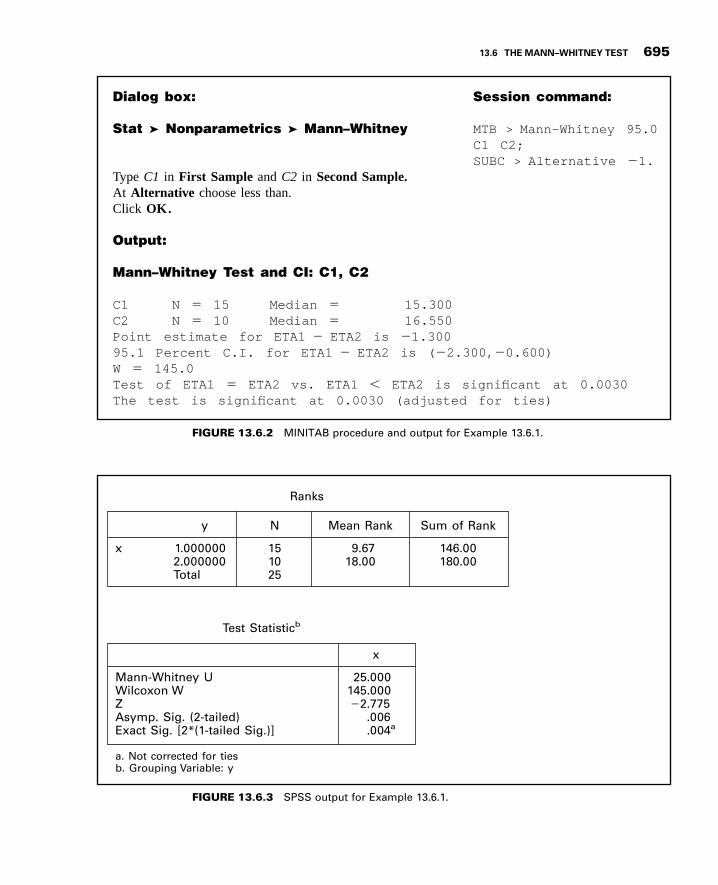
3GC13 11/24/2012 15:46:20 Page 695


Stat Nonparametrics Mann–Whitney MTB > Mann-Whitney 95.0C1 C2;SUBC > Alternative 1.

Type C1 in First Sample and C2 in Second Sample.At Alternative choose less than.Click OK.

Output:

Mann–Whitney Test and CI: C1, C2

C1 N 15 Median 15.300C2 N 10 Median 16.550Point estimate for ETA1 ETA2 is 1.30095.1 Percent C.I. for ETA1 ETA2 is ( 2.300, 0.600)W 145.0Test of ETA1 ETA2 vs. ETA1 ETA2 is significant at 0.0030The test is significant at 0.0030 (adjusted for ties)


Ranks

y N Mean Rank Sum of Rank

x 1.000000 15 9.67 146.002.000000 10 18.00 180.00Total 25

Test Statisticb

x

000.52U yentihW-nnaM000.541W noxocliW

Z 2.775600.)deliat-2( .giS .pmysA

Exact Sig. [2*(1-tailed Sig.)] .004a

a. Not corrected for tiesb. Grouping Variable: y



3GC13 11/24/2012 15:46:20 Page 696

Mann–Whitney-Wilcoxon test. Indeed, many computer packages give the test value ofboth the Mann–Whitney test (U) and the Wilcoxon test (W). These two tests arealgebraically equivalent tests, and are related by the following equality when there areno ties in the data:

U þW ¼ m mþ 2nþ 1ð Þ2

(13.6.3)

Computer Analysis Many statistics software packages will perform the Mann–Whitney test. With the data of two samples stored in Columns 1 and 2, for example,MINITAB will perform a one-sided or two-sided test. The MINITAB procedure and outputfor Example 13.6.1 are shown in Figure 13.6.2.

The SPSS output for Example 13.6.1 is shown in Figure 13.6.3. As we seethis output provides the Mann–Whitney test, the Wilcoxon test, and large-sample zapproximation.

EXERCISES

13.6.1 Cranor and Christensen (A-4) studied diabetics insured by two employers. Group 1 subjects wereemployed by the City of Asheville, North Carolina, and group 2 subjects were employed by Mission–St. Joseph’s Health System. At the start of the study, the researchers performed the Mann–Whitneytest to determine if a significant difference in weight existed between the two study groups. The dataare displayed in the following table.

Weight (Pounds)

Group 1 Group 2

252 215 240 185 195 220240 190 302 310 210 295205 270 312 212 190 202200 159 126 238 172 268170 204 268 184 190 220170 215 215 136 140 311320 254 183 200 280 164148 164 287 270 264 206214 288 210 200 270 170270 138 225 212 210 190265 240 258 182 192203 217 221 225 126

Source: Data provided courtesy of Carole W. Carnor, Ph.D.

May we conclude, on the basis of these data, that patients in the two groups differ significantly withrespect to weight? Let a ¼ :05.

13.6.2 One of the purposes of a study by Liu et al. (A-5) was to determine the effects of MRZ 2/579(a receptor antagonist shown to provide neuroprotective activity in vivo and in vitro) on neurological


3GC13 11/24/2012 15:46:21 Page 697

deficit in Sprague–Dawley rats. In the study, 10 rats were to receive MRZ 2/579 and nine rats were toreceive regular saline. Prior to treatment, researchers studied the blood gas levels in the two groups ofrats. The following table shows the pO2 levels for the two groups.

Saline (mmHg) MRZ 2/579 (mmHg)

112.5 133.3106.3 106.499.5 113.198.3 117.2

103.4 126.4109.4 98.1108.9 113.4107.4 116.8

116.5

Source: Data provided courtesy of Ludmila Belayev, M.D.

May we conclude, on the basis of these data, that, in general, subjects on saline have, on average,lower pO2 levels at baseline? Let a ¼ :01.

13.6.3 The purpose of a study by researchers at the Cleveland (Ohio) Clinic (A-6) was to determine if the useof Flomax® reduced the urinary side effects commonly experienced by patients following brachy-therapy (permanent radioactive seed implant) treatment for prostate cancer. The following tableshows the American Urological Association (AUA) symptom index scores for two groups of subjectsafter 8 weeks of treatment. The higher the AUA index, the more severe the urinary obstruction andirritation.

AUA Index (Flomax®) AUA Index (Placebo)

1 5 11 1 6 121 5 11 1 6 122 6 11 2 6 132 6 11 2 6 142 7 12 2 6 172 7 12 3 7 183 7 13 3 8 193 7 14 3 8 203 8 16 3 9 234 8 16 4 9 234 8 18 4 104 8 21 4 104 9 31 5 114 9 5 114 10 5 12

Source: Data provided courtesy of Chandana Reddy, M.S.

May we conclude, on the basis of these data, that the median AUA index in the Flomax® group differssignificantly from the median AUA index of the placebo group? Let a ¼ :05.

EXERCISES 697

3GC13 11/24/2012 15:46:21 Page 698

13.7 THE KOLMOGOROV–SMIRNOVGOODNESS-OF-FIT TEST

When one wishes to know how well the distribution of sample data conforms to sometheoretical distribution, a test known as the Kolmogorov–Smirnov goodness-of-fit testprovides an alternative to the chi-square goodness-of-fit test discussed in Chapter 12. Thetest gets its name from A. Kolmogorov and N. V. Smirnov, two Russian mathematicianswho introduced two closely related tests in the 1930s.

Kolmogorov’s work (6) is concerned with the one-sample case as discussed here.Smirnov’s work (7) deals with the case involving two samples in which interest centers ontesting the hypothesis that the distributions of the two-parent populations are identical. Thetest for the first situation is frequently referred to as the Kolmogorov–Smirnov one-sampletest. The test for the two-sample case, commonly referred to as the Kolmogorov–Smirnovtwo-sample test, will not be discussed here.

The Test Statistic In using the Kolmogorov–Smirnov goodness-of-fit test, acomparison is made between some theoretical cumulative distribution function, FT(x), anda sample cumulative distribution function, FS(x). The sample is a random sample from apopulation with unknown cumulative distribution function F(x). It will be recalled (Section4.2) that a cumulative distribution function gives the probability that X is equal to or lessthan a particular value, x. That is, by means of the sample cumulative distribution function,FS(x), we may estimate P X � xð Þ. If there is close agreement between the theoretical andsample cumulative distributions, the hypothesis that the sample was drawn from thepopulation with the specified cumulative distribution function, FT(x), is supported. If,however, there is a discrepancy between the theoretical and observed cumulative distribu-tion functions too great to be attributed to chance alone, when H0 is true, the hypothesisis rejected.

The difference between the theoretical cumulative distribution function, FT(x), andthe sample cumulative distribution function, FS(x), is measured by the statistic D, which isthe greatest vertical distance between FS(x) and FT(x). When a two-sided test is appropri-ate, that is, when the hypotheses are

H0 : F xð Þ ¼ FT xð Þ for all x from �1 to þ1HA : F xð Þ 6¼ FT xð Þ for at least one x

the test statistic is

D ¼ supx

FS xð Þ � FT xð Þj j (13.7.1)

which is read, “D equals the supremum (greatest), over all x, of the absolute value of thedifference FS Xð Þ minus FT Xð Þ.”

The null hypothesis is rejected at the a level of significance if the computed valueof D exceeds the value shown in Appendix Table M for 1 � a (two-sided) and the samplesize n.


3GC13 11/24/2012 15:46:22 Page 699

Assumptions The assumptions underlying the Kolmogorov–Smirnov test includethe following:

1. The sample is a random sample.

2. The hypothesized distribution FT xð Þ is continuous.

When values of D are based on a discrete theoretical distribution, the test isconservative. When the test is used with discrete data, then, the investigator shouldbear in mind that the true probability of committing a type I error is at most equal to a, thestated level of significance. The test is also conservative if one or more parameters have tobe estimated from sample data.

EXAMPLE 13.7.1

Fasting blood glucose determinations made on 36 nonobese, apparently healthy, adultmales are shown in Table 13.7.1. We wish to know if we may conclude that these data arenot from a normally distributed population with a mean of 80 and a standard deviation of 6.

Solution:


2. Assumptions. The sample available is a simple random sample from acontinuous population distribution.

3. Hypotheses. The appropriate hypotheses are

H0 : F xð Þ ¼ FT xð Þ for all x from �1 to þ1HA : F xð Þ 6¼ FT xð Þ for at least one x

Let a ¼ :05.


5. Distribution of test statistic. Critical values of the test statistic forselected values of a are given in Appendix Table M.

6. Decision rule. Reject H0 if the computed value of D exceeds .221, thecritical value of D for n ¼ 36 and a ¼ :05.

7. Calculation of test statistic. Our first step is to compute values of FS xð Þas shown in Table 13.7.2.

TABLE 13.7.1 Fasting Blood Glucose Values

(mg/100ml) for 36 Nonobese, ApparentlyHealthy, Adult Males

75 92 80 80 84 72

84 77 81 77 75 81

80 92 72 77 78 76

77 86 77 92 80 78

68 78 92 68 80 81

87 76 80 87 77 86

13.7 THE KOLMOGOROV–SMIRNOV GOODNESS-OF-FIT TEST 699

3GC13 11/24/2012 15:46:22 Page 700

Each value of FS xð Þ is obtained by dividing the correspondingcumulative frequency by the sample size. For example, the first value ofFS xð Þ ¼ 2=36 ¼ :0556.

We obtain values of FT xð Þ by first converting each observed valueof x to a value of the standard normal variable, z. From AppendixTable D we then find the area between �1 and z. From these areas weare able to compute values of FT xð Þ. The procedure, which is similar tothat used to obtain expected relative frequencies in the chi-squaregoodness-of-fit test, is summarized in Table 13.7.3.

TABLE 13.7.2 Values of FS xð Þ for

Example 13.7.1

x FrequencyCumulativeFrequency FS xð Þ

68 2 2 .0556

72 2 4 .1111

75 2 6 .1667

76 2 8 .2222

77 6 14 .3889

78 3 17 .4722

80 6 23 .6389

81 3 26 .7222

84 2 28 .7778

86 2 30 .8333

87 2 32 .8889

92 4 36 1.0000

36

TABLE 13.7.3 Steps in Calculationof FT xð Þ for Example 13.7.1

x z ¼ x � 80ð Þ=6 FT xð Þ

68 �2:00 .0228

72 �1:33 .0918

75 �:83 .2033

76 �:67 .2514

77 �:50 .3085

78 �:33 .3707

80 .00 .5000

81 .17 .5675

84 .67 .7486

86 1.00 .8413

87 1.17 .8790

92 2.00 .9772


3GC13 11/24/2012 15:46:23 Page 701

The test statistic D may be computed algebraically, or it may bedetermined graphically by actually measuring the largest vertical dis-tance between the curves of FS xð Þ and FT xð Þ on a graph. The graphs ofthe two distributions are shown in Figure 13.7.1.

Examination of the graphs of FS xð Þ and FT xð Þ reveals thatD � :16 ¼ :72 � :56ð Þ. Now let us compute the value of D algebrai-cally. The possible values of FS xð Þ � FT xð Þj j are shown in Table 13.7.4.This table shows that the exact value of D is .1547.

8. Statistical decision. Reference to Table M reveals that a computed D of.1547 is not significant at any reasonable level. Therefore, we are notwilling to reject H0.

9. Conclusion. The sample may have come from the specified distribution.

10. p value. Since we have a two-sided test, and since :1547 < :174, wehave p > :20.

&

68 70 72 74 76 78 80 82 84 86 88 90 92 94

Cu

mu

lati

ve r

elat

ive

freq

uen

cy

1.00.90.80.70.60

.50

.40

.30

.20

.10

FIGURE 13.7.1 FS xð Þ and FT xð Þ for Example 13.7.1.

TABLE 13.7.4 Calculation of Fs xð Þ � FT xð Þj jfor Example 13.7.1

x Fs xð Þ FT xð Þ Fs xð Þ � FT xð Þj j

68 .0556 .0228 .0328

72 .1111 .0918 .0193

75 .1667 .2033 .0366

76 .2222 .2514 .0292

77 .3889 .3085 .0804

78 .4722 .3707 .1015

80 .6389 .5000 .1389

81 .7222 .5675 .1547

84 .7778 .7486 .0292

86 .8333 .8413 .0080

87 .8889 .8790 .0099

92 1.0000 .9772 .0228

13.7 THE KOLMOGOROV–SMIRNOV GOODNESS-OF-FIT TEST 701

3GC13 11/24/2012 15:46:23 Page 702

StatXact is often used for nonparametric statistical analysis. This particular softwareprogram has a nonparametric module that contains nearly all of the commonly usednonparametric tests, and many less common, but useful, procedures as well. Computeranalysis using StatXact for the data in Example 13.7.1 is shown in Figure 13.7.2.Note that it provides the test statistic of D ¼ 0:156 and the exact two-sided p valueof .3447.

A Precaution The reader should be aware that in determining the value of D, it isnot always sufficient to compute and choose from the possible values of FS xð Þ � FT xð Þj j.The largest vertical distance between FS xð Þ and FT xð Þmay not occur at an observed value,x, but at some other value of X. Such a situation is illustrated in Figure 13.7.3. We see that ifonly values of FS xð Þ � FT xð Þj j at the left endpoints of the horizontal bars are considered,we would incorrectly compute D as :2 � :4j j ¼ :2. One can see by examining the graph,however, that the largest vertical distance between FS xð Þ and FT xð Þ occurs at the rightendpoint of the horizontal bar originating at the point corresponding to x ¼ :4, and thecorrect value of D is :5 � :2j j ¼ :3.

One can determine the correct value of D algebraically by computing, in addition tothe differences FS xð Þ � FT xð Þj j, the differences FS xi�1ð Þ � FT xið Þj j for all values ofi ¼ 1; 2; . . . ; r þ 1, where r ¼ the number of different values of x and FS x0ð Þ ¼ 0.The correct value of the test statistic will then be

D ¼ maximum1�i�r

maximum FS xið Þ � FT xið Þj j; FS xi�1ð Þ � FT xið Þj j½ �f g (13.7.2)

FIGURE 13.7.2 StatXact output for Example 13.7.1


3GC13 11/24/2012 15:46:23 Page 703

Advantages and Disadvantages The following are some important pointsof comparison between the Kolmogorov–Smirnov and the chi-square goodness-of-fit tests.

1. The Kolmogorov–Smirnov test does not require that the observations be grouped asis the case with the chi-square test. The consequence of this difference is that theKolmogorov–Smirnov test makes use of all the information present in a set of data.

2. The Kolmogorov–Smirnov test can be used with any size sample. It will be recalledthat certain minimum sample sizes are required for the use of the chi-square test.

3. As has been noted, the Kolmogorov–Smirnov test is not applicable when parametershave to be estimated from the sample. The chi-square test may be used in thesesituations by reducing the degrees of freedom by 1 for each parameter estimated.

4. The problem of the assumption of a continuous theoretical distribution has alreadybeen mentioned.

EXERCISES

13.7.1 The weights at autopsy of the brains of 25 adults suffering from a certain disease were as follows:

Weight of Brain (grams)

859 1073 1041 1166 1117962 1051 1064 1141 1202973 1001 1016 1168 1255904 1012 1002 1146 1233920 1039 1086 1140 1348

.2 .4 .5 .8 1.0

Cu

mu

lati

ve r

elat

ive

freq

uen

cy.1

.2

.3

.4

.5

.6

.7

.8

.9

1.0

FIGURE 13.7.3 Graph of fictitious data showing correct calculation of D.

EXERCISES 703

3GC13 11/24/2012 15:46:24 Page 704

Can one conclude from these data that the sampled population is not normally distributed with a meanof 1050 and a standard deviation of 50? Determine the p value for this test.

13.7.2 IQs of a sample of 30 adolescents arrested for drug abuse in a certain metropolitan jurisdiction wereas follows:

IQ

95 100 91 106 109 11098 104 97 100 107 11992 106 103 106 105 112

101 91 105 102 101 110101 95 102 104 107 118

Do these data provide sufficient evidence that the sampled population of IQ scores is not normallydistributed with a mean of 105 and a standard deviation of 10? Determine the p value.

13.7.3 For a sample of apparently normal subjects who served as controls in an experiment, the followingsystolic blood pressure readings were recorded at the beginning of the experiment:

162 177 151 167130 154 179 146147 157 141 157153 157 134 143141 137 151 161

Can one conclude on the basis of these data that the population of blood pressures fromwhich the sample was drawn is not normally distributed with m ¼ 150 and s ¼ 12? Determinethe p value.

13.8 THE KRUSKAL–WALLIS ONE-WAYANALYSIS OF VARIANCE BY RANKS

In Chapter 8 we discuss how one-way analysis of variance may be used to test the nullhypothesis that several population means are equal. When the assumptions underlying thistechnique are not met, that is, when the populations from which the samples are drawn arenot normally distributed with equal variances, or when the data for analysis consist only ofranks, a nonparametric alternative to the one-way analysis of variance may be used to testthe hypothesis of equal location parameters. As was pointed out in Section 13.5, the mediantest may be extended to accommodate the situation involving more than two samples. Adeficiency of this test, however, is the fact that it uses only a small amount of theinformation available. The test uses only information as to whether or not the observationsare above or below a single number, the median of the combined samples. The test does notdirectly use measurements of known quantity. Several nonparametric analogs to analysis ofvariance are available that use more information by taking into account the magnitude of


3GC13 11/24/2012 15:46:24 Page 705

each observation relative to the magnitude of every other observation. Perhaps the bestknown of these procedures is the Kruskal–Wallis one-way analysis of variance byranks (8).

The Kruskal–Wallis Procedure The application of the test involves thefollowing steps.

1. The n1; n2; . . . ; nk observations from the k samples are combined into a singleseries of size n and arranged in order of magnitude from smallest to largest.The observations are then replaced by ranks from 1, which is assigned to thesmallest observation, to n, which is assigned to the largest observation. When twoor more observations have the same value, each observation is given the mean ofthe ranks for which it is tied.

2. The ranks assigned to observations in each of the k groups are added separately togive k rank sums.

3. The test statistic

H ¼ 12

n nþ 1ð ÞXkj¼1

R2j

nj� 3 nþ 1ð Þ (13.8.1)

is computed. In Equation 13.8.1,

k ¼ the number of samplesnj ¼ the number of observations in the jth samplen ¼ the number of observations in all samples combinedRj ¼ the sum of the ranks in the jth sample

4. When there are three samples and five or fewer observations in each sample, thesignificance of the computed H is determined by consulting Appendix Table N.When there are more than five observations in one or more of the samples, H iscompared with tabulated values of x2 with k � 1 degrees of freedom.

EXAMPLE 13.8.1

In a study of pulmonary effects on guinea pigs, Lacroix et al. (A-7) exposedovalbumin (OA)-sensitized guinea pigs to regular air, benzaldehyde, or acetaldehyde.At the end of exposure, the guinea pigs were anesthetized and allergic responses wereassessed in bronchoalveolar lavage (BAL). One of the outcome variables examinedwas the count of eosinophil cells, a type of white blood cell that can increase withallergies. Table 13.8.1 gives the eosinophil cell count �106

� �for the three treatment

groups.Can we conclude that the three populations represented by the three samples differ

with respect to eosinophil cell count? We can so conclude if we can reject the nullhypothesis that the three populations do not differ in eosinophil cell count.

13.8 THE KRUSKAL–WALLIS ONE-WAY ANALYSIS OF VARIANCE BY RANKS 705

3GC13 11/24/2012 15:46:24 Page 706

Solution:


2. Assumptions. The samples are independent random samples from theirrespective populations. The measurement scale employed is at leastordinal. The distributions of the values in the sampled populations areidentical except for the possibility that one or more of the populationsare composed of values that tend to be larger than those of the otherpopulations.

3. Hypotheses.

H0: The population centers are all equal.

HA: At least one of the populations tends to exhibit larger valuesthan at least one of the other populations.

Let a ¼ :01.


5. Distribution of test statistic. Critical values of H for various samplesizes and a levels are given in Appendix Table N.

6. Decision rule. The null hypothesis will be rejected if the computedvalue of H is so large that the probability of obtaining a value that largeor larger when H0 is true is equal to or less than the chosen significancelevel, a.

7. Calculation of test statistic. When the three samples are combined intoa single series and ranked, the table of ranks shown in Table 13.8.2 maybe constructed.

The null hypothesis implies that the observations in the threesamples constitute a single sample of size 15 from a single population.If this is true, we would expect the ranks to be well distributed amongthe three groups. Consequently, we would expect the total sum ofranks to be divided among the three groups in proportion to group size.

TABLE 13.8.1 Eosinophil Count for

Ovalbumin-Sensitized Guinea Pigs

Eosinophil Cell Count ð�106Þ

Air Benzaldehyde Acetaldehyde

12.22 3.68 54.36

28.44 4.05 27.87

28.13 6.47 66.81

38.69 21.12 46.27

54.91 3.33 30.19

Source: Data provided courtesy of G. Lacroix.


3GC13 11/24/2012 15:46:25 Page 707

Departures from these conditions are reflected in the magnitude of thetest statistics H.

From the data in Table 13.8.2 and Equation 13.8.1, we obtain

H ¼ 12

15 16ð Þ47ð Þ2

5þ 16ð Þ2

5þ 57ð Þ2

5

" #� 3 15 þ 1ð Þ ¼ 9:14

8. Statistical decision. Table N shows that when the nj are 5, 5, and 5, theprobability of obtaining a value of H ¼ 9:14 is less than .009. The nullhypothesis can be rejected at the .01 level of significance.

9. Conclusion. We conclude that there is a difference in the averageeosinophil cell count among the three populations.

10. p value. For this test, p < :009. &

Ties When ties occur among the observations, we may adjust the value of H bydividing it by

1 �P

T

n3 � n(13.8.2)

where T ¼ t3 � t. The letter t is used to designate the number of tied observations in agroup of tied values. In our example there are no groups of tied values but, in general, theremay be several groups of tied values resulting in several values of T.

The effect of the adjustment for ties is usually negligible. Note also that the effect ofthe adjustment is to increase H, so that if the unadjusted H is significant at the chosen level,there is no need to apply the adjustment.

More than Three Samples/Large Samples Now let us illustrate theprocedure when there are more than three samples and at least one of the nj is greaterthan 5.

TABLE 13.8.2 The Data of Table 13.8.1

Replaced by Ranks

Air Benzaldehyde Acetaldehyde

5 2 13

9 3 7

8 4 15

11 6 12

14 1 10

R1 ¼ 47 R2 ¼ 16 R3 ¼ 57

13.8 THE KRUSKAL–WALLIS ONE-WAY ANALYSIS OF VARIANCE BY RANKS 707

3GC13 11/24/2012 15:46:25 Page 708

EXAMPLE 13.8.2

Table 13.8.3 shows the net book value of equipment capital per bed for a sample ofhospitals from each of five types of hospitals. We wish to determine, by means of theKruskal–Wallis test, if we can conclude that the average net book value of equipmentcapital per bed differs among the five types of hospitals. The ranks of the 41 values, alongwith the sum of ranks for each sample, are shown in the table.

Solution: From the sums of the ranks we compute

H ¼ 12

41 41 þ 1ð Þ68ð Þ2

10þ 246ð Þ2

8þ 124ð Þ2

9þ 159ð Þ2

7þ 264ð Þ2

7

" #� 3 41 þ 1ð Þ

¼ 36:39

Reference to Appendix Table F with k � 1 ¼ 4 degrees of freedom indi-cates that the probability of obtaining a value of H as large as or larger than36.39, due to chance alone, when there is no difference among thepopulations, is less than .005. We conclude, then, that there is a differenceamong the five populations with respect to the average value of the variableof interest. &

Computer Analysis The MINITAB software package computes the Kruskal–Wallis test statistic and provides additional information. After we enter the eosinophilcounts in Table 13.8.1 into Column 1 and the group codes into Column 2, the MINITABprocedure and output are as shown in Figure 13.8.1.

TABLE 13.8.3 Net Book Value of Equipment per Bed by Hospital Type

Type Hospital

A B C D E

$1735(11) $5260(35) $2790(20) $3475(26) $6090(40)

1520(2) 4455(28) 2400(12) 3115(22) 6000(38)

1476(1) 4480(29) 2655(16) 3050(21) 5894(37)

1688(7) 4325(27) 2500(13) 3125(23) 5705(36)

1702(10) 5075(32) 2755(19) 3275(24) 6050(39)

2667(17) 5225(34) 2592(14) 3300(25) 6150(41)

1575(4) 4613(30) 2601(15) 2730(18) 5110(33)

1602(5) 4887(31) 1648(6)

1530(3) 1700(9)

1698(8)

R1 ¼ 68 R2 ¼ 246 R3 ¼ 124 R4 ¼ 159 R5 ¼ 264


3GC13 11/24/2012 15:46:26 Page 709

EXERCISES

For the following exercises, perform the test at the indicated level of significance and determine thep value.

13.8.1 In a study of healthy subjects grouped by age (Younger: 19–50 years, Seniors: 65–75 years, andLongeval: 85–102 years), Herrmann et al. (A-8) measured their vitamin B-12 levels (ng/L). Allelderly subjects were living at home and able to carry out normal day-to-day activities. The followingtable shows vitamin B-12 levels for 50 subjects in the young group, 92 seniors, and 90 subjects in thelongeval group.

Young (19–50 Years) Senior (65–75 Years) Longeval (85–102 Years)

230 241 319 371 566 170 148 149 631 198477 442 190 460 290 542 1941 409 305 321561 491 461 440 271 282 128 229 393 2772347 279 163 520 308 194 145 183 282 428566 334 377 256 440 445 174 193 273 259260 247 190 335 238 921 495 161 157 111

Data:C1: 12.22 28.44 28.13 38.69 54.91 3.68 4.05 6.47 21.12 3.33 54.36 27.87 66.81 46.27 30.19

C2: 1 1 1 1 1 2 2 2 2 2 3 3 3 3 3


Stat Nonparametrics Kruskal–Wallis MTB > Kruskal–Wallis C1 C2.Type C1 in Response and C2 in Factor. Click OK.

Output:

Kruskal–Wallis Test: C1 versus C2

Kruskal–Wallis Test on C1

C2 N Median Ave Rank Z1 5 28.440 9.4 0.862 5 4.050 3.2 -2.943 5 46.270 11.4 2.08

0.851llarevO

H = 9.14 DF = 2 P = 0.010

FIGURE13.8.1 MINITAB procedure and output, Kruskal–Wallis test of eosinophil count data in

Table 13.8.1.

(Continued)

EXERCISES 709

3GC13 11/24/2012 15:46:27 Page 710

Young (19–50 Years) Senior (65–75 Years) Longeval (85–102 Years)

300 314 375 137 525 1192 460 400 1270 262230 254 229 452 298 748 548 348 252 161215 419 193 437 153 187 198 175 262 1113260 335 294 236 323 350 165 540 381 409349 455 740 432 205 1365 226 293 162 378315 297 194 411 248 232 557 196 340 203257 456 780 268 371 509 166 632 370 221536 668 245 703 668 357 218 438 483 917582 240 258 282 197 201 186 368 222 244293 320 419 290 260 177 346 262 277569 562 372 286 198 872 239 190 226325 360 413 143 336 240 241 203275 357 685 310 421 136 195 369172 609 136 352 712 359 220 162

2000 740 441 262 461 715 164 95240 430 423 404 631 252 279 178235 645 617 380 1247 414 297 530284 395 985 322 1033 372 474 334883 302 170 340 285 236 375 521

Source: Data provided courtesy of W. Herrmann and H. Schorr.

May we conclude, on the basis of these data, that the populations represented by these samples differwith respect to vitamin B-12 levels? Let a ¼ :01.

13.8.2 The following are outpatient charges �$100ð Þ made to patients for a certain surgical procedure bysamples of hospitals located in three different areas of the country:

Area

I II III

$80.75 $58.63 $84.2178.15 72.70 101.7685.40 64.20 107.7471.94 62.50 115.3082.05 63.24 126.15

Can we conclude at the .05 level of significance that the three areas differ with respect to the charges?

13.8.3 A study of young children by Flexer et al. (A-9) published in the Hearing Journal examines theeffectiveness of an FM sound field when teaching phonics to children. In the study, children in aclassroom with no phonological or phonemic awareness training (control) were compared to a classwith phonological and phonemic awareness (PPA) and to a class that utilized phonological andphonemic awareness training and the FM sound field (PPA/FM). A total of 53 students from threeseparate preschool classrooms participated in this study. Students were given a measure of phonemicawareness in preschool and then at the end of the first semester of kindergarten. The improvementscores are listed in the following table as measured by the Yopp–Singer Test of PhonemicSegmentation.


3GC13 11/24/2012 15:46:28 Page 711

Improvement (Control) Improvement PPA Improvement PPA/FM

0 1 2 1 19�1 1 3 3 20

0 2 15 7 211 2 18 9 214 3 19 11 225 6 20 17 229 7 5 17 159 8 17 17

13 9 18 1718 18 18 190 20 19 220 19

Source: Data provided courtesy of John P. Holcomb, Jr., Ph.D.

Test for a significant difference among the three groups. Let a ¼ :05.

13.8.4 Refer to Example 13.8.1. Another variable of interest to Lacroix et al. (A-7) was the number ofalveolar cells in three groups of subjects exposed to air, benzaldehyde, or acetaldehyde. Thefollowing table gives the information for six guinea pigs in each of the three treatment groups.

Number of Alveolar Cells ð�106ÞAir Benzaldehyde Acetaldehyde

0.55 0.81 0.650.48 0.56 13.697.8 1.11 17.118.72 0.74 7.430.65 0.77 5.481.51 0.83 0.990.55 0.81 0.65

Source: Data provided courtesyof G. Lacroix.

May we conclude, on the basis of these data, that the number of alveolar cells in ovalbumin-sensitizedguinea pigs differs with type of exposure? Let a ¼ :05.

13.8.5 The following table shows the pesticide residue levels (ppb) in blood samples from four populationsof human subjects. Use the Kruskal–Wallis test to test at the .05 level of significance the nullhypothesis that there is no difference among the populations with respect to average level of pesticideresidue.

Population Population

A B C D A B C D

10 4 15 7 44 11 9 437 35 5 11 12 7 11 512 32 10 10 15 32 9 2

(Continued)

EXERCISES 711

3GC13 11/24/2012 15:46:28 Page 712

Population Population

A B C D A B C D

31 19 12 8 42 17 14 611 33 6 2 23 8 15 39 18 6 5

13.8.6 Hepatic g-glutamyl transpeptidase (GGTP) activity was measured in 22 patients undergoingpercutaneous liver biopsy. The results were as follows:

Subject Diagnosis Hepatic GGTP Level

1 Normal liver 27.72 Primary biliary cirrhosis 45.93 Alcoholic liver disease 85.34 Primary biliary cirrhosis 39.05 Normal liver 25.86 Persistent hepatitis 39.67 Chronic active hepatitis 41.88 Alcoholic liver disease 64.19 Persistent hepatitis 41.1

10 Persistent hepatitis 35.311 Alcoholic liver disease 71.512 Primary biliary cirrhosis 40.913 Normal liver 38.114 Primary biliary cirrhosis 40.415 Primary biliary cirrhosis 34.016 Alcoholic liver disease 74.417 Alcoholic liver disease 78.218 Persistent hepatitis 32.619 Chronic active hepatitis 46.320 Normal liver 39.621 Chronic active hepatitis 52.722 Chronic active hepatitis 57.2

Can we conclude from these sample data that the average population GGTP level differs among thefive diagnostic groups? Let a ¼ :05 and find the p value.

13.9 THE FRIEDMAN TWO-WAY ANALYSISOF VARIANCE BY RANKS

Just as we may on occasion have need of a nonparametric analog to the parametric one-wayanalysis of variance, we may also find it necessary to analyze the data in a two-wayclassification by nonparametric methods analogous to the two-way analysis of variance.Such a need may arise because the assumptions necessary for parametric analysis ofvariance are not met, because the measurement scale employed is weak, or because results


3GC13 11/24/2012 15:46:29 Page 713

are needed in a hurry. A test frequently employed under these circumstances is theFriedman two-way analysis of variance by ranks (9,10). This test is appropriate wheneverthe data are measured on, at least, an ordinal scale and can be meaningfully arranged in atwo-way classification as is given for the randomized block experiment discussed inChapter 8. The following example illustrates this procedure.

EXAMPLE 13.9.1

A physical therapist conducted a study to compare three models of low-volt electricalstimulators. Nine other physical therapists were asked to rank the stimulators in order ofpreference. A rank of 1 indicates first preference. The results are shown in Table 13.9.1. Wewish to know if we can conclude that the models are not preferred equally.

Solution:


2. Assumptions. The observations appearing in a given block are inde-pendent of the observations appearing in each of the other blocks, andwithin each block measurement on at least an ordinal scale is achieved.

3. Hypothesis. In general, the hypotheses are:

H0: The treatments all have identical effects.HA: At least one treatment tends to yield larger observations than

at least one of the other treatments.

For our present example we state the hypotheses as follows:

H0: The three models are equally preferred.HA: The three models are not equally preferred.

Let a ¼ :05.

TABLE 13.9.1 Physical Therapists’ Rankings ofThree Models of Low-Volt Electrical Stimulators

Model

Therapist A B C

1 2 3 1

2 2 3 1

3 2 3 1

4 1 3 2

5 3 2 1

6 1 2 3

7 2 3 1

8 1 3 2

9 1 3 2

Rj 15 25 14

13.9 THE FRIEDMAN TWO-WAY ANALYSIS OF VARIANCE BY RANKS 713

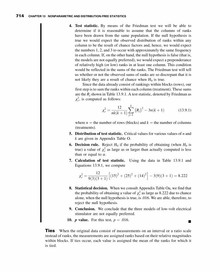
3GC13 11/24/2012 15:46:29 Page 714

4. Test statistic. By means of the Friedman test we will be able todetermine if it is reasonable to assume that the columns of rankshave been drawn from the same population. If the null hypothesis istrue we would expect the observed distribution of ranks within anycolumn to be the result of chance factors and, hence, we would expectthe numbers 1, 2, and 3 to occur with approximately the same frequencyin each column. If, on the other hand, the null hypothesis is false (that is,the models are not equally preferred), we would expect a preponderanceof relatively high (or low) ranks in at least one column. This conditionwould be reflected in the sums of the ranks. The Friedman test will tellus whether or not the observed sums of ranks are so discrepant that it isnot likely they are a result of chance when H0 is true.

Since the data already consist of rankings within blocks (rows), ourfirst step is to sum the ranks within each column (treatment). These sumsare the Rj shown in Table 13.9.1. A test statistic, denoted by Friedman asx2r , is computed as follows:

x2r ¼

12

nk k þ 1ð ÞXkj¼1

Rj

� �2 � 3n k þ 1ð Þ (13.9.1)

where n ¼ the number of rows (blocks) and k ¼ the number of columns(treatments).

5. Distribution of test statistic. Critical values for various values of n andk are given in Appendix Table O.

6. Decision rule. Reject H0 if the probability of obtaining (when H0 istrue) a value of x2

r as large as or larger than actually computed is lessthan or equal to a.

7. Calculation of test statistic. Using the data in Table 13.9.1 andEquations 13.9.1, we compute

x2r ¼

12

9 3ð Þ 3 þ 1ð Þ 15ð Þ2 þ 25ð Þ2 þ 14ð Þ2h i

� 3 9ð Þ 3 þ 1ð Þ ¼ 8:222

8. Statistical decision. When we consult Appendix Table Oa, we find thatthe probability of obtaining a value of x2

r as large as 8.222 due to chancealone, when the null hypothesis is true, is .016. We are able, therefore, toreject the null hypothesis.

9. Conclusion. We conclude that the three models of low-volt electricalstimulator are not equally preferred.

10. p value. For this test, p ¼ :016. &

Ties When the original data consist of measurements on an interval or a ratio scaleinstead of ranks, the measurements are assigned ranks based on their relative magnitudeswithin blocks. If ties occur, each value is assigned the mean of the ranks for which itis tied.


3GC13 11/24/2012 15:46:29 Page 715

Large Samples When the values of k and/or n exceed those given in Table O, thecritical value of x2

r is obtained by consulting the x2 table (Table F) with the chosen a andk � 1 degrees of freedom.

EXAMPLE 13.9.2

Table 13.9.2 shows the responses, in percent decrease in salivary flow, of 16 experimentalanimals following different dose levels of atropine. The ranks (in parentheses) and the sumof the ranks are also given in the table. We wish to see if we may conclude that the differentdose levels produce different responses. That is, we wish to test the null hypothesis of nodifference in response among the four dose levels.

Solution: From the data, we compute

x2r ¼

12

16 4ð Þ 4 þ 1ð Þ�

20ð Þ2 þ 36:5ð Þ2 þ 44ð Þ2 þ 59:5ð Þ2�� 3 16ð Þ 4 þ 1ð Þ ¼ 30:32

Reference to Table F indicates that with k � 1 ¼ 3 degrees of freedomthe probability of getting a value of x2

r as large as 30.32 due to chance aloneis, when H0 is true, less than .005. We reject the null hypothesis and concludethat the different dose levels do produce different responses.

&

TABLE 13.9.2 Percent Decrease in Salivary Flow ofExperimental Animals Following Different Dose

Levels of Atropine

Dose Level

Animal Number A B C D

1 29(1) 48(2) 75(3) 100(4)

2 72(2) 30(1) 100(3.5) 100(3.5)

3 70(1) 100(4) 86(2) 96(3)

4 54(2) 35(1) 90(3) 99(4)

5 5(1) 43(3) 32(2) 81(4)

6 17(1) 40(2) 76(3) 81(4)

7 74(1) 100(3) 100(3) 100(3)

8 6(1) 34(2) 60(3) 81(4)

9 16(1) 39(2) 73(3) 79(4)

10 52(2) 34(1) 88(3) 96(4)

11 8(1) 42(3) 31(2) 79(4)

12 29(1) 47(2) 72(3) 99(4)

13 71(1) 100(3.5) 97(2) 100(3.5)

14 7(1) 33(2) 58(3) 79(4)

15 68(1) 99(4) 84(2) 93(3)

16 70(2) 30(1) 99(3.5) 99(3.5)

Rj 20 36.5 44 59.5

13.9 THE FRIEDMAN TWO-WAY ANALYSIS OF VARIANCE BY RANKS 715

3GC13 11/24/2012 15:46:30 Page 716

Computer Analysis Many statistics software packages, including MINITAB,will perform the Friedman test. To use MINITAB we form three columns of data. We may,for example, set up the columns so that Column 1 contains numbers that indicate thetreatment to which the observations belong, Column 2 contains numbers indicating theblocks to which the observations belong, and Column 3 contains the observations. If we dothis for Example 13.9.1, the MINITAB procedure and output are as shown in Figure 13.9.1.

EXERCISES

For the following exercises perform the test at the indicated level of significance and determine thep value.

13.9.1 The following table shows the scores made by nine randomly selected student nurses on finalexaminations in three subject areas:

Subject AreaStudentNumber Fundamentals Physiology Anatomy

1 98 95 772 95 71 79


Stat Nonparametrics Friedman MTB > FRIEDMAN C3 C1 C2

Type C3 in Response, C1 in Treatment and C2 inBlocks. Click OK.

Output:

Friedman Test: C3 versus C1 blocked by C2

S 8.22 d.f. 2 p 0.017

Est. Sum ofC1 N Median RANKS1 9 2.0000 15.02 9 2.6667 25.03 9 1.3333 14.0

Grand median 2.0000


(Continued)


3GC13 11/24/2012 15:46:31 Page 717

Subject AreaStudentNumber Fundamentals Physiology Anatomy

3 76 80 914 95 81 845 83 77 806 99 70 937 82 80 878 75 72 819 88 81 83

Test the null hypothesis that student nurses constituting the population from which the above samplewas drawn perform equally well in all three subject areas against the alternative hypothesis that theyperform better in, at least, one area. Let a ¼ :05.

13.9.2 Fifteen randomly selected physical therapy students were given the following instructions: “Assumethat you will marry a person with one of the following handicaps (the handicaps were listed anddesignated by the letters A to J). Rank these handicaps from 1 to 10 according to your first, second,third (and so on) choice of a handicap for your marriage partner.” The results are shown in thefollowing table.

Handicap

Student Number A B C D E F G H I J

1 1 3 5 9 8 2 4 6 7 102 1 4 5 7 8 2 3 6 9 103 2 3 7 8 9 1 4 6 5 104 1 4 7 8 9 2 3 6 5 105 1 4 7 8 10 2 3 6 5 96 2 3 7 9 8 1 4 5 6 107 2 4 6 9 8 1 3 7 5 108 1 5 7 9 10 2 3 4 6 89 1 4 5 7 8 2 3 6 9 10

10 2 3 6 8 9 1 4 7 5 1011 2 4 5 8 9 1 3 7 6 1012 2 3 6 8 10 1 4 5 7 913 3 2 6 9 8 1 4 7 5 1014 2 5 7 8 9 1 3 4 6 1015 2 3 6 7 8 1 5 4 9 10

Test the null hypothesis of no preference for handicaps against the alternative that some handicaps arepreferred over others. Let a ¼ :05.

13.9.3 Ten subjects with exercise-induced asthma participated in an experiment to compare theprotective effect of a drug administered in four dose levels. Saline was used as a control. Thevariable of interest was change in FEV1 after administration of the drug or saline. The resultswere as follows:

EXERCISES 717

3GC13 11/24/2012 15:46:32 Page 718

Dose Level of Drug (mg/ml)

Subject Saline 2 10 20 40

1 �:68 �:32 �:14 �:21 �:322 �1:55 �:56 �:31 �:21 �:163 �1:41 �:28 �:11 �:08 �:834 �:76 �:56 �:24 �:41 �:085 �:48 �:25 �:17 �:04 �:186 �3:12 �1:99 �1:22 �:55 �:757 �1:16 �:88 �:87 �:54 �:848 �1:15 �:31 �:18 �:07 �:099 �:78 �:24 �:39 �:11 �:51

10 �2:12 �:35 �:28 þ:11 �:41

Can one conclude on the basis of these data that different dose levels have different effects?Let a ¼ :05 and find the p value.

13.10 THE SPEARMAN RANKCORRELATION COEFFICIENT

Several nonparametric measures of correlation are available to the researcher. Of these afrequently used procedure that is attractive because of the simplicity of the calculationsinvolved is due to Spearman (11). The measure of correlation computed by this method iscalled the Spearman rank correlation coefficient and is designated by rs. This proceduremakes use of the two sets of ranks that may be assigned to the sample values of X and Y, theindependent and continuous variables of a bivariate distribution.

Hypotheses The usually tested hypotheses and their alternatives are as follows:

(a) H0: X and Y are mutually independent.HA: X and Y are not mutually independent.

(b) H0: X and Y are mutually independent.HA: There is a tendency for large values of X and large values of Y to be paired

together.

(c) H0: X and Y are mutually independent.HA: There is a tendency for large values of X to be paired with small values of Y.

The hypotheses specified in (a) lead to a two-sided test and are used when it is desiredto detect any departure from independence. The one-sided tests indicated by (b) and (c) areused, respectively, when investigators wish to know if they can conclude that the variablesare directly or inversely correlated.

The Procedure The hypothesis-testing procedure involves the following steps.

1. Rank the values of X from 1 to n (numbers of pairs of values of X and Y in the sample).Rank the values of Y from 1 to n.


3GC13 11/24/2012 15:46:32 Page 719

2. Compute di for each pair of observations by subtracting the rank of Yi from therank of Xi.

3. Square each di and computeP

d2i , the sum of the squared values.

4. Compute

rs ¼ 1 � 6P

d2i

n n2 � 1ð Þ (13.10.1)

5. If n is between 4 and 30, compare the computed value of rs with the critical values, rs ,of Appendix Table P. For the two-sided test, H0 is rejected at the a significance levelif rs is greater than rs or less than �rs , where rs is at the intersection of the columnheaded a=2 and the row corresponding to n. For the one-sided test withHA specifyingdirect correlation, H0 is rejected at the a significance level if rs is greater than rs for aand n. The null hypothesis is rejected at the a significance level in the other one-sidedtest if rs is less than �rs for a and n.

6. If n is greater than 30, one may compute

z ¼ rsffiffiffiffiffiffiffiffiffiffiffin� 1

p(13.10.2)

and use Appendix Table D to obtain critical values.

7. Tied observations present a problem. The use of Table P is strictly valid only whenthe data do not contain any ties (unless some random procedure for breaking ties isemployed). In practice, however, the table is frequently used after some other methodfor handling ties has been employed. If the number of ties is large, the followingcorrection for ties may be employed:

T ¼ t3 � t

12(13.10.3)

where t ¼ the number of observations that are tied for some particular rank. Whenthis correction factor is used, rs is computed from

rs ¼P

x2 þPy2 �P

d2i

2ffiffiffiffiffiffiffiffiffiffiffiffiffiffiffiffiffiffiffiffiffiP

x2P

y2p (13.10.4)

instead of from Equation 13.10.1.

In Equation 13.10.4,

Px2 ¼ n3 � n

12�X

Tx

Py2 ¼ n3 � n

12�X

Ty

Tx ¼ the sum of the values of T for the various tied ranks in XTy ¼ the sum of the values of T for the various tied ranks in Y

Most authorities agree that unless the number of ties is excessive, the correction makesvery little difference in the value of rs. When the number of ties is small, we can follow the

13.10 THE SPEARMAN RANK CORRELATION COEFFICIENT 719

3GC13 11/24/2012 15:46:33 Page 720

usual procedure of assigning the tied observations the mean of the ranks for which they aretied and proceed with steps 2 to 6.

EXAMPLE 13.10.1

In a study of the relationship between age and the EEG, data were collected on 20 subjectsbetween ages 20 and 60 years. Table 13.10.1 shows the age and a particular EEG outputvalue for each of the 20 subjects. The investigator wishes to know if it can be concluded thatthis particular EEG output is inversely correlated with age.

Solution:


2. Assumptions. We assume that the sample available for analysis is asimple random sample and that both X and Yare measured on at least theordinal scale.

3. Hypotheses.

H0: This EEG output and age are mutually independent.HA: There is a tendency for this EEG output to decrease with age.

Suppose we let a ¼ :05.

TABLE 13.10.1 Age and EEG OutputValue for 20 Subjects

SubjectNumber Age (X)

EEG OutputValue (Y)

1 20 98

2 21 75

3 22 95

4 24 100

5 27 99

6 30 65

7 31 64

8 33 70

9 35 85

10 38 74

11 40 68

12 42 66

13 44 71

14 46 62

15 48 69

16 51 54

17 53 63

18 55 52

19 58 67

20 60 55


3GC13 11/24/2012 15:46:33 Page 721


5. Distribution of test statistic. Critical values of the test statistic aregiven in Appendix Table P.

6. Decision rule. For the present test we will reject H0 if the computedvalue of rs is less than �:3789.

7. Calculation of test statistic. When the X and Y values are ranked, wehave the results shown in Table 13.10.2. The di, d

2i , and

Pd2i are shown

in the same table.Substitution of the data from Table 13.10.2 into Equation 13.10.1

gives

rs ¼ 1 � 6 2340ð Þ20½ 20ð Þ2 � 1� ¼ �:76

8. Statistical decision. Since our computed rs ¼ �:76 is less than thecritical rs , we reject the null hypothesis.

9. Conclusion. We conclude that the two variables are inversely related.

10. p value. Since �:76 < �0:6586, we have for this test p < :001.

&

TABLE 13.10.2 Ranks for Data of Example 13.10.1

SubjectNumber Rank (X) Rank (Y) di d2

i

1 1 18 �17 289

2 2 15 �13 169

3 3 17 �14 196

4 4 20 �16 256

5 5 19 �14 196

6 6 7 �1 1

7 7 6 1 1

8 8 12 �4 16

9 9 16 �7 49

10 10 14 �4 16

11 11 10 1 1

12 12 8 4 16

13 13 13 0 0

14 14 4 10 100

15 15 11 4 16

16 16 2 14 196

17 17 5 12 144

18 18 1 17 289

19 19 9 10 100

20 20 3 17 289

Pd2i ¼ 2340


3GC13 11/24/2012 15:46:34 Page 722

Let us now illustrate the procedure for a sample with n > 30 and some tiedobservations.

EXAMPLE 13.10.2

In Table 13.10.3 are shown the ages and concentrations (ppm) of a certain mineral in thetissue of 35 subjects on whom autopsies were performed as part of a large researchproject.

The ranks, di, d2i , and

Pd2i are shown in Table 13.10.4. Let us test, at the .05 level of

significance, the null hypothesis that X and Y are mutually independent against the two-sided alternative that they are not mutually independent.

Solution: From the data in Table 13.10.4 we compute

rs ¼ 1 � 6 1788:5ð Þ35

�35ð Þ2 � 1

� ¼ :75

To test the significance of rs we compute

z ¼ :75ffiffiffiffiffiffiffiffiffiffiffiffiffiffi35 � 1

p¼ 4:37

TABLE 13.10.3 Age and Mineral Concentration (ppm) in Tissue of 35 Subjects

SubjectNumber

Age(X)

MineralConcentration

(Y)SubjectNumber

Age(X)

MineralConcentration

(Y)

1 82 169.62 19 50 4.48

2 85 48.94 20 71 46.93

3 83 41.16 21 54 30.91

4 64 63.95 22 62 34.27

5 82 21.09 23 47 41.44

6 53 5.40 24 66 109.88

7 26 6.33 25 34 2.78

8 47 4.26 26 46 4.17

9 37 3.62 27 27 6.57

10 49 4.82 28 54 61.73

11 65 108.22 29 72 47.59

12 40 10.20 30 41 10.46

13 32 2.69 31 35 3.06

14 50 6.16 32 75 49.57

15 62 23.87 33 50 5.55

16 33 2.70 34 76 50.23

17 36 3.15 35 28 6.81

18 53 60.59


3GC13 11/24/2012 15:46:35 Page 723

Since 4.37 is greater than z ¼ 3:89; p < 2 :0001ð Þ ¼ :0002, and wereject H0 and conclude that the two variables under study are not mutuallyindependent.

For comparative purposes let us correct for ties using Equation 13.10.3and then compute rs by Equation 13.10.4.

In the rankings of X we had six groups of ties that were broken byassigning the values 13.5, 17, 19.5, 21.5, 23.5, and 32.5. In five of the groupstwo observations tied, and in one group three observations tied. We,therefore, compute five values of

Tx ¼ 23 � 2

12¼ 6

12¼ :5

and one value of

Tx ¼ 33 � 3

12¼ 24

12¼ 2

From these computations, we haveP

Tx ¼ 5 :5ð Þ þ 2 ¼ 4:5, so that

Xx2 ¼ 352 � 35

12� 4:5 ¼ 3565:5

TABLE 13.10.4 Ranks for Data of Example 13.10.2

SubjectNumber

Rank(X)

Rank(Y) di d2

i

SubjectNumber

Rank(X)

Rank(Y) di d2

i

1 32.5 35 �2:5 6.25 19 17 9 8 64.00

2 35 27 8 64.00 20 28 25 3 9.00

3 34 23 11 121.00 21 21.5 21 .5 .25

4 25 32 �7 49.00 22 23.5 22 1.5 2.25

5 32.5 19 13.5 182.25 23 13.5 24 �10:5 110.25

6 19.5 11 8.5 72.25 24 27 34 �7 49.00

7 1 14 �13 169.00 25 6 3 3 9.00

8 13.5 8 5.5 30.25 26 12 7 5 25.00

9 9 6 3 9.00 27 2 15 �13 169.00

10 15 10 5 25.00 28 21.5 31 �9:5 90.25

11 26 33 �7 49.00 29 29 26 3 9.00

12 10 17 �7 49.00 30 11 18 �7 49.00

13 4 1 3 9.00 31 7 4 3 9.00

14 17 13 4 16.00 32 30 28 2 4.00

15 23.5 20 3.5 12.25 33 17 12 5 25.00

16 5 2 3 9.00 34 31 29 2 4.00

17 8 5 3 9.00 35 3 16 �13 169.00

18 19.5 30 �10:5 110.25

Pd2i ¼ 1788:5


3GC13 11/24/2012 15:46:36 Page 724

Since no ties occurred in the Y rankings, we haveP

Ty ¼ 0 and

Xy2 ¼ 353 � 35

12� 0 ¼ 3570:0

From Table 13.10.4 we haveP

d2i ¼ 1788:5. From these data we may now

compute by Equation 13.10.4

rs ¼ 3565:5 þ 3570:0 � 1788:5

2ffiffiffiffiffiffiffiffiffiffiffiffiffiffiffiffiffiffiffiffiffiffiffiffiffiffiffiffiffiffiffi3565:5ð Þ 3570ð Þp ¼ :75

We see that in this case the correction for ties does not make any difference inthe value of rs. &

Computer Analysis We may use MINITAB, as well as many other statisticalsoftware packages, to compute the Spearman correlation coefficient. To use MINITAB, wemust first have MINITAB rank the observations and store the ranks in separate columns,one for the X ranks and one for the Y ranks. If we rank the X and Y values of Example13.10.1 and store them in Columns 3 and 4, we may obtain the Spearman rank correlationcoefficient with the procedure shown in Figure 13.10.1. Other software packages such asSAS® and SPSS, for example, automatically rank the measurements before computing thecoefficient, thereby eliminating an extra step in the procedure.

EXERCISES

For the following exercises perform the test at the indicated level of significance and determine thep value.

13.10.1 The following table shows 15 randomly selected geographic areas ranked by population density andage-adjusted death rate. Can we conclude at the .05 level of significance that population density andage-adjusted death rate are not mutually independent?


Stat Basic Statistics Correlation MTB > CORRELATION C3 C4

Type C3–C4 in Variables. Click OK.

Output:

Correlations (Pearson)

Correlation of (X)Rank and (Y)Rank -0.759

FIGURE 13.10.1 MINITAB procedure and output for computing Spearman rank correlation

coefficient, Example 13.10.1.


3GC13 11/24/2012 15:46:36 Page 725

Rank by Rank by

AreaPopulationDensity (X)

Age-AdjustedDeath Rate (Y) Area

PopulationDensity (X)

Age-AdjustedDeath Rate (Y)

1 8 10 9 6 82 2 14 10 14 53 12 4 11 7 64 4 15 12 1 25 9 11 13 13 96 3 1 14 15 37 10 12 15 11 138 5 7

13.10.2 The following table shows 10 communities ranked by decayed, missing, or filled (DMF) teeth per 100children and fluoride concentration in ppm in the public water supply:

Rank by Rank by

Community

DMF Teethper 100

Children (X)

FluorideConcentration

(Y) Community

DMF Teethper 100

Children (X)

FluorideConcentration

(Y)

1 8 1 6 4 72 9 3 7 1 103 7 4 8 5 64 3 9 9 6 55 2 8 10 10 2

Do these data provide sufficient evidence to indicate that the number of DMF teeth per 100 childrentends to decrease as fluoride concentration increases? Let a ¼ :05.

13.10.3 The purpose of a study by Nozawa et al. (A-10) was to evaluate the outcome of surgical repair of parsinterarticularis defect by segmental wire fixation in young adults with lumbar spondylolysis. Theauthors cite literature indicating that segmental wire fixation has been successful in the treatment ofnonathletes with spondylolysis and point out that no information existed on the results of this type ofsurgery in athletes. In a retrospective study of subjects having surgery between 1993 and 2000, theauthors found 20 subjects who had undergone the surgery. The following table shows the age (years)at surgery and duration (months) of follow-up care for these subjects.

Duration of Follow-Up(Months)

Age(Years)


Age(Years)

103 37 38 2768 27 36 3162 12 34 2460 18 30 2360 18 19 14

(Continued)

EXERCISES 725

3GC13 11/24/2012 15:46:37 Page 726


Age(Years)


Age(Years)

54 28 19 2349 25 19 1844 20 19 2942 18 17 2441 30 16 27

Source: Satoshi Nozawa, Katsuji Shimizu, Kei Miyamoto, and Mizuo Tanaka, “Repair of Pars InterarticularisDefect by Segmental Wire Fixation in Young Athletes with Spondylolysis,” American Journal of Sports Medicine,31 (2003), pp. 359–364.

May we conclude, on the basis of these data, that in a population of similar subjects there is anassociation between age and duration of follow-up? Let a ¼ :05.

13.10.4 Refer to Exercise 13.10.3. Nozawa et al. (A-10) also calculated the Japanese Orthopaedic Associationscore for measuring back pain (JOA). The results for the 20 subjects along with the duration offollow-up are shown in the following table. The higher the number, the lesser the degree of pain.

Duration of Follow-Up(Months) JOA

Duration of Follow-Up(Months) JOA

103 21 38 1368 14 36 2462 26 34 2160 24 30 2260 13 19 2554 24 19 2349 22 19 2044 23 19 2142 18 17 2541 24 16 21

Source: Satoshi Nozawa, Katsuji Shimizu, Kei Miyamoto, and Mizuo Tanaka,“Repair of Pars Interarticularis Defect by Segmental Wire Fixation in YoungAthletes with Spondylolysis,” American Journal of Sports Medicine, 31 (2003),pp. 359–364.

Can we conclude from these data that in general there is a relationship between length of follow-upand JOA score at the time of the operation? Let a ¼ :05.

13.10.5 Butz et al. (A-11) studied the use of noninvasive positive-pressure ventilation by patients withamyotrophic lateral sclerosis. They evaluated the benefit of the procedure on patients’ symptoms,quality of life, and survival. Two variables of interest are PaCO2, partial pressure of arterial carbondioxide, and PaO2, partial pressure of arterial oxygen. The following table shows, for 30 subjects,values of these variables (mm Hg) obtained from baseline arterial blood gas analyses.

PaCO2 PaO2 PaCO2 PaO2 PaCO2 PaO2

40 101 54.5 80 34.5 86.547 69 54 72 40.1 74.7

(Continued)


3GC13 11/24/2012 15:46:37 Page 727

PaCO2 PaO2 PaCO2 PaO2 PaCO2 PaO2

34 132 43 105 33 9442 65 44.3 113 59.9 60.454 72 53.9 69.2 62.6 52.548 76 41.8 66.7 54.1 76.953.6 67.2 33 67 45.7 65.356.9 70.9 43.1 77.5 40.6 80.358 73 52.4 65.1 56.6 53.245 66 37.9 71 59 71.9

Source: M. Butz, K. H. Wollinsky, U. Widemuth-Catrinescu, A.Sperfeld, S. Winter, H. H. Mehrkens, A. C. Ludolph, and H.Schreiber, “Longitudinal Effects of Noninvasive Positive-PressureVentilation in Patients with Amyotrophic Lateral Sclerosis,” Ameri-can Journal of Medical Rehabilitation, 82 (2003) 597–604.

On the basis of these data may we conclude that there is an association between PaCO2 and PaO2

values? Let a ¼ :05.

13.10.6 Seventeen patients with a history of congestive heart failure participated in a study to assess theeffects of exercise on various bodily functions. During a period of exercise the following data werecollected on the percent change in plasma norepinephrine (Y) and the percent change in oxygenconsumption (X):

Subject X Y Subject X Y

1 500 525 10 50 602 475 130 11 175 1053 390 325 12 130 1484 325 190 13 76 755 325 90 14 200 2506 205 295 15 174 1027 200 180 16 201 1518 75 74 17 125 1309 230 420

On the basis of these data can one conclude that there is an association between the two variables? Leta ¼ :05.

13.11 NONPARAMETRICREGRESSION ANALYSIS

When the assumptions underlying simple linear regression analysis as discussed in Chapter9 are not met, we may employ nonparametric procedures. In this section we presentestimators of the slope and intercept that are easy-to-calculate alternatives to the least-squares estimators described in Chapter 9.

13.11 NONPARAMETRIC REGRESSION ANALYSIS 727

3GC13 11/24/2012 15:46:38 Page 728

Theil’s Slope Estimator Theil (12) proposes a method for obtaining a pointestimate of the slope coefficient b. We assume that the data conform to the classicregression model

yi ¼ b0 þ b1x1 þ ei; i ¼ 1; . . . ; n

where the xi are known constants, b0 and b1 are unknown parameters, and Yi is an observedvalue of the continuous random variable Y at xi. For each value of xi, we assume asubpopulation of Y values, and the ei are mutually independent. The xi are all distinct (noties), and we take x1 < x2 < < xn.

The data consist of n pairs of sample observations, x1; y1ð Þ; x2; y2ð Þ; . . . ; xn; ynð Þ,where the ith pair represents measurements taken on the ith unit of association.

To obtain Theil’s estimator of b1 we first form all possible sample slopesSij ¼ yj � yi

� �= xj � xi� �

, where i < j. There will be N ¼ nC2 values of Sij. The estimatorof b1 which we designate by b1 is the median of Sij values. That is,

b1 ¼ median Sij� �

(13.11.1)

The following example illustrates the calculation of b1.

EXAMPLE 13.11.1

In Table 13.11.1 are the plasma testosterone (ng/ml) levels (Y) and seminal citric acid(mg/ml) levels in a sample of eight adult males. We wish to compute the estimate of thepopulation regression slope coefficient by Theil’s method.

Solution: The N ¼ 8C2 ¼ 28 ordered values of Sij are shown in Table 13.11.2.If we let i ¼ 1 and j ¼ 2, the indicators of the first and second values of

Y and X in Table 13.11.1, we may compute S12 as follows:

S12 ¼ 175 � 230ð Þ= 278 � 421ð Þ ¼ �:3846

When all the slopes are computed in a similar manner and ordered asin Table 13.11.2, �:3846 winds up as the tenth value in the orderedarray.

The median of the Sij values is .4878. Consequently, our estimate of thepopulation slope coefficient b1 ¼ :4878.

TABLE 13.11.1 Plasma Testosterone and Seminal Citric Acid

Levels in Adult Males

Testosterone: 230 175 315 290 275 150 360 425

Citric acid: 421 278 618 482 465 105 550 750


3GC13 11/24/2012 15:46:39 Page 729

&

An Estimator of the Intercept Coefficient Dietz (13) recommends twointercept estimators. The first, designated b0

� �1;M

is the median of the n terms yi � b1xi inwhich b1 is the Theil estimator. It is recommended when the researcher is not willing toassume that the error terms are symmetric about 0. If the researcher is willing to assume asymmetric distribution of error terms, Dietz recommends the estimator b0

� �2;M

which isthe median of the n nþ 1ð Þ=2 pairwise averages of the yi � b1xi terms. We illustrate thecalculation of each in the following example.

EXAMPLE 13.11.2

Refer to Example 13.11.1. Let us compute a1;M and a2;M from the data on testosterone andcitric acid levels.

Solution: The ordered yi � :4878xi terms are: 13.5396, 24.6362, 39.3916, 48.1730,54.8804, 59.1500, 91.7100, and 98.7810. The median, 51.5267, is theestimator b0

� �1;M

.The 8 8 þ 1ð Þ=2 ¼ 36 ordered pairwise averages of the yi � :4878xi are

13.5396 49.2708 75.4319.0879 51.5267 76.830724.6362 52.6248 78.965526.4656 53.6615 91.7130.8563 54.8804 95.245532.0139 56.1603 98.78134.21 57.015236.3448 58.1731

TABLE 13.11.2 Ordered Values of Sij

for Example 13.11.1

�:6618 .5037

.1445 .5263

.1838 .5297

.2532 .5348

.2614 .5637

.3216 .5927

.3250 .6801

.3472 .8333

.3714 .8824

.3846 .9836

.4118 1.0000

.4264 1.0078

.4315 1.0227

.4719 1.0294

(Continued)

13.11 NONPARAMETRIC REGRESSION ANALYSIS 729

3GC13 11/24/2012 15:46:39 Page 730

36.4046 59.1539.3916 61.708639.7583 65.550841.8931 69.086343.7823 69.941547.136 73.295248.173 73.477

The median of these averages, 53.1432, is the estimator a2;M. The estimatingequation, then, is yi ¼ 53:1432 þ :4878xi if we are willing to assume thatthe distribution of error terms is symmetric about 0. If we are not willingto make the assumption of symmetry, the estimating equation isyi ¼ 51:5267 þ :4878xi. &

EXERCISES

13.11.1 The following are the heart rates (HR: beats/minute) and oxygen consumption values (VO2:cal/kg/24 h) for nine infants with chronic congestive heart failure:

HR(X): 163 164 156 151 152 167 165 153 155VO2(Y): 53.9 57.4 41.0 40.0 42.0 64.4 59.1 49.9 43.2

Compute b1; b0

� �1;M

; and b0

� �2;M

13.11.2 The following are the body weights (grams) and total surface area (cm2) of nine laboratoryanimals:

Body weight (X): 660.2 706.0 924.0 936.0 992.1 888.9 999.4 890.3 841.2Surface area (Y): 781.7 888.7 1038.1 1040.0 1120.0 1071.5 1134.5 965.3 925.0

Compute the slope estimator and two intercept estimators.

13.12 SUMMARY

This chapter is concerned with nonparametric statistical tests. These tests may be usedeither when the assumptions underlying the parametric tests are not realized or when thedata to be analyzed are measured on a scale too weak for the arithmetic proceduresnecessary for the parametric tests.

Nine nonparametric tests are described and illustrated. Except for the Kolmogorov–Smirnov goodness-of-fit test, each test provides a nonparametric alternative to a well-known parametric test. There are a number of other nonparametric tests available. Theinterested reader is referred to the many books devoted to nonparametric methods,including those by Gibbons (14) and Pett (15).


3GC13 11/24/2012 15:46:40 Page 731



13.3.1 Sign test statisticP k � x

n; p� � ¼ Xxk¼0

nCk pkqn�k

13.3.2 Large-sampleapproximation ofthe sign test

z ¼ k þ 0:5ð Þ þ 0:5n

0:5ffiffiffin

p ; if k <n

2

z ¼ k � 0:5ð Þ � 0:5n

0:5ffiffiffin

p ; if k � n

2

13.6.1 Mann–Whitney teststatistic

T ¼ S� n nþ 1ð Þ2

13.6.2 Large-sampleapproximation of theMann–Whitney test

Z ¼ T � mn=2ffiffiffiffiffiffiffiffiffiffiffiffiffiffiffiffiffiffiffiffiffiffiffiffiffiffiffiffiffiffiffiffiffiffiffiffiffinm nþ mþ 1ð Þ=12

p

13.6.3 Equivalence of the Mann–Whitney and Wilcoxontwo-sample statistics

U þW ¼ m mþ 2nþ 1ð Þ2

13.7.1–13.7.2 Kolmogorov–Smirnovtest statistic

D ¼ supx

Fs xð Þ � FT xð Þj j

¼ max1�i�r

max Fs xið Þ � FT xið Þj j; Fs xi�1ð Þj½f

�FT xi�1ð Þj�g

13.8.1 Kruskal–Wallis teststatistic H ¼ 12

n nþ 1ð ÞXkj¼1

R2j

nj� 3 nþ 1ð Þ

13.8.2 Kruskal–Wallis teststatistic adjustmentfor ties

1 �P

T

n3 � n

13.9.2 Friedman test statisticx2r ¼

12

nk k þ 1ð ÞXkj¼1

Rj

� �2 � 3n k þ 1ð Þ

13.10.1 Spearman rank correlationtest statistic rs ¼ 1 � 6

Pd2i

n n2 � 1ð Þ


3GC13 11/24/2012 15:46:40 Page 732

13.10.2 Large-sampleapproximation of theSpearman rank correlation

z ¼ rsffiffiffiffiffiffiffiffiffiffiffin� 1

p

13.10.3–13.10.4 Correction for tiedobservations in theSpearman rank correlation

T ¼ t3 � t

12

with

rs ¼P

x2 þPy2 �P

d2i

2ffiffiffiffiffiffiffiffiffiffiffiffiffiffiffiffiffiffiffiffiffiP

x2P

y2p

13.11.1 Theil’sestimator of b

b ¼ median Sif g

Symbol Key � b ¼ Theil’s estimator of b� x2 orX2

� � ¼ chi-square� D ¼ Kolmogorov � Smirnov test statistic� Fi xð Þ ¼ distribution function of i� H ¼ Friedman test ststictic� k ¼ sign test statistic and the number of columns in the Friedman test� m ¼ sample size of the smaller of two samples� n ¼ sample size of the larger of two samples� p ¼ probability of success� q ¼ 1 � p ¼ probability of failure� R ¼ rank� rs ¼ Spearman rank correlation coefficient� S ¼ sum of ranks� Sij ¼ slope between point i and j� sup ¼ supremum ðgreatestÞ� t ¼ number of tied observations� T ¼ correction for tied observations� x and y ¼ data value for variables x and y� U ¼ Mann�Whitney test ststistic� W ¼ Wilcoxon test ststistic� z ¼ normal variate


1. Define nonparametric statistics.

2. What is meant by the term distribution-free statistical tests?

3. What are some of the advantages of using nonparametric statistical tests?

4. What are some of the disadvantages of the nonparametric tests?


3GC13 11/24/2012 15:46:41 Page 733

5. Describe a situation in your particular area of interest where each of the following tests could be used.Use real or realistic data and test an appropriate hypothesis using each test.

(a) The sign test

(b) The median test

(c) The Wilcoxon test

(d) The Mann–Whitney test

(e) The Kolmogorov–Smirnov goodness-of-fit test

(f) The Kruskal–Wallis one-way analysis of variance by ranks

(g) The Friedman two-way analysis of variance by ranks

(h) The Spearman rank correlation coefficient

(i) Nonparametric regression analysis

6. The following are the ranks of the ages (X) of 20 surgical patients and the dose (Y) of an analgesicagent required to block one spinal segment.

Rank ofAge inYears (X)

Rank of DoseRequirement

(Y)

Rank ofAge in

Years (X)

Rank of DoseRequirement

(Y)

1 1 11 132 7 12 53 2 13 114 4 14 165 6 15 206 8 16 187 3 17 198 15 18 179 9 19 10

10 12 20 14

Compute rs and test (two-sided) for significance. Let a ¼ :05. Determine the p value for this test.

7. Otani and Kishi (A-12) studied seven subjects with diabetic macular edema. They measured thefoveal thickness mmð Þ in seven eyes pre- and post-unilateral vitrectomy surgery. The results areshown in the following table:

Subject Pre-op Foveal Thickness ðmmÞ Post-op Foveal Thickness ðmmÞ1 690 2002 840 2803 470 2304 690 2005 730 5606 500 2107 440 200

Source: Data provided courtesy of Tomohiro Otani, M.D.

Use the Wilcoxon signed-rank test to determine whether one should conclude that the surgery iseffective in reducing foveal thickness. Let a ¼ :05. What is the p value?


3GC13 11/24/2012 15:46:42 Page 734

8. The subjects of a study by J. Jose and S. R. Ell (A-13) were 303 healthy volunteers who self-assessed their own nasal flow status by indicating whether their nasal airway was (1) totally clear,(2) not very clear, (3) very blocked, or (4) totally blocked. Following the self-assessment, an In-Check meter was used to measure peak inspiratory nasal flow rate (PINFR, L/min). Data on 175subjects in three of the self-assessment categories are displayed in the following table. The authorsperformed a Kruskal–Wallis test to determine if these data provide sufficient evidence to indicate adifference in population centers of PINFR among these three response groups. Let a ¼ :01. Whatis the test statistic value for this test?

Peak Inspiratory Nasal Flow Rate (L/min)

Totally Clear Not Very Clear Partially Blocked

180 105 150 120 160 190 130 100150 150 110 95 200 95 110 100200 240 130 140 70 130 110 100130 120 100 135 75 240 130 105200 90 170 100 150 180 125 95120 135 80 130 80 140 100 85150 110 125 180 130 150 230 50150 155 115 155 160 130 110 105160 105 140 130 180 90 270 200150 140 140 140 90 115 180110 200 95 120 180 130 130190 170 110 290 140 210 125150 150 160 170 230 190 90120 120 90 280 220 135 210180 170 135 150 130 130 140140 200 110 185 180 210 125130 160 130 150 140 90 210230 180 170 150 140 125 120200 170 130 170 120 140 115140 160 115 210 140 160 100150 150 145 140 150 230 130170 100 130 140 190 100 130180 100 170 160 210 120 110160 180 160 120 130 120 150200 130 90 230 190 150 110

90 200 110 100 220 110 90130 120 130 190 160 150 120140 145 130 90 105 130 115200 130 120 100 120 150 140220 100 130 125 140 130 130200 130 180 180 130 145 160120 160 140 200 115 160 110310 125 175 160 115 120 165160 100 185 170 100 220 120115 140 190 85 150 145 150

(Continued)


3GC13 11/24/2012 15:46:43 Page 735

Peak Inspiratory Nasal Flow Rate (L/min)

Totally Clear Not Very Clear Partially Blocked

170 185 130 150 130 150 170130 180 160 280 130 120 110220 115 160 140 170 155 120250 260 130 100 130 100 85160 160 135 140 145 140130 170 130 90130 115 120 190150 150 190 130160 130 170

Source: Data provided courtesy of J. Jose, MS, FRCS.

9. Ten subjects with bronchial asthma participated in an experiment to evaluate the relative effective-ness of three drugs. The following table shows the change in FEV1 (forced expired volume in 1second) values (expressed as liters) 2 hours after drug administration:

Drug Drug

Subject A B C Subject A B C

1 .00 .13 .26 6 .03 .18 .252 .04 .17 .23 7 .05 .21 .323 .02 .20 .21 8 .02 .23 .384 .02 .27 .19 9 .00 .24 .305 .04 .11 .36 10 .12 .08 .30

Are these data sufficient to indicate a difference in drug effectiveness? Let a ¼ :05. What is the pvalue for this test?

10. One facet of the nursing curriculum at Wright State University requires that students use mathematicsto perform appropriate dosage calculations. In a study by Wendy Gantt (A-14), undergraduatenursing students were given a standardized mathematics test to determine their mathematicalaptitude (scale: 0–100). The students were divided into two groups: traditional college age (18–24 years, 26 observations) and nontraditional (25þ, eight observations). Scores on the mathematicstest appear in the following table:

Traditional Students’ Scores Nontraditional Students’ Scores

70 6 88 7757 79 68 7285 14 88 5455 82 92 8787 45 85 85

(Continued)


3GC13 11/24/2012 15:46:44 Page 736

Traditional Students’ Scores Nontraditional Students’ Scores

84 57 56 6256 91 31 7768 76 80 8694 60

Source: Data provided courtesy of Wendy Gantt and the Wright State UniversityStatistical Consulting Center.

Do these data provide sufficient evidence to indicate a difference in population medians? Let a ¼ :05.What is the p value for this test? Use both the median test and the Mann–Whitney test and comparethe results.

11. The following are the PaCO2 (mm Hg) values in 16 patients with bronchopulmonary disease:

39, 40, 45, 48, 49, 56, 60, 75, 42, 48, 32, 37, 32, 33, 33, 36

Use the Kolmogorov–Smirnov test to test the null hypothesis that PaCO2 values in the sampledpopulation are normally distributed with m ¼ 44 and s ¼ 12.

12. The following table shows the caloric intake (cal/day/kg) and oxygen consumption VO2 (ml/min/kg)in 10 infants:

CalorieIntake (X) VO2(Y)

CalorieIntake (X) VO2(Y)

50 7.0 100 10.870 8.0 150 12.090 10.5 110 10.0

120 11.0 75 9.540 9.0 160 11.9

Test the null hypothesis that the two variables are mutually independent against the alternative thatthey are directly related. Let a ¼ 0:5. What is the p value for this test?

13. Mary White (A-15) surveyed physicians to measure their opinions regarding the importance of ethicsin medical practice. The measurement tool utilized a scale from 1 to 5 in which a higher valueindicated higher opinion of the importance of ethics. The ages and scores of the study subjects areshown in the following table. Can one conclude on the basis of these results that age and ethics scoreare directly related? Let the probability of committing a type I error be .05. What is the p value?

Age Ethics Age Ethics Age Ethics

25 4.00 26 4.50 26 4.5034 4.00 29 4.75 27 5.0030 4.25 30 4.25 22 3.7531 3.50 26 4.50 22 4.2525 4.75 30 4.25 24 4.50

(Continued)


3GC13 11/24/2012 15:46:44 Page 737

Age Ethics Age Ethics Age Ethics

25 3.75 25 3.75 22 4.2525 4.75 24 4.75 24 3.7529 4.50 24 4.00 38 4.5029 4.50 25 4.50 22 4.5026 3.75 25 4.00 22 4.5025 3.25 26 4.75 25 4.0029 4.50 34 3.25 23 3.7527 3.75 23 4.50 22 4.2529 4.25 26 3.25 23 4.0025 3.75 23 5.00 22 4.2525 4.50 24 4.25 25 3.5025 4.00 45 3.25 26 4.2526 4.25 23 3.75 25 4.2526 4.00 25 3.75 27 4.7524 4.00 25 3.75 23 3.7525 4.00 23 3.75 22 4.0022 3.75 23 4.75 26 4.7526 4.50 26 4.00 22 4.25

23 4.00

Source: Data provided courtesy of Mary White,Ph.D. and Wright State University StatisticalConsulting Center.

14. Dominic Sprott (A-16) conducted an experiment with rabbits in which the outcome variable was thefatty infiltration in the shoulder mass (PFI, measured as a percent). At baseline, 15 rabbits had arandomly chosen shoulder muscle detached. The shoulder was then reattached. Six weeks later, fiverandomly chosen rabbits were sacrificed and the differences in the PFI between the reattachedshoulder and the nondetached shoulder were recorded (group A). Six months later, the 10 remainingrabbits were sacrificed and again the differences in the PFI between the reattached shoulder and thenondetached shoulder were recorded (group B).

Percent Fatty Infiltration Difference(Nondetached–Reattached)

Group A Group B

2.55 1.04 1.380.9 3.29 0.750.2 0.99 0.36

�0:29 1.79 0.741.11 �0:85 0.3 Source: Data provided courtesy of Dominic Sprott, M.D. and the

Wright State University Statistical Consulting Center.

Can we conclude, at the .05 level of significance, that the treatments have a differential effect on PFIbetween the two shoulder muscles? What is the p value for the test?

In each of the Exercises 15 through 29, do one or more of the following that you think areappropriate:




3GC13 11/24/2012 15:46:45 Page 738

(c) Formulate relevant hypotheses, perform the appropriate tests, and find p values.

(d) State the statistical decisions and clinical conclusions that the results of your hypothesis testsjustify.

(e) Describe the population(s) to which you think your inferences are applicable.

(f) State the assumptions necessary for the validity of your analyses.

15. The purpose of a study by Damm et al. (A-17) was to investigate insulin sensitivity and insulinsecretion in women with previous gestational diabetes (GDM). Subjects were 12 normal-weightglucose-tolerant women (mean age, 36.6 years; standard deviation, 4.16) with previous gestationaldiabetes and 11 controls (mean age, 35 years; standard deviation, 3.3). Among the data collectedwere the following fasting plasma insulin values (mmol/L). Use the Mann–Whitney test to determineif you can conclude on the basis of these data that the two populations represented differ with respectto average fasting plasma insulin level.

Controls Previous GDM Controls Previous GDM

46.25 30.00 40.00 31.2540.00 41.25 30.00 56.2531.25 56.25 51.25 61.2538.75 45.00 32.50 50.0041.25 46.25 43.75 53.7538.75 46.25 62.50

Source: Data provided courtesy of Dr. Peter Damm.

16. Gutin et al. (A-18) compared three measures of body composition, including dual-energy x-rayabsorptiometry (DXA). Subjects were apparently healthy children (21 boys and 22 girls) between theages of 9 and 11 years. Among the data collected were the following measurements of body-composition compartments by DXA. The investigators were interested in the correlation between allpossible pairs of these variables.

Percent Fat Fat MassFat-FreeMass

BoneMineralContent

Fat-FreeSoftTissue

11.35 3.8314 29.9440 1.19745 28.746522.90 6.4398 21.6805 0.79250 20.888012.70 4.0072 27.6290 0.95620 26.672842.20 24.0329 32.9164 1.45740 31.459024.85 9.4303 28.5009 1.32505 27.175826.25 9.4292 26.4344 1.17412 25.260323.80 8.4171 26.9938 1.11230 25.881537.40 20.2313 33.8573 1.40790 32.449414.00 3.9892 24.4939 0.95505 23.538819.35 7.2981 30.3707 1.45545 28.915329.35 11.1863 26.8933 1.17775 25.7156

(Continued)


3GC13 11/24/2012 15:46:46 Page 739

Percent Fat Fat MassFat-FreeMass

BoneMineralContent

Fat-FreeSoftTissue

18.05 5.8449 26.5341 1.13820 25.395913.95 4.6777 28.9144 1.23730 27.677132.85 13.2474 27.0849 1.17515 25.909711.40 3.7912 29.5245 1.42780 28.09679.60 3.2831 30.8228 1.14840 29.6744

20.90 7.2277 27.3302 1.24890 26.081344.70 25.7246 31.8461 1.51800 30.328117.10 5.1219 24.8233 0.84985 23.973416.50 5.0749 25.7040 1.09240 24.611614.35 5.0341 30.0228 1.40080 28.622015.45 4.8695 26.6403 1.07285 25.567428.15 10.6715 27.2746 1.24320 26.031418.35 5.3847 23.9875 0.94965 23.037915.10 5.6724 31.9637 1.32300 30.640737.75 25.8342 42.6004 1.88340 40.717039.05 19.6950 30.7579 1.50540 29.252522.25 7.2755 25.4560 0.88025 24.575715.50 4.4964 24.4888 0.96500 23.523814.10 4.3088 26.2401 1.17000 25.070126.65 11.3263 31.2088 1.48685 29.721920.25 8.0265 31.5657 1.50715 30.058623.55 10.1197 32.8385 1.34090 31.497646.65 24.7954 28.3651 1.22575 27.139430.55 10.0462 22.8647 1.01055 21.854126.80 9.5499 26.0645 1.05615 25.008328.10 9.4096 24.1042 0.97540 23.128824.55 14.5113 44.6181 2.17690 42.441217.85 6.6987 30.8043 1.23525 29.569020.90 6.5967 24.9693 0.97875 23.990533.00 12.3689 25.1049 0.96725 24.137744.00 26.1997 33.3471 1.42985 31.917219.00 5.0785 21.6926 0.78090 20.9117

Source: Data provided courtesy of Dr. Mark Litaker.

17. The concern of a study by Crim et al. (A-19) was the potential role of flow cytometric analysisof bronchoalveolar lavage fluid (BALF) in diagnosing acute lung rejection. The investigatorsnote that previous studies suggested an association of acute lung rejection with increases inCD8þ lymphocytes, and increased expression of human lymphocyte antigen (HLA)-DRantigen and interleukin-2 receptor (IL-2R). Subjects consisted of lung transplant (LT) recipientswho had no histologic evidence of rejection or infection, normal human volunteers (NORM),healthy heart transplant (HT) recipient volunteers, and lung transplant recipients who wereexperiencing acute lung rejection (AR). Among the data collected were the followingpercentages of BALF CD8þ lymphocytes that also express IL-2R observed in the four groupsof subjects.


3GC13 11/24/2012 15:46:47 Page 740

Norm HT LT AR

0 0 1 6 122 0 0 6 01 5 5 8 90 4 0 16 70 6 0 24 22 0 5 5 63 0 18 3 140 4 2 22 100 8 2 10 31 8 8 0 0

0 8 07 3 12 4 15 4 01 18 0

0 4Source: Data provided courtesyof Dr. Courtney Crim.

18. Ichinose et al. (A-20) studied the involvement of endogenous tachykinins in exercise-inducedairway narrowing in patients with asthma by means of a selective neurokinin 1-receptorantagonist, FK-888. Nine subjects (eight male, one female) ages 18 to 43 years with at least a40 percent fall in the specific airway conductance participated in the study. The following are theoxygen consumption (ml/min) data for the subjects at rest and during exercise while undertreatment with a placebo and FK-888:

Placebo FK-888

At Rest Exercise At Rest Exercise

303 2578 255 2406288 2452 348 2214285 2768 383 3134280 2356 328 2536295 2112 321 1942270 2716 234 2652274 2614 387 2824185 1524 198 1448364 2538 312 2454

Source: Data provided courtesyof Dr. Kunio Shirato.

19. Transforming growth factor a (TGFa), according to Tomiya and Fujiwara (A-21), is alleged to play arole in malignant progression as well as normal cell growth in an autocrine manner, and its serumlevels have been reported to increase during this progression. The present investigators havedeveloped an enzyme-linked immunosorbent assay (ELISA) for measuring serum TGFa levelsin the diagnosis of hepatocellular carcinoma (HCC) complicating cirrhosis. In a study in which theyevaluated the significance of serum TGFa levels for diagnostic purposes, they collected the following


3GC13 11/24/2012 15:46:48 Page 741

measurements on the liver function tests, TGFa (pg/ml), and serum a-fetoprotein (AFP) (ng/ml)from HCC patients:

TGFa AFP TGFa AFP TGFa AFP TGFa AFP

32.0 12866 44.0 23077 100.0 479 15.0 92165.9 9 75.0 371 12.0 47 34.0 11825.0 124.3 36.0 291 32.0 177 100.0 6.230.0 9 65.0 700 98.0 9 26.0 1922.0 610 44.0 40 20.0 1063 53.0 59440.0 238 56.0 9538 20.0 21 140.0 1052.0 153 34.0 19 9.0 206 24.0 29228.0 23 300.0 11 58.0 32 20.0 1111.0 28 39.0 42246 39.0 628 35.0 3745.0 240 82.0 12571 52.0 3529.0 66 85.0 20 50.0 74245.0 83 24.0 29 95.0 1021.0 4 40.0 310 18.0 29138.0 214 9.0 19

Source: Data provided courtesy of Dr. Kenji Fujiwara.

20. The objective of a study by Sakhaee et al. (A-22) was to ascertain body content of aluminum (A1)noninvasively using the increment in serum and urinary Al following the intravenous administrationof deferoxamine (DFO) in patients with kidney stones and osteoporotic women undergoing long-term treatment with potassium citrate (K3Cit) or tricalcium dicitrate (Ca3Cit2), respectively. Subjectsconsisted of 10 patients with calcium nephrolithiasis and five patients with osteoporosis who weremaintained on potassium citrate or calcium citrate for 2–8 years, respectively, plus 16 normalvolunteers without a history of regular aluminum-containing antacid use. Among the data collectedwere the following 24-hour urinary aluminum excretion measurements mg=dayð Þ before (PRE) andafter (POST) 2-hour infusion of DFO.

Group PRE POST Group PRE POST

Control 41.04 135.00 Control 9.39 12.32Control 70.00 95.20 Control 10.72 13.42Control 42.60 74.00 Control 16.48 17.40Control 15.48 42.24 Control 10.20 14.20Control 26.90 104.30 Control 11.40 20.32Control 16.32 66.90 Control 8.16 12.80Control 12.80 10.68 Control 14.80 62.00Control 68.88 46.48 Patient 15.20 27.15Control 25.50 73.80 Patient 8.70 38.72Patient 0.00 14.16 Patient 5.52 7.84Patient 2.00 20.72 Patient 13.28 31.70Patient 4.89 15.72 Patient 3.26 17.04Patient 25.90 52.40 Patient 29.92 151.36Patient 19.35 35.70 Patient 15.00 61.38

(Continued)


3GC13 11/24/2012 15:46:49 Page 742

Group PRE POST Group PRE POST

Patient 4.88 70.20 Patient 36.80 142.45Patient 42.75 86.25

Source: Data provided courtesy of Dr. Khashayar Sakhaee.

21. The purpose of a study by Dubuis et al. (A-23) was to determine whether neuropsychological deficitof children with the severe form of congenital hypothyroidism can be avoided by earlier onset oftherapy and higher doses of levothyroxine. Subjects consisted of 10 infants (ages 3 to 24 days) withsevere and 35 infants (ages 2 to 10 days) with moderate congenital hypothyroidism. Among the datacollected were the following measurements on plasma T4 (nmol/L) levels at screening:

Severe Cases Moderate Cases

SexT4

(nmol/L) SexT4

(nmol/L) SexT4

(nmol/L)

M 16 F 20 F 62M 57 F 34 M 50M 40 F 188 F 40F 50 F 69 F 116F 57 F 162 F 80F 38 F 148 F 97F 51 F 108 F 51F 38 F 54 F 84M F 96 F 51F 60 M 76 F 94

M 122 M 158M 43 F

F 40 M 47F 29 M 143F 83 M 128F 62 M 112

M 111F 84M 55

Source: Data provided courtesyof Dr. Guy Van Vliet.

¼ Missing data.

22. Kuna et al. (A-24) conducted a study concerned with chemokines in seasonal allergic rhinitis.Subjects included 18 atopic individuals with seasonal allergic rhinitis caused by ragweed pollen.Among the data collected on these subjects were the following eosinophil cationic protein (ECP) andhistamine measurements:

ECP (ng/ml) Histamine (ng/ml) ECP (ng/ml) Histamine (ng/ml)

511.0 31.2 25.3 5.6388.0 106.0 31.1 62.7

14.1 37.0 325.0 138.0314.0 90.0 437.0 116.0

(Continued)


3GC13 11/24/2012 15:46:50 Page 743

ECP (ng/ml) Histamine (ng/ml) ECP (ng/ml) Histamine (ng/ml)

74.1 29.0 277.0 70.68.8 87.0 602.0 184.0

144.0 45.0 33.0 8.656.0 151.8 661.0 264.0

205.0 86.0 162.0 92.0

Source: Data provided courtesy of Dr. Allen P. Kaplan.

23. The purpose of a study by Kim et al. (A-25) was to investigate the serial changes in Lp(a) lipoproteinlevels with the loss of female sex hormones by surgical menopause and with estrogen replacementtherapy in the same women. Subjects were 44 premenopausal women who underwent a trans-abdominal hysterectomy (TAH). Thirty-one of the women had a TAH and unilateral salpingo-oophorectomy (USO), and 13 had a TAH and bilateral salpingo-oophorectomy (BSO). The womenranged in age from 30 to 53 years. Subjects in the BSO group received .625 mg of conjugated equineestrogen daily 2 months after the operation. The following were the subjects’ total cholesterol levelsbefore (TC0), 2 months after (TC2), and 4 months after (TC4) the surgical procedure and hormonereplacement therapy.

USO USO

Subject TC0 TC2 TC4 Subject TC0 TC2 TC4

1 202 203 196 25 134 131 1352 204 183 203 26 163 190 1853 206 199 192 27 196 183 1924 166 180 176 28 181 194 2085 150 171 154 29 160 162 1816 137 134 129 30 188 200 1817 164 168 171 31 172 188 1898 207 249 2239 126 121 140

10 131 141 167BSO

11 133 159 149Subject TC0 TC2 TC4

12 142 152 140 32 224 218 23913 225 193 180 33 202 196 23114 158 182 179 34 181 182 20815 184 177 182 35 191 230 20816 223 244 234 36 248 284 27917 154 178 187 37 224 228 19918 176 137 162 38 229 318 27219 205 253 288 39 147 199 19420 167 156 136 40 248 258 30221 164 176 191 41 160 218 22922 177 168 185 42 175 187 16623 140 175 167 43 262 260 24724 167 186 195 44 189 199 181

Source: Data provided courtesy of Dr. Chee Jeong Kim.


3GC13 11/24/2012 15:46:51 Page 744

24. Velthuis et al. (A-26) conducted a study to evaluate whether the combination of passivelyimmobilized heparin-coating and standard heparization can reduce complement activation in patientsundergoing cardiac surgical intervention. The investigators note that heparin-coated extracorporealcircuits reduce complement activation during cardiac operations, but that little in vivo information isavailable on the reduction in alternative and classic pathway activation. Complement activationinitiates a systemic inflammatory response during and after cardiac operations and is associated withpathophysiologic events such as postoperative cardiac depression, pulmonary capillary leakage, andhemolysis. Subjects were 20 patients undergoing elective cardiopulmonary bypass (CPB) graftingrandomly allocated to be treated with either heparin-coated extracorporeal circuits (H) or uncoatedcircuits (U). Among the data collected were the following plasma terminal complement complex(SC5b-9) concentrations at baseline, 10 minutes after start of CPB, at cessation of CPB, and after theadministration of protamine sulfate:

Patient Treatment Baseline 10 min CPB End CPB Protamine

1 U 0.37 0.81 1.88 2.122 U 0.48 0.73 3.28 3.313 U 0.48 0.42 2.94 1.464 H 0.37 0.44 1.28 3.825 H 0.38 0.31 0.50 0.686 U 0.38 0.43 1.39 5.047 H 0.46 0.57 1.03 1.298 H 0.32 0.35 0.75 1.109 U 0.41 0.94 1.57 2.53

10 U 0.37 0.38 2.07 1.6911 H 0.48 0.33 1.12 1.0412 H 0.39 0.39 1.69 1.6213 U 0.27 0.41 1.28 2.2614 H 0.51 0.27 1.17 1.0515 H 0.97 0.75 1.82 1.3116 U 0.53 1.57 4.49 2.1517 U 0.41 0.47 1.60 1.8718 U 0.46 0.65 1.49 1.2419 H 0.75 0.78 1.49 1.5720 H 0.64 0.52 2.11 2.44

Source: Data provided courtesy of Dr. Henk te Velthuis.

25. Heijdra et al. (A-27) state that many patients with severe chronic obstructive pulmonary disease(COPD) have low arterial oxygen saturation during the night. These investigators conducted a studyto determine whether there is a causal relationship between respiratory muscle dysfunction andnocturnal saturation. Subjects were 20 (five females, 15 males) patients with COPD randomlyassigned to receive either target-flow inspiratory muscle training (TF-IMT) at 60 percent of theirmaximal inspiratory mouth pressure (PImax) or sham TF-IMT at 10 percent of PImax. Among the datacollected were the following endurance times (Time, s) for each subject at the beginning of trainingand 10 weeks later:


3GC13 11/24/2012 15:46:52 Page 745

Time (s) TF-IMT60% PImax

Time (s) TF-IMT10% PImax

Week 0 Week 10 Week 0 Week 10

330 544 430 476400 590 400 320720 624 900 650249 330 420 330144 369 679 486440 789 522 369440 459 116 110289 529 450 474819 1099 570 700540 930 199 259

Source: Data provided courtesy of Dr. Yvonne F. Heijdra.

26. The three objectives of a study by Wolkin et al. (A-28) were to determine (a) the effects of chronichaloperidol treatment on cerebral metabolism in schizophrenic patients, (b) the relation betweennegative symptoms and haloperidol-induced regional changes in cerebral glucose utilization, and (c)the relation between metabolic change and clinical antipsychotic effect. Subjects were 18 maleveterans’ hospital inpatients (10 black, five white, and three Hispanic) with either acute or chronicdecompensation of schizophrenia. Subjects ranged in age from 26 to 44 years, and their duration ofillness ranged from 7 to 27 years. Among the data collected were the following pretreatment scoreson the digit-symbol substitution subtest of the WAIS-R (DSY1RW) and haloperidol-induced changein absolute left dorsolateral prefrontal cortex (DLLA3V1) and absolute right dorsolateral prefrontalcortex (DLRA3V1) measured in units of mmol glucose/100 g tissue/min:

DSY1RW DLLA3V1 DLRA3V1 DSY1RW DLLA3V1 DLRA3V1

47 �7:97 �17:17 18 �4:91 �9:5816 �8:08 �9:59 0 �1:71 .4031 �10:15 �11:58 29 �4:62 �4:5734 �5:46 �2:16 17 9.48 11.3122 �17:12 �12:95 38 �6:59 �6:4770 �12:12 �13:01 64 �12:19 �13:6159 �9:70 �12:61 52 �15:13 �11:8141 �9:02 �7:48 50 �10:82 �9:450 4.67 7.26 62 �4:92 �1:87

Source: Data provided courtesy of Dr. Adam Wolkin.

27. The purpose of a study by Maltais et al. (A-29) was to compare and correlate the increase in arteriallactic acid (La) during exercise and the oxidative capacity of the skeletal muscle in patients withchronic obstructive pulmonary disease (COPD) and control subjects (C). There were nine subjects ineach group. The mean age of the patients was 62 years with a standard deviation of 5. Controlsubjects had a mean age of 54 years with a standard deviation of 3. Among the data collected were the


3GC13 11/24/2012 15:46:52 Page 746

following values for the activity of phosphofructokinase (PFK), hexokinase (HK), and lactatedehydrogenase (LDH) for the two groups:

PFK HK LDH

C COPD C COPD C COPD

106.8 49.3 2.0 2.3 241.5 124.319.6 107.1 3.2 1.4 216.8 269.627.3 62.9 2.5 1.0 105.6 247.851.6 53.2 2.6 3.6 133.9 200.773.2 105.7 2.4 1.3 336.4 540.589.6 61.3 2.4 2.9 131.1 431.147.7 28.2 3.5 2.2 241.4 65.3

113.5 68.5 2.2 1.5 297.1 204.746.4 40.8 2.4 1.6 156.6 137.6

Source: Data provided courtesy of Dr. FranScois Maltais.

28. Torre et al. (A-30) conducted a study to determine serum levels of nitrite in pediatric patients withhuman immunodeficiency virus type 1 (HIV-1) infection. Subjects included 10 healthy controlchildren (six boys and four girls) with a mean age of 9.7 years and a standard deviation of 3.3. Theremainder of the subjects were 21 children born to HIV-1-infected mothers. Of these, seven (threeboys and four girls) were affected by AIDS. They had a mean age of 6 years with a standard deviationof 2.8. The remaining 14 children (seven boys and seven girls) became seronegative for HIV-1 duringthe first year of life. Their mean age was 3.3 years with a standard deviation of 2.3 years. Among thedata collected were the following serum levels of nitrite mmol=Lð Þ:

Controlsn ¼ 10

Seronegativized Childrenn ¼ 14

HIV-1-Positive Patientsn ¼ 7

0.301 0.335 0.5030.167 0.986 0.2680.201 0.846 0.3350.234 1.006 0.9460.268 2.234 0.8460.268 1.006 0.2680.201 0.803 0.2680.234 0.3010.268 0.9360.301 0.268

0.1340.3350.1670.234

Source: Data provided courtesy of Dr. Donato Torre.

29. Seghaye et al. (A-31) analyzed the influence of low-dose aprotinin on complement activation,leukocyte stimulation, cytokine production, and the acute-phase response in children undergoing


3GC13 11/24/2012 15:46:53 Page 747

cardiac operations. Inclusion criterion for the study was a noncyanotic congenital cardiac defectrequiring a relatively simple primary surgical procedure associated with a low postoperative risk.Among the data collected were the following measurements on interleukin-6 (IL-6) and C-reactiveprotein (CRP) obtained 4 and 24 hours postoperatively, respectively:

IL-6 CRP IL-6 CRP IL-6 CRP

122 32 467 53 215 50203 39 421 29 415 41458 63 421 44 66 12

78 7 227 24 58 14239 62 265 31 213 9165 22 97 12

Source: Data provided courtesy of Dr. Marie-Christine Seghaye.


1. California State Assembly Bill 2071 (AB 2071) mandated that patients at methadone clinics berequired to undergo a minimum of 50 minutes of counseling per month. Evan Kletter (A-32)collected data on 168 subjects who were continuously active in treatment through the Bay AreaAddiction Research and Treatment (BAART) centers for 1 year prior to, and 2 years after AB2071’s implementation. Prior to AB 2071, BAART center counselors spent two sessions of atleast 15 minutes per session per month with each client. The subjects in the study were alsoidentified as cocaine abusers. The observations in KLETTER are the percentages of failing acocaine drug test for each of the subjects pre- and post-AB 2071. For example, a pre-value of 60implies that the patient failed a cocaine test 60 percent of the time prior to adoption of AB 2071.Dr. Kletter performed a Wilcoxon rank sum test to determine if the percentage of failed testsdecreased significantly after the passage of AB 2071. Use the data to determine what conclusionhe was able to reach. Report the test statistic and p value.

REFERENCES


1. FRANK WILCOXON, “Individual Comparisons by Ranking Methods,” Biometrics, 1 (1945), 80–83.2. A. M. MOOD, Introduction to the Theory of Statistics, McGraw-Hill, New York, 1950.3. J. WESTENBERG, “Significance Test for Median and Interquartile Range in Samples from Continuous Populations

of Any Form,” Proceedings Koninklijke Nederlandse Akademie Van Wetenschappen, 51 (1948), 252–261.4. G. W. BROWN and A. M. MOOD, “On Median Tests for Linear Hypotheses,” Proceedings of the Second Berkeley

Symposium onMathematical Statistics and Probability, University of California Press, Berkeley, 1951, 159–166.5. H. B. MANN and D. R. WHITNEY, “On a Test of Whether One of Two Random Variables Is Stochastically Larger

than the Other,” Annals of Mathematical Statistics, 18 (1947), 50–60.6. A. N. KOLMOGOROV, “Sulla Determinazione Empirial di una Legge di Distribuizione,” Giornale dell’ Institute

Italiano degli Altuari, 4 (1933), 83–91.7. N. V. SMIRNOV, “Estimate of Deviation Between Empirical Distribution Functions in Two Independent Samples”

(in Russian), Bulletin Moscow University, 2 (1939), 3–16.

REFERENCES 747


3GC13 11/24/2012 15:46:53 Page 748

8. W. H. KRUSKAL and W. A. WALLIS, “Use of Ranks in One-Criterion Analysis of Variance,” Journal of theAmerican Statistical Association, 47 (1952), 583–621; errata, ibid., 48 (1953), 907–911.

9. M. FRIEDMAN, “The Use of Ranks to Avoid the Assumption of Normality Implicit in the Analysis of Variance,”Journal of the American Statistical Association, 32 (1937), 675–701.

10. M. FRIEDMAN, “A Comparison of Alternative Tests of Significance for the Problem of m Rankings,” Annals ofMathematical Statistics, II (1940), 86–92.

11. C. SPEARMAN, “The Proof and Measurement of Association Between Two Things,” American Journal ofPsychology, 15 (1904), 72–101.

12. H. THEIL, “A Rank-Invariant Method of Linear and Polynomial Regression Analysis. III,” KoninklijkeNederlandse Akademie Van Wetenschappen, Proceedings, Series A, 53 (1950), 1397–1412.

13. E. JACQUELIN DIETZ, “Teaching Regression in a Nonparametric Statistic Course,” American Statistician, 43(1989), 35–40.

14. JEAN D. GIBBONS, Nonparametric Methods for Quantitative Analysis, Third Edition, American Sciences Press,Syracuse, NY, 1996.

15. MARJORIE A. PETT, Nonparametric Statistics for Health Care Research, Sage Publications, Thousand Oaks, CA,1997.


A-1. ROBERT B. PARKER, RYAN YATES, JUDITH E. SOBERMAN, and CASEY LAIZURE, “Effects of Grapefruit Juice on IntestialP-glycoprotein: Evaluation Using Digoxin in Humans,” Pharmacotherapy, 23 (2003), 979–987.

A-2. CHRISTINA GRAPE, MARIA SANDGREN, LARS-OLAF HANSSON, MATS ERICSON, and T€oRES THEORELL, “Does SingingPromote Well-Being?: An Empirical Study of Professional and Amateur Singers During a Singing Lesson,”Integrative Physiological and Behavioral Science, 38 (2003), 65–74.

A-3. R. S. ZUCKERMAN and S. HENEGHAN, “The Duration of Hemodynamic Depression During LaparoscopicCholecystectomy,” Surgical Endoscopy, 16 (2002), 1233–1236.

A-4. CAROLE W. CRANOR and DALE B. CHRISTENSEN, “The Asheville Project: Short-Term Outcomes of aCommunity Pharmacy Diabetes Care Program,” Journal of the American Pharmaceutical Association, 43(2003), 149–159.

A-5. YITAO LIU, LUDMILA BELAYEV, WEIZHAO ZHAO, RAUL BUSTO, and MYRON D. GINSBURG, “MRZ 2(579, a NovelUncompetitive N-Methyl-D-Aspartate Antagonist, Reduces Infarct Volume and Brain Swelling and ImprovesNeurological Deficit After Focal Cerebral Ischemia in Rats,” Brain Research, 862 (2000), 111–119.

A-6. MOHAMED A. ELSHAIKH, JAMES C. ULCHAKER, CHANDANA A. REDDY, KENNETH ANGERMEIER, ERIC A. KLEIN, and JAY P.CIEZKI, “Prophylactic Tamsulosin (Flomax®) in Patients Undergoing Prostate125I Brachytherapy for ProstateCarcinoma. Final Report of a Double-Blind Placebo-Controlled Randomized Study,” International Journal ofRadiation Oncology, Biology, Physics, (forthcoming).

A-7. G. LACROIX, S. TISSOT, F. ROGERIEUX, R. BEAULIEU, L. CORNU, C. GILLET, F. ROBIDEL, J. P. LEF�EVRE, and F. Y. BOIS,“Decrease in Ovalbumin-Induced Pulmonary Allergic Response by Benzaldehyde but Not AcetaldehydeExposure in a Guinea Pig Model,” Journal of Toxicology and Environmental Health, Part A, 65 (2002),995–1012.

A-8. W. HERRMANN, H. SCHORR, J. P. KNAPP, A. MU€ LLER, G. STEIN, and J. GEISEL, “Role of Homocysteine, Cystathionineand Methylmalonic Acid Measurement for Diagnosis of Vitamin Deficiency in High-Aged Subjects,” EuropeanJournal of Clinical Investigation, 30 (2000), 1083–1089.

A-9. CAROL FLEXER, KATE KEMP BILEY, ALYSSA HINKLEY, CHERYL HARKEMA, and JOHN. HOLCOMB, “Using Sound-Field toTeach Phonemic Awareness to Pre-schoolers,” Hearing Journal, 55 (3) (2002), 38–44.

A-10. SATOSHI NOZAWA, KATSUJI SHIMIZU, KEI MIYAMOTO, and MIZUO TANAKA, “Repair of Pars Interarticularis Defect bySegmental Wire Fixation in Young Athletes with Spondylolysis,” American Journal of Sports Medicine, 31(2003), 359–364.

A-11. M. BUTZ, K. H. WOLLINSKY, U. WIDEMUTH-CATRINESCU, A. SPERFELD, S. WINTER, H. H. MEHRKENS, A. C. LUDOLPH,and H. SCHREIBER, “Longitudinal Effects of Noninvasive Positive-Pressure Ventilation in Patients with Amyo-trophic Lateral Sclerosis,” American Journal of Medical Rehabilitation, 82 (2003), 597–604.

A-12. TOMOHIRO OTANI and SHOJI KISHI, “A Controlled Study of Vitrectomy for Diabetic Macular Edema,” AmericanJournal of Ophthalmology, 134 (2002), 214–219.

A-13. J. JOSE and S. R. ELL, “The Association of Subjective Nasal Patency with Peak Inspiratory Nasal Flow in a LargeHealthy Population,” Clinical Otolaryngology, 28 (2003), 352–354.


3GC13 11/24/2012 15:46:53 Page 749

A-14. WENDY GANTT and the Wright State University Statistical Consulting Center (2002).A-15. MARY WHITE and the Wright State University Statistical Consulting Center (2001).A-16. DOMINIC SPROTT and the Wright State University Statistical Consulting Center (2003).A-17. PETER DAMM, HENRIK VESTERGAARD, CLAUS KU€ HL, and OLUF PEDERSEN, “Impaired Insulin-Stimulated Non-

oxidative Glucose Metabolism in Glucose-Tolerant Women with Previous Gestational Diabetes,” AmericanJournal of Obstetrics and Gynecology, 174 (1996), 722–729.

A-18. BERNARD GUTIN, MARK LITAKER, SYED ISLAM, TINA MANOS, CLAYTON SMITH, and FRANK TREIBER, “Body-Composition Measurement in 9-11-yr-Old Children by Dual-Energy X-Ray Absorptiometry, Skinfold-ThicknessMeasurements, and Bioimpedance Analysis,” American Journal of Clinical Nutrition, 63 (1996), 287–292.

A-19. COURTNEY CRIM, CESAR A. KELLER, CHERIE H. DUNPHY, HORACIO M. MALUF, and JILL A. OHAR, “Flow CytometricAnalysis of Lung Lymphocytes in Lung Transplant Recipients,” American Journal of Respiratory and CriticalCare Medicine, 153 (1996), 1041–1046.

A-20. MASAKAZU ICHINOSE, MOTOHIKO MIURA, HIDEYUKI YAMAUCHI, NATSUKO KAGEYAMA, MASAFUMI TOMAKI, TATSUYA

OYAKE, YUZURU OHUCHI, WATARU HIDA, HIROSHI MIKI, GEN TAMURA, and KUNIO SHIRATO, “A Neurokinin 1-ReceptorAntagonist Improves Exercise-Induced Airway Narrowing in Asthmatic Patients,” American Journal ofRespiratory and Critical Care Medicine, 153 (1996), 936–941.

A-21. TOMOAKI TOMIYA and KENJI FUJIWARA, “Serum Transforming Growth Factor a Level as a Marker of HepatocellularCarcinoma Complicating Cirrhosis,” Cancer, 77 (1996), 1056–1060.

A-22. KHASHAYAR SAKHAEE, LISA RUML, PAULETTE PADALINO, SHARON HAYNES, and CHARLES Y. C. PAK, “The Lack ofInfluence of Long-Term Potassium Citrate and Calcium Citrate Treatment in Total Body Aluminum Burden inPatients with Functioning Kidneys,” Journal of the American College of Nutrition, 15 (1996), 102–106.

A-23. JEAN-MICHEL DUBUIS, JACQUELINE GLORIEUX, FAISCA RICHER, CHERI L. DEAL, JEAN H. DUSSAULT, and GUYVan VLIET,“Outcome of Severe Congenital Hypothyroidism: Closing the Developmental Gap with Early High DoseLevothyroxine Treatment,” Journal of Clinical Endocrinology and Metabolism, 81 (1996), 222–227.

A-24. PIOTR KUNA, MARK LAZAROVICH, and ALLEN P. KAPLAN, “Chemokines in Seasonal Allergic Rhinitis,” Journal ofAllergy and Clinical Immunology, 97 (1996), 104–112.

A-25. CHEE JEONG KIM, WANG SEONG RYU, JU WON KWAK, CHONG TAIK PARK, and UN HO RYOO, “Changes in Lp(a)Lipoprotein and Lipid Levels After Cessation of Female Sex Hormone Production and Estrogen ReplacementTherapy,” Archives of Internal Medicine, 156 (1996), 500–504.

A-26. HENK TE VELTHUIS, PIET G. M. JANSEN, C. ERIK HACK, LE�ON EIJSMAN, and CHARLES R. H. WILDEVUUR, “SpecificComplement Inhibition with Heparin-Coated Extracorporeal Circuits,” Annals of Thoracic Surgery, 61 (1996),1153–1157.

A-27. YVONNE F. HEIJDRA, P. N. RICHARD DEKHUIJZEN, CEES L. A.van HERWAARDEN, and HANS TH. M. FOLGERING,“Nocturnal Saturation Improves by Target-Flow Inspiratory Muscle Training in Patients with COPD,” AmericanJournal of Respiratory and Critical Care Medicine, 153 (1996), 260–265.

A-28. ADAM WOLKIN, MICHAEL SANFILIPO, ERICA DUNCAN, BURTON ANGRIST, ALFRED P. WOLF, THOMAS B. COOPER,JONATHAN D. BRODIE, EUGENE LASKA, and JOHN P. ROSTROSEN, “Blunted Change in Cerebral Glucose UtilizationAfter Haloperidol Treatment in Schizophrenic Patients with Prominent Negative Symptoms,” American Journalof Psychiatry, 153 (1996), 346–354.

A-29. FRAN SCOIS MALTAIS, ANDR�EE-ANNE SIMARD, CLERMONT SIMARD, JEAN JOBIN, PIERRE DESGAGN�ES, and PIERRE LEBLANC,“Oxidative Capacity of the Skeletal Muscle and Lactic Acid Kinetics During Exercise in Normal Subjects and inPatients with COPD,” American Journal of Respiratory and Critical Care Medicine, 153 (1996), 288–293.

A-30. DONATO TORRE, GIULIO FERRARIO, FILIPPO SPERANZA, ROBERTO MARTEGANI, and CLAUDIA ZEROLI, “Increased Levelsof Nitrite in the Sera of Children Infected with Human Immunodeficiency Virus Type 1,” Clinical InfectiousDiseases, 22 (1996), 650–653.

A-31. MARIE-CHRISTINE SEGHAYE, JEAN DUCHATEAU, RALPH G. GRABITZ, KARSTEN JABLONKA, TOBIAS WENZL, CHRISTIANE

MARCUS, BRUNO J. MESSMER, and GOETZ von BERNUTH, “Influence of Low-Dose Aprotinin on the InflammatoryReaction Due to Cardiopulmonary Bypass in Children,” Annals of Thoracic Surgery, 61 (1996), 1205–1211.

A-32. EVAN KLETTER, “Counseling as an Intervention for the Cocaine-Abusing Methadone Maintenance Patient,”Journal of Psychoactive Drugs, 35 (2003), 271–277.

REFERENCES 749

3GC14 12/04/2012 16:21:57 Page 750

CHAPTER14SURVIVAL ANALYSIS

CHAPTER OVERVIEW

This chapter provides an introduction to the analysis of data arising fromstudies where the time to the occurrence of an event is the outcome of interest.These types of studies have historically been used to monitor the survival timeof patients who face the possibility of dying during the study, hence the use ofthe description of these techniques as “survival analysis.” However, in thischapter we will learn techniques that can be used in the context of any outcomewhere the time to occurrence of an event is of interest. We will be employingtechniques similar to those we have learned in previous chapters, including themethods for analyzing frequency data, the methods for developing linearmodels for making predictions, and topics in nonparametric statistics.

TOPICS

14.1 INTRODUCTION

14.2 TIME-TO-EVENT DATA AND CENSORING

14.3 THE KAPLAN–MEIER PROCEDURE

14.4 COMPARING SURVIVAL CURVES

14.5 COX REGRESSION: THE PROPORTIONAL HAZARDS MODEL

14.6 SUMMARY

LEARNING OUTCOMES


1. understand time-to-event data and how censored observations can be handledstatistically.

2. be able to develop and use survival curves to make conclusions.

3. be able to statistically compare survival curves.

4. understand how to develop models designed to handle time-to-event data.

14.1 INTRODUCTION

In many studies, the outcome of interest is related to the timing of the occurrence of anevent. In a clinical setting, one may be interested in measuring how long a chronically ill

750

3GC14 12/04/2012 16:21:57 Page 751

patient survives after receiving a certain treatment. In another scenario, one may beinterested in determining which of three drugs, compared to a placebo, provides symptomrelief most rapidly.

Imagine that a cardiac rehabilitation clinic is interested in determining if enrollmentin a traditional health education program or enrollment in a program that provides diet andnutritional planning along with patient education is more effective at preventing theoccurrence of a second myocardial infarction following a first heart attack. The study couldbegin when the first patient, following his or her first heart attack, is randomly assigned to atreatment program, with additional patients enrolled through time. Conversely, the studycould begin with a cohort of subjects, each of whom has had their first heart attack, who arerandomly assigned to a treatment program. In either case, there are potentially threeoutcomes that could occur with each patient, with the event of interest being a second heartattack. These are (1) the patient has a second heart attack; (2) the patient drops out of thestudy—thereby becoming a loss to follow-up—which could occur for any number ofreasons, including death, or relocating geographically, for example; or (3) the event ofinterest does not occur to the patient during the period of study. These three mutuallyexclusive events are the foundation for survival analysis studies.

Though the vast majority of published research using the methods of survival analysisis clinical in nature, it should be mentioned that there are many nonclinical uses for survivalanalysis as well. With the advent of computer-based statistical programs to help with complexcalculations, the use of survival analysis methodologies has increased demonstrably amongmany disciplines. For example, engineers may wish to know the time it takes for a battery tolose its charge, a quality-control scientist at a manufacturing plant may wish to understand atwhat point machines need to be recalibrated, or an ecologist may want to estimate how longthe average carcass remains in a study area before it is scavenged.

14.2 TIME-TO-EVENT DATA AND CENSORING

Measurement data for survival analysis studies utilizes the time that it takes for a well-defined event of interest to occur. For each subject enrolled in a study, the researcherrecords the amount of time (this could be months, days, years, or any measure of time)elapsing between the point at which each subject entered into the study until he or sheexperiences one of the three possible events just presented—the event occurs, the eventdoes not occur, or the subject is lost to follow-up. The total amount of time between theinitial enrollment in the study and the occurrence of one of the three outcomes is known asthe research subject’s survival time, or time-to-event. Hence, the information gathered oneach subject is often referred to as survival data or time-to-event data. In addition to thesurvival data, covariates, such as age, gender, medication type, and diet, for example canalso be gathered for the development of complex models.

DEFINITION

Survival data, or time-to-event data, are measurements of elapsed timebetween the initial enrollment in a study and the final disposition of thestudy subject. This elapsed time could be represented by the time ofinitial diagnosis or it could be represented by the point in time when one

14.2 TIME-TO-EVENT DATA AND CENSORING 751

3GC14 12/04/2012 16:21:57 Page 752

enters the study. Survival in this context simply means that an event hasnot occurred, not, necessarily, that the endpoint of interest involved anexamination of “life” and “death.”

Suppose we consider patients who entered into the heart-attack study described in theIntroduction. For illustrative purposes, suppose we examine the fate of three patients whowere in the study (Figure 14.2.1).

Patient A entered the study on January 1, 2002 and had a myocardial infarction onDecember 31, 2003. Patient A’s survival time is therefore 24 months. Patient B entered thestudy on July 1, 2002 and moved out of state 6 months later on December 31, 2002. PatientB’s survival time in the study is 6 months. Finally, Patient C entered the study on August 1,2002 and remained in the study until it ended on December 31, 2004. Patient C’s survivaltime is 29 months. We, therefore, have survivorship information on these three patients thatmight be useful for analysis; however, we notice that the survival times for Patients B and Care not known exactly. That is, Patient B provides an example of a patient lost to follow-up,and patient C provides an example of a patient that completed the study withoutexperiencing the event of interest. Patients B and C have survival times that are calledcensored survival times and hence these survival times are referred to as censored data.

DEFINITION

Censored data are represented by measurements for which we have someinformation about survival time, but the exact survival time is notknown.

Censored data can occur in a number of ways. In singly censored data, a fixed number ofsubjects enter into a study at the same time. Once in the study, some of the subjects will notexperience the event. Their survival time is known to be some length of time greater than thelength of the study. This is known as type I censoring. It could also be that for research or ethicalreasons the study is ended after a certain proportion of the subjects experience the condition ofinterest, with the remaining proportion having not experienced the event when the study isended. This is called type II censoring. It should be noted that these concepts are not related totheconcepts of Type I error and Type II error introduced in Chapter 7. Another type of censoring

Jan.12002

July 12002

Jan. 12003

Jan. 12004

Dec. 312004

A

B

C

Pati

ent

FIGURE 14.2.1 Patients entering a study at different times with known (�) and censored (�)

survival times.

752 CHAPTER 14 SURVIVAL ANALYSIS

3GC14 12/04/2012 16:21:57 Page 753

that may occur is known asprogressively censoreddata in which the period of study is fixed, butsubjects may enter the experiment at different times. Patients may then either experience or notexperience the event of interest, with those not experiencing the event having unknown survivaltimes. This is called type III censoring. Data for which exact endpoints are not known, eitherbecause the subject dropped out of the study, was withdrawn from the study, or survived beyondthe termination of the study are called right-censored data because the survival times extendbeyond the right tail of the distribution of survival times. Conversely, we could have data forwhich exact beginning points are not known. This could arise, for example, if a subject with thecondition enters the study, but it is not known exactly when the condition developed in thepatient. These data are known as left-censored data because their survival times are truncatedon the left side of the distribution of the survival time distribution, causing the difference in timebetween diagnosis and entering into the study to be unknown. Clearly, details surroundingcensored data are complex and require much more detailed analysis than is covered in thisintroductory text. For those interested in further reading, we suggest the books by Kleinbaumand Klein (1), Lee (2), and Hosmer and Lemeshow (3).

Generally, for purposes of analysis, a dichotomous, or indicator, variable is used todistinguish survival times of those subjects who experience the event of interest and thosethat do not because of one of the censoring mechanisms described above. Typically thisvariable is called a status variable, with a zero indicating that an event did not occur andhence the survival time is censored, and a 1 indicating that the event of interest did occur.

In studies where different treatments are being investigated, we are interested in threeitems of information for each subject: (1) Which treatment was given to the patient? (2) Forwhat length of time was the patient observed? (3) Did the patient experience the event ofinterest during the study or was the survival time censored for some reason? In studies thatare not concerned with comparing different treatment conditions, only the last two items ofdata are relevant. Additionally, we may be interested in different covariates associated withpatients (e.g., age, gender, income level) in order to develop more complex models, andtherefore we may develop questions based on these covariates of interest.

With these three items of information in hand, along with any covariates of interest,we are able, in studies such as the myocardial infarction example mentioned in Section14.1, to estimate the median survival time of the group of patients who received onetreatment compared to another. Comparison of different treatment medians allows us toanswer the following question: Based on the information from our study, which treatmentdo we conclude delays for a longer period of time, on the average, the occurrence of asecond heart attack? The data collected in follow-up studies such as we have described mayalso be used to answer another question of considerable interest to the clinician: What is theestimated probability that a patient will survive for a specified length of time? Or, Is there adifference in survivorship of males and females who have experienced heart attacks? Forthe myocardial infarction study, the clinician may ask: “What is the probability that apatient who received treatment A will survive more than 2 years?” The methods employedto answer these types of questions are known as survival analysis methods.

Statistical Distribution Functions Before presenting survival analysismethods, it is important to consider data distributions commonly encountered in suchanalyses. Time-to-event data are distributed temporally, such that events occur either atsome point, or within some interval, of time. These events are considered to represent a


3GC14 12/04/2012 16:21:57 Page 754

random variable having some probability of occurrence at each time period for each subjectin the study.

We have already encountered two useful representations of probability distributionsin Chapter 4. These were the cumulative distribution function and the probabilitydistribution function. If we let the event time be represented by T, then the cumulativedistribution function of T is represented by FðtÞ, such that

FðtÞ ¼ PðT � tÞ (14.2.1)

That is, the cumulative distribution function represents the probability that an eventtime is less than or equal to some specified measurement time, t. As you recall fromChapter 4, FðtÞ is an increasing function that runs from a value of zero (it is assumedtheoretically that no events have occurred at the initiation of the study), to a value of 1 (it isassumed theoretically that all events have occurred at the conclusion of the study). In thecontext of survival analysis, a closely related function that is more commonly used thanFðtÞ is a function that runs from a value of 1 (it is assumed that all subjects at the initiationof the study have “survived” to that point) to a value of zero (it is assumed theoretically thatnone of the subjects have “survived” when the study ends, though some subjects may becensored). Conveniently, this is known as the survival distribution, SðtÞ, and is mathemati-cally related to the cumulative distribution function by

SðtÞ ¼ 1 � FðtÞ (14.2.2)

Both of these distributions are illustrated in Figure 14.2.2. It is the survival curve wegenerally are most interested in, and comparisons of various survival curves provide astatistical means to compare such things as individual survival and differences in survivalamong different treatments.

1

0.9

0.8

0.7

0.6

0.5

0.4

0.3

0.2

0.1

00 2 4 6 8 10

Time

Pro

ba

bil

ity

12 14 16 18 20

F(t)

S(t)

FIGURE 14.2.2 Illustration of the cumulative distribution function, F(t), and the survival

distribution, S(t).


3GC14 12/04/2012 16:21:57 Page 755

The probability distribution function, just as defined in Chapter 4, is represented bythe set of probabilities that specify the possible values of a random variable. In the contextof survival analysis, this density function represents the probability of an event occurringin a defined interval of time. We might ask, for example, what is the probability ofsurviving 2 months? Although fully appreciating the intricacies of this probabilitydistribution requires knowledge of calculus, we can illustrate its meaning conceptuallyby remembering a concept from our discussion of the normal distribution in Chapter 4.When we calculated probabilities for the normal distribution, we were interested incalculating the area under a curve that was bounded by two values. Similarly, in survivalanalysis we are interested in calculating the probability of an event bounded by an intervalof time, say Dt, and then finding our probability as the interval becomes very small, that isas Dt ! 0. Hence, the probability distribution function, f ðtÞ, is defined by

f ðtÞ ¼ Pðt � T < t þ DtÞDt

; asDt ! 0 (14.2.3)

That is, the set of probabilities of events that occur in an infinitesimally small interval oftime defines the probability function. It is also possible to find this function by examiningwhat happens during a change in FðtÞ, say DFðtÞ, or a change in S(t), say DSðtÞ, in a giveninterval of time. That is

f ðtÞ ¼ DFðtÞDt

¼ �DSðtÞDt

(14.2.4)

Finally, a function that is often encountered in survival analysis is the hazard function,hðtÞ. This function is used to define the instantaneous probability of an event occurring giventhat the subject has survived up to a given time, t. This function is defined as

hðtÞ ¼ Pðt � T < t þ DtjT � tÞDt

; asDt ! 0 (14.2.5)

Note that this function is based on a conditional probability, wherein we are interested incalculating the probability of an event occurring given that the subject has already survivedto a defined time. The condition of having already survived to a given time means that theprobability of surviving into the future is influenced by having already survived previoustime periods. This idea can be very important in some instances, where surviving the earlystages of a disease may dramatically decrease the potential of an event occurring in the nearfuture. As an example, consider cancer where nonrecurrence, or remission, for a period of5 years generally increases survivorship. This function can also be expressed in terms oftwo functions previously defined. This expression is

hðtÞ ¼ f ðtÞSðtÞ (14.2.6)

Because the hazard function can exceed 1, it is not truly a probability, though it is based onthe conditional probability of an event occurring. The hazard function is often defined insurvival analysis by a known distribution such as the lognormal, exponential, or Weibull


3GC14 12/04/2012 16:21:57 Page 756

distribution. Excellent descriptions of the various models used to represent hazard functionsare provided by Allison (4) and Kleinbaum and Klein (1).

14.3 THE KAPLAN–MEIER PROCEDURE

Now let us show how we may use the data usually collected in follow-up studies of the typewe have been discussing to estimate the probability of surviving for a specified length oftime. The method we use was introduced by Kaplan and Meier (5) and for that reason iscalled the Kaplan–Meier procedure. Since the procedure involves the successive multipli-cation of individual estimated probabilities, it is sometimes referred to as the product-limitmethod of estimating survival probabilities.

As we shall see, the calculations include the computations of proportions of subjects in asamplewho survive for various lengths of time. We use these sample proportions as estimates ofthe probabilities of survival that we would expect to observe in the population represented byour sample. In mathematical terms we refer to the process as the estimation of a survivorshipfunction. Frequency distributions and probability distributions may be constructed fromobserved survival times, and these observed distributions may show evidence of followingsome theoretical distribution of known functional form. When the form of the sampleddistribution is unknown, it is recommended that the estimation of a survivorship function beaccomplished by means of a nonparametric technique, of which the Kaplan–Meier procedureis one. Nonparametric techniques are defined and discussed in detail in Chapter 13.

Calculations for the Kaplan–Meier Procedure We let

n ¼ the number of subjects whose survival times are available

p1 ¼ the proportion of subjects surviving at least the first time period(day, month, year, etc.)

p2 ¼ the proportion of subjects surviving the second time periodafter having survived the first time period

p3 ¼ the proportion of subjects surviving the third time periodafter having survived the second time period

..

.

pk ¼ the proportion of subjects surviving the kth time periodafter having survived the k � 1ð Þth time period

We use these proportions, which we may relabel p1; p2; p3; . . . ; pk as estimates of theprobability that a subject from the population represented by the sample will survive timeperiods 1, 2, 3, . . . , k, respectively.

For any time period, t, where 1 � t � k, we estimate the probability of surviving thetth time period, pt, as follows:

pt ¼number of subjects surviving at least t � 1ð Þ time periods who also survive the tth period

number of subjects alive at end of time period t � 1ð Þ(14.3.1)


3GC14 12/04/2012 16:21:59 Page 757

The probability of surviving to time t, SðtÞ, is estimated by

S tð Þ ¼ p1 � p2 � � � � � pt (14.3.2)

We illustrate the use of the Kaplan–Meier procedure with the following example.

EXAMPLE 14.3.1

To assess results and identify predictors of survival, Martini et al. (A-1) reviewed their totalexperience with primary malignant tumors of the sternum. They classified patients ashaving either low-grade (25 patients) or high-grade (14 patients) tumors. The event(status), time to event (months), and tumor grade for each patient are shown in Table 14.3.1.We wish to compare the 5-year survival experience of these two groups by means of theKaplan–Meier procedure.

Solution: The data arrangement and necessary calculations are shown in Table 14.3.2.The entries for the table are obtained as follows.

TABLE 14.3.1 Survival Data, Subjects with Malignant Tumors of the Sternum

SubjectTime

(Months)Vital

StatusaTumorGradeb Subject

Time(Months)

VitalStatusa

TumorGradeb

1 29 dod L 21 155 ned L

2 129 ned L 22 102 dod L

3 79 dod L 23 34 ned L

4 138 ned L 24 109 ned L

5 21 dod L 25 15 dod L

6 95 ned L 26 122 ned H

7 137 ned L 27 27 dod H

8 6 ned L 28 6 dod H

9 212 dod L 29 7 dod H

10 11 dod L 30 2 dod H

11 15 dod L 31 9 dod H

12 337 ned L 32 17 dod H

13 82 ned L 33 16 dod H

14 33 dod L 34 23 dod H

15 75 ned L 35 9 dod H

16 109 ned L 36 12 dod H

17 26 ned L 37 4 dod H

18 117 ned L 38 0 dpo H

19 8 ned L 39 3 dod H

20 127 ned L

adod¼dead of disease; ned¼no evidence of disease; dpo¼dead postoperation.bL¼ low-grade; H¼high-grade.Source: Data provided courtesy of Dr. Nael Martini.

14.3 THE KAPLAN–MEIER PROCEDURE 757

3GC14 12/04/2012 16:22:0 Page 758

TABLE 14.3.2 Data Arrangement and Calculations for Kaplan–Meier Procedure,

Example 14.3.1

1 2 3 4 5 6

Time(Months)

Vital Status0 ¼ Censored

1 ¼ DeadPatientsat Risk

PatientsRemaining

AliveSurvival

Proportion

CumulativeSurvival

Proportion

Patients with Low-Grade Tumors

6 0

8 0

11 1 23 22 22=23 ¼ :956522 .956522

15 1

15 1 22 20 20=22 ¼ :909090 .869564

21 1 20 19 19=20 ¼ :950000 .826086

26 0

29 1 18 17 17=18 ¼ :944444 .780192

33 1 17 16 16=17 ¼ :941176 .734298

34 0

75 0

79 1 14 13 13=14 ¼ :928571 .681847

82 0

95 0

102 1 11 10 10=11 ¼ :909090 .619860

109 0

109 0

117 0

127 0

129 0

137 0

138 0

155 0

212 1 2 1 1=2 ¼ :500000 .309930

337 0

(Continued)


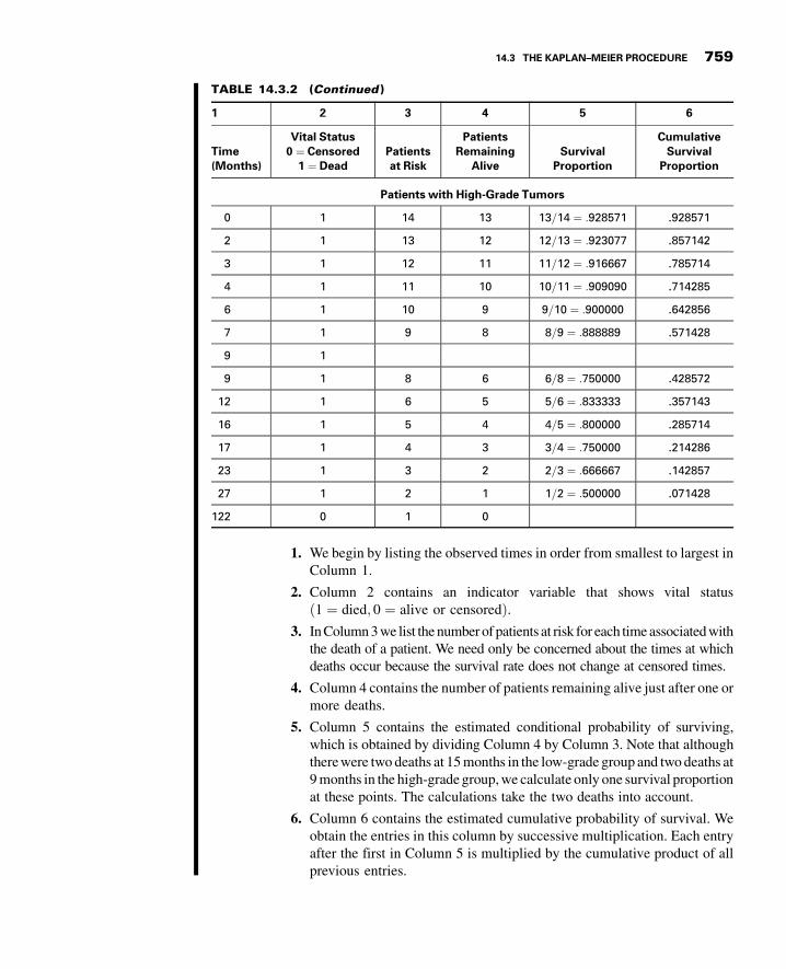
3GC14 12/04/2012 16:22:2 Page 759

1. We begin by listing the observed times in order from smallest to largest inColumn 1.

2. Column 2 contains an indicator variable that shows vital status1 ¼ died; 0 ¼ alive or censoredð Þ.

3. In Column 3 we list the number of patients at risk for each time associated withthe death of a patient. We need only be concerned about the times at whichdeaths occur because the survival rate does not change at censored times.

4. Column 4 contains the number of patients remaining alive just after one ormore deaths.

5. Column 5 contains the estimated conditional probability of surviving,which is obtained by dividing Column 4 by Column 3. Note that althoughthere were two deaths at 15 months in the low-grade group and two deaths at9 months in the high-grade group, we calculate only one survival proportionat these points. The calculations take the two deaths into account.

6. Column 6 contains the estimated cumulative probability of survival. Weobtain the entries in this column by successive multiplication. Each entryafter the first in Column 5 is multiplied by the cumulative product of allprevious entries.

Patients with High-Grade Tumors

0 1 14 13 13=14 ¼ :928571 .928571

2 1 13 12 12=13 ¼ :923077 .857142

3 1 12 11 11=12 ¼ :916667 .785714

4 1 11 10 10=11 ¼ :909090 .714285

6 1 10 9 9=10 ¼ :900000 .642856

7 1 9 8 8=9 ¼ :888889 .571428

9 1

9 1 8 6 6=8 ¼ :750000 .428572

12 1 6 5 5=6 ¼ :833333 .357143

16 1 5 4 4=5 ¼ :800000 .285714

17 1 4 3 3=4 ¼ :750000 .214286

23 1 3 2 2=3 ¼ :666667 .142857

27 1 2 1 1=2 ¼ :500000 .071428

122 0 1 0

TABLE 14.3.2 (Continued )

1 2 3 4 5 6

Time(Months)

Vital Status0 ¼ Censored

1 ¼ DeadPatientsat Risk

PatientsRemaining

AliveSurvival

Proportion

CumulativeSurvival

Proportion

14.3 THE KAPLAN–MEIER PROCEDURE 759

3GC14 12/04/2012 16:22:2 Page 760

After the calculations are completed we examine Table 14.3.2 to deter-mine what useful information it provides. From the table we note the followingfacts, which allow us to compare the survival experience of the two groups ofsubjects: those with low-grade tumors and those with high-grade tumors:

1. Median survival time. We can determine the median survival time by locatingthe time, in months, at which the cumulative survival proportion is equal to .5.None of the cumulative survival proportions are exactly .5, but we see that in thelow-grade tumor group, the probability changes from .619860 to .309930 at 212months; therefore, the median survival for this group is 212 months. In the high-grade tumor group, the cumulative proportion changes from .571428 to .428572at 9 months, which is the median survival for this group.

2. Five-year survival rate. We can determine the 5-year or 60-month survivalrate for each group directly from the cumulative survival proportion at60 months. For the low-grade tumor group, the 5-year survival rate is.734298 or 73 percent; for the high-grade tumor group, the 5-year survivalrate is .071428 or 7 percent.

3. Mean survival time. We may compute for each group the mean of thesurvival times, which we will call TL and TH for the low-grade and high-grade groups, respectively. For the low-grade tumor group we computeTL ¼ 2201=25 ¼ 88:04, and for the high-grade tumor group we computeTH ¼ 257=14 ¼ 18:35. Since so many of the times in the low-grade groupare censored, the true mean survival time for that group is, in reality, higher(perhaps, considerably so) than 88.04. The true mean survival time for thehigh-grade group is also likely higher than the computed 18.35, but with justone censored time we do not expect as great a difference between thecalculated mean and the true mean. Thus, we see that we have still anotherindication that the survival experience of the low-grade tumor group is morefavorable than the survival experience of the high-grade tumor group.

4. Average hazard rate. From the raw data of each group we may also calculateanother descriptive statistic that can be used to compare the two survivalexperiences. This statistic is called the average hazard rate. It is a measure ofnonsurvival potential rather than survival. A group with a higher averagehazard rate will have a lower probability of surviving than a group with alower average hazard rate. We compute the average hazard rate, designated hby dividing the number of subjects who do not survive by the sum of theobserved survival times. For the low-grade tumor group, we computehL ¼ 9=2201 ¼ :004089. For the high-grade tumor group we computehH ¼ 13=257 ¼ :05084, We see that the average hazard rate for the high-grade group is higher than for the low-grade group, indicating a smallerchance of surviving for the high-grade group.

The cumulative survival proportion column of Table 14.3.2 may beportrayed visually in a survival curve graph in which the cumulative survivalproportions are represented by the vertical axis and the time in months by thehorizontal axis. We note that the graph resembles stairsteps with “steps”occurring at the times when deaths occurred. The graph also allows us


3GC14 12/04/2012 16:22:3 Page 761

to represent visually the median survival time and survival rates such as the5-year survival rate. The graph for the cumulative survival data ofTable 14.3.2 is shown in Figure 14.3.1.

These observations strongly suggest that the survival experience ofpatients with low-grade tumors is far more favorable than that of patients withhigh-grade tumors. &

EXERCISES

14.3.1 Fifty-three patients with medullary thyroid cancer (MTC) were the subjects of a study by Dottoriniet al. (A-2), who evaluated the impact of different clinical and pathological factors and the type oftreatment on their survival. Thirty-two of the patients were females, and the mean age of all patientswas 46.11 years with a standard deviation of 14.04 (range 18–35 years). The following table showsthe status of each patient at various periods of time following surgery. Calculate the survival functionusing the Kaplan–meier procedure and plot the survival curve.

Subject Timea (Years) Statusb Subject Timea (Years) Statusb

1 0 doc 28 6 alive2 1 mtc 29 6 alive3 1 mtc 30 6 alive4 1 mtc 31 6 alive5 1 mtc 32 7 mtc6 1 mtc 33 8 alive7 1 mtc 34 8 alive8 1 mtc 35 8 alive9 1 alive 36 8 alive

10 2 mtc 37 8 alive

1.0

.8

.6

.5

.4

.2

0.0120 24 36 48 60

73%

72 84 96 108 120

Time (Months)

Low–grade (N = 25)

7% High–grade (N = 14)

FIGURE 14.3.1 Kaplan–Meier survival curve, Example 14.3.1, showing median survival times

and 5-year (60-month) survival rates.

(Continued)

EXERCISES 761

3GC14 12/04/2012 16:22:4 Page 762

11 2 mtc 38 9 alive12 2 mtc 39 10 alive13 2 alive 40 11 mtc14 2 alive 41 11 doc15 3 mtc 42 12 mtc16 3 mtc 43 12 doc17 3 alive 44 13 mtc18 4 mtc 45 14 alive19 4 alive 46 15 alive20 4 alive 47 16 mtc21 4 alive 48 16 alive22 5 alive 49 16 alive23 5 alive 50 16 alive24 5 alive 51 17 doc25 5 alive 52 18 mtc26 6 alive 53 19 alive27 6 alive

a Time is number of years after surgery.b doc ¼ dead of other causes; mtc ¼ dead of medullary thyroid cancer.source: Data provided courtesy of Dr. Massimo E. Dottorini.

14.3.2 Banerji et al. (A-3) followed non–insulin-dependent diabetes mellitus (NIDDM) patients from onsetof their original hyperglycemia and the inception of their near–normoglycemic remission followingtreatment. Subjects were black men and women with a mean age of 45.4 years and a standarddeviation of 10.4. The following table shows the relapse/remission experience of 62 subjects.Calculate the survival function using the Kaplan–Meier procedure and plot the survival curve.

TotalDuration ofRemission(Months)

RemissionStatusa


RemissionStatusa


RemissionStatusa

3 1 8 2 26 13 2 9 2 27 13 1 10 1 28 23 1 10 1 29 13 1 11 2 31 24 1 13 1 31 14 1 16 1 33 24 1 16 2 39 25 1 17 2 41 15 1 18 2 44 15 1 20 1 46 15 1 22 1 46 25 1 22 2 48 15 1 22 2 48 2

Subject Timea (Years) Statusb Subject Timea (Years) Statusb

(Continued)


3GC14 12/04/2012 16:22:5 Page 763

5 1 23 1 48 16 1 24 2 49 16 1 25 2 50 16 1 25 2 53 17 1 26 1 70 28 2 26 1 94 18 18 2

a 1 ¼ yes (the patient is still in remission); 2 ¼ no (the patient has relapsed).Source: Data provided Courtesy of Dr. Mary Ann Banerji.

14.4 COMPARING SURVIVAL CURVES

Examination of a survival curve for a single group of individuals is valuable in that it allowsone to see characteristics that are not as easily seen by examining a set of tabulated values.This includes visualizing the temporal trajectory to find time periods in which there weredramatic changes in survival, finding time periods in which relatively little changeoccurred, or in finding the approximate median of the data distribution. The constructionof survival curves, however, finds its greatest use when comparisons among survivaldistributions are of interest. For example, one may wish to examine differences in treatmentin which subjects were randomly assigned, or may wish to know which medication delaysthe onset of the event of interest for the longest period of time.

The results of comparing the survival experiences of different groups will not alwaysbe as dramatic as those of our previous example. For an objective comparison of thesurvival experiences of different groups, it is desirable that we have an objective techniquefor determining whether they are statistically significantly different. We know also that theobserved results apply strictly to the samples on which the analyses are based. Of muchgreater interest is a method for determining if we may conclude that there is a differencebetween survival experiences in the populations from which the samples were drawn. Inother words, at this point, we desire a method for testing the null hypothesis that there is nodifference in survival experience between populations against the alternative that there is adifference. Such a test is provided by the log-rank test. The log-rank test is an application ofthe Mantel–Haenszel procedure discussed in Section 12.7. The extension of the procedureto survival data was proposed by Mantel (6). Though we may wish to compare survivalcurves of many populations, we will limit our discussion to the comparison of two groups:To accomplish this task, we calculate the log-rank statistic and proceed as follows:

1. Order the survival times until death for both groups combined, omitting censoredtimes. Each time constitutes a stratum as defined in Section 12.7.

2. For each stratum or time, ti, we construct a 2 � 2 table in which the first rowcontains the number of observed deaths, the second row contains the number of


RemissionStatusa


RemissionStatusa


RemissionStatusa

14.4 COMPARING SURVIVAL CURVES 763

3GC14 12/04/2012 16:22:5 Page 764

patients alive, the first column contains data for one group, say, group A, and thesecond column contains data for the other group, say, group B. Table 14.4.1 showsthe table for time ti.

3. For each stratum compute the expected frequency for the upper left-hand cell of itstable by Equation 12.7.5.

4. For each stratum compute vi by Equation 12.7.6.

5. Finally, compute the Mantel–Haenszel statistic (now called the log-rank statistic) byEquation 12.7.7.

We illustrate the calculation of the log-rank statistic with the following example.

EXAMPLE 14.4.1

Let us refer again to the data on primary malignant tumors of the sternum presented inExample 14.3.1. Examination of the data reveals that there are 20 time periods (strata).For each of these a 2 � 2 table following the pattern of Table 14.4.1 must be constructed.The first of these tables is shown as Table 14.4.2. By Equations 12.7.5 and 12.7.6 wecompute ei and vi as follows:

ei ¼ 0 þ 1ð Þ 0 þ 25ð Þ39

¼ :641

vi ¼ 0 þ 1ð Þ 25 þ 13ð Þ 0 þ 25ð Þ 1 þ 13ð Þ392 38ð Þ ¼ :230

The data for Table 14.4.2 and similar data for the other 19 time periods are shown inTable 14.4.3. Using data from Table 14.4.3, we compute the log-rank statistic by Equation12.7.7 as follows:

x2MH ¼ 9 � 17:811ð Þ2

3:140¼ 24:724

TABLE 14.4.2 Contingency Table for First Stratum (TimePeriod) for Calculating the Log-Rank Test, Example 14.4.1

Low-Grade High-Grade Total

Deaths 0 1 1

Patients alive 25 13 38

Patients at risk 25 13 39

TABLE 14.4.1 Contingency Table for Stratum (Time) ti for Calculating the Log-

Rank Test

Group A Group B Total

Number of deaths observed ai bi ai + bi

Number of patients alive ci di ci + di

Number of patients “at risk” ai + ci bi + di ni ¼ ai + bi + ci + di


3GC14 12/04/2012 16:22:6 Page 765

Reference to Appendix Table F reveals that since 24:724 > 7:879, the p value for this testis < :005. We, therefore, reject the null hypothesis that the survival experience is the samefor patients with low-grade tumors and high-grade tumors and conclude that they aredifferent.

There are alternative procedures for testing the null hypothesis that two survivalcurves are identical. They include the Breslow test (also called the generalized Wilcoxontest) and the Tarone–Ware test. Both tests, as well as the log-rank test, are discussed inParmar and Machin (7) and Allison (4). Like the log-rank test, the Breslow test and theTarone–Ware test are based on the weighted differences between actual and expectednumbers of deaths at the observed time points. Whereas the log-rank test ranks all deathsequally, the Breslow and Tarone–Ware tests give more weight to early deaths. For Example12.8.1, SPSS computes a value of 24:93 p < :001ð Þ for the Breslow test and a value of25:22 p < :001ð Þ for the Tarone–Ware test. Kleinbaum (27) discusses another test calledthe Peto test. Formulas for this test are found in Parmar and Machin (7). The Peto test alsogives more weight to the early part of the survival curve, where we find the larger numbersof subjects at risk. When choosing a test, then, researchers who want to give more weight tothe earlier part of the survival curve will select either the Breslow, the Tarone–Ware, or thePeto test. Otherwise, the log-rank test is appropriate.

TABLE 14.4.3 Intermediate Calculations for the Log-Rank Test, Example 14.4.1

Time, ti ai ci ai þ ci bi di bi þ di ni ei yi

0 0 25 25 1 13 14 39 0.641 0.230

2 0 25 25 1 12 13 38 0.658 0.225

3 0 25 25 1 11 12 37 0.676 0.219

4 0 25 25 1 10 11 36 0.694 0.212

6 0 25 25 1 9 10 35 0.714 0.204

7 0 24 24 1 8 9 33 0.727 0.198

9 0 23 23 2 6 8 31 1.484 0.370

11 1 22 23 0 6 6 29 0.793 0.164

12 0 22 22 1 5 6 28 0.786 0.168

15 2 20 22 0 5 5 27 1.630 0.290

16 0 20 20 1 4 5 25 0.800 0.160

17 0 20 20 1 3 4 24 0.833 0.139

21 1 19 20 0 3 3 23 0.870 0.113

23 0 19 19 1 2 3 22 0.864 0.118

27 0 18 18 1 1 2 20 0.900 0.090

29 1 17 18 0 1 1 19 0.947 0.050

33 1 16 17 0 1 1 18 0.944 0.052

79 1 13 14 0 1 1 15 0.933 0.062

102 1 10 11 0 1 1 12 0.917 0.076

212 1 1 2 0 0 0 2 1.000 0.000

Totals 9 17.811 3.140

14.4 COMPARING SURVIVAL CURVES 765

3GC14 12/04/2012 16:22:7 Page 766

We have covered only the basic concepts of survival analysis in this section. Thereader wishing to pursue the subject in more detail may consult one or more of severalbooks devoted to the topic, such as those by Kleinbaum (8), Lee (9), Marubini andValsecchi (10), and Parmar and Machin (7).

Computer analysis

Several of the available statistical software packages, such as SPSS, are capable ofperforming survival analysis and constructing supporting graphs as described in this section.

A standard SPSS analysis of the data discussed in Examples 14.3.1 and 14.4.1 isshown in Figure 14.4.1. &

Tumor_grade

H

L

Overall

18.357

88.040

63.026

Chi-Square

24.704

24.92725.217

1

df Sig.

.000

.000

.000

Test of equality of survival distributions for the different levels of tumor_grade.

11

Log Rank (Mantel-Cox)Breslow (GeneralizedWilcoxon)Tarone-Ware

8.251

15.258

11.490

2.186

58.134

40.505

34.528

117.946

85.546

9.000

82.000

27.000

1.852

16.653

7.492

5.371

49.359

12.317

12.629

114.641

41.683

Estimate

a Estimation is limited to the largest survival time if it is censored.

95% Confidence Interval 95% Confidence Interval

Meana

Estimate

Median

Std.Error

Std.Error

LowerBound

LowerBound

UpperBound

UpperBound

Means and Medians for Survival Time

Overall Comparisons

FIGURE 14.4.1 SPSS output for Examples 14.3.1 and 14.4.1.


3GC14 12/04/2012 16:22:8 Page 767

EXERCISES

14.4.1 If available in your library, read the article, “Impact of Obesity on Allogeneic Stem Cell TransplantPatients: A Matched Case-Controlled Study,” by Donald R. Fleming et al. [American Journal ofMedicine, 102 (1997), 265–268] and answer the following questions:

(a) How was survival time determined?

(b) Why do you think the authors used the Wilcoxon test (Breslow test) for comparing the survivalcurves?

(c) Explain the meaning of the p values reported for Figures 1 through 4.

(d) What specific statistical results allow the authors to arrive at their stated conclusion?

14.4.2 If available in your library, read the article, “Improved Survival in Patients with Locally AdvancedProstate Cancer Treated with Radiotherapy and Goserelin,” by Michel Bolla et al. [New EnglandJournal of Medicine, 337 (1997), 295–300], and answer the following questions:

(a) How was survival time determined?

(b) Why do you think the authors used the log-rank test for comparing the survival curves?

(c) Explain the meaning of the p values reported for Figures 1 and 2.

(d) What specific statistical results allow the authors to arrive at their stated conclusion?

14.4.3 Fifty subjects who completed a weight-reduction program at a fitness center were divided into twoequal groups. Subjects in group 1 were immediately assigned to a support group that met weekly.Subjects in group 2 did not participate in support group activities. All subjects were followed for aperiod of 60 weeks. They reported weekly to the fitness center, where they were weighed and adetermination was made as to whether they were within goal. Subjects were considered to be withingoal if their weekly weight was within 5 pounds of their weight at time of completion of the weight-reduction program. Survival was measured from the date of completion of the weight-reductionprogram to the termination of follow-up or the point at which the subject exceeded goal. Thefollowing results were observed:

SubjectTime

(Weeks)

Status(G ¼Within Goal

Gþ ¼ Exceeded GoalL ¼ Lost to Follow-Up) Subject

Time(Weeks)


Gþ ¼ Exceeded GoalL ¼ Lost to Follow-Up)

Group 1 Group 2

1 60 G 1 20 Gþ2 32 L 2 26 Gþ3 60 G 3 10 Gþ4 22 L 4 2 Gþ5 6 Gþ 5 36 Gþ6 60 G 6 10 Gþ7 60 G 7 20 Gþ8 20 Gþ 8 18 L9 32 Gþ 9 15 Gþ

10 60 G 10 22 Gþ11 60 G 11 4 Gþ12 8 Gþ 12 12 Gþ

(Continued)

EXERCISES 767

3GC14 12/04/2012 16:22:8 Page 768

13 60 G 13 24 Gþ14 60 G 14 6 Gþ15 60 G 15 18 Gþ16 14 L 16 3 Gþ17 16 Gþ 17 27 Gþ18 24 L 18 22 Gþ19 34 L 19 8 Gþ20 60 G 20 10 L21 40 L 21 32 Gþ22 26 L 22 7 Gþ23 60 G 23 8 Gþ24 60 G 24 28 Gþ25 52 L 25 7 Gþ

Analyze these data using the methods discussed in this section.

14.5 COX REGRESSION: THE PROPORTIONALHAZARDSMODEL

In previous chapters, we saw that regression models can be used for continuous outcomemeasures and for binary outcome measures (logistic regression). Additional regressiontechniques are available when the dependent measures may consist of a mixture of eithertime-to-event data or censored time observations. Returning to our example of a clinicaltrial of the effectiveness of two different medications to prevent a second myocardialinfarction, we may wish to control for additional characteristics of the subjects enrolled inthe study. For example, we would expect subjects to be different in their baseline systolicblood pressure measurements, family history of heart disease, weight, body mass, andother characteristics. Because all of these factors may influence the length of the timeinterval until a second myocardial infarction, we would like to account for these factors indetermining the effectiveness of the medications. The regression method known as Coxregression (after D. R. Cox (11), who first proposed the method) or proportional hazardregression can be used to account for the effects of continuous and discrete covariate(independent variable) measurements when the dependent variable is possibly censoredtime-to-event data.

We describe this technique by first reviewing the hazard function from Section 14.2,which describes the conditional probability that an event will occur at a time just largerthan ti conditional on having survived event-free until time ti. This function is often writtenas h(ti). The regression model requires that we assume the covariates have the effect of

SubjectTime

(Weeks)


Gþ ¼ Exceeded GoalL ¼ Lost to Follow-Up) Subject

Time(Weeks)


Gþ ¼ Exceeded GoalL ¼ Lost to Follow-Up)

Group 1 Group 2


3GC14 12/04/2012 16:22:9 Page 769

either increasing or decreasing the hazard for a particular individual compared to somebaseline value for the function. In our clinical trial example we might measure k covariateson each of the subjects where there are i ¼ 1; . . . ; n subjects and h0 tið Þ is the baselinehazard function. We describe the regression model as

h tið Þ ¼ h0 tið Þ exp b1zi1 þ b2zi2 þ � � � þ bkzikð Þ (14.5.1)

The regression coefficients represent the change in the hazard that resultsfrom the risk factor, zik, that we have measured. Rearranging the above equationshows that the exponentiated coefficient represents the hazard ratio or the ratio of theconditional probabilities of an event. This is the basis for naming this methodproportional hazards regression. You may recall that this is the same way we obtainedthe estimate of the odds ratio from the estimated coefficient when we discussed logisticregression in Chapter 11.

h tið Þh0 tið Þ ¼ exp b1zi1 þ b2zi2 þ � � � þ bkzikð Þ (14.5.2)

Estimating the covariate effects, b requires the use of a statistical software package becausethere is no straightforward single equation that will provide the estimates for this regressionmodel. Computer output usually includes estimates of the regression coefficients, standarderror estimates, hazard ratio estimates, and confidence intervals. In addition, computer outputmay also provide graphs of the hazard functions and survival functions for subjects withdifferent covariate values that are useful to compare the effects of covariates on survival.

EXAMPLE 14.5.1

To determine whether time to relapse among drug users is related to patient age and/orthe drug of choice, Cross (unpublished clinical data) reviewed a random sample of casefiles for high-risk drug users in an outpatient treatment clinic. The data represent the self-reported time that relapse occurred (or the time at which the patient was lost to follow-up), patient status, drug of choice, and patient age. The data are summarized inTable 14.5.1.

TABLE 14.5.1 Survival Data for Patients in an Outpatient Treatment Clinic

Subject

Time

(Weeks)

Status

0¼Censored

1¼Relapse

Drug

1¼Opiate

2¼Other Age Subject

Time

(Weeks)

Status

0¼Censored

1¼Relapse

Drug

1¼Opiate

2¼Other Age

1 12 1 1 21 21 21 1 2 28

2 8 1 1 18 22 41 1 2 31

3 5 1 1 17 23 23 0 2 22

4 17 1 1 17 24 15 1 2 31

5 19 1 1 25 25 15 0 2 25

6 12 0 1 30 26 21 1 2 19

(Continued)

14.5 COX REGRESSION: THE PROPORTIONAL HAZARDSMODEL 769

3GC14 12/04/2012 16:22:11 Page 770

For this example, we will employ the Cox Regression method algorithms provided inSPSS software. All references to tables and figures in the explanations below refer toFigure 14.5.1, which shows selected SPSS output for this example.

1. Overall test. SPSS provides an overall test of significance much like that reported forlogistic regression discussed in Chapter 11. In this test, the likelihood is used tocompare a model with no parameters (the null model) and a model with the variablesof interest included. If there is a significant difference in the likelihood functionbetween the model with parameters and the null model, then the Cox regressionmodel is significant, and at least one of the variables of interest is significantly relatedto the outcome variable. An examination of the output shows that the Omnibus Testfor Model Coefficients with age and drug entered in the model is significantlydifferent from the null model, with p< .001.

2. Variables in the model. Next SPSS provides a table for each of the variables enteredinto the model. Much like a standard regression model, the model parameter, itsstandard error, and a significance test are provided to test the null, Ho: b¼ 0. Forthese data, type of drug was significantly predictive of time to relapse (p< .001), butage was not (p¼ .792).

3. Survival curves. Since drug of choice was found to be significantly related to thetime of relapse, it is instructive to examine the survival curves for these data. It isclear from examining these curves that there is a difference in time to relapse, withthose reporting opiate use as their primary drug of choice relapsing at a much fasterrate than those reporting use of drugs other than opiates.

4. Hazard ratios. The hazard ratios are provided for each variable in the model. As inlogistic regression where we calculated odds ratios, hazard ratios are found by

7 10 1 1 16 27 45 1 2 21

8 11 1 1 23 28 37 1 2 23

9 5 1 1 31 29 51 1 2 15

10 2 1 1 21 30 50 1 2 29

11 10 1 1 19 31 42 1 2 28

12 7 0 1 18 32 21 1 2 31

13 19 1 1 18 33 20 1 2 31

14 11 1 1 21 34 15 1 2 26

15 11 1 1 23 35 40 1 2 28

16 19 1 1 15 36 39 1 2 31

17 19 1 1 17 37 33 1 2 23

18 24 1 1 21 38 37 1 2 23

19 21 1 1 22 39 15 0 2 29

20 14 1 1 17 40 52 0 2 37

Source: Data provided courtesy of Dr. Chad L. Cross.

TABLE 14.5.1 (Continued )

Subject

Time

(Weeks)

Status

0¼Censored

1¼Relapse

Drug

1¼Opiate

2¼Other Age Subject

Time

(Weeks)

Status

0¼Censored

1¼Relapse

Drug

1¼Opiate

2¼Other Age


3GC14 12/04/2012 16:22:11 Page 771

calculating exp(b). Examining the variable drug, where opiates were used as theindicator variable in SPSS, the hazard of relapse is nearly 8.5 times more likely foropiates compared to other drugs, controlling for the covariate of age. Although wecan calculate the hazard ratio for age in much the same way as for drug, it isoften useful for quantitative covariates to consider calculating the function100(exp(b)� 1), which provides an estimate of the percent change in the hazardwhen the covariate increases by one unit. In the present example for age, this leads to

1.0

Variables in the Equation

Omnibus Tests of Model Coefficients

Drug

age

2.139

–.009

.531

.032

.000

.792

8.492

.991

3.000

.930

24.036

1.057

95.0% Cl for Exp(B)

LowerExp(B)Sig.dfWald

Overall (score)

Chi-square

–2 LogLikelihood

167.407 25.558df Sig.

2 .000

SEB Upper16.239

.070

1

1

0.8

0.6

drugOpiateOther

0.4

Cu

mu

lati

ve

Su

rviv

al

0.2

0.0

.00 10.00 20.00 30.00

Weeks

40.00 50.00 60.00

FIGURE 14.5.1 Cox Regression survival analysis output from SPSS software for

Example 14.5.1.

14.5 COX REGRESSION: THE PROPORTIONAL HAZARDSMODEL 771

3GC14 12/04/2012 16:22:11 Page 772

100(.991� 1)¼�.9. Therefore, for each 1 year increase in age, the hazard forrelapse decreases by an average of about .9 percent.

5. Conclusion. Based on the results of this limited sample, we have learned that age ofthe patient, though not statistically significant, suggest that in general age may besomewhat protective in that risk of relapse decreases with age. We have alsolearned that those experiencing addiction to opiates are prone to relapse muchearlier in their treatment. The results of this preliminary study may be used todevelop further studies to determine if different, and perhaps more intensive,treatment programs are more successful for targeting those experience opiateaddiction compared to other drugs. &

Clearly Cox regression can become very complex as the number of variablesincreases. As with standard regression models discussed in early chapters, one may optto use selection procedures (forward, backward, or stepwise) or examine interactionsamong variables in the models. Additionally, one may have time-dependent covariates inwhich the value of the covariate may change at each measurement time. Examples of thismay be marriage or diagnosis with a health condition. These covariates are in contrast totime-constant covariates, which do not change (e.g., gender). In summary, Cox regressionis a very useful technique for modeling survival data. For those interested in furtherreading, the texts by Kleinbaum and Klein (1), Lee (2), Hosmer and Lemeshow (3), andAllison (4) are highly recommended.

EXERCISES

14.5.1 In a study examining time-to-onset of cancer after exposure to UV light in rats, age (months) wasused as a covariate in a Cox regression model. In the model, the parameter estimate for weight was .19and had a p-value of .021. Provide an interpretation of this parameter estimate in terms of the hazardratio.

14.5.2 In the study described in Exercise 14.5.1, the researchers were also interested to know if there was adifference between gender in the time it took to develop cancer. For gender, the parameter estimatewas .77 and had a p-value of 0.014. Provide an interpretation of this parameter estimate in terms of thehazard ratio.

14.5.3 The intent of a study by Weaver et al. (A-4) was to assess whether occult lymph node metastases areimportant indicators of disease recurrence or survival in breast cancer patients. The data belowprovide some of the pertinent results of a Cox regression model for these data.

(a) Calculate the regression parameter coefficients for each variable.

(b) Provide an interpretation of these results using the concepts learned in this section.

Variable Hazard Ratio (HR) 95% CI for HR p-value

Age (50þ vs. <50) 1.69 (1.24, 2.31) .001Tumor size (>2 cm vs. � 2 cm) 1.32 (.98, 1.76) .060Chemotherapy vs. no chemotherapy .88 (.68, 1.13) .31Radiation vs. no radiation 0.54 (.40, .73) .001


3GC14 12/04/2012 16:22:11 Page 773

14.6 SUMMARY

In this chapter an introduction to time-to-event data was provided. In particular, theconcept of data censoring, in which exact times are not known for subjects, wasintroduced. Distributions useful in survival analysis, including the cumulative distribu-tion function, the survival function, and the hazard function were discussed. Calculatingbasic survival curves using the Kaplan–Meier procedure was discussed, as were methodsfor comparing survival curves using nonparametric methods. Regression concepts usingCox regression were provided, and detailed analysis of examples was given. Therelationship of several methods covered in this chapter was tied to concepts learnedearlier in the text, including linear regression, analysis of frequency data, and non-parametric statistics.


FormulaNumber

Name Formula

14.2.1 Cumulativedistribution function

FðtÞ ¼ PðT � tÞ

14.2.2 Survival function SðtÞ ¼ 1 � FðtÞ14.2.3 Probability

distribution functionf ðtÞ ¼ Pðt � T < t þ DtÞ

Dt; as Dt ! 0

14.2.4 Relationship ofprobabilitydistribution functionto the cumulativedistribution functionand the survivalfunction

f ðtÞ ¼ DFðtÞDt

¼ �DSðtÞDt

14.2.5 Hazard functionhðtÞ ¼ Pðt � T < t þ DtjT � tÞ

Dt; as Dt ! 0

14.2.7 Relationship of thehazard function tothe probabilitydistribution functionand the survivalfunction

hðtÞ ¼ f ðtÞSðtÞ

14.3.1 Survival probability number of subjects surviving at least t � 1ð Þ time period

pi ¼who also survive the tth period

number of subjects alive at end of time period t � 1ð Þ14.3.2 Estimated survival

functionS tð Þ ¼ p1 � p2 � � � � � pt


3GC14 12/04/2012 16:22:12 Page 774

14.5.1 Hazard regressionmodel

h tið Þ ¼ h0 tið Þ exp b1zi1 þ b2zi2 þ � � � þ bkzikð Þ

14.5.2 Proportional hazardmodel

h tið Þho tið Þ ¼ exp b1zi1 þ b2zi2 þ � � � þ bkzikð Þ

SymbolKey

� b¼ regression coefficient� D¼ change� F(t)¼ cumulative distribution function� f(t)¼ probability density function� h(t)¼ hazard function� p¼ probability� S(t)¼ survival function� T¼ time of interest� t¼ time to event� z¼ risk factor in Cox regression


1. Describe in words the concept of data censoring.


(a) Hazard ratio

(b) Hazard function

(c) Probability distribution function

(d) Survival function

(e) Kaplan–Meier estimate

3. Explain the concepts underlying the Cox regression model.

4. What is the difference between right censoring and left censoring? Provide an example of each.

5. Discuss why it is often preferable to use a nonparametric test for comparisons of survival curves.

6. Why is Cox regression called a “proportional hazards” model?

7. If the probability distribution function at time 5 is equal to .25 and the survival function at time 5 isequal to .15, what is the hazard function at time 5?

8. If we find that a measurement in the time interval between time 2 and 10 results in a probabilitydistribution function estimate of 0.03, what is the estimated change in the cumulative distributionfunction?

9. Using the data from question 8, what is the estimated change in the survival function?

10. Explain why the cumulative distribution function and the survival function are mirror images of oneanother.

11. The objective of a study by Lee et al. (A-5) was to improve understanding of the biologic behavior ofgastric epithelioid stromal tumors. They studied the clinical features, histologic findings, and DNAploidy of a series of the tumors to identify factors that might distinguish between benign andmalignant variants of these tumors and have relevance for prognosis. Fifty-five patients with tumors


3GC14 12/04/2012 16:22:14 Page 775

(Continued)

were classified on the basis of whether their tumors were high-grade malignant (grade 2), low-grademalignant (grade 1), or benign (grade 0). Among the data collected were the following:

PatientTumorGrade

Outcome(1 ¼ Death

fromDisease)

Number ofDays to LastFollow-Up or

Death PatientTumorGrade

Outcome(1 ¼ Death

fromDisease)

Number ofDays to LastFollow-Up or

Death

1 0 0 87 8 0 0 16162 0 0 775 9 0 0 19823 0 0 881 10 0 0 20354 0 0 914 11 0 0 21915 0 0 1155 12 0 0 24726 0 0 1162 13 0 0 25277 0 0 1271 14 0 0 2782

15 0 0 3108 36 0 0 731816 0 0 3158 37 0 0 744717 0 0 3609 38 0 0 952518 0 0 3772 39 0 0 993819 0 0 3799 40 0 0 1042920 0 0 3819 41 1 1 45021 0 0 4586 42 1 1 55622 0 0 4680 43 1 1 210223 0 0 4989 44 1 0 275624 0 0 5675 45 1 0 349625 0 0 5936 46 1 1 399026 0 0 5985 47 1 0 568627 0 0 6175 48 1 0 629028 0 0 6177 49 1 0 849029 0 0 6214 50 2 1 10630 0 0 6225 51 2 1 16931 0 0 6449 52 2 1 30632 0 0 6669 53 2 1 34833 0 0 6685 54 2 1 54934 0 0 6873 55 2 1 97335 0 0 6951

Source: Data provided courtesy of Dr. Michael B. Farnell.

12. Girard et al. (A-6) conducted a study to identify prognostic factors of improved survival afterresection of isolated pulmonary metastases (PM) from colorectal cancer. Among the data collectedwere the following regarding number of resected PM, survival, and outcome for 77 patients whounderwent a complete resection at the first thoracic operation:

PatientNumber ofResected PM

Survival(Months) Status Patient

Number ofResected PM

Survival(Months) Status

1 1 24 Alive 8 1 15 Dead2 1 67 Alive 9 1 10 Dead3 1 42 Alive 10 1 41 Dead4 > 1 28 Dead 11 > 1 41 Dead5 1 37 Dead 12 1 27 Dead6 1 133 Alive 13 1 93 Alive7 1 33 Dead 14 > 1 0 Dead

15 1 60 Dead 47 1 54 Dead


3GC14 12/04/2012 16:22:15 Page 776

PatientNumber ofResected PM

Survival(Months) Status Patient

Number ofResected PM

Survival(Months) Status

16 1 43 Dead 48 > 1 57 Alive17 > 1 73 Alive 49 > 1 16 Dead18 1 55 Alive 50 1 29 Dead19 1 46 Dead 51 1 14 Dead20 1 66 Alive 52 > 1 29 Dead21 1 10 Dead 53 > 1 99 Dead22 > 1 3 Dead 54 > 1 23 Dead23 > 1 7 Dead 55 1 74 Alive24 > 1 129 Alive 56 1 169 Alive25 1 19 Alive 57 > 1 24 Dead26 > 1 15 Dead 58 > 1 9 Dead27 1 39 Alive 59 1 43 Dead28 1 15 Dead 60 1 3 Alive29 > 1 30 Dead 61 > 1 20 Dead30 1 35 Alive 62 1 2 Dead31 > 1 18 Dead 63 > 1 41 Dead32 1 27 Dead 64 > 1 27 Dead33 1 121 Alive 65 1 45 Alive34 > 1 8 Dead 66 1 26 Dead35 1 24 Alive 67 > 1 10 Dead36 1 127 Alive 68 1 143 Alive37 1 26 Dead 69 1 16 Dead38 > 1 7 Dead 70 1 29 Alive39 > 1 26 Dead 71 1 17 Dead40 > 1 17 Dead 72 > 1 20 Dead41 1 18 Dead 73 1 92 Alive42 1 17 Dead 74 > 1 15 Dead43 > 1 10 Dead 75 1 5 Dead44 > 1 33 Dead 76 > 1 73 Alive45 > 1 42 Alive 77 1 19 Dead46 1 40 Alive

Source: Data provided courtesy of Dr. Philippe Girard.

13. In a study by Alicikus et al. (A-7), long-term control of prostate cancer receiving radiotherapy wasexamined in patients after 10 years. The authors using Cox regression analysis to analyze these data,which resulted in the data summarized in the table below. For these data:

(a) Calculate the parameter estimates for the Cox regression model.

(b) Provide an explanation of the hazard ratios (HR) and their meaning.

(c) For age, provide an alternative measure for the HR and provide its meaning in terms of thepercent change in years.

Variable Hazard Ratio (HR) 95% CI for HR p-value

Age 1.02 (.96, 1.08) .51Hormone therapy (yes vs. no) .89 (.44, 1.81) .75Pre-PSA, >10 ng/mL vs. �10 ng/mL 2.41 (1.19, 4.88) .015Tumor classification 1.42 (1.17, 1.71) <.001

Source: ZUMRE A. ALICIKUS, YOSHIYA YAMADA, ZHIGANG ZHANG, XIN PEI, MARGIE HUNG, MARISA KOLLMEIER, BRETT

COX, and MICHAEL J. ZELEFSKY, “Ten-year Outcomes of High-Dose, Intensity-Modulated Radiotherapy forLocalized Prostate Cancer,” Cancer, 117 (2010), 1429–1437.


3GC14 12/04/2012 16:22:15 Page 777

REFERENCES


1. DAVID G. KLEINBAUM and MITCHEL KLEIN, Survival Analysis: A Self-Learning Text, Second Edition, Springer, NewYork, 2005.

2. ELISA T. LEE, Statistical Methods for Survival Data Analysis, Third Edition, Wiley, New York, 2003.3. DAVID W. HOSMER, JR. and STANLEY LEMESHOW, Applied Survival Analysis: Regression Modeling of Time to Event

data, Wiley, New York, 1999.4. PAUL D. ALLISON, Survival Analysis using SAS®: A Practical Guide, Second Edition, SAS Publishing, Cary, NC,

2010.5. E. L. KAPLAN and P. MEIER, “Nonparametric Estimation from Incomplete Observations,” Journal of the American

Statistical Association, 53 (1958), 457–481.6. NATHAN MANTEL, “Evaluation of Survival Data and Two New Rank Order Statistics Arising in Its Consideration,”

Cancer Chemotherapy Reports, 50 (March1966), 163–170.7. MAHEESH K. B. PARMAR and DAVID MACHIN, Survival Analysis: A Practical Approach, Wiley, New York, 1995.8. DAVID G. KLEINBAUM, Survival Analysis: A Self-Learning Text, Springer, New York, 1996.9. ELISAT. LEE, StatisticalMethods for Survival Data Analysis, Lifetime Learning Publications, Belmont, CA, 1980.

10. ETTORE MARUBINI and MARIA GRAZIAVALSECCHI, Analysing Survival Data from Clinical Trials and ObservationalStudies, Wiley, New York, 1995.

11. DAVID R. COX, “Regression Models and Life Tables” (with discussion), Journal of the Royal Statistical Society,B34 (1972), 187–220.

Application References

1. NAEL MARTINI, ANDREW G. HUVOS, MICHAEL E. BURT, ROBERT T. HEELAN, MANJIT S. BAINS, PATRICIA M. MCCORMACK,VALERIE W. RUSCH, MICHAEL WEBER, ROBERT J. DOWNEY, and ROBERT J. GINSBERG, “Predictions of Survival inMalignant Tumors of the Sternum,” Journal of Thoracic and Cardiovascular Surgery, 111 (1996), 96–106.

2. MASSIMO E. DOTTORINI, AGNESE ASSI, MARIA SIRONI, GABRIELE SANGALLI, GIANLUIGI SPREAFICO, and LUIGIA COLOMBO,“Multivariate Analysis of Patients with Medullary Thyroid Carcinoma,” Cancer, 77 (1996), 1556–1565.

3. MARY ANN BANERJI, ROCHELLE L. CHAIKEN, and HAROLD E. LEBOVITZ, “Long-Term Normoglycemic Remission inBlack Newly Diagnosed NIDDM Subjects,” Diabetes, 45 (1996), 337–341.

4. DONALD L. WEAVER, TAKAMARU ASHIKAGA, DAVID N. KRAG, JOAN M. SKELLY, STEWART J. ANDERSON, SETH P. HARLOW,THOMAS B. JULIAN, ELEFTHERIOS P. MAMOUNAS, and NORMAL WOLMARK, “Effect of Occult Metastases on Survival inNode-Negative Breast Cancer,” The New England Journal of Medicine, 364 (2011), 412–421.

5. JOY S. Y. LEE, ANTONIO G. NASCIMENTO, MICHAEL B. FARNELL, J. AIDAN CARNEY, WILLIAM S. HARMSEN, and DUANE M.ILSTRUP, “Epithelioid Gastric Stromal Tumors (Leiomyoblastomas): A Study of Fifty-five Cases,” Surgery, 118(1995), 653–661.

6. PHILIPPE GIRARD, MICHEL DUCREUX, PIERRE BALDEYROU, PHILIPPE LASSER, BRICE GAYET, PIERRE RUFFI�E, and DOMINIQUE

GRUNENWALD, “Surgery for Lung Metastases from Colorectal Cancer: Analysis of Prognostic Factors,” Journal ofClinical Oncology, 14 (1996), 2047–2053.

7. ZUMRE A. ALICIKUS, YOSHIYA YAMADA, ZHIGANG ZHANG, XIN PEI, MARGIE HUNG, MARISA KOLLMEIER, BRETT COX, andMICHAEL J. ZELEFSKY, “Ten-year Outcomes of High-Dose, Intensity-Modulated Radiotherapy for LocalizedProstate Cancer,” Cancer, 117 (2010), 1429–1437.

REFERENCES 777

3GC14 12/04/2012 16:22:15 Page 778

3GBAPP 12/04/2012 16:42:56 Page 1

A P P E N D I X

STATISTICAL TABLES

A-1

3GBAPP 12/04/2012 16:42:57 Page 2

A-2 APPENDIX STATISTICAL TABLES

3GBAPP 12/04/2012 16:43:5 Page 3

APPENDIX STATISTICAL TABLES A-3

3GBAPP 12/04/2012 16:43:8 Page 4


3GBAPP 12/04/2012 16:43:11 Page 5


3GBAPP 12/04/2012 16:43:16 Page 6


3GBAPP 12/04/2012 16:43:19 Page 7


3GBAPP 12/04/2012 16:43:22 Page 8


3GBAPP 12/04/2012 16:43:26 Page 9


3GBAPP 12/04/2012 16:43:30 Page 10


3GBAPP 12/04/2012 16:43:33 Page 11


3GBAPP 12/04/2012 16:43:36 Page 12


3GBAPP 12/04/2012 16:43:38 Page 13


3GBAPP 12/04/2012 16:43:41 Page 14


3GBAPP 12/04/2012 16:43:46 Page 15


3GBAPP 12/04/2012 16:43:54 Page 16


3GBAPP 12/04/2012 16:43:55 Page 17


3GBAPP 12/04/2012 16:43:56 Page 18


3GBAPP 12/04/2012 16:43:57 Page 19


3GBAPP 12/04/2012 16:43:57 Page 20


3GBAPP 12/04/2012 16:43:58 Page 21


3GBAPP 12/04/2012 16:43:58 Page 22


3GBAPP 12/04/2012 16:43:59 Page 23


3GBAPP 12/04/2012 16:44:0 Page 24


3GBAPP 12/04/2012 16:44:1 Page 25


3GBAPP 12/04/2012 16:44:5 Page 26


3GBAPP 12/04/2012 16:44:6 Page 27


3GBAPP 12/04/2012 16:44:7 Page 28


3GBAPP 12/04/2012 16:44:8 Page 29


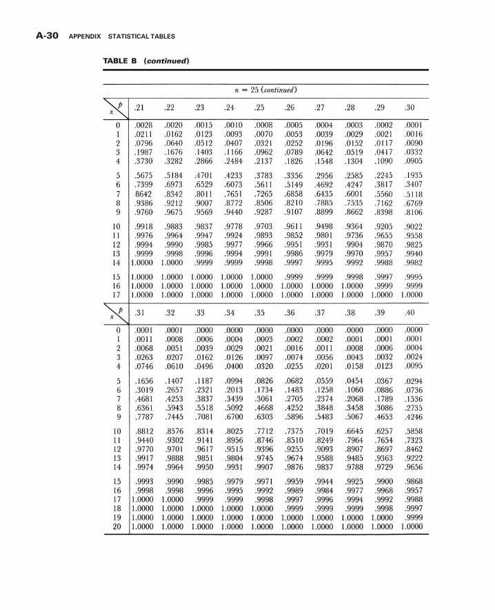
3GBAPP 12/04/2012 16:44:8 Page 30


3GBAPP 12/04/2012 16:44:9 Page 31


3GBAPP 12/04/2012 16:44:9 Page 32


3GBAPP 12/04/2012 16:44:10 Page 33


3GBAPP 12/04/2012 16:44:10 Page 34


3GBAPP 12/04/2012 16:44:14 Page 35


3GBAPP 12/04/2012 16:44:17 Page 36


3GBAPP 12/04/2012 16:44:18 Page 37


3GBAPP 12/04/2012 16:44:21 Page 38


3GBAPP 12/04/2012 16:44:23 Page 39


3GBAPP 12/04/2012 16:44:24 Page 40


3GBAPP 12/04/2012 16:44:25 Page 41


3GBAPP 12/04/2012 16:44:26 Page 42


3GBAPP 12/04/2012 16:44:29 Page 43


3GBAPP 12/04/2012 16:44:30 Page 44


3GBAPP 12/04/2012 16:44:33 Page 45


3GBAPP 12/04/2012 16:44:34 Page 46


3GBAPP 12/04/2012 16:44:35 Page 47


3GBAPP 12/04/2012 16:44:36 Page 48


3GBAPP 12/04/2012 16:44:39 Page 49


3GBAPP 12/04/2012 16:44:40 Page 50


3GBAPP 12/04/2012 16:44:41 Page 51


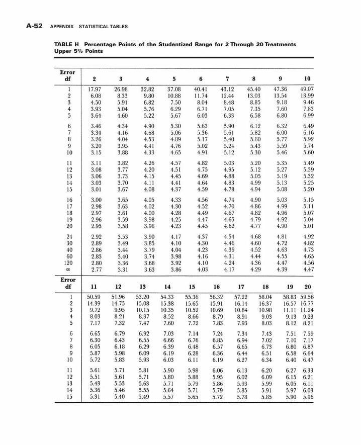
3GBAPP 12/04/2012 16:44:42 Page 52


3GBAPP 12/04/2012 16:44:43 Page 53


3GBAPP 12/04/2012 16:44:45 Page 54


3GBAPP 12/04/2012 16:44:47 Page 55


3GBAPP 12/04/2012 16:44:50 Page 56


3GBAPP 12/04/2012 16:44:51 Page 57


3GBAPP 12/04/2012 16:44:54 Page 58


3GBAPP 12/04/2012 16:44:55 Page 59


3GBAPP 12/04/2012 16:44:59 Page 60


3GBAPP 12/04/2012 16:45:1 Page 61


3GBAPP 12/04/2012 16:45:7 Page 62


3GBAPP 12/04/2012 16:45:11 Page 63


3GBAPP 12/04/2012 16:46:15 Page 64


3GBAPP 12/04/2012 16:46:19 Page 65


3GBAPP 12/04/2012 16:46:20 Page 66


3GBAPP 12/04/2012 16:46:22 Page 67


3GBAPP 12/04/2012 16:46:22 Page 68


3GBAPP 12/04/2012 16:46:23 Page 69


3GBAPP 12/04/2012 16:46:24 Page 70


3GBAPP 12/04/2012 16:46:25 Page 71


3GBAPP 12/04/2012 16:46:26 Page 72


3GBAPP 12/04/2012 16:46:27 Page 73


3GBAPP 12/04/2012 16:46:29 Page 74


3GBAPP 12/04/2012 16:46:30 Page 75


3GBAPP 12/04/2012 16:46:31 Page 76


3GBAPP 12/04/2012 16:46:35 Page 77


3GBAPP 12/04/2012 16:47:15 Page 78


3GBAPP 12/04/2012 16:47:27 Page 79


3GBAPP 12/04/2012 16:47:29 Page 80


3GBAPP 12/04/2012 16:47:30 Page 81


3GBAPP 12/04/2012 16:47:31 Page 82


3GBAPP 12/04/2012 16:47:31 Page 83


3GBAPP 12/04/2012 16:47:33 Page 84


3GBAPP 12/04/2012 16:47:34 Page 85


3GBAPP 12/04/2012 16:47:36 Page 86


3GBAPP 12/04/2012 16:47:37 Page 87


3GBAPP 12/04/2012 16:47:37 Page 88


3GBAPP 12/04/2012 16:47:39 Page 89


3GBAPP 12/04/2012 16:47:40 Page 90


3GBAPP 12/04/2012 16:47:42 Page 91


3GBAPP 12/04/2012 16:47:44 Page 92


3GBAPP 12/04/2012 16:47:45 Page 93


3GBAPP 12/04/2012 16:47:46 Page 94


3GBAPP 12/04/2012 16:47:47 Page 95


3GBAPP 12/04/2012 16:47:50 Page 96


3GBAPP 12/04/2012 16:47:51 Page 97


3GBAPP 12/04/2012 16:47:52 Page 98


3GBAPP 12/04/2012 16:47:53 Page 99


3GBAPP 12/04/2012 16:47:54 Page 100


3GBAPP 12/04/2012 16:47:55 Page 101


3GBAPP 12/04/2012 16:47:56 Page 102


3GBAPP 12/04/2012 16:47:57 Page 103


3GBAPP 12/04/2012 16:47:58 Page 104


3GBAPP 12/04/2012 16:48:0 Page 105

REFERENCES FOR STATISTICAL TABLES

A. The Rand Corporation, A Million Random Digits with 1000,000 Normal Deviates, The FreePress, Glencoe, IL, 1955.

E. Laboratories Geigy, Documenta Geigy, Scientific Tables, Seventh Edition, CIBA-GeigyLimited, Basel, Switzerland, 1970.

F. A. Hald and S. A. Sinkbaek, “ATable of Percentage Points of the x2 Distribution,”Skandinavisk Astuartietidskrift, 33 (1950), 168–175.

G. H. O. Hartley and E. S. Pearson, Biometrika Tables for Statisticians, Volume 1, ThirdEdition, Bentley House, London, 1970.

H. H. O. Hartley and E. S. Pearson, Biometrika Tables for Statisticians, Volume 1, ThirdEdition, Bentley House, London, 1970.

J. E. S. Pearson and H. O. Hartley, Biometrika Tables for Statisticians, Volume 1, Third Edition,The Syndics of the Cambridge University Press, 1966. And R. Latscha, “Tests ofSignificance in a 2 � 2 Contingency Table: Extension of Finney’s Table,” Biometrika, 40(1953), 74–86.

K. Frank Wilcoxon, S. K. Katti, and Roberta A. Wilcox, Critical Values and Probability Levelsfor the Wilcoxon Signed Rank Test, Lederle Laboratories Division, American CyanamidCompany, Pearl River, NY, in cooperation with the Department of Statistics, The FloridaState University, Tallahassee, Florida, 1963.

L. L. R. Verdooren, “Extended Tables of Critical Values for Wilcoxon’s Test Statistic,”Biometrika, 50 (1963), 177–186. And W. J. Conover, Practical Nonparametric Statistics,John Wiley and Sons, New York, 1971, 384–388.

M. L. H. Miller, “Table of Percentage Points of Kolmogorov Statistics,” Journal of the AmericanStatistical Association, 51 (1956), 111–121. And W. J. Conover, Practical NonparametricStatistics, Third Edition, John Wiley and Sons, New York, 1999, 547.

N. W. H. Kruskal and W. A. Wallis, “Use of Ranks in One-Criterion Analysis of Variance,”Journal of the American Statistical Association, 47 (1952), 583–621; errata, ibid, 48 (1953),907–911.

O. M. Friedman, “The Use of Ranks to Avoid the Assumption of Normality Implicit in theAnalysis of Variance,” Journal of the American Statistical Association, 32 (1937), 675–701.

P. Gerald J. Glasser and Robert F. Winter, “Critical Values of the Coefficient of RankCorrelation for Testing the Hypothesis of Independence,” Biometrika, 48 (1961), 444–448.


3GBAPP 12/04/2012 16:48:3 Page 106

3GBANSW 11/12/2012 13:38:15 Page 107

ANSWERS TOODD-NUMBERED EXERCISES

Chapter 1

Review Exercises

7. Situation A(a) 300 households (b) all households in the small southern town(c) number of school-aged children present (d) all that reported one or morechildren (e) nominal (categories: 0 children, 1 child, and so on)

Situation B(a) 250 patients (b) all patients admitted to the hospital during the pastyear (c) distance patient lives from the hospital (d) 250 distances(e) ratio

Chapter 2

2.3.1. (a)


CumulativeFrequency

RelativeFrequency

CumulativeRelative

Frequency

0–0.49 3 3 3.33 3.33.5–0.99 3 6 3.33 6.67

1.0–1.49 15 21 16.67 23.33(Continued)

Pindex

Histogram of pindex

0

10

20

30

40

50

Freq

uen

cy

0.750.25 1.25 1.75 2.25 2.75

Pindex

Frequency polygon of pindex

0

10

20

30

40

50

Freq

uen

cy

0.750.25 1.25 1.75 2.25 2.75 3.25

A-107

3GBANSW 11/12/2012 13:38:16 Page 108


CumulativeFrequency

RelativeFrequency

CumulativeRelative

Frequency

1.5–1.99 15 36 16.67 40.002.0–2.49 45 81 50.00 90.002.5–2.99 9 90 10.00 100.00

(b) 40.0% (c) .7667 (d) 16.67% (e) 9 (f) 16.67%(g) 2.17, because it composes almost 25 percent of the data and is the mostfrequently occurring value in the data set. (h) Skewed to the left.

2.3.3. (a)


CumulativeFrequency

RelativeFrequency

CumulativeRelative

Frequency

20–24.99 2 2 0.069 6.9025–29.99 11 13 0.3793 44.8330–34.99 6 19 0.2069 65.5235–39.99 2 21 0.069 72.4140–44.99 5 26 0.1724 89.6645–49.99 2 28 0.069 96.5550–54.99 1 29 0.0345 100.00

(b) 44.83% (c) 24.14% (d) 34.48% (e) The data are rightskewed (f) 21

BMI

Histogram of BMI

0

10

12

6

8

2

4Freq

uen

cy

22.5 27.5 32.5 37.5 42.5 47.5 52.5

BMI

Frequency polygon of BMI

0

10

12

6

8

2

4Freq

uen

cy

17.5 27.5 37.5 47.5 57.5

A-108 ANSWERS TO ODD-NUMBERED EXERCISES

3GBANSW 11/12/2012 13:38:18 Page 109

2.3.5. (a)ClassInterval Frequency

RelativeFrequency

0–2 5 0.11113–5 16 0.35566–8 13 0.28899–11 5 0.111112–14 4 0.088915–17 2 0.0444

45 1.000

(b) Skewed right

18

16

14

12

10

8

6

4

2

0

Hours

Histogram of HoursFre

qu

en

cy

1 4 7 10 13 16

–2

18

16

14

12

10

8

6

4

2

01 4 7 10

Hours

Frequency Polygon of Hours

Fre

qu

en

cy

13 16 19

ANSWERS TO ODD-NUMBERED EXERCISES A-109

3GBANSW 11/12/2012 13:38:19 Page 110

2.3.7. (a)


CumulativeFrequency

RelativeFrequency

CumulativeRelative

Frequency

110–139 8 8 0.0516 0.0516140–169 16 24 0.1032 0.1548170–199 46 70 0.2968 0.4516200–229 49 119 0.3161 0.7677230–259 26 145 0.1677 0.9354260–289 9 154 0.0581 0.9935290–319 1 155 0.0065 1.0000

(b) Not greatly skewed

50

40

30

20

10

0

Histogram of Scores

Fre

qu

en

cy

125 155 185 215Scores

245 275 305

95

50

40

30

20

10

0125 155 185 215

Scores

Frequency Polygon of Scores

Fre

qu

en

cy

245 275 305 335


3GBANSW 11/12/2012 13:38:20 Page 111

2.3.9. (a)

Stem-and-Leaf Display:

Hospital A

Stem-and-Leaf Display:

Hospital B

Stem-and-leaf of C1 N = 25

Leaf Unit = 1.0

1 17 1

2 18 4

4 19 15

9 20 11259

(6) 21 233447

10 22 2259

6 23 389

3 24 589


Leaf Unit = 1.0

1 12 5

2 13 5

4 14 35

9 15 02445

(4) 16 5678

12 17 38

10 18 466

7 19 0059

3 20 3

2 21 24

(b) Both asymmetric: A is skewed left, and B is skewed right.

2.3.11. (a)


CumulativeFrequency

RelativeFrequency

CumulativeRelative

Frequency

.0–.0999 45 45 20.83 20.83

.1–.1999 50 95 23.15 43.98

.2–.2999 34 129 15.74 59.72

.3–.3999 21 150 9.72 69.44

.4–.4999 23 173 10.65 80.09

.5–.5999 12 185 5.56 85.65

.6–.6999 11 196 5.09 90.74

.7–.7999 6 202 2.78 93.52

.8–.8999 4 206 1.85 95.37

.9–.9999 5 211 2.31 97.69

1.0–1.0999 4 215 1.85 99.54

1.1–1.1999 1 216 0.46 100.00


3GBANSW 11/12/2012 13:38:20 Page 112


Leaf Unit = 0.010

46 0 1245566777888899999999999999999999999999999999

96 1 00000000001122233334444555555666666677777778888999

(34) 2 0011111223444444445566666788889999

86 3 001111244445556668999

65 4 00001122223333444568899

42 5 002334444599

30 6 02236788999

19 7 012289

13 8 0237

9 9 05588

4 10 236

1 11 6

0.05

50

40

30

20

10

00.15 0.25 0.35 0.45

S/R Ratio

Histogram of S/R Ratio

Fre

qu

en

cy

0.55 0.65 0.75 0.85 0.95 1.05

50

40

30

20

10

0

S/R Ratio

Frequency Polygon of S/R Ratio

Fre

qu

en

cy

–0.0

5

0.05

0.15

0.25

0.35

0.45

0.55

0.65

0.75

0.85

0.95

1.05

1.15

1.25


3GBANSW 11/12/2012 13:38:21 Page 113

(b) Skewed right (c) 10, 4.62% (d) 196, 90.74%; 67, 31.02%, 143,19.91%

2.5.1. (a) 193.6 (b) 205.0 (c) no mode (d) 255 (e) 5568.09(f) 74.62 (g) 38.54 (h) 100.5

2.5.3. (a) 47.42 (b) 46.35 (c) 54.0, 33.0 (d) 29.6 (e) 76.54(f) 8.75 (g) 18.45 (h) 13.72

2.5.5. (a) 16.75 (b) 15 (c) 15 (d) 43 (e) 124.02 (f) 11.14(g) 66.51 (h) 8.25

2.5.7. (a) 1.8172 (b) 2 (c) 2.17 (d) 2.83 (e) .3164(f) .5625 (g) 30.95 (h) .6700

2.5.9. (a) 33.87 (b) 30.49 (c) none (d) 29.84 (e) 64.00(f) 8.00 (g) 23.62 (h) 13.4

2.5.11. (a) 6.711 (b) 7.00 (c) 7.00 (d) 16 (e) 16.21(f) 4.026 (g) 59.99 (h) 5.5

2.5.13. (a) 204.19 (b) 204 (c) 198, 204, 205, 212 (d) 196(e) 1257.99 (f) 35.47 (g) 17.37 (h) 46

Review Exercises

13. (a) Leaf Unit = 1.0

2 2 55

4 2 67

7 2 999

10 3 001

17 3 2223333

(12) 3 444555555555

21 3 666666666666666666677

(b) skewed (c) surgery is performed before birth; birth is generally around 37weeks (d) �x ¼ 33:680, median ¼ 35:00, s ¼ 3:210, s2 ¼ 10:304

15. (a) �x ¼ 43:39, median ¼ 42, s ¼ 17:09, C:V: ¼ 39:387, s2 ¼ 292:07(b) Stem-and-leaf of GFR N = 28

Leaf Unit = 1.0

1 1 8

6 2 11377

12 3 022267

(7) 4 1223388

9 5 158

6 6 02378

1 7

1 8 8

(c) See graph on following page (A-113)(d) 67.9%, 96.55%, 100%


3GBANSW 11/12/2012 13:38:21 Page 114

17. Some examples include difference, diversity, departure, discrepancy, deviation, andentropy

19. �x ¼ 3:95, Median ¼ 3, s ¼ 3:605, s2 ¼ 12:99821. Answers will vary: It is not uncommon for students to score higher on exams as a

semester progresses; therefore, the exam scores are likely to be left skewed, makingthe median, which is less affected by skew, to be the better choice.

23. Answers will vary: Using Sturges’s rule, where w ¼ Rk ; k ¼ 1 þ 3:322 log10300ð Þ

’ 9:23. An estimate of sample standard deviation can be found by dividing thesample range by 4. Therefore, s � R

4 so that R � 4s. Using this formula, then R ¼ 160and w ¼ 160

9:23 ¼ 17:33 suggesting that (d) or (e) may be appropriate.25. Answers will vary: Imagine you are examining protein intake among college students.

In general most students are likely to consume the average daily protein intake, butamong this population, there is likely to be a fair number of athletes who consumelarge amounts of protein owing to the demands of their sport. In that case, the data arelikely to be positively skewed, and the median better represents the central tendencyof the data.

27. Variable N Mean Median TrMean StDev SE Mean

S/R 216 0.3197 0.2440 0.2959 0.2486 0.0169

Variable Minimum Maximum Q1 Q3

S/R 0.0269 1.1600 0.1090 0.4367

IQR ¼ :3277, Range ¼ 1:1331, IQR=R ¼ :2892

10

20

90

80

70

60

50

40

30G

FR

Boxplot of GFR

0.0

1.2

1.0

0.8

0.6

0.4

0.2

S/R

rat

io

Boxplot of S/R Ratio

*****


3GBANSW 11/12/2012 13:38:22 Page 115

29. (a) Variable N Mean Median TrMean StDev SE Mean

nutri 107 75.40 73.80 74.77 13.64 1.32

Variable Minimum Maximum Q1 Q3

nutri 45.60 130.00 67.50 80.60

Variance ¼ 186:0496, Range ¼ 84:4, IQR ¼ 13:1, IQR=R ¼ :1552


Leaf Unit = 1.0

1 4 5

5 5 0004

12 5 5556899

18 6 013444

31 6 5555666777888

(28) 7 0000011122222222333333344444

48 7 666666666677888999

0

10

40

30

20

Freq

uen

cy

60 80

Nutritional Status

Histogram of Status

100 120

40

30

20

10

050 75 100

Nutritional Status

Frequency Polygon of Status

Fre

qu

en

cy

125 150


3GBANSW 11/12/2012 13:38:23 Page 116

30 8 000002234444

18 8 56889

13 9 01223

8 9 679

5 10 00

3 10 9

2 11

2 11

2 12 3

1 12

1 13 0

(d) 75:4 � 13:64; 61.76, 89.04; 79=107 ¼ :7383; 75:4 � 2 13:64ð Þ; 48.12, 102.68;103=107 ¼ :9626; 75:4 � 3 13:64ð Þ; 34.48, 116.32; 105=107 ¼ :9813

(e) 102=107 ¼ :9533 (f) 1=107 ¼ :0093

Chapter 3

3.4.1. (a) .6631 (b) marginal (c) .0332 (d) joint (e) .0493(f) conditional (g) .3701 (h) addition rule

3.4.3. (a) male and split drugs, .3418 (b) male or split drugs or both, .8747(c) male given split drugs, .6134 (d) male, .6592

3.4.5. .953.4.7. .3013.5.1. (a) A subject having the symptom (S) and not having the disease.

(b) A subject not having S but having the disease. (c) .96(d) .9848 (e) .0595 (f) .99996 (g) .00628, .999996, .3895, .9996,.8753, .9955 (h) predictive value increases as the hypothetical disease rateincreases

3.5.3. .9999977

Review Exercises

3. (a) .2143 (b) .5519 (c) .1536 (d) .4575 (e) .5065

5. (a) .1349 (b) .6111 (c) .3333 (d) .5873 (e) .3571(f) .6667 (g) 0 (h) .3269

40

130120

100

80706050

110

90

Sta

tus

Boxplot of Status

*

*

**


3GBANSW 11/12/2012 13:38:24 Page 117

7. (a) 1. .2200 2. .5000 3. .0555 4. .1100 5. .5900(b) 1. .3000 2. .3900 3. .3900 4. .1667 5. .0700 6. .6000

9. (a) .0432 (b) .0256 (c) .0247 (d) .9639 (e) .5713(f) .9639 (g) .9810

11. .006013. .062515. mothers under the age of 2417. null set, as events are mutually exclusive19. (a) plasma lipoprotein between 10–15 or greater than or equal to 30.(b) plasma lipoprotein between 10–15 and greater than or equal to 30.(c) plasma lipoprotein between 10–15 and less than or equal to 20.(d) plasma lipoprotein between 10–15 or less than or equal to 20.21. (a) .7456 (b) .330023. .0125

Chapter 4

4.2.1. (a)Number ofSubstances Used

Frequency RelativeFrequency

CumulativeFrequency

0 144 .19 .191 342 .44 .632 142 .18 .813 72 .09 .904 39 .05 .955 20 .03 .986 6 .01 .997 9 .01 1.008 2 .003 1.0039 1 .001 1.004Total 777 1.004

(b) 0.5

0.4

0.3

0.2

0.1

0.0

Number of Substances Used

Fre

qu

en

cy

0 1 2 3 4 5 6 7 8 9


3GBANSW 11/12/2012 13:38:24 Page 118

4.2.3. �x ¼ 1:58, s2 ¼ 2:15, s ¼ 1:474.3.1. (a) .1484 (b) .8915 (c) .1085 (d) .80804.3.3. (a) .2536, (b) .3461 (c) .7330 (d) .9067 (e) .00084.3.5. mean ¼ 4:8, variance ¼ 3:2644.3.7. (a) .5314 (b) .3740 (c) .0946 (d) .9931 (e) .0946

(f) .00694.3.9.

Number ofSuccesses, x

Probability, f(x)

0 3!

0!3!:2ð Þ3 :8ð Þ0 ¼ :008

1 3!

1!2!:2ð Þ2 :8ð Þ1 ¼ :096

2 3!

2!1!:2ð Þ1 :8ð Þ2 ¼ :384

3 3!

3!0!:2ð Þ0 :8ð Þ3 ¼ :512

Total 1

4.4.1. (a) .156 (b) .215 (c) .629 (d) .3204.4.3. (a) .105 (b) .032 (c) .007 (d) .4404.4.5. (a) .086 (b) .946 (c) .463 (d) .664 (e) .0264.6.1. .42364.6.3. .29124.6.5. .00994.6.7. .954.6.9. .901

4.6.11. �2.544.6.13. 1.774.6.15. 1.32

0

1.0

0.9

0.8

0.7

0.6

0.5

0.4

0.3

0.2

0.11 2 3 4Number of Substances Used

Fre

qu

en

cy

5 6 7 8 9


3GBANSW 11/12/2012 13:38:25 Page 119

4.7.1. (a) .6321 (b) .4443 (c) .0401 (d) .30644.7.3. (a) .1357 (b) .2389 (c) .6401 (d) .0721 (e) .15754.7.5. (a) .3413 (b) .1056 (c) .0062 (d) .38304.7.7. (a) .0630 (b) .0166 (c) .7719

Review Exercises

15. (a) .0212 (b) .0949 (c) .0135 (d) .712417. (a) .034 (b) .467 (c) .923 (d) .010 (e) .10519. (a) .4967 (b) .5033 (c) .1678 (d) .0104 (e) .821821. (a) .0668 (b) .6247 (c) .682623. (a) .0013 (b) .0668 (c) .893125. 57.127. (a) 64.75 (b) 118.45 (c) 130.15 (d) 131.829. 14.9031. 10.633. (a) Bernoulli assuming there is an equal probability of both genders (b) Not

Bernoulli—more than two possible outcomes (c) Not Bernoulli—weight is not abinary variable

Chapter 5

5.3.1. 204, 6.22255.3.3. (a) .1841 (b) .7980 (c) .06685.3.5. (a) .0020 (b) .1736 (c) .9777 (d) .40415.3.7. (a) .9876 (b) .0668 (c) .0668 (d) .69025.3.9.

Sample �x

6, 8, 10 8.006, 8, 12 8.676, 8, 14 9.336, 10, 12 9.336, 10, 14 10.006, 12, 14 10.678, 10, 12 10.008, 10, 14 10.678, 12, 14 11.3310, 12, 14 12.00

m�x ¼ 10; s�x ¼ 1:333

5.4.1. .38975.4.3. .00385.4.5. .01395.5.1. .11315.5.3. .08085.5.5. (a) .1539 (b) .3409 (c) .52305.6.1. .10565.6.3. .7938


3GBANSW 11/12/2012 13:38:25 Page 120

Review Exercises

11. .000313. .026215. .133517. .109319. .129221. 25223. .53, .047625. At least approximately normally distributed27. .994229. (a) No (b) Yes (c) No (d) Yes (e) Yes (f) Yes

Chapter 6

6.2.1. (a) 88, 92 (b) 87, 93 (c) 86, 946.2.3. (a) 7.63, 8.87 (b) 7.51, 8.99 (c) 7.28, 9.226.2.5. 1603.688, 1891.563; 1576.125, 1919.125; 1521.875, 1973.3756.3.1. (a) 2.1448 (b) 2.8073 (c) 1.8946 (d) 2.04526.3.3. (a) 1.549, .387 (b) 2.64, 4.36; .49, .91 (c) Nitric oxide diffusion rates

are normally distributed in the population from which the sample wasdrawn. (d) narrower (e) wider

6.3.5. 66.2, 76.8; 65.1, 77.9; 62.7, 80.36.4.1. �549:82;�340:17;�571:28;�318:72;�615:52;�274:486.4.3. �5:90; 17:70; � 8:15; 19:95; � 12:60; 24:406.4.5. 64.09, 479.91; 19.19, 524.81; �77:49, 621.496.4.7. 2.1, 4.5; 1.8, 4.8; 1.3, 5.36.4.9. �32:58;�25:42;�33:33;�24:67;�34:87;�23:136.5.1. .1028, .16426.5.3. .4415, .66156.6.1. .0268, .10766.6.3. �:0843, .26676.7.1. 27, 166.7.3. 196.8.1. 683, 10686.8.3. 385, 2896.9.1. 6.334, 44.636.9.3. 793.92, 1370.416.9.5. 1.17, 2.096.9.7. 170:98503 � s2 � 630:65006

6.10.1. .44, 17.376.10.3. .49, 2.956.10.5. .9, 3.526.10.7. 5.13, 60.30

Review Exercises

13. �x ¼ 79:87, s2 ¼ 28:1238, s ¼ 5:3; 76.93, 82.8115. p ¼ :30; .19, .41


3GBANSW 11/12/2012 13:38:26 Page 121

17. p1 ¼ :20; p2 ¼ :54, .26, .4219. p ¼ :90; .87, .9321. �x ¼ 19:23, s2 ¼ 20:2268; 16.01, 22.4523. �2:18, 2.8225. 362.73, 507.2727. .44, .7429. �:416, .18831. Level of confidence decreases. The interval would have no width. The level of

confidence would be zero.33. z, 8.1, 8.135. All drivers ages 55 and older. Drivers 55 and older participating in the vision study.37. .2865, .3529 (Use z since n > 30)

Chapter 7

7.2.1. Reject H0 because �2:57 < �2:33, p ¼ :0051 < :017.2.3. Fail to reject H0 because :76 < 1:333: p > :107.2.5. Yes, reject H0, z ¼ �5:73 < �1:645: p < :00017.2.7. No, fail to reject H0. t ¼ �1:5 > �1:709: :05 < p < :107.2.9. Yes, reject H0, z ¼ 3:08: p ¼ :0010

7.2.11. z ¼ 4, reject H0, p < :00017.2.13. t ¼ :1271, fail to reject H0. p > :27.2.15. z ¼ �4:18, reject H0. p < :00017.2.17. z ¼ 1:67, fail to reject H0. p ¼ 2ð:0475Þ ¼ :0957.2.19. Reject H0 since z ¼ �4:00: p < :00017.3.1. Reject H0 because �10:9 < �2:388; p < :0057.3.3. Reject H0 because �9:60 < �2:6591; p < 2ð:005Þ7.3.5. Reject H0 because z ¼ 3:39 > 1:96: p ¼ 2ð:0003Þ7.3.7. s2

p ¼ 5421:25; t ¼ �6:66. Reject H0. p < 2ð:005Þ ¼ :0107.3.9. z ¼ 3:39. Reject H0. p ¼ 2ð1 � :9997Þ ¼ :00067.3.11. t ¼ �3:3567. Reject H0. p < :017.4.1. Reject H0 because 3:17 > 2:624; p < :0057.4.3. Reject H0�3:1553 < �1:8125; :005 < p < :017.4.5. Reject H0 since �4:4580 < �2:4469; p < :017.5.1. Reject H0 since �1:62 > �1:645: p ¼ :05267.5.3. Reject H0 because �1:77 < �1:645; p ¼ :03847.5.5. Reject H0 because z ¼ �2:21; p ¼ :01367.6.1. Reject H0 because �2:86 < �2:58; p ¼ :00427.6.3. Fail to reject H0 because z ¼ 1:70 < 1:96; p ¼ :0887.7.1. Do not reject H0 since 5:142 < 20:723 < 34:267; p > :01 (two-sided test).7.7.3. x2 ¼ 6:75. Do not reject H0. p > :05 (two-sided test)7.7.5. x2 ¼ 28:8. Do not reject H0. p > :107.7.7. x2 ¼ 22:036; :10 > p > :057.8.1. Fail to reject because V:R: ¼ 1:226 < 1:74p > :107.8.3. No, V:R: ¼ 1:83; p > :107.8.5. Reject H0. V:R: ¼ 4; :02 < p < :057.8.7. V:R: ¼ 2:1417; p > :10


3GBANSW 11/12/2012 13:38:26 Page 122

7.9.1.AlternativeValue of m b

Value of PowerFunction 1� b

516 0.9500 0.0500521 0.8461 0.1539528 0.5596 0.4404533 0.3156 0.6844539 0.1093 0.8907544 0.0314 0.9686547 0.0129 0.9871

7.9.3.

AlternativeValue of m b

Value of PowerFunction 1� b

4.25 0.9900 0.01004.50 0.8599 0.14014.75 0.4325 0.56755.00 0.0778 0.92225.25 0.0038 0.9962

515 520 525 530 535 540 545 550

1.0

0.8

0.6

0.4

0.2

0.0

Alternative values of mu

Po

wer

4.2 4.4 4.6 4.8 5.0 5.2

1.0

0.8

0.6

0.4

0.2

0.0

Alternative values of mu

Po

wer


3GBANSW 11/12/2012 13:38:27 Page 123

7.10.1. n ¼ 548; C ¼ 518:25. Select a sample of size 548 and compute �x. If �x � 518:25,reject H0. If �x < 518:25 do not reject H0.

7.10.3. n ¼ 103; C ¼ 4:66. Select a sample of size 103 and compute �x If �x � 4:66, rejectH0. If �x < 4:66, do not reject H0.

Review Exercises

19. Reject H0 since 29:49 > 2:33: p < :000121. Fail to reject the null because z ¼ 1:48 < 1:96: p ¼ :138823. Reject H0 since 12:79 > 2:58: p < :000125. Fail to reject H0 because 1:10 < 1:645; p ¼ :135727. t ¼ 3:873; p < :00529. �d ¼ 11:49; s2

d ¼ 256:679; sd ¼ 16:02; t ¼ 2:485; :025 > p > :0131. Reject H0 since �2:286 < 1:7530; :025 > p > :01

Answers to Exercises 41–55 obtained by MINITAB

41. 95.0% C.I.(456.8, 875.9)

t p value7.09 0.0000Test of m ¼ 0 vs. m not ¼ 0

43. 95.0% C.I.(0.224, 0.796)

t p value3.65 0.0010Test of m ¼ 0 vs. m not ¼ 0

45. Leg press: 95.0% C.I.(32.22, 56.45)

t p value7.85 0.0000

Test of m ¼ 0 vs. m not ¼ 0Hip flexor: 95.0% C.I.

(3.079, 6.388)t p value

6.14 0.0000Test of m ¼ 0 vs. m not ¼ 0Hip extensor: 95.0% C.I.

(6.031, 10.236)t p value

8.30 0.0000Test of m ¼ 0 vs. m not ¼ 0

Arm abductor: 95.0% C.I.(3.717, 7.217)

t p value6.70 0.0000

Test of m ¼ 0 vs. m not ¼ 0Arm abductor: 95.0% C.I.

(4.597, 7.670)t p value

8.56 0.0000Test of m ¼ 0 vs. m not ¼ 0

47. 95.0% C.I.�71:9;�26:5ð Þ

t p value�4:34 0.0001

Test of m ¼ 0 vs. m not ¼ 0


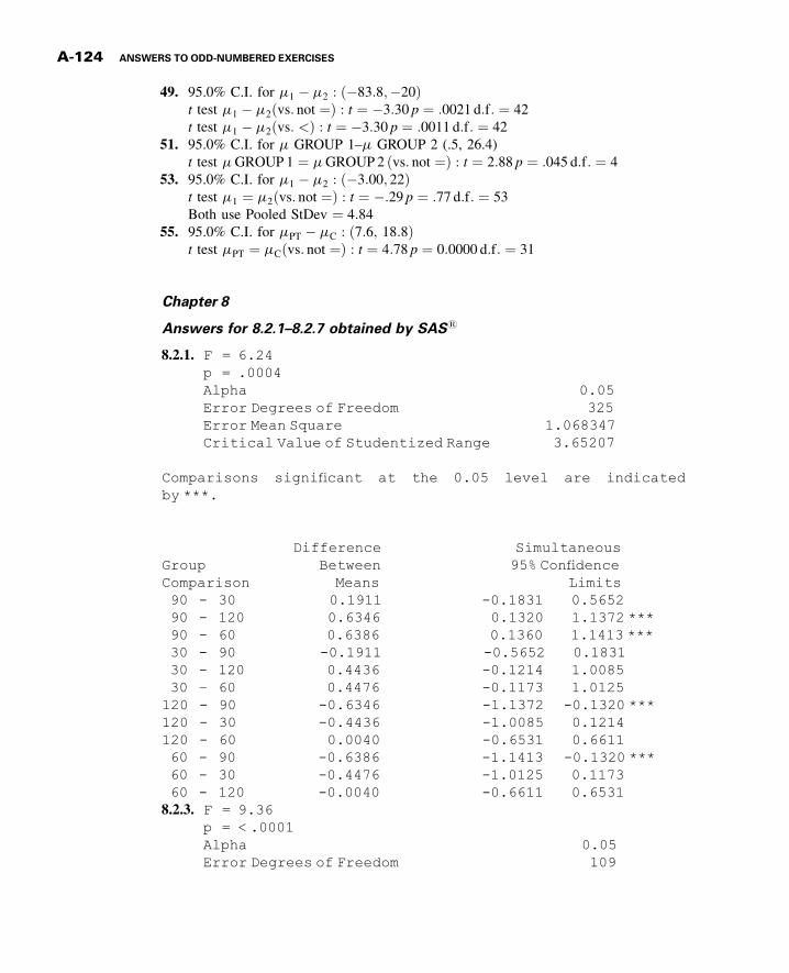
3GBANSW 11/12/2012 13:38:27 Page 124

49. 95.0% C.I. for m1 � m2 : �83:8;�20ð Þt test m1 � m2 vs: not ¼ð Þ : t ¼ �3:30 p ¼ :0021 d:f: ¼ 42t test m1 � m2 vs: <ð Þ : t ¼ �3:30 p ¼ :0011 d:f: ¼ 42

51. 95.0% C.I. for m GROUP 1–m GROUP 2 (.5, 26.4)t test mGROUP 1 ¼ mGROUP 2 vs: not ¼ð Þ : t ¼ 2:88 p ¼ :045 d:f: ¼ 4

53. 95.0% C.I. for m1 � m2 : �3:00; 22ð Þt test m1 ¼ m2 vs: not ¼ð Þ : t ¼ �:29 p ¼ :77 d:f: ¼ 53Both use Pooled StDev ¼ 4:84

55. 95.0% C.I. for mPT � mC : ð7:6; 18:8Þt test mPT ¼ mC vs: not ¼ð Þ : t ¼ 4:78 p ¼ 0:0000 d:f: ¼ 31

Chapter 8

Answers for 8.2.1–8.2.7 obtained by SAS1

8.2.1. F = 6.24

p = .0004

Alpha 0.05

Error Degrees of Freedom 325

Error Mean Square 1.068347


Comparisons significant at the 0.05 level are indicated

by ***.

Difference Simultaneous

Group Between 95% Confidence

Comparison Means Limits

90 - 30 0.1911 -0.1831 0.5652

90 - 120 0.6346 0.1320 1.1372 ***

90 - 60 0.6386 0.1360 1.1413 ***

30 - 90 -0.1911 -0.5652 0.1831

30 - 120 0.4436 -0.1214 1.0085

30 – 60 0.4476 -0.1173 1.0125

120 - 90 -0.6346 -1.1372 -0.1320 ***

120 - 30 -0.4436 -1.0085 0.1214

120 - 60 0.0040 -0.6531 0.6611

60 - 90 -0.6386 -1.1413 -0.1320 ***

60 - 30 -0.4476 -1.0125 0.1173

60 - 120 -0.0040 -0.6611 0.6531

8.2.3. F = 9.36

p = < .0001

Alpha 0.05



3GBANSW 11/12/2012 13:38:28 Page 125




by ***.




A - B 455.72 45.73 865.71 ***

A - C 574.54 235.48 913.59 ***

A - D 596.63 287.88 905.39 ***

B - A -455.72 -865.71 -45.73 ***

B - C 118.82 -271.45 509.09

B - D 140.91 -223.34 505.17

C - A -574.54 -913.59 -235.48 ***

C - B -118.82 -509.0 271.45

C - D 22.10 -259.95 304.14

D - A -596.63 -905.39 -287.88 ***

D - B -140.91 -505.17 223.34

D - C -22.10 -304.14 259.95

8.2.5. F = 9.26

p = .0009

Alpha 0.05





by ***.




Y - MA 18.16 -10.67 46.98

Y - E 48.13 20.07 76.19 ***

MA - Y -18.16 -46.98 10.67

MA - E 29.97 1.15 58.80 ***

E - Y -48.13 -76.19 -20.07 ***

E - MA -29.97 -58.80 -1.15 ***

8.2.7. F = 4.94

p = .0026

Alpha 0.05





3GBANSW 11/12/2012 13:38:28 Page 126


by ***.




0 - 1 0.10165 -0.13866 0.34196

0 - 2 0.17817 -0.2188 0.37822




0 - 3 0.35447 0.10511 0.60383 ***

1 - 0 -0.10165 -0.34196 0.13866

1 - 2 0.07652 -0.17257 0.32561

1 - 3 0.25281 -0.03737 0.54300

2 - 0 -0.17817 -0.37822 0.02188

2 - 1 -0.07652 -0.32561 0.17257

2 - 3 0.17630 -0.08154 0.43413

3 - 0 -0.35447 -0.60383 -0.10511 ***

3 - 1 -0.25281 -0.54300 0.03737

3 - 2 -0.17630 -0.43413 0.08154

8.3.1. V:R: ¼ 19:79; p < :0058.3.3. V:R: ¼ 30:22; p < :0058.3.5. V:R: ¼ 7:37; :025 > p > :018.3.7. Total d:f : ¼ 41 Block (Dogs) d:f : ¼ 5 Treatments (Times) d:f : ¼ 6, Error d:f : ¼

308.4.1. V:R: ¼ 48:78; p < :0058.4.3. V:R: ¼ 16:45; p < :0058.4.5. Total d:f : ¼ 29, Block (Subject) d:f : ¼ 9, Treatment (Time) d:f : ¼ 2, Error

d:f : ¼ 188.5.1. Ion V:R: ¼ 6:18; p ¼ :023; dose V:R: ¼ 74:59; p ¼ :000; inter V:R: ¼ :89 p ¼

:4278.5.3. Migraine V:R: ¼ 19:98; p < :0001; treat V:R: ¼ 2:13; p ¼ :1522; interaction

V:R: ¼ 1:42; p ¼ :2404

Review Exercises

13. V:R: ¼ 7:04; p ¼ :000. The sample mean for the healthy subjects is significantlydifferent from the means of categories B, C, and D. No other differences betweensample means are significant.

15. V:R: ¼ 1:35; p ¼ :274. Do not reject H0.17. Smoking status V:R: ¼ 3:16; p ¼ :052, Vital Exhaustion Group

V:R: ¼ 6:84; p ¼ :003, Interaction V:R: ¼ 2:91; p ¼ :03219. V:R: ¼ 4:23; p < :00121. V:R: ¼ 6:320; p ¼ :00823. V:R: ¼ 3:1187; p ¼ :043. The sample D mean is significantly different from the

sample B mean. No other differences between sample means are significant.


3GBANSW 11/12/2012 13:38:28 Page 127

25. V:R: ðAgeÞ ¼ 29:38; p < :001; Occupation V:R: ¼ 31:47; p < :001; InteractionV:R: ¼ 7:12; p < :001

27. 499.5, 9, 166.5, 61.1667, 2.8889, 57.6346, < :00529. (a) Completely randomized, (b) 3, (c) 30, (d) No, because

1:0438 < 3:3531. V:R: ¼ 26:06; p < :001:HSD ¼ 2:4533. All differences significant except mLight �

mModerate

33. V:R: ¼ 2:37; p ¼ :117, Tukey HSD not necessary.35. (a) One-way ANOVA

(b) Response: post-pre training score(c) Factors: Groups of years of experience (with 4 levels)(d) surgical experience and interest in obstetrics(e) no carryover effects(f) treatment is years of experience d:f: ¼ 3, total d:f: ¼ 29, error d:f: ¼ 26.

37. (a) repeated measures(b) Response: BMD(c) Factors: time periods (with six levels)(d) diet, exercise, and calcium intake(e) no carryover effects(f) time factor d:f: ¼ 5, subject factor d:f: ¼ 25, total, error d:f: ¼ 125.

39.Analysis of Variance for bilirubi

Source DF SS MS F P

subject 17 2480.83 145.93 45.57 0.000

time 6 89.09 14.85 4.64 0.000

Error 102 326.65 3.20

Total 125 2896.57

41. CR = Compression Ratio

Analysis of Variance for C.R.

Source DF SS MS F P

Group 4 9092 2273 8.12 0.001

Error 19 5319 280

Total 23 14411

Level N Mean StDev

Control 6 79.96 5.46

I 4 78.69 21.44

II 4 47.84 23.74

III 5 43.51 10.43

IV 5 33.32 20.40

Pooled StDev = 16.73

Tukey’s pairwise comparisons

Mean For CIs 95% Individual StDevPooled on Based

---+---------+---------+---------+---(-----*-----)

(------*------)(------*------)(-----*------)

(-----*------)---+---------+---------+---------+---

100755025


3GBANSW 11/12/2012 13:38:29 Page 128

Family error rate = 0.0500

Individual error rate = 0.00728

Critical Value = 4.25

Intervals for (column level mean) - (row level mean)

Control I II III

I -31.19

33.72

II -0.34 -4.70

64.58 66.41

III 6.00 1.45 -29.41

66.89 68.91 38.05

IV 16.19 11.64 -19.21 -21.61

77.08 79.10 48.24 41.99

43. Two-way ANOVA: BC versus heat, chromo

Analysis of Variance for BC

Source DF SS MS F P

heat 1 0.1602 0.1602 3.95 0.061

chromo 1 0.6717 0.6717 16.55 0.001

Interaction 1 0.0000 0.0000 0.00 0.994

Error 20 0.8119 0.0406

Total 23 1.6438

Analysis of Variance for AC

Source DF SS MS F P

heat 1 0.0468 0.0468 1.99 0.174

chromo 1 0.4554 0.4554 19.34 0.000

Interaction 1 0.0039 0.0039 0.16 0.690

Error 20 0.4709 0.0235

Total 23 0.9769

Analysis of Variance for AC/BC

Source DF SS MS F P

heat 1 0.04524 0.04524 15.62 0.001

chromo 1 0.00000 0.00000 0.00 1.000

Interaction 1 0.00385 0.00385 1.33 0.262

Error 20 0.05793 0.00290

Total 23 0.10702

45. C.A. = Congruence angle

Analysis of Variance for C.A.

Source DF SS MS F P

Group 3 7598 2533 14.83 0.000

Error 86 14690 171

Total 89 22288


3GBANSW 11/12/2012 13:38:29 Page 129

Level N Mean StDev

Lateral 27 6.78 15.10

Medial 26 -10.81 10.80

Multi 17 -18.29 15.09

Normal 20 -7.00 10.76





Critical value = 3.71


Lateral Medial Multi

Medial 8.16

27.01

Multi 14.46 -3.21

35.69 18.18

Normal 3.66 -14.01 -22.60

23.89 6.39 0.02

47.Analysis of Variance for response

Source DF SS MS F P

subject 5 25.78 5.16 4.72 0.018

temp 2 30.34 15.17 13.87 0.001

Error 10 10.93 1.09

Total 17 67.06

49. G.C. = glucose concentration

Analysis of Variance for G.C.

Source DF SS MS F P

group 3 8.341 2.780 10.18 0.001

subject 5 8.774 1.755 6.43 0.002

Error 15 4.096 0.273

Total 23 21.210

51.Analysis of Variance for T3

Source DF SS MS F P

subject 11 8967 815 2.55 0.030

day 2 12466 6233 19.50 0.000

Error 22 7033 320

Total 35 28467

MeanFor CIs 95% Individual StDevPooled on Based

-----+---------+---------+---------+-(----*----)

(----*----)(------*-----)

(-----*-----)-----+---------+---------+---------+-

100-10-20


3GBANSW 11/12/2012 13:38:29 Page 130

53. BBL = blood bilirubin levels

Analysis of Variance for BBL

Source DF SS MS F P

Group 2 4077 2039 3.31 0.090

Error 8 4931 616

Total 10 9008

Level N Mean StDev

Control 4 63.50 28.25

Hypercar 4 50.00 22.69

Hyperosm 3 98.00 22.27







Control Hypercar

Hypercar -36.7

63.7

Hyperosm -88.7 -102.2

19.7 6.2

55.Analysis of Variance for breathing scores

Source DF SS MS F P

group 2 244.17 122.08 14.50 0.000

Error 38 319.88 8.42

Total 40 564.05

Level N Mean StDev

1 13 13.231 1.739

2 14 13.786 2.833

3 14 18.643 3.713







---+---------+---------+---------+---(--------*---------)

(---------*--------)(----------*----------)

---+---------+---------+---------+---120906030


----+---------+---------+---------+--(------*-----)

(-----*-----)(------*-----)

----+---------+---------+---------+--20.017.515.012.5


3GBANSW 11/12/2012 13:38:30 Page 131


1 2

2 -3.281

2.171

3 -8.138 -7.532

-2.686 -2.182

57. PSWQ ¼ PSWQ score

Analysis of Variance for PSWQ

Source DF SS MS F P

Group 3 16654.9 5551.6 74.11 0.000

Error 115 8614.6 74.9

Total 118 25269.5

Level N Mean StDev

1 15 62.933 8.556

2 30 38.333 7.494

3 19 64.158 10.259

4 55 66.536 8.678







1 2 3

2 17.459

31.741

3 -9.025 -32.446

6.575 -19.203

4 -10.181 -33.329 -8.388

2.975 -23.077 3.631


-----+---------+---------+---------+-(---*---)

(--*--)(---*---)

(--*-)-----+---------+---------+---------+-

70605040


3GBANSW 11/12/2012 13:38:30 Page 132

59.Analysis of Variance for Age

Source DF SS MS F P

Group 2 16323.2 8161.6 139.79 0.000

Error 189 11034.7 58.4

Total 191 27357.9

Level N Mean StDev

Daughter 50 49.420 7.508

Husband 65 71.985 7.516

Wife 77 68.649 7.828







Daughter Husband

Husband -25.959

-19.170

Wife -22.507 0.296

-15.952 6.375

61. SAP ¼ serum alkaline phosphatase level

Analysis of Variance for SAP

Source DF SS MS F P

Grade 2 36181 18091 5.55 0.009

Error 29 94560 3261

Total 31 130742


-+---------+---------+---------+-----(--*-)

(-*-)(-*-)

-+---------+---------+---------+-----72.064.056.048.0


3GBANSW 11/12/2012 13:38:31 Page 133

Level N Mean StDev

I 9 118.00 61.85

II 8 143.63 55.90

III 15 194.80 54.82







I II

II -94.1

42.8

III -136.2 -112.9

-17.4 10.5

63.Analysis of Variance for Hematocrit

Source DF SS MS F P

Group 2 817.5 408.8 20.26 0.000

Error 27 544.8 20.2

Total 29 1362.3

Level N Mean StDev

Sham 10 38.200 2.573

Treated 15 40.200 5.348

Untreated 5 53.200 4.604






--+---------+---------+---------+----(----*----)

(---*---)(------*------)

--+---------+---------+---------+----54.048.042.036.0


-+---------+---------+---------+-----(---------*--------)

(---------*---------)(-------*------)

-+---------+---------+---------+-----20016012080


3GBANSW 11/12/2012 13:38:32 Page 134



Sham Treated

Treated -6.551

2.551

Untreated -21.106 -18.757

-8.894 -7.243

65. Both ¼ rhIGF-I þ rhGH

Analysis of Variance for Response

Source DF SS MS F P

Group 3 4.148 1.383 1.39 0.282

Error 16 15.898 0.994

Total 19 20.046

Level N Mean StDev

Both 5 11.520 0.653

rhGH 5 11.250 0.570

rhIGF-I 6 10.800 1.418

Saline 4 10.250 0.971







Both rhGH rhIGF-I

rhGH -1.5354

2.0754

rhIGF-I -1.0086 -1.2786

2.4486 2.1786

Saline -0.6450 -0.9150 -1.2927

3.1850 2.9150 2.3927


---------+---------+---------+-------(--------*---------)

(--------*---------)(---------*--------)

(---------*----------)---------+---------+---------+-------

12.011.010.0


3GBANSW 11/12/2012 13:38:32 Page 135

Chapter 9

9.3.1. (a) Direct, (b) Direct, (c) Inverse9.3.3. y ¼ 560 þ 0:140x9.3.5. y ¼ 68:6 � 19:5x9.3.7. y ¼ 0:193 þ 0:00628x9.4.1 Predictor Coef SE Coef T P

Constant 559.90 29.13 19.22 0.000

Meth Dos 0.13989 0.06033 2.32 0.035

S = 68.28 R-Sq = 26.4% R-Sq(adj) = 21.5%


Source DF SS MS F P

Regression 1 25063 25063 5.38 0.035

Residual Error 15 69923 4662

Total 16 94986

Confidence interval for b1 .011, .268

9.4.3. Predictor Coef SE Coef T P

Constant 68.64 16.68 4.12 0.006

Cmax w/ -19.529 4.375 -4.46 0.004

S = 18.87 R-Sq = 76.9% R-Sq(adj) = 73.0%


Source DF SS MS F P

Regression 1 7098.4 7098.4 19.93 0.004

Residual Error 6 2137.4 356.2

Total 7 9235.9

Confidence interval for b1 -30.23, -8.82

9.4.5. Predictor Coef SE Coef T P

Constant 0.19290 0.04849 3.98 0.001

DTPA GFR 0.006279 0.001059 5.93 0.000

S = 0.09159 R-Sq = 58.5% R-Sq(adj) = 56.8%


Source DF SS MS F P

Regression 1 0.29509 0.29509 35.18 0.000

Residual Error 25 0.20972 0.00839

Total 26 0.50481

Confidence interval for b1 0.0041, 0.0085


3GBANSW 11/12/2012 13:38:32 Page 136

9.5.1. (a) 580.6, 651.2 (b) 466.1, 765.69.5.3. (a) �30:42, 5.22 (b) �62:11, 36.929.5.5. (a) 0.3727, 0.4526 (b) 0.2199, 0.60559.7.1. r ¼ :466; t ¼ 2:23; p ¼ :038; :030 < r < :7759.7.3. r ¼ �:812; t ¼ �3:11; p ¼ :027; � 1 < r < �:1529.7.5. r ¼ �:531; t ¼ �3:31; p ¼ :003; � :770 < r < �:211

Review Exercises

17. BOARD ¼ �191 þ 4:68 AVG; r2 ¼ :772; t ¼ 17:163; p < :00119. y-hat = 12.6 + 1.80x

Predictor Coef SE Coef T P

Constant 12.641 2.133 5.93 0.000

no. of p 1.8045 0.5585 3.23 0.005

S = 7.081 R-Sq = 38.0% R-Sq(adj) = 34.4%


Source DF SS MS F P

Regression 1 523.41 523.41 10.44 0.005


Total 18 1375.79

21. The regression equation is

B = 1.28 + 0.851 A


Constant 1.2763 0.3935 3.24 0.006

A 0.8513 0.1601 5.32 0.000

S = 0.2409 R-Sq = 68.5% R-Sq(adj) = 66.1%


Source DF SS MS F P

Regression 1 1.6418 1.6418 28.29 0.000


Total 14 2.3963

23. y ¼ 61:8819 þ :509687x; V:R: ¼ 4:285; :10 > p > :05; t ¼ 2:07; 95% C.I. forp : �:03,.79; 110.3022; 87.7773, 132.8271


3GBANSW 11/12/2012 13:38:32 Page 137

25. y ¼ 37:4564 þ :0798x; V:R: ¼ 77:13; p < :005; t ¼ 8:78; 95% C.I. for r: .91, 1;40.63, 42.27.


A = 570 + 0.429 B


Constant 569.8 141.2 4.03 0.000

B 0.42927 0.04353 9.86 0.000

S = 941.6 R-Sq = 54.0% R-Sq(adj) = 53.4%

Pearson correlation of B and A = 0.735

P-Value = 0.000


y = 45.0 + 0.867 x


Constant 44.99 33.54 1.34 0.193

x 0.86738 0.07644 11.35 0.000

S = 102.9 R-Sq = 84.8% R-Sq(adj) = 84.2%

Pearson correlation of x and y = 0.921

P-Value = 0.000


S = -1.26 + 2.10 DBS


Constant -1.263 3.019 -0.42 0.680

DBS 2.0970 0.1435 14.62 0.000

S = 8.316 R-Sq = 90.3% R-Sq(adj) = 89.9%

Pearson correlation of S and DBS = 0.950

P-Value = 0.000


log y = 2.06 + 0.0559 PCu


Constant 2.0603 0.3007 6.85 0.000

PCu 0.05593 0.01631 3.43 0.001


3GBANSW 11/12/2012 13:38:33 Page 138

S = 0.3873 R-Sq = 16.4% R-Sq(adj) = 15.0%

Pearson correlation of PCu and log y = 0.405

P-Value = 0.001


C6 = -0.141 - 1.33 C5


Constant -0.1413 0.2267 -0.62 0.540

C5 -1.3286 0.1242 -10.69 0.000

S = 1.086 R-Sq = 84.5% R-Sq(adj) = 83.7%

Pearson correlation of IGELogE and SkinLogE = -0.919

P-Value = 0.000

39. Normotensive C6 ¼ C4 � C5; C7 ¼ C4 þ C5ð Þ=2; C8 ¼ C2 � C3; C9 ¼C2 þ C3ð Þ=2


C6 = 4.2 + 0.106 C7


Constant 4.19 17.30 0.24 0.811

C7 0.1060 0.1590 0.67 0.512

S = 5.251 R-Sq = 2.0% R-Sq(adj) = 0.0%

Pearson correlation of C6 and C7 = 0.141

P-Value = 0.512


C8 = 0.2 + 0.268 C9


Constant 0.25 18.53 0.01 0.989

C9 0.2682 0.2932 0.91 0.370

S = 5.736 R-Sq = 3.7% R-Sq(adj) = 0.0%

Pearson correlation of C8 and C9 = 0.191

P-Value = 0.370

Preeclamptic


C6 = 57.9 - 0.363 C7


3GBANSW 11/12/2012 13:38:33 Page 139


Constant 57.89 17.10 3.39 0.003

C7 -0.3625 0.1273 -2.85 0.009

S = 7.109 R-Sq = 26.9% R-Sq(adj) = 23.6%

Pearson correlation of C6 and C7 = -0.519

P-Value = 0.009


C8 = 54.4 - 0.540 C9


Constant 54.377 9.771 5.56 0.000

C9 -0.5403 0.1154 -4.68 0.000

S = 5.787 R-Sq = 49.9% R-Sq(adj) = 47.6%

Pearson correlation of C8 and C9 = -0.707

P-Value = 0.000


LBMD = 0.131 + 0.511 ABMD


Constant 0.13097 0.05413 2.42 0.018

ABMD 0.51056 0.05935 8.60 0.000

S = 0.09188 R-Sq = 53.6% R-Sq(adj) = 52.9%

Pearson correlation of ABMD and LBMD = 0.732

P-Value = 0.000

43. WL, VO2


WL = 0.01 + 0.262 VO2


Constant 0.013 1.308 0.01 0.992

VO2 0.26237 0.07233 3.63 0.003

S = 1.835 R-Sq = 52.3% R-Sq(adj) = 48.3%

Pearson correlation of WL and VO2 = 0.723

P-Value = 0.003


3GBANSW 11/12/2012 13:38:33 Page 140

WL, AT


WL = 0.75 + 0.367 AT


Constant 0.752 1.761 0.43 0.677

AT 0.3668 0.1660 2.21 0.047

S = 2.241 R-Sq = 28.9% R-Sq(adj) = 23.0%

Pearson correlation of WL and AT = 0.538

P-Value = 0.047

WL, ET


WL = 0.74 + 0.00637 ET


Constant 0.739 1.173 0.63 0.541

ET 0.006375 0.001840 3.46 0.005

S = 1.879 R-Sq = 50.0% R-Sq(adj) = 45.8%

Pearson correlation of WL and ET = 0.707

P-Value = 0.005


CL/F = 19.4 + 0.893 CLer


Constant 19.393 4.496 4.31 0.000

CLer 0.89250 0.05671 15.74 0.000

S = 28.20 R-Sq = 59.3% R-Sq(adj) = 59.1%

Pearson correlation of CL/F and CLer = 0.770

P-Value = 0.000

Chapter 10

10.3.1. y ¼ �31:4 þ 0:473x1 þ 1:07x2

10.3.3. y ¼ 13:45 þ 4:02x1 þ 281x2

10.3.5. y ¼ �422:00 þ 11:17x1 � :63x2


3GBANSW 11/12/2012 13:38:33 Page 141

10.4.1.Analysis of Variance

Source DF Sum of MeanSquares Square F value Pr > F

Model 2 1576.99011 788.49506 185.13 <.0001

Error 32 136.29516 4.25922


Root MSE 2.06379 R-Square 0.9204

Dependent Mean 51.25086 Adj R-Sq 0.9155

Coeff Var 4.02684

Parameter Estimates

Parameter Standard

Variable DF Estimate Error t Value Pr > |t| 95% Confidence Limits

Intercept 1 -31.42480 6.14747 -5.11 <.0001 -43.94678 -18.90282

X1 1 0.47317 0.06117 7.74 <.0001 0.34858 0.59776

X2 1 1.07117 0.06280 17.06 <.0001 0.94326 1.19909

(a) .9204 (c) X1 p-value < :0001; X2 p-value < :0001 (d) 95% C.I. forslope for X1 : ð0:34858 � 0:59776Þ, 95% C.I. for slope for X2 :ð0:94326 � 1:19909Þ

10.4.3.Analysis of Variance


Model 2 452.56375 226.28188 7.05 0.0210

Error 7 224.70025 32.10004




Coeff Var 9.91198

Parameter Estimates

Parameter Standard


Intercept 1 13.44923 13.23156 1.02 0.3433 -17.83843 44.73689

X1 1 4.01680 1.07136 3.75 0.0072 1.48344 6.55016

X2 1 2.81175 1.37859 2.04 0.0808 -0.44809 6.07160

(a) .6682 (c) X1 p-value ¼ :0072; X2 p-value ¼ :0808 (d) 95% C.I. forslope for X1 : ð1:48344 � 6:55016Þ


3GBANSW 11/12/2012 13:38:33 Page 142

10.4.5.



Model 2 17018 8508.89242 4.89 0.0175

Error 22 38282 1740.10069

Corrected Total 24 55300



Coeff Var 7.76807

Parameter Estimates

Parameter Standard


Intercept 1 -421.99671 339.76199 -1.24 0.2273 -1126.61995 282.62653

X1 1 11.16613 3.65523 3.05 0.0058 3.58564 18.74663

X2 1 -0.63032 0.93826 -0.67 0.5087 -2.57615 1.31552

(a) .3077 (c) X1 p-value ¼ :0058; X2 p-value ¼ :5807 (d) 95% C.I. forslope for X1 : ð3:58564 � 18:74663Þ

10.5.1. C.I.: 50.289, 51.747. P.I.: 46.751, 55.28410.5.3. C.I.: 44.22, 56.59; P.I.: 35.64, 65.1710.5.5. C.I.: 514.31, 550.75; P.I.: 444.12, 620.9410.6.1. (a) Pairwise correlations:

DNA-Bloo Co-cult DNA-Rect

Co-cult 0.360

DNA-Rect 0.532 0.303

RNA-Rect 0.202 0.674 0.430

(b) R ¼ :370; F ¼ 7:06; p ¼ :001(c) ry1:23 ¼ :3472; ry2:13 ¼ :5232; ry3:12 ¼ �:2538(d) r12:y3 ¼ �:1660(e) r13:y2 ¼ :6615(f) r23:y1 ¼ :3969

10.6.3. (a) R ¼ :9517; F ¼ 57:638; p < :005(b), (c)ry1:2 ¼ :9268; t ¼ 8:549; p < :01; ry2:1 ¼ :3785; t ¼ 1:417; :20 > p > :10;r12:y ¼ �:1789; t ¼ �:630; p > :20

Review Exercises

7. R ¼ :3496F ¼ :83 ðp > :10Þ9. (a) y ¼ 11:419 þ 1:2598x1 þ 3:1067x2 (b) R2 ¼ :92


3GBANSW 11/12/2012 13:38:35 Page 143

(c)Source SS d.f. MS V.R. p

Regression 1827.004659 2 913.50 69.048 <.005Residual 158.728641 12 13.23

1985.7333 14

(d) y ¼ 11:419 þ 1:2598ð10Þ þ 3:1067ð5Þ ¼ 39:55

11. (a) y ¼ �126:505 þ :176x1 � 1:563x2 þ 1:575x3 þ 1:6292x4

(b)Source SS d.f. MS V.R. p

Regression 30873.47 4 7718.367 13.37 <.005Residual 5774.93 10 577.493

36648.40 14

(c) t1 ¼ 4:40; t2 ¼ �:78; t3 ¼ 3:53; t4 ¼ 2:59(d) R2

y :1234 ¼ :842423; Ry:1234 ¼ :91784

13. (a) correlation(b) log plasma adiponectin levels(c) age and glomerular filtration rate(d) both correlations were not significant(e) subjects with end-stage renal disease

15. (a) correlation(b) static inspiratory mouth pressure(c) forced expiratory volume, peak expiratory flow, and maximal inspiratroy flow(d) both correlations were not significant(e) boys and girls ages 7–14

17.

x1 x2 x3 x4 x5 x6 x7 x8 x9 x10 x11 x12 x13

X1 1X2 .737(��) 1X3 �.109 .244 1X4 .760(��) .698(��) .316 1X5 .556(��) .608(��) .273 .760(��) 1X6 .040 �.213 �.136 �.101 �.647(��) 1X7 �.291 �.289 �.093 �.293 �.412(�) .231 1X8 .570(��) .659(��) .227 .568(��) .763(��) �.481(�) �.555(��) 1X9 .555(��) .566(��) .146 .454(�) .717(��) �.503(��) �.650(��) .922(��) 1X10 .345 .508(��) .419(�) .455(�) .640(��) �.377 �.480(�) .905(��) .788(��) 1X11 �.467(�) �.400(�) �.224 �.621(��) �.702(��) .388(�) .732(��) �.652(��) �.646(��) �.582(��) 1X12 �.250 �.260 �.178 �.228 �.448(�) .390(�) .778(��) �.641(��) �.717(��) �.667(��) .796(��) 1X13 �.271 �.305 �.380 �.346 �.518(��) .348 .524(��) �.645(��) �.707(��) �.729(��) .744(��) .864(��) 1

�� correlation is significant at the 0.01 level (2-tailed).� correlation is significant at the 0.05 level (2-tailed).


3GBANSW 11/12/2012 13:38:35 Page 144

19.v1 v2 v3 v4 v5 v6 v7 v8

v1 1v2 .123 1v3 .115 .963(��) 1v4 .417(��) �.063 �.041 1v5 .005 �.102 �.103 �.059 1v6 .001 .270(��) .295(��) �.036 .137 1v7 �.113 �.074 �.076 .052 .134 .061 1v8 .077 �.002 �.023 .146 .165 �.202 �.032 1

�� Correlation is significant at the 0.01 level (2-tailed).

Chapter 11

11.2.1. mobilizer: 0 G-CSF, 1-Etoposide


conc = 12.9 - 0.0757 age - 5.48 mobilizer


Constant 12.933 2.787 4.64 0.000

age -0.07566 0.04388 -1.72 0.092

mobilize -5.480 1.429 -3.83 0.000

S = 3.965 R-Sq = 27.1% R-Sq(adj) = 23.6%


Source DF SS MS F P

Regression 2 240.02 120.01 7.63 0.002


Total 43 884.62

11.2.3.


QTc = 23.0 + 39.4 sex + 0.825 dose


Constant 22.98 46.92 0.49 0.632

sex 39.40 42.14 0.93 0.366

dose 0.82456 0.07556 10.91 0.000

S = 84.10 R-Sq = 89.6% R-Sq(adj) = 88.1%


3GBANSW 11/12/2012 13:38:35 Page 145


Source DF SS MS F P

Regression 2 850164 425082 60.10 0.000

Residual Error 14 99018 7073

Total 16 949182

11.3.1.

Step 1 2 3

Constant 51.93 116.07 115.54

MEM 0.66 0.60 0.57

T-Value 5.75 5.87 5.53

P-Value 0.000 0.000 0.000

SOCIALSU -0.476 -0.492

T-Value -5.28 -5.51

P-Value 0.000 0.000

CGDUR 0.122

T-Value 1.88

P-Value 0.064

S 17.4 15.4 15.2

R-Sq 25.20 41.92 43.97

R-Sq(adj) 24.44 40.72 42.22

11.3.3.

Alpha-to-Enter: 0.15 Alpha-to-Remove: 0.15

Response is REACTIVE on 6 predictors, with N = 68

Step 1 2 3

Constant 3.374 5.476 5.418

AGEABUSE -0.38 -0.45 -0.42

T-Value -2.49 -3.00 -2.91

P-Value 0.015 0.004 0.005

VERBALIQ -0.0219 -0.0228

T-Value -2.75 -2.93

P-Value 0.008 0.005

STIM 0.61

T-Value 2.05

P-Value 0.044


3GBANSW 11/12/2012 13:38:36 Page 146

S 1.06 1.01 0.990

R-Sq 8.57 18.10 23.15

R-Sq(adj) 7.19 15.58 19.55

C-p 10.4 4.6 2.5

11.4.1.Standard Wald

Parameter DF Estimate Error Chi-Square Pr > ChiSq

Intercept 1 2.1192 0.1740 148.3439 <.0001

sex 1 0.0764 0.2159 0.1252 0.7234

Odds Ratio Estimates

Effect Point Estimate 95% Wald Confidence Limits

sex 1.079 0.707 1.648

Review Exercises

15. y ¼ 1:87 þ 6:3772x1 þ 1:9251x2

Coefficient Standard Error t

1.867 .3182 5.876.3772 .3972 16.061.9251 .3387 5.68

R2 ¼ :942


Regression 284.6529 2 142.3265 202.36954Residual 17.5813 25 .7033

302.2342 27

17. y ¼ �1:1361 þ :07648x1 þ :7433x2 � :8239x3 � :02772x1x2 þ :03204x1x3

Coefficient Standard Deviation t pa

�1:1361 .4904 �2:32 :05 > p > :02.07648 .01523 5.02 < :01.7433 .6388 1.16 > :20

�:8239 .6298 �1:31 :20 > p > :10�:02772 .02039 �1:36 :20 > p > :10

.03204 .01974 1.62 :20 > p > :10

a Approximate. Obtained by using 35 d.f.R2 ¼ :834.


3GBANSW 11/12/2012 13:38:36 Page 147


Regression 3.03754 5 .60751 34.04325Residual .60646 34

3.64400 39 .01784

x2 ¼ 1 if A0 if otherwise

�x3 ¼ 1 if B

0 if otherwise

�

For A: y ¼ ð�1:1361 þ :7433Þ þ ð:07648 � :02772Þx1 ¼ �:3928 þ :04875x1

For B: y ¼ ð�1:1361 þ :8239Þ þ ð:07648 þ :03204Þx1 ¼ �1:96 þ :10852x1

For C: y ¼ 1:1361 þ :07648x1

23.Response ¼ V, Dummy1 ¼ 1 if infant, 0 otherwise, Dummy2 ¼ 1 if Child, 0

otherwise


V = 11.7 + 0.137 W - 11.4 DUMMY1 -11.7 DUMMY2 + 0.226 INTER1 + 0.223

INTER2


Constant 11.750 3.822 3.07 0.004

W 0.13738 0.05107 2.69 0.010

DUMMY1 �11.421 4.336 �2.63 0.012

DUMMY2 �11.731 3.966 �2.96 0.005

INTER1 0.2264 0.2208 1.03 0.311

INTER2 0.22332 0.06714 3.33 0.002

S = 1.73234 R=sq = 94.9% R=sq(adj) = 94.3%


Source DF SS MS F P

Regression 5 2304.47 460.89 153.58 0.000


Total 46 2427.51

Source DF Seq SS

W 1 2265.07

DUMMY1 1 5.59

DUMMY2 1 0.00

INTER1 1 0.60

INTER2 1 33.20


3GBANSW 11/12/2012 13:38:37 Page 148

Unusual Observations

Obs W V Fit SE Fit Residual St Resid

17 10.8 8.366 4.257 0.496 4.109 2.48R

36 47.0 15.400 16.971 1.145 �1.571 �1.21X

41 96.0 20.000 24.938 1.265 �4.938 �4.17RX

46 87.0 30.900 23.702 0.881 7.198 4.83R

R denotes an observation with a large standardized residual.

X denotes an observation whose X value gives it large influence.

Chapter 12

12.3.1. X2 ¼ 2:072; p > :0512.3.3. X2 ¼ 3:417; p > :1012.3.5. X2 ¼ 2:21; p > :1012.4.1. X2 ¼ :078; p > :1012.4.3. X2 ¼ 816:410; p < :00512.4.5. X2 ¼ 42:579; p < :00512.5.1. X2 ¼ 3:622; d:f : ¼ 3; p > :1012.5.3. X2 ¼ :297; d:f : ¼ 1; p > :1012.5.5. X2 ¼ 82:373; d:f : ¼ 2; p < :00512.6.1. Since b ¼ 7 > 3 ðforA ¼ 10;B ¼ 10; a ¼ 8Þ; p > 2ð:035Þ ¼ :070. Do not reject

H0.12.6.3. Since b ¼ 1 ðforA ¼ 9;B ¼ 7; a ¼ 16Þ; p ¼ 2ð:002Þ ¼ :004. Reject H0.12.7.1. cRR ¼ 13:51, 95% C.I. 9.7, 18.812.7.3. X2 ¼ 12:898; p < :005; cOR ¼ 1:96712.7.5. cORMH ¼ 3:733;X2

MH ¼ 25:095; p < :005

Review Exercises

15. X2 ¼ 7:124; d:f : ¼ 3; p > :05, Fail to reject.17. X2 ¼ 2:40516; p > :1019. X2 ¼ 5:1675; p > :1021. X2 ¼ 67:8015; p < :00523. X2 ¼ 7:2577:05 > p > :02525. Independence27. Homogeneity35. Overall Satisfaction

X2 ¼ 3:143d:f: ¼ 2; p ¼ 0:2082 cells with expected counts less than 5.0


3GBANSW 11/12/2012 13:38:37 Page 149

Pain

X2 ¼ 0:444d:f: ¼ 2; p ¼ 0:801

2 cells with expected counts less than 5.0Nausea and Vomiting

X2 ¼ 0:483d:f: ¼ 2; p ¼ 0:785

37. cOR ¼ 2:06; 95% C.I.: .92, 4.6141. X2 ¼ 13:530

d:f: ¼ 1; p ¼ 0:000

43. Test statistic ¼ 2; p ¼ :019 (one-sided test)45. X2 ¼ 8:749

d:f: ¼ 1; p ¼ 0:003

47. X2 ¼ 4:875d:f: ¼ 1; p ¼ 0:027

49. cOR ¼ 3:79; 95% C.I.: 1.52, 9.48OR51. X2 ¼ 11:589

d:f: ¼ 1; p ¼ 0:001

Chapter 13

13.3.1. P ¼ :3036, p ¼ :607213.3.3. P ðx � 2j13; :5Þ ¼ :0112. Since :0112 < :05, reject H0: p ¼ :011213.4.1. Tþ ¼ 48:5. :1613 < p < :17413.4.3. T ¼ 11:5, :1054 < p < :130813.5.1. X2 ¼ 16:13, p < :005.13.6.1. T ¼ 712:5, p ¼ :2380, Fail to reject H0.13.6.3. S ¼ 1772:5, p ¼ :7566, Fail to reject H0.13.7.1. D ¼ :3241, p < :0113.7.3. D ¼ :1319, p > :2013.8.1. H ¼ 11:38, p ¼ :003, df ¼ 3.13.8.3. H ¼ 18:13, p < :0001, d:f : ¼ 2.13.8.5. H ¼ 19:61 (adjusted for ties), p < :00513.9.1. x2

r ¼ 8:67, p ¼ :0113.9.3. x2

r ¼ 29:38, p < :00513.10.1. rs ¼ �0:07, p > :2013.10.3. rs ¼ :018, n ¼ 20, p > :0513.10.5. rs ¼ �:43, n ¼ 30, :01 < p < :0213.11.1. b1 ¼ 1:429

b0

� �1;M

¼ �176:685

b0

� �2;M

¼ �176:63


3GBANSW 11/12/2012 13:38:37 Page 150

Review Exercises

7. T ¼ 0, n ¼ 7, p ¼ :00789. x2

r ¼ 16:2, p < :00511. D ¼ :1587, p > :2013. rs ¼ :09, p ¼ :453215. T ¼ 29:5, p ¼ 0:0263, Reject H0

17. H ¼ 9:02, d:f: ¼ 3, p ¼ 0:029H ¼ 9:30, d:f: ¼ 3, p ¼ 0:026 (adjusted for ties)

19. rs ¼ �:036, p ¼ :80221. T ¼ 62:5, p ¼ :0072, Reject H0

23. USO: x2r ¼ 3:94, p ¼ :140

BSO: x2r ¼ 4:77, p ¼ :093

25. T ¼ 89, p ¼ :0046, Reject H0

27. PFK: T ¼ 38, p ¼ :8598, Fail to reject H0

HK: T ¼ 61:5, p ¼ :0703, Fail to reject H0

LDH: T ¼ 37, p ¼ :7911, Fail to reject H0

29. rs ¼ :733, p ¼ :001

Chapter 14

14.3.1Number of Cases : 53 Censored :34 (64.1 5%) Events: 19

Survival Time Standard Error 95% Confidence Interval

Mean: 12.57 1.10 ( 10.40, 14.73 )

(Limited to 19.00 )

Median: 16.00 1.80 ( 12.47, 19.53 )

Percentiles

25.00 50.00 75.00

Value 18.00 16.00 4.00

Standard Error 1.80 3.76

14.4.3 Support group:Number of Cases: 22 Censored: 0 ( .00%) Events: 22


Mean: 45.09 3.98 ( 37.29, 52.89 )

Median: 60.00 .00 ( . , . )

Percentiles

25.00 50.00 75.00

Value 60.00 60.00 26.00

Standard Error . . 6.96


3GBANSW 11/12/2012 13:38:37 Page 151

Nonsupport group:Number of Cases: 28 Censored: 0 ( .00%) Events: 28


Mean: 16.04 1.86 ( 12.39, 19.68 )

Median: 15.00 5.29 ( 4.63, 25.37 )

Percentiles

25.00 50.00 75.00

Value 22.00 15.00 7.00

Standard Error 3.44 5.29 .92

Log Rank Statistic and (Significance): 29.22 ( .0000)

Breslow Statistic and (Significance): 23.42 ( .0000)

Tarone-Ware Statistic and (Significance): 26.28 ( .0000)

Breslow’s Test = 21.843, p < 0.001

14.5.1 The variable “weight” was significant in this model when used to predict time-to-onset of cancer after exposure to UV light. 100ðe:19 � 1Þ ¼ 20:9%; therefore, foreach unit increase in weight, the hazard for time-to-onset of cancer increases by20.9%.

14.5.3 (a) Age: b ¼ lnð1:69Þ ¼ :525; Tumor size: b ¼ lnð1:32Þ ¼ :278; Chemotherapy:b ¼ lnð:88Þ ¼ �:128; Radiation: b ¼ lnð:54Þ ¼ �:616.(b) The hazard of metastases is increased to 1.69 times for those 50þ, 1.32 times ifthe tumor size is > 2 cm, .88 times for those receiving chemotherapy, and is .54times for those receiving radiation. Hence, increased age and larger tumor size arepredictive of increased metastases, whereas chemotherapy and radiation areprotective against metastases.

Review Exercises

7. hðtÞ ¼ :25=:15 ¼ 1:67

9. 03 ¼ � DsðtÞð10 � 2Þ ¼ �:24

11. Survival Analysis for DAYS

Factor GRADE = 1

Time Status Cumulative Standard Cumulative Number

Survival Error Events Remaining

450 1 . 8889 .1048 1 8

556 1 .7778 .1386 2 7

2102 1 .6667 .1571 3 6

2756 0 3 5

3496 0 3 4

3990 1 .5000 .1863 4 3

5686 0 4 2

6290 0 4 1

8490 0 4 0


3GBANSW 11/12/2012 13:38:38 Page 152

Number of Cases: 9 Censored: 5 ( 55 .56%) Events: 4


Mean: 5255 1197 ( 2910, 7601 )

(Limited to 8490 )

Median: 3990 . ( ., . )

Survival Analysis for DAYS

Factor GRADE = 2

Time Status Cumulative Standard Cumulative Number

Survival Error Events Remaining

106 1 .8333 .1521 1 5

169 1 .6667 .1925 2 4

306 1 .5000 .2041 3 3

348 1 .3333 .1925 4 2

549 1 .1667 .1521 5 1

973 1 .0000 .0000 6 0

Number of Cases: 6 Censored: ( .00%) Events: 6


Mean: 409 129 ( 155, 662 )

Median: 306 110 ( 91, 521 )

Survival Analysis for DAYS

Total Number Number Percent

Events Censored Censored

GRADE 0 40 0 40 100.00

GRADE 1 9 4 5 55.56

GRADE 2 6 6 0 .00

Overall 55 10 45 81.82

Breslow’s Test 73.630, p < 0.001

13. (a) Age: b ¼ lnð1:02Þ ¼ :020; Hormone therapy: b ¼ lnð:89Þ ¼ �:117; Pre-PSA:b ¼ lnð2:41Þ ¼ :880; Tumor classification: b ¼ lnð1:42Þ ¼ :351.(b) Age and hormone therapy were not significant in terms of long-term control ofprostate cancer. Having a pre-treatment PSA of > 10 ng=mL and a high tumorclassification were both significant risk factors (Pre-PSA increased the hazard by 2.41times and high tumor classification increased the hazard y 1.42 times).(c) 100 e:02 � 1ð Þ ¼ 2%; therefore, an increase in 1 unit of age increases long-termcancer risk by 2%.

Chapter 15–ONLINE ONLY

15.2.1 (a) 5.8 (b) White: 10.0, Black: 3.7, (c) 9.43 (d) 5.5(e) 9.43 (f) MN 22 .2, MCD 34.5


3GBANSW 11/12/2012 13:38:38 Page 153

15.2.3

Age(Years)

Populationa Deathsb U.S.Populationc

Age-SpecificDeathRates(per100,000)

StandardPopulationBased onU.S.Population2000

Number ofExpectedDeaths inStandardPopulation

0–4 539,509 1,178 19,175,798 218.3 68139 1495–14 1,113,920 224 41,077,577 20.1 145964 2915–24 1,117,439 954 39,183,891 85.4 139235 11925–34 1,213,415 1,384 39,891,724 114.1 141751 16235–44 1,287,120 2,823 45,148,527 219.3 160430 35245–54 1,085,150 5,271 37,677,952 485.7 133884 65055–64 723,712 8,035 24,274,684 1110.2 86257 95865 andOver 969,048 51,863 34,991,753 5352.0 124339 6655

Total 8,049,313 71,732 281,421,906 891.2 1000000 9073

Age-adjusted death rate ¼ 9:1

15.3.1 (a) (10–14): 1.3, (15–19): 59.9, (20–24): 126.7, (25–29): 112.6, (30–34): 83.6,(35–39): 36.5, (40–over): 2.6; (b) 2142.1 (c) (10–14): 6.3, (15–19):305.9, (20–24): 939.2, (25–29): 1502.3, (30–34): 1920.2, (35–39): 2102.9, (40–over): 2142.1 (d) 46.7

15.3.3 (a) (10–14): 1.2, (15–19): 58.5, (20–24): 120.2, (24–29): 113.7, (30–34): 84.2,(35–39): 33.8, (40–44): 6.0, (45 and over): .5; (b) 2089.6 (c) (10–14):6.1, (15–19): 298.5, (20–24): 899.6, (25–29): 1468.1, (30–34): 1889.3, (35–39):2058.2, (40–44): 2088.1, (45 and over): 2089.6 (d) 45.6

15.4.1 (a) immaturity ratio: 1997—7.3, 2001—8.1 (b) prevalence ratio: Nevada—22.2, United States—20.5 (c) incidence rate—14.5 per 100,000

Review Exercises

9. 8.911. Infant mortality: Total—5.7; white—5.3; nonwhite—6.5; Cause of death: heart

disease total—36.8; white 37.7; nonwhite 32.3 Cancer total—23.7; white—23.8;nonwhite—23.1 AIDS total—1.5; white .8; nonwhite 4.9 Immaturity ratio: total—7.0; white—6.7; nonwhite—7.5 Incident rate C-section: total—22.6; white 25.0;nonwhite—18.3

13. 15.9, 51.6


3GBANSW 11/12/2012 13:38:38 Page 154

3GBINDEX 11/24/2012 2:6:30 Page 1

INDEX

Numbers preceded by A refer to Appendix pages.

AAccuracy, 14Addition rule, 72–73Analysis of variance, 306–308

assumptions, 307completely randomized design, 308–334one-way, 309–334procedure, 307–308randomized complete block design, 334–346repeated measures design, 346–356two-way, 336–346

Arithmetic mean, 38Average hazard rate, 760

BBackward elimination, 564Bayes’s theorem, 68, 80–83Bernoulli process, 99–101b1, confidence interval, 438

hypothesis test, 432–434Binomial distribution, 99–108

parameters, 105–107table, A-3–A-31Use of table, 104–105

Biostatistics, 3Birth rate, crude, 15-10Bivariate normal distribution, 445Bonferroni’s method, 324, 327Box-and-whisker plot, 50–52

CCase-fatality ratio, 15-14Cause-of-death ratio, 15-8Censored data, 752Central limit theorem, 139–140Central tendency, measures, 38–43

Chi-square distribution, 195–197, 600–657mathematical properties, 601–604table, A-41use in goodness-of-fit tests, 604–619

small expected frequencies, 604use in tests of homogeneity, 630–634

small expected frequencies, 633use in tests of independence, 619–630

small expected frequencies, 6252 � 2 table, 625–627

Class interval, 22Coefficient of determination, 427–428Coefficient of multiple determination,

501–503Coefficient of variation, 45–46Combination, 101Completely randomized design, 308–334

ANOVA table, 317assumptions, 311

Compound symmetry, 348Computers:

and analysis of variance, 308, 321–323, 326–327,341–343, 350–351, 355

and biostatistical analysis, 15–16and chi-square, 615, 623and descriptive statistics, 21, 22–30, 47and hypothesis testing, 232–233, 243–244,

258–259and interval estimation, 169–170and logistic regression, 573and multiple correlation analysis, 512–519and multiple regression analysis, 494–496and random numbers, 16and simple linear regression and correlation

analysis, 450–451and stepwise regression, 560–563

I-1

3GBINDEX 11/24/2012 2:6:30 Page 2

Confidence coefficient, 169Confidence interval:

for b1, 438multiple regression, 506

for difference between two population means,177–185

nonnormal populations, 179–180for difference between two population

proportions, 187–188for mean of Y, given X, 441–442for myj1� � �k, 508–509for population mean, 165–178

nonnormal populations, 168–171for population proportion, 185–186practical interpretation, 167for predicted Y, 441–442, 508–509probabilistic interpretation, 167for ratio of two variances, 198–201for r, 454for variance, 194–198

Confusion matrix, 219Contingency table, 619Correction for continuity, 152Correlation coefficient:

multiple, 510–513simple, 446–450

Correlation model:multiple, 510–519simple, 445–446

Cox regression model, 768–772hazard function, 768–769

Critical region, 224Critical value, 224Cumulative frequencies, 25Cumulative relative frequencies, 25

DData, 2

grouped, 22–37raw, 20sources, 3

Death rate:crude, 15-3fetal, 15-7specific, 15-3standardized, 15-3

Death rates and ratios, 15-3 through 15-10Death ratio, fetal, 15-7Decision rule, 218Degrees of freedom, 45Density function, 115Descriptive statistics, 2, 19–64Dispersion, measures, 43–49Distribution-free procedures, 671Dummy variable, 544–559

EEpidemiology, 779Estimation, 161–210

in simple linear regression analysis, 434,441

Estimator, 165robust, 170

Events:complementary, 74independent, 73–74mutually exclusive, 68

EXCEL:and binomial distribution, 106

Exclusive or, 73Experiments, 10

designing, 14–15Exploratory data analysis, 52Extrapolation, 442, 459–460

FFactorial, 101Factorial experiment, 358–369


False negative, 79False positive, 79Family-wise error rates, 506F distribution, 199

table of, A-42–A-51Fecundity, 15-10Fertility, 15-10

measures, 15-10 through 15-12Fertility rate:

age-specific, 15-11cumulative, 15-12general, 15-10

I-2 INDEX

3GBINDEX 11/24/2012 2:6:30 Page 3

standardized, 15-12total, 15-12

Finite population correction, 141Fisher exact test, 636–640

table for, A-55–A-85Fisher’s z, 453–454

table, A-54Fixed effects model, 311F-max test, 198Forward selection, 563Frequency distribution, 22–37Frequency polygon, 27Friedman test, 712–716

table for, A-102–A-103F test, 316–317

GGoodness-of-fit tests, 604–616Grouped data, 22–37

HHistogram, 25–28Hypothesis, 215

alternative, 216formulating, 14null, 216research, 215statistical, 216

Hypothesis tests, 215–303by means of confidence interval, 225–226difference between means, 236–249

nonnormal populations, 242–243population variances known, 236–238population variances unknown, 238–243

for bi, multiple regression, 504–506for b1, simple linear regression, 427–432one-sided, 226–228purpose, 215, 220single population mean, 222–236

non-normal population, 230–232population variance known, 222–228population variance unknown, 228–230

single population proportion, 257–259single population variance, 264–266steps in, 216two population proportions, 261–264

two population variances, 267–272two-sided, 226

IImmaturity ratio, 15-14Incidence rate, 15-13Inclusive or, 73Inferential statistics, 2, 162Interaction, 359–360, 550Interpolation, 442Interquartile range, 48Interval estimate, 165Interval scale, 6

JJoint distribution, 445

KKaplan-Meier procedure, 756–761Kolmogorov-Smirnov test, 698–703

advantages and disadvantages, 703and StatXact computer analysis, 702table for, A-99

Kruskal-Wallis test, 704–709table for, A-l00–A-101

Kurtosis, 48–49

LLeast squares, method, 420Least-squares line, 420–422Levene’s test, 201, 270Location parameters, 47Log rank test, 763–765Logistic regression, 569–581Loss to followup, 751

MMann-Whitney test, 690–696

table for, A-95–A-98Mantel-Haenszel statistic, 650–653Margin of error, 168Mean, 38–40

properties, 40Measurement, 6Measurement scales, 5–6Median, 40

properties, 41

INDEX I-3

3GBINDEX 11/24/2012 2:6:30 Page 4

Median test, 686–689MINITAB:

and binomial distribution, 107and box-and-whisker plots, 51–52and chi-square, 615–616, 623, 632and confidence intervals for a mean, 169–170and descriptive measures, 47and dummy variables, 546–547, 550, 555and factorial experiment, 367–368and frequency distributions, 27and Friedman test, 716and histograms, 26–27and hypothesis testing, 253, 258–259and Kruskal-Wallis test, 709and Mann-Whitney test, 694–696and median test, 689and multiple correlation, 512, 515, 517and multiple regression, 495, 508and normal distribution, 126–127and one-way ANOVA, 321–322and ordered array, 20–21and Poisson distribution, 111–112and repeated measures ANOVA, 349–350and sign test, 680and simple linear regression, 421, 444and Spearman rank correlation, 724and stem-and-leaf displays, 29–30and stepwise regression, 560–563and two-way ANOVA, 341–342and Wilcoxon test, 685

Mode, 41Morbidity, 15-13

measures, 15-13 through 15-14Mortality rate:

infant, 15-7maternal, 15-6neonatal, 15-7perinatal, 15-7

Multicollinearity, 542Multiple comparison, 322–326Multiple correlation coefficient,

510–513Multiple correlation model, 510–513Multiplication rule, 71–72Multivariate distribution, 510Multivariate normal distribution, 510

NNominal scale, 6Nonparametric statistics, 671–747Nonrejection region, 218Normal distribution, 118–127

applications, 122–127characteristics, 118–119standard, 118–122table, A-38–A-39

OObservation, 14Observational study, 642–643Odds ratio, 645–648Ogive, 96Operating characteristic curve, 277Ordered array, 20–21Ordinal scale, 6Outliers, 52

PPaired comparisons, 249–254Parameter, 38Partial correlation, 513–519Partial regression coefficients, 492Percentile, 47Point estimate, 163Poisson distribution, 108–113

table of, A-32–A-37Poisson process, 109Population, 5

finite, 5infinite, 5sampled, 164target, 164

Power, 272–279Precision, 14, 168Predictive value negative, 80Predictive value positive, 80Prospective study, 642Prediction interval

multiple regression, 508–509simple linear regression, 441–442

Prevalence rate, 15-14Probability, 65–85

posterior, 68

I-4 INDEX

3GBINDEX 11/24/2012 2:6:31 Page 5

prior, 68classical, 66–67conditional, 70joint, 71marginal, 70, 75objective, 66–67personalistic, 67properties, 68–69relative frequency, 67subjective, 67–68

Probability distributions, 92–132of continuous variables, 113–128of discrete variables, 93–113

cumulative, 96–98properties, 95

Product-limit method, see Kaplan-Meier procedureProportional hazards model, see Cox regression

modelProportional mortality ratio, 15-8p values, 225

QQualitative variables, 4, 543–556Quartile, 47–48

RR

and box-and-whisker-plots, 51and confidence interval between two means,

183Random digits, table, A-2

use, 9–10Randomized complete block design, 334–346


Range, 43–44Rank transformation, 672Rate, 15-2Ratio, 15-2Ratio scale, 6Regression:

logistic, 569–581multiple, 489–510

assumptions, 491equation, 491–492model, 490–492

nonparametric, 727–730resistant line, 442–444simple linear, 413–446

assumptions, 415–416equation, 417–423model, 414–416

stepwise, 560–564Rejection region, 218Relative frequencies, 24–25Relative risk, 643–645Reliability, 14Reliability coefficient, 167Repeated measures design, 346–356

assumptions, 347–348definition, 347

Research study, 10Residual, 429Resistant line, 442–444Retrospective study, 643Risk factor, 642

SSample, 5

convenience, 165nonrandom, 164–165random, 164–165simple random, 7–10size for controlling Type II errors,

277–279size for estimating means, 189–191size for estimating proportions, 191–193stratified proportional to size, 13stratified random, 12stratified systematic, 12systematic, 11

Sampling distribution, 135–160characteristics, 136construction of, 135definition, 135of difference between sample means, 145–150

nonnormal populations, 148of difference between sample proportions,

154–156of sample mean, 136–145

nonnormal populations, 139–141of sample proportion, 150–153

INDEX I-5

3GBINDEX 11/24/2012 2:6:31 Page 6

SAS:and chi-square analysis, 623–625and descriptive measures, 47and factorial experiment, 367, 368and hypothesis testing, 233, 244–245and logistic regression, 572–576and multiple regression, 493, 496and one-way ANOVA, 322and repeated measures ANOVA, 350–351and simple linear regression and correlation,

442–443, 450–451and Tukey’s HSD test, 326and two-way ANOVA, 341–342

Scatter diagram, 419–420Scientific methods, 13–15Secondary attack rate, 15-14Sensitivity, 80Significance level, 218–219Sign test, 673–680Simple random sampling, 7–10

without replacement, 7–8with replacement, 7–8

Skewness, 41–42Slope, 415Spearman rank correlation coefficient, 718–724

table for, A-104Specificity, 80Sphericity, 348SPSS:

and Fisher exact test, 640and frequency distribution, 25–26and kurtosis, 49and logistic regression, 577and Mann-Whitney test, 695–696and Mantel-Haenzcel test, 652–653and multiple regression, 493and odds ratio, 648and partial correlation, 516, 518–519and repeated measures ANOVA, 350–351and skewness, 43and survival analysis, 665–666and Tukey’s HSD test, 327

Standard deviation, 45Standard error of mean, 139Standard normal distribution, 118–122

table of, A-38–A-39

Statistic, 38Statistical inference, 7, 162Statistics, 2Stem-and-leaf-display, 28–30Stepwise regression, 560–569Studentized range, 324

table of, A-52–A-54Student’s distribution, 172–177

table of, A-40Sturges’ rule, 22Survival analysis, 750–776

censored survival times, 752types, 752–753

Cox regression, hazard function, 768–772cumulative distribution function, 754Kaplan–Meier procedure, 756–761

nonparametric technique, 756probability of surviving, 756–757

probability distribution function, 755statistical distribution functions, 753survival curves, comparing, 763–766time-to-event data, 751–756

Tt distribution, 171–177

and difference between means, 179–183population variances equal, 179–180population variances not equal, 180–183

properties, 172table of, A-40

Time-to-event data, see Survival analysisTest statistic, 217–218Trimmed mean, 170Tukey’s HSD test, 323–324Tukey’s line, 443–444Type I error, 219Type II error, 219, 272–279

UUnbiasedness, 163Uniform distribution, 614–616Unit of association, 459

VVariable, 3

continuous random, 4

I-6 INDEX

3GBINDEX 11/24/2012 2:6:31 Page 7

dependent, 415discrete random, 4dummy, 544–556explanatory, 490extraneous, 307independent, 415predictor, 417, 490qualitative, 4, 543–556quantitative, 4random, 4response, 307, 417treatment, 307

Variable selectionprocedures, 560–564

Variance, 44–45interval estimation, 194–197

Variance ratio, 316Variance ratio test, 198, 268–272Vital statistics, 778–796

WWeibull distribution, 755–756Wilcoxon test, 681–686

table for, A-86–A-95

YYates’ correction, 627

y-intercept, 415

INDEX I-7

Biostatistics: A Foundation for Analysis in the Health Sciences ...

Documents

Transcript of Biostatistics: A Foundation for Analysis in the Health Sciences ...