counting independent sets in cubic graphs of given girth

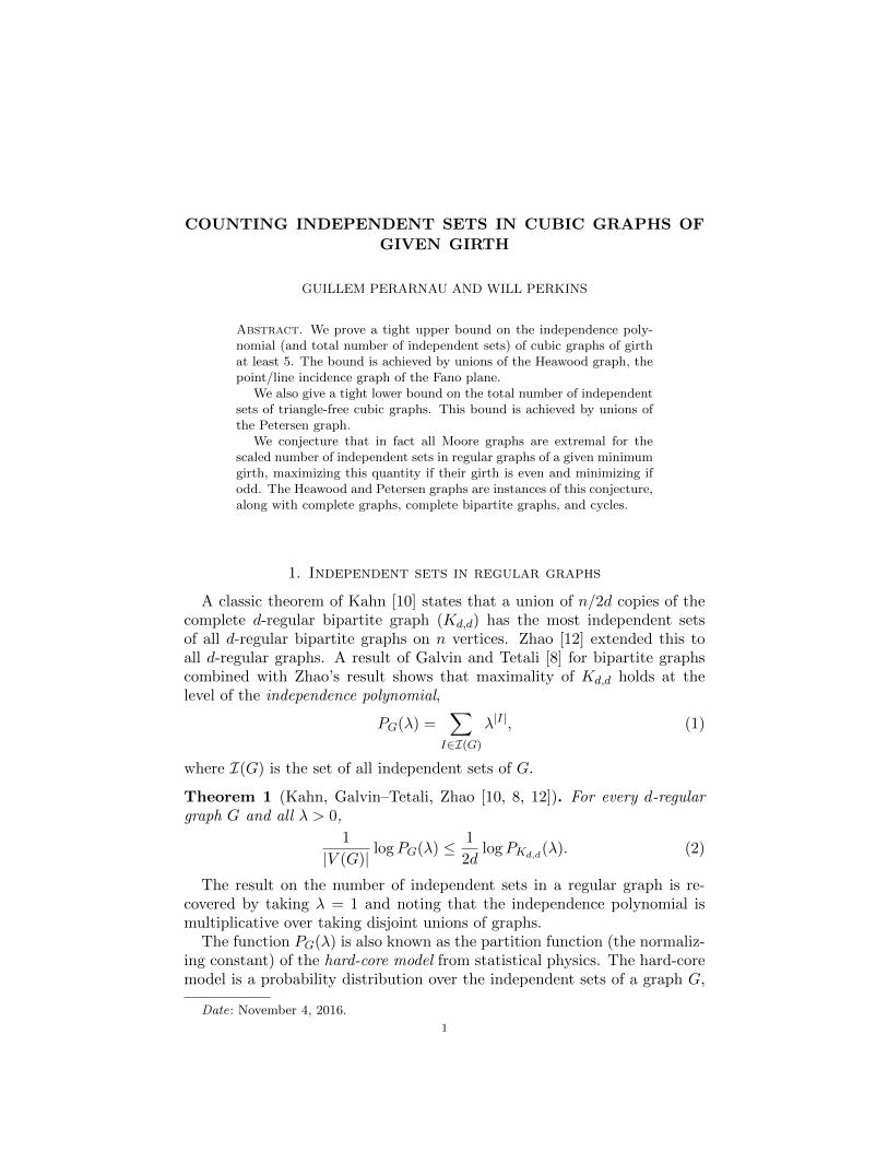
COUNTING INDEPENDENT SETS IN CUBIC GRAPHS OF

GIVEN GIRTH

GUILLEM PERARNAU AND WILL PERKINS

Abstract. We prove a tight upper bound on the independence poly-nomial (and total number of independent sets) of cubic graphs of girthat least 5. The bound is achieved by unions of the Heawood graph, thepoint/line incidence graph of the Fano plane.

We also give a tight lower bound on the total number of independentsets of triangle-free cubic graphs. This bound is achieved by unions ofthe Petersen graph.

We conjecture that in fact all Moore graphs are extremal for thescaled number of independent sets in regular graphs of a given minimumgirth, maximizing this quantity if their girth is even and minimizing ifodd. The Heawood and Petersen graphs are instances of this conjecture,along with complete graphs, complete bipartite graphs, and cycles.

1. Independent sets in regular graphs

A classic theorem of Kahn [10] states that a union of n/2d copies of thecomplete d-regular bipartite graph (Kd,d) has the most independent setsof all d-regular bipartite graphs on n vertices. Zhao [12] extended this toall d-regular graphs. A result of Galvin and Tetali [8] for bipartite graphscombined with Zhao’s result shows that maximality of Kd,d holds at thelevel of the independence polynomial,

PG(λ) =∑

I∈I(G)

λ|I|, (1)

where I(G) is the set of all independent sets of G.

Theorem 1 (Kahn, Galvin–Tetali, Zhao [10, 8, 12]). For every d-regulargraph G and all λ > 0,

1

|V (G)|logPG(λ) ≤ 1

2dlogPKd,d

(λ). (2)

The result on the number of independent sets in a regular graph is re-covered by taking λ = 1 and noting that the independence polynomial ismultiplicative over taking disjoint unions of graphs.

The function PG(λ) is also known as the partition function (the normaliz-ing constant) of the hard-core model from statistical physics. The hard-coremodel is a probability distribution over the independent sets of a graph G,

Date: November 4, 2016.

1

2 GUILLEM PERARNAU AND WILL PERKINS

parametrized by a positive real number λ, the fugacity. The distribution isgiven by:

Pr[I] =λ|I|

PG(λ).

The derivative of 1|V (G)| logPG(λ) has a nice probabilistic interpretation:

it is the occupancy fraction, αG(λ), the expected fraction of vertices of G inthe random independent set drawn from the hard-core model:

αG(λ) :=1

|V (G)|E|I|

=λP ′G(λ)

|V (G)| · PG(λ)

=λ

|V (G)|(logPG(λ))′.

Davies, Jenssen, Perkins and Roberts recently gave a strengthening of The-orem 1, showing that (2) holds at the level of the occupancy fraction.

Theorem 2 (Davies, Jenssen, Perkins, Roberts [5]). For every d-regulargraph G and all λ > 0,

αG(λ) ≤ αKd,d(λ). (3)

Theorem 1 can be recovered from Theorem 2 by noting that logPG(0) = 0

for all G, and then integrating αG(t)t from 0 to λ.

Now Kd,d contains many copies of the 4-cycle, C4, as subgraphs (in factthe highest possible C4 density of a d-regular triangle-free graph). Heuris-tically we might imagine that having many short even cycles increases theindependent set density, while having odd cycles decreases it. So what hap-pens if we forbid 4-cycles?

Similarly, Cutler and Radcliffe [3] show that 1|V (G)| logPG(λ) is minimized

over all d-regular graphs by a union of copies of Kd+1, the complete graphon d + 1 vertices. But Kd+1 has (many) triangles. So what happens if weforbid triangles?

Question 1.

• Which d-regular graphs of girth at least 4 have the fewest independentsets?• Which d-regular graphs of girth at least 5 have the most independent

sets?• More generally, for g even, which d-regular graphs of girth at leastg have the fewest independent sets, and for g odd, which d-regulargraphs of girth at least g have the most independent sets?

Here we answer the first two questions for the class of cubic (3-regular)graphs: the triangle-free cubic graphs with the fewest independent sets arecopies of the Petersen graph P5,2, and the cubic graphs of girth at least 5with the most independent sets are copies of the Heawood graph H3,6.

COUNTING INDEPENDENT SETS IN CUBIC GRAPHS OF GIVEN GIRTH 3

Figure 1

Petersen Graph P5,2 Heawood Graph H3,6

Notably, in all of the cases that we know (Kd+1,Kd,d, the cycles Cn, andthe Petersen and Heawood graphs), the optimizing graph is a Moore graph.A (d, g)-Moore graph, for g odd, is a d-regular graph with girth g, diameter(g − 1)/2 and exactly

1 + d

(g−3)/2∑j=0

(d− 1)j

vertices. If g is even, then a (d, g)-Moore graph is d-regular, has girth g andexactly

1 + (d− 1)g/2−1 + d

(g−4)/2∑j=0

(d− 1)j

vertices. Moore graphs are necessarily cages: regular graphs with the fewestnumber of vertices for their girth.

Moore graphs do not exist for every pair d, g. But we conjecture thatif such a Moore graph exists, then it is extremal for the scaled number ofindependent sets in a d-regular graph of girth at least g − 1 (and of courseextremal for graphs of girth at least g as well).

Conjecture 1. Suppose g is odd and there exists a (d, g)-Moore graph, G∗d,g.Then for every d-regular graph G of girth at least g − 1,

1

|V (G)|log |I(G)| ≥ 1

|V (G∗d,g)|log |I(G∗d,g)|.

Suppose g is even and there exists a (d, g)-Moore graph G∗d,g. Then for everyd-regular graph G of girth at least g − 1,

1

|V (G)|log |I(G)| ≤ 1

|V (G∗d,g)|log |I(G∗d,g)|.


1.1. The Petersen graph. The Petersen graph, P5,2, has 10 vertices, is3-regular and vertex-transitive, has girth 5 and is a (3, 5)-Moore graph (seeFigure 1). Its independence polynomial is

PP5,2(λ) = 1 + 10λ+ 30λ2 + 30λ3 + 5λ4,

and its occupancy fraction is

αP5,2(λ) =λ(1 + 6λ+ 9λ2 + 2λ3

)PP5,2(λ)

. (4)

Our first result provides a tight lower bound on the occupancy fractionof triangle-free cubic graphs for every λ ∈ (0, 1]:

Theorem 3. For any triangle-free, cubic graph G, and for every λ ∈ (0, 1],

αG(λ) ≥ αP5,2(λ),

with equality if and only if G is a union of copies of P5,2.

By integrating αG(λ)λ from λ = 0 to 1 we obtain the corresponding counting

result:

Corollary 4. For any triangle-free, cubic graph G, and any λ ∈ (0, 1],

1

|V (G)|logPG(λ) ≥ 1

10logPP5,2(λ),

and in particular,

1

|V (G)|log |I(G)| ≥ 1

10log |I(P5,2)|,

with equality if and only if G is a union of copies of P5,2.

Recently, Cutler and Radcliffe [4] proved a lower bound on the occupancyfraction of triangle-free cubic graphs that gave 1

|V (G)| log |I(G)| ≥ 0.430703,

while the tight bound above is 110 log |I(P5,2)| = log(76)

10 ≈ 0.43307. Cutlerand Radcliffe also conjectured that for every cubic triangle-free graph G onn vertices and for every λ > 0

1

nlogPG(λ) ≥ min

{1

10logPP5,2(λ),

1

14logPP7,2(λ)

},

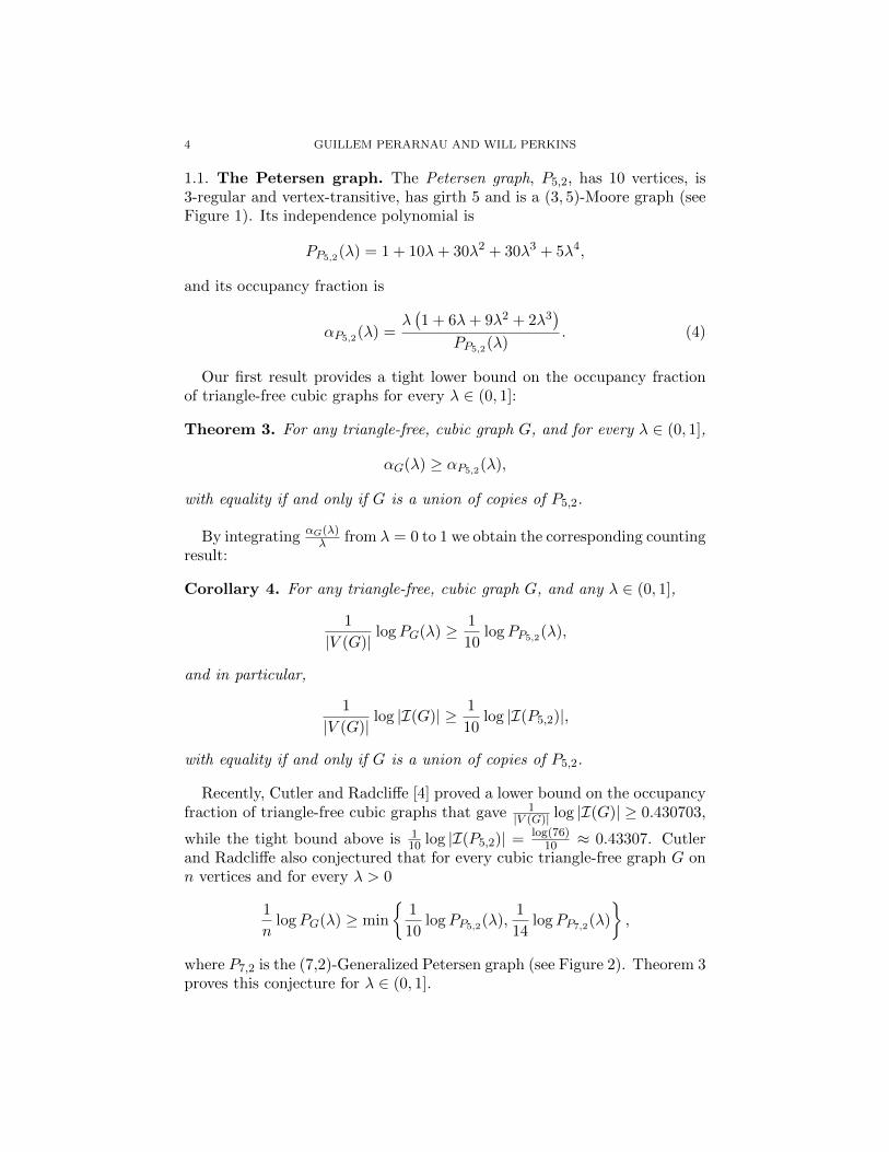
where P7,2 is the (7,2)-Generalized Petersen graph (see Figure 2). Theorem 3proves this conjecture for λ ∈ (0, 1].


Figure 2

(7,2)-Generalized Petersen P7,2

1.2. The Heawood graph. The Heawood graph, H3,6, has 14 vertices, is3-regular and vertex-transitive, has girth 6, and is a (3, 6)-Moore graph (seeFigure 1). It can be constructed as the point-line incidence graph of theFano plane. Its independence polynomial is

PH3,6(λ) = 1 + 14λ+ 70λ2 + 154λ3 + 147λ4 + 56λ5 + 14λ6 + 2λ7,

and its occupancy fraction is

αH3,6(λ) =λ(1 + 10λ+ 33λ2 + 42λ3 + 20λ4 + 6λ5 + λ6)

PH3,6(λ). (5)

Our second result provides a tight upper bound on the occupancy fractionof cubic graphs with girth at least 5:

Theorem 5. For any cubic graph G of girth at least 5, and for every λ > 0,

αG(λ) ≤ αH3,6(λ),

with equality if and only if G is a union of copies of H3,6.

And by integrating αG(t)t from t = 0 to λ we obtain the corresponding

counting results.

Corollary 6. For any cubic graph G of girth at least 5, and for every λ > 0,

1

|V (G)|logPG(λ) ≤ 1

14logPH3,6(λ),

and in particular,

1

|V (G)|log |I(G)| ≤ 1

14log |I(H3,6)|,

with equality if and only if G is a union of copies of H3,6.

Note that Theorem 5 applies to all positive λ, while Theorem 3 requiresλ ∈ (0, 1]. Some bound on the interval for which P5,2 minimizes the oc-cupancy fraction is necessary: for large λ, P7,2 has a smaller occupancy


fraction, and in fact in the limit as λ → ∞, it is minimal: Staton [11]proved the independence ratio of any triangle-free cubic graph is at least5/14 and this is achieved by P7,2.

Corollaries 4 and 6 answer the 3-regular case of a question of Zhao [13]and confirm his conjecture in these cases that minimum and maximum nor-malized number of independent sets under local constraints are attained byfinite graphs.

We prove Theorems 3 and 5 by introducing several local constraints thatthe hard-core model induces on any 3-regular graph of a given girth. Wethen relax the optimization problem to the set of all probability distributionson local configurations that satisfy these constraints and solve the relaxationusing linear programming.

We begin in Section 2 with an overview of the method that we use toprove Theorems 3 and 5.

In Section 3 we prove Theorem 5 under the additional assumption thatG has girth at least 6. This illustrates the method and introduces the typeof local constraints we will use in the other proofs. In Section 4 we extendthe proof to all graphs of girth at least 5 by introducing new variables intoour maximization problem. In Section 5 we prove Theorem 3 by switchingfrom maximization to minimization and by introducing further variablescorresponding to graphs containing 4-cycles. Nonetheless, the constraintsremain unchanged from those in Sections 3 and 4.

We conclude in Section 6 with some further questions on the number ofindependent sets and graph homomorphisms in regular graphs with girthconstraints.

2. On the method and related work

The method we use is an extension of the method used in [5] to prove The-orem 2 and the analogous theorem for random matchings in regular graphs.At a high level, the method works as follows. To bound the occupancyfraction of the hard-core model on a graph G, we consider the experimentof drawing an independent set I from the hard-core model, then indepen-dently choosing a vertex v uniformly from the graph. We then record a localview of both G and I from the perspective of v. The depth-t local viewfrom v includes both the information of the graph structure of the depth-tneighborhood of v as well as the boundary conditions the independent setI induces on this neighborhood (that is, which vertices at the boundary areblocked from being in the independent set by some external vertex). In [5],the local view considered was of the first neighborhood of v, with each neigh-bor labeled according to whether or not it had an occupied neighbor amongthe second neighbors of v.

In this paper, we extend the local view to include the first and secondneighborhood of v. We call a realization of the local view a configuration.


The probabilistic experiment of drawing I and v at random induces a proba-bility distribution on the set of all possible configurations. Not all probabil-ity distributions over the configuration set are attainable by graphs; certainconsistency conditions must hold. For instance, here we use the fact that theprobability that v has t occupied neighbors in this experiment must equalthe probability that a random neighbor u of v has t occupied neighbors.Such consistency conditions serve as constraints in an optimization prob-lem in which the variables are the individual probabilities of each possibleconfiguration.

The art in applying the method is choosing the right local view and whichconsistency conditions to impose. Enriching the local view as we have donehere adds power to the optimization program, but comes at the cost of in-creasing the complexity of the resulting linear program. As an example, com-pare the upper bound on the independence polynomial in d-regular triangle-free graphs [5] with the lower bound for 3-regular triangle-free graphs givenby Theorem 3: the proof of the first is short and elementary, while the proofof the second requires (at least in this iteration) a large mass of calculationsgiven in the appendix and in the ancillary files.

This suggests several directions for further inquiry into this method.

(1) Is there a general theory of which problems can be solved using thismethod and is there an underlying principle that indicates whichdistributions and graphs are extremal?

(2) Can the proof procedure be efficiently automated, in a way thatgiven the definition of the local view, the allowed configurations,and the objective function, a computer outputs a bound along witha proof certificate?

(3) Is there a more analytic and less computational analysis of the linearprograms than the proofs we give here?

The method has to this point been used for upper and lower bounds onindependent sets and matchings in regular graphs [5, 7, 4], as well as theWidom-Rowlinson model [2], another statistical physics model with hardconstraints. In [6], the method is applied to models with soft constraints,namely the Ising and Potts models on regular graphs, which in the ‘zero-temperature limit’ yield extremal bounds on the number of q-colorings ofcubic graphs. See the survey of Zhao [13] for more on extremal problems forregular graphs.

3. Proof of Theorem 5 for girth at least 6

Let G be a 3-regular graph of girth at least 6. Since G has girth greaterthan 5, every vertex v ∈ V (G) has 6 distinct second neighbors, and itssecond neighbors form an independent set.

Draw an independent set I ∈ I(G) from the hard-core distribution on Gwith fugacity λ > 0. We say that a vertex is occupied if it is in I. Pick avertex v uniformly at random from V (G). We say that a vertex u of the


second neighborhood of v is externally uncovered if none of its neighbors atdistance 3 from v are in I. Order the neighbors of v arbitrarily, u1, u2, u3.Describe the local view of v with respect to I by C = (c1, c2, c3) with cibeing the number of externally uncovered second neighbors joined to ui.

Let

C6 = {(0, 0, 0), (0, 0, 1), (0, 0, 2), (0, 1, 1), (0, 1, 2),

(0, 2, 2), (1, 1, 1), (1, 1, 2), (1, 2, 2), (2, 2, 2)}be the set of all possible configurations C that can arise from cubic graphsof girth at least 6. As the functions that appear in the optimization problembelow do not depend on the ordering of the ci’s we can restrict ourselves tomultisets; that is, the configuration (1, 1, 2) is equivalent (2, 1, 1). We abusenotation and let C refer to the vector (c1, c2, c2) as well as the graph formedby the configuration: v joined to its three neighbors u1, u2, u3, each joinedto c1, c2, c3 second neighbors of v respectively.

Consider the following quantities,

Z−(C) =

3∏i=1

(λ+ (1 + λ)ci)

Z+(C) = λ(1 + λ)∑3

i=1 ci

Z(C) = Z−(C) + Z+(C).

Here, Z−(C) is the partition function of C restricted to independent setswith v unoccupied; Z+ is the same restricted to v occupied, and Z(C) is thetotal partition function of C. We reserve the letter P for a partition functionof a full cubic graph, as in PH3,6 , and use Z for the partition function ofconfiguration. Then the probability that v is occupied given configurationC is

αC,v(λ) := Pr[v ∈ I|C] =Z+(C)

Z(C).

Observe that the occupancy fraction of G can be written as

αG(λ) =1

n

∑v∈V (G)

Pr[v ∈ I] =∑C∈C6

αC,v(λ) Pr[C],

where Pr[C] is the probability that the configuration C is observed when I ∈I(G) is chosen according to the hard-core model and v is chosen uniformlyat random.

Given the choice of v, let u be a vertex chosen uniformly at randomfrom the neighbors of v. We can write down formulae for the conditionalprobabilities that either v or u has a given the number of occupied neighbors.Let

γvt (C) = Pr[v has t occupied neighbors|C] and

γut (C) = Pr[u has t occupied neighbors|C].


Lemma 7.

γv0 (C) =1 + λ

λαC,v(λ)

γv1 (C) = αC,v(λ) ·3∑i=1

(1 + λ)−ci

γv2 (C) =λ2

Z(C)·

3∑i=1

(1 + λ)ci

γu0 (C) = (1− αC,v(λ))1 + λ

3

3∑i=1

1

λ+ (1 + λ)ci

γu1 (C) = αC,v(λ) · 1

3

3∑i=1

(1 + λ)−ci + (1− αC,v(λ)) · 1

3

3∑i=1

ciλ

λ+ (1 + λ)ci

γu2 (C) = αC,v(λ) · 1

3

3∑i=1

ciλ(1 + λ)−ci + (1− αC,v(λ)) · 1

3

∑i∈{1,2,3}

ci=2

λ2

λ+ (1 + λ)ci.

Proof. Here we show how to obtain the expressions for γv2 (C) and γu2 (C);the others follow similarly. For γv2 (C) we need to select a vertex ui in theneighborhood of v that will not be included in I, and insist that the twoother neighbors of v are in I. Given this choice, we may additionally includeany subset of the externally uncovered neighbors of ui (different from v),contributing the factor (1 +λ)ci . The term λ2 accounts for the contributionof uj with j 6= i. It follows that

γv2 (C) =λ2

Z(C)·

3∑i=1

(1 + λ)ci

For γu2 (C) we need to distinguish between the case where v is occupied andthe case where it is unoccupied. Let us assume first that v is occupied, then itcontributes with a factor of λ, and accounts for 1 of the two required occupiedneighbors of u. Select a vertex u = ui in the neighborhood of v uniformlyat random. Since v ∈ I, we need to include exactly one of its externallyuncovered neighbors, contributing a factor of ciλ. The neighbors uj withj 6= i cannot be included in I since v is occupied, thus we can include anysubset of their externally uncovered neighbors, contributing with a factor

of (1+λ)c1+c2+c3

(1+λ)ci = Z+(C)(1+λ)−ci

λ . The probability that u has 2 occupied

neighbors and that v is occupied is

1

Z(C)· λ · 1

3

3∑i=1

ciλ ·Z+(C)(1 + λ)−ci

λ= αC,v(λ) · 1

3

3∑i=1

ciλ(1 + λ)−ci .


The probability that u has 2 occupied neighbors and that v is unoccupiedcan be computed in a similar way, giving that

γu2 (C) = αC,v(λ) · 13

3∑i=1

ciλ(1+λ)−ci +(1−αC,v(λ)) · 13

∑i∈{1,2,3}

ci=2

λ2

λ+ (1 + λ)ci.

�

Now we can form the following linear program with decision variablesp(C) with C ∈ C6 corresponding to Pr[C]:

αmax(λ) = max∑C∈C6

αC,v(λ)p(C) subject to

∑C∈C6

p(C) = 1

∑C∈C6

p(C) · (γvt (C)− γut (C)) = 0 for t = 0, 1, 2

p(C) ≥ 0 ∀C ∈ C6The dual program with decision variables Λp,Λ0,Λ1,Λ2 is:

αmax(λ) = min Λp subject to

Λp +

2∑t=0

Λt [γvt (C)− γut (C)] ≥ αC,v(λ) ∀C ∈ C6.

To show that αG(λ) ≤ αH3,6(λ) for all cubic G of girth at least 6, weneed to show that αmax(λ) ≤ αH3,6(λ) (the reverse inequality is immediatesince the distribution induced by H3,6 is a feasible solution). To prove thisusing linear programming duality, it is enough to find a feasible solutionto the dual program with Λp = αH3,6 . We define the slack function of aconfiguration C as:

SLACKmax(λ,Λ0,Λ1,Λ2, C) = αH3,6 − αC,v(λ) +

2∑t=0

Λt [γvt (C)− γut (C)] .

(6)

Our goal is now to find values for the dual variables Λ∗0,Λ∗1,Λ

∗2 so that

SLACKmax(λ,Λ∗0,Λ∗1,Λ

∗2, C) ≥ 0

for all configurations C ∈ C6 and λ > 0.Our candidate solution is the Heawood graph H3,6 (see Figure 2). There

are only 4 possible configurations arising fromH3,6: (0, 0, 0), (1, 0, 0), (1, 1, 1),and (2, 2, 2). These correspond respectively to having 3 or 4, 2, 1 and 0 ver-tices from I in the third neighborhood of v.


Figure 3

Heawood Graph H3,6 viewed from a vertex

If we set the dual constraints to hold with equality for the configura-tions (0, 0, 0), (1, 0, 0), and (1, 1, 1), and set Λp = αH3,6 , we get the followingsystem of equations.

λ

λ+ (1 + λ)3= αH3,6 + Λ0

[1 + 2λ

λ+ (1 + λ)3− 1

]+ Λ1 ·

2λ

(λ+ 1)3 + λ+ Λ2

3λ2

λ+ (1 + λ)3

λ

2λ2 + 4λ+ 1= αH3,6

− Λ05λ(λ+ 1)

6λ2 + 12λ+ 3− Λ1

λ(λ2 − 2λ− 5

)3(λ+ 1) (2λ2 + 4λ+ 1)

+ Λ2λ2(3λ+ 8)

3 (2λ3 + 6λ2 + 5λ+ 1)

λ(λ+ 1)3

λ(λ+ 1)3 + (2λ+ 1)3=

αH3,6+ Λ0

λ(λ3 − 2λ− 1

)λ4 + 11λ3 + 15λ2 + 7λ+ 1

+ Λ1λ− 2λ3

λ4 + 11λ3 + 15λ2 + 7λ+ 1+ Λ2

λ2(−λ2 + λ+ 2

)λ4 + 11λ3 + 15λ2 + 7λ+ 1

Solving these equations give candidate values for the dual variables.

Claim 8. With the following assignments to the dual variables,

SLACKmax(λ,Λ∗0,Λ∗1,Λ

∗2, C) ≥ 0

for all configurations C ∈ C6.

Λ∗0 =−3− 27λ− 94λ2 − 139λ3 − 20λ4 + 139λ5 + 124λ6 + 45λ7 + 9λ8 + λ9

(1 + λ)(1 + 2λ) · PH3,6(λ)

Λ∗1 =−3− 24λ− 73λ2 − 99λ3 − 25λ4 + 63λ5 + 55λ6 + 15λ7 + λ8

(1 + 2λ) · PH3,6(λ)

Λ∗2 =−3− 27λ− 94λ2 − 160λ3 − 132λ4 − 46λ5 − 3λ6 + λ7

(1 + 2λ) · PH3,6(λ)

In particular, Claim 8 shows that in the primal αmax(λ) = αH3,6(λ). Toprove Claim 8 we will show that for all C ∈ C6, the following scaling of the


slack function

Fmax(C) := 3(λ+ 2) · PH3,6(λ) · Z(C) · SLACKmax(λ,Λ∗0,Λ∗1,Λ

∗2, C), (7)

is identically 0 if C is in the support of the Heawood graph and a polynomialin λ with positive coefficients otherwise. This suffices to prove Claim 8 since3(λ+2) ·PH3,6(λ) ·Z(C) is itself a polynomial in λ with positive coefficients.

Using (5) and Lemma 7, we calculate:

Fmax((0, 0, 0)) = 0

Fmax((0, 0, 1)) = 0

Fmax((0, 0, 2)) = λ5(λ+ 1)(λ+ 2)(λ5 + 13λ4 + 47λ3 + 69λ2 + 36λ+ 6

)Fmax((0, 1, 1)) = λ6

(2λ5 + 11λ4 + 30λ3 + 41λ2 + 20λ+ 3

)Fmax((0, 1, 2)) = λ5

(4λ7 + 47λ6 + 209λ5 + 458λ4 + 523λ3 + 303λ2 + 84λ+ 9

)Fmax((0, 2, 2)) = λ5(λ+ 2)

(4λ7 + 49λ6 + 218λ5 + 463λ4 + 502λ3 + 269λ2 + 66λ+ 6

)Fmax((1, 1, 1)) = 0

Fmax((1, 1, 2)) = λ5(λ+ 1)3(3λ4 + 37λ3 + 77λ2 + 39λ+ 6

)Fmax((1, 2, 2)) = 2λ5(λ+ 1)3

(λ5 + 15λ4 + 52λ3 + 62λ2 + 24λ+ 3

)Fmax((2, 2, 2)) = 0.

Indeed for all C in the support of the Heawood graph Fmax(C) = 0, and forall other C, Fmax(C) is a polynomial in λ with positive coefficients. Thisproves Claim 8 and thus shows that αG(λ) ≤ αH3,6(λ) for all λ > 0 and allcubic G of girth at least 6. Uniqueness follows from complementary slacknessand the fact that we have 4 linearly independent constraints; therefore theonly feasible distribution whose support is contained in the support of theHeawood graph is the Heawood graph.

4. Girth at least 5

Now we extend the proof to include graphs of girth 5. If G is cubic andhas girth at least than 5, then every vertex v ∈ V (G) has 6 distinct secondneighbors, but now its second neighborhood may contain some edges.

Draw an independent set I ∈ I(G) from the hard-core distribution on Gwith fugacity λ > 0. Recall that a vertex u of the second neighborhood of vis externally uncovered if none of its neighbors at distance 3 from v are in I.For i ∈ {1, 2, 3}, let ui be the neighbors of v and for j ∈ {1, 2} let wij be theneighbors of ui that are second neighbors of v. Let C = (W,E12, E22) be aconfiguration where W is the set of second neighbors of v that are externallyuncovered, E12 is the set of edges between first neighbors of v and W , andE22 is the set of edges within W in the configuration C.

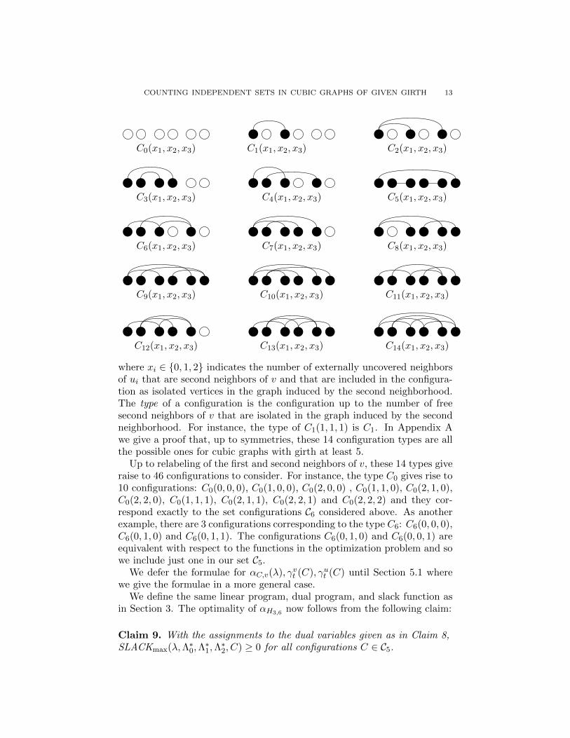
Let C5 be the set of all possible configurations C that can arise from acubic graph of girth at least 5. The possible configurations are the following:


C0(x1, x2, x3) C1(x1, x2, x3) C2(x1, x2, x3)

C3(x1, x2, x3) C4(x1, x2, x3) C5(x1, x2, x3)

C6(x1, x2, x3) C7(x1, x2, x3) C8(x1, x2, x3)

C9(x1, x2, x3) C10(x1, x2, x3) C11(x1, x2, x3)

C12(x1, x2, x3) C13(x1, x2, x3) C14(x1, x2, x3)

where xi ∈ {0, 1, 2} indicates the number of externally uncovered neighborsof ui that are second neighbors of v and that are included in the configura-tion as isolated vertices in the graph induced by the second neighborhood.The type of a configuration is the configuration up to the number of freesecond neighbors of v that are isolated in the graph induced by the secondneighborhood. For instance, the type of C1(1, 1, 1) is C1. In Appendix Awe give a proof that, up to symmetries, these 14 configuration types are allthe possible ones for cubic graphs with girth at least 5.

Up to relabeling of the first and second neighbors of v, these 14 types giveraise to 46 configurations to consider. For instance, the type C0 gives rise to10 configurations: C0(0, 0, 0), C0(1, 0, 0), C0(2, 0, 0) , C0(1, 1, 0), C0(2, 1, 0),C0(2, 2, 0), C0(1, 1, 1), C0(2, 1, 1), C0(2, 2, 1) and C0(2, 2, 2) and they cor-respond exactly to the set configurations C6 considered above. As anotherexample, there are 3 configurations corresponding to the type C6: C6(0, 0, 0),C6(0, 1, 0) and C6(0, 1, 1). The configurations C6(0, 1, 0) and C6(0, 0, 1) areequivalent with respect to the functions in the optimization problem and sowe include just one in our set C5.

We defer the formulae for αC,v(λ), γvt (C), γut (C) until Section 5.1 wherewe give the formulae in a more general case.

We define the same linear program, dual program, and slack function asin Section 3. The optimality of αH3,6 now follows from the following claim:

Claim 9. With the assignments to the dual variables given as in Claim 8,SLACKmax(λ,Λ∗0,Λ

∗1,Λ

∗2, C) ≥ 0 for all configurations C ∈ C5.


Again we scale the slack function by the same positive polynomial usedin the previous section:

Fmax(C) := 3(λ+ 2) · PH3,6(λ) · Z(C) · SLACKmax(λ,Λ∗0,Λ∗1,Λ

∗2, C), (8)

One can verify that Fmax(C) is either identically 0 or a polynomial inλ with positive coefficients. We have verified this by having a computerprogram compute Fmax(C) for all C ∈ C5 and collect coefficients. Thecomputer code and printout is included as an ancillary file.

For all C ∈ C5 in the support of the Heawood graph Fmax(C) ≡ 0. For allother C ∈ C5 different than C1(1, 1, 0), Fmax(C) is a polynomial in λ withpositive coefficients. However, we also find that Fmax(C1(1, 1, 0)) ≡ 0. Thisproves that the dual solution is feasible but does not prove uniqueness ofthe solution.

In order to prove that unions of copies of H3,6 are the only graphs thatmaximize αG(λ) among all 3-regular graphs G of girth at least 5, we firstneed to exclude the configuration C1(1, 1, 0). Let C be the random configu-ration obtained by choosing I ∈ I(G) according to the hard-core model andv ∈ V (G) uniformly at random.

Claim 10. Let G be a 3-regular graph of girth at least 5 with αG(λ) =αH3,6(λ). Then Pr[C = C1(1, 1, 0)] = 0.

Proof. Suppose that Pr[C = C1(1, 1, 0)] > 0. Let v∗ ∈ V (G) be such thatthe second neighborhood of v∗ in G contains at least one edge. Since Gattains the maximum occupancy fraction, complementary slackness tell usthat the only configurations that can appear with positive probability areC0(0, 0, 0), C0(1, 0, 0), C0(1, 1, 1), C0(2, 2, 2) and C1(1, 1, 0). Consider theempty independent set I0 = ∅. The configuration induced by I0 in the secondneighborhood of v∗ is of the form Ci(2, 2, 2) for some i 6= 0, but all theseconfigurations have probability 0 to appear, leading to a contradiction. �

Therefore, any maximizer has support in C0(0, 0, 0), C0(1, 0, 0), C0(1, 1, 1)and C0(2, 2, 2). It suffices to prove that H3,6 is the only graph with thissupport. Fix v ∈ V (G). First observe that there are no edges within thesecond neighborhood of v. The fact that Pr[C = C0(2, 2, 1)] = Pr[C =C0(2, 1, 1)] = Pr[C = C0(2, 2, 0)] = 0, implies that every vertex in the thirdneighborhood of v is adjacent to 3 vertices in the second neighborhood ofv. Thus, G is the disjoint union of 3-regular graphs of girth 5 and order 14.Uniqueness now follows from the well-known fact that H3,6 is the only suchgraph.

5. Proof of Theorem 3

Here we prove Theorem 3 by showing that an appropriate linear program-ming relaxation shows that for all 3-regular G of girth at least 4 (triangle-free) and all λ ∈ (0, 1],

αG(λ) ≥ αP5,2(λ).


We remark that the statement of Theorem 3 may still be true for someλ > 1, but it is not true for λ > λ∗3 ≈ 1.84593, since for λ > λ∗3 theoccupancy fraction of the (7, 2)-Generalized Petersen graph is smaller thanthat of the Petersen graph. In Section 6 we present a conjecture that extendsTheorem 3 for every λ > 0.

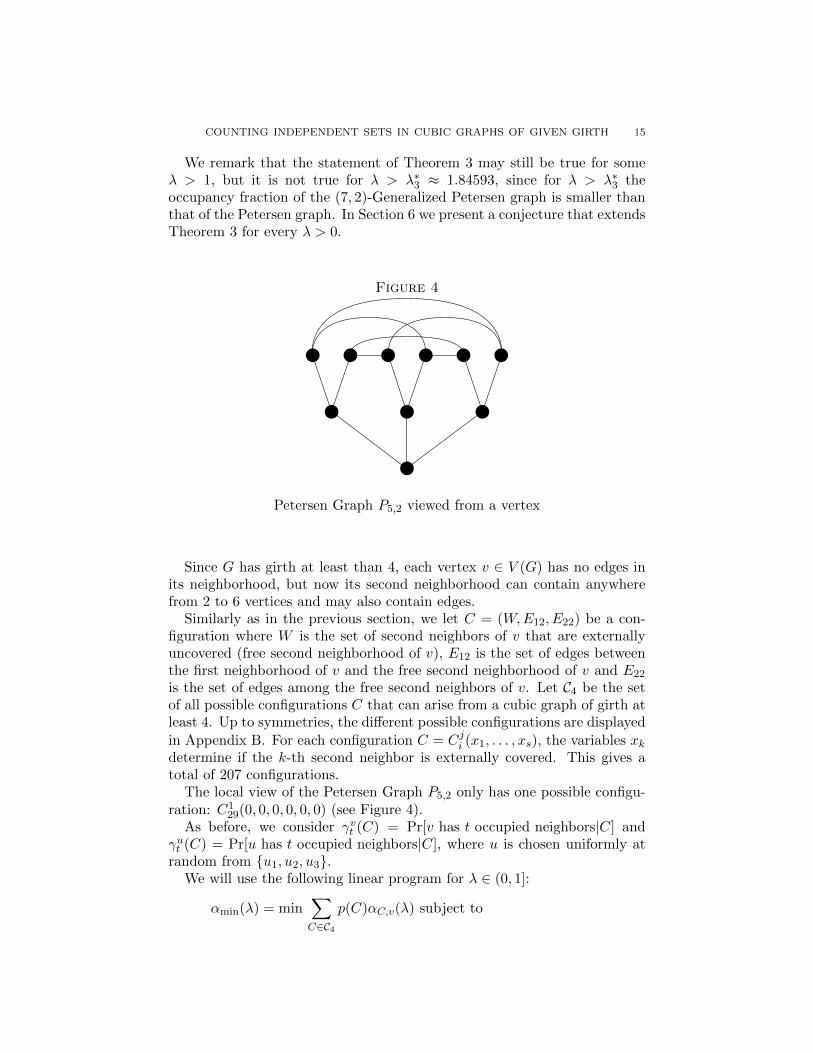
Figure 4

Petersen Graph P5,2 viewed from a vertex

Since G has girth at least than 4, each vertex v ∈ V (G) has no edges inits neighborhood, but now its second neighborhood can contain anywherefrom 2 to 6 vertices and may also contain edges.

Similarly as in the previous section, we let C = (W,E12, E22) be a con-figuration where W is the set of second neighbors of v that are externallyuncovered (free second neighborhood of v), E12 is the set of edges betweenthe first neighborhood of v and the free second neighborhood of v and E22

is the set of edges among the free second neighbors of v. Let C4 be the setof all possible configurations C that can arise from a cubic graph of girth atleast 4. Up to symmetries, the different possible configurations are displayed

in Appendix B. For each configuration C = Cji (x1, . . . , xs), the variables xkdetermine if the k-th second neighbor is externally covered. This gives atotal of 207 configurations.

The local view of the Petersen Graph P5,2 only has one possible configu-ration: C1

29(0, 0, 0, 0, 0, 0) (see Figure 4).As before, we consider γvt (C) = Pr[v has t occupied neighbors|C] and

γut (C) = Pr[u has t occupied neighbors|C], where u is chosen uniformly atrandom from {u1, u2, u3}.

We will use the following linear program for λ ∈ (0, 1]:

αmin(λ) = min∑C∈C4

p(C)αC,v(λ) subject to

16 GUILLEM PERARNAU AND WILL PERKINS∑C∈C4

p(C) = 1

∑C∈C4

p(C) · (γvt (C)− γut (C)) = 0 for t = 0, 1, 2

p(C) ≥ 0 ∀C ∈ C4.

The respective dual program is:

αmin(λ) = max Λp subject to (9)

Λp +2∑t=0

Λt [γvt (C)− γut (C)] ≤ αC,v(λ) ∀C ∈ C4.

Our goal is to show that αmin(λ) = αP5,2(λ) for all λ ∈ [0, 1].If we take Λp = αP5,2 , then we can define the slack function of the config-

uration C ∈ C4 as a function of the dual variables Λ0,Λ1,Λ2:

SLACKmin(λ,Λ0,Λ1,Λ2, C) = αC,v(λ)− αP5,2 −2∑t=0

Λt [γvt (C)− γut (C)] .

(10)

Our goal is now to find values for the dual variables Λ∗0,Λ∗1,Λ

∗2 so that, for

all configurations C ∈ C4,

SLACKmin(λ,Λ∗0,Λ∗1,Λ

∗2, C) ≥ 0

In this case, we need to divide the interval [0, 1] into four intervals, andselect different functions for the dual variables depending on which intervalλ is in. We will not be able to show that the slack functions are positivepolynomials in λ: instead we will perform four different substitutions, writ-ing λ as function of an auxiliary variable t and show that the slack functionsare the ratio of positive polynomials in t.

Note that for any a ≤ b, the function λ(t) = b(a/b+t)1+t maps [0,∞) to

[a, b). Since the function SLACKmin(λ,Λ∗0(λ),Λ∗1(λ),Λ∗2(λ), C) is a continu-ous function of λ, if we can show

SLACKmin(λ(t),Λ∗0(λ(t)),Λ∗1(λ(t)),Λ∗2(λ(t)), C) ≥ 0

for all t ≥ 0, then we have

SLACKmin(λ,Λ∗0(λ),Λ∗1(λ),Λ∗2(λ), C) ≥ 0

for all λ ∈ [a, b].In each of the four claims below, we will assign values to the dual variables,

Λ∗0,Λ∗1,Λ

∗2. We arrived at these values by solving the dual constraints to hold

with equality for a given subset of the configurations; we determined thesesubsets by solving instances of the dual program for fixed values of λ andobserving which constraints were tight.


Claim 11. Let λ1(t) = 316

t1+t . Let

Λ∗0(λ) = 0

Λ∗1(λ) =3(4λ8 + 21λ7 + 57λ6 + 67λ5 + 38λ4 + 10λ3 + λ2

)(4λ4 + 10λ3 + 11λ2 + 7λ+ 1) (5λ4 + 30λ3 + 30λ2 + 10λ+ 1)

Λ∗2(λ) =3(4λ8 + 31λ7 + 68λ6 + 64λ5 + 33λ4 + 9λ3 + λ2

)(4λ4 + 10λ3 + 11λ2 + 7λ+ 1) (5λ4 + 30λ3 + 30λ2 + 10λ+ 1)

.

Then, for every C ∈ C4:

SLACKmin(λ1(t), 0,Λ∗1(λ1(t)),Λ

∗2(λ1(t)), C)

is either identically 0 or the ratio of two polynomials in t with all positivecoefficients.

This implies αmin(λ) = αP5,2(λ) for λ ∈ [0, 3/16].

Claim 12. Let λ2(t) = 1120 ·

316

2011

+t

1+t . Let

Λ∗0(t) = 0

Λ∗1(λ) =4λ7 − 13λ6 − 64λ5 − 75λ4 − 36λ3 − 6λ2

2 (5λ7 + 40λ6 + 100λ5 + 135λ4 + 111λ3 + 52λ2 + 12λ+ 1)

Λ∗2(λ) =−6λ6 − 45λ5 − 49λ4 − 21λ3 − 3λ2

2 (λ2 + λ+ 1) (5λ4 + 30λ3 + 30λ2 + 10λ+ 1).



∗2(λ2(t)), C)


This implies αmin(λ) = αP5,2(λ) for λ ∈ [3/16, 11/20].

Claim 13. Let λ3(t) =√

35 ·

1120

√53+t

1+t . Let

Λ∗0 = 0

Λ∗1(λ) =5λ7 − 41λ6 − 125λ5 − 111λ4 − 42λ3 − 6λ2

2 (10λ7 + 75λ6 + 165λ5 + 205λ4 + 152λ3 + 63λ2 + 13λ+ 1)

Λ∗2(λ) =−12λ7 − 96λ6 − 140λ5 − 83λ4 − 24λ3 − 3λ2

2 (2λ3 + 3λ2 + 3λ+ 1) (5λ4 + 30λ3 + 30λ2 + 10λ+ 1).



∗2(λ3(t)), C)


This implies αmin(λ) = αP5,2(λ) for λ ∈ [11/20,√

3/5].


Claim 14. Let λ4(t) =t+√

3/5

t+1 . Let

Λ∗0(λ) =12λ7 + 66λ6 + 86λ5 − 88λ4 − 196λ3 − 117λ2 − 30λ− 3

6λ(λ+ 1)2 (5λ4 + 30λ3 + 30λ2 + 10λ+ 1)

Λ∗1(λ) =−18λ6 − 3λ5 − 54λ4 − 118λ3 − 87λ2 − 27λ− 3

6λ(λ+ 1) (5λ4 + 30λ3 + 30λ2 + 10λ+ 1)

Λ∗2(λ) =−6λ6 − 18λ5 − 100λ4 − 160λ3 − 105λ2 − 30λ− 3

6λ(λ+ 1) (5λ4 + 30λ3 + 30λ2 + 10λ+ 1).


SLACKmin(λ4(t),Λ∗0(λ4(t)),Λ

∗1(λ4(t)),Λ

∗2(λ4(t)), C)


This implies αmin(λ) = αP5,2(λ) for λ ∈ [√

3/5, 1].

The proof of these claims again proceeds by computing

SLACKmin(λi(t),Λ∗0(λi(t)),Λ

∗1(λi(t)),Λ

∗2(λi(t)), C)

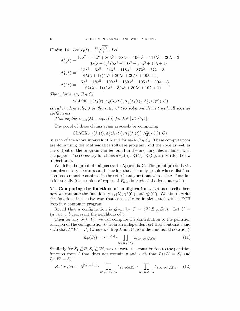
in each of the above intervals of λ and for each C ∈ C4. These computationsare done using the Mathematica software program, and the code as well asthe output of the program can be found in the ancillary files included withthe paper. The necessary functions αC,v(λ), γvt (C), γut (C), are written belowin Section 5.1.

We defer the proof of uniqueness to Appendix C. The proof proceeds viacomplementary slackness and showing that the only graph whose distribu-tion has support contained in the set of configurations whose slack functionis identically 0 is a union of copies of P5,2 (in each of the four intervals).

5.1. Computing the functions of configurations. Let us describe herehow we compute the functions αC,v(λ), γvt (C), and γut (C). We aim to writethe functions in a naive way that can easily be implemented with a FORloop in a computer program.

Recall that a configuration is given by C = (W,E12, E22). Let U ={u1, u2, u3} represent the neighbors of v.

Then for any S2 ⊆ W , we can compute the contribution to the partitionfunction of the configuration C from an independent set that contains v andsuch that I∩W = S2 (where we drop λ and C from the functional notation):

Z+(S2) = λ1+|S2| ·∏

w1,w2∈S2

1(w1,w2)/∈E22. (11)

Similarly for S1 ⊆ U, S2 ⊆W , we can write the contribution to the partitionfunction from I that does not contain v and such that I ∩ U = S1 andI ∩W = S2.

Z−(S1, S2) = λ|S1|+|S2| ·∏

u∈S1,w∈S2

1(u,w)/∈E12·

∏w1,w2∈S2

1(w1,w2)/∈E22. (12)


Then we can sum over all possible sets to compute the partition function:

Z(C) =∑S2⊆W

Z+(S2) +∑

S1⊆U,S2⊆WZ−(S1, S2). (13)

The probability v is in I is then:

αC,v(λ) =

∑S2⊆W Z+(S2)

Z(C). (14)

We compute the γvt functions:

γvt (C) = (1 + 1t=0λ)

∑S1⊆U,S2⊆W 1|S1|=t · Z−(S1, S2)

Z(C). (15)

We next compute the γut functions:

γu0 (C) =1

3

∑u∈U

1

ZC

∑S1⊆U,S2⊆W

1|S2∩N(u)|=0 · Z−(S1, S2), (16)

and for t ≥ 1,

γut (C) =1

3

∑u∈U

1

Z(C)

∑S2⊆W

1|S2∩N(u)|=t−1 · Z+(S2) +∑

S1⊆U,S2⊆W

1|S2∩N(u)|=t · Z−(S1, S2)

.(17)

6. Extensions

6.1. Conjectured extremal graphs. Conjecture 1 states that all Mooregraphs are extremal for the quantity 1

|V (G)| log |I(G)| for a given regularity

and minimum girth. Here we give several specific instances of this conjec-ture that may be amenable to these methods, and give some strengthenedconjectures on the level of the occupancy fraction.

Our first conjecture extends Theorem 3 and is the occupancy fractionversion of the conjecture proposed in [4] (though neither implies the other).

Conjecture 2. Let λ∗3 ≈ 1.84593 be the largest root of the equation 21λ4 −50λ2 − 36λ = 7. Then for every 3-regular triangle-free graph G,

(1) If λ ∈ (0, λ∗3],αG(λ) ≥ αP5,2(λ);

(2) If λ ≥ λ∗3,αG(λ) ≥ αP7,2(λ).

Conjecture 2 is known in the limit as λ → ∞: all triangle-free graphs ofmaximum degree 3 have independence ratio at least 5/14 and this is achievedby P7,2 [11].

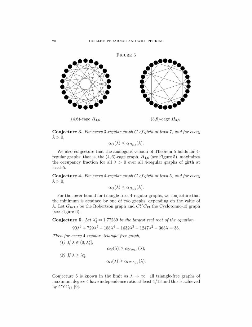
We conjecture that the (3, 8)-cage graph, H3,8, also known as the Levigraph or the Tutte-Coxeter graph (see Figure 5), maximizes the occupancyfraction for all λ > 0 over all 3-regular graphs of girth at least 7.


Figure 5

(4,6)-cage H4,6 (3,8)-cage H3,8

Conjecture 3. For every 3-regular graph G of girth at least 7, and for everyλ > 0,

αG(λ) ≤ αH3,8(λ).

We also conjecture that the analogous version of Theorem 5 holds for 4-regular graphs; that is, the (4, 6)-cage graph, H4,6 (see Figure 5), maximizesthe occupancy fraction for all λ > 0 over all 4-regular graphs of girth atleast 5.

Conjecture 4. For every 4-regular graph G of girth at least 5, and for everyλ > 0,

αG(λ) ≤ αH4,6(λ).

For the lower bound for triangle-free, 4-regular graphs, we conjecture thatthe minimum is attained by one of two graphs, depending on the value ofλ. Let GROB be the Robertson graph and CY C13 the Cyclotomic-13 graph(see Figure 6).

Conjecture 5. Let λ∗4 ≈ 1.77239 be the largest real root of the equation

90λ6 + 729λ5 − 188λ4 − 1632λ3 − 1247λ2 − 363λ = 38.

Then for every 4-regular, triangle-free graph,

(1) If λ ∈ (0, λ∗4],

αG(λ) ≥ αGROB(λ);

(2) If λ ≥ λ∗4,

αG(λ) ≥ αCY C13(λ).

Conjecture 5 is known in the limit as λ → ∞: all triangle-free graphs ofmaximum degree 4 have independence ratio at least 4/13 and this is achievedby CY C13 [9].


Figure 6

Cyclotomic-13 graph CY C13 Robertson Graph GROB

6.2. Graph homomorphisms. We can also ask about generalizations fromindependent sets to graph homomorphisms. Let Hom(G,H) denote thenumber of graph homomorphisms from G into H; that is, the number ofmappings φ : V (G) → V (H) so that (u, v) ∈ E(G) ⇒ (φ(u), φ(v)) ∈ E(H).The number of independent sets of G is Hom(G,Hind) where Hind is a singleedge with one looped vertex. The number of proper vertex q-colorings of Gis Hom(G,Kq). Galvin and Tetali [8] showed that for all d-regular bipartiteG, and all H,

Hom(G,H)1/|V (G)| ≤ Hom(Kd,d, H)1/2d.

In [1], Cohen, Csikvari, Perkins, and Tetali conjectured thatG being triangle-free can replace the bipartite condition. We ask (but don’t dare conjecture)whether something analogous holds for graphs of larger girth.

Question 2. Is it true that for all graphs H and all cubic graphs G of girthat least 6,

Hom(G,H)1/|V (G)| ≤ Hom(H3,6, H)1/14 ?

There are counterexamples if we replace girth at least 6 by girth at least5, e.g. H is two looped vertices.

Acknowledgements

We thank Daniela Kuhn and Deryk Osthus for fruitful discussions duringthe initial steps of this project.

References

[1] E. Cohen, P. Csikvari, W. Perkins, and P. Tetali. The Widom-Rowlinson model,the hard-core model and the extremality of the complete graph. arXiv preprintarXiv:1606.03718, 2016.

[2] E. Cohen, W. Perkins, and P. Tetali. On the Widom-Rowlinson occupancy fractionin regular graphs. Probability, Combinatorics and Computing, in press.


[3] J. Cutler and A. Radcliffe. The maximum number of complete subgraphs in a graphwith given maximum degree. Journal of Combinatorial Theory, Series B, 104:60–71,2014.

[4] J. Cutler and A. J. Radcliffe. Minimizing the number of independent sets in triangle-free regular graphs. arXiv preprint arXiv:1610.05714v1, 2016.

[5] E. Davies, M. Jenssen, W. Perkins, and B. Roberts. Independent sets, matchings,and occupancy fractions. arXiv preprint arXiv:1508.04675, 2015.

[6] E. Davies, M. Jenssen, W. Perkins, and B. Roberts. Extremes of the internal energyof the Potts models on cubic graphs. arXiv preprint arXiv:1610.08496, 2016.

[7] E. Davies, M. Jenssen, W. Perkins, and B. Roberts. On the average size of indepen-dent sets in triangle-free graphs. arXiv preprint arXiv:1606.01043, 2016.

[8] D. Galvin and P. Tetali. On weighted graph homomorphisms. DIMACS Series inDiscrete Mathematics and Theoretical Computer Science, 63:97–104, 2004.

[9] K. F. Jones. Independence in graphs with maximum degree four. Journal of Combi-natorial Theory, Series B, 37(3):254–269, 1984.

[10] J. Kahn. An entropy approach to the hard-core model on bipartite graphs. Combi-natorics, Probability and Computing, 10(03):219–237, 2001.

[11] W. Staton. Some ramsey-type numbers and the independence ratio. Transactions ofthe American Mathematical Society, 256:353–370, 1979.

[12] Y. Zhao. The number of independent sets in a regular graph. Combinatorics, Proba-bility and Computing, 19(02):315–320, 2010.

[13] Y. Zhao. Extremal regular graphs: independent sets and graph homomorphisms.arXiv preprint arXiv:1610.09210, 2016.


Appendix A. Proof that C5 is the set of all possibleconfigurations for free second neighborhoods of

cubic graphs with girth at least 5.

Let u1, u2, u3 be the neighbors of v. For i ∈ {1, 2, 3}, let Wi = {wi1, w21}be the neighbors of ui that are second neighbors of v, and let W = W1 ∪W2 ∪W3.

Suppose that G[W ] contains a copy of a graph H, then we will write φ :V (H)→W for the map that assigns each vertex of H to its correspondingvertex in the copy of H in G[W ]. If H is a graph that can be contained inG[W ], then its order is at most 6, its maximum degree of H is at most 2 andit has girth at least 5. Moreover, the endpoints of an edge from H cannotbe mapped to the same set Wi, since otherwise Wi ∪ {ui} would induce atriangle in G.

Let Sn denote the symmetric group of order n. Two configuration typesare equal up to symmetries if there exist σ ∈ S3, τ1, τ2, τ3 ∈ S2 such thatthe bijection ρ : W → W defined by ρ(wij) = wσ(i)τi(j) transforms oneconfiguration into the other one.

We now enumerate the different configurations for the second neighbor-hood of v, depending on the number of edges in G[W ]:

0) If G[W ] induces no edges, the configuration is of type C0.1) If G[W ] induces one edge, then, up to symmetries, C1 is the only

possible type of configuration.2) If G[W ] induces two edges, then we have two cases for H:

2.a) H is a path x1x2x3 of length 2. Since no edges can be containedin any Wi, we have that that φ(x2) lies in a different set Wi

that the images of the other two vertices. We may assumeφ(x2) ∈ W1 and φ(x1) ∈ W2. If φ(x3) ∈ W2, then G[W ∪ u2]contains a C4. Therefore, φ(x3) ∈ W3, and C2 is the onlypossible configuration type.

2.b) H is composed by two vertex-disjoint edges x1x2 and y1y2. Wemay assume that W1 contains the images of two vertices. Sinceno edge is included within W1, we may assume φ(x1) = w11

and φ(y1) = w12. If φ(x2) and φ(y2) lie in the same set Wi,we may assume that φ(x2) = w22 and φ(y2) = w21, giving riseto a configuration of type C3. Otherwise, up to symmetries,φ(x2) = w21 and φ(y2) = w31, giving rise to a configuration oftype C4.

3) If G[W ] induces 3 edges, then we have three cases for H:3.a) H is composed by three vertex-disjoint edges x1x2, y1y2 and

z1z2. Since edges cannot lie within the sets Wi, the type ofconfiguration C5 is the only possible one, up to symmetries.

3.b) H is a path of length 3, x1x2x3x4. We can assume it containstwo vertices in W1. Moreover, these should be φ(x1) and φ(x4),since otherwise G[W ∪ {u1}] would contain a C4. A similar


argument shows that φ(x2) and φ(x3) lie in different sets Wi

and thus, up to symmetries, the only type of configuration isC6.

3.c) H is composed by the vertex-disjoint union of a path of length2, x1x2x3, and an edge y1y2. As in the case where we wereembedding only a path of length 2, we may assume that φ(x1) =w11, φ(x2) = w21 and φ(x3) = w31. Up to symmetries we mayassume that φ(y1) = w22. If φ(y2) = w12, then we obtain aconfiguration of type C7 and if φ(y2) = w32, of type C8.

4) If G[W ] induces 4 edges, then we have three cases for H:4.a) H is composed by two vertex disjoint paths of length 2, x1x2x3

and y1y2y3. Then we may assume that φ(x2) = w11. If φ(y2) 6=w12, we may assume that φ(y2) = w32 and, up to symmetries,we obtain a configuration of type C9. If φ(y2) = w12, up tosymmetries, the only type of configuration is C10.

4.b) H is composed by the disjoint union of a path of length 3,x1x2x3x4 and an edge y1y2. Then we may assume that φ(y1) =w22 and φ(y2) = w23 and, as in the case where we were embed-ding only a path of length 3, we should have φ(x1) = w11 andφ(x4) = w12. Up to symmetries, this gives rise to a configura-tion of type C11.

4.c) H is composed by a path of length 4, x1x2x3x4x5. We can as-sume it contains only one vertex in W3. Since H contains a pathof length 4 as a subpath, we can also assume that φ(x1) = w11,φ(x2) = w21, φ(x3) = w31 and φ(x4) = w12. Up to symmetries,the only possible type of configuration is C12.

5) If G[W ] induces 5 edges, then G[W ] must be isomorphic to a path oflength 5. Note that if G[W ] would induce a C5, one could find a setWi such that wi1 and wi2 have a common neighbor in W , creating aC4 in G[W ∪{ui}]. Let H be a path of length 5, x1x2x3x4x5x6. SinceH contains a path of length 4, we can assume that φ(x1) = w11,φ(x2) = w21, φ(x3) = w31, φ(x4) = w12 and φ(x5) = w22. Thenφ(x6) = w32 and the only type of configuration is C13.

6) If G[W ] induces 6 edges, then G[W ] must be isomorphic to a cycle oflength 6. A similar argument as before gives C14 as the only possibleconfiguration.


Appendix B. Configurations for second free neighborhoods intriangle-free graphs

In this part of the appendix we display all the configurations in C4.

B.1. The following configurations are obtained if the second neighborhoodof a vertex has size six. The variables xi ∈ {0, 1} indicates whether the i-thvertex in the second neighborhood is externally uncovered (xi = 1) or not(xi = 0).

u1 u1 u2 u2 u3 u3 u1 u1 u2 u2 u3 u3 u1 u1 u2 u2 u3 u3

C10 (x1, x2, . . . , x6) C1

1 (x1, x2, . . . , x6) C12 (x1, x2, . . . , x6)


C13 (x1, x2, . . . , x6) C1

4 (x1, x2, . . . , x6) C15 (x1, x2, . . . , x6)


C16 (x1, x2, . . . , x6) C1

7 (x1, x2, . . . , x6) C18 (x1, x2, . . . , x6)


C19 (x1, x2, . . . , x6) C1

10(x1, x2, . . . , x6) C111(x1, x2, . . . , x6)


C112(x1, x2, . . . , x6) C1

13(x1, x2, . . . , x6) C114(x1, x2, . . . , x6)


C115(x1, x2, . . . , x6) C1

16(x1, x2, . . . , x6) C117(x1, x2, . . . , x6)



C118(x1, x2, . . . , x6) C1

19(x1, x2, . . . , x6) C120(x1, x2, . . . , x6)


C121(x1, x2, . . . , x6) C1

22(x1, x2, . . . , x6) C123(x1, x2, . . . , x6)


C124(x1, x2, . . . , x6) C1

25(x1, x2, . . . , x6) C126(x1, x2, . . . , x6)


C127(x1, x2, . . . , x6) C1

28(x1, x2, . . . , x6) C129(x1, x2, . . . , x6)

u1 u1 u2 u2 u3 u3

C130(x1, x2, . . . , x6)

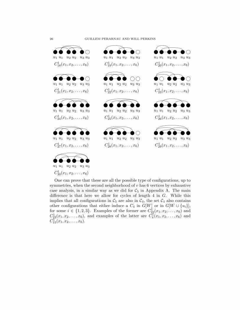
One can prove that these are all the possible type of configurations, up tosymmetries, when the second neighborhood of v has 6 vertices by exhaustivecase analysis, in a similar way as we did for C5 in Appendix A. The maindifference is that here we allow for cycles of length 4 in G. While thisimplies that all configurations in C5 are also in C4, the set C4 also containsother configurations that either induce a C4 in G[W ] or in G[W ∪ {ui}],for some i ∈ {1, 2, 3}. Examples of the former are C1

22(x1, x2, . . . , x6) andC123(x1, x2, . . . , x6), and examples of the latter are C1

4 (x1, x2, . . . , x6) andC115(x1, x2, . . . , x6).


B.2. The following configurations are obtained if the second neighborhoodof a vertex has size five.

u1 u1,u2 u2 u3 u3 u1 u1,u2 u2 u3 u3 u1 u1,u2 u2 u3 u3

C20 (x1, x2, . . . , x5) C2

1 (x1, x2, . . . , x5) C22 (x1, x2, . . . , x5)


C23 (x1, x2, . . . , x5) C2

4 (x1, x2, . . . , x5) C25 (x1, x2, . . . , x5)


C26 (x1, x2, . . . , x5) C2

7 (x1, x2, . . . , x5) C28 (x1, x2, . . . , x5)


C29 (x1, x2, . . . , x5) C2

10(x1, x2, . . . , x5) C211(x1, x2, . . . , x5)


C212(x1, x2, . . . , x5) C2

13(x1, x2, . . . , x5) C214(x1, x2, . . . , x5)


C215(x1, x2, . . . , x5) C2

16(x1, x2, . . . , x5) C217(x1, x2, . . . , x5)


C218(x1, x2, . . . , x5) C2

19(x1, x2, . . . , x5) C220(x1, x2, . . . , x5)

u1 u1,u2 u2 u3 u3 u1 u1,u2 u2 u3 u3

C221(x1, x2, . . . , x5) C2

22(x1, x2, . . . , x5)

To prove that these are the only configurations in C4 when the secondneighborhood of v has 5 vertices one can proceed again by case analysis.Now, less connections are allowed within the second neighborhood but the


set of symmetries among the vertices in W is also smaller. For instance,there are three different type of configurations with one edge in G[W ]: C2

1 ,C22 and C2

3 .

B.3. The following configurations are obtained if the second neighborhoodof a vertex has size four. There are two possibilities for the edges betweenthe first and the second neighborhood of v, corresponding to the types C3

j

and C4j .

u1 u1,u2 u2,u3 u3 u1 u1,u2 u2,u3 u3 u1 u1,u2 u2,u3 u3

C30 (x1, x2, x3, x4) C3

1 (x1, x2, x3, x4) C32 (x1, x2, x3, x4)

u1 u1,u2 u2,u3 u3 u1 u1,u2 u2,u3 u3 u1 u1,u2 u2,u3 u3

C33 (x1, x2, x3, x4) C3

4 (x1, x2, x3, x4) C35 (x1, x2, x3, x4)

u1 u1,u2,u3 u2 u3 u1 u1,u2,u3 u2 u3 u1 u1,u2,u3 u2 u3

C40 (x1, x2, x3, x4) C4

1 (x1, x2, x3, x4) C42 (x1, x2, x3, x4)

B.4. The following configurations are obtained if the second neighborhoodof a vertex has size three. There are two possibilities for the edges betweenthe first and the second neighborhood of v, corresponding to the types C5

j

and C6j .

u1,u2 u1,u3 u2,u3 u1 u1,u2,,u3 u2,u3 u1 u1,u2,,u3 u2,u3

C50 (x1, x2, x3) C6

0 (x1, x2, x3) C61 (x1, x2, x3)

B.5. The following configurations are obtained if the second neighborhoodof a vertex has size 2. In this case, the vertex belongs to a copy of K3,3.

u1,u2,u3 u1,u2,u3

C70 (x1, x2)


Appendix C. Proof that unions of P5,2 are the only graphsthat minimize the occupancy fraction for every

λ ∈ [0, 1].

In this appendix we prove that unions of P5,2 are the only graphs thatattain the minimum in Theorem 3. As in the proof of the Theorem 3, we willsplit the proof into 4 cases. For each case, there is an assignment of Λ∗0(λ),Λ∗1(λ) and Λ∗2(λ) such that SLACKmin(λ,Λ∗0(λ),Λ∗2(λ),Λ∗2(λ), C) defined asin (10) is non-negative for every C ∈ C4 and is 0 for a subset of configurations

C that include C129(1, 1, 1, 1, 1, 1), corresponding to the Petersen graph. We

need to show that the only solutions induced by graphs and supported in Care, in fact, only supported in C1

29(1, 1, 1, 1, 1, 1). It follows that unions ofP5,2 are the only graphs that attain the minimum.

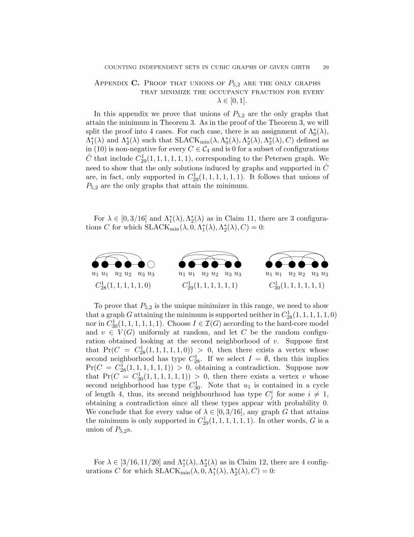
For λ ∈ [0, 3/16] and Λ∗1(λ),Λ∗2(λ) as in Claim 11, there are 3 configura-tions C for which SLACKmin(λ, 0,Λ∗1(λ),Λ∗2(λ), C) = 0:


C128(1, 1, 1, 1, 1, 0) C1

29(1, 1, 1, 1, 1, 1) C130(1, 1, 1, 1, 1, 1)

To prove that P5,2 is the unique minimizer in this range, we need to showthat a graphG attaining the minimum is supported neither in C1

28(1, 1, 1, 1, 1, 0)nor in C1

30(1, 1, 1, 1, 1, 1). Choose I ∈ I(G) according to the hard-core modeland v ∈ V (G) uniformly at random, and let C be the random configu-ration obtained looking at the second neighborhood of v. Suppose firstthat Pr(C = C1

28(1, 1, 1, 1, 1, 0)) > 0, then there exists a vertex whosesecond neighborhood has type C1

28. If we select I = ∅, then this impliesPr(C = C1

28(1, 1, 1, 1, 1, 1)) > 0, obtaining a contradiction. Suppose nowthat Pr(C = C1

30(1, 1, 1, 1, 1, 1)) > 0, then there exists a vertex v whosesecond neighborhood has type C1

30. Note that u1 is contained in a cycleof length 4, thus, its second neighbourhood has type Cij for some i 6= 1,obtaining a contradiction since all these types appear with probability 0.We conclude that for every value of λ ∈ [0, 3/16], any graph G that attainsthe minimum is only supported in C1

29(1, 1, 1, 1, 1, 1). In other words, G is aunion of P5,2s.

For λ ∈ [3/16, 11/20] and Λ∗1(λ),Λ∗2(λ) as in Claim 12, there are 4 config-urations C for which SLACKmin(λ, 0,Λ∗1(λ),Λ∗2(λ), C) = 0:



C13 (1, 1, 1, 0, 1, 0) C1

28(1, 1, 1, 1, 1, 0) C129(1, 1, 1, 1, 1, 1)

u1 u1,u2 u2 u3 u3

C27 (1, 0, 1, 1, 1)

To prove that P5,2 is the unique minimizer in this range, as before, justobserve that if any configuration Cij(x1, x2, . . . , xs) has positive probability

to appear, then Cij′(1, 1, . . . , 1) must also have positive probability to appear,

for some j′ such that Cij is isomorphic to an induced subgraph of Cij′ . This is

not the case for the configurations C13 (1, 1, 1, 1, 0, 1, 0), C1

28(1, 1, 1, 1, 1, 1, 0)and C2

7 (1, 0, 1, 1, 1). Therefore, any graph attaining the minimum is a unionof P5,2.

For λ ∈ [11/20,√

3/5] and Λ∗1(λ),Λ∗2(λ) as in Claim 13, there are 6 con-figurations C for which SLACKmin(λ, 0,Λ∗1(λ),Λ∗2(λ), C) = 0:


C10 (1, 0, 1, 0, 1, 0) C1

3 (1, 1, 1, 0, 1, 0) C129(1, 1, 1, 1, 1, 1)

u1 u1,u2 u2 u3 u3 u1 u1,u2 u2 u3 u3 u1 u1,u2,u3 u2 u3

C20 (1, 0, 1, 1, 0) C2

7 (1, 0, 1, 1, 1) C40 (1, 0, 1, 1)

The argument used previously, proves that the minimizer should be sup-ported in C1

0 (1, 0, 1, 0, 1, 0) and C129(1, 1, 1, 1, 1, 1). However C1

0 (1, 0, 1, 0, 1, 0)cannot appear with positive probability since otherwise there is a configu-ration C1

j with j 6= 29 such that C1j (1, 1, 1, 1, 1, 1) appears with positive

probability. Therefore, any graph attaining the minimum is a union of P5,2.

For λ ∈ [√

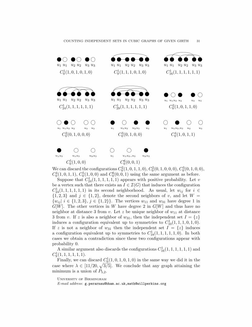
3/5, 1] and Λ∗0(λ),Λ∗1(λ),Λ∗2(λ) as in Claim 14, there are 11configurations C for which SLACKC(λ,Λ∗0(λ),Λ∗1(λ),Λ∗2(λ)) = 0:



C10 (1, 0, 1, 0, 1, 0) C1

9 (1, 1, 1, 0, 1, 0) C116(1, 1, 1, 1, 1, 1)

u1 u1 u2 u2 u3 u3 u1 u1 u2 u2 u3 u3 u1 u1,u2 u2 u3 u3

C124(1, 1, 1, 1, 1, 1) C1

29(1, 1, 1, 1, 1, 1) C20 (1, 0, 1, 1, 0)

u1 u1,u2 u2 u3 u3 u1 u1,u2 u2,u3 u3 u1 u1,u2,u3 u2 u3

C20 (0, 1, 0, 0, 0) C3

0 (0, 1, 0, 0) C40 (1, 0, 1, 1)

u1,u2 u1,u3 u2,u3 u1 u1,u2,,u3 u2,u3

C50 (1, 0, 0) C6

0 (0, 0, 1)

We can discard the configurations C20 (1, 0, 1, 1, 0), C2

0 (0, 1, 0, 0, 0), C30 (0, 1, 0, 0),

C40 (1, 0, 1, 1), C5

0 (1, 0, 0) and C60 (0, 0, 1) using the same argument as before.

Suppose that C124(1, 1, 1, 1, 1, 1) appears with positive probability. Let v

be a vertex such that there exists an I ∈ I(G) that induces the configurationC124(1, 1, 1, 1, 1, 1) in its second neighborhood. As usual, let wij for i ∈{1, 2, 3} and j ∈ {1, 2}, denote the second neighbors of v, and let W ={wij | i ∈ {1, 2, 3}, j ∈ {1, 2}}. The vertices w11 and w31 have degree 1 inG[W ]. The other vertices in W have degree 2 in G[W ] and thus have noneighbor at distance 3 from v. Let z be unique neighbor of w11 at distance3 from v. If z is also a neighbor of w31, then the independent set I = {z}induces a configuration equivalent up to symmetries to C1

10(1, 1, 1, 0, 1, 0).If z is not a neighbor of w31 then the independent set I = {z} inducesa configuration equivalent up to symmetries to C1

18(1, 1, 1, 1, 1, 0). In bothcases we obtain a contradiction since these two configurations appear withprobability 0.

A similar argument also discards the configurations C116(1, 1, 1, 1, 1, 1) and

C19 (1, 1, 1, 1, 1, 1).Finally, we can discard C1

0 (1, 0, 1, 0, 1, 0) in the same way we did it in the

case where λ ∈ [11/20,√

3/5]. We conclude that any graph attaining theminimum is a union of P5,2.

University of BirminghamE-mail address: [email protected],[email protected]

counting independent sets in cubic graphs of given girth

Documents

Transcript of counting independent sets in cubic graphs of given girth