J. theor. Biol. (1996) 178, 169–182

0022–5193/96/020169+14 $12.00/0 7 1996 Academic Press Limited

The Cubic Ternary Complex Receptor-Occupancy Model II.

Understanding Apparent Affinity

J M. W†, P H. M‡, M W. L‡

T P. K‡

†Biomathematics Program, Department of Statistics, North Carolina State University,Raleigh, NC 27695 and ‡Departments of Research Computing and Cellular Biochemistry,

Glaxo Inc. Research Institute, Five Moore Drive, Research Triangle Park, NC 27709, U.S.A.

(Received on 26 July 1994, Accepted in revised form on 21 August 1995)

In part I of this series of papers, we described the cubic ternary complex (CTC) model. In part II, weexamine the pharmacological notion of apparent ligand affinity in the light of this model. The highdegree of symmetry that characterizes the CTC model makes it possible to use simple geometricaldevices to visualize chemical transitions. This geometric point of view provides a motivation for thedevelopment of a biological interpretation for apparent affinity.

Using this geometrical point of view, an analytical expression for apparent ligand affinity is derivedthat can be applied to any receptor-occupancy model. When unbound receptors are distributed amonga number of states, apparent affinity is a composite measure, a weighted average of the affinities thata ligand has for each of the receptor states. In general, apparent affinity can be interpreted as themathematical expectation of the simple affinities of members of a native receptor ensemble. The‘‘expectation’’ method of computing apparent affinity is algebraically equivalent to an even simplercomputational method, here called the ‘‘diagonalization’’ method. The use of each method isdemonstrated.

The CTC model corroborates what other models and some experimental work have previouslysuggested. Affinity, as it is calculated experimentally for G-protein-coupled receptors, is not purely areceptor property but is a function both of the receptor and of the suite of transitional proteins withwhich the receptor interacts.

7 1996 Academic Press Limited

Introduction

A word is dead when it is said some say.I say it just begins to live that day.

—Emily Dickinson

Ligand affinity is a measure of the attraction thata ligand has for a receptor. For bimolecular reactions,the equilibrium dissociation constant, KD , of theligand-receptor binding equation has been used asa numerical measure of affinity because it has unitsof concentration. (As will be shown below, theequilibrium association constant, KA , is a more

natural measure.) Consider the simple bimolecularreaction of a ligand, A, and a receptor, R,

A+R ghk1

k2

AR

where k1 and k2 are the forward and backwardreaction rate constants (Clark, 1937). Let

[A]=total ligand concentration (assumed inexcess),

[R]=free receptor concentration,[RT ]=total recptor concentration (fixed), and[AR]=ligand-receptor complex concentration.

169

. . .170

At equilibrium the rates of formation and dissociationof the ligand-receptor complex are equal. Thus, wehave

k2[AR]=k1[A]([RT ]−[AR]).

Letting KD=k2/k1, the equilibrium dissociationconstant, and simplifying yields

[AR][RT ]

=[A]

KD+[A]. (1)

This last equation goes by many names, the Langmuiradsorption isotherm (Langmuir, 1918), the Hillequation with n=1 (Hill, 1910), among others. Itrelates receptor occupancy, the left-hand side of theequation, to ligand concentration. KD serves as alocation parameter in the equation.

Virtually all the classical pharmacological methodsfor computing KD from experimental data are derivedfrom some version of this equation. In partialreceptor inactivation, as suggested by Furchgott(1966), a fraction of the receptor population isinactivated and dose-response curves are obtainedboth before and after inactivation. Under theassumption that, in a given tissue, equal receptoroccupancies yield equal responses, a comparison ofthe ligand concentrations that yield equal responsesbefore and after receptor inactivation can be used toestimate KD (Mackay, 1966a, b). In radioligandsaturation binding experiments, the fraction ofradioactively labeled ligand that is bound to receptorsis measured and from this an estimate of KD isobtained, either by Scratchard analysis or throughdirect nonlinear fitting of the data to an equationderived from eqn (1).

A complication arises though when AR is not theonly bound receptor species, the so-called problem ofdistributed receptor states (Black & Shankley, 1990).In the simple ternary complex model the boundspecies are AR and ARG. Thus we have

A+R ghKA

AR+G ghKG

ARG

where KA and KG are the equilibrium associationconstants for the indicated reactions. G-proteinmediated removal of AR to form ARG has the effectof perturbing the first equilibrium, thus allowing thefirst reaction to progress further than it wouldwithout G-protein. In terms of association constants,the apparent affinity, KAapp , of ligand A for receptor Rin the presence of G-protein is greater than the simpleaffinity KA , i.e., KAappqKA . (In terms of dissociationconstants, KDqKDapp .) As it is the fraction of boundreceptor species (independent of whether the boundspecies is AR or ARG) that is measured in standardpharmacological experiments, the presence of

additional receptor species forces the calculatedassociation constant to be a measure of apparentaffinity KAapp, rather than of the simple affinity KA .

If we take the Langmuir adsorption isotherm,eqn (1), and replace [AR] by [RB ], the totalconcentration of bound species ([AR]+[ARG] in thesimple ternary complex model), we obtain anexpression from which apparent affinity can becalculated.

[RB ][RT ]

=[A]

KDapp+[A]. (2)

(This has been done for the ternary complex modeland the extended ternary complex model. SeeMackay, 1988, 1990; Samama et al., 1993. For amuch simpler approach, see Section 5.) Two of thequantities that appear in eqn (2), the fraction of thebound receptor ([RB ]/[RT ]) and ligand concentration([A]), are readily obtainable from equilibriumpharmacological experiments, so in principle the thirdquantity, KDapp , is estimable from data.

Equations (1) and (2) have the same form.Although a particular model, the simple mass actionmodel of receptor action (Clark, 1937), generateseqn (1), no specific model motivates eqn (2). Equation(2) can be fit to equilibrium pharmacological dataregardless of the true mechanism of receptor action.If Clark’s model applies, eqns (1) and (2) are identi-cal and KDapp is just KD . If Clark’s model does notapply, KD and KDapp need not be the same. In whatways might Clark’s model not apply? Figure 1illustrates the scenario we have in mind.

First, instead of a single receptor species as inClark’s model, suppose we have a suite of receptorspecies. In part I of this series of papers, we used theterm receptor ensemble for a family of receptor

F. 1. Complexity in receptor models.

–. 171

species that are in equilibrium with each other. The‘‘unbound receptor cloud’’ of Fig. 1 contains areceptor ensemble with four members: two confor-mational forms of a receptor (R and Ra ) as wellas their G-protein coupled counterparts (RG andRaG). In a similar fashion, one can envision acorresponding suite of ligand-bound receptor species,the ‘‘ligand-bound receptor cloud’’ of Fig. 1.

Second, suppose that more than one member of thereceptor ensemble can bind to ligand. Thus, insteadof the single affinity constant in Clark’s model, thereare multiple simple affinity constants. Figure 1 showsfour such simple affinity constants, K1, K2, K3, and K4,one for each member of the receptor ensemble.

Third, there need not be a one-to-one correspon-dence between the members of the bound andunbound receptor clouds. In Fig. 1, the specieslabeled ARaG* does not have a counterpart in theunbound receptor cloud in the sense of being linkedto it by a simple affinity constant. Thus, we considergeneralizations of Clark’s model that allow thepossibility of multiple receptor species, multipleligand-bound receptor species, and multiple simpleaffinity constants.

So, imagine that we fit eqn (2) to data generated bya model such as that of Fig. 1. Necessarily, the simpleaffinity of Clark, KD , becomes an apparent affinity,KDapp . We consider the following questions.

(1) Does KDapp have a meaningful biologicalinterpretation, perhaps an extension, in somesense, of Clark’s KD ?

(2) If so, is there a simple relationship betweenKDapp and the simple affinity constants andparameters of the model so that an explicitequation for KDapp can be constructed byinspection?

To answer these questions we use a specific modelof receptor action, the cubic ternary complex (CTC)model, to guide us. The CTC model is as complexas the schematic model shown in Fig. 1 but has theadvantage of being completely symmetrical. Itssymmetry in turn motivates a simple interpretationfor KDapp . We review the details of the CTC model inthe next section.

1. Overview of the Cubic Ternary Complex

(CTC) Model

The cubic ternary complex (CTC) model isexplained in detail in part I of this series. In thissection we summarize the features of this modelrequired for an understanding of apparent affinity.The CTC model generalizes the extended ternary

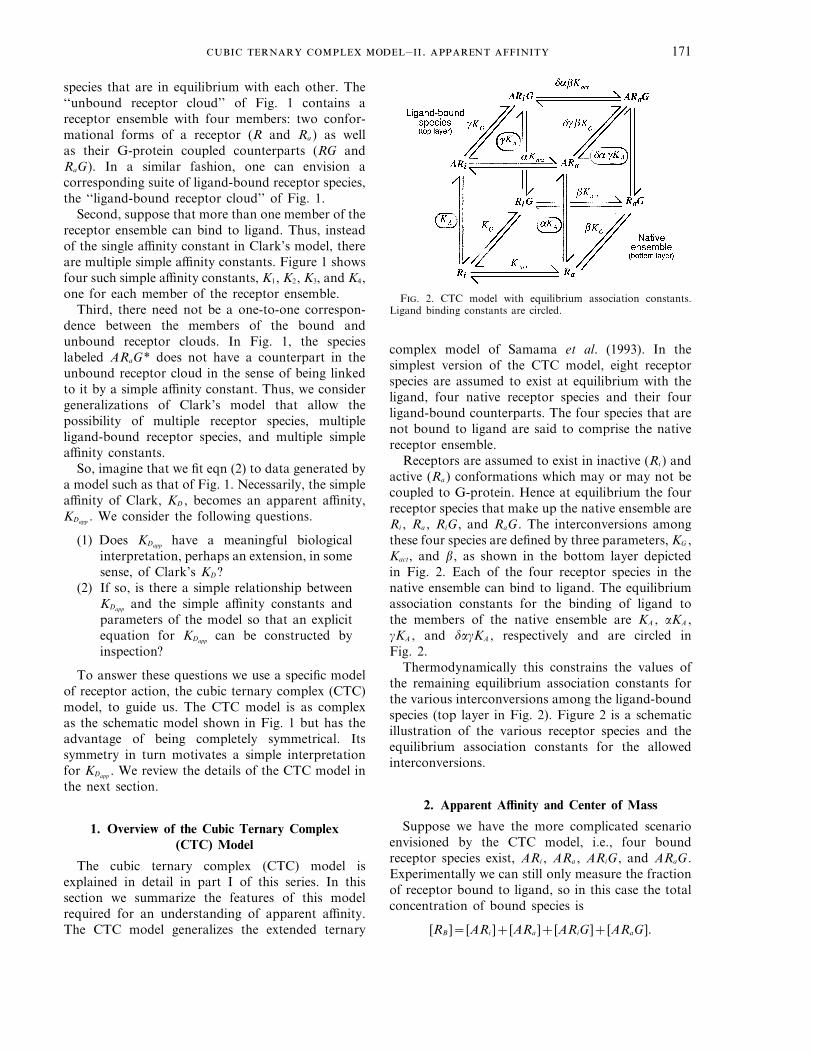
F. 2. CTC model with equilibrium association constants.Ligand binding constants are circled.

complex model of Samama et al. (1993). In thesimplest version of the CTC model, eight receptorspecies are assumed to exist at equilibrium with theligand, four native receptor species and their fourligand-bound counterparts. The four species that arenot bound to ligand are said to comprise the nativereceptor ensemble.

Receptors are assumed to exist in inactive (Ri ) andactive (Ra ) conformations which may or may not becoupled to G-protein. Hence at equilibrium the fourreceptor species that make up the native ensemble areRi , Ra , RiG, and RaG. The interconversions amongthese four species are defined by three parameters, KG ,Kact, and b, as shown in the bottom layer depictedin Fig. 2. Each of the four receptor species in thenative ensemble can bind to ligand. The equilibriumassociation constants for the binding of ligand tothe members of the native ensemble are KA , aKA ,gKA , and dagKA , respectively and are circled inFig. 2.

Thermodynamically this constrains the values ofthe remaining equilibrium association constants forthe various interconversions among the ligand-boundspecies (top layer in Fig. 2). Figure 2 is a schematicillustration of the various receptor species and theequilibrium association constants for the allowedinterconversions.

2. Apparent Affinity and Center of Mass

Suppose we have the more complicated scenarioenvisioned by the CTC model, i.e., four boundreceptor species exist, ARi , ARa , ARiG, and ARaG.Experimentally we can still only measure the fractionof receptor bound to ligand, so in this case the totalconcentration of bound species is

[RB ]=[ARi ]+[ARa ]+[ARiG]+[ARaG].

. . .172

Let [RU ] be the total concentration of ligand-unboundreceptor species. Thus, total receptor concentrationcan be decomposed as [RT ]=[RB ]+[RU ]. Using thiswe can write eqn (2) as follows.

[RB ][RB ]+[RU ]

=[A]

KDapp+[A]. (3)

Next we cross-multiply in eqn (3) and solve for KDapp .

[RB ]KDapp+[RB ][A]=[A][RB ]+[A][RU ]

\ KDapp=[A][RU ][RB ]

. (4)

The implications of eqn (4) can be better understoodif we rewrite it in terms of KAapp , the reciprocal of KDapp .Here KAapp is the apparent equilibrium associationconstant.

KAapp=[RB ]

[A][RU ]\ KAapp [A][RU ]=[RB ]. (5)

From eqn (5) we see that KAapp can be interpreted asthe equilibrium association constant for the bulkreaction

A+RU g1hKAapp

RB .

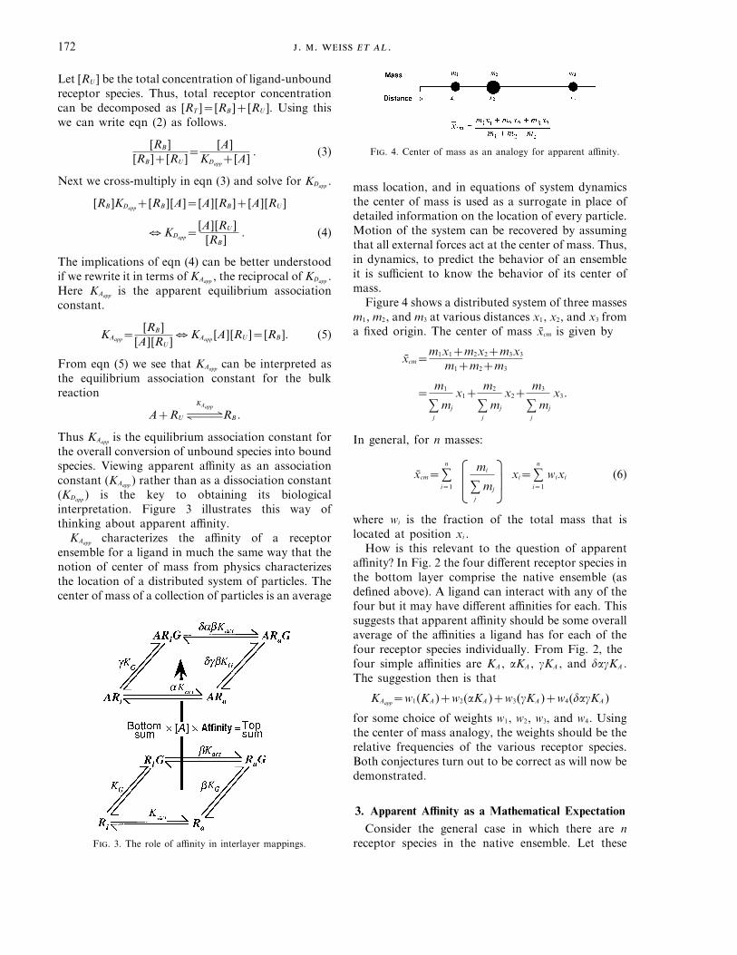
Thus KAapp is the equilibrium association constant forthe overall conversion of unbound species into boundspecies. Viewing apparent affinity as an associationconstant (KAapp ) rather than as a dissociation constant(KDapp ) is the key to obtaining its biologicalinterpretation. Figure 3 illustrates this way ofthinking about apparent affinity.

KAapp characterizes the affinity of a receptorensemble for a ligand in much the same way that thenotion of center of mass from physics characterizesthe location of a distributed system of particles. Thecenter of mass of a collection of particles is an average

F. 4. Center of mass as an analogy for apparent affinity.

mass location, and in equations of system dynamicsthe center of mass is used as a surrogate in place ofdetailed information on the location of every particle.Motion of the system can be recovered by assumingthat all external forces act at the center of mass. Thus,in dynamics, to predict the behavior of an ensembleit is sufficient to know the behavior of its center ofmass.

Figure 4 shows a distributed system of three massesm1, m2, and m3 at various distances x1, x2, and x3 froma fixed origin. The center of mass x̄cm is given by

x̄cm=m1x1+m2x2+m3x3

m1+m2+m3

=m1

sj

mj

x1+m2

sj

mj

x2+m3

sj

mj

x3.

In general, for n masses:

x̄cm=sn

i=1 GF

f

mi

sj

mjGJ

jxi=s

n

i=1

wixi (6)

where wi is the fraction of the total mass that islocated at position xi .

How is this relevant to the question of apparentaffinity? In Fig. 2 the four different receptor species inthe bottom layer comprise the native ensemble (asdefined above). A ligand can interact with any of thefour but it may have different affinities for each. Thissuggests that apparent affinity should be some overallaverage of the affinities a ligand has for each of thefour receptor species individually. From Fig. 2, thefour simple affinities are KA , aKA , gKA , and dagKA .The suggestion then is that

KAapp=w1(KA )+w2(aKA )+w3(gKA )+w4(dagKA )

for some choice of weights w1, w2, w3, and w4. Usingthe center of mass analogy, the weights should be therelative frequencies of the various receptor species.Both conjectures turn out to be correct as will now bedemonstrated.

3. Apparent Affinity as a Mathematical Expectation

Consider the general case in which there are nreceptor species in the native ensemble. Let theseF. 3. The role of affinity in interlayer mappings.

–. 173

unbound receptor species be denoted by u1, u2, . . . , un

and the corresponding bound species by Au1,Au2, . . . , Aun with equilibrium association constantsK1, K2, . . . , Kn . For the ith species we have

A+ui ghKi

Aui

so that at equilibrium [Aui ]=Ki [A][ui ]. Using thenotation RB and RU for total bound and unboundspecies that was introduced earlier we have

[RB ]=sn

i=1

[Aui ]=sn

i=1

Ki [A][ui ]

[RU ]=sn

i=1

[ui ].

Inserting these expressions for [RB ] and [RU ] intoequation (5) yields

KAapp=[RB]

[A][RU ]=

si

[Aui ]

[A] si

[ui ]=

si

Ki [A][ui ]

[A] si

[ui ]

=

[A] si

Ki [ui ]

[A] si

[ui ]=

si

Ki [ui ]

si

[ui ]

=si

Ki2 [ui ]si

[ui ]3=si

Kiwi (7)

where we see that the postulated weights, wi , are

wi=[ui ]/si

[ui ].

Observe that wi represents the fraction of unboundnative ensemble that is made up of receptor species ui .Equation (6) for center of mass and eqn (7) forapparent affinity are exactly of the same form.

We can reformulate the result obtained in eqn (7)using standard statistical notation. Let U be anindicator random variable that identifies the unboundspecies. Using the equally likely assumption, we canconstruct a probability distribution for U by definingP(U=ui ) to be the relative frequency of ui in thenative ensemble, i.e.,

P(U=ui )=[ui ]

si

[ui ].

Let k(ui ) be a function that assigns to an unboundreceptor species ui its equilibrium association constantKi . With these identifications, eqn (7) becomes

KAapp=si

Ki2 [ui ]si

[ui ]3=si

Ki · P(U=ui )

=si

k(ui ) · P(U=ui )=E(k(U)) (8)

where E is just ordinary mathematical expectationtaken with respect to the probability distribution ofU. The apparent affinity constant then is simply anexpected affinity. It is a weighted average of theequilibrium association constants of the ligand for allthe unbound receptor species. The weights are therelative frequencies of the various receptor species.We refer to the method for calculating apparentaffinity given in eqn (8) as the ‘‘expectation method’’.

Equation (7) suggests that apparent affinity isdetermined by two things:

(1) the simple affinities of all the unboundreceptor species, and

(2) the relative proportions, at equilibrium, ofeach of the unbound receptor species.

This result makes intuitive sense. By mass action, aligand molecule will tend to meet the more abundantreceptor species more often. Whether such anencounter results in binding is then a function of thesimple affinity constant for that receptor species.Thus, the overall affinity should be a function of boththe simple affinities of the receptor species and theirrelative frequencies.

4. The Diagonalization Method

There is another way to interpret eqn (8) that willprove useful in calculating apparent affinity inequilibrium models that are less symmetrical thanthe CTC model. We call the resulting calculation

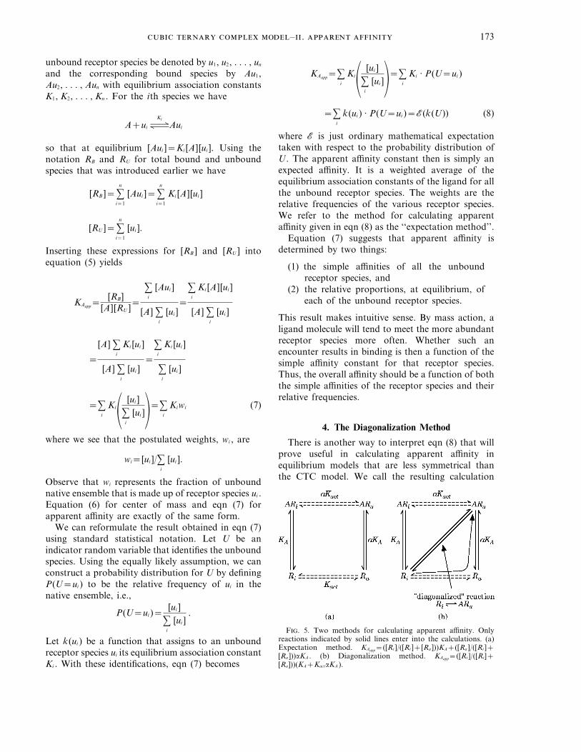
F. 5. Two methods for calculating apparent affinity. Onlyreactions indicated by solid lines enter into the calculations. (a)Expectation method. KAapp=([Ri ]/([Ri ]+[Ra ]))KA+([Ra ]/([Ri ]+[Ra ]))aKA . (b) Diagonalization method. KAapp=([Ri ]/([Ri]+[Ra]))(KA+KactaKA ).

. . .174

F. 6. Diagonalization method for a general reaction scheme. (a) Reaction scheme before diagonalization. (b) Set-up afterdiagonalization.

formula the ‘‘diagonalization method’’. To motivateit, consider the two-state model illustrated in Fig. 5.

Using the method of expectation, we canimmediately write down the formula for apparentaffinity as a weighted sum of the two equilibriumassociation constants KA and aKA . The weights arethe relative frequencies of Ri and Ra in the nativeensemble. Thus we have

KAapp=[Ri ]

[Ri ]+[Ra ]KA+

[Ra ][Ri ]+[Ra ]

aKA. (9)

Observe, though, that [Ra ] can be obtained from[Ra ]=Kact [Ri ] so that eqn (9) becomes

KAapp=[Ri ]

[Ri ]+[R a ]KA+

Kact [Ri ][Ri ]+[Ra ]

aKA

=[Ri ]

[Ri ]+[Ra ][KA+KactaKA ]. (10)

Examining eqn (10) term by term, we see that

(1) [Ri ]/([Ri ]+[Ra ])=fraction of receptors in‘‘state’’ Ri ,

(2) KA=association constant for the reactionRi _ ARi ,

(3) KactaKA=the thermodynamically - derivedoverall association constant for the reactionRi _ ARa .

We refer to this last reaction as a ‘‘diagonalized’’reaction because it doesn’t actually occur as written,but instead occurs in two steps: Ri _ Ra followed byRa _ ARa . By treating it as a single reaction the pathhas been shortened by traversing the diagonal.

This alternative method of computing apparentaffinity suggested by eqn (10) is true in general.Consider the general reaction scheme shown inFig. 6(a). R1, R2, . . . , Rn are n receptor species in thenative receptor ensemble and AR1, AR2, . . . , ARm arem bound receptor species. Suppose R1 binds to ligand

A to form AR1 with equilibrium association constantKA . (Other reactions between ligand and the nativeensemble are allowed but will not affect the followingcalculations.) The various equilibrium constants areas shown in Fig. 6(a).

From eqn (5) we have

KAapp=[RB ]

[A][RU ]

=[AR1]+[AR2]+[AR3]+· · ·+[ARm ][A]{[R1]+[R2]+[R3]+· · ·+[Rn ]}

=

{[A][R1]KA+[A][R1]KAJ1+[A][R1]KAJ1J2

+· · ·+[A][R1]KAJ1J2 · · · Jm−1}[A]{[R1]+[R2]+[R3]+· · ·+[Rn ]}

=[R1]

[R1]+[R2]+[R3]+· · ·+[Rn ]

×{KA+KAJ1+KAJ1J2

+ · · ·+KAJ1J2 · · · Jm−1}. (11)

This last equation is the generalization of eqn (10).Apparent affinity is just the product of two terms:(i) the fraction of the native ensemble that is madeup of R1 and (ii) the sum of all apparent associationfactors from all possible diagonalized reactions thatoriginate from R1 and terminate at a ligand-boundspecies.

Equation (11) can be transformed further, theunbound receptor layer can be diagonalized and eachof the receptor species can be written as the productsof equilibrium association constants and [R1].

KAapp=

[R1]{KA+KAK1+KAJ1J2

+· · ·+KAJ1J2 · · · Jm−1}[R1]+K1[R1]+K1K2[R1]+· · ·+K1K2 · · · Kn−1[R1]

–. 175

=

[R1]{KA+KAJ1+KAJ1J2

+· · ·+KAJ1J2 · · · Jm−1}[R1]{1+K1+K1K2

+· · ·+K1K2 · · · Kn−1}

=

{KA+KAJ1+KAJ1J2

+· · ·+KAJ1J2 · · · Jm−1}{1+K1+K1K2

+· · ·+K1K2 · · · Kn−1}

=KA

{1+J1+J1J2

+· · ·+J1J2 · · · Jm−1}{1+K1+K1K2

+· · ·+K1K2 · · · Kn−1}

· (12)

Thus the apparent KA is related to the simple KA

by a scaling factor that has a very simple form. Itis a ratio of two similar quantities, a sum of productsof association constants. The terms in the sum arethe overall association factors for the conversion ofa given receptor species to each of the other recep-tor species, including itself. The numerator repre-sents conversions between ligand-bound receptorspecies while the denominator represents conversionsbetween receptor species in the native ensemble.

We use the term overall association ‘‘factor’’ ratherthan ‘‘constant’’ because this ‘‘factor’’ can alsoinclude the equilibrium concentrations of reactants,such as G-proteins. Select any receptor species of thenative ensemble as a starting point. Call it R. Theoverall association factor for a bound species is theterm dictated thermodynamically that, when multi-plied by [R][A] (the product of concentrations of freereceptor and ligand), yields the concentration of thebound species. The overall association factor for areceptor in the native ensemble is the term that whenmultiplied by [R], the concentration of free receptor,yields the concentration of the given receptor species.

The two methods of computing apparent affinityoutlined above complement each other. The expec-tation method of eqn (8) provides a reasonablemechanistic interpretation of apparent affinity insymmetric models, models in which there is aone-to-one mapping between the receptor species inthe native ensemble and the receptor species that arebound to ligand. The diagonalization method ofeqns (11) and (12), although not particularly intuitive,provides a simple calculation formula that canbe applied to any conceivable receptor-occupancymodel.

To illustrate the relative simplicity of thesemethods, we use them to calculate apparent affinity inthree receptor-occupancy models of varying degreesof complexity: (i) the simple ternary complex model,(ii) a CTC model with one receptor, one G-protein,

and one ligand—the 1,1,1-CTC model, and (iii) amodel in which both receptor and ligand are allowedto exist in multiple conformations.

5. Apparent Affinity in the Simple Ternary

Complex Model

Mackay (1988) considered a simple ternarycomplex model of the following form:

A+R ghK1A

AR+X ghK2A

ARX

where, in Mackay’s notation, A is an agonist, R areceptor, X a G-protein, and K1A and K2A areequilibrium association constants. (Mackay referredto K1A and K2A as ‘‘affinity constants’’ without fur-ther qualification.) He then used a so-called ‘‘nullmethod’’ developed by Furchgott (1966) to estimatethe apparent KA of this reaction.

To use this method one finds agonist concen-trations that yield equal responses before, denoted[A], and after, denoted [A'], irreversible inactivation(generally by chemical alkylation) of a proportion ofthe receptor population. Mackay first solved for theequilibrium concentrations of [ARX] and [A'RX].Assuming the observed response was proportional tothe concentration of ternary complex, he then setthese concentrations equal to each other. After aseries of algebraic transformations, and assuming thatG-protein is in excess so that [X]1[XT ], he con-verted the equation to the standard double-reciprocalform from which, using Furchgott (1966), Mackayobtained

KA(app)=InterceptSlope−1

=K1A (1+K2A · XT ). (13)

This expression for apparent affinity in the simpleternary complex model also appears in Kenakin(1993), p. 230, where the choice is made to expresseverything in terms of dissociation constants:

Kobs=K1

1+[X]/K2.

Here Kobs , K1, and K2 are the reciprocals of KA(app), K1A ,and K2A .

The association constant version of apparentaffinity, eqn (13), can be readily obtained with thediagonalization method outlined above. Figure 7shows the simple ternary complex model written instandard and ‘‘diagonalized’’ form. Following ouralgorithm, the sum of the association constants forthe diagonalized reactions is K1A+K1AK2A [X]. There isonly one species, R, in the native ensemble, hence

. . .176

its fraction is [R]/[R]=1. Thus, the apparentassociation constant for the simple ternary complexmodel is

KA(app)=[R][R]

(K1A+K1AK2A [X])=K1A+K1AK2A [X]

which is the same result obtained by Mackay (1988).

6. Apparent Affinity in the Cubic Ternary

Complex Model

We use eqn (7) to calculate apparent affinity in aone receptor-one G-protein-one ligand CTC model(see Fig. 2). Ligand affinity has four components: KA ,aKA , gKA, and dagKA , depending upon whether theligand is binding to Ri , Ra , RiG, or RaG. The relativecontribution of the simple affinities to the overallaffinity is simply based on the relative contributionsRi , Ra , RiG, and RaG make to the total receptorpopulation. Thus we have

KAapp=KA[Ri ]

[Ri ]+[Ra ]+[RiG]+RaG

+aKA[Ra ]

[Ri ]+[Ra ]+[RiG]+[RaG]

+gKA[RiG]

[Ri ]+[Ra ]+[RiG]+[RaG]

+dagKA[RaG]

[Ri ]+[Ra ]+[RiG]+[RaG]

=KA [Ri ]+aKA [Ra ]+gKA [RiG]+dagKA [RaG]

[Ri ]+[Ra ]+[RiG]+[RaG]

=

(KA [Ri ]+aKactKA [Ri ]+gKAKG [G]×[Ri ]+dagKAbKGKact [G][Ri ])([Ri ]+Kact [Ri ]+KG [Ri ]

×[G]+bKGKact [G][Ri ])

=KA (1+aKact+gKG [G]+dagbKGKact [G])

1+Kact+KG [G]+bKGKact [G].

(14)

If G-protein is absent, then we have the two-statemodel. In this case we see that affinity is just aweighted sum of KA and aKA .

KAapp ([GT ]=0)=1

1+KactKA+

Kact

1+KactaKA . (15)

As the weights multiplying the simple affinities ineqn (15) sum to one (and lie between zero and one),the apparent affinity, KAapp , is increased relative to thesimple affinity, KA , if aq1 (the case for an agonist)and decreased if aQ1. Observe that if Kact is small, sothat native receptor is largely in the inactive state,then apparent affinity will be approximately equal tothe equilibrium constant KA . If, on the other hand,Kact is sizeable, apparent affinity will be different fromKA with the magnitude of the difference dependingupon the magnitude of a, the degree to which receptoractivation affects the binding of ligand.

If G-protein is in excess and its concentration islarge relative to the other parameters then eqn (14)expresses apparent affinity as a weighted sum of gKA

and dagKA , the other terms are negligible.

KAapp ([GT ]:a)0 KG [G]KG [G]+bKG [G]Kact

gKA

+bKG [G]Kact

KG [G]+bKG [G]KactdagKA

=1

1+bKactgKA+

bKact

1+bKactdagKA .

(16)

In eqn (16) we see that apparent affinity depends uponthe magnitudes of a, g, d, and the weights. Theweights are functions only of b and Kact and henceare completely determined by the receptor ensembleand are not affected by ligand.

For unimodal receptor distributions eqn (16)simplifies even further. If the product bKact is small,so that native receptor is largely in the inactive statepre-coupled to G-protein, then apparent affinity is ameasure of gKA and a measure of unconditional

F. 7. Apparent affinity in the simple ternary complex model. (a) Standard version. (b) Diagonalized version, ‘‘diagonalized’’ reactionshown.

–. 177

T 1Effect of model parameters on apparent affinity, KAapp ,

versus the simple affinity, KA

Case Parameter constraints Effect on affinity

1 gq1, dagq1 KAappqKA

2 gQ1, dagQ1 KAappQKA

3 gq1, dagQ1 Depends upon weights4 gQ1, dagq1 Depends upon weights

F. 8. ‘‘Diagonalized’’ reactions emanating from Ri toligand-bound receptor species. Numerator=KA+KAgKG [G] +KAaKact+KAdagbKG [G]Kact .

affinity only if g11. The latter is the case only ifbinding of ligand does not promote or inhibitG-protein coupling. If, on the other hand, the productbKact is large, so that the native receptor is largely inthe active state pre-coupled to G-protein, thenapparent affinity is a measure of dagKA and only ameasure of the simple affinity KA if dag11.

For bimodal receptor distributions, i.e., situationswhere the concentrations of neither RiG nor RaG arenegligible, the situation is more complicated. Theoutcome depends upon whether or not the parametercombinations are concordant or discordant, concor-dant if g and dag are both greater than one or bothless than one and discordant otherwise. As Table 1shows, there are four cases to consider.

Because the weights in eqn (16) sum to one, theorder relation between KA and KAapp is independent ofthe weights when g and dag are concordant. These arecases 1 and 2 in Table 1. This can be seen as follows.Denote the weights in eqn (16) by p and 1−p.Suppose both g and dag are larger than 1. Theneqn (16) becomes

KAapp ([GT ]:a)0pgKA+(1−p)dagKA

=( pg+(1−p)dag)KA

e( p min{g, dag}

+(1−p) min{g, dag})KA

=(min{g, dag})KA

q1 · KA

=KA .

A similar argument yields the reverse inequality whenboth g and dag are less than one. In both casesapparent affinity will in general not be a measure ofthe simple affinity KA .

If g and dag are not concordant, the order relationdoes depend upon the weights. In part I of this serieswe explained how a, g, and d can be viewed as inter-action terms in a log-linear model. In the log-linearsetting, a, g, and d are constrained to be non-negative.Thus in the CTC model, all four cases shown inTable 1 are theoretically possible. Furthermore, eachcase can be generated by different ligands in differentways. Table 2 gives an example of this for case 3.

Although g=3/2 and dag=1/2 for the threeexamples shown in Table 2, the interpretation of eachexample is different. Furthermore, in each instancethe relative magnitudes of KA and KAapp are determinedby the relative concentrations of RiG and RaG inthe receptor ensemble, quantities that are effectivelyindependent of ligand. We can have KAappQKA ,KAapp=KA , or KAappqKA depending upon whether[RiG]Q[RaG], [RiG]=[RaG], or [RiG]q[RaG] atequilibrium.

T 2Parameter combinations with g=3/2 and dag=1/2 and their interpretations

g a d dag Interpretation

3/2 1/z3 1/z3 1/2 Ligand inhibits receptor activation (aQ1) andpromotes coupling of G-protein to receptor (gq1) butonly for receptor in its inactive form (dQ1)

3/2 1/6 2 1/2 Ligand inhibits receptor activation (aQ1) andpromotes coupling of G-protein to receptor (gq1) butmore so for receptor in its active form (dq1)

3/2 2 1/6 1/2 Ligand promotes receptor activation (aQ1) andpromotes coupling of G-protein to receptor (gq1) butonly for receptor in its inactive form (dQ1)

. . .178

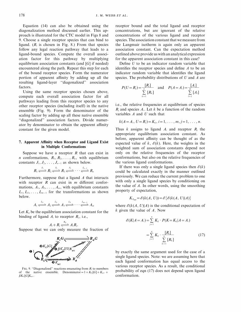
Equation (14) can also be obtained using thediagonalization method discussed earlier. This ap-proach is illustrated for the CTC model in Figs 8 and9. Choose a single receptor species that can bind toligand. (Ri is chosen in Fig. 8.) From that speciesfollow any legal reaction pathway that leads to aligand-bound species. Compute the overall associ-ation factor for this pathway by multiplyingequilibrium association constants (and [G] if needed)encountered along the path. Repeat this step for eachof the bound receptor species. Form the numeratorportion of apparent affinity by adding up all theresulting ligand-layer ‘‘diagonalized’’ associationfactors.

Using the same receptor species chosen above,compute each overall association factor for allpathways leading from this receptor species to anyother receptor species (including itself) in the nativeensemble (Fig. 9). Form the denominator of thescaling factor by adding up all these native ensemble‘‘diagonalized’’ association factors. Divide numer-ator by denominator to obtain the apparent affinityconstant for the given model.

7. Apparent Affinity when Receptor and Ligand Exist

in Multiple Conformations

Suppose we have a receptor R that can exist inn conformations, R1, R2, . . . , Rn , with equilibriumconstants J1, J2, . . . , Jn−1 as shown below.

R1ghJ1

R2ghJ2

R3ghJ3

· · ·ghJn−1

Rn

Furthermore, suppose that a ligand A that interactswith receptor R can exist in m different confor-mations, A1, A2, . . . , Am , with equilibrium constantsL1, L2, . . . , Lm−1 for the transformations as shownbelow.

A1ghL1

A2ghL2

A3ghL3

· · ·ghLm−1

Am

Let Kij be the equilibrium association constant for thebinding of ligand Ai to receptor Rj , i.e.,

Ai+Rj ghKij

AiRj.Suppose that we can only measure the fraction of

receptor bound and the total ligand and receptorconcentrations, but are ignorant of the relativeconcentrations of the various ligand and receptorspecies. The association constant thatwemeasure fromthe Langmuir isotherm is again only an apparentassociation constant. Can the expectation methodoutlinedaboveprovideuswith ananalytical expressionfor the apparent association constant in this case?

Define U to be an indicator random variable thatidentifies the receptor species and define A to be anindicator random variable that identifies the ligandspecies. The probability distributions of U and A are

P(U=Rj )=[Rj ]

sn

k=1

[Rk ]and P(A=Ai )=

[Ai ]

sm

l=1

[Al ]

i.e., the relative frequencies at equilibrium of speciesRj and species Ai . Let k be a function of the randomvariables A and U such that

k(A=Ai , U=Rj )=Kij , i=1, . . . , m, j=1, . . . , n.

Thus k assigns to ligand Ai and receptor Rj theappropriate equilibrium association constant. Asbefore, apparent affinity can be thought of as theexpected value of k, E(k). Here, the weights in theweighted sum of association constants depend notonly on the relative frequencies of the receptorconformations, but also on the relative frequencies ofthe various ligand conformations.

If there was only a single ligand species then E(k)could be calculated exactly in the manner outlinedpreviously. We can reduce the current problem to onewith only a single ligand species by conditioning onthe value of A. In other words, using the smoothingproperty of expectation,

KAapp=E(k(A, U))=E{E(k(A, U)=A)}

where E(k(A, U)=A) is the conditional expectation ofk given the value of A. Now

E(K=A=Ai )=sn

j=1

Kij · P(K=Kij =A=Ai )

=sn

j=1

Kij ·[Rj ]

sn

k=1

[Rk ](17)

by exactly the same argument used for the case of asingle ligand species. Note: we are assuming here thateach ligand conformation has equal access to thevarious receptor species. As a result, the conditionalprobability of eqn (17) does not depend upon ligandconformation.

F. 9. ‘‘Diagonalized’’ reactions emanating from Ri to membersof the native ensemble. Denominator=1+KG [G]+Kact +bKG [G]Kact .

–. 179

F. 10. Model in which ligand and receptor exist in two conformations. (a) Schematic view of model. (b) Model with equilibriumassociation constants.

Thus we have

KAapp=E(K)=E{E(K=A)}

=sm

i=1

E(K=A=Ai ) · P(A=Ai)

=sm

i=1 gG

G

F

fGG

G

F

f

sn

j=1

Kij ·[Rj ]

sn

k=1

[Rk ]GG

G

J

j

·[Ai ]

sm

l=1

[Al ]hG

G

J

j

=

sm

i=1

sn

j=1

Kij [Ai ][Rj ]

sn

k=1

[Rk ] sm

l=1

[Al ]. (18)

As an example of the use of eqn (18), consider thecase of a receptor and a ligand each existing in twoconformations. The situation is illustrated in Fig. 10.Equation (18) yields

KAapp=

(K11[A1][R1]+K12[A1][R2]+K21[A2][R1]+K22[A2][R2])([A1]+[A2])([R1]+[R2])

. (19)

Since [R2]=J1[R1] and [A2]=L1[A1], eqn (19) can befurther simplified.

KAapp=

(K11[A1][R1]+K12[A1]J1[R1]+K21L1[A1][R1]+K22L1[A1]J1[R1])

([A1]+L1[A1])([R1]+J1[R1])

=K11+K12J1+K21L1+K22L1J1

(1+J1)(1+L1)

=1

(1+J1)(1+L1)K11

+J1

(1+J1)(1+L1)K12

+L1

(1+J1)(1+L1)K21

+L1J1

(1+J1)(1+L1)K22. (20)

From the weights that multiply the equilibriumassociation constants in eqn (20) we can read off thejoint probability distribution of A and U, which,because A and U are independent random variables,factors into a product of the individual marginalprobability distributions. The results are summarizedin Fig. 11. With the joint probability distribution ofU and A in Fig. 11 we could have obtained the resultsin eqn (20) directly by applying the expectationformula of eqn (7).

8. Limitations to the Probabilistic Interpretation of

Apparent Affinity

The probabilitistic interpretation for apparentaffinity has a great deal of appeal. Just as simpleaffinity is a property of a receptor species, apparentaffinity is a property of a receptor ensemble. If weknow the simple affinities and the relative frequenciesof the receptor species in the receptor ensemble, then

F. 11. Joint probability distribution of U and A.

. . .180

T 3Equilibrium concentrations of receptors in the native

ensemble

Receptor Concentration with Concentration in thespecies ligand absent presence of ligand

Ri x yRa xKact yKact

RiG xKGG yKGG*RaG xKactbKGG yKactbKGG*

Apparent affinity, though, only depends upon therelative concentrations of these four species and noton their absolute concentrations. To compute therelative concentrations we divide the concentrationgiven in each cell of the table by its column sum(Table 4). The relative frequencies of receptor speciesin the presence and absence of ligand are the sameonly if the introduction of ligand does not change theconcentration of free G-protein, i.e., only if G=G*.This will be the case if G-protein is in excess or forcertain sets of simple ligand binding constants, but itwill not be true in general if G-protein is limiting.

If accessory proteins are not in excess, the mappingthat transforms the relative frequencies of themembers of the native ensemble in the absence ofligand into their relative frequencies in the presence ofligand is not the identity mapping. Thus, knowing theinitial distribution of receptors among the variousreceptor states before the introduction of ligand andknowing the individual simple affinities of thereceptor species for ligand does not allow one topredict the overall apparent affinity. One has toessentially carry out the binding experiment andobtain the equilibrium distribution of members of thenative receptor ensemble to be able to use theformulas developed here.

Discussion

In a typical equilibrium binding experiment thefraction of total receptor, R, that is bound to a ligand,A, is measured and this information is used to obtainan estimate of the equilibrium dissociation constantfor the receptor-ligand complex, AR. When receptorsexist in distributed states, the bound fraction is nolonger pure AR, but is instead a heterogeneousassemblage of bound receptor species. As a result, theaffinity constant that is measured is an apparent

we can calculate apparent affinity. It is a weightedsum of simple affinities where the weights are just therelative frequencies.

All this assumes that the equilibrium frequencies donot change after a ligand is introduced. The weightsare based on the relative abundance of unboundreceptor species after the introduction of ligand andnot before. Unfortunately, these need not be the sameif the frequencies depend upon the concentrations ofaccessory proteins, concentrations that may changeappreciably after the introduction of ligand. As anexample, consider again the cubic ternary complexmodel where the unbound receptor species areRi , Ra , RiG, and RaG. Let x=concentration of freereceptor before the introduction of ligand andy=concentration of free receptor after the introduc-tion of ligand. Using the notation for the equilibriumassociation constants introduced in Section 1 weobtain the equilibrium concentrations shown inTable 3.

Here G and G* are the concentrations of freeG-protein in the absence and presence of ligandrespectively. As is clear from the table, the absoluteabundance of each species is different in the twoscenarios since free receptor concentration and freeG-protein concentration will certainly change afterligand is introduced, x becomes y and G becomes G*.

T 4Frequency distribution of receptors in the native ensemble at equilibrium

Receptor Relative concentration Relative concentration inspecies with ligand absent the presence of ligand

Ri1

1+Kact+KGG+KactbKGG1

1+Kact+KGG*+KactbKGG*

RaKact

1+Kact+KGG+KactbKGGKact

1+Kact+KGG*+KactbKGG*

RiGKGG

1+Kact+KGG+KactbKGGKGG*

1+Kact+KGG*+KactbKGG*

RaGKactbKGG

1+Kact+KGG+KactbKGGKactbKGG*

1+Kact+KGG*+KactbKGG*

–. 181

affinity constant rather than a simple affinityconstant.

The problem that distributed receptor states posesfor the measurement of ligand affinity from bindingexperiments has received considerable attention inthe pharmacological literature. In general, formulasfor apparent affinity have been developed on a caseby case basis without an appeal to general principles.Explicit formulas have been developed for the simpletwo-state model (Colquhoun, 1987), the simpleternary complex model (Mackay, 1988), and theextended ternary complex model (Samama et al.,1993). Usually apparent affinity is regarded as anuisance value, it’s the quantity measured when infact it is the value of a specific simple affinity constantthat is desired, and its biological meaning has beenunexplored.

In this paper we have approached the ‘‘apparentaffinity problem’’ strictly as a mathematical detectivestory. Put simply, if you fit an equation thatis derived from one model (Clark, 1937) to datathat is generated by a different but relatedmodel, do any of the parameters retain theiroriginal interpretations? The answer is yes if theparameter in question is apparent affinity and thegenerating model is a highly symmetric one. If, onthe other hand, the generating model is notsymmetric, then apparent affinity no longer has asimple interpretation. Even so, it is still possibleto connect apparent affinity with the parameters ofthe underlying model in a very straight-forwardmanner.

We have relied on the CTC model in this paper tohelp unravel this detective story. We did so notbecause we necessarily believe that there are specificbiological systems that are well represented by thismodel. Instead, we use it because its inherentsymmetry and structural elegance as a model make itan exceptional tool for understanding the complexi-ties that arise out of simpler but less elegant models.We view the CTC model not so much as a windowinto biology but more as a window into biologicalmodels.

From it we’ve developed two general algorithms,the diagonalization method and the expectationmethod, that yield explicit expressions for apparentaffinity in any equilibrium model with distributedreceptor states. The elegance of the expectationmethod is that it decomposes apparent affinity intoa sum of the products of the simple affinities of thereceptor species for a ligand and the relativefrequencies of those species—eqn (7). The elegance ofthe diagonalization method is that it reshuffles theterms in the apparent affinity expression as KA times

a ratio, a ratio in which factors representinginterconversions between bound species appear inthe numerator and factors representing interconver-sions among unbound species appear in thedenominator, eqn (12). This ratio makes explicit howdistributed receptor states cause apparent affinityto deviate from simple affinity and how the effectdiffers depending upon whether or not G-proteins areinvolved.

Of the two methods, the diagonalization method isthe more general one. The expectation method canonly be applied to symmetric models, models inwhich there exists a one-to-one mapping between theset of bound receptor species and the set of unboundspecies. In symmetric models, if Rn is a receptorspecies, then perforce ARn is a bound species in themodel. Alternatively, if ARm is a bound species in asymmetric model, then Rm is a receptor species in themodel. Thus each receptor species has its own simpleaffinity constant with ligand.

In symmetric models apparent affinity can be givena probabilistic interpretation, it is a weighted sum ofthe simple affinity constants. The weights are therelative abundances of the different unboundreceptor species at equilibrium. Notice that apparentaffinity is a sensible concept in this setting, it is thereceptor-ensemble analog of the single simple affinityconstant that appears in Clark’s model. Observe alsothat the probabilistic interpretation only applieswhen affinity constants are measured as equilibriumassociation constants and not as dissociation con-stants.

In analysing biological systems, choosing theappropriate level of analysis is often not a trivialenterprise—the level at which we choose to describebiological phenomena can profoundly influence thedepth of our understanding. Phenomena that seemmysterious at one level become less so at another.Surprisingly, the greatest insights need not arise atthe lowest conceivable level of description (Cohen &Stewart, 1994).

If a ligand is able to bind to multiple componentsof a receptor ensemble, it may make more sense towork with the affinity of the ligand to the receptorensemble as a whole than to work with the ligand’sindividual simple affinities to the components of theensemble. In physics, the translational motion of arotating, vibrating, interacting collection of particleshas a simple macroscopic description when attentionis focused on the movement of its center of massrather than the movements of individual components.Similarly, the affinity of a ligand for a ‘‘receptor’’which is, in reality, an interconverting nexus ofreceptor species, each with its own simple affinity

. . .182

constant, has a simple holistic characterization if theindividual affinities are subsumed into a singleapparent affinity. Apparent affinity thus becomes ahigher level analog of the individual simple affinities.To the extent that the receptor ensemble is a naturalunit, apparent affinity becomes its natural metric.

REFERENCES

B, J. W. & S, N. P. (1990). Interpretation of agonistaffinity estimations: the question of distributed receptor states.Proc. R. Soc. Lond., B. 240, 503–518.

C, A. J. (1937). General Pharmacology. In: Heffner’sHandbuch der Experimentellen Pharmakologie ErganzungswerkBand 4. Berlin: Springer-Verlag.

C, J. & S, I. (1994). The Collapse of Chaos: DiscoveringSimplicity in a Complex World. New York: Viking.

C, D. (1987). Affinity, efficacy, and receptor classifi-cation: is the classical theory still useful? In: Perspectives onReceptor Classification. (Black, J. W., Jenkinson, D. H. &Gerskowitch, V. P., eds.), pp. 103–114. New York: A. R. Liss.

F, R. F. (1966). The use of b-haloalkylamines in the

differentiation of receptors and in the determination ofdissociation constants of receptor agonist complexes. In:Advances in Drug Research, Vol. 3. (Harper, N. J. & Simmonds,A. B., eds.), pp. 21–55. New York: Academic Press.

H, A. V. (1910). The possible effects of the aggregation of themolecules of haemoglobin on its dissociation curves. J. Physiol.(London) 40, iv–viii.

K, T. (1993). Pharmacologic Analysis of Drug-ReceptorInteraction. New York: Raven Press.

L, I. (1918). The adsorption of gases on plane surfaces ofglass, mica and platinum. J. Am. Chem. Soc. 40, 1361–1403.

M, D. (1966a). A general analysis of the receptor-druginteraction. Brit. J. Pharmacol. 26, 9–16.

M, D. (1966b). A new method for the analysis ofdrug-receptor interactions. In: Advances in Drug Research, Vol. 3(Harper, N. J. & Simmonds, A. B., eds.), pp. 1–19. New York:Academic Press.

M, D. (1988). Continuous variation of agonist affinityconstants. Trends Pharmacol. Sci. 9, 156–157.

M, D. (1990). Agonist potency and apparent affinity:interpretation using classical and steady-state ternary-complexmodels. Trends Pharmacol. Sci. 11, 17–22.

S, P., C, S., C, T. & L, R. J. (1993).A mutation-induced activated state of the b2-adrenergicreceptor. J. Biol. Chem. 268, 4625–4636.