Quasi-cyclic LDPC codes with high girth

arX

iv:0

906.

3410

v1 [

cs.IT

] 18

Jun

200

9

Quasi-cyclic LDPC codes with highgirth

June 18, 2009

Christian Spagnol([email protected])Department of Electronic engineering, UCC Cork, Ireland.

Marta Rossi ([email protected])Department of Mathematics and Appl., University of Milan-Bicocca, Italy.

Massimiliano Sala([email protected])Department of Mathematics university of Trento, Italy /Boole Centre for Researchin Informatics, UCC Cork, Ireland.

Abstract. We study a class of quasi-cyclic LDPC codes. We provide precise con-ditions guaranteeing high girth in their Tanner graph. Experimentally, the codes wepropose perform no worse than random LDPC codes with their same parameters,which is a significant achievement for algebraic codes.

Keywords: LDPC codes, quasi-cyclic codes, Tanner graph.

1 Introduction

The LDPC codes are codes that approach optimal decoding performances, withan acceptable decoding computational cost ([1, 2, 3]). In this paper we present aclass of quasi-cyclic LDPC codes and we show that we are able to guarantee somerelevant properties of the codes. Experimentally, their decoding performance iscomparable with the performance obtained by random LDPC codes.

Traditionally, coding theory is divided into two main research areas: algebraiccoding theory and probabilistic coding theory. The former ([4]) deals with codesendowed with a nice algebraic structure, which allows both to study their internalproperties and to have efficient encoding-decoding techniques, the latter deals withconvolutional codes, which are very difficult to study and randomly constructed,

1

http://arxiv.org/abs/0906.3410v1

but having superior decoding performance. However, the rediscovery of the LDPCcodes by MacKay ([3]) triggered a radical change in coding theory: now we havelinear block codes that may reach decoding performance close to the upper boundgiven by the Shannon limit ([5]). Dozens of papers have appeared since MacKay’spaper, some of them trying to endow some structure (either algebraic or geomet-rical) on LDPC codes. However this has seldom been successful, because thestructure brings a regularity in the parity-check matrix ofthe code, which natu-rally pushes towards the creation of many dangerous small cycles in their Tannergraph. It the object of this paper to propose a family of LDPC codes, possessing analgebraic structure but not suffering from the performancelimitations common toother similar families. The family of quasi-cyclic LDPC codes are of great interestfor the possibility of exploiting the structure of the parity check matrix to achievevery fast and efficient encoding and decoding. Unfortunately the BER/SNR per-formance of this class of codes is known to be worst than random generated LDPCcodes in particular for medium/long length.

The object of this contribution is to study the family of quasi-cyclic LDPCcodes, and provide precise conditions guaranteeing high girth in the Tanner graph.Although several families of quasi-cyclic LDPC codes have been proposed, nogeneral study on their girth properties have been published. Previous researchespresented in the literature focuses on studies of the properties of particular classesof quasi-cyclic LDPC codes constructed from circulant matrices obtained from amonomial. It is our purpose to fill this gap, by formally classify all cases whencycles of length less than10 may arise in the general case. Therefore, in thiscontribution matrices obtained from polynomial are also considered. The study isrestricted to polynomials composed of two or less monomials, the reason for suchlimitation is the fact that circulant obtained from polynomial composed by three ormore monomials internal cycles of length h6 always exist. Hence such polynomialare of no interest if codes with higher girth is wanted.

From the classification obtained, it is obvious how to identify necessary andsufficient conditions for any quasi-cyclic LDPC code to havegirth at least10. Var-ious constructions are presented that perform no worse thanrandom LDPC codeswith the same parameters, which is a significant achievementfor algebraic codes.

The remainder of this paper is structured as follows:

• Section 2 provides notations, recall some relevant well-known facts andprove some simple preliminary statements;

• Section 3 deals with theclassification of the cases when cycles up to length8 may arise for a rather general code family;

• Section 4 improves results from Section 3 for the generic quasi-cyclic case;

• In section 5 the existence of short cycles is linked with condition on thepolynopmial representation of the circulant matrices;

2

• In sections 7, 8 and 9 varius subclass of quasi-cyclic codes are studied indetails and detailed conditions to avoid short cycles are given. The perfor-mances of such codes is compared with other codes,

• Finnaly in section 10 comments, conclusions, and outline some further re-search are presented.

2 Preliminaries and notation

In this section some known facts are recalled, some notationare given and somesimple statements that will be useful later on are proved.

2.1 LDPC codes and Tanner graphs

The parity-check matrixH = (hi,j) of any binary[n, k, d] linear codeC may berepresented by a graphΓ, known as the Tanner graph ([6, 7]). The Tanner graph isformed by two types of nodes: the “bit nodes” and the “check nodes”. Bit nodescorrespond to matrix columns and check nodes correspond to matrix rows, so thatthere arer = n − k check nodes andn bit nodes. We connect the check nodeito the bit nodej if and only if the entryhi,j = 1. There is no edges connectingtwo check nodes or two bit nodes (this kind of graph is called abipartite graph).In other words,H is the adjacency matrix ofΓ.

Example 2.1. An example of a binary LDPC code and relative Tanner graph canbe seen in Figure 1

H =

2

6

6

6

6

6

4

1 0 1 0 1 0 0 0 0 0

0 1 0 1 0 1 0 0 0 0

0 0 0 0 0 0 1 1 1 0

0 0 1 0 1 0 0 0 0 1

0 0 0 1 0 0 1 0 0 0

0 0 0 0 0 0 0 1 1 1

3

7

7

7

7

7

5

c0 c1 c2 c3 c2 c3

b0 b1 b2 b3 b4 b5 b6 b7 b8 b9

Check Nodes

Variable Nodes

Figure 1: Parity check matrix H and the associated Tanner Graph, the presence ofa cycle is highlighted

Now we introduce LDPC codes - Low-Density Parity-Check codes - a class oflinear error correcting codes. Historically, these codes were discovered by Gallagerin 1963 in his PhD thesis [1]. These codes were largely ignored, because of someimplementation issues. In the 1990’s they were rediscovered by MacKay [3] andnow the research continues vigorously, with dozens of papers published every year([8]).

Definition 2.2. An LDPC code is a linear block code for which the parity checkmatrix has a low density of non-zero entries.

3

A (c, s)-regular LDPC code is a linear code whose parity check matrixHcontains exactlyc ones per column ands ones per row.

We do not specify what we mean by low density because it depends on thecontext. For example, for a typical(3, 6)-regular binary code (rate1/2) of blocklengthn, there are only three ones in each column ofH and so the fraction of onesin this matrix is6/n.

The decoding algorithm for these codes is usually called the“sum-product al-gorithm”. We summarize some properties of these codes:

• the LDPC codes have excellent decoding performance, near tothe channelcapacity ([1, 3, 9]),

• the sum-product algorithm is based on the probabilities received from thechannel and it may be idealized as a belief-propagation algorithm (see [10]),with information being passed and updated by the bit nodes tothe checknodes and vice-versa, in a loop;

• the information propagation is heavily hindered by the presence of smallcycles in the Tanner graph ([11]);

• the best LDPC codes are irregular and are created by some random-walkoptimization algorithm ([5, 9, 12, 13, 14]);

• there is no known algebraic class of LDPC codes that has performance com-parable to the best known LDPC codes.

There are two serious issues for a code not possessing an algebraic structure:

• the encoding process is computationally expensive,

• it is very difficult to study its properties.

There are many family of LDPC codes that have been proposed endowed withan algebraic (or geometrical) structure, but none of them has clearly shown, atpresent, a decoding performance comparable with the randomLDPC codes (see[15, 16, 17, 18, 19, 20, 21, 22]).

2.2 Girth

Definition 2.3. In a graph, acycle is a path that starts from a vertexv and ends inv. Thegirth of a graph is the smallest of its cycles.

Obviously the girth of a bipartite graph is always even. The girth is consideredone of the important parameters of a LDPC code, it is commonlyaccepted that thepresence of short cycles in the graph is one of the main parameters affecting thecoding gain achievable by the LDPC code [23]. The dependencyof the perfor-mances of a LDPC code on its girth distribution, in particular when small cycles

4

have been avoided, is still under debate since mathematicalproof has not yet beenobtained. In contrast with the deteriorating effect of cycles on the performanceof the LDPC codes, Etzionet al. [24, 25] proved how cycle-free graphs cannotsupport good codes. Still, simulations and applications have shown that the beliefpropagation algorithm is generally very effective, even inthe presence of cycles inthe graph [26, 5]. Nevertheless it is commonly accepted thatthe presence of shortcycles in the graph is one of the main causes of reducing the coding gain achievedby the LDPC code [23], and so the girth is considered one of thesignificant param-eters of a code.

For Tanner graphs of(c, s)-regular LDPC codes, it is possible to give upperbounds on the girth, see [22].

Theorem 2.4. Consider a(c, s)-regular [N,K, d] LDPC code. LetR = N − Kand α = (c − 1)(s − 1). If the girth g ≡ 2 mod (4), theng ≤ 4 logα r + 2,otherwiseg ≤ 4 logα r + 4.

Whenr = 404 andα = (3− 1)(6− 1) = 10 (as for our simulation), we get inthe worst case g ≤ 4 log10(404) + 4 = 14, but in practice it is very difficult tofind such codes withg ≥ 10, so that ensuringg ≥ 8 is already interesting.

One of the most promising families of LDPC codes with a nice structure wasproposed by Rosenthal and Vontobel ([22]). These are based on Tanner graphsbuilt starting from Ramanujan graphs and hence are guaranteed to have a very highgirth. Unfortunately, their decoding performance have been questioned ([27]) andit is not evident how an efficient encoding could be implemented.

There is a family of LDPC codes, which has been proposed by Fossorier ([28]),which is particularly interesting for us, because they are quasi-cyclic and so theirstructure is quite similar to ours. With Fossorier’s codes,it is easy to get a girthas high as8 or 10. However, the construction by Fossorier does not provide codeswhose Tanner graph has a girth higher than12, as shown by Fossorier himself inthe same paper.

Another interesting construction has been provided in [21,29]. They can getvery high girth, but there are some open problems, in particular on how to get anefficient encoding.

To simplify the search for cycle in a Tanner graph representing aH parity checkmatrix, a novel and convenient definition of cycles of lengthlc in an arbitrary binarymatrix is given here.

Definition 2.5. Let s,N,M be natural numbers withs ≥ 2 andN,M ≥ 3, anddefinelc = 2s. LetB be anyN × M matrix over Z 2. A sub-setV of lc entries ofB is calledlinked if the entries lay ins columns ands rows.

Definition 2.6. Let B be anyN × M matrix over Z 2. A sub-setV of lc entries(lc = 2s) of B is called a2s-cycle if :

• V is linked, and

5

• for anyr such that2 ≤ r < s there is no linked sub-setW ⊂ V of 2r entries.

In order to clarify the meaning of the definitions two examples are shown inFigure 2.2

1 1

1 11 1

1 1

8 entries linked set thatdoes not form a8-cycle

1 1

1 11 1

1 1

8 entries linked set thatdoes form a8-cycle

Figure 2: Example of linked sets withs = 4, t = 8

Matrix (a) contains8 entries, they form a linked set since they lie in4 rowsand4 columns but they do not form a8-cycle since they can be grouped in twosmaller linked sets of4 elements each. Matrix (b) represents a linked set of entriesthat form a8-cycle, since the8 entries lie in4 rows and4 columns but there are nosmaller linked sets.

Note that if a matrix column contains a point of a2s-cycleV then it containsexactly two points ofV . The same is true for the rows. Moreover a linked sub-setV of 2s entries either is a2s-cycle or it contains at least a2r-cycle with2 ≤ r < s.

2.3 Circulant matrices

Binary circulant matrices are important as they form the “bricks” with which parity-check matrices for quasi-cyclic LDPC codes are “built”.

Definition 2.7. Letm ≥ 6. LetC be anm×m matrix overF2. C is circulant if itsrows are obtained by successive shifts (to the right). The matrix C is weight-l if theweight of any row isl. In case of circulant of weight-2, that are used extensively inthis work, the polynomial representation of the first row,p(x) ∈ F2[x], is called thepolynomial of C. Letp(x) = xa + xb, with a < b. s(p) = min(b− a, a + m− b)is called theseparationof p (or of C).

Consider, for example, the following weight-2 circulant matrix.

(1) C =

1 1 0 0 00 1 1 0 00 0 1 1 00 0 0 1 11 0 0 0 1

6

Its polynomial isp = x + 1, with parametersm = 5, b = 1, a = 0, s(p) = 1.Note, similar matrices can be described as an superimposition of two permu-

tation matrices used by other authors (e.g. [30]), in such case the exponents arerelated to the power of the single permutation matrices, andthe analysis presentedin this chapter can be rewritten with such notation.

When the natural numberm is greater or equal to3 the equations:

(2) a ≡ b mod (m), p(x) ≡ q(x) mod (xm + 1) ,

will be abbreviated with, respectively, :

(3) a ≡ b, p(x) ≡ q(x) ,

where the polynomial congruence is inZ 2[x].Let p = xa + xb, sometimes some statements where the role ofa andb may

be exchanged are needed. To provide a concise formulation inthese cases, thenotationǫ(p) in congruences modulom is introduced. Letf be any functionf :N 7→ Z, then

• f(ǫ(p)) ≡ l, means “f(a) ≡ l or f(b) ≡ l”,

• f(ǫ(p)) 6≡ l, means “f(a) 6≡ l andf(b) 6≡ l”.

In the case of a circulant matrix of weight-1, ǫ(p) refers to the exponent of themonomial.

This notation is extended to the case when more polynomials,p1 . . . ps, areinvolved in a function, as follow. Letp1 = xa1 + xb1 , . . . , ps = xas + xbs . Let fbe any functionf : N

s 7→ Z. Then

• f(ǫ(p1), . . . , ǫ(ps)) ≡ l, means that there is a combination(z1, . . . , zs)wherezi ∈ {ai, bi} such thatf(z1, . . . , zs) ≡ l and

• f(ǫ(p1), . . . , ǫ(ps)) 6≡ l, means that for every possible combinations(z1, . . . , zs)wherezi ∈ {ai, bi} thenf(z1, . . . , zs) 6≡ l.

Remark 2.8. To avoid ambiguity, statements of kind:f(ǫ(p1), . . . ǫ(pr)) ≡ f(ǫ(pr+1), . . . , ǫ(ps)) orf(ǫ(p1), . . . ǫ(pr)) 6≡ f(ǫ(pr+1), . . . , ǫ(ps)) .will never be used.

Some simple facts on weight-2 circulant matrices are collected here. Thesefollow directly from the circularity of the matrix.

Proposition 2.9. LetC = {ci,j} be an(m×m) weight-2 circulant matrix overZ

2[x] with polynomialp(x). Then:

1. ci,j = 1 if and only ifj ≡ i + ǫ(p),

2. cx,y = ct,y = 1 (with x 6= t) if and only ift − x ≡ ±s(p),

7

3. cx,y = cx,z = 1 (with y 6= z) if and only ifz − y ≡ ±s(p),

4. cx,y = ct,y = 1 andcx,z = cw,z = 1 (with y 6= z, x 6= t, x 6= w) if and onlyif x − t ≡ ±s(p) andw − x ≡ x − t ≡ ±s(p).

Lemma 2.10. Letp andq be two polynomials inZ 2[x] with degree at mostm−1.Then

s(p) = s(q) ⇔ s(p) ≡ ±s(q)

Proof. Note thats(p) ands(q) are not greater thanm/2 and positive.

Definition 2.11. Letm ≥ 3. Letp andq be two polynomials inZ 2[x] with degreeat mostm − 1. We say thatp is a shift of q if there is0 ≤ µ ≤ m − 1 s.t.

p ≡ xµq .

In this case we writep ∼ q.

Observe that∼ is an equivalence relation in the set formed by all polynomialsover Z 2 with degree less thanm.

Lemma 2.12. Letp andq be two polynomials inZ 2[x] with degree at mostm−1.Then

s(p) = s(q) ⇔ s(p) ≡ ±s(q)

Proof. Note thats(p) ands(q) are not greater thanm/2 and positive.

There is a link between the separation of a polynomial and itsroots.

Fact 2.13. Let m ≥ 3. Let p and q be two weight-2 polynomials in Z 2[x] withdegree at mostm − 1. Then

p ∼ q ⇔ s(p) = s(q) .

Moreover, ifp and q are both maximal or if they are both minimal, then thenon-zero roots ofp andq are the same (and with the same multiplicity) if and onlyif p ∼ q.

Proof. Let p = xap + xbp andq = xaq + xbq , with ap < bp andaq < bq.p ∼ q ⇒ s(p) = s(q).

If p ∼ q, thenp ≡ xµq, for some0 ≤ µ ≤ m−1. That is,p+xµq = λ(xm+1), forsomeλ ∈ Z2[x]. Butdeg(p+xµq) ≤ 2m−2, sincedeg(p) ≤ m−1, ∂q ≤ m−1andµ ≤ m − 1. Also, either∂ (λ(xm + 1)) ≥ m or λ = 0.There are three cases:

8

1. deg(xµq) ≤ m − 1.Thenλ = 0 andp = xµq, which means

bp − ap ≡ ±s(p), s(p) = s(xµq) = s(xaq+µ + xbq+µ) ,

s(xaq+µ + xbq+µ) ≡ ±(

(bq + µ) − (aq + µ)) ≡ ±(bq − aq) ≡ ±s(q) ,

so thats(p) ≡ ±s(q) and hences(p) = s(q) (Lemma 2.12).

2. deg(xµq) ≥ m and we havexµq = xaq+µ + xbq+µ, with aq + µ ≤ m − 1andbq + µ ≥ m.Thenxbq+µ = xbq+µ−m(xm + 1) + xbq+µ−m, so thatλ = xbq+µ−m andeitherap = bq + µ − m, bp = aq + µ, or bp = bq + µ − m,ap = aq + µ,which impliess(p) ≡ ± ((aq + µ) − (bq + µ − m)) ≡ ±(aq − bq + m) ≡≡ ±(bq − aq) ≡ ±s(q) and hences(p) = s(q) (Lemma 2.12).

3. deg(xµq) ≥ m and we havexµq = xaq+µ + xbq+µ, with aq + µ ≥ m andbq + µ ≥ m.This case is the same as case 1), with the role ofp andq exchanged. Since∼ is an equivalence relation, we do not have to deal with it.

s(p) = s(q) ⇒ p ∼ q.If s(p) = s(q), there are four cases:

• s(p) = bp−ap ands(q) = bq−aq. Thenbp−ap = bq−aq. We may assumebq ≥ bp, so thatbq − bp = aq − ap, i. e. q = xbq−bpp.

• s(p) = m− ap + bp ands(q) = m− aq + bq. Againbp − ap = bq − aq andso we may argument as before.

• s(p) = bp − ap ands(q) = m− bq + aq. It is enough to takeµ = bp − aq =ap + m − bq: xµ(xaq + xbq) = xbp + xap+m ≡ xbp + xap .

• s(p) = m − bp + ap ands(q) = bq − aq. Same argument.

We now suppose bothp andq minimal and we want to show thatp ∼ q if andonly if they have the same non-zero roots (with the same multiplicity). The casewhen they are both maximal is analogous and will not be shown.It is obvious that two polynomialsp andq have the same non-zero roots with thesame multiplicity if and only ifp = xiq, for somei. Assuming bothp and qminimal, we havep ∼ q ⇔ p = xµq, and so our desired logical equivalencefollows.

3 Cycle configurations for generic matrices

In this section some notations, facts and lemmas useful to identify which cycles canexist in a given matrix are presented. A rather general classof matrices is studied.

9

The general results obtained here will be specialized to thequasi-cyclic case infollowing subsections.

For the remainder of this chapter, if not differently specified,m,α, βγ are nat-ural numbers withm ≥ 3, α, β, γ ≥ 1,

Definition 3.1. Given a matrixB over Z 2, B is said to be inMm,α,β,γ if it maybe written as

B =

A1,1 · · · A1,αβ

......

...Aαγ,1 · · · Aαγ,αβ

where theAi,j ’s are binary square matrices of dimensionm. This decompositionis referred to as thestandard decompositionof B in Mm,α,β,γ . Any matrixAi,j

is called adecomposition sub-matrix(d.s.). For anyi in {1, . . . , αγ}, that the set{Ai,j | 1 ≤ j ≤ αβ} is called adecomposition row(d.r.) of B. Similarly, forany j in {1, . . . , αβ}, the set{Ai,j | 1 ≤ i ≤ αγ} is called adecompositioncolumn(d.c.) ofB.

The d.s.’s{Ai,j} are defined unambiguously and the uniqueness of the standarddecomposition inMm,α,β,γ is obvious. The term “standard decomposition” willbe used rather than “standard decomposition inMm,α,β,γ”. If B ∈ Mm,α,β,γ , Bcan also be viewed as:(4)

B =

L1,1 · · · L1,β...

......

Lγ,1 · · · Lγ,β

, Lr,s =

A(r−1)α+1,(s−1)α+1 · · · A(r−1)α+1,sα...

......

Arα,(s−1)α+1 · · · Arα,sα

,

whereLr,s is a square matrix of sub-matrices, with dimensionαm, (1 ≤ r ≤ γ,1 ≤ s ≤ β).

Remark 3.2. If H ∈ Mm,α,β,γ has full rank andβ > γ, then it represent a binarylinear code with dimension(β − γ)mα and lengthβmα. The information rate is

K

N=

(β − γ)mα

βmα=

β − γ

β.

If H ∈ Mm,α,β,γ is not full rank the rate of the code is lower and the value pre-sented above can be considered as designed rate. Note that insome cases addingredundant rows, hence not having full, can be used as a methodto improve perfor-mances tanks to the extra checks that a codeword has to satisfy.

It is clear that any rate can be achieved with this code construction by choosingβandγ appropriately.

Definition 3.3. LetB ∈ Mm,α,β,γ and let{Ai,j}1≤i≤αγ,1≤j≤αβ form its standarddecomposition. Define the sets of indexesI = {i1, . . . , ir} ⊂ {1, . . . , αγ} andJ = {j1, . . . , js} ⊂ {1, . . . , αβ}. With the notationBI,J the sub-matrix ofB

10

defined by the d.r.’s inI and the d.c.’s inJ is denoted. The sub-matrixBI,J is saidto be of type(r, s) andBI,J is called adecomposition minor(d.m.). Given twod.m.’sBI,J and CI′,J ′ , they are consideredequivalent if it is possible to obtainone from the other by d.r. permutations or by d.c. permutations or by both. Anequivalence class is called aconfiguration of type(r, s).

Foe example the following two matrices are decomposition minors of matrixBin 4 and are equivalent configurations sinceD′ can be obtained fromD by switch-ing the first and second rows and then the first and second columns.

D =

L1,2 L1,4 L1,6

L2,2 L2,4 L2,6

L4,2 L4,4 L4,6

, D′ =

L2,4 L2,2 L2,6

L1,4 L1,2 L1,6

L4,4 L4,2 L4,6

,

Note that the relation defined on d.m.’s is actually an equivalence relation, so that“an equivalence class” makes sense.

The following lemma will be useful later on.

Lemma 3.4. Let I be them × m identity matrix over Z 2. Let B ∈ Mm,α,β,γ

and let{Ai,j} form its standard decomposition. Suppose that there arei andj s.t.Ai,j = I. LetBx,y be an entry ofB included inAi,j . Then

Bx,y = 1 ⇔ x ≡ y

Proof. It is know thatx = x′ +(i−1)m andy = y′ +(j−1)m, with 1 ≤ x′ ≤ mand1 ≤ y′ ≤ m. The pair(x′, y′) represents the components insideAi,j. But Ai,j

is the identity, so that

Bx,y = 1 ⇔ x′ = y′ ⇔ x ≡ y

Using this notation and the definitions of cycles on a matrix given previously 2.6,the following lemmas are obvious.

Lemma 3.5. Let BI,J andCI′,J ′ be equivalent d.m.’s of a matrixB ∈ Mm,α,β,γ .ThenBI,J (strictly) contains a2s-cycle if and only ifCI,J does.

Lemma 3.5 allows us to talk about “configuration of cycles”(see Def. 3.3),meaning equivalent decomposition minors that contain cycles of the same type.

All the possible (d.m.) configurations with2s-cycles are classified next.

Lemma 3.6. With the notation introduced above, letB ∈ Mm,α,β,γ . Then theonly configurations ofB that may (strictly) contain a2s-cycle are of type1:

• (1, 1) |Aij| ,

1For brevity any configuration that is the transpose of another is omitted.

11

•(1, 2) |Ai,j1Ai,j2| ,

......

• (1, s) |Ai,j1 · · ·Ai,js| ,

•(2, 2)

∣

∣

∣

∣

Ai1,j1 Ai1,j2

Ai2,j1 Ai2,j2

∣

∣

∣

∣

,

......

•(2, s)

∣

∣

∣

∣

Ai1,j1 · · · Ai1,js

Ai2,j1 · · · Ai2,js

∣

∣

∣

∣

,

......

• (s − 1, s − 1)

∣

∣

∣

∣

∣

∣

∣

Ai1,j1 · · · Ai1,js−1

......

Ais−1,j1 · · · Ais−1,js−1

∣

∣

∣

∣

∣

∣

∣

,

• (s − 1, s)

∣

∣

∣

∣

∣

∣

∣

Ai1,j1 · · · Ai1,js

......

Ais−1,j1 · · · Ais−1,js

∣

∣

∣

∣

∣

∣

∣

,

• (s, s)

∣

∣

∣

∣

∣

∣

∣

Ai1,j1 · · · Ai1,js

......

Ais,j1 · · · Ais,js

∣

∣

∣

∣

∣

∣

∣

.

Proof. Since a2s-cycleV needss matrix rows, it needs at mosts d.r’s, and anal-ogously for the d.c.’s. So configuration(s, s) is the largest that can occur. Sincematrix rows (and matrix columns) can be grouped in d.r.’s (d.c.’s), any d.m. of(s, s) is possible. This proves the claim.

To any d.m. configuration, one or more cycle configurations may be associated.To proceed it is necessary to characterize the cycle configurations arising from theprevious lemma. In order to do so, a convenient notation for acycle configurationis presented. Any d.m. configuration in the statement of Lemma 3.6 is a sub-configuration of an(s, s) configuration, which can generically be represented as

∣

∣

∣

∣

∣

∣

∣

T1,1 · · · T1,s

......

Ts,1 · · · Ts,s

∣

∣

∣

∣

∣

∣

∣

,

where anyTi,j is anAh,k, for someh andk. A numerical representation for cyclesis adopted as follows. LetV be any2s-cycle contained in the(s, s) configurationas above. For any matrixTi,j With ti,j ≥ 0 the number of points ofV contained inTi,j is denoted. With d.r. and d.c. permutations, it can be supposes that

(5) t1,1 ≥ ti,j, 1 ≤ i, j ≤ s, t1,2 ≥ t1,3 ≥ . . . ≥ t1,s, t2,1 ≥ t3,1 ≥ . . . ≥ ts,1 .

12

A cycle presentation fulfilling conditions (5) will be called a(1)-presentation.It is obvious that for a2s-cycle it must be:

(6)∑

1≤i,j≤s

ti,j = 2s .

For example, a4-cycleV , a 6-cyclesV , and a8-cycle V may be representedas

V =

∣

∣

∣

∣

2 20 0

∣

∣

∣

∣

, V =

∣

∣

∣

∣

∣

∣

2 2 00 2 00 0 0

∣

∣

∣

∣

∣

∣

, V =

∣

∣

∣

∣

∣

∣

∣

∣

2 2 0 00 1 1 00 1 1 00 0 0 0

∣

∣

∣

∣

∣

∣

∣

∣

,

and all these representations are (1)-presentations. To clarify the implications ofthe representation consider the following cycle configurations:

W =

∣

∣

∣

∣

2 10 3

∣

∣

∣

∣

, W =

∣

∣

∣

∣

∣

∣

2 0 12 0 10 0 0

∣

∣

∣

∣

∣

∣

,

they do not form valid (1)-representations since inW t1,1 is not the maximum ofthe elements and inW the elements of the first row are not ordered.

Note that cycleV allows another (1)-presentation that is a column permutationof it:

V =

∣

∣

∣

∣

∣

∣

2 2 02 0 00 0 0

∣

∣

∣

∣

∣

∣

.

For convenience, in a cycle presentation d.r.’s and d.c.’s containing only zeroswill be dropped. The previous presentations may be written as follows

V =∣

∣ 2 2∣

∣ , V =

∣

∣

∣

∣

2 20 2

∣

∣

∣

∣

, V =

∣

∣

∣

∣

∣

∣

2 2 00 1 10 1 1

∣

∣

∣

∣

∣

∣

.

The notation presented above leaves some ambiguity. In fact, for example,t1,1 = 2 does not specify whether the two points inT1,1 lie in the same cyclecolumn or cycle row or in neither.

Remark 3.7 (Transpose). Let D be a d.m. of a matrixB ∈ Mm,α,β,γ and DT

its transpose. It is clear thatD contains a2s-cycle if and only ifDT contains a2s-cycle. In the general case, it is not possible to obtainD from DT by d.c. or d.r.operations, soD andDT arenotnecessarily equivalent according to the definitiongiven. However, if all cycle configurations associated to a given configurationare classified, then, automatically, all cycle configurations for its transpose areobtained (by transposing all of its cycle configurations).

Two lemmas are provided next, these are applied in the analysis of the2s-cycleconfigurations arising in Lemma 3.6.

13

Definition 3.8. The row weight of a d.r. in a cycle configuration is defined as thesum of theti,j ’s in the d.r, and similarly for the d.c.’s.

Lemma 3.9. In any cycle configuration, column weights and row weights are even.

Proof. By transposing, the statement for d.c.’s is true if and only if it is true ford.r.’s. It is here shown for d.r.’s. Given a d.r., if the relevant ti,j ’s sum to an oddnumber, then one point in not in a cycle row with another. But,by definition, anypoint in a 2s-cycle shares one cycle row with one and only one other point in thecycle, hence there cannot be d.r. with odd weight.

Lemma 3.9 will be applied many times. To simplify the relevant notation, thephrase “Lemma 3.9 r-1” will be used meaning “Lemma 3.9 applied to the first d.r.”.Similarly with notations like “r-2”, “r-3”. The same notation is used the columns(e.g. “c-2”).

Lemma 3.10(Isolation). In any d.m. configurationD containing a2s-cycle, thefollowing situation cannot occur with2 ≤ r < s:

D =

∣

∣

∣

∣

D1 00 D2

∣

∣

∣

∣

where:

D1 =

∣

∣

∣

∣

∣

∣

∣

T1,1 · · · T1,r

......

Tr,1 · · · Tr,r

∣

∣

∣

∣

∣

∣

∣

, D2 =

∣

∣

∣

∣

∣

∣

∣

Tr+1,r+1 · · · Tr+1,s

......

Ts,r+1 · · · Ts,s

∣

∣

∣

∣

∣

∣

∣

Proof. It is known, by definition 2.6, how in any row (and column) of a cycle Vthere must be exactly two cycle points. If one cycle point lies in a d.r. of theD1

then also the second cycle point of that d.r. must lie inD1. Hence, for every d.r. inD1 there are two cycle points, the same is true for the d.c.’s. Soin D1 there are2rpoints that lie inr d.r.’s andr d.c.’s , hence they arelinked, but r < s and so thiscontradicts the definition of cycle given (Definitions 2.6).

To ease the reading in situations where lemma 3.10 is not satisfy for a certaind.m.D1 phrases of the type ”D1 is isolated” are used throughout the chapter.

3.1 Possible configurations

The aim is now to determineall the possible2s-cycle configuration (using (1)-presentations) that can arise in a matrix. Some new terminology and lemmas areintroduced first.

Definition 3.11. Theweights vectorof a 2s-cycle configuration is defined as thevector containing all thetij ’s in such configuration.

14

For example the cycle configurations presented previously:

V =∣

∣ 2 2∣

∣ , V =

∣

∣

∣

∣

2 20 2

∣

∣

∣

∣

, V =

∣

∣

∣

∣

∣

∣

2 2 00 1 10 1 1

∣

∣

∣

∣

∣

∣

.

have weights vectors

[2, 2], [2, 2, 2], [2, 2, 1, 1, 1, 1].

Theorem 3.12. The weights vectors that can make a2s-cycle configuration areall the possible combinations of numbers, that sum to2s and that do not containexactly two odd values.

Proof. The sum of the elements in a weights vector must be2s for the definition.Hence all the possible vectors that sum to2s are candidate to be weights vectors ofa 2s-cycle configuration. The vectors that have two odd weights can be dischargesince in such cases it is impossible to have even row weight and column weight foreach d.r. and d.c.. In fact, if both sub-matrices with odd weights are in the samed.r. the two d.c.’s where they lie have odd weight, and vice-versa.

The following theorem specifies which of these weights vectors can form acycle configuration of chosen dimension.

Theorem 3.13.An(r, c) 2s-cycle configuration can be obtained only from weightsvectors that have the following characteristics:

• they containat least r + c − 1 elements,

• they containno more thanmin(cr, 2s) elements,

• the value ofthe biggest element is no more than 2s − 2(c − 1)

Proof. Supposer ≤ c, for remark 3.7 the caser > c can be reduce to this bytransposing the configuration. Any d.r. must have at least one element withtij 6= 0otherwise it would be a(r−1, c) cycle configuration, the same is true for the d.c.’s.

The valuet1,1 must not be0 for the definition of (1)-presentation, then forLemma 3.10 there must be at least another d.m. withtij 6= 0 in the same d.r. ord.c. Suppose, without loss of generality, thatt1,2 6= 0. Applying Lemma 3.10 tothe sub-matrix[T1,1, T1,2] implies that there must be another d.m. withti,j 6= 0 inthe first d.r. or in one of the first two d.c.’s, otherwise[T1,1, T1,2] would be isolated.Assumingt1,3 6= 0 another sub-matrix,[T1,1, T1,2, T1,3], is obtained. Repeatingthe process until allt1,x 6= 0, r − 1 d.r.’s that must have at least oneti,j 6= 0element are left, hence a total of at leastc + r − 1 weights are needed. Note thatthe same result will be obtained if instead of ”filling” the d.c.’s first the d.r.’s arefilled, or any combination. It is obvious that any weights vector cannot have morethat 2s values. Moreover, the sums of the elements in a weights vector is 2s but

15

there cannot be more elements that d.m. hence the max number of elements in aweights vector ismin(2s, rc). Using the (1)-presentation thent1,1 ≥ ti,j for everyi, j, the remaining d.c. must not be zero and have at least row weight 2. Since thesum of all row weights must be2s, the max value oft1,1 is 2s − 2(c − 1).

Using theorems 3.12 and 3.13 it is possible to determine the set of possibleweights vectors that can be used to form a(r, s) 2s-cycle configuration. Obtainingthe configurations from the weights vectors is a mater of placing the weights insuch a way that they satisfy Lemma 3.9 and Lemma 3.10.

Next, an example is presented. The aim is to find which configurations of type(4, 5) can have10-cycles. The process starts by looking for all possible vectors ofnumber that sum to10.

[10] ,

[9, 1] ,

[8, 2] , [8, 1, 1] ,

[7, 3] , [7, 2, 1] , [7, 1, 1, 1] ,

[6, 4] , [6, 3, 1] , [6, 2, 2] , [6, 2, 1, 1] , [6, 1, 1, 1, 1] ,

[5, 5] , [5, 4, 1] , [5, 3, 2] , [5, 3, 1, 1] , [5, 2, 2, 1] , [5, 2, 1, 1, 1] , [5, 1, 1, 1, 1, 1] ,

[4, 4, 2] , [4, 4, 1, 1] , [4, 3, 3] , [4, 3, 2, 1] , [4, 3, 1, 1, 1] , [4, 2, 2, 2] , [4, 2, 2, 1, 1] ,

[4, 2, 1, 1, 1, 1] , [4, 1, 1, 1, 1, 1, 1] ,

[3, 3, 3, 1] , [3, 3, 2, 2] , [3, 3, 2, 1, 1] , [3, 3, 1, 1, 1, 1] , [3, 2, 2, 2, 1] , [3, 2, 2, 1, 1, 1] ,

[3, 2, 1, 1, 1, 1, 1] , [3, 1, 1, 1, 1, 1, 1, 1] ,

[2, 2, 2, 2, 2] , [2, 2, 2, 2, 1, 1] , [2, 2, 2, 1, 1, 1, 1] , [2, 2, 1, 1, 1, 1, 1, 1] ,

[2, 1, 1, 1, 1, 1, 1, 1, 1] , [1, 1, 1, 1, 1, 1, 1, 1, 1, 1] .

The crossed out vectors are not to be considered since they contain exactly two oddnumbers. Applying Theorem 3.13 it is possible to eliminate weights vectors thatdo not have length between8(= 5+4− 1) and10(= min(10, 20)) and that do nothave max value less or equal to2(= 10− 2(5− 1)). The remaining candidates are:

[2, 2, 1, 1, 1, 1, 1, 1] , [2, 1, 1, 1, 1, 1, 1, 1, 1] , [1, 1, 1, 1, 1, 1, 1, 1, 1, 1] .

It is now necessary to place the values of the weights vectorsinside the(4, 5) d.m..It is now proved how the only possible configurations are :

1.

∣

∣

∣

∣

∣

∣

∣

∣

2 1 1 0 00 1 0 1 00 0 1 0 10 0 0 1 1

∣

∣

∣

∣

∣

∣

∣

∣

, 2

∣

∣

∣

∣

∣

∣

∣

∣

1 1 1 1 01 0 0 0 10 1 1 0 00 0 0 1 1

∣

∣

∣

∣

∣

∣

∣

∣

,

This can be proved with some easy considerations. There are twenty Ti,j with1 ≤ i ≤ 4, 1 ≤ j ≤ 5 . It must be

∑

i,j ti,j = 10, andt1,1 ≥ ti,j, ∀i, ∀j s.t. i ≤

16

4, j ≤ 4 . There are five columns and for any of this column the weight must beeven and not zero, (if there is a zero column then it falls in a smaller configuration),the only possibility to have a total sum of ten and column weights even is that allcolumns have weight2. Moreover, there are four rows and for any of these rowsthe weight must be even and not zero, (if there is a zero columnthen it falls ina smaller configuration), the only possibility for the totalsum to be ten and rowweights even is to have one row with weight4 and the remaining with weight2.

• Considering the weights vector[2, 2, 1, 1, 1, 1, 1, 1].An elementti,j = 2 cannot be on a d.r. of weight2 because both the d.c.andd.r. would be completed but this cannot be otherwise it wouldbe isolated (Lemma 3.10). So, both the elementsti,j = 2 must be in the same row, theonly row with weight4. In this case such a row has weight4 and cannothave other non zero elements in it, but also the two columns are completed,since they have weight2. This situation does not satisfy Lemma 3.10, hencethis weights vector does not lead to any cycle configuration of this size.

• Considering the weights vector[2, 1, 1, 1, 1, 1, 1, 1, 1].Elementt1,1 = 2 since it is the max. Lemma 3.10 implies that there mustbe at least another non zero element in row one, but since onlyweight ofvalue one are present and the row weight must be even then there must betwo one elements in row one. Supposed thatt1,2 = t1,3 = 1. Consideringnow Lemma 3.9 applied to the remaining rows and columns configuration1,or a column/row permutation of it, is found.

• Considering the weights vector[1, 1, 1, 1, 1, 1, 1, 1, 1, 1].It can be supposed that the first row has weight4 hence it must have fourelementst1,j = 1 that can bet1,1 = t1,2 = t1,3 = t1,4 = 1. ApplyingLemma 3.9 to all remaining rows and columns configuration2, or a col-umn/row permutation of it, is obtained.

And this prove the claim.

3.2 4-cycle configurations for generic H matrices

In this section all the possible configurations that can givecycles of length4 in thecase of a generic matrix are found and listed.

Theorem 3.14. Let B ∈ Mm,α,β,γ . The only possible4-cycle configuration, in(1)-presentation, are as follows2:

1. (1, 1),|4| ,

2. (1, 2),|2 2| ,

17

3. (2, 2),∣

∣

∣

∣

1 11 1

∣

∣

∣

∣

.

Proof. Following from Theorem 3.12 the only possible weights vectors for a 4-cycles are:

[4], [2, 2], [1, 1, 1, 1].

From them it is straightforward to find the configurations listed in the statement.

3.3 6-cycle configurations for generic H matrices

In this section all the possible configurations that can givecycles of length6 in thegeneral case are found and listed.

Theorem 3.15. Let B ∈ Mm,α,β,γ . The only possible6-cycle configurations, in(1)-presentation, are as follows2 :

1. (1, 1),|6| ,

2. (1, 2),∣

∣ 4 2∣

∣ ,

3. (1, 3),∣

∣ 2 2 2∣

∣ ,

4. (2, 2),

4.1

∣

∣

∣

∣

2 20 2

∣

∣

∣

∣

, 4.2,

∣

∣

∣

∣

3 11 1

∣

∣

∣

∣

,

5. (2, 3),∣

∣

∣

∣

2 1 10 1 1

∣

∣

∣

∣

,

6. (3, 3),∣

∣

∣

∣

∣

∣

1 1 01 0 10 1 1

∣

∣

∣

∣

∣

∣

.


18

Proof. Lemma 3.6 proves that these are all the dimensions that6-cycle configura-tions can have. It is now necessary to prove that the listed configurations are thealland onlypossible configuration that can have6-cycles. To do so it is necessary toprove that for each dimension all the possible configurations associated it are listedin the statement.

Following from Theorem 3.12 the only possible weights vectors for a 6-cyclesare:

[6] ,

[5, 1] ,

[4, 2] , [4, 1, 1] ,

[3, 3] , [3, 2, 1] , [3, 1, 1, 1] ,

[2, 2, 2] , [2, 2, 1, 1] , [2, 1, 1, 1, 1] ,

[1, 1, 1, 1, 1, 1] ,

The weights vectors are used to simplify the process of determining the validconfigurations. The study of each case is presented next.

Configuration (1,1). A type(1, 1) configuration can be generated only by weightsvector[6] and it corresponds to case 1.

Configuration (1,2). A type(1, 2) configuration can be generated only by weightsvector [4, 2] and it corresponds to case 2.

Configuration (1,3). A type(1, 3) configuration can be generated only by weightsvector [2, 2, 2] and it corresponds to case 3.

Configuration (2,2). Applying Theorem 3.13, configurations of type(2, 2) musthave one of the following weights vectors:

[2, 2, 2] , [3, 1, 1, 1] .

Applying Lemma 3.9 it is straightforward that these two weights vectors result inconfigurations 3.1 and 3.2.


[2, 1, 1, 1, 1] , [1, 1, 1, 1, 1, 1] .

• [1, 1, 1, 1, 1, 1] is not a possible choice because it would require to have anodd (3) row weight since there are only two d.r.’s

• [2, 1, 1, 1, 1] results in configuration 5. This can be proved with some shortconsiderations. The valuet1,1 = 2 since it is the max value andt2,1 = 0because otherwise column weight of c-1 would be odd. It follows that all theother must be1 and this proves the claim.

19


[2, 1, 1, 1, 1] , [1, 1, 1, 1, 1, 1]

• [2, 1, 1, 1, 1] is not a possible choice. In fact, there are three d.r.’s and forany of this d.r.’s the row weight must be even and not zero (if there is a zerorow then it fall in a smaller configuration). The sum of all d.r.’s must be six,hence all d.r’s must have row weight 2. The same is true for thed.c.’s. If anyti,j = 2 then that element is isolated (Lemma 3.10) but this is not allowedhence this weights vector cannot generate valid configurations.

• [1, 1, 1, 1, 1, 1] results in configuration 6. To prove this it is sufficient to con-sider that as discussed in the previous configuration each d.r. and d.c. mushhave weight two. Any possible way to put two 1-elements in each d.r. andd.c., satisfying Lemma 3.10, results in configuration 6 or ina column/rowpermutation of it.

Thanks to Remark 3.7, it is not necessary to prove the transposed configurations

3.4 8-cycle configurations for genericH matrix

In this section all the possible configurations that can givecycles of length8 in thecase of general matrices are found and listed.

Theorem 3.16. Let B ∈ Mm,α,β,γ . The only possible8-cycle configurations, in(1)-presentations, are as follows3:

1. (1, 1),|8| ,

2. (1, 2),

2.1∣

∣ 6 2∣

∣ , 2.2∣

∣ 4 4∣

∣ ,

3. (1, 3),∣

∣ 4 2 2∣

∣ ,

4. (1, 4),∣

∣ 2 2 2 2∣

∣ ,


20

5. (2, 2),

5.1

∣

∣

∣

∣

5 11 1

∣

∣

∣

∣

, 5.2

∣

∣

∣

∣

4 22 0

∣

∣

∣

∣

, 5.3

∣

∣

∣

∣

4 20 2

∣

∣

∣

∣

,

5.4

∣

∣

∣

∣

3 13 1

∣

∣

∣

∣

, 5.5

∣

∣

∣

∣

3 11 3

∣

∣

∣

∣

, 5.6

∣

∣

∣

∣

2 22 2

∣

∣

∣

∣

,

6. (2, 3),

6.1

∣

∣

∣

∣

4 1 10 1 1

∣

∣

∣

∣

, 6.2

∣

∣

∣

∣

3 2 11 0 1

∣

∣

∣

∣

, 6.3

∣

∣

∣

∣

3 1 01 1 2

∣

∣

∣

∣

,

6.4

∣

∣

∣

∣

2 2 22 0 0

∣

∣

∣

∣

, 6.5

∣

∣

∣

∣

2 1 12 1 1

∣

∣

∣

∣

, 6.6

∣

∣

∣

∣

2 2 02 0 2

∣

∣

∣

∣

,

7. (2, 4),

7.1

∣

∣

∣

∣

2 2 1 10 0 1 1

∣

∣

∣

∣

, 7.2

∣

∣

∣

∣

2 1 1 00 1 1 2

∣

∣

∣

∣

, 7.3

∣

∣

∣

∣

1 1 1 11 1 1 1

∣

∣

∣

∣

,

8. (3, 3),

8.1

∣

∣

∣

∣

∣

∣

3 1 01 0 10 1 1

∣

∣

∣

∣

∣

∣

, 8.2

∣

∣

∣

∣

∣

∣

2 1 12 0 00 1 1

∣

∣

∣

∣

∣

∣

, 8.3

∣

∣

∣

∣

∣

∣

2 1 11 1 01 0 1

∣

∣

∣

∣

∣

∣

, 8.4

∣

∣

∣

∣

∣

∣

2 0 01 1 01 1 2

∣

∣

∣

∣

∣

∣

.

9. (3, 4),

9.1

∣

∣

∣

∣

∣

∣

2 1 1 00 1 0 10 0 1 1

∣

∣

∣

∣

∣

∣

, 9.2,

∣

∣

∣

∣

∣

∣

1 1 1 11 1 0 00 0 1 1

∣

∣

∣

∣

∣

∣

,

10. (4, 4),∣

∣

∣

∣

∣

∣

∣

∣

1 1 0 01 0 1 00 1 0 10 0 1 1

∣

∣

∣

∣

∣

∣

∣

∣

.

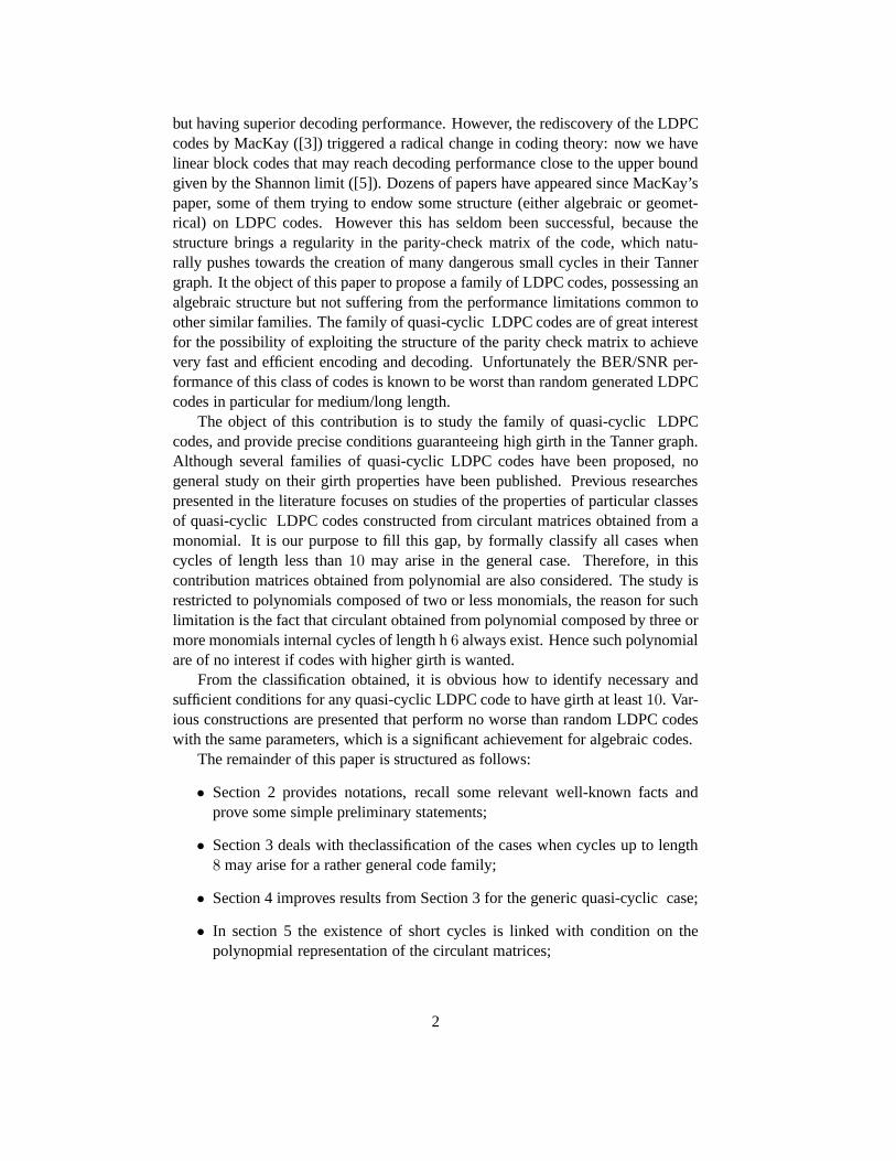
Proof. The proof of this theorem is long and similar to the proof of theorems 3.14and 3.15, with the addition of some logical reasoning. To improve readabilityit is here omitted, an interested reader can find the full and detailed process inAppendix.

21

The previous three theorems list all the configurations thatcan contain cyclesof length less than ten. In particular such configurations identify how many cyclepoints lie in each sub-matrix (d.m.). To improve such resultit is necessary to endowthe d.m. with some structure that allows to predict the positions of such point. Thenext section considers the case where the d.m.’s are circulant matrices.

4 The quasi-cyclic case

This section restricts the discussion to matrices which canbe used as parity-checkmatrices for LDPC quasi-cyclic codes, and gives some generic definitions andlemmas.

A quasi-cyclic code of indext is a linear block code C in which a cyclic shiftof any codeword in C byt positions is also a codeword. The generator matrixG

for these codes is a matrix where every row is at circular shift of the previousrow. It can be shown that every generator matrix for a quasi-cyclic code can be de-composed in circulant matrices. This property makes the encoding suitable for lowcost hardware implementation. Major results on a Array codes, a class of quasi-cyclic codes, have been presented by Fan [31] and later by Fossorier [28]. Arraycodes are composed byJ rows ofL circulant matrices. The circulant matrices usedwas limited to have weight-1. The condition given by Fan [31](later re-proposedin Theorem 2.1 in [28]) gives the conditions for the existence of cycles in suchclass and is rewritten here using the notations presented previously. We remind thereader that with our notationsǫ(p) is any of the exponents of the polynomialp ands(p) is the separation of the two monomials.

Theorem 4.1(Fan-2000). A necessary and sufficient condition for the matrixH tohave a2s-cycle is:

s−1∑

k=0

[

ǫ(p1,k) − ǫ(p2,k)]

= 0 mod p

wereǫ(p1,k) and ǫ(p2,k) are the exponents of the circulant matrices that containthe two cycle-points that lie in the same cycle-columnk.

Remark 4.2. The theorem was given in the case of a particular case of quasi-cyclic codes with only weight 1 circulants but the same theorem holds in the casewhen weight-2 circulant matricesC are present. The presence of weight-2 circu-lant matrices allows cycle columns to lie in the same circulant. In such case thedifferenceǫ(p1,k) − ǫ(p2,k) is equivalent to thes(pk) of such circulant. Previouswork considering weight-2 circulant matrices was presented by Smarandache andVontobel et al. [32] but focuses on the problem of minimum distance and not girthproperties.

However, the construction by Fossorier cannot provide codes whose Tannergraph has a girth higher than12, as shown by Fossorier himself in the same paperand known from Fan. To overtake such limitations and to complete the study of

22

the cycles in quasi-cyclic codes a wider class of quasi-cyclic LDPC codes areconsidered in this thesis.

Definition 4.3. LetB ∈ Mm,α,β,γ and let{Ai,j} form its standard decomposition.The matrixB is said to be inCm,α,β,γ if any d.s.Ai,j can only be either a weight-2circulant matrix, a weight-1 circulant matrix or anm × m zero matrix.

It is well-known that any quasi-cyclic code has a parity-check matrixH made ofcirculant sub-matrices. However, if an LDPC code with good girth characteristicsis desired, it is necessary to avoid sub-matrices that are weight-t circulant matrix,with t ≥ 3, since they contain internal 6-cycles [33] and codes with higher girthare wanted. Matrices inCm,α,β,γ are the only interesting parity-check matrices forgood quasi-cyclic LDPC codes. This family ofH matrices is the focus of the studypresented here.

In the case of quasi-cyclic LDPC codes a cycle configurationc in Cm,α,β,γ willbe described as:

(7) c =

∣

∣

∣

∣

C − 2 J − 1 C − 1O J − 1 J − 1

∣

∣

∣

∣

,

whereC − 2 is a weight-2 circulant matrix containing two points of the cycle,O isa zero matrix,J − 1 is a weight-1 matrix containing one point of the cycle,C − 1is a weight-2 circulant matrix containing one point, and so on. Clearly, notationsof the typeO− i are not used because it is obvious that in a zero matrix there mustbe i = 0. In a situation like (7) it will be written thatc “contains” a matrix (d.s.)C−2, three matricesJ −1 and a matrixC−1. When no confusion can arise, evenlooser notation will be adopted. For example, in (7) it may besaid thatc containsC − 2, thatc containsC − 1 and thatc containsJ − 1. Similarly, phrases of thetype “c contains d.m.’s, d.s.’s,d.r.’s, d.c.’s” will be used with the obvious meaning.For example, in (7)c contains the following d.m.’s

∣

∣ C − 2 J − 1 C − 1∣

∣ ,∣

∣ O J − 1 J − 1∣

∣ ,

∣

∣

∣

∣

C − 2 J − 1O J − 1

∣

∣

∣

∣

.

It is sometimes convenient to gather together cycle configurations possessing agiven number of cycle points. To be more precise, the notation ∆ − i means that∆ can be any allowable matrix containingi points. In other words, the notation

∣

∣ C − 2 ∆ − 2∣

∣ ,

is equivalent to the union of∣

∣ C − 2 C − 2∣

∣ and∣

∣ C − 2 J − 2∣

∣ .

Let c be a cycle configuration, the following easy lemmas can be used to showthatc cannot exist inCm,α,β,γ . The expression “to discard configurationc” is syn-onymous with “to show that configurationc cannot exist inCm,α,β,γ”.

23

Lemma 4.4. Supposec containsJ − i, with i ≥ 2. Then

1. J − i can contain neither a cycle column nor a cycle row,

2. in c, any d.r. and any d.c. containingJ − i (i ≥ 1) must contain anothernon-zero matrix,

3. c can be discarded if it contains only one d.r. or only one d.c. .

Proof. Point one is obvious, because aJ is a shift of an identity matrix hence thereis only one non zero entry for each row and column. Point two follows from pointone and the fact that the cycle point contained in theJ must be part of a linked set.Part three follows from part two.

Lemma 4.5. If c correspond to a 2s-cycle with2s ≤ 8, it cannot contain a weight-1circulant matrixJ − i with i ≥ 3.

Proof. Otherwise any cycle point inJ will need another point in the same row andone in the same column, to form a linked set. For lemma 4.4 thispoints cannot bein theJ but this implies the existence of at least nine points in the linked set, butthis defies the definitions of 2s-cycle with2s ≤ 8

The following two lemmas are obvious and are reported here only for clarity.

Lemma 4.6. Supposec has a(1, 2) d.m. composed of two weight-1 circulantmatrices|J − i J − 1|, i ≥ 1. Then in that d.m. there cannot be more than one cycle row.Similarly for a(2, 1) d.m. inc.

Lemma 4.7. Suppose thatc contains a matrixJ − i, i ≥ 1. If C − i is substitutedto J − i, another possible cycle configuration is obtained.

Passing from a cycle configurations obtained with the procedure outlined in theprevious section to the respective configurations in the quasi-cyclic case requirethe application of lemma 4.4, lemma 4.6, lemma 4.7 and lemma 4.5 to the originalconfiguration. For example, configuration:

∣

∣

∣

∣

∣

∣

∣

∣

2 1 1 0 00 1 0 1 00 0 1 0 10 0 0 1 1

∣

∣

∣

∣

∣

∣

∣

∣

,

results in a cycle configuration for quasi-cyclic codes

∣

∣

∣

∣

∣

∣

∣

∣

C − 2 ∆ − 1 ∆ − 1 0 00 ∆ − 1 0 1 00 0 ∆ − 1 0 ∆ − 10 0 0 ∆ − 1 ∆ − 1

∣

∣

∣

∣

∣

∣

∣

∣

.

24

In fact cycle configuration:

∣

∣

∣

∣

∣

∣

∣

∣

J − 2 ∆ − 1 ∆ − 1 0 00 ∆ − 1 0 1 00 0 ∆ − 1 0 ∆ − 10 0 0 ∆ − 1 ∆ − 1

∣

∣

∣

∣

∣

∣

∣

∣

,

can be discard because inJ − 2 there is no cycle column (lemma 4.4).In the following subsections the theorems presented previously (3.14, 3.15, 3.16)

are specialized for the quasi-cyclic case. All the cycle configurations that can ap-pear in such case are listed. For every circulant in a configuration the possibleweights that such a circulant can have is discussed.

4.1 4-cycle configurations for quasi-cyclic H matrices

Theorem 4.8. Let beM ∈ Cm,α,β,γ . The configurations inM that may containcycles of length4, are the following:4

1.|C − 4| ,

2.|C − 2 C − 2| ,

3.∣

∣

∣

∣

∆ − 1 ∆ − 1∆ − 1 ∆ − 1

∣

∣

∣

∣

.

Proof. All the configurations, for the generic case, that appeared in theorem 3.14.For each configuration it is proved how only configurations listed in the theoremare valid in the case of a quasi-cyclic LDPC code.

Configuration 1 gives

|C − 4| .

Since cycle configuration|J − 4| may be discard (Lemma 4.5).


∣

∣ C − 2 C − 2∣

∣ .

Cycle configurations|C − 2J − 2| and|J − 2J − 2| may be discard becausein J − 2 there is no cycle column (Lemma 4.4-1).


25

Configuration 3 gives∣

∣

∣

∣

∆ − 1 ∆ − 1∆ − 1 ∆ − 1

∣

∣

∣

∣

.

Note how, thanks to Lemma 4.7, it is necessary only to show that the followingconfiguration is possible:

∣

∣

∣

∣

J − 1 J − 1J − 1 J − 1

∣

∣

∣

∣

.

and this is obvious. For Remark 3.7 it is not necessary to study the cycle configu-rations that are transposed of the one considered. Hence it has been proved that thelisted configurations are the only valid ones.

To better explain the meaning of∆ and what it implies the (non-equivalent)cycle configurations present in the statement of Theorem 4.8case 3 , are reported:

∣

∣

∣

∣

J − 1 J − 1J − 1 J − 1

∣

∣

∣

∣

,

∣

∣

∣

∣

C − 1 J − 1J − 1 J − 1

∣

∣

∣

∣

,

∣

∣

∣

∣

C − 1 C − 1J − 1 J − 1

∣

∣

∣

∣

,

∣

∣

∣

∣

C − 1 J − 1C − 1 J − 1

∣

∣

∣

∣

,

∣

∣

∣

∣

C − 1 C − 1C − 1 J − 1

∣

∣

∣

∣

,

∣

∣

∣

∣

C − 1 C − 1C − 1 C − 1

∣

∣

∣

∣

.


Theorem 4.9. Let beM ∈ Cm,α,β,γ . The configurations inM that may contain acycle of length6, are the following5

1.|C − 6| ,

2.|C − 4 C − 2| ,

3.|C − 2 C − 2 C − 2| .

4.∣

∣

∣

∣

C − 2 ∆ − 2O C − 2

∣

∣

∣

∣

,

5.∣

∣

∣

∣

C − 3 J − 1J − 1 J − 1

∣

∣

∣

∣

5For brevity any cycle configuration that is the transpose of another is omitted.

26

6.∣

∣

∣

∣

C − 2 ∆ − 1 ∆ − 1O ∆ − 1 ∆ − 1

∣

∣

∣

∣

,

7.∣

∣

∣

∣

∣

∣

∆ − 1 ∆ − 1 O∆ − 1 O ∆ − 1

O ∆ − 1 ∆ − 1

∣

∣

∣

∣

∣

∣

.

Proof. All the configurations that appear in Theorem 3.15 are considered and itis proved how there exist no other cycle configurations from the one listed in thestatement. The process also proves that no unnecessary cycle configurations arelisted.


|C − 6| .

Since cycle configuration|J − 6| can be discard (Lemma 4.5).


∣

∣ C − 4 C − 2∣

∣ .

Other cycle configurations|C − 4J − 2|, |J − 4J − 2| and|J − 4C − 2| may bediscard, because inJ − 2 and inJ − 4 there is no cycle column.


∣

∣ C − 2 C − 2 C − 2∣

∣ .

Other cycle configurations may be discard because they contain J − 2 and inJ − 2 there is no cycle column (Lemma 4.4-1).

Configuration 4

1. Configuration 4.1 gives∣

∣

∣

∣

C − 2 C − 2O C − 2

∣

∣

∣

∣

,

∣

∣

∣

∣

C − 2 J − 2O C − 2

∣

∣

∣

∣

.

Other cycle configurations may be discard because they contain J − 2 as theonly non-zero matrix in a d.r. or d.c. (Lemma 4.4-2).


∣

∣

∣

C − 3 ∆ − 1∆ − 1 ∆ − 1

∣

∣

∣

∣

.

27

In fact any cycle configuration of kind∣

∣

∣

∣

J − 3 ∆ − 1∆ − 1 ∆ − 1

∣

∣

∣

∣

can be discarded (lemma 4.5). On the other hand, cycle configuration∣

∣

∣

∣

C − 3 J − 1J − 1 J − 1

∣

∣

∣

∣

is obviously acceptable and so lemma 4.7 can be applied.


∣

∣

∣

∣

C − 2 ∆ − 1 ∆ − 1O ∆ − 1 ∆ − 1

∣

∣

∣

∣

.

In fact , the following cycle configuration is obviously possible∣

∣

∣

∣

C − 2 J − 1 J − 1O J − 1 J − 1

∣

∣

∣

∣

.

Hence lemma 4.7 can be apply.To discard all cycle configurations of type

∣

∣

∣

∣

J − 2 ∆ − 1 ∆ − 1O ∆ − 1 ∆ − 1

∣

∣

∣

∣

,

it is enough to apply Lemma 4.4-2 to d.c. 1.


∣

∣

∣

∣

∣

∣

∆ − 1 ∆ − 1 O∆ − 1 O ∆ − 1

O ∆ − 1 ∆ − 1

∣

∣

∣

∣

∣

∣

.

Clearly, the following cycle configuration is possible∣

∣

∣

∣

∣

∣

J − 1 J − 1 OJ − 1 O J − 1

O J − 1 J − 1

∣

∣

∣

∣

∣

∣

,

hence Lemma 4.7 can be applied.For remark 3.7 it is not necessary to study the cycle configurations that are

transposed of the one considered. Hence it has been proved that the listed configu-rations are the only valid ones.

28


Theorem 4.10. Let beM ∈ Cm,α,β,γ . The configurations inM that may containa cycles of length8, are the following6

1.|C − 8| ,

2.|C − 6 C − 2| ,

3.|C − 4 C − 4| ,

4.|C − 4 C − 2 C − 2| .

5.|C − 2 C − 2 C − 2 C − 2| .

6.∣

∣

∣

∣

C − 5 ∆ − 1∆ − 1 ∆ − 1

∣

∣

∣

∣

,

7.∣

∣

∣

∣

C − 4 ∆ − 20 C − 2

∣

∣

∣

∣

,

8.∣

∣

∣

∣

C − 4 C − 2C − 2 0

∣

∣

∣

∣

,

9.∣

∣

∣

∣

C − 3 C − 3∆ − 1 ∆ − 1

∣

∣

∣

∣

,

10.∣

∣

∣

∣

C − 3 ∆ − 1∆ − 1 C − 3

∣

∣

∣

∣

,

11.∣

∣

∣

∣

∆ − 2 ∆ − 2∆ − 2 ∆ − 2

∣

∣

∣

∣

,

12.∣

∣

∣

∣

C − 4 ∆ − 1 ∆ − 1O ∆ − 1 ∆ − 1

∣

∣

∣

∣

,

6For brevity any cycle configuration that is the transpose of another is omitted.

29

13.∣

∣

∣

∣

C − 3 C − 2 ∆ − 1∆ − 1 O ∆ − 1

∣

∣

∣

∣

,

14.∣

∣

∣

∣

C − 3 O ∆ − 1∆ − 1 C − 2 ∆ − 1

∣

∣

∣

∣

,

15.∣

∣

∣

∣

∆ − 2 C − 2 C − 2C − 2 O O

∣

∣

∣

∣

,

16.∣

∣

∣

∣

∆ − 2 ∆ − 1 ∆ − 1∆ − 2 ∆ − 1 ∆ − 1

∣

∣

∣

∣

,

17.∣

∣

∣

∣

C − 2 ∆ − 2 OO ∆ − 2 C − 2

∣

∣

∣

∣

,

18.∣

∣

∣

∣

C − 2 C − 2 ∆ − 1 ∆ − 1O O ∆ − 1 ∆ − 1

∣

∣

∣

∣

,

19.∣

∣

∣

∣

C − 2 O ∆ − 1 ∆ − 1O C − 2 ∆ − 1 ∆ − 1

∣

∣

∣

∣

,

20.∣

∣

∣

∣

∆ − 1 ∆ − 1 ∆ − 1 ∆ − 1∆ − 1 ∆ − 1 ∆ − 1 ∆ − 1

∣

∣

∣

∣

,

21.∣

∣

∣

∣

∣

∣

C − 3 ∆ − 1 O∆ − 1 O ∆ − 1

O ∆ − 1 ∆ − 1

∣

∣

∣

∣

∣

∣

.

22.∣

∣

∣

∣

∣

∣

∆ − 2 ∆ − 1 ∆ − 1C − 2 O O

O ∆ − 1 ∆ − 1

∣

∣

∣

∣

∣

∣

.

23.∣

∣

∣

∣

∣

∣

∆ − 2 ∆ − 1 ∆ − 1∆ − 1 ∆ − 1 O∆ − 1 O ∆ − 1

∣

∣

∣

∣

∣

∣

.

30

24.∣

∣

∣

∣

∣

∣

C − 2 O O∆ − 1 ∆ − 1 O∆ − 1 ∆ − 1 C − 2

∣

∣

∣

∣

∣

∣

.

25.∣

∣

∣

∣

∣

∣

C − 2 ∆ − 1 ∆ − 1 OO ∆ − 1 O ∆ − 1O O ∆ − 1 ∆ − 1

∣

∣

∣

∣

∣

∣

.

26.∣

∣

∣

∣

∣

∣

∆ − 1 ∆ − 1 ∆ − 1 ∆ − 1∆ − 1 ∆ − 1 O 0

O O ∆ − 1 ∆ − 1

∣

∣

∣

∣

∣

∣

.

27.∣

∣

∣

∣

∣

∣

∣

∣

∆ − 1 ∆ − 1 O O∆ − 1 O ∆ − 1 O

O ∆ − 1 O ∆ − 1O O ∆ − 1 ∆ − 1

∣

∣

∣

∣

∣

∣

∣

∣

.

Proof. Once more for brevity the full proof is omitted here and can befound inAppendix.

5 Relations between polynomials and the existence of cy-cles

This subsection gives an interpretation to the cycle configurations presented pre-viously in terms of the polynomials associated to the circulant matrices involved.First a general statement on the girth of the Tanner graph associated to a binaryweight-2 circulant matrix is given. The following proposition has first been pre-sented in [34] and [35]. Here only the main result is reported.

The notation introduced in subsection 2.3 is presented again here for clarity:

• ǫ(p) : any of the exponents (a, b) of the polynomialp(x) = xa + xb,

• s(p) : the separation (min(b − a, a + m − b)) of the polynomialp.

Proposition 5.1. Letm ≥ 3. LetM = (Mi,j) be a circulant binarym×m matrix,generated by a weight-2 polynomialp. Lets(p) be the separation ofp andg be thegirth of the Tanner graph ofM . Then

g = 2m

gcd(m, s(p))

31

Proof. Let G be the Tanner graph ofM . Then each check node is connectedexactly to two bit nodes, and vice-versa. We denote byc1, . . . , cm andb1, . . . , bm,respectively, the check nodes and the bit nodes ofG. Without loss of generality,we may suppose thatM1,1 = 1. By circularity, Mj,j = 1 for 1 ≤ j ≤ m, whichimplies thatcj is connected tobj , for 1 ≤ j ≤ m.

By definition of separation, we have eithers = b − a or s = m − (b − a).By circularity we may assumes = b − a, so thatM1,s+1 = 1 andb − a ≤ m/2.But then we haveMj,s+j = 1, for 1 ≤ j ≤ m − s, andMj,s+j−m = 1, form− s+1 ≤ j ≤ m. Therefore, check nodecj is also connected to: either bit nodebs+j, which happens when1 ≤ j ≤ m − s, or bit nodebs+j−m, which happenswhenm − s + 1 ≤ j ≤ m. No other non-zero entry is present inM and so noother connection exists among nodes inG.

For anyi, we want to find the lengthgi of the minimum length cycle containingci. The girth ofG will be g = min1≤i≤m gi. By symmetry ofG, gi does not dependon i, in particularg = g1.We now determineg1, constructing a path as follows:

• we start fromc1. Fromc1, we may go either tob1 or to bs+1. We choose togo tob1. Clearly, the cycle will be closing when we will find ourself in bs+1,as the next step will bec1. From now on, the path allows no more choices.We will use arrows to shorten our notation.

• c1 → b1, b1 → cm−s+1. If m − s + 1 = 1, the cycle will be closed andg1 = 2: this is impossible sinces < m.

• cm−s+1 → bm−s+1, bm−s+1 → cm−2s+1 (m − 2s + 1 ≥ 1).If m − 2s + 1 = 1, the cycle is closed andg1 = 4.

• We perform steps of type

cm−(l−1)s+1 → bm−(l−1)s+1, bm−(l−1)s+1 → cm−ls+1 ,

until either there is anl ≥ 1 s.t. m − ls + 1 = 1 or there is no suchl. Weanalyze the two cases separately.There is anl s.t.m = ls. This is equivalent tos|m. This is also equivalent tog1 = 2l because we have formed a length-2l cycle and we have encounteredno smaller cycles.Or there is nol s.t.m− ls + 1 = 1. In this case letl = |m/s|. Theng ≥ 2l,i.e. g > 2m/s. The next two steps will be

cm−ls+1 → bm−ls+1, bm−ls+1 → c2m−(l+1)s+1 ,

i.e. we have to “wrap on the graph”.

• We perform steps of type

c2m−(l−1)s+1 → b2m−(l−1)s+1, b2m−(l−1)s+1 → c2m−ls+1 ,

32

until either there is anl ≥ |m/s| s.t. 2m − ls + 1 = 1 or there is no suchl.We analyze the two cases separately.There is anl > |m/s| s.t. 2m = ls (but nol ≥ 1 is s.t.m = ls). Obviouslythis is equivalent tos|2m and nots|m.

This is also equivalent tog1 = 2l because we have formed a length-2l cycleand we have encountered no smaller cycles.Or there is nol s.t. 2m− ls = 0 (but nol ≥ 1 is s.t.m = ls). This is equiv-alent tos not dividing2m (ands not dividingm). This is also equivalent tog > |2m/s|. In this case letl = |2m/s|. The next two steps will be

c2m−ls+1 → b2m−ls+1, b2m−ls+1 → c3m−(l+1)s+1 ,

i.e. we have to “wrap on the graph” again.

• In the general case, after2l steps we reachcqm−ls+1, wheres does notdivide anyzm for 1 ≤ z ≤ q−1, by a generalization of the above arguments.At some stage we must meet againc1, so thatcqm−ls+1 = c1. In other words,the girth is2l, with l = qm/s, if q is s.t.

s|qm, s 6 |zm, 1 ≤ z ≤ q − 1 .

This means thatqm is the smallest multiple ofm that is also a multiple ofs,i.e. qm is the minimum common multiple ofm ands.Let [, ] denote minimum common multiple. For any two integersa andb, wehave[a, b]/a = b/ gcd(a, b), so that

qm

s=

[m, s]

s=

m

gcd(m, s).

Remark 5.2(Minimum dimension of the circulants). Theorem 5.1 indirectly givesa minimum dimension that the circulant matrices must have toallow high girth. Inparticular if H matrices with girth10 (or higher) are desired the circulant matricesmust be at least[5 × 5]. To prove this is sufficient to consider that to haveg ≥ 10it must be m

gcd(m,s(p)) ≥ 5, hencem ≥ 5.

A plot of the girth that can be obtained given a certain circulant dimension,changing the value of the separation, is presented in Figure3. It is evident that themaximum girt (g = 2m) is also achievable, e.g. by choosing the separation to beone. Of more interest is to consider that which values ofm ands must be avoidedto guarantee a good girth.

The following theorems present which conditions, on separations and expo-nents, must be satisfied for a certain cycle, in a cycle configurations, to exist. Oncethis set of conditions is known matrices with high girth can be generated by choos-ing the polynomials of the circulants in such a way that none of the conditions aresatisfied.

33

2 3 4 5 6 7 8 9 10 11 12 13 14 15 16 17 18 19 20

4

6

8

10

12

14

16

18

20

22

24

26

28

30

32

34

36

38

40

s=2 s=3

s=2

s=2

s=3

s=4

s=3

s=2

s=2

s=2

s=2

s=2

s=3

s=3

s=5

s=5s=4

s=4

s=4

s=2

s=5

s=6

s=6

s=7 s=8 s=9 s=10

Circulant dimensionm

Ach

ieva

ble

girt

h

Figure 3: Girth values that can be obtained with a single circulant given its dimen-sion

5.1 Conditions for the 4-cycles

Theorem 5.3. Let beM ∈ Cm,α,β,γ . The configurations inM that may contain acycles of length4 and associated conditions, are the following

1.

|C − 4| , s(p) = m/2

2.

∣

∣C1 − 2 C2 − 2∣

∣ , s(p1) = s(p2)

3.∣

∣

∣

∣

∆1 − 1 ∆2 − 1∆3 − 1 ∆4 − 1

∣

∣

∣

∣

, ǫ(p1) − ǫ(p2) − ǫ(p3) + ǫ(p4) = 0

Proof. It is of interest to note that the conditions associated withevery configu-ration can be proved applying theorem 4.1, that is the generalization of Fossoriertheorem for weight-2 circulants.

It has been chosen to follow a different methodology that slightly reduces thenotation and allow to use a graphical representation that easier to understand. Theuse of separations instead of the difference of exponents makes the conditions

34

clearer and more evident; it also reduces the number of variables involved mak-ing them easier to check. The proof is divided in shorter lemmas each consideringa case of the main theorem. An4-cycle is formed by two cycle columns calledy, zand two cycle rows calledx, t. In every4-cycle there are4 cycle points, they takethe name of the column and row where they lie in(x, y), (x, z), (t, y), (t, z). Thenotation is used to compute the conditions. To allow the reader to better understandthe meaning of the formulae for each lemma a graphical representation of the cycleis presented. For example Figure 4 presents an example of4-cycle on two weight-2circulants. The two rectangular blocks represent the two circulants and the dasheddiagonal lines the position of the ones in the matrices. The cycle columns and cyclerows are marked by the dash-doted lines and the cycle is outlined with a wider line.

Lemma 5.4. There is a4-cycle in case 1 if and only if

2|m and s(p) = m/2 .

Proof. There is a4-cycle if and only if g = 4, because smaller girths are notpossible. Applying Proposition 5.1 to the caseg = 4 and M = C, there is a4-cycle if and only if

4 = g = 2m

gcd(m, s)

i.e. m = 2gcd(m, s). In particular,m is even andm/2|s, but s ≤ m/2, so thats = m/2. On the other hand, ifm is even ands = m/2 thengcd(m, s) = s =m/2.


s(p1) = s(p2)

Proof. It can be assumed that there is a4-cycle if and only if columny lies in C1

and columnz lies inC2 (Figure 4).

x

t

y z

Figure 4: Example of4-cycle on two weight-2 circulants.

35

Applying Prop. 2.9-2 to columny yields

(8) x − t ≡ ±s1 .

Applying Proposition 2.9-2 to cycle columnz yields

(9) x − t ≡ ±s2 .

From (8) and (9),s1 ≡ ±s2 is obtained and hences1 = s2 (Lemma 2.10).


ǫ(p1) − ǫ(p2) − ǫ(p3) + ǫ(p4) = 0

Proof. It can be assumed that there is a4-cycle if and only if, simultaneously, cyclepoint (x, y) lies in ∆1, cycle point(x, z) lies in ∆2, cycle point(t, y) lies in ∆3

and cycle point(t, z) lies in∆4 (Figure 5).

x

t

y z

Figure 5: Example of4-cycle on four weight-1 circulants.

Since cycle point(x, y) lies in∆1, using Proposition 2.9-1:

(10) y ≡ x + ǫ(p1) .

36

Since cycle point(x, z) lies in∆2, using Proposition 2.9-1:

(11) z ≡ x + ǫ(p2) .

Since cycle point(t, y) lies in∆3, using Lemma 3.4:

(12) y ≡ t + ǫ(p3) .

Since cycle point(t, z) lies in∆4, using Lemma 3.4:

(13) z ≡ t + ǫ(p4) .

The desired result is obtained from (10), (11), (12) and (13).

It has hence been proved that the conditions listed on the statement considersall the possible4-cycles that can exist on the studied quasi-cyclic matrices.

For example consider the polynomialp(x) = 1 + x3 with m = 6 for suchpolynomials(p) = 3 hences(p) = m/2 and for condition1 a4-cycle exist.

1 0 0 1 0 00 1 0 0 1 00 0 1 0 0 11 0 0 1 0 00 1 0 0 1 00 0 1 0 0 1


Theorem 5.7. Let beM ∈ Cm,α,β,γ . The configurations inM that may contain acycles of length6, are the following

1.

|C − 6| , s(p) = m/3

2.

∣

∣C1 − 4 C2 − 2∣

∣ , s(p2) ≡ ±2s(p1)

3.

∣

∣C1 − 2 C2 − 2 C3 − 2∣

∣ , s(p1) ± s(p2) ± s(p3) ≡ 0,

37

4.∣

∣

∣

∣

C1 − 2 ∆2 − 2O C3 − 2

∣

∣

∣

∣

,

ǫ(p2) − ǫ(p2) ≡ ±s(p1) ± s(p3),

5.∣

∣

∣

∣

C1 − 3 ∆2 − 1∆3 − 1 ∆4 − 1

∣

∣

∣

∣

,

ǫ(p1) − ǫ(p2) − ǫ(p3) + ǫ(p4) ≡ ±s(p1),

6.∣

∣

∣

∣

C1 − 2 ∆2 − 1 ∆3 − 1O ∆4 − 1 ∆5 − 1

∣

∣

∣

∣

,

ǫ(p2) − ǫ(p3) − ǫ(p4) + ǫ(p5) ≡ ±s(p1),

7.∣

∣

∣

∣

∣

∣

∆1 − 1 ∆2 − 1 O∆3 − 1 O ∆4 − 1

O ∆5 − 1 ∆6 − 1

∣

∣

∣

∣

∣

∣

,

ǫ(p1) − ǫ(p2) − ǫ(p3) + ǫ(p4) + ǫ(p5) − ǫ(p6) ≡ 0

Proof. As for the previous theorem the proof is once more divided in smallerlemmas each considering a particular case. An6-cycle is formed by three cy-cle columns calledy, z, v and three cycle rows calledx, t, w. In every6-cyclethere are6 cycle points, they take the name of the column and row where theylie: (x, y), (x, z), (t, y), (t, v), (w, v), (w, z). The notation is used to compute theconditions.

Lemma 5.8. There is a6-cycle and there are no4-cycles in case 1 if and only if

3|m and and s(p) = m/3 .

Proof. There is a6-cycle and no4-cycle if and only ifg = 6. Applying Prop. 5.1to the caseg = 6 andM = C, this is equivalent to

6 = g = 2m

gcd(m, s)

i.e. m = 3gcd(m, s). In particular,3|m andm/3|s, but s ≤ m/2, so thats =m/3. On the other hand, ifm is divisible by3 ands = m/3 thengcd(m, s) = s =m/3.

38

x

t

w

y z v



s(p2) ≡ ±2s(p1)

Proof. It can be assumed that there is a6-cycle if and only if if both (cycle) columny and columnz lie in C1 and columnv lies inC2 (Figure 6).

Applying Proposition 2.9-4 to cycle columny and cycle columnz yields

(14) x − t ≡ ±s1j ,

(15) x − w ≡ ∓s1j .

Applying Proposition 2.9-2 to cycle columnv yields

(16) w − t ≡ ±s2j .

Sincex − t = (x − w) + (w − t), from (14), (15) and (16):

±s1 ≡ ∓s1 + ±s2 ,

from which the desired result is obtained:

s2 ≡ 2s1 .


s1 ± s2 ± s3 ≡ 0 .

39

x

t

w

y z v

Figure 7: Example of6-cycle on three weight-2 circulants.

Proof. It can be assumed that there is a6-cycle if and only if columny lie in C1,columnz lie in C2 and columnv lies inC3 (Figure 7).

Applying Proposition 2.9-2 to cycle columny yields

(17) x − t ≡ ±s1 ,

Applying Proposition 2.9-2 to cycle columnz yields

(18) t − w ≡ ±s2 ,

Applying Proposition 2.9-2 to cycle columnv yields

(19) w − t ≡ ±s3 ,

Since(x − t) + (w − x) + (t − w) = 0, from (17), (18) and (19):

±s1 ± s2 ∓ s3 ≡ 0 ,

from which the desired result is obtained. Note how the sign of one of the separa-tions,s1 in the main theorem, can be fixed. In fact if−s1 + s2 − s3 ≡ 0 then alsos1 − s2 + s3 ≡ 0 and this is part of the conditions.


ǫ(p2) − ǫ(p2) ≡ ±s(p1) ± s(p3)

Proof. It can be assumed that there is a6-cycle if and only if simultaneously cyclecolumny lies inC1, cycle points(x, z) and(t, v) lie in ∆2 and cycle roww lies inC3 (Figure 8).

Since cycle columny lies inC1, applying Prop. 2.9-2:

(20) x − t ≡ ±s1 .

40

x

t

w

y z v

Figure 8: Example of6-cycle on three weight-2 circulants.

Since cycle roww lies inC3, applying Proposition 2.9-3:

(21) v − z ≡ ±s3 .

Since cycle points(x, z) and(t, v) lie in ∆2, applying Lemma 3.4:

(22) z ≡ x + ǫ2, v ≡ t + ǫ2 .

Substituting (22) and (20) into (21) the desired result is obtained.


ǫ(p1) − ǫ(p2) − ǫ(p3) + ǫ(p4) ≡ ±s(p1)

Proof. It may be assumed that there is a6-cycle if and only if, simultaneously,cycle columny lies in C1, cycle point(x, z) lies in C1, cycle point(w, z) lies in∆3, cycle point(w, v) lies in∆4 and cycle point(t, v) lies in∆2 (Figure 9). Sincecycle columny lies inC1, applying Proposition 2.9-2:

(23) x − t ≡ ±s1 .

41

x

t

w

y zv

Figure 9: Example of6-cycle on one weight-2 and three weight-3 circulants.

Since cycle point(x, z) lies inC1, applying Proposition 2.9-1:

(24) z ≡ x + ǫ(p1) .

Since cycle points(w, v) lies in∆4, applying Proposition 2.9-1:

(25) v ≡ w + ǫ(p4) .

Since cycle points(w, z) lies in∆3, applying Lemma 3.4:

(26) z ≡ w + ǫ(p3) .

Since cycle points(t, v) lies in∆2, applying Lemma 3.4:

(27) v ≡ t + ǫ(p2) .

The desired result is obtained from (23), (24), (25), (26) and (27).


ǫ(p2) − ǫ(p3) − ǫ(p4) + ǫ(p5) ≡ ±s(p1)

42

Proof. It may be assumed that there is a6-cycle if and only if, simultaneously,cycle columny lies in C1, cycle point(x, z) lies in ∆2, cycle point(w, z) lies in∆4, cycle point(w, v) lies in∆5 and cycle point(t, v) lies in∆3 (Figure 10). Sincecycle columny lies inC1, applying Proposition 2.9-2:

(28) x − t ≡ ±s1 .

Since cycle points(x, z) lies in∆2, applying Proposition 2.9-1:

(29) z ≡ x + ǫ(p2) .


(30) v ≡ w + ǫ(p5) .


(31) z ≡ w + ǫ(p4) .


(32) v ≡ t + ǫ(p3) .

The desired result is obtained from (28), (29), (30), (31) and (32).


ǫ(p1) − ǫ(p2) − ǫ(p3) + ǫ(p4) + ǫ(p5) − ǫ(p6) ≡ 0

Proof. It can be assumed that there is a6-cycle if and only if, simultaneously, cyclepoint (x, y) lies in ∆1, cycle point(t, y) lies in ∆3, cycle point(x, z) lies in ∆2,cycle point(w, z) lies in∆5, cycle point(w, v) lies in∆6 and cycle point(t, v) liesin ∆4 (Figure 11). Since cycle points(x, y) lies in∆1, applying Proposition 2.9-1:

(33) y ≡ x + ǫ(p1) .

Since cycle points(t, y) lies in∆3, applying Proposition 2.9-1:

(34) y ≡ t + ǫ(p3) .

Since cycle points(x, z) lies in∆2, applying Proposition 2.9-1:

(35) z ≡ x + ǫ(p2) .


(36) v ≡ w + ǫ(p6) .


(37) z ≡ w + ǫ(p5) .


(38) v ≡ t + ǫ(p4) .

The desired result is obtained from (33), (34), (35), (36), (37) and (38).

43

x

t

w

y z v

Figure 10: Example of6-cycle on one weight-2 and four weight-1 circulants.

x

t

w

y z v

Figure 11: Example of6-cycle on six weight-1 circulants.

44


Following two examples. In the first the polynomialp(x) = 1 + x2 withm = 6 for such polynomials(p) = 2 hences(p) = m/3 and for condition1 a6-cycle exist.

1 0 1 0 0 00 1 0 1 0 00 0 1 0 1 00 0 0 1 0 11 0 0 0 1 00 1 0 0 0 1

In the second example the first polynomial isp1(x) = 1 + x2 with m = 7 for suchpolynomial s(p1) = 2 and the second isp2(x) = x + x5 for which s(p2) = 4hences2(p) = 2s1(p) and for condition2 a6-cycle exist.

0 1 0 1 0 0 00 0 1 0 1 0 00 0 0 1 0 1 00 0 0 0 1 0 11 0 0 0 0 1 00 1 0 0 0 0 11 0 1 0 0 0 0

0 1 0 0 0 1 00 0 1 0 0 0 11 0 0 1 0 1 00 1 0 0 1 0 10 0 1 0 0 1 00 0 0 1 0 0 11 0 0 0 1 0 0


The following lemma reduces the number of cycle configurations to be considered.

Lemma 5.15. For any matrixM ∈ Cm,α,β,γ s.t. at least two weight-2 circulantslie in the same row or column then the girth is less or equal to8.

Proof. The case of two weight-2 circulants laying in the same d.r is considered,the other case is the transpose of such case. when two weight-2 circulants lie in thesame d.r. The following cycle configuration always arises

∣

∣ C1 − 4 C2 − 4∣

∣ .

It can be assumed that there is a8-cycle if columnsy andu lie in the firstC andcolumnsv andz lie in the secondC. Cycle columny and cycle columnu satisfy

(39) x − t ≡ ±s1 ,

(40) w − l ≡ ±s1 .

45

dy u vx

w

t

l


Cycle columnv and cycle columnz satisfy

(41) t − w ≡ ±s2 ,

(42) x − l ≡ ±s2 .

Combining equations (39), (40),( 41),( 42) an equation of the form±s1±s1±s2±s2 ≡ 0 is obtained. In particular consider the cases1 − s1 + s2 + s2 it is equal to0 independently to the values of the two separations.

The previous lemma shows how anyH matrix of a LDPC quasi-cyclic codemay have girth bigger than 8 if and only if, or it contain only weight-1 circulants orthe weight-2 circulants are not in the same row or column. Hence the lemma givesa practical guideline to the construction of quasi-cyclic codes with high girth.

The following theorem lists all the possible configurationsthat may containcycles of length8. Beside each configuration the conditions on separations andexponents under which such cycles exist are given.

46

Theorem 5.16. Let beM ∈ Cm,α,β,γ . The configurations inM that may containa cycles of length exactly8, are the following7

1.

|C − 8| , s(p) = m/4

2.∣

∣

∣

∣

C1 − 5 J2 − 1J3 − 1 ∆4 − 1

∣

∣

∣

∣

,

ǫ(p1) − ǫ(p2) − ǫ(p3) + ǫ(p4) ≡ ±2s(p1),

3.∣

∣

∣

∣

C1 − 4 J2 − 20 C3 − 2

∣

∣

∣

∣

,

±s(p3) ≡ 2s(p1)

4.∣

∣

∣

∣

C1 − 3 J2 − 1J3 − 1 C4 − 3

∣

∣

∣

∣

,

ǫ(p1) − ǫ(p2) − ǫ(p3) + ǫ(p4) ≡ ±s(p1) ± s(p3),

5.∣

∣

∣

∣

∆1 − 2 ∆2 − 2∆3 − 2 ∆4 − 2

∣

∣

∣

∣

,

ǫ(p1) + ǫ(p1) − ǫ(p2) − ǫ(p2) − ǫ(p3) − ǫ(p3) + ǫ(p4) + ǫ(p4) ≡ 0 ,

6.∣

∣

∣

∣

C1 − 4 J2 − 1 J3 − 1O ∆4 − 1 ∆5 − 1

∣

∣

∣

∣

,

ǫ(p2) − ǫ(p3) − ǫ(p4) + ǫ(p5) ≡ ±2s(p1),

7.∣

∣

∣

∣

C1 − 3 O J2 − 1J3 − 1 C4 − 2 J5 − 1

∣

∣

∣

∣

,

ǫ(p1) − ǫ(p2) − ǫ(p3) + ǫ(p5) ≡ ±s(p1) ± s(p4),

7 Configurations with two or more weight-2 circulants in the same row or column are not listedsince they always contain a cycle of at most8 (Lemma 5.15), hence they do not add any new infor-mation.

47

8.∣

∣

∣

∣

∆1 − 2 ∆2 − 1 ∆3 − 1∆4 − 2 ∆5 − 1 ∆6 − 1

∣

∣

∣

∣

,

ǫ(p1) + ǫ(p1) − ǫ(p2) − ǫ(p3) − ǫ(p4) − ǫ(p4) + ǫ(p5) + ǫ(p6) = 0 , or

ǫ(p2) − ǫ(p3) + ǫ(p4) − ǫ(p4) − ǫ(p5) + ǫ(p6) = ±s(p1) , or

ǫ(p2) − ǫ(p3) + ǫ(p1) − ǫ(p1) − ǫ(p5) + ǫ(p6) = ±s(p4) .

9.∣

∣

∣

∣

C1 − 2 J2 − 2 OO J3 − 2 C4 − 2

∣

∣

∣

∣

,

s(p1) ≡ s(p4),

10.∣

∣

∣

∣

C1 − 2 O J3 − 1 J4 − 1O C2 − 2 J5 − 1 J6 − 1

∣

∣

∣

∣

,

ǫ(p3) − ǫ(p4) − ǫ(p5) + ǫ(p6) ≡ ±s(p1) ± s(p2),

11.∣

∣

∣

∣

∆1 − 1 ∆2 − 1 ∆3 − 1 ∆4 − 1∆5 − 1 ∆6 − 1 ∆7 − 1 ∆8 − 1

∣

∣

∣

∣

,


ǫ(p1) − ǫ(p2) + ǫ(p3) − ǫ(p4) − ǫ(p5) + ǫ(p6) − ǫ(p7) + ǫ(p8) = 0 , or

ǫ(p1) − ǫ(p2) − ǫ(p3) + ǫ(p4) − ǫ(p5) + ǫ(p6) + ǫ(p7) − ǫ(p8) = 0 .

12.∣

∣

∣

∣

∣

∣

C1 − 3 J2 − 1 OJ3 − 1 O ∆4 − 1

O ∆5 − 1 ∆6 − 1

∣

∣

∣

∣

∣

∣

,

ǫ(p1) − ǫ(p2) − ǫ(p3) + ǫ(p4) + ǫ(p5) − ǫ(p6) ≡ ±s(p1),

13.∣

∣

∣

∣

∣

∣

J1 − 2 ∆2 − 1 ∆3 − 1C4 − 2 O O

O ∆5 − 1 ∆6 − 1

∣

∣

∣

∣

∣

∣

,

ǫ(p2) − ǫ(p3) − ǫ(p5) + ǫ(p6) ≡ ±s(p4)

48

14.∣

∣

∣

∣

∣

∣

∆1 − 2 ∆2 − 1 ∆3 − 1∆4 − 1 ∆5 − 1 O∆6 − 1 O ∆7 − 1

∣

∣

∣

∣

∣

∣

,

ǫ(p1) + ǫ(p1) − ǫ(p2) − ǫ(p3) − ǫ(p4) + ǫ(p5) − ǫ(p6) + ǫ(p7) = 0 , or

ǫ(p2) − ǫ(p3) + ǫ(p4) − ǫ(p5) − ǫ(p6) + ǫ(p7) = ±s(p1),

15.∣

∣

∣

∣

∣

∣

C1 − 2 O OJ2 − 1 ∆3 − 1 OJ4 − 1 J5 − 1 C6 − 2

∣

∣

∣

∣

∣

∣

,

ǫ(p2) − ǫ(p3) − ǫ(p4) + ǫ(p5) ≡ ±s(p1) ± s(p6),

16.∣

∣

∣

∣

∣

∣

∆1 − 2 ∆2 − 1 ∆3 − 1 ∆4 − 1∆5 − 1 ∆6 − 1 O 0

O O ∆7 − 1 ∆8 − 1

∣

∣

∣

∣

∣

∣

,

ǫ(p2) − ǫ(p3) − ǫ(p4) + ǫ(p5) + ǫ(p6) − ǫ(p7) = ±s(p1),

17.∣

∣

∣

∣

∣

∣

C1 − 2 J2 − 1 J3 − 1 OO ∆4 − 1 O ∆5 − 1O O ∆6 − 1 ∆7 − 1

∣

∣

∣

∣

∣

∣

,

ǫ(p2) − ǫ(p3) − ǫ(p4) + ǫ(p5) + ǫ(p6) − ǫ(p7) = ±s(p1),

18.∣

∣

∣

∣

∣

∣

∣

∣

∆1 − 1 ∆2 − 1 O O∆3 − 1 O ∆4 − 1 O

O ∆5 − 1 O ∆6 − 1O O ∆7 − 1 ∆8 − 1

∣

∣

∣

∣

∣

∣

∣

∣

,

ǫ(p1) − ǫ(p2) − ǫ(p3) + ǫ(p4) + ǫ(p5) − ǫ(p6) − ǫ(p7) + ǫ(p8) = 0,

Proof. Proving this theorem is particularly long, the arguments used are similar tothe ones used to prove the two previous theorems. The detailed proof can be foundin Appendix.

The theorems above listed all the conditions (regarding theexponents and sepa-rations) that must be satisfied for a cycle of length less thanten to exist on a generic

49

quasi-cyclic H matrix. Checking all the conditions listed in aH matrix can be adaunting task. The complexity raises from the fact that for every configuration allthe possible row and column permutations must be considered. The following sec-tions present several classes of quasi-cyclic codes that have some regularity andreduce the total number of conditions needed.

6 A first subclass of codes

In this section a first family of quasi-cyclic matrices is presented. The structure ofthis class has been developed to achieve high sparsity and toease implementationaspects. This class of codes contain the matricesM in which each d.c. can haveat most oneH and/or oneI, whereI is the identity matrix. NotationDm,α,β,γ

denotes such a class. Theorems 3.14, 3.15 and 3.16 can be applied toDm,α,β,γ .The use ofI sub-matrices reduces the number of variables present in theconditionsto be check.

Theorem 5.3, 5.7, 5.16 are applied toDm,α,β,γ .

Proposition 6.1. LetM ∈ Dm,α,β,γ . The d.m.’s inM that contain cycles of length< 8 and the associate conditions are the following:

1. Containing4-cycles:

1.1

|H − 4| , s(p) = m/2

1.2

∣

∣H1 − 2 H2 − 2∣

∣ , s(p1) = s(p2)

1.3∣

∣

∣

∣

H1 − 1 I − 1I − 1 H2 − 1

∣

∣

∣

∣

, ǫ(p1) + ǫ(p2) ≡ 0

1.4∣

∣

∣

∣

H1 − 1 H2 − 1I − 1 I − 1

∣

∣

∣

∣

, ǫ(p1) − ǫ(p2) ≡ 0

2. Containing6-cycles:

2.1

|H − 6| , s(p) = m/3

50

2.2∣

∣H1 − 4 H2 − 2∣

∣ , s(p2) ≡ ±2s(p1)

2.3∣

∣H1 − 2 H2 − 2 H3 − 2∣

∣ , s(p1) ± s(p2) ± s(p3) ≡ 0

2.4∣

∣

∣

∣

H1 − 2 I − 2O H2 − 2

∣

∣

∣

∣

, s(p1) = s(p2)

2.5∣

∣

∣

∣

H1 − 3 H2 − 1I − 1 I − 1

∣

∣

∣

∣

, ǫ(p1) − ǫ(p2) ≡ ±s(p1)

2.6∣

∣

∣

∣

H1 − 3 I − 1I − 1 H2 − 1

∣

∣

∣

∣

, ǫ(p1) + ǫ(p2) ≡ ±s(p1)

2.7∣

∣

∣

∣

H1 − 2 H2 − 1 H3 − 1O I − 1 I − 1

∣

∣

∣

∣

ǫ(p2) − ǫ(p3) ≡ ±s(p1)

2.8∣

∣

∣

∣

H1 − 2 H2 − 1 I − 1O I − 1 H3 − 1

∣

∣

∣

∣

, ǫ(p2) + ǫ(p3) ≡ ±s(p1)

2.9∣

∣

∣

∣

H1 − 2 I − 1 I − 1O H2 − 1 H3 − 1

∣

∣

∣

∣

ǫ(p2) − ǫ(p3) ≡ ±s(p1)

2.10∣

∣

∣

∣

∣

∣

H1 − 1 H2 − 1 OI − 1 O H3 − 1

O I − 1 I − 1

∣

∣

∣

∣

∣

∣

ǫ(p1) − ǫ(p2) + ǫ(p3) ≡ 0

2.11∣

∣

∣

∣

∣

∣

H1 − 1 I − 1 OI − 1 O H3 − 1

O H2 − 1 I − 1

∣

∣

∣

∣

∣

∣

ǫ(p1) + ǫ(p2) + ǫ(p3) ≡ 0

Proof. The theorem can be demonstrated using a case by case analysisof the con-figurations presented in previous sessions.

51

7 Bresnan Codes

A variation of the previous class of codes that first appearedin [36] and later stud-ied by mean of Grobner bases in [35, 37], is investigated. This class is beingused to reduce hardware complexity of the decoder in [38]. Such class of codesis here referred to with the name ”Bresnan codes”, they consist of two [α × α]square blocks of circulants. Each square block has weight-2 circulants in the maindiagonal and identities in another diagonal. The structureof the parity check ma-trix allows the codes to be(3, 6)-regular LDPC codes and reduces the number ofconditions that need to be satisfied to have girth8.

Definition 7.1 (Bresnan codes). Letα,m be positive integers such thatα,m ≥ 4.ThenHm,α denotes the class of the(mα × 2mα) matrices of the form

H =

H11 0 . . . 0 I H2

1 I 0 . . . 0

I H12 0 . . . 0 0 H2

2 I...

0 I. . . . . .

...... 0

. . . . . . 0...

. . . . . . 0 0. . . . . . I

0 . . . 0 I H1α I 0 . . . 0 H2

α

.

where everyHci , with c ∈ {1, 2} andi ∈ {1, 2, .., α}, is anm×m binary weight-2

circulant matrix andI is them×m identity matrix. Given any matrixH ∈ Hm,α,pc

i denotes the polynomial ofHci

The following fact is obvious.

Fact 7.2. Letα,m be positive integers such thatα,m ≥ 4, then

Hm,α = Cm,α,2,1

The following theorem, presented in [39] and later generalized in [34], gives acondition to ensure thatH has full rank.

Proposition 7.3. Letα,m be positive integers such thatα,m ≥ 4. For any matrixH in Hm,α, let C be the[N,K, d] quasi-cyclic code with parity-check matrixH.Suppose

gcd(1 +∏

1≤h≤α

p1h, xm + 1) = 1

ThenN = 2K.

To further simplify the notation, the sentence “d.s.A is under d.s.B” meansthat bothA andB belong to the same d.c. but that the d.r. ofA is d.r. iA and thed.r. ofB is d.r. iB , with iA > iB is used. Similarly for “A is at the right ofB” andother intuitive positional expressions.

The Bresnan Codes are a subclass of the class presented in section 6 and it ispossible to apply theorem 6.1 to it. It is clear that any configuration presented inthe theorems is possible except for 2.8, 2.10-2.14. Moreover for configurations 2.9only these special cases can arise:

52

1.∣

∣

∣

∣

H1j − 1 0 I2

j − 1

I1j+1 − 1 H1

j+1 − 2 H2j+1 − 1

∣

∣

∣

∣

, j ∈ {1, .., α − 1}, ǫ(p1j ) + ǫ(p2

j+1) ≡ ±s(p1j+1)

2.∣

∣

∣

∣

H1j − 1 H2

j − 2 I2j − 1

I1j+1 − 1 0 H2

j+1 − 1

∣

∣

∣

∣

, j ∈ {1, .., α − 1}, ǫ(p1j ) + ǫ(p2

j+1) ≡ ±s(p2j)

3.∣

∣

∣

∣

H11 − 2 I1

1 − 1 H21 − 1

0 H1α − 1 I2

α − 1

∣

∣

∣

∣

, ǫ(p1α) + ǫ(p2

1) ≡ ±s(p11)

4.∣

∣

∣

∣

I11 − 1 H2

1 − 1 0H1

α − 1 I2α − 1 H2

α − 2

∣

∣

∣

∣

, ǫ(p1α) + ǫ(p2

1) ≡ ±s(p2α).

The following important theorem provides acompletecharacterization for cy-cles of length< 8 in Hm,α. A definition is needed in order to present compactstatements.

Definition 7.4. Letα ≥ 4 thenJα denotes the sub-set ofN2 such that(i, j) ∈ Jα

if and only ifi, j ∈ {1, . . . , α}, for j ≡ i + 1 mod (α).

Proposition 7.5. Letα,m ≥ 4 andM ∈ Hm,α.

• There is a cycle of length 4 inM if and only if at least one of the nextconditions holds:

1. m is even and there is1 ≤ i ≤ α andc ∈ {1, 2} such that

s(pci ) =

m

2,

2. there is1 ≤ i ≤ α s.t.s(p1

i ) = s(p2i ) .

3. there is(i, j) ∈ Jα s. t.

ǫ(p1i ) + ǫ(p2

j) ≡ 0 .

• There is a cycle of length 6 inM if and only if at least one of the nextconditions holds:

1. m is divisible by3 and there is1 ≤ i ≤ α andc ∈ {1, 2} such that

s(pci ) =

m

3,

53

2. there is1 ≤ i ≤ α s.t.

s(p2i ) ≡ ±2s(p1

i ), or s(p1i ) ≡ ±2s(p2

i ) ,


s(p1i ) = s(p1

j) ,


s(p2i ) = s(p2

j) ,


s(p1i ) = s(p2

j) ,


ǫ(p1i ) + ǫ(p2

j ) ≡ ±s(p1i ) ,


ǫ(p1i ) + ǫ(p2

j ) ≡ ±s(p2i ) ,


ǫ(p1i ) + ǫ(p2

j ) ≡ ±s(p1j) ,


ǫ(p1i ) + ǫ(p2

j ) ≡ ±s(p2j) .

At this stage, it is finally possible to write down the theoremthat allows theconstruct of Bresnan Codes with girth at least8.

Theorem 7.6. Let α,m ≥ 4 and M ∈ Hm,α. Let g be the girth of the Tannergraph ofM . Theng ≥ 8 if and only if all the following conditions hold:

1. for any1 ≤ i ≤ α andc ∈ {1, 2}

s(pci ) 6=

m

3, s(pc

i) 6=m

2,

2. for any1 ≤ i ≤ α,

s(p2i ) 6= s(p1

i ), s(p2i ) 6≡ ±2s(p1

i ), s(p1i ) 6≡ ±2s(p2

i ),

3. for any(i, j) ∈ Jα,

s(p1i ) 6= s(p1

j ), s(p2i ) 6= s(p2

j), s(p1i ) 6= s(p2

j ),

ǫ(p1i ) + ǫ(p2

j) 6≡ 0,

ǫ(p1i ) + ǫ(p2

j) 6≡ ±s(p1i ), ǫ(p1

i ) + ǫ(p2j ) 6≡ ±s(p2

i ),

ǫ(p1i ) + ǫ(p2

j) 6≡ ±s(p1j), ǫ(p1

i ) + ǫ(p2j ) 6≡ ±s(p2

j).

54

7.1 Existence of Bresnan Codes

An exhaustive search has been carried out to show that collections of circulantsthat satisfy Theorem 7.6 exist. First some value ofm can be excluded because theycannot have solutions.

Proposition 7.7. Letα ≥ 4 andM ∈ Hm,α. There does not exist anyM ∈ Hm,α

with m ≤ 10 such thatg ≥ 8.

Proof. The aim of the following proof is to show that withm ≤ 10 the number ofconditions is too big to allow any solution. The conditions related to the sum ofexponent in 7.6 will be considered. For sake of simplicity the various separationsare calleds(p1

i ) = a, s(p2i ) = b, s(p1

j ) = c, s(p2j) = d, note also that the conditions

of Theorem 7.6 imply that{a, b, c} are different and that{a, d, c} are different butthey allow b = d. The second exponent is written as the sum between the firstand the separation (i.e. e1

i (2) = e1i (1) + a), with this notation it is possible to

write the conditione1i (2) + e2

j (1) 6= b, ase1i (1) + e2

j (1) 6= b − a, The list of allconditions related to the sum of exponents in theorem 7.6, using the new notation,is the follow:

e1i (1) + e2

j (1) 6= 0, a, b, c, d,

e1i (1) + e2

j (1) 6= −a,−c,−b,−d,

e1i (1) + e2

j (1) 6= b − a, c − a, d − a,−2a,−b − a,−c − a,−d − a

e1i (1) + e2

j (1) 6= a − c, b − c, d − c,−a − c,−b − c,−2c,−d − c

e1i (1) + e2

j (1) 6= b − a − c, c − a − c, d − a − c,

e1i (1) + e2

j (1) 6= −2a − c,−b − a − c,−2c − a,−d − a − c

(43)

The conditions are symmetrical fora andc so it can be supposed, without lossof generality, thata < c.

The case withb 6= d is considered first. Under the condition that{a, b, c, d} aredifferent and considering that the separations are less than m/2, the first two rowsof the previous list form nine independent conditions that must be satisfied. Theycan be satisfied if and only ifm > 9. To prove that there are no solution form = 10it is necessary to find another condition that is independentfrom the previous nine.Conditione1

i (1)+ e2j (1) 6= b−a is chosen, this new condition is independent from

the previous nine ifb − a is different from{0, a, b, c, d,−a,−b,−c,−d}. Thefollowing investigate what happen ifb − a is equal to any of these.

b − a = 0 => b = a Not possibleb − a = a => b = 2a Not possible b − a = −a => b = 0 Not possibleb − a = b => a = 0 Not possible b − a = −b => a = 2b Not possibleb − a = c => b = a + c b − a = −c => a = c + b => a < c Not possibleb − a = d => b = d + a b − a = −d => a = b + d

Some cases have been marked impossible because, if they occur, they will breakconditions related to the separation, in Theorem 7.6. Such cases cannot give codes

55

with girth higher than8 so there is no need to study if the new condition is inde-pendent. Next it is analyzed what happen in the cases that cannot be discharged,considering that withm ≤ 10 {a, b, c, d} ≤ 4.

b=a+c The conditionsa < c anda 6= c imply thatb ≥ 3.

• If b = 3 thena = 1 andc = 2 but in this casee1i (1)+e2

j (1) 6= −2c−a isan independent condition, in fact the set{0, a, b, c, d,−a,−b,−c,−d}became{0, 1, 3, 2, 4, 9, 7, 8, 6} and−2c − a = 5. Note thatd must be4 to be different from{a, b, c} andd ≤ m/2.

• If b = 4 thena = 1 andc = 3 (sincea 6= 2) but in this casee1i (1) +

e2j (1) 6= −2a − c is an independent condition,

b=d+a The conditiona 6= d implies thatb ≥ 3.

• If b = 3 then ora = 1 andd = 2 or a = 1 andd = 2

– if a = 1 andd = 2 then does not existc such thatc > a, c 6= d,c 6= b andc 6= 2a,

– if a = 2 andd = 1 thenc = 4 (sincec 6= b) ande1i (1) + e2

j (1) 6=m− d− c is an independent condition. In fact with this values theconditions becamee1

i (1) + e2j (1)& 6= {0, 1, 2, 3, 4, 9, 8, 7, 6} but

m − d − c = 10 − 1 − 4 = 5

• If b = 4 then ora = 1 andd = 3 or a = 3 andd = 1 (sincea 6= d)

– if a = 1 andd = 3 thenc = 2 (sincec 6= b) in this casee1i (1) +

e2j (1) 6= m − d − c is still an independent condition,

– if a = 3 andd = 1 then does not existc such thatc > a andc 6= b.

a=b+d Considering thata < c < m/2 then ora = 2 or a = 3.

• if a = 2 thenb = d = 1 that is not possible sinceb 6= 2a.

• if a = 3 thend 6= 2 sincec 6= 2d so d = 1 andb = 2, in this casee1i (1) + e2

j (1) 6= m − d − c is still an independent condition,

It has been shown how ifd 6= b it always exist a new independent condition.Hence a group of ten conditions that must be satisfied exist, this implied that forM ∈ Hm,α andb 6= d, it is possible to haveg ≥ 8 if and only if m > 10.

Next step is to find a group of ten independent condition in thecaseb = d. Ifb = d the first two rows of 43 reduce to seven independent conditions so that theycannot be satisfied form < 8. To prove the proposition it is necessary to find threemore independent conditions.

The conditione1i (1) + e2

j (1) 6= b − a is reconsidered whenb = d. Followingthe previous reasoning this is an independent condition ifb − a is different from{0, a, b, c,−a,−b,−c}.

56

The following studies what happen ifb − a is equal to any of these.

b − a = 0 => b = a Not possibleb − a = a => b = 2a Not possible b − a = −a => b = 0 Not possibleb − a = b => a = 0 Not possible b − a = −b => a = 2b Not possibleb − a = c => b = a + c b − a = c => a = c + b => a < c Not possible

For the caseb = a + c, equivalent to the cases (a = 1,b = 3,c = 2) and(a = 1,b = 4,c = 3), it is easy to verify that condition−2a − c is an independentcondition form ≤ 10. Note how form = 8 the casea = 1,b = 4,c = 3 is notallowed sinceb = m/2.

Hencee1i (1) + e2

j (1) 6= b − a (or e1i (1) + e2

j(1) 6= m − 2a − c in the caseb = a + c) is a new independent condition form ≤ 10. A set of eight independentconditions form ≤ 10 has been obtained, another two are still needed. The twoconditions needed must be independent form = {9, 10} but not necessary form = 8, since it has been proved that form ≤ 8 there cannot be Bresnan codeswith girth more than8.

Conditione1i (1)+ e2

j (1) 6= b− c is considered next, this new condition is inde-pendent from the previous eight ifd−c is different from{0, a, b, c,−a,−b,−c, b−a}. Note the caseb = a+c for which the eight conditions are{0, a, b, c,−a,−b,−c,−2a−c} ( and not{0, a, b, c,−a,−b,−c, b − a}) will be considered, together with otherparticular cases, at the end.

The following considers what happen ifb − c is equal to any of these, consid-ering thatd = b

b − c = 0 => d = c Not possibleb − c = a => b = a + c b − c = −a => c = a + bb − c = b => c = 0 Not possible b − c = −b => c = 2d Not possibleb − c = c => d = 2c Not possible b − c = −c => b = 0 Not possibleb − c = b − a => a = c Not possible

As mention above, the caseb = a+c will be treated apart, the only case to consideris whenc = a + b .

• c = a + b; m ≤ 10 impliesc ≤ 4

– if c = 2 thena = b that is not allow,

– if c = 3 thena = 2b or b = 2a that is not allow,

– if c = 4 then the only two possible situations area = 1, b = 3 ora = 3, b = 1. These are not possible ifm = 9 because one separationis equal tom/3. In the casem = 10 e1

i (1) + e2j (1) 6= m− a− b− c is

a new independent condition.

This proves howe1i (1)+e2

j (1) 6= d−c is an independent condition form ≤ 10apart for the cases (a = 1,b = 3,c = 4) and (a = 3,b = 1,c = 4) in which casee1i (1) + e2

j (1) 6= −a − b − c is.

57

At this point it is possible to build a set of nine independentconditions form ≤ 10 . Hence it is proved that form ≤ 9 there cannot be a code with girth≥ 8.It is now necessary to prove the existence of at least anotherindependent conditionfor m = 10. Condition e1

i (1) + e2j (1) 6= b − a − c is now considered. The

situations when this new condition is dependent to the condition e1i (1) + e2

j(1) 6=0, a, b, c,−a,−b,−c, b − a, b − c are studied next. In other word situations whenb− a− c is equal to any of0, a, b, c,−a,−b,−c, b − a, b − c are considered . Thespecial cases (a = 1,b = 3,c = 4) and (a = 3,b = 1,c = 4) will be considered atthe end.

b − a − c = 0 => b = a + cb − a − c = a => b = 2a + c b − a − c = −a => b = c Not possible

b − a − c = b => a = −c Not possible b − a − c = −b => 2b = a + cb − a − c = c => b = a + 2c b − a − c = −c => b = a < c Not possible

The caseb = a + c will be treated a part and it is of no concern at the moment.What happen in the cases that cannot be discharged is studied; remembering thatwith m ≤ 10.

b=2a+c sincea < c andb < 5 b is 4. This impliesa = 1 andc = 2. This is notpossible sincec = 2b = 2d

2b=a+c sincea < c andb < 5 it is :

– if b = 2 thena = 1 andc = 3. This is not possible sinceb = 2a

– if b = 3 thena = 2 andc = 4. In this case−b−a is a new independentcondition

– if b = 4 this is not possible since does not exista, c s.t. a + c = 8 anda < c ≤ 4.

b=2c+a this is impossible sincea < c impliesb = 2c + a > 4

This proves howe1i (1)+e2

j (1) 6= b−a−c is an independent condition form ≤ 10

apart for the case (a = 2,b = 3,c = 4) in which casee1i (1) + e2

j (1) 6= −b − a is.It has so been proved that the set of conditions

e1i (1) + e2

j (1) 6= 0, a, b, c,−a,−b,−c, b − a, b − c, b − a − c

(or in the case (a = 2,b = 3,c = 4) the sete1i (1)+e2

j (1) 6= 0, a, b, c,−a,−b,−c, b−a, b− c,−b− a) consist on a set of independent inequalities that must be satisfied,hence this required thatm > 10.

To prove the proposition it is necessary to consider the fourspecial cases thathas been neglected : (a = 1,b = 3,c = 2), (a = 1,b = 4,c = 3), (a =1,b = 3,c = 4) and (a = 3,b = 1,c = 4) and demonstrate that for any of thesecases exist three independent conditions to add to the basicsete1

i (1) + e2j (1) 6=

0, a, b, c,−a,−b,−c, whenm ≤ 10.These special cases do not need to be considered form = 8 since it has already

been proved that there is no Bresnan codes withg ≥ 8 in such case. Moreover, in

58

all four cases one of the separation is equal to three but thisis not allow ifm = 9,hence any of this cases cannot happen ifm = 9.

It is only necessary to consider these cases form = 10; every case is consideredsingularly.

(a = 1, b = 3, c = 2) It is straight forward to verify that the following set of con-ditions are independent{0, a, b, c,−a,−b,−c,−2a− c,−a− b− c,−b− c}

(a = 1, b = 4, c = 3) It is straight forward to verify that the following set of con-ditions are independent{0, a, b, c,−a,−b,−c,−2a − c,−a − b − c,−2a}

(a = 1, b = 3, c = 4) It is straight forward to verify that the following set of con-ditions are independent{0, a, b, c,−a,−b,−c, b − a,−a − c,−2a}

(a = 3, b = 1, c = 4) It is straight forward to verify that the following set of con-ditions are independent{0, a, b, c,−a,−b,−c, b − a,−a − b − c,−b − c}

It has so been proved that for everym ≤ 10 it is always possible to find a set ofmindependent values from whom the sum of exponents must differ. This implies thatfor m ≤ 10 it is never possible to meet such conditions hence to find a Bresnancode with girth8.

Table 1 shows how many solutions exist for any value ofα andm. The percent-age given beside some values indicates that due to memory overflow the completesearch could not be completed. The given number is an estimate based on thatpercentage. Table 2 shows the time taken to find all the possible codes with givenα and m. It can be seen that the number of Bresnan codes increases with thedimension of the circulants (m) and with the dimension of the block (α).

59

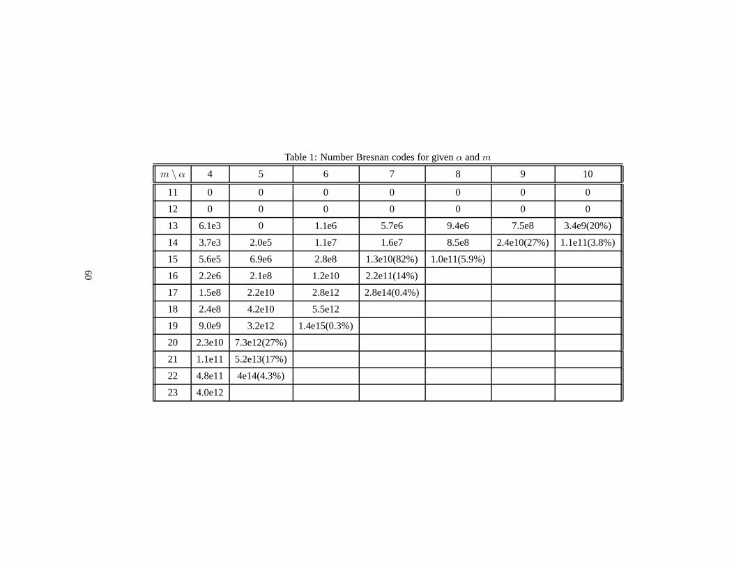
Table 1: Number Bresnan codes for givenα andm

m \ α 4 5 6 7 8 9 10

11 0 0 0 0 0 0 0

12 0 0 0 0 0 0 0

13 6.1e3 0 1.1e6 5.7e6 9.4e6 7.5e8 3.4e9(20%)

14 3.7e3 2.0e5 1.1e7 1.6e7 8.5e8 2.4e10(27%) 1.1e11(3.8%)

15 5.6e5 6.9e6 2.8e8 1.3e10(82%) 1.0e11(5.9%)

16 2.2e6 2.1e8 1.2e10 2.2e11(14%)

17 1.5e8 2.2e10 2.8e12 2.8e14(0.4%)

18 2.4e8 4.2e10 5.5e12

19 9.0e9 3.2e12 1.4e15(0.3%)

20 2.3e10 7.3e12(27%)

21 1.1e11 5.2e13(17%)

22 4.8e11 4e14(4.3%)

23 4.0e12

60

Table 2: Timing (in seconds) for find all Bresnan codes for givenα andm

m \ α 4 5 6 7 8 9 10

11 0 0 0 1 1 1 1

12 0 0 0 1 1 1 1

13 0 0 1 7 70 8.6e2 4.8e3

14 0 1 5 58 1.1e3 1.0e4 6.4e4

15 0 5 1.2e2 3.4e3 7.1e4

16 1 61 3.1e3 1.5e5

17 22 2.9e3 3.7e5 4.5e7

18 15 2.3e3 3.3e5

19 4.5e2 1.6e5 8.3e7

20 8.8e2 4.7e5

21 2.1e3 1.2e6

22 8.1e3 7.3e6

23 4.7e4

7.2 Performance

A study of the performances of the Bresnan codes when compared with randomlike code is presented here.

All simulations presented in the remainder of this thesis have been obtainedusing a maximum limit of20 iterations. For every SNRdB point a minimum of 10block errors has been found. Error bars are plotted on plots in this thesis. The errorassociated with the Frame Error rate is defined as ([40]):

(44) FER± = FER × exp

(

√

N − Nerror

N × Nerror

)

,

whereN is the number simulation trials andNerror is the number of frame errorsrecorded. This is to be considered an important aspect of theperformance graphsoften overlooked.

The simulations show that the codes of the family here developed behave verywell, even for medium lengths. First the result for aN = 808 code. In Figure 13a comparison between one of the new codes and three codes taken from knowngood families is provided. All codes are LDPC codes, with rate 1/2 and lengthN = 808. The new code is a regular code with a structure, while the others arerandomly constructed using some optimization method. To bemore precise, thesethree literature codes are:

61

• A MacKay code withN = 808, K = 404, dv = 3, dc = 6 obtained withthe method presented in [40];

• A randomly constructed code withN = 808, K = 404, dv = 3, dc = 6 thiscode has been obtained by running the optimized edge-placement algorithmfor five passes (see for example [36]);

• A Richardson irregular code withN = 808, K = 404, this code has beencreated using the optimized weight distributions proposedby Richardsonetal. [9, 12];

The performance of the new code is close to that of the random-edge one, withthe Random code hitting an error floor around3dbm 1e− 05. The MACKAY codeperforms worse than the new codes losing0.5dB at1e− 06. The Richardson codehas particularly poor performance, it is possible that the code constructed is a badrepresentative of the ensemble of which it is part. It is known that for medium andshorter length codes the performance of the single codes varies widely from theaverage performance of the ensemble and from the performance of long codes forthe same construction. On the other hand the situation highlights the problem offinding good random codes: creation and simulation of many codes are necessaryto find a good one.

Figure 14 shows the performances comparison betweenN = 1048 R = 1/2codes constructed with MacKay method [40], Random code [41]and a quasi-cycliccode of this class. It can be seen that the performance of the quasi-cyclic code isclose to the one of the random one, it is slightly worse when the code meets a noisefloor. The performance of the MacKay code in the1dB − 4dB range is worse thanthe quasi-cyclic code. For low values of SNR the quasi-cyclic code performancecompares well with the random code, and both are superior to the MacKay one.

Even if the main interest of this thesis is on medium length codes it is interest-ing to evaluate the construction presented for longer codesto have an idea of howsuch family performs in such case, for this reason two code with N ≈ 10, 000, arepresented. In Figure 15 a Bresnan code is compared with a MacKay code, it can beseen how the MacKay code has a much better defined waterfall region that makethe code outperform the Bresnan code for high SNR, this couldbe due to low min-imum distance or to the presence of trapping sets. The resultis in line with whatis a know fact: analytic codes do not perform as well as randomcodes for highlength. Moreover it proves that the MacKay codes for this length start to behave asit is theoretically proved for infinite length.

Finally it is important to consider that for the concentration theorem [9] it ismore likely that a code taken at random from the ensemble performs as well asthe average performance of the ensemble for this value ofN . It is important toobserve that the construction of good random codes, such as the three confrontedhere, requires a consistent amount of computation, while the new codes can beobtained immediately, thanks to their simple structure.

62

Figure 13: Block error rate performance forN = 808 Bresnan code compared withthree random like codes of the same length obtained from MacKay, Richardson andrandom permutations methods.

Figure 14: Block error rate performance forN = 1048 Bresnan code com-pared with the a code obtained with the random permutation method and one withMacKay methods.

63

Figure 15: Block error rate performance forN ≈ 10, 000. A Bresnan quasi-cycliccode and a MacKay code are compared.

8 Extension of the Bresnan Codes

In this section an approach to construct Bresnan-like codeswith rate higher than1/2 is presented that maintain girth8.

The Bresnan codes are formed by two square blocks of circulants, the codesdeveloped in this section are formed by three blocks. A rate of 2/3 is achievablein such way. The method is expandable to more blocks and any rate of the type(l − 1)/l can be achieved.

Definition 8.1 (Rate2/3 Bresnan codes). Let α,m be positive integers such thatα > 4,m ≥ 3. Hm,α denotes the class of the(mα × 3mα) matrices of the form

H =

H11 0 . . . 0 I H2

1 I 0 . . . 0 H31 0 I . . . 0

I H12 0 . . . 0 0 H2

2 I... 0 H3

2 0 I . . .

0 I. . . . . .

...... 0

. . . . . . 0... 0

. . . . . . .. ....

. . . . . . 0 0. . . . . . I

.... . . . . . 0

0 . . . 0 I H1α I 0 . . . 0 H2

α 0 I . . . 0 H3α

.

where everyHci , with c ∈ {1, 2} andi ∈ {1, 2, .., α}, is anm×m binary weight-2

circulant matrix andI is them × m identity matrix.

To simplify the discussion the three blocks that form theH matrix are calledB1, B2 andB3 andH = [B1|B2|B3]. The following theorem lists all the condi-tions that must hold for anH matrix of this type to have girth exactly eight.

64

Theorem 8.2. Letm ≥ 3, α > 4 andM ∈ Hm,α. Letg be the girth of the Tannergraph ofM . Theng = 8 if and only if all the following conditions hold:

1. for any1 ≤ i ≤ α andc ∈ {1, 2, 3}

s(pci ) 6=

m

3, s(pc

i) 6=m

2,

2. for any1 ≤ i ≤ α andc, d ∈ {1, 2, 3} andc 6= d,

s(pci) 6= s(pd

i ), s(pci ) 6≡ ±2s(pd

i ),

3. for any1 ≤ i ≤ α,s(p1

i ) ± s(p2i ) ± s(p3

i ) 6≡ 0,

4. for any(i, j) ∈ Jα,

4.1 ǫ(p1i ) + ǫ(p2

j) 6≡ 0,

4.2 ǫ(p1i ) + ǫ(p2

j) 6≡ {±s(p1i ),±s(p2

j )},

4.3 ǫ(p1i ) + ǫ(p2

j) 6≡ {±s(p1j),±s(p2

i ),±s(p3i ),±s(p3

j)}.

5. for any1 ≤ i ≤ α,s(p1

i ) 6≡ {s(p1i+1), s(p

2i+1), s(p

3i+1), s(p

3i+2)},

s(p2i ) 6≡ {s(p2

i+1), s(p3i+2)},

s(p3i ) 6≡ {s(p3

i+2), s(p2i+1)},

6. for any1 ≤ i ≤ α,

6.1 ǫ(p1i ) + ǫ(p1

i+1) + ǫ(p3i+2) 6≡ 0

6.2 ǫ(p2i ) + ǫ(p2

i+1) − ǫ(p3i+1) 6≡ 0

6.3 ǫ(p1i ) − ǫ(p2

i ) + ǫ(p3i+1) 6≡ 0

6.4 ǫ(p1i ) − ǫ(p2

i+2) + ǫ(p3i+2) 6≡ 0

Proof. It is necessary to prove that the conditions listed in the statement cover allthe possible cycle configurations existing for the construction presented. To provethis it is necessary to show that the configurations, regarding cycles of length4 and6 in theorem 6.1, or are not possible for this construction, orare associated withconditions listed in the statement.

• Configurations 1.1 and 2.1 in theorem 6.1 are evidently associated with theconditions in point 1.

• Configurations 1.2 and 2.2 are covered by the conditions in point 2.

• Point 3 considers configuration 2.3 in theorem 6.1.

65

• Configuration 1.3 is considered by condition in point 4.1. Note that due tothe position of the diagonal of identities inB3 such configuration can existonly betweenB1 andB2.

• Configuration 1.4 cannot exist in the proposed class thanks to the position ofthe identities diagonals. There cannot be any couple of columns that haveHandI sub-matrices in the same two rows.

• Configuration 2.4 in considered by the conditions in point 5.In fact everyH sub-matrix has threeI sub-matrices lying in the same row and one in thesame column. Hence for everyH sub-matrix six possible cycles of the type2.4 can exist, three formed by the three identities in the same row and threeformed by the identity in the same column and the threeH sub-matriceslying in the row of suchI.The conditions for cycles to existing in such configuration are:

s(p1i ) ≡ {s(p1

i−1), s(p2i+1), s(p

3i+2)},

s(p1i ) ≡ {s(p1

i+1), s(p2i+1), s(p

3i+1)},

s(p2i ) ≡ {s(p2

i−1), s(p2i+1), s(p

3i+2)},

s(p2i ) ≡ {s(p2

i−1), s(p2i−1), s(p

3i−2)},

s(p3i ) ≡ {s(p3

i+2), s(p1i−1), s(p

2i+1)},

s(p3i ) ≡ {s(p3

i−2), s(p1i−2), s(p

2i−2)},

Eliminating from the list above the conditions that are equivalent the set ofconditions in point 5 is obtained.

• Configurations 2.5 cannot exist for the same reason discussed for configura-tion 1.4, the same is true for configurations 2.7 and 2.9 of theorem 6.1.

• Cycles from configuration 2.6 can exist only between sub-matrices inB1

and sub-matrices inB2 . In fact the position of the diagonal of identities inB3 does not allow any of the columns in the third block to overlapin twopositions with any of the other columns. Conditions in point4.2 evidentlycover all the possible cycles of this type.

• For the same reason of the previous point, configuration 2.8 can exist only

when the∣

∣

∣

H2−2 II H3−2

∣

∣

∣ columns are inB1 andB2. The remaining column

can be in any of the three blocks, the relative cycles are avoided by the con-ditions in point 4.3.

• Cycles from configurations 2.10 and 2.11 are associated to conditions inpoint 6. To prove this it is necessary to show that the conditions listed in point6 considerall possible cycles that can arise from the two configurations.

Both configurations require that the distance from anH sub-matrix and theidentity in the same column is the sum of the distances from the other two

66

H sub-matrices and relative identities. It is evident from the position of theidentities diagonals that such case is possible only if one column lies inB3

and the other two columns do not. If the other columns both liein B1 it isonly a matter of connecting the sub-matrices to see that the resulting cycleis part of configuration 2.11 and it is not allowed by the condition 6.1. Ifthe other columns both lie inB2 it is only a matter of connecting the sub-matrices to see that the resulting cycle is part of configuration 2.10 and itis not allowed by the condition 6.2. If one of the remaining column liesin B1 and the other inB2 there are two possibilities to form a cycle, bothcorresponding to configuration 2.10. The fist case has theH sub-matricesin B1 andB2 lying in the same d.r., the second case has theH sub-matricesin B2 and B3 lying in the same d.r. The resulting cycles are avoided byconditions 6.3 and 6.4 respectively.

Note that if the twoH sub-matrices inB1 andB3 lie in the same d.r. is notpossible to form a cycle due to the position of the identitiesdiagonals

It has been proved that all the possible cycles that can existin theH matrix for thisclass of codes is avoided by one of the condition listed.

The performance of such class of codes is presented next. Figure 16 shows thecomparison between a code from the class of quasi-cyclic codes presented versusa random code and a MacKay code obtained from [42], the codes have lengthN ≈ 200. The codes have similar length and rate, the MacKay code is slightlylonger but has higher rateR ≈ 0.7. It can be seen how the quasi-cyclic code andMacKay code perform closely and slightly better than the random code.

The comparison of the same families of codes forN ≈ 1, 000 is presented inFigure 17. The codes have similar length and rate, the MacKaycode is slightlylonger but has higher rateR ≈ 0.85. For such length the proposed quasi-cycliccode outperforms both the random code and the MacKay code. Inparticular therandom code seems to hit an early error floor and the MacKay code perform fewtens of dB worse for all the SNR range considered.

Finally Figure 18 presents the comparison of a quasi-cycliccode with a ran-dom code forN = 2457. Unfortunately it has not been possible to obtain aMacKay code with such rate and length due to failure of the search carried out.The random code performs slightly better than thequasi-cyclic code for low SNRbut it is affected by early error floor that makes its performance poor at higherSNR. In contrast the quasi-cyclic code does not show the presence of any earlyerror floor.

It can be concluded that the construction proposed is a validalternative to ran-dom like codes for high rate. The quasi-cyclic codes, for thedimensions con-sidered, perform at least as well as other constructions butoffer the advantage ofreduced complexity and minimize memory requirement. Thoseare important as-pects for many applications where high rate codes are used.

67

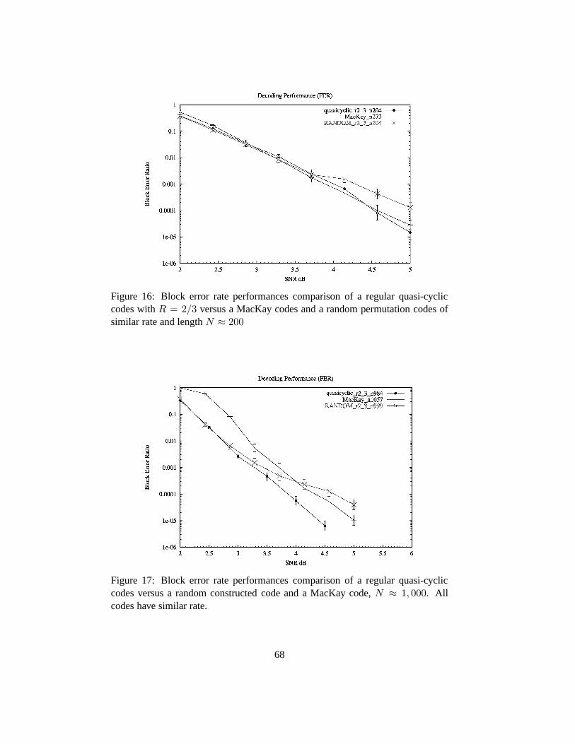
Figure 16: Block error rate performances comparison of a regular quasi-cycliccodes withR = 2/3 versus a MacKay codes and a random permutation codes ofsimilar rate and lengthN ≈ 200

Figure 17: Block error rate performances comparison of a regular quasi-cycliccodes versus a random constructed code and a MacKay code,N ≈ 1, 000. Allcodes have similar rate.

68

Figure 18: Block error rate performances comparison of a regular quasi-cycliccodes versus a random constructed code with same rate and length N ≈ 2, 000

9 Two families of quasi-cyclic codes with girth 10

In this section two families of quasi-cyclic LDPC codes withgirth at least 10 andrate1/2 are presented. The first construction is a(2, 4)-regular codes, the seconda (3, 6)-regular codes. The constructions are based on the idea of using blocks ofcirculants to compose theH matrix. The circulants lie in the diagonals of theblock, this help to detect the possible configurations arising and can be exploitedto reduce hardware complexity of the decoding algorithm (see [38]).

9.1 Regular(2, 4)

This family of codes has been studied first because its structure drastically reducethe number of conditions necessary to ensure high girth.

Definition 9.1 ( (2, 4)-regular quasi-cyclic codes girth 10). Let α,m be positiveintegers such thatα > 4,m ≥ 3. NotationCm,α denotes the class of the(mα ×2mα) matrices of the form

H = [B1 |B2]

where

B1 =

H0 0 . . . 0 00 H1 0 . . . 0

0 0. . . . . .

......

. . . . . . 00 . . . 0 0 Hα−1

69

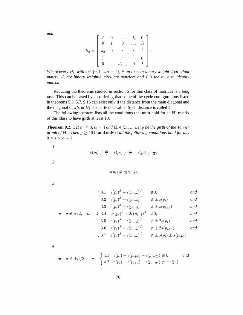
and

B2 =

I 0 . . . J0 00 I 0 . . . J1

J2 0. .. . ..

......

. .. . .. 00 . . . Jα−1 0 I

.

Where everyHi, with i ∈ {0, 1, .., α − 1}, is anm × m binary weight-2 circulantmatrix, Ji are binary weight-1 circulant matrices andI is the m × m identitymatrix.

Reducing the theorems studied in section 5 for this class of matrices is a longtask. This can be eased by considering that some of the cycle configurations listedin theorems 5.3, 5.7, 5.16 can exist only if the distance fromthe main diagonal andthe diagonal ofJ ’s in B2 is a particular value. Such distance is calledδ.

The following theorem lists all the conditions that must hold for anH matrixof this class to have girth at least10.

Theorem 9.2. Letm ≥ 3, α > 4 andH ∈ Cm,α. Letg be the girth of the Tannergraph ofH . Theng ≥ 10 if and only if all the following conditions hold for any0 ≤ i ≤ α − 1.

1.s(pi) 6=

m2 , s(pi) 6=

m3 , s(pi) 6=

m4 ,

2.

s(pi) 6= s(pi+δ),

3.

or δ 6= α/2, or

3.1 ǫ(pi)J + ǫ(pi+δ)

J 6≡0, and


J 6≡ ± s(pi) and


J 6≡ ± s(pi+δ) and

3.4 2ǫ(pi)J + 2ǫ(pi+δ)

J 6≡0, and


J 6≡ ± 2s(pi) and


J 6≡ ± 2s(pi+δ) and


J 6≡ ± s(pi) ± s(pi+δ)

4.

or δ 6= ±α/3, or

{

4.1 ǫ(pi) + ǫ(pi+δ) + ǫ(pi+2δ) 6≡ 0 and

4.2 ǫ(pi) + ǫ(pi+δ) + ǫ(pi+2δ) 6≡ ±s(pi)

70

5.

or δ 6= ±α/4, or ǫ(pi) + ǫ(pi+δ) + ǫ(pi+2δ) + ǫ(pi+3δ) + ǫ(pi+4δ) 6≡ 0

Where the index operations are moduloalpha.

Proof. It is necessary to prove that the conditions listed cover allthe possible cycleconfigurations existing in such class of codes. To prove thisit is necessary to showthat the configurations listed in theorems 5.3, 5.7 and 5.16 are not possible for thisconstruction or are associated with a condition listed in the statement. First theconfigurations that can have4-cycles, listed in theorem 5.3, are considered.

• Configuration 1 is associated with the first condition in point 1.

• Configuration 2 cannot exist because there cannot be twoH sub-matrices inthe same row or column.

• Configuration 3 can exist in this construction only ifδ = α/2. In any othercase there cannot be four sub-matrices lying in two columns and two rows.If δ = α/2 condition 3.1 assures that the cycle cannot exist.

The configurations that can have6-cycles, listed in theorem 5.7, are considerednext.

• Configuration 1 is associated with the second condition in point 1.

• Configurations 2 and 3 cannot exist because there cannot be two H sub-matrices in the same row or column.

• Configurations 4 and 5 cannot exist because for this construction everyHsub-matrix lies alone in a column.

• For the same reason discusses for configuration 3 of theorem 5.3, configura-tion 6 can exist in this construction only ifδ = α/2. If δ = α/2 conditions3.2 and 3.3 assure that the cycle cannot exist.

• Configurations 7 requires that the distance from two sub-matrices in the samecolumn is the sum of the two other such distances for the remaining d.c.’s inthe configuration. It is evident that all the columns must liein B2 since inB1

there is only one sub-matrix in each column. Moreover such situation existsonly if δ = ±α/3. If δ = ±α/3 conditions 4.1 assures that the cycle cannotexist. To determine the sign of the terms in the condition it is sufficient toconsider that there cannot be twoJ ’s in the same column. Hence theJ ’stake alternate positions in the cycle configuration hence they all have thesame sign.

71

The configurations that can have8-cycles, listed in theorem 5.16 are considerednext.

• Configuration 1 is associated with the third condition in point 1.

• Configurations 2, 3, 4, 7, 12 and 15 cannot exist because for this constructioneveryH sub-matrix lies alone in a column.

• For the same reason discussed for configuration 3 of theorem 5.3, configura-tion 5 can exist in this construction only ifδ = α/2. If δ = α/2 conditions3.4 assures that the cycles cannot exist.

• For the same reason of previous point, configuration 6 can exist in this con-struction only ifδ = α/2. If δ = α/2 conditions 3.5 and 3.6 assure that thecycles cannot exist.

• Configuration 8 cannot exist because the structure of theH does not allowto have6 sub-matrices lying in two rows and three columns.

• Configuration 9 is evidently associated with condition 2.

• Configuration 10 can exist only withδ = α/2 for the same reason discussedin previous cases. Ifδ = α/2 conditions 3.7 assures that the cycles cannotexist.

• Configuration 11 cannot exist because the structure of theH does not allowto have8 sub-matrices lying in two rows and four columns.

• Configuration 13 cannot exist because it implies the existence of three nonzero sub-matrices in the same column or the existence of a column with anH and one identity, both cases are not possible due to the particular structureof theH matrix.

• Configuration 14 cannot exist because it implies to have three non zero sub-matrices in the same column that is not possible due to the particular struc-ture of theH matrix.

• Configuration 16 cannot exist because it implies to have fournon zero sub-matrices in the same column or row that is not possible due to the particularstructure of theH matrix.

• Configuration 17 requires that the distance from an two sub-matrices in thesame column is the sum of the two other such distances for the remainingd.c.’s in the configuration. It is evident that the columns not containingHmust lie inB2. Moreover such situation exist only ifδ = ±α/3. If δ =±α/3 conditions 4.2 assures that the cycle cannot exist. The samereasoningapplied to configuration 7 of theorem 5.7 can be used to explain the signs ofthe terms of the condition.

72

• Configurations 18 requires that the distance from the two sub-matrices in thesame column is the sum of the three other such distances for the remainingd.c.’s in the configuration. It is evident that all the columns must lie inB2.Moreover such situation exist only ifδ = ±α/4. If δ = ±α/4 conditions 5assures that the cycles cannot exist.


Aside from the degenerative cases whereδ = α/2, δ = α/3 andδ = α/4 theconditions to check are extremely simple. Even in the degenerative cases the listof conditions is quite short. Thanks to this, finding exponents and conditions thatallows girth10 is an easy task. Following the performances of three of such codesare presented. The codes have been obtained avoiding the degenerative cases ofδand imposing the conditions on the separations.

In Figure 19 the block error ratio versus noise performance graph of a smallcode (N = 810) from this family can be seen. The code is compared with arandom code. Both codes have same length and are(2, 4)-regular. The randomcodes has been obtained with a optimal permutations method and has a girth of14 and an average girth of15.7, the quasi-cyclic codes has girth10. In the samefigure the quasi-cyclic code is compared also with a more advanced ProgressiveEdge Grow (PEG) code from [43, 44]. The code is(2, 7)-regular. It can be seenhow this code performs as well as the random code and comparesevenly with acarefully constructed code, this is a good result for such class of codes.

Figure 19: Block error rate performances comparison of a quasi-cyclic code com-pared with a random code and a PEG code withN ≈ 800

Figure 20 presents a comparison of a quasi-cyclic code from this family versusa random code in the case of longer codes. Both the codes haveN ≈ 6, 500. It

73

Figure 20: Block error rate performances comparison of a quasi-cyclic code com-pared with a random code. Both codes are(2, 4)-regular withN ≈ 6, 500

can be seen how the performance of the quasi-cyclic code withgirth 10 do not hitan error floor as soon as the random code. The random code has average girth of20.37 but girth of only6.

Regular(2, 4)-LDPC codes are not often used in practice due to their poor per-formances. As an example of this a comparison between a(3, 6)-regular Gallaghercode and the PEG code is presented in Figure 21 It can be seen how the(3, 6)- reg-ular code has up to 5db gain when compared with(2, 4)-regular codes both randomand quasi-cyclic . For this reason the interest is on build(3, 6)-regular quasi-cyclicLDPC codes with girth ten.

9.2 Regular(3, 6)

The construction presented here is the result of few considerations. Lemma 5.15shows how any quasi-cyclic LDPC code with girth at least10 cannot exist if twoweight-2 circulants lie in the same row or column. For this reason all weight-2circulants are placed in the main diagonal ofB1. To keep the column weight equalto three it is necessary to insert another weight-1 circulant for each column and thisis done inserting another diagonal of identities. The second blockB2 cannot con-tain weight two circulants hence any row and column must contain three weight-1circulants to form a(3, 6)-regular code. Aiming to maintain some regularity toallow reduced hardware complexity of the decoding algorithm, the circulant matri-ces have been disposed in three diagonals. To simplify the number and complexityof the checks necessary to guarantee girth10 identity matrices, as special case ofweight-1 circulant matrices, have been used where possible.The resulting familyof codes is the following.

74

Figure 21: Block error rate performances comparison of a(2, 4)-regular quasi-cyclic codes versus a(3, 6)-regular codeN ≈ 800

Definition 9.3 ((3, 6)-regular quasi-cyclic code). Let α,m be positive integerssuch thatα > 4,m ≥ 3. NotationDm,α denotes the class of the(mα × mα)matrices of the form

H = [B1 |B2]

where

B1 =

H0 0 . . . 0 II H1 0 . . . 0

0 I. . . . . .

......

. . . . . . 00 . . . 0 I Hα−1

75

and

B2 =

J0 0 . . . 0 I 0 . . . 0 I 0 . . . 0

0 J1 0 . . . 0 I 0 . . . 0 I . . ....

..... .

. . .. . . 0

.... .. . . . I

I 0. .. .. . 0

0. . . . . . . .. 0

..... .

. . .. . . 0

. .. . . . I

I. .. .. . 0

0. . . . . . . ..

......

.. . . . . . . .0 I . . . I . . . Jα−1

.

where everyHi, with i ∈ {0, 1, .., α−1}, is anm×m binary weight-2 circulantmatrix andI is them×m identity matrix, andJi are weight-1 circulant matrices.

Some of the cycle configurations listed in theorems 5.3, 5.7 and 5.16 exist onlyif the distance from the main diagonal and the diagonals of identities inB2 takeparticular values. Such distances are calledδ2, δ3, and for simplicity the notationδ3 − δ2 is calledδ32. Such values can be seen in Figure 22. Moreover the positionof the diagonal of identities inB1 is calledδ1. For the construction presented hereδ1 = α − 1.

Note that it is not possible to substitute the diagonal ofJ ’s with identities. Infact in such case6-cycle configurations will always arise independently fromthepositions of the diagonals. The existence of this configurations carry a parallelwith the existence of6-cycles on a weight-3 circulant matrix [33]. A graphicalrepresentation of such case is given in Figure 22. It can be seen that the particular6-cycle exists ifδ2 + δ32 = δ3 but δ2 + δ3 − δ2 = δ3 hence the condition is alwayssatisfied and the cycle exists independently from the valuesof the deltas. If all thematrix involved in the cycle are identities it is not possible to avoid such cycle.Setting the main diagonal to containJ ’s, and not identities, it is possible to avoidsuch cycle by imposing proper conditions on the exponents.

A new class of matrices is presented next. The matrices are part of the previousclass but some limitations on the position of the diagonals of identities are added.Such limitations on the values of deltas are not strictly necessary but help to reducethe number of possible configurations, and so the complexityof the conditions tocheck.

Definition 9.4 ((3, 6)-regular quasi-cyclic code girth 10). Let Em,α denotes theclass of the(mα × mα) matrices inDm,α that satisfy the following conditions on

76

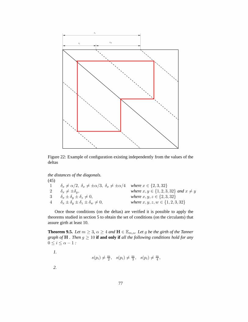
δ2

δ3

δ32

Figure 22: Example of configuration existing independentlyfrom the values of thedeltas

the distances of the diagonals.(45)1 δx 6= α/2, δx 6= ±α/3, δx 6= ±α/4 wherex ∈ {2, 3, 32}2 δx 6= ±δy, wherex, y ∈ {1, 2, 3, 32} andx 6= y3 δx ± δy ± δz 6= 0, wherex, y, z ∈ {2, 3, 32}4 δx ± δy ± δz ± δw 6= 0, wherex, y, z, w ∈ {1, 2, 3, 32}

Once those conditions (on the deltas) are verified it is possible to apply thetheorems studied in section 5 to obtain the set of conditions(on the circulants) thatassure girth at least 10.

Theorem 9.5. Let m ≥ 3, α ≥ 4 andH ∈ Em,α. Letg be the girth of the Tannergraph ofH . Theng ≥ 10 if and only if all the following conditions hold for any0 ≤ i ≤ α − 1 :

1.s(pi) 6=

m2 , s(pi) 6=

m3 , s(pi) 6=

m4 ,

2.

77

2.1 s(pi) 6≡ s(pi+δ1),

2.2 s(pi) 6≡ ±2s(pi+δ1),

2.3 s(pi+δ1) 6≡ ±2s(pi),

3.s(pi) 6≡ s(pi+δx

), wherex ∈ {2, 3, 32}

4.

4.1 ǫ(pi)J − ǫ(pi±δ32)

J 6≡ 0,

4.2 ǫ(pi)J − ǫ(pi+±δ32)

J 6≡ ±s(pi),

5.

5.1 ǫ(pi)H − ǫ(piδ32)

H 6≡ 0,

5.2 ǫ(pi)H − ǫ(pi−δx

)H + ǫ(pi+1)J − ǫ(pi)

J 6≡ 0 wherex ∈ {2, 3}

Proof. It is necessary to prove that the conditions listed cover allthe possible cycleconfigurations existing in such class of codes. To prove thisit is necessary to showthat the configurations listed in theorems 5.3, 5.7 and 5.16,or are not possible forthis construction, or are associated with a condition listed in the statement. Firstthe configurations that can have4-cycles, listed in theorem 5.3 are considered.

• Configuration 1 is associated with the first condition in point 1.

• Configuration 2 cannot exist because there cannot be twoH sub-matrices inthe same row or column.

• Configuration 3 cannot exist in this construction and with the conditionsimposed on the deltas. In fact such configuration can exist only if thereare four sub-matrices lying in two column and two rows. This can happenonly if two deltas are equals modulo alpha, or if one of the delta is equalto α/2. These cases are not allowed by conditions 1 and 2 in definition 9.4hence the cycle configuration cannot exist.


• Configuration 1 is associated with the second condition in point 1.

• Configurations 2 and 3 cannot exist because there cannot be two H sub-matrices in the same row or column.

• Configuration 4 contains twoC sub-matrices in the two d.c. hence both thecolumns must be in theB1. EveryH sub-matrix can form a cycle only withthe row above and below itself. All this cases are consideredby condition2.1. The remaining sub-matrix in the configuration is an identity hence thetwo exponent terms are not present in the final condition.

78

• Configurations 5 and 6 cannot exist for the same reason discussed for con-figuration 3 of theorem 5.3.

• Configurations 7 requires that the distance from two sub-matrices in the samecolumn is the sum of the two other such distances for the remaining d.c.’s inthe configuration. This is not allowed by condition 3 in definition 9.4 withthe exception of the case depicted in Figure 22. Such cycles are avoided bycondition 4.1.


• Configuration 1 is associated with the third condition in point 1.

• Configurations 2, 4, 5, 6, 7, 8, 10, 11, 13, 14, 15 and 16 cannot exist for thesame reason discussed for configuration 3 of theorem 5.3 .

• The same reasoning done for configuration 4 of theorem 5.7 applies to con-figuration 3 and all the possible resulting cycles are avoided by conditions2.2 and 2.3.

• Configuration 9 contains twoC sub-matrices in the two d.c. hence both thecolumns must be inB1. The remaining column contains twoJ sub-matriceshence it must lieB2. The sub-matrices in the column inB2 are spaced atdistanceδx with x ∈ {2, 3, 32} hence all the possible cycles are consideredby condition 3.

• Configuration 12 requires that the distance from two sub-matrices in thesame column is the sum of the two other such distances for the remain-ing d.c.’s in the configuration. This is not allowed by condition 3 in defini-tion 9.4. Note that the presence of a weight-2 circulant forces one d.c. to bein B1 hence the case depicted in Figure 22 does not exist here.

• Following the same reasoning done for configuration 7 of theorem 5.7. Con-figuration 17 exists only if the three columns lying in B2 havethe configu-ration depicted in Figure 22 and the last column lies in B1. Such cycles areavoided by condition 4.2.

• Configuration 18 is associated to conditions in point 5. To prove this it isnecessary to show that the conditions listed in point 5 consider all possiblecycles that can arise from the configuration.

The configuration requires that the distance of two sub-matrices in the samecolumn is the sum of the three other such distances for the remaining d.c.’s inthe configuration. Such configurations are not possible thanks to condition 4in definition 9.4. A particular case remains to be considered. If two columnsof the cycle configuration lie inB1 and two inB2 then the existence of this

79

configurations carry a parallel with the existence of8-cycles on two weight-2 circulants in the same row or column (Figure 12). It has been provedin lemma 5.15 that such cycle exists independently from the value of theseparations. In this case the delta’s take the part of the separation, hence thecycle configuration exists independently from the value of delta’s. ButB2

has three diagonals so three different cycles can exist, andsuch cycles areavoided by the three conditions in point 5.

To better understand this passage consider that the two cycle columns inB1

contain an identity and anH sub-matrix each, hence exponents of twoHsub-matrices must be part of the condition. From Figure 12 itcan be seenthat the cycle exists only if both the cycle columns inB2 contain two sub-matrices appertaining to the same two diagonals. There are three possibili-ties: one sub-matrix is in the second diagonal and one in the main diagonal,one sub-matrix is in the third diagonal and one in the main diagonal and fi-nally one sub-matrices in the second diagonal and one in the third diagonal.The first two cases lead to condition 5.2 the third to condition 5.1.


Following the performances of codes of this family for different lengths arepresented.

Figure 23 shows the performance of a medium length quasi-cyclic code whencompared with a random generated code. Both codes are(3, 6)-regular codes ofdimensionN = 2, 294. It can be seen how the quasi-cyclic codes from this familyperforms really close to the random code, but it seems that the quasi-cyclic codeshit an error floor at1e − 09 BER.

Even if out of the boundaries of the range of codes that are themain focusof this thesis the comparison of quasi-cyclic codes with random codes usinglonger codes is presented next for completeness. Figure 24 and 25 present sucha comparison. Figure 24 shows the performances of two(3, 6)-regular codes withN ≈ 6, 500 and Figure 25 shows the performances of two(3, 6)-regular codeswith N ≈ 19, 500 It can be seen the quasi-cyclic codes are quite close to the ran-dom codes. WithN ≈ 6, 500 only 0.1db, at1e − 09, divides the two codes, withN ≈ 19, 500 the difference increased but remain under the0.5db, at1e − 05, thatis a considerable achievement for algebraic codes of this length.

10 Conclusions anf future work

In this contribution a study on the presence of cycles on the quasi-cyclic LDPCcodes has been presented. The aim of the study is to identify the configurationsof circulant matrices that allow cycles of a given length to exist. Once all suchconfigurations are known it is possible to associate to each of them a condition,on the exponents and separations of the circulants involvedin the cycle, that must

80

Figure 23: Block error rate performances of a girth 10 quasi-cyclic code comparedwith a random generated codes. Both codes are(3, 6)-regular withN = 2, 294


81


be satisfied for the cycle to exist. The collection of these conditions gives a wayto construct quasi-cyclic codes without undesired cycle byensuring that all theconditions are not satisfied. The chapter started with a novel definition of cycles ina matrix, opposed to the normal definition that is given on graph. Such a definitionis used to prove the “isolation” (lemma 3.10), the lemma is extensively used in thesearch of which configurations are valid and can contain cycles. The configurationsthat allows cycle of length less then10 are found first for the generic case of amatrix that can be partitioned in sub-matrices, then in the case of the matrices forquasi-cyclic codes. Our approach is not restricted to circulant matrices of weightone as is commonly done in literature but considers also circulant matrix of weight-2 (weight-3 circulant matrices are of no interest for this search because they haveinternal 6-cycles). The set of conditions for the generic case is foundand thenthe conditions are applied for various particular constructions. The first class ofquasi-cyclic codes studied are the Bresnan Codes [36], several aspects of thesecodes are studied and their performances presented. Such class is then extendedfor higher rate codes. Finally two new structures and the relative set of conditionsthat guarantee girth at least10 are developed and their performances presented.The contribution of this work is not only the four classes of quasi-cyclic codeswith high girth but mainly the creation of the list of conditions that every quasi-cyclic codes (of any possible construction method) must satisfy to have a givengirth. This not only covers all the existing cases but can be used when constructingnew structures for quasi-cyclic codes to easily identify where the cycles can existand how to avoid them.

The methodology presented in this thesis could be used to expand the under-standing of quasi-cyclic codes. It would be possible to continue the search of

82

codes with high girth and look for the conditions that guarantee girth twelve but,in the authors opinion, such work would be long, tedious and would carry littlebenefit. In fact, other parameters of the code, such as the minimum distance, thediameter, the minimum stopping set and others, will became dominant and preventimprovement in the performance of the code. Of more interestwould be to study ifthe methodology presented could be applied to the problem offinding codes withgood diameter value. It could be possible to develop a set of conditions that en-sures the diameter to be a certain value. The study of how these rules intersect withthe girth conditions could lead to classes of codes that can achieve given girth anddiameter and offer a good balance between the two.

References

[1] R. Gallager, “Low density parity check codes,” 1963, Ph.D. Thesis, MITpress, Cambridge, MA,.

[2] X. Y. Hu, E. Eleftheriou, D. M. Arnold, and A. Dholakia, “Efficient imple-mentations of the sum-product algorithm for decoding LDPC codes,” Pro-ceedings of IEEE Global Communications Network, (GLOBECOM), pp. 25–29, 2001.

[3] D. MacKay and R. Neal, “Good codes based on very sparse matrices,” Pro-ceedings of IMA Cryptography and Coding conference, pp. 100–111, 1995.

[4] F. J. MacWilliams and N. J. A. Sloane,The Theory of Error-CorrectingCodes. North Holland, 1977.

[5] T. R. S.Y. Chung, G.D. Forney and R. Urbanke, “On the design of LDPCcodes within 0.0045 db of the shannon limit,”IEEE Commun. Lett., vol. 5,no. 2, pp. 58–60, 2001.

[6] R. M. Tanner, D. Sridhara, and T. Fuja, “A class of group-structured LDPCcodes,”Proceedings of International Symposium on Communication Theoryand Application (ICTA), 2001.

[7] R. Tanner, “A recursive approach to low complexity codes,” IEEE Trans. In-form. Theory, vol. 27, no. 5, pp. 533–547, 1981.

[8] W. E. Ryan,An introduction to LDPC codes. CRC Handbook for CSP forRS B. Vasic, Ed. CRC Press, 2004.

[9] T. Richardson, M. Shokrollahi, and R. Urbanke, “Design of capacity ap-proaching irregular LDPC codes,”IEEE Trans. Inform. Theory, vol. 47, no. 2,pp. 619–637, 2001.

[10] D. J. MacKay, Information Theory, Inference, and Learning Algorithms.Cambridge University Press, 2003.

83

[11] T. Tian, C. Jones, J. Villasenor, and R. Wesel, “Selective avoidance of cyclesin irregular ldpc code construction,”IEEE Trans. Commun., vol. 52, no. 8,pp. 1242–1247, 2004.

[12] T. Richardson and R. Urbanke, “The capacity of low-density parity-checkcodes under message-passing decoding,”IEEE Trans. Inform. Theory,vol. 47, no. 2, pp. 599–618, 2001.

[13] ——, “Efficient encoding of low-density parity-check codes,” IEEE Trans.Inform. Theory, vol. 47, no. 2, pp. 638–656, 2001.

[14] T. Tian, C.Jones, J. D. Villasenor, and R. D. Wesel, “Construction of irreg-ular LDPC codes with low error floors,”Proceedings of IEEE intenationalConference on Communications, (ICC), vol. 5, pp. 3125–3129, 2003.

[15] S. J. Johnson and S. R. Weller, “Quasi-cyclic LDPC codesfrom differencefamilies,” in Proceedings of the Austr. Comm. Th. Workshop, 2002, pp. 18–22.

[16] S. Johnson and S. Weller, “A family of irregular LDPC codes with low en-coding complexity,”IEEE Commun. Lett., vol. 7, no. 2, pp. 79–81, 2003.

[17] S. J. Johnson and S. R. Weller, “Codes for iterative decoding from partialgeometries,”IEEE Trans. Commun., vol. 52, no. 2, pp. 236–243, 2004.

[18] I. P. Jon-Lark Kim, Uri N. Peled and V. Pless, “Explicit construction offamilies of LDPC codes with no 4-cycles,”INFORMATION THEORY, IEEETRANSACTIONS ON, vol. VOL. 50, NO. 10, pp 2378-2388, OCT. 2004.

[19] S. L. Y. Kou and M. Fossorier, “Low-density parity-check codes based on fi-nite geometries: A rediscovery and new results,”IEEE Trans. Inform. Theory,vol. 47, no. 7, pp. 2711–2736, 2001.

[20] Y. Kou, J. Xu, H. Tang, S. Lin, and K. Abdel-Ghaffar, “On circulant lowdensity parity check codes,” inProceedings of IEEE International Symposiumon Information Theory (ISIT), 2002, pp. 200–.

[21] M. E. O’Sullivan, M. Greferath, and R. Smarandache, “Construction ofLDPC codes from affine permutation matrices,”Proceedings of the AnnualAllerton Conference on Communication, Control, and Computing, pp. 1159–1167, 2002.

[22] J. Rosenthal and P. Vostobel, “Construction of regularand irregular LDPCcodes using Ramanujan graph and ideas from Margulis,”Proceedings ofIEEE International Symposium on Information Theory, (ISIT), p. 4, 2001.

[23] D. J. C. MacKay, “Good error correcting codes based on very sparse matri-ces,”IEEE Trans. Inform. Theory, vol. 45, no. 2, pp. 399–431, 1999.

84

[24] T. Etzion, A. Trachtenberg, and A. Vardy, “Which codes have cycle-free tan-ner graphs?”Proceedings of IEEE International Symposium on InformationTheory (ISIT), p. 207, 1998.

[25] ——, “Which codes have cycle-free tanner graphs?”IEEE Trans. Inform.Theory, vol. 45, no. 6, pp. 2173–21 812, 1999.

[26] D. MacKay and R. Neal, “Near shannon limit performance of low densityparity check codes,”Elec. Lett., vol. 32, pp. 1645–1646, 1996.

[27] D. J. C. MacKay and M. J. Postol, “Weaknesses of Margulisand Ramanujan–Margulis low-density parity-check codes,”Proceedings of the 4th Irish Con-ference on mathematical foundations of computer science and informationtechnology, (MFCSIT), vol. 74, pp. 97–104, 2003.

[28] M. P. C. Fossorier, “Quasi-cyclic low-density parity-check codes from circu-lant permutation matrices,”IEEE Trans. Inform. Theory, vol. 50, no. 8, pp.1788–1783, 2004.

[29] M. E. O’Sullivan and R. Smarandache, “High rate short length(3, 3s)-regularLDPC codes of girth 6 and 8,”Procceding of IEEE International SymposioumInformatuin Theory (ISIT), p. 59, 2003.

[30] O. Milenkovic, N. Kashyap, and D. Leyba, “Shortened array codes of largegirth,” IEEE Trans. Inform. Theory, vol. 52, no. 8, pp. 3707–3722, Aug. 2006.

[31] J. L. Fan, “Array codes as low-density parity-check codes,” Proc. 2ndInt. Symp. Turbo Codes, pp. 543–546, 2000.

[32] R. Smarandache and P. Vontobel, “On regular quasicyclic LDPC codes frombinomials,” Proceedings of IEEE International Symposium on InformationTheory (ISIT), p. 274, 2004.

[33] J. Bond, S. Hui, and H. Schmidt, “Linear-congruence construction of low-density check codes,”Proceedings of IMA Codes, Systems and GraphicalModels Conference, vol. 123, pp. 83–100, 2001.

[34] M. Giorgetti, M.Rossi, and M. Sala, “On the groebner basis of a familyof quasi-cyclic LDPC codes,”Bulletin of the Iranian Mathematical society,vol. 31, no. 2, pp. 13–32, 2005.

[35] M.Rossi, “Construction of quasi-cyclic LDPC codes,” 2004, Master. Thesis,Dept. of Math., Univ. of Milan-Bicocca.

[36] R. Bresnan, “Novel code construction and decoding techniques for LDPCcodes,” 2004, Master. Thesis, Dept. of Elec. Eng., UCC Cork,2004.

[37] M. Rossi and M. Sala, “On a class of quasi-cyclic codes,”Proceedings of theEffective Methods in Algebraic Geometry conference (MEGA), 2005.

85

[38] C. Spagnol, E. Popovici, and W. Marnane, “Reduced complexity, FPGA im-plementation of quasi-cyclic LDPC decoder,”Proceedings of IEEE EuropeanConference on Circuit Theory and Design (ECCTD), vol. 1, pp. 289–292,2005.

[39] M.Rossi and M.Sala, “On a class of quasi-cyclic LDPC codes,” 2005, BCRIpreprint, available atwww.bcri.ucc.ie.

[40] D. MacKay, S. Wilson, and M. Davey, “Comparison of constructions of irreg-ular gallager codes,”IEEE Trans. Commun., vol. 47, no. 10, pp. 1449–1454,1998.

[41] Y. Mao and A. H. Banihashemi, “A heuristic search for good low-densityparity-check codes at short block lengths,”Proceedings of IEEE intenationalConference on Communications, (ICC), vol. 1, pp. 41–44, 2001.

[42] D. J. C. MacKay. Encyclopedia of sparse graph codes.Database of codes. Department of Physics. CavendishLaboratory, University of Cambridge. [Online]. Available:http://www.inference.phy.cam.ac.uk/mackay/codes/data.html

[43] A. Venkiah, D. Declercq, and C. Poulliat, “Design of cages with a randomizedprogressive edge-growth algorithm,”IEEE Commun. Lett., vol. 12, no. 4, pp.301–303, 2008.

[44] E. E. Xiao-Yu Hu and D. M. Arnold, “Regular and irregularprogressive edge-growth tanner graphs,”IEEE Trans. Inform. Theory, vol. 52, no. 1, pp. 386–398, 2005.

86

http://www.inference.phy.cam.ac.uk/mackay/codes/data.html

Appendix

Proof of theorem 3.16

Theorem 10.1(3.16). LetB ∈ Mm,α,β,γ .The only possible8-cycle configurations are as follows (1)-presentations):

1. (1, 1),|8| ,

2. (1, 2),

2.1∣

∣ 6 2∣

∣ , 2.2∣

∣ 4 4∣

∣ ,

3. (1, 3),∣

∣ 4 2 2∣

∣ ,

4. (1, 4),∣

∣ 2 2 2 2∣

∣ ,

5. (2, 2),

5.1

∣

∣

∣

∣

5 11 1

∣

∣

∣

∣

, 5.2

∣

∣

∣

∣

4 22 0

∣

∣

∣

∣

, 5.3

∣

∣

∣

∣

4 20 2

∣

∣

∣

∣

,

5.4

∣

∣

∣

∣

3 13 1

∣

∣

∣

∣

, 5.5

∣

∣

∣

∣

3 11 3

∣

∣

∣

∣

, 5.6

∣

∣

∣

∣

2 22 2

∣

∣

∣

∣

,

6. (2, 3),

6.1

∣

∣

∣

∣

4 1 10 1 1

∣

∣

∣

∣

, 6.2

∣

∣

∣

∣

3 2 11 0 1

∣

∣

∣

∣

, 6.3

∣

∣

∣

∣

3 1 01 1 2

∣

∣

∣

∣

,

6.4

∣

∣

∣

∣

2 2 22 0 0

∣

∣

∣

∣

, 6.5

∣

∣

∣

∣

2 1 12 1 1

∣

∣

∣

∣

, 6.6

∣

∣

∣

∣

2 2 02 0 2

∣

∣

∣

∣

,

7. (2, 4),

7.1

∣

∣

∣

∣

2 2 1 10 0 1 1

∣

∣

∣

∣

, 7.2

∣

∣

∣

∣

2 1 1 00 1 1 2

∣

∣

∣

∣

, 7.3

∣

∣

∣

∣

1 1 1 11 1 1 1

∣

∣

∣

∣

,

8. (3, 3),

8.1

∣

∣

∣

∣

∣

∣

3 1 01 0 10 1 1

∣

∣

∣

∣

∣

∣

, 8.2

∣

∣

∣

∣

∣

∣

2 1 12 0 00 1 1

∣

∣

∣

∣

∣

∣

, 8.3

∣

∣

∣

∣

∣

∣

2 1 11 1 01 0 1

∣

∣

∣

∣

∣

∣

, 8.4

∣

∣

∣

∣

∣

∣

2 0 01 1 01 1 2

∣

∣

∣

∣

∣

∣

.

87

9. (3, 4),

9.1

∣

∣

∣

∣

∣

∣

2 1 1 00 1 0 10 0 1 1

∣

∣

∣

∣

∣

∣

, 9.2,

∣

∣

∣

∣

∣

∣

1 1 1 11 1 0 00 0 1 1

∣

∣

∣

∣

∣

∣

,

10. (4, 4),∣

∣

∣

∣

∣

∣

∣

∣

1 1 0 01 0 1 00 1 0 10 0 1 1

∣

∣

∣

∣

∣

∣

∣

∣

.

Proof. Lemma 3.6 proves that these are all the possible dimensions that 8-cycleconfigurations can have. It is now necessary to prove that they are also all and onlyvalid configurations.

Following from Theorem 3.12 the only possible weights vectors for a 8-cyclesare:

[8] ,

[7, 1] ,

[6, 2] , [6, 1, 1] ,

[5, 3] , [5, 2, 1] , [5, 1, 1, 1] ,

[4, 4] , [4, 3, 1] , [4, 2, 2] , [4, 2, 1, 1] , [4, 1, 1, 1, 1] ,

[3, 3, 2] , [3, 3, 1, 1] , [3, 2, 2, 1] , [3, 2, 1, 1, 1] , [3, 1, 1, 1, 1, 1] ,

[2, 2, 2, 2] , [2, 2, 2, 1, 1] , [2, 2, 1, 1, 1, 1] , [2, 1, 1, 1, 1, 1, 1] ,

[1, 1, 1, 1, 1, 1, 1, 1] ,

Configuration 1 A type(1, 1) configuration can be generated only by weights vec-tor [8] and it corresponds to case 1.

Configuration 2 Type(1, 2) configurations can be generated only by weights vec-tors [6, 2] and[4, 4]. They correspond to the cases 2.1 and 2.2.

Configuration 3 A type (1, 3) configuration can be generated only by weightsvector [4, 2, 2] and it corresponds to case 3.

Configuration 4 A type (1, 4) configuration can be generated only by weightsvector [2, 2, 2, 2] and it corresponds to case 4.

Configuration 5Applying Theorem 3.13, configurations of type(2, 2) must have one of the

following weights vectors:

[5, 1, 1, 1] , [4, 2, 2] , [3, 3, 1, 1] , [2, 2, 2, 2] .

88

• [5, 1, 1, 1] clearly can only generate configuration 5.1

• [4, 2, 2] can only results in configurations 5.2 and 5.3. It is necessary to provethat they are the only two configurations arising from this weights vector.t1,1 is equal to 4 because it is the max. There are two d.c.’s and forany ofthese d.c.’s the column weight must be even and not zero (if there is a zerorow then it falls in a smaller configuration). The sum of the column weightsmust be8 hence, or c-1 and c-2 column weights are4, or c-1 weights6 andc-2 weights2 (the case c-1 column weight equal to2 and c-2 column weightequal to6 is not considered becauset1,1 = 4). In the first case the onlypossibility is c-1=

∣

∣ 4 0∣

∣

T, and c-2=

∣

∣ 2 2∣

∣

T, this is configuration 5.3. In

the second case c-1 can only be∣

∣ 4 2∣

∣

T, c-2 can be or

∣

∣ 2 0∣

∣

Tand that is

configuration 5.2, or∣

∣ 0 2∣

∣

Tthat is the transpose of configuration 5.3.

• [3, 3, 1, 1] can only results in configurations 5.4 and 5.5.t1,1 is equal to 3 because itis the max. As in the previous case or c-1 and c-2 have weight 4,or c-1 has weight6 and c-2 has weight 2.

In the first case, or c-1 is∣

∣ 3 1∣

∣

Tand c-2 is

∣

∣ 1 3∣

∣

T, or c-1 is

∣

∣ 3 1∣

∣

Tand

c-2 is∣

∣ 3 3∣

∣

T, the first correspond to configuration 5.5 the second to the trans-

pose of Configuration 5.4.

In the second case c-1 must be∣

∣ 3 3∣

∣, and c-2 must be∣

∣ 1 1∣

∣

T, this is config-

uration 5.4.

• [2, 2, 2, 2] evidently can generate only configuration 5.6.



[4, 1, 1, 1, 1] , [3, 3, 1, 1] , [3, 2, 1, 1, 1] , [3, 1, 1, 1, 1, 1] ,[2, 2, 2, 2] , [2, 2, 1, 1, 1, 1] .

• [4, 1, 1, 1, 1] is the weights vector for configuration 6.1. This is the onlypossible configurations rising from such weights vector because otherwisethere would be a column with odd weight.

• [3, 3, 1, 1] does not result in any valid configurations. In fact all entries areodd, hence every d.c. must have two elements to make its column weighteven, but there are not sufficient entries to fill three columns.

• [3, 2, 1, 1, 1] can results only in configurations 6.2 and 6.3. It is necessaryto prove that they are the only two configurations erasing from this weightsvector.t1,1 is equal to 3 because it is the max. As discussed previously the columnweights of each column must be at least2. The sum of the columns weightmust be8 hence there must be one d.c. with weight4 and two d.c.’s with

89

weight2. c-1 must have weight4 sincet1,1 = 3. Considering also that thereare two d.r.’s and the sum of their row weights must be8 then it must beeither that both the row weights are4 or one is6 and the other2. If r-1 hasweight6 thent1,2 + t1,3 = 3 hencet1,2 = 2 andt1,3 = 1 ( remember thatt1,2 ≥ t1,3), applying Lemma 3.9 c-2 c-3 configuration 6.2 is obtained. If r-1has weight4 thent1,2 + t1,3 = 1 that impliest1,2 = 1, t1,3 = 0 (t1,2 ≥ t1,3),applying Lemma 3.9 configuration 6.3 is found.

• [3, 1, 1, 1, 1, 1] cannot generate valid configurations. In fact there are 6 en-tries for six positions so the configurations must be full, but this cause bothd.r.’s to have odd row weight.

• [2, 2, 2, 2] can only results in configurations 6.4 and 6.6.t1,1 is equal to 2because it is the max. As for the previous case or r-1 has weight 6 and r-2has weight 2 or both have weight 4. It is clear that one case generate 6.4 andthe other 6.6 or equivalent.

• [2, 2, 1, 1, 1, 1] can only generate configurations 6.5, in fact it is the onlypossible way to arrange the entries such that Lemma 3.9 is valid for everycolumn.



[2, 2, 1, 1, 1, 1] , [2, 1, 1, 1, 1, 1, 1] , [1, 1, 1, 1, 1, 1, 1, 1] .

• [2, 2, 1, 1, 1, 1] can only generate configurations 7.1 and 7.2.t1,1 is equal to2, and each d.c. must have column weight two because there arefour nonzero columns that must sum to 8. Considering also that there are two d.r.’sand the sum of their row weights must be8 then or one has row weight6and the other2 or both the row weights are4. In the first case the d.r. ofweight 6 must be[2, 2, 1, 1] (the only four entries that sum to six), applyingLemma 3.9 on all the d.c.’s configuration 7.1 or equivalent isobtained. Inthe second case both rows must contain the entries2, 1, 1, 0 (in the properorder), in fact if a d.r. contains[2, 2] then the other elements of that rowmust be zeros (otherwise the row weight would be greater than4) but alsothe elements of the two columns must be zero (column weight must be two).This situation cannot be for Lemma 3.10. Once fixed the first row the secondrow can be obtained applying Lemma 3.9 on all the d.c.’s and configuration7.1 or equivalent is obtained.

• [2, 1, 1, 1, 1, 1, 1] cannot generate valid configurations. In factt1,1 = 2 andLemma 3.9 c-1 implies thatt2,1 = 0. The other six positions must be filledwith 1-elements but this cause both d.r.’s to have odd row weight.

90

• [1, 1, 1, 1, 1, 1, 1, 1] clearly can only results in configuration 7.3.



[4, 1, 1, 1, 1] , [3, 2, 1, 1, 1] , [3, 1, 1, 1, 1, 1] , [2, 2, 1, 1, 1, 1] , [2, 1, 1, 1, 1, 1, 1] , [1, 1, 1, 1, 1, 1, 1, 1] .

• [4, 1, 1, 1, 1] cannot generate valid configurations. In fact there are threed.c.’s and for any of this column the weight must be even and not zero, theonly possibility to have a total sum of eight and column weight even is tohave one column with weight4 and two with weight2; the same is true forthe d.r.’s. This forces the 4-element to be isolated and thiscannot be.

• [3, 2, 1, 1, 1] cannot generate valid configurations. As proved in the previouscase one d.c. and one d.r. have column weight four and the others weighttwo. t1,1 is equal to 3, hence the row weight of r-1 and column weight ofc-1 must be 4, this implies that the d.m. with the 2-element isisolated, since

it can only be in the row and column with weights 2:

∣

∣

∣

∣

∣

∣

3 1 01 1 00 0 2

∣

∣

∣

∣

∣

∣

and this

cannot be.

• [3, 1, 1, 1, 1, 1] can only generate configuration 8.1. As proved in the previous caseone d.c. and one d.r. have column weight and row weight four and the others weighttwo, moreovert1,1 = 3. This implies that in r-1 and c-1 there must be only another1-element to complete r-1 and c-1 to row and column weight four. Without loss ofgenerality it is supposed them to be int1,2 andt2,1. In r-2 and c-2 now there must beonly another1-element (column and row weights of the column/rows different fromthe first must have weight2). If the 1-element falls int2,2 then there a configuration

of the type

∣

∣

∣

∣

∣

∣

3 1 01 1 00 0 x

∣

∣

∣

∣

∣

∣

is obtained.

This configuration is not possible for Lemma 3.10.If the 1-element does not fall int2,2 then there must be a 1-element in positiont3,2

to complete c-2 and one int2,3 to complete r-2, hencet3,3 = 1 Lemma 3.9 r-3 c-3.Configuration 8.1 is obtained.

• [2, 2, 1, 1, 1, 1] can generate only configurations 8.2 and 8.4. c-1 has weight four,sincet1,1 = 2 and it is not possible to obtain row weight four without usinga 2-element. Note that it is not possible to fix also r-1 to have weight four becausethe d.r. with weight four could be composed with the other 2-element. Two casesare considered. In the first case c-1 is completed with a2-element, without loss ofgenerality it is possible to suppose to bet2,1 = 2. In this case the first column wouldbe: |2 2 0|T . In the second case c-1 is completed with two1-elements, hence thefirst column would be:|2 1 1 |

T .

– c-1 is|2 2 0|T . One of r-1, r-2 must have row weight four and it must be com-

pleted with two1-elements. Supposing this to be r-1, then for Lemma 3.9 c-2

91

c-3 and the fact that r-2 has already weight 2,t3,2 = t3,3 = 1. Configuration8.2 is obtained. It the d.r. with row weight four is r-2 a configuration that is arow permutation of this is obtained.

– c-1 is|2 1 1|T . If t1,2 = 2 andt1,3 = 0, or t1,2 = 0 andt1,3 = 2 the transpose

of the previous case is obtained and the resulting configuration is the transposeof the previous configuration. Due to Lemma 3.9 r-1 and the fact that the rowsum cannot be> 4 there are only two possibility for the remaining elements ofr-1: t1,2 = t1,3 = 1 or t1,2 = t1,3 = 0. The first case cannot be because thereis no possibility to place the 2-element satisfying Lemma 3.9 r-2 r-3 c-2 c-3.In the second case for Lemma 3.9 applied to r-2 (or r-3) it mustbet2(3),2 = 1,t2(3),3 = 2 or t2(3),2 = 1, t2(3),3 = 0. It is evident how choosing betweenone of these two possibilities fixes (Lemma 3.9 c-2 c-3) the values in r-3 in aconfiguration that is (apart for row or column permutation) configuration 8.4.

• [2, 1, 1, 1, 1, 1, 1] can generate only configuration 8.3. c-1 has weight four, sincet1,1 = 2 and it is the only 2-element. For the same reason r-1 has row weightfour, hencet1,2 = t1,3 = t2,1 = t3,1 = 1. Applying Lemma 3.9 r-2, r-3, c-2, c-3a configuration that is (apart for row or column permutation)Configuration 8.3 isobtained.

• [1, 1, 1, 1, 1, 1, 1, 1] cannot generate valid configurations. In fact it would be impos-sible to have column weight four.



[2, 2, 1, 1, 1, 1] , [2, 1, 1, 1, 1, 1, 1] , [1, 1, 1, 1, 1, 1, 1, 1] .

• [2, 2, 1, 1, 1, 1] cannot generate valid configurations. In fact there are fourd.c.’s and for any of this column the weight must be at least2. This impliesthat for each column the weight is exactly2 otherwise the total sum wouldexceed8. Also, there are three rows hence, as discussed previously for asimilar case, the only possibility is to have one row with rowweight4 andthe other two with row weights2. If a 2-element lies on a d.r. with rowweight two that row is complete ans so it is column, hence the 2-elementis isolated and this is not possible (Lemma 3.10). It must be that both the2-elements lie in the row with row weight four, nothing else lies in the suchrow, but this cannot be because they would be isolated since all d.c.’s havecolumn weight two.

• [2, 1, 1, 1, 1, 1, 1] can only generate our configuration 9.1.t1,1 is equal to2, hence r-1 must have row weight four, otherwiseT1,1 would be isolated.Hence there are two 1-elements in r-1. Applying Lemma 3.9 r-2, r-3, c-2, c-3a configuration that is (apart for row or column permutation)Configuration9.1 is obtained.

92

• [1, 1, 1, 1, 1, 1, 1, 1] can generate only configuration 9.2. The row with weightfour must have all1-elements, suppose this is the first. Considering Lemma3.9 applied to all columns and rows and the fact that row weight of r-2 andr-3 are equal to2, configuration 9.2 or equivalent is obtained.



[2, 1, 1, 1, 1, 1, 1] , [1, 1, 1, 1, 1, 1, 1, 1] .

• [2, 1, 1, 1, 1, 1, 1] cannot generate valid configurations. In fact there are fourd.c.’s and four d.r.’s, for any of this column the weight mustbe at least2. Thisimplies that for each column and row the weight is exactly2 otherwise thetotal sum will exceed8. Wherever the 2-element lies that row and column iscompleted (every row and column has weight two), hence it is isolated, butthis cannot be for Lemma 3.10.

• [1, 1, 1, 1, 1, 1, 1, 1] can only generate configuration 9. It is only a case bycase analysis to prove that any possible distribution of ones, such that form acycle, can be re-conduced to configuration 10 by a combination of rows andcolumn permutations. .


Theorem 10.2(4.10). Let beM ∈ Cm,α,β,γ. The configurations inM that maycontain a cycles of length8, are the following8

1.|C − 8| ,

2.|C − 6 C − 2| ,

3.|C − 4 C − 4| ,

4.|C − 4 C − 2 C − 2| .

5.|C − 2 C − 2 C − 2 C − 2| .

8For brevity the transposes are omitted

93

6.∣

∣

∣

∣

C − 5 ∆ − 1∆ − 1 ∆ − 1

∣

∣

∣

∣

,

7.∣

∣

∣

∣

C − 4 ∆ − 20 C − 2

∣

∣

∣

∣

,

8.∣

∣

∣

∣

C − 4 C − 2C − 2 0

∣

∣

∣

∣

,

9.∣

∣

∣

∣

C − 3 ∆ − 1C − 3 ∆ − 1

∣

∣

∣

∣

,

10.∣

∣

∣

∣

C − 3 ∆ − 1∆ − 1 C − 3

∣

∣

∣

∣

,

11.∣

∣

∣

∣

∆ − 2 ∆ − 2∆ − 2 ∆ − 2

∣

∣

∣

∣

,

12.∣

∣

∣

∣

C − 4 ∆ − 1 ∆ − 1O ∆ − 1 ∆ − 1

∣

∣

∣

∣

,

13.∣

∣

∣

∣

C − 3 C − 2 ∆ − 1∆ − 1 O ∆ − 1

∣

∣

∣

∣

,

14.∣

∣

∣

∣

C − 3 ∆ − 1 O∆ − 1 ∆ − 1 C − 2

∣

∣

∣

∣

,

15.∣

∣

∣

∣

∆ − 2 C − 2 C − 2C − 2 O O

∣

∣

∣

∣

,

16.∣

∣

∣

∣

∆ − 2 ∆ − 1 ∆ − 1∆ − 2 ∆ − 1 ∆ − 1

∣

∣

∣

∣

,

17.∣

∣

∣

∣

C − 2 ∆ − 2 OO ∆ − 2 C − 2

∣

∣

∣

∣

,

18.∣

∣

∣

∣

C − 2 C − 2 ∆ − 1 ∆ − 1O O ∆ − 1 ∆ − 1

∣

∣

∣

∣

,

94

19.∣

∣

∣

∣

C − 2 ∆ − 1 ∆ − 1 OO ∆ − 1 ∆ − 1 C − 2

∣

∣

∣

∣

,

20.∣

∣

∣

∣

∆ − 1 ∆ − 1 ∆ − 1 ∆ − 1∆ − 1 ∆ − 1 ∆ − 1 ∆ − 1

∣

∣

∣

∣

,

21.∣

∣

∣

∣

∣

∣

C − 3 ∆ − 1 O∆ − 1 O ∆ − 1

O ∆ − 1 ∆ − 1

∣

∣

∣

∣

∣

∣

.

22.∣

∣

∣

∣

∣

∣

∆ − 2 ∆ − 1 ∆ − 1C − 2 O O

O ∆ − 1 ∆ − 1

∣

∣

∣

∣

∣

∣

.

23.∣

∣

∣

∣

∣

∣

∆ − 2 ∆ − 1 ∆ − 1∆ − 1 ∆ − 1 O∆ − 1 O ∆ − 1

∣

∣

∣

∣

∣

∣

.

24.∣

∣

∣

∣

∣

∣

C − 2 O O∆ − 1 ∆ − 1 O∆ − 1 ∆ − 1 C − 2

∣

∣

∣

∣

∣

∣

.

25.∣

∣

∣

∣

∣

∣

C − 2 ∆ − 1 ∆ − 1 OO ∆ − 1 O ∆ − 1O O ∆ − 1 ∆ − 1

∣

∣

∣

∣

∣

∣

.

26.∣

∣

∣

∣

∣

∣

∆ − 1 ∆ − 1 ∆ − 1 ∆ − 1∆ − 1 ∆ − 1 O 0

O O ∆ − 1 ∆ − 1

∣

∣

∣

∣

∣

∣

.

27.∣

∣

∣

∣

∣

∣

∣

∣

∆ − 1 ∆ − 1 O O∆ − 1 O ∆ − 1 O

O ∆ − 1 O ∆ − 1O O ∆ − 1 ∆ − 1

∣

∣

∣

∣

∣

∣

∣

∣

.

Proof. All the configurations appeared in Theorem 3.16 are considerand the rela-tive cycle configurations are provided.

95


|C − 8| .

Cycle configuration|J − 8| may be discarded (Lemma 4.5).

Configuration 2

1. Configuration 2.1 gives

∣

∣ C − 6 C − 2∣

∣ .

2. Configuration 2.2 gives

∣

∣ C − 4 C − 4∣

∣ .

In fact other cycle configurations|C − 6 J − 2|, |J − 6 J − 2| , |J − 6 C − 2|and|C − 4 J − 4|, |J − 4 J − 4| , |J − 4 C − 4| may be discarded becausein J − 2 and inJ − 4 there is no cycle columns (Lemma 4.4-1).


∣

∣ C − 6 C − 2 C − 2∣

∣ .

Other cycle configurations may be discarded because they contain a d.s.J − 2 orJ − 6 and in them there is no cycle columns (Lemma 4.4-1).


∣

∣ C − 2 C − 2 C − 2 C − 2∣

∣ .

Other cycle configurations may be discarded because they contain a d.s.J − 2 andin it there is no cycle column (Lemma 4.4-1).

Configuration 5


∣

∣

∣

C − 5 ∆ − 1∆ − 1 ∆ − 1

∣

∣

∣

∣

.

Other cycle configurations may be discarded because they contain a d.s.J−5(Lemma 4.5).

96


∣

∣

∣

C − 4 C − 2C − 2 0

∣

∣

∣

∣

.

Other cycle configurations may be discarded because they contain a d.s.J−2as the only non-zero matrix in a d.r./d.c. or aJ−4 and that cannot be (Lemma4.5).


∣

∣

∣

C − 4 ∆ − 2C − 2

∣

∣

∣

∣

.

Other cycle configurations may be discarded because they contain a d.s.J−2or J − 4 as the only non-zero matrix in a d.r. or d.c.


∣

∣

∣

C − 3 ∆ − 1C − 3 ∆ − 1

∣

∣

∣

∣

.



∣

∣

∣

C − 3 ∆ − 1∆ − 1 C − 3

∣

∣

∣

∣

.



∣

∣

∣

∆ − 2 ∆ − 2∆ − 2 ∆ − 2

∣

∣

∣

∣

.

This cover all the possibilities cycle configuration for theparticular case.

97

Configuration 6


∣

∣

∣

C − 4 ∆ − 1 ∆ − 10 ∆ − 1 ∆ − 1

∣

∣

∣

∣

.



∣

∣

∣

C − 3 C − 2 ∆ − 1∆ − 1 0 ∆ − 1

∣

∣

∣

∣

.

Other cycle configurations may be discarded because they contain a d.s.J−2as the only non-zero matrix in a d.c. or aJ − 3 and this cannot be (Lemma4.5).


∣

∣

∣

C − 3 ∆ − 1 0∆ − 1 ∆ − 1 C − 2

∣

∣

∣

∣

.

Other cycle configurations may be discarded because they contain a d.s.J−2as the only non-zero matrix in a d.c. or they contain aJ − 3 this cannot be(Lemma 4.5).


∣

∣

∣

∆ − 2 C − 2 C − 2C − 2 0 0

∣

∣

∣

∣

.

Other cycle configurations may be discarded because they contain a d.s.J−2as the only non-zero matrix in a d.c. or d.r. .


∣

∣

∣

∆ − 2 ∆ − 1 ∆ − 1∆ − 2 ∆ − 1 ∆ − 1

∣

∣

∣

∣

.



∣

∣

∣

∆ − 2 C − 2 0∆ − 2 0 C − 2

∣

∣

∣

∣

.

Other cycle configurations may be discarded because they contain a d.s.J−2as the only non-zero matrix in a d.c. .

98

Configuration 7


∣

∣

∣

C − 2 C − 2 ∆ − 1 ∆ − 10 0 ∆ − 1 ∆ − 1

∣

∣

∣

∣

.



∣

∣

∣

C − 2 ∆ − 1 ∆ − 1 00 ∆ − 1 ∆ − 1 C − 2

∣

∣

∣

∣

.



∣

∣

∣

∆ − 1 ∆ − 1 ∆ − 1 ∆ − 1∆ − 1 ∆ − 1 ∆ − 1 ∆ − 1

∣

∣

∣

∣

.


Configuration 8


∣

∣

∣

∣

∣

C − 3 ∆ − 1 0∆ − 1 0 ∆ − 1

0 ∆ − 1 ∆ − 1

∣

∣

∣

∣

∣

∣

.

Other cycle configurations may be discarded because they contain a d.s.J−3(Lemma 4.5) .


∣

∣

∣

∣

∣

∆ − 2 ∆ − 1 ∆ − 1C − 2 0 0

0 ∆ − 1 ∆ − 1

∣

∣

∣

∣

∣

∣

.

Other cycle configurations may be discarded because they contain a d.s.J−2as the only non-zero matrix in a d.r. .

99


∣

∣

∣

∣

∣

∆ − 2 ∆ − 1 ∆ − 1∆ − 1 ∆ − 1 0∆ − 1 0 ∆ − 1

∣

∣

∣

∣

∣

∣

.



∣

∣

∣

∣

∣

C − 2 0 0∆ − 1 ∆ − 1 0∆ − 1 ∆ − 1 C − 2

∣

∣

∣

∣

∣

∣

.

Other cycle configurations may be discarded because they contain a d.s.J−2as the only non-zero matrix in a d.r. or d.c. .

Configuration 9


∣

∣

∣

∣

∣

∆ − 1 ∆ − 1 ∆ − 1 ∆ − 1∆ − 1 ∆ − 1 0 0

0 0 ∆ − 1 ∆ − 1

∣

∣

∣

∣

∣

∣

.



∣

∣

∣

∣

∣

C − 2 ∆ − 1 ∆ − 1 00 ∆ − 1 0 ∆ − 10 0 ∆ − 1 ∆ − 1

∣

∣

∣

∣

∣

∣

.


Configuration 10

∣

∣

∣

∣

∣

∣

∣

∣

∆ − 1 ∆ − 1 0 0∆ − 1 0 ∆ − 1 0

0 ∆ − 1 0 ∆ − 10 0 ∆ − 1 ∆ − 1

∣

∣

∣

∣

∣

∣

∣

∣

.

This cover all the possibilities cycle configuration for theparticular case.For Remark 3.7 it is not necessary to study the cycle configurations that are

transposed of the one considered. Hence it has been proved that the listed configu-rations are the only valid.

100


Theorem 10.3(5.16). Let beM ∈ Cm,α,β,γ. The configurations inM that maycontain a cycles of length exactly8, are the following9

1.

|C − 8| , s(p) = m/4

2.∣

∣

∣

∣

C1 − 5 J2 − 1J3 − 1 ∆4 − 1

∣

∣

∣

∣

,

ǫ(p1) − ǫ(p2) − ǫ(p3) + ǫ(p4) ≡ ±2s(p1),

3.∣

∣

∣

∣

C1 − 4 J2 − 20 C3 − 2

∣

∣

∣

∣

,

±s(p3) ≡ 2s(p1)

4.∣

∣

∣

∣

C1 − 3 J2 − 1J3 − 1 C4 − 3

∣

∣

∣

∣

,

ǫ(p1) − ǫ(p2) − ǫ(p3) + ǫ(p4) ≡ ±s(p1) ± s(p3),

5.∣

∣

∣

∣

∆1 − 2 ∆2 − 2∆3 − 2 ∆4 − 2

∣

∣

∣

∣

,


6.∣

∣

∣

∣

C1 − 4 J2 − 1 J3 − 1O ∆4 − 1 ∆5 − 1

∣

∣

∣

∣

,

ǫ(p2) − ǫ(p3) − ǫ(p4) + ǫ(p5) ≡ ±2s(p1),

7.∣

∣

∣

∣

C1 − 3 O J2 − 1J3 − 1 C4 − 2 J5 − 1

∣

∣

∣

∣

,

ǫ(p1) − ǫ(p2) − ǫ(p3) + ǫ(p5) ≡ ±s(p1) ± s(p4),

9 Configurations with two or more weight-2 circulants in the same row or column are n not listedsince they always contain a cycle of at most8 (Lemma 5.15), hence they do not add any information.

101

8.∣

∣

∣

∣

∆1 − 2 ∆2 − 1 ∆3 − 1∆4 − 2 ∆5 − 1 ∆6 − 1

∣

∣

∣

∣

,



ǫ(p2) − ǫ(p3) + ǫ(p1) − ǫ(p1) − ǫ(p5) + ǫ(p6) = ±s(p4) .

9.∣

∣

∣

∣

C1 − 2 J2 − 2 OO J3 − 2 C4 − 2

∣

∣

∣

∣

,

s(p1) ≡ s(p4),

10.∣

∣

∣

∣

C1 − 2 O J3 − 1 J4 − 1O C2 − 2 J5 − 1 J6 − 1

∣

∣

∣

∣

,

ǫ(p3) − ǫ(p4) − ǫ(p5) + ǫ(p6) ≡ ±s(p1) ± s(p2),

11.∣

∣

∣

∣

∆1 − 1 ∆2 − 1 ∆3 − 1 ∆4 − 1∆5 − 1 ∆6 − 1 ∆7 − 1 ∆8 − 1

∣

∣

∣

∣

,




12.∣

∣

∣

∣

∣

∣

C1 − 3 J2 − 1 OJ3 − 1 O ∆4 − 1

O ∆5 − 1 ∆6 − 1

∣

∣

∣

∣

∣

∣

,

ǫ(p1) − ǫ(p2) − ǫ(p3) + ǫ(p4) + ǫ(p5) − ǫ(p6) ≡ ±s(p1),

13.∣

∣

∣

∣

∣

∣

J1 − 2 ∆2 − 1 ∆3 − 1C4 − 2 O O

O ∆5 − 1 ∆6 − 1

∣

∣

∣

∣

∣

∣

,

ǫ(p2) − ǫ(p3) − ǫ(p5) + ǫ(p6) ≡ ±s(p4)

102

14.∣

∣

∣

∣

∣

∣

∆1 − 2 ∆2 − 1 ∆3 − 1∆4 − 1 ∆5 − 1 O∆6 − 1 O ∆7 − 1

∣

∣

∣

∣

∣

∣

,

ǫ(p1) + ǫ(p1) − ǫ(p2) − ǫ(p3) − ǫ(p4) + ǫ(p5) − ǫ(p6) + ǫ(p7) = 0 , or

ǫ(p2) − ǫ(p3) + ǫ(p4) − ǫ(p5) − ǫ(p6) + ǫ(p7) = ±s(p1),

15.∣

∣

∣

∣

∣

∣

C1 − 2 O OJ2 − 1 ∆3 − 1 OJ4 − 1 J5 − 1 C6 − 2

∣

∣

∣

∣

∣

∣

,

ǫ(p2) − ǫ(p3) − ǫ(p4) + ǫ(p5) ≡ ±s(p1) ± s(p6),

16.∣

∣

∣

∣

∣

∣

∆1 − 2 ∆2 − 1 ∆3 − 1 ∆4 − 1∆5 − 1 ∆6 − 1 O 0

O O ∆7 − 1 ∆8 − 1

∣

∣

∣

∣

∣

∣

,

ǫ(p2) − ǫ(p3) − ǫ(p4) + ǫ(p5) + ǫ(p6) − ǫ(p7) = ±s(p1),

17.∣

∣

∣

∣

∣

∣

C1 − 2 J2 − 1 J3 − 1 OO ∆4 − 1 O ∆5 − 1O O ∆6 − 1 ∆7 − 1

∣

∣

∣

∣

∣

∣

,

ǫ(p2) − ǫ(p3) − ǫ(p4) + ǫ(p5) + ǫ(p6) − ǫ(p7) = ±s(p1),

18.∣

∣

∣

∣

∣

∣

∣

∣

∆1 − 1 ∆2 − 1 O O∆3 − 1 O ∆4 − 1 O

O ∆5 − 1 O ∆6 − 1O O ∆7 − 1 ∆8 − 1

∣

∣

∣

∣

∣

∣

∣

∣

,

ǫ(p1) − ǫ(p2) − ǫ(p3) + ǫ(p4) + ǫ(p5) − ǫ(p6) − ǫ(p7) + ǫ(p8) = 0,

Proof. As for the theorems 5.3 and 5.7 the proof is once more divided in smallerlemmas each considering a particular case.An 8-cycle is formed by four cycle comumns calledy, z, v, u and four cycle rowscalledx, t, w, l. In every8-cycle there are8 cycle points, they take the name of thecolumn and row where they lie:(x, y), (x, z), (t, y), (t, v), (w, u), (w, z), (l, u), (l, v).The notation is used to compute the conditions.

103

Lemma 10.4. There is a8-cycle and there are no6-cycles or4-cycles in case 1 ifand only if

4|m and s(p) = m/4 .

Proof. There is a8-cycle and no6-cycle or4-cycle if and only ifg = 6. ApplyingProp. 5.1 to the caseg = 8 andM = C, this is equivalent to

8 = g = 2m

gcd(m, s)

i.e. m = 4gcd(m, s). In particular,4|m andm/4|s, but s ≤ m/2, so thats =m/4. On the other hand, ifm is divisible by4 ands = m/4 thengcd(m, s) = s =m/4.


ǫ(p1) − ǫ(p2) − ǫ(p3) + ǫ(p4) ≡ ±2s(p1)

Proof. It can be assumed that there is a8-cycle if and only if, simultaneously,cycle columnsy andz lie in C1, cycle point(t, v) lies in C1, cycle point(w, u)lies in ∆2, cycle point(l, v) lies in ∆3 and cycle point(l, u) lies in ∆4. ApplyingProposition 2.9-4 to cycle columny and cycle columnz yields

(46) x − t ≡ ±s1 ,

(47) x − w ≡ ∓s1 .

Since cycle point(t, v) lies inC1, applying Proposition 2.9-1

(48) v ≡ t + ǫ(p1) .

Since cycle point(w, u) lies in∆2, applying Proposition 2.9-1

(49) u ≡ w + ǫ(p2) .

Since cycle point(l, v) lies in∆3, applying Lemma 3.4

(50) v ≡ l + ǫ(p3) .

Since cycle point(l, u) lies in∆4, applying Lemma 3.4

(51) u ≡ l + ǫ(p4) .

From (48), (50), and (49), (51) :

(52) l + ǫ(p3) ≡ t + ǫ(p1) .

(53) l + ǫ(p4) ≡ w + ǫ(p2) .

104

Subtracting (52) from (53) :

ǫ(p4) − ǫ(p3) ≡ w − t + ǫ(p2) − ǫ(p1)(54)

ǫ(p2) − ǫ(p1) − ǫ(p3) + ǫ(p4) ≡ w − t(55)

but (w − t) = (x − t) − (x − w) hence from (46) and (47),

(56) w − t = ±2s(p1)

The condition can eb obtained from (54) and (56).

Lemma 10.6. There is an8-cycle in case 3 if and only if

ǫ(p2) − ǫ(p2) ≡ ±s(p3) ± 2s(p1)

Proof. It can be assumed that there is a8-cycle if and only if columnsy andz lie inC1, cycle rowl lies inC3, cycle point(t, v) lies in∆2, and cycle point(w, u) liesin ∆2. Applying Proposition 2.9-4 to cycle columny and cycle columnz yields

(57) x − t ≡ ±s1 ,

(58) x − w ≡ ∓s1 .

Since cycle point(t, v) lies in∆2, applying Lemma 3.4

(59) v ≡ t + ǫ(p2) .

Since cycle point(w, u) lies in∆2, applying Lemma 3.4

(60) u ≡ w + ǫ(p2) .

Since cycle rowl lies inC3, applying Proposition 2.9-3

(61) v − u ≡ ±s3.

Subtracting (60) to (59) and substituting the result into (61) and using (57), (58)the desired result is obtained.


ǫ(p1) − ǫ(p2) − ǫ(p3) + ǫ(p4) ≡ ±s(p1) ± s(p4)

Proof. It can be assumed that there is a8-cycle if and only if cycle rowx lies inC1, cycle rowl lies in C4, cycle point(w, z) lies in C1, cycle point(w, u) lies inJ2, cycle point(t, y) lies in J3, and cycle point(t, v) lies in C4. Since cycle rowx lies inC1, applying Proposition 2.9-3

(62) z − y ≡ ±s1 .

105

Since cycle rowl lies inC4, applying Proposition 2.9-3

(63) u − v ≡ ±s4 .

Since cycle point(w, z) lies inC1, applying Lemma 3.4

(64) z ≡ w + ǫ(p1) .

Since cycle point(w, u) lies inJ2, applying Lemma 3.4

(65) u ≡ w + ǫ(p2) .

Since cycle point(t, y) lies inJ3, applying Lemma 3.4

(66) y ≡ t + ǫ(p3) .

Since cycle point(t, v) lies inC4, applying Lemma 3.4

(67) v ≡ t + ǫ(p4) .

The desired result can be computed form the previous formulas.



Proof. Two cases are considered, the first when there is a circulant column or rowin ∆1, the other when there is not. The aim is now to prove that in thefirst caseno 8 cycle can be formed for the class of quasi-cyclic codes considered. Thanksto the equivalence of the configurations over row column permutation it is possibleto suppose that the cycle column/row lies in∆1, moreover only the case of cyclecolumn need to be considered since the case with∆1 containing a cycle row is thetranspose of this.To have a cycle column in∆1 it must be a weight2 circulant. For lemma 5.15∆2 and∆3 cannot be weight-2 circulants. The two cycle points lying in∆3 cannotform a cycle column because∆3 is a weight-1 circulant, hence they must be part oftwo different cycle columns but this is not possible becausein C1 there are no otherpoints to form cycle columns. This shows how cycles exist in this configuration ifand only if none of the four circulants contain a cycle columnor a cycle row.

If there are no cycle columns or row in any circulant it can be assumed thatthere is a8-cycle if and only if cycle point(x, y) lies in ∆1, cycle point(l, u) liesin ∆1, cycle point(x, z) lies in∆2, cycle point(l, v) lies in∆2, cycle point(w, u)lies in ∆3, cycle point(t, y) lies in ∆3, cycle point(w, z) lies in ∆4, cycle point(t, v) lies in∆4, since cycle point(x, y) lies in∆1, applying Lemma 3.4

(68) y ≡ x + ǫ(p1) .

106


(69) u ≡ l + ǫ(p1) .

Since cycle point(x, z) lies in∆2, applying Lemma 3.4

(70) z ≡ x + ǫ(p2) .


(71) v ≡ l + ǫ(p2) .


(72) u ≡ w + ǫ(p3) .

Since cycle point(t, y) lies in∆3, applying Lemma 3.4

(73) y ≡ t + ǫ(p3) .

Since cycle point(w, z) lies in∆4, applying Lemma 3.4

(74) z ≡ w + ǫ(p4) .


(75) v ≡ t + ǫ(p4) .

From (69) and (72) eq. 76 is obtained, substituting (in order) (71), (75), (73), (68),(70) and (74) the desired condition is found.

(76) l − w + ǫ(p1) − ǫ(p3) = 0

Remark 10.9. x In the case when all the circulants in the configuration are weight-1 circulants then this condition is redundant. In fact is such case the conditionbecame:

2ǫ(p1) − 2ǫ(p2) − 2ǫ(p3) + 2ǫ(p4) ≡ 0

that is equivalent to case 3 of Theorem 5.3 hence this condition assure the existenceof a4-cycle and not of an8-cycle.

Lemma 10.10.There is a8-cycle in case 6 if and only if

ǫ(p2) − ǫ(p3) − ǫ(p4) + ǫ(p5) ≡ ±2s(p1)

107

Proof. It can be assumed that there is a8-cycle if and only if cycle columnsy andz lie in C1, cycle point(t, v) lies in ∆2, cycle point(w, u) lies in ∆3, cycle point(l, v) lies in ∆4, and cycle point(l, u) lies in ∆5. Applying Proposition 2.9-4 tocycle columny and cycle columnz yields

(77) x − t ≡ ±s1 ,

(78) x − w ≡ ∓s1 .


(79) v ≡ t + ǫ(p2) .


(80) u ≡ w + ǫ(p3) .


(81) v ≡ l + ǫ(p4) .


(82) u ≡ l + ǫ(p5) .

Substituting (78) into (77) :

(83) w − t ≡ ±2s1 .

Substituting (79), (80), (81) and (82) in (83) the desired condition is obtained.


ǫ(p1) − ǫ(p2) − ǫ(p3) + ǫ(p5) ≡ ±s(p1) ± s(p4)

Proof. It can be assumed that there is a8-cycle if and only if cycle columnsy liesin C1, cycle columnsu lies in C4, cycle point(t, v) lies in C1, cycle point(x, z)lies in J2, cycle point(l, v) lies in J3, and cycle point(w, z) lies in J5. ApplyingProposition 2.9-2 to cycle columny

(84) x − t ≡ ±s1 .

Applying Proposition 2.9-2 to cycle columnz

(85) w − l ≡ ±s2 .


(86) v ≡ t + ǫ(p1) .

108

Since cycle point(x, z) lies inJ2, applying Lemma 3.4

(87) z ≡ x + ǫ(p2) .

Since cycle point(l, v) lies inJ3, applying Lemma 3.4

(88) v ≡ l + ǫ(p3) .

Since cycle point(w, z) lies inJ5, applying Lemma 3.4

(89) z ≡ w + ǫ(p5) .

Substituting in the proper order the desired result is obtained.




ǫ(p2) − ǫ(p3) + ǫ(p1) − ǫ(p1) − ǫ(p5) + ǫ(p6) = ±s(p3) .

Proof. Two cases must be considered, the first when nor∆1 neither∆4 contain acycle column or a cycle row, the second when one of them contains a cycle row.Note how for lemma 5.15∆1 and∆4 cannot be weight-2 circulants at the sametime hence they cannot both contain a cycle row or cycle column. The situationwith only one cycle columns in∆1 or in ∆4 can be dismissed, in fact it can beassumed the cycle column to lie in∆1. Then the two cycle points in∆4 must be intwo different columns but these columns cannot exist because there are not otherpoint in∆1 to complete them.

• If there are no cycle columns or row in any circulant it can be assumed thatthere is a8-cycle if and only if cycle point(x, y) lies in∆1, cycle point(l, u)lies in ∆1, cycle point(x, z) lies in ∆3, cycle point(l, v) lies in ∆2, cyclepoint (w, u) lies in ∆4, cycle point(t, y) lies in ∆4, cycle point(w, z) liesin ∆6, and cycle point(t, v) lies in ∆5. Since cycle point(x, y) lies in ∆1,applying Lemma 3.4

(90) y ≡ x + ǫ(p1) .


(91) u ≡ l + ǫ(p1) .


(92) z ≡ x + ǫ(p3) .


(93) v ≡ l + ǫ(p2) .

109


(94) u ≡ w + ǫ(p4) .


(95) y ≡ t + ǫ(p4) .


(96) z ≡ w + ǫ(p6) .


(97) v ≡ t + ǫ(p5) .

From (91) and (94) eq. 98 is obtained and substituting (in order) (93), (97),(95), (90), (92) and (96) the listed condition is obtained.

(98) l − w + ǫ(p1) − ǫ(p4) = 0

• If there is a cycle row in a circulant it can be assumed that it is in C1. Thenthere is not any other cycle row or cycle column inC4, hence it can beassumed that there is a8-cycle if and only if cycle rowx lies in C1, cyclepoint (w, z) lies in ∆4, cycle point(t, y) lies in ∆4, cycle point(t, v) liesin ∆6, cycle point(w, u) lies in ∆5, cycle point(l, u) lies in ∆2, and cyclepoint (l, v) lies in ∆3. Since cycle rowx lies in C1, applying Proposition2.9-3

(99) y − z ≡ ±s1 .


(100) z ≡ w + ǫ(p4) .


(101) y ≡ t + ǫ(p4) .


(102) v ≡ t + ǫ(p6) .


(103) u ≡ w + ǫ(p5) .


(104) u ≡ l + ǫ(p2) .

110


(105) v ≡ l + ǫ(p3) .

Staring from (99) and substituting in order (100), (101), (102), (103), (104)and (105) the result is obtained:

ǫ(p2) − ǫ(p3) + ǫ(p4) − ǫ(p4) − ǫ(p5) + ǫ(p6) = ±s(p1)

The last condition

ǫ(p2) − ǫ(p3) + ǫ(p1) − ǫ(p1) − ǫ(p5) + ǫ(p6) = ±s(p3)

Is equivalent to this case but with cycle row laying inC4 instead ofC1.


ǫ(p2) − ǫ(p2) + ǫ(p3) − ǫ(p3) ≡ ±s(p1) ± s(p4).

Proof. It can be assumed that there is a8-cycle if and only if cycle columny liesin C1, cycle columnu lies in C4, cycle point(x, z) lies in ∆2, cycle point(t, v)lies in∆2, cycle point(w, z) lies in∆3, and cycle point(l, v) lies in∆3. ApplyingProposition 2.9-2 to cycle columny

(106) x − t ≡ ±s1 .

Applying Proposition 2.9-2 to cycle columnu

(107) w − l ≡ ±s4 .


(108) z ≡ x + ǫ(p2) .


(109) v ≡ t + ǫ(p2) .


(110) z ≡ w + ǫ(p3) .


(111) v ≡ l + ǫ(p3) .

Substituting (108) and (109) into (106) and then (107), (110) and (111), the desiredresult is obtained.

111


ǫ(p3) − ǫ(p4) − ǫ(p5) + ǫ(p6) ≡ ±s(p1) ± s(p2) .

Proof. This can be prove with identical reasoning used to prove Lemma 10.14





Proof. To prove this lemma it is sufficient to consider that there is one cycle pointfor each circulant in the configuration, hence even if the circulant may have weight2 they act as weight one. Such situation is identical to the class of codes used byFossorier in [28]. Theorem 4.1 presented in section 4 can be applied directly tothis class. The three listed conditions are the expansion ofthe theorem apply to theonly possible cycles in such configuration.In particular fixed the first cycle column to be fixed between∆1 and∆5 there arethree possible column that the second row can lie in. For eachof this possibilitiesthere are two possible positions of the remaining two cycle columns. A total ofsix possible cycles are obtained but they are two by two equivalent by row swap(see 26). Since there are only two rows a row swap changes the sign to all the termshence only three conditions are required.

≡

≡

≡

Figure 26: All possible8-cycles for configuration11


ǫ(p1) − ǫ(p2) − ǫ(p3) + ǫ(p4) + ǫ(p5) − ǫ(p6) ≡ ±s(p1) .

Proof. It can be assumed that there is a8-cycle if and only if cycle columny lies inC1, cycle point(t, v) lies inC1, cycle point(x, z) lies in∆2, cycle point(l, v) lies

112

in ∆3, cycle point(l, u) lies in ∆4, cycle point(w, z) lies in ∆5, and cycle point(w, u) lies in∆6. Applying Proposition 2.9-2 to cycle columny

(112) x − t ≡ ±s1 .


(113) v ≡ t + ǫ(p1) .


(114) z ≡ x + ǫ(p2) .


(115) v ≡ l + ǫ(p3) .


(116) lem : u ≡ l + ǫ(p4) .


(117) z ≡ w + ǫ(p5) .


(118) u ≡ w + ǫ(p6) .

Starting from (112) and substituting the other equations itis easy to find the desiredresult.


ǫ(p1) − ǫ(p1) + ǫ(p2) − ǫ(p3) − ǫ(p5) + ǫ(p6) ≡ ±s(p4) .

Proof. It can be assumed that there is a8-cycle if and only if cycle rowx lies inC4, cycle point(w, z) lies in∆1, cycle point(t, y) lies in∆1, cycle point(t, v) liesin ∆2, cycle point(w, u) lies in ∆3, cycle point(l, v) lies in ∆5, and cycle point(l, u) lies in∆6. Since cycle rowx lies inC4, applying Proposition 2.9-3

(119) z − y ≡ ±s4 .


(120) z ≡ w + ǫ(p1) .


(121) y ≡ t + ǫ(p1) .

113


(122) v ≡ t + ǫ(p2) .


(123) u ≡ w + ǫ(p3) .


(124) v ≡ l + ǫ(p5) .


(125) u ≡ l + ǫ(p6) .



ǫ(p1) + ǫ(p1) − ǫ(p2) − ǫ(p3) − ǫ(p4) + ǫ(p5) − ǫ(p6) + ǫ(p7) ≡ 0 , or

ǫ(p2) − ǫ(p3) + ǫ(p4) − ǫ(p5) − ǫ(p6) + ǫ(p7) ≡ ±s(p1)

Proof. Two possible cases must be considered. The first is when the two pointlaying in∆1 form a cycle column (or row) the second when they do not.

• If there is a cycle column in∆1 it can be assumed that there is a8-cycle ifand only if cycle columny lies in ∆1, cycle point(x, z) lies in ∆3, cyclepoint (t, v) lies in ∆2, cycle point(l, v) lies in ∆5, cycle point(l, u) lies in∆4, cycle point(w, z) lies in∆7, and cycle point(w, u) lies in∆6. ApplyingProposition 2.9-2 to cycle columny

(126) x − t ≡ ±s1 .


(127) z ≡ x + ǫ(p3) .


(128) v ≡ t + ǫ(p2) .


(129) v ≡ l + ǫ(p5) .


(130) u ≡ l + ǫ(p4) .

114


(131) z ≡ w + ǫ(p7) .


(132) u ≡ w + ǫ(p6) .

Starting from (126) and substituting the other equations itis easy to find thecondition in the statement.If the two points in∆1 form a cycle row and not a cycle column it is sufficientto transpose the matrix (it is a symmetric 3x3 matrix) and thesame conditionis valid.

• If there is no cycle column or row in∆1 it can be assumed that there is a8-cycle if and only if cycle point(x, y) lies in ∆1, cycle point(l, u) lies in∆1, cycle point(x, z) lies in ∆2, cycle point(l, v) lies in ∆3, cycle point(w, u) lies in ∆4, cycle point(w, z) lies in ∆5, cycle point(t, y) lies in ∆6,and cycle point(t, v) lies in∆7. Since cycle point(x, y) lies in∆1, applyingLemma 3.4

(133) y ≡ x + ǫ(p1) .


(134) u ≡ l + ǫ(p1) .


(135) z ≡ x + ǫ(p2) .


(136) v ≡ l + ǫ(p3) .


(137) u ≡ w + ǫ(p4) .


(138) z ≡ w + ǫ(p5) .


(139) y ≡ t + ǫ(p6) .


(140) v ≡ t + ǫ(p7) .

Starting from (134) and (137) eq. 141 is obtained and substituting the otherequations into this the desired condition is found.

(141) l + ǫ(p1) ≡ w + ǫ(p4).

115


ǫ(p2) − ǫ(p3) − ǫ(p4) + ǫ(p5) ≡ ±s(p1) ± s(p6) .

Proof. It can be assumed that there is a8-cycle if and only if cycle rowx lies inC1, cycle columnv lies inC6, cycle point(w, z) lies in∆2, cycle point(w, u) liesin ∆3, cycle point(t, y) lies in ∆4, and cycle point(l, u) lies in ∆5. Since cyclerow x lies inC1, applying Proposition 2.9-3

(142) z − y ≡ ±s1 .

Applying Proposition 2.9-2 to cycle columnv

(143) t − l ≡ ±s6 .


(144) z ≡ w + ǫ(p2) .


(145) u ≡ w + ǫ(p3) .


(146) y ≡ t + ǫ(p4) .


(147) u ≡ l + ǫ(p5) .



ǫ(p2) − ǫ(p3) − ǫ(p4) + ǫ(p5) + ǫ(p6) − ǫ(p7) = ±s(p1),

Proof. It can be assumed that there is a8-cycle if and only if cycle point(x, y) liesin ∆1, cycle point(t, y) lies in∆5, cycle point(x, z) lies in ∆4, cycle point(t, v)lies in ∆6, cycle point(w, z) lies in ∆8, cycle point(w, u) lies in ∆7, cycle point(l, v) lies in∆2, and cycle point(l, u) lies in∆3.

Since cycle point(x, y) lies in∆1, applying Lemma 3.4

(148) y ≡ x + ǫ(p1) .

116


(149) y ≡ t + ǫ(p5) .


(150) z ≡ x + ǫ(p4) .


(151) v ≡ t + ǫ(p6) .


(152) z ≡ w + ǫ(p8) .


(153) u ≡ w + ǫ(p7) .


(154) v ≡ l + ǫ(p2) .


(155) u ≡ l + ǫ(p3) .



ǫ(p2) − ǫ(p3) − ǫ(p4) + ǫ(p5) + ǫ(p6) − ǫ(p7) ≡ ±s(p1) .

Proof. It can be assumed that there is a8-cycle if and only if cycle columny liesin C1, cycle point(x, z) lies in∆2, cycle point(t, v) lies in∆3, cycle point(w, z)lies in ∆4, cycle point(w, u) lies in ∆5, cycle point(l, v) lies in ∆6, and cyclepoint (l, u) lies in∆7. Applying Proposition 2.9-2 to cycle columny

(156) x − t ≡ ±s1 .


(157) z ≡ x + ǫ(p2) .


(158) v ≡ t + ǫ(p3) .

117


(159) z ≡ w + ǫ(p4) .


(160) u ≡ w + ǫ(p5) .


(161) v ≡ l + ǫ(p6) .


(162) u ≡ l + ǫ(p7) .



ǫ(p1) − ǫ(p2) − ǫ(p3) + ǫ(p4) + ǫ(p5) − ǫ(p6) − ǫ(p7) + ǫ(p8) ≡ 0 .

Proof. It can be assumed that there is a8-cycle if and only if cycle point(x, y) liesin ∆1, cycle point(x, z) lies in ∆2, cycle point(t, y) lies in ∆3, cycle point(t, v)lies in ∆4, cycle point(w, z) lies in ∆5, cycle point(w, u) lies in ∆6, cycle point(l, v) lies in ∆7, and cycle point(l, u) lies in ∆8. Since cycle point(x, y) lies in∆1, applying Lemma 3.4

(163) y ≡ x + ǫ(p1) .


(164) z ≡ x + ǫ(p2) .


(165) y ≡ t + ǫ(p3) .


(166) v ≡ t + ǫ(p4) .


(167) z ≡ w + ǫ(p5) .


(168) u ≡ w + ǫ(p6) .

118


(169) v ≡ l + ǫ(p7) .


(170) u ≡ l + ǫ(p8) .

From (163) and (165) eq. 171 is obtained and substituting theother equations intothis the desired result is found.

(171) x + ǫ(p1) ≡ t + ǫ(p3).


119

Quasi-cyclic LDPC codes with high girth

Documents

Transcript of Quasi-cyclic LDPC codes with high girth