arX

iv:0

807.

0415

v2 [

mat

h.SP

] 4

Dec

200

8

The Asymptotics of Wilkinson’s Shift:

Loss of Cubic Convergence

Ricardo S. Leite, Nicolau C. Saldanha and Carlos Tomei

December 4, 2008

Abstract

One of the most widely used methods for eigenvalue computation is theQR iteration with Wilkinson’s shift: here the shift s is the eigenvalue ofthe bottom 2 × 2 principal minor closest to the corner entry. It has beena long-standing conjecture that the rate of convergence of the algorithm iscubic. In contrast, we show that there exist matrices for which the rate ofconvergence is strictly quadratic. More precisely, let TX be the 3 × 3 matrixhaving only two nonzero entries (TX )12 = (TX )21 = 1 and let TΛ be the setof real, symmetric tridiagonal matrices with the same spectrum as TX . Thereexists a neighborhood U ⊂ TΛ of TX which is invariant under Wilkinson’sshift strategy with the following properties. For T0 ∈ U , the sequence ofiterates (Tk) exhibits either strictly quadratic or strictly cubic convergence tozero of the entry (Tk)23. In fact, quadratic convergence occurs exactly whenlim Tk = TX . Let X be the union of such quadratically convergent sequences(Tk): the set X has Hausdorff dimension 1 and is a union of disjoint arcs X

σ

meeting at TX , where σ ranges over a Cantor set.

Keywords: Wilkinson’s shift, asymptotic convergence rates, symbolic dynamics.

MSC-class: 65F15; 37E99; 37N30.

1 Introduction

The QR iteration is a standard algorithm to compute eigenvalues of matrices inT , the vector space of n × n real symmetric tridiagonal matrices ([15], [4], [13]).More precisely, consider T ∈ T and a shift s ∈ R so that T − sI is an invertiblematrix. Given the QR decomposition T − sI = QR, where Q is orthogonal andR is upper triangular with positive diagonal, the shifted step obtains a new matrixF(s, T ) = Q∗TQ = RTR−1. Let ω−(T ) ≤ ω+(T ) be the eigenvalues of the bottom2 × 2 principal minor of T and let ω(T ) be the eigenvalue closer to the bottomentry (T )nn. Wilkinson’s shift is the choice s = ω(T ) and Wilkinson’s step isW(T ) = F(ω(T ), T ), provided ω(T ) is well defined and is not an eigenvalue of T .

A matrix T ∈ T is unreduced if (T )i,i+1 = (T )i+1,i 6= 0 for 1 ≤ i < n. Recall thatif T0 is unreduced and the iterates Tk = Wk(T0), k ∈ N, are well defined then Tk isalso unreduced and the bottom off-diagonal entry (Tk)n−1,n tends to 0. The quickconvergence of Wilkinson’s algorithm is a well known fact, as discussed in Section8-11 of [13]: we are interested in the precise rate of convergence of this sequence.It has been conjectured ([13], [4]) that it should be cubic, i.e., |(Tk+1)n,n−1| =O(|(Tk)n,n−1|3). Here, instead, we show that cubic convergence does not hold ingeneral: there are unreduced matrices T0 for which the rate of convergence of thesequence (Tk)23 to 0 is, in the words of Parlett, merely quadratic.

Given T ∈ T , the above formulae imply that W(T ), if well defined, is symmetricand upper Hessenberg and therefore T and W(T ) are matrices in T with the same

1

spectrum. For Λ = diag(1,−1, 0), denote by TΛ the set of matrices in T similar toΛ and consider W as a map from TΛ to TΛ. There are some technical aspects toconsider. First, there are matrices T ∈ TΛ with bottom entry T3,3 equidistant fromω− and ω+. This introduces a step discontinuity in the map W: when T tendsto such a matrix T0, W(T ) may approach either F(ω−(T0), T0) or F(ω+(T0), T0).Also, strictly speaking, the definition of W does not apply to matrices T for whichT23 = 0 because then ω(T ) is an eigenvalue of T . It turns out, however, that Wcan be continuously extended to such matrices.

We introduce the notation required to state the main result of this paper. Let

TX =

0 1 01 0 00 0 0

∈ TΛ.

An infinite sign sequence is a function σ : N → {+,−}. Let Σ be the set ofinfinite sign sequences: Σ admits the natural metric d(σ1, σ2) = 2−n where n is thesmallest number for which σ1(n) 6= σ2(n). The metric space Σ is homeomorphic tothe middle-third Cantor set contained in [0, 1]. For σ ∈ Σ, let σ♯ ∈ Σ be obtainedby deleting the first sign, i.e., σ♯(n) = σ(n + 1).

Theorem 1.1 There is an open neighborhood U ⊂ TΛ of TX with the followingproperties.

(a) If T ∈ U then W(T ) ∈ U .

(b) If T0 ∈ U then the sequence Tk = Wk(T0) converges to T∞ with (T∞)23 = 0. IfT∞ = TX then the convergence rate of (Tk)23 to 0 is strictly quadratic; otherwiseit is strictly cubic.

(c) Let X ⊂ U be the set of initial conditions T0 for which T∞ = TX . Then X isthe union of arcs X

σ, σ ∈ Σ, which are disjoint except for the common point

TX . Also, W(X σ) ⊆ Xσ♯

.

(d) The set X ⊂ U has Hausdorff dimension 1.

We opted to make this paper as self-contained as reasonably possible at theexpense of rendering several sections more technical. The inductive argumentsemployed to control the iteration make use of an assortment of explicit estimates.The parameters obtained are loose and might be replaced by a chain of existentialarguments: we hope that our choice led to a clearer presentation.

In Section 2 we introduce an explicit chart φ : R2 → TΛ, satisfying φ(pX ) = TX

where pX = (2, 0). Shifted steps in these (x, y) coordinates, i.e., the functionsF (s, x, y) = φ−1(F(s, φ(x, y))), admit a simple formula:

F (s, x, y) =

(

1 + s

1 − sx,

|s|1 + s

y

)

.

One may think of (x, y) coordinates as a variation of spectral data in the sense of[2], [3] and [7]: eigenvalues and the absolute values of the first coordinates of thenormalized eigenvectors. The map φ is an instance of bidiagonal coordinates ([8]),which form an atlas of TΛ: φ is a chart whose image is an open dense set containingTX . In this chart, convergence issues reduce to local theory. The present text mightserve as an illustration of the general construction: the downside is that the formulafor φ is presented without a natural process leading to it.

The rather technical Section 3 is dedicated to the study of the sub-eigenvaluesω±(T ) and their counterparts in (x, y) coordinates ω± = ω± ◦φ. We also introduce

2

the rectangle Ra = [2 − a, 2 + a] × [−a/10, a/10], 0 < a ≤ 1/10, whose imageRa = φ(Ra) is the closure of the invariant neighborhood U in Theorem 1.1. Thediscontinuities of ω lie on the vertical line x = 2: if x < 2 (resp. x > 2), ω(x, y) =ω+(x, y) (resp. ω(x, y) = ω−(x, y)).

In Section 4 we show that Ra is invariant under W = φ−1◦W◦φ (for sufficientlysmall a). The discontinuous map W has smooth restrictions to the interior of therectangles Ra,+ = [2 − a, 2] × [−a/10, a/10] and Ra,− = [2, 2 + a] × [−a/10, a/10]which extend continuously to W± : Ra,± → Ra.

The rest of the proof of Theorem 1.1 proceeds by studying the iterations ofW . At this point, the vocabulary and techniques from dynamical systems arenatural (another application of dynamical systems to numerical spectral theory isthe work of Batterson and Smillie [1] on the Rayleigh quotient iteration). In Section5 we provide different characterizations of the set X = φ−1(X ) and show its non-triviality.

In Section 6 we construct a continuous map from [−a/10, a/10]×Σ → X takinga pair (y, σ) to the only point p0 = (gσ(y), y) ∈ X for which pk = W k(p0) ∈ Ra,σ(k).Informally, the sign sequence σ specifies the side of the rectangle Ra in which pk

lies. This yields the decomposition of X as a union of the Lipschitz arcs X σ, σ ∈ Σ.Sharper estimates concerning gσ(y) are needed to prove that X is very thin, i.e.,that its Hausdorff dimension is 1. The concept of Hausdorff dimension is only usedat the very end of the argument in order to obtain a more concise formulation ofan estimate on the number of balls of radius r required to cover X .

2 Local coordinates and s-steps

The QR decomposition of an invertible matrix M is M = Q(M)R(M), whereQ(M) is orthogonal and R(M) is upper triangular with nonnegative diagonal. Thes-step with shift s is the map

F(s, M) = (Q(M − sI))∗ M Q(M − sI) (1)

= R(M − sI)M (R(M − sI))−1. (2)

This is well defined provided M − sI is invertible.As an example, to be used in the sequel, consider

TX =

0 1 01 0 00 0 0

.

Clearly, the matrix TX − sI is invertible if s 6= 0,±1. For s 6= 0, |s| < 1, the QRdecomposition of TX − sI is

Q(TX − sI) R(TX − sI) =

−ss1 s1 0s1 ss1 00 0 −sign(s)

s−11 −2ss1 00 (1 − s2)s1 00 0 |s|

where s1 = (1 + s2)−1/2. Notice that Q(T − sI) has a jump discontinuity at s = 0while R(TX − sI) is continuously defined but ceases to be invertible at s = 0.Standard s-steps for TX are given by

F(s, TX ) =1

1 + s2

−2s 1 − s2 01 − s2 2s 0

0 0 0

.

Notice that this formula extends continuously to s = 0 with F(0, TX ) = TX . Suchcontinuous extensions will be important throughout the paper.

3

Let T be the set of 3 × 3 real, symmetric, tridiagonal matrices. Let Λ =diag(1,−1, 0) and TΛ = {Q∗ΛQ, Q ∈ O(n)} be the set of matrices in T similarto Λ. In fact, TΛ is a bitorus ([14], [8]) but this kind of global information will notbe used in this paper.

We now define the relevant parametrization of TΛ near TX . Let E be the setof signature matrices, i.e., diagonal n × n matrices with diagonal entries equal to±1. An invertible matrix M is LU -positive if there exist lower and upper triangularmatrices L and U with positive diagonals so that M = LU ; equivalently, M isLU -positive if its leading principal minors have positive determinant. For instance,the only LU -positive orthogonal matrix Q with TX = Q∗ΛQ is

Q = QX =

1/√

2 1/√

2 0

−1/√

2 1/√

2 00 0 1

.

Proposition 2.1 Set pX = (2, 0) and φ : R2 → T ,

φ(x, y) =1

r21r

22

(4 − x2)r22 2xr3

2 02xr3

2 −4(4 − x2 − 4x2y4 + x4y4) 2yr31

0 2yr31 y2(x2 − 4)r2

1

,

where r1 =√

4 + x2 + 4x2y2 and r2 =√

4 + 4y2 + x2y2. Then φ(pX ) = TX andthere exist neighborhoods U1 ⊂ R

2 of pX and B1 ⊂ T of TX such that φ|U1 isan immersion with image U1 = TΛ ∩ B1. Also, sign(x) = sign((φ(x, y))12) andsign(y) = sign((φ(x, y))23). Finally, for matrices T = φ(x, y) ∈ U1, the only LU -positive orthogonal matrix for which T = Q∗ΛQ is

Q =1

r1r2

2r2 2x(1 + 2y2) xyr1

−xr2 2(2 + x2y2) −2yr1

−2xyr2 y(4 − x2) 2r1

.

Since we are interested in the behavior of Wilkinson’s step near TX , we succes-sively define nested neighborhoods Uk of TX and Uk of pX : the process stops withthe contruction of the rectangle Ra at Proposition 3.3. Constructions on matricesuse boldface symbols.

Proof: The example above obtains TX = φ(pX ). The remaining statements alsofollow from numerical checks, but instead we provide motivation for the constructionof the map φ. Given the eigenvalue matrix Λ, any matrix T ∈ TΛ admits anorthogonal diagonalization T = Q∗ΛQ, which is not unique: all other orthogonaldiagonalizations are of the form T = Q∗EΛEQ for some signature matrix E ∈ E .

Now, the rows of Q are normal eigenvectors of T , so its columns q1, q2 and q3

are also orthonormal. For vectors q and w, we write q ∼ w to indicate that they arecollinear. Say q1 ∼ w1 = (2,−x,−2xy)∗. It is well known that simple eigenvaluesand their normalized eigenvectors vary smoothly with the related matrix; thus, forT ∈ TΛ, T near TX , the first column of Q can indeed be written in the form abovefor an appropriate choice of x and y, (x, y) near pX . Since 0 = T31 = 〈q3, Λq1〉, wemust have q3 orthogonal both to w1 and Λw1 and therefore q3 ∼ w1 ×Λw1 ∼ w3 =(xy,−2y, 2)∗. Similarly, q2 ∼ w2 = w3 ×w1 = (2x(1+2y2), 2(2+x2y2), y(4−x2))∗.Thus, we search for an LU -positive orthogonal matrix Q = EWN where E ∈ E , Whas columns wi and N is a positive diagonal matrix. It is now easy to verify thatN = diag(1/r1, 1/(r1r2), 1/r2) where r1 and r2 are given in the statement; also,by computing signs of pricipal minors, WN is LU -positive and therefore E = I.Expansion of the product Q∗ΛQ obtains the formula for φ.

To show that φ is an immersion near TX , it suffices to verify that the JacobianDφ at pX is injective. This is easily seen by computing partial derivatives of theentries T11 and T23 of T = φ(x, y) with respect to x and y. �

4

Actually, φ is a diffeomorphism from R2 to its image [8], but this will not be used

in this text. A reason for choosing such a parametrization for the first column of Qwill be clarified by the next proposition: an s-step admits a simple representationin (x, y)-coordinates.

Proposition 2.2 There are open neighborhoods S2 ⊂ (−1, 1) of s = 0, U2 ⊂ U1 ofp = pX and U2 = φ(U2) ⊂ U1 with the following properties.

(a) The function F : (S2 r {0}) × U2 → U1 is smooth and extends continuously(but not smoothly) to S2 × U2.

(b) Let F : S2 × U2 → U1 be F expressed in (x, y)-coordinates, i.e., F (s, p) =φ−1(F(s, φ(p))). Then, for p = (x, y) ∈ U2,

F (s, x, y) =

(

1 + s

1 − sx,

|s|1 + s

y

)

.

Proof: By definition, F(s, T ) = (Q(T −sI))∗TQ(T −sI). For T ≈ TX (i.e., T nearTX ) and s ≈ 0, s 6= 0, we have T − sI ≈ TX . The first two columns of Q(T − sI)can be obtained from the corresponding columns of T − sI by the Gram-Schmidtalgorithm and therefore

Q(T − sI) ≈

0 1 01 0 00 0 −sign(det(T − sI))

.

Whatever the sign of det(T − sI), F(s, T ) ≈ TX so that

lims→0,s6=0,T→TX

F(s, T ) = TX .

This proves that there exist open neighborhoods S2 and U2 such that F : (S2 r

{0})×U2 → U1 is well defined and extends continuously to the point (0, TX ) withF(0, TX ) = TX . The smoothness of F in (S2r{0})×U2 follows from the smoothnessof Q in the set of invertible matrices. The fact that F extends continuously toS2 × U2 will follow from the explicit formula in item (b).

As in the proof of Proposition 2.1, for (s, T0) ∈ S2 × U2, write T0 − sI =Q∗

0(Λ − sI)Q0, where Q0 is LU -positive. Notice that if (a0, b0, c0)∗ is the first

column of Q0 and T0 = φ(x0, y0) then x0 = −2b0/a0 and y0 = c0/(2b0). For s 6= 0,let (x1, y1) = G(s, x0, y0) and T1 = F(s, T0) = φ(x1, y1) = Q∗

1ΛQ1 where Q1 isLU -positive. Let (a1, b1, c1) be the first column of Q1: we have x1 = −2b1/a1 andy1 = c1/(2b1). We must therefore compute a1, b1, c1.

By definition,

T1 = (Q(T0 − sI))∗T0Q(T0 − sI) = (Q(T0 − sI))∗Q∗0ΛQ0Q(T0 − sI),

so that Q1 = EQ0Q(T0 − sI) for some signature matrix E = diag(e1, e2, e3) ∈ E .Set Q1 = EQ(Q0(T0 − sI)) = EQ((Λ − sI)Q0). Assuming |s| < 1, we have thepositive collinearity (a1, b1, c1)

∗ ∼ (e1(1 − s)a0, e2(−1 − s)b0, e3(−s)c0)∗ and thus

x1 = −e2

e1

1 + s

1 − sx0, y1 =

e3

e2

s

1 + sy0.

Now, sign(xi) = sign((Ti)12), i = 0, 1, and sign((T1)12) = sign((T0)12) (fromProposition 2.1 and equation (2)) and therefore sign(x1) = sign(x0); similarlysign(y1) = sign(y0), completing the proof. �

5

The computations above fit into a larger context, which we now outline. Aswith s-steps, many eigenvalue algorithms act on n × n Jacobi matrices (as in [2],[7] and [12], real symmetric tridiagonal matrices T with Ti+1,i > 0, i = 1, 2, . . . , n−1) with non-Jacobi limit points. Recall that Jacobi matrices have simple (real)eigenvalues λi and that its normalized eigenvectors vi can be chosen so that thefirst coordinates ci are positive; notice that

∑

c2i = 1. The eigenvalues λi and the

norming constants ci form a standard set of coordinates for Jacobi matrices. Inthese standard coordinates ([3]), the s-step acting on a Jacobi matrix T is given by

(λi, ci), 7→ (λi,|λi − s|ci

∑

i(|λi − s|ci)2), i = 1, . . . , n

provided T −sI is invertible. Such coordinates require some modification in order toextend beyond the set of Jacobi matrices. The bidiagonal coordinates in [8] are, upto multiplicative constants, quotients ci+1/ci which admit a simpler evolution unders-steps. The map φ(x, y) retrieves a matrix from one among 3! possible choices ofbidiagonal coordinates. In general, each permutation π of the eigenvalues obtainsa map φπ : R

n → TΛ and this family of maps is an atlas for TΛ.

3 Sub-eigenvalues

For a matrix T ∈ T , let T be its bottom 2 × 2 diagonal block. Given T ∈ TΛ,the eigenvalues ω−(T ) ≤ ω+(T ) of T are the sub-eigenvalues of T . Notice thatω−(TX ) = ω+(TX ) = 0.

Consider the circles ch, cv ⊂ TΛ through TX parametrized by

sin θ cos θ 0cos θ − sin θ 0

0 0 0

,

0 cos θ 0cos θ 0 sin θ

0 sin θ 0

,

respectively. Clearly, T ∈ ch if and only if T23 = T33 = 0; also, T ∈ cv if and onlyif T11 = T22 = T33 = 0.

Proposition 3.1 There is an open connected neighborhood U3 ⊂ U2 of TX withthe following properties.

(a) For all T ∈ U3 the following interlacing inequalities hold:

−1 ≤ ω−(T ) ≤ 0 ≤ ω+(T ) ≤ 1, ω−(T ) ≤ T33 ≤ ω+(T ).

(b) The only matrix T ∈ U3 for which ω−(T ) = ω+(T ) is T = TX . The functionsω± : U3 → R are continuous and smooth on U3 r {TX}.

(c) A matrix T ∈ U3 belongs to ch if and only if at least one sub-eigenvalue of Tcoincides with an eigenvalue of T . In particular, T12 > 0 for all T ∈ U3.

(d) A matrix T ∈ U3 belongs to cv if and only if T33 is equidistant from the sub-eigenvalues of T .

(e) For all T ∈ U3, ω±(T ) ∈ S2.

The set S2 mentioned in item (e) was defined in Proposition 2.2.

Proof: The first inequality is the interlacing of the eigenvalues of T and T , thesecond is the interlacing of those of T and T33.

From item (a), if the sub-eigenvalues are equal then ω−(T ) = ω+(T ) = T33 = 0.Thus, T = 0 and since the trace of T equals 0, one has T11 = 0 and T12 = ±1: only

6

the positive choice, which gives rise to TX itself, is relevant. Continuity in U3 andsmoothness in U3 r {TX} of the functions ω± are now easy.

For item (c), suppose that det(T −ω+(T )I) = 0 (the case det(T −ω−(T )I) = 0is similar). By construction, ω+(T ) must be a common eigenvalue of T and T .Expand the characteristic polynomial of T along the first row to obtain

det(λI − T ) = (λ − T11) det(λI − T ) + (−T 212λ + T 2

12T33).

A common eigenvalue annihilates the two determinants, thus T 212(T33−ω+(T )) = 0.

Since T12 ≈ 1 and ω+(T ) equals an eigenvalue of Λ we have ω+(T ) = T33 = 0. Nowdet T = 0, which implies T23 = 0. Notice that T12 = 0, T23 6= 0 implies that somesub-eigenvalue equals ±1: this possibility was excluded above.

For item (d), if T33 is equidistant from the sub-eigenvalues, T ∈ TΛ must be ofthe form

−2d b 0b d c0 c d

.

Now det(T − λ) = λ3 − λ = λ3 + (−3d2 − b2 − c2)λ − 2dc2 + db2 + 2d3, so d(b2 −2c2 + 2d2) = 0 and b2 + c2 + 3d2 = 1. If d = 0, T belongs to cv: notice that TX

corresponds to θ = 0 in the parametrization of cv. If d 6= 0, T lies in one of twocurves in TΛ which may be assumed to be disjoint from U3.

Continuity of the functions ω± allows for a choice of U3 satisfying the finalcondition. �

Let U3 = φ−1(U3). From item (c) above, (x, y) ∈ U3 implies x > 0. Letrh ⊂ R

2 be the horizontal axis and rv ⊂ R2 be the vertical line x = 2. Let

U3,+ = U3 ∩ {(x, y) | x ≤ 2}, U3,− = U3 ∩ {(x, y) | x ≥ 2}, U3,± = φ(U3,±).It is convenient to work with a domain for (x, y) coordinates which is more

explicit than the set U3.

Definition 3.2 Let Ra = [2−a, 2+a]× [−a/10, a/10] ⊂ U3 be a rectangle centeredin pX = (2, 0). The rectangle Ra is split by rv in two closed rectangles Ra,+ =Ra ∩ U3,+ and Ra,− = Ra ∩ U3,−.

From [8], it follows easily that U3 can be taken to contain R1/10: using this result,as we shall see, all the subsequent constructions are compatible with a = 1/10. Tomake this paper self-contained the working hypothesis is only a ≤ 1/10, Ra ⊂ U3.

We rephrase Proposition 3.1 in (x, y)-variables. Write ω±(x, y) = ω±(φ(x, y))so that the functions ω± are continuous in Ra with a non-smooth point pX . SetRa = φ(Ra).

Proposition 3.3 The diffeomorphism φ : Ra → Ra ⊂ U3 yields bijections fromrh ∩Ra to ch ∩Ra and from rv ∩Ra to cv ∩Ra. The functions ω±(x, y) are evenwith respect to y, i.e, ω±(x, y) = ω±(x,−y). For points (x, y) ∈ Ra,+ (resp. Ra,−),(φ(x, y))33 is to the right (resp. left) of (ω+(x, y) + ω−(x, y))/2.

Signs in the notation Ra,± indicate which among ω± is closer to (φ(x, y))33:unfortunately, they are the reverse of what their position might suggest.

Proof: We already saw in Proposition 2.1 that sign((φ(x, y))23) = sign(y). Clearly,φ(2, (tan θ)/

√2) equals the matrix used to parametrize cv in the statement of Propo-

sition 3.1. Evenness of ω±(x, y) in y is immediate from the explicit form of φ inProposition 2.1. Finally, to decide which sub-eigenvalue of T = φ(x, y) is closer toT33, compare tr T = T22 + T33 = ω+(x, y) + ω−(x, y) with 2T33:

(2T33 − trT )r21r

22 = (x − 2)(x + 2)(x2y2 + 8x2y4 − 4 + 4y2).

7

For x slightly smaller (resp. larger) than 2, the expression is positive (resp. negative)and thus T33 is to the right (resp. left) of (ω+(x, y) + ω−(x, y))/2. Since the onlypoints where T33 = (ω+(x, y)+ω−(x, y))/2 are those in rv∩Ra and Ra is connectedthe result follows. �

We need more precise estimates for the sub-eigenvalues ω± near pX = (2, 0).

Definition 3.4 The wedge X0 is {(x, y) ∈ Ra | |y| ≥ |x − 2|/10}; set X0,± =X0 ∩Ra,±.

Figure 1 contains some of the geometric objects defined in this section; thetriangles D0,± will be defined in the next section.

2 − a 2 + a

Ra,+ Ra,−

D0,+ D0,−

X0,+ X0,−

rh (y = 0)

rv (x = 2)

pX

Figure 1: The rectangle Ra; in Ra,+, ω = ω+ and in Ra,−, ω = ω−.

Lemma 3.5 Near the point pX = (2, 0) the functions ω± have a cone-like behavior:

ω± =(x − 2) ±

√

(x − 2)2 + 32y2

4+ O(d2)

where d2 = (x − 2)2 + y2. In Ra,±, y2 ≤ |ω±(x, y)| ≤ 2|y|; in X0,±, |y|/5 ≤|ω±(x, y)| ≤ 2|y|.

Proof: As in Proposition 2.1, set r21 = 4 + x2 + 4x2y2. The sub-eigenvalues solve

r21ω

2 + (4 − x2)ω − 4x2y2 = 0,

ω± =−4 + x2 ±

√∆

2r21

, (3)

where ∆ = ∆(x, y) = ((x + 2)2 + 8x2y2)((x − 2)2 + 8x2y2) ≥ 0, ∆ = O(d2). Inparticular, ∆ = 0 in Ra only for pX = (2, 0). The expression for ω± in the statementof the lemma follows directly from

∆ − 16((x − 2)2 + 32y2) = O(d3).

For y > 0, the inequality ω+ ≤ 2|y| is equivalent to ∆ ≤(

4r21y + 4 − x2

)2which is

in turn equivalent to8r2

1y(4 − x2 + 8y + 8x2y3) ≥ 0,

which is clearly true for 0 < x ≤ 2. The case y < 0 follows from the fact that ω+ iseven in y. A similar factorization holds for ω−. Also, we have ω+(x, y)ω−(x, y) =−4x2y2/r2

1 and |ω−(x, y)|, |ω+(x, y)| ≤ 1. Since a ≤ 1/10 we have that 4x2/r21 ≤ 1

for (x, y) ∈ Ra. The estimate for ω± in X0,± is now somewhat cumbersome butstraightforward. �

8

We also need estimates for partial derivatives of ω± in terms of x and y.

Lemma 3.6 For all (x, y) ∈ Ra − {pX} the partial derivatives (ω±)x and (ω±)y

satisfy 0 ≤ (ω±)x < 1 and |(ω±)y| < 7/3. The equality (ω+)x = 0 (resp. (ω−)x = 0)holds exactly for y = 0, x < 2 (resp. x > 2); for y 6= 0, ±y(ω±)y > 0.

Proof: The partial derivatives of ω± are

(ω±)x =8x

r41

√∆

((

(1 + 2y2)√

∆)

±(

−4 + x2 + 8y2 + 6x2y2 + 16x2y4)

)

,

(ω±)y =4x2y

r41

√∆

((

(4 − x2)√

∆)

±(

16 + 24x2 + x4 + 32x2y2 + 8x4y2)

)

,

which are well defined provided ∆ 6= 0, i.e., outside of pX = (2, 0). Also,

(

(1 + 2y2)√

∆)2

−(

−4 + x2 + 8y2 + 6x2y2 + 16x2y4)2

= 8y2r41 ≥ 0

whence (1 + 2y2)√

∆ ≥∣

∣−4 + x2 + 8y2 + 6x2y2 + 16x2y4∣

∣ and (ω±)x ≥ 0; equalityimplies y = 0. Also, (ω±)x ≤ 16x(1 + 2y2)/r4

1 < 1.In the rectangle Ra,

115 < 16 + 24x2 + x4 + 32x2y2 + 8x4y2 < 142,∣

∣

∣(4 − x2)√

∆∣

∣

∣ < 1/4

and the signs of (ω±)y are settled. Since

y2

∆≤ 1

(x + 2)2 + 8x2y2

y2

8x2y2<

1

360

we also have

|(ω±)y | ≤|y|√∆

4x2 ·(

16 + 24x2 + x4 + 32x2y2 + 8x4y2 +∣

∣

∣(4 − x2)√

∆∣

∣

∣

)

r41

<7

3.

�

4 Wilkinson’s step

Take ω(T ) to be the sub-eigenvalue of T closer to T33; in case of a draw, we arbitrar-ily choose ω(T ) = ω+(T ). Wilkinson’s step is the map W(T ) = F(ω(T ), T ). Fromnow on we shall work in (x, y) coordinates, i.e., with W (x, y) = φ−1(W(φ(x, y))) =F (ω(x, y), x, y) where ω(x, y) = ω(φ(x, y)). Write W±(x, y) = F (ω±(x, y), x, y).From Propositions 2.2 and 3.1, the maps W± : Ra → U1 are continuous andW : Ra → U1 is well defined with step discontinuities along rv ∩Ra. From Propo-sition 2.2 and the fact that ω−(x, y) ≤ 0 ≤ ω+(x, y),

W±(x, y) = (X±(x, y), Y±(x, y)) =

(

1 + ω±(x, y)

1 − ω±(x, y)x,

±ω±(x, y)

1 + ω±(x, y)y

)

(4)

and therefore W± are smooth functions in Ra r{pX}. Evenness of ω± with respectto y (Proposition 3.3) yields X±(x, y) = X±(x,−y), Y±(x, y) = −Y±(x,−y).

The rectangles Ra = [2 − a, 2 + a] × [−a/10, a/10] for a ≤ 1/10 are invariantunder W ; furthermore, the maps W± are injective on Ra,±. Figure 2 providesstrong evidence to these facts, proved in Propositions 4.1 and 4.3.

9

−2·10−4−2·10−4

2·10−4 2·10−4

2.1

2.12.04 1.96

1.9

1.9

W+(Ra,+) W−(Ra,−)

W (Ra)

Figure 2: W+(Ra,+), W−(Ra,−) and W (Ra), a = 1/10; vertical scales are stretched.

Proposition 4.1 Take a ≤ 1/10 satisfying also Ra ⊆ U3. Then W (Ra) ⊆ Ra.Moreover, |Y (x, y)| ≤ |y|/49 for all (x, y) ∈ Ra, X+(x, y) ≥ x for all (x, y) ∈ Ra,+

and X−(x, y) ≤ x for all (x, y) ∈ Ra,−. Also, W±({2∓a}× [−a/10, a/10]) ⊂ Ra,±,W±(rv) ⊂ Ra,∓.

Proof: From Lemma 3.5, we have |ω±(x, y)| ≤ 2a/10 ≤ 1/50 and therefore|Y (x, y)| ≤ |y|/49. We now prove that W+(Ra,+) ⊂ Ra. Clearly, (x, y) ∈ Ra,+

implies |Y (x, y)| ≤ a/10 so we must prove that 2 − a ≤ X+(x, y) ≤ 2 + a. Fromequation (4), X+(x, y) ≥ x with equality exactly when y = 0. Since (ω+)x(x, y) ≥ 0we have Xx(x, y) ≥ 0 and it therefore suffices to prove the two claims in the state-ment, i.e., X+(2 − a, y) < 2 and X+(2, y) < 2 + a. For a ≤ 1/10, the inequalitiesfollow from ω+(x, y) ≤ 2a/10 < a/(4 + a) < a/(4 − a). Similar checks apply toW−. �

Each rectangle Ra,± is not invariant. Denote the interior of a set X ⊂ R2

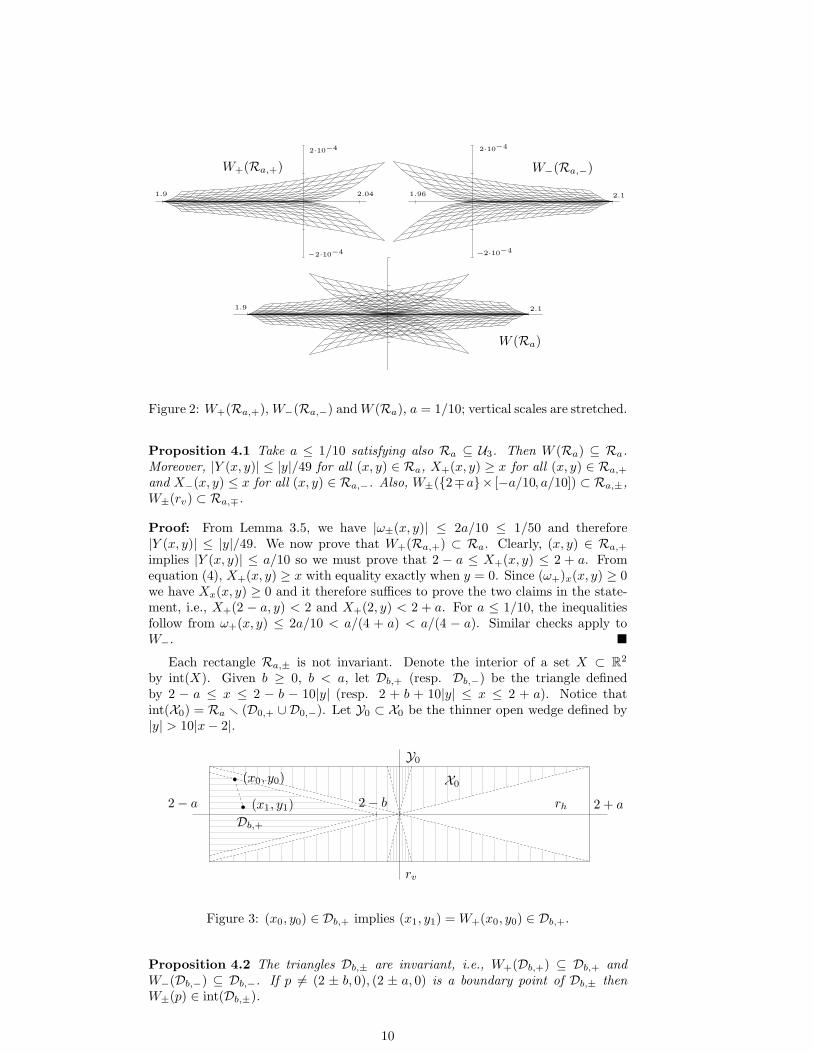
by int(X). Given b ≥ 0, b < a, let Db,+ (resp. Db,−) be the triangle definedby 2 − a ≤ x ≤ 2 − b − 10|y| (resp. 2 + b + 10|y| ≤ x ≤ 2 + a). Notice thatint(X0) = Ra r (D0,+ ∪ D0,−). Let Y0 ⊂ X0 be the thinner open wedge defined by|y| > 10|x− 2|.

(x0, y0)

(x1, y1) 2 − b2 − a 2 + a

Db,+

X0

Y0

rh

rv

Figure 3: (x0, y0) ∈ Db,+ implies (x1, y1) = W+(x0, y0) ∈ Db,+.

Proposition 4.2 The triangles Db,± are invariant, i.e., W+(Db,+) ⊆ Db,+ andW−(Db,−) ⊆ Db,−. If p 6= (2 ± b, 0), (2 ± a, 0) is a boundary point of Db,± thenW±(p) ∈ int(Db,±).

10

Finally, W+(Y0) ⊂ int(D0,−) and W−(Y0) ⊂ int(D0,+).

This will imply (Proposition 5.1) that points in D0,± and Y0 have cubic conver-gence to points in rh different from pX .

Proof: We prove that W+(Db,+) ⊆ Db,+ by computing the slope α of the segmentjoining (x0, y0) and

(x1, y1) = W+(x0, y0) =

(

1 + ω+(x0, y0)

1 − ω+(x0, y0)x0,

ω+(x0, y0)

1 + ω+(x0, y0)y0

)

,

given by

α =−y0

ω+

1 − ω+

2x0(1 + ω+)

where ω+ stands for ω+(x0, y0) (see Figure 3). By Lemma 3.5, |ω±| ≤ 2|y|: simplealgebra then shows that, for a ≤ 1/10, we have |α| > 1/10 and the segment issteeper than the non-vertical sides of Db,+. Since y0 and y1 have the same sign,invariance of Db,+ follows. The argument for Db,− is similar.

The verification that W±(Y0) ⊂ int(D0,∓) uses estimates of the form |y|/2 <|ω±(p)| < 1/20 in the closure of Y0; details are left to the reader. �

Proposition 4.3 Each map W± : int(Ra,±)rrh → Ra is an orientation preservingdiffeomorphism to its image.

Proof: We consider the Jacobian matrix

DW±(x, y) =

2(ω±)x

(1 − (ω±))2x +

1 + (ω±)

1 − (ω±)

2(ω±)y

(1 − (ω±))2x

± (ω±)x

(1 + (ω±))2y ± (ω±)y

(1 + (ω±))2y ± (ω±)

1 + (ω±)

. (5)

From Lemma 3.6, (X±)x > 0 and (Y±)y ≥ 0 with equality precisely for y = 0.Similarly, for y 6= 0, sign((X±)y) = sign((Y±)x) = ±sign(y).

To prove that W± are local diffeomorphisms in int(Ra,±) r rh, write

detDW±(x, y) = ± 1

1 − ω2±

(

2(ω±)xω±x

1 − ω±+ (ω±)yy + ω±(1 + ω±)

)

.

From Lemma 3.6, all terms in the sum in parenthesis have the same sign and thusdetDW±(x, y) > 0 if y 6= 0.

We now prove the injectivity of W+ on int(Ra,+) r rh. From symmetry, itsuffices to prove the injectivity of W+ on Ra,++ = {(x, y) ∈ int(Ra,+) | y ≥ 0}.In other words, given (x1, y1) ∈ Ra, y1 > 0, we must prove that there exists atmost one point (x, y) ∈ Ra,++ with W+(x, y) = (x1, y1). Let γ : [0, 1] → R

2 bethe piecewise affine counterclockwise parametrization of the boundary of Ra,++

with γ(0) = γ(1) = (2 − a, 0), γ(1/4) = (2, 0), γ(1/2) = (2, a/10) and γ(3/4) =(2 − a, a/10). Since detDW+(x, y) > 0 for y > 0 and y1 > 0, (x1, y1) is a regularvalue of W+ and, assuming (x1, y1) /∈ (W+ ◦ γ)([0, 1]), the number of solutions ofW+(x, y) = (x1, y1) is given by the winding number c1 of W+ ◦ γ around (x1, y1).Recall that a simple way to compute 2c1 is to count with signs the intersectionsof W+ ◦ γ with the vertical line through (x1, y1). From the signs of the entries ofDW+, the x coordinate of (W+◦γ)(t) is strictly increasing from t = 0 to t = 1/2 andstrictly decreasing from t = 1/2 to t = 1. Thus, there are at most two intersectionpoints and |c1| ≤ 1 implying injectivity. If (x1, y1) ∈ (W+ ◦ γ)([0, 1]), the argumentabove applies to nearby points and the result follows by continuation outside rh.The proof of the analogous statement for W− is similar. �

11

Actually, the maps W± : Ra,± → Ra are homeomorphisms to their respectiveimages; we omit details.

We conclude the section with some estimates on DW± which will be used in thelast section. A vector v = (v1, v2) is near-horizontal if v1 > 0 and |v2|/v1 < 1/25.

Lemma 4.4 Take p ∈ Ra, p 6= pX . Let v = (v1, v2) be a near-horizontal vector.Then v = DW±(p)v = (v1, v2) is also near-horizontal and 0 < v1/2 < v1 < 10v1.

Proof: From the expressions of the entries of

DW± =

(

m11 m12

m21 m22

)

in equation (5) above and the estimates in Lemma 3.5 and Lemma 3.6,

0.96 < m11 < 5.5, |m12| < 10.5, |m21| < 0.0105, |m22| < 0.045.

The claims now follow from easy computations. �

5 Convergence rates of Wilkinson’s shift strategy

We now consider the asymptotic behavior of Wilkinson’s shift strategy. Given aW-orbit (Tk), Tk+1 = W(Tk), we study the decay of the entry (Tk)23. In (x, y)coordinates, the W -orbits (pk) are defined by pk+1 = W (pk), p0 ∈ Ra; the rele-vant issue is the convergence rate of the y coordinate since, from Proposition 2.1,(φ(x, y))32/y = 2r1/r2

2 > 0 is bounded and bounded away from 0 in Ra.A W -orbit (pk) has strictly quadratic (resp. cubic) convergence if there exist

constants c, C > 0 such that, for all k ∈ N,

c|yk|r ≤ |yk+1| ≤ C|yk|r

for r = 2 (resp. r = 3) (here pk = (xk, yk)).

Proposition 5.1 Let p ∈ Ra r rh, pk = W k(p). If pk ∈ D0,± for some k thenthe W -orbit (pk) has strictly cubic convergence. Otherwise pk ∈ X0 for all k andconvergence is strictly quadratic.

Proof: The case yk = 0 is trivial. Assume without loss that pk ∈ D0,+. FromProposition 4.2, there exists b > 0 such that pk+1 ∈ Db,+ and therefore pj ∈ Db,+

for all j > k. From Proposition 3.1, ω+ is an even, smooth function in the y-variablein Db,+. From compactness and Lemma 3.5, given b > 0 there exists C > 0 suchthat for all (x, y) ∈ Db,+ we have y2 ≤ ω+(x, y) ≤ Cy2. From equation (4),

|y|3/2 ≤ |Y+(x, y)| =ω+

1 + ω+|y| ≤ 2C|y|3

for (x, y) ∈ Db,+, yielding strictly cubic convergence.We now consider orbits in the wedge X0 = X0,+ ∪ X0,−. From Lemma 3.5,

|y|/5 ≤ |ω±(x, y)| ≤ 2|y| for (x, y) ∈ X0,±: strictly quadratic convergence nowfollows from

|y|2/10 ≤ |Y+(x, y)| =ω(x, y)

2 + ω(x, y)|y| ≤ 4|y|2,

completing the proof. �

12

Notice that the constant C in the proof depends on b and therefore the rate ofcubic convergence is not uniform in D0,+, consistent with strictly quadratic conver-gence for orbits in X0.

Corollary 5.2 Given p ∈ Ra r rh, consider the W -orbit pk = W k(p). The follow-ing conditions are equivalent:

(a) limk→∞ pk = pX ;

(b) pk ∈ X0 for all k;

(c) the W -orbit (pk) has strictly quadratic convergence.

Proof: The estimate |Y (x, y)| ≤ |y|/50 guarantees convergence to some point p∞in rh. Orbits contained in X0 must then converge to pX . Conversely, if p∞ 6= pXthen p∞ ∈ int(Db,±) for some b > 0 and pk ∈ Db,± for sufficiently large k. �

Let X ⊂ Ra be the set of points p for which lim pk = pX . From Proposition 4.2,X ⊂ X0 r Y0 and therefore rv ∩ X = rh ∩ X = {pX}. We still need to prove thatX 6= {pX}: this and more will be done in this section.

Figure 4 shows X extended to a rectangle much larger than R1/10: numerical ev-idence indicates that even in such larger regions the qualitative descriptions remainvalid.

A compact set K ⊂ R is a Cantor set if K has empty interior and no isolatedpoints. As we shall prove in Theorem 6.1, horizontal sections of X are Cantor sets.The set X is the union of uncountably many arcs, disjoint except at pX . Each arcintersects a horizontal line in a single point.

The Hausdorff dimension of the middle-third Cantor is log 2/ log 3 ≈ 0.63 ([5]and [6] contain a thorough discussion of Hausdorff dimension). More generally, self-similar Cantor sets have positive Hausdorff dimension. The horizontal sections of Xare much thinner: they have Hausdorff dimension 0. That is why the fine structureis invisible in this figure, unlike most figures of Cantor sets in the quoted books.

Numerical evidence also indicates that the northwest-southeast leg of set X isthe union of a family of analytic curves, tangent (not crossing) at pX : we shall notpursue this matter further.

pX (3, 0)

Figure 4: The set X near pX ; in scale.

We provide another description of X as the intersection of a nested sequence ofcompact sets Xn. From Corollary 5.2, p = p0 ∈ X if and only if pk = W k(p) ∈ X0

for all k. Define Xn ⊂ Ra to be the set of points p ∈ Ra such that pk ∈ X0 for0 ≤ k ≤ n. Thus X0 = X0, Xn+1 = W−1(Xn) ⊂ Xn and X =

⋂

n Xn. Figure5 indicates the first few sets. As the diagram suggests, the interior of Xn has2n+1 connected components which we now describe. In a sense, the Cantor sets onhorizontal lines are limits of this successive doubling of components.

13

PSfrag

X0X (+)1 X (−)

1

X (++)2 X (+−)

2 X (−+)2 X (−−)

2

Figure 5: The upper halves of the sets X0, X±1 and X±±

2 ; schematic.

Decompose the sets Xn by tracking on which side of rv the points pk lie. A signsequence of length n is a function τ : {0, . . . , n − 1} → {+,−} or, equivalently, astring of n signs (τ(0), τ(1), . . . , τ(n − 1)). Define

X τn = {p ∈ Ra | pk ∈ X0,τ(k), 0 ≤ k < n; pn ∈ X0}.

Figure 6 shows a simple example: the upper half of X (+)1 is a curvilinear triangle

with base contained in the top side of Ra,+ and vertex in pX ; the upper half of

X (−)1 is a similar triangle in Ra,−. Also, X (+)

1 = W−1+ (X0) ∩Ra,+ ⊂ X0.

A B C

W−1+ (A) W−1

+ (B) W−1+ (C)

X (+)1

pX

X0 ∩ W+(Ra,+)

W+(Ra,+)

Figure 6: The upper halves of X0 ∩ W+(Ra,+) and X (+)1 = W−1

+ (X0); schematic.

We also consider infinite sign sequences, i.e., functions σ : N → {+,−}, and thecorresponding sets

X σ =⋂

n∈N

X σ|{0,1,...,n−1}n .

Let Σ be the set of infinite sign sequences: Σ admits the natural metric d(σ1, σ2) =2−n where n is the smallest number for which σ1(n) 6= σ2(n). The metric space Σis homeomorphic to the middle-third Cantor set contained in [0, 1]. The sets X σ

are compact, the intersection of two distinct such sets is {pX} and the union of allX σ is X . We conclude this section by proving that the intersection of each X σ witha horizontal line is not empty.

Let ℓ± be the sides y = ±a2, −a ≤ x ≤ a, of Ra.

Proposition 5.3 Let γh : [0, 1] → Ra r{pX} be a parametrized curve with γh(0) ∈D0,+, γh(1) ∈ D0,−. Let σ be an infinite sign sequence: there exists t ∈ [0, 1] suchthat γh(t) ∈ X σ.

Notice that we do not claim that such t is unique: this requires stronger hypoth-esis and will be discussed in the next section.

Proof: We first prove by induction on n that the connected component containingpX of each set X τ

n has elements on the sides ℓ± (here τ is a sign sequence of length

14

n). The case n = 0 is trivial and the case n = 1 has already been discussed (Figure6). Assume the connected component of X τ

n containing pX to have a point in ℓ+.Consider a path γv : [0, 1] → X τ

n with γv(0) = pX , γv(1) ∈ ℓ+. The image of γv

must intersect the curve W+(ℓ+): let t0 be the smallest t in this intersection. Theimage of the restriction of γv to [0, t0] is contained in W+(Ra,+). Since W+ is ahomeomorphism on its image (Proposition 4.3), there exists γv+ : [0, t0] → Ra,+

with W+(γv+(t)) = γv(t) for all t. Also, the image of γv+ is contained in X (+,τ)n+1 . A

similar construction works for ℓ− and for X (−,τ)n+1 , completing the proof of the claim.

Consider an infinite sign sequence σ and its restrictions τn = σ|{0,1,...,n−1}. Foreach n let

Kn = {t ∈ [0, 1] | γh(t) ∈ X τnn }.

The sets Kn are nested, compact and nonempty and therefore their intersection isalso nonempty. Any t in the intersection satisfies γh(t) ∈ X σ. �

As we shall see in the last section, the sets X τn and X σ are connected but the

proof of this fact requires more careful estimates.

6 Geometry of XThe main result of this section, Theorem 6.1, is that X is very thin, almost as thinas a finite union of curves. More precisely, X has Hausdorff dimension 1.

Denote the length of an interval I by µ(I). Given an infinite sign sequenceσ, define σ♯ by σ♯(k) = σ(k + 1) (this is the standard shift operator in symbolicdynamics). Similarly, for a sign sequence τ of length n+1 let τ ♯ be the sign sequenceof length n defined by τ ♯(k) = τ(k + 1).

Theorem 6.1 For any infinite sign sequence σ, the set X σ is a curve X σ ={(gσ(y), y), y ∈ [−a/10, a/10]} where gσ : [−a/10, a/10] → [2 − a, 2 + a] is a Lips-

chitz function. Wilkinson’s step takes curves to curves: W (X σ) ⊂ X σ♯

. The set Xhas Hausdorff dimension 1 and the intersection of X with any horizontal line is aCantor set of Hausdorff dimension 0.

We need a few preliminary definitions. A near-horizontal curve is a C1 functionγ : I → Ra r {pX} such that, for all t in the interval I, the tangent vector γ′(t) isnear-horizontal (as defined at the end of Section 4). A near-horizontal curve γ isstandard if the first coordinate of γ(t) is x = t. For any near-horizontal curve γ thereexists a unique strictly increasing C1 function α, the standard reparametrization ofγ, for which γ = γ ◦ α is standard. The height of a near-horizontal curve γ isy∗ = γ(2) so that γ crosses rv at (2, y∗).

Near-horizontality is preserved by Wilkinson’s step: from Lemma 4.4, if γ : I →Ra,+ r{pX} (resp. Ra,− r{pX}) is a near-horizontal curve then so is W+ ◦γ (resp.W− ◦ γ). This process squeezes near-horizontal curves towards the line rh. Theconstant 1/25 in the definition is somewhat arbitrary but it can not be replaced byvery small numbers since W does not take horizontal lines to horizontal lines.

Recall that Y0 ⊂ X0 is an open wedge with the property that p ∈ Y0 impliesW±(p) ∈ D0,∓. For a sign sequence τ of length n, define

Yτn = {p ∈ Ra | pk ∈ X0,τ(k), 0 ≤ k < n; pn ∈ Y0}.

In particular, the orbit (pk) with p0 ∈ Yτn escapes X0 starting from k = n+1. Also,

Yτn is an open subset of X τ

n disjoint from Xn+1.

15

t0 t1

γ(t0)

γ(t1)

γ(2) = (2, y∗)

D0,+ D0,−

pX = (2, 0)

Figure 7: A near-horizontal curve (not in scale).

Lemma 6.2 Let γ : [t0, t1] → Ra r {pX} be a standard near-horizontal curve.Assume that γ(t0) ∈ D0,+, γ(t1) ∈ D0,−. Let y∗ = γ(2) be the height of γ. Then,for γ(t) = (t, y) ∈ X0,

|y∗|/3 < |y| < 3|y∗|.Let τ be a sign sequence of length n. The sets

Iτn = {t ∈ [t0, t1] | γ(t) ∈ X τ

n }, Jτn = {t ∈ [t0, t1] | γ(t) ∈ Yτ

n}

are intervals and their lengths satisfy

1

10n+1

∣

∣

∣

y∗90

∣

∣

∣

2n

< µ(Jτn) < µ(Iτ

n) < 2n |40y∗|2n

< 2(−2(n−1)).

Proof: As a basis for an inductive proof, we first consider the case n = 0. Set

I0 = {t ∈ [t0, t1] | γ(t) ∈ X0}, J0 = {t ∈ [t0, t1] | γ(t) ∈ Y0}.

Draw lines through the point (2, y∗) with linear coefficients ±1/25, as in Figure 7,and compute their intersections with the diagonals of Ra. Since these diagonalsare steeper than γ, the intersection of the image of γ with X0 is contained in theshaded triangles. An elementary geometric argument proves the first claim, verifiesthat I0 and J0 are intervals and obtains the estimates for their lengths.

X τ♯

n

X τn+1

y♯∗

y∗

γ♯

γ

Iτ♯

nIτn+1

D0,+ D0,−

(x, y)

Figure 8: A near-horizontal curve (not in scale).

We now do the induction step. For a sign sequence τ of length n + 1 withτ(0) = + (the other case is similar), consider

Iτn+1 = {t ∈ [t0, t1] | γ(t) ∈ X τ

n+1}

16

and γ+, the restriction of γ to [t0, 2]. Set γ♯ = W+ ◦ γ+ (see Figure 8): as remarked

above, γ♯ is a near-horizontal curve. Let α♯ : [t♯0, t♯1] → [t0, 2] be the standard

reparametrization of γ♯ so that γ♯ = γ♯ ◦ α♯ is a standard near-horizontal curvewith height y♯

∗ = γ♯(2). Notice that γ♯(t♯0) ∈ D0,+ and γ♯(t♯1) ∈ D0,− so, by theinduction hypothesis, the sets

Iτ♯

n = {t ∈ [t♯0, t♯1] | γ♯(t) ∈ X τ♯

n }, Jτ♯

n = {t ∈ [t♯0, t♯1] | γ♯(t) ∈ Yτ♯

n }

are intervals whose lengths ℓ♯I , ℓ

♯J satisfy

1

10n+1

∣

∣

∣

∣

∣

y♯∗

90

∣

∣

∣

∣

∣

2n

< ℓ♯J < ℓ♯

I < 2n∣

∣40y♯∗

∣

∣

2n

. (6)

Clearly, t ∈ Iτ♯

n (resp. Jτ♯

n ) if and only if α♯(t) ∈ Iτn+1 (resp. Jτ

n+1), proving thatIτn+1 and Jτ

n+1 are intervals; let ℓI , ℓJ be their lengths. By Lemma 4.4, 1/10 <(α♯)′(t) < 2 for all t ∈ In and therefore

(1/10)ℓ♯J < ℓJ < ℓI < 2ℓ♯

I . (7)

Let γ(α♯(2)) = (x, y) so that W+(x, y) = (2, y♯∗). From the first claim, |y∗|/3 <

|y| < 3|y∗|. By Lemma 3.5, (1/5)|y| < ω+(x, y) < 2|y|. Thus, by equation 4,

(1/10)y2 < |y♯∗| < 3y2. Combining these estimates,

∣

∣

∣

y∗90

∣

∣

∣ >

∣

∣

∣

∣

∣

y♯∗

90

∣

∣

∣

∣

∣

2

,∣

∣40y♯∗

∣

∣ < |40y∗|2 . (8)

The required estimate now follows from estimates 6, 7, 8 and the fact that |y∗| ≤a/10 ≤ 1/100. �

Proof of Theorem 6.1: We organize the proof by stating a few claims, mostof which in terms of a standard near-horizontal curve γ; notation will be borrowedfrom Lemma 6.2. For a sign sequence τ of length n, consider the sign sequences(τ, +) and (τ,−) of length n + 1.

(a) The intervals I(τ,+)n+1 and I

(τ,−)n+1 are contained in different connected components

of Iτn r Jτ

n .This claim is proved by induction. The case n = 0 follows from the inclusions

X±1 ⊂ X0,±rY0. The induction step employs the same construction used in Lemma

6.2: for γ♯ = W+ ◦ γ ◦ α♯, the standard reparametrization α♯ maps the intervalsconstructed from τ ♯ to the corresponding intervals for τ .

(b) For an infinite sign sequence σ there is a unique tσ ∈ [t0, t1] with γ(tσ) ∈ X σ.This follows directly from Lemma 6.2 since

limn→∞

µ(Iσ|{0,1,...,n−1}n ) = 0.

In particular, a horizontal line at height y (which is near-horizontal) meets X σ ata single point (gσ(y), y). The Lipschitz estimate |gσ(y1) − gσ(y2)| ≤ 25|y1 − y2|likewise follows by taking lines of slope less than 1/25.

(c) Let σ1 and σ2 be distinct sign sequences and n be the smallest integer for whichσ1(n) 6= σ2(n). Then

1

10n+1

∣

∣

∣

y∗90

∣

∣

∣

2n

< |tσ1 − tσ2 | < 2n |40y∗|2n

< 2(−2(n−1)).

17

Let τ be the restriction of σ1 or σ2 to {0, 1, . . . , n−1}. Without loss, tσ1 ∈ I(τ,+)n+1

and tσ2 ∈ I(τ,−)n+1 : Lemma 6.2 and claim (a) obtain the inequalities.

In particular, the map from the Cantor set Σ to K = {t ∈ [t0, t1] | γ(t) ∈ X}taking σ to tσ is a homeomorphism.

We now construct a very thin open cover of K. For a positive integer n letS+

n ⊂ Σ be the set of the 2n sign sequences σ for which k ≥ n implies σ(k) = +.Let Br(p) be the ball of radius r and center p.

(d) Take r > 0 and let n be a positive integer such that r > 2(−2(n−1)). Then the

balls Br(tσ+

) ⊂ R, σ+ ∈ S+n , form an open cover of K.

From step (b), given t ∈ K there is some σ ∈ Σ for which t = tσ. Let σn ∈ S+n

be defined by

σn(k) =

{

σ(k), 0 ≤ k < n,

+, k ≥ n

so that σn ∈ S+n . From claim (c), |tσn − tσ| < 2(−2(n−1)) and therefore t ∈ Br(t

σn).The open cover of K above is now adapted to yield a thin open cover of X . For

a positive integer m, let Ym ⊂ [−a/10, a/10] be a set of 2m equally spaced pointsso that given y ∈ [−a/10, a/10] there is y0 ∈ Ym with |y − ym| < a/(10m). Also,for positive integers n and m, let Xn,m ⊂ X be the set of m2(n+1) elements of theform (gσ(y), y), σ ∈ S+

n , y ∈ Ym.

(e) Consider r > 0 and positive integers n and m such that r > 2(1−2(n−1)) andr > 1/m. Then the balls Br(p) ⊂ R

2, p ∈ Xn,m, form an open cover of X .Given p = (gσ(y), y) let y0 be the point of Ym closest to y and let σn ∈ S+

n bedefined as in claim (d). Let p1 = (gσn(y), y) and p0 = (gσn(y0), y0). Notice thatp0 ∈ Xn,m. In order to prove that p belongs to Br(p0) we estimate |p − p1| and|p1−p0|. From claim (d), |p−p1| < r/2. Since a ≤ 1/10, |y−y0| < a/(10m) ≤ r/100;from the Lipschitz estimate after claim (b), |gσ0(y) − gσ0(y0)| ≤ r/4 and therefore|p1 − p0| < r/2.

(f) The set K has Hausdorff dimension 0.Given r > 0, let n = ⌈1 + log2(− log2 r)⌉. Claim (d) obtains on open cover of K

by 2n < −4 log2 r balls of radius r. For all d > 0 we have

limr→0

(−4 log2 r)rd = 0.

Thus, µd(K), the Hausdorff measure of dimension d of K, equals 0.

(g) The set X has Hausdorff dimension 1.Since X contains curves this dimension is at least one. It suffices therefore to

prove that µd(X ) = 0 for all d > 1.Given r > 0, let n = ⌈2 + log2(− log2 r)⌉ and m = ⌈1/r⌉. Claim (e) obtains an

open cover of X by m2n+1 < −32(log2 r)r−1 balls of radius r. For all d > 1 we have

limr→0

−32(log2 r)r−1rd = 0.

This implies µd(X ) = 0, proving the claim and completing the proof of the theorem.�

7 Conclusion

Recall that ω+(T ) and ω−(T ) are the roots of a quadratic polynomial with smoothcoefficients (in T ). The algorithm to obtain ω given T is thus multivalued: invariables x and y, the domains of choice of each sign are rectangles sharing the line

18

rv. In a sense, dynamical systems techniques arose naturally in this paper becauseorbits may switch sides arbitrarily often and according to arbitrary patterns (signsequences). An outstanding example of the use of sign sequences to label orbits arekneading sequences ([11]). Many numerical algorithms do not exhibit this kind ofcomplexity.

Unsurprisingly, the set X of atypical points is more complicated than an al-gebraic surface. This is why Hausdorff dimension becomes the relevant tool toquantify the size of X . Theorem 6.1 shows that X is very thin.

A matrix is an AP-matrix if its spectrum contains an arithmetic progressionwith three terms and is AP-free otherwise. This paper concentrated on the sim-plest examples of AP-matrices, with eigenvalues −1, 0 and 1. We conjecture thatthe presence of three term arithmetic progressions in the spectrum (and whetherthe three eigenvalues are consecutive) dictates the possible rates of convergence ofWilkinson’s shift. In a forthcoming paper we show that for AP-free tridiagonalmatrices, cubic convergence of Wilkinson’s shift indeed holds ([9], [10]).

Acknowledgements: The editorial board of FoCM did an extraodinary job inarticulating a diverse collection of referees which led to a far more readable text. Weare very grateful to these editors and referees. The authors acknowledge supportfrom CNPq, CAPES, IM-AGIMB and Faperj.

References

[1] Batterson, S. and Smillie, J., Rayleigh quotient iteration for nonsymmetricmatrices, Math. of Comp., 55, 169-178, 1990.

[2] de Boor, C. and Golub, G. H., The numerically stable reconstruction of aJacobi matrix from spectral data, Lin. Alg. Appl. 21, 245-260, 1978.

[3] Deift, P., Nanda, T., Tomei, C., Differential equations for the symmetriceigenvalue problem, SIAM J. Num. Anal. 20, 1-22, 1983.

[4] Demmel, J. W., Applied Numerical Linear Algebra, SIAM, Philadelphia,1997.

[5] Falconer, K. J., Fractal geometry: mathematical foundations and applica-tions, John Willey, Chichester, 2003.

[6] Federer, H., Geometric measure theory, Classics in Mathematics, Springer-Verlag, New York, 1996.

[7] Gragg, W. B. and Harrod, W. J., The numerically stable reconstruction ofJacobi matrices from spectral data, Numer. Math. 44, 317-335, 1984.

[8] Leite, R. S., Saldanha, N.C. and Tomei, C., An atlas for tridiagonal isospectralmanifolds, Linear Algebra Appl. 429, 387-402, 2008.

[9] Leite, R. S., Saldanha, N.C. and Tomei, C., The asymptotic of Wilkinson’sshift: cubic convergence for generic spectra, in preparation.

[10] Leite, R. S., Saldanha, N.C. and Tomei, C., The asymptotics of Wilkinson’sshift iteration, preprint, http://www.arxiv.org/abs/math.NA/0412493.

[11] Milnor, J. and Thurston, W., On iterated maps of the interval, in DynamicalSystems (ed. Alexander, J. C.), Lecture Notes in Math. 1342, 465-563, NewYork: Springer-Verlag, 1988.

19

[12] Moser, J., Finitely many mass points on the line under the influence ofan exponential potential, in Dynamic systems theory and applications (ed.J. Moser), Lecture Notes in Phys. 38, 467-497, New York, 1975.

[13] Parlett, B. N., The Symmetric Eigenvalue Problem, Prentice-Hall, EnglewoodCliffs, NJ 1980.

[14] Tomei, C., The Topology of Manifolds of Isospectral Tridiagonal Matrices,Duke Math. J., 51, 981-996, 1984.

[15] Wilkinson, J. H., The algebraic eigenvalue problem, Oxford University Press,1965.

Ricardo S. Leite, Departamento de Matematica, UFESAv. Fernando Ferrari, 514, Vitoria, ES 29075-910, Brazil

Nicolau C. Saldanha and Carlos Tomei, Departamento de Matematica, PUC-RioR. Marques de S. Vicente 225, Rio de Janeiro, RJ 22453-900, Brazil

rsleite@pq.cnpq.brnicolau@mat.puc-rio.br; http://www.mat.puc-rio.br/∼nicolau/tomei@mat.puc-rio.br

20