arX

iv:1

212.

6526

v4 [

cs.IT

] 10

Sep

201

3PREPRINT, SEPTEMBER 11, 2013. 1

High-SNR Asymptotics of Mutual Information forDiscrete Constellations with Applications to BICM

Alex Alvarado, Fredrik Brannstrom, Erik Agrell, and Tobias Koch

Abstract—Asymptotic expressions of the mutual informationbetween any discrete input and the corresponding output of thescalar additive white Gaussian noise channel are presentedin thelimit as the signal-to-noise ratio (SNR) tends to infinity. Asymp-totic expressions of the symbol-error probability (SEP) and theminimum mean-square error (MMSE) achieved by estimatingthe channel input given the channel output are also developed. Itis shown that for any input distribution, the conditional entropyof the channel input given the output, MMSE and SEP have anasymptotic behavior proportional to the Gaussian Q-function.The argument of the Q-function depends only on the minimumEuclidean distance (MED) of the constellation and the SNR, andthe proportionality constants are functions of the MED and theprobabilities of the pairs of constellation points at MED. Thedeveloped expressions are then generalized to study the high-SNR behavior of the generalized mutual information (GMI) forbit-interleaved coded modulation (BICM). By means of theseasymptotic expressions, the long-standing conjecture that Graycodes are the binary labelings that maximize the BICM-GMI athigh SNR is proven. It is further shown that for any equallyspaced constellation whose size is a power of two, there alwaysexists an anti-Gray code giving the lowest BICM-GMI at highSNR.

Index Terms—Anti-Gray code, additive white Gaussian noisechannel, bit-interleaved coded modulation, discrete constellations,Gray code, minimum-mean square error, mutual information,high-SNR asymptotics.

I. I NTRODUCTION

W E consider the discrete-time, real-valued, additivewhite Gaussian noise (AWGN) channel

Y =√ρX + Z (1)

whereX is the transmitted symbol;Z is a Gaussian randomvariable, independent ofX , with zero mean and unit variance;and ρ > 0 is an arbitrary scale factor. The capacity ofthe AWGN channel (1) under an average-power constraint

Research supported by the European Community’s Seventh’s Frame-work Programme (FP7/2007-2013) under grant agreements No.271986 andNo. 333680, by the Swedish Research Council, Sweden (under grants #621-2006-4872 and #621-2011-5950) and by the Ministerio de Economıa yCompetitividad of Spain (TEC2009-14504-C02-01, CSD2008-00010, andTEC2012-38800-C03-01). This work was presented in part at the IEEEInternational Symposium on Information Theory, Istanbul,Turkey, July 2013,and at the IEEE Communication Theory Workshop, Phuket, Thailand, June2013.

A. Alvarado is with the Dept. of Engineering, University of Cambridge,Cambridge CB2 1PZ, United Kingdom (email: alex.alvarado@ieee.org).

E. Agrell and F. Brannstrom are with the Dept. of Signals and Sys-tems, Chalmers Univ. of Technology, SE-41296 Goteborg, Sweden (email:{fredrik.brannstrom, agrell}@chalmers.se).

T. Koch is with the Department of Signal Theory and Communica-tions, Universidad Carlos III de Madrid, 28911 Leganes, Spain (email:koch@tsc.uc3m.es).

ρEX [X2] ≤ γ is given by [1]

Caw(γ) =1

2log(1 + γ) (2)

where γ can be viewed as the maximal allowed signal-to-noise ratio (SNR). Although inputs distributed according tothe Gaussian distribution attain the capacity, they sufferfromseveral drawbacks which prevent them from being used inpractical systems. Among them, especially relevant are theunbounded support and the infinite number of bits needed torepresent signal points. In practical systems, discrete distribu-tions are typically preferred.

The mutual information (MI) between the channel inputXand the channel outputY of (1), where the distribution ofX is constrained to be a probability mass function (PMF)over a discrete constellation, represents the maximum rateatwhich information can be reliably transmitted over (1) usingthat particular constellation. While the low-SNR asymptoticsof the MI for discrete constellations are well understood (see[1]–[4] and references therein), to the best of our knowledge,only upper and lower bounds are known for the high-SNRbehavior [5]–[7]. It was observed in [6, p. 1073] that fordiscrete constellations, maximizing the MI is equivalent tominimizing either the symbol-error probability (SEP) or theminimum mean-square error (MMSE) in estimatingX fromY . In [8, App. E], two constellations with different minimumEuclidean distances (MEDs) are compared, and it is shownthat, for sufficiently large SNR, the constellation with largerMED gives a higher MI. Upper and lower bounds on theMI and MMSE for multiple-antenna systems over fadingchannels can be found in [9]–[11]. Using the Mellin transform,asymptotic expansions for the MMSE and MI for scalar andvectorial coherent fading channels were recently derived in[12].

In this paper, we study the high-SNR asymptotics of the MIfor discrete constellations. In particular, we consider arbitraryconstellations and input distributions (independent ofρ) andfind exact asymptotic expressions for the MI in the limitas the SNR tends to infinity. Exact asymptotic expressionsfor the MMSE and SEP are also developed. We prove thatfor any constellation and input distribution, the conditionalentropy of X given Y , the MMSE, and the SEP have anasymptotic behavior proportional toQ

(√ρd/2

), whereQ(·)

is the Gaussian Q-function andd is the MED of the constel-lation. While this asymptotic behavior has been demonstratedfor uniform input distributions (e.g., [6, eqs. (36)–(37)], [6,Sec. II-C], [9, Sec. III], [11, Sec. III]), we show that it holdsfor any discrete input distribution that does not depend on the

2 PREPRINT, SEPTEMBER 11, 2013.

SNR. Furthermore, in contrast to previous works, we provideclosed-form expressions for the coefficients in front of theQ-functions, thereby characterizing the asymptotic behavior ofthe MI, MMSE, and SEP more accurately.

While these asymptotic results are general, we use themto study bit-interleaved coded modulation (BICM) [13]–[15],which can be viewed as a pragmatic approach for codedmodulation [15, Ch. 1]. The key element in BICM is the useof a (suboptimal) bit-wise detection rule, which was cast in[16] as a mismatched decoder. BICM is used in many of thecurrent wireless communications standards, e.g., HSPA, IEEE802.11a/g/n, and the DVB standards (DVB-T2/S2/C2).

The BICM generalized mutual information (BICM-GMI) isan achievable rate for BICM [16] and depends heavily on thebinary labeling of the constellation. The optimality of a Graycode (GC) in the sense that it maximizes the BICM-GMI wasconjectured in [14, Sec. III-C]; however, it was shown in [17]that for low and medium SNRs, there exist other labelings thatgive a higher BICM-GMI (see also [18, Ch. 3]). For furtherresults on BICM at low SNR see [19]–[22]. On the other hand,numerical results presented in [18, Ch. 3] and [23] suggest thatGCs are indeed optimal at high SNR in terms of BICM-GMI.However, to the best of our knowledge, the optimality of GCsat high SNR has never been proven.

In this paper, we derive an asymptotic expression for theBICM-GMI as a function of the constellation, input distribu-tion, and binary labeling. Using this expression, we then provethe optimality of GCs at high SNR. Using the MI-MMSErelationship, an asymptotic expression for the derivativeofthe BICM-GMI is also developed. The obtained asymptoticexpressions for the BICM-GMI and its derivative, as well asthe one for the bit-error probability (BEP), are all shown toconverge to their asymptotes proportionally toQ

(√ρd/2

).

This paper is organized as follows. In Sec. II, the notationconvention and system model are presented. The asymptoticsof the MI and MMSE are presented in Sec. III and BICM isstudied in Sec. IV. The conclusions are drawn in Sec. V.

II. PRELIMINARIES

A. Notation Convention

Row vectors are denoted by boldface lettersx =[x1, x2, . . . , xM ] and sets are denoted by calligraphic lettersX . An exception is the set of real numbers, which is denotedby R. All the logarithms are natural logarithms and all theMIs are therefore given in nats. Probability density functions(PDFs) and conditional PDFs are denoted byfY (y) andfY |X(y|x), respectively. Analogously, PMFs are denoted byPX(x) andPX|Y (x|y). Expectations over a random variableX are denoted byEX [·].

B. Model

We consider the discrete-time, real-valued AWGN chan-nel (1). The transmitted symbolsX belong to a real, one-dimensionalconstellationX , {x1, x2, . . . , xM} whereM =2m, and they are, without loss of generality, assumed to bedistinct and ordered, i.e.,x1 < x2 < · · · < xM . Each symbolis transmitted with probabilitypi , PX(xi), 0 < pi < 1, and

the vector of probabilitiesp , [p1, . . . , pM ] is called theinputdistribution. We assume that neither the constellation nor theinput distribution depends onρ. We denote the set of indicesin X andp with IX , {1, . . . ,M}.

The transmitted average symbol energy is

Es , EX [X2] =∑

i∈IX

pix2i . (3)

It follows that the SNR isγ = ρEs.

An M -ary pulse-amplitude modulation (MPAM) constella-tion havingM equally spaced symbols (separated by2∆) isdenoted byE , {xi = −(M − 2i + 1)∆ : i = 1, . . . ,M}. Auniform distribution ofX is denoted byP u

X , i.e., pi = 1/M∀i. A uniform input distribution withX = E is denoted byP euX , where in this case∆2 = 3Es/(M

2 − 1).

The Gaussian Q-function is defined as

Q(x) ,1√2π

∫ ∞

x

e−12 ξ

2

dξ. (4)

The entropy of the random variableX is defined as

HPX, −EX [log (PX(X))] (5)

the MI betweenX andY , I(X ;Y ), as

IPX(ρ) , EX,Y

[log(fY |X(Y |X)/fY (Y )

)](6)

and the MMSE as

MPX(ρ) , EX,Y [(X − Xme(Y ))2] (7)

whereXme(y) , EX [X |Y = y] is the conditional (posterior)mean estimator (ME). We further define the SEP as

SPX(ρ) , Pr{Xmap(Y ) 6= X} (8)

whereX is the transmitted symbol and

Xmap(y) , argmaxx∈X

PX|Y (x|y) (9)

is the decision made by a maximum a posteriori probability(MAP) symbol demapper.

The MED of the constellation is defined as

d , mini,j∈IX :i6=j

|xi − xj |. (10)

We further defineAX as twice the number of pairs ofconstellation points at MED, i.e.,

AX ,∑

i∈IX

∑

j∈IX

|xi−xj |=d

1. (11)

By using the fact that for any real-valued constellation thereare at least one and at mostM−1 pairs of constellation pointsat MED, we obtain the bound

2 ≤ AX ≤ 2(M − 1). (12)

The upper bound is achieved by anMPAM constellation, forwhich

AE = 2(M − 1). (13)

3

Finally, for a givenPX , we define the constant

BPX,∑

i∈IX

∑

j∈IX

|xi−xj|=d

√pjpi. (14)

For a uniform input distribution,PX = P uX , and thus,

BPuX=

AXM

. (15)

Example 1:Consider an unequally spaced4-ary constella-tion with x1 = −4, x2 = −2, x3 = 2, andx4 = 4, and theinput distributionpi = i/10 with i = 1, 2, 3, 4. The MED in(10) is d = 2, Es in (3) is Es = 10, AX in (11) is AX = 4(two pairs of constellation points at MED), andBPX

in (14)is BPX

= 2√p1p2 + 2

√p3p4 ≈ 0.98.

III. H IGH-SNR ASYMPTOTICS

There exists a fundamental relationship between the MI andthe MMSE for AWGN channels [24] (see also [25, Ch. 2]):

d

dρIPX

(ρ) =1

2MPX

(ρ). (16)

Exploiting this MI-MMSE relation, bounds on the MI canbe used to derive bounds on the MMSE andvice versa. Therelationship in (16) will be used in the proof of Theorem 1.

Upper and lower bounds on the MI and MMSE for discreteconstellations at high SNR can be found, e.g., in [5]–[7],[9]–[12]. While these bounds describe the correct asymptoticbehavior, they are, in general, not tight in the sense that theratio between them does not tend to one asρ → ∞. In whatfollows, we present exact asymptotic expressions for the MIand MMSE for any arbitraryPX . We further present exactasymptotic expressions for the SEP.

A. Asymptotics of the MI, MMSE, and SEP

For any given input distributionPX , the MI tends toHPX

asρ tends to infinity. In the following we study how fast theMI converges towards its maximumHPX

by analyzing thedifferenceHPX

− IPX(ρ), i.e., by analyzing the conditional

entropy of X given Y . Theorem 1 is the main result ofthis paper and characterizes the high-SNR behavior of theconditional entropyH(X |Y ) = HPX

− IPX(ρ).

Theorem 1:For anyPX

limρ→∞

HPX− IPX

(ρ)

Q(√

ρd/2) = πBPX

(17)

whereBPXis given by (14).

Proof: See Appendix A.Similar to Theorem 1, we have the following asymptotic

expressions for the MMSE and the SEP.Theorem 2:For anyPX

limρ→∞

MPX(ρ)

Q(√

ρd/2) =

πd2

4BPX

. (18)

Proof: See Appendix B.Theorem 3:For anyPX

limρ→∞

SPX(ρ)

Q(√

ρd/2) = BPX

. (19)

Proof: See Appendix C.Theorems 1–3 reveal that, at high SNR, the MI, MMSE,

and SEP behave as

IPX(ρ) ≈ HPX

− πBPXQ (

√ρd/2) (20)

MPX(ρ) ≈ πd2

4BPX

Q (√ρd/2) (21)

SPX(ρ) ≈ BPX

Q (√ρd/2) . (22)

The results in (20)–(22) show that for any input distribution,the conditional entropy, MMSE, and SEP have the same high-SNR behavior: i.e., they are all proportional to a GaussianQ-function, where the proportionality constants depend ontheinput distribution and, in the case of the MMSE, also on theMED of the constellation.

Remark 1:While the results presented in this section werederived only for one-dimensional (real-valued) constellations,they directly generalize to multidimensional constellations thatare constructed asordered direct products[21, eq. (1)] of one-dimensional constellations. For example, the results directlygeneralize to rectangular quadrature amplitude modulationconstellations.

B. Discussion and Examples

For a uniform input distribution (PX = P uX ), Theorems 1–3

particularize to the following result.Corollary 4: For anyX and a uniform input distribution

limρ→∞

logM − IPuX(ρ)

Q(√

ρd/2) = π

AXM

(23)

limρ→∞

MPuX(ρ)

Q(√

ρd/2) =

πd2

4

AXM

(24)

limρ→∞

SPuX(ρ)

Q(√

ρd/2) =

AXM

(25)

whereAX is given by (11).Proof: From Theorems 1–3 and (15).

The expression (25) corresponds to the well-known high-SNR approximation for the SEP [26, eq. (2.3-29)]. Corollary4shows that for a uniform input distribution, the MI, the MMSE,and the SEP for discrete constellations in the high-SNR regimeare functions of the MED of the constellation and the numberof pairs of constellation points at MED.

For MPAM and a uniform input distribution (PX = P euX ),

it follows from Corollary 4 and (13) that

IP euX(ρ) ≈ logM − 2π(M − 1)

MQ (

√ρd/2) (26)

MP euX(ρ) ≈ 6πEs

M(M + 1)Q (

√ρd/2) (27)

SP euX(ρ) ≈ 2(M − 1)

MQ (

√ρd/2) . (28)

Table I summarizes the results obtained in Theorems 1–3,Corollary 4, and (26)–(28).

Example 2: In Fig. 1, we showlogM − IP euX(ρ) for 4PAM

and 16PAM with uniform input distributions1 together with

1Calculated numerically using Gauss–Hermite quadratures [23, Sec. III]with 300 quadrature points.

4 PREPRINT, SEPTEMBER 11, 2013.

TABLE ISUMMARY OF ASYMPTOTICS OFMI, MMSE, AND SEP.

Input Distribution PX P u

X P eu

X

limρ→∞

HPX − IPX (ρ)

Q(√

ρd/2) πBPX π

AX

M

2π(M − 1)

M

limρ→∞

MPX (ρ)

Q(√

ρd/2)

πd2

4BPX

πd2

4

AX

M

6πEs

M(M + 1)

limρ→∞

SPX (ρ)

Q(√

ρd/2) BPX

AX

M

2(M − 1)

M

0

0.1

0.2

0.3

0.4

0.5

0.6

0.7

0.8

0.9

1

5 10 15 20 25 30 3510

−6

10−5

10−4

10−3

10−2

10−1

100

101

ρ [dB]

logM

−I P

eu

X(ρ)

[nat

s/sy

mb

ol]

ExactAsymptoticLB [6]UB [6]LB [11]UB [11]

4PAM

16PAM

Fig. 1. logM − IP euX

(ρ) for 4PAM and16PAM (solid lines) constellations(normalized toEs = 1) and the asymptotic expression in (26) (thick dashedlines). The lower and upper bounds [6, eq. (34)–(35)] and [11, eq. (17)–(19)]are also shown.

the asymptotic expression in (26). We also show the lower andupper bounds derived in [6, eq. (34)–(35)] and [11, eq. (17)–(19)]. Observe that (26) approximatesIP eu

X(ρ) accurately for a

large range of SNR. In Fig. 2, analogous results for the MMSEare presented, where the bounds derived in [6, eq. (30)–(31)]and [11, eq. (13)–(15)] are also included. Again, the asymp-totic expression (27) approximates the MMSE accurately fora large range of SNR. For other examples with unequallyspaced4-ary constellations and nonuniform input distributionssee [27, Example 3].

Remark 2: It follows from Corollary 4 that the constellationthat maximizes the MI (or equivalently, the constellation thatminimizes the MMSE and the SEP) at high SNR is theconstellation that first maximizes the MED and then minimizesAX . It is easy to see that the one-dimensional constellation thatmaximizes the MED for a givenEs is theMPAM constellation(X = E).

IV. A PPLICATION: BINARY LABELINGS FOR

BIT-INTERLEAVED CODED MODULATION

BICM can be viewed as a pragmatic approach for codedmodulation. In BICM (see Fig. 3), the encoder is realized as aserial concatenation of a binary encoder, a bit-level interleaver,

0

0.1

0.2

0.3

0.4

0.5

0.6

0.7

0.8

0.9

1

0 5 10 15 20 25 30 3510

−6

10−5

10−4

10−3

10−2

10−1

100

101

ρ [dB]

MP

eu

X(ρ)

ExactAsymptoticLB [6]UB [6]LB [11]UB [11]

4PAM

16PAM

Fig. 2. MP euX

(ρ) for 4PAM and 16PAM (solid lines) constellations(normalized toEs = 1) and the asymptotic expression in (27) (thick dashedlines). The lower and upper bounds [6, eq. (30)–(31)] and [11, eq. (13)–(15)]are also shown.

and a memoryless mapper; see [13]–[15] for more details.A key element in BICM is the memoryless mapperΦ :{0, 1}m → X , which maps the coded bitsQ = [Q1, . . . , Qm]to constellation symbols. At the receiver side, the demappercomputes a bit metric, typically in the form of a logarithmiclikelihood ratio (LLR)

Λk , logfY |Qk

(y|1)fY |Qk

(y|0) (29)

for k = 1, . . . ,m. The vector of LLRsΛ = [Λ1, . . . ,Λm] isdeinterleaved and then decoded.

The BICM-GMI is an achievable rate for BICM, and thus,is an important quantity for such systems. In this section, wegeneralize the results in Sec. III to obtain asymptotic expres-sions for the BICM-GMI. We further study the relationshipbetween the BICM-GMI and the BEP as well as the derivativeof the BICM-GMI with respect toρ. Finally, we show that athigh SNR, GCs maximize BICM-GMI for one-dimensionalconstellations and uniform input distributions.

A. BICM Model

A binary labeling for a constellation is defined by thevector l = [l1, l2, . . . , lM ] where li ∈ {0, 1, . . . ,M − 1} isthe integer representation of theith length-m binary labelqi = [qi,1, . . . , qi,m] ∈ {0, 1}m associated with the symbolxi, with qi,1 being the most significant bit. The labelingdefines2m subconstellationsXk,b ⊂ X for k = 1, . . . ,mand b ∈ {0, 1}, given byXk,b , {xi ∈ X : qi,k = b} with|Xk,b| = M/2. We defineIXk,b

⊂ {1, . . . ,M} as the indicesof the symbols inX that belong toXk,b.

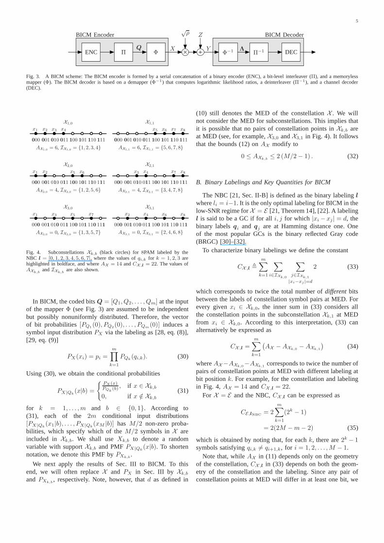
Example 3: In Fig. 4, we show the6 subconstellationsfor an 8PAM constellation labeled by the NBCl =[0, 1, 2, 3, 4, 5, 6, 7] [21, Sec. II-B], as well as the correspond-ing values ofIXk,b

andAXk,b(defined below).

5

BICM Encoder

QENC Π Φ

X

√ρ Z

YΦ−1 Π−1 DEC

Λ

BICM Decoder

Fig. 3. A BICM scheme: The BICM encoder is formed by a serial concatenation of a binary encoder (ENC), a bit-level interleaver (Π), and a memorylessmapper (Φ). The BICM decoder is based on a demapper (Φ−1) that computes logarithmic likelihood ratios, a deinterleaver (Π−1), and a channel decoder(DEC).

0

0.1

0.2

0.3

0.4

0.5

0.6

0.7

0.8

0.9

1

x1

x1

x1

x2

x2

x2

x3

x3

x3

x4

x4

x4

x5

x5

x5

x6

x6

x6

x7

x7

x7

x8

x8

x8

000000 001001 010010 011011 100100 101101 110110 111111

000000 001001 010010 011011 100100 101101 110110 111111

000000 001001 010010 011011 100100 101101 110110 111111

X1,0 X1,1

X2,0 X2,1

X3,0 X3,1

AX1,0 = 6, IX1,0 = {1, 2, 3, 4} AX1,1 = 6, IX1,1 = {5, 6, 7, 8}

AX2,0 = 4, IX2,0 = {1, 2, 5, 6} AX2,1 = 4, IX2,1 = {3, 4, 7, 8}

AX3,0 = 0, IX3,0 = {1, 3, 5, 7} AX3,1 = 0, IX3,1 = {2, 4, 6, 8}

Fig. 4. SubconstellationsXk,b (black circles) for8PAM labeled by theNBC l = [0, 1, 2, 3, 4, 5, 6, 7], where the values ofqi,k for k = 1, 2, 3 arehighlighted in boldface, and whereAX = 14 andCX ,l = 22. The values ofAXk,b

andIXk,bare also shown.

In BICM, the coded bitsQ = [Q1, Q2, . . . , Qm] at the inputof the mapperΦ (see Fig. 3) are assumed to be independentbut possibly nonuniformly distributed. Therefore, the vectorof bit probabilities [PQ1(0), PQ2(0), . . . , PQm

(0)] induces asymbol input distributionPX via the labeling as [28, eq. (8)],[29, eq. (9)]

PX(xi) = pi =

m∏

k=1

PQk(qi,k). (30)

Using (30), we obtain the conditional probabilities

PX|Qk(x|b) =

{PX (x)PQk

(b) , if x ∈ Xk,b

0, if x /∈ Xk,b

(31)

for k = 1, . . . ,m and b ∈ {0, 1}. According to(31), each of the 2m conditional input distributions[PX|Qk

(x1|b), . . . , PX|Qk(xM |b)] has M/2 non-zero proba-

bilities, which specify which of theM/2 symbols inX areincluded in Xk,b. We shall useXk,b to denote a randomvariable with supportXk,b and PMFPX|Qk

(x|b). To shortennotation, we denote this PMF byPXk,b

.

We next apply the results of Sec. III to BICM. To thisend, we will often replaceX and PX in Sec. III by Xk,b

and PXk,b, respectively. Note, however, thatd as defined in

(10) still denotes the MED of the constellationX . We willnot consider the MED for subconstellations. This implies thatit is possible that no pairs of constellation points inXk,b areat MED (see, for example,X3,0 andX3,1 in Fig. 4). It followsthat the bounds (12) onAX modify to

0 ≤ AXk,b≤ 2 (M/2− 1) . (32)

B. Binary Labelings and Key Quantities for BICM

The NBC [21, Sec. II-B] is defined as the binary labelingl

whereli = i−1. It is the only optimal labeling for BICM in thelow-SNR regime forX = E [21, Theorem 14], [22]. A labelingl is said to be a GC if for alli, j for which |xi − xj| = d, thebinary labelsqi and qj are at Hamming distance one. Oneof the most popular GCs is the binary reflected Gray code(BRGC) [30]–[32].

To characterize binary labelings we define the constant

CX ,l ,

m∑

k=1

∑

i∈IXk,0

∑

j∈IXk,1

|xi−xj|=d

2 (33)

which corresponds to twice the total number ofdifferentbitsbetween the labels of constellation symbol pairs at MED. Forevery givenxi ∈ Xk,0, the inner sum in (33) considers allthe constellation points in the subconstellationXk,1 at MEDfrom xi ∈ Xk,0. According to this interpretation, (33) canalternatively be expressed as

CX ,l =m∑

k=1

(AX −AXk,0

−AXk,1

)(34)

whereAX−AXk,0−AXk,1

corresponds to twice the number ofpairs of constellation points at MED with different labeling atbit positionk. For example, for the constellation and labelingin Fig. 4,AX = 14 andCX ,l = 22.

For X = E and the NBC,CX ,l can be expressed as

CE,lNBC = 2

m∑

k=1

(2k − 1)

= 2(2M −m− 2) (35)

which is obtained by noting that, for eachk, there are2k − 1symbols satisfyingqi,k 6= qi+1,k, for i = 1, 2, . . . ,M − 1.

Note that, whileAX in (11) depends only on the geometryof the constellation,CX ,l in (33) depends on both the geom-etry of the constellation and the labeling. Since any pair ofconstellation points at MED will differ in at least one bit, we

6 PREPRINT, SEPTEMBER 11, 2013.

have for anyX and l

CX ,l ≥ AX . (36)

To state our main results on BICM, and in analogy to (14),we define the constant

DPX ,l ,

m∑

k=1

∑

i∈IXk,0

∑

j∈IXk,1

|xi−xj |=d

2√pjpi. (37)

Analog to (15), for a uniform input distribution

DPuX,l =

CX ,l

M. (38)

C. Asymptotic Characterization of BICM

The BICM-GMI is an achievable rate for BICM [16] andis one of the key quantities used to analyze BICM systems.For anyPX andl, the BICM-GMI is defined as [16, eq. (10)],[21, eqs. (32) and (41)]2

IbicmPX ,l(ρ) ,

m∑

k=1

I(Qk;Y ) (39)

=

m∑

k=1

(

IPX(ρ)−

∑

b∈{0,1}PQk

(b)IPXk,b(ρ)

)

. (40)

Twice the derivative ofIbicmPX ,l(ρ) is given by [33, eq. (3)]3

MbicmPX ,l(ρ) , 2

dIbicmPX ,l(ρ)

dρ(41)

=

m∑

k=1

(

MPX(ρ)−

∑

b∈{0,1}PQk

(b)MPXk,b(ρ)

)

.

(42)

In these expressions,IPXk,b(ρ) andMPXk,b

(ρ) are defined, inanalogy to (6)–(7), as

IPXk,b(ρ) , EXk,b,Y

[log(fY |Xk,b

(Y |Xk,b)/fY (Y ))]

(43)

and

MPXk,b(ρ) , EXk,b,Y [(Xk,b − Xme

PXk,b(Y ))2] (44)

XmePXk,b

(y) , EXk,b[Xk,b|Y = y] (45)

whereY is the random variable resulting from transmittingXk,b ∈ Xk,b over the AWGN channel (1).

We define the BEP as4

BPX ,l(ρ) ,1

m

m∑

k=1

Pr{Qmapk (Y ) 6= Qk} (46)

whereQk is the transmitted bit andQmapk (Y ) is a hard-decision

on the bit, i.e.,[Qmap1 (y), . . . , Qmap

m (y)] = Φ−1(Xmap(y)) with

2Even though the BICM-GMI is fully determined by the bit probabilities[PQ1

(0), PQ2(0), . . . , PQm(0)], we express it as a function of the input

distributionPX in (30).3Since the BICM-GMI is not an MI, its derivative is not an MMSE [33].

We thus avoid using the name MMSE, although we do use the MMSE-likenotationMbicm

PX ,l(ρ).

4Note that (46) is the BEP averaged over them bit positions, in contrastto the BICM-GMI in (40), which is a sum ofm bit-wise MIs.

TABLE IIDIFFERENT PARAMETERS FOR THE CONSTELLATION AND INPUT

DISTRIBUTIONS IN EXAMPLE 4.

p PQ1(0), PQ2(0) HPX DPX ,l d

p′ 1/2, 1/2 1.3863 1.0000 0.6325

p′′ 1/2, 1/4 1.2555 0.8660 0.7559

p′′′ 4/5, 4/5 1.0008 0.8000 0.5423

Xmap(y) given by (9).5

The BICM-GMI tends toHPXas ρ tends to infinity. The

following theorem shows how fastIbicmPX ,l(ρ) converges toHPX

.

Theorem 5:For anyPX and l

limρ→∞

HPX− Ibicm

PX ,l(ρ)

Q(√

ρd/2) = πDPX ,l (47)

whereDPX ,l is given by (37).Proof: See Appendix D.

Similar to Theorems 2 and 3, we have following asymptoticexpressions forMbicm

PX ,l(ρ) and the BEP.Theorem 6:For anyPX and l

limρ→∞

MbicmPX ,l(ρ)

Q(√

ρd/2) =

πd2

4DPX ,l. (48)

Proof: See Appendix E.Theorem 7:For anyPX and l

limρ→∞

BPX ,l(ρ)

Q(√

ρd/2) =

DPX ,l

m. (49)

Proof: See Appendix F.It follows from Theorems 5–7 that, at high SNR, the BICM-

GMI, MbicmPX ,l(ρ), and the BEP behave as

IbicmPX ,l(ρ) ≈ HPX

− πDPX ,lQ (√ρd/2) (50)

MbicmPX ,l(ρ) ≈

πd2

4DPX ,lQ (

√ρd/2) (51)

BPX ,l(ρ) ≈DPX ,l

mQ (

√ρd/2) . (52)

For a given constellation and input distribution, the resultsin (50)–(52) indicate that, at high SNR, a maximizationof the BICM-GMI over binary labelings is equivalent to aminimization of both its derivative and the BEP.

Example 4:Consider the constellationX = {±4,±2} inExample 1 and the labelinglGC = [0, 1, 3, 2], which givesAX = CX ,l = 4. Furthermore, consider the three inputdistributions

p′ = [1/4, 1/4, 1/4, 1/4]

p′′ = [1/8, 3/8, 3/8, 1/8]

p′′′ = [16/25, 4/25, 1/25, 4/25]

5The BEP in (46) is based on hard-decisions made by thesymbol-wiseMAP demapper. Alternatively, one could study abit-wiseMAP demapper forwhich Qmap

k(y) = argmaxb∈{0,1} PQk|Y

(b|y). This demapper minimizesthe BEP [34] (see also [35]), but its analysis is much more involved.

7

0

0.1

0.2

0.3

0.4

0.5

0.6

0.7

0.8

0.9

1

−10 −5 0 5 10 15 200

0.2

0.4

0.6

0.8

1

1.2

ρ [dB]

Ibi

cmP

X,l(ρ)

[nat

s/sy

mb

ol]

p′

p′′

p′′′

Fig. 5. IbicmPX ,l

(ρ) for the three input distributions in Example 4 and theconstellationX = {±4,±2} (normalized toEs = 1) (solid lines withmarkers) and the asymptotic expression in (50) (thick dashed lines).

0

0.1

0.2

0.3

0.4

0.5

0.6

0.7

0.8

0.9

1

10 12 14 16 18 20 22 24 2610

−6

10−5

10−4

10−3

10−2

10−1

100

ρ [dB]

HP

X−I

bicm

PX,l(ρ)

[nat

s/sy

mb

ol]

p′

p′′

p′′′

Fig. 6. HPX− Ibicm

PX ,l(ρ) for the three input distributions in Example 4

and the constellationX = {±4,±2} (normalized toEs = 1) (solid lineswith markers) and the asymptotic expression in (50) (thick dashed lines),i.e., HPX

− IbicmPX ,l

(ρ) ≈ πDPX ,lQ(√

ρd/2)

.

which are induced by the bit probabilities listed in the secondcolumn of Table II. Table II further listsHPX

, DPX ,l, anddwhen the constellation is normalized toEs = 1. Fig. 5 showsthe BICM-GMI curves and Fig. 6 shows the correspondingcurves forHPX

− IbicmPX ,l(ρ). The asymptotic expression (50) is

also shown. Observe how this asymptotic expression approx-imates well the BICM-GMI for a large range of SNR.

For a uniform input distribution, Theorems 5–7 particularizeto the following result.

Corollary 8: For anyX and l and a uniform input distri-

TABLE IIISUMMARY OF ASYMPTOTICS OF THEBICM-GMI, TWICE ITS

DERIVATIVE , AND THE BEP.

Input Distribution PX P u

X

limρ→∞

HPX − IbicmPX ,l(ρ)

Q(√

ρd/2) πDPX ,l π

CX ,l

M

limρ→∞

MbicmPX ,l(ρ)

Q(√

ρd/2)

πd2

4DPX ,l

πd2

4

CX ,l

M

limρ→∞

BPX ,l(ρ)

Q(√

ρd/2)

DPX ,l

m

CX ,l

mM

bution

limρ→∞

logM − IbicmPu

X,l(ρ)

Q(√

ρd/2) = π

CX ,l

M(53)

limρ→∞

MbicmPu

X,l(ρ)

Q(√

ρd/2) =

πd2

4

CX ,l

M(54)

limρ→∞

BPuX,l(ρ)

Q(√

ρd/2) =

CX ,l

mM(55)

whereCX ,l is given by (33).Proof: From Theorems 5–7 and (38).

The expression in (55) for the BEP is well-known, see, e.g.,[36, p. 130]. The asymptotic results for BICM are summarizedin Table III.

D. Classification of Labelings at high SNR

To study the asymptotic behavior of the BICM-GMI fordifferent labelingsl, we introduce the two functions

KmiPX ,l(ρ) ,

HPX− Ibicm

PX ,l(ρ)

HPX− IPX

(ρ)(56)

KmmsePX ,l(ρ) ,

MbicmPX ,l(ρ)

MPX(ρ)

. (57)

Noting thatIbicmPX ,l(ρ) ≤ IPX

(ρ) [14, eq. (16)], [21, Theorem 5],we have

KmiPX ,l(ρ) ≥ 1. (58)

We further define

TPX ,l , limρ→∞

KmiPX ,l(ρ) (59)

= limρ→∞

KmmsePX ,l (ρ) (60)

where (60) follows from L’Hopital’s rule. Theorems 1 and 5yield

TPX ,l =DPX ,l

BPX

. (61)

Furthermore, by (58),

TPX ,l ≥ 1. (62)

We next studyTPX ,l for a uniform input distributionP uX .

With a slight abuse of notation, we will refer toTPuX,l asTX ,l.

8 PREPRINT, SEPTEMBER 11, 2013.

Corollary 9: For any labelingl and constellationX ,

TX ,l =CX ,l

AX. (63)

Proof: Follows by using (38) and (15) in (61).By Corollary 9, an upper bound onCX ,l yields an upper

bound onTX ,l.Theorem 10:For any one-dimensional constellationX and

any labelingl

CX ,l ≤ min (mAX , (m− 1)AX +M) (64)

and hence

TX ,l ≤min (mAX , (m− 1)AX +M)

AX. (65)

Proof: By definition, we haveAXk,0≥ 0 andAXk,1

≥ 0which by (34) yields

CX ,l ≤ mAX . (66)

This bound holds with equality if the labels of allAX /2pairs of constellation points at MED differ in exactlym bits.Conversely, (66) can only hold with equality ifAX ≤ M ,since there are onlyM/2 pairs of labels at Hamming distancem. ForAX > M , the quantityCX ,l is maximized if the labelsof M/2 constellation pairs differ inm bits and the labels ofthe remaining(AX −M)/2 pairs differ inm− 1 bits, whichgives

CX ,l ≤ mM + (m− 1)(AX −M) (67)

= (m− 1)AX +M, AX > M. (68)

Combining (66) and (68) proves (64), which together with (63)proves (65).

For anMPAM constellation, Theorem 10 specializes to

CE,l ≤ 2mM − 2m−M + 2 (69)

TE,l ≤ m− M − 2

2M − 2. (70)

Furthermore, if theMPAM constellation is labeled with theNBC, we obtain from (35)

TE,lNBC =2M −m− 2

M − 1. (71)

Example 5: In Fig. 7, we show the functionsKmiP eu

X,l(ρ)

and KmmseP eu

X,l(ρ) in (56) and (57), respectively, for a4PAM

constellation with a uniform input distribution (PX = P euX ,

AX = 6) and the three labelings that give a different BICM-GMI: lGC = [0, 1, 3, 2], lNBC = [0, 1, 2, 3], and lAGC =[0, 3, 2, 1].6 The values ofTE,l are also shown. In contrastto the BICM-GMI curves plotted, e.g., in [17, Fig. 3] and[33, Fig. 1], the functionsKmi

P euX

,l(ρ) andKmmseP eu

X,l(ρ) allow us

to study different labelings at high SNR. Observe that theGC givesTE,lGC = 1, and that the AGC achieves the upperbound in (70), i.e.,TE,lAGC = 5/3. The functionKmmse

P euX ,l(ρ)

also allows us to study different labelings at low SNR: Fig. 7shows that the NBC is the binary labeling for4PAM that givesthe largest value forMbicm

PuX ,l(ρ) asρ tends to zero, which agrees

6The anti-Gray code (AGC) will be formally introduced in Sec.IV-E.

0

0.1

0.2

0.3

0.4

0.5

0.6

0.7

0.8

0.9

1

−20 −15 −10 −5 0 5 10 15 200

0.2

0.4

0.6

0.8

1

1.2

1.4

1.6

1.8

ρ [dB]

KmiP eu

X,l(ρ)

KmmseP eu

X,l(ρ)

TE,lGC = 3/3

TE,lNBC = 4/3

TE,lAGC = 5/3

Fig. 7. FunctionsKmiP euX

,l(ρ) (dashed lines) andKmmse

P euX

,l(ρ) (solid lines)

for 4PAM (normalized toEs = 1) and all three nonequivalent labelings. Thevalues ofTE,l are also shown.

0

0.1

0.2

0.3

0.4

0.5

0.6

0.7

0.8

0.9

1

−20 −15 −10 −5 0 5 10 15 20 250

0.5

1

1.5

2

2.5

TE,lGC = 77

TE,lNBC = 117

TE,lAGC = 187

ρ [dB]

Km

mse

Peu

X,l(ρ)

Fig. 8. KmmseP euX

,l(ρ) for the458 labelings that give a different BICM-GMI for

8PAM (normalized toEs = 1). The values ofTE,l for the three nonequivalentGCs, the NBC, and the AGC are also shown (thick lines).

with [20], [21, Theorem 14].7

Example 6: In Fig. 8, we show the functionKmmseP eu

X,l(ρ) for

8PAM (PX = P euX , AX = 14) and all the458 labelings

that give a different BICM-GMI [23]. The valueTE,lNBC

obtained using (71) is also shown. We further highlight thethree nonequivalent GCs (in terms of BEP) [31, Table I]: theBRGC l = [0, 1, 3, 2, 6, 7, 5, 4], l = [0, 1, 3, 2, 6, 4, 5, 7], andl = [0, 1, 3, 7, 5, 4, 6, 2]. All these GCs giveTE,l = 1. Observethat there are12 possible values ofTE,l, which is consistent

7The relationship between the coefficientα determining the low-SNRbehavior of a zero-mean constellation with a uniform input distribution [21,eq. (47)] andKmmse

P euX

,l(ρ) is α log 2 = limρ→0 Kmmse

P euX

,l(ρ) (see also [24,

eq. (86)]).

9

0

0.2

0.4

0.6

0.8

1

1 1.5 2 2.5 3 3.5

10−8

10−6

10−4

10−2

Upper Bound

NBC

GCs

t

OTX

,l(t)

Fig. 9. ApproximatedOTX,l(t) using 109 randomly generated labelings

for 16PAM (normalized toEs = 1). For GCs, we haveTE,lGC= 1 and for

the NBC, we haveTE,lNBC= 26/15. The upper bound (70) is also shown.

with [23, Fig. 3].8 Using (55), the12 values ofTE,l in Fig. 8translate into12 different asymptotic BEP curves, which wererecently reported in [35, Fig. 4].

Example 7:Motivated by [21, Fig. 6], we study the relativeoccurrence of labelings with a givenTX ,l, i.e.,

OTX,l(t) ,

number of labelings withTX ,l = t

total number of labelings. (72)

In Fig. 9, we present an approximation ofOTX,l(t) for 16PAM,

obtained by randomly generating109 labelings. We highlightTE,lGC and TE,lNBC . The upper bound (70) is also shown.Observe that most of the possible labelings are not Gray.

E. Gray Codes, Anti-Gray Codes, and Asymptotic Optimality

In view of the lower bound (62), we say that a labelinglis asymptotically optimal(AO) in terms of BICM-GMI for aconstellationX and a uniform input distribution if it satisfiesTX ,l = 1. Intuitively, an AO labeling is a binary labeling forwhich the BICM-GMI approachesHPX

as fast as the MI doesfor the same constellationX .

By inspection of (71), we see that the NBC forMPAMis not an AO labeling form ≥ 2. The following theoremdemonstrates that GCs are AO at high SNR. Thus, it provesthe conjecture of the optimality of GCs at high SNR in termsof BICM-GMI [14, Sec. III-C].

Theorem 11:For any constellationX and a uniform inputdistribution, a labeling is AO if and only if it is a GC.

Proof: By definition, for a GC, all pairs of labelings ofconstellation points at MED are at Hamming distance one.Thus,AX = CX ,l, and by (63),TX ,l = 1, demonstrating thatevery GC is AO. Conversely, for every non-GC, there is atleast one pair of constellation points at MED with Hammingdistance larger than one. Consequently, every non-GC givesCX ,l > AX , and therefore,TX ,l > 1.

8Further note thatlimρ→0 KmmseP euX

,l(ρ) reveals the 72 classes of labelings

reported in [21, Fig. 6 (a)].

Remark 3:The optimality of GCs directly extends to mul-tidimensional constellations that are constructed as directproducts of one-dimensional constellations, provided that thelabeling is generated via an ordered direct product of GCs.This construction of constellation and labelings was formallystudied e.g., in [21, Theorem 15].

Remark 4:While the NBC is not AO for anMPAM con-stellation, it may be AO for an unequally spaced constellation.For example, this is the case if the NBC is used with theconstellation in Example 1, in which case the NBC is a GC.

Theorem 11 shows that GCs minimizeTX ,l. In what fol-lows, we show that, forMPAM constellations, it is alwayspossible to construct a labeling that maximizesTE,l, i.e., alabeling that achieves the upper bound (70).

Let CX denote the set of all possible values thatCX ,l cantake. Noting thatCX ,l is an even integer bounded by (36) and(64), it follows that, for any constellationX , the cardinalityof CX satisfies

|CX | ≤ 1

2min {(m− 1)AX + 2, (m− 2)AX +M + 2} .

(73)

The expression (73) is an upper bound on the number ofclasses of labelings with different high-SNR behavior in termsof BICM-GMI (or equivalently BEP). For the particular caseof X = E , we obtain from (13) and (73)

|CE | ≤ mM − 3M

2−m+ 3. (74)

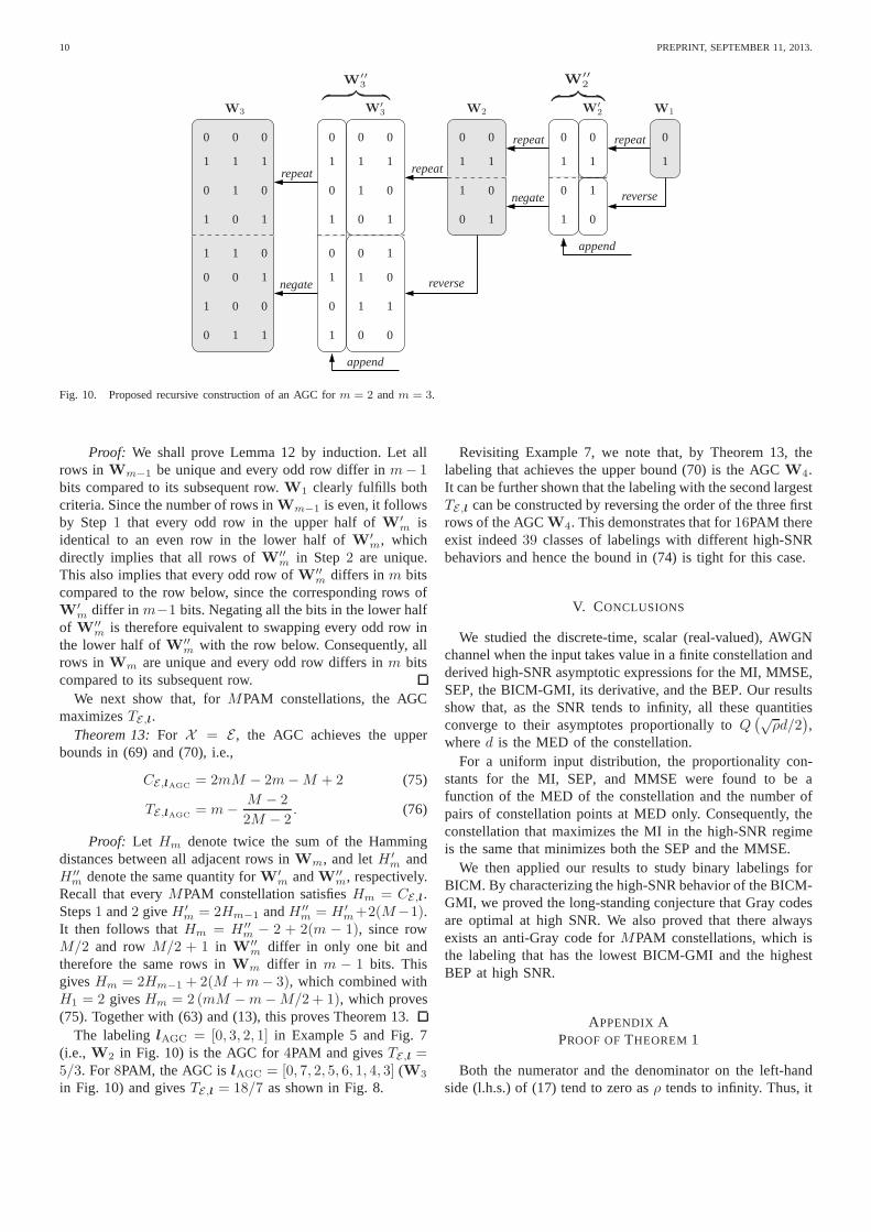
For example, for4PAM we have|CE | ≤ 3 and for 8PAMwe have|CE | ≤ 12, which is consistent with the3 and 12classes at high SNR shown in Fig. 7 and Fig. 8, respectively.For 16PAM, the upper bound (74) indicates that there are atmost 39 classes. However, Fig. 9 shows only37 classes, allgiving rise to aTE,l strictly smaller than (70). This raises thequestion of whether to produce Fig. 9 we were drawing notenough labelings9 or whether the upper bounds (70) and (74)are loose. As we shall show next, (70) is achieved by an AGC.

The AGC of orderm ≥ 2 is defined by theM ×m binarymatrixWm (theith row is the binary label forxi) whereWm

is constructed according to the following recursive procedure:Let W1 = [0, 1]T. ConstructWm from Wm−1 following

the next three steps:

Step 1 Reverse the order of theM/2 rows in Wm−1, andappend them belowWm−1 to construct a new matrixW

′m with M rows andm− 1 columns.

Step 2 Append the length M column vector[0, 1, 0, 1, . . . , 0, 1]T to the left of W

′m to create

W′′m, with M rows andm columns.

Step 3 Negate all bits in the lower half ofW′′m to obtainWm.

This recursive construction is illustrated in Fig. 10 form =2 andm = 3. The following lemma shows that it indeed leadsto a valid labeling.

Lemma 12:All the rows inWm are unique and every oddrow differs inm bits compared to its subsequent row.

9Without discarding trivial operations, there are16! ≈ 2.1 ·1013 labelings,so randomly generating109 labelings covers only a small fraction of allpossible labelings.

10 PREPRINT, SEPTEMBER 11, 2013.

0

00

0

0

0 0 0

00

0

0

00

0

0

00 0 00

0

0

0

0

0

0

0

0

0

0

0 0

1

1

1

1

1

1

1

1

1 1

1 1

1

1

1

1

1 1

1

1

1 1

1

1

1

1

1

1

1

1

1 11

W1W′2

W′′

2︷ ︸︸ ︷

W2W′3

W′′

3︷ ︸︸ ︷

W3

append

append

repeat

repeat repeat

repeat

negate

negate reverse

reverse

Fig. 10. Proposed recursive construction of an AGC form = 2 andm = 3.

Proof: We shall prove Lemma 12 by induction. Let allrows inWm−1 be unique and every odd row differ inm− 1bits compared to its subsequent row.W1 clearly fulfills bothcriteria. Since the number of rows inWm−1 is even, it followsby Step1 that every odd row in the upper half ofW′

m isidentical to an even row in the lower half ofW′

m, whichdirectly implies that all rows ofW′′

m in Step2 are unique.This also implies that every odd row ofW′′

m differs inm bitscompared to the row below, since the corresponding rows ofW

′m differ in m−1 bits. Negating all the bits in the lower half

of W′′m is therefore equivalent to swapping every odd row in

the lower half ofW′′m with the row below. Consequently, all

rows inWm are unique and every odd row differs inm bitscompared to its subsequent row.

We next show that, forMPAM constellations, the AGCmaximizesTE,l.

Theorem 13:For X = E , the AGC achieves the upperbounds in (69) and (70), i.e.,

CE,lAGC = 2mM − 2m−M + 2 (75)

TE,lAGC = m− M − 2

2M − 2. (76)

Proof: Let Hm denote twice the sum of the Hammingdistances between all adjacent rows inWm, and letH ′

m andH ′′

m denote the same quantity forW′m andW′′

m, respectively.Recall that everyMPAM constellation satisfiesHm = CE,l.Steps1 and2 giveH ′

m = 2Hm−1 andH ′′m = H ′

m+2(M−1).It then follows thatHm = H ′′

m − 2 + 2(m − 1), since rowM/2 and rowM/2 + 1 in W

′′m differ in only one bit and

therefore the same rows inWm differ in m − 1 bits. ThisgivesHm = 2Hm−1 + 2(M +m− 3), which combined withH1 = 2 givesHm = 2 (mM −m−M/2 + 1), which proves(75). Together with (63) and (13), this proves Theorem 13.

The labelinglAGC = [0, 3, 2, 1] in Example 5 and Fig. 7(i.e., W2 in Fig. 10) is the AGC for4PAM and givesTE,l =5/3. For 8PAM, the AGC islAGC = [0, 7, 2, 5, 6, 1, 4, 3] (W3

in Fig. 10) and givesTE,l = 18/7 as shown in Fig. 8.

Revisiting Example 7, we note that, by Theorem 13, thelabeling that achieves the upper bound (70) is the AGCW4.It can be further shown that the labeling with the second largestTE,l can be constructed by reversing the order of the three firstrows of the AGCW4. This demonstrates that for16PAM thereexist indeed39 classes of labelings with different high-SNRbehaviors and hence the bound in (74) is tight for this case.

V. CONCLUSIONS

We studied the discrete-time, scalar (real-valued), AWGNchannel when the input takes value in a finite constellation andderived high-SNR asymptotic expressions for the MI, MMSE,SEP, the BICM-GMI, its derivative, and the BEP. Our resultsshow that, as the SNR tends to infinity, all these quantitiesconverge to their asymptotes proportionally toQ

(√ρd/2

),

whered is the MED of the constellation.For a uniform input distribution, the proportionality con-

stants for the MI, SEP, and MMSE were found to be afunction of the MED of the constellation and the number ofpairs of constellation points at MED only. Consequently, theconstellation that maximizes the MI in the high-SNR regimeis the same that minimizes both the SEP and the MMSE.

We then applied our results to study binary labelings forBICM. By characterizing the high-SNR behavior of the BICM-GMI, we proved the long-standing conjecture that Gray codesare optimal at high SNR. We also proved that there alwaysexists an anti-Gray code forMPAM constellations, which isthe labeling that has the lowest BICM-GMI and the highestBEP at high SNR.

APPENDIX APROOF OFTHEOREM 1

Both the numerator and the denominator on the left-handside (l.h.s.) of (17) tend to zero asρ tends to infinity. Thus, it

11

follows from L’Hopital’s rule that

limρ→∞

HPX− IPX

(ρ)

Q(√

ρd/2) = lim

ρ→∞

ddρ (HPX

− IPX(ρ))

ddρQ

(√ρd/2

) (77)

=4

d2limρ→∞

MPX(ρ)

G(√

ρd/2) (78)

=4

d2limρ→∞

MPX(ρ)

Q(√

ρd/2) (79)

= πBPX(80)

whereG(x) is defined as

G(x) ,1

x

1√2π

e−x2

2 . (81)

Here the last step follows from Theorem 2 (proved in Ap-pendix B), which also demonstrates that the limit on the right-hand side (r.h.s.) of (77) exists. To pass from (77) to (78) weused (16) and

d

dρQ (

√ρd/2) = −d2

8G (

√ρd/2) . (82)

To pass from (78) to (79) we used [37, Prop. 19.4.2] to obtain

limx→∞

G(x)

Q(x)= 1. (83)

This proves Theorem 1.

APPENDIX BPROOF OFTHEOREM 2

For the AWGN channel in (1), the conditional ME is givenby [5, eq. (22)]

Xme(y) =

∑

j∈IXpjxje

− 12 (y−

√ρxj)

2

∑

j∈IXpje−

12 (y−

√ρxj)2

. (84)

By using (84) in (7), we obtain

MPX(ρ) =

∑

i∈IX

pi

∫ ∞

−∞

1√2π

e−12 (y−

√ρxi)

2

·(∑

j∈IXpj(xi − xj)e

− 12 (y−

√ρxj)

2

∑

j∈IXpje−

12(y−√

ρxj)2

)2

dy (85)

=∑

i∈IX

piVi(ρ) (86)

where

Vi(ρ) ,

∫ ∞

−∞

e−t2

√π

∑

δ∈D(i)X

δR(i)PX

(δ) · e−√2ρtδ− ρδ2

2

∑

δ∈D(i)X

R(i)PX

(δ) · e−√2ρtδ− ρδ2

2

2

dt

(87)

with D(i)X , {δ : δ = xi − x, x ∈ X} and

R(i)PX

(δ) ,

{pj

pi, if ∃xj ∈ X : xi − xj = δ

0, otherwise(88)

and where to pass from (85) to (86) we used the substitutiony −√

ρxi =√2t.

Combining (83) and (86), we obtain

limρ→∞

MPX(ρ)

Q(√

ρd/2) =

∑

i∈IX

pi limρ→∞

Vi(ρ)

G(√

ρd/2) . (89)

As will become apparent later, the limit on the r.h.s. of (89)exists and, hence, so does the limit on the l.h.s.

Using (87) and (81), and the substitutionr = d√

ρ/8, weobtain

limρ→∞

Vi(ρ)

G(√

ρd/2) = 2

(

limr→∞

F−i (r) + lim

r→∞F+i (r)

)

(90)

where

F−i (r) ,

∫ 0

−∞rer

2−t2

∑

δ∈D(i)X

δR(i)PX

(δ)e−4rt δd−4r2 δ2

d2

∑

δ∈D(i)X

R(i)PX

(δ)e−4rt δd−4r2 δ2

d2

2

dt (91)

and

F+i (r) ,

∫ ∞

0

rer2−t2

∑

δ∈D(i)X

δR(i)PX

(δ)e−4rt δd−4r2 δ2

d2

∑

δ∈D(i)X

R(i)PX

(δ)e−4rt δd−4r2 δ2

d2

2

dt. (92)

We will next calculate the first limit in (90). Using thesubstitutiont = u/r − r we expressF−

i (r) as

F−i (r) =

∫ ∞

−∞f−i (r, u) du (93)

where

f−i (r, u) , h(r2 − u) · e2u−u2

r2

·

∑

δ∈D∗

iδR

(i)PX

(δ)e−4u δd−4r2U(δ)

1 +∑

δ∈D∗

iR

(i)PX

(δ)e−4u δd−4r2U(δ)

2

(94)

with D∗i , D(i)

X \ {0},

U(δ) ,δ

d

(δ

d− 1

)

(95)

and h(x) being Heaviside’s step function (i.e.,h(x) = 1 ifx ≥ 0 andh(x) = 0 if x < 0). Using the fact thatU(δ) ≥0, ∀δ ∈ D∗

i andU(d) = 0, we obtain

limr→∞

f−i (r, u) = d2e2u

(

R(i)PX

(d)e−4u

1 +R(i)PX

(d)e−4u

)2

. (96)

As we shall prove in Lemma 14 ahead,u 7→ f−i (r, u) is

uniformly bounded by some integrable functionu 7→ g−i (u)that is independent ofr. It thus follows from Lebesgue’s

12 PREPRINT, SEPTEMBER 11, 2013.

Dominated Convergence Theorem [38, Theorem 1.34] that

limr→∞

F−i (r) =

∫ ∞

−∞limr→∞

f−i (r, u) du (97)

=d2√

R(i)PX

(d)

2

∫ ∞

0

ξ2

(1 + ξ2)2dξ (98)

=d2π√

R(i)PX

(d)

8(99)

where (98) follows from (96) and the substitution√

R(i)PX

(d)e−2u = ξ, and (99) follows from [39, eq. (3.241.5)].

It thus remains to show thatu 7→ f−i (r, u) is uniformly

bounded by some integrable functionu 7→ g−i (u) that isindependent ofr. We do this in the following lemma.

Lemma 14:For anyr > 0

0 ≤ f−i (r, u) ≤ g−i (u), u ∈ R (100)

where

g−i (u) ,d2(M − 1)2

p2ie−2|u| (101)

andd is the maximum Euclidean distance of the constellation,i.e., d , maxi,j∈IX

|xi − xj |. Furthermore,∫ ∞

−∞g−i (u) du =

d2(M − 1)2

p2i< ∞. (102)

Proof: We first note thatf−i (r, u) ≥ 0, r > 0, u ∈ R.

It thus remains to show the second inequality in (100). To

this end, we useh(r2 − u) ≤ 1, e−u2

r2 ≤ 1, and δ ≤ d toupper-bound (94) as

f−i (r, u) ≤ d2e2u

∑

δ∈D∗

iR

(i)PX

(δ)e−4u δd−4r2U(δ)

1 +∑

δ∈D∗

iR

(i)PX

(δ)e−4u δd−4r2U(δ)

2

(103)

= d2e2u

1 +1

∑

δ∈D∗

iR

(i)PX

(δ)e−4u δd−4r2U(δ)

−2

.

(104)

Since R(i)PX

(δ) < 1/pi and e−4r2U(δ) ≤ 1, we can furtherupper-bound (104) as

f−i (r, u) < d2e2u

(

1 +pi

∑

δ∈D∗

ie−4u δ

d

)−2

(105)

<d2e2u

p2i

(

1 +1

∑

δ∈D∗

ie−4u δ

d

)−2

(106)

where to pass from (105) to (106) we usedpi < 1.

For u ≥ 0, we have

f−i (r, u) <

d2e2u

p2i

(

1 +1

(M − 1)e−4u

)−2

(107)

<d2(M − 1)2

p2ie−6u (108)

<d2(M − 1)2

p2ie−2|u| (109)

where to pass from (106) to (107) we upper-bounded the(M−1) exponentials in the summation bye−4u.

For u ≤ 0, we have

f−i (r, u) <

d2e2u

p2i(110)

≤ d2(M − 1)2

p2ie−2|u| (111)

where (110) follows from discarding the sum of exponentialsin (106). Combining (109) and (111) gives (101). This provesLemma 14.

Returning to the proof of Theorem 2, the second limit onthe r.h.s. of (90) can be computed along the same lines byusing the substitutiont = u/r + r in (92):

limr→∞

F+i (r) =

d2π√

R(i)PX

(−d)

8. (112)

Using (99) and (112) in (90), and combining the result with(89) yields

limρ→∞

MPX(ρ)

Q(√

ρd/2) =

∑

i∈IX

piπd2

4

(√

R(i)PX

(d) +

√

R(i)PX

(−d)

)

(113)which in view of (88) and (14) is equal toπd2BPX

/4. Thisproves Theorem 2.

APPENDIX CPROOF OFTHEOREM 3

Using Bayes’ rule,Xmap(y) in (9) can be expressed as

Xmap(y) = argmaxx∈X

{fY |X(y|x)PX(x)

}(114)

= xj , if y ∈ Yj(ρ) (115)

whereYj(ρ) is the decision region for the symbolxj withj = 1, . . . ,M . For sufficiently largeρ, these decision regionscan be written as

Yj(ρ) , {y ∈ R : βj−1(ρ) ≤ y < βj(ρ)} (116)

whereβℓ(ρ) with ℓ = 0, . . . ,M are theM + 1 thresholdsdefining theM regions, i.e.,

βℓ(ρ) =

−∞, ℓ = 0log(pℓ/pℓ+1)√ρ(xℓ+1−xℓ)

+√ρ(xℓ+1+xℓ)

2 , ℓ = 1, . . . ,M − 1

+∞, ℓ = M

(117)

which are obtained by solving

pℓfY |X(βℓ(ρ)|xℓ) = pℓ+1fY |X(βℓ(ρ)|xℓ+1). (118)

13

The following lemma will be used in this proof as well asin the proof of Theorem 7 (Appendix F).

Lemma 15:For anyPX and i ∈ IX

limρ→∞

Q(|βℓ(ρ)−

√ρxi|

)

Q(√

ρd/2)

=

√

R(i)PX

(d), if ℓ = i − 1√

R(i)PX

(−d), if ℓ = i

0, if ℓ /∈ {i− 1, i}

(119)

whereβℓ(ρ) is given by (117) andR(i)PX

(δ) by (88).Proof: We use (117) to obtain

βℓ(ρ)−√ρxi =

log(pℓ/pℓ+1)√ρ(xℓ+1 − xℓ)

+

√ρǫi,ℓ

2(120)

where for anyi, ℓ

ǫi,ℓ , xℓ+1 + xℓ − 2xi. (121)

We form the ratio

G(|βℓ(ρ)−

√ρxi|

)

G(√

ρd/2) =

ρd(xℓ+1 − xℓ)

|2 log(pℓ/pℓ+1) + ρǫi,ℓ(xℓ+1 − xℓ)|

· exp

−(log pℓ

pℓ+1

)2

2ρ(xℓ+1 − xℓ)2−

ǫi,ℓ logpℓ

pℓ+1

2(xℓ+1 − xℓ)−

ρ(ǫ2i,ℓ − d2)

8

(122)

and study the limit

limρ→∞

G(|βℓ(ρ)−

√ρxi|

)

G(√

ρd/2) . (123)

To this end, we distinguish between three cases:

(i) If i = ℓ andxℓ+1 − xℓ = d, thenǫi,ℓ = xℓ+1 − xℓ = dand the limit in (123) ise− log (pℓ/pℓ+1)/2 =

√

pℓ+1/pℓ.(ii) If i = ℓ+1 andxℓ+1 −xℓ = d, thenǫi,ℓ = xℓ −xℓ+1 =

−d and the limit in (123) is√

pℓ/pℓ+1.(iii) In all other cases,|ǫi,ℓ| > d and the limit in (123) is

zero.

A slight change in notation then yields

limρ→∞

G(|βℓ(ρ)−

√ρxi|

)

G(√

ρd/2)

=

√pi+1

pi, if ℓ = i andxℓ+1 − xℓ = d

√pi−1

pi, if ℓ = i− 1 andxℓ+1 − xℓ = d

0, otherwise

. (124)

Combining (124) with (88) and (83) proves Lemma 15.Returning to the proof of Theorem 3, using (115) and (116),

the SEP in (8) can be written as

SPX(ρ) =

∑

i∈IX

pi Pr{Y /∈ Yi(ρ)|X = xi} (125)

=∑

i∈IX

pi

(

Q (βi(ρ)−√ρxi)

+Q (√ρxi − βi−1(ρ))

)

(126)

which gives

limρ→∞

SPX(ρ)

Q(√ρd/2)

=∑

i∈IX

pi

(

limρ→∞

Q(βi(ρ)−

√ρxi

)

Q(√ρd/2)

+ limρ→∞

Q(√

ρxi − βi−1(ρ))

Q(√ρd/2)

)

(127)

=∑

i∈IX

pi

(√

R(i)PX

(−d) +

√

R(i)PX

(d)

)

(128)

where to pass from (127) to (128) we used Lemma 15 twice,observing that the arguments of both Q-functions are positivefor large enoughρ. The proof of Theorem 3 is completed bycombining (128) with (14) and (88).

APPENDIX DPROOF OFTHEOREM 5

Using the expression for the BICM-GMI (40), we have

HPX− Ibicm

PX ,l(ρ)

=

m∑

k=1

(HPX− IPX

(ρ))

−m∑

k=1

∑

b∈{0,1}PQk

(b)(HPXk,b− IPXk,b

(ρ))

− (m− 1)HPX+

m∑

k=1

∑

b∈{0,1}PQk

(b)HPXk,b. (129)

The last two terms on the r.h.s. of (129) cancel becausem∑

k=1

∑

b∈{0,1}PQk

(b)HPXk,b

= −m∑

k=1

∑

b∈{0,1}

∑

i∈IXk,b

PQk(b)PXk,b

(xi) logPXk,b(xi)

(130)

= −m∑

k=1

∑

i∈IX

pi logpi

PQk(qi,k)

(131)

= mHPX+∑

i∈IX

pi

m∑

k=1

logPQk(qi,k) (132)

= mHPX+∑

i∈IX

pi logm∏

k=1

PQk(qi,k) (133)

= mHPX−HPX

(134)

where to pass from (130) to (131) we used (31), and to passfrom (133) to (134) we used (30).

We divide both sides of (129) byQ(√ρd/2) and take the

limit as ρ → ∞. For the first two terms, we change the orderof summation and limit and apply Theorem 1 to each term.

14 PREPRINT, SEPTEMBER 11, 2013.

This gives

limρ→∞

HPX− Ibicm

PX ,l(ρ)

Q(√

ρd/2)

= π

m∑

k=1

(

BPX−

∑

b∈{0,1}PQk

(b)BPXk,b

)

. (135)

Theorem 5 follows by showing that the r.h.s. of (135) is equalto πDPX ,l. We shall do this in the following lemma, whichwill also be used in the proof of Theorem 6.

Lemma 16:We havem∑

k=1

(

BPX−

∑

b∈{0,1}PQk

(b)BPXk,b

)

= DPX ,l (136)

whereBPXis given by (14),DPX ,l by (37),

BPXk,b,

∑

i∈IXk,b

∑

j∈IXk,b

|xi−xj|=d

√

PXk,b(xi)PXk,b

(xj) (137)

andPXk,b(x) is given by (31).

Proof: Express the inner sum on the l.h.s. of (136) using(31) and (137) as

∑

b∈{0,1}PQk

(b)BPXk,b=

∑

b∈{0,1}

∑

i∈IXk,b

∑

j∈IXk,b

|xi−xj |=d

√pjpi.

(138)

Expanding the sum in (14) usingX = Xk,0 ∪Xk,1, we obtain

BPX=

∑

b∈{0,1}

∑

i∈IXk,b

∑

j∈IXk,b

|xi−xj|=d

√pjpi

+ 2∑

i∈IXk,0

∑

j∈IXk,1

|xi−xj |=d

√pjpi. (139)

Lemma 16 follows by applying (138) and (139) to the l.h.s.of (136) and by using the definition ofDPX ,l in (37).

APPENDIX EPROOF OFTHEOREM 6

We divide the l.h.s. of (41) and (42) byQ(√ρd/2) and take

the limit asρ → ∞ to obtain

limρ→∞

MbicmPX ,l(ρ)

Q(√

ρd/2)

= limρ→∞

m∑

k=1

(

MPX(ρ)

Q(√

ρd/2) −

∑

b∈{0,1}PQk

(b)MPXk,b

(ρ)

Q(√

ρd/2)

)

.

(140)

Changing the order of summation and limit, and applyingTheorem 2 yields

limρ→∞

MbicmPX ,l(ρ)

Q(√

ρd/2) =

πd2

4

m∑

k=1

(

BPX−

∑

b∈{0,1}PQk

(b)BPXk,b

)

(141)

whereBPXk,bis given by (137). Theorem 6 follows by noting

that, by Lemma 16, the r.h.s. of (141) is equal toπd2

4 DPX ,l.

APPENDIX FPROOF OFTHEOREM 7

Using the law of total probability, the BEP in (46) can bewritten as

BPX ,l(ρ)

=1

m

m∑

k=1

∑

b∈{0,1}

∑

i∈IXk,b

pi Pr{Qmapk (Y ) 6= qk,i|X = xi}

(142)

=1

m

m∑

k=1

∑

b∈{0,1}

∑

i∈IXk,b

pi Pr

{

Y ∈⋃

j∈IXk,b

Yj(ρ)

∣∣∣∣∣X = xi

}

(143)

with Yj(ρ) given by (116) and were we useb to denote thenegation of a bitb. Using the fact thatYj(ρ) are disjoint, werewrite (143) as

BPX ,l(ρ)

=1

m

m∑

k=1

∑

b∈{0,1}

∑

i∈IXk,b

pi∑

j∈IXk,b

Pr{Y ∈ Yj(ρ)|X = xi

}

(144)

=1

m

m∑

k=1

∑

b∈{0,1}

∑

i∈IXk,b

pi∑

j∈IXk,b

Γi,j(ρ) (145)

=1

m

m∑

k=1

∑

b∈{0,1}

∑

i∈IXk,b

pi

(∑

j∈IXk,b

:j<i

Γi,j(ρ)

+∑

j∈IXk,b

:j>i

Γi,j(ρ)

)

(146)

where

Γi,j(ρ) , Q (βj−1(ρ)−√ρxi)−Q (βj(ρ)−

√ρxi) (147)

= Q (√ρxi − βj(ρ)) −Q (

√ρxi − βj−1(ρ)) (148)

and where we have used thatQ(−x) = 1−Q(x).

By using (147) and (148) in (146), dividing both sides of(146) by Q

(√ρd/2

), and taking the limit asρ → ∞, we

obtain

limρ→∞

BPX ,l(ρ)

Q(√

ρd/2) =

1

m

m∑

k=1

∑

b∈{0,1}

∑

i∈IXk,b

pi

4∑

ℓ=1

sℓ (149)

15

where

s1 =∑

j∈IXk,b

:j<i

limρ→∞

Q(√

ρxi − βj(ρ))

Q(√

ρd/2) (150)

s2 = −∑

j∈IXk,b

:j<i

limρ→∞

Q(√

ρxi − βj−1(ρ))

Q(√

ρd/2) (151)

s3 =∑

j∈IXk,b

:j>i

limρ→∞

Q(βj−1(ρ)−

√ρxi

)

Q(√

ρd/2) (152)

s4 = −∑

j∈IXk,b

:j>i

limρ→∞

Q(βj(ρ)−

√ρxi

)

Q(√

ρd/2) . (153)

Note that, for sufficiently largeρ, the arguments of the Q-functions in (150)–(153) are positive.

By Lemma 15, s2 = s4 = 0. Furthermore, applyingLemma 15 to (150) and (152), we conclude that the onlynonzero contribution tos1 and s3 can come from the termsj = i− 1 andj = i+1, respectively. We therefore expresss1as

s1 =

{√pi−1

pi, if ∃xi−1 ∈ Xk,b : xi − xi−1 = d

0, otherwise(154)

ands3 as

s3 =

{√pi+1

pi, if ∃xi+1 ∈ Xk,b : xi+1 − xi = d

0, otherwise. (155)

Using (154) and (155) in (149), we obtain

limρ→∞

BPX ,l(ρ)

Q(√

ρd/2)

=1

m

m∑

k=1

∑

b∈{0,1}

∑

i∈IXk,b

pi∑

j∈IXk,b

|xi−xj |=d

√pjpi. (156)

The proof is completed by movingpi to the inner sum in (156)and by comparing the resulting expression with (37).

ACKNOWLEDGMENT

The authors wish to thank the Associate Editor Robert F.H. Fischer and the anonymous reviewers for their valuablecomments.

REFERENCES

[1] C. E. Shannon, “A mathematical theory of communications,” Bell SystemTechnical Journal, vol. 27, pp. 379–423 and 623–656, July and Oct.1948.

[2] S. Verdu, “On channel capacity per unit cost,”IEEE Trans. Inf. Theory,vol. 36, no. 5, pp. 1019–1030, June 1990.

[3] ——, “Spectral efficiency in the wideband regime,”IEEE Trans. Inf.Theory, vol. 48, no. 6, pp. 1319–1343, June 2002.

[4] V. V. Prelov and S. Verdu, “Second-order asymptotics ofmutual infor-mation,” IEEE Trans. Inf. Theory, vol. 50, no. 8, pp. 1567–1580, Aug.2004.

[5] A. Lozano, A. M. Tulino, and S. Verdu, “Optimum power allocationfor parallel Gaussian channels with arbitrary input distributions,” IEEETrans. Inf. Theory, vol. 52, no. 7, pp. 3033–3051, July 2006.

[6] F. Perez-Cruz, M. R. D. Rodrigues, and S. Verdu, “MIMO Gaussianchannels with arbitrary inputs: Optimal precoding and power allocation,”IEEE Trans. Inf. Theory, vol. 56, no. 3, pp. 1070–1084, Mar. 2010.

[7] Y. Wu and S. Verdu, “MMSE dimension,”IEEE Trans. Inf. Theory,vol. 57, no. 8, pp. 4857–4879, Aug. 2011.

[8] D. Duyck, J. Boutros, and M. Moeneclaey, “Precoding for outageprobability minimization on block fading channels,”IEEE Trans. Inf.Theory (to appear), 2013, available at http://arxiv.org/abs/1103.5348.

[9] M. R. D. Rodrigues, “On the constrained capacity of multi-antennafading coherent channels with discrete inputs,” inIEEE InternationalSymposium on Information Theory (ISIT), Saint Petersburg, Russia, July-Aug. 2011.

[10] ——, “Characterization of the constrained capacity of multiple-antennafading coherent channels driven by arbitrary inputs,” inIEEE Interna-tional Symposium on Information Theory (ISIT), Cambridge, MA, July2012.

[11] ——, “Multiple-antenna fading coherent channels with arbitrary inputs:Characterization and optimization of the reliable information transmis-sion rate,” Oct. 2012, available at http://arxiv.org/abs/1210.6777.

[12] A. G. C. P. Ramos and M. R. D. Rodrigues, “Coherent fadingchan-nels driven by arbitrary inputs: Asymptotic characterization of theconstrained capacity and related information- and estimation-theoreticquantities,” Oct. 2012, available at http://arxiv.org/abs/1210.4505.

[13] E. Zehavi, “8-PSK trellis codes for a Rayleigh channel,” IEEE Trans.Commun., vol. 40, no. 3, pp. 873–884, May 1992.

[14] G. Caire, G. Taricco, and E. Biglieri, “Bit-interleaved coded modula-tion,” IEEE Trans. Inf. Theory, vol. 44, no. 3, pp. 927–946, May 1998.

[15] A. Guillen i Fabregas, A. Martinez, and G. Caire, “Bit-interleavedcoded modulation,”Foundations and Trends in Communications andInformation Theory, vol. 5, no. 1–2, pp. 1–153, 2008.

[16] A. Martinez, A. Guillen i Fabregas, and G. Caire, “Bit-interleaved codedmodulation revisited: A mismatched decoding perspective,” IEEE Trans.Inf. Theory, vol. 55, no. 6, pp. 2756–2765, June 2009.

[17] C. Stierstorfer and R. F. H. Fischer, “(Gray) Mappings for bit-interleavedcoded modulation,” inIEEE Vehicular Technology Conference (VTC-Spring), Dublin, Ireland, Apr. 2007.

[18] C. Stierstorfer, “A bit-level-based approach to codedmulticarriertransmission,” Ph.D. dissertation, Friedrich-Alexander-UniversitatErlangen-Nurnberg, Erlangen, Germany, 2009, available athttp://www.opus.ub.uni-erlangen.de/opus/volltexte/2009/1395/.

[19] A. Martinez, A. Guillen i Fabregas, and G. Caire, “Bit-interleaved codedmodulation in the wideband regime,”IEEE Trans. Inf. Theory, vol. 54,no. 12, pp. 5447–5455, Dec. 2008.

[20] C. Stierstorfer and R. F. H. Fischer, “Asymptotically optimal mappingsfor BICM with M -PAM and M2-QAM,” IET Electronics Letters,vol. 45, no. 3, pp. 173–174, Jan. 2009.

[21] E. Agrell and A. Alvarado, “Optimal alphabets and binary labelingsfor BICM at low SNR,” IEEE Trans. Inf. Theory, vol. 57, no. 10, pp.6650–6672, Oct. 2011.

[22] ——, “Signal shaping for BICM at low SNR,”IEEE Trans. Inf. Theory,vol. 59, no. 4, pp. 2396–2410, Apr. 2013.

[23] A. Alvarado, F. Brannstrom, and E. Agrell, “High SNR bounds for theBICM capacity,” in IEEE Information Theory Workshop (ITW), Paraty,Brazil, Oct. 2011.

[24] D. Guo, S. Shamai (Shitz), and S. Verdu, “Mutual information andminimum mean-square error in Gaussian channels,”IEEE Trans. Inf.Theory, vol. 51, no. 4, pp. 1261–1282, Apr. 2005.

[25] D. Guo, “Gaussian channels: Information, estimation and multiuserdetection,” Ph.D. dissertation, Princeton University, Princeton, NewJersey, Nov. 2004.

[26] J. B. Anderson and A. Svensson,Coded Modulation Systems. Springer,2003.

[27] A. Alvarado, F. Brannstrom, E. Agrell, and T. Koch, “High-SNRasymptotics of mutual information for discrete constellations,” in IEEEInternational Symposium on Information Theory (ISIT), Istanbul, Turkey,July 2013.

[28] A. Guillen i Fabregas and A. Martinez, “Bit-interleaved coded mod-ulation with shaping,” inIEEE Information Theory Workshop (ITW),Dublin, Ireland, Aug.–Sep. 2010.

[29] T. Nguyen and L. Lampe, “Bit-interleaved coded modulation withmismatched decoding metrics,”IEEE Trans. Commun., vol. 59, no. 2,pp. 437–447, Feb. 2011.

[30] F. Gray, “Pulse code communications,” U. S. Patent 2 632058, Mar.1953.

[31] E. Agrell, J. Lassing, E. G. Strom, and T. Ottosson, “Onthe optimalityof the binary reflected Gray code,”IEEE Trans. Inf. Theory, vol. 50,no. 12, pp. 3170–3182, Dec. 2004.

[32] E. Agrell, J. Lassing, E. G. Strom, and T. Ottosson, “Gray coding formultilevel constellations in Gaussian noise,”IEEE Trans. Inf. Theory,vol. 53, no. 1, pp. 224–235, Jan. 2007.

16 PREPRINT, SEPTEMBER 11, 2013.

[33] A. Guillen i Fabregas and A. Martinez, “Derivative ofBICM mutualinformation,” IET Electronics Letters, vol. 43, no. 22, pp. 1219–1220,Oct. 2007.

[34] M. Ivanov, F. Brannstrom, A. Alvarado, and E. Agrell,“On the exactBER of bit-wise demodulators for one-dimensional constellations,” IEEETrans. Commun., vol. 61, no. 4, pp. 1450–1459, Apr. 2013.

[35] ——, “General BER expression for one-dimensional constellations,” inIEEE Global Telecommunications Conference (GLOBECOM), Anaheim,

CA, Dec. 2012.[36] U. Madhow, Fundamentals of Digital Communication. Cambridge

University Press, 2008.[37] A. Lapidoth, A Foundation in Digital Communication. Cambridge

University Press, 2009.[38] W. Rudin, Real and Complex Analysis, 3rd ed. McGraw-Hill, 1987.[39] I. S. Gradshteyn and I. M. Ryzhik,Tables of Integrals, Series and

Products, 6th ed. Academic Press, 2000.