3GFFIRS 09/29/2014 9:24:54 Page ii

3GFFIRS 09/29/2014 9:24:54 Page i

Corporate and ProjectFinance Modeling

3GFFIRS 09/29/2014 9:24:54 Page ii

3GFFIRS 09/29/2014 9:24:54 Page iii

Corporate and ProjectFinance Modeling

Theory and Practice

EDWARD BODMER

3GFFIRS 09/29/2014 9:24:54 Page iv

Cover image: iStock.com/Kamil Krawczyk

Cover design: Wiley

Copyright 2015 by Edward Bodmer. All rights reserved.

Published by John Wiley & Sons, Inc., Hoboken, New Jersey.

Published simultaneously in Canada.

No part of this publication may be reproduced, stored in a retrieval system, or transmittedin any form or by any means, electronic, mechanical, photocopying, recording, scanning,or otherwise, except as permitted under Section 107 or 108 of the 1976 United StatesCopyright Act, without either the prior written permission of the Publisher, or authorizationthrough payment of the appropriate per-copy fee to the Copyright Clearance Center, Inc.,222 Rosewood Drive, Danvers, MA 01923, (978) 750-8400, fax (978) 646-8600, or on theWeb at www.copyright.com. Requests to the Publisher for permission should be addressedto the Permissions Department, John Wiley & Sons, Inc., 111 River Street, Hoboken, NJ07030, (201) 748-6011, fax (201) 748-6008, or online at http://www.wiley.com/go/permissions.

Limit of Liability/Disclaimer of Warranty: While the publisher and author have used theirbest efforts in preparing this book, they make no representations or warranties with respectto the accuracy or completeness of the contents of this book and specifically disclaim anyimplied warranties of merchantability or fitness for a particular purpose. No warranty maybe created or extended by sales representatives or written sales materials. The advice andstrategies contained herein may not be suitable for your situation. You should consult witha professional where appropriate. Neither the publisher nor author shall be liable for anyloss of profit or any other commercial damages, including but not limited to special,incidental, consequential, or other damages.

For general information on our other products and services or for technical support, pleasecontact our Customer Care Department within the United States at (800) 762-2974, outsidethe United States at (317) 572-3993 or fax (317) 572-4002.

Wiley publishes in a variety of print and electronic formats and by print-on-demand. Somematerial included with standard print versions of this book may not be included in e-booksor in print-on-demand. If this book refers to media such as a CD or DVD that is not includedin the version you purchased, you may download this material at http://booksupport.wiley.com. For more information about Wiley products, visit www.wiley.com.

Library of Congress Cataloging-in-Publication Data:

Bodmer, E. (Edward)Corporate and project finance modeling/Edward Bodmer.

pages cmISBN 978-1-118-85436-5 (cloth); ISBN 978-1-118-85446-4 (ePDF);

ISBN 978-1-118-85445-7 (ePub); ISBN 978-1-118-95739-4 (oBook)1. Valuation—Mathematical models. 2. Finance—Mathematical models. 3.

Financial risk—Mathematical models. I. Title.HG4028.V3B52 2014658.15011́–dc23

2014016731

Printed in the United States of America

10 9 8 7 6 5 4 3 2 1

3GFTOC 09/29/2014 9:28:12 Page v

Contents

Preface xvii

Acknowledgments xxiii

PART I FINANCIAL MODELING STRUCTURE AND DESIGN:STRUCTURE AND MECHANICS OF DEVELOPINGFINANCIAL MODELS FOR CORPORATE FINANCEAND PROJECT FINANCE ANALYSIS

CHAPTER 1 Financial Modeling and Valuation Nightmares: ProblemsThat Financial Models Cannot Solve 3

CHAPTER 2 Becoming a Black Belt Modeler 9

CHAPTER 3 General Model Objectives of Structuring Transactions,Risk Analysis, and Valuation 13

CHAPTER 4 The Structure of Alternative Financial Models 17

Structure of a Corporate Model: Incorporating Historyand Deriving Forecasts from Historical Analysis 21

Use of the INDEX Function in Corporate Models 26

Easing the Pain of Acquiring PDF Data 28

Structure of a Project Finance Model That Accountsfor Different Risks in Different Phases over the Lifeof a Project 30

Reconciliation of Internal Rate of Return in Project Financewith Return on Investment in Corporate Finance 33

Structure of an Acquisition Model: AlternativeTransaction Prices and Financing Terms 35

v

3GFTOC 09/29/2014 9:28:12 Page vi

Structure of an Integrated Merger Model: ForecastingEarnings per Share 37

CHAPTER 5 Avoiding Bad Programming Practices and CreatingEffective Auditing Processes 41

How to Make Financial Models More Efficient and Accurate 44

CHAPTER 6 Developing and Efficiently Organizing Assumptions 55

Assumptions in Demand-Driven Models versusSupply-Driven Models: The Danger of Overcapacityin an Industry 55

Creating a Flexible Input Structure for ModelAssumptions 60

Alternative Input Structures for Project Finance andCorporate Finance Models 62

Setting Up Inputs with Code Numbers and the INDEXFunction 62

CHAPTER 7 Structuring Time Lines 67

Timing in Corporate Finance Models: Distinguishing theHistorical Period, Explicit Period, and Terminal Period 67

Development to Decommissioning: Phases in the Lifeof a Project Finance Model 69

Timing in Acquisition Models: Separating the TransactionPeriod, the Holding Period, and the Exit Period 70

Structuring a Time Line to Measure History, ExplicitPeriods, and Terminal Periods in Corporate Modelsand Risk Phases in Project Finance Models 72

Computing Start of Period and End of Period Dates 73

TRUE and FALSE Switches in Modeling Time Periods 75

Computing the Age of a Project in Years on a Monthly,Quarterly, or Semiannual Basis 77

The Magic of a HISTORIC Switch in a Corporate Model 78

Transferring Data from a Corporate Model to anAcquisition Model Using MATCH and INDEX Functions 82

CHAPTER 8 Projecting Revenues, Expenses, and Capital Expendituresto Derive Pretax Cash Flow 85

Transparent Calculations of Pretax Cash Flow 85

vi Contents

3GFTOC 09/29/2014 9:28:12 Page vii

Inflation and Growth Rates in Calculations of PretaxCash Flow 88

Valuation Analysis from Prefinancing, PretaxCash Flow 90

CHAPTER 9 Moving from Pretax Cash Flow to After-Tax FreeCash Flow 91

Working Capital Analysis 91

Problems in Computing Depreciation Expense inCorporate Models Involving Asset Retirements 92

Portfolios of Assets with a Vintage Process 94

Accounting for Asset Retirements in Corporate Models 99

Alternative Methods for Deriving Retirements Associatedwith Existing Assets in Corporate Models 103

Depreciation Issues in Project Finance Models 109

Modeling the Change in Deferred Taxes in CorporateModels 110

Adjusting the Tax Basis in an Acquisition 111

CHAPTER 10 Adding Debt to a Corporate or Project Finance Modelby Programming Cash Flow Waterfalls 113

Adding the Debt Schedule to a Financial Model 114

Modeling Scheduled Debt Repayments 116

Connecting Debt to Cash Flow in Corporate Models 117

With a Structured Process, You Can Model Any CashFlow Waterfall 119

Defaults on Debt and Measuring the Debt Internal Rateof Return 124

Assessing Risk and Return Characteristics ofSubordinated Debt 127

CHAPTER 11 Alternative Calculations of Equity Distributions 131

Modeling Dividend Distributions 132

Computing a Target Capital Structure through SimulatingNew Equity Issues and Buybacks 136

CHAPTER 12 Putting Together Financial Statements and CalculatingIncome Taxes 139

Contents vii

3GFTOC 09/29/2014 9:28:12 Page viii

Computation of Taxes Paid and Taxes Deferred 140

Cash Flow Statement and Balance Sheet 144

PART II ANALYZING RISKS WITH FINANCIAL MODELS:SENSITIVITY ANALYSIS, SCENARIO ANALYSIS,BREAK-EVEN ANALYSIS, TIME SERIES, ANDMONTE CARLO SIMULATION

CHAPTER 13 Risk Assessment: The Centerpiece of All Valuation,Contracting, and Credit Issues in Finance 149

Six Alternative Ways to Assess the Risk of a Company,a Project, or a Contract 151

Using Direct Risk Assessment to Measure Cash Flowand Financial Ratios 154

CHAPTER 14 Defining, Describing, and Assessing Risk in a RiskAllocation Matrix 159

CHAPTER 15 Presentation of Risk Analysis through Adding SensitivityAnalysis to Financial Models 165

Setting Up Data for Making Graphs by ConvertingPeriodic Data into Annual, Semiannual,or Quarterly Data 167

Using the INDIRECT Function to Automate Conversionto Time Period Data 172

Making Flexible Graphs for Sensitivity Analysis 173

CHAPTER 16 Using Financial Models to Establish Break-Even Pointsfor Key Input Variables with Data Tables 185

Establishing Break-Even Criteria When AnalyzingFinancial Models 188

Mechanics of Using Data Tables to Compute Break-EvenPoints Automatically 193

Creating Data Tables Using VBA Instead of the DataTable Tool 201

Summary of Break-Even Analysis 205

CHAPTER 17 Constructing Flexible Scenario Analysis for RiskAssessment 207

viii Contents

3GFTOC 09/29/2014 9:28:13 Page ix

Mechanics of Scenario Analysis 210

Using VBA Code to Create a Scenario Analysis 221

Getting the Best of Both Worlds: Creating a SpecialCustom Scenario That Allows Use of SpinnerButtons and Drop-Down Boxes 223

CHAPTER 18 Generating Tornado Diagrams, Spider Charts, andWaterfall Graphs 231

Tornado Diagrams That Display Which Variables Havethe Largest Effect on Value and Which VariablesHave the Least Effect on an Output Variable 232

Creating a Tornado Diagram by Extending ScenarioAnalysis 234

Creating a Tornado Diagram Using a Two-WayData Table 242

Spider Diagrams That Illustrate How Each Rangein Input Variables Affects an Output Variable 246

How to Create a Spider Diagram Using a Two-WayData Table 247

Presenting Sensitivity Analysis with a Waterfall Chart 250

CHAPTER 19 Adding Probabilistic Risk Analysis and Time SeriesEquations to Financial Models 253

Definition of Some Terms for Adding StochasticAnalysis to Your Financial Models 256

Using Probability Distributions with SpreadsheetFunctions Rather Than Equations with Greek Letters 258

CHAPTER 20 Taking the Mystery out of Applying Time Series Analysisand Monte Carlo Simulation in Financial Models 263

Step-by-Step Procedure to Incorporate a Monte CarloSimulation into Your Models 266

CHAPTER 21 Constructing Probability Distributions with Trends,Mean Reversion, Price Boundaries, and Correlationsamong Variables 277

Starting Point for Developing Time Series Equations—Brownian Motion and Normal Distributions 279

Contents ix

3GFTOC 09/29/2014 9:28:13 Page x

Testing the Assumption That Input Variables AreNormally Distributed 281

Price Boundaries and Short-Run Marginal Cost 285

Mean Reversion and Long-Run Equilibrium Analysis 286

Modeling Correlations among Variables in Time SeriesEquations 289

CHAPTER 22 The Difficult Problem of Estimating Volatility, MeanReversion, Time Trends, Correlations, and PriceBoundaries from Historical Data or Market Data 295

Calculation of Volatility from a Random Walk Process 296

Attempting to Measure the Presence of Mean Reversionin Historical Data 297

Attempting to Measure the Presence of Mean Reversionby Evaluating Changes in Periodic Volatility 300

Risk Analysis Summary 303

PART III ADVANCED CORPORATE MODELING: MODELINGTERMINAL VALUE WITH STABLE RATIOS IN THEDISCOUNTED CASH FLOW MODEL, DERIVING IMPLIEDMULTIPLES, AND COMPUTING THE BRIDGE BETWEENEQUITY VALUE AND ENTERPRISE VALUE

CHAPTER 23 Overview of Issues When Computing NormalizedCash Flow and Terminal Value 307

CHAPTER 24 Computing the Return on Invested Capital for Historicaland Projected Periods in Corporate Models 313

Working with a Free Cash Flow Perspective, an EquityCash Flow Perspective, or Both in ComputingFinancial Ratios 314

Presenting Return on Invested Capital in FinancialModels 316

CHAPTER 25 Calculation of Invested Capital 321

Dissecting the Financial Structure of a Corporation toUnderstand the Bridge from Enterprise Value toEquity Value 323

x Contents

3GFTOC 09/29/2014 9:28:13 Page xi

Drawing an Imaginary Line underneath EBIT toUnderstand the Financial Structure of a Corporation 326

Constructing a Long-Term Model to Create Proof ofCorporate Finance Concepts 328

CHAPTER 26 Complex Items in Balance Sheet Analysis: Deferred Taxes,Operating Cash, and Derivative Assets 337

Treatment of Accumulated Deferred Taxes Arising fromDepreciation 337

Classification of Operating Cash That Produces InterestIncome below the EBITDA Line 341

Treatment of Derivative Assets and Liabilities Dependingon How Derivatives Affect EBITDA 344

CHAPTER 27 Four General Terminal Value Methods 347

Method 1: Stable Growth Using the (1 + g)/(WACC – g)Formula 349

Method 2: Value Driver Method—Incorporating theReturn Relative to Cost of Capital in Terminal Value 351

Method 3: Use of Multiples from Comparative Analysis 352

Method 4: Derived Multiple Formula 353

CHAPTER 28 Terminal Value and Philosophy: Company GrowthRates and Overall Economic Growth 357

Computing Transition Periods Using CompoundGrowth Rates and Switch Variables 359

Computing Explicit Period Cash Flow and TerminalValue with Different Starting and Ending Points 362

Computing Value with Changing Weighted AverageCost of Capital and a Midyear Convention 365

CHAPTER 29 Normalizing Terminal Year Cash Flows for StableWorking Capital Investment 369

Effect of Changes in Growth on Working CapitalInvestment, Capital Expenditures, Depreciation,and Deferred Taxes 370

Developing a Simple Equation for NormalizingWorking Capital 371

Contents xi

3GFTOC 09/29/2014 9:28:13 Page xii

Incorporating Terminal Period Normalized Cash Flow in aCorporate Model 375

CHAPTER 30 Relationship of Growth, Capital Expenditures,Depreciation, and Return on Investment 377

The Long-Term Stable Ratio of Capital Expenditures toDepreciation and the Ratio of Depreciation Expenseto Net Plant 378

Computing the Ratio of Capital Expenditures toDepreciation When Historical Growth Differsfrom Prospective Growth 385

Computing the Ratio of Capital Expenditures toDepreciation 390

Implementing the Stable Ratio of Capital Expendituresto Depreciation in Valuation Analysis 393

CHAPTER 31 Computing Normalized Deferred Tax Changes 399

Stable Ratio of Deferred Tax to Capital Expenditurewithout Change in Growth Rate 400

Normalized Deferred Tax with Change in Growth Rate 404

CHAPTER 32 Terminal Value and the Ability of a Company to EarnReturns above the Cost of Capital 407

The Myth of Convergence of Return on Capital toCost of Capital 408

CHAPTER 33 Errors and Distortions in Applying the Value DriverFormula 415

Deriving the Value Driver Formula for the Price/EarningsRatio and Equity Value 416

Deriving Implicit Assumptions about the Progressionof the Incremental Return on Equity in theEquity-Based Value Driver Formula 418

Deriving the Value Driver Formula Using the Returnon Invested Capital and the Weighted AverageCost of Capital 425

Biases in the Value Driver Formula in a Case with OnlyWorking Capital 427

xii Contents

3GFTOC 09/29/2014 9:28:13 Page xiii

Problems of the Value Driver Formula When InvestedCapital Includes Net Plant 432

CHAPTER 34 Computing Implied Price/Earnings Ratios for Use inTerminal Value Calculations 435

Model for Deriving the P/E Ratio from Value Drivers 438

CHAPTER 35 Computing an Implied EV/EBITDA Ratio in TerminalValue Calculations 445

Simulation Model to Derive Implied EV/EBITDA Ratiofrom Invested Capital with Constant Growth 446

Function to Derive Implied EV/EBITDA Ratio 448

Comprehensive Analysis to Derive Implied EV/EBITDARatio with Changing Growth, Deferred Taxes,and Working Capital 449

CHAPTER 36 Developing Value Drivers for P/E and EV/EBITDARatios with Benchmarking and Regression 453

Benchmarking Multiples to Derive Cost of Capital 454

Downloading Data for a Sample of Companies fromthe Internet into a Spreadsheet 455

Running Regression Analysis on Financial Data 458

Advanced Corporate Modeling Summary 460

PART IV COMPLEX ISSUES: CIRCULAR REFERENCESAND OTHER COMPLEX ISSUES FROM FINANCIALSTRUCTURING IN PROJECT FINANCE ANDCORPORATE FINANCE MODELS

CHAPTER 37 Resolving Circular References in Acquisition Models:Computing Interest Expense on the Average Balanceof Debt 465

Circular References and Use of Opening Balances inAnnual Models 466

Alternative Techniques for Solving Circular ReferenceLogic Problems in Financial Models 468

Resolution of Circular References from a Cash FlowSweep Using the Iteration Button 470

Contents xiii

3GFTOC 09/29/2014 9:28:13 Page xiv

Solving Circular References from Cash Sweeps withGoal Seek and Solver 472

Solving Basic Circular References from Cash Sweepswith a Horrible Copy and Paste Macro 474

Solving Circular References Related to a Cash SweepUsing Algebra 475

Solving Circular References with Functions ThatIterate around Equations That Cause the Problem 479

CHAPTER 38 Creating a Structured Cash Flow Process in a CorporateModel to Resolve Circular References 483

Structuring a Corporate Model with a Cash Flow Waterfall 483

Resolving Circular References in a Corporate ModelUsing an Iterative User-Defined Function 487

CHAPTER 39 Overview of Complex Project Finance ModelingStructuring Issues 491

Difficult Project Finance Problems: Structuring versusRisk Analysis Elements of a Model 493

Items in Project Finance Models That Cause Circularity 495

CHAPTER 40 Funding Techniques in Project Finance and theAssociated Circular Reference Problems 497

Case 1: No Circular Reference—Pro-Rata Funding,Interest Paid during Construction, and Debt Sizefrom Cash Flow 499

Case 2: Circular Reference from Pro-Rata Fundingwith Capitalized Interest or Debt Ratio Input 501

Case 3: Pro-Rata Funding with Capitalized Fees 506

Case 4: Cascade with Equity Funded before Debt ThatCan Be Solved with Backward Induction 508

Case 5: Bond Financing in a Single Period 513

CHAPTER 41 Debt Sculpting in a Project Finance Model 515

Sculpting Method 1: Use of Solver 517

Sculpting Method 2: Goal Seek and Algebra 519

Sculpting Method 3: Net Present Value of Target DebtService 521

xiv Contents

3GFTOC 09/29/2014 9:28:13 Page xv

Sculpting Method 4: Backward Induction 524

Sculpting Approaches in Complex Cases with Taxes,Debt Service Reserve Accounts, and Interest Income 526

Solving Difficult Sculpting Problems with User-DefinedFunctions 532

CHAPTER 42 Automating the Goal Seek Process for Annuity and EqualInstallment Repayments 539

Debt Sizing with Level Repayments or AnnuityRepayments Using a Goal Seek Macro 541

Computing Debt Size for Equal Installment Structuringwith a User-Defined Function 542

Computing Debt Size for Annuity Structure withUser-Defined Function 545

CHAPTER 43 Modeling Debt Service Reserve Accounts 547

Structuring the Debt Service Reserve Account in aProject Finance Model 548

Avoiding Circular References in Funding Debt ServiceReserve Accounts through Separating ConstructionDebt from Permanent Debt 550

Avoiding Circular References Due to Cash Flow Sweepsand the Debt Service Reserve Account 552

CHAPTER 44 Modeling Maintenance Reserve Accounts 555

MRA Case 1: Constant Maintenance Time PeriodIncrements and Level Expenditures 556

MRA Case 2: Constant Time Period Increments andChanging Expenditures 557

MRA Case 3: Varying Time Period Increments andChanging Expenditures Using the MATCH Function 559

CHAPTER 45 Refinancing and Valuing a Project Given Risk Changesover the Life of a Project 563

Computed Internal Rate of Return with Changes inDiscount Rate over Project Life 563

Effects of Refinancing on the Value of a Project 565

Mechanics of Implementing Refinancing into aProject Finance Model 568

Contents xv

3GFTOC 09/29/2014 9:28:14 Page xvi

CHAPTER 46 Covenants and Cash Flow Sweeps in Project FinanceModels 571

Mechanics of Modeling Covenants and Cash FlowSweeps 572

CHAPTER 47 Asset Portfolios, Progress Payments, and Lease Rollsin Real Estate Models 577

Modeling a Single Real Estate Project 579

Modeling Multiple Projects That Are Part of a CombinedPortfolio with Percent of Time Function 580

Modeling a Portfolio with the INDEX Function andData Table Tools 584

About the Author 589

About the Website 591

Index 593

xvi Contents

3GFPREF 09/29/2014 9:31:7 Page xvii

Preface

Corporate and Project Finance Modeling: Theory and Practice is intendedto be a comprehensive guidebook for anyone who is interested in

creating and/or interpreting and/or understanding financial models. Throughcompiling many years of experience in creating, reviewing, and teachingcorporate finance, project finance, acquisition, and real estate modeling, Idescribe in this book how you can master many difficult modeling problemsand how you can build highly structured models from the ground up. Flexible,efficient, and stable model structures are explained along with describingunique solutions that address complex issues. In explaining model design aswell as detailed programming techniques, Corporate and Project FinanceModeling can help you to become a much better modeler, whether you arejust beginning or are very experienced and want to take your skills to a reallyhigh level. By covering how to build, analyze, and present results from avariety of alternative financial models, the book will provide an understandingof why particular modeling features are generally included in one kind ofmodel but not in others. It is hoped that you will be able to find creative waysto borrow subtle concepts from issues addressed in different modelingapplications and apply them to your own models.

Corporate and Project Finance Modeling explains how you can buildflexible, transparent, and accurate financial analyses, but it does not simplydocument techniques that are commonly applied in modern models, whichhave become ever more elaborate and artistic over the past few years. Instead,the book also introduces unique modeling techniques that address manycomplex issues that are not typically used by even the most experiencedmodelers. For example, you can learn how to build user-defined functions tosolve circular logic and avoid cumbersome copy and paste macros or how towrite a function that derives the ratio of enterprise value to earnings beforeinterest, taxes, depreciation, and amortization (EV/EBITDA) that accounts forasset life, historical growth, taxes, return on investment, and cost of capital.Distinctive modeling techniques introduced in Corporate and Project FinanceModeling include accounting for retirements when computing depreciation,automating models to incorporate additional periods of historical data, com-bining and presenting scenario and sensitivity analysis in a flexible manner,accurately computing net operating loss carryforwards and deferred taxes,adding time series equations and Monte Carlo simulations into financial

xvii

3GFPREF 09/29/2014 9:31:7 Page xviii

models without any Microsoft Excel add-ins, normalizing terminal periodcapital expenditures and deferred taxes, sculpting debt repayments to after-taxcash flow, computing debt service and maintenance reserve accounts, model-ing portfolios of assets with different starting and ending periods, andestablishing long-term models to prove the treatment of items in the bridgebetween equity value and enterprise value. Some of the topics address thingsthat you may not even have realized are issues, such as automaticallycomputing the stable level of capital expenditures to depreciation as a functionof historical and prospective growth when normalizing cash flow in a corpo-rate model. Many of the unique ways to address risk analysis, circular logic,normalized cash flow, depreciation expense, and modeling multiple assetswith different start and end dates are solved by programming user-definedVisual Basic for Applications (VBA) functions.

The goal of Corporate and Project Finance Modeling is not only to showyou how to solve a modeling problem but also to explain the finance theoryunderlying why you should construct your models in a particular way. Toaddress modeling issues ranging from the fundamental structure of differenttypes of financial models to the creation of user-defined VBA functions thatresolve circular references, each topic is introducedwith theoretical discussionclarifying why the issue is relevant from a financial perspective. Theoreticaltopics that precede explanation of step-by-step modeling mechanics coverdifferent corporate structures; valuation in the context of project finance,corporate finance, and acquisition finance; risk allocation resulting from cashflow waterfalls; credit analysis in corporate and project finance; debt structur-ing in the context of risk analysis; determination of items that should be in thebridge between enterprise value and equity value; and many other subjects.The modeling subjects are also described in the context of patterns ofvaluation mistakes and whether a particular aspect of constructing modelassumptions could have avoided some of the common and recurring financialblunders. After the theoretical discussion of each modeling concept, modelingproblems are explained on a step-by-step basis with many diagrams andscreen shots from actual models.

The website, www.wiley.com/go/internationalvaluation, accompaniesCorporate and Project Finance Modeling and includes exercises, model exam-ples, video explanations, and case studies and is integral to the book. Thiswebsite contains hundreds of customized exercises; many template projectfinance, corporate finance, and acquisition models; and a number of featuredcompletedmodels of business enterprises inawidevarietyofdifferent industries.In addition, you can download special utilities to read PDF files into Excel, tomake automated waterfall charts, to automatically color cells linked to differentsheets, to create a table of contents with hyperlinks, and many other things.

Through using information on the website, there are various ways you canread the book and work with the exercises, models, and videos on the

xviii Preface

3GFPREF 09/29/2014 9:31:7 Page xix

website. One way is to read Corporate and Project Finance Modeling fromcover to cover without touching an Excel workbook. This would be likereading a cookbook without ever trying out the recipes. Alternatively, if youare relatively new to modeling and you want to become a top-notch modeler,you could work through accompanying models on the website as you readeach chapter. A third way to use the book if you already have a lot ofexperience in modeling is to treat it as a reference manual where you canselectively look up new ways to tackle difficult modeling issues.

In working through the theory and practice of financial modeling, thebook is divided into four parts. Part I explains the structure of alternative typesof financial models and how to build a financial model from A to Z. Part IIdescribes how to add risk analysis to your financial model. Part III addressescomplex issues in corporate models related to computing normalized cashflow, deriving implicit valuation multiples, and evaluating the bridge betweenenterprise value and equity value. Part IV introduces unique approaches tosolving complex problems in project finance and corporate models arisingfrom circular logic related to cash flow sweeps, project funding prior tooperation, debt sculpting, and reserve accounts.

The first part of the book describes how to build different types offinancial models that can ultimately be effective in performing risk analysis,structuring transactions, and assessing value from a debt and equity perspec-tive. Philosophical differences between a project finance investment withdefinite begin and end dates relative to a corporation with an indefinite life arediscussed from the perspective of designing the architecture of a financialmodel. These model structures are then used to guide an explanation of howan efficient model should be put together, beginning with a discussion ofprogramming practices that should be avoided. Explanations of how toconstruct audit checks that quickly identify errors in a model are introducedbefore working through the logical flow of a model. In describing themodeling process on a step-by-step basis, the manner in which assumptionsshould be laid out in a model, along with the economic theory underlying theconstruction of different assumptions is explained first. Next, techniques tocreatively build time lines that solve the pesky problems of adding newhistorical periods in corporate models, evaluating construction delays inproject finance models, and simulating alternative transaction dates in acqui-sition models are described. Once time lines are established, the centralstructuring idea of beginning with pretax cash flow, moving to after-taxcash flow, and then incorporating financing is covered. In computing taxesand depreciation, techniques that create user-defined functions that dynami-cally solve for historical growth rates and asset retirements are explained.Adding debt financing to alternative types of models is discussed in the contextof simulating cash flow distributions to alternative investors and efficientlymodeling cash flow waterfalls.

Preface xix

3GFPREF 09/29/2014 9:31:8 Page xx

The second part of Corporate and Project Finance Modeling explainshow you can use the financial models you build to analyze risks of theinvestment. The theory of risk analysis is introduced by discussing differentpossible ways to evaluate risk ranging from a qualitative risk matrix tostochastic time series equations. Next, a host of risk analysis techniquesthat can be used in different financial models, including sensitivity analysis,break-even analysis, scenario analysis, and Monte Carlo simulation areaddressed. Each technique is explained on a step-by-step basis that includeshow tomake effective presentations using dynamic graphs, drop-down boxes,data tables, and selected macros. A form of scenario analysis that sets up acockpit master scenario page to drive the model and at the same time allowsmanagement to play aroundwith a model using sensitivity tools is described indetail. After discussing scenario analysis, techniques are presented to quicklybuild tornado diagrams and spider graphs into the financial models. Next,Monte Carlo simulation is explained. Using a bit of VBA programming, youwillsee how sophisticated Monte Carlo simulation can easily be added to justabout any financial model without any add-in programs. In describing how toincorporate stochastic approaches to modeling, Corporate and ProjectFinance Modeling explains how you can use various tools to realisticallymeasure risk rather than just presenting elegant distribution charts. In buildingsimulation models, you will understand the importance of estimating meanreversion, correlation among variables, and boundary conditions for timeseries equations.

The third part of Corporate and Project Finance Modeling addresseschallenging issues in corporate models associated with computing terminalvalue, normalizing cash flow, interpreting and deriving valuationmultiples, andcomputing the bridge between enterprise value and equity value. This part ofthe book begins by discussing how you can often verify the reasonableness ofyour assumptions by making an effective presentation of the historical andprospective return on invested capital. Advanced corporatemodeling issues areintroduced by working through how to decipher which balance sheet itemsshould be classified as financing related andwhich items should be classified asEBITDA related. To resolve thorny issues of how to treat alternative items invaluation analysis, the efficacy of building a theoretical model that simulatesaccounting and cash flow elements over a long-term period is demonstrated.The theoretical modeling approach is used to derive simple formulas forapplying the half-year convention with varying costs of capital in discountedcash flow models and to explain how valuation errors occur from things likeincorrectly assuming that accumulated deferred tax should be treated like debt.A central idea in this part of the book is showing you how to develop uniquesolutions to the challenging problem of computing normalized EBITDA, capitalexpenditures, and deferred taxes through writing user-defined VBA functions.After demonstrating how you can master calculation of normalized cash flow

xx Preface

3GFPREF 09/29/2014 9:31:8 Page xxi

techniques, the value driver formula (1 � g/ROIC)/(WACC � g) is shown to behighly flawed for purposes of computing terminal value. As the value driverformula should not be used in valuations, Corporate and Project FinanceModeling shows you how to construct a more accurate user-defined function tocompute the EV/EBITDA and price/earnings ratios automatically in the contextof changing growth rates, costs of capital, returns, and other factors.

The final part of Corporate and Project Finance Modeling explains how tosolve complex financial modeling issues using methods that are not tradition-ally applied in elaborate models built by experienced modelers. The user-defined functions that are developed to work out difficult financial modelingproblems do not require you to have a lot of programming knowledge or towrite lengthy VBA code. Much of the last part of the book deals with resolvingcircular logic that arises in corporate models, acquisition models, and espe-cially in project finance models. A central theme of this part of the book is thatall circularity references can be resolved without copy and paste macros thatarguably ruin a model. After discussing the philosophy of circular referencelogic, a simple problem that occurs in acquisition models for cash sweeps isused to introduce the issue. Five different techniques for addressing thecircular reference problem, including the clumsy copy and paste macroapproach, are discussed, and a method of isolating equations in a user-definedfunction is suggested as a much better solution. A user-defined function withisolated equations is used to resolve the famous circular problem of interestexpense and interest income. Difficult modeling issues in project financemodels are covered, including: (1) funding, capitalized interest, and fees; (2)debt repayments and sculpting with taxes; (3) debt service reserve accounts;(4) maintenance reserve accounts; (5) cash sweeps and dividend lockupcovenants; (6) debt refinancing and valuation of projects in different stages;and (7) incorporating portfolios of assets in real estate models.

Preface xxi

3GFPREF 09/29/2014 9:31:8 Page xxii

3GFLAST 09/30/2014 13:21:22 Page xxiii

Acknowledgments

Iowe a great debt to my many students, from Moscow to Munich, toSingapore, to Bangkok, to Lagos, to Copenhagen, to Lima, to Pretoria, to

Paris, to Prague, to Zurich, and so many other cities, who have inspired meto write this book and given me so many ideas, suggestions, modelingtechniques, and practical insight.

xxiii

3GFLAST 09/30/2014 13:21:22 Page xxiv

3GC01 09/27/2014 8:8:45 Page 1

PART IFinancial Modeling Structure

and Design

Structure and Mechanics of DevelopingFinancial Models for Corporate Finance

and Project Finance Analysis

3GC01 09/27/2014 8:8:45 Page 2

3GC01 09/27/2014 8:8:45 Page 3

CHAPTER 1Financial Modeling andValuation Nightmares

Problems That Financial Models Cannot Solve

An inevitable step in just about any financial analysis these days is makingsome kind of explicit or implicit projection of cash flow and/or earnings

and/or financial ratios that measure profitability, credit quality, or other keyperformance indicators. Since valuation of debt or equity is all about makingforecasts, you could go to a fortune-teller or read the astrology section of yournewspaper to make a prediction about the future. These days, however,forecasts used in valuation are more often founded on fancy financial modelsbuilt using elaborate spreadsheets. After the East Asian crisis of 1997, thebursting of the dot-com bubble in 2000, the global financial crisis of 2008, theEuropean debt crisis in 2010, and innumerable other less famous valuationdisasters or missed investment opportunities where debt and equity valua-tion failures had relied on sophisticated financial models, it could be arguedthat going to astrologers and fortune-tellers would have been a betterstrategy.

Notwithstanding serious questions about the general efficacy of makingfinancial projections and the dangerous ways in which people make forecasts,the fact is that financial models are becomingmore andmore complex and theyare also being used more than ever before in all types of investment analysis.Seemingly sophisticated financial models using elaborate programming func-tions can appear impressive and even artistic. But these beautiful models arealso often almost impossible to use in assessing risk and value. Given theprominenceofmodeling infinancial analysis, thefirst part of this bookdescribeshow to buildflexible, accurate, structured, and transparentfinancialmodels thatcan be used to assess various different valuation problems.

When studying many valuation mistakes made in the past decades, itbecomes clear very quickly that the most important pitfall in modeling is the

3

3GC01 09/27/2014 8:8:45 Page 4

development of economic assumptions for prices, volumes, capital expendi-tures, and operating expenses that are put into the models. The problemsdid not happen because of making a spreadsheet that did not follow somebureaucratic best practice defined by some IT staff. If you take a step backand think about all sorts of past financial failures ranging from the globalfinancial crisis to bankruptcies of small business enterprises to industry-specific failures such as solar panel manufacturers, there are a few patternsof mistakes that are repeated and that seem obvious after the fact. Beforedelving into sophisticated mathematical equations, spreadsheet techniques,and model structure issues that deal with methods to resolve difficult projectand corporate finance modeling challenges, you should think about why theoutcomes of financial analysis using financial models sometimes fail somiserably. You can then leave these ideas somewhere in the back of yourbrain while you create the ornate models that follow all of the rules aboutflexibility, accuracy, structuring, and transparency.

Some recurring valuation mistakes related to financial modeling that con-tinue to be made despite more and more sophistication in financial analysisinclude the following nine errors:

1. Making assumptions in financial models that business entitiesearning a rate of return substantially higher than their cost of capitaland growing quickly can continue this financial performance for along time even when they do not have some kind of sustainedcompetitive advantage.

Earning a higher return than the cost of capital and growing quicklyseems to put a company in the famous powerhouse square shown onmanagement consultant PowerPoint slides, which is supposedly the bestplace to be for valuation. But when returns and growth are high, valuationsare also high. More important, other companies from all over the world willattempt to enter the industry no matter how unique managers of thecompany claim to be. New capital expenditures from other companiesentering the market then lead to industrywide overcapacity, followed byreduced prices and sudden dramatic declines in returns. If demand growth isslower than expected, which happens more often than not, the overcapacityand depressed prices can last for many years and the company suddenlyfinds itself in the worst box on those management consulting slides.Examples of high growth and returns leading to industry expansion followedby surplus capacity and price crashes include the famous telecom industrymeltdown in the late 1990s, in which more than 50 percent of loansdefaulted; the merchant electric power crash of 2000–2001 in the UnitedKingdom, where virtually every electricity plant without a fixed pricecontract defaulted on its debt; the real estate industry during many periods,most notably before the U.S. crash of 2008; very high returns earned by solar

4 Financial Modeling Structure and Design

3GC01 09/27/2014 8:8:45 Page 5

manufacturing companies, followed by massive new entry and dramaticprice declines after Chinese manufacturers entered the industry; high returnsearned by bulk cargo vessels before 2008, followed by overcapacity anddepressed prices that have continued long after commodity prices and otherindustries recovered; and depressed occupancy rates and room rates forhotels in Iquitos, Peru, following a period of overbuilding that was initiatedwhen the region received UNESCO heritage site status.2. Entering projected prices in financial models that remain abovethe long-run cost of production even when capacity is increasing in anindustry.

You can define a bubble as a situation in which prices are above long-run marginal cost and/or asset values are not consistent with levels thatprovide investors with a reasonable return on their investment. Assumingthat prices can be sustained above marginal cost is an error that hashappened before the U.S. real estate crash, when people believed theycould profit by buying and selling (or flipping) a product. It occurredduring the famous tulip bubble in Holland in the seventeenth century,and it may be happening in U.S. natural gas prices above the marginal cost ofproducing shale gas. The assumption that prices could remain abovemarginal cost was behind the valuation mistakes just discussed in comparingreturns to the cost of capital, ranging from the telecom industry crash tooverproduction of container ships.3. Using information in financial models that relies on so-calledindependent experts, whether these people or institutions are creditrating agencies, large and reputable corporations, consulting compa-nies that create very fancy models, experts speaking on CNBC orBloomberg, famous finance professors, or former politicians.

Many valuation nightmares have demonstrated after the fact that it ismore important to put your feet on the ground by visiting countries, meetingwith real consumers, trying out products and services, and having a thoroughindependent understanding of the business idea than to trust on so-calledexpertswhen developingfinancial projections. Reliance on entities like ratingagencies not only was a cause of the global financial crisis of 2008, buthas also occurred with traffic studies made for project financings such as theEurotunnel; toll roads and toll bridges all over the world; theme parks; andthe Iridium disaster, in which Motorola promoted its satellite phones; andcountless other cases. The famous PanamaCanal catastrophe inwhich Frenchinvestors lost so much money in the nineteenth century resulted fromtrusting the opinion of a famous engineer who had visited Panama onlyonce. Relying on the reputations of companies that were thought to be themost innovative in their industry—such as Enron, WorldCom, and LehmanBrothers—without thinking through the fundamental competitive advan-tages and product quality has turned out to be very dangerous.

Financial Modeling and Valuation Nightmares 5

3GC01 09/27/2014 8:8:45 Page 6

4. Trusting financial model results where increasing returns are pro-jected by management, but not recognizing that the projected returnscome about only because the company is taking on increased risks.

Companies with declining returns or lower margins than their peersoften desperately try to increase or maintain equity returns. But thesecompanies (or individuals) can generally meet their return objectives onlyby incurring increased risks and then trying to hide those risks using thelatest business jargon and/or creative accounting. When taking on newventures or deploying capital that involves taking greater risk, it is temptingfor management to directly or indirectly cover up the risks through not fullydisclosing things or worse, by using very sophisticated and confusingfinancial terms along with financial models that are impossible to under-stand. Examples of valuation errors caused by presenting confusing infor-mation include Constellation Energy in 2006–2008, Enron’s impossible tounderstand financial statements, and innumerable financial institutions thatmade risky loans or engaged in risky trading behavior to boost their returnsbefore the financial crisis of 2008.5. Ignoring shifts in the cost structure and demand changes that canquickly render existing assets obsolete when developing risk analysisusing financial models.

Sudden shifts in demand and/or price is a particular problem in model-ing oligopolistic industries where seemingly stable returns and cash flowscan suddenly change on the whim of competitor actions and/or changes inconsumer taste and/or global events. Think about the sequence of Hewlett-Packard (HP), Nokia, Research in Motion (RIM, now BlackBerry), and Apple.A few years ago Nokia was all the rage with investors and the company wasassumed to have unique products that would yield a sustainable competitiveadvantage and strong returns over an indefinite period. Then Nokia lost itsluster and Research in Motion was the poster child for investors. A coupleof years later RIM lost its popularity and Apple became the most valuablecompany in the world as it somehow made people even more addicted totheir cell phones. In the case of automobile companies and airlines, suddenchanges in industry demand could not be absorbed by companies with coststructures that contained high proportions of fixed cost from labor contracts,such as General Motors and United Airlines. Commodity industries may bevery volatile and not offer extraordinary returns, but at least you can applybasic economic principles when thinking about prices, volumes, industrycapacity, and market demand. Oligopolistic industries can be more challeng-ing to evaluate in financial models because seemingly stable cash flows aresubject to sudden changes that can occur that result in returns falling to levelsbelow those of companies in competitive industries.6. Putting faith in fancy, complicated, and innovative new financialparadigms when creating financial models.

6 Financial Modeling Structure and Design

3GC01 09/27/2014 8:8:45 Page 7

At the turn of the twenty-first century the so-called new economy wassupposed to replace traditional financial analysis that relied on cash flowand rate of return relative to cost of capital. New economy principles couldexplain why dot-com companies did not need cash flow or profit to gene-rate value; real option models were used to justify new electricity peakingpower plants that did not make economic sense using traditional discountedcash flow analysis; collateralized debt obligations supposedly could some-how reduce risk by putting together a bunch of shady loans that had beengranted to people who could not repay them. When such new modelscannot be explained in simple terms and when the seemingly sophisticatedfinancial models cannot explain why one can somehow earn high returnswithout having a sustained competitive advantage, they almost always turnout to be rubbish. It is much better to study fixed and variable costs togetherwhen evaluating different possibilities of demand growth.7. Having confidence in contracts that may be well drafted bysophisticated lawyers but that do not make economic sense, andincorporating those contracts into financial models.

Financial contracts that have turned out to be unsustainable includedsubprime loans issued before the financial crisis of 2008; electricity purchasecontracts called power purchase agreements in Senegal, India, Indonesia, theUnited States, the Philippines, and many other places; construction contractsfor large, complex projects such as the Eurotunnel and Euro Disney thatchronically underestimated the actual cost; oil projects where ownershipstructures resulted in extreme economic profit for private investors; andfinancial subsidies from governments in Spain and the Czech Republic thatled to very high returns for project developers. In each of these cases, financialprojections made by analysts assumed contracts that would remain in placeeven though the contracts allocated risks in crazy ways and led to pricesand returns that were far away from returns that could be realized on otherprojects with comparable risk. When contracts lead to returns that seem toogood to be true, they probably are.8. Inputting symmetrical upside case and downside assumptionsinto models when developing risk analysis without adequately con-sidering differences in upward limits and downward exposures thatcreate skewed returns.

Not properly accounting for deviations between upside and downsidevariation led to the California crisis in electricity prices in 2000–2001; it alsoleads to underestimating exposure to risk of nationalization when oil pricesare low, and to retiring large plants when prices are low and have much morepotential movement to the upside than to the downside.9. Ignoring long-term trends in historic data and not understandingthe value of long-term historic returns when evaluating financialprojections.

Financial Modeling and Valuation Nightmares 7

3GC01 09/27/2014 8:8:45 Page 8

In making financial forecasts you should carefully study the past andtest your projections in light of any historic data that you can get your handson. If results of your model do not make sense in the context of history, thensomething is probably wrong with the assumptions in your model. Similarly,investments for which you have good quality historic data are better thaninvestments that rely on some kind of business plan or consulting study, allelse being equal. Valuation mistakes that arise from not looking at historyare illustrated by the stock price of General Electric in 2007–2009. In 2007GE’s stock price reached a high of $42 while in March 2009 the stock pricefell to a level of $5. The valuation mistake in this case did not concernmaking a bad investment that went down, but rather failing to capitalize onan investment opportunity. To justify a stock price of $5 you would have hadto make a series of pretty unrealistic assumptions about GE’s rate of return inlight of a long series of historic data. The return would have to reach levelsfar below those ever experienced in history and it would have to stay atthose low levels for a very long time. With hindsight, it is clear that notaccounting for historical data when investing in GE and realizing upside wasa big mistake.

8 Financial Modeling Structure and Design

3GC02 09/27/2014 7:57:4 Page 9

CHAPTER 2Becoming a Black Belt Modeler

The four parts of this book explain how to: (1) build and interpret corporatefinance, project finance, and acquisition financial models; (2) perform risk

analysis using all different kinds of financial models; (3) analyze multiples,terminal values, the bridge between equity value and enterprise value, andnormalized cash flow in deriving value from corporate models; and (4) usemathematical programming techniques to resolve circular logic problemsrelated to financing, sculpting, and credit enhancements in corporate andproject finance models. While the mechanical descriptions along with practi-cal exercises of these subjects will make your life easier, explaining on astep-by-step basis how to construct the best financial models in the world haslittle direct effect on the recurring human mistakes discussed in Chapter 1.Because of the importance of recurring valuation mistakes that are a backdropto the description of modeling techniques, introduction to various subjects inthe four parts of the book will periodically return to these chronic errors.

In describing model structure, risk analysis, corporate valuation, andcircular logic, this book discusses different model types, including corporatefinance models, project finance models, and acquisition models. You maywonder whether the subject is too broad for a single book and if some ofthe intricate issues that arise in different modeling contexts can be ade-quately all addressed in one place. The philosophy of dealing with a varietyof different types of model types and valuation analyses is that you candiscover creative modeling techniques by contrasting different kinds ofmodels. You can also understand why certain model structures are used inparticular analyses and others are used in different models through con-trasting the different genres of financial models. This will reinforce yourability to set up analyses that address financial structuring, credit analysis,valuation, and risk analysis in your models. Further, while one can makegeneralizations about the different modeling categories, many actual trans-actions and investment analyses have overlapping aspects of projectfinance, corporate finance, and acquisition finance. An investment may

9

3GC02 09/27/2014 7:57:4 Page 10

be initially structured using project finance concepts; it may then gaincharacteristics of a corporate finance analysis as it develops a history andexpands into other activities. After the corporation has existed for a fewyears, it may consider acquiring new companies or be the target of anacquisition, requiring acquisition analysis.

Asmuchof this book is designed to be a practical reference guide onhow tostructure and build models, there are a number of ways to read the book. Oneway is to read through different chapters without touching a spreadsheet. Thismay not be very exciting and would be something akin to reading a cookbookwithout tryingout the recipes. A secondway to read the book is towork throughone of the many accompanying models while you tackle the various issues.More than 200 customized exercises with instructions along with projectfinance, corporate model, and acquisition model templates are included onthe associated website, www.wiley.com/go/internationalvaluation. There arealso many carefully designed featured example models that may be the mosthelpful tools for learning how to become a truly top-notch modeler. Theseexercises and template models, and the completed model examples on thewebsite, are an integral part of this book. A third way to use this book if youalready have experience inmodeling is to treat it as a referencemanual. You canselectively look up difficult modeling issues, such as constructing a debt servicereserve account in a project finance model without any circularity, or writing afunction to deal with retirements of assets and accelerated depreciation in acorporate model.

Probably the only real way to learn financial modeling is by working lateat night under a tight deadline with the time pressure of a transaction. Actualfinancial modeling is not a linear process, but instead involves gatheringpotential information that may or may not be useful, focusing on data that isrelevant, and coming up with ways to best represent the revenues and cashflow of a business given available information, which is sometimes verylimited. The process of developing the top-line revenue from volume soldand capacity is, and certainly should generally be, the most important part ofthe model that requires a lot of time and creative thinking. Notwithstandingthis nonlinearity of the real-world modeling process, outlining the structureof models and presenting real-world examples in this part of the book canprovide a head start for those who have not built models and will eventuallyhave to learn how to do so the hard way.

The principal objective of this first part of the book is to provide youwith practical instructions on how to build a well-structured financial modelthat clearly delineates inputs, effectively presents key value drivers, usesseparate modules to organize various components in a logical manner,accurately computes cash flow that is available to different debt and equityinvestors, and presents results of the analysis that effectively represents risks

10 Financial Modeling Structure and Design

3GC02 09/27/2014 7:57:4 Page 11

of the investment. A bit of theoretical discussion of how different types ofmodels can be used to establish value and measure risk is offered for manyof the modeling subjects, but the main objective is simply to provide detailson how to build better models. In discussing the process for building anefficient financial model, the book covers the following subjects, whichcorrespond to the general structure of a financial model:

■ Model objectives and the general notion of keeping models simple■ Structure and layout of alternative types of models■ Avoiding bad spreadsheet programming practices without becoming toobureaucratic

■ Sensibly thinking about model inputs and structuring the assumptionsin an effective manner

■ Organizing and programming time lines in different models■ Projecting revenues, expenses, and capital expenditures to establish pre-tax cash flow in a working analysis

■ Developing after-tax free cash flow through computing depreciationexpense and working capital

■ Programming the debt schedule and modeling cash flow waterfalls thatestablish the priority of payments to different capital providers

■ Creating the financial statements and projected tax payments that includeexpiring net operating losses

■ Performing different types of risk analysis ranging from sensitivity graphsto Monte Carlo simulation

■ Including stable ratios and implied multiples in corporate models toaccurately measure terminal value, normalized cash flow, and impliedvaluation multiples

■ Programming difficult project finance issues associated with sculpting,debt service reserve accounts, funding, and refinancing

Some of the subjects discussed in the first part of the book such asorganizing time periods of the model, using techniques to verify the accuracyof mechanical calculations, and computing tax depreciation are not veryglamorous compared to topics such as Monte Carlo simulation, normalizedcash flow in terminal value calculations, and sizing debt in project finance.While these topics may not have dramatic effects on valuation, use of goodmodeling practice can improve the efficiency of the process and allow you tospend more time on the important issue of risk analysis and assumptiondevelopment. There are many practitioners who have created models thewrong way for a long time who can attest that a few simple ideas regardingstructuring and programming models can dramatically improve the operationof a model and ultimately improve valuation analysis.

Becoming a Black Belt Modeler 11

3GC02 09/27/2014 7:57:4 Page 12

3GC03 09/30/2014 13:16:43 Page 13

CHAPTER 3General Model Objectives ofStructuring Transactions, Risk

Analysis, and Valuation

Financial models have three general objectives that should be understoodbefore you start writing any spreadsheet formulas or combing the

Internet to support your assumptions. These are: (1) coming up with theexpected value of an investment, (2) assessing the risk of the investment,and (3) developing the financial structure of a transaction given its risk.Effective assessment of risk is the centerpiece of valuation, and it is also themost fundamental reason any financial model is created. If you believe thatall risks in an investment can somehow be avoided, meaning that you donot need a financial model, you will probably make bad decisions andengage in dangerous activities. Taking measured risk is a fundamental factof life and an inherent part of just about any economic analysis. The mostgeneral objective of any financial model is that it can, one hopes, help withyour judgment in accepting risk.

Given the importance of risk analysis in valuation, one of the centralobjectives in building a model of future cash flows is to assess risk ina transaction, whether the transaction is purchasing a stock, borrowingmoney, investing in an airport, acquiring a company, or signing a contract.Using a financial model to accept prudent risk can involve evaluating thereasonableness of a host of financial ratios ranging from price/earningsratios when valuing a stock to the senior loan life coverage ratio in a projectfinancing. Depending on the valuation approach, analysis using a financialmodel may address risk to equity holders, risk to senior debt providers,or risk to other parties such as contract counterparties. Another generalobjective of building a financial model corresponds to the inference of riskfrom debt capacity and structuring of transactions. Structuring a transactionusing a financial model as a tool may mean sculpting debt repayments in a

13

3GC03 09/30/2014 13:16:43 Page 14

project financing transaction, sizing the senior debt in a leveraged buyout, ordeveloping the share exchange ratios in a merger.

Once you have attempted to measure risk with your financial model youcan then see what kinds of financing structure make sense for a particulartransaction given these risks. Creating a transaction structure with differentdebt and equity characteristics that makes sense in light of your risk analysisintroduces you to one of the most difficult balancing acts in finance. Thatis, to assess the rate of return you would like to earn in order to accept acertain level of risk. Construction of a well-structured financial model alongwith assessment of real-world prevailing transaction parameters like debttenors and target returns can allow you to do things like derive the impliedvalue or cost of capital without using the capital asset pricing model thathas so many well-documented problems. Creating flexible financial modelsalso lets you judge the value of different transactions through using a setof observed financial statistics such as enterprise value/earnings beforeinterest, taxes, depreciation, and amortization valuation ratios.

After the financial crisis of 2008 that arose in large part from very poorrisk analysis and financial modeling of subprime loans made to U.S. home-owners, some have suggested that risk analysis of complicated investmentsis simply too difficult and opaque for average investors to understand. Whenpackaging subprime and other loans into the famous collateralized debtobligations (CDOs), investment bankers had supposedly created dangerous,overly complex products that could not be modeled or analyzed. To modelrisks of these structured investments that split up operating cash flows todifferent investors, financial models had to be created that would measurenot only operating cash flow, but also who gets the cash flow in what orderfor alternative states of the world. Methods used to model the risks of theseCDOs were famous for relying on complex statistics like coplets, whichwere all but impossible to interpret. The outputs of fancy statistical analysiswere sold as really representing economic behavior, and sophisticatedmodels that measured value at risk and the probability of default gavepeople a false sense of comfort that they could take risks that in hindsightturned out to be ridiculously underestimated.

By working through the financial modeling mechanics in this part ofthe book, you should see that valuation errors made because models orother analyses are incomprehensible is no excuse at all for poor riskassessment. Building a financial analysis where you can see which investorreceives cash flow in what order and then performing risk analysis evenfor a toxic collateralized debt obligation is not difficult. Decision makingcan be improved if you are careful with the structure of the model, if youmake the model flexible enough to handle alternative scenarios, if you makethe model easy to understand, and if you make a series of tests to assure themodel is accurate. A central idea of this first part of the book is that financial

14 Financial Modeling Structure and Design

3GC03 09/30/2014 13:16:43 Page 15

modeling is not very complex or mysterious even though financial modelerssometimes seem to be involved in a conspiracy that makes their analysis allbut impossible to understand. It is hoped that the modeling discussionfollows Warren Buffett’s comment: “Business schools reward difficult,complex behavior more than simple behavior, but simple behavior ismore effective.”

In order to guide the discussion of different modeling issues associatedwith valuation, risk analysis, and debt structuring, financial models can bebroadly categorized into three different types: deterministic models, sto-chastic models, and back-of-the-envelope models. Deterministic modelsare addressed in this first part of the book while the second part of the bookmoves to stochastic models. Back-of-the-envelope models that should beused to test the other models are too often overlooked when you get lost ina myriad of detailed assumptions and complex mathematical formulas.Back-of-the-envelope models are indirectly covered in the remainder ofthe book in the context of effectively displaying summary statistics.

1. Deterministic models.Deterministic models are the kind of model mostof us are familiar with and involve detailed projections of revenues, cashflow, and profit from a series of economic and financial assumptions.Even with all of the methods presented in the following chapters to makethe models transparent and logically structured, these deterministic mod-els can become large and difficult to understand unless you spend awholelot of time in front of your computer. Risk analysis in deterministic modelsis generally performed using judgmental assessments about how selectedvariables can change relative to base case assumptions.

2. Stochastic models. Stochastic models begin as deterministic models butare modified to include probability distributions around key variables.The probability distributions depend on seemingly sophisticated mathe-matical analysis of economic variables and their correlation with oneanother. After the stochastic equations are added to a financial model,you can compute probability distributions associated with key valuationmeasures such as rate of return or probability of default, which allow youto answer questions like what is the probability of receiving a return ofbelow 3%. These models are essentially trying to transform a businessinto a mathematical equation with a probability distribution. Whether abusiness can really be represented by mathematical equations is one ofthe most controversial issues in finance.

3. Back-of-the-envelope models. Simple back-of-the-envelope modelscan be more important than the other two model types in assessing thevalue of an investment. These models or analyses may involve developingsome kind of metric such as the rate of return on invested capital tocheck whether the complex model results are reasonable, or they may

General Model Objectives of Structuring Transactions, Risk Analysis, and Valuation 15

3GC03 09/30/2014 13:16:43 Page 16

involve simple benchmark checks of the valuation. Back-of-the-envelopechecks in valuing a hotel could involve calculating the value per roomand ensuring it is reasonable relative to the costs of other similar hotels.Alternatively, you may compute the pretax internal rate of return andcompare it to the interest rate. If a big fancy deterministic or stochasticmodel comes up with a really high return derived from very detailed dailyroom rate, occupancy measures, and fixed and variable operations costs,then you probably need to step back and ask why other investors wouldnot enter the market. Coming up with effective ways to step back andmake a simple analysis that checks a model can require more creativityand be more difficult than the other deterministic and stochastic models.An important check is often to evaluate the prefinancing rate of returnand question whether the model results in an outcome that is too goodto be true.

Large deterministic and stochastic models generally receive the mostattention when making valuations and people develop strong attachmentsto their fancy models. In the past decade simple back-of-the-envelopemodels seem to be less and less part of the process. Most of the writingin this part and the next part of the book explains many aspects ofdeterministic and stochastic models in a lot of detail. This does not inany way mean that back-of-the-envelope models should be considered lessessential in the valuation process. In fact, developing simple models—andsimple is in no way synonymous with easy—may at the end of the day bemore important than any of the other analyses. Proving a valuation conceptwith a relatively simple analysis should take place at both the beginning andthe end of the analysis.

16 Financial Modeling Structure and Design

3GC04 10/02/2014 2:32:49 Page 17

CHAPTER 4The Structure of Alternative

Financial Models

In developing a deterministic financial model it is essential to think aboutthe architecture of a spreadsheet before you begin to enter data, write

any spreadsheet formulas, or make any valuations. This notion of comingup with the model structure applies to virtually any analysis in finance,economics, or, for that matter, science and engineering. It involves care-fully organizing the model inputs, understanding mathematical calculationsthat derive key outputs, and effectively presenting outputs. The generaldesign of a financial model involves deciding how to organize the inputsfrom various information sources in a structured manner, how to formulatethe mechanical calculations in a transparent way that is easy to audit andunderstand, and finally how to present the outputs for purposes of riskassessment and valuation. Other than these basic elements of structuringthe inputs, calculations, and outputs of a model, subjects that should beconsidered in laying out the architecture of a model include programmingof time lines, considering methods for verifying model accuracy, and thesetting up of alternative scenarios for risk analysis. Much of the process ofdeveloping an effective model is understanding the starting point of themodel, putting things in a sensible order, and letting the model flow in anatural manner from the inputs to the outputs.

One of the most influential and lasting ideas in finance arose from thework of Franco Modigliani and Merton Miller in 1958, who suggested that thefocus of valuation should be on aggregate free cash flow rather than the waythe cash flow is split up between alternative investors. If you still believe in thetheory developed by Modigliani and Miller that debt and other forms offinancing do not make any difference in the way real-world investments aremade, or that debt does not influence valuation, then you could end all of yourfinancial models after computing earnings before interest, taxes, depreciation,and amortization (EBITDA), capital expenditures, working capital changes,

17

3GC04 10/02/2014 2:32:49 Page 18

and taxes on operating earnings. EBITDA, capital expenditures, and workingcapital changes are the components of the typical definition of free cash flow.There is no need to worry much about the financial structure of a model andcreate an income statement or compute earnings per share (EPS), equity cashflow, debt service coverage, or a balance sheet. The idea coming from Millerand Modigliani that is essential in any financial model is that you should beginwith EBITDA and then evaluate what is needed to generate EBITDA beforepaying money to investors. Capital expenditures are necessary to generateEBITDA and working capital changes adjust the EBITDA to reflect essentialcash flow. Taxes should also be paid before any money is paid to investors.

Although calculating prices, demand, operating cost structure, and theamount paid for new capital equipment to generate EBITDA—the drivers ofunleveraged free cash flow—is surely the most important aspect of any model,almost all of the valuation techniques discussed later on in this book requireanalysis of financing items as well as free cash flow. When financing isexplicitly considered, financial models may concentrate on earnings afterinterest and/or debt and equity cash flows and/or financial ratios such as debt/EBITDA that include balance sheet items. As valuation of debt and equity doesdepend on financing, much of the discussion of financial models in thischapter considers the financial structure of a company or project financedinvestment and the distribution of free cash flow to debt investors and equityinvestors. Notwithstanding the importance of debt analysis to many valuationproblems, the structure of virtually any financial model should conform to theideas of Merton Miller in that your thinking must begin with what the companyreally does and the free cash flow available to investors. The financing sectionof a model is then just about separating that cash flow into various differentbuckets.

The layout and ordering of financing calculations and inputs in a deter-ministic financial model depend to a large extent on the type of investmentbeing assessed. Most financial models can be classified into six generalcategories—corporate models, project finance models, acquisition models,merger integration, and financial institution and real estate models. Because ofdifferent data sources and alternative valuation techniques, the layout issomewhat different for each of these model types. The valuation techniques,data sources, and outputs of the different model types can be summarized asfollows:

■ Corporate model. The distinguishing feature of this first and mostcommon model type is that a corporation has a history and it is assumedto last indefinitely (although virtually all companies will end up either inbankruptcy or eventually be purchased). This means that valuation of acorporation can only be a snapshot in time that begins with somehistorical analysis and ends with some kind of terminal value assumption.

18 Financial Modeling Structure and Design

3GC04 10/02/2014 2:32:49 Page 19

The terminal value calculation is necessary because it is not reasonable tomake detailed forecasts of cash flow items for the indefinite life of thecorporation, which would require forecasts for 30 to 500 years into thefuture. An important objective in corporate models is often the projectionof earnings per share since this is the number that drives valuation byinvestment analysts. Return on investment and return on equity are alsocritical outputs of a model that measure the performance of the manage-ment of a corporation.

■ Project finance model. The second type of model, for a project financetransaction, differs from a standard corporate model because the invest-ment is characterized by alternative time phases that have different risks;by the fact that no history on cash flows exists for the investment (nomatter how many times a similar new combined cycle plant is built, youdon’t know how it will work until you switch it on); by the defined lifetimeof a project; and by the isolation and quantification of detailed andparticular risks. Rather than spending time on studying history as incorporate finance, project finance analysis involves evaluating consultingstudies and engineering reports such as traffic studies, price forecasts, andmarketing analyses. The project finance models focus on cash flowsaccruing to equity holders and lenders rather than earnings or balancesheet items, and projections in a project financemodel generally cover theentire defined lifetime of the project. Rather than evaluating return oninvestment, the key outputs of a project finance model are generally theinternal rate of return (IRR) that accrues to equity holders or is computedon the basis of free cash flow (project IRR).

■ Acquisition model. The third type of model, an acquisition or leveragedbuyout (LBO) model, measures the returns earned by different types ofinvestors in a transaction. This type of model is built from the amount ofconsideration paid for the equity of the acquired company, the holdingperiod of the investment, and the assumed exit price, as well as themanner in which the acquisition is financed. To compute equity returns,acquisition models measure the way in which alternative financingsources are repaid, and ultimately compute the IRR earned by equityinvestors as in project finance models. The information base of evaluatingan acquisition is the historical financial statements of a company as incorporate finance models along with management strategy after thetransaction.

■ Merger model. An integrated consolidation model computes earningsper share and credit quality measures both on a stand-alone basis and on aconsolidated basis before and after two companies merge. This type offinancial model considers the specific financing and accounting of thetransaction as well as cost savings or synergies generated by the transac-tion. An application of such an integratedmerger model is to evaluate how

The Structure of Alternative Financial Models 19

3GC04 10/02/2014 2:32:49 Page 20

much can be paid for a company along with how the transaction will befinanced so that earnings dilution will be avoided and bond ratings can bemaintained.

■ Financial institution model. The financial model of a bank, insurancecompany, or other financial institution cannot begin with pretax cashflow and EBITDA, as with all of the other models. Instead, the modelbegins with items like loan balances and deposit amounts. Each balancesheet account is used to compute profit loss items such as interest income,fees, or interest expense. Cash flow depends on the increase in loans anddeposits where the remaining net cash flow after loan increases andprovision of new deposits goes either to temporary securities or otherliabilities. A financial institution model should include a target equity-to-asset ratio that is used to compute net new equity issues. When valuingthe financial institution, equity cash flow is the basis of the analysis andterminal value is generally computed from a derived market-to-book ratioor a price/earnings (P/E) ratio.

■ Real estate model. A real estate model is a cousin of project financemodels but also has some elements similar to corporate finance analysisand poses some unique modeling challenges. Rather than concentratingon a single investment, a group of multiple investments in a portfolio areoften combined together in real estate analysis. A mixed developmentmodel may include various alternative residential properties with differentconstruction start and finish dates as well as alternative office, commercial,and shopping mall properties. Real estate models must be able to evaluatecash flows that are produced at different time periods without a clearlydefined construction and operation period. Further, the models must beable to quantify the effects of different holding period strategies analogousto terminal valuation analysis in corporate models as well as alternativetax treatments.

The six different model types have many principles and programmingtechniques in common. They each should have structured time lines, need tobe segregated into modules beginning with layout of operating and financingassumptions, require audit and verification procedures, have a starting point,must not contain bad programming practices, and should be structured so asto facilitate effective risk analysis. Except for the financial institution model, allof the financial models should begin by evaluating pretax cash flow fromrevenues, operating expenses, and capital expenditures and then workthrough free cash flow after depreciation tax shields and working capitalinvestment. After free cash flow is derived, the financing for all of the modeltypes is computed in a separate module and in any financial model, thebalance sheets should compile closing balances from previously defined

20 Financial Modeling Structure and Design

3GC04 10/02/2014 2:32:49 Page 21

accounts in various sections of the model. However, each model structurecontains unique complexities in terms of incorporating history, computingfinancing, and constructing valuation. Differences between the structures ofalternative model types are discussed next.

Structure of a Corporate Model: Incorporating Historyand Deriving Forecasts from Historical Analysis

Among other things, forecasts derived from corporate models are used tocompute free cash flow and earnings for making valuations and they are thebasis for assessing the credit quality of a company in the context of providingloans. Valuation analysis may use discounted free cash flow, it may apply theearnings per share results to P/E ratios, or it could be derived from equity cashflow. Loans may be assessed by gauging the ability to repay debt service fromcash flow or, more important, through evaluating the capability of thecorporation to repay the loans by making new loans, given a set of creditquality indicators such as ratios of debt to equity and debt to cash flow and/orinterest coverage.

The structure of a corporate model is directly tied to the idea that acompany has a history and an indefinite future. This contrasts directly with aproject finance investment that generally has no historical record and will endonce the asset is no longer useful. Whereas a project finance analysis isanalogous to a person’s life or to a relationship—both of which have a definitebeginning and end—a corporation is more analogous to a family, a country, ora city that may have seen better times in the past or may have bright futureprospects. For example, Detroit may be having difficult times, but a city of thissize and importance will probably not disappear from the map. A corpora-tion—like a city, family, or country—may have ups and downs, but it does nothave a certain end date.

The indefinite life of a corporation means that a financial model can onlytake a snapshot of the company that covers a portion of its history and also thatthe forecast must stop at some point—the terminal period—while the com-pany is still generating earnings and cash flows. It is usually impracticable toinclude all periods of history in the corporate financial model, and it would besilly to try to make a forecast that extends infinitely. While incorporating all ofthe historical financial statements is not realistic most of the time, includingenough history in amodel so that you canmake judgments about its exposuresto economic downturns and potential volatility in its cash flow is an essentialpart of making a corporate model. When Winston Churchill said, “The fartherbackward you can look, the farther forward you can see,” he surely was nottalking about the architecture of a corporate financial model, but the quote is

The Structure of Alternative Financial Models 21

3GC04 10/02/2014 2:32:49 Page 22

relevant to the design of a model. Perhaps the most prominent feature thatdifferentiates corporate models from project finance models is incorporationof historical data, allowing analysis of all sorts of financial information withprojected results alongside historical data.

Designing a corporate model should follow a logical and natural progres-sion beginning with history, moving to assumptions, computing operatingcash flows, and then adding debt financing to split up cash flow. When settingup a corporate model, the structure should allow users of the model to makejudgments easily with respect to whether assumptions are reasonable in thecontext of historical performance. As part of this historical evaluation ofassumptions, it is a good idea to present historical together with projectedfinancial ratios such as return on invested capital, EBITDA margin, and creditratios in order to tell a story about what has happened to the company in thepast and what you expect to happen in the future. By presenting historical andprojected financial ratios such as return on investment adjacent to the keyassumptions, you and others can quickly see if you made some nonsensicalassumptions and your model will be less of a mystery. In addition torecounting a tale about what happened in the past, financial statement analysisof history in a corporate model provides a basis for comparing projections withactual results that can be used as a simple check on the reasonableness of aforecast. If the return on investment has consistently hovered between 8percent and 10 percent and your forecast produces a return of 20 percent, youhad better have a very good and simple explanation about what kind ofspecial thing the company is going to do to earn this higher return. Finally, themost important forecast period in a corporate model is the terminal periodafter which it is assumed the corporation will somehow reach a period ofstability and tranquillity.

To illustrate how corporate finance analysis is centered on analysis ofhistory and should include a narrative about the company, the excerpt shownin Figure 4.1 from the summary page of a corporate model shows how graphsof historical data are connected to assumptions and how the valuation is mosteffective when it is judged in light of historical and projected financial ratios.The first graph in Figure 4.1 allows you to look at a series of operatingassumptions where the past data is shown alongside the projected amounts.The second graph in Figure 4.1 shows the history and forecast for one of thekey financial ratios, in this case the return on invested capital. The drop-downboxes allow you to see a wide range of assumptions while the graph on thebottom of the page shows the historical and projected return on investedcapital. In a corporate model these kinds of graphs can be shown together withsome of the key operating assumptions and a summary of valuation and creditquality indicators.

In a corporate model two very simple ideas can dramatically improve thestructure of the model. The first is understanding that the starting point for all

22 Financial Modeling Structure and Design

3GC04 10/02/2014 2:32:49 Page 23

of the fixed asset accounts, debt balances, working capital items, deferred taxaccounts, accumulated depreciation balances, surplus cash accounts, andother items come straight from historical balance sheets. The second is settingup separate accounts for all of these items where historical closing balancescome from the historical balance sheet and projected amounts are oftendirectly or indirectly derived from capital expenditure, revenue, and expenseforecasts. After painting a picture of the company with historical financialstatement analysis, the structuring of forecasts in a corporate model involvesdefining how you can incorporate history as well as prospective industrystructure and economic assumptions to assess the value of a business. Themechanical process uses historical balance sheet items and connects interestexpense and interest income in the income statement to the balance sheet debtthrough evaluating the cash flow. The architecture of a corporate model isillustrated in Figure 4.2.

Figure 4.2 is intended to illustrate some of the important points instructuring a corporate model. You generally begin with an analysis ofhistory and using the historical balance sheets to set up accounts. Theworking analysis that develops pretax cash flow, the fixed asset balancethat derives depreciation expense and enables calculation of after-taxfree cash flow, and the debt schedule are all essential intermediate stepsthat should be completed before even thinking about constructing anyfinancial statements. Determining revenues, operating expenses, and capitalexpenditures is just about always the most important part of the analysis.

FIGURE 4.1 Illustration of Summary Analysis for a Corporate Model

The Structure of Alternative Financial Models 23

3GC04 10/02/2014 2:32:50 Page 24

When making forecasts of revenues, expenses, and capital expenditures, it isgenerally a good idea to graph history and projections of key variables thatdrive these three things, such as prices, market share, industry demandgrowth, capacity utilization, the structure of fixed and variable costs, andcapital expenditures per unit.

Once the operating analysis, depreciation, and debt analysis are com-plete, financial statements can be constructed. Most of the components offinancial statements, such as revenues, depreciation, and interest expenses,have already been recorded in separately structured sections. You still need tocompute taxes and allocate the remaining cash flow to different financialsecurities. This last part of the analysis that puts together financial statementsshould be straightforward once you have a good model structure. In makingthe model, you should allow your users to input alternative terminal valuationperiods as you do not really know when a company will reach the mythicalstable equilibrium.

Two of the computational challenges in a corporate model are (1) todetermine how surplus or deficit cash should be deployed, and (2) how todevelop projections of depreciation and deferred taxes that account for theretirements of different asset classes. Figure 4.2 illustrates how the cash flowcalculation can be made by connecting the profit and loss statement with theinterest expense and interest income. As interest depends on cash flow andcash flow depends on interest, a famous circular logic problem arises. Thearrow on the right-hand side of Figure 4.2 is meant to show that interest

Revenue, Expense, and Capital Expenditure Analysis

Working Capital Analysis

Schedule of Debt Issues and Cash Balance

Fixed Asset Schedule Book and Tax Depreciation

Inputs:

Historical

Balance SheetIncome

Statement

Operating

Drivers

Financing

Tax

Balance Sheet

Profit and LossFixed Interest

Changing Interest

Taxes Paid and Taxes Deferred

Cash Flow Statement

Cash BalanceDebt Balance

Surplus Cash Balance

Equity Balance

Develop Assumptions next to history

for operations, tax, and

financing

Compute EBITDA, Free Cash Flow, ROIC,

and DCF

Valuation

Circular

FIGURE 4.2 Structure of a Standard Corporate Model

24 Financial Modeling Structure and Design

3GC04 10/02/2014 2:32:50 Page 25

expense on new debt calculated from the model is not known until the debtbalance is computed from the cash flow, and interest income is not knownuntil the amount of surplus cash is derived. Unlike project finance modelswhere any extra cash flow is distributed, in a corporate model dividends aretypically determined from an algorithm such as a payout ratio and are not theend result of the cash flow process.

The final parts of Figure 4.2 show that in structuring a corporate model thebalance sheet should be an output of the model rather than part of themechanical calculations. To construct a projected balance sheet, the commonequity balance should be calculated from historical balance sheet data alongwith projections of net income and dividends as with the other balance sheetaccounts (a similar account can be computed for minority interest). With all ofthe accounts completed, including the equity balance, the balance sheet canthen be tabulated by simply gathering together the closing balances of all ofthe accounts that have already been computed elsewhere in the model. Thenyou can experience the joy of having your balance sheet in balance for everysingle period of the model. Much of the remainder of this part of the text isstructured to work through each part of the model shown in Figure 4.2. Thereare separate chapters devoted to discussing economic, financial, and model-ing issues associated with the input section, the operating section that derivespretax cash flow, the debt schedule, the profit and loss statement, and the cashflow statement.

Some of the more difficult computational challenges in corporate modelsare:

■ Development of effective assumptions that reflect prospective industrysupply and demand (potential surplus capacity) and conversion ofcapacity, demand, and market share parameters into forecasts of reve-nues, expenses, and capital expenditures.

■ Flexible incorporation of new historical financial data to accept updatedfinancial statements when future financial data become available.

■ Modeling projected depreciation expenses that accurately reflects assetretirements, deferred taxes, and net operating losses.

■ Computing stable ratios of depreciation to net plant property andequipment (referred to as plant), capital expenditure to depreciation,deferred tax to capital expenditure, and enterprise value (EV) toEBITDA in computing terminal value.

■ Including target capital structures in the models rather than simplyassuming net cash flow builds up cash balances or accumulates debt.

■ Dealing with unfunded pensions, derivative assets and liabilities, stockoptions, intangible assets, and other items that affect the differencebetween enterprise value and equity value.

The Structure of Alternative Financial Models 25

3GC04 10/02/2014 2:32:50 Page 26

Use of the INDEX Function in Corporate Models

In describing various modeling issues, conceptual issues associated withfinancial and economic modeling are introduced and then practical spread-sheet techniques that demonstrate how to implement the ideas are presented.To introduce analytical methods, the INDEX and the MATCH functions, whichare central to many corporate finance modeling techniques, are introduced inthis section. The names of spreadsheet functions are capitalized to clarify thedata that you type directly into your model from theoretical equations. For acorporate model, one of the most useful spreadsheet functions is the INDEXfunction. Among other things, the INDEX function allows development ofscenario analysis, can be used to create graphs of all of the assumptions withdrop-down boxes, and permits you to make flexible valuation analysis withdifferent valuation start dates and terminal dates.

The INDEX function does nothing other than find the value of a cell in agiven area after defining a row, a column, or both a row and a column (it couldbe called the “find” function or the “search in area” function, but the FINDfunction is used in working with strings). Oneway to use the INDEX function isto select all of the cells in an entire sheet and then provide the row and columnnumber to find a value in the sheet. Alternatively, select an entire column (orrow) of data and provide the single row (or column) number to find a value.Other examples of using the INDEX function in a corporate model include:

Value = INDEX(Defined Area, Input Row of Area, Input Column of Area)Value = INDEX(Entire Sheet, Input Row of Sheet, Input Column of Sheet)Value = INDEX(Defined Column, Row of Column Area)Value = INDEX(Entire Column, Row in Sheet)Value = INDEX(Defined Row Area, Column of Row Area)Value = INDEX(Entire Row of Sheet, Column in Sheet)

The way different ratios, assumptions, or historical items are selected inFigure 4.1 for making graphs of financial ratios and assumptions is to find therow or the column for the item using the MATCH function. This function is thebrother of the INDEX function. Suppose the word “revenue” is in the fourthrow of the sheet, as shown in the following example. TheMATCH function cangive you the number 4 if you enter this formula:

Row of Sheet = MATCH(“Revenue”, Entire Row of Titles, 0)

The MATCH function can also be used to give you the column number ifyou are looking across a row, and it is not necessary to use the MATCHfunction with an entire row or an entire column. The zero at the end of thepreceding formula is used as an option that specifies that the exact value must

26 Financial Modeling Structure and Design

3GC04 10/02/2014 2:32:50 Page 27

be found (this is discussed in more detail later). Once the row is defined fromthe MATCH function, the INDEX function can use this number to find a value.This is done by copying the INDEX function and fixing the row number (usingthe F4 shortcut key to fix the row number in different columns). Examples ofusing the MATCH and INDEX together are:

Value = INDEX(Defined Area, MATCH(Value, Column), MATCH(Value,Row))

Value = INDEX(Entire Sheet, MATCH(Value, Row of Sheet), MATCH(Value, Column of Sheet))

Value = INDEX(Defined Column, MATCH(Value, Row of Sheet))Value = INDEX(Entire Column, MATCH(Value, Entire Row in Sheet)Value = INDEX(Defined Row Area, MATCH(Value, Column of Row

Area))Value = INDEX(Entire Row of Sheet, MATCH(Value, Entire Column in

Sheet))

When explaining analysis techniques an excerpt from a spreadsheet isoften presented to illustrate how the process works. Figure 4.3 includes part ofa spreadsheet to show how the MATCH and INDEX functions can be usedtogether. In Figure 4.3 the data validation feature in Microsoft Excel is used topick alternative variables in a sheet. Once the data item is selected, the MATCHfunction is used to find the row number from entering the target item andlooking in the entire column. After the INDEX function that chooses alternativevalue is defined, you can create a graph by shading the values computed from

FIGURE 4.3 Illustration of INDEX and MATCH Functions in Corporate Models

The Structure of Alternative Financial Models 27

3GC04 10/02/2014 2:32:51 Page 28

the INDEX function and then pressing the ALT and F1 shortcut keys. As youbecome a spreadsheet wizard, you should show your prowess by stating in anarrogant manner how you use the MATCH and INDEX functions to differen-tiate you from unsophisticated users who use functions like VLOOKUP.

Easing the Pain of Acquiring PDF Data

In a corporate model, gathering historical data continues to be one of thebiggest real world challenges even with all of the data you can get from theInternet. When making forecasts in the 1980s, you had to ring up the companyon the phone and beg for somebody to send you an annual report. After that,you had to type in all of the data manually. Life is better now, but certainly notperfect. You can directly download data from free websites or you can pay a lotofmoney to a service for the data, but you still often need to use some data fromthe annual report of a company that is not in a nicely structured spreadsheet butinstead is very often part of a PDF file. Copying data from a PDF file into Excel

FIGURE 4.4 Copied Data from PDF before Reformatting Data

28 Financial Modeling Structure and Design

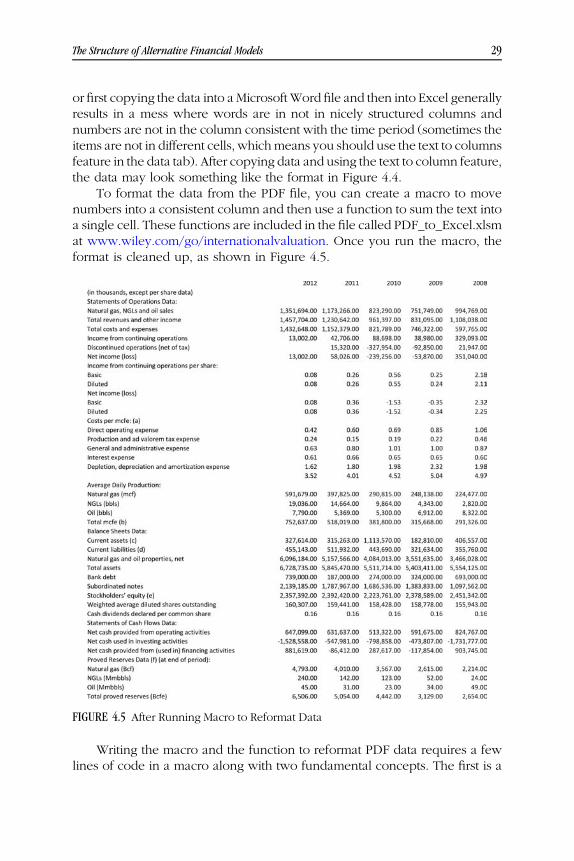
3GC04 10/02/2014 2:32:52 Page 29

or first copying the data into a Microsoft Word file and then into Excel generallyresults in a mess where words are in not in nicely structured columns andnumbers are not in the column consistent with the time period (sometimes theitems are not in different cells, which means you should use the text to columnsfeature in the data tab). After copying data and using the text to column feature,the data may look something like the format in Figure 4.4.

To format the data from the PDF file, you can create a macro to movenumbers into a consistent column and then use a function to sum the text intoa single cell. These functions are included in the file called PDF_to_Excel.xlsmat www.wiley.com/go/internationalvaluation. Once you run the macro, theformat is cleaned up, as shown in Figure 4.5.

Writing the macro and the function to reformat PDF data requires a fewlines of code in a macro along with two fundamental concepts. The first is a

FIGURE 4.5 After Running Macro to Reformat Data

The Structure of Alternative Financial Models 29

3GC04 10/02/2014 2:32:52 Page 30

FOR and NEXT loop, and the second is the CELLS command. In the next fewchapters these concepts are described in detail.

Structure of a Project Finance Model ThatAccounts for Different Risks in Different Phasesover the Life of a Project

Whereas you can think of corporate finance analysis and corporate models asbeing akin to computing the value of a family, a city, or a country, you can thinkof project finance models as representing the value of one person from the timethat person is conceiveduntil heor shedies.Unlike in corporatefinanceanalysis,there is no history in project finance analysis because themodel starts before theperson (or project) is born. Instead, theprojectfinancemodels evaluate risks andreturns for different phases in the defined lifetime of a project. As with anyinvestment, when the risk changes, the value also changes and a financialmodelmust be able to represent these different risks. The source of information forproject finance analysis is some kind of contract, consulting report, or engineer-ing analysis made before the project is conceived rather than the historicalfinancial statements. If you were evaluating the life of a person rather than thevalueof a familyor a city, youmayaccount for changing risks over the courseof alife. The risksmaybehigher during the teenageyears, and the valueof remainingcashflows declineswith age.Of course, this example ismeant to be takenwith agrain of salt and to highlight the issue of changing risk in different phases of aproject’sfinancial investment,which ismuch less of an issue incorporatefinance.Not all teenagers have high-risk behavior and not all elderly people becomeworthless. Since there is no historical balance sheet for a project finance entityknown as a special purpose vehicle (SPV), the launching point for a model isconstruction of a sources and uses of funds analysis during the constructionphase of a project. Key financial outputs from a project finance model comedirectly from the cash flow statement rather than the profit and loss statement.

The single statistic that has the most importance for project owners is theequity internal rate of return (IRR) that measures the growth rate in cash flowsafter money has been paid to lenders (debt service). The equity IRR is oftenstrongly influenced by the amount of debt financing, the method and timing ofthe debt repayment, and the tenor of the debt. The realized equity IRR alsodepends on whether and when the project is sold before it ends, as well aswhether andwhen the debt is refinanced. As the financing structure has a largeeffect on the economics of projects, evaluating a project from the perspective oflenders is an essential part of the modeling process and structure. From thelender perspective, the buffer of cash flow relative to debt service (whatpercentage is the cash flow above the debt service) that is measured by thedebt service coverage ratio (DSCR) is very often a key component of themodel. The fact that IRR is a primary output of the model does not mean it is an

30 Financial Modeling Structure and Design

3GC04 10/02/2014 2:32:52 Page 31

ideal statistic for analysis of value. The IRR has a number of problems,including the following four: (1) it assumes reinvestment occurs at the samerate as the IRR itself. This can be inappropriate if the IRR is very high or verylow; (2) the IRR does not account for the probability of realizing success inthe development or exploration stage of the project; (3) the IRR does notvalue the true risk premium earned from cash flows that are realized indistant future years; and (4) if the IRR is compared to a cost of capital thatincludes a country risk premium, it will often undervalue the investment.

An example of outputs from a project finance model is shown inFigure 4.6, which includes a representation of the project during the construc-tion phase (before the person is born) as shown by the sources and uses offunds analysis. After the commercial operation, the picture of the project canbe summarized by the cash flow relative to the debt service that is shown onthe graph that compares cash flow available to pay debt service with the levelof debt service. The two pictures of the project demonstrate the fundamentalseparation between the preoperation phase and the postoperation phase.

Project finance models typically have two distinct objectives. The first is tostructure the debt and equity that will be issued in the transaction, includingthe size of the debt, the tenor of the debt, and the manner in which debt will berepaid. The second is to assess specific risks in different time periods of theproject life after the defined financial structure is given. Project finance modelsshould be also be able to assess the effects of different types of refinancing and

FIGURE 4.6 Illustration of Summary Analysis for a Project Finance Model

The Structure of Alternative Financial Models 31

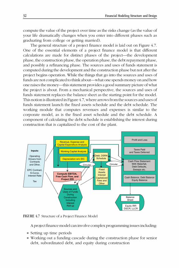
3GC04 10/02/2014 2:32:53 Page 32

compute the value of the project over time as the risks change (as the value ofyour life dramatically changes when you enter into different phases such asgraduating from college or getting married).

The general structure of a project finance model is laid out on Figure 4.7.One of the essential elements of a project finance model is that differentcalculations are made for distinct phases of the project—the developmentphase, the construction phase, the operation phase, the debt repayment phase,and possibly a refinancing phase. The sources and uses of funds statement iscomputed during the development and the construction phase but not after theproject begins operation. While the things that go into the sources and uses offunds arenot complicated to think about—what one spendsmoneyon and howone raises themoney—this statement provides a good summary picture ofwhatthe project is about. From a mechanical perspective, the sources and uses offunds statement replaces the balance sheet as the starting point for the model.This notion is illustrated in Figure 4.7,where arrows from the sources anduses offunds statement launch the fixed assets schedule and the debt schedule. Theworking module that computes revenues and expenses is similar to thecorporate model, as is the fixed asset schedule and the debt schedule. Acomponent of calculating the debt schedule is establishing the interest duringconstruction that is capitalized to the cost of the plant.

Aprojectfinancemodel can involvecomplexprogramming issues including:

■ Setting up time periods■ Working out a funding cascade during the construction phase for seniordebt, subordinated debt, and equity during construction

Revenue, Expense and Capital Expenditure Analysis

Working Capital Analysis Inputs:

Operating

Drivers from Contracts

and Other,

EPC Contract,

S-Curve, Interest Rate

Tax

Profit and Loss

Taxes Paid and Taxes Deferred

Cash Flow Statement With Waterfall, Debt Defaults,

Sweeps etc.

Cash Balance, Debt Balance Equity Balance

Balance Sheet

Equity IRR DSCR, LLCR

Sources and Uses of Funds

During

Construction Including

Interest Roll-up

Debt, DSRA Schedule

Fixed Assets Interest

Capitalized Fees and

Other

Compute EBITDA, Free Cash Flow, and

Project IRR

Depreciation w/o IDC

Circular Circular

FIGURE 4.7 Structure of a Project Finance Model

32 Financial Modeling Structure and Design

3GC04 10/02/2014 2:32:53 Page 33

■ Modeling the debt service reserve account (DSRA) and the maintenancereserve account

■ Developing a cash flow waterfall that works through cash flow prioritiesafter operation begins

■ Sculpting debt repayments to meet a debt service coverage constraint■ Modeling depreciation that depends on calendar years■ Refinancing debt and incorporating cash sweep covenants.

The difficult challenge in creating a project finance model is to addressthese issues without making the model hopelessly complex and cumbersomewith many macros to deal with circular references and with long andcomplicated formulas. Part IV of the book addresses programming issuesto resolve these issues in as painless a manner as possible.

Since a project is generally a one-off investment where debt and equityinvestors focus on cash flow rather than accounting earnings, the structure forcomputing cash flow is also different in a project finance model than in acorporate model. For a project finance model, the final part of the cash flowwaterfall is the dividends paid to the owners of the SPV (sponsors), meaning thatdividends are not defined from a dividend payout ratio, dividends per share, orsome other algorithm, but rather are the residual cash flow not paid or reservedelsewhere. Effective modeling of cash flows in a project finance model involvesintegration of the debt schedule with the cash flow waterfall in the cash flowanalysis aswell as launching themodel froma sources andusesof funds analysis.Finally, aswith the corporatemodel, the balance sheet is part of the output ratherthan a mechanical calculation. All of the accounts such as plant balance, debtservice reserves, senior debt balance, subordinated debt balance, and commonequity balance are alreadydefinedelsewhere in themodel and thebalance sheetsimply tabulates these accounts.Anumberofprojectfinancemodels for differentindustries are found at www.wiley.com/go/internationalvaluation.

Reconciliation of Internal Rate of Return in ProjectFinance with Return on Investment in Corporate Finance

The return on historic investment is an important number in corporate finance.However, it is all but irrelevant in project finance. On the other hand, theproject IRR is computed in project finance but not used in corporate models.While the metrics seem completely different, over the lifetime of a project, thereturn on investment weighted by investment level and the cost of money isthe same as the internal rate of return (IRR). The equivalence of the IRR and thereturn on investment (ROI) is illustrated alongwith a fewmore Excel techniquesin Figure 4.8. A very simple project finance model with no taxes, no debt, anda one-year construction period is shown at the top of the figure. Earningsare computed after depreciation expense on the construction expenditure.

The Structure of Alternative Financial Models 33

3GC04 10/02/2014 2:32:53 Page 34

Because the net investment declines over time, the return on investmentincreases from 3.2 percent to 117 percent over the lifetime of the project.The IRR on the investment lies somewhere between the low value and the highvalue of the return on investment. Figure 4.8 demonstrates that the IRR can becomputed by typing the IRR function and then clicking on the entire row aslong as no numbers other than the cash flow are in the row. Instead of clickingon an entire row, you can press SHIFT and then the SPACEBAR key.

In reconciling the IRR and the ROI, you can compute a series of weightingfactors. Then you can apply these weighting factors to the period by periodROI using the SUMPRODUCT function and compute the weighted average. Incomputing weighting factors, the notion of using the SUM function and anentire row is illustrated on Figure 4.8. The SUMPRODUCT function and theSUM functions illustrated in Figure 4.8 use the entire row number rather thanentering both a row and a column number. When entering SUM(34:34), youcan simply click on the entire row 34 and save a few seconds’ time. The lastequation on the diagram shows that you can also click on multiple rows whenmaking calculations with the SUMPRODUCT function. Once the ROI isweighted by both the level of investment in the denominator of the ROI

FIGURE 4.8 Reconciliation of Return on Investment and Internal Rate of Return

34 Financial Modeling Structure and Design

3GC04 10/02/2014 2:32:53 Page 35

formula and the cost of money as defined by the IRR result, the weightedaverage ROI is exactly the same as the IRR.

Structure of an Acquisition Model: AlternativeTransaction Prices and Financing Terms

If a project finance model is analogous to simulating your life and a corporatefinance model is like representing your family, an acquisition model could bethought of as modeling a dramatic change in the structure of a family—perhaps migrating to a different country, changing religion, or borrowing a lotof money for education. To make a model of the future prospects of the familyafter such an event, you could start with the history of the family as with thecorporate model. But then you probably want to adjust the model to reflectthe new structure that arises because of the dramatic new event. Making anacquisition model involves both incorporating history as in the corporatemodel and also starting the new restructured company with a differentfinancial structure as in the project finance model.

Acquisition models may be developed to determine howmuch to pay for atarget company and how much of the purchase price can be financed withdifferent types of financing, including amortizing debt, debt with a bulletmaturity, and debt with capitalizing interest (this is sometimes known as“ABC”). Key assumptions in an acquisition model include how much theoperating cash flow can grow after new owners take over and a new strategyis developedalongwithhowmuch the companycanbe sold for after theholdingperiod. Financial ratios used in assessing an acquisition are often related to theEBITDA. These include the EV (net debt plus equity value) to the EBITDA, thesenior debt level to the EBITDA, and the total debt level to the EBITDA. Aswith aproject financemodel, an acquisitionmodel can be used to determinewhether afinancial structure is applied that makes sense as well as risk assessment.

Figure 4.9 illustrates the summary output from an acquisition model thattries to paint a picture of the transaction as well as the net value of theacquisition. Information on the left in the Sources and Uses section showsreturns that result from different providers of capital. The graph on the upperright-hand side of Figure 4.9 demonstrates the IRR generated in differentperiods with different assumed exit values.

The architecture of an acquisition model is illustrated in Figure 4.10. Thisdiagram demonstrates that modeling an acquisition transaction involvescombining some aspects of corporate models with other features of projectfinance models. As with a corporate model, the history of the company is astarting point for painting a picture of the company. However, like in a projectfinance model, equations in an acquisition model should begin with a sourcesand uses of funds analysis that shows how much cash is used for the

The Structure of Alternative Financial Models 35

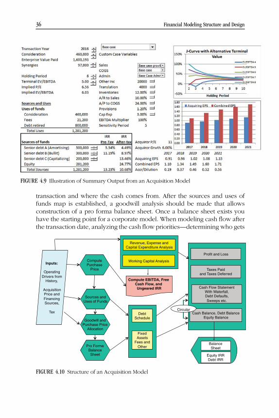
3GC04 10/02/2014 2:32:53 Page 36

transaction and where the cash comes from. After the sources and uses offunds map is established, a goodwill analysis should be made that allowsconstruction of a pro forma balance sheet. Once a balance sheet exists youhave the starting point for a corporate model. When modeling cash flow afterthe transaction date, analyzing the cash flow priorities—determining who gets

FIGURE 4.9 Illustration of Summary Output from an Acquisition Model

Revenue, Expense and Capital Expenditure Analysis

Working Capital Analysis Inputs:

Operating

Drivers from History,

Acquisition Price and

Financing Sources,

Tax

Goodwill and Purchase Price

Allocation

Profit and Loss

Taxes Paid and Taxes Deferred

Cash Flow Statement With Waterfall, Debt Defaults,

Sweeps etc.

Cash Balance, Debt Balance Equity Balance

Balance Sheet

Equity IRR Debt IRR

Sources and Uses of Funds

Pro FormaBalance Sheet

Debt Schedule

Fixed Assets

Fees and

Other

Compute EBITDA, Free Cash Flow, and Ungeared IRR

Compute Purchase

Price

Circular

FIGURE 4.10 Structure of an Acquisition Model

36 Financial Modeling Structure and Design

3GC04 10/02/2014 2:32:54 Page 37

the cash first andwho gets it last—is central to the process. You should see thatsome things are like project finance and some are like corporate finance. If youare evaluating acquisitions it is good to have some knowledge of bothcorporate finance models and project finance models.

The design aspects of an acquisition model involving computation of a proforma balance sheet throughmapping the sources and uses of funds along witha goodwill analysis that incorporates the accounting aspects of the transaction isshown in the second columnof Figure 4.10.Once thepro forma balance sheet iscreated, the modeling process contains similarities to both a corporate modeland a project finance model. As with a corporate model that works throughdifferent balance sheet asset and liability accounts, an acquisition model doesthe same thing but the first year closing balance comes from the pro formabalance sheet. Aswith a projectfinancemodel, defining phases in an acquisitionmodel is an essential part of the process—the transaction period should beflexible and should be distinguished from the holding period and the terminalperiod. The right-hand side of Figure 4.10 shows that the cash flow modelingprocess is analogous to the methods described for a project finance modelwhere a waterfall progressionmeasures the priority of cash flows to the varioussources of funds and ultimately the equity holders.

Some of the challenges in creating models that measure the value of anacquisition or a leveraged buyout are:

■ Creating a cash flow waterfall with alternative amortizing, bullet, andcapitalizing debt, as well as cash requirements and revolving debt facilities

■ Allowing the model to begin at different dates and transferring data from astand-alone corporate model to an acquisition model

■ Developing alternative structuring assumptions and a pro forma balancesheet

■ Structuring the cash flow analysis to determine the points at whichalternative financing instruments yield returns below the risk-free rate

■ Simulating alternative purchase prices to yield required returns withdifferent holding periods, exit multiples, and holding periods

■ Modeling income taxes and alternative tax treatments (tax free exchangesor asset purchases) of transactions

■ Simulating the structure of equity cash flows to alternative investors fromearn-out provisions and equity kickers

Structure of an Integrated Merger Model:Forecasting Earnings per Share

The objective of a merger integration model is to evaluate howmuch to pay asequity consideration for a company and how to structure the financing of a

The Structure of Alternative Financial Models 37

3GC04 10/02/2014 2:32:54 Page 38

merger transaction. This kind of model is like a royal marriage in the sixteenthcentury where the merger of two families was supposed to make thecombined new royal family more powerful than the sum of the individualfamilies through putting two countries together. You could also make ananalogy to the European Union where synergies are supposed to improve anintegrated system. An integrated merger model typically compares earningsper share and credit statistics in the scenario where a merger takes place to adifferent scenario without a merger. The prospective earnings of the mergedcompany depend on how much is paid for the acquisition and how manysynergies are generated from changing management as well as the financingof the transaction. Whenmeasuring the costs and benefits of a merger using anintegrated model, the information base is the historical operations, projectedcost savings, and/or revenue increases for both the target company and theacquiring company, as well as the transaction terms.

Figure 4.11 demonstrates that an integrated model structure mixes ele-ments of an acquisition model and a standard corporate model. As withacquisition models, the starting point of a merger integration model is asources and uses of funds analysis of the transaction and the pro formabalance sheet after goodwill and other adjustments. A difference between theacquisition model and the integrated model is that the pro forma balance sheetbegins with existing balance sheets of both the target company and theacquiring company. For an integration model, the transaction assumptionsincorporated in the sources and uses of funds analysis may include a shareexchange, multiple debt issues, and new equity offerings.

Target Company Financials

Acquiring Company Financials

Inputs:

Operating

Drivers from History,

Acquisition Price and

Financing Sources,

Tax

Goodwill and Purchase Price

Allocation

Profit and Loss

Taxes Paid and Taxes Deferred

Cash Flow Statement

Cash Balance, Debt Balance Equity Balance

Balance Sheet

EPS Accretion Credit Measures

Sources and Uses of Funds

Pro FormaBalance Sheet

Debt Schedule

Fixed Assets

Fees and

Other

FIGURE 4.11 Structure of an Integrated Consolidation Model

38 Financial Modeling Structure and Design

3GC04 10/02/2014 2:32:56 Page 40

Once the starting balance sheet is established through the pro formaanalysis, the remaining calculations and the cash flow process are similar tothe corporate model where computation of net cash flow leads to theaccumulation of a net cash balance and the net cash balance is separatedbetween short-term debt and surplus cash. In an integrated model the debtschedule includes debt issues retired in the transaction as well as new debtfinancing to pay for the merger, along with the associated fees and breakagecosts. Shares issued in the transaction could come from a new share offering orfrom the shares issued to target company shareholders as part of a shareexchange. Figure 4.11 shows that instead of computing a working analysis toderive revenues, expenses, and capital expenditures, these numbers comefrom individual stand-alone corporate models for the target company and theacquiring company. The most difficult item to forecast in this type of model isoften the synergies that arise from changes in management strategy that comeabout from the transaction. In practice, these synergy projections must bemade with only public information and little time when using a model toconstruct an offer for a company.

A comparison of the elements that are included in the layouts of differenttypes of financial models is shown in Table 4.1. Subsequent chapters discusscomputational issues in creating each of the major model components. Inaddition to the general descriptions of how equations should be created, thereare discussions of some practical programming tips to make the process moreefficient for those who are involved in construction of models on a regularbasis.

40 Financial Modeling Structure and Design

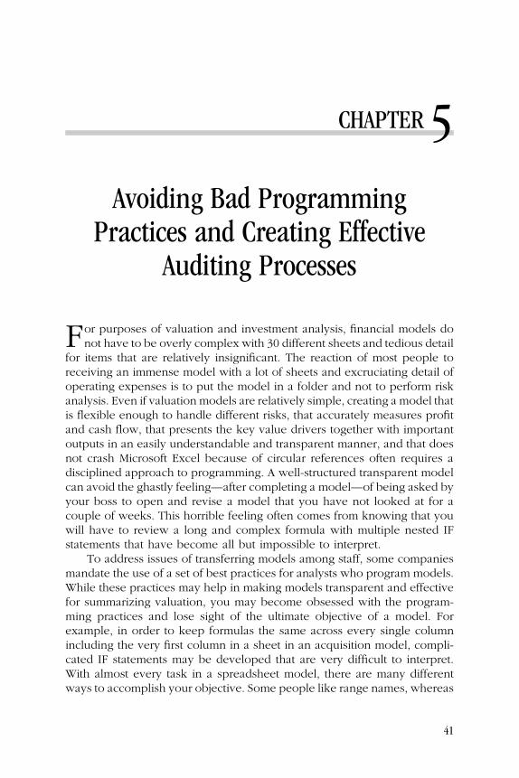
3GC05 10/02/2014 2:37:17 Page 41

CHAPTER 5Avoiding Bad Programming

Practices and Creating EffectiveAuditing Processes

For purposes of valuation and investment analysis, financial models donot have to be overly complex with 30 different sheets and tedious detail

for items that are relatively insignificant. The reaction of most people toreceiving an immense model with a lot of sheets and excruciating detail ofoperating expenses is to put the model in a folder and not to perform riskanalysis. Even if valuation models are relatively simple, creating a model thatis flexible enough to handle different risks, that accurately measures profitand cash flow, that presents the key value drivers together with importantoutputs in an easily understandable and transparent manner, and that doesnot crash Microsoft Excel because of circular references often requires adisciplined approach to programming. A well-structured transparent modelcan avoid the ghastly feeling—after completing a model—of being asked byyour boss to open and revise a model that you have not looked at for acouple of weeks. This horrible feeling often comes from knowing that youwill have to review a long and complex formula with multiple nested IFstatements that have become all but impossible to interpret.

To address issues of transferring models among staff, some companiesmandate the use of a set of best practices for analysts who program models.While these practices may help in making models transparent and effectivefor summarizing valuation, you may become obsessed with the program-ming practices and lose sight of the ultimate objective of a model. Forexample, in order to keep formulas the same across every single columnincluding the very first column in a sheet in an acquisition model, compli-cated IF statements may be developed that are very difficult to interpret.With almost every task in a spreadsheet model, there are many differentways to accomplish your objective. Some people like range names, whereas

41

3GC05 10/02/2014 2:37:17 Page 42

others hate them; some like drop-down boxes, whereas others don’t; someuse SUMPRODUCT and some accomplish the same thing with SUMIF andyet others like using the regular old SUM function with a formula insideand pressing SHIFT, CNTL, ENTER. It is good to keep an open mindabout different programming issues and generally it is also best to try tobe as lazy as possible with spreadsheet functions. You should also notbecome too bureaucratic about best practice rules, especially when they donot make a lot of sense.

Instead of suggesting there is such a thing as a best practice, it is easier tomake a list that explains why some bad practices should be avoided and writedown good practices that shouldn’t be overlooked. Through avoiding some ofthe bad practices listed here and following the good practices, a model shouldbe easier to interpret and modify:

■ There should be no inputs in any part of the model other than in the inputpage(s). One of the worst and most obvious problems is to include inputsas part of a formula (e.g., A11*5); these partial inputs are difficult to find,and they make the models inflexible.

■ Avoid long and overly complex formulas. Keep formulas in the model assimple as possible, and clearly delineate how each formula is derivedfrom the inputs (this is often a problem with long IF statements). Longformulas can almost always be avoided by splitting up equations intomultiple different rows and by using TRUE/FALSE switches. Never usenested IF statements. This does not mean that you should follow the sillyrule of thumb that formulas not be longer than your thumb (unless youhave a very long thumb). But it is safe to say that overly complicatedformulas are the worst practice of all.

■ Avoid inconsistency. Make sure that spreadsheet columns are consistentthroughout the model and that the formulas for each column are identical(with the exception of the very first period in corporate models andacquisition models).

■ Include the units (such as tons of gold or thousands of euros) for eachcolumn of the inputs and on the working sheet.

■ Carefully specify the time period of the model using codes that definealternative phases of the analysis. Put the time line at the top of each sheet.Use the LOOKUP or MATCH and INDEX functions rather than theVLOOKUP or HLOOKUP function to associate inputs with the timeperiod, so users can add rows or columns to the model without worryingabout getting different results.

■ Divide the model into separate modules. Begin with input modules andmake the inputs a separate color (the word “module” simply refers to aseparate part of the model—it could be a separate spreadsheet page or

42 Financial Modeling Structure and Design

3GC05 10/02/2014 2:37:17 Page 43

simply a segment of one sheet). When entering inputs in one or moremodules, operating inputs should be separated from financial inputs.

■ Work through every single balance sheet item. For each asset and liabilityshow the opening balance, additions and subtractions from the account,and the closing balance for the account. This analysis should be made forevery single title in the balance sheet, ranging from cash accounts tocommon equity.

■ Limit or avoid the use of macros and iterations to resolve circularreferences. Circular references are not present in the real world, andfixing circularity makes many risk analysis programming techniquesdifficult.

■ Use the balance sheet and other tests as auditing tools, and include aseparate integrity page of the model to present verification checks. Thereshould be a cell in the verification page that points to the location of themodel errors so you do not have to look around the model to findproblems. Include a dashboard at the top of each page of the model tomonitor the integrity and show key outputs of the model.

■ Ensure that no formulas in the output part of a model affect anything inany other section of the model. This means that you should be able todelete the output section without causing any reference errors in themechanical calculation parts of the model.

■ Use MIN and MAX instead of IF statements in cash flow analysis. Whenworking through a cash flow waterfall, test various balances such as thedebt balance, the net asset balance, the reserve balance, and other itemsrelative to the opening balance using the MIN function instead of IFstatements. The MIN function together with the opening balance puts acap on things that can lead to negative balances. For example, thescheduled debt repayment can be capped at the opening balance—you do not want to pay more than the existing balance back to the bank.

These principles seem obvious when written down in a book. However,in the midst of creating a model to meet a tight deadline, it is very easy toignore them, as they seem to slow you down. Examples of bad practicesinclude entering input data in the fifth sheet of a model, including compli-cated revenue and expense calculations with long IF statements directly inthe income statement, forcing the balance sheet to balance using some kindof a cash balancing item, computing interest expense without separatelylisting debt issues, and not being consistent with time periods.

The single worst practice that is often made by otherwise very goodmodelers is to make formulas that are far too long. An example of a formulafrom an actual model (for evaluating projected prices of a wind farm) that isnot transparent and is almost impossible to verify is shown here:

Avoiding Bad Programming Practices and Creating Effective Auditing Processes 43

3GC05 10/02/2014 2:37:17 Page 44

=IF(AB5<14,IF(AB2=6,AA39*(1+inflation),AA39),IF

(AB5=14,’OperatingInputs'!$E$103/'OperatingInputs'!$E$104,IF

(LEN(AB5)=2,AA39,AA39*(1+inflation))))

This formula contains a number of bad practices. One problem is thatfixed numbers are included in the formula (i.e., the number 14 and thenumber 6). The larger problem is that the formula is far too complex to easilyverify and audit. This formula could be vastly improved if one would splitit up into a number of separate rows where one could show the inflationrate, the logical tests, and the alternative results of different conditions. If youare asked to review somebody else’s model, it is a good idea to split upformulas like this one. This particular formula was split into about 15 rows,and once the more transparent separate rows were presented, severalobvious errors in the formula became apparent.

How to Make Financial Models More Efficientand Accurate

The paragraphs that follow highlight a few programming techniques thatimplement some of the concepts listed earlier and offer tips to prevent yourmodel from becoming a hopeless mess. If you are more interested in generalmodeling concepts rather than the implementation details or if you want to beable to read models but not to program them, you should skip the detaileddiscussion of practical programming and begin reading the next chapter ontime periods and valuation.

Creating Shortcut Keys and Setting Up the Model Area SoYou Can Build Your Model Quickly

This seems like a trivial little detail, but in structuring a model you can makeit much easier to read—the transparency objective—by doing a few thingsbefore you start typing a single number in the spreadsheet. Models generallyare presented in a similar manner to financial statements from annual reportswhere time (years, quarters, or months) is shown across columns and itemssuch as revenues are listed on different rows. In setting up the columns, itis nice to include some thin columns at the beginning of the sheet so that youcan press the CNTL, UP and the CNTL, DOWN keys and move from sectionto section. The time line section will often be the first section, followed bythe assumptions section, the operations section, and the depreciationsection. By putting headings in the first column (e.g., the words “timeline,” “assumptions,” “operations,” etc.), you can quickly move from sectionto section. It is also essential to leave a few blank columns between the titles

44 Financial Modeling Structure and Design

3GC05 10/02/2014 2:37:17 Page 45

and the model equations. In these special columns after the row names butto the left of the equations, you can display the units, show what inputs areused to drive the equations, and incorporate verification checks of variousitems. This little idea of including a few extra columns is indispensable inmaking the process transparent where a reader can, it is hoped, visualizehow the equations are working. The idea of using special columns betweenthe row titles and the equations is illustrated in the model excerpt shown inFigure 5.1.

Using shortcut keys rather than using the mouse will enable you towork faster and more easily develop and modify the model. (In some financialmodeling courses imposed on young bankers, the mouse is removed fromcomputers so students learn how to navigate around spreadsheets much morequickly, lest they waste a minute in creating collateralized debt securities outof subprime loans.) Arguing that shortcut keys should be applied instead ofdragging your finger across an iPhone may seem a bit odd when you first usethem instead of the mouse. But if you practice, they really canmake your workon the model easier. Shortcut keys that are very useful for formatting areSHIFT, CNTL, 1 for decimals; SHIFT, CNTL, 3 for dates; SHIFT, CNTL, 4 forcurrency; and SHIFT, CNTL, 5 for percentages. One of the most helpfulshortcuts is the combination of the following two keystrokes, which allowsyou to very quickly copy and paste rows in a financial model:

1. Press SHIFT, CNTL, → (right arrow) at the same time to mark a row2. Press CNTL, R to copy the formula or data to the right

FIGURE 5.1 Setting Up the Structure of a Transparent Model

Avoiding Bad Programming Practices and Creating Effective Auditing Processes 45

3GC05 10/02/2014 2:37:17 Page 46

This involves two steps rather than pressing CNTL, C and highlighting anarea and then pressing CNTL, V. It also works with CNTL, down arrow andCNTL, D. The problemwith this shortcut is that it copies the contents of the firstcell to each column of the sheet, all the way to the right end of the sheet. Tolimit the copying of columns to the maximum rows of your sheet (themaximum number of periods that you may forecast), you can hide thecolumns to which you do not want the item to be copied. To hide columnsto the right of the model periods, you can group all of the columns to the rightof the last column in your program. To use this method, use the SHIFT, ALT,→combination to group columns and press the number 1 on the top left cornerof the spreadsheet as summarized in these four steps:

1. Highlight the entire column of the first column to be hidden (you can usethe CNTL, SPACEBAR combination).

2. Press SHIFT, CNTL, → to highlight the remaining columns in the sheet.3. Use the SHIFT, ALT, → combination to group the remaining selected

columns.4. Press the number 1 in the square box at the top left of the sheet.

If you need the columns to the right, you can press the number 2 buttoninstead of the number 1 button on the top left of the spreadsheet. Results of thegrouping approach are shown in Figure 5.1, where the right part of the sheetafter the columns have been grouped is tinted gray. After you’ve done this afew times, setting up the spreadsheet should take a few seconds.

These shortcut combinations are pretty cool, but it is even more useful tomake your own shortcuts. When making your own shortcuts, you can simplycreate a macro around the task you want to repeat. You can, for example,make a CNTL, U and a CNTL, L combination to copy up and to the left as theseare not part of a standard workbook. When making a macro to create yourown shortcut, you enter a shortcut key as illustrated in the next section, but ifyou make the macro run with CNTL and lowercase c, then the copy functionwill no longer work. Instead, you can create the macro with CNTL and capitalC so that it works when you press SHIFT, CNTL, C. When creating your ownshortcut to do something like formatting cells with two decimal places (unlikethe SHIFT, CNTL, 5 combination, which does not include decimals), you cando the following:

Step 1 Go to the cell that you will format with a percent sign and twodecimals. You must be on the cell because you should not movethe cell as part of the macro process.

Step 2 Record a macro, which is like recording a video on your phone.Do not do anything during the recording process that you do notwant to appear in the video (macro). After pressing the record

46 Financial Modeling Structure and Design

3GC05 10/02/2014 2:37:18 Page 47

button, define a shortcut key with the SHIFT keyboard key (e.g.,press capital D for decimals.) Do not ever move the cursor toanother cell after you begin recording the macro, or that willbecome part of the macro. In this case after you press SHIFT,CNTL, D the cursor will do the same thing that you record.

Step 3 Change the formatting in the cell (you could use the CNTL, 1shortcut).

Step 4 Stop recording the macro without moving the cursor.

A shortcut that avoids the irritating Excel feature that automaticallyswitches inputs to percentages can be made with the simple macro shownin Figure 5.2.

Color Conventions and Creating the SHIFT, CNTL, C Macroto Color Inputs

In a well-structured financial model colors should be used as a guide to whatis happening in various cells of the model. This means the colors should notbe used to make the model into an attractive piece of art; it is better that theyprovide readers of the model with a quick understanding of where thenumbers in a cell come from. One principle is that input cells should becolored differently from other cells, generally through using the fill color andthe background color. Some accountants use the cmyk rule where cells thatcome from another sheet are colored red, cells that come from a link in thesame sheet are colored green, and cells that are inputs are colored blue.There are a few methods you can use to color inputs automatically. Onemethod is to use the F5 key and then press the Special tab on the bottom leftof the menu box that pops up (see Figure 5.3). After the menu appears,select the Constants option that will find all of the inputs except for the text,as shown in Figure 5.4. After finding the inputs, simply select the foregroundcolor you want from the Home tab.

When using the F5 key and the Special button, you can create theprocess in a macro that allows you to redo the coloring process every timeyou make a change in your model. To create this macro, you can assign themacro to a CNTL combination and then have your own shortcut key, such as

Sub fix_decimal()

ActiveCell = ActiveCell * 100

Selection.NumberFormat = "#,##0.00"

End Sub

FIGURE 5.2 Function to Fix Problem of Percentage Formatting

Avoiding Bad Programming Practices and Creating Effective Auditing Processes 47

3GC05 10/02/2014 2:37:18 Page 48

SHIFT, CNTL, C, redo the colors any time you want. Figure 5.5 shows how tobegin recording the macro.

A second principle in addition to coloring inputs is that a different fontcolor should be used for cells in which data comes from another sheet. If pricedata is transferred from the input sheet to the working sheet, that cell shouldhave a color to notify users in what sheet they can quickly find the source ofthe data. A macro that sets the font color of a cell from the tab color of the sheetis included at www.wiley.com/go/internationalvaluation. Other colors can be

FIGURE 5.3 Using the F5 Key to Color Input Cells

FIGURE 5.4 Selecting Input Cells with the F5 key

48 Financial Modeling Structure and Design

3GC05 10/02/2014 2:37:18 Page 49

used for cells that have been computed from the Goal Seek feature or theSolver add-in tool and for cells that are computed through the operation of amacro. Finally, cells in which calculations that are not direct links are madefrom information in the same sheet should not have a font or a fill color.

Figure 5.1 illustrates a few of the setup ideas just discussed. The sheet is setup using the SHIFT, ALT, → method to limit the size of the sheet with thegrouping method. When you press 1 at the top left, the columns are hidden,whereas when the number 2 is pressed, the columns are unhidden. Red cellscome from the scenario sheet to the left of the sheet presented, which has a redtab color. Cells with a blue font are inputs in the sheet that are colored with theSHIFT, CNTL, Cmacro. Figure 5.1 illustrates that it is a good idea to make a fewsmall columns on the left of the spreadsheet so that it is clear what rows aresubtotals and headings.

When setting up your workbook it is often useful to program a couple ofuser-defined functions in addition to your customized shortcut keys. Makinguser-defined functions can open up a whole new set of power in financialmodels and is discussed at length in solving depreciation problems, comput-ing the EV/EBITDA ratio and dealing with circular references in an efficientmanner that avoids the nasty copy and paste macros. Some who are snobbishcomplain that Excel is a very blunt tool and software programs such asMATLAB are much better. They are in a sense correct that a spreadsheetby definition is somewhat limiting. But you can open up another whole worldby adding functions to your workbook that vastly expand its power. Creatingyour own user-defined functions has some important contrasts to making amacro. In the spreadsheet, your function works like any other function such asthe SUM function where you use an equals sign and put cell references or

FIGURE 5.5 Recording a Macro for Creating a Shortcut for Coloring Cells

Avoiding Bad Programming Practices and Creating Effective Auditing Processes 49

3GC05 10/02/2014 2:37:19 Page 50

range references inside the parentheses. When creating a function rather thana standard macro, there are a couple of basic concepts that always apply:

1. The name of the function title must be defined as an output variablesomewhere in the code.

2. Any value that is used from the spreadsheet must be read into thefunction; for example, you cannot use something like RANGE(“A1”)inside the function.

To introduce how functions can help you, a few simple ones areintroduced in this chapter. One function that is useful is to show formulasadjacent to the cell where the calculation is made (this function was used insome of the excerpts shown previously). To create such a function you shouldfirst go to the Visual Basic screen. To do this you can press ALT and F11. Thenyou can type in a function as illustrated in Figures 5.6 and 5.7. A simple versionof the function named show_form is illustrated in Figure 5.6, and a little fancierversion named show_formula is illustrated in Figure 5.7. Note that you muststart the code with the name Function rather than SUB.

It is also often useful when setting up a spreadsheet to create a function forshowing the sheet name as a formula. This function requires only one line ofcode, as demonstrated in Figure 5.8.

Function show_form(cell)

show_form = cell.Formula

End Function

FIGURE 5.6 Basic Function for Displaying Formulas

Function show_formula(cell)

show_formula = _

"< ---- Formula for: " & cell.Address & " " & cell.Formula

End Function

FIGURE 5.7 Function to Show Display Formulas with Arrow

Function sheet_name(cell)

sheet_name = cell.Parent.Name

End Function

FIGURE 5.8 Function for Showing the Sheet Name

50 Financial Modeling Structure and Design

3GC05 10/02/2014 2:37:20 Page 51

After entering this function, you can type = SHEET_NAME(cell) in any celland refer to the current sheet or another sheet and find the sheet name.

If you have created a whole lot of functions and extra shortcut keys in onesheet and would like to use them in other workbooks, you can go to the VisualBasic for Applications (VBA) menu and export your file, which is like savinga file using any software. Then, in your new workbook, you can import allof the codes by referring to the name of the file that you just exported. Thewebsite, www.wiley.com/go/internationalvaluation, has a file named generic.bas that contains many extra shortcut keys and functions.

Creating an Audit Page That Tells You Where Errors AreLocated

Part of an efficient model design is creating an auditing method where theprogram itself reports things that do not work. You can write a message some-where at the top of each sheet that documents the location of mechanicalproblems with the model so you do not have to look around the workbookcontinually to find the source of the problem. On the top of each page you maywant to show an overall check on the integrity of the model: Does the balancesheet balance; is the debt balance positive; are the dividends nonnegative; do thesources of cash equal the uses of cash? Sometimes it is useful to also include aseriesofauditchecksas towhetherdebt is indefaultaswell asmechanical checks.

A good way to set up the integrity check of a model is to use TRUE andFALSE logical variables. Application of TRUE/FALSE switches is helpful inmanydifferent parts of the model. Use of TRUE/FALSE variables eliminates the needfor painful, nested IF statements that can be very difficult to audit. TRUE/FALSEvariables are almost essential in structuring the time line of a model. A TRUE/FALSE switch variable can be created by simply using an equals sign. In theequation= 1= 1, the result is TRUE. It is often useful to apply the AND functiontogether with a series of logical variables to test if the overall value is TRUE; forexample,AND(1=1,2= 2) isTRUE. Further,when IF statements areentered, theTRUE/FALSE switch can be used in the logical section of the function. Thefollowing step-by-step process illustrates how to create a verification page withTRUE/FALSE switch variables that will show you where you made an error:

Step 1 After making the balance sheet, subtract the total assets fromliabilities on a separate row to compute the difference, whichshould be 0. Create similar calculations for the debt balance, thesources and uses of funds, and other items. Sometimes creating anequation that tests the model results is not as obvious as it is whenyou only want to test something in one period of themodel or onephase of the analysis. In such situations you can often use theSUMIF function.

Avoiding Bad Programming Practices and Creating Effective Auditing Processes 51

3GC05 10/02/2014 2:37:20 Page 52

Step 2 In a separate row, use a TRUE/FALSE logical variable created bysetting one cell equal to another to test whether the difference,after rounding, is equal to 0. In the balance sheet case, the test iswhether the difference is 0. The rounding is often necessarybecause the difference is not precisely equal to 0 if, for example,there is a division by 3 somewhere in the model. For the balancesheet, the formula in each model period is:

�ROUND�difference; 3� � 0

Step 3 Once the TRUE/FALSE result is established for each period, theAND function can be used to test the balance sheet balances inevery period of the model. The AND function can be applied to arange of TRUE/FALSE logical variables and placed to the left of allof the year-by-year tests as illustrated in Figure 5.9.

Figure 5.9 illustrates the verification of the balance sheet thatthen feeds into an aggregate balance sheet test. The row labeled“test” uses a switch and the ROUND function to make sure thebalance sheet balances in each period. If all of the other tests likethe aggregate balance sheet test are TRUE, then the aggregate testcomputed with the AND function (shown at the left) is also TRUE.

FIGURE 5.9 Illustration of Balance Sheet Verification

52 Financial Modeling Structure and Design

3GC05 10/02/2014 2:37:20 Page 53

Figure 5.9 also shows how a SUMIF function can be used alongwith a time period switch to limit the test to the historical periodin a model.

Step 4 Link the TRUE/FALSE results from the AND and SUMIF statementsand any other test to a separate page of the model that contains allof the other verification checks.

Step 5 Type a title for each individual test and put the linked cell with thevalue of TRUE or FALSE next to the test title. Identify the sectionsof the model that have problems using an IF statement that usesthe title of the test and the TRUE/FALSE result of the test. TheIF statement has the form:

� IF�test; “”; title�Whenmaking the balance sheet test, the test in the preceding

formula would be the aggregate TRUE/FALSE test from themodel. The title would be something like “Balance Sheet Test.”

Step 6 Once the sections of the model with problems are identified,make an aggregate presentation of all of the problems in themodel. This cell that aggregates all of the problems can be placedin each sheet to allow you to find problems without lookingaround the model each time you make a change. The aggregatepresentation of all of the tests has the form:

� problem1&problem2& . . .&problem10

In this equation the problem1, problem2 cells come fromthe IF statement in step 5. The “&” function allows the text to beput together as if you were adding things. For better presenta-tion, it is a good idea to put a space before each title so theproblems are delineated. It is surprising that Excel does nothave a function that allows you to add all of the text togetherwithout all of the irritating & symbols. This is another situationwhen you can create your own function. This function that addstext together is illustrated in Figure 5.10. In this case the functionaccepts an array variable and it needs to count the number ofelements in the array. A FOR NEXT loop is included in thefunction to aggregate the text together using the & symbol as ifit were done in the spreadsheet. As with the show formulafunction, the name of the function must be assigned to some-thing in the body of the function. To write your own functionslike this, simply go to the VBA editing screen by pressing ALT,F11, and type the following text.

Avoiding Bad Programming Practices and Creating Effective Auditing Processes 53

3GC05 10/02/2014 2:37:21 Page 54

An example of a page that shows verification checks usingthe step-by-step process discussed here is illustrated in Fig-ure 5.11. The end result of this process is a single cell that tellsyou where you made your errors.

Function add_text(series)

num = series.Count

For i = 1 To num

add_text = add_text & " " & series(i)

Next i

End Function

FIGURE 5.10 Function to Combine an Array of Text

FIGURE 5.11 Illustration of an Audit Page for a Project Finance Model

54 Financial Modeling Structure and Design

3GC06 10/02/2014 2:43:44 Page 55

CHAPTER 6Developing and EfficientlyOrganizing Assumptions

In discussing the architecture of various models in Chapter 4 for thecorporate model, project finance model, acquisition model, and inte-

grated model, it was evident that each of the financial models have manythings in common. All of the models begin with an input section and endwith a balance sheet. Each model includes a working section that computespretax cash flow comprising revenues, expenses, and capital expenditures;each model moves from pretax cash flow to after-tax free cash flow bycomputing depreciation, taxes, and working capital; each model type has adebt schedule; and each model contains an income statement and a cashflow analysis. These components that are common across the different typesof models are described in the next few chapters. This chapter begins thediscussion of common model elements by explaining some theory andpractical issues associated with model inputs.

Assumptions in Demand-Driven Models versusSupply-Driven Models: The Danger of Overcapacityin an Industry

The most important part of the modeling process is to accurately defineand analyze input items that drive the value of an investment and theneffectively present how risks associated with these value drivers affect theultimate investment value. Value drivers can be economic parameters suchas industry demand, behavior of competitors, product prices, cost of capitalexpenditures per unit, and the fixed and variable cost structures. The driversproduce revenues, cash operating expenses, and capital expenditures,which define pretax cash flow and are the starting point of any model.The things that really drive value and should be primary inputs to a model

55

3GC06 10/02/2014 2:43:44 Page 56

are generally not items such as revenue growth, operating margins, returnon investment, or the ratio of capital expenditures to sales, although for verylarge corporations it may be necessary to use these kinds of gross inputs.The real value drivers that are affected by business strategy and economicconditions are rather quantities of capacity, price per unit, variable operatingcost per unit, fixed cost and capital expenditure relative to the amount of newcapacity built. The art of modeling involves identifying how changes in theindustry structure resulting from capacity additions and demand changes,technology changes, consumer tastes, product life cycles, and other factorsaffect these primary value drivers. Modeling and valuation mistakes intro-duced in Chapter 1 were not due to incorrectly structuring a model or havinga financial model that was too simple; they were instead generally the resultof not using valid economic and financial principles in developing industrydemand, supply, and price inputs to the valuation process. These inputscan be studied by reviewing historical data, performing statistical analysis,applying marginal cost concepts, and evaluating changes in the industrystructure. When entering value drivers into a model, you should also usejudgment as to whether sudden nonlinear changes can occur.

When developing a financial model you can distinguish whether profitsand cash flow of a company are primarily driven by demand and market shareor, alternatively, if financial results are driven by commodity prices and costmanagement. The former type of model where demand is the starting point fora model can be referred to as a demand-driven model while the latter in whichcommodity prices determine revenues can be called a supply-driven model.The starting point for the assumptions should generally be the capacity of thecompany (reserves of oil, megawatts of electricity, number of planes) in asupply-driven model. The starting assumption is the industry-wide demandin a demand-driven model.

To understand the difference between demand-driven and supply-driven models, consider an upstream oil project for a relatively small pro-ducer. The most likely place to begin thinking about the upstream model iswith the capacity of oil fields owned by the company in terms of oil and gasreserves. You would probably not begin with an analysis of the worldwidedemand for oil as in a demand-driven model because the company operatesin a commodity business and it will sell whatever it can produce. Alterna-tively, for a company operating in a limited market region such as a port or atelecommunications company, the model would begin with demand for theproduct in the industry followed by an assessment of the industry capacity.With industry-wide demand and supply, an allocation of the industry-widedemand can be made to the particular firm through some kind of marketshare assessment.

The diagram in Figure 6.1 illustrates construction of value drivers and themodeling process for an electricity generating plant in a supply-driven model.

56 Financial Modeling Structure and Design

3GC06 10/02/2014 2:43:44 Page 57

The drivers for capital expenditures, revenues, and operating expenses allbegin with the capacity of the plant. Economic drivers for revenue, operatingexpenses, and capital expenditures include the cost per unit of building theplant, future trends and volatility in prices, capacity utilization of the plant,and the variable and fixed costs of operating the plant.

The most common form of corporate and acquisition models is thedemand-driven model where the starting point should be evaluation ofindustry supply, demand, and prices. Many valuation mistakes are madewhen oversupply occurs in an industry because demand does not increaseas expected or high returns prompt excessive new supply. The famous topright quadrant of a diagram of return relative to cost of capital versus growthcan be an effective way to think about industry demand and supply assump-tions in a model. The top right quadrant, called powerhouse companies,includes companies that are both growing fast and earning high returns. Thisseems like the place that you always want to be. As discussed in Chapter 1, theproblem is that it is also the place everybody else wants to be. Unless reallystrong competitive advantages and barriers to entry exist and companies canmake you addicted to their products, other firms from all over the world willwant to enter businesses represented by this quadrant. The new entrants willresult in industry-wide surplus capacity. When surplus capacity occurs in anindustry, prices can dramatically move from levels that support high returns oninvestment all the way down to the short-run marginal cost of production.With the new entrants coming in and surplus capacity, companies fiercelyfight for market share. In thinking about how surplus capacity can arise, the

FIGURE 6.1 Value Drivers for an Electricity Model

Developing and Efficiently Organizing Assumptions 57

3GC06 10/02/2014 2:43:44 Page 58

return on investment for firms in an industry alongwith barriers to entry shouldbe an essential part of the modeling process. If returns are relatively high andentry of new firms is not limited, surplus capacity can come quickly. A recentexample of such a phenomenon is the solar power manufacturing industrywhere high market valuation and strong returns encouraged addition of newcapacity. New entrants from all over the world began setting up factories thatwere fairly easy to build. The new capacity led to dramatic price reductionsand declines in market value.

Setting up inputs for a demand-driven model beginning with industrydemand and supply is illustrated on the graph in Figure 6.2. In this graph thecapacity additions planned by different companies (the shaded areas) arecompared to demand (the thick line), demonstrating a looming danger ofovercapacity if all of the planned capacity comes on line. When constructinga demand-driven model, illustrating capacity and demand in the entireindustry can be very helpful even if inputs for the industry demand andsupply cannot be precisely obtained and the capacity additions for othercompanies has to be subjectively estimated. The idea of understandingprojected supply and demand conditions relative to historical levels is anessential conceptual step of the process.

–

2,000.00

19

99

20

01

20

03

20

05

20

07

20

09

20

11

20

13

20

15

20

17

20

19

20

21

20

23

20

25

20

27

20

29

20

31

20

33

20

35

20

37

20

39

4,000.00

6,000.00

8,000.00

10,000.00

12,000.00

14,000.00

Container Demand and Capacity in Pakistan,

1999–2040 (TEU 000s)

PDWCT – Berths 5–10

PDWCT – Berths 1–4

PICT

KICPT

Qasim Port

Total Demand

FIGURE 6.2 Illustration of Incorporating Industry Supply and Demand in a CorporateModel

58 Financial Modeling Structure and Design

3GC06 10/02/2014 2:43:44 Page 59

Once the industry supply and demand expectation is established,projections of market share and product prices can be estimated for anindividual firm. The next example is intended to prompt you to thinkabout industry demand and supply in setting up assumptions. It is notnecessarily a guide as to how a particular model should be set up. Theframework for which volume demand and price for a single company couldbe derived from industry demand and supply estimates is illustrated usinga step-by-step process something like the following:

Step 1 Make some kind of projection of industry demand. Possibleapproaches to calculating prospective demand includes regres-sion analysis, evaluation of historical volatility, exponentialsmoothing, and judgment.

Step 2 Second, evaluate the industry capacity from the existing supply ofindividual companies as well as specific knowledge of expectednew additions and expected retirements. It is difficult to projectsurplus capacity without detailed industry knowledge. Compa-nies may not publish capacity expansion plans and it may be verydifficult to compile the data, but this assumption may be the mostimportant item in your whole model.

Step 3 Third, calculate the industry-wide surplus capacity. You can thencalculate the capacity margin and attribute this industry capacitymargin of supply relative to demand for individual companies.You can develop individual company volumes assuming thatmarket share is driven by the capacity of a single companyrelative to total industry capacity. This calculation is illustratedusing the following equation:

ReserveCapacityPercentage= IndustryCapacity/IndustryDemandCompany Demand = Company Capacity/Reserve Capacity

Percentage

Step 4 Derive the assumed price of the product as a function of thereserve capacity percentage. In creating price assumptions, youcould relate the price level to the amount of the surplus capacityin an input table. When the surplus capacity is above a certainassumed level you may assume that the price can fall all the wayto short-run marginal cost. For other levels of surplus capacity youcould input different prices ranging from prices that exceed long-run cost to prices that fall between long-run marginal cost andshort-run marginal cost. To implement a process where prices area function of the relationship between supply and demand andare input in a table you can use a LOOKUP function as shownhere. The LOOKUP function is more flexible and stable than

Developing and Efficiently Organizing Assumptions 59

3GC06 10/02/2014 2:43:44 Page 60

either the VLOOKUP or the HLOOKUP functions because it doesnot require a row or column number.

Price = LOOKUP(Reserve Capacity, Reserve Capacity Range,Price Range)

Creating a Flexible Input Structure forModel Assumptions

When organizing the inputs of a financial model you should group variousrelevant input categories together. In general, the order of the inputs shouldreflect the order of calculations in the model, where timing parameters areentered first, followed by pretax cash flow, after-tax cash flow, and financing.This means inputs should begin with timing parameters, followed by operat-ing inputs, tax and depreciation inputs, financing inputs, and valuationparameters. Inputs can be structured on a period-by-period basis across aspreadsheet page or they can be entered in alternative time increments. Theinputs can be in different pages or put in one page while you are developingthe model. In a corporate model, the inputs should generally be entered nextto historical values and it may be convenient to use conditional formatting toillustrate the history in a different color than the forecast values.

The inputs should be set up in a way that anybody can easily find theassumptions and understand exactly what each input means. If a model hasan input labeled “development expense percentage,” this may be confusingbecause one has no idea what the basis is for the percentages. Second, inputsshould allow the model to be adjusted and not be restrictive; if there is oneinflation rate applicable to all future years, the model has limited flexibility.Third, the inputs should be arranged in a logical manner and groupedtogether by categories that reflect the structure of subsequent calculationsin the model—capital expenditures and revenues first, followed by cashoperating costs, working capital, tax and book depreciation, and, finally,financing and valuation parameters. The five general assumption categoriesshould include:

1. Timing assumptions corresponding to the different types of models. Inproject finance models, the key timing parameters are the financial closedate, the commercial date, the debt repayment date, and the decom-missioning date. In corporate models, the timing assumptions are thehistorical period, the explicit period, and the terminal period. Foracquisition models the key dates are the acquisition date and the exitperiod.

60 Financial Modeling Structure and Design

3GC06 10/02/2014 2:43:44 Page 61

2. Capital expenditures enable a company to generate EBITDA and grow. Itis essential to include the quantity of incremental production that can begenerated from the capital expenditures and associate EBITDA withcapital expenditures in as direct a manner as possible. The cost perunit of the capital expenditures and capital expenditures required tomaintain the existing plant must also be input. In project finance models,entering an S-curve that is flexible and can accommodate constructiondelays can be tricky.

3. Revenue assumptions that include the quantity sold and the price, wherethe price can depend on industry capacity and supply analysis, asdescribed in the earlier discussion of potential surplus capacity. Whenmaking long-run assumptions, understanding the long-run marginal costof production should be considered in the price analysis.

4. Cash operating cost assumptions that are separated between fixed andvariable cost so that different sales quantity assumptions can be evaluatedand the model can measure risks arising from operating leverage. Under-standing what costs are fixed and what costs are variable can be essentialin evaluating risk as demonstrated by the bankruptcies of General Motors(GM) and many U.S. airline companies. When GM’s demand declinedwith high oil prices and the cost structure could not react, the EBITDAdeclined dramatically. To study fixed and variable cost in a corporatemodel you can make a scatter plot of total costs relative to revenues.

5. Working capital assumptions that can be expressed as days outstandingof accounts receivable and accounts payable and so forth. Alternativelythe working capital can be expressed as accounts receivable as apercent of sales and accounts payable as a percent of cost of goodssold (COGS) along with other ratios.

These five assumption categories determine the pretax return oninvested capital in a corporate analysis and the pretax internal rate of return(IRR) in a project finance analysis. Two remaining assumption categoriesare used to derive the after-tax return on invested capital and the projectIRR as well as the return after gearing, including the return on equity and theequity IRR. Those categories are:

1. Tax and associated depreciation assumptions, including tax rates, depre-ciation rates, and inputs associated with the difficult issue of retirements ina corporate model.

2. Financing assumptions that include the amount of debt issued, themanner in which debt will be borrowed and repaid, the interest andfees incurred while debt is outstanding, and credit enhancement featuresof the debt such as covenants and reserves that are designed to protectlenders.

Developing and Efficiently Organizing Assumptions 61

3GC06 10/02/2014 2:43:44 Page 62

Alternative Input Structures for Project Financeand Corporate Finance Models

The manner in which inputs are entered into a model corresponds to thestructural differences between corporate models and project finance mod-els. Corporate finance models are built from history and virtually every inputshould be a time series variable. Most of the variables should be entered in away that enables you to change the inputs from year to year. In a corporatemodel it is a good idea to display the assumptions adjacent to the history andprogram the model so the assumptions can either vary by time period or theassumption can be input as a single number that remains constant over theforecast horizon. Figure 6.3 illustrates alternative assumptions for a corpo-rate model using this idea. In Figure 6.3, the first assumption for sales growthincludes different sets of time varying inputs that change from year to year.In contrast, the assumptions for working capital apply a single number that isfixed over the forecast period. For sales growth, the different time series aredriven by a code number that is shown in red because it comes from anothersheet that has a red tab color. The fixed number that drives the projection ofaccounts receivable is also colored red, but is not a code number. The ideaof using a code number to set up assumptions can be implemented witheither the INDEX function or the CHOOSE function, as explained in the nextsection.

In the case of project finance models, the format does not have the samestructure where the history is consistently shown next to the forecast. Someinputs may be annual; some may be one-time scalar numbers; some maybe switches. An excerpt from project finance model inputs is shown inFigure 6.4.

Setting Up Inputs with Code Numbers and theINDEX Function

To prepare a model for risk analysis, you should set up inputs to the modelby entering different possible scenarios in the data input section. For manyinputs such as volume growth, prices, interest rates, and other factorsdifferent scenarios may have time-changing values over the forecast period,as shown in Figures 6.3 and 6.4. When inputs can take on different valuesover time like this, your challenge is to enter input data without inordinatelycluttering up the model. One reasonable way to enter input data thatcontains changing values over time and different possible scenarios is touse a code number together with the INDEX or CHOOSE function. Thegeneral process of setting up flexible input variables that can change overtime at different date increments is summarized as follows:

62 Financial Modeling Structure and Design

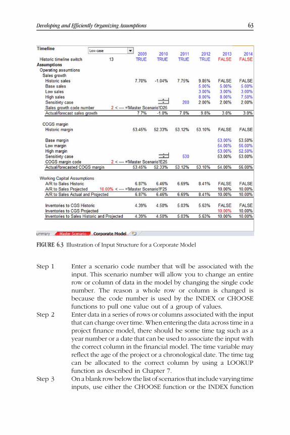
3GC06 10/02/2014 2:43:45 Page 63

Step 1 Enter a scenario code number that will be associated with theinput. This scenario number will allow you to change an entirerow or column of data in the model by changing the single codenumber. The reason a whole row or column is changed isbecause the code number is used by the INDEX or CHOOSEfunctions to pull one value out of a group of values.

Step 2 Enter data in a series of rows or columns associated with the inputthat can change over time.When entering the data across time in aproject finance model, there should be some time tag such as ayear number or a date that can be used to associate the input withthe correct column in the financial model. The time variable mayreflect the age of the project or a chronological date. The time tagcan be allocated to the correct column by using a LOOKUPfunction as described in Chapter 7.

Step 3 On ablank rowbelow the list of scenarios that include varying timeinputs, use either the CHOOSE function or the INDEX function

FIGURE 6.3 Illustration of Input Structure for a Corporate Model

Developing and Efficiently Organizing Assumptions 63

3GC06 10/02/2014 2:43:45 Page 64

along with the scenario code number from step 1. You will usenumbers created with the INDEX or the CHOOSE functions as thebasis of inputs to equations in the model. These two functionssimply find a number from a group of numbers according to agiven row or column number, which is why the code number is anessential part of the process. Recall that the INDEX function worksby highlighting an area or a group of numbers in a row or columnfollowed by a single row or column number that defines whichnumber in the group to select. When using the INDEX function,you should highlight the items for one period and then use thescenario code number as the row or column number. Then youshould lock it with the F4 key for the row or column.

Selected Value for Period= INDEX(Column of Data for Scenarios,Scenario Code Number)

Step 4 Once the variable is defined use the LOOKUP function to insertthe appropriate variable into the financial model. To apply theLOOKUP function, use the relevant time period indicator in thefinancial model as the look up index. Then shade the time periodin the input data and finally shade the items that will be trans-ferred from the INDEX function.

Value in Model = LOOKUP(Time Line Value, Column or Row ofTime Tags in the Input Section, Column or Row of Input Values

in the Input Section)

FIGURE 6.4 Illustration of Input Structure for a Project Finance Model

64 Financial Modeling Structure and Design

3GC06 10/02/2014 2:43:45 Page 65

The example in Figure 6.5 illustrates how to set up flexible inputs in aproject finance context. The top part of the example shows date inputs thatdrive the different timing switches. The capacities per turbine are input asfixed amounts that do not change over time. There are typically few inputsthat are entered as scalars like this in a corporate model. Items wherescenario analysis has multiple different values that can change over timeare entered with a code number that defines the scenario in Figure 6.5.Some inputs can be entered on a year-by-year basis even if the model isstructured on a monthly or semiannual basis. In Figure 6.5 the timing of theinput is flexible and varies according to the date to the left of the input whenthe financial close and/or the commercial operation date changes. Forproject finance models, where timing is so essential to the analysis, it isoften a good idea to structure many variables according to the time line ofthe model.

The colors of the inputs shown in Figure 6.5 are made using the SHIFT,CNTL, C homemade shortcut key discussed in Chapter 5, and the selectedscenario can be displayed using the conditional formatting feature along withthe option that allows you to use a formula for making the formatting. Tomakeconditional formatting, highlight the entire column or row that has been

FIGURE 6.5 Illustration of Using INDEX Function and Conditional Formatting in Displaying Inputs

Developing and Efficiently Organizing Assumptions 65

3GC06 10/02/2014 2:43:46 Page 66

selected with the code number; you can use the general TRUE and FALSEswitches introduced in Chapter 5. For creating this highlighting process, youcan select the area of the time series inputs that you want to format on aflexible basis depending on the code number that is chosen. Then, underconditional formatting you select the “new rule” and, after that, “use formula todetermine which cells to format” option. The formula you enter is the codenumber (fixed with the F4 key) equal to the individual numbered scenarios(adjusted so that the column is locked but the row is not).

66 Financial Modeling Structure and Design

WEBC07 10/02/2014 2:50:8 Page 67

CHAPTER 7Structuring Time Lines

When filling out applications, applying for a license, and evaluating yourperformance in various tasks ranging from sporting competitions to

employment, one of the first items of information that you are generally askedfor is your birth date. The same general notion applies to companies orprojects where dates, ages, and life stages go a long way in the programmingof a model and in constructing a valuation analysis. This implies that the firstthing to program in a well-structured financial model is a carefully designedtime line. Presenting the time line in a financial model is like showing the mostfundamental facts of a person’s life on his or her tombstone, which are the dateof birth and the date of death.

Efficiently structuring time periods in a model ensures that you can gaugethe effect of valuation issues such as the length of the holding period in anacquisition or real estate project, delays in the construction of a large project orlengthening the concession period in project finance, or evaluating effectsof the amount of time before which a stable growth rate is achieved for acorporation. Carefully setting up time periods allows flexible and accuratecalculations of items such as interest during construction, terminal value,depreciation and amortization, debt repayments, gain on sale of assets andmany other items. An efficient time line also allows you to smoothly move fromthe historic period to the projected period in a corporate model. Much of theflexibility in all types of financial models directly comes from the carefulprogramming of a time line and the associated TRUE/FALSE switches.

Timing in Corporate Finance Models:Distinguishing the Historical Period, ExplicitPeriod, and Terminal Period

One of the big challenges in a corporate model is to make it flexible enough toaccept new data from historical financial statements in the future periods

67

WEBC07 10/02/2014 2:50:8 Page 68

without having to rebuild the entire workbook. This can be accomplished byconstructing a historic TRUE/FALSE switch just below the timeline. Thetimeline of a corporate model should contain a historical period, an explicitforecast period, a valuation date, a terminal period, and sometimes a fadeperiod. For these models, the structure of time periods should begin with thedefinition of a historical period that is established from the availability offinancial statements and allows you to update the model with actual financialdata as it becomes available. In corporate valuation and modeling for highgrowth firms there is a great deal of subjectivity in estimating future growth.You know that high growth rates cannot last indefinitely simply because of thelaw of large numbers. But claiming that you know exactly when growth willslow down and how much it will slow by is not only arrogant, it is fraudulent.When creating a corporate model, you should therefore construct the time lineso as to be able to evaluate different periods after which the explicit highgrowth forecast period ends.

Corporate models can also be structured to include a fade period in whichcash flow growth gradually declines from the rate achieved just before theterminal cash flow period until a stable growth rate is obtained. During thefade period, the growth rate in revenues moves from the relatively high short-term growth rate to a sustainable equilibrium growth rate over the long term,the operating margin may move from the current returns to returns that arereasonable to expect in the long run, and capital expenditures move to levelsthat are consistent with growth rates and the lifetime of the assets. Figure 7.1illustrates different time periods in a corporate model and the importance ofthe assumptions developed for the terminal forecast period.

Explicit Forecast Period Terminal Value

Year t Infinity

Step 1: PV to year t – End of period t, so Gordon’s method

must use t + 1 cash flows

Step 2: PV from year t to current year

PV of Cash

Valuation Date

History

Gordon’s

CF x (1 + g)/

(WACC – g)

EV/EBITDA That Reflects

Long-Term Growth Rate

and ROIC

Market-to- Book Ratio That

Reflects Long-Term

ROE

Make sure cash flow in period t reflects realistic ROIC, working capital

that reflects long-term growth, and realistic

capital expenditures

Year after explicit period to establish stable cash flows

FIGURE 7.1 Terminal Value in Corporate Model

68 Financial Modeling Structure and Design

WEBC07 10/02/2014 2:50:8 Page 69

Development to Decommissioning: Phases in theLife of a Project Finance Model

Structuring the dates is critical in project finance models where alternativeaccounting, financing, and, most important, risk analysis occur for differentphases of the project. Stages that occur when making a new investment caninclude the time period when the project is being developed beforeconstruction begins. This development period when risks that the projectwill not even proceed are high should be evaluated with a staged investmentanalysis that accounts for probabilities of proceeding to the next step. Forthis period, the probability of reaching different stages can be used to deriveimplicit required returns and changing required discount rates for differentproject stages. Other phases include the period when construction occursand technical problems may arise, the period of operation of the projectwhen revenues and expenses must be collected, and finally the period inwhich the project terminates. Many mechanical calculations in a model aredifferent for these different time periods because cash flows into the projectbefore commercial operation while it flows out of the project after thecommercial operation. Further, the length of the periods in a model shouldbe flexible to allow for different time periods to be simulated for variousphases of a project such as a delay in construction. In modeling the time lineof a project’s financing you can think of the phases and dates in a projectfinance model like phases of a relationship. The dating period is thedevelopment period that has a high risk of exit; the construction periodoccurs after a commitment fee (the engagement ring) and risks includethe relationship falling apart (technical risks). The marriage date is thecommercial operation date when everything completely changes around.After this date you and the project eventually reach the end, or the decom-missioning date.

The length of the individual periods represented by columns in aspreadsheet can differ in project finance models depending on the phaseof the project. In many project finance models, the construction period iscalculated on a monthly basis in order to accurately measure interest duringconstruction since the interest calculation depends on accumulation of debton a month-by-month basis. When the plant begins operation, the financepage of the model switches to semiannual periods because the debt is repaidon a semiannual basis. In order to construct time periods you can createswitches that define each phase of the project as well as the importantmilestone dates such as the financial close and the commercial operationdate when important events such as paying the commitment fee occur. Theprogramming of different phases can become quite complex if the milestonedates do not start at the beginning of a month and if there are different timeperiods modeled in each phase of a portfolio of projects. This issue is

Structuring Time Lines 69

WEBC07 10/02/2014 2:50:8 Page 70

important when there are multiple plants in a project and for real estateinvestments. An effective technique is to compute the percentages ofoperation and construction in different periods with a user-defined functioninstead of switches. This issue is addressed fully in Chapter 47.

A technique you can use to make the modeling relatively simple is toconstruct a period code that is less than one before operation, accumulates tothe number 1 at the commercial operation date, and then becomes positiveafter commercial operation. Since the period counter is 1 at commercialoperation and then grows by 1 for each subsequent period it measures theage of the project. After the model is created where the length of time periodsis not annual it is convenient to show numbers on an annual basis and/or asemiannual basis and/or a quarterly basis.

Figure 7.2 illustrates the various stages of a project financing. Thechallenging finance theory associated with the different stages is how thevalue of a project changes as the risk of the project moves through the differentphases. This issue is discussed in detail in Chapter 45.

Timing in Acquisition Models: Separating theTransaction Period, the Holding Period, and theExit Period

For acquisition models, setting up time lines and time period indicators isjust as important as in corporate or project finance models as alternative timeperiods affect risk and return. For acquisition models different calculations

Setup of a Project Finance Model with Different Phases

Development Construction

Financial

Close

Commercial

Operation

Date

Debt Repayment

Date Retirement

Period 1Period 0

Debt RepaymentLarge

Dividends

Periods of

Operation – e.g., 20

x 2 periods peryear = 40

Negative of

Construction +

DevelopmentPeriods less 1

Start +

Development

FIGURE 7.2 Changing Risks in Phases of a Project Finance Model

70 Financial Modeling Structure and Design

WEBC07 10/02/2014 2:50:9 Page 71

are made for the acquisition period, the holding period, and the exit period.Through setting up time period switches, a corporate model can be effec-tively converted into an acquisition model where the transaction can beassumed to occur at different dates. Alternative holding periods can berepresented to measure the optimal period to exit the investment. Wheninitially constructing time periods in an acquisition model, a few guidelinescan be followed:

■ The acquisition period should be a separate period in the model that lastsonly one day so that the mechanics of the ongoing calculations are notmixed up with the transaction assumptions.

■ The period subsequent to the acquisition period can be a fraction of a yearfollowed by annual periods until the final sale period.

■ The exit period can be modeled in a separate column from the holdingperiod in order to isolate assumptions with respect to the sale of thecompany.

■ The MATCH and INDEX functions can be used to transfer differentperiods of a corporate model into an acquisition model.

Developing periods for an acquisition model in this manner allowsyou to simulate movements in the transaction date as well as alternative

0.00%

10.00%

20.00%

30.00%

40.00%

50.00%

60.00%

1 2 3 4 5 6 7 8 9 10

E

q

u

i

t

y

I

R

R

Holding Period

J–Curve from Flexible Time Line in LBO Model

FIGURE 7.3 Effects of Different Holding Periods in Acquisition Models

Structuring Time Lines 71

WEBC07 10/02/2014 2:50:9 Page 72

holding periods of the investment. You can then evaluate what happensto the rate of return earned on a transaction when the holding period ofthe transaction changes and when the exit multiple varies. With the flexibletime periods defined, a J-curve illustrating how the rate of return is affectedby the length of time between the purchase and the sale can be established.This type of analysis of the effect of different holding periods is illustrated inFigure 7.3. You could also show the graph along with different assumptionsfor terminal multiples and earnings before interest, taxes, depreciation, andamortization (EBITDA) growth rates. To make the graph you create a datatable and vary the holding period while recording the equity internal rate ofreturn. Data tables are explained in Chapter 16.

Structuring a Time Line to Measure History,Explicit Periods, and Terminal Periods inCorporate Models and Risk Phases in ProjectFinance Models

The remainder of this chapter addresses mechanical issues associated withdefining time lines, switch variables, and methods to facilitate differentmodeling and risk analysis techniques. A few issues that make the time lineprocess more manageable for all project types include:

■ Begin the process by defining some kind of age variable (in yourpersonal life, your age tells a lot about you; before you are born,you are assumed to have a negative age).

■ Compute the number of months per period that will be in columns ofyour model from the age variable if the length of a period is input as adifferent number according to the project phase (such as monthlyduring construction and semiannual after construction). Use an IFstatement with the age variable to define the periods per year (e.g.,12 or 2) in a model.

■ Put time lines at the top of each spreadsheet page in which you makeforecasts. The time line should generally show the start of the period andthe end of the period in each column.

■ Explicitly show the start date and the end date of the model, beginningwith the first date of history, the date of the financial close, or the date ofthe transaction, depending on the model type.

■ Specify the periodicity of the model in terms of the number of monthsrepresented in each column, the number of periods per year representedin a column, and sometimes even the number of days per period (usingeither a 360-day basis with the DAYS360 function or a 365-day basis bysubtracting the end date from the beginning date).

72 Financial Modeling Structure and Design

WEBC07 10/02/2014 2:50:9 Page 73

■ Add switch variables for the construction phase and the operating phasein a project finance model and for the historical period and explicit periodin a corporate model.

Computing Start of Period and End of Period Dates

To set up a model that includes different time increments in alternativecolumns for different project phases as in some project finance models, itis useful to begin with a period counter that measures how old the project is ineach period. Note that this step is not necessary if the timing increments of themodel do not change as a function of different time periods. Once you havemade such a time period counter and defined the periods included in acolumn, the dates of the model can be established. These dates can then beused to compute each phase of the project and a host of other essential items.To do this you can use the following step-by-step process:

■ First compute the number of periods before commercial operation byadding the number of construction periods to the number of developmentperiods. Use this number to make a period code starting with a negativenumber for the preoperation periods. If the construction plus develop-ment periods are 65, the initial negative number is �64 and the counteradds 1 to that number for each of the construction periods.

■ Once the period code is defined with a negative number for periodsbefore you were born (i.e., before the operation date), create a TRUE/FALSE switch that delineates the preoperation period from the operationperiod. This code defines the time period before which the project isrunning is created by the following statement:

Pre-Operation Period Code � Period < 1

■ Third, use the time period switch from step 2 to define the number ofmonths in each column. The months per period may be 1 during theconstruction period, meaning the model is computed on a monthly basis,and 6 afterward, implying that operation periods are computed on a semi-annual basis. The 1 and the 6 in the following equation should be definedin the timing input section of the model. Your model’s periods could bemeasured quarterly or annually or use other time periods. It is generally agood idea to also compute the number of months a column takes toaccumulate to a year, called the periods per year.

Months per Period in Column =IF(Construction Period, 1, 6)

Number of Period per Year in Column = 12/Months per Period

Structuring Time Lines 73

WEBC07 10/02/2014 2:50:9 Page 74

■ Fourth, enter the start date and the end date for each column using theEDATE and the EOMONTH functions as explained in the next paragraph.The ending date should generally be established first and the beginningdate is the ending date plus one day. Start with the ending period (the firstperiod is the start date of the model), and increment the date using theEDATE function and the months per period.

Ending Period Date � EDATE�Beginning Period;Months per Period� � 1

Next Beginning Period Date � Ending Period Date � 1

Very First Ending Date in Model � Model Start Date � 1

In general it is not useful to work with days if you want to incrementdates. Instead, when increasing a date by one month, the new date cannotbe incremented by simply adding a constant number of days to the priordate, because each month does not have the same number of days. Unlikethe number of months in a year, which stays constant at 12, this days-per-month problem complicates the analysis of dates. For people working withhourly data, similar problems can arise when there are not 24 hours in a day,because, for example, clocks are changed for daylight savings time. Toresolve this problem, instead of working with days to increment dates, youcan use the EDATE function or the DATE function to directly increment adate by the number of months instead of by the number of days. When usingthe EDATE function the number of months is used to increment a date:EDATE (prior date, months as defined by months per period in column). TheEOMONTH function takes you to the last date in a month from the definedstarting date. EOMONTH(1/1/2016,0) gives you the last day in January. Youcan also use the DATE function, which uses the YEAR, MONTH, and DAYarguments. To use the DATE function, you should refer to the previous date,and the periods per year should be added to the MONTH argument. Onceyou have defined the periods per year in a column from the switches thatyou define, the DATE function would be DATE(YEAR(prior date), MONTH(prior date) + periods per year, DAY(prior date)).

Quarterlymodels are often used in real estate analysis.Whenworkingwithdates for a quarterly model there is no analogous function that can easilyestablish the end of a quarter or the start of the next quarter in a similar mannerto the EDATE and the EOMONTH functions. This means that quarterlycalculations can sometimes be difficult. In particular, if you have a monthlymodel and you want to aggregate data across quarters, you need to define theendof thequarter corresponding to eachmonthlyperiod in themodel. Tomakethings easy, you can create a user-defined function. The following functionaccepts a date and then computes the end of the quarter corresponding to that

74 Financial Modeling Structure and Design

WEBC07 10/02/2014 2:50:9 Page 75

date. It works by first defining the month of a quarter given the month in thedate. Next, the user-defined function uses the EOMONTH function to establishthe date associatedwith the end of the quarter. This function demonstrates howyou can access most other spreadsheet functions in a user-defined function orin a macro by using the WORKSHEET.FUNCTION statement.

Function EOQtr(date1)

If Month(date1) = 1 Or Month(date1) = 4 Or Month(date1) = 7 Or Month(date1) = 10 Then mnth_eoq = 2

If Month(date1) = 2 Or Month(date1) = 5 Or Month(date1) = 8 Or Month(date1) = 11 Then mnth_eoq = 1

If Month(date1) = 3 Or Month(date1) = 6 Or Month(date1) = 9 Or Month(date1) = 12 Then mnth_eoq = 0

EOQtr = WorksheetFunction.EoMonth(date1, month1)

End Function

TRUE and FALSE Switches in ModelingTime Periods

When creating a switch variable that has a value of TRUE or FALSE for a timeperiod phase you can think of a light switch that is either turned on or off.In many places light or power switches have a number 1 representing on anda 0 to indicate off. In a project finance model, the construction phase,operating phase, debt repayment phase, and specific dates should be definedusing TRUE/FALSE switch variables that are switched on or off depending ondates defined in the model. In a corporate model similar TRUE/FASLE switchvariables should be developed for the historical period, the explicit forecastperiod and the terminal value period. Use of the logical variables that have avalue of TRUE or FALSE was already introduced in Chapter 5 and they areessential in creating the time line section of a model. Using the fact that TRUEis equal to 1 and FALSE is equal to 0 means that you can use these variables toeliminate the need for long IF statements and make the model moretransparent.

A switch can be created for defining a time phase by simply using an equalsign (for example, period = test date, period <= 0 or period < decommission-ing date). It can also be created using the AND, OR, or NOT functions (forexample, AND (period > 0, period <= retirement date) defines a switch forwhen the plant is operating. When programming the time phase switches, twolittle structuring hints can be useful. First, the switches always compare a dateor a period counter generally at the top of the page that changes for eachcolumn to a fixed defined date. Second, it is good to place the starting andending dates that define a phase in the special left-hand side columns that arebetween the row title and the model equation. Assuming the time line is in thefirst row, the switch is evaluated for column G, and the criterion for the

Structuring Time Lines 75

WEBC07 10/02/2014 2:50:9 Page 76

terminal year is in cell D10, the formulas for the switches would have thefollowing form:

Terminal Switch: Time Line Year (G1) = Terminal Date ($D$10)

Explicit Switch: AND(Time Line (G1) > Start Criteria ($D$11), Time Line(G1) <= Terminal Date($D$10))

Repayment Switch: AND(Time Line(G1)>COD, Time Line(G1)<DebtRetirement Date)

Note how the fixing of cells works in these formulas. The time line shouldnot have a dollar sign in the column, but the column of cell reference for thecriteria should be fixed with the F4 shortcut key. An illustration of setting uptime period codes is shown in Figure 7.4. In this example, which shows thetime line for selected columns of a project finance model, each formula is veryshort and simple, conforming to the transparency objective of a model. Theinputs that drive the time switches are shown in the special column to the leftof the calculations. Different age variables are computed from the switches by,for example, accumulating the TRUE values for the operation phase. Theswitch variables shown in Figure 7.4 include conditional formatting that allowsyou to immediately see when it is turned on. This can be done by shading thearea and using the conditional formatting feature that allows you to colorvariables depending on text that contains a certain letter. Since FALSE does notcontain the letter T and TRUE does not contain the letter F you can use theseletters to create your format.

FIGURE 7.4 Illustration of Time Switches in Project Finance Model

76 Financial Modeling Structure and Design

WEBC07 10/02/2014 2:50:10 Page 77

Some examples of using switch variables after they have been defined inthe model include:

Construction Expenditures = Total Cost/Construction Period ×Construction Period Switch

Debt Balance = IF(Historical Period Switch, Actual Amount, OpeningBalance – Repayments)

Terminal Proceeds = Terminal EV/EBITDA Ratio × EBITDA ×Terminal Switch

Interest during Construction = Interest Accrued × Construction Switch

Stable Capital Expenditures = Capital Expenditures/Depreciation ×Depreciation × Stable Period Switch

After you are finished defining the time line you can create an annual pagethat computes all of the variables on an annual or quarterly or semiannualbasis. This process involves using the SUMIF and/or SUMIFS functions alongwith clicking on entire rows of the spreadsheet page with detailed analysis(something like the page shown in Figure 7.4). Conversion from periodic datato more aggregated date is accomplished by using the SUMIF function asillustrated here for establishing annual data and compiling quarterly data fromthe end of quater (EOqtr) user-defined function discussed earlier.

Annual Data Amount � SUMIF�Year Row in Periodic Model;

Year in Annual Model Page;Data Item in Periodic Model�Quarterly Data Amount � SUMIF�End of Quarter Row Constructed

from EOqtr Function;Quarter Established from the EOMONTHFunction in on a Quarterly Page; Item in Periodic Model�

The way in which this process can be made transparent and performedefficiently is described in Chapter 15 in the context of making annual graphs.

Computing the Age of a Project in Years on aMonthly, Quarterly, or Semiannual Basis

When developing a model where time increments are not computed on anannual basis (e.g., a monthly model or a quarterly model), it is sometimesuseful to express the age of a project or the age of an acquisition in years. Manyinputs such as the credit spread, the operation and maintenance expense, thetax depreciation rate, production changes, the extraordinary maintenance,and other variables depend on the age of a project rather than the calendar

Structuring Time Lines 77

WEBC07 10/02/2014 2:50:10 Page 78

year, and these variables are often input to the model on an annual rather thana periodic basis. Computing the age of a project in years can be a little tricky incases where the number of periods is not constant over time. There may be adetailed monthly analysis that is deemed necessary for the initial few years of aproject’s life, after which a quarterly model could be used.

To calculate the age of a project in years and to make many other analyseswith dates, you can use a two-step process. The first step is computing a vari-able that counts the number of periods (months, quarters, semiannual periods)in the year and then repeats for subsequent years. In a monthly model, youwould count from 1 to 12, and in a quarterly model you would count from 1to 4 for each year in the model. The second step after counting the periods inthe year is to compute an age variable in years that increases once a new yearhas been reached. Increments in the age occur when the counter variable hasa value of 1, as if your birthday is on the first day of January. A step-by-stepprocess is illustrated next that addresses these issues and applies to manymodeling applications, for example, when you are working with hourly data orwhen you want to summarize detailed historic statistics on an aggregated basis:

Step 1 Compute a period counter variable. In a project finance modelwithout changing periods per year, this could be calculated usingan IF statement where the counting restarts after the maximumnumber of periods is reached. For example, when the counterreaches 12, reset the counter to 1:

IF�Prior Period Counter � Maximum Periods;Reset to 1;Increment Counter by 1�

Step 2 Increment the age variable when the counter defined previouslyis equal to 1. This is like having a birthday on one day (or month,or quarter) and increasing your age in years on your birthday.

IF�Counter Variable � 1; Increase Age;Don’t Increase Age�Difficulties in this process involve making sure that the counter begins

with a value of 1 at the start of commercial operation and that the countervariable appropriately restarts when the periods of the model change. This canbe done by only starting the process in the operation period.

The Magic of a HISTORIC Switch in aCorporate Model

A HISTORIC switch may be the most essential concept in efficiently designinga corporate model. The most painful part of a corporate model is generallyacquiring historical data (sometimes from copying PDF files) and finding the

78 Financial Modeling Structure and Design

WEBC07 10/02/2014 2:50:10 Page 79

data for plant balances, maintenance capital expenditures, production levels,and so forth. The last thing youwant to do is to have to repeat this process overand over again each period when new data become available. Application of ahistorical switch can be established by using a simple logical variable justbelow the time period as follows:

HISTORIC Switch : �Year <� Last Historical Year�In this equation the last historical year is a defined input in the model.

Placing a historical switch at the top of the page just below the years of themodel allows you to do the following:

■ You can change the last historical year or quarter of data and seamlesslyadd another period of historic data without having to change any of theformulas, without having to add columns, and without having to changethe valuation formulas in the model. You simply have to change the inputvariable that defines the last historic period of the model.

■ When entering a formula for assumptions, like the ratio of accountsreceivable (A/R) to revenues, you can make a formula that uses theHISTORIC switch as follows:

Historical A=R to Revenues � IF�HISTORIC Switch;A=R Level=Revenues�This formula produces a value of FALSE for periods after the historical

period and the calculation will automatically update when new data is enteredas subsequent data becomes available. It is often useful to leave out the FALSEcondition in an IF statement and allow the model to present FALSE whensomething does not satisfy the logical test of an IF statement. In using thepreceding equation, the FALSE result shows up in the projected years.

■ You can model miscellaneous items such as other income as the lasthistorical level or as a fixed level of zero by using another IF function asfollows:

Historical=Projected Other Income � IF�HISTORIC Switch;Historical Level; Prior Level�

or

Historical=Projected Other Income � IF�HISTORIC Switch;HistoricalLevel;AVERAGEIF�HISTORIC Switch;TRUE;Historical Amount�or

Historical=Projected Other Income � IF�HISTORIC Switch;HistoricalLevel; Fixed Input Amount�

Structuring Time Lines 79

WEBC07 10/02/2014 2:50:11 Page 80

If a fixed input amount is used corresponding to the third equation,the fixed level should be shown in the special column to the left of thehistorical data after the row titles.

■ You can enter assumptions that have varying time series amounts fordifferent years by using the INDEX function together with the HISTORICswitch. This formula may apply to items such as revenue growth, cost ofgoods sold as a percent of revenues, and capital expenditures to sales. Thehistorical switch also facilitates the presentation of assumptions next to thehistorical level. The way you implement this is to use a scenario code thatonly applies after the historical period. In this case the formula is a bit longbut very useful:

Historical=Projected Price � IF�HISTORIC Switch;Historical Level;INDEX�Scenario Column;Code��

■ For some assets and liabilities that are held constant after the historicalperiod, the HISTORIC switch can be used together with an IF statement tohold the values at the value of the last historical balance sheet. This type ofprocess applies to items like goodwill, the level of other assets, andunfunded pension liabilities. In this case for balance sheet items thefollowing formula can be applied:

Historical Projected Balance � IF�HISTORIC Switch;Historical; Prior Level�Using selected columns of a model, Figure 7.5 illustrates the various

different ways the HISTORIC switch can be used in developing assumptionsand how it can present the historic data next to the forecast assumptions.The simple incorporation of a time switch allows the presentation ofassumptions to be more transparent. In addition, the time switch makesthe model flexible with respect to the addition of new time periods whenmore data become available. The formulas shown in column G illustratehow the historical switch in row 3 is used to develop different types ofassumptions.

The historical switch is also helpful in making a series of calculationsafter the inputs are developed in the working section of a model. The switchcan be used to compute revenues, operating expenses as well as deprecia-tion expense, and items associated with debt issues. In developing formulaswhere growth rate assumptions are made, the growth rate assumption canbe entered first and then the amount can be derived with the historicalswitch as follows:

Projected Amount � IF�HISTORIC Switch;Actual; Prior Year Amount� �1 � Growth Rate��

80 Financial Modeling Structure and Design

WEBC07 10/02/2014 2:50:11 Page 81

When working through model equations, it is useful to test whether allaccounts have been included in the balance sheet and whether the historicalamounts computed correspond to the historical amounts reported in thefinancial statements. If the EBITDA is computed as revenues less operatingexpenses other than depreciation, the difference between the computed leveland the actual historical reported level can also be tested. If you want toinclude tests of equations only in the historical period, the difference can besummed over the historical period using the HISTORIC switch together withthe SUMIF function as follows:

Sum of Differences versus History � SUMIF�HISTORIC Switch;TRUE;Computed Difference�

Once the sum of the difference is computed, a variable can be created bytesting whether the sum is equal to 0 and then including this variable in theaudit page of the model:

Test of History : Sum of Difference using SUMIF with Historic Switch � 0

One of the most important ways the historic switch is used in a corporatemodel is in writing equations for various accounts such as the plant balance,

FIGURE 7.5 Illustration of Uses of the HISTORIC Switch in a Corporate Finance Model

Structuring Time Lines 81

WEBC07 10/02/2014 2:50:12 Page 82

the cash balance, the debt balance, and the equity balance. Here theHISTORIC switch can be used to move seamlessly from reported historicallevels to projected levels without having different equations across thecolumns and without making the formulas too long. When you computethese balance sheet items, the closing balance should come directly from thebalance sheet in historical years; for projected years, the closing balance is theopening balance plus changes that are projected for the current period. Usingthe historical switch in this manner is illustrated with the following formula:

Closing Balance � IF�HISTORIC Switch;Historical Amount;Opening Balance � Change�

Transferring Data from a Corporate Model to anAcquisition Model Using MATCH and INDEXFunctions

One of the most useful programming techniques that can be applied in manycircumstances is combining the MATCH and INDEX function as introduced inChapter 4. An example of this technique is to create flexible timing foran acquisition model derived from a completed stand-alone corporate model.To demonstrate this process, take the example that a stand-alone corporatemodel is computed with annual or quarterly data. After you have made yourcorporate model with a completed balance sheet you would like to transferselected data such as prospective EBITDA into a new sheet that corresponds toan assumed transaction date for an acquisition (that may be in the middle ofthe period). To do this, you can use the following approach:

■ Assuming the corporate model is computed on an annual basis and theacquisition model will be computed on a quarterly or a monthly basis, theYEAR function can be used to define the yearly data to be transferred.

■ After theyear number is established in the stand-alonecorporatemodel, usethe MATCH function to find a row or column number that can associatedates in the acquisitionmodel pagewith the corporatemodel. The bestwayto use the MATCH function is not to worry about highlighting partialcolumns and fixing ranges, but to just click on the entire row. This findsthe column number associated with the year from the corporate model:

Column Number � MATCH�Year in Acquisition Model; Entire Row ofYears in Corporate Model�

■ Once the column number is established from the MATCH function, youcan use the INDEX function to find a variable given a row or columnnumber or both. Assume the revenues are being transferred from the

82 Financial Modeling Structure and Design

WEBC07 10/02/2014 2:50:12 Page 83

corporate model to the acquisition model. The INDEX function can beused as follows:

Revenue � INDEX�Entire Annual Revenues Row in Corporate Model;Column Number from Above from Match�

Figure 7.6 illustrates how data can be extracted from a corporate modeland converted into an acquisition model that begins at an assumed transactiondate. Results of the MATCH function are highlighted with a border while theinput data that comes from the corporate model using the INDEX function iscolored red.

FIGURE 7.6 Illustration of Extracting Data from a Corporate Model into an AcquisitionModel Using MATCH and INDEX

Structuring Time Lines 83

WEBC07 10/02/2014 2:50:12 Page 84

WEBC08 10/02/2014 2:52:42 Page 85

CHAPTER 8Projecting Revenues, Expenses,and Capital Expenditures toDerive Pretax Cash Flow

When constructing the section of a model that forecasts essential pretaxfree cash flow items other than working capital changes—revenues,

operating expenditures, and capital expenditures—making clear presenta-tions using short formulas that are easy to follow should guide the modelingprocess. If possible, the working analysis that computes these items shouldbegin with production capacity and quantity demand where the amount ofnew capacity is connected to the demand and production through makingcapital expenditures. A mistake sometimes made in some corporate models isto assume that historical capital expenditures that occurred during periods ofsurplus capacity continue after the capacity becomes constrained even thoughrevenues continue to grow. In project finance models a challenge in comput-ing the capital expenditure component of pretax cash flow is making themodel flexible enough to simulate delays in construction and at the same timereflect the different patterns of construction expenditures that may occurover time.

Transparent Calculations of Pretax Cash Flow

To document how formulas for capacity levels, prices, capacity expansion,and revenues are computed, you should try to make the equations astransparent as possible. For a project finance model you generally showthe capacity, the production and the prices that drive revenues, expenses, andcapital expenditures as illustrated in Figure 8.1. If you set up the calculations ina logical order, they should be clear and easy to understand for people whoare reading the model and who have no idea about how to type a single

85

WEBC08 10/02/2014 2:52:42 Page 86

formula in a spreadsheet. A fundamental point in project financemodels is thatcalculations should be documented clearly, showing the units in a column tothe right of the name of the item being calculated. Further, where factors usedto derive the calculation come from an input item in the assumptions section,each of the driver inputs should be shown in another column to the left of thecalculations. This is why it is essential when you are setting up a sheet to leaveblank columns between the titles of the rows and the calculations. In Figure 8.1,inputs that drive the calculations are shown in red, implying that they camefrom the input sheet that has a red tab color. Each row includes units, whichgoes a long way in explaining how the calculations are made.

Capital expenditures in a project finance model or a real estate model areoften computed through multiplying the total construction cost by an S-curve.The S-curve is a series of percentages that add up to 1.0 across columns of thesheet that are multiplied by the total construction cost in deriving period byperiod capital expenditures. When making the project finance model flexiblein terms of capital expenditures you can convert the S-curve into a formulathat is easily changed when, for example, a different construction period isassumed and/or a different spending pattern is assumed. To accomplish this,

FIGURE 8.1 Illustration of Working Analysis to Compute Pretax Cash Flow in a ProjectFinance Model

86 Financial Modeling Structure and Design

WEBC08 10/02/2014 2:52:43 Page 87

you can fit different types of distributions to represent the S-curve. InFigure 8.1 the S-curve is derived from a Weibull distribution that acceptsinputs for deviation, midlevel, and the skewness parameters.

In the case of corporate finance models, the documentation of formulas isdifferent than project financemodels because of the structure of the inputs thatare derived from historical analysis. For corporate finance it is often notpossible to display the input assumption in a column to the left of thecalculations. Instead, the rows of historic and projected data from the assump-tion section can be repeated just above the working calculations to make theanalysis transparent for a reader of the model. Figure 8.2 illustrates this notionby illustrating a portion of the pretax cash flow analysis for a corporate model.This model is launched from the capacity balance calculation that is in turndriven by industry demand calculations. Once the amount of new capacity isknown, computation of capital expenditures comes from the amount of newcapacity added along with the assumed cost of new capacity. The capacitycalculations are also used directly or indirectly in computing revenues asyou cannot sell a product if you do not have enough capacity to produce it.Figure 8.2 also illustrates the issue of separating fixed and variable costs in an

FIGURE 8.2 Illustration of Working Analysis to Compute EBITDA and CapitalExpenditures in a Corporate Finance Model

Projecting Revenues, Expenses, and Capital Expenditures to Derive Pretax Cash Flow 87

WEBC08 10/02/2014 2:52:43 Page 88

analysis. After revenues are computed, the cash operating expense excludingdepreciation and amortization are presented. Even if the company does notspecify which expenses are fixed and variable, you can perform somestatistical analysis to dissect the expenses once you have accumulated thehistorical data.

Many items in the working analysis section are modeled using the timeperiod switches discussed in the previous chapter. In a project finance modelthe capacity of a project begins during the operating period defined with atiming switch. For a corporate model, the gross margin is computed usingactual data with the historical switch when it is TRUE and then changes to theforecast assumptions when the historical period is FALSE.

Inflation and Growth Rates in Calculationsof Pretax Cash Flow

Pretax cash flow items such as prices, variable operating cost per unit, andthe cost of new capital expenditures per unit of new capacity added areinfluenced by the inflation rate. Other inputs such as demand may includeassumptions with respect to real growth. In computing formulas for inflationrates or growth rates associated with these items, various problems can arisewhen time period lengths change in a model such as changing from monthlyto semiannual periods and when the starting point for inflation indexes arenot clearly laid out in the input section. Inflation should generally beincluded in the corporate and project finance models rather than makingthe analysis in real terms, as it is more difficult to convert depreciation andtaxes into real terms than it is to add inflation and use the nominal cost ofcapital when making valuations.

Interest rates, growth rates, and inflation rates are generally input into amodel in the assumption module as annual percentage rates. But whenmodeling inflation rates using periods that do not constitute annual periods,it is not accurate to simply compute the fraction of the year and multiply thisfraction by the annual percentage. Dividing the annual inflation rate orgrowth rate by the periods in a year per column will result in overstatementof interest or inflation. This occurs because amounts that are adjusted byinflation or growth will be compounded in a model. Say the annual inflationrate is very high, such as 120 percent per annum. If the real expenditure forthe year before the year’s inflation is 100, then the level with inflation shouldbe 220 after inflation is included. If you divide the 120 by 12 and use aperiodic rate of 10 percent per month, then by the end of the year theinflation index compounds to 3.38 [(1+10%)^12], resulting in a value of 338.This is different from the amount that you wanted, 220. To resolve this

88 Financial Modeling Structure and Design

WEBC08 10/02/2014 2:52:44 Page 89

problem of overcompounding, the periodic rate can be established using thefollowing formulas:

End-of-Period Expenditure�Beginning of Period ��1�Periodic Rate�^Periods

and

End-of-Period Expenditure�Beginning of Period��1�Annual Rate�or �1�Periodic Rate�̂ Periods� �1�Annual Rate�

�1�Periodic Rate� � �1�Annual Rate�̂ �1=Periods�Periodic Rate� �1�Annual Rate�̂ �1=Periods��1

To apply this periodic inflation or growth rate formula in your model, youcan use the fraction of a full year that the model period represents. This isillustrated in the following formula:

Periodic Rate � �1 � Annual Rate�^�Months per Period=12� � 1

In modeling items that are subject to inflation you should be careful aboutspecifying the inflation start date and making inflation indices consistent withthe assumed real level of costs, prices, or capital expenditures that are part ofthe input section. If inflation assumptions are made, the fundamental data forprices, operating expenses, and capital expenditures per unit are input in realterms at some given date. To start the inflation index at the appropriate date,you can create a switch that is only TRUE after the inflation begins. Then whenyou compute the inflation index as (1+ periodic inflation rate) you can turn onthe inflation rate only after the inflation start using the formula (1 + periodicinflation rate × inflation switch). This will keep the inflation index at 1 until thebeginning of the inflation period. Figure 8.3 illustrates components of a

FIGURE 8.3 Illustration of Periodic Inflation Calculations in Project Finance Model

Projecting Revenues, Expenses, and Capital Expenditures to Derive Pretax Cash Flow 89

WEBC08 10/02/2014 2:52:44 Page 90

working analysis with varying inflation rates, adjustments to convert periodicrates from annual rates, and a start date for inflation that is not the same as thestart date of the model.

Valuation Analysis from Prefinancing, PretaxCash Flow

Once you have calculated revenues, expenses, and capital expenditures, youcan compute a few important financial ratios that test whether your results arereasonable before proceeding to the next step of the model. In a projectfinance model you could calculate the pretax project internal rate of return(IRR) from EBITDAminus capital expenditures. For corporate models you cancompute the level of EBITDA relative to gross assets that generate EBITDA. Ifthe pretax IRR in a project finance model (that can be computed on both a realbasis and a nominal basis) is lower than the interest rate, then you do not haveto go any further with all of the tax and financing aspects of the model.

A basic proposition of finance is that the return should be greater than thecost of capital. If the project has a lower return than the interest rate it isprobably realizing a return below the cost of capital and it will not be feasible.By contrast, if the pretax project IRR yields a very high number, you shouldstep back and ask yourself what makes your project so special and why thishigh IRR will not prompt companies all over the world to try to copy yourproject. If other companies invest in similar hotels, electricity plants, ormanufacturing plants because of the high IRRs, more capacity will be built.Then there will be a whole lot of pressure on prices, margins, and fixed pricecontracts. Like so many things in life, when the pretax IRR seems too good tobe true, it probably is.

In a corporate model, computing the level of EBITDA to assets accom-plishes a task similar to evaluating the pretax project IRR. You may label this isthe pretax return on investment (although the return should be computed afterdepreciation.) The net assets can be computed from the accumulated capitalexpenditures and working capital. Once the ratio of EBITDA to net assets iscomputed, the important next step is to compare projected levels to thehistorical ratio. This notion of comparing history with projection is discussed indetail in Chapter 24 using the return on invested capital. If the rate of return onassets skyrockets compared to the history, you need to ask what has changedabout the company that allows it to earn such high returns. What you probablyneed to dowhen the ratio changes like this is go back and revisit your revenue,expense, and capital expenditure assumptions.

90 Financial Modeling Structure and Design

WEBC09 10/02/2014 2:55:6 Page 91

CHAPTER 9Moving from Pretax Cash Flow to

After-Tax Free Cash Flow

You may reject the theory proposed by Miller and Modigliani or you maybe a true believer in free cash flow and the irrelevance of the financial

structure when assessing investment value. No matter what your opinion ofthe theory itself, the general approach of separating calculations betweenoperations and financing that these two professors developed is central to thestructure of any financial model. The structure of a model (with the exceptionof financial institution models) becomes much more logical and rigorouswhen free cash flow is calculated first and only afterward are the debt andequity split in the cash flows included. Once free cash flow is computed fromEBITDA less capital expenditures, working capital changes, operating taxes,changes in deferred taxes, and changes in warranty and other provisions, ahost of valuations and financial statistics can also be calculated.

In a project finance model the project internal rate of return (project IRR)(but not the equity IRR) can be computed from free cash flow and the valueof the project assets at different sale dates. In a corporate finance model thereturn on invested capital (but not the return on equity) can be derived andthe discounted cash flow value can be established with the after-tax freecash flow. Given the usefulness of starting with after-tax operating cash flowand then later splitting that cash flow into debt and equity cash flow, thischapter addresses working capital, depreciation, and deferred tax items thatare necessary to move from pretax cash flow to after-tax free cash flowcalculation.

Working Capital Analysis

Once revenues, expenses, and capital expenditures have been established,the primary remaining items to compute free cash flow are the working

91

WEBC09 10/02/2014 2:55:7 Page 92

capital changes and taxes. Working capital changes can be thought of asadjusting the EBITDA to reflect the true cash flow collected by the company.Working capital is often computed directly from revenues and operatingexpenses through inputting the ratio of accounts receivable to revenues,inventories to cost of goods sold, and so forth. For purposes of constructing amodel, working capital includes trade working capital and does not includecash, short-term securities, short-term debt, or current maturities of long-termdebt. If the days sales outstanding are 30, meaning that you have to wait amonth to get paid after you sell an item, then the onemonth of revenues that isnot collected represents about 8.33 percent of total annual revenues. Theworking capital sectionmust be developed after revenues and expenses havebeen computed, because the 8.33 percent is multiplied by the level of sales.

The working capital section first derives the level of different workingcapital items, which will appear on the projected balance sheet. Aftercomputing the total level of current assets and the total level of currentliabilities, working capital is expressed as the difference between the twoamounts. Finally, once the level of working capital is computed, the changein working capital is calculated as the current period working capital lessthe prior period working capital. Financial institution models such as modelsof a retail bank follow a similar approach where loan balances, depositbalances, and reserve balances are the starting point of the model. Only afterthe balances have been established are the cash flow implications derivedfrom the difference in the balances between one period and the next.

One complexity in computing working capital may involve deriving thelevel of inventories and accounts receivable during periods of decliningdemand, like the fall in sales that occurred after the financial crisis of 2008.In a detailed model, production can be computed separately from unit sales,implying that inventories grow with production and are used up as sales aremade. Here an opening and closing balance of inventories can be establishedwhere additions to inventories are a function of production while deductionsfrom inventories can be modeled as a function of demand. If there is a suddenreduction in demand without a similar reduction in production, the inventorybalances will shoot up. When sales of a retailing business decline andinventories remain in the stores, the ratio of inventories to sales and costof goods sold will rise.

Problems in Computing Depreciation Expense inCorporate Models Involving Asset Retirements

In corporate finance models, project finance models, and acquisition models,a well-structured analysis should calculate free cash flow before incorporatingfinancing of assets. It bears restating that there must be a clear distinctionbetween financing and operating analysis in all model types. Previous

92 Financial Modeling Structure and Design

WEBC09 10/02/2014 2:55:7 Page 93

discussion covered the modeling of revenues, expenses, and capital expen-ditures as well as working capital changes that are all components of the freecash flow calculation. The remaining item necessary to compute free cash flowis the level of operating tax, defined as the incremental statutory tax ratemultiplied by the earnings before interest and taxes (EBIT) and changes indeferred tax. EBIT multiplied by the tax rate is a hypothetical amount of taxthat would be paid if the company were financed entirely with equity and hadno interest expense, interest income, or income from other activities notrelated to operations. In order to calculate EBIT and derive operating taxes, aprojection of depreciation and amortization expense is necessary. As such,calculating the property plant and equipment assets along with depreciation isthe next logical part of the structure of financial models.

Accurately representing depreciation expense in amodel is important formany reasons. Tax depreciation influences income tax payments; deprecia-tion expense affects taxes used in computing free cash flow; depreciationexpense is used in terminal value calculations where the ratio of capitalexpenditure to depreciation expense may be applied to derive normalizedcash flow; depreciation expense affects earnings and return on equity; andthe net plant depreciation rate is a component of deriving stable enterprisevalue/earnings before interest, taxes, depreciation, and amortization (EV/EBITDA) ratios. Unfortunately, the calculation of depreciation in a corporatemodel can be one of the trickiest aspects of the whole process. Much of thediscussion in Part 3 of the book dealing with stable ratios in a discounted cashflow analysis and computing the implied EV/EBITDA ratio builds from ideaspresented in this chapter.

A few difficult programming issues arise when modeling depreciationexpense in the different types of models. The biggest problem is in corporatemodels related to incorporating the effects of asset retirements that comeabout because of historical capital expenditures that were made before thestart of the forecast period. The projected retirements must look backward tothe time at which the capital expenditures were made. Another problem thatcomes about in corporate models is when the depreciation rate is notcomputed on a straight-line basis. With accelerated depreciation, the ageof each tranche of capital expenditure must be remembered so that one canlook up the appropriate depreciation rate that depends on the age. Forproject finance models, the retirement problem for existing assets does notexist because there is no history. However, other programming problemsarise because the depreciation expense may be a function of the calendaryear rather than the annual age of the project. Depending on the taxtreatment of a transaction, distinguishing tax depreciation and book depre-ciation can be difficult in acquisition models.

Many of these difficult modeling issues associated with depreciation canbe resolved with a few user-defined functions. User-defined functions that arediscussed next include:

Moving from Pretax Cash Flow to After-Tax Free Cash Flow 93

WEBC09 10/02/2014 2:55:7 Page 94

■ A function to compute vintage depreciation expense from accelerateddepreciation rates, given capital expenditures and depreciation rate

■ A function to derive the depreciation rate on net plant given differentassumptions about asset life and projected growth rates

■ A function that evaluates implied retirements on existing assets derivedfrom historical growth rates

■ A function that finds implied historical growth rates computed fromaccumulated depreciation to gross plant as well as asset life

Portfolios of Assets with a Vintage Process

Corporate models should include effects of differences between tax deprecia-tion and book depreciation because tax depreciation rather than bookdepreciation affects real taxes paid and ultimate cash flow. If EBIT multipliedby the tax rate is computed using book depreciation in the free cash flowcalculation, then there should be a separate adjustment for changes indeferred taxes derived from calculation of tax depreciation. The bettercalculation of free cash flow to the firm (FCFF) is:

FCFF � EBITDA �WC Change � Capital Expenditure�EBIT � Tax Rate � Change in Deferred Tax

Calculation of tax depreciation can be complex when the depreciation rateis not constant for each year if accelerated depreciation rates are part of the taxcode. Tomodel tax depreciation expensewith accelerated rates and continuingcapital expenditures, a matrix with a diagonal pattern is often presented incorporate and project finance models. The matrix comes about because thedepreciation expense for an asset depends on its age. If you compute futuredepreciation youneed to remember both the ageand the capital expenditure forthe calculation. These fancy-looking matrices are sometimes also shown forstraight-line depreciation, which is not necessary because the depreciation ratedoes not depend on the age of the asset (perhaps modelers want to show howsophisticated they can be). Figure 9.1 illustrates calculation of accelerateddepreciation using such a vintage matrix.

To make one of these sophisticated-looking matrices, the biggest trick is tocompute the age of separate assets that are completed at different times. In theexample shown inFigure9.1, theageof the asset vintage that goes into service in2015 is one year old in 2015,while the ageof the asset class thatwent into servicein 2014 is two years old in 2016, and so forth. A rectangle can be created thatshows the date the asset is born on the left and the date of the model at the topthat allows the age at each vintage to be computed.Once the ageof each vintageof plant for each asset class is established, the LOOKUP function can then be

94 Financial Modeling Structure and Design

WEBC09 10/02/2014 2:55:7 Page 95

used with the age as the lookup index to find the appropriate depreciation rate.Tomake thevintagedepreciationexpense calculations from theageofplant, thefollowing steps can be applied in a spreadsheet that contains the year of themodel and the projected capital expenditure:

Step 1 Enter the depreciation rate as a function of the age of the plant in atable.

Step 2 Set up a rectangle with the year that the asset was born as a verticalcolumn to the left and model years at the top. To transfer the yearnumbers from the top row to a column use the TRANSPOSEfunction (not the copy and paste special as transpose.) To imple-ment the TRANSPOSE function, first highlight the target area (i.e.the column of years the asset is born), then type the function name=TRANSPOSE, and finally press SHIFT, CNTL, ENTER instead ofsimply pressing the enter key. The result, called an array variable,will include brackets around the result.

FIGURE 9.1 Illustration of Vintage Process to Compute Depreciation Expense

Moving from Pretax Cash Flow to After-Tax Free Cash Flow 95

WEBC09 10/02/2014 2:55:8 Page 96

Step 3 Compute the age of the plant by subtracting the model year at thetop of the rectangle from the year the asset was born at the left ofthe rectangle. Make the calculation using relative references suchas B$6 – $D10 and allow the age to be negative in years before theasset was created. Create relative references by pressing the F4key multiple times.

Step 4 Use the LOOKUP function to relate the depreciation rate to theage of the plant by using the age that you just computed as thelookup index and then separately shading the age in the depre-ciation table followed by the depreciation rate.

Step 5 Place the projected capital expenditures in a column next to theyear born by using the TRANSPOSE function again. To do this,shade the column next to the year and enter the TRANSPOSEfunction. Then highlight the projected capital expenditures andpress the SHIFT, CNTL, and ENTER keys.

Step 6 Multiply the depreciation rate by the cost of the asset beingdepreciated that is now in the column next to the year createdcolumn. Put the IFERROR function around the calculation toavoid problems created by N/A.

Step 7 Sum the depreciation for each modeled year column from thedifferent vintages to account for the fact that the older plant haslower depreciation rates and will retire.

Step 8 Repeat the process for assets with different vintages and for bothbook and tax depreciation.

Instead of this rather long and laborious process, you can create your ownfunction with a few lines of code that accepts capital expenditures and depre-ciation rates and then produces the projected depreciation expense. You donot show the fancy diagonal matrix, but the modeling is much faster. Onceyou have created the function one time it can be used in all of your files. Thenature of this function is like the TRANSPOSE function in that the output—period-by-period depreciation expense—does not go into one cell, but ratherinto anarray of cells. Thismeans that youmust press SHIFT,CNTL, ENTERwhenyou are finished entering the function. To create a function that produces a rowor column of depreciation expense from an array of capital expenditures andan array of depreciation rates, youneed to knowa couple of tricks in computingan array function. The five elements in generating an array function are:

1. Define the function as a VARIANT in the title of the function.2. Compute the length of the array (the number of years of capital expen-

diture) being read into the function for capital expenditures by using theCOUNT extension.

3. Create an array variable to store period-by-period depreciation expenseusing the REDIM statement to define the size of the depreciation outputarray.

96 Financial Modeling Structure and Design

WEBC09 10/02/2014 2:55:8 Page 97

4. Assign the array variable definedwith the REDIM statement to the name ofthe function (rather than a single value).

5. Put the Option Base 1 at the top of the program.

Once you knowhow to do these things, you can createmany sophisticatedfunctions that can make your models efficient and you can make the spread-sheet a powerful tool. The code that produces total depreciation from comput-ing vintages uses two FOR NEXT loops to create an age matrix and then sumsthe depreciation rate for different vintages across vintage; it is shown inFigure 9.2. As with the step-by-step process for computing a matrix, you firstcompute the age of the assets class. This is done by making a FOR NEXT loopthat goes around both the model year and the year born as was the case when

’ When the output is an array define as Variant

Function depreciation(capital_expenditure, depreciation_rate) As Variant

asset_life = depreciation_rate.Count ‘ Find Life from the dep rate array

cap_exp_periods = capital_expenditure.Count

ReDim Depreciation_Expense(cap_exp_periods) As Single

For model_year = 1 To cap_exp_periods ’ loop around each period

For vintage = 1 To cap_exp_periods ’ make a second loop asset by asset

age = model_year - vintage + 1 ’ calculate the age of each exp

If (age > 0 And age <= asset_life) Then ’ Only when alive

Depreciation_Expense(model_year) = _

capital_expenditure(vintage) * _

depreciation_rate(age) + Depreciation_Expense(model_year)

End If

Next vintage

Next model_year

depreciation = Depreciation_Expense

End Function

FIGURE 9.2 Function for Depreciation Expense

Moving from Pretax Cash Flow to After-Tax Free Cash Flow 97

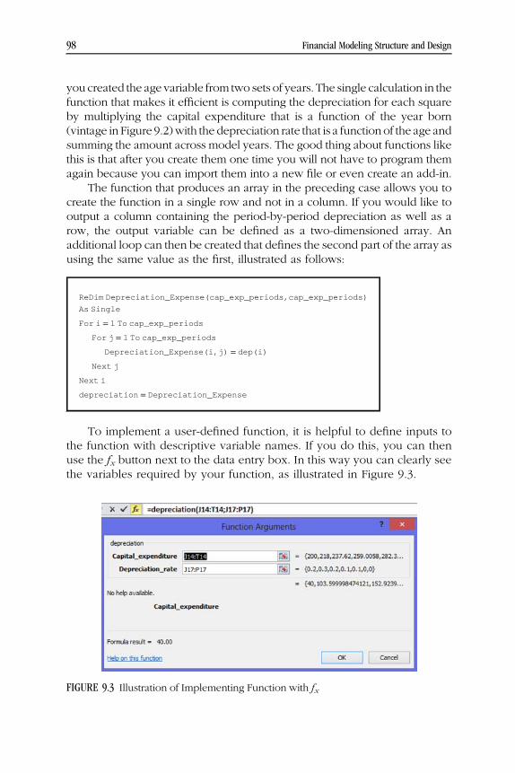
WEBC09 10/02/2014 2:55:8 Page 98

you created the age variable from two sets of years. The single calculation in thefunction that makes it efficient is computing the depreciation for each squareby multiplying the capital expenditure that is a function of the year born(vintage in Figure 9.2)with the depreciation rate that is a function of the age andsumming the amount across model years. The good thing about functions likethis is that after you create them one time you will not have to program themagain because you can import them into a new file or even create an add-in.

The function that produces an array in the preceding case allows you tocreate the function in a single row and not in a column. If you would like tooutput a column containing the period-by-period depreciation as well as arow, the output variable can be defined as a two-dimensioned array. Anadditional loop can then be created that defines the second part of the array asusing the same value as the first, illustrated as follows:

ReDim Depreciation_Expense(cap_exp_periods,cap_exp_periods)

As Single

For i = 1 To cap_exp_periods

For j = 1 To cap_exp_periods

Depreciation_Expense(i,j) = dep(i)

Next j

Next i

depreciation = Depreciation_Expense

To implement a user-defined function, it is helpful to define inputs tothe function with descriptive variable names. If you do this, you can thenuse the fx button next to the data entry box. In this way you can clearly seethe variables required by your function, as illustrated in Figure 9.3.

FIGURE 9.3 Illustration of Implementing Function with fx

98 Financial Modeling Structure and Design

WEBC09 10/02/2014 2:55:9 Page 99

The depreciation expense function can be used in project finance modelsas well as in corporate models. This is particularly helpful where the timing offuture capital expenditures for something like new turbines or new inverters ina solar panel project may change depending on input assumptions. In thiscase, you simply select the entire series of future capital expenditures for thegenerator or inverter, all of which can be 0 except for the one year the capitalexpenditure is made, and input them into your depreciation function. As withthe function used in the corporate model, you press SHIFT, CNTL, ENTERwhen you are finished and the entire depreciation expense array is computed.

Accounting for Asset Retirementsin Corporate Models

Addressing the problem of asset retirements in corporate models is difficultbecause information on the plant retirements associated with previously builtplants is difficult to obtain. In the previous section, the age of the asset had tobe retained when computing accelerated depreciation. A not-so-differentproblem exists for computing book depreciation in corporate models. Retire-ment associated with an existing plant depends on previous capital expendi-tures that occurred a long time ago, write-offs, asset sales, and revaluations formany historical years. As this information on prospective asset retirements isvirtually impossible to obtain, modelers have developed various methods toaddress the problem. Most of the time analysts firmly believe in their ownapproach and have elegant arguments to support their position. But theycannot really prove their method is accurate. In this section different methodsfor simulating depreciation and incorporating retirements are addressed and amethod to test the efficacy of the different approaches is introduced.

Tomeasure the benefits andproblemsof alternative depreciationmodelingmethods it is useful to develop a long-term hypothetical model that computesthe theoretically correct level of depreciation expense. This theoretical modelcan be used as a reference point in evaluating differentmethods and it illustratesthe importance ofmany capital asset and depreciation issues.Whendevelopingsuch a theoretical model of the true depreciation expense, you should keep inmind the most fundamental aspect of corporate models. This is the fact thatcorporations have a history and an indefinite life, and themodel cannot cover allof the historical and projected periods in the life span of a corporation. Althougha real model cannot account for all of these periods, a theoretical model thatcovers the start-up of the firm, a historical period, a modeled period, and a long-term stable period can be used to prove which of the alternative modelingmethods is most accurate in modeling capital assets, retirements, depreciationexpense, and net plant depreciation rates. The theoretical model that includesdifferent growth rates for each period can produce the true depreciation

Moving from Pretax Cash Flow to After-Tax Free Cash Flow 99

WEBC09 10/02/2014 2:55:9 Page 100

expense, the true asset retirements, and the true cash flow for alternative startdates given assumptions with respect to the life of assets and various growthrates.Once this theoretical base is established, alternativemethods canbe testedagainst the true value. You can then evaluate what kinds of growth rateassumptions produce really big errors and whether it is reasonable to adopta particular approach to modeling depreciation expense.

In developing a theoretical base for evaluating different depreciationmethods, you can input different growth rates for different periods (thehistorical period, the modeled period, and the long-term period). The growthrates are used to compute the balance of plant that is required to support theEBITDA. If there is a higher growth rate in EBITDA, a higher growth rate inplant is necessary. The required plant balance to support EBITDA is applied toderive the implied level of capital expenditures. Calculation of the capitalexpenditures required to support the EBITDA is a bit tricky because thechange in plant must compensate for the retirements of plant as well as newgrowth. The capital expenditures are given by the formula:

Change in Plant = Plant1 � Plant0 = Capital Expenditures � Retirements

Capital Expenditures = Plant1 � Plant0 + Retirements

Retirements thatmust be replaced to support EBITDAcanbedeterminedbygoing back and remembering the amount of money spent on capital expendi-tures in earlier periods. If the plant life is five years, then retirements should bethe amount of capital expenditures that occurred five years ago. When simulat-ing retirements that in part drive future capital expenditures through evaluatingthe lag in capital expenditures, one problem is that retirements cannot becomputed until a full life cycle of plant has been completed. The first part of aformula for retirements should therefore be an IF statement involving whetherthe year of the model is greater than the life of the plant—before the first lifecycle of plant there are no retirements related to the capital expenditures. Afterthe period of the model is greater than the lifetime of the assets, the retirementscan be computed. At this point retirements should look backward from thecurrent year and move backward by the length of the life of the plant. Lookingbackward can be accomplished using the OFFSET function that begins with areference cell and moves up or down and backward or forward as shown:

Retirements =IF(Year >= Asset Life, OFFSET(Capital Expenditure Cell,0,-Asset Life))

The final problem with simulating retirements is that the retirementsassociated with the initial gross plant must be simulated without a historicalrecord for the capital expenditures that were made to accumulate to thoseexpenditures. To measure these retirements that come from the start-upphase, you can assume that the historical gross plant property and equipment

100 Financial Modeling Structure and Design

WEBC09 10/02/2014 2:55:9 Page 101

was accumulated throughmaking a series of capital expenditures at a constantgrowth rate. This can be done by deriving the base level of capital expendi-tures that were made a lifetime before the current level of property plant andequipment. When the prospective retirements sum to plant balance, theprospective retirements will correctly account for all of the gross plant balance.If you know or make an assumption regarding the earlier growth rate in assetsand capital expenditures over the plant life, you could compute this baseamount of retirements by making a little model and then using a Goal Seek.Say the plant balance is 1,000, the growth is 10 percent, and the plant life is 10.You could then use the Goal Seek tool to find how much the expendituremade 10 years ago that, when grown by 10 percent, will sum to 1,000. ThisGoal Seek that finds the base level of capital expenditure ensures that the sumof retirements equals the gross plant property and equipment balance. Whilethis Goal Seek process works, it would be very tedious to put into all of yourmodels. A better way to deal with the problem is to create a flexible functionthat does the same thing as the Goal Seek.

One trick to making a function that does the same thing as a Goal Seekon a dynamic basis is to use FOR NEXT loops with STEP counters that havesmaller and smaller increments. You can then go around the loop withsmaller and small increments until the Goal Seek criteria are met. Once youhave exceeded the Goal Seek criteria, you go back and reduce the STEPincrement in the FOR NEXT loop. You do this until the increment is verysmall and the Goal Seek value is found. The process of making a Goal Seekthat is flexible and changes when you change inputs is illustrated using aflow chart in Figure 9.4.

Define Increment

FOR NEXT Loop with

an IncrementIf yes, then

reduce

increment

If no, then continue loop

Test for

Test Whether

ConvergenceIf yes,

then test increment

Goal Seek Criteria Are

ExceededIf no, then finished

FIGURE 9.4 Diagram of Process to Compute Goal Seek Using a Function

Moving from Pretax Cash Flow to After-Tax Free Cash Flow 101

WEBC09 10/02/2014 2:55:10 Page 102

A function to create a flexible Goal Seek formula is shown in Figure 9.5.All of the inputs and formulas for computing the Goal Seek must becontained in the function (you cannot refer to a range name in the spread-sheet). This means that you generally cannot create such a function to

’

’ This function finds the cap exp that were made at beg of the life

’ It is the automation of a goal seek function

’

Function find_base(growth, life) ’ Backs into the pct start

min_base = 0 ’ Set initial low value

max_base = 1 ’ set the cap for testing

new_increment:

increment = (max_base - min_base) / 10 ‘Re-compute Increment

For Base = min_base To max_base Step increment ’ loop around small inc

plant = Base ’ Try different values for base

total_plant = plant ’ This is the integral. You are aiming for 1

For i = 1 To life - 1

plant = plant * (1 + growth) ’ Incr the plant by the grwth rate

total_plant = total_plant + plant ’ Add the plant together

Next i

If total_plant > 1 Then ’ When too high go back;if not, continue

min_base = Base - increment ’ Find a smaller starting point

max_base = Base + increment

GoTo new_increment

End If

If Abs(total_plant - 1) < 0.0000000001 Then ’ Test for convergence

find_base = Base

Exit Function

End If

Next Base ’ Loop over base

End Function

FIGURE 9.5 Function for Computing Base Retirements Using Goal Seek Process

102 Financial Modeling Structure and Design

WEBC09 10/02/2014 2:55:10 Page 103

replicate a Goal Seek inside a big financial model to do something like findthe price to meet a target IRR. The function that finds a base capitalexpenditure level as a percent of the gross plant must be between0 and 1. The function works by first assuming the initial base expenditurepercentage is 0. Then the initial base is increased in the FOR NEXT loopusing the initial step increment and the total plant is computed that shouldsum to 1.0. After an initial base is found whereby the sum exceeds 1.0, youstop the loop and the increment is recomputed that is just below andjust above the base value from the last iteration. Then, the FOR NEXTloop is re-computed using the smaller increments. The process continuesuntil the increment is very small. Once you are finished with making thefunction you can find the base retirement level that occurred a lifetime ago.All you have to do is to put in assumptions for the lifetime of plant and thegrowth rate into the function. After you have the base level of retirement,then subsequent retirements are the base retirement multiplied by 1 plus thegrowth rate.

Once you have derived the retirements associated with historical capitalexpenditures, you can complete a theoretical model that lasts for hundreds ofyears with changing growth rates. The model needs to look backwardcontinually to find capital expenditures from the prior life cycles that affectthe current levels of capital expenditures.

Alternative Methods for Deriving RetirementsAssociated with Existing Assets in Corporate Models

For a single asset with no terminal value, straight-line depreciation is the grossamount spent on an asset divided by the plant life. Given this fact, oneapproach to computing depreciation expense in a corporate model is to keeptrack of the balance of the gross property plant and equipment (i.e., withoutdeductions for accumulated depreciation). This is tabulated from a balancetable beginning with existing plant and adding prospective capital expendi-tures. As explained in Chapter 7 in the context of timing phase switches, thegross plant balance can be set to actual gross plant during the historical period.It can then be computed as the opening balance plus the capital expendituresin the projection period. Gross plant balance can subsequently be multipliedby the depreciation rate to establish projected depreciation.

The problemwith this gross plantmethod of computing depreciation is thatit does not account for any prospective retirements associated with existingplant. By ignoring retirements that reduce gross plant, the method overstatesdepreciation expense. This implies taxeswill be underestimated, incomewill betoo lowandahost of other errorswill arise. Errors areworsewhen the asset life isshort and when the projected growth rate is relatively slow. If the asset life is

Moving from Pretax Cash Flow to After-Tax Free Cash Flow 103

WEBC09 10/02/2014 2:55:10 Page 104

short, there would be a lot of retirements on exiting plant but these are ignored.When the growth rate is slow, the retirements should in theory approach 100percent of depreciation and this is ignored in the calculation.

Figure 9.6 uses the theoretical model that computes true depreciation toevaluate the gross plant method. Comparing the theoretical model with thegross plant method demonstrates that when the growth rate is 5 percent andthe asset life is 5 years, the overstatement of depreciation approaches 100percent after just a few years. If the growth rate is constant, the ratios ofaccumulated depreciation to net plant, depreciation to net plant, and capitalexpenditures to depreciation remain stable.

A second approach sometimes used in modeling depreciation is to sepa-rate the depreciation on existing assets from the depreciation on new assets.The depreciation on new assets can be computed using the vintage methoddescribed earlier. This accounts for retirements on the newassets. Depreciationon existing assets can either be computed by simply continuing the existinglevel of depreciation or, better, assuming a decline to account for retirements.If the existing level of depreciation expense does not include any accountingfor prospective retirements and the lifetime of new assets is fairly long, themethod is not very different from the simple gross plant method discussedpreviously. In this casewhere there are no retirements of new assets or existingassets, the depreciation expense can be overstated by a wide margin.

If retirements associated with existing assets are accounted for, some kindof retirement statistic must be entered and then the accumulated retirementsshould be calculated. Once the accumulated retirements are tabulated, theadjustment to existing depreciation can be computed as the accumulated

FIGURE 9.6 Illustration of Errors in Model from Not Accounting for Retirements onExisting Assets

104 Financial Modeling Structure and Design

WEBC09 10/02/2014 2:55:10 Page 105

retirements multiplied by a depreciation rate. When using this method, a MINtest should be included so that the depreciation reduction on the retirementsdoes not exceed the existing depreciation expense. The approach of separat-ing existing and future assets to model depreciation expense relative to thetrue depreciation is illustrated in Figure 9.7. When these adjustments are madefor retirements, the depreciation expense is more accurate. There are twoproblems with this method: (1) it is a bit tedious to implement because ofaccumulating retirements and adjusting the retirements only after the historicalperiod, and (2) one needs information on historical growth and the retirementsas a percentage of depreciation expense, which is difficult to obtain.

To approximate retirements associated with exiting plant, some modelersproject depreciation on existing assets using the net property plant and equip-ment balancemultiplied by the net plant depreciation rate. They then separatelycompute the depreciation on new assets from depreciation on existing plant asdiscussed earlier. Because the balance of net plant declines each period withdepreciation expense, the depreciation expense on the net plant balance alsodeclines. This suggests that some level of retirement of assets for existingassets is

FIGURE 9.7 Illustration of Method for Computing Retirements from Separating ExistingPlant from New Plant and Estimating Retirements on Existing Plant

Moving from Pretax Cash Flow to After-Tax Free Cash Flow 105

WEBC09 10/02/2014 2:55:11 Page 106

implicitly reflected in the forecast. If this net plant method is applied, youmust make sure that the net plant balance on existing plant does not becomenegative. Although this approach of splitting up depreciation does indirectlyaccount for retirements, it is not an accurate reflection of retirements unlessthe rate of retirement for existing assets relative to net plant happens to be sameas the net plant depreciation rate in each period.

By reducing depreciation expense according to the declining balance ofnet plant, the approach assumes that if the net plant depreciation rate is15 percent, then the implicit retirement rate percentage of existing netproperty plant and equipment is also 15 percent. Unless the growth rate forthe historical period is zero, there is no basis for making this assumption.Another problem with this approach is the assumption that the net plantdepreciation remains constant over the lifetime of existing assets. If the trueretirements are less than capital expenditures, then the depreciation rate onnet plant will increase as the net plant balance declines. To see this, think ofa single asset with constant depreciation expense. Over the lifetime of asingle asset, the ratio of depreciation expense to net plant—the gross plantless the accumulated depreciation expense—increases as depreciationremains constant but net plant reduces. In the last year of the life of anasset the net plant depreciation reaches 100 percent. For a corporation withmany assets, multiplying net plant by a constant depreciation rate can alsoresult in similarly biased results when existing assets are split from futurecapital expenditures. In the last year before all of the existing assets are

FIGURE 9.8a Percent Error from Using Net Plant Method: Five-Year Plant Life and2 Percent Historical Growth Rate

106 Financial Modeling Structure and Design

WEBC09 10/02/2014 2:55:11 Page 107

retired, the depreciation rate on net plant should be 100 percent just like inthe single asset case.

The pattern of errors from applying the net plant method is illustrated inFigures 9.8a and 9.8b for cases with different growth rates and different plantlives. Through simulating the theoretical depreciation and the computeddepreciation from the net plant method, Figure 9.8a demonstrates that thenet plant method understates depreciation in early years, but overstatesdepreciation in later years with a short life of 5 years and a low growthrate of 2 percent. Figure 9.8b shows that depreciation is consistently under-stated using the net plant method when the asset life is long (25 years) and thegrowth rate is relatively high (7 percent). Where depreciation is understated,the cash flow is understated and the income is overstated. If you are using theformula NOPAT × (1 � g/ROIC)/(WACC � g) to compute value, then theunderstatement in depreciation expense results in an overstatement of termi-nal value. Finally, note that the error in computing depreciation is less usingthe net plant method than the error from completely ignoring retirements.

The third method of computing depreciation is to directly model theretirements of existing plant using the historical growth rate in capital expendi-tures and to separately model the new assets using a vintage approach.Application of this method can be accomplished with two user-defined func-tions. The first finds the historic level of growth and the second finds the baselevel of capital expenditures. With the two functions and information regularly

2%

Modeled Depreciation versus Theoretical DepreciationExpense Using Net Plant Method

0%

–4%

–2%

0%26252423222120191817

–4%

–8%–8%

–6%

–10%

–12%

–13%

–14%–14% –14%

–14%

–16%

–14%

–12%

–10%

Life 25.0Historic Growth 7%Modeled Growth 7%

FIGURE 9.8b Percent Error from Using Net Plant Method: 25-Year Plant Life and7 Percent Historical Growth Rate

Moving from Pretax Cash Flow to After-Tax Free Cash Flow 107

WEBC09 10/02/2014 2:55:11 Page 108

reported on the financial statements, you quickly make the more accuratedepreciation calculation. To make this calculation of depreciation on existingassets from the theoretical retirements, you can follow this step-by-step process:

Step 1 Compute the ratio of the accumulated depreciation to plant fromnotes in the historical financial statements.

Step 2 Compute the implied historical growth from the accumulateddepreciation to net plant by making a user-defined function usingthe Goal Seek approach. This function is similar to the functiondiscussed earlier to find the base level of retirements in Figure 9.5.It is a function that does the same thing as a Goal Seek on adynamic basis. You start with a loop with a high level of growth asthe increment of a FOR NEXT Loop from 100 percent downgrowth to 0 percent growth and set the “step by” increment in theFOR NEXT LOOP to 1 percent. With each growth rate youcompute the ratio of accumulated depreciation to plant throughsimulating the depreciation over the plant life. Once the targetratio of accumulated depreciation to net plant has been found,you make a smaller increment than 1 percent and repeat the FORNEXT loop with smaller step increments. You repeat the FORNEXT process with smaller step increments until you find thegrowth rate that makes the computed ratio of accumulateddepreciation to plant to be just equal to your target level.

Step 3 Compute the base retirements as a percentage of gross plant byusing the base retirement function defined previously and dem-onstrated in Figure 9.5. Recall that this function accepts the growthrate and the plant life, both of which have now been determined.

Step 4 Compute retirements of the existing plant over the projectedperiod using the base retirements and the historic growth rate.This can be accomplished by making a switch for the firstmodeled period to start the calculation with the base retirements.In this first period, the retirements are the opening plant balancemultiplied by the base retirements established from the function.For subsequent periods, the retirements are the prior value ofretirements multiplied by the growth rate computed in step 2. Theformula for retirements that can be inserted in one row is:

Existing Retirements � IF�First Modeled Period;Opening Gross Plant � Base; Prior Value � �1 � Growth��

Step 5 Compute the opening balance of plant, the depreciation onexisting plant, and the depreciation on new plant through multi-plying gross plant deprecation rates by gross plant balances.

108 Financial Modeling Structure and Design

WEBC09 10/02/2014 2:55:12 Page 109

An example of this process for computing the depreciation is demon-strated in Figure 9.9. Note that the theoretical depreciation and the actualdepreciation shown at the bottom of the table converge to be the same.

If the historical growth rate is not constant, computing the implied growthrate from the accumulated depreciation ratio may not be precise and,assuming the retirements follow a constant growth rate, will not be perfect.However, an experiment with random growth demonstrates that the error isvery small.

Depreciation Issues in Project Finance Models

In a project finance model depreciation should be computed throughestablishing a gross plant balance account that increases with the construc-tion costs over the construction period. To begin the depreciation at com-mencement of operation, the tax depreciation rate (which may vary with theage of the project) is multiplied by the balance of the plant as well as theoperating switch. As with the nonproject finance models, the accumulateddepreciation should be computed after the depreciation expense row.

Computing depreciation can be complicated in a project finance modelbecause of themanner in which tax depreciation is driven by the calendar yearrather than the date at which the project begins operation. In some countries if

FIGURE 9.9 Illustration of Accounting for Retirements with Base Historical Retirementsand Implied Historical Growth Rate

Moving from Pretax Cash Flow to After-Tax Free Cash Flow 109

WEBC09 10/02/2014 2:55:12 Page 110

the operation date is December 27, the depreciation is the same as if theoperation date had been January 5 of the same year, meaning it is much betterto put the plant in service at the end of the calendar year. To resolve thisproblem, the number of calendar months in the year should be computed andthe calendar year must be computed. The following are five tasks you can doto accomplish this:

1. Compute a switch for a new calendar year by making a test switch thatevaluates when the month of the start date is greater than the month of theend date. To do this you can use the MONTH function and include a rowspecifying the month of the model.

2. Use the same switch to make a counter for the calendar year throughaccumulating the switch.

3. Make an adjustment for the first operating year for which the countershould begin (you also have to make an adjustment so that you do notdouble-count the first year).

4. Use the COUNTIF function for both the range and the criteria as theannual year to find the number of periods per year.

5. The depreciation rate for the period is 1/life divided by the periodsper year.

Modeling the Change in Deferred Taxesin Corporate Models

Measuring free cash flow is one of the primary objectives of any financialmodel. When evaluating real cash flow received by debt and equity investors,the taxes actually paidmust be computed rather than the taxes recorded on theprofit-and-loss statement. The taxes paid can be approximated by adding thechange in deferred tax to taxes booked, as illustrated by the next formula. Thisimplies that you need to compute deferred taxes in a model. Deferred taxesassociated with tax loss carryforwards are discussed in Chapter 12 anddeferred taxes associated with financing items such as fair valuation ofderivatives are discussed in Chapter 26. This section explains how to dealwith the issue of deferred taxes other than by simply pretending that deferredtaxes do not exist or that the change in deferred tax will always be 0 (whichseems to be a common practice).

Taxes Paid versus Taxes Booked: Change in DeferredTax Liability

The approach for computing changes in deferred tax related to capitalexpenditures and depreciation is similar in logic to calculation of depreciation

110 Financial Modeling Structure and Design

WEBC09 10/02/2014 2:55:12 Page 111

expenses. As with depreciation expense, it is convenient to separate thechange in deferred tax between amounts associated with existing assets fromamounts associated with new assets. For the new assets, tax depreciation canbe computed once you know the tax depreciation life and the tax depreciationmethod. The vintage approach discussed earlier incorporating accelerateddepreciation methods for tax depreciation is often more relevant for thatpurpose than for book depreciation. Once the tax depreciation is computed,the change in deferred tax liability associated with new assets is simply thetax depreciation less the book depreciation multiplied by the tax rate:

Change in Deferred Tax Liability

� �Tax Depreciation � Book Depreciation� � Tax Rate

As with book depreciation expense, finding the change in deferred taxassociated with existing assets is more difficult than computing deferredtaxes associated with new assets. Just as the gross plant balance from the lasthistorical year had to somehow be spread across future years, the prospec-tive reversal of deferred tax changes from accumulated deferred tax associ-ated with accelerated depreciation on existing assets can also bedetermined. In the case of deferred tax associated with existing assets,the manner in which the liability will reverse that represents a change indeferred tax depends on how the deferred tax originally arose. You coulduse something like the find_base function illustrated in Figure 9.5 previ-ously, you could simply spread the deferred taxes over the remaining life ona straight-line basis, or you could come up with a more refined approach.

Adjusting the Tax Basis in an Acquisition

For tax purposes, an acquisition can be treated as a purchase of assets or apurchase of shares of stock. This tax treatment must be distinguished from thebook accounting for an acquisition that results in revaluation of assets andreestablishing the equity. Assume the acquisition is classified as a purchase ofassets rather than the purchase of stock for tax purposes. Then the acquisitionprice should be higher, as the asset base will be higher and the value ofdepreciation deductions increases. In evaluating an acquisition, comparativeprice/earnings or EV/EBITDA multiples should account for the difference invalue for purchase of stock versus purchase of assets, just as the multiplesshould account for the difference in tax rates for different countries. For anasset purchase, the accumulated deferred tax should be set to 0 at the date ofthe acquisition.

If the acquisition is a tax-free stock transaction, no write-up for taxpurposes occurs. Here the seller does not pay tax on the gain realized

Moving from Pretax Cash Flow to After-Tax Free Cash Flow 111

WEBC09 10/02/2014 2:55:12 Page 112

from selling assets, and the buyer can often use the existing net operating loss.For an asset purchase relative to a stock purchase, the tax depreciationdeductions take place over an extended period while the taxable gainmust be paid immediately by the seller. Therefore, from the perspectivesof both the acquiring company and the target company on a combined basis, astock transaction generally has a positive tax outcome (lower taxes) becausethe gain on the sale is taxable as current incomewhile the write-up is deductedon a prospective basis. In terms of present value, if the transaction is classifiedas an asset purchase, the government treasury wins and the combinedshareholders of the two companies lose. In situations with net operatingloss, the situation is even worse, as the value of the net operating losscarryforward is lost with an asset purchase.

To establish the tax and book depreciation expense in alternativetransaction structures, the following steps can facilitate the developmentof a model:

Step 1 The existing deferred taxes can be used to derive the existingdifference between the tax and book base through dividing theaccumulated deferred tax related to depreciation by the incometax rate.

Existing Basis Difference = Accumulated DeferredTax/Income Tax Rate

Step 2 In a stock transaction, the valuation of the assets increases forbooks, but the tax basis does not change. The difference in thebasis increases the balance of accumulated deferred tax asdemonstrated in the following formula:

Accumulated Deferred Tax after Transaction = (New BookBasis � Existing Basis) × Income Tax Rate

Step 3 When computing the goodwill for developing the pro formabalance sheet, the increase in assets as well as the increase ofaccumulated deferred tax must be accounted for. In addition toother goodwill adjustments, the goodwill formula should include:

Goodwill = Goodwill � Increase in AssetValuation + Increase in Accumulated Deferred Tax Liability

112 Financial Modeling Structure and Design

WEBC10 10/02/2014 2:58:44 Page 113

CHAPTER 10Adding Debt to a Corporate orProject Finance Model by

Programming Cash Flow Waterfalls

Once after-tax free cash flow has been established you can think of theremaining calculations in the model as allocating the cash flow among

different investors into alternative buckets. If debt is part of a project finance oracquisition transaction or it is on the balance sheet of a corporation, then someof the free cash flow is distributed to the lenders and some of the cash flowis left over for equity investors. There may be multiple debt tranches and it ispossible that further allocations of cash flow must be made among variousdifferent debt and equity investors. While much of the time spent in financialmodeling must involve analyzing the economics of free cash flow drivers, it isalso often essential to accurately reflect the financial structure of the companyand the allocation of the free cash flow. This chapter addresses variousmodeling issues that arise when incorporating debt into a corporate finance,project finance, acquisition, or merger model.

Evaluating risks faced by lenders is vital for a host of financial andeconomic issues. This implies that reflecting the specific features of debt canbe a crucial part of the modeling process. Debt features that need to beaddressed in all sorts of financial models include: (1) the size of debt, (2) themanner in which debt is borrowed, (3) the repayment structure and tenor ofthe debt, (4) interest rates and fees paid on the debt while it is outstanding,and (5) credit enhancements designed to protect lenders, including cove-nants, cash flow sweeps, and required debt service reserves. The amount ofdebt issued in leveraged buyouts and project finance transactions (the firstitem) is a key driver of equity returns and also a big determinant of whetherthe investment even takes place. The way in which debt is borrowed ordrawn (the second item) can have a big effect on the equity internal rate ofreturn (IRR) in project finance. The structure of debt repayments and new

113

WEBC10 10/02/2014 2:58:44 Page 114

debt issues (the third item) is related to the size of the debt and can bethe item that consumes the most time in working with lenders in projectfinance and acquisition finance. The base interest rate and the credit spreads(the fourth item) relative to the project IRR is the whole reason that debtincreases returns to equity holders. Depending on the transaction, thecovenants and cash sweeps (the fifth item) may be a function of financialratios, such as the debt service coverage or the ratio of debt to earningsbefore interest, taxes, depreciation, and amortization (EBITDA) and be a bigdriver of equity returns and lender risk. Debt structuring is also crucial in manycorporate models and merger integration models as the amount of debt issuedin a merger can highly influence the accretion or dilution in earnings per shareand assessment of credit ratings. In these corporate models evaluating whetherdebt can be refinanced and how lenders assess the risk of the company is oftenone of the primary reasons for creating the model.

The amount of debt that can be issued and maintained on the balancesheet for either a project financed investment or for a corporation followsthe general idea of using the risk analysis process made by lenders to backinto the value of an investment. Rather than coming upwith risk through tryingto directly measure cost of capital using the failed capital asset pricing modelor other tools, the implicit cost of capital can be inferred from the debt leveland other loan terms. If, for example, investors typically require a return onequity of about 20 percent when investing in a leveraged buyout, theminimum overall project rate of return, which is the same thing as theweighted average cost of capital, can be backed out with a Goal Seek processonce the debt financing terms are known.

Adding the Debt Schedule to a Financial Model

The fundamental process of adding debt to any financial model is to define adebt schedule that reports the balance of debt outstanding and derives theinterest expense from the balance of the debt. Presentation of debt amountsshould be structured by explicitly including separate rows for the openingbalance, the new borrowings, the debt repayments, and the closing balance.Debt balance schedules should be separately entered for each existing andprospective debt facility that will be present during the forecast horizon. It isbest if the debt schedule also compiles information on the debt commitment,the method of borrowing, the terms of repayment, the details of interest andfees, and the convents and reserves. For corporate models, the debtschedule may include all of the debt issues that are outstanding as of thelast balance sheet date plus any defined new issues that may occur overthe forecast period. In the case of project finance models, loans reported on

114 Financial Modeling Structure and Design

WEBC10 10/02/2014 2:58:44 Page 115

the debt schedule include all of the different tranches of debt that are issuedto finance construction as well as facilities for letters of credit, potential fordefaults, and reserve accounts that you can think of as negative debt.Acquisition models generally include debt issues that are used in financingthe acquisition as well as debt that was issued prior to the acquisition andthat will be assumed by the new owners.

In modeling any account that has an opening and closing balance, it isthe closing balance that must start the process. The starting point for the debtschedule that establishes the closing debt balance differs depending on thetype of model. For corporate models, the closing balance of each debtbalance is launched from the financial inputs that should list the amountoutstanding in the last historical period balance sheet year for each debtissue. The sum of these individual issues should correspond to the totalamount of long-term debt on the balance sheet (including current maturitiesclassified as short-term debt). If the sum of the closing balance of all of thedebt issues does not equal the total amount on the balance sheet, theprospective balance sheet will not balance. It is therefore good to include averification check to ensure that the total debt level on the balance sheetequals the sum of the individual debt issues. Once the opening and closingbalances are established, the interest cost (whether capitalized or expensed)can be computed.

For models that include capitalized interest during the construction periodor a cash flow sweep, it is convenient and sometimes essential to assume thatrepayments and/or borrowings occur at the end of the period, meaning theopening balance is the basis for computing accrued interest. Circular referenceissues that arise when the average debt balance rather than the openingbalance is used as the basis for computing interest are addressed in detail inChapters 37 through 41. If the repayment and borrowing occurs at the end ofthe period (say the payments to construction workers are made at the end ofthe month) then there is no accrued interest on borrowings related to theexpenditures. In a corporate model if revenues are collected at the end of theperiod there is no interest benefit from cash flow received during the period interms of paying off debt. Where all operating cash flow occurs at the end of theperiod, the accrued interest is computed on the debt that was outstandingbefore the new debt was issued or repaid in the current period. This impliesthat the basis of interest expense should be the opening balance and you canrelax about some of the circular reference issues. For monthly or evenquarterly models, this idea of assuming that cash flow occurs at the end ofthe period may be reasonable. For annual models, assuming that all revenuesare received on December 31 and assuming that all expenses are paid onDecember 31 and assuming all capital expenditures are made onDecember 31is not acceptable.

Adding Debt to a Corporate or Project Finance Model by Programming Cash Flow Waterfalls 115

WEBC10 10/02/2014 2:58:44 Page 116

The process of adding a debt schedule to a financial model can besummarized as follows:

■ Set up the debt schedule with separate lines for:■ The opening balance■ Additions from new issues■ Subtractions from debt repayments■ The closing balance

■ The total closing debt balance in historical years should be derived fromthe balance sheet.

■ The opening balance is always equal to the closing balance in the priorperiod.

■ Put the periodic interest rate in a row below the closing balance.■ Compute the accrued interest and separate the interest between capital-ized interest and expensed interest for project finance models throughmultiplying the accrued interest by the construction switch or the operat-ing switch.

■ Include separate lines for the commitment fee and the up-front fee.■ For more complex debt repayment schedules such as sculpted debtinclude the repayment calculations in rows below the closing balance.

Modeling Scheduled Debt Repayments

The manner in which debt is repaid depends on the nature of the debt issueand the type of the financial model. Repayments may range from complexdebt sculpting in project finance models to relatively simple bullet paymentsin corporate models. For some models, computing the debt repayment is themost complex element of the modeling process that results in seeminglyhopeless circularity. Given the importance and the difficulty of computingdebt repayments in project finance models, much of the discussion in Part 4addresses mechanical aspects of debt repayment and associated circularityin detail. In corporate models where loans may be repaid on a single bulletpayment date, a simple test can be created from the debt repayment year toensure that repayment occurs on only a single date. This involves thefollowing:

■ Add the usual row for the repayment of the debt after the openingbalance.

■ Enter a formula that compares the model year with the repayment year tocreate a logical variable (year = repayment year) within the repaymentrow that can be multiplied by the opening balance of the debt.

116 Financial Modeling Structure and Design

WEBC10 10/02/2014 2:58:45 Page 117

The manner of debt repayment in a project finance model or a leveragedfinance model is often designed to correspond to the expected cash flowsgenerated by the investment. Repayments can be input into a model withpercentages that are applied to the aggregate amount of debt issued ratherthan the closing or opening balance. This means it is sometimes a good ideato show the total accumulated amount of the debt issued as a separate lineitem above the debt balance. Unlike the closing debt balance this amountdoes not decline over time. The amount of accumulated debt shown abovethe opening balance can then be multiplied by the repayment percentage toestablish the periodic repayments. The balance for the repayment can alsobe computed as the accumulated debt draws and be put in one of the specialcolumns to the right of the titles and to the left of the calculations.

Because of early debt repayments that can occur if covenants or cashsweeps are triggered, you should make sure that the amounts in the repay-ment line of a debt schedule do not exceed the opening balance of debtoutstanding. To program this, the MIN function can be used. The MIN functioncompares the opening balance of the debt with the otherwise scheduled debtrepayments.

Repayment =MIN(Scheduled Repayment, Opening Balance)

An important audit test in a model is that the debt balance must be 0 afterthe repayment period. Furthermore, one of the crucial time switches in anyproject finance model is a debt repayment phase TRUE/FALSE switch. Usingthis time switch for debt repayment you can design the test with the SUMIFfunction and one of the two following formulas:

SUMIF(Repayment Switch Row, FALSE, Opening Debt Balance) = 0

SUMIF(Beginning of Period Row, “>=Last Repayment Date”, ClosingDebt Balance) = 0

Connecting Debt to Cash Flow in Corporate Models

When working with corporate models it is useful to set up a cash accountalongwith some kind of new debt account as the last part of the debt schedule.These accounts connect the balance sheet with the cash flow analysis and arean essential part of the corporate model. There are many different ways to setup the surplus cash and new debt accounts. One relatively simple approach isto make a net cash account that nets short-term debt from surplus cash. Thisnet cash account is a lot like other debt accounts with a couple of important

Adding Debt to a Corporate or Project Finance Model by Programming Cash Flow Waterfalls 117

WEBC10 10/02/2014 2:58:45 Page 118

exceptions. The account includes opening and closing balances but thestarting point of the account is the cash minus the short-term debt on thehistorical balance sheets and not a simple reference to debt balances. Second,unlike other accounts, the net cash less debt amount is incremented with itemsfrom the net cash flow analysis at the very end of the cash flow statement. Thismeans that formulas for this account cannot be completed until the cash flowstatement is finished.

The net cash account contains many features of cash flow waterfallmodeling that will apply to more complex analyses in project finance, acquisi-tion finance, and in more detailed corporate models. Four themes with respectto the net cash balance as well as all sorts of debt analysis are: (1) at some pointin any financial model there must be some indirect or direct connectionbetween the cash flow analysis and the debt balances, (2) the debt balancescollect information from the cash flow statement and not the other wayaround, (3) in structuring financial aspects of a model it is useful to constructthe titles for debt balances and cash flow items before you fill in the modelwith formulas, and (4) calculations for cash flow allocation generally havedifferent formulas if the cash flow is negative or if the cash flow is positive.

To illustrate how the net cash account works using these four notions,assume there is a negative net cash balance in the last historical year becausethere is more short-term debt than surplus cash on the balance sheet. If thenet cash flow from the cash flow analysis after everything is accounted for ispositive by more than the opening negative net cash balance, then the cashcan be used to pay off the short-term debt and also build up surplusbalances. By contrast, if the net cash account is negative after accountingfor new cash flow, then the negative amount can be labeled as debt. Thismeans the net cash account should be split between cash and debt after ithas been constructed. To separate the account between cash when it ispositive and debt when it is negative you can use the MAX function. The ideaof doing one thing if cash is negative and another if cash is positive iscommon to many different aspects of debt modeling. Use of the MAXfunction to split up the cash account involves two alternative formulas:

Surplus Cash = MAX(Cash Net of Debt Balance,0)

Short-Term Debt Balance = MAX(�Cash Net of Debt Balance,0)

The first equation simply takes a number and makes sure it is not negative.The second equation takes a negative number, switches it around to apositive number, and then does the same test on the now positive number.These two equations amount to doing one thing if the net cash balance ispositive (putting cash on the balance sheet) and another if the net cashbalance is negative (putting debt on the balance sheet). To implement thenet cash concept you should:

118 Financial Modeling Structure and Design

WEBC10 10/02/2014 2:58:45 Page 119

■ Enter an account for surplus cash net of short-term debt with an openingbalance and a closing balance. During the historical period, the closingbalance comes from the balance sheet, while during the projected periodthe closing balance is the opening balance plus the net changes in cashthat are linked to the last line of the cash flow analysis.

■ Net changes in cash come directly from the cash flow statement that hasnot been developed yet. This implies that the account cannot be com-pleted until the cash flow statement has been made. You can leave thecash flow changes on the net cash schedule empty until the cash flowstatement has been completed or you can enter all of the row titles downthrough the end of the cash flow statement and then find the correct row.

■ When linking the changes in net cash to the cash flow statement do notmake any calculations other than to link the amount.

■ After you have computed the closing balance of the net cash balance,which can either be positive or negative, use the MAX function to put thenet cash into a positive surplus cash account if it is positive or a debtaccount if it is negative. As the net cash account can only be positive,negative, or 0 for a single period, both the surplus cash account and theshort-term debt account cannot have positive balances.

■ Compute the interest income on the cash balance and the interest expenseon short-term debt from the opening balance of the accounts (the prioryear’s closing balance) to avoid circularity.

As suggested by the last item in the list, a problem of circularity can arisein modeling net cash balances because interest expense drives cash flow,but the debt balance or the interest expense is affected by cash flow itself.The most common circularity problem in corporate models comes from theassumption that operating cash flows and therefore interest expenses occurin the middle of the year. As with most circular references, the problemcomes about because of an artifact of the financial model—in the real worldyou do not first compute interest expense and then recompute it because thedebt is increased by the interest expense itself. Solutions to the famouscircular reference problem for corporate models using a relatively simpleuser function and more complex modeling processes that include minimumbalances are discussed in Chapter 38.

With a Structured Process, You Can ModelAny Cash Flow Waterfall

Any time debt is issued to finance capital expenditures and other cashoutflows, a loan agreement can define various restrictions on uses of cash topay dividends, subordinated debt service, discretionary expenditures, and

Adding Debt to a Corporate or Project Finance Model by Programming Cash Flow Waterfalls 119

WEBC10 10/02/2014 2:58:45 Page 120

other items. These credit enhancements require you to construct a cash flowwaterfall when modeling debt facilities. A cash flow waterfall simulates themanner in which a loan agreement establishes priorities in the use of cashflow. Cash flow waterfalls can be thought of as analogous to multiplehydroelectric plants in a cascade on a river. For such a cascade, watercan be held in reservoirs and not be allowed to flow downstream by closingvarious taps. Only if the reservoirs are full can the water be allowed to flowdownstream. If reservoirs are not full there may be requirements to fill themup before any water can be used by subsequent hydroelectric plants in thecascade.

In the hydroelectric plant analogy, water that is allowed to drip down atthe very end of the cascade represents the dividend paid to equity investors.Restrictions on cash flow defined by a loan agreement may include a cashflow sweep, a cash trap covenant, and a debt service reserve account. A cashflow sweep of 100 percent does not allow any dividends to be paid until allof the debt is paid off. This is like a big reservoir where all the debt must bepaid before any cash can flow down to subordinated claims. A debt servicereserve account forces the company to maintain a minimum cash balance.The debt service reserve (reservoir) has to be filled up before cash can bereleased to other sources. A cash trap dividend covenant means that cash isnot allowed to flow to other sources unless a financial ratio like the debtservice coverage ratio or debt-to-EBITDA ratio is above the covenant leveldefined in the loan agreement. Dividends are only allowed when thefinancial ratios are above the covenant level, at which time cash can bereleased from the reserves. A cash flow waterfall that defines priorities inuses of cash is illustrated in Figure 10.1. For project finance models andacquisition models, simulating the mechanics of cash flow waterfalls thatinclude cash flow sweeps, new borrowings, and repayment of revolvingcredit facilities, cash trap covenants, top-ups and withdrawals from debtservice reserve accounts (DSRAs), debt defaults and repayment of defaults,as well as interest and repayment of subordinated debt seem intimidating,much less able to be analyzed in a clear and concise manner.

When setting up a cash flowwaterfall you can apply a few techniques andmake the seemingly complex waterfall process relatively easy to program.Procedures that facilitate the waterfall modeling include the following four:(1) setting up the row names for debt schedule items without any formulasbecause inflows and outflows from the debt balance are not known until thecash flow statement is complete, (2) structuring the cash flow statement with alot of subtotals so that MIN and MAX functions can be used, (3) separatelymodeling dispositions and accumulations of cash flowwhen subtotal accountsare positive or negative using the MAX function, and (4) ensuring that youhave not exceeded defined limits of debt or reserve balances by using theMIN function. These techniques are analogous to the discussion of the net

120 Financial Modeling Structure and Design

WEBC10 10/02/2014 2:58:45 Page 121

cash account with added details. Construction of a waterfall using a five-stepprocess includes:

1. Type in account titles for the debt schedule and reserve balance schedule.Along with opening and closing balances the titles may include prepay-ments from sweeps, uses of revolving credit, repayments of revolvingcredit, and availability of revolving credit. Reserve balances could includetitles for required balances, uses of the reserve, and top-ups of reserve. Abalance for defaulted debt can be added that contains movements fromdefaults and repayments of default.■ For each item like cash flow sweeps, defaulted debt, and repaymentof defaulted debt that comes from the cash flow statement, leave theamount in the debt schedule blank and just enter the title. Calculationsof these amounts are made in the cash flow statement and not in thedebt schedule. Links to the cash flow analysis should occur at the endof the process, meaning that all of the formulas to determine howmuch will be removed or placed in a debt or cash account or a debtbalance are performed in the cash flow analysis. An example of debtschedule accounts without formulas for an acquisition model isshown in Figure 10.2.

FIGURE 10.1 Example of Project Flow of Funds

Adding Debt to a Corporate or Project Finance Model by Programming Cash Flow Waterfalls 121

WEBC10 10/02/2014 2:58:46 Page 122

■ For accounts such as letters of credit and debt service accounts, you willneed to know how much is available to meet cash flow needs or howmuchmore cash is needed tomeet required balances definedby the loanagreement. To do this you can set up account titles that track theremaining amount of available usage or the remaining required fundingthat is in the account. For a letter of credit, the remaining amount that isavailable for use is the total commitment less the amount that has alreadybeen borrowed. The amount already borrowed is in turn the openingbalance. For a debt service reserve account, the amount that must befunded is the total required funding often defined by prospective debtservice less the amount that is already in the account. Accumulatedamounts already in the accounts are defined by the opening balances ofthe accounts. Setting up a letter of credit that can be used to fund deficitcash flow is illustrated as follows, where the borrowings and the repay-ments come from the cash flow analysis:

Total Debt CommitmentLess: Amount Already Borrowed (Opening Balance of Loan)Remaining Amount to BorrowOpening Balance of LoanAdd: Amount Borrowed (Linked from Cash Flow Statement)

FIGURE 10.2 Illustration of Titles for Debt Facilities Used for Modeling a Cash FlowWaterfall

122 Financial Modeling Structure and Design

WEBC10 10/02/2014 2:58:46 Page 123

Less: Amount Repaid (Linked from Cash Flow Statement)Closing Balance

2. Set up the cash flow account titles and the priorities of the cash flowwaterfall in the model without entering any formulas. It is a lot easier to fillin the formulas after the structure of the cash flow statement has beenbuilt. Make the cash flow statement with various titles before filling in theincome statement even though the income statement will be between thedebt schedule and the cash flow statement.■ In setting up titles include many subtotals. Subtotal accounts should bemade after virtually every element, including before and after borrow-ing from and paying back the working capital facility, before and afterdebt service reserve flows, before and after debt defaults and repay-ment of defaults, before the cash flow sweep, and before the cashtrapped by the covenant.

■ The order of priority in terms of which investor receives cash flowsshould be the same as the ordering of items in a cash flow analysis. Anexample of setting up the cash flow analysis with subtotals with a debtservice reserve account, a letter of credit, and defaults and a cash flowsweep is illustrated as follows:

Operating Cash FlowLess: Interest Expense on Senior DebtLess: Repayments of Scheduled DebtSubtotal 1: Cash Flow after Scheduled Debt RepaymentAdd: Withdrawals from DSRA if Cash Flow Is NegativeLess: Top-ups of DSRA if Cash Flow Is PositiveSubtotal 2: Cash Flow after DSRAAdd: Uses of Letter of Credit if Cash Flow Is NegativeLess: Repayment of Letter of Credit if Cash Flow Is PositiveSubtotal 3: Cash Flow after Letter of CreditAdd: Defaults on Debt if Cash Flow Is NegativeLess: Repayments of Defaulted Debt if Cash Flow Is PositiveSubtotal 4: Cash Flow after DefaultLess: Cash Flow Sweep if Cash Flow Is PositiveSubtotal 5: Cash Flow after SweepLess: Cash Flow Trap if Covenant FailsAdd: Cash Released from Lock-up Account if Covenant Passes

3. Enter formulas for each step of the cash flow waterfall that depends onwhether the cash flow subtotal is positive or negative using variouscombinations of the MAX and MIN functions. As you get the hang ofusing the MIN and MAX functions you will forget about any possibility ofusing IF statements. The MAX and MIN functions make the cash flowformulas more transparent and less subject to error.

Adding Debt to a Corporate or Project Finance Model by Programming Cash Flow Waterfalls 123

WEBC10 10/02/2014 2:58:46 Page 124

■ Use the MAX(Subtotal Cash Flow,0) function to test for positive num-bers, and use the MAX(�Subtotal Cash Flow,0) to test for negativenumbers. If the cash flow after senior debt service is negative thenyou may have to draw from the revolving credit account. Thismeans you would use MAX(�Subtotal Cash Flow,0). If cash flow ispositive you should use available cash to repay balances and apply theMAX(Subtotal Cash Flow,0) function.

4. In determining how much cash is available to repay debt or how muchcash must be used to pay back various items, use the MIN function. Thistests the cash flow level against the opening balance to see if anymore canbe borrowed or to see if there are limits on repayment.■ Many calculations in the cash flowwaterfall will include both a MIN anda MAX function. For example, when modeling the amount of cash flowthat is borrowed from the letter of credit account, the formula shouldlook something like:

MIN(Balance of Available to Borrow, MAX(�Subtotal Cash Flow,0))

■ If the cash flow subtotal is positive in the previous formula, then thesecond component of the formula is zero. This means the minimum ofzero or the balance available to borrow will also be zero.

■ When the cash flow is positive, cash flow can be used to repay amountsin the working capital facility, as shown in the following formula. If theopening balance is zero, meaning that the debt is paid off, then theformula will result in zero, as it will if the cash flow is negative:

MIN(Opening Balance of Revolving Debt, MAX(Cash Flow Subtotal,0))

5. Link accounts in the cash flow waterfall to the debt schedule. This impliesthat all computational formulas with MIN and MAX are in the cash flowportion of the model. The debt schedule additions and subtractionsshould only include links without any math.■ In linking debt schedule accounts, the formulas should all be simplelinks. The evaluations computed with MAX and MIN formulas need toassess cash flow availability that is part of the waterfall. The rule is tokeep the formulas in the debt schedule extremely simple. Figure 10.3illustrates how the cash flow waterfall is a collection of MIN and MAXfunctions and subtotals.

Defaults on Debt and Measuring the Debt InternalRate of Return

In using a model to assess an investment financed with debt you may want todetermine the point at which a loss occurs for lenders. The loss on debt is

124 Financial Modeling Structure and Design

WEBC10 10/02/2014 2:58:46 Page 125

defined to be the point at which attempts to restructure the debt do not allowearlier defaults to be repaid, meaning that at the end of the life debt is stilloutstanding. Modeling the point at which cash flow is low enough to make aloss arise can be useful in credit analysis. If you know the probability ofrealizing the loss, you also know the probability of default multiplied by theloss given default associated with the debt. Once you have measuredthe probability of default and the loss given default you can then evaluatethe credit spread on a loan that compensates lenders for taking default risk.

If debt cannot be repaid by the end of the life of a project and a loss on theloan arises, then the IRR realized by lenders is less than the promised interestrate. The IRR earned on debt can be computed in a similar manner to anyother IRR where cash outflows are compared to cash inflows. In measuringthe debt IRR, the cash flow dispersed to lenders is the cash outflow and thedebt service received by lenders along with fees is the inflow. If there is a losson the debt, the cash inflow realized is less than the scheduled debt service.The highest the debt IRR can be is the promised interest rate plus the feesreceived by lenders. But in the downside the loss is not limited.

The process of incorporating defaults into a financial model and meas-uring the potential loss on debt involves linking the cash flow statement withthe debt schedule. This can be done using the cash flow waterfall conceptsdiscussed earlier. The amount of the default is computed in the cash flow

FIGURE 10.3 Illustration of Formulas in Cash Flow Waterfall with MIN and MAXFunctions

Adding Debt to a Corporate or Project Finance Model by Programming Cash Flow Waterfalls 125

WEBC10 10/02/2014 2:58:47 Page 126

analysis using a subtotal account and the MAX function. The amount ofdefault that can be repaid is computed by comparing the opening balance inthe default account with the cash flow after other obligations, so long as thecash flow is positive. Because a positive test is made and the amount of therepayment is limited by the opening balance, you can use the MAX and MINfunctions together. The following step-by-step process works through howto compute the defaults:

Step 1 Set up a balance for the defaulted debt in the debt schedule withline items, including the opening balance of defaulted debt, theadditions from defaults, the repayments from positive cash flow,and the ending balance of defaulted debt.

Step 2 Compute the subtotal of the cash flow account after the sched-uled debt is paid and after all possible other contingent accountshave been used up, including the debt service reserve accounts,letters of credit, and working capital facilities. Evaluate thedefaults in two rows below this subtotal. When the amount inthe subtotal is negative a default occurs. If the amount is positiveyou may have to repay the default if there is any opening balancein the defaulted debt. The amount of the default that occurswhen cash flow is negative is limited to the amount of debtservice that was assumed to be paid earlier in the cash flowwaterfall and can be computed using the formula MAX(�SubtotalCash Flow,0) along with a MIN function that limits the default tothe debt service. The following formula can be used to make thiscalculation:

Default � MIN�Debt Service;MAX��Subtotal Cash Flow; 0��Step 3 Below the debt defaulted row in the cash flow statement, set up a

line for the repayment of default. The repayment of default is afunction of the subtotal cash flow and the opening balance for thedebt default. Repayment of cash flow occurs only when the cashflow is positive, meaning a MAX(Subtotal Cash Flow,0) functionshould be used. The repayment of default cannot be more thanthe total amount of the default, which means it should be cappedby the opening balance of the defaulted debt. This means thedefaulted debt repaid is the minimum of the positive cash flow orthe opening balance of the defaulted debt as shown in thefollowing formula.

Repayments of Default � MIN�Opening Balance of DefaultedDefaulted Debt;MAX�Subtotal Cash Flow; 0��

126 Financial Modeling Structure and Design

WEBC10 10/02/2014 2:58:47 Page 127

Step 4 Link the defaults in debt and the repayment of defaulted debt tothe defaulted debt in the debt schedule. As with other items in thecash flow waterfall such as the debt service reserve account andletters of credit, calculations of cash flow movements should bemade in the cash flow statement where they can be directly linkedto subtotals. For the debt schedule the only formula should bea link.

Step 5 Compute the cash inflow realized by lenders for the purpose ofcomputing the debt IRR and the debt net present value of the debtthrough deducting defaults and adding repayment of defaults tothe scheduled debt service. The debt cash flow can be computedusing the following formula:

Debt Cash Flow = Interest Paid + Repayments � Defaults+ Repayment of Default � Cash Debt Invested

Assessing Risk and Return Characteristicsof Subordinated Debt

The most basic issue in finance is assessing risks of receiving cash flow relativeto returns from an investment. The issue of risk and return is highlighted inanalysis of subordinated debt. Here, the higher credit spread on subordinateddebt relative to senior debt can be evaluated relative to the higher risk ofsubordinated debt not realizing the interest rate as compared to senior debt.To consider the value of subordinated debt, a financial model should be ableto determine the point at which the loss occurs so as to measure the risk andreturn characteristics of the subordinated debt. In modeling subordinated debtfor a project finance transaction or for an acquisition model, the first step is toinclude the debt in the sources and uses of funds analysis that builds up theamount of the debt. This is explained in detail in Chapter 40. When developinga subordinated debt schedule for this risk analysis, it is possible that interestaccruals are capitalized and added to the balance of the debt rather thancurrently paid. If interest is capitalized in this manner, then in the final periodwhen the subordinated debt matures, the amount of the debt repayment isthe sum of the opening debt balance and the interest capitalized for thefinal year.

Once the structure and row titles of the subordinated debt balance isestablished, the cash flow statement analysis should reflect the lower priorityof the subordinated debt relative to senior debt service. If debt with a differingpriority is included in the cash flow statement, then a cash flow waterfallshould be modeled that presents the specific priority of each debt provision,including the interest, repayment of debt service, covenants, and cash sweeps

Adding Debt to a Corporate or Project Finance Model by Programming Cash Flow Waterfalls 127

WEBC10 10/02/2014 2:58:47 Page 128

18%

20%

Entry Multiple 11.60 Exit Multiple 9.00

Senior Debt/Capital 27.0% Mezz Debt 43%

8%

10%

12%

14%

16%

E

q

u

i

t

y

I

Equity IRR

Junior IRR

Senior IRR

Difference in break-even for senior

and mezzeninedebt

0%

2%

4%

6%

0%5%10%15%20%25%30%35%40%45%50%55%60%65%70%75%80%

I

R

R

Project IRR

14%

16%

18%

Entry Multiple 11.60 Exit Multiple 9.00

Senior Debt/Capital 43.3% Mezz Debt 27%

EBITDA Sensitivty

6%

8%

10%

12%

E

q

u

i

t

y

I

R

Equity IRR

Junior IRR

Senior IRR

Project IRR

0%

2%

4%

0%5%10%15%20%25%30%35%40%45%50%55%60%65%70%75%80%

R

EBITDA Sensitivty

More Subordinated Debt

More Senior Debt

Difference break-even for seniorand mezzenine debt

FIGURE 10.4 Internal Rate of Return on Senior versus Subordinated Debt with DifferentCapital Structures

128 Financial Modeling Structure and Design

WEBC10 10/02/2014 2:58:47 Page 129

that could all be part of a loan agreement for subordinated debt as well as asenior debt agreement. When structuring a cash flow analysis with alternativepriorities, the ordering of titles in the cash flow analysis must conform to thepriority of cash flow claims in the different loan documents. If there is a cashflow sweep for senior debt and subordinated debt interest paid rather thancapitalized, then the senior debt sweep must occur after the junior debtinterest payments and not before. Otherwise the subordinated interest line inthe cash flow analysis would never receive any money.

To illustrate how a financial model can be used to assess the risk ofsenior debt relative to subordinated debt a sensitivity analysis on operatingcash flow or EBITDA can be performed for the senior IRR, subordinated IRR,equity IRR, and the overall project IRR. The difference in EBITDA level atwhich the senior IRR and the junior IRR cross can be a measure of the risk. Ifthere is a big difference in the points at which the EBITDA leads to declinesin the IRR, then there is a large difference in risk for the senior relative to thesubordinated loan. If the difference is small, then there is not much of adifference in EBTIDA that will cause the loss on debt and in theory the creditspread should not be very different. Figure 10.4 illustrates this idea wheredifference in EBITDA is shown on the x-axis and the different IRR levels areshown on the y-axis. The graph in Figure 10.4 is made using a data table thatis explained in detail in Chapter 15. The case with more subordinated debthas more risk, as demonstrated by the break-even points.

Adding Debt to a Corporate or Project Finance Model by Programming Cash Flow Waterfalls 129

WEBC10 10/02/2014 2:58:47 Page 130

WEBC11 10/02/2014 3:1:57 Page 131

CHAPTER 11Alternative Calculationsof Equity Distributions

The final aspect of allocating free cash flow in a financial model relates tothe manner in which dividends are paid to equity holders and new equity

issues or buybacks are added to a model. Some shareholder agreements maydistribute dividends using complex formulas rather than simply allocatingcommon dividends in a proportionate manner to all shareholders. Theseagreements define the manner in which some investors receive a priority onthe cash flow after debt service relative to others, which is analogous to theway in which loan agreements define priorities on free cash flow. Shareholderdistribution structures can involve a technique known as a flip where onegroup of priority or senior shareholders is allocated the majority of dividendsuntil a given internal rate of return (IRR) criterion is met. After achieving theIRR target, the dividend distribution scheme changes and the second investorreceives a majority of the dividends. Other dividend structures known asratchets can allocate a portion of cash flow in excess of a target to managementor to developers. In these structures management may receive 10 percent ofthe excess cash flow after a target IRR of 20 percent is obtained. In acquisitiontransactions, earn-out provisions can be established whereby a portion of thepurchase price is allocated to existing owners, but they are allowed to share inupside profits only after a defined target is obtained.

Addressing the equity cash flow in a model may also involve simulating atarget capital structure rather than allowing surplus cash or short-term debt tobuild up on the balance sheet. If a target capital structure is used as an inputassumption then the model needs to allow for the possibility of new equityissues or share buybacks in the cash flow analysis. The manner in which targetcapital structures can be reflected in corporate models is addressed alongwith different possible dividend distributions in this chapter. Techniques forincorporating target capital structures in a corporate model are the same asprovisions for simulating capital adequacy ratios for a financial institution,

131

WEBC11 10/02/2014 3:1:57 Page 132

which is an essential part of the analysis in modeling banks and other financialfirms. The target debt-to-capital calculations can be made on the basis of thebook value of debt and equity or the simulated market value.

Modeling Dividend Distributions

Cash flow sharing that is defined in shareholder agreements has analogies tothe cash flow waterfall applied for debt modeling discussed in Chapter 10.When modeling a cash flow waterfall applied to equity distributions, theformula for dividend payments must be understood and reflected in the cashflow analysis so as to compute returns to different groups of shareholders.If dividends are not distributed in a proportional manner to all shareholders,there must be some kind of trigger mechanism that defines the distributionamong different investors. In some cases, selected investors can receive animplicit priority on cash flow through either a shareholder loan or the right to ahigher proportion of dividends relative to their investment in early cash flowperiods. As these investors have lower risk they should also in theory have alower expected return.

As with the cash flow waterfall for computing debt balances and reserveaccounts, cash flow should be distributed among investors who have thedifferent priority claims according to the definitions of relevant financingagreements. Complexity in modeling the cash flow distributions can arise if thecriterion for defining when senior equity receives cash flow depends on anIRR limit, as previously described. One technique is to compute a rolling IRRthat gradually increases as the project matures. You could then change thedividend formula after the target IRR has been achieved. However, becauseyou have to allocate cash among equity investors for the period in which thetarget IRR is obtained, this method may not produce completely accurateresults. In this period when the target IRR for investors with the higher priorityon cash flow has just been achieved, some of the cash flow must be allocatedto the highest priority investor, and some is allocated to a second investor whoreceives residual cash flow. To resolve this issue of cash flow distributions inthe flip period, a more accurate technique than computing a rolling IRR is to setup a yield tracking account. Similar techniques to the yield tracking accountscan be applied to alternative equity distribution structures including earn-outs,management incentives, and equity kickers.

The yield tracking account has many analogies to a debt balance account.As with loans, an opening balance and a closing balance are reported on aschedule. Like debt issues that contain cash flow sweeps, the amount that ispaid to each equity investor as a dividend depends on the cash flow analysis.Furthermore, in a similar manner that capitalized interest increases the debtbalance of subordinated debt, the tracking account balance increases by the

132 Financial Modeling Structure and Design

WEBC11 10/02/2014 3:1:57 Page 133

target IRR before the flip occurs. Finally, when writing equations associatedwith the tracking account in the cash flow statement, the MIN function is used.The process of setting up a yield tracking account includes the following sixsteps:

First, assumptions are input for both the amount of the funding that will bemade by alternative equity investor groups and the manner in which thedividends are paid before and after the defined flip IRR criteria. The manner inwhich you can enter these inputs in the financial analysis section of a model isillustrated in Figure 11.1.

Second, set up an equity tracking account in a module somewhere abovethe cash flow analysis. This account has a repayment row that representsdividends paid to the senior equity tranche and it reaches a level of zero oncethe flip IRR target is achieved. The yield tracking account keeps track of theamount of money that is due to the senior equity after reflecting the earningsthat must be realized for the yield or IRR to be met. To demonstrate how theaccount works, pretend the flip criterion IRR is zero. Here the dividends wouldstop after the opening balance of the tracking account falls to zero as dividendsare paid, and the tracking account is like a debt balance account where all ofthe repayments (dividends) come from a cash flow sweep. With a positive IRRflip criterion, the cost of funding should be added to the opening balance likethe opening balance of capitalized interest is added to payment-in-kind debt.After adding the yield to the balance of the account, the total amount of

FIGURE 11.1 Illustration of Alternative Equity Funding in Project Finance Model

Alternative Calculations of Equity Distributions 133

WEBC11 10/02/2014 3:1:58 Page 134

dividend payments to the senior equity results in the target IRR when theaccount balance reaches a zero balance. The tracking account is similar to theother balance accounts except that the opening balance is increased by yieldthat must be earned. This is illustrated in the layout of the yield trackingaccount. As with a debt schedule where you do not fill in amounts for the cashflow sweep until the cash flow statement is complete, do not fill in the formulafor the dividends until the cash flow statement has been laid out.

Opening BalanceAdd: Earnings on Investment (Opening Balance × Required Yield)Subtotal: Balance after YieldLess: Dividends Distributed to Senior PartnerClosing Balance

Third, whenmodeling the sources and uses of funds for a project financedinvestment or an acquisition, incorporate the different equity contributionsthrough multiplying the total amount of equity issued by the input fundingpercentages. Assuming you know the total required equity funding amount,this process multiplies that total funding by the given percentages from theinputs as illustrated in Figure 11.1. Further detailed discussion of modeling asources and uses of funds analysis is included in Chapter 40.

Fourth, add a subtotal in the cash flow waterfall measuring the cashavailable to equity. You can use this subtotal line to evaluate how much cashflow should be paid to shareholders with the higher dividend priority. Theamount that is received by the senior equity cash claim can be computed fromthe minimum of the (1) cash flow subtotal multiplied by the pre-flip inputdividend percentage or (2) the subtotal balance of the tracking account, asdemonstrated here:

Senior Equity Dividend before Flip � MIN�Opening Balance of TrackingAccount after Yield; Subtotal Cash Flow� � Percent

Distribution Percentage to Senior Priority Equity before Flip

Fifth, compute the junior equity claim cash flows before the flip hasoccurred as the using a similar formula, except the cash flow is computed withthe junior dividend percentage instead of the senior percentage:

Junior Equity Dividend before Flip � MIN�Opening Balance of TrackingAccount after Yield; Subtotal Cash Flow� � Percent Distribution Percentage

to Junior Equity before Flip

Sixth, after the tracking account has been extinguished, meaning thetarget IRR has been reached, apply the alternative post-flip dividend

134 Financial Modeling Structure and Design

WEBC11 10/02/2014 3:1:58 Page 135

percentages that are defined by the flip. This can be computed by creatinganother subtotal account and using this new subtotal as the basis for thesecond dividend formula. The set up of a cash flow waterfall that includes thealternative dividend calculation could have the following titles:

Total Cash Flow to Investors after DebtSubtotal 1: Cash Flow to Senior Investors before Yield ConstraintLess: Cash Flow to Senior Investors before Yield Constraint Using Pre-flip

Distribution Percent and MIN FunctionLess: Cash Flow to Junior Investors before Yield Constraint Using Pre-flip

Distribution Percent and MIN FunctionSubtotal 2: Cash Flow after Yield ConstraintLess: Cash Flow to Senior Investors after Yield Constraint Using Post-flip

Distribution PercentSubtotal 3: Cash Flow after Yield Constraint and Senior DividendCash Flow to Junior Investors

An example of applying a flip structure with a cash flow waterfall appliedto tax equity is illustrated in Figure 11.2.

FIGURE 11.2 Illustration Process for Equity Distributions in Project Finance Model withFlip Structure

Alternative Calculations of Equity Distributions 135

WEBC11 10/02/2014 3:1:59 Page 136

Computing a Target Capital Structure throughSimulating New Equity Issues and Buybacks

Equity cash flow accruing to investors may include share buybacks or newequity issues as well as dividends. Share buybacks go into the pocket ofexisting shareholders while new issues dilute the interests of current share-holders and influence value when using equity cash flow as the basis forvaluation. Including equity issues in a model may be necessary if you wouldlike the balance sheet to reflect a target capital structure where debt and equityproportions remain at some predetermined level. This contrasts with accu-mulating cash on the balance sheet in the case of negative cash flow orallowing debt to continually rise if cash flow is negative. One way toincorporate a given target capital structure is to use the SOLVER tool. Youcan think of using the SOLVER when you need to run the goal seek multipledifferent times. In using the SOLVER you derive the amount of new equityissues or buybacks in each period so that the capital structure resulting fromthe model equals the capital structure that you enter as an input. If you areworking on a financial institution model, implementing a target capitaladequacy ratio can be an essential part of the process. You can also solvethe problem by working through some algebra or by creating a user-definedfunction.

When simulating a target capital structure you will need to add inputs forthe target capital structure and you will need space somewhere in the modelfor the new equity issues that will be established from using the SOLVER.New equity issues should be included in a separate row and they must be onthe same page as the cash flow statement in the model because the SOLVERonly works if all calculations are made on one spreadsheet page. Making thecalculation for the target capital structure only works if you already haveconstructed a balance sheet and you can compute the projected debt tocapital ratio or the debt to equity ratio. Once you have completed theSOLVER, you can attach it to a macro so that you can rerun it any time youmake a change in model assumptions.

To incorporate a target capital structure in your model you can use thefollowing steps:

1. Input the year-by-year target debt to capital ratio or the equity to assetratio or the capital adequacy ratio at the bottom of the assumption modulethat contains other financing inputs.

2. Just below the balance sheet add a row for the computed debt to capitalratio or the other ratio that you are using to design your target capitalstructure. Also enter a row title for the target ratio that you put into yourassumptions module as well as the period-by-period difference betweenthe target and actual.

136 Financial Modeling Structure and Design

WEBC11 10/02/2014 3:1:59 Page 137

3. Enter a row at the top of the cash flow analysis or above the debt schedulenamed equity issues and share buybacks. This row will be the placewhere the outputs of the SOLVER will be placed. You should then insert asimilar row near the bottom of the cash flow statement and link it to therow that will contain results of the SOLVER analysis. Revise the subtotal atthe bottom of the cash flow statement so that net cash balances areincremented to include the new equity issues.

4. Include the new equity issues in your calculation of the equity balancethat now should begin with the opening equity balance taken from thebalance sheet in historical periods. The equity balance is then incre-mented by both retained earnings as well as the net new equity issues inthe projection period.

5. Add-in the SOLVER feature to your spreadsheet and create a routine thatsets the difference between the target and the actual debt to capital ratioto zero by changing the new equity issues. If you were making thiscalculation for only one period, you could easily use the Goal Seek featureto do this. Since you are in a sense rerunning the Goal Seek every period

FIGURE 11.3 Illustration Using the Solver to Compute New Equity Issues in a Financial InstitutionModel

Alternative Calculations of Equity Distributions 137

WEBC11 10/02/2014 3:2:0 Page 138

you can accomplish the same result with the SOLVER feature. To use theSOLVER, you enter a range of set cells as the row of the equity issues. Youcan then add a constraint that the row containing the differences betweenthe modeled target debt to capital ratio and the input debt to capital ratiois zero.

6. You can add a macro to the SOLVER that enables the process to be easilyrepeated. Adding a macro is explained in Chapter 37.

Use of the SOLVER feature to derive a target capital structure is illustratedin Figure 11.3. In this case equity issues are defined by a range name and thedifference between the modeled and ratio and the input ratio is also defined asa range name.

138 Financial Modeling Structure and Design

WEBC12 10/02/2014 3:13:9 Page 139

CHAPTER 12Putting Together FinancialStatements and Calculating

Income Taxes

Once the module that computes revenues, expenses, and working capitalis established along with the depreciation schedule to derive after-tax

cash flow and the debt schedule to calculate interest expense, the profit andloss statement, the cash flow statement and the balance sheet can be puttogether. In a corporate model, the profit and loss statement producesessential results for valuation analysis, as the net income defines the earningsper share and the return on equity. For a project finance model, earnings arenot so important in presentation of the results, but calculation of the profit andloss statement is required to develop the line item for taxes paid that is used inthe cash flow waterfall.

An effective way to structure the profit and loss statement is to computeearnings before interest, taxes, depreciation, and amortization (EBITDA) afterrevenues are subtracted from cash operating expenses and then subtractvarious letters like DA to end up with E (earnings). The EBITDA can becomputed from the revenues and cash operating expenses that were devel-oped in the pretax analysis. Depreciation and amortization (DA) can then besubtracted to derive EBIT. If you have set up your model with differentmodules, this is easy because the depreciation expense is already defined asa component of computing free cash flow. After computing EBIT, interestexpense is subtracted and interest income is added, resulting in EBT. As withdepreciation expense, the interest expense and interest income are taken froma module that you have already computed, this time from the debt schedule.With EBT tabulated, book taxes—the single calculation in the profit and lossstatement that is not a subtotal—are computed throughmultiplying the EBT bythe tax rate. This is the only item in the profit and loss statement, except forminority interest, that is not derived from somewhere else in the analysis.

139

WEBC12 10/02/2014 3:13:9 Page 140

Finally, you can subtract income claimed by minority shareholders to arrive atearnings that are realized by common shareholders.

The one calculation in the profit and loss statement that can involve somedetailed analysis is the calculation of cash taxes. The tax analysis maysometimes seem complicated, but as with so many other issues, it is nottoo painful if the model is efficiently structured. The computation of taxes canhave an important effect on capital-intensive projects such as renewableenergy projects where rapid tax depreciation may be allowed, but the taxableincome is not sufficient to use all of the tax deductions that include high levelsof interest expense at the beginning of the modeling period. To address issuessuch as tax depreciation and other tax/book timing differences you can adda separate tax schedule after the profit and loss statement. This moduleevaluates taxes paid that can be derived from a net operating loss (NOL)carryforward analysis as well as the timing and permanent differences in pre-tax income for books and for tax returns. Errors in the calculation of taxes paidand/or simplistic accounting for taxes can cause large overstatement orunderstatement of cash flow and end up in distorted valuation.

Computation of Taxes Paid and Taxes Deferred

A modeling technique you can use to compute taxes is to first calculate taxesrecorded on the books in the income statement and then subsequentlycalculate the cash taxes actually paid in a separate section. One of the itemsthat can seem difficult to incorporate in the model are net operating losscarryforwards. After the income statement is completed, the EBT that wascomputed in the income statement can be used as the first step forcomputing the cash taxes that are paid on tax returns. If the company isgenerating a loss, book taxes can be negative but actual taxes paid must bepositive or zero.

In making a tax analysis and starting with the book EBT, the first step is tomake adjustments that convert the EBT that comes from book accountingpolicies into the earnings before taxes for purposes of computing real taxespaid. Taxes paid use expenses that are allowed to be recorded on the taxreturn that may be different from book taxes. These adjustments to arrive attaxable income on a tax return may involve adding back book depreciationand then deducting tax depreciation, adding back intangible amortization ormaking adjustments for other items such as the recording income on thechange in derivative value.

Once the adjustments for book versus tax expenses and income aremade, a new EBT line for purposes of computing cash taxes should be created.This line item representing EBT on the tax return drives the analysis of netoperating loss carryforwards. Analysis of net operating loss carryforward

140 Financial Modeling Structure and Design

WEBC12 10/02/2014 3:13:9 Page 141

involves determining the balance of the net operating loss and making variousadjustments that increase or decrease the carryforward balance. The carryfor-ward generated and the net operating loss used can be evaluated using verysimilar concepts to the cash flow waterfall with the MIN and MAX functionsdiscussed in Chapters 10 and 11. When you have finished calculating taxespaid, you can also calculate the change in deferred taxes and the balance ofaccumulated deferred tax.

To compute taxes paid and a net operating loss carryforward, you can usethe following step-by-step process in the module that is placed below theincome statement. The process described here assumes that book taxeshave been computed on the income statement through multiplying EBT bythe statutory tax rate. The net operating loss balance is computed on the basisof taxable income rather than taxes paid.

Step 1 Begin by creating a row that repeats the EBT from the incomestatement.

Step 2 Adjust the book EBT for depreciation and other items that causecash taxes to differ from the taxes accounted for on the book profitand loss statement. Use the adjustments to derive a line itemnamed EBT for taxes.

Step 3 Set up an account that maintains the NOL balance, including theopening balance, additions that accrue to the account fromcreating the NOL when taxable income is negative, and reduc-tions in the NOL when the carryforwards from earlier years areused to reduce taxes that would otherwise be paid if there ispositive taxable income.

Step 4 Compute the amounts deposited into the NOL balance accountwhen EBT for the tax return is negative through converting thenegative amounts into positive numbers. As with the cash flowwaterfall, you can use the MAX function to convert negativenumbers into positive numbers and then to cap the convertednumber to zero.

Additions to NOL � MAX��EBT; 0�Step 5 Calculate the amounts removed from the operating loss balance

and used to offset taxable income through determining theminimum of either the opening balance or the taxable incomein a similar manner to the tests that were made in evaluatingthe cash flowwaterfall with the MIN function. As the net operatingloss balance can only be used when taxable income is positive, aMAX function is also necessary. Thus, the use of net operating losscarryforwards applies to both the MIN and the MAX functions—

Putting Together Financial Statements and Calculating Income Taxes 141

WEBC12 10/02/2014 3:13:9 Page 142

the MIN function limits the use to the taxable income or theopening NOL balance.

Applications of NOL to Reduce Taxable Income� MAX�MIN�Opening Balance; EBT for Tax Return�; 0�

Step 6 Compute the adjusted taxable income after accounting for inflowsand outflows from the net operating loss carryforward balance.Taxable income is increased by the additions to the NOL to assurethat it cannot be negative. Taxable income is reduced by appli-cations or subtractions to the NOL balance.

EBT after NOL � EBT for Tax � Additions to NOL�Application of NOL to Taxable Income

Step 7 Multiply the adjusted taxable income by the statutory tax rate todetermine the cash taxes per the tax return.

Step 8 Subtract the book taxes from the cash taxes to compute thechange in accumulated deferred tax liability. When the booktaxes are greater than taxes paid, the liability increases, andwhen book taxes are less than taxes paid, the liability declines.

Step 9 Accumulate the deferred taxes through adding the changes indeferred taxes computed in Step 8 to the prior year’s balance. Ifthe balance of accumulated deferred taxes is positive, put thebalance on the liabilities side of the balance sheet; if they arenegative, change the sign and put the account on the assets side ofthe balance sheet.

This step-by-step process to compute taxes paid is illustrated in Figure 12.1.If the tax law includes provisions whereby the NOL can expire after a

certain period of time, then the calculations of the NOL balance become a lotmore painful. The problem with an expiring NOL is that one needs to lookbackward to find when the NOL was previously lost and, more important, theexpired NOL must be adjusted so as not to include NOL balances that havealready been applied to taxable income. To compute this more complex NOLcalculation that includes potential for expirations, a three-step process can beapplied beginning with calculation of the amount of NOL that would haveexpired had no NOL been used up. The NOL that was generated in priorperiods, however, does not necessarily represent the amount that will expirebecause some of the NOL may have already been used up from positive EBTin the intervening periods. In the extreme it is possible that all of the NOL wasalready used before the expiration date, meaning there is no expired NOL.

142 Financial Modeling Structure and Design

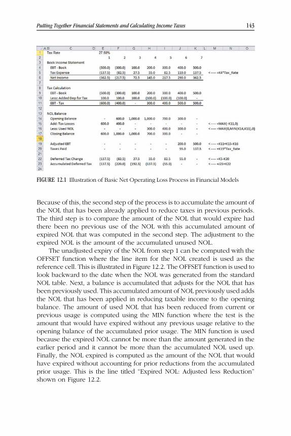
WEBC12 10/02/2014 3:13:9 Page 143

Because of this, the second step of the process is to accumulate the amount ofthe NOL that has been already applied to reduce taxes in previous periods.The third step is to compare the amount of the NOL that would expire hadthere been no previous use of the NOL with this accumulated amount ofexpired NOL that was computed in the second step. The adjustment to theexpired NOL is the amount of the accumulated unused NOL.

The unadjusted expiry of the NOL from step 1 can be computed with theOFFSET function where the line item for the NOL created is used as thereference cell. This is illustrated in Figure 12.2. The OFFSET function is used tolook backward to the date when the NOL was generated from the standardNOL table. Next, a balance is accumulated that adjusts for the NOL that hasbeen previously used. This accumulated amount of NOL previously used addsthe NOL that has been applied in reducing taxable income to the openingbalance. The amount of used NOL that has been reduced from current orprevious usage is computed using the MIN function where the test is theamount that would have expired without any previous usage relative to theopening balance of the accumulated prior usage. The MIN function is usedbecause the expired NOL cannot be more than the amount generated in theearlier period and it cannot be more than the accumulated NOL used up.Finally, the NOL expired is computed as the amount of the NOL that wouldhave expired without accounting for prior reductions from the accumulatedprior usage. This is the line titled “Expired NOL: Adjusted less Reduction”shown on Figure 12.2.

FIGURE 12.1 Illustration of Basic Net Operating Loss Process in Financial Models

Putting Together Financial Statements and Calculating Income Taxes 143

WEBC12 10/02/2014 3:13:10 Page 144

Cash Flow Statement and Balance Sheet

The structure of all types of financial models includes a cash flow statementand a balance sheet as the final part of the model calculations before riskanalysis and valuation. Detailed issues associated with the cash flow statementwere discussed earlier in the context of the cash flow waterfall, and the cashflow statement should have a similar presentation to the cash flow waterfall.With the exception of cash flow waterfall issues, programming the cash flowstatement and the balance sheet should only involve linking to other calcula-tions that have already been made.

Because of issues associated with making a cash flow waterfall, it is betterto construct a cash flow statement in a direct manner with revenues, expenses,and EBITDA rather than using an indirect method that begins with net income.If net income is the starting point of cash flow, then interest expense andinterest income are already included in net income. But to compute a cashflowwaterfall, the senior interest may have to be separated from subordinatedinterest expense, and interest income generally is available for cash flow.Other than the MIN and MAX statements that are used to define the cash flowpriorities discussed in Chapter 10 and Chapter 11, every item on the cash flowstatement either is a subtotal calculation or comes directly from the debtschedule, the income statement, the working capital module, or another

FIGURE 12.2 Illustration of Complex Net Operating Loss Calculations with ExpiredNOL

144 Financial Modeling Structure and Design

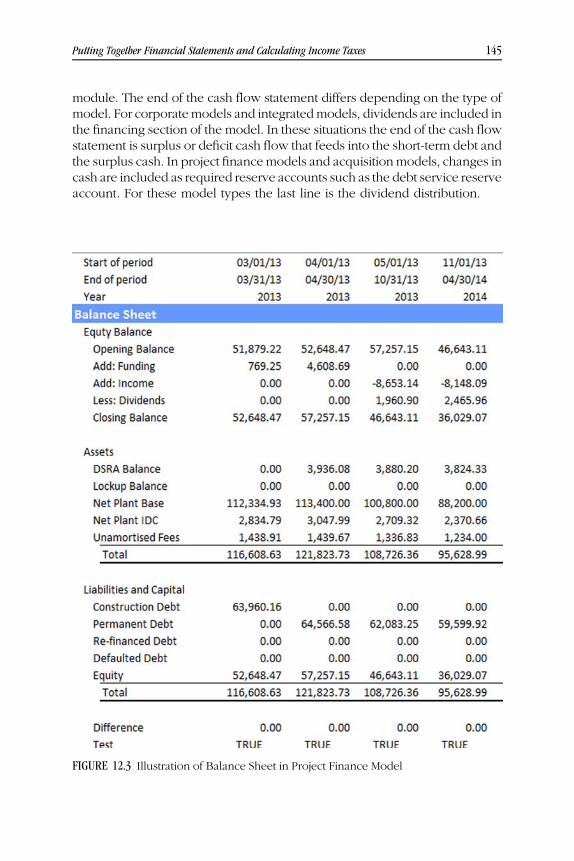
WEBC12 10/02/2014 3:13:10 Page 145

module. The end of the cash flow statement differs depending on the type ofmodel. For corporate models and integrated models, dividends are included inthe financing section of the model. In these situations the end of the cash flowstatement is surplus or deficit cash flow that feeds into the short-term debt andthe surplus cash. In project finance models and acquisition models, changes incash are included as required reserve accounts such as the debt service reserveaccount. For these model types the last line is the dividend distribution.

FIGURE 12.3 Illustration of Balance Sheet in Project Finance Model

Putting Together Financial Statements and Calculating Income Taxes 145

WEBC12 10/02/2014 3:13:11 Page 146

The last part of constructing a model is the balance sheet. For people whohave done a lot of modeling, seeing their balance sheet balance can be one ofthe best feelings in the world. To the contrary, not being able to find where thebalance sheet has gone wrong can be very frustrating. For the balance sheet tobe an effective auditing tool, each item in the balance sheet should already becomputed in the model. The balance sheet should have no calculations otherthan links, meaning you should simply find and collect all of the closingbalances and connect them to an integrated balance sheet. The balance ofaccounts receivable, cash, plant, and debt should already exist in various othermodules. For other assets on the balance sheet that are not modeled in detailsuch as investments and operating reserve accounts, balances should also beestablished. Separate accounts should be created for the book balance ofassets and the tax balance of assets if there is a difference in depreciationmethods or in the basis for depreciation.

An essential part of putting an integrated balance sheet together is makingan equity balance account. This account is like any other balance and includesthe additions to an opening balance for net income and reductions fordividends. Since net income is the last line of the profit and loss statementand dividends are at or near the end of the cash flow statement, the accountcannot be computed until the other statements are complete. The equityaccount and a balance sheet are illustrated in Figure 12.3. A similar presenta-tion should be made for minority interest that also derives items from theincome statement and the cash flow statement. Figure 12.3 illustrates thisprocess of putting together all of the closing balances and seeing if the balancesheet balances with a TRUE/FALSE test at the end.

146 Financial Modeling Structure and Design

WEBC13 10/02/2014 3:15:33 Page 147

PART IIAnalyzing Risks withFinancial Models

Sensitivity Analysis, Scenario Analysis, Break-EvenAnalysis, Time Series, and Monte Carlo Simulation

WEBC13 10/02/2014 3:15:33 Page 148

WEBC13 10/02/2014 3:15:33 Page 149

CHAPTER 13Risk Assessment

The Centerpiece of All Valuation, Contracting,and Credit Issues in Finance

One of the tasks required to manage any business is the honest andsomewhat boring job of accounting for its historical financial results by

keeping track of profit and asset value. A perhaps less noble and much morechallenging task faced by all but the very simplest of business endeavors aswell as by those who make investments is to make implicit or explicit forecastsof future cash flow. The problem with making such a forecast is that it bydefinition encompasses an unknown and uncertain future. With the possibleexception of forecasting nominal cash flow earned on German governmentbonds, all cash flow forecasts from all financial models will turn out to bewrong.

Financial modeling techniques described in the first part of the bookaddressed issues involving how to construct a financial model but did notconsider how to quantify potential uncertainty in assumptions for key vari-ables that drive projected revenues, operating expenses, and capital expen-ditures. This part of the book moves to the more difficult and interestingquestion of how to assess the uncertainty associated with economic variablessuch as price, industry demand, expense structure, cost of new productioncapacity, and interest rates. The amount by which implicit or explicit forecastsof these items could differ from realized results forms the framework forthinking about risk. This framework contrasts with attempting to measure riskwith elaborate statistics advocated by academics such as beta and value at risk(VaR). Assessing the risk associated with potential variation in future cashflows is at the heart of just about every issue in finance and is essential in manyother professions. WhenWinston Churchill said that “true genius resides in thecapacity for evaluation of uncertain, hazardous, and conflicting information,”he was probably not talking about adding risk analysis to financial models, buthe could have been.

149

WEBC13 10/02/2014 3:15:33 Page 150

The process of evaluating uncertainty that comes from how much cashflow forecasts will differ from expected levels may involve estimation of howmuch estimated growth rates will be wrong, what will be the possiblechange in interest rates, how much actual product prices and costs will bedifferent from predicted prices and costs, what will be the change in publicattitudes to various products, or what sudden changes in political eventscould occur. This somewhat ambiguous concept of risk that is defined asthe potential variation in outputs of a financial model from base caseamounts is not consistent with suggestions that risk can be captured in asingle number defined from statistical analysis that is the subject of muchfinance literature.

Attempting to measure risk is by no means a new subject in finance, andover the past 50 years Nobel Prizes have been awarded to economistswho have developed various supposedly revolutionary mathematical orstatistical approaches to measuring risk ranging from beta, to probability ofdefault, to VaR. Notwithstanding the elegant formulas and complex statisticsthat attempt to put a specific number on risk, application of new andseemingly promising innovative mathematical methods to risk assessmenthave turned out to be frustrating in practice. As more and more complexmathematical risk assessment tools are developed, the conflict as to whetherrisk should be evaluated using statistical analysis or if it should be measuredby more traditional business judgment has become an issue that provokes alively debate in finance. After the global financial crisis of 2008 when manywere burned by relying on statistics like VaR, bankers, stock analysts,financial managers, and consultants often would rather perform a relativelysimple scenario analysis instead of attempting to represent a company as acomplex mathematical equation that incorporates a probability distribution.

In describing the mechanics of measuring risk, this part of the book beginsby reviewing risk assessment techniques that rely on business savvy andeconomic judgment—qualitative risk matrices, sensitivity analysis, break-evenanalysis, scenario analysis, and tornado diagrams. This fundamental riskanalysis is explained in Chapters 14 to 18 using step-by-step explanationsof how to add various features to a financial model. After addressing riskassessments that require judgment with respect to what can happen to aparticular variable or sets of variables, Chapters 19 through 22 describe how tocreate stochastic time series models that measure risk on a mathematical basis.The discussion of mathematical risk analysis demonstrates how you can use acombination of mathematics and judgment to create probability distributionsof various outputs in your financial model. To develop mathematical modelsand probability distributions, a tool kit of statistical parameters is introducedthat includes volatility (the dispersion in prices), mean reversion (the speed atwhich prices come back to long-run average levels), correlations amongvariables (such as the correlation between natural gas and oil prices), lower

150 Analyzing Risks with Financial Models

WEBC13 10/02/2014 3:15:33 Page 151

and upper price boundaries on movements in a parameter, sudden jumps,long-run trends, and long-run equilibrium prices.

Six Alternative Ways to Assess the Risk of aCompany, a Project, or a Contract

These days, corporations hire people with finance, mathematics, physics, oreconomics degrees and give them a title of risk manager. Presumably, in oneway or another, riskmanagers are supposed to evaluate how various decisionsaffect risk and value of equity and debt investors or other stakeholders. Thesomewhat mysterious job title of risk manager seems to encompass everythingfrom a junior analyst computing historical financial ratios for periodic creditreviews to a person with a PhD in physics who develops VaR statistics derivedfrom complex mathematical equations. In practice, quantification of risk canencompass a whole lot of different analyses, ranging from simply graphing aneconomic driver of your model and observing how that variable affects cashflows and value, to computing the probability distribution of cash flows usingtime series equations and Monte Carlo simulations.

The different sorts of risk analysis can be classified according to theirmathematical and programming complexity. At one end of the risk assessmentscale is a purely qualitative list of risks that may include some kind of estimateof their relative importance as well as their possible mitigation. Otherapproaches along the mathematical complexity spectrum move from sensi-tivity analysis to break-even analysis to scenario analysis to tornado diagramsand finally to Monte Carlo simulations. Table 13.1 lists six different approachesto risk analysis along with a brief description of what sort of analysis isinvolved in each technique.

Table 13.1 puts judgmental approaches to risk assessment in the leftcolumns and moves to the more mathematical methods in the columns listedat the right. A lot of the discussion in this part of the book addresses MonteCarlo simulation, the rightmost column of the table. This approach seems tomeasure risks in a financial model without having to apply much judgment.Instead, the variation in parameters comes from supposedly objective statisti-cal analysis. The lack of business judgment required when implementingthis approach does not imply that Monte Carlo models produce a betterassessment of risk than does careful business judgment. Very intelligentpeople who have made a large personal investment in the study of complexmathematical approaches to risk assessment do have a natural desire to applytheir knowledge in practice. However, none of the valuation mistakes dis-cussed at the beginning of the book would have been rectified through moreuse of elaborate statistical analysis, simulation, and time series models. Indeed,some business valuation mistakes have been aggravated by inappropriately

Risk Assessment 151

WEBC13 10/02/2014 3:15:34 Page 153

applying historical data to complex financial models without using enoughjudgment as to how distributions of cash flow can change in the future.

A valuation nightmare that illustrates conflicts between different ways toassess risk is found in the case of Long-Term Capital Management (LTCM) andits demise in the late 1990s. LTCM was a hedge fund created in part by Nobellaureates Myron Scholes and Robert Merton that, when it failed, almostbrought the entire financial system to its knees and required federal govern-ment intervention—although the problems seem like very small changecompared to Lehman Brothers, Merrill Lynch, American International Group,and other problem institutions of 2008. LTCM is interesting to study from a riskmanagement perspective because it was created to make money by develop-ing sophisticated mathematical models that evaluated statistical relationshipsand supposedly carefully managed many risks. Risks were measured throughcomplex mathematical techniques, so at the heart of the LTCM case is thequestion of whether mathematical models and statistics can replace businessjudgment when gauging risk.

In making investments on the basis of statistical analysis andmathematicalmodels, the LTCM case contained an explosive mixture of the valuation errorsdiscussed in Chapter 1. Some of the errors included:

■ Assumptions that historical statistical relationships can be used to predictthe future and be reestablished after a period of time. LTCM failed whenmany economic variables did not act as they had in the past and suddennonlinear shocks occurred without historical precedent.

■ Lack of transparency in presenting financial information (that’s manage-ment speak). Both investors and lending banks (the largest Wall Streetbanks) were not allowed to see how trades were made and what modelswere used. It was impossible for outsiders to measure risk with sensitivityanalysis or break-even analysis.

■ Belief that staff employed by the fund was smart enough to continuallybeat the market and earn returns well above the cost of capital inextremely competitive financial markets. This notion that the fund couldcontinually earn returns that were seemingly above the cost of capital (thepowerhouse square) ultimately caused the fund to take on higher andhigher risks when returns began to fall (return envy). The changing riskstructure of the companywas not apparent to outside investors because ofthe secrecy rules.

■ Investment strategies that were derived from highly complex mathemati-cal models that supposedly discovered newways to make money withoutbeing fully vetted. If LTCM could really make money by studyingmathematical relationships (anathema to believers in efficient marketssuch as Scholes and Merton themselves), then others would be able tocopy the formulas. After a business is copied, the potential to earn profits

Risk Assessment 153

WEBC13 10/02/2014 3:15:34 Page 154

above the cost of capital goes away (new business entry when returns arehigh).

■ Faith in the reputation of other people—Merton, Scholes, and a famousbond trader named John Meriwether—without independently assessingwhether the fundamental business concepts were viable. This is similar tomany other cases in which the name of a bond rating agency, thereputation of a large corporation, or trust in a famous person ends badly.

■ Investments that were made without verifying the underlying economicswith simple back-of-the-envelope checks and putting your feet on theground. The fund invested in Russian bonds by studying mathematicalrelationships rather than by visiting the country and seeing that militaryofficers and secretaries were not being paid. Similar problems occurredbefore the 2008 financial crisis when financial modelers refused to get outof the tour bus to look at real estate facilities they were modeling.

The LTCM case raises a fundamental question of whether risk analysis canreally be reduced to a series of mathematical equations. LTCM’s dramaticdemise demonstrated that complex quantitative techniques for risk measure-ment cannot be used without any supplemental business judgment. Thistension between relying on mathematical equations on the one hand versususing judgment on the other that was raised in the LTCM case provides abackdrop in considering how best to assess the six different approaches to riskassessment introduced in Table 13.1.

Using Direct Risk Assessment to Measure Cash Flowand Financial Ratios

None of the methods shown in Table 13.1 mentions the single parameter thatfinance theory implies is the only thing you need tomeasure the relative risk ofa stock, namely the beta parameter. Finance courses and textbooks implicitlyor explicitly suggest that one has to go further than measuring beta from stockprices, which then translates into the weighted cost of capital, whenmeasuringrisk. This risk-adjusted discount rate along with expected cash flows canmeasure value; no scenario analysis, no Monte Carlo simulation, no otherdirect measurement of risk is necessary. As beta supposedly contains allrelevant information about risk, none of the techniques in the table should benecessary, because risk is measured in the discounting process. Risk analysismethods discussed in Chapter 14 through Chapter 22 are premised on thealternative notion that risks cannot magically be stuffed into one cost of capitalnumber.

To contrast risk analysis using beta and weighted cost of capital with otherapproaches, consider the following two different hypothetical presentations

154 Analyzing Risks with Financial Models

WEBC13 10/02/2014 3:15:34 Page 155

made by well-dressed investment bankers who are pitching an acquisitionproposal.

Investment Banker Number 1: Valuation from FinancialTheory and Risk Measurement with Beta

In pitching his proposal, the first adviser values the target company bycarefully applying techniques taught in business school, including computa-tion of free cash flow, measurement of the weighted average cost of capital(WACC), and use of stable terminal growth rates after an explicit forecastperiod. He makes elegant calculations of the cost of equity capital fromstatistical analysis of historical stock prices through computing the unleveredbeta with mean reversion on daily stock prices, and applies market weights tothe capital structure through relevering the beta. This method results invaluation of the target company on a stand-alone basis that is adjusted forthe value of synergies generated from the merger. The first investment bankereven makes a fancy waterfall graph that shows the different components ofvalue as illustrated in Figure 13.1. You can make this graph yourself in minutesby using a template file included at www.wiley.com/go/internationalvaluation.

FIGURE 13.1 Illustration of Waterfall Chart Showing Components of Value in anAcquisition

Risk Assessment 155

WEBC13 10/02/2014 3:15:37 Page 156

In coming up with the valuation, many people looking at the discountedcash flow (DCF) analysis will immediately recognize that two of the mostsubjective assumptions in the valuation—the weighted average cost of capitalderived from beta and the growth rate—can lead to a very wide variation invalue, as illustrated in Table 13.2. Table 13.2 is a typical presentation of valuemade by investment banks that often produce a large difference in valueresulting from different discount rates and growth rates. Note that in Table 13.2the top right-hand entry has a value of 5.75 while the bottom left-hand entryhas a value of 16.61.

Adviser Number 2: Accretion and Dilutionfrom Financial Models

The second adviser uses an integrated financial model (see the discussion onthe structure in Chapter 4) to assess risk and value of the merger rather thanapplying discounted cash flow analysis. He creates two corporate models:one for the acquiring company without a merger, and another for thecombined acquiring company and the target company using the integratedmerger model. Then, after synergies are included in the analysis, he makesa presentation of whether earnings per share are higher in the combinedcase (accretion) then the stand-alone case or whether earnings per sharedecline (dilution). He also makes an assessment of whether the companycan maintain its investment-grade bond rating given the proposed financingapplied in the merger. This integrated analysis accounts for the actualproposed financing of the transaction, the effect of the transaction oninterest costs and earnings, the estimated synergies, the accounting forgoodwill, and the fees paid for advisory services. This second investmentbanker defines the maximum value that can be paid for the target companyas the purchase price level that avoids dilution in earnings per share.

TABLE 13.2 Range in Implied EV/EBITDA from Applying the Discounted Cash FlowModel

Weighted Average Cost of Capital

7% 8% 9% 10%

0% 8.34 7.26 6.42 5.75Terminal 1% 9.38 8.00 6.97 6.17Growth 2% 10.82 8.99 7.68 6.70Rate 3% 12.99 10.37 8.62 7.37

4% 16.61 12.44 9.94 8.27

156 Analyzing Risks with Financial Models

WEBC13 10/02/2014 3:15:37 Page 157

An example of the type of analysis that comes from his integrated model isshown in Figure 13.2. In the presentation made by this second investmentbanker, there is no WACC to be computed from beta and no terminal valueor growth rate to be estimated. Further, the investment banker can applysimilar assumptions for the acquiring company and the target company toeliminate bias.

Knowing that valuations using the DCF technique can be so easilymanipulated by making small changes in the beta-driven WACC or theterminal growth rate—two variables that are very difficult if not impossibleto measure—the company considering the merger most likely would paymore attention to the technique presented by the second adviser. Then,rather than pretending that the risk of making the acquisition can really all beincorporated in the WACC, the decision maker could ask for a series ofdifferent scenarios and break-even analyses that test how sensitive theaccretion or dilution estimates are to key variables that drive the forecasts.This type of risk analysis may evaluate the break-even point for the growthrate before which the merger becomes dilutive. Through applying break-even analysis, sensitivity analysis, or scenario analysis to the integratedfinancial model, the financial officer is directly assessing risk rather than

FIGURE 13.2 Illustration of Summary Outputs from an Integrated Merger Model

Risk Assessment 157

WEBC13 10/02/2014 3:15:38 Page 158

assuming it can be stuffed into the beta parameter. In a similar vein, decisionmakers assessing the risk of a project-financed investment or a leveragedacquisition can use direct risk analysis techniques to directly assess risks ofthe equity IRR falling below a certain level and/or the cash flow not coveringdebt service.

158 Analyzing Risks with Financial Models

WEBC14 10/02/2014 3:20:2 Page 159

CHAPTER 14Defining, Describing, and AssessingRisk in a Risk Allocation Matrix

The first step in assessing risk is often to categorize, describe, and put somekind of subjective probability weight on different risks in a structured

manner rather than diving into any quantitative analysis. At this stage of theanalysis, a financial model is not part of the process. The idea of categorizingrisks by writing them down in a table should force you to think about, discuss,and understand a variety of different risks; how the risks may be mitigated bycontracts; the likelihood of the risks occurring; the magnitude of the problem ifthe risks arise and how those risks could potentially affect investment returns.Qualitative analysis may involve preparing a memo on key risk issues,categorizing various risks into a matrix that describes the risks, or some othersimilar approach. This first step of risk analysis highlights the problem withlack of transparency when a company uses fancy financial language that maybe a method of hiding real problems. Without information being presented ina transparent manner and without access to data that allows assessment ofvalue drivers, analysts cannot even identify the risks.

In creating a structured list of potential risks, the matrix can become ratherboring and mechanical where construction delay risks are mitigated byliquidated damages, interest rate changes are mitigated by interest rate swaps,operation and maintenance (O&M) expenses are mitigated by a fixed-priceO&M contract, and so forth. But this mechanical process often misses thepoint. You should instead use the risk identification and analysis exercise tothink carefully about small risks that can explode, whether the cost structure ofthe investment makes sense, and whether mitigation measures are reallyeffective. When categorizing risks, describing risks, and then mitigating risks,you should also implicitly or explicitly put some kind of weighting on thelikelihood of the risks becoming a problem and the magnitude of difficulties ifthe risk is realized.

159

WEBC14 10/02/2014 3:20:2 Page 160

Once the risks are defined and described in a risk allocation matrix, youshould consider whether some of the risks can be mitigated. Mitigationtechniques generally boil down to one of three techniques: (1) insurance,(2) contracts, and (3) hedges. Mitigation of risks using one of these threemethods involves some kind of explicit or implicit cost to investors fortransferring the risk. One of the objectives in financial models may be toconsider trade-offs between the benefits and the costs of mitigating differentrisks. To demonstrate how risk matrices could be useful in evaluating the costsand benefits of mitigation strategies, you could imagine applying the processin your personal life every day when you wake up in the morning. Alterna-tively you could make a qualitative risk assessment in the context of evaluatingthe health care of a relative who has recently fallen down. Health professionalssometimes tend to concentrate primarily on attempting to minimize a riskwithout evaluating the cost of the risk mitigation in terms of lifestyle andmonetary cost. In the extreme, you may eliminate the risk of someone fallingdown by not allowing a person to leave the bedroom. The real task should beto assess whether the benefits of this mitigation strategy to reduce theprobability of a fall is worth the cost of the loss of freedom from being lockedin a room. When developing a financial model, the real task is often to gaugewhether measured risks that cannot be mitigated are acceptable.

Say all risks in an investment could somehow be perfectly mitigated (ifyou could do this for your life, it would be unbearably boring). In this case theinvestment would be risk free, and valuation could be established throughsimply discounting cash flows at the risk-free interest rate. For virtually anyinvestment, some risks will not be mitigated by insurance, contracts, orhedging. Further, even if the risks could seemingly be mitigated by contracts,those contracts could be broken, resulting in a different type of risk.

For risks that cannot be completely mitigated, financial models can beused to assess whether the unmitigated risk is acceptable. The relationshipbetween a financial model and a risk allocation matrix is the column of thematrix that lists unmitigated risk. These risks in the last column should beevaluated with the financial model. When using a financial model to evaluatewhether the risks are worth taking, you can apply one or more of the other riskassessment techniques like break-even analysis, scenario analysis, and MonteCarlo analysis. The risk analysis techniques evaluate the magnitude of the riskand determine whether the risk is acceptable for lenders and/or equityinvestors. Consider an extreme case where all of the risks are mitigated exceptfor changes in the interest rate. Once the risk matrix demonstrates that otherrisks are mitigated, you can use the financial model to do things like determinehow high interest rates would have to move before the investment cannot payback its debt or how high interest rates would have to rise before returns toequity holders fall below the risk-free rate.

Table 14.1 illustrates the types of items that could be included in a riskmatrix. Examples of items to include are the likelihood and the impact of a risk.

160 Analyzing Risks with Financial Models

WEBC14 10/02/2014 3:20:8 Page 164

Thematrix should specify a low-probability risk with high consequences and arelatively high-probability risk with relatively low consequences. It should alsoinclude the technique for mitigation of the risk using contracts, problems withthe risk mitigation such as a counterparty default on contracts, the relativeimportance of residual risks not mitigated, and the risk analysis used toevaluate the residual risks. The column on the right of Table 14.1 lists selectedcases in which unmitigated risks caused problems with the performance ofinvestments.

164 Analyzing Risks with Financial Models

WEBC15 10/02/2014 3:23:13 Page 165

CHAPTER 15Presentation of Risk Analysisthrough Adding SensitivityAnalysis to Financial Models

Risk analysis is often a lot about effective presentation. One of the simplestand most effective ways to analyze risk is through changing one of the

inputs to the financial model and gauging the effect on key output variablessuch as the value of the company, the internal rate of return, or the debt servicecoverage ratio (DSCR). If management can visualize how a key variable suchas energy production affects cash flow and at the same time can see statisticssuch as the DSCR, there may be little else managers really need to do inanalyzing risk. Allowing people to play around with variables and to under-stand what happens to cash flow, earnings, or debt balances may be one of themost important things you can do with a financial model and a lot of it is aboutpresentation. This sensitivity analysis process involves making an effectivedisplay, often with a graph, to illustrate what happens to some measure ofvalue when the level of a key value driver changes.

High-powered analysts who compute statistics such as value at risk (VaR),probability of default, and complex option price premiums for credit defaultswaps may scoff at sensitivity analysis as being overly simplistic. But considera variable that is very difficult to predict such as the level of traffic that willoccur between England and France in the famous Eurotunnel project, elec-tricity demand growth in the Philippines, the level of U.S. housing pricesbefore 2007, or electricity prices after a change in the structure of the UKmarket—all of which caused valuation nightmares. Given the difficulty inforecasting these variables, an effective picture of what happens to the valueof the investment when the variable changes may be the best thing that youcan realistically do. Think about assessing the value of collateral debt obliga-tions that accumulated subprime mortgages. It surely would have been veryuseful to employ your financial model and paint a picture of what would

165

WEBC15 10/02/2014 3:23:13 Page 166

happen to the value of the investments under alternative housing demand-and-supply assumptions. For example, if the supply of housing increased by20 percent in a region, what would happen to the value of the debt? Orconsider the case of Constellation Energy Corporation after the 2008 financialcrisis. Management of the company presented VaR statistics and maintainedthat the purpose of its trading activities was primarily to hedge other parts ofthe business. This risk analysis, which included all sorts of VaR statistics,frustrated some investors and provided little useful information. In hindsight, amuch more helpful presentation would have been a simple graph with asensitivity analysis illustrating what happens to Constellation’s cash flow andearnings when the prices of oil and natural gas change. This chapter addressespresentation issues for risk analysis.

Figure 15.1 illustrates sensitivity analysis in the case of evaluating theacquisition of an upstream oil company. This model evaluates acquisition ofthe company that was funded by senior debt, subordinated debt, preferredstock, and common equity. The graph in Figure 15.1 is taken from a cash flowwaterfall that is accumulated on an annual basis. A series of controls to managesensitivity analysis allow you to examine how projected cash flow is distrib-uted in the context of different financing structures and different operatingassumptions. Through pushing the oil price up or down with the spinner

FIGURE 15.1 Sensitivity Analysis in the Case of Evaluating Acquisition of an UpstreamOil Company

166 Analyzing Risks with Financial Models

WEBC15 10/02/2014 3:23:13 Page 167

button shown in Figure 15.1, you can see how the length of time for therepayment of a loan changes, what happens to the rate of return earned ondifferent securities, and the point at which the given rate of return cannot beachieved. For a senior debt, subordinated debt, or equity investor, you couldimagine decision makers spending their time pushing the spinner button up ordown to vary the oil price. Rather than wasting a lot of time on forecasting oilprices, the investor could begin with the desired return and back into whatlong-term level of oil price is required to attain the desired cash flow and thetarget rate of return. The picture shown in Figure 15.1 is intended to demon-strate that sensitivity analysis mostly involves presentation and creativelysummarizing key input drivers along with different measures of value.

Setting Up Data for Making Graphs by ConvertingPeriodic Data into Annual, Semiannual, orQuarterly Data

Tomake an effective presentation of sensitivity analysis, it is generally better tograph data on an annual basis rather than showing detailed monthly orquarterly data, which may be the basis of your financial model. This canbe particularly useful in graphing components of a cash flow waterfall thatshows where cash comes from and where it goes. If a model is developed on aperiodic basis using monthly, quarterly, or semiannual time increments, youcan quickly create a summary of annual cash flows or income statement itemsthat can be used for presentation of a sensitivity analysis. In a similar way, youcould also make a quarterly analysis out of monthly data. You can also presentbalance sheet accounts that do not accumulate over the year, such as theclosing balance of plant or debt on an annual basis.

Annualizing periodic data can be accomplished by first defining the yearor quarter value below the date in the sheet or sheets of the model that aremodeled on a detailed monthly, quarterly, or semiannual basis. You can thenuse the SUMIF function or the SUMIFS function to accumulate the periodiccash flows within the year and present these variables in an annual sensitivitygraph. To demonstrate the process of creating annual (or quarterly) numbersfrom periodic data, the following steps walk through a technique that allowsyou to very quickly convert periodic cash statements to annual statements.

Step 1 Compute a time variable such as a year and switch indicator forthe end of the fiscal year in a detailed section of the model.

The SUMIF or the AVERAGEIF functions are very useful inmany parts of financial models and can compute a series ofaggregated values or aggregated averages across a larger series ofrows or columns. A straightforward example is a case where there

Presentation of Risk Analysis through Adding Sensitivity Analysis to Financial Models 167

WEBC15 10/02/2014 3:23:14 Page 168

are data for 12 months of a year that should be summed in a sheetthat simulates many years of monthly data. To find the annualsum across many years of monthly data, first establish the yearnumber in the sheet with detailed time increments (using theYEAR function) or a quarter end date (with the EOqtr user-defined function discussed in Chapter 6). This year or quartervariable is the basis for the summations. The year or quarter end iscalled the range in the SUMIF or the SUMIFS functions.

In creating a quarter by quarter variable, you can also make aquarterly counter from a month indicator. To do this, use theROUNDUP function on the month number divided by 3. Theformula for a quarter number and adding time periods for use inthe SUMIF is illustrated in Figure 15.2.

Quarter � ROUNDUP�Month=3; 0�

If you are summing balance sheet accounts or items such asaccumulated production capacity, you can add an identifier forthe end of the period that will be summed. Oneway to do this is tomake a switch variable that will be true at the end of the year (e.g.,month = 12). In a project finance model, it is convenient to usethe month after the commercial operation date. If the month ofthe period after the commercial operation date of a model is equalto the fiscal month (e.g., June), then the fiscal month switch isTRUE.

Period Switch: Month�Ending Date� � Fiscal Month

Step 2 To make an annual or quarterly summary that can be used forsensitivity graphs, you generally add a new sheet that will containaggregated data. In this new sheet begin with a simple year or

FIGURE 15.2 Illustration of Preparing Periodic Model for Summary Quarterly Model

168 Analyzing Risks with Financial Models

WEBC15 10/02/2014 3:23:14 Page 169

quarter counter by starting with the first year or quarter that youwant to present and then increment the year by one. To create aquarterly counter, select an end of quarter date to begin theprocess and use the EOMONTH function and with 3 as theincrement.

Step 3 Copy selected account titles of cash flow, balance sheet, and otheritems that you would like to present on an annual basis into theannual sheet. This sheet will be the basis for presenting data withgraphs in the risk analysis.

Step 4 Apply the SUMIF function or the SUMIFS function for cash flowitems, profit and loss items, or operating items. The SUMIFfunction accepts three variables—a range, a criterion, and asum range. The first argument for the SUMIF function is therange from the model with detailed time periods (the yearnumber or end of quarter) that you are summarizing into aggre-gate periods. The range is often the year from the model that iscomputed on a monthly, quarterly, or semiannual basis as illus-trated in Figure 15.2 and explained in step 1. If a monthly model isused, then there are 12 columns that have the same year number.The second argument required in the SUMIF function is a singlecriterion that will be used to summarize the data. This is thecounter variable from the annual sheet or the quarterly sheet thatwas described in step 2. The third argument is the sum range orthe average range. This range variable comes from the detailedsheet that contains the monthly data.

The most effective way to apply the SUMIF function formaking graphs and creating sensitivity analysis is through clickingon the entire row (or column) for the year range and the sumrange in the page with the detailed periodic data (the first andthird arguments). If you are pressing the F4 key to make fixedreferences when using the SUMIF function, you are wasting a lotof time. The idea of clicking on an entire row (which can be doneby pressing the SHIFT and SPACEBAR keys for rows and theCNTL and SPACEBAR keys for columns) makes the process fareasier and avoids the need for fiddling around with creating fixedreferences for columns.

To aggregate data by time period, first click on the entire rowof years (or quarter and year) in the detailed sheet with periodicdata and press the F4 shortcut key to fix the first argument in theSUMIF function. This establishes the test for which columns willbe summed. Next, refer to the year entered in the annual sheet instep 2 and use a relative reference to lock in the row number butnot the column name (press the F4 key twice). Finally, refer to the

Presentation of Risk Analysis through Adding Sensitivity Analysis to Financial Models 169

WEBC15 10/02/2014 3:23:14 Page 170

range to be summed by clicking on the entire row in the detailedsheet without locking in the row number or the column numberusing the F4 key. The SUMIF function using this idea is illustratedin the two formulas in Figure 15.3. The sheet with the detailedperiodic data is named “Working,” and row 10 of that sheetincludes the year associated with each monthly period. The keytomaking this process easy is to use the entire rows in the detailedsheet, as demonstrated in Figure 15.3.

Annualized Amount = SUMIF(Row of Years in MonthlySheet, Year Counter in Annual Sheet, Row of Data)

Annualized Amount = SUMIF(Working!$10:$10,Annual:C$5,Working!20:20)

Step 5 Sometimes you would like to present items such as debt orproduction capacity on the annual sheet when graphing sensitiv-ity analyses. The problem with these balance sheet accounts isthat they do not accumulate across months or quarters and youcannot use the SUMIF approach described in step 1 to step 4. Toset up accumulated accounts for sensitivity graphs, one method isto use a TRUE/FALSE switch in the detailed monthly sheet toseparate dates that will be used to accumulate single values overthe year. As there is only one TRUE switch for a year in theperiodic sheet, the sum will be taken only from the column in thedetailed sheet at the end of the fiscal year period. Then you canuse the SUMIFS function to include the year end TRUE switches asa criteria as the SUMIFS function allows you to enter multiplecriteria. You enter one criterion for the year number and anotherfor the switch that defines the end of the year. In the followingexample, row number 21 is summed in the detailed model androw number 13 includes a switch variable that is true only for thelast period in each year (e.g., December in a monthly model):

FIGURE 15.3 Illustration of Using SUMIF and AVERAGEIF to Compute Annual Data for Purposes ofSensitivity Graphs

170 Analyzing Risks with Financial Models

WEBC15 10/02/2014 3:23:15 Page 171

Annualized Amount = SUMIFS(Sum Range in Detail, Rangefor Testing Period, Criteria 1, Range for Testing Period 2,

Criteria 2, . . . )

or

Annualized Amount = SUMIFS(Detail!21:21,Detail!$12:$12,Annual:C$5,Detail$13:$13,TRUE)

Step 6 A problem with the preceding process is that when you wantto pull a variable from the detailed spreadsheet for making asensitivity analysis you have to adjust the SUMIF formula manu-ally. The equation must refer to a particular row in the detailedsheet. This means that you have to manually change the lastargument of the SUMIF formula. You cannot simply copy theSUMIF formula for each line item in the annual or quarterly sheetand then somehow refer to a row and have the formula automat-ically adjust. Instead of retyping the last part of the SUMIF formulayou can use a fancier method that allows you simply to put a rownumber from the detailed model into the annual sheet. Then youcan copy the SUMIF or the SUMIFS function to as many rows asyou want and you do not have to change the formula. Thisapproach uses the INDIRECT function.

The INDIRECT function accepts a range name like D10 andgives you the value associated with this range. You may wonderwhy you do not just enter =D10 instead of the function=INDIRECT(“D10”). But the INDIRECT function can be surpris-ingly useful and is probably worth learning. This is especially trueif you create a macro that automatically reads data from theInternet as described in Chapter 36. The advantage of using theINDIRECT function is that if you are going to collect data fromD10, D15, D32, and so on, then you can make a flexible variablewith the & sign. With this function you do not have to manuallychange the cell references in the spreadsheet formula.

To create a flexible process where you do not need tomanually change the row number in the SUMIF or SUMIFSformulas, you can use the INDIRECT function to refer to therow number in the detailed sheet that contains the data you wantto collect. This can be accomplished by using the ROW functionas well as a sheet name. The spreadsheet name can be created bymaking a simple user-defined function. Using the INDIRECTfunction you can then make a range name that is used as thelast argument in the SUMIF function rather thanmanually changingthe row number for each accumulated item. The trick to using the

Presentation of Risk Analysis through Adding Sensitivity Analysis to Financial Models 171

WEBC15 10/02/2014 3:23:15 Page 172

INDIRECT function is tomake a range name that includes the sheetnameof the sheet that contains thedetailedfinancial data. To createa rangename, youcanuse the&operator and enter an exclamationpoint, as explained in the next section.

Using the INDIRECT Function to Automate Conversionto Time Period Data

The following process shows how you can use the INDIRECT function toautomatically adjust the SUMIF function without having to retype details forthe last argument for the function.

Step 1 Use the ROW function to enter the selected row number in theannual sheet. You can refer to any column for the row in thedetailed periodic model that you would like to summarize inthe annual sheet. For example:

Row number � ROW�detail! :A20�Step 2 Unlike when using the ROW and COLUMN functions, there is no

simple function to find the sheet name. To resolve this you cancreate your own function. In creating this function that can findthe sheet name of the detailed sheet, you can use the code shownhere. You just need to remember a rather obtuse extension called.Parent.Name:

Function sheet_name(cell_reference)

sheet_name = cell_reference.Parent.Name

End Function

Step 3 Use the sheet name and the row number found from previoussteps to create a cell reference for the INDIRECT function. Do thisby combining the row, column, and sheet name cells into onerange name. To make a range name from the sheet name and therow number, you need to add quotation marks and codes thatare used in a range name, as illustrated:

Range Name � “‘“& Sheet Name “‘!”&

Row Number & “ : ”& Row Number

If youhave a lot of instances that requiremaking a rangename,you could create a function that accepts the sheet name and therow number and puts in all of the tedious quotation marks.

172 Analyzing Risks with Financial Models

WEBC15 10/02/2014 3:23:15 Page 173

Step 4 Once the range name is defined, the INDIRECT function can beused as an argument in the SUMIF function or the SUMIFSfunction. To apply the SUMIF function using the previous exam-ple, the following formula would be entered:

SUMIF�Range of Years in Detail Sheet; Year Criteria inAnnual Sheet; INDIRECT�Range Name�

Use of the INDIRECT function in creating a quarterly sum-mary report is illustrated in Figure 15.4. It may seem somewhattedious from the preceding description, but when you havecreated one SUMIF function with the INDIRECT function, youcan copy it as much as you like. Now you do not have tomanuallychange the row numbers in the detailed sheet.

Making Flexible Graphs for Sensitivity Analysis

In creating a financial model you can easily generate thousands of graphs forsensitivity analysis by selecting different variables and pressing the F11 key.Some models have 20 to 30 graphs while others have none at all. Rather thanpresenting information that has marginal use for valuation, the art in makingan effective sensitivity analysis presentation is often to select data that showsrisks and values in a summary page. For a project finance model, one of theessential graphs should be of the cash flow available for debt service relativeto the debt service over the operating life of the project, which can be taken

FIGURE 15.4 Illustration of Using the INDIRECT Function in Creating a QuarterlySummary Report

Presentation of Risk Analysis through Adding Sensitivity Analysis to Financial Models 173

WEBC15 10/02/2014 3:23:15 Page 174

directly from the cash flow waterfall. This graph not only demonstrates thecash flow buffer for cash relative to debt service payments, but alsoillustrates the equity returns that are driven by the various structuring aspectsof the debt, including the DSCR, the debt tenor, the type of funding, the debtservice reserve account, and so forth. In the case of a corporate model,presenting historical and projected return on invested capital effectivelysummarizes many of the important assumptions and results of the analysis.Both the graph of the cash flow and debt service in a project finance modeland the graph of return on investment in a corporate model can be obtainedfrom the accumulated annual analysis. The graphs should be flexible withrespect to different key dates used in the model such as the terminal date in acorporate model or the construction period and the operating life in a projectfinance model. It is more important to make these focused graphs flexibleand effective than to present a hundred graphs that do not have muchmeaning in terms of risk and value.

Figure 15.5 is a presentation of cash flow and debt service that paints apicture of what is happening in the operating phase of a project financemodel.Using graphs like this you can create a spinner button to see how muchselected variables such as the electricity production of the plant can fall inorder for cash flows in a downside case to cover debt service. If cash flowscannot cover debt service in a downside case, then bankers may suggest thatthe amount of the debt should be reduced or the terms of the debt structureshould change. In order to help you quickly and effectively graph importantcash flow and valuation statistics in the context of economic and financialstructuring variables, the remainder of this chapter walks through how tomake the data ready for graphing, how to create graphs that correspond totiming variables in your financial model, how to put flexible titles on yourgraphs, and how to add spinner buttons to graphs when making sensitivityanalysis.

Step 1: Using F11 or ALT, F1 to Make a Quick Graph

To make a graph that summarizes risk, select a variable from the financialmodel and put the data in a separate section of the annual or quarterly sheetin the model. If you structure the rows and columns in this part of the modelwith the title for the output variable in the cell that is immediately to the leftof the data and then add the x-axis for the graph (e.g., the year) just abovethe row of data, then you can press the F11 key and very quickly make agraph of the data. The F11 key should quickly become one of your favoriteshortcut keys. You can also use the ALT and F1 keys to place the graph in thesame spreadsheet. The general approach of structuring the data for a graphis shown in Figure 15.6.

174 Analyzing Risks with Financial Models

WEBC15 10/02/2014 3:23:15 Page 175

FIGURE 15.5 Debt Capacity from Cash Flows with Different Volatilities

FIGURE 15.6 Setting Up Data to Graph Using the F11 Key or the ALT and F1 Keys

Presentation of Risk Analysis through Adding Sensitivity Analysis to Financial Models 175

WEBC15 10/02/2014 3:23:17 Page 176

While the F11 key is a very nice and simple method, there are a few pointsthat canmake the process of creating a graphmuchmore flexible and effective:

■ Create a variable for the x-axis above the data if the data is arranged inrows (and to the left of the data if the data is arranged in columns). If youwant years to be shown on the x-axis of the graph, then add a rowwith theyears above the rows of data to be graphed.

■ Delete the title of the x-axis from the cell above the row that you want tograph. This means that if the years are going to appear on the x-axis, thenmake sure the word “year” is not to the left of the data. The way thespreadsheet program knows that it is supposed to put the item on thex-axis is if the there is no title for the row (or column). This idea of leavingthe title of the x-axis blank is an important point that can make all sorts ofpresentations much easier. It is also essential when you want to make x-ycharts quickly that can evaluate the fixed versus variable cost to evaluaterisks associated with operating leverage.

■ If there are blank columns between the data that are to be graphed and thetitles of the data, then begin the x-axis data only in the column that is to begraphed. If the graph begins in the year 2014, which is in column G, andthe titles are in column D (i.e., E and F are blank), then enter the yearabove columnG and leave the year title for other columns (E and F) blank.

■ Shade the area of the data, including the x-axis and the blank cell that is tothe left of the data for the x-axis. After the data are highlighted, press theF11 key (or the ALT and F1 keys).

An example of setting up data to graph it effectively using the F11 key orthe ALT and F1 keys is illustrated in Figure 15.6.

Step 2: Illustrating the Effect of Selected Variables withSpinner Buttons and Drop-Down Forms

The idea of presenting sensitivity analysis is to show how an input variableaffects the output variables that are chosen for presentation with somethinglike a spinner button or a drop-down box. A spinner button or one of the otherforms such as a drop-down box or a scroll bar can be effective because youcan keep your assumption variables in the input sheet, but you can alsomanipulate those input variables from other places in a workbook such as onthe summary page or on the top of an output graph. The input for operatingexpenses should still be on the input page, but if you use a spinner button, youcan change the value of the operating expenses from either the summarypage or a graph or both, while keeping the input where it is supposed to be.The disadvantage of using spinner buttons is that you can forget what thevalues were for the original data that you input in the base case. Resolving

176 Analyzing Risks with Financial Models

WEBC15 10/02/2014 3:23:17 Page 177

this problem and having the ability to quickly return to base case values isdiscussed in Chapter 17. To make a graph with a spinner button that can beused to adjust the input variables, first choose one or more input variables thathave an important effect on the rate of return, value, or credit quality. InFigure 15.1 a spinner button was attached to the oil price input. Unfortunately,there are a few quirks that complicate this process, particularly when the graphis on a different page from the input data. A process for making the use offorms such as the spinner button more effective includes the following:

■ In order to create a form such as a spinner button, use the View, Toolbars,Forms menu in Excel 2003. In Excel 2007 or later you must include theDeveloper tab on your ribbon, which can be a little tricky to find from theFILE ribbon. Once the forms are shown on the menu or the Developerribbon is on the screen, you can use the Insert Controls tab from theDeveloper menu (make sure to use the Form Controls and not the ActiveXControls) and insert a spinner button, drop-down box, or slider bar on thesheet. Click on one of the forms (at the top part) and then paint the form inthe spreadsheet. Figure 15.7 illustrates how to find Form Controls.

■ Once you have painted the form on the sheet, click on the form with yourmouse and then press the right mouse button (right click). After that, selectthe Format Controls option to attach the control to the input cell with thecell link and define minimum and maximum values. The nice thing abouta form like a spinner button is that you can copy it anywhere else in theworkbook and still maintain the input number in an appropriate place.

■ The problem with using the cell link is that the spinner button or the drop-down box form attaches only to a cell in the particular sheet where theform is placed. If you put the spinner button in Sheet 1, then a particularcell attached in the cell link such as E1 will be changed in Sheet 1 when

FIGURE 15.7 How to Find Form Controls

Presentation of Risk Analysis through Adding Sensitivity Analysis to Financial Models 177

WEBC15 10/02/2014 3:23:17 Page 178

you change the spinner button. But if you copy the spinner form toSheet 2, the spinner button will change to E1 in Sheet 2 rather than thenumber that you wanted to be changed in Sheet 1. This all but defeats thebenefit of using forms like the spinner button because the point of aspinner button is to be able to change data in the input sheet withoutmoving inputs to another sheet such as a summary sheet. It also meansthat you cannot copy the form to a graph if the graph is in a separate stand-alone sheet.

■ The solution to this problem of copying or moving the spinner button andother Form Controls to different sheets is to include the name of the sheet(e.g., input sheet) in the cell link value of the spinner button. This can beaccomplished with a technique some call the windshield wiper method.To use the windshield wiper approach, first click on any sheet that isdifferent from the sheet that contains the input value that you are adjusting(other than a chart sheet). Then move the cursor right back to the currentsheet so that the sheet name is included in the cell link. Including the sheetname in the cell link is illustrated in Figure 15.8. Once you have created aform and attached it to an input cell in this manner you can copy the formto other sheets as much as you want and place the spinner button or otherform directly at the top of the graph.

Step 3: Adding Titles to a Graph with Summary Statistics

It is often useful to display a title on the graph that contains both text andnumerical statistics that represent important valuation outputs. Maybe youwould like to have the title of the graph show the internal rate of return for the

FIGURE 15.8 Illustration of the Windshield Wiper Method in Creating Spinner Buttonsand Drop-Down Forms

178 Analyzing Risks with Financial Models

WEBC15 10/02/2014 3:23:17 Page 179

project, the minimum debt service coverage ratio, or the net present value ofcash flows. You may want to show one or more of the key input variables thatare being changed with the Form Controls, such as the oil price that wasillustrated in the Figure 15.1. Using the process to copy a spinner button to agraph described in step 2, you can add a title (or a text box or a custom datalabel) from a set of spreadsheet cells using the following process:

■ When combining text and numbers on a graph, you must first enter all ofthe information that will be included in the title into a single row (orcolumn) somewhere in your workbook. You can change the format of thenumbers and make the title as long as you would like. But the title of thegraph cannot come from two or more different rows (or two differentcolumns). Say you want to show the discounted cash flow value—theoutput—and the weighted average cost of capital (WACC)—the input—on the graph. You could then enter the following information on differentcells of a single row:

Enterprise Value: 4,556 Euros Using WACC of 6.4%

■ Once the information that will become the graph title has been entered inthe single row or column, select the existing title on the graph (if there isno existing title, then you must create one). When selecting the title, makesure that you do not double-click on the title. With the title selected, pressthe equals sign on the keyboard and then shade the single row or columnof the title where you entered the data. This process of making a flexibletitle is illustrated on Figure 15.9. After shading the area where you typed inthe single row representing the title, press the ENTER key and the titleshould appear on the graph.

■ If you would like the title on the graph to have multiple rows as in the oilprice example in Figure 15.1, you cannot press the ENTER key on thegraph title to make a new line. Instead, you can create a new line characterin the single row graph title. To insert a new line character, press the ALTand ENTER keys together at various cutoff points in the single row thatyou constructed for the graph title.

Optional Step 4: Making Dynamic Graphs with the OFFSETFunction or the #N/A Symbol

Sometimes you would like to make a flexible graph in which the length of thedata on the x-axis of the graph can vary. In a project finance model, the lengthof the concession agreement may vary, in a corporate model the explicitperiod may change, and in an acquisition model the length of the holdingperiod may vary. There are two ways to make a dynamic graph where thex-axis changes as a function of the model timing inputs and where periods that

Presentation of Risk Analysis through Adding Sensitivity Analysis to Financial Models 179

WEBC15 10/02/2014 3:23:17 Page 180

you do not want to present on the graph can be excluded. One relatively easyway is to make the x-axis have a #N/A symbol for periods that you do not wantto be graphed. A second technique is to construct a graph using a dynamicrange name created from the OFFSET function.

To apply the #N/A technique, you must replace the x-axis with #N/A forall of the periods that you do not want on the graph. When the scale of thegraph is a date (not a year), you must also replace the data itself that youwant to graph with the #N/A symbol. You could make a #N/A symbolsomewhere in the sheet and then create a range name so you do not have totype #N/A multiple times (being lazy with spreadsheet formulas is a goodthing). This can be accomplished by using the MATCH function with bothTRUE and FALSE �MATCH(TRUE,FALSE)=#N/A. To use the #N/A approachin making a graph with a flexible time line you should select the x-axis andchange the scale to a DATE AXIS. This will exclude all of the columns thathave the #N/A from the graph. Setting up the x-scale of a graph with the #N/A method is illustrated in Figure 15.10. In using the #N/A technique, there isa quirk whereby you must make the data itself have values of #N/A if thegraph is not annual. If the graph is from an annual summary sheet, you donot need to make this adjustment.

FIGURE 15.9 Adding a Flexible Title to a Sensitivity Graph

180 Analyzing Risks with Financial Models

WEBC15 10/02/2014 3:23:18 Page 181

A second technique that you can use to make dynamic graphs is tocreate a flexible range name with the OFFSET function. You can then use theflexible range name as the source of data in the graph. This method is moreflexible than the #N/A method. Further, if you are creating a lot of statisticalanalysis, it does not slow down your calculations the way that the #N/Amethod sometimes does. To create such a dynamic range name and aflexible graph, the first step is to understand the OFFSET function, which hasthe following form:

=OFFSET(Reference Cell, Rows Down, Columns Across, Length, Width)

The first three arguments in the OFFSET function are required argumentsand the last two are optional. But the last two are essential in creating a flexiblerange name. The first argument in the OFFSET function is the cell reference

FIGURE 15.10 Illustration of Use of #N/A Method for Creating a Dynamic Graph

Presentation of Risk Analysis through Adding Sensitivity Analysis to Financial Models 181

WEBC15 10/02/2014 3:23:19 Page 182

that will be used as a starting point. The second argument is the number ofrows to go down from this starting cell reference. The third is the number ofcolumns to move to the right of the cell reference. The function OFFSET(A1,1,1) would result in cell B2; it would start with A1 and then go down byone row and to the right one column. The number of rows and columns can benegative, implying you can go up rather than down and you can go to the leftrather than to the right.

The important part of the OFFSET function in creating dynamic rangenames is not the two arguments just discussed that allow you to move around,but rather the final two arguments relating to the height and the width. Thesearguments are generally used in the context of another function or as an arrayfunction. An example of how the height and width arguments can be used isshown in the following two examples of making an operation on a flexiblerange, which varies according to some other variable in the spreadsheet:

=SUM(OFFSET(A1,2,3,2,5))

=NPV(10%,OFFSET(Cash Flow Reference,0,Last HistoricPeriod+1,1,Explicit Period)

The SUM function begins with the cell A1 and then moves down tworows to row 3 and moves across three columns to the right to column D. Thisimplies that the starting point for the sum calculation is D3. The NPVfunction begins with the first column, which is a historical period, andthen moves across to the end of the historical data. Once the starting cell isestablished, the sum in the first statement covers two rows and five columnsbecause of the last two arguments of the function. This means the area fromD3 to H5 is summed with a length of 2 from 3 to 5 and a width of 5 fromcolumn D to H. In the second statement, the NPV is computed for a singlerow that extends for the explicit period. If the explicit period is changed, theNPV adapts to the new period.

Once you understand the general way that the OFFSET function works,you can create a dynamic range name. Then you can create a chart with adynamic range using the following steps:

Step 1 Create a range name that will use the OFFSET function as anequation that defines the length and the width of the range. Tomake a new range name, you can press the CNTL and F3 keys(shortcut keys associated with range names use the F3 key).

Step 2 After defining the name of the range, select the range name andenter the OFFSET function in the “refers to” part of the rangename menu with the equal sign. You can use an equation with afunction in a range name instead of simply referring to a cell or a

182 Analyzing Risks with Financial Models

WEBC15 10/02/2014 3:23:19 Page 183

range of cells. If you want to make a range called flex_name thatbegins at D5 and has a width of 8, the OFFSET function in therange name would not move away from D5 as the starting point.It would have a height of 1 and a width of 8, as demonstrated inFigure 15.11. The parameters for the OFFSET function—the rowstart, column start, the height, and the width—should generallybe entered as cells in the spreadsheet as shown Figure 15.11:

=OFFSET(D5,0,0,1,8)

Step 3 Make a graph that will soon be changed to include the flexiblerange name instead of a normal fixed area. To make the graph,you can use the F11 shortcut as described earlier.

Step 4 After making the graph, select the data series option from thegraph drop-downmenu. When editing the data series, modify therange and replace the current range reference with the rangename that you created. But when modifying the range, do notchange the sheet name. This means that you should only replacethe range after the exclamation point in the current range andkeep the name of the sheet preceding the explanation point. Forexample, if the range is sheet1!A1:A5, the A1:A5 will be replacedby the defined range name. Do not change the sheet name to theleft, as illustrated in Figure 15.12.

FIGURE 15.11 Use of the OFFSET Function to Create Dynamic Range Names

Presentation of Risk Analysis through Adding Sensitivity Analysis to Financial Models 183

WEBC15 10/02/2014 3:23:20 Page 184

Before moving to the next part of risk analysis, it should be reiterated thatadding a whole lot of spinner buttons to inputs in a financial model can be abad idea. The danger is that you mess around with a lot of different variablesusing spinner buttons and then you forget what the base case values were.Say there is a spinner button for oil price variables, quantity variables, marginvariables, and other items. A solution to this problem is described inChapter 17, where the spinner buttons are combined with scenario analysisand where a special custom scenario is created that allows you to use spinnerbuttons. Later, after using the spinner buttons, you can reset values in them. Ifthis technique is used, you can switch back to the base case or the downsidecase after playing around with the different variables.

FIGURE 15.12 Illustration of Using a Flexible Range Name in a Graph by Changing theRange Name Only after the Exclamation Point

184 Analyzing Risks with Financial Models

WEBC16 10/02/2014 3:26:45 Page 185

CHAPTER 16Using Financial Models to EstablishBreak-Even Points for Key InputVariables with Data Tables

The value of a corporation comes from differentiation in cost structure,technological innovation, location, marketing strategy, and various other

aspects of business strategy. In the long run, relative value does not generallyarise because a company is better than its competitors in forecasting com-modity prices, gross domestic product growth, trends in interest rates, or othereconomic variables. These variables to be sure do have important if notdramatic effects on value. But anybody who claims to differentiate theirbusiness by making superior forecasts of variables such as the oil price isarguably committing fraud. Instead of wasting time on consulting studies ormarketing reports that attempt to forecast variables such as GDP growth orinterest rates, you can use your financial models to compute break-evenvalues for the economic variables that are difficult to forecast. Break-evenanalysis is similar to making a graph with a drop-down box discussed inChapter 15. The subtle but important difference between methods introducedin this chapter and those discussed in Chapter 15 is that with break-evenanalysis you can quantify risk as a single number that represents the cushion orthe distance from current levels that various different value drivers can moveup or down before something really bad happens. Once you have this cushiondefined you can use your judgment to assess whether the buffer is sufficientlybig to accept the risk.

One of the supposed advantages of fancy statistical measures such asvalue at risk, the probability of default, or beta is that these numbers seeminglyplace all of the risk of an investment into a single number. With risk put into asingle statistic or letter grade such as AAA, analysts can supposedly comparethe levels of risk of different investments without doing a lot of work. By

185

WEBC16 10/02/2014 3:26:45 Page 186

expressing risk as the break-even point, a similar kind of thing is accom-plished, but in a more intuitive way.

A famous valuation debacle was the case of the Eurotunnel, in whichdramatic errors from forecasting the volume of traffic created massive losseson debt and equity capital. If you were an investor in one of the manytranches of junior debt and you wanted to evaluate the risk that your debtservice would not be paid, you could construct a financial model of theproject, then you could keep pushing the traffic volume down (with aspinner box if you like) until it reaches the level at which your debt cannotbe repaid and you lose money. Once you have computed this break-eventraffic level, you could then think hard about the chances that the actualtraffic level will be below this break-even traffic level. If you believe thechance of reaching the break-even level is very low, you can then beconfident that your debt will be repaid. On the other hand, if the cushionbetween your base case traffic level and the break-even level is thin, then thelikelihood of default on your debt may be quite high. The break-even trafficlevel has implicitly defined the risk of the project.

Similar break-even statistics could be developed for commodity prices,demand growth, cost structure, and other items. The break-even statistics canbe computed for different classes of investors—equity, senior debt, subordi-nated debt, and preferred stock. For each investor group you could find outhow low a variable can go before the IRR reaches the risk-free rate. When theIRR is equal to the risk-free rate you might have just as well invested in a safebond. Here the break-even value shows the risk you are taking relative to arisk-free investment, meaning you can directly gauge risk and return. Anexample of break-even analysis from a project finance analysis is illustrated inFigure 16.1, where the break-even that would produce a debt service coverageratio (DSCR) of at least 1.0 is compared to the historic level of the oil price. Asthe break-even price for the project is consistently below historical levels in thegraph, you could be reasonably confident that falling prices would not cause abig problem with the project.

Figure 16.2 illustrates break-even analysis using the oil transaction intro-duced in Figure 15.1 for senior debt, subordinated debt, and equity. The threelines on the graph show the rate of return earned on senior debt, subordinateddebt, and equity, while the x-axis lists a range in potential oil prices. The levelat which the variables fall below the risk-free interest rate can be defined as thebreak-even point since a basic alternative to investing in any security is thepurchase of a risk-free bond. Different levels of break-even oil prices at whichthe senior debt, subordinated debt, and the equity yield a return below therisk-free rate are shown in the title of the graph. The graph title is created usingthe method described in Chapter 15, involving placing the items that you wantin the title on one row somewhere in the spreadsheet. For example: Whenmaking a risk assessment with the information in Figure 16.2, say the current

186 Analyzing Risks with Financial Models

WEBC16 10/02/2014 3:26:45 Page 187

oil price is $82 per barrel. The cushion for the equity break-even is quite thin,while the cushion for the senior debt is much greater because prices can fall allthe way down to $43 per barrel before the internal rate of return (IRR) onsenior debt falls below the risk-free rate.

The break-even analysis can be used in structuring a transaction as well asin making risk assessment from a given capital structure. If the transactionwas financed with different levels of debt or equity, the break-even valueswould change. Were more senior debt and less equity issued, the break-evencushion would be thinner for the senior debt. Making a break-even presenta-tion like the one shown in Figure 16.2 may not define the exact required returnnecessary to compensate for taking risk, but it does display risks relative toreturns for alternative funding groups and it does allow you to make ajudgment concerning whether the expected return on the security compen-sates for its risk.

While the general intuition behind a break-even analysis is straightfor-ward, there are a few issues in computing and presenting break-even analysisthat can be tricky. The first issue is establishing an effective criterion forpurposes of deriving the break-even point. Choosing the criterion at which thebreak-even is assumed to occur—when the DSCR equals 1.0 or the IRR equalsthe risk-free rate interest rate—seems pretty obvious. However, the break-even criteria can require judgment and understanding of the principles

30.00

35.00

40.00

45.00

Actual Price

Break-Even

15.00

20.00

25.00

0.00

5.00

1979M

12

1980M

04

1980M

08

1980M

12

1981M

04

1981M

08

1981M

12

1982M

04

1982M

08

1982M

12

1983M

04

1983M

08

1983M

12

1984M

04

1984M

08

1984M

12

1985M

04

1985M

08

1985M

12

1986M

04

1986M

08

1986M

12

1987M

04

1987M

08

1987M

12

1988M

04

1988M

08

1988M

12

1989M

04

1989M

08

1989M

12

1990M

04

1990M

08

1990M

12

1991M

04

1991M

08

1991M

12

1992M

04

1992M

08

1992M

12

10.00

FIGURE 16.1 Break-Even Level of Oil Prices from a Financial Model Compared toHistorical Oil Prices

Using Financial Models to Establish Break-Even Points for Key Input Variables 187

WEBC16 10/02/2014 3:26:45 Page 188

underlying financial ratios. A second issue in working with break-evenanalysis involves developing mechanical techniques to automatically com-pute the break-even level whenever a structural variable changes in yourfinancial model. When you vary the level of senior and/or subordinated debtor the interest rate or the purchase price in a transaction, the break-even pointschange. In presenting the break-even analysis on a summary page of yourmodel you may want to display new different break-even points automaticallywhen something else in your model changes. The mechanical discussion ofcreating break-even analysis with data tables later in the chapter demonstratesa technique you can use to automatically compute changing the break-evenpoints.

Establishing Break-Even Criteria When AnalyzingFinancial Models

The process of establishing a criterion for determining the break-even point isnot as simple as it seems at first blush. To understand the problem, consider

FIGURE 16.2 Illustration of Break-Even Analysis for Oil Prices for Different Securities

188 Analyzing Risks with Financial Models

WEBC16 10/02/2014 3:26:46 Page 189

the perspective of senior lenders in a project finance transaction and assumethat the most important risk variable is the projected growth rate in somevariable. Pretend the break-even analysis involves finding the lowest growthrate before something bad happens to the loans. For a project finance analysis,one approach is to measure how low the growth rate can fall before theminimum debt service coverage ratio becomes 1.0. The break-even amount isthe level at which cash flow just covers debt service on a year-by-year basis.This occurs because the debt service coverage ratio is defined as cash flowavailable for debt service (CFADS) divided by debt service. The 1.0 criterionmeasures the level at which cash flow is insufficient to meet the required loanpayment, which seems to be a natural basis uponwhich to compute the break-even point. If the DSCR falls below 1.0 and there are no reserve accounts, thenthere is a default whereby lenders will not be paid.

The minimum debt service coverage, however, does not necessarilyrepresent the actual loss on debt that the bank would incur. Even if theDSCR is below 1.0, the project company may still be able to ultimately repay itsdebt after missing a single debt service payment, as there could be enoughcash flow to restructure the debt from available cash flow after the scheduledtenor of the debt. An alternative break-even analysis therefore could involvecomputing how low the growth rate can go until debt cannot be repaid at thevery end of a project. A third way to look at the issue could be to evaluate howlow the variable such as the growth rate can fall until the IRR on debt fallsbelow the risk-free rate. This approach uses the notion that an investor has anoption to invest in either a risk-free security or risky investments and the break-even should showwhat risks are taken to achieve a higher return than the risk-free rate.

These three different criteria—the DSCR, the debt outstanding at the endof the project, or the point at which the IRR falls below the risk-free rate—canlead to substantially different break-even points. Similar issues arise withrespect to break-even points for equity investors, for acquiring companies inmerger analysis, for government agencies, and for other decision makers.Figure 16.3, showing cash flow available for debt service and debt service in ahypothetical project finance transaction, illustrates the difference betweenevaluating break-even points using a debt service coverage ratio criterion andbreak-even points derived from a criterion that accounts for the total cash flowover the lifetime of a project. In a project financing much of the analysis from adebt perspective is about buffers or cushions in cash flow relative to debtservice. A primary buffer is the area between the cash flow and the debtservice over the debt tenor that defines the debt service coverage ratio (DSCR).The second buffer is the area of surplus cash flow after the debt has beenrepaid, which can be called the tail. If the break-even point is derived from theDSCR, then the risk buffer from the tail is ignored. To account for the value of

Using Financial Models to Establish Break-Even Points for Key Input Variables 189

WEBC16 10/02/2014 3:26:46 Page 190

the tail, the project life coverage ratio (PLCR) can be used as the basis forcomputing the break-even point instead. This ratio is similar to the DSCR butdefined in terms present value. This time the present value of the cash flowover the life of the project using the interest rate on debt is divided by thepresent value of the debt service. When the PLCR reaches a level of 1.0, thecash flow is just barely sufficient to pay off debt by the very end of the projecteven if the DSCR is below 1.0. As the present value of debt service equals thevalue of the loan, the DSCR and the PLCR can be defined as follows:

DSCR � Cash Flow Available for Debt Service=Debt Service

PLCR � NPV�Interest Rate on Loan;CFADS�=LoanA third ratio can be computed that evaluates the ability of cash flow to

service the loan over the term of the debt, called the loan life coverage ratio(LLCR). This ratio ignores the value of the tail but evaluates the safety buffer ofthe cash flow to debt service over the entire period of the loan. When the LLCRis 1.0, cash flow is just enough to pay off debt at the end of the debt tenor evenif the DSCR is below 1.0 for individual periods. To compute this ratio, theformula is the same as for the PLCR, except that the present value of cash flowis limited to the life of the loan rather than the life of the project. The following

FIGURE 16.3 Illustration of Cash Flow Relative to Debt Service with Tail Measured byPLCR

190 Analyzing Risks with Financial Models

WEBC16 10/02/2014 3:26:47 Page 191

formula can be accomplished by pressing SHIFT, CNTL, ENTER rather thanonly ENTER. Whenever you would like to put a formula inside the parenthesisof a function, you just have to make it an array variable by pressing the SHIFT,CNTL, ENTER sequence.

LLCR � NPV�Rate;CFADS � Loan Phase Switch�=LoanFigures 16.4a, 16.4b, and 16.4c demonstrate the difference in computing

break-even points using three different financial ratio criteria. In Figure 16.4a,there is no tail and the debt service buffer (the DSCR) remains constant overthe life of the project, which is called sculpting. Here the DSCR, PLCR, andLLCR all result in the same break-even value. In this first case, the DSCR can beused to derive the approximate break-even point. If the DSCR is 1.6 then cashflow can decline by about 37 percent (60 divided by 160) and debt service canstill be met.

In Figure 16.4b, the debt service buffer is sculpted to the cash flow, butthere is a tail that offers additional protection to lenders. In this second case, theLLCR equals the DSCR but the PLCR is greater than either the DSCR or the LLCRbecause of the risk buffer from the tail. If the break-even is defined on the basisof the amount that cash flow can decline and still pay off the loan, the cash flowcan decline by a larger amount in Figure 16.4a than in Figure 16.4b.

The third graph, in Figure 16.4c, assumes the debt service is not tailored tothe cash flow and the buffer increases over the term of the loan. Here, theminimum DSCR in the first year is less than the DSCR in later years. If you usethe minimum DSCR of 1.0—the point at which a default occurs—to gauge thebreak-even point, the analysis will be different fromwhen you use the LLCR orthe PLCR as the break-even criterion. Where the DSCR is used as the break-even point there is a single year default, but the loan may eventually berestructured and repaid. If the LLCR of 1.0 is used as the criterion in the break-even analysis, the break-even point is defined as the point where one or moresingle-year defaults may occur, but the loan is repaid by its scheduledrepayment date. If you would like to find out how low a variable can gobefore an ultimate loss occurs on the loan, the PLCR of 1.0 can be used as thebreak-even criterion.

Establishing break-even criteria from a lender perspective in corporatefinance can be more challenging than in project finance because there is nodefined life and because the real source of repayment for corporate loans isrefinancing of the loan. In corporate finance, the break-even analysis mustevaluate how bad things can get before refinancing becomes impossible. Todo this, some financial ratio such as the debt-to-EBITDA ratio can bemeasured and then judgment must be used in determining how high thedebt-to-EBITDA ratio can get before refinancing will not be possible andthe company will not be able to continue financing capital expansion. Say

Using Financial Models to Establish Break-Even Points for Key Input Variables 191

WEBC16 10/02/2014 3:26:47 Page 192

FIGURE 16.4b Alternative Break-Even Criteria from Applying DSCR, LLCR, and PLCR—II

FIGURE 16.4a Alternative Break-Even Criteria from Applying DSCR, LLCR, and PLCR—I

FIGURE 16.4c Alternative Break-Even Criteria from Applying DSCR, LLCR, and PLCR—III

192

WEBC16 10/02/2014 3:26:48 Page 193

the highest the debt-to-EBITDA criterion can get for a BB-rated companywith similar business risk characteristics is six times. The break-even analysismay then involve pushing down a variable until the ratio reaches this levelthat implies new financing will become impossible.

Mechanics of Using Data Tables to ComputeBreak-Even Points Automatically

Once you have come up with financial criteria that will be used to derive thelevel at which break-even occurs, the mechanics of computing and pre-senting the break-even statistics can be developed by applying a fewdifferent spreadsheet techniques. One technique is to use a spinner buttonand a graph to push down a variable until something like the PLCR reaches alevel of 1.0. Here, implementing break-even analysis can be simply thoughtof as a subset of sensitivity graphs discussed in Chapter 15. Say that you wereassessing the risk of subordinated debt for the transaction shown inFigure 15.1. You could then push down the oil price with the spinnerbutton shown on the graph until the IRR on the subordinated debt fallsbelow the risk-free interest rate. Another method of computing the break-evenpoint is to use theGoal Seek tool to derive the required level of the input variablethat just meets the break-even point.

A third approach described in the following paragraphs is to use the datatable tool and list increments of thebreak-even variable such as theoil price nextto values produced for the financial criteria variables. For the case shown inFigure 15.1, the oil price would be part of a table along with the debt and/orequity IRR. By placingmultiple financial ratios next to a list of different values forthe key variable in question you could compute break-even points for differentinvestments using alternative financial criterion such as theDSCR and the PLCR.With the data table tool you can then present the break-even points in a sum-mary output section of your model without rerunning the Goal Seek processeach time something else changes in the model. Data tables that can be used toperform break-even analysis are often a favorite tool of bankers but be awarethat they can also mess up your spreadsheets and make Excel operate veryslowly. The step-by-step instructions that followexplain how to compute break-even values using data tables and also show you how to avoid some of the badaspects of data tables using a bit of Visual Basic for Applications (VBA) code.

Step 1: Creating a Data Table

The first step in the process of automatically presenting break-even pointsin the summary section of your model is to use the data table tool to createa one-way data table. For a one-way data table, the sensitivity values are

Using Financial Models to Establish Break-Even Points for Key Input Variables 193

WEBC16 10/02/2014 3:26:48 Page 194

increments of the break-even variable and are listed in a column or a row. Thedata table produces a set of values for the output criteria such as the DSCR,LLCR, or PLCR next to each of the increments. The data table tool accessedfrom the what-if button in the Data tab is both one of the best and one of theworst features of Excel. The good aspect of data tables is that you can quicklycreate scenarios and produce different break-even values for varying transac-tion structures. The bad aspects include: (1) the data tables must be in the samesheet as the input variable used (i.e. the break-even variable); (2) data tablescan seriously slow down the spreadsheet (unless the automatic except datatables option is used in the Formula tab); (3) data tables cannot be usedtogether with the Goal Seek or copy and paste macros; (4) data tables cannotbe used easily to make a graph; and (5) the data tables are recomputed whenyou save the file even if you use automatic except data tables as the calculationoption, meaning that after you press CNTL, S, the program will be very slow.To fix these problems, an alternative to data tables that uses VBA code isexplained at the end of the chapter.

In understanding how to effectively use data tables, you should firstknow the difference between setting up one-way data tables and two-waydata tables. The objective of data tables is to perform a sensitivity analysiswhere an output variable (such as DSCR, debt/EBITDA, or IRR) is presentednext to a range of input variables. The differences between a two-way tableand a one-way table are:

■ A two-way data table can evaluate only one output variable but allowsyou to enter two sensitivity input variables to be used in presenting thesensitivity analysis of the single output variable.

■ A one-way data table allows only one sensitivity input variable to be usedin the sensitivity analysis, but it can display the sensitivity analysis of thissingle variable for as many output variables as you want.

Creating a two-way table is a little more intuitive than creating a one-waydata table and is explained first. Two-way data tables can be developed byapplying the following three steps:

Step 1 Type in ranges for two different input variables somewhere in thesame spreadsheet where you entered the inputs. You must enterthe variables in a particular structured format where one of thesensitivity variables is typed in a row and the other is typed in acolumn. When you begin, there must be an empty cell in the topleft corner between typing in the range of one input variable andthe second input variable. The cell between the input variableswill contain an equation that is linked to an equation in the modelthat depends on the values of the row range and the column

194 Analyzing Risks with Financial Models

WEBC16 10/02/2014 3:26:48 Page 195

range. The top left cell is highlighted in Figure 16.5. If you do nottype the sensitivities in like this and if you do not link the top leftcell, the data table will not work.

After typing in the ranges of input variables, link an outputvariable in the cell that you initially left blank (the cell in the upperleft-hand corner) between the row and the column cell. You cancall this variable in the upper left-hand corner the output variable.In Figure 16.5, the row sensitivity is the percent debt commitment,the column sensitivity is the product price, and the outputvariable in the top left cell is the PLCR that is computed in themodel. So far, the input ranges you put in the row and the columnsensitivities have absolutely no effect whatsoever on any outputof the model including the PLCR.

Step 2 When you have finished carefully typing the structure of thesensitivity variable as illustrated in Figure 16.5 with the outputvariable at the top left, you can fill in the sensitivity analysis. InFigure 16.5, the data table is completed through changing the debtpercent in the model from 50 percent to 90 percent and changingthe product price input in the model assumptions from 50 to 140.These sensitivity variables that are typed in the row and columnranges are not connected to anything in the financial model anddo not yet have any effect on the output variable. To implementthe data table and connect the row and column sensitivity rangesto the output variable, the spreadsheet program must know howto make the sensitivity variables listed to the left and above thedata table run the model. This is done by first selecting the area of

FIGURE 16.5 Illustration of the Setup of a Two-Way Data Table

Using Financial Models to Establish Break-Even Points for Key Input Variables 195

WEBC16 10/02/2014 3:26:48 Page 196

the table that includes the output variable beginning in the top leftcorner, the numbers in the sensitivity row and column ranges, andthe results area. The selection must not include the titles to the leftof the column sensitivity or on top of the row sensitivity. In Figure16.5 begin by selecting the top left (output variable) cell andshade up to the 90 percent and down to the 140.

Step 3 After selecting the area of the data table including the row andcolumn sensitivities, select the data ribbon and then the what-ifanalysis ribbon. Then youwill be asked to type in something calleda row input and a column input,whichmaybe confusingwhenyoudo this for thefirst 10or 100 timesyou try. This iswhereyouconnectthe sensitivity ranges that you typed in the rowand the columnwithinputs in the model that drive the output variable. You must find asingle variable in the model inputs that corresponds to the sensi-tivity row. In the example shown in Figure 16.5 you should find asingle cell in the model where you input the debt percent. This isone cell and it is not any cell that you just typed from the data tablestructure. Next, you must find the single variable that correspondsto the sensitivity column. This is the price input variable in Figure16.5,which is entered in the assumptions section, far away from thedata table. This business of finding single row and column inputsmay seem somewhat confusing at first. But youwill get used to theidea after trying it a few times if you remember that the data youentered in the rows and columns have no connection at all to themodel. The process of entering row input and column input isillustrated in Figure 16.6. Note that the row and column inputs askfor a one single input cell and not a range of cells.

In developing a break-even analysis, the two-way data table shown inFigure 16.6 is not veryuseful. Adata tablewhere youdisplay anumberofoutputsalong with a single input variable is much more useful. This is called a one-waydata table. A one-way table concentrates on one input rather than two inputvariables. With two dimensions inside a spreadsheet you are limited to eitherputting in two input variables and creating a sensitivity analysis for one outputvariable or entering a single input sensitivity with multiple output variables. Forbreak-even analysis where you may want to evaluate the break-even points formultiple funding sources and/or multiple financial ratios like the DSCR, LLCR,and PLCR, you often will want the tables structured as a one-way data table.

When structuring a one-way table you must arrange the output variablesand the single input variable in a different way than in the two-way table. Witha one-way table, the sensitivity data is entered in a single column (or row) andyou leave the rectangular corner cell above the sensitivity column and to theleft of the output variables blank (see Figure 16.7). The one or many output

196 Analyzing Risks with Financial Models

WEBC16 10/02/2014 3:26:48 Page 197

variables can then be entered through linking the cells to the right and abovethe single column that contains the sensitivity range. As with the two-waytable, there is no flexibility at all in structuring the table. If you set it up wrong,it won’t work. Figure 16.7 shows that when you are finished setting up thetable, there should be a blank cell above the sensitivity variables and to the leftof the output variables. The process would also work if you entered thesensitivity range as a row and you put the links to the output variables belowand to the right of the sensitivity row.

When you have finished carefully setting up the one-way data table asillustrated in Figure 16.7 you should then select the area of the data table. Aswith the two-way table, start shading by including the top left corner blank cellillustrated in Figure 16.7. Again, you must not include the titles of the row andthe column in the selection. After shading the area, go to the data tab and thewhat-if ribbon and again enter a row and a column input cell. The nonintuitiveaspect of a one-way data table is that you should leave the row inputcompletely blank because the items across the rows are outputs, not inputs.For the column input cell you need to find an input assumption in the financialmodel in a similar manner as you did with the two-way data table. After

FIGURE 16.6 Illustration of the Process of Entering a Row Input Cell and a ColumnInput Cell in a Data Table

Using Financial Models to Establish Break-Even Points for Key Input Variables 197

WEBC16 10/02/2014 3:26:49 Page 198

entering the data table, it should have a structure something like that shown inFigure 16.8. You can use a similar process if you want the row to be thesensitivity variable. In this case enter the output variables on a column insteadof a row and the sensitivity variables in a row instead of a column. If you makea one-way table like this you must enter a connection to the variables in thesensitivity row for the row input and nothing at all in the column input.Entering nothing whatsoever in the row input cell is another thing that maytake some practice and make you frustrated.

Data tables can make the spreadsheets run slowly and the file can seem totake forever to save. This can be such a bad problem that some companies donot accept spreadsheets that contain data tables. There are a couple of thingsyou can do to make this problem a little more bearable. First, you can changethe calculation option in the workbook to automatic except data tables, whichcan be found in the Formula tab. Then when you want to run a data table youcan press the SHIFT and F9 keys (F9 recalculates all sheets in all openworkbooks whereas the SHIFT, F9 combination recalculates only the currentsheet). To make the spreadsheet run faster after you press CNTL, S for saving,you can include the following command in the AUTO_OPEN macro, whichruns when you open the spreadsheet. To implement this macro, you mustchange the calculation setting to manual and then you can reset the setting atthe end of the code that saves the file.

Application:CalculateBeforeSave � False

FIGURE 16.7 Illustration of the Setup of a One-Way Data Table

198 Analyzing Risks with Financial Models

WEBC16 10/02/2014 3:26:50 Page 199

Step 2: Using MATCH and INDEX Functions to FindBreak-Even Points

After creating a one-way data table you can pull out the value that representsthe break-even point, which is what youwant for the risk analysis. Say that youhave created a data table that lists the input sensitivity variable such as capacityfactor of a wind farm next to the output variable(s) such as DSCR, LLCR, andPLCR. If the break-even is defined by you to occur when the values reach alevel of 1.0, you can return to the two functions that are like good friends anduseful in so many different instances, the MATCH function and the INDEXfunction. TheMATCH function finds the break-even value and then the INDEXfunction displays the break-even value for each financial statistic criterion.Recall that the MATCH function produces a row number or column numberonce you enter a criterion. The INDEX function picks out an item from a given

FIGURE 16.8 Illustration of One-Way Data Table Together with MATCH and INDEXUsing Conditional Formatting

Using Financial Models to Establish Break-Even Points for Key Input Variables 199

WEBC16 10/02/2014 3:26:51 Page 200

area after providing a row and/or a column number—INDEX(Area, Row fromMATCH, and Column from MATCH).

To use the MATCH and INDEX functions in finding a break-even point,first enter the MATCH function to find the row number of the table thatcorresponds to the break-even criterion (in the following example, theassumed criterion for the risk-free rate is 6 percent). The MATCH functionwould then be written in the equation that follows for a table with differentIRRs. An example of using the MATCH function in the context of break-evenanalysis is shown in Figure 16.8. That figure also uses conditional formattingto show values below the break-even.

Row of Break-Even =MATCH(Break-Even Criterion (6%), Column ofNumbers in Data Table)

Once the row number has been found by using the MATCH function, theINDEX function can be applied to find the break-even value of the inputvariable that is associated with the row number that has been identified. To dothis you first highlight the input sensitivity value of the data table. In Figure16.8, for example, this is the oil price. Then enter the break-even row from theMATCH function as follows:

Break-Even Value � INDEX�Sensitivity Row Range;Break-Even Rowfrom MATCH�

Step 3: Attaching Spinner Buttons for Sensitivity Analysis

After you have created the one-way data table with the sensitivity variables onthe left-hand side and the output variables inside the table, the break-evenvalue resulting from the INDEX function can be presented in the summarysheet or the dashboard of your model. Using the INDEX and MATCH to findthe break-even value means that if you change a structuring variable such asthe level of debt in the transaction, you can then immediately see whathappens to a variety of different break-even values for DSCR, IRR, and otherfinancial ratios. To make the break-even value flexible, the formulas must beset to automatic or a simple macro should be recorded from pressing theSHIFT and F9 keys. You can then attach this recalculate macro to your spinnerbuttons and drop-down boxes.

Say you want to recompute the break-even analysis with different debt tocapital ratios. You can make a spinner button for the debt-to-capital ratio andcopy it to above the data table (after you have used the windshield wipermethod discussed in Chapter 15). You can then attach the recalculation macroto the spinner button, meaning that every time you change the debt to capitalratio, the whole data table will recalculate.

200 Analyzing Risks with Financial Models

WEBC16 10/02/2014 3:26:51 Page 201

Creating Data Tables Using VBA Instead of the DataTable Tool

Data tables can surely be useful tools in break-even analysis, sensitivityanalysis, and many other applications. However, despite the benefits of thedata table tool, they may present a number of difficulties, including: (1) thedata table cannot be presented in a sheet other than where the inputs areused in the data table; (2) a data table cannot be used together with GoalSeek or macros in the model; (3) a data table is awkward for making graphsbecause you cannot make the upper left-hand cell blank, which is soimportant for making a graph with the F11 key; and (4) a data table cannotbe used from another table where the inputs to a second data table comefrom the first data table. To resolve these issues, a macro can be created inlieu of the data table. The key to creating a data table with VBA is to use aFOR NEXT loop together with the CELLS statement. If you get used to writingcode with FOR NEXT loops, a whole world of possibilities will open. TheFOR NEXT loop goes around different rows or columns and then uses theCELLS statement to define an input according to a cell reference, oralternatively assigns a cell defined by a row and a column in a sheet. Tosee how to combine a FOR NEXT loop with the CELLS function, a simpleone-way data table is demonstrated with only one output variable. After that,additional complexities are added to the VBA process through creating aone-way table with multiple output variables and finally a two-way datatable.

To create a one-way data table, first make a FOR NEXT loop. This looprepeats calculations over the number of rows in the data table. Once you goaround the rows, you can then use the CELLS statement in VBA to redefinean input cell in the spreadsheet from the row and the column number thatyou input. Finally, you can use the CELLS statement to define the output. Thefollowing two statements drive the process:

Input � Cells�Row Number;Column Number�Cells�Row Number;Column Number� � Output

By cycling around the rows and entering different values into an inputcell (such as the price of the product) you can first assign the input variableover and over again to the sensitivity column of a data table. Each time youchange the input variable you can then assign an output cell to a series ofdifferent rows defined in the FOR NEXT loop. You must assign the inputvariable before extracting the output variable because of the logic of a datatable. For a one-way table with only one output variable, the FOR NEXT loopcould have the following form where the input variable row could have any

Using Financial Models to Establish Break-Even Points for Key Input Variables 201

WEBC16 10/02/2014 3:26:51 Page 202

valid range name. After the FOR NEXT loop goes around rows in thespreadsheet, the first command shown in the following VBA code assignsthe input variable such as the product price to the series of numbers definedin the sensitivity range. In the next line, the output cell is recomputed foreach of the values for the input. The VBA code represents just what a datatable does. It goes around a row or a column, changes the input variable (therow or column input), and then compiles the output variable in a data table.

For row = 1 to number of rows

Range(financial model input) = CELLS(row, column number of sensitivity

variable)

CELLS(row, column number of break-even output) = Range(financial model output)

Next row

To make a one-way data table with more than one output variable, youcan just add one or more output variables and define more column numberswhere the other output variables will be placed. In this case youwould have toadd lines after the definition of output cells in the VBA code in the previousexample.

If you want to make a two-way table, the trick is to use two FOR NEXTloops. The first one loops around rows as before; the second FOR NEXT loopworks through the columns. The number of rows is the length of the columnsensitivity, and the number of columns is the length of the row sensitivity,meaning that you do not have to input these values into the macro. Thefollowing code demonstrates the technique of using two FOR NEXT loops toconstruct a two-way data table. One input variable (the column input) shouldbe changed as you go around the rows. The second input variable (the rowinput) should be changed as part of the column loop. Finally, the outputvariable is assigned inside both the row and column loop. You can then addrange names to make the two-way table flexible.

For row = 1 to number of rows

Range(column input) = cells(row, column of sensitivity variable)

For column = 1 to number of columns

Range(row input) = cells(column, row of sensitivity variable)

Cells(row, column) = range(output)

Next column

Next row

To make any of the data tables more flexible, you should use namedranges for the column number of the sensitivity variable, the column numberof the output variable, the number of rows, and the range name for the inputand output variables. There should be no code that refers to cell referencessuch as A1. In this way you can put the data table wherever you want in thesheet by changing the row or the column start and you need only enter the

202 Analyzing Risks with Financial Models

WEBC16 10/02/2014 3:26:51 Page 203

range names for the input and output variables in your sheet rather thanputting the range names in the VBA code. You could even make multiple datatables by using the INDEX function that picks out different row and columnnumbers from a series of possibilities. Further, when you create a flexible tablelike this you can copy the code into other sheets and replicate the process. Thiscan be accomplished by using the ROW and COLUMN functions as illustrated:

Row Start = ROW(First Row of Sensitivity)

Row End = ROW(Last Row of Sensitivity)

Column number of sensitivity variable = COLUMN(One of the Sensitivity

Variables)

Column of sensitivity variable output = COLUMN(Column Where You

Want Output)

Figure 16.9 illustrates how you can create a series of range names for aflexible data table using VBA through typing the name in an adjacent columnand then shading the value as well as the name. After typing the names intoadjacent rows or columns, the SHIFT, CNTL, F3 shortcut can be an effectivetechnique to use in creating the names because it forces you to document thenames in your spreadsheet.

The code illustrated in Figure 16.10 demonstrates how a flexible data tablecan be made whereby you can create multiple data tables using range namestogether with the INDEX function. To make the VBA data tables flexible,everything in the macro shown in Figure 16.10—the row and column numbersand even the range names for the output variables and the column and rowinput variables—comes from a named range. This ensures that when you addor delete rows or columns, the code still works. It also means that you cancreate multiple data tables with the same VBA code. Further, the initial valuefor the input variable is retained at the beginning of the program, and it isrestored at the end of the program. In Figure 16.10 the status bar is adjusted to

FIGURE 16.9 Illustration of Creating Range Names for Use in Data Tables

Using Financial Models to Establish Break-Even Points for Key Input Variables 203

WEBC16 10/02/2014 3:26:51 Page 204

display the row that is being computed. To make the data table, instead ofpressing the F9 key, you must press a button that runs the macro. It is a littlemore work when you first do it, but it removes all of the irritations andproblems with the data tables.

Sub data_table()

'

' First, Define Variables from range names

'

output = Range("Output_Variable")

row_input = Range("Row_Input")

col_input = Range("Col_Input")

row_start = Range("Row_Start")

row_end = Range("Row_End")

column_start = Range("Column_Start")

column_end = Range("Column_End")

initial_row_input = Range(row_input) ' keep initial value of row input

initial_col_input = Range(col_input) ' keep initial value of col input

'

' Loop around and first change inputs, then get the outputs

'

For Row = row_start To row_end

Range(col_input) = Cells(Row, column_start - 1)

For Col = column_start To column_end

Range(row_input) = Cells(row_start - 1, Col)

Cells(Row, Col) = Range(output) ' define the output cell

Next Col

Next Row

Range(row_input) = initial_row_input ' reset to initial value

Range(col_input) = initial_col_input ' reset to initial value

End Sub

FIGURE 16.10 VBA Code for Creating Flexible Two-Way Data Tables

204 Analyzing Risks with Financial Models

WEBC16 10/02/2014 3:26:51 Page 205

Summary of Break-Even Analysis

Although the break-even analysis presents risk as a single number, there are afew problems with the break-even risk analysis technique. First, the break-even analysis does not measure what happens when a cohesive set ofvariables can move together, for example, when quantity declines and pricedeclines at the same time because of increased capacity and competition. In anextended recession, sales, prices, and fixed costs may all decline together. Allof the perfect storms that seem to occur much more than would be expectedif variables would really move independently demonstrate this point. Second,the analysis depends on a single value of the break-even variable; the oil price,for example, is assumed to stay at the constant level over the term of themodeling period. This means that use of a break-even analysis is difficult toaccomplish when a variable is volatile and the price can have sharp upwardand downward moves as well as mean reversion. Analysis of multiplevariables is addressed by a scenario analysis in the next chapter. Changesin variables that may be volatile from period to period are discussed inChapters 19 through 22, which walk through a Monte Carlo simulation ona step-by-step basis.

Using Financial Models to Establish Break-Even Points for Key Input Variables 205

WEBC16 10/02/2014 3:26:51 Page 206

WEBC17 10/02/2014 3:31:48 Page 207

CHAPTER 17Constructing Flexible ScenarioAnalysis for Risk Assessment

An alternative to using beta, value at risk, or other statistics to measure therisk of a corporation or a project is to ask bankers how much money they

will lend to a company. The debt capacity of a project, an acquisition, or acorporation can be one of the best ways—much better than the Capital AssetPricing Model—to derive the implicit equity risk. This is because banks intheory should be willing to lend relatively more money to a company that hasless volatile cash flow and is not taking dangerous risks. These are exactly thesame kind of risks that equity investors should be worried about. Theextensive due diligence made by lenders in assessing downsides has somuch importance in finance because a banker should in theory have nodirect vested personal or psychological interest in completing the project. Byputting his stamp of approval on a project and by directly investing money inthe project or corporation, the risk analysis made by the banker providescrucial risk information to decision makers. Similarly, the investment willprobably not be made if bankers do not approve a loan for the project. If thebanker concludes that the project is too risky, an equity investor has a verystrong signal that something is fundamentally wrong with the investment andhe should probably stay away from the investment. So much for Modiglianiand Miller.

In evaluating how much debt can be supported by an investment there isno single statistical formula that can give you a simple answer. No one reallyknows exactly how banks and other lenders make decisions when theydiscuss loans in the credit committee. However, one often-mentioned rea-sonable theory is that bankers come up with a carefully considered downsidecase and thenmake sure there is some remaining buffer of cash flow relative todebt obligations in this downside scenario. When bankers do not makereasoned decisions, overinvestment can arise and economic crises can occur.This is why scenario analysis is so crucial.

207

WEBC17 10/02/2014 3:31:48 Page 208

To illustrate the general idea of using a downside case to derive debtcapacity and infer equity risk, consider the example of a wind farm inGermany that receives a fixed feed-in tariff from the state and can hedgeoperations and maintenance risk using contracts with equipment suppliers.With energy prices and expenses fixed, the primary remaining risk is thepossibility of electricity output from wind being lower than expected. Thisproduction risk is addressed by consultants who make detailed probabilisticforecasts of how turbines will work in different wind conditions. They comeup with a host of statistical parameters that measure relationships betweendifferent wind speeds and a variety of technical parameters associated with thewind turbines. In determining how much debt a wind project like this cansupport, a one-year P90 production level for wind speed computed by theconsultant could be used as a downside case, meaning that in any one yearthere is a 90 percent chance that the wind will be higher than the P90 level. Tocompute the debt capacity of the project, the bankmay add a 15 percent bufferon top of the downside case cash flow (implying a debt service coverage ratioof about 1.18). The example demonstrates how assumptions made in thedownside scenario drive the debt sizing and hence the investment decision.The size of the debt and the viability of the investment depend not on the basecase, which may be a P50 case, but rather on the P90 downside caseassumptions. The equity investment decision in turn is driven by the abilityto raise debt in the transaction.

The big difference between scenario analysis compared to the sensitivityand break-even techniques discussed inChapters 15 and 16 is that for a scenarioanalysis, multiple different input variables are changed at the same time ratherthan only focusing on a single variable. In developing a scenario analysis, youmust come up with a comprehensive outlook with respect to a number ofeconomic variables rather than simply seeing how much one variable canchange before something bad happens. If a company can easily survive adownside case and it can repay debt out of cash flow or easily refinance debtmaturities without cutting dividends and without changing capital expenditurepolicy, then the credit rating should be well above investment grade. If thecompany cannot survive the downside case—perhaps meaning it cannot repayor refinance maturing debt without big cuts in discretionary capital expendi-tures, dividends, and other items—then the credit rating could be belowinvestment grade (BBB– in the Standard & Poor’s scale). In a project financecontext, the downside case can be used to establish covenants, debt servicereserves, and other elements of a transaction, as shown in Table 17.1.

When developing a scenario analysis to make a valuation for a corporatemodel, a base case, downside case, and upside case could be created withdifferent terminal valuation techniques. The result of this scenario analysis willdemonstrate the range in valuation of equity. A well-structured scenarioanalysis should be able to present the variation in any output variable in

208 Analyzing Risks with Financial Models

WEBC17 10/02/2014 3:31:48 Page 209

the financialmodel such as theDSCR, loan life coverage ratio (LLCR), project lifecoverage ratio (PLCR), or internal rate of return (IRR) in the context of differentfinancial structuring assumptions. For a project finance model, downsidescenarios may be presented with different assumptions for the debt commit-ment, debt tenor, and other debt structuring variables, meaning that after youchange a debt structuring variable, you can immediately see statistics like theDSCR, LLCR, and PLCR in the downside case scenario. A simple version of thisanalysis would be to put a spinner button on the top of a data table and see howmuch debt can be put in a downside case scenario before the LLCR falls to 1.0. Ifthe LLCR is below 1.0, you can just reduce the amount of the debt with thespinner button.

The most important issue in developing scenario analysis is determiningassumptions for the levels of different variables in the alternative cases. It isdifficult enough to come up with base case assumptions that are intended togive the expected or most likely outcome (generally not the budgeted casepresented by company management, which often contains an optimism biasrelated to completion of projects and implementation of business strategy). Increating a downside case, you must not only derive reasonable values for thevariables, but you should also have some sense of what the downside case issupposed to represent. Banks sometimes define the downside case as a 20percent probability case, which demonstrates that the downside case is notsimply imagining some very negative outcomes for each of the variables.However, when a guideline such as 20 percent is given, nobody has any ideawhether the comprehensive set of variables representing a downside scenarioreally has a 20 percent chance of occurring. It is very easy to come up with anextremely pessimistic set of variables with a very low probability; it is muchmore difficult to develop a set of consistent variables that are quite negativeand guide the acceptance of taking a prudent amount of risk.

In the wind project example discussed earlier, the downside case isrelatively easy to develop if you believe consultant forecasts of wind produc-tion, because the risks of different wind conditions and technical functioningof a turbine can be observed from objective past data. As the structure of windvariation should not deviate much from historical data (there can be variation

TABLE 17.1 Potential Uses of Different Scenarios in a Financial Model

Scenario Use in Project Finance Model

Base case Establish the schedule for repayment of debt.Downside case Establish the level of debt service reserve.

Set the covenant levels.Develop repayment flexibility.

Upside case Establish cash sweep mechanics.Develop the prepayment structure.

Constructing Flexible Scenario Analysis for Risk Assessment 209

WEBC17 10/02/2014 3:31:50 Page 210

from year to year), future possibilities for wind speeds can be taken from aprobability distribution. In contrast, construction of a downside case forsubprime mortgages would have been much more difficult to establish. Tocome up with a subprime downside scenario, you would have to projectfuture housing prices, future income levels, the relationship between housingforeclosure and income, and many other economic variables. Unlike projec-tion of the wind speed in the case of the German wind turbines, historicalobservations of past data proved to not be very useful in forecasting whatcould happen to the value of homes underlying subprime mortgages. Thedifficulty in coming up with the sort of judgmental analysis required forscenario analysis is one motivation for developing mathematical representa-tions of variables (Chapters 19 to 22) that supposedly measure the probabilityof the scenarios.

An example of potential variation in variables from the base case to thedownside case is illustrated in Table 17.2, which deals with technical parame-ters associated with electricity generating plants. Table 17.2 replicates rangesin values that the Fitch Ratings agency uses for base case and downsidescenarios. Other reports can be found that describe the downside criteria usedin other industries.

Mechanics of Scenario Analysis

The remainder of this chapter describes the mechanics of adding a scenarioanalysis to a financial model whereby different assumed cases can be quicklyadded to any model. The manner in which scenario analysis can be tested andpresented along with alternative transaction structuring variables is alsodiscussed. Programming a scenario analysis in a spreadsheet is certainlynot as important as coming up with the appropriate values to use in thedifferent cases—particularly in the downside case. But creating a well-struc-tured and effectively presented scenario analysis can allow you to spend moretime on the important issue of debating what assumptions should be included

TABLE 17.2 Indicative Rating Case Stress Levels for Thermal Projects

Change from Base Case (%)

Project StressCoalPlants

CombinedCycle

PeakingPlant

Heat rate +1 to +5 +1 to +5 +1 to +5Availability �1 to �10 �1 to �10 �1 to �10Operation and maintenance costs +5 to +15 +5 to +15 +5 to +15

Source: Fitch Ratings.

210 Analyzing Risks with Financial Models

WEBC17 10/02/2014 3:31:50 Page 211

in the downside case. The type of scenario analysis explained in the followingparagraphs describes a technique where you can adjust structural variablessuch as the size of debt and you can view what happens in alternative base,low, and high cases. The approach adds a master scenario page to a model inwhich a host of different variables are chosen including variables that havechanging values over time. The scenario analysis technique also allows you touse spinner buttons and drop-down box features in the context of a masterscenario page without losing track of the values that were established in thebase case.

A well-designed scenario analysis in a financial model should allowyou to:

■ Add multiple different scenario cases and evaluate as many differentoutput variables as you would like.

■ Change transaction structuring variables such as debt size and evaluatewhat happens to outputs across multiple scenarios such as what happensto the PLCR in the worst case.

■ Easily insert a separate master scenario page that can be adjusted tochange input variables, output variables, and scenario cases.

■ Include variables in the scenario analysis that are structured with changingvalues over time such as varying inflation rates, growth rates, interestrates, and commodity prices.

■ Insert a special custom scenario case that uses spinner buttons and drop-down boxes for sensitivity analysis and at the same time resets thosevariables to the base case and other cases any time you would like.

■ Extend the scenario analysis into a tornado diagram and a spider diagram,which are described in Chapter 18 and Chapter 19.

All of the mechanical items listed can be accomplished by using theINDEX function together with the Data Table tool or, alternatively, a smallVisual Basic for Applications (VBA) program to replace the Data Table tool,as described in Chapter 16. You could also try to use the scenario managertool to construct scenario analyses, allowing you to change a number ofdifferent variables and create a report containing multiple output variables.However, the scenario manager is not very flexible. Problems with thescenario manager tool include: (1) new scenario pages must be created eachtime a change in the structure of the transaction, and you must rerun thescenario manager each time a new scenario is evaluated; (2) the titles of theinput variables and output variables must be manually entered; (3) the inputvariables must be input into a data form rather than on a spreadsheet; (4) thescenario manager is difficult to manage when input variables are located ondifferent pages; and (5) you cannot make drop-down boxes to manage andpresent the scenarios. Given these problems, the alternative of using the

Constructing Flexible Scenario Analysis for Risk Assessment 211

WEBC17 10/02/2014 3:31:50 Page 212

INDEX function combined with a one-way Data Table is described next on astep-by-step basis. Once you have inserted a master scenario page a fewtimes, you will see that it is easier than the scenario manager and much moreflexible.

To explain the mechanics of developing a scenario analysis that uses acombination of the INDEX function and the Data Table feature, a basicexample is presented first. This example uses variables that do not varyover time; it does not include the flexibility to add spinner buttons to a specialcustom case; it is not extended to include tornado diagrams or spider graphs;and it does not incorporate any VBA code. After the fundamental approach isestablished, subsequent discussion explains how to incorporate other itemsthat are slightly more complex. These additional items include incorporatingtime series variables and inserting a custom case with spinner buttons. At theend of the chapter a somewhat more elegant technique that links variableswith range names and applies VBA instead of Data Tables is described.Chapter 18 extends the scenario analysis through describing how to modifyit to add tornado charts and spider diagrams.

Step 1: Setting Up a Master Scenario Pagewith a Scenario Number

To create a scenario analysis, the initial step is to add a new page to yourmodel and name it something like “master scenario page.” The first thingyou can put on the page is a scenario code number. You normally enter thisnumber somewhere at the top of the page. A fundamental concept behindcreating any scenario analysis is that various scenarios should be associatedwith some type of code number. The single scenario number at the top ofthe page defines which scenario will be implemented in your financialmodel. The scenario number will also be the row or column number forimplementing the INDEX function and it will be the cell link for the drop-down or combo box that allows different scenarios to be operated fromalternative places in the model. In addition, the scenario number becomesthe column input or row input cell for the data table. The scenario analysisprocess works by using the code number to identify variables that will beused in running the model, and it defines the scenario variables that will beused as inputs to run the model. If scenario number 1 is used, then input datafor the scenario on the first row of the table are applied. This is illustrated inFigure 17.1, where the scenario number is placed at the top of the page and,because number 1 is entered for the scenario number, the first row of data isalso presented at the bottom of the table. The notion of using a scenarionumber is similar to the manner in which time series variables with achanging structure over time were discussed in Chapter 6.

212 Analyzing Risks with Financial Models

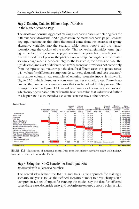
WEBC17 10/02/2014 3:31:50 Page 213

Step 2: Entering Data for Different Input Variablesin the Master Scenario Page

Themost time consuming part of making a scenario analysis is entering data fordifferent base, downside, and high cases in the master scenario page. Becausekey input parameters that drive the model come from this exercise of typingalternative variables into the scenario table, some people call the masterscenario page the cockpit of the model. This somewhat gimmicky term high-lights the fact that the scenario page becomes the place from which you candrive the model as if you are the pilot of a rocket ship. Putting data in themasterscenario page means that data entry for the base case, the downside case, theupside case, and a set of different sensitivity scenarios now does not come onlyfrom the input sheet. You can put the data for different cases in separate rows,with values for different assumptions (e.g., price, demand, and cost structure)in separate columns. An example of entering scenario inputs is shown inFigure 17.1, which illustrates a completed master scenario page. There is nolimit to the number of scenario cases that can be added in this process. Theexample shown in Figure 17.1 includes a number of sensitivity scenarios inwhich only one variable differs from the base case value that is discussed furtherin Chapter 18. It also includes a custom scenario row at the bottom.

Step 3: Using the INDEX Function to Find Input DataAssociated with a Scenario Number

The central idea behind the INDEX and Data Table approach for making ascenario analysis is to use the defined scenario number to drive changes in acomprehensive set of inputs for running the model. Say the data for differentcases (base case, downside case, and so forth) are entered across a columnwith

FIGURE 17.1 Illustration of Entering Input Data into the Master Scenario Page with INDEXFunction at the Bottom of the Table

Constructing Flexible Scenario Analysis for Risk Assessment 213

WEBC17 10/02/2014 3:31:51 Page 214

different scenarios listed in rows as shown in Figure 17.1. Then the arrayargument in the INDEX function uses one single column across the rows thatyou have input. The row number used in the INDEX function is the scenarionumber and it is the same for each column. The result of the INDEX function isthe shaded row at the bottom of the table in Figure 17.1. These values are thesame as the first row of the table because 1 is used as the scenario number. Theyare the values that will now be used in driving the financial model. If you want,you could call the data in the row createdwith the INDEX function the driver rowfor the model. In making the INDEX function, the scenario number should befixedwith the F4key soyou can copy the same formula acrossdifferent columns.

Model Driver = INDEX(Shaded Area of Rows in a Single Column,Scenario Number Fixed with the F4 Shortcut)

Step 4: Adding a Drop-Down Box to Run Scenarios fromDifferent Places in the Workbook

To present results of your different scenarios in graphs or on the summarypage or in the guts of the financial model, it is often convenient to include adrop-down box that lists the alternative scenarios (the base case, low case, andso forth). Adding a drop-down box is similar to the process of adding a spinnerbutton described in Chapter 16 for making flexible sensitivity graphs. Inthe case of the drop-down box, you select the Developer ribbon go to theInsert icon in the middle of the page, and paint a combo box somewhere onthe scenario spreadsheet page. To create a drop-down list that contains thescenario names, right-click on the combo box, and then select the FormControls option, as was the case for the spinner button. The combo boxrequires an input range, which is the list of items that will appear in the drop-down box. For a drop-down box associated with a scenario analysis, the drop-down list should be the names of the various scenarios such as the base caseand downside case. The input range can only contain a series of row titles inone column of data and it does not work with titles that are listed across rows.

As was the case with the spinner button, the windshield-wiper method ofclicking on another sheet with the mouse and then moving back to thescenario sheet should be used to ensure that the sheet name is included in theinput range that lists the different scenario cases. After selecting the inputrange, a cell link must be entered into the format control. The cell link simplyreports the result of the drop-down selection as a number. It puts the numberfor the row of the selected name from the drop-down list in a spreadsheet cell.In the case of our scenario analysis, the cell link will be the same number as thescenario number. Because INDEX function is used to drive the selection ofthe scenario, the scenario number or the cell link now also corresponds to thescenario list. The same windshield-wiper method should be used with the cell

214 Analyzing Risks with Financial Models

WEBC17 10/02/2014 3:31:51 Page 215

link, which is attached to the scenario number so that the cell link includes thesheet name. Figure 17.2 illustrates the process of entering the input range andthe cell link on the left-hand side of the diagram. Results of applying the drop-down box to the scenario list are shown on the right-hand side of Figure 17.2.Almost every time you make a drop-down box you will probably use theINDEX function. You will use the INDEX function because once you input thecell link that is a counter for the input range of rows, you can use this numberto find elements associated with the input data. The process is just the way theINDEX function works through defining a continuous array and finding anassociated cell. Note also that the cell link is simply an input, as was the celllink in the spinner button. This means that by using a drop-down box you canstill directly input the master scenario number manually in the cell (which alsochanges the selection of the combo box). Alternatively, you can select an itemin the combo box, which changes the scenario number and is the cell link forthe drop-down box.

FIGURE 17.2 Application of the Windshield-Wiper Method to a Drop-Down Box

Constructing Flexible Scenario Analysis for Risk Assessment 215

WEBC17 10/02/2014 3:31:52 Page 216

Step 5: Linking Financial Model Inputs to Scenario Page

The only tricky and somewhat awkward aspect of the scenario approach usingINDEX and Data Table is that financial model assumptions that were directlyinput to the model must now be linked to the driver row in the master scenariopage. This is the row defined by the INDEX function. Say that one of theassumptions on the master scenario page is for the price of the product, andthat many alternative prices are input for the different downside, upside,recession, and other scenario cases in your cockpit page. Through using theINDEX function described earlier to establish the driver row, a single one ofthe price inputs (depending on the scenario number selected) is listed at thebottom of the scenario page. The single price input that comes from the INDEXline (or the line to the right of the inputs if scenarios are set up with columnsinstead of rows) must now drive the model instead of the input that wasoriginally entered. To ensure the model is driven by the line on the masterscenario page, the input part of the financial model should be linked to thecell defined by the INDEX or model driver line of the master scenario page. Toemphasize, the model inputs come from the value driver and not the otherway around. Do not link the value driver line to the model inputs. After linkingthe model inputs to the master scenario page, you can change the scenarionumber either manually or by using the drop-down box, and then all of theassumptions in the model input page that are linked to the master scenariowill change. If you do not like this idea of adjusting model inputs, see the VBAcode discussion at the end of the chapter for an alternative apporach.

To make the process of linking model inputs to the master scenario pageless tedious, you can display both the model input sheet and the masterscenario sheet on the same screen. After presenting two sheets on one screenyou can go to the model inputs section, enter an equals sign, and then linkyour assumptions from the model input pages to the INDEX line of thescenario sheet. To be able to edit two different sheets of the same workbookon the same page, go to the View menu and first press New Window. Thisopens two versions of the same workbook. Next, press the Arrange All optionand select the “Windows of active workbook.” Also, check the box for thevertical option, as shown in Figure 17.3.

After you have two views of the same workbook open you can use theCNTL, PAGEUP or CNTL, PAGEDN shortcut keys so that one sheet showsinputs to the financial model and the second shows the master scenario page.Then you canwork your way down the financial model inputs and link variousinputs to the INDEX or the driver line of the master scenario page. The processis illustrated in Figures 17.3 and 17.4 where the arrows indicate that the linksare made and the flow is from the master scenario page to the financial model.The rule is always that the numbers in the financial model come from thescenario page and not the other way around. It is data from the master

216 Analyzing Risks with Financial Models

WEBC17 10/02/2014 3:31:52 Page 217

FIGURE 17.3 Illustration of the Process to Create Two Views of a Workbook on OnePage

FIGURE 17.4 Illustration of the Process of Linking Numbers from the INDEX line of theMaster Scenario Page to the Input Section of the Model

Constructing Flexible Scenario Analysis for Risk Assessment 217

WEBC17 10/02/2014 3:31:53 Page 218

scenario page or the cockpit that is now driving the model. In Figure 17.4 thenumbers that come from the financial model have the same color as the masterscenario page.

For some inputs such as the tax rate, a gross margin percentage that isassumed to be constant over the forecast horizon, or a single ratio of accountsreceivable to sales that does not change for future years, there is one inputnumber in the financial model. For this type of variable the process of linkingfrom the INDEX row to the input value in the assumption page is straightfor-ward. Other inputs that are structured as time series variables have changingvalues over time. As discussed in Chapter 6, these inputs use code numbers todefine the time series row that is selected. If the inflation rate changes from oneyear to the next and you have a few possible inflation rate scenarios, themethod described in Chapter 6 worked by entering a code number and usingthe INDEX function. The code number combined with the INDEX function ismuch like the method just described for the master scenario page. To selectdifferent series of time-varying inputs in the master scenario page, you canenter different code numbers in the scenario table. Figure 17.1 contains inputsfor general U.S. inflation and general Mexican inflation. In the input section ofthe model, the time series variables for this data were entered with a codenumber. When implementing amaster scenario, link the code number input inthe assumption sheet to the INDEX line in the master scenario page in thesame way you would for any other variables. Do not link a code number to themaster scenario code, ever. Linking the code number from the master scenariosheet to the input sheet is illustrated in Figure 17.5 where the number 1.00 inthe box in the center of the financial input page comes from the INDEX line ofthe master scenario page.

If you use the method discussed in this step of the process to linkvariables, one minor problem is that financial model inputs come from themaster scenario page. This means that inputs contain formulas that are nowlinked to the master scenario page instead of being pure numbers withoutformulas. You may not like this part of the technique because the input page isno longer pure in the sense that you can type hard inputs on that page. Youwould mess up the model if you typed an input number over the formula thatis now linked to the master scenario page. Some people would rather keep theassumptions in the model as hard inputs and make the scenario analysisindependent of the master scenario page. To do this you can use the VBAapproach described in the last part of this chapter.

Step 6: Linking a Set of Outputs alongside the ScenarioInputs in the Master Scenario Page

Once the INDEX function has been used to drive financial model inputs fromthe master scenario page you can create a table that presents selected

218 Analyzing Risks with Financial Models

WEBC17 10/02/2014 3:31:53 Page 219

outputs from the model next to the various scenarios. An easy way to do thisis to make a one-way data table to the right of the scenario inputs. Recall thatin creating a data table the format of the inputs is crucial. You can construct adata table that displays outputs like the DSCR, LLCR, and PLCR next to thebase case, downside, and other scenarios by entering the code number ofthe scenario in a single column between the inputs and the outputs. Youmust first gather the outputs from the model and place them into the masterscenario page. This involves linking the output variables to the masterscenario page. Note that the direction of the link is now the opposite of thelinks for the inputs. Here the formula remains in the financial model and itwill be put into the master scenario sheet. Because of restrictions in the way aone-way data table must be formatted, the links to these variables from themodel calculation sheet should be placed one row above and one row to theright of the scenario numbers. For such a one-way data table to work, thecolumn sensitivity range is the list of the scenario numbers, meaning that youmust enter a counter for thevarious scenarios one column to the left andone rowbelow the output variables. The format and result of the data table process isillustrated in Figure 17.6.

FIGURE 17.5 Illustration of Linking Code Numbers for Time Series Variables from theMaster Scenario Table to the Input Page

Constructing Flexible Scenario Analysis for Risk Assessment 219

WEBC17 10/02/2014 3:31:54 Page 220

Step 7: Creating a One-Way Table That Lists the Resultsof Multiple Scenarios

The final step of creating a scenario analysis is using the Data Table tool tolist the results of each scenario on the master scenario page. This involvesthe same techniques as described previously for the break-even analysiswhere the one-way data table was introduced. When the scenarios arecarefully set up in the manner described in step 6 with a counter to the left,the outputs one row above, and a blank cell in the upper left corner, you cancreate the data table. This is accomplished by selecting the area beginningwith the sequential list of scenario numbers and then using the Data, What-IfAnalysis, and Data Table tools. After the data table is highlighted and thedata table feature is selected, the column input of the data table is assignedto the single scenario number, which cycles through each scenario and liststhe output variables for the scenarios.

Once you have created the one-way data table, alternative transactionstructuring variables can be added to the analysis. In this way you can see thescenario case results with different transaction structures such as differentlevels of debt. The table in Figure 17.6 includes a spinner button next to thedebt leverage that allows you to see what happens to the IRR in differentscenarios when the leverage changes. If the leverage is increased or decreasedby moving the spinner button around, all of the results for the different

FIGURE 17.6 Illustration of Creating a Data Table with Code Numbers in a ScenarioAnalysis

220 Analyzing Risks with Financial Models

WEBC17 10/02/2014 3:31:54 Page 221

scenarios change along with the change in leverage (you could attach a simplecalculation macro to the spinner button as explained in Chapter 16). In thisway you can test things such as how much debt a project can support beforethe DSCR, LLCR, or the PLCR falls to a level of 1.0 in the downside case or thestress case.

Using VBA Code to Create a Scenario Analysis

There are two potential problems with the INDEX and Data Table scenarioprocess just discussed that some people may not like. The first probleminvolves the fact that the workbook becomes slow and clumsy (even if thecalculation option specifying recalculation without data tables is selected fromthe Formula ribbon) because data tables are used for the spreadsheetcalculations. The second is that the financial model variables are linked tothe master scenario page, meaning that the assumption section of the financialmodel no longer contains fixed data that can be adjusted manually. Instead, ifyou want to change data you must go back to the master scenario page. Bothof these problems can be solved byworking through similar steps as describedearlier, but with a little VBA code. If you add a macro to the analysis you willhave to press a button each time youwant to run a new scenario, which is not abig deal. The first part of a macro to create scenario analysis assigns data toinputs in the financial model, eliminating the need to link variables. Thesecond part of themacro replaces the data table with a FORNEXT loop and theCELLS statement as explained at the end of Chapter 16.

Creating a Macro That Assigns Variables from the INDEXLine of the Scenario Page to the Financial Model Inputs

If you want to develop VBA code that links the financial model inputs to themaster scenario page you can assign variables in the financial model input pageto the INDEX row of the master scenario cockpit. When you assign a numberwith amacro rather than linking thevaluewith a formula, theprocess is similar tocopying and pastingwithfixed values. Thismeans that there is no formula in theinput page even though the values that are changed still come from the masterscenario page. Programming this can be a little tedious, as you must make aformula that corresponds to each input. You also should enter a range name foreach of the variables that will be possibly adjusted from the master scenariopage. The following code illustrates how to assign a variable that has anassignedrange name (actual range names would be much shorter with no spaces):

Range(“Financial Modeling Inputs”) = Range(“Index Formula for Item

in Index Function on Scenario Page”)

Constructing Flexible Scenario Analysis for Risk Assessment 221

WEBC17 10/02/2014 3:31:54 Page 222

This code will replace the various financial model inputs, but it willleave the cells with input data as fixed values rather than formulas thatare linked with an equals sign to the master scenario page. As with the otherVBA code discussed previously, it is essential to name the ranges whencreating a macro. In this situation each input in the financial model thatwill be assigned a variable from the master scenario page should beassigned a range name (it is good to use the SHIFT, CNTL, F3 shortcutto do this). For the INDEX range that will be used to transfer the variables tothe financial model input page, a range name can be assigned to the wholerow (you can also construct a range name that covers multiple cells with theSHIFT, CNTL, F3 sequence). Once the range name is assigned, the CELLSstatement can be used to find the column of that range name that will beused as the basis of assigning the variables. To illustrate the approach ofassigning variables from a range name that contains multiple cells usingVBA code, assume the price variable is being defined to come from themaster scenario page. In the financial model, the range name is assumed tobe named PRICE, and the row computed with the INDEX function in themaster scenario page is named SCENARIO. Also assume that on the masterscenario page the price variable defined by the various scenarios is thethird variable from the left. Using the CELLS method, the VBA code wouldhave the following form:

Range(“PRICE”) = Range(“SCENARIO”).Cells(3,1)

If you want to link the input using this macro method, this kind of codewould have to be added for each variable that is changed by the masterscenario page. The macro can be assigned to the drop-down box that lists thescenarios so that whenever you chose a new scenario, the data that haveassigned range names will be revised. If the macro is attached to the drop-down box, whenever you run the drop-down box the macro will assign newdata to the variables to the financial model. In the macro you should addroutines that allow you to return to the place where you began, and put backthe inputs that were originally in the assumptions page. You can do this withthe Activesheet.Name statement and the Activecell.Address statement asshown in the next section.

The second kind of VBA code that can be used in developing scenarioanalysis is a macro that creates the data table. The method of using FORNEXT loops along with the CELLS statement that was described Chapter 16in the context of creating break-even analysis. Exactly the same code couldbe used for the scenario analysis can be applied. Using VBA code to createdata tables for a scenario analysis is illustrated in Figure 16.10.

222 Analyzing Risks with Financial Models

WEBC17 10/02/2014 3:31:54 Page 223

Getting the Best of Both Worlds: Creating a SpecialCustom Scenario That Allows Use of SpinnerButtons and Drop-Down Boxes

In Chapter 15, the idea of creating a flexible graph with spinner buttons anddrop-down boxes was described in detail. The attraction of this method for riskanalysis is that you can allow management to play around with key variablesand visualize what happens to things like cash flow, earnings, or debtbalances. If all of the key input variables come from a structured masterscenario or, if you like, cockpit page, there are no spinner buttons and the ideaof playing aroundwith a variable seems to be no longer an option. Recall that aproblem with allowing management to play around with a model is that theycan ruin your inputs and you may not be able to remember what values youhad input for the base case. This section describes a technique by which youcan still use spinner buttons and drop-down boxes for risk analysis presenta-tion. But then when you are finished playing around, you can also quicklyreset all of the inputs to one of the cases in the master scenario page.

One way to create a combined scenario and sensitivity analysis is to insertan extra scenario case in a line below all the rest of the scenario cases on themaster scenario page. In this special scenario case you can attach spinnerbuttons or combo boxes to all the data in the scenario so that the variables canbe adjusted in a similar manner as in the sensitivity analysis discussion. In themaster scenario page illustrated on Figure 17.1, the last row named the customcase is an example of this idea. If you look back at Figure 17.1, each input onthat last row that is not a time series variable is assigned a spinner button. Thevariables that change over time such as the inflation rate and are enteredwith acode number have an associated combo box. By attaching spinner buttonsand drop-down boxes to inputs in such a custom scenario, you can changeindividual variables in the summary page of a model as long as the scenariocase number is set to the number for the special custom case.

There are two challenges when creating this type of special custom case.The first problem is that you would probably like to reset the custom case tothe base case, low case, or high case after playing around with the spinnerbuttons and combo boxes. This is because you will soon forget values for thebase case and it is a pain to push the spinner buttons around until you get backto the original values. The second problem is that when attaching the spinnerbuttons to values in the custom scenario, many of the inputs are expressed aspercentages or as very large numbers. Spinner buttons, however, accept onlywhole numbers between 0 and 30,000. This means that spinner buttons do notwork for percentage inputs, for large numbers without adjustments, or forinputs that you would like to present with decimal numbers such as 5.26. Tofix this problem you canmake a spinner buttonwith the CELL LINK attached to

Constructing Flexible Scenario Analysis for Risk Assessment 223

WEBC17 10/02/2014 3:31:54 Page 224

an intermediate number instead of the input that the spinner button repre-sents. Then you can make the input a formula that adjusts the intermediatenumber created with the CELL LINK. To better understand this, say you wantto enter a percentage input that moves between 1 percent and 100 percent.You can then create an intermediate cell that moves from 1 to 100 that isattached to the CELL LINK. After that, you can divide the intermediate numbercreated with the CELL LINK by 100 and use the spinner button. This means thatwhenever you want to present a number that is not a whole number using thespinner button, you must develop a two-step process. The first part of theprocess is to set the CELL LINK to an indirect cell and the second part is todivide or multiply that intermediate CELL LINK number by some constant suchas 100 or 0.10.

In the context of a custom scenario case you can address the problems ofattaching spinner button when the data are not simple whole numbers andalso address the business of resetting data by adding a few rows below the linethat was created with the INDEX function. Using a little VBA code you canautomatically reset the scenario to the base case or another case by making acopy and paste macro that puts the base case or other cases back into thecustom case.

The new added rows include space for adjustments to address problemswith the spinner buttons. One of the lines contains intermediate cells thatcan be transferred through multiplying or dividing data, which can thenestablish the custom case. The added rows also allow you to reset the customcase to the base case, high case, or low case. The last additional row belowthe INDEX model driver row contains the data that can be referred to in thespinner button row. This row can be attached to the CELL LINK as it containsnumbers like 10 instead of 10 percent or 100 instead of 100,000. The numbersused that adjust the CELL LINK values back to input values can be calledmultipliers. With the 10 percent and the 100,000 input value examples, thefirst multiplier could be 100 and the second multiplier could be 0.01. Thesemultipliers that are entered to a row below the INDEX row have two functions.The first objective is to multiply the unadjusted data that is copied from thebase case so that it can be used in CELL LINK of the spinner button. The secondfunction is to readjust the intermediate spinner button values so that they canbe expressed in the correct units in the financial model. Using this idea ofmultipliers, the following step-by-step process explains the technique that youcan use to reset the custom case to the base case, low case, or high casescenarios and also make the custom case operate with spinner buttons.

Step 1 Begin the process by recording amacro.With themacro recording,copy the base case row, the low case, or any other case to a row afew lines below the INDEX function line. This line is named theCopied row in Figure 17.7. The Copied row cannot be used with

224 Analyzing Risks with Financial Models

WEBC17 10/02/2014 3:31:54 Page 225

spinner buttons if any of the variables are expressed as percentagesor may have values larger than 30,000 or have values that canchange in manner other than whole numbers. After copying thescenario row to the raw data line, stop recording the macro.

Step 2 Input the various multipliers in a row below the raw data rowcopied from step 1. This data that you enter is not directly affectedby a macro. If the scenario data are code numbers that adjust timeseries inputs or the data are already whole numbers between 10and 30,000 that can be expressed without fractions, then themultiplier can be 1.0. For other data that contain percentages,where a fraction is desired, or where the number is larger than30,000, a multiplier should be entered that is either a multipleor a fraction of 10. An illustration of this process is shown inFigure 17.7 were the multipliers are 1.0 for time series variableswith code numbers, but are 1,000 when the input data isexpressed as a percentage.

Step 3 Create a third row that you can name the Adjusted row. In this rowmultiply or divide the row copied from the base case or anothercase by the multipliers in a third row. This row will have valuesthat can be adjusted with either spinner buttons or combo boxes.In the example shown in Figure 17.7, the row is named Adjustedand it is the Copied row divided by the Multiplier row. Theformula in this row should be left alone, meaning that it shouldnot be attached to a spinner button or a drop-down box. You willneed formulas in this row to remain intact when you redo the

FIGURE 17.7 Illustration of Inserting Rows below the Scenario Table to Create aFlexible Custom Case Scenario

Constructing Flexible Scenario Analysis for Risk Assessment 225

WEBC17 10/02/2014 3:31:55 Page 226

process later on. If you are using the spinner button to push avalue up or down, you want to adjust a fixed value and nota formula.

Step 4 Start recording a second macro that copies the Adjusted row(the Copied row divided by the multiplier) and paste it asvalues into yet another fourth and final row. Then stop record-ing the macro. This fourth row has fixed values rather thanformulas. It is the row named Spinner in Figure 17.7. It is the rowthat is used as the intermediate CELL LINK by all of the spinnerbuttons and the combo boxes for defining the custom case. Youneed to copy and paste the cells as values to this new rowbecause the spinner button will fix values and you will want toredo the process later on. If you do not create this intermediatestep by copying and pasting with values, you can perform theprocess after copying the base case only a single time. After that,you could not reset the custom case scenario. Say you wouldlike to change the base case or run the custom case from the lowcase. This process allows you to retain the flexibility wherebythe raw Copied data is adjusted with a formula without fixingthe data. Once you have copied and pasted the final Adjustedrow to the Spinner row, stop recording the macro. For cosmeticpurposes, after you have recorded the macro, add a line in theVBA code to turn off the marking for the copied row using thestatement:

Application.CutCopyMode = FALSE

Step 5 To create the spinner buttons for each data item in the customcase, refer to the Spinner row in step 4 when you are connectingeach CELL LINK. This value in the Spinner row should be a wholenumber that can be adjusted by the spinner button. The Spinnerrow is the last row shown on Figure 17.7.

Step 6 When you have computed the last row containing the intermedi-ate data that is adjusted by the multiplier, you can establishthe custom scenario row that will be used in the model whenthe master scenario code is set to the custom case number. Thecustom case scenario uses the Spinner line that you createdcontaining fixed adjusted values and then readjusts this line usingthe multiplier factors. For example, if the base case input is aninterest rate of 5.2 percent, then the value expressed as a decimalis copied to the raw data row, resulting in the number 0.052using the first macro. Next, the raw data row named Copied is

226 Analyzing Risks with Financial Models

WEBC17 10/02/2014 3:31:55 Page 227

multiplied by 1,000, yielding a value of 52. This value of 52 is inturn copied to the fixed Spinner row. The value of 52 is attachedto the spinner button as the CELL LINK using the windshield-wiper method of clicking on another sheet and returning to themaster scenario sheet. Finally, the number in the custom rowof the scenario table and used to transfer data to the model isdivided by 1,000, and that number is ultimately used in thefinancial model.

This all sounds a bit dense but remember it is really accom-plished by two copy and paste macros. When you are finishedwith the process, management can select the custom scenariowith the drop-down box and then play around with the interestrate as much as they want. But when they have finished playingaround you can reset the custom case scenario back to the basecase by pressing a button attached to the copy and pastemacros.

Step 7 The final step of the process to create a custom scenario caseis to put the two macros that you created from the precedingsteps together. As with any macro you should create rangenames for anything that is copied and pasted. This macroshould be attached to the drop-down box so that the basisfor the custom case can be the base case, the low case, or anyother case.

To program a macro that copies different cases depending on thescenario chosen you can use the SELECT CASE statement in VBA followedby the END SELECT statement. This method will allow you to copy differentcases to the copied data row depending on which scenario is selected. Ifyou are attaching the macro to the drop-down scenario box, then whenyou use the SELECT CASE statement, you can apply a different copy andpaste routine depending on the scenario selected. To use the SELECT CASEmethod, put the variable that will change next to SELECT CASE. In this casea reference to the master scenario number is entered after the SELECT CASEstatement using the RANGE statement as shown next. The variable is therange name for our famous scenario code number. If the scenario numberis assigned a range name (as it should be) the VBA code would be:

SELECT CASE RANGE(“Scenario Number”)

Below this statement you would enter CASE 1:, CASE 2:, and so forthdepending on how many cases can be copied to the raw data Copied line andused in the custom case. Here, the numbers 1, 2, and 3 refer to the scenariocode number. Underneath CASE 1: you then put the copy and paste statement

Constructing Flexible Scenario Analysis for Risk Assessment 227

WEBC17 10/02/2014 3:31:56 Page 228

that copies the base case to the raw data line below the INDEX function asillustrated:

CASE 1:

Copy base case to raw data row

CASE 2:

Copy low case to raw data row

Sub custom()

’

’ custom Macro

’

Application.ScreenUpdating = False ’ Turn off screen updating for copy

If Range("scenario") > 4 Then Exit Sub ’ Only copy the first three scenarios

current_cell = ActiveCell.Address ’ Remember cell for re-set

current_sheet = ActiveSheet.Name ’ Remember sheet for re-set

scenario_sheet = Range("scenario_sheet") ’ Get scenario sheet name

Sheets(scenario_sheet).Select

Select Case Range("scenario") ’ Select different cases for copying

Case 1: Range("base_case").Select

Case 2: Range("low_case").Select

Case 3: Range("high_case").Select

End Select

Selection.Copy

Range("copied").Select ’ Copy to first row

Selection.PasteSpecial Paste:=xlPasteValues, Operation:=xlNone, SkipBlanks _

:=False, Transpose:=False

Range("adjusted").Select ’ Select line after the multiplier formulas

Selection.Copy

Range("spinner").Select ’ Copy to fixed spinner box line as fixed

Selection.PasteSpecial Paste:=xlPasteValues, Operation:=xlNone, SkipBlanks _

:=False, Transpose:=False

Application.CutCopyMode = False

Sheets(current_sheet).Select ’ Re-set the sheet and the cell

Range(current_cell).Activate

End Sub

FIGURE 17.8 Illustration of Macro to Create Custom Scenario from Copying and PastingAlternative Cases

228 Analyzing Risks with Financial Models

WEBC17 10/02/2014 3:31:56 Page 229

Once you are finished with the copy and paste functions as part of theSELECT CASE process, you must write the END SELECT statement. Then,below the END SELECT statement, move the copy and paste code that copiesthe Adjusted row to the Spinner row. This part of the macro copies theAdjusted line computed from the raw data multiplied or divided by themultiplier to the fixed Spinner row. The second part of the macro is necessarybecause this last fixed line is used by the spinner button. Finally, if you do notwant the copy and paste functions to apply to selections from the drop-downbox other than the first three cases (base case, the low case, and the high case),you can use the following code:

Case > 3

Exit Sub

A completed macro to accomplish this custom case process with rangenames is shown in Figure 17.8. This macro includes the ability to remember thesheet location and the cell location where you were when you began runningthe macro and it will take you back to the same starting point.

Constructing Flexible Scenario Analysis for Risk Assessment 229

WEBC17 10/02/2014 3:31:56 Page 230

WEBC18 10/03/2014 8:46:13 Page 231

CHAPTER 18Generating Tornado Diagrams,

Spider Charts, and Waterfall Graphs

When constructing a scenario analysis using the procedure discussed inChapter 17, there is often a very large difference between an output for

the base case and the downside case as a whole lot of inputs are changed atthe same time. The base case may have something like a 12 percent internalrate of return (IRR) whereas the downside case could have a �20 percent IRR.To make sense of a scenario analysis such as this, it is useful to understandwhich of the input variables are most instrumental and which are leastinstrumental in causing the IRRs to change. An analysis that isolates on theeffect of individual variables is useful for a few reasons. First, it can allow youto better understand which particular variable is the one that really matters indriving changes in the output. Second, it is a very effective way for you to finderrors in your model. Third, it is a good way to impress people with fancygraphs that demonstrate your prowess in spreadsheet programming.

When isolating the effect of individual assumptions on the differencebetween scenario outcomes, the general approach described in this chapter isto create a number of different sensitivity cases that adjust the base case by onesingle variable at a time. Once you have created these multiple sensitivitycases you can present the analysis in various different forms. One technique isto make a tornado diagram, which involves making a bar chart that illustratesdifferences in a model output between low case and base case inputs as wellas differences between high case and base case inputs. Bars on the chart canbe arranged from the input variable that has the highest effect to the inputvariable that has the lowest effect on the selected output parameter. A secondpresentation technique for displaying the sensitivity analysis is creating aspider diagram. This type of graph shows increments for all of the selectedinput variables on the x-axis and presents the resulting output on a series ofline graphs. A third style of presentation involves displaying how the low case

231

WEBC18 10/03/2014 8:46:13 Page 232

or the high case is built up from the base case value. This is often referred to asa waterfall graph.

This chapter begins by discussing why you may want to present a tornadodiagram or a spider diagram in risk analysis. It then explains how to make thetornado and spider graphs through extending the scenario analysis discussedin Chapter 17. The next few paragraphs describe two different ways to create atornado diagram. A subsequent section of the chapter discusses how to makespider diagrams. The final part of the chapter explains how to presentsensitivity analysis in a waterfall chart.

Tornado Diagrams That Display Which VariablesHave the Largest Effect on Value and WhichVariables Have the Least Effect on anOutput Variable

The scenario analysis described in Chapter 17 did not show which of the inputvariables aremost important andwhichare insignificant in influencing anoutputvariable of your model. You can perform this kind of risk analysis by making atornadodiagram.A tornadodiagramgets its namebecause it is supposed to looklike the whirlwind created by a tornado, which is normally larger on the top andsmaller on the bottom. In this vein, input variables that have thehighest effect ona selected output variable are shown as horizontal bars at the top of the graphand variables that have a smaller impact are shown at the bottom. Throughpresenting sensitivity analysis in thismanner a tornado diagram can be used as atool to determinewhich variables aremost important in a sensitivity analysis andshould thus be the focus ofmore study and due diligence. In addition, a tornadopresentation can be used to illustrate whether an investment has more upsiderisk or more downside exposure. If the tornado is bending toward the upsidecase or the downside case, as tornadoes sometimes do, then there is moreupside potential or downside risk in your investment. Third, a tornado diagramcan be used as an auditing tool to test the mechanics of a financial model. If thevariables that have thehighest effect on theoutputmetric arenot intuitiveor theyhave not effect at all, you should then go back to the financial model andcarefully examine the formulas related to the nonintuitive variable.

Figure 18.1 illustrates how a tornado diagram can be used in risk analysis.Data is entered for a number of inputs for the base case, downside case, andupside case scenarios in the same format as the scenario analysis discussed inChapter 17. While the structure is the same as the scenario analysis, thedownside and upside cases do not necessarily have to represent a consistentsingle integrated scenario. In the case of a tornado diagram, every variable isentered as a low or a high value and one variable does not mitigate the effect of

232 Analyzing Risks with Financial Models

WEBC18 10/03/2014 8:46:13 Page 233

another. If sales decrease, then operating costs may also decrease in a scenarioanalysis, but this would not be part of a tornado analysis. Figure 18.1 illustratesthe format of a tornadodiagram.Data shownon the left of the y-scale are the lowcase, base case, and high case inputs. Which of these to use depends on yourjudgment. Given the inputs for the three cases, each bar on the diagram showshow the variation in the downside case input relative to the base case inputor the upside input relative to the base case input affects the output variable.

The tornado diagram illustrated in Figure 18.1 shows which variables havethe largest effect on the loan life coverage ratio (LLCR) for a toll road projectfinancing. It demonstrates that the variable that has the highest effect on theLLCR is the background traffic. For the downside case assumption, this variablecauses the LLCR to fall by 0.21, when all other variables are set to the base case.The top bar also shows that if the background traffic increases by 3 percent peryear the LLCR increases by 0.26 relative to the base case. Other bars onthe chart representing variables such as the operation and maintenanceexpense and the long-term traffic projections have a smaller effect on theLLCR. If the LLCR is an important statistic for lenders, you would not have toworry quite as much about getting these other variables right in your model aslong as the judgmental downside and upside assumptions are reasonable.

FIGURE 18.1 Illustration of a Tornado Diagram for a Toll Road Project

Generating Tornado Diagrams, Spider Charts, and Waterfall Graphs 233

WEBC18 10/03/2014 8:46:14 Page 234

Creating a Tornado Diagram by ExtendingScenario Analysis

You do not need some kind of fancy add-in to create a tornado diagram.Instead, you can make the diagram that illustrates the sensitivity of eachvariable straight from extending the scenario analysis described in Chapter 17.To construct a tornado diagram similar to the one displayed in Figure 18.1 youshould add two new scenario rows for each input variable. Then you can usethe Data Table tool to summarize all of the scenarios at the same time. Oncea data table is constructed with all of the additional scenario rows, informa-tion from the resulting data table output can be used to build a graph likeFigure 18.1. As with the scenario analysis, the entire process is accomplishedwith a combination of the Data Table and the INDEX function. Detailed stepsto construct the Tornado diagram that displays sensitivity analysis include:

Step 1 First, add a whole lot of new scenario rows that representdeviations from the base case for each separate input variable.The good news about this is that you do not have to spend muchtime typing in data for the scenarios. This is because data for thenew rows come straight from the base case, low case, and highcase inputs. The new scenarios you enter will contain base casevalues for each input except for the single input value defined asthe sensitivity case. This set up of sensitivity scenarios isillustrated in Figure 18.2. The first sensitivity case representsthe low case for sales growth. This sensitivity scenario uses basecase inputs for all values except for the sales growth. For thesales growth input, the low case is assumed. By creating thisnew scenario you will be able to see how much the sales growthassumption affects the value of the company in isolation,because all of the other inputs are still set to the base case.

Tomake these scenarioswhere a single value is altered from thebase case you should first insert a lot of rows to allow space for thescenarios. You can then use the TRANSPOSE function to makescenario titles for each of the new sensitivity rows. Say that youalready have the base low and high case scenarios in a table on themaster scenario page. First, count on your fingers how many inputvariables you have. Then in the column that contains the scenariotitles select the number of rows that you just counted. Next, make atitle for each of the new sensitivity scenarios by highlighting thevariable titles and using the TRANSPOSE function. If one of thevariables represents prices, another represents quantities, anda thirdrepresents interest rates, then these variable names are presented assensitivity scenarios below the low case as shown in Figure 18.2.

234 Analyzing Risks with Financial Models

WEBC18 10/03/2014 8:46:14 Page 235

To use the TRANSPOSE function, you need to press SHIFT,CNTL, ENTER rather than just the ENTER key as TRANSPOSE is anarray function. Say there are six variables in the scenario analysisas shown in Figure 18.2. You then can insert 12 new rows that willhave a low case and a high case next to the name for eachvariable. In each scenario, the values all are the base case inputsexcept for one variable that has the low case or high case title. Thesensitivity row titles can say something like “Base Case ExceptSales Growth Low Case.”

To make these titles you can either add the text to theTRANSPOSE function with the & symbol or you can simply referto the low case and high case title. If you are creating your owntext, next to each sensitivity row you can use the TRANSPOSEfunction as follows:

■ Select six rows.■ Enter “Base Case Except” & TRANSPOSE(“Variable RowTitles”) & “Low Case.”

■ Press the SHIFT, CNTL, ENTER combination.

FIGURE 18.2 Illustration of Scenario Table with Sensitivity Analysis for Each Variable

Generating Tornado Diagrams, Spider Charts, and Waterfall Graphs 235

WEBC18 10/03/2014 8:46:19 Page 236

If you just want to use the low case or high case title that youalready have entered, you can use the TRANSPOSE functiontogether with another cell reference as follows:

■ Select six rows.■ Enter TRANSPOSE(“Variable Row Titles”) & Cell Referencefor low case (e.g. C7).

■ Press the SHIFT, CNTL, ENTER combination.Once you have made the sensitivity titles like these for the

low case, you can shade the next six rows and make similar titlesfor the high case.

Step 2 After making row titles for the different sensitivity scenario cases,copy all of the values in every single scenario to the base case.You can quickly copy all of the values from the base case to otherrows by linking one of the variables with the equals sign and thenpressing the F4 key twice so that the row number will be fixed andthe column number will be flexible. When you have linked thebase case value for one cell, copy the same link to the entire blockof remaining rows and remaining columns using SHIFT, CNTL,→and SHIFT, CNTL, Down Arrow. Alternatively, you can hold theSHIFT key and go to the bottom right column and then click. Afterthe entire block is shaded then press CNTL, R and CNTL, D tocopy the base case value to each cell.

Step 3 Once you have the block of new rows for the sensitivity cases allassigned to the base case, work through each row and change thevalueof thevariable that is listed in the sensitivity case to the lowcase.If the first row is a sensitivity case for sales growth, then you shouldlink the cell in the column for the sales growth to the low case valueinstead of the base case. Thismeans that the sales lowcase sensitivityrowwill have the base case value for every input except for the salesgrowth. After you have finished the same process for each sensitivitycase row, there should be a diagonal pattern. All variables shouldhave the samebasecasevalueexceptone single input that is differentin one row below and one cell to the right of the previous changedcell. Creating thesemultiple scenarios allows you to isolate the effectof the downside value or the upside value for each data item.

If you want to illustrate which values in a scenario are alteredfrom the base case, you can use the conditional formatting tool.As with previous examples of conditional formatting you canwork with the option to enter a formula. To apply this approachof formatting depending on the equality of two values, begin byhighlighting the area that you want to format. Next, enter thecurrent cell in the conditional formatting slot without any fixedreferences (i.e., without the dollar signs) by pressing the F4 key

236 Analyzing Risks with Financial Models

WEBC18 10/03/2014 8:46:19 Page 237

a few times. Then, test whether the variable is equal to the lowcase or the high case. When testing the value relative to the lowor high case, use the fixed reference on the row number for thelow or high case so the conditional formatting will work acrossall of the scenarios. Coloring cells that are equal to the low caseor high case using this technique is illustrated in Figure 18.3.

Step 4 After adjusting the selected values of individual variables in thedownside case, follow the same process for the upside case,meaning that you first transpose the titles. As was the case for thedownside scenario, link the base case values to the whole block

FIGURE 18.3 Use of Conditional Formatting with the Formula Option to Color CellsThat Are Not the Same as the Base Case

Generating Tornado Diagrams, Spider Charts, and Waterfall Graphs 237

WEBC18 10/03/2014 8:46:20 Page 238

of inputs and then change the input value to the upside case foronly the sensitivity variable in question.

Step 5 When data for the low case and the high case sensitivities areentered as new sensitivity rows, adjust the INDEX function and theData Table to include the additional cases. To revise the INDEXfunction, include the added rows as part of the array in INDEXfunction. You must also add the new sensitivity case numbers inthe column to the right of the data table as was shown in Fig-ure 18.2. The data table is developed as usual by shading theextended scenarios and attaching the column input to the scenarionumber. Since numbers from the INDEX row are already attachedto the financial model inputs, the data table should work just fine.

Step 6 With the extended data table created you can evaluate the effect ofeach input variable on the output variable in isolation. Tomake thiscomparison, add some rows below the data table where you willsubtract values in the data table for each sensitivity case from thebase case value in the table. In subtracting, compute the change ofthe sensitivity case from the base case. First create a list of thevariables using the TRANSPOSE function. Next to the list computethe upside case valueminus the base case value for each sensitivityrow. In a second column make a similar calculation for the down-side sensitivity. This process is illustrated in Figure 18.4. Calcula-tions for these incremental differences can be made by fixing thebase case cell in the data table with the F4 key and then subtractingeach of the different scenarios one at a time without fixing the cell.

Step 7 With a table like the one shown at the bottom of Figure 18.4, youcan make a graph that demonstrates which variables have thelargest effect on the output variable and which have the smallesteffect on the variable. Simply highlight the table including thetitles and the blank cell at the top left as shown in Figure 18.4.Then use the F11 key to create a graph. After that, change thechart type to a bar chart. The only issue with this graph is that it isnot yet sorted for presentation. An example of the unsorted graphis illustrated in Figure 18.5.

Step 8 The remaining task in creating a tornado diagram is sorting the data(although you may be satisfied with the unsorted graph that is theresult of the process in Figure 18.5). If you sort the absolute value ofthe difference between the base case and low case combined withthe difference between the base case and the high case, the graphwill have the shape of a tornado as was illustrated in Figure 18.1.Unfortunately, use of the sort tool is not very helpful in this instancefor a variety of reasons. First, you probably do not want to changethe order of all the variables in the scenario table. Second, if you

238 Analyzing Risks with Financial Models

WEBC18 10/03/2014 8:46:20 Page 239

have used the Data Table function, you cannot sort items in the datatable. Third, when you rerun the analysis by changing something inyour model, you do not want to redo the sort.

Instead of using the sort tool you can use a combination ofthe SMALL function, the MATCH function, and the INDEX func-tion. If you use the SMALL function along with the MATCH andthe INDEX functions, the original values that you sort will be leftalone and you can perform the sort process somewhere else inthe spreadsheet. The general approach is to begin by using theSMALL function to sort the variables, where you list the array ofitems to sort and a counter variable. Then you must create aspecial variable representing a sort key that will be used fortabulating the whole set of variables in a sorted order. This can be

FIGURE 18.4 Creating a Table Showing the Incremental Downside Sensitivity Casesand the Upside Sensitivity Cases Relative to the Base Case

Generating Tornado Diagrams, Spider Charts, and Waterfall Graphs 239

WEBC18 10/03/2014 8:46:25 Page 240

accomplished with the MATCH function. Once the sort key iscreated from the MATCH function, you can use the INDEXfunction to present selected variables in sorted order andmake your graph. Details of this process include the followingfive actions:

1. First compute the absolute value of the differences betweenthe low case and the base case combinedwith the differencebetween the high case and the base case. Then make a newcolumn or row next to the sum of the absolute values. To usethe SMALL function to sort these absolute values you need acounter variable, as the SMALL function gives you the firstsmallest value, the second smallest value, and so forth. Todo this, enter the SMALL as illustrated:

SMALL(Row or Column to Sort, Counter)

2. After you have used the SMALL function to sort the absolutevalues, you have the sorted values but you have lost thevariable names and other information associated with eachof the values. To retrieve the names associated with each ofthe values and to retrieve the base relative to low and thebase relative to high values, you can make a counter orindex variable. You can use this variable to associate the

FIGURE 18.5 Illustration of Creating a Sensitivity Graph from the Sensitivity Table

240 Analyzing Risks with Financial Models

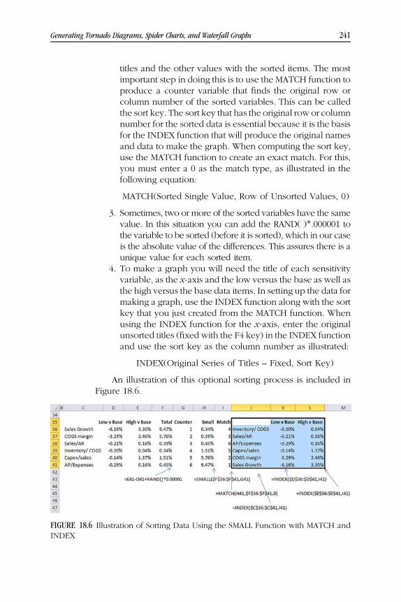
WEBC18 10/03/2014 8:46:25 Page 241

titles and the other values with the sorted items. The mostimportant step in doing this is to use the MATCH function toproduce a counter variable that finds the original row orcolumn number of the sorted variables. This can be calledthe sort key. The sort key that has the original row or columnnumber for the sorted data is essential because it is the basisfor the INDEX function that will produce the original namesand data to make the graph. When computing the sort key,use the MATCH function to create an exact match. For this,you must enter a 0 as the match type, as illustrated in thefollowing equation:

MATCH(Sorted Single Value, Row of Unsorted Values, 0)

3. Sometimes, two or more of the sorted variables have the samevalue. In this situation you can add the RAND( )*.000001 tothe variable to be sorted (before it is sorted), which in our caseis the absolute value of the differences. This assures there is aunique value for each sorted item.

4. To make a graph you will need the title of each sensitivityvariable, as the x-axis and the low versus the base as well asthe high versus the base data items. In setting up the data formaking a graph, use the INDEX function along with the sortkey that you just created from the MATCH function. Whenusing the INDEX function for the x-axis, enter the originalunsorted titles (fixed with the F4 key) in the INDEX functionand use the sort key as the column number as illustrated:

INDEX(Original Series of Titles – Fixed, Sort Key)

An illustration of this optional sorting process is included inFigure 18.6.

FIGURE 18.6 Illustration of Sorting Data Using the SMALL Function with MATCH andINDEX

Generating Tornado Diagrams, Spider Charts, and Waterfall Graphs 241

WEBC18 10/03/2014 8:46:25 Page 242

5. Graph the sorted variables using the F11 function, andchange the chart type to a stacked bar chart. As usual,make sure that there is no caption next to the titles inthe upper left-hand cell so Excel will know that this is thex-axis.

Creating a Tornado Diagram Using a Two-WayData Table

A tornado diagram can also be constructed using a two-way data tabletogether with a TRUE/FALSE test variable and a row number code. Thismethod changes each variable one at a time and also changes the scenarionumber for the base case, low case, or high case. For each change in thevariable and the scenario, the result is reported in a two-way data table. Whenimplementing this second method you do not have to make a lot of sensitivityrows as with the TRANSPOSE process shown previously. However, there are acouple of drawbacks to this method. First, you need to add extra steps if youwant the flexibility to present both the sensitivity analysis and the scenarioanalysis. Second, adding a separate custom scenario is difficult. Creating atwo-way table to make a tornado diagram is similar to the method that isdescribed later on to create spider diagrams. As with the row-by-row methodof creating tornado diagrams discussed in the previous section, the generalprocess involves isolating the effect of one variable while all of the othervariables are held at the base case value. When using the two-way data tableapproach, you can think of cycling around each input variable one at a timeand finding the output variable and also cycling around the base case, lowcase, and high case scenarios. If you were writing a program, there would betwo FOR NEXT loops.

To create a tornado using this two-way data table process, you can takethe following steps:

Step 1 Set up a scenario analysis using the normal INDEX andData Tableapproach described in Chapter 17, but do not add all of the extrascenarios below the low case.

Step 2 To prepare the analysis for a two-way data table rather than a one-way table, add a code number for the variable number in additionto the scenario code number at the top of the sheet. The variablenumber could be entered near the scenario number that was thefirst thing entered in themaster scenario page at the top. Next, adda number associated with each variable in an analogous mannerto the way you entered the scenario number to the left of the datatable. Entering the variable number above each variable name

242 Analyzing Risks with Financial Models

WEBC18 10/03/2014 8:46:26 Page 243

and putting the single variable number code at the top of the sheetare illustrated in Figure 18.7.

Step 3 Underneath the normal INDEX row for the basic scenario analy-sis, add a new row that includes a TRUE/FALSE test. This switchvariable tests whether the variable number in the column of thetable is the same as the variable code number that you input at thetop of the page. If there are six variables, there should be a list ofnumbers from 1 to 6 above the variables. The switch variableevaluates whether the code number at the top of the table equalsthe number associated with the variable. If the row code numberis 2, then the row below the INDEX function will be FALSE inevery column except for the second column. Because of the waythe numbers are set up there is always only one value that is TRUEfor the list of variables. The formula for the test variable shoulduse the F4 key for the variable code number and compare this toeach formula as illustrated:

=Variable Number Input at the Top = Number Associated withEach Variable

Step 4 Add another row below the TRUE/FALSE switch variable that usesan IF function to establish the model driver. This row assures thatonly one variable at a time will be changed in your financialmodel. If the test variable is TRUE, then use the value from theINDEX function discussed in step 2 to run the model. If thevariable is FALSE, then you simply use the base case value. Usingthis approach, every variable remains at the base case valueexcept the variable that equals the variable code number that youinput. This is the trick that allows the two-way table to present

FIGURE 18.7 Formulas for the Switch Variable and the IF Test to Set Up a Two-WayData Table for a Tornado Diagram

Generating Tornado Diagrams, Spider Charts, and Waterfall Graphs 243

WEBC18 10/03/2014 8:46:26 Page 244

how each variable affects the output value in isolation from theothers. The IF test has the following form:

IF(TRUE/FALSE Test, INDEX from Normal Scenario in Step 3,Base Case from Scenario Table)

Figure 18.7 shows formulas for the switch variable thatcontains either TRUE or FALSE as well as the variable createdwith the IF test that will drive the model.

Step 5 After entering scenario inputs, the variable code number, the testTRUE/FALSE switch variable, and the IF test as shown in Figure18.7, you should link the input variables in the financial modelrow with the last row that contains the IF test instead of linkingthem to the INDEX function row. This means when you changethe variable code number and put the scenario number to the lowcase, only the low case is implemented for the single variablenumber in the financial model. When you have finished linkingvariables in the input section to the last row shown in Figure 18.7,you are ready to set up a two-way data table where one of thesensitivity variables is the variable number and a second variablerepresents the scenario number for the base case, low case, andhigh case. The general structure of this two-way data table isillustrated in Figure 18.8.

Step 6 In Figure 18.8, the first row represents the base case, the second isthe low case, and the third is the high case. Each column containsthe value of the selected output variable whereby the inputvariable is changed in isolation and every other variable remainsset to the base case value. Once the table is set up, run either atwo-way table or, if you want to be a little fancier, write some VBAcode that does the same thing. The row input for the two-way datatable is the variable code number and the column input is thescenario number.

Step 7 When the two-way data table has been calculated, the base caseoutput is repeated for each variable and there is no difference inthe output variable across the row. The downside and the highcase contain the sensitivity effect of the single value. After the

FIGURE 18.8 Setup of Two-Way Data Table for Tornado Diagram

244 Analyzing Risks with Financial Models

WEBC18 10/03/2014 8:46:26 Page 245

table is computed, the base case relative to the low case and thebase case relative to the high case can be established. This is doneby subtracting the low case row from the base case row and bysubtracting the high case row from the base case row. Thesubtraction of the alternative cases from the base case are thebars that can then be presented in the tornado diagram. All that isleft to do is to sort and present the data. An illustration of thisprocess is shown in Figure 18.9. In this example the variable withthe largest effect is variable number 6 and the second largest isvariable number 2. Variable number 4 comes in last place. To findthe ordering of the variables, look in the row named “AbsoluteDifference,”which adds the absolute value of the low case relativeto the base case and the high case relative to the base case.

Step 8 To sort the data from highest to lowest when making a tornadograph, use the same process described in step 8 in the previousstep-by-step description of extending the scenario analysis. Thisinvolves first computing the sum of the absolute values ofthe differences and then using the SMALL, MATCH, and INDEXfunctions as shown in Figure 18.9.

Step 9 A drawback of this approach is that if you connect the financialmodel inputs to the row with the IF statement that isolates onone variable, you can no longer use the same data for making astandard scenario analysis. To rectify this you can add anoption variable that switches between the scenario analysisand the sensitivity analysis. In allowing this flexibility you can

FIGURE 18.9 Creating Tornado Analysis from Two-Way Data Table

Generating Tornado Diagrams, Spider Charts, and Waterfall Graphs 245

WEBC18 10/03/2014 8:46:29 Page 246

add a form control that permits selection of either a scenarioanalysis or a tornado diagram. If the scenario analysis is chosen,the link to the financial model will come from the INDEX row.If the tornado diagram is selected, the link will come from the IFstatement. Instead of using a spinner button or a drop-downbox you can use multiple option buttons this time. To applyoption buttons, insert a button from the developer tab and thenright click on the button as usual and select a cell link. Whereasdrop-down boxes work together with the INDEX function, theoption buttons work well with the CHOOSE function.

Step 10 In order tomake themodel operate with either the scenario analysisor a tornado diagram, you can enter yet another row below the IFstatement row. This row selects whether the INDEX function row isused to drive the financial model inputs as was discussed in Chapter17, or the IF statement that sets all variables to the base case exceptfor the single variable in question is the model driver. To tell themodelwhether toapply the INDEXrowor the IF rowyoucanuse theCHOOSE function togetherwith the cell link from the option button.The new row will be set to either the INDEX value for the scenariooption, or the IF function for the tornadooption.An illustrationof thispart of setting up a tornado diagram was presented in Figure 18.8.The last line in the table shown in Figure 18.8 is used as the basis forthe link that drives inputs of the financial model.

Spider Diagrams That Illustrate How Each Rangein Input Variables Affects an Output Variable

In evaluating how different input variables affect an output variable, somepeople like to see a graph where the percentage variation of different inputvariables is shown on the x-axis and the output variable changes are presentedon the y-axis. As the graph can be presented for many variables, you comparethe slope of different variables to see how sensitive the output variable reactsto changes in the various input variables. This diagram with multiple linegraphs is called a spider diagram. If the output variable is the IRR, then theprice input variable should have an upward-sloping line because priceincreases raise the IRR. On the other hand, the cost variable should have adownward slope. Variables that have a steeper slope havemore of an effect onthe output variable, whereas variables that do not have much of an effectshould have a relatively flat line.

While this kind of diagrammay have someminor cosmetic interest, the bigproblem is that each variable may not have the same level of potentialvariation. Some variables may have a range of only 5 percent whereas others

246 Analyzing Risks with Financial Models

WEBC18 10/03/2014 8:46:29 Page 247

may have a range of 200 percent, but a typical spider diagram uses the samepercentage changes for each of the input variables.

Figure 18.10 illustrates the format of a spider diagram where various inputvariables that affect the net present value of an investment are shown togetherwith the associated effect on the output variable. Instead of showing simplepercentages on the x-axis, the x-axis range in Figure 18.10 displays potentialvalues labeled from very low to very high. In this diagram a judgment ismade asto the range that a potential variable can change by in terms of percentages. Thisamount by which a variable can potentially change is similar to the idea ofvolatility discussed later. Indeed, thinking about percentage ranges in the inputvariables is a transitionbetweenpurely judgmental lowcaseandhighcase inputsto the discussion of stochastic risk analysismethods. In Figure 18.10, the amountspent on the capital investment has the largest negative effect on the value, asvery low values lead to a high net present valuewhile the terminal value has theopposite effect. The real question in this analysis is to determine how large thepossible percentage variation (or volatility) is for each of the variables.

How to Create a Spider Diagram Usinga Two-Way Data Table

The mechanics of creating a spider diagram are similar to the construction of atornado diagram using a two-way data table. The graph in Figure 18.10 is

FIGURE 18.10 Illustration of Spider Diagram That Shows How Net Present Value Reactsto Changes in Different Variables

Generating Tornado Diagrams, Spider Charts, and Waterfall Graphs 247

WEBC18 10/03/2014 8:46:29 Page 248

created by highlighting results produced by the two-way data table andpressing the F11 key. The two-way data table is generated by allowing yourfinancialmodel to accept percentage factors for variousdifferent input variables,adding a row code number associated with the different input variables to ascenario-type table, linking the percentage factors in the financial model to therow of sensitivity factors created with an INDEX function, creating a two-waydata table with a variable row code number and a scenario code number, and,finally, producing the two-way data table that can be graphed. The process forcreating the spider diagram using this process includes the following steps:

Step 1 Insert a newsheet inyourmodel (press the SHIFTandF11keys). Setupa tablewith input datamuch like the list of scenarios in themasterscenario page discussed earlier, with the input variable names ondifferent columns. This time enter percentages in each row ratherthan naming the scenarios the base case, downside case, andupside case. The first rowmay contain 10 percent across the wholerow, the second row could contain 20 percent across all of thecolumns, and so forth. Include enough rows so that the percentageseventually increase towell above 100percent. Somewhere near themiddle of the table a rowwith 100 percent across all of the columnsshould be included. This 100 percent row is like the base casescenario for a tornado diagram. These percentage changes willdrive the output variable changes in the spider diagram. You canthink of each of the percentage change rows as a different scenarioin a scenario table.

Step 2 Revise the financial model so that sensitivity factors can beaccepted as inputs. This means that a factor like 80 percent shouldbe added to each important input in amodel. A goodway to do thisis to put the percentages in a column to the left of the calculationsand multiply the existing formula by the percentage factor.

Step 3 Create a scenario code number and a variable code number in thesame way that you entered the variable code and the scenariocode number for the analysis of a tornado diagram using a two-way data table. As with the two-way table for the tornadodiagram, enter a line below the last row of the table using theINDEX function and the scenario number. Then add another rowthat includes a TRUE/FALSE test derived from the variable num-ber. Finally, add an IF statement that applies either the number inthe INDEX row or 100 percent base case, depending on theTRUE/FALSE switch variable. An example of the setup for a spiderdiagram is shown in Figure 18.11.

Step 4 Link the row created with the IF test to the percentage factors inthe financial model. As in all of the scenario analysis, the direction

248 Analyzing Risks with Financial Models

WEBC18 10/03/2014 8:46:29 Page 249

of the link is from the scenario or spider table toward the financialmodel input, meaning that the financial model has an equals signthat links to the spider diagram page.

Step 5 Create a two-way data table by entering the variable numbers ondifferent columns and the scenario numbers associated withdifferent percentages across the rows as illustrated in Figure 18.8.Then pick one of the output variables from the financial modelsuch as the IRR, and place it in the upper left-hand corner cell ofthe table. Now you can create the two-way data table. As with thetornado analysis discussed previously, the row input cell for thedata table is the variable code number and the column input cell isthe scenario code number. Once you have made the data table,add titles above the first row for the names of the variables, andadd the percentage inputs to the left of the columns. In Figure18.11, the titles for the rows are the variable names and the titlesfor the columns are the percentage changes.

Step 6 Use the data table combined with F11 or ALT, F1 to create the linegraphs. To adjust the data table and make a graph, you can group

FIGURE 18.11 Illustration of the Setup of Spider Diagram Analysis with a Two-WayData Table

Generating Tornado Diagrams, Spider Charts, and Waterfall Graphs 249

WEBC18 10/03/2014 8:46:31 Page 250

(temporarily hide) the scenario numbers and the variable num-bers that are the basis for the row and column inputs of the datatable. This can be done by clicking on the single row and thesingle column and then using the SHIFT, ALT, → shortcut. Thisstep is unfortunately necessary to avoid the upper left cornernumber messing up the graph as illustrated on Figure 18.11. If youcreate a data table with a macro, you do not need the number inthe top left corner and this step is not required.

Step 7 Adjust the input percentage ranges to reflect different potentialvariations in the variables. For all variables, the 100 percent linewill remain the same, but commencing from the 100 percent linethere could be movements up or down by different percentages.For example, the price may vary by 20 percent to the upside and10 percent to the downside. The cost of goods sold (COGS)percentage on the other hand may vary by only 5 percentto both the upside and the downside for each increment. If thereare five rows to the upside and five rows to the downside, thepercent change in each price increment is 20 percent divided by5 (= 4 percent) while the percent change in the downside caseis 10 percent divided by 5 (= 2 percent). In the case of the COGSpercent, the upside and the downside percentages are increasedand decreased by 5 percent divided by 5 (= 1 percent).

If the percentages are not constant, you cannot use them asdata labels for thex-axis of a spider diagram. Instead,whenmakingtitles, you can use labels such as the high case, the very high case,and the high range case. Everything else is similar to the processdescribed previously where all variables increase or decrease bythe same percentage. The process of adjusting ranges in thismanner illustrates that variables do not have the same volatility,that there are lower or upper boundaries on variables, and that theupside may not be the inverse of the downside case.

Presenting Sensitivity Analysiswith a Waterfall Chart

A third way to present sensitivity analysis in addition to the tornado chart or thespiderdiagram is to create awaterfall graph. Thiswayof presenting sensitivity canshowhowdifferent variables fall down from the base case to the lowcaseor buildup from the base case to the high case. An example of using a waterfall chart todemonstrate sensitivity analysis is shown in Figure 18.12 in the context of anelectricity generating plant. The graph visually demonstrates which of the differ-ent variables is most instrumental in moving from the base case to the low case.

250 Analyzing Risks with Financial Models

WEBC18 10/03/2014 8:46:31 Page 251

Making this graph with connector lines, data labels, hidden bars, differentcolors, and negative values can be time consuming and bothersome. Becauseof this, a template is provided at www.wiley.com/go/internationalvaluation. Allyou have to do is to open a file and you can put the graph in any model. Thetemplatewill allowyou to changeanything in thefile and thewaterfall graphwillalso change. You don’t have to import anymacros or apply some kind of add-in.Once the graph is made, if you change inputs, the graph will also change.

To set up data for a waterfall chart the process is similar to the first methodfor making a tornado diagram, where separate sensitivity rows were added tothemaster scenario page. The difference in this case is that instead of changingonly one variable at a time, you keep accumulating the variable changes asshown in Figure 18.13. To do this you can put row numbers above the variablenames and column numbers next to the variable names. Then you can writean IF statement and use the low case whenever the row number is greaterthan the column number. Otherwise you use the base case row. For the finalstep of the process you can make a data table as usual and compute theincrements from one case to the next. The manner in which increments arecomputed from the data table and set up for the waterfall chart template isshown in Figure 18.14.

FIGURE 18.12 Illustration of a Waterfall Graph to Demonstrate Downside Sensitivities

Generating Tornado Diagrams, Spider Charts, and Waterfall Graphs 251

WEBC18 10/03/2014 8:46:31 Page 252

FIGURE 18.13 Adding Cumulative Sensitivity Rows for a Waterfall Graph

FIGURE 18.14 Computing Increments from the Data Table to Create a Waterfall Graph

252 Analyzing Risks with Financial Models

WEBC19 10/03/2014 9:6:11 Page 253

CHAPTER 19Adding Probabilistic Risk Analysisand Time Series Equations to

Financial Models

The remainder of the risk analysis addressed in this chapter and inChapters 20 through 22 addresses application of mathematics and prob-

ability analysis to risk assessment in financial models. One of the differences inusing statistical analysis to gauge risk as compared to the methods discussed inChapters 13 to 18 is that the mathematics and probability analysis does notdepend as much as the prior methods do on the subjective opinions of peoplewith respect to the assumption of how high or how low some variable maymove in the future. Another difference is that a range of output values forsingle periods and variations in the output variable across multiple periods isproduced from inputs that are expressed in terms of volatility and othermathematical parameters. With these ranges of output values, you cangenerate probability distributions for any output variable computed in yourfinancial model.

One way to think about stochastic risk analysis is that ranges in variablesfor sensitivity analysis, break-even analysis, and scenario analysis come fromstatistical parameters rather than judgmental assessments of potential ranges.Inputs to scenario and sensitivity analysis that drive the analysis for techniquesdescribed in Chapters 15 to 18 can be biased upward by managers having afavorable attitude toward an investment concept. The judgment can also bebiased downward if managers disagree with a business idea or if, as happenedin the dark days of the financial crisis of October and November 2008, bankershad such a pessimistic outlook on the future that they would not make loans tocorporations like Siemens. Such biases can theoretically be avoided by usingcold, hard statistics such as volatility parameters that can be computed fromhistorical data or derived from forward-looking market expectations throughanalyzing traded securities.

253

WEBC19 10/03/2014 9:6:11 Page 254

Using fancier language, the process of developing statistical analysis tomeasure risk can be termed applying a stochastic diffusion process to predic-tion of economic variables. Because probability distributions are output fromthe diffusion process, applying probabilistic analysis in financial models allowsyou to answer questions that cannot be seemingly resolved with sensitivityanalysis, break-even analysis, or scenario analysis. Examples of some financialquestions that can be answered include: What is the probability of the internalrate of return (IRR) to equity and the IRR to different debt tranches being belowthe risk-free rate?What is the required credit spread on alternative types of debtsecurities? What is the probability of achieving different levels of earnings pershare (EPS)? What is the chance of financial ratios such as the interest coverageratio falling to levels below those of investment grade companies?

Some people reading the preceding paragraphs may already be red in theface with disgust from a listing of these supposed benefits of mathematical riskanalysis. Skeptics of this kind of stochastic risk analysis scoff at the idea thatjudgment can somehow be taken out of the risk analysis process. Thesedoubters may emphasize that the pretention that you can transform a businessinto a mathematical equation with a probability distribution is pure fantasy.Five of the problems in attempting to apply probabilistic risk analysis infinancial models are:

Problem 1 Historical data used in establishing probability distributions isoften a poor predictor of the future dispersion in economicvariables, especially where the variables are driven in part byhuman behavior. Economic variables like price and demandgrowth are distinguished from physical variables such as windspeeds, reserves of oil underneath the ground, or hydroelectricpower conditions that do not depend on the whims of humanbeings. Prices and volumes can experience sudden jumps or fallsnot seen in historical statistics when industry market structurechanges. The changes are often not close to being linear whensurplus capacity increases above a certain level and pricescollapse to short-run marginal cost.

Problem 2 Parameters required for implementing probability analysis infinancial models—especially mean reversion, correlation, pricetrends, boundary levels, and jumps—are often very difficult if notimpossible to estimate on an objective basis from historical dataor from implied market expectations. However, in many situa-tions the mean reversion parameter and the other factors thatcannot be reasonably estimated have a more important effect onthe outcome of the risk analysis than the volatility estimate. Ifmodels require parameters that cannot be computed, they are notreally very useful.

254 Analyzing Risks with Financial Models

WEBC19 10/03/2014 9:6:11 Page 255

Problem 3 If prices or other variables follow cyclical patterns that containmean reversion, then an estimate of the long-run equilibriumvalue must be included in the analysis. If this long-run value alsois stochastic, the whole process seems to boil down to a whole lotof random numbers.

Problem 4 The implicit or explicit assumption that rates of changes invariables come from a normal distribution is very often not valid.This renders the whole process biased if not useless, especiallywhen analyses focus on the tail end of distributions in estimatingcredit losses. Attempting to incorporate distributions other thanthe normal distribution into a financial model requires addedparameters for potential jumps, skewness, or changing volatilitythat can be almost impossible to estimate.

Problem 5 Even with efficient software and fast computers, the process ofimplementing Monte Carlo simulation into large financial modelscan be time-consuming and tedious.

Given the problematic issues that arise when attempting to convert abusiness into a stochastic mathematical equation, you may wonder why somuch discussion is devoted to the subject of stochastic modeling in this part ofthe book. The answer is that the objective of discussing mathematicalapproaches to risk analysis is not necessarily to advocate the approach orto suggest that you should go out and immediately apply time series andMonte Carlo simulation to your financial models. Five reasons for under-standing stochastic risk analysis techniques besides making a Monte Carlosimulation in your financial model are: (1) making sure that you will not beintimidated or overly impressed when presentations are made using MonteCarlo simulation from financial models, (2) explaining the flaws as well as thebenefits of the stochastic modeling techniques, (3) discussing how themathematical techniques can be combined with business judgment tomake the process applicable in some practical situations, (4) using thestochastic representations of economic variables as a framework to thinkabout how differences in the risk structure of input variables affect value, and(5) using the statistical analysis associated with Monte Carlo simulation tounderstand various problems in finance and economics that do not directlyuse Monte Carlo simulation but do involve analogous statistical analysis.Examples of issues that involve statistical analysis associated with financialmodels that do not necessarily involve Monte Carlo simulation can be found inrenewable energy analysis as well as in oil and gas production. For renewableenergy financial models, electricity production is often represented by prob-abilities associated with wind speeds, solar irradiation, and hydroelectricityproduction. Similar probability distributions can be applied in financial modelsfor oil and gas reserves and traffic studies.

Adding Probabilistic Risk Analysis and Time Series Equations to Financial Models 255

WEBC19 10/03/2014 9:6:11 Page 256

The fourth point in the last paragraph involving how key variables canmove is worthy of a bit more elaboration. To implement a time seriesequation for a variable, you must come up with statistical parameters thatrepresent long-term trends, variations around the trends, eventual reversionto long-run levels, lower and upper boundary values, possible suddenmoves, and the relationship between the variable in question and othervariables. Computing these parameters and, more important, thinkingcarefully about what economic factors influence them forces you to considerhow key input variables can potentially move in the future whether or notyou ever make a Monte Carlo simulation. When coming up with parametersin time series equations you should understand the underlying economicsupply and demand factors that drive parameters such as volatility and meanreversion, so that you can better deal with the real sources of risk in aninvestment. If you think about the statistical parameters when you establishthe downside case and upside case assumptions for scenario analysis youshould think about such questions as: What is the lower limit? How muchcan the variable move in a year? Will the variable move back to a long-termequilibrium level? What is that equilibrium level? Can a perfect storm cause adramatic change in the variable? How does the variable move when othervariables change?

Definition of Some Terms for Adding StochasticAnalysis to Your Financial Models

Much of the challenge in applying aMonte Carlo simulation to financial modelsis understanding the terminology. A few terms that are used in creatingprobabilistic analysis include “time series equations,” “volatility,” “normaldistributions,” “mean reversion,” “long-term equilibrium,” and “Monte Carlosimulation.” The manner in which probability analysis is applied in financialmodels can be achieved through expressing various operating assumptions interms of time series equations. Time series equations aremathematical formulasthat describe an economic variable in terms of its potential dispersion as well asthe expected level of the variable. Say the formula for product price in afinancialmodel is Pt = Pt�1 × 1.1. This simply means that the current year’s price is lastyear’s price increasing at a rate of 10 percent. An equation such as this is adeterministic equation. If the equation were changed to a time series equation,then the next year price would be modeled with a possible dispersion aroundthe expected price. Say the price may increase by 20 percent, 10 percent, 0percent, or by some other amounts. The expected value is still a 10 percentincrease, but the time series equation includes probabilities of different valueswithin the range. The manner in which the price can vary around the expectedincrease of 10 percent can be expressed by a volatility parameter. If the volatility

256 Analyzing Risks with Financial Models

WEBC19 10/03/2014 9:6:11 Page 257

is close to 0, there is little chance of the price moving by much more or muchless than 10 percent. If the volatility parameter is high, the price can move by awider amount.

Using time series equations rather than deterministic equations in afinancial model allows you to project ranges in values rather than focusingon only one case scenario at a time. This also means that all of the outputs ofthe model such as the IRR, the debt service coverage ratio (DSCR), the amountof debt that is repaid, and any other output variable from the model can beexpressed as a probability distribution with ranges that result from the inputtime series equations. Among other things, including time series equationswith volatility parameters drives the probability of default in credit analysis, thetime series equations determine the value of real options, time series equationsare used to measure the effect of hedging risks through long-term contracts,and the time series equations with volatility are central in computing value atrisk. Volatility, which is generally expressed as a percentage, can be defined asthe standard deviation of the rate of change in a variable. The rate of returnupon which the standard deviation is computed can be the rate of change instock prices, the rate of change in oil prices, the rate of change in demand, therate of change in cost, or any other assumption in a financial model.

If you could somehow know that the percent change in a variable comesfrom a normal distribution, volatility as measured with standard deviation canbe used to measure the probability that future values will be above or below acertain level. To see how volatility is related to standard deviation it isnecessary to remember a little bit of statistics that most of us forget. In anormal distribution the probability of being within one standard deviationabove and below the mean is 68.27 percent. The probability of being twostandard deviations above and below the mean is 95.4 percent. If the mean is 4and the standard deviation is 3, then there is a 68.27 percent chance that theobserved value will be between 7 (4 + 3) and 1 (4 � 3).

The normal distribution is so convenient in working with volatilitybecause any probability can be obtained if you know only the mean andthe standard deviation. Since volatility is generally defined as the standarddeviation of the annual percent change in a variable, if you know the volatility,the probability of achieving a value for the next year can be estimated. Say thevolatility of oil prices is 20 percent per year, which is the approximate actualvolatility from historical levels before 2007. Also say the average oil price inJanuary is $54 per barrel, which was the actual oil price at the beginning of2007. Then there is a 68 percent chance that the oil price will fall between$43.20 and $64.80 by the end of the year (an increase and decrease of 20percent). Similarly, there is a 95 percent chance that the oil price will bebetween $32.40 and $75.60, which represent two standard deviations aboveand below the mean or a 40 percent increase and a 40 percent decrease. Theseapproximate values for 2007 oil prices are driven by the assumption of a

Adding Probabilistic Risk Analysis and Time Series Equations to Financial Models 257

WEBC19 10/03/2014 9:6:11 Page 258

normal distribution. By the way, the price at the end of 2007 was $96 perbarrel, well outside of the 95 percent range. Either the change in price for 2007was a very low probability event, or oil price changes do not really come froma normal distribution.

Using Probability Distributions with SpreadsheetFunctions Rather Than Equations withGreek Letters

To understand time series equations you can work through the mechanics of acouple of spreadsheet functions that derive the probabilities of normaldistributions. In evaluating normal distributions there are two functions thatare particularly useful in determining whether the rate of change in variablesreally comes from a normal distribution. The first function, NORMDIST, usesthe mean, the standard deviation, and an observed value from the distributionas inputs and then returns the probability of achieving a particular value. If themean rate of change is 2 percent, the standard deviation is 15 percent, and youwould like to know the probability of realizing a rate of change of less than 20percent, you can use the cumulative option in the NORMDIST function asfollows:

Cumulative Probability � NORMDIST�x � 20%;Mean of 2%;

Standard Deviation of 15%; 1�In this equation, the switch of 1 at the end of the formula means that the

probability output is a cumulative distribution, and the x = 20% means thatthe probability output is less than or equal to 20 percent (NORMDIST(20%,2%,15%,1)). The probability of achieving a growth rate of 20 percentor less is 88.5 percent (the mean of 2 percent is much lower than 20 percent).If a distance of one standard deviation above the mean or 17 percent is used(2 percent plus 15 percent) in the NORMDIST function (NORMDIST(17%,2%,15%,1)), then the probability of being below this number is84.13 percent. If the observation is one standard deviation below themean or �13 percent (2 percent minus 15 percent), then the probabilityfrom the NORMDIST is 15.87 percent (NORMDIST(�13%,2%,15%,1)). Thedifference between these values found with the NORMDIST function (84.13percent minus 15.87 percent) gives you the famous 68 percent chance ofbeing within one standard deviation above or below the mean.

You can also use the NORMDIST function to compute the probability offalling into various increments on a noncumulative basis. In the precedingexample you may want to find the probability of achieving 20 percent rather

258 Analyzing Risks with Financial Models

WEBC19 10/03/2014 9:6:11 Page 259

than the probability of the result being less than or equal to 20 percent. Thiscan be accomplished by using the same NORMDIST function with a switch ofFALSE or 0, rather than TRUE or 1. The problem with this formula whencomputing a noncumulative or incremental number is that you have not toldExcel the width of the range to use in computing the probability. Theprobability of achieving a particular number in a very small range between.19999999 and .20000001 would be very low. In contrast, the probability ofachieving a number between 0 and 1.2 would be large. To resolve the problemwhen using the NORMDIST function to find incremental probabilities, you cansimply multiply the NORMDIST formula by the increment desired and you willget the probability. In the example using a mean of 2 percent and a standarddeviation of 15 percent, if you wanted the probability within 1 percent of the20 percent number (i.e., between 19 percent and 20 percent), you wouldmultiply the outcome of the NORMDIST function by 1 percent. This wouldyield a probability value of 1.29 percent. The 1 percent multiplied by theNORMDIST function represents the difference between 19 percent and 20percent. To demonstrate how this works say you are working with wind speeddata and there is a mean wind speed of 7 meters per second along with astandard deviation of 0.5 meters per second. Say also that you want to find theprobability of achieving 8 meters per second. You would use the NORMDISTfunction for a range of 1.0 to get the value between 7.5 and 8.5. This time youdo not multiply the result by 1 percent but by 1.0 as the increment between 7.5and 8.5 is 1.0. You can verify the noncumulative method for creating incre-ments of a variable and then inserting the probability into an adjacent column.As this whole noncumulative business of using the NORMDIST is a bitconfusing, when you use the NORMDIST function it is a good idea to putall of the incremental probabilities in a table and then sum the probabilities tomake sure they add up to 1.0.

A second function that is useful when working through mechanical issuesassociated with stochastic modeling is a function in which you input aprobability and you then reverse the process to find the number in the normaldistribution associated with this probability. Using the previous example,suppose you would like to find the percent change that has a 99 percentprobability, meaning that there is a 99 percent chance that the actual value willbe below the computed value (on a cumulative basis). This is the essentialconcept of value at risk. In the example using a 2 percent mean and 15 percentstandard deviation, you can use the inverse of the normal distribution calledthe NORMINV function to find a particular value. The arguments for theNORMINV function are the probability, the mean, and the standard deviation(without a cumulative or noncumulative switch). To find the percent changefor which you can be sure that 99 percent of the time we will be below thenumber, you would enter NORMINV(99%,2%,15%). The result of this formulais 37 percent. This value can be called the P1 case as there is a 99 percent

Adding Probabilistic Risk Analysis and Time Series Equations to Financial Models 259

WEBC19 10/03/2014 9:6:12 Page 260

chance of it being below the number. Using the oil price example from 2007discussed earlier, if the volatility is 20 percent and we want to be 99 percentsure that the price will be below a computed value, we would find that theimplied percent change in price is 47 percent. This implies a 2007 year-endprice of $79.19 per barrel and means that if the price was $54 at the beginningof the year, you could be 99 percent sure that the price would be below $79.19at the end of the year. Recall that the actual price was $96. With a beginningprice for the year of $54, a volatility of 20 percent, and an ending price of $96,you can use the NORMDIST function to show that the probability of achievingthat value or more is 99.996 percent.

To see how the NORMINV function can be used in financial models,consider the example of wind power where estimates are made for electricityproduction with a short-term P90 case and a long-term P90 case. Thesestatistics measure the production or the capacity factor at which one canbe 90 percent sure that the production will be exceeded. If the P50 case has a25 percent capacity factor, the P90 case would have a lower value ofsomething like 18 percent. The short-term P90 case includes variation inpower that occurs from changes in wind from year to year, whereas the long-term P90 case averages out short-term fluctuations.

The long-term P90 case includes factors such as badly estimating theeffects of wind speeds at different heights (wind shear) and the effects ofone wind turbine on other turbines (the wake effect). If the wind shear, thewake effect, or a host of other variables are wrong, they will be wrong for theentire life of the project. For the long-term P90 value, there is no cyclical effectof high wind speeds in one year offsetting lowwind speeds in another year. Asthe short-term P90 covers both the cyclical effects of wind speed changes andthe estimation problems discussed earlier, there is a bigger dispersion in theshort-term measure than the long-term measure. For example, if the P50 casecapacity factor is 25 percent, the short-term P90 case may have a lowercapacity factor value of 15 percent and the long-term P90 case may have avalue of 18 percent.

Using the data for short-term and long-term P90 values, the standarddeviation associated with long-term changes and the standard deviationassociated with both long-term and short-term changes can be derived usingthe Goal Seek tool along with the NORMINV function. As the P90 case has a10 percent change of occurring, the NORMINV formula can be used with asimple Goal Seek function to derive the standard deviation in capacity factorthat will result in the P90 value. Once you have the standard deviation, you canconvert this to a volatility statistic and apply it in the Monte Carlo analysisdiscussed in the next three chapters.

Any point on a normal distribution curve can be expressed in terms of themean and standard deviation. This implies that you can subtract themean fromeach value of a distribution and divide the result by the standard deviation to

260 Analyzing Risks with Financial Models

WEBC19 10/03/2014 9:6:12 Page 261

come up with a standard normal value. The standard normal value gives youthe number of standard deviations away from the mean for any value of thedistribution. In the earlier example where the mean was 2 percent and thestandard deviation was 15 percent, the standard normal value of 20 percent is(20% � 2%)/15%, or 1.2. This means that the 20 percent value is 1.2 standarddeviations from the mean. The probability of this value can be found with theNORMSDIST function where the S is included for the standard normaldistribution. A graph of the standard normal distribution is shown in Figure19.1 (as usual the graph is created by pressing the F11 key). To make thisgraph, simply enter in a spreadsheet the standard normal values beginningwith �4 and increasing to +4 (the chance of a normal distribution fallingoutside of four standard deviations is tiny). Once this series of numbers from�4 to +4 is entered in a column, use the NORMSDIST function in the adjacentcell and make the graph.

In addition to the NORMSINV function that accepts the number ofstandard deviations and produces a probability, a reverse function, theNORMSINV is available. To use this function you enter the probability andthe standard normal value or the number of standard deviations away from themean is generated. The NORMSINV function is convenient to use together

FIGURE 19.1 Illustration of Creating a Standard Normal Distribution Using theNORMDIST or NORMSDIST Function

Adding Probabilistic Risk Analysis and Time Series Equations to Financial Models 261

WEBC19 10/03/2014 9:6:12 Page 262

with the RAND() function. This is because the RAND() function gives aprobability of falling between 0 and 1 and the NORMSINV function cantranslate the RAND() function into the distance that a random number fallsaway from the average. Time series equations discussed in Chapter 20 through22 use this idea: Accept a random number and find how many standarddeviations from the mean are produced. If this number of standard deviationsfrom the mean is multiplied by the standard deviation or the volatility, you canfind the percentage change in a value associated with a random number.

262 Analyzing Risks with Financial Models

WEBC20 10/03/2014 9:18:29 Page 263

CHAPTER 20Taking the Mystery out of Applying

Time Series Analysis andMonte Carlo Simulation in

Financial Models

Some who have studied hard in university or who work with stochasticmodels and computer programs such as At Risk or Crystal Ball may

develop a little arrogance about the superiority of stochastic models. Forthese people, deterministic models are looked down upon as being intellec-tually inferior. One of the ideas of this and the next couple of chapters is toshow how you can make elegant analysis with stochastic models so you don’thave to feel inferior. You will be able to present statistics such as probability ofloss, earnings at risk, and many pictures of the distribution of financial ratiosthat would not be possible with deterministic models. But even if graphs arebeautiful and the equations are complicated, the attitude that creating a timeseries equation and running a simulation somehow produce better riskanalysis is naive and dangerous. Attempting to remove judgment frompredicting how economic variables will move is simply impossible in model-ing most businesses. Analysis of underlying economic and business factorsthat drive key assumptions in a model cannot be avoided.

Before discussing some of the nuances of time series models, a step-by-step example of how you can easily create risk measures with Monte Carlosimulation is presented in this chapter. The idea of this is to remove anyanxiety you may have about applying Monte Carlo simulation and time seriesanalysis to financial models. But the fact that the mechanics of applying MonteCarlo simulation are not complicated does not mean that you should go outand add Monte Carlo simulation to all of your financial models. Instead, themechanics of Monte Carlo simulation are explained so as to ensure that you

263

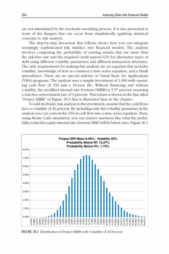
WEBC20 10/03/2014 9:18:29 Page 264

are not intimidated by the stochastic modeling process. It is also presented towarn of the dangers that can occur from simplistically applying statisticalconcepts to risk analysis.

The step-by-step discussion that follows shows how you can integrateseemingly sophisticated risk statistics into financial models. The analysisinvolves computing the probability of earning returns that are more thanthe risk-free rate and the required credit spread (CS) for alternative types ofdebt using different volatility parameters and different transaction structures.The only requirements for making this analysis are an equation that includesvolatility, knowledge of how to construct a time series equation, and a blankspreadsheet. There are no special add-ins or Visual Basic for Applications(VBA) programs. The analysis uses a simple investment of 1,000 with operat-ing cash flow of 150 and a 10-year life. Without financing and withoutvolatility, the modified internal rate if return (MIRR) is 5.57 percent assuminga risk-free reinvestment rate of 3 percent. This return is shown in the line titled“Project MIRR” of Figure 20.3 that is illustrated later in the chapter.

To add stochastic risk analysis to the investment, assume that the cash flowshave a volatility of 20 percent. By including only this volatility parameter in theanalysis you can convert the 150 of cash flow into a time series equation. Then,using Monte Carlo simulation, you can answer questions like what the proba-bility is that the equity internal rate of return (IRR)will be belowzero. Figure 20.1

5.00%

6.00%

7.00%

8.00%

Project IRR Mean 6.46% ; Volatility 20%

Probability Below Rf: 15.27%

Probability Below 0%: 1.72%

0.00%

1.00%

2.00%

3.00%

4.00%

–5.4

9%

–4.8

8%

–4.2

7%

–3.6

5%

–3.0

4%

–2.4

3%

–1.8

1%

–1.2

0%

–0.5

9%

0.0

3%

0.6

4%

1.2

5%

1.8

6%

2.4

8%

3.0

9%

3.7

0%

4.3

2%

4.9

3%

5.5

4%

6.1

6%

6.7

7%

7.3

8%

7.9

9%

8.6

1%

9.2

2%

9.8

3%

10

.45

%

11

.06

%

11

.67

%

12

.29

%

12

.90

%

13

.51

%

14

.12

%

14

.74

%

15

.35

%

15

.96

%

16

.58

%

17

.19

%

17

.80

%

18

.42

%

FIGURE 20.1 Distribution of Project MIRR with Volatility of 20 Percent

264 Analyzing Risks with Financial Models

WEBC20 10/03/2014 9:18:29 Page 265

illustrates the distribution of IRRs that results when the volatility of cash flows isincluded in the analysis and there is no debt in the financial model. The graphdemonstrates that it is possible to earn as much as 18 percent and that theprobability of earning a return less thanor equal to 0 is 1.7percent.Without debt,the IRR distribution is not skewed.

To make the example a bit more interesting, the investment of 1,000 isassumed to be financed with 600 of senior debt and 100 of subordinated debt.Also, the volatility is assumed to increase from 20 percent to 30 percent. Thisfinancial structure changes the equity IRR but leaves the project IRR at 5.57percent. Without volatility the base case equity IRR increases to 12.47 percentas shown in Figure 20.3. But this statistic does not tell us about the risk to eitherlenders or equity investors when debt is included in the financing structure.Throughmaking the Monte Carlo simulation you can see that the probability ofrealizing a return below 0 increases to 13 percent for equity investors. This isillustrated in Figure 20.2. But there is also a chance of earning as much as55 percent rather than being limited to 18 percent upside. Further, throughadding the Monte Carlo simulation to the financial model, the risk incurred bysenior and subordinated debt holders can bemeasured. The senior debt needsa credit spread of 0.09 percent while the subordinated debt needs a creditspread of 6.21 percent to make the debt have returns that are equivalent with

8.00%

10.00%

12.00%

14.00%

Volatility 30% Equity IRR Mean 12.76% Probability Below 0%: 13.83%Senior Debt 800 IRR 2.91% Prob of Default 0.82% Reqd CS 0.09%Sub Debt 100 IRR -3.21% Prob of Default 8.73% Reqd CS 6.21%

0.00%

2.00%

4.00%

6.00%

–1

00

.00%

–95

.67%

–91

.35%

–87

.02%

–82

.70%

–78

.37%

–74

.05%

–69

.72%

–65

.40%

–61

.07%

–56

.75%

–52

.42%

–48

.10%

–43

.77%

–39

.45%

–35

.12%

–30

.80%

–26

.47%

–22

.15%

–17

.82%

–13

.50%

–9.1

7%

–4.8

5%

–0.5

2%

3.8

1%

8.1

3%

12

.46

%

16

.78

%

21

.11

%

25

.43

%

29

.76

%

34

.08

%

38

.41

%

42

.73

%

47

.06

%

51

.38

%

55

.71

%

60

.03

%

64

.36

%

68

.68

%

FIGURE 20.2 Illustration of Applying a Monte Carlo Simulation to a Model with Seniorand Subordinated Debt

Taking the Mystery out of Applying Time Series Analysis 265

WEBC20 10/03/2014 9:18:30 Page 266

returns on risk-free debt. Figure 20.2 shows that distributions of returns toequity holders with debt financing no longer have a normal distribution eventhough volatility in the time series equation is assumed to be normally distrib-uted. The large bar on the left of the graph shows the probability that the equityholders will lose their entire investment. Since the equity holders cannot losemore than their investment, the distribution of equity IRR is highly skewed,meaning that there is a limited downside and a wide variation of upside returns.

Results of the analysis change with different volatility parameters. If thevolatility of cash flows is 20 percent instead of 30 percent, then the upside andthe downside for equity holders decrease. The probability of a return below 0decreases to about 4.7 percent, but the relative chances of earning a very highreturn also decrease.

Step-by-Step Procedure to Incorporate a MonteCarlo Simulation into Your Models

The remainder of this chapter describes how to add distribution graphs andanalysis of alternative loan structures such as those shown in Figures 20.1 and20.2 to any financial model. The first step is reformulating a few of the equationsof the financial model so as to compute output variables that can be measuredwith probability distributions. Next, time series equations that contain a volatilityparameter are attached to the cash flow. Finally, the possible variability inselected output variables is evaluated through using random number variablescombined with a probability distribution and Monte Carlo simulation.

To perform the Monte Carlo analysis, the discussion begins with instruc-tions on how to build a one-column financial model that evaluates IRRs andthe defaults on senior and subordinated debt. Next, the theory and mechanicsof putting a simple time series equation into the one-column financial model isexplained. The final section describes techniques for computing risk statisticsthrough making many different scenarios by drawing random numbers andapplying them to the time series equation. The one-column model is createdso that Monte Carlo simulation can be illustrated without a macro. After thesimulation is established without a macro through copying and pasting theone-column model, the last part of the chapter explains how the simulationcan be performed with a short VBA program.

Step 1: Building a Flexible Deterministic Financial ModelThat Accepts Wide Variation in Cash Flow

The first and perhaps the most difficult step in the exercise of incorporatingMonte Carlo analysis in a model is not the time series equation or compilingthe simulations. It is instead creating a financial model that computes thedefault on different types of debt as well as the rate of return earned by equity

266 Analyzing Risks with Financial Models

WEBC20 10/03/2014 9:18:30 Page 267

using a modified IRR calculation. The general method of creating a model tocompute defaults using subtotals and the MIN function was described inChapter 10 in the context of cash flow waterfalls. Here, the waterfall conceptsare converted to a one-column model.

The one-column model uses the following five-step process and isillustrated in Figure 20.3:

1. Compute the future value (FV) of cashflowswith nofinancing, showing theyear-by-year cash flow in a single column. To do this, make a column for aFV factor with an index calculation using an assumed risk-free rate. The FVfactor is a compound index of the risk-free rate beginning with 1.0. The FVof the cash flows can be computed through using the SUMPRODUCTfunctionandmultiplying thecashflowbyeachFV factor. These calculationscould be computed using present value rather than FV. The only reason forcomputing FV is computation of the IRR, discussed next.

2. Compute the FV of the senior debt and the subordinated debt obligations.The FV of debt is the amount of debt issued multiplied by the FV factor forfinal period.

3. Compute the FV of the operating cash flows accruing to senior andsubordinated debt assuming a cash sweep structure is applied. If the valueof the future operating cash flows is less than the FV of the senior debt,then there is a default on the senior debt. This means that the value of thesenior debt is theminimumof the nominal value of future debt or the FV ofthe cash flow. The debt default only occurs when the cash flow minus thenominal debt is negative. This means the value to the senior debt can becomputed with a MIN function comparing the nominal FV to the FV of theoperating cash flow.

FV Realized by Senior Debt � MIN�Nominal FV of Debt; FV ofOperating Cash Flow�

4. Compute the value of the cash flow available to subordinated debt. Aftercalculating the FV of senior debt using theMIN function, include a subtotalcomputing the value of the total cash flow less the value of the senior debt.Then use the MIN function with this subtotal to compute the valueavailable to the subordinated debt as shown below.

Subtotal Value to Subordinated Debt � FV of Operating Cash Flow�Senior Debt Value Realized

Value Realized by Subordinated Debt � MIN�Nominal FV ofSubordinated Debt; Subtotal to Subordinated Debt�

Taking the Mystery out of Applying Time Series Analysis 267

WEBC20 10/03/2014 9:18:30 Page 268

5. Determine the cash flow to equity as the FV of operating cash flowwith nofinancing less the FV of senior and subordinated debt. The modifiedinternal rate of return on equity can then be computed as the compoundgrowth rate in equity cash flow. This is the growth implied by the FV ofequity cash flow relative to the equity investment. To make this IRR orgrowth rate calculation, divide the FV by the original equity issued andraise the product to 1.0 divided by the number of years. The only reasonfor using FV rather than present value in the preceding analysis is so thatthe IRR can be computed as a growth rate in cash flow. The FV iscomputed using a predetermined reinvestment of rate, which in thiscase is the risk-free rate. This means the IRR is the modified IRR rather thanthe typical IRR computedwith the IRR function. In the typical IRR function,the re-investment rate is the same as the IRR itself, which is why the IRRfunction requires a guess. You could make a user-defined function toreplicate computation of the IRR using this approach and iterating aroundthe process with new estimates of the reinvestment rate.

FV of Equity � FV of Operating Cash Flow � FV ofSenior Debt Paid � FV of Subordinated Debt Paid

Equity IRR � �FV of Equity=Equity Issued�^ �1=Years of Analysis� � 1

The IRR is computed in a similar manner for project cash flow, seniordebt cash flow, and subordinated debt cash flow.

An example of such a one-column model is shown in Figure 20.3. Theproject IRR and the equity IRR shown in Figure 20.3 are the 5.57 percent and12.47 percent numbers referred to earlier. As the reinvestment rate is the risk-free rate, when the IRR is equal to the risk-free rate, no risk premium has beenearned. You could make a more elaborate model and display separate rowsfor interest expense on senior debt and subordinated debt as well as the debtlevels and the amount of defaulted debt. The reason for making a one-columnmodel is so that it can be copied across multiple columns creating manydifferent scenarios. This idea of copying the model allows you to make aMonte Carlo simulation without any VBA code.

Step 2: Creating Time Series Equations for Key Assumptionsin a Financial Model

To incorporate stochastic analysis in the financial model, the operating cashflow can be modeled as a time series equation that includes random variation.

268 Analyzing Risks with Financial Models

WEBC20 10/03/2014 9:18:30 Page 269

The simplest form of a time series equation is driven by only the volatilityparameter. When creating random variations, you can assume the cash flowfollows a random walk process that is a function of volatility and no otherparameters. For a random walk, the variable can move up or down from oneperiod to the next with equal probability. One can think of this process byimagining a drunken man starting to walk along a line. After each step, theman may stumble in one direction or another with equal probability. After hetakes the first stumble, the process begins again from the point of the laststumble. From that point, the man can stumble again in each direction withequal probability. The prior stumble has no effect on the direction of subse-quent stumbles. Depending on the how many steps the man takes, he maywander in quite large lateral directions from the initial starting point. The rangein size of each lateral stumble can be thought of as volatility.

FIGURE 20.3 Illustration of a One-Column Financial Model for Generating Monte CarloSimulations

Taking the Mystery out of Applying Time Series Analysis 269

WEBC20 10/03/2014 9:18:31 Page 270

The randomwalk model could bemodeled with the following equation ofthe current price purely a function of last period’s price and random move-ment, ε:

Pt � Pt�1 � ε

The ε term in this equation is a random term that can move up or downwith equal probability. Furthermore, movements of ε in one period areindependent of movements in other periods. To make this formula workin a spreadsheet, this ε term can be replaced by the volatility percentagecombined with a random number draw:

Pt � Pt�1 � Random Number � Volatility Percentage � Pt�1

When applying the equation, the random number should have an expectedvalue of 0, meaning that when a lot of random numbers are drawn, theaverage of the random numbers should be zero. In the time seriesequation, the current period price is a function of the prior period price,the random variable, and volatility. Volatility influences the price becauseit magnifies the effect of the random shock represented by the randomnumber. To see how the equation works say the volatility parameter is 20percent and the random number happens to be 1.0, then the price wouldincrease by 20 percent above the earlier price. Should the random numberbe �1, then the price would decrease by 20 percent. If the volatilityparameter were 0 in the last part of the equation, there would be nomovement in prices no matter what the random number is. If the randomnumber would happen to be 0, then the price would not move no matterwhat the volatility parameter is.

To implement the preceding time series equation into a financial modelassume that the volatility is the standard deviation of the percent change in thecash flow variable. Assume also that the cash flow percentage changes comefrom a normal distribution. By assuming a normal distribution, the number ofpossible deviations from 0 should range from a maximum of +4 to a minimumof �4, reflecting the potential number of standard deviations away from theaverage. If the volatility or the standard deviation is 20 percent, then the mostextreme cases are where the price moves by four times the standard deviationof 20 percent (i.e., 80 percent) in a single year.

To create this time series equation with such a normal distribution, thefunctions RAND() and NORMSINV can be used together. The NORMSINVfunction accepts a probability number from 0 to 1.0 and produces the standardnormal value that is the number discussed previously, which can vary fromabout �4 to +4. This number represents the possible number of deviationsfrom the mean. Since the RAND() function generates a number between 0 and1.0 this function can be used to derive a random draw from a normaldistribution.

270 Analyzing Risks with Financial Models

WEBC20 10/03/2014 9:18:31 Page 271

Cash Flowt � Cash Flowt�1 � Volatility Parameter

� �NORMSINV�RAND��� � Cash Flowt�1

If cash flow is derived from a continuous distribution, the equation takesthe form:

Cash Flowt � Cash Flowt�1 � EXP � :5 � Volatility^2

� Volatility Parameter � �NORMSINV�RAND����When this equation is plugged into your spreadsheet, if the random

number is 0.5, then the result of the NORMSINV is 0 and the whole latter termdrops out. Only in very extreme probability cases when RAND() is very closeto 0 or when RAND() is very close to 1.0 does the NORMSINV produce valuesanywhere near +4 to �4. Due to the characteristics of a normal distributiondiscussed in Chapter 19, there is a 68 percent chance that the NORMSINV(RAND()) factor will produce a value between +1 and �1. This means there isa 68 percent chance the next year price will be between 1.0 plus the volatilitypercentage and 1.0 minus the volatility percentage.

To implement this time series formula in the one-column financial model,simply change the formula in the second year of the model (i.e., the second150 in the model shown in Figure 20.3). Instead of making the second yearcash flow equal to the first cash flow, add a term that allows the cash flow tovary as a function of the randomdraw. For example, if the first year cash flow isin cell C5, the formula for the next period cash flow in C6 is C5 × (1 + Volatility× NORMSINV(RAND())). Once this formula is entered for the second yearcash flow, copy the same formula to all of the remaining rows. This means anew random number will be drawn for each year after the first year. It alsoimplies that the next value is a function of the prior value like the drunkenmantaking lateral steps.

Step 3: Adding Monte Carlo Analysis without VBA Code

Once a time series equation is defined using themethod described in step 2, thefinancial model can be used to create probability distributions of model outputsthrough using Monte Carlo simulation. Monte Carlo simulation was supposedlyoriginally used in development of the atomic bomb in the 1940s (although,without computers back then, somebodywould have had to spend a lot of timetyping random numbers on sheets of paper). The general idea of Monte Carlosimulation is to construct a large number of possible scenarios from usingmultiple random numbers in the time series model. In the alternative scenarios,the movements in a variable are driven by the volatility parameter that repre-sents the standard deviation of percent changes in the variable.

Using the time series equation in the one-column financial model, theMonte Carlo simulation can be created by copying the same one column over

Taking the Mystery out of Applying Time Series Analysis 271

WEBC20 10/03/2014 9:18:31 Page 272

and over again thereby creating many different scenarios with differentrandom numbers. In Excel 2007 and later versions, there are more than16,000 columns that can be used for the multiple simulations. This meansthat using SHIFT, CNTL,→ combined with the CNTL, R technique to copy themodel across the columns of the page results in more than 16,000 differentscenarios. As each scenario has nine different random numbers, the spread-sheet becomes very slow. The first six cash flow scenarios from this copyingprocess with the 30 percent volatility scenario are shown in Figure 20.4. Notehow some scenarios result in a cash flow near 0 whereas others result in veryhigh cash flows. In general, the variance in prices for different scenariosincreases as time passes, which is expected for a random walk process.

Step 4: Presenting Results of Simulations ina Frequency Chart

With the results of multiple scenarios created by copying the single-columnmodel over and over again, the IRR and the default statistics can be summa-rized. Some of the scenarios result in a relatively high IRR and some a low IRR;some result in no default and some result in a large default. With all of the

FIGURE 20.4 Paths for Six Scenarios

272 Analyzing Risks with Financial Models

WEBC20 10/03/2014 9:18:33 Page 273

scenarios computed, the average level of default across scenarios can bedivided by the level of the debt to compute the required credit spread onsenior debt and subordinated debt. Using output variables from the multipledifferent scenarios, the frequency graphs displayed in Figures 20.1 and 20.2can be calculated using the FREQUENCY function as follows:

■ Compute the maximum and minimum values across all scenarios for thevariable that you would like to present in the frequency graph. Alterna-tively, you can calculate the mean plus and minus 3 or 4 standarddeviations. Say you are making a frequency distribution for the IRR.You would first compute the standard deviation across all of the MonteCarlo scenarios made from copying the model across columns with theSTDEV function. Then you could multiply the standard deviation value by+4 and �4 and add the product to the average. This process of computingmaximum and minimum values is demonstrated in Figure 20.5.

■ With the maximum and minimum values established, you can create adata list of bins then that will accumulate the number of scenarios intovarious increments and list the increments in a row or a column. Theformula for the increment is the maximum minus the minimum dividedby the number of increments minus 1. You need to enter the number ofincrements desired. If the minimum from step 1 is�200 and the maximumis 1,000, then you could make increments beginning with �200 andincreasing by 50 until 1,000 is reached. This formula that contains 25 binsis also shown in Figure 20.5.

FIGURE 20.5 Calculating Bins and Increments for Computation of FrequencyDistributions

Taking the Mystery out of Applying Time Series Analysis 273

WEBC20 10/03/2014 9:18:34 Page 274

■ Select a group of cells across rows in the column next to the increments andenter theFREQUENCY function. This is anarray function,whichfirst acceptsthe entire range of values from the simulation and then accepts the bins youcreated in the last step.Whenyou arefinished entering these arguments intothe function, press the SHIFT, CNTL, ENTER sequence as you did for theTRANSPOSE function. The SHIFT, CNTL, ENTER function is used becauseresults of the function go into a range of cells rather than a single cell.

■ Once the bins are entered and the numbers from the FREQUENCYfunction are created, you can use the F11 key to make a graph. Youcan also compute associated probabilities through dividing the frequencyby the sum of all of the observations. If there are no other numbers in therow or the column of the frequency data, you can use the SUM function forthe entire row or column as illustrated:

Probability � C10=SUM�C :C�The process of using the FREQUENCY function to create probability

distributions is illustrated in Figure 20.5 and Figure 20.6. Figure 20.5 shows

FIGURE 20.6 Computing Frequency Distribution from a Monte Carlo Simulation

274 Analyzing Risks with Financial Models

WEBC20 10/03/2014 9:18:35 Page 275

how to compute the minimum value and the increment used to establish the15 bins of the distribution. Figure 20.6 illustrates how to use the FREQUENCYarray function to make the graph.

Step 5: Creating Monte Carlo Scenarios withSimple VBA Code

Instead of using the SHIFT, CNTL,→ shortcut and copying the model over andover again to added colums, with CNTL, R you can create many differentscenarios by writing a little macro that repeats the random draw process andoutputs selected variables. Two of the advantages of using such a macro arethat (1) you can keep the output from the simulation in a separate sheet and (2)you do not have to make a one-column model so that you can copy it. Tocreate this macro, you can combine the FOR NEXT loop with the CELLSstatement in a similar manner as discussed in Chapter 16 in the context ofcreating a data table with VBA. The FOR NEXT and the CELLS statements aresuch good friends because the FOR NEXT can loop around rows or columnsand the CELLS can read or write to the area covered by the FOR NEXT loop.

The code shown next can perform the Monte Carlo simulation and placeoutputs in a sheet named output_sheet beginning in column 5 for the firstvariable to be output. In this program, the number of simulations are enteredfrom the INPUTBOX tool, and two different outputs from the financial modelare collected, the Project IRR and the Senior Default. The STATUSBARcommand in the FOR NEXT loop allows you to see which iteration numberis being computed at the bottom of the spreadsheet. It should be reset toFALSE after the loop. The CELLS statements allow you to put results of themultiple random draws in a separate sheet.

num_of_simulations = INPUTBOX(“ Enter Number of Simulations”)

FOR Row = 10 to num_of_simulations

Sheets(“output_sheet”).CELLS(Row, 5) = Range(“Project_IRR”)

Sheets(“output_sheet”).CELLS(Row, 6) = Range(“Senior_default”)

Further rows for recording other variables . . .

Application.StatusBar = “ Iteration Number ” & Row

NEXT Row

Application.StatusBar = FALSE

Taking the Mystery out of Applying Time Series Analysis 275

WEBC20 10/03/2014 9:18:35 Page 276

WEBC21 10/03/2014 9:29:36 Page 277

CHAPTER 21Constructing Probability

Distributions with Trends, MeanReversion, Price Boundaries, andCorrelations among Variables

This chapter turns to more complex aspects of time series models thatinclude parameters for time trends, mean reversion, lower and upper

boundaries, jump processes, and correlations. The time series equationintroduced in Chapter 20 that only has a volatility parameter would notgenerally be appropriate for use in financial models. That equation assumeda normal distribution of random numbers, no mean reversion, no upper orlower price boundaries, and no interdependence between different variables.Actual time series equations for financial models should be more complexbecause representation of real variables generally include added parameters(trends, boundaries, jumps, and so forth), because of transformation tologarithms, and because the random draws may be filtered through a proba-bility distribution other than the normal distribution. A more representativetime series equation (without jumps, price boundaries, or correlations, and notin logs) could be written as:

Pricet � Pricet�1�Trend Factor��Average Price Adjusted for Trend�Pricet�1�� Mean Reversion Factor�Volatility Parameter� Inverse Normal

Distribution �RandomDraw��Pricet�1�Adjustment for Correlation

277

WEBC21 10/03/2014 9:29:36 Page 278

While this equation is more complex than the basic equation that onlyhad volatility, no matter how the time series equation is specified and nomatter what probability distribution is used, the process always boils down tothe idea of drawing a random number, adjusting it for volatility, and makingthe next period price a function of the prior period price. For purposes of thediscussion in this chapter, parameters such as volatility, mean reversionfactors, correlations, and other factors are assumed to be given in advance.The important question of how to find these parameters is discussed inChapter 22.

Figure 21.1 shows the summary page of a project finance model withMonte Carlo simulation added for two different variables. When you press theF9 button in this model, a new scenario is computed from new randomvariables. The new scenario results in different cash flow and credit statisticssuch as the debt service coverage ratio (DSCR), loan life coverage ratio (LLCR),and project life coverage ratio (PLCR). Instead of pressing the F9 button for onescenario, you can run thousands of simulations and compute distributions forany of the output variables. The remainder of this chapter explains how youcan add this sort of process with more complex time series equations to any ofyour models.

FIGURE 21.1 Illustration of Summary Page from a Project Finance Model with Time SeriesEquations Included

278 Analyzing Risks with Financial Models

WEBC21 10/03/2014 9:29:37 Page 279

Starting Point for Developing Time SeriesEquations—Brownian Motion and NormalDistributions

The most common set of time series models applied to financial instrumentssuch as stocks, options, and other derivatives are randomwalk models built onthe assumptions that rates of change follow a normal distribution and thatchanges in price are independent of past prices. In the Black-Scholes optionpricing model, for example, an underlying assumption is that prices follow anormal distribution and historical price changes have nothing to do withprospective price changes. A fundamental mathematical property of thesemodels is that prices are nonstationary, meaning that they have no memoryand they can wander all about without coming back to some average level.

Efficient markets theory in finance is consistent with the notion that stockprices follow a random walk process where price changes should be inde-pendent from earlier price changes. The general idea is that any change instock prices arises from new information—the change from new informationdoes not have a memory of earlier information that has already beenincorporated into the price. If new information is normally distributed andif prior information has already been included in prices of a security, the priceprocess follows a random walk process where past prices—Pt–2, Pt–3, and soforth—have no forecasting value. If past prices are irrelevant, then there is nomean reversion in prices; prices are only correlated with other prices that alsohave random walks; and, in terms of the rate of return, there is no upper orlower boundary. While this theory may or may not apply to stock prices, itclearly does not apply to many variables that are entered into financial modelsand that drive risk assessment. In the case of electricity prices, a change of onedirection in the price of electricity often means that subsequent prices will atsome point in the future change in the opposite direction. Here, past electricityprices are clearly very relevant in predicting future price changes, implyingthat electricity prices do not follow a random walk.

The equation used to represent time series distributions for financialsecurities is similar to the equation used in Chapter 20 where random drawsare extracted from a normal distribution. However, an assumption is made thatthe rate of change in prices follows a continual change process rather thanchanges happening in discrete increments at the end of a period. Withcontinual growth, the price in the next period is not defined as this period’sprice multiplied by 1.0 plus the volatility as in the previous equation, but ratherthis period’s price change is the exponent of volatility, as shown:

Discrete: Pt � Pt�1 � �1 � Pt�1 � Volatility Percent � Standard Normal Draw�Continuous: Pt � Pt�1 � �EXP��Volatility Percent ^ 2 � :5

� Standard Normal Draw��

Constructing Probability Distributions 279

WEBC21 10/03/2014 9:29:37 Page 280

Use of the continuous distribution prevents the possibility of a negativeprice (the EXP function cannot result in a negative value even when the vola-tility is negative) and involves mathematical equations that are a bit morecomplicated. If the time increments are continuous rather than discrete, therandom walk becomes Brownian motion. In Brownian motion the ϵ term is adraw from a normal distribution with a variance that increases on a linear basisover time. If the variance is expressed on an annual basis, the variance for twoyears is twice the variance for one year. If the standard deviation or volatility isused rather than the variance, the increase for two years is multiplied by thesquare root of 2.

Figure 21.2 illustrates how you can add volatility into your model using theidea that the standard deviation should be adjusted by the square root of thetime period in a year. The top part of Figure 21.2 demonstrates how to convertannual volatility into periodic volatility when your model is not an annualmodel. The lower part of Figure 21.2 demonstrates equations for applying thevolatility, random variable, and normal distribution into your model. The basevalue before the time series is shown followed by the volatility and the randomfactor. Then the adjusted parameter is shown along with switch variables thatallow you to turn the random process on and off.

FIGURE 21.2 Illustration of Applying Volatility in a Financial Model

280 Analyzing Risks with Financial Models

WEBC21 10/03/2014 9:29:38 Page 281

Testing the Assumption That Input VariablesAre Normally Distributed

One of the fundamental assumptions in a model with Brownian motion is theunderlying assumption of a normal distribution and independence of pricechanges between periods. If you want to test whether rates of change in avariable have followed a normal distribution in the past, you can use theNORMDIST function that is explained in Chapter 20. In order to comparethe historical distribution of a variable to a normal distribution, you can use thefollowing process:

Step 1 Compute historical percent changes in the time series from periodto period and then calculate the mean and the standard deviationof those percent changes. Establishing the mean and the standarddeviation is almost always the starting point for analysis of anormal distribution.

Step 2 Create a list of bins to use for a frequency distribution that arelisted on a column starting with a low number and graduallyincreasing. You can begin with something like themeanminus thestandard deviation times 4, which would be a very extreme lowvalue for the normal distribution. Then you can enter the numberof increments that you would like to present on your graph,perhaps something like 20. The increment for the graph and thecounter for the bins would then be the standard deviation multi-plied by 8 and divided by 20. You could start with the minimumdefinition and increase the counter by the increment.

Step 3 Count the number of observations that fit into the various bins byusing the FREQUENCY function. To use the FREQUENCY func-tion, highlight the area next to the bins, type = FREQUENCY andpress the SHIFT, CNTL, ENTER series of keys. Then you cancompute the probability associated with each number in the binthrough dividing the frequency calculation by the total number ofobservations. This column of data is the actual distribution.

Step 4 Establish the probability distribution that would exist if it came froma normal distribution. The probability can be derived by using theNORMDIST function. You can compute this with the mean andstandard deviation that youhave already established. Inmaking thecalculation you should use the switch for a noncumulative distri-bution as the last argument. Tomake a normal distribution from themean and standard deviation of the time series on a noncumulativebasis, you need tomultiply the result of the NORMDIST function byan increment as explained in Chapter 20. For this analysis, the

Constructing Probability Distributions 281

WEBC21 10/03/2014 9:29:38 Page 282

increment is the same as the increment used to compute the binsin step 2.

Step 5 Use the F11 key to make a graph. Shade the frequency distributioncolumn together with the distribution that would exist from thestandard deviation and the mean using the normal distribution.

Figure 21.3 demonstrates how you can compute the range for the bins andthe increments for distributions with different characteristics. The column onthe left is the data that is used to make the graphs and can be taken fromalternative data series. It uses a similar approach to the selection of a scenario,where a code number is entered; a drop-down box is created from using thecode number as a CELL LINK, and the INDEX function is used to select fromthe various options.

Once you work through the process for creating bins and increments afew times, it will go quickly and you can test all kinds of different time series fornormality. Say you want to test whether the distribution of wind over a yearcomes from a normal distribution. You would first compute the mean and the

FIGURE 21.3 Setting Up Bins and Increments for Evaluating Normal Distributions withthe FREQUENCY and the NORMDIST Functions

282 Analyzing Risks with Financial Models

WEBC21 10/03/2014 9:29:40 Page 283

standard deviation of wind speeds across many years. Next you can thensimulate the series as a normal distribution by using the NORMDIST function.To illustrate how you can test for normality, the results for daily changes in thevalue of the Standard & Poor’s (S&P) 500 index are shown in Figure 21.4,where percent changes are computed from LN(price/prior price). These datacan be easily accessed from the Yahoo! Finance website at finance.yahoo.com. You can make a process to automatically read the data fromthe Internet by finding the URL, then using the F3 function from a browserto copy the data to your spreadsheet and making a macro with theWORKBOOKS.OPEN statement. This process of automatically reading datafrom the Internet is explained in detail in Chapters 32 and 36. Without makingany highly sophisticated econometric analysis, the question of whether stockprices follow a normal distribution can be evaluated. Figure 21.4 illustrates thatdaily stock price changes have not been normal. The little bar on the right isof particular concern because it demonstrates that extreme downside possi-bilities are much more than would be predicted from a normal distribution.

Given that changes in stock prices do not follow a normal distribution, youcould attempt to fit another kind of distribution to the data such as a Weibulldistribution. But that also would be difficult and dangerous. The danger comesfrom the very small chance that the percent change in price has been as much

FIGURE 21.4 Distribution of Returns from the Standard & Poor’s 500 Index

Constructing Probability Distributions 283

WEBC21 10/03/2014 9:29:41 Page 284

as six times away from the mean. Since 1950, there have been 17 days thatpercent changes have been in the negative six standard deviations bucket. In anormal distribution, the chance of reaching minus six standard deviationsaway from the mean is one day in 4.02 million years. This can be computedusing the NORMSDIST function, plugging in –6 to find the probability, whichyields 9.86588E-10. If this number is multiplied by 10 billion, it implies that9.8 days out of 10 billion years would be six standard deviations away fromthe mean. To arrive at the 402 million years, you multiply the probability by252 trading days per year and then compute 1 divided by the result.

Normality tests can be made for any time series where you can acquiresufficient data. You can go to the World Bank website and pick up data for allsorts of commodity prices and compare the distributions of percent changes toa normal distribution. Then you can make a macro with the WORKBOOKS.OPEN statement to automate the process as described in Chapter 36.Figure 21.5 shows the distribution of the monthly rate of change in real oilprices compared to a normal distribution. As with the S&P 500 stock prices,there are a number of observations that exceed four standard deviations,which would be almost impossible if monthly oil price changes were reallynormally distributed.

FIGURE 21.5 Distribution of the Monthly Rate of Change in Real Oil Prices Comparedto a Normal Distribution

284 Analyzing Risks with Financial Models

WEBC21 10/03/2014 9:29:41 Page 285

Price Boundaries and Short-Run Marginal Cost

For the time series equation introduced in Chapter 20, the price cansuddenly or gradually fall to low levels or reach very high levels. Becauseof the mathematical formulation of the time series equations, after the pricereaches a low level, the volatility is applied to the new low price level andprices tend to remain at low levels. The opposite can occur with highprices, where the volatility parameter is magnified after high prices arereached. This mathematical effect does not necessarily represent how theinput variables in your financial models really work. If prices of commodi-ties or other products would really reach the extreme values in actualmarkets, the prices would prompt responses by consumers or suppliersthat would effectively put upper and lower limits on the prices. In the caseof low prices, limits occur because producers will cease production whenprices fall to short-run marginal cost. In the case of high prices, upper limitscome from consumers who reduce demand. If prices fall below short-runmarginal costs, companies will eventually choose not to produce. Thereduced supply increases price and limits the decline in price to short-runmarginal cost. This implies that prices in time series models should have alower boundary defined by short-run marginal cost. Upper price bounda-ries can also be appropriate in time series models, because if prices reachhigh levels, demand may be curtailed by influences such as substituteproducts.

Boundary conditions can be incorporated into time series modelsthrough placing limits on the lower or upper possible prices. The modelequations can include a conditional formula using an IF function so thatwhen prices drift above the upper boundary or below the lower boundarythe price is set to the boundary level. As with the other components of atime series equation, these boundaries themselves could be stochasticrandom variables with volatility and mean reversion. Implementing lowerand upper boundaries can be accomplished through using a MIN and aMAX function instead of the IF function, as shown in Figure 21.6. Theexcerpt shown in Figure 21.6 illustrates that the production before applyingthe MAX and MIN is above the maximum constraint in the two periods.When you want to turn the constraints off, you can enter FALSE as valuesfor the minimum and maximum inputs. If you enter zero, the MIN and MAXcombination will not work, because the maximum limit of zero will alwaysbe in force.

Adjusted Value =MAX(Min, MIN(Unconstrained Value, Max))

Constructing Probability Distributions 285

WEBC21 10/03/2014 9:29:42 Page 286

Mean Reversion and Long-RunEquilibrium Analysis

When an economic variable exhibits cyclical behavior or reverts to some kindof average level such as long-run marginal cost, the variable can be modeledas a mean-reverting process rather than as a random walk process. For timeseries equations with mean reversion, variables still have random shocksdriven by volatility, but after a random shock causes the process to move awayfrommean levels, prices in subsequent periods tend tomove back to a definedequilibrium level. The speed at which prices revert to the long-run equilibriumafter a random shock can be expressed in terms of an annual percentage. If thelong-term equilibrium or average price is 100 and a shock causes prices tomove to 150, then a mean reversion parameter of 40 percent would mean thatthe next year’s price tends to move down by 50 × 40% = 20. The equation for amean-reverting process that includes a mean reversion factor begins with themean price and subtracts the prior period price. When you enter this kind offormula in a spreadsheet make sure the mean price is always first, ahead of thelast period price, as the formula produces crazy results if the mean price andthe last period price are reversed:

Pt � Pt�1 �Mean Reversion Factor � �Pm � Pt�1� � ε

FIGURE 21.6 Implementing Lower and Upper Boundaries by Using a MIN Functionand a MAX Function

286 Analyzing Risks with Financial Models

WEBC21 10/03/2014 9:29:45 Page 287

For a time series equation with mean reversion, the mean price term Pmshould in theory approximate the long-run cost of production, and the εterm incorporates volatility and draws from a normal distribution, as wasthe case for random walk processes using the NORMSINV(RAND()) func-tions. The mean reversion factor in the equation should generally bebetween 0 and 1.0, although it in theory could be negative. If the meanreversion parameter is 1.0, then the Pt–1 terms cancel and the equationbecomes Pt = Pm + ε. This equation implies that prior period observationshave no influence on the forecast and everything starts again from theaverage in the next period. When the mean reversion parameter is 1.0,there are still movements away from the mean level due to random shocks,but the process starts over at the mean level in the next period. You couldthink of variations in wind and solar power due to wind speed or solarirradiation as following a process like this. On the other hand if the meanreversion factor is 0, the equation becomes the same as the random walk.In this case, prior period prices have no forecasting value and the process isnonstationary.

It is sometimes helpful to think of the mean reversion factor in terms ofhow many years it takes for a market to come back to equilibrium after arandom shock. For example, if a market has deficient supply resulting inhigh prices and it takes three years to construct new manufacturing plants,then the annual mean reversion factor should theoretically be around 33percent. If the prices are expressed in annual terms, 1.0 divided by themean reversion factor in the equation can be thought of as roughly thenumber of years it takes for prices to come back to the equilibrium level.With a mean reversion factor of 0.5, it takes two years on average to revertto the mean.

Variables that are modeled as Brownian motion wander around andgradually move farther and farther away from their initial value. While thisbehavior may be characteristic of some variables such as the percent changein stock prices, many if not most economic variables move in cycles ratherthan in random walks. In the case of price variables for a financial model, thecyclical movement back to an average value is due to the simple fact thathigh prices will prompt increased supply, thereby moderating the priceincrease. Very low prices in contrast will cause new supply to slow downand demand to increase. For electricity prices, where storage is not generallyavailable, the very high level of mean reversion comes from the fact thatdemand itself is mean reverting due to the weather and due to the steepslope of the supply curve. Most commodity prices, including oil, gas, realestate, iron, copper, coal, and electricity, should eventually move in thedirection of their long-run cost of production rather than continually movingup or down without limits.

Constructing Probability Distributions 287

WEBC21 10/03/2014 9:29:45 Page 288

The Effect of Mean Reversion Parameters on RiskDistributions from a Financial Model

Adding mean reversion factors to a time series equation can have a large effecton the measures of risk as compared to implementing a time series equationwithout mean reversion. If a modest annual mean reversion parameter of only10 percent is assumed, which implicitly assumes that it takes 10 years to reachequilibrium through changes in construction of newplant or demand increases,measures of risk can be reduced a lot compared to a situation with no meanreversion. The fact that a small mean reversion parameter has large effects onthe credit statistics and the variation in return on equity demonstrates the carethat must be takenwhen trying to applyMonte Carlo simulation to yourmodels.Creating the pretty graphs is not too difficult, but thinking about how variablescan move in the future and incorporating factors such as mean reversion andprice boundaries into your time series analysis can be very challenging.

Figures 21.7 and 21.8 show results of a project finance analysis withoutmean reversion andwith 10 percent mean reversion. The probability of defaultis measured by compiling the number of scenarios that result in defaulted debtremaining at the end of the project life. Without mean reversion, the loss

FIGURE 21.7 Illustration of Summary Results of a Project Finance Analysis withoutMean Reversion

288 Analyzing Risks with Financial Models

WEBC21 10/03/2014 9:29:47 Page 289

probability is 11.55 percent. With 10 percent mean reversion, probability ofloss falls to 9.92 percent.

The simulation summarized in Figures 21.7 and 21.8 is made by creatingthe same kind of Visual Basic for Applications (VBA) code discussed at the endof Chapter 20 with a FOR NEXT loop and the CELLS statement. This code canbe added to any financial model that includes time series equations with arandom variable process. The model can be as large and as complex as youlike. It just must have the NORMSINV(RAND()) or a similar process some-where in the spreadsheet. The simulation is made by pressing the Simulatebutton shown in the figures and using 1,000 simulations. The excerpts inFigures 21.7 and 21.8 illustrate the manner in which you can summarize resultsof a simulation and how differences caused by mean reversion affect variousoutputs of the model.

Modeling Correlations among Variables in TimeSeries Equations

Up to this point the time series equations have been discussed for one variablewithout regard to how the movement in that variable is affected by changes in

FIGURE 21.8 Illustration of Summary Results of a Project Finance Analysis with 10Percent Mean Reversion

Constructing Probability Distributions 289

WEBC21 10/03/2014 9:29:47 Page 290

other variables. Inmost situations, analyzing a time series equation in isolation isinappropriate because key variables are correlated with one another. Thismeans thatmovement of one variablewill affect thewayother variables change.In some cases, correlated variables can aggravate the variability in cash flow.When demand falls and overcapacity becomes prevalent, price can also falldramatically. Prices can quickly move from levels that resulted in profits abovethe cost of capital all the way down to levels close to short-run marginal cost.This implies that demand and prices in a model may be closely correlated.In other circumstances, the correlation among variables can mitigate riskbecause, for example, costs may decline at the same time that prices decline.If a time series equation is used in forecasting the price of electricity, changes inthe price of natural gas in many markets should move closely together withchanges in the price of electricity. This is because of the ability to substitute fuels,because natural gas plants are often marginally running plants that drive theprice, and because the price of natural gas influences the type of newplants thatare constructed.Because of themovement of natural gas andelectricity prices intandem, the cash flow volatility of gas plants may be less than the cash flowvolatility of other technologies.

When simulating the potential distribution of more than one variable, themechanical process is straightforward if the variables are not correlated withone another. In this case with independent variables, the time series equationsfor each variable can be modeled as separate equations. As random draws areindependent from one another when the RAND() function is applied, thestandard normal draws from the NORMSINV(RAND()) are also independent.This means that if you want to create a model with a series of independentvariables, the Monte Carlo analyses described earlier can be run separately foreach variable. However, if the variables you are simulating are correlated withone another, the single Monte Carlo simulation without accounting forcorrelation is not correct. Instead, you should model the variables simulta-neously using an analytical approach that adjusts time series equations so thatthe random variation of one variable is dependent on the random variation ofanother variable.

If you are creating time series equations for variables that are correlatedwith one another, the correlation coefficient combined with volatility param-eters can be used to make a forecast of how variables move in tandem. Theprocedure for incorporating correlation between variables into a time seriesmodel involves changing the way random draws are computed. Whenconstructing a random draw for the second correlated variable, you want itto be, in part, a function of the random draw for the first variable. To make therandom draws related, you can use something called Cholesky factors fordeveloping the random draw for the second series. In the case where twovariables are correlated with each other and there is no mean reversion orboundaries and the variables come from a normal distribution, the standard

290 Analyzing Risks with Financial Models

WEBC21 10/03/2014 9:29:47 Page 291

normal draw for the correlated second variable is the weighted combination ofa new random draw and the random draw for the first variable. The followingequations illustrate how Cholesky factors can be applied. In these equations avolatility parameter is multiplied by a factor (zt) that is driven by a randomvariable.

z1 � Inverse of Standard Normal�u1 for First Variable� or NORMSINV�RAND���When applying a similar factor to the second correlated variable, the

standard normal draw for this variable can be defined as z2:

z2 � Inverse of Standard Normal�u2� or NORMSINV�RAND���After the second random draw is made and filtered through the normal

distribution, an adjusted random factor is applied to the volatility from thecorrelation between the variables. The adjusted factor for the second variableis a weighted average of the first two factors according to the followingequation:

z adj2 � z1 � Correlation1;2 � z2 � �1 � Correlation1;22�1=2

z adj2 � NORMSINV�RAND��� � Correlation1;2 � NORMSINV�RAND���� �1 � Correlation1;2

2�1=2The weighting factor for the two different random draws depends on the

correlation between the variables. Two extreme cases demonstrate the waycorrelation is implemented in a financial model using these two equations:

1. If there is no correlation between the two variables, the factor for thesecond variable should not be influenced by random draws for the firstvariable. In applying the preceding equation, when the correlation factoris 0, z1 falls out of the equation for the z2 adjusted term. The second termof the equation is not affected by the correlation, as 1.0 minus 0 raised tothe ½ power is still 1.0. Therefore, with no correlation, the entire weight ofthe standard normal draw is given to the second random draw asexpected; z2 adjusted = z2.

2. If the variables are perfectly correlated, the entire process should bedriven by the random draw for the first variable and there should be noweight given to the second random draw. When the correlation factor is1.0, the second part of the equation for z2 adjusted falls out, and z2adjusted = z1. This is the expected result because any random shock thataffects the first variable should directly affect the second variable.

Constructing Probability Distributions 291

WEBC21 10/03/2014 9:29:48 Page 292

After entering the equation for the adjusted random factor, the z2 adjus-ted variable has characteristics should be present for a standard normaldistribution. In particular, it should have a mean of 0 and a standard deviationof 1.0. Figures 21.9 and 21.10 demonstrate how you can verify this using a littleVBA code and a simple simulation. The excerpt in Figure 21.9 illustrates thatthe second variable representing z2 has a standard deviation of 1.0 and a meanof 0, which is what should happen. The top panel of Figure 21.9 demonstrateshow to create the random factors with correlation. Figure 21.10 shows how towrite VBA code to make a simulation with correlated variables.

FIGURE 21.9 Results of Monte Carlo Simulation for Correlated Variables

292 Analyzing Risks with Financial Models

WEBC21 10/03/2014 9:29:50 Page 293

If three variables are correlated with one another rather than only two, asimilar process can be used as in the two-variable case. In this situation thecorrelation between the third variable and the second can be used in theequation for deriving the adjusted random variable. Further, the equation forthe third random draw does not require a memory of the random draw fromthe first variable even though they are correlated. This is because as the secondvariable is already affected by the first variable. When the simulation process isfinished, the first variable will be correlated with the third variable. Say theprice of coal (variable 3) is correlated with the price of natural gas (variable 2),which in turn is correlated with the price of oil (variable 1). If the correlationbetween the price of gas and the price of coal is defined as ρ2,3, the standardnormal draw for the third variable, the coal price is:

Standard Normal Draw3 � Standard Normal Draw2 �ρ2;3�NORSMINV�New Random Draw� � �1� ρ2;3

2�1=2

Sub simulate()

For Row = 6 To 1006

Cells(Row, 9) = Range("z1_")

Cells(Row, 10) = Range("z2_")

Cells(Row, 11) = Range("z2_adj")

Application.StatusBar = " Iteration " & Row - 6

Next Row

End Sub

FIGURE 21.10 VBA Code for Creating Monte Carlo Simulation

Constructing Probability Distributions 293

WEBC21 10/03/2014 9:29:50 Page 294

3GC22 09/27/2014 10:50:29 Page 295

CHAPTER 22The Difficult Problem of EstimatingVolatility, Mean Reversion, TimeTrends, Correlations, and PriceBoundaries from Historical Data

or Market Data

You may have noticed that none of the discussion in Chapters 20 or 21explained how to compute parameters necessary to run a simulation such

as mean reversion, volatility, or any of the other parameters that are input intotime series equations. The exercises in Chapter 21 show the importance ofvolatility, mean reversion, correlation, and other variables in the risk mea-surement process, but not what those parameters should be. If the construc-tion of time series equations using parameters of volatility, mean reversion,price boundaries, price jumps, and correlations is to be useful in modeling,you must be able to derive the parameters.

This chapter discusses practical and theoretical issues that arise whenattempting to use analysis of past data in computing the various parametersrequired for a time series equation. In discussing how to compute the variousparameters, this chapter explains how to test whether the parameters that areinput produce consistent and expected output results as well as mechanicalcomputation of statistics from historical data. To illustrate the importance oftesting input parameters relative to output results, assume that a volatility of20 percent is computed from monthly historical data. But also assume thatthere is a high degree of mean reversion that is modeled as part of the process.Because of the tight mean reversion, the input parameter of 20 percent forvolatility computed from historic data will not necessarily be the same as theresulting volatility in simulated cash flows in your financial model when cash

295

3GC22 09/27/2014 10:50:30 Page 296

flow is computed on an annual basis, which may be much lower than 20percent. If you compute 20 percent volatility from annual time series datausing the standard volatility formula and then put a high mean reversionparameter into your model computed on a monthly basis, the resultingvolatility will not correspond to the true underlying volatility. Instead, itwill be much lower than 20 percent for long-term periods.

Calculation of Volatility from a RandomWalk Process

Volatility is often defined as the standard deviation of annual percent changesin a time series. Since volatility is computed from the percent change ratherthan from absolute price levels, the unit of measurement for volatility ispercentage. Volatility can be 20 percent, but it would not be expressed as $30.Because volatility is stated in terms of an annual percentage rather than a dailyor monthly percentage, if the standard deviation is computed from percentagechanges in smaller time increments than annual increments, annualizationadjustments are required. In the case of Brownian motion, when smaller timeperiods than annual increments are used in computing volatility, the standarddeviation should be multiplied by the square root of the number of timeperiods in a year. This is because the variance increases directly with time.However, if the time series includes mean reversion or boundaries, thisperiodic adjustment using the square root of time cannot necessarily bemade. This crucial property of price series that do not contain mean reversioncan be used to test whether a series has mean reversion or other properties notconsistent with Brownian motion.

There are a variety of ways to compute the volatility of a time series thatdoes not havemean reversion, price boundaries, or price jumps. The importantthing is that the way you compute volatility must correspond to the time seriesequation that you input in your model. You could calculate volatility as thestandard deviation of historical price changes, you could also measure thestandard deviation of historical price divided by the average level, or alterna-tively you can use regression analysis of the change in price against the priorperiod price. If traded options exist for the variable in question, you could alsocompute thevolatility parameter that themarketbelieveswill occur in the future.

The three-step procedure for calculating volatility of a randomwalk serieswithout mean reversion using historical data involves first computing the rateof change in prices using the LN function so the changes are assumed to occuron a continual rather than a discrete basis. After deriving continual percentchanges, the standard deviation of the series of rates of change is calculated.Finally, an adjustment is made for cases in which the rate of change iscalculated for time increments different from the time dimension of measuredvolatility, which is usually annual. Three formulas corresponding to these

296 Analyzing Risks with Financial Models

3GC22 09/27/2014 10:50:30 Page 297

three steps show how to compute volatility using both discrete and continualcompounding. In the discrete and continual cases, the first step is computingthe rate of return over the period for reported prices. In the case of continualcompounding, the rate of return is computed using the natural log of thecurrent price divided by the prior period price:

Rate of Returni � Natural Log �Pricei=Pricei�1�For discrete compounding where the change is assumed to occur at the

end of the period, the return is just the growth rate:

Rate of Returni � �Pricei=Pricei�1� � 1

Once a series of rates of return is established, the standard deviation of theperiodic rate of return is measured. If the prices are reported on an annualbasis, the standard deviation of annual returns is volatility.

Period Volatility � Standard Deviation �Rate of Returni�The third part of the process for computing annual volatility where

periodic prices are not measured on an annual basis is converting the periodicvolatility into an annual figure. Because of the mathematical propertiesassociated with Brownian motion already discussed, standard deviation ofthe rate of return increases with longer time periods. Since the variance ofBrownian motion increases directly with time, the standard deviationincreases with the square root of time. This means the period volatility definedfrom the standard deviation of the rate of return should be multiplied by thesquare root of the time increment measured in years (t) to develop the annualvolatility. Annual volatility is therefore defined as:

Annual Volatility � Standard Deviation �Rate of Returni� � �t�1=2

The three equations can be programmed into a user-defined function thataccepts the raw time series data, computes percent changes using the WORK-SHEETFUNCTION.LN statement, and then works through a loop to derive thestandard deviation and the adjustment for the number of periods in a year.

Attempting to Measure the Presence of MeanReversion in Historical Data

The mean reversion parameter that measures how long it takes for a series tocome back to average levels is very difficult to extract from historical data.Further, when volatility is computed from historical data using the standard

The Difficult Problem of Estimating Volatility, Mean Reversion, Time Trends, Correlations 297

3GC22 09/27/2014 10:50:30 Page 298

deviation of the rate of change and then applied in a time series equation withmean reversion, the volatility parameter that is input will not necessarily be thesame as the resulting volatility of cash flow in your financial model. Ifthe volatility is measured from historic prices that bounce around from 10to 100 in a short-term period but are measured on a long-term basis, theresulting volatility will be much less than the volatility that should be inputon a short-term basis. Unfortunately, methods using simple formulas to derivethe volatility and mean reversion from historical data do not work very well.

When making a simple graph of many commodity prices, it is often prettyobvious to see that mean reversion exists. Prices follow cyclical patterns andtend to decline after a large increase. The question is not really whether meanreversion is present, but how to compute the mean reversion parameters. Oneway that statisticians suggest to test for the presence of, and also to estimate,mean reversion is to make a regression equation of the change in price relativeto the last period price. If there is no mean reversion, the coefficient on thechange in prices should be close to 0, because the current period change doesnot depend on historical prices. However, if there is mean reversion, thecoefficient should be significantly different from zero since when there is a bigchange in price in one direction, there should eventually be an oppositechange. The suggested regression equation is:

Change in Price � �Pt � Pt�1� � α � β � Pt�1

If the regression equation is estimated using annual data, resultingcoefficients can be used to compute both the mean reversion parameterand the volatility parameter. When the data are expressed in monthly, daily, orhourly terms, adjustments must be made to convert the regression estimates toannual parameters. In this regression equation there are some statisticalproblems with the β parameter, which is biased toward zero. This meansthat that true mean reversion is difficult to detect and that there may be meanreversion even if the parameter is zero. But if you do use the regression, youcan easily compute statistics using the SLOPE, INTERCEPT, and TTESTfunctions. If the slope is significantly different from 0 as measured by a t-statistic that is above 2.0, the process is clearly mean reverting. When runningthe regression, there is no need to make fancy adjustments for autocorrelationor other complexities.

Before discussing how to use regression estimates of α, β, and thestandard error of the regression to establish the mean reversion and the vola-tility parameters, expected parameters of the regression equation aredescribed. Consider first the situation where the β coefficient is equal tozero. In this case the change in price has no relationship to the last periodprice. When the price is very low, changes in price are not more typicallypositive than negative if the process is mean reverting. For a mean-reverting

298 Analyzing Risks with Financial Models

3GC22 09/27/2014 10:50:30 Page 299

process, if the price is high, then the change in price would tend to benegative, meaning the slope parameter should be negative. Similarly if theprice is low after a decline, some future change in price would tend to bepositive. If the change in price is independent of historical prices, the equationmeets one of the basic presumptions of Brownian motion process and arandom walk. That is, that changes in price are not a function of past prices.

The standard error of the regression is a similar notion to standarddeviation. For a regression equation, the standard error is defined as thedeviation in the computed predicted relative to actual values. When the βparameter is zero, the standard error of the regression is about the same as thestandard deviation of the change in price. With the slope of zero, the priorprice changes do not influence the equation and the standard error is thestandard deviation of the price change. The standard deviation of the changein price divided by the average price is about the same as the volatilitycomputed from the standard deviation of the price change.

If the β parameter is significantly different from zero, the regressionsuggests that mean reversion is present in the time series. With meanreversion, the price change depends to a certain extent on the history ofprices. Using the regression equation, the mean price is computed as:

Mean Price � �α=βThe fact that this formula produces the mean price is demonstrated by a

little algebra. The formula for the change in price is: (Pt�Pt�1)= α+ β×Pt�1.Over the sample period, the expected value of the change in price is zero.Further, the expected value of the last period price—E(Pt�1)—is the averageprice. Therefore, on an expected value basis, the formula reduces to:

0 � α � β � Average Price

This formula can be rearranged to �α/β=Average Price. The mean rever-sion factor can in theory be computed from the β coefficient in the regressionequation:

Mean Reversion Factor � �log�1 � β�

In this equation if β is 0, the natural log of 1 minus 0 or 1 is also 0, so themean reversion parameter is 0. If β is �0.63, the mean reversion factor is 1.0. Ifthe β coefficient estimated from the regression equation is �0.395, the meanreversion factor is 0.5, implying that in each period, prices move halfway backto the mean level after a shock.

The Difficult Problem of Estimating Volatility, Mean Reversion, Time Trends, Correlations 299

3GC22 09/27/2014 10:50:30 Page 300

The third parameter of a time series equation that can be derived from theregression equation is the volatility. Volatility can be defined from theregression equation using the formula:

Absolute Volatility � Standard Error of Regression

� ��log�1 � β�=��1 � β�2 � 1���1=2�

andPercent Volatility � Absolute Volatility=Average Price

The percent volatility is the standard error of the regression divided bythe average price, or the standard deviation of the change in price dividedby the average price. If β is greater than zero, the term log(1+ β) is less than theterm (1+ β)2. This means that the greater the β term, the smaller the volatilityestimate. Intuitively, this means that if reversion to and back from the mean iscausing some of the observed volatility that would exist without meanreversion. This volatility created from mean reversion should be removedfrom the volatility that occurs exclusive of the mean reversion.

Attempting to Measure the Presence of MeanReversion by Evaluating Changes in PeriodicVolatility

While the use of regression seems like an elegant way to try to find meanreversion, it usually does not work very well. You can test this out by enteringa mean reversion parameter and a volatility parameter in a spreadsheet with atime series equation. Then you can run a simulation using the techniquesdescribed in Chapter 20 and Chapter 21 to establish a time series of projectedvalues. Finally, you can run a regression on each separate one of the timeseries equations that comes out of the simulation process and compute themean reversion as well as the volatility implied from the regression and theformulas discussed in the last section. When you do this, you end up withmean reversion and volatility parameters for all of the time series simulations.

After computing all of the mean reversion parameters from eachsimulated time series using the SLOPE and INTERCEPT functions, youcan compute the average, graph the data and compute other statistics(you have to construct your own function to compute the standard errorof the regression in one single cell). If the regression produces similar resultsin terms of the mean reversion parameters that you input into the time seriesequation, then the exercise demonstrates that the regression process is valid.If it does not generate mean reversion and volatility parameters that are

300 Analyzing Risks with Financial Models

3GC22 09/27/2014 10:50:30 Page 301

similar to the numbers that you input, then something is wrong. Whenperforming this exercise, you will find that unless a mean reversion param-eter of zero is used, the regression does not work well at all.

Given that the regression does not produce effective estimates of themean reversion parameter, an alternative way to find the mean reversionparameter is to use the power of your computer and back into the number.This can be done through evaluating how volatility for different time periodincrements changes in the time series when different mean reversion param-eters are used. In the presence of mean reversion, the volatility is not constantwhen it is measured for different time period increments. If there is meanreversion, the longer the time period increment, the lower the volatility. With ahigh level of mean reversion, the volatility measured on an annual basis is lessthan the volatility measured on a monthly basis. However, in the case of arandom walk series, the annualized volatility should be about the same whenthe calculation is made for average values over long time period increments asit is for prices in short periods. You could compute the volatility for daily,average weekly, average monthly, average quarterly, average annual, andfive-year average prices. Without mean reversion, the annualized volatilityshould be similar using all of the time increments. With mean reversion, thevolatility gradually declines as the period increment becomes longer.

The alternative method for computing mean reversion is to first computethe volatility for different time periods. You can then input different measuresof volatility and mean reversion and run multiple simulations. As explained inChapter 20 and demonstrated further in Chapter 21, this is not a complicatedprocess and can be accomplished with a few lines of Visual Basic forApplications (VBA) code. Once you have entered the mean reversion andthe volatility parameters, you can compare the simulated results with theactual volatility parameters for different time increments to see if you entered areasonable level of mean reversion and volatility. You would compare theresults of the simulations in your model with the changing volatility that ispresent in the historical data.

To illustrate this alternative process for deriving the mean reversionparameter, assume you have a long historical time series and you computethe average for one-year time increments as well as the moving average forlonger periods such as three years or six years. Once these historical calcula-tions have been made, volatility (or the standard deviation of the percentchange) in three-year and six-year average prices can be compared to thestandard deviation of price changes computed on an annual or monthly basis.Without mean reversion, the standard deviation of percent changes for thelonger three-year period should be about six times as great as the monthlystandard deviation (the square root of 3× 12). If the standard deviation ofpercent changes for the longer three-year period is smaller than the standarddeviation of the monthly percent changes, there is evidence of mean reversion.

The Difficult Problem of Estimating Volatility, Mean Reversion, Time Trends, Correlations 301

3GC22 09/27/2014 10:50:32 Page 302

Changes in volatility are illustrated in Table 22.1 and Table 22.2 for thecases of natural gas prices and stock prices, respectively. For natural gasprices, the volatility is much higher for shorter periods than for long-termaverages. This clearly demonstrates mean reversion in the case of natural gas.For stock prices, changing volatility over different time periods is much less. Inthe stock price case there is evidence of mean reversion, but the volatilitydecline using weekly, monthly, annual, or multiannual periods is minorcompared to that of natural gas. If you are making a stochastic model withnatural gas prices it is far more important to include the mean reversion than inthe case of stock prices.

To make sure that the results of your model are consistent with historicaldata, meaning, for example, that you would mimic the natural gas pricechanges in volatility, you can test different mean reversion factors and run asimulation. If the volatility over long-term periods such as a year relative to amonth, or five years relative to one year, is not as much as the change in thehistorical data, then you can put in a higher mean reversion and a highervolatility and rerun the simulation. This may mean you have to run a lot ofsimulations with different inputs for mean reversion and volatility, and checkwhether the output is consistent with the input. It seems painful, but with alittle coding you can make it reasonable. You can write some VBA codeanalogous to the code that replicates the Goal Seek to run multiple batches ofthe simulations. Each of the simulations would show the historical values forchanges in volatility beside the simulated changes in volatility. The followingstep-by-step process shows how this could be done.

Step 1 Compute the historical volatility using averages for different timeperiod increments in the data. If you have annual data, you can

TABLE 22.1 Volatility for Natural Gas Prices for Different Periods

Monthly Annual Three-Year

Standard deviation 14.93% 28.29% 9.25%Annualized 51.71% 28.29% 5.34%

TABLE 22.2 Volatility for Stock Prices for Different Periods

Monthly Annual Three-Year

Standard deviation 2.08% 12.88% 20.12%Annualized 15.03% 12.88% 11.62%

302 Analyzing Risks with Financial Models

3GC22 09/27/2014 10:50:32 Page 303

compute volatility for a three-year average and over a one-yearperiod. Alternatively, if you have monthly data, you can computethe volatility on a monthly basis and on an annual basis as shownin Tables 22.1 and 22.2.

Step 2 Create a time series equation and run a simulation with a meanreversion parameter as well as a short-term volatility parameter. Ifyou are making a monthly series, input a monthly volatilityparameter and start with zero mean reversion. After runningthe simulation, compute the volatility for different periods inthe simulated data. Then try the process with higher and higherlevels of mean reversion and volatility parameters.

Step 3 Inspect the simulated volatility for different time periods in each ofthe Monte Carlo scenarios. Modify the mean reversion and theshort-term volatility parameters until the simulated volatilitiesresemble the historical volatilities for different time period incre-ments. This can be done by creating a function that changesincrements of mean reversion and short-term volatility untilresemblance with historical periodic volatility is realized.

Risk Analysis Summary

The risk analysis chapters have walked through a variety of different tech-niques. The objective in Chapters 13 through 22 is to explain how to usefinancial models to understand whether accepting a reasonable level of risk isworth the added profit benefits that can be realized from taking the risk. This isthe fundamental reason for sensitivity analysis, break-even analysis, scenarioanalysis, and Monte Carlo simulation. When running simulations to evaluatewhether taking a risk and getting paid to take the risk are reasonable, it is theparameters for volatility, mean reversion, correlations, and boundaries that areimportant. It is hoped that the step-by-step techniques explained in this part ofthe book will allow you to spend more time on the crucial questions of whatrange in assumptions or time series parameters you should enter into yourfinancial model.

The Difficult Problem of Estimating Volatility, Mean Reversion, Time Trends, Correlations 303

3GC22 09/27/2014 10:50:32 Page 304

3GC23 09/27/2014 11:8:13 Page 305

PART IIIAdvanced Corporate Modeling:Modeling Terminal Value withStable Ratios in the DiscountedCash Flow Model, DerivingImplied Multiples, andComputing the Bridge

between Equity Value andEnterprise Value

3GC23 09/27/2014 11:8:13 Page 306

3GC23 09/27/2014 11:8:13 Page 307

CHAPTER 23Overview of Issues When Computing

Normalized Cash Flow andTerminal Value

When thinking about the most important things that affect valuations incorporate analysis, making appropriate assumptions is front and center.

As Chapter 1 discusses, classic and recurring valuation problems arise from thefollowing seven causes:

1. Assuming that firms in industries where entry is relatively easy canindefinitely earn a rate of return substantially higher than their cost ofcapital

2. Ignoring the effects of looming increases in capacity in an industry whereplanned capacity additions outpace growth in demand

3. Relying on opinions and analysis of big companies, famous consultingfirms, well-respected experts, and others who are not putting their ownmoney into the investment

4. Believing in fancy newfangled valuation analysis that supposedly pro-duces value from factors other than earning a return above the cost ofcapital

5. Trusting optimistic forecasts of companies that are trying to increase ormaintain returns in the face of stiff competition and that hide informationby using incomprehensible financial jargon

6. Misjudging shifts in cost structures and demand in an oligopolistic industrythat can quickly render existing assets obsolete

7. Not appreciating and using historical data when evaluating forecasts

While avoiding these types of pitfalls from making bad assumptions is thecentral basis for any valuation along with having good business judgment,there are also some mechanical financial modeling issues that can distort

307

3GC23 09/27/2014 11:8:13 Page 308

measurements of the value of a corporation. These problems are related tocalculation of terminal value; use and interpretation of price/earnings (P/E)and enterprise value/earnings before interest, taxes, depreciation, and amor-tization (EV/EBITDA) multiples; computation of weighted average cost ofcapital (WACC); and correctly measuring the difference between enterprisevalue and equity value.

Unlike humans or project financed investments, corporations are assumedto last indefinitely. The indefinite life means that when making a valuation youhave two choices. First, you could make a forecast that lasts for centuries.Second, you could stop the forecast at some arbitrary date a few years from nowand try to compute the value at that future date. The latter approach of finishingthe forecast sometime in the not too distant future means that you have tocompute terminal value. Given the indefinite life, calculating terminal value istheonly practicalway to construct the valuation of a corporation. In virtually anyanalysis that is derived from an explicit period of earning free cash flow ordividends followedby realizinga lump-sum terminal value, it is the set of explicitor implicit assumptions used to derive the terminal value that usually has thelargest influence on value.

Coming up with terminal value in a financial model means that you haveto make explicit or implicit assumptions about the three fundamental itemsthat affect the value of just about anything: (1) how the corporation will be ableto earn returns in the long run, (2) what will be the risk or cost of capital forthe corporation, and (3) how high is the sustainable growth rate that can berealized over an indefinite period in the future. To incorporate these items inthe terminal value of a corporate model you need to input the weightedaverage cost of capital applicable to the terminal cash flow; youmust computethe bridge between enterprise value and equity value; you should understandthe derivation of P/E and EV/EBITDA multiples; and you need to incorporatestable rates of depreciation, capital expenditures, deferred taxes, and workingcapital in calculation of normalized cash flow for the terminal period.

Chapters 23 through 36 address terminal value, multiples, and other issuesspecifically related to corporate valuation. The discussion is not intended to bea typical textbook treatment of discounted cash flow (DCF) analysis thatdescribes how to compute free cash flow, add the terminal value to explicitcash flow, and then discount the cash flow to the present at the WACC.Instead, the focus in this part of the book is on more subtle nuances in thevaluation analyses that arise from incorrectly considering stable rates ofearnings growth, capital expenditures, deferred taxes, and working capitalwhen evaluating normalized cash flow, earnings multiples, and items thatform the bridge between equity value and enterprise value. Further, whenevaluating P/E, EV/EBITDA, and market-to-book multiples in a valuationanalysis, issues like how to select comparable company samples for applyingthe P/E and EV/EBITDA ratios are not the primary focus. Instead, financial

308 Advanced Corporate Modeling

3GC23 09/27/2014 11:8:13 Page 309

models discussed in the next chapters are used to demonstrate which factorssuch as asset life, inflation, growth, risk premium, rate of return, tax policies,and timing factors are the most important drivers of implied multiples.Concepts that establish stable ratios of capital expenditures and deferredtaxes also drive the computation of multiples when growth rates, returns, andcost of capital are changing over time.

Many ideas about valuation such as the definitions of the weightedaverage cost of capital, free cash flow, and net debt are taken for grantedby finance professionals, students, and academics without working throughthe underlying valuation logic. Some calculations commonly applied are toosimplistic and others are just plain wrong. For example, a value driver formulathat includes returns, growth, and the cost of capital, (1 � g/ROIC)/(WACC �g), is sometimes used in computing terminal value. But this formula contains alarge number of implicit assumptions as well as mechanical errors when it isapplied in a model with changing growth rates. Use of this formula results inbiased valuations when the typical assumption of a return on invested capital(ROIC) that converges to the cost of capital is assumed. A second example of acommonly applied technique that can be wrong is that when applying theDCF in amodel, the terminal value is universally discounted at the same rate asthe free cash flow over the explicit period. This assumption is made eventhough the company is assumed to have stable cash flow after the terminalperiod and should be less risky because of the less volatile cash flow. A thirdexample of a commonly applied technique is the practice of delevering andthen relevering the beta in computing cost of capital. The formula generallyused is mathematically incorrect if the cost of debt is different from the risk-freerate. Other examples of practices that are wrong include incorrectly assumingthat deferred taxes should be treated like debt, ignoring the value of deriv-atives on the balance sheet, using inflated country risk premiums taken fromthe Internet that implicitly assume extremely high probability of expropriation,and making calculations of equity value that subtract the balance sheet valueof warranty provisions. The next few chapters explain how you can potentiallyavoid the many distortions in the terminal value calculations and other aspectsof discounted cash flow analysis in your corporate models.

Modeling issues that are addressed in this part of the book relating toterminal value, multiples, and stable ratios include:

■ How can you make reasonable explicit or implicit assumptions withrespect to the long-term growth, profitability, and risk that are required interminal value calculations and in the derivation of multiples?■ For companies that are expected to grow faster than the overalleconomy over the explicit forecast period and that are earning returnssubstantially above their cost of capital, one generally should assumethat growth and returns stabilize. The problem is that the time frame for

Overview of Issues When Computing Normalized Cash Flow and Terminal Value 309

3GC23 09/27/2014 11:8:14 Page 310

stabilization, the transition speed of the movement to stabilization, andthe ultimate level of long-term profitably are virtually impossible topredict. The first step is admitting that this is a fundamental problemwith DCF analysis that cannot be resolved by elegant financial theory,fancy financial models, or use of the value driver formula, (1 � g/ROIC)/(WACC � g).

■ How should normalized cash flows in the stable period that is the basisfor terminal value be adjusted when alternative assumptions are made forstable growth rates, profitability, and cost of capital over time?■ All elements of free cash flow in the terminal period including capitalexpenditures, working capital changes, deferred taxes, and EBITDAshould be normalized to be consistent with growth and return assump-tions. When EBITDA is assumed to grow at a lower stable level in thefuture relative to the explicit cash flow forecast period, capital expen-ditures that support that EBITDA growth should also change and beconsistent with the new growth rate. So should working capital invest-ment and deferred taxes. Mechanically, this means the ratio of depre-ciation to net plant, the ratio of capital expenditures to depreciation,the ratio of deferred taxes to capital expenditures, and the ratio ofthe movement in working capital to EBITDA can be used to derivestable values when the assumed stable growth rate changes. It is wrongto assume that the terminal growth rate can be applied on a simple basisonly to EBITDA in a financial model without also changing a variety ofother relationships that drive normalized cash flow.

■ How can you compute the ratio of capital expenditure to depreciation fornormalized cash flow in a financial model after a change in growth rate,given that it takes at least a full life cycle of a plant before the ratiostabilizes again?■ If the growth rates in investment changes and capital assets have a lifespan of more than one year, a new ratio of depreciation to net plant andcapital expenditures to depreciation is not achieved immediately.Instead, because future capital investments must replace retiring assetsandbecause depreciationon anew investment continues to affect thenetplant balance, the change in these ratios is gradual. Themanner inwhichfuture capital expenditures are needed to support continuing EBITDAdepends on retirements of existing plant that are in turn affected by thehistorical growth rate of assets. Normalized cash flow in afinancialmodelshould account for transition effects that arise over the life cycle of theinvestment and that depend on historical growth.

■ How can you compute implied P/E ratios, EV/EBITDA ratios, and market-to-book ratios so that they are consistent with stable growth rates alongwith alternative assumptions for the cost of capital and the earned returnon invested capital?

310 Advanced Corporate Modeling

3GC23 09/27/2014 11:8:14 Page 311

■ Deriving multiples such as the EV/EBITDA ratio is a reasonable way toavoid many of the errors that regularly occur in computing terminalvalue. Use of multiples also limits the extreme sensitivity of DCFvaluations to variations in the cost of capital. It is possible to developformulas that derive multiples that account for changes in growth rates,stable ratios of depreciation to capital expenditures, taxes, and otherfactors. However, the multiples cannot be accurately computed fromthe value driver formula TV = NOPLAT × (1 � g/ROIC)/(WACC � g),unless there is no change in the rate of return and/or the growth ratefrom current levels. Carefully computing implied multiples that do notcome from this value driver formula can be used to establish terminalvalues. These implied multiples need to account for transition periodsthat work through an entire life cycle of a plant.

■ When you make a growth rate assumption, how is valuation affected bythe type of growth in EBITDA or capital expenditures that you areimplicitly assuming?■ If the growth rate changes from 15 percent in the explicit period to 3percent in the terminal period, the decline in growth may be due to:(1) sales declines where the return on invested capital stays constant,(2) declines in the return on investment that cause revenues to fall, or(3) declines in outlays for capital expenditures and working capitalinvestment along with a constant return, which means that the salesdecline is not the same as the assumed growth rate decline. Moreimportant, you cannot assume that all three occur together or even thattwo out of the three are present. Depending on which factor drives thegrowth rate, the terminal value will differ.

Overview of Issues When Computing Normalized Cash Flow and Terminal Value 311

3GC23 09/27/2014 11:8:14 Page 312

WEBC24 10/03/2014 9:48:18 Page 313

CHAPTER 24Computing the Return on InvestedCapital for Historical and Projected

Periods in Corporate Models

The value of any investment comes from the ability to earn a return abovethe cost of capital as well as the growth rate in sales or income applied to

the premium return. Given this most basic proposition in finance, the return oninvestment and the growth rate should be prominently presented and ana-lyzed in a corporate financial model. You could compute hundreds of differentratios from financial statements generated by a model, but the key ratio thatultimately drives the value of a company and also demonstrates the reason-ableness of the assumptions you have made in the model is the return onequity and/or the return on invested capital. These rate of return statisticscompare to the amount of investment that providers of capital have made inthe company to the profit that is generated. The invested capital that is put intoa company comes either directly from capital provided or indirectly throughshareholders not taking dividends when earnings are created.

To illustrate how returns are important in verifying assumptions, pretendthat the return on investment was 10 percent in historical periods, but yourforecast assumes the return will increase to 30 percent in the next few years.For the return to increase like this you had better have a very good story usingeconomic fundamentals—competitive position, cost analysis, industry struc-ture, and so forth—and proving that the competitive advantage of the firm willbecome stronger. You’d better also have a theory about how long the increasecan be sustained. You can create a highly sophisticated model with carefuldevelopment of many detailed assumptions, but if you do not show the returnon investment, your model is not really complete, and, worse, it might notmake any sense and you don’t even realize it.

313

WEBC24 10/03/2014 9:48:20 Page 314

Working with a Free Cash Flow Perspective, anEquity Cash Flow Perspective, or Both inComputing Financial Ratios

Some people become emotional about whether it is better to focus on thereturn on equity or the return on invested capital when measuring theperformance of a company and whether value should be calculated throughdiscounting equity cash flow at the equity cost of capital or free cash flow atthe weighted average cost of capital. The equity versus free cash flow issuecomes from a more general debate as to whether it is better to focus on overallassets or on equity investment and return that comes frommoney taken out of,and put into, the pockets of shareholders. While there is important and subtlereasoning underneath the free cash flow versus equity cash flow argument,when making a financial model it is usually a good idea to include bothfree cash flow and equity cash flow perspectives as you paint a picture ofmanagement performance and value.

Various different measures of profitability, cost of capital, rate of return,value, and other ratios can be computed from either a free cash flow stand-point or an equity cash flow point of view. The ratios computed for thetwo perspectives are shown in Table 24.1. At this point in the discussion ofcorporate modeling and valuation no position is taken about which side ofthe column you should use. Instead, it is more important to keep equityvaluation measures consistent with equity returns, equity cash flows, andequity cost of capital, and to do the same for the free cash flow column.

If a company does not have associated investments, surplus cash, dis-continued operations, unfunded pension liabilities, deferred taxes, provisionsfor warranties and reclamation cost, fair valuation of derivatives, minority

TABLE 24.1 Free Cash Flow versus Equity Cash Flow Perspective in ComputingFinancial Ratios and Measures of Value

Item Equity Cash Flow Free Cash Flow

Cost of capital Cost of equity (k) WACCValue measure Market capitalization Enterprise valueIncome Net income NOPAT [EBIT× (1� t)]Profitability Return on equity Return on invested capitalGrowth Earnings growth Asset/EBITDA growthEarnings valuation P/E ratio EV/EBITDA ratioMarket valuation Market-to-book ratio EV/invested capitalRate of return Equity IRR Project IRRPresent value PV of equity cash flow PV of free cash flowValue driver formula (1� g/ROE)/(k� g) (1� g/ROIC)/(WACC� g)

314 Advanced Corporate Modeling

WEBC24 10/03/2014 9:48:20 Page 315

interests, stock options, or other complicated items on its balance sheet, thereturn on equity can easily be reconciled to the return on invested capital. Inthis simple case without any complicated balance sheet items, the return oninvested capital can be computed in an analogous way to return on equitywhere debt is included along with equity in the denominator, as illustrated inthe following equation. The return on debt to lenders or the all-in cost of debtis the interest expense plus the interest tax shield divided by the net debt.Using a couple of equations, the return on invested capital (ROIC), the returnon debt, and the return on equity can be reconciled.

EBIT � �1 � t� � Net Income � Net Interest � �1 � t�and

Return on Equity � Net Income=Equity Invested

and

Return on Debt � Net Interest Expense � �1 � t�=Net Debt CapitalCombining the two implies

Return on Capital �ROIC� � �Net Income�Net Interest��1� t��=�Equity�Net Debt�

This means:

ROIC�EBIT��1� t�=Capital InvestedGiven the frequency of using EBIT× (1� t) in the ROIC formula and in

other circumstances, the number is often labeled net operating profit after tax(NOPAT). This means the definition of return on invested capital can berestated as:

ROIC � NOPAT=Invested Capital

In this formula, invested capital is assumed to be equal to the level of debtplus the level of equity. Because the balance sheet balances, the sumof debt andequity also equals total net assets. Further, as the balance sheet still balanceswhenmore complex items are included, the idea that theROICcanbe computedfrom the asset side or the liability side of a balance sheet remains true. Therefore,the level of investedcapital couldbe replacedby the termnet assets that generateEBITDA. The alternative definition of return on invested capital is:

ROIC � NOPAT=Net Assets That Generate EBITDA

Computing the Return on Invested Capital for Historical and Projected Periods 315

WEBC24 10/03/2014 9:48:20 Page 316

This alternative definition of ROIC using the asset side of the balance sheetcan be helpful in corporate models because it can be computed before thefinancial structure of the model is developed. The calculation requiresEBITDA, capital expenditures, working capital, and depreciation to deriveNOPAT and net assets. The net assets that generate EBITDA include itemssuch as net working capital and net plant assets, which are part of the free cashflow development of a model that should be developed before the financingsection. The notion of computing returns after free cash flow but beforefinancing is similar to computing the project internal rate of return (IRR) forproject finance models before working through any of the financing items.

When evaluating your operating assumptions, an argument for focusingon the ROIC rather than the return on equity (ROE) is that the ROE is affectedby changes in the capital structure, assumptions with respect to other income,dividend policy, interest rate changes, and other factors not directly related tothe fundamental business of the company. Through reviewing the ROIC in amodel, you can make sure that your evaluation is not affected by these otheritems. As explained further in Chapter 25, the more refined definition ofinvested capital should be carefully defined by evaluating capital that isfunding activities that generate EBITDA.

Presenting Return on Invested Capitalin Financial Models

A summary page that paints a picture of the key outputs of the model is anessential part of the modeling process (these days people use the termdashboard). For a corporate model, the historical and projected ROIC aswell as some of key operating assumptions can be presented as part of thesummary. In the example shown in Figure 24.1, you can select from a list ofdifferent assumptions in the top left-hand side panel, show various financialratios in the bottom left-hand side panel, and look at the valuations fordifferent scenarios in an area adjacent to the graphs. When creating a pagelike this that summarizes the model, it is a good practice to allow flexiblepresentation of a host of different assumptions next to historical levels andobserve what happens to the rate of return. By including the drop-down boxfor scenarios you can review both the returns and the assumptions to seewhether various cases are reasonable in light of history.

To create flexible graphs as part of a summary page like that shown inFigure 24.1, the following things can be done:

Step 1 Make a section of the model below your working analysis whereyou can put all of the assumption titles and their values as well asthe financial ratio titles and their values for purposes of making

316 Advanced Corporate Modeling

WEBC24 10/03/2014 9:48:20 Page 317

graphs. To make a combo box that displays outputs or inputs youprobably want to exclude blank lines and you want to put somecolumn titles together. You can do this by creating a couple ofadditional small columns at the left of the sheet. These columnscan be grouped and then hidden with SHIFT, ALT, —>. In one ofthe columns at the left, use the ISBLANK function that evaluateswhether a column of the model that is part of the history orprojection. If the value of ISBLANK is TRUE, exclude the line fromthe drop-down box. You can then make a counter variable thatincrements only when the value of ISBLANK is FALSE. Accumu-late a counter variable that is a function of the ISBLANK test in oneof the added columns.

Step 2 Insert a drop-down box and use the INDEX function to create aflexible graph. This could be below the assumptions and/or thefinancial ratios. The code number from the drop-down box willselect one of the assumptions and/or one of the financial ratios.The accumulation of assumptions in a section and the addition of adrop-down box are illustrated in Figure 24.2. Chapter 15 includes

FIGURE 24.1 Illustration of Summary Page for a Corporate Model Displaying Return onInvested Capital, Key Assumptions, and Valuation from Equity and Free Cash FlowPerspective

Computing the Return on Invested Capital for Historical and Projected Periods 317

WEBC24 10/03/2014 9:48:21 Page 318

a detailed step-by-step explanation of making drop-down boxeswith the INDEX function.

Step 3 Once you have the selected ratio or assumption from the INDEXfunction, create two additional rows below the table that split theselected variable between historical and projected levels. Use theHISTORIC period switch to separate the variable into two rows.After the rows are separated as shown at the bottom of Figure 24.2,make a graph using the F11 key. Finally, move the graph of boththe assumptions and the financial ratios onto the summary page.

Step 4 Sometimes there is an irritating problem of the minimum y-scalechanging or becoming 0 when you change graphs with the drop-down box. To fix this problem you can create a function to round avariable depending on the value of the variable. After making therounding function, you can compute the minimum value of therow after rounding. Finally, you can create a little macro to adjustthe scale on the graph and set the lower scale to the numbergenerated from the minimum function. This macro can beattached to the drop-down box.

FIGURE 24.2 Illustration of Creating a List of Assumptions with a Drop-Down Box forSelecting a Particular Assumption

318 Advanced Corporate Modeling

WEBC24 10/03/2014 9:48:22 Page 319

The idea behind presenting the return on investment is to allow you tojudge whether your assumptions are reasonable. This is analogous to projectfinance analysis where you can evaluate whether returns are too good to betrue by looking at the project IRR. It does not make sense to compute thereturn on invested capital in project finance, because as a plant depreciatesand dividends are paid, the level of invested capital declines, as was demon-strated in Figure 4.8. If the EBITDA is stable or increases over time, the returnon investment increases over the life of the project, meaning that assessing thereturn on invested capital does not tell you much about the investment. Thismeans the project IRR is a good place to stop modeling and take a look at theresults in a project finance model rather than the ROIC in a corporate model. Ifthe project IRR is below the interest rate on debt, it is doubtful that the projectwill proceed. However, if the project IRR is very high, you need to ask whyother developers are not racing to create similar projects. If they are coming tothe market, you should ask how the IRR can be sustained when supply isincreasing. The project IRR therefore provides a sanity check on the modelbefore other complicated details involving debt structuring are programmed.For a corporate model, the analogy is analysis of the return on invested capital,which should also be independent of financing and can be computed beforefinancing elements are added to the model.

If computed correctly, the return on invested capital measures the returnon all capital provided from the primary business activities of the company andis not affected by the financing structure. The return on invested capital is notaffected by whether a company like Apple has $140 billion of cash on itsbalance sheet earning about 1 percent or if another company has 90 percentleverage. Financial aspects of a companymay change over the forecast horizon,but these financing items do not affect the return on invested capital. This is oneof the reasons that the return on invested capital is such a convenient way tocheck whether you have made reasonable operating assumptions and explainwhy the value of a company is changing with different operating assumptions.Before proceeding to the next chapter where detailed mechanics of the returnon invested capital calculation are discussed, a few of the difficulties withcomputing the return on invested capital should be noted. If a corporation hashad a large impairment of plant, the equity balance and the invested capitalbalance will suddenly decline, which decreases both equity investment andinvested capital. In subsequent years, the return on invested capital will behigher than it would have been if thewrite-off had not occurred. This is becausethe denominator of the ratio will be lower in future years. The higher returnafter thewrite-off has nothing to dowith efficient operations, and the amount ofinvestment made by investors has not gone down. A similar problem occursafter a large impairment to goodwill or a large restructuring charge where theequity is reduced. Over time and adjusted for the time value of money, the lowreturn on investment with the plant write-off is the same as it would have been

Computing the Return on Invested Capital for Historical and Projected Periods 319

WEBC24 10/03/2014 9:48:22 Page 320

had nowrite-off occurred, but return statistics are typically not computed in thismanner. Alternatively, after a large acquisition where goodwill and intangibleassets increase, the return on invested capital can fall suddenly.

In these situations with write-offs and acquisitions you should be cautiousabout interpretation of the return on invested capital and potentially makeadjustments to the calculation. In particular, when attempting to make com-parisons between the return on investment and the cost of capital, the analysiscan be distorted if management seems to be efficient simply because returnsincrease after a large write-off of plant. Sometimes it may be preferable to re-compute the invested capital by going back in time and taking away the effectof the write-offs or even attempting to compute the incremental NOPLATearned from one year to the next divided by the incremental invested capital.Similarly, you could present the ROIC with and without goodwill andintangible assets for purposes of evaluating the fundamental performanceof the company. The ROIC without goodwill represents the return on originalinvestment made by investors, while the ROIC with goodwill demonstrateswhether a corporate strategy of making acquisitions results in satisfactoryreturns from the investors who are putting up capital for the acquisitions.

320 Advanced Corporate Modeling

WEBC25 10/03/2014 9:57:5 Page 321

CHAPTER 25Calculation of Invested Capital

The invested capital calculation used for computing the return on investedcapital (ROIC) involves dissecting the balance sheet into different cate-

gories. The idea is to identify items that are related to generating earningsbefore interest, taxes, depreciation, and amortization (EBITDA) such asworking capital and net plant and equipment. These items should be distin-guished from items that produce income and expenses other than EBITDAsuch as financial investments in bonds that generate interest income. It mayseem mundane and relatively simple to establish asset and liability items thatshould be included in the invested capital using the guiding principle as towhether the balance sheet items are involved in producing EBITDA. However,when dealing with actual balance sheets, the process can be quite tricky. Thenext two chapters are devoted to this subject because understanding whatassets or liabilities are associated with the operating and EBITDA side of abusiness rather than the financing part of a company provides the foundationfor many valuation and financial modeling subjects. Three specific benefitsfrom carefully segregating the balance sheet include:

1. Once balance sheet items are identified and segregated on the basis ofthose that lead to the generation of EBITDA for purposes of computinginvested capital, the same segregation process can be used to evaluate thedifference between equity value and enterprise value. This is an essentialstep of computing equity value using the discounted cash flow method.While the same segregation is made, in computing the difference betweenequity value and enterprise value, all of the balance sheet items should bemeasured at market value rather than book value.

2. In the context of an acquisition, when deriving enterprise value frommarket capitalization for establishing the transaction EV/EBITDA ratio orfor computing the aggregate value, it is also necessary to identify balancesheet categories that bridge the enterprise value with the equity value.

321

WEBC25 10/03/2014 9:57:5 Page 322

Items that form this bridge (and should be measured at market value) canbe identified using the same thought process in segregating the balancesheet and computing invested capital.

3. When computing the weighted average cost of capital (WACC) associatedwith free cash flow, not only should the weights and percentages used in atable include things like debt and preferred stock, but the capital structurepercentages should also in theory be adjusted for items like associatedinvestments, surplus cash and long-term investments, fair value of deriv-atives, and other items in the bridge between equity value and enterprisevalue. This means that if you are measuring cost of equity with valuationmetrics derived from equity cash flow such as equity beta, more itemsthan just plain debt should be used in deriving the WACC from the equitycost. If equity cost of capital is derived from the market-to-book ratioanalysis or from using a growth rate together with the P/E ratio, the sameseries of adjustments derived from the invested capital analysis should bemade in computing WACC.

To illustrate the general process of segregating balance sheet items forpurposes of computing invested capital, assume a company has associatedinvestments on the balance sheet and assume that other income fromassociated investments is not included in EBITDA. Income from associatedinvestments is not included in the numerator of the ROIC calculation becauseit is not included in EBITDA, EBIT, or net operating profit after tax (NOPAT),which is defined as EBIT× (1� t). As income from associated investments isnot in the numerator of the calculation, the investment in associated assetsshould also not be included in the denominator of the ROIC calculation. Thismeans that some of the debt and equity that is tabulated as the invested capitalof the company has been implicitly used to finance those investments that donot produce EBITDA. As some of the financing on the balance sheet isattributable to non EBITDA-producing assets, the amount of debt and equityon the balance sheet that can be attributed to financing EBITDA should bereduced. For purposes of invested capital where investments are measured atthe historical amount invested, the invested capital should be reduced by theassociated investments. If the income from associated investments wereincluded in EBITDA, there would be no adjustment in the invested capitalcalculation. As the treatment depends on the calculation of EBITDA, thisexample is presented to demonstrate how generation of EBITDA is the guidingprinciple in balance sheet segregation.

The example of associated investments can be extended to valuationusing the discounted cash flow method. Because free cash flow begins withEBITDA, the present value of free cash flow and therefore also the enterprisevalue also do not include the income generated from investments in associatedcompanies if income from associated investments is not included in EBITDA.

322 Advanced Corporate Modeling

WEBC25 10/03/2014 9:57:5 Page 323

But income from associated investments does accrue to the equity owners ofthe company, as these assets have value if they are generating incomeand they can be sold off. This means that the value of investments in associatedcompanies should be added to the enterprise value. Here, the associatedinvestments are part of the bridge between equity value and enterprise value.The manner in which the associated investments are an adjustment to theinvested capital calculation and at the same time an adjustment in the bridgethat moves from enterprise value to equity value is the same for many otheritems on the balance sheet. The general rule is that if an item is removed frominvested capital because it is not directly associated with producing EBITDA,this item is probably also a component of the bridge between enterprise valueand equity value.

Dissecting the Financial Structure of a Corporationto Understand the Bridge from Enterprise Value toEquity Value

Determining which items should be included and which should not beincluded in the invested capital calculation can be messy until you strictlyfollow the principle that items that do not generate ongoing EBITDA shouldnot be included in invested capital. Further, because the level of investedcapital comes from items on the balance sheet and because the balance sheetmust balance, invested capital can be computed from an indirect financingperspective or a direct EBITDA perspective. The two methods of computinginvested capital can be defined as follows:

1. The first perspective is the indirect financing method. This is the methodthat is most commonly applied in deriving invested capital. The idea is tocompute debt and equity capital provided by investors associated withinvestments that generate EBITDA. When starting from the debt andequity capital perspective, any net asset that provides cash flow that is notpart of EBITDA should not be included in invested capital. Similarly, anyliability that involves finance costs should be included in invested capital.This perspective is often labeled the financing perspective in the followingdiscussion.

2. The second perspective is directly identifying assets and liabilities that areassociated with producing EBITDA. For example, the balance of net plant,the level of accounts receivable (A/R), and the level of accounts payable(A/P) are items that are directly associated with the operations of acompany and the EBITDA. This perspective is labeled the net asset–producing EBITDA perspective.

Calculation of Invested Capital 323

WEBC25 10/03/2014 9:57:6 Page 324

Both the indirect and the direct method should provide the same answerin terms of invested capital, and it is a good idea to make the calculation bothways to be sure you have worked through the entire balance sheet. A methodthat can be applied is to create a couple of columns next to all of the items onthe balance sheet and input a �1,0,1 code number in a column next to eachitem specifying whether the account is related to EBITDA or to financing. Youcan then use the SUMPRODUCT with the code number columns and thebalance sheet items to aggregate balance sheet items into the invested capitalcalculation. If the direct method is used, the TRUE or 1 would be placed next toitems such as net plant and working capital. For the indirect financing method,you would add another column and add switch inputs next to items suchequity capital and debt capital. After you have computed invested capitalusing the SUMPRODUCT and the 0/1 inputs and ensured that you end up withthe same invested capital number, you have also completed a lot of theprocess for identifying items that are in the bridge between equity capital andenterprise value. Items other than equity capital that use the financingperspective do not affect enterprise value but are part of the equity valueof the company and should be included in the bridge between equity valueand enterprise value.

Figure 25.1 illustrates how you can derive invested capital beginning withthe liability side of the balance sheet and subtracting net assets that do notproduce EBITDA using inputs that are �1, 0, or 1 switches. It also shows howyou can use the switch variables to compute the same number starting fromthe asset side of the balance sheet. The test row below the two calculationsshown on Figure 25.1 verifies the equality of both approaches. The inputs�1, 0, or 1 are entered next to each balance sheet item to identify whether itis EBITDA related or financing related. Using this approach, there are twocolumns, one for the EBITDA-related direct method and one for the financingmethod. For each balance sheet item that is not a subtotal or a total, you canenter +1 or �1 in one of the two columns. For example, under the financingmethod, you would enter a +1 for the equity account, as this is added toinvested capital, and a�1 for surplus cash. In the EBITDA-related column, youwould enter a +1 for plant-related assets and a �1 for accounts payable. Onceyou have entered the +1 and �1 in columns in this manner, you can use theSUMPRODUCT function to compute the invested capital using both methodsfor each period of the model, as illustrated in the following formulas:

Invested Capital � SUMPRODUCT �EBITDA � 1 or � 1 Input;

Balance Sheet Item�Invested Capital � SUMPRODUCT �Financing � 1 or � 1 Input;

Balance Sheet Item�

324 Advanced Corporate Modeling

WEBC25 10/03/2014 9:57:6 Page 325

You can use similar approaches with+1 or�1 in a column to the left of thebalance sheet to compute total debt, net debt, total capital, and the book valueof items that form the bridge between equity value and enterprise value.

Figure 25.1 is consistent with adjustments that are made in movingbetween the enterprise value and the equity value when computing theequity value in a discounted cash flow analysis. The exercise of computinginvested capital in this manner ensures that you have not left anything out andthat you have considered which side of the ledger every item should be on as afunction of whether it generates EBITDA. The next paragraphs of this chapterdiscuss how to classify various items that may appear on the balance sheetof a company.

A similar process to reconciling invested capital can be developed fordetermining the aggregate enterprise value of a transaction in the context of anacquisition. Once the aggregate value is computed, you can determine theoverall project IRR on the transaction before taxes as well as the project IRRafter taxes in a similar way to how these statistics are computed in a project

FIGURE 25.1 Reconciliation of Investment Calculation Using the Direct EBITDAApproach and the Indirect Financing Approach

Calculation of Invested Capital 325

WEBC25 10/03/2014 9:57:7 Page 326

finance analysis. In an acquisition analysis, the aggregate value of thetransaction should stay the same no matter how the acquisition is financed.As with the case for reconciling the balance sheet, the acquisition can bepresented using two different approaches, both of which result in enterprisevalue. One way to compute the enterprise value is to start with the equityamount paid in the sources and uses of funds and then add debt financing andother items that are assumed in the transaction. Another way to computeaggregate value is to begin with equity consideration and adjust for existingbalance sheet items like debt, pensions, and associated investments as shownin Figure 25.2.

Drawing an Imaginary Line underneath EBIT toUnderstand the Financial Structure of a Corporation

The important and tricky part of computing invested capital is determiningwhether a balance sheet item is associated with generating ongoing EBITDA.Using EBITDA to guide onwhich side of the invested capital ledger to place anitem is not always clear from the title of an item on the balance sheet or evenfrom a theoretical perspective. Further, it is difficult to come up with a simplechecklist that can be used in every case to split up the balance sheet forpurposes of computing invested capital or for establishing the bridge between

FIGURE 25.2 Reconciliation of Enterprise Value in Corporate Acquisition Beginningwith Equity Paid and Equity Consideration

326 Advanced Corporate Modeling

WEBC25 10/03/2014 9:57:7 Page 327

enterprise value and equity value. In deriving invested capital from theperspective of funding, you can begin with equity capital, including minorityinterest. All of the short-term debt, long-term debt capital leases, and otheritems that carry an interest charge should be included in the invested capitalusing the indirect financing perspective as long as the interest expense is notincluded in EBITDA. Somewhat more complex items involve pension liabil-ities, long-term notes and accounts receivable, vendor financing, derivatives,stock options, decommissioning provisions, warranty provisions, deferredtaxes, and operating cash. If a vendor provides an interest-free loan that at thesame time increases operating expenses that are part of EBITDA, then thevendor loan should not be part of invested capital using the indirect financingmethod. On the other hand, if the vendor loan includes interest and thus doesnot affect the EBITDA, it should not be included in invested capital.

To illustrate this guiding principle of EBITDA, consider the example oflong-term notes receivable and long-term accounts receivable. A companymay provide loans to other associated companies or to nonassociated com-panies that produce some kind of interest income. If the interest income is notincluded in the EBITDA and free cash flow that establishes enterprise value,then the notes receivable, whether classified as long-term notes or short-termnotes, should be part of the bridge between enterprise value and equity value,as they do not generate EBITDA.When the notes are redeemed, cash flowwillbe realized by investors, and this cash flow from note redemption should notbe part of EBITDA or free cash flow. If the notes receivable are made at below-market rates of interest, then the market value of the notes included in thebridge should be lower than the amount that is recorded on the balance sheetbecause investors will receive as much on the notes as they would on otherinvestments. A long-term account receivable should in theory be similar to anote receivable, and the timing of when the receivable is due is not relevant inthe analysis. If the redemption of the account receivable is not alreadyincluded in free cash flow as an increase from lower working capital, thenit should be included in the bridge between equity value and enterprise value.Otherwise redemption of the long-term receivable is included in the free cashflow, and no adjustment to invested capital is necessary.

On the liability side of the balance sheet, the guiding principle of EBITDA isillustrated by the case of unfunded pension obligations that arise when acompany does not place sufficient funds in a trust fund to cover liabilitiescreated from its defined benefit plans. These liabilities should be included ascomparable to any other kind of debt when segragating the balance sheet. Todemonstrate this, consider an example with two companies that have differentunfunded pension obligations. The first company has a surplus in its pensiontrust fund, and the second company has a liability for unfunded pensionobligations. For the company with the pension surplus, part of the debt andequity investment in the company made by investors was implicitly used to

Calculation of Invested Capital 327

WEBC25 10/03/2014 9:57:7 Page 328

finance the extra amount in the pension fund over and above defined liabilities.This amount of investment is not needed to fund EBITDA and the amount ofcash taken from equity investors will be realized by investors because they haveless pension obligations than the trust fund investment. Here, the investmentattributed to the surplus pension fund does not generate EBITDA, and it shouldnot be included in the invested capital using the direct method. Where thecompany has a deficit in the pension plan, the principle is the same. This timenot enough debt and equity have been invested to support the EBITDA,meaning that the invested capital must be increased.

Distinguishing between accounts receivable and inventory as well asother related current assets on the one hand and surplus cash on the otherhand illustrates a more complex process of segregating balance sheetaccounts. If a company stopped operating today, the accounts receivableand inventory would produce cash flow for shareholders just like the surpluscash. However, there are key differences between these current asset itemsand the surplus cash. First, the implicit finance cost of accounts receivable andinventory is incorporated in EBITDA and enterprise value. If a companydemands faster payment to reduce accounts receivable balances, the decreasein these balances will probably force the company to reduce prices or thevolumes of sales may be lowered. Alternatively, if a company is moregenerous with payment terms, revenues and EBITDA should increase. Inboth of these situations the financing effects of accounts receivable are part ofthe EBITDA. For the case of inventories, the company may be able to reduceits inventory, but it may have to increase the cost of goods sold expense thatreduces EBITDA to offset the inventory reduction, implying that financingeffects of the inventories are included in the EBITDA. In contrast to theaccounts receivable and inventory items, there should be no relationshipbetween surplus cash and EBITDA, because the income from the surplus cashasset is recorded as interest income. Furthermore, unlike surplus cash, theaccounts receivable and inventory items are necessary in order to producethe free cash flow and are therefore incorporated into enterprise value. Third,as long as the firm is in existence and growing, the value of accountsreceivable and inventories will never be realized as cash flow to equityinvestors over and above enterprise value, because previous accounts receiv-able are replaced with investments in new accounts receivable and oldinventories are replaced with new inventories.

Constructing a Long-Term Model to Create Proofof Corporate Finance Concepts

When attempting to segregate various items in determining how a particularitem such as deferred reclamation provisions on the liability side of a balance

328 Advanced Corporate Modeling

WEBC25 10/03/2014 9:57:7 Page 329

sheet affects value, analysts often make general theoretical arguments that canbe disputed by counter opinions. A lot of time is wasted by smart people withquasi-political beliefs about the treatment of items in a valuation analysis. Forexample, in arguing that accumulated deferred taxes should be included in thecalculation of invested capital, an analyst sent an e-mail noting that: “Buffett’sBerkshire has over $50b in deferred tax liability, and he brags about it for over30 years now more as a source of ‘asset’ financing than a pure liability reality.Hence, I think deferred taxes are a form of financing (and hence included ininvested capital).”

Instead of wasting a lot of time going around and around on this type ofargument, you candevelop a long-term simulationmodel to prove how the itemis treated for purposes of the invested capital calculation. The notion of creatinga long-term financial model comes directly from the idea that a corporation issupposed to have an indefinite life. By working through the accounting and thecash flow implications of various issues you can use the long-term analysis todefinitively resolve many concerns such as treatment of deferred taxes inenterprise value. The general idea of creating a long-term analysis as describedis also applicable to a number of subjects addressed in this part of the book.Later on, questions about whether the value driver formula (1� g/ROIC)/(WACC� g) really works and how to compute stable levels of capital expendi-tures relative to depreciation are addressed using this framework. Developing along-term analysis to demonstrate the appropriate treatment of an item invaluation can be accomplished using the five steps that follow:

Step 1 Set up assumptions for the long-term analysis, including thegrowth rate and discount rate. Create rows for cash flow gener-ated to equity holders and model accounting aspects of the issuethat establish the balance sheet amount. Use about 300 columnsin the spreadsheet, which is enough to represent forever (formu-las for net present value [NPV] will not work if you go all the wayto the end of a sheet).

Step 2 Input a valuation year after the start of the model so that balancesheet items such as accumulated deferred taxes, accounts pay-able, and other items are allowed to accumulate in value for ahistorical period. This also allows the accounting balances to beevaluated for purposes of the simulated valuation.

Step 3 Create a TRUE/FALSE switch beginning in the valuation year(after a few periods that establish balance sheet items) andextending to the end of the model. This represents the posthis-torical period for evaluating cash flow in a corporate model.Starting from the valuation year and going all the way to the finalyear, compute the true value of the cash flows through discount-ing cash flow over the long-term period.

Calculation of Invested Capital 329

WEBC25 10/03/2014 9:57:8 Page 330

Step 4 Input an assumed terminal year and create a terminal switch aswell as an explicit period switch as you would if you weremaking any valuation analysis in a corporate model. Use thesame growth and cost of capital assumptions to simulate asecond discounted cash flow model with a terminal value anda bridge between equity value and enterprise value. This meansthat you compute the second discounted cash flow to equityusing a model with the standard truncated explicit period ratherthan the indefinite period.

Step 5 Evaluate the difference between the equity value computed instep 2 using the long-term analysis (model 1) and the equity valuecomputed in step 3 (model 2) using the explicit period to verifythe valuation treatment of an item in a truncated model.

To illustrate the manner in which such a long-term model can resolvedifferent valuation issues, consider the relatively simple case of accountspayable. One could potentially make the argument that accounts payableare not unlike other debt obligations that come due. If that was the case,accounts payable should be included as part of financing in the indirect methodof computing invested capital, just like notes payable and long-term debt. Butunlike other forms of debt, the implicit cost of delaying payments fromsuppliers is part of EBITDA. If a supplier offers very attractive payment termsbut at the same time increases the direct cost of supplying materials, thisincreased cost is included as an operating expense and is implicitly part ofEBITDA. The valuation treatment of payables is also affected by the question ofwhether the level of accounts payable changes over time. In general, theaccounts payable are assumed to increase with the growth of the company,implying that the accounts payable provide cash flow and never become alump-sum liability that must be repaid. If the accounts payable continue to growand the growth is included in the working capital changes in the free cash flow,then there is no cash flow outflow that must be incurred by equity investors.Instead, they are replaced by new payables, and the implicit financing cost ofthe new higher level of accounts payable is included in the operating expenses.

The first part of a long-term simulation model demonstrating the appro-priate treatment of accounts payable is shown in Figure 25.3. The exampleassumes a sales growth rate of 5 percent, an operating margin of 30 percent(implying that expenses are 70 percent of sales), aWACC of 10 percent, and anassumption that expenses are paid in 100 days. In modeling the accountspayable, the increase in true cash flow that is paid to suppliers is computedfrom the cash flow that is avoided in the current period, which is 27.4 percentof the operating expense (100 days/365 days). This true cash flow consists ofthe revenues less the outflow of cash to suppliers. A portion of the model isillustrated in Figure 25.3 (the actual model extends to year 300).

330 Advanced Corporate Modeling

WEBC25 10/03/2014 9:57:8 Page 331

To model the value of a corporation assuming that the company is valuedin year 5, a number of techniques that were introduced in Part I can be appliedas follows:

1. Construct a period counter that extends to 300 years (the entire spread-sheet using 16,000 columns cannot be used with the NPV function andcauses the spreadsheet to be slow and large). Use the SHIFT, CNTL,→ andSHIFT, ALT,→ keys to cut off the sheet after deleting the year number forcolumns after the year 300.

2. Create a switch variable that is TRUE when the period counter isgreater than the valuation year. This is assumed to be year 5 inFigure 25.3.

3. To compute the net present value at year 5 using the NPV function,replace the equity cash flows before the year in question with FALSEusing the IF function. If the cash flows before year 5 have a value of zeroinstead of FALSE, then the present value of the cash flow accrues to thefirst year in the model instead of the year 5 valuation year. In order toplace a FALSE in the cash flow cells rather than a zero for the first five

FIGURE 25.3 Excerpt from Theoretical Long-Term Model Demonstrating ValueTreatments

Calculation of Invested Capital 331

WEBC25 10/03/2014 9:57:12 Page 332

years, use an IF statement without an argument for the false condition asillustrated:

Cash Flow for Valuation � IF �Valuation Period Switch; Equity Cash Flow�Value � NPV�Cost of Capital; Cash Flow for Valuation�

4. You can use conditional formatting to make the prevaluation period, theexplicit period, and the long-term period different colors. To do this, youcan highlight the entire sheet. Then, after selecting conditional formatting,use the option to set the formatting with a formula. Next, find the rowwiththe TRUE/FALSE switches and use the relative reference for the first cellwith in the row.

Once the correct value has been established from the long-term model,another model that contains an explicit period and terminal period along withdifferent theories of value using balance sheet items can be developed. Increating this model, you can start with the initial year of themodel and see howmuch the balance sheet item—in this case accounts payable—has built up.Then you can compute the explicit cash flows and the terminal value andsimulate the valuation calculation where the accounts payable are treated likedebt in the bridge between enterprise value and equity value. To simulate avaluation that begins in year 6 and ends in year 9 you can do the following:

1. Construct switch variables for the valuation year, the explicit period, andthe terminal year using the AND function.

2. Compute the accounts payable balance using an opening balance, addingthe amounts created from the delaying expenses in the current year, andsubtracting amounts paid from liabilities in the prior year as shown inFigure 25.4. You can also compute the EBITDA that is used as the startingpoint for cash flow (CF) in the DCF model that does not account for thetiming of revenues and expenses. This EBITDA represents the entire cashflow if accounts payable are treated as debt rather than a change inworking capital. The exercise demonstrates that when you make a proof,you need to work through both the accounting treatment and the truecash flow.

3. Compute the explicit period cash flowusing an IF statement as for the long-term model where the explicit cash flow has a value of FALSE in periodsbefore the valuation year and it also has a value of FALSE after the terminalperiod. By applying the switch, valuation of the explicit cash flowwill be asof year 5, and years prior to the valuation yearwill contain a value of FALSE.After adjusting the explicit cash flowwith the switch, compute the value ofthe explicit period cash flows using the NPV formula.

332 Advanced Corporate Modeling

WEBC25 10/03/2014 9:57:13 Page 333

4. Compute the terminal value using the formula CF× (1+ g)/(WACC� g),and multiply the result by the terminal value switch so it is only applied inone year. To ensure that the value will be computed as of the valuationyear, also create an IF statement with the explicit year switch. This willinsert a zero in the terminal value row for the years after the valuation yearand before the terminal period. The formula is demonstrated in thefollowing equation and shown in Figure 25.4. After using the formulato put in FALSE values, compute the present value of the terminal valueusing the NPV function.

Terminal Value � IF �Explicit Switch; CF � �1 � g=�WACC � g�*Terminal Switch�

5. As accounts payable are assumed to be treated like debt, deduct thebalance from the NPV of cash flow. To find the balance of the accountspayable in the valuation year you can use the MATCH and INDEXfunctions. The MATCH function can be used with the entire row of theperiod counter to find the column number for the valuation year. Then theINDEX function can be used with the accounts payable balance line asfollows:

A=P in Valuation Year � INDEX �A=P Balance Row; MATCH

�Value Year; Entire Row of Years��6. Sum the NPV of the explicit cash flows and the NPV of the terminal cash

flow to establish the total enterprise value. Then you can subtract theclosing balance of the accounts payable to compute the equity value.

FIGURE 25.4 Illustration of Simulated Valuation Assuming Accounts Payable Are Treated Like Debt

Calculation of Invested Capital 333

WEBC25 10/03/2014 9:57:15 Page 334

Finally, compare this value to the true value of the equity cash flows usingthe long-term model.

Figure 25.4 demonstrates that if accounts payablewere to be treated as debtin the bridge between enterprise value and equity value, the value of thecompany would be understated relative to the true value. In Figure 25.4, whichdemonstrates selected columns including the column representing the terminalyear, this understatement is 97.90. The understatement comes about because(1) accounts payable are subtracted from the enterprise value even they do notcome due, and (2) the EBITDA does not reflect true cash flow in that true cashoutflows are reduced because of the continuing delay in payment of bills.

When correcting these two problems and computing the value using thetechniques just shown with the explicit period and terminal period cash flow,the value becomes exactly the same as the true long-term amount. This isillustrated in Figure 25.5. In this excerpt, the accounts payable changes areadded together with EBITDA to establish free cash flow. Further, the balanceof accounts payable is not included in the bridge between equity value andenterprise value.

This whole process may seem like a lot of work to prove something thatyou probably already know, but the idea of making the proof is important inmany aspects of corporate modeling. It is hoped that the idea of creating along-term analysis and then establishing balance sheet items from growth rate

FIGURE 25.5 Valuation Model Where Working Capital Changes Are Added to EBITDA and AccountsPayable Are Not Included in the Bridge between Enterprise Value and Equity Value

334 Advanced Corporate Modeling

WEBC25 10/03/2014 9:57:17 Page 335

assumptions can help you resolve the arguments. The same approach can beused to demonstrate that changes in deferred tax related to depreciationshould be included in the direct invested capital, that provisions for warrantyexpense should be treated like accounts payable, and that deferred taxesrelated to derivative assets should be in the indirect calculation of investedcapital, and so forth.

Calculation of Invested Capital 335

WEBC25 10/03/2014 9:57:17 Page 336

WEBC26 10/03/2014 10:6:52 Page 337

CHAPTER 26Complex Items in Balance

Sheet AnalysisDeferred Taxes, Operating Cash,

and Derivative Assets

Many balance sheet items can be simulated with the type of processdescribed in Chapter 25 used for accounts payable and have an

unambiguous classification in terms of invested capital and enterprise value.The answer for other balance sheet items in terms of classification for investedcapital analysis in a financial model is sometimes not as clear. Items discussedin this chapter that are more ambiguous than accounts payable for structuringa financial model include accumulated deferred taxes, operating cash, andderivative assets and liabilities. The treatment of these and other items can beresolved only by understanding the accounting as well as ongoing cash flowimplications of the items. An issue related to classification of these assets andliabilities discussed in this chapter is how the various classifications affect theweighted average cost of capital (WACC) calculation.

Treatment of Accumulated Deferred Taxes Arisingfrom Depreciation

Accumulated deferred taxes are a common source of error and confusionwhen segregating balance sheet items between those related to generation ofearnings before interest, taxes, depreciation, and amortization (EBITDA) andthose related to costs and income that are not part of EBITDA in a corporatemodel. Accumulated deferred taxes often appear as a liability on the balancesheet representing the accumulated amount of taxes that have not yet beenpaid relative to the amount of taxes that have been recorded on the profit andloss statement. The accounting notion behind deferred tax is that actual taxes

337

WEBC26 10/03/2014 10:6:52 Page 338

paid to the government have been reduced on a temporary basis and thatbook taxes should reflect the book income recorded on the income statement.Eventually, the taxes paid will be more than the taxes recorded on the booksbecause the beneficial tax deductions that are temporary in nature will expire.The most typical example is that of book and tax depreciation, where the taxdepreciation rate is greater than the book depreciation in the early years of thelife of an asset. In computing book income taxes for net operating profit aftertax (NOPAT), in calculating book tax on the income statement, and in thecalculation of free cash flow, book depreciation and intangible amortizationare used rather than tax depreciation. However, actual cash taxes paid by acompany determine true cash flow. Value is therefore driven in part by taxdepreciation and amortization allowable for tax purposes.

The accounting and cash flow treatment of deferred taxes recognizes thatfuture tax will increase when the accelerated depreciation expense deductedon tax returns becomes less than book depreciation expense. Since thesefuture taxes above recoded taxes will come due, a liability is recorded. Theidea of accumulated deferred taxes on the balance sheet reversing is illustratedin Figure 26.1, where an asset has a four-year book life and a two-year tax life.In this example, the accumulated deferred tax liability increases for the first

FIGURE 26.1 Simple Example of Deferred Tax from Difference between Book and TaxLife

338 Advanced Corporate Modeling

WEBC26 10/03/2014 10:6:53 Page 339

two years when the tax depreciation expense is greater than book deprecia-tion expense and taxes paid are less than taxes booked. After the taxdepreciation expires in the third year, the deferred tax change becomesnegative and the accumulated deferred taxes decline. By the end of thelife of the asset, the accumulated deferred tax balance falls to zero.

The problem with the simple example shown in Figure 26.1 is that ifcapital expenditures are continually made, tax depreciation keeps increasingand it remains more than book depreciation on an indefinite basis. Again, thefundamental distinguishing feature of a corporation is that it has an indefinitelife and keeps growing. Chapter 31 includes a discussion of how growthaffects the amount of deferred taxes on the balance sheet. It is demonstrated inChapter 31 that after a cycle of plant is complete and retirements of earliercapital expenditures begin, the changes in deferred tax stabilize to a fixed levelrelative to capital expenditures as long as the growth rate in capital expendi-tures is constant. As capital expenditures continue to be made for a corpora-tion to support EBITDA growth, the deferred tax liability never comes due andit continues to increase.

If accumulated deferred taxes recorded on the balance sheet cause equityinvestors to have to incur future cash outflows for tax payments that arenot already deducted as part of free cash flow, as in the example shown onFigure 26.1, then the value of the accumulated deferred tax liability should bededucted from enterprise value. This would account for the cash outflows thatare not part of EBITDA or the free cash flow calculation. However, when acompany is continually making capital expenditures, the negative future cashflows that this liability represents are never incurred. Here, as was the casewith accounts payable, a new and larger cash inflow from a new liabilitycontinually replaces the earlier liability as the company grows. Further, as isthe case with accounts payable, there are no interest expenses below theEBITDA line that are associated with this liability. Thus, when segregatingdeferred taxes for purposes of computing invested capital and enterprisevalue, the treatment for deferred taxes associated with capital expendituressuch as accelerated depreciation should be treated as a positive part of freecash flow and not included as an obligation of equity holders. Therefore, freecash flow for purposes of defining enterprise value should be computed byadding deferred tax changes using the formula:

Free Cash Flow � EBITDA�Capital Expenditures�Working Capital Changes�Deferred Tax Changes

The notion of including deferred tax changes as part of cash flow and notadjusting the bridge between enterprise value and equity value for deferredtaxes can be demonstrated using the type of theoretical financial model

Complex Items in Balance Sheet Analysis 339

WEBC26 10/03/2014 10:6:53 Page 340

discussed in Chapter 25 in the context of accounts payable. This idea thatdeferred taxes are analogous to accounts payable implies that when comput-ing invested capital, accumulated deferred taxes should generally be on thedirect EBITDA side of the ledger along with accounts payable, net plant,inventory, and other items that support EBITDA. Accumulated deferred taxshould not be on the financing side along with items such debt and surpluscash. Deferred taxes associated with depreciation are a fundamental compo-nent of investing in the asset and affect the cash flow arising from the asset. Todemonstrate this, assume that two companies are identical in every respectexcept that one company is able to use accelerated depreciation and thesecond cannot. The company that can use deferred taxes has a cost advantagevis-à-vis the other company. It should have higher value and a higher return oninvested capital (ROIC) by virtue of a lower invested capital balance.

Deferred taxes can arise from many items that are not related to acceler-ated depreciation. One example is the case of deferred tax assets generatedfrom a tax carryforward where the company’s income is negative. Thissituation is more complex, in part because these deferred taxes do notnecessarily arise from EBITDA and free cash flow items. When the carryfor-ward is created in periods of negative income, taxes recorded on the books arenegative while the actual taxes paid are zero. In later periods when the incomeis positive and the carryforward is used up, recorded taxes are positive. Butcash flow is now greater than recorded income because of the net operatingloss (NOL) that is used. In this case the accumulated deferred tax is an asset onthe balance sheet as taxes paid of zero are higher than negative tax recordedon the profit and loss statement. The NOL should result in increased futurecash flow just like any other asset such as an account receivable or plantbalance. For deferred taxes associated with carryforwards, one can imaginethat the company has made an investment in the deferred tax assets and willreceive the cash flow and returns on the asset when the carryforward is used.This deferred tax asset related to the carryforward does not generate NOPAT,as the taxes are derived from book income.

The classification of deferred taxes associated with carryforwards forpurposes of valuation is more complicated than the case of accumulateddeferred taxes that arise from accumulated depreciation. If the cash flow fromthe explicit period encompasses the full period until the extinguishment of thecarryforward, then the free cash flow should include all of the effects ofbuilding up and extinguishing the NOL. This case of including the wholeperiod of the NOL in a model implies that no adjustment should be in theterminal value calculation and is similar to the treatment of deferred taxesassociated with accelerated depreciation. However, if the explicit periodends when the carryforward is still being used up or being generated, thenthere is some value of the carryforward that continues after the terminalperiod. This value cannot be measured by simply assuming that the after-tax

340 Advanced Corporate Modeling

WEBC26 10/03/2014 10:6:53 Page 341

cash flow adjusted for the use of the NOL continues and grows using thestandard growth formula.

Unless the NOL is completely used up by the end of the explicit period,accumulated deferred taxes associated with an NOL cannot be modeled in thesameway as deferred taxes associated with accelerated depreciationwhere thechange in deferred tax is reflected in cash flow and the invested capital from afinancing perspective does not include the accumulated deferred tax. However,adding the accumulated deferred tax associated with NOL to the enterprisevalue is also not precise, as the deferred tax balance is measured in nominalterms without discounting the future value of cash flows. The pure way tomeasure the cash flow associated with an expiring tax loss carryforward is todirectly estimate the cash flows associated with the NOL over the remainingperiod in which the NOL will be entirely used up (that could be longer than theexplicit cash flow period) and then to discount those cash flows at the cost ofcapital in the free cash flow calculation. If this is impossible, the alternative ofadding the accumulated deferred taxes arising from the NOL that is presented inthe notes to the balance sheet and then including this amount in the bridgebetween enterprise value and equity value is most accurate. This means thatdeferred taxes resulting from NOLs have a different treatment than deferredtaxes from accelerated depreciation. The difference in treatment comes aboutbecause deferred taxes associated with the NOL do not continue to grow alongwith the EBITDA and cash flow as do other items. Similar issues arise withdeferred taxes related to goodwill that do not continue to grow.

Classification of Operating Cash That ProducesInterest Income below the EBITDA Line

In terms of surplus cash and other investments that are not necessary foroperating a business, the treatment for the invested capital calculation is clear.However, appropriate classification of operating cash (sometimes measured as2 percent of revenues as a rule of thumb)needed to operate thebusiness ismorecomplex. In the case of surplus cash, income is recorded as interest incomebelow the EBITDA line, and the surplus cash is not an asset that is necessary toproduce EBITDA. When computing amounts of financing required to generateEBITDA, as some of the debt and equity financing has been used to financesurplus cash instead of assets that generate EBITDA, this amount should bededucted from the total invested capital used to finance EBITDA producingassets. Turning to operating cash, you could make the argument that operatingcash is like surplus cash because it generates income below the EBITDA line.You could also make the argument that operating cash is like accountsreceivable where the investment made is necessary to generate EBITDA.When a company needs more operating cash, it will have to increase invested

Complex Items in Balance Sheet Analysis 341

WEBC26 10/03/2014 10:6:53 Page 342

capital. If operating cash is classified as a financing item like surplus cash, theequityvalue is increased relative to theenterprise value,whereas if theoperatingcash is considered as a necessary asset for running the business, then free cashflow is lower and the equity value is reduced as is the case for accountsreceivable. Using the 2 percent rule of thumb, this swing could be 4 percent ofthe equity value of a company.

It is often taken for granted that operating cash should be differentiatedfrom surplus cash. In practice, this issue is not so obvious. The idea behindaccounting for operating cash in a similar manner to accounts receivable is thatsome level of operating cash is necessary to run the business and that EBITDA/free cash flow could not be generated without the operating cash. However, acounterargument can bemade that operating cash is a by-product of operatinga company, and it provides value to equity through reducing the cost of capitalas well as through generating interest income. The issue can be clarified bytaking account of the effect of cash on the weighted average cost of capital.The fact that cash normally generates a lower return than is earned on otherinvestments is offset by the effect of the cash on the cost of capital. Once theeffect on the cost of capital is included, the treatment of operating cash as partof the bridge between equity value and enterprise value is clarified. If theweighted average cost of capital does not include an adjustment for operatingcash, then the valuation is biased. In an example of two companies with thesame assets and financing except that one of them requires much moreoperating cash, the company with the bigger cash balance will have a lowerrisk and lower weighted average cost of capital. If the weighted cost of capitalwithout the effect of operating cash is applied to free cash flow of bothcompanies, and if operating cash flow is not included in the bridge betweenenterprise value and equity value, the company with a lot of cash will beundervalued relative to the company with little cash. The best way to accountfor operating cash is to both change the cost of capital and include it as a bridgebetween enterprise value and equity value as is the case for surplus cash.

The relationship between measurement of the weighted cost of capitaland treatment of operating cash is demonstrated by the process of deleverag-ing and then releveraging the beta, which is common in analyses made byinvestment banks. The net debt rather than the gross debt is often usedwhen computing the unleveraged beta and cost of capital, as illustrated inFigure 26.2. Note that this approach produces biased results if the cost of debtdoes not equal the risk-free rate used in establishing the cost of equity capital.You can demonstrate this bias by backing into the cost of equity from aweighted average cost of capital table where you assume that companies witha different capital structure have the same weighted cost of capital. When youhold the WACC constant and back into the cost of equity and then derive thebeta from that cost of equity, the levered beta is not correct unless the interestrate equals the risk-free rate. As the cash lowers the amount of net debt, the

342 Advanced Corporate Modeling

WEBC26 10/03/2014 10:6:53 Page 343

implicit cost of capital and the unleveraged beta increase. Consider the case ofcompanies like Apple and Microsoft that have a whole lot of cash on theirbalance sheets. The measured equity beta of each company from stock pricesunderstates the risk associated with free cash flow because equity cash flowincludes the low volatility safe cash on the balance sheet. If net debt ratherthan gross debt is used in adjusting the cost of capital, then the measured costof capital relative to the observed equity beta increases because of more cashon the balance sheet. The cost of capital adjusted for net debt reflects thevolatility associated with the underlying EBITDA excluding the effects of cashbalance, which is what it is supposed to do. If the operating cash as well as thesurplus cash is used in unleveraging and releveraging beta for computingWACC, then the treatment of operating cash flow as an element of the bridgebetween equity value and enterprise value is correct.

The idea of adjusting the weighted average cost of capital calculation soas to isolate the risk associated with operating cash flow does not only applyto operating and surplus cash. Say a company has associated investmentsthat are much more risky than the assets that create EBITDA. In this case thecost of capital applied to free cash flow should remove the effects of theserisky investments. This is accomplished by removing the associated invest-ments from the asset beta of comparable companies as operating cash wasremoved from the calculation, and by attributing a cost of capital to theassociated investments. Similarly, if a company is financing itself withunfunded pensions instead of debt, the asset beta should be adjusted forthis form of financing that is equivalent to debt. You should see a pattern.

FIGURE 26.2 Illustration of Cost of Capital Calculation with Net Debt Instead of GrossDebt

Complex Items in Balance Sheet Analysis 343

WEBC26 10/03/2014 10:6:54 Page 344

Every item that is classified on the financing side of the invested capitalledger should also be part of the process of adjusting the asset beta and beincorporated into the weighted average cost of capital. The process ofsegregating the balance sheet for purposes of invested capital not onlydrives the return on investment, but also affects the enterprise value toequity value bridge and the weighted average cost capital.

Treatment of Derivative Assets and LiabilitiesDepending on How Derivatives Affect EBITDA

The fair value of derivative liabilities and assets recorded on the balancesheet must be classified on either the finance side or the net asset side of theinvested capital ledger like any other asset or liability. A few years ago, thevalue of derivative assets or liabilities such as interest rate, foreign exchange,or commodity swaps, options, and forward contracts were not valued infinancial statements before settlement of the contracts. These days, themarket value changes of derivatives are put on the balance sheet eventhough the changes in value did not arise from a cash outflow made byinvestors. For example, if an interest rate swap used to hedge variable-ratedebt has a positive value because short-term interest rates have risen, thevalue that could be realized from selling the swap in financial markets wouldbe classified as an asset. Similarly, if a commodity price swap has a negativevalue because oil prices have declined, then a liability is recorded on thebalance sheet. Changes in the values of these derivatives may or may notbe included on the profit and loss statement, depending on whether thederivatives are classified as hedges. If the derivatives are classified ashedges, the income from the change in value is not included in EBITDA,interest income, or interest expense. Instead, the change in value is put intoaccumulated other comprehensive income.

To understand how derivatives should be treated in the invested capitalcalculation and in the bridge between enterprise value and equity value, thefirst step is to understand the accounting, as was the case for deferred taxes,accounts payable, or any other item. Derivatives that are classified as hedgesdo not have an effect on income recorded on financial statements until thecontract is settled, whereas derivatives under the fair value treatment affectprofit any time the value changes. To illustrate the accounting and valuationeffects of a derivative, one can consider two cases of interest rate swaps andcommodity price swaps. For the first case say a futures contract fixes the priceof oil for three years for an upstream exploration company. Assume that theprice is fixed at 150 in the commodity price swap while the current price of oilis 100, implying that the swap contract has a positive market value. The secondcase is an interest rate swap that fixes interest rates at 4 percent for three years.

344 Advanced Corporate Modeling

WEBC26 10/03/2014 10:6:54 Page 345

In this case assume the current market interest rate is 2 percent, implying thatthe swap has a negative value and is classified as a liability. If hedgeaccounting is used for the oil futures contract, revenue and EBITDA arenot recognized until the oil exploration company settles the contract in threeyears. For the intervening years, the value appears on the balance sheet as anasset, and the accumulated other comprehensive income is also increased. Bythe expiration date of the contract when it is settled, the swap has no value andthe value shown on the balance sheet must also decline to zero. This happenswhen income that is recognized from settlement of the contract is offset byreduction in some other income or increase in an expense. If the companyuses fair value treatment for the oil price forward contract, the EBITDA isincreased when the value of the contract changes, rather than when thecontract is settled in three years. With the fair value treatment, accumulatedother comprehensive income does not change as the value of the swapchanges because income affects the common equity account. The same sort oftreatment could occur for the interest rate swap, but there would be a liabilityinstead of an asset and the loss would be below the EBITDA line.

Unlike other balance sheet items, the segregation of derivatives may differfor purposes of computing invested capital and for purposes of evaluating thebridge between enterprise value and equity value. Recall from Chapter 23 thatinvested capital is supposed to represent the amount of money that investorsinitially put into the business in order to generate EBITDA. For derivatives thatare accounted for either using the hedge treatment or the fair value treatment,the balance sheet value no longer represents investment that has been madeby investors. Instead, the balance sheet value includes some components thatare measured from market value changes. If the invested capital is to bemeasured, then the value of the derivatives could be removed from the equityvalue in the financing side of the ledger. But they also should not be includedon the direct EBITDA-related side of the invested capital calculation becausethey were not investments made to produce EBITDA. Note that using thislogic, any impairment or asset write-up should also be adjusted for purposes ofcomputing invested capital because these things also essentially representchanging the balance sheet from an invested capital calculation to a market-based number.

The reason for not including derivatives on the net asset side of the ledgercan be demonstrated by thinking of the derivatives as taking a bet. If thecompany has made a good bet and derivatives, then the ROIC increases andmanagement performance looks good. If the company hasmade a bad bet, theROIC declines. But there was no investment associated with making this bet.The denominator of the ROIC should not be affected by changes in the valueof the derivative. The implication of all of this is that the equity balance on thebalance sheet should in theory be adjusted for the value of the derivative wheneither the ROE or the ROIC is computed.

Complex Items in Balance Sheet Analysis 345

WEBC26 10/03/2014 10:6:54 Page 346

Classification of derivatives for purposes of evaluating the bridge betweenenterprise value and equity value depends on the nature of the derivative and ismore straightforward. For purposes of computing the bridge between equityvalue and enterprise value, the market value of derivatives can be used tocompute the difference between the market value and the book value of itemson the balance sheet. The general rule for classifying derivatives when comput-ing the bridge between enterprise value and equity value is the same as usualand is driven by whether ultimate cash flows from the derivative are alreadyincluded in EBITDA. If settlement of the derivative is already reflected inprojected EBITDA and free cash flow as part of the forecast, the value of thederivative is already in the enterprise value and including it again in the bridgebetween equity value and enterprise value would amount to double-countingthe item. On the other hand, if the derivative has not been valued as part ofEBITDA and free cash flow, it should be part of the bridge. To demonstrate thisidea, return to the example of the oil forward contract and the interest rate swapintroduced at the beginning of this section. If the 150 oil price from settlement ofthe forward contract is included in the projection of EBITDA, then the value ofthe derivative is already in the enterprise value derived from discounting freecash flow value. In the case of the interest rate swap, if the book value of debt istaken from thebalance sheet for computing thebridge, thevalueof the swapcanbe used tomove the debt from book value to market value. For the interest-rateswap, the derivative should be included as part of the value of the debt ratherthan left out of the analysis. As the WACC should use debt and equity marketvalue, the derivatives that are included in the bridge between equity value andenterprise value should also be included in the WACC table.

When discussing the discounted cash flow model, finance texts oftendescribe the example of land that is held for a future factory as something thatshould be included in the bridge between enterprise value and equity value.Similarly, a large lawsuit that has a certain probability of resulting in large cashoutflows is sometimes discussed. If the land is not currently earning incomebut it has a market value and could be sold at a substantial sum, the additionalamount should be included in the bridge between enterprise value and equityvalue. You could also even make an adjustment to the weighted average costof capital calculation for this land. Say a hotel company buys land all over theworld that may or may not be used in developing hotels; then the betaassociated with the free cash flow should adjust for risks associated with landspeculation, implying that the value of the land should be included as anelement in the weighted average cost of capital calculation and attributed ahigh beta. This adjustment to theWACCwould probably never really bemade,but it illustrates how to think through the problems.

346 Advanced Corporate Modeling

WEBC27 10/03/2014 10:13:11 Page 347

CHAPTER 27Four General Terminal

Value Methods

The discounted cash flow (DCF) model is the culmination of a series offinance theories encompassing Modigliani and Miller, the capital asset

pricing model (CAPM), and the philosophy that companies with an indefinitelife eventually reach some kind of stable equilibrium. In theory, a DCF analysisshould be made that reflects the fundamental factors that drive the value of acompany, including return on capital, cost of capital, and growth rates. TheDCF method is the central valuation approach taught by academics, and in itspure form it is not dependent on the opinions of other investment analysts. Theprimary alternative valuation approach to theDCFmodel appliesmultiples suchas the price/earnings (P/E) ratio and enterprise value/earnings before interest,taxes, depreciation, and amortization (EV/EBITDA) to current or projectedincome. Application ofmultiples is sometimes called relative valuation because,in contrast to the DCF model, these valuations are at least in part dependent onthe judgments of others. P/E and EV/EBITDA multiples taken from a compara-ble sample indirectly depend on the implied returns required in the market aswell as expectations of future incomegrowth.Whenusingmultiples and relativevaluation, you are constrained by the implicit assumptions that players in themarket have made about future rates of return, risks, and growth.

In spite of the theoretical advantages of the DCF model in its pure form(i.e., without using multiples in the terminal value), the method is fraught withboth practical and theoretical difficulties. Big problems in computing the costof capital include the accuracy of beta in measuring risk and difficulties inassessing the equity market risk premium. Uncertainties associated with costof capital problems can translate into such wide ranges of value whenapplying the discounted cash flow model that the whole process can becomeall but useless in practical situations. Difficulties in measuring the cost ofcapital are compounded by required assumptions with respect to the date at

347

WEBC27 10/03/2014 10:13:11 Page 348

which a company will reach some kind of mythical equilibrium and willbegin to grow in a slow and smooth manner. Finally, applying growth ratesin the terminal value formula of the DCF method without being very carefulabout adjustments to depreciation expense, working capital (WC) changes,capital expenditures (Capexp), and deferred tax can lead to highly biasedvaluations.

Perhaps the biggest practical problem with the DCF method in its pureform is that there is such a high dependence on the weighted average cost ofcapital (WACC) to compute the present value of cash flows. All one has to dois ask somebody who has made a valuation analysis using the discountedcash flow technique to see how much the results can be fudged throughtinkering a bit with the terminal growth, the discount rate, or one of theassumptions to see how it is subject to manipulation. An illustration ofthe classic DCF problem is shown in Figure 27.1, taken from a sell-sidestock analyst presentation. In Figure 27.1, the WACC changes only from5.7 percent to 6.3 percent—a very small variation given all of the well-known problems and uncertainties associated with the capital asset pricingmodel. Further, the terminal growth rate varies only between 2.5 percentand 3.1 percent, which again is a very small range considering all of theunknowns about the future state of the economy, future inflation, and othercompany-specific factors. Given this small variation in the cost of capital andthe growth rates, the value of the stock varies from a low of 31.98 to a high of65.43 or a range of more than 100 percent. This wide range in valuation thatresults from small changes in variables that are very difficult to estimate—WACC and growth—renders the model useless even if the model faithfullyapplies all of the financial theories.

FIGURE 27.1 Example of Extreme Range from Using the DCF Model

Source: Company data, Credit Suisse estimates.

348 Advanced Corporate Modeling

WEBC27 10/03/2014 10:13:12 Page 349

The reason for such wide value differences in the table is almost entirelydue to the manner in which terminal value is computed using the formula:

Terminal Value � �Stable Cash Flow � �1 � g�=�WACC � g��=�1 �WACC�number of periods

This formula applies WACC in two places, both in computing the terminalvalue for the last period and then also for discounting the value back to thepresent. This sensitivity of the terminal valuation to WACC is the driving forcebehind analyses that range from creating integrated models with accretion anddilution to using a leveraged buyout model to derive the implicit cost ofcapital. The alternative methods do not include a direct estimate of WACC anddo not contain a terminal value assumption.

To introduce issues in applying theDCFmodel that arise frommeasurementof terminal value, four alternative approaches to the terminal value are com-pared in this chapter. These methods include the stable growth method justdiscussed; using a predetermined EV/EBITDA multiple applied to EBITDA inthe terminal year constituting relative valuation; applying the value driverformula (1� g/ROIC)/(WACC� g) to estimates of net operating profit aftertax (NOPAT) in the terminal year; or using an implied EV/EBITDA multiplethat accounts for return on invested capital (ROIC), WACC, and growth throughbenchmarking or in a regression analysis. Before describingmechanical model-ing details that apply to all of thesemethods in subsequent chapters, a few of thebenefits and the problems associated with each option are discussed here.

Method 1: Stable Growth Using the(1 + g)/(WACC – g) Formula

Application of a stable growth formula discussed in the introduction to thischapter derives value from a normalized cash flow estimate when computingterminal value. This method assumes a constant growth rate in the normalizedcash flow that applies in perpetuity. Advantages of the constant growthmethod are that it does not depend on the valuation made by others, andthat it can be applied with a simple formula. Disadvantages are that it does notaccount for changes in cash flow that arise from changes in the future rate ofreturn and that it results in a very wide range of results as already demonstratedin Figure 27.1.

Using a little bit of calculus you can prove that the integral of a series that isdiscounted at a constant cost of capital for an infinite period results in theformula:

Value0 � Cash Flow1=Cost of Capital

Four General Terminal Value Methods 349

WEBC27 10/03/2014 10:13:12 Page 350

Since the growth rate applied to normalized cash flow is the reverse ofdiscounting and since the cash flow in the next period is the current periodmultiplied by 1 plus the growth rate, the formula is the same as assuming thatthe cash flow continually grows and the risk associated with the normalizedcash flow does not change. Because the WACC is in the denominator of theformula, the terminal value changes by a wide margin when the WACC varies.The formula is also very sensitive to the growth rate, as a high growth rate canmake the denominator very small.

The stable growth formula can be translated into the EV/EBITDA ratio.Terminal value computed by the formula is the enterprise value, and free cashflow to the firm (FCFF) is a function of the EBITDA. The following equationdemonstrates how you could compute the implied EV/EBITDA ratio from thegrowth and cost of capital assumptions, and the factors that would lead to adifferent implied EV/EBITDA ratio. The implication of this equation is thatwhen you put an EV/EBITDA assumption in your model, you are implicitlymaking an estimate of cost of capital and growth. Similarly, if you input growthand cost of capital into the terminal value calculation, you are making animplicit assumption with respect to the EV/EBITDA ratio.

EV � FCFF=�WACC � g� � �EBITDA � Capexp �WC Change � Tax�=�WACC � g�

When applying the growth formula to compute terminal value it is commonto assume that growth is limited to the rate of inflation.While questionable logicsuch as assuming real growth will stop is part of this assumption, and errors inthe prediction of growth are pervasive in valuation, the problems in valuationanalysis discussed in the next few chapters are not related to underestimating oroverestimating growth. Precisely because the exercise of predicting growth is sodifficult, it would be presumptuous to assert that valuation analyses wereflawed when someone made an optimistic or pessimistic growth rate estimate.One area in which growth rate logic can lead to mechanical distortions is therelationship between nominal growth and cost of capital. Difficulty in predict-ing growth is a big part of the reason that cash flows themselves are uncertain.Where valuations depend on high growth, there should also be a high cost ofcapital nomatter what the CAPM suggests.When you grow fast there is a biggerchance of falling harder. Given the inherent uncertainty of guessing atwhat dategrowth rates will change, investments that do not depend on achieving highgrowth for a long time period should have less risk than investment strategiesthat cannot easily adjust to changes in growth.

One of the big challenges in applying the constant growth method isdetermining thenormalized level of all of the cashflow items that shouldbeusedwhen the growth rate changes. A basic and simple idea that surprisingly is not

350 Advanced Corporate Modeling

WEBC27 10/03/2014 10:13:12 Page 351

often applied when implementing the DCF model with constant growth is thenotion of consistency between EBITDA growth and investment. Capital expen-ditures and working capital investment that are necessary to support EBITDAshould be directly related to the terminal growth assumption. A fundamentalnotion in any model is that if there is more growth in EBITDA, more capitalexpenditures and more working capital investment are necessary to generatethat higher level of EBITDA. The next few chapters explain how you candevelop assumptions for normalized working capital investment, deferredtaxes, capital expenditures and other items that are consistent with changinggrowth rates. Earlier chapters described computation and presentation of thereturn on invested capital that is so important in judging whether your modelsare reasonable. The ROIC in the terminal EBITDA is themost important numberto evaluate.

To summarize issues in computing terminal valueusing theconstant growthformula, you can evaluate each of the items in the free cash flow formula. Indeveloping a reasonable normalized cash flow calculation, the followinganalysis techniques can be applied to each of the components of cash flow:

EBITDA: Review ROIC in the terminal year and ensure that forecasts arereasonable in the context of history and the competitive structure ofthe industry.

Working Capital Investment: Apply the formula, Stable WC Change=WC/EBITDA× EBITDA× g/(1+ g).

Capital Expenditure: Develop a user-defined function that computes astable value of capital expenditures to depreciation that can beapplied to an accurate estimate of depreciation in the terminal period.

Deferred Tax: Develop a user-defined function that computes a stablevalue of deferred taxes to capital expenditures.

Depreciation Expense: Assume that the growth rate of depreciation isconsistent with the growth rate in EBITDA.

Method 2: Value Driver Method—Incorporatingthe Return Relative to Cost of Capital inTerminal Value

In theory, there are only three things that drive the value of any businessenterprise. The first is how much money is earned relative to the amount ofinvestment, measured by the return on invested capital. The second is the riskassociated with those earnings as measured by the WACC. The third is thegrowth rate in the investment, the importance of which depends on yourability to earn a return above the cost of capital. You can account for both

Four General Terminal Value Methods 351

WEBC27 10/03/2014 10:13:12 Page 352

growth and return on capital relative to the cost of capital through applying aformula to derive EV from the NOPAT. Recall that NOPAT is EBIT× (1� t):

Enterprise Value � NOPAT � �1 � Asset Growth=ROIC�=�WACC � Asset Growth�

This formula implies that the value of a company can be computed fromthe three value drivers—the growth rate, the cost of capital, and the returnparameters—along with the current level of after-tax income.

The formula seems to be magic in a few different ways. First, the equationaccounts for all of three value drivers instead of only growth andWACC, whichwas the case with the stable growth rate method. Second, the value driverformula does not include capital expenditures or working capital investmentso that you do not seem to have to worry about the stable ratios for these items.Third, if the ROIC is assumed to be equal to WACC, the value is not sensitive tothe growth rate, and the problem of wide ranges in value with respect todifferent growth rate assumptions can be eliminated.

While some analysts argue that this formula is the only way to computeterminal value (TV), there are a number of problems with the method thatmake applying it not such a good idea. First, although it is easy to plug thingsinto the formula, it is difficult to explain the logic of the different items in asimple way. Second, implicit assumptions about the manner in which acompany moves from the current return to the stable rate of return dependon the growth rate. With a faster growth rate there is a faster decline in the rateof return, which is not consistent with economic theory. Third, and mostimportant, the equation is not mechanically correct when the growth rate and/or the rate of return changes from one level to another. This problem is veryserious because evaluating changing growth and return is the whole reason forapplying the formula in the first place. These problems with the formulaTV=NOPAT× (1� g/ROIC)/(WACC� g) are so important that they are theentire subject of Chapter 33. Valuation errors from applying the formula canbe demonstrated by applying a long-term model for proving what the valueshould be with different growth and return assumptions using the techniquethat is introduced in Chapter 25.

Method 3: Use of Multiples fromComparative Analysis

If the ROIC is assumed to be greater than the WACC, the range in valueresulting from alternative WACC and growth can be almost as much asthe range that results from the first method when the value driver formula

352 Advanced Corporate Modeling

WEBC27 10/03/2014 10:13:12 Page 353

(1� g/ROIC)/(WACC� g) is applied. The effect of the WACC in DCF analysiscan be reduced if you multiply the terminal EBITDA by an assumed EV/EBITDA ratio. To see why the range is less sensitive to the WACC, look at thetwo terminal value formulas. The formula for the stable growth includesWACC in two places:

Terminal Value � �Stable Cash Flow � �1 � g�=�WACC � g��=�1 �WACC�number of periods

By contrast, if a terminal multiple is used from multiplying EV/EBITDA byEBITDA, the WACC is in only one place:

Terminal Value � �EBITDA � EV=EBITDA�=�1 �WACC�number of periods

To implement this method, you could try to estimate the EV/EBITDA bymaking some kind of comparative company analysis in which the ratios forsimilar companies are evaluated. Some suggest that if you examine multiplesover many years they tend to stabilize. Furthermore, if the multiples areapplied, you do not have to worry about the normalized amount of workingcapital, capital expenditures, or deferred tax in a stable year. Despite theseadvantages, applying an EV/EBITDA ratio to terminal value has some serioustheoretical problems. Two of the problems are: (1) the EV/EBITDA ratioderived from financial market data may have dramatically different implicitgrowth, return, and cost of capital assumptions relative to the assumptions onterminal growth and cost of capital in your financial model; and (2) the EV/EBITDA ratio in the initial valuation year when there is expected growth inEBITDA differs from the terminal year when the growth rate declines. Thislatter problem is illustrated in Figure 27.2, in which the EV/EBITDA at thevaluation date is 22.2 while the ratio at the terminal date after the growth slowsis 14.8. The example also shows the wide range in valuation from changes inthe growth rate and in the discount rate, as the highest multiple is 48.4 and thelowest implied multiple is 14.9.

Method 4: Derived Multiple Formula

A final method for computing the terminal value is to derive a theoretical EV/EBITDA multiple from explicit assumptions about growth rates, returns, costof capital, capital expenditures to depreciation, asset lives, working capital,and tax rates. This method still requires measuring the cost of capital, but itallows you to see the implicit assumptions associated with multiples in themarket, and the method avoids many of the problems of the other three

Four General Terminal Value Methods 353

WEBC27 10/03/2014 10:13:12 Page 354

methods discussed. Some of the advantages of computing derived multiplesand applying these multiples include:

■ Deriving a multiple from the three value drivers along with explicittransition periods, tax rates, asset lives, and working capital allows youto compute the EV/EBITDA ratio that is consistent with marginal changesin growth, cost of capital, and rate of return included in the model. It alsocorrects problems with applying the EV/EBITDA multiple from compara-ble public company analysis without any adjustment for changes ingrowth and cost of capital, which is a major problem with method 3.

■ Computing the EV/EBITDA multiple with explicit assumptions abouthistorical growth, future growth, tax and book asset lives, and the taxrate eliminates problems associated with the value driver formula thatarise because of the difficulty of interpretation of the formula and thelogical errors in the formula.

■ Through using a formula to derive implicit multiples along with regressionanalysis, you can benchmark cost of capital and/or growth rate inputs tobe consistent with financial markets. You can then adjust these impliednumbers to be consistent with stable conditions. This can eliminate thelarge range in value that occurs with the stable growth method.

FIGURE 27.2 Illustration of Difference in Terminal EV/EBITDA Relative to Initial EV/EBITDA

354 Advanced Corporate Modeling

WEBC27 10/03/2014 10:13:13 Page 355

Coming up with a model for the EV/EBITDA ratio that can be applied inthe terminal value calculation should account for varying transition growthand return periods, stable ratios of capital expenditures to depreciation, stabledepreciation rates, and stable levels of deferred taxes relative to net plant. Thisapproach of deriving the implicit EV/EBITDA multiple forces you to considerdirectly a host of variables that drive the long-term value, including differentrates of convergence between return and cost of capital, declines in cost ofcapital during stable growth periods, changing growth rates, income tax rates,and required asset replacements necessary to support ongoing EBITDA.Advantages of this approach are that it is flexible and it reduces large variationin valuations. Disadvantages of the method are that it requires a number ofsomewhat complicated calculations and it is not commonly used in valuation.

The remainder of this part of the book addresses theoretical issuesassociated with measuring stable growth rates and resolving DCF problemsusing the four alternative approaches. Topics include the theoretical andpractical issues associated with applying a terminal growth rate formula tonormalized cash flow (Chapters 28 through 31); the value driver formula andgeneral issues related to the convergence of cost of capital and return oncapital (Chapter 32); how growth and cost of capital can be translated into aP/E ratio; and how the derived P/E ratio can consider changes in real growth,movements in rates of return, and variation in the cost of capital (Chapters 33and 34). Chapter 35 works through calculation of the implicit EV/EBITDA ratiogiven assumptions for growth, asset lives, tax rates, and other factors. Thisanalysis is built upon development of stable ratios for depreciation rates on netplant, capital expenditures to net plant, and deferred tax to net plant.

Four General Terminal Value Methods 355

WEBC27 10/03/2014 10:13:13 Page 356

WEBC28 10/03/2014 10:27:14 Page 357

CHAPTER 28Terminal Value and Philosophy

Company Growth Rates and OverallEconomic Growth

The necessity of computing terminal value in corporate models comes fromthe idea that corporations, unlike humans, are assumed to last indefinitely.

This notion means that long-term forecasts of items such as earnings beforeinterest, taxes, depreciation, and amortization growth, rate of return, and costof capital cannot be avoided when valuing a company. Winston Churchill’scommented: “It is always wise to look ahead, but difficult to look further thanyou can see” summarizes the fundamental problem when thinking aboutgrowth in a financial model. In forecasting cash flow, you cannot really seemore than a few years into the future at the absolute furthest, which begs thequestion of how you can possibly make a reasonable forecast of growth,return on capital, and risk on an infinite basis.

Given this problem, the convention in valuation is to resort to a rathervague philosophical concept rather than to attempt to make a detailed fore-cast. Since valuation of a corporation requires some explicit or implicit assump-tion with respect to growth, you can begin by eliminating unreasonableassumptions. It does not make sense to assume that high growth rates canoccur for long periods above the overall nominal growth rate in the economy.You can easily demonstrate that if a company grows by 10 percent above thegrowth rate in the economy, it will, in the not-too-distant future, take overthe economy. If you assume that Apple can continue to grow at 40 percentwhile the overall economy is growing by 3 percent, then in about 30 yearsthere would be nothing other than Apple products in the economy—no food,no clothes, and no cars, just iPhones, iPads, and other Apple products (somemay believe this could be possible). This is just due to the law of largenumbers.

However, it is just as unreasonable to assume that every company willeventually simply fail and end up in bankruptcy. As products of a company

357

WEBC28 10/03/2014 10:27:14 Page 358

reach the end of their life cycle or become obsolete, management obsessivelytries to develop new products and new business lines in an attempt to sustainhigh growth and profitability. It is not likely that the management of allcompanies will become so bureaucratic and so inept that they cannot find anyinvestment that earns a return above the cost of capital.

With the two extremes, (1) maintaining growth above the overall econ-omy or (2) simply dying, the philosophy of making a compromise andassuming a stable growth rate seems reasonable in making valuations. Whilethis idea of realizing a stable growth rate sometime in the future can bedefended relative to other possible approaches, the date at which the transi-tion from short-term to long-term growth begins and the length of thetransition period are still completely arbitrary, as is the assumption for thelong-term nominal growth rate of the economy.

To resolve problems with making unreasonably high growth rate assump-tions, analysts who perform discounted cash flow (DCF) analysis generallymake a pessimistic assumption that growth in cash flow once a terminal periodoccurs will be limited to the projected rate of inflation. This means thatcompanies will stabilize to a tranquil zero real growth rate in a period ofsomewhere between 5 and 10 years, perhaps after a smooth transition perioduntil this supposed tranquility is obtained. The typical assumptions derivedfrom the philosophy that a company will stabilize to a zero real growth rate areillustrated in Figure 28.1.

Long-Term Growth and ROIC

The short term Based on best estimate of likely outcome

The medium term transition to tranquillity

Assessment of industry outlook and company

position

• ROIC fades towards the cost of capital

• Growth fades towards GDP

The long run – tranquillity and equilibrium

Long run assumptions:

• ROIC = Cost of capital

• Real growth = 0%

FIGURE 28.1 Typical Assumptions Made in DCF Analysis with Respect to Long-TermGrowth and Return Relative to Cost of Capital

358 Advanced Corporate Modeling

WEBC28 10/03/2014 10:27:15 Page 359

Given the well-documented optimism of sell-side stock analysts, it mayseem a little surprising that analysts, consultants, investment bankers, andothers who perform discounted cash flow analysis generally make assump-tions like those shown in Figure 28.1, where growth in cash flow once aterminal period occurs will be limited to the projected rate of inflation. Growthat only the rate of inflation implies that there is no real growth in any company.While the assumption is commonly made, it is difficult to come up with anycompany—or person, for that matter—that has reached this kind of tranquilnirvana or has managed such a transition to equilibrium. Further, if allcompanies somehow reach this kind of equilibrium where there is no realgrowth in cash flow, no companies would contribute to real economic growth,and the world economy would stagnate in a never-ending recession. It couldalso be argued that all growth in the economy will come from new start-upcompanies that do not currently exist and that all existing companies willbecome inefficient slow-growth entities.

When reviewing the growth rate in revenues for individual companiesover long time periods you can find downward trends in growth due to thedifficulty of achieving a high rate of growth after becoming really big. But youcannot find the sudden changes from high growth to no real growth that aregenerally assumed in the discounted cash flow model. Over the past decade,the growth rate of Microsoft has declined, but the decline did not happen infive years and the growth rate has not come all the way down to the overallrate of inflation. Similar examples can be found with many companies thathave become large and successful. In evaluating these large companies, oneshould keep in mind the issue of survivorship bias, as it is more difficult toacquire data on smaller companies that have never grown or have failed. Ifyou are valuing ABC Company, there is a chance that it will continue to growlike Samsung, but there is also a probability that it will decline to nothing, ashappened to Eastman Kodak. Needless to say, one can get into endlessphilosophical and economic arguments about growth rates, survivorship bias,and reaching a period of stability. But when applying the DCF model, someexplicit or implicit assumption is required, and assuming a high rate of growthover an indefinite period is not reasonable. At the end of the day, there is nosingle correct answer, and it is not useful to get emotional about the issue. It isbetter to admit that you simply don’t know the length of the period beforegrowth stabilizes and what the stable growth rate will be.

Computing Transition Periods Using CompoundGrowth Rates and Switch Variables

If you would like to make a model that has a transition period like the lineshown in the graph in Figure 28.1, you can use a technique that applies switch

Terminal Value and Philosophy 359

WEBC28 10/03/2014 10:27:15 Page 360

variables to a time line along with computing the implied compound annualgrowth rate (CAGR) during a transition period. To illustrate the mechanics ofcomputing growth during the transition period, pretend that you would like toassume growth of 15 percent for the first five years followed by a transitionperiod of seven years and then a stable growth rate of 3 percent. The followingstep-by-step process shows how to develop multiperiod growth rates fromassumed given short-term growth, a transition period, and then a constantlong-term growth rate.

Step 1: Set Up Switches for the Short-Term, Long-Term, andTransition Periods

Begin the process by defining time period inputs for the short-term period andthe transition period. The long-term period can then be calculated as the short-term period plus the transition period. If the short-term period is 5 and thetransition period is 7, the long-term period is 12. Once the time period andgrowth rate inputs are defined, enter the period number beginning at the topof the sheet with the number 1 and then add three rows for switch variables.The three switch variables, all of which have values of TRUE or FALSE, arecomputed using the following:

■ For the first switch variable, simply make a comparison of the periodnumber with the definition of the short-term period:

Short-Term Switch : Period <� Short-Term Period

■ For the second switch variable, define the long-term period as: period >long-term period. The long-term period can be calculated as the short-term period plus the transition period:

Long-Term Switch : Period > Short-Term Period � Transition Period

■ The transition period can then be derived as the equivalence of the short-term period and the long-term period. This is because during both theshort-term period and the long-term period there is one TRUE and oneFALSE value, while in the transition period the two values are FALSE.Because of this, the transition period can be simply defined as:

Transition Period : Short-Term Period � Long-Term Period

Step 2: Compute Compound Growth Rates for Interpolationin the Transition Period

During the transition period, the different growth, return, cost of capital, andother variables gradually move from the level defined at the end of the

360 Advanced Corporate Modeling

WEBC28 10/03/2014 10:27:15 Page 361

short-term period to the long-run stable amounts. To calculate the value on aperiod-by-period basis in the transition period, a compound growth rate canbe used to interpolate the period-by-period values. Once the transitionperiod growth rate is computed, the value during the transition period canbe established using the following formula:

Valuet � Valuet�1 � �1 � Transition Period Growth Rate�

In deriving the growth rate for the transition period, the compoundannual growth rate equation can be established using the long-term assumedvalue and the short-term assumed value. When applying the formula, thenumber of periods you should use is the number of transition years plus 1.

Transition PeriodGrowth Rate��Long-TermValue=Short-TermValue�̂�1=�Transition Years�1���1

To see why you must add 1 to the transition years in the formula, considera simple example where the transition period is only one year. With a singleperiod transaction, if the transition factor were computed without adding 1, thegrowth rate would be the ratio of the long-term value to the short-term value,yielding a simple one-period growth rate. However, because of the singletransition period between the short-term and the long-term, this would not becorrect. With a transition period of one year, if this growth were multiplied bythe short-term value, the transition year would contain the long-term value andnot something in between. When the transition factor is computed throughadding a year to the transition period, the transition factor correctly measuresthe CAGR because the transition adds another year to the process. Using theexample with a short-term value of 10 and a long-term value of 15 along with aone-year transition period, the transition growth rate would be 22.5 percentand not 50 percent:

Transition Growth � �Long-Term Value=Short-Term Value�̂�1=�Transition Years � 1�� � 1 � �15=10�̂ �1=2� � 1 � 1:225 � 1 � 22:5%

Step 3: Compute Compound Growth Rates for Interpolationin the Transition Period

Given different TRUE and FALSE values for the short-term, long-term, andtransition period switches as well as the transition factors and the long-and short-term parameters, the period-by-period values for growth, return,

Terminal Value and Philosophy 361

WEBC28 10/03/2014 10:27:15 Page 362

and other factors can be computed using the following formula if the growthrate method for transition is used:

Periodic Value � Short-Term Value � Short-Term Switch � Long-Term Value

� Long-Term Switch � Last Year Value

� Transition Growth Rate � Transition Switch

Figure 28.2 illustrates how the three switches can be used to derivetransitional values for inflation and costs of capital. The formulas include rangenames.

Computing Explicit Period Cash Flow andTerminal Value with Different Startingand Ending Points

Subsequent chapters address conceptual problems associatedwith computingterminal value using the four different approaches introduced in Chapter 27.Before considering the numerous theoretical issues arising from differentgrowth and rate of return assumptions associated with normalizing cash flow,

FIGURE 28.2 Illustration of the Use of Switches to Compute Transition Growth Rates

362 Advanced Corporate Modeling

WEBC28 10/03/2014 10:27:16 Page 363

computing implied multiples, and evaluating the value driver formula forterminal value calculations, a couple of mechanical issues associated withcomputing the discounted cash flow in an annual model are addressed in theparagraphs that follow. To illustrate timing and discounting issues, assume thatthe value of a company after reaching the stable period is calculated by thenormal stable growth model:

Terminal Value � �Free Cash Flow in Terminal Period

� �1 � Terminal Growth��=�WACC � Terminal Growth�This formula was previously introduced in the context of proving valua-

tion concepts related to the bridge between equity value and enterprise value.The reason one plus the growth rate is in the numerator of the formula is due tothe mathematics of discounting cash flows whereby an integration from zeroto infinity is used. This comes from the mathematical fact that the value of acash flow in perpetuity is the next period cash flow—not the current periodcash flow—divided by the discount rate.

If an annual model is used for valuation and the standard NPV functionis applied, then you are implicitly assuming that the cash flows all occur atthe end of the year. This means that a company selling food would receiveall of its revenues, pay all of its expenses, and incur all of its capitalexpenditures at midnight on December 31. Making this assumption is ofcourse unrealistic and can result in valuation errors. Not all revenuessuddenly occur on the last day of December of each year, and eachvaluation does not happen on the first day of January of the year. Cashflows actually occur in small increments, day by day or hour by hour. If yourmodel uses annual periods, a reasonable approximation of continual cashflow is to assume that cash flows occur in the middle of the year as long asthere is not too much seasonality. However, if the company were to be soldand valued at the end of some defined holding period, as is the assumptionfor terminal value, this cash flow does occur at a single point in time and notin small separate increments. If more realistic timing assumptions are madein a valuation model rather than end-of-year assumptions, the measuredvalue of the company is increased.

To correctly incorporate timing of cash flows in a model, it can be helpfulto draw a time line as shown in Figure 28.3. Laying out a time line seems tosuggest that the discount factor should be different for the terminal value andthe periodic cash flows because the terminal value comes in one period whilethe cash flows are modeled in the middle of the year.

You could work through the time line shown in Figure 28.3 and createdifferent discount factors for the explicit cash flows and the terminal cash floweach time that you make a model. Alternatively, you can create a theoreticallong-term model where the company is not sold, but it instead lasts for

Terminal Value and Philosophy 363

WEBC28 10/03/2014 10:27:16 Page 364

something like 300 years as introduced in Chapter 25. If the company is notsold and cash flows are always realized in the middle of the year, the valueof the company should be the same as if you separately compute the presentvalue of explicit period cash flows and the present value of terminal cash flow.This long-term theoretical exercise demonstrates that all of the business ofmidyear discounting ends up in a simple formula that can be implemented asfollows:

■ Compute the value of explicit cash flows and the value of the terminalvalue as if you were using the end-of-year cash flows, meaning that youcan use the regular old NPV function.

■ Multiply the final result by (1+WACC)^.5 to adjust for the half-yearassumption.

To demonstrate that this formula works, you can create a proof in thesame manner for proving how items associated with the bridge betweenenterprise value and equity value should be treated. The value of cash flows inthe long-term model establishes the theoretically correct value of the com-pany. This is the same value that should be obtained from the sum of theterminal value and the value of the explicit cash flow. The value of the terminalcash flow as measured by the terminal value is in a sense just a shortcut, as the

FIGURE 28.3 Diagram of Time Line for Half-Year Discounting Convention in DCFAnalysis

364 Advanced Corporate Modeling

WEBC28 10/03/2014 10:27:17 Page 365

buyer at the terminal date should pay the theoretical long-term value. Whenyou assume that the explicit cash flows occur at the middle of the period andthe terminal value occurs at the end of the period, but the buyer makes avaluation from receipt of cash flow in the middle of the period, the valuation isthe same as the simple formula shown earlier. Figure 28.4 illustrates how toprove that you can use end-of-year discounting and then adjust your finalanswer, multiplying by the factor (1+WACC)^.5.

Computing Value with Changing Weighted AverageCost of Capital and a Midyear Convention

The preceding example works well when the weighted average cost of capital(WACC) is constant in each period, but not if the WACC varies over time.WACC should not in theory change when the capital structure changes but it

FIGURE 28.4 Illustration of Model That Proves the Half-Year Convention Should Be Made Using theFormula (1+WACC)^.5

Terminal Value and Philosophy 365

WEBC28 10/03/2014 10:27:19 Page 366

could change if different inflation rates are input or a sensible assumption ismade that the risk is lower when things are assumed to stabilize. When theWACC changes, you cannot use the formula 1/(1+WACC)period to discountcash flows in different periods. This formula has no memory of prior cashflows and does not account for changes in WACC that occurred in earlierperiods. If there was a high rate of inflation in the past or if the risk haschanged, the value of prospective cash flows depends on the prior value thathas already been discounted. Instead of using the old-fashioned discountfactor, you should create a compound index using the same process as youapply for an inflation index. In this case you can just use the changing WACCrather than the changing inflation rate. Then, when you compute the presentvalue (NPV) of the cash flow, apply the SUMPRODUCT function with adivide sign as illustrated next. Note that the Excel explanation of theSUMPRODUCT formula does not include the operators like multiply anddivide even though they are much more effective than the comma operator.Allowing multiplication and division operators makes the SUMPRODUCT amuch better tool:

NPV � SUMPRODUCT�Cash Flow Array=Compound WACC Index Array�

Applying a midyear cash flow assumption together with a changingWACC is a little more challenging than if you are using a midyear conventionwith a constant cost of capital. With changing WACC, the compoundingformula should include half of the current-year WACC and half of theprior-year WACC. To implement the half-year convention, in the very firstyear the prior-year WACC is zero. Further, when applying the half-year WACCyou should account for partial-year compounding to be precise. Formulas forcomputing the compound discount rate include:

Half-Year Discount Rate with Compounding � �1 �WACC�̂ :5 � 1

Compound Factort � Compound Factort�1 � �1 � Half-Year Ratet�� �1 � Half-Year Ratet�1�

When computing the terminal value, the normal formula CF× (1+ g)/(WACC� g) can be used, but it must be discounted to the present using thecompound factor just shown. As with the simple case where the WACC doesnot change, the efficacy of themethod can be demonstrated through creating atheoretically true value in a long-term model. An excerpt from this sort of

366 Advanced Corporate Modeling

WEBC28 10/03/2014 10:27:19 Page 367

analysis along with a display of the various formulas is shown in Figure 28.5.The bottom part of Figure 28.5 shows that if you apply the SUMPRODUCTformula with the compound discount factor along with the standard terminalvalue formula, you arrive at the theoretically correct value.

FIGURE 28.5 Excerpt from Long-Term Analysis with Changing WACC and MidyearConvention

Terminal Value and Philosophy 367

WEBC28 10/03/2014 10:27:21 Page 368

WEBC29 10/03/2014 10:36:47 Page 369

CHAPTER 29Normalizing Terminal Year Cash

Flows for Stable WorkingCapital Investment

The next few chapters consider various adjustments to normalized cashflow in the terminal period that should be made to accurately measure

valuewhengrowth rateschange fromshort-termassumptions to long-termsteadyrates and when rates of return on investment are assumed to stabilize. If youreview articles about valuation, you can comb the Internet and find hundreds ofreferences to normalizing cash flow in the terminal period. But it is difficult to findanybody who explains exactly how you should compute this normalized cashflow in practice. Instead, you typically just come accross some general languageabout cashflowbeingat a steady level. This chapter introduces thenotionofusingstable relationships to determine normalized cash flow. The effects of stablerelationships that can be used to derive normalized cash flow and that result fromchanging growth and rate of return come into play in addressing various issues.The stable ratios are used in normalizing cash flow in the terminal period,computing terminal value using the value driver formula (1 – g/ROIC)/(WACC– g), and deriving implied price/earnings (P/E) and enterprise value/earningsbefore interest, taxes, depreciation, and amortization (EV/EBITDA) ratios.

To understand both the valuation theory and the modeling mechanicsinvolving changes that move from a growth rate in the explicit period to astable growth rate, it is convenient to begin the discussion with working capital(WC) and then proceed to capital expenditures, depreciation, and deferredtaxes. Working capital investment is simpler to analyze than capital expendi-tures, depreciation, and deferred taxes because the change in working capitalis a function only of current and the last period revenues and expenses. Thiscontrasts with depreciation and capital expenditures, where a change ingrowth in capital expenditures affects depreciation expense for an entirefuture life span of plant. Once the modeling of working capital is established,

369

WEBC29 10/03/2014 10:36:47 Page 370

you will have a stepping-stone to understand the more difficult issuesassociated with depreciation, capital expenditures, and deferred taxes.

Effect of Changes in Growth on Working CapitalInvestment, Capital Expenditures, Depreciation,and Deferred Taxes

When the growth rate in revenue and expense changes as a result of thephilosophy that companies will reach a state of stable equilibrium, analystssometimes do not assume that other items of cash flow, including workingcapitalmovement and capital expenditures, change to support different EBITDAgrowth rates. In the explicit forecast period, capital expenditures and workingcapital investment aremade to support the EBITDA growth. Over the long term,increased growth in EBITDA can occur only if capital expenditures andworkingcapital investment are made to support that growth. When the growth rate inEBITDA changes, the investment made tomaintain the changing growth shouldalso change. An assumption that capital investment and working capital invest-ment remainat levels thatwere consistentwithgrowthduring the explicit period,even though theprospective and stableEBITDAhas adifferent (generally lower)growth rate, creates a number of inconsistencies that can distort valuation.

When youmake errors in logic with respect to normalized cash flow in theterminal period, working capital investment and capital expenditures arewrong from the terminal period to infinity. If the revenues grow at a slowerrate after the explicit forecast period, then the rate of EBITDA also slows,which means that less working capital investment and lower capital expen-ditures are required to support the slower EBITDA growth. Further, with lowercapital expenditures, there will be less deferred taxes. Accurately modeling themanner in which investment changes when growth rate changes should be anessential part of the modeling and valuation process. In the standard free cashformula defined as EBITDA less working capital changes less capital expen-ditures less operating tax less change in deferred tax, each of the four itemsthat are subtracted from EBITDA should be normalized to be consistent withthe terminal growth rate of EBITDA along with the WACC.

When creating a corporate financial model, the normal assumption is thatif revenues and income change, the working capital changes in a direct linearmanner as a function of revenues. Most of the time accounts receivable aremodeled as a percentage of revenues, and many operating costs are alsoexpressed as a percentage of revenues. This implies that if accounts payableand inventories are related to expenses, they also move in direct proportion torevenues. All of this means that if the growth rate in revenues slows, then thegrowth of working capital investment will also slow. Errors in modeling

370 Advanced Corporate Modeling

WEBC29 10/03/2014 10:36:47 Page 371

normalized working capital changes in the terminal year can occur if in the lastyear of the explicit forecast period, the revenue growth that drives workingcapital change does not reflect the new terminal growth rate. But the workingcapital investment in the future will decline if the terminal growth rate is lowerthan the growth rate in the explicit period. The decline in revenues from thelower terminal growth rate is reflected in the valuation because the total freecash flow, including working capital investment and everything else, implicitlygrows at the terminal growth rate when the formula Terminal Value = FinalYear Cash Flow × (1 + Terminal Growth)/(WACC – Terminal Growth) isapplied. Nothing in this formula adjusts for the prospective lower investmentin working capital associated with the lower growth rate. If the working capitalinvestment is not normalized, a downward bias in valuation arises because thegrowth rate declines and working capital investment does not move in acommensurate manner. Working capital changes in the terminal year cashflow must be consistent with prospective working capital changes that willoccur to support the lower terminal growth rate.

To illustrate the problem of not normalizing terminal cash flow for stableworking capital, say that revenue growth is 50 percent in the final explicitforecast year, and assume this results in a revenue level of 150 for cash flow atthe end of the year. Also assume that (1) the terminal growth is 3 percent, (2)the company has only revenues and accounts receivable, and (3) the increasein working capital resulting from the revenue increase in the final explicitperiod with high growth is 50. In this example, the cash flow in the final yearsubtracts a large number associated with investment in working capital that isderived from the last explicit year’s projected 50 percent growth. If thestandard perpetuity formula is applied to the last explicit year cash flow,the revenues of 150 less working capital investment of 50 is implicitly assumedto grow at 3 percent. This means the 150 revenues are assumed to grow at3 percent and also the working capital investment of 50 is assumed to grow at3 percent. In fact, if revenues grow by only 3 percent, the working capitalinvestment will be much less than 50, meaning the starting base of net cashflow after working capital change that grows at 3 percent should be higher. Tosolve this problem, you should create a separate calculation for the normalizedterminal year cash flow that includes an adjusted amount for the workingcapital investment.

Developing a Simple Equation for NormalizingWorking Capital

A relatively simple formula can be developed to normalize working capitalchanges in the terminal year. If assumptions for the days accounts receivable,days accounts payable, days of inventory, and the operating margin are

Normalizing Terminal Year Cash Flows for Stable Working Capital Investment 371

WEBC29 10/03/2014 10:36:48 Page 372

constant, then the level of working capital relative to EBITDA will also beconstant. With the constant ratio of working capital to EBITDA, the workingcapital in two different periods can be expressed as:

Working Capitalt�1 � Working Capital=EBITDA � EBITDAt�1

and

Working Capitalt � Working Capital=EBITDA � EBITDAt�1 � �1 � Growth�These two formulas can be combined to derive the amount of working capitalchanges as a function of growth:

Working Capital Change � Working Capital=EBITDA

� �EBITDAt�1 � �1 � Growth� � EBITDAt�1�or

Working Capital Change � Working Capital=EBITDA � EBITDAt�1 � Growth

Substituting EBITDAt /(1 + Growth) for EBITDAt–1 gives:

Working Capital Change � Working Capital=EBITDA � EBITDAt

�Growth=�1 � Growth�This formula for working capital change can be applied in a corporate

financial model to normalize working capital for changes in terminal growth.When implementing this formula in your model, the normalized free cash

flow for purposes of computing terminal value is different from the last yearexplicit period cash flow. The normalized cash flow should include theworking capital change from the preceding formula where the growth rateis the terminal growth rather than the last period working capital computedfrom the explicit period cash flow. However, cash flows during the explicitperiod remain the same and include the working capital change that is drivenby cash flow in the last period that is modeled.

To demonstrate that this formula appropriately normalizes cash flow youcan create a long-term proof in a similar manner as was used to verify otherissues. In establishing the proof, make one scenario where the model con-tinues for a couple of hundred years and the true theoretical value is derivedfrom the long-term cash flow. In this long-term simulation you should includechanging growth rates where the explicit period growth rate is modeled for afew years and then the terminal growth occurs for all of the remaining years.

372 Advanced Corporate Modeling

WEBC29 10/03/2014 10:36:48 Page 373

The changing growth rates drive revenues and EBITDA as well as the level ofworking capital. Working capital investment is modeled as the change in theworking capital balance. Once you have established the long-term model,using the same assumptions, you can simulate an explicit period and aterminal value with no adjustment for normalizing working capital investment.This will show that the valuation is biased. Finally, you can create a third casethat normalizes working capital changes in the terminal period using theformula shown earlier. This will demonstrate that the normalized cash flowproduces the same value as the first theoretical case that simulated cash flowfor hundreds of years after a changed growth rate.

The following few steps demonstrate how to develop a model thatcontains such as a proof. If you work through this theoretical model youwill be able to apply many of the same ideas in the valuation analysis that ispart of a standard corporate model.

Step 1 Start by creating a long-term model to compute the theoreticaltrue value after a change in growth rates. Include growth rates thatchange from a high rate in the explicit period to a low terminalgrowth rate. You can use a short-term switch and a long-termswitch as in many of the other examples. With the switchesdefined, compute revenues, working capital level, and thechange in working capital using the changing growth rates.Calculate free cash flow from revenues less working capitalchanges and discount free cash flow over the entire period tocompute the true value.

Step 2 Use the growth rate and working capital inputs to computevaluation with a terminal period and no stable period adjustment.Add switches for the explicit period and the terminal period, andthen compute value from the explicit period cash flow plus theterminal value rather than over the entire long-term period.Calculate the explicit period value using the explicit period switchmultiplied by the cash flow established in step 1. Compute theterminal value using the terminal value switch, the perpetuityformula, and the terminal year cash flow. The discounted presentvalue computed from this method produces a lower number thanthe true theoretical value established from the long period modelin step 1.

Step 3 Use the same explicit period and terminal period switches fromstep 2, but add a calculation for the normalized working capitalchange in the terminal value cash flow using the formula:

Working Capital Change � Working Capital=EBITDA � EBITDA

� Terminal Growth=�1 � Terminal Growth�

Normalizing Terminal Year Cash Flows for Stable Working Capital Investment 373

WEBC29 10/03/2014 10:36:48 Page 374

Add a line for the terminal year cash flow by using theEBITDA in the terminal year but replacing the working capitalchange with the amount computed from the working capitalequation to normalize cash flow in the terminal period. Do notchange any of the explicit cash flow calculations. When thepresent value of the terminal value is recomputed and the presentvalue of explicit cash flows are added to the terminal valuecomputed using the normalized cash flow, the total value isthe same as the theoretically correct value established in step 1.

Figure 29.1 illustrates results of this step-by-step process. The valuationsshow that the true value of the corporation is obtained when the normalizedadjustment is made and that the valuation is biased if the non-normalized freecash flow from the explicit period is used. In Figure 29.1, the terminal periodis shaded using conditional formatting. This formatting is made by usingthe formula option and putting in the terminal value switch with a relative

FIGURE 29.1 Excerpt from Theoretical Model Demonstrating the Importance ofNormalizing Working Capital Investment

374 Advanced Corporate Modeling

WEBC29 10/03/2014 10:36:49 Page 375

reference (fixing the row number) after shading the whole area where thecalculations are made.

Incorporating Terminal Period Normalized CashFlow in a Corporate Model

Once the formula for the stable ratio of working capital changes derived fromthe terminal growth rate, the working capital-to-EBITDA ratio, and EBITDAhas been established, the normalized working capital can be incorporated intoa corporate model. This can be done in a transparent and flexible mannerusing the terminal value switch. The normalized cash flow calculation shouldaccept different explicit time period assumptions, with different workingcapital assumptions, different stable growth rates, and different EBITDAprojections. In structuring a corporate model so that it can be changed toallow different timing, normalized cash flow, and terminal growth assump-tions, a good presentation is important. A few ideas for computing andpresenting normalized cash flow are illustrated in Figure 29.2:

■ You can create an input variable that is TRUE or FALSE to apply thenormalized or unadjusted cash flows in computing the terminal value.

FIGURE 29.2 Illustration of Incorporating Normalized Terminal Cash Flow in aCorporate Model

Normalizing Terminal Year Cash Flows for Stable Working Capital Investment 375

WEBC29 10/03/2014 10:36:49 Page 376

This way you can demonstrate the effects of applying the techniques tonormalize cash flow. In Figure 29.2 the terminal value column has adifferent shading.

■ Include rows that show the EBITDA, the working capital, and the ratio ofEBITDA to working capital, as well as the terminal growth rate that aredrivers for the stable ratio calculation. Alternatively, you can include thedrivers such as the ratios of working capital to EBITDA, capital expendi-tures to depreciation, or deferred tax to capital expenditures in a columnto the left. This is illustrated in Figure 29.2.

■ Add a separate line for the normalized working capital change that iscomputed from the formula WC/EBITDA × EBITDA × g/(1 + g).

■ Include a section in your valuation analysis for displaying normalized cashflow separately from cash flow over the explicit period.

The row in Figure 29.2 titled “Normalized Working Capital” illustrates thatyou should think about each line item of the free cash flow calculation whennormalizing cash flow. The normalized EBITDA should be consistent with asustainable return on invested capital.

376 Advanced Corporate Modeling

WEBC30 10/03/2014 10:44:22 Page 377

CHAPTER 30Relationship of Growth, CapitalExpenditures, Depreciation, and

Return on Investment

If you could come up with formulas for normalized depreciation expense,capital expenditures, and deferred tax in the same sort of way that the stable

working capital formula was derived in Chapter 29, computing normalizedcash flow would be a straightforward process. You could then make a routineadjustment in the valuation section of your corporate models through addingnormalized calculations for working capital, capital expenditures, anddeferred taxes in the terminal free cash flow calculation. Similar types ofadjustments could be made in using these types of formulas for stable ratios tocompute implicit valuation multiples and in evaluating the value driverformula. Unfortunately, while the approach of applying a formula can beused for working capital changes, finding easy formulas to apply for capitalexpenditures and deferred taxes is more complex. The difficulty arisesbecause of the manner in which changes in growth influence prospectivelevels of depreciation and because capital expenditures have a lifetime that ismore than one year.

Because a simple one-line formula for normalized capital expenditurecannot be developed, the ultimate objective of this chapter is to come up withan easy-to-apply user-defined function for the ratio of capital expenditures todepreciation expense. With such a function that you can pop into anycorporate model from information that is readily available from financialreports, the process of making normalized adjustments can be manageable.This function can be programmed to accept the historical growth rate, theweighted average cost of capital (WACC), future growth, and the plant life tocompute a ratio of capital to depreciation that is used to compute terminalcash flow. The remainder of this chapter explains how you can create two

377

WEBC30 10/03/2014 10:44:22 Page 378

user-definedfunctions thatwillderive thestable levelofcapital expenditures thataccomplish this. These functions, which will be documented in detail next, are:

Historical Growth � Find_Growth�Accumulated Depreciation to

Gross Plant; Plant Life�Stable Capital Expenditures to Depreciation � Stable_Cap_Exp�Historical

Growth; Future Growth; Plant Life;WACC�You can use these two functions in the left-hand columns of the valuation

section of your financial model to establish the stable level of capital expen-ditures to depreciation. Then you can include stable ratios for working capitalchanges as well as stable capital expenditures in deriving normalized terminalcash flow. In Chapter 31, similar adjustments are discussed for computingnormalized deferred tax changes. The subject of how to develop functions thatcompute normalized capital expenditures and depreciation expense does notapply only to stable ratios in the free cash flow analysis. A similar problemrequiring these functions arises in computing the implicit enterprise value/earnings before interest, taxes, depreciation, and amortization (EV/EBITDA)ratio given the value drivers and to correct for major flaws in the value driverformula (1 � g/ROIC)/(WACC � g). As with other corporate valuationproblems discussed in previous chapters, the user-defined functions areverified by developing a theoretical long-term analysis. The big challengein this process is to derive the function that correctly accounts for changes ingrowth between the explicit modeled period and the terminal period.

The Long-Term Stable Ratio of CapitalExpenditures to Depreciation and the Ratio ofDepreciation Expense to Net Plant

The general question of how to compute capital expenditures in a corporatemodel is important in valuation, particularly in the terminal period. Some levelof capital expenditures is needed to generate the EBITDA in virtually anymodel. The capital expenditures should be consistent with the assumed long-term stable growth rate in the same way that the working capital investment isnecessary to earn income. If capital expenditures in the past few years havebeen relatively low, perhaps because of surplus capacity, and you assume thatthe future capital expenditures will be consistent with the recent past, thenyour valuation will be too high because the EBITDA cannot grow over anindefinite period from this base of low capital expenditures. In contrast, if thecapital expenditures are high during the explicit period and they are assumed

378 Advanced Corporate Modeling

WEBC30 10/03/2014 10:44:23 Page 379

to continue to grow from the high base, assuming that the EBITDAwill declinealong with the terminal growth assumption will produce a valuation that is toolow. This is because the level of capital expenditures subtracted from free cashflowwould support a higher growth rate in EBITDA. The difficult question is ifand how this mysterious level of sustainable capital expenditures for purposesof normalizing cash flow can be computed from available financial data.

When deriving a stable level of capital expenditures, it is often convenientto express the capital expenditures as a percentage of depreciation expense.The ratio of capital expenditures to sales or the ratio of capital expenditures toEBITDA could also be computed, but these ratios depend on the return oninvestment. If the return on investment is higher, for example, then the ratiosimply a lower level of capital expenditures relative to EBITDA. To understandthe relationship between capital expenditures and depreciation, consider acase where a company does not grow in nominal terms. In this case thedepreciation expense just covers the amount of money that is required toreplace retiring assets. If the level of periodic capital expenditures is equal tothe depreciation expense in this no-growth case and the return on investmentremains constant, then the capital expenditures that are equivalent to depre-ciation will support the continuing nongrowing level of EBITDA. When acompany is growing in nominal terms, the capital expenditures should begreater than the depreciation expense. Here, the future capital expendituresinclude the replacement of assets as well as increases in capital expendituresresulting from the requirement to allow growth in EBITDA. This occurs even ifthe growth is only related to inflation, because the depreciation expensemeasures past expenditures, and the new capital expenditures to replaceretiring assets are expressed in nominal current currency.

To rectify errors that can arise because of using the final-year capitalexpenditures that come from the explicit period in a model, analysts some-times assume that a level of capital expenditures equal to depreciation willsustain the EBITDA growth. This means that in the terminal year you wouldcompute the capital expenditures directly from the depreciation expense.While this may seem to be too simple a rule of thumb, it does have some logic.If there were no growth in EBITDA, which is not so different from a lowinflation rate assumption, the plant balance should be sufficient to maintainthe EBITDA. This process of setting capital expenditures equal to depreciationdemonstrates the importance of making an accurate forecast of depreciationexpense that is discussed in Chapter 9.

There are a few problems in simply equating depreciation and capitalexpenditures for purposes of developing normalized cash flow. First, ifinflation and growth have occurred in the past, the depreciation expensemay overstate or understate the required replacement capital expenditures.Replacement of assets involve looking backward to prior capital expenditures.Equating capital expenditures with depreciation only works if there has been

Relationship of Growth, Capital Expenditures, Depreciation, and Return on Investment 379

WEBC30 10/03/2014 10:44:23 Page 380

no growth in the past because the timing of retirements that result fromreplacing existing capital can affect the future requirements. This means that iflow levels of retirements occur in the upcoming years because of high pastgrowth, implying that plant is relatively new, the capital expenditures could beoverstated if they are equated to depreciation. Finally, if the nominal growthrate in EBITDA is above zero, the capital expenditures should exceed thedepreciation expense.

Developing a formula to compute the sustainable ratio of capital expen-ditures to depreciation after a full life cycle of plant is analogous to deriving thesustainable payout ratio from the growth rate in earnings [Dividend payoutratio = (1 � g/ROE)] or computing the stable ratio of working capital ratiochanges [WC Change = WC/EBITDA × EBITDA × g/(1 + g)] discussed inChapter 29. The formula for prospective growth in assets can be derived asfollows:

Growth � Depreciation Rate on Net Plant

� �Capital Expenditures=Depreciation � 1�The retention rate formula is much more useful when it is rearranged as

dividend payout ratio = 1 � growth/ROE. Similarly, it is useful to rearrange thecapital expenditures growth formula. You can then compute the ratio ofcapital expenditures to depreciation as a function of the net depreciation rateand the growth rate. Note that the formula does not work with the grossdepreciation rate. Unlike the gross depreciation rate which is simply 1 dividedby the lifetime of the assets, the net depreciation rate depends on the age of theplant. If there was no issue about earlier capital expenditures resulting indifferent replacement requirements and if you could easily establish the netplant depreciation rate, then you could stop with this formula for the stableratio:

Capital Expenditures=Depreciation � Growth=Net Depreciation Rate � 1

This formula implies that if the stable growth rate is 0, then the ratio ofcapital expenditures to depreciation is equal to unity. If the stable growth rateis positive, then the ratio is above 1. As the depreciation rate is lower with alonger plant life, the ratio of capital expenditures to depreciation is greater forlong-lived assets than for short-lived assets. Say the lifetime of assets is onlyone year, implying a depreciation rate of 100 percent. In this case the formulafor capital expenditures to depreciation expense becomes 1 plus the growthrate. This result is intuitive because the capital expenditures must cover theretirements from the past year, but they must also increase by the growth raterequired to support the additional EBITDA.

380 Advanced Corporate Modeling

WEBC30 10/03/2014 10:44:23 Page 381

One problem with the formula (g/net depreciation rate + 1) is that youprobably do not know the net depreciation rate. The gross depreciation rate,which is 1 divided by the asset life for straight-line depreciation, cannot beused in the formula. The net depreciation rate is not constant across the life of aplant like the gross depreciation rate. The net depreciation rate becomes largeras a plant ages. This is like comparing the depreciation of an old man to that ofa teenager. Because things in your body fall apart as you age, you depreciate.This depreciation can be divided by the state of your body as a healthy youngteenager, which is the gross rate. Alternatively, the rate can be computed bythe current state of your body, which is the net depreciation rate. As youbecome old, the net depreciation rate approaches 100 percent because there isnot much left of your body. You may depreciate by the same amount, but thenet rate is much larger when you get old. The net plant depreciation rate isalways greater than or equal to the gross plant depreciation rate because thenet plant is defined as the gross amount spent for capital expenditures less theaccumulated depreciation. For a portfolio of assets, the net depreciation ratedepends on the growth rate, which drives the age of the portfolio, whereas thegross depreciation rate is independent of growth. If the growth rate is veryhigh and assets are relatively new like the young population of a country, thedepreciation on net plant approaches the depreciation rate on gross plant, butif the growth rate is low, the depreciation rate on net plant can be much higherthan the depreciation rate on gross plant.

To compute the stable rate of capital expenditures to depreciation usingdifferent growth rate assumptions, you can create a relatively simple user-defined function that derives the net depreciation rate as a function ofgrowth. The net depreciation rate depends on two things: (1) the life of theplant and (2) the growth rate in capital expenditures. Computing the netdepreciation rate as a function of the growth rate and the plant life can beaccomplished by making a little model and working through a life cycle ofplant where the capital expenditures continue to grow over the lifetime of aninvestment. Once the life cycle is finished and old assets are replaced bynew assets, the retirements of plant offset the new additions. Eventually, thenet plant depreciation rate reaches a stable level so long as the growth ratedoes not change. This stable net plant depreciation rate can be convertedto a user-defined function that uses the life of the plant and the growth rateas inputs.

After deriving a function for the net depreciation rate you can compute theratio of capital expenditures to depreciation. All you have to do is inputthe growth and the plant life in a function for net depreciation and then usethe formula capital expenditures to depreciation= growth/net depreciation rate+ 1. Before deriving the user-defined function for establishing the net deprecia-tion rate, a theoretical long-term model is be used to demonstrate the process.To compute the relationship between capital expenditures and depreciation

Relationship of Growth, Capital Expenditures, Depreciation, and Return on Investment 381

WEBC30 10/03/2014 10:44:23 Page 382

and other problems associated with capital assets, a life cycle model verifies thecapital expenditures to depreciation formula and the net plant depreciationfunction. The model can be extended indefinitely, but it shows that all sorts ofratios stabilize at the end of the life cycle of the plant as long as the growth ratedoes not change.

To set up a capital asset model, begin with capital expenditures thatgrow continually and then compute retirements from the lagged level ofcapital expenditures. Next, simulate future retirements as the time lag incapital expenditures. Retirements cannot be computed until a full life cycleof plant has completed. The first part of a formula for retirements should bean IF statement to test whether the year is greater than the life of the plantbecause before the first plant life cycle is complete, there are no retire-ments related to the capital expenditures. But when the year of the modelis greater than or equal to the lifetime of the asset, the retirements canbegin. After the first life cycle is complete, retirements should lookbackward from the current year by the length of the life of the plant.Looking backward can be accomplished by using the OFFSET function thatbegins with a reference cell and moves up or down and backward orforward from that cell. For computing retirements, the OFFSET formula canbe used as follows, assuming that the capital expenditures are in the lineabove the retirements:

Prospective Retirements � IF�Year >� Asset Life;OFFSET�Current Cell; -1;-Asset Life��

Alternatively, the OFFSET function can start with the capital expendituresrow as follows:

Prospective Retirements � IF�Year>� Asset Life;OFFSET�Capital Expenditure;0; -Asset Life��

Once retirements are established, the gross plant balance can bedefined as the opening balance plus new capital expenditures less theretirements. Depreciation expense can then be calculated as the grossplant balance divided by the plant life. As with the gross plant balance, thebalance of accumulated depreciation can be computed once the retire-ments are known. The accumulated depreciation balance is defined as theopening balance of the accumulated depreciation balance plus the depre-ciation expense and less the retirements. Finally, once the gross plantbalance and the accumulated depreciation balances are derived, the netplant balance is the gross investment balance less the accumulated depre-ciation. These formulas for computing balances of plant and depreciation

382 Advanced Corporate Modeling

WEBC30 10/03/2014 10:44:23 Page 383

given the retirements are:

Gross Plantt � Gross Plantt�1 � Capital Expenditures � Retirement

Depreciation Expense � Gross Plantt�1=Plant Life

Accumulated Depreciation � Accumulated Depreciationt�1� Depreciation Expense � Retirement

Net Plant � Gross Plant � Accumulated Depreciation

With the balance of net plant established you can compute the ratio of netplant to depreciation and the ratio of capital expenditures to depreciation. Themodel excerpt in Figure 30.1 demonstrates that these two ratios stabilize after alife cycle of plant. In addition to the ratio of capital expenditures to depreciation,

FIGURE 30.1 Capital Asset Simulation Showing Stable Ratios after Five-Year PeriodAssuming 10 Percent Growth Rate

Relationship of Growth, Capital Expenditures, Depreciation, and Return on Investment 383

WEBC30 10/03/2014 10:44:24 Page 384

other ratios including the ratio of depreciation to net plant, the ratio of capitalexpenditures to netplant, and the ratioof capital expenditures to EBITDAcanbecomputed. Figure 30.1 illustrates how the ratio of capital expenditures todepreciation, the ratio of net plant to depreciation, and the ratio of accumulateddepreciation to gross plant all stabilize to constant ratios after the five-yearperiod that is the defined five-year life. Driven by the assumed 10 percentgrowth rate, the ratio of capital expenditures to depreciation stabilizes at132 percent.

Instead of computing the ratios with a model like that shown inFigure 30.1, you can make a function that does all of the calculationsand puts the output into one single cell. The function uses plant life andgrowth as inputs and then works through the lifetime of the investment aswith the preceding formulas. The theoretical model shown in Figure 30.1illustrates that you only have to go through one life cycle to establish thestable percentages. A function for computing the net plant depreciation ratethat makes the same calculation is shown in Figure 30.2. This function uses aFOR NEXT loop to cycle around each year of the plant life and computes

’ Function for computing net depreciation rate

Function net_depreciation_rate(life, growth)

cap_exp = 100

plant_balance = 0

For i = 1 To life + 1

net_plant = plant_balance - accum_dep ’ Opening Balance

depreciation_exp = plant_balance / life

cap_exp = cap_exp * (1 + growth) ’Cap Exp After Depreciation

plant_balance = plant_balance + cap_exp ’ Closing Balances

accum_dep = accum_dep + depreciation_exp

Next i

net_depreciation_rate = depreciation_exp / net_plant

End Function

FIGURE 30.2 Function for Computing the Stable Level of Depreciation Expense to NetPlant

384 Advanced Corporate Modeling

WEBC30 10/03/2014 10:44:24 Page 385

capital expenditures, plant balances, depreciation expense, and accumu-lated depreciation for each year of the plant life. Functions similar to the oneshown in Figure 30.2 can be created for the stable ratio of accumulateddepreciation to net plant, the stable level of capital expenditures to depre-ciation, the stable level of retirement to gross plant, and other ratios. Thesefunctions could be written by either assuming that the depreciation iscomputed on the basis of the opening plant balance, the closing balance,or the average plant balance.

After you have written the depreciation function or alternatively copied itfrom another sheet, you can use the function in a spreadsheet to create asensitivity analysis. Figure 30.3 demonstrates results of the sensitivity analysisfor the plant life and for the growth rate using a data table. Relative to the grossplant depreciation rate, the net plant depreciation rate is highest when thegrowth rate is slow and when the life of the plant is long. Alternatively, with along life and a very high rate of growth, the net plant is similar to the grossplant and the net plant depreciation rate is similar to the gross plant deprecia-tion rate.

Computing the Ratio of Capital Expenditures toDepreciation When Historical Growth Differs fromProspective Growth

Calculation of the stable ratio of capital expenditures to depreciation andcalculation of the stable net plant depreciation rate could be accomplishedusing the function described in the preceding section if the growth rate incapital expenditures never changed. With a constant growth rate you could

FIGURE 30.3 Sensitivity Analysis of Net Plant Depreciation Rate to Growth and PlantLife

Relationship of Growth, Capital Expenditures, Depreciation, and Return on Investment 385

WEBC30 10/03/2014 10:44:28 Page 386

put the net plant depreciation rate in a column to the left of the calculationsin the same way that working capital changes can be adjusted. Then youcould compute normal capital expenditures directly from the depreciationexpense. This process of using the net plant depreciation rate function doesnot work however, if the growth rate changes because future capitalexpenditures for replacing assets in part depend on the growth rate thatoccurred in the past. If the past growth rate was relatively slow, implying oldplant while the future growth rate is relatively fast, capital expendituresrequired to replace prior assets may be almost as much as depreciation. Incontrast, if past growth was high and the average age of plant is young,replacement capital expenditures will look back to the beginning of the lifecycle when expenditures were low and when the company was smaller. Toillustrate the problem of changing growth, consider the analogy of a countrywith changing population rates. If you were simulating the long-term growthin the population of a country and you wanted to know how many births(capital expenditures) it will take to both replace dying people (retirements)as well as to increase the population, you would have to measure how longpeople live, when they die, the average age of the population, and the rateof births. Say there was a large increase in births after a war, implying a highhistorical growth rate of the population. Even if attitudes toward family sizesubsequently change, resulting in a lower birth rate (a lower terminalgrowth), new births would be necessary to support population growth untilthe baby boomers die. In the context of financial models, the pattern of pastexpenditures from historical growth similarly affects future required replace-ment of assets necessary to maintain a future assumed rate of growth.

When growth rates change, the calculation of the ratio of capital expen-ditures to depreciation requires inputs for both historical growth and projectedgrowth. Dissecting historical data from financial statements to derive the levelof capital expenditures that supports a level of EBITDA where the growth ratechanges is challenging because of the issue of past growth introduced in theprevious paragraph. The issue of adjusting the ratio of capital expenditures todepreciation for past growth also arises when computing the implied EV/EBITDA ratio where growth rates change. This issue also comes up inevaluating whether the value driver formula (1 � g/ROIC)/(WACC � g)can produce reasonable results. Because the pattern of earlier expendituresaffect prospective capital expenditures, you need to know the historicalgrowth rates to make an accurate calculation of normalized capitalexpenditures.

To derive the historical growth rate from financial statements you can usethe ratio of accumulated depreciation to gross plant and the plant life. Thisprocess was introduced in Chapter 9 where a user-defined function thatperforms a dynamic Goal Seek is explained to derive the implied growth usinga FOR NEXT loop. The loop includes declining increments in the STEP part of

386 Advanced Corporate Modeling

WEBC30 10/03/2014 10:44:28 Page 387

the FOR NEXT process. To find the historical growth rate you can start with avery low growth rate that implies a high ratio of accumulated depreciation togross plant and then gradually increase growth rates until the target ratio ofaccumulated depreciation to gross plant has been achieved. Once the targetaccumulated depreciation ratio that you input has been exceeded, you moveto a smaller STEP increment for the growth rate and repeat the process. Eachtime you exceed the target ratio of accumulated depreciation to gross plant,you can reduce the size of the STEP increment until the growth increment isvery small. Results of a function named Growth_Find that derives the impliedgrowth rate from the plant life and the ratio of accumulated depreciation togross plant is illustrated in Figure 30.4. The bottom of the figure shows how thederived growth from the user-defined function is the same as the growth ratethat is input into the model. In this analysis, the plant life cycle and theaccumulated depreciation ratio are simulated. The fact that the input growthrate equals the simulated growth rate establishes the accuracy of the process.

In pondering the modeling of depreciation and capital expenditures, youcan imagine jumping from one platform to another platform in awarehouse. Inthe case of working capital, the relationship between working capital invest-ment and growth is immediate and one directly jumps to the second platform.In the case of capital expenditures and deferred taxes, the transition can take a

FIGURE 30.4 Illustration of Using a Function to Find Implied Historical Growth

Relationship of Growth, Capital Expenditures, Depreciation, and Return on Investment 387

WEBC30 10/03/2014 10:44:30 Page 388

long time and you cannot jump from one platform to another. Instead, theprocess will take an entire life cycle of plant and the value depends on howone jumps to each intermediate platform. Because the normalized capitalexpenditures depend on the replacement of capital expenditures that in turndepend on the average age of existing assets, the calculation is morecomplex. Working with historical growth makes it difficult to create a simpleformula for the ratio of capital expenditures to depreciation in the face ofchanging growth.

When the terminal growth rate declines, the capital expenditures requiredfor increasing the size of the plant to support EBITDA growth decline, but thecapital expenditures to replace old plant must still be made. The growth rateover the historical period affects the replacement capital expenditures, mean-ing that historical growth has an effect on the stable ratio of capital expendi-tures to depreciation used for computing normalized cash flow. Over theprospective life cycle of a plant, the level of capital expenditures required toreplace the existing plant is equal to the current level of gross plant on thebalance sheet. This is the level of plant that has not yet been retired or writtenoff. Without any historical growth, the level of replacement capital expendi-tures would be flat. Alternatively, with a high rate of historical growth, thereplacement of the fixed level of plant is pushed into the future, meaning thatless replacement capital expenditure occurs early on and more replacementcapital expenditure occurs in the later years. Figures 30.5a and 30.5b illustrate

FIGURE 30.5a Ratio of Prospective Capital Expenditures to Depreciation with HistoricalGrowth of 6 Percent and Terminal Growth of 3 Percent

388 Advanced Corporate Modeling

WEBC30 10/03/2014 10:44:31 Page 389

the pattern of capital expenditures after a change in growth rate for twodifferent scenarios. Figure 30.5a shows a case with a relatively slow historicalgrowth rate of 6 percent, a terminal growth rate of 3 percent, and, byimplication, plant that is relatively old. In Figure 30.5a, the pattern of historicalexpenditures is similar to the future expenditures, and the future ratio ofcapital expenditures to depreciation is relatively flat. Figure 30.5b shows a casewith 15 percent historical growth and a 3 percent terminal growth rate. In thiscase the replacement capital expenditures are delayed and the pattern offuture capital expenditures follows a sawtooth pattern. The challenge incomputing normalized cash flow is to convert the varying capital expendituresinto a normalized stable level.

To create a practical technique that accurately measures normalized futurecapital expenditures when the prospective growth rate is different thanhistorical growth that be practically used in a financial model, the varyingpatterns of the ratio of capital expenditures to depreciation shown in the graphsmust be reduced to a single number. Because the patterns of capital expendi-tures differ with time, if youwould simply compute the average level of the ratioof capital expenditures to depreciation in the future, you would not account forthe time value of money. To find a single number to plug into terminal valuecalculations, the different values of future expenditures relative to currentexpenditures must be accounted for using a discount rate. A low discount rate

FIGURE 30.5b Ratio of Prospective Capital Expenditures to Depreciation with HistoricalGrowth of 15 Percent and Terminal Growth of 3 Percent

Relationship of Growth, Capital Expenditures, Depreciation, and Return on Investment 389

WEBC30 10/03/2014 10:44:35 Page 390

near zero would mean that future expenditures have a similar value to currentexpenditures, and you could apply the ratio of capital expenditures to depre-ciation by averaging the ratios illustrated in Figures 30.5a and 30.5b. Here theshape and the time pattern that results from historical growth of capitalexpenditures would not have much of an effect on the valuation analysis.However, when the discount rate is high, the historical growth can have a moreimportant effect on valuation and you should put more weight on the ratio inthe near term than in the long term. The discount rate can be used to compute aweighted average level of capital expenditures to depreciation that is some-times called a levelized amount.

Computing the Ratio of Capital Expendituresto Depreciation

Creating a function to simulate a single number for the ratio of capitalexpenditures to depreciation must account for (1) the level of capitalexpenditures driven by the prospective terminal growth rate, (2) the patternof expenditures required to replace existing plant, and (3) the valuationeffects of the shape of future expenditures driven by the discount rate.A single levelized value of capital expenditures to depreciation can beestablished by developing a user-defined function that accepts the discountrate and the historical growth rate as well as the future growth rate and theplant life. The notion of computing levelized amounts is used in otherapplications to summarize the value of a time series with different values.A prominent example is computing the levelized cost of electricity fordifferent types of technologies.

Step 1: Computing the Normalized Depreciation Expensefrom Changing Growth Rates

To see how to create a function that adjusts for historical growth, consider asimple example of how changing growth affects capital expenditures.Assume that your company makes some kind of product and you needfactories to produce your product. The cost of building the factory is 1,000per unit (pretend that there is no inflation). If you produce a lot more, youmust buy new equipment that costs 1,000 per unit, whereas if your companygrows at a slower rate, you need less new equipment. As your businessgrows older, you also must buy new equipment to replace the old equip-ment that has worn out.

In thinking about how capital expenditures work, begin with the amountof capacity rather than any financial data. If you want to grow revenues by2 percent per year, then the capacity must also grow by 2 percent per year, as

390 Advanced Corporate Modeling

WEBC30 10/03/2014 10:44:35 Page 391

demonstrated by the following simple equation:

Capacityt � Capacityt�1 � �1 � Growth Rate�The amount of new capacity you build each period cannot bemodeled by

the equation Capacityt � Capacityt�1 because new capacity must also bepurchased to replace old capacity that is retiring. If you know how muchcapacity must be replaced, then the new capacity can be represented as:

New Capacity � Capacityt � Capacityt�1 � Retirementst

As the cost per unit of capacity remains constant, the balance of capacitygrows at the same rate as the EBITDA. While the balance of the gross plantgrows at the same rate as the capacity, the capital expenditures and the netplant do not. The net plant depends on depreciation and can grow at differentrates. Since the depreciation expense is driven by the gross plant balancemultiplied by the constant gross plant depreciation rate and not the net plantbalance, the depreciation expense does grow at the same rate as the overallplant balance, which in turn grows at the EBITDA growth rate. All of this leadsto the key implication that the depreciation expense grows at the same rate asthe overall EBITDA. This applies to historical growth as well as projectedgrowth. If the EBITDA growth was 5 percent in the historical period and thecost per unit of capital expenditures remains constant, the gross plant had togrow at that 5 percent rate to support the growth, meaning that the deprecia-tion would have grown at the same rate.

In the terminal period, the starting base for depreciation is the same as thestarting base for EBITDA and the depreciation grows at the same rate asthe EBITDA. This implies that if the ratio of capital expenditures to deprecia-tion is used to compute normalized capital expenditures, you can apply it todepreciation expense without making any normalization adjustment to depre-ciation expense itself. You do not have to worry about normalizing the level ofdepreciation expense in the way that capital expenditures are adjusted,because depreciation will grow at the same rate as EBITDA if the firmdoes not have surplus or deficit capacity at the terminal date. The relationshipbetween depreciation expense and growth is illustrated by the followingformulas:

EBITDAt � EBITDAt�1 � �1 � Growth Rate�Plant Balancet � Plant Balancet�1 � �1 � Growth Rate�

Because the gross depreciation rate is constant as long as the asset life does notchange:

Depreciationt � Depreciationt�1 � �1 � Growth Rate�

Relationship of Growth, Capital Expenditures, Depreciation, and Return on Investment 391

WEBC30 10/03/2014 10:44:35 Page 392

Step 2: Establishing Retirements from Historical Growthin First Pass

In developing a normalized ratio of capital expenditures to depreciation thatcan be applied to simulate future capital expenditures in a financial model, theeffect of historical data that drives replacement capital expenditures should beaccounted for. The following equations illustrate how historical retirementsaffect prospective capital expenditures:

Future Capital Expenditurest � Plant Balancet � Plant Balancet�1� Retirementst

whereRetirementst � Capital Expenditurest�life

To compute new capital expenditures associated with replacing retire-ments arising from the prior life cycle of plant, the base level of retirements thatoccurred at the start of the earlier life cycle should be established. This baselevel of capital expenditures from the prior life cycle can be computed using afunction that automates a Goal Seek to find a starting level of capitalexpenditures to accumulate to a given level of plant with inputs for the lifeof the plant and growth rate. Such a function, named find_base, is described indetail in Chapter 9. Once the base level of capital expenditures from thebeginning of the prior life cycle is established, the capital expenditures for theremaining prior life cycle are given by a historical growth rate index:

Starting Replacement Capital ExpendituresCurrent period�life �Find_Base�Historical Growth Rate; Life�

Capital Expenditures to Replace Retirement �Replacement Capital Expendituret�1 � �1 � Historical Growth�

The objective of the process is to derive the ratio of future capitalexpenditures to depreciation that include capital expenditures for prospec-tive growth as well as for replacement of retirements. With this data onprospective capital expenditures, the present value of the capital expendi-ture to deprecation ratio can be established in a function. To do this, you cancreate a function with two different FOR NEXT loops. The first pass worksaround one life cycle of the plant with a FOR NEXT loop to simulateprospective retirements associated with existing plant. This begins withthe find_base function to establish the starting capital expenditures. This firstof the process places derived historical capital expenditures into an arrayvariable that can later be used to compute prospective retirements andcreate a pattern like that shown in Figures 30.5a and 30.5b. The pattern ofthe retirements that is placed in the array is driven by the historical growthrate that finds the implied starting value of the capital expenditures. If the

392 Advanced Corporate Modeling

WEBC30 10/03/2014 10:44:35 Page 393

historical growth rate is higher, meaning the average age of plant is younger,the starting level of retirements is lower because the total level of currentgross plant must equal the sum of the historical capital expenditures. Oncehistorical capital expenditures that drive retirements are computed, thesecond pass and FOR NEXT loop works around the future capital expendi-tures. This second loop computes the present value of these expendituresover a very long period and accounts for the changing sawtooth pattern ofexpenditures that can come from a changing growth rate.

Step 3: Computing Present Value of Future CapitalExpenditures in Second Pass

Once the retirements from the prior life cycle have been established with thefirst path around the plant life, the second FOR NEXT loop is added tocompute the prospective capital expenditures and the prospective deprecia-tion yielding the future ratio of capital expenditures to depreciation. As thisratio is not constant because of the difference between the historical growthrate and terminal growth rate, you should compute the present value of thecapital expenditures to depreciation ratio. The present value calculationresults in a single ratio that can be applied in terminal value calculationsand normalized cash flow. A present value calculation should be made over along period of time as the level of capital expenditures follows a cyclicalpattern and the shape of the curve influences the normalized level of capitalexpenditures. The second loop includes calculation of a present value factorand derives a single levelized value for the level of capital expenditures todepreciation. The function that includes both FOR NEXT loops is shown inFigure 30.6. This function has similar functions as other Visual Basic forApplications (VBA) programs described in previous chapters. The first partcontains a loop from 1 to the plant life, and the second part has a loop thatstarts with the plant life plus 1 and continues indefinitely. The functionincludes provision to compute depreciation expense from the openingbalance, the average balance, or the closing balance of plant.

Implementing the Stable Ratio of CapitalExpenditures to Depreciation in Valuation Analysis

The function shown in Figure 30.6 accepts historical growth, terminal growth,WACC, and plant life and gives you a single value for the ratio of capitalexpenditures to depreciation. One of the good things about developing a user-defined function like the one shown in Figure 30.6 is that once you have madethe function a single time you can use it in all of your models and you do nothave to reprogram it. To reuse the function, you can simply find a model that

Relationship of Growth, Capital Expenditures, Depreciation, and Return on Investment 393

WEBC30 10/03/2014 10:44:36 Page 394

already has the function and then copy the code into your model. You can alsoimport the module containing the function into your VBA code or, alterna-tively, you can create an Excel add-in with an .XLA file that you canincorporate into your spreadsheet.

Function stable_capexp(historic_growth, future_growth, _ life, wacc,

timing_code)

Dim cap_exp(800)

base_retirement = find_base(historic_growth, life)

cap_exp(1) = base_retirement ’ First pass around history

For i = 2 To life ’ First Pass to find retirements

cap_exp(i) = cap_exp(i - 1) * (1 + historic_growth)

Next i

Balance = 1 ’ Begin long-term loop

Starting_Balance = 1

pv_factor = (1 + wacc)

For i = life + 1 To 500 ’ Second pass using retirements from first round

Balance = Balance * (1 + future_growth)

Select Case timing_code

Case 1: Base = Starting_Balance

Case 2: Base = (Balance + Starting_Balance) / 2

Case 3: Base = Balance

End Select

Depreciation_Expense = Base / life ’ Depreciation

retirement = cap_exp(i - life) ’ Retirements from lag

cap_exp(i) = Starting_Balance * (1 + future_growth) _

- Starting_Balance + retirement ’ Replace retirements

Starting_Balance = Balance ’ retain opening balance

pv_factor = pv_factor * (1 + wacc) ’ PV factor for valuation

pv_cap_exp = pv_cap_exp + cap_exp(i) / pv_factor

pv_dep = pv_dep + Depreciation_Expense / pv_factor

Next i

stable_capexp = pv_cap_exp / pv_dep

End Function

FIGURE 30.6 Integrated Function for Computing the Normalized Capital Expendituresto Depreciation That Incorporates Historical Growth and Cost of Capital

394 Advanced Corporate Modeling

WEBC30 10/03/2014 10:44:36 Page 395

To illustrate the effect of modeling the normalized capital expenditures inthe terminal period with different formulas and different growth rates, Fig-ures 30.7a and 30.7b show theeffects of four different normalization approachesfor capital expenditures. The first method establishes terminal valuewith a baselong-term theoretical analysis as discussed in the context of other issues anddoes not require a stable ratio or normalized cash flow as themodel extends forhundreds of years. In this analysis the company begins in some historical periodwith stable ratios of capital expenditures to depreciation, accumulated depreci-ation to gross plant, and other factors driven by historical growth. The companyis then assumed to experience a sudden change in the growth rate. After thechange in growth rate, the company’s EBITDA, plant balances, depreciationexpense, and return grow at the lower terminal growth rate. After the change ingrowth rate, the capital expenditures, net plant, and return on investment do notgrow at that constant rate. The value of EBITDA less capital expenditures after

FIGURE 30.7a Simulation of Alternative Methods for Computing Normalized CapitalExpenditures with 6 Percent Historical Growth Rate and 3 Percent Terminal Growth

Relationship of Growth, Capital Expenditures, Depreciation, and Return on Investment 395

WEBC30 10/03/2014 10:44:37 Page 396

the change in growth rate in this first theoretical long-term model is used as thebenchmark for evaluating the effectiveness of other approaches.

Once the true theoretical value of the corporation is established fromlong-term analysis, three techniques of deriving normalized capital expendi-tures are compared to the theoretical true value. The first of these does notmake use a stable ratio for in normalizing cash flow. Instead it simply appliesthe last year of capital expenditures from the free cash flow formula incomputing the terminal value. The level of capital expenditures does notchange when the terminal growth rate changes if this method is applied. Cashflow from the terminal period is converted to value using the standard (1 + g)/(WACC � g) formula.

The next method applies a stable ratio of capital expenditures to depre-ciation expense, but makes no adjustment for historical growth. This secondmethod uses the user-defined function shown in Figure 30.2 to derive the netplant depreciation rate. The net plant depreciation rate is computed with the

FIGURE 30.7b Simulation of Alternative Methods for Computing Normalized CapitalExpenditures with 15 Percent Historical Growth Rate and 3 Percent Terminal Growth

396 Advanced Corporate Modeling

WEBC30 10/03/2014 10:44:39 Page 397

terminal growth rate. After the net plant depreciation rate is derived, it is usedto compute the stable level of capital expenditures using the formula capitalexpenditures to depreciation = growth/net plant depreciation rate + 1. Thisstable value of capital expenditures to depreciation does not account for theeffects of historical growth on the ratio. Terminal value is computed throughmultiplying the depreciation in the terminal period by the stable capitalexpenditures to depreciation ratio and then applying the factor (1 + g)/(WACC � g) to the normalized cash flow.

The final method uses the function shown in Figure 30.6 to compute theadjusted stable ratio of capital expenditures to depreciation. This method usesthe present value of capital expenditures relative to depreciation and itaccounts for the historical growth rate that drives the time pattern of prospec-tive asset retirements.

The effects of applying different methods to compute normalized capitalexpenditures are demonstrated with two different historical and future growthscenarios in Figures 30.7a and 30.7b. Figure 30.7a shows the true value and thethree other capital expenditure methods assuming a relatively slow historicalgrowth rate of 6 percent and a terminal growth rate of 3 percent, which is notvery different from the historical growth rate. Figure 30.7b demonstrates thevaluations using the three alternative capital expenditure methods in ascenario that assumes 15 percent historical growth and 3 percent terminalgrowth. Figures 30.7a and 30.7b also demonstrate the stable ratio of capitalexpenditures to depreciation used to normalize capital expenditures in theterminal period.

In the scenario shown in Figure 30.7a that assumes similar historical andterminal growth rates, two of the methods come reasonably close to thetheoretical value. But the technique with no adjustment at all to normalize forgrowth understates value by 25 percent. The method using the function thataccounts for historical growth correctly values the corporation because itapplies essentially the same formulas as used in the theoretically true model.

Figure 30.7b illustrates that making the adjustment for historical growth ismore crucial when the growth rate changes by a large margin from thehistorical period to the forecast period. Without any adjustment to normalizecash flow, the capital expenditures are far too high, which understatesvaluation by almost 100 percent. Using the technique that does not considerhistorical growth but does include future growth understates value by 10percent. Further sensitivity analysis demonstrates that the effect of the adjust-ment is more when the asset life is long than when the asset life is short.

Relationship of Growth, Capital Expenditures, Depreciation, and Return on Investment 397

WEBC30 10/03/2014 10:44:39 Page 398

WEBC31 10/03/2014 10:59:14 Page 399

CHAPTER 31Computing Normalized Deferred

Tax Changes

Financial analysts are sometimes intimidated by working through issuesassociated with deferred taxes because of all of the accounting techniques

that underlie the calculation. Yet errors and inconsistencies in modelingdeferred taxes can result in big valuation biases. Without too much accountingand using concepts introduced in earlier chapters, you can work through thedeferred taxes and develop a level of normalized deferred tax changes that isconsistent with the terminal growth rate. As explained in Chapter 25 whendiscussing the bridge between enterprise value and equity value, deferredtaxes associated with accelerated depreciation should be directly included inthe calculation of free cash flow and should not be part of the bridge betweenenterprise value and equity value. If increases in deferred tax liability areadded to the free cash flow, value is higher as compared to the cash with nodeferred taxes. However, if the inappropriate assumption is made thataccumulated deferred tax should be treated as a debt like liability, the valueis less than it would be if there were no deferred tax. Other deferred tax itemsthat arise from free cash flow items such as warranty provisions should also bepart of the free cash flow analysis.

For the case of deferred taxes associated with acceleration of tax depre-ciation where the tax depreciation rate is greater than the book depreciationrate, taxes paid are less than taxes booked in the early part of a plant’s life.Since taxes booked are more than taxes paid, the change in deferred taxliability results in increased free cash flow. This means that instead of thesimple free cash flow calculation that includes earnings before interest, taxes,depreciation, and amortization (EBITDA), capital expenditures, and working

399

WEBC31 10/03/2014 10:59:15 Page 400

capital (WC) changes, a more careful calculation of free cash flow should be ofthe form:

Free Cash Flow� EBITDA�WCChange�Capital Expenditures�DeferredTax Changes Associated with Accelerated Depreciation�Change in

Warranty Provisions Associated with EBITDA�Deferred Tax ChangesAssociated with Provisions

In computing the deferred taxes during the explicit modeling period, thedeferred taxes associated with existing plant should be separated fromdeferred taxes associated with new plant. This is the same way that deprecia-tion expense should be modeled during the explicit period where existing andnew plant are separated. As was the case for retirements associated withexisting plant that should be accounted for in computing book depreciation,the challenge for the deferred tax calculation is discerning the amount ofdeferred taxes associated with existing plant from information in financialstatements.

Stable Ratio of Deferred Tax to Capital Expenditurewithout Change in Growth Rate

Stable ratios that incorporate normalized changes in deferred taxes into afinancial model can be computed in a similar manner to the normalized capitalexpenditures. As with establishing normalized capital expenditures, a stableratio that reflects historical growth, projected growth, and the lifetime of assetscan be established by writing a user-defined function. When deferred tax is aliability on the balance sheet, the future tax depreciation will be less than thebook depreciation. The accumulated deferred tax on the balance sheetcontains the nominal value, not discounted, of the liability that would bedue if there were no more capital expenditures or if the tax depreciation ratesuddenly was changed and made equal to the book depreciation rate. But ifthe company keeps growing as is assumed with a terminal growth rate, thenew capital expenditures will continue to generate new deferred taxes. Usingthe terminal growth rate, a stable rate of new deferred taxes can be computedin a similar manner to the ratio of capital expenditures to depreciation that isthe subject of Chapter 30. The stable ratio can be thought of as analogous tothe ratio of accounts payable to EBITDA, as accounts payable is also recordedas a liability and is not paid back as long as the company does not ceaseoperations.

To compute the ratio of deferred tax changes to capital expenditures forpurposes of computing normalized cash flow, you can create a model with

400 Advanced Corporate Modeling

WEBC31 10/03/2014 10:59:15 Page 401

continuing capital expenditure growth analogous to the model used tocompute the net plant depreciation rate and the ratio of capital expendituresto depreciation (as shown in Figure 30.6). As with book depreciation and thebook plant balance, an investment balance is set up for the tax plant balanceand the tax depreciation. The difference between the tax depreciation andthe book depreciation multiplied by the tax rate yields the change indeferred tax, which is the amount that is added to free cash flow forvaluation.

In developing the stable ratio of deferred tax change to capital expendi-tures, the amount is influenced both by the prospective terminal growth rate ofEBITDA and by the historical growth rate, as is the case for the ratio of capitalexpenditures to depreciation. The process of computing the ratio of deferredtax changes to capital expenditures can be understood by beginning with acase where the growth rate does not vary between the historical and explicitperiod relative to the growth rate after the terminal period. Once the stableratio is calculated in this constant growth case, the effects of changes in growthrate for the historical period and the terminal period can be incorporated. Thisrequires working through the historical life cycle and using a discount rate toestablish a levelized stable value for the change in deferred taxes relative tocapital expenditures, just as in the case for the ratio of capital expendituresto depreciation.

If the growth rate does not change, calculation of the ratio of stabledeferred tax change to capital expenditure can be computed in a similarmanner to the net plant depreciation rate explained in Chapter 30 anddemonstrated in Figures 30.1 and 30.2. As with the ratio of capital expendituresto depreciation, the ratio of deferred tax change to capital expendituresstabilizes immediately after a single life cycle of a plant has been simulated.This ratio measures the amount that the capital expenditures are implicitlyreduced because of advantageous tax depreciation. To compute the stableratio of deferred taxes to capital expenditures you can make a long-termfinancial model. Alternatively, you can create a user-defined function thatestablishes the calculation in a single cell. If you are calculating the stable ratiousing a constant growth rate assumption, you need to input both the tax andbook depreciation rates as well as the tax rate.

Figure 31.1 illustrates how the ratio of deferred tax to capital expendituresstabilizes at a constant 15.57 percent after a plant life cycle. The ratio inFigure 31.1 is high for the following four reasons: (1) the tax life is short, (2) adouble declining balance method for tax depreciation is applied, (3) theincome tax rate is high, and (4) the growth rate is high. Because capitalexpenditures are growing and the tax depreciation rate is not straight-line, thetax depreciation is computed using the depreciation function explained inChapter 9. The implication of the ratio of deferred tax change to capitalexpenditures is that the tax depreciation reduces the cost of making the capital

Computing Normalized Deferred Tax Changes 401

WEBC31 10/03/2014 10:59:15 Page 402

expenditures by 15.57 percent relative to a case where the tax depreciation isequal to the book depreciation.

The ratio shown in Figure 31.1 can also be computed through making auser-defined function that works through the life cycle of a plant investmentjust like the case with the function for computing capital expenditures todepreciation. This function should compute both tax and book depreciation,and you will need to input both the book depreciation life and the taxdepreciation rate into the model as shown in Figure 31.2.

Without accounting for the differences between prospective growth andhistorical growth, the ratio of deferred tax to capital expenditure is a functionof the tax rate, the tax life, the type of tax depreciation rate applied (doubledeclining balance, etc.), and the growth rate. Assuming a growth rate of5 percent, a tax rate of 30 percent, and a book life of 20 years, Figure 31.3demonstrates the stable ratio that results from different tax lives and differentdepreciation methods. The table shows that the method of depreciationranging from triple declining balance to straight-line depreciation does notmake much of a difference compared to the tax life when the tax life isrelatively short. The ratios in Figure 31.3 illustrate that the ratio of deferred

FIGURE 31.1 Computation of the Stable Ratio of Deferred Tax Changes to CapitalExpenditures from Simulation Model

402 Advanced Corporate Modeling

WEBC31 10/03/2014 10:59:16 Page 403

Function deferred_tax(growth, life, tax_rate, _

timing_code, tax_depreciation_rate) As Variant

asset_life = tax_depreciation_rate.Count

plant_balance = 0

opening_plant_Balance = 0

Dim capital_exp(100) As Single

For year1 = 1 To life ’ loop around each period

If year1 = 1 Then cap_exp = 100

If year1 > 1 Then cap_exp = cap_exp * (1 + growth)

capital_exp(year1) = cap_exp

tax_depreciation_expense = 0

For vintage = 1 To life ’ make a loop to evaluate asset by asset

age = year1 - vintage + 1 ’ calculate the age of each expenditure

If (age > 0 And age <= asset_life) Then ’ Only when asset is alive

tax_depreciation_expense = _

capital_exp(vintage) * _

tax_depreciation_rate(age) + tax_depreciation_expense

End If

Next vintage ’ Vintage is used for capital expenditure

opening_plant_Balance = plant_balance

plant_balance = plant_balance + cap_exp - retirement

average_plant_balance = (opening_plant_Balance + plant_balance) / 2

Select Case timing_code

Case 1: depreciation_base = opening_plant_Balance

Case 2: deprecaition_base = average_plant_balance

Case 3: depreciation_base = plant_balance

End Select

book_depreciation_expense = depreciation_base / life

deferred_tax = ((tax_depreciation_expense - book_depreciation_expense) _

* tax_rate) / cap_exp

Next year1

End Function

FIGURE 31.2 Function for Computing Stable Ratio of Deferred Tax Change to CapitalExpenditures

Computing Normalized Deferred Tax Changes 403

WEBC31 10/03/2014 10:59:16 Page 404

tax change to capital expenditures stabilizes at a relatively low percentage of3 percent to 10 percent if the tax rate is 30 percent.

Normalized Deferred Tax with Change inGrowth Rate

The notion of recording accumulated deferred tax as a liability is that loweramounts of taxes that have been paid in early years because of things likeaccelerated tax depreciation will reverse one day in the future. When accel-erated depreciation is no longer available, you will have to pay more taxesthan the amount recorded on the books and the tax cash flow amount impliedby the formula EBIT × (1 � t). If capital expenditures stopped, the deferredtaxes would become negative and the liability really would be paid throughactual taxes paid that are higher than reported book taxes. The general idea ofdeferred taxes reversing when capital expenditures decline is similar to thisidea that deferred taxes completely reverse when capital expenditures stop.For the extreme example with zero capital expenditures, you should use anegative amount for the normalized level of deferred tax changes. Say thegrowth rate during the explicit period was 30 percent and then it becomes �5percent in the terminal period. The capital expenditures have not stopped, butsomething not so very different has happened. The normalized deferred taxshould account for the prospective reversal of deferred tax resulting from

FIGURE 31.3 Stable Ratio of Deferred Tax Change Relative to Capital Expenditures ThatResults from Different Tax Lives and Depreciation Methods

404 Advanced Corporate Modeling

WEBC31 10/03/2014 10:59:17 Page 405

deferred taxes created during the high-growth historical period in addition tothe new deferred taxes generated from the ongoing EBITDA and capitalexpenditure growth. To account for this decline in deferred taxes associatedwith existing depreciation, you need to put the historical growth rate into theanalysis just as was the case for deriving normalized capital expenditures.Then you can work through both the historical life cycle and the future lifecycle and compute the present value of the prospective deferred tax changesas well as the prospective capital expenditures. Once you have created thisfunction, you can add it to your model and use it in the left-hand columns ofthe model.

Computing Normalized Deferred Tax Changes 405

WEBC31 10/03/2014 10:59:17 Page 406

WEBC32 10/03/2014 11:6:29 Page 407

CHAPTER 32Terminal Value and the Ability ofa Company to Earn Returnsabove the Cost of Capital

The most fundamental objective of any business entity is to createeconomic profit. Economic profit occurs when the rate of return earned

exceeds the opportunity cost of capital that reflects the risk of the business. Ifa company earns economic profit, new investment and capital expendituresincrease the value of the corporation. If the return is below the cost of capital,management should contract the business. Any financial model that com-putes the value of a firm implicitly measures the ability of a firm to earn aneconomic profit. For business enterprises operating in a competitive envi-ronment, earning an economic profit is certainly not easy, and companiesare by no means always able to earn a return above their cost of capital. But ifa business cannot earn a return on invested capital that exceeds theweighted average cost of capital (WACC), it should try to exit the businessor it may be forced to exit in one way or another. In computing valuationmultiples, the next three chapters address different ways to account explic-itly for the level of economic profit in the terminal value section of acorporate financial model.

The discussions of stable ratios in Chapters 29, 30, and 31 that addressnormalized cash flow do not explicitly discuss the return on invested capital.But that does not mean return on invested capital is not an implicit assumptionin the valuation analysis made in those chapters. If the growth rate terminalvalue method is used in valuation, the rate of return earned in the final explicitcash flow period is assumed to approximately continue indefinitely. Asemphasized in Chapter 24, one of the best ways to review whether yourmodel makes sense is to make a graph of the return on invested capital and askdifficult questions about whether the projected return is reasonable. By thetime that your EBITDA forecast reaches the stable level in the terminal period,

407

WEBC32 10/03/2014 11:6:29 Page 408

the rate of return should be reasonable and reflective of the ability to earn thatvalue in the long run. This is the underlying philosophy of constructingnormalized cash flow in a stable period. Just because your model does nothave an explicit assumption for the return on invested capital relative to theWACC, it does not mean that you have not implicitly made such an assump-tion. In making valuations using the value driver formula or the impliedvaluation multiples, the return assumption is an explicit rather than an implicitassumption.

The Myth of Convergence of Return on Capital toCost of Capital

The discussion of terminal growth made it seem that if a company can grow, itsvalue will increase. While the growth formula [CF × (1 + g)/(WACC � g)] doesapply two key factors that drive value—the growth rate and the cost of capital—it does not account for the third factor, namely the rate of return on capital. Therate of return on capital earned relative to the cost of capital influences the waygrowth rate affects value. If a company is earning a return below its cost ofcapital, then value increases with lower growth or, better yet, a negative growthrate. The implication that higher growth increases value only if the return isabove the cost of capital is that the return relative to the cost of capital shouldexplicitly or implicitly be a consideration in computing terminal value. Toillustrate this idea, consider a very simple example where a company is createdto buy Treasury bills and give the interest and principal payments back toshareholders as dividends. This example is used because the cost of capital isclear. Say that the initial investment made by owners of the company is 100 andthe return is 2 percent after the companywastesmoney on administrative costs.To finance the company, a bank makes loans at an interest rate of 5 percent,which is the same rate that investors couldmake if they invested in the Treasurybills themselves. The return of 2 percent is below the cost of capital of 5 percent.Anytime this company grows by either reinvesting profits or by acquiring newequity capital, it is making its investors worse off. This case is clear becauseinvestors are earning a return belowwhat they could havemade by investing inthe Treasury bills themselves. The best case for investors is for the company tocease operations and certainly not to grow.

If the earned return is equal to the cost of capital, then the growth ratedoes not affect the value to investors, as the company is doing nothing either toadd or to destroy value. This implies that to resolve problems with widevariation in terminal value driven by growth rates, you could try taking thegrowth rate out of the process by simply assuming that the future rate of returnequals the cost of capital in your model. If the return is equal to the cost ofcapital, then the value does not change whether the growth rate is 10 percent

408 Advanced Corporate Modeling

WEBC32 10/03/2014 11:6:29 Page 409

or �5 percent. All you have to do is to make a seemingly sensible assumptionthat over the long run, competition will push returns down to the cost of capitalas products become more commoditized. An additional justification for thisassumption is sometimes that the product life cycle may be coming to an endand competitive advantages may be lost.

While one can make general arguments that competitive advantages willeventually cease and returns will converge to the cost of capital, the idea thatrate of return will decline to the cost of capital is more difficult to accept thanthe idea that companies will stop growing at a faster rate than the economy. If acompany cannot earn more than its cost of capital, it should not be in businessand it should not make new investments. So then how could you make anassumption that is inconsistent with the fundamental notion about why firmsexist? One way to look at the issue is that companies will make more and moreefforts to make consumers addicted to their products.

The fact that the market value divided by the book value of most tradedcompanies is substantially above 1.0 provides empirical evidence that thecompanies do realize a rate of return above their cost of capital. Figure 32.1demonstrates the market-to-book ratio for a variety of companies and showsthat the companies generally have a market-to-book above 1.0. If mature

FIGURE 32.1 Market-to-Book Ratio for Variety of Companies

Terminal Value and the Ability of a Company to Earn Returns above the Cost of Capital 409

WEBC32 10/03/2014 11:6:30 Page 410

companies are earning their cost of capital, the market-to-book ratios inFigure 32.1 would hover around 1.0. This is because when the return onequity equals the cost of equity, the present value of equity cash flows equalsthe amount of the original common equity investment. The market-to-bookratio demonstrates whether management has taken the investment of equityinvestors and done something productive or not. When management doessomething productive, meaning the returns are above the cost of capital, themarket-to-book ratio is above 1.0. If management has wasted shareholdermoney by making investments that earn returns below the cost of capital, themarket-to-book ratio is less than 1.0.

Figure 32.1 is developed by creating Visual Basic for Applications (VBA)code that uses the WORKBOOKS.OPEN statement together with theINDIRECT function. In working with data for corporate models, this statementcan allow you to create powerful techniques to read data for multiplecompanies from the Internet. To apply the WORKBOOKS.OPEN methodcombined with the INDIRECT function you can use the following steps:

■ To read data from the Internet for a variety of companies, go to theInternet and copy the URL for one company into a spreadsheet. Anexample of the link is:

http://finance.yahoo.com/q/ks?s=AAPL+Key+Statistics

■ To read data from the Internet for a variety of companies, you can copythe URL to two cells and then split it into two parts, one before the tickersymbol and one after the ticker symbol. With the URL split into two parts,you can create a new URL that accepts different ticker symbols throughconcatenating the two parts of the URL with alternative ticker symbols:

http://finance.yahoo.com/q/ks?s=+Key+Statisticshttp://finance.yahoo.com/q/ks?s=XOM+Key+Statistics

■ After creating the combined URL through concatenating the two cells, youcan create VBA code to read multiple files and then put the informationread from the Internet into different files. When creating this VBA code,begin by storing the name of the workbook, the sheet name, and cellreference. The VBA code can loop around different ticker symbols andread the new information from the Internet for each ticker. After readingthe data you can copy and paste it to a new sheet in your current book asshown in Figure 32.2.

■ The data that is put into different sheets will have the same format since itis read from different Internet pages. Once you have put the data inseparate sheets, you can use the INDIRECT statement to put the data into a

410 Advanced Corporate Modeling

WEBC32 10/03/2014 11:6:30 Page 411

master sheet that pulls data out from the various individual spreadsheetscreated from the VBA code. Chapter 15 introduces the INDIRECT functionthat accepts cell references, including the sheet name. This function canallow you to create an equation that extracts data from different sheetswhere each sheet has the same structure. Figure 32.3 illustrates how youcan use the INDIRECT function with the MATCH function to find rownumbers and to select particular data.

Sub get_all()

For num = 1 To Range("count_no")

Range("ticker_no") = num

get_company

Next num

End Sub

Sub read_company()

Workbooks.Open (Range("url"))

End Sub

Sub get_company()

’

current_book = ActiveWorkbook.Name

current_sheet = ActiveSheet.Name

read_company

temp_book = ActiveWorkbook.Name

Cells.Select

Selection.Copy

Windows(current_book).Activate

Sheets.Add After:=Sheets(Sheets.Count)

Selection.PasteSpecial Paste:=xlPasteValues,_

Operation:=xlNone, SkipBlanks _

:=False, Transpose:=False

On Error Resume Next

ActiveSheet.Name = Range("ticker")

Windows(temp_book).Close

End Sub

FIGURE 32.2 VBA Code to Read Data from the Internet for Multiple Companies

Terminal Value and the Ability of a Company to Earn Returns above the Cost of Capital 411

WEBC32 10/03/2014 11:6:31 Page 412

The market-to-book ratio analysis shown in Figure 32.1 demonstratesthat returns do not generally converge to the cost of capital for largecompanies. This is logical. Even in circumstances where companies aremature and have a slow growth rate, it makes little sense to assume thatthe company will make new investments without expecting some kind ofeconomic profit. On the other hand if a company is currently earning returnsfar above its cost of capital, it is not reasonable to assume that such profits canlast indefinitely. In this situationwhere returns are very high, companies fromall over the world can copy products, management techniques, marketingstrategies, and cost structures. As new companies enter the business, com-panies will not be able to realize extraordinary returns in the long run unlessthey have some kind of strong competitive advantage.

For mature companies it is more difficult from a theoretical and empiricalstandpoint to find a consistent trend where the return on capital converges to

FIGURE 32.3 Use of INDIRECT and MATCH Functions to Extract Data from IndividualSpreadsheets

412 Advanced Corporate Modeling

WEBC32 10/03/2014 11:6:32 Page 413

the cost of capital than to find evidence of declining growth rates. Figure 32.1shows that it is quite rare to find companies that are just earning their cost ofcapital as evidenced by a market-to-book ratio of 1.0. As explained inChapter 24, it is also sometimes tricky to compute the return on capitalafter the company experiences a large write-off for goodwill or assetimpairment as the subsequent investment balance declines and the balancesheet no longer represents invested capital. Some argue that finding evi-dence of declining returns in statistics like the market-to-book ratio is flawedbecause of survivorship bias in the statistical analysis of financial data,meaning that companies where returns fall to low levels and/or that gobankrupt and/or that stop producing things do not show up in comparativeinformation. Others argue that when companies become big, they are verycareful to make investments only where the return will be above the cost ofcapital, and you cannot assume that the economic profit will go to 0. As withthe survivorship bias argument involving growth rates, this argument isimpossible to ever resolve as, by definition, the data to prove the case do notexist if companies do not survive. One is again left with only some generalphilosophical beliefs.

Despite logical difficulties in making the assumption that returns willsuddenly or even gradually converge to the cost of capital, three generalpoints about the relationship between returns and the cost of capital should bekept in mind as you develop valuations from financial models:

1. When a company is earning a very high return on invested capital, it isreasonable to assume that the return will begin to converge toward thecost of capital, although it is not at all reasonable that the return willcompletely converge to the cost of capital.

2. When constructing a financial model, you should be very suspicious ofprojected returns that are substantially above the level of historical returns.This implies that computing and presenting returns on equity and returnson invested capital for historical and projected time periods is an essentialpart of the corporate modeling process.

3. When evaluating returns, it is often better to use the return on investedcapital rather than the return on equity. The return on equity can bedistorted by changes in the historical or future capital structure of acompany. If you do not maintain a constant capital structure in yourfinancial models, the return on equity is less comparable with historic datathan return on invested capital.

Terminal Value and the Ability of a Company to Earn Returns above the Cost of Capital 413

WEBC32 10/03/2014 11:6:32 Page 414

WEBC33 10/03/2014 11:29:36 Page 415

CHAPTER 33Errors and Distortions in Applying

the Value Driver Formula

A formula referred to in this chapter as the value driver formula explicitlyconsiders both the growth rate and the prospective return in establishing

value. This formula, (1 � Growth/Return)/(Cost of Capital � Growth), canseemingly simulate alternative assumptions with respect to convergence inreturns and cost of capital over the long term. The formula is popular withsome technicians for computing terminal value and with some universityprofessors. As the value driver formula considers all three value drivers—returns, risks, and growth—it seems to solve problems inherent with both thestable growth rate method and the application of valuation multiples. Further,as the formula is applied to operating income rather than cash flow, it seems toavoid the need for evaluating normalized working capital, capital expendi-tures, and deferred taxes. The biggest difference between the stable growthmethod discussed in the last couple of chapters and the value driver formuladiscussed in this chapter is that you can directly make an assumption withrespect to the rate of return relative to the cost of capital. The growth rateformula FCFF/(WACC � g) used in Chapters 30, 31, and 32 implicitly assumesthat the return on investment that exists in the terminal period will beapproximately the same indefinitely. Note that the return in the growthformula does not stay precisely the same as the return in the terminal periodbecause the net plant, which is the basis for investment, does not grow at thesame rate as the gross plant, which is the basis for revenue and EBITDAgrowth.

This chapter presents a critical analysis of the value driver formula anddemonstrates that the formula is not the nirvana that can solve all of yourvaluation problems. To the contrary, the value driver formula contains biasesand implicit assumptions that leave it all but useless unless youmake irrelevantvaluations. The formula does not work when you assume changes in thegrowth rate between the historical period and the terminal period, which is a

415

WEBC33 10/03/2014 11:29:36 Page 416

fundamental proposition of the discounted cash flow method. It also does notwork if you assume returns will gradually converge to the cost of capital,which is the whole idea of applying the formula. Some of the problems withthe value driver formula include:

■ The implicit manner in which the current realized return converges to theincremental return in the formula is not logical and does not incorporatethe replacement of existing assets.

■ When the earnings growth rate or the earnings before interest, taxes,depreciation, and amortization (EBITDA) growth rate changes, meaningthat the investment required to support thenew level of earningsor EBITDAalso changes, then the return on investment changes, too. Attempting tomake the return on investment a fixed input is not possible when thingschange. This idea that growth affects return is inconsistent with the basicpremise of the value driver formula and implies that the formula produces abiased valuation. Capital expenditures that are made to support EBITDAgrowth result in earnings that do not grow at the same rate as investment. Ifgrowth of EBITDA is input into the value driver formula and investmentgrowth exceeds earnings growth, valuation is overstated.

Before discussing how the value driver produces biased results andrenders the formula useless, derivation of the formula is reviewed.

Deriving the Value Driver Formula for the Price/EarningsRatio and Equity Value

To assess the value driver formula, it is useful to begin by working throughderivation of the formula. In deriving the equation you can begin with anequity perspective that establishes the formula for the price/earnings (P/E)ratio using return on equity (ROE), cost of equity, growth in earnings alongwith the current level of earnings. Once the formula for the P/E is establishedas (1 � g/ROE)/(k � g), an analogous formula can be developed for theenterprise value/net operating profit after tax (EV/NOPAT) multiple using thereturn on invested capital (ROIC) and the weighted average cost of capital(WACC). While the formula for enterprise value is more useful in computingterminal value, the formula for equity value that uses ROE, growth, and cost ofequity is more convenient in demonstrating the derivation.

To understand the value driver formula, begin with the dividend discountmodel in which the current price of a stock is determined by the cost of capitaland an estimate of the growth rate in equity cash flow. By assuming thatmarginal investors believe the growth rate in dividends is constant forever, thedividend discount formula can be derived from calculus where an equation is

416 Advanced Corporate Modeling

WEBC33 10/03/2014 11:29:36 Page 417

integrated from 0 to infinity. The value of a share is the next period anticipateddividend divided by the difference in the cost of equity and the growth rate individends. This comes from the mathematics of the formula (integrating thepresent value of dividends from zero to infinity) that requires using the next-year cash flow rather than the current-period dividend:

P0 � D1=�k � g�When combining this dividend discount formula with the sustainable

growth rate formula, you can replicate the value driver formula. The sustain-able dividend growth formula demonstrates that the dividend growth rate isdependent on the rate of return and the dividend payout ratio. If all earningsare reinvested, meaning that the dividend payout ratio is 0, then the equitybalance grows by the ROE. If equity grows by the ROE, dividends also grow bythe ROE. In contrast, when the dividend payout ratio is 100 percent, none ofthe income is reinvested and the growth rate is 0. These two extreme situationsdemonstrate that the dividend payout ratio and the ROE are a function ofgrowth. The growth rate is a function of the ROE and the payout ratio in thesustainable growth rate formula:

Sustainable Growth � ROE � �1 � Dividend Payout�This formula canbe rearranged and ismuchmore usefulwhen the dividend

payout ratio is evaluated as a function of growth. In real companies, it is thegrowth rate opportunities or lack thereof that drive dividends and not the otherway around. If management cannot find investments that exceed the cost ofcapital, it might as well distribute dividends. After rearranging the sustainablegrowth equation, the formula for the dividend payout ratio becomes:

Dividend Payout � 1 � Sustainable Growth=ROE

Since dividends equal the dividend payout ratio multiplied by the divi-dendspershare, thedividends in the formulaP0=D1/(k�g)canbeexpressedas:

D1 � EPS1 � Dividend Payout � �1 � g=ROE� � EPS1

By substituting the formula for dividends into the stock price formula, thevalue and the P/E ratio can be expressed in terms of key value drivers—theability to earn more than the cost of capital and the ability to grow earnings atthat difference. By substituting the formula for D1 into the formula for thecurrent price, D1/(k � g), the price of the share becomes:

P0 � EPS1 � �1 � g=ROE�=�k � g�

Errors and Distortions in Applying the Value Driver Formula 417

WEBC33 10/03/2014 11:29:36 Page 418

This formula demonstrates that value is directly related to the current levelof earnings, EPS1, as well as the ROE, cost of capital, and growth. The valuedepends on the current level of return inherent in EPS1 as well as the futuregrowth rate and the rate of return. In deriving the formula, the ROE is constantand begins from the initial period. To illustrate the relationship between EPS1and ROE, say two companies have the same level of investment, the same costof capital, and the same future return and growth, but they have differentcurrent levels of earnings (EPS1). The difference in valuation between the twocompanies will directly depend on this difference in the current rate of returnearned applied to the same level of investment. The company with the higherlevel of current return will have higher beginning dividends, higher cash flowand a higher value. The effect of the rate of return embedded in the currentreturn is why the ROE in the value driver equation is often referred to as theincremental ROE. The incremental ROE applied to future investment can thenbe distinguished from the ROE implicit in current earnings.

If the equation is rearranged a little and the earnings are divided by theprice of the share, then it can be used to define the forward P/E ratio. Here, theP/E ratio multiple is a function of the three value drivers. This equation can intheory be used to derive the cost of capital from the P/E ratio:

P0=EPS1 � �1 � g=ROE�=�k � g�

Deriving Implicit Assumptions about theProgression of the Incremental Return on Equityin the Equity-Based Value Driver Formula

The tricky part about the value driver formula is not the basic equation justdiscussed, but what happens to value when you change the growth rate and/or the rate of return. Analysts who think they are fancy will tell you that all youneed to understand is that the rate of return in the value driver formula is theincremental return on new investments and the formula can appropriately beused in valuation. They explain that the value formula does not assume thatthe return suddenly falls to the return input into the formula but rather itmystically moves gradually from the existing return to the new return. To seewhat these people mean, you can restate the formula developed earlier on anearnings basis instead of on a per-share basis:

Equity Value0 � Net Income1 � �1 � g=ROE�=�k � g�The ROE inherent in the net income1 term is not necessarily the same as

the ROE in the right-hand side of the equation. The 1 � g/ROE term drives

418 Advanced Corporate Modeling

WEBC33 10/03/2014 11:29:37 Page 419

future dividend growth where the ROE is the return on new investments. Butthis ROE is not the same as the ROE inherent in current income. Net incomecan be defined as existing ROEmultiplied by existing investment, and the ROEin the value driver equation can be defined as the incremental ROE. Theequation is now:

Equity Value0 � ROE1 � Current Equity0 � �1 � g=Incremental ROE�=�k � g�To evaluate implications of the value driver formula, a theoretical analysis

is created where the equity investment is divided into the existing investmentand new investment. The existing investment earns the initial rate of returnwhile the new incremental investment earns the incremental ROE. Dividendsthat represent cash flow to investors can then be computed from the weightedaverage ROE and the assumed growth as demonstrated by the followingformulas.

Total Equity Investment � Current Equity � �1 � Growth Rate�New Equity Investment � Total Equity Investment � Current Equity

Total Income � ROE1 � Current Equity � Incremental ROE

� New Equity Investment

Weighted ROE � �ROE1 � Current Equity � Incremental ROE

� New Equity�=Total EquityDividends � Total Return � New Equity Investment

Figure 33.1 illustrates a case where the incremental return equals theexisting return. In this special (and irrelevant) case, the valuation derived fromthe value driver formula equals the theoretical valuation as shown at thebottom of the figure.

When the incremental return is different from the current return, the valuedriver formula begins to produce biased and unexplainable results. A changingreturn means that the growth rate in dividends, which is the definition of equitycash flow, cannot be equal to the growth rate in investment that is plugged intothe formula. This is because the new incremental equity investment is driven bydividends,which are in turn drivenby the existing aswell as the incremental rateof return. Figure 33.2 shows a case with an ROE that declines from 20 percent to12 percent and a growth rate of 5 percent. The value driver formula overstatesthe value bymore than 6 percent relative to the true value, where the true valueis defined as a case that consists of earning 20 percent on the initial investmentand earning 12 percent on new investment.

Errors and Distortions in Applying the Value Driver Formula 419

WEBC33 10/03/2014 11:29:37 Page 420

FIGURE 33.1 Illustration of the Equity Value Driver Formula When Incremental Return Equals Return onExisting Equity

FIGURE 33.2 Value Driver Formula versus Theoretical Value When Return on Incremental Investment Isbelow Current Return

420 Advanced Corporate Modeling

WEBC33 10/03/2014 11:29:41 Page 421

If the existing equity investment used as the basis for the application of thecurrent ROE were assumed to decline rather than to stay flat, the true value of20 shown in Figure 33.2 would be lower. The value driver formula would notchange, and the bias from applying the value driver formula would be evengreater. The exercise illustrated in Figure 33.2 demonstrates that the valuedriver formula does not produce a correct valuation even in a relatively simplecase with flat growth rates and equity cash flow.

The bias from applying the value driver formula depends on the growthrate assumption as well as the difference between the current return and thefuture return. If the growth rate is 0 or if the difference between the currentreturn and the incremental return is 0, there is no bias from applying thevalue driver formula. Figure 33.3 shows the valuation error with changinggrowth rates as well as different returns. When both changing growth andchanging returns are simulated, the bias is not consistently positive or nega-tive. In Figure 33.3 the cost of capital is assumed to be 12 percent and theexisting ROE is assumed to be 16 percent. In cases where the incrementalreturn equals the cost of capital of 12 percent, the bias is zero and the valuedriver formula becomes equivalent to the constant growth formula. However,in cases where the incremental return is below the current return and there is apositive growth, the value driver formula produces a higher number than thetheoretical value. If there is no growth, the error is also 0, as is the case wherethe incremental return equals the existing return. In these special cases, thevalue driver formula produces the same results as the growth rate formula.

FIGURE 33.3 Table of Bias in Value Driver Formula from Applying Different Rates ofReturn and Growth Rates

Errors and Distortions in Applying the Value Driver Formula 421

WEBC33 10/03/2014 11:29:41 Page 422

In simulating the cash flows using the value driver formula, a weightedaverage return can be established. This is computed as the ROE from existinginvestment weighted by the existing investment divided by the total invest-ment plus the incremental ROE multiplied by the incremental investmentdivided by the total investment:

Weighted ROE � Current ROE � Current Investment=

Total Investment � Incremental ROE

� Accumulated New Investment=Total Investment

When applying the value driver formula using equity cash flows, if there ispositive growth, the weighted average return gradually converges to theincremental return. With growth, the current level of investment is a lessand less important component of the total investment. The manner in whichthe ROE gradually converges to the incremental ROE with different growthrates is illustrated in Figures 33.4 and 33.5. Figure 33.4 assumes 1 percentgrowth. Here, the ROE remains more than 200 basis points above theincremental ROE after 50 years. The second case, shown in Figure 33.5,applies 6 percent growth. This time the weighted return converges much fasterto the incremental return as more of the equity consists of the new equity.

FIGURE 33.4 Weighted Average Return on Equity and Incremental Return on EquityAssuming 1 Percent Growth

422 Advanced Corporate Modeling

WEBC33 10/03/2014 11:29:42 Page 423

Some people may be quite satisfied with the graphs shown in Figures 33.4and 33.5 and will explain how the marginal rate of return on investmentsshould drive value. Since the weighted average return does not suddenlydecline to the incremental return, the formula seems to result in a reasonabletransition period. Supporters of the value driver formula would insist that youjust have to get into your head the difference between the marginal return andthe existing return. In the extreme, if there is no growth, the incremental returnis irrelevant. This is because the incremental return applies only to newinvestment and existing investment is assumed to be isolated from competitivepressures that drive the value down. The zero growth case is verified byputting a zero growth in the formula and showing that the incremental returnfalls out of the equation and becomes a perpuitity:

Equity Value � ROE1 � Current Equity � �1 � 0=Incremental ROE�=�k � 0�Equity Value � ROE1 � Current Equity=k

In the zero growth case earnings are all paid as dividends, and this formulais the same as D1/k, which is the standard growth rate formula. The existinginvestment of the company has no exposure to the convergence of return tothe cost of capital.

FIGURE 33.5 Weighted Average Return on Equity and Incremental Return on EquityAssuming 6 Percent Growth

Errors and Distortions in Applying the Value Driver Formula 423

WEBC33 10/03/2014 11:29:43 Page 424

The relationship between growth and convergence of total returns to theincremental return conflicts with the consumer behavior principles that under-lie the formula. The general idea behind convergence of return and cost ofcapital is that products are supposed to have a life cycle, and competitivepressure is supposed to eventually push down returns. This is counter to theidea that if there is no growth, the return can somehow be protected and largemature companies can avoid pressures of becoming inefficient bureaucracies.The implicit assumption in the value driver formula is that the existinginvestment somehow is insulated from pressures to converge to incrementalreturn forever. If you believed that existing investments can by hook or bycrook continue to earn their existing rate of return in the face of competitivepressure, you are also assuming that the existing assets are some sort of thingthat never dies or that these assets can be replaced and continue to earn theirhigh return even though other new investments earn an incremental return.

In practice, more people probably care about the weighted average ROEthan the incremental ROE. If you own a factory that makes portable tele-phones and your style of telephones falls out of favor, you would not careabout some kind of theoretical incremental ROE on hypothetical new invest-ments in new factories that you have not built yet. You would care about whyyour existing investment cannot make money anymore because of competi-tive pressure. Similarly, if you own a food business and the margins aresqueezed by increasing costs of inputs, it is not the marginal return on newinvestments that is causing the problem. Instead, your interest is in theprogression of the overall return on your equity investment. When you derivethe P/E and EV/EBITDA equations from a series of different value drivers inChapters 34 and 35, the return on overall investment and a transition periodare explicit inputs into the model.

The analysis of the equity value driver formula that is driven by ROE andearnings growth demonstrates a few serious problems with trying to apply theequation as a basis for computing terminal value. First, the formula producesbiased valuation if the return on new investments is different from the returnon existing assets. Second, the manner in which the weighted average rate ofreturn changes over time is not logical. If the growth rate is lower, thecompetitive advantage that results in a high return is probably disappearingmore quickly and the convergence from current return to incremental returnshould probably be quicker instead of slower. There is no economic theorythat suggests returns on existing investments can be maintained and thatcompetitive pressures on existing investments can be isolated from pressureson new investments. Third, when applying the formula, the time it takes toconverge is relatively long and there is no flexibility to adjust the time frame formoving the convergence of the rate of return. Finally, the length of time for thereturns to converge does not account for depreciation and aging of existingassets. If the return on existing investment declines, the bias in the formula

424 Advanced Corporate Modeling

WEBC33 10/03/2014 11:29:43 Page 425

may be greater. In summary, the idea of plugging in value drivers and comingup with a result that can be plugged into the terminal value is attractive. Theproblem is that the value driver formula does not work.

Deriving the Value Driver Formula Using theReturn on Invested Capital and the WeightedAverage Cost of Capital

The value driver formula applied to prefinancing income and free cash flow tothe firm (FCFF) is similar to the formula derived previously using equity returnsand growth in dividends, except that NOPAT replaces earnings per share(EPS), WACC replaces the equity cost of capital, and the growth in investedcapital replaces the growth in equity capital investment. When applying thevalue driver formula to NOPAT, the current level of return implied in theexisting NOPAT generally has a different value than the incremental ROIC inthe formula, just as the ROE implied in current earnings is different from theincremental ROE. To understand the logic of the formula, you can begin withthe equation for free cash flow and invested capital derived from NOPAT:

Free Cash Flow � NOPAT � Depreciation � Capital Expenditures

�Working Capital Changes � Deferred Tax

Growth in Invested Capital � Growth in Net Property; Plant; and Equipment

� Growth in Net Working Capital

� Growth in Accumulated Deferred Tax

Growth in Invested Capital � Capital Expenditures � Depreciation Expense

�Working Capital Changes � Deferred Tax Changes

The value driver equation can be established because invested capital—net plant assets plus working capital less accumulated deferred tax—grows bycapital expenditures and working capital changes, and declines by deferredtax changes and depreciation. Substituting growth for the capital expendi-tures, depreciation, working capital changes, and deferred tax changes, theformula for free cash flow can be rewritten as:

Free Cash Flow � NOPAT � Growth in Invested Capital

Since the NOPAT can be expressed as the current return multiplied by theinvested capital, and, inversely, the invested capital = NOPAT/ROIC, the freecash formula can be further restated as:

Free Cash Flow � ROIC � �Invested Capital � g � Invested Capital�

Errors and Distortions in Applying the Value Driver Formula 425

WEBC33 10/03/2014 11:29:43 Page 426

or, since NOPAT = Invested Capital × ROIC,

Free Cash Flow � NOPAT � g � NOPAT=ROIC

orFree Cash Flow � NOPAT � �1 � g=ROIC�

Given that NOPAT increases by the growth rate in invested capital, if theROIC remains constant, the enterprise value is the FCFF/(WACC � g), or:

Enterprise Value � NOPAT � �1 � g=ROIC�=�WACC � g�Adjusting for growth and the mathematics of using the subsequent-period

cash flow, if the terminal period is time period t and the terminal growth rateis g, then:

Enterprise Value � NOPATt � �1 � g� � f1 � �g=�1 � g��=ROICg=�WACC � g�

Derivation of the value driver formula demonstrates that the growth rateapplied in the formula is the growth rate in invested capital. This is notnecessarily the same as the growth rate in EBITDA if the return is changing. Aswith the equity-based formula, the formula for enterprise value can beexpressed in terms of the current return implied in the NOPAT and the returnthat is implied in future growth, as shown:

Enterprise Value � Invested Capital � ROIC1 � �1 � Asset Growth=ROIC2�=�WACC � Asset Growth�

The formula can be used to demonstrate that when the incremental futurereturn equals the cost of capital, the growth rate does not matter in establishingthe enterprise value. If the incremental return is the same as the cost of capital,the formula boils down to the simple perpetuity formula. The value of thecompany is simply the current level of invested capital multiplied by the ROICdivided by the cost of capital, which is the same as the standard perpetuityformula with no growth. To work though this formula, assume that ROIC =WACC; then:

Enterprise Value � Invested Capital � ROIC1 � �1 � g=WACC�=�WACC � g�

Enterprise Value � Invested Capital � ROIC1

� ��WACC � g�=WACC�=�WACC � g�

426 Advanced Corporate Modeling

WEBC33 10/03/2014 11:29:43 Page 427

The term WACC � g falls out of the equation, and enterprise value becomes:

Enterprise Value � Invested Capital � ROIC1=WACC

The last formula implies that if the cost of capital equals the return investedcapital on future assets, all of the value of a company comes from the existingassets and the return on those assets relative to the cost of capital. In thissituation it is not necessary to worry about future growth and the long-termprospects for the company, because each new investment adds no value. Thecompany could grow really fast or it could decline, and it would not matter interms of valuation. In this special case the value of the company is analogousto project finance investments, and the fact that a corporation is supposed tolast indefinitely does not matter for valuation.

Biases in the Value Driver Formula in a Case withOnly Working Capital

As with the formula for equity returns, a big problem with the value driverformula is that the equation is difficult and unintuitive with respect to thedefinition and interpretation of incremental return relative to current return.This is a big enough problem that renders the equation useless. But difficultieswith the formula are even worse when one delves into the formula in moredetail and applies it on an enterprise value basis rather than a simple equitybasis. The value driver formula in the context of enterprise value is not onlyalmost impossible to interpret, but it can also produce biased valuations. Aswith the discussion of stable ratios in Chapters 29, 30, and 31, to demonstratehow various valuation issues are applied, studying working capital is thestarting point. One would think that in a hypothetical case with only workingcapital—meaning there are no taxes, no capital expenditures, no depreciation,and no deferred taxes—that there would not be any biases in valuation.However, when working through a case where a company has nothing otherthan working capital, the formula results in a biased valuation if the incre-mental return is not equal to the existing return.

To work through the working capital analysis, assume that you have somesort of retail or trading business in Abu Dhabi (you pay no taxes and you havevirtually no plant investment, capital expenditures, or depreciation). Yourprimary investment is inventory. Currently you have one store that is earninga good return of 20 percent. But new retail stores will be subject to morecompetitive pressure, and these new storeswill earn a return of only 12 percent.Further, assume the cost of capital for the business enterprise is 9 percent. Thenext couple of paragraphs demonstrate that the value driver formula produces

Errors and Distortions in Applying the Value Driver Formula 427

WEBC33 10/03/2014 11:29:43 Page 428

biased value in this very simple case because it is impossible to construct a casewhere cash flow grows at the same rate as the working capital investment andat the same time the rate of return on new investment differs from the rate ofreturn on existing plant.

To understand problems with the value driver formula in this simpleexample with only working capital investment, consider a couple of formulasin a case where there is no change from the existing rate of return to theincremental return. If the return on incremental investment is the same as thereturn on existing investment, the value driver formula produces an unbiasedvaluation. Without a change in the rate of return, the value driver formulaproduces the same result as the stable growth rate formula where you justdivide the next period cash flow by the WACC minus growth. This casewithout changes in the rate of return provides a base for illustrating problemswhen the rate of return changes.

If there is no depreciation and there are no taxes, then EBITDA is the sameas NOPAT. Where working capital is the only asset, then invested capital isequal to working capital. Further, if the return remains constant, then thegrowth rate in investment is the same as the growth rate in NOPAT. Finally, ifworking capital is the only asset on the balance sheet, the ratio of workingcapital to EBITDA contains the same information as the return on investment.WC/EBITDA that defines the level of working capital is the inverse of NOPAT/WC or EBITDA/WC, which is the return on investment. You cannot change theworking capital level relative to EBITDA without also changing the return oninvestment.

If the only asset is working capital, the ROIC depends on the managementof working capital. If you are going to increase the return on invested capital,the only thing you can do is something that will be measured by managingworking capital more efficiently. By contrast, if the ROIC declines this meansthe working capital management is not as efficient. Nothing else affects ROICother than the amount of EBITDA relative to working capital investment. If thegrowth rate in working capital investment remains constant, but the incre-mental ROIC declines relative to the current level of the ROIC, then theEBITDA growth must decline. There is nothing else that can happen becauseof the definition of return in this special case. There is nowhere else to go andno room or degrees of freedom in the equation. This all implies the EBITDAmust have a different growth rate from the growth in invested capital if thereturn changes. It is not possible to change the ratio of working capitalinvestment to EBITDA without changing the rate or return and vice versa:

Working Capital Ratio � Working Capital Investment=EBITDA

Working Capital Ratio � Invested Capital=EBITDA

428 Advanced Corporate Modeling

WEBC33 10/03/2014 11:29:44 Page 429

But, since NOPAT = EBITDA,

Return on Investment � EBITDA=Invested Capital

which means:

Return on Investment � 1=Working Capital Ratio

These formulas imply that if a 20 percent return on investment is assumed,then the working capital ratio is 1 divided by the return or 1/20 percent or 500percent. If the growth rate is 5 percent and the initial value amount of workingcapital is 100, then the theoretically correct enterprise value is the return of20 percent applied to the 100 with a constant growth rate. To compute theenterprise value in the case with only working capital, your model couldinclude: (1) working capital investment as defined by the 5 percent growthassumption, (2) EBITDA is computed through dividing the 100working capitalinvestment by 500 percent or multiplying the number by 20 percent, (3) freecash flow to the firm is the EBITDA that starts at 20 less the changes in workingcapital, and (4) the value of the firm is the present value of cash flows at9 percent over a long-term period. Using these assumptions, the theoreticalvaluation using a long-term simulation model is illustrated in Figure 33.6.

When current return is the same as the incremental return, the stablegrowth formula results in the same value as that shown in Figure 33.6. Theformula developed for stable working capital changes in Chapter 30, WC/EBITDA × EBITDA × g/(1 + g), can be subtracted from EBITDA and thenapplied in the formula FCFF × (1 + g)/(WACC � g). This yields the same valueas the theoretical value from assuming that cash flow keeps growing for acouple of hundred years. Alternatively, the value can be established byemploying the value driver formula with 20 percent return, 5 percent growth,and 9 percent cost of capital to NOPAT (which in this case without deprecia-tion is the same as EBITDA):

Enterprise Value � NOPATt � �1 � g� � f1 � �g=�1 � g��=ROICg=�WACC � g�536:03 � 26:8 � 1:05 � �1 � �0:05=1:05�=20%�=�9% � 5%�

The problems with the value driver formula begin when the simple case ismodified to reflect changing returns and/or changing growth. In the caseof changing return, the working capital investment still grows at the assumed5 percent rate, but it is segregated between one part that continues to earn20 percent and the remainder that reflects the lower incremental return asdiscussed for the Abu Dhabi retail store example. The investment over andabove the base working capital investment is assumed to earn a lower return

Errors and Distortions in Applying the Value Driver Formula 429

WEBC33 10/03/2014 11:29:44 Page 430

of 12 percent, which is still above the assumed cost of capital of 9 percent.The EBITDA earned on the incremental investment and the new investmentcan be summed and the change in working capital can be subtracted from theEBITDA to establish the free cash flow. This free cash flow can be valued usingthe 9 percent WACC to arrive at the theoretical value. An excerpt from thelong-term model is illustrated in Figure 33.7. The bottom of Figure 33.7demonstrates that when the value driver formula is applied in the case of achanging return, the computed amount from the value driver formula issubstantially above the correct theoretical value.

When the working capital growth and returns are segregated as inputs inthe value driver formula, it is impossible to keep the growth in free cash flowequivalent to the growth in investment. This is because the return has nodegrees of freedom relative to the working capital ratio, and both have exactlythe same information. The difference in effective cash flow growth relative tothe input investment growth means that valuation from the value driverformula will not correspond to the true theoretical value if the growth ratechanges over time or the return on investment changes. In the scenario shownearlier with 5 percent growth and 9 percent WACC, the value driver formula

FIGURE 33.6 Enterprise of Firm with Only Working Capital Investment Earning a Current andIncremental Rate of Return of 20 Percent

430 Advanced Corporate Modeling

WEBC33 10/03/2014 11:29:47 Page 431

overstates the true value by 14 percent. For this simple hypothetical examplewith only working capital, the bias implicit in the value driver formula dependson the rate of return difference as well as the growth rate. When returns are notequivalent or growth is not zero, the mathematics of the value driver formuladoes not produce the correct value. Figure 33.8 illustrates errors for various

FIGURE 33.7 Excerpt from Long-Term Analysis with Changing Rate of Return

FIGURE 33.8 Sensitivity Table of Value Error from Value Driver Equation in SimpleWorking Capital Case with Different Growth and Returns

Errors and Distortions in Applying the Value Driver Formula 431

WEBC33 10/03/2014 11:29:49 Page 432

combinations of incremental returns and growth. The general idea of comingup with a formula from value drivers in the terminal value is a good idea. Theproblem again is that the value driver formula does not work.

Problems of the Value Driver Formula WhenInvested Capital Includes Net Plant

Instead of assuming that a company’s only investment is working capital, youcould pretend that invested capital includes only accumulated capital expen-ditures associated with property and plant investment. Issues that producedvaluation distortions for the case with only working capital apply in the sameway to plant investment, but in the case of capital expenditures and depreci-ation there are some additional problems. If the plant investment somehowdid not depreciate or had a one-year life, the ratio of EBIT to plant is directlyanalogous to the ratio of working capital to EBITDA. In the case with onlyplant investment, return on investment is defined as EBIT divided by netplant. This means that when the rate of return changes, the ratio of plant toEBIT must also change. If the ratio of the plant balance to EBIT changesbecause of different return assumptions, then the input growth rate inEBITDA cannot be the same as the resulting growth in investment. Sincethe growth rate in cash flow or EBITDA less capital expenditures is not thesame as the growth rate in investment that is input, the value driver formuladoes not equal the correct value of the EBITDA. This is the same problem thatcaused biases when only working capital investment is included in theanalysis.

The problems that arise with working capital are compounded whenemploying the value driver formula to depreciating assets. One additionalproblem is that the level of future capital expenditures depends on thegrowth rate of existing assets, as discussed at length in Chapter 31, where thestable ratio of capital expenditures to depreciation was derived. The analysisin that chapter demonstrates that with different historical growth rates, thetrue theoretical value of the firm changes. As the historical growth rate isnowhere in the value driver formula it cannot account for the age of acompany’s assets. If there is no input for the historical growth in the valuedriver formula, the equation cannot account for the way in which historicalgrowth affects future capital expenditures. Another problem is that whendepreciating assets are included in the analysis, existing investment does notremain constant, as was the case for working capital. Instead, the investmentdeclines with accumulated depreciation. This is like the retail store in AbuDhabi becoming less and less important as it becomes older rather thanalways being able to earn the 20 percent return on investment. Withdepreciating assets, the return on existing investment is applied to a

432 Advanced Corporate Modeling

WEBC33 10/03/2014 11:29:50 Page 433

progressively lower and lower base over time. If the return on new assets isless than the return on existing assets and if the existing balance of assetsdecline, the stream of income from existing assets declines. As the valuedriver formula overstates value even when existing assets do not decline, theproblem is aggravated for depreciating assets.

To measure errors in valuation that arise from using the value driverformula, the theoretical analysis developed to evaluate stable ratios of capitalexpenditures to depreciation in Chapter 31 is modified. The model can beaugmented to incorporate assumed changes in rates of return, which is thekey element of the value driver formula. Capital expenditures and level ofplant still grow at the rates that are input, but now the EBITDA generated fromthe net plant changes when the assumed return on investment changes. Asthe net plant depends on future capital expenditures and future capitalexpenditures depend on replacing retirements associated with historicalgrowth, the rate of return depends in part on historical growth as well asfuture growth. Using the long-term simulation model augmented to includechanges in return as well as growth, the value driver formula can becompared to the true theoretical enterprise value. Figures 33.9a, 33.9b,and 33.9c summarize different scenarios of growth and return changes.These figures demonstrate that the error from applying the value driverformula can become large. In a case where the existing return equals theincremental return and the growth rate is zero, the value driver formula doesproduce a correct valuation. In this case, with no return differences and a zerogrowth rate, a simple perpetuity formula could also be used. However, assoon as the growth and return assumptions are relaxed, the value driverformula results in erroneous valuations.

In Figure 33.9a, the return on existing investments implied in currentNOPAT is the same as the future incremental return but the future growthrate is different from explicit period growth. This results in a 6 percent

FIGURE 33.9a Sensitivity Analysis of Value Driver Formula with Net Plant Using 11Percent Historical Growth and 5 Percent Terminal Growth with Existing Return Equalto Incremental Return

Errors and Distortions in Applying the Value Driver Formula 433

WEBC33 10/03/2014 11:29:50 Page 434

understatement in value. In Figure 33.9b, the growth rate is the same, but thereturn declines, which is the fundamental reason for applying the value driverformula. This case results in a large overstatement of value by 33 percent. InFigure 33.9c, both the growth rate and the return change resulting in anoverstatement of value by 49 percent. To employ value drivers in the terminalvalue calculation, more work is necessary. The solution is to create a user-defined function that replicates the theoretical value as described in subse-quent chapters.

FIGURE 33.9c Sensitivity Analysis of Value Driver Formula with Net Plant Using Changein Growth and Difference between Incremental Return and Existing Return

FIGURE 33.9b Sensitivity Analysis of Value Driver Formula with Net Plant UsingConstant Growth and Lower Incremental Return on Invested Capital Than ExistingReturn

434 Advanced Corporate Modeling

WEBC34 10/03/2014 11:50:10 Page 435

CHAPTER 34Computing Implied Price/Earnings

Ratios for Use in TerminalValue Calculations

If you spend time watching financial analysts on television sounding highlyintelligent in expressing their opinions about the value of a stock, they

generally pontificate about both the projected earnings and the valuation.Most of the time the analysts make some kind of earnings projection (moreoften than not optimistic) and then employ a future price/earnings (P/E) ratioto the projected earnings to arrive at what they think the future stock price willbe.What they have done is estimate equity cash flow rather than free cash flowand then apply a terminal valuation using the P/E ratio. When the analysts goon about the future earnings multiplied by the P/E, they are talking aboutterminal value while the dividends received during the intermediate period arelike the explicit free cash flows. These valuations are analogous to all ofthe discounted cash flow (DCF) discussion in previous chapters except theanalysis is madewith equity cash flow rather than free cash flow. In computingthe equity value using a future P/E ratio, the financial analysts often seem tohave some kind of magical way to project the future P/E ratio that drives thevaluation.

The next two chapters discuss techniques to evaluate P/E and enterprisevalue/earnings before interest, taxes, depreciation, and amortization (EV/EBITDA) multiples for purposes of computing terminal value, and take somemystery out of the process of evaluating multiples. Employing a multiple suchas the P/E and the EV/EBITDA in terminal value involves multiplying incomein the terminal year by an assumed multiple. If this approach is used, the

435

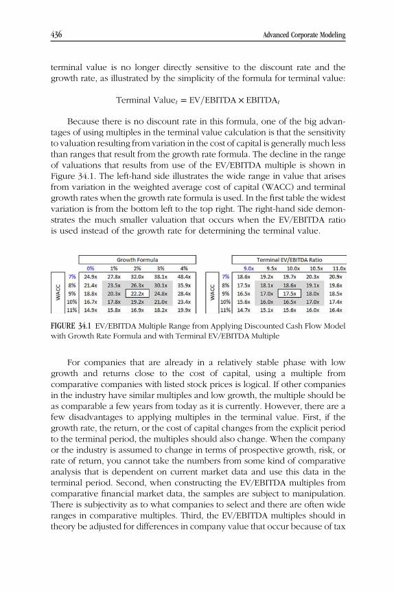
WEBC34 10/03/2014 11:50:10 Page 436

terminal value is no longer directly sensitive to the discount rate and thegrowth rate, as illustrated by the simplicity of the formula for terminal value:

Terminal Valuet � EV=EBITDA � EBITDAt

Because there is no discount rate in this formula, one of the big advan-tages of using multiples in the terminal value calculation is that the sensitivityto valuation resulting from variation in the cost of capital is generally much lessthan ranges that result from the growth rate formula. The decline in the rangeof valuations that results from use of the EV/EBITDA multiple is shown inFigure 34.1. The left-hand side illustrates the wide range in value that arisesfrom variation in the weighted average cost of capital (WACC) and terminalgrowth rates when the growth rate formula is used. In the first table the widestvariation is from the bottom left to the top right. The right-hand side demon-strates the much smaller valuation that occurs when the EV/EBITDA ratiois used instead of the growth rate for determining the terminal value.

For companies that are already in a relatively stable phase with lowgrowth and returns close to the cost of capital, using a multiple fromcomparative companies with listed stock prices is logical. If other companiesin the industry have similar multiples and low growth, the multiple should beas comparable a few years from today as it is currently. However, there are afew disadvantages to applying multiples in the terminal value. First, if thegrowth rate, the return, or the cost of capital changes from the explicit periodto the terminal period, the multiples should also change. When the companyor the industry is assumed to change in terms of prospective growth, risk, orrate of return, you cannot take the numbers from some kind of comparativeanalysis that is dependent on current market data and use this data in theterminal period. Second, when constructing the EV/EBITDA multiples fromcomparative financial market data, the samples are subject to manipulation.There is subjectivity as to what companies to select and there are often wideranges in comparative multiples. Third, the EV/EBITDA multiples should intheory be adjusted for differences in company value that occur because of tax

FIGURE 34.1 EV/EBITDA Multiple Range from Applying Discounted Cash Flow Modelwith Growth Rate Formula and with Terminal EV/EBITDA Multiple

436 Advanced Corporate Modeling

WEBC34 10/03/2014 11:50:10 Page 437

rate differences, asset life variation, alternative operating risk, as well asdifferent growth rate and return expectations. Academics who complain aboutusing multiples in the DCF model insist that the multiple that is present whenmaking comparisons using today’s market conditions cannot be used interminal value calculations. They insist that the use of multiples pollutesthe whole DCF process.

Use of a multiple such as the P/E ratio or the EV/EBITDA ratio means thatthe valuation ultimately depends on the opinions of other people and it can becalled relative valuation. To demonstrate the problem with applying compara-tive multiples from samples of supposedly similar companies, think aboutvaluing homes in the United States before the financial crisis of 2008. Apprais-ers would play games with comparative samples where houses that sold forrelatively low values would be excluded from a comparative sample, buthomes with high selling prices—perhaps because of better features such aslocation or a new air conditioning system—would be included in the sample.As the appraiser would arrive at a higher value because of the sample selection,the loan would also be higher, and the selling price would be increased. Thehigher selling price of the home that was the subject of the transaction wouldthen be used in the next appraisal, and a vicious circle would be created thatpushed up appraised values because of sampling methods.

Figure 34.2 illustrates analogous problems when using multiples in thecontext of valuing a corporation. This figure shows how samples in derivingmultiples can be very subjective and lack logic. The company being valuedin Figure 34.2 is a small airfreight company with a market capitalization of

FIGURE 34.2 Example of Problems That Arise from Constructing Comparative Samplesto Derive Valuation MultiplesSource: Company reports and Scott and Stringfellow estimates.

Computing Implied Price/Earnings Ratios for Use in Terminal Value Calculations 437

WEBC34 10/03/2014 11:50:11 Page 438

$175 million. It is compared to Federal Express with a market capitalizationthen of $5.971 billion. The amount of debt that affects risk is not shown in theanalysis, the returns of the different companies are not known, and the price ofa share of equity compared to the EBITDA is included in one column(comparing postfinancing equity value with prefinancing EBITDA).

Problems with creating a sample like the one shown in Figure 34.2 promptthe question of whether an alternative approach can be used to find impliedmultiples that combine returns and growth rate assumptions with market data.A solution suggested in this chapter and the next is developing equations forcomputing implied multiples. By calculating the P/E ratio and the EV/EBITDAratio rather than simply plopping in numbers from the Internet, you candirectly input the return on investment and the terminal growth rate whilebacking into the implied cost of capital.

Even though the value driver formula discussed in Chapter 33 is not usefulinmaking valuations, the general idea of explicitly accounting for value driversof return, growth, and cost of capital in computing terminal value andmultiples is attractive. Through computing implied multiples you can createa user-defined function that accepts inputs for: (1) historical EBITDA growth,(2) projected EBITDA growth, (3) current return on invested capital, (4) pro-spective return on invested capital, (5) the ratio of working capital to EBITDA,(6) book life, (7) tax depreciation rate, (8) income tax rate, and (9) WACC.Once you have created a user-defined function that uses these inputs, out willpop an EV/EBITDA ratio that you can use in terminal value and othercalculations. You can try out different rates of return and market growthexpectations to derive the cost of capital from the current market multiple withthe Goal Seek function. You also could benchmark the computed multiples tocurrent market conditions and then adjust the EV/EBITDA multiple forincremental changes in the growth rate, the rate of return, and even thecost of capital that should decline along with more stable conditions. The user-defined function for computing multiples can also incorporate a transitionperiod between current growth/return and long-term growth/return. Toexplain how such a user-defined function for computing the EV/EBITDAratio is developed, a general review of howmultiples are used and a derivationof the P/E ratio are presented in the next section.

Model for Deriving the P/E Ratio fromValue Drivers

The P/E ratio and the EV/EBITDA ratio are influenced by cost of capital,growth, and return. If the P/E ratio increases because of higher expectedgrowth, the EV/EBITDA should increase as well. Similarly, if the EV/EBITDA

438 Advanced Corporate Modeling

WEBC34 10/03/2014 11:50:11 Page 439

declines because of higher perceived risk, the P/E ratio should also decline.Differences between the P/E and EV/EBITDA multiples are driven by taxes,the lifetime of assets in computing depreciation, and debt leverage. Thesedifferences can be demonstrated by considering an extreme case of acompany with no taxes, no net debt, and no depreciation. Maybe it couldbe our retailing company located in the United Arab Emirates that wasintroduced in Chapter 33. In this extreme case, the equity value is the sameas the enterprise value because the company has no net debt, and theEBITDA is the same as the net income (EBITDA minus depreciation minusamortization minus interest minus taxes equals net income). Since the netincome equals EBITDA and enterprise value equals the equity value, the P/Eratio also equals the EV/EBITDA ratio. This means that when factors such asgrowth, return, and cost of capital influence the P/E ratio, these same thingswill affect the EV/EBITDA ratio. The example also demonstrates that thedifferences between P/E and EV/EBITDA are driven by depreciation oncapital expenditures, taxes, and debt, or the DA, the T, and the I in EBITDA.

Deriving the P/E ratio and the EV/EBITDA ratio from value drivers may ormay not be of much value in everyday valuations. But understanding how tocompute the P/E and EV/EBITDA ratios from items like growth, returns, andcost of capital forces you to see what really drives the ratios. It also allows youto benchmark the multiples and understand the effect of incremental changesto the value drivers. To demonstrate how implicit multiples can be derived, theP/E ratio is described in this chapter. The derived P/E ratio is calculated fromdifferent long-term and short-term earnings growth rates, different short-termand long-term returns on equity, and changing cost of equity capital. Throughexplicitly considering these three factors along with transition periods foreach variable, the P/E multiple can be derived without resorting to relativevaluations that are subject to sampling bias andwithout distortions in the valuedriver formula that does not produce an accurate result. If you then use theimplied P/E multiples in the terminal value calculation and compute thosemultiples from value drivers and transition factors, your valuation is explicitlydriven by things like the long-term real growth rate and the difference betweenthe return and cost of capital.

To analyze the drivers of value and the level of the P/E ratio, growth ratescan be separated into short-term and long-termgrowth rates. Further, the cost ofcapital can be broken down to its building blocks that include the real rate ofinterest, the inflation rate, and the risk premium. Each of these building blockscan be differentiated by time period. The rate of return earned on equity can beexpressed as the cost of capital plus a premium. In setting up amodel of the P/Eratio, drivers include (1) the real growth rate in earnings in the short run and thelong run, (2) the rate of return earned above the cost of capital in the short runand the long run, (3) the rate of inflation in the short run and the long run, (4) thereal rate of interest, and (5) the risk premium in the short run and the long run.

Computing Implied Price/Earnings Ratios for Use in Terminal Value Calculations 439

WEBC34 10/03/2014 11:50:11 Page 440

A model to compute the implied P/E ratio involves measuring cash flowto equity. The trick in computing equity cash flow from dividends is usingthe formula for the dividend payout ratio that depends on growth and return.This formula for dividend payout is explained in Chapter 33 in the context ofthe value driver formula:

Dividend Payout � 1 � Earnings Growth=Return on Equity

In developing the model to simulate P/E, after the implied dividendpayout ratio is computed, a table of the progression in the balance of equity,the net income per share, the book value per share, and the dividends pershare can be calculated. When creating this long-term simulation model,the closing balance of the equity investment is the opening balance plus theincome less the dividends. The period-by-period income and dividends arethen computed from the following formulas:

Net Income � Return on Equity �Short-Term; Long-term; or Transition��Opening Equity Balance

Dividends � Dividend Payout �Short-Term; Long-Term; or Transition�� Net Income

Since the discount rate changes, an index of the cost of capital can becomputed and the SUMPRODUCT function can be used:

Value � SUMPRODUCT �Dividends=Discount Index�P=E Ratio � First Year Net Income=Value of Equity

Computation of the P/E ratio using a simulation model is illustrated inFigure 34.3. The model includes timing switches to define the short-termperiod and a long-term period. The year-by-year return, dividend payout ratio,and cost of equity are computed using the switches, and the SUMPRODUCTfunction. The discount rate is calculated using a compounding index becausethe cost of capital changes over time, as explained in Chapter 28 and illustratedin Figure 28.5. Once the equity value is computed as the present value of thedividends in the output section shown on Figure 34.3, it is divided by the nextyear’s earnings to establish the implied P/E ratio.

To derive the P/E or the EV/EBITDA ratio that theoretically would existwith changing growth rates and returns, transition factors can be included inthe analysis. When variables have time differentiation such as the short-termand long-term values shown in Figure 34.3, it is generally not reasonable toassume that the change in the variable suddenly happens in one single year.

440 Advanced Corporate Modeling

WEBC34 10/03/2014 11:50:11 Page 441

Instead, the variable gradually moves from the short-term rate to the long-termrate. This means the transition period as well as the short-term period can bedefined with timing switches. In computing values during the transitionperiod, equations for compound growth or linear growth can be used tointerpolate variables that move from a short-run value to a long-term value.The different interpolation approaches apply the following equations:

ROEt � �1 � g� � ROEt�1

where

g � �ROElong-term=ROEshort-term��1=�1�transition period��

FIGURE 34.3 Illustration of Computing the Implied P/E Ratio with Value Drivers

Computing Implied Price/Earnings Ratios for Use in Terminal Value Calculations 441

WEBC34 10/03/2014 11:50:12 Page 442

or

ROEt � ROEt�1 � Linear Factor

where

Linear Factor � �ROElong-term � ROEshort-term�=�1 � Transition Period�

Considerations about whether to use the compound growth rate equationor the linear equation depend on whether it is possible to have a negativevalue for one of the factors such as ROE or growth. If one of the variables canbe a negative number such as negative growth rate, the formula using thecompound growth does not work, but the linear factor still can be applied.

When deriving inputs for the value drivers shown in Figure 34.3, someconsiderations include:

■ The real growth rate in the long run should not be more than the expectednominal growth rate in the economy. Without exports and imports, thegrowth rate in an economy is defined by population growth and produc-tivity increases. The real growth rate is also the theoretical real rate ofinterest as this amount must be held back from consumption to allowfuture investment. The spread between the earned return on equity (ROE)and the cost of capital in the long run should narrow with increasedcompetition and other factors as described in Chapter 32, but it shouldprobably not be zero. Without earning a return above the cost of capital, acompany has no reason to make new investments.

■ Despite all of the elegant theory and many articles that are related toestimating the risk premium, a couple of simple ideas can be used to put aboundary on the number. First, when growth rates and returns arerelatively low in a stable period, the risk is also probably low. Withouthigh return and high growth, there is less room to fall. Second, if youwould like a quick way to estimate the cost of capital, you can use the factthat when the cost of capital is the same as the return on equity, themarket-to-book ratio should be equal to 1. You can gather data ondifferent market-to-book ratios as well as the forward return on equityusing the technique with the WORKBOOKS.OPEN statement and theINDIRECT function as described in Chapters 33 and 35. Then you cancreate a regression equation of the forward ROE as a function of themarket-to-book ratio using the following equation:

M=Bi � A � B � ROEi

442 Advanced Corporate Modeling

WEBC34 10/03/2014 11:50:12 Page 443

Using this equation, you can plug in a market-to-book ratio of 1 andcompute the resulting ROE. Because of the idea that the market valueequals the accumulated investment when return equals cost of capital,the point at which the market-to-book ratio is equal to 1 should be thesame as the cost of equity. A graph illustrating the regression is shownin Figure 34.4.

FIGURE 34.4 Use of Market-to-Book Ratio and Forward Return on Equity to Estimatethe Cost of Equity Capital

Computing Implied Price/Earnings Ratios for Use in Terminal Value Calculations 443

WEBC34 10/03/2014 11:50:13 Page 444

WEBC35 10/03/2014 12:39:52 Page 445

CHAPTER 35Computing an Implied EV/EBITDA

Ratio in Terminal ValueCalculations

Chapter 34 explains that if there were no taxes and no capital expendituresand if there was no net debt, the price/earnings (P/E) ratio and the

enterprise value/earnings before interest, taxes, depreciation, and amortiza-tion (EV/EBITDA) ratio would be the same. This implies that if you want tocompute the implied EV/EBITDA ratio, the fundamental factors of growth,return, and cost of capital will drive the ratio just as they do for the P/E ratio. Asdepreciation, taxes, and debt are the factors that cause differences betweenthe EV/EBITDA ratio and the P/E ratio, these factors must also be accountedfor when computing the implied EV/EBITDA ratio.

To establish the implied EV/EBITDA ratio rather than the implied P/E ratiofrom all of the factors that drive enterprise value, including return, growth, costof capital, tax rate, plant life, working capital, and tax depreciation, must beconsidered. The process of making a financial model to simulate the EV/EBITDA ratio involves creating a balance of net invested capital rather than theequity balance. Chapter 24 explains that invested capital can be calculatedusing either the balance of net assets associated with generating EBITDA or,alternatively, a balance of financing obligations including equity and net debtdevoted to financing EBITDA. The model for computing the EV/EBITDA ratioworks best using the direct method that begins with the asset side of thebalance sheet to establish the invested capital balance. The opening balance ofinvested capital is then converted to net operating profit less adjusted taxes

445

WEBC35 10/03/2014 12:39:52 Page 446

(NOPAT) and free cash flow to the firm (FCFF). Net assets grow by capitalexpenditures and net working capital changes, and are reduced by deferredtax changes.

To demonstrate the mechanics of computing the implied EV/EBITDAratio from value drivers, consider a case where net plant is required togenerate net operating profit after tax but without working capital anddeferred taxes are not considered. This analysis uses inputs for (1) returnon invested capital (ROIC), (2) weighted average cost of capital (WACC), (3)the ratio of capital expenditures to depreciation, (4) the depreciation rate onnet plant, and (5) the tax rate. Using the ratio of capital expenditures todeprecation and the net depreciation rate derived from the growth rate andplant life is analogous to the way the dividend payout ratio derived fromthe growth rate is used in computing the P/E ratio. By working through thecomputation of the EV/EBITDA ratio using the ratios of capital expenditures todepreciation and the net plant depreciation rate you can, it is hoped, see thebenefit of computing the stable ratios. As explained in Chapters 30 and 31, theratio of capital expenditures to depreciation and the net depreciation rate canbe calculated from user-defined functions that accept the book life of the plantand the asset growth rate. A constant growth case demonstrates the mechanicsof a model to derive the EV/EBITDA ratio. This is later extended into a modelthat includes changing growth, returns, and cost of capital. Recall that thevalue driver formula falls apart when growth rate and/or return changes.

Simulation Model to Derive Implied EV/EBITDARatio from Invested Capital with Constant Growth

Construction of a model to derive the EV/EBITDA ratio with a constant growthassumption is derived before a more complex model that accounts forchanging growth and changing returns is introduced. Figure 35.1 is an excerptof a simulation model that calculates the EV/EBITDA ratio from the investedcapital balance using an assumption of constant growth. Calculations ofinvested capital are analogous to computing the balance of the equity capitalwhen deriving the P/E ratio that was illustrated in Figure 34.3. The netinvestment balance decreases from depreciation expense and it increaseswith capital expenditures. These movements in the invested capital balancefrom depreciation and capital expenditures shown in Figure 35.1 are com-puted as follows:

■ The depreciation expense is computed from the opening balance multi-plied by the net depreciation rate. The function explained in Chapter 30

446 Advanced Corporate Modeling

WEBC35 10/03/2014 12:39:52 Page 447

can be used to establish the net depreciation rate using inputs for plant lifeand growth rate using the constant growth assumption.

■ Once the depreciation is established, the capital expenditures are derivedthrough multiplying the depreciation by the ratio of capital expendituresto depreciation. For the constant growth rate case you can use a functionthat computes the ratio of capital expenditures to depreciation thataccepts projected growth and plant life.

■ After you have computed the net investment balance, the NOPAT, whichis EBIT multiplied by 1, the tax rate can be computed. This is computed asthe rate of return on invested capital multiplied by the opening balance ofthe investment.

FIGURE 35.1 Illustration of Model That Derives the EV/EBITDA Ratio from Value Drivers andUser-Defined Functions

Computing an Implied EV/EBITDA Ratio in Terminal Value Calculations 447

WEBC35 10/03/2014 12:39:54 Page 448

■ Because NOPAT is equal to EBIT × (1 � tax rate), the EBIT can be derivedas the NOPAT/(1 � tax rate).

■ After computing the EBIT, the depreciation expense that has already beencomputed as part of the invested capital balance can be added to the EBITto derive the EBITDA.

With the EBITDA, EBIT, the tax rate, and capital expenditures computed,items for free cash flow (EBITDA, capital expenditures, and taxes) are availa-ble. You can then compile the free cash flow and compute its present value,which is the enterprise value. With the enterprise value and EBITA established,the EV/EBITDA ratio can be computed as illustrated in Figure 35.1.

Function to Derive Implied EV/EBITDA Ratio

You can make a user-defined function to compute the EV/EBITDA in a waythat is similar to how capital expenditures to depreciation, deferred taxchanges, asset retirements, and net plant depreciation were derived. Thisfunction allows you to compute the EV/EBITDA ratio automatically withoutmaking a whole new spreadsheet each time you would like to evaluate theEV/EBITDA ratio for purposes of computing terminal value. A function thatevaluates the EV/EBITDA in net plant case (i.e., still without working capitalchanges, deferred taxes, and other items such as provisions) is shown inFigure 35.2. This function accepts the three drivers of growth, cost of capital,and return along with the plant life and the tax rate. The function then worksthrough the same equations shown in Figure 35.1. Results of the function areshown in Figure 35.1 below the calculation of the EV/EBITDA ratio, demon-strating that the same result is obtained.

After writing the function for a simple case without varying growth rates,returns, and transition factors, you could create a more complex function thatloops through a historical period to establish prospective retirements, as wasthe case for the more complex evaluation for the ratio of capital expendituresto depreciation. The more advanced function is adjusted for adding deferredtaxes and working capital to the analysis using the stable working capitalequation explained in Chapter 29 and the deferred tax function described inChapter 31. The comprehensive function can also be modified to differenti-ate between long-term, transition, and short-term parameters using conceptsof multiple FOR NEXT loops discussed in Chapter 30, where the historicperiod is used to establish retirements. The EV/EBITDA ratio is then finallyderived from the lifetime of plant, the tax depreciation life and method, thehistorical growth rate in assets, and the ratio of working capital to EBITDA aswell as the WACC, projected growth, tax rate, and the projected rate ofreturn.

448 Advanced Corporate Modeling

WEBC35 10/03/2014 12:39:57 Page 449

Comprehensive Analysis to Derive Implied EV/EBITDARatio with Changing Growth, Deferred Taxes, andWorking Capital

An excerpt from a simulation analysis that includes deferred taxes, workingcapital, changing growth, and changing returns is shown in Figure 35.3. Thefinancial model and/or function to derive the EV/EBITDA with the additionalparameters are a compilation of the concepts developed from Chapters 29through 34. Figure 35.3 illustrates how a variety of different ratios changewhen the growth rate changes and that the ratios do not stabilize after asingle year. Instead, ratios of capital expenditure to depreciation, net plantdepreciation rate, and deferred taxes take a full life cycle to change after thegrowth rate changes.

Results of a comprehensive analysis in terms of the EV/EBITDA ratio areshown in Figure 35.4. This figure demonstrates the inputs required for the

Function EV_EBITDA_Simple(ROIC, WACC, Growth, Life, Tax_Rate)

cap_exp_ratio = cap_exp_depreciation_simple(Life, Growth, 1)

depreciation_ratio = net_depreciation_rate(Life, Growth)

net_investment = 1000 ’ Initialise variables

PV_factor = 1

For i = 1 To 300

NOPLAT = net_investment * ROIC ’ Compute OPENING BALANCE

EBIT = NOPLAT / (1 - Tax_Rate)

depreciation = depreciation_ratio * net_investment

cap_exp = cap_exp_ratio * depreciation

EBITDA = EBIT + depreciation

FCFF = EBITDA - cap_exp - EBIT * Tax_Rate

If i = 1 Then EBITDA_1 = EBITDA ’ Remember the EBITDA

PV_factor = PV_factor * (1 + WACC) ’ Accumulate the PV factor

EV = EV + FCFF / PV_factor

net_investment = net_investment + cap_exp - depreciation

Next i

EV_EBITDA_Simple = EV / EBITDA_1 ’ Compute function on next period EBITDA

End Function

FIGURE 35.2 Function for Computing Implied EV/EBITDA Ratio without WorkingCapital Changes and Deferred Taxes

Computing an Implied EV/EBITDA Ratio in Terminal Value Calculations 449

WEBC35 10/03/2014 12:39:57 Page 450

FIGURE 35.3 Excerpt from Comprehensive Model That Computes the EV/EBITDA Ratio from ValueDrivers and Transition Assumptions

FIGURE 35.4 Illustration of Output from a Comprehensive Calculation of the Implied EV/EBITDARatio

450 Advanced Corporate Modeling

WEBC35 10/03/2014 12:40:1 Page 451

analysis and compares the comprehensive analysis with the value driverformula and the growth rate method. Figure 35.4 includes periodic valuedrivers, transition time periods, deferred taxes, and working capital in derivingthe ultimate EV/EBITDA ratio. Factors that drive the EV/EBITDA ratio includethe life of the assets, tax rates, transition factors, rates of return, costs of capital,working capital ratios, and growth rates. All of the inputs that drive the ratio areeither standard valuation inputs such as the growth rate and the cost of capitalor should be available from elsewhere in the model. The table at the bottomleft of Figure 35.4 reports the implied EV/EBITDA ratio for the current year andfor the assumed terminal period. The importance of creating a comprehensivefunction rather than using a simple growth equation or the value driverformula is demonstrated by the difference between the model output andthe value driver model or the growth model. The enterprise value computedfrom the alternative methods includes:

The Value Driver Equation: EV � NOPAT � �1 � g=ROIC�=�WACC � g�The Growth Rate Method : FCFF � �1 � g�=�WACC � g�

Figure 35.4 illustrates that the value driver formula and the growth rateformula do not produce accurate results compared to the true value estab-lished with the function that considers historical growth and works throughthe investment balances. The computation of EV/EBITDA that considershistoric growth, future growth, tax rates, plant life, cost of capital, and transi-tion factors can be established in a user-defined function. This functioncan then be put in the left-hand columns of your financial model like theresults of other functions.

Computing an Implied EV/EBITDA Ratio in Terminal Value Calculations 451

WEBC35 10/03/2014 12:40:2 Page 452

WEBC36 10/03/2014 12:53:1 Page 453

CHAPTER 36Developing Value Drivers for P/Eand EV/EBITDA Ratios with

Benchmarking and Regression

Creating models and functions to compute price/earnings (P/E) and enter-prise value/earnings before interest, taxes, depreciation, and amortization

(EV/EBITDA) multiples does not address how to come up with value driverinputs that should be put into the analysis. Let’s say that you have a good ideaabout the current EV/EBITDA multiple, and you only want to adjust themultiple for changes in items like a lower growth rate, a different cost ofcapital, or a lower return on invested capital (ROIC). The problem withputting values in one of the functions to compute multiples discussed inChapters 34 and 35 is that you do not know the biggest factor that drives anyof the multiples, namely the cost of capital. When implementing thecomputed multiples into corporate finance models, you could attempt tofocus on incremental changes from the current market multiples rather thanstarting from scratch in building up the multiple. To do this you can usemarket data for multiples and make estimates of what you think the marketexpectations are for growth and return as well as other inputs like the taxrate and the plant life. With current multiples observed in the market you canthen apply a Goal Seek process to find the implied weighted average cost ofcapital (WACC) or the implied cost of equity by moving the cost of capitalaround until the derived multiple equals the market observed value. Theidea of making incremental changes to current multiples for differentgrowth, return, and stable cost of capital can also be accomplished byconstructing a regression equation that simulates current market multiples asa function of growth, return, cost of capital, tax rate, and depreciation rate.

453

WEBC36 10/03/2014 12:53:2 Page 454

Benchmarking Multiples to Derive Cost of Capital

Chapters 34 and 35 demonstrate how the various factors such as growth, plantlife, tax rates, returns, and most of all cost of capital should affect P/E andEV/EBITDA multiples. When evaluating the P/E ratio or the EV/EBITDA ratio,you may imagine creating a statistical test to see whether these factors actuallyinfluence the ratio that is suggested by the different equations. If projectedgrowth for one company is higher than another and the return is above thecost of capital, the P/E ratio should be greater. Similarly, you should be able toobserve P/E variances among a sample of companies from arising differencesin projected future growth.

The derived EV/EBITDA ratio and the P/E ratio can be used together withthe Goal Seek tool to compute implied cost of capital. This process involvesinputting all of the variables necessary to calculate the multiple and thencomparing the computed multiple with the actual multiple observed frommarket data. When you enter inputs for short-term and long-term growth inthis process you should attempt to enter realistic market expectations. Theseexpected growth rates are not the published numbers for earnings growthpredicted by sell-side analysts that you can pick up on the Internet, which havebeen demonstrated to be optimistic and lead to overestimations of the cost ofcapital. When entering realistic growth rates into the derived multiples you canalso input alternative estimates of the progression of return on capital to the costof capital. After you come up with inputs and compute the implied valuationmultiple youcancreate aGoal Seek function toderive the implied cost of capital.Using the P/E ratio, the cost of capital computed from this process is the cost ofequity; if the EV/EBITDA ratio is evaluated, the weighted average cost of capitalis the result.

A range in possible implied costs of capital can be simulated from differentgrowth rates and rates of return with the Goal Seek tool and a little Visual Basicfor Applications (VBA) code. To present such a range in your spreadsheet, youcan first write a macro that records the Goal Seek process. This should be oneline of code that includes the set cell (a formula), the target cell (a fixed input),and the changing cell (an input in the spreadsheet). One of the most commonmacros made in a spreadsheet is recording the Goal Seek macro and thenenabling the target cell to be read from the spreadsheet rather than being inputinto the Goal Seek tool. The initial macro and adjustments are shown in thefollowing statements.

Before range names:

Range("D8").goalseek Goal:=0, ChangingCell:=Range("D4")

454 Advanced Corporate Modeling

WEBC36 10/03/2014 12:53:2 Page 455

After range names:

Range("EV_EBITDA").goalseek Goal:=0, ChangingCell:=Range("Cost of

Capital")

With target from cell in spreadsheet:

Range("EV_EBITDA").goalseek Goal:=Range(“Target”), ChangingCell:=Range

("Cost of Capital")

After recording the macro you should replace the cell references withrange names as shown. When creating the process you can input the actualEV/EBITDA ratio or the actual P/E ratio adjacent to the computed ratio.Next you can compute the difference and use the Goal Seek process to setthe difference to zero by changing the cost of capital input. To create a tablethat shows the range in costs of capital given different growth rates and/orcosts of capital, the data table tool does not work for two reasons. First, theoutput of the table is the input cell for the cost of capital rather than aformula. Second, the Goal Seek must be rerun with each new scenario.Instead of using the data table tool, the FOR NEXT process described inChapter 16 and illustrated in Figure 16.10 can be applied to develop thesensitivity table. When creating this macro to replicate the Data Table toolyou should then add the Goal Seek code just before the macro reports theresults using the CELLS statement.

Downloading Data for a Sample of Companiesfrom the Internet into a Spreadsheet

Increasing amounts of data has been published on websites in recent years.You can often (but not always) create VBA code to download data for youranalysis. Once you have downloaded data on estimated growth, return, andmeasurable cost of capital factors for a group of companies, it can be pluggedin to arrive at multiples that can be applied in the discounted cash flowmodel.A regression could take the form:

P=E � A � B � g=ROE � C � g � D � Beta � E � Debt to Capital

In this equation the coefficient on the g/ROE should be negative, thecoefficient on the beta should be negative, and the coefficient on the growth

Developing Value Drivers for P/E and EV/EBITDA Ratios with Benchmarking and Regression 455

WEBC36 10/03/2014 12:53:2 Page 456

rate should be positive. Before running the regression to establish such anequation, you can program some code to efficiently download data from theInternet and then copy new data into different spreadsheets of a workbook.In VBA there is a wonderful statement that allows you to do just this.The statement WORKBOOKS.OPEN(Range(“URL”)) can open all sorts ofdifferent web pages and spreadsheets that are downloadable from websitesand put the data into your workbook. It can also open spreadsheet files thatare downloadable once you know the URL. In the WORKBOOKS.OPEN(Range(“URL”)) statement, the URL should be pasted into your spreadsheet.As explained in Chapter 32, you can modify the URL to make it flexible sothat it can read all sorts of data from websites of different companies. TheVBA code can then be adjusted to place that data into different sheets. Thistechnique of automatically downloading files may be one of the most usefulmacros for all sorts of analysis even though it is not documented in many ofthe thick books on VBA programming.

The process of downloading data that enables incorporation of marketdata into the implied P/E and EV/EBITDA analysis is illustrated in the twoexamples that follow. The first example that downloads data from the Sloveniastock exchange and puts information from the various companies intodifferent sheets is illustrated in Figures 36.1 and 36.2. Figure 36.1 demonstrateshow to create a URL that can be modified to accept different companies on theexchange using the INDEX function and a ticker symbol. Figure 36.2 shows

FIGURE 36.1 Illustration of How to Modify a URL to Accept Different Ticker Symbolsfor Reading into VBA

456 Advanced Corporate Modeling

WEBC36 10/03/2014 12:53:4 Page 457

how to use the WORKBOOKS.OPEN statement to read different companiesand then pop the information into separate sheets. With the data in separatesheets you can use the data in statistical analysis from applying the INDIRECTfunction. Note that in the VBA code, the paste special as values is used insteadof the simple Paste function. This avoids all of the irritating advertisements thatare part of so many Web pages.

If you want to read from Excel or PDF files that are uploaded to websitesyou can use the same kind of approach. This time you press the F3 key on thewebsite to copy the URL name to your spreadsheet. If you use the copied URLwith the WORKBOOKS.OPEN statement, the macro will find and open theExcel or PDF file. After defining the URL and opening the file, you are left withputting the data into a new sheet of your current workbook. VBA code tocomplete this process is illustrated in Figure 36.3. When you have put all of thesheets that you read from different URLs together in a single workbook, youcan use the INDIRECT function to extract data and make comparisons. TheINDIRECT function was discussed in Chapters 15 and 32.

Sub get_company()

current_book = ActiveWorkbook.Name ’ Remember the current workbook

current_sheet = ActiveSheet.Name ’ remember the current sheet

Workbooks.Open (Range("url")) ’ This is the essential function

temp_book = ActiveWorkbook.Name ’ Copy cells from workbooks.open

Cells.Select

Selection.Copy

Windows(current_book).Activate ’ Go back to workbook for pasting

Sheets.Add After:=Sheets(Sheets.Count)

Selection.PasteSpecial Paste:=xlPasteValues, Operation:=xlNone, _

SkipBlanks _

:=False, Transpose:=False ’ Paste to new sheet of current workbook

ActiveSheet.Name = Range("ticker") ’ Re-define name of sheet to be copied

Windows(temp_book).Close ’ Close the workbook from URL Read

End Sub

FIGURE 36.2 Illustration of How to Use the WORKBOOKS.OPEN Statement to ReadDifferent Companies

Developing Value Drivers for P/E and EV/EBITDA Ratios with Benchmarking and Regression 457

WEBC36 10/03/2014 12:53:4 Page 458

Running Regression Analysis on Financial Data

After you have finished uploading data for comparative multiples and otherstatistics such as the expected growth rate as well as cost of capital indicatorssuch as beta, stock price volatility, and debt leverage, you can make theanalysis of value drivers. When using data for statistical analysis, creating aflexible range namewith the OFFSET function you can add a lot of flexibility tothe statistical analysis. Using the OFFSET function to create a flexible rangename will allow you to change variables in the regression, select alternativecompanies with market data, and it will allow you to experiment with differenttime periods. Use of the OFFSET function to create a dynamic range name isdescribed in detail in Chapter 15 and illustrated in Figure 15.11. If the data isarranged with companies in columns and time in rows and the data starts inrange A1, then the flexible range name can be created with the OFFSETfunction as follows:

Range Name � OFFSET�A1; 0; 0; Row Length; Column Width�In this example the row length and the column width would be put

as inputs somewhere in the sheet. By changing the number of companies in

Sub run_stock(current_symbol) ’ Data from downloaded

spreadsheets

workbook_name = ActiveWorkbook.Name ’ Keep current workbook

sheet_name = ActiveSheet.Name ’ keep the current sheet

Range("Symbol").Value = current_symbol ’ Ticker symbol from reading

Workbooks.Open (qurl) ’ Here is the main function

Cells.Select ’ Get all of the data

Windows(workbook_name).Activate ’ Go back to org workbook

Sheets.Add ’ Add a new sheet at the end

num = Sheets.Count

ActiveSheet.Move After:=Sheets(num) ’ Move the sheet to end

ActiveSheet.Name = Symbol ’ Rename the new sheet

ActiveSheet.Paste ’ Paste into the new sheet

Windows("table.csv").Close ’ Close sheet from internet

End Sub

FIGURE 36.3 Macro for Reading Data from Excel Files Created by Website

458 Advanced Corporate Modeling

WEBC36 10/03/2014 12:53:4 Page 459

the data set and the length of the time series, the statistical results can beviewed immediately. To do this, the flexible range names can be used instatistical functions such as the LINEST, SLOPE, INTERCEPT, and RSQfunctions.

With a database of financial data that is assigned to flexible range namesyou can see how the actual data reconciles with the simulated impliedmultiples and derive the implied multiples for a range of companies. Alterna-tively, you can run a regression on a sample of different companies. Anexample of such a regression that produces an R-squared of 61 percent isshown in the table and the graph presented in Figures 36.4 and 36.5. The tablein Figure 36.4 shows that the coefficients have the expected signs. The graphin Figure 36.5 illustrates the difference between the simulated P/E ratio and theactual P/E ratio for each company in the analysis. In Figure 36.4 the selectedvariables that are put together with the OFFSET function and used in theregression are shaded. Outputs from the regression that are derived usingthe LINEST function are shown in the top right-hand side of the sheet. Theflexible range name is created by changing TRUE and FALSE switches abovethe variable names.

FIGURE 36.4 Regression Results of P/E Equation Using Sample of Diverse Companies

Developing Value Drivers for P/E and EV/EBITDA Ratios with Benchmarking and Regression 459

WEBC36 10/03/2014 12:53:6 Page 460

Advanced Corporate Modeling Summary

This part of the book began by emphasizing the importance of presenting thereturn on invested capital in your corporate models and paying particularattention to the rate of return projected for the terminal period. Whendiscussing return on invested capital, the notion of distinguishing betweenfinancial ratios and valuation measures that use equity cash flow versusfinancial ratios and valuation measures that focus on free cash flow wasintroduced. In later chapters the value driver formula and implied multiplesused to compute the equity value and enterprise value followed from thisdiscussion and used either an equity perspective or a free cash flow perspec-tive. To explain calculation of the return on invested capital, the balance sheetwas segregated, driven by the guiding principle that net assets, which generateEBITDA should be included in invested capital. Difficult elements of thebalance sheet to allocate were evaluated by creating a long-term theoreticalmodel that mirrors the notion of corporations having an indefinite life.This sort of long-term theoretical analysis was used repeatedly in subsequentchapters.

After the background discussion of the invested capital and the ROIC,alternative terminal methods for computing value were introduced. In dis-cussing the first method of assuming a constant growth rate applied to

FIGURE 36.5 Expected Relative to Actual P/E Ratios from Regression Analysis

460 Advanced Corporate Modeling

WEBC36 10/03/2014 12:53:9 Page 461

normalized cash flow, complex issues of normalizing the cash flow forworking capital changes, capital expenditures, and deferred tax changeswere addressed at length. Explanations of normalizing terminal cash flowdemonstrated that in order to normalize cash flow in your models, you cancreate user-defined functions that compute the stable ratios of capital expen-ditures to depreciation and deferred tax changes to capital expenditure.

The second terminal value approach of including the ROIC versus WACCspread in terminal value was evaluated after the discussion of normalizingcash flow. While the general idea of developing a formula that can account forgrowth, WACC, and also return is very attractive, it was demonstrated that thevalue driver equation (1 � g/ROIC)/(WACC � g) does not yield accuratemeasures of value. To correct problems with the value driver formula, the finalmethod of computing terminal value discussed was a technique that derivesthe P/E, market-to-book, and EV/EBITDA ratios from value drivers. Theseratios can be inferred from growth rates, returns, cost of capital, plant life, taxrate, working capital ratios, and tax depreciation. Finally, techniques tocombine market data with implied multiples to infer the cost of capitalwere discussed in this chapter.

Developing Value Drivers for P/E and EV/EBITDA Ratios with Benchmarking and Regression 461

WEBC36 10/03/2014 12:53:9 Page 462

WEBC37 10/03/2014 13:3:27 Page 463

PART IVComplex Issues: Circular

References and Other ComplexIssues from Financial

Structuring in Project Financeand Corporate Finance Models

WEBC37 10/03/2014 13:3:27 Page 464

WEBC37 10/03/2014 13:3:27 Page 465

CHAPTER 37Resolving Circular References in

Acquisition ModelsComputing Interest Expense on the Average

Balance of Debt

Anissue that not too many people care about is developing an elegant wayto compute the interest expense on the average of the opening and the

closing debt balances in a financial model. But for a few people who spendmuch of their lives in front of their laptops working on financial models, thisand other circular reference problems are more important than many otherissues that you read about in the newspaper where politicians go around andaround in a circular manner and things never seem to get resolved. The topicof interest expense on average balances and other circular reference problemsin which one calculation is a function of the second, but the second dependson the first, can cause many difficulties in financial models. Complicated debtstructuring issues in project finance and corporate financemodels that result incircular logic and other tricky programming issues are addressed in this part ofthe book.

Some analysts suggest that from a philosophical standpoint, circularityshould not occur in financial models. The argument is that this problem of oneitem depending on another and the other item depending on the first does notoccur in real-life transactions and therefore it should not be part of a financialmodel. If circularity existed in structuring a transaction, the process wouldwork something like what happens in the following story of a developerasking a banker for a loan. First, the developer goes to the bank and asks for aloan commitment. Then the bank uses the amount of the requested loancommitment to compute fees. After that, the developer asks for a larger loan tocover the fees. With the larger loan, more fees are charged and then the

465

WEBC37 10/03/2014 13:3:27 Page 466

developer needs an even higher loan.With each increment, the loan amount ishigher and the process keeps iterating on and on and on.

This circular reference resembles the film Groundhog Day in which lifenever moves forward and things just get stuck. Instead of such a scenario withthe banker and the sponsor going around and around in increments, it is morerealistic if the sponsor asks for a fixed loan commitment that will already haveincluded the arrangement fee, the commitment fee, the debt service reserveaccount (DSRA), and the interest during construction. All of these fees, interestcosts, and DSRA reserves can cause a circular reference problem similar to thesimple feeexample.Whenacompanygoes toabank to ask for a loan inaprojectfinancing transaction, the company has already created a financial model andfixed the sizingof debt, presumably throughmodeling thedebt service coverageor some other criterion. By fixing the amount of the debt, the circular referencegoes away and there is no need to go around and around where increments ofloan size influence the fees, interest, andDSRA, but these items in turn drive theloan size. Thosewho assert that circular references do not exist in the real worldwould argue that this manner of fixing variables is the way transactions reallywork in practice and a financial model should reflect this reality.

Notwithstanding this sort of philosophical debate about whether circularreferences occur in the real world, financial models are often used to derivethe structure of a transaction, meaning that debt and other transactionparameters are not fixed in advance. In project finance models, variouscombinations of debt draws, fees, interest, and debt service reserves cannotbe solved without iterating and running into a circular reference problem. Thereason for this circular logic is that the fees and the loan commitment dependon the financial model, but the model itself must be computed with some kindof fee and debt commitment assumption. In analysis of the financial structureof a transaction, when the level of an item in the model depends on using themodel itself, a circular logic problem simply cannot be avoided.

Circular References and Use of Opening Balancesin Annual Models

Circular reference problems are not unique to project finance models. Cor-porate and acquisition models are often created using annual time periods,whereas interest is computed on daily cash and debt balances in real bankloans. When making calculations of interest expense in an annual model, animplicit assumption is that the cash flows occur on a continual basis through-out the year. This means that various revenue, expense, and capital expendi-tures can be approximated with an assumption that cash flow occurs in themiddle of the year. If an implicit or explicit assumption is made that cashinflows and outflows occur on a continual basis throughout the year, it is

466 Complex Issues

WEBC37 10/03/2014 13:3:27 Page 467

incorrect to compute incremental interest expense or incremental interestincome on the basis of the opening debt or the opening cash balance.

When you compute interest from the opening balance, over the course ofthe year no positive cash flow is being used to pay down debt and there is nocash buildup that increases interest income. Interest expense and/or interestincome computed on the basis of opening balances means that you havemade an implicit assumption that all revenues are received and all expensesand capital expenditures occur right at the very end of the year. Because cashreally flows on a continual basis throughout the year, if the balance of debtdoes not change until the end of the period, then the interest expense andinterest income calculations are not correct. Where cash flow is positive, thetrue interest expense is less than the interest computed on the opening debtbalance, as debt is being repaid over the course of the year. The oppositeoccurs when cash flow is negative and the true cash flow is less than the cashflow computed in a model where opening balances are assumed.

While making the assumption that the revenues occur in the middle of theperiod is much more reasonable than pretending that all cash flow suddenlyappears on December 31, it creates a circular logic problem. The circularreference occurs because the closing balance of the debt or cash influencesthe interest expense and/or interest income. But the interest expense and/orinterest income is a determinant of cash flow that drives the closing debtand cash balances. The circular reference is illustrated by the diagram inFigure 37.1, which shows that the closing debt balance is driven by cash flowbut cash flow is driven by interest expense and in turn the closing debtbalance.

If you want your model to be precise and reflect the reduction in interestexpense from positive cash flow realized over the course of the year, thiscircular logic problem can be tricky to resolve. While the problem of moreaccurately measuring interest expense is not generally a key driver in mostmodels if the interest rate is not very high, addressing the problem doesillustrate elegant ways in which user-defined functions can be used to solveproblems in financial models. For many advanced financial modeling issues,including the problems of stable ratios discussed in Part 3, creating your ownuser-defined functions opens a whole new world of solving problems thatotherwise use things like tedious copy and paste macros.

Closing Balance Interest Expense Interest Expense Net Cash Flow Net Cash Flow Closing Balance

FIGURE 37.1 Circular Reference Logic Diagram of Interest Expense and Closing DebtBalance in Corporate Model

Resolving Circular References in Acquisition Models 467

WEBC37 10/03/2014 13:3:27 Page 468

Alternative Techniques for Solving CircularReference Logic Problems in Financial Models

There are various different ways to address the problem of circular referencesin financial models. Five of the possible techniques that can be used to solvecircular references such as the problem of interest expense on the averagedebt balance in annual models and funding in project finance models areshown in Table 37.1. The table lists different techniques to resolve circularreferences along with comments about the problems that arise with eachmethod. The right-hand column of the table explains that there are bigproblems with using the iteration button method as well as the copy andpaste macro method. The remainder of this chapter illustrates problems withthe iteration button and the copy and paste process and then describes how tocreate a flexible and transparent function using one of the last two methodsshown on the table—the algebraic equation approach or the isolated functionapproach.

TABLE 37.1 Alternative Techniques to Address Circular Reference Problems inFinancial Models

Method Problems with Method

Use the Enable Iterative Calculationbutton in Excel (the iteration button).

This method can destroy models and isdangerous to use. The models becomeunstable, Goal Seek does not work, anderrors cannot be undone. The methodshould virtually never be used.

Input fixed values in cells that cause thecircular problem, and use a Goal Seek tofind the fixed value by setting thedifference to zero.

This method can avoid the dangers of theiteration button, but it means thatwhenever you change something in amodel, you must run a Goal Seek. Asecond problem with this method is that itcannot be used to solve circular referenceproblems that occur in more than one cell.

Input fixed values in a similar manner tothe Goal Seek method, but use the Solverto find multiple values at the same time.

Using the Solver resolves problems of theGoal Seek whereby circular references inmultiple different cells can be computed.But it leaves the problem that you mustrerun the Solver any time you change astructuring or cash flow input in themodel. Another problem with this methodis that the Solver can be very slow andclumsy for anything but very smallmodels. The Solver is also problematicbecause all calculations used in the Solvermust be in one sheet.

468 Complex Issues

WEBC37 10/03/2014 13:3:28 Page 469

TABLE 37.1 (continued)

Method Problems with Method

Use a copy and paste macro to find fixedvalues in cells that cause the circular logicwith an iteration routine.

This is the most common method usedthese days in fancy models. You computethe item causing the circular reference andthen copy and paste special the computedvalue to a fixed cell. The method solvesthe problem with Goal Seek wheremultiple circular references cannot besolved, and it is better than the Solvermethod, which can be very slow andlimits the calculations to one sheet. Butthis method leaves the models just asclumsy as the previous Goal Seek andSolver methods, and it means the copyand paste macro must be used wheneveryou want to do any sensitivity analysis oroptimization.

Resolve circular references using analgebraic equation.

Using algebra is an old-fashioned methodthat is the most elegant way to solvecircular references. It requires no iterationon an indirect or a direct basis. Alloptimization and scenario analysis can bedirectly applied without any specialadjustments. The problem with thismethod is that coming up with analgebraic solution can be tedious andsometimes almost impossible.

Resolve circular references using anisolated user-defined function thatcontains an iteration loop.

This method, in which calculations thatcause the circular reference are repeatedin a function, resolves problems with theclumsiness and the lack of transparencycaused by standard copy and pastemacros. All data tables, optimization, andscenario analysis can be automated, andany circular reference can be resolved.The problem with this method is that itinvolves a bit of old-fashionedprogramming and the VBA code is notunderstood by people used to seeingmodels with copy and paste macros.

Resolving Circular References in Acquisition Models 469

WEBC37 10/03/2014 13:3:28 Page 470

In describing how to solve the circular references and some otherchallenging problems in financial modeling, it is helpful to simplify theproblem to isolate the issue. Once the issue is isolated, complexities canbe gradually added so that the process can be used in real models. Theorganization of this part of the book follows such an approach in describinghow to resolve circular reference problems in corporate and acquisitionmodels. An acquisition model with a cash flow sweep and a cash flowwaterfall without taxes is the starting point for the analysis. This case isrelatively simple to solve, because in a leveraged acquisition all of the cashflow is used to pay down debt or pay dividends rather than either building upcash balances or reducing balances of a revolving credit line. The first case of acash sweep is also somewhat less complex because dividend payouts do notdepend on net income and interest expense. Taxes, in particular net operatinglosses, differences between interest income and interest expense rates, anddividends are also excluded so as not to complicate the problem.

Resolution of Circular References from a CashFlow Sweep Using the Iteration Button

To demonstrate how the problem of circular references in corporate financeand acquisition models can be solved, imagine a model with a cash flowsweep where interest expense is computed on the basis of the average debtbalance rather than on the opening debt balance. In an acquisition model witha cash sweep, the cash flow available for repaying debt is the minimum of thecash flow after interest or the opening debt balance:

Debt Repayment � MIN�Cash Flow After Interest;Opening Debt Balance�Once you have computed the cash flow after interest, you should attach

the repayments in the debt schedule to the cash flow analysis as is the case forany cash flow waterfall. The debt schedule includes the usual: an openingbalance, a repayment line linked to the preceding formula, a closing balanceline, and an interest expense calculation. Because the interest expense iscomputed on the average debt balance, a component of interest depends ondebt repayment, which is in turn dependent on the cash flow after interest. Thecircular reference can be demonstrated by splitting up the interest expenseformula into two components and seeing that interest expense depends in parton the closing balance of the debt:

Interest Expense � Beginning Balance=2 � Interest Rate � Ending Balance=

2 � Interest Rate

470 Complex Issues

WEBC37 10/03/2014 13:3:28 Page 471

Since the ending balance is the beginning balance less the cash sweep, theinterest expense is a function of the cash sweep and debt repayment as follows:

Interest Expense � Beginning Balance=2 � Interest Rate

� �Beginning Balance � Sweep�=2 � Interest Rate

If you construct this cash flow sweep model with interest computed fromaverage balances, after you calculate the interest expense a dreaded bluearrow will appear indicating you have a circular reference. The simple modelthat is the basis for the subsequent discussion and illustrates the circularreference is shown in Figure 37.2.

Excel has a feature to resolve this kind of circular reference throughmaking iterative calculations using a special button that you can access fromthe File tab. The iteration button can be accessed by going to the File tab,clicking on Formulas, and then selecting the Enable Iterative Calculation checkbox. The last part of this process is illustrated in Figure 37.3. After pressing the

FIGURE 37.2 Illustration of Circular Reference Arising from Cash Flow Sweep withInterest on Average Balance

FIGURE 37.3 Finding the Iteration Button from the File Tab

Resolving Circular References in Acquisition Models 471

WEBC37 10/03/2014 13:3:29 Page 472

button in the box shown on the excerpt in Figure 37.3, the whole circularreference issue seems to go away. This solution seems to be a nice feature ofExcel that solves the circular reference problem. But using the iteration buttoncan be a dangerous thing to do. Some of the negative consequences of usingthe iteration button include:

■ The model can become unstable, meaning that when you make any littleerror that results in a bunch of #VALUEs, you cannot use the undo key.This can cause big problems, especially if you have not saved your work.

■ The Goal Seek tool, which is central to a lot of analysis in a model used tostructure debt and contracts in a transaction, will stop functioning andsome other tools also will not work.

■ If the model is large, it can become very slow if the iteration button ispressed, as the whole model will be computed over and over again.

■ When the iteration button is pressed, the model equations sometimes donot even work.

The next paragraphs discuss alternative ways to resolve circular referenceswithout using the iteration button. While these methods correct the modelstability problems, the various different techniques can create different problemsthat are even worse than those that arise from using the iteration button.

Solving Circular References from Cash Sweeps withGoal Seek and Solver

One way to resolve the circular reference problem is to compute the interestexpense somewhere outside of the cash flow process in your model. Afteryou make a second interest calculation somewhere else in the spreadsheetusing the average balance of the debt, enter an arbitrary fixed value for theinterest expense in the cash flow section of the model. Then you cancompute the difference between the computed value that is made outside ofthe cash flow statement and the fixed value you entered in the cash flowstatement. If the model is correct, this difference between the fixed valueand the computed value should be zero. To compute the fixed value, youcan use the Goal Seek tool or the Solver tool as follows:

Step 1 Link the interest expense in the cash flow statement to an arbitraryfixed value rather than the computed amount. An example ofusing a fixed value for interest expense in the cash sweepexample is illustrated in Figure 37.4.

Step 2 Calculate the average interest expense outside of the cash flowstatement above or below the fixed value that is input from step 1.Also calculate the difference between the fixed interest expenseand the computed interest expense.

472 Complex Issues

WEBC37 10/03/2014 13:3:29 Page 473

Step 3 Use the Goal Seek tool to set the difference between the fixedvalue and the computed value to zero by finding the fixed interestexpense. The set cell in the Goal Seek is the difference, the inputvalue is zero, and the changing cell is the fixed interest expense.

Step 4 Repeat the process for each year of the model.

Instead of repeating the Goal Seek in step 4, you could use the Solver tool.To use the Solver effectively, do not put anything in the top part of the Solverscreen. Then set the changing cells to the series of fixed interest expenses, andadd a constraint that the difference between the computed value and the fixedvalue must be zero.

Both the Goal Seek method and the Solver method have many problems,including the following three:

1. If you have another circular reference somewhere else in your model, theprocess of using the Goal Seek or the Solver can be difficult (it may beimpossible with the Goal Seek).

2. If you want to use the Goal Seek tool to do things like find debt capacity orbreak-even points, you cannot solve the problem because there will betwo Goal Seeks. While you can find solutions to these problems with theSolver tool, the process can become very cumbersome and it does notwork if Solver inputs are in different pages.

3. You cannot use most of the risk analysis tools discussed in Part 2including the Data Table, spinner buttons, and other scenario andsensitivity tools.

FIGURE 37.4 Illustration of Model Setup for Use of the Goal Seek or Solver to ResolveCircular References with a Row for Computed Amounts, a Row for Fixed Amounts,and a Row for the Difference

Resolving Circular References in Acquisition Models 473

WEBC37 10/03/2014 13:3:29 Page 474

Solving Basic Circular References from CashSweeps with a Horrible Copy and Paste Macro

An approach that is analogous to the Goal Seek method is to create a copy andpaste macro that iterates until the difference between a fixed value and acomputed value is equal to zero. Some people consider themselves sophisti-cated if they can employ this method and make a nifty-looking button that isattached to the macro and named something like model optimization. Whilethis method is becoming more and more popular, it has all of the problemslisted previously in terms of limiting risk analysis. A copy and paste macro toresolve circular references can be constructed using the following steps:

Step 1 Input a fixed value and add a row for the computed value for theitem that is causing the circularity as described in the case of theGoal Seek technique (e.g., the average interest expense calcu-lated in the debt schedule).

Step 2 Compute the year-by-year difference between the two calculationsand then sumall of thedifferences in a separate cell. If youare reallycareful, you could sum the absolute value of the differences.

Step 3 Begin recording a macro. With the record button switched on, usethe copy and paste special as values feature to copy from thecomputed interest expense to the fixed interest expense. Whenyou make a copy and paste macro you will always copy from thecomputed value to the fixed value. Since you are using a macro,create range names for the computed interest expense, the fixedinterest expense, and the sum of the difference.

Step 4 Use the ALT and F11 keys to go the VBA menu and modify themacro by including range names and creating a WHILE looparound the copy and paste commands. The WHILE loop repeatsthe copy and paste process until the sum of the differencesconverges to zero. First put a WHILE statement above thecopy and paste statements that repeats the copy and pasteprocess as long as the difference computed in step 2 is notzero. Then include a WEND statement below the copy and pastestatements. You can be fancy with the copy and paste macro andadd features to test the number of iterations and report results, butthe essence of the process is simply to put a loop around the copyand paste process. Making a macro that includes a WHILE loop isillustrated in Figure 37.5.

Fancier ways to add bells and whistles to this kind of copy and pastemacro by adding iteration limits, displaying the progress of iterations, and

474 Complex Issues

WEBC37 10/03/2014 13:3:30 Page 475

simplifying the copy and paste code are described in the context of projectfinance analysis in Chapter 40 (see Figure 40.5).

The copy and paste method for resolving circular references has manydisadvantages even if you attach the macro to a fancy button and call it anoptimization routine. With a copy and paste macro your financial modelcannot be used together with the Goal Seek or Solver tools without a lot ofother macros; data tables cannot be created for sensitivity analysis; you cannotput spinner buttons on your graphs; the iteration macro can occasionally resultin an infinite loop; you have to enter a lot of range names, which is tedious;and doing any sort of optimization or sensitivity analysis with the model canbecome a cumbersome and ugly process. In short, most of the objectives ofbuilding the model in the first place, including risk analysis and transactionstructuring, are not met.

Solving Circular References Related to a CashSweep Using Algebra

A more elegant solution to the problem of circular references than usingmacros or allowing the iteration button to be active is creating an equation

Sub CopyPaste()

While Range("difference") <> 0 ’ while statement above copy and paste

Range("computed").Select

’

’ Include copy and paste routing from recording the macro

’

Selection.Copy

Range("fixed").Select

Selection.PasteSpecial Paste:=xlPasteValues, _

Operation:=xlNone, SkipBlanks _

:=False, Transpose:=False

Wend ’ Put the Wend at the end of copy and paste

routine

Application.CutCopyMode = False ’ Turn of the dotted lines for copying files

End Sub

FIGURE 37.5 Illustration of Copy and Paste Macro to Resolve Circular Referenceswithout Bells and Whistles

Resolving Circular References in Acquisition Models 475

WEBC37 10/03/2014 13:3:30 Page 476

that derives the interest expense from an algebraic process. The algebraicsolution is complicated by taxes, dividends, and variations in interest ratesbetween income and expense. But it is not very complicated in the cashsweep case. To demonstrate the algebraic solution, consider an acquisitionmodel where all excess cash flow is used to pay down debt before anydividends are allowed. This is the cash sweep formula. Further, assume notaxes. In this case, the repayment of debt can be computed in the cash flowstatement using the MIN function consistent with the discussion of cash flowwaterfalls in Chapter 10.

When working through the circular reference functions and creating analgebraic formula, the general idea is to write down a bunch of equations thatinclude a term for debt repayment. You can then substitute variables,rearrange things, and ultimately replace the repayment termwith an equationthat does not depend on interest expense. This equation for repayment ofdebt that does not depend on interest is then used in the cash flow section ofthe model rather than the normal MIN function described earlier. Aftercreating the algebraic equation, you can convert it into a user-definedfunction if you choose to. In the example of a cash flow sweep with notaxes, the arguments for the function are the operating cash flow (EBITDAless working capital changes and capital expenditures), the interest rate, andthe opening balance of the debt.

To solve the circular logic problem with algebra in the cash sweep case,begin by writing down a few of the equations that define interest expense andthe repayment of debt from assuming that the interest is derived from theaverage debt balance rather than the opening debt balance, as was shown inthe discussion of setting up the model:

Interest Expense � Opening Debt Balance � Interest Rate � Repayment

� Interest Rate=2

Repayment � MIN�Cash Flow;Opening Balance�Cash Flow � Operating Cash Flow � Interest Expense

Using these equations you can create an expression for the repayment bysubstituting and rearranging variables. The goal of this process is to createan equation for repayment that is independent of the interest expense andthe closing balance. Begin substituting variables and rearranging until therepayment does not depend on interest expense:

Repayment � Operating Cash Flow � �Opening Debt Balance � Interest Rate

� Repayment � Interest Rate=2�

476 Complex Issues

WEBC37 10/03/2014 13:3:30 Page 477

Repayment � Repayment � Interest Rate=2 �Operating Cash Flow �Opening Balance � Interest Rate

Repayment � �1 � Interest Rate=2� � Operating Cash Flow

�Opening Balance � Interest Rate

Repayment � �Operating Cash Flow �Opening Balance

� Interest Rate�=�1 � Interest Rate=2�After you have found an equation for debt repayment that does not

depend on the interest expense, it is sometimes fairly long and burdensome toput it into a spreadsheet. As an alternative to typing out the equation, you canput the equation into a function. Then you can combine your function (namedSWEEP in this example) with the MIN function as illustrated:

Function Sweep(EBITDA, rate, Opening_balance)

Sweep = (EBITDA – Opening_balance * rate)/(1 – Rate/2)

End Function

Contents of the function and implementation of the function in the cashsweep acquisition model are illustrated in Figures 37.6 and 37.7. Developingan algebraic equation avoids all of the problems associated with the iterationbutton, the Goal Seek, and the copy and paste methods. The model is stableand does not require any iterative process. You can still run Goal Seeks,Solvers, and Data Tables. The model does not slow down and it is transparent.In entering the function, you can use the fx box to guide the inputs that you aresupposed to put into the formula. This is illustrated in Figure 37.7 where theinputs to the function appear in a box.

A problem with the algebraic method for solving circular references is thatequations become a lot more tedious once taxes, carryforwards, and othercomplexities are added. But the general principle of substituting variables andrearranging equations in more complex examples is the same when you try tosolve theproblem in any situation. Thebadnews aboutmore tedious formulas isthat they can take a lot of algebra and are sometimes boring to work through.The good news is that if you create a function and use variable names that areeasy to interpret, you only have to do it one time. Once you have made thefunction that contains the algebraic equation, you can copy it to other work-books or even create an add-in to Excel. The formulas are generally easy totransfer from one spreadsheet to another, because by the time you get down toan income statement and a cash flow statement in a financial model, the formatshould be similar across models for all different types of corporations.

Resolving Circular References in Acquisition Models 477

WEBC37 10/03/2014 13:3:30 Page 478

FIGURE 37.6 Illustration of Using a Function That Incorporates the Algebraic Equation

FIGURE 37.7 Illustration of Use of the fx Box to Enter Arguments to the SWEEP Function

478 Complex Issues

WEBC37 10/03/2014 13:3:31 Page 479

Solving Circular References with Functions ThatIterate around Equations That Cause the Problem

The final method for solving the circular reference problem extends the idea ofcreating a user-defined function method introduced in the previous sectionand at the same time applies some of the iteration ideas from the earliermethods. This approach solves problems in a similar manner to the algebraicmethod in that you need to write down equations, but you do not have to workthrough substituting and rearranging the equations. Creating a function withan iteration process allows you to use all of the Goal Seek and Data Table toolsand keeps the model stable. Furthermore, the iterative function method oftenhas advantages vis-à-vis the algebraic method because finding a singleequation is very difficult if not impossible in many circular reference logicproblems such as the case with taxes and a net operating loss.

To apply the method of creating an iterative function, the first step is todecide which equation should be fixed with the function so as to remove thecircular reference. In the example that follows, the average interest expense isused. But unlike the copy and paste macro method you do not have to copyformulas and create a fixed value in the spreadsheet. Once you have decidedwhich cell to solve for, you can write down equations for the items that arerelated to the equation and that are causing the circular reference. In this caseyou compute the average interest expense from the opening and closing debtbalance, meaning you have to compute the closing balance and the cash flowsweep that constitutes the repayment. After the equations are established, all ofthe inputs to the equations must be included as inputs to the function becauseyou cannot directly use cell referenceswhenwriting equations in a user-definedfunction.Finally, an iterationprocessmust beadded to the functionbywhich theequations are repeated until some kind of convergence test is met. The iterationprocess in the function could compare the interest expense from the prioriteration with the currently computed interest expense and keep going untilthere is no difference.

Figure 37.8 illustrates the function with an iterative process. You canbegin by making a FOR NEXT loop with an arbitrary number of iterations.Next, you keep track of the prior value of the item being resolved, in thiscase the interest expense. Then you work through the same equations thatyou created in your spreadsheet. The last step in the function is testingwhether the repayment computed from the prior iteration is the same as therepayment computed from the current iteration. If the values of the repay-ment from the last iteration and the current iteration are the same, theiteration process can be stopped and the function can be finished.

When implementing this kind of function in your financial model, it worksin much the same way as the function demonstrated for the algebraictechnique in Figure 37.7. The spreadsheet does not lose any functionality

Resolving Circular References in Acquisition Models 479

WEBC37 10/03/2014 13:3:32 Page 480

associated with stability, sensitivity analysis, or optimization. Further, thefunction is fairly easy to change and adapt to more complex equations.Finally, the function does not slow down the spreadsheet calculations.

If taxes are included in the cash sweep model with a loss carryforward,developing an equation using the algebraic method becomes a lot morecomplex. The problem with including taxes in a financial model that containscircularity is that interest expense affects taxes, but taxes affect the cash flowavailable to repay debt. This adds a lot of terms to the algebraic equation.When you apply the user-defined function technique, you need to add the taxequations to the function. The example of adding taxes in themodel reinforcesthe concept that the equations in the function must correspond to theequations in the model. In a sense you must rewrite the model in yourVBA code when you use this method.

If equations for a net operating loss carryforward are included in the cashflow analysis, using the algebraic equation would not be possible because ofthe conditional nature of the operating loss and because of the accumulationof the carryforward. However, if the iterative function is used, then the effectsof net operating loss on circularity can be included in the circular referenceresolution. To incorporate the loss carryforward, the function must read in the

Function average_interest(interest_rate, cash_flow,

opening_debt_balance)

For Iteration = 1 To 30

last_interest = average_interest ’ maintain prior value for test

average_interest = _

((opening_debt_balance + closing_debt_balance) / 2) _

* interest_rate

sweep = WorksheetFunction.Min(cash_flow -

average_interest, _ opening_debt_balance)

closing_debt_balance = opening_debt_balance - sweep

converge = Abs(average_interest - last_interest) ’convergence

If converge < 0.000001 Then Exit Function

Next Iteration

End Function

FIGURE 37.8 Illustration of Iterative Function to Solve Circular Reference

480 Complex Issues

WEBC37 10/03/2014 13:3:32 Page 481

opening carryforward balance as well as the tax rate and then work throughthe opening balance, increases to the carrryforward balance from negativetaxable income, and uses from positive income. The carryforward can thenbe included in the function using the same equations that are in the modelthat is illustrated in Figure 37.9. For the function shown in Figure 37.9, thestatements WORKSHEETFUNCTION.MIN and WORKSHEETFUNCTION.MAXdemonstrate how you can use many standard functions when creating theuser-defined functions.

Function average_interest_taxes(interest_rate, cash_flow,

opening_debt_balance, tax_rate, opening_NOL_Balance)

For Iteration = 1 To 30

last_sweep = sweep

average_interest_taxes = _

((opening_debt_balance + closing_debt_balance) / 2) _

* interest_rate

taxable_income = cash_flow - average_interest_taxes

NOL_created = WorksheetFunction.Max(0, 0 - taxable_income)

NOL_used = WorksheetFunction.Min(opening_NOL_Balance, _

WorksheetFunction.Max(0, taxable_income))

closing_NOL_Balance = opening_NOL_Balance + NOL_created -NOL_used

adjusted_taxable_income = taxable_income + NOL_created - NOL_used

taxes_paid = adjusted_taxable_income * tax_rate

sweep = WorksheetFunction.Min(cash_flow - average_interest_taxes _

- taxes_paid, opening_debt_balance)

closing_debt_balance = opening_debt_balance - sweep

converge = Abs(sweep - last_sweep)

If converge < 0.000001 Then Exit Function

Next Iteration

End Function

FIGURE 37.9 Illustration of Function That Includes Tax and Net Operating LossCalculations

Resolving Circular References in Acquisition Models 481

WEBC37 10/03/2014 13:3:32 Page 482

Implementing the function in your model is similar to any other functionin your spreadsheet like the SUM function or the AVERAGE function. Withmore arguments, using the fx icon in the formula box is more important, asillustrated in Figure 37.10.

FIGURE 37.10 Illustration of Implementing a Function with Additional Arguments forthe Tax Rate and the Net Operating Loss Balance

482 Complex Issues

WEBC38 10/03/2014 13:27:55 Page 483

CHAPTER 38Creating a Structured Cash FlowProcess in a Corporate Model toResolve Circular References

If you thought the process of incorporating the net operating loss into anacquisitionmodel with a cash flow sweepwas not bad enough, the formulas

become even more tedious and there are more complex iterative adjustmentswhen solving the problem for a standard corporate model. Added complexi-ties in solving circular references for a corporate model arise from differencesbetween the interest income rate and the interest expense rate and becausedividends may be deducted before computing the net cash flow. The processcan also include equity issues or buybacks to meet a target capital structure.Dividends will probably have some sort of relationship with income, which inturn is driven by interest income and interest expense. The good news aboutthis problem is that it is possible to solve the problem using an iterative user-defined function, and, after you have done it one time, you can use the samefunction over and over again in other models.

Structuring a Corporate Model with aCash Flow Waterfall

Before discussing the formulas and iterative procedures for developingfunctions in a corporate model, a financing structure for a standard corporatemodel is reviewed and developed with a cash flow waterfall process. Becausethe interest rates for income and the interest rates for interest expense areusually assumed to be different, the surplus cash and short-term debt shouldnot be lumped together in a single net debt and cash account as explained inChapter 10. Instead, two accounts can be maintained with separate balancesand separate inflows and outflows in the debt schedule. The account for

483

WEBC38 10/03/2014 13:27:55 Page 484

required operating cash should be segregated from surplus cash, as shouldother existing debt and existing instruments that create income such as notesreceivable.

When the surplus cash and the short-term debt are included as separateaccounts with opening and closing balances, the end of the cash flowstatement for a corporate model can be structured to resemble a cash flowwaterfall. As with other cash flow waterfall structures, subtotals should be setup along with using the MAX and MIN functions. Minimum cash balance canbe incorporated in the analysis by comparing the required minimum balancewith the opening balance. For a corporate model, the analysis of movementsinto the debt and cash balance accounts begins with a subtotal account forcash flow after dividends, scheduled interest, taxes, and everything else beforeevaluating cash and debt balances. The cash flow subtotal is the row in themodel that can be used to isolate the circular reference. This line item dependson interest expense and interest income and drives the analysis of the debt andcash balance. If this cash flow subtotal line is computed from a user-definedfunction rather than from earlier rows in the cash flow statement, then thecircular reference can be eliminated.

Potential reductions in the debt and cash account are assessed after the cashflow is established. If the first cash flow subtotal is positive, then short-term debtis reduced until it is fully paid off. If the cash flow subtotal is negative, thensurplus cash is reduced until the amounts in the account are used up. Afterthe reductions in debt and cash are evaluated first, you should create anothersubtotal account to evaluate additions to the accounts. This second subtotalaccount is used to compute theadditions to surplus cashor theadditional debt. Ifthe second subtotal is positive, surplus cash is added into the cash account. If thesubtotal is negative, additional debt is issued. As with the cash flow waterfallprocess described in Chapter 10, the MAX function is used to test whether anitem is positive or negative, so you know whether the cash account or the debtaccount will be incremented. The MIN function is used to cap or limit an itemwhen computing the reductions in the first step of the process where reductionsin debt and cash occur. In evaluating reductions in cash and debt after the firstsubtotal account, both the MAX and MIN are used because the cash and debtaccounts cannot decline by more than their opening balances. For the secondsubtotal, only the MAX function is necessary to test whether surplus cash flowis put into the cash account or negative cash flow is applied to increase debt.

The cash flow process at the bottom of a corporate model cash flowstatement can be represented by the step-by-step process described next. Thekey to this waterfall technique is to structure the analysis such that first priorityis removing items from the cash balance and debt balance accounts. At thisstage, tests are made to assure that the minimum cash balance is not violatedand that the debt balance does not fall below zero using the MIN function.After a second subtotal, the cash balance and the debt balance are increased.

484 Complex Issues

WEBC38 10/03/2014 13:27:55 Page 485

Step 1 Compute the cash flow after dividends at the end of the cash flowstatement. This remaining cash flow after dividends drives thechanges in the surplus cash and the changes in the short-termdebt balance. The remaining cash flow line is first divided intoreductions in debt and cash using the MIN and MAX functions.

Step 2 The first priority of the cash flow waterfall is to reduce debt orreduce surplus cash balances to the maximum extent possible. Ifthe cash flow subtotal is negative, you should remove moneyfrom the surplus cash account. Use the MAX(-cash flow,0) func-tion to test whether the function is negative, and then compare theamount of the cash flow removed with the opening balance of theaccount using the MIN function:

Reduction in Surplus Cash � MIN�MAX�-Cash Flow; 0�;Opening Surplus Cash Balance�

If an assumed minimum cash balance is part of the analysis, asubtotal in the debt and cash schedule establishing the maximumreduction in cashflowshouldbepart of the test. This is the requiredminimum cash balance less the opening balance that is similar toother subtotal calculations discussed in Chapter 10. When theminimum cash assumption is part of the model, the potentialreduction in surplus cash evaluates the negative cash flow com-pared to thebalance of cash that is available for use. The alternativeequation that includes provision for minimum cash balance is:

Reduction in Surplus Cash � MIN�MAX�-Cash Flow;

Maximum Possible Reduction in Cash�;Opening Surplus Cash�If the minimum cash balance is used, additional amounts that

must be deposited in the cash account should also be deductedfrom the cash flow subtotal. If sales have increased, implying thatthe minimum cash balance is more, then the increase in theminimum balance must be computed before the subtotal.

Step 3 Continuing with the first subtotal that drives reductions in debtand cash balances, if the cash flow is positive, then you shouldremove money from the debt balance account as long as theopening balance has a positive balance. As described in Chapter10, the MAX andMIN functions are the key to efficiently modelinga cash flowwaterfall. This time the equation for reducing the debtbalance when the cash balance is positive using the MAX andMINcan be written as:

Reduction in Short-Term Debt � MIN�MAX�Cash Flow; 0�;Opening Debt Balance�

Creating a Structured Cash Flow Process in a Corporate Model to Resolve Circular References 485

WEBC38 10/03/2014 13:27:55 Page 486

Step 4 After the reductions in cash and debt are computed and testedwith MIN function, compute the second subtotal that is used toevaluate additions to the debt and cash account.

Step 5 The final two lines of the cash flow statement measure the increaseindebt and the increase in surplus cash thatwill beputback into thecash and debt balances. For increases in debt and increases in cash,use theMAX(-cash,0) and theMAX(cash,0) functions. This time testfor a negative cash flow to determine how much debt to add andtest for positive cash flow to test for how much cash to add. Whenallocating the final subtotal between cash and debt do not includethe MIN function:

Increase in Cash � MAX�Cash Flow Subtotal; 0�Increase in Debt � MAX�-Cash Flow Subtotal; 0�

The format of a cash flowwaterfall at the end of the corporate model usingthese concepts is illustrated in Figure 38.1.

FIGURE 38.1 Illustration of Cash Flow Process for a Corporation Modeled with a Cash FlowWaterfall

486 Complex Issues

WEBC38 10/03/2014 13:27:56 Page 487

Resolving Circular References in a CorporateModel Using an Iterative User-Defined Function

When resolving circular references in the context of a corporate model thatarise because of average interest expense, you could apply any of the fivemethods introduced in Chapter 37. If you use the iteration button, the model isunstable; if you use the Goal Seek or the copy and paste method, the modelbecomes nontransparent, clumsy, and unusable for sensitivity and optimiza-tion analysis; if you try the algebraic method, the equations become long andmessy because of dividends, taxes, and the difference between interestincome and interest expense. Given these problems, the iterative user-definedfunction method is described. The trick in resolving circular references in acorporate model is to fix the remaining cash flow line and compute this rowwith a function. This is like cutting out all of the blue arrows that appear afteryou enter a circular reference. The problem with breaking the circularreference with a function in this case is that cash flow is influenced by interestincome, interest expense, taxes, and dividends. All of these items are affectedby the debt and cash balance. To create the iterative function, you shouldbegin by writing down the same equations that are used in the corporatemodel. To develop this function, you can use the following steps:

Step 1 Make a new function that will compute the subtotal for cash flowafter dividends, which is the cause of the circular references.

Step 2 Write down equations for anything that is causing the circularreference in the function including interest expense, interestincome, income taxes, and dividends. You can have the VisualBasic for Applications (VBA) window open next to the spread-sheet to make sure that you are mimicking all of the spreadsheetmodel equations in the function. If the equations in the functionare not consistent with the financial model, the function will notwork correctly. For example, if dividends are computed fromMAX(Net Income × Payout Ratio,0) in the spreadsheet, the exactsame equation must be in the function.

Step 3 Read all the variables that are necessary for computing theequations for cash flow, dividends, taxes, interest income, andinterest expense into the function, including the interest incomerate, the interest expense rate, the tax rate, the dividend payoutratio, and the operating cash flow before dividends, taxes, andfinancing. The variable names should have good descriptions inthe VBA code so that you can apply the fx method when you areentering the function into your model.

Step 4 When creating the user-defined function, you must includeconditional statements that reflect the cash flow disposition

Creating a Structured Cash Flow Process in a Corporate Model to Resolve Circular References 487

WEBC38 10/03/2014 13:27:57 Page 488

process as described earlier. If the cash flow is negative, computethe reduction in surplus cash and use the MIN and MAX functionsto evaluate how much of the negative cash flow is applied toreduce surplus cash. The WORKSHEETFUNCTION.MIN functioncan be used to test how much surplus cash can be applied by

Function cash_flow(EBIT, cash_from_operations, interest_expense_rate, _

interest_income_rate, opening_debt, opening_cash, _

payout_ratio, min_cash)

For Iteration = 1 To 30

last_cash_flow = cash_flow

earnings = EBIT - interest_expense + interest_income

dividends = WorksheetFunction.Max(earnings * payout_ratio, 0)

interest_expense = (opening_debt + closing_debt) / 2 * _

interest_expense_rate

interest_income = ((opening_cash + closing_cash) / 2) * _

interest_income_rate

cash_flow = cash_from_operations - interest_expense + _

interest_income - dividends - min_cash

reduced_debt = _

WorksheetFunction.Min(WorksheetFunction.Max(cash_flow,

0), _opening_debt)

reduced_cash = _

WorksheetFunction.Min(WorksheetFunction.Max(0 -

cash_flow,0), _opening_cash)

cash_after_reductions = cash_flow + reduced_cash - reduced_debt

add_debt = WorksheetFunction.Max(0 - cash_after_reductions, 0)

add_cash = WorksheetFunction.Max(cash_after_reductions, 0)

closing_debt = opening_debt + add_debt - reduced_debt

closing_cash = opening_cash + add_cash - reduced_cash + min_cash

converge = Abs(last_cash_flow - cash_flow)

If converge < 0.000001 Then Exit Function

Next Iteration

End Function

FIGURE 38.2 Function for Resolving Circular Reference in Corporate Model

488 Complex Issues

WEBC38 10/03/2014 13:27:57 Page 489

comparing the opening cash balance to the amount of requiredcash. This implies you must read the opening debt and cashbalances into the function.

Step 5 If the cash flow is positive, compute the reduction in new debtand use the MIN and MAX functions to evaluate how much of thepositive cash flow is applied to the debt reduction.

Step 6 Put an iteration loop around equations in the function and make atest for when the cash flow from the prior iteration converges withthe cash flow from the current iteration. The convergence can beevaluated by creating a variable that stores the prior cash flow andthen compares the cash flow for the current iteration with thestored cash flow for the last iteration.

A user-defined function that can resolve circular references in a corporatemodel is illustrated in Figure 38.2. In creating the function, you can open theVBA window and then work through each formula. You have to isolate thearea that is causing the circular reference and then make sure the inputs youread into the function such as EBITDA and interest rates are independent ofthe circularity. When there are formulas in themodel that use functions like theMIN and MAX functions, you can use the WorksheetFunction feature of VBA.

Creating a Structured Cash Flow Process in a Corporate Model to Resolve Circular References 489

WEBC38 10/03/2014 13:27:57 Page 490

WEBC39 10/03/2014 13:35:44 Page 491

CHAPTER 39Overview of Complex Project

Finance Modeling Structuring Issues

Some elements of project finance analysis and modeling are among themost difficult challenges in programming and cause continuing headaches

for modelers. The worst nightmares often result from circular logic, resolutionof which can sometimes make a model far less flexible for structuring analysisand canmake calculations very difficult to trace. Project financemodels can bevery elegant, detailed, and sophisticated in terms of representing a project.They often include Visual Basic for Applications (VBA) programs to resolvecircular references (for example, pressing a picture of a beautiful sculpture foroperating a macro that sculpts debt). But if you are afraid to use these large andsophisticated models to evaluate the effects of different debt structures such asdebt sizing from thedebt service coverage ratio (DSCR)or varying thedebt tenorand drawdown provisions or refinancing, then the model is all but useless.Similarly, if a model contains hundreds of lines of detail about operatingexpenses but it cannot be used tomeasure easily how a few of the key variablesaffect returns and ability to repay debt, then how can you call it a good model?

The remaining chapters explain how circular references and other similarproblems related to sculpting debt, financing funding needs during construc-tion, refinancing, credit enhancement provisions, and reserve accounts can bedealt with in a project finance model. The chapters work through alternativetechniques that should leave your models more flexible and transparent.Project finance modeling issues addressed in this context include:

■ Funding of capital expenditures, capitalized interest, and fees■ Alternative debt repayments, including sculpting debt repayment toafter-tax cash flow

■ Debt service reserve accounts (DSRAs)■ Maintenance reserve accounts (MRAs)■ Cash sweeps and dividend lockup covenants

491

WEBC39 10/03/2014 13:35:44 Page 492

■ Debt refinancing and changing valuation of projects at different stages■ Incorporating portfolios of assets in real estate and other project models

Before discussing details of alternative techniques a summary of items thatcannot be resolved without running into circular logic is presented in the nextfew paragraphs. Issues that genuinely cause circular references should bedistinguished from other issues that seem to cause circularity but can beresolved in order to avoid jumping to create VBA programs as soon assome blue arrows appear in your spreadsheet.

Circular references that can limit the flexibility and transparency of amodel and that seem unavoidable in a project finance model arise from debtsculpting, interest capitalization, and funding priorities. Experienced modelersmay not believe this, but all project finance circular references can be resolvedwithout copy and paste macros that arguably ruin a model. With a copy andpaste macro, the model cannot be used effectively for deriving capacitypricing bids; Goal Seeks cannot be used to evaluate engineering, procure-ment, and construction (EPC) contracts; data tables cannot be created todemonstrate the effects of different price terms on the equity internal rate ofreturn (IRR); spinner buttons cannot be used in graphs; and models can blowup. In short, the structuring analysis can become a cumbersome, ugly process.To solve the circular reference problem without copy and paste macros orother equally bad techniques, user-defined functions can be created thatisolate the circular reference and allow all of the flexible analysis that would bepresent had the good old SUM function somehow been used to resolvethe problem.

The general philosophy in addressing these difficult circular logic issuesassociated with project finance models applies this four-part approach:

1. Understand the source of the circular logic and whether some sort of reso-lution process is necessary. Many of the DSRA problems that seem impossi-ble, for example, can be resolved without a circular reference and insteadsplitting up the construction debt from the permanent debt.

2. Program equations for the model into your spreadsheet so as to isolate thecircular reference problem into a single cell if at all possible. Present thecircular reference issues in a summary sources and uses table that istransparent and easy to follow.

3. Understand and isolate the portions of the model that are causing thecircular reference problem and rewrite formulas from the spreadsheet intoa user-defined function. This not only solves the circular reference but itcreates a very good auditing tool for the model.

4. Create an iteration process around the isolated formulas in the user-defined function and use values from the function rather than the fixedcell that would otherwise be part of a copy and paste macro. For auditing

492 Complex Issues

WEBC39 10/03/2014 13:35:44 Page 493

purposes, show the values computed by the model next to the valuesgenerated from the function.

Difficult Project Finance Problems: Structuringversus Risk Analysis Elements of a Model

In addressing the issues of debt sculpting, debt funding, DSRAs, and MRAs, it isessential to distinguish between the notion of using a project finance model forrisk analysis and using it for contract structuring. The issue of structuringcontracts in a transaction is less important in corporate finance models becauseyou are not creating a company from scratch. Most of the challenging projectfinance problems discussed in the next few chapters address structuring ratherthan risk analysis elements of a model. One of the recurring issues in projectfinance structuring is that when evaluating various terms of a loan agreement,debt sizing can be derived either from the prospective cash flow available fordebt service (CFADS) or, alternatively, from defined debt gearing parameters.

Structuring analysis in a project finance model refers to the process ofcoming up with the debt and equity commitments as well as repayments,funding amounts, and reserve accounts using a particular cash flow scenario.Issues in structuring include deriving the amount of debt in a loan agreementthat may be computed from a target debt service coverage ratio; computingthe bid price in a long-term contract such as a power purchase agreementderived from required return and debt parameters; developing debt repay-ment percentages from the debt tenor and the target debt service coverage;testing different possible structures for a debt service coverage ratio covenant;evaluating the efficacy of including different levels of credit enhancementssuch as DSRAs, cash sweeps, and MRAs in a transaction; and comparing theeffects of different funding possibilities such as equity invested first, pro-ratafunding, debt first, or an equity bridge loan.

When considering multiple transaction structuring options before aproject is born, it can be difficult to evaluate different debt structuringpossibilities efficiently if macros are used to resolve circular references. If amacro button must be pressed every time the debt service coverage ratio ischanged, the process can be cumbersome, as you have to wait for themacro toclunk along its various iterations before determining how a certain structuringelement influences returns. Further, if you would like to evaluate manydifferent structuring options including funding and debt sculpting, the macroscan become so elaborate with multiple IF statements and different tests thatthey can make your model almost impossible to audit. Worst of all, if themodel is used to compute the required contract prices that can achieve IRRtargets and DSCR objectives, changing the contract payment requires runninga macro. But after you compute a new price with a Goal Seek, the copy and

Overview of Complex Project Finance Modeling Structuring Issues 493

WEBC39 10/03/2014 13:35:44 Page 494

paste must be run again. In the end, the process of computing a Goal Seek,running the macro, recalculating the Goal Seek, and rerunning the macro canbecome almost impossible. This is because the macro button to size debt and/or to sculpt the debt must be pressed each time one of the operatingparameters changes. Given the difficulties in efficiently analyzing debt struc-turing where macros are used to resolve circular references, the next couple ofchapters include explanations of how to develop algebraic equations and/orisolated iteration functions to avoid the copy and paste process.

In contrast to transaction structuring, risk analysis in a model addresseshow the transaction works if certain operating assumptions are varied afterthe contract structure has been established. This was the entire subject ofPart II. In developing risk analysis, the amount of debt, the repayment ofdebt, and deposits to and scheduled removals from the debt service reserveaccount are established and fixed. Unless covenants that look into the futureare modeled, there should be no circular reference. This includes potentialcircularity associated with the use of prospective debt service in a debtservice reserve account when cash flow sweeps are present. Aspects of thecash flow waterfall that may kick in under downside or stress scenarios suchas cash flow sweeps, covenants, refinancing, backup credit facilities, anduse of debt service reserves are part of the risk analysis process. Figure 39.1illustrates a project finance structure with sculpting followed by calculationof the DSRA followed by calculation of debt funding.

v

Inputs: Operating

Drivers from Contracts

and Other EPC Contract,

S-Curve, Interest Rate

Tax

Depreciation on Plant w/o IDC

Revenue, Expense, and Capital Expenditure Analysis

Working Capital Analysis 1. Debt Sculpting and Debt Commitment from CFADS

2. DSRA Requirements from Debt Service

3. Debt Funding from Debt Commitment, DSRA, and CapExp

Debt Schedule with Construction and Permanent Debt

Profit and Loss Statement and Tax Calculation

Cash Flow Statement and Waterfall

FIGURE 39.1 Structure of Project Finance Model with Debt Size Derived from Cash Flow

494 Complex Issues

WEBC39 10/03/2014 13:35:45 Page 495

Items in Project Finance ModelsThat Cause Circularity

In resolving the problem of circular references, the first step is understandingexactly why the circular logic exists. Knowing the source of the circularreference is like being a doctor who must diagnose a problem before comingup with alternative possible cures. Once you understand precisely where thecircularity comes from, you can isolate the cell or cells that cause the circularityand attempt to make the solution as transparent as possible. Three of theprincipal items that cause circular references in a project finance model are:

1. Debt funding, interest during construction, and debt-related fees.The amount of debt that is available to fund constructionmay be driven bya given percentage of the total defined project cost, or alternatively, thedebt size may be driven by CFADS. If debt is determined from amaximumdebt-to-total capital percentage, a problem arises because the total projectcost includes capitalized fees during construction, capitalized interestduring construction, and the balance of a debt service reserve account thatis funded before operation. Since the amount of debt funding influencesinterest, fees, and the DSRA, but interest, fees, and the DSRA drive totalproject cost, a circularity problem arises. To compute the interest, fees, andthe DSRA, the amount of debt borrowed that is the basis of these calcula-tions is a required input. But this amount of debt borrowing is not knownuntil the interest, fees, and theDSRAare computed,because the total projectcost includes interest, the DSRA balance, and fees. The process can beresolved by creating a table that sums the items that cause the problemduring the construction period. This summary of sources and uses of fundscan be presented next to the procedure that solves the problem. Thesetypes of funding issues are addressed in Chapter 40.

2. Sculpting, taxes, and interest during construction. When comput-ing debt repayments using debt sculpting, repayments are deriveddirectly from cash flow after tax. Because the debt repayments influencetax deductible interest expense and because cash flow is defined to beafter tax, a circular reference arises. Cash flow and tax drive debt andinterest, but interest is a component of computing taxes. The circularreference problem is compounded because of the tax effects of depre-ciation that comes from interest during construction and the tax effect ofamortization of fees that are compiled during construction. While thiscircular reference is very difficult to avoid without a copy and pastemacro you can create a user-defined function that encompasses both thefunding and the repayment phases of a project to solve the problem.Structuring of debt repayments and the associated tax effects arediscussed in Chapter 41 and Chapter 42.

Overview of Complex Project Finance Modeling Structuring Issues 495

WEBC39 10/03/2014 13:35:45 Page 496

3. Interest income, DSRAs, and taxes. DSRAs impose a cash buffer onthe project to protect lenders in the case of short-term liquidity problems.These accounts seem to create an impossible circular reference and manyproject finance models employ some kind of elaborate copy and pastemacro associated with modeling the account. When a debt servicecoverage ratio is used to size debt from cash flow, the pattern of debtrepayments influence the DSRA, but the interest income on the DSRAinfluences CFADS and the amount of debt. Despite the seeminglyintractable problems created by DSRAs, many of the problems associatedwith the accounts can be solved through careful model structuring andthereby avoiding the need for VBA programs. However, in cases wherethe debt size is driven by an input gearing ratio, the total project cost isdetermined in part in by the DSRA but the DSRA depends on the level ofdebt, resulting in a funding circular problem. DSRA problems are dis-cussed in Chapter 43.

The order of the next few chapters that cover some of the complexstructuring issues in project finance models corresponds to the aforemen-tioned three elements and includes discussion of maintenance reserves as wellas refinancing, covenants, and developing a portfolio of projects:

■ The first challenging item is computing the total debt commitment and theDSRA to establish the debt capacity of a project. If interest is capitalizedinstead of paid, part of the debt commitment is used up by interest andfees during construction meaning that not all of the debt commitment canbe used to fund cash construction expenditures. To solve this fundingproblem, some kind of process for separately computing the transactioncost adders that come from debt to the project cost must be developed.

■ The second problem is related to sizing debt and computing the amountof debt commitment from the operating cash flows. Resolution of debtsizing depends on the method of structuring repayments. If sculpting isused to size debt and structure repayments, a circularity problem associ-ated with taxes must be resolved. If equal installment payments or annuitypayments are assumed, a flexible Goal Seek process can be incorporatedinto a function.

■ The third problem relates to DSRAs and MRAs. Once the total debtcommitment and the debt repayments are established, the DSRA canbe computed from prospective debt service. If the debt commitment isderived from cash flow then the debt service reserve is independent of thefunding process and depends only on prospective debt service, which inturn depends on operating cash flow.

496 Complex Issues

WEBC40 10/03/2014 13:58:16 Page 497

CHAPTER 40Funding Techniques in ProjectFinance and the AssociatedCircular Reference Problems

The manner in which a project is funded with senior debt, subordinateddebt, and equity during the construction phase can have important effects

on the earned rate of return to equity holders. Different techniques to size debtreflect fundamental differences in philosophical approaches to lending. Whenfunding is derived from a debt to capital ratio, the general philosophical notionis that cash flow forecasts are not required and may not even be trustworthy.Instead, the money is lent on the basis that equity holders are sensible andtrustworthy people and, as they generally get paid after lenders, that the debtshould be safe. In the case of lending on the basis of cash flow, a buffer of debtservice relative to projected cash flow drives the process. Here a forecast ofcash flow is trusted in one way or another by lenders and the debt size isbacked out from analysis of the debt service coverage ratio (DSCR) and abuffer in different scenarios.

This chapter primarily uses the first philosophy of debt sizing where debtis determined from a maximum debt to capital criteria. Given the debt sizingcriteria, three modeling options that may need to be addressed for thefinancing stage of a project finance transaction are:

1. Funding. In some projects with parent support from letters of credit orstrong engineering, procurement, and construction contracts, the equitymay not be contributed until the construction of the project is completed. Inmore traditionally financed projects with less parent support, the lendersmay insist that equity is contributed before debt to demonstrate that theequity holders have “skin in the game” and to ensure that the investorscannot abandon the project before investing anymoney. In yet other cases,the equity and debt are contributed on a proportional or pro-rata basis

497

WEBC40 10/03/2014 13:58:16 Page 498

relative to their aggregate commitment amount. The different methodsof funding pose different modeling problems and are addressed in thischapter.

2. Capitalized interest and fees. When financing a project, the interestaccrued on a loan is sometimes paid to a lender, which increases fundingneeds. In other cases the interest is not paid to the lender duringconstruction but instead is capitalized or rolled up to increase the sizeof the loan. As with interest costs, the fees paid to lenders can also eitherbe currently paid or be capitalized.

3. Bond financing. If projects are financed with bonds instead of bankloans, the funding occurs in discrete periods and the amount of moneycontributed to the project from bondholders in a single constructionperiod is often more than necessary for funding the project in that period.Since the amount of funding exceeds the uses of funds, a cash accountshould be modeled to account for the surplus funding.

Depending on which set of funding techniques is used, the fundingsection of a project finance model can be relatively simple or it can representone of the most difficult problems in the programming of a model. Variouspossible combinations of funding structures are discussed in this chapter,including bond financing with draws occurring in a single period, funding on apro-rata basis or funding equity before debt, and capitalization or currentpayment of fees. When some of the financing combinations are used—inparticular when interest and fees are not capitalized—then circular referencecan sometimes be avoided through use of algebra or through carefullystructuring a model. In most other circumstances, the best solution is to writea user-defined function that solves the funding problem in a variety of differentstructuring possibilities.

One of the most frequent circular reference problems in funding occursfrom interest and fees when the total gearing ratio is a predetermined input. Toillustrate this problem, assume that the total project cost without interest andfees is $1 million and the input gearing ratio is 50 percent. The amount ofborrowing actually allowed is more than 50 percent of the $1 millionconstruction expenditures because interest and fees on the loan are capital-ized to the cost of the project. If the construction period covers more than oneperiod in the model, then there is no easy algebraic formula that can bedeveloped to find the amount of debt issued associated with the cost,including interest and fees. Instead, calculation of the amount of the loanrequires some kind of Goal Seek function, copy and paste macro, or user-defined function that depends on the interest rate.

To analyze the circularity problem associated with funding, the nextsection begins with cases where no circularity exists. After that, subsequentsections address various structural features that cause circularity and are added

498 Complex Issues

WEBC40 10/03/2014 13:58:16 Page 499

one item at a time to illustrate why the circularity arises and how to resolve theparticular circularity problem. A fundamental idea in working through thesecircular logic issues is that it is good to first find, and then to fully understandthe ultimate source of the circular reference and to solve the problem at thesource rather than treating a symptom of the problems after you see a lot ofblue arrows. Through understanding the original source of the circularity,redundant circular references should not be included in the macros orfunctions. Solving redundant circular references can cause big problems ina model in terms of flexibility and transparency.

Case 1: No Circular Reference—Pro-Rata Funding,Interest Paid during Construction, and Debt Sizefrom Cash Flow

Circular references can arise from the manner in which debt and equity fundconstruction and from the way in which interest and fees during construc-tion are paid or capitalized. The case described in this section is a situationwhere circular logic does not exist. This case is important as a base becauseyou can use it to see how relaxed assumptions from this base scenario resultin circular logic. Assume the amount of debt funding is determined inadvance from applying a DSCR to the cash flow available for debt service(CFADS). This means the debt size does not depend on the project cost andthat the debt size is not a function of interest during construction because itonly depends on future cash flow. Further assume that debt is borrowed on apro-rata basis as a function of the amount of money that is spent on physicalconstruction. The drawdown percentages are computed from a schedulewhere the construction expenditure for the current period is divided by thetotal construction cost. This means that the drawdown percentage is inde-pendent of the equity or debt financing. For example, if one-fifth of thetotal expenditures is made in the first period, one-fifth of the total debt isdrawn.

In this case where debt is sized on the basis of a target DSCR and fundingis pro-rata, the amount of equity funding can be computed on a residualbasis from the total funding needs less the debt funding. The debt fundingcomes from multiplying the aggregate debt size by the pro-rata percentage.If the interest during construction is paid and not capitalized, it does notaffect the size of the debt and there is no circular reference. The reason thereis no circular reference in this special case is that the total debt and equityfunding can be determined from the construction expenditures withoutmaking any adjustments for interest expense and fees that are paid on thedebt. The step-by-step approach for computing funding in this introductory

Funding Techniques in Project Finance and the Associated Circular Reference Problems 499

WEBC40 10/03/2014 13:58:16 Page 500

case of pro-rata draws and debt sizing determined from cash flows is asfollows:

Step 1 Compute cash funding requirements for each period from con-struction expenditures plus the interest paid.

Step 2 Calculate the debt draw percentages for each period where drawpercentage = Constructiont/Σ Construction.

Step 3 Derive the amount of debt funding per construction period fromthe draw percentage using the formula:

Debt Funding � Fixed Debt Commitment

� Draw Percentage�i:e:; Independent of Funding�Step 4 Compute the equity funding as the residual amount of funding

requirements from step 1 minus debt funding computed in step 3,just as equity cash flow or dividends is the residual amount in thecash flow waterfall for a project finance model:

Equity Funding � Funding Requirements � Debt Funding

The set-up of this modeling process shown in Figure 40.1 is the basis forevaluating subsequent cases. The first step is computing the debt draws for thethree-year construction period that, in this case, is independent of later steps inthe model. Calculation of the total uses of funds and the funding requirementsshown on the bottom left-hand side drives the equity financing requirements.Accumulated equity and debt balances are presented on the right-hand side.Note that the debt commitment is independent of the funding process as it isassumed to come from cash flow and DSCR analysis.

FIGURE 40.1 Sources and Uses of Funds and Debt Schedule for Pro-Rata Case WhereDebt Is Given from Cash Flow and No Circular Logic Is Present

500 Complex Issues

WEBC40 10/03/2014 13:58:17 Page 501

Case 2: Circular Reference from Pro-Rata Fundingwith Capitalized Interest or Debt Ratio Input

If the total debt commitment is defined by a given debt-to-capital ratio ratherthan from prospective cash flow and the DSCR, or if debt is determined by agiven DSCR and interest is capitalized, then the headaches begin. In thesecond case the funding is still assumed to be derived from pro-rata funding.When interest is capitalized rather than paid to lenders during the construc-tion period, the total amount of debt that can be used to pay for the cashexpenditures of the project is not known until the interest cost is computed.If an input debt ratio is applied, the interest during construction affects theproject cost, which in turn affects the total debt commitment. Both of thesesituations cause a circular reference as illustrated in Figures 40.2 and 40.3.The diagram in Figure 40.2 demonstrates that periodic debt draws to fund cashconstruction drive the capitalized interest, but capitalized interest drives theaccumulated amount of debt that can be used to fund construction. This amountof debt funding in turn determines the interest during construction.

A circular reference problem similar to the capitalized interest issue ariseswhen the debt commitment is determined from a given or input debt-to-capitalratio, as shown in Figure 40.3. This causes a circular reference because debt isdriven by total project cost, including interest and fees,which are labeled addersin Figure 40.3. But the adders are in turn driven by the amount of debt.

The circular reference from a scenario where the debt-to-capital ratio isfixed in advance is shown in Figure 40.4. The arrows in Figure 40.4 illustratehow the interest during construction drives the total project cost, but the totalcost in turn drives the debt and the interest. In this diagram, a summary of thesources and uses of funds during the construction period is presented so thatyou can see the total project cost. If you could make the interest duringconstruction or the total debt commitment a fixed cell in the summary sources

Periodic Cash Debt Funding Capitalized Interest Capitalized Interest Total Cash Funding of DebtTotal Cash Funding of Debt Periodic Cash Debt Funding

FIGURE 40.2 Circular Logic Diagram for Capitalized Interest in the Funding Phase of aProject

Total Debt Commitment Cost plus Adders x Debt RatioCost plus Debt Related Adders Debt Issued per PeriodDebt Issued per Period Total Debt Commitment

FIGURE 40.3 Circular Logic Diagram in the Case of a Given Debt-to-Capital Ratio Usedfor Debt Sizing

Funding Techniques in Project Finance and the Associated Circular Reference Problems 501

WEBC40 10/03/2014 13:58:17 Page 502

and uses of funds analysis, you could remove the arrows that signify thecircular reference.

As discussed in Chapter 37, there are five general approaches that can beused to resolve this type of circular reference problem:

■ The first approach is to use the iteration option in Excel, which seems verysimple but can lead to big problems when you are using the model instructuring analysis. The target debt in Figure 40.4 is included to illustrateproblemswith the iteration button. If the Goal Seek is used to find the debtratio that equates committed debt with the target debt amount, the processdoes not work.

■ The second option to solve the circular reference is to replace the cell foraccumulated interest during construction in the summary sources anduses summary with a fixed amount. Then you can recompute the interestduring construction and other debt-related adders somewhere else in thesheet. With the fixed and computed cells you can use a Goal Seek to setthe difference between the fixed level and the computed level to zero.This option is problematic because multiple Goal Seeks may be necessaryif you want to find the debt-to-capital ratio the matches the target input.After one Goal Seek is used, it cannot be used again to solve things like bidprices, break-even points, or other optimization analyses.

FIGURE 40.4 Illustration of Circular References in Model with Input Debt-to-Capital Ratio

502 Complex Issues

WEBC40 10/03/2014 13:58:18 Page 503

■ The third option is to set-up a fixed and computed cell as in the GoalSeek method. Then you could create a macro that copies and pastescomputed values of the accumulated interest during construction andother adders into the fixed cell that is used to compute total project cost.Once you have copied the computed cell to the fixed cells, you canwrite a macro with an iteration loop. A copy and paste macro such asthis is common in project finance models but it has the same problems interms of limiting the flexibility of the model that is associated with theGoal Seek method.

■ The fourth option is to develop an algebraic solution that accumulates theinterest during construction and is independent of the debt commitment.This takes a lot of work because the interest during construction iscomputed over multiple periods.

■ Thefifthoption is to create a structureduser-defined function that re-createsthe accumulated interest during construction in the summary sources anduses of funds statement. This process requires two FOR NEXT loops. Thefirst FOR NEXT loop computes period-by-period interest during construc-tion across the construction periods. The second FOR NEXT loop is aniteration process that recomputes the accumulated interest during construc-tion from the first loop until the interest during construction stabilizes.

In a sense, the first three options are tantamount to giving up on keeping amodel flexible and transparent, whereas the fourth option of developing a setof algebraic functions can be a big challenge requiring a lot of creativity andperseverance. The fifth option of creating a user-defined function can be usedto solve the circular reference, but it is more complex than the functionsintroduced for corporate models because the accumulated interest duringconstruction must be evaluated over the entire construction period. The mainproblem in creating a user-defined function is to be careful with spellingvariable names and to make sure the function has the same equations that arein your spreadsheet. The iteration check box option, the copy and pastemacro, and the user-defined function in the context of the funding circularityproblem are addressed in the subsequent paragraphs.

As discussed in Chapter 37, Excel has an option to resolve circularreferences through making iterative calculations. Recall that to use this optionyou press the iteration button from the File tab. In a large project financemodel with the type of funding circular logic discussed for this funding case,leaving a circular reference in a file using the iteration option is dangerous.With the iteration button switched on, the large models become unstable andalmost impossible to work with in terms of risk analysis and financialstructuring. Furthermore, the Goal Seek function, which may be one of themost useful tools in deriving a contractual structure that meets variousconflicting objectives of different stakeholders, no longer works.

Funding Techniques in Project Finance and the Associated Circular Reference Problems 503

WEBC40 10/03/2014 13:58:18 Page 504

To resolve the funding problem with a copy and paste macro you can usethe following step-by-step process:

1. Replace the accumulated interest during construction that is part of thesummary sources and uses table, showing the project cost with a fixedcell. This summary sources and uses of funds statement that accumulatesfunds over the pre-operation period can comprise the area of the modelwhere the circular references related to funding will be resolved. Makingthe summary sources and uses of funds statement is useful no matter whatcircular method resolution is applied.

2. Link the accumulated interest during construction in the summary sourcesand uses statement that is causing the circular reference to a fixed number.If multiple items such as fees, accumulated interest during construction,and the debt service reserve account (DSRA) cause the funding circularity,then you can add these numbers into a subtotal and use the fixed value ofthis subtotal in computing the total project cost.

3. Create a cell for the calculated total debt adders that is linked to the totalproject cost calculation. The computed adders are the sum of interestduring construction and fees from the debt schedule.

4. Evaluate the difference between the computed debt adders and the fixeddebt adders in a separate cell. The macro will work by copying andpasting the computed subtotal in step 3 to the fixed cells in step 1 overand over again until this difference cell becomes 0.

5. To create the macro, start recording the macro and then repeat step 4.Copy the computed subtotal in step 3 to the fixed cells in step 1. Afterdoing the copy and paste, stop recording the macro. You then need tomodify it in order to copy over and over until the difference goes to zero.

6. To modify the macro so that it repeats the copy and paste routine until thedifference goes to zero, you can add two lines to the macro and make aWHILE loop. (There are many other ways to accomplish this with FORNEXT loops and other code that can do the same thing.) Using the WHILEloop, a line above the copy and paste code begins the loop with theWHILE statement. The second line associated with the loop belowthe copy and paste code ends the WHILE loop. The WHILE functioncan be written something like WHILE RANGE(“Difference”) <> 0, mean-ing that the process will continue as long as the cell containing thedifference is not zero. The WEND statement simply tells what commandsshould be repeated until the difference becomes zero.

7. As with any other macro, you should name the ranges so themacro will beflexible when you insert or delete rows or columns in your sheet.

A copy and pastemacro that performs these steps and contains some extrabells and whistles is demonstrated in Figure 40.5. The variable named Iteration

504 Complex Issues

WEBC40 10/03/2014 13:58:19 Page 505

keeps track of howmany times the copy and paste macro is looping around. Itis good practice to create an IF statement in the macro to limit the number ofiterations so that the loop does not continue indefinitely. It is also useful toround the difference range in case an exact value is not computed. The macroshown in Figure 40.5 uses the APPLICATION.STATUSBAR function to docu-ment how many times the computed cells are copied to the fixed cell.When you set up the copy and paste macro, if there is only one cell suchas the debt adders that is fixed rather than an entire row of cells being copied,then all of the copy and paste coding created when you copy the macrocan be replaced with a simple statement such as RANGE(“Fixed_Amount”) =RANGE(“Computed_Amount”).

The problem with the copy and paste macros is that they can make themodels far less transparent and flexible, because each time an input such asthe debt-to-capital ratio is changed it is necessary to run the macro. Eventually,when macros are added for the sculpting with tax problem and the DSRA,remembering where all of the fixed cells are, and replicating the process canbe messy.

To make a user-defined function for resolving the circular referenceproblem associated with funding and interest during construction, you couldcreate a function that computes the total debt commitment or, alternatively,the total debt adders. In either case it is necessary to loop through theconstruction period. Figure 40.6 shows a function for computing the debtcommitment. This function is somewhat more complex then the circular

Sub copy_and_paste()

Iteration = 1 ’ create a counter

for the iteration

While Round(Range("difference"), 4)<> 0 ’round the difference

Iteration = Iteration + 1

If Iteration > 100 Then Exit Sub ’ limit the

iterations to 100

Range("fixed_amount") = Range("computed_amount")

Application.StatusBar = "Iteration " & Iteration

Wend

Application.StatusBar = False ’ re-set the status bar

End Sub

FIGURE 40.5 Copy and Paste Macro with Iteration Count and Display

Funding Techniques in Project Finance and the Associated Circular Reference Problems 505

WEBC40 10/03/2014 13:58:19 Page 506

functions in Chapters 37 and 38 because you have to compute the interest overthe whole construction period before you can recalculate the total debtcommitment and test for convergence. Since the debt commitment amountdepends on the total interest during construction aggregated over the con-struction period, the total project cost should be computed outside of theconstruction phase FOR NEXT loop. The iteration loop is a second FOR NEXTloop around the construction loop. Computing a function with these two loopsto resolve this circular reference is shown in Figure 40.6. The figure illustratesthe spreadsheet with formulas next to the function. This demonstrates thatwhen you write the function you are just repeating the same equations thatyou wrote in your financial model.

Case 3: Pro-Rata Funding with Capitalized Fees

If the total debt commitment is determined from the cash flow rather than adebt-to-capital ratio and up-front and commitment fees are capitalized or paid,another circular reference problem arises. In the case of capitalized fees, partof the debt commitment is taken up by the fees, meaning that less funding isavailable to finance cash construction. In the case of paid fees, the fees cannotbe determined until the debt commitment is known. The fee problem differs abit from the interest during construction because while the interest is com-puted from the debt balance that is accumulated in increments over theconstruction period, the calculation of up-front or commitment fees requiresthe total debt commitment.

FIGURE 40.6 Illustration of Function with Excel Sheet to See Formulas

506 Complex Issues

WEBC40 10/03/2014 13:58:20 Page 507

To demonstrate the process of computing fees, begin by assuming asimple one construction period model, which is later extended to multipleconstruction periods. The one construction period example with capitalizedfees is represented by the following formulas:

Total Debt Commitment � Debt Funding � Capitalized Fees

Up-Front Capitalized Fees � Total Debt Commitment � Fee Percent

Total Debt Commitment � Debt Funding � Total Debt Commitment

� Fee Percent

Once these equations that include debt funding are established, thefunction shown in Figure 40.6 that included only capitalized interest canbe modified to include the fee equations. That’s all. After you understand thegeneral approach of making a function that mirrors the financial modelequations, you can include more and more items.

In addition to up-front fees, commitment fees are generally charged by thelender during the construction period for debt that is committed but notfunded. From the perspective of the lender, the commitment that is not fundedrepresents a risky asset and must receive compensation with some kind of fee.As with the up-front fee, a problem arises if the commitment fee is capitalizedrather than paid because the commitment fees change the debt commitmentrelative to the amount of money that must be borrowed. In the commitmentfee case, the total amount of debt that can be used to fund the cash expendituresof the project is not known until the fees are computed. But the fees are afunction of the total amount of the debt commitment, which is not known untilthe debt funding is computed. And the debt commitment depends on the feesthemselves. Aswith the prior example for capitalized interest, a circular diagramcan be drawn for capitalized fees, shown in Figure 40.7.

To solve the circular reference problem of commitment fees, an equationfor the debt that has not been borrowed can be added to the user-definedfunction and the commitment fees can be computed as the commitment feepercent multiplied by the undrawn balance. To add this commitment feecalculation into the function shown in Figure 40.6, the process of definingthe equations from the financial model is the same as for the other circular

Total Debt Commitment Capitalized Fees Capitalized Fees Debt FundingDebt Funding Total Debt Commitment

FIGURE 40.7 Circular Logic Diagram of Debt Commitment and Commitment Fees

Funding Techniques in Project Finance and the Associated Circular Reference Problems 507

WEBC40 10/03/2014 13:58:21 Page 508

reference problems. The first step is making the calculations on your spread-sheet. The second step is reprogramming the equations into a function thatcontains an iterative loop.

Case 4: Cascade with Equity Funded before DebtThat Can Be Solved with Backward Induction

If the owner of a project does not provide any credit support to the lendersduring the construction phase or, alternatively, if the sponsor of the project hasweak credit, then lenders often require the equity contribution to be fundedbefore any debt is borrowed. When equity is contributed before debt, theequity internal rate of return on a project is reduced relative to the pro-ratafunding method because the negative equity cash flow occurs earlier, andequity owners must still wait until commercial operation before receivingpositive cash flow.

Before addressing circular reference problems caused by the timing ofequity funding, this section presents the general mechanics of modeling anordered cascade of debt and equity draws with alternative funding priority.When priorities of funding are modeled such as the equity going in firstassumption, the programming technique is similar to the cash flow waterfallmechanics. The difference is that this time the cash flow is all negative. As withmodeling any cash flow waterfall, the programming process is expedited by:(1) using a lot of subtotals, (2) setting up criteria for the maximum amount ofdebt or equity that is still available for funding deficit cash flow, (3) making allof the calculations in the cash flow analysis and not in the debt or equityschedules, and (4) using the MIN function with opening balances or criteriaderived from opening balances. This time the waterfall process begins withcash funding requirements rather than earnings before interest, taxes, depre-ciation, and amortization and works through the priority order of the fundingrather than the priority order of cash flow distributions.

The following layout demonstrates how you can set up a funding cascadeto compute the equity and debt funding. The key to implementing theseequations is using the MIN function to compute the amount of equity fundingbefore any debt funding is used.

Funding Needs (Construction Plus Debt Service Reserve Funding PlusInterest and Fees Paid)

Total Equity Commitment (Project Cost × Equity Percent, or Project Cost�Debt Commitment)

Less: Equity Already Funded (Opening Balance of Equity Below)Remaining Equity Available for FundingOpening Equity Balance

508 Complex Issues

WEBC40 10/03/2014 13:58:21 Page 509

Add: Equity Issued from Funding Analysis Using MIN Function ofFunding Needs and Remaining Equity Balance

Closing Equity BalanceSubtotal 1: Cash Flow after Equity FundingEquals: Debt Funding Required

One of the keys to making the preceding calculation is to compute theremaining equity balance available for funding the project, which increases asnew equity is issued in each period. This process can be demonstrated bywriting down a few formulas that distinguish between debt funded and debtcommitment. The equations for debt funding and debt commitment applywhether the total debt commitment is computed from the total project costmultiplied by the given debt-to-capital ratio or it is computed from a sizinganalysis of the DSCR and the prospective cash flow. The following calculationsare onetime accumulated amounts that should be made by adding amountsover the entire construction period:

Accumulated Total Funding Needs = Sum(Construction, DSRA,Interest, and Fees Paid)

Accumulated Debt Funding = Total Debt Commitment� Capitalized Interest and Fees

Total Equity Commitment= Accumulated Funding Needs�Debt Funding

Calculations on a period-by-period basis during the construction periodinclude:

Remaining Equity Commitmentt = Total Equity Commitment� Opening Equity Balancet

Closing Equity Balancet = Opening Equity Balancet + Equity FundedtEquity Fundedt = MIN(Remaining Fundingt, Current Funding Needst)

Opening Equity Balancet = Closing Equity Balancet�1

Funding a project using the equity first priority causes circular referenceproblems because the equity commitment that starts the process depends onthe amount of debt funding. But the debt funding requirement is driven bythe amount of interest during construction and the fees, which depends ontiming of the debt and in turn on the equity funding itself. Further, the feesare driven by the equity funding because the greater the equity funding, theless time the debt is outstanding over the construction period and the higherthe commitment fee. A circular reference problem also occurs when theinterest is paid rather than capitalized during construction. If interest is paid,then interest is included in funding requirements. This interest included in

Funding Techniques in Project Finance and the Associated Circular Reference Problems 509

WEBC40 10/03/2014 13:58:21 Page 510

funding requirement drives the amount of debt funding and thus also theequity commitment, which starts the process. Figure 40.8 illustrates how thecircular problem arises when there is an equity first priority for the fundingorder and when interest is capitalized (funding needs include constructionexpenditures and debt service reserve funding).

The circular reference problem resulting from the equations for comput-ing the funding cascade using the equity first funding technique is illustrated inFigure 40.9. As with the second case involving interest during construction, asummary sources and uses of funds accumulated for the construction period isincluded as part of the process to define the total equity funded and the totaldebt commitment. Figure 40.9 demonstrates that the accumulated interestduring construction at the top left of the diagram creates the circular problem.This implies that if you can fix the interest during construction, you can resolvethe circular reference.

If the debt commitment is known from prospective cash flow along with agiven DSCR, the circular reference problem can be solved using a backward

Equity Funding Funding Needs minus Debt FundingDebt Funding Interest Charged, Fees Charged Interest and Fees Equity Funding

FIGURE 40.8 Circular Logic Diagram of Equity Funding, Debt Funding, and Interestduring Construction

FIGURE 40.9 Illustration of Circular Reference in Model Where Equity Is Issued before Debt in aFunding Cascade

510 Complex Issues

WEBC40 10/03/2014 13:58:22 Page 511

induction approach. Using the backward induction technique, the closingbalance of debt equals the next year opening balance rather than the normalsituation where opening balance equals the prior year closing balance. Withbackward induction, the last period closing debt balance is established andthen the opening balance is reduced for each period until it reaches zero.When the opening debt balance is pushed down to zero in earlier and earlierperiods of the construction phase, then the equity funding must start andcontinue for the remaining earlier periods of the construction phase. As theclosing balance is the next period opening balance except in the last period ofconstruction, the opening balance must be calculated. For debt during theconstruction period computed with backward induction, the opening balanceis the closing balance of the debt less the draws and less the interestcapitalized. This implies that the opening balance declines. Eventually theopening balance reaches zero. To prevent the debt balance falling below zero,the debt draws must be constrained using a MIN function. The MIN functioncompares the closing balance with the debt draws and assures that the debtdraws cannot be more than the closing balance. After the debt draws fall tozero because of the MIN function, the equity funding kicks in.

If backward induction is applied and if the total debt commitment isderived from prospective cash flow and the DSCR, a circular reference canbe avoided. The circular reference does not exist because the debt commitmentdrivenby cashflow is independent of the equity balance. To set up a backward-moving debt balance table in the context of the funding cascade, you can beginwith the closing debt balance at the end of the construction period using aTRUE/FALSE switch. At this point the closing balance is equal to the amount ofthe total debt commitment, including all capitalized interest and fees. Whenbeginning with the closing balance at the end of the construction period, theopening balance is computed as: opening balance = closing balance � debtdraws � interest and fees capitalized. The prior period closing balance is thenext period opening balance in a process that works backward. This contrastswith the normal case where the closing balance is computed from the openingbalance plus the draws and the capitalized interest and fees, and the openingbalance is the prior closing balance. Once the opening balance is derived, theamount of debt draws is computed from the funding requirements and islimitedwith aMIN function so that theopeningbalance cannot benegative. TheMIN function has the form MIN(funding requirements, closing balance).

If the debt-to-capital ratio drives financing or if you do not want to usebackward induction, you can write a user-defined function to compute thedebt adders (the interest during construction, DSRA, and fees). As withthe other functions, you should type the same equations in the functionthat are in the financial model. The aggregate sources and uses are computedoutside a FOR NEXT loop that works through the construction period. For thisfunction the order of equations makes a difference and interest should be

Funding Techniques in Project Finance and the Associated Circular Reference Problems 511

WEBC40 10/03/2014 13:58:23 Page 512

computed before closing balances are derived. A completed function wherethe interest is paid and the debt funding is driven by an input ratio is shown inFigure 40.10. For functions that require a loop over the construction period,some inputs are read as array variables such as the interest rate and theconstruction expenditure. Other equations for interest during construction aresimilar to those shown in Figure 40.6. If you want to create a cascade with debtrather than equity being issued first, you could develop a similar function butbegin by deriving the remaining equity rather than the remaining equity.

Function debt_adders(Debt_Ratio, Interest_Rate_Array, Construction_

Array)

base_project_cost = WorksheetFunction.Sum(Construction_Array)

number_of_periods = Construction_Array.Count ’ Construction periods

For Iteration = 1 To 30 ’ Iter to find adders

Total_cost = base_project_cost + accum_idc

Debt_funded = Total_cost * Debt_Ratio ’ Work through S&U

Equity_Funded = Total_cost - Debt_funded ’ Eq Funding is start

Opening_Equity_Balance = 0 ’ Initialise variables

last_idc = accum_idc

Debt_Balance = 0

accum_idc = 0

interest = 0

For i = 1 To number_of_periods

Remaining_equity = Equity_Funded - Opening_Equity_Balance

interest = Debt_Balance * Interest_Rate_Array(i)

funding_needs = Construction_Array(i) + interest

Equity_funding = _

WorksheetFunction.Min(Remaining_equity, funding_needs)

debt_draws = funding_needs - Equity_funding

accum_idc = accum_idc + interest

Debt_Balance = Debt_Balance + debt_draws

Opening_Equity_Balance = Opening_Equity_Balance + Equity_funding

Next i

If Abs(accum_idc - last_idc) < 0.001 Then

debt_adders = accum_idc

Exit Function

End If

Next Iteration

End Function

FIGURE 40.10 Function for Deriving Total Debt Adders with Equity Priority Funding

512 Complex Issues

WEBC40 10/03/2014 13:58:23 Page 513

Case 5: Bond Financing in a Single Period

If bonds are used to finance a project, the total debt draws occur in a singledate at some point during the construction phase. As proceeds from the bondsnormally exceed the funding needs, a bond fund account can be established inthe model that holds the extra cash. A model with bond financing is shown inFigure 40.11. Draws in the sources of funds providing cash that meets fundingneeds are linked to the bond account using a MIN function. The MIN functioncompares the funding requirements with the opening balance of the fundingaccount. This is analogous to the manner in which the cascade works wherethe remaining balance is used to test the amount that can be funded withequity. You can keep taking money out of the account until the openingbalance is less than the required funding needs, as shown in this equation:

Debt Draws in Funding � MIN�Opening Balance of Bond Fund;

Funding Needs�

The modeling process for bond funding begins with the period-by-periodfunding requirements as in the previous cases. One exception is that theinterest income from the bond account is used as an element to reduce theamount of funding needs. Adjustments to increase or decrease the bond cash

FIGURE 40.11 Illustration of Funding Section of Model with Bond Financing

Funding Techniques in Project Finance and the Associated Circular Reference Problems 513

WEBC40 10/03/2014 13:58:23 Page 514

balance account include the initial amount of the bond financing and the useof cash to meet funding requirements, which is the smaller of the use of theopening balance of the cash account or the funding requirements. The bondfunding account has the following form:

Opening BalanceAdd: Bond Funding in Single Period from Date InputLess: Use of Bond Funding from MIN functionClosing Balance

After the bond account is used up, the remaining funding process is thesame as in the other funding techniques. The example shown in Figure 40.11assumes the remaining funding needs come from equity and subdebt funding.

Setting up the funding process for discrete bond issues funded at particu-lar dates can be accomplished by the following step-by-step process:

Step 1 Compute period-by-period total funding requirements thatincludes a row for deduction of interest income earned on thebond fund.

Step 2 Create a TRUE/FALSE switch variable in the timeline that is TRUEat the date of the bond issuance.

Step 3 Construct a table for the bond fund including the openingbalance, additions, and withdrawals for a bond cash account.Additions are the bond financing amount multiplied by the switchestablished in step 2. Subtractions from the bond fund depend onthe funding requirements.

Step 4 Compute subtractions from the bond fund account using the MINfunction:

Subtractions � MIN�Total Funding Requirements;

Opening Balance of Cash Account�Step 5 Compute interest income on the bond cash account from the

opening balance and link it to the funding requirements analysisdiscussed in step 1. If the opening balance is used, then nocircular reference occurs.

Step 6 After the bond funding account is extinguished, compute theremaining funding requirements and use one of the aforemen-tioned techniques to compute the funding from other sources.

514 Complex Issues

WEBC41 10/03/2014 14:21:28 Page 515

CHAPTER 41Debt Sculpting in a Project

Finance Model

Determining the debt size and establishing the structure of debt repay-ments are often the most time-consuming and important structuring

elements of a project finance transaction. When structuring debt, lenders canstart with the prospective cash flow and the target level of the debt servicecoverage. The size of the debt commitment that will make the computed debtservice coverage ratio (DSCR) equal the target amount is then determined. Forexample, the target minimum DSCR to obtain a BBB–rating could be 1.4 usingbase case cash flow. Alternatively, the debt may be sized by evaluating cashflows in the downside case, and the target DSCR may have a lower value suchas 1.2. A financial institution may then choose the lower debt size resultingfrom the two different debt-sizing techniques. Project finance transactionsoften also have a debt leverage constraint. If the debt size results in a level ofdebt leverage above some number like 80 percent, then the debt size is alsoconstrained by the financing ratio.

Debt repayments computed on the basis of annuity payments imply thatthe debt service is constant over the life of the loan. Alternatively, repaymentscan be computed on the basis of equal installments where the debt repay-ments are level over time. In these two situations a Goal Seek process and/orVisual Basic Applications (VBA) can be used to establish the debt size, asdiscussed in Chapter 42. In the cases of equal installments or annuitypayments, the DSCR is not constant over the life of the loan unless by chancethe cash flow happens to have the same pattern as the debt service over time.Instead of targeting the minimum DSCR for one period and allowing theremaining coverage ratios in periods other than the minimum period to havehigher DSCRs, the debt repayments can be varied over time so that the DSCR isthe same in each period. The notion of deriving the debt repayments togetherwith the debt size in order to meet a single target or multiple target DSCR ratios

515

WEBC41 10/03/2014 14:21:29 Page 516

is known as sculpting. The manner in which debt sculpting results in debtservice tied to the cash flow is illustrated in Figure 41.1.

There are a variety of different ways to compute debt repayments andmake the sculpting process seem relatively simple. This chapter reviews fourdifferent techniques that demonstrate sizing the debt at the same time ascomputing repayments. Unfortunately, the simple methods become a wholelot more difficult when taxes and the debt service reserve account (DSRA)interest income are included in the calculation of cash flow available for debtservice (CFADS). The discussion of sculpting begins with an artificial case withno taxes and no DSRA. After different sculpting methods in the simple no-taxcase are reviewed, sculpting techniques in more complex situations thatinclude a DSRA and taxes are addressed.

Four methods that can be used to compute sculpting provide a survey ofvarious spreadsheet tools and alternative mathematical formulations. Thefirst method uses the Solver tool to find both the size of the debt and eachdebt repayment given the pattern of expected cash flow. The secondapproach uses algebra along with the Goal Seek tool to size the debt andat the same time find the debt repayments. The third method uses the fact thatthe present value of cash flow at the debt interest rate equals the amount ofdebt initially issued in computing debt size. This present value calculationthat derives debt size along with algebra from the second method canestablish the repayment amount and the debt size. The fourth method sizesthe debt using a backward induction method through setting the closing debt

FIGURE 41.1 Cash Flow Available for Debt Service and Debt Service in Project FinanceModel for Structuring Analysis

516 Complex Issues

WEBC41 10/03/2014 14:21:29 Page 517

balance at the end of the debt tenor to zero. Once the closing balance isestablished, the opening balance of the debt is computed for periods earlierthan the debt tenor. The opening balance gradually builds up period byperiod to the commercial operation date. The debt level at the commercialoperation date defines the debt size using this backward induction approach.

Sculpting Method 1: Use of Solver

The general objective of sculpting is to derive debt repayments so that theDSCR will be equal to a target value in each period given the varying operatingcash flow. To illustrate the alternative sculpting approaches, a case is usedwhere the operating cash flow varies over time and where earnings beforeinterest, taxes, depreciation, and amortization equals the CFADS. After settingup a debt schedule with an arbitrary amount of initial debt you could imagineusing multiple Goal Seeks to solve for the periodic repayment in each periodsuch that the computed DSCR equals the target DSCR. Whenever multipleGoal Seeks are required, you can switch to the Solver tool, which allows youto find values for multiple target cells instead of only one cell. When runningthe Solver to find debt repayments by changing each repayment such that thetarget DSCR equals the computed DSCR, the process works nicely to find thedebt repayment. But the closing balance of the debt does not reach a value ofzero unless you happened to enter an amount of initial debt that by chance isat just the right amount to repay all of the debt.

Making sure that the debt is fully repaid, meaning that the closing balanceat the debt tenor is zero, is a central part of the process for all of the sculptingapproaches. The way in which you can set the closing debt balance to zero isto change the initial amount of debt issued at commercial operation. The factthat you have to set the debt size and the debt repayments together highlightsthe notion that in any of the sculpting techniques, the task is to find eachperiodic debt repayment and at the same time derive the initial debt capacity.Using the Solver tool, the closing debt can be set to zero by adding anadditional constraint on top of the DSCR constraints. This added constraint setsthe closing balance of the debt to zero. In implementing the Solver, when youadd another constraint, an additional target (by changing) variable should beadded that allows the size of the debt issued to change.

The mechanical process for using the Solver to sculpt debt as illustrated inFigure 41.2 includes the following steps.

■ Access the Solver from the Data ribbon in Excel. If the Solver option is notpresent, then go to the File tab, find the add-ins, and press the GO buttonto install the Solver.

■ When entering items in the Solver tool, it is not necessary to put anythinginto the top section named SET OBJECTIVE (except when you arerecording a macro around the Solver). For the sculpting problem, leave

Debt Sculpting in a Project Finance Model 517

WEBC41 10/03/2014 14:21:29 Page 518

FIGURE 41.2 Illustration of Using the Solver to Perform Debt Sculpting Analysis in the StructuringProcess of Project Finance

the SET OBJECTIVE blank. The top section replicates the Goal Seek tool,meaning that you can generally use the Solver instead of the Goal Seek.

■ Put the debt amount or the debt leverage percentage along with therepayment amount for each period in the CHANGING CELLS or targetsection of the Solver. You can put ranges of multiple cells and/orindividual cell references in the CHANGING CELLS part of the Solver.

■ Add a constraint to the Solver. Define the constraint to be that the entire rowfor the computed DSCR to be equal to the entire row for the target DSCR.Alternatively, you can make the constraint that the difference between thetarget DSCR and the computed DSCR in each period is equal to zero.

■ Add a second constraint that the final debt balance is equal to zero.

If you are running the Solver multiple times it may be helpful to set up amacro to rerun the Solver. Then you can just press a button and the Solver canbe repeated without continually going to the Data tab and sometimes havingto reenter all of the arguments. Unfortunately, adding amacro to run the Solveris a bit complex because the VBA code must be adjusted to allow the Solver towork. This process for enabling the Solver to run with a macro involves:

Step 1 Press the Alt-F11 key to get the VBA menu.Step 2 Go to the TOOLS, REFERENCE tab, and then click on the Solver

option from the VBA screen.

518 Complex Issues

WEBC41 10/03/2014 14:21:30 Page 519

Step 3 After beginning to record a macro, reset the Solver.Step 4 Make sure the first part of the Solver with the SET OBJECTIVE is

not blank. To do this, you could set the ending debt to zero.Step 5 Reenter the arguments into the Solver.Step 6 Edit the VBA code and add the statement UserFinish= FALSE after

the SolverSolve.

An example of the Solver code with the adjusted finish is illustrated next.All of the lines of code except the last line come from simply recording themacro after running the Solver.

SolverReset

SolverOk SetCell:=“$I$5”, MaxMinVal:=3, ValueOf:=“0”,

ByChange:=“$G$32,$G$46”

SolverAdd CellRef:=“$L$2”, Relation:=2, FormulaText:=“0”

SolverSolve UserFinish = False

The disadvantage of the Solver method is that it is clumsy and itperforms very slowly in a large model. If you change the tenor of thedebt, then you would have to go back to the Solver tool and reenter all of therepayments and the target DSCR arrays. You could enter a series of flexiblerange names using the OFFSET function as described in Chapter 15, but thisis time-consuming and not very transparent. Because of these problems, it isnot likely that you would use the Solver method in your real models.However, it is useful to begin the discussion with this method because itillustrates the various considerations that must be made in establishing therepayments and at the same time sizing the debt. In particular, the notionthat the debt is sized by setting the ending debt to zero is important for all ofthe methods.

Sculpting Method 2: Goal Seek and Algebra

A more elegant solution for sculpting debt is to compute debt repaymentsusing an algebraic formula tied to cash flow and then size the debt with theGoal Seek tool by setting the ending debt to zero. The process used in thissecond method involves rearranging the basic equation for DSCR, which isdefined as the cash flow available for debt service divided by the debt service,together with the formula that debt service is defined as interest expense plusthe debt repayments. Using the Goal Seek tool, repayments can be derived asa function of the DSCR combined with the operating cash flow and then theending debt balance can be set to zero. The fundamental formulas used forapplying the method are shown next. This formula can be applied only if the

Debt Sculpting in a Project Finance Model 519

WEBC41 10/03/2014 14:21:31 Page 520

interest expense is computed from the opening balance of the debt, implyingthe cash flows occur at the end of the period:

DSCR � Cash Flow=�Interest � Repayment��Repayment � Interest� � DSCR � Cash Flow

Repayment � Cash Flow=DSCR � Interest

When using this equation for repayment derived from cash flow andDSCR, the repayment produces the target DSCR, namely the DSCR that youinput. The bad news is that the formula does not mean the ending balance ofdebt at the final repayment date is zero as was the case with the Solver. Todeal with the problem of a nonzero ending debt, the Goal Seek tool can beused to determine the leverage percent or the total debt commitment in orderto set the ending debt balance to zero:

Set Closing Balance to Zero by Changing Initial Debt Issued

You can add a macro to the Goal Seek so that any time you change aninput into the model you can resize the debt. One difficulty with writing amacro around the Goal Seek is that the location in the spreadsheet of theending debt cell may vary depending on the term of the debt. To fix thisproblem, you can use the SUMPRODUCT function along with a TRUE/FALSEtest that puts the ending debt in the same cell no matter what the tenor of thedebt is, as illustrated:

Goal Seek Debt � SUMPRODUCT�Closing Debt Balance Row

� �Period � Term of Debt��The result of this SUMPRODUCT function can then be used as the BY

CHANGING item in the Goal Seek. You could also use the SUMIF functionwith a debt tenor switch for the range, TRUE for the criteria and the closingdebt balance. Using the SUMPRODUCT or the SUMIF formula, the macro canbe made in a flexible manner to establish the debt level that works with thesculpting. While this method is more flexible than the Solver method, theapproach still requires a Goal Seek function. The Goal Seek must be run afterchanging any input for operating cash flow, the interest rate on debt, the tenorof the debt, or the target DSCR. If you are structuring the model to find a pricethat will realize an equity internal rate of return target, this means two GoalSeek functions must be run. Whenever two Goal Seeks that depend on eachother are included in the model, after you run one Goal Seek it changes theway the second Goal Seek works. After you run the second Goal Seek, itchanges the way the first one operates.

520 Complex Issues

WEBC41 10/03/2014 14:21:31 Page 521

Sculpting Method 3: Net Present Value of TargetDebt Service

An elegant way to solve the sculpting problem is to use the repayment formula(repayment = cash flow/DSCR � interest) discussed in the previous approachfor computing debt repayments and then also to use the fact that the netpresent value (NPV) of debt service equals the nominal remaining value of thedebt. When implementing this net present value method in your financialmodel, the Goal Seek can be avoided, and then you can compute both thedebt size and debt repayments without running any Goal Seek, Solver, ormacro at all. The trick in this calculation is to use the fact that the present valueof the debt service equals the debt size and also to make the debt service beindependent of the interest expense or repayment calculations in the debtschedule. If the debt service from interest expense and repayments in thedebt schedule is used to compute the present value of the debt, then the debtservice depends on the initial balance of the debt, but the debt balance is thepresent value of the debt. This makes you end up with a hopeless circularreference. Thewhole problem can be solved by using the notion that the targetdebt service can be defined as the CFADS/target DSCR. If you use the targetdebt service rather than components of the debt schedule in the present valueformula, then the present value of the series of debt service numbers does notdepend on the balances of debt in the debt schedule. With this formula thepresent value is independent of the debt, and net present value of debt serviceis used as the initial closing balance in the debt balance table. Using thistechnique, the whole sculpting process can be boiled down to the followingthree formulas:

Required Debt Service � CFADS=Target DSCR

and

Total Debt Issued � NPV�Interest Rate;Required Debt Service�Repayment � Required Debt Service � Interest Expense

The big advantage of this method is that the DSCR can be entered as aninput and the size of the debt is immediately established. There is no Solver, noGoal Seek, no macro. This is the kind of thing you want to make a financialmodel really flexible. All of the risk analysis tools such as data tables can beapplied, and you can use the Goal Seek and Solver tools to optimize thecontract structure.

When applying the NPV formula as the basis for debt sculpting, therepayment and the target debt service must occur only in the debt repayment

Debt Sculpting in a Project Finance Model 521

WEBC41 10/03/2014 14:21:31 Page 522

periods. To implement the NPV method a switch variable can be created forthe debt repayment phase of the project. Then the target debt service as well asthe repayment shown in the preceding formulas should be multiplied by thedebt repayment switch.

An issue that arises when applying this formula is that the NPV functioncannot be used if the interest rate varies over time. In project financetransactions, the credit spread often increases over the term of the debt toencourage refinancing, meaning the initial debt will probably only be out-standing in the downside case. Further, when computing the present value ofthe loan with changing interest rates, the normal formula for the discountfactor—1/(1 + interest rate)^period—does not work. This is because thecompounding effects of earlier changes in interest rates are ignored in theformula. To illustrate the problem with sculpting when interest rates change,assume an extreme case where the interest rate is 50 percent in the first yearand then for some reason it falls to zero in the second year. Also assume thatthe target debt service from CFADS divided by the DSCR is 100 in each of thetwo years. In this case the present value of the cash flow using the traditionaldiscounting formula 1/(1 + r)^t is 166.7. There is no discounting of the secondtarget debt service flow but the first cash flow is substantially discounted:

PV of Cash Flow � 100=�1:5� � 100=1:0 � 66:67 � 100 � 166:67

If the present value amount of 166.7 is substituted for the initial debtbalance in a debt schedule, then the balance of the closing balance ofdebt does not fall to zero at the end of the debt term, but incorrectly remains50, as illustrated in Figure 41.3.

FIGURE 41.3 Illustration of the Problem from Using 1/(1 + Rate)^year to Discount CashFlows in Sculpting When the Interest Rate Changes

522 Complex Issues

WEBC41 10/03/2014 14:21:31 Page 523

The discounting problem in Figure 41.3 occurs because the value of thesecond 100 cash flow should be reduced by the 50 percent interest rate thatoccurred in the first period. In this extreme example you have to pay the 50percent interest rate in the first year on the amount you have not paid back ifyou want to borrow the 100 in the second year. As with other circumstanceswhen discount rates change (see, for example, Chapter 28), you cannot ignorethe discounting effects related to the cost of money in the prior years. Whenadjusting for prior period discounting, the present value in the second yearshould be 100/1.5 or 66.67, which is the same as the value from the first year.With this adjustment, the total debt is 133.33. The correct discount factor canbe computed by first calculating an index of the interest rate in the samemanner as you would compute the index for the inflation rate. After theinterest rate index is computed, the discount factor is 1 divided by the index, asillustrated:

Indext � Indext�1 � �1 � Ratet�Discount Factor � 1=Indext

In the little example when the compound discount factor is used, then thediscount factor is 1.5 for both years. In the second year when the interest rate iszero, the index remains at the same level as the first year. With the correcteddiscounting process, the total present value of the debt is 133.3 and closingbalance of the debt falls appropriately to zero as shown in Figure 41.4. Theidea of computing a compound interest index is useful for other problems in

FIGURE 41.4 Illustration of Using a Compound Interest Rate Index to Compute thePresent Value of Debt for Sculpting

Debt Sculpting in a Project Finance Model 523

WEBC41 10/03/2014 14:21:32 Page 524

project finance models in addition to calculating the size of debt fromsculpting. In particular, the same approach can be used to compute thepresent value of cash flow over the loan life for the loan life coverage ratioand the present value of cash flow over the project life for the project lifecoverage ratio.

Sculpting Method 4: Backward Induction

The process of sculpting starts with prospective cash flow generated from aproject after commercial operation and then works backward from theprospective cash flow to find debt service. With periodic debt serviceestablished, the backward process continues in order to arrive at the amountof debt that a project can support to cover the debt service and just repay allof the debt by the final period. A fourth method for computing sculptingworks backward conforming to these ideas and can be used to compute thesculpted debt repayments as well as the amount of debt issued. To apply thisapproach you begin with the closing balance of debt at the end of the debtterm rather than the normal balance of the debt at the beginning ofcommercial operation. If you begin with the closing balance at the endof the loan tenor instead of the opening balance, you can work backwardand make the closing balance equal to the prior opening balance rather thanthe typical opening balance equal to the prior closing balance. The back-ward induction method can sometimes eliminate circular reference prob-lems in complex cases and solve sculpting issues without macros, GoalSeeks, or Solvers. Through beginning with the zero closing balance at theend of the debt term and working backward, no present value formula isnecessary. Even if you will not use this backward induction, it is instructiveto work through ideas in the repayment formula for other aspects of afinancial model such as the DSRA.

In setting the closing debt balance to zero at the end of the debt term, it isconvenient to create a TRUE/FALSE switch for the final period in which theloan will be outstanding.

Closing Debt Balance � IF�Debt Tenor; 0;Next Period Opening Balance�

For periods except this end of the debt term period, the closing balance isequal to the next period opening balance. This contrasts with the normal casein which the opening balance is equal to the prior period closing balance.Once the closing balance is set from the preceding equation, the openingbalance is equal to the closing balance plus the repayments. This contrastswith the normal case in which the closing balance is equal to the opening

524 Complex Issues

WEBC41 10/03/2014 14:21:32 Page 525

balance minus the repayments.

Closing Debt Balance � Next Period Opening Debt Balance

Opening Debt Balance � Closing Debt Balance � Debt Repayment

The debt repayments cannot be computed using the formula CFADS/DSCR– interest expense as in the prior example without creating a circular reference.The circular reference occurs because the interest expense depends on theopening debt balance and not the closing balance. But the opening balance ofthedebt is nowa functionof thedebt repayment itself,which in turn is a functionof the interest expense.With algebra you can compute the debt repayment thatdoes not depend on the interest expense. To avoid circularity, the currentinterest expense can be computed as a function of the closing balance of thedebt instead of the opening balance. Through substituting the opening balancewith the closingbalanceplus repayment, interest expense canbe expressed as afunction of the repayment and the next period interest expense as shown:

Interest Expense � Opening Balance � Interest Rate

Interest Expense�Closing Balance� Interest Rate�Repayment� Interest Rate

Interest Expense� Repayment� Interest Rate�Next Period Interest Expense

With the definition of interest expense in the last equation, the repaymentcan be derived from the debt service so as to remain independent of theinterest. Since the debt service can be defined as the CFADS divided by thetarget DSCR, no circular reference problem should be present. The repaymentcomputed independently of the interest expense is illustrated in the subse-quent set of equations. All elements that include repayment are moved to theleft-hand side of the equation. The third equation substitutes the interestexpense from the earlier formulas and the fourth and fifth equations rearrangethings to come up with an equation for repayment that is independent ofinterest expense:

Required Debt Service � Interest Expense � Repayment

Repayment � Required Debt Service � Interest Expense

Repayment � Required Debt Service � Repayment � Interest Rate

� Closing Balance � Interest Rate

Repayment � Repayment � Interest Rate � Required Debt Service

� Closing Balance � Interest Rate

Debt Sculpting in a Project Finance Model 525

WEBC41 10/03/2014 14:21:32 Page 526

Repayment � �Required Debt Service

� Closing Balance � Interest Rate�=�1 � Interest Rate�

In applying the backward induction method, the above repayment equa-tion is used, the closing balance at the debt tenor is set to zero, and the openingbalance is computed as the closing balance plus the debt repayment. Startingfrom the end, the closing and opening balances grow when you go backwardbecause you are adding the debt repayments to arrive at progressive increasesin the opening balance. Finally, the opening debt balance at the start ofcommercial operation defines the total debt commitment.

Sculpting Approaches in Complex Cases with Taxes,Debt Service Reserve Accounts, and Interest Income

The CFADS defined in a loan agreement is intended to represent cash flow thatis available to pay debt service. CFADS should measure all net cash flows thatare available to pay debt service. Revenues that are collected after accountingfor working capital changes are available for paying debt service, but onlyafter operating expenses are paid and after provisions for reserves are inputinto a maintenance reserve account. In most circumstances, taxes paid arededucted from the revenues, and interest income earned on reserve accountsis also included in the CFADS. A final item that may or may not be included inthe definition of CFADS is the changes in the DSRA that may provide cash orrequire cash. Inclusion of taxes, interest income, and changes in the DSRAcomplicate the debt sculpting process because the level of these itemsdepends on debt, which in turn is a function of the items themselves andcreates circular logic. Problems associated with taxes and the DSRA in thecontext of sculpting are discussed in the remainder of the chapter.

Problem 1: Interest Income in Cash Flow Available for DebtService

The first potential circular reference problem associated with sculptinginvolves interest income computed on DSRAs. CFADS is used to computesculpted repayments, but the CFADS depends on interest income from theDSRA. The DSRA in turn depends on debt. The problem of circularity fromincome associated with DSRAs is illustrated in Figure 41.5.

If your model is computed on a semiannual basis with a six-month DSRA,the DSRA represents the next debt service payment. In this relatively commonsituation, an algebraic formula can be used to resolve the sculpting problemwithout a circular reference. This technique uses the third NPV method

526 Complex Issues

WEBC41 10/03/2014 14:21:32 Page 527

discussed earlier. To avoid a circular reference, the trick is to recognize that theopening balance of the DSRA is equal to the debt service, as illustrated by thefollowing equations:

Interest Income � Opening DSRA Balance � Interest Income Rate

Closing Debt Service Reserve Balance � Next Period Debt Service

Opening Debt Service Reserve Balance � Current Debt Service

Once you recognize that current debt service is the same as the openingdebt service reserve balance, a series of other formulas fall into place. Thefollowing list of equations demonstrates that you can just adjust the formula forthe target debt service to incorporate the interest income (in the formulas DSstands for debt service). If you compute target debt service with this formula,then the target debt service and the associated NPV does not depend on theinterest income:

DS � �Operating Cash Flow � Interest Income�=Target DSCRDS � Operating Cash Flow=DSCR � DS � Income Rate=DSCR

DS � DS � Income Rate=DSCR � Operating Cash Flow=DSCR

DS � �Operating Cash Flow=DSCR�=�1 � Income Rate=DSCR�If you put this formula in a financial model, the debt service can be made

independent of the interest income, and the present value of the debt servicecan still be used to compute the balance of the debt. The present valuefunction can be applied to the fourth debt service equation in the previous set.Other problems caused by the DSRA are discussed in Chapter 43, includingcases where the debt service is not computed for one six-month model period.

Problem 2: Sculpting and the Interest Expense Deductionfor Income Taxes

When you include income taxes in your model and taxes are part of thedefinition of CFADS, the problem of sculpting becomes much more difficult.The challenging problem arises because the amount of debt drives the interest

Debt DSRA DSRA Interest Income, DSRA Changes Interest Income, DSRA Changes CFADS CFADS Debt

FIGURE 41.5 Circular Logic Diagram of DSRA, Interest Income, CFADS, and Sculpting

Debt Sculpting in a Project Finance Model 527

WEBC41 10/03/2014 14:21:32 Page 528

expense, which in turn drives taxes. But the taxes influence CFADS, whichdrives the debt calculation. Unfortunately, a simple equation like the oneshown in the previous section for interest income on the DSRA cannot be usedto conveniently solve the problem. The circular reference problem with taxesand debt sculpting is illustrated in Figure 41.6.

The circular reference problem from sculpting and tax is illustrated inFigure 41.7. The example includes a construction phase and an operatingphase. It demonstrates that as soon as taxes come into play the feared arrowsshow up. The complexity of the arrows suggests that this circular reference ischallenging. This example does not include depreciation on interest duringconstruction that further complicates the issue.

The circular reference problem illustrated in Figure 41.7 can be justabout avoided if the backward method introduced earlier is modified for

Debt and Sculpting Interest Expense Interest Expense Taxes Taxes CFADS CFADS Debt and Sculpting

FIGURE 41.6 Circular Logic Diagram of Debt Sizing, Interest Expense, Taxes, andCFADS Arising from Sculpting

FIGURE 41.7 Illustration of Circular Reference from Sculpting and Income Taxes inProject Finance Model

528 Complex Issues

WEBC41 10/03/2014 14:21:33 Page 529

incorporation of taxes. If this method is used, some tedious equations can bedeveloped to find the debt balance. However, even this backward inductionmethod falls apart when you incorporate the tax effects of depreciation oninterest during construction.

When employing the backward induction technique, an equation can bedeveloped to compute debt repayments where the repayments are a functionof interest rates as well as tax rates but not of interest expense. The process ofcreating an equation for the debt repayment with taxes is demonstrated next.To begin, the required debt service is defined as a function of CFADS lesstaxes.

CFADS � Operating Cash Flow � Taxes

DS � �Operating Cash Flow � Taxes�=Target DSCRWith these equations you can create a separate equation for taxes that is

substituted into the required debt service calculation. In the equations shownnext, T is the tax rate, and the tax equation is substituted into the previous debtservice equation, yielding a modified equation for target debt service:

Taxes � �Operating Cash Flow � Depreciation � Interest� � T

DS � �Operating Cash Flow �Operating Cash Flow � T � Depreciation

� T � Interest � T�=DSCRDS � �Operating Cash Flow � �1 � T� � �Depreciation � Interest� � T�=DSCR

The last equation cannot be used to compute the present value of debtservice, because it still includes interest expense. To come up with a formulathat does not include interest you can rearrange the equation by collecting thedebt repayment terms and putting them on the left-hand side of the equation.As the backward induction method will be applied with an equation for debtrepayment, the closing balance can be computed without creating a circularityproblem.

To create an equation that is independent of interest, begin with theequation for the interest expense that was the first step in the simple no-taxcase. To make the equation manageable, various abbreviations are used asfollows: CB, closing balance; IR, interest rate; RP, repayment; DS, debt service;OCF, operating cash flow; T, tax rate; and DP, depreciation expense. Withthese abbreviations, the formula for debt service is:

Interest � CB � IR � RP � IR

Debt Sculpting in a Project Finance Model 529

WEBC41 10/03/2014 14:21:34 Page 530

DS � Interest � RP

Interest � RP � �OCF � �1 � T� � �DP � Interest� � T�=DSCR

Substituting the first formula for interest expense into the last equationyields a longer equation that includes interest rate and the repayment:

CB� IR�RP� IR�RP � �OCF� �1�T� � �DP�CB� IR�RP� IR� �T�=DSCR

Finally, collect any terms that contain repayment and move them to theleft-hand side of the equation. You then end up with an equation forrepayment that is independent of the debt service or the interest expense:

RP � IR � RP � RP � IR � T=DSCR � �OCF � �1 � T� � �DP � CB � IR�� T�=DSCR � CB � IR

RP � �1 � IR � IR � T=DSCR� � �OCF � �1 � T� � �DP � CB � IR�� T�=DSCR � CB � IR

RP � f�OCF � �1 � T� � �DP � CB � IR� � T�=DSCR � CB � IRg=�1 � IR � IR � T=DSCR�

The last equation in the previous set can be used to define debt repay-ments when applying the backward induction approach where the debtbalance is set to zero period of the debt maturity. Since the closing debtbalance is the next period opening balance and the repayment is added to findthe opening balance, the debt gradually builds up. As for the backwardinduction case without taxes, the debt at commercial operation defines thedebt commitment. This equation is long and certainly not transparent, but thedifficult problem of sculpting seems to be solved with no circular reference. Itis just too bad that this seemingly elegant is the solution does not quite work.The remaining problem is the depreciation expense on interest duringconstruction, which is introduced at the end of the next section.

Problem 3: Debt Service Reserve Account with Taxes andthe Tax Effect of Depreciation on Interest during Construction

If there is a debt service reserve account (DSRA) and no depreciation oninterest during construction, then sculpting can be resolved without a

530 Complex Issues

WEBC41 10/03/2014 14:21:34 Page 531

circular reference as discussed in problem 1. The size of the DSRA isdetermined independently of the sculpting calculation, and the initial sizeof the debt service reserve does not directly affect the debt sizing. However,if interest income from the DSRA is included with taxes, the sculptingproblem becomes complex.

The following equation shows how the previous tax equation can bemodified to include the effect of interest income on the DSRA, as well as thetax effect of that interest income. In this equation additional abbreviations areused as follows: R, interest income rate; I, interest expense rate; OI, otherinterest deductions; OP, other principal payments; and SI, subordinatedinterest expense. The derivation process for arriving at the equation is similarto the process for establishing the equation in the previous section. Needlessto say, implementing this equation in a backward induction process would bepainful because of the length of the equation.

RP � ��OCF � �1 � T�=DSCR � CB � �R � T=DSCR � R � DP � I

� �1 � T�=DSCR � R� � �OI �OM� � DP � I � �1 � T�=DSCR �OI

�OP � �OI � SI� � T=DSCR�=�1 � R � R � T=DSCR � R � DP � I

� �1 � T�=DSCR � DP � I � �1 � T�=DSCR�

Even if you put this very long formula into your model with backwardinduction, there is a remaining issue with the method that continues toproduce circularity. The term DP used in the equation to represent deprecia-tion is not independent of the repayment because it includes depreciation oninterest during construction and amortization of fees booked during construc-tion. Because the debt sculpting process affects a component of the deprecia-tion expense related to interest during construction, when you definedepreciation expense as the total depreciation including depreciation oncapitalized interest and amortization of up-front and commitment fees inthis formula, all of the work will still result in a circular reference. A diagramdemonstrating why the tax effect of interest during construction causesproblems with circular logic is in Figure 41.8.

Debt Interest during Construction Interest during Construction Depreciation Expense Depreciation Expense Taxes Taxes CFADS CFADS Debt

FIGURE 41.8 Circular Logic Diagram of Depreciation on Interest during Construction,Taxes, CFADS, and Debt Size

Debt Sculpting in a Project Finance Model 531

WEBC41 10/03/2014 14:21:34 Page 532

Attempting to make the depreciation on interest during construction andthe amortization of fees independent of the debt commitment is a lot moredifficult than deriving the long equation in the earlier paragraph. To derivethe depreciation on interest during construction you need to work throughthe period-by-period construction phase. The equation also does not workin cases when there is a tax loss carryforward because the tax carryforward isaccumulated and then tested with a MIN function from the opening balance.In these cases a user-defined function or copy and paste macro must beused.

Solving Difficult Sculpting Problems withUser-Defined Functions

Instead of working through the backward induction and the tedious algebra,you can solve the sculpting circular reference problem with a user-definedfunction that has an iteration loop. This is the fourth time a user-definedfunction has been discussed to resolve circular reference logic, and it hasmore complexities than the previous cash flow sweep, corporate modelfunding, and project finance model funding examples. After demonstratinghow you can write a user-defined function to solve this problem, you shouldbe convinced that you can resolve just about any circular reference problemwith this user-defined function method. In the case of sculpting and taxes,the additional complications arise from the depreciation on interest duringconstruction. The circular logic comes because sculpting drives debt com-mitment, but debt commitment drives interest during construction, anddepreciation on interest during construction drives taxes and CFADS, whichis the determinant of debt sizing with sculpting. Because interest duringconstruction is affected by timing of expenditures during the constructionperiod, but resolution of the circular reference for the associated deprecia-tion depends on the pattern of operating cash flow during the operationphase, the function must have a loop around both the prospective cashflows in the operation period and another loop around capital expendituresin the construction period. Because the debt commitment must be fixed tosolve the sculpting problem from interest deductions associated with taxes,the debt-related adders must account for the effects of the interest duringconstruction and the fees.

You can divide the user-defined function into two parts correspondingto the construction phase and the operation phase. The first part establishesthe debt commitment using a sculpting process during the operating phasegiven an assumed value for interest during construction. The second part

532 Complex Issues

WEBC41 10/03/2014 14:21:34 Page 533

derives the interest during construction from simulating cash flow during theconstruction period assuming the debt commitment is given. Once you havecreated these two parts of the function with two different FOR NEXT loops,you can create a third function that calls the other two functions and includesthe iteration loop.

To demonstrate the process, three different functions that correspond tothe three tasks are shown in Figures 41.9, 41.10, and 41.11. Figure 41.9illustrates the master iteration loop that calls the other functions that compute

Function scuplt(DSCR, cash_flow, construction, interest_rate, tax_rate, _

depreciation, construction_period, operation_period) As Variant

’

’ Read in all of the variables that will be used by all functions

’ Define as variant because array is output

’

Dim output(2) ’ Define an array for output of the function

For Iteration = 1 To 30 ’ Put iteration around both functions

last_debt = debt ’ Record the prior value for convergence test

debt = debt_capacity(DSCR, cash_flow, interest_rate, tax_rate, _

depreciation, accum_idc, _

operation_period, last_debt)

accum_idc = funding(debt, construction, _

interest_rate, construction_period)

output(1) = debt ’ For array function, put outputs into an array

output(2) = accum_idc

Next Iteration

If Abs(last_debt - debt) < 0.0001 Then

scuplt = output ’ Define the output of the function

Exit Function

End If

End Function

FIGURE 41.9 Primary Function for Computing Debt Sculpting That Calls Debt SizeFunction and Interest during Construction Functions

Debt Sculpting in a Project Finance Model 533

WEBC41 10/03/2014 14:21:35 Page 534

the interest during construction and the amount of debt sculpting. This isthe function that is used in your financial model. The function shown inFigure 41.9 must also read all of the variables that will be used by the otherfunctions. Debt is first computed from the target DSCR, cash flow, taxes, andthe interest rate and the internally calculated accumulated interest duringconstruction, which is zero in the first pass. Unlike the other iterative functionsdiscussed in previous chapters, this function produces two outputs that are

Function debt_capacity_DSRA(DSCR, cash_flow, interest_rate, tax_rate, _

depreciation, accum_idc, operation_period, _

prior_debt, inc_rate)

Dim Target_DebtS(100) As Single

total_periods = cash_flow.Count ’ Get total periods for the loop

Total_Plant = WorksheetFunction.Sum(depreciation)

For Iteration = 1 To 10

Debt_Balance = prior_debt ’ Starting level of debt from prior iteration

PV_factor = 1

debt = 0 ’ This is the debt that is computed from NPV

For i = 1 To total_periods

If operation_period(i) = True Then ’ Operation period switch

Interest = Debt_Balance * interest_rate(i)

Dep_rate = depreciation(i) / Total_Plant

IDC_dep = Dep_rate * accum_idc

If i > 1 Then int_income = Target_DebtS(i) * inc_rate(i)

taxes = (cash_flow(i) - depreciation(i) - Interest - _

IDC_dep + int_income) * tax_rate(i)

CFADS = cash_flow(i) - taxes + int_income

Target_DS = CFADS / DSCR

PV_factor = PV_factor * (1 + interest_rate(i))

debt = debt + Target_DS / PV_factor

repayment = Target_DS - Interest

Debt_Balance = Debt_Balance - repayment

Target_DebtS(i) = Target_DS

End If

Next i

prior_debt = debt

Next Iteration

debt_capacity_DSRA = debt

End Function

FIGURE 41.10 Secondary Function for Debt Sculpting That Computes Debt Capacity ofthe Project over the Debt Repayment Phase

534 Complex Issues

WEBC41 10/03/2014 14:21:35 Page 535

required in the project finance model. The first output is the total debt, andthe second is the amount of accumulated interest during construction that canbe called the debt adders if fees are included in the analysis. Since two outputsare produced by the function, the function can be defined as a VARIANT andan array should be defined to produce the output. This primary function thatcalls the other two functions, reads in all of the variables, performs theiterations, and produces an array output is shown in Figure 41.9.

The function that derives the debt commitment is made with a FOR NEXTloop over the debt repayment period. This function, which is illustrated inFigure 41.10, derives the present value of the debt from the after tax CFADS. Inwriting equations you have to be a little careful about defining the beginningdebt balance, because you want to retain the last iteration of the debt balance.A debt balance is defined by the present value of the target debt service and itis recomputed for multiple iterations. When you read in an array into afunction like that shown in Figure 41.10, you also should be careful aboutremembering to put the array indexes in your code. Finally, note that the

Function funding(debt, construction, interest_rate, construction_period)

total_periods = construction.Count ’ Get total periods

total_cost = WorksheetFunction.Sum(construction) ’ Total cost

Debt_Balance = 0

accum_idc = 0 ’ Be careful to re-set items

that accumulate

For i = 1 To total_periods

If construction_period(i) = True Then ’ Loop over the const period

If total_cost > 0 Then funding_ratio = construction(i) / total_cost

debt_funding = funding_ratio * debt

Interest = Debt_Balance * interest_rate(i)

Debt_Balance = Debt_Balance + debt_funding ’ Accumulate Items

accum_idc = accum_idc + Interest

End If

Next i

funding = accum_idc

End Function

FIGURE 41.11 Secondary Function for Computing Sculpting That Computes Interestduring Construction over the Construction Phase

Debt Sculpting in a Project Finance Model 535

WEBC41 10/03/2014 14:21:35 Page 536

function shown in Figure 41.10 requires the accumulated interest duringconstruction depreciation as an input, which has not even been calculatedin the first iteration and is the cause of one of the circular reference problems.

The second function called by the master sculpting function shown inFigure 41.9 is the calculation of interest during construction computed over theconstruction phase. This function is similar to the funding functions discussedin Chapter 40 that resolved circular references related to debt adders. In theexample of the interest during construction function shown in Figure 41.11,the function assumes pro-rata funding, no fees, and interest paid rather thanbeing capitalized. The function in Figure 41.11 that works over the construc-tion phase could be modified to incorporate alternative assumptions.

Figure 41.12 illustrates how to implement the sculpting function and howto verify that the function produces the correct results. You can use the fx itemon the menu to find the names of all of the inputs. Unfortunately, when thereare more than a few inputs you cannot look at them all at the same time on thepop-up menu and you must scroll down. When using the user-definedfunction there is no requirement to mess up your model with range names.In Figure 41.12 the debt is computed in a separate cell from the function tomake sure that your function is correct. To check that you have made the samecalculations in the function as in your financial model, you can test whether

FIGURE 41.12 Implementing the Sculpting Function in a Financial Model

536 Complex Issues

WEBC41 10/03/2014 14:21:36 Page 537

the result of the function is the same as the model by calculating the presentvalue of CFADS. Since that cell to compute the PV of CFADS is not used in thedebt balance calculation, there is no circular reference. The debt calculationfrom the user-defined function is like a fixed cell when you use a copy andpaste macro. A by-product of creating this type of user-defined function is thatyou are repeating and documenting the model equations and thereby check-ing your models.

Debt Sculpting in a Project Finance Model 537

WEBC41 10/03/2014 14:21:36 Page 538

WEBC42 10/03/2014 14:35:28 Page 539

CHAPTER 42Automating the Goal SeekProcess for Annuity and

Equal Installment Repayments

Some project finance loans are structured with repayments that are notsculpted to cash flow, but rather are repaid in either equal installments or

with annuity repayments. These styles of repayment are illustrated in Fig-ures 42.1 and 42.2. Figure 42.1 shows a project financing transaction withequal installment payments resulting in total debt service that declines overthe loan life as the interest expense is reduced from a declining debt balance.Figure 42.2 demonstrates an annuity repayment structure where the debtservice is the same over the loan life. This annuity repayment structureimplies that the declines in interest expense are offset by increased repay-ments over the loan life. If the debt commitment is an input to the model andrepayments are computed on the basis of either equal installment paymentsor annuity payments, then the amount of the total debt capacity can becomputed using the Goal Seek or the Solver to conform to the debt servicecoverage ratio (DSCR) constraint. Applying the Goal Seek or the Solver toresolve circular references creates many of the same problems as applyingthe copy and paste macros. The Goal Seek must be rerun every time youwant to put in any new terms for a pricing contract or any other aspect ofthe transaction structure. A more elegant approach is to make the modelflexible and more transparent is by writing a user-defined function toreplicate the Goal Seek process in a dynamic manner. This chapter firstexplains how to size debt using the equal installment and the annuitymethods with the Goal Seek and then describes the more flexible user-defined functions.

539

WEBC42 10/03/2014 14:35:28 Page 540

FIGURE 42.1 Illustration of Cash Flow and Debt Service Graph with Level RepaymentStructure

FIGURE 42.2 Illustration of Cash Flow and Debt Service Graph with AnnuityRepayment Structure

540 Complex Issues

WEBC42 10/03/2014 14:35:29 Page 541

Debt Sizing with Level Repayments or AnnuityRepayments Using a Goal Seek Macro

When the target minimum DSCR is input, the level of debt commitment can bederived to yield the minimum DSCR given alternative equations for the debtrepayment. Since the repayments are not sculpted, the DSCR in the period ofwhen the minimum is reached will not be the same as the DSCRs for otherperiods. If an equal installment repayment structure is used, the debt repay-ment is the total debt commitment divided by the term of the debt. When theannuity repayment method is employed, the PPMT function can be applied tocompute repayments from theperiodic interest rate, theperiodof themodel, thetotal debt term, and the initial amount of the debt at commercial operation. Foreither method you can use the Goal Seek to find the debt size that results in aminimum DSCR that is equal to the target DSCR. You can also create a macroaround the Goal Seek using the following four steps:

1. Enter the target debt service coverage in your model and name the rangefor the target DSCR using the SHIFT, CNTL, F3 key.

2. Switch on the record macro button and use the Goal Seek tool to set theminimum debt service coverage ratio computed in the model to the targetDSCR by changing the debt commitment.

3. Turn off the macro and modify the recorded macro by using the macroedit button or the ALT, F11 shortcut.

4. When editing the macro, you will see code that defines the Goal Seekprocess. Replace the fixed number in the middle of the statement with therange name for the cell reference representing the target input DSCR.

Before: Range(“F14”).GoalSeek Goal≔1.5,ChangingCell≔Range

(“F4”)

After: Range(“F14”).GoalSeek Goal≔Range(“F20”),

ChangingCell≔Range(“F4”)

After replacing the fixed cell with the range reference, replace all of thecell references with range names. This is something you should always dobecause otherwise the macro will not work when you insert or delete rowsand/or columns in your spreadsheet.

Range(“C_DSCR”).GoalSeek Goal≔Range(“Target”),

ChangingCell≔Range(“Debt”)

Create a spinner button linked to the target debt service coverage ratio.Since the debt service coverage is expressed as a decimal, you should use anintermediate cell and divide that cell by 100 as explained in Chapter 14. Once

Automating the Goal Seek Process for Annuity and Equal Installment Repayments 541

WEBC42 10/03/2014 14:35:30 Page 542

you have made the spinner button, attach the goal seek macro to it by right-clicking on the spinner button.

Computing Debt Size for Equal InstallmentStructuring with a User-Defined Function

Instead of using a macro and attaching it to spinner buttons you can computethe debt size in the equal installment case with a function. You could do this intwo different ways. One way is to make a dynamic Goal Seek function with aFOR NEXT loop that reduces the size of steps of debt size as explained inChapter 9. Alternatively, you can create a two-step process that first finds theperiod of the minimum DSCR and then uses a formula starting with the cashflow available for debt service (CFADS) to back into the debt size. As theminimum DSCR period could change when the debt size changes, an iterativeloop should be put around the process that is similar to the iterative processused in resolving circular functions. The process of finding theminimumDSCRinvolves computing taxes and making adjustments for the depreciation oninterest during construction as discussed in Chapter 42.

The first part of the process is creating a loop to work around operatingperiods and compute the DSCR in each period. This loop must include the taxeffects that the interest expense and the interest during construction depreciationhaveon theCFADS.Once inputs for theCFADSareestablished, youcancomputethe minimum DSCR by comparing the current period DSCR to the minimumDSCR. After finding the minimum DSCR, save the cash flow and the periodnumber of theminimumDSCR. Thisfirst part of the process involving finding theminimum DSCR in a comprehensive example is illustrated in Figure 42.3.

Once the minimum DSCR and the cash flow in the minimum period havebeen established, you can use a formula to derive the implieddebt size. This canbe accomplished by recognizing that the debt balance declines by a constantamount each period. If you multiply the number of periods by the repayment,you can find the accumulated repayment that defines the debt balance. Repay-ment is derived from the debt service that is computed from the CFADS. Theformula for deriving the repayment is found using the following process:

In the first period:Repayment � Total Debt Balance=Debt Tenor

In later periods:Repayment � Remaining Debt Balance=Remaining Tenor

Remaining Balance � �Total Balance � Year of Debt � Repayment�Repayment � �Total Balance � Year of Debt � Repayment�=

�Tenor Year of Debt�

542 Complex Issues

WEBC42 10/03/2014 14:35:31 Page 543

Function Level_Debt(Opening_Debt_Balance, Interest_Rate_Array, start_repay, _

end_repay, EBITDA_Array, amort_rate, _

Tax_Rate, Depreciation_Expense_Array, Accumulated_IDC, _

Accumulated_Fees, DSCR, plant_cost, _

debug1, MRA_Funding_Array, Added_Dep_Array)

Base_Debt_Balance = Opening_Debt_Balance

term = end_repay - start_repay + 1 ’ Find the implied term of the

debt

min_DSCR = 100000000 ’ Set the DSCR very high for

computing the minimum

NOL_Balance = 0

Period = 0

For i = start_repay To end_repay Step 1 ’ loop through each repayment

period

Period = Period + 1

EBITDA = EBITDA_Array(i) ’ Define EBITDA for period

Int_Rate = Interest_Rate_Array(i) ’ Define Interest Rate

Interest_Expense = Opening_Debt_Balance * Int_Rate

EBT = EBITDA - Current_depreciation_Expense - Interest_Expense + _

interest_income

Adjusted_EBT = EBT + Tax_loss - NOL_Used

Taxes_Paid = Adjusted_EBT * Tax_Rate

cfads = EBITDA - Taxes_Paid + interest_income - MRA_Funding_Array(i)

Level_Repay = Base_Debt_Balance / term

Debt_Service = Interest_Expense + Level_Repay

If (Debt_Service > 0) Then

If Debt_Service > 0 Then DSCR_Period = cfads / Debt_Service

Else: DSCR_Period = 100

End If

If DSCR_Period < min_DSCR Then ’ Find the minimum DSCR

min_DSCR = DSCR_Period

min_yr = Period

min_CFADS = cfads

int_rate_min = Int_Rate ’ Find the interest rate at min period

End If

End Function

FIGURE 42.3 Illustration of the Portion of a Function for Debt Sizing from EqualInstallments That Finds Minimum DSCR

Automating the Goal Seek Process for Annuity and Equal Installment Repayments 543

WEBC42 10/03/2014 14:35:32 Page 544

Repayment � Year � Repayment=�Tenor � Year� � Total Balance=

�Tenor � Year�Repayment � �1 � Year=�Tenor � Year� � Total Balance=�Tenor � Year�Repayment � �Total Balance=�Tenor � Year��=�1 � Year=�Tenor � Year��

Once you have computed the repayment in the minimum DSCR periodfrom the last formula, you can derive the total balance that yields the DSCR in

Function Level_Debt(Opening_Debt_Balance, Interest_Rate_Array,

start_repay, _end_repay, EBITDA_Array, amort_rate, _

Tax_Rate, Depreciation_Expense_Array, Accumulated_IDC, _

Accumulated_Fees, DSCR, plant_cost, _

debug1, MRA_Funding_Array, Added_Dep_Array)

Base_Debt_Balance = Opening_Debt_Balance

term = end_repay - start_repay + 1 ’ Find the implied term of the debt

min_DSCR = 100000000 ’ Set the DSCR very high for the minimum

For i = start_repay To end_repay Step 1 ’ loop through each repayment period

If DSCR_Period < min_DSCR Then ’ Find the minimum DSCR

min_DSCR = DSCR_Period

min_yr = Period

min_CFADS = cfads

int_rate_min = Int_Rate

End If

Opening_Debt_Balance = Opening_Debt_Balance - Level_Repay

Next i ’ Finish of loop around the years

’ Re-compute the debt balance from the minimum DSCR

factor1 = min_CFADS / DSCR

factor2 = (int_rate_min * (term - min_yr + 1) + 1) / term

debt_balance = factor1 / factor2

Level_Debt = debt_balance

End Sub

FIGURE 42.4 Illustration of the Portion of a Function for Debt Sizing from EqualInstallments That Computes the Debt Balance

544 Complex Issues

WEBC42 10/03/2014 14:35:33 Page 545

the minimum DSCR period. With the balance of debt established you cancreate an iteration loop and rerun the year-by-year loop. The iteration processis necessary because the year of the minimum DSCR may change when thedebt commitment changes. If the year of the minimum DSCR does not changethen convergence has been achieved.

The portion of a function with these calculations is shown in Figure 42.4.The factor1 term finds the total debt service. When the first factor is divided bythe second factor, the debt balance is derived.

Computing Debt Size for Annuity Structure withUser-Defined Function

Calculating the debt size with annuity payments is somewhat easier than theequal installment case because the debt service does not change over the lifeof the loan. This means the year of the minimum debt service that is defined bythe operating cash flow does not depend on the debt size. Once you havecomputed the period of the minimum cash flow after tax, you can use a fewformulas to derive the level of the debt. The only reason you may need aniteration loop is because taxes drive the CFADS. Debt influences taxes andtaxes change the cash flow available for debt service. This may affect theperiod of the minimum DSCR.

Once the minimum DSCR period is established, the debt balance can bederived. Begin by establishing debt service that can be used to find the debtbalance because the payment as a percent of the original debt remainsconstant. The debt payment percent is in turn defined by the PMT functionusing a value of �1.0 for the present value.

DSCR � Minimum CFADS=Debt Service or

Debt Service � Minimum CFADS=DSCR

Debt Service � Debt Commitment � Payment Percent

Therefore,

Debt Commitment � Payment Percent � Minimum CFADS=DSCR

implying

Debt Commitment � �Minimum CFADS=DSCR�=Payment Percent

where

Payment Percent = PMT(Rate, Debt Tenor, �1.0)

Automating the Goal Seek Process for Annuity and Equal Installment Repayments 545

WEBC42 10/03/2014 14:35:33 Page 546

WEBC43 10/03/2014 14:42:20 Page 547

CHAPTER 43Modeling Debt ServiceReserve Accounts

Project finance loans and some leveraged acquisition loans include require-ments to put cash aside in a restricted bank account. The idea is to ensure

that a liquidity buffer is available to meet prospective debt service require-ments. A typical requirement in project finance is that six months of prospec-tive debt service must be held in a cash account. Such an account ensures thattemporary declines in cash flowwill not cause a default because of insufficientliquidity. It also ensures that if something bad happens and the debt needs tobe restructured, there will be sufficient time to make alternative arrangements.For owners of the project, the problem with locking up cash in this manneris that holding cash on the balance sheet and earning a return much lower thanthe overall equity return can be very expensive in terms of internal rate ofreturn (IRR) on equity. The reason that a funded debt service reserve account(DSRA) has such negative effects on returns is that the interest income rate isgenerally much lower than the overall return on the project. If a projectborrows money at a rate of 7 percent to fund the debt service reserveaccount (DSRA) and then puts the borrowed money right back into thesame bank, it may receive interest income at a much lower rate, say 1.5percent. This interest rate differential can have a significant negative effect onthe equity IRR in the case of projects with tight coverage where the equitycontribution may be so small that it is similar to the size of the DSRA. Analternative to holding cash in a DSRA that is sometimes permitted by lendersis to use a letter of credit. In this case a commitment fee must be paid so thatcash is available when necessary, but the project does not experience the costof borrowing money at a high rate and earning a much lower rate.

Modeling of DSRAs is often associated with some kind of long macro thatcopies and pastes an entire row in amodel because of seemingly impossible to

547

WEBC43 10/03/2014 14:42:20 Page 548

resolve circular references. Circular references seem to arise because of themanner in which the DSRA is funded and also because of the way the DSRA iscomputed from prospective debt service. While programming the DSRA canbe complex, some issues associated with the DSRA do not necessarily have tocause major headaches if the structure of the DSRA equations is formulated ina careful and structured manner in the model. This chapter demonstrates thatcircular references are not necessarily inherent in modeling the DSRA if thedebt size is established from prospective cash flow combined with the targetdebt service coverage ratio. A couple of tricks, including separating construc-tion debt from permanent debt and structuring cash sweeps before DSRAmovements in a cash flow waterfall can reduce circularity problems.

Two of the reasons DSRAs seem to present tricky modeling issues arebecause (1) the DSRA is computed from the debt service on a prospectivebasis and (2) the size of the debt service reserve is tied to the amount of debtissued. Since the debt service reserve balances depend on the next period debtservice and the next period cash, the debt service may depend in part onmovements into and out of the debt service reserve, implying a difficultcircularity problem. Other programming issues with the DSRA include:(1) computing changes in the DSRA on a period-by-period basis that arisefrom changes in debt service, (2) calculating subtractions from the DSRA in acash flow waterfall when there is deficit cash flow, (3) building up the DSRAfrom cash flow in a project, (4) adjusting amounts of the required debt servicereserve to account for interest expense changes that arise from a cash flowsweep, and (5) transferring amounts from a cash reserve built up during theconstruction period into a DSRA at the commercial operation.

Structuring the Debt Service Reserve Account in aProject Finance Model

TheDSRA can be considered negative debt in an analogous manner to thewaysurplus cash is subtracted from gross debt to arrive at net debt in a corporateanalysis. Following this logic, cash in a DSRA should be modeled in a similarmanner to senior and subordinated debt facilities like surplus cash in acorporate model. An account with an opening balance, additions and sub-tractions, a closing balance, and interest income (instead of interest expense)should be structured. Before setting up the reserve account, you shouldestablish the required amount that should be in the debt service reserve.As the DSRA balance should equal this required balance when it has not beenused to make up for deficit cash flow, the net required inflows to the accountcan be computed as the required balance less the opening balance of theaccount. Specific steps to structure the DSRA include:

548 Complex Issues

WEBC43 10/03/2014 14:42:21 Page 549

Step 1 Compute the amount of the required balance of the DSRA fromprospective debt service. The required balance can include a fewrows—the first for the current scheduled debt service, another forthe prospective debt service, and still another for the accumulatedinterest on a cash flow sweep. If you are working with a monthlymodel, the OFFSET function can be used together with the SUMfunction to look ahead when computing the future debt service.The prospective debt service should be independent of interestexpense reductions that arise from the current period cash sweepas discussed later in this chapter.

Step 2 Set up the opening balance, deposits, and removals from theDSRAaccount. Include a line item for withdrawals from the account thatare used to fund deficit cash flow andwill be calculated in the cashflow waterfall.

Step 3 Subtract the opening balance of the DSRA balance in step 2 todetermine positive or negative amounts that that are required tobe deposited or can be withdrawn from the account. This can bedefined as the required DSRA funding. In the period beforeconstruction ends, the required debt service amount is the debtservice from the prospective first operating period. For this period,just before construction finishes, the opening balance of the DSRAis zero, implying that the required funding in the period just beforeconstruction is the first period debt service.

Step 4 In structuring the funding needs and sources and uses of fundsanalysis, include the amount required to be funded in the DSRA inthe last period of construction. This can be computed by multi-plying the required DSRA funding in step 3 by a TRUE/FALSEswitch that is TRUE only in the last period of construction.

Step 5 When laying out the cash flowwaterfall, include a line item for top-ups of theDSRA before any analysis of cash flow sweeps. Tomakesure there is enough cash flow to top up the account, create asubtotal line in the cash flow statement named something like thecash flow before DSRA flows. If this amount is positive, then theDSRAcanbe fundedup to the amount that is required as illustrated:

DSRA Top Up � MIN�MAX�cash flow for DSRA; 0�;Required DSRA Funding�

Step 6 When you set up the cash flowwaterfall, include a subtotal line toreflect the potential for negative cash flows. If negative cash flowsare present, evaluate whether the deficit amount can be met fromthe reserve balance. The ability to meet the negative cash flowfrom the reserve account depends on the amount of money in the

Modeling Debt Service Reserve Accounts 549

WEBC43 10/03/2014 14:42:21 Page 550

DSRA at the beginning of the period. The formula for withdrawalsfrom the DSRA to meet deficit funding is:

DSRA Withdrawls � MIN�Opening Balance of DSRA;

MAX�-Subtotal Cash Flow; 0��The setup of a DSRA with required balances and required top-ups is

illustrated in Figure 43.1.

Avoiding Circular References in Funding DebtService Reserve Accounts through SeparatingConstruction Debt from Permanent Debt

The level of the DSRA is driven by the debt commitment, which in turndepends on either the project cost or the cash flow. If the debt servicecoverage ratio (DSCR) is used to size debt and if there is no interest incomeon the DSRA, then the size of the debt commitment depends on after-taxoperating cash flow and it is not dependent by the size of the DSRA. Thediagram in Figure 43.2 shows that if the DSCR and operating cash flow drivedebt capacity, then the DSRA does not affect the cash flow available for debtservice (CFADS) and therefore the DSRA does not cause circularity unless

FIGURE 43.1 Illustration of Debt Service Reserve Account Setup

550 Complex Issues

WEBC43 10/03/2014 14:42:22 Page 551

there is interest income. In terms of funding during construction, the DSRAsimply reallocates the funding between construction and other funding uses.Despite this theoretical lack of circular logic, the DSRA often seems to generateelaborate copy and paste macros. The messy copy and paste macros are oftenworse than other macros because they copy and paste entire rows of formulas.These macros can make the model a whole lot less flexible.

If the debt is sized from prospective cash flow, many of the DSRAproblems that seem to result in circular logic can be avoided by separatingthe construction financing in the debt schedule from the term or permanentfinancing. The trick is to make the permanent financing a function of the fixedamount of debt (from the user-defined functions discussed in Chapters 41and 42 or from a copy and paste macro) rather than from the accumulatedconstruction debt. The debt service is driven by the debt balance after theconstruction period and can be determined independently of the debt in thefunding analysis, which includes a component for funding the DSRA. The trickto avoiding circularity associated with the DSRA (without interest income)where debt is driven by prospective cash flow and the DSCR is importantenough to warrant the following step-by-step description:

Step 1 Separate the construction debt from the permanent term debtduring the operating period through creating two different loanschedules in the debt section of the model. The construction loanis paid off at the period before the commercial operation datethrough creating a final construction period TRUE/FALSE switch.Repayment at the end of the construction period is, for theconstruction loan, modeled by summing the opening balanceplus draws as well as capitalized interest and fees for the periodjust before commercial operation.

Construction Debt Repayment � �Opening Balance � Draws

� Capitalized Interest and Fees� � Switch

Step 2 Create a separate account for permanent term debt where theamount of the loan that is drawn or issued comes not from thepayoff of the construction debt, but instead arises from the loancommitment definedby the sculpting process.When youmake the

Debt Service Reserve Debt SculptingDebt Sculpting Operating Cash Flow (CFADS)CFADS <> Debt Service Reserve

FIGURE 43.2 Diagram That Illustrates Lack of Circular Logic from DSRA If Debt Is Sizedfrom Prospective Cash Flow

Modeling Debt Service Reserve Accounts 551

WEBC43 10/03/2014 14:42:22 Page 552

debt issuance for the term debt independent of the constructiondebt, many of the circularity problems are reduced or eliminated.

Term Debt Issued � Commitment from Sculpting Function

� Switch for End of Construction

Step 3 Include the DSRA in the funding requirements and source and useanalysis that drive the amount of debt and equity financing. Whenthe DSRA is part of the funding requirements, a circular referencedoes not arise because the DSRA comes from the debt commit-ment and does not have anything to do with amounts that makeup the financing calculations.

Funding � Construction � DSRA Funding Needs

� Funding Switch

Avoiding Circular References Due to Cash FlowSweeps and the Debt Service Reserve Account

A cash flow sweep seems to create an impossible circular reference whenmodeling the DSRA because the prospective interest expense that drives thedebt service reserve requirement depends on DSRAmovements. The problemcomes about because cash flow for the sweep depends on the DSRA itself. Ifthere is a cash flow sweep, the ending debt balance is reduced from cash flowthat influences the next period interest expense. While the model logic seemsto produce circular logic, the cash flow sweep should not create a circularreference problem from a conceptual standpoint. DSRA provisions in the loanagreement that define prospective required balances should not require aforecast of uncertain prospective cash flow from the cash flow sweep in orderto project the interest expense. Instead, the real information available forsizing the DSRA is the interest expense computed from the opening balance ofthe loan before consideration of the cash flow sweep.

By carefully constructing the formula for the next period required debtservice, you should be able to eliminate the circular reference problem arisingfrom a cash flow sweep. Interest expense for the current period is thebeginning balance of the debt multiplied by the interest rate. In the subsequentperiod, the interest expense declines as the debt is repaid. This means that theprospective period interest expense can be defined as the opening balance ofthe debt less the next period repayments multiplied by the next period interestrate, all of which do not depend on the debt service reserve flows.

Current Period Interest � Opening Debt Balance � Interest Rate

Next Year Interest � Closing Debt Balance � Interest Rate �Next Period�Next Year Interest � �Opening Debt Balance � Repayment� � Interest Rate

552 Complex Issues

WEBC43 10/03/2014 14:42:22 Page 553

The last equation and, most important, putting the DSRA flows for deficitcash flow below the cash flow sweep in the cash flow waterfall are the keys toavoiding the circular reference. Using this equation as the interest componentof future debt service requirement assures that the debt repayment does notdepend on the future cash flow. Now the debt service reserve calculation isnot a function of estimating the cash flow, which should be the case in a realloan agreement.

Modeling Debt Service Reserve Accounts 553

WEBC43 10/03/2014 14:42:22 Page 554

WEBC44 10/03/2014 14:47:29 Page 555

CHAPTER 44Modeling MaintenanceReserve Accounts

In project financing and some other transactions, lenders require cashreserves to be set aside to accumulate money for the prospective payment

of major maintenance expenditures. Examples of such maintenance expen-ditures include the overhaul of a wind turbine or the periodic resurfacing of atoll road. Holding cash reserves in a separate account generally causes the rateof return on equity for the overall project to be lower, as the earnings on thecash account will almost always be much less than either the equity return orthe borrowing interest rate. The cash in a maintenance reserve or a debtservice reserve account is in a sense sleeping. The developers of a project cancomplain that they must pay an interest rate of 7 percent to borrow money forthe reserve account that is put right back into the bank and earns an interestrate of only 1 percent.

At first blush it seems that the modeling of these maintenance reserveaccounts (MRAs) does not seem to pose too many programming issues. Ifmajor maintenance occurs in discrete similar time periods such as every fiveyears, you can just add a switch for the maintenance period and then ensurethat enough money is accumulated in the reserve accounts so that funds willbe available to pay for the major maintenance activities. However, there arepesky programming issues with testing for the maintenance period, comput-ing the contributions to the reserve by looking forward to the prospectivemaintenance expenditure, and adjusting the reserve calculations in the latterportion of the loan tenor after which putting money aside in an MRA will notbe necessary. Programming techniques that are useful for calculating thereserves include establishing a switch for the maintenance period, creating acounter variable to track the remaining periods until the next expenditure,using the OFFSET function to find the prospective amount of money requiredfor the reserves, and computing a debt repayment phase TRUE/FALSE switchto make sure that contributions do not occur for expenditures after the debt is

555

WEBC44 10/03/2014 14:47:29 Page 556

repaid. These modeling issues are discussed for different cases of increasingcomplexity in the rest of this chapter.

MRA Case 1: Constant Maintenance Time PeriodIncrements and Level Expenditures

To address programming issues associated with MRAs, a simplified case isused to introduce the issue. This case does not include complications of(1) changing levels of major maintenance expenditures in different periods,(2) major maintenance expenditures occurring in a later period than the finaldebt payment, and (3) nonconstant time periods between expenditures. In thisfirst case, the OFFSET function is not necessary and the principal issueinvolves establishing a TRUE/FALSE switch to define the period of theexpenditure. The inputs that define this case are the amount of the mainte-nance expenditure and the time period between expenditures expressed inperiods or years. For this situation where maintenance occurs on a regularbasis and the level of expenditure does not change, the step-by-step process toincorporate the MRA in a financial model involves:

Step 1 Calculate a switch variable for the maintenance period. To do thisyou can create a TRUE/FALSE switch that uses the MOD function.This function computes the remainder between two numbers. TheMOD function can be used with the time period counter of themodel and the maintenance period as illustrated in the followingequation. When the MOD function is zero, meaning there is noremainder, then the switch is TRUE, such as if the maintenanceperiod is 5 and the model period is 5, 10, or 15. This switch isreferred to as the MOD switch in the discussion that follows.

MOD�Period; Maintenance Period� � 0

The MOD switch can be adjusted to be turned on only duringthe operating period or the debt repayment period. This can bedone through multiplying the first switch by the operating period:

Maintenance Switch � MOD Switch �Operating Period Switch

Step 2 Compute the spend amount and the contribution to the MRA.Using the maintenance switch, the total amount spent as well asthe contributions to the MRA can be established. The total amountspent for maintenance is the input for constant expendituremultiplied by the maintenance switch. Periodic contributions to

556 Complex Issues

WEBC44 10/03/2014 14:47:29 Page 557

themaintenance reserve are the total amount spent divided by thetime periods between the expenditures. This amount should alsobemultiplied by a debt repayment switch, as contributions are notgenerally required for expenditures that occur after debtrepayment.

Step 3 Construct an MRA schedule with an opening and closing balance.Contributions to the reserve account increase the balance andexpenditures during the maintenance period reduce the balance.At the end of the debt repayment period, the reserve balanceshould be zero.

Step 4 Reduce the operating cash flow in the expenditure period eitherby classifying the major maintenance expenditure as a capitalexpenditure or an operating expense. If the expenditure isclassified as a capital expenditure, the depreciation functiondiscussed in Chapter 9 can be used. These adjustments formaintenance expenditure and depreciation should be reflectedin the project IRR calculation.

Step 5 Adjust the cash flow waterfall to include MRA contributions, MRAreductions, and income on the MRA balance as well as theexpenditures. The profit and loss statement should incorporatetheexpenses and/ordepreciationexpenseand the interest income.It shouldnot include the contributionsorwithdrawls from theMRA.

MRA Case 2: Constant Time Period Increments andChanging Expenditures

If the maintenance expenditures are not the same in each period because, forexample, they increase with inflation, then the problem of determining MRAcontributions becomes more complex. The difficulty comes about because ofthe necessity to look into forward periods and see what future expenditureswill be, so you can determine current contributions to the reserve account.Beginning at the commercial operation date when cash flow is first generated,the contributions to the MRA should reflect the next expenditure, which mayoccur five or more years into the future. When you must look forward orbackward from a cell, the OFFSET function should come into mind. In order toapply the OFFSET function you can create a counter for the number of periodsuntil the next expenditure. If the number of periods between expenditures is10, then a counter beginning with 1 and ending with 10 can be established byusing the switch variable. Once the counter is put into the model, this numbershould be subtracted from the input total time periods between the expendi-tures. This difference between the total time periods and the counter yields theremaining periods until the next expenditure. The remaining periods until

Modeling Maintenance Reserve Accounts 557

WEBC44 10/03/2014 14:47:30 Page 558

the next expenditure should be 0 for the period of the expenditure. With theremaining time periods until the next expenditure computed, you can applythe OFFSET function.

TheMRAcontribution shouldalsobeadjusted so that no funding ismade forexpenditures that occur after the final debt repayment. The purpose of theMRAis toprotect the lenders, so for expenditures thatwill occur after the loanmaturesno MRA is necessary. To make this adjustment, the amount of the maintenanceexpenditure can be multiplied by the debt repayment switch before it is lookedup with the OFFSET function. Through adjusting the basis for the OFFSETfunction using the debt repayment switch, prospective expenditures after thedebt repayment period do not generate contributions and the last expendituredoes not have to be in the final debt repayment period. To verify the calcula-tions, a test variable can be created tomake sure theMRA balance is 0 at the endof each spend period and is 0 at the end of the debt term.

Steps to accomplish the MRA contributions and withdrawals with varyingexpenditures include:

Step 1 Use the MOD function as in the first case to determine the spendperiods.

Step 2 Enter the time periods between expenditures as a row in thespreadsheet. If the periods between expenditures are 5, then thisrow will contain 5 for each period.

Step 3 Use the spend period switch as the basis for computing thecounter variable until the next spend date. Reset the countervariable to 0 at the period when an expenditure occurs. For thecounter to accumulate to the time period between expenditures, avariable can be created from the TRUE/FALSE switch.

Counter � IF�OR�Spend Switch; Precommercial Switch�; 0;Last Counter � 1�

Step 4 Compute the periods until the next spend as the total periodsbetween expenditure minus the period counter. This variable isnecessary for the OFFSET function to look forward and pull thefuture expenditure back to the current column.

Remaining Periods � Total Periods between Spend � Counter

Step 5 Calculate the total inflated expenditure for MRA through multi-plying the base expenditure by the inflation index. A separate lineshould also be computed where this inflated expenditure ismultiplied by the debt repayment switch so that no reserve isaccumulated for expenditures after the debt is repaid.

Spend Subject to MRA � Expenditure � Debt Repayment Switch

558 Complex Issues

WEBC44 10/03/2014 14:47:30 Page 559

Step 6 Create a separate line for the prospective expenditure that con-tains the OFFSET function. The OFFSET function uses the inflatedexpenditure adjusted by the repayment switch as the cell refer-ence, no movement in rows and the periods as the column tomove to the right.

Prospective Expenditure � OFFSET�Spend Subject to MRA; 0;

Remaining Periods�Step 7 Divide the prospective future required expenditure computed

using theOFFSET function by the total number of periods betweenthe expenditures. Use an IF test to make sure that a divide by 0does not occur.

MRA Contribution � Prospective Expenditure=

Periods between Spend

Step 8 Compute the MRA balance and then make a test variable toensure that the account goes to 0 in the spend period. The formulafor this test could be something like the following equation:

Test � IF�Spend Switch; Closing MRA � 0; TRUE�

MRA Case 3: Varying Time Period Increments andChanging Expenditures Using the MATCH Function

The preceding example assumed maintenance expenditures were made inidentical time increments. If the expenditures are input with varying timeperiods as illustrated in Figure 44.1, a different method using the MATCH andINDEX functions can solve the problem. To apply this method, specific datesbeginning with the commercial operation date should be input to define themaintenance periods. In Figure 44.1, the number of periods is input in one ofthe right-hand columns, and these period increments derive the dates shownin the left-hand column. The table includes a switch defining whether theexpenditure occurs during the repayment period. This switch can be eval-uated with the LOOKUP function as shown in the figure.

With varying timeperiods betweenexpenditures, theMOD function cannotbe applied. Instead, to find the expenditure period, a MATCH function can beused with the FALSE switch. The MATCH function compares the dates in theinput tablewithdates in the time line.When the result of theMATCHfunction is anumber rather than the #N/A symbol, the period is amaintenance spendperiod.When the result of the MATCH is #N/A, the result signifies that there is nomajormaintenance expenditure. To make a TRUE/FALSE switch for the maintenance

Modeling Maintenance Reserve Accounts 559

WEBC44 10/03/2014 14:47:30 Page 560

period, youcanadd another rowusing the ISNUMBER function. The ISNUMBERfunction produces a value of TRUEwhen there is a maintenance period, and forthe #N/A values the ISNUMBER produces a value of FALSE.

Solving the MRA problem with varying periods and varying expenditurescan be accomplished without the OFFSET function. Alternatively, you can alsouse the MATCH and INDEX functions. Steps of the process are summarized asfollows and illustrated in Figure 44.2:

Step 1 Use theMATCH functionwith the FALSEor 0 switch combinedwiththe start of perioddate in the time line tofind theexpenditure for theperiod. In periods other than the spend period the result is #N/A.

MATCH of Expenditure Date � MATCH�Start Period Date in

Model; Series of Dates in Table; FALSE�

FIGURE 44.1 Example of Inputs for Maintenance Expenditures with Varying TimePeriods

FIGURE 44.2 Example of Implementing Maintenance Reserve Account with Varying MaintenancePeriods and Amounts

560 Complex Issues

WEBC44 10/03/2014 14:47:31 Page 561

Step 2 Create a SWITCH variable for the maintenance spend period(TRUE if a spend period) by using the ISNUMBER function fromthe result of the MATCH function in step 1.

Maintenance Switch � ISNUMBER�Match of Expenditure Date�Step 3 Compute the maintenance expenditure by using the INDEX

function together with the match of the maintenance date. Toavoid #N/A, an IF statement that tests whether the maintenanceswitch is TRUE can be used rather than multiplying the result bythe maintenance switch. As with the previous OFFSET method,the actual expenditure should be distinguished from the expen-diture subject to an MRA that depends on the debt repaymentswitch by including two separate rows.

Maintenance Expenditure � IF�Maintenance Switch;

INDEX�Expenditure Series Input from Input Table;

Match of Expenditure Date��Step 4 Compute the maintenance expenditure subject to requirements

that contributions are made to the MRA. After the debt is repaid,there is no need to put money aside in the MRA for prospectiveexpenditures. TheMRA is necessary only to ensure that the projectwill not have to borrowmoney to pay expenditures while a loan isoutstanding. To make this adjustment, the input section should beadjusted by the debt repayment switch as shown in Figure 44.1.

Maintenance Expenditure Subject to MRA � Maintenance

Expenditure � Debt Repayment Switch

Step 5 Compute the number of periods until the next expenditure. This isnecessary so that you can compute contributions to the MRA fromthe prospective expenditure in step 4. To do this, use the MATCHfunction again, but this time with the TRUE or 1 switch instead ofthe FALSE switch. This will produce a number that corresponds tothe row of the input table.

Maintenance Row Number � MATCH�Start Period in Model;

Series of Dates in Table; TRUE�Step 6 Compute the number of periods until the next maintenance

expenditure through using the INDEX function that looks into

Modeling Maintenance Reserve Accounts 561

WEBC44 10/03/2014 14:47:31 Page 562

the input table shown in Figure 44.1. When you use the INDEXfunction for finding the number of prospective periods, the arrayfor the INDEX function should begin with the second row date inthe input table rather than the first row. The prior periods are usedas the base of the INDEX function because the periods from theprior expenditure should change in the period after the spendswitch.

Periods to Next Maintenance Spend � INDEX�PriorPeriod Array; Maintenance Row from MATCH in Step 5�

Step 7 Compute the next period expenditure amount that will be subjectto the MRA contributions using the maintenance expenditure rowand the debt repayment switch. This requires a two-step processthat uses the INDEX function and the debt repayment switch.

Next Maintenance Spend � INDEX�Next Expenditure Array

� Debt Repayment; Maintenance Row�Step 8 Compute the contributions to the MRA through dividing the next

period maintenance expenditure by the number of periods untilthe next period expenditure. Both of these numbers are com-puted from the INDEX function.

Step 9 Compute a balance schedule of theMRAwith an opening balance,contributions, withdrawals, and a closing balance. Finally, make atest to ensure that the closing balance does not decline below 0.

An illustration of the process for computing the maintenance reserveusing these steps is shown in Figure 44.2. The figure shows the end of a projectwhere one of the expenditures is not subject to the MRA. MRA contributionsare determined from the prospective expenditures and prospective periodsbetween expenditures.

562 Complex Issues

WEBC45 10/03/2014 14:53:10 Page 563

CHAPTER 45Refinancing and Valuing a Project

Given Risk Changes over theLife of a Project

As a project goes through different stages of its life, its risk can changedramatically because of elimination of construction risks, building up an

historical track record, resolution of permitting risks, and many other factors.When the risk of anything changes, its value also changes. Any project financeanalysis should in theory account for risk changes across phases whenassessing a variety of valuation metrics from both a debt and an equityperspective. This idea of risk changing during different phases may bemost relevant for project financing but it can also apply to corporate finance.If a corporation somehow reaches the stable state where growth slows andreturn is close to the cost of capital, the risk is surely also different. Accountingfor changes in risk during the life of a project is an essential part of thevaluation analysis that is very often ignored. Risk changes over the life of aproject should be incorporated in a project finance model in a number ofdifferent ways. The project should be valued at different discount rates thatreflect the changing risk of the project. Measured rates of return on the projectshould be adjusted so as to reflect the changes in risk, meaning the internal rateof return (IRR) does not really work. Financing assumptions for a projectshould incorporate the ability to refinance a project after the risk profile haschanged. The political risk of a project can also change dramatically, and theuse of a country risk premium usually undervalues a project dramatically.

Computed Internal Rate of Return with Changes inDiscount Rate over Project Life

When a project is being developed there is often a large chance that theproject will not proceed. This is particularly true in the case of geothermal

563

WEBC45 10/03/2014 14:53:10 Page 564

projects and oil projects where large and speculative exploration expendi-tures are made to find resources. Expenditures during the exploration phaseor the development phase that have a high probability of producing nothingshould have a different IRR requirement than other expenditures. At theother end of the spectrum, after a project has a history and establishedresource potential, traffic volumes, operating costs, and political acceptabil-ity, the risk may be only slightly higher than the risk-free rate. Between thespeculative development stage and the stable stage, many risks, includingpolitical risks, are reduced. After the construction period and the technicalrisks have been resolved the projected cash flow of the project still comesfrom the consulting studies. A few years later, once real data exists onproduction, demand, prices, cost structure, and political acceptance, therisks are reduced even more.

A big problem with using the IRR as an indicator of value is that it does notreflect the changes in risk and gives equal weight to exploration expendituresas revenues received during the stable stage. If there is a 40 percent chancethat an exploration expenditure of 200 will be successful and the requiredreturn on subsequent construction expenditures of 1000 is 10 percent, then therequired IRR after including the development expenditure is 15.8 percent.Similar changes in the discount rate as the change from 15.8 to 10 percent canbe gauged with other phases in the project life. Problems with using a countryrisk premium can be demonstrated by converting the usually overstatedpremium into the probability of political expropriation. Taking country riskpremiums from, say, the New York University Stern School of Businesswebsite and adjusting the IRR is like extracting money from a developingcountry.

When valuing a project you can assume the project is sold after a givenperiod and that the buyer will gradually demand a lower and lower IRR untilthe stable phase is reached. If the project is sold rather than held over itslife, the realized IRRwill be higher with an assumed sale as long as the IRR overthe entire life of the project is higher than the IRR required by the new buyer.The IRR computed with the sale can be established by calculating the netpresent value of future cash flows and then using this number as an assumedexit value. You can make the sale date a variable, include a sale date TRUE/FALSE switch, and then compute the optimal date of sale using a data table.Increased IRR in cases where the project is sold rather than held for its lifereflects the reduced risk regardless of whether the project is actually sold. If aproject was held by a publicly listed company, its stock price would theoreti-cally increase after the risk declines. This is not measured by the IRR. Thus, theargument that the IRR with an assumed sale should not be evaluated when theproject will be held until its life is finished is not valid because this simplyreflects the declining risk of the project that cannot be measured with thenormal IRR.

564 Complex Issues

WEBC45 10/03/2014 14:53:10 Page 565

Effects of Refinancing on the Value of a Project

After a project has begun operations and has demonstrated stable cash flow fora few years, it may be able to pay off existing debt and issue new debt withmore advantageous terms because of reduced risk. If the amount of the debtfrom refinanced debt exceeds the balance of the existing debt, then equityinvestors can pay themselves a super dividend with the surplus cash. Thetiming of this super dividend relative to the increased debt service that is paidlater in the life of the project for the refinanced debt has a positive effect on theequity IRR. As part of the refinancing, the project may achieve a lower interestrate, have a longer tenor, or it may be able to increase the size of the debt.Refinancing debt that was originally used to finance the project can havesignificant positive effects on the economics of a project in terms of therealized equity IRR. If the project meets or exceeds its expected cash flow aftera few years, the risk may have diminished a lot compared to risks during theconstruction phase and periods just after commercial operation, when allinformation is still from consulting studies. When lenders perform their duediligence, for them to have some real history is generally much more valuablethan the cash flow projections made by a consultant. Once actual financialstatements can be reviewed, the lenders may accept a lower debt servicecoverage ratio (DSCR), a longer tenor, less burdensome debt service reserveaccount (DSRA) provisions, and narrower credit spreads. If you make a modelof a project-financed investment and ignore potential benefits from refinanc-ing, one could argue that you have not made a complete analysis of the returnson the project.

The problem with modeling refinancing is that you do not know (1) whenthe refinancing will occur, (2) what sort of metrics lenders will use such as theDSCR to determine the size of the new loan, (3) what the terms of the new debtwill be such as the tenor of the newdebt and theDSRAprovisions, (4)what kindof fees will be charged for the new loan, and (5) whether there will be multiplerefinancing after the first financing. All of these uncertainties imply that if youinclude refinancing in your model, you should make sure the techniques areveryflexible so that all sorts of refinancing terms and timingcanbe incorporated.

Refinancing can be a particularly important assumption in situationswhere the original loan is repaid relatively early and/or the terms of the firstloan are not very attractive. By contrast, if the DSCR on the original loan is lowand/or the tenor of the loan is long and/or sculpting is applied in structuringrepayments, then there is not much upside from the refinancing. You can getan idea of the potential for refinancing by looking at a graph of cash flow anddebt service over the life of a project. If there is a lot of area in the graph that isnot shaded with debt service, then there is more potential for gaining benefitsfrom refinancing. Instances where refinancing can be attractive may occurwith relatively new technology or in countries that do not havemuch history in

Refinancing and Valuing a Project Given Risk Changes over the Life of a Project 565

WEBC45 10/03/2014 14:53:10 Page 566

project financing. In these situations the terms of the original loan may not bebeneficial from the standpoint of levering the equity IRR.

To illustrate the effects of refinancing, Figures 45.1, 45.2, 45.3, and 45.4show different scenarios of initial financing and refinancing using the sameoperating cash flow. In the scenario shown on Figure 45.1, the originalfinancing was assumed to be aggressive with a 1.2 DSCR used to size thedebt, a debt tenor of 19 years, sculpted repayments, and DSRA structuredwith a letter of credit. In this case, the project IRR of 5.36 percent is increasedto a 20.33 percent equity IRR because the all-in cost of debt is less than theafter-tax project IRR. Figure 45.1 shows that unless interest rates can changeby virtue of the refinancing, the potential upside is limited because there isvery little area between the debt service and the cash flow on the graph towork with. By including the user-defined functions for sculpting and funding

FIGURE 45.1 Illustration of Cash Flow and Debt Service Diagram with Little Potentialfor Benefits from Refinancing

FIGURE 45.2 Illustration of Cash Flow and Debt Service in Case with ConservativeFinancing and Short Debt Tenor

566 Complex Issues

WEBC45 10/03/2014 14:53:11 Page 567

discussed in Chapter 40 and Chapter 41, you can change the debt structuringand examine the type of contract price that is acceptable given the financingstructure.

In the second case, shown in Figure 45.2, the same operating cash flowsare assumed, yielding the 5.36 percent project IRR. But this time a lessaggressive initial financing structure is assumed. The debt tenor is eightyears, the gearing level is 50 percent, and annuity repayments are applied.With this financing structure, the equity IRR falls all the way down to 5.87percent. When refinancing is added to the two scenarios presented inFigures 45.1 and 45.2, the financial implications are very different. If anew refinancing sized from a 1.15 DSCR with sculpting and a tenor thatallows a one-year buffer or tail before the end of the project life is assumed,the equity IRR increases by a small amount from 20.65 percent to 21 percent

FIGURE 45.4 Illustration of Cash Flow and Debt Service in Conservative InitialFinancing Case with Aggressive Refinancing

FIGURE 45.3 Illustration of Cash Flow and Debt Service in Aggressive Initial FinancingCase with Aggressive Refinancing

Refinancing and Valuing a Project Given Risk Changes over the Life of a Project 567

WEBC45 10/03/2014 14:53:14 Page 568

in the aggressive financing case. Results of this case with refinancing areillustrated in Figure 45.3. On the other hand, if the same refinancing isassumed in the conservative financing case, the equity IRR increases from5.87 percent up to 9.90 percent. This refinancing case with the much largerpositive effect on the equity IRR is shown on Figure 45.4. The main reasonthat refinancing has such a positive effect on the equity IRR in the secondcase is that the new debt sized from a 1.15 DSCR produces a higher level ofdebt than the initial 50 percent gearing amount. This difference in debt size isdistributed as a super dividend.

Some argue that including refinancing in a model is speculative becauseyou do not know what the financial markets will be like in the future and youdo not know what kind of terms would be offered for a mature project in thefuture. However, you could just as well argue that to assume no refinancingwould be an extreme assumption, as very many projects seem to be refi-nanced on a continual basis. Just because an assumption is difficult to predictdoes not mean it should be arbitrarily assigned a value of zero. You wouldnot make this kind of zero assumption for the price of oil just because it isdifficult to predict.

Mechanics of Implementing Refinancing into aProject Finance Model

To implement flexible refinancing in a project finance model, some of theessential things to include are: (1) time switches for the refinancing date andthe refinanced debt repayment period, (2) a separate sources and uses offunds analysis in the refinancing period or periods, (3) a new debt schedule forthe refinanced debt, (4) a user-defined function to compute the size of the debtgiven the new DSCR, and (5) provisions in the existing debt schedule to repaythe debt early with proceeds from the refinanced debt. Once you arecomfortable with creating switches from the period codes, creating the addedsources and uses of funds analysis, and structuring debt schedules, which areall fundamental elements in structuring a model without refinancing, pro-gramming the refinancing is nothing new.

Inputs for refinancing are demonstrated in Figure 45.5. Other than the dateof refinancing and a TRUE/FALSE switch that allows you to turn the refinanc-ing on or off, the inputs should be similar to inputs for the initial debt. As withany debt facility, you need to define (1) the size of the debt, (2) the way it isborrowed with drawdowns, (3) the manner in which the debt is repaid interms of debt tenor and repayment type, (4) the interest and fees paid to thelender while the debt is outstanding, and (5) credit enhancements such as theDSRA and covenants. Figure 45.5 includes a function that sizes the refinanceddebt from the DSCR and the prospective cash flow.

568 Complex Issues

WEBC45 10/03/2014 14:53:14 Page 569

Figure 45.6 illustrates how refinancing can be incorporated into a projectfinance model. The first step is setting up the switches for refinancing.Switches and refinancing inputs are inputs to a user-defined function thatsizes debt. The debt sizing function is much like the function illustrated in

FIGURE 45.5 Illustration of Inputs for Refinanced Debt in a Project Finance Model

FIGURE 45.6 Illustration of Incorporating Refinancing into a Project Finance Model with TimingSwitches, Sources and Uses of Funds Analysis, and a New Debt Schedule

Refinancing and Valuing a Project Given Risk Changes over the Life of a Project 569

WEBC45 10/03/2014 14:53:19 Page 570

Figure 41.10 and discussed in Chapter 41 to size the debt from the DSCR withincome taxes using sculpting. Sources and uses of funds analysis in therefinancing period begins with the funds realized from refinancing andends up at the bottom with equity (in this case, dividends) as usual. Othertricks in putting refinancing into your model involve creating a line on thesources and uses of funds statement during refinancing that accounts for theremaining balance of the original debt using the refinancing switch. Payoff ofexisting debt must be calculated on the basis of the opening balance less anyscheduled repayments and repayments from the cash flow sweep thatoccurred in the year of the refinancing. The closing balance of existingdebt cannot be used in the sources and uses of funds analysis, becausethe closing balance already includes reduction in the debt balance from therefinancing itself. The cash flow analysis should be modified to include linesfor new debt financing, debt service on the refinancing, and repayment ofexisting debt. The profit and loss statement and the cash flow statement mustinclude the interest on the current debt as well as the refinanced debt as well asfees or fee amortization from the refinanced debt.

570 Complex Issues

WEBC46 10/03/2014 15:10:15 Page 571

CHAPTER 46Covenants and Cash Flow Sweeps

in Project Finance Models

When negotiating loan agreements, one of the issues that may beanalyzed with a financial model are the credit enhancements, including

the level of covenants and cash flow sweeps. Along with the debt servicereserve account (DSRA), these provisions could be called credit enhance-ments because they improve the safety of loans from the lender perspective.Loan covenants can range from mandating that the equipment is in goodworking order and providing financial statements to lenders, to strict limita-tions on payment of dividends. Covenants that limit dividends change the cashflow distribution pattern over time between lenders and equity shareholdersand/or subordinated debt investors. For modeling purposes, it is the latter typeof negative financial covenant that limits dividends that are generally eval-uated. These covenants can influence returns to equity investors because theyaffect the timing of cash flows that are paid out as dividends. The effect ofequity cash flow timing resulting from covenants is analogous to the way thatrefinancing influences the equity internal rate of return (IRR) because of theacceleration of dividends. Covenants should be analyzed in the context of afundamental aspect of project finance loans that some dividends must beallowed before all of the debt is paid off. If equity investors had towait decadesfor any cash return at all they probably would not make investments.

Covenants that limit dividendpayments can take the formof cash flow trapsthat prevent dividends when times are bad and there is not much cash flowavailable for dividends anyway. Cash trap or dividend lockup covenants oftenrequire that the prior period, current period, and next period debt servicecoverage ratios (DSCRs) must be above someminimum criteria. For example, ifthe covenant is 1.15, then approximately 15 percent of the cash flow (or less in areally bad period) can be captured to protect lenders and be put away in alockupcash reserve account.Alternatively, the credit enhancement canbe in theformof cashflowsweeps,which limit the cashflow that canbedistributedwhen

571

WEBC46 10/03/2014 15:10:15 Page 572

times may be either good or bad. A cash flow sweep may be linked to the ratioof debt to earnings before interest, taxes, depreciation, and amortization(EBITDA). Here, the sweep may mandate that if the debt-to-EBITDA ratio isabove some level, a predetermined percentage of the cash flowmust be used topay down debt rather than being allowed to be distributed as a dividend.Lenders canbe creative in defining cashflowsweeps and can limit thedividendsif all sorts of specific criteria are notmet, such as the wake effect on awind farm.

Covenants and cash sweeps do not change the operating cash flow of aproject and they cannot transform a bad project into a good project. If thepresent value of cash flow is less than the debt, there is nothing a banker cando with debt structure to protect lenders. Instead, the covenants can onlychange the timing of who receives the money and in what order. With morerestrictive covenants, the equity holders must wait longer to get their dividendpayments. Without covenants, the equity holders can receive all of the cashflows that are left over after paying scheduled debt service.

Credit enhancements, including the DSRAs, sweeps, and traps, involve atrade-off between risk for lenders and return for shareholders. This trade-offcould be assessed with a financial model using the various risk analysistechniques discussed in Part II. The benefit of a cash flow sweep in terms oflender protection depends on the volatility of the cash flow. If cash flow isincreasing over time and not volatile, such as for a toll road or an airport, thecovenant will not be effective in reducing risk because in downside cases whencash flow is low at the beginning of the project, there are no dividends to trap.However, in other situations, if the cash flow can suddenly fall off a cliff after afew years in the event of a financial or other crisis, the sweep and covenants canbe effective in protecting lenders from situations where a lot of dividends arepaid only to have the loan subsequently default. Figure 46.1 illustrates ahypothetical case where cash flow suddenly declines. With a cash flow sweepcovenant, dividends are limited as shown in the right-hand panel. The left-handpanel shows the same operating cash flow where dividends are allowed.Without reductions in the level of debt that result from the cash flow sweep,the dividends can aggravate or even cause a default later on in the life of the loan.

Mechanics of Modeling Covenants and CashFlow Sweeps

The mechanics of implementing covenants in a project finance model involvethe oft-repeated cash flow waterfall techniques. In the case of cash flowsweeps, subtotals are included in the cash flowwaterfall, line items in the debtschedule are linked directly to the cash flow statement, and the MIN and MAXfunctions are used to compute sweep amounts after the subtotals in the cashflow statement. In modeling cash trap covenants, the cash that is not allowed

572 Complex Issues

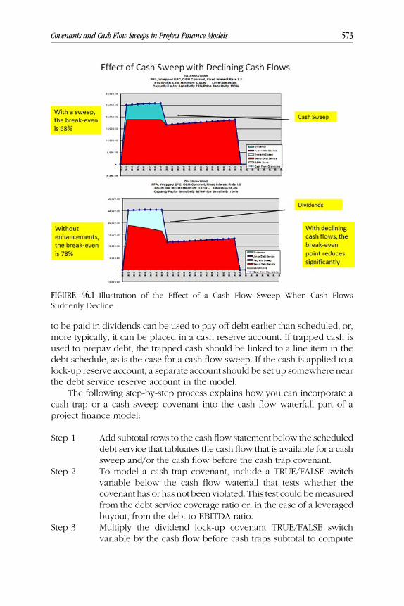
WEBC46 10/03/2014 15:10:15 Page 573

to be paid in dividends can be used to pay off debt earlier than scheduled, or,more typically, it can be placed in a cash reserve account. If trapped cash isused to prepay debt, the trapped cash should be linked to a line item in thedebt schedule, as is the case for a cash flow sweep. If the cash is applied to alock-up reserve account, a separate account should be set up somewhere nearthe debt service reserve account in the model.

The following step-by-step process explains how you can incorporate acash trap or a cash sweep covenant into the cash flow waterfall part of aproject finance model:

Step 1 Add subtotal rows to the cash flow statement below the scheduleddebt service that tabluates the cash flow that is available for a cashsweep and/or the cash flow before the cash trap covenant.

Step 2 To model a cash trap covenant, include a TRUE/FALSE switchvariable below the cash flow waterfall that tests whether thecovenant has or has not been violated. This test could bemeasuredfrom the debt service coverage ratio or, in the case of a leveragedbuyout, from the debt-to-EBITDA ratio.

Step 3 Multiply the dividend lock-up covenant TRUE/FALSE switchvariable by the cash flow before cash traps subtotal to compute

FIGURE 46.1 Illustration of the Effect of a Cash Flow Sweep When Cash FlowsSuddenly Decline

Covenants and Cash Flow Sweeps in Project Finance Models 573

WEBC46 10/03/2014 15:10:16 Page 574

the amount of cash trapped. You could also include a MAXfunction when making the multiplication to make sure thatyou are not trapping negative cash flow.

Step 4 For modeling a cash flow sweep, include a line item that lists thecash flow sweep percentage as a function of the debt-to-EBITDAratio or some other criterion. Put the sweep percentage above orbelow the cash flow statement. This sweep percentage may betied to the debt-to-EBITDA ratio or some other criterion.

Step 5 Multiply the cash sweep percentage by the cash flow beforesweep subtotal in the cash flow waterfall.

Step 6 The cash flow that is trapped or swept and cannot pay dividendsmust go somewhere. It is generally used to prepay debt in thecase of a sweep. If cash is used to pay down debt, then the MINfunction must be used in the cash sweep line to assure that thesweep does not exceed the debt balance. The MIN should test theamount of the sweep relative to the opening debt balance minusthe scheduled debt repayments that have already been accountedfor above the cash sweep in the cash flow waterfall MIN(openingbalance less repayments, subtotal × cash sweep percent). With acash sweep, the scheduled debt repayment must also include a

FIGURE 46.2 Illustration of Connecting Reserve Account to Cash Flow Waterfall inModeling a Cash Trap Covenant

574 Complex Issues

WEBC46 10/03/2014 15:10:17 Page 575

MIN statement relative to the opening balance, because the debtbalance is reduced from the cash flow sweep. To make surenegative cash is not swept, the MAX function should also be usedin the cash sweep equation. Figure 46.2 illustrates how theprocess for covenants or cash flow sweeps links the cash flowstatement to a reserve balance or the debt schedule.

Step 7 In the case of a dividend trap covenant, the cash that is depositedin the lock-up reserve can be released and paid as dividends if thedebt service coverage ratio is above the covenant level. To releasethe cash you can multiply the opening balance of the lock-upreserve by the opposite of the lock-up test, meaning that when thetest is FALSE the dividends can be released. The released cashcomputed as the opening balancemultiplied by the switch shouldthen be included in the cash flow statement. This cash releasedamount can then be linked to the lock-up reserve account.

Covenants and Cash Flow Sweeps in Project Finance Models 575

WEBC46 10/03/2014 15:10:17 Page 576

WEBC47 10/03/2014 15:18:7 Page 577

CHAPTER 47Asset Portfolios, Progress Payments,

and Lease Rolls in RealEstate Models

Real estate analysis and modeling encompass a combination of aspectsfrom both corporate finance and project finance. The financial model of a

hotel project or a commercial building has many similar characteristics toproject finance analysis. These investments move through different stages,revenue contracts are important in risk analysis, and the financial analysis isdriven by cash flows and internal rates of return (IRRs) rather than reportedprofits on the income statement. However, hotels and commercial buildingsdo not have a precise defined life, prospective cash flow analysis relies onrental market history, and the projects are often valued using a flexibleterminal date driven by market multiples—characteristics that resemble cor-porate analysis. Other real estate investments such as residential and com-mercial mixed development projects have more elements in common withcorporate analysis. These mixed developments consist of portfolios thatcontain several individual projects with different cash flow patterns anddifferent risks. Financing is driven by loan-to-value leverage ratios ratherthan cash flow coverage ratios such as the debt service coverage ratio andthe residual values at some terminal date are central to the valuation. Yet theindividual developments that comprise these mixed-use investments dohave similarities to project finance analysis. Their value is defined by stages,IRRs are used rather than net present value of free cash flow, they have nohistoric financial statements, and risks can potentially be mitigated by aseries of contracts.

577

WEBC47 10/03/2014 15:18:7 Page 578

Even though real estate analysis applies modeling concepts from bothcorporate and project finance analysis, there are some unique modeling issuesassociated with real estate models. A few of the issues are the following:

■ Putting together portfolios of real estate projects in which each individualproject has a different start date, holding period, and construction profile.

■ Incorporating dates for components of projects that do not begin at thestart of a quarter or a month as is commonly assumed in project financemodeling.

■ Computing progress payment revenues that may be received fromresidential properties earlier than the dates at which the projects arecompleted and that may depend on alternative marketing strategies.

■ Calculating different spending patterns for capital expenditures known asS-curves that are flexible enough to reflect different construction periodtenors as well as sensitivity analysis with respect to delay.

■ Reflecting a portfolio of revenue lease contracts for commercial buildingsthat have different lease terms, potential idle time periods between newleases, and renewal probabilities.

■ Evaluating the financing of a portfolio of different projects where there isno single defined commercial operation date for the overall bundle ofprojects and where some projects are producing cash flow while otherprojects continue to require financing of capital expenditures.

In explaining how to deal with these complex issues this chapter buildsupon earlier chapters that address project finance models issues related tosetting up project phases and establishing time period switches. The focushere is on features of a real estate model that are different from a projectfinance model. Unique aspects in the structure of real estate models include:

■ In modeling a single project such as a multifamily development or a hotel,the sale of a project after a given holding period is often assumed using amarket multiple and a cap rate.

■ In modeling developments that include a portfolio of different projects,cash flow is normally generated from some projects before construction ofall of the projects is completed. This means that a separate sources anduses of funds analysis or a separate funding cascade analysis is not a goodway to structure models, as it is with project finance analysis.

■ In modeling real estate projects, there are often multiple units andbuildings that are started and completed at different dates. To consolidateprojects with different start and end dates, separate project-by-projecttime lines should generally be established and coordinated with acommon master time line for all projects.

578 Complex Issues

WEBC47 10/03/2014 15:18:7 Page 579

■ In modeling commercial real estate investments, the analysis shouldincorporate the effects of different lease terms with alternative expirydates. Modeling idle time and lease renewals can result in long andnontransparent formulas because revenues are computed on a differentbasis for the initial lease term, subsequent idle periods, prospective fixedleases, and spot market rentals.

■ To model portfolios of investments with start dates and end dates that donot occur at the beginning of the period in the model, a user-definedfunction can be created that yields the percentage of the period the projectis under construction and/or the percentage of the period in which it isbeing operated.

■ In modeling some real estate projects, you may have to incorporatemultiple participating tranches of debt and equity with different returntargets and sharing mechanisms in the cash flow waterfall.

Modeling a Single Real Estate Project

Discussion of real estate financial models in this chapter begins with a singleproject and later puts projects together into a portfolio. Modeling asingle project is similar to modeling a normal project finance investment,with the exception that a holding period is defined after which the project issold. Operating inputs that drive the value of the project include the occu-pancy rate that varies over the life of the project, potentially volatile marketrental rates, occupancy rates that are probably correlated with the rental rates,and fixed and variable operating expenses. Instead of using the total projectlife to measure the operating period as in a typical project finance model, aholding period before which the project is sold applies. Then, as withacquisition models, the project is sold at an assumed exit date. The exitproceeds may be computed through dividing the terminal cash flow by astatistic called the capitalization rate (cap rate).

A cap rate measures the pretax cash flow generated from rental paymentsdivided by the current market value as measured by purchase and salestransactions. It is approximately the same as the inverse of the ratio ofenterprise value to earnings before interest, taxes, depreciation, and amorti-zation (EV/EBITDA). In applying the cap rate in a model, you can create aterminal value TRUE/FALSE switch similar to the switch created for acquisitionand corporate models. The theory behind the cap rate is very similar to theideas underlying computing the terminal value that were discussed in Part 3using the final year cash flow divided by the cost of capital minus the growthrate. Say you believe the growth rate in rents is 2.5 percent and the cap rate is5 percent, then the implied weighted average cost of capital (WACC) is7.5 percent, as shown in the following formula. With a higher growth rate

Asset Portfolios, Progress Payments, and Lease Rolls in Real Estate Models 579

WEBC47 10/03/2014 15:18:7 Page 580

in rental payments, the cap rate should be lower, and if the cash flows are lessrisky, then the cap rate is also reduced.

Cap Rate � WACC � g or WACC � Cap Rate � g

The cap rate and the proceeds from selling a real estate asset can beaffected by some accounting and tax issues. Many purchase and salestransactions occur for real estate investment trusts where there are no taxconsequences. Here, the cap rate and the calculation of WACC are simple. Inother circumstances, when an asset is sold, a capital gain tax can be computedas the sales proceeds less the net book value of the fixed assets. The taxtreatment may have to be accounted for in exit proceeds of a financial modeland the implied WACC from the cap rate formula. If capital allowance or taxdepreciation can be used after the sale of a project, the seller requires higherproceeds and the buyer is willing to pay more for the asset.

Modeling Multiple Projects That Are Part of aCombined Portfolio with Percent of Time Function

One of the challenging aspects of real estate modeling can be to account formultiple projects that are part of a combined portfolio with different construc-tion start dates, construction completion dates and holding periods as well asalternative cash flow generation formulas. When creating such a model, theoccupancy rates, the construction periods, the S-curves, the timing of pro-ceeds from selling residential projects, and other items should be flexible. Theremainder of this chapter addresses various tricky aspects of modeling such areal estate portfolio. An effective way to structure a model with differentprojects in a portfolio is to create a user-defined function that computes thepercentage of a particular period that a project is being constructed andthe percentage of the period that the project is occupied by tenants. Thispercentage of time user-defined function largely replaces the timing switchesin a model. An alternative method discussed at the end of the chapter is to usea combination of the INDEX function and the Data Table tool without the user-defined function. This second approach is analogous to creating scenarios,which is discussed in Chapter 17. No matter what method is used to consoli-date a portfolio of projects, the first essential step is to establish a common timeline that will be used for all projects. This time line should be placed at the topof the spreadsheet page and it does not depend on any individual project. Themodel is structured so that each column of the spreadsheet has the same dateand the projects are placed in different columns to conform to those dates. Youcan then add up all of the items for separate projects in one column to obtain

580 Complex Issues

WEBC47 10/03/2014 15:18:7 Page 581

the aggregate capital expenditure, operating cash flow, and terminal proceedsfor the calendar period defined by the column. This contrasts with manyproject finance models where the start date of the model and the start date ofthe construction or development are the same, and the spreadsheet page isseparated between the precommercial phase and the postcommercial stage.

To model a portfolio of projects you should generally define the key timeperiods for different individual projects. A portion of the input page is shownin Figure 47.1 with various dates. The temporary occupation permit (TOP)date shown for each project is analogous to the commercial operation date inproject finance. In Figure 47.1 the construction start date and the TOP date isnot at the beginning of the period.

The method that can just about be classified as a magic trick to make theportfolio modeling much easier is to create a user-defined function thataccepts the project start and end dates and then uses the master time line onthe top of the page to determine what percentage of each period a project isoperating or under construction. Excel does not have a function thatautomatically does this, and if you tried to make a formula to computethe percent of time a project is in service and is in its last year, it would behorribly long and messy. Instead you can make a user-defined function thatmeasures what percentage of the period a project is in service or underconstruction that accepts four different arguments. Two of the arguments arethe start date and the end date of the master time line with no locked cells

FIGURE 47.1 Excerpt from Input Real Estate Model with Portfolio of Projects

Asset Portfolios, Progress Payments, and Lease Rolls in Real Estate Models 581

WEBC47 10/03/2014 15:18:8 Page 582

(via the F4 key) for the column. The other two inputs are the start and end ofthe project that should have fixed references for the column. Figure 47.2shows how this function works for three different projects where the percentof the period for the start of operation and end of operation are not 100percent. Once you have developed this function, you can use thesepercentages for a lot of other calculations. In Figure 47.2, the start andend dates are included in the special left-hand side columns of the model tomake the process more transparent.

The VBA code for the percent of time function involves setting updifferent techniques to calculate the ratio of time depending on whether aproject has not yet been born, is in the period of birth, is operating, or is in theperiod of its end. The ratio can be computed by using the integer numbers thatdefine the various dates. For periods after the birth period and before the deathperiod, the ratio is defined as 100 percent. The percent of a period function isprogrammed through comparing the beginning and end dates of a project withmaster time line start and end dates. The tricky aspect of this function is to

FIGURE 47.2 Use of Percent of Time Function

582 Complex Issues

WEBC47 10/03/2014 15:18:10 Page 583

compute the portion of the period for the first birth period and the last deathperiod. This function can be useful for many modeling applications other thanreal estate models when key dates do not occur at the exact beginning or endof a period. Construction of the percent of time function is demonstrated inFigure 47.3.

Function percent_of_time(start_operation, end_operation, _

start_of_period, end_of_period)

If start_operation > start_of_period Then

ratio = 0

End If’

’ Partial period at birth of the project’

If start_operation >= start_of_period _

And start_operation < end_of_period Then

ratio = (end_of_period - start_operation) / (end_of_period - _

start_of_period + 1)

End If’

’ Full period when the ratio is 1.0’

If start_operation <= start_of_period And end_operation > end_of_period Then

ratio = 1

End If’

’ Partial period at end’

If end_operation >= start_of_period And end_operation <= end_of_period Then

ratio = (end_operation - start_of_period) / (end_of_period - _

start_of_period + 1)

End If

’

’ After the death of the project’

If end_operation < start_of_period Then

ratio = 0

End If

percent_of_time = ratio ’ definition of the function

End Function

FIGURE 47.3 Code for Percent of Time Function

Asset Portfolios, Progress Payments, and Lease Rolls in Real Estate Models 583

WEBC47 10/03/2014 15:18:10 Page 584

In addition to the percent of time function, a couple of other user-definedfunctions can be helpful in creating a project portfolio. Two functions that canmake the modeling process much easier include:

1. A function that computes the TOP date of a project given the S-curve. Thisallows you to enter different S-curve arrays, and then automatically derivedifferent TOP dates. If you use a different S-curve and keep the construc-tion start date the same, the TOP date changes, which in turn is used todetermine the operational revenues. This function adds the number ofperiods defined in the S-curve to the start of construction date so that youcan use the percent of time user-defined function.

2. A function that computes the revenue received for a residential projectgiven a combined progress payment schedule and a sales or marketingschedule. This problem involves workingwith two different series of dates,one for the progress payment and another for the marketing schedule.Some projects may receive the whole series of progress payments, andother residential projects that are sold later receive the revenues duringsubsequent periods and must accumulate the payments that were sched-uled. The function should allow you to enter different marketing andprogress payment scenarios and see how the revenue changes.

Modeling a Portfolio with the INDEX Function andData Table Tools

The second method that can be used to create a portfolio is to combine theINDEX function with the Data Table tool. This method involves developing atemplate model for one project that is flexible enough to compute theoperating cash flow, capital expenditures, and depreciation expense foreach separate project. The template should be designed to accept any oneof the projects, much like a regular financial model can accept differentscenarios. To implement the technique, each project is assigned a codenumber, much like the way a master scenario page works.

To use this second method, you should set up a project assumption tablewhere inputs to all of the projects are structured in a consistent manner.When making a template that can accept inputs for each individual project,you can use the INDEX function along with a code number that defines theindividual project in the portfolio. In the example shown in Figure 47.4, theINDEX function is used to define the construction cost, the sale price,the construction profile, and the time periods from the project code number.If the inputs are set up in a structured manner, the amounts can be extractedfor each separate project through defining a row and column number withthe INDEX function.

584 Complex Issues

WEBC47 10/03/2014 15:18:10 Page 585

Using the master time line you can compute a period code in the templatemodel. This is accomplished through comparing the commercial operationdate with the common start date in the master time line. If the inputs in theexample in Figure 47.4 are used, the period codes are different for the firstproject and the second project—there would be a larger negative number forthe project with the further-out date.

The manner in which the template model for individual components ofthe portfolio can be set up is illustrated in Figure 47.5. The top part of the figurelists the code number for the project that is an input like the master scenarionumber discussed in Chapter 17. With the project code number entered, aseries of INDEX functions is used to establish inputs for the template model. InFigure 47.4, another code number is used to define the S-curve table that inturn is used to compute construction expenditures as a function of the timeperiod counter. After the S-curve code number extracted, the S-curve can beestablished by using a LOOKUP function.

Once the cash flow model for a single project is developed, various seriesfrom the individual projects should be aggregated for creating a financialmodel. As usual, the EBITDA, capital expenditures, working capital changes,and depreciation are the items needed to establish free cash flow and beginthe financing aspects of the model. The aggregation can be automated bycreating a one-way data table with the Data Table tool using the code numberas the column input. To see how the process of using the INDEX and DataTable works in construction a portfolio of projects, assume that the commonstart date of the master time line is January 1, 2014, and that there are two

FIGURE 47.4 Illustration of Setup for Project Portfolio Using the INDEX and Data Table Method forConsolidation

Asset Portfolios, Progress Payments, and Lease Rolls in Real Estate Models 585

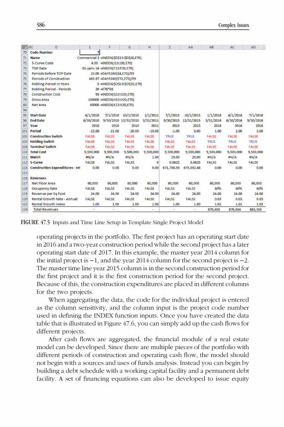
WEBC47 10/03/2014 15:18:10 Page 586

operating projects in the portfolio. The first project has an operating start datein 2016 and a two-year construction period while the second project has a lateroperating start date of 2017. In this example, the master year 2014 column forthe initial project is �1, and the year 2014 column for the second project is �2.The master time line year 2015 column is in the second construction period forthe first project and it is the first construction period for the second project.Because of this, the construction expenditures are placed in different columnsfor the two projects.

When aggregating the data, the code for the individual project is enteredas the column sensitivity, and the column input is the project code numberused in defining the INDEX function inputs. Once you have created the datatable that is illustrated in Figure 47.6, you can simply add up the cash flows fordifferent projects.

After cash flows are aggregated, the financial module of a real estatemodel can be developed. Since there are multiple pieces of the portfolio withdifferent periods of construction and operating cash flow, the model shouldnot begin with a sources and uses of funds analysis. Instead you can begin bybuilding a debt schedule with a working capital facility and a permanent debtfacility. A set of financing equations can also be developed to issue equity

FIGURE 47.5 Inputs and Time Line Setup in Template Single Project Model

586 Complex Issues

WEBC47 10/03/2014 15:18:11 Page 587

before or after the issuance of debt, as discussed in the context of projectfinance funding in Chapter 40. As usual, methods to develop the debt scheduleand a cash flow statement with a waterfall involve structuring the cash flowstatement and using the MIN and MAX functions and making a lot of subtotals.It is hoped that you can see that even if these waterfall techniques may look abit different in different models, they all have a similar skeleton.

In some real estate projects cash flow is generated from receiving progresspayments before construction is complete. This cash that is generated fromselling a project reduces the need for additional debt. If the proceeds are morethan the total amount of debt required, the cash can be deposited into areserve account. If there is money in this cash reserve account and futurefinancing needs occur, then the reserve account is used for those future cashneeds. If there is no debt left, then dividends can be distributed in ananalogous manner to a cash flow sweep. This cash process can be modeledin a similar manner to the cash build-up technique that is described in astandard corporate model in Chapter 38, where deficit cash flow is funded byraising new debt, and surplus cash goes to retiring cash and/or reducing debt.

FIGURE 47.6 Illustration of Using the Data Table Tool to Aggregate Individual Projects in a Portfolio

Asset Portfolios, Progress Payments, and Lease Rolls in Real Estate Models 587

WEBC47 10/03/2014 15:18:12 Page 588

3GBABOUT 09/29/2014 9:35:55 Page dlxxxix

About the Author

EdwardBodmer provides financial and economic consulting services to avariety of clients, and he teaches professional development courses in an

assortment of modeling topics (project finance, mergers and acquisitions,renewable energy, and electric power). He is passionate about teaching inAfrica, South America, Asia, and Europe, and much of the unique modelinghe has developed has arisen from discussions with participants in his courses.Mr. Bodmer’s consulting activities include developing complex projectfinance, corporate finance, and simulationmodels; providing expert testimonyand analysis on financial and economic issues before regulatory agencies; andadvisory services to support merger and acquisition projects. In addition, hehas been involved in formulating significant government policy related toelectricity deregulation and energy efficiency; he has prepared models andanalyses for the Asian Development Bank, Argonne National Laboratory, andthe city of Chicago; he has evaluated energy purchasing decisions for manycorporations; and he has provided advice on corporate strategy. Mr. Bodmerhas taught customized courses for MIT’s Sloan Business School, Shell Oil,Gasprom Bank, Capitaland, DBS, Society General, General Electric, HSBC,Citibank, CIMB, Lindlakers, HSBC, Saudi Aramco, and many other financial,energy, and industrial clients.

Mr. Bodmer was formerly vice president at the First National Bank ofChicago and president of the Energy Exchange of Chicago. He received a BScin finance from the University of Illinois and an MBA in econometrics from theUniversity of Chicago. He has authored many articles and is in the process ofcompleting a second text on valuation theory. Mr. Bodmer was born inManchester, England, and has lived in Switzerland, the United Kingdom,and the United States. Further information about his work and uniqueanalytical approaches to different issues are described on the website,www.wiley.com/go/internationalvaluation.

589

3GBABOUT 09/29/2014 9:35:55 Page dxc

3GBWEB 09/29/2014 10:6:13 Page 591

About the Website

This book includes a companion website, which can be found at www.wiley.com/go/internationalvaluation (password: bodmer123). This site

includes hundreds of exercises, model examples, and case studies and isintegral to the book. It contains hundreds of customized exercises; manytemplate project finance, corporate finance, and acquisition models; and anumber of featured completed models of business enterprises in a widevariety of industries. In addition, you can download special utilities to readPDF files into Excel, to make automated waterfall charts, to automatically colorcells linked to different sheets, to create a table of contents with hyperlinks,and much more.

Exercises and complete models are arranged by chapter, meaning thatyou can follow along the discussion in each chapter with different Excelfiles. You can also see how the principles are applied in actual situations.Upon opening each file, you will find a link to a video that explains themodeling process.

591

3GBWEB 09/29/2014 10:6:13 Page 592

3GBINDEX 09/29/2014 11:5:35 Page 593

Index

Accretion and dilution, 156, 349Accumulating periodic data, 167–72automatically adjusting formulas, 167–72balance sheet accounts, 167detailed sheet, 167–72fiscal month switch, 168income statement items, 167quarterly counter, 168quarterly summary report, 167–72

Acquiring PDF data, 28Acquisition model phasesacquisition period, 71alternative holding periods, 71exit period, 71–72optimal period, 71

Acquisition model structurecash flow priorities, 36exit values, 30–33goodwill analysis, 30–33holding period, 35pro forma balance sheet, 30–33sources and uses, 35

Aggregate test, 52ALT and F1, 28, 175, 176Annual page, 73–84Annuity and equal installment repaymentstax effects, 542

Arrange all option, 216Array variable, 53, 95, 96, 97, 191Asset retirementsfull life cycle of plant, 100gross plant balance, 101new growth, 100percent of depreciation, 99–109true cash flow, 100

Automatic except data tables, 194, 198

Back-of-the-envelope models, 15, 16Bad programming practice, 41–54

auditing processes, 41inputs as part of a formula, 41–54

Balance sheet test, 17–41Benchmarking and regression of multiples, 453–61

implied cost of capital, 453regression analysis and offset function, 458

Bond cash account, 514Break-even analysis, 185–205

corporate finance, 191debt service coverage ratio, 186deriving the break-even point, 185–205forecasting commodity prices, 185–205Goal Seek, 185–205

IRR on senior debt, 185–205Bridge between equity value and enterprise valueanalogy to invested capital segregation, 322and weighted average cost of capital, 322use of market value, 321

Brownianmotion, 279, 280, 281, 287, 296, 297, 299

Cap exp to depreciation, 379–84and implied EV/EBITDA, 447net plant depreciation formula, 381nominal current currency, 379and plant age, 380stabalization, 384

Capital asset pricing model, 207, 347, 348failed, 14, 114

Capital asset simulation, 383Capitalizing debt, 37Cap rate, 578, 579, 580Cash flow available for debt service, 173,

189, 190, 493, 499, 516, 519, 526, 542,545, 550

Cash flow sweep. See Debt and cash waterfallChanges in growth rates, 311Churchill, Winston, 21, 149, 357Circular logic philosophy, 465Circular reference and cash sweep, 464–81algebraic method, 477average interest expense, 465interest on average debt balance, 470problems with iteration button, 471use of opening debt balance, 467

Circular reference five methods, 468–75algebra, 469benefits of user-defined function, 480iterative calculation button, 468solver, 470user-defined function, 469

Circular references in corporate model, 483–89Circular refernce, user-defined function methoduse of fx icon, 482

Code number, 55–67Color conventionsf5 key, 47, 48

Commitment fee, 69, 116, 466, 507, 509, 547Commodity prices, 5, 56, 186, 211, 284,

287, 298Comparative multiplessamples, 436tax rate differences, 437

Comparing history with projection, 90Conditional formatting, 60, 65, 66, 76, 199, 200, 236,

237, 332, 374. See Long-term proof

593

3GBINDEX 09/29/2014 11:5:36 Page 594

Copy and paste macros, 49, 194, 227, 467, 469, 492,505, 539, 551

Corporate debt analysisbullet payment, 116circular reference, 115credit enhancements, 120

Corporate model structureanalysis of history, 21–25historical balance sheets, 23return on invested capital, 21–25summary page, 21–25terminal valuation, 21–25

Corporate valuation issuesbridge enterprise value and equity value, 308cost of capital, 307–12earned returns, 308indefnite life, 308sustainable growth rate, 307–12terminal value, 307–12

Correlated variables, 290, 292CorrelationCholesky factors, 290, 291

Cost of capital building blocks, 439Country risk premium, 309Covenants and cash flow sweeps, 571–76limitations on payment of dividends, 571lockup cash reserve account, 571volatility of the cash flow, 572

Credit enhancements, 9, 113, 120, 493, 569, 571, 572Credit support, 508Custom scenario, 184, 211, 213, 223, 224, 226, 227,

228, 242attach spinner, 223combo box, 223VBA, 227

Customized exercises, 10

Data table, 72, 129, 193–98, 248, 249, 250, 251, 252,275, 385, 455, 473, 479, 564, 580, 584, 585, 586,587

bad aspects, 193column input, 196, 197, 198, 202, 204, 212, 220,

238, 244, 249, 585, 586one-way, 193, 194, 196, 197, 198, 199, 200, 201,

202, 212, 219, 220, 585output variable, 185–205row input, 196, 197, 198, 202, 203, 204, 212, 244,

249same sheet as the input variable, 194sensitivity range, 185–205sensitivity variables, 194, 195, 197, 198, 200, 203,

244top left corner, 185–205two-way, 194, 195, 196, 197, 201, 202, 204, 242,

243, 244, 245, 247, 248, 249upper left-hand cell blank, 201

DCF model, timing, 363–67(1+WACC)^.5, 364compound index, 366compound index and SUMPRODUCT, 366mid-year assumption, 363theoretical long-term model, 363varying WACC, 365

Debt analysis, 113–30

cash flow waterfalls, 113–30credit spreads, 113–30debt schedule, 114interest rates and fees, 113repayment structure, 113size of debt, 113tenor of debt, 113–30

Debt and cash waterfallcovenant, 120debt defaults, 119–30five-step process, 121hydroelectric plants, 120IRR realized by lenders, 125linking debt schedule, 124priorities of cash flow, 123probability of loss, 125remaining available usage, 122revolving credit, 119–30subtotal accounts, 123subtotals, 120test for positive, 119–30total commitment, 122

Debt corporate analysiscash account, 117cash minus short-term debt, 118connect the balance sheet, 115–18connecting debt to cash flow, 115–18connection of cash flow and debt balances, 118end of the cash flow statement, 115–18negative or positive, 118net cash account, 117net changes in cash, 119split up the cash account, 115–18

Debt IRR, 36, 125, 127Debt repayment switch, 522, 557, 558,

561, 562Debt sculpting, 515–37closing balance of the debt, 517solver method, 516, 517–19

Debt service coverage ratio, 30, 32, 39, 152, 165, 174,186, 187, 189, 190, 191, 192, 193, 194, 196, 199,200, 209, 219, 221, 257, 278, 491, 493, 497, 499,500, 521. See Sensitivity analysis

tail, 189, 190, 191, 255Debt service reserve account, 10, 33, 120, 127, 466,

494, 504, 516, 530, 547–53, 547, 548, 549–51,550, 552, 565, 571, 573. See Debt and cashwaterfall

circularity problem, 548cost to sponsor, 547separating construction debt from permanent debt,548

Deferred taxes, 24, 25, 399–406, 400, 401, 404,405, 415, 427, 446, 448, 449, 451. See Investedcapital

Deferred taxes and deprecation, 91–112adjusting the tax basis, 91–112

Deferred tax to cap exp ratio, 401–5simulation, 402stabalization, 401

Delevering and then relevering the beta, 309Demand-driven model, 56, 57, 58Depreciationasset retirements, 92–112

594 Index

3GBINDEX 09/29/2014 11:5:37 Page 595

depreciation and free cash flow, 92–112depreciation rate, 95

Depreciation and acquisition, 91–112purchase of assets, 91–112purchase of shares of stock, 91–112stock transaction, 111, 112

Depreciation methodsaccumulated depreciation ratio, 92–112accumulated depreciation to net plant, 104direct model of retirements, 107gross plant method, 92–112implicit retirement rate, 92–112net plant method, 105overstatement of depreciation, 104prospective retirements, 92–112

Depreciation vintageage matrix, 94–99depreciation function, 94–99depreciation table, 94–99tax depreciation, 94–99year born, 94–99

Deterministic models, 15, 263Developer tab, 177, 214, 246Drop-down box, 26, 42, 176, 177, 185, 211, 214, 215,

216, 222, 225, 227, 229, 246, 282, 316, 317, 318windshield-wiper method, 214, 215

DSRA and cash sweep, 552Dynamic Goal Seek, 542Dynamic graphs, 179, 181#n/a symbol, 179, 180, 559flexible range name, 458flexible range name with offset, 181

Dynamic range names, 182, 183offset function, 183replace the range, 183

End of quarter, 77, 169. See Accumulating periodicdata

End of the quarter function, 74Enterprise valueworking capital only case, 429

Equilibrium growth rate, 67–84Equity cash flowand DCF, 435dividend priority, 134earn-out provisions, 131flip structure, 135funding percentages, 134highest priority investor, 132IRR target, 131–38new equity issues, 119–30, 131–38priorities on free cash flow, 131–38ratchets, 131–38tax equity, 135tracking account, 132trigger mechanism, 132yield tracking, 133

Equity consideration, 37, 326Equity kickers, 37, 132Estimating mean reversion, 295–304

changes in price and past prices, 299historical volatilities for different time periods, 303inspect the simulated volatility, 303regression equation, 298

VBA code, 302volatilityon a monthly and annual bais, 301

Estimating volatility, 295–304annual, 295–304annualization adjustments, 295–304annual time series data, 295–304discrete and continual compounding, 297square root of time periods, 296standard deviation of annual percent changes,295–304

standard deviation of price changes, 295–304user-defined function, 297

Eurotunnel, 5, 7, 161, 165, 186

Financial institution, 18, 20, 92Financial statement analysis, 21–25Financial statements, 139–46balance sheet, 146cash flow statement, 144collecting closing balances, 146earnings per share, 139end of the cash flow statement, 145equity balance account, 146indirect cash flow method, 144minority shareholders, 139–46profit and loss statement, 139–46tax schedule, 140

Fitch Ratings agency, 210Fixed and variable costs, 7, 24, 87Flip IRR, 133. See Equity cash flowFree cash flow and equity cash flow, 313–20Frequency distributionsbins, 273increments, 273minimum value, 275

FunctionsAVERAGEIF, 79, 167, 170CHOOSE, 62, 63, 64, 152, 177, 246COUNTIF, 110DAYS360, 72EDATE, 74EOMONTH, 74, 75, 77, 169FREQUENCY, 272, 273, 274, 275, 281, 282, 315HLOOKUP, 42, 60INDEX, 26, 28, 42, 62, 63, 64, 65, 71, 80, 82, 83, 88,89, 95, 96, 199, 200, 203, 211, 212, 213, 214, 215,216, 217, 218, 221, 222, 224, 228, 234, 238, 239,240, 241, 242, 243, 244, 245, 246, 248, 267, 282,283, 317, 318, 333, 366, 392, 440, 456

INDIRECT, 118, 144, 171, 172, 173, 224, 324, 325,327, 335, 410, 412, 442, 457, 469

ISBLANK, 317ISNUMBER, 560, 561LOOKUP, 42, 59, 60, 63, 64, 94, 95, 96MATCH, 26, 28, 42, 71, 82, 83, 180, 199, 200, 239,240, 241, 245, 333, 412

MOD, 556, 558NORMDIST, 258, 259, 260, 261, 281, 282, 283NORMINV, 259, 260NORMSINV, 261, 262, 270, 271, 287, 289, 290, 291NPV, 152, 182, 191, 329, 331, 332, 333, 363, 364,366

OFFSET, 100, 141, 143, 179, 180, 181, 182, 183,342, 345, 381, 382, 458, 459, 557, 558

Index 595

3GBINDEX 09/29/2014 11:5:38 Page 596

Functions (Continued )RAND(), 262, 270, 271, 287, 289, 290ROUND, 52, 318, 394ROUNDUP, 168SMALL, 231–52SUMIF, 42, 51, 53, 77, 81, 117, 167, 168, 169, 170,

171, 172, 173SUMIFS, 77, 167, 168, 169, 170, 171, 173SUMPRODUCT, 34, 42, 267, 324, 366, 367, 440TRANSPOSE, 95, 96, 228, 234, 235, 236, 237, 238,

242, 274, 411, 457, 475VLOOKUP, 28, 42, 60

Funding from bonds, 514remaining funding needs, 514

Funding techniques in project finance, 497–514lending philosophy, 497

Funding with equity first, 508–13backward induction, 510circular logic problems, 509funding cascade, 508user-defined function, 513

General Electric, 8Generic.bas, 51Global financial crisis, 3Goal Seek, 49, 101, 102, 103, 108, 114, 136, 137, 193,

201, 260, 302, 386, 392, 438, 453, 454, 455, 468,469, 479, 487, 493, 496, 498, 502, 503, 516, 517,519, 521, 539, 541, 542, 543, 545

automation, 102convergence, 101, 102, 355, 415, 423, 479, 480,

489, 506, 533, 545flexible function, 101initial base, 103smaller increments, 101step increments, 101, 102, 108, 103, 387

Graph of inputs and outputs, 317minimum y-scale, 318

Graph titles, 178, 179combining text and numbers on a graph, 179multiple rows, 34, 179

Graphs with ALT and F1, 174, 249Graphs with F11 key, 173, 174, 175, 176, 183, 201,

238, 248, 261, 274, 282, 318, 518delete the title of the x-axis, 176no title for the row, 176x-y charts, 176

Gross plant depreciation rate, 381, 385, 391

HISTORIC switch, 79add another period, 79closing balance, 78–83last historical balance sheet, 80plant balance, 78–83presentation of assumptions, 80

Historic TRUE/FALSE, 67–84

Implied EV/EBITDA ratio, 445–51changing growth, returns, and cost of capital,

446comparison with value driver formula, 451complex function, 448constant growth case, 446growth, return, and cost of capital, 445

transition factors, 451user-defined functions, 447

Implied P/E ratio, 435–43smaller value range, 436user-defined function, 438

Incorporating defaults, 125Indirect financing perspective, 323INDIRECT function. See Reading from InternetInflation analysisinflation indexes, 88–90inflation start, 89overcompounding, 89periodic inflation, 89real level of costs, 88–90varying inflation rates, 88–90

Integrated merger model structuregoodwill, 37–38pro forma balance sheet, 37–38sources and uses of funds, 37–38target company, 37–38

Internal rate of return, 90, 254, 316Invested capitaland acquisition analysis, 326and notes receivable, 327and surplus cash, 328associated investments, 322equality of approaches, 324using flags, 324

Invested capital calculation, 321–36dissecting the balance sheet, 321

Invested capital, complex, 337–46deferred taxes, 338derivative liabilities, 344net operating loss, 340operating cash, 341tax depreciation, 338

IRR and ROI, 30–33IRR problemsdistant future years, 31probability of realizing success, 30–33reinvestment, 30–33

Iteration button, 468, 470, 471, 472, 475–476, 477,487, 502, 503

Iterative loop, 508Iteration loop for circular reference, 469, 489, 503,

532, 533, 545

J-curve, 71, 72

Letter of credit, 122, 123, 124, 547, 565Levelized cost of electricity, 390Leveraged buyout, 14, 37, 114Loan life coverage ratio, 13, 32, 190, 191, 192, 194,

196, 199, 209, 219, 221, 233, 278, 524Long-Term Capital Management, 153–54

business judgment, 153–54mathematical models, 153–54mathematical relationships, 153–54

Long-term proof, 329–35bridge between enterprise value and equity value,332

explicit switch, 333free cash flow, 334terminal switch, 330

596 Index

3GBINDEX 09/29/2014 11:5:39 Page 597

true cash flow, 330valuation year, 329

Loss on debt, 124, 125, 129, 189

Maintenance reserve account, 555–62and debt repayment, 561constant time period increments, 557cost to sponsors, 555maintenance switch, 556, 561varying expeditures, 558varying time increments, 559

Making your own shortcut, 44–51SHIFT keyboard key, 44–51SHIFT, CNTL, C, 44–51

Market-to-book value, 409–14and cost of capital, 409–14measuring cost of capital, 413

Mean reversion estimatesstandard error of the regression, 298, 299, 300

Merton, Robert, 153Miller and Modigliani, 17, 18, 91, 207, 347Miller, Merton, 17, 18MIN and MAX, 43, 120, 123, 124, 125, 141, 144, 285,

485, 489, 572, 587Minimum DSCR, 541Model assumptionsdanger of overcapacity, 55–67excessive new supply, 57industry demand, supply, and price, 56industry-wide surplus capacity, 57, 59long-run marginal cost, 59marginal cost, 56market share, 59powerhouse companies, 57value drivers, 55–67variable and fixed costs, 57

Model inputscapital expenditures, 55–67financing assumptions, 55–67input categories, 55–67input section, 55–67revenue assumptions, 55–67scalars, 55–67timing assumptions, 55–67working capital assumptions, 55–67

Model objectives, 13–16financing structure, 13–16risk analysis, 13–16

Model structurefree cash flow, 17–41indefinite life, 19internal rate of return, 16, 19, 30, 33, 34, 61, 91,

128, 131, 165, 178, 209, 264, 268, 492, 508, 563return on investment, 19starting point, 17terminal value, 17–41

Modified IRR, 267, 268Monte Carlo simulation, 11, 147, 151, 152, 154, 205,

255, 256, 263, 264, 265, 266, 268, 271, 274, 275,278, 288, 290, 292, 293, 303

Named range, 203Nested if statements, 42, 51Net operating loss, 140–43

balance of the net operating loss, 140–43converting negative numbers, 141intangible amortization, 140loss carryforward, 140–43permanent differences, 140statutory tax rate, 141taxes in previous periods, 140–43taxes per the tax return, 142

Net plant depreciation rate, 93, 105, 106, 380, 381,384, 385, 386, 397, 401, 446. See Depreciationmethods

and plant age, 381life cycle of plant, 382

New economy, 7NOL expiration, 140–43accumulated expired, 143look backward, 143

NOPAT, 315, 316, 322, 338, 340, 349, 352, 416, 425,426, 428, 429, 433, 446, 447, 448, 451

Normal distribution, 255, 257, 258, 259, 260, 261, 266,270, 271, 277, 279, 280, 281, 282, 283, 284, 287,290, 291, 292

Normalized capital expenditure, 377–98asset replacement, 379changing growth, 388four different normalization approaches, 395ratio of accumulated depreciation, 387theoretical long-term analysis, 378user-defined function, 377–98

Normalized cash flow, incorporating in model, 375Normalized cash flows, 310Normalized deferred tax, 399–406book and tax depreciation, 400existing and new plant, 400tax rates, 404

Normalized working capital, 369–76long-term proof, 372support of EBIDTA growth, 370working capital formula, 373

Oligopolistic industries, 6One-year p90, 208Option buttons, 246

P/E and EV/EBITDA reconciliation, 439Payment-in-kind debt, 133PDF file. See Acquiring PDF dataPercent of time function, 581–85Powerhouse square, 153Pretax analysiscost of new capacity, 87historical analysis, 87production capacity, 85transparent calculations, 85working capital changes, 84–90

Price boundaries, 151, 152, 277, 285, 288, 295, 296Probabilistic risk analysis, 253–62

mean reversion, 255problems, 254questions answered, 254stochastic diffusion process, 254time series equations, 253–62

Probability distribution, 15, 150, 151, 210, 254, 257,266, 277, 278, 281

Index 597

3GBINDEX 09/29/2014 11:5:40 Page 598

Probability of default, 14Product life cycle, 409Programmingauditing tools, 41–54balance sheet item, 43include the units, 42separate modules, 41–54specify the time period, 42time line at the top, 42

Project feasiblity, 90Project finance analysisconsulting studies, 19, 185, 564, 565development phase, 563development stage, 564different stages, 563–70risk changes, 563, 565, 567–568, 569

Project finance model structurerisk changes, 30sources and uses of funds, 30–33

Project IRR, 19, 32, 39, 61, 90, 91, 114, 128, 129, 264,265, 268, 275, 314, 319, 325, 557, 566, 567–568

Project life coverage ratio, 189, 190, 191, 192, 193,194, 195, 196, 199, 209, 211, 219, 221, 278, 524

Project phasescommercial operation date, 69construction period, 69–70delay in construction, 69–70development period, 69–70financial close, 69–70period code, 69–70phases, 69–70

Pro-rata funding with debt leverage, 501–6Goal Seek, 504iteration button, 502

Pro-rata funding and interest paid, 500–502Pro-rata funding with leverage ratiouser-defined function method, 506

Random walk process, 269, 272, 279, 286, 296Range names, 41, 103, 138, 171, 172, 173, 180, 181, 182,

183, 184, 201, 202, 221, 222, 227, 458, 459, 541Reading from Internetcopy and paste to new sheets, 409–14INDIRECT function, 171INDIRET and MATCH functions, 412splitting URL, 410

Reading from Internet and INDIRECT function, 457Reading from Internet with WORKBOOKS.OPEN,

283, 410, 411, 442, 456, 457, 458Real estate analysis, 577–87

idle time, 578, 579multifamily development, 578occupancy date, 10, 34, 43, 46, 49, 51, 57, 65, 72,

79, 94, 95, 96, 97, 120, 121, 123, 137, 156, 176,177, 178, 194, 195, 196, 197, 208, 209, 212, 232,233, 238, 242, 243, 250, 280, 292, 316, 360, 436,459, 473, 510, 517, 549, 550, 580, 581, 584, 585

occupancy rate, 579portfolio, 581–85progress payment, 578, 584project-by-project time lines, 578similarities to corporate and project finance, 578unique modeling issues, 578

Real estate models, 20, 86

Real estate timing, 581–85common time line, 580commpn start date, 585

Real estate, time varying inputs, 62Record a macro, 46, 519Refinancing, 563–70mechanics of implementing, 568sources and uses, 570time switches, 568uncertainties, 566user-defined function for sizing, 569

Relative valuation, 347, 349, 437Resource studies, 162Return on invested capital, 313–20all-in cost of debt, 315associated investments, 322driver of value, 313economic fundamentals, 313impairment of plant, 319involved in producing ebitda, 321management performance, 314reasonable assumptions, 319sanity check, 319

Return on investmentgoodwill, 320and project IRR, 319

Revolving debt facilities, 37Risk allocation matrix, 159–64acceptable risk, 160categorizing risks, 159liquidated damage, 162mitigation by contracts, 159–64probability weight, 159–64small risks that explode, 159unmitigated risk, 159–64

Risk analysisbreak even, 152business judgment, 149–58capture risk in single number, 150mathematical risk analysis, 149–58risk manager, 151statistical analysis, 149–58

Risk assessment, 149–58uncertainty in assumptions, 149–58

ROIC and cost of capital, 407–14converging in long-run, 413implicit assumption, 407myth of convergence, 408value creation, 407

Scenario analysis, 207–30assessing downsides, 207–30counter, 219custom scenario case, 207–30downside case, 207–30driver row, 214, 216, 224infer equity risk, 207–30master scenario page, 211optimism bias, 209scenario manager tool, 211scenario number, 63, 212, 213, 214, 215, 216, 220,227, 238, 242, 244, 248, 585

Scenario code number, 63, 64, 212, 227, 242, 248, 249Scholes, Myron, 153

598 Index

3GBINDEX 09/29/2014 11:5:40 Page 599

S-curve, 32, 61, 86, 87, 494, 578, 580, 584, 585Weibull distribution, 87

Sensitivity analysis, 165–84converting periodic data, 165–84effective presentation, 165–84sensitivity graphs, 167–72

Share exchange, 38SHIFT, CNTL, ENTER, 42, 95, 99, 190, 235, 236, 274,

281Shortcuts, 28, 44, 45, 49, 51, 174, 182ALT, F11, 50, 53, 474, 541CNTL and SPACEBAR, 169CNTL, Down Arrow, 46, 236CNTL, PAGEDN, 216CNTL, PAGEUP, 216CNTL, R, 45, 236, 272, 275CNTL, SPACEBAR, 46F4, 64, 66, 76, 96, 169, 170, 214, 236, 238, 241, 243,541, 581

F9, 198, 200, 204, 278SHIFT and F11, 248SHIFT and F9 keys, 198, 200SHIFT and SPACEBAR, 169SHIFT, ALT,®, 46, 49, 250, 331SHIFT, CNTL,®, 45, 46, 272SHIFT, CNTL, 1, 45SHIFT, CNTL, 3, 45SHIFT, CNTL, 4, 45SHIFT, CNTL, 5, 45, 46SHIFT, CNTL, ENTER, 191, 235SHIFT, CNTL, F3, 203, 222, 541SHIFT, CNTL,®, 236

Slider bar, 177Solver, 136, 137, 138, 468, 469, 472, 473, 475add-in, 137adding a macro, 138and Goal Seek, 136

Solver with macro, 519Source of the circular reference, 495, 499Special purpose vehicle, 30Spider charts, 231–52Spider diagrams, 246–50level of potential variation, 246–50sensitivity factors, 248x-axis, 250

Spinner button, 167, 174, 176, 177, 178, 179, 184,193, 200, 209, 211, 212, 214, 215, 220, 221, 223,224, 225, 226, 227, 229, 246, 473, 475, 492, 541,542

cell link, 177, 178, 212, 214, 215, 223, 224, 226,227, 246, 282

combined with scenario analysis, 184intermediate number, 224multipliers, 224, 225two-step process, 224windshield wiper, 178, 200

Spreadsheet structurecolor conventions, 44–51grouping, 44–51special columns, 44–51thin columns, 44–51time line section, 44–51verification checks, 44–51

Stand-alone corporate models, 40

Standard deviation, 253–62Stochastic analysis, 263–76creating a time series equation, 263–76drawing random numbers, 266multiple random draws, 275one-column financial model, 266required credit spread, 264standard normal value, 263–76time series equation, 266

Stochastic models, 15, 16, 263Structure of project finance modeldebt service coverage ratio, 30–33lender perspective, 30–33postoperation phase, 30–33preoperation phase, 31Project IRR, 33refinancing, 11, 31, 32, 33, 163, 191, 491, 492, 494,496, 522, 571

Subordinated debt, 32, 33, 39, 119, 120, 127, 128,129, 132, 166, 167, 186, 188, 193, 265, 266, 267,268, 273, 497, 548, 571

Subprime loans, 7, 14, 45Summary sources and uses of funds, 502, 503, 504,

510Supply-driven model, 56Synergies, 19, 38, 40

Target capital structure, 136–38financial institution model, 136new equity issues, 136–38share buybacks, 136–38target debt to capital ratio, 136

Template models, 10Terminal growth rate, 357–68compromise philosophy, 358eliminating unreasonable assumptions, 357survivorship bias, 359transition to equilibrium, 359

Terminal value methods, 347–56dependence on the weighted average cost ofcapital, 348

EV/EBITA multiple, 353predicting growth, 350–51stable growth method, 350–51value drivers, 351–53wide ranges of value, 347–56

Text to columns, 29Time line, 67–84explicit period, 67–84fade period, 67–84TRUE/FALSE switches, 67–84

Time line mechanicsage variable, 73–84daylight savings time, 74periods per year, 73–84quarterly models, 74semiannual basis, 73–84start date andend date, 73–84TRUE/FALSE switch, 73–84

Time series analysischanges in stock prices, 283continual growth, 277–94correlation coefficient, 290long-run equilibrium, 277–94

Index 599

3GBINDEX 09/29/2014 11:5:46 Page 600

Time series analysis (Continued )mean reversion, 277–94nonstationary, 279, 287

Time series models, 277–94correlations, 277–94mean reversion, 277–94

Tornado diagram with two-way table, 231–52variable code number, 243

Tornado diagrams, 231–52creating, 234diagonal pattern, 236new scenario rows, 234sensitivity row titles, 235sorting, 238sort key, 241

Traffic studies, 5, 19, 255Transition period, 360–62compound growth rate, 360, 361switch variables, 360transition years plus 1, 361

TRUE/FALSE logical variable, 52TRUE/FALSE switch, 51, 117, 170, 243, 244, 248, 324,

329, 511, 514, 524, 549, 551, 555, 556, 559, 564,568, 573, 579

TRUE/FALSE test, 53, 146, 242, 243, 244, 248

Up-front fees, 507User-defined array function, 96, 182, 274, 275, 533REDIM statement, 96, 97two-dimensioned array, 98VARIANT, 96, 97, 403, 533, 535

User-defined function method for circular reference,479, 487, 532

User-defined functions, 44–51add_text, 54basic concepts, 44–51find_base, 102, 111, 392, 394function sheet_name, 50, 172fx button, 98net plant depreciation rate, 380percent of a period, 582show formulas, 50vintage depreciation, 94, 95

Valuation mistakesconfusing financial terms, 6Constellation Energy, 6, 166Enron, 17–41Euro disney, 7independent experts, 17–41merchant electric power crash, 4powerhouse square, 4quality historic data, 8

rating agencies, 17–41telecom industry meltdown, 4

Value at risk, 14, 149, 150, 151, 165, 166, 185, 207,257, 259

Value driver formula, 415–34aggregate errors in valuation, 433and P/E ratio, 418bias from capital expenditure, 432biases from equity basis, 424biases in working capital only case, 428current and prospective ROE, 418derivation from free cash flow, 426derivation from ROE, 418equity basis, 417growth and average return, 423incremental return, 419problems with return convergence, 416

VBAauto_open, 198cells, 26, 29, 30, 46, 47, 48, 49, 53, 66, 76, 96, 138,172, 179, 183, 196, 197, 201, 202, 204, 221, 222,224, 226, 237, 274, 275, 289, 293, 331, 411, 455,457, 458, 468, 469, 473, 495, 502, 503, 504, 505,517, 518, 581

correlation, 292data table, 202, 203data table and Goal Seek, 454–55for next loop, 53, 101, 103, 108, 201, 202, 221, 275,289, 385, 386, 392, 393, 479, 503, 506, 511, 542

Goal Seek macro, 454–55multiple data tables, 203recalculate macro, 200scenario analysis, 221select case, 227, 228, 229, 394, 403simulation macro, 275VLOOKUP, 30

Verification check, 43, 53, 54, 115Verification testdebt, 117verification of the balance sheet, 52

Volatility, 253–62, 266

Waterfall graphs, 155, 231, 232, 233, 235, 237, 239,241, 243, 245, 247, 249, 250, 251, 252

sensitivity rows, 251template, 251

Weighting factors, 34Working capital changes, 92accounts receivable to revenues, 92closing balance of inventories, 92periods of declining demand, 92production, 92ratio of inventories to sales, 92

600 Index

WILEY END USER LICENSEAGREEMENT

Go to www.wiley.com/go/eula to access Wiley's ebookEULA.